Embed Size (px)
Citation preview
Page | 1
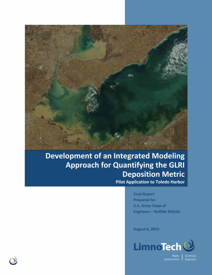
Development of an Integrated Modeling Approach for Quantifying the GLRI
Deposition Metric Pilot Application to Toledo Harbor
Final Report
Prepared for:
U.S. Army Corps of
Engineers – Buffalo District
August 6, 2013

Page | ii
Blank Page

Page | iii
Development of an Integrated Modeling Approach for
Quantifying the GLRI Deposition Metric: Pilot Application to
Toledo Harbor
Final Report
Prepared for:
USACE – Buffalo District Review
Under Contract to:
Ecology & Environment, Inc.
August 6, 2013

Page | iv
Blank page

Development of an Integrated Modeling Approach for Quantifying the GLRI Deposition Metric August 6, 2013
Page | v
TABLE OF CONTENTS
Executive Summary ................................................. ES-1
1 Introduction ................................................................1
1.1 Background and Project Objectives ................................... 1
1.2 Problem Specification ......................................................... 3
1.2.1 Management Objectives............................................ 3
1.2.2 System Characteristics .............................................. 4
1.2.3 Programmatic Constraints........................................ 4
1.3 Project Approach ................................................................ 4
1.3.1 Problem Specification ............................................... 5
1.3.2 Model Selection ......................................................... 5
1.3.3 Model Configuration ................................................. 5
1.3.4 Model Calibration & Confirmation .......................... 5
1.3.5 Model Application ..................................................... 6
1.4 Scope of Report ................................................................... 6
2 Characteristics of the Lower Maumee River – Maumee Bay System .............................................................. 7
2.1 Geometry & Physical Configuration .................................. 7
2.2 Hydraulic Characteristics ................................................... 9
2.2.1 Lower Maumee River ................................................ 9
2.2.2 Maumee Bay / Western Lake Erie Basin ................ 11
2.3 Sediment Characteristics .................................................. 12
2.3.1 Lower Maumee River .............................................. 13
2.3.2 Maumee Bay / Western Lake Erie Basin ............... 14
2.3.3 Toledo Harbor Federal Navigation Channel ......... 15
3 Lower Maumee River – Maumee Bay Model Development .......................................................... 17
3.1 Overview of Model Framework ........................................ 17
3.2 Hydrodynamic Model (EFDC) ......................................... 19
3.2.1 Model Framework & Configuration ....................... 19
3.2.2 Model Segmentation ............................................... 19
3.2.3 Boundary Conditions .............................................. 22
3.3 Wind-Wave Model (SWAN) ............................................. 24
3.3.1 Model Framework & Configuration ....................... 24
3.3.2 Boundary Conditions .............................................. 25
3.3.3 Linkage to EFDC Model .......................................... 25
3.4 Sediment Transport Model (SNL-EFDC) ........................ 26
3.4.1 Model Framework & Configuration ....................... 26
3.4.2 Boundary Conditions ............................................. 30
3.4.3 Sediment Bed Characteristics ................................. 36
4 Lower Maumee River – Maumee Bay Model Calibration & Confirmation................................... 39

Development of an Integrated Modeling Approach for Quantifying the GLRI Deposition Metric August 6, 2013
Page | vi
4.1 Hydrodynamic Model ....................................................... 39
4.1.1 Calibration Approach .............................................. 39
4.1.2 Calibration Results ................................................. 40
4.2 Wind-Wave Model ............................................................ 46
4.3 Sediment Transport Model .............................................. 49
4.3.1 General Approach & Data Targets.......................... 49
4.3.2 Model Calibration Results ...................................... 54
4.3.3 Model Confirmation Results .................................. 69
5 Model Application for Great Lakes Restoration Initiative Deposition Metric .................................. 73
5.1 Introduction to the GLRI Deposition Metric .................. 73
5.2 Overview of Approach ...................................................... 74
5.3 Estimation of Loading Reductions for Post-2008 Period .......................................................................................... 77
5.3.1 Delineation of High-Flow Events ........................... 78
5.3.2 Long-Term Trends in Sediment Loading Reduction .................................................................................... 79
5.3.3 Sediment Loading Reduction Trend for Pre-2009 and Post-2008 Conditions ...................................... 80
5.4 Evaluation of the GLRI Deposition Metric Based on Comparison of the “Adjusted” and “Actual” Sediment Loading Scenarios for 2009-12 .......................................83
5.4.1 Inter-Annual Variability in Navigation Channel Deposition ................................................................. 87
5.4.2 Spatial Trends in Navigation Channel Deposition 88
5.5 Components Analysis for Sediment Deposition............. 89
6 Conclusions & Recommendations ............................ 93
6.1 Conclusions Related to the GLRI Deposition Measure for Toledo Harbor .................................................................. 93
6.2 Recommendations for Quantifying Deposition Trends for Other Great Lakes Harbor Systems ................................ 94
6.3 Recommendations for Quantifying GLRI Nutrient-Related Metrics ................................................................ 95
6.4 Recommendations for Quantifying GLRI Program Contributions to Sediment and Nutrient Loading Reductions........................................................................ 96
7 References ................................................................ 99
Appendix A: Maumee River Daily Flow and Cumulative Sediment Loading by Year .................................. 103

Development of an Integrated Modeling Approach for Quantifying the GLRI Deposition Metric August 6, 2013
Page | vii
LIST OF FIGURES
Figure ES-1. Comparison of Navigation Channel Deposition
Profile for the “Actual” and “Adjusted” (Mean Regression)
Loading Cases .................................................................... ES-3 Figure 1-1. Project Location and Relevant Geographic Features .. 2 Figure 2-1. Map of the Extent and Bathymetry of the Model
Domain for the Lower Maumee River, Maumee Bay, and
Western Lake Erie Basin ......................................................... 8 Figure 2-2. Transition in Longitudinal Velocities through the
Lower Maumee River ............................................................ 10 Figure 2-3. Flow Reversals in the Lower Maumee River at River
Mile 6 base on NOAA Monitoring Data ................................ 11 Figure 2-4. Satellite Imagery During a Wind-Wave Resuspension
Event on March 29, 2007 ..................................................... 12 Figure 2-5. Maumee River Discharge (blue line) and Cumulative
Sediment Load (red line) for the 2006-09 Period .............. 13 Figure 2-6. Summary of Estimated Sediment Loadings to the
Western Lake Erie Basin for 2006-12 .................................. 14 Figure 2-7. Percentage of Sand Content in Surficial Bed
Sediments near Maumee Bay ............................................... 15 Figure 3-1. Lower Maumee River – Maumee Model Linked
Model Framework ................................................................. 18 Figure 3-2. Maumee River Model Grid, Waterville to Mouth
(plates A-D show sections from downstream to upstream)20 Figure 3-3. LMR-MB Model Horizontal Grid and Bathymetry .. 21 Figure 3-4. LMR-MB Model Grid and Bathymetry for Maumee
Bay .......................................................................................... 21 Figure 3-5. Sediment Transport Processes Represented in SNL-
EFDC ...................................................................................... 27 Figure 3-6. Modeled Sediment Bed Profile .................................. 29 Figure 3-7. Difference in Bed Elevation Change with Data-driven
bathymetry (Base Run) and Uniform Project Depth (Test
Run) ...................................................................................... 30 Figure 3-8. Observed Time Series of Suspended Sediment
Concentrations for the Maumee River at Waterville, OH
(2006-12) ............................................................................... 31 Figure 3-9. Suspended Sediment Concentration versus Daily
Flow Rate for the Maumee River at Waterville, OH (2006-
09) .......................................................................................... 32 Figure 3-10. Maumee River Total Annual Discharge Volume and
Suspended Sediment Load for Calibration and Application
Periods (2006-12) ................................................................. 33 Figure 3-11. Sediment Particle Size Distribution versus Flow Rate
for the Maumee River at Waterville, OH ............................. 35 Figure 3-12. Sediment Bed Types Derived From Western Lake
Erie Basin and Maumee Bay Sediment Sampling Data ......38

Development of an Integrated Modeling Approach for Quantifying the GLRI Deposition Metric August 6, 2013
Page | viii
Figure 4-1. Model-Data Comparison of Rating Curve for Maumee
River near Waterville, OH .................................................... 41 Figure 4-2. Model-Data Time Series Comparison of Current
Velocities at Maumee River Mile 6 (January 1 – February
18, 2008) ................................................................................ 42 Figure 4-3. Model-Data 1:1 Comparison of Current Velocities at
Maumee River Mile 6 ............................................................ 42 Figure 4-4. Model-Data Comparison of Water Levels in Maumee
Bay (2004-05) ....................................................................... 43 Figure 4-5. Model-Model Comparisons of Velocity Magnitude
near end of Navigation Channel ........................................... 44 Figure 4-6. Model-Model Comparisons of Velocity Direction near
end of Navigation Channel ................................................... 44 Figure 4-7. Comparison of Observed (points) and Predicted
(grid) Chloride Concentrations in Maumee Bay for May 17,
2004 ....................................................................................... 45 Figure 4-8. Comparison of Model-Predicted Conservative Tracer
Plume Extent to ..................................................................... 46 Figure 4-9. IFYLE 2005 Monitoring Locations ........................... 47 Figure 4-10. Comparison between Observed and Predicted
Significant Wave Height in the Western Lake Erie Basin
(June 23 – July 31, 2005) .................................................... 48 Figure 4-11. Comparison between Observed and Predicted
Significant Wave Height in the Western Lake Erie Basin
(September 19 – November 5, 2005) .................................. 48 Figure 4-12. Comparison of Observed and Predicted Significant
Wave Height Cumulative Frequency Distribution in
Western Lake Erie Basin for June 23 – November 5, 200549 Figure 4-13. Toledo Harbor Federal Navigation Channel ........... 51 Figure 4-14. Spatial and Temporal Variability in Data-Based
“Bed Elevation Change” Estimates for 2006-09 ................. 52 Figure 4-15. Calibrated Maumee River Sediment Loading Particle
Size Distribution as a Function of Maumee River Flow ...... 56 Figure 4-16. Spatial and Temporal Variability in Model-
Simulated “Bed Elevation Change” for 2006-09 ................. 58 Figure 4-17. Comparison of Simulated to Observed “Bed
Elevation Change” in the Toledo Harbor Navigation
Channel (summer/fall 2006 – summer/fall 2007) ............ 60 Figure 4-18. Comparison of Simulated to Observed “Bed
Elevation Change” in the Toledo Harbor Navigation
Channel (summer/fall 2007 – summer/fall 2008) ............ 61 Figure 4-19. Comparison of Simulated to Observed “Bed
Elevation Change” in the Toledo Harbor Navigation
Channel (summer/fall 2008 – spring 2009) ....................... 62 Figure 4-20. One-to-One Comparison of Model-Simulated versus
Observed Bed Elevation Change for the 2006-09
Calibration Period ................................................................. 64

Development of an Integrated Modeling Approach for Quantifying the GLRI Deposition Metric August 6, 2013
Page | ix
Figure 4-21. Comparison of Model-Simulated Suspended
Sediment Plume (left) and MODIS Imagery (right) for April
18, 2006 ................................................................................. 66 Figure 4-22. Model-Data Comparison for Total Suspended Solids
Concentrations in Maumee Bay and Western Lake Erie
Basin (September 18, 2007; Maumee Flow = 1,340 cfs) .... 67 Figure 4-23. Model-Data Comparison for Total Suspended Solids
Concentrations in Maumee Bay and Western Lake Erie
Basin (October 6, 2009; Maumee Flow = 730 cfs) .............. 67 Figure 4-24. Model-Data Comparison for Total Suspended Solids
Concentrations in Maumee Bay and Western Lake Erie
Basin (July 10, 2008; Maumee Flow = 16,600 cfs) ............ 68 Figure 4-25. Model-Data Comparison for Total Suspended Solids
Concentrations in Maumee Bay and Western Lake Erie
Basin (June 11, 2008; Maumee Flow = 14,900 cfs) ........... 68 Figure 4-26. Comparison of Simulated to Observed “Bed
Elevation Change” in the Toledo Harbor Navigation
Channel (March 2004 – May 2005) .................................... 70 Figure 4-27. Comparison of Simulated (grid) to Observed
(points) Total Suspended Solids Concentrations in Maumee
Bay (August 23, 2004; Maumee Flow = 5,450 cfs) ............. 71 Figure 4-28. Comparison of Simulated (grid) to Observed
(points) Total Suspended Solids Concentrations in Maumee
Bay (June 3, 2004; Maumee Flow = 22,600 cfs) ................ 71 Figure 5-1. Maumee River Annual Total Discharge Volume and
Suspended Sediment Load for the 2004-12 Period ............ 75 Figure 5-2. Flow Chart of Approach for Quantifying the GLRI
Deposition Metric for 2009-12 ............................................. 77 Figure 5-3. Long-Term Trend in Average Annual “Event Mean
Concentrations” for Maumee River High-Flow Events ..... 80 Figure 5-4. Regression of Log10-Normalized TSS “Event Mean
Concentration” vs. Log10-Normalized Event Peak Flow Rate
for 2004-08 ........................................................................... 81 Figure 5-5. Comparison of Navigation Channel Deposition
Profile for the “Actual” and “Adjusted” (Mean Regression)
Loading Cases ....................................................................... 84 Figure 5-6. Comparison of Navigation Channel Deposition
Profile for the “Actual” and “Adjusted” (Lower 95% CI)
Loading Cases ........................................................................ 85 Figure 5-7. Comparison of Navigation Channel Deposition
Profile for the “Actual” and “Adjusted” (Upper 95% CI)
Loading Cases ........................................................................ 85 Figure 5-8. Comparison of Model-Simulated Navigation Channel
Deposition for Calendar Years 2011 and 2012 (“actual”
loading case) ......................................................................... 88 Figure 5-9. Relative Contributions of Maumee River and “Other”
Sediment Loading Components to Total Deposition in the
Toledo Harbor Navigation Channel .................................... 90

Development of an Integrated Modeling Approach for Quantifying the GLRI Deposition Metric August 6, 2013
Page | x
Figure 5-10. Longitudinal Profile of Maumee River – Derived
Navigation Channel Deposition to Total Deposition for the
“Actual” Loading Case ........................................................... 91
LIST OF TABLES
Table 2-1. Geometric and Hydraulic Properties of the Lower
Maumee River ......................................................................... 8 Table 2-2. Geometric and Hydraulic Properties of the Western
Lake Erie Basin ........................................................................ 9 Table 2-3. Summary of Sediment Bed Conditions in the Maumee
River Portion of the Toledo Harbor Federal Navigation
Channel .................................................................................. 14 Table 3-1. LMR-MB Model Inflow Boundary Conditions (2006-
12) ........................................................................................... 23 Table 3-2. Suspended Sediment Boundary Conditions for
Maumee Bay / WLEB Flow Sources .................................... 34 Table 3-3. Tributary Average Annual Suspended Loading for
2006-12 Calibration Period .................................................. 34 Table 3-4. Particle Size Distribution Summary for Maumee Bay /
WLEB Flow Sources (excluding the Maumee River) .......... 35 Table 3-5. Sediment Bed Characteristics for each Modeled Bed
Type ........................................................................................ 37 Table 4-1. Calibration Datasets for LMR-MB Hydrodynamic
Model .................................................................................... 40 Table 4-2. Modeled Particle Size Class Characteristics ............... 54 Table 4-3. Summary of Sediment Bed Parameterization ............ 57 Table 5-1. Summary of Loading Conditions for the “Actual” and
“Adjusted” Scenarios .............................................................83

Development of an Integrated Modeling Approach for Quantifying the GLRI Deposition Metric August 6, 2013
Page | xi
ACRONYMS AND ABBREVIATIONS
BEC Bed elevation change
BMP Best management practice
CDF Confined Disposal Facility
cfs Cubic feet per second
cm Centimeter
cy Cubic yards
E & E Ecology and Environment, Inc.
EFDC Environmental Fluid Dynamics Code (model)
EMC Event mean concentration
ft feet
GLNPO Great Lakes National Program Office
GLRI Great Lakes Restoration Initiative
LMR-MB Lower Maumee River – Maumee Bay
LWD Low Water Datum
m Meter
mg/l Milligram per liter
NRCS Natural Resources Conservation Service
RM River Mile (for Maumee River)
SNL-EFDC Sandia National Laboratories – Environmental
Fluid Dynamics Code (model)
SWAN Simulating Waves Nearshore (model)
SWAT Soil & Water Assessment Tool (model)
TSS Total suspended solids (or sediment)
URL Uniform resource locator (web address)
USEPA U. S. Environmental Protection Agency
USACE U. S. Army Corps of Engineers
USGS U. S. Geological Survey
WLEB Western Lake Erie Basin
yr Year

Development of an Integrated Modeling Approach for Quantifying the GLRI Deposition Metric August 6, 2013
Page | ES-1
Executive Summary
In the Great Lakes Restoration Initiative (GLRI) Action Plan for 2010-14, the Great Lakes National
Program Office (GLNPO) established a series of metrics (also referred to as “measures”) and targets to
track progress in achieving the goals of the “Nearshore Health and Non-point Source Pollution Focus
Area” of the GLRI (White House Council on Environmental Quality 2010). One of the metrics in this focus
area requires quantifying the reduction of the “annual volume of sediment deposition in defined harbor
areas in targeted watersheds.” Although the metric will eventually be applied to river-harbor systems
throughout the Great Lakes, the GLRI Action Plan prescribes that the metric be initially developed and
applied for Toledo Harbor. Therefore, Toledo Harbor is intended to serve as a pilot case study for this
metric. Toledo Harbor receives the highest sediment loading and deposition of any Great Lakes harbor.
Sediments depositing in the Toledo Harbor navigation channel are predominantly derived from the
Maumee River watershed, which represents a large drainage basin (6,354 square miles) with
approximately 85% agricultural land use. A recent USACE report estimated that the annual dredging
requirement for Toledo Harbor is approximately 850,000 cubic yards (USACE 2009). The GLRI target is
to reduce sediment accumulation relative to the 2008 baseline by 1% for 2012 and by 2.5% by 2014.
These targets would be accomplished through various soil erosion reduction activities in the watershed
that have been implemented or enhanced since the establishment of the GLRI in 2009. This report
describes the results of an integrated data/modeling approach for assessing the GLRI sedimentation
target for the Toledo Harbor navigation channel.
Extensive suspended sediment loading and navigation channel bathymetry datasets are available to
support an assessment of the GLRI deposition metric for Toledo Harbor. Total suspended solids (TSS)
concentration data are available from Heidelberg University for the Maumee River at Waterville, OH for
the 1975-2012 period. Combined with USGS flow gauging data at Waterville, these data support robust
estimates of sediment loading to Toledo Harbor. The USACE – Buffalo District conducts a “project
conditions” bathymetry survey annually that covers portions of the navigation channel in order to assess
and prioritize dredging needs. In addition, “before dredge” and “after dredge” surveys are conducted for
each dredging event to provide a basis for estimating the volume of sediment removed by the dredging
contractor. These surveys provide valuable data for supporting the quantification of the GLRI sediment
deposition metric. However, for a variety of reasons, the bathymetry measurements alone cannot provide
an accurate measure of progress towards the GLRI deposition targets for 2009-14. For example, the
bathymetry surveys are not conducted for the entire navigation channel for a given year, and the extent
and timing of surveys varies considerably. In addition, sediment deposition to the navigation channel in
any given year is a combination of: 1) “direct” deposition of sediments loaded by the Maumee River, and
2) re-deposition of material resuspended from the sediment bed in Maumee Bay and the Western Lake
Erie Basin. Furthermore, both annual and seasonal sediment delivery by the Maumee River is highly
variable, with the magnitude and timing of the load depending on the frequency and timing of watershed
runoff events in the Maumee Basin.
An integrated data analysis and modeling approach was proposed to overcome the limitations associated
with the available bathymetry data and other supporting datasets. The objective of this project was to
integrate recent bathymetry and TSS loading estimates with the “Lower Maumee River / Maumee Bay”
(LMR-MB) model, and to use the integrated tool to develop and apply an approach for tracking the GLRI
annual sediment deposition metric for the Toledo Harbor system that accounts for the challenges

Development of an Integrated Modeling Approach for Quantifying the GLRI Deposition Metric August 6, 2013
Page | ES-2
mentioned above. The LMR-MB model was originally developed by LimnoTech under a previous project
for the USACE – Buffalo District, and it simulates hydraulics/hydrodynamics, wind-wave characteristics,
and sediment transport processes (including navigation channel deposition) for the Lower Maumee River
/ Maumee Bay / Western Lake Erie system (LimnoTech 2010a). For this project the LMR-MB model was
further developed and the sediment transport component of the model recalibrated to bathymetry data
for the 2006-09 period to provide a robust integrated modeling tool that could specifically be used to
evaluate the deposition reduction targets prescribed by the GLRI Action Plan.
Following completion of the model development, recalibration, and confirmation efforts for the 2004-
2009 period, a series of application scenarios were designed and implemented with the LMR-MB model
based on 2009-12 conditions. The successful outcome of the LMR-MB model recalibration, and
confirmation efforts provides a high level of confidence that the model can be used to address the annual
harbor deposition reduction targets prescribed by the GLRI Action Plan. The first step in the application
effort was to use daily monitoring data for Waterville, OH to quantify the effective change in TSS loading
that occurred for the post-2008 period relative to the pre-2009 period (2004-08, representing “pre-
GLRI” conditions). Within this context, the term “effective” refers to changes in loading (or deposition)
that are estimated once differences in river flow conditions have been factored out. Observed hydrologic
and meteorological conditions for the 2009-12 period were used as the basis for each scenario. However,
the TSS concentration time series for these scenarios were specified differently, as summarized below:
“Actual” Loading Case: TSS concentrations were defined based on daily observed concentrations
for the 2009-12 (post-2008) period.
“Adjusted” Loading Case: A synthetic TSS concentration time series was developed based on the
relationship between “event mean concentrations” and peak event flows for the 2004-08 (pre-
2009) monitoring period. The assigned concentrations represent an increase in event TSS
concentrations and loadings relative to the actual observed TSS concentrations and loadings for
the 2009-12 period.
The TSS concentration time series were incorporated into the LMR-MB model, and simulations were
designed and implemented to evaluate reductions in navigation channel deposition for the Toledo Harbor
system for the “actual” loading case relative to the “adjusted” loading case. Figure ES-1 compares the
longitudinal profile of “bed elevation change” in the navigation channel for the mean “adjusted” loading
scenario and the “actual” loading scenario. Uncertainties in the effective reduction in TSS loading between
the “adjusted” and “actual” cases were quantified by estimating the lower and upper 95% confidence
bounds around the estimated mean change in loading. The key finding of this analysis is that the
overall post-2008 reduction in Toledo Harbor navigation channel deposition was 10±6%,
which suggests that the GLRI sedimentation target of a 2.5% reduction by 2014 has already
been achieved.

Development of an Integrated Modeling Approach for Quantifying the GLRI Deposition Metric August 6, 2013
Page | ES-3
Figure ES-1. Comparison of Navigation Channel Deposition Profile for the “Actual” and “Adjusted” (Mean Regression) Loading Cases
A summary of the key findings and conclusions developed in this study based on the outcomes of the
model application and the supporting Maumee River suspended sediment loading analysis is provided
below:
Inter-annual variability in Maumee River high-flow event frequency and magnitude and associated
suspended solids loading is very significant. Consequently, the magnitudes of sediment deposition in
the navigation channel and the spatial distribution of the deposited mass are likely to vary
considerably from year to year.
When inter-annual variability in Maumee River flow and suspended solids loading is factored out, it
can be shown that the effective reduction in the Maumee River TSS load has been significant over the
past several decades as agricultural management practices have improved in the Maumee Basin.
Effective reductions in Maumee River suspended solids loading have continued to occur within the
past 10 years, with an effective loading reduction of approximately 19% (+/- 11%) estimated for the
2009-12 period relative to the earlier 2004-08 period.
Effective reductions in sediment deposition within the navigation channel have also occurred within
the past 5-10 years in response to reductions in the TSS loadings from the Maumee River, with
roughly 50% of the loading reduction realized as reduction in deposition.
The effective reductions in deposition realized for the 2009-12 period (i.e., relative to the pre-2009
(2004-08) period) based on the model application are 10 +/-6%. Therefore, all reductions within the
range associated with the 95% confidence interval exceed the 2014 GLRI 2.5% target for reductions in
annual deposition.
Reductions in effective deposition are most significant near the Maumee River mouth and within the
inner area of Maumee Bay. Effective reductions in deposition diminish for the navigation channel in
the vicinity of the Maumee Bay / WLEB boundary and beyond.

Development of an Integrated Modeling Approach for Quantifying the GLRI Deposition Metric August 6, 2013
Page | ES-4
Key caveats that must be kept in mind when reviewing and evaluating the results, findings, and
conclusions of this study include the following:
Sediment transport processes in Great Lakes Harbor systems such as Toledo Harbor are highly
complex. Although considerable data are available to inform and constrain the LMR-MB sediment
transport model, there is a degree of uncertainty in this analysis and the associated findings and
conclusions. Nevertheless, the extensive data and state-of-the-art integrated model used in this
analysis provide a high degree of confidence that there has been a measurable reduction in sediment
deposition in the Toledo Harbor navigation channel over the past 5-8 years.
Reductions in Maumee River sediment loading over the past 5-8 years have been the net result of
multiple watershed initiatives being conducted in parallel under funding from various agencies,
including the Natural Resources Conservation Service, the Farm Bill, and USACE 516(e) sediment
reduction programs. These programs are operating, and will continue to operate, in parallel with
GLRI initiatives in the Maumee Basin, and the integrated modeling approach developed under this
study cannot be directly used to distinguish the relative contributions of these different programs to
the overall Maumee River sediment loading reductions. An inventory of management actions in the
basin and a complementary watershed modeling analysis would be needed to estimate reductions
resulting from GLRI initiatives and/or other individual programs.
Planning of GLRI-funded “best management practices” to reduce sediment delivery in the Maumee
Basin has been ongoing since the inception of the GLRI in 2009. However, actual implementation of
sediment reduction practices has only recently begun. Furthermore, it is common for the realization
of benefits from such projects to lag their implementation (e.g., by one or more years). Therefore, the
GLRI-funded sediment reduction programs cannot be expected to produce measurable reductions in
sediment delivery within the first few years of the GLRI program.
The success of the integrated model development, calibration, and application efforts for this project has
important implications for other Great Lakes river-harbor systems outside of the Western Lake Erie
Basin. In particular, the approaches and implementation steps developed for the Toledo Harbor pilot
evaluation could be transferred to other major river-harbor systems where reductions in sediment
deposition are a high priority. Examples of such river-harbor systems include: Saginaw River - Saginaw
Harbor (MI), St. Louis River - Duluth-Superior Harbor (MN), Lower Fox River - Green Bay Harbor (WI),
and Cuyahoga River - Cleveland Harbor (OH). The overall approach and methods presented in this report
are generally applicable to these other river-harbor systems. For example, annual bathymetry survey data
should be available from the USACE Chicago, Detroit, and Buffalo districts to support the “bed elevation
change” analysis, which is of central importance in understanding and quantifying depositional behavior
within the context of developing an integrated sediment transport model. Although the modeling
approach developed here can be readily applied to any harbor and navigation channel system, the
availability of supporting data to calibrate and apply the model will ultimately dictate the level of
uncertainty associated with the outcomes of the modeling analysis. With that in mind, additional data
collection (e.g., for sediment loading) and/or modifications to the integrated modeling approach
developed for Toledo Harbor may be useful when evaluating the GLRI deposition reduction targets for
other river-harbor systems.
The “Nearshore Health and Nonpoint Source Pollution” focus area described in the GLRI Action Plan
includes metrics and associated targets related to reductions in nutrient delivery and associated nutrient-
driven in-lake impacts in addition to the sediment deposition metric that is the focus of the current
project and this report. Nutrient-related measures presented in the GLRI Action Plan include (p. 29 in
White House Council on Environmental Quality 2010):
Development of an Integrated Modeling Approach for Quantifying the GLRI Deposition Metric August 6, 2013
Page | ES-5
“Five-year average annual loadings of soluble phosphorus from tributaries draining targeted
watersheds.” (Great Lakes tributary watersheds for which specific metrics are prescribed for this
measure include the Fox, Saginaw, Maumee, St. Louis, and Genesee rivers.)
“Extent (sq. miles) of Great Lakes Harmful Algal Blooms”
The current project and this report focused exclusively on the hydrodynamic, wind-wave, and sediment
transport capabilities of the LMR-MB model. However, the LMR-MB model has also been linked to a
water quality and eutrophication sub-model, and this overall model framework is referred to as the
“Western Lake Erie Ecosystem Model” (WLEEM). The development of the WLEEM dates back to the
original model development and calibration effort conducted by LimnoTech for the USACE – Buffalo
District to support evaluation of various sediment and nutrient management scenarios (LimnoTech
2010a). Since its inception in 2010, LimnoTech has continued to develop and apply the WLEEM
framework under the umbrella of other projects focused on the Western Lake Erie Basin ecosystem. For
example, a Maumee Basin-wide Soil & Water Assessment Tool (SWAT) model has been linked to the
WLEEM to provide an overall watershed-WLEB integrated modeling tool that can be used to quantify the
impact of management actions in the watershed on: 1) reductions in Maumee River delivery of total and
soluble reactive phosphorus, and 2) harmful algal bloom development and extent in the WLEB under
various climate conditions. The linked watershed-WLEB water quality and ecosystem modeling
framework is unique within the context of the Great Lakes, and it provides a suite of existing integrated
modeling tools that could be used to evaluate progress in meeting the nutrient loading and eutrophication
targets prescribed by the GLRI Action Plan. Although this linked modeling framework has only been
developed and applied for Maumee Basin and the Western Lake Erie Basin, it also could be transferred to
other Great Lakes basins and tributary systems, similar to the approach recommended above for the
LMR-MB linked hydrodynamic – wind-wave – sediment transport model.

Development of an Integrated Modeling Approach for Quantifying the GLRI Deposition Metric August 6, 2013
Page | 1
1 Introduction
This report describes a project undertaken by LimnoTech under sub-contract to, and in partnership with,
Ecology and Environment, Inc. (E & E) to evaluate existing data and to further develop, calibrate, and
apply a linked hydrodynamic – wind-wave – sediment transport model to support the quantification of
harbor deposition metrics established by the Great Lakes Restoration Initiative (GLRI) Action Plan
(White House Council on Environmental Quality 2010). The model, which is referred to in this report as
the “Lower Maumee River – Maumee Bay” (LMR-MB) model, was originally developed under a previous
project with the U.S. Army Corps of Engineers (USACE) – Buffalo District to inform sediment-related and
nutrient-related issues in Maumee Bay and the Western Lake Erie Basin (WLEB) (LimnoTech 2010a).
This project is funded by the U.S. Environmental Protection Agency’s (USEPA’s) Great Lakes National
Program Office (GLNPO) and the USACE – Buffalo District through the GLRI program.
1.1 Background and Project Objectives
Section 516(e) of the Water Resources Development Act (WRDA) authorizes the USACE to develop
sediment transport models for all major Great Lakes tributaries contributing sediment to Federal
navigation projects or Areas of Concern (AOCs). This program of the Corps serves to assist Federal, State,
and local agencies with planning and implementation of actions for soil conservation and non-point
source pollution reduction, reduction of the amount of dredging and related costs, and support of the AOC
delisting process. Recently, GLNPO established a series of metrics to measure progress in achieving the
goals of the “Nearshore Health and Non-point Source Pollution Focus Area” of the GLRI (White House
Council on Environmental Quality 2010). One of the metrics in this focus area involves quantifying the
reduction of the “annual volume of sediment deposition in defined harbor areas in targeted watersheds.”
GLNPO asked the USACE – Buffalo District to assist them with the quantification of this metric for the
Toledo Harbor area. Therefore, the objective of this project is to combine the LMR-MB sediment
transport model with annual monitoring of bathymetry in the Toledo Harbor navigation channel
conducted by the USACE – Buffalo District and suspended solids monitoring at Waterville, OH to develop
and apply an approach for tracking the GLRI annual sediment deposition metric for the Toledo Harbor
system. Although not a specific objective of the current project, the intent of the project is to develop an
approach that can be extended to other targeted Great Lakes harbor areas, such as the Saginaw Harbor,
Green Bay Harbor, and Duluth-Superior Harbor.
Toledo Harbor receives the largest amount of sediment deposition of any Great Lakes harbor, which is the
reason why this harbor was targeted for this initial investigation. Sediments depositing in the Toledo
Harbor navigation channel are predominantly derived from the Maumee River watershed, which is a very
large watershed (6,354 square miles) with approximately 85% agricultural land use. Figure 1-1 shows the
project location and highlights major geographic features. A recent USACE report estimated that the
annual dredging requirement for Toledo Harbor is approximately 850,000 cubic yards (USACE 2009).
The GLRI target is to reduce sediment accumulation relative to the 2008 baseline by 1% for 2012 and by
2.5% by 2014. These targets would be accomplished by soil erosion reduction activities in the watershed
that have begun to be implemented since the establishment of the GLRI in 2009.

Development of an Integrated Modeling Approach for Quantifying the GLRI Deposition Metric August 6, 2013
Page | 2
Figure 1-1. Project Location and Relevant Geographic Features
The USACE – Buffalo District conducts a “project conditions” bathymetry survey annually that covers all
or portions of the navigation channel in order to assess the spatial dredging needs. In addition, “before
dredge” and “after dredge” surveys are conducted for each dredging event to provide a basis for estimating
the volume of sediment removed by the dredging contractor(s). These surveys provide valuable data for
supporting the quantification of the GLRI sediment deposition metric. However, there are a number of
reasons why the bathymetry measurements alone cannot provide an accurate measure of progress
towards the GLRI metric targets for 2009-14. Specific concerns about relying exclusively on these surveys
include:
1. The GLRI targets for reduction in sediment accumulation are smaller (1-2.5%) than the range of
uncertainty in the bathymetry measurements. Assuming the reductions in sediment accumulation
are spread over much of the channel area that receives sediment deposits, a 1% target requires
only a small reduction in annual sediment accumulation, on the order of 1 cm or less.
2. The sediment deposition in any given year is a combination of direct deposition of sediments into
the channel that have been delivered from the Maumee River and sediments that are resuspended
by wind-generated shear stress from the Western Lake Erie Basin (a fraction of which may have
come from the river during previous years) and re-deposited into the channel. There is a need to
separate the contribution from these two sources to total deposition in the navigation channel.
3. The sediment delivered by the Maumee River to the Western Lake Erie Basin in any given year is
highly variable, depending on the annual hydrograph. This inter-annual variability is known to
Toledo Harb
or
Navigation C
hannel
IProject Location
0 4 82Miles

Development of an Integrated Modeling Approach for Quantifying the GLRI Deposition Metric August 6, 2013
Page | 3
be considerably larger than the load reduction that might be achieved in a given year by actions in
the watershed.
4. The “project conditions” bathymetry surveys for a given year are typically conducted piece-wise
over a time period that spans many months. Hence, the bathymetry measurements for a given
reach of the channel may not be associated with the same timeframe as the bathymetry
measurements for a different reach.
5. The “project conditions” surveys do not provide complete coverage of the navigation channel each
year. Therefore, there are significant spatial gaps in year-to-year analyses of bathymetry changes.
Due to the inherent limitations of the bathymetry datasets in supporting the quantification of the GLRI
sediment deposition metric, an integrated modeling approach is needed to permit the necessary
interpolation and extrapolation of deposition patterns in the navigation channel and inter-annual
variability of system hydrology. The project approach described in Section 1.3 below outlines the planned
use of USACE bathymetry data, other data sources, including USGS flow data and Heidelberg University
water quality data collected at Waterville, OH, and the LimnoTech LMR-MB model to develop and
implement an approach for quantifying annual changes in sediment deposition in the Toledo Harbor
navigation channel as an indicator of benefits from Maumee River management initiatives undertaken
with GLRI support.
1.2 Problem Specification
Explicit specification of the problem to be addressed (i.e., detailed statement of management questions) is
a critical element of any modeling project. Planning the project with the end in mind assures the
development of the most appropriate conceptual model and the most appropriate model complexity and
the data needed to support that model complexity. Therefore, the problem specification must include a
clear and complete statement of policy, management, and/or scientific objectives, model spatial and
temporal domain and resolution characteristics, as well as programmatic constraints (e.g., legal,
institutional, data, time and economics). Some considerations for each aspect include:
Management objectives are statements of what questions a model has to answer. The statement of
modeling objectives should include: the water quality state variables of concern; the stressors (model
inputs) driving those state variables and their control options; and, very importantly, the desired
accuracy of the model.
Specifying the model domain characteristics includes: identification of the environmental domain
being modeled; specification of transport and transformation processes within that domain that are
relevant to the policy/management/research objectives; specification of important time and space
scales inherent in transport and transformation processes within that domain in comparison with the
time and space scales of the problem objectives; and any peculiar conditions of the domain that will
affect model selection or new model construction.
Problem specification should include a discussion of the potential programmatic constraints. These
address: time and budget; available data or resources to acquire more data; legal and institutional
considerations; computer resource constraints; and experience and expertise of the modeling staff.
1.2.1 Management Objectives
As stated above, the primary objective of the current project is to quantify the effective reduction in
Toledo Harbor navigation channel deposition for the post-2008 period in response to reduced loadings of
suspended solids from the Maumee River relative to the pre-GLRI (pre-2009) time period. Based on
discussions between GLNPO, USACE, and LimnoTech staff it was determined that an integrated
hydrodynamic – sediment transport modeling framework model would be required to meet this objective.

Development of an Integrated Modeling Approach for Quantifying the GLRI Deposition Metric August 6, 2013
Page | 4
The integrated model would need to be supported by, and calibrated to, datasets available for the Maumee
River and the Western Lake Erie Basin so that the model could be applied with a high degree of
confidence to quantify effective reductions in Maumee River suspended sediment loading and the
resulting effective reductions of deposition in the Toledo Harbor navigation channel. Within this context,
the term “effective” refers to changes in loading or deposition that are estimated/calculated once
differences in the raw sediment loading that are attributed to differing river flow conditions for two time
periods have been factored out. For example, a 50,000 cfs high-flow event during “Year 2” will inevitably
have a higher rate of sediment loading than a smaller 10,000 cfs event that occurred the prior year (“Year
1”), primarily due to the disparity in the magnitudes of the events. The effective change in loading,
however, would be determined based on an assessment of whether a comparable 50,000 cfs event in
“Year 1” would have (hypothetically) delivered a higher, lower, or equivalent sediment load relative to the
“Year 2” event. The use of the term “effective” is of critical importance here because inter-annual
variability in Maumee River runoff event-driven flow and sediment loading conditions is significant, and
additional effort is needed to factor out this variability in order to appropriately quantify trends with
respect to loading (and deposition) reductions that have occurred over time.
1.2.2 System Characteristics
The complex nature of the Lower Maumee River / Maumee Bay / Western Lake Erie Basin system and the
management objectives described above require a model that is not only relatively complex in terms of
process resolution but has fine spatial and temporal resolution. The Lower Maumee River stretches
approximately 21 miles between Waterville and the mouth at Maumee Bay. Maumee Bay covers a total
area of approximately 23 square miles, and the WLEB represents an area of 1,200 square miles (refer to
Figure 2-1). Outflow from the Maumee River, water circulation patterns in the Bay and WLEB, and wind-
induced currents and sediment resuspension all interact to drive complex sediment transport and fate
processes.
1.2.3 Programmatic Constraints
Based on past work conducted and the additional data acquisition and analysis conducted for this project,
the available hydrodynamic, bathymetry, and other supporting data were determined to be sufficient to
support the further development, recalibration, and application of the LMR-MB model to the Lower
Maumee River / Maumee Bay /WLEB system, with an emphasis on sediment transport processes as they
relate to deposition in the Toledo Harbor Federal navigation channel.
1.3 Project Approach
The general approach to model development and application for the Lower Maumee River / Maumee Bay
(LMR-MB) model followed these steps:
Specify the problem: Identify management objectives, system characteristics, and programmatic
constraints.
Select the model framework: Develop a conceptual model, and then evaluate options and select a
model framework that will best address factors identified in the problem specification phase.
Configure the model framework: Configure the model framework to the LMR-MB system based
on site-specific data, and develop/revise the necessary linkages between individual sub-models.
Evaluate, calibrate, and confirm the model: Evaluate, calibrate, and confirm the model
simulation outcomes against available site-specific datasets and conduct diagnostic analyses to
understand the behavior of the model under various conditions.

Development of an Integrated Modeling Approach for Quantifying the GLRI Deposition Metric August 6, 2013
Page | 5
Apply the model: Quantify the effective reduction in Toledo Harbor navigation channel deposition
for the 2009-12 period relative to the pre-GLRI (i.e., pre-2009) period, and quantify the relative
contributions of various sediment sources to navigation channel deposition for this period.
1.3.1 Problem Specification
An understanding of key management objectives was achieved through interactions with GLNPO and
USACE staff during the course of several teleconferences during summer/fall 2011. Significant portions of
these meetings were dedicated to discussing management concerns and questions pertaining to the GLRI
deposition metric for Great Lakes harbor systems. These discussions served as the basis for determining
how to refine, configure, and utilize the LMR-MB model framework to best address each management
issue.
1.3.2 Model Selection
A suite of public domain modeling tools was originally selected under a previous project to form the
overall framework for the LMR-MB model. The original components of the model framework were
generally kept intact, although enhancements were made to the sediment fate and transport sub-model to
improve model stability and efficiency. The Environmental Fluid Dynamics Code (EFDC) model was
selected to serve as both the hydrodynamic sub-model and the sediment transport sub-model. EFDC is an
open source, public-domain model code developed and supported by the U.S. EPA. The Simulating
Waves Nearshore (SWAN) was selected as the wind-wave sub-model. The selection of these sub-models is
described in detail in Chapter 3.
1.3.3 Model Configuration
The linked hydrodynamic – wind-wave – sediment transport model has been configured to represent the
LMR-MB system based on available data obtained from a variety of sources, including the USACE –
Buffalo District, U.S. Geological Survey (USGS), Heidelberg University, the University of Toledo, and a
variety of other sources. The configuration of the model framework to the LMR-MB system is described in
Chapter 3.
1.3.4 Model Calibration & Confirmation
The existing LMR-MB model framework was previously calibrated for the 2004-05 period using a limited
set of bathymetry datasets for the Toledo Harbor navigation channel and suspended solids/sediment1 data
acquired from the University of Toledo (Bridgeman et al. 2013). However, the ability to develop a robust
calibration of the LMR-MB sediment transport sub-model to the 2004-05 period was made difficult by: 1)
the limited spatial extent of “bed elevation change” estimates developed for this period; and 2) the lack of
suspended solids concentration/loading data at Waterville, OH for a key high-flow event that occurred in
the Maumee River during December 2004 – January 2005. During the planning phases of this project, it
was determined that the calibration of the sediment transport model should be revised, including
incorporating available bathymetry data and suspended solids monitoring data available for the later
2006-09 period.
The first step in the model recalibration process was to configure the model to the Lower Maumee River /
Maumee Bay system for the 2006-09 period, including compiling all necessary model input data,
including loads, flows, boundary conditions, hydro-meteorological inputs, and initial conditions. A
detailed description of this process is provided in Chapter 3. Once the model was configured to the
1 Note that the terms “suspended solids” and “suspended sediment” are used interchangeably throughout this report.

Development of an Integrated Modeling Approach for Quantifying the GLRI Deposition Metric August 6, 2013
Page | 6
system, it was calibrated and evaluated against field data in order to develop a set of model coefficients
that were both consistent with theory and provided the best overall fit to the spatial and temporal profiles
of the sediment state variables represented in the model. Bathymetry and water column monitoring data
available for the 2006-09 period were used to calibrate the model, and similar datasets available for the
2004-05 period were used to confirm model performance. The 2006-09 period was selected as the focus
of the recalibration effort because a wealth of dredging survey datasets (available from USACE – Buffalo
District) and other supporting datasets (e.g., water column monitoring surveys from University of Toledo)
were available for these specific years and because calibrating the model to an extended 4-year period
would increase confidence in the model’s representation of sediment dynamics. The bathymetry and
water column datasets used to confirm the model were identical to those used to support the original
calibration of the LMR-MB model.
The overall approach for evaluating the model performance consisted of a suite of evaluation techniques
to assess the goodness of fit to available hydrodynamic and sediment datasets. Because all models are
simplifications of the real world, and because numerical wind-wave and sediment transport models are
not fully mechanistic, no model can ever be truly validated (Oreskes et al. 1994). In fact, the term
“confirmation” or “corroboration” is typically used in place of the term “validation” for the model
evaluation process. Hence, evaluating the model against the secondary 2004-05 datasets available outside
the calibration period (2006-09) is referred to as model “confirmation” in this report. A detailed
presentation and discussion of model calibration and confirmation are provided in Chapter 4.
1.3.5 Model Application
The LMR-MB model was applied to simulate sediment delivery and deposition dynamics for a suite of
scenarios designed to address the management objectives. The primary focus of the scenarios developed
was quantifying the reduction in sediment deposition in the Toledo Harbor navigation channel during the
2009-12 period relative to the earlier 2006-08 period. Additional scenarios were designed and
implemented to quantify (via the model) the relative contribution of the various sources of sediment that
contribute deposition to the navigation channel. In order to support the quantification of the GLRI metric
it was necessary to develop an “upscaled” sediment loading condition for the 2009-12 period that reflects
the relatively higher rate of sediment delivery from the watershed associated with the earlier 2004-08
period. A detailed discussion of this approach is provided in Chapter 5 along with the results of the GLRI
metric quantification.
1.4 Scope of Report
This report provides a comprehensive description of the linked hydrodynamic – wind-wave – sediment
transport model developed for the LMB-MB system. Chapter 2 provides a data-based discussion of key
characteristics of the system with respect to hydraulics, sediment transport, and water quality. Chapter 3
provides a description of the model framework development and refinement, and Chapter 4 discusses the
development of data-based metrics and calibration and confirmation of the model framework to those
data-based metrics. Application of the LMR-MB model to quantify the reductions in deposition achieved
for the Toledo Harbor navigation channel during the 2009-12 timeframe is discussed in Chapter 5, and a
summary of conclusions and recommendations is provided in Chapter 6.

Development of an Integrated Modeling Approach for Quantifying the GLRI Deposition Metric August 6, 2013
Page | 7
2 Characteristics of the Lower Maumee River –
Maumee Bay System
This chapter provides a discussion of the key characteristics of the Lower Maumee River, Maumee Bay,
and Western Lake Erie Basin (WLEB) systems and the datasets that are available to support a modeling
assessment of these systems. The physical configuration and the observed hydraulic, wind-wave, and
sediment characteristics of the system provide a necessary foundation for configuring and calibrating the
LMR-MB model framework components to the Lower Maumee River / Maumee Bay system.
2.1 Geometry & Physical Configuration
The domain specified for the LMR-MB model includes the Lower Maumee River from Waterville, OH
through the entire WLEB. It is necessary to include this entire domain in addressing the project objectives
described in Chapter 1 because of the presence of important transport and exchange processes between
the River, Maumee Bay, and Lake Erie. A map showing the extent and bathymetry of the LMR-MB model
domain is provided in Figure 2-1. The major tributaries to Maumee Bay and the WLEB are also
highlighted in this figure and include Maumee River, Detroit River, River Raisin, Huron River, Ottawa
River, Stony Creek, Cedar River, and Portage River.
The physical and hydraulic characteristics of the riverine portion of the modeled system are presented in
Table 2-1. The Lower Maumee River experiences a wide range of flows. While the average flow of the river
is 5,800 cfs (cubic feet per second), the 10th percentile flow is only 400 cfs and the 90th percentile flow is
16,000 cfs. The time of travel in the lower river (RM 20.3 to RM 0.0) from Waterville to the bay is very
short during high flow (approximately a day), leaving relatively little time for suspended solids to deposit
in the river. In fact, sediments that previously deposited in the river during low flow periods (i.e., when
the time of travel is much longer) may be resuspended as a result of elevated velocities experienced during
high-flow conditions. The physical and hydrologic properties of Maumee Bay and the WLEB are
summarized in Table 2-2. Note that Maumee Bay has a large surface area and a relatively shallow mean
depth, which suggests that wind-driven sediment resuspension is likely to be important with respect to
resuspension and redistribution of sediments in the Bay.

Development of an Integrated Modeling Approach for Quantifying the GLRI Deposition Metric August 6, 2013
Page | 8
Figure 2-1. Map of the Extent and Bathymetry of the Model Domain for the Lower Maumee River, Maumee Bay, and Western Lake Erie Basin
Table 2-1. Geometric and Hydraulic Properties of the Lower Maumee River
Maumee River Reach
River Miles Length (miles)
Mean Depth (ft)
Time of Travel (days)
Average Flow
10th
Percentile
Flow
90th
Percentile
Flow
Reach 1 (riverine)
20.3 – 12.6 7.7 3.2 0.2 0.6 0.1
Reach 2 (estuarine)
12.6 – 0.0 12.6 15.0 2.6 14.8 1.1

Development of an Integrated Modeling Approach for Quantifying the GLRI Deposition Metric August 6, 2013
Page | 9
Table 2-2. Geometric and Hydraulic Properties of the Western Lake Erie Basin
Lake Region Volume
(ft3)
Surface Area (ft
2)
Mean Depth (ft)
Hydraulic Residence Time (days)
Average Flow
10th
Percentile
Flow
90th
Percentile
Flow
Maumee Bay 7.62e+09 6.31e+08 12.1 15.2 220.5 5.5
Western Lake Erie Basin
8.67e+11 3.31e+10 26.2 51.4 52.9 48.5
The Toledo Harbor federal navigation channel, which extends from the Maumee River into the WLEB, is
an important feature of the LMR-MB system (Figure 2-1). The USACE – Buffalo District has the authority
to maintain the navigation channel, which begins near River Mile 7 in the Maumee River and extends
approximately 18 miles into Lake Erie, for a total length of approximately 25 miles. The Federal project
depth (relative to LWD of 569.2 ft, IGLD85) is 28 ft in the lake approach portion of the channel and 27 ft
in the river channel. The objective of the USACE is to maintain the entire channel at the target depth;
however, it is not feasible to dredge the entire extent of the channel each year due to its enormous surface
area and the relatively limited resources available to support dredging activities. The current approach is
to dredge targeted portions of the channel in a given year, with the targeted areas varying each year. Over
the 2004-08 period the average annual dredged volume of sediment from the navigational channel was
approximately 640,000 cubic yards.
2.2 Hydraulic Characteristics
This section provides a discussion of the major hydraulic characteristics of the Lower Maumee River,
Maumee Bay, and the WLEB.
2.2.1 Lower Maumee River
The hydraulic characteristics of the Lower Maumee River significantly influence transport of sediment
and nutrients into the WLEB. The Maumee River is the major tributary to the WLEB with an annual
average flow rate of approximately 7,000 cubic feet per second (cfs). In comparison, the next largest
tributary to the WLEB, the Raisin River, has an average flow rate that is approximately an order of
magnitude lower at 700 cfs.
As the Maumee River approaches the WLEB, it experiences a major transition in hydraulic characteristics.
The Maumee River transitions from a shallow, fast-moving river upstream of River Mile (RM) 14 (near
Perrysburg, OH) to a deeper, slower-moving river downstream of RM 11 (downstream of the I-80 bridge
crossing). Figure 2-2 illustrates this transition in river velocities for low and moderate high-flow
conditions over the lower 20 miles of the Maumee River based on EFDC model simulation results.

Development of an Integrated Modeling Approach for Quantifying the GLRI Deposition Metric August 6, 2013
Page | 10
Figure 2-2. Transition in Longitudinal Velocities through the Lower Maumee River
The transition in river velocities has important implications for the transport of sediments into the WLEB.
First, as river velocities decrease and water depths increase, the river’s ability to carry sediments
decreases. Second, low river velocities increase the residence time of suspended sediments and tend to
increase deposition within the system. During elevated flow conditions, travel times are about five to ten
times greater in the lower river (RM 0 to 10) than they are between RM 10 and RM 20.
Wind-driven circulation and seiche activity through Lake Erie also have a major influence on conditions
in the Lower Maumee River. Seiche activity is strong enough to cause flow reversals in the Maumee River
as far upstream as RM 15 during low flow conditions. Measurements taken by the National Oceanic and
Atmospheric Administration (NOAA) near RM 6 provide specific observations of flow reversals in the
Lower Maumee River (Figure 2-3)2.
2 These data are available from the NOAA “Tides & Currents” website: http://tidesandcurrents.noaa.gov/data_menu.shtml?stn=gl0201+Maumee%20River&type=Current%20Data&curr_id=gl0201.

Development of an Integrated Modeling Approach for Quantifying the GLRI Deposition Metric August 6, 2013
Page | 11
Figure 2-3. Flow Reversals in the Lower Maumee River at River Mile 6 base on NOAA Monitoring Data
In addition to the influence of natural phenomena, the Bayshore Power Plant, operated by First Energy
Generation Corporation, impacts flow patterns near the Maumee River mouth during low flow conditions.
The intake for the Bayshore plant extracts water at a significant rate (749 MGD, or approximately 1,160
cfs) near the river mouth, and then discharges the majority of the withdrawn volume to a protected area of
Maumee Bay south of the confined disposal facility (CDF) area.
In summary, the transport of Maumee River water, suspended solids, and dissolved constituents is driven
by the transition in river velocities, as well as the wind-driven circulation and seiche conditions in Lake
Erie that influence the River. Data presented in the figures and tables above were utilized in the LMR-MB
model to accurately describe these characteristics of the system.
2.2.2 Maumee Bay / Western Lake Erie Basin
The Maumee River and a range of small to medium tributary systems drain to Maumee Bay and the
WLEB. For 2005, the Detroit River accounted for roughly 96% of the total inflow to the WLEB, with the
Maumee River accounting for roughly 4%, and other tributaries accounting for less than 1%. Once water
and sediments have been transported out of the Maumee River and other tributaries, their transport is
driven primarily by wind-driven circulation within Lake Erie. Typically, Lake Erie circulates in a counter-
clockwise direction, but given the shallow nature of the WLEB, circulation patterns may change
temporarily with changing wind conditions.
Wind-wave activity in Maumee Bay and the WLEB significantly impacts the transport of sediments. The
WLEB is shallow compared to other portions of Lake Erie. The shallow nature of the WLEB, coupled with
the long fetches of water over which wind energy is applied, can result in the generation of waves that that
cause high stresses along the lake bed. For the majority of days during a typical year, wind-wave activity is

Development of an Integrated Modeling Approach for Quantifying the GLRI Deposition Metric August 6, 2013
Page | 12
not significant enough to resuspend bed sediments; however, sporadic wind-wave events can cause
widespread sediment resuspension throughout the WLEB. For example, Figure 2-4 illustrates the
sediment plume associated with a wind-wave resuspension event in the WLEB on March 29, 2007.
Figure 2-4. Satellite Imagery During a Wind-Wave Resuspension Event on March 29, 2007
Ice cover in the WLEB also influences system hydrodynamics. Again, due to the shallow nature of the
WLEB, significant portions of the bay become covered in ice during a typical winter period. During
periods of ice cover, the Bay and Lake Erie are protected from high winds that would typically generate
waves and resuspend bed sediments if no ice cover was present. A dataset available from the NOAA
National Ice Center3 provides graphical summaries of ice cover conditions in the WLEB, and these
summaries were used in the model to eliminate the influence of wind with respect to hydrodynamic
behavior (i.e., currents and circulation) and wave generation during periods of ice cover.
2.3 Sediment Characteristics
This section provides a discussion of key sediment characteristics for Lower Maumee River, Maumee Bay,
and the WLEB. Given the complexity of sediment behavior in the LMR-MB system, it was important to
revisit and update the conceptual understanding of sediment behavior in the system based on available
data. This conceptual model provides the basis for developing and refining the numerical model of
sediment transport dynamics for the system.
3 http://www.natice.noaa.gov/products/great_lakes.html
L a k e
S t . C l a i r
W e s t e r n
L a k e E r i e
B a s i n
C e n t r a l
L a k e E r i e
B a s i n
IMODIS Aerial Image
March 29, 2007
0 10 205
Miles

Development of an Integrated Modeling Approach for Quantifying the GLRI Deposition Metric August 6, 2013
Page | 13
2.3.1 Lower Maumee River
The Maumee River suspended sediment load was described using two datasets collected near RM 20 near
Waterville, Ohio. A dataset collected by Heidelberg University was used to describe the magnitude of the
suspended sediment load, while data collected by the USGS was used inform the size distribution of
suspended particles. Three important characteristics of the Maumee River sediment load are apparent
based on analysis of these two datasets. First, the Heidelberg University suspended solids dataset
illustrates that the majority of the sediment load from the Maumee River is transported during high-flow
conditions. Figure 2-5 illustrates the cumulative sediment load from the Maumee River along with the
Maumee River flow hydrograph for the 2006-09 period. This figure reveals that the cumulative sediment
load increases substantially during high-flow events with peak flows greater than approximately 15,000
cubic feet per second (cfs). Similar figures showing daily mean flow and cumulative sediment loading for
each individual year within the 2004-12 period are provided in Appendix A.
Figure 2-5. Maumee River Discharge (blue line) and Cumulative Sediment Load (red line) for the 2006-09 Period
A second important characteristic is that the USGS suspended sediment particle size data suggest that
very fine (i.e., < 10 micron) clay particles dominate the suspended load at low flow, but the particle size
distribution tends to become coarser as the Maumee River flow rate increases. Third, the USGS
suspended sediment particle size data show that the vast majority of suspended sediments are silt- or
clay-sized particles. In a typical sample of suspended sediments, approximately 95% of primary particles
have diameters less than 31 microns. The fine-grained (i.e., clay and silt) particles that dominate the
Maumee River sediment load will generally tend to aggregate into aggregates of particles via flocculation
processes (Lick 2009). Flocculated material will typically have different settling rates than the “parent”
particles that formed the aggregates, and this is important to keep in mind when configuring and
calibrating settling/deposition rates in a sediment transport model.

Development of an Integrated Modeling Approach for Quantifying the GLRI Deposition Metric August 6, 2013
Page | 14
It was also necessary to understand and describe sediment bed conditions in the Lower Maumee River in
order to accurately characterize the sediment bed in the model. Two sources of information were used to
characterize river bed conditions: particle size distribution data available from the USACE – Buffalo
District and anecdotal evidence. A report describing a study of the Maumee River sediment bed by the
Ohio Department of Natural Resources described the Maumee River bed between RM 20 and RM 12 as
being mostly bedrock (Mackey et al. 2001). The same report indicates that “sand is the dominant surficial
sediment” in the sediment bed between RM 12 and RM 8. Within the navigation channel, the river bed is
dominated by a cohesive mud. USACE particle size data collected within the navigation channel, which
are summarized in Table 2-3, were used to describe the particle size distribution of this cohesive mud.
Table 2-3. Summary of Sediment Bed Conditions in the Maumee River Portion of the Toledo Harbor Federal Navigation Channel
Particle Description
Minimum
Diameter (m)
Maximum
Diameter (m) Average Composition of
Sample
Clay 0 5 43.2%
Silt 5 75 37.9%
Sand 75 4,750 18.9%
2.3.2 Maumee Bay / Western Lake Erie Basin
Sediment bed characteristics in Maumee Bay and the WLEB are controlled by both sediment sources and
hydrodynamic characteristics within the WLEB. As the major source of sediments to the WLEB, the
Maumee River has a major influence on the sediment bed in the WLEB. For example, Figure 2-6
summarizes the relative magnitude of annual sediment loads to the WLEB based on available flow,
concentration, and loading data for 2006-12 (Dr. David Dolan, personal communication).
Figure 2-6. Summary of Estimated Sediment Loadings to the Western Lake Erie Basin for 2006-12

Development of an Integrated Modeling Approach for Quantifying the GLRI Deposition Metric August 6, 2013
Page | 15
An extensive set of particle size distribution measurements collected by GeoSea (McLaren and Hill 2003)
was used in this modeling effort to describe WLEB and Maumee Bay bed sediments. Bed sediment size
distributions vary widely through the system as some areas are periodically subjected to very high shear
stresses associated with wind-wave activity, while other areas are more protected from wind-wave activity
due to local shoreline geometry and/or greater local water depth. Figure 2-7 illustrates the variability in
the fraction of sand measured in samples throughout Maumee Bay. Locations that are predominantly
composed of sand particles are likely strongly influenced by wind-wave activity because they would
otherwise contain deposits of cohesive particles from the Maumee River and other tributaries to the
WLEB.
Figure 2-7. Percentage of Sand Content in Surficial Bed Sediments near Maumee Bay
2.3.3 Toledo Harbor Federal Navigation Channel
Due to the enormous loads of sediment from the Maumee watershed (approximately 1.5 million cubic
yards per year (cy/yr), based on an estimated bulk density of 1.9 grams per cubic centimeter), the USACE
spends approximately $5 million per year for dredging operations. An average of 640,000 cubic yards per
year (cy/yr) was dredged by the USACE between 2004 and 2008. Approximately 70% of the dredged
material was open-lake disposed during this time period. During 2009, approximately 720,000 cy were
dredged, and the entire amount went to the open-lake disposal site. A review of pre- and post-dredging
bathymetry surveys for the navigation channel provided by the USACE – Buffalo District suggests that a
majority of the dredging operations occur near the mouth of the River and in the first 2 miles of the lake
approach channel. There is also regular dredging in the lake approach channel from the River mouth to
Toledo Harbor Light (roughly 9 miles from the mouth). Dredging in the Maumee River portion of the
navigation channel is not as common as dredging in the lake approach channel; small portions of the
lower river channel were most recently dredged in 2002 and 2007.

Development of an Integrated Modeling Approach for Quantifying the GLRI Deposition Metric August 6, 2013
Page | 16
Blank Page

Development of an Integrated Modeling Approach for Quantifying the GLRI Deposition Metric August 6, 2013
Page | 17
3 Lower Maumee River – Maumee Bay Model
Development
This chapter describes the development of the Lower Maumee River – Maumee Bay (LMR-MB) modeling
framework and the configuration of that framework to simulate hydrodynamics, wind-wave activity, and
sediment transport and fate for the Lower Maumee River, Maumee Bay, and the WLEB. Building upon
original application of the LMR-MB model, the model was extended to represent the 2006-12 period in
order to assess temporal and spatial trends in navigation channel deposition to support quantification of
the GLRI annual deposition metric.
3.1 Overview of Model Framework
The fine-scale, linked hydrodynamic – sediment transport – water quality model framework developed
for the Lower Maumee River / Maumee Bay system utilizes the following model components:
Environmental Fluid Dynamics Code (EFDC) for the hydrodynamic sub-model;
Simulating Waves Nearshore (SWAN) for the wind-wave sub-model; and
Sandia National Laboratory EFDC (SNL-EFDC) algorithms for the sediment transport sub-model.
EFDC is a state-of-the-art finite difference model that can be used to simulate hydrodynamic and
sediment transport behavior in one, two, or three dimensions in riverine, lacustrine, and estuarine
environments (TetraTech 2007a, 2007b). EFDC was developed by John Hamrick at the Virginia Institute
of Marine Science in the 1980s and 1990s, and the model is currently maintained under support from the
USEPA. The model has been applied to hundreds of water bodies, including Chesapeake Bay and the
Housatonic River. Recently, LimnoTech has successfully applied EFDC to a number of sites in the Great
Lakes, including Saginaw Bay, Saginaw River, and the Tittabawassee River. The EFDC model is both
public domain and open source, meaning that the model can be used free of charge, and the original
source code can be modified to tailor the model to the specific needs of a particular application. As a
result, EFDC provides a powerful and highly flexible framework for simulating hydrodynamic behavior
and sediment transport dynamics for the Lower Maumee River / Maumee Bay / WLEB system.
The SWAN model is a numerical wave model for predicting wave conditions in coastal areas, lakes, and
estuaries based on site-specific wind, depth, friction, and water velocity conditions (Young 1999, Booij et
al. 1999). The SWAN model is based on the wave action balance equation and is capable of simulating
various wave propagation (movement) processes, as well as wave generation processes (e.g., by wind) and
dissipation processes, such as dissipation by bottom friction. SWAN provides the flexibility to simulate
either steady-state or dynamic wave conditions. As part of the model development effort on this project,
the SWAN model was linked to the EFDC hydrodynamic and sediment transport sub-models. The SWAN-
EFDC linkage involved two steps: 1) water level/depth and current velocity results generated by the
hydrodynamic sub-model were processed and input as forcing functions to the SWAN wind-wave
simulations; and 2) SWAN results for wave characteristics (e.g., height, frequency) were fed as input
forcing functions to the EFDC sediment transport sub-model to inform calculations of bottom shear
stress.

Development of an Integrated Modeling Approach for Quantifying the GLRI Deposition Metric August 6, 2013
Page | 18
The SNL-EFDC model is a modified version of the original EFDC code developed and maintained by
Sandia National Laboratory (James et al. 2005, Thanh et al. 2008). This version of the EFDC model
incorporates a custom sediment transport sub-model based on the SEDZLJ model algorithms developed
by Craig Jones and Wilbert Lick at the University of California – Santa Barbara (Jones and Lick 2001).
The SNL-EFDC / SEDZLJ models are typically used along with site-specific data obtained using
SEDflume, a custom-designed flume device that can be used to measure erosion rates and sediment
properties for an intact sediment core. Use of the SNL-EFDC sediment transport algorithms represents a
departure from the sediment transport approach employed in the original version of the LMR-MB model.
The original LMR-MB model utilized the sediment transport algorithms provided in the standard version
of EFDC. The standard EFDC and SNL-EFDC sediment transport algorithms provide a similar set of
sediment transport algorithms and coefficients; however, the SNL-EFDC model provides better stability
and efficiency for long-term simulations of sediment transport. Therefore, the SNL-EFDC algorithms
were adopted for the current project to ensure the feasibility of continuous, multi-year sediment transport
simulations. The integration of the SNL-EFDC code into LimnoTech’s in-house version of the EFDC
model code and associated testing work was accomplished previously under a separate LimnoTech
modeling project (LimnoTech 2010a).
The linked modeling framework comprised of EFDC, SWAN, and the SNL-EFDC sediment transport sub-
model, collectively referred to as the “Lower Maumee River – Maumee Bay” (LMR-MB) model, provides a
powerful and flexible tool for evaluating hydrodynamic, wind-wave, and sediment transport processes at a
variety of temporal and spatial scales. The linkages between the individual components of the model are
illustrated in Figure 3-1 and discussed in greater detail in the following sections.
Figure 3-1. Lower Maumee River – Maumee Model Linked Model Framework

Development of an Integrated Modeling Approach for Quantifying the GLRI Deposition Metric August 6, 2013
Page | 19
3.2 Hydrodynamic Model (EFDC)
This section discusses the framework configuration, model segmentation, and boundary conditions
developed for the hydrodynamic sub-model applied to the Lower Maumee River / Maumee Bay / WLEB
system.
3.2.1 Model Framework & Configuration
The LMR-MB hydrodynamic sub-model was developed based on the Environmental Fluid Dynamics Code
(EFDC) model framework, an EPA-endorsed modeling framework that has been applied at many riverine
sites throughout the United States. Since 1996, Tetra Tech, Inc. has maintained EFDC with primary
support from the U.S. EPA. In a review of an EFDC application to the Housatonic River and floodplain
(Hayter 2006), the EPA found EFDC to be a “robust modeling system that can be successfully
implemented at other contaminated sediment sites.” EFDC contains a hydrodynamic sub-model that can
simulate water movement in one, two, and three dimensions. It is considered one of the most technically
defensible hydrodynamic models available. In addition to solving the basic equations for fluid motion
(i.e., momentum and energy), EFDC also solves the dynamically coupled transport equations for turbulent
kinetic energy, turbulent length scale, salinity and temperature (Tetra Tech, 2007b). The model utilizes a
wetting and drying scheme that conserves volume and allows for reliable predictions of hydrodynamics.
3.2.2 Model Segmentation
A model grid was developed that represents the WLEB and the Maumee River from its mouth to RM 20,
near Waterville, Ohio. Model boundaries were located at the interface between the Western and Central
basins of Lake Erie and at Maumee River RM 20 because data were available at these locations to describe
external hydrodynamic boundary conditions. Additionally, these boundaries are sufficiently far from the
modeled area of interest (primarily the Maumee River navigation channel and Maumee Bay) such that
boundary condition effects would not impact conclusions drawn from model results.
The model grid was developed to accurately represent key bathymetric features in the system while
minimizing the time required to conduct model simulations. Along nearly the entire length of the
navigation channel, two grid cells span the channel in the lateral direction. The model grid is more
detailed in Maumee Bay than in the rest of the WLEB and closely aligned with the Federal navigation
channel so that management questions regarding sediment transport and deposition behavior along the
navigation channel can be adequately addressed. In general, grid cells have been sized to meet the
competing demands of computational burden and the spatial resolution required to address key sediment
management questions.
After initial testing of the entire model, it was recognized that significant model run time savings could be
achieved by splitting the model into two domains: a river model extending from River Mile 20 at
Waterville, OH downstream to the Maumee River mouth (Figure 3-2), and a sub-model that represents
the entire WLEB and a downstream portion of the river. For this setup, the river model is used to translate
the boundary condition from its original location at Waterville to the upstream boundary of the sub-
model near RM 15. Time savings are achieved by splitting the model in this way because velocities in the
upstream section of the river severely limit the simulation time step, while velocities in the lower river
allow for a significantly larger time step. The river model time step is one second, and the sub-model time
step is six seconds.

Development of an Integrated Modeling Approach for Quantifying the GLRI Deposition Metric August 6, 2013
Page | 20
Figure 3-2. Maumee River Model Grid, Waterville to Mouth (plates A-D show sections from downstream to upstream)
The model domain representing Maumee Bay, the WLEB, and the lower 15 miles of the Maumee River
will be the focus of the discussion and results provided in this report. The term “LMR-MB model” will
generally be used to refer to this portion of the overall model domain. The horizontal grid and bathymetry
for the entire LMR-MB model are shown in Figure 3-3, and Figure 3-4 provides a close-up view of the
Maumee Bay portion of the grid. The LMR-MB model domain is represented by an orthogonal curvilinear
grid with a total of 4,613 horizontal cells. The grid is fitted to the Lake Erie and Maumee River shoreline
boundaries. In addition, the grid was specifically designed to follow the curvature of the navigation
channel as it extends from the Maumee River to the middle of the WLEB (Figure 3-4). In general, two
cells are used to represent the width of the navigation channel in the Bay and Lake Erie, although as many
as three or four cells are used to represent the channel within the Maumee River.
Water depths shown in Figures 3-3 and 3-4 are relative to the Lake Erie low water datum (“LWD”, 173.5
meters IGDL85) and vary from less than 1 meter in Maumee Bay to greater than 10 meters in northeast
quadrant of the WLEB. As shown in Figure 3-4, much of Maumee Bay is very shallow, with water depths
in the inner bay typically less than 2 meters relative to low water datum. The bathymetry of the navigation
channel is represented consistent with the design maintenance depth of approximately 29 feet (8.86
meters) LWD.

Development of an Integrated Modeling Approach for Quantifying the GLRI Deposition Metric August 6, 2013
Page | 21
Figure 3-3. LMR-MB Model Horizontal Grid and Bathymetry
Figure 3-4. LMR-MB Model Grid and Bathymetry for Maumee Bay

Development of an Integrated Modeling Approach for Quantifying the GLRI Deposition Metric August 6, 2013
Page | 22
The EFDC model provides a flexible framework with respect to simulating the model domain in two or
three dimensions. For the two-dimensional (2-D) case, the water column at each grid location is
represented by a single, completely mixed vertical layer. For simulating hydrodynamics in three
dimensions (3-D), EFDC provides the option of using either a “sigma” (or stretched) vertical grid or a
“generalized vertical coordinate” (GVC) system (TetraTech 2006). For the current project a 2-D version of
the LMR-MB model was used exclusively for the following reasons:
Comparisons between 2-D and 3-D simulations conducted for the original LMR-MB model
development effort (i.e., under a prior contract with USACE – Buffalo District) suggested that
differences in predictions of sediment deposition in the navigation channel were minimal (< 5-10%)
over a 12-month period.
Multi-year simulations were required to adequately recalibrate the LMR-MB sediment transport sub-
model, and to apply the revised model to quantify the GLRI deposition metrics. Computational
runtime associated with a 2-D version of the model were reasonable given the project timeframe;
however runtime for the 3-D version of the model would not have permitted calibration and
application of the model within the prescribed timeframe for the project.
3.2.3 Boundary Conditions
Model boundary conditions provide a basis, or starting point, for calculations internal to the model. Four
types of hydrodynamic forcings were applied as boundary conditions to the hydrodynamic model,
including:
A water level boundary condition in Lake Erie;
Inflow boundary conditions for the Maumee River, the Detroit River, and other tributaries;
Atmospheric forcings (wind, air temperature, etc.); and
Withdrawal/return boundary conditions associated with power plants.
A water level boundary was applied at the interface of the Central and Western basins. Data from NOAA
station number 9063079 (Marblehead, OH) was used to describe hourly variations in water level at this
location. This boundary forcing controls the depth of water and circulation patterns in the WLEB and also
influences the strength of flow reversals in the lower Maumee River.
Various inflows to the system were represented in the model using available data (Table 3-1). Flow
gauging datasets available from the USGS were used to develop daily flow time series for each tributary.
In many cases, the USGS gauge dataset did not represent the entire drainage area a given tributary;
therefore, drainage area ratios were used to scale the daily flow time series to be representative of the
entire watershed. In cases where portions of a watershed were ungaged, measured discharges were scaled
by drainage area ratios to estimate the total outflow of that tributary. Table 3-1 summarizes inflows that
were simulated in the LMR-MB model for the overall 2006-12 simulation period.
A withdrawal/return boundary condition was used to represent the power plant intake and discharge
associated with the Bayshore Power Plant located at the mouth of the Maumee River. This
withdrawal/return condition extracts water at a rate of 1,159 cfs (749 MGD) and any associated
constituent (e.g., sediment, phosphorus) mass from the Maumee River near its mouth. Approximately
85% of the withdrawal volume (990 cfs) and mass is returned to the model domain in Maumee Bay just
south of the confined disposal facility (CDF). The remaining 15% of the withdrawal volume is considered
to be lost via evaporation to the atmosphere, per the Bayshore Plant NPDES permit.

Development of an Integrated Modeling Approach for Quantifying the GLRI Deposition Metric August 6, 2013
Page | 23
Table 3-1. LMR-MB Model Inflow Boundary Conditions (2006-12)
Inflow Source Total
Drainage Area (mi
2)
Mean Flow (cfs)
Drainage Area Ratio
Detroit River n/a 186,000 1.00
Maumee River @ Waterville, OH 6,330 6,750 1.00
Raisin River 1,063 1,040 1.02
Huron River 918 780 1.23
Stony Creek 286 440 1.00
Ottawa River +Frontal Lake Erie
236 240 1.57
Swan Creek1 205 190 n/a
Cedar/Portage Rivers 969 1,260 1.0
Maumee River – Crooked/Grassy Cr., direct drainage
2
57.3 52 n/a
Maumee River – Delaware Cr., direct drainage
2
19.2 18 n/a
Toledo Bay View WWTP n/a 130 n/a
DTE Monroe Power Plant n/a 3,000 n/a
DTE Fermi Nuclear Plant n/a 65 n/a
First Energy Nuclear Plant n/a 62 n/a
1 Swan Creek daily flow rates calculated by multiplying Ottawa Creek daily flow by a factor of 1.22, based on a
Swan/Ottawa correlation developed for the 1945-48 period.
2 Maumee River “direct drainage” and tributary inflows between Waterville and the mouth are calculated by
applying drainage area ratios to Swan Creek daily flows.
Wind forcings were applied to the model using wind speed and direction time series extracted from the
Great Lakes Coastal Forecasting System (GLCFS) model of Lake Erie, a Princeton Ocean Model (POM)
developed by NOAA-GLERL (Dr. Dima Beletsky, personal communication). Wind data were extracted
from the Great Lakes Observing System (GLOS) GLCFS point query website4. This website allows a user
to extract GLCFS model inputs or model outputs at a specified location and for a specified time interval. A
spreadsheet utility was developed to automate the download process given the need to download several
months of data at multiple locations. A detailed analysis of multiple wind stations was then performed to
construct a spatially-varying wind map over Lake Erie. Wind time series were extracted for ten locations
within the LMR-MB model domain. A thiessen polygon analysis was then performed on the model grid
and the wind forcing locations so that each grid cell in the LMR-MB model grid was attributed with
weighting factors for the nearest of these ten wind forcings. In this way, the model utilizes a spatially-
variable wind forcing that is consistent with the established POM model.
Ice cover in the WLEB was represented using a dataset acquired from NOAA’s National Ice Center that
describes the spatial coverage of ice during winter months5. Based on a review of the data, complete ice
cover (100%) was assumed for the WLEB for the following periods within the overall 2006-2011
simulation period:
4 http://glos.us/data-tools/point-query-tool-glcfs 5 http://www.natice.noaa.gov/products/great_lakes.html

Development of an Integrated Modeling Approach for Quantifying the GLRI Deposition Metric August 6, 2013
Page | 24
1/1/2006 – 1/5/2006;
2/1/2007 – 3/22/2007;
1/24/2008 – 3/25/2008;
12/18/2008 – 3/5/2009 (with intermittent thawing);
12/17/2009 – 3/11/2010; and
12/16/2010 – 3/17/2011.
During periods of total ice cover, the model wind forcing was set to zero for all grid locations to eliminate
the effect of wind energy on WLEB circulation and wave generation.
3.3 Wind-Wave Model (SWAN)
The SWAN model was used to simulate wind-driven wave behavior in the Lower Maumee River /
Maumee Bay / WLEB system. This component of the overall model framework was critical to realistic
simulation of sediment transport behavior due to the geometrical configuration of Maumee Bay, which
allows for significant wave action to influence relatively shallow areas, with typical depths of less than 2
meters relative to low water datum. This section describes the configuration of the SWAN model to the
Maumee Bay / WLEB system, model segmentation, boundary conditions and other inputs, and the
linkage to the EFDC hydrodynamic and sediment transport sub-models.
3.3.1 Model Framework & Configuration
SWAN is a numerical model for estimating wave conditions in coastal areas, lakes, and estuaries based on
site-specific wind, depth, friction, and water velocity conditions (Young 1999, Booij et al. 1999). The
SWAN model is based on the wave action balance equation and is capable of simulating various wave
propagation (movement) processes, as well as wave generation processes (e.g., generation from wind) and
dissipation processes, such as dissipation by bottom friction. SWAN provides the flexibility to simulate
either steady-state or dynamic wave conditions. The ability of SWAN to realistically simulate wave
conditions resulting from complex shoreline conditions and wind patterns makes it well-suited for
application to the Maumee Bay / WLEB system. A complete description of the capabilities of the SWAN
model is provided in the user manual and related publications (Delft University of Technology 2004,
Young 1999, Booij et al. 1999). SWAN is under continuous development at Delft University, and new
versions are frequently released by the authors. Version 40.72 of the model was used for the current
project.
SWAN version 40.72 provides the option of utilizing a Cartesian (rectilinear) or curvilinear horizontal
grid. For this system, the model was configured to use the same computational curvilinear orthogonal grid
that was developed for the hydrodynamic model (see Section 3.2). Processing macros were written in
Microsoft Excel’s Visual Basic for Applications (VBA) language to convert the EFDC geometry input files,
including grid cell dimensions and bed elevations, to the geometry input format required for SWAN.
Maintaining a consistent computational grid for the hydrodynamic, wind-wave, and sediment transport
models made it possible to develop an efficient linkage between SWAN and EFDC, as discussed in Section
3.3.3.
SWAN provides the flexibility to simulate wave conditions for either steady-state (“stationary”) or non-
steady-state (“non-stationary”) conditions. Stationary simulations have the advantage of using a much
simpler input structure relative to non-stationary simulations; however, steady-state simulations lack the
capability to predict how wave characteristics will evolve in response to rapidly changing wind patterns.
Given the complexity of wind and wave patterns in Maumee Bay and Lake Erie and the need for
continuous predictions of wave characteristics to predict bottom shear stresses in EFDC, SWAN was

Development of an Integrated Modeling Approach for Quantifying the GLRI Deposition Metric August 6, 2013
Page | 25
applied in non-stationary (i.e., dynamic) mode for this system. A 20-minute time step was used for all
model simulations to insure that the model solution converged for nearly all wind forcing conditions.
SWAN provides a variety of settings that can be used to control the complexity of the algorithms used to
compute wave conditions. Specific settings used for the LMR-MB application of SWAN included:
Time-varying and spatially-varying forcing functions for wind, current velocity, and water level;
Third-generation mode for wind input, quadruplets, and white-capping;
Activation of triad wave-wave interactions;
Representation of bottom friction based on the semi-empirical JONSWAP model (Hasselmann et al.
1980) with a default constant friction factor; and
Use of the BSBT scheme (to ensure convergence of the model solution).
More detailed descriptions of these settings and alternative settings can be found in the SWAN user
manual (Delft University of Technology, 1994).
3.3.2 Boundary Conditions
A variety of boundary conditions and other inputs are required for running SWAN model simulations to
predict wave conditions, including:
Wind velocity magnitude and direction (expressed as north and east components of the velocity
vector);
Current velocity (expressed as north and east components of the current vector); and
Water level.
Because the model was applied in its “non-stationary” (i.e., dynamic) mode and over a complex
computational grid, wind velocity, current velocity, and water level were all input as individual time series
for each horizontal grid location. Wind velocity components were input on an hourly interval based on the
spatially-varying wind time series specified in the EFDC model (i.e., using 10 distinct spatial zones).
Water current velocity and water level results generated by the EFDC hydrodynamic model were
processed and provided as input time series to SWAN using a 4-hour interval. In general, water level and
current conditions change less rapidly than wind conditions observed in the system, so it was determined
that a 4-hour interval was sufficient to represent the hydrodynamic forcing functions.
Individual SWAN model simulations were conducted for each year within the 2006-12 period, consistent
with the hydrodynamic and sediment transport models. Ice cover conditions were not explicitly
represented in the wind-wave simulations, but the EFDC sediment transport code was modified to set all
wave heights to zero when a zero wind condition is encountered. This approach ensures that bottom shear
stress calculations will not consider the influence of wave during periods of ice cover represented in the
hydrodynamic model (see Section 3.2).
3.3.3 Linkage to EFDC Model
A pre-existing linkage between the SWAN and EFDC models was not available prior to the development of
the LMR-MB model framework; therefore, it was necessary to develop a linkage between these two
models to achieve the objectives of the USACE project for which the model was originally developed and
the current study. The linkage between these models involved two major steps:
1. Providing input time series to SWAN based on EFDC wind forcing inputs and EFDC spatially-
varying output time series for water level and current velocity; and
2. Providing SWAN model output time series for wave characteristics to EFDC for use in bottom
shear stress calculations within the sediment transport sub-model.

Development of an Integrated Modeling Approach for Quantifying the GLRI Deposition Metric August 6, 2013
Page | 26
The linkage of EFDC input and output time series to SWAN was accomplished through the development
of macros coded in Microsoft Excel’s Visual Basic for Applications (VBA). The macros were designed to
convert the native format of the wind forcing input file (“wser.inp”) and the binary output files generated
by EFDC for water level (“SURFCON.bin”) and current velocity (“VELVEC.bin”) to the input formats
required by the SWAN model. Wind forcings provided to SWAN were handled in similar fashion to EFDC,
with hourly wind time series specified for 10 distinct spatial zones (each representing a subset of cells
within the model domain). EFDC simulation output for water level and current velocity output were used
to provide grid cell-specific values at a 4-hour interval.
The linkage of SWAN model predictions for wave characteristics required modifications to both the EFDC
and SWAN source codes. SWAN was modified to write hourly results for all grid cells to unformatted
binary FORTRAN files for the following variables:
Significant wave height, in meters (“WVHGT.bin” file);
Wave direction, in degrees counter-clockwise from true east (“WVDIR.bin” file); and
Significant wave period, in seconds (“WVPER.bin” file).
The EFDC source code was modified to read the three binary output files generated by SWAN at an hourly
interval for the 2006-12 period. After reading the cell-specific wave characteristics from the linkage file,
the EFDC code internally calculates a series of variables to support shear stress calculations, including: 1)
wavelength as a function of significant wave period and water depth, and 2) wave orbital velocity as a
function of wave height, wave period, and wavelength.
3.4 Sediment Transport Model (SNL-EFDC)
The SNL-EFDC sediment transport algorithms as incorporated into LimnoTech’s in-house version of the
EFDC model were used to simulate sediment transport behavior for the Lower Maumee River / Maumee
Bay / WLEB system. This component of the overall LMR-MB model framework was used to specify the
loading of individual cohesive and non-cohesive sediment size classes and predict the transport,
deposition, and resuspension of cohesive and non-cohesive sediments throughout the system. This
section provides a summary of the model framework and its configuration to the system, as well as model
boundary conditions and initial conditions specified in the model.
3.4.1 Model Framework & Configuration
Similar to the EFDC hydrodynamic sub-model, the SNL-EFDC sediment transport sub-model can be used
to simulate sediment transport in one, two, or three dimensions. SNL-EFDC provides a flexible set of
options for simulating erosion, deposition, and bed armoring and handling for cohesive and non-cohesive
sediment types (James et al. 2005; Thanh et al. 2008). Multiple cohesive and non-cohesive sediment size
classes may be represented in a single model simulation. This section provides a summary of the transport
processes, selection of sediment particle size classes, and bottom shear stress calculations for the LMR-
MB sediment transport model.
3.4.1.a Sediment Transport Process Representation
The transport processes represented in the EFDC model for cohesive and non-cohesive sediments are
illustrated in Figure 3-5 and include the following:
Loading of sediments from upstream and watershed sources;
Horizontal transport between adjacent model cells (based on velocity and flow magnitude and
direction predicted by the hydrodynamic sub-model);
Settling and deposition to the sediment bed from the water column;

Development of an Integrated Modeling Approach for Quantifying the GLRI Deposition Metric August 6, 2013
Page | 27
Erosion and resuspension of sediments from the bed to the water column;
Transport of non-cohesive sediments as bedload or suspended load based on applied bottom shear
stress and particle characteristics;
Representation of the sediment bed as discrete layers (to permit tracking of changes in particle size
distribution by depth); and
Armoring of the sediment bed, including the use of an “active layer”.
Figure 3-5. Sediment Transport Processes Represented in SNL-EFDC
3.4.1.b Sediment Particle Size Classes
For the LMR-MB application of the sediment transport model, a total of seven sediment particle classes
were specified, including four cohesive and three non-cohesive classes. The purpose of simulating four
cohesive classes was to represent a range of settling rates to capture the overall settling and deposition
behavior of cohesive sediments, taking into consideration that flocculation (i.e., aggregation) of cohesive
particles is common in a system like the Maumee River and can have a significant influence on settling
rates. Cohesive sediments consist of clay and silt particles, which range in size from less than 1 micron
(clay) to approximately 62 microns (coarse silt). Discrete-particle settling rates for sediments of this size
vary over a wide range, with clay particles settling at rates as low as 1E-6 m/s (0.1 m/day) and coarse silts
settling at rates as high as 3E-3 m/s (260 m/day) based on the Cheng formulation (Cheng 1997a; Cheng
1997b). Flocculated cohesive particles typically settle at speeds within a similar, but somewhat narrower,
range. The larger size of flocculated particles is offset to some degree by lower densities and irregular
shapes of the aggregates. This prevents flocs from settling much faster than the speed of discrete coarse
silts; however, most flocs will settle faster than the speeds associated with discrete clays or fine silts (Lick
2009). Based on an analysis of particle size distribution (PSD) data for suspended sediment in the
Maumee River (at Waterville, OH) and for the Maumee Bay sediment bed, a range of cohesive particles

Development of an Integrated Modeling Approach for Quantifying the GLRI Deposition Metric August 6, 2013
Page | 28
are present in the LMR-MB system from clays to coarse silts. Therefore, the four cohesive classes were
designated to represent clay, fine silt, medium silt, and coarse silt. Representative particle diameters and
their associated settling speeds were assigned to these sediment classes as follows:
Cohesive Class #1: clay (1.3 microns, 1E-6 m/s);
Cohesive Class #2: fine silt (15 microns, 1E-4 m/s);
Cohesive Class #3: medium silt (27 microns, 4E-4 m/s); and
Cohesive Class #4: coarse silt (54 microns, 2E-3 m/s).
The three non-cohesive classes were designated to represent fine sand, medium sand, and gravel,
consistent with non-cohesive particle types observed for the Maumee Bay and WLEB sediment bed. The
representative particle diameters and their associated settling speeds assigned to the non-cohesive classes
were as follows:
Non-cohesive Class #1: fine sand (125 microns, 8E-3 m/s);
Non-cohesive Class #2: medium sand (300 microns, 3E-2 m/s); and
Non-cohesive Class #3: gravel (2,500 microns, 2E-1 m/s).
3.4.1.c Bottom Shear Stress
Bottom shear stresses represented in the LMR-MB system are generated by the combined effect of waves
and current velocities (Lick 2009). The combined effect of these distinct physical forces can greatly
enhance the shear stress experienced by the surficial bed sediments relative to what would be experienced
if only currents were responsible for generating the stress. Because the interactions between waves and
currents are highly non-linear, estimation of bottom shear stresses requires a sub-model of its own to
properly account for these interactions.
Grant and Madsen (1979) developed an approach that represents separate wave boundary and current
boundary layers. Their original approach has since been built upon and refined through other research
efforts. One refinement of the original Grant and Madsen approach is the model developed by
Christofferson and Jonsson (1985). This model was selected as the basis for the bottom shear stress
calculations. The SNL-EFDC model includes an algorithm for the Christofferson-Jonsson method based
on a suite of equations presented by Lick (2009). Calculations of bottom shear stress based on the
Christofferson-Jonsson method require estimates of wave frequency, orbital velocity, and direction at a
given time and point in space (i.e., grid cell). As described in Section 3.3.3, wave characteristics (height,
direction, and period) predicted by the SWAN model are provided as hourly input to the SNL-EFDC
sediment transport sub-model via a binary linkage file. Within the EFDC code, wave frequency is
calculated as a function of the SWAN predictions for significant wave period, and wave orbital velocity is
computed as a function of local wave height, period, and water depth. Calculated wave properties are then
used in conjunction with hydrodynamic sub-model predictions of local current velocity magnitude and
direction to calculate bottom shear stress for each grid cell at each time step for the sediment transport
sub-model.
3.4.1.d Sediment Bed Representation
The sediment bed representation for the LMR-MB system includes an “active” layer that simulates the
armoring of the sediment bed during resuspension events. The active layer is represented as a very thin
layer of varying thickness at the surface of the bed, with the thickness determined by the shear stress
applied to the bed and the median particle diameter (d50) in the surficial layer. Because this layer is only
the thickness of a few particles, it can become enriched with coarser (i.e., non-cohesive) sediment
particles as finer cohesive and non-cohesive (e.g., fine sand) particles are eroded during a resuspension
event. Experimental work conducted by van Rijn and others (e.g., van Niekerk et al. 1992) has

Development of an Integrated Modeling Approach for Quantifying the GLRI Deposition Metric August 6, 2013
Page | 29
demonstrated that use of an active layer is important for realistically simulating physical armoring
behavior that occurs in a heterogeneous sediment bed during such events. Following a resuspension
event, the active layer gradually becomes less armored as finer particles deposit, and the layer becomes
less and less coarse.
A “deposition layer” is present immediately below the active layer. This layer serves as a repository for
sediments that deposit to the sediment bed from the water column during a model simulation. For a
model grid location that experiences a net accumulation of sediment, the deposition layer will generally
increase in volume and thickness, although erosion events can temporarily reduce the volume of sediment
in this layer. The sediment bed below the deposition layer is represented as four discrete layers with initial
thicknesses of 5 cm, 5 cm, 10 cm, and 5 cm. The topmost layer of 5-cm thickness represents the “parent”
layer that exchanges sediment mass with the active layer. During the course of a model simulation,
sediment mass deposited to the active layer is transferred to the “parent” layer, thus increasing the
thickness of this layer. Conversely, removal of sediment mass from the active layer via erosion removes
mass from the deposition layer (if sediment is available in this layer) or the “parent” layer, thus decreasing
its thickness. Figure 3-6 illustrates the modeled sediment bed profile.
For grain sizes less than 200 µm, cohesive forces and sediment consolidation become important in the
sediment bed. For particles in this region, critical shear stress begins to increase as grain size decreases,
and critical shear stress becomes strongly dependent on bulk density (Roberts et al. 1998). Consolidation
of the sediment bed can be an important process in the LMR-MB system and other system where
deposition of cohesive sediments is an important process.
Figure 3-6. Modeled Sediment Bed Profile
Significant amounts of net deposition or erosion to/from the sediment bed can result in local changes in
the bed elevation over time. Because the EFDC hydrodynamic and sediment transport sub-models are
dynamically coupled within a common model code, predictions of bed elevation changes can be passed
from the sediment transport model to the hydrodynamic calculations. However, the LMR-MB model was

Development of an Integrated Modeling Approach for Quantifying the GLRI Deposition Metric August 6, 2013
Page | 30
applied without morphological feedback between sediment transport and hydrodynamics. This was
deemed appropriate given that changes in bed elevation in the navigation channel are minor relative to
the channel depth. Model testing showed that changes in navigation channel bed elevations had little
impact on channel deposition. The calibrated model was run using elevations from the 2005 project
condition survey and a sensitivity test was run using uniform project depths which differed significantly in
some locations from the 2005 survey data. These runs produced very similar deposition in the navigation
channel. Figure 3-7 illustrates the difference in navigation channel bed elevation change between the two
simulations. On average over the navigation channel, the difference in bed elevation change and deposited
sediment volume between the simulations was zero, and the maximum percent difference in bed elevation
change (i.e., at a single location within the navigation channel) over a four year period was 5.7%. These
results confirm that the additional complexity and increased runtimes incurred when simulating
morphological changes and feedback to the hydrodynamic model are not warranted for the current
evaluation.
Figure 3-7. Difference in Bed Elevation Change with Data-driven bathymetry (Base Run) and Uniform Project Depth (Test Run)
3.4.2 Boundary Conditions
Sediment transport boundary conditions describe the quantity and particle size distribution of suspended
sediments entering the model domain from various sources. This section describes the sediment
boundary conditions developed for the Maumee River and other tributary sources and point sources to
Maumee Bay / WLEB that are represented in the LMR-MB model.

Development of an Integrated Modeling Approach for Quantifying the GLRI Deposition Metric August 6, 2013
Page | 31
3.4.2.a Suspended Sediment Concentrations
An extensive suspended solids dataset is available for the Maumee River at Waterville, OH based on long-
term research conducted by Heidelberg University’s National Center for Water Quality Research
(NCWQR). A total of 3,509 suspended sediment concentration observations are available for the 2006-12
period, an average of more than one observation per day (Figure 3-8). For this period, suspended
sediment concentrations frequently exceeded 100 mg/l during watershed runoff events, and the peak
measured concentration was greater than 600 mg/l. Observed suspended sediment concentrations are
also plotted against Maumee River flow rate in Figure 3-9. This figure shows the increase in suspended
concentrations corresponding to higher flow rates. The Heidelberg data were used directly to define
Maumee River boundary concentration points for the 2006-12 period.
Figure 3-8. Observed Time Series of Suspended Sediment Concentrations for the Maumee River at Waterville, OH (2006-12)

Development of an Integrated Modeling Approach for Quantifying the GLRI Deposition Metric August 6, 2013
Page | 32
Figure 3-9. Suspended Sediment Concentration versus Daily Flow Rate for the Maumee River at Waterville, OH (2006-09)
For days when multiple samples were collected, the arithmetic average concentration was computed for
use in the boundary concentration time series. Linear interpolation was generally used to fill gaps in the
Heidelberg suspended solids dataset, and the adjusted dataset was used to specify daily total suspended
solids concentration for the Maumee River boundary locations in the LMR-MB model. Figure 3-10
summarizes the total annual discharge volume (in million cubic feet) and total annual suspended
sediment loading (in metric tons per year, MT/yr) for each year within the 2006-12 period, which
represents the combined LMR-MB model calibration and application timeframe. Appendix A provides
plots showing the Maumee River cumulative daily suspended sediment loading and daily hydrograph for
each year within the 2006-09 calibration period.

Development of an Integrated Modeling Approach for Quantifying the GLRI Deposition Metric August 6, 2013
Page | 33
Figure 3-10. Maumee River Total Annual Discharge Volume and Suspended Sediment Load for Calibration and Application Periods (2006-12)
Several other tributary inflows are represented in the LMR-MB model in addition to the Maumee River,
including the Detroit River, Swan Creek, Ottawa River, River Raisin, Huron River, Stony Creek, and
Portage River / Cedar River. In addition, inflows are represented for the Toledo Bay View WWTP and
Maumee River direct drainage contributions between Waterville, OH and the mouth. Suspended
sediment boundary conditions were developed for each of these flow sources. The boundary condition for
the Detroit River was set at a constant value of 10 mg/l based on a review of available data for this Great
Lakes connecting channel. The Bay View WWTP was also assigned a constant concentration of 10 mg/l
based on available data from the plant’s discharge monitoring reports (DMRs).
Sufficient suspended sediment data were also available to develop a tributary-specific relationship
between sediment concentration and flow rate for Swan Creek, Ottawa River, River Raisin, and Portage
River. The relationships between suspended sediment concentration and flow are described in Table 3-2.

Development of an Integrated Modeling Approach for Quantifying the GLRI Deposition Metric August 6, 2013
Page | 34
Table 3-2. Suspended Sediment Boundary Conditions for Maumee Bay / WLEB Flow Sources
Flow Source Description Flow-Based Regression1
Detroit River CTSS = 10
Swan Creek CTSS = 0.085*Q + 30.52
Ottawa River CTSS = 0.13*Q + 24.81
River Raisin CTSS = 0.0415*Q + 10.60
Portage River + Cedar River CTSS = 0.0406*Q + 20.42
Toledo Bay View WWTP CTSS = 10 1In all cases, flow rates (Q) have units of cubic feet per second (cfs) and suspended sediment concentrations (CTSS)
have units of mg/l.
Suspended sediment boundary conditions for the Huron River and Stony Creek were assigned the same
concentration time series that was developed for River Raisin. Likewise, direct drainage inflows for the
Maumee River were assigned the same boundary concentration time series as Swan Creek. These direct
drainage inflows were assumed to capture all sediment loadings introduced by separate stormwater and
combined sewer overflow (CSO) sources located outside the Swan Creek catchment. The FirstEnergy
Bayshore coal power plant, which withdraws water from the Maumee River near its mouth and discharges
into Maumee Bay, is represented as a “withdrawal/return” entity in the EFDC model, and modeled
sediment concentrations in withdrawn water volumes are assigned to the return flows. Table 3-3 below
summarizes the total loading of suspended sediment contributed by each tributary and point source to the
model over the entire 2006-12 period.
Table 3-3. Tributary Average Annual Suspended Loading for 2006-12 Calibration Period
Flow Source Description Annual Average Loading (MT/yr)
Maumee River @ Waterville
965,100
Detroit River 1,657,000
Swan Creek 17,900
Ottawa River 38,600
River Raisin 114,700
Huron River 59,500
Stony Creek 48,300
Portage River + Cedar River
269,400
Maumee River – direct drainage
6,700
Toledo Bay View WWTP 1,200
The open boundary condition at the interface between the WLEB and the Central Lake Erie Basin is
characterized with a constant concentration of 10 mg/l based on available monitoring data from the
International Field Year in Lake Erie (IFYLE) datasets (Hawley et al. 2006).
3.4.2.b Suspended Sediment Particle Size Distributions
In addition to describing the total concentration and mass loading of suspended sediments from each
point and non-point source, model boundary conditions must also describe the distribution of sediment
mass across the various particle classes represented in the model. Describing the particle size distribution

Development of an Integrated Modeling Approach for Quantifying the GLRI Deposition Metric August 6, 2013
Page | 35
(PSD) of suspended sediment was especially important for Maumee River sediments, because they
represent the primary source of accretion in the Toledo Harbor federal navigation channel.
Available particle size distribution data for the Maumee River at Waterville, OH suggest that the
suspended sediment load is dominated by cohesive sediments, with more than 95% of all suspended
solids less than 63 microns in diameter. Therefore, all loadings from the Maumee were assumed to be
treated as cohesive and were distributed across the four cohesive sediment classes (i.e., clay, fine silt,
medium silt, and coarse silt). The PSD dataset for Waterville indicates that the suspended cohesive
material tends to coarsen with increasing flow rate (Figure 3-11). For example, for a flow rate of
approximately 10,000 cfs, only 10% of the suspended load is greater than 8 microns. However, on
average, 30% of the load is greater than 8 microns for flows greater than 15,000 cfs. The particle size
distribution of the Maumee River suspended sediment boundary condition was calibrated to be consistent
with this observed behavior and in consideration of the fact that cohesive particles in the system exist as
flocculated aggregates, not just discrete particles. Calibration of the Maumee River particle size
distribution is discussed further in Section 4.3.2. Particle size distributions for all other sediment sources
are described in Table 3-4.
Figure 3-11. Sediment Particle Size Distribution versus Flow Rate for the Maumee River at Waterville, OH
Table 3-4. Particle Size Distribution Summary for Maumee Bay / WLEB Flow Sources (excluding the Maumee River)
Flow Source Description Threshold Flow (cfs)
Low-Flow Distribution
1
High-Flow Distribution
1
Swan Creek 205 30/60/10/0 17/33/25/25
Ottawa River 234 30/60/10/0 17/33/25/25
River Raisin 1,330 30/60/10/0 17/33/25/25
0
10
20
30
40
50
60
70
80
90
100
2 um 4 um 8 um 16 um 31 um 62 um
% F
ine
r Th
an
Particle Size Bin
Q = 10,000 cfs Q > 15,000 cfs

Development of an Integrated Modeling Approach for Quantifying the GLRI Deposition Metric August 6, 2013
Page | 36
Flow Source Description Threshold Flow (cfs)
Low-Flow Distribution
1
High-Flow Distribution
1
Portage River + Cedar River 1,548 30/60/10/0 17/33/25/25
Detroit River n/a 40/40/20/0 40/40/20/0
Toledo Bay View WWTP n/a 50/50/0/0 50/50/0/0
Lake Erie open boundary n/a 33/33/33/0 33/33/33/0
1Represents the percent distribution between clay, fine silt, medium silt, and coarse silt.
3.4.3 Sediment Bed Characteristics
Initial sediment bed conditions should reflect the long-term sediment transport patterns of a system. For
example, sediment bed particle size distribution data reflect the degree to which a portion of the bed is
susceptible to erosion or deposition. In Maumee Bay, areas with surficial sediments that are dominated by
cohesive particles are likely to be zones where long-term net deposition occurs. Conversely, areas that are
dominated by non-cohesive sediments (i.e., sands and gravels) are likely affected by periodic resuspension
events caused either by high-flow or wind-wave conditions. For the LMR-MB model, analyses of actual
sediment bed particle size distributions guided the specification of sediment bed initial conditions.
Three datasets informed sediment bed initial particle size distributions: GeoSea data collected as part of
its Sediment Trends Analysis (STA) project (McLaren and Hill 2003), USACE data collected in the
navigation channel, and data from a study by Thomas et al. (1976). These datasets were integrated and
analyzed to develop sediment bed characteristics throughout the model domain. Sediment bed
characteristics were estimated and input to the model for five sediment bed types: muddy, muddy sand,
sand, gravel, and hardpan. The particle size distribution thresholds that were used to define these bed
types are summarized below:
Muddy: 0 – 50% sand
Muddy Sand: 50 – 80% sand
Sand: >80% sand
Gravel: >80% sand and classified with “gravel” in the physical sample descriptor
Hardpan: Sample not retrievable
In addition to these five bed types, a “navigation channel” bed type was included in the model. The
navigation channel bed type is the same as the muddy bed in terms of particle size distribution; however,
as part of the model calibration process, other bed characteristics were allowed to differ from the muddy
bed areas outside of the navigation channel. Figure 3-12 maps the sediment bed types that were
represented in the model. Sediment bed types tend to be more variable near Maumee Bay due to the
greater density of sediment samples in this region.
The sediment bed properties (e.g. bulk density, particle size distribution, erodibility) of each bed type
were represented by average properties for the type. Table 3-5 lists the bed properties for each sediment
bed type. These model inputs were developed based on the best available data and estimates of basic bed
properties. Differences in wet bulk densities reflect expected differences in porosity and specific gravity
among each bed type, with values ranging from 0.35 to 0.4 and 2.5 to 2.6, respectively. Critical shear
stresses were calculated as a function of median grain diameter according to erodibility data published by
Roberts et al. (1998). Relationships between applied grain stress and erosion rate were also developed
based on the Roberts data. Bed size fractions were calculated based on the detailed Geosea particle size
data.

Development of an Integrated Modeling Approach for Quantifying the GLRI Deposition Metric August 6, 2013
Page | 37
Table 3-5. Sediment Bed Characteristics for each Modeled Bed Type
Sediment Bed Type
Wet Bulk
Density (g/cm
3)
Critical Shear Stress at Surface
1
(dynes/cm2)
Clay Fraction
(%)
Fine Silt Fraction
(%)
Med. Silt
Fraction (%)
Coarse Silt
Fraction (%)
Fine Sand
Fraction (%)
Med. Sand
Fraction (%)
Gravel Fraction
(%)
Muddy 1.90 4.5 3.1 6.2 36.9 30.8 17.9 5.1 0
Navigation Channel
1.90 6.0 3.1 6.2 36.9 30.8 17.9 5.1 0
Muddy Sand
1.98 3.1 1.5 3.0 14.3 17.3 44.4 18.8 0.7
Sand 2.04 3.6 0.2 0.5 2.4 3.0 54.3 34.8 4.8
Gravel 2.04 5.3 0.5 0.9 3.7 3.3 15.0 38.1 38.5
Hardpan2 N/A 9999 N/A N/A N/A N/A N/A N/A N/A
1 For Muddy, Navigation Channel, and Muddy Sand bed types, critical shear stress was increased in deeper sediment bed layers
to reflect consolidation. 2
Hardpan areas received a critical shear stress that is high enough to prevent erosion, so other hardpan bed properties have no influence on model results and are listed as “N/A”
The sediment bed representation for the LMR-MB system features a set of surficial layers, which includes
an “active” layer that simulates the armoring of the sediment bed during resuspension events and an
underlying “deposition layer” that accumulates “new” sediments as they are deposited to the bed. The
inputs for these sediment layers were developed similarly to the parent bed layers described above,
relying on the Roberts data as well as estimates of basic bed properties. Critical shear stress in the active
and deposition layers was refined during the calibration process, which is described in Chapter 4. One
millimeter of sediment was initialized in the deposition layer for each sediment bed type except the
hardpan type. This sediment represents recently deposited sediment that is relatively unconsolidated and
more susceptible to resuspension.

Development of an Integrated Modeling Approach for Quantifying the GLRI Deposition Metric August 6, 2013
Page | 38
Figure 3-12. Sediment Bed Types Derived From Western Lake Erie Basin and Maumee Bay Sediment Sampling Data
##
##
#
## # #
##
#
# # # # #
# # ##
# # #
# # # #
##
##
# ## #
##
# # #
##
## # # # #
##
##
##
#
#
##
#
#
# #
## # #
# ##
# ##
# # ## # #
## #
##
## # #
# # ## #
#
# ##
# ## # #
# # ## # #
# # #
## # #
# ## # #
# # ## # #
# ##
# # ## # #
## # #
# # ## # #
# # ## #
## # #
# ## # #
# # ## # #
# # ## # #
# ## # #
# ## #
# # ## # #
# # ## # #
#
# # ## # #
# # ## # #
# # ## # #
# # ## #
##
# # ## # #
# # ## # #
# # ## # #
# # #
##
# # ## # #
# # ## # #
# # ## # #
#
##
# ## # #
# # ## # #
#
# ## # #
# # ##
##
## # #
# # ## #
# ## # #
# # #
## #
## # # #
# # #
# # ## #
## #
# # # ##
# ## # #
# # ## # #
# # ## # #
# #
# # ## # #
# # ## # #
# # ## # #
##
# # ## # #
# # ##
# ## # #
# # ## #
## # #
# # ## # #
# ## # #
# # ##
## # #
# # ## #
# # ## # #
# # #
# ## #
# # ## # #
#
##
# # ## #
# # # ## #
## # #
# # ##
## # #
# # ## #
## # #
# # ##
## # #
# #
# ## # #
# # ##
# #
# # # ## # # # # #
# # # # ## # # # # #
# #
# # ## # # # # #
# # # #
## # # # # #
# # # # #
# # # # ## # # # # #
# # ## # # # # #
#
## # # # # #
# #
# # # # ## # #
# # ## # #
# # # # ## # #
# # # ## # # #
# # ## # # # #
# # ##
# # # # # #
# # ## #
# # ## #
## # # #
# # # # #
# # # ## # #
## #
# ##
# ## #
#
# # ## #
# #
# ## # #
# # #
# # # # ### # # #
# # ## # # # # #
## # # # # #
#
# # # ##
# ##
### # # # #
# # # # # # ## # # # #
#
# # # ## #
# # ## # # #
## # # # #
# # # # # ##
# # # ## #
# ## # # #
## # # # #
# # # # # ## # # #
# #
# ## # # #
# ## # #
## # #
# ## # #
#
# # ## # # # # #
# # # # #
##
# ## # # # # #
# # # # # ##
## # # # # #
# # # # # ## #
# ## # # # #
# # # # # ## # # #
# # ### # # # # # #
# # # # ## # # #
# ## # # # # #
# # # # ## # # #
#
# # # ## # # # # #
# # # # ##
# # ## # #
# # #
# ## # # ## # # #
#
#
#
#
#
##
##
#
#
#
#
##
#
#
#
#
#
#
#
##
#
#####
####
#####
#
##
#####
###
#
## #
## #
##
## #
## #
#
# ##
## #
#
##
## #
## #
##
# ##
# ##
# ##
# ##
#
##
## #
## #
## #
##
# #
# ##
# ##
# ##
## #
## #
##
##
# ##
## #
# ##
## #
## #
#
## #
##
# ##
# ##
# ##
## #
#
## #
## #
## #
## #
## #
## #
#
# ##
# ##
# ##
# ##
# ##
## #
##
##
# ##
# ##
# ##
## #
## #
## #
#
##
# ## #
##
# ##
# ##
# ##
# ##
# #
# ##
## #
## #
## #
## #
## #
## #
##
# ##
# ##
# ##
# ##
# ##
# ##
## #
##
##
# ##
# ##
# ##
# ##
## #
## #
## #
#
## #
## #
##
# ##
# ##
# ##
# ##
# ##
# #
# ##
## #
# ##
## #
## #
## #
## #
## #
##
##
## #
## #
## #
## #
## #
##
# ##
# ##
# #
##
# ##
# ##
# ##
# ##
# ##
## #
## #
## #
##
# ##
# ##
# ##
## #
# ##
## #
## #
## #
## #
#
## #
## #
## #
## #
## #
## #
## #
## #
## #
##
# ##
# ##
# ##
# ##
# ##
## #
# ##
## #
#
# ##
# ##
# ##
## #
## #
## #
## #
## #
## #
# ##
# ##
# ##
## #
## #
## #
## #
## #
##
##
# ##
# ##
# ##
# ##
# ##
# ##
# ##
## #
# ##
## #
# ##
# ##
# ##
## #
## #
## #
##
# ##
# ##
## #
## #
## #
## #
## #
## #
#
## #
##
# ##
# ##
# ##
# ##
# ##
# ##
# #
# ##
# ##
# ##
# ##
# ##
# ##
## #
## #
#
# ##
# ##
# ##
## #
# ##
## #
## #
##
## #
## #
## #
##
# ##
# ##
# ##
# ##
##
## #
## #
## #
## #
## #
## #
##
#
# ##
# ##
# ##
# ##
# ##
## #
## #
## #
## #
## #
##
# ##
# ##
# ##
#
# ##
# ##
# ##
# ##
# ##
# ##
# #
# ##
# ##
# ##
# ##
# ##
## #
#
## #
## #
## #
## #
##
# ##
#
##
# ##
# ##
## #
## #
## #
## #
## #
## #
## #
## #
#
##
# ##
# ##
# ##
# ##
#
# ##
# ##
# ##
# ##
# #
# ##
## #
## #
##
## #
## #
## #
## #
##
#
#
#
#
Sources: Esri, DeLorme, NAVTEQ, TomTom, Intermap, increment P Corp., GEBCO, USGS, FAO,
NPS, NRCAN, GeoBase, IGN, Kadaster NL, Ordnance Survey, Esri Japan, METI, Esri China (HongKong), swisstopo, and the GIS User Community
Sediment Bed Types
0 4 82Miles
Muddy
Muddy Sand
Sand
Gravel
Hardpan
Navigation Channel
# Sediment Sample
I

Development of an Integrated Modeling Approach for Quantifying the GLRI Deposition Metric August 6, 2013
Page | 39
4 Lower Maumee River – Maumee Bay Model
Calibration & Confirmation
This chapter describes the approach for evaluating and calibrating the various sub-models developed for
the Lower Maumee River – Maumee Bay modeling framework and the results of calibration and
recalibration efforts.
4.1 Hydrodynamic Model
This section describes the approach followed and the results obtained for calibration of the EFDC
hydrodynamic sub-model to available data for the Lower Maumee River / Maumee Bay / WLEB system.
Under the original LMR-MB model development effort, the hydrodynamic sub-model was calibrated to 1)
water surface elevation data available for the Maumee River and Maumee Bay, and 2) current velocity
data available for the Maumee River for the 2004-05 period. The current modeling effort extended the
simulation timeframe for the hydrodynamic model to include the 2006-12 period; however, the original
model coefficients (e.g., bottom roughness) and protocols for specifying external boundary conditions
(e.g., Lake Erie water level) were consistent with those established for the original 2004-05 simulation
period. Because the approach used to extend the simulation timeframe was consistent with the original
effort, recalibration of the hydrodynamic model was not considered to be necessary to support the
sediment transport recalibration and application efforts. However, water surface elevation and current
velocity results generated by the hydrodynamic sub-model for the 2006-12 period were evaluated against
available data and imagery to confirm the model’s performance for the extended simulation period. The
following sections document the original calibration approach and results, as well as model-data
comparisons developed for the 2006-12 period.
4.1.1 Calibration Approach
The hydrodynamic model was calibrated to ensure that three important processes were captured in the
model: riverine flow, seiche in the lower river, and circulation in the WLEB. In general, these processes
are strongly driven by the various boundary conditions applied at inflow locations, the Lake Erie open
boundary, and atmospheric forcings at the water surface (see Section 3.2.3). Therefore, model coefficients
such as bottom roughness and eddy viscosity have a minimal effect on the performance of the
hydrodynamic model. For the LMR-MB model calibration, the bottom roughness was set at 1 millimeter
to reflect the relatively smooth bottom characteristics of Maumee Bay and the WLEB. Calibration of the
model mainly involved refinement of the various boundary conditions (e.g., Lake Erie water level) to
ensure that the model reproduced observed conditions for the system.
For the original model development effort, hydrodynamic sub-model results were compared against
multiple datasets for the 2004-05 period to confirm that the model effectively represented the processes
outlined above. Additional qualitative comparisons between simulation results and available data for the
2006-12 period were developed under the current project to confirm that the hydrodynamic performed
adequately for the extended simulation timeframe. Table 4-1 below summarizes each major dataset that

Development of an Integrated Modeling Approach for Quantifying the GLRI Deposition Metric August 6, 2013
Page | 40
was used for the original hydrodynamic calibration for 2004-05 and/or the confirmation exercise for
2006-12, including a description of the significance of each dataset with respect to the calibration.
Table 4-1. Calibration Datasets for LMR-MB Hydrodynamic Model
Parameter Data
Source Significance for Model Calibration
Maumee River Water Surface Elevation
USGS Represents riverine flow – depths and velocities in Maumee River
Maumee River Current Velocity
NOAA Represents river seiche – fluctuations in lower river velocities
Maumee Bay Water Levels
NOAA Represents river seiche and water depths in Maumee Bay
Maumee Bay Chloride Concentrations
Univ. of Toledo
Represents circulation of Maumee River water in Maumee Bay
Western Lake Erie Basin Suspended Sediment Plumes
MODIS Represents circulation of Maumee River water in Western Lake Erie Basin
4.1.2 Calibration Results
Comparisons between model results and the calibration datasets illustrate the model’s ability to represent
important hydrodynamic processes. Figure 4-1 demonstrates that the model is capable of reproducing the
Maumee River rating curve at the USGS gage near Waterville, OH. By representing depths and discharges
accurately, the model appropriately represents the capacity of the river to transport sediments, as well as
the timing of sediment delivery to the river mouth. For extremely high Maumee River flows (i.e. flows
greater than 40,000 cfs), the model slightly over-predicts water surface elevations near Waterville due to
the fact that the Maumee River floodplain is not represented in this model. This slight bias is not likely to
significantly impact sediment transport or water quality results because this reach primarily acts as a
conduit between the upper/middle watershed and the lower Maumee River reach of interest.

Development of an Integrated Modeling Approach for Quantifying the GLRI Deposition Metric August 6, 2013
Page | 41
Figure 4-1. Model-Data Comparison of Rating Curve for Maumee River near Waterville, OH
Measured current velocities at River Mile (RM) 6 reflect the variable influence that Lake Erie seiche
activity has on Maumee River flow rate. Therefore, comparisons of model results to these data illustrate
the ability of the model to represent both riverine flow and seiche impacts in the lower reach of the river.
The model-data time series and one-to-one (1:1) comparisons in Figures 4-2 and 4-3, respectively,
illustrate the model’s ability to represent current velocity fluctuations at this location between January 1,
2008 and February 18, 2008. The time series comparison illustrates that the model captures the
magnitude and variability in river velocities for both low-flow and high-flow conditions. Negative
velocities shown in Figures 4-2 and 4-3 indicate observed flow reversals in the River, and the model
reproduces these velocities as well as the “positive” (i.e., downstream) velocities during non-reversal
periods. The slope of the one-to-one plot is nearly unity, indicating that the model is unbiased over the
range of measured velocities. Additionally, an R-squared value of 0.95 indicates that the model
consistently and accurately reproduces measured velocities in the Maumee River.

Development of an Integrated Modeling Approach for Quantifying the GLRI Deposition Metric August 6, 2013
Page | 42
Figure 4-2. Model-Data Time Series Comparison of Current Velocities at Maumee River Mile 6 (January 1 – February 18, 2008)
Figure 4-3. Model-Data 1:1 Comparison of Current Velocities at Maumee River Mile 6
(January 1 – February 18, 2008)

Development of an Integrated Modeling Approach for Quantifying the GLRI Deposition Metric August 6, 2013
Page | 43
Comparisons were also made between measured and simulated water levels in Maumee Bay. These
comparisons reflect the model’s ability to represent water depths and to represent wind-driven
circulation. Figure 4-4 illustrates the model’s ability to reproduce water levels measured at NOAA station
9063085 (Toledo, OH) in Maumee Bay for the 2004-05 period.
Figure 4-4. Model-Data Comparison of Water Levels in Maumee Bay (2004-05)
Simulation results from the LMR-MB model were also compared to results from the NOAA Great Lakes
Environmental Laboratory (GLERL) Princeton Ocean Model (POM) application for Lake Erie to confirm
that simulated circulation patterns were generally consistent with results from other modeling efforts for
Lake Erie. Figures 4-5 and 4-6 illustrate the distribution of measured current velocity directions and
magnitudes at a station near the end of the navigation channel in the WLEB. These figures show that the
circulation patterns predicted by the model are generally consistent with circulation patterns predicted by
the POM model for the 2004-05 period.

Development of an Integrated Modeling Approach for Quantifying the GLRI Deposition Metric August 6, 2013
Page | 44
Figure 4-5. Model-Model Comparisons of Velocity Magnitude near end of Navigation Channel
Figure 4-6. Model-Model Comparisons of Velocity Direction near end of Navigation Channel
Further support that the model accurately represents circulation patterns in the WLEB was developed by
comparing model results with measurements of chloride concentrations and by comparing the modeled
suspended solids plume with aerial imagery that clearly delineates the plume. Conservative tracer
simulations were set up to simulate the chloride plume which enters Maumee Bay from the Maumee
River. These tracer simulations were compared to chloride measurements collected by University of
Toledo in Maumee Bay over several months. Figure 4-7 provides an example of the ability of the model to
reproduce the distribution of chloride in Maumee Bay for a sampling date in May 2004.

Development of an Integrated Modeling Approach for Quantifying the GLRI Deposition Metric August 6, 2013
Page | 45
Figure 4-7. Comparison of Observed (points) and Predicted (grid) Chloride Concentrations in Maumee Bay for May 17, 2004
Similar tracer simulations were set up to roughly represent the Maumee River plume of suspended solids
that is observable in MODIS satellite imagery for the Western Lake Basin. In these simulations, the tracer
was forced to settle slowly at a rate of 1 m/day through the water column to mimic the behavior of a plume
of cohesive suspended sediments. Figure 4-8 demonstrates that the model-predicted extent of the
Maumee River tracer plume projecting into the WLEB is consistent with the plume shown in the aerial
image for a high-flow event occurring in the river during late spring in 2011.

Development of an Integrated Modeling Approach for Quantifying the GLRI Deposition Metric August 6, 2013
Page | 46
Figure 4-8. Comparison of Model-Predicted Conservative Tracer Plume Extent to
MODIS Image for Late Spring 2011 Event (5/31/11 – 6/1/11)
4.2 Wind-Wave Model
Calibration or evaluation of a wind-wave model requires that specific data on wind characteristics be
available at one or more locations in the model domain. Wave data are challenging to collect and can be
subject to higher uncertainty than other types of physical data due to the dynamic nature of wave
behavior. In addition, due to the expense of collecting wave data, it is typical that only a very limited
number of monitoring locations are available relative to the full area being modeled. Despite these
inherent limitations, any available data on wave characteristics can be used to provide a useful check on
the ability of the model to realistically simulate wave conditions in the system that is being modeled.
For Lake Erie, wave observational data are available for summer and fall of 2005 from the International
Field Year in Lake Erie (IFYLE) monitoring program (Hawley et al. 2006). The IFYLE monitoring
program measured wave characteristics at several locations throughout Lake Erie, including stations
“W02”, “W04”, and “W05”, which are shown in Figure 4-9. Because stations “W04” and “W05” fall near
or outside the interface between the eastern boundary of the WLEB, SWAN model results were only
compared against available data for station “W02.” Wave observational data available at this station
include significant wave height, significant wave period, and wave direction for late June through July and
mid-September through early November, 2005.

Development of an Integrated Modeling Approach for Quantifying the GLRI Deposition Metric August 6, 2013
Page | 47
Figure 4-9. IFYLE 2005 Monitoring Locations
Comparisons between hourly SWAN predictions and observed values for significant wave height at station
“W02” are provided in Figures 4-10 and 4-11 for the summer and fall monitoring periods in 2005. The
earlier summer period shown in Figure 4-10 demonstrates relatively low wave activity, with peak wave
heights in the 0.6 to 0.8 meter range. In contrast, the fall period (Figure 4-11) exhibits more significant
wave action, with wave heights peaking in the 0.8 to 1.4 meter range for major storm events. The
comparisons in these figures suggest that the model generally reproduces the patterns and peak values for
significant wave height quite well at the “W02” monitoring location. On a specific storm basis, some
differences in the timing or absolute magnitude of the peaks are evident between the predicted and
observed wave heights. This is to be expected because of the complex nature of wind activity through time
and space in the WLEB. In addition to time series comparisons, it is useful to compare the predicted and
observed cumulative frequency distributions (CFDs). The modeled and observed CFD curves provided in
Figure 4-12 are based on all hours for which data were available between June 23, 2005 and November 5,
2005 (n = 1015). The CFD curve based on model predictions closely matches the CFD based on
observations, which suggests that the distribution of model results is highly consistent with the observed
distribution.
The time series and CFD comparisons presented here suggest that the model fits the available IFYLE data
for significant wave height quite well. Model-data comparisons were also made for wave period and
direction, which are somewhat less critical than wave height in terms of shear stress predictions. Overall,
the comparisons to observed wave characteristics provide confidence that the SWAN model is realistically
simulating wave conditions for the WLEB, and that the model can be used to reliably predict wind-wave
conditions that drive resuspension events in Maumee Bay and the WLEB.

Development of an Integrated Modeling Approach for Quantifying the GLRI Deposition Metric August 6, 2013
Page | 48
Figure 4-10. Comparison between Observed and Predicted Significant Wave Height in the Western Lake Erie Basin (June 23 – July 31, 2005)
Figure 4-11. Comparison between Observed and Predicted Significant Wave Height in the Western Lake Erie Basin (September 19 – November 5, 2005)
0.0
0.2
0.4
0.6
0.8
1.0
1.2
1.4
1.6
6/23/05 6/28/05 7/3/05 7/8/05 7/13/05 7/18/05 7/23/05 7/28/05
Sign
ific
ant W
ave
He
igh
t (m
ete
rs)
Date
IFYLE data (W02)
SWAN prediction
0.0
0.2
0.4
0.6
0.8
1.0
1.2
1.4
1.6
9/19/05 9/24/05 9/29/05 10/4/05 10/9/05 10/14/05 10/19/05 10/24/05 10/29/05 11/3/05
Sign
ific
ant W
ave
He
igh
t (m
ete
rs)
Date
IFYLE data (W02)
SWAN prediction

Development of an Integrated Modeling Approach for Quantifying the GLRI Deposition Metric August 6, 2013
Page | 49
Figure 4-12. Comparison of Observed and Predicted Significant Wave Height Cumulative Frequency Distribution in Western Lake Erie Basin for June 23 – November 5, 2005
4.3 Sediment Transport Model
This section describes the approach and results for recalibrating the EFDC sediment transport sub-model
to available data for the Lower Maumee River / Maumee Bay / WLEB system. The original calibration
effort focused on the earlier 2004-05 period. Sediment loading and “bed elevation change” data
limitations associated with this time period limited the degree to which the sediment transport model
could be constrained. The contemporary recalibration effort was focused on evaluating and recalibrating
the LMR-MB sediment transport sub-model against a more robust set of data targets for the 2006-09
period. Because the revised sediment transport sub-model is well-constrained to observed conditions in
and around the Toledo Harbor Federal navigation channel, the model can be applied with confidence to
evaluate relative reductions in sediment deposition to inform the GLRI annual deposition metric (see
Chapter 5).
4.3.1 General Approach & Data Targets
As briefly discussed in Chapter 1, the original calibration of the LMR-MB sediment transport sub-model
(i.e., for the 2004-05 period) was limited by two major factors:
1. “Bed elevation change” estimates for the 2004-05 period were relatively sparse because there was
limited spatial overlap available for successive bathymetric surveys that occurred during this 2-
year period.
2. Suspended solids data for the Maumee River at Waterville, OH were unavailable for an
approximately 40-day period during back-to-back major high-flow events (peak flow: ~88,000
cfs) occurring during December 2004 through January 2005. These combined events likely
0.0
0.2
0.4
0.6
0.8
1.0
1.2
1.4
1.6
0% 20% 40% 60% 80% 100%
Sign
ific
ant W
ave
He
igh
t (m
ete
rs)
Percent of Values Less Than
IFYLE data (station 'W02')
SWAN prediction

Development of an Integrated Modeling Approach for Quantifying the GLRI Deposition Metric August 6, 2013
Page | 50
represented the most significant loading of suspended sediment to the system during the 2004-05
period. The need to rely on a very rough estimate of the sediment loading for these events
produces significant uncertainties in the total loading represented for this time period, as well as
for the overall 2004-05 period.
Due to these limitations, it was determined that recalibration of the sediment transport sub-model to a
longer period of “bed elevation change” (BEC) data would need to be undertaken, so that the LMR-MB
model could be applied with confidence to quantitatively evaluate the GLRI annual deposition metric. The
2006-09 period was selected as the time period for recalibration because: 1) bathymetry surveys available
for this period covered a significant portion of the longitudinal extent of the navigation channel, and 2)
the availability of daily suspended solids data for major Maumee River flow/loading events during this
period was very good. Daily suspended solids data records were 96% complete, with data available for all
but 63 days within the 2006-09 period. The sediment transport recalibration approach was designed to
make optimal use of available sediment data for the LMR-MB system, including observed deposition
patterns in the navigation channel and water column suspended solids data for 2006-09. Qualitative
comparisons between model-simulated sediment plume extent and satellite observations of plume extent
were also used to support the model calibration.
Data-based targets developed to support the LMR-MB sediment transport recalibration included the
following:
1. BEC estimates for the Toledo Harbor navigation channel during the 2006-09 period;
2. Observed water column total suspended solids (TSS) concentrations in Maumee Bay and the
WLEB during the 2006-09 period; and
3. Satellite imagery documenting the location and extent of sediment plumes within Maumee Bay
and the WLEB.
The data-based targets for navigation channel BEC and water column TSS concentrations developed
previously to support the original LMR-MB calibration were not compared against the model during the
recalibration process. However, near the conclusion of the calibration effort, the revised sediment
transport model was run for the 2004-05 period and results were compared against the 2004-05 targets
to serve as a confirmation of model performance.
The USACE - Buffalo District performs several types of bathymetric surveys in the Toledo Harbor Federal
navigation channel during any given year. A “project conditions” survey is typically conducted once per
year for the full extent of the navigation channel. Additional surveys are conducted for specific areas
where dredging is planned, including a “before-dredge” survey prior to any sediment removal, and a
“after-dredge” survey following completion of dredging activities. Dredging activities and the various
surveys occur at various times throughout the spring, summer, and fall seasons. Figure 4-13 provides a
map showing the stationing for the Toledo Harbor navigation channel. The portion of the navigation
channel within the Maumee River extends from station 0+00 near River Mile 7 to station 388+00 at the
mouth. The portion of the channel in Maumee Bay extends from station 388+00 at the mouth to
approximately station 700+00, a distance of roughly 6 miles. The channel extends an additional 12 miles
to station 1350+00 where it meets the navigation channel extending south from the Detroit River mouth.

Development of an Integrated Modeling Approach for Quantifying the GLRI Deposition Metric August 6, 2013
Page | 51
Figure 4-13. Toledo Harbor Federal Navigation Channel
The development of BEC targets for the 2006-09 period was a major undertaking, and an entire project
task was dedicated to developing and implementing an approach for quantifying those targets.
Bathymetry points for surveys conducted during 2004-09 had been acquired by LimnoTech from the
USACE – Buffalo District during the original LMR-MB model development project. These data were
provided to E & E staff, who conducted Geographic Information System (GIS) analyses to develop the
BEC estimates. LimnoTech staff provided guidance and internal technical review throughout the process.
The bathymetry analysis resulted in the development of over 200 individual BEC estimates on an
individual model grid cell basis. A detailed discussion of the methods and the results for the BEC analysis
is provided in a technical memorandum developed by E & E (E&E 2012).
Figure 4-14 provides a “matrix” view of the BEC estimates to highlight the spatial and temporal variability
in sediment deposition to the navigation channel. The “x” axis of the matrix represents a time continuum
extending from January 1, 2006 through December 31, 2009. The “y” axis represents the longitudinal
extent of the navigation channel, extending from the head of the channel (at the top of the matrix) to
approximately station 825+00 in the channel within the WLEB. (The channel stationing indicated for the
Maumee River mouth, the CDF, and the WLEB boundary is consistent with that shown in Figure 4-13.)

Development of an Integrated Modeling Approach for Quantifying the GLRI Deposition Metric August 6, 2013
Page | 52
Figure 4-14. Spatial and Temporal Variability in Data-Based “Bed Elevation Change” Estimates for 2006-09
Western
Lake Erie
Basin
CDF
Mouth
Lake Erie
2006
Station
390+00
Station
514+00
Station
715+00
Head of Nav Channel
(Station 0+00)
2007 2008 2009
Color Bin Min BEC (cm) Max BEC (cm)
-50 -5
-5 5
5 10
10 15
15 20
20 25
25 30
30 35
35 40
40 9999
Note: Positive (+) and negative (-) values in the matrix
indicate net deposition and net erosion, respectively.

Development of an Integrated Modeling Approach for Quantifying the GLRI Deposition Metric August 6, 2013
Page | 53
Each rectangle shown in the matrix in Figure 4-14 represents a model grid location and a timeframe for
which a BEC estimate is available. The left and right edge of each rectangle represents the timing of a
specific survey event, which could be either a “project conditions” survey, a “before dredge” survey, or an
“after dredge” survey at a given location. The estimate for each rectangle is expressed as an average
change in bed elevation (in centimeters (cm)) for extent of a model grid cell for the time period shown,
with positive values indicating net deposition and negative values indicating net erosion over the
evaluation period. The color scheme used for the rectangles depicted in Figure 4-14 is summarized in the
legend provided in the lower right-hand corner of the figure. Blue indicates net erosion greater than 5 cm.
The color gray indicates small erosion/deposition within a range of -5 cm to +5 cm, which is considered to
be within the uncertainty of the measurements. The green-yellow-orange-red progression of colors
indicates increasing net deposition, with the darkest red color associated with greater than 40 cm of
deposition. No BEC estimate is shown in Figure 4-14 for locations and time periods impacted by dredging
events (i.e., bed elevation changes derived from “before dredge” to “after dredge” surveys are not shown).
A comparison of the extents and the colors of the various BEC rectangles shown in Figure 4-14 highlights
the complex behavior of sediment deposition in the navigation channel. For example, relatively high net
deposition was observed for the channel sub-reach just upstream of the CDF (and downstream of the
mouth) during the 2006-07 period. However, net erosion is observed in the same reach during the 2007-
09 period. These contrasting observations underscore the important role of Maumee River flow events, as
well as wind-wave resuspension events, in driving deposition and erosion processes and overall
deposition patterns within the navigation channel. The spatial and temporal trends represented by the
collective BEC estimates provide a strong test for the predictive capability of the LMR-MB sediment
transport model. If the model can be calibrated to the diverse deposition behavior exhibited by the data,
then a high level of confidence can be placed in the model’s ability to accurately predict deposition rates
throughout the navigation channel under various Maumee River loading scenarios and other
environmental scenarios (e.g., high wind-wave activity).
Although the BEC estimates discussed above were the primary calibration targets, model predictions of
TSS concentration were also periodically compared against water column TSS data and satellite imagery
for the 2006-09 period. As discussed in Chapter 2, water quality data, including observed turbidity and
TSS concentrations, were obtained from Tom Bridgeman (University of Toledo) for the entire monitoring
period (2002-2011). Samples were analyzed for a suite of water quality variables, including turbidity
measured in Nephelometric Turbidity Units (NTUs). A total of 39 samples collected in 2003 were also
analyzed for total suspended solids (TSS). Paired turbidity-TSS data for these samples exhibited a strong
linear correlation given by: [TSS (mg/l)] = 0.53 * [Turbidity (NTU)] (R2 = 0.98). This relationship was
used to calculate TSS concentration as a function of turbidity for each of the approximately 550 samples
collected during the 2006-09 calibration period. Model predictions of TSS in Maumee Bay during the
May-October period were compared against these turbidity-based TSS estimates to assess the model’s
ability to reproduce observed conditions in the water column under various conditions.
A significant limitation of the University of Toledo datasets is that many of the samples are collected
during relatively quiescent conditions during the summer. (The primary objective of the monitoring effort
is to characterize algal productivity in Maumee Bay and the WLEB.) Despite the large number of data
points available, relatively few data are available to characterize water column TSS concentrations
following a major Maumee River high-flow event or a major wind-wave resuspension event. Therefore,
the University of Toledo datasets were used primarily to constrain model predictions of water column TSS
concentration during non-event conditions. To supplement the turbidity datasets, MODIS satellite
imagery6 was used to help understand the size and extent of sediment plumes resulting from Maumee
River high-flow event delivery of sediment and wind-wave resuspension activity.
6 http://lance-modis.eosdis.nasa.gov/imagery/subsets/?project=aeronet&subset=Egbert

Development of an Integrated Modeling Approach for Quantifying the GLRI Deposition Metric August 6, 2013
Page | 54
4.3.2 Model Calibration Results
This section describes the outcomes of the LMR-MB sediment transport model recalibration effort,
including a summary of key model parameters and a presentation of model-data comparisons for BEC
estimates for the navigation channel and TSS concentrations in Maumee Bay and the WLEB.
4.3.2.a Sediment Transport Model Parameterization
As discussed in Section 3.4.1.b, the selected particle classes for the revised LMR-MB model sediment
transport sub-model included four (4) cohesive and three (3) non-cohesive representative particle sizes.
The settling rate for an individual particle class in the sediment transport model is dictated by the
effective particle diameter and is computed based on the Cheng formula (Cheng 1997a; Cheng 1997b).
Table 4-2 provides a listing of the selected particle size class diameters and the associated settling rates
computed internally by the model.
Table 4-2. Modeled Particle Size Class Characteristics
General Sediment Type
Class No. Particle Class Description
Particle Size Range
(microns)
(Lick 2009)
Effective Particle
Diameter (microns)
Settling Rate
(m/s)
Cohesive
1 Clay < 1 – 4 1.3 1.03e-06
2 Fine silt 4 – 16 15 1.37e-04
3 Medium silt 16 – 31 27 4.42e-04
4 Coarse silt 31 – 63 54 1.73e-03
Non-cohesive
5 Fine sand 63 – 250 125 8.26e-03
6 Medium sand 250 – 500 300 3.16e-02
7 Very coarse sand / gravel
500 – 6,400 2,500 1.97e-01
An important task accomplished prior to initiating the sediment transport model recalibration effort was
identifying the model parameters to be adjusted as part of the iterative calibration process. In general,
calibration parameters were selected as those parameters that: 1) have the potential to significantly
impact the model-simulated deposition in the navigation channel, and 2) could not be tightly constrained
by physical data available for the LMR-MB system. Based on these criteria, the key parameters that were
selected for evaluation and adjustment through calibration include:
Particle size distribution (i.e., of the four cohesive types) for Maumee River sediment loadings at low,
moderate, and high-flow conditions;
Skin friction roughness parameter (used as an input to the applied shear stress calculations);
Critical shear stresses for 1) initiation of motion and 2) full suspension of cohesive and non-cohesive
particles; and
Rates of erosion from the sediment bed within the Maumee River, Maumee Bay, the Federal
navigation channel, and the WLEB.
As discussed in Chapters 2 and 3, sediment loadings from the Maumee River have been measured and
studied intensively by Heidelberg University, and the daily loading rates are known with a relatively high
degree of certainty for the 2006-09 recalibration period, as well as for the 2009-12 application period.
Loadings from other tributary sources and point sources are less certain, but these loads are of much
lower importance relative to the Maumee River sediment load with respect to sediment accumulation in
the navigation channel. Overall, daily rates of total suspended sediment loading to the lower Maumee

Development of an Integrated Modeling Approach for Quantifying the GLRI Deposition Metric August 6, 2013
Page | 55
River and Maumee Bay are well-understood, and the uncertainty associated with these loadings is very
low compared to a typical Great Lakes river mouth system.
While the magnitude of sediment loadings to the system is well-established, there is greater uncertainty
associated with the particle size distribution of the sediment load. The USGS particle size distribution data
for Waterville, OH suggest that the Maumee River load is dominated by clay and fine silt particles during
both low-flow and high-flow conditions (see Figure 3-9). For example, the data indicate that
approximately 90% of discrete suspended particles are finer than 16 microns. This suggests that the load
is typically dominated by clay and fine silt particles. However, it is critical to recognize that flocculation
(i.e., particle aggregation) processes in the Maumee River are likely very significant (Lick 2009),
especially given the predominance of fine-grained material. Discrete-particle settling rates for sediments
of this size vary over a wide range, with clay particles settling at rates as low as 1E-6 m/s (0.1 m/day) and
coarse silts settling at rates as high as 3E-3 m/s (260 m/day) based on the Cheng formulation (Cheng
1997a; Cheng 1997b). Flocculated cohesive particles typically settle at speeds within a similar, but
somewhat narrower, range. The larger size of flocculated particles is offset to some degree by lower
densities and irregular shapes of the aggregates. This prevents flocs from settling much faster than the
speed of discrete coarse silts; however, most flocs will settle faster than the speeds associated with discrete
clays or fine silts (Lick 2009). For this reason, the distribution of the Maumee River sediment load across
the four cohesive classes (clay, fine silt, medium silt, and coarse silt) was continuously evaluated and
adjusted through calibration rather than specified directly from discrete particle size analyses. Deposition
patterns in the navigation channel were generally quite sensitive to adjustment of the particle size
distributions associated with the Maumee River load, which is expected because the range of settling rates
associated with the four cohesive classes spans four orders of magnitude.
The final calibrated cohesive particle size distributions as a function of flow are plotted in Figure 4-15.
Three flow rate thresholds are used to define particle class percentages that define the overall function:
15,000 cfs, 30,000 cfs, and 50,000 cfs. These flow rate thresholds are highlighted by vertical dashed lines
in Figure 4-15. The particle size distribution functions for each class follow a progression that is consistent
with the expectation of the sediment load coarsening and being characterized by higher settling rates as
flow rate increases. For example, clay and fine silt comprise 70% of the total sediment loading in the
lowest flow range (0 – 15,000 cfs). In contrast, only 20% of the total sediment load is comprised of clay
and fine silt for the highest flow range (> 50,000 cfs), with coarse silt representing 45% of the load.
In addition to adjusting the particle size distribution of the Maumee River load, the calibration effort
included adjustments to skin friction roughness coefficients, critical shear stresses, and sediment bed
erosion rates. Skin friction roughness, which is specified in units of length (microns) and is typically
correlated with the size of particles in the local sediment bed, was generally defined lower in the
navigation channel than in the non-channel areas of Maumee Bay and the WLEB. This is consistent with
observations of muddy, fine-grained material in the navigation channel and generally coarser material
present in the sediment bed outside the navigation channel. Critical shear stress values were generally
specified higher in the navigation channel than outside the channel based on similar reasoning.
Resistance to erosion (as represented by critical shear stress) is typically highest in areas of the sediment
bed that are dominated by clay and silt materials. Cohesive effects tend to keep particles in a cohesive-
dominated sediment bed closely associated, and higher applied shear stresses are required to erode
material relative to a sediment bed that has higher sand content (DePinto et al. 2011, Roberts et al. 1998,
van Rijn 1984a, van Rijn 1984b). Table 4-3 provides the ranges of skin friction roughness and critical
shear stress values used within and outside of the navigation channel.
Sediment bed erosion rates were initially defined based on a laboratory study conducted by Roberts et al.
(1998), taking into consideration the specific distributions of particle size classes associated with a given
sediment bed type. See Sections 3.4.1.d and 3.4.3 for further discussion on the development of

Development of an Integrated Modeling Approach for Quantifying the GLRI Deposition Metric August 6, 2013
Page | 56
representative bed types and associated base erosion rates for the LMR-MB system. The base erosion
rates provide a reasonable starting point and provide a relative progression among the different bed types
used to represent differing sediment bed characteristics within and outside the navigation channel.
However, previous experience has shown that laboratory experiments used to measure erosion rates do
not necessarily provide an accurate representation of sediment bed conditions and erosion rates that
actually occur in natural environments. Therefore, the absolute magnitudes of the base erosion rates
should be considered uncertain and adjustment of the rates through calibration is necessary. Erosion
rates were adjusted downward during the LMR-MB model calibration process to prevent excessive
erosion and unrealistic suspended sediment concentrations during and following wind-wave resuspension
events. Calibrated erosion rate scale factors are listed in Table 4-3; the use of a lower scale factor for the
surficial bed layer in the navigation channel reflects USACE observations that the sediment bed within the
navigation channel behaves as an erosion-resistant cohesive mud (Arnold Page, personal
communication).
Figure 4-15. Calibrated Maumee River Sediment Loading Particle Size Distribution as a Function of Maumee River Flow
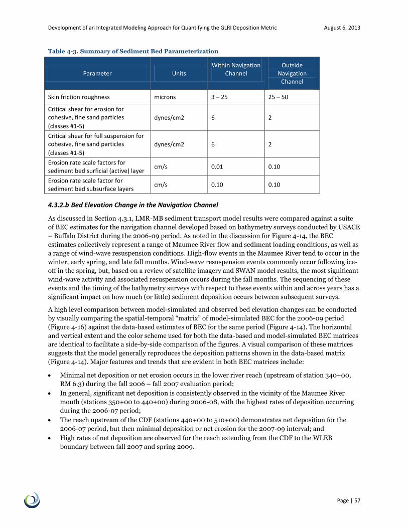
Development of an Integrated Modeling Approach for Quantifying the GLRI Deposition Metric August 6, 2013
Page | 57
Table 4-3. Summary of Sediment Bed Parameterization
Parameter Units Within Navigation
Channel Outside
Navigation Channel
Skin friction roughness microns 3 – 25 25 – 50
Critical shear for erosion for cohesive, fine sand particles
(classes #1-5)
dynes/cm2 6 2
Critical shear for full suspension for cohesive, fine sand particles
(classes #1-5)
dynes/cm2 6 2
Erosion rate scale factors for sediment bed surficial (active) layer
cm/s 0.01 0.10
Erosion rate scale factor for sediment bed subsurface layers
cm/s 0.10 0.10
4.3.2.b Bed Elevation Change in the Navigation Channel
As discussed in Section 4.3.1, LMR-MB sediment transport model results were compared against a suite
of BEC estimates for the navigation channel developed based on bathymetry surveys conducted by USACE
– Buffalo District during the 2006-09 period. As noted in the discussion for Figure 4-14, the BEC
estimates collectively represent a range of Maumee River flow and sediment loading conditions, as well as
a range of wind-wave resuspension conditions. High-flow events in the Maumee River tend to occur in the
winter, early spring, and late fall months. Wind-wave resuspension events commonly occur following ice-
off in the spring, but, based on a review of satellite imagery and SWAN model results, the most significant
wind-wave activity and associated resuspension occurs during the fall months. The sequencing of these
events and the timing of the bathymetry surveys with respect to these events within and across years has a
significant impact on how much (or little) sediment deposition occurs between subsequent surveys.
A high level comparison between model-simulated and observed bed elevation changes can be conducted
by visually comparing the spatial-temporal “matrix” of model-simulated BEC for the 2006-09 period
(Figure 4-16) against the data-based estimates of BEC for the same period (Figure 4-14). The horizontal
and vertical extent and the color scheme used for both the data-based and model-simulated BEC matrices
are identical to facilitate a side-by-side comparison of the figures. A visual comparison of these matrices
suggests that the model generally reproduces the deposition patterns shown in the data-based matrix
(Figure 4-14). Major features and trends that are evident in both BEC matrices include:
Minimal net deposition or net erosion occurs in the lower river reach (upstream of station 340+00,
RM 6.3) during the fall 2006 – fall 2007 evaluation period;
In general, significant net deposition is consistently observed in the vicinity of the Maumee River
mouth (stations 350+00 to 440+00) during 2006-08, with the highest rates of deposition occurring
during the 2006-07 period;
The reach upstream of the CDF (stations 440+00 to 510+00) demonstrates net deposition for the
2006-07 period, but then minimal deposition or net erosion for the 2007-09 interval; and
High rates of net deposition are observed for the reach extending from the CDF to the WLEB
boundary between fall 2007 and spring 2009.

Development of an Integrated Modeling Approach for Quantifying the GLRI Deposition Metric August 6, 2013
Page | 58
Figure 4-16. Spatial and Temporal Variability in Model-Simulated “Bed Elevation Change” for 2006-09
Western
Lake Erie
Basin
CDF
Mouth
Lake Erie
2006
Station
390+00
Station
514+00
Station
715+00
Head of Nav Channel
(Station 0+00)
2007 2008 2009
Color Bin Min BEC (cm) Max BEC (cm)
-50 -5
-5 5
5 10
10 15
15 20
20 25
25 30
30 35
35 40
40 9999
Note: Positive (+) and negative (-) values in the matrix
indicate net deposition and net erosion, respectively.

Development of an Integrated Modeling Approach for Quantifying the GLRI Deposition Metric August 6, 2013
Page | 59
More detailed comparisons of spatial trends exhibited by the model-simulated and data-based BEC
results can be made using longitudinal profile plots, such as those provided in Figures 4-17, 4-18, and 4-
19. The horizontal access for these longitudinal profile plots represents the navigation channel stationing
(in feet) from upstream (left) to downstream (right), extending from near the head of the channel to
approximately the end of the Toledo Harbor navigation channel in the middle of the WLEB. The locations
of the Maumee River mouth, the CDF boundary, and the WLEB boundary are highlighted by vertical black
lines for reference. The vertical axis represents the change in bed elevation (BEC) for a given model grid
cell location, ranging from -20 cm to +80 cm. Model-simulated (blue squares) and data-based (red
circles) BEC estimates are shown on each plot for a specific time period.
The longitudinal profile plot in Figure 4-17 shows model-simulated and data-based BEC estimates for the
time period generally spanning summer/fall 2006 – summer/fall 2007. (The BEC results located between
stations 550+00 and 720+00 are an exception, as these results are associated with the May 2007 –
July/September 2007 timeframe). The following observations can be made based on visual comparisons
of the model-simulation and data-based estimates for the 2006-07 timeframe:
The model generally predicts small net deposition (< 10 cm) or net erosion in the lower river
upstream of the mouth (i.e., upstream of station 330+00). These results are consistent with the data-
based estimates for this reach.
Both the model and the data-based estimates in the vicinity of the Maumee River mouth (stations
350+00 to 450+00) demonstrate relatively high net deposition ranging from 10 to 50 cm for the
2006-07 period. This deposition is primarily the result of a series of about 10 intermediate high-flow
events (20,000 – 60,000 cfs) occurring between fall 2006 and spring 2007 (see Figures A-1 and A-2
in Appendix A). Data-based and model-simulated (depositional) BECs in the vicinity of the CDF also
indicate relatively high deposition, but are lower than BECs at the mouth. For this time period, the
model tends to somewhat under-predict the data-based estimates of BEC for these reaches, although
spatial trends are very similar.
Data-based BEC estimates available for relatively short timeframes (< 4 months) within summer
2007 and 2009 suggest that minimal deposition occurs during these periods. This is consistent with
expectations because these time periods experience minimal loading from the Maumee River and
wind-wave activity in Maumee Bay and the WLEB is also minimal. The model accurately captures the
low rates of deposition that are observed during these brief periods in 2007 and 2009.
Relatively high rates of deposition ranging from 10 to 30 cm are also observed for the data-based
estimates near the WLEB boundary. The sediment transport model reproduces these BEC estimates
very well for this time period.

Development of an Integrated Modeling Approach for Quantifying the GLRI Deposition Metric August 6, 2013
Page | 60
Figure 4-17. Comparison of Simulated to Observed “Bed Elevation Change” in the Toledo Harbor Navigation Channel (summer/fall 2006 – summer/fall 2007)
The longitudinal profile plot in Figure 4-18 shows model-simulated and data-based BEC estimates for the
time period generally spanning summer/fall 2007 – summer/fall 2008. (The BEC results located between
stations 500+00 and 550+00 and beyond station 900+00 are an exception, as these results are based on
timeframes for spring/summer 2008). The following observations can be made based on visual
comparisons of the model-simulation and data-based estimates for the 2007-08 timeframe:
The model accurately reproduces the data-based BEC estimates in the vicinity of the Maumee River
mouth, which range from 10 to 30 cm. Deposition at the mouth during this time period is generally
lower than the 10-50 cm of deposition observed for the 2006-07 period.
Likewise, the model closely reproduces the high net deposition (30 to 40 cm) indicated by the data-
based BEC estimates for the reach between the CDF and the WLEB boundary.
The data-based BEC estimates for the reach beyond the WLEB boundary (stations 800+00 to
900+00) suggest net deposition of approximately 10 to 25 cm. The model generally under-predicts
these BEC estimates, with simulated deposition of 5 to 15 cm. This under-prediction is indicative of
the challenges of accurately representing the effects of wind-wave resuspension activity on deposition
in the navigation channel, especially beyond the Maumee Bay / WLEB boundary.
May ‘07 –
Jul/Sep ‘07

Development of an Integrated Modeling Approach for Quantifying the GLRI Deposition Metric August 6, 2013
Page | 61
Figure 4-18. Comparison of Simulated to Observed “Bed Elevation Change” in the Toledo Harbor Navigation Channel (summer/fall 2007 – summer/fall 2008)
The longitudinal profile plot in Figure 4-19 shows model-simulated and data-based BEC estimates for the
time period generally spanning summer/fall 2008 – spring 2009. Data-based BEC estimates for the reach
extending from the Maumee River mouth to just beyond the CDF suggest that that relatively low net
deposition (0-15 cm) occurred during this period. Deposition during the 2008-09 period was likely
limited by two extreme high-flow event (~65,000 cfs in February, and ~90,000 cfs in March) occurring
during winter of 2009 (see Figure A-4 in Appendix A). Model simulation results indicate that in-channel
velocities and shear stresses that occur during these extreme flow events are sufficiently high to prevent
(or at least significantly limit) deposition in the navigation channel between the mouth and the CDF, thus
providing natural “maintenance” of the channel and limiting the overall deposition that occurs during
these periods.
Data-based BEC estimates are also available just “upstream” of the Maumee Bay / WLEB boundary
(stations 600+00 to 700+00) for the 2008-09 period. These estimates suggest net deposition on the
order of 40 to 50 cm between fall 2008 and spring 2009. Model-simulated deposition for this reach over
this same time period are considerably lower (~15 cm). The elevated data-based BEC estimates for this
reach are in contrast to the much lower deposition estimates near the mouth and CDF for the same time
period. The apparent “disconnect” suggests that while the extreme high-flow events that occurred during
February-March 2009 prevented (or significantly limited) deposition in the navigation channel near the
mouth and CDF, shear stresses beyond station 600+00 were likely sufficiently low to permit deposition of
sediment to the channel. The model represents this transition from relatively high energy near the mouth
to lower energy near the Maumee Bay / WLEB boundary reasonably well. The discrepancy between the
model-simulated and data-based deposition estimates near the WLEB boundary appear to be the result of
the model under-predicting deposition resulting from wind-wave resuspension during this time period.
Although the model appears to represent wind-wave resuspension relatively well over the 2006-09
May ‘08 –
Jul ‘08Apr ‘08 –
May ‘08

Development of an Integrated Modeling Approach for Quantifying the GLRI Deposition Metric August 6, 2013
Page | 62
period, the under-prediction for the 2008-09 timeframe speaks to the challenges in accurately capturing
resuspension and re-deposition behavior for a specific time period.
Available particle size distribution data for the navigation channel suggest that sediments that deposit in
the reach between the mouth and CDF are dominated by cohesive (i.e., clay and silt) particles. Only
limited particle size observations are available for the navigation channel near the Maumee Bay / WLEB
boundary; however, these data suggest that a significant fraction (20-50%) of deposited sediments in this
area are non-cohesive (Jay Miller, USACE – Buffalo District, personal communication). The upstream-to-
downstream transition from a predominantly cohesive bed (with only small fractions of sand) to a mixed
cohesive / non-cohesive bed reflects the higher sand content of sediments in Maumee Bay and the WLEB
shoreline extending to the north and south of the Bay. Although there are not sufficient data available at
present to confirm this, LMR-MB model simulations suggest that a large fraction of the overall deposition
in the vicinity of the Bay / WLEB boundary is likely the result of longshore drift of sand (as well as clay
and silt material) from the north or south shoreline depending on the circulation patterns at the time of a
wind-wave mediated resuspension event. Developing a better understanding of the complex interactions
between the WLEB shoreline, wind-wave activity, and deposition in this reach of the channel would
require additional data collection, evaluation, and modeling that is beyond the scope of the current
project.
Figure 4-19. Comparison of Simulated to Observed “Bed Elevation Change” in the Toledo Harbor Navigation Channel (summer/fall 2008 – spring 2009)
Given the complexity of sediment transport behavior in this system, the overall performance of the model
with respect to reproducing temporal and spatial trends in BECs is considered to be very good.
Approximately 100 sediment transport calibration simulations were conducted for the 2006-09 period to
optimize the fit of the model-predicted BECs to the data-based BECs. As the calibration process
approached completion, it was determined that the model fit to BEC data near the river mouth and CDF

Development of an Integrated Modeling Approach for Quantifying the GLRI Deposition Metric August 6, 2013
Page | 63
for a given time period could not be further improved without sacrificing performance for a different time
period. For example, the under-prediction of BECs for 2006-07 (Figure 4-17) could not be further
improved without causing a significant over-prediction of BECs for the 2007-08 and 2008-09 periods
(Figures 4-18 and 4-19). Considerable effort was also invested in evaluating potential improvements to
model-predicted BECs near the WLEB boundary. However, it was ultimately determined that the lack of
water column TSS data during resuspension events and the lack of sediment bed information along the
WLEB shoreline are key factors limiting the further refinement and calibration of the resuspension and
re-deposition processes represented in the model for this region. Therefore, as noted above, additional
data collection would be necessary to support further refinement of the model in this region.
The preceding figures and discussion have focused on spatial trends within the navigation channel, as well
as temporal trends within the overall 2006-09 calibration period. It is also valuable to pair all of the
associated data-based and model-simulated BEC estimates in order to evaluate the “goodness of fit” and
potential bias for the model-simulated results (i.e., relative to the data-based estimates). Figure 4-20 plots
a one-to-one comparison of paired simulated and data-based BEC values. Consistent with previous
figures, each point represents net deposition (or net erosion) for a (laterally-averaged) model grid cell for
a specific timeframe within the 2006-09 period. The solid red line represents the one-to-one line, and the
dashed red lines represent +/- 15 cm around the one-to-one line for reference. The model-simulated BEC
values were linearly regressed against the data-based estimates, and the resulting line of best fit is shown
as a black line. The line of best fit has a slope of 0.68 and a coefficient of correlation (R2) of 0.60. These
results suggest that the model is slightly biased low relative to the data, meaning that overall the model
tends to under-predict the data-based estimates more than it over-predicts. This is generally consistent
with the observations discussed above for the longitudinal plots in Figures 4-17 through 4-19. When
evaluating the sediment transport model, it is important to keep in mind that the point-by-point
comparisons presented here are the most severe test of the model’s ability to reproduce observed system
behavior. Collapsing of the model-simulated and data-based BEC estimates across space and/or time
would tend to improve the model’s “goodness of fit” through averaging of outlier points. Taking the
specificity of the model-data comparisons into consideration and the strong coefficient of correlation for
the regression (R2 = 0.60), the model is demonstrating a high level of performance overall. This provides
confidence that the LMR-MB sediment transport model can be used to accurately assess current and
future deposition patterns in the Toledo Harbor navigation channel in support of the GLRI deposition
metric evaluation.
When reviewing model-data comparisons for bed elevation change, it is also important to keep in mind
that the LMR-MB sediment transport model is only able to account for the natural physical processes of
sediment delivery, transport, deposition, and erosion/resuspension resulting from elevated shear stresses
due to elevated velocities and/or wind-wave activity. The model does not directly account for other
processes that may contribute to deposition or erosion in the navigation channel including:
1. Episodic “natural” sloughing of the navigation channel “walls” – given the steep slopes
encountered on either side of the channel in Maumee Bay, sloughing is likely to periodically
contribute to and enhance local “deposition” in the channel.
2. Sloughing of material into the navigation channel as a result of barge/freighter passage or
turning.
3. Resuspension and/or redistribution of sediments within the channel due to barge/freighter
passage. Bathymetry survey data clearly show a “strip” of lower bed elevations along the
centerline of the navigation channel, which suggests that ship traffic tends to maintain the center
of the channel by eroding or “pushing” sediments.

Development of an Integrated Modeling Approach for Quantifying the GLRI Deposition Metric August 6, 2013
Page | 64
Figure 4-20. One-to-One Comparison of Model-Simulated versus Observed Bed Elevation Change for the 2006-09 Calibration Period
4.3.2.c Total Suspended Solids in Maumee Bay and Western Lake Erie Basin
Model predictions for total suspended solids in Maumee Bay were qualitatively compared against
available satellite imagery and water column TSS data. Qualitative (i.e., visual) comparisons were made
against MODIS satellite imagery to assess the presence or absence wind-wave resuspension events and/or
the projection of the Maumee River sediment plume into Maumee Bay and the WLEB. For example,
Figure 4-21 compares the model-simulated TSS concentration plume (bottom panel) to a MODIS satellite
image (top panel) for April 18, 2006. This comparison is for a day approximately two weeks after a peak
event flow of 14,200 cfs in the Maumee River on April 4. The satellite image clearly shows the residual
sediment plume from this loading event within Maumee Bay and pushing out in the WLEB. In addition,
wind-wave activity in the preceding days has generated resuspension of bottom sediments along the
shoreline, especially the southern shoreline between Maumee Bay and Sandusky Bay to the east. A visual
comparison of the top and bottom panels suggest that the TSS concentration plume(s) simulated by the
sediment transport model closely resemble the observed extent of the TSS plumes in the satellite image.
In addition to the Maumee-driven plume positioned in and around Maumee Bay, the model appears to
accurately simulate the extent of the suspended sediment plume resulting from a wind-wave resuspension
event along the southern shoreline. Although only a qualitative comparison is possible to this and other
satellite images, the consistency in the extents of the simulated sediment plumes relative to the observed
plumes provides confidence that the model is accurately predicting 1) circulation patterns in the WLEB,
and 2) the timing of wind-wave resuspension events.
As discussed in Section 4.3.1, approximately 550 turbidity measurements were made by University of
Toledo researchers at location throughout Maumee Bay during the 2006-09 period (Bridgeman et al.
+/- 15 cm

Development of an Integrated Modeling Approach for Quantifying the GLRI Deposition Metric August 6, 2013
Page | 65
2013). A regression developed based on paired turbidity and TSS concentration data from the 2003
monitoring effort was used to estimate TSS concentrations based on these turbidity measurements.
Model-predicted TSS concentrations were compared against the data-based estimates for the following
sampling dates:
For year 2006: 5/4, 5/31, 7/13, 8/1, 8/16, 9/5, 9/26;
For year 2007: 5/21, 6/12, 6/21, 6/27, 7/3, 7/10, 7/24, 8/2, 8/14, 8/24, 9/18, 10/8;
For year 2008: 5/13, 5/29, 6/11, 6/24, 7/10, 7/16, 7/24, 8/6, 8/12, 8/21, 9/1, and 9/25; and
For year 2009: 5/29, 6/15, 7/1, 7/13, 8/6, 8/19, 9/11, and 10/6.
Figures 4-22 through 4-25 provide a series of map-based comparisons of model-simulated TSS (as
colored grid cells) to data-based TSS concentrations (as colored points) under a variety of conditions in
Maumee Bay. A brief discussion of the model-data comparisons in these figures is provided below:
Figure 4-22 depicts a TSS model-data comparison during a period of relatively low river flow and
quiescent conditions (i.e., no wind-wave activity) in Maumee Bay. TSS concentrations observed in
Maumee Bay and further out into the WLEB on this day fall within the 10-20 mg/l range. The model
consistently simulates TSS concentrations within the 10-20 mg/l range within Maumee Bay under
these conditions.
Figure 4-23 depicts a TSS model-data comparison during a period of very low river flow when there
has been some relatively recent wind-wave resuspension activity in Maumee Bay. Observed and
simulated TSS concentrations in the WLEB and near the outer edge of Maumee Bay are generally in
the 5-20 mg/l range. However, residual suspended sediments in inner Maumee Bay are measured in a
range of 30-60 mg/l north of the navigation channel and Grassy Island. The model simulates TSS
concentrations in the 30-100 mg/l range within inner Maumee Bay (with areas of TSS > 100 mg/l in
Ottawa Bay).
Figures 4-24 and 4-25 depict TSS model-data comparisons on days of peak event flow in the Maumee
River on July 10, 2008 and June 11, 2008. Peak flows for these events were in the 14,000 – 17,000 cfs
range, so these events are small to moderate in size relative to the large to extreme events (60,000 –
90,000 cfs) discussed earlier in this chapter. A comparison of the model-simulated TSS
concentrations to the observed TSS concentrations in Figures 4-24 and 4-25 suggests that the model
generally captures the extent of the Maumee River sediment plume during these events. Sediment
plumes generated by the Maumee River load tend to be well-defined, resulting in a sharp gradient in
TSS concentration when moving from within the plume to just outside the plume. Therefore, even
relatively small differences in plume location can have a dramatic impact on the observed or
simulated TSS concentration.
It should be noted that some of the TSS concentrations measured by the University of Toledo during the
summer and early fall months in Maumee Bay and the WLEB may reflect high algal productivity and/or
local resuspension due to barge/freighter passage. For example, a TSS concentration in the 60-100 mg/l
range was measured near the end of the Toledo Harbor navigation channel on July 10, 2008. Wind-wave
resuspension cannot explain such a high concentration during a quiescent period in the WLEB.
Overall, the model-data comparisons for TSS concentrations in Maumee Bay and the WLEB for the 2006-
09 period suggest that the model reasonably reproduces suspended solids conditions observed in the
water column during this time. The model compares favorably to monitoring data collected for low-flow
and high-flow periods in the Maumee River, which provides confidence that the model reasonably
represents the magnitude and extent of the Maumee River sediment plume under a range of conditions.
Likewise, model-data comparisons for time periods exhibiting a range of wind-wave activity (i.e., from
quiescent conditions to high wind-wave activity) provide confidence that the resuspension and
subsequent sediment plume transport simulated by the model is realistic.

Development of an Integrated Modeling Approach for Quantifying the GLRI Deposition Metric August 6, 2013
Page | 66
Figure 4-21. Comparison of Model-Simulated Suspended Sediment Plume (left) and MODIS Imagery (right) for April 18, 2006

Development of an Integrated Modeling Approach for Quantifying the GLRI Deposition Metric August 6, 2013
Page | 67
Figure 4-22. Model-Data Comparison for Total Suspended Solids Concentrations in Maumee Bay and Western Lake Erie Basin (September 18, 2007; Maumee Flow = 1,340 cfs)
Figure 4-23. Model-Data Comparison for Total Suspended Solids Concentrations in Maumee Bay and Western Lake Erie Basin (October 6, 2009; Maumee Flow = 730 cfs)

Development of an Integrated Modeling Approach for Quantifying the GLRI Deposition Metric August 6, 2013
Page | 68
Figure 4-24. Model-Data Comparison for Total Suspended Solids Concentrations in Maumee Bay and Western Lake Erie Basin (July 10, 2008; Maumee Flow = 16,600 cfs)
Figure 4-25. Model-Data Comparison for Total Suspended Solids Concentrations in Maumee Bay and Western Lake Erie Basin (June 11, 2008; Maumee Flow = 14,900 cfs)

Development of an Integrated Modeling Approach for Quantifying the GLRI Deposition Metric August 6, 2013
Page | 69
4.3.3 Model Confirmation Results
Once the recalibration of the LMR-MB sediment transport model had been substantially completed, the
model was run for the 2004-05 period and compared against available datasets used for the original
calibration effort. The purpose of this exercise was to confirm that the model performed reasonably well
against data for a time period that falls outside of the recalibration timeframe (i.e., 2006-09).
Demonstrating that the model performs well relative to data for 2004-05 would provide even greater
confidence in the ability of the model to predict current and future spatial and temporal sediment
deposition trends in the Toledo Harbor navigation channel.
4.3.3.a Bed Elevation Change in the Navigation Channel
The primary calibration target for the original calibration were bed elevation changes estimated at various
locations in the navigation channel between the Maumee River mouth (station 400+00) and station
800+00 for the March 2004 – May 2005 timeframe. Model-simulated BECs for the same time period are
compared against the data-based estimates in Figure 4-26. The model appears to somewhat over-predict
the magnitude of sediment deposition just downstream of the mouth and for the reach between the CDF
and the Maumee Bay / WLEB boundary. This is not unexpected given the uncertainty in the sediment
loading estimated for the December 2004 - January 2005 high-flow events (see discussion in Section
4.3.1). Suspended sediment concentrations for roughly 40 days during this period were filled in using
data from a similar series of winter events that occurred in January 1991. Suspended sediment loads in
the Maumee River have declined consistently over the past two decades, so it is reasonable to expect that
the TSS concentrations and resulting loads estimated via the 1991 events overstate the actual sediment
load for the winter 2004-05 events.
Despite the probable loading bias discussed above, the model reproduces the overall spatial pattern of
deposition for this time period very well. The data-based BEC estimates suggest that the deposition
between the CDF and the Maumee Bay / WLEB boundary is higher than the deposition between the
mouth and the CFD for this period. The model captures this spatial trend, although deposition beyond the
Maumee Bay / WLEB boundary appears to be over-predicted. Overall the model captures the major
features of the data-based BEC estimates quite well, and, furthermore, the results from the recalibrated
model represent a clear improvement over the original calibration (original calibration figures are
available in LimnoTech (2010a)). This provides additional support and confidence for the predictive
capability of the model with respect to simulating spatial and temporal deposition trends for the Toledo
Harbor navigation channel.

Development of an Integrated Modeling Approach for Quantifying the GLRI Deposition Metric August 6, 2013
Page | 70
Figure 4-26. Comparison of Simulated to Observed “Bed Elevation Change” in the Toledo Harbor Navigation Channel (March 2004 – May 2005)
4.3.3.b Total Suspended Solids in Maumee Bay and Western Lake Erie Basin
The turbidity and TSS datasets acquired and processed for the original LMR-MB model calibration effort
were used to develop map-based model-data comparisons for the 2004-05 period. Example TSS
concentration comparisons for this time period are shown in Figures 4-27 and 4-28. The comparison in
Figure 4-27 is for August 23, 2004 and corresponds to low Maumee River flow conditions and a quiescent
period with respect to wind-wave activity in Maumee Bay. Observed TSS concentrations in Maumee Bay
consistently fall within the 10-20 mg/l, with concentrations further out in the WLEB measured at less
than 5 mg/l. The model captures both the magnitude and the spatial trend in TSS concentrations very
well. The TSS comparison in Figure 4-28 corresponds to a period of high flow and sediment loading in the
Maumee River. University of Toledo sampling for this date included roughly 20 locations, and the
measured TSS concentrations can be used to visually delineate the plume. The model-simulated plume
extent and concentration magnitudes generally match observations, with in-plume TSS concentrations
ranging from 30 to 100 mg/l in Maumee Bay. The model appears to slightly over-predict the extent of the
plume to the southeast and to the north of the Bay, suggesting that there are likely minor differences in
simulated versus actual movement of Maumee River water through the Bay. Overall, the model-data TSS
concentration comparisons for 2004-05 provide further confirmation that the calibrated model can
accurately simulate sediment transport and fate behavior in Maumee Bay and the WLEB.

Development of an Integrated Modeling Approach for Quantifying the GLRI Deposition Metric August 6, 2013
Page | 71
Figure 4-27. Comparison of Simulated (grid) to Observed (points) Total Suspended Solids Concentrations in Maumee Bay (August 23, 2004; Maumee Flow = 5,450 cfs)
Figure 4-28. Comparison of Simulated (grid) to Observed (points) Total Suspended Solids Concentrations in Maumee Bay (June 3, 2004; Maumee Flow = 22,600 cfs)

Development of an Integrated Modeling Approach for Quantifying the GLRI Deposition Metric August 6, 2013
Page | 72
Blank Page

Development of an Integrated Modeling Approach for Quantifying the GLRI Deposition Metric August 6, 2013
Page | 73
5 Model Application for Great Lakes Restoration
Initiative Deposition Metric
Following completion of the model development, recalibration, and confirmation efforts, a series of
application scenarios were designed and implemented with the LMR-MB linked hydrodynamic –
sediment transport – water quality model framework to evaluate the GLRI annual deposition metric for
Toledo Harbor. A brief introduction to the GLRI annual deposition metric is provided in Section 5.1. An
overview of the approach undertaken for developing and evaluating the application scenarios to address
the metric for the Toledo Harbor case study is provided in Section 5.2. Model application development
necessarily involved an in-depth analysis of Maumee River suspended sediment concentration and
loading data to identify recent trends in loading. This analysis is presented and discussed in Section 5.3.
Model application results and findings related to evaluation of the GLRI deposition metric are presented
in Section 5.4, and supporting model diagnostic results are presented in Section 5.5.
5.1 Introduction to the GLRI Deposition Metric
The GLRI Action Plan identifies goals, measureable outcomes, and actions for five focus areas (White
House Council on Environmental Quality 2010). Focus Area 3 is “Nearshore Health and Nonpoint Source
Pollution”; this focus area places priority on reducing the runoff of pollutants, including sediment and
nutrients, from urban and agricultural sources in Great Lakes watersheds. Six long-term goals are
defined within the nearshore focus area, and “Goal 5” is directly relevant to the current project. “Goal 5” is
pertinent to the current sedimentation evaluation for Toledo Harbor (White House Council on
Environmental Quality 2010):
“Goal 5: A significant reduction in soil erosion and the loading of sediment, nutrients and
pollutants into tributaries is achieved through greater implementation of practices that
conserve soil and slow overland flow in agriculture, forestry, and urban areas.” (pg. 27)
Five “Measures of Progress” are described to achieve the six goals defined for the “Nearshore Health and
Nonpoint Source Pollution” focus area, including a specific measure related to sediment deposition in
Great Lakes harbors. This measure is defined as the “annual volume of sediment deposition in defined
harbor areas in targeted watershed (cu yards).” Toledo Harbor is defined as the initial target for this
measure, and the initial deposition volume associated with the baseline year (2008) is specified as one
million cubic yards. Targeted reductions for years 2010-2014 are specified as follows:
2010 Target: 0% improvement (deposition = 1 million cubic yards);
2011 Target: 1% improvement (deposition = 0.99 million cubic yards);
2012 Target: 1% improvement (deposition = 0.99 million cubic yards);
2013 Target: 2% improvement (deposition = 0.98 million cubic yards); and
2014 Target: 2.5% improvement (deposition = 0.975 million cubic yards).
The discussion provided in the Introduction (Chapter 1) for the sediment deposition metric recognizes
that USACE bathymetry survey data can serve as useful supporting datasets but are insufficient on their

Development of an Integrated Modeling Approach for Quantifying the GLRI Deposition Metric August 6, 2013
Page | 74
own for evaluating the sediment deposition measure. The remainder of this chapter documents the
approach developed based on the Maumee River loading data and the calibrated LMR-MB model to
evaluate the deposition measure and associated metrics.
5.2 Overview of Approach
As discussed in Chapter 1, the primary objective of the LMR-MB model development and calibration
effort was to develop an integrated modeling tool that can be used to evaluate changes in sediment
deposition in the Toledo Harbor navigation channel resulting from reductions in Maumee River sediment
loading in response to watershed management activities funded by GLRI and other initiatives. The
general approach for this project was predicated upon comparing model-simulated deposition in the
Toledo Harbor navigation channel for two Maumee River loading conditions:
1. “Actual” Loading Case – the “actual” loading case is intended to represent sediment loading
conditions following the inception of the GLRI program. Daily flow and suspended solids data for
the 2009-11 time period were used to evaluate the “actual” loading condition.
2. “Adjusted” Loading Case – the “adjusted” loading case represents sediment loading
conditions resulting from watershed land conditions and management prior to the first year of the
GLRI program. Daily flow and suspended solids data for the 2004-08 time period were used to
evaluate the “adjusted” loading condition. The timeframe for the pre-2009 period was expanded
to include 2004 and 2005, which are prior to the recalibration period, because: 1) inclusion of
additional years tends to strengthen the trend analysis, and 2) the flow and sediment data were
readily available from the original model calibration effort. Essentially, the “adjusted” loading
case represents an upscaling of the “actual” loading case described above, where “upscaling”
refers to the process of increasing sediment concentrations/loads to represent the higher Maumee
River sediment loading conditions associated with the earlier time period.
The more general terms “adjusted” and “actual” are employed here rather than “pre-GLRI” and “post-
GLRI” because it is recognized that reductions in Maumee River sediment loadings occurring over the
past 5-8 years have been the net result of multiple watershed initiatives being conducted in parallel under
funding from various agencies, including:
Natural Resources Conservation Service (NRCS);
Farm Bill;
USACE 516(e) sediment reduction program; and
Great Lakes Restoration Initiative.
Furthermore, the implementation of GLRI-funded sediment reduction programs cannot be expected to
produce measurable results in the first few years of their installation.
A variety of conservation practices have been implemented for agricultural lands in the Maumee River
watershed over the past 30 years that have served to reduce sediment loading to Maumee Bay and the
WLEB over time. Because the loading of suspended solids by the Maumee River is the dominant driver of
deposition in the Toledo Harbor navigation channel, it follows that an analysis of temporal trends in TSS
loading is needed to support a model-based evaluation of deposition trends. Unfortunately, time trends in
Maumee River sediment loading are obscured by the considerable inter-annual variability observed in the
magnitude and frequency of high-flow events in the Maumee River system. This is illustrated in Figure 5-
1, which compares annual total discharge volume and total annual sediment loading for individual years
within the time period of interest for this project (2004-12).
A comparison of flow and suspended sediment loading for calendar year 2011 versus calendar year 2012
provides a powerful example of inter-annual variability in Maumee River event conditions. Spring and fall
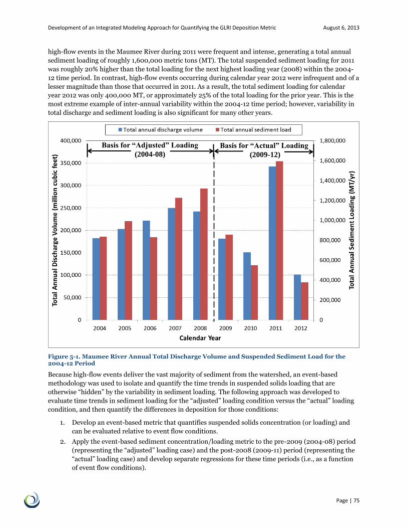
Development of an Integrated Modeling Approach for Quantifying the GLRI Deposition Metric August 6, 2013
Page | 75
high-flow events in the Maumee River during 2011 were frequent and intense, generating a total annual
sediment loading of roughly 1,600,000 metric tons (MT). The total suspended sediment loading for 2011
was roughly 20% higher than the total loading for the next highest loading year (2008) within the 2004-
12 time period. In contrast, high-flow events occurring during calendar year 2012 were infrequent and of a
lesser magnitude than those that occurred in 2011. As a result, the total sediment loading for calendar
year 2012 was only 400,000 MT, or approximately 25% of the total loading for the prior year. This is the
most extreme example of inter-annual variability within the 2004-12 time period; however, variability in
total discharge and sediment loading is also significant for many other years.
Figure 5-1. Maumee River Annual Total Discharge Volume and Suspended Sediment Load for the 2004-12 Period
Because high-flow events deliver the vast majority of sediment from the watershed, an event-based
methodology was used to isolate and quantify the time trends in suspended solids loading that are
otherwise “hidden” by the variability in sediment loading. The following approach was developed to
evaluate time trends in sediment loading for the “adjusted” loading condition versus the “actual” loading
condition, and then quantify the differences in deposition for those conditions:
1. Develop an event-based metric that quantifies suspended solids concentration (or loading) and
can be evaluated relative to event flow conditions.
2. Apply the event-based sediment concentration/loading metric to the pre-2009 (2004-08) period
(representing the “adjusted” loading case) and the post-2008 (2009-11) period (representing the
“actual” loading case) and develop separate regressions for these time periods (i.e., as a function
of event flow conditions).
Basis for “Adjusted” Loading
(2004-08)
Basis for “Actual” Loading
(2009-12)

Development of an Integrated Modeling Approach for Quantifying the GLRI Deposition Metric August 6, 2013
Page | 76
3. Develop daily suspended sediment concentration and loading time series based on Maumee River
flow conditions for the 2009-12 period that are representative of the “actual” and “adjusted”
loading conditions.
4. Develop model scenarios based on the “actual” and “adjusted” loading cases established for the
observed 2009-12 flow conditions.
5. Quantify the decrease in simulated (net) deposition to the Toledo Harbor navigation channel for
the “actual” loading scenario relative to the “adjusted” loading scenario.
Figure 5-2 provides a flow chart highlighting the key steps of the approach. Section 5.3 describes the
process of identifying TSS concentration and loading trends (steps #1-3 above) based on an analysis of
“event mean concentrations” (EMCs) and associated event flow conditions. Section 5.4 presents the
development of the “actual” and “adjusted” loading scenarios in the LMR-MB sediment transport model
and the results of those scenarios (steps #4-5 above).
It should be noted that the analysis of sediment loading trends for the “actual” loading case (post-2008
period) did not consider flow and loading conditions for calendar year 2012, because the necessary data
were not available at the time the analysis was conducted. However, because the low-flow conditions in
2012 are of interest with respect to evaluating system behavior and the GLRI deposition metric for an
extreme low-flow year, the timeframe for model application was extended to include 2012. Therefore, the
time period for the model application corresponded to 2009-12.

Development of an Integrated Modeling Approach for Quantifying the GLRI Deposition Metric August 6, 2013
Page | 77
Figure 5-2. Flow Chart of Approach for Quantifying the GLRI Deposition Metric for 2009-12
5.3 Estimation of Loading Reductions for Post-2008 Period
As discussed in Chapters 2 and 3, the daily flow and TSS concentration data that have been collected at
Waterville, OH provide long-term datasets that can be used for examining sediment loading trends.
Maumee River daily flow data have been collected by the USGS at the Waterville gaging location since the
late 19th century, and daily TSS concentration data have been measured by Heidelberg University since
1975. Therefore, the available flow and sediment data records can support not only an evaluation of recent
trends in suspended solids loading, but potentially also a 35+ year analysis of loading trends. Daily flow

Development of an Integrated Modeling Approach for Quantifying the GLRI Deposition Metric August 6, 2013
Page | 78
and TSS records were initially obtained for the 1975-2011 time period. Daily flow data were obtained from
the USGS website7 for gauging station 04193500. Daily TSS records were obtained from the National
Center for Water Quality Research at Heidelberg University8. The flow record was continuous throughout
the 1975-2011 period, but the TSS record contained data gaps which required occasional estimation of TSS
values. The 2004-08 period had 161 days missing TSS observations and the 2009-2011 period had 52 days
missing TSS observations. These missing values were filled in using a combination of linear interpolation
and best professional judgment. Estimation of TSS values was typically accomplished by identifying a flow
event for which TSS data were available and which had similar characteristics to the flow event requiring
TSS estimates (e.g., peak flow rate, duration, season). For brief gaps of 1-3 days, linear interpolation was
typically used. In addition to flow and TSS data, daily precipitation and snowpack records were also
gathered to provide supporting information.
Evaluation of the flow and sediment loading data proceeded as follows:
1. Long-term trends were evaluated for the 1975-2011 period, in order to provide context for the
shorter term analysis;
2. Potential flow and sediment metrics for high-flow events were explored, and a final set of metrics
was selected to support the sediment loading trend analysis for the “adjusted” (pre-2009) and
“actual” (post-2008) loading conditions.
3. A regression was developed based on the relationship between the sediment and flow metrics
defined for the 2004-08 period.
4. The actual observed suspended solids concentrations and associated loadings for the 2009-12
period were defined as the “actual” loading case. The above-mentioned regression was used as the
basis for increasing (i.e., “upscaling”) flow-dependent TSS concentrations for the 2009-12
hydrology period to be consistent with observed 2004-08 suspended sediment concentrations.
This upscaling of TSS concentrations produced the “adjusted” TSS daily loading time series.
5. Model simulations were performed to quantify deposition to the navigation channel for both the
“actual” and the “adjusted” loading scenarios.
The following sections provided a detailed discussion of the implementation of these steps.
5.3.1 Delineation of High-Flow Events
The delineation of Maumee River high-flow (i.e., runoff) events was a prerequisite for evaluating the long-
and short-term trends using the event-based approach alluded to above. A set of criteria were developed
to define the initiation and termination of individual events based on manual inspection of the daily
hydrograph for 1975-2011. These criteria were ultimately defined as follows:
Event Initiation: The initiation of a high-flow event occurs when either 1) the mean daily flow is less
than 10,000 cfs on the prior day and then exceeds 10,000 cfs, or 2) the flow is already greater than
10,000 cfs but the hydrograph transitions from the falling limb of a prior event to the rising limb of
the new event.
Event Termination: A high-flow event is terminated when either 1) the mean daily flow rate drops
below 6,500 cfs, or 2) the flow is greater than 6,500 cfs, but the rising limb of a subsequent event
begins.
As indicated above, bimodal events were delineated as separate events based on the point in time where
the hydrograph transitioned from the falling (declining) limb of the first event to the rising limb of the
second event. A macro program was developed in Microsoft Excel Visual Basic for Applications (VBA) to
7 http://waterdata.usgs.gov/nwis/dv/?site_no=04193500&agency_cd=USGS&referred_module=sw 8 http://www.heidelberg.edu/academiclife/distinctive/ncwqr/data/data)

Development of an Integrated Modeling Approach for Quantifying the GLRI Deposition Metric August 6, 2013
Page | 79
automate the delineation of high-flow events based on these criteria. The VBA program also tabulates key
flow and sediment metrics, including:
Peak flow rate (cfs) and date of peak flow occurrence;
Number of days between event initiation and the date of peak flow;
Total event volume (km3);
Total suspended solids load (MT);
Total suspended solids EMC (mg/l);
Maximum TSS concentration (mg/l) and date of occurrence.
A total of 436 events were defined for the 1975-2011 period (average of 11.8 events per year). A total of 76
events were observed in the 2004-08 period (average of 15.2 events per year), and 38 events were
observed within the 2009-2011 period (average of 12.7 events per year). EMCs for TSS were computed
using the following equation:
NDays
n n
NDays
n nn
event
Q
QCEMC
1
1 (5-1)
where EMCevent (mg/l) is the event mean concentration, NDays is the total number of days associated with
an event, and Qn (cfs) and Cn (mg/l) are the mean daily flow and the observed (or estimated) TSS
concentration, respectively, for the nth day of the event. Because the EMC represents the mean
concentration during a particular event, an alternative method for calculating the EMC is to divide the
total suspended sediment loading for the event (in MT) by the total event volume, making appropriate
corrections to obtain the desired units of mg/l.
5.3.2 Long-Term Trends in Sediment Loading Reduction
In order to provide historical context for the shorter term evaluation of Maumee River sediment loading
trends for the 2004-2011 period, the long-term trend in suspended solids loading was analyzed for the
period of TSS monitoring (1975-2011). As discussed previously, analyzing the trend in Maumee River
sediment loads requires that the inter-annual variability in event flows and loads be somehow factored
out of the analysis. To accomplish this, an average annual EMC was calculated for each year in the 1975-
2011 period using the event-specific EMCs (calculated via Equation 5-1) and based on the following
equation:
NEvent
i i
NEvents
i ii
annual
V
VEMCEMC
1
1 (5-2)
where EMCannual (mg/l) represents the “annual average” EMC for all events within the year, NEvents is
the total number of events for the year, EMCi is the event mean concentration of the ith event (computed
using Equation 5-1), and Vi is the total discharge volume for the ith event. The annualized EMCs generated
with this equation were considered to be reasonably representative of average TSS concentrations for the
universe of events experienced during a given year, while recognizing that the magnitude and frequency of
extreme runoff events could skew the annualized EMC value calculated for years when such events
occurred.
The EMC results for 1975-2011 are plotted in Figure 5-3, including a linear regression fit to the data. This
analysis reveals a generally consistent downward trend in EMC values over the past 37 years, with the
EMC declining by approximately 3.9 mg/l each year. Richards et al. (2008) have reported a comparable
long-term trend for Maumee River TSS concentrations, with the “flow-adjusted” concentration declining

Development of an Integrated Modeling Approach for Quantifying the GLRI Deposition Metric August 6, 2013
Page | 80
from 90 mg/l in 1975 to roughly 40 mg/l by 2005. The EMCs computed for 1989 and 1990 are outliers for
the analysis, with values in the 500-600 mg/l range. The reason for the exceptionally high TSS EMCs in
1989 and 1990 is not entirely clear, although an extreme flow event of 86,000 cfs in 1990 is a major driver
for the 600 mg/l EMC for that year.
Figure 5-3. Long-Term Trend in Average Annual “Event Mean Concentrations” for Maumee River High-Flow Events
5.3.3 Sediment Loading Reduction Trend for Pre-2009 and Post-2008 Conditions
A variety of metrics were calculated and evaluated for Maumee River TSS concentration and daily flow
rate. Event peak TSS concentration and EMCs for TSS were compared to both event peak flow rates and
total event discharge volumes, and linear regressions were developed to quantify the (potential)
relationships between candidate TSS and flow metrics. The TSS and flow metrics were uniformly log-
transformed prior to the development of the linear regressions because both TSS concentrations and daily
flow values are log-normally distributed. Seasonal variation in the TSS EMCs was also examined, but the
seasonal variation did not appear to be strong enough to warrant inclusion in the regressions. Five of the
events in the 2004-08 period had no TSS observation available during the events, so these events were
excluded from the regression analysis.
An additional consideration for the regression analysis was the effect of runoff events that were primarily
driven by snow melt in the Maumee River watershed. Daily precipitation and snowpack records were
obtained and compared with the daily flow and TSS records. Rainfall that occurs while snowpack is
present tends to cause runoff events with lower TSS concentrations. Reductions in TSS runoff
concentration and loading under these conditions will be highly variable and event-specific, depending on
the initial thickness of the snowpack and the extent to which the snowpack is reduced during the runoff
event. Likewise, reductions in TSS loading associated with these events in response to improvements in
agricultural land are also uncertain. In recognition of the uncertainties and variability associated with
these events, it was conservatively assumed that sediment loading associated with runoff events involving
melting of the snowpack has not decreased as the result of watershed management activities during the
2004-12 period. The meteorological record from 2004-2011 was reviewed, and runoff events which

Development of an Integrated Modeling Approach for Quantifying the GLRI Deposition Metric August 6, 2013
Page | 81
involved melting snowpack were flagged and excluded from the regression analysis, as well as from the
application of the regression to the 2009-12 period (used to develop the “adjusted” loading case).
Candidate regressions were assessed based on the coefficient of correlation (R-squared value) they yielded
and consideration of how the relationship could be used to modify the daily loading time series associated
with the actual 2009-12 period (representing the “actual” loading case). The sediment/flow metric
combination that demonstrated the strongest correlation involved the TSS EMC (mg/l) calculated and the
peak flow rate (in units of cfs) observed for individual events. A final regression was developed for the
2004-08 period using the log (base 10)-transformed peak flow as the independent variable and log (base
10)-transformed EMC as the dependent variable. “Snowmelt” events and events with no TSS
concentration data within the 2004-08 period were excluded, as discussed above.
The resulting mean regression for log10-normalized TSS EMC (mg/l) and peak flow rate (Qp, cfs) is shown
in Figure 5-4 (solid red line). The mean regression fit to the log10-transformed data yielded a coefficient of
correlation (R2) of 0.54 for the following equation:
22.178.01010
p
QLogEMCLog (5-3)
The data in Figure 5-4 exhibit considerable variability around the mean regression, which is expected
given the inherent variability in environmental conditions affecting sediment delivery from the Maumee
watershed to the mouth during runoff events. In order to help bound the uncertainty in the linear
regressions, 95% confidence bands were calculated for the regression lines based on statistical methods
documented in Benjamin and Cornell (1970). The confidence bands indicate a 95% degree of confidence
that the true fit to the data lies within the bands. The lower and upper 95th percentiles are plotted as
dotted red lines in Figure 5-4.
Figure 5-4. Regression of Log10-Normalized TSS “Event Mean Concentration” vs. Log10-Normalized Event Peak Flow Rate for 2004-08
Mean regression
Lower 95% C.I.
(Log EMC) = 0.78 * (Log Qpeak) – 1.22
R2 = 0.54
Upper 95% C.I.

Development of an Integrated Modeling Approach for Quantifying the GLRI Deposition Metric August 6, 2013
Page | 82
The regression trend line was used to estimate the sediment loading that would have occurred for the
2009-12 period if average watershed conditions and associated rates of sediment export to Toledo Harbor
for the 2004-08 period had remained constant beyond 2008. The following steps were followed to
“upscale” the actual observed sediment loads for 2009-12 (i.e., “actual” loading case) to represent the
“adjusted” loading case:
1. The relationship between TSS EMC and peak flow rate for the 2004-08 period (Equation 5-3) was
used to replace the observed EMCs (i.e., those calculated based on actual TSS observations) for
each individual event within the 2009-12 period.
2. The total sediment loading for each individual event within the 2009-12 period was recalculated
based on the “adjusted” EMCs calculated and substituted in step 1.
3. The total sediment loading for the 2009-12 hydrograph was calculated for both the “adjusted”
(i.e., “upscaled” based on 2004-08 concentrations) and the “actual” (i.e., actual observed) TSS
EMCs.
4. The difference between the total sediment loading for the “adjusted” and “actual” loading cases
were computed.
These steps were followed to compute total sediment loading for the 2009-12 period for the mean
regression, as well as for the regressions calculated for the lower and upper 95% confidence interval (CI).
For the lower/upper 95% CI cases, the “adjusted” TSS EMCs were calculated for each runoff event in
2009-12 by entering peak flow rates into the equations associated with those cases. Observed TSS
concentrations for non-event days within the 2009-12 period were not replaced, nor were concentrations
for snowmelt events. Approximately 23% of the days in the 2009-12 period were updated with TSS values
from the regression, while 77% of the days used the original measured TSS value without change.
Table 5-1 provides a summary of the total and annual average TSS loads and the percent reductions
relative to the “actual” loading case (i.e., observed loading for 2009-12) calculated for the mean and
lower/upper 95% CI regression cases. For the mean regression for the “adjusted” loading case, a 29%
increase in total sediment loading is calculated relative to the “actual” loading case. The 2009-12
sediment loads calculated for the lower and upper 95% CI regressions are 8% and 29% higher,
respectively, than the sediment load for the “actual” loading case. Overall, this analysis suggests that the
effective reduction in TSS loading for the “actual” loading case relative to the “adjusted” loading case is in
the range of 8-29%, with a mean value of approximately 19%. Within this context, the term “effective”
refers to changes in loading or deposition that are estimated/calculated once differences in the raw
sediment loading that are attributed to differing river flow conditions for two time periods have been
factored out. For example, a 50,000 cfs high-flow event during “Year 2” will inevitably have a higher rate
of sediment loading than a smaller 10,000 cfs event that occurred the prior year (“Year 1”), primarily due
to the disparity in the magnitudes of the events. The effective change in loading, however, would be
determined based on an assessment of whether a comparable 50,000 cfs event in “Year 1” would have
(hypothetically) delivered a higher, lower, or equivalent sediment load relative to the “Year 2” event.
The loads summarized in Table 5-1 served as the basis for developing a series of LMR-MB model
application simulations aimed at quantifying the reduction in Toledo Harbor navigation channel
deposition associated with the effective reduction in the TSS loading for the 2009-12 period relative to the
2004-08 period. The design, implementation, and outcome of those model simulations are discussed in
Section 5.4 below.

Development of an Integrated Modeling Approach for Quantifying the GLRI Deposition Metric August 6, 2013
Page | 83
Table 5-1. Summary of Loading Conditions for the “Actual” and “Adjusted” Scenarios
Loading Scenario (for 2009-12) Total TSS Load
(MT) Annualized TSS Load (MT/yr)
% Difference Relative to
“Actual” Case
“Actual” Case (observed loads) 3,378,715 844,679 --
“Adjusted” Case (mean regression) 4,186,652 1,046,663 +19%
“Adjusted” Case (lower 95% CI) 3,691,210 922,803 +8%
“Adjusted” Case (upper 95% CI) 4,780,453 1,195,113 +29%
5.4 Evaluation of the GLRI Deposition Metric Based on Comparison of the
“Adjusted” and “Actual” Sediment Loading Scenarios for 2009-12
A suite of LMR-MB model simulations were developed to quantify the navigation channel deposition
volumes associated with the various loading scenarios summarized in Table 5-1. A total of four scenarios
were developed, corresponding to the four loading scenarios:
1. “Actual” Case – representing observed TSS concentrations and loadings for the 2009-12 period;
2. “Adjusted” Mean Regression Case – representing “upscaled” TSS loadings for the 2009-12 period
based on the EMC regression developed for the 2004-08 period (see Figure 5-4 and Equation 5-
3);
3. “Adjusted” Lower 95% CI Case – representing “upscaled” TSS loadings for the 2009-12 period
based on the lower bound EMC regression developed for the 2004-08 period; and
4. “Adjusted” Upper 95% CI Case – representing “upscaled” TSS loadings for the 2009-12 period
based on the upper bound EMC regression developed for the 2004-08 period.
Daily TSS concentrations for the Maumee River inflow boundary were specified using the modified TSS
concentration time series discussed earlier in this chapter, and continuous model simulations were run
starting on January 1, 2009 and ending on September 30, 2012. (The October-December, 2012 period was
not simulated due to missing input data for flows and TSS concentration for these months.) Bed elevation
change (BEC) results for each grid cell within the navigation channel were extracted for the final day of
the simulation (9/30/2012). A comparative spreadsheet analysis was conducted for the four simulations
in order to calculate the difference in simulated BEC by grid cell and for the navigation channel as a
whole. Longitudinal profile plots comparing the simulated BECs for the navigation channel for the
“actual” and the various “adjusted” loading scenarios were developed and are presented and discussed
below.
The longitudinal profile comparing the “actual” case to the “adjusted” mean regression case is shown in
Figure 5-5. Similar profiles comparing the “actual” case to the “adjusted” lower 95% CI case and the upper
95% CI case are provided in Figure 5-6 and Figure 5-7, respectively. Similar to model-data comparisons
figures presented in Section 4.3, the horizontal axis in Figure 5-5 represents the longitudinal extent of the
navigation channel extending from the head of the channel (station 0+00, far left) into the WLEB (station
1200+00). The vertical axis shows the bed elevation change calculated by the model for each of the 4-year
simulations (representing the 2009-12 hydrograph period). Multiple (2-3) cells represent the channel
laterally, and an area-weighted average of the BEC (i.e., net deposition) for those cells was taken to
calculate an average BEC for each set of model cells representing the longitudinal dimension of the
channel. The following observations can be made based on the simulation results for the “actual” loading
scenario and the “adjusted” mean regression and lower/upper 95% CI loading scenarios:

Development of an Integrated Modeling Approach for Quantifying the GLRI Deposition Metric August 6, 2013
Page | 84
Minimum net deposition or net erosion is predicted to occur in the navigation channel upstream of
the Maumee River mouth.
For the 4-year simulation period (2009-12), the simulated net deposition (BEC) for the reach
extending from the mouth to the Maumee Bay / WLEB boundary ranges from 20 to 130 cm (or 5 to
32 cm/yr). “Downstream” of the Bay / WLEB boundary a maximum deposition of 160 cm (40 cm/yr)
is predicted.
The model simulations translate the overall difference (“delta”) in Maumee River TSS loading of 19%
to a deposition “delta” of approximately 10% for the mean regression case.
The results for the lower/upper 95% CI “adjusted” scenarios suggest that the range of the deposition
“delta” is 4 to 16% (corresponding to a range of 8 to 29% for the effective load reduction).
The deposition “delta” between the “adjusted” and “actual” cases is most significant in the vicinity of
the mouth and downstream of the CDF, but the deposition profiles converge downstream of the
Maumee Bay / WLEB boundary.
If only the “inner bay” portion of the navigation channel (approximately station 335+00 to 600+00)
is considered, the deposition “delta” for the mean regression case is approximately 13% (compared to
10% when the entire channel is considered).
Figure 5-5. Comparison of Navigation Channel Deposition Profile for the “Actual” and “Adjusted” (Mean Regression) Loading Cases

Development of an Integrated Modeling Approach for Quantifying the GLRI Deposition Metric August 6, 2013
Page | 85
Figure 5-6. Comparison of Navigation Channel Deposition Profile for the “Actual” and “Adjusted” (Lower 95% CI) Loading Cases
Figure 5-7. Comparison of Navigation Channel Deposition Profile for the “Actual” and “Adjusted” (Upper 95% CI) Loading Cases

Development of an Integrated Modeling Approach for Quantifying the GLRI Deposition Metric August 6, 2013
Page | 86
These results suggest that the overall effective reduction in deposition for the post-2008
period (represented by the “actual” loading case) is approximately 10% with a 95%
confidence interval range of 4-16% when the entire navigation channel is considered. For
these loading scenarios, which are based on the 2009-12 hydrograph period, the model predicts that
roughly 50% of the effective loading reduction is realized as an effective reduction in deposition for the
navigation channel. The model-simulated (effective) reductions in deposition to Toledo Harbor navigation
channel exceed the ultimate GLRI-prescribed target of 2.5% for all three “adjusted” loading scenarios,
including the mean regression case and the lower/upper 95% CI cases. The following conclusions can be
made based on the results of the model application and the supporting Maumee River loading analysis:
Inter-annual variability in Maumee River high-flow event frequency and magnitude and associated
suspended solids loading is very significant. Consequently, the actual magnitudes of sediment
deposition in the navigation channel and the spatial distribution of the deposited mass are likely to
vary considerably from year to year.
When inter-annual variability in Maumee River flow and suspended solids loading is factored out, it
can be shown that the effective reduction in the Maumee River TSS load has been significant over the
past several decades as agricultural management practices have improved in the Maumee Basin.
Effective reductions in Maumee River suspended solids loading have continued to occur within the
past 10 years, with an effective loading reduction of approximately 19% (+/- 11%) estimated for the
2009-12 period relative to the earlier 2004-08 period.
Effective reductions in sediment deposition within the navigation channel have also occurred within
the past 5-10 years in response to reductions in the TSS loadings from the Maumee River, with
roughly 50% of the loading reduction realized as reduction in deposition. This finding will be further
explored in Sections 5.4.3 and 5.5.
The effective reductions in deposition realized for the 2009-12 period (i.e., relative to the pre-2009
(2004-08) period) based on the model application are 10 +/-6%. Therefore, all reductions within the
range associated with the 95% confidence interval exceed the 2014 GLRI 2.5% target for reductions in
annual deposition.
Reductions in effective deposition are most significant near the Maumee River mouth and within the
inner area of Maumee Bay. Effective reductions in deposition diminish for the navigation channel in
the vicinity of the Maumee Bay / WLEB boundary and beyond.
Key caveats that must be kept in mind when reviewing and evaluating the results, findings, and
conclusions of this study include the following:
Sediment transport processes in Great Lakes Harbor systems such as Toledo Harbor are highly
complex. Although considerable data are available to inform and constrain the LMR-MB sediment
transport model, there is a degree of uncertainty in this analysis and the associated findings and
conclusions. Nevertheless, the extensive data and state-of-the-art integrated model used in this
analysis provide a high degree of confidence that there has been a measurable reduction in sediment
deposition in the Toledo Harbor navigation channel over the past 5-8 years.
Reductions in Maumee River sediment loading over the past 5-8 years have been the net result of
multiple watershed initiatives being conducted in parallel under funding from various agencies,
including the Natural Resources Conservation Service, the Farm Bill, and USACE 516(e) sediment
reduction programs. These programs are operating, and will continue to operate, in parallel with
GLRI initiatives in the Maumee Basin, and the integrated modeling approach developed under this
study cannot be directly used to distinguish the relative contributions of these different programs to
the overall Maumee River sediment loading reductions. An inventory of management actions in the
basin and a complementary watershed modeling analysis would be needed to estimate reductions
resulting from GLRI initiatives and/or other individual programs.

Development of an Integrated Modeling Approach for Quantifying the GLRI Deposition Metric August 6, 2013
Page | 87
Planning of GLRI-funded “best management practices” to reduce sediment delivery in the Maumee
Basin has been ongoing since the inception of the GLRI in 2009. However, actual implementation of
sediment reduction practices has only recently begun. Furthermore, it is common for the realization
of benefits from such projects to lag their implementation (e.g., by one or more years). Therefore, the
GLRI-funded sediment reduction programs cannot be expected to produce measurable reductions in
sediment delivery within the first few years of the GLRI program.
5.4.1 Inter-Annual Variability in Navigation Channel Deposition
The longitudinal profiles presented in Figures 5-5 through 5-7 plot the total cumulative sediment
deposition as a function of distance along the navigation channel for the entire 4-year (2009-12)
simulation period. The profiles in those figures summarize the overall simulation deposition behavior for
the 4-year period, but they do not provide insights into the year-to-year variability of deposition in
response to inter-annual variations in Maumee River TSS loads. Section 5.2 and Figure 5.1 previously
highlighted the significant differences in TSS loading for calendar years 2011 and 2012. Given the
disparity in loading behavior for these years, it is instructive to contrast the deposition patterns for these
years as well. Figure 5-8 provides a longitudinal profile comparison of the BEC predicted for calendar year
2011 and January-September, 2012. As noted on the figure, the total sediment loading for calendar year
2012 was roughly 76% less than the loading for calendar year 2011. The model simulation results suggest
that the difference in deposition is similar (~71%).
The spatial patterns in deposition are markedly different for 2011 and 2012. The BEC profile for 2012
indicates a continuous and relatively smooth pattern of deposition from the head of the navigation
channel to the Maumee Bay / WLEB boundary. The BEC profile for 2011, on the other hand, indicates that
the model predicts net erosion of the sediment bed on the order of 8-20 cm upstream of the mouth.
Significant deposition is predicted in the vicinity of the mouth, with a maximum net deposition of
approximately 60 cm. Net deposition in the reach extending from upstream of the CDF to the Maumee
Bay / WLEB boundary is also significant and ranges from 10 to 40 cm. The simulation of net erosion in
for the navigation channel reach within the lower river is a consequence of the extreme high-flow events
that occurred during this year. Two events within 2011 had peak flows approaching 80,000 cfs, and two
additional events exceeded 50,000 cfs (see Figure A-8 in Appendix A). These results support the
hypothesis that periodic extreme events in the Maumee River provide “maintenance” of the navigation
channel in the lower river reach as a result of elevated velocities and bottom shear stresses that remove
previously deposited material from the channel and transport it downstream. This hypothesis is also
supported by the available BEC estimates based on “project conditions” surveys conducted for the river
(see discussion in Section 4.3) and the anecdotal evidence that dredging activities in the riverine section of
the channel have been infrequent during the past decade. Although not shown in Figure 5-8, much of the
10-20 cm of the bed erosion that the model predicts during 2011 is for sediments that were deposited in
the channel during lower flow conditions experienced during the 2009-10 simulation years.

Development of an Integrated Modeling Approach for Quantifying the GLRI Deposition Metric August 6, 2013
Page | 88
Figure 5-8. Comparison of Model-Simulated Navigation Channel Deposition for Calendar Years 2011 and 2012 (“actual” loading case)
5.4.2 Spatial Trends in Navigation Channel Deposition
Wind-wave resuspension and re-deposition processes, which act to focus sediments into the navigation
channel from shallower areas of Maumee Bay and the WLEB, provide the explanation for the deposition
reduction being roughly one-half of the loading reduction. The spatial trends in the (simulated) effective
reduction in deposition moving from upstream to downstream in the channel provide insights into the
relative importance of wind-wave resuspension and re-deposition processes for various reaches of the
channel. The effective reduction is greatest near the mouth and just downstream of the CDF, suggesting
that the impact of direct deposition of the Maumee River TSS load is most significant at these locations,
which are in relatively close proximity to the mouth. The effective reduction in deposition decreases for
the reaches of the channel in the vicinity of the Maumee Bay / WLEB boundary and further out into the
WLEB. This suggests that the role of resuspension and re-deposition of bottom sediments in Maumee Bay
and nearshore areas of the WLEB becomes increasingly important as the channel approaches and extends
beyond the WLEB boundary. It is likely that a portion of the sediment that is derived from the sediment
bed and delivered to the channel in the open WLEB reach was originally derived from the Maumee River
load. However, both USACE observations of particle size distributions and model simulation results for
this area of the channel suggest that resuspension and re-deposition of alluvial sands due to wind-wave
activity and longshore transport within the WLEB may also be a significant factor. These processes are
generally represented in the model as follows:
1. Significant wind-wave activity generates erosion of cohesive and non-cohesive materials from
shallower areas of outer Maumee Bay and shallow, nearshore areas of the WLEB;
2. The circulation simulated in the model for that time period moves the sediment plume along the
WLEB shoreline and across the navigation channel near the Maumee Bay / WLEB boundary; and
Development of an Integrated Modeling Approach for Quantifying the GLRI Deposition Metric August 6, 2013
Page | 89
3. As the sediment plume is transported across the navigation channel, the bottom shear stress
drops markedly allowing non-cohesive material and medium to coarse silt material to rapidly
deposit in the navigation channel.
The potential role of wind-wave resuspension and longshore transport in focusing material into the
navigation channel has important implications for management because, while reductions in Maumee
River load will be effective in reducing deposition at the mouth, deposition in the vicinity of the WLEB
boundary (and beyond) is likely being controlled by the availability of alluvial sands and the level of wind-
wave resuspension activity experienced in a particular year.
Additional data collection would likely provide further insights into the role of alluvial sands in deposition
in the outer reaches of the channel. For example, the collection of additional surface sediment grab
samples (e.g., using a ponar device) at various locations along the navigation channel would permit
particle size analyses that could be used to confirm the presence or absence of non-cohesive sediment
(fine to coarse sands). A radioisotope analysis could also be conducted for the sediment samples and the
relative quantities and activities of 7Be and 210Pb measured. Previous studies have demonstrated that the 7Be/210Pb ratio can be used to estimate the “age” and sources of deposited sediment (e.g., Matisoff et al.
2005). In addition, particle size analysis of suspended solids during or immediately following a wind-wave
resuspension event (e.g., with a LISST device) would provide information regarding the relative quantities
of cohesive and non-cohesive material in suspension and the vertical stratification of particle types in the
water column.
5.5 Components Analysis for Sediment Deposition
As discussed in Section 5.4.3, a comparison of the BEC simulation results for the modeled “actual” and
“adjusted” loading scenarios indicates that the greatest difference in net deposition for these scenarios is
realized near the Maumee River mouth and in the vicinity of the CDF. The benefits of reducing the
Maumee River TSS load with respect to reducing deposition in the navigation channel diminish near the
Maumee Bay / WLEB boundary and further “downstream” along the channel. Additional model
simulations were designed and conducted to further investigate this finding from the initial four model
scenario simulations. The specific intent of these simulations was to quantify the fraction of the
deposition that was derived from the following three components:
1. Maumee River “direct” deposition – This component represents all sediment mass that is loaded
by the Maumee River and then permanently deposits within the navigation channel (i.e., during
the timeframe of the simulations).
2. Maumee River “indirect” deposition – This component represents all sediment mass that is
loaded by the Maumee River and then temporarily settles during the course of the 2009-12
simulation in any location outside of the navigation channel prior to being resuspended and re-
deposited within the navigation channel.
3. Other “direct” and “indirect” deposition – This component represents all sediment mass that
deposits to the navigation channel during the simulation and is not originally derived from
Maumee River loading during the 2009-12 simulation period. This includes sediments that are
initially present in the sediment bed outside of the navigation channel at the beginning of the
simulation (including sediments that would have been delivered by the Maumee River prior to
2009), as well as suspended sediment loads delivered to Maumee Bay and the WLEB by the Lake
Erie boundary, the Detroit River, and other minor tributaries to the WLEB represented in the
model (Ottawa River, Huron River, etc.).

Development of an Integrated Modeling Approach for Quantifying the GLRI Deposition Metric August 6, 2013
Page | 90
The following simulations were designed and implemented based on the original “actual” (post-2008)
loading scenario to quantify these three components of the total navigation channel deposition calculated
by the model for the 2009-12 simulation period:
A version of the “actual” loading scenario with four additional cohesive particle types added to the
model and used to “tag” only sediments loaded by the Maumee River during the 2009-12 simulation
timeframe;
A version of the “actual” loading scenario that “tagged” Maumee River suspended sediment loads as
noted above, but also “turned off” the resuspension process for all model cells outside of the
navigation channel.
The combined results of these simulations were used to calculate the percentage of navigation channel
deposition associated with each of the three components described above. The pie charts in Figure 5-9
summarize the results of this analysis in two ways: 1) for the entire longitudinal extent of the navigation
channel, and 2) for the “interior bay” portion of the channel only (approximately station 335+00 to
600+00). When the entire navigation channel is taken into consideration, only one-third of the deposition
is derived from “direct” Maumee River loads, and roughly 16% is derived from “indirect” Maumee
deposition. Therefore, Maumee River sediment loads for the 2009-12 period are responsible for roughly
half of the total deposition. The components summary for the “interior bay” area reinforces observations
from Figure 5-5 through 5-7 and the discussion in Section 5.4.3 concerning the reduction of effective
deposition in the vicinity of the Maumee Bay / WLEB boundary and further out into the WLEB. When
only the interior bay is considered the fraction of the total deposition derived from Maumee River loading
(“direct” + “indirect”) during the 2009-12 simulation increases to approximately 70% (i.e., 20% greater
than for the entire navigational channel).
Figure 5-9. Relative Contributions of Maumee River and “Other” Sediment Loading Components to Total Deposition in the Toledo Harbor Navigation Channel
The spatial trend can be evaluated in more detail by comparing the longitudinal profiles provided in
Figure 5-10 for the “total deposition” (red line) and “Maumee ‘direct’ + ‘indirect’” (blue line) cases. These
results indicate that upstream of the CDF, a large majority of the deposition is derived by Maumee River
direct/indirect “sources.” Furthermore, deposition from the Maumee River acts to counteract the

Development of an Integrated Modeling Approach for Quantifying the GLRI Deposition Metric August 6, 2013
Page | 91
“maintenance” erosion that occurs within the navigation channel during the 2009-12 simulation period.
Beyond the CDF location, the contribution of the Maumee River sediment sources declines rapidly when
moving downstream along the channel profile towards the Maumee Bay / WLEB boundary. Near the
boundary, the Maumee-derived components contribute 20% or less to the total deposition.
Figure 5-10. Longitudinal Profile of Maumee River – Derived Navigation Channel Deposition to Total Deposition for the “Actual” Loading Case

Development of an Integrated Modeling Approach for Quantifying the GLRI Deposition Metric August 6, 2013
Page | 92
Blank Page

Development of an Integrated Modeling Approach for Quantifying the GLRI Deposition Metric August 6, 2013
Page | 93
6 Conclusions & Recommendations
This report describes LimnoTech’s development and application of a linked hydrodynamic – wind-wave –
sediment transport model for the Lower Maumee River below Waterville, OH through the entire WLEB.
The model, which is referred to as the “Lower Maumee River – Maumee Bay” (LMR-MB) model, was
originally developed under a previous USACE-funded project to address a variety of sediment and
nutrient management issues, including potential alternatives for open-lake disposal of dredged material,
for Toledo Harbor and the Maumee Bay / WLEB system (LimnoTech 2010a). The LMR-MB model was
further developed and the sediment transport component of the model recalibrated to provide a robust
integrated modeling tool that could specifically be used to inform management objectives prescribed by
the GLRI Action Plan (White House Council on Environmental Quality 2010).
6.1 Conclusions Related to the GLRI Deposition Measure for Toledo Harbor
The successful completion of the LMR-MB model development, recalibration, and confirmation efforts
provides a high level of confidence that the model can be used to address the annual harbor deposition
metrics prescribed by the GLRI Action Plan. As presented in Chapter 5, the LMR-MB model was
effectively applied to evaluate reductions in navigation channel deposition for the Toledo Harbor system
in response to estimated sediment loadings for the “actual” loading case (representing 2009-12 loading
conditions) relative to the “adjusted” loading case (representing 2004-08 loading conditions). The
following conclusions can be made based on the outcomes of the model application and the supporting
Maumee River suspended sediment loading analysis:
Inter-annual variability in Maumee River high-flow event frequency and magnitude and associated
suspended solids loading is very significant. Consequently, the magnitudes of sediment deposition in
the navigation channel and the spatial distribution of the deposited mass are likely to vary
considerably from year to year.
When inter-annual variability in Maumee River flow and suspended solids loading is factored out, it
can be shown that the effective reduction in the Maumee River TSS load has been significant over the
past several decades as agricultural management practices have improved in the Maumee Basin.
Effective reductions in Maumee River suspended solids loading have continued to occur within the
past 10 years, with an effective loading reduction of approximately 19% (+/- 11%) estimated for the
2009-12 period relative to the earlier 2004-08 period.
Effective reductions in sediment deposition within the navigation channel have also occurred within
the past 5-10 years in response to reductions in the TSS loadings from the Maumee River, with
roughly 50% of the loading reduction realized as reduction in deposition.
The effective reductions in deposition realized for the 2009-12 period (i.e., relative to the pre-2009
(2004-08) period) based on the model application are 10 +/-6%. Therefore, all reductions within the
range associated with the 95% confidence interval exceed the 2014 GLRI 2.5% target for reductions in
annual deposition.

Development of an Integrated Modeling Approach for Quantifying the GLRI Deposition Metric August 6, 2013
Page | 94
Reductions in effective deposition are most significant near the Maumee River mouth and within the
inner area of Maumee Bay. Effective reductions in deposition diminish for the navigation channel in
the vicinity of the Maumee Bay / WLEB boundary and beyond.
Key caveats that must be kept in mind when reviewing and evaluating the results, findings, and
conclusions of this study include the following:
Sediment transport processes in Great Lakes Harbor systems such as Toledo Harbor are highly
complex. Although considerable data are available to inform and constrain the LMR-MB sediment
transport model, there is a degree of uncertainty in this analysis and the associated findings and
conclusions. Nevertheless, the extensive data and state-of-the-art integrated model used in this
analysis provide a high degree of confidence that there has been a measurable reduction in sediment
deposition in the Toledo Harbor navigation channel over the past 5-8 years.
Reductions in Maumee River sediment loading over the past 5-8 years have been the net result of
multiple watershed initiatives being conducted in parallel under funding from various agencies,
including the Natural Resources Conservation Service, the Farm Bill, and USACE 516(e) sediment
reduction programs. These programs are operating, and will continue to operate, in parallel with
GLRI initiatives in the Maumee Basin, and the integrated modeling approach developed under this
study cannot be directly used to distinguish the relative contributions of these different programs to
the overall Maumee River sediment loading reductions. An inventory of management actions in the
basin and a complementary watershed modeling analysis would be needed to estimate reductions
resulting from GLRI initiatives and/or other individual programs.
Planning of GLRI-funded “best management practices” to reduce sediment delivery in the Maumee
Basin has been ongoing since the inception of the GLRI in 2009. However, actual implementation of
sediment reduction practices has only recently begun. Furthermore, it is common for the realization
of benefits from such projects to lag their implementation (e.g., by one or more years). Therefore, the
GLRI-funded sediment reduction programs cannot be expected to produce measurable reductions in
sediment delivery within the first few years of the GLRI program.
6.2 Recommendations for Quantifying Deposition Trends for Other Great Lakes
Harbor Systems
The success of the integrated model development, calibration, and application efforts for this project has
important implications for other Great Lakes river-harbor systems outside of the Western Lake Erie
Basin. In particular, the approaches and implementation steps developed for the Toledo Harbor pilot
evaluation could be transferred to other major river-harbor systems where reductions in sediment
deposition are a high priority. Examples of such river-harbor systems include: Saginaw River - Saginaw
Harbor (MI), St. Louis River - Duluth-Superior Harbor (MN), Lower Fox River - Green Bay Harbor (WI),
and Cuyahoga River - Cleveland Harbor (OH). The overall approach and methods presented in this report
are generally applicable to these other river-harbor systems. For example, annual bathymetry survey data
should be available from the USACE Chicago, Detroit, and Buffalo districts to support the “bed elevation
change” analysis, which is of central importance in understanding and quantifying depositional behavior
within the context of developing an integrated sediment transport model. Although the modeling
approach developed here could be readily applied to any harbor and navigation channel system, the
availability of supporting data to calibrate and apply the model will ultimately dictate the level of
uncertainty associated with the outcomes of the modeling analysis. Specific data considerations related to
informing the development, calibration, and application of the integrated modeling approach documented
here include:

Development of an Integrated Modeling Approach for Quantifying the GLRI Deposition Metric August 6, 2013
Page | 95
The availability of historical and recent TSS concentration data for the local tributary (or tributaries)
that affect deposition in the navigation channel;
The availability of physical data (e.g., bathymetry, wind time series) to support development of a
linked hydrodynamic – wind-wave – sediment transport model; and
The availability of bathymetry surveys from USACE to constrain model predictions of deposition to
the navigation channel system.
The availability of tributary TSS concentration data is likely to be the most significant issue. Keeping in
mind that tributary loading data are likely to be a limiting factor for other river-harbor systems, the
following adjustments to the integrated modeling approach for Toledo Harbor are recommended for other
applications:
1. Develop and calibrate a linked hydrodynamic – wind-wave – sediment transport model for the
Great Lakes river-harbor system under study;
2. Apply the model in a diagnostic mode to “back out” the sediment loading reduction for the local
watershed system (e.g., Saginaw River watershed) that would be required to meet the overall 2.5%
deposition reduction prescribed by the GLRI Action Plan;
3. Develop a watershed model or a statistical approach based on recent and historical tributary
monitoring to quantify pre-2009 and post-2009 loading relationships for the tributary
watershed(s); and
4. Apply the tributary TSS loading tool to ascertain whether GLRI-funded (and other relevant)
watershed initiatives sufficiently reduce the suspended sediment loading to the required level
(based on step 2 above) within the 2010-14 timeframe.
The collection of additional suspended solids data for the tributary watershed(s) may still be necessary to
better quantify flow-concentration relationships for the 2010-14 period and support steps 3 and 4 above.
6.3 Recommendations for Quantifying GLRI Nutrient-Related Metrics
The “Nearshore Health and Nonpoint Source Pollution” focus area described in the GLRI Action Plan
includes an indicator and quantitative metrics related to reductions in nutrient delivery and associated
nutrient-driven in-lake impacts in addition to the sediment deposition metric that is the focus of the
current project and this report. Nutrient-related measures presented in the GLRI Action Plan include (p.
29 in White House Council on Environmental Quality 2010):
“Five-year average annual loadings of soluble phosphorus from tributaries draining targeted
watersheds.” (Great Lakes tributary watersheds for which specific metrics are prescribed for this
measure include the Fox, Saginaw, Maumee, St. Louis, and Genesee rivers.)
“Extent (sq. miles) of Great Lakes Harmful Algal Blooms”
The current project and this report are exclusively focused on the hydrodynamic, wind-wave, and
sediment transport capabilities of the LMR-MB model. However, the LMR-MB model has also been
linked to a water quality and eutrophication sub-model, and this overall model framework is referred to as
the “Western Lake Erie Ecosystem Model” (WLEEM). The development of the WLEEM dates back to the
original model development and calibration effort conducted by LimnoTech for the USACE – Buffalo
District to support evaluation of various sediment and nutrient management scenarios (LimnoTech
2010a). Since its inception in 2010, LimnoTech has continued to develop and apply the WLEEM
framework under the umbrella of other projects focused on the Western Lake Erie Basin ecosystem,
including:

Development of an Integrated Modeling Approach for Quantifying the GLRI Deposition Metric August 6, 2013
Page | 96
“Extreme Event Impacts on Water Quality in the Great Lakes” (funded by the National Science
Foundation, with expected completion in 2015);
“Great Lakes Watershed Ecological Sustainability Strategy” (GLWESS) (funded by the Great Lakes
Protection Fund, with expected completion in 2014); and
“Influence of Open-Lake Placement of Dredged Material on Western Lake Erie Harmful Algal
Blooms” (funded by the USACE – Buffalo District, with expected completion in 2014).
The WLEEM framework is being continuously developed and calibrated based on recent and emerging
datasets available from various monitoring efforts being conducted in the WLEB and the Maumee River
watershed. LimnoTech has also conducted multiple watershed modeling efforts within the Maumee River
Basin, developing and applying watershed management tools based on the Soil & Water Assessment Tool
(SWAT) model and the Annual Agricultural Non-Point Source Pollution (AnnAGNPS) model. Tributary
subwatersheds that have been assessed within the greater Maumee River Basin under 516(e) funding
provided by the USACE – Buffalo District include the Tiffin River and the Blanchard River (LimnoTech
2010b). In addition LimnoTech is currently applying a Maumee Basin-wide SWAT model for the
“GLWESS” project noted above.
As part of the GLWESS development process, the Maumee Basin-wide SWAT model has been linked to
the WLEEM to provide an overall watershed-WLEB tool that can be used to quantify the impact of
management actions in the watershed on: 1) reductions in Maumee River delivery of total and soluble
reactive phosphorus, and 2) harmful algal bloom development and extent in the WLEB under various
climate conditions. The linked watershed-WLEB water quality and ecosystem modeling framework is
unique in the context of the Great Lakes, and it provides a suite of existing integrated modeling tools that
could be used to evaluate progress in meeting the targets prescribed by the GLRI Action Plan for: 1)
soluble reactive phosphorus loading reductions, and 2) reductions in the areal extent of harmful algal
blooms. Although this linked modeling framework has only been developed and applied for the Maumee
Basin and the Western Lake Erie Basin, it also could be transferred to other Great Lakes basins and
tributary systems, similar to the approach recommended in Section 6.2 for the LMR-MB linked
hydrodynamic – wind-wave – sediment transport model.
6.4 Recommendations for Quantifying GLRI Program Contributions to Sediment
and Nutrient Loading Reductions
As noted in various locations throughout this report, a significant caveat for the results of the current
study is that the effective reductions in Maumee River sediment loading and navigation channel
deposition for the 2009-2012 period relative to the earlier 2004-08 period are the net result of multiple
watershed initiatives being conducted in the Maumee Basin in parallel under funding from various
agencies. The integrated modeling analysis conducted for this project focuses exclusively on the transport
and fate of sediments following their delivery to the Lower Maumee River / Maumee Bay / WLEB system,
and neither the data nor the model characterize what is occurring in the Maumee River watershed to
generate the sediment loads. Therefore, the approach documented herein cannot be used to distinguish
between the relative contributions of GLRI and other programs to the overall reduction in sediment load
and navigation channel deposition. However, the contributions of the various sediment/nutrient
reduction programs in the Maumee Basin to the ultimate reductions in sediment/nutrient loading (i.e., at
Waterville, OH) could be quantified through “best management practice” (BMP) data
acquisition/management and watershed modeling. Specific recommendations are as follows:
Develop a database that fully documents the BMPs implemented under the various
agency programs within the Maumee Basin during the past 5-10 years. Data that should be
collected and maintained in the “BMP database” includes BMP type and description, geographic
Development of an Integrated Modeling Approach for Quantifying the GLRI Deposition Metric August 6, 2013
Page | 97
location and extent (i.e., area), year of implementation, year of completion, goals associated with the
action, and a description of the outcome of the action(s) taken, and agency contact information.
Further develop, refine/calibrate as necessary, and apply one of the existing Soil &
Water Assessment Tool (SWAT) models of the Maumee Basin to evaluate sediment and
nutrient reductions resulting from BMPs implemented in the basin. A coarse-scale SWAT
model already exists for the entire Maumee Basin (Bosch et al. 2011), and a fine-scale SWAT model is
currently under development by the NRCS Agricultural Research Service for the basin. The BMP
database described above could be used to develop SWAT model simulations that represent the suite
of BMPs implemented through the GLRI program (or any number of different programs). The results
of these simulations could then be compared against the results of a SWAT “baseline” case (i.e., a
simulation that does not represent the BMPs of interest), and the reduction in sediment/nutrient
loading could be assessed based on that comparison.
The “BMP database” described above is a critical component, but it likely will not be sufficient to
quantify the impact of the BMPs on sediment and nutrient loading. The reason for this is that
deposition and resuspension processes will act on watershed-delivered sediments and nutrients as
they traverse the basin’s stream networks prior to reaching the Lower Maumee River. As a result, the
proximity of a BMP to the Maumee River mouth is likely to have a significant influence on how much
sediment/nutrient reduction is ultimately achieved downstream. Therefore, an integrated watershed
modeling approach is necessary to quantify the relative contributions of different “sources” of the
sediment/nutrient loading reduction. Once the relative contributions of the GLRI-funded initiatives
and/or other watershed initiatives have been calculated, then this information can be integrated with
the results of the Toledo Harbor modeling assessment presented here to determine the percent
change in loading corresponding to a specific initiative.

Development of an Integrated Modeling Approach for Quantifying the GLRI Deposition Metric August 6, 2013
Page | 98
Blank Page

Development of an Integrated Modeling Approach for Quantifying the GLRI Deposition Metric August 6, 2013
Page | 99
7 References
Benjamin, Jack R. and C. Allin Cornell. 1970. “Probability, Statistics, and Decision for Civil Engineers.”
McGraw-Hill.
Booij, N., R.C. Ris, and L.H. Holthuijsen. 1999. “A third-generation wave model for coastal regions – Part
I, Model description and validation.” J. Geophys. Res., 104:C4, 7649-7666.
Bosch, N.S., J.D. Allan, D.M. Dolan, H. Han and R.P. Richards. 2011. “Application of the Soil and Water
Assessment Tool for six watershed of Lake Erie: Model parameterization and calibration.” J. of Gr.
Lakes Res. 37: 263-271.
Bridgeman, T.B., J.D. Chaffin, and J.E. Filbrun. 2013. “A novel method for tracking western Lake Erie
Microsystis blooms, 2002-2011.” J. Great Lakes Res., 39(1):83-89.
Cheng, Nian-Sheng. 1997a. “Simplified Settling Velocity Formula for Sediment Particles.” J. Hydraul.
Eng., 123(2):149-152.
Cheng, Nian-Sheng. 1997b. “Effect of Concentration on Settling Velocity of Sediment Particles.” J.
Hydraul. Eng., 123:728-731.Christoffersen, J.B. and I.G. Jonsson. 1985. “Bed friction and dissipation
in a combined current and wave motion.” Ocean Engr., 12(5):387-423.
Christoffersen, J., and I. Jonsson. 1985. “Bed friction and dissipation in a combined current and wave
motion.” Ocean Engr., 17(4):479-494.
Delft University of Technology. 2004. “SWAN User Manual – SWAN Cycle III Version 40.31.” Delft, The
Netherlands.
DePinto, J.V., R.D. McCulloch, T.M. Redder, J.R. Wolfe, and T.J. Dekker. 2011. “Chapter 10: Deposition
and Resuspension of Particles and the Associated Chemical Transport across the Sediment-Water
Interface.” Chapter in “Handbook of Chemical Mass Transport in the Environment.” eds. L.J.
Thibodeaux and D. Mackay. CRC Press – Taylor & Francis Group, Boca Raton, FL.
E&E. 2012. “Maumee Sedimentation Great Lakes Tributary Modeling Program: 2006 – 2009 Bathymetry
Evaluation.” Ecology and Environment, Inc. technical memorandum provided to B. LaSpada, USACE
– Buffalo District. December 5.
Hasselmann, D.E., M. Dunckel, J. A. Ewing, 1980. Directional Wave Spectra Observed during JONSWAP
1973.” J. Phys. Oceanogr., 10:1264–1280.
Hawley, N., T.H. Johengen, Y.R. Rao, S.A. Ruberg, D. Beletsky, S.A. Ludsin, B.J. Eadie, D.J. Schwab, T.E.
Croley, and S.B. Brandt. 2006. “Lake Erie hypoxia prompts Canada-U. S. study.” Eos, Transations
American Geophysical Union, 87(32):313-319.
Hayter, E.J. 2006. “Evaluation of the State-of-the-Art Contaminated Sediment Transport and Fate
Modeling System.” USEPA Office of Research and Development. September.
Grant, W.D. and O.S. Madsen. 1979. “Combined wave and current interaction with a rough bottom.” J.
Geophys. Res. 84:C4, 1797-1808.

Development of an Integrated Modeling Approach for Quantifying the GLRI Deposition Metric August 6, 2013
Page | 100
James, S.C., C. Jones, and J.D. Roberts. 2005. “Consequence Management, Recovery & Restoration after
a Contamination Event.” Sandia National Laboratory report SAND2005-6797.
Jones, C. and W. Lick. 2001. “SEDZLJ: A sediment transport model.” University of California – Santa
Barbara. Santa Barbara, CA.
Lick, W.J. 2009. “Sediment and contaminant transport in surface waters.” CRC Press, Taylor & Francis
Group. Boca Raton, FL.
LimnoTech. 2010a. “Development, Calibration, and Application of the Lower Maumee River – Maumee
Bay Model.” Report prepared for U.S. Army Corps of Engineers, Buffalo District. December 30, 2010.
LimnoTech. 2010b. “Blanchard Watershed AnnAGNPS Modeling Final Report.” Report prepared for U.S.
Army Corps of Engineers, Buffalo District. October 19, 2010.
Mackey, S.D., D.L. Leibenthal, and J.A. Fuller. 2001. “Sediment Distribution of the Lower Maumee and
Ottawa Rivers.” Final report submitted to the Ohio Department of Natural Resources, Division of
Geological Survey. May 15.
Matisoff, G., C.G. Wilson, and P.J. Whiting. 2005. “7Be/210Pb Ratio as an indicator of suspended sediment
age or fraction new sediment in suspension.” Earth Surface Processes and Landforms, 30:1191-1201.
McLaren, P. and S. Hill. 2003. “The Results of a Sediment Trend Analysis (STA) in Maumee Bay, Lake
Erie.” GeoSea Consulting Ltd. Report submitted to the U.S. Army Corps of Engineers, Buffalo District.
February.
Oreskes, N., Shrader-Frechette, K., and Belitz, K., 1994. "Verification, Validation, and Confirmation of
Numerical Models in the Earth Sciences," Science, Vol. 263, pp. 641-646.
Richards, R.P, D.B. Baker, J.P. Crumrine, J.W. Kramer, D.E. Ewing, and B.J. Merryfield. 2008. “Thirty-
Year Trends in Suspended Sediment in Seven Lake Erie Tributaries.” J. Environ. Qual., 37:1894-
1908.
Roberts, J.D., R.A. Jepsen, and W. Lick. 1998. “Effects of particle size and bulk density on erosion of
quartz particles.” J. Hydraul. Eng., 124(12):1261-1267.
TetraTech, Inc. 2006. “Theoretical and Computational Aspects of the Generalized Vertical Coordinate
Option in the EFDC Model.” Technical memorandum prepared for the U. S. Environmental
Protection Agency, Region 4. March.
TetraTech, Inc. 2007a. “The Environmental Fluid Dynamics Code User Manual: USEPA Version 1.01.”
June. URL: http://www.epa.gov/ceampubl/swater/efdc/EFDC-dl.html.
TetraTech, Inc. 2007b. “The Environmental Fluid Dynamics Code Theory and Computation – Volume 1:
Hydrodynamics and Mass Transport.” June. Fairfax, VA.
Thanh, P.H.X., M.D. Grace, and S.C. James. 2008. “Sandia National Laboratories Environmental Fluid
Dynamics Code: Sediment Transport User Manual.” Sandia National Laboratory report SAND2008-
5621.
Thomas, R.L., J.-M. Jaquet, A.L.W. Kemp, and C.F.M. Lewis. 1976. “Surficial sediments of Lake Erie.” J.
Fish. Res. Board Can., 33:385-403.
USACE, 2009. “Finding of No Significant Impact and Environmental Assessment. Operations and
Maintenance: Dredging and Placement of Dredged Material. Toledo Harbor, Lucas County, Ohio.”
April 2009.

Development of an Integrated Modeling Approach for Quantifying the GLRI Deposition Metric August 6, 2013
Page | 101
van Niekerk, A., K.R. Vogel, R.L. Slingerland, and J.S. Bridge. 1992. “Routing of Heterogeneous
Sediments over Movable Bed: Model Development.” J. Hydraul. Eng., 118(2):246-262.
van Rijn, L.C. 1984a. “Sediment Transport, Part I: Bed Load Transport.” J. Hydraul. Eng., 110(10):1431-
1455.
van Rijn, L.C. 1984b. “Sediment Transport, Part II: Suspended Load Transport.” J. Hydraul. Eng.,
110(11):1613-1641.
White House Council on Environmental Quality. 2010. "Great Lakes Restoration Initiative Action Plan for
Fiscal Year 2010-2014". February 21.
Young, I.R. 1999. “Wind Generated Ocean Waves.” Eds. R. Bhattacharyya and M.E. McCormick. Ocean
Engineering Series, Elsevier, Amsterdam, 288 pp.

Development of an Integrated Modeling Approach for Quantifying the GLRI Deposition Metric August 6, 2013
Page | 102
Blank Page

Development of an Integrated Modeling Approach for Quantifying the GLRI Deposition Metric August 6, 2013
Page | 103
Appendix A: Maumee River Daily Flow and Cumulative Sediment
Loading by Year

Development of an Integrated Modeling Approach for Quantifying the GLRI Deposition Metric August 6, 2013
Page | 104
Blank Page

Development of an Integrated Modeling Approach for Quantifying the GLRI Deposition Metric August 6, 2013
Page | 105
Figure A-1. Maumee River Daily Flow (blue line) and Cumulative Suspended Sediment Loading (red line) for Calendar Year 2004
Figure A-2. Maumee River Daily Flow (blue line) and Cumulative Suspended Sediment Loading (red line) for Calendar Year 2005

Development of an Integrated Modeling Approach for Quantifying the GLRI Deposition Metric August 6, 2013
Page | 106
Figure A-3. Maumee River Daily Flow (blue line) and Cumulative Suspended Sediment Loading (red line) for Calendar Year 2006
Figure A-4. Maumee River Daily Flow (blue line) and Cumulative Suspended Sediment Loading (red line) for Calendar Year 2007

Development of an Integrated Modeling Approach for Quantifying the GLRI Deposition Metric August 6, 2013
Page | 107
Figure A-5. Maumee River Daily Flow (blue line) and Cumulative Suspended Sediment Loading (red line) for Calendar Year 2008
Figure A-6. Maumee River Daily Flow (blue line) and Cumulative Suspended Sediment Loading (red line) Calendar Year 2009

Development of an Integrated Modeling Approach for Quantifying the GLRI Deposition Metric August 6, 2013
Page | 108
Figure A-7. Maumee River Daily Flow (blue line) and Cumulative Suspended Sediment Loading (red line) Calendar Year 2010
Figure A-8. Maumee River Daily Flow (blue line) and Cumulative Suspended Sediment Loading (red line) Calendar Year 2011

Development of an Integrated Modeling Approach for Quantifying the GLRI Deposition Metric August 6, 2013
Page | 109
Figure A-9. Maumee River Daily Flow (blue line) and Cumulative Suspended Sediment Loading (red line) Calendar Year 2012