i

Development of an integrated geophysical and hydrological approach to study

submarine groundwater discharge into the Forge River

A Final Report Presented

by

Jonathan Wanlass

to

The Graduate School

In Partial Fulfillment of the

Requirements

for the Degree of

Master of Science

in

Geosciences

with concentration in Hydrogeology

Stony Brook Unviversity

August 2009

ii

Stony Brook University

The Graduate School

_______________________Jonathan Scott Wanlass_______________________

We, the Final Report committee for the above candidate for the

Master of Science in Geosciences with concentration in Hydrogeology degree,

Hereby recommend acceptance of this Final Report.

________________________________________________________ Teng-fong Wong, Research Advisor, Professor,

Department of Geosciences

________________________________________________________ Daniel Davis, Deputy Chairperson, Professor

Department of Geosciences

__________________________________________________________________ Gilbert Hanson, Distinguished Service Professor

Department of Geosciences

iii

ACKNOWLEDGMENTS

I would like to thank Ronald Paulsen, Ralph Milito, Frank Basile and Louis Velasquez of the Suffolk County Department of Health Services, Office of Water Resources for their help during this project. I would also like to thank Neal Stark at the Cornell University Cooperative Extension of Suffolk County for his help in the field and the preparation of this report. I would also like to acknowledge the help received from Teng-fong Wong at Stony Brook University, Geosciences Department.

iv

Abstract of the Development of an integrated geophysical and hydrological approach to study submarine

groundwater discharge into the Forge River

By

Jonathan Scott Wanlass

Master of Science

in

Geosciences

with concentration in Hydrogeology

Stony Brook University

2009

This study was undertaken to determine the spatial and temporal distribution of SGD

at selected sites along Forge River, using a multidisciplinary approach employing three

complementary techniques. The Trident Probe is a direct-push system that integrates a

temperature probe, an electrical conductivity probe, and a water sampler. Contrasts in

temperature and conductivity between surface water and groundwater can be used to locate

likely areas of groundwater impingement at depth. Stationary DC resistivity surveys were

conducted using an Advanced Geosciences Inc. (AGI) SuperSting eight channel receiver,

interfaced to a 112 foot cable with 56 electrodes at a spacing of two feet. The Ultrasonic

Groundwater Seepage system is a seepage meter system for quantifying specific discharge

rates from groundwater flow to coastal waters. Traditional seepage technology was modified

and improved to include continuous flow detection with ultrasonic flow meters. The data

collected showed similar results when comparing the different techniques. All of the

approaches were able to recognize areas of SGD and some were able to quantify those

findings. The SuperSting was used during a tidal cycle to determine if SGD rates are affected

by tidal fluctuations. The results showed the increased movement of SGD through the

underlying sediments during the period of a high to low tide. The increased SGD movement

indicates that tidal fluctuations play a major role in the discharge rate of submarine

groundwater. This study also showed that by using a multidisciplinary approach for

determining SGD we are able to definitively map areas of high and low SGD rates.

v

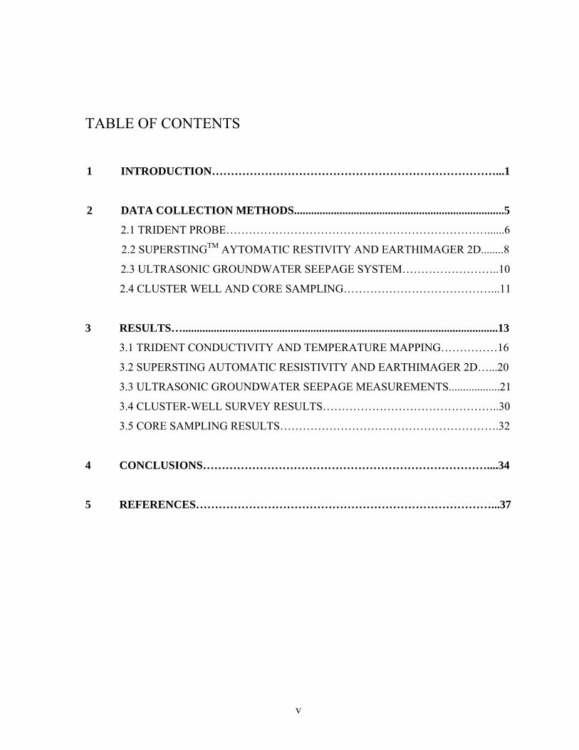
TABLE OF CONTENTS

1 INTRODUCTION…………………………………………………………………...1

2 DATA COLLECTION METHODS..........................................................................5

2.1 TRIDENT PROBE……………………………………………………………......6

2.2 SUPERSTINGTM AYTOMATIC RESTIVITY AND EARTHIMAGER 2D........8

2.3 ULTRASONIC GROUNDWATER SEEPAGE SYSTEM……………………..10

2.4 CLUSTER WELL AND CORE SAMPLING…………………………………...11

3 RESULTS…...............................................................................................................13

3.1 TRIDENT CONDUCTIVITY AND TEMPERATURE MAPPING……………16

3.2 SUPERSTING AUTOMATIC RESISTIVITY AND EARTHIMAGER 2D…...20

3.3 ULTRASONIC GROUNDWATER SEEPAGE MEASUREMENTS..................21

3.4 CLUSTER-WELL SURVEY RESULTS………………………………………..30

3.5 CORE SAMPLING RESULTS………………………………………………….32

4 CONCLUSIONS…………………………………………………………………....34

5 REFERENCES……………………………………………………………………...37

vi

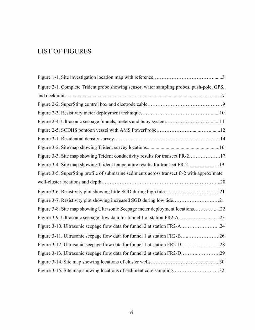
LIST OF FIGURES

Figure 1-1. Site investigation location map with reference……………………………….......3

Figure 2-1. Complete Trident probe showing sensor, water sampling probes, push-pole, GPS,

and deck unit………………………………………………………………………………......7

Figure 2-2. SuperSting control box and electrode cable………………………………………9

Figure 2-3. Resistivity meter deployment technique…………………………………….......10

Figure 2-4. Ultrasonic seepage funnels, meters and buoy system……………………….......11

Figure 2-5. SCDHS pontoon vessel with AMS PowerProbe………………….......……........12

Figure 3-1. Residential density survey……………………………………………………….14

Figure 3-2. Site map showing Trident survey locations..........................................................16

Figure 3-3. Site map showing Trident conductivity results for transect FR-2……………….17

Figure 3-4. Site map showing Trident temperature results for transect FR-2……………….19

Figure 3-5. SuperSting profile of submarine sediments across transect fr-2 with approximate

well-cluster locations and depth……………………………………………………………...20

Figure 3-6. Resistivity plot showing little SGD during high tide……………………………21

Figure 3-7. Resistivity plot showing increased SGD during low tide…………………….…21

Figure 3-8. Site map showing Ultrasonic Seepage meter deployment locations………….....22

Figure 3-9. Ultrasonic seepage flow data for funnel 1 at station FR2-A…………………….23

Figure 3-10. Ultrasonic seepage flow data for funnel 2 at station FR2-A…………………...24 Figure 3-11. Ultrasonic seepage flow data for funnel 1 at station FR2-B…..……………….26

Figure 3-12. Ultrasonic seepage flow data for funnel 1 at station FR2-D………..………….28

Figure 3-13. Ultrasonic seepage flow data for funnel 2 at station FR2-D………..………….29

Figure 3-14. Site map showing locations of cluster wells…………………………………...30

Figure 3-15. Site map showing locations of sediment core sampling……………………….32

vii

LIST OF TABLES

Table 3-1. Water quality results for the shoreline wells…......................................................15

Table 3-2. Trident results for the Forge River transect FR-2..................................................16

Table 3-3. Results of cluster well sampling.............................................................................31

Table 3-4. Core sample classification for transect FR-2.........................................................33

1

1 INTRODUCTION

2

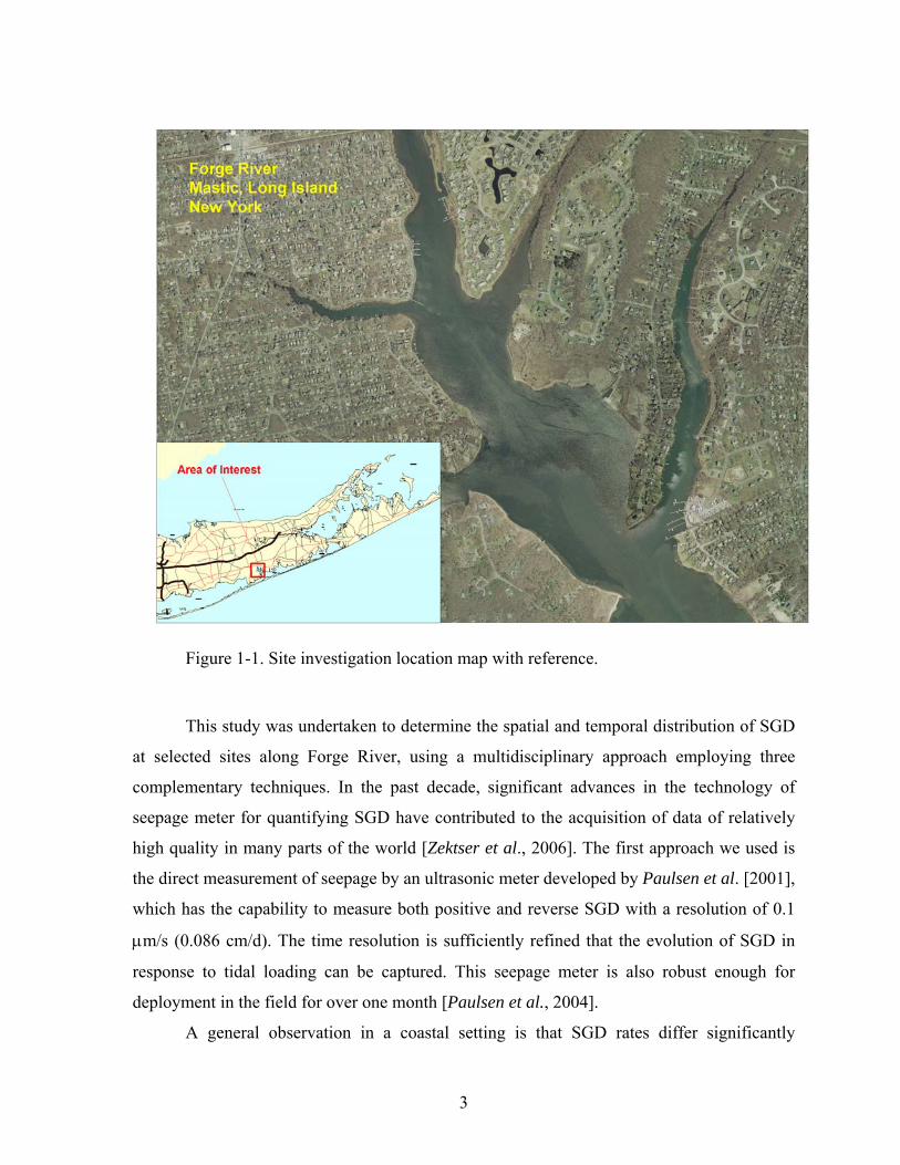
The Forge River is located between the hamlets of Moriches and Mastic on the

southwestern portion of Suffolk County in New York State (Figure 1-1). As a major tributary

of Moriches Bay on the south shore of Long Island, it has been an important and productive

natural resource for both commercial and recreational users for many decades. Since 2005

the Forge River has experienced chronic hypoxia due to excessive nitrogen input from a

number of natural and anthropogenic sources, including storm water discharges, submarine

discharges that contain effluent from unsewered high-density residential housing, and

wastewater from a commercial duck farm upstream. These events have triggered concerns

over the health of the River, the most alarming of which was a fish-kill during the summer of

2006. As a result of this particular event and documented evidence of a general decline in its

state of health, Forge River was added to the 2006 New York State 303(d) List of Impaired

Water Bodies.

Management and ecological restoration of the Forge River watershed hinge upon a

comprehensive understanding of where and how nutrient loading is occurring. As is typical

of Long Island streams, a significant portion of the freshwater flow of Forge River derives

from groundwater, which may transport a disproportionate concentration of nutrients from

the underground aquifer by submarine groundwater discharge (SGD). In a recent study of

benthic fluxes of Forge River, Aller et al. [2009] observed that the groundwater fluxes are

relatively high, representing up to 73% of the total external supply of nitrogen. As this flux is

largest on the more densely populated western side of the Forge watershed, it has probably

contributed to the greater hypoxia and nitrogen, as well as lower oxygen levels observed in

the tributaries and shorelines along the western portions of the Forge River.

In relation to this issue, it is important to characterize the SGD and its spatial

distribution along the Forge River. In addition, SGD is expected to vary over time, especially

in connection with the tidal cycles. The tidal portion of Forge River is approximately three

miles long, encompassing four branches off its main stem on the west side and two on the

east side. Tidal loading can exert significant influence over the encroachment of saltwater

from the ocean that is counteracted by underground underflow driven by the hydraulic

gradient of the aquifer. The temporal evolution of SGD is such that its peak occurs near low

tide and vice versa [Paulsen et al., 2001; Taniguchi, 2002].

3

Figure 1-1. Site investigation location map with reference.

This study was undertaken to determine the spatial and temporal distribution of SGD

at selected sites along Forge River, using a multidisciplinary approach employing three

complementary techniques. In the past decade, significant advances in the technology of

seepage meter for quantifying SGD have contributed to the acquisition of data of relatively

high quality in many parts of the world [Zektser et al., 2006]. The first approach we used is

the direct measurement of seepage by an ultrasonic meter developed by Paulsen et al. [2001],

which has the capability to measure both positive and reverse SGD with a resolution of 0.1

μm/s (0.086 cm/d). The time resolution is sufficiently refined that the evolution of SGD in

response to tidal loading can be captured. This seepage meter is also robust enough for

deployment in the field for over one month [Paulsen et al., 2004].

A general observation in a coastal setting is that SGD rates differ significantly

4

between the off-shore and near-shore environments. Typically the discharge rate is the

highest just landward of the saltwater-freshwater interface, and decays as one moves offshore

towards the ocean [Bokuniewicz and Zeitlin, 1980; Taniguchi et al., 2006]. Although the

ultrasonic seepage meter provides data of high quality, it has an intrinsic limitation in that the

spatial coverage is localized and it cannot conveniently map out the spatial heterogeneity of

SGD over a relatively large area. In recent years there has been an increased use of electrical

resistivity methods in hydrogeologic investigations, since they can provide extensive spatial

coverage and in the context of a coastal setting, the electrical resistivity of the sediments

provides a proxy for SGD [Day-Lewis et al., 2006]. Electrical resistivity data acquired by a

linear array on the surface can be inverted to derive the 2-dimensional resistivity profile of a

vertical cross-section. Since the electrical resistivity of a porous medium is primarily

controlled by its porosity and the electrical resistivity of the electrolyte in the pore space

[Telford et al., 1990], the inferred electrical resistivity at a given point on the vertical section

can be related to the electrolyte resistivity if the sediment porosity is relatively uniform in the

section. In particular, a relatively high electrical resistivity would imply a relatively low

salinity, probably due to the influx of SGD [Swarzenski et al., 2007]. If repeated

measurements during a tidal cycle were able to resolve changes in the spatial distribution of

electrical conductivity, then the data can be inverted to infer the temporal evolution of SGD

related to tidal fluctuation.

Since the interpretation of electrical resistivity data depends solely on inversion of

surface measurements, it is important to validate the inferred values by conducting direct

measurements of conductivity at depth. In this study this is achieved by our third approach

using the Trident probe [Chadwick et al., 2003], which measures the bulk electrical

conductivity and subsurface temperature at selected locations. We will synthesize the three

types of measurements, and compare them to water chemistry data that were collected from

monitoring wells installed beneath the river bottom.

5

2 DATA COLLECTION METHODS

6

2.1 TRIDENT PROBE

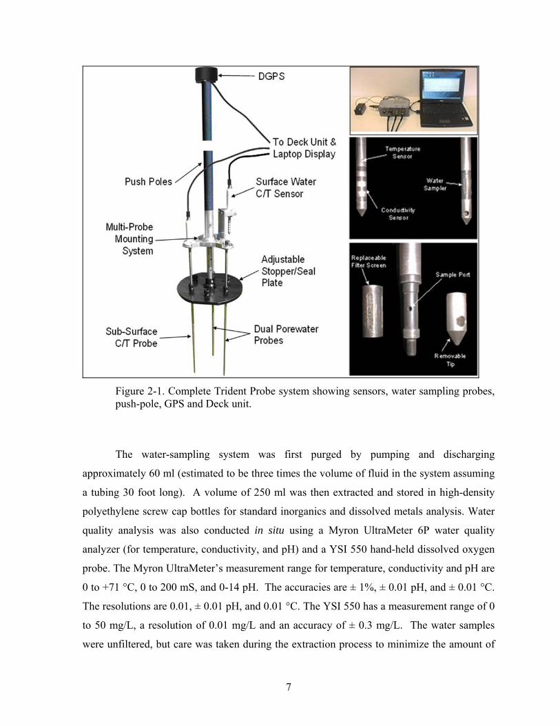
The Trident Probe (Figure 2-1) is a direct-push system that integrates a temperature

probe, an electrical conductivity probe, and a water sampler [Chadwick et al., 2003].

Contrasts in temperature and conductivity between surface water and groundwater can be

used to locate likely areas of groundwater impingement at depth. The water-sampling device

is then used to collect samples for detailed chemical characterization of contaminants. The

two probes and sampler are collocated in a triangular pattern with a spacing of about 11

inches on an aluminum mounting base. A push-pole is used to drive this assembly into the

sediment to a selected depth. The head of the push-pole is fitted with a GPS unit with WAAS

capability. Data from this GPS unit and the two probes are fed to a data logger, which

provides real-time measurement of the temperature and conductivity of the porous sediment

as functions the spatial coordinates.

The temperature sensor housed in titanium has a measurement range of -5 to +35 °C

at an accuracy of 0.001 °C, and a resolution of 0.001 °C. Areas of groundwater seepage may

appear either as warm or cold contrast to the surface water, depending on the seasonal and

site characteristics.

The electrical conductivity probe utilizes a Wenner-type configuration, with two pairs

of stainless steel electrodes. The pairs of electrodes are coupled through an underwater

connecter and cable to a control unit, which applies a known current between the outer

electrode pair while monitoring the voltage between the inner pair of electrodes. The probe

measures the electrical conductivity of the porous medium saturated with fluid in a volume

that encloses the electrode array, which is a function of primarily the salinity, and secondarily

of clay content and porosity. Areas of SGD originating from a terrestrial origin are generally

associated with low conductivity.

The water-sampling unit can extract interstitial water from the sediment at selected

depths down to about three feet below the sediment water interface. The porewater is

extracted by a low-flow peristaltic pump through Teflon tubing (inside diameter 1/16 inch)

that is housed in a stainless steel casing fitted with a solid tip (Figure 2-1). On the side of the

casing near the tip there is an inlet port consisting of a slot covered by a small mesh size (241

μm) stainless steel screen.

7

Figure 2-1. Complete Trident Probe system showing sensors, water sampling probes, push-pole, GPS and Deck unit.

The water-sampling system was first purged by pumping and discharging

approximately 60 ml (estimated to be three times the volume of fluid in the system assuming

a tubing 30 foot long). A volume of 250 ml was then extracted and stored in high-density

polyethylene screw cap bottles for standard inorganics and dissolved metals analysis. Water

quality analysis was also conducted in situ using a Myron UltraMeter 6P water quality

analyzer (for temperature, conductivity, and pH) and a YSI 550 hand-held dissolved oxygen

probe. The Myron UltraMeter’s measurement range for temperature, conductivity and pH are

0 to +71 °C, 0 to 200 mS, and 0-14 pH. The accuracies are ± 1%, ± 0.01 pH, and ± 0.01 °C.

The resolutions are 0.01, ± 0.01 pH, and 0.01 °C. The YSI 550 has a measurement range of 0

to 50 mg/L, a resolution of 0.01 mg/L and an accuracy of ± 0.3 mg/L. The water samples

were unfiltered, but care was taken during the extraction process to minimize the amount of

8

suspended solids in the samples. Between stations, the screen zone was cleaned and the

tubing replaced. The entire sampling system was then flushed with a series of solutions

including surface seawater and deionized water.

In this study all the Trident measurements were made when the probes had been

inserted to a depth of 1.5 feet below the sediment surface using the push-pole system. If the

Trident push met with strong resistance at a depth less than the target depth of 1.5 fee5t. due

to geological conditions or other obstructions, the station would be relocated laterally by a

distance of approximately 1-2 feet. and the push repeated. Occasionally it was necessary to

repeat the process up to three times to arrive at a location for a successful push. There were

also instances when the sediments were so silty that the pumping system was unable to

extract water samples. In these cases the station was relocated by a lateral distance of

approximately 3-4 feet. and the push was repeated.

2.2 SUPERSTINGTM AUTOMATIC RESTIVITY AND EARTHIMAGER 2D

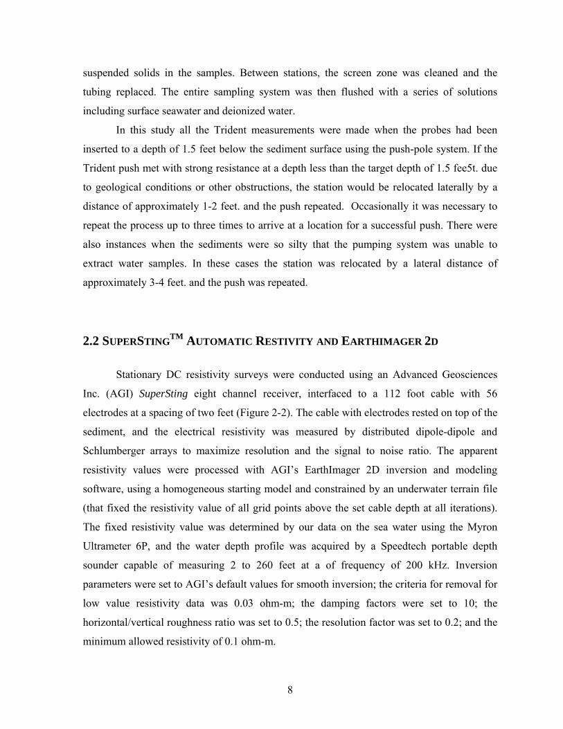
Stationary DC resistivity surveys were conducted using an Advanced Geosciences

Inc. (AGI) SuperSting eight channel receiver, interfaced to a 112 foot cable with 56

electrodes at a spacing of two feet (Figure 2-2). The cable with electrodes rested on top of the

sediment, and the electrical resistivity was measured by distributed dipole-dipole and

Schlumberger arrays to maximize resolution and the signal to noise ratio. The apparent

resistivity values were processed with AGI’s EarthImager 2D inversion and modeling

software, using a homogeneous starting model and constrained by an underwater terrain file

(that fixed the resistivity value of all grid points above the set cable depth at all iterations).

The fixed resistivity value was determined by our data on the sea water using the Myron

Ultrameter 6P, and the water depth profile was acquired by a Speedtech portable depth

sounder capable of measuring 2 to 260 feet at a of frequency of 200 kHz. Inversion

parameters were set to AGI’s default values for smooth inversion; the criteria for removal for

low value resistivity data was 0.03 ohm-m; the damping factors were set to 10; the

horizontal/vertical roughness ratio was set to 0.5; the resolution factor was set to 0.2; and the

minimum allowed resistivity of 0.1 ohm-m.

9

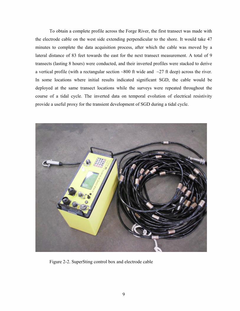
To obtain a complete profile across the Forge River, the first transect was made with

the electrode cable on the west side extending perpendicular to the shore. It would take 47

minutes to complete the data acquisition process, after which the cable was moved by a

lateral distance of 83 feet towards the east for the next transect measurement. A total of 9

transects (lasting 8 hours) were conducted, and their inverted profiles were stacked to derive

a vertical profile (with a rectangular section ~800 ft wide and ~27 ft deep) across the river.

In some locations where initial results indicated significant SGD, the cable would be

deployed at the same transect locations while the surveys were repeated throughout the

course of a tidal cycle. The inverted data on temporal evolution of electrical resistivity

provide a useful proxy for the transient development of SGD during a tidal cycle.

Figure 2-2. SuperSting control box and electrode cable

10

Figure 2-3. Resistivity meter deployment technique

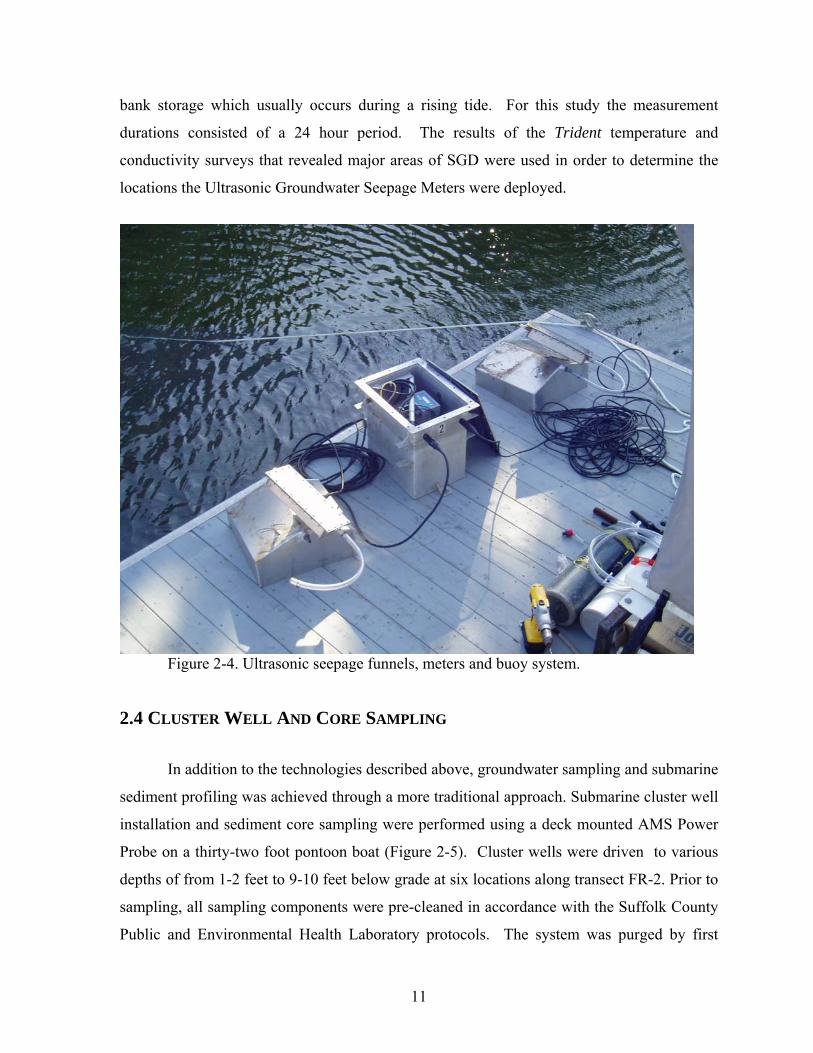
2.3 ULTRASONIC GROUNDWATER SEEPAGE SYSTEM

The Ultrasonic Groundwater Seepage system is a seepage meter system for

quantifying specific discharge rates from groundwater flow to coastal waters (Figure 2-4).

Traditional seepage technology was modified and improved to include continuous flow

detection with ultrasonic flow meters [Paulsen et.al., 2001]. Groundwater flow is captured

and directed through a stainless steel funnel with a square cross section of 2.3 ft2 that are

inserted approximately four inches into the sediment and connected to the ultrasonic device

by Tygon tubing. The ultrasonic meter houses two piezoelectric transducers mounted at

opposite ends of a cylindrical flow tube. The transducers continually generate bursts of

ultrasonic signals from one end to the other. Arrival of the ultrasonic signals is continuously

monitored by the piezoelectric transducers and corrected for temperature and conductivity.

In a static fluid, the sound speed is sensitively dependent on temperature and salinity. If the

fluid flows with a velocity then travel time for the upstream propagation of sound waves

against the flow direction is prolonged relative to that for downstream propagation. The

ultrasonic seepage meters are able to measure SGD at rates as low as 0.1 µm/sec. The full

explanation of the technology is described in detail in Paulsen et al. 2001. The data is stored

internally in a logger as it is being collected and downloaded at the end of the sampling

period. The data produced are time series, over tidal cycles of specific discharge. This allows

an accurate determination of the presence or absence of TSGD into a bay or estuary. A

positive measurement indicates SGD (falling tide) while a negative measurement indicates

11

bank storage which usually occurs during a rising tide. For this study the measurement

durations consisted of a 24 hour period. The results of the Trident temperature and

conductivity surveys that revealed major areas of SGD were used in order to determine the

locations the Ultrasonic Groundwater Seepage Meters were deployed.

Figure 2-4. Ultrasonic seepage funnels, meters and buoy system.

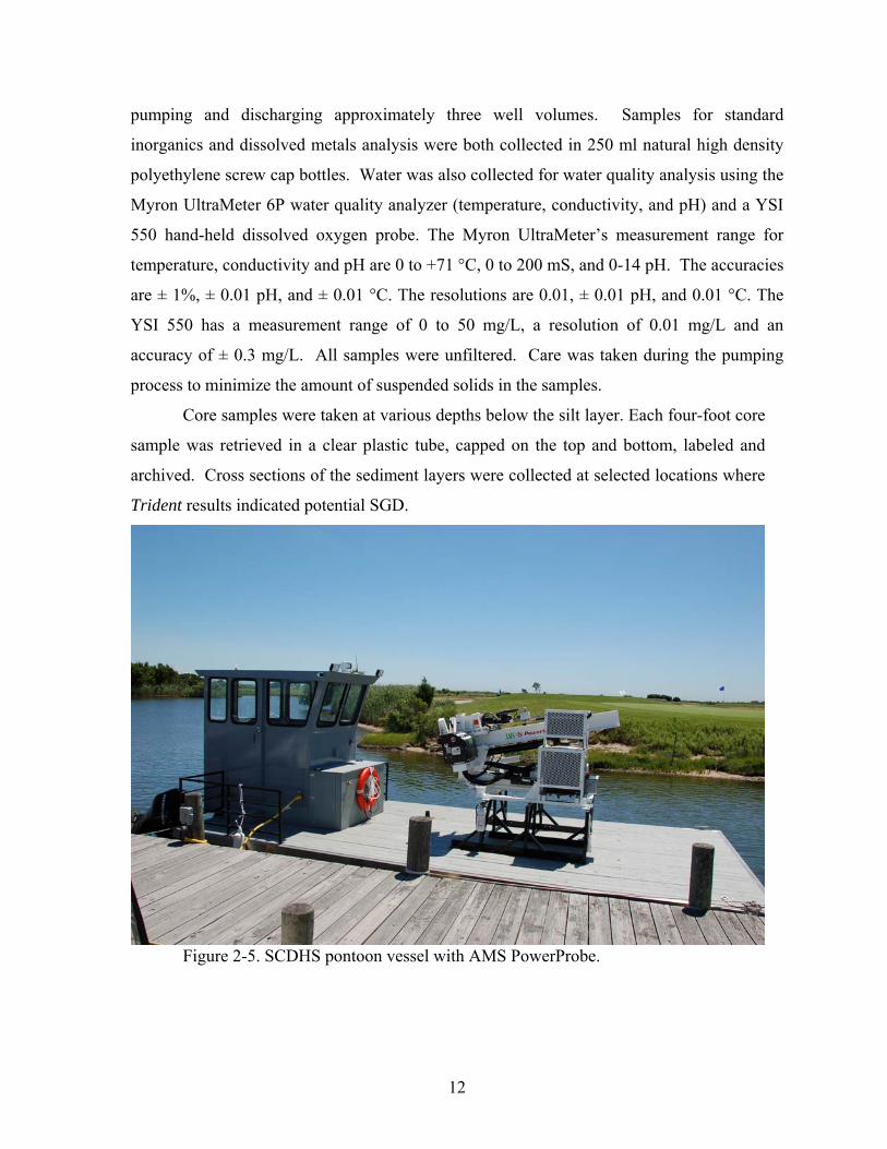
2.4 CLUSTER WELL AND CORE SAMPLING

In addition to the technologies described above, groundwater sampling and submarine

sediment profiling was achieved through a more traditional approach. Submarine cluster well

installation and sediment core sampling were performed using a deck mounted AMS Power

Probe on a thirty-two foot pontoon boat (Figure 2-5). Cluster wells were driven to various

depths of from 1-2 feet to 9-10 feet below grade at six locations along transect FR-2. Prior to

sampling, all sampling components were pre-cleaned in accordance with the Suffolk County

Public and Environmental Health Laboratory protocols. The system was purged by first

12

pumping and discharging approximately three well volumes. Samples for standard

inorganics and dissolved metals analysis were both collected in 250 ml natural high density

polyethylene screw cap bottles. Water was also collected for water quality analysis using the

Myron UltraMeter 6P water quality analyzer (temperature, conductivity, and pH) and a YSI

550 hand-held dissolved oxygen probe. The Myron UltraMeter’s measurement range for

temperature, conductivity and pH are 0 to +71 °C, 0 to 200 mS, and 0-14 pH. The accuracies

are ± 1%, ± 0.01 pH, and ± 0.01 °C. The resolutions are 0.01, ± 0.01 pH, and 0.01 °C. The

YSI 550 has a measurement range of 0 to 50 mg/L, a resolution of 0.01 mg/L and an

accuracy of ± 0.3 mg/L. All samples were unfiltered. Care was taken during the pumping

process to minimize the amount of suspended solids in the samples.

Core samples were taken at various depths below the silt layer. Each four-foot core

sample was retrieved in a clear plastic tube, capped on the top and bottom, labeled and

archived. Cross sections of the sediment layers were collected at selected locations where

Trident results indicated potential SGD.

Figure 2-5. SCDHS pontoon vessel with AMS PowerProbe.

13

3 RESULTS

14

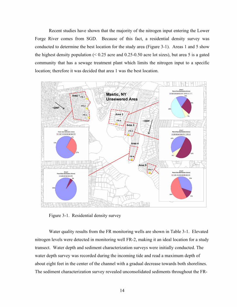
Recent studies have shown that the majority of the nitrogen input entering the Lower

Forge River comes from SGD. Because of this fact, a residential density survey was

conducted to determine the best location for the study area (Figure 3-1). Areas 1 and 5 show

the highest density population (< 0.25 acre and 0.25-0.50 acre lot sizes), but area 5 is a gated

community that has a sewage treatment plant which limits the nitrogen input to a specific

location; therefore it was decided that area 1 was the best location.

Figure 3-1. Residential density survey

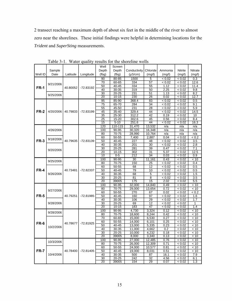
Water quality results from the FR monitoring wells are shown in Table 3-1. Elevated

nitrogen levels were detected in monitoring well FR-2, making it an ideal location for a study

transect. Water depth and sediment characterization surveys were initially conducted. The

water depth survey was recorded during the incoming tide and read a maximum depth of

about eight feet in the center of the channel with a gradual decrease towards both shorelines.

The sediment characterization survey revealed unconsolidated sediments throughout the FR-

15

2 transect reaching a maximum depth of about six feet in the middle of the river to almost

zero near the shorelines. These initial findings were helpful in determining locations for the

Trident and SuperSting measurements.

Table 3-1. Water quality results for the shoreline wells

Well IDSample

Date Latitude Longitude

Well Depth (fbg)

Screen Depth (fbg)

Conductivity (µS/cm)

Chloride (mg/l)

Ammonia (mg/l)

Nitrite (mg/l)

Nitrate (mg/l)

90 80-85 1500 5 < 0.02 < 0.02 0.370 60-65 334 57 < 0.02 < 0.02 12.650 40-45 334 55 1.12 < 0.02 11.440 30-35 319 50 2.25 < 0.02 9.830 20-25 231 51 1.13 < 0.02 8.220 10-15 230 26 0.02 < 0.02 12.795 85-90 368.4 83 < 0.02 < 0.02 0.575 65-70 284 34 < 0.02 < 0.02 9.155 45-50 231 28 < 0.02 < 0.02 5.945 35-40 329.4 44 < 0.02 < 0.02 14.535 25-30 312.2 42 0.19 < 0.02 1025 15-20 302.6 45 0.56 < 0.02 8.415 5-10 251.6 44 < 0.02 < 0.02 16.3120 110-115 31,470 13,532 n/a n/a n/a100 90-95 30,320 16,348 n/a n/a n/a80 70-75 28,990 10,764 n/a n/a n/a60 50-55 7,400 2,887 0.04 < 0.02 < 0.250 40-45 227 48 < 0.02 < 0.02 3.540 30-35 201 30 < 0.02 < 0.02 2.830 20-25 281 39 0.47 < 0.02 7.120 10-15 302 31 5.37 < 0.02 12.510 0-5 212 34 0.03 < 0.02 0.9100 90-95 30 11,161 0.43 < 0.02 < 1080 70-75 150 25 < 0.02 < 0.02 0.460 50-55 68 12 < 0.02 < 0.02 0.550 40-45 79 10 < 0.02 < 0.02 0.540 30-35 68 5 < 0.02 < 0.02 1.530 20-25 81 8 < 0.02 < 0.02 3.520 39005 175 15 2.02 < 0.02 5.5100 90-95 32,000 14,840 0.49 < 0.02 < 1080 70-75 29,000 13,654 0.72 < 0.02 < 1060 50-55 270 67 0.02 < 0.02 < 0.250 40-45 160 97 < 0.02 < 0.02 1.640 30-35 106 29 < 0.02 < 0.02 1.730 20-25 69 12 < 0.02 < 0.02 120 10-15 183 47 < 0.02 < 0.02 1.4100 90-95 4,730 3,324 0.12 < 0.02 < 1080 70-75 18,600 8,244 0.42 < 0.02 < 1070 60-65 15,000 6,530 0.27 < 0.02 < 1060 50-55 14,000 6,101 0.25 < 0.02 < 1050 40-45 13,000 5,335 0.23 < 0.02 < 1040 30-35 11,000 4,662 0.2 < 0.02 < 1030 20-25 10,000 4,232 0.18 < 0.02 < 1020 39005 8,000 3,340 0.13 < 0.02 < 10100 90-95 27,000 12,485 0.76 < 0.02 < 1080 70-75 26,000 12,309 0.71 < 0.02 < 1060 50-55 24,000 10,577 0.81 < 0.02 < 1050 40-45 19,000 8,031 0.51 < 0.02 < 1040 30-35 500 87 16.1 < 0.02 7.930 20-25 242 32 4.56 < 0.02 6.120 39005 154 29 0.07 < 0.02 1.3

-72.81405

FR-6

9/28/2006

10/2/2006

FR-7

10/3/2006

10/4/200640.78400

-72.81985

40.73481 -72.82337

-72.81925

FR-59/27/2006

9/28/2006

40.78677

40.79251

-72.83139

FR-2 4/20/2006

FR-3 40.79635

FR-4

9/25/2006

9/26/2006

40.80052 -72.83192

40.79833 -72.83199

4/26/2006

9/18/2006

9/20/2006

FR-19/21/2006

9/25/2006

16

3.1 TRIDENT CONDUCTIVITY AND TEMPERATURE MAPPING

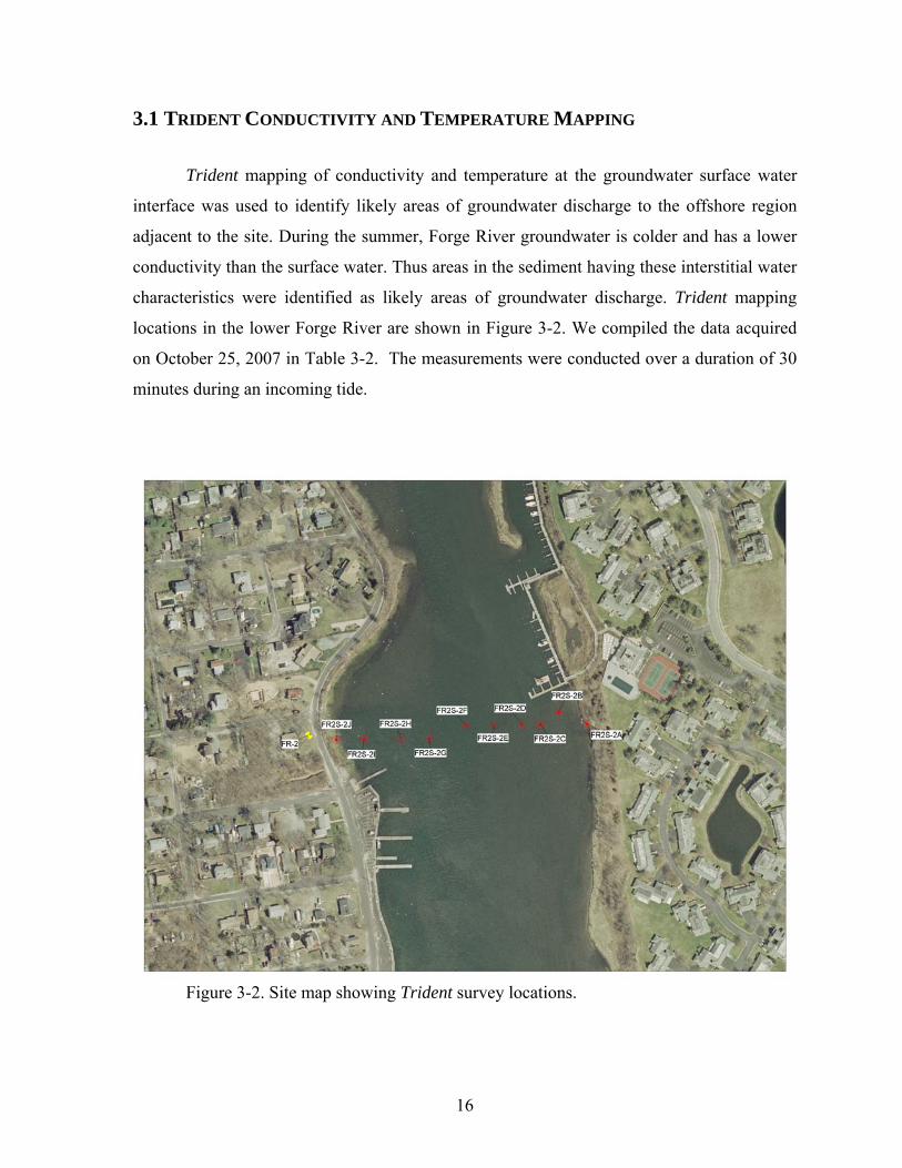
Trident mapping of conductivity and temperature at the groundwater surface water

interface was used to identify likely areas of groundwater discharge to the offshore region

adjacent to the site. During the summer, Forge River groundwater is colder and has a lower

conductivity than the surface water. Thus areas in the sediment having these interstitial water

characteristics were identified as likely areas of groundwater discharge. Trident mapping

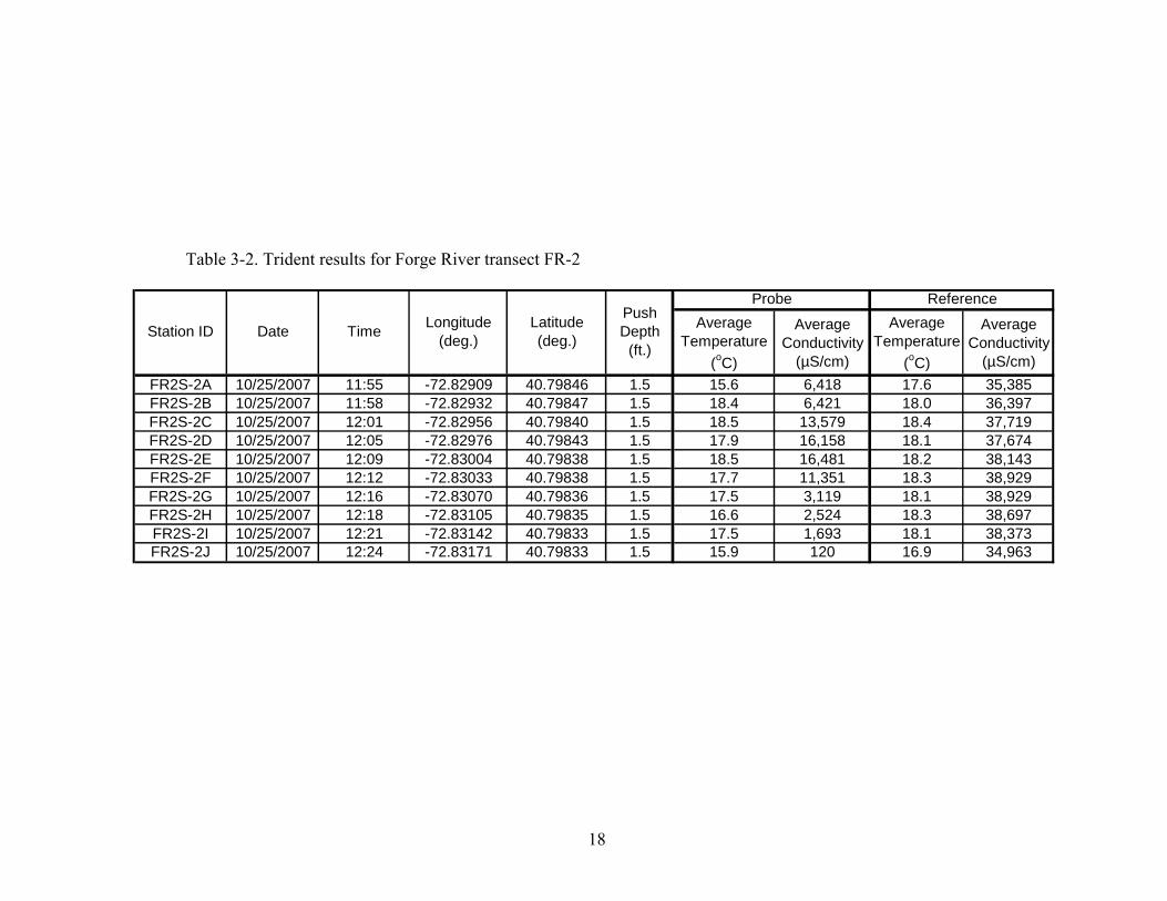
locations in the lower Forge River are shown in Figure 3-2. We compiled the data acquired

on October 25, 2007 in Table 3-2. The measurements were conducted over a duration of 30

minutes during an incoming tide.

Figure 3-2. Site map showing Trident survey locations.

17

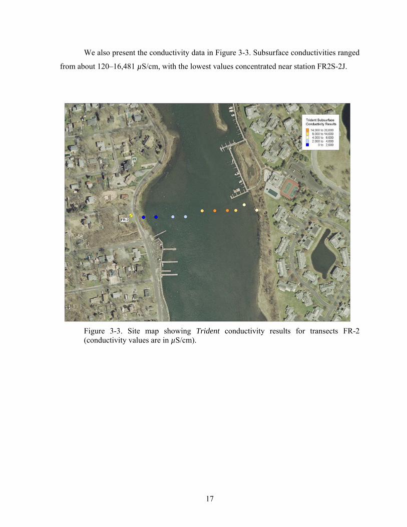
We also present the conductivity data in Figure 3-3. Subsurface conductivities ranged

from about 120–16,481 µS/cm, with the lowest values concentrated near station FR2S-2J.

Figure 3-3. Site map showing Trident conductivity results for transects FR-2 (conductivity values are in µS/cm).

18

Table 3-2. Trident results for Forge River transect FR-2

Average Temperature

(oC)

Average Conductivity

(µS/cm)

Average Temperature

(oC)

Average Conductivity

(µS/cm)FR2S-2A 10/25/2007 11:55 -72.82909 40.79846 1.5 15.6 6,418 17.6 35,385FR2S-2B 10/25/2007 11:58 -72.82932 40.79847 1.5 18.4 6,421 18.0 36,397FR2S-2C 10/25/2007 12:01 -72.82956 40.79840 1.5 18.5 13,579 18.4 37,719FR2S-2D 10/25/2007 12:05 -72.82976 40.79843 1.5 17.9 16,158 18.1 37,674FR2S-2E 10/25/2007 12:09 -72.83004 40.79838 1.5 18.5 16,481 18.2 38,143FR2S-2F 10/25/2007 12:12 -72.83033 40.79838 1.5 17.7 11,351 18.3 38,929FR2S-2G 10/25/2007 12:16 -72.83070 40.79836 1.5 17.5 3,119 18.1 38,929FR2S-2H 10/25/2007 12:18 -72.83105 40.79835 1.5 16.6 2,524 18.3 38,697FR2S-2I 10/25/2007 12:21 -72.83142 40.79833 1.5 17.5 1,693 18.1 38,373FR2S-2J 10/25/2007 12:24 -72.83171 40.79833 1.5 15.9 120 16.9 34,963

Station ID Date Time Longitude (deg.)

Latitude (deg.)

Push Depth

(ft.)

Probe Reference

19

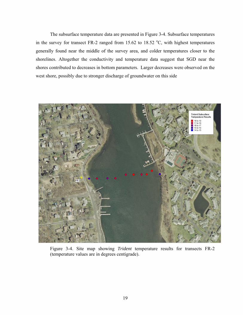
The subsurface temperature data are presented in Figure 3-4. Subsurface temperatures

in the survey for transect FR-2 ranged from 15.62 to 18.52 oC, with highest temperatures

generally found near the middle of the survey area, and colder temperatures closer to the

shorelines. Altogether the conductivity and temperature data suggest that SGD near the

shores contributed to decreases in bottom parameters. Larger decreases were observed on the

west shore, possibly due to stronger discharge of groundwater on this side

Figure 3-4. Site map showing Trident temperature results for transects FR-2 (temperature values are in degrees centigrade).

20

3.2 SUPERSTING AUTOMATIC RESISTIVITY AND EARTHIMAGER 2D

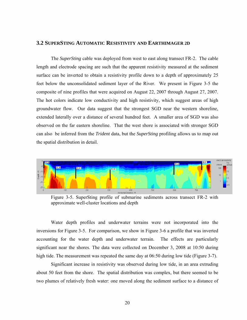
The SuperSting cable was deployed from west to east along transect FR-2. The cable

length and electrode spacing are such that the apparent resistivity measured at the sediment

surface can be inverted to obtain a resistivity profile down to a depth of approximately 25

feet below the unconsolidated sediment layer of the River. We present in Figure 3-5 the

composite of nine profiles that were acquired on August 22, 2007 through August 27, 2007.

The hot colors indicate low conductivity and high resistivity, which suggest areas of high

groundwater flow. Our data suggest that the strongest SGD near the western shoreline,

extended laterally over a distance of several hundred feet. A smaller area of SGD was also

observed on the far eastern shoreline. That the west shore is associated with stronger SGD

can also be inferred from the Trident data, but the SuperSting profiling allows us to map out

the spatial distribution in detail.

Figure 3-5. SuperSting profile of submarine sediments across transect FR-2 with approximate well-cluster locations and depth

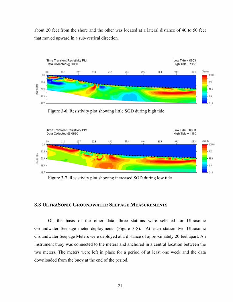
Water depth profiles and underwater terrains were not incorporated into the

inversions for Figure 3-5. For comparison, we show in Figure 3-6 a profile that was inverted

accounting for the water depth and underwater terrain. The effects are particularly

significant near the shores. The data were collected on December 3, 2008 at 10:50 during

high tide. The measurement was repeated the same day at 06:50 during low tide (Figure 3-7).

Significant increase in resistivity was observed during low tide, in an area extruding

about 50 feet from the shore. The spatial distribution was complex, but there seemed to be

two plumes of relatively fresh water: one moved along the sediment surface to a distance of

21

about 20 feet from the shore and the other was located at a lateral distance of 40 to 50 feet

that moved upward in a sub-vertical direction.

Figure 3-6. Resistivity plot showing little SGD during high tide

Figure 3-7. Resistivity plot showing increased SGD during low tide

3.3 ULTRASONIC GROUNDWATER SEEPAGE MEASUREMENTS

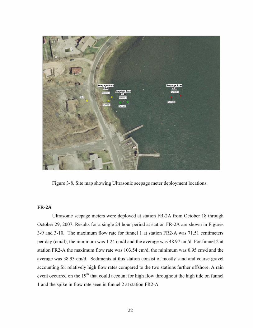
On the basis of the other data, three stations were selected for Ultrasonic

Groundwater Seepage meter deployments (Figure 3-8). At each station two Ultrasonic

Groundwater Seepage Meters were deployed at a distance of approximately 20 feet apart. An

instrument buoy was connected to the meters and anchored in a central location between the

two meters. The meters were left in place for a period of at least one week and the data

downloaded from the buoy at the end of the period.

22

Figure 3-8. Site map showing Ultrasonic seepage meter deployment locations.

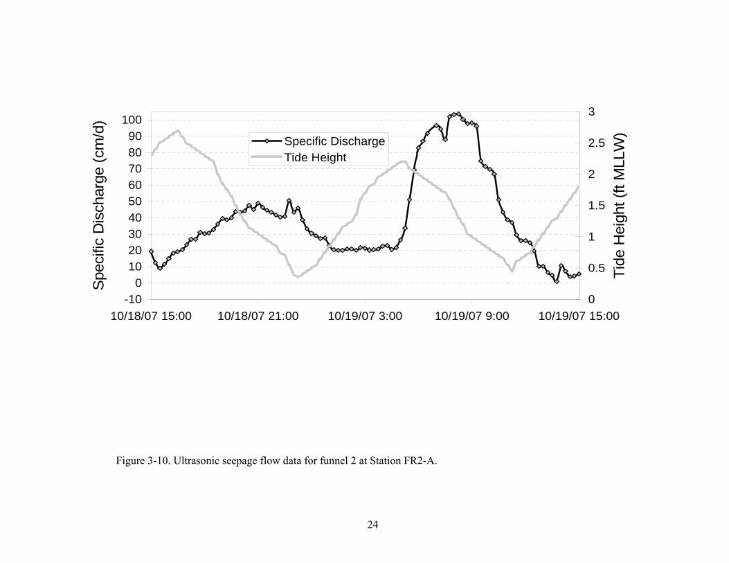
FR-2A

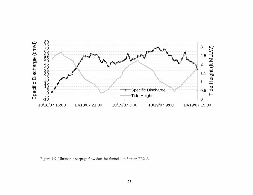
Ultrasonic seepage meters were deployed at station FR-2A from October 18 through

October 29, 2007. Results for a single 24 hour period at station FR-2A are shown in Figures

3-9 and 3-10. The maximum flow rate for funnel 1 at station FR2-A was 71.51 centimeters

per day (cm/d), the minimum was 1.24 cm/d and the average was 48.97 cm/d. For funnel 2 at

station FR2-A the maximum flow rate was 103.54 cm/d, the minimum was 0.95 cm/d and the

average was 38.93 cm/d. Sediments at this station consist of mostly sand and coarse gravel

accounting for relatively high flow rates compared to the two stations further offshore. A rain

event occurred on the 19th that could account for high flow throughout the high tide on funnel

1 and the spike in flow rate seen in funnel 2 at station FR2-A.

23

-10-505

101520253035404550556065707580

10/18/07 15:00 10/18/07 21:00 10/19/07 3:00 10/19/07 9:00 10/19/07 15:00

Spe

cific

Dis

char

ge (c

m/d

)

0

0.5

1

1.5

2

2.5

3

Tide

Hei

ght (

ft M

LLW

)

Specific DischargeTide Height

Figure 3-9. Ultrasonic seepage flow data for funnel 1 at Station FR2-A.

24

-100

102030405060708090

100

10/18/07 15:00 10/18/07 21:00 10/19/07 3:00 10/19/07 9:00 10/19/07 15:00

Spe

cific

Dis

char

ge (c

m/d

)

0

0.5

1

1.5

2

2.5

3

Tide

Hei

ght (

ft M

LLW

)Specific DischargeTide Height

Figure 3-10. Ultrasonic seepage flow data for funnel 2 at Station FR2-A.

25

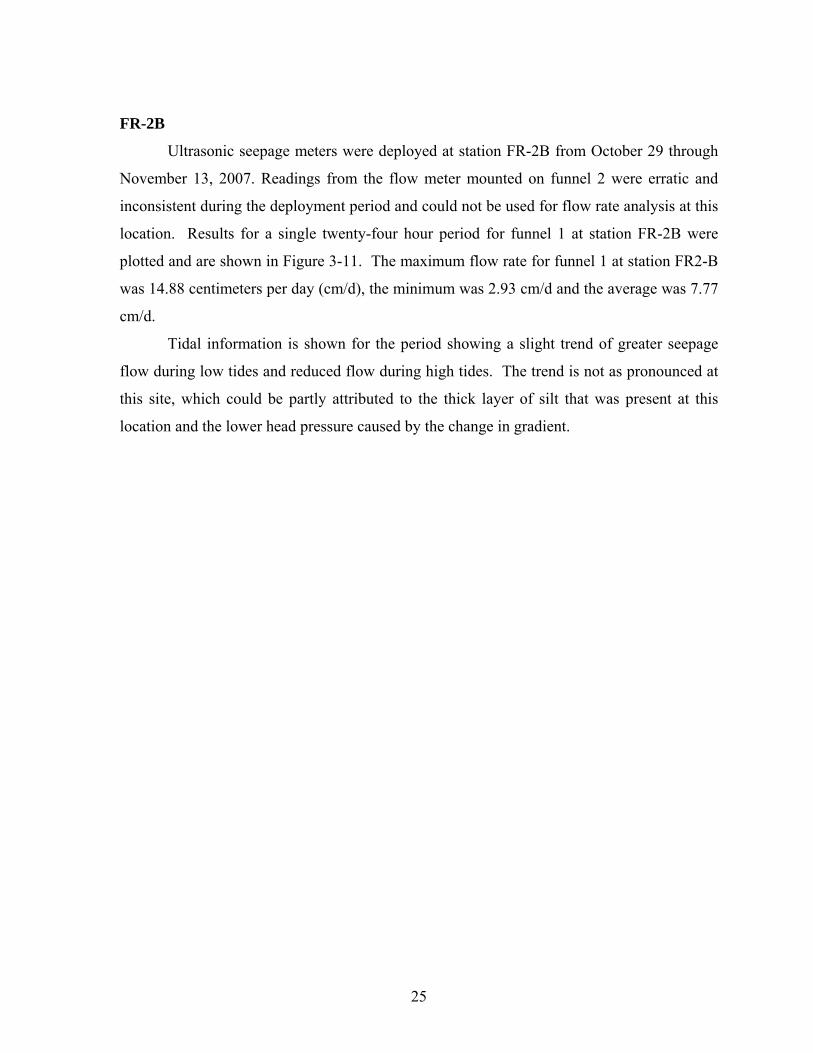
FR-2B

Ultrasonic seepage meters were deployed at station FR-2B from October 29 through

November 13, 2007. Readings from the flow meter mounted on funnel 2 were erratic and

inconsistent during the deployment period and could not be used for flow rate analysis at this

location. Results for a single twenty-four hour period for funnel 1 at station FR-2B were

plotted and are shown in Figure 3-11. The maximum flow rate for funnel 1 at station FR2-B

was 14.88 centimeters per day (cm/d), the minimum was 2.93 cm/d and the average was 7.77

cm/d.

Tidal information is shown for the period showing a slight trend of greater seepage

flow during low tides and reduced flow during high tides. The trend is not as pronounced at

this site, which could be partly attributed to the thick layer of silt that was present at this

location and the lower head pressure caused by the change in gradient.

26

0123456789

1011121314151617

11/11/07 12:15 11/11/07 18:15 11/12/07 0:15 11/12/07 6:15 11/12/07 12:15

Spe

cific

Dis

char

ge (c

m/d

)

-0.5

0

0.5

1

1.5

2

2.5

3

Tide

Hei

ght (

ft M

LLW

)

Specific DischargeTide Height

Figure 3-11. Ultrasonic seepage flow data for funnel 1 at Station FR2-B.

27

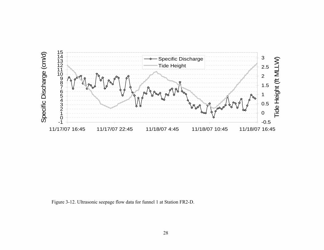
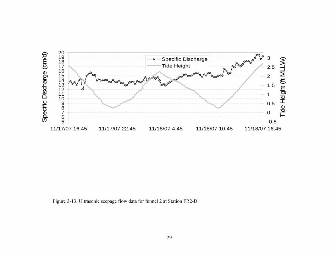
FR-2D

Ultrasonic seepage meters were deployed at station FR-2D from November 13

through November 29, 2007. Results for a single twenty-four hour period at station FR-2D

were plotted and are shown in Figure 3-12 and 3-13. The maximum flow rate for funnel 1 at

station FR2-D-1 was 10.08 centimeters per day (cm/d), the minimum was 0.08 cm/d and the

average was 5.39 cm/d. Funnel 2 at station FR2-D-2 had a maximum flow rate of 19.59

cm/d, a minimum flow rate of 12.03 cm/d and an average flow rate of 14.89 cm/d. Station

FR-2D is in close proximity to the core sample that had a layer of gravel approximately 12 to

13 feet below the silt layer.

Tidal information is shown for the period indicating a slight trend of greater seepage

flow during low tides and reduced flow during high tides. The trend is not as pronounced at

this site which could be partly attributed to the thick layer of silt that was present at this

location and gradient change.

28

-10123456789

101112131415

11/17/07 16:45 11/17/07 22:45 11/18/07 4:45 11/18/07 10:45 11/18/07 16:45

Spe

cific

Dis

char

ge (c

m/d

)

-0.5

0

0.5

1

1.5

2

2.5

3

Tide

Hei

ght (

ft M

LLW

)Specific DischargeTide Height

Figure 3-12. Ultrasonic seepage flow data for funnel 1 at Station FR2-D.

29

56789

1011121314151617181920

11/17/07 16:45 11/17/07 22:45 11/18/07 4:45 11/18/07 10:45 11/18/07 16:45

Spe

cific

Dis

char

ge (c

m/d

)

-0.5

0

0.5

1

1.5

2

2.5

3

Tide

Hei

ght (

ft M

LLW

)Specific DischargeTide Height

Figure 3-13. Ultrasonic seepage flow data for funnel 2 at Station FR2-D.

30

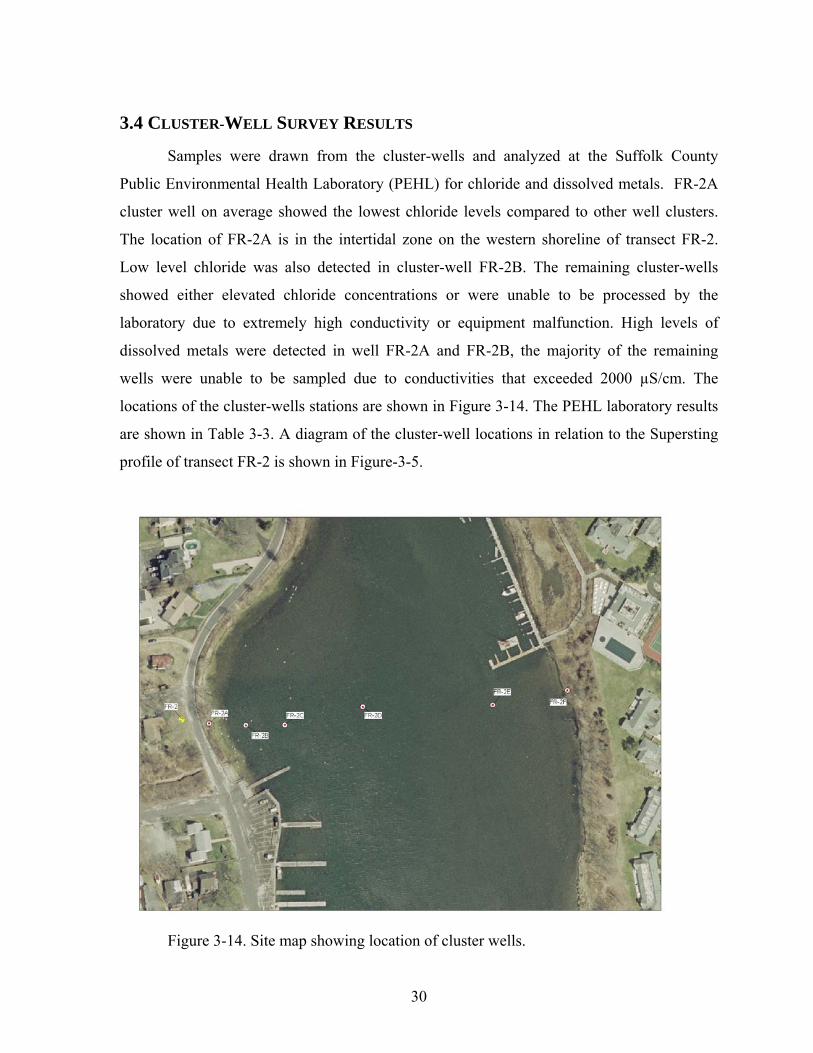
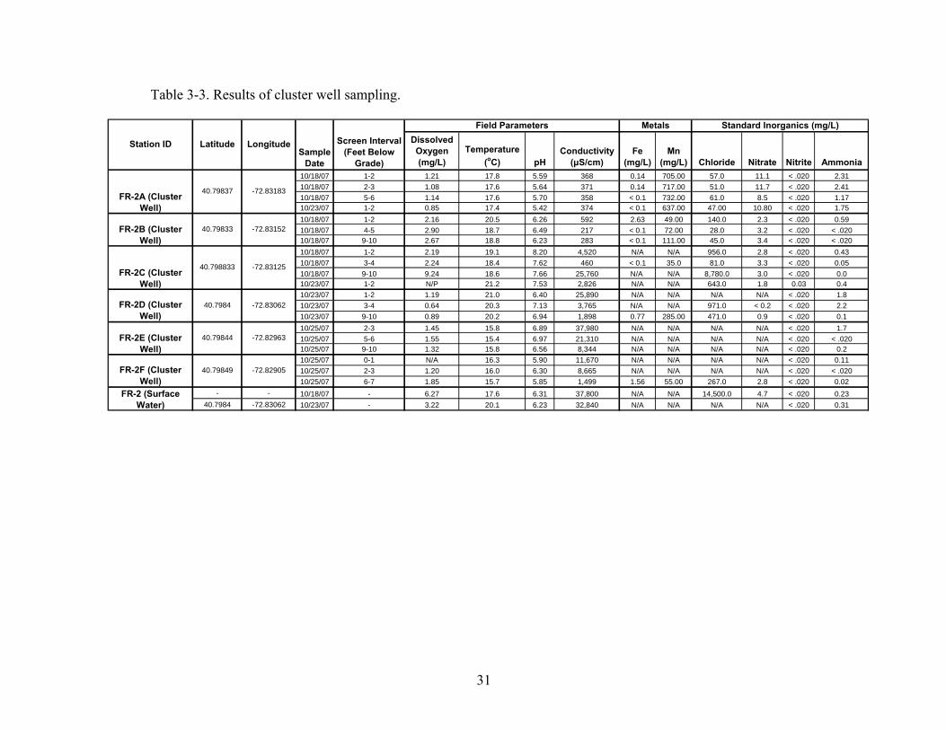
3.4 CLUSTER-WELL SURVEY RESULTS

Samples were drawn from the cluster-wells and analyzed at the Suffolk County

Public Environmental Health Laboratory (PEHL) for chloride and dissolved metals. FR-2A

cluster well on average showed the lowest chloride levels compared to other well clusters.

The location of FR-2A is in the intertidal zone on the western shoreline of transect FR-2.

Low level chloride was also detected in cluster-well FR-2B. The remaining cluster-wells

showed either elevated chloride concentrations or were unable to be processed by the

laboratory due to extremely high conductivity or equipment malfunction. High levels of

dissolved metals were detected in well FR-2A and FR-2B, the majority of the remaining

wells were unable to be sampled due to conductivities that exceeded 2000 µS/cm. The

locations of the cluster-wells stations are shown in Figure 3-14. The PEHL laboratory results

are shown in Table 3-3. A diagram of the cluster-well locations in relation to the Supersting

profile of transect FR-2 is shown in Figure-3-5.

Figure 3-14. Site map showing location of cluster wells.

31

Table 3-3. Results of cluster well sampling.

Dissolved Oxygen (mg/L)

Temperature (oC) pH

Conductivity (μS/cm)

Fe (mg/L)

Mn (mg/L) Chloride Nitrate Nitrite Ammonia

10/18/07 1-2 1.21 17.8 5.59 368 0.14 705.00 57.0 11.1 < .020 2.3110/18/07 2-3 1.08 17.6 5.64 371 0.14 717.00 51.0 11.7 < .020 2.4110/18/07 5-6 1.14 17.6 5.70 358 < 0.1 732.00 61.0 8.5 < .020 1.1710/23/07 1-2 0.85 17.4 5.42 374 < 0.1 637.00 47.00 10.80 < .020 1.7510/18/07 1-2 2.16 20.5 6.26 592 2.63 49.00 140.0 2.3 < .020 0.5910/18/07 4-5 2.90 18.7 6.49 217 < 0.1 72.00 28.0 3.2 < .020 < .02010/18/07 9-10 2.67 18.8 6.23 283 < 0.1 111.00 45.0 3.4 < .020 < .02010/18/07 1-2 2.19 19.1 8.20 4,520 N/A N/A 956.0 2.8 < .020 0.4310/18/07 3-4 2.24 18.4 7.62 460 < 0.1 35.0 81.0 3.3 < .020 0.0510/18/07 9-10 9.24 18.6 7.66 25,760 N/A N/A 8,780.0 3.0 < .020 0.010/23/07 1-2 N/P 21.2 7.53 2,826 N/A N/A 643.0 1.8 0.03 0.410/23/07 1-2 1.19 21.0 6.40 25,890 N/A N/A N/A N/A < .020 1.810/23/07 3-4 0.64 20.3 7.13 3,765 N/A N/A 971.0 < 0.2 < .020 2.210/23/07 9-10 0.89 20.2 6.94 1,898 0.77 285.00 471.0 0.9 < .020 0.110/25/07 2-3 1.45 15.8 6.89 37,980 N/A N/A N/A N/A < .020 1.710/25/07 5-6 1.55 15.4 6.97 21,310 N/A N/A N/A N/A < .020 < .02010/25/07 9-10 1.32 15.8 6.56 8,344 N/A N/A N/A N/A < .020 0.210/25/07 0-1 N/A 16.3 5.90 11,670 N/A N/A N/A N/A < .020 0.1110/25/07 2-3 1.20 16.0 6.30 8,665 N/A N/A N/A N/A < .020 < .02010/25/07 6-7 1.85 15.7 5.85 1,499 1.56 55.00 267.0 2.8 < .020 0.02

- - 10/18/07 - 6.27 17.6 6.31 37,800 N/A N/A 14,500.0 4.7 < .020 0.2340.7984 -72.83062 10/23/07 - 3.22 20.1 6.23 32,840 N/A N/A N/A N/A < .020 0.31

Station ID Latitude LongitudeSample

Date

Screen Interval (Feet Below

Grade)

Standard Inorganics (mg/L)MetalsField Parameters

FR-2F (Cluster Well)

FR-2 (Surface Water)

FR-2C (Cluster Well)

FR-2D (Cluster Well)

FR-2A (Cluster Well)

FR-2B (Cluster Well)

FR-2E (Cluster Well)

40.79837

40.7984

-72.83183

40.79833 -72.83152

40.798833 -72.83125

-72.83062

40.79849 -72.82905

40.79844 -72.82963

32

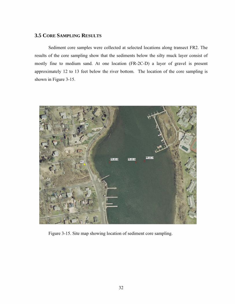
3.5 CORE SAMPLING RESULTS

Sediment core samples were collected at selected locations along transect FR2. The

results of the core sampling show that the sediments below the silty muck layer consist of

mostly fine to medium sand. At one location (FR-2C-D) a layer of gravel is present

approximately 12 to 13 feet below the river bottom. The location of the core sampling is

shown in Figure 3-15.

Figure 3-15. Site map showing location of sediment core sampling.

33

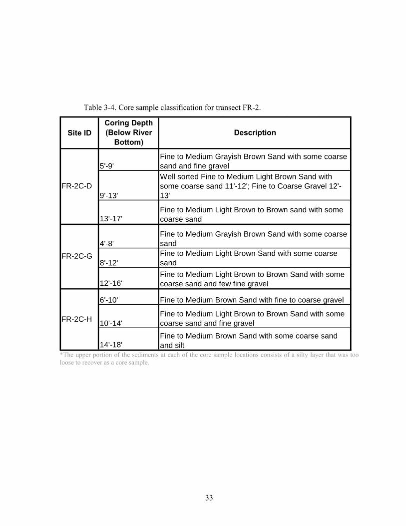
Table 3-4. Core sample classification for transect FR-2.

Site IDCoring Depth (Below River

Bottom)

5'-9'

9'-13'

13'-17'

4'-8'

8'-12'

12'-16'

6'-10'

10'-14'

14'-18'

FR-2C-H

Fine to Medium Brown Sand with fine to coarse gravel

Fine to Medium Light Brown to Brown Sand with some coarse sand and fine gravelFine to Medium Brown Sand with some coarse sand and silt

FR-2C-G

Fine to Medium Grayish Brown Sand with some coarse sandFine to Medium Light Brown Sand with some coarse sandFine to Medium Light Brown to Brown Sand with some coarse sand and few fine gravel

Description

FR-2C-D

Fine to Medium Grayish Brown Sand with some coarse sand and fine gravelWell sorted Fine to Medium Light Brown Sand with some coarse sand 11'-12'; Fine to Coarse Gravel 12'-13'

Fine to Medium Light Brown to Brown sand with some coarse sand

*The upper portion of the sediments at each of the core sample locations consists of a silty layer that was too loose to recover as a core sample.

34

4 CONCLUSIONS

35

4.1 CONCLUSIONS

Based on the data that was collected, the following conclusions have been

reached. The Trident sampling system was able to distinguish and map the spatial

distribution of low conductivity areas which indicate possible SGD. These areas were

concentrated around the shorelines, with the strongest SGD signal occurring on the

western shore. This is most likely attributed to the greater relief of the onshore terrain,

which would cause a larger hydraulic gradient, thus increasing the amount of SGD

compared to the eastern shore. One of the main drawbacks of the Trident system is the

inability to collect data points at a depth greater then three feet. Areas that have deeper

SGD pockets will be undiscovered if the Trident system was the only tool being used.

The SuperSting Resistivity system, which is also able to characterize the spatial

distribution of SGD, does not have the same limiting depth factor as the Trident system

and therefore will be able to delineate deeper SGD pockets. The SuperSting system

also has the ability to determine temporal distribution of SGD. The results over a tide

cycle showed the increased movement of SGD through the underlying sediments

during the period of a high to low tide. The increased SGD movement indicates that

tidal fluctuations play a major role in the discharge rate of submarine groundwater.

One disadvantage when using the SuperSting system for a time transient event is the

fact that the system needs to be restarted after each test period. This limits the amount

of data that can be collected due to time restraints and availability of field personnel.

The ultrasonic seepage meter, though very site specific can be deployed easily

and left over a longer period with little interaction required from field personnel. The

data recorded from the ultrasonic seepage meter gives you the ability to compare

specific discharge rates with tide fluctuations and even rain events.

During this study, six cluster wells were installed and sub-surface samples were

collected. These samples were used for data validation against the techniques

previously described. By comparing the results from the shallow levels of the cluster

wells, we are able see that the Trident conductivities and well samples both show a

fresh water signal near shore and a much weaker to non existent signal towards the

center of the river. This positive comparison proves that the Trident is a useful and

36

effective tool when conducting a multi point survey. By comparing the water

chemistry against the SuperSting resistivity results we are able to see that the

SuperSting has the ability to detect and map freshwater pockets in the sub-surface

sediments. We are also able to conclude that the SuperSting is measuring the resistivity

of the pore fluids and not the electrical resistivity of the porous medium.

The different techniques used in this study to detect SGD have been proven

effective. Each piece of equipment has been specially designed to complete a certain

task. By using a single device one can only see part of the picture. In order to create a

clear and concise understanding of how SGD enters a body of water, an in-depth

survey needs to be completed using all of the equipment described.

37

5 REFERENCES

38

Aller, R. C., C. J. Gobler, and B. J. Brownawell (2009), Data report on benthic flux studies

and the effect of organic matter remineralization in sediments on nitrogen and oxygen

cycling in the Forge River, New York; Task #1 and 2, Prepared for Suffolk County

Department of Health Services, 62 pp, School of Marine and Atmospheric Sciences,

Stony Brook University, Stony Brook.

Bokuniewicz, H. J., and M. J. Zeitlin (1990), Characteristics of the Ground-Water Seepage

Into Great South Bay, 32 pp, Marine Sciences Research Center, State University of New

York, Stony Brook.

Chadwick, D. B., A. Gordon, J. Groves, C. Smith, R. Paulsen, and B. Harre (2003), New

tools for monitoring coastal contaminant migration, Sea Technology, 17-22.

Day-Lewis, F. D., E. A. White, C. D. Johnson, J. W. J. Lane, and M. Belaval (2006),

Continuous resistivity profiling to delineate submarine groundwater discharge -

examples and limitations, The Leading Edge, 724-728.

Mao, X., P. Enot, et al. (2006), Tidal influence on behaviour of a coastal aquifer adjacent to a

low-relief estuary, Journal of Hydrology, 327, 110-127.

Martin, J. B., J. E. Cable, et al. (2007), Magnitudes of submarine groundwater discharge

from marine and terrestrial sources: Indian River Lagoon, Florida. Water Resources

Research , 43.

Paulsen, R. J., C. F. Smith, D. O'Rourke, and T.-f. Wong (2001), Development and

evaluation of an ultrasonic ground water seepage meter, Ground Water, 39, 904-911.

Paulsen, R. J., D. O'Rourke, C. F. Smith, and T.-f. Wong (2004), Tidal load and saltwater

influences on submarine ground water discharge, Ground Water, 42, 990-999.

39

Swarzenski, P. W., F. W. Simons, A. J. Paulson, S. Kruse, and C. Reich (2007), Geochemical

and geophysical examination of submarine groundwater discharge and associated

nutrient loading estimates into Lynch Cove, Hood Canal, WA, Eng. Sci. Tech., 41, 7022-

7029.

Taniguchi, M. (2002), Tidal effects on submarine groundwater discharge into the ocean,

Geophys. Res. Lett., 29, 2-1, 10.1029/2002GL014987.

Taniguchi, M., T. Ishitobi, and J. Shimada (2006), Dynamics of submarine groundwater

discharge and freshwater-seawater interface, J. Geophys. Res., 111, C01008,

doi:10.1029/2005JC002924.

Telford, W. M., L. Geldart, and R. E. Sheriff (1990), Applied Geophysics, 2nd ed., 770 pp.,

Cambridge University Press, Cambridge.

Zektser, I. S., L. G. Everett, and R. G. Dzhamalov (2006), Submarine Groundwater, 466 pp.,

CRC Press, Boca Raton, FL.