Embed Size (px)
Citation preview
University of Tennessee, KnoxvilleTrace: Tennessee Research and CreativeExchange
Masters Theses Graduate School
12-2011
Development of an Environmental MonitoringSystem for Greenhouse Disease ManagementCrystal Marie [email protected]
This Thesis is brought to you for free and open access by the Graduate School at Trace: Tennessee Research and Creative Exchange. It has beenaccepted for inclusion in Masters Theses by an authorized administrator of Trace: Tennessee Research and Creative Exchange. For more information,please contact [email protected].
Recommended CitationKelly, Crystal Marie, "Development of an Environmental Monitoring System for Greenhouse Disease Management. " Master's Thesis,University of Tennessee, 2011.https://trace.tennessee.edu/utk_gradthes/1075

To the Graduate Council:
I am submitting herewith a thesis written by Crystal Marie Kelly entitled "Development of anEnvironmental Monitoring System for Greenhouse Disease Management." I have examined the finalelectronic copy of this thesis for form and content and recommend that it be accepted in partialfulfillment of the requirements for the degree of Master of Science, with a major in BiosystemsEngineering.
John B. Wilkerson, Major Professor
We have read this thesis and recommend its acceptance:
Mark T. Windham, John R. Buchanan
Accepted for the Council:Carolyn R. Hodges
Vice Provost and Dean of the Graduate School
(Original signatures are on file with official student records.)

Development of an Environmental Monitoring System for Greenhouse
Disease Management
A Thesis Presented for the Master of Science
Degree The University of Tennessee, Knoxville
Crystal Marie Kelly December 2011

ii
Dedication
I would like to dedicate this thesis to my husband, Shaun Kelly, for being so patient through the
research process and for helping to proof read. I would also like to dedicate this to my parents,
Ed and Terese Dillard, my grandparents, Ron and Norma Yost, and to all of my family members
and friends for supporting me throughout my education and my life. I love you all.

iii
Acknowledgements
I would like to acknowledge my committee members, Dr. John Wilkerson, Dr. Mark Windham,
and Dr. John Buchanan for all of their help and support with this research project and my
education. I would also like to thank Dr. Stacy Worley and Mr. David Smith for the long hours
and hard work they put into this project and for getting me through all of my panicky meltdowns.

iv
Abstract A commercial African violet (Saintpaulia ionantha) grower experiences yield loss due to a leaf
spot disease known as Corynespora casssiicola. Spotted leaves make the plants
unmarketable. Outbreaks of the disease are costly and difficult to prevent. Greenhouse
monitoring systems currently available on the commercial market do not have sufficient spatial
or temporal resolution to be able to correlate the environmental conditions of the greenhouse
with disease outbreaks. A new system was designed specifically to monitor for disease
favorable conditions. The system developed for this project consists of several sensor stations
and a coordinator station. The coordinator station is connected to a PC and periodically collects
data from all sensor stations through a wireless communications network. Data enters the PC
in an easy to analyze comma-delimited format. Each sensor station is entirely self-contained
and battery operated to minimize inconvenience to producers. The stations are small enough to
fit into the footprint of a four inch potted plant. Each station measures temperature, relative
humidity, and light levels and can last for at least two months on a single battery charge. When
tested in a commercial greenhouse, sensor stations were able to detect significant spatial
differences in environmental conditions. By placing these stations at regular, close intervals
throughout the greenhouse producers can gain a more accurate picture of current
environmental conditions in their crop than they have been able to obtain in the past. If these
readings are combined with disease outbreak information, producers will be able to determine if
there is a correlation between certain environmental conditions and disease outbreaks.
v
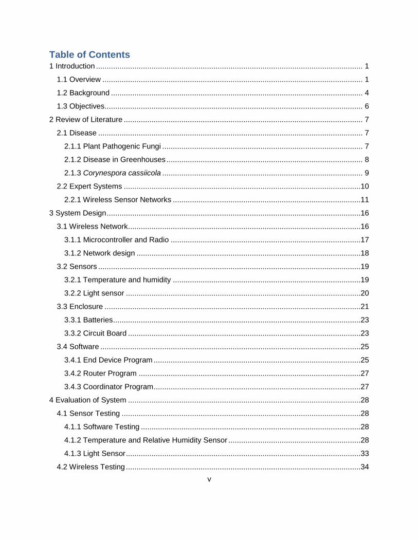
Table of Contents 1 Introduction ............................................................................................................................. 1
1.1 Overview .......................................................................................................................... 1
1.2 Background ...................................................................................................................... 4
1.3 Objectives ......................................................................................................................... 6
2 Review of Literature ................................................................................................................ 7
2.1 Disease ............................................................................................................................ 7
2.1.1 Plant Pathogenic Fungi .............................................................................................. 7
2.1.2 Disease in Greenhouses ............................................................................................ 8
2.1.3 Corynespora cassiicola .............................................................................................. 9
2.2 Expert Systems ...............................................................................................................10
2.2.1 Wireless Sensor Networks ........................................................................................11
3 System Design .......................................................................................................................16
3.1 Wireless Network .............................................................................................................16
3.1.1 Microcontroller and Radio .........................................................................................17
3.1.2 Network design .........................................................................................................18
3.2 Sensors ...........................................................................................................................19
3.2.1 Temperature and humidity ........................................................................................19
3.2.2 Light sensor ..............................................................................................................20
3.3 Enclosure ........................................................................................................................21
3.3.1 Batteries ....................................................................................................................23
3.3.2 Circuit Board .............................................................................................................23
3.4 Software ..........................................................................................................................25
3.4.1 End Device Program .................................................................................................25
3.4.2 Router Program ........................................................................................................27
3.4.3 Coordinator Program .................................................................................................27
4 Evaluation of System .............................................................................................................28
4.1 Sensor Testing ................................................................................................................28
4.1.1 Software Testing .......................................................................................................28
4.1.2 Temperature and Relative Humidity Sensor ..............................................................28
4.1.3 Light Sensor ..............................................................................................................33
4.2 Wireless Testing ..............................................................................................................34
vi
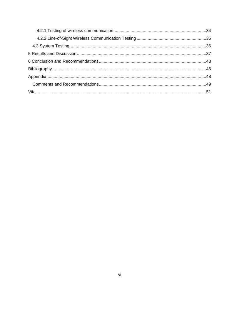
4.2.1 Testing of wireless communication ............................................................................34
4.2.2 Line-of-Sight Wireless Communication Testing .........................................................35
4.3 System Testing ................................................................................................................36
5 Results and Discussion ..........................................................................................................37
6 Conclusion and Recommendations ........................................................................................43
Bibliography ..............................................................................................................................45
Appendix ...................................................................................................................................48
Comments and Recommendations ........................................................................................49
Vita ...........................................................................................................................................51
vii
List of Figures
Figure 1: Conceptual drawing of a sensor station. ...................................................................... 3
Figure 2: Overhead illustration of sensor station on a greenhouse table. ................................... 3
Figure 3: Overhead illustration of sensor stations dispersed throughout a greenhouse.. ............ 4
Figure 4: Disease Triangle (Trigiano et al., 2008). ...................................................................... 7
Figure 5: Conidium of Corynespora Cassiicola. .......................................................................... 8
Figure 6: Illustration of a typical wireless sensor network. .........................................................12
Figure 7: Illustration of a "Star-Pattern" mesh network. .............................................................13
Figure 8: Illustration of a mesh network made only of routers ....................................................14
Figure 9: Conceptual map of sensor station ..............................................................................18
Figure 10: Sensor Station .........................................................................................................22
Figure 11: Inside view of Sensor Station ..................................................................................23
Figure 12: Top side view of circuit boards .................................................................................24
Figure 13: Bottom view of circuit boards....................................................................................24
Figure 14: Flow chart of sensor station program .......................................................................26
Figure 15: Temperature sensor testing in environmental chamber ............................................30
Figure 16: Relative humidity sensor testing in environmental chamber .....................................30
Figure 17: Comparison of relative humidity sensors ..................................................................31
Figure 20: Light sensor calibration curve ...................................................................................34
Figure 22: Line-of-sight signal strength testing based on distance between routers. .................36
Figure 22: Illustrates the spatial and temporal temperature variability within a production .........37
Figure 23: Relative humidity data for the same time period as noted in figure 22. .....................38
Figure 24: Natural light measurements collected in the greenhouse. ........................................38
Figure 26: Sample of light data obtained in a commercial greenhouse. .....................................40
Figure 27: Commercial greenhouse light data ...........................................................................41
Figure 28: Photograph of sensor station #4 during a commercial greenhouse system evaluation.
.................................................................................................................................................41
Figure 29: Sensor station #9 located in a commercial greenhouse…..…………….........……....42 Figure 30: Graph of environmental chamber data with programming error………………………50
1
1 Introduction
1.1 Overview
Greenhouse production is an expensive and high-risk method of producing a crop. While the
financial benefits of being able to deliver a crop at any time of year are high, the costs of
growing the crop and maintaining the facilities are also high. By definition, all greenhouses offer
some degree of environmental control. The simplest structures are covered with a translucent
material that protects crops from adverse environmental conditions. Greenhouses that are
more sophisticated can provide precise temperature control through heating and cooling, shade
cloth and supplemental lighting to ensure an exact range of light and high-end control systems
to automate the production of plants from start to finish. In addition to controlling the
environment, producers must also be concerned with managing insect pests and plant
pathogens. In the wild or in field-grown crops, large-scale outbreaks are mitigated by predators
or by host plants being spaced further apart. In a greenhouse, the densely packed, sheltered
plants are more vulnerable to pathogens. Once a disease outbreak occurs, the warm, humid
environment and the continual presence of the host plant make the disease nearly impossible to
control. The most common cause of disease in plants is fungi. Producers must continually
spray fungicides to prevent the loss of a crop due to infection. This prolonged use of fungicides,
in addition to posing a safety hazard to exposed workers, can reduce sensitivity of fungi to
pesticides.
Fungi that cause disease in plants have optimum environments at which they are able to infect
plants and spread throughout a crop. If the optimal environment is known for a particular
disease, the disease may be avoided or reduced by preventing the triggering environmental

2
conditions from occurring. If environmental conditions conducive for disease outbreaks cannot
be avoided, fungicide usage may be necessary. The quantity of fungicides used for disease
control may be reduced if they are applied only when conditions are conducive for disease
development. One major challenge of this environmental approach to disease prevention is the
large variation that exists spatially in the microenvironment surrounding a crop in a greenhouse.
The environment for a field crop is assumed to be more or less homogenous; however the
environment in a greenhouse crop can vary greatly. It is difficult to obtain information on where
environmental differences occur in the crop and what the differences are. Environmental control
of disease in a greenhouse crop would require high resolution spatial and temporal monitoring
through a vast network of sensors. These sensors would need to be near the plant canopy
where they could measure the actual environmental conditions the plants are experiencing. A
large network of sensors integrated into crop production can be costly to producers and interfere
with their normal operations.
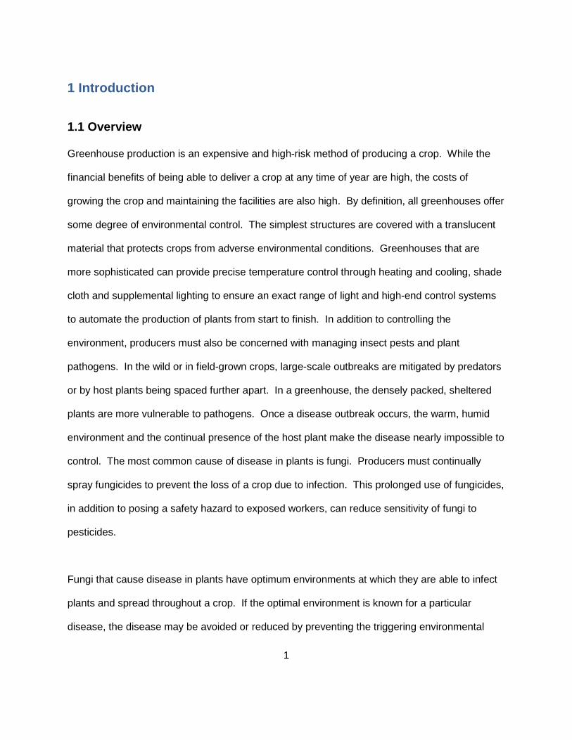
The disease monitoring system developed for this project overcomes these challenges by
utilizing low cost, wireless technologies to create a system that is transportable and occupies no
more space than a small flowerpot (figures 1 and 2). No point-to-point wiring is required for
sensor stations in the system. The individual sensor stations in the monitoring system operate
for several months without requiring maintenance. All data from sensor stations transmit to a
single coordinator station where the data is downloaded by the producer for analysis. Because
the system is wireless, sensor stations can be moved around the greenhouse at will, and the
system can be scaled to any size operation with very little set up. Producers simply have to turn
on the system, setup the sensor stations throughout the greenhouse (figure 3), and they are
ready to start monitoring and recording environmental conditions throughout the crop.
3
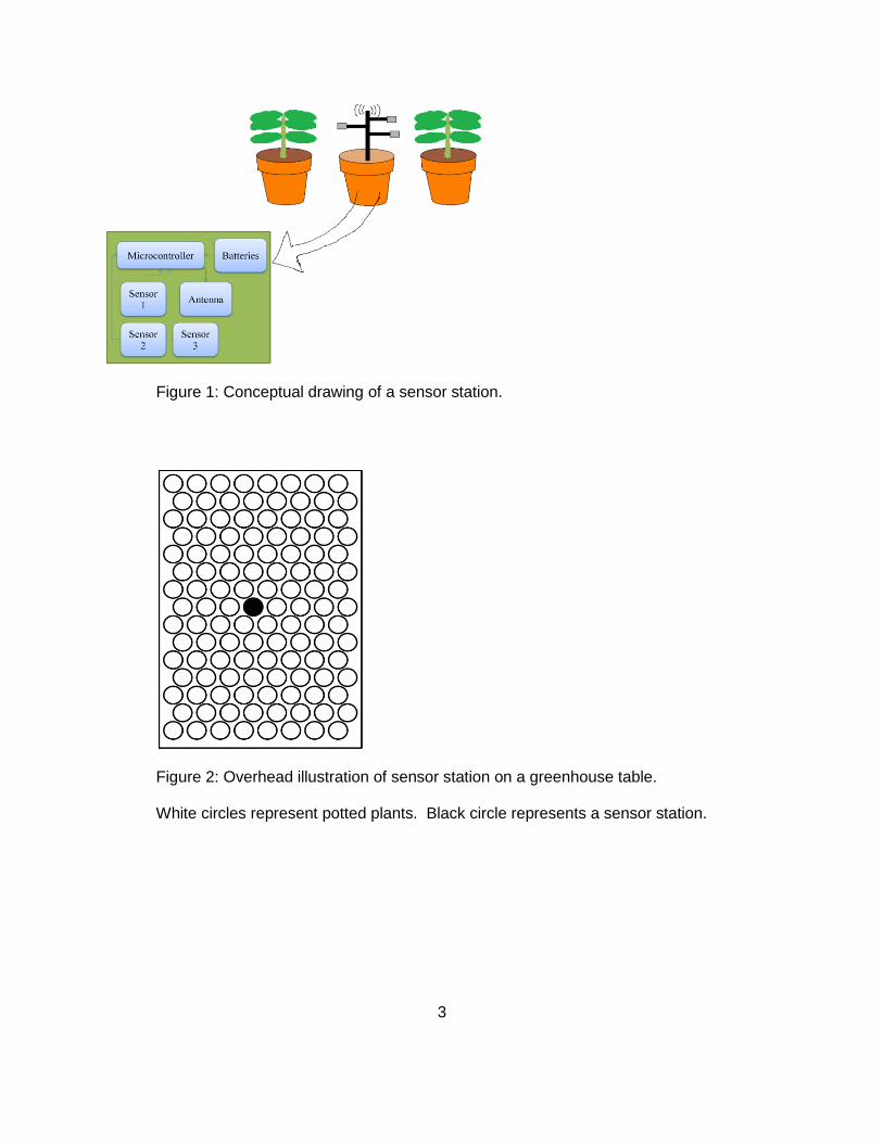
Figure 1: Conceptual drawing of a sensor station.
Figure 2: Overhead illustration of sensor station on a greenhouse table.
White circles represent potted plants. Black circle represents a sensor station.
4
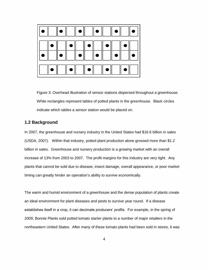
Figure 3: Overhead illustration of sensor stations dispersed throughout a greenhouse.
White rectangles represent tables of potted plants in the greenhouse. Black circles
indicate which tables a sensor station would be placed on.
1.2 Background
In 2007, the greenhouse and nursery industry in the United States had $16.6 billion in sales
(USDA, 2007). Within that industry, potted plant production alone grossed more than $1.2
billion in sales. Greenhouse and nursery production is a growing market with an overall
increase of 13% from 2003 to 2007. The profit margins for this industry are very tight. Any
plants that cannot be sold due to disease, insect damage, overall appearance, or poor market
timing can greatly hinder an operation’s ability to survive economically.
The warm and humid environment of a greenhouse and the dense population of plants create
an ideal environment for plant diseases and pests to survive year round. If a disease
establishes itself in a crop, it can decimate producers’ profits. For example, in the spring of
2009, Bonnie Plants sold potted tomato starter plants to a number of major retailers in the
northeastern United States. After many of these tomato plants had been sold in stores, it was
5
discovered that the crop had a potential infection of late blight. Late blight is a very serious
plant disease. All of the tomato plants had to be recalled. The recall cost Bonnie Plants an
estimated $1 million in sales in addition to damaging their reputation among retailers and
customers (Unknown, 2009).
Holtkamp Greenhouses, Inc. is a business operating in Nashville, TN that specializes in potted
ornamental plants. While they grow a large variety of plants such as coleus, poinsettias, and
ferns, the majority of their space is dedicated to the production of African violets (Saintpaulia
ionantha). In the past few years, Optimara has encountered a disease problem on their African
violets caused by the target leaf spot caused by Corynespora cassiicola. Corynespora
cassiicola is a fungus that causes necrotic spots on the leaves of the plants. Since these plants
are sold as ornamentals, spotted leaves make the plants unmarketable. Although severe
outbreaks of disease occur periodically, there are always a few plants in the greenhouse with
the leaf spot. As long as the number of spots is small, the affected leaves can be removed, and
the plant can be salvaged. During a severe outbreak, symptomatic plants are rouged, and the
remaining plants are sprayed with a prophylactic fungicide. These outbreaks cause a significant
economic loss to the company. Since it is certain that a susceptible host, African violets, is
always present, and the pathogen is constantly present since low levels of the disease can
always be detected, the most likely cause for severe outbreaks of disease is a change in the
environment. An environmental monitoring system is needed to monitor the crop with a high
spatial and temporal resolution and determine what type of an environment is triggering the
outbreak of the disease. A search was made of commercially available systems and none was
found that could easily meet or be adapted to meet the needs of this project. This unrealized
need was the inspiration for the greenhouse monitoring system developed for this project and
detailed in this document.
6
1.3 Objectives
The general objective was to develop a system to control or prevent outbreaks of Corynespora
cassiicola in Saintpaulia ionantha greenhouses by early detection of disease favorable
conditions. This project designs, prototypes, and evaluates an environmental monitoring
system to determine if there is a correlation between conditions inside the greenhouse and
outbreaks of the disease. Specifically, this system should:
Integrate multiple sensor stations and a coordinator station into a network
Be deployable in a commercial greenhouse environment
Have sensor stations entirely self contained and battery operated
Collect data on environmental conditions
Fit in the footprint of a four inch potted plant
Be minimally invasive to minimize inconvenience to producers
Be simple to operate
7
2 Review of Literature
2.1 Disease
2.1.1 Plant Pathogenic Fungi
The most prevalent cause of plant disease is pathogenic fungi. Devastating plant diseases
caused by fungi have been observed since ancient times. Plant pathogenic fungi were
responsible for chestnut blight and the Irish potato famine. Fungi obtain their nutrients by
excreting digestive exoenzymes and absorbing the nutrients through cell walls (Trigiano et al.,
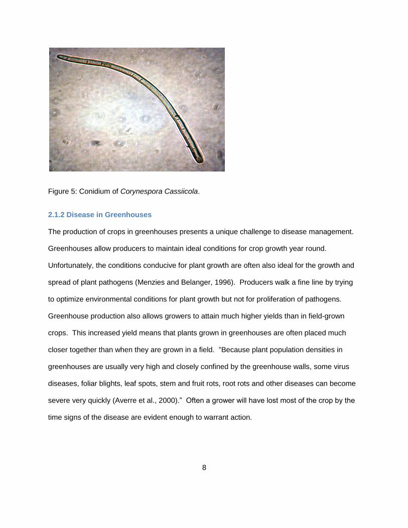
2008). One way that fungi can spread through a crop is through asexually produced spores
called conidia (figure 5). For a fungus to cause disease in a plant the proper environment must
be present (figure 4). Fungi prefer damp high humidity environments. Moisture is needed to
carry nutrients to hyphal cells, for fungi to germinate, and for penetration of leaf tissue. The
optimum environment for most species of fungi is between 25°C-30°C with a pH between 4 and
7 (Trigiano et al., 2008).
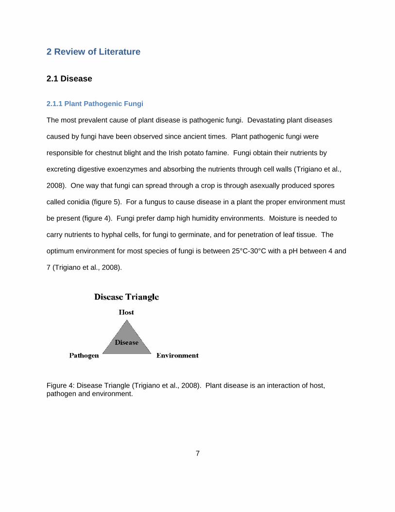
Figure 4: Disease Triangle (Trigiano et al., 2008). Plant disease is an interaction of host, pathogen and environment.
8
Figure 5: Conidium of Corynespora Cassiicola.
2.1.2 Disease in Greenhouses
The production of crops in greenhouses presents a unique challenge to disease management.
Greenhouses allow producers to maintain ideal conditions for crop growth year round.
Unfortunately, the conditions conducive for plant growth are often also ideal for the growth and
spread of plant pathogens (Menzies and Belanger, 1996). Producers walk a fine line by trying
to optimize environmental conditions for plant growth but not for proliferation of pathogens.
Greenhouse production also allows growers to attain much higher yields than in field-grown
crops. This increased yield means that plants grown in greenhouses are often placed much
closer together than when they are grown in a field. “Because plant population densities in
greenhouses are usually very high and closely confined by the greenhouse walls, some virus
diseases, foliar blights, leaf spots, stem and fruit rots, root rots and other diseases can become
severe very quickly (Averre et al., 2000).” Often a grower will have lost most of the crop by the
time signs of the disease are evident enough to warrant action.
9
Along with these challenges, greenhouses also have potential advantages in disease
management. “The high labor, high technology inputs of the greenhouse industry provide
unique opportunities for disease control (Belanger and Menzies, 1996).” By growing crops in a
greenhouse, producers have demonstrated their willingness to spend extra resources to deliver
a crop out of season. Through the environmental control technology in place in many
greenhouses and simple changes in management practices, growers may be able to reduce the
severity of disease in their crops. “Since plant disease [is] strongly affected by temperature and
humidity, the best way to combat disease is to manipulate the greenhouse environment. Unlike
the weather outdoors, we can control the greenhouse environment (Eshenaur and Anderson,
2004).” Most plant pathogenic fungi need high humidity or standing water to germinate and
develop properly. These conditions can be avoided in greenhouses without hurting the plants
through practices like, spacing plants further apart to prevent humidity build up in the canopy
and delivering water straight to the media when possible rather than by overhead watering.
Also, monitoring light levels, temperature, and humidity to determine plant water needs and
watering only when needed can reduce the humidity in a greenhouse and especially in the
micro-climate surrounding the plants (Eshenaur and Anderson, 2004).
2.1.3 Corynespora cassiicola
Corynespora cassiicola is a plant pathogenic fungus that was described by Wei in 1950. The
fungus spreads from plant to plant by germ tubes germinating from conidia. Corynespora
cassiicola is commonly known as target leaf spot because of the necrotic lesions left on plants.
The extensive list of plants for which C. cassiicola is a pathogen and the many more plants on
which it can survive as an endophyte makes this fungus difficult to study or control. Not every
strain of C. cassiicola is pathogenic on the same plants (Schlub et al., 2009). The strain that
causes disease in African violets has not been well studied.
10
Schlub et al. (2009) reported that disease caused by C. cassiicola was observed above 20°C
with severe disease occurring at 32°C. He also reported that high humidity and leaf wetness
were needed for 16-44 hours for disease to be present (Schlub et al., 2009). Madhavi et al.
(2009) confirmed the high humidity requirement when he reported maximum germination and
germ tube growth occurred at 95%RH. He also reported that when C. cassiicola was cultured in
alternate darkness and light, germination was greater than when it was cultured under
continuous light or continuous dark. UV exposure reduced spore germination (Madhavi et al.,
2009).
When searching for environmental causes that enhance disease outbreaks, one must identify
the proper parameters and when they occur. Some diseases remain latent for long periods, and
epidemics can explode once detected. The triggering environmental event may have long since
passed. Fernandes et al. (2003) reported that after inoculating coleus plants with a known
pathogenic strain of C. cassiicola that disease spots were evident on the plants in less than 24
hours. Rapid spread of the disease is implied by growers who report that one day there is only
a small amount of disease and the next day most of the crop is showing symptoms of infection.
Madhavi et al. (2009) also noted that while some conidia had germinated within one hour, 90%
were germinated within 24 hours. It is important to note that the strains of C. cassiicola in these
two studies and the plants they were studied on are not the same as those being observed in
this research, so there is a possibility that times for germination and infection will differ.
2.2 Expert Systems
As electronics and computers become smaller and more affordable, their use in agriculture has
become more prevalent. The combination of computers and sensors in the greenhouse can be
11
invaluable in helping growers make informed, timely decisions that will increase yields, produce
higher quality plants, and decrease the instances of disease. One way of utilizing electronics in
the greenhouse and nursery industry is through expert systems. An expert system is “a
computer program using expert knowledge to attain high levels of performance in a narrow
problem area (Donahue et al., 1991).” Expert systems were being developed for use in
agriculture as early as the 1990’s (Donahue et al., 1991). These systems consisted of yes/no
questions that farmers would answer on a computer screen. The computer program would then
determine what type of problem the farmer was facing and suggest an appropriate course of
action. As computer power has increased and sensors have become smaller and cheaper,
newer models have been created that rely more on electronic measurements and less on
human input. Expert systems today can collect information from the greenhouse environment,
analyze it, and then inform the grower about what is happening. There are many systems
available on the market that interface with the control systems to adjust the environment or alert
the grower as necessary. Hu et al. (2007) recently developed an expert system for managing
greenhouse vegetable production. The system measured environmental parameters that affect
plant production such as temperature, humidity, and light intensity inside and outside of the
greenhouse. The data acquisition also had the ability to measure CO2 concentration, wind
speed and direction, and rainfall. Their system had one sensing station placed on the
greenhouse rafters high above the plant canopy in each greenhouse. These stations were hard
wired to a PC dedicated to greenhouse data acquisition. An alarm was in place to alert the
growers if any parameter exceeded acceptable operating conditions.
2.2.1 Wireless Sensor Networks
One hurtle that has been preventing the implementation of expert systems in many smaller and
midsized greenhouse operations is the high start up cost and the inconvenience of the hard
12
ware. A promising solution to these issues is wireless sensor networks (Pawlowski et al., 2009).
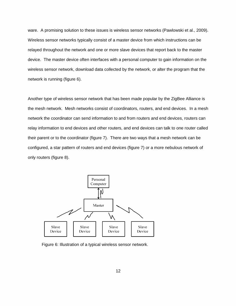
Wireless sensor networks typically consist of a master device from which instructions can be
relayed throughout the network and one or more slave devices that report back to the master
device. The master device often interfaces with a personal computer to gain information on the
wireless sensor network, download data collected by the network, or alter the program that the
network is running (figure 6).
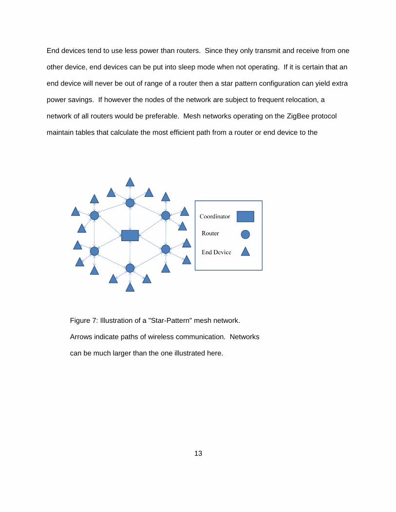
Another type of wireless sensor network that has been made popular by the ZigBee Alliance is
the mesh network. Mesh networks consist of coordinators, routers, and end devices. In a mesh
network the coordinator can send information to and from routers and end devices, routers can
relay information to end devices and other routers, and end devices can talk to one router called
their parent or to the coordinator (figure 7). There are two ways that a mesh network can be
configured, a star pattern of routers and end devices (figure 7) or a more nebulous network of
only routers (figure 8).
Figure 6: Illustration of a typical wireless sensor network.
13
End devices tend to use less power than routers. Since they only transmit and receive from one
other device, end devices can be put into sleep mode when not operating. If it is certain that an
end device will never be out of range of a router then a star pattern configuration can yield extra
power savings. If however the nodes of the network are subject to frequent relocation, a
network of all routers would be preferable. Mesh networks operating on the ZigBee protocol
maintain tables that calculate the most efficient path from a router or end device to the
Figure 7: Illustration of a "Star-Pattern" mesh network.
Arrows indicate paths of wireless communication. Networks
can be much larger than the one illustrated here.
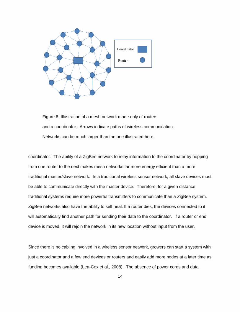
14
Figure 8: Illustration of a mesh network made only of routers
and a coordinator. Arrows indicate paths of wireless communication.
Networks can be much larger than the one illustrated here.
coordinator. The ability of a ZigBee network to relay information to the coordinator by hopping
from one router to the next makes mesh networks far more energy efficient than a more
traditional master/slave network. In a traditional wireless sensor network, all slave devices must
be able to communicate directly with the master device. Therefore, for a given distance
traditional systems require more powerful transmitters to communicate than a ZigBee system.
ZigBee networks also have the ability to self heal. If a router dies, the devices connected to it
will automatically find another path for sending their data to the coordinator. If a router or end
device is moved, it will rejoin the network in its new location without input from the user.
Since there is no cabling involved in a wireless sensor network, growers can start a system with
just a coordinator and a few end devices or routers and easily add more nodes at a later time as
funding becomes available (Lea-Cox et al., 2008). The absence of power cords and data
15
cables also makes wireless sensor networks less intrusive to growing operations. Van Tuijl et
al. (2008) implemented a 100 node mesh network in a cucumber greenhouse. They noted that
mesh networks are ideal for studying containerized plants that will be moved throughout the
greenhouse and the small size and relatively low cost of wireless sensors allow for the study of
temperature variation and disease progression. The attempt at measuring temperature and
humidity in a large greenhouse using a wireless sensor network was successful. However,
several challenges that still hinder the expanded use of wireless sensors in a greenhouse were
identified. One issue identified was the packaging of sensors. Most plastics cannot withstand
the solar radiation and high humidity of a greenhouse, and many packaging choices can cause
heat buildup that electronics cannot tolerate. Temperature and humidity sensors must be
shielded from direct solar radiation to prevent erroneous readings but must still be in contact
with the surrounding environment. One potential concern is that the 2.4 GHz frequency used in
wireless systems is attenuated by water rich objects such as plants (Van Tuijl et al., 2008).

16
3 System Design
To be able to monitor the environment of greenhouses closely enough to be able to predict
disease outbreaks, a monitoring system with high spatial and temporal resolution is needed.
The system designed for this project is capable of that type of high resolution monitoring. The
goal of this project was to develop a proof of concept prototype system that could later be
refined and implemented on a commercial scale. The system should:
Demonstrate an ability to communicate wirelessly in a fully operational greenhouse
Design sensor stations that could operate for multiple months without recharging or
replacing
Collect environmental data that could lead to a disease prediction model
o Measure temperature, humidity, and light
Incorporate an enclosure to protect electronics in a greenhouse environment
Transmit data from individual sensor stations to a coordinator
Transmit data from a coordinator to a personal computer
Be easy to install, maintain, and utilize
3.1 Wireless Network
There are multiple choices for wireless communication currently on the market such as
Bluetooth and ZigBee. For this project, the wireless communication protocol chosen needs to:
Operate over at least two hundred feet in a greenhouse environment
Allow for seventy five sensor stations on one network
Operate for at least 90 days on a single battery charge from a battery small enough to fit
into a device that meets the previously stated requirement of a footprint no bigger than a
four inch potted plant.
17
Both Bluetooth and ZigBee fulfill the first two requirements. While Bluetooth is more widely
implemented in the market today and is older and consequently more well tested, a Bluetooth
system requires far more power to relay information over the same distance as a ZigBee
system. This is due largely to the fact that ZigBee allows for a mesh network design whereas
Bluetooth does not. Since the greenhouse monitoring system is a network of sensor stations
distributed throughout a greenhouse, the mesh network is ideal, and the power savings that can
be realized with a ZigBee system make it the preferred communication protocol for this project.
3.1.1 Microcontroller and Radio
For the sake of keeping the sensor stations as small as possible, a combined microcontroller
(MCU) and wireless communication system was chosen. The Texas Instruments(TI) CC2530 is
a low power “system-on-a-chip” able to perform the basic tasks needed for this project and is a
ZigBee capable receiver and transmitter. The CC2530 has 21 general input/output pins, 256
KB of programmable flash memory, four internal timers, and three power modes. There is also
an on board 12-bit analog-to-digital converter (ADC) with 8 channels. The MCU operates on a
supply voltage between 2 and 3.6VDC power. Battery voltage is monitored using the onboard
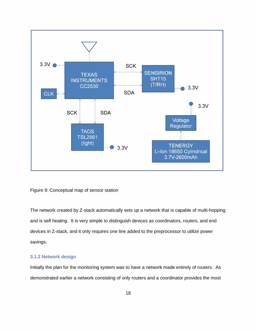
ADC. Figure 9 illustrates how the TI CC2530 interacts with other sensor station components at
a system level.
The ZigBee stack (Z-stack) program, provided by TI with the CC2530, is compliant with the
latest ZigBee and ZigBee PRO stack profiles. The manufacturer’s intention is for end users to
develop programs within Z-stack. By adding their personal code to the designated areas within
a Z-stack workspace, end users gain access to all the necessary functions of a fully operational
ZigBee network. Z-stack is developed in the C/C++ programming language. The preferred
compiler of Texas Instruments for the CC2530 is the IAR Embedded Workbench.
18
Figure 9: Conceptual map of sensor station
The network created by Z-stack automatically sets up a network that is capable of multi-hopping
and is self healing. It is very simple to distinguish devices as coordinators, routers, and end
devices in Z-stack, and it only requires one line added to the preprocessor to utilize power
savings.
3.1.2 Network design
Initially the plan for the monitoring system was to have a network made entirely of routers. As
demonstrated earlier a network consisting of only routers and a coordinator provides the most
19
flexibility in a system and ensures there will be no issues with reaching the coordinator in a
system where devices may be continually moving. Z-stack does not allow routers to use power
saving modes. Only end devices are permitted to enter sleep modes. This is due to the fact
that a router must always be ready to act as a hopping point and be able to receive data from
one device that needs to be passed on to another device in the system. Not only does this
mean that a router’s CPU cannot sleep but also that the radio on a router will be functioning
most of the time. The radio draws more power in the sensor stations than any other
component. For this reason, it became necessary to configure the sensor stations as end
devices. The routers draw too much power to meet all of the design objectives. For example, if
each station were given enough battery power to last for a few months, the size of the battery
would exceed the footprint of a four-inch pot. If the routers and batteries were designed to fit
into a four-inch pot, operating them would be limited to one or two days. The compromise was
to only use routers when the system was implemented in a greenhouse too large to be serviced
by a coordinator and end devices alone and to use as few routers as possible to be able to
reach all areas of the greenhouse. When routers are needed, sensor stations can be converted
to accept auxiliary power (electrical utility or solar).
3.2 Sensors
3.2.1 Temperature and humidity
To simplify the sensor station programming, circuit board design, and sensor station housing
design, the SHT15 combined temperature and humidity sensor from Sensirion was selected.
The combination of humidity and temperature sensing in one device saves physical space on
the sensor station and also limits the number of input pins being used on the microcontroller.
The SHT15 digitally interfaces with the microcontroller through the I2C protocol. According to
the manufacture, the sensors are interchangeable and do not require individual calibration
20
curves. The interchangeability of sensors was confirmed in this project through testing in an
environmental chamber. The reported operating range for the temperature sensor (-40 to
123.8°C) and the humidity sensor (0-100%) falls well within the range of expected
environmental conditions in a greenhouse. The SHT15 can operate on 2.4-5.5V input. Sensors
only take readings when commanded by the microcontroller. This power saving mode reduces
the overall cumulative power requirements. The reported accuracy of this device is ±0.3°C for
the temperature and ±1.8%RH for relative humidity. While 1.8%RH in the range of 0-100%RH
may seem like a large error, it is acceptable for this project. The monitoring system is designed
to collect environmental data within a greenhouse for the purposes of tracking disease. The
sensors in this monitoring system are monitoring a population of plants. As with any population
of living organisms there will be great variation from specimen to specimen. While there will be
similarities and general patterns that can be discovered, there will not be an exact temperature
and humidity combination that will trigger disease in a plant. Instead there will be a range of
environmental conditions in which the occurrence of disease is more likely. The accuracy of the
SHT15 is more than capable of distinguishing the changing environmental conditions that may
trigger disease. The accuracy of the humidity sensor will decrease as the relative humidity rises
above 90%RH but is still acceptable for this project.
3.2.2 Light sensor
The initial goal for the project was to measure ultra-violet light, photosynthetically active
radiation(PAR), and infrared light. However, no cost effective filters were found that could be
adjusted to fit over a photodiode to provide the desired spectrums. Hence, ultra-violet light was
not included in the final design objectives. A single device that approximates the human eye
response was used instead. The TSL2561 from Texas Advanced Optoelectronic Solutions
(TAOS) is a light-to-digital converter. It has a 16 bit digital output with an I2C digital interface.
21
The TSL2561 is comprised of two photodiodes. The first is sensitive only to the infrared
range(750nm ≤ λ ≤ 1000nm). The second is sensitive over the visible and infrared range
(380nm ≤ λ ≤ 1000nm). By using a calibration curve the infrared reading can be subtracted out
of the reading from the second diode providing a human eye approximation. The visible
spectrum is close enough to the same range as PAR (400nm ≤ λ ≤ 700nm) to be considered
synonymous in this project. Therefore, this one device provides both the desired PAR and
infrared readings. The TSL2561 operates on 2.7-3.6V input within the ranges of -30 to 70°C.
The light reaches the sensor through a light pipe in the sensor station housing. The light pipe
attenuates the light, so, as the manufacturer notes in the data sheet, it was necessary to
recalibrate the light sensors. The sensor is equipped with an onboard ADC that converts the
signal from the photodiodes to a digital output. The sensor automatically rejects 50/60Hz
lighting allowing discrimination between natural and supplemental (AC) illumination. There is
also a programmable sleep mode that allows the microcontroller to turnoff power to the
photodiodes when they are not being read. This ability of the sensor to sleep is important for
keeping the power requirements of the sensor stations as low as possible.
3.3 Enclosure
The enclosure chosen for the sensor stations was an ABS plastic NEMA 4 enclosure made by
Budd Industries. It was important to have a NEMA 4 or better enclosure to protect the
electronics against water and dirt that will be encountered during normal greenhouse operations
of a greenhouse. Enclosures were fabricated in house to accommodate mounting holes for
sensors, the antenna, and external power switch. The power switch was mounted in the lid of
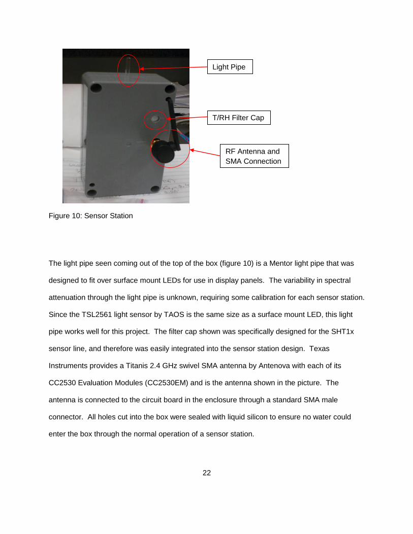
the enclosure. All other mounting points were in the main body of the enclosure (figure 10).
22
Figure 10: Sensor Station
The light pipe seen coming out of the top of the box (figure 10) is a Mentor light pipe that was
designed to fit over surface mount LEDs for use in display panels. The variability in spectral
attenuation through the light pipe is unknown, requiring some calibration for each sensor station.
Since the TSL2561 light sensor by TAOS is the same size as a surface mount LED, this light
pipe works well for this project. The filter cap shown was specifically designed for the SHT1x
sensor line, and therefore was easily integrated into the sensor station design. Texas
Instruments provides a Titanis 2.4 GHz swivel SMA antenna by Antenova with each of its
CC2530 Evaluation Modules (CC2530EM) and is the antenna shown in the picture. The
antenna is connected to the circuit board in the enclosure through a standard SMA male
connector. All holes cut into the box were sealed with liquid silicon to ensure no water could
enter the box through the normal operation of a sensor station.
Light Pipe
T/RH Filter Cap
RF Antenna and
SMA Connection
23
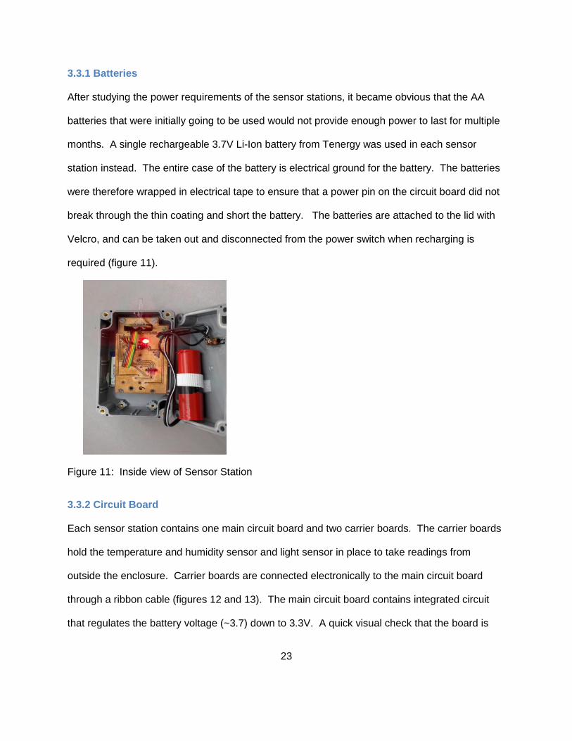
3.3.1 Batteries
After studying the power requirements of the sensor stations, it became obvious that the AA
batteries that were initially going to be used would not provide enough power to last for multiple
months. A single rechargeable 3.7V Li-Ion battery from Tenergy was used in each sensor
station instead. The entire case of the battery is electrical ground for the battery. The batteries
were therefore wrapped in electrical tape to ensure that a power pin on the circuit board did not
break through the thin coating and short the battery. The batteries are attached to the lid with
Velcro, and can be taken out and disconnected from the power switch when recharging is
required (figure 11).
Figure 11: Inside view of Sensor Station
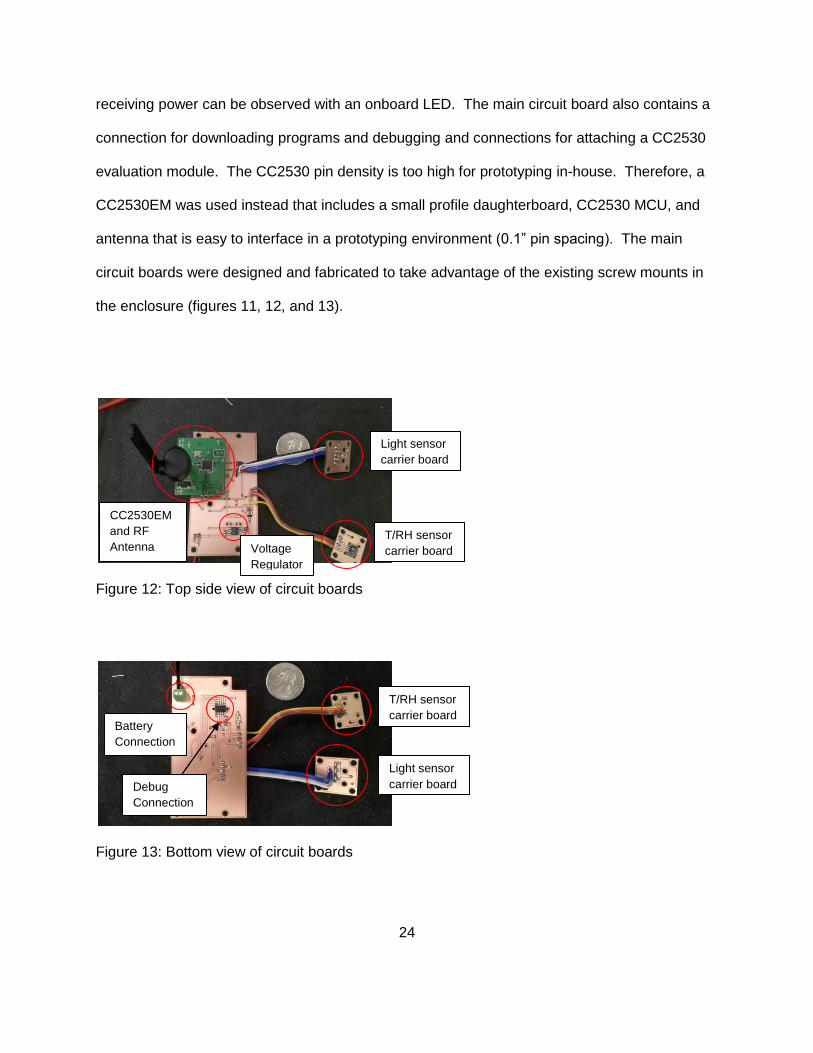
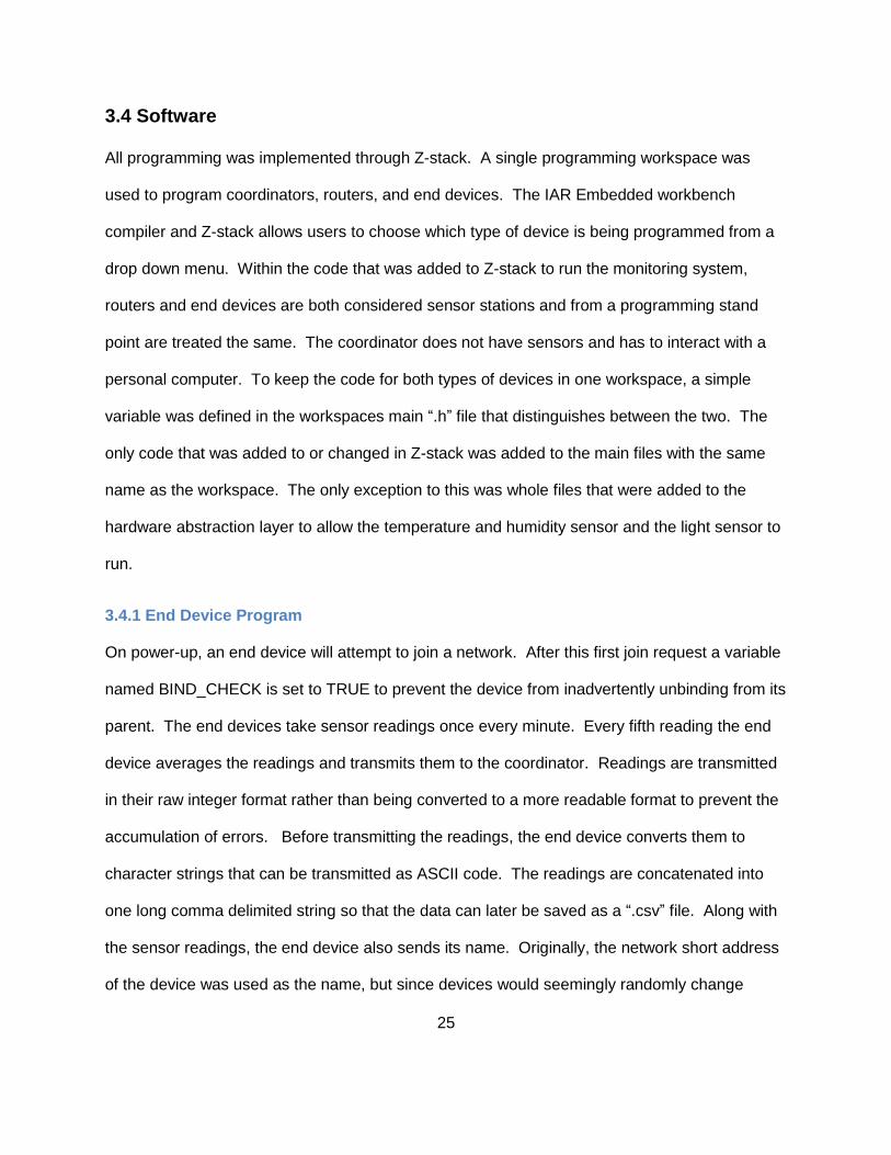
3.3.2 Circuit Board
Each sensor station contains one main circuit board and two carrier boards. The carrier boards
hold the temperature and humidity sensor and light sensor in place to take readings from
outside the enclosure. Carrier boards are connected electronically to the main circuit board
through a ribbon cable (figures 12 and 13). The main circuit board contains integrated circuit
that regulates the battery voltage (~3.7) down to 3.3V. A quick visual check that the board is
24
receiving power can be observed with an onboard LED. The main circuit board also contains a
connection for downloading programs and debugging and connections for attaching a CC2530
evaluation module. The CC2530 pin density is too high for prototyping in-house. Therefore, a
CC2530EM was used instead that includes a small profile daughterboard, CC2530 MCU, and
antenna that is easy to interface in a prototyping environment (0.1” pin spacing). The main
circuit boards were designed and fabricated to take advantage of the existing screw mounts in
the enclosure (figures 11, 12, and 13).
Figure 12: Top side view of circuit boards
Figure 13: Bottom view of circuit boards
Battery
Connection
Debug
Connection
Light sensor
carrier board
Light sensor
carrier board
T/RH sensor
carrier board
T/RH sensor
carrier board
CC2530EM
and RF
Antenna Voltage
Regulator
25
3.4 Software
All programming was implemented through Z-stack. A single programming workspace was
used to program coordinators, routers, and end devices. The IAR Embedded workbench
compiler and Z-stack allows users to choose which type of device is being programmed from a
drop down menu. Within the code that was added to Z-stack to run the monitoring system,
routers and end devices are both considered sensor stations and from a programming stand
point are treated the same. The coordinator does not have sensors and has to interact with a
personal computer. To keep the code for both types of devices in one workspace, a simple
variable was defined in the workspaces main “.h” file that distinguishes between the two. The
only code that was added to or changed in Z-stack was added to the main files with the same
name as the workspace. The only exception to this was whole files that were added to the
hardware abstraction layer to allow the temperature and humidity sensor and the light sensor to
run.
3.4.1 End Device Program
On power-up, an end device will attempt to join a network. After this first join request a variable
named BIND_CHECK is set to TRUE to prevent the device from inadvertently unbinding from its
parent. The end devices take sensor readings once every minute. Every fifth reading the end
device averages the readings and transmits them to the coordinator. Readings are transmitted
in their raw integer format rather than being converted to a more readable format to prevent the
accumulation of errors. Before transmitting the readings, the end device converts them to
character strings that can be transmitted as ASCII code. The readings are concatenated into
one long comma delimited string so that the data can later be saved as a “.csv” file. Along with
the sensor readings, the end device also sends its name. Originally, the network short address
of the device was used as the name, but since devices would seemingly randomly change
26
names, it became necessary to program in a specific name for each sensor station. The name
was manually set in the “.h” file for each device before downloading to the board. This is
cumbersome and not desirable for any kind of mass production, but, with careful attention to
detail, it works.
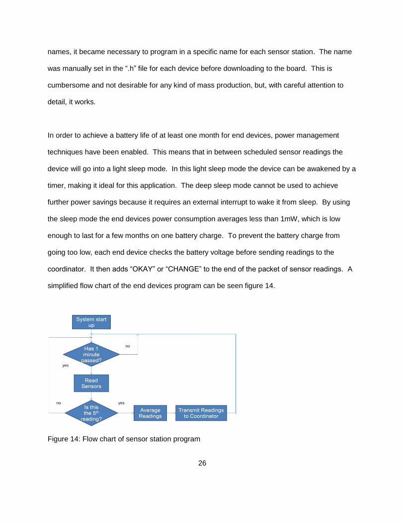
In order to achieve a battery life of at least one month for end devices, power management
techniques have been enabled. This means that in between scheduled sensor readings the
device will go into a light sleep mode. In this light sleep mode the device can be awakened by a
timer, making it ideal for this application. The deep sleep mode cannot be used to achieve
further power savings because it requires an external interrupt to wake it from sleep. By using
the sleep mode the end devices power consumption averages less than 1mW, which is low
enough to last for a few months on one battery charge. To prevent the battery charge from
going too low, each end device checks the battery voltage before sending readings to the
coordinator. It then adds “OKAY” or “CHANGE” to the end of the packet of sensor readings. A
simplified flow chart of the end devices program can be seen figure 14.
Figure 14: Flow chart of sensor station program
no
no
yes
yes
27
3.4.2 Router Program
The router program operates in exactly the same way as an end device program except that it
does not sleep. Routers must be prepared to transmit and receive at all times and therefore
cannot enter a sleep mode. Other than that, they are named, take readings, and transmit data
in the same way as an end device.
3.4.3 Coordinator Program
The coordinator program is responsible for setting up and maintaining the network. Every time
the coordinator program passes through the five-second timer loop it attempts to join with any
device in the network requesting to join. The coordinator does not take any sensor readings of
its own. Sensor stations wirelessly relay their data packets at predetermined intervals to the
coordinator. The coordinator then sends these packets to a personal computer through a
universal asynchronous receiver/transmitter (UART) connection via an RS232 cable. The data
packets are sent in a comma delimited format for ease of processing. The coordinator performs
no further analysis or conversion of the data. The coordinator sends the data through the UART
connection in the same raw format that it receives it in from the sensor station. Rather than
having the sensor stations sending a time stamp along with their data packets, the coordinator
maintains one clock for the entire system and appends the current system time to data packets
after they are received and before they are transmitted to the PC.

28
4 Evaluation of System
4.1 Sensor Testing
4.1.1 Software Testing
The software for this project was developed over a period of many months. After experimenting
with the CC2530 in the ZigBee development kit and determining that it would work for the
project, hardware abstraction layer (HAL) files needed to be written to operate the sensors.
Both the light sensor and the temperature and humidity sensor utilize the I2C communication
protocol. The CC2530 and its associated software are not preprogrammed to handle I2C
communications. This means that it was necessary to develop the code for I2C communication
and add it to the HAL. To test that these files were implementing a proper I2C communication,
an oscilloscope was connected to the clock line and data line of the sensors. Signals were
captured on the screen and examined to make sure the clock line was pulsing correctly, and
that both the CC2530 and the sensors were controlling the data lines in turn, and that the data
bit was changing at the proper time.
Each portion of the program was tested for functionality in the lab and corrected until every part
was working, however a program can never truly be said to be free of bugs.
4.1.2 Temperature and Relative Humidity Sensor
Three initial prototype boards were placed in an environmental test chamber and cycled through
temperature and humidity ranges that are typical of a greenhouse environment (0-40°C and 40-
100%RH). One test cycled through a range of temperatures while holding humidity steady.
Another test cycled humidity while holding temperature steady. The environmental chamber
29
was not able to control humidity at lower temperatures. When this happened, the resulting
profile was too erratic to be useful for sensor station testing. Data points in these ranges were
not considered for analysis. The prototype boards were not enclosed and did not have filter
caps over the sensors. The initial prototype boards used an SHT75, the same sensor as the
SHT15, but it comes on a carrier board that makes it easier for initial prototyping. The initial
prototype boards were running an earlier version of the monitoring program. Sensors collected
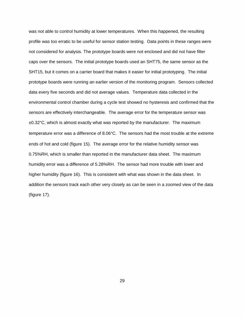
data every five seconds and did not average values. Temperature data collected in the
environmental control chamber during a cycle test showed no hysteresis and confirmed that the
sensors are effectively interchangeable. The average error for the temperature sensor was
±0.32°C, which is almost exactly what was reported by the manufacturer. The maximum
temperature error was a difference of 8.06°C. The sensors had the most trouble at the extreme
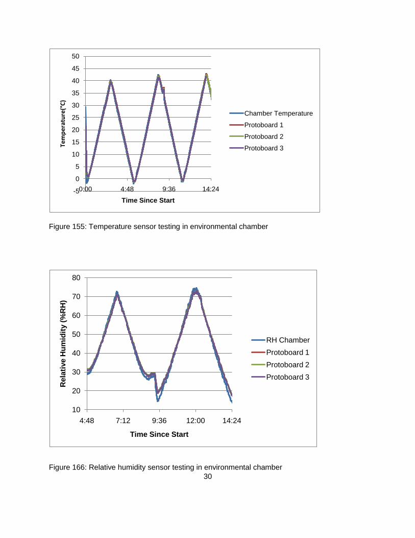
ends of hot and cold (figure 15). The average error for the relative humidity sensor was
0.75%RH, which is smaller than reported in the manufacturer data sheet. The maximum
humidity error was a difference of 5.28%RH. The sensor had more trouble with lower and
higher humidity (figure 16). This is consistent with what was shown in the data sheet. In
addition the sensors track each other very closely as can be seen in a zoomed view of the data
(figure 17).
30
Figure 155: Temperature sensor testing in environmental chamber
Figure 166: Relative humidity sensor testing in environmental chamber
-5
0
5
10
15
20
25
30
35
40
45
50
0:00 4:48 9:36 14:24
Temperature(°C)
Time Since Start
Chamber Temperature
Protoboard 1
Protoboard 2
Protoboard 3
10
20
30
40
50
60
70
80
4:48 7:12 9:36 12:00 14:24
Re
lati
ve
Hu
mid
ity (
%R
H)
Time Since Start
RH Chamber
Protoboard 1
Protoboard 2
Protoboard 3
31
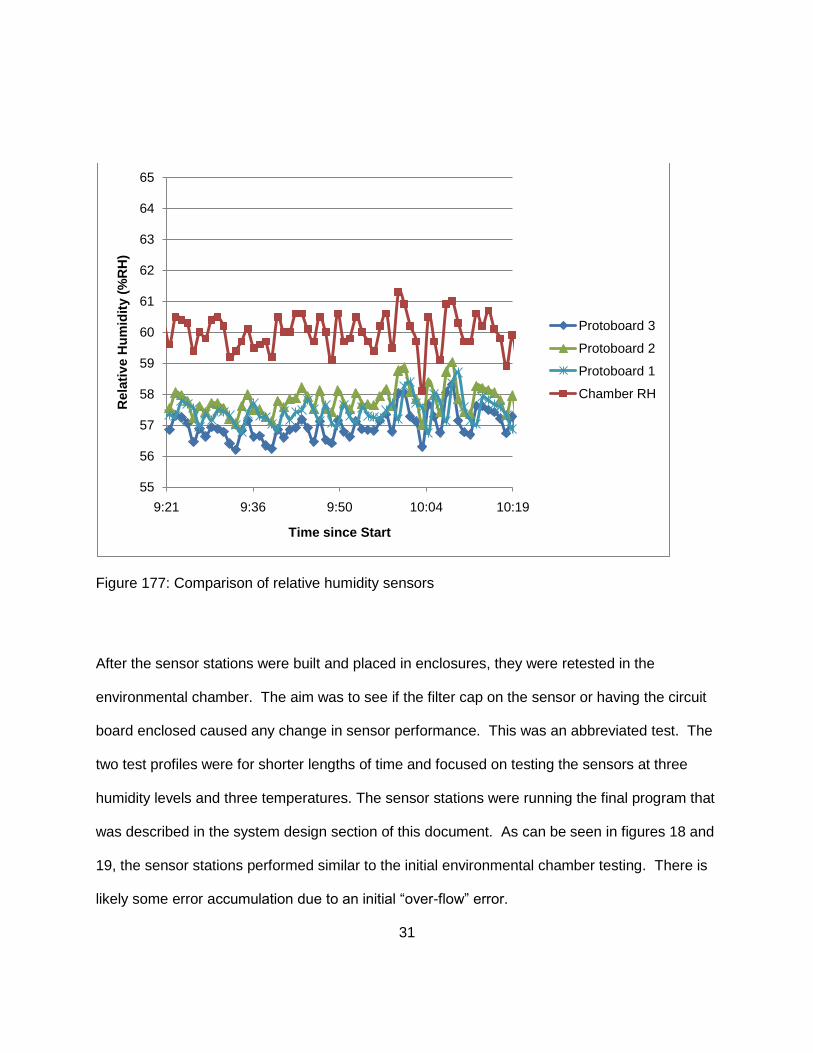
Figure 177: Comparison of relative humidity sensors
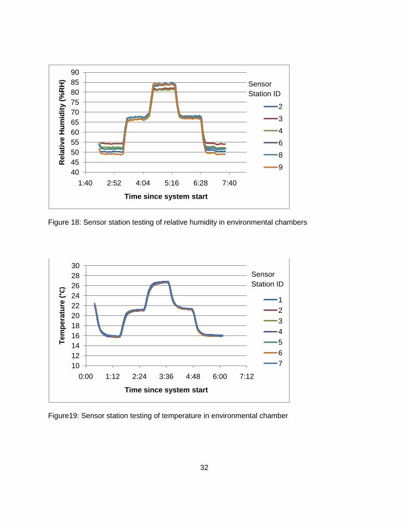
After the sensor stations were built and placed in enclosures, they were retested in the
environmental chamber. The aim was to see if the filter cap on the sensor or having the circuit
board enclosed caused any change in sensor performance. This was an abbreviated test. The
two test profiles were for shorter lengths of time and focused on testing the sensors at three
humidity levels and three temperatures. The sensor stations were running the final program that
was described in the system design section of this document. As can be seen in figures 18 and
19, the sensor stations performed similar to the initial environmental chamber testing. There is
likely some error accumulation due to an initial “over-flow” error.
55
56
57
58
59
60
61
62
63
64
65
9:21 9:36 9:50 10:04 10:19
Rela
tiv
e H
um
idit
y (
%R
H)
Time since Start
Protoboard 3
Protoboard 2
Protoboard 1
Chamber RH
32
Figure 18: Sensor station testing of relative humidity in environmental chambers
Figure19: Sensor station testing of temperature in environmental chamber
40
45
50
55
60
65
70
75
80
85
90
1:40 2:52 4:04 5:16 6:28 7:40
Re
lati
ve
Hu
mid
ity (
%R
H)
Time since system start
2
3
4
6
8
9
10
12
14
16
18
20
22
24
26
28
30
0:00 1:12 2:24 3:36 4:48 6:00 7:12
Te
mp
era
ture
(°C)
Time since system start
1
2
3
4
5
6
7
Sensor
Station ID
Sensor
Station ID
33
4.1.3 Light Sensor
The three initial prototype boards were tested under several different light sources and levels,
and those readings were compared with readings from a light meter. It was discovered that
The light sensors were saturated in full sunlight
The provided calibration curve for the light sensors did not agree with the light meter.
A representative of TAOS, the manufacturer of the light sensor pointed out that a recalibration
would be required after the light pipe was added, since the light pipe would attenuate the signal.
No further calibration was done with the light sensors on the initial prototype boards.
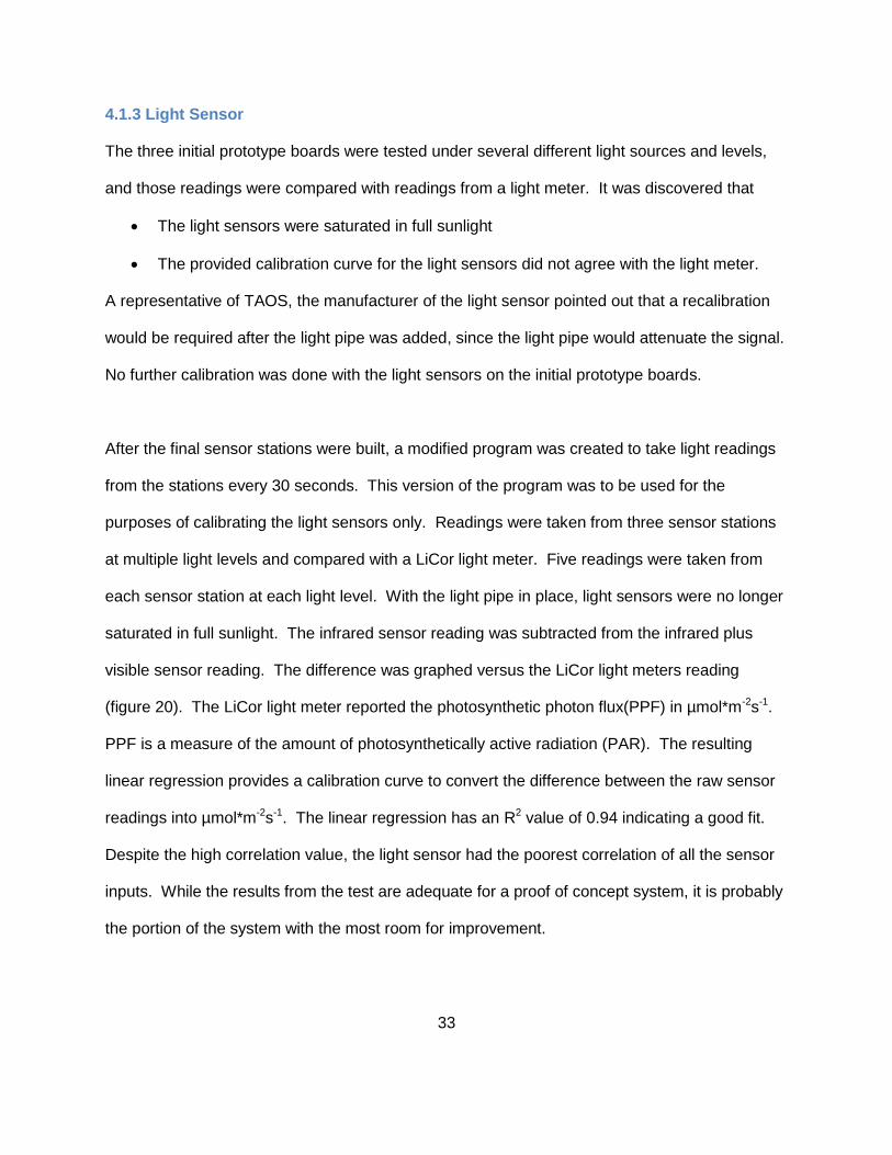
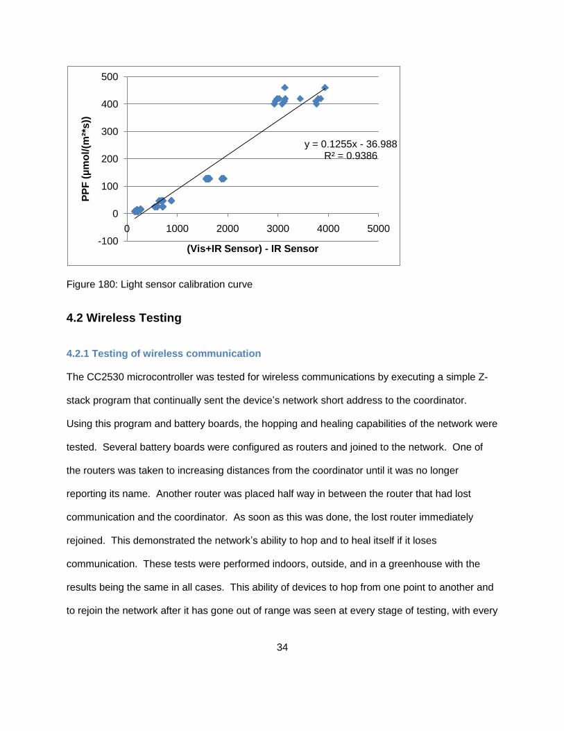
After the final sensor stations were built, a modified program was created to take light readings
from the stations every 30 seconds. This version of the program was to be used for the
purposes of calibrating the light sensors only. Readings were taken from three sensor stations
at multiple light levels and compared with a LiCor light meter. Five readings were taken from
each sensor station at each light level. With the light pipe in place, light sensors were no longer
saturated in full sunlight. The infrared sensor reading was subtracted from the infrared plus
visible sensor reading. The difference was graphed versus the LiCor light meters reading
(figure 20). The LiCor light meter reported the photosynthetic photon flux(PPF) in µmol*m-2s-1.
PPF is a measure of the amount of photosynthetically active radiation (PAR). The resulting
linear regression provides a calibration curve to convert the difference between the raw sensor
readings into µmol*m-2s-1. The linear regression has an R2 value of 0.94 indicating a good fit.
Despite the high correlation value, the light sensor had the poorest correlation of all the sensor
inputs. While the results from the test are adequate for a proof of concept system, it is probably
the portion of the system with the most room for improvement.
34
Figure 180: Light sensor calibration curve
4.2 Wireless Testing
4.2.1 Testing of wireless communication
The CC2530 microcontroller was tested for wireless communications by executing a simple Z-
stack program that continually sent the device’s network short address to the coordinator.
Using this program and battery boards, the hopping and healing capabilities of the network were
tested. Several battery boards were configured as routers and joined to the network. One of
the routers was taken to increasing distances from the coordinator until it was no longer
reporting its name. Another router was placed half way in between the router that had lost
communication and the coordinator. As soon as this was done, the lost router immediately
rejoined. This demonstrated the network’s ability to hop and to heal itself if it loses
communication. These tests were performed indoors, outside, and in a greenhouse with the
results being the same in all cases. This ability of devices to hop from one point to another and
to rejoin the network after it has gone out of range was seen at every stage of testing, with every
y = 0.1255x - 36.988R² = 0.9386
-100
0
100
200
300
400
500
0 1000 2000 3000 4000 5000
PP
F (
µm
ol/
(m²*
s))
(Vis+IR Sensor) - IR Sensor
35
program throughout the project. It can be assumed that despite some of its pitfalls, Z-stack
does creates robust ZigBee networks.
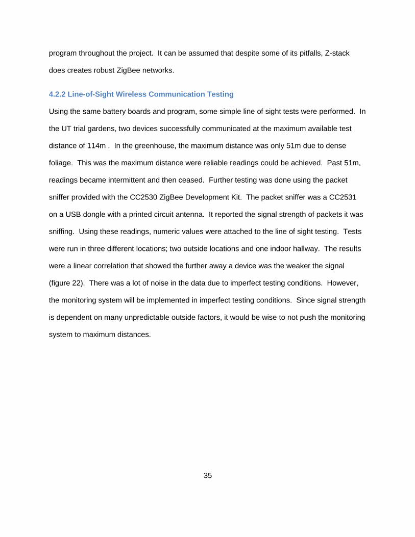
4.2.2 Line-of-Sight Wireless Communication Testing
Using the same battery boards and program, some simple line of sight tests were performed. In
the UT trial gardens, two devices successfully communicated at the maximum available test
distance of 114m . In the greenhouse, the maximum distance was only 51m due to dense
foliage. This was the maximum distance were reliable readings could be achieved. Past 51m,
readings became intermittent and then ceased. Further testing was done using the packet
sniffer provided with the CC2530 ZigBee Development Kit. The packet sniffer was a CC2531
on a USB dongle with a printed circuit antenna. It reported the signal strength of packets it was
sniffing. Using these readings, numeric values were attached to the line of sight testing. Tests
were run in three different locations; two outside locations and one indoor hallway. The results
were a linear correlation that showed the further away a device was the weaker the signal
(figure 22). There was a lot of noise in the data due to imperfect testing conditions. However,
the monitoring system will be implemented in imperfect testing conditions. Since signal strength
is dependent on many unpredictable outside factors, it would be wise to not push the monitoring
system to maximum distances.
36
Figure 19: Line-of-sight signal strength testing based on distance between routers.
4.3 System Testing
After testing all of the individual components of the data acquisition system, the system was
tested as a whole to see if all of the sub-components worked together. This was done by
allowing the system to run over night in the lab. After the system was shown to be working in
the lab a two day test in a greenhouse at the University of Tennessee, East Tennessee
AgResearch and Education Center’s Plant Sciences Unit and a one day test at a commercial
greenhouse in Nashville were successfully conducted. Minor adjustments were made to the
operating program after each test. The greenhouse at the plant science farm was small so no
routers were required. For the commercial greenhouse, two end devices were reconfigured as
routers to achieve the desired distances for sensing. With only a single router in place the
system was capable of receiving data from sensor stations over 91m from the coordinator.
y = 1894.4x + 2E+06R² = 0.4
0
5000000
10000000
15000000
20000000
25000000
30000000
35000000
0 2000 4000 6000 8000 10000 12000
(Po
wer(
mW
))^
-1
(Distance(ft))^2
37
5 Results and Discussion
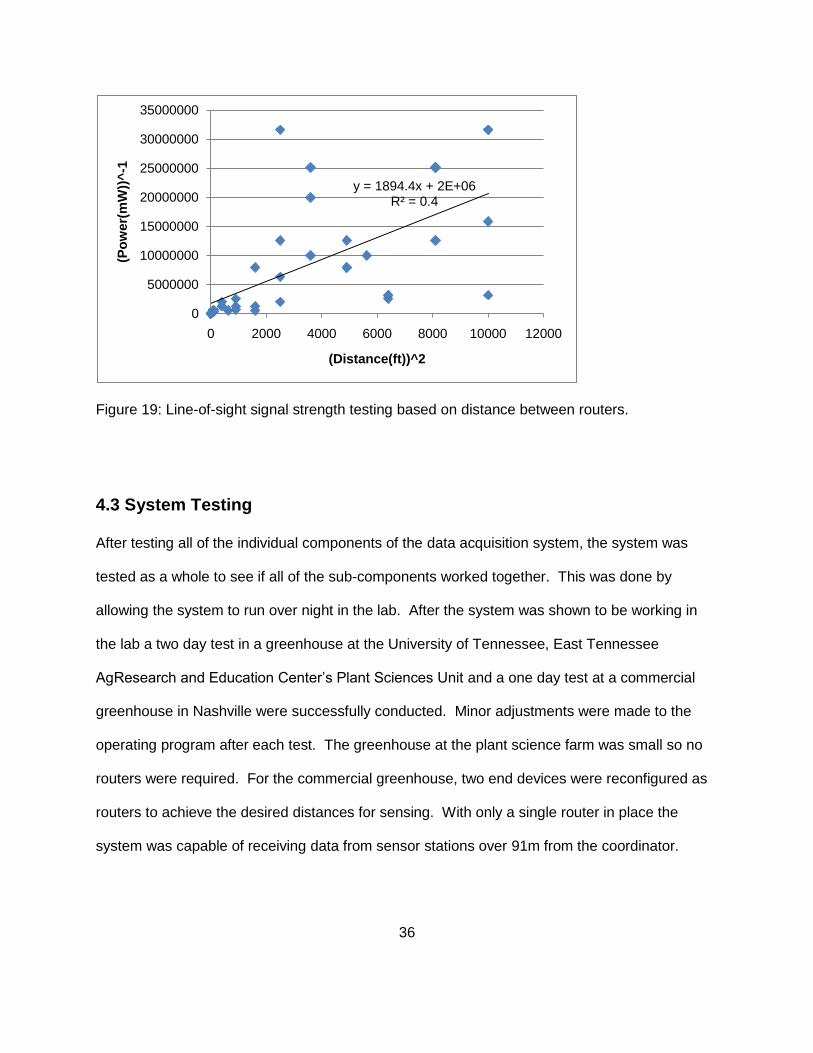
During field tests at the plant science greenhouse, eight sensor stations were setup in a network
with a coordinator and left to run for two days. The sensor stations were placed on different
tables with strawberry plants at varying levels of maturity. The strawberry greenhouse was a
Quonset style house covered with plastic. Data from four of the sensor stations were graphed
(figures 22, 23, and 24).
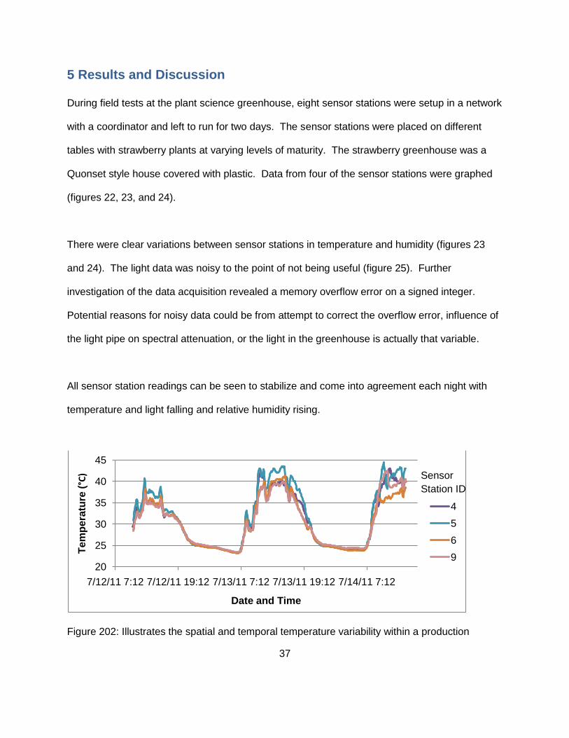
There were clear variations between sensor stations in temperature and humidity (figures 23
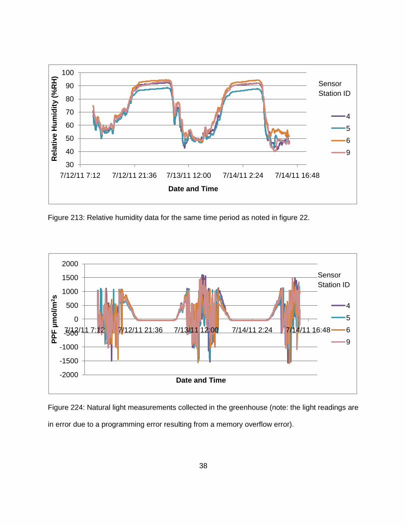
and 24). The light data was noisy to the point of not being useful (figure 25). Further
investigation of the data acquisition revealed a memory overflow error on a signed integer.
Potential reasons for noisy data could be from attempt to correct the overflow error, influence of
the light pipe on spectral attenuation, or the light in the greenhouse is actually that variable.
All sensor station readings can be seen to stabilize and come into agreement each night with
temperature and light falling and relative humidity rising.
Figure 202: Illustrates the spatial and temporal temperature variability within a production
20
25
30
35
40
45
7/12/11 7:12 7/12/11 19:12 7/13/11 7:12 7/13/11 19:12 7/14/11 7:12
Te
mp
era
ture
(°C)
Date and Time
4
5
6
9
Sensor
Station ID
38
Figure 213: Relative humidity data for the same time period as noted in figure 22.
Figure 224: Natural light measurements collected in the greenhouse (note: the light readings are
in error due to a programming error resulting from a memory overflow error).
30
40
50
60
70
80
90
100
7/12/11 7:12 7/12/11 21:36 7/13/11 12:00 7/14/11 2:24 7/14/11 16:48
Re
lati
ve
Hu
mid
ity (
%R
H)
Date and Time
4
5
6
9
-2000
-1500
-1000
-500
0
500
1000
1500
2000
7/12/11 7:12 7/12/11 21:36 7/13/11 12:00 7/14/11 2:24 7/14/11 16:48
PP
F µ
mo
l/m
2s
Date and Time
4
5
6
9
Sensor
Station ID
Sensor
Station ID
39
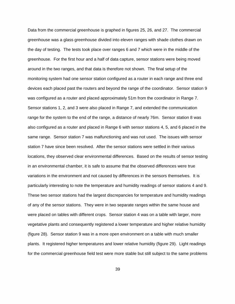
Data from the commercial greenhouse is graphed in figures 25, 26, and 27. The commercial
greenhouse was a glass greenhouse divided into eleven ranges with shade clothes drawn on
the day of testing. The tests took place over ranges 6 and 7 which were in the middle of the
greenhouse. For the first hour and a half of data capture, sensor stations were being moved
around in the two ranges, and that data is therefore not shown. The final setup of the
monitoring system had one sensor station configured as a router in each range and three end
devices each placed past the routers and beyond the range of the coordinator. Sensor station 9
was configured as a router and placed approximately 51m from the coordinator in Range 7.
Sensor stations 1, 2, and 3 were also placed in Range 7, and extended the communication
range for the system to the end of the range, a distance of nearly 76m. Sensor station 8 was
also configured as a router and placed in Range 6 with sensor stations 4, 5, and 6 placed in the
same range. Sensor station 7 was malfunctioning and was not used. The issues with sensor
station 7 have since been resolved. After the sensor stations were settled in their various
locations, they observed clear environmental differences. Based on the results of sensor testing
in an environmental chamber, it is safe to assume that the observed differences were true
variations in the environment and not caused by differences in the sensors themselves. It is
particularly interesting to note the temperature and humidity readings of sensor stations 4 and 9.
These two sensor stations had the largest discrepancies for temperature and humidity readings
of any of the sensor stations. They were in two separate ranges within the same house and
were placed on tables with different crops. Sensor station 4 was on a table with larger, more
vegetative plants and consequently registered a lower temperature and higher relative humidity
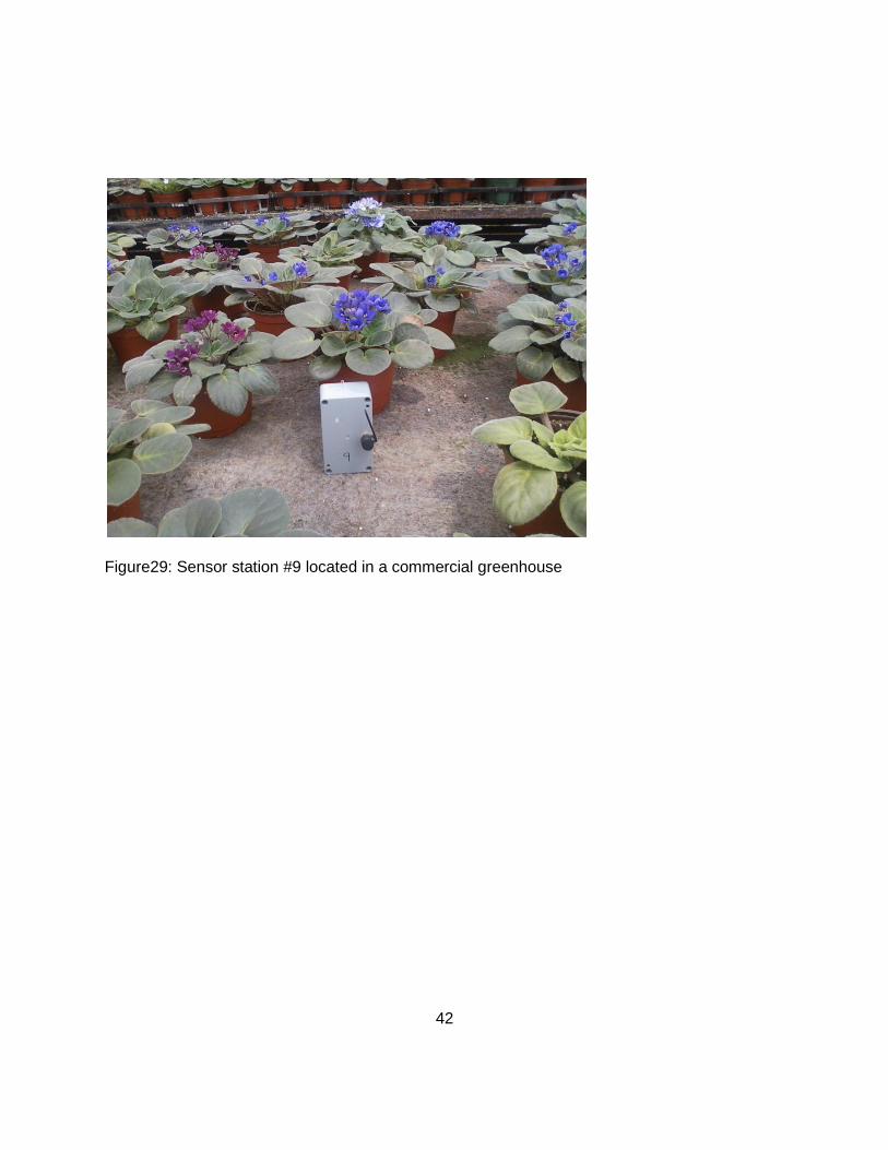
(figure 28). Sensor station 9 was in a more open environment on a table with much smaller
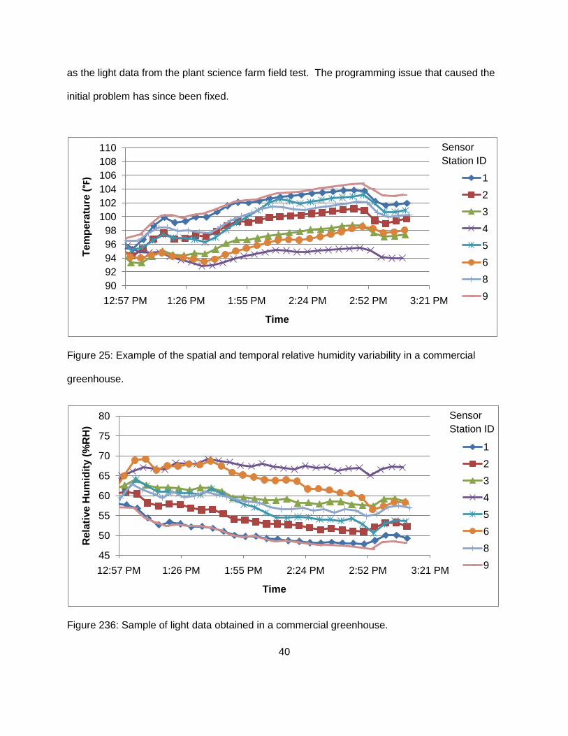
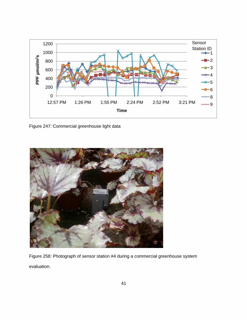
plants. It registered higher temperatures and lower relative humidity (figure 29). Light readings
for the commercial greenhouse field test were more stable but still subject to the same problems
40
as the light data from the plant science farm field test. The programming issue that caused the
initial problem has since been fixed.
Figure 25: Example of the spatial and temporal relative humidity variability in a commercial
greenhouse.
Figure 236: Sample of light data obtained in a commercial greenhouse.
90
92
94
96
98
100
102
104
106
108
110
12:57 PM 1:26 PM 1:55 PM 2:24 PM 2:52 PM 3:21 PM
Te
mp
era
ture
(°F)
Time
1
2
3
4
5
6
8
9
45
50
55
60
65
70
75
80
12:57 PM 1:26 PM 1:55 PM 2:24 PM 2:52 PM 3:21 PM
Re
lati
ve
Hu
mid
ity (
%R
H)
Time
1
2
3
4
5
6
8
9
Sensor
Station ID
Sensor
Station ID
41
Figure 247: Commercial greenhouse light data
Figure 258: Photograph of sensor station #4 during a commercial greenhouse system
evaluation.
0
200
400
600
800
1000
1200
12:57 PM 1:26 PM 1:55 PM 2:24 PM 2:52 PM 3:21 PM
PP
F µ
mo
l/m
2s
Time
1
2
3
4
5
6
8
9
Sensor
Station ID
42
Figure29: Sensor station #9 located in a commercial greenhouse
43
6 Conclusion and Recommendations
The monitoring system designed for this project was able to bring all the individual components
of sensors, programming, and wireless communication together to work as a cohesive system.
In addition, the system was able to detect significant differences in environmental conditions
spatially within a greenhouse. This ability to detect spatial variations demonstrates the benefit
to greenhouse management that a system of several sensors placed at the plant canopy can
have over one or two centrally located sensors. It also demonstrates that, fully implemented,
the system should be able to meet the project goal of collecting data at a high spatial and
temporal resolution to determine if there is a correlation between specific environmental
conditions and the outbreak of Corynespora cassiicola.
While the monitoring system performed adequately enough to meet the design goals for a
prototype, proof of concept system, there are still many things that can be improved in later
versions.
The sensor stations’ ability to join the network could be improved by having sensor
stations check for prior joins before terminating the joining process
The overall program could be improved to make data analysis quicker and easier (e.g.
an improved graphical user interface).
Enclosures for the routers and coordinator need to be optimized for production
Further studies are needed on the light sensor to determine if the sensor has adequate
accuracy for use in the creation of disease prediction models
Improve the user interface to make the system more appealing to a commercial market
44
Overall, the monitoring system has demonstrated the feasibility of creating a low power,
greenhouse monitoring system consisting of several wireless devises. Similar monitoring
systems could have applications in agriculture that reach far beyond predicting disease in
greenhouse crops. As the radio and MCU technology continue to improve, this will allow users
to create wireless networks that are smaller and cheaper. Before these types of systems can
find wide acceptance within agriculture, the developing environments will need to be made
simpler and more robust. If development can be simplified so that any engineer can
understand and use the wireless technology, then wireless monitoring systems will become a
valuable tool in the spatial management of greenhouse and conventional cropping systems.

45
Bibliography
46
Averre, C. W., J. B. Ristaino, and J. G. Shultheis. 2000. Disease management for vegetables and herbs in greenhouses using low input sustainable methods. Plant Pathology Extension, North Carolina State University. http://www.ces.ncsu.edu/depts/pp/notes/oldnotes/vg2.htm.
Belanger, R. R. and J. G. Menzies. 1996. Recent advances in cultural management of diseases
of greenhouse crops. Canadian Journal of Plant Pathology. 18:186-193. Donahue, D. W., R. S. Sowell, N. T. Powell, and T. A. Melton. 1991. An expert system for
diagnosing diseases of tobacco. Transactions of ASABE.7(4): 499-503.
Eshenaur, B. and R. Anderson. 2004. Plant pathology fact sheet - managing the greenhouse environment to control plant disease. University of Kentucky Cooperative Extension Service. http://www.ca.uky.edu/agcollege/plantpathology/ext_files/PPFShtml/PPFS-GH-1.pdf.
Fernandes, R. C., and R. W. Barreto. 2003. Corynespora cassiicola causing leaf spots on
coleus barbatus. Plant Pathology. 52:786.
Hu, Y., P. Li, X. Zhang, J. Wang, L. Chen, and W. Liu. 2007. Integration of an environment information acquisition system with a greenhouse management expert system. New Zealand Journal of Agricultural Research. 50: 855-860.
Lea-Cox, J. D., A. G. Ristvey, F. Arguedas Rodriguez, D. S. Ross, J. Anhalt, and G. Kantor. 2008. A low-cost multihop wireless sensor network, enabling real-time management of environmental data for the greenhouse and nursery industry. Acta Hort. 801: 523-530.
Madhavi, G. B., and K. V. M Krishna Murthy. 2009. Effect of spore concentration, light and relative humidity on spore germination and germ tube growth of corynespora cassiicola (Berk. and Curt.) Wei. Agric. Sci. Digest. 29(1): 12-15.
Munro, B. H. 2001. Ch. 13: Logistic regression. In Statistical Methods for Health Care Research, 283-302. Philadelphia, Pa.: Lippincott.
Pawlowski, A., J. L. Guzman, F. Rodriquez, M. Berenquel, J. Sanchez, and S. Dormido. 2009. Simulation of greenhouse climate monitoring and control with wireless sensor network and event-based control. Sensors.9: 232-252.
Ramsey, F. L., and D. W. Schafer. 2002. Ch 20: Logistic regression for binary response variables. In The Statistical Sleuth: A Course in Methods of Data Analysis. 2nd ed., 579- 608. Australia: Duxbury.
Schlub, R. L., L. J. Smith, L. E. Datnoff, and K. Pernezny.2009. An overview of target spot of tomato caused by corynespora cassiicola. Acta Hort.808: 25-28.
Trigiano, R. N., M. T. Windham, and A. S. Windham. 2008. Plant Pathology Concepts and Laboratory Exercises. 2nd ed. Boca Raton, Fla.: CRC Press.
47
United States Department of Agriculture, National Agricultural Statistics Service. 2007. The Census of Agriculture. Volume 1 Ch 1 Table 37.
Unknown. 2009. Disease costs bonnie plants $1M in recall. Greenhouse Grower.
http://www.greenhousegrower.com/news/?storyid=2407.
Van Tuijl, B., E. van Os, and E. van Henten. 2008. Wireless sensor networks: state of the art and future perspective. Acta Hort. 801: 547-554.
Wei, C. T. 1950. Notes on corynespora. Mycological Papers. 34: 10

48
Appendix

49
Comments and Recommendations
Although the idea of an easy ZigBee programming environment was initially appealing, Z-stack and the CC2530 proved to have many problems. There are over 37 documents associated with Z-stack and the CC2530 that range from a few pages to 260 pages in length. These documents and the Z-stack program itself are still being updated, often without any notification to the end user. This array of documents is difficult to navigate and seems to be incomplete from the perspective of new user. It is not always clear where to find needed information. Important details often can only be found by reading the code itself. TI gives users the freedom to change anything within the Z-stack, but it is not always clear when one piece of code interacts with another, causing end users to make seemingly benign changes that in effect crash the whole program. The method in which they have asked users to splice in their own code also makes it difficult to save different iterations of programs without having to reformat the entire workspace. Added to these difficulties, Texas Instruments has, unfortunately, proven themselves to be either unwilling or unable to assist end users in understanding the product and adjusting it to use in non-TI projects. Despite the many difficulties encountered, once the user has a basic grasp on how to make the whole system work, the CC2530 along with Z-stack does deliver on its promise of quick implementation of a low power ZigBee network.
There were many errors in the first few attempts at programming the I2C subroutines. Some examples of things that had to be corrected are incorrect start conditions and extra clock cycles. Once the I2C program had been well tested, there was not much trouble in following the corresponding data sheets to write the code for the different sensor and add that code to the HAL.
It was recently discovered that the five minute totals of sensors readings were being saved into a variable that was too small to store them. This caused the larger sums to wrap back around and give erroneous readings. Since it was not an issue with smaller sums it did not show up in bench top testing where the lab is dim, cool, and dry, but in the environmental chamber the error became clear(figure 15). Obviously, it never reached 500°C in the environmental chamber. In fact, during the time that the sensor stations where showing 500°C the chamber temperature sensor was reading 26.6°C. Once the sensor stations reached a certain temperature, the five minute total was too large and caused the variable to overflow. Since every sensor station was showing the same error, it was clear that this was a programming issue. This issue has now been corrected by storing the totals in a larger variable. Even though the program appears to be working, new programming errors will surely surface over time.
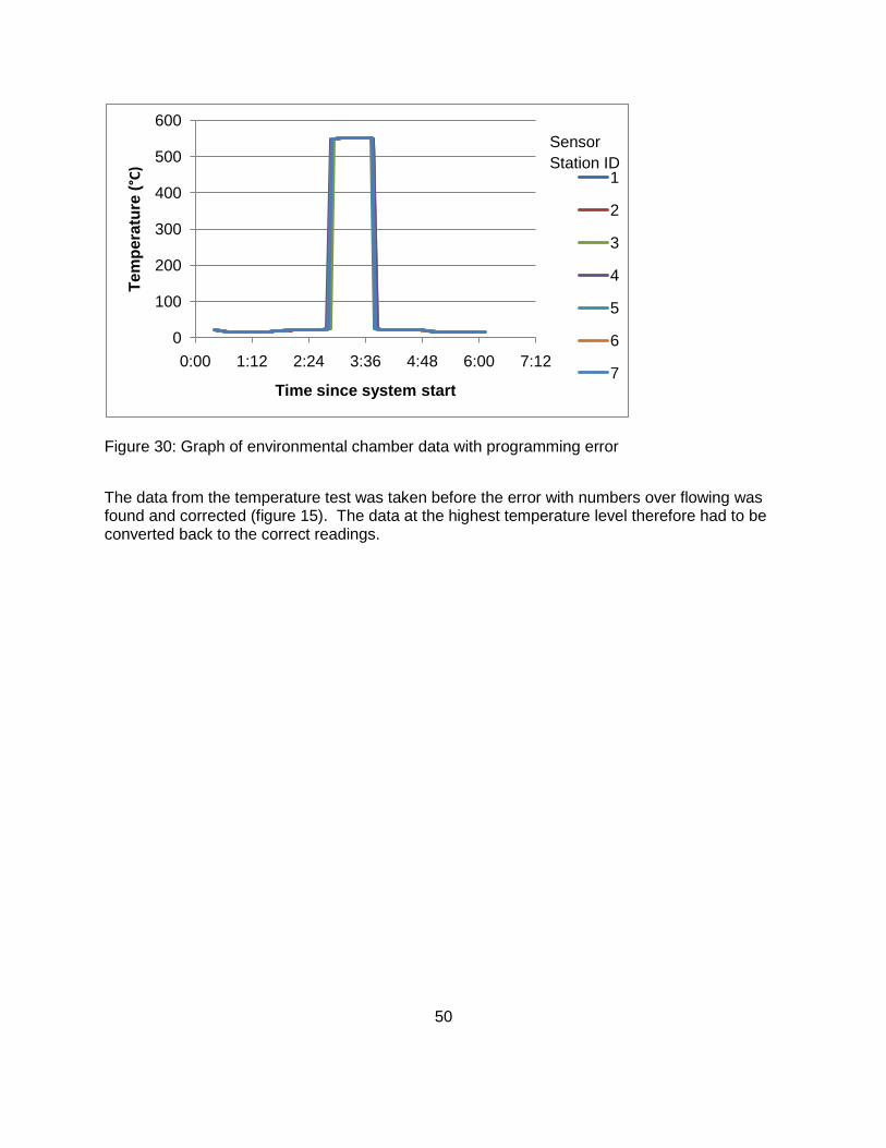
50
Figure 30: Graph of environmental chamber data with programming error
The data from the temperature test was taken before the error with numbers over flowing was found and corrected (figure 15). The data at the highest temperature level therefore had to be converted back to the correct readings.
0
100
200
300
400
500
600
0:00 1:12 2:24 3:36 4:48 6:00 7:12
Te
mp
era
ture
(°C)
Time since system start
1
2
3
4
5
6
7
Sensor
Station ID

51
Vita Crystal Kelly was born on April 7th, 1986 in Louisville, Kentucky. She was raised in
Chattanooga, Tennessee were she attended Harrison Elementary School, Brown Middle
School, and The Baylor School. In August of 2004 she began attending the University of
Tennessee at Knoxville. While at UTK, she was involved in many different activities including
the engineering honor society, Tau Beta Pi, and serving as president of the College of
Engineering Ambassadors. Crystal was also fortunate enough to spend five semesters
throughout her undergraduate career as a co-op student at the NASA Kennedy Space Center in
Florida. She graduated magna cum laude in May of 2009 with a Bachelor’s degree in
Biosystems Engineering and a Minor in Mathematics. She began pursuing a Master’s of
Science degree in Biosystems Engineering in August of 2009. Her first year in graduate school
she received the J. Wallace and Katie Dean Fellowship award. In her second year, she was
inducted into the honor society of agriculture, Gamma Sigma Delta, and served as the colleges
graduate student representative on the University of Tennessee Institute of Agriculture advisory
board.