Development of a Two-Stage Life Cycle Model for

U.S. Department of the InteriorU.S. Geological Survey

Open-File Report 2020–1068

Prepared in cooperation with Tacoma Power

Development of a Two-Stage Life Cycle Model for Oncorhynchus kisutch (Coho Salmon) in the Upper Cowlitz River Basin, Washington

Cover: Looking downstream on the Cowlitz River at Cowlitz Falls Dam, Washington. Photograph by Tobias Kock, U.S. Geological Survey, June 2006.


By John M. Plumb and Russell W. Perry

Prepared in cooperation with Tacoma Power

Open-File Report 2020–1068

Open File Report 2020–XXXX

U.S. Department of Interior U.S. Geological Survey

U.S. Department of the Interior U.S. Geological Survey

U.S. Department of the Interior DAVID BERNHARDT, Secretary

U.S. Geological Survey James Reilly II, Director

U.S. Geological Survey, Reston, Virginia: 2020

For more information on the USGS—the Federal source for science about the Earth, its natural and living resources, natural hazards, and the environment—visit https://www.usgs.gov/ or call 1–888–ASK–USGS (1–888–275–8747).

For an overview of USGS information products, including maps, imagery, and publications, visit https:/store.usgs.gov.

Any use of trade, firm, or product names is for descriptive purposes only and does not imply endorsement by the U.S. Government.

Although this information product, for the most part, is in the public domain, it also may contain copyrighted materials as noted in the text. Permission to reproduce copyrighted items must be secured from the copyright owner.

Suggested citation: Plumb, J.M., and Perry, R.W., 2020, Development of a two-stage life cycle model for Oncorhynchus kisutch (coho salmon) in the upper Cowlitz River Basin, Washington: U.S. Geological Survey Open-File Report 2020–1068, 25 p., https://doi.org/10.3133/ofr20201068.

ISSN 2331-1258 (online)

https://www.usgs.gov/

http://www.usgs.gov/pubprod

https://doi.org/10.3133/ofr20201068

iii

Contents Abstract ......................................................................................................................................................... 1 Introduction .................................................................................................................................................... 2 Methods ......................................................................................................................................................... 3

Life Cycle Structure of Upper Cowlitz River Basin Coho Salmon ............................................................... 4 The Observation Model .............................................................................................................................. 8 Factors Affecting Key Demographic Parameters ........................................................................................ 8 Parameter Estimation ................................................................................................................................. 9

Results ........................................................................................................................................................... 9 Summary of Data Used in the Life Cycle Model ......................................................................................... 9 Parameter Estimates Under the State-Space Model ................................................................................ 13

Discussion ................................................................................................................................................... 19 References Cited ......................................................................................................................................... 21 Appendix 1. Coho Salmon Life Cycle Parameter Estimates ....................................................................... 23

Figures 1. Image of Cowlitz River Basin, Washington, showing dams, reservoirs, and major tributaries .................. 2 2. Schematic showing structure of the two-stage life cycle model for Cowlitz River coho salmon ................ 4 3. Image showing the reconstruction of age-specific juvenile abundance that gives rise to the total number of recruits from a given brood year, and the age- and sex-specific adult return conditional on their juvenile outmigration strategy from recruits generated by spawners in brood year y ........................ 6 4. Graph showing escapement of adult female Cowlitz River Basin coho salmon, by brood year, upstream from Cowlitz Falls Dam, Washington ........................................................................................... 10 5. Time series graph showing fraction of hatchery-origin female spawners, by brood year, for coho salmon spawning upstream from Cowlitz Falls Dam, Washington ............................................................... 10 6. Graph showing juvenile coho salmon collected, by migration (collection) year, at Cowlitz Falls Dam, Washington ........................................................................................................................................ 11 7. Graph showing fish collection efficiency of juvenile coho salmon, by migration (collection) year, at Cowlitz Falls Dam, Washington ................................................................................................................... 12 8. Time series graph showing number of days that spill occurred during September 1–April 30 at Cowlitz Falls Dam, Washington. .................................................................................................................. 12 9. Posterior distribution graphs showing the intercept and effect of fish collection efficiency (FCE) on productivity, the mean productivity when FCE=1, and effect of the number of spill days under the Ricker stock-recruitment model for coho salmon in the Cowlitz River Basin, Washington ........................... 14 10. Posterior distribution graphs showing capacity as estimated under the Ricker stock-recruitment model for coho salmon in the Cowlitz River Basin, Washington .................................................................. 15 11. Graph showing relation between fish collection efficiency and the number of juveniles per spawner ... 15 12. Posterior distribution graph showing the juvenile-to-adult return rate for coho salmon in the Cowlitz River Basin, Washington……………………………………………………………………………………………..16 13. Graphs showing fitted Ricker function based on posterior medians of parameters expressed as production of juvenile recruits when fish collection efficiency (FCE) was 1 and underobserved FCE .......... 17 14. Graphs showing annual estimates of juvenile-to-adult return rate and productivity .............................. 18

iv

Conversion Factors U.S. customary units to International System of Units

Multiply By To obtain

Volume

acre-foot (acre-ft) 1,233 cubic meter (m3)

Flow rate

cubic foot per second (ft3/s) 0.02832 cubic meter per second (m3/s) International System of Units to U.S. customary units

Multiply By To obtain

Length

kilometer (km) 0.6214 mile (mi)

Abbreviations CFD Cowlitz Falls Dam CI credible interval FCE fish collection efficiency JAGS Just Another Gibbs Sampler JAR juvenile-to-adult return rate USGS U.S. Geological Survey MCMC Markov Chain Monte Carlo SD standard deviation

1


John M. Plumb and Russell W. Perry

Abstract Recovery of salmon populations in the upper Cowlitz River Basin depends on trap-and-haul

efforts owing to impassable dams. Therefore, successful recovery depends on the collection of out-migrating juvenile salmon at Cowlitz Falls Dam (CFD) for transport below downstream dams, as well as the collection of adults for transport upstream from the dams. Tacoma Power began downstream fish collection efforts at CFD in the mid-1990s and has been working consistently since then to improve collection efficiency to support self-sustaining salmon and steelhead (Onchorhynchus spp.) populations in the upper Cowlitz River Basin. Although much work has focused on estimating fish collection efficiency (FCE), there has been relatively little focus on modeling population dynamics to understand how fish collection efficiency and other factors drive production of both juvenile and adult salmon over their life cycle. As a first step towards understanding the factors affecting population dynamics of Oncorhynchus kisutch (coho salmon) in the upper Cowlitz River Basin, we developed a statistical life cycle model using adult escapement and age structure data, juvenile collection data, and juvenile fish collection efficiency estimates. The goal of the statistical life cycle model is to estimate annual production and survival during two critical life-stage transitions: the freshwater production from escapement of adults upstream from CFD to collection of juveniles at CFD, and the juvenile-to-adult survival from the time of collection at the dam to the return of adults. To structure the life cycle model, we used the Ricker stock-recruitment model to estimate juvenile production from the number of parent spawners. This approach allowed us to account for density dependence at high spawner abundances while estimating annual productivity, defined as the number of juveniles produced per spawner at low spawner abundance. We then expressed productivity as a function two key variables affecting the number of juveniles collected and transported at CFD: (1) annual FCE, and (2) the annual number of days that spill occurred at CFD from September 1 to April 30.

Our key findings were as follows: 1. FCE was the primary factor affecting productivity of coho salmon upstream from CFD because

FCE affects the number of juveniles that survive to continue downstream migration;2. Juvenile-to-adult return (JAR) rates were relatively high considering that harvest was included

in the estimate, averaging about 3.6 percent and ranging as high as 9.1 percent, suggesting that adult coho salmon may be able to return to CFD at sustainable population sizes; and

3. Much variation in the estimates of juvenile fish production upriver of CFD was unexplained even after adult escapement and FCE were accounted for, suggesting that the model may be improved by exploring different covariates and model structures for juvenile production as well as JAR rates.

2

Additionally, by including FCE in the model, we estimated that the median pre-collection productivity, defined as the number of juveniles produced per spawner when FCE=1, was 108.4 juveniles per spawner. Because this two-stage life cycle model partitions factors that affect fish production in river compared to the ocean environment and fish life stages, the model estimates should help inform fishery managers about the overall role that fish collection at CFD may have on the recovery and sustainability of coho salmon populations.

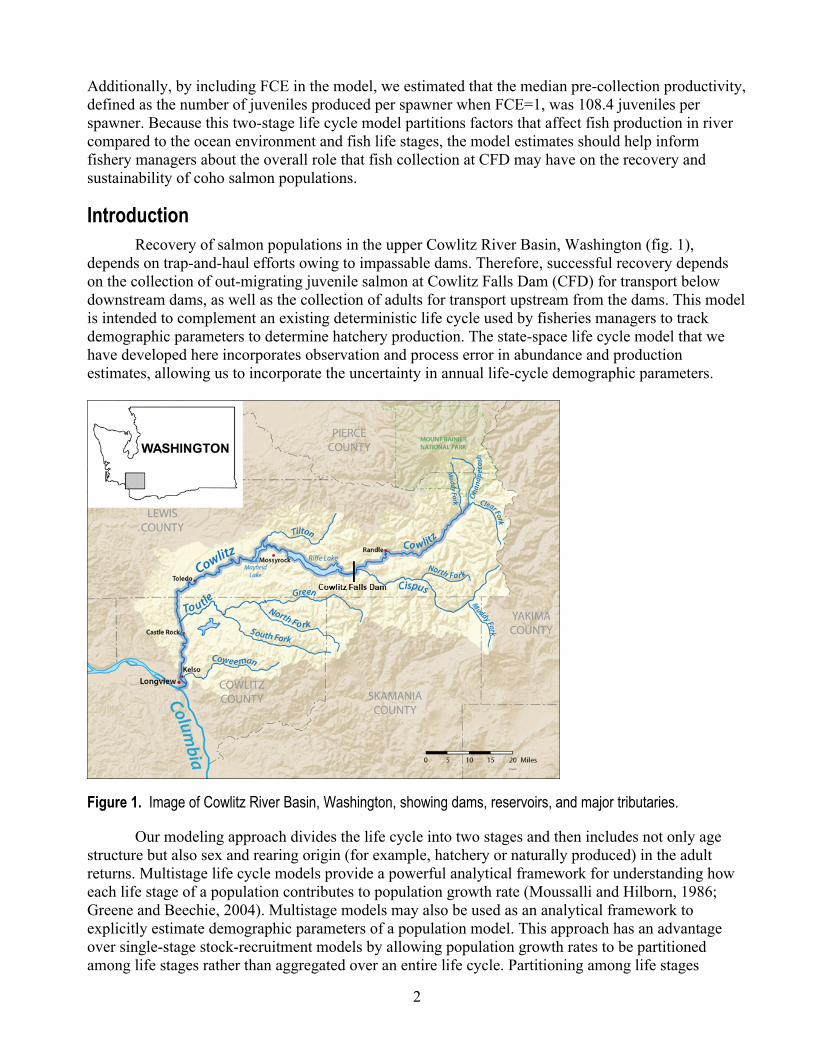
Introduction Recovery of salmon populations in the upper Cowlitz River Basin, Washington (fig. 1),

depends on trap-and-haul efforts owing to impassable dams. Therefore, successful recovery depends on the collection of out-migrating juvenile salmon at Cowlitz Falls Dam (CFD) for transport below downstream dams, as well as the collection of adults for transport upstream from the dams. This model is intended to complement an existing deterministic life cycle used by fisheries managers to track demographic parameters to determine hatchery production. The state-space life cycle model that we have developed here incorporates observation and process error in abundance and production estimates, allowing us to incorporate the uncertainty in annual life-cycle demographic parameters.

Figure 1. Image of Cowlitz River Basin, Washington, showing dams, reservoirs, and major tributaries.

Our modeling approach divides the life cycle into two stages and then includes not only age structure but also sex and rearing origin (for example, hatchery or naturally produced) in the adult returns. Multistage life cycle models provide a powerful analytical framework for understanding how each life stage of a population contributes to population growth rate (Moussalli and Hilborn, 1986; Greene and Beechie, 2004). Multistage models may also be used as an analytical framework to explicitly estimate demographic parameters of a population model. This approach has an advantage over single-stage stock-recruitment models by allowing population growth rates to be partitioned among life stages rather than aggregated over an entire life cycle. Partitioning among life stages

3

facilitates estimation of (1) stage-specific density dependence, and (2) stage-specific effects of environmental factors or management actions. For example, Zabel and others (2006) estimated parameters of a multistage model used in the context of a population viability analysis for spring/summer Oncorhynchus tshawytscha (Chinook salmon) in the Snake River, but such an approach has yet to be applied to a salmon population in another river basin.

Typically, data informing estimates of abundance at particular “check points” in the life cycle determine the complexity of the multistage model that can be fit to the data. For Oncorhynchus kisutch (coho salmon) at Cowlitz Falls Dam (CFD), we have developed a two-stage model that encompasses (1) upstream passage of spawners at CFD to subsequent downstream passage of their progeny at the dam, and (2) downstream collection of juveniles at CFD to their subsequent return from the ocean and collection at the downstream barrier dam 2‒3 years later. This approach partitions the life cycle of coho salmon spatially and temporally, which allows us to fit and compare alternative models with covariates specific to each stage. This report describes the structure of the two-stage life cycle model as applied to Cowlitz River coho salmon, presents preliminary results from fitting the model to data, and outlines future directions and developments.

Methods Our model extends the single-stage state-space framework first developed by Fleischman and

others (2013) and applied by Courter and others (2019) to Clackamas River steelhead. The state-space model consists of two parts: (1) a process model for the underlying state dynamics, and (2) an observation model that links the data to the true underlying state. The state-space model also may be viewed as a hierarchical model where the state (abundance of fish) evolves according to a dynamic population process model (for example, a Ricker model) with some process error, and observations on the state (“the data”) are made conditional on the true but unobservable state. Life cycle models can range from very simple theoretically based population models (for example, the Beverton-Holt stock-recruitment model) to very complex spatially explicit simulation models linked to hydrosystem hydrodynamic models (for example, the COMPASS model for a single transition in a life cycle model; Zabel and others, 2008). We decided to develop a model of intermediate complexity that casts the two-stage life cycle model in a state-space framework (Newman and others, 2014). We used a state-space framework implemented in a Bayesian context because of the following:

• The model provides a statistical estimation framework for retrospective statistical analysis and a stochastic simulation framework for prospective analysis to evaluate alternative management actions.

• The model accounts for uncertainty in abundance estimates. A state-space framework accounts for observation uncertainty in the abundance estimates and other data (for example, age structure) while estimating process uncertainty.

• The model allows for missing data. By drawing missing data from an appropriate probability model, uncertainty owing to missing data can be propagated without having to omit data or assume fixed values for missing data.

Thus, a two-stage state-space life cycle model for coho salmon strikes an appropriate balance between model complexity, tractability, and applicability given the goals of performing both retrospective and prospective analyses to guide future management.

4

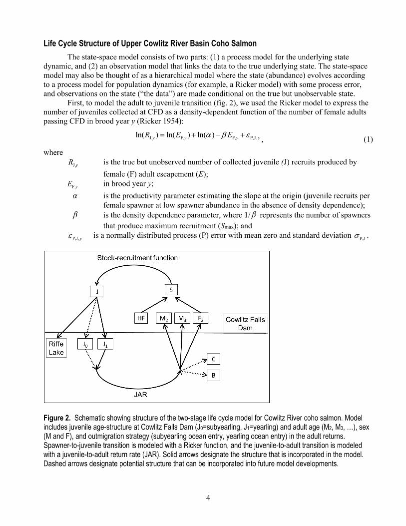
Life Cycle Structure of Upper Cowlitz River Basin Coho Salmon The state-space model consists of two parts: (1) a process model for the underlying state

dynamic, and (2) an observation model that links the data to the true underlying state. The state-space model may also be thought of as a hierarchical model where the state (abundance) evolves according to a process model for population dynamics (for example, a Ricker model) with some process error, and observations on the state (“the data”) are made conditional on the true but unobservable state.

First, to model the adult to juvenile transition (fig. 2), we used the Ricker model to express the number of juveniles collected at CFD as a density-dependent function of the number of female adults passing CFD in brood year y (Ricker 1954):

J, F, F, P,J,ln( ) ln( ) ln( )y y y yR E Eα β ε= + − + , (1) where J,yR is the true but unobserved number of collected juvenile (J) recruits produced by

female (F) adult escapement (E); F,yE in brood year y; α is the productivity parameter estimating the slope at the origin (juvenile recruits per

female spawner at low spawner abundance in the absence of density dependence); β is the density dependence parameter, where 1/ β represents the number of spawners

that produce maximum recruitment (Smax); and P,J, yε is a normally distributed process (P) error with mean zero and standard deviation P,Jσ .

Figure 2. Schematic showing structure of the two-stage life cycle model for Cowlitz River coho salmon. Model includes juvenile age-structure at Cowlitz Falls Dam (J0=subyearling, J1=yearling) and adult age (M2, M3, …), sex (M and F), and outmigration strategy (subyearling ocean entry, yearling ocean entry) in the adult returns. Spawner-to-juvenile transition is modeled with a Ricker function, and the juvenile-to-adult transition is modeled with a juvenile-to-adult return rate (JAR). Solid arrows designate the structure that is incorporated in the model. Dashed arrows designate potential structure that can be incorporated into future model developments.

5

Because productivity of juveniles directly depends on the fraction of juvenile coho salmon collected at CFD, we modeled the productivity parameter (α ) as a function of the annual fish collection efficiency (FCE) for coho salmon at CFD in year y+2 in the following manner:

0 1 2 2 1ln( )y y yFCE Spα θ θ θ+ += + + , (2) where 0θ is the intercept, 1θ is the slope for the effect of fish collection efficiency on productivity, and 2θ is the slope for the effect of the number of days of spill (Sp) at CFD between

September 1st to April 30th in year y+1 on coho salmon productivity. This period was chosen because it coincides with winter spill conditions that can pass parr into Riffe Lake where they become landlocked and lost to the anadromous fishery (Kock and others, 2012). Specifically, we used the number of days that the exceeded 10,000 ft3/s as recorded at the Kosmos river gage site (U.S. Geological Survey [USGS] 14233500; see https://waterdata.usgs.gov/wa/nwis/uv?site_no=14233500) because these flows indicate involuntary spill conditions at CFD. The number of days of spill was standardized such that setting FCE=1 and Sp=0 provides estimates of pre-collection productivity of juvenile coho salmon at the mean number of days of spill.

For the juvenile-to-adult transition, we model the number of adult returns as a log-normal function of a density independent juvenile-to-adult return rate (JAR):

A, J, P,A,ln( ) ln( ) ln(JAR)y y yR R ε= + + , (3) where A, yR is the number of adult (A) recruits (male and female) produced from the ,J yR

juveniles passing CFD that arose from female spawners in brood year y, and P,A,yε is a normally distributed process (P) error with a mean of zero and standard

deviation= P,Aσ . Given that juveniles can pass CFD at ages 1–2 (from brood year not actual fish age) and adults

return at ages 2–3, the initial 2 years of juvenile recruits and 2 years of adult recruits that produced returns beginning in 2000 were not linked to the two-stage stock-recruitment model. These initial state vectors were estimated as draws from common log-normal distributions with parameters ( )J,0ln R ,

RJ0σ and ( )A,0ln R , RA0σ , respectively, for juveniles and adults.

Given juvenile recruits, the number of juveniles ( Ja ) passing CFD in calendar year t was modeled as:

J J J J, J, J, ,t a t a t a aJ R p− −= , (4) where

J,t aJ is the number of juveniles in year t of age Ja , and

J JJ, ,t a ap − is the proportion of juvenile recruits from brood year Jy t a= − emigrating at age Ja (fig. 3).

https://waterdata.usgs.gov/wa/nwis/uv?site_no=14233500

6

Given adult recruits, we modeled the number of adults returning at age Aa of sex s and outmigration strategy o as:

A A A A, , , A, , , ,t a s o t a a t a s oN R p− −= , (5) where

A, , ,t a s oN is the number of adults returning in year t at age Aa , of sex s, and outmigration strategy o; and

A A, , ,a t a s op − is the proportion of recruits from brood year Ay t a= − returning at age Aa , sex s,

and outmigration strategy o (fig. 3). Here, outmigration strategy refers to whether juveniles were collected at CFD as subyearlings

or yearlings. Fish that pass CFD as subyearling fry are currently transported to locations upstream from CFD and released into the wild. Because subyearling and yearling smolts have only been tracked since 2014, our current formulation of the two-state model does not yet account for the collection and transport of subyearling coho salmon outmigrants. The model also does not account for juvenile outmigration strategy in the adult returns, but in the future such information would allow us to estimate SAR separately for each outmigration strategy. Nonetheless, given 2 adult age classes and 2 outmigration strategies, the brood-year specific return probabilities are

A AA, , , ,y a t a s op −=p .

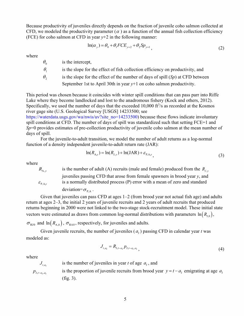
Figure 3. Image showing the reconstruction of age-specific juvenile abundance (green cells; J0 and J1) that gives rise to the total number of recruits (RJ) from a given brood year, and the age- and sex-specific adult return (blue cells; RA) conditional on their juvenile outmigration strategy (J0 adults, J1 adults) from recruits generated by spawners in brood year y.

Vectors of brood-year specific outmigration J, yp and return A, yp probabilities can be modeled hierarchically as draws from a Dirichlet distribution:

( ), Dirichleti y iγp , (6) where i is J (juvenile) or A (adult), and iγ is a vector of parameters of the same length as ,i yp . Under this formulation, the expected proportion of the kth class is

,

,1

k iK

k ik

γ

γ=∑

, (7)

and the inverse of the sum in the denominator scales with annual variation in ,i yp .

Brood year Spawners Age 0 Age 1 Age2 Age3 Age2 Age3 RJ RA2 1601 11302 28583 0 04 11302 291 05 872 0 1695

Juveniles Adult Males Adult Females

7

Given age-specific juvenile emigration and adult returns from brood year y in calendar year t, the total number of juveniles passing CFD in calendar year t is the sum of the abundance-at-age over all ages:

J

J

,t t aa

J J=∑. (8)

The current model for coho salmon at CFD does not account for juvenile outmigration strategy, brood stock removal, or harvest rates; however, we show here how these estimates can be incorporated in the current framework of the model for future applications. For example, the total number of returning adults in calendar year t is the sum of the abundances across all age, sex, and outmigration classes:

A

A

, , ,t t a s os o a

N N=∑∑∑. (9)

Returns of subclasses in year t are calculated similarly by summing over the appropriate indices. For example, the number of female returns in calendar year t is

A

A

F, , , F,t t a s oo a

N N ==∑∑. (10)

Additionally, the age, sex, and outmigration structure in the adult returns each calendar year is

A

A

, , ,, , ,

a t s oa t s o

t

Nq

N=

, (11) where

A , , ,a t s oq is the fraction of the adults returning in calendar year t at age Aa , sex s, and outmigration strategy o (that is, if data on outmigration strategy were included in the model).

Escapement (Et) of spawners past CFD in calendar year t includes hatchery-origin adults

released upriver of CFD to spawn in the wild (Ht) plus naturally produced spawners (Nt). The model can accommodate those that survive harvest (Ct) and naturally produced fish taken for hatchery brood stock (Bt):

t t t t tE N C B H= − − + . (12) The annual harvest rate below CFD can be a composite of ocean and in-river harvest that is

assumed constant across ages and sexes of returns in a given year such that catch is:

t t tC U N= , (13) where tU is the composite harvest rate representing the fraction of returns that were harvested

in calendar year t.

Escapement of female spawners, which dictates juvenile recruits, is:

, , , , , ,F t F t F t F t F t t F t tE N q C q B f H= − − + , (14)

8

where ,F tf is the fraction of hatchery-origin adults that are female; and ,F tq is the proportion of females in naturally produced returns, calculated as:

A

A

F, , , F, t a t s oo a

q q ==∑∑. (15)

The Observation Model Observations to inform the parameters of the state model include the following: 1. Collected abundances for naturally produced subyearling and yearling outmigrants

collected at CFD from 2000 to 2018. Estimates of subyearling migrants collected at CFD and transported back upstream have not yet been included in the model.

2. Estimates of annual collection efficiency for juvenile coho salmon at CFD for 2000–18. 3. Estimates of abundance of hatchery-origin and naturally produced adults released upstream

from CFD for 2000–18. 4. Estimates of run composition of hatchery and naturally produced adults in terms of age and

sex, 2000–18. 5. Estimates of the number of naturally produced adults removed for hatchery brood stock for

2000–18 (not yet included into the model). 6. Estimates of ocean and in-river harvest rate indices as well as harvest upstream from CFD

for 2000–18 (not yet included in the model). As this list of input data indicates, each observation component is an estimate of the true value

and therefore has uncertainty associated with the estimate (data provided by Tacoma Power in partnership with Washington Department of Fish and Wildlife). This uncertainty arises from several sources such as sampling at the dam and during transport. Potential future expansions of the model include improving the incorporation of observation error in estimates of productivity and capacity.

Factors Affecting Key Demographic Parameters Exogenous environmental factors can affect survival during the adult-to-juvenile transition

upstream from CFD and the juvenile-to-adult transition downstream from CFD. Our model can be extended to allow productivity (α) in the adult-to-juvenile transition and JAR in the juvenile-to-adult transition to be expressed as a function of covariates hypothesized to influence survival:

1ln( )

K

y k kk

Xαα µ θ=

= +∑, (16)

JAR1

ln(JAR )J

y j jj

Zµ λ=

= +∑ , (17)

where α is the annual productivity expressed on a log scale, JAR is juvenile-to-adult return rates expressed on a log scale, μ is the overall log-mean of α or JAR when covariates are centered about their mean, kθ is the effect of the kth covariate Xk on α , and jλ is the effect of the jth covariate jZ .

9

Covariates are expressed on an annual scale and may be lagged appropriately relative to brood year to represent alternative hypotheses about when a given covariate influenced a particular life stage and demographic parameter. For example, we may hypothesize that the productivity of juveniles arising from brood year y is influenced by spill levels in brood year y+1 corresponding to the period when subyearling migrants from brood year y may be flushed downstream of CFD. Although equation 2 describes how we express productivity as a function of FCE and spill, here we describe more generally how both productivity and JAR can be modeled as functions of covariates

Parameter Estimation All parameters and unknown states were estimated in a Bayesian framework using Just

Another Gibbs Sampler (JAGS) software (Plummer, 2017) as implemented through the ‘runjags’ package of the R statistical programming platform (R Core Team, 2019). JAGS is a Bayesian estimation software package that implements Markov Chain Monte Carlo (MCMC) sampling using a Gibbs or Metropolis-Hastings sampler. Prior distributions for parameters were set according to Fleischman and others (2013). We ran three independent MCMC chains each for 80,000 iterations, discarding the first 30,000 to ensure that each chain had converged to its stationary stable distribution. We then thinned the final 50,000 iterations to 1 in 50 to reduce autocorrelation, yielding a final sample of 1,000 draws from each chain. Convergence of each parameter was checked visually to ensure mixing of the chains and quantitatively by ensuring that the Rubin-Gelman statistic ( R̂ ) was less than 1.1 (Gelman and others, 2004).

Results Summary of Data Used in the Life Cycle Model

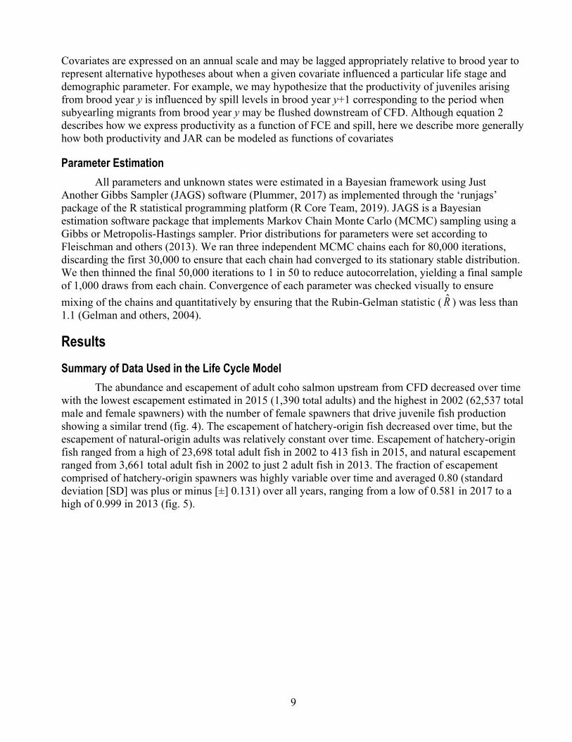
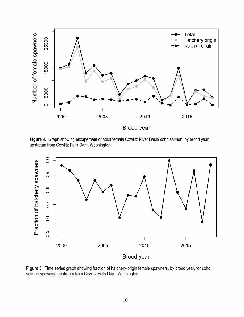
The abundance and escapement of adult coho salmon upstream from CFD decreased over time with the lowest escapement estimated in 2015 (1,390 total adults) and the highest in 2002 (62,537 total male and female spawners) with the number of female spawners that drive juvenile fish production showing a similar trend (fig. 4). The escapement of hatchery-origin fish decreased over time, but the escapement of natural-origin adults was relatively constant over time. Escapement of hatchery-origin fish ranged from a high of 23,698 total adult fish in 2002 to 413 fish in 2015, and natural escapement ranged from 3,661 total adult fish in 2002 to just 2 adult fish in 2013. The fraction of escapement comprised of hatchery-origin spawners was highly variable over time and averaged 0.80 (standard deviation [SD] was plus or minus [±] 0.131) over all years, ranging from a low of 0.581 in 2017 to a high of 0.999 in 2013 (fig. 5).

10

Figure 4. Graph showing escapement of adult female Cowlitz River Basin coho salmon, by brood year, upstream from Cowlitz Falls Dam, Washington.

Figure 5. Time series graph showing fraction of hatchery-origin female spawners, by brood year, for coho salmon spawning upstream from Cowlitz Falls Dam, Washington.

11

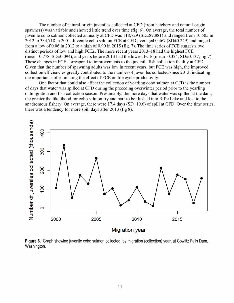
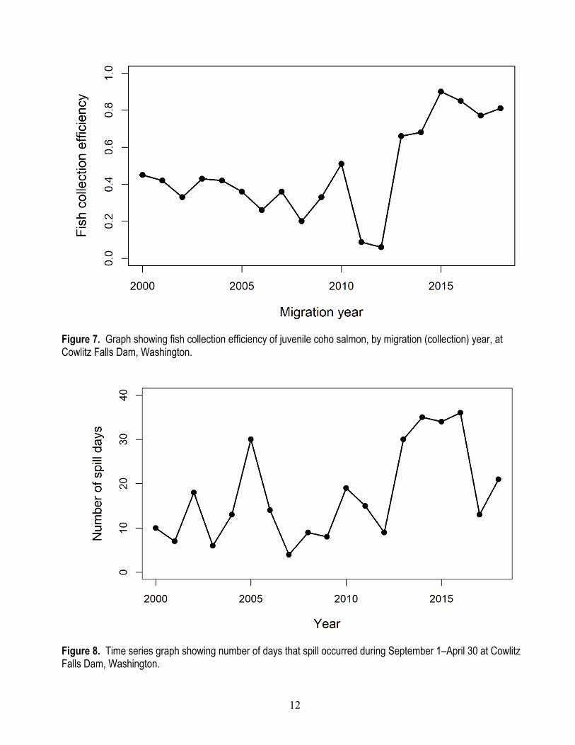
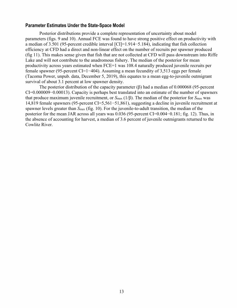
The number of natural-origin juveniles collected at CFD (from hatchery and natural-origin spawners) was variable and showed little trend over time (fig. 6). On average, the total number of juvenile coho salmon collected annually at CFD was 118,729 (SD±87,881) and ranged from 10,505 in 2012 to 334,718 in 2001. Juvenile coho salmon FCE at CFD averaged 0.467 (SD±0.249) and ranged from a low of 0.06 in 2012 to a high of 0.90 in 2015 (fig. 7). The time series of FCE suggests two distinct periods of low and high FCEs. The more recent years 2013–18 had the highest FCE (mean=0.778, SD±0.094), and years before 2013 had the lowest FCE (mean=0.324, SD±0.137; fig 7). These changes in FCE correspond to improvements to the juvenile fish collection facility at CFD. Given that the number of spawning adults was low in recent years, but FCE was high, the improved collection efficiencies greatly contributed to the number of juveniles collected since 2013, indicating the importance of estimating the effect of FCE on life cycle productivity.

One factor that could also affect the collection of yearling coho salmon at CFD is the number of days that water was spilled at CFD during the preceding overwinter period prior to the yearling outmigration and fish collection season. Presumably, the more days that water was spilled at the dam, the greater the likelihood for coho salmon fry and parr to be flushed into Riffe Lake and lost to the anadromous fishery. On average, there were 17.4 days (SD±10.6) of spill at CFD. Over the time series, there was a tendency for more spill days after 2013 (fig 8).

Figure 6. Graph showing juvenile coho salmon collected, by migration (collection) year, at Cowlitz Falls Dam, Washington.

12

Figure 7. Graph showing fish collection efficiency of juvenile coho salmon, by migration (collection) year, at Cowlitz Falls Dam, Washington.

Figure 8. Time series graph showing number of days that spill occurred during September 1–April 30 at Cowlitz Falls Dam, Washington.

13

Parameter Estimates Under the State-Space Model Posterior distributions provide a complete representation of uncertainty about model

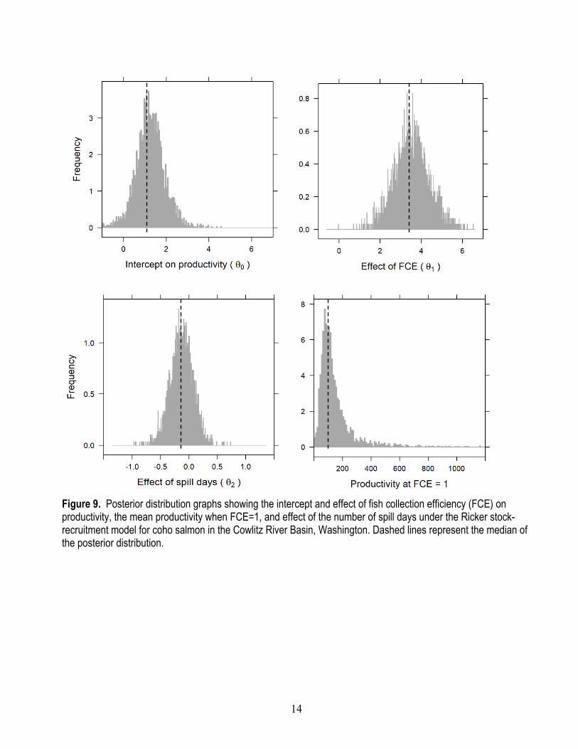
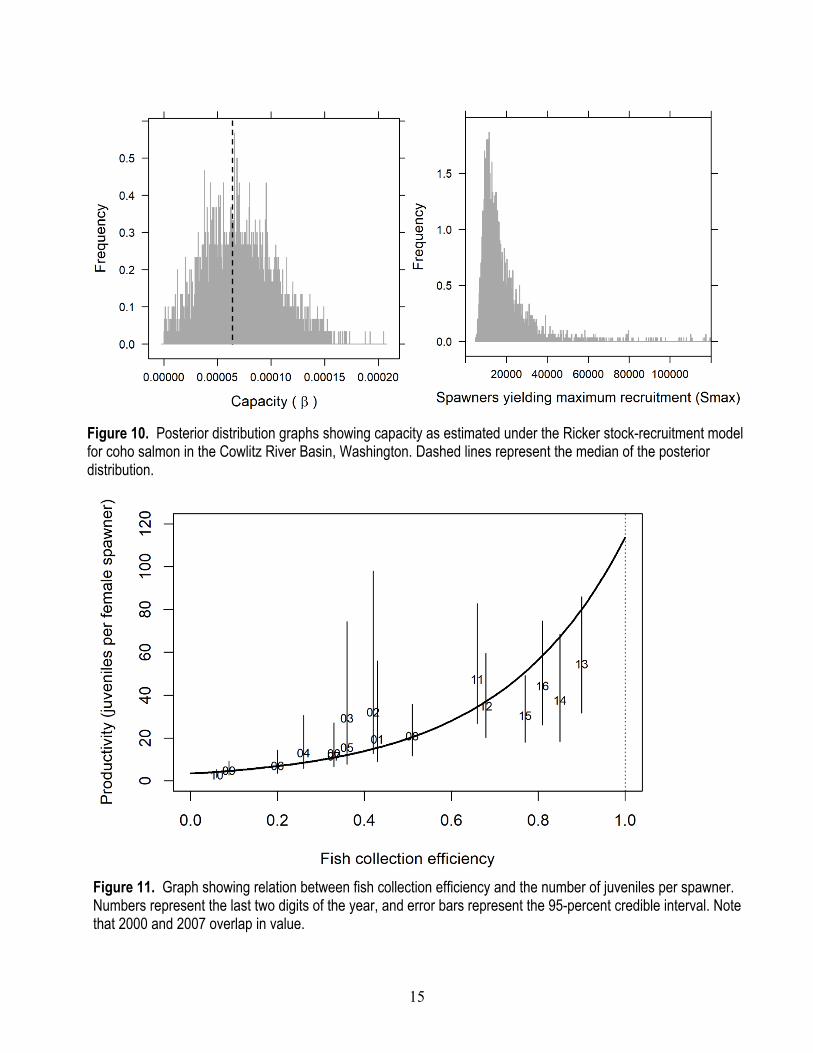
parameters (figs. 9 and 10). Annual FCE was found to have strong positive effect on productivity with a median of 3.501 (95-percent credible interval [CI]=1.914−5.184), indicating that fish collection efficiency at CFD had a direct and non-linear effect on the number of recruits per spawner produced (fig 11). This makes sense given that fish that are not collected at CFD will pass downstream into Riffe Lake and will not contribute to the anadromous fishery. The median of the posterior for mean productivity across years estimated when FCE=1 was 108.4 naturally produced juvenile recruits per female spawner (95-percent CI=1−404). Assuming a mean fecundity of 3,513 eggs per female (Tacoma Power, unpub. data, December 5, 2019), this equates to a mean egg-to-juvenile outmigrant survival of about 3.1 percent at low spawner density.

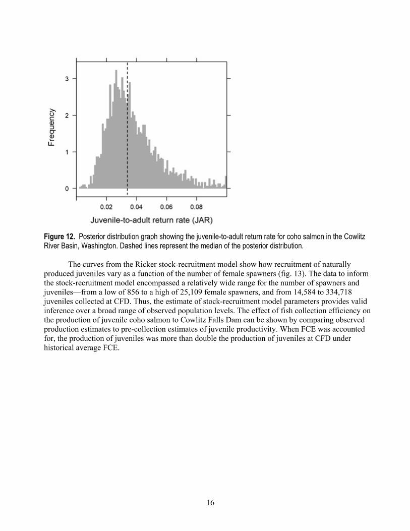
The posterior distribution of the capacity parameter (β) had a median of 0.000068 (95-percent CI=0.000009−0.00013). Capacity is perhaps best translated into an estimate of the number of spawners that produce maximum juvenile recruitment, or Smax (1/β). The median of the posterior for Smax was 14,819 female spawners (95-percent CI=5,561−51,861), suggesting a decline in juvenile recruitment at spawner levels greater than Smax (fig. 10). For the juvenile-to-adult transition, the median of the posterior for the mean JAR across all years was 0.036 (95-percent CI=0.004−0.181; fig. 12). Thus, in the absence of accounting for harvest, a median of 3.6 percent of juvenile outmigrants returned to the Cowlitz River.

14

Figure 9. Posterior distribution graphs showing the intercept and effect of fish collection efficiency (FCE) on productivity, the mean productivity when FCE=1, and effect of the number of spill days under the Ricker stock-recruitment model for coho salmon in the Cowlitz River Basin, Washington. Dashed lines represent the median of the posterior distribution.

15

Figure 10. Posterior distribution graphs showing capacity as estimated under the Ricker stock-recruitment model for coho salmon in the Cowlitz River Basin, Washington. Dashed lines represent the median of the posterior distribution.

Figure 11. Graph showing relation between fish collection efficiency and the number of juveniles per spawner. Numbers represent the last two digits of the year, and error bars represent the 95-percent credible interval. Note that 2000 and 2007 overlap in value.

16

Figure 12. Posterior distribution graph showing the juvenile-to-adult return rate for coho salmon in the Cowlitz River Basin, Washington. Dashed lines represent the median of the posterior distribution.

The curves from the Ricker stock-recruitment model show how recruitment of naturally produced juveniles vary as a function of the number of female spawners (fig. 13). The data to inform the stock-recruitment model encompassed a relatively wide range for the number of spawners and juveniles—from a low of 856 to a high of 25,109 female spawners, and from 14,584 to 334,718 juveniles collected at CFD. Thus, the estimate of stock-recruitment model parameters provides valid inference over a broad range of observed population levels. The effect of fish collection efficiency on the production of juvenile coho salmon to Cowlitz Falls Dam can be shown by comparing observed production estimates to pre-collection estimates of juvenile productivity. When FCE was accounted for, the production of juveniles was more than double the production of juveniles at CFD under historical average FCE.

17

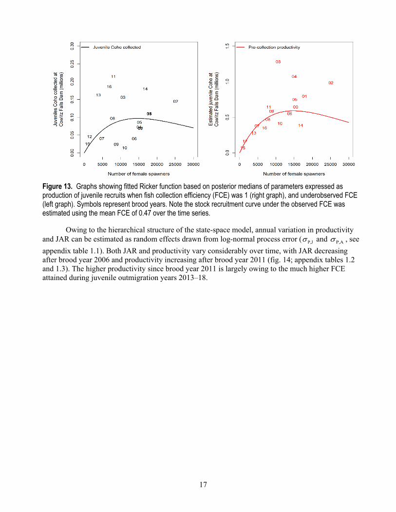
Figure 13. Graphs showing fitted Ricker function based on posterior medians of parameters expressed as production of juvenile recruits when fish collection efficiency (FCE) was 1 (right graph), and underobserved FCE (left graph). Symbols represent brood years. Note the stock recruitment curve under the observed FCE was estimated using the mean FCE of 0.47 over the time series.

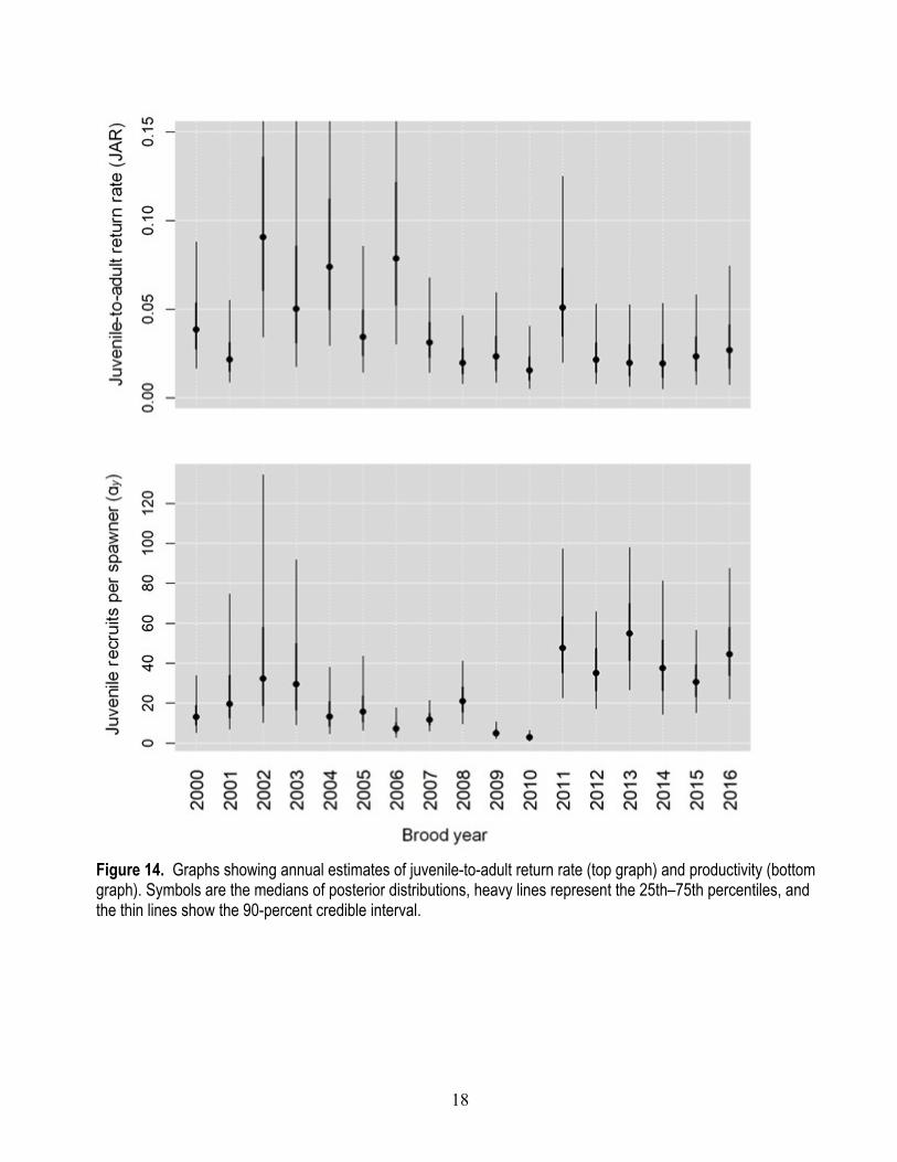
Owing to the hierarchical structure of the state-space model, annual variation in productivity and JAR can be estimated as random effects drawn from log-normal process error ( P,Jσ and P,Aσ , see appendix table 1.1). Both JAR and productivity vary considerably over time, with JAR decreasing after brood year 2006 and productivity increasing after brood year 2011 (fig. 14; appendix tables 1.2 and 1.3). The higher productivity since brood year 2011 is largely owing to the much higher FCE attained during juvenile outmigration years 2013–18.

18

Figure 14. Graphs showing annual estimates of juvenile-to-adult return rate (top graph) and productivity (bottom graph). Symbols are the medians of posterior distributions, heavy lines represent the 25th–75th percentiles, and the thin lines show the 90-percent credible interval.

19

Discussion The state-space life cycle model for upper Cowlitz River Basin coho salmon is a model of

intermediate complexity but can be used to gain insight about population dynamics and factors affecting different life stages of Cowlitz River Basin coho salmon. The state-space formulation of the model accounts for observation and process error, provides estimates of uncertainty in abundance and demographic parameters, and quantifies contributions of age and sex to the aggregate population. Our formulation of the state-space model provides a wealth of information about population dynamics such as estimates of process uncertainty, carrying capacity and density dependence, juvenile-to-adult survival rates, and factors affecting production of juvenile coho salmon in the upper Cowlitz River Basin, the latter being particularly important for understanding how fish collection efforts at CFD affect population recovery. We also show how the model can be expanded to include outmigration strategy, the transport of fry upstream (or downstream), harvest, as well as ocean effects on demographic parameters such as juvenile-to-adult return rate.

The life cycle model for Cowlitz River coho salmon is fully functional at this time and can be used to provide estimates of the effect of FCE on adult-to-juvenile productivity. Nonetheless, we consider this analysis to be a pilot effort and proof of concept that shows the utility of multistage, statistical life cycle models for understanding the interplay between population dynamics and water-management activities that influence those dynamics. We have yet to probe many other aspects of the dynamics of this population. For example, the Ricker model suggests that the population may overcompensate owing to density dependence but estimates of juvenile production at the upper end of the spawning distribution are uncertain. Therefore, firm conclusions regarding overcompensation should be withheld at this time. By incorporating a fuller set of covariates, harvest rates, and juvenile age structure in the model, parameter estimates, a broader set of inferences may be drawn about the individual contribution of these factors to the life cycle of coho salmon in upper Cowlitz River.

Several significant updates could improve model fit and provide greater inference for fishery management. These updates are (1) accounting for harvest and broodstock removal, (2) including fry transportation (upstream or downstream) in the model framework, (3) evaluating whether the Ricker or Beverton-Holt stock-recruitment model provides a better fit to the data, (4) evaluating other covariates to explain variation in adult-to-juvenile productivity (ɑ) and juvenile-to-adult return rates (JAR; Logerwell and others, 2003), and (5) incorporating error in FCE in the modeled estimates and error.

Some of the covariates that could help explain variation in adult-to-juvenile production include the following:

• The fraction of hatchery fish released at each upriver location, • The fraction of hatchery spawners (that is, pHOS), • Peak wintertime flows (to estimate the effect of redd scour), • Recreational harvest upstream from CFD (affects the number of available spawners), and • The fall back of adults to below CFD.

Covariates that may help explain variation in the annual juvenile-to-adult return rates are the following:

• Pacific Decadal Oscillation (PDO), • Coastal Upwelling Index (CUI), • Sea Surface Temperatures (SST), and • Ocean harvest estimates and harvest downstream of CFD.

Including and evaluating these covariates with the two-stage life cycle model could greatly improve the inferences drawn about the production and viability of Cowlitz River coho salmon.

20

Regardless of the improvements that can be made to the model, we were able to quantify how FCE at CFD directly influences the productivity of juveniles, as shown by the relation between mean annual productivity and FCE (fig. 11) and in the estimates of pre-collection relative to post-collection production (fig. 14). We also estimated a median JAR of about 3.6 percent, which is relatively high, especially when one considers that this return rate does not include harvest. In some brood years (2002–06) estimates of JAR ranged from about 5 to 10 percent (fig. 14). These findings suggest that adult return rates for Cowlitz River coho salmon may be high enough to meet replacement and sustain the population so long as juvenile production and fish collection remain sufficiently high. Future application of the model could include a population viability analysis to determine what FCE target may be needed to sustain Cowlitz River coho salmon.

Ultimately, fisheries managers need tools to help understand how potential management actions affect population abundance at different parts of the life cycle to assess whether recovery goals are being achieved. Our life cycle model for upper Cowlitz coho salmon is a first step towards development of such a tool. Additional work is needed to better account for key management factors affecting the population (for example, harvest and brood stock) to quantify effects of the trap-and-haul program, and to incorporate effects of environmental variation. Nonetheless, because our model incorporates unaccounted for variability in demographic parameters, we can use it to simulate stochastic population trajectories that include important management “knobs” (for example, FCE, harvest) and environmental variation. Such a model would allow managers to assess the relative effect of alternative management scenarios on population trajectories in a probabilistic manner to understand the likelihood of success of a given management action in the face of environmental variability and uncertainty.

21

References Cited Courter, I.I., Wyatt, G.J., Perry, R.W., Plumb, J.M., Carpenter, F.M., Ackerman, N.K., Lessard, R.B.,

and Galbreath, P.F., 2019, A natural-origin steelhead population’s response to exclusion of hatchery fish: Transactions of the American Fisheries Society, v. 148, p. 339–351.

Fleischman, S.J., Catalano, M.J., Clark, R.A., and Bernard, D.R., 2013, An age-structured state-space stock–recruit model for Pacific salmon (Oncorhynchus spp.): Canadian Journal of Fisheries and Aquatic Sciences, v. 70, p. 401–414.

Gelman, A., Carlin, J.B. Stern, H.S., and Rubin, D.B., 2014, Bayesian data analysis: Boca Raton, Florida, Chapman and Hall, p. 1–661.

Greene, C.M., and Beechie, T.J., 2004, Consequences of potential density-dependent mechanisms on recovery of ocean-type Chinook salmon (Oncorhynchus tshawytscha): Canadian Journal of Fisheries and Aquatic Sciences, v. 61, p. 590–602.

Kock, T., Liedtke, T., Rondorf, D., Serl, J., Kohn, M., and Bumbaco, K., 2012, Elevated streamflows increase dam passage by juvenile coho salmon during Winter—Implications of climate change in the Pacific Northwest: North American Journal of Fisheries Management, v. 32, p. 1070–1079.

Logerwell, E.A., Mantua, N.J., Lawson, P.W., Francis, R.C., and Agostini, V.N,. 2003, Tracking environmental processes in the coastal zone for understanding and predicting Oregon coho (Oncorhynchus kisutch) marine survival: Fisheries Oceanography, v. 12, p. 554–568.

Moussalli, E. and Hilborn, R., 1986, Optimal stock size and harvest rate in multistage life history models: Canadian Journal of Fisheries and Aquatic Sciences, v. 43, p. 135–141.

Newman, K.B., Buckland, S.T., Morgan, B.J.T., King R., Borchers, D.L., Cole, D.J., Besbeas, P., Gimenez, O., and Thomas, L., 2014, Modeling population dynamics—Model formulation, fitting and assessment using state-space methods: New York, Springer, p. 39–50.

Plummer, M., 2017, Jags version 4.3.0 user manual—Technical report, p. 1–73, accessed January 15, 2019, at https://web.sgh.waw.pl/~atoroj/ekonometria_bayesowska/jags_user_manual.pdf.

R Core Team, 2019, R—A language and environment for statistical computing, Vienna, Austria, R Foundation for Statistical Computing, accessed January 25, 2019, at http://www.R-project.org/.

Ricker, W.E., 1954, Stock and recruitment: Journal of the Fisheries Research Board of Canada, v. 11, p. 559–623.

Zabel, R.W., Faulkner, J., Smith, S.G., Anderson, J.J., Van Holmes, C., Beer, N., Iltis, S., Krinke, J., Fredricks, G., Bellerud, B., Sweet, J., and Giorgi, A., 2008, Comprehensive passage (COMPASS) model: a model of downstream migration and survival of juvenile salmonids through a hydropower system: Hydrobiologia, v. 609, p. 289–300.

Zabel, R.W., Scheuerell, M.D., McClure, M.M., and Williams. J.G., 2006, The interplay between climate variability and density dependence in the population viability of Chinook salmon: Conservation Biology, v. 20, p. 190–200.

https://web.sgh.waw.pl/%7Eatoroj/ekonometria_bayesowska/jags_user_manual.pdf

22

This page intentionally left blank.

23

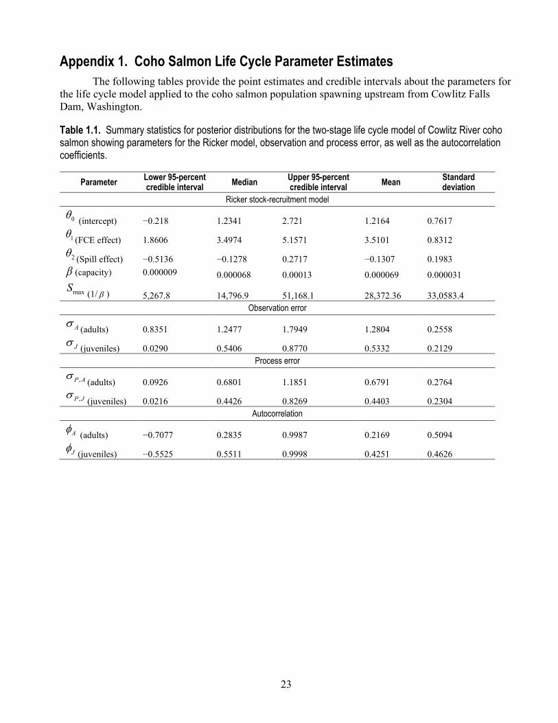
Appendix 1. Coho Salmon Life Cycle Parameter Estimates The following tables provide the point estimates and credible intervals about the parameters for

the life cycle model applied to the coho salmon population spawning upstream from Cowlitz Falls Dam, Washington.

Table 1.1. Summary statistics for posterior distributions for the two-stage life cycle model of Cowlitz River coho salmon showing parameters for the Ricker model, observation and process error, as well as the autocorrelation coefficients.

Parameter Lower 95-percent credible interval Median Upper 95-percent

credible interval Mean Standard deviation

Ricker stock-recruitment model

0θ (intercept) −0.218 1.2341 2.721 1.2164 0.7617

1θ (FCE effect) 1.8606 3.4974 5.1571 3.5101 0.8312

2θ (Spill effect) −0.5136 −0.1278 0.2717 −0.1307 0.1983 β (capacity) 0.000009 0.000068 0.00013 0.000069 0.000031

maxS (1/ β ) 5,267.8 14,796.9 51,168.1 28,372.36 33,0583.4 Observation error

Aσ (adults) 0.8351 1.2477 1.7949 1.2804 0.2558

Jσ (juveniles) 0.0290 0.5406 0.8770 0.5332 0.2129 Process error

,P Aσ(adults) 0.0926 0.6801 1.1851 0.6791 0.2764

,P Jσ(juveniles) 0.0216 0.4426 0.8269 0.4403 0.2304

Autocorrelation

Aφ (adults) −0.7077 0.2835 0.9987 0.2169 0.5094

Jφ (juveniles) −0.5525 0.5511 0.9998 0.4251 0.4626

24

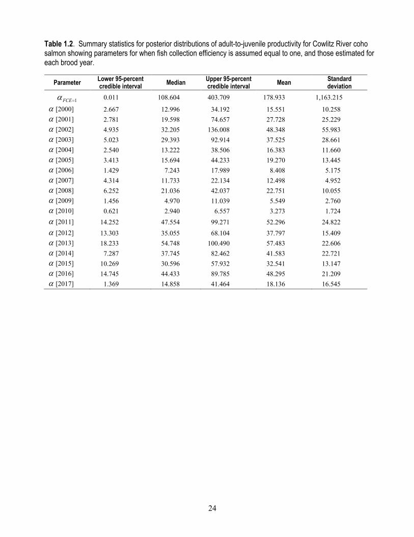
Table 1.2. Summary statistics for posterior distributions of adult-to-juvenile productivity for Cowlitz River coho salmon showing parameters for when fish collection efficiency is assumed equal to one, and those estimated for each brood year.



1FCEα = 0.011 108.604 403.709 178.933 1,163.215

α [2000] 2.667 12.996 34.192 15.551 10.258 α [2001] 2.781 19.598 74.657 27.728 25.229 α [2002] 4.935 32.205 136.008 48.348 55.983 α [2003] 5.023 29.393 92.914 37.525 28.661 α [2004] 2.540 13.222 38.506 16.383 11.660 α [2005] 3.413 15.694 44.233 19.270 13.445 α [2006] 1.429 7.243 17.989 8.408 5.175 α [2007] 4.314 11.733 22.134 12.498 4.952 α [2008] 6.252 21.036 42.037 22.751 10.055 α [2009] 1.456 4.970 11.039 5.549 2.760 α [2010] 0.621 2.940 6.557 3.273 1.724 α [2011] 14.252 47.554 99.271 52.296 24.822 α [2012] 13.303 35.055 68.104 37.797 15.409 α [2013] 18.233 54.748 100.490 57.483 22.606 α [2014] 7.287 37.745 82.462 41.583 22.721 α [2015] 10.269 30.596 57.932 32.541 13.147 α [2016] 14.745 44.433 89.785 48.295 21.209 α [2017] 1.369 14.858 41.464 18.136 16.545

25

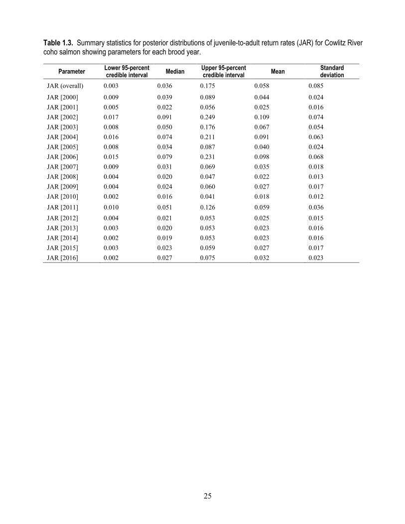
Table 1.3. Summary statistics for posterior distributions of juvenile-to-adult return rates (JAR) for Cowlitz River coho salmon showing parameters for each brood year.



JAR (overall) 0.003 0.036 0.175 0.058 0.085

JAR [2000] 0.009 0.039 0.089 0.044 0.024 JAR [2001] 0.005 0.022 0.056 0.025 0.016 JAR [2002] 0.017 0.091 0.249 0.109 0.074 JAR [2003] 0.008 0.050 0.176 0.067 0.054 JAR [2004] 0.016 0.074 0.211 0.091 0.063 JAR [2005] 0.008 0.034 0.087 0.040 0.024 JAR [2006] 0.015 0.079 0.231 0.098 0.068 JAR [2007] 0.009 0.031 0.069 0.035 0.018 JAR [2008] 0.004 0.020 0.047 0.022 0.013 JAR [2009] 0.004 0.024 0.060 0.027 0.017 JAR [2010] 0.002 0.016 0.041 0.018 0.012 JAR [2011] 0.010 0.051 0.126 0.059 0.036 JAR [2012] 0.004 0.021 0.053 0.025 0.015 JAR [2013] 0.003 0.020 0.053 0.023 0.016 JAR [2014] 0.002 0.019 0.053 0.023 0.016 JAR [2015] 0.003 0.023 0.059 0.027 0.017 JAR [2016] 0.002 0.027 0.075 0.032 0.023

Publishing support provided by the U.S. Geological SurveyScience Publishing Network, Tacoma Publishing Service Center

For more information concerning the research in this report, contact the Director, Western Fisheries Research Center U.S. Geological Survey 6505 NE 65th Street Seattle, Washington 98115-5016 https://www.usgs.gov/centers/wfrc

https://www.usgs.gov/centers/wfrc

ISSN 2331-1258 (online)https://doi.org/10.3133/ofr20201068

Plumb and Perry—

Developm

ent of a Life Cycle Model for Coho Salm

on in the Upper Cow

litz River Basin, W

ashington—Open-File Report 2020–1068

Documents

Development of a Two-Stage Life Cycle Model for