DEVELOPMENT OF A TSUNAMI FORECAST MODEL FOR HOMER,

ALASKA

Arun Chawla

October 30, 2008

Contents Abstract .................................................................................................................................... 6 1.0 Background and Objectives .................................................................................................... 6 2.0 Forecast Methodology ............................................................................................................ 7 

2.1 Study Area – context ............................................................................................... 7 2.2 Historical Events ...................................................................................................... 8 2.3 Tide gauges/water level data ..................................................................................... 8 2.3.2 Bathymetry and Topography ................................................................................... 9 2.4 Model setup ............................................................................................................ 9 

3.0 Results .............................................................................................................................. 11 3.1 Model Validation .................................................................................................... 11 3.2 Results of tested event ........................................................................................... 11 3.2.1 1996 Andreanov Tsunami ..................................................................................... 11 3.3 Model stability and reliability .............................................................................. 13 3.3.1 Artificial 9.5 Mw Tsunami ..................................................................................... 13 

4.0 Summary ........................................................................................................................... 16 5.0 References ......................................................................................................................... 16 6.0 Appendix A ......................................................................................................................... 17 7.0 Appendix B ......................................................................................................................... 19 

7.1 SIM *.in file .......................................................................................................... 19 8.0 Appendix C ......................................................................................................................... 20 

2

List of Tables

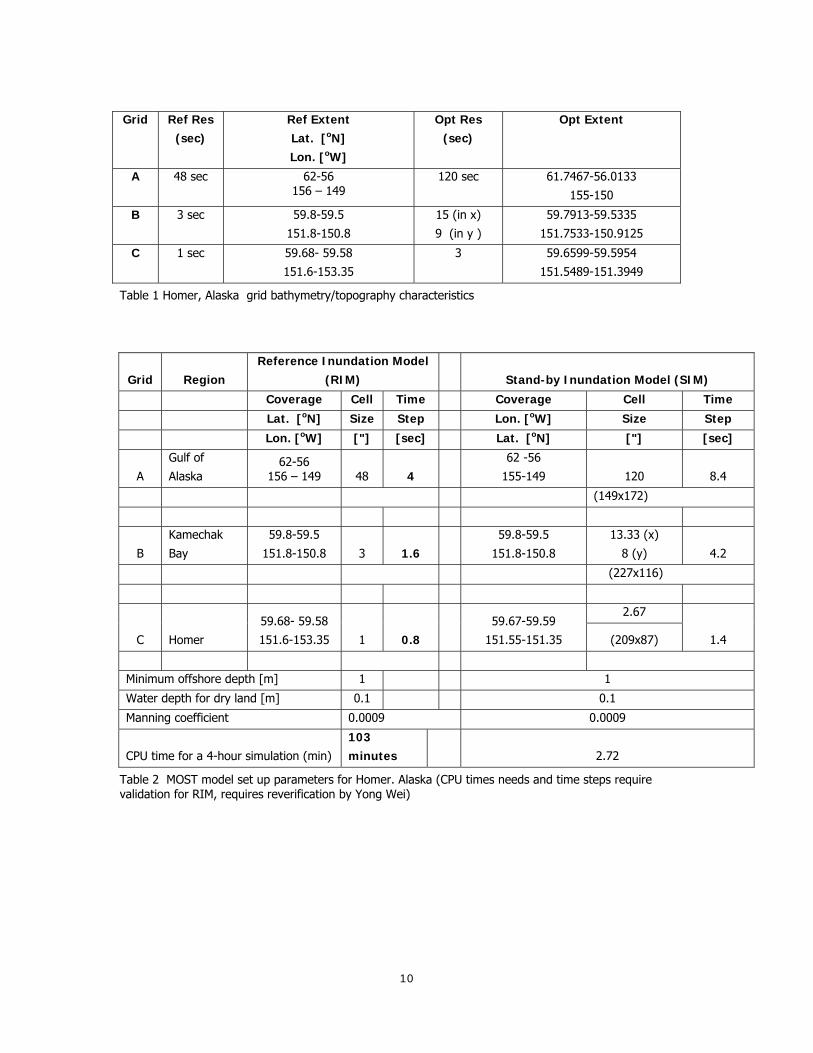
Table 1 Homer, Alaska grid bathymetry/topography characteristics ..................... 10 

Table 2 MOST model set up parameters for Homer. Alaska (CPU times needs and time steps require validation for RIM, requires reverification by Yong Wei) ............ 10 

Table 3 Events used for SIFT 3.0 Testing for Homer, Alaska -April 2009. ............... 20 

3

List of Figures

Figure 1 Google Earth image of Homer, Alaska ................................................... 7 

Figure 2 Location of Seldovia tide gauge in relation to Homer. .............................. 8 

Figure 2 Maximum elevations in cms of the Optimized SIM at Homer for the Andreanov tsunami. ...................................................................................... 12 

Figure 3 Maximum elevations in cms of Reference SIM for Homer for an artificial 9.5 Mw tsunami event originating in the Alaska Subduction zone. .............................. 14 

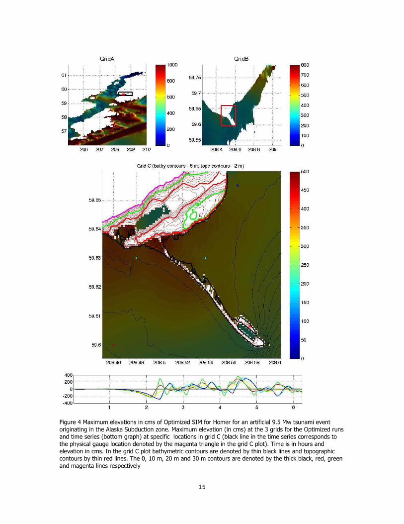
Figure 4 Maximum elevations in cms of Optimized SIM for Homer for an artificial 9.5 Mw tsunami event originating in the Alaska Subduction zone. .............................. 15 

Figure 5 Bathymetric differences for the Reference SIMS at Homer, Alaska. ........................ 17 

Figure 6 Bathymetric differences for the Optimized SIMS at Homer, Alaska. .......... 18 

Figure 8 Inundation Forecast for Homer, Alaska SIM C Grid for the 2006 Tonga tsunami. ...................................................................................................... 21 

Figure 9 Water level time series result for the Homer, AK warning point for the 2006 Tonga tsunami. ............................................................................................. 22 

Figure 10 Inundation Forecast for Homer, Alaska SIM C Grid for the 2006 Kuril tsunami. ...................................................................................................... 23 

Figure 11 Water level time series result for the Homer, AK warning point for the 2006 Kuril tsunami. ....................................................................................... 24 

Figure 12 Inundation Forecast for Homer, Alaska SIM C Grid for the synthetic Alaska 9.3 Mw tsunami event. .................................................................................. 25 

Figure 13 Water level time series result for the Homer, AK warning point for synthetic Alaska 9.3 Mw tsunami event. ........................................................... 26 

4

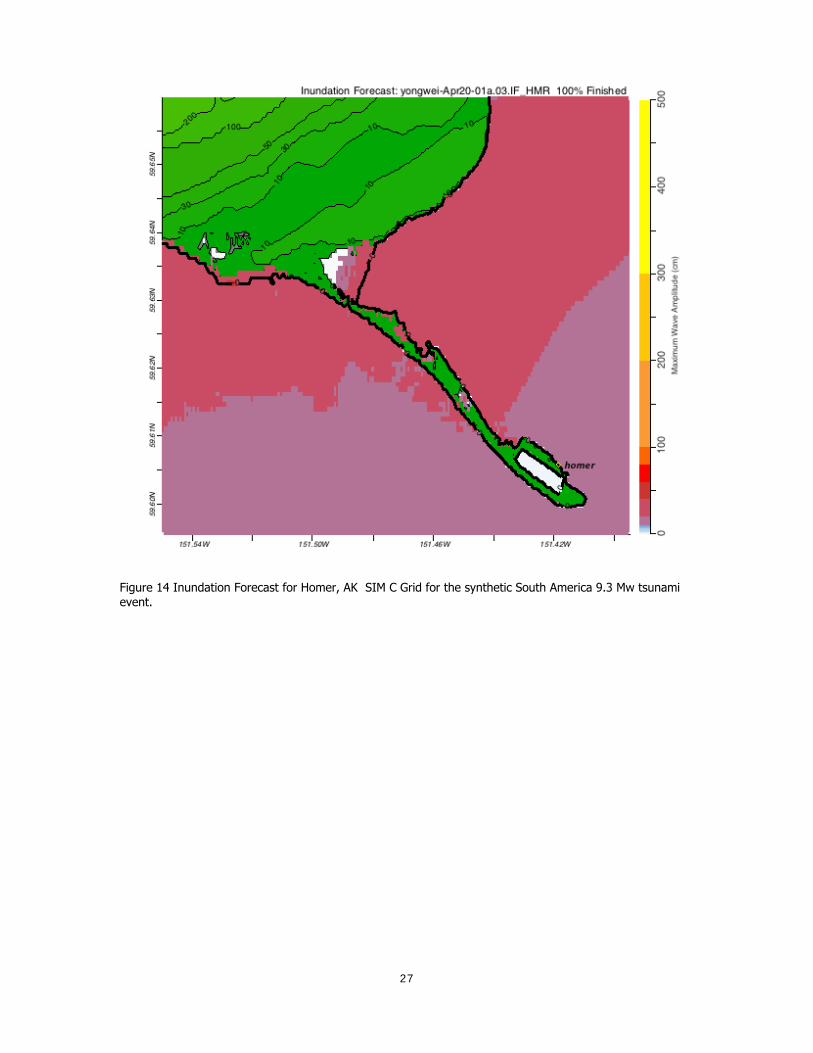
Figure 14 Inundation Forecast for Homer, AK SIM C Grid for the synthetic South America 9.3 Mw tsunami event. ...................................................................... 27 

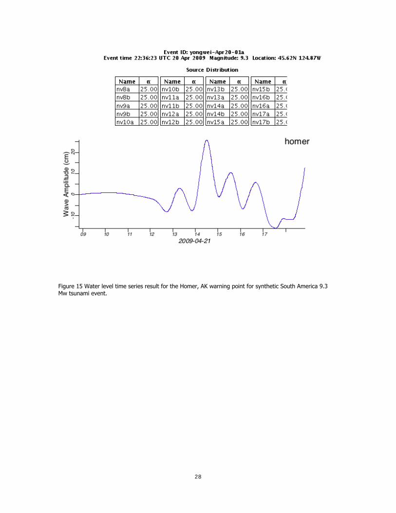
Figure 15 Water level time series result for the Homer, AK warning point for synthetic South America 9.3 Mw tsunami event. ................................................ 28 

Figure 16 Inundation Forecast for Homer, AK SIM C Grid for the synthetic New Zealand/Kermadec 9.3 Mw tsunami event. ....................................................... 29 

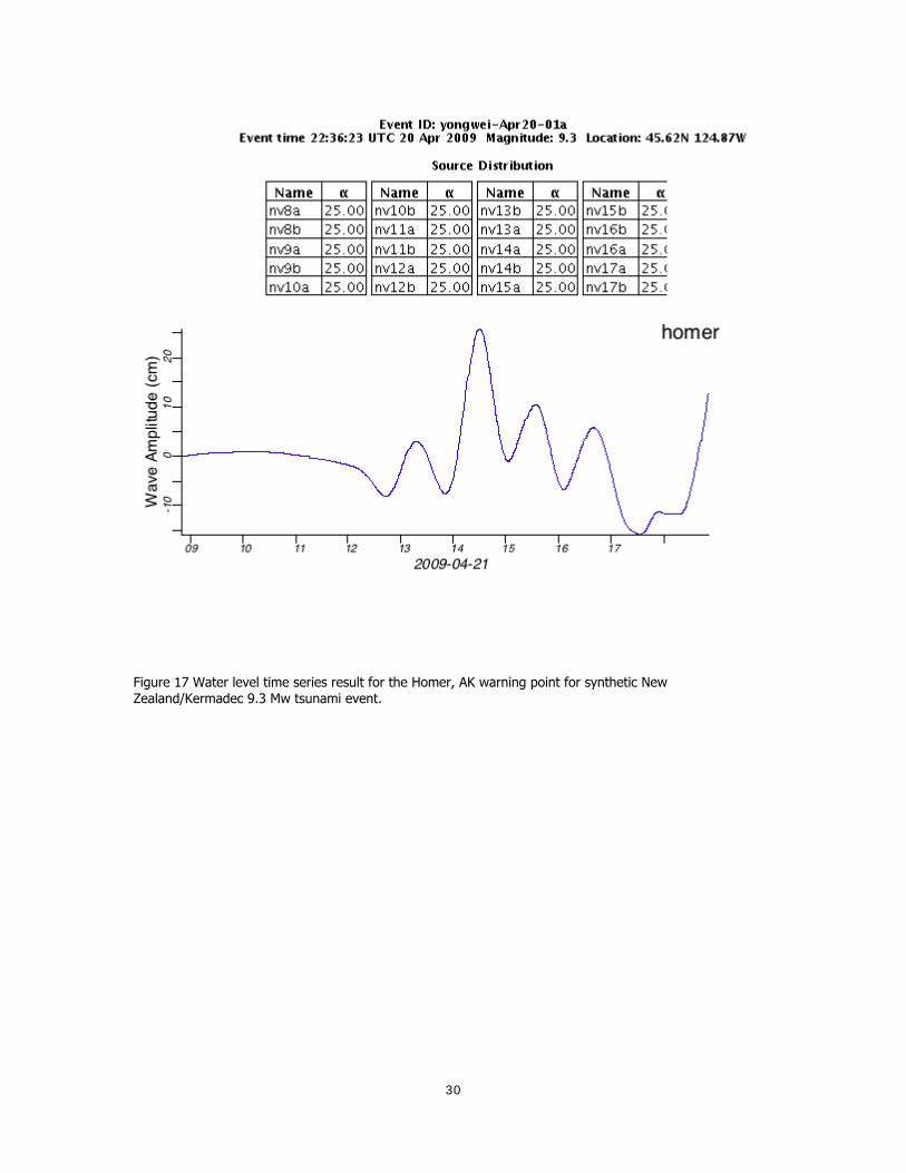
Figure 17 Water level time series result for the Homer, AK warning point for synthetic New Zealand/Kermadec 9.3 Mw tsunami event. ................................... 30 

5

Development of a Tsunami Forecast Model for Homer, Alaska

Arun Chawla

October 30. 2009

6

Abstract

A tsunami forecast model was built for Homer, Alaska in support of the Short Term Inundation Forecast system for Tsunamis (SIFT) system. With the lack of historical tide gauge data for the Homer area, SIMs and Reference Inundation Models (RIM) were developed using synthetic data to simulate the run up values noted during the 1964 and 1996 tsunamis. Synthetic megatsunami events originating in the Pacific Rim were run to test the stability and sensitivity of the Homer SIM and demonstrated that the SIM and RIM remained stable in the case of a mega event. Additional testing of the Sitka SIM was completed with Desktop SIFT and found that a near field source (west of Kodiak Island) would greatly impact the Seward region and additionally, earthquake sources from Indonesia have a lesser impact on the SIM.

1.0 Background and Objectives

An efficient tsunami forecast system provides timely basin-wide warning of in-progress tsunami waves accurately and quickly (Titov et al., 2005). NOAA’s Short-term Inundation Forecast of Tsunami (SIFT) is an advanced tsunami forecasting system that combines real-time tsunami event data with numerical models to produce estimates of tsunami wave arrival times and amplitudes. The SIFT system integrates several key components: the tsunameters for real-time monitoring of tsunami signals in the deep ocean, a basin-wide pre-computed propagation database of water level and flow velocities based on potential seismic unit sources, an inversion algorithm to derive the tsunami source based on the tsunameter observations during a tsunami event, and the Stand-by Inundation Models (SIMs) to provide accurate and speedy numerical modeling of tsunami impact for coastal communities. A SIM is used to create the forecast model to provide an estimate of wave arrival time, wave height, and inundation immediately after a tsunami event. Tsunami forecast models are run in real time while a tsunami is propagating in the open ocean; consequently they are designed to perform under very stringent time limitations. The Stand-by Inundation Model (SIM), based on the Method of Splitting Tsunami (MOST), emerges as the solution in SIFT by modeling real-time tsunami in minutes while employing high resolution grids. Each SIM consists of three telescoped grids with increasing spatial resolution, and temporal resolution for simulation of wave inundation onto dry land.

The SIM utilizes the most recent bathymetry and topography available to reproduce the correct wave dynamics during the inundation computation. SIMs are constructed for populous coastal communities at risk for tsunamis in the Pacific, Atlantic and Caribbean. Previous and present development of SIM in the Pacific (Titov et al., 2005; Titov, 2009; Tang et al., 2008; Wei et al., 2008) has shown the accuracy and efficiency of the up-to-date SIMs implemented in SIFT in the real-time tsunami forecast, as well as in hindcast research.

This report describes the development and testing of a reference and forecast inundation model for Homer, Alaska. The forecast model will be incorporated into the U.S. tsunami warning system for use at the Pacific and West Coast-Alaska Tsunami Warning Center. Synolakis et al. (2007) and Tang et al. (2008) describe the technical aspects of SIM development, stability testing and robustness.

7

2.0 Forecast Methodology

The methodology for modeling these coastal areas is to develop a set of three nested grids (A, B, C), each of which is successively finer in resolution, until the near-shore details can be resolved to the point that tide gauge data from historical tsunamis in the area match reasonably with the modeled results. The procedure is to start with large spatial extent merged bathymetric topographic grids at high resolution, referred to as “reference SIM”, and then after a reasonable data fit is achieved to optimize these grids by coarsening the resolution and shrinking the grid size until the model runs in under 10 min of wall-clock time. This allows for the significant portion of the modeled tsunami waves, typically 4 to 10 hr of modeled tsunami time, to pass through the model domain without too much signal degradation. This final model is referred to as the optimized SIM.

2.1 Study Area – context

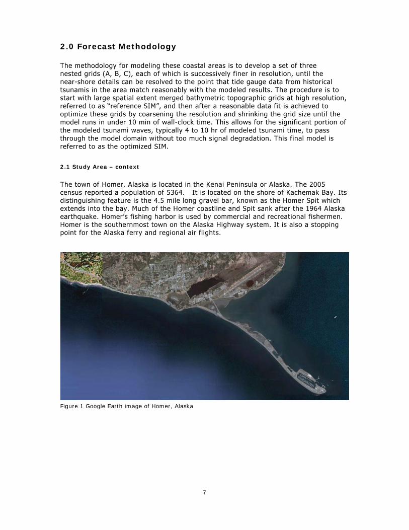
The town of Homer, Alaska is located in the Kenai Peninsula or Alaska. The 2005 census reported a population of 5364. It is located on the shore of Kachemak Bay. Its distinguishing feature is the 4.5 mile long gravel bar, known as the Homer Spit which extends into the bay. Much of the Homer coastline and Spit sank after the 1964 Alaska earthquake. Homer’s fishing harbor is used by commercial and recreational fishermen. Homer is the southernmost town on the Alaska Highway system. It is also a stopping point for the Alaska ferry and regional air flights.

Figure 1 Google Earth image of Homer, Alaska

8

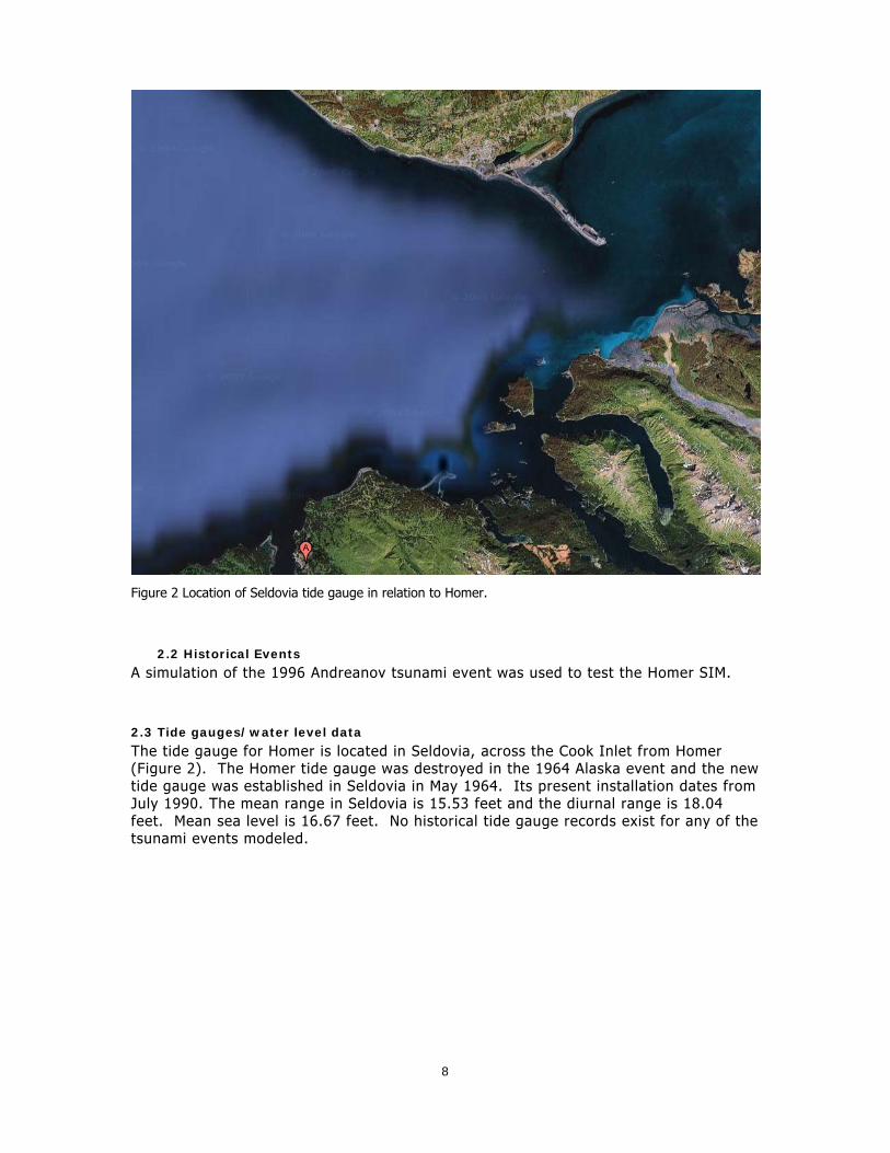
Figure 2 Location of Seldovia tide gauge in relation to Homer.

2.2 Historical Events

A simulation of the 1996 Andreanov tsunami event was used to test the Homer SIM.

2.3 Tide gauges/water level data

The tide gauge for Homer is located in Seldovia, across the Cook Inlet from Homer (Figure 2). The Homer tide gauge was destroyed in the 1964 Alaska event and the new tide gauge was established in Seldovia in May 1964. Its present installation dates from July 1990. The mean range in Seldovia is 15.53 feet and the diurnal range is 18.04 feet. Mean sea level is 16.67 feet. No historical tide gauge records exist for any of the tsunami events modeled.

9

2.3.2 Bathymetry and Topography

Accurate bathymetry and topography are crucial inputs to developing the reference and standby models, especially for the inundation of the near-shore environment. To develop each grid, we attempt to gather and use the best available data for the area studied. Grids may be updated if newer, more accurate data are available.

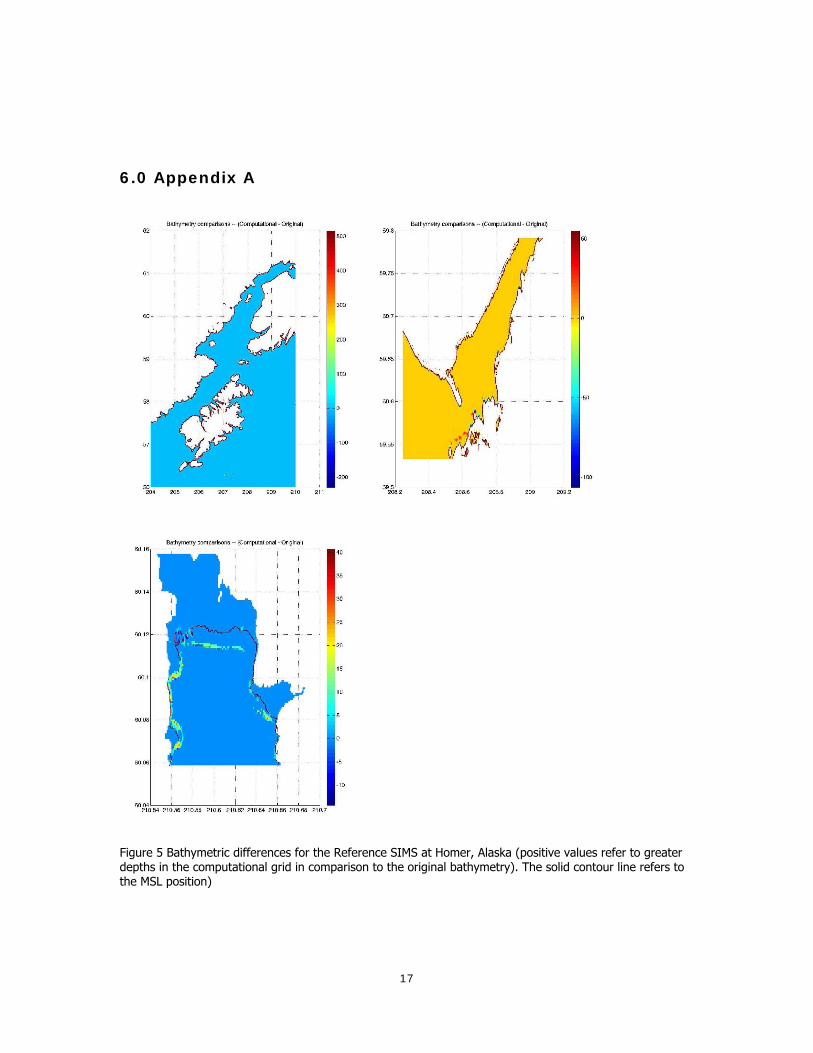
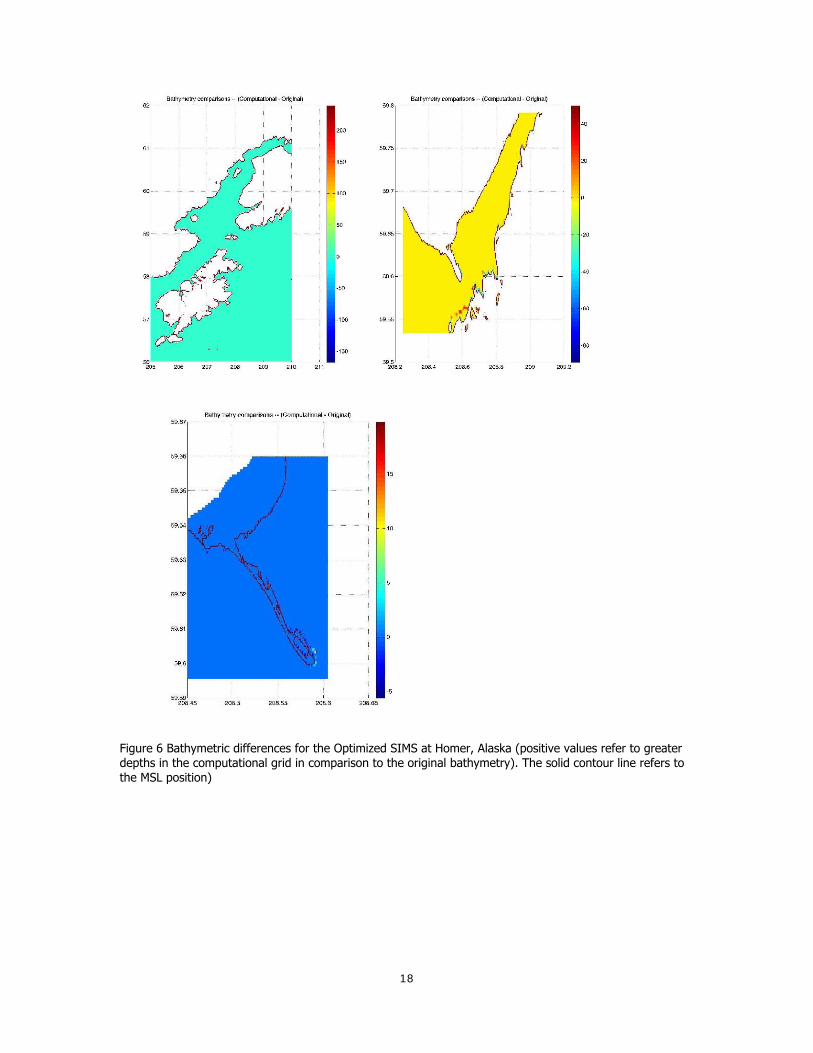
Eight, three, one arc second merged bathymetry and topography data built by NCTR were used to create the grids used for building the RIMs and SIMs for Homer. Plots of the modified bathymetry files for the reference and the optimized grids are located in Appendix A (Figures 6 and 7). The SIM C grid shows little difference between the original the modified bathymetry values.

2.4 Model setup

The model used to estimate tsunami amplitude is the MOST model (Tang et al. 2008) which is a finite difference method of characteristic model which takes input from a propagation run data base and then, via a series of nested grids, resolves the near shore bathymetry and topography to estimate the water level at coastal sites. Adjustable parameters include: time step, number of time steps, near shore wet/dry boundary depth, coarse grid wet/dry boundary depth, run down or not in coarse grids friction coefficient, output time, grid size, grid resolution and grid position.

Once tested these parameters remain fixed from run to run, under the assumption that the parameters may be location dependent (sharp bathymetric changes, high resolution needed for channels, bars etc.) but should not depend on the flow field (i.e. the particular tsunami being modeled).

For Homer, the grid resolution and extents for the reference and optimized grids are given in Table 1. Figures of the model extents for reference and optimized grids are found in the attached Appendix A (Figures 6 and 7). These grid parameters are not unique to the stand by inundation model and could be modified considerably as the results indicate. They are sufficient to show that the model reproduces historical tsunami, and that the model is stable enough with these grids to handle a large tsunami simulation.

10

Grid Ref Res (sec)

Ref Extent Lat. [oN] Lon. [oW]

Opt Res (sec)

Opt Extent

A 48 sec 62-56 156 – 149

120 sec 61.7467-56.0133

155-150

B 3 sec 59.8-59.5

151.8-150.8

15 (in x)

9 (in y )

59.7913-59.5335

151.7533-150.9125

C 1 sec 59.68- 59.58

151.6-153.35

3 59.6599-59.5954

151.5489-151.3949

Table 1 Homer, Alaska grid bathymetry/topography characteristics

Grid Region Reference Inundation Model

(RIM) Stand-by Inundation Model (SIM)

Coverage Cell Time Coverage Cell Time

Lat. [oN] Size Step Lon. [oW] Size Step

Lon. [oW] ["] [sec] Lat. [oN] ["] [sec]

A

Gulf of

Alaska 62-56

156 – 149 48 4

62 -56

155-149 120 8.4

(149x172)

B

Kamechak

Bay

59.8-59.5

151.8-150.8 3 1.6

59.8-59.5

151.8-150.8

13.33 (x)

8 (y) 4.2

(227x116)

C Homer

59.68- 59.58

151.6-153.35 1 0.8

59.67-59.59

151.55-151.35

2.67

1.4 (209x87)

Minimum offshore depth [m] 1 1

Water depth for dry land [m] 0.1 0.1

Manning coefficient 0.0009 0.0009

CPU time for a 4-hour simulation (min)

103 minutes 2.72

Table 2 MOST model set up parameters for Homer. Alaska (CPU times needs and time steps require validation for RIM, requires reverification by Yong Wei)

11

3.0 Results

3.1 Model Validation

Since no historical gauge records exist for Homer, the model was validated using data simulating the 1996 Andreanov tsunami event and run up observations.

3.2 Results of tested event

3.2.1 1996 Andreanov Tsunami

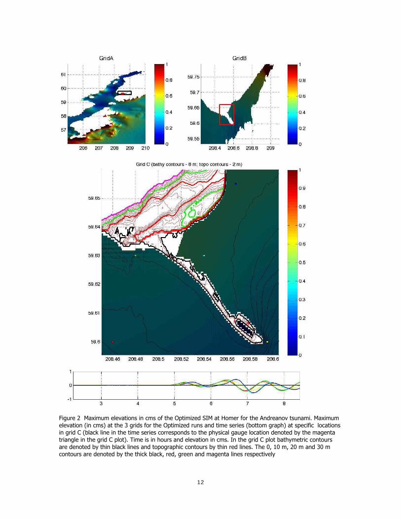
The 1996 Andreanov event was simulated to test the Optimized SIMs for Homer. (Figure 4) The plots show that there was no detectable signal at Homer, which is consistent with the event at those locations.

12

Figure 2 Maximum elevations in cms of the Optimized SIM at Homer for the Andreanov tsunami. Maximum elevation (in cms) at the 3 grids for the Optimized runs and time series (bottom graph) at specific locations in grid C (black line in the time series corresponds to the physical gauge location denoted by the magenta triangle in the grid C plot). Time is in hours and elevation in cms. In the grid C plot bathymetric contours are denoted by thin black lines and topographic contours by thin red lines. The 0, 10 m, 20 m and 30 m contours are denoted by the thick black, red, green and magenta lines respectively

13

3.3 Model stability and reliability

3.3.1 Artificial 9.5 Mw Tsunami

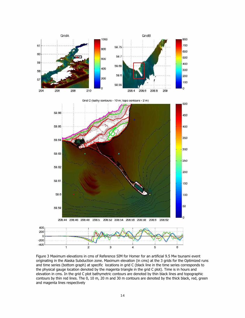
A large artificial tsunami equivalent to a 9.5 Mw earthquake on the Alaska subduction zone was simulated outside the B grid region to show the pattern of run up in the Homer area as well as to indicate the stability of the model for potential large events. In general; each simulated earthquake involves 20 unit sources (10 pairs) and a uniform slip of 29 m. (Tang et. al 2008)

14

Figure 3 Maximum elevations in cms of Reference SIM for Homer for an artificial 9.5 Mw tsunami event originating in the Alaska Subduction zone. Maximum elevation (in cms) at the 3 grids for the Optimized runs and time series (bottom graph) at specific locations in grid C (black line in the time series corresponds to the physical gauge location denoted by the magenta triangle in the grid C plot). Time is in hours and elevation in cms. In the grid C plot bathymetric contours are denoted by thin black lines and topographic contours by thin red lines. The 0, 10 m, 20 m and 30 m contours are denoted by the thick black, red, green and magenta lines respectively

15

Figure 4 Maximum elevations in cms of Optimized SIM for Homer for an artificial 9.5 Mw tsunami event originating in the Alaska Subduction zone. Maximum elevation (in cms) at the 3 grids for the Optimized runs and time series (bottom graph) at specific locations in grid C (black line in the time series corresponds to the physical gauge location denoted by the magenta triangle in the grid C plot). Time is in hours and elevation in cms. In the grid C plot bathymetric contours are denoted by thin black lines and topographic contours by thin red lines. The 0, 10 m, 20 m and 30 m contours are denoted by the thick black, red, green and magenta lines respectively

16

.0

4.0 Summary A stand by inundation model (SIM) was built for Homer, Alaska in support of the short term inundation forecast system for tsunamis (SIFT) system built for the NOAA tsunami warning center. With the lack of historical tide gauge data for the Homer area, SIMs and RIMs were developed using synthetic data to simulate the run up values noted during the 1964 and 1996 tsunamis. A larger magnitude (Mw 9.5) event was simulated to test the stability and sensitivity of the Homer SIM. Synthetic mega tsunami events were run to test the stability and sensitivity of the SIM.

5.0 References http://explorenorth.com/alaska/history/Homer-history.html (last accessed 23 January 2009)

http://en.wikipedia.org/wiki/Homer,_Alaska (last accessed 23 January 2009)

Synolakis, C.E., E.N. Bernard, V.V. Titov, U. Kânoğlu, and F.I. González (2007): Standards, criteria, and procedures for NOAA evaluation of tsunami numerical models. NOAA Tech. Memo. OAR PMEL-135, NOAA/Pacific Marine Environmental Laboratory, Seattle, WA, 55 pp

Tang, L., C. Chamberlin, and V.V. Titov (2008): Developing tsunami forecast inundation models for Hawaii: Procedures and Testing. NOAA Tech. Memo. OAR PMEL-141, 46 pp

Titov, V., and F.I. González (1997): Implementation and testing of the Method of Splitting Tsunami (MOST) model. NOAA Tech. Memo. ERL PMEL-112 (PB98-122773), NOAA/Pacific Marine Environmental Laboratory, Seattle, WA, 11 pp.

17

6.0 Appendix A

Figure 5 Bathymetric differences for the Reference SIMS at Homer, Alaska (positive values refer to greater depths in the computational grid in comparison to the original bathymetry). The solid contour line refers to the MSL position)

18

Figure 6 Bathymetric differences for the Optimized SIMS at Homer, Alaska (positive values refer to greater depths in the computational grid in comparison to the original bathymetry). The solid contour line refers to the MSL position)

19

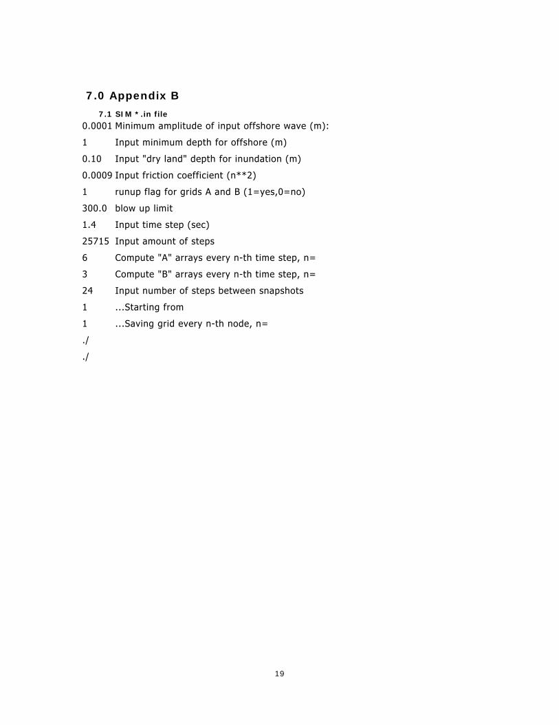
7.0 Appendix B

7.1 SIM *.in file

0.0001 Minimum amplitude of input offshore wave (m):

1 Input minimum depth for offshore (m)

0.10 Input "dry land" depth for inundation (m)

0.0009 Input friction coefficient (n**2)

1 runup flag for grids A and B (1=yes,0=no)

300.0 blow up limit

1.4 Input time step (sec)

25715 Input amount of steps

6 Compute "A" arrays every n-th time step, n=

3 Compute "B" arrays every n-th time step, n=

24 Input number of steps between snapshots

1 ...Starting from

1 ...Saving grid every n-th node, n=

./

./

20

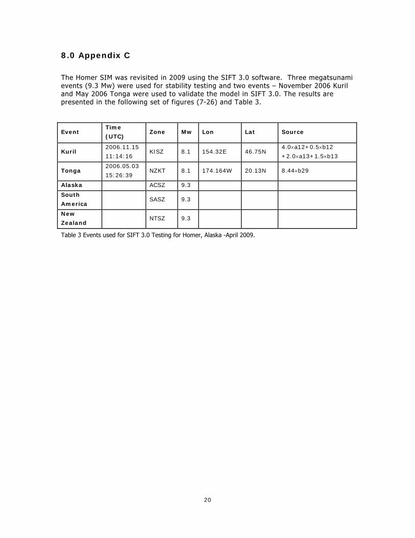
8.0 Appendix C

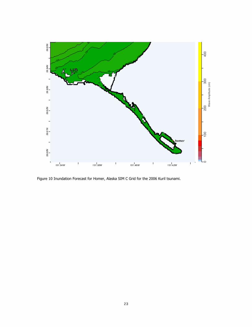
The Homer SIM was revisited in 2009 using the SIFT 3.0 software. Three megatsunami events (9.3 Mw) were used for stability testing and two events – November 2006 Kuril and May 2006 Tonga were used to validate the model in SIFT 3.0. The results are presented in the following set of figures (7-26) and Table 3.

Event Time

(UTC) Zone Mw Lon Lat Source

Kuril 2006.11.15

11:14:16 KISZ 8.1 154.32E 46.75N

4.0×a12+0.5×b12

+2.0×a13+1.5×b13

Tonga 2006.05.03

15:26:39 NZKT 8.1 174.164W 20.13N 8.44×b29

Alaska ACSZ 9.3

South

America SASZ 9.3

New

Zealand NTSZ 9.3

Table 3 Events used for SIFT 3.0 Testing for Homer, Alaska -April 2009.

21

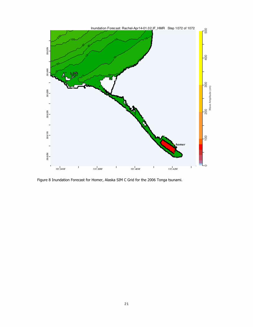
Figure 8 Inundation Forecast for Homer, Alaska SIM C Grid for the 2006 Tonga tsunami.

22

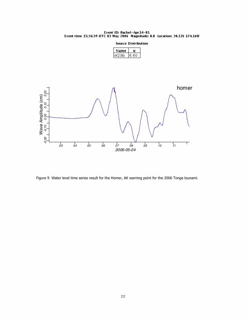
Figure 9 Water level time series result for the Homer, AK warning point for the 2006 Tonga tsunami.

23

Figure 10 Inundation Forecast for Homer, Alaska SIM C Grid for the 2006 Kuril tsunami.

24

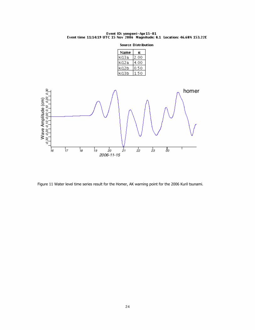
Figure 11 Water level time series result for the Homer, AK warning point for the 2006 Kuril tsunami.

25

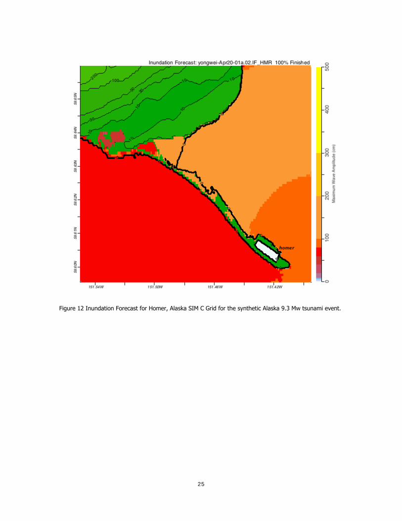
Figure 12 Inundation Forecast for Homer, Alaska SIM C Grid for the synthetic Alaska 9.3 Mw tsunami event.

26

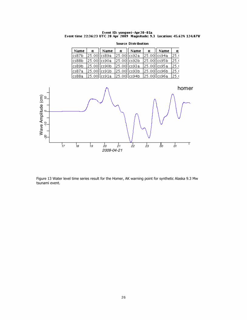
Figure 13 Water level time series result for the Homer, AK warning point for synthetic Alaska 9.3 Mw tsunami event.

27

Figure 14 Inundation Forecast for Homer, AK SIM C Grid for the synthetic South America 9.3 Mw tsunami event.

28

Figure 15 Water level time series result for the Homer, AK warning point for synthetic South America 9.3 Mw tsunami event.

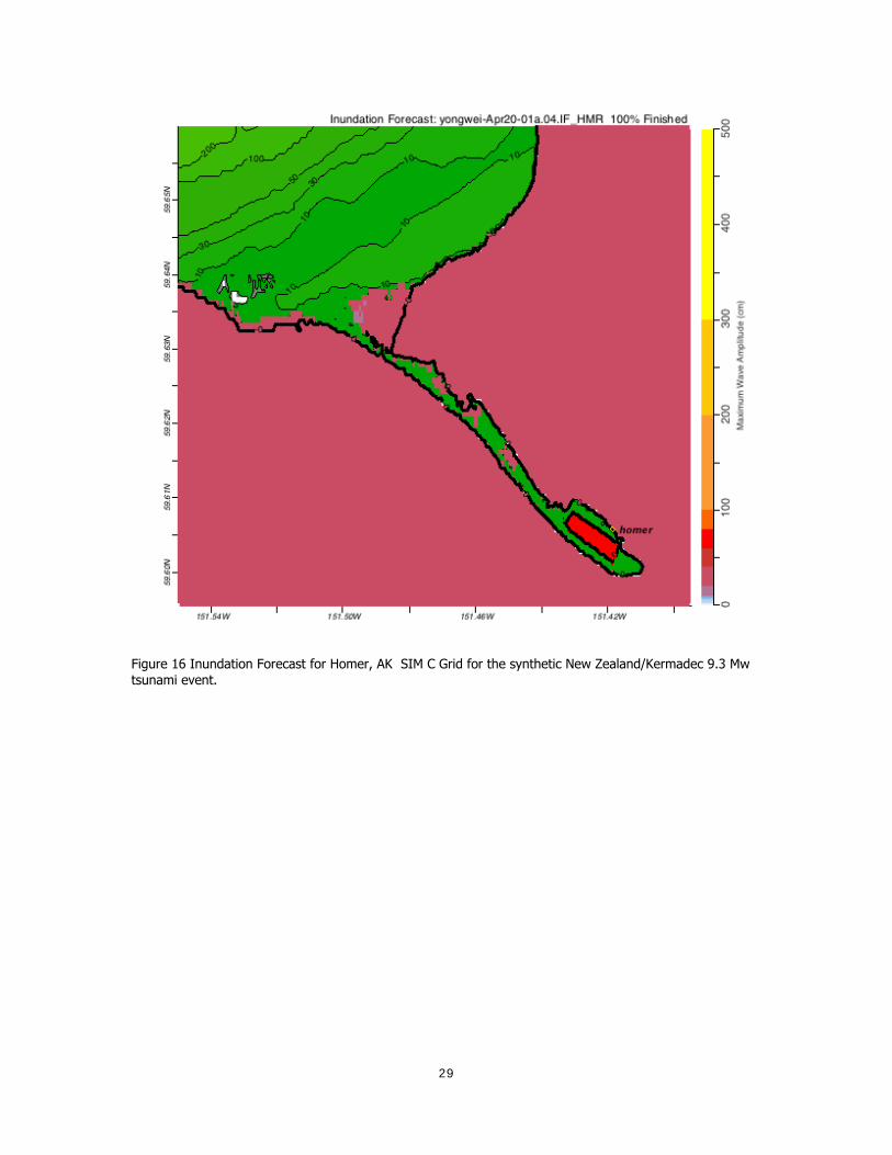
Figure 16 Inundation Forecast for Homer, AK SIM C Grid for the synthetic New Zealand/Kermadec 9.3 Mw tsunami event.

29

30

Figure 17 Water level time series result for the Homer, AK warning point for synthetic New Zealand/Kermadec 9.3 Mw tsunami event.