Development of a Stained Cell Nuclei Counting System

Niranjan Timilsina1, Chris Moffatt

2, Kazunori Okada

1

San Francisco State University, 1600 Holloway Ave, San Francisco, CA USA 94132 1Department of Computer Science,

2Department of Biology

niranjan@mail.sfsu.edu, moffatt@sfsu.edu, kazokada@sfsu.edu

ABSTRACT:

This paper presents a novel cell counting system which exploits the Fast Radial Symmetry Transformation (FRST)

algorithm [1]. The driving force behind our system is a research on neurogenesis in the intact nervous system of

Manduca Sexta or the Tobacco Hornworm, which was being studied to assess the impact of age, food and environment

on neurogenesis. The varying thickness of the intact nervous system in this species often yields images with

inhomogeneous background and inconsistencies such as varying illumination, variable contrast, and irregular cell size.

For automated counting, such inhomogeneity and inconsistencies must be addressed, which no existing work has done

successfully. Thus, our goal is to devise a new cell counting algorithm for the images with non-uniform background. Our

solution adapts FRST: a computer vision algorithm which is designed to detect points of interest on circular regions such

as human eyes. This algorithm enhances the occurrences of the stained-cell nuclei in 2D digital images and negates the

problems caused by their inhomogeneity. Besides FRST, our algorithm employs standard image processing methods,

such as mathematical morphology and connected component analysis. We have evaluated the developed cell counting

system with fourteen digital images of Tobacco Hornworm’s nervous system collected for this study with ground-truth

cell counts by biology experts. Experimental results show that our system has a minimum error of 1.41% and mean error

of 16.68% which is at least forty-four percent better than the algorithm without FRST.

Key words: Automated cell counting, tobacco hornworm, fast radial symmetry transformation, image inhomogeneity

1. INTRODUCTION

Cell counting [4] is a technique commonly employed in biological research. By assessing the number and distribution of

cells in a tissue, researchers can make inferences about a tremendous variety of biological processes from neuroscience

and developmental biology to cancer biology. Such scientific research requires accurate and reliable data to make

reliable inferences and draw accurate conclusions. Counting the nuclei is effectively the same as counting the cells

because there exists only one nucleus per cell. Thus, we will be using these terms interchangeably.

The driving force for our work is research on neurogenesis in a species called Manduca Sexta, commonly

known as Tobacco Hornworm. Neurogenesis [14] refers to the generation of new neurons (brain cells) and takes place in

the nervous systems during early development and adulthood. The main goal of the present research project was to

observe the impact of age and food availability on neurogenesis in larval Tobacco hornworms. The advantage of using

the Tobacco Hornworm as a model organism is that it has a large and easily accessible nervous system [15].

Our pilot study for counting cells using optical images taken from whole mounts of the tobacco hornworm

nervous system revealed that the existing applications such as SCION Image are unsuitable for the purpose. This is

because the brain of the species Manduca Sexta is observed intact without sectioning it into thin, uniform slices, which

means that any slide prepared from the brain tissue necessarily yields unevenly illuminated microscopic views. Digital

images of these whole mounts have non-uniform foreground and background. Thus, we attempt to develop a new

method to count cells in images with uneven background intensities.

1.1 Related Studies

A project whose goal was to distinguish dead and living liver cells required a cell counting application [6] which uses

histogram equalization for image preprocessing, followed by cluster counting with approximate area-based estimation

i.e. dividing the area of the cluster by an average cell size. Segmentation is done based on eight surrounding pixel values.

Area-based cell counting has higher chances of inaccuracies. In [7], concavity detection based on averaged cell size is

introduced for segmentation. Once concavity is detected, ellipse fitting and segmentation process are carried out. Authors

mention that factors such as case of overlapping cells and color segmentation can affect the accuracy and also the fitting

and segmentation error due to false detection might hinder the accuracy of the results. Based on the fact that watershed

based algorithms may cause over or under segmentation in the case when the cells are touching or overlapping each

other consistently, authors of [8] have proposed the new approach of splitting overlapping cells. Their method carries out

the contour preprocessing followed by polygon approximation and ellipse fitting. During the ellipse fitting the polygon

refinement is carried out and finally the overlapping cells are split [8]. Errors can still remain using this approach

because the cells are not always elliptical as assumed. All of these previously proposed methods did not address the non-

uniformity of a microscopic image.

1.2 Existing standard applications

Existing general-purpose standard imaging applications, such as ImageJ and SCION Image, do include cell-counting

functions but they use simple thresholding methods and perform well only with images having uniform foreground and

background and struggle with accuracy when dealing with images that are non-uniform. Both ImageJ and SCION Image

are widely used cell counting applications and we used them as baseline standards to compare against our proposed

methods.

2. METHODS

2.1 Definition and Terminology

Input and Output: The system takes a grayscale image as an input and processes it through various steps and finally

yields a visual output along with the estimated number of stained cell nuclei. Apart from the grayscale image, the system

needs some internal parameters in order to produce accurate counts. These basic parameters for our system are:

a) fth : the threshold value for FRST [1]

b) bth: threshold value for Binarization

c) cs: the range of cell size in pixels.

After our extensive experimental pilot study, the default values of the parameters were determined and set to 0.23 for

fth, 100 for bth, and 10-350 pixels for cs. We provide an intuitive user interface to overwrite these default values at the

users’ discretion. Hereafter, we will call our overall cell counting system Cell Quantifying Application, CQA in short.

Fig.1 shows the flowchart diagram of this system.

2.2 Proposed Method

2.2.1 Image Conditioning [IC]

This is the first step of CQA and is required to counter the problems associated with the size, dimension and type of the

input image. This step is used to normalize various image types and dimensions and also to standardize the grayscale

order so that 0 corresponds to black and 255 corresponds to white.

2.2.2 Image Enhancement[IE]

This is the second step of CQA and is used to enhance the quality of input images and to adjust their color contrast

levels. This is an optional step. Currently, standard histogram equalization has been implemented in this step.

Histogram equalization [9-10], also known as intensity normalization, is a technique of changing the pixel

intensity values to modify the pixel intensity range of distorted, over-exposed or under-exposed images to a normalized

range. Histogram equalization spreads out the most frequent intensity values and allows the areas of image with lower

local contrasts to achieve higher contrasts. The intensities are better distributed in the histogram after the equalization.

Mathematically, it is represented as,

(1)

where n is the total number of pixels in the image, is the number of pixels with gray level , and L is the number of

discrete gray levels. The discrete formulation of Eq. (1) is obtained from the given histogram , i = 0,1, 2,……L-1; L

being the highest pixel value.

Fig 1: The CQA Flowchart. Path-A represents the advanced-CQA approach while Path-B represents the Basic-CQA approach.

2.2.3 FRST Transformation [FT]

FRST Algorithm: Fast Radial Symmetry Transformation [1], FRST is a general-purpose feature detection technique

that uses local radial symmetry technique to identify regions of interest within a scene and is much faster than other

transformation algorithms that utilize radial symmetry [1]. Authors have reported that FRST transformation has worked

well with a large set of images and is useful for both “Point of Interest Detection” and “Face Detection” technologies.

Fig.2 illustrates the FRST algorithm.

Fig 2: The FRST algorithm overview. This schematic is adopted from [1].

In the FRST algorithm, for every pixel , of an input image , the gradient and the magnitude are determined for

all the radii of interest r. In Fig. 2, is the length of radii vector, and and are the magnitude and orientation

transformations. is calculated based on and and final result, a transformed image S, is produced [1].

The Fast Radial Symmetry Transform is calculated on a set of radii n є N, where N is a set of one or more radii.

The value of radius n at any point of transformation indicates the contribution to the radial symmetry of the gradients a

distance n away from that point. An orientation projection image and a magnitude projection image are formed at

each radius n. These projection images are generated by examining the gradients g at each point p from which a

corresponding positively-affected pixel p+ve(p) and negatively-affected pixel p-ve(p) are determined [1].

Formally, the transformation takes the following form of Gaussian convolution,

(2)

where,

(3)

and

(4)

is a Gaussian filter [5] and is the strictness parameter that denotes the strictness of radial symmetry. is

a scaling factor which normalizes and for all the different radii. The final FRST transformation result S is given as

follows:

(5)

The FRST transformation has a number of predefined parameters:

N: a set of radii in pixels N = {n1, n2, n3, . . . } at which is to be calculated. This value is user determined

according to the image being processed

: Gaussian kernels which are rotation invariant and are automated in the algorithm to calculate the value

according to the length of vector of radii.

α: Strictness parameter for ignoring small gradients default value is 2. Higher values of α attenuates non-radially

symmetric objects such as a line, while lower values speed up the computations yielding some noise.

: Normalizing factor if n=1 the value is 9 else the value is 8.8.

β: Threshold value default value is 0.05, but it can also be a user-chosen value. Small values eliminate the lowest 1-

2% of gradient, which help remove noise. Higher values may increase computation speed.

These FRST parameters are set to their default values provided in the source code developed by the authors of

[1], except for a threshold parameter for the transformation because the threshold value should be adapted to specific

images depending on their nature. A default value for this parameter has been determined experimentally, but it can be

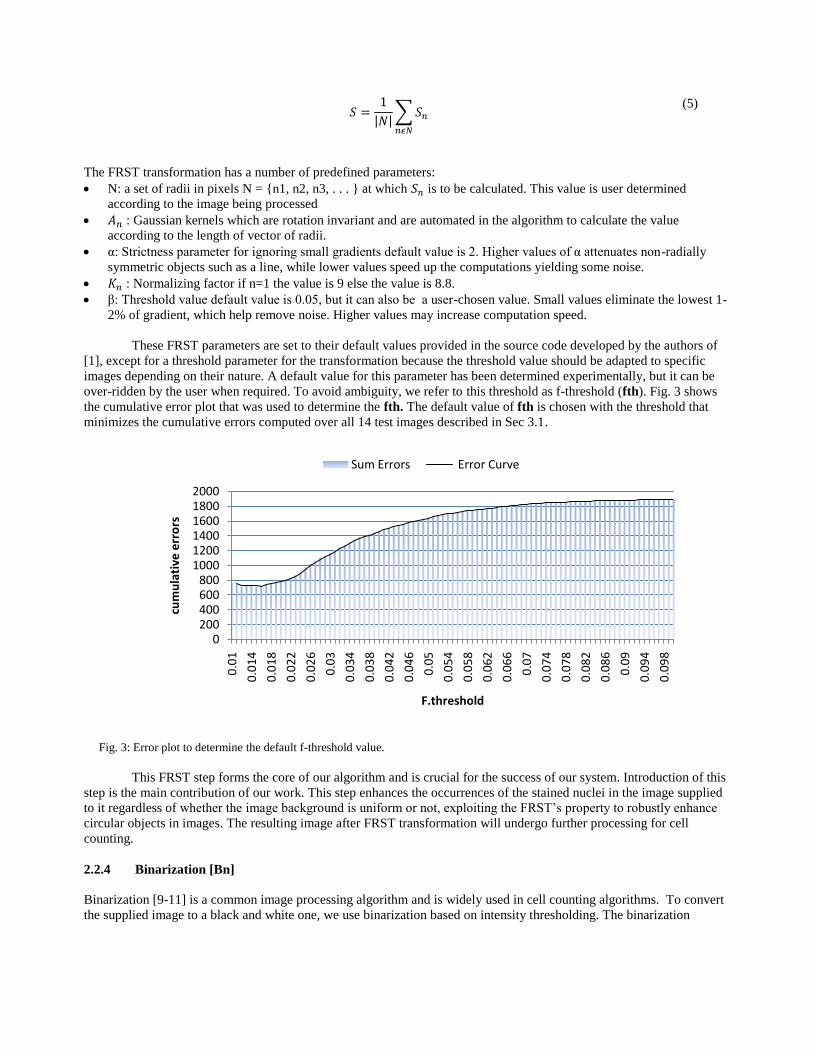
over-ridden by the user when required. To avoid ambiguity, we refer to this threshold as f-threshold (fth). Fig. 3 shows

the cumulative error plot that was used to determine the fth. The default value of fth is chosen with the threshold that

minimizes the cumulative errors computed over all 14 test images described in Sec 3.1.

Fig. 3: Error plot to determine the default f-threshold value.

This FRST step forms the core of our algorithm and is crucial for the success of our system. Introduction of this

step is the main contribution of our work. This step enhances the occurrences of the stained nuclei in the image supplied

to it regardless of whether the image background is uniform or not, exploiting the FRST’s property to robustly enhance

circular objects in images. The resulting image after FRST transformation will undergo further processing for cell

counting.

2.2.4 Binarization [Bn]

Binarization [9-11] is a common image processing algorithm and is widely used in cell counting algorithms. To convert

the supplied image to a black and white one, we use binarization based on intensity thresholding. The binarization

0200400600800

100012001400160018002000

0.0

1

0.0

14

0.0

18

0.0

22

0.0

26

0.0

3

0.0

34

0.0

38

0.0

42

0.0

46

0.0

5

0.0

54

0.0

58

0.0

62

0.0

66

0.0

7

0.0

74

0.0

78

0.0

82

0.0

86

0.0

9

0.0

94

0.0

98

cum

ula

tive

err

ors

F.threshold

Sum Errors Error Curve

process sets pixel values at 0 or 1 based on threshold and current pixel value.

(6)

where is the resulting ith

Pixel for the actual pixel value . Pixel values of 0 and 1 represent black and white,

respectively.

For binarization, apart from the input image, another threshold value has to be provided. A default value for this

threshold has been determined and set, but which can be overridden if needed. To avoid ambiguity, this threshold is

named as b-threshold (bth).

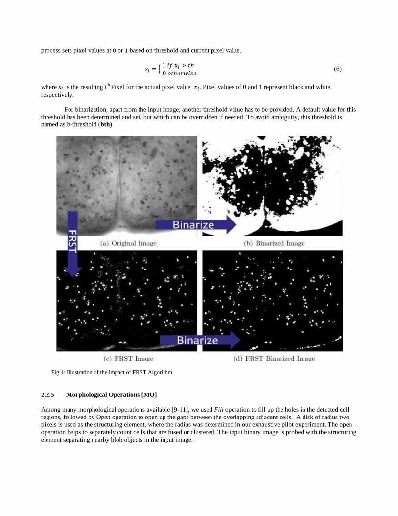
Fig 4: Illustration of the impact of FRST Algorithm

2.2.5 Morphological Operations [MO]

Among many morphological operations available [9-11], we used Fill operation to fill up the holes in the detected cell

regions, followed by Open operation to open up the gaps between the overlapping adjacent cells. A disk of radius two

pixels is used as the structuring element, where the radius was determined in our exhaustive pilot experiment. The open

operation helps to separately count cells that are fused or clustered. The input binary image is probed with the structuring

element separating nearby blob objects in the input image.

2.2.6 Connected Component Analysis [CCA]

A binary image, after morphological Open operation, is processed using the connected component analysis [10]. The

connected-components are grouped on the basis of the 8-pixel neighborhood. The cell size is quantified as the number of

pixels that constitute a connected region. The cells that has its size smaller than or larger than the provided cell size range

cs are discarded. The default cell-size has been determined experimentally. The default area we set is 10 to 350 pixels.

The level of magnification used when capturing images significantly affects the apparent size of the nuclei, the higher

the magnification, the larger the cell size, while the lower the magnification, the smaller the cell size. Blobs having

smaller or larger area than the pre-defined range for cells are discarded as noise and/or artifacts. The remaining blobs are

then processed and labeled. The labeled blobs are then counted in the image and the output image with marked stained

nuclei is generated along with the corresponding count estimate.

2.3 What FRST does?

Fig. 4 demonstrates what the impact of FRST Transformation in our algorithm is. The original image in Fig. 4(a) loses

considerable portion of its area to binarization as seen in Fig. 4(b). But the same image if processed with FRST as seen

Fig. 4(c) retains its marked cell spots as shown in Fig. 4(d). This clearly illustrates the advantage of the FRST algorithm

in helping to refine the cell image in case of inhomogeneous background.

3. EXPERIMENTS

3.1 Data

Our data in the form of the 2D digital images are obtained with a light microscope during the observation of stained

tissues. We used thirteen digital images taken of Tobacco Hornworm brains (images 2-14) and one image of a tissue

section taken from the brain of a rat (image 1). The latter provided a tissue section that had an even background and

widely dispersed stained cell nuclei. These images were fed into our system for cell quantification. We compared these

numbers with the manual cell counts of these same images made by biologists to validate our system. Manual counts are

the ground truth data for each image. The typical procedure for manually counting cells in Tobacco Hornworm brains

during an experiment is for two or more people to count independently the number of cells in an image and then compare

the results. If the differences in their counts are less than 10%, the counts are averaged out and set as the cell number for

that image; if not, the counts are repeated. Depending on the number and complexity of the images, this can require a

large amount of time and effort on the part of the researchers. The images may have different size, bit-depth and

compression technology. Some of our data are illustrated in Fig. 5 and information of all the data we used are tabulated

in Table 1.

Different types of images for our system with manual counts

Manual Count:97 Manual Count:135 Manual Count:287 Manual Count:64 Manual Count:136

Fig. 5: Some examples of our data.

Table 1: The summary of data: image data with their ground truth cell counts

Image Name Manual Count Dimension [Pix] Size [KB] Bit-depth Format

Image 1 97 640 X 480 1800 8-bit bmp

Image 2 135 640 X 480 1800 8-bit bmp

Image 3 118 480 X 640 800 24-bit jpeg

Image 4 95 640 X 480 800 24-bit jpeg

Image 5 287 640 X 480 800 24-bit jpeg

Image 6 98 640 X 480 800 24-bit jpeg

Image 7 64 640 X 480 1800 8-bit bmp

Image 8 103 640 X 480 1800 8-bit bmp

Image 9 111 640 X 480 1800 8-bit bmp

Image 10 298 640 X 480 1800 8-bit bmp

Image 11 71 640 X 480 1800 8-bit bmp

Image 12 199 640 X 480 1800 8-bit bmp

Image 13 136 640 X 480 1800 8-bit bmp

Image 14 103 640 X 480 1800 8-bit bmp

3.2 Results

We performed quantitative experiments with the above data in order to validate the effectiveness of our proposed

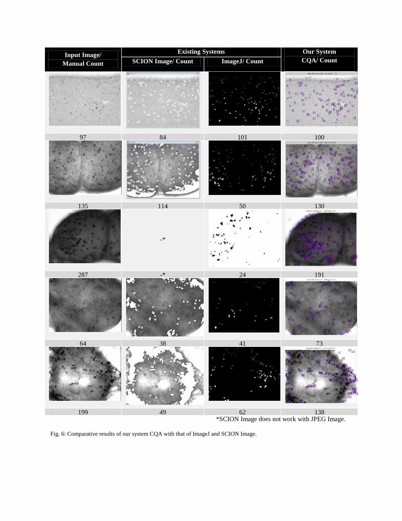
method. As shown in Fig. 6, our proposed method performs much better than the existing applications. In the best case

scenario, the accuracy is near 100 percent and even in the worst case scenario; it performs better than the others. For an

instance of best case, the image 2 has manual count of 135 and the corresponding readings for the ImageJ, SCON Image

and CQA are 50, 114 and 130 respectively. This shows the better performance of our method in comparison to the

ImageJ and SCION Image. For an instance of worst case, the image 10 has manual count 298 but ImageJ count for the

same is 31 and the SCION Image count is 63. Our method gives the count 166, which is better than the results for other

applications even though its accuracy is not perfect. The images like that of image 10, has profusely clustered and

overlapping cells and thus, are the ones that fall under the worst case scenario.

Fig. 6 clearly demonstrates how the applications that do not implement FRST struggle to obtain the required blobs after

they binarize the images. The quantitative results are summarized in Table 2 and plotted in Fig. 7. They show that our

FRST-based method (CQA) outperformed the one without FRST (B-CQA), clearly demonstrating the advantage of using

the FRST. The results also show that the proposed method performs better than or similar to other leading cell counting

tools like SCION and ImageJ. Our method resulted in the following error statistics: minimum: 1.41%, maximum:

47.79%, mean: 16.68% and std. deviation: 16.16%.

Input Image/

Manual Count

Existing Systems Our System

CQA/ Count SCION Image/ Count ImageJ/ Count

97 84 101 100

135 114 50 130

-*

287 -* 24 191

64 38 41 73

199 49 62 138 *SCION Image does not work with JPEG Image.

Fig. 6: Comparative results of our system CQA with that of ImageJ and SCION Image.

Table 2: Count result from four different systems for all the fourteen images

Image

Name

Manual

Count

ImageJ Count SCION

Count

B-CQA

Count

CQA Count

Image 1 97 101 84 94 100

Image 2 135 50 114 87 130

Image 3 118 29 - * 31 110

Image 4 95 25 - * 25 98

Image 5 287 24 - * 27 191

Image 6 98 17 - * 17 95

Image 7 64 38 41 30 73

Image 8 103 27 36 25 92

Image 9 111 50 55 42 121

Image 10 298 31 63 33 166

Image 11 71 52 35 31 70

Image 12 199 49 62 43 138

Image 13 136 46 46 45 71

Image 14 103 70 53 34 126

*SCION Image does not work with JPEG Image.

Fig. 7: Error plot for the results across all the systems [ImageJ, SCION Image, B-CQA and CQA]. CQA stands for the proposed

system while B-CQA is a baseline case without FRST used.

16.68

64.85 64.1661.02

16.1623.07

29.72 26.08

0.00

10.00

20.00

30.00

40.00

50.00

60.00

70.00

CQA B-CQA SCION Image ImageJ

Pe

rce

nta

ge E

rro

r [%

]

Avg. Error Std. Dev

4. CONCLUSIONS

We have proposed a novel cell-counting system which is effective to images with non-uniform background. We have

compared our system with and without FRST algorithm to highlight the effectiveness of FRST Algorithm. We have also

compared our system with the existing ImageJ and Scion image tools. Our system with FRST is better than the one

without FRST and has better accuracy in comparison to existing systems due to the inclusion of FRST Algorithm.

Our experimental results demonstrated that our method improves the accuracy in cell counting. System with

FRST is more than 40% better than those without FRST. Our final system CQA has minimum error of 1.41%, an

average error of 16.68% and a standard deviation of 16.16%. The final CQA is 48%, 47% and 44% better than B-CQA,

SCION Image and ImageJ, respectively.

As our future work, the system we developed can be further enhanced by modifying or changing the procedure

at the image processing step. To make the system fully automated, threshold determination must be automated. The cases

with overlapping cells and clustered cells must also be addressed using other advanced techniques that implement

contour detection and separation of the cells from a cluster.

ACKNOWLEDGMENTS

We extend our thanks to biology department at San Francisco State University for providing the data and helpful

feedback. ImageJ is a JAVA based, open source and open-architecture, image processing application developed at

National Institute of Health (NIH) [12]. SCION Image is a PC version of NIH Image developed for MAC and is freely

available for download and use [13]. These two applications are in wide usage in the academic arena.

REFERENCES

[1] Gareth Loy and Alexander Zelinsky, “Fast Radial Symmetry for detecting points of interest.” IEEE Trans. Pattern

Anal. and Machine Intell., 25:959 973, 2003.

[2] N. Otsu, “A threshold selection method from gray-level histogram,” IEEE Transactions on System Man Cybernetics,

Vol. SMC-9, No. 1, 1979, pp. 62-66.

[3] R. Gentilini, C. Piazza, and A. Policriti, “Computing strongly connected componenets in a linear number of symbolic

steps, in Symposium on Discrete Algorithms, Baltimore, MD, 2003.

[4] Biology Online. Scell, 2010. [Online; accessed 12-April-2010]

[5] J. R. Parker, [Algorithms for Image processing and Computer Vision], Wiley Computer Publishing, 1997.

[6] Refai, H.; Li, L.; Teague, T.K.; Naukam, R.;, "Automatic count of hepatocytes in microscopic images," Image

Processing, 2003. ICIP 2003. Proceedings. 2003 International Conference on , vol.2, no., pp. II- 1101-4 vol.3, 14-17

Sept. 2003 doi: 10.1109/ICIP.2003.1246878

[7] Kothari, S.; Chaudry, Q.; Wang, M.D.; , "Automated cell counting and cluster segmentation using concavity

detection and ellipse fitting techniques," Biomedical Imaging: From Nano to Macro, 2009. ISBI '09. IEEE International

Symposium on, vol., no., pp.795-798, June 28 2009-July 1 2009 doi: 10.1109/ISBI.2009.5193169

[8] Xiangzhi Bai; Changming Sun; Fugen Zhou; , "Touching Cells Splitting by Using Concave Points and Ellipse

Fitting," Computing: Techniques and Applications, 2008. DICTA '08.Digital Image , vol., no., pp.271-278, 1-3 Dec.

2008 doi: 10.1109/DICTA.2008.11

[9] Richard E. Woods Rafael C. Gonzalez. [Digital Image Processing2nd Ed.],Prentice Hall, 2002

[10] Richard E. Woods Rafael C. Gonzalez and Steven L. Eddins. [Digital Image Processing using MATLAB], Prentice

Hall, 2004

[11] William K. Pratt. [Digital Image Processing: PIKS Inside, 3rd Ed. ], John Wiley and Sons, 2001.

[12] Website http://rsb.info.nih.gov/ij/

[13] Website http://www.scioncorp.com/

[14] Wellesley College Biology Department. Neurogenesis: What is it?, 2010. [Online;accessed 10-April-2010].

[15] University of Nebraska Department of Entomology. Insect biology: Tobacco hornworms, 2010. [Online; accessed

24-April-2010]