Graduate Theses, Dissertations, and Problem Reports

2012

Development of a Software Tool to Estimate Airfoil Feature Development of a Software Tool to Estimate Airfoil Feature

Variations Variations

Prasheel Chaganti West Virginia University

Follow this and additional works at: https://researchrepository.wvu.edu/etd

Recommended Citation Recommended Citation Chaganti, Prasheel, "Development of a Software Tool to Estimate Airfoil Feature Variations" (2012). Graduate Theses, Dissertations, and Problem Reports. 228. https://researchrepository.wvu.edu/etd/228

This Thesis is protected by copyright and/or related rights. It has been brought to you by the The Research Repository @ WVU with permission from the rights-holder(s). You are free to use this Thesis in any way that is permitted by the copyright and related rights legislation that applies to your use. For other uses you must obtain permission from the rights-holder(s) directly, unless additional rights are indicated by a Creative Commons license in the record and/ or on the work itself. This Thesis has been accepted for inclusion in WVU Graduate Theses, Dissertations, and Problem Reports collection by an authorized administrator of The Research Repository @ WVU. For more information, please contact researchrepository@mail.wvu.edu.

Development of a Software Tool to Estimate Airfoil

Feature Variations

Prasheel Chaganti

Thesis submitted to the Benjamin M. Statler College of Engineering and Mineral Resources at West Virginia University in

partial fulfillment of the requirements for the degree of

Master of Science in

Industrial Engineering

Dr. Rashpal S. Ahluwalia, Chair

Dr. Majid Jaridi Mr. Donald J. Scott

Morgantown, West Virginia December 2012

Keywords: Airfoil Manufacturing; Compressor blade; Software tool; CMM Inspection

ABSTRACT Development of a Software Tool to Estimate Airfoil Feature

Variations

Prasheel Chaganti

The objective of this thesis is to design and develop a software tool that analyzes the

incoming raw material inspection data obtained from a Coordinate Measuring Machine

(CMM) and estimates feature variation created within the manufacturing process i.e.

from the raw material stage to finished stage. This tool is used not only to disposition

whether a lot is conforming or non-conforming, but also to provide the root installation

operators an ideal N-angle, Leading Edge Angle (LEA) and Trailing Edge Angle (TEA)

target that maximize the yield of the lot after further processing. The tool also helps

reduce the number of airfoil sections which need to be inspected both at In-Process and

Final CMM inspection stages, thereby saving a considerable amount of inspection time as

well as providing estimated cost savings of over a million dollars a year to the business.

iii

ACKNOWLEDGEMENT

I would like to acknowledge, first and foremost, Dr. Ahluwalia for his unwavering

support throughout the degree program. He was very understanding, helpful and

extremely patient when I was going through the toughest phases of my life in losing my

mother a year after I started my master’s program.

My sincere thanks to Dr. Majid Jaridi for serving as a member of my thesis committee; I

would also like to sincerely thank the Industrial and Management Systems Engineering

department for giving me the opportunity to study at this prestigious university. I am

forever indebted to each and everyone who helped me throughout my master’s.

I would also like to thank Mr. James Dalton; he was a great mentor throughout my time

in the mechanical lab, his dedication, hard work, relentless pursuit for safety is

contagious.

I would like to acknowledge Mr. Donald Scott for his help throughout this project. I

would also like to thank my director of technical services Mr. Patrick Markham for

allowing me to work and present this project as my thesis.

I would like to thank Mr. Richard Zappulla II for his immense help working on

MATLAB programming; I thoroughly enjoyed working with him. He is probably the

smartest person I have ever met in my life.

I would like to thank my family members, my father Mr. Raghava Rao Chaganti, for his

immense sacrifices to fund my studies. Of course my brother Prasanth and my sister

iv

Geetha, for not letting me give up on my master’s, and for their unconditional love and

support.

I would like to dedicate this thesis to my beloved mother (Late) Mrs. Sujatha Chaganti.

She was the biggest inspiration in my life; she always preached that through hard work

one can achieve anything. I hope that I made her proud. I love you mom and I really

miss you.

Last but not the least to my lovely wife Mrs. Caitlin Murphy Chaganti, for her immense

support and help when I really needed to focus and work on my master’s. Thank you for

being there for me; without you none of this would be possible. You are my great source

of strength and inspiration. I love you.

v

TABLE OF CONTENTS ABSTRACT ...................................................................................................................... iii 

ACKNOWLEDGEMENT ............................................................................................... iii 

TABLE OF CONTENTS ................................................................................................. v 

LIST OF FIGURES ....................................................................................................... viii 

LIST OF TABLES ........................................................................................................... xi 

LIST OF NOTATIONS .................................................................................................. xii 

CHAPTER 1. INTRODUCTION .................................................................................... 1 

1.1 Introduction ............................................................................................................... 1 

1.2 Background ............................................................................................................... 2 

1.3 Business Challenges.................................................................................................. 4 

1.4 Objective ................................................................................................................... 4 

1.5 Methodology ............................................................................................................. 4 

1.6 Thesis Outline ........................................................................................................... 5 

CHAPTER 2. COMPRESSOR BLADE GEOMETRY ................................................ 7 

2.1 Introduction ............................................................................................................... 7 

2.2 Compressor Blade Geometry .................................................................................... 8 

2.3 Dovetail/Root Geometry ......................................................................................... 17 

2.4 Aircraft Engines / Part families ............................................................................... 17 

CHAPTER 3. COMPRESSOR BLADE MANUFACTURING PROCESS .............. 19 

3.1 Introduction ............................................................................................................. 19 

3.2 Manufacturing Process............................................................................................ 19 

CHAPTER 4. COMPRESSOR BLADE INSPECTION ............................................. 29 

4.1 Introduction ............................................................................................................. 29 

4.2 Coordinate Measuring Machine .............................................................................. 29 

vi

4.3 Curve and Surface Fitting ....................................................................................... 32 

4.4 Airfoil Data Processing (PC-DMIS Blade)............................................................. 32 

ASCII File ................................................................................................................. 33 

CHAPTER 5. SOFTWARE TOOL ............................................................................... 36 

5.1 Introduction ............................................................................................................. 36 

5.2 Processing Models .................................................................................................. 36 

5.3 Algorithms .............................................................................................................. 36 

True position of Centroid (XXX, YYY) ................................................................... 37 

Delta True Position (DTPXXX, DTPYYY, DTPN), Adjacent Section Deviation (ADJC, ADJMXT) .................................................................................................... 37 

Chord Loss Simulation ............................................................................................. 39 

Thickness Simulation (LET, TET, MXT) ................................................................. 41 

Profile Features (LEP, TEP, PSP, SSP, APP)........................................................... 42 

Peen Simulation (N-angle, LEA, and TEA) ............................................................. 42 

Automatic N-Angle Targeting .................................................................................. 45 

5.4 Input data ................................................................................................................ 46 

5.5 Output ..................................................................................................................... 49 

5.6 Data Analysis and Interpretation ............................................................................ 81 

5.7 Software Validation ................................................................................................ 83 

CHAPTER 6. CONCLUSION AND FUTURE WORK .............................................. 86 

6.1 Conclusion .............................................................................................................. 86 

6.2 Future Work ............................................................................................................ 87 

REFERENCES ................................................................................................................ 88 

APPENDIX: SOURCE CODE ...................................................................................... 90 

Main Program: .......................................................................................................... 90 

vii

Standard Deviation & Average Calculations: ........................................................... 97 

DTP Calculations: ..................................................................................................... 98 

Chord Loss Calculations: .......................................................................................... 99 

Cp & Cpk Calculations: ........................................................................................... 101 

Maximizer599 Calculations: ................................................................................... 102 

Minimum Cpk Calculations: ................................................................................... 104 

Post Peen Calculations: ........................................................................................... 106 

Spreadsheet Maker Calculations: ............................................................................ 107 

Normal Plot Calculations: ....................................................................................... 111 

Post Peen Plot Calculations: ................................................................................... 115 

DTP Calculations: ................................................................................................... 118 

Root Calculations: ................................................................................................... 121 

Supporting Functions: ............................................................................................. 125 

viii

LIST OF FIGURES Figure 1-1: A typical Compressor Blade ............................................................................ 3 

Figure 2-1: Axial Flow Jet Engine [11] .............................................................................. 7 

Figure 2-2: Airfoil section labels ...................................................................................... 10 

Figure 2-3: Blade Root Center Plane ................................................................................ 10 

Figure 2-4: Section Label and Z-gage .............................................................................. 11 

Figure 2-5: True position XXX, YYY .............................................................................. 12 

Figure 2-7: Leading, Trailing, and Maximum Thickness ................................................. 13 

Figure 2-8: N-angle Deviation .......................................................................................... 14 

Figure 2-9: Leading and Trailing Edge Angle .................................................................. 15 

Figure 2-10: All-Around Profile ....................................................................................... 15 

Figure 2-11: Pressure and Suction Side Profile ................................................................ 16 

Figure 2-12: Leading Edge and Tailing Edge Profile ....................................................... 16 

Figure 2-13: Typical Compressor Blade ........................................................................... 17 

Figure 2-14: CF6 Engines Compressor Stages 6 to 14 ..................................................... 18 

Figure 3-1: Typical forging with near net finish airfoil .................................................... 20 

Figure 3-2: Encapsulation Fixture & Encapsulated Part ................................................... 21 

Figure 3-3: Forging (green) and Finished part (metallic) overlap view ........................... 23 

Figure 3-4: ECG tip ground part before and after ............................................................. 24 

Figure 3-5: Penetrant application & dwell, crack readout under a black light[21][22] .... 26 

Figure 3-6: Shot peening dimple, compressive layer after shot peening .......................... 27 

Figure 3-7: Different shapes & sizes of media, ceramic & plastic media ........................ 28 

Figure 4-1: System Components of a CMM [24] ............................................................. 31 

Figure 4-2: Sample ASCII file for a section of airfoil ...................................................... 34 

ix

Figure 4-3: Airfoil Section Definition by Points and Local Normals ............................... 35 

Figure 5-1: Airfoil Section Centroid Deviation Differences ............................................ 39 

Figure 5-2: Visual representation fo post peen Cpk vs Offset .......................................... 46 

Figure 5-3: XXX Section A-G .......................................................................................... 52 

Figure 5-4: DTPX ............................................................................................................. 53 

Figure 5-5: YYY Section A-G .......................................................................................... 54 

Figure 5-6: DTPY ............................................................................................................. 55 

Figure 5-7: Chord Section A-G ......................................................................................... 56 

Figure 5-8: Chord Final Section A-G ............................................................................... 57 

Figure 5-9: N-angle (pre-peen) Section A-G .................................................................... 58 

Figure 5-10: DTPN ........................................................................................................... 59 

Figure 5-11: Leading Edge Angle (pre-peen) Section A-G .............................................. 60 

Figure 5-12: CLEA (Camber LEA)- Information only ..................................................... 61 

Figure 5-13: Trailing Edge Angle (pre-peen) Section A-G .............................................. 62 

Figure 5-14: CTEA (Camber TEA)- Information only ..................................................... 63 

Figure 5-15: Leading Edge Profile Section A-G .............................................................. 64 

Figure 5-16: Trailing Edge Profile Section A-G ............................................................... 65 

Figure 5-17: Pressure Side Profile Section A-G ............................................................... 66 

Figure 5-18: Suction Side Profile Section A-G ................................................................ 67 

Figure 5-19: Leading Edge Thickness Section A-G ......................................................... 68 

Figure 5-20: Leading Edge Thickness Final Section A-G ................................................ 69 

Figure 5-21: Trailing Edge Thickness Section A-G ......................................................... 70 

Figure 5-22: Trailing Edge Thickness Final Section A-G ................................................ 71 

Figure 5-23: Maximum Thickness Section A-G ............................................................... 72 

x

Figure 5-24: Maximum Thickness Final Section A-G ..................................................... 73 

Figure 5-25: N-angle (post-peen) Section A-G with N-angle target offset ...................... 74 

Figure 5-26: Leading Edge Angle (post-peen) Section A-G with N-angle target ............ 75 

Figure 5-27: Trailing Edge Angle (post-peen) Section A-G with N-angle target ............ 76 

Figure 5-28: Adjacent Chord ............................................................................................ 77 

Figure 5-29: Adjacent MXT ............................................................................................. 78 

Figure 5-30: Platform deviation ........................................................................................ 79 

Figure 5-31: Fillet Sections CV3, CV4 and CV5 ............................................................. 80 

Figure 5-32: IMS sheet for N-Angle target and CMM reduced section inspection .......... 82 

xi

LIST OF TABLES Table 5-1: Centroid deviation per section ......................................................................... 38 

Table 5-2: Centroid deviation calculations ....................................................................... 38 

Table 5-3: Z-prime vector calculations ............................................................................. 44 

Table 5-4: Airfoil Inspection Data .................................................................................... 47 

Table 5-5: Fillet Inspection Data ...................................................................................... 48 

Table 5-6: Platform Inspection Data ................................................................................. 48 

Table 5-7: Raw data forging to final calculations ............................................................. 50 

Table 5-8: Cp and Cpk calculations at IP (In-Process) ....................................................... 51 

Table 5-9: Cpk at final processing ...................................................................................... 51 

Table 5-10: Calculated feature output from the software tool .......................................... 84 

Table 5-11: Actual feature output of manufactured lot (CMM Final Inspection) ............ 84 

Table 5-12: Difference between calculated and actual feature output .............................. 84 

Table 5-13: Cost saving before and after tool implementation ......................................... 85 

xii

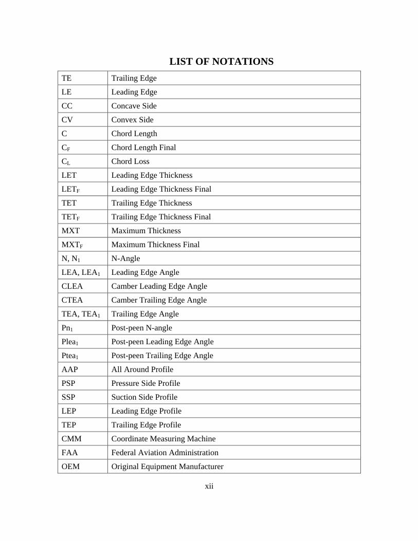
LIST OF NOTATIONS TE Trailing Edge

LE Leading Edge

CC Concave Side

CV Convex Side

C Chord Length

CF Chord Length Final

CL Chord Loss

LET Leading Edge Thickness

LETF Leading Edge Thickness Final

TET Trailing Edge Thickness

TETF Trailing Edge Thickness Final

MXT Maximum Thickness

MXTF Maximum Thickness Final

N, N1 N-Angle

LEA, LEA1 Leading Edge Angle

CLEA Camber Leading Edge Angle

CTEA Camber Trailing Edge Angle

TEA, TEA1 Trailing Edge Angle

Pn1 Post-peen N-angle

Plea1 Post-peen Leading Edge Angle

Ptea1 Post-peen Trailing Edge Angle

AAP All Around Profile

PSP Pressure Side Profile

SSP Suction Side Profile

LEP Leading Edge Profile

TEP Trailing Edge Profile

CMM Coordinate Measuring Machine

FAA Federal Aviation Administration

OEM Original Equipment Manufacturer

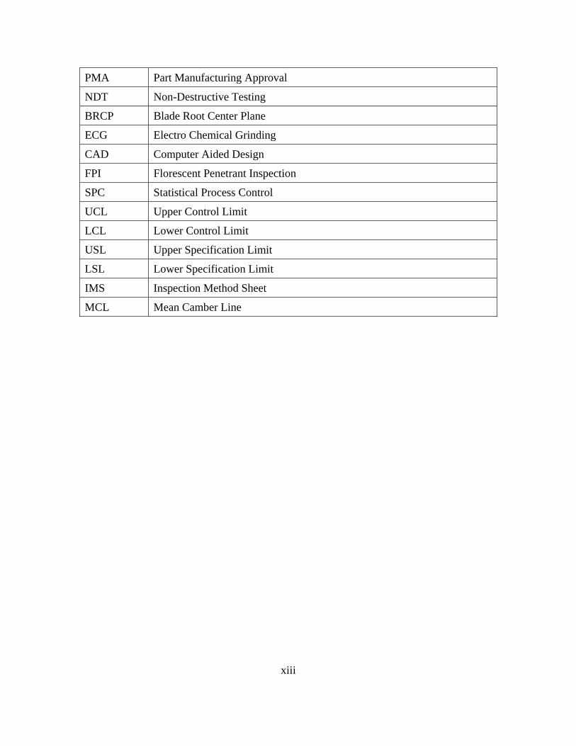
xiii

PMA Part Manufacturing Approval

NDT Non-Destructive Testing

BRCP Blade Root Center Plane

ECG Electro Chemical Grinding

CAD Computer Aided Design

FPI Florescent Penetrant Inspection

SPC Statistical Process Control

UCL Upper Control Limit

LCL Lower Control Limit

USL Upper Specification Limit

LSL Lower Specification Limit

IMS Inspection Method Sheet

MCL Mean Camber Line

1

CHAPTER 1. INTRODUCTION

1.1 Introduction

Two of the inventions that have greatly shaped our modern day lives are the invention of the computer

and the invention of the fixed wing aircraft [1]. Both of these have come a long way since their

inception. Computers [2], for instance, are used in nearly every facet of our lives from smallest

microchips to the largest servers. Modern day computers are put to use in every major industry. They

power our healthcare industry, aid in supplying energy to our homes, and drive most elements in our

manufacturing facilities. In manufacturing, computers have taken the production of aircraft components

to a whole new level. The computer’s impact on component design, prototyping, test simulation etc

made manufacturing of these modern day aircraft possible. Without computers, airplanes, as we know

it, would not exist.

The impact of an aircraft on our modern world is felt in many aspects of our lives; the products and

services that were never available are at our finger tips today, the exotic foods that we eat, the

medication we use, the life saving organ transplants, the manner in which we go to wars, national

surveillance, etc. The accessibility of air travel on an international level has changed the way we do

business, taking local and regional markets to a global stage. Both the computer and the fixed wing

aircraft have had a critical impact on the development and globalization of our modern society [3].

The jet engine [4] is one of the most critical components of an aircraft. A typical jet engine has a fan,

compressor, combustor, turbine and an exhaust system. It is imperative to understand the workings of a

jet engine in order to know compressor blade design. Essentially the engine sucks the air in at the front

of the engine through a fan, and the air flows into the compressor section where it is compressed thus

2

raising the pressure. This compressed air is then mixed with fuel, and an electric spark ignites the

mixture. The burning gas expands in the turbine section and blasts through the exhaust system or nozzle

at the back of the engine. Since the working fluid passes through the engine parallel to the axis of

rotation of the engine, these engines are known as axial flow engines [5].

1.2 Background

The airfoil is a very common shape found in nature; the most obvious ones are the wings of a bird, the

fins of a fish etc. Each airfoil shape has a distinct character, and they vary by shape and sizes depending

on the function of that airfoil. The most notable airfoils are used in airplane wings, fan blades, and

propellers. One such application of an airfoil is the compressor blade that is used in the high pressure

and low pressure compressor sections of a jet engine. The focus of this thesis is on compressor blades

[6].

Forging

“Forging is defined as the plastic deformation of metals at elevated temperature into a predetermined

size or shape using compressive forces exerted through some means of hand hammers, small power

hammers, die, press or upsetting machine” [7]. The metal is normally, but not always, preheated to a

desired temperature before the forging operation [8]. The forging processes can be classified into hot

forging and cold forging, with each classification providing its own advantages and disadvantages.

In the forging process, as the metal is pounded, the grain deformation causes an unbroken chain of grain

flow following the shape of the part; this creates parts that are significantly stronger than those created

from other conventional metal working processes. This advantage of a high strength-to-weight ratio is

the reason why they are used in applications where human safety and reliability are critical. Some of the

3

applications of the forged parts are found within items such as airplanes, automobiles, earth mowing

equipment, golf equipment, missiles etc [8].

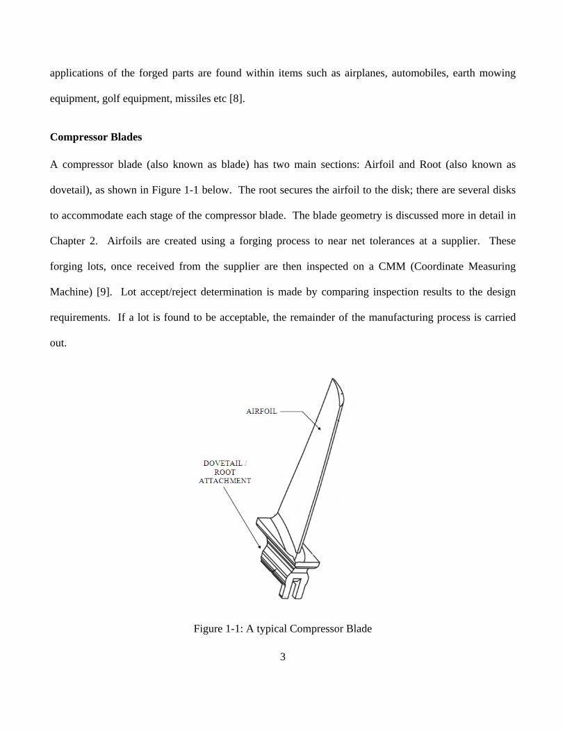
Compressor Blades

A compressor blade (also known as blade) has two main sections: Airfoil and Root (also known as

dovetail), as shown in Figure 1-1 below. The root secures the airfoil to the disk; there are several disks

to accommodate each stage of the compressor blade. The blade geometry is discussed more in detail in

Chapter 2. Airfoils are created using a forging process to near net tolerances at a supplier. These

forging lots, once received from the supplier are then inspected on a CMM (Coordinate Measuring

Machine) [9]. Lot accept/reject determination is made by comparing inspection results to the design

requirements. If a lot is found to be acceptable, the remainder of the manufacturing process is carried

out.

Figure 1-1: A typical Compressor Blade

4

1.3 Business Challenges

The compressor blade is a key component of a jet engine. Due to the importance of its application and

consequences of its failure causing in-flight shutdowns, the FAA (Federal Aviation Administration) has

classified them as “major” parts. The complex design, in addition to the significant characterization,

makes the manufacturing and inspection of the compressor blades a daunting task. Some of the

dimensional tolerances that are required to be maintained are defined to ten thousands of an inch. Due

to the high volume of the manufacturing and the inspection of all airfoil features, the inspection costs

have increased significantly. Here in lies a serious need to reduce the inspection costs while maintaining

the highest levels of quality.

1.4 Objective

The objective of this thesis is to design and develop a software tool that estimates airfoil feature

variations throughout the manufacturing process which will help reduce the CMM inspection time and

CMM inspection costs.

1.5 Methodology

The airfoil section of the compressor blade is forged and shipped from a supplier; the dovetail is

installed and the compressor blade is processed through the remainder of the manufacturing process.

Once the forgings are received they are CMM inspected; the inspection data are then analyzed to verify

the dimensional accuracy of the forgings, essentially to accept or reject the forging lots before

proceeding with the rest of the manufacturing process.

Because of the considerable variation inherent in the forging process, we must take it upon ourselves to

capture these process effects and adjust the manufacturing process accordingly to conform to the design

5

requirements. The idea is that once we understand all process effects on the features, one can accurately

predict these feature variations throughout the manufacturing process thereby eliminating some of the

redundant airfoil section CMM inspections which are built into the process. Hence the process effects

are analyzed throroughly, and models are formulated and packaged into a software tool for simplifying

the calculations to assist in lot disposition, reduced section inspection. The end result is to reduce

considerable inspection time and inspections costs.

In addition to the above, an ideal N-angle offset, which will be discussed in detail in Chapter 3, will

assist the grind operator target the critical airfoil features like N-angle, LEA, TEA in relation to the root,

to maximixe the yield of the manufacturing lot.

To summarize the methodology:

a) Develop a software tool that can estimate changes in airfoil features from forging to finish stage.

This will help reduce the number of airfoil section inspections, therefore decreasing inspection

time and inspection costs.

b) Compute the Ideal N-angle offset target value which will potentially eliminate fallouts at final

inspection, thereby increasing the yield.

c) Develop criteria to accept or reject a forging lot based on the inspection results. 

1.6 Thesis Outline

In Chapter 1 the topic of interest is introduced to the reader and business challenges were explained

which leads to a methodology that is clearly defined to set the boundaries of this thesis leading to the

objective of the thesis.

6

Chapter 2 gives the reader a thorough knowledge of the compressor blade features that are discussed in

this thesis. This chapter also briefly discusses different jet engines and different stages of compressor

blades.

Chapter 3 addresses the compressor blade manufacturing process to provide a better understanding of

how the compressor blade features are affected by the manufacturing process.

Chapter 4 discusses the Coordinate Measuring Machine, the compressor blade inspection process, and

understanding curve fitting to process airfoil feature data.

Chapter 5 covers the software tool development, algorithms, data input, computations and output from

the tool. An example is studied which explains in detail the data analysis and interpretation of the

results and also the validation of the results.

Chapter 6 deals with the conclusion and future work.

7

CHAPTER 2. COMPRESSOR BLADE GEOMETRY

2.1 Introduction

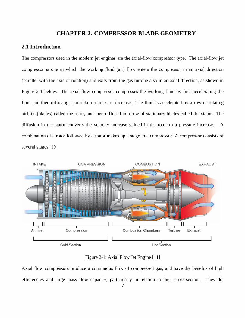
The compressors used in the modern jet engines are the axial-flow compressor type. The axial-flow jet

compressor is one in which the working fluid (air) flow enters the compressor in an axial direction

(parallel with the axis of rotation) and exits from the gas turbine also in an axial direction, as shown in

Figure 2-1 below. The axial-flow compressor compresses the working fluid by first accelerating the

fluid and then diffusing it to obtain a pressure increase. The fluid is accelerated by a row of rotating

airfoils (blades) called the rotor, and then diffused in a row of stationary blades called the stator. The

diffusion in the stator converts the velocity increase gained in the rotor to a pressure increase. A

combination of a rotor followed by a stator makes up a stage in a compressor. A compressor consists of

several stages [10].

Figure 2-1: Axial Flow Jet Engine [11]

Axial flow compressors produce a continuous flow of compressed gas, and have the benefits of high

efficiencies and large mass flow capacity, particularly in relation to their cross-section. They do,

8

however, require several rows of airfoils to achieve large pressure rises making them complex and

expensive relative to other designs [12].

2.2 Compressor Blade Geometry

All gas turbine propulsion systems must have a compressor component that develops some or all the

pressure increase specified by the system design cycle. Shaft for the compression process is supplied by

the turbine component of the system. In a modern jet engine, the compressor unit is typically divided

into two sections: the low-pressure compressor and high-pressure compressor. Compressor blades

designs are drastically different from engine to engine as they depend on the design characteristics that

change with each stage within a jet engine. It is rather interesting to note that these compressor airfoils

would exhibit some of the same behavioral characteristics that you would see in isolated airfoils (wings,

etc). For example, they are subjected to lift and drag forces, they stall, and they generate boundary

layers, wakes and under certain circumstances shock waves. However, compressor blades operate under

conditions unlike typical isolated airfoils [13].

Airfoil Geometry

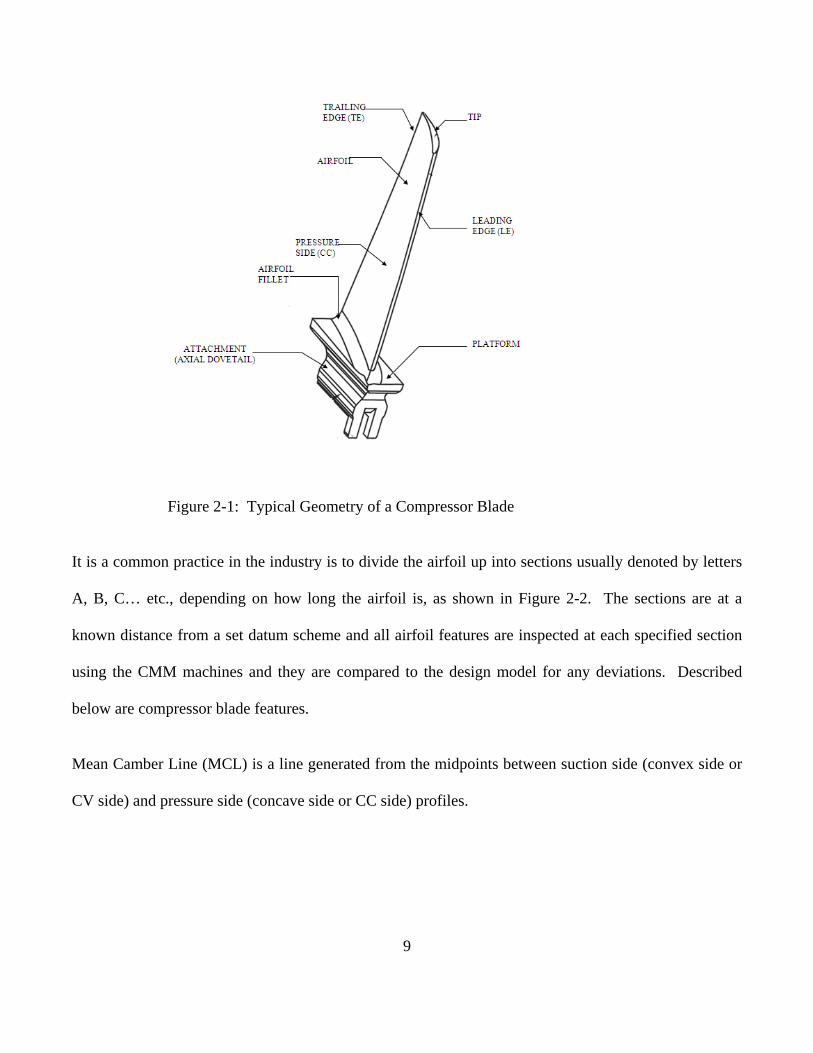
Typical compressor blade geometry is shown in Figure 2-1. It consists of four main segments: airfoil,

airfoil fillet, platform and root also known as dovetail due to its shape. An airfoil is an aerodynamic

surface mounted within a flow area intended to redirect the working fluid with that area. An airfoil’s

pressure side is the concave surface of the airfoil, while an airfoil’s suction side is the convex surface of

the airfoil. The airfoil’s leading edge is the forward facing edge surface of the airfoil, and the trailing

edge is the aft edge surface of the airfoil [14].

9

Figure 2-1: Typical Geometry of a Compressor Blade

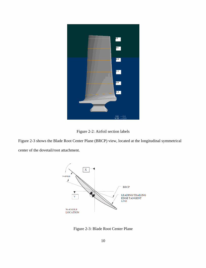
It is a common practice in the industry is to divide the airfoil up into sections usually denoted by letters

A, B, C… etc., depending on how long the airfoil is, as shown in Figure 2-2. The sections are at a

known distance from a set datum scheme and all airfoil features are inspected at each specified section

using the CMM machines and they are compared to the design model for any deviations. Described

below are compressor blade features.

Mean Camber Line (MCL) is a line generated from the midpoints between suction side (convex side or

CV side) and pressure side (concave side or CC side) profiles.

10

Figure 2-2: Airfoil section labels

Figure 2-3 shows the Blade Root Center Plane (BRCP) view, located at the longitudinal symmetrical

center of the dovetail/root attachment.

Figure 2-3: Blade Root Center Plane

11

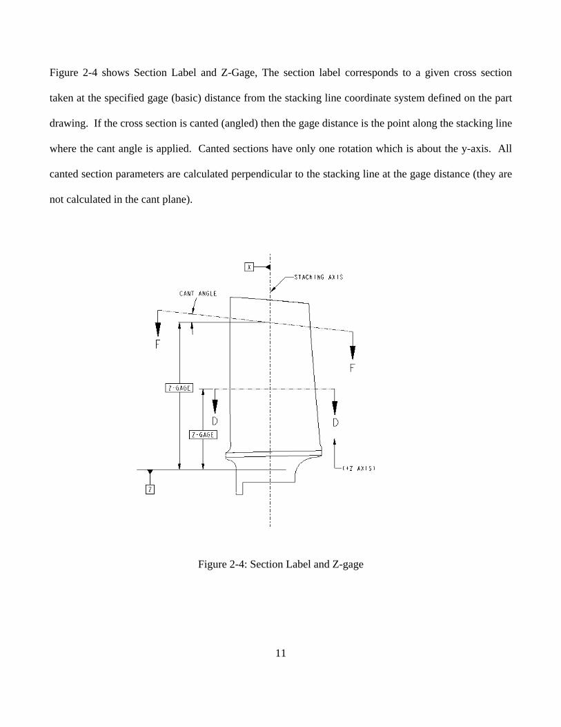
Figure 2-4 shows Section Label and Z-Gage, The section label corresponds to a given cross section

taken at the specified gage (basic) distance from the stacking line coordinate system defined on the part

drawing. If the cross section is canted (angled) then the gage distance is the point along the stacking line

where the cant angle is applied. Canted sections have only one rotation which is about the y-axis. All

canted section parameters are calculated perpendicular to the stacking line at the gage distance (they are

not calculated in the cant plane).

Figure 2-4: Section Label and Z-gage

12

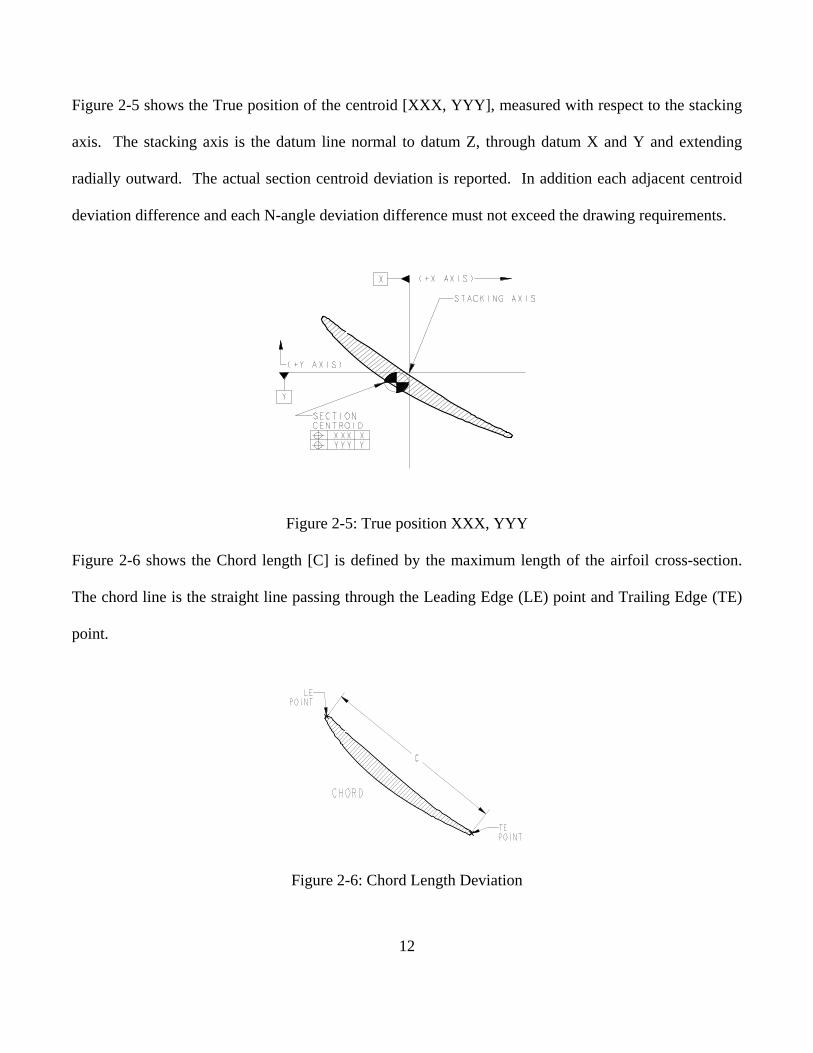
Figure 2-5 shows the True position of the centroid [XXX, YYY], measured with respect to the stacking

axis. The stacking axis is the datum line normal to datum Z, through datum X and Y and extending

radially outward. The actual section centroid deviation is reported. In addition each adjacent centroid

deviation difference and each N-angle deviation difference must not exceed the drawing requirements.

Figure 2-5: True position XXX, YYY

Figure 2-6 shows the Chord length [C] is defined by the maximum length of the airfoil cross-section.

The chord line is the straight line passing through the Leading Edge (LE) point and Trailing Edge (TE)

point.

Figure 2-6: Chord Length Deviation

13

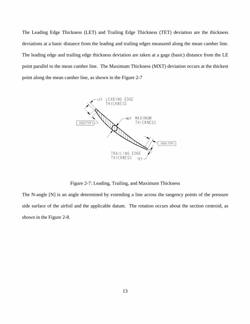
The Leading Edge Thickness (LET) and Trailing Edge Thickness (TET) deviation are the thickness

deviations at a basic distance from the leading and trailing edges measured along the mean camber line.

The leading edge and trailing edge thickness deviation are taken at a gage (basic) distance from the LE

point parallel to the mean camber line. The Maximum Thickness (MXT) deviation occurs at the thickest

point along the mean camber line, as shown in the Figure 2-7

Figure 2-7: Leading, Trailing, and Maximum Thickness

The N-angle [N] is an angle determined by extending a line across the tangency points of the pressure

side surface of the airfoil and the applicable datum. The rotation occurs about the section centroid, as

shown in the Figure 2-8.

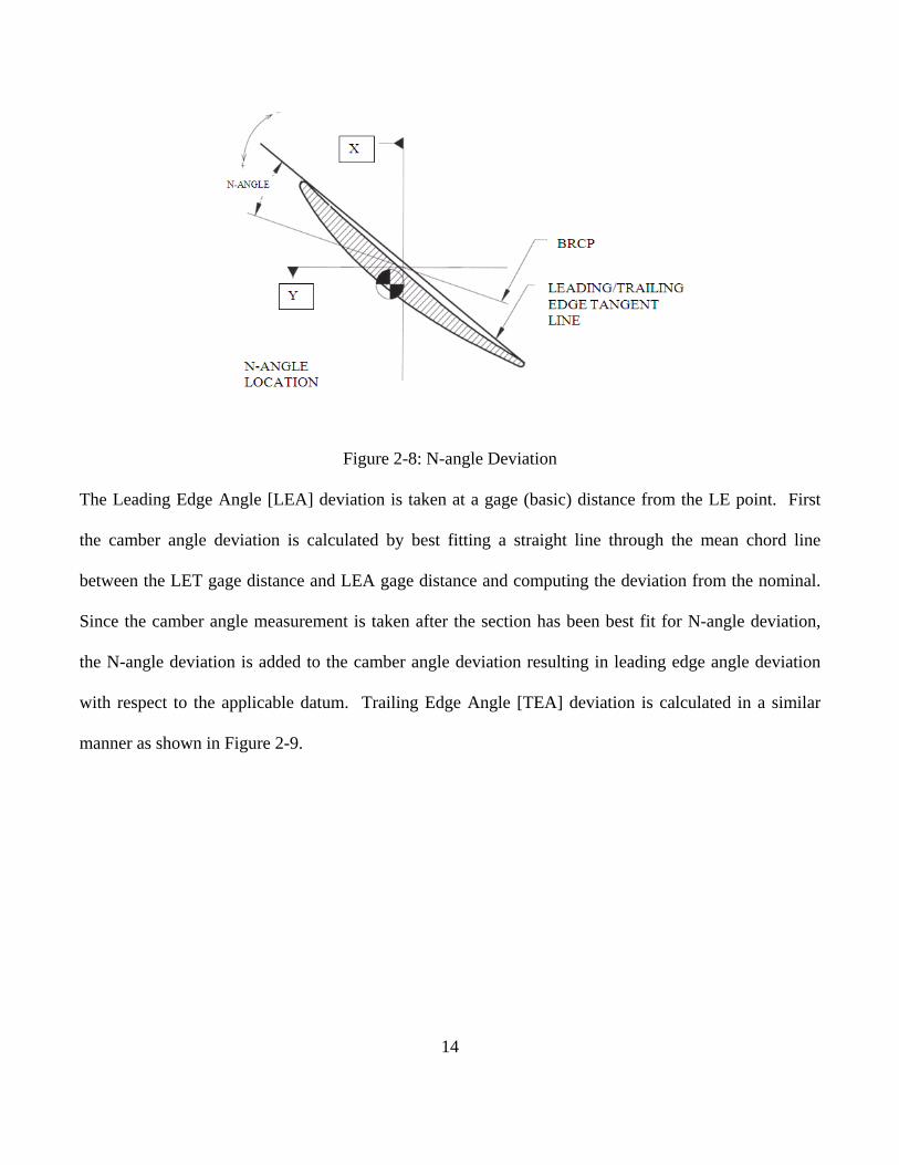
14

Figure 2-8: N-angle Deviation

The Leading Edge Angle [LEA] deviation is taken at a gage (basic) distance from the LE point. First

the camber angle deviation is calculated by best fitting a straight line through the mean chord line

between the LET gage distance and LEA gage distance and computing the deviation from the nominal.

Since the camber angle measurement is taken after the section has been best fit for N-angle deviation,

the N-angle deviation is added to the camber angle deviation resulting in leading edge angle deviation

with respect to the applicable datum. Trailing Edge Angle [TEA] deviation is calculated in a similar

manner as shown in Figure 2-9.

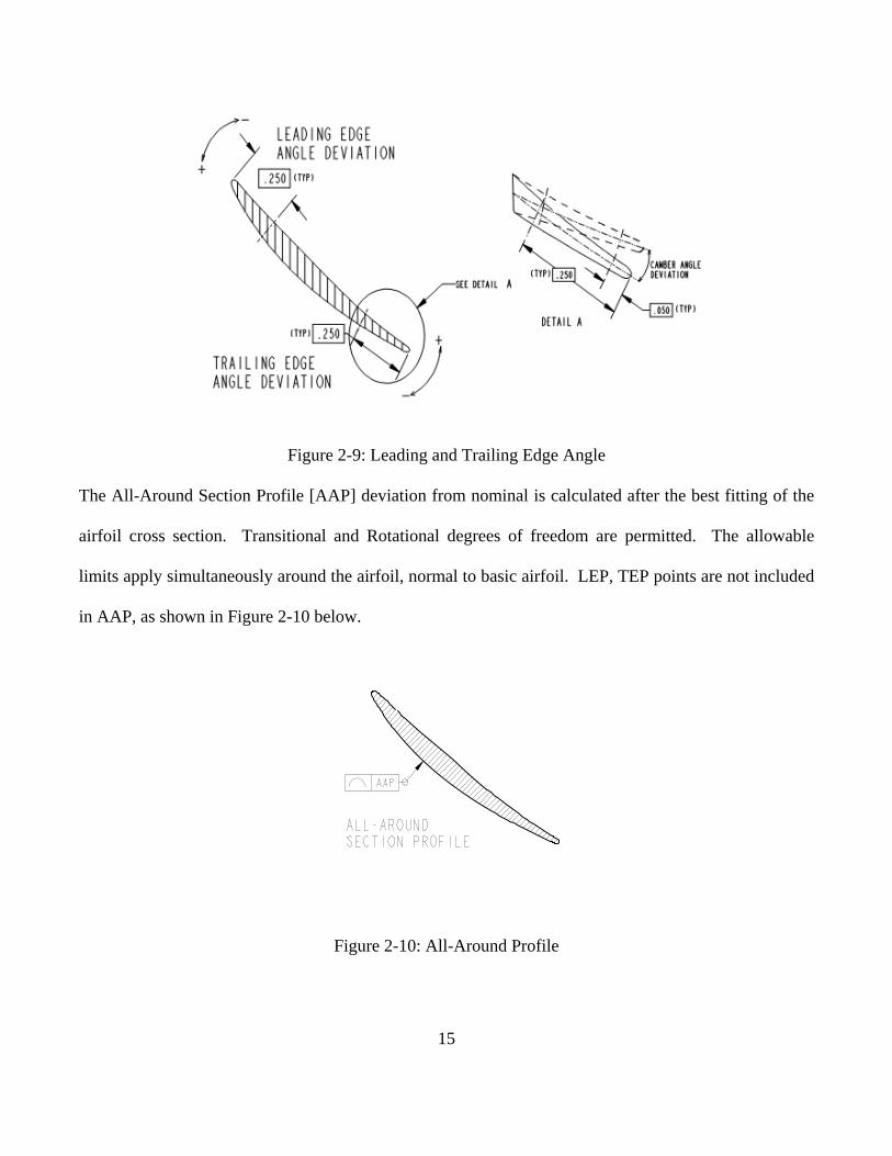
15

Figure 2-9: Leading and Trailing Edge Angle

The All-Around Section Profile [AAP] deviation from nominal is calculated after the best fitting of the

airfoil cross section. Transitional and Rotational degrees of freedom are permitted. The allowable

limits apply simultaneously around the airfoil, normal to basic airfoil. LEP, TEP points are not included

in AAP, as shown in Figure 2-10 below.

Figure 2-10: All-Around Profile

16

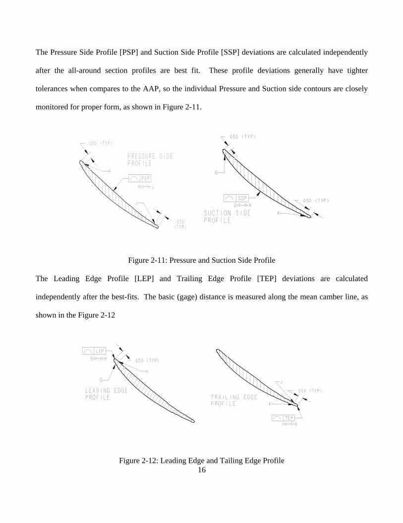
The Pressure Side Profile [PSP] and Suction Side Profile [SSP] deviations are calculated independently

after the all-around section profiles are best fit. These profile deviations generally have tighter

tolerances when compares to the AAP, so the individual Pressure and Suction side contours are closely

monitored for proper form, as shown in Figure 2-11.

Figure 2-11: Pressure and Suction Side Profile

The Leading Edge Profile [LEP] and Trailing Edge Profile [TEP] deviations are calculated

independently after the best-fits. The basic (gage) distance is measured along the mean camber line, as

shown in the Figure 2-12

Figure 2-12: Leading Edge and Tailing Edge Profile

17

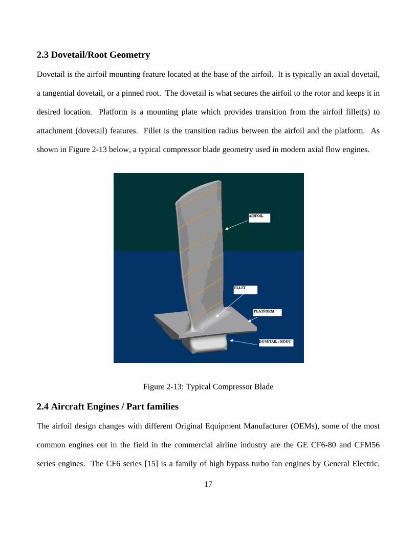
2.3 Dovetail/Root Geometry

Dovetail is the airfoil mounting feature located at the base of the airfoil. It is typically an axial dovetail,

a tangential dovetail, or a pinned root. The dovetail is what secures the airfoil to the rotor and keeps it in

desired location. Platform is a mounting plate which provides transition from the airfoil fillet(s) to

attachment (dovetail) features. Fillet is the transition radius between the airfoil and the platform. As

shown in Figure 2-13 below, a typical compressor blade geometry used in modern axial flow engines.

Figure 2-13: Typical Compressor Blade

2.4 Aircraft Engines / Part families

The airfoil design changes with different Original Equipment Manufacturer (OEMs), some of the most

common engines out in the field in the commercial airline industry are the GE CF6-80 and CFM56

series engines. The CF6 series [15] is a family of high bypass turbo fan engines by General Electric.

18

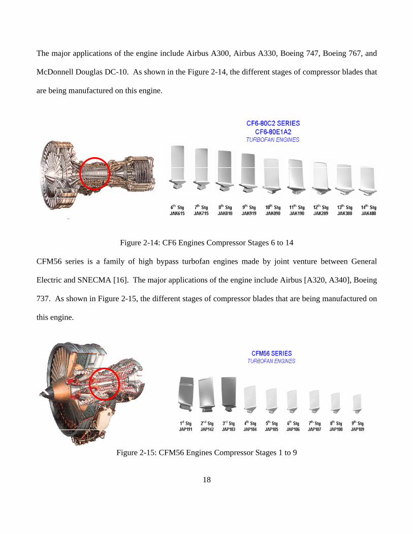
The major applications of the engine include Airbus A300, Airbus A330, Boeing 747, Boeing 767, and

McDonnell Douglas DC-10. As shown in the Figure 2-14, the different stages of compressor blades that

are being manufactured on this engine.

Figure 2-14: CF6 Engines Compressor Stages 6 to 14

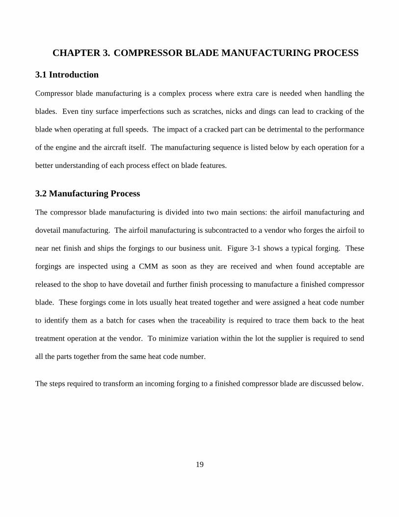
CFM56 series is a family of high bypass turbofan engines made by joint venture between General

Electric and SNECMA [16]. The major applications of the engine include Airbus [A320, A340], Boeing

737. As shown in Figure 2-15, the different stages of compressor blades that are being manufactured on

this engine.

Figure 2-15: CFM56 Engines Compressor Stages 1 to 9

19

CHAPTER 3. COMPRESSOR BLADE MANUFACTURING PROCESS

3.1 Introduction

Compressor blade manufacturing is a complex process where extra care is needed when handling the

blades. Even tiny surface imperfections such as scratches, nicks and dings can lead to cracking of the

blade when operating at full speeds. The impact of a cracked part can be detrimental to the performance

of the engine and the aircraft itself. The manufacturing sequence is listed below by each operation for a

better understanding of each process effect on blade features.

3.2 Manufacturing Process

The compressor blade manufacturing is divided into two main sections: the airfoil manufacturing and

dovetail manufacturing. The airfoil manufacturing is subcontracted to a vendor who forges the airfoil to

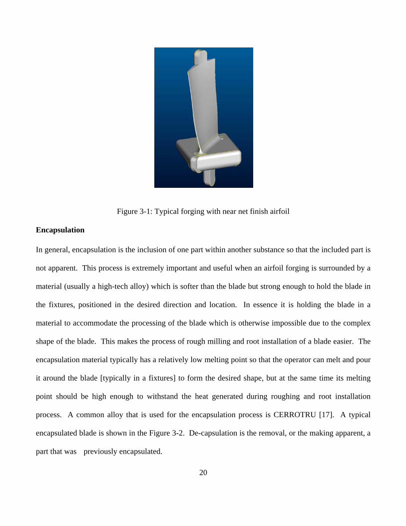
near net finish and ships the forgings to our business unit. Figure 3-1 shows a typical forging. These

forgings are inspected using a CMM as soon as they are received and when found acceptable are

released to the shop to have dovetail and further finish processing to manufacture a finished compressor

blade. These forgings come in lots usually heat treated together and were assigned a heat code number

to identify them as a batch for cases when the traceability is required to trace them back to the heat

treatment operation at the vendor. To minimize variation within the lot the supplier is required to send

all the parts together from the same heat code number.

The steps required to transform an incoming forging to a finished compressor blade are discussed below.

20

Figure 3-1: Typical forging with near net finish airfoil

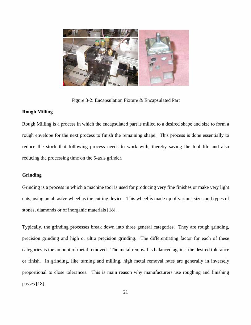
Encapsulation

In general, encapsulation is the inclusion of one part within another substance so that the included part is

not apparent. This process is extremely important and useful when an airfoil forging is surrounded by a

material (usually a high-tech alloy) which is softer than the blade but strong enough to hold the blade in

the fixtures, positioned in the desired direction and location. In essence it is holding the blade in a

material to accommodate the processing of the blade which is otherwise impossible due to the complex

shape of the blade. This makes the process of rough milling and root installation of a blade easier. The

encapsulation material typically has a relatively low melting point so that the operator can melt and pour

it around the blade [typically in a fixtures] to form the desired shape, but at the same time its melting

point should be high enough to withstand the heat generated during roughing and root installation

process. A common alloy that is used for the encapsulation process is CERROTRU [17]. A typical

encapsulated blade is shown in the Figure 3-2. De-capsulation is the removal, or the making apparent, a

part that was previously encapsulated.

21

Figure 3-2: Encapsulation Fixture & Encapsulated Part

Rough Milling

Rough Milling is a process in which the encapsulated part is milled to a desired shape and size to form a

rough envelope for the next process to finish the remaining shape. This process is done essentially to

reduce the stock that following process needs to work with, thereby saving the tool life and also

reducing the processing time on the 5-axis grinder.

Grinding

Grinding is a process in which a machine tool is used for producing very fine finishes or make very light

cuts, using an abrasive wheel as the cutting device. This wheel is made up of various sizes and types of

stones, diamonds or of inorganic materials [18].

Typically, the grinding processes break down into three general categories. They are rough grinding,

precision grinding and high or ultra precision grinding. The differentiating factor for each of these

categories is the amount of metal removed. The metal removal is balanced against the desired tolerance

or finish. In grinding, like turning and milling, high metal removal rates are generally in inversely

proportional to close tolerances. This is main reason why manufacturers use roughing and finishing

passes [18].

22

In rough grinding, the desired work piece/wheel interaction is focused on cutting. In these applications,

maximum metal removal is the goal. Cutting off billets, snagging gates and risers from castings, or

grinding weld beads smooth, are all processes where the maximum amount of metal removal is the goal.

Precise control of the size and surface finish is a secondary consideration [18].

To create size and surface finish control for high metal removal in the precision grinding application,

roughing passes are generally followed by finish passes. Precision grinding applications combine high

metal removal with good part size control [18].

In ultra precision grinding operations, little or no actual cutting is done. Instead, the work piece surface

is in effect rubbed clean primarily by sliding action from very fine abrasive grains. Ultra precision

grinding is the surface finishing of a very precisely sized work piece. Most surface finishing processes

generally fall into this category. These include lapping and polishing [18].

The grinding wheel designs are created using the finished part CAD models where the form of the

dovetail is controlled extremely carefully. The 5-axis grinders install the entire dovetail features using

the rough grinding wheel on the first few passes, and then finishing wheel cleans up for final finish.

The grinding process is where 80% of the airfoil/dovetail features are installed, leaving the remaining

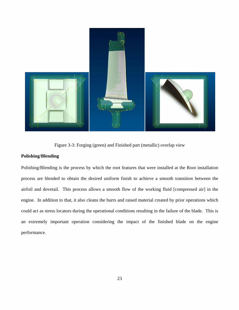
20% for further finishing processes. A typical ground part is shown in the Figure 3-3, which shows an

overlap of a forging (transparent green color) and a finished part (metallic color) to illustrate the

transformation process.

23

Figure 3-3: Forging (green) and Finished part (metallic) overlap view

Polishing/Blending

Polishing/Blending is the process by which the root features that were installed at the Root installation

process are blended to obtain the desired uniform finish to achieve a smooth transition between the

airfoil and dovetail. This process allows a smooth flow of the working fluid [compressed air] in the

engine. In addition to that, it also cleans the burrs and raised material created by prior operations which

could act as stress locators during the operational conditions resulting in the failure of the blade. This is

an extremely important operation considering the impact of the finished blade on the engine

performance.

24

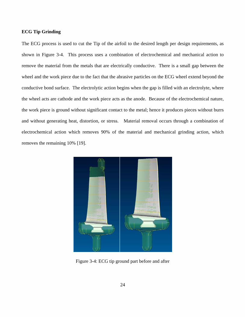
ECG Tip Grinding

The ECG process is used to cut the Tip of the airfoil to the desired length per design requirements, as

shown in Figure 3-4. This process uses a combination of electrochemical and mechanical action to

remove the material from the metals that are electrically conductive. There is a small gap between the

wheel and the work piece due to the fact that the abrasive particles on the ECG wheel extend beyond the

conductive bond surface. The electrolytic action begins when the gap is filled with an electrolyte, where

the wheel acts are cathode and the work piece acts as the anode. Because of the electrochemical nature,

the work piece is ground without significant contact to the metal; hence it produces pieces without burrs

and without generating heat, distortion, or stress. Material removal occurs through a combination of

electrochemical action which removes 90% of the material and mechanical grinding action, which

removes the remaining 10% [19].

Figure 3-4: ECG tip ground part before and after

25

Pre-cleaning [ETCH]

Etching is a process in which the surface of a material is altered by inducing a chemical reaction. This is

a cleaning requirement to be carried out prior to FPI, which is discussed in the section below. The test

surface should be free of any contamination s such as, oil, dirt, or grease that could keep the penetrant

out of a defect such as cracks, dents etc. This can give false indications. Etching takes care of any kind

of contamination which is why it is the most stable cleaning technique used in the aerospace industry.

The etching process is also used to remove the top surface of the material depending on the

concentration of the acid. In softer materials like titanium, the etch process is used to removed a portion

of abusive machined layer.

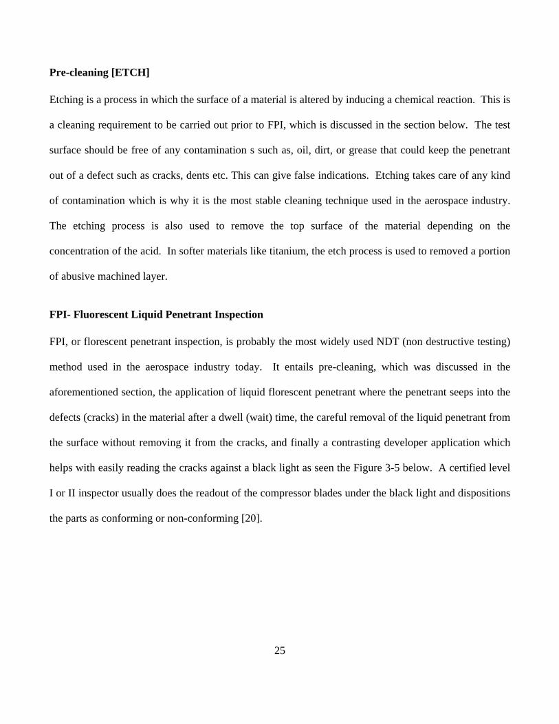
FPI- Fluorescent Liquid Penetrant Inspection

FPI, or florescent penetrant inspection, is probably the most widely used NDT (non destructive testing)

method used in the aerospace industry today. It entails pre-cleaning, which was discussed in the

aforementioned section, the application of liquid florescent penetrant where the penetrant seeps into the

defects (cracks) in the material after a dwell (wait) time, the careful removal of the liquid penetrant from

the surface without removing it from the cracks, and finally a contrasting developer application which

helps with easily reading the cracks against a black light as seen the Figure 3-5 below. A certified level

I or II inspector usually does the readout of the compressor blades under the black light and dispositions

the parts as conforming or non-conforming [20].

26

Figure 3-5: Penetrant application & dwell, crack readout under a black light[21][22]

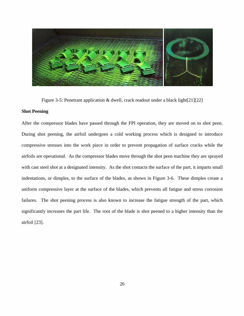
Shot Peening

After the compressor blades have passed through the FPI operation, they are moved on to shot peen.

During shot peening, the airfoil undergoes a cold working process which is designed to introduce

compressive stresses into the work piece in order to prevent propagation of surface cracks while the

airfoils are operational. As the compressor blades move through the shot peen machine they are sprayed

with cast steel shot at a designated intensity. As the shot contacts the surface of the part, it imparts small

indentations, or dimples, to the surface of the blades, as shown in Figure 3-6. These dimples create a

uniform compressive layer at the surface of the blades, which prevents all fatigue and stress corrosion

failures. The shot peening process is also known to increase the fatigue strength of the part, which

significantly increases the part life. The root of the blade is shot peened to a higher intensity than the

airfoil [23].

27

Figure 3-6: Shot peening dimple, compressive layer after shot peening

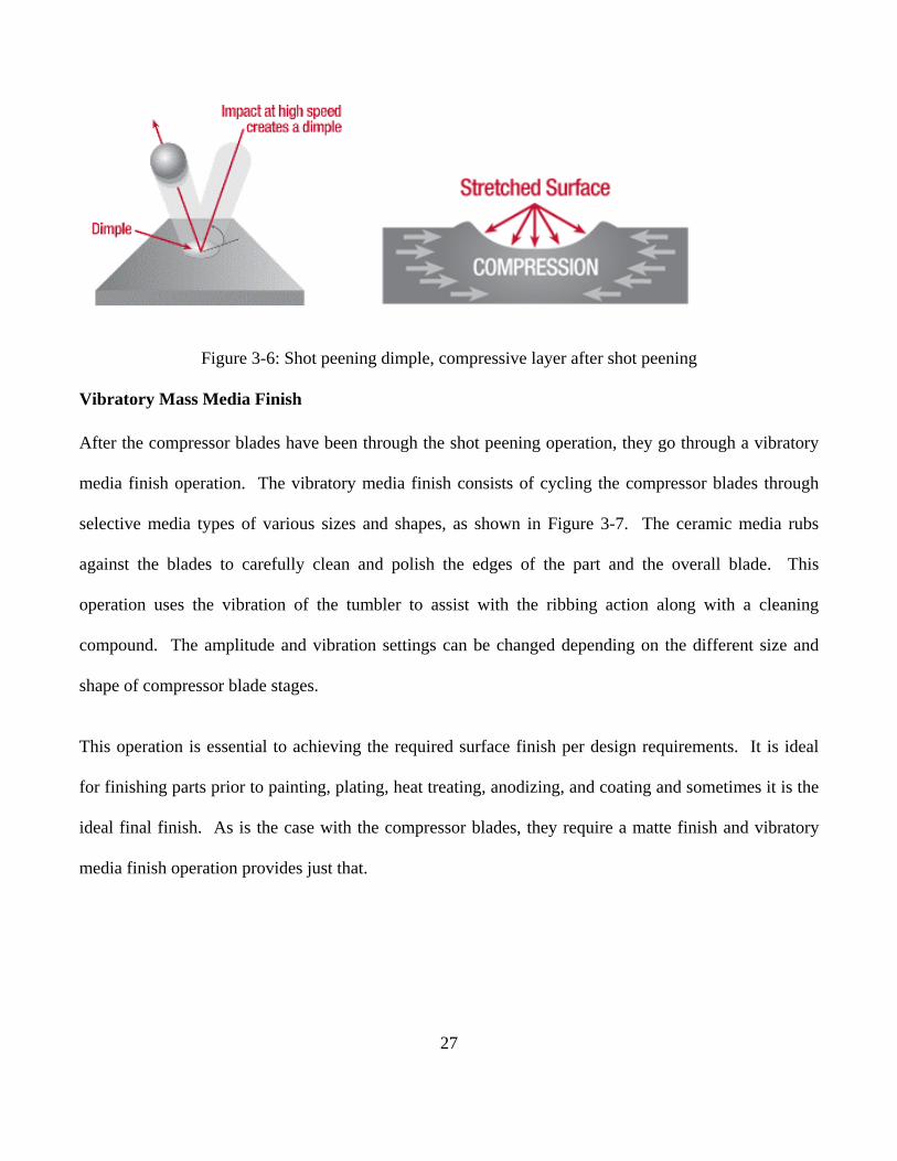
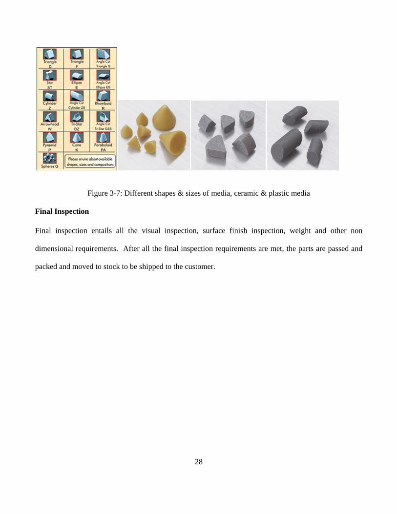
Vibratory Mass Media Finish

After the compressor blades have been through the shot peening operation, they go through a vibratory

media finish operation. The vibratory media finish consists of cycling the compressor blades through

selective media types of various sizes and shapes, as shown in Figure 3-7. The ceramic media rubs

against the blades to carefully clean and polish the edges of the part and the overall blade. This

operation uses the vibration of the tumbler to assist with the ribbing action along with a cleaning

compound. The amplitude and vibration settings can be changed depending on the different size and

shape of compressor blade stages.

This operation is essential to achieving the required surface finish per design requirements. It is ideal

for finishing parts prior to painting, plating, heat treating, anodizing, and coating and sometimes it is the

ideal final finish. As is the case with the compressor blades, they require a matte finish and vibratory

media finish operation provides just that.

28

Figure 3-7: Different shapes & sizes of media, ceramic & plastic media

Final Inspection

Final inspection entails all the visual inspection, surface finish inspection, weight and other non

dimensional requirements. After all the final inspection requirements are met, the parts are passed and

packed and moved to stock to be shipped to the customer.

29

CHAPTER 4. COMPRESSOR BLADE INSPECTION

4.1 Introduction

In looking back over the evolution of the measurement, since the days of ancient Egyptians building

pyramids to modern day architecture, the measurement systems have come a long way to the point that

measurement is an integral part of our everyday lives. Since the concept of interchangeable parts gained

increased recognition, the automobile industry flourished with mass production, and as a result it was

necessary to have parts made to absolute standards. The automation of machine tools created the need

for faster and more flexible means of measuring. This requirement resulted in a new industry of three-

dimensional measuring machines. In recent times, the emphasis on Statistical Process Control (SPC) for

quality improvement has accelerated the demand for faster and more accurate measurements.

Coordinate Measuring Machines (CMM’s) have become more capable to fulfill these growing

requirements [24].

4.2 Coordinate Measuring Machine

A CMM is a great tool to reduce time taken to inspect complex parts. There are few limitations to the

feature types whose dimensions cannot be measured by a CMM, as it depends on the size and shape of

the part being inspected and as long as there is accessibility of the probe to the features, they can be

measured. The flexibility coupled with accuracy of measurement is the reason why CMMs are widely

accepted in the metrology world. One of the biggest advantages is the decreased inspection time which

always translates into cost saving for the businesses [24].

The primary function of a CMM is to measure the actual shape of a workpiece, compare it against the

desired shape, and evaluate the metrological information such as size, form, location, and orientation.

30

The actual comparison is usually accomplished using data processing software with some advanced

features to calculate complex feature dimensions [24].

The form of the workpiece is obtained by collecting a cloud of data points over the surface of the part.

The data collection can be carried using contact and non-contact measuring heads. The data collection is

carried using hard probing touch sensors that are scanning head and non-scanning head for continuous

and discrete data points. Every measurement point is expressed in terms of its measured coordinates.

Some sensors are capable of also collecting direction vectors of the measured points, which usually

allows for better accuracies. However, it is not possible to evaluate the dimensional parameters directly

from the measured coordinates. An analytical model is needed to compare it against the measured data

to evaluate the parameters. The model contains ideal geometric data that is obtained usually from the

CAD design. This is accomplished by applying the best-fit algorithms to fit the measured data set to the

geometric model [24].

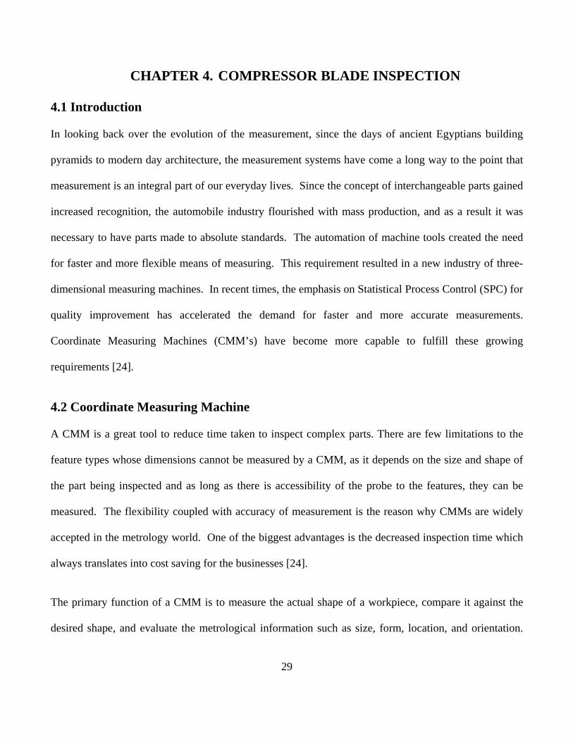
A standard CMM consists of following essential system components, as shown in Figure 4-1 [24]:

• A mechanical frame with three axes

• Probe head carrying the sensor that actually measures the part

• A control unit

• A computer with peripheral equipment (printer, plotter etc.) and software to calculate and display

measurement results. The computer usually is connected to a network from where it can get

programs and computer-aided design (CAD) files and it can send the measurement reports and

data.

31

Figure 4-1: System Components of a CMM [24]

The three carriages of a CMM form a Cartesian reference coordinate system to which the probe head is

attached. Transducers or scales determine the displacement along a coordinate path. This allows any

point in the measurement volume of the CMM to be covered by the measurements using a spatial

reference point on the probe head. This reference point is usually the center of the probe tip for contact

sensors [24]. A measurement with a CMM comprises of the following steps:

• Calibration of the stylus or probe tip with respect to the probe head reference point, normally

using a calibrated sphere (provided an electromechanical three-dimensional probe is used)

• Determination of the workpiece position and orientation (workpiece coordinate system) in

relation to the machine coordinate system.

32

• Measurement of the surface points on the workpiece

• Evaluation of the geometric parameters of the workpiece

• Representation or reporting of the measurement results

4.3 Curve and Surface Fitting

CMMs can measure a variety of features including sizes, forms, and locations for an extremely wide

array of features simply provided that the CMM probe has the necessary access to the features. From its

appearance, the CMM seems to only detect a collection of individual points. But it is, in fact, the

software that processes these points that turns the CMM from a mere point collector into an immensely

flexible, powerful measuring instrument [24].

A key component of CMM software is curve and surface fitting. Such fitting of CMM data points is

necessary in order to assess feature size, location, or form deviation, or to establish a local coordinate

system from datum features.

4.4 Airfoil Data Processing (PC-DMIS Blade)

PC-DMIS Blade software, developed by WILCOX Associates in partnership with various blade

manufactures, is a turnkey solution for the analog scanning of blade sections. PC-DMIS Blade is a

Visual Basic add-on to the basic PC-DMIS package. It has a simple to use interface, which lets you

quickly identify parts, select the sections to measure and initiate scanning sequences [25].

PC-DMIS Blade uses traditional, section-based techniques to analyze blade measurements. Blade

manufacturers have historically relied on guillotine gages to measure blade characteristics like contour

and twist angles. These gages provide concise information, but they are expensive to make and

33

maintain. A CMM using PC-DMIS Blade provides a faster, more flexible and less costly approach

without compromising accuracy [25].

PC-DMIS Blade produces easy to understand graphical reports. Making blade measurement easy is

only half of the equation. The second half is providing useful, concise information to operators on the

shop floor. PC-DMIS Blade provides a wide range of outputs in simple to read, one-page reports. Users

can configure it to report on important characteristics including things like chord width, leading edge

thickness, twist angle, and mean camber line [25].

PC-DMIS Blade includes a range of alignment procedures. Proper alignment is the key to proper blade

measurement. In addition to supporting the preferred method of root holding with XYZ offsets and A-

angle rotation to the stacking axis, PC-DMIS Blade also supports 3D iterative alignments using either

CAD surface models or 6 point rest [25].

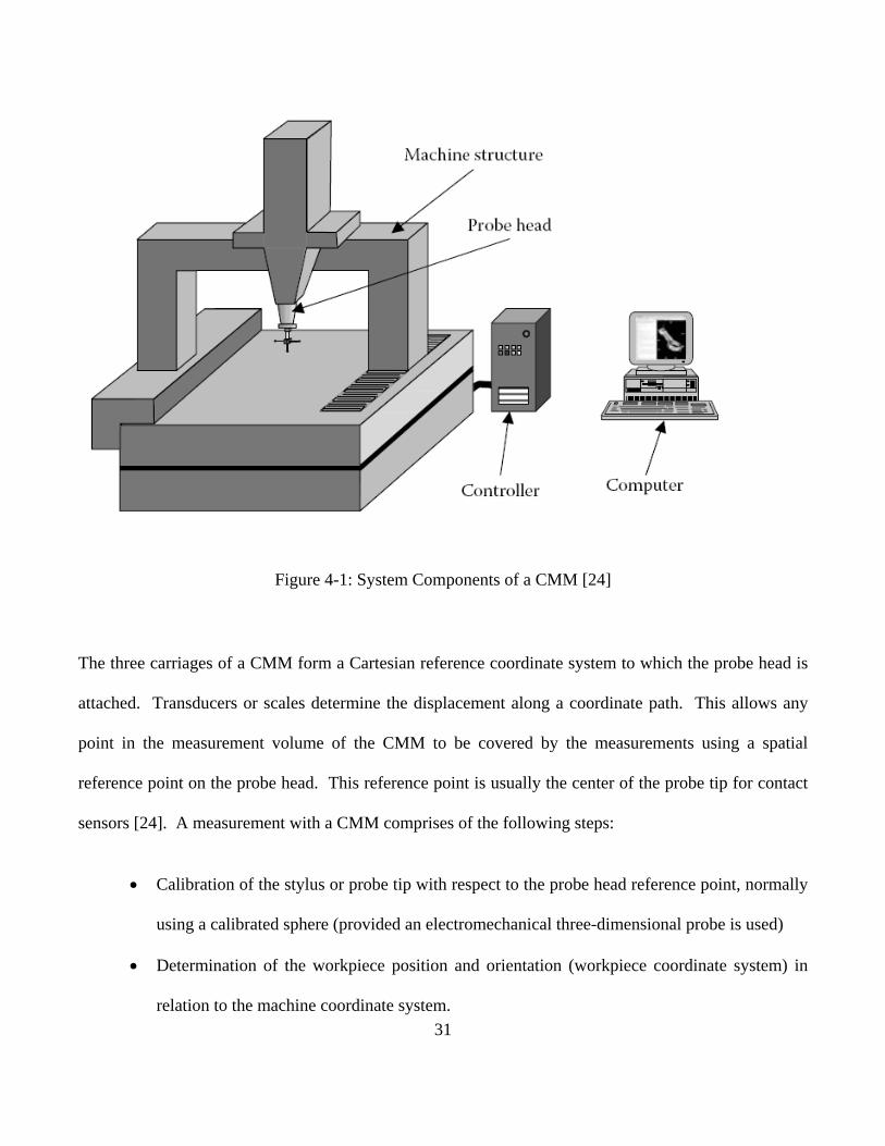
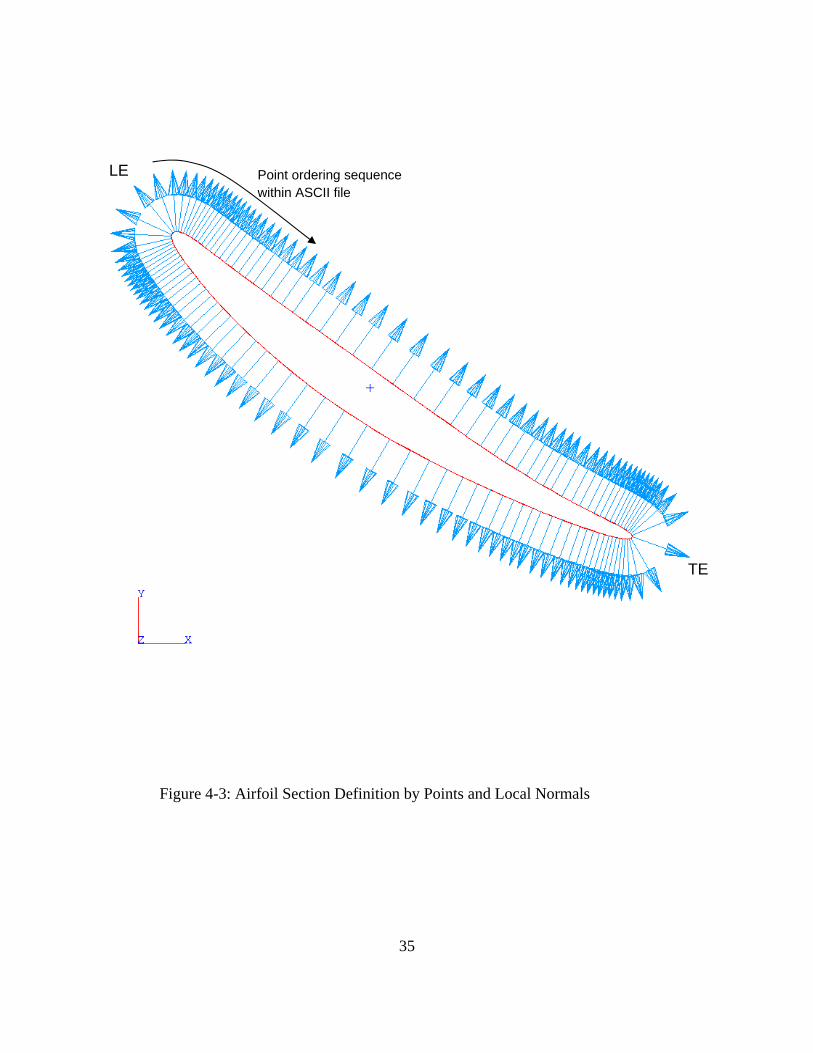
ASCII File

The ASCII file contains airfoil section geometry definition that is defined by the drawing and the

corresponding model, as shown in Figure 4-2. Section geometry is comprised of a series of point

coordinates and corresponding normal vectors (as shown in Figure 4-3) derived from the parent airfoil

surface. This data is used by the PCDMIS Blade software as the calculation basis for all airfoil section

geometric characteristics defined in Chapter 2.

34

Figure 4-2: Sample ASCII file for a section of airfoil

35

Figure 4-3: Airfoil Section Definition by Points and Local Normals

TE

LE Point ordering sequence within ASCII file

36

CHAPTER 5. SOFTWARE TOOL

5.1 Introduction

The software tool was initially programmed in Minitab [26] using individual macros. Minitab is a

powerful statistical analysis software when it comes to basic statistics, but it lacked the ability to

program complex algorithms and mathematical equations. MATLAB, on the other hand, provided just

the things Minitab was lacking, in addition to having the flexibility with data manipulation and

visualization [27]. Once all the algorithms were tested, and validated in Minitab the program was re-

written in MATLAB for advanced programming flexibility.

5.2 Processing Models

Different stages of compressor blades were studied from forging to finish stage by inspecting all features

using different heat code lots and the data was analyzed and compared to forging data to understand the

processing effects. These processing effects were then formulated into each part-specific model that

accurately estimated the airfoil feature tolerance variations from forging to finish process. The

following section provides an overview of material types associated with the different stages of

compressor blades. Due to proprietary reasons, process details and their effects are not discussed.

5.3 Algorithms

Each airfoil feature algorithms and its calculations that are packaged in the tool are discussed in this

section. It describes the design and development of a software tool specific to each compressor blade

feature that is being estimated. It is essential to have a thorough knowledge of compressor blade

features discussed in Chapter 2 and compressor blade manufacturing process discussed in Chapter 3 to

understand the material in this section.

37

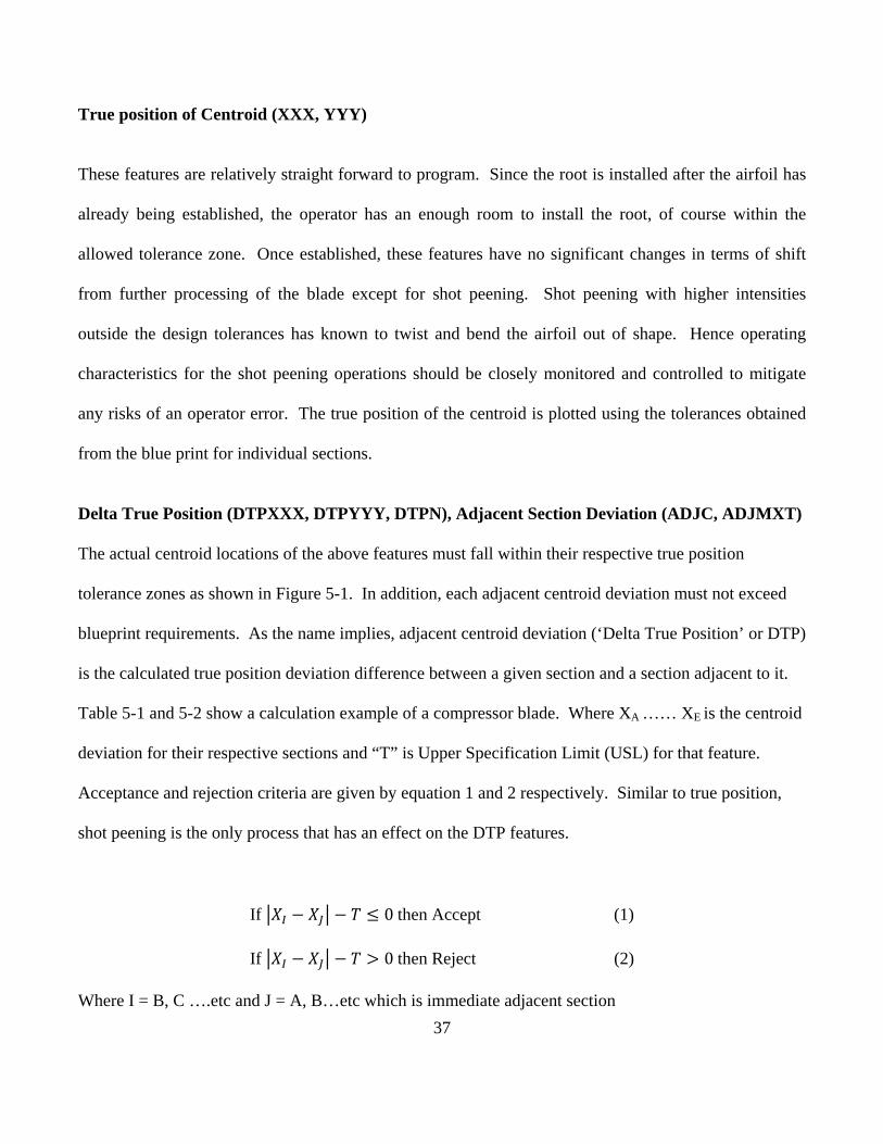
True position of Centroid (XXX, YYY)

These features are relatively straight forward to program. Since the root is installed after the airfoil has

already being established, the operator has an enough room to install the root, of course within the

allowed tolerance zone. Once established, these features have no significant changes in terms of shift

from further processing of the blade except for shot peening. Shot peening with higher intensities

outside the design tolerances has known to twist and bend the airfoil out of shape. Hence operating

characteristics for the shot peening operations should be closely monitored and controlled to mitigate

any risks of an operator error. The true position of the centroid is plotted using the tolerances obtained

from the blue print for individual sections.

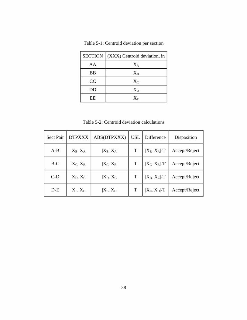
Delta True Position (DTPXXX, DTPYYY, DTPN), Adjacent Section Deviation (ADJC, ADJMXT)

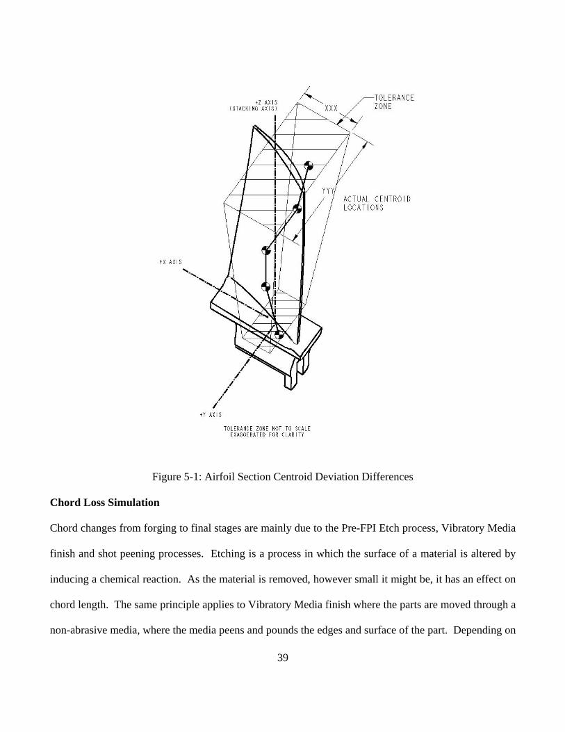
The actual centroid locations of the above features must fall within their respective true position

tolerance zones as shown in Figure 5-1. In addition, each adjacent centroid deviation must not exceed

blueprint requirements. As the name implies, adjacent centroid deviation (‘Delta True Position’ or DTP)

is the calculated true position deviation difference between a given section and a section adjacent to it.

Table 5-1 and 5-2 show a calculation example of a compressor blade. Where XA …… XE is the centroid

deviation for their respective sections and “T” is Upper Specification Limit (USL) for that feature.

Acceptance and rejection criteria are given by equation 1 and 2 respectively. Similar to true position,

shot peening is the only process that has an effect on the DTP features.

If 0 then Accept (1)

If 0 then Reject (2)

Where I = B, C ….etc and J = A, B…etc which is immediate adjacent section

38

Table 5-1: Centroid deviation per section

SECTION (XXX) Centroid deviation, in

AA XA

BB XB

CC XC

DD XD

EE XE

Table 5-2: Centroid deviation calculations

Sect Pair DTPXXX ABS(DTPXXX) USL Difference Disposition

A-B XB- XA |XB- XA| T |XB- XA|-T Accept/Reject

B-C XC- XB |XC- XB| T |XC- XB|-T Accept/Reject

C-D XD- XC |XD- XC| T |XD- XC|-T Accept/Reject

D-E XE- XD |XE- XD| T |XE- XD|-T Accept/Reject

39

Figure 5-1: Airfoil Section Centroid Deviation Differences

Chord Loss Simulation

Chord changes from forging to final stages are mainly due to the Pre-FPI Etch process, Vibratory Media

finish and shot peening processes. Etching is a process in which the surface of a material is altered by

inducing a chemical reaction. As the material is removed, however small it might be, it has an effect on

chord length. The same principle applies to Vibratory Media finish where the parts are moved through a

non-abrasive media, where the media peens and pounds the edges and surface of the part. Depending on

40

the length of time in the vibratory media finish the parts have shown to have some material loss. The

shot peening process, on the other hand, entails impacting the surface of the blade with shot (cast steel,

ceramic etc.) with force sufficient to create plastic deformation; this drastically alters the surface of the

blade. Also, the fact that the blades are pre-twisted at the forging level and untwisted after the shot

peening process has direct effect on the chord length.

Chord loss varies with the type of material for different compressor stage blades. Typical chord loss due

to the above mentioned reasons ranges from .002 to .003 inches. But for softer alloys, like titanium, the

chord loss is usually higher.

Various studies were conducted for different material types and different stages of the compressor

blades using different heat codes chosen randomly. The methodology for conducting different studies

and its results are out of the scope of this thesis. The chord loss function for a typical compressor blade

is given by equation 3:

(3)

Where

is the Chord Final;

is the Chord at forging level;

is the chord loss during the process.

Chord loss equations for nickel alloy, stainless steel and titanium alloy are given by equations 4, 5 and 6

respectively

0.0 0.002 / (4)

41

0.002 0.001 / (5)

0.002 0.002 / (6)

Where is a sequential number allocated to each airfoil section from first to last; usually from (0, 1,

2….etc.)

Thickness Simulation (LET, TET, MXT)

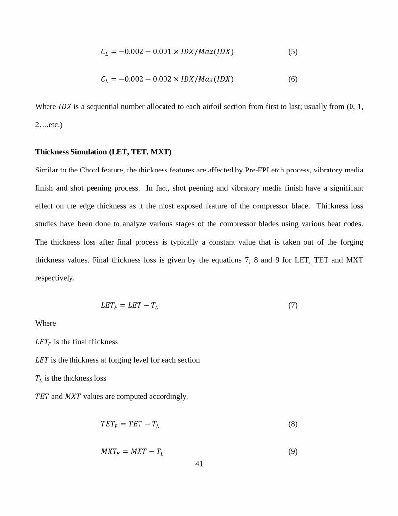
Similar to the Chord feature, the thickness features are affected by Pre-FPI etch process, vibratory media

finish and shot peening process. In fact, shot peening and vibratory media finish have a significant

effect on the edge thickness as it the most exposed feature of the compressor blade. Thickness loss

studies have been done to analyze various stages of the compressor blades using various heat codes.

The thickness loss after final process is typically a constant value that is taken out of the forging

thickness values. Final thickness loss is given by the equations 7, 8 and 9 for LET, TET and MXT

respectively.

(7)

Where

is the final thickness

is the thickness at forging level for each section

is the thickness loss

and values are computed accordingly.

(8)

(9)

42

Profile Features (LEP, TEP, PSP, SSP, APP)

The compressor blade profiles are critical features that affect the performance of the blade and the

engine itself. These features also have an impact on the life of the blades; the efficiency of the fluid

transfer between stages has a drastic effect on the efficiency of the engine. At first the all around profile

deviation from the nominal is calculated after the least squares best-fit of the airfoil cross section. All

other profile features are calculated after AAP is calculated. Please refer to Chapter 2 for airfoil

geometry for further understanding these features.

All processing effects have an impact on the profile features, including Pre-FPI etch process, vibratory

media finish and shot peening process. The profile tolerances won’t change from forging to finish as the

actual profile values are always best fitted to the nominal values.

Peen Simulation (N-angle, LEA, and TEA)

The shot peening operation is carried to produce a compressive residual stress layer and modify the

mechanical properties of the metals. It entails impacting the surface with shot (cast Steel, glass, ceramic

etc.) with force sufficient to create plastic deformation. Due to the high intensity of the shot peening,

the airfoil tends to untwist after the shot peening process, and hence it is a common practice to introduce

a pre-twist to compensate for the un-twist. These pre-twist values were studied across the different

stages of compressor blades, and as with the other features, the amount of twist completely depends on

the material of the compressor blade and also the intensity with which the surface being shot peened.

In order to provide the grind operator a simple way to target the N, LEA, and TEA with respect to the

true position XXX and YYY, it is a common practice to center the data to the lowest section of the N-

angle values. LEA and TEA are directly controlled by how the N-angle is targeted, and they follow suit.

43

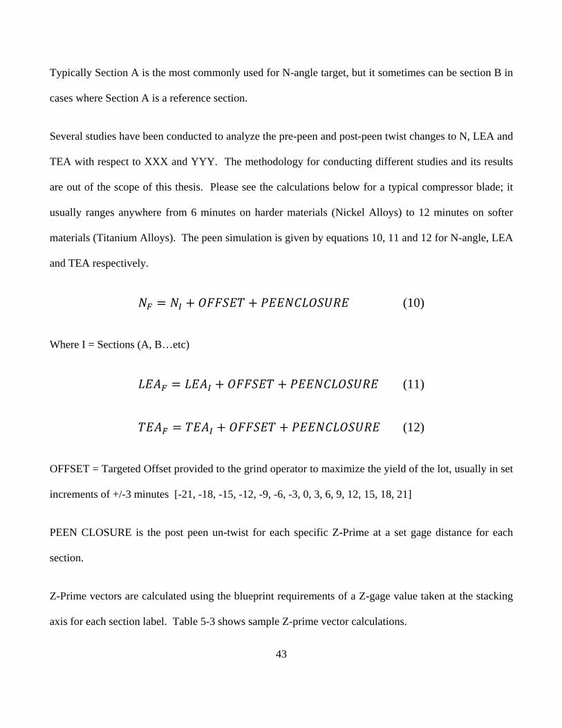
Typically Section A is the most commonly used for N-angle target, but it sometimes can be section B in

cases where Section A is a reference section.

Several studies have been conducted to analyze the pre-peen and post-peen twist changes to N, LEA and

TEA with respect to XXX and YYY. The methodology for conducting different studies and its results

are out of the scope of this thesis. Please see the calculations below for a typical compressor blade; it

usually ranges anywhere from 6 minutes on harder materials (Nickel Alloys) to 12 minutes on softer

materials (Titanium Alloys). The peen simulation is given by equations 10, 11 and 12 for N-angle, LEA

and TEA respectively.

(10)

Where I = Sections (A, B…etc)

(11)

(12)

OFFSET = Targeted Offset provided to the grind operator to maximize the yield of the lot, usually in set

increments of +/-3 minutes [-21, -18, -15, -12, -9, -6, -3, 0, 3, 6, 9, 12, 15, 18, 21]

PEEN CLOSURE is the post peen un-twist for each specific Z-Prime at a set gage distance for each

section.

Z-Prime vectors are calculated using the blueprint requirements of a Z-gage value taken at the stacking

axis for each section label. Table 5-3 shows sample Z-prime vector calculations.

44

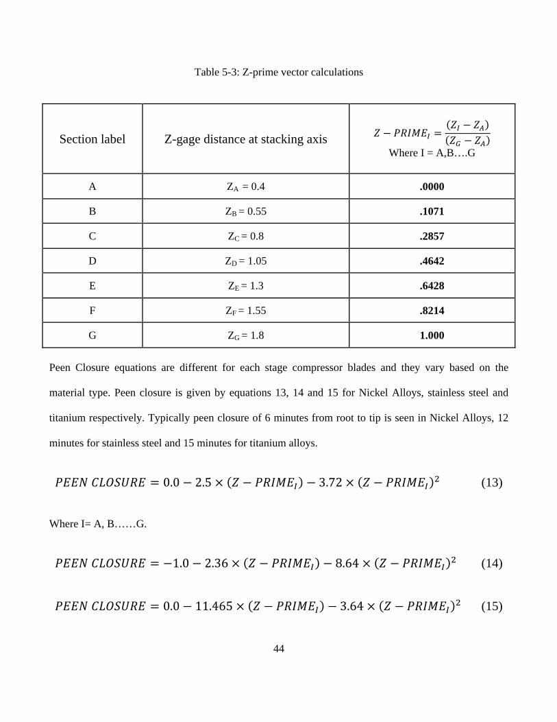
Table 5-3: Z-prime vector calculations

Section label Z-gage distance at stacking axis

Where I = A,B….G

A ZA = 0.4 .0000

B ZB = 0.55 .1071

C ZC = 0.8 .2857

D ZD = 1.05 .4642

E ZE = 1.3 .6428

F ZF = 1.55 .8214

G ZG = 1.8 1.000

Peen Closure equations are different for each stage compressor blades and they vary based on the

material type. Peen closure is given by equations 13, 14 and 15 for Nickel Alloys, stainless steel and

titanium respectively. Typically peen closure of 6 minutes from root to tip is seen in Nickel Alloys, 12

minutes for stainless steel and 15 minutes for titanium alloys.

0.0 2.5 3.72 (13)

Where I= A, B……G.

1.0 2.36 8.64 (14)

0.0 11.465 3.64 (15)

45

Automatic N-Angle Targeting

The ideal N-angle offset should be calculated in a way that all three (N-angle, LEA and TEA) features

for all sections for a given lot sample have the highest Cpk values, which essentially means that no part

falls out of specification tolerances after final processing. Calculation of N-angle offset can help the

grind operator maximize the yield.

The algorithm that accomplishes the above is maximize999. The function of this algorithm is that, given

the measured N-angle, LEA and TEA data, it returns an ideal N-angle that will provide the greatest post-

peen yield. This is accomplished by maximizing both the lower centered data as well as the upper

centered data as a function of N-Angle.

Optimizing the N-Angle

The theory behind finding the optimal N-Angle is that in order to maximize any yield using SPC

(Statistical Process Control) is to have very small variations that are closely grouped around the nominal

value, in other words, have close to zero deviation from the target value. This results in a high process

capability (Cpk) value. Cpk is given by the Equation 16

Cpk Min

, 16

The function then generates post-peen Cpk data for both the upper and lower centered data for non-

reference sections. That is, it generates both sets of data but does not assign either value as the Cpk

value for sections that are inspected. Instead, it compares the two values and finds the minimum

difference between the two. Essentially, maximizer599 is finding the offset angle that will result in both

the upper and lower centered data being as similar as possible and producing the greatest yield possible.

46

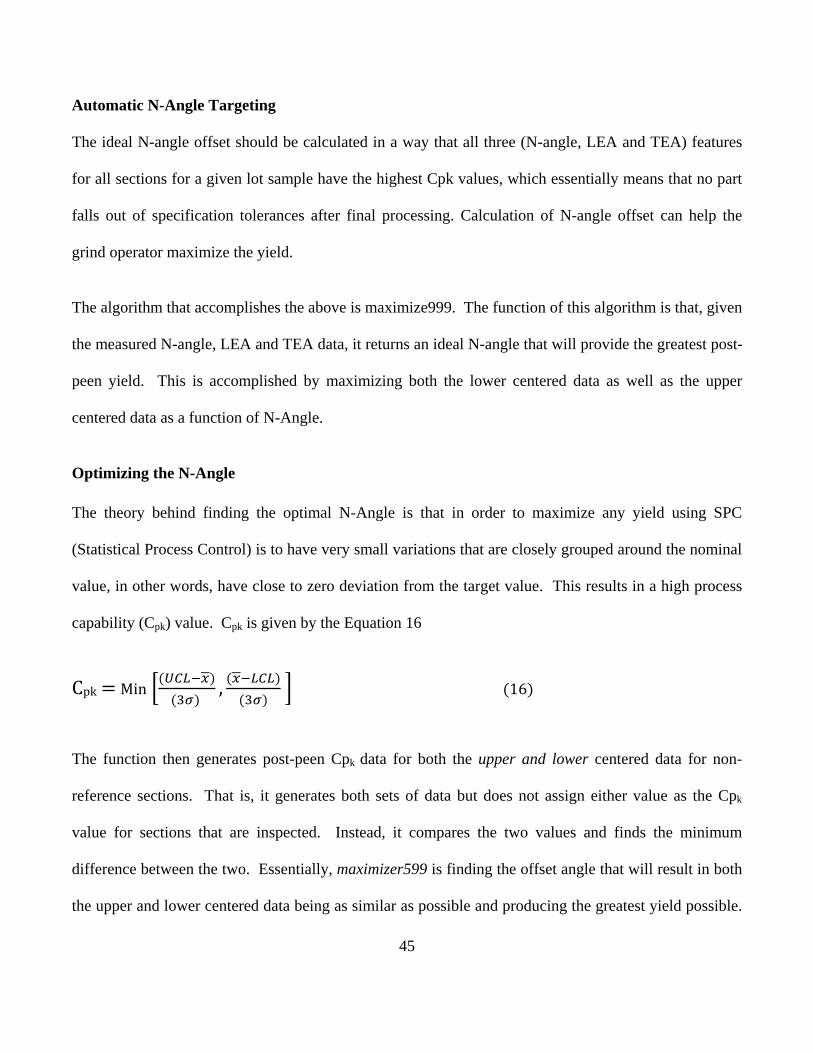
Visually, as represented in the Figure 5-2 below, maximizing both the lower and upper centered data

will result in an offset of approximately -12 minutes and an average Cpk of approximately 1.7.

Figure 5-2: Visual representation fo post peen Cpk vs Offset

5.4 Input data

The forging lots that were received from the supplier have to be inspected using the CMM to accept or

reject the lot. A random sample is taken from the lot for inspection; the sample size selection criteria

used is based on MIL-STD-105E [28]. General inspection level II is used and based on single sample

plan for normal inspection the sample size quantity of 10% (of the lot size ) or 20 minimum is used for

47

selection. These parts are then inspected; the raw inspection data is processed through blade software

that performs the liner and curvilinear fitting for each cross section based on the feature definitions. The

data is then compared to the original reverse engineered airfoil section data comprising of a series of

point coordinates and corresponding normal vectors to calculate the deviations for each feature. These

deviations are then reported in a text file output which is used as an input to the software tool, developed

during this project.

The input is then compiled in a spreadsheet which has airfoil, fillet and platform data each on a separate

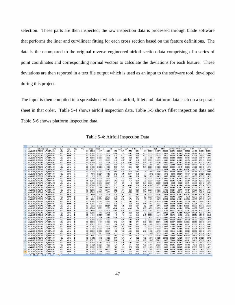
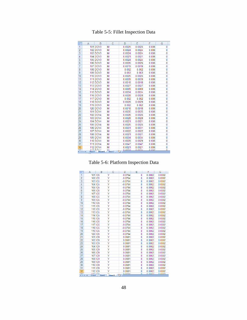
sheet in that order. Table 5-4 shows airfoil inspection data, Table 5-5 shows fillet inspection data and

Table 5-6 shows platform inspection data.

Table 5-4: Airfoil Inspection Data

48

Table 5-5: Fillet Inspection Data

Table 5-6: Platform Inspection Data

49

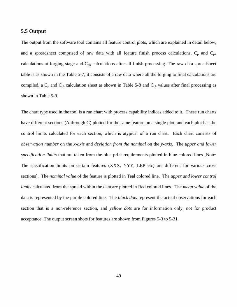
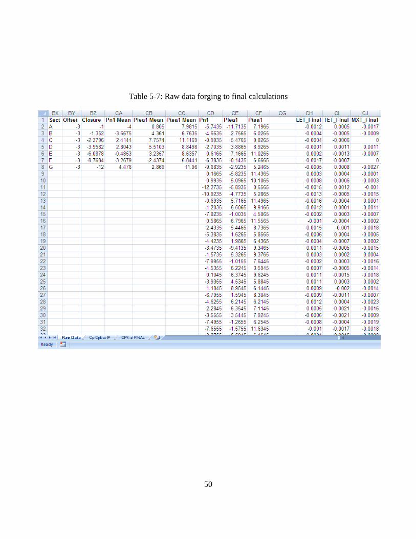
5.5 Output

The output from the software tool contains all feature control plots, which are explained in detail below,

and a spreadsheet comprised of raw data with all feature finish process calculations, Cp and Cpk

calculations at forging stage and Cpk calculations after all finish processing. The raw data spreadsheet

table is as shown in the Table 5-7; it consists of a raw data where all the forging to final calculations are

compiled, a Cp and Cpk calculation sheet as shown in Table 5-8 and Cpk values after final processing as

shown in Table 5-9.

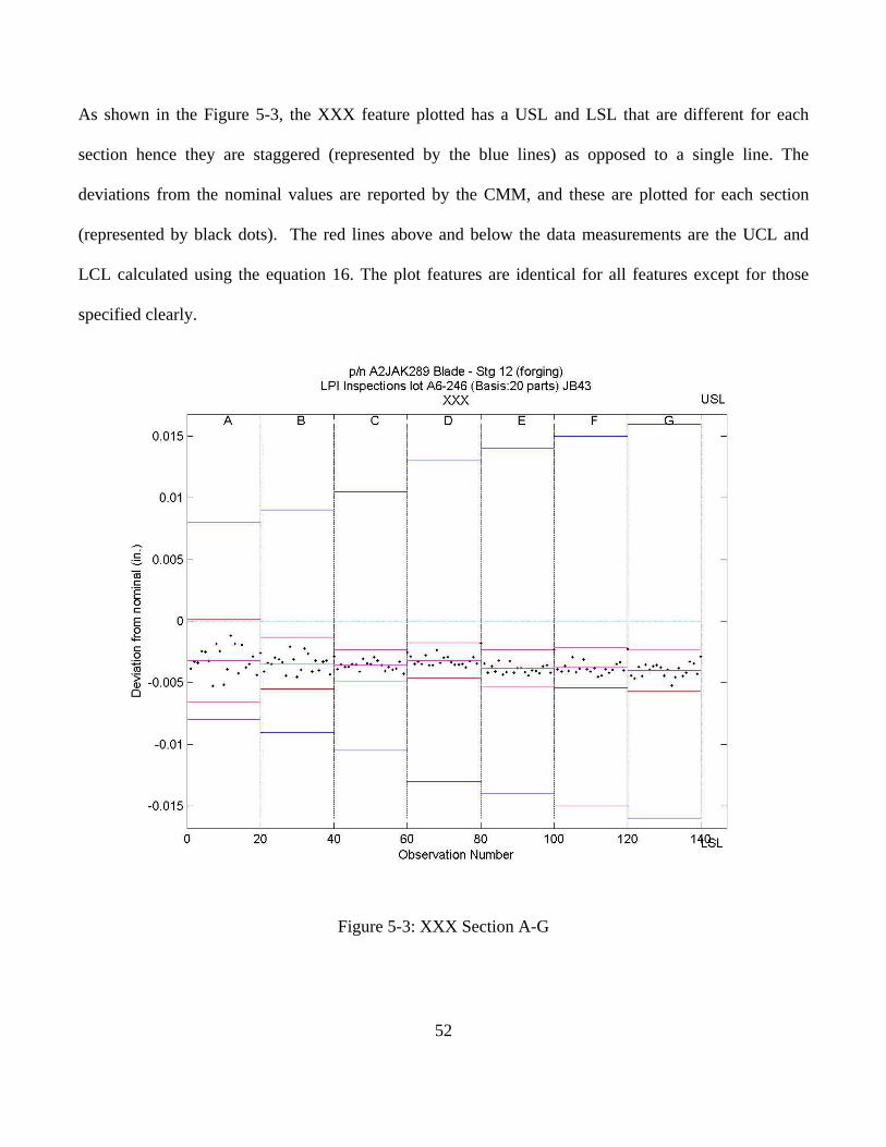
The chart type used in the tool is a run chart with process capability indices added to it. These run charts

have different sections (A through G) plotted for the same feature on a single plot, and each plot has the

control limits calculated for each section, which is atypical of a run chart. Each chart consists of

observation number on the x-axis and deviation from the nominal on the y-axis. The upper and lower

specification limits that are taken from the blue print requirements plotted in blue colored lines [Note:

The specification limits on certain features (XXX, YYY, LEP etc) are different for various cross

sections]. The nominal value of the feature is plotted in Teal colored line. The upper and lower control

limits calculated from the spread within the data are plotted in Red colored lines. The mean value of the

data is represented by the purple colored line. The black dots represent the actual observations for each

section that is a non-reference section, and yellow dots are for information only, not for product

acceptance. The output screen shots for features are shown from Figures 5-3 to 5-31.

50

Table 5-7: Raw data forging to final calculations

51

Table 5-8: Cp and Cpk calculations at IP (In-Process)

Table 5-9: Cpk at final processing

52

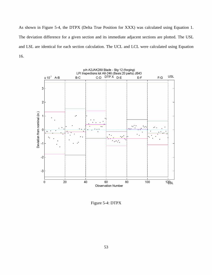
As shown in the Figure 5-3, the XXX feature plotted has a USL and LSL that are different for each

section hence they are staggered (represented by the blue lines) as opposed to a single line. The

deviations from the nominal values are reported by the CMM, and these are plotted for each section

(represented by black dots). The red lines above and below the data measurements are the UCL and

LCL calculated using the equation 16. The plot features are identical for all features except for those

specified clearly.

Figure 5-3: XXX Section A-G

53

As shown in Figure 5-4, the DTPX (Delta True Position for XXX) was calculated using Equation 1.

The deviation difference for a given section and its immediate adjacent sections are plotted. The USL

and LSL are identical for each section calculation. The UCL and LCL were calculated using Equation

16.

Figure 5-4: DTPX

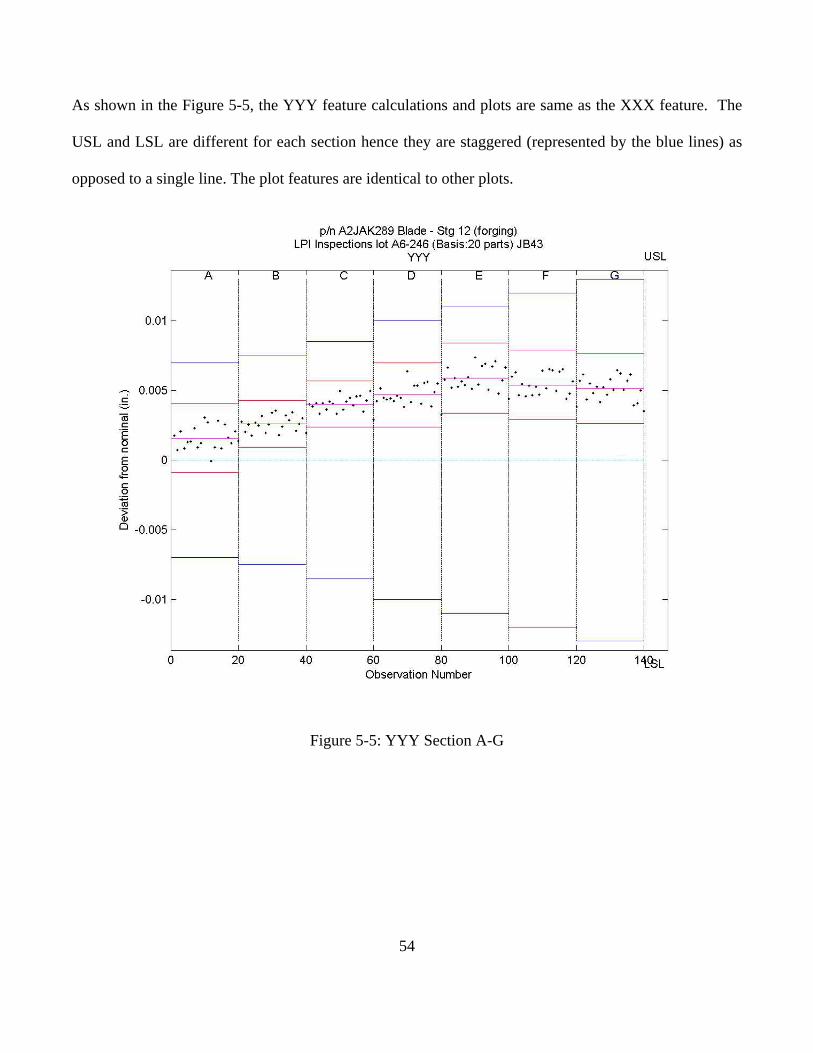
54

As shown in the Figure 5-5, the YYY feature calculations and plots are same as the XXX feature. The

USL and LSL are different for each section hence they are staggered (represented by the blue lines) as

opposed to a single line. The plot features are identical to other plots.

Figure 5-5: YYY Section A-G

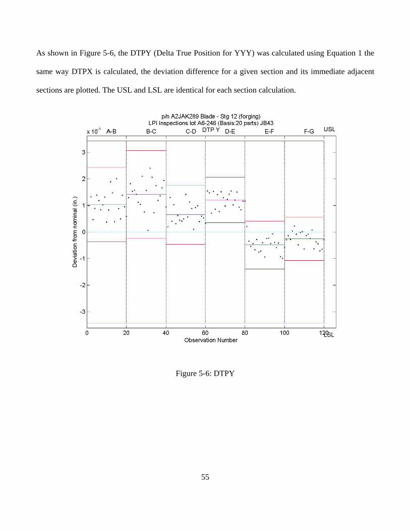
55

As shown in Figure 5-6, the DTPY (Delta True Position for YYY) was calculated using Equation 1 the

same way DTPX is calculated, the deviation difference for a given section and its immediate adjacent

sections are plotted. The USL and LSL are identical for each section calculation.

Figure 5-6: DTPY

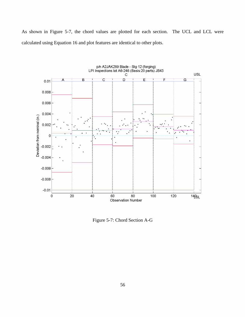
56

As shown in Figure 5-7, the chord values are plotted for each section. The UCL and LCL were

calculated using Equation 16 and plot features are identical to other plots.

Figure 5-7: Chord Section A-G

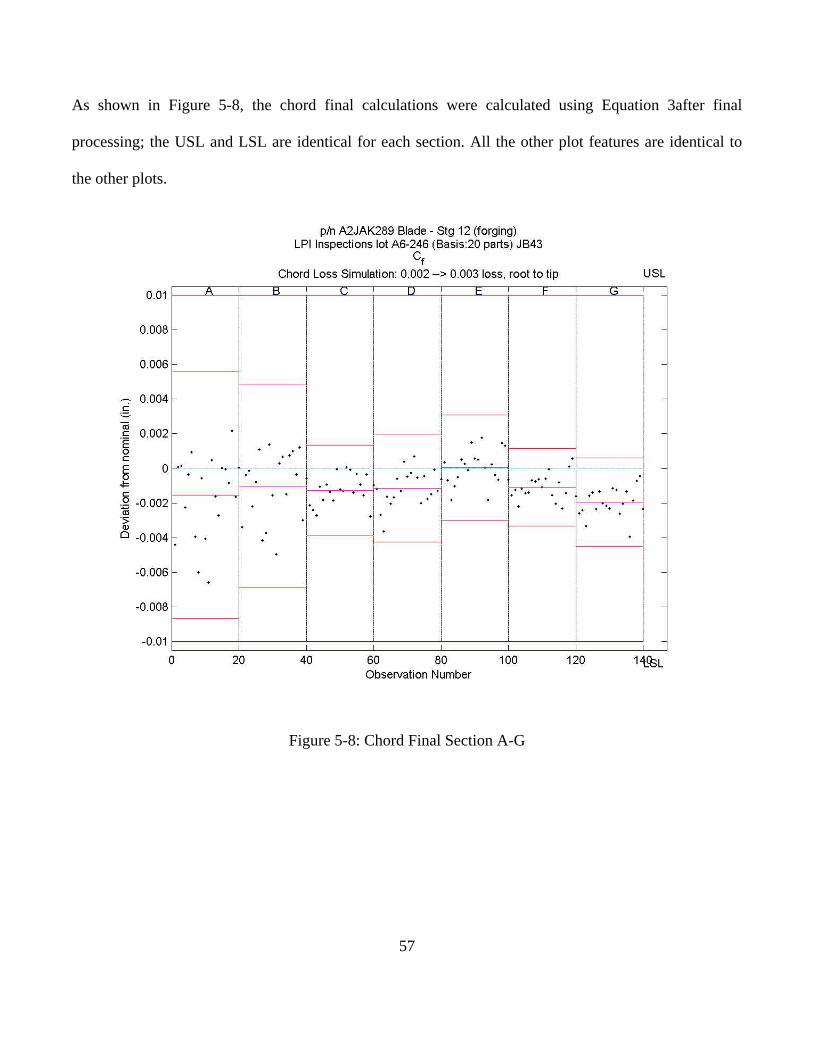
57

As shown in Figure 5-8, the chord final calculations were calculated using Equation 3after final

processing; the USL and LSL are identical for each section. All the other plot features are identical to

the other plots.

Figure 5-8: Chord Final Section A-G

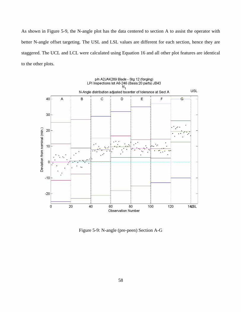
58

As shown in Figure 5-9, the N-angle plot has the data centered to section A to assist the operator with

better N-angle offset targeting. The USL and LSL values are different for each section, hence they are

staggered. The UCL and LCL were calculated using Equation 16 and all other plot features are identical

to the other plots.

Figure 5-9: N-angle (pre-peen) Section A-G

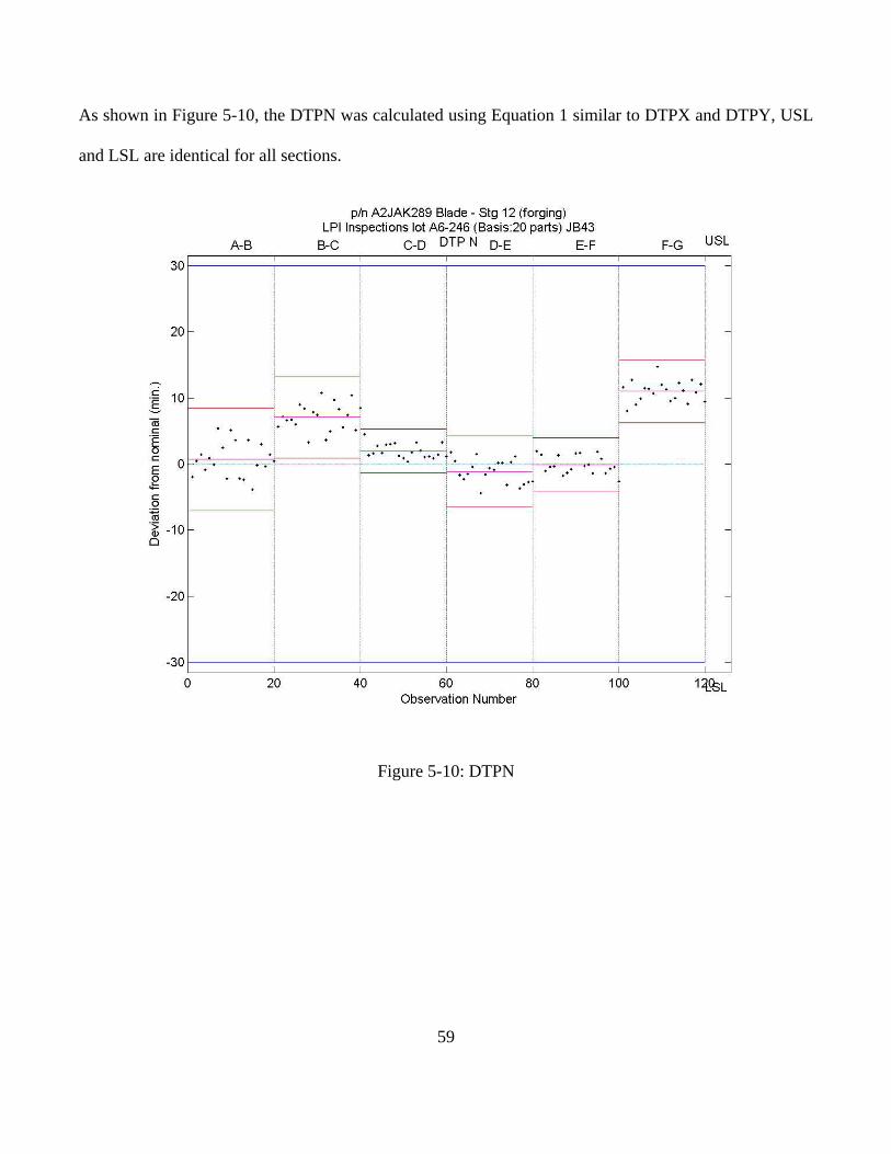
59

As shown in Figure 5-10, the DTPN was calculated using Equation 1 similar to DTPX and DTPY, USL

and LSL are identical for all sections.

Figure 5-10: DTPN

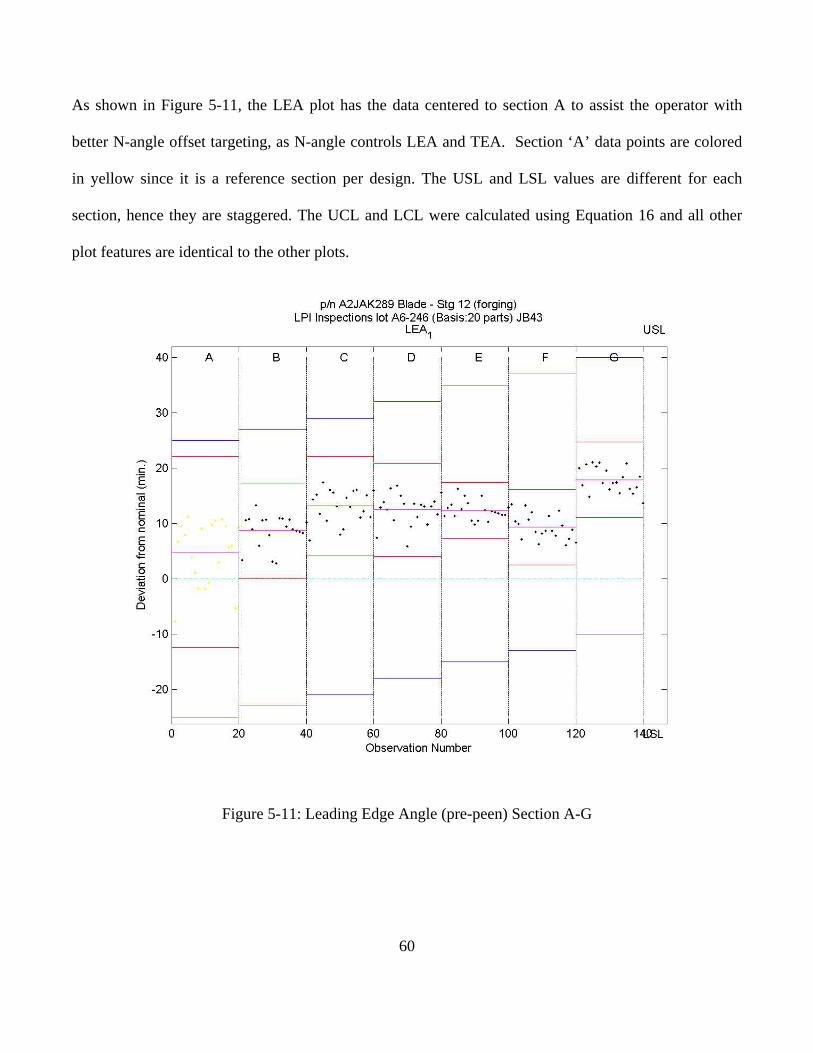
60

As shown in Figure 5-11, the LEA plot has the data centered to section A to assist the operator with

better N-angle offset targeting, as N-angle controls LEA and TEA. Section ‘A’ data points are colored

in yellow since it is a reference section per design. The USL and LSL values are different for each

section, hence they are staggered. The UCL and LCL were calculated using Equation 16 and all other

plot features are identical to the other plots.

Figure 5-11: Leading Edge Angle (pre-peen) Section A-G

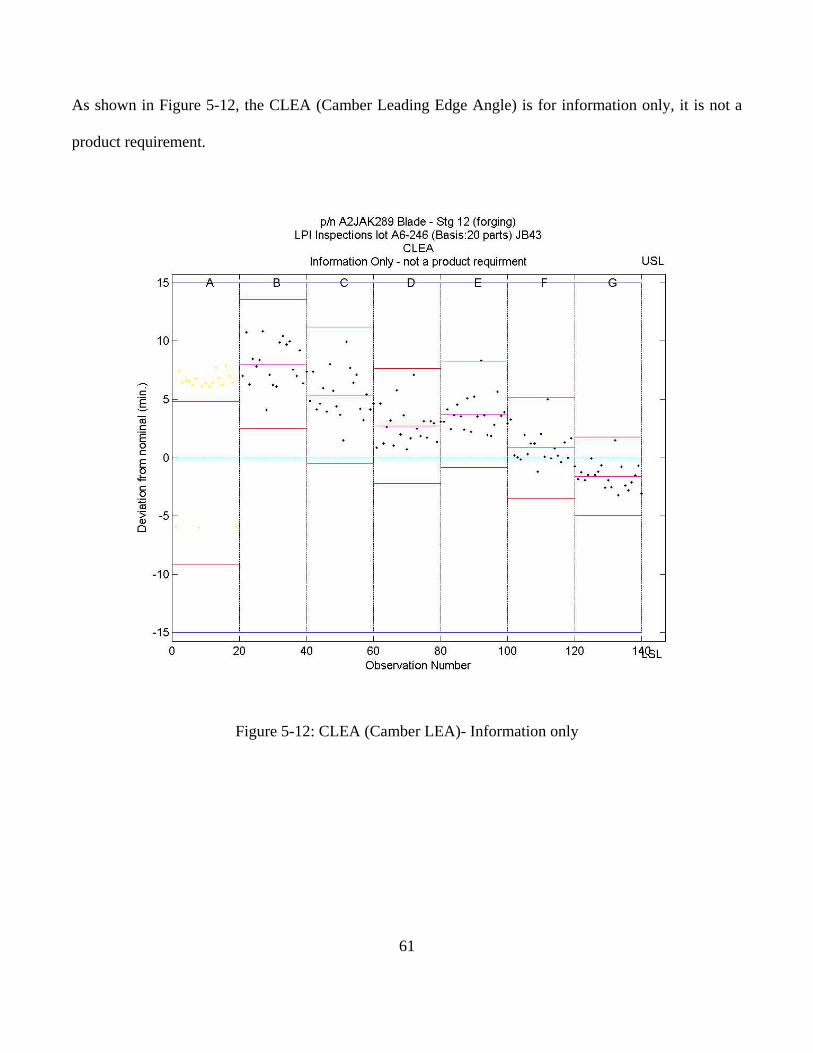
61

As shown in Figure 5-12, the CLEA (Camber Leading Edge Angle) is for information only, it is not a

product requirement.

Figure 5-12: CLEA (Camber LEA)- Information only

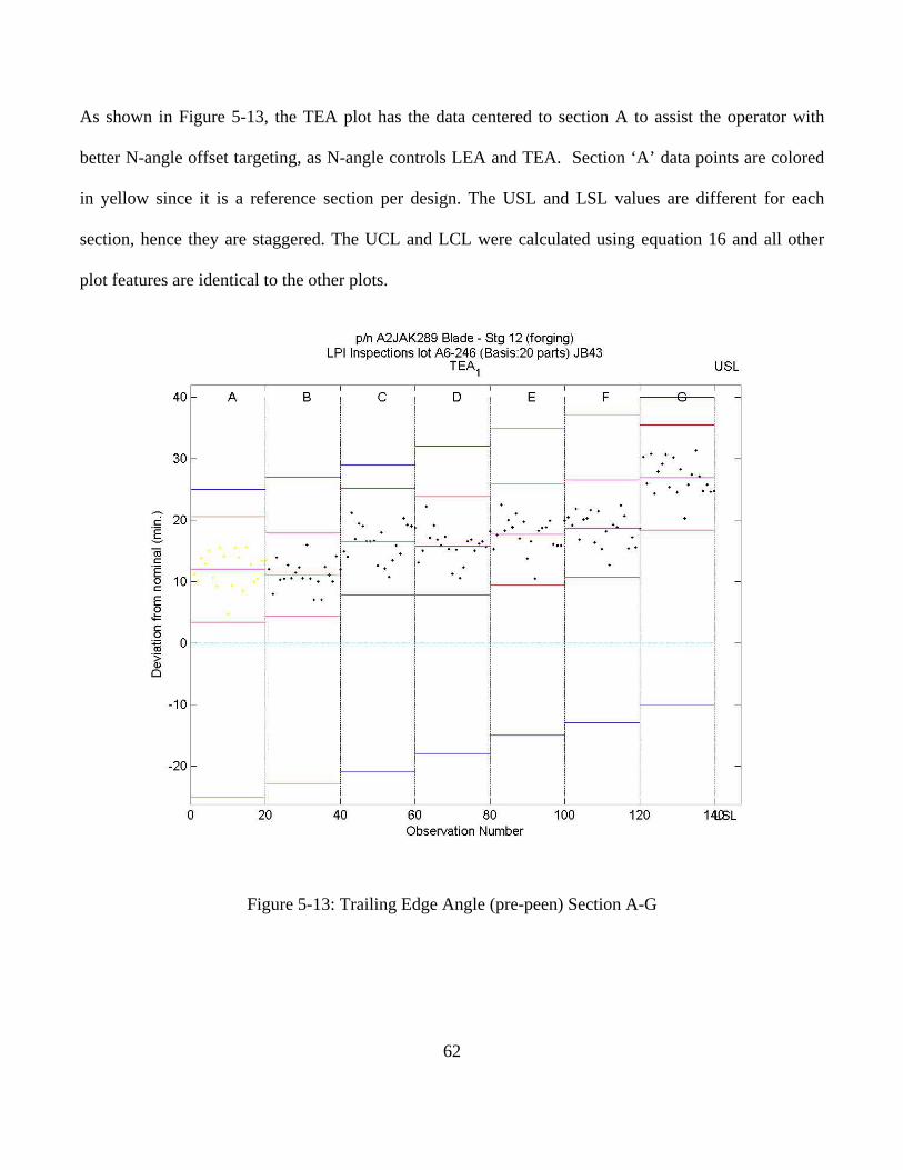
62

As shown in Figure 5-13, the TEA plot has the data centered to section A to assist the operator with

better N-angle offset targeting, as N-angle controls LEA and TEA. Section ‘A’ data points are colored

in yellow since it is a reference section per design. The USL and LSL values are different for each

section, hence they are staggered. The UCL and LCL were calculated using equation 16 and all other

plot features are identical to the other plots.

Figure 5-13: Trailing Edge Angle (pre-peen) Section A-G

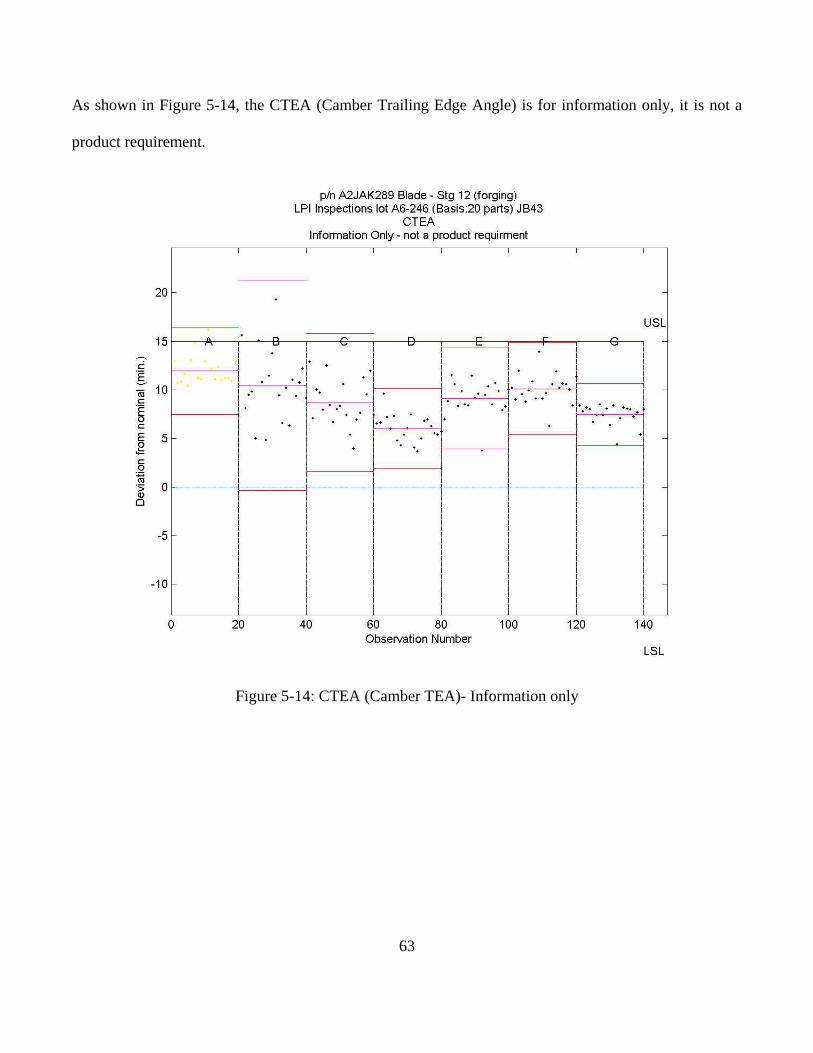
63

As shown in Figure 5-14, the CTEA (Camber Trailing Edge Angle) is for information only, it is not a

product requirement.

Figure 5-14: CTEA (Camber TEA)- Information only

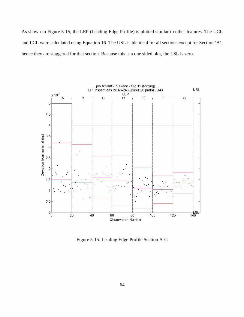
64

As shown in Figure 5-15, the LEP (Leading Edge Profile) is plotted similar to other features. The UCL

and LCL were calculated using Equation 16. The USL is identical for all sections except for Section ‘A’;

hence they are staggered for that section. Because this is a one sided plot, the LSL is zero.

Figure 5-15: Leading Edge Profile Section A-G

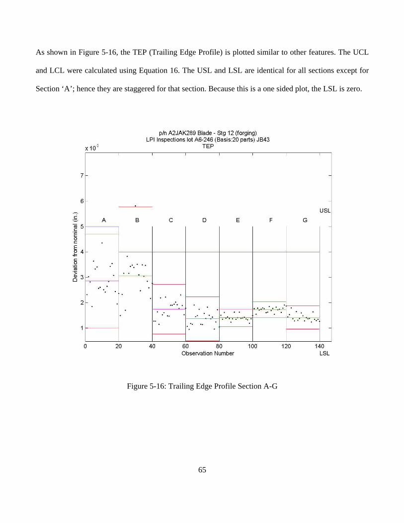
65

As shown in Figure 5-16, the TEP (Trailing Edge Profile) is plotted similar to other features. The UCL

and LCL were calculated using Equation 16. The USL and LSL are identical for all sections except for

Section ‘A’; hence they are staggered for that section. Because this is a one sided plot, the LSL is zero.

Figure 5-16: Trailing Edge Profile Section A-G

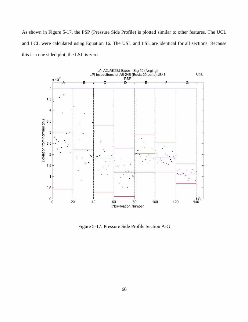
66

As shown in Figure 5-17, the PSP (Pressure Side Profile) is plotted similar to other features. The UCL

and LCL were calculated using Equation 16. The USL and LSL are identical for all sections. Because

this is a one sided plot, the LSL is zero.

Figure 5-17: Pressure Side Profile Section A-G

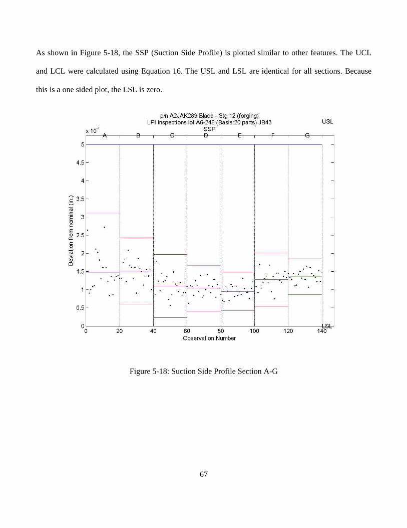
67

As shown in Figure 5-18, the SSP (Suction Side Profile) is plotted similar to other features. The UCL

and LCL were calculated using Equation 16. The USL and LSL are identical for all sections. Because

this is a one sided plot, the LSL is zero.

Figure 5-18: Suction Side Profile Section A-G

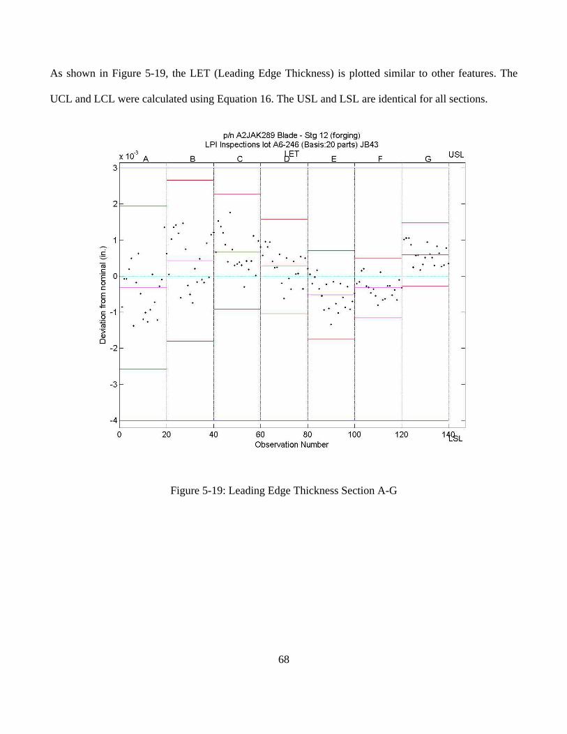
68

As shown in Figure 5-19, the LET (Leading Edge Thickness) is plotted similar to other features. The

UCL and LCL were calculated using Equation 16. The USL and LSL are identical for all sections.

Figure 5-19: Leading Edge Thickness Section A-G

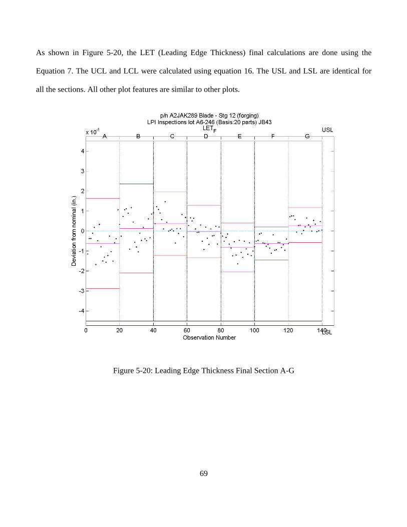
69

As shown in Figure 5-20, the LET (Leading Edge Thickness) final calculations are done using the

Equation 7. The UCL and LCL were calculated using equation 16. The USL and LSL are identical for

all the sections. All other plot features are similar to other plots.

Figure 5-20: Leading Edge Thickness Final Section A-G

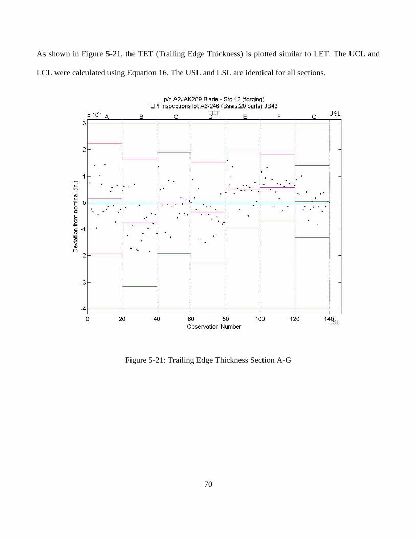
70

As shown in Figure 5-21, the TET (Trailing Edge Thickness) is plotted similar to LET. The UCL and

LCL were calculated using Equation 16. The USL and LSL are identical for all sections.

Figure 5-21: Trailing Edge Thickness Section A-G

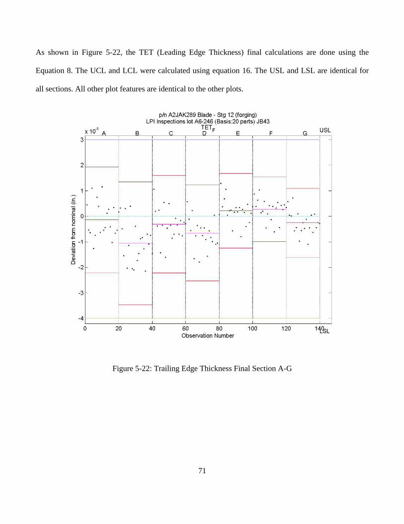
71

As shown in Figure 5-22, the TET (Leading Edge Thickness) final calculations are done using the

Equation 8. The UCL and LCL were calculated using equation 16. The USL and LSL are identical for

all sections. All other plot features are identical to the other plots.

Figure 5-22: Trailing Edge Thickness Final Section A-G

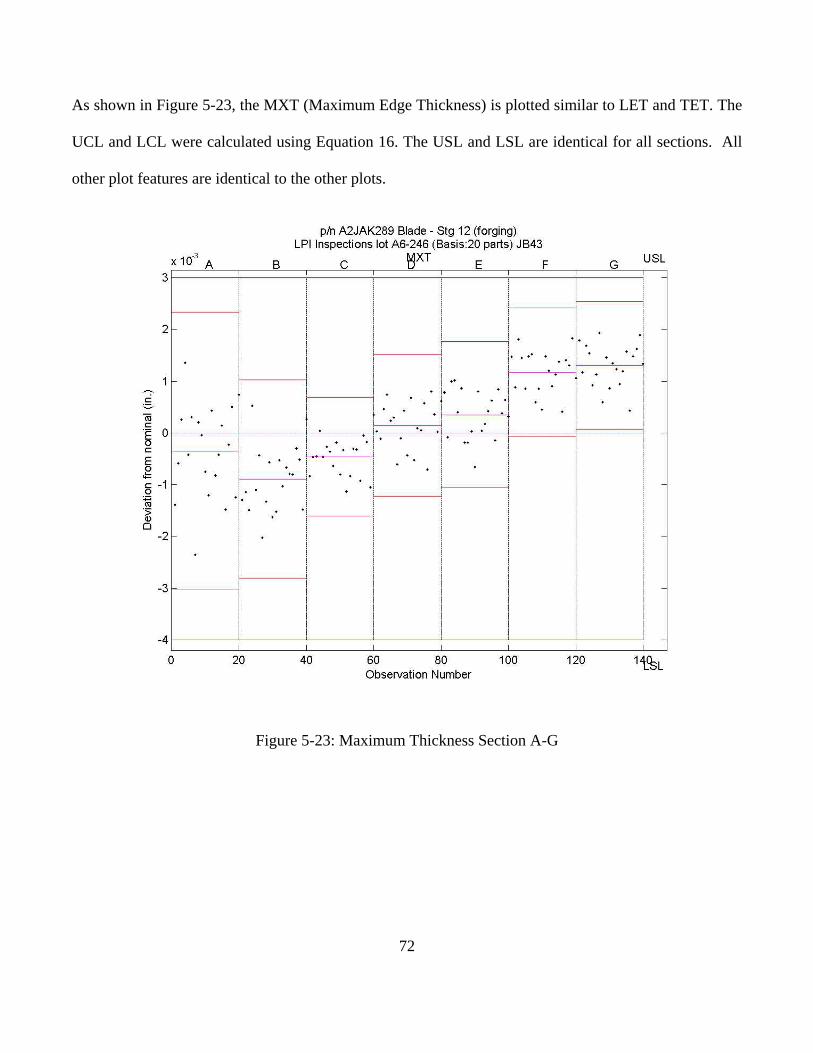
72

As shown in Figure 5-23, the MXT (Maximum Edge Thickness) is plotted similar to LET and TET. The

UCL and LCL were calculated using Equation 16. The USL and LSL are identical for all sections. All

other plot features are identical to the other plots.

Figure 5-23: Maximum Thickness Section A-G

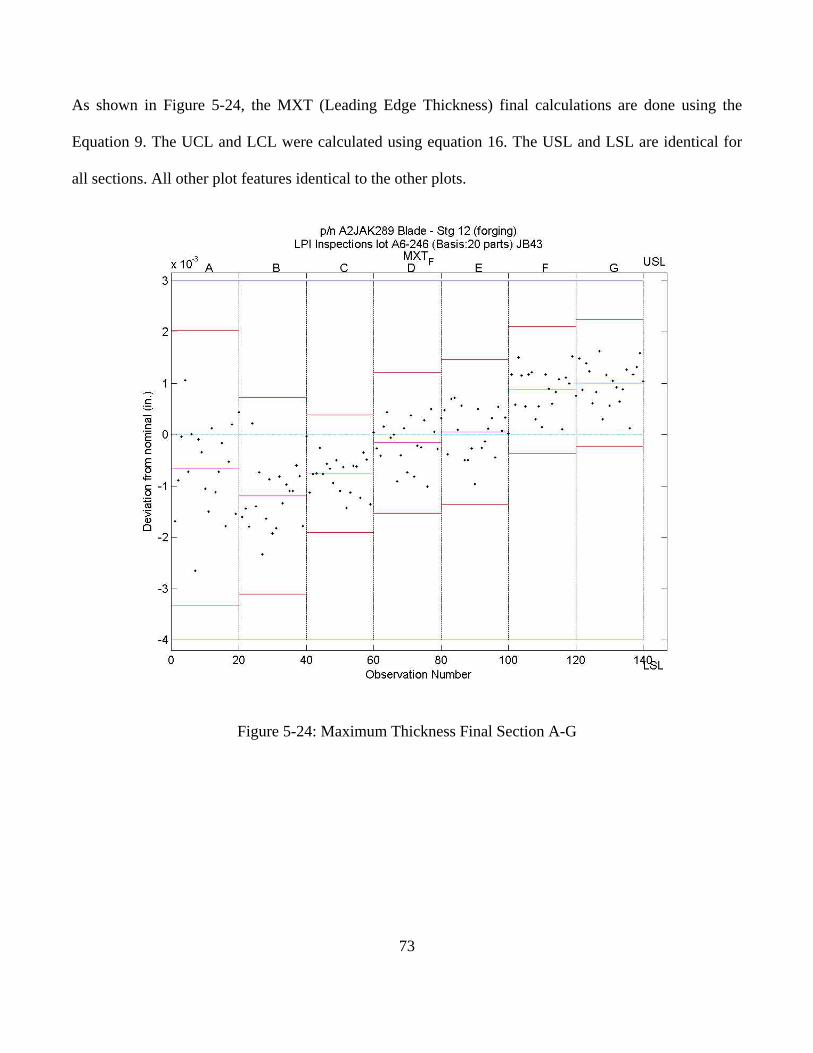
73

As shown in Figure 5-24, the MXT (Leading Edge Thickness) final calculations are done using the

Equation 9. The UCL and LCL were calculated using equation 16. The USL and LSL are identical for

all sections. All other plot features identical to the other plots.

Figure 5-24: Maximum Thickness Final Section A-G

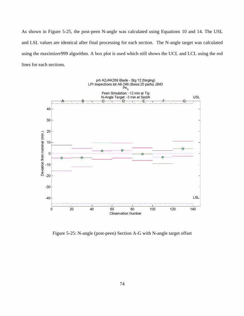
74

As shown in Figure 5-25, the post-peen N-angle was calculated using Equations 10 and 14. The USL

and LSL values are identical after final processing for each section. The N-angle target was calculated

using the maximizer999 algorithm. A box plot is used which still shows the UCL and LCL using the red

lines for each sections.

Figure 5-25: N-angle (post-peen) Section A-G with N-angle target offset

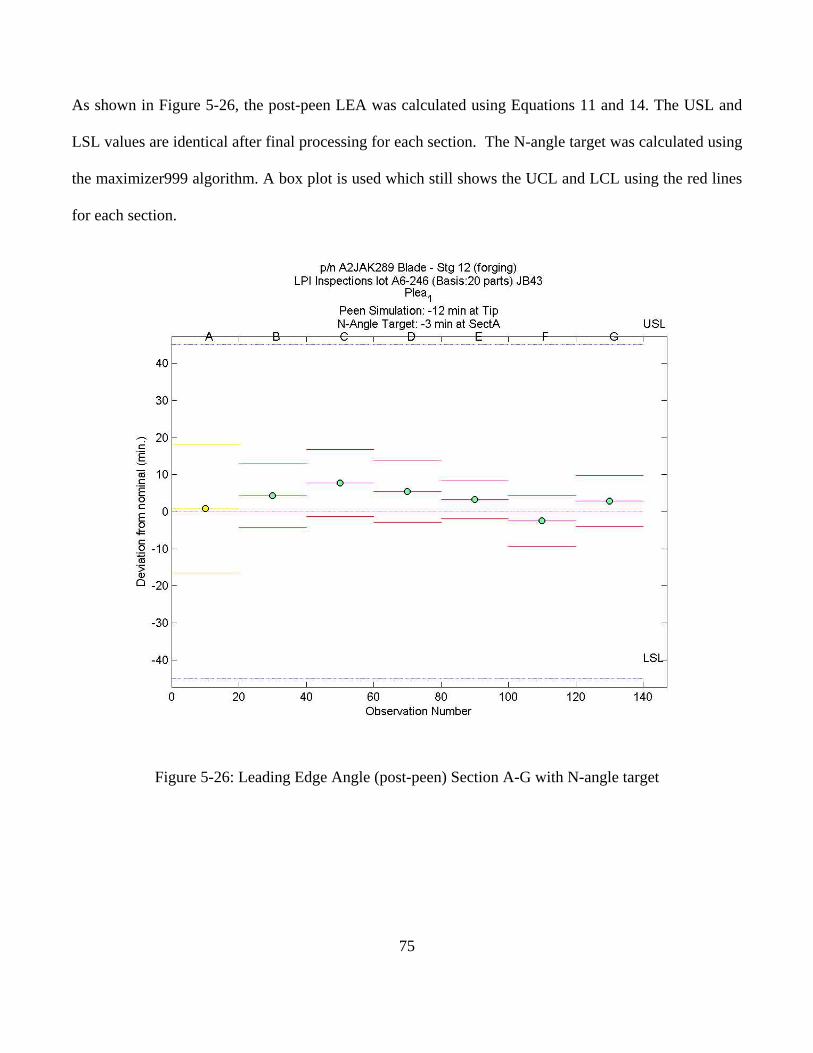
75

As shown in Figure 5-26, the post-peen LEA was calculated using Equations 11 and 14. The USL and

LSL values are identical after final processing for each section. The N-angle target was calculated using

the maximizer999 algorithm. A box plot is used which still shows the UCL and LCL using the red lines

for each section.

Figure 5-26: Leading Edge Angle (post-peen) Section A-G with N-angle target

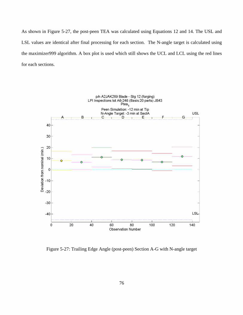
76

As shown in Figure 5-27, the post-peen TEA was calculated using Equations 12 and 14. The USL and

LSL values are identical after final processing for each section. The N-angle target is calculated using

the maximizer999 algorithm. A box plot is used which still shows the UCL and LCL using the red lines

for each sections.

Figure 5-27: Trailing Edge Angle (post-peen) Section A-G with N-angle target

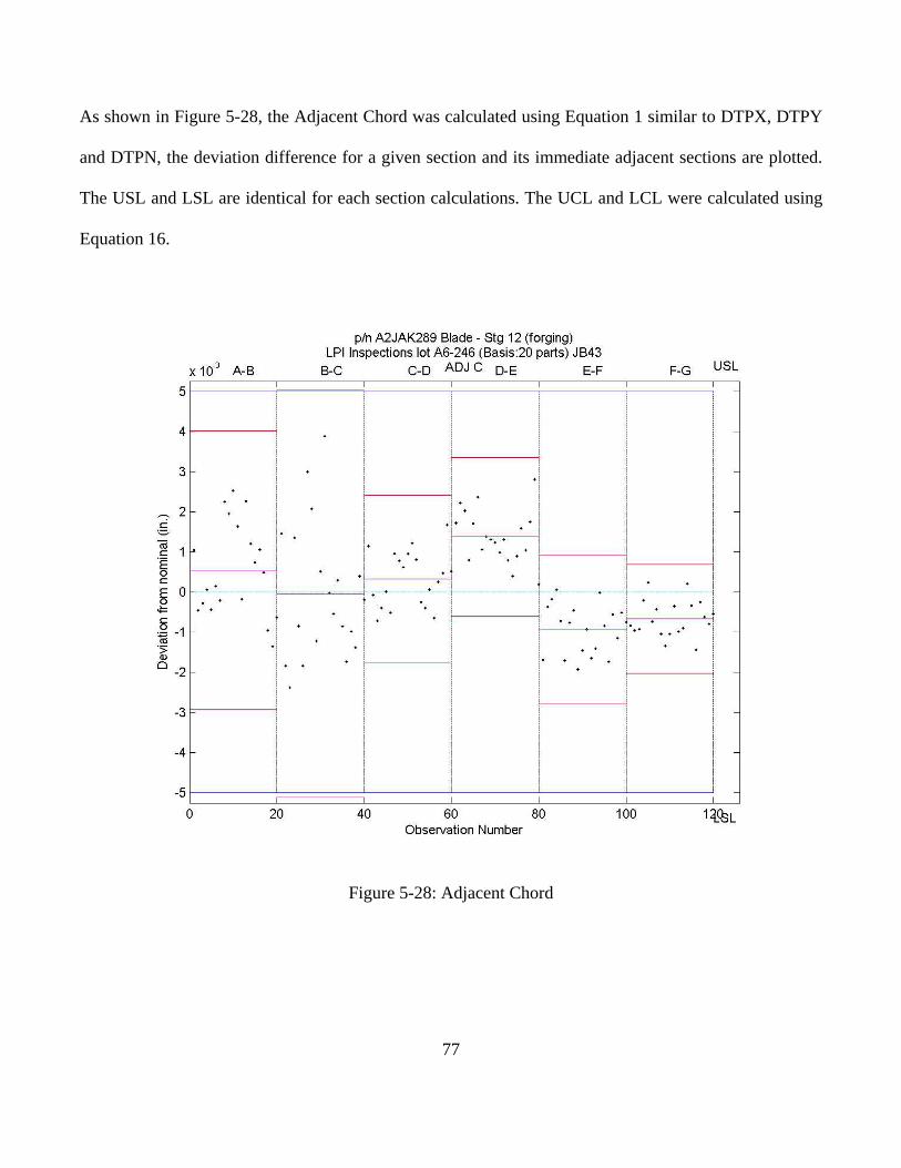
77

As shown in Figure 5-28, the Adjacent Chord was calculated using Equation 1 similar to DTPX, DTPY

and DTPN, the deviation difference for a given section and its immediate adjacent sections are plotted.

The USL and LSL are identical for each section calculations. The UCL and LCL were calculated using

Equation 16.

Figure 5-28: Adjacent Chord

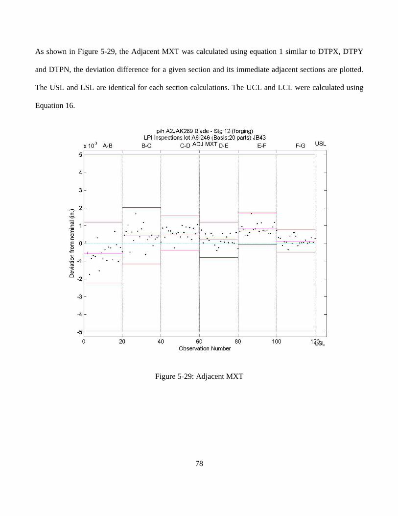
78

As shown in Figure 5-29, the Adjacent MXT was calculated using equation 1 similar to DTPX, DTPY

and DTPN, the deviation difference for a given section and its immediate adjacent sections are plotted.

The USL and LSL are identical for each section calculations. The UCL and LCL were calculated using

Equation 16.

Figure 5-29: Adjacent MXT

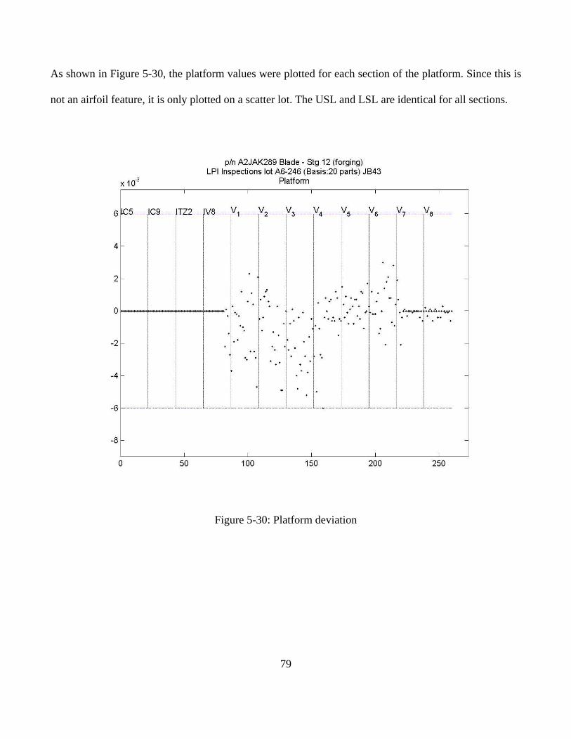
79

As shown in Figure 5-30, the platform values were plotted for each section of the platform. Since this is

not an airfoil feature, it is only plotted on a scatter lot. The USL and LSL are identical for all sections.

Figure 5-30: Platform deviation

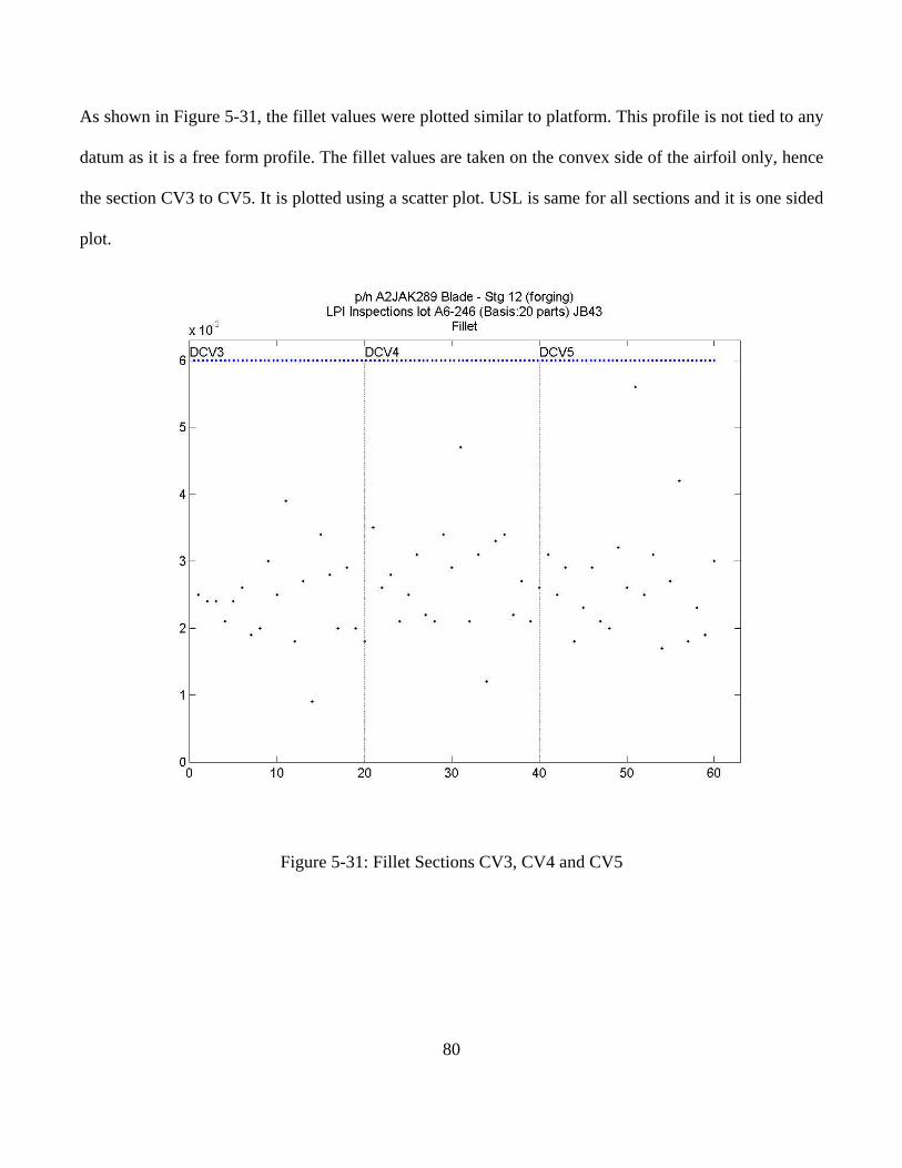
80

As shown in Figure 5-31, the fillet values were plotted similar to platform. This profile is not tied to any

datum as it is a free form profile. The fillet values are taken on the convex side of the airfoil only, hence

the section CV3 to CV5. It is plotted using a scatter plot. USL is same for all sections and it is one sided

plot.

Figure 5-31: Fillet Sections CV3, CV4 and CV5

81

5.6 Data Analysis and Interpretation

The output data from the software tool is a spreadsheet with all raw data and final calculations for all

compressor blade features. The Cp and Cpk values (see Table 5-8) for the established features [XXX,

YYY, C, N, LEA, TEA, LET, TET, and MXT] are reviewed to understand whether the forging process

was in control by looking at Cp and the targeting of the data using Cpk. Typically in a manufacturing

process it is common practice to aim to have Cp and Cpk greater than 1.33 (4-sigma), but in general Cp

and Cpk values of less than 1.0 (3-sigma) are considered bad and anything greater than 1.0 (3-sigma) as

good. The Cpk (see Table 5-9) after final processing gives you a clear picture of how the lot is going to

behave after all processing. This is a great way to focus your inspection efforts on features with bad Cp

and Cpk and specifically their respective sections that need to be inspected to have a safety net, in case

there is fallout. It is a requirement to inspect a minimum of three sections even if every feature and their

corresponding sections of the lot have relatively good Cp and Cpk values. This way minimum

inspection requirement is met to have enough confidence within our manufacturing process.

Disposition

Based on the results provided by the tool an engineer dispositions whether the lot is accepted or rejected.

If the lot is accepted an IMS [Inspection Method Sheet] is created that has the ideal N-angle target offset

and minimum sections that are needed to be inspected from the In-process stage to final stage, as shown

in Figure 5-32.

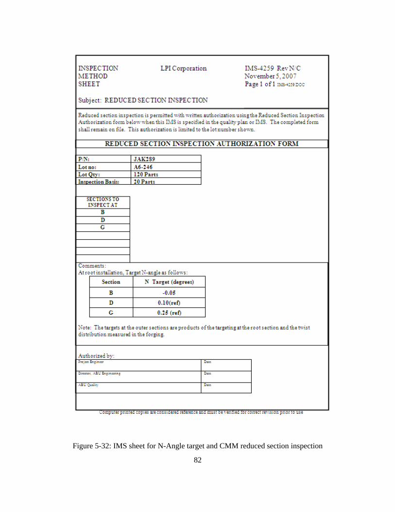
82

Figure 5-32: IMS sheet for N-Angle target and CMM reduced section inspection

83

5.7 Software Validation

The processing effects on all compressor blade features that were modeled are compared to actual data

to validate the effects; this process has taken much iteration to fine tune the models. Certain caution is

used while finalizing the models, as we took a conservative approach towards calculations of feature

variations. As with any model, continuous studies have to be carried out to understand the process shifts

and revalidate the calculations to accommodate any process shifts due to introducing new machines,

complete new approach to machine setups etc.

One such validation to a compressor blade is shown below. The forging data from several heat codes

was inspected, and feature variations were calculated using this software tool, and all the features are

inspected at final CMM inspection to validate the tool and its feature variation calculations. In the final

CMM inspection data, certain non-conforming parts were scrapped due to operator mishandling and

visual rejections. The Table 5-4 below shows the estimated final values for each main feature calculated

by the software tool, while Table 5-5 shows the actual final CMM inspection values, and Table 5-6

shows the difference between the calculated and actual values. Based on the data within the tables it can

be concluded that the software tool has accurately calculated the airfoil feature variations to within the

CMM inspection capability tolerances.

The cost saving shown in Table 5-13, shows the calculations based on hourly shop floor rate of $96.71

commonly used in savings calculations. The average number of airfoil sections used is 8, this number

varied from small (6 sections) to large compressor blades (13 sections). Total number of blades used is

50 per lot and 100 lots per month. The airfoil sections are CMM inspected twice, once at the In-process

stage at root installation and again at final CMM stage after all the processing has been completed.

Average inspection time per section is around 3 minutes using a scanning head probe, and this varies

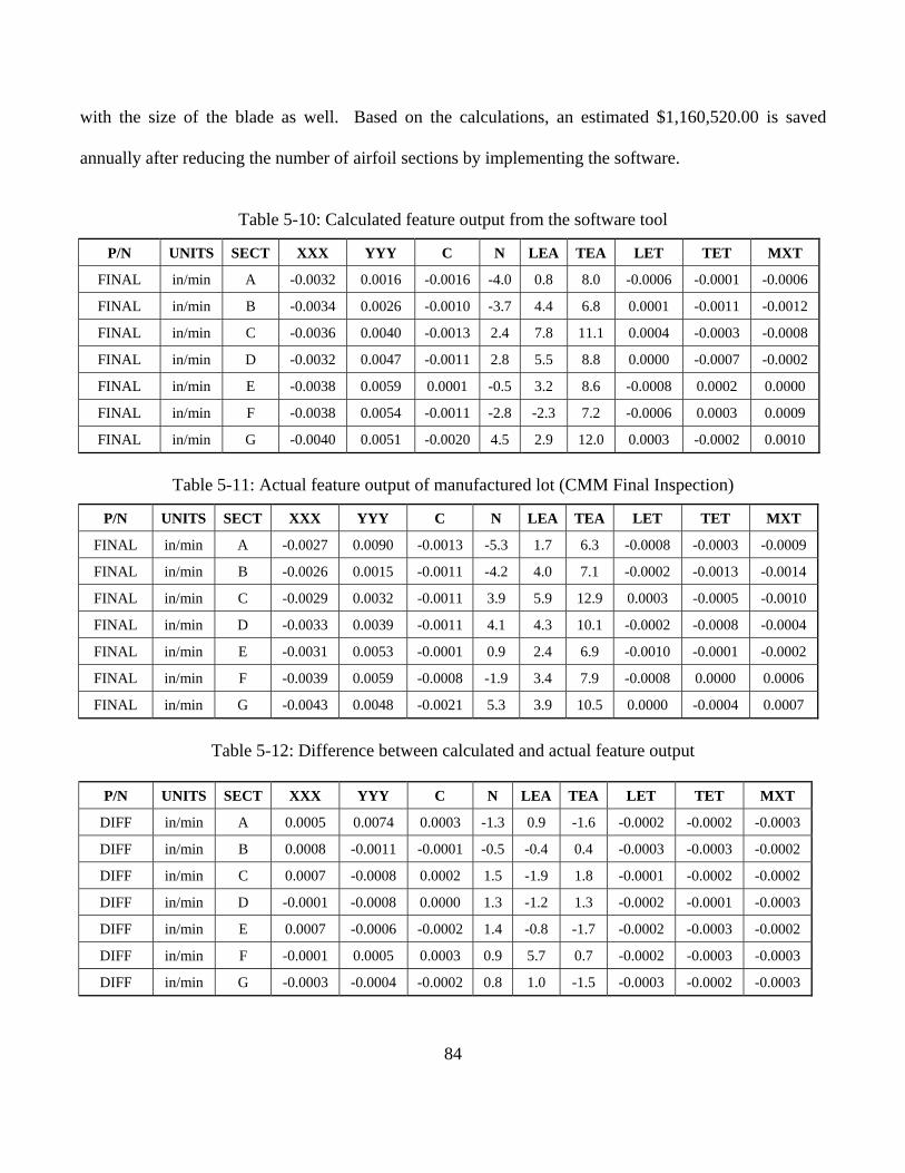
84

with the size of the blade as well. Based on the calculations, an estimated $1,160,520.00 is saved

annually after reducing the number of airfoil sections by implementing the software.

Table 5-10: Calculated feature output from the software tool

P/N UNITS SECT XXX YYY C N LEA TEA LET TET MXT

FINAL in/min A -0.0032 0.0016 -0.0016 -4.0 0.8 8.0 -0.0006 -0.0001 -0.0006

FINAL in/min B -0.0034 0.0026 -0.0010 -3.7 4.4 6.8 0.0001 -0.0011 -0.0012

FINAL in/min C -0.0036 0.0040 -0.0013 2.4 7.8 11.1 0.0004 -0.0003 -0.0008

FINAL in/min D -0.0032 0.0047 -0.0011 2.8 5.5 8.8 0.0000 -0.0007 -0.0002

FINAL in/min E -0.0038 0.0059 0.0001 -0.5 3.2 8.6 -0.0008 0.0002 0.0000

FINAL in/min F -0.0038 0.0054 -0.0011 -2.8 -2.3 7.2 -0.0006 0.0003 0.0009

FINAL in/min G -0.0040 0.0051 -0.0020 4.5 2.9 12.0 0.0003 -0.0002 0.0010

Table 5-11: Actual feature output of manufactured lot (CMM Final Inspection)

P/N UNITS SECT XXX YYY C N LEA TEA LET TET MXT

FINAL in/min A -0.0027 0.0090 -0.0013 -5.3 1.7 6.3 -0.0008 -0.0003 -0.0009

FINAL in/min B -0.0026 0.0015 -0.0011 -4.2 4.0 7.1 -0.0002 -0.0013 -0.0014

FINAL in/min C -0.0029 0.0032 -0.0011 3.9 5.9 12.9 0.0003 -0.0005 -0.0010

FINAL in/min D -0.0033 0.0039 -0.0011 4.1 4.3 10.1 -0.0002 -0.0008 -0.0004

FINAL in/min E -0.0031 0.0053 -0.0001 0.9 2.4 6.9 -0.0010 -0.0001 -0.0002

FINAL in/min F -0.0039 0.0059 -0.0008 -1.9 3.4 7.9 -0.0008 0.0000 0.0006

FINAL in/min G -0.0043 0.0048 -0.0021 5.3 3.9 10.5 0.0000 -0.0004 0.0007

Table 5-12: Difference between calculated and actual feature output

P/N UNITS SECT XXX YYY C N LEA TEA LET TET MXT

DIFF in/min A 0.0005 0.0074 0.0003 -1.3 0.9 -1.6 -0.0002 -0.0002 -0.0003

DIFF in/min B 0.0008 -0.0011 -0.0001 -0.5 -0.4 0.4 -0.0003 -0.0003 -0.0002

DIFF in/min C 0.0007 -0.0008 0.0002 1.5 -1.9 1.8 -0.0001 -0.0002 -0.0002

DIFF in/min D -0.0001 -0.0008 0.0000 1.3 -1.2 1.3 -0.0002 -0.0001 -0.0003

DIFF in/min E 0.0007 -0.0006 -0.0002 1.4 -0.8 -1.7 -0.0002 -0.0003 -0.0002

DIFF in/min F -0.0001 0.0005 0.0003 0.9 5.7 0.7 -0.0002 -0.0003 -0.0003

DIFF in/min G -0.0003 -0.0004 -0.0002 0.8 1.0 -1.5 -0.0003 -0.0002 -0.0003

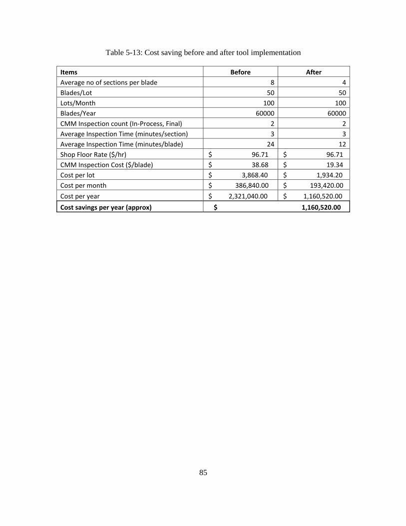
85

Table 5-13: Cost saving before and after tool implementation

Items  Before  After Average no of sections per blade  8 4Blades/Lot  50 50Lots/Month  100 100Blades/Year  60000 60000CMM Inspection count (In‐Process, Final)  2 2Average Inspection Time (minutes/section)  3 3Average Inspection Time (minutes/blade)  24 12Shop Floor Rate ($/hr)   $                        96.71    $                        96.71  CMM Inspection Cost ($/blade)   $                        38.68    $                        19.34  Cost per lot   $                  3,868.40    $                  1,934.20  Cost per month   $              386,840.00    $              193,420.00  

Cost per year   $          2,321,040.00    $          1,160,520.00  

Cost savings per year (approx)   $                                                   1,160,520.00  

86

CHAPTER 6. CONCLUSION AND FUTURE WORK

6.1 Conclusion

In conclusion the objective of this thesis is to develop and implement a software tool to calculate the

airfoil feature variations throughout the manufacturing process. The author did not come across any

literature where such a tool was presented or described, at least not on open literature. The tool was

developed mainly to help reduce the number of airfoil sections that are being inspected by using the

process control data (Cp, Cpk). The reduced section inspection was justified based on validation results

for each stage compressor blade’s forging airfoil inspection data, where each of the feature values that

are estimated by the tool after all manufacturing process is compared to the actual process data. Only

after the data is validated, by making sure that the tool is predicting the feature variations per processing

models, the tool is approved and implemented for that stage blade. The reduced sections are chosen

based on the Cp and Cpk values after all processing; the criteria suggested to choose a particular section

to be inspected is if for that section the airfoil feature Cp and Cpk values are <1 (3-sigma), and if all the

sections have values greater than 1, then only a minimum of three sections are required to be inspected

for the blade, usually bottom, middle and top section of the blade. This ensures that quality of the airfoil

is not compromised as those three sections are inspected for all compressor blades in that lot.

The N-angle target is a substantial aid to the grind operators as they target at an optimal N-angle offset

suggested as opposed to targeting at nominal. This eliminated all the fallouts after final CMM

inspection due to N-angle, LEA and TEA non-conformances.

87

And last but the least, the team is now able to disposition the forging lot as accept or reject based on the

information provided. This saved a lot of scrapped parts that would have otherwise been processed and

provided huge cost savings for the company.

Since the implementation of the tool, the business unit has saved approximately$ $1,160,520.00 per

year; numbers are calculated based on $96.71/hr shop floor compensation rate. This dollar amount is

based on average 8 section blade and the numbers are also calculated using a conservative estimate. The

biggest impact is the dollars we have saved for the business, also potentially eliminating the bottleneck

operation that was the CMM inspection.

6.2 Future Work

Future enhancements to the software tool might help generic audiences with the tool usage, for example

writing the tool as a standalone executable will eliminate the need of having the parent software installed

on the computer. Improved graphical user interface would help the users get a progress bar to

understand what the status of the tool is. Automation of the current manual data crunching of the CMM

inspection data (Input data) and programming the tool in a way the data output from the CMM can be

directly used as the input to the tool would further enhance this tool. Another farfetched idea is to use

the N-angle offset target as a live tool where the data can be adjusted real time after each CMM

inspected part that feeds into the tool real time and gives an automatic N-angle target for the next part

improving the yield of the lot. Lastly use similar methodologies towards root inspection and help reduce

the number of root features inspected, this would significantly help in cutting down the CMM inspection

time while providing cost savings to the business.

88

REFERENCES

[1] E. Torenbeek, H. W. (2002). Flight Physics: Essentials of Aeronautical Disciplines and Technology, with Historical Notes. London, NY: Springer Dordrecht Heidelberg.

[2] Allan, R. A. (2001). A History of the Personal Computer: The People and the Technology. London, Ontario, Canada: Allan Publishing.

[3] O'Regan, G. (2008). A Brief History of Computing. New York: Springer London Dordrecht Heidelberg.

[4] Hunecke, K. (2003). Jet Engines: Fundamentals of Theory, Design and Operation. Osceola, WI: Motorbooks International Publishers & Wholesalers.

[5] Brown, R. N. (2005). Compressors: Selection And Sizing. Elsevier, Inc.

[6] http://www.wisegeek.com/. (n.d.). Retrieved from http://www.wisegeek.com/: http://www.wisegeek.com/what-is-an-airfoil.htm

[7] Siṃha, R. (2006). Introduction To Basic Manufacturing Process & Workshop Technology. New Delhi: New Age International (P) Ltd, Publishers.

[8] FIA: Forging Industry Association. (n.d.). https://www.forging.org/forging-facts#1. Retrieved 2012, from http://www.forging.org: http://www.forging.org

[9] Hocken, R. J. (1995). Coordinate Measuring Machines and Systems. New York: Marcel Dekker, Inc.

[10] Boyce, M. P. (2012). Gas Turbine Engineering Handbook. Oxford: Elsevier Inc.

[11] FAA-H-8083-3A. (2004). Airplane Flying Handbook. U.S. Department of Transporation.FAA.

[12] Axial Compressor. (n.d.). Retrieved 11 2012, from wikipedia: http://en.wikipedia.org/wiki/Axial_compressor

[13] Oates, G. C. (1985). Aerothermodynamics of Aircraft Engine Components. N.Y: American Institute of Aeronautics and Astronautics, Inc.

[14] JA650. (02/14/2002). Engineering SPecification. Airfoil Geometric Definition, Terminology, and Methods .

[15] Wiki_GE_CF6. (n.d.). Retrieved from http://en.wikipedia.org/wiki/General_Electric_CF6

[16] wiki_CFM56. (n.d.). Retrieved from http://en.wikipedia.org/wiki/CFM_International_CFM56

89

[17] Hitech Alloy Products. (n.d.). Retrieved 11 2012, from www.hitechalloys.com: http://www.hitechalloys.com/hitechalloys_002.htm

[18] Grinding (abrasive cutting). (n.d.). Retrieved 05 2012, from wikipedia.org: http://en.wikipedia.org/wiki/Grinding_%28abrasive_cutting%29

[19] Benedict, G. F. (1987). Nontraditional Manufacturing Processes. N.Y: Marcel Dekker, Inc.

[20] Donald O. Thompson, D. E. (1997). Review of Progress in Quantitative Nondestructive Evaluation, Volume 16. N.Y: Plenum Press, New York.

[21] Fluorescent Penetrant Inspection. (n.d.). Retrieved 11 2012, from http://turbineresourcesinc.com: http://turbineresourcesinc.com/services/services.htm

[22] Fluorescent penetrant inspection materials. (n.d.). Retrieved 11 2012, from http://www.tjskl.org.cn/: http://www.tjskl.org.cn/products/cza23159/fluorescent_penetrant_inspection_materials-pz25d74cd.html

[23] Shot Peening. (n.d.). Retrieved from www.wikipedia.org: http://en.wikipedia.org/wiki/Shot_peening

[24] Hocken, R. (2011). Coordinate measuring machines and systems. CRC Press Inc.

[25] PC-DMIS Blade. (n.d.). Retrieved 11 2012, from www.pcdmis.com: http://www.pcdmis.com/products/pc-dmis-blade

[26] Barbara F. Ryan, B. L. (2005). Minitab Handbook: Updated for Release 14. Canada: Thomson Learning, Inc.

[27] MATLAB: Guide by Higham, Desmond J; Higham, Nicholas J; Books24x7, Inc

[28] Defense, D. o. (1989). MIL-STD-105E. U. S. Army Armament Research, Development and Engineering Center.

90

APPENDIX: SOURCE CODE Main Program:

function forecast(str) close all clc global bladeCount c_loss r lot sectQ global header sect closure Pref partFile global NaOffset Psim Ftol Ptol disp('Please select from the following: ') disp('1 - Full Forecast (Lots over 100 pieces)') disp('2 - Limited Forecast (Lots 100 pieces and less)') choice = input(' Please choose a number and press enter: '); clc disp('Please select from the following: ') disp('1 - Automatic N-Angle Targeting') disp('2 - Manual N-Angle Entry') nChoice = input(' Please choose a number and press enter: '); clc %Read in and determine size of the raw data from the Excel Spreadsheet [num txt raw] = xlsread(str,'Sheet1'); clear txt; %Reading in excel file with raw data. [r c] = size(raw); lot = raw{2,2}; %Sets the lot name from the raw data partFile = raw{2,1}; %Finds what part is being estimated %Determine what sections are present and how many sections in total section = raw{2,7}; count = 1; sectQ = []; sectCount = []; for index = 3:r test = raw{index,7}; if strcmpi(test,section) count = count + 1; if index == r sectQ = [sectQ,section]; sectCount = [sectCount, count]; end

91

elseif ~strcmpi(test,section) sectQ = [sectQ, section]; sectCount = [sectCount,count]; count = 1; section = test; end end sect = length(sectQ); bladeCount = (r-1)/sect; test=[]; count=[]; %Check to make sure there are an equal number of files present for each %blade. for index = 2:length(sectCount) if sectCount(index-1) ~= sectCount(index) error('ErrorTests:failTest', 'Check the number of files for each section, "re-crunch" and put \n into a new excel spreadsheet') break end end run(partFile); %Tolerance File %%%% Begin Actual Blade Calculations %%%% %%% Forging Level Calculations %%%% %Mean and Standard Deviation of features [Xavg Xdev] = staker2(num(:,2),sect); [Yavg Ydev] = staker2(num(:,3),sect); [Cavg Cdev] = staker2(num(:,4),sect); [Naavg Nadev] = staker2(num(:,5),sect); [Laavg Ladev] = staker2(num(:,7),sect); [Taavg Tadev] = staker2(num(:,9),sect); [Ltavg Ltdev] = staker2(num(:,10),sect); [Ttavg Ttdev] = staker2(num(:,11),sect); [Mtavg Mtdev] = staker2(num(:,12),sect); [Clavg Cldev] = staker2(num(:,6),sect); [Ctavg Ctdev] = staker2(num(:,8),sect); [Lpavg Lpdev] = staker2(num(:,15),sect); [Ppavg Ppdev] = staker2(num(:,16),sect); [Tpavg Tpdev] = staker2(num(:,17),sect); [Spavg Spdev] = staker2(num(:,18),sect); %N, LEA, TEA "Normalization" if strcmpi(partFile,'A2JAK818') normalizer = Naavg(2);

92

else normalizer = Naavg(1); end N1 = num(:,5) - normalizer; N1avg = staker2(N1,sect); LEA1 = num(:,7) - normalizer; LEA1avg = staker2(LEA1,sect); TEA1 = num(:,9) - normalizer; TEA1avg = staker2(TEA1,sect); normAngs = [N1 LEA1 TEA1]; avgs = [Xavg Yavg Cavg N1avg LEA1avg TEA1avg Ltavg Ttavg Mtavg]; %Puts all the features together in a matrix devs = [Xdev Ydev Cdev Nadev Ladev Tadev Ltdev Ttdev Mtdev]; %DTP %individual DTP dtpMat = DTPer(num(:,[2,3,5,4,12])); %Output colums: X,Y,N,C,MXT % Averages [dXavg dXdev] = staker2(dtpMat(:,1),(sect-1)); [dYavg dYdev] = staker2(dtpMat(:,2),(sect-1)); [dNavg dNdev] = staker2(dtpMat(:,3),(sect-1)); [aCavg aCdev] = staker2(dtpMat(:,4),(sect-1)); [aMavg aMdev] = staker2(dtpMat(:,5),(sect-1)); dtpMat = dtpMat(1:(bladeCount*(sect-1)),:); %reduces size of dtpMat to elimate unnecessary zeros. deltaAvg =[dXavg dYavg dNavg aCavg aMavg]; %%%Cp/Cpk @ IP: [xcpk xcp] = CpKer([Xavg Xdev],XSL); [ycpk ycp] = CpKer([Yavg Ydev],YSL); [ccpk ccp] = CpKer([Cavg Cdev],CSL); [nacpk nacp] = CpKer([N1avg Nadev],NaSL); [lacpk lacp] = CpKer([LEA1avg Ladev],LaSL); [tacpk tacp] = CpKer([TEA1avg Tadev],TaSL); [ltcpk ltcp] = CpKer([Ltavg Ltdev],LETSL); [ttcpk ttcp] = CpKer([Ttavg Ttdev],TETSL); [mtcpk mtcp] = CpKer([Mtavg Mtdev],MXTSL); cp_IP = [xcp ycp ccp nacp lacp tacp ltcp ttcp mtcp];

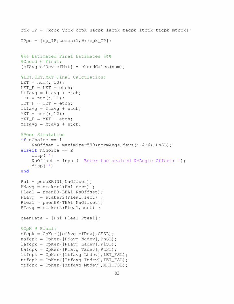
93

cpk_IP = [xcpk ycpk ccpk nacpk lacpk tacpk ltcpk ttcpk mtcpk]; IPpc = [cp_IP;zeros(1,9);cpk_IP]; %%% Estimated Final Estimates %%% %Chord @ Final: [cfAvg cfDev cfMat] = chordCalcs(num); %LET,TET,MXT Final Calculation: LET = num(:,10); LET_F = LET + etch; Ltfavg = Ltavg + etch; TET = num(:,11); TET_F = TET + etch; Ttfavg = Ttavg + etch; MXT = num(:,12); MXT_F = MXT + etch; Mtfavg = Mtavg + etch; %Peen Simulation if nChoice == 1 NaOffset = maximizer599(normAngs,devs(:,4:6),PnSL); elseif nChoice == 2 disp('') NaOffset = input(' Enter the desired N-Angle Offset: '); disp('') end Pn1 = peenER(N1,NaOffset); PNavg = staker2(Pn1,sect) ; Plea1 = peenER(LEA1,NaOffset); PLavg = staker2(Plea1,sect) ; Ptea1 = peenER(TEA1,NaOffset); PTavg = staker2(Ptea1,sect) ; peenData = [Pn1 Plea1 Ptea1]; %CpK @ Final: cfcpk = CpKer([cfAvg cfDev],CFSL); nafcpk = CpKer([PNavg Nadev],PnSL); lafcpk = CpKer([PLavg Ladev],PlSL); tafcpk = CpKer([PTavg Tadev],PtSL); ltfcpk = CpKer([Ltfavg Ltdev],LET_FSL); ttfcpk = CpKer([Ttfavg Ttdev],TET_FSL); mtfcpk = CpKer([Mtfavg Mtdev],MXT_FSL);

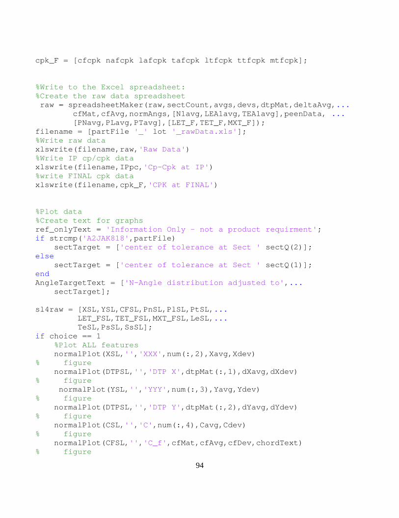
94

cpk_F = [cfcpk nafcpk lafcpk tafcpk ltfcpk ttfcpk mtfcpk]; %Write to the Excel spreadsheet: %Create the raw data spreadsheet raw = spreadsheetMaker(raw,sectCount,avgs,devs,dtpMat,deltaAvg,... cfMat,cfAvg,normAngs,[N1avg,LEA1avg,TEA1avg],peenData, ... [PNavg,PLavg,PTavg],[LET_F,TET_F,MXT_F]); filename = [partFile '_' lot '_rawData.xls']; %Write raw data xlswrite(filename,raw,'Raw Data') %Write IP cp/cpk data xlswrite(filename,IPpc,'Cp-Cpk at IP') %write FINAL cpk data xlswrite(filename,cpk_F,'CPK at FINAL') %Plot data %Create text for graphs ref_onlyText = 'Information Only - not a product requirment'; if strcmp('A2JAK818',partFile) sectTarget = ['center of tolerance at Sect ' sectQ(2)]; else sectTarget = ['center of tolerance at Sect ' sectQ(1)]; end AngleTargetText = ['N-Angle distribution adjusted to',... sectTarget]; sl4raw = [XSL,YSL,CFSL,PnSL,PlSL,PtSL,... LET_FSL,TET_FSL,MXT_FSL,LeSL,... TeSL,PsSL,SsSL]; if choice == 1 %Plot ALL features normalPlot(XSL,'','XXX',num(:,2),Xavg,Xdev) % figure normalPlot(DTPSL,'','DTP X',dtpMat(:,1),dXavg,dXdev) % figure normalPlot(YSL,'','YYY',num(:,3),Yavg,Ydev) % figure normalPlot(DTPSL,'','DTP Y',dtpMat(:,2),dYavg,dYdev) % figure normalPlot(CSL,'','C',num(:,4),Cavg,Cdev) % figure normalPlot(CFSL,'','C_f',cfMat,cfAvg,cfDev,chordText) % figure

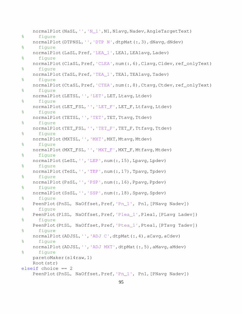
95

normalPlot(NaSL,'','N_1',N1,N1avg,Nadev,AngleTargetText) % figure normalPlot(DTPNSL,'','DTP N',dtpMat(:,3),dNavg,dNdev) % figure normalPlot(LaSL,Pref,'LEA_1',LEA1,LEA1avg,Ladev) % figure normalPlot(ClaSL,Pref,'CLEA',num(:,6),Clavg,Cldev,ref_onlyText) % figure normalPlot(TaSL,Pref,'TEA_1',TEA1,TEA1avg,Tadev) % figure normalPlot(CtaSL,Pref,'CTEA',num(:,8),Ctavg,Ctdev,ref_onlyText) % figure normalPlot(LETSL,'','LET',LET,Ltavg,Ltdev) % figure normalPlot(LET_FSL,'','LET_F',LET_F,Ltfavg,Ltdev) % figure normalPlot(TETSL,'','TET',TET,Ttavg,Ttdev) % figure normalPlot(TET_FSL,'','TET_F',TET_F,Ttfavg,Ttdev) % figure normalPlot(MXTSL,'','MXT',MXT,Mtavg,Mtdev) % figure normalPlot(MXT_FSL,'','MXT_F',MXT_F,Mtfavg,Mtdev) % figure normalPlot(LeSL,'','LEP',num(:,15),Lpavg,Lpdev) % figure normalPlot(TeSL,'','TEP',num(:,17),Tpavg,Tpdev) % figure normalPlot(PsSL,'','PSP',num(:,16),Ppavg,Ppdev) % figure normalPlot(SsSL,'','SSP',num(:,18),Spavg,Spdev) % figure PeenPlot(PnSL, NaOffset,Pref,'Pn_1', Pn1,[PNavg Nadev]) % figure PeenPlot(PlSL, NaOffset,Pref,'Plea_1',Plea1,[PLavg Ladev]) % figure PeenPlot(PtSL, NaOffset,Pref,'Ptea_1',Ptea1,[PTavg Tadev]) % figure normalPlot(ADJSL,'','ADJ C',dtpMat(:,4),aCavg,aCdev) % figure normalPlot(ADJSL,'','ADJ MXT',dtpMat(:,5),aMavg,aMdev) % figure paretoMaker(sl4raw,1) Root(str) elseif choice == 2 PeenPlot(PnSL, NaOffset,Pref,'Pn_1', Pn1,[PNavg Nadev])

96

% figure PeenPlot(PlSL, NaOffset,Pref,'Plea_1',Plea1,[PLavg Ladev]) % figure PeenPlot(PtSL, NaOffset,Pref,'Ptea_1',Ptea1,[PTavg Tadev]) % figure paretoMaker(sl4raw,1) Root(str) end

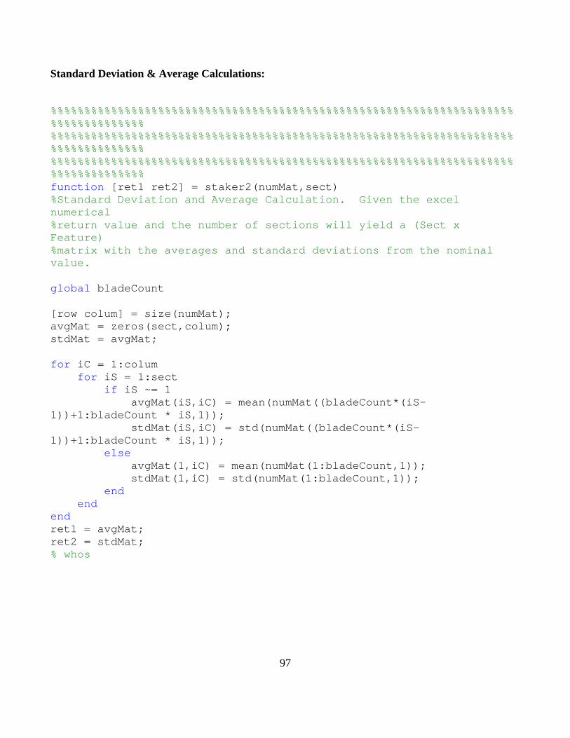
97

Standard Deviation & Average Calculations:

%%%%%%%%%%%%%%%%%%%%%%%%%%%%%%%%%%%%%%%%%%%%%%%%%%%%%%%%%%%%%%%%%%%%%%%%%%%%%%%%%%% %%%%%%%%%%%%%%%%%%%%%%%%%%%%%%%%%%%%%%%%%%%%%%%%%%%%%%%%%%%%%%%%%%%%%%%%%%%%%%%%%%% %%%%%%%%%%%%%%%%%%%%%%%%%%%%%%%%%%%%%%%%%%%%%%%%%%%%%%%%%%%%%%%%%%%%%%%%%%%%%%%%%%% function [ret1 ret2] = staker2(numMat,sect) %Standard Deviation and Average Calculation. Given the excel numerical %return value and the number of sections will yield a (Sect x Feature) %matrix with the averages and standard deviations from the nominal value. global bladeCount [row colum] = size(numMat); avgMat = zeros(sect,colum); stdMat = avgMat; for iC = 1:colum for iS = 1:sect if iS ~= 1 avgMat(iS,iC) = mean(numMat((bladeCount*(iS-1))+1:bladeCount * iS,1)); stdMat(iS,iC) = std(numMat((bladeCount*(iS-1))+1:bladeCount * iS,1)); else avgMat(1,iC) = mean(numMat(1:bladeCount,1)); stdMat(1,iC) = std(numMat(1:bladeCount,1)); end end end ret1 = avgMat; ret2 = stdMat; % whos

98

DTP Calculations:

%%%%%%%%%%%%%%%%%%%%%%%%%%%%%%%%%%%%%%%%%%%%%%%%%%%%%%%%%%%%%%%%%%%%%%%%%%%%%%%%%%% %%%%%%%%%%%%%%%%%%%%%%%%%%%%%%%%%%%%%%%%%%%%%%%%%%%%%%%%%%%%%%%%%%%%%%%%%%%%%%%%%%% %%%%%%%%%%%%%%%%%%%%%%%%%%%%%%%%%%%%%%%%%%%%%%%%%%%%%%%%%%%%%%%%%%%%%%%%%%%%%%%%%%% function ret = DTPer(numMat) global bladeCount sect%Delta True Position Calculations. % xxx = numMat(:,1); % yyy = numMat(:,2); % n = numMat(:,3); % chord = numMat(:,4); % mxt = numMat(:,5); c = zeros(bladeCount*sect,5); for i = 1:sect - 1 if i ~= 1 a = numMat((bladeCount*(i-1))+1:bladeCount*i,:); b = numMat((bladeCount*i)+1:(bladeCount*(i+1)),:); c((bladeCount*(i-1))+1:(bladeCount*i),:) = b-a; else a = numMat(1:bladeCount,:); b = numMat(bladeCount+1:bladeCount*2,:); c(1:bladeCount,:) = b-a; end end ret = c;

99

Chord Loss Calculations:

%%%%%%%%%%%%%%%%%%%%%%%%%%%%%%%%%%%%%%%%%%%%%%%%%%%%%%%%%%%%%%%%%%%%%%%%%%%%%%%%%%% %%%%%%%%%%%%%%%%%%%%%%%%%%%%%%%%%%%%%%%%%%%%%%%%%%%%%%%%%%%%%%%%%%%%%%%%%%%%%%%%%%% %%%%%%%%%%%%%%%%%%%%%%%%%%%%%%%%%%%%%%%%%%%%%%%%%%%%%%%%%%%%%%%%%%%%%%%%%%%%%%%%%%% function [mu sigma data] = chordCalcs(numMat) %Chord average and Chord Loss Calculation. Plots Chord and the predicated %final chord deviations. %NOTE: This sub-function returns the average and standard deviation @ FINAL global bladeCount Cindex c_loss sect b = []; %Chord Loss Calculations for iS = 1:length(c_loss) if iS ~= 1 a = numMat((bladeCount*(iS-1))+1:bladeCount*iS,4) + c_loss(iS); b = [b; a]; else a = numMat(1:bladeCount * iS,4) + c_loss(iS); b = [b; a]; end end %Chord Average @ final avgMat = zeros(sect,1); stdMat = avgMat; for iS = 1:sect if iS ~= 1 avgMat(iS) = mean(b((bladeCount*(iS-1))+1:bladeCount * iS)); stdMat(iS) = std(b((bladeCount*(iS-1))+1:bladeCount * iS)); else avgMat(iS) = mean(b(1:bladeCount)); stdMat(iS) = std(b(1:bladeCount)); end end mu = avgMat;

100

sigma = stdMat; data = b; % whos

101

Cp & Cpk Calculations:

%%%%%%%%%%%%%%%%%%%%%%%%%%%%%%%%%%%%%%%%%%%%%%%%%%%%%%%%%%%%%%%%%%%%%%%%%%%%%%%%%%% %%%%%%%%%%%%%%%%%%%%%%%%%%%%%%%%%%%%%%%%%%%%%%%%%%%%%%%%%%%%%%%%%%%%%%%%%%%%%%%%%%% %%%%%%%%%%%%%%%%%%%%%%%%%%%%%%%%%%%%%%%%%%%%%%%%%%%%%%%%%%%%%%%%%%%%%%%%%%%%%%%%%%% function [Cpk Cp] = CpKer(data,spec) %DATA: Two element vector containg mean and devation SECTION information %DATA = [MEAN,STD] %Spec: Two element vector containing USL and LSL information %SPEC = [LSL,USL] ub = spec(:,2); lb = spec(:,1); if lb > ub USL = lb; LSL = ub; else USL = ub; LSL = lb; end mu = data(:,1); sigma = data(:,2); a = (USL - LSL)./(6.*sigma); b = min( ((USL - mu)./(3.*sigma)) , ((mu-LSL)./(3.*sigma))); Cp = round(a/.001)*.001; Cpk = round(b/.01)*.01;

102

Maximizer599 Calculations:

%%%%%%%%%%%%%%%%%%%%%%%%%%%%%%%%%%%%%%%%%%%%%%%%%%%%%%%%%%%%%%%%%%%%%%%%%%%%%%%%%%% %%%%%%%%%%%%%%%%%%%%%%%%%%%%%%%%%%%%%%%%%%%%%%%%%%%%%%%%%%%%%%%%%%%%%%%%%%%%%%%%%%% %%%%%%%%%%%%%%%%%%%%%%%%%%%%%%%%%%%%%%%%%%%%%%%%%%%%%%%%%%%%%%%%%%%%%%%%%%%%%%%%%%% function NaOffset = maximizer599(data,dev,specs) %MAXIMIZER599 %This function produces the optimal N-Angle offset for this data set. % Input the NORMALIZED N,LEA,TEA information into the DATA variable. %DATA = [N,LEA,TEA] %DEV = [N,LEA,TEA] <-- **Standard Deviation** global sect Pref offset = [-21:3:21]; N = data(:,1); LEA = data(:,2); TEA = data(:,3); Nadev = dev(:,1); Ladev = dev(:,2); Tadev = dev(:,3); Ncpk = []; Ucpk = []; Lcpk = []; for ind = offset pn1 = peenER(N,ind); PNavg = staker2(pn1,sect); plea1 = peenER(LEA,ind); PLavg = staker2(plea1,sect); ptea1 = peenER(TEA,ind); PTavg = staker2(ptea1,sect); Pavgs = [PNavg;PLavg;PTavg]; Pdevs = [Nadev;Ladev;Tadev]; [Uc Lc] = CpKer10([Pavgs,Pdevs],[specs(1,1),specs(1,2)], Pref); Ncpk = [Ncpk , CpKer([PNavg,Nadev],[specs(1,1),specs(1,2)])]; Ucpk = [Ucpk , Uc];

103

Lcpk = [Lcpk , Lc]; end plot(offset,Lcpk,offset,Ucpk) ULdiff = abs(Ucpk - Lcpk); maxYield = min(ULdiff); NaOffset = offset(find(maxYield == ULdiff));

104

Minimum Cpk Calculations:

%%%%%%%%%%%%%%%%%%%%%%%%%%%%%%%%%%%%%%%%%%%%%%%%%%%%%%%%%%%%%%%%%%%%%%%%%%%%%%%%%%% %%%%%%%%%%%%%%%%%%%%%%%%%%%%%%%%%%%%%%%%%%%%%%%%%%%%%%%%%%%%%%%%%%%%%%%%%%%%%%%%%%% %%%%%%%%%%%%%%%%%%%%%%%%%%%%%%%%%%%%%%%%%%%%%%%%%%%%%%%%%%%%%%%%%%%%%%%%%%%%%%%%%%% function [Ucpk Lcpk] = CpKer10(data,spec,Pref) %This Cpk function returns the minumum Cpk values of the Upper-centered and %Lower-Centered data %DATA: Two element vector containg mean and devation information %DATA = [MEAN,STD] %Spec: Two element vector containing USL and LSL information %SPEC = [LSL,USL] global sect sectQ %Set the appropriate tolerance to the respective variable: ub = spec(:,2); lb = spec(:,1); if lb > ub USL = lb; LSL = ub; else USL = ub; LSL = lb; end mu = data(:,1); sigma = data(:,2); %Create the upper and lower Cpk values Ucpk = ((USL - mu)./(3.*sigma)); Ucpk = Ucpk(:,1); Lcpk = (((mu-LSL)./(3.*sigma))); Lcpk = Lcpk(:,1); %Check to see if there are any reference sections present if ~isempty(Pref) refPos = find(Pref == sectQ); else refPos = [];

105

end a = true; b = false; c = b; while a Ucpkp = find(min(Ucpk) == Ucpk); Lcpkp = find(min(Lcpk) == Lcpk); if Ucpkp == (refPos + sect) || Ucpkp == (sect*2) + refPos Ucpk(Ucpkp) = Inf; b = true; else b = false; Ucpk = Ucpk(Ucpkp); end if Lcpkp == (refPos + sect) || Lcpkp == (sect*2) + refPos Lcpk(Lcpkp) = Inf; c= true; else c = false; Lcpk = Lcpk(Lcpkp); end if b == false && c == false a = false; else a = true; end end

106

Post Peen Calculations:

%%%%%%%%%%%%%%%%%%%%%%%%%%%%%%%%%%%%%%%%%%%%%%%%%%%%%%%%%%%%%%%%%%%%%%%%%%%%%%%%%%% %%%%%%%%%%%%%%%%%%%%%%%%%%%%%%%%%%%%%%%%%%%%%%%%%%%%%%%%%%%%%%%%%%%%%%%%%%%%%%%%%%% %%%%%%%%%%%%%%%%%%%%%%%%%%%%%%%%%%%%%%%%%%%%%%%%%%%%%%%%%%%%%%%%%%%%%%%%%%%%%%%%%%% function postPeen = peenER(data,offset) %DATA = Actual NORMALIZED data in either a (1xN) or (Mx1) %[P]eenER simulates the peening process and returns how each blade is %affected at each section. global closure bladeCount b=[]; for iS = 1:length(closure) if iS ~= 1 a = data((bladeCount*(iS-1))+1:bladeCount*iS) + closure(iS) + offset; b = [b; a]; else a = data(1:bladeCount * iS) + closure(iS) + offset; b = [b; a]; end end postPeen = b;

107

Spreadsheet Maker Calculations:

%%%%%%%%%%%%%%%%%%%%%%%%%%%%%%%%%%%%%%%%%%%%%%%%%%%%%%%%%%%%%%%%%%%%%%%%%%%%%%%%%%% %%%%%%%%%%%%%%%%%%%%%%%%%%%%%%%%%%%%%%%%%%%%%%%%%%%%%%%%%%%%%%%%%%%%%%%%%%%%%%%%%%% %%%%%%%%%%%%%%%%%%%%%%%%%%%%%%%%%%%%%%%%%%%%%%%%%%%%%%%%%%%%%%%%%%%%%%%%%%%%%%%%%%% function ret=spreadsheetMaker(raw,sCounter,avg,dev,dtpMat,deltaAvg,chordFinal,cFavg,normAngs,normAngsMean,pangs,pangsMean,thickness) % Takes in the data matrices and places them in a cell array that is ready % to be written to an Excel file. global sect sectQ closure c_loss NaOffset format bank offset = NaOffset; raw{1,end+2} = 'Sect'; for index = 1:sect raw{index + 1,end} = sectQ(index); end %Chord loss "index" raw{1,end+1} = 'Chord Loss'; for index = 1:length(c_loss) raw{index+1,end} = c_loss(index); end %Estimated chord lengths raw{1,end +1} = 'Chord Final'; for index = 1:length(chordFinal) raw{index+1,end} = round(chordFinal(index)/.0001)*.0001; end raw{1,end+2} = 'Sect'; for index = 1:sect raw{index + 1,end} = sectQ(index); end %Averages raw{1,end+1} = 'XXX Mean'; raw{1,end+1} = 'YYY Mean'; raw{1,end+1} = 'C Mean'; raw{1,end+1} = 'N Mean'; raw{1,end+1} = 'LEA Mean';

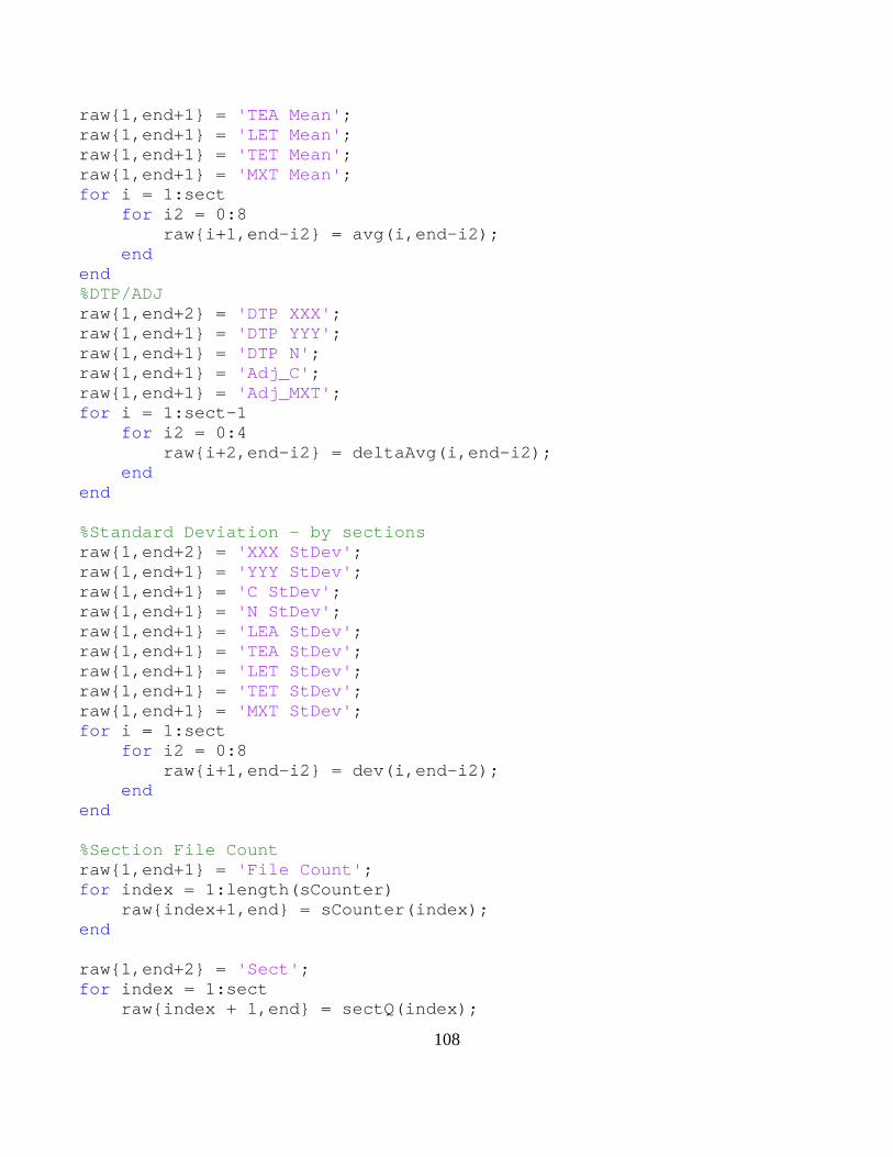
108

raw{1,end+1} = 'TEA Mean'; raw{1,end+1} = 'LET Mean'; raw{1,end+1} = 'TET Mean'; raw{1,end+1} = 'MXT Mean'; for i = 1:sect for i2 = 0:8 raw{i+1,end-i2} = avg(i,end-i2); end end %DTP/ADJ raw{1,end+2} = 'DTP XXX'; raw{1,end+1} = 'DTP YYY'; raw{1,end+1} = 'DTP N'; raw{1,end+1} = 'Adj_C'; raw{1,end+1} = 'Adj_MXT'; for i = 1:sect-1 for i2 = 0:4 raw{i+2,end-i2} = deltaAvg(i,end-i2); end end %Standard Deviation - by sections raw{1,end+2} = 'XXX StDev'; raw{1,end+1} = 'YYY StDev'; raw{1,end+1} = 'C StDev'; raw{1,end+1} = 'N StDev'; raw{1,end+1} = 'LEA StDev'; raw{1,end+1} = 'TEA StDev'; raw{1,end+1} = 'LET StDev'; raw{1,end+1} = 'TET StDev'; raw{1,end+1} = 'MXT StDev'; for i = 1:sect for i2 = 0:8 raw{i+1,end-i2} = dev(i,end-i2); end end %Section File Count raw{1,end+1} = 'File Count'; for index = 1:length(sCounter) raw{index+1,end} = sCounter(index); end raw{1,end+2} = 'Sect'; for index = 1:sect raw{index + 1,end} = sectQ(index);

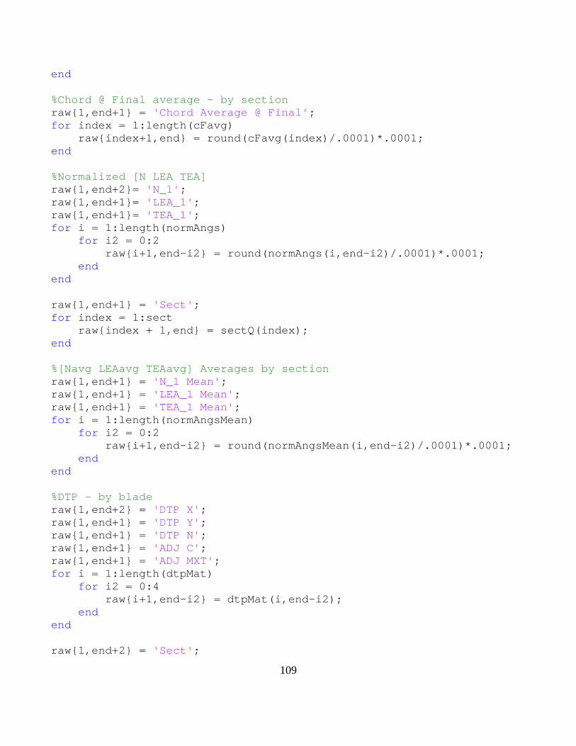
109

end %Chord @ Final average - by section raw{1,end+1} = 'Chord Average @ Final'; for index = 1:length(cFavg) raw{index+1,end} = round(cFavg(index)/.0001)*.0001; end %Normalized [N LEA TEA] raw{1,end+2}= 'N_1'; raw{1,end+1}= 'LEA_1'; raw{1,end+1}= 'TEA_1'; for i = 1:length(normAngs) for i2 = 0:2 raw{i+1,end-i2} = round(normAngs(i,end-i2)/.0001)*.0001; end end raw{1,end+1} = 'Sect'; for index = 1:sect raw{index + 1,end} = sectQ(index); end %[Navg LEAavg TEAavg] Averages by section raw{1,end+1} = 'N_1 Mean'; raw{1,end+1} = 'LEA_1 Mean'; raw{1,end+1} = 'TEA_1 Mean'; for i = 1:length(normAngsMean) for i2 = 0:2 raw{i+1,end-i2} = round(normAngsMean(i,end-i2)/.0001)*.0001; end end %DTP - by blade raw{1,end+2} = 'DTP X'; raw{1,end+1} = 'DTP Y'; raw{1,end+1} = 'DTP N'; raw{1,end+1} = 'ADJ C'; raw{1,end+1} = 'ADJ MXT'; for i = 1:length(dtpMat) for i2 = 0:4 raw{i+1,end-i2} = dtpMat(i,end-i2); end end raw{1,end+2} = 'Sect';

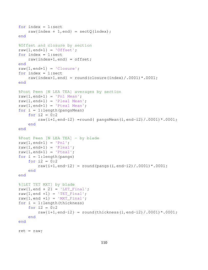
110

for index = 1:sect raw{index + 1,end} = sectQ(index); end %Offset and closure by section raw{1,end+1} = 'Offset'; for index = 1:sect raw{index+1,end} = offset; end raw{1,end+1} = 'Closure'; for index = 1:sect raw{index+1,end} = round(closure(index)/.0001)*.0001; end %Post Peen [N LEA TEA] averages by section raw{1,end+1} = 'Pn1 Mean'; raw{1,end+1} = 'Plea1 Mean'; raw{1,end+1} = 'Ptea1 Mean'; for i = 1:length(pangsMean) for i2 = 0:2 raw{i+1,end-i2} =round( pangsMean(i,end-i2)/.0001)*.0001; end end %Post Peen [N LEA TEA] - by blade raw{1,end+1} = 'Pn1'; raw{1,end+1} = 'Plea1'; raw{1,end+1} = 'Ptea1'; for i = 1:length(pangs) for i2 = 0:2 raw{i+1,end-i2} = round(pangs(i,end-i2)/.0001)*.0001; end end %[LET TET MXT] by blade raw{1,end + 2} = 'LET_Final'; raw{1,end +1} = 'TET_Final'; raw{1,end +1} = 'MXT_Final'; for i = 1:length(thickness) for i2 = 0:2 raw{i+1,end-i2} = round(thickness(i,end-i2)/.0001)*.0001; end end ret = raw;

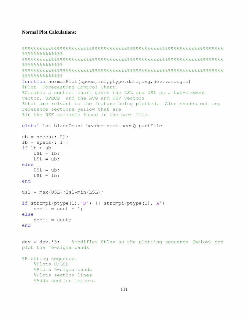
111

Normal Plot Calculations:

%%%%%%%%%%%%%%%%%%%%%%%%%%%%%%%%%%%%%%%%%%%%%%%%%%%%%%%%%%%%%%%%%%%%%%%%%%%%%%%%%%% %%%%%%%%%%%%%%%%%%%%%%%%%%%%%%%%%%%%%%%%%%%%%%%%%%%%%%%%%%%%%%%%%%%%%%%%%%%%%%%%%%% %%%%%%%%%%%%%%%%%%%%%%%%%%%%%%%%%%%%%%%%%%%%%%%%%%%%%%%%%%%%%%%%%%%%%%%%%%%%%%%%%%% function normalPlot(specs,ref,ptype,data,avg,dev,varargin) %Plot Forecasting Control Chart. %Creates a control chart given the LSL and USL as a two-element vector, SPECS, and the AVG and DEV vectors %that are relvant to the feature being plotted. Also shades out any reference sections yellow that are %in the REF variable found in the part file. global lot bladeCount header sect sectQ partFile ub = specs(:,2); lb = specs(:,1); if lb > ub USL = lb; LSL = ub; else USL = ub; LSL = lb; end usl = max(USL);lsl=min(LSL); if strcmpi(ptype(1),'D') || strcmpi(ptype(1),'A') sectt = sect - 1; else sectt = sect; end dev = dev.*3; %modifies StDev so the plotting sequence (below) can plot the "6-sigma bands" %Plotting sequence: %Plots U/LSL %Plots 6-sigma bands %Plots section lines %Adds section letters

112

sectQ = char(sectQ); sectLine = linspace(lsl,usl,500); limitLine = linspace(0,bladeCount*sectt,500); plot(limitLine,0, 'c--','LineWidth',0.5) hold on %For DTP plots, letter the sections 'A-B','B-C',etc. if strcmpi(ptype(1),'d') || strcmpi(ptype(1),'a') plot(data,'k.') for i = 2:sectt+1 xx = linspace(bladeCount.*(i-2),bladeCount.*(i-1),250); letter1 = sectQ(i-1); letter2 = sectQ(i); plot(xx,LSL(i-1), 'b-','LineWidth',2) plot(xx,USL(i-1), 'b-','LineWidth',2) plot(xx,avg(i-1),'-m','LineWidth',1.25) plot(xx,avg(i-1) + dev(i-1),'-r','LineWidth',1.25) plot(xx,avg(i-1) - dev(i-1),'-r','LineWidth',1.25) plot(bladeCount*(i-1),sectLine,'--k','LineWidth',0.5) x = ((bladeCount*(i-2))+ bladeCount/2); y = usl * 1.1; letter = [letter1 '-' letter2]; text(x,y,letter) end else for i = 1:sectt x = [bladeCount*(i-1)+1:bladeCount*i]; xx = linspace(bladeCount.*(i-1),bladeCount.*i,250); letter = sectQ(i); if letter == ref plot(x,data(x),'y.') else plot(x,data(x),'k.') end plot(xx,LSL(i), 'b-','LineWidth',2) plot(xx,USL(i), 'b-','LineWidth',2) plot(xx,avg(i),'-m','LineWidth',1.25) plot(xx,avg(i) + dev(i),'-r','LineWidth',1.25) plot(xx,avg(i) - dev(i),'-r','LineWidth',1.25) plot(bladeCount*i,sectLine,'--k','LineWidth',0.5) x = ((bladeCount*(i-1))+ bladeCount/2); y = (max(sectLine) + .00025);

113

text(x,y,letter) end end %Adds text to the graph if strcmpi(ptype,'n_1') || strcmpi(ptype,'lea_1') || strcmpi(ptype,'tea_1') || strcmpi(ptype,'DTP N') || strcmpi(ptype,'CLEA') || strcmpi(ptype,'CTEA') ylabel('Deviation from nominal (min.)');xlabel('Observation Number') else ylabel('Deviation from nominal (in.)');xlabel('Observation Number') end bc = num2str(bladeCount); str2 = ['LPI Inspections lot ' lot ' (Basis:' bc ' parts) JB43']; %Create title for graph if ~isempty(varargin) titleStr = {header;str2;ptype;varargin{1}}; else titleStr = {header;str2;ptype}; end clear str2 str1 bc %Free up some space and variables clear str2 str1 bc %Free up some space and variables title(titleStr) text(bladeCount*sectt,usl + ((usl*.25)/2),'USL') text(bladeCount*sectt,lsl + ((lsl*.25)/2),'LSL') %Re-sizes the graph if max(data) < usl && min(data) > lsl set(gca,'xlim',[0 (length(data)+length(data)*.05)]) set(gca,'ylim',[(lsl + lsl*.05) (usl + usl*.05) ]) else set(gca,'xlim',[0 (length(data)+length(data)*.05)]) set(gca,'ylim',[(lsl+min(data)*.5) (usl+max(data)*.5)]) end hold off %save the graph toa jpeg file %build filename

114

filename = [partFile '_' lot '_' ptype '.jpg']; print('-djpeg50',filename);

115

Post Peen Plot Calculations:

%%%%%%%%%%%%%%%%%%%%%%%%%%%%%%%%%%%%%%%%%%%%%%%%%%%%%%%%%%%%%%%%%%%%%%%%%%%%%%%%%%% %%%%%%%%%%%%%%%%%%%%%%%%%%%%%%%%%%%%%%%%%%%%%%%%%%%%%%%%%%%%%%%%%%%%%%%%%%%%%%%%%%% %%%%%%%%%%%%%%%%%%%%%%%%%%%%%%%%%%%%%%%%%%%%%%%%%%%%%%%%%%%%%%%%%%%%%%%%%%%%%%%%%%% function PeenPlot(specs,offset,ref,ptype,data,stats) %Specs: [LSL,USL] %DATA: Raw data from peenER() function %STATS: [MEAN StDeviation] *Note: Both are vertical vectors concatenated %together that are section averages. global lot bladeCount header sect sectQ global Psim partFile mu = stats(:,1); sigma = stats(:,2); %Set the appropriate limit to the respective variable. ub = specs(1,2); lb = specs(1,1); if lb > ub USL = lb; LSL = ub; else USL = ub; LSL = lb; end usl = max(USL);lsl=min(LSL); sigma = sigma .*3; %Prep for 6-sigma band plots %Determine position of any outliers UCL = mu + sigma; LCL = mu - sigma; outlierPos = []; for ind = 1:length(mu) if ind == 1 testData = data(1:bladeCount); posModifier = 0; else testData = data(bladeCount*(ind-1) + 1: bladeCount*ind);

116

posModifier = bladeCount*(ind-1); end pos = find( testData >= UCL(ind) | testData <= LCL(ind)); if ~isempty(pos) outlierPos = [outlierPos, (pos' + posModifier)]; end end %Plot any outliers if ~isempty(outlierPos) outlierPos = sort(outlierPos); plot(outlierPos,data(outlierPos),'*k','MarkerSize',8); hold on end %Plot sequence sectQ = char(sectQ); limitLine = linspace(0,bladeCount*sect,500); plot(limitLine,LSL,'-b','LineWidth',2) hold on plot(limitLine,USL,'-b','LineWidth',2) plot(limitLine,0,'--c','LineWidth',0.5) for i = 1:sect xx = linspace(bladeCount.*(i-1),bladeCount.*i,250); x = bladeCount.*(i-1) + round(bladeCount/2); letter = sectQ(i); mu_i = mu(i); if strcmpi(ref,letter) && ~strcmpi(ptype(2),'n') plot(xx,mu_i,'y') plot(x,mu_i,'-om','LineWidth',1.25,'MarkerEdgeColor',... 'k','MarkerFaceColor','y',... 'MarkerSize', 6) plot(xx,UCL(i),'-y','LineWidth',1.25) plot(xx,LCL(i),'-y','LineWidth',1.25) else plot(xx,mu_i,'m') plot(x,mu_i,'-om','LineWidth',1.25,'MarkerEdgeColor',... 'k','MarkerFaceColor',[0.49 1 0.63],... 'MarkerSize', 6) plot(xx,UCL(i),'-r','LineWidth',1.25) plot(xx,LCL(i),'-r','LineWidth',1.25) end

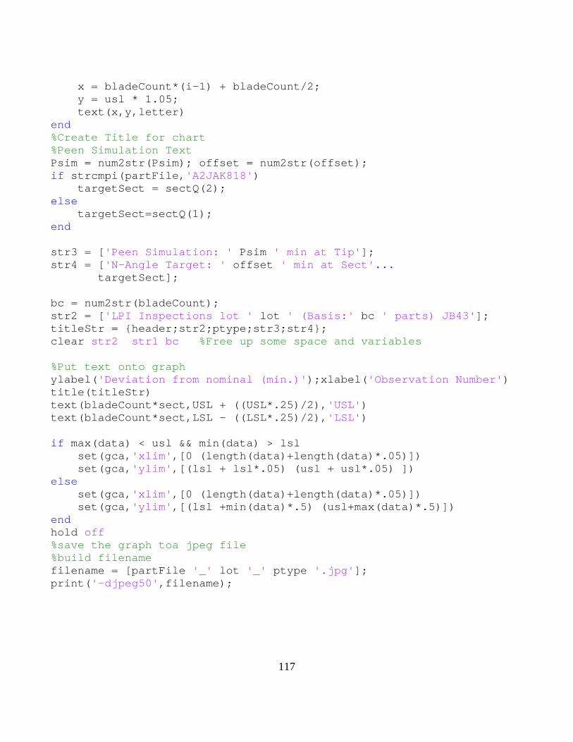
117

x = bladeCount*(i-1) + bladeCount/2; y = usl * 1.05; text(x,y,letter) end %Create Title for chart %Peen Simulation Text Psim = num2str(Psim); offset = num2str(offset); if strcmpi(partFile,'A2JAK818') targetSect = sectQ(2); else targetSect=sectQ(1); end str3 = ['Peen Simulation: ' Psim ' min at Tip']; str4 = ['N-Angle Target: ' offset ' min at Sect'... targetSect]; bc = num2str(bladeCount); str2 = ['LPI Inspections lot ' lot ' (Basis:' bc ' parts) JB43']; titleStr = {header;str2;ptype;str3;str4}; clear str2 str1 bc %Free up some space and variables %Put text onto graph ylabel('Deviation from nominal (min.)');xlabel('Observation Number') title(titleStr) text(bladeCount*sect,USL + ((USL*.25)/2),'USL') text(bladeCount*sect,LSL - ((LSL*.25)/2),'LSL') if max(data) < usl && min(data) > lsl set(gca,'xlim',[0 (length(data)+length(data)*.05)]) set(gca,'ylim',[(lsl + lsl*.05) (usl + usl*.05) ]) else set(gca,'xlim',[0 (length(data)+length(data)*.05)]) set(gca,'ylim',[(lsl +min(data)*.5) (usl+max(data)*.5)]) end hold off %save the graph toa jpeg file %build filename filename = [partFile '_' lot '_' ptype '.jpg']; print('-djpeg50',filename);

118

DTP Calculations:

%%%%%%%%%%%%%%%%%%%%%%%%%%%%%%%%%%%%%%%%%%%%%%%%%%%%%%%%%%%%%%%%%%%%%%%%%%%%%%%%%%% %%%%%%%%%%%%%%%%%%%%%%%%%%%%%%%%%%%%%%%%%%%%%%%%%%%%%%%%%%%%%%%%%%%%%%%%%%%%%%%%%%% %%%%%%%%%%%%%%%%%%%%%%%%%%%%%%%%%%%%%%%%%%%%%%%%%%%%%%%%%%%%%%%%%%%%%%%%%%%%%%%%%%% function paretoMaker(specs,count) %rawCellarr = [xxx,yyy,cF,pn1,plea1,ptea1,let_f,tet_f,mxt_f,lep,tep,psp,ssp] %SPECS is in the same order as MAT but contains the USL and LSL %Function searches throught the data for blades out of tolerance % and creates a list of the defects and the measurement. global defectCount names header global bladeCount sect lot partFile filename = [partFile '_' lot '_rawData.xls']; [num txt raw] = xlsread(filename,'Raw Data'); col = [2:3,22,75:77,79:81,15,17,16,18]; posMod = 7; defectCount =[]; names ={}; dc =[]; for p = 1:length(col) ub = specs(:,2); lb = specs(:,1); if lb > ub USL = lb; LSL = ub; else USL = ub; LSL = lb; end test = num(:,col(p)); defect = raw{1,(col(p) + posMod)}; for iS = 1:sect if iS ~= 1 data = test((bladeCount*(iS-1))+1:bladeCount*iS); ub = USL(iS); lb = LSL(iS);

119

defectCount =[defectCount data(find(data > ub)) data(find(data < lb))]; if ~isempty(defectCount) for index = 1:length(defectCount) names{count} = defect; count = count +1; end dc = [dc defectCount']; end defectCount =[]; else data = test(1:bladeCount); ub = USL(iS); lb = LSL(iS); defectCount =[defectCount data(find(data > ub)) data(find(data < lb))]; if ~isempty(defectCount) for index = 1:length(defectCount) names{count} = defect; dc = [dc defectCount']; count = count +1; end end defectCount =[]; end end specs(:,1:2) =[]; end if isempty(names) disp('Airfoil is free from any defects') elseif ~isempty(names) disp('Creating pareto chart') list = []; defectCount = []; count = 1; if length(names) > 1 for index = 2:length(names) if strcmpi(names(index-1),names(index)) count = count + 1; if index == length(names) list = [list,names(index)]; defectCount = [defectCount,count]; end

120

elseif ~strcmpi(names(index-1),names(index)) list = [list,names(index-1)]; defectCount = [defectCount,count]; count = 1; if index == length(names) list = [list,names(index)]; defectCount = [defectCount,count]; end end end else list = names; defectCount = 1; end pareto(defectCount,list) hold on bc = num2str(bladeCount); str2 = ['LPI Inspections lot ' lot ' (Basis:' bc ' parts) JB43']; titleStr = {header;str2}; title(titleStr) hold off fileName = [partFile '_' lot '_PARETO.jpg']; print('-djpeg',fileName) close end

121

Root Calculations:

%%%%%%%%%%%%%%%%%%%%%%%%%%%%%%%%%%%%%%%%%%%%%%%%%%%%%%%%%%%%%%%%%%%%%%%%%%%%%%%%%%% %%%%%%%%%%%%%%%%%%%%%%%%%%%%%%%%%%%%%%%%%%%%%%%%%%%%%%%%%%%%%%%%%%%%%%%%%%%%%%%%%%% %%%%%%%%%%%%%%%%%%%%%%%%%%%%%%%%%%%%%%%%%%%%%%%%%%%%%%%%%%%%%%%%%%%%%%%%%%%%%%%%%%% function Root(str) global Ftol Ptol lot partFile header bladeCount [num1 t1 raw1] = xlsread(str,'Sheet2'); clear t1 %Create a check to see if data is present if isempty(num1) disp('No Fillet or Platform data is present') return end [r c] = size(raw1); section = raw1{1,2}; count = 1; queue = {}; qCount =[]; for index = 2:r test = raw1{index,2}; if strcmpi(test,section) count = count + 1; if index == r queue{end+1} = section; qCount = [qCount,count]; end elseif ~strcmpi(test,section) queue{end+1} = section; qCount = [qCount,count]; count = 1; section = test; end end data = num1(:,4); sectIndex = linspace(0,r,length(queue)+1); limitLine = linspace(0,sectIndex(end),r*2); sectLine = linspace(0,Ftol,(1/Ftol)*3);

122

plot(data,'.k') hold on plot(limitLine,Ftol,'.b') for i = 1:length(sectIndex)-1; x = sectIndex(i); y = Ftol + (Ftol*.02); text(x,y,queue(i)); plot(x,sectLine); end bc = num2str(bladeCount); str2 = ['LPI Inspections lot ' lot ' (Basis:' bc ' parts) JB43']; titleStr = {header;str2;'Fillet'}; title(titleStr) reinspPos = find(data > Ftol); reinspCN = num1(reinspPos,1); if ~isempty(reinspPos) fprintf('The following control number MUST be reinspected \n for fillet rejection: %i \n',reinspCN) end %Resize plot area if max(data) > Ftol set(gca,'xlim',[0 (length(data)+length(data)*.05)]) set(gca,'ylim',[0 (max(data) + max(data)*.05) ]) else set(gca,'xlim',[0 (length(data)+length(data)*.05)]) set(gca,'ylim',[0 (Ftol+ (Ftol*.05))]) end hold off %save the graph toa jpeg file beg = [partFile '_' lot]; filename = [ beg '_FILLET.jpg']; print('-djpeg50',filename) %%Find and report out of tolerance Fillets reinspPos = find(data > Ftol); reinspCN = num1(reinspPos,1); if ~isempty(reinspPos) fid = fopen([saveFile '\Fillet Rejections.txt'],'w'); for i = 1:length(reinspPos) fprintf(fid,'The following control number is out of tolerance for the FILLET feature: %i \n',reinspCN(i));

123

end fclose(fid); end [num2 t2 raw2] = xlsread(str,'Sheet3'); clear t2 [r c] = size(raw2); section = raw2{1,2}; count = 1; queue = {}; qCount =[]; for index = 2:r test = raw2{index,2}; if strcmpi(test,section) count = count + 1; if index == r queue{end+1} = section; qCount = [qCount,count]; end elseif ~strcmpi(test,section) queue{end+1} = section; qCount = [qCount,count]; count = 1; section = test; end end data = num2(:,5); sectIndex = linspace(0,r,length(queue)+1); limitLine = linspace(0,sectIndex(end),r*2); sectLine = linspace(Ptol(1),Ptol(2),(1/Ptol(2))*3); plot(data,'.k') hold on plot(limitLine,Ptol(1),'-b') plot(limitLine,Ptol(2),'-b') for i = 1:length(sectIndex)-1; x = sectIndex(i); y = Ptol(2) + (Ptol(2)*.02); sectText = queue(i); text(x,y,sectText); plot(x,sectLine); end

124

titleStr = {header;str2;'Platform'}; title(titleStr) %Resize plot area if max(data)< Ptol(2) && min(data) > Ptol(1) set(gca,'xlim',[0 (length(data)+length(data)*.05)]) set(gca,'ylim',[(Ptol(1) + Ptol(1)*.05) (Ptol(2) + Ptol(2)*.05) ]) else set(gca,'xlim',[0 (length(data)+length(data)*.05)]) set(gca,'ylim',[(Ptol(1) + min(data)*.5) (Ptol(2) + max(data)*.5)]) end hold off %save the graph toa jpeg file %build filename filename = [ beg '_PLATFORM.jpg']; print('-djpeg50',filename) reinspPos = find(data > Ptol(2) | data < Ptol(1)); reinspCN = num2(reinspPos,1); if ~isempty(reinspPos) fid = fopen([saveFile '\Platform Rejections.txt'],'w'); for i = 1:length(reinspPos) fprintf(fid,'The following control number is out of tolerance for the PLATFORM feature: %i \n',reinspCN(i)); end fclose(fid); end

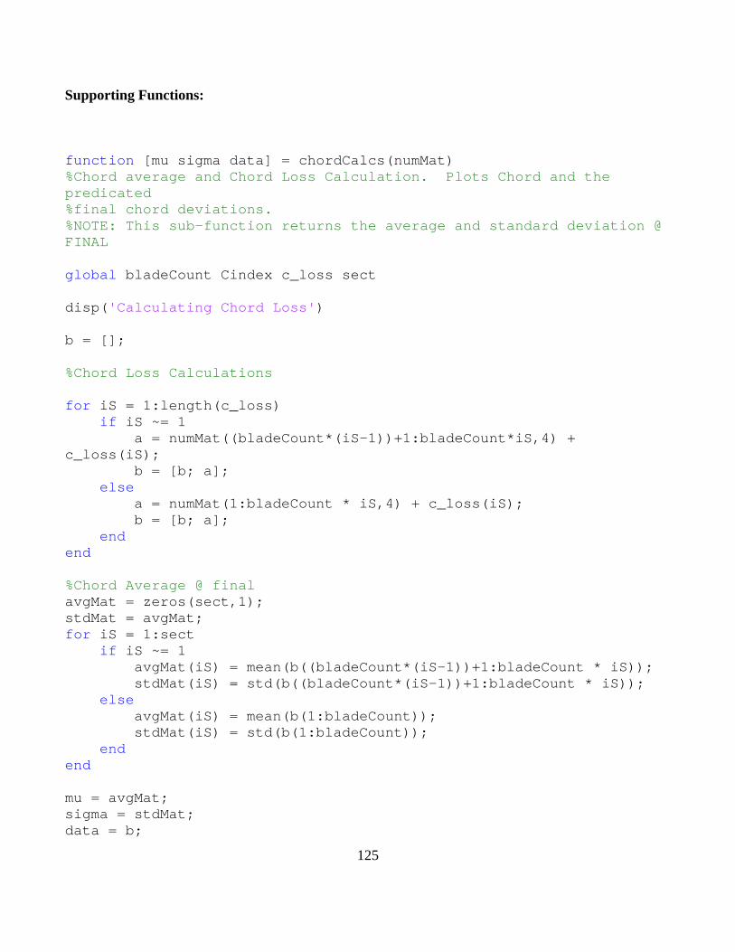
125

Supporting Functions:

function [mu sigma data] = chordCalcs(numMat) %Chord average and Chord Loss Calculation. Plots Chord and the predicated %final chord deviations. %NOTE: This sub-function returns the average and standard deviation @ FINAL global bladeCount Cindex c_loss sect disp('Calculating Chord Loss') b = []; %Chord Loss Calculations for iS = 1:length(c_loss) if iS ~= 1 a = numMat((bladeCount*(iS-1))+1:bladeCount*iS,4) + c_loss(iS); b = [b; a]; else a = numMat(1:bladeCount * iS,4) + c_loss(iS); b = [b; a]; end end %Chord Average @ final avgMat = zeros(sect,1); stdMat = avgMat; for iS = 1:sect if iS ~= 1 avgMat(iS) = mean(b((bladeCount*(iS-1))+1:bladeCount * iS)); stdMat(iS) = std(b((bladeCount*(iS-1))+1:bladeCount * iS)); else avgMat(iS) = mean(b(1:bladeCount)); stdMat(iS) = std(b(1:bladeCount)); end end mu = avgMat; sigma = stdMat; data = b;

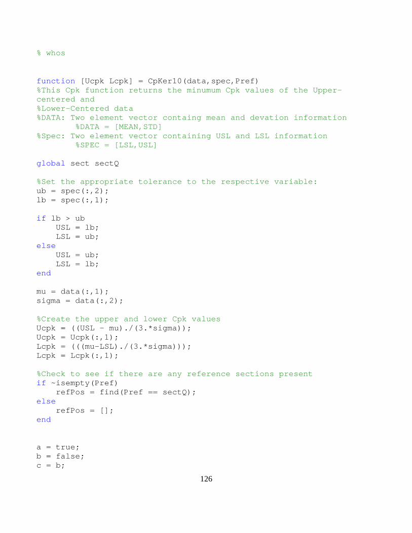
126

% whos

function [Ucpk Lcpk] = CpKer10(data,spec,Pref) %This Cpk function returns the minumum Cpk values of the Upper-centered and %Lower-Centered data %DATA: Two element vector containg mean and devation information %DATA = [MEAN,STD] %Spec: Two element vector containing USL and LSL information %SPEC = [LSL,USL] global sect sectQ %Set the appropriate tolerance to the respective variable: ub = spec(:,2); lb = spec(:,1); if lb > ub USL = lb; LSL = ub; else USL = ub; LSL = lb; end mu = data(:,1); sigma = data(:,2); %Create the upper and lower Cpk values Ucpk = ((USL - mu)./(3.*sigma)); Ucpk = Ucpk(:,1); Lcpk = (((mu-LSL)./(3.*sigma))); Lcpk = Lcpk(:,1); %Check to see if there are any reference sections present if ~isempty(Pref) refPos = find(Pref == sectQ); else refPos = []; end a = true; b = false; c = b;

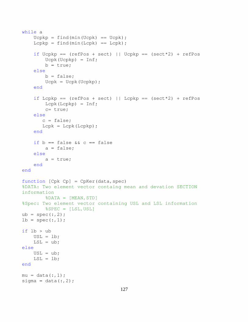
127

while a Ucpkp = find(min(Ucpk) == Ucpk); Lcpkp = find(min(Lcpk) == Lcpk); if Ucpkp == (refPos + sect) || Ucpkp == (sect*2) + refPos Ucpk(Ucpkp) = Inf; b = true; else b = false; Ucpk = Ucpk(Ucpkp); end if Lcpkp == (refPos + sect) || Lcpkp == (sect*2) + refPos Lcpk(Lcpkp) = Inf; c= true; else c = false; Lcpk = Lcpk(Lcpkp); end if b == false && c == false a = false; else a = true; end end function [Cpk Cp] = CpKer(data,spec) %DATA: Two element vector containg mean and devation SECTION information %DATA = [MEAN,STD] %Spec: Two element vector containing USL and LSL information %SPEC = [LSL,USL] ub = spec(:,2); lb = spec(:,1); if lb > ub USL = lb; LSL = ub; else USL = ub; LSL = lb; end mu = data(:,1); sigma = data(:,2);

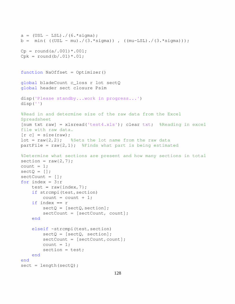
128

a = (USL - LSL)./(6.*sigma); b = min( ((USL - mu)./(3.*sigma)) , ((mu-LSL)./(3.*sigma))); Cp = round(a/.001)*.001; Cpk = round(b/.01)*.01;

function NaOffset = Optimizer() global bladeCount c_loss r lot sectQ global header sect closure Psim disp('Please standby...work in progress...') disp('') %Read in and determine size of the raw data from the Excel Spreadsheet [num txt raw] = xlsread('test4.xls'); clear txt; %Reading in excel file with raw data. [r c] = size(raw); lot = raw{2,2}; %Sets the lot name from the raw data partFile = raw{2,1}; %Finds what part is being estimated %Determine what sections are present and how many sections in total section = raw{2,7}; count = 1; sectQ = []; sectCount = []; for index = 3:r test = raw{index,7}; if strcmpi(test,section) count = count + 1; if index == r sectQ = [sectQ,section]; sectCount = [sectCount, count]; end elseif ~strcmpi(test,section) sectQ = [sectQ, section]; sectCount = [sectCount,count]; count = 1; section = test; end end sect = length(sectQ);

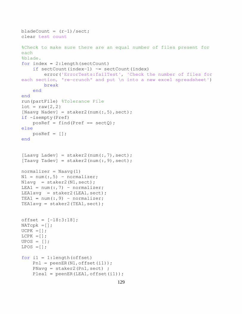
129

bladeCount = (r-1)/sect; clear test count %Check to make sure there are an equal number of files present for each %blade. for index = 2:length(sectCount) if sectCount(index-1) ~= sectCount(index) error('ErrorTests:failTest', 'Check the number of files for each section, "re-crunch" and put \n into a new excel spreadsheet') break end end run(partFile) %Tolerance File lot = raw{2,2} [Naavg Nadev] = staker2(num(:,5),sect); if ~isempty(Pref) posRef = find(Pref == sectQ); else posRef = []; end [Laavg Ladev] = staker2(num(:,7),sect); [Taavg Tadev] = staker2(num(:,9),sect); normalizer = Naavg(1) N1 = num(:,5) - normalizer; N1avg = staker2(N1,sect); LEA1 = num(:,7) - normalizer; LEA1avg = staker2(LEA1,sect); TEA1 = num(:,9) - normalizer; TEA1avg = staker2(TEA1,sect); offset = [-18:3:18]; NATcpk =[]; UCPK =[]; LCPK =[]; UPOS = []; LPOS =[]; for i1 = 1:length(offset) Pn1 = peenER(N1,offset(i1)); PNavg = staker2(Pn1,sect) ; Plea1 = peenER(LEA1,offset(i1));

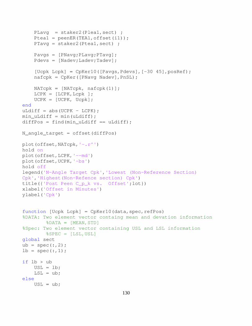
130

PLavg = staker2(Plea1,sect) ; Ptea1 = peenER(TEA1,offset(i1)); PTavg = staker2(Ptea1,sect) ; Pavgs = [PNavg;PLavg;PTavg]; Pdevs = [Nadev;Ladev;Tadev]; [Ucpk Lcpk] = CpKer10([Pavgs,Pdevs],[-30 45],posRef); nafcpk = CpKer([PNavg Nadev],PnSL); NATcpk = [NATcpk, nafcpk(1)]; LCPK = [LCPK,Lcpk ]; UCPK = [UCPK, Ucpk]; end uLdiff = abs(UCPK - LCPK); min_uLdiff = min(uLdiff); diffPos = find(min_uLdiff == uLdiff); N_angle_target = offset(diffPos) plot(offset,NATcpk,'-.r^') hold on plot(offset,LCPK,'--md') plot(offset,UCPK,'-bs') hold off legend('N-Angle Target Cpk','Lowest (Non-Reference Section) Cpk','Highest(Non-Refence section) Cpk') title({'Post Peen C_p_k vs. Offset';lot}) xlabel('Offset in Minutes') ylabel('Cpk') function [Ucpk Lcpk] = CpKer10(data,spec,refPos) %DATA: Two element vector containg mean and devation information %DATA = [MEAN,STD] %Spec: Two element vector containing USL and LSL information %SPEC = [LSL,USL] global sect ub = spec(:,2); lb = spec(:,1); if lb > ub USL = lb; LSL = ub; else USL = ub;

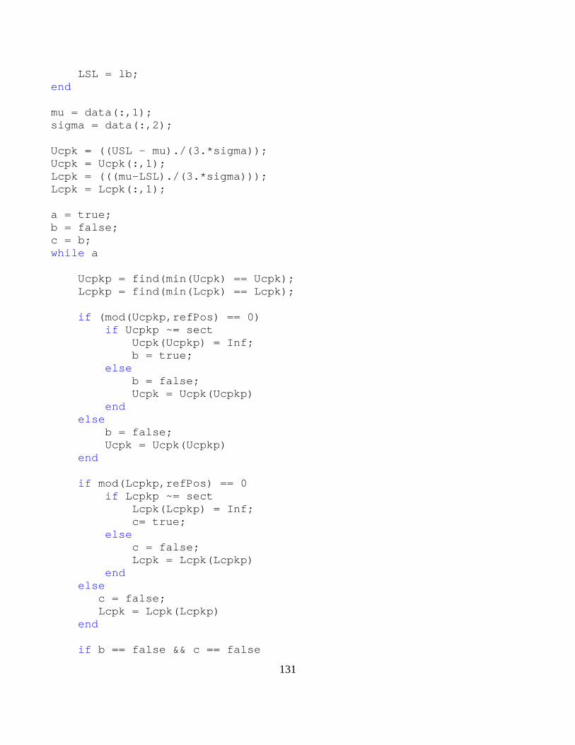
131

LSL = lb; end mu = data(:,1); sigma = data(:,2); Ucpk = ((USL - mu)./(3.*sigma)); Ucpk = Ucpk(:,1); Lcpk = (((mu-LSL)./(3.*sigma))); Lcpk = Lcpk(:,1); a = true; b = false; c = b; while a Ucpkp = find(min(Ucpk) == Ucpk); Lcpkp = find(min(Lcpk) == Lcpk); if (mod(Ucpkp,refPos) == 0) if Ucpkp ~= sect Ucpk(Ucpkp) = Inf; b = true; else b = false; Ucpk = Ucpk(Ucpkp) end else b = false; Ucpk = Ucpk(Ucpkp) end if mod(Lcpkp,refPos) == 0 if Lcpkp ~= sect Lcpk(Lcpkp) = Inf; c= true; else c = false; Lcpk = Lcpk(Lcpkp) end else c = false; Lcpk = Lcpk(Lcpkp) end if b == false && c == false

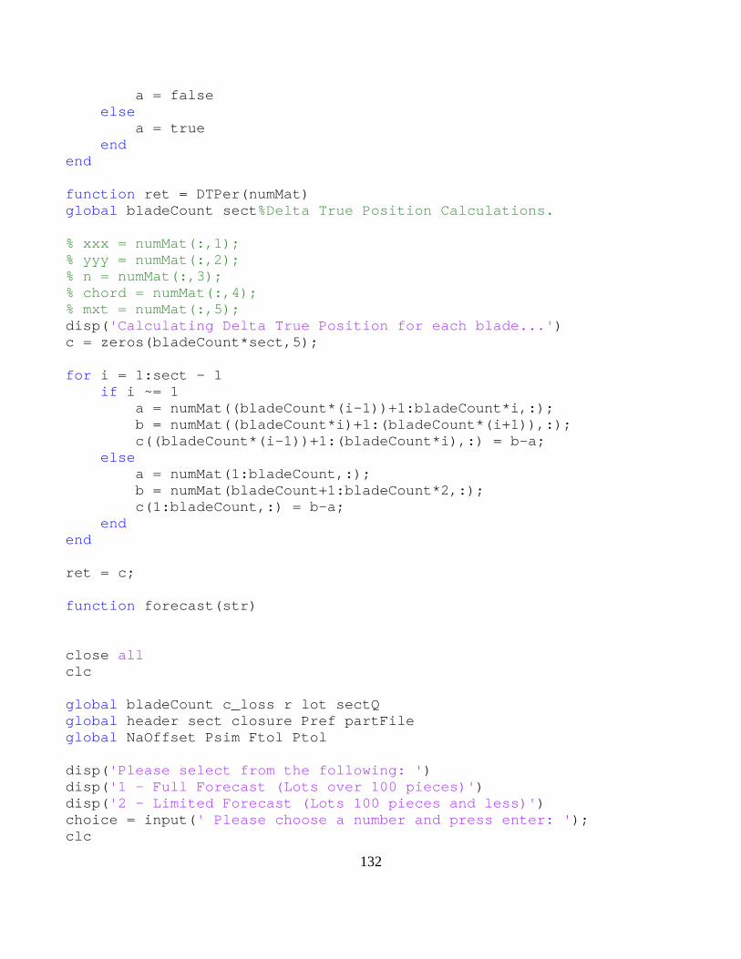
132

a = false else a = true end end function ret = DTPer(numMat) global bladeCount sect%Delta True Position Calculations. % xxx = numMat(:,1); % yyy = numMat(:,2); % n = numMat(:,3); % chord = numMat(:,4); % mxt = numMat(:,5); disp('Calculating Delta True Position for each blade...') c = zeros(bladeCount*sect,5); for i = 1:sect - 1 if i ~= 1 a = numMat((bladeCount*(i-1))+1:bladeCount*i,:); b = numMat((bladeCount*i)+1:(bladeCount*(i+1)),:); c((bladeCount*(i-1))+1:(bladeCount*i),:) = b-a; else a = numMat(1:bladeCount,:); b = numMat(bladeCount+1:bladeCount*2,:); c(1:bladeCount,:) = b-a; end end ret = c; function forecast(str) close all clc global bladeCount c_loss r lot sectQ global header sect closure Pref partFile global NaOffset Psim Ftol Ptol disp('Please select from the following: ') disp('1 - Full Forecast (Lots over 100 pieces)') disp('2 - Limited Forecast (Lots 100 pieces and less)') choice = input(' Please choose a number and press enter: '); clc

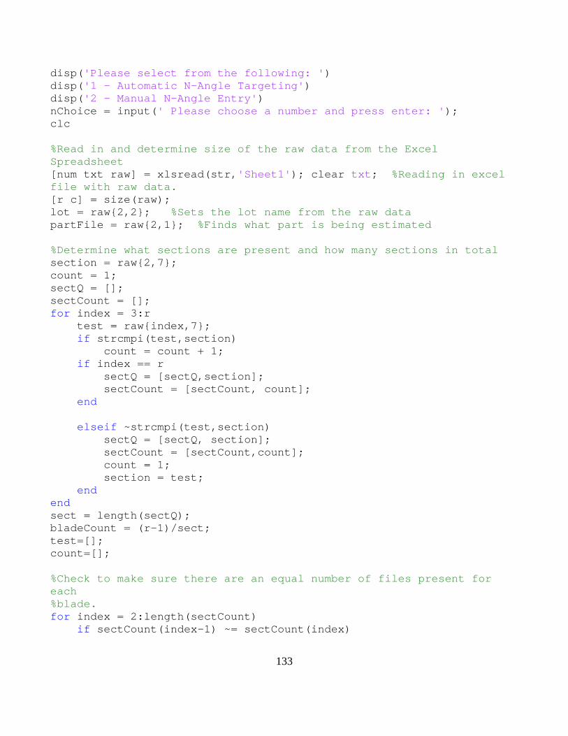
133

disp('Please select from the following: ') disp('1 - Automatic N-Angle Targeting') disp('2 - Manual N-Angle Entry') nChoice = input(' Please choose a number and press enter: '); clc %Read in and determine size of the raw data from the Excel Spreadsheet [num txt raw] = xlsread(str,'Sheet1'); clear txt; %Reading in excel file with raw data. [r c] = size(raw); lot = raw{2,2}; %Sets the lot name from the raw data partFile = raw{2,1}; %Finds what part is being estimated %Determine what sections are present and how many sections in total section = raw{2,7}; count = 1; sectQ = []; sectCount = []; for index = 3:r test = raw{index,7}; if strcmpi(test,section) count = count + 1; if index == r sectQ = [sectQ,section]; sectCount = [sectCount, count]; end elseif ~strcmpi(test,section) sectQ = [sectQ, section]; sectCount = [sectCount,count]; count = 1; section = test; end end sect = length(sectQ); bladeCount = (r-1)/sect; test=[]; count=[]; %Check to make sure there are an equal number of files present for each %blade. for index = 2:length(sectCount) if sectCount(index-1) ~= sectCount(index)

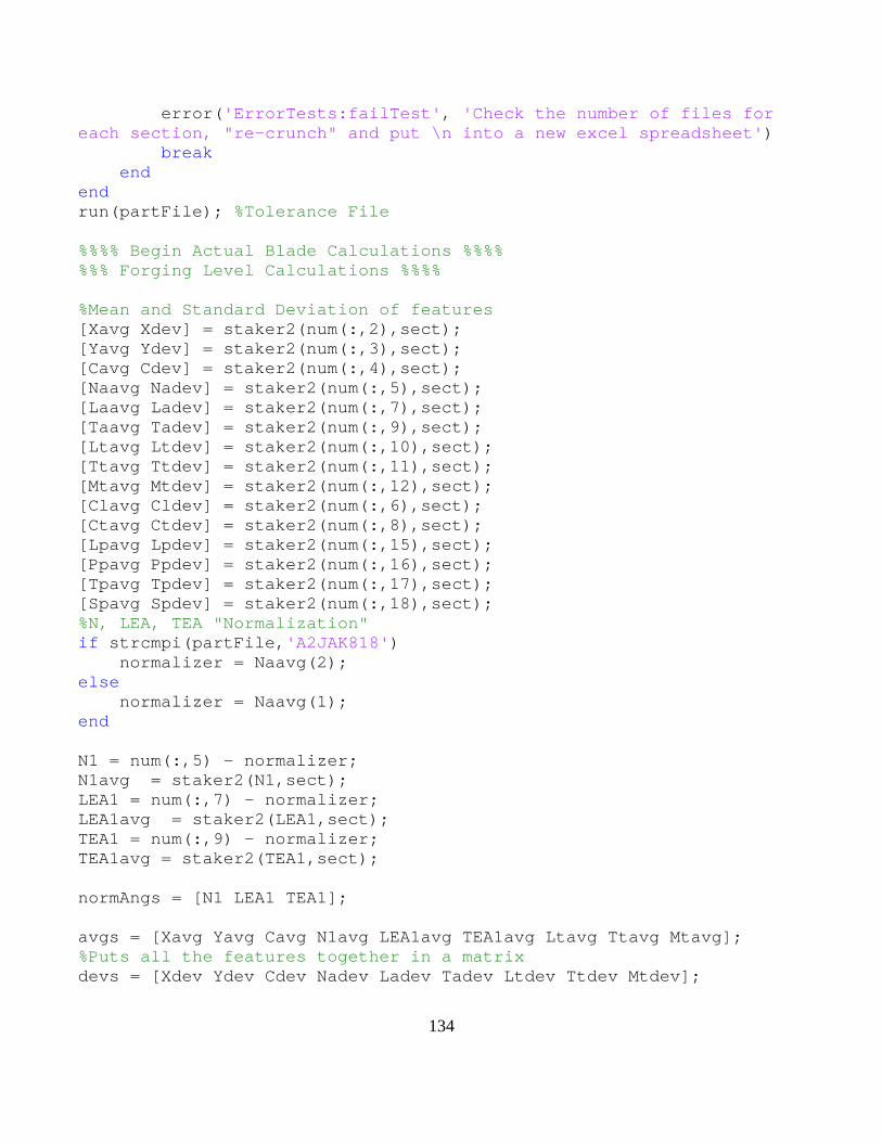
134

error('ErrorTests:failTest', 'Check the number of files for each section, "re-crunch" and put \n into a new excel spreadsheet') break end end run(partFile); %Tolerance File %%%% Begin Actual Blade Calculations %%%% %%% Forging Level Calculations %%%% %Mean and Standard Deviation of features [Xavg Xdev] = staker2(num(:,2),sect); [Yavg Ydev] = staker2(num(:,3),sect); [Cavg Cdev] = staker2(num(:,4),sect); [Naavg Nadev] = staker2(num(:,5),sect); [Laavg Ladev] = staker2(num(:,7),sect); [Taavg Tadev] = staker2(num(:,9),sect); [Ltavg Ltdev] = staker2(num(:,10),sect); [Ttavg Ttdev] = staker2(num(:,11),sect); [Mtavg Mtdev] = staker2(num(:,12),sect); [Clavg Cldev] = staker2(num(:,6),sect); [Ctavg Ctdev] = staker2(num(:,8),sect); [Lpavg Lpdev] = staker2(num(:,15),sect); [Ppavg Ppdev] = staker2(num(:,16),sect); [Tpavg Tpdev] = staker2(num(:,17),sect); [Spavg Spdev] = staker2(num(:,18),sect); %N, LEA, TEA "Normalization" if strcmpi(partFile,'A2JAK818') normalizer = Naavg(2); else normalizer = Naavg(1); end N1 = num(:,5) - normalizer; N1avg = staker2(N1,sect); LEA1 = num(:,7) - normalizer; LEA1avg = staker2(LEA1,sect); TEA1 = num(:,9) - normalizer; TEA1avg = staker2(TEA1,sect); normAngs = [N1 LEA1 TEA1]; avgs = [Xavg Yavg Cavg N1avg LEA1avg TEA1avg Ltavg Ttavg Mtavg]; %Puts all the features together in a matrix devs = [Xdev Ydev Cdev Nadev Ladev Tadev Ltdev Ttdev Mtdev];

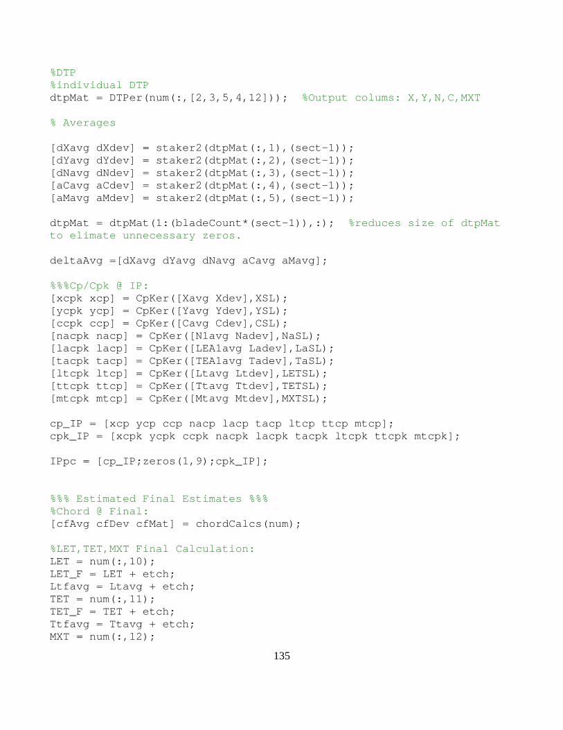
135

%DTP %individual DTP dtpMat = DTPer(num(:,[2,3,5,4,12])); %Output colums: X,Y,N,C,MXT % Averages [dXavg dXdev] = staker2(dtpMat(:,1),(sect-1)); [dYavg dYdev] = staker2(dtpMat(:,2),(sect-1)); [dNavg dNdev] = staker2(dtpMat(:,3),(sect-1)); [aCavg aCdev] = staker2(dtpMat(:,4),(sect-1)); [aMavg aMdev] = staker2(dtpMat(:,5),(sect-1)); dtpMat = dtpMat(1:(bladeCount*(sect-1)),:); %reduces size of dtpMat to elimate unnecessary zeros. deltaAvg =[dXavg dYavg dNavg aCavg aMavg]; %%%Cp/Cpk @ IP: [xcpk xcp] = CpKer([Xavg Xdev],XSL); [ycpk ycp] = CpKer([Yavg Ydev],YSL); [ccpk ccp] = CpKer([Cavg Cdev],CSL); [nacpk nacp] = CpKer([N1avg Nadev],NaSL); [lacpk lacp] = CpKer([LEA1avg Ladev],LaSL); [tacpk tacp] = CpKer([TEA1avg Tadev],TaSL); [ltcpk ltcp] = CpKer([Ltavg Ltdev],LETSL); [ttcpk ttcp] = CpKer([Ttavg Ttdev],TETSL); [mtcpk mtcp] = CpKer([Mtavg Mtdev],MXTSL); cp_IP = [xcp ycp ccp nacp lacp tacp ltcp ttcp mtcp]; cpk_IP = [xcpk ycpk ccpk nacpk lacpk tacpk ltcpk ttcpk mtcpk]; IPpc = [cp_IP;zeros(1,9);cpk_IP]; %%% Estimated Final Estimates %%% %Chord @ Final: [cfAvg cfDev cfMat] = chordCalcs(num); %LET,TET,MXT Final Calculation: LET = num(:,10); LET_F = LET + etch; Ltfavg = Ltavg + etch; TET = num(:,11); TET_F = TET + etch; Ttfavg = Ttavg + etch; MXT = num(:,12);

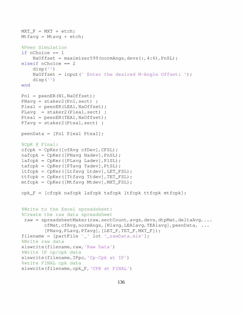
136

MXT_F = MXT + etch; Mtfavg = Mtavg + etch; %Peen Simulation if nChoice == 1 NaOffset = maximizer599(normAngs,devs(:,4:6),PnSL); elseif nChoice == 2 disp('') NaOffset = input(' Enter the desired N-Angle Offset: '); disp('') end Pn1 = peenER(N1,NaOffset); PNavg = staker2(Pn1,sect) ; Plea1 = peenER(LEA1,NaOffset); PLavg = staker2(Plea1,sect) ; Ptea1 = peenER(TEA1,NaOffset); PTavg = staker2(Ptea1,sect) ; peenData = [Pn1 Plea1 Ptea1]; %CpK @ Final: cfcpk = CpKer([cfAvg cfDev],CFSL); nafcpk = CpKer([PNavg Nadev],PnSL); lafcpk = CpKer([PLavg Ladev],PlSL); tafcpk = CpKer([PTavg Tadev],PtSL); ltfcpk = CpKer([Ltfavg Ltdev],LET_FSL); ttfcpk = CpKer([Ttfavg Ttdev],TET_FSL); mtfcpk = CpKer([Mtfavg Mtdev],MXT_FSL); cpk_F = [cfcpk nafcpk lafcpk tafcpk ltfcpk ttfcpk mtfcpk]; %Write to the Excel spreadsheet: %Create the raw data spreadsheet raw = spreadsheetMaker(raw,sectCount,avgs,devs,dtpMat,deltaAvg,... cfMat,cfAvg,normAngs,[N1avg,LEA1avg,TEA1avg],peenData, ... [PNavg,PLavg,PTavg],[LET_F,TET_F,MXT_F]); filename = [partFile '_' lot '_rawData.xls']; %Write raw data xlswrite(filename,raw,'Raw Data') %Write IP cp/cpk data xlswrite(filename,IPpc,'Cp-Cpk at IP') %write FINAL cpk data xlswrite(filename,cpk_F,'CPK at FINAL')

137

%Plot data %Create text for graphs ref_onlyText = 'Information Only - not a product requirment'; if strcmp('A2JAK818',partFile) sectTarget = ['center of tolerance at Sect ' sectQ(2)]; else sectTarget = ['center of tolerance at Sect ' sectQ(1)]; end AngleTargetText = ['N-Angle distribution adjusted to',... sectTarget]; sl4raw = [XSL,YSL,CFSL,PnSL,PlSL,PtSL,... LET_FSL,TET_FSL,MXT_FSL,LeSL,... TeSL,PsSL,SsSL]; if choice == 1 %Plot ALL features normalPlot(XSL,'','XXX',num(:,2),Xavg,Xdev) % figure normalPlot(DTPSL,'','DTP X',dtpMat(:,1),dXavg,dXdev) % figure normalPlot(YSL,'','YYY',num(:,3),Yavg,Ydev) % figure normalPlot(DTPSL,'','DTP Y',dtpMat(:,2),dYavg,dYdev) % figure normalPlot(CSL,'','C',num(:,4),Cavg,Cdev) % figure normalPlot(CFSL,'','C_f',cfMat,cfAvg,cfDev,chordText) % figure normalPlot(NaSL,'','N_1',N1,N1avg,Nadev,AngleTargetText) % figure normalPlot(DTPNSL,'','DTP N',dtpMat(:,3),dNavg,dNdev) % figure normalPlot(LaSL,Pref,'LEA_1',LEA1,LEA1avg,Ladev) % figure normalPlot(ClaSL,Pref,'CLEA',num(:,6),Clavg,Cldev,ref_onlyText) % figure normalPlot(TaSL,Pref,'TEA_1',TEA1,TEA1avg,Tadev) % figure normalPlot(CtaSL,Pref,'CTEA',num(:,8),Ctavg,Ctdev,ref_onlyText) % figure normalPlot(LETSL,'','LET',LET,Ltavg,Ltdev) % figure normalPlot(TETSL,'','TET',TET,Ttavg,Ttdev) % figure normalPlot(MXTSL,'','MXT',MXT,Mtavg,Mtdev)

138

% figure normalPlot(LET_FSL,'','LET_F',LET_F,Ltfavg,Ltdev) % figure normalPlot(TET_FSL,'','TET_F',TET_F,Ttfavg,Ttdev) % figure normalPlot(MXT_FSL,'','MXT_F',MXT_F,Mtfavg,Mtdev) % figure normalPlot(LeSL,'','LEP',num(:,15),Lpavg,Lpdev) % figure normalPlot(TeSL,'','TEP',num(:,17),Tpavg,Tpdev) % figure normalPlot(PsSL,'','PSP',num(:,16),Ppavg,Ppdev) % figure normalPlot(SsSL,'','SSP',num(:,18),Spavg,Spdev) % figure PeenPlot(PnSL, NaOffset,Pref,'Pn_1', Pn1,[PNavg Nadev]) % figure PeenPlot(PlSL, NaOffset,Pref,'Plea_1',Plea1,[PLavg Ladev]) % figure PeenPlot(PtSL, NaOffset,Pref,'Ptea_1',Ptea1,[PTavg Tadev]) % figure normalPlot(ADJSL,'','ADJ C',dtpMat(:,4),aCavg,aCdev) % figure normalPlot(ADJSL,'','ADJ MXT',dtpMat(:,5),aMavg,aMdev) % figure paretoMaker(sl4raw,1) Root(str) elseif choice == 2 PeenPlot(PnSL, NaOffset,Pref,'Pn_1', Pn1,[PNavg Nadev]) % figure PeenPlot(PlSL, NaOffset,Pref,'Plea_1',Plea1,[PLavg Ladev]) % figure PeenPlot(PtSL, NaOffset,Pref,'Ptea_1',Ptea1,[PTavg Tadev]) % figure paretoMaker(sl4raw,1) Root(str) end function NaOffset = maximizer599(data,dev,specs) %MAXIMIZER599 %This function produces the optimal N-Angle offset for this data set. % Input the NORMALIZED N,LEA,TEA information into the DATA variable. %DATA = [N,LEA,TEA] %DEV = [N,LEA,TEA] <-- **Standard Deviation**

139

global sect Pref offset = [-21:3:21]; N = data(:,1); LEA = data(:,2); TEA = data(:,3); Nadev = dev(:,1); Ladev = dev(:,2); Tadev = dev(:,3); Ncpk = []; Ucpk = []; Lcpk = []; for ind = offset pn1 = peenER(N,ind); PNavg = staker2(pn1,sect); plea1 = peenER(LEA,ind); PLavg = staker2(plea1,sect); ptea1 = peenER(TEA,ind); PTavg = staker2(ptea1,sect); Pavgs = [PNavg;PLavg;PTavg]; Pdevs = [Nadev;Ladev;Tadev]; [Uc Lc] = CpKer10([Pavgs,Pdevs],[specs(1,1),specs(1,2)], Pref); Ncpk = [Ncpk , CpKer([PNavg,Nadev],[specs(1,1),specs(1,2)])]; Ucpk = [Ucpk , Uc]; Lcpk = [Lcpk , Lc]; end plot(offset,Lcpk,offset,Ucpk) ULdiff = abs(Ucpk - Lcpk); maxYield = min(ULdiff); NaOffset = offset(find(maxYield == ULdiff)); function normalPlot(specs,ref,ptype,data,avg,dev,varargin) %Plot Forecasting Control Chart. %Creates a control chart given the LSL and USL as a two-element vector, SPECS, and the AVG and DEV vectors %that are relvant to the feature being plotted. Also shades out any reference sections yellow that are %in the REF variable found in the part file.

140

global lot bladeCount header sect sectQ partFile ub = specs(:,2); lb = specs(:,1); if lb > ub USL = lb; LSL = ub; else USL = ub; LSL = lb; end usl = max(USL);lsl=min(LSL); if strcmpi(ptype(1),'D') || strcmpi(ptype(1),'A') sectt = sect - 1; else sectt = sect; end dev = dev.*3; %modifies StDev so the plotting sequence (below) can plot the "6-sigma bands" %Plotting sequence: %Plots U/LSL %Plots 6-sigma bands %Plots section lines %Adds section letters sectQ = char(sectQ); sectLine = linspace(lsl,usl,500); limitLine = linspace(0,bladeCount*sectt,500); plot(limitLine,0, 'c--','LineWidth',0.5) hold on %For DTP plots, letter the sections 'A-B','B-C',etc. if strcmpi(ptype(1),'d') || strcmpi(ptype(1),'a') plot(data,'k.') for i = 2:sectt+1 xx = linspace(bladeCount.*(i-2),bladeCount.*(i-1),250); letter1 = sectQ(i-1);

141

letter2 = sectQ(i); plot(xx,LSL(i-1), 'b-','LineWidth',2) plot(xx,USL(i-1), 'b-','LineWidth',2) plot(xx,avg(i-1),'-m','LineWidth',1.25) plot(xx,avg(i-1) + dev(i-1),'-r','LineWidth',1.25) plot(xx,avg(i-1) - dev(i-1),'-r','LineWidth',1.25) plot(bladeCount*(i-1),sectLine,'--k','LineWidth',0.5) letter = [letter1 '-' letter2]; x = ((bladeCount*(i-1))+ bladeCount/2); y = (max(sectLine) + .00025); text(x,y,letter) end else for i = 1:sectt x = [bladeCount*(i-1)+1:bladeCount*i]; xx = linspace(bladeCount.*(i-1),bladeCount.*i,250); letter = sectQ(i); if letter == ref plot(x,data(x),'y.') else plot(x,data(x),'k.') end plot(xx,LSL(i), 'b-','LineWidth',2) plot(xx,USL(i), 'b-','LineWidth',2) plot(xx,avg(i),'-m','LineWidth',1.25) plot(xx,avg(i) + dev(i),'-r','LineWidth',1.25) plot(xx,avg(i) - dev(i),'-r','LineWidth',1.25) plot(bladeCount*i,sectLine,'--k','LineWidth',0.5) x = ((bladeCount*(i-1))+ bladeCount/2); y = (max(sectLine) + .00025); text(x,y,letter) end end %Adds text to the graph if strcmpi(ptype,'n_1') || strcmpi(ptype,'lea_1') || strcmpi(ptype,'tea_1') || strcmpi(ptype,'DTP N') || strcmpi(ptype,'CLEA') || strcmpi(ptype,'CTEA') ylabel('Deviation from nominal (min.)');xlabel('Observation Number') else ylabel('Deviation from nominal (in.)');xlabel('Observation Number') end bc = num2str(bladeCount);

142

str2 = ['LPI Inspections lot ' lot ' (Basis:' bc ' parts) JB43']; %Create title for graph if ~isempty(varargin) titleStr = {header;str2;ptype;varargin{1}}; else titleStr = {header;str2;ptype}; end clear str2 str1 bc %Free up some space and variables clear str2 str1 bc %Free up some space and variables title(titleStr) text(bladeCount*sectt,usl + ((usl*.25)/2),'USL') text(bladeCount*sectt,lsl + ((lsl*.25)/2),'LSL') %Re-sizes the graph if max(data) < usl && min(data) > lsl set(gca,'xlim',[0 (length(data)+length(data)*.05)]) set(gca,'ylim',[(lsl + lsl*.05) (usl + usl*.05) ]) else set(gca,'xlim',[0 (length(data)+length(data)*.05)]) set(gca,'ylim',[(lsl+min(data)*.5) (usl+max(data)*.5)]) end hold off %save the graph toa jpeg file %build filename filename = [partFile '_' lot '_' ptype '.jpg']; print('-djpeg50',filename); function paretoMaker(specs,count) %rawCellarr = [xxx,yyy,cF,pn1,plea1,ptea1,let_f,tet_f,mxt_f,lep,tep,psp,ssp] %SPECS is in the same order as MAT but contains the USL and LSL %Function searches throught the data for blades out of tolerance % and creates a list of the defects and the measurement. global defectCount names header global bladeCount sect lot partFile filename = [partFile '_' lot '_rawData.xls']; [num txt raw] = xlsread(filename,'Raw Data'); disp('Gathering rejections @ FINAL...')

143

col = [2:3,22,75:77,79:81,15,17,16,18]; posMod = 7; defectCount =[]; names ={}; dc =[]; for p = 1:length(col) ub = specs(:,2); lb = specs(:,1); if lb > ub USL = lb; LSL = ub; else USL = ub; LSL = lb; end test = num(:,col(p)); defect = raw{1,(col(p) + posMod)}; for iS = 1:sect if iS ~= 1 data = test((bladeCount*(iS-1))+1:bladeCount*iS); ub = USL(iS); lb = LSL(iS); defectCount =[defectCount data(find(data > ub)) data(find(data < lb))]; if ~isempty(defectCount) for index = 1:length(defectCount) names{count} = defect; count = count +1; end dc = [dc defectCount']; end defectCount =[]; else data = test(1:bladeCount); ub = USL(iS); lb = LSL(iS); defectCount =[defectCount data(find(data > ub)) data(find(data < lb))]; if ~isempty(defectCount)

144

for index = 1:length(defectCount) names{count} = defect; dc = [dc defectCount']; count = count +1; end end defectCount =[]; end end specs(:,1:2) =[]; end if isempty(names) disp('Airfoil is free from any defects') elseif ~isempty(names) list = []; defectCount = []; count = 1; if length(names) > 1 for index = 2:length(names) if strcmpi(names(index-1),names(index)) count = count + 1; if index == length(names) list = [list,names(index)]; defectCount = [defectCount,count]; end elseif ~strcmpi(names(index-1),names(index)) list = [list,names(index-1)]; defectCount = [defectCount,count]; count = 1; if index == length(names) list = [list,names(index)]; defectCount = [defectCount,count]; end end end else list = names; defectCount = 1; end pareto(defectCount,list) hold on bc = num2str(bladeCount); str2 = ['LPI Inspections lot ' lot ' (Basis:' bc ' parts) JB43'];

145

titleStr = {header;str2}; title(titleStr) hold off fileName = [partFile '_' lot '_PARETO.jpg']; print('-djpeg',fileName) close end function postPeen = peenER(data,offset) %DATA = Actual NORMALIZED data in either a (1xN) or (Mx1) %[P]eenER simulates the peening process and returns how each blade is %affected at each section. global closure bladeCount b=[]; for iS = 1:length(closure) if iS ~= 1 a = data((bladeCount*(iS-1))+1:bladeCount*iS) + closure(iS) + offset; b = [b; a]; else a = data(1:bladeCount * iS) + closure(iS) + offset; b = [b; a]; end end postPeen = b; function PeenPlot(specs,offset,ref,ptype,data,stats) %Specs: [LSL,USL] %DATA: Raw data from peenER() function %STATS: [MEAN StDeviation] *Note: Both are vertical vectors concatenated %together that are section averages. global lot bladeCount header sect sectQ global Psim partFile mu = stats(:,1); sigma = stats(:,2); %Set the appropriate limit to the respective variable. ub = specs(1,2); lb = specs(1,1); if lb > ub USL = lb; LSL = ub;

146

else USL = ub; LSL = lb; end usl = max(USL);lsl=min(LSL); sigma = sigma .*3; %Prep for 6-sigma band plots %Determine position of any outliers UCL = mu + sigma; LCL = mu - sigma; outlierPos = []; for ind = 1:length(mu) if ind == 1 testData = data(1:bladeCount); posModifier = 0; else testData = data(bladeCount*(ind-1) + 1: bladeCount*ind); posModifier = bladeCount*(ind-1); end pos = find( testData >= UCL(ind) | testData <= LCL(ind)); if ~isempty(pos) outlierPos = [outlierPos, (pos' + posModifier)]; end end %Plot any outliers if ~isempty(outlierPos) outlierPos = sort(outlierPos); plot(outlierPos,data(outlierPos),'*k','MarkerSize',8); hold on end %Plot sequence sectQ = char(sectQ); limitLine = linspace(0,bladeCount*sect,500); plot(limitLine,LSL,'-b','LineWidth',2) hold on plot(limitLine,USL,'-b','LineWidth',2) plot(limitLine,0,'--c','LineWidth',0.5) for i = 1:sect xx = linspace(bladeCount.*(i-1),bladeCount.*i,250);

147

x = bladeCount.*(i-1) + round(bladeCount/2); letter = sectQ(i); mu_i = mu(i); if strcmpi(ref,letter) && ~strcmpi(ptype(2),'n') plot(xx,mu_i,'y') plot(x,mu_i,'-om','LineWidth',1.25,'MarkerEdgeColor',... 'k','MarkerFaceColor','y',... 'MarkerSize', 6) plot(xx,UCL(i),'-y','LineWidth',1.25) plot(xx,LCL(i),'-y','LineWidth',1.25) else plot(xx,mu_i,'m') plot(x,mu_i,'-om','LineWidth',1.25,'MarkerEdgeColor',... 'k','MarkerFaceColor',[0.49 1 0.63],... 'MarkerSize', 6) plot(xx,UCL(i),'-r','LineWidth',1.25) plot(xx,LCL(i),'-r','LineWidth',1.25) end x = bladeCount*(i-1) + bladeCount/2; y = usl * 1.05; text(x,y,letter) end %Create Title for chart %Peen Simulation Text Psim = num2str(Psim); offset = num2str(offset); str3 = ['Peen Simulation: ' Psim ' min at Tip']; str4 = ['N-Angle Target: ' offset ' min at Sect'... sectQ(1)]; bc = num2str(bladeCount); str2 = ['LPI Inspections lot ' lot ' (Basis:' bc ' parts) JB43']; titleStr = {header;str2;ptype;str3;str4}; clear str2 str1 bc %Free up some space and variables %Put text onto graph ylabel('Deviation from nominal (min.)');xlabel('Observation Number') title(titleStr) text(bladeCount*sect,USL + ((USL*.25)/2),'USL') text(bladeCount*sect,LSL - ((LSL*.25)/2),'LSL') if max(data) < usl && min(data) > lsl set(gca,'xlim',[0 (length(data)+length(data)*.05)]) set(gca,'ylim',[(lsl + lsl*.05) (usl + usl*.05) ])

148

else set(gca,'xlim',[0 (length(data)+length(data)*.05)]) set(gca,'ylim',[(min(data)+min(data)*.5) (max(data)+max(data)*.5)]) end hold off %save the graph toa jpeg file %build filename filename = [partFile '_' lot '_' ptype '.jpg']; print('-djpeg50',filename); function Root(str) global Ftol Ptol lot partFile header bladeCount [num1 t1 raw1] = xlsread(str,'Sheet2'); clear t1 %Create a check to see if data is present if isempty(num1) disp('No Fillet or Platform data is present') return end [r c] = size(raw1); section = raw1{1,2}; count = 1; queue = {}; qCount =[]; for index = 2:r test = raw1{index,2}; if strcmpi(test,section) count = count + 1; if index == r queue{end+1} = section; qCount = [qCount,count]; end elseif ~strcmpi(test,section) queue{end+1} = section; qCount = [qCount,count]; count = 1; section = test; end end data = num1(:,4); sectIndex = linspace(0,r,length(queue)+1);

149

limitLine = linspace(0,sectIndex(end),r*2); sectLine = linspace(0,Ftol,(1/Ftol)*3); plot(data,'.k') hold on plot(limitLine,Ftol,'.b') for i = 1:length(sectIndex)-1; x = sectIndex(i); y = Ftol + (Ftol*.02); text(x,y,queue(i)); plot(x,sectLine); end bc = num2str(bladeCount); str2 = ['LPI Inspections lot ' lot ' (Basis:' bc ' parts) JB43']; titleStr = {header;str2;'Fillet'}; title(titleStr) reinspPos = find(data > Ftol); reinspCN = num1(reinspPos,1); if ~isempty(reinspPos) fprintf('The following control number MUST be reinspected \n for fillet rejection: %i \n',reinspCN) end %Resize plot area if max(data) > Ftol set(gca,'xlim',[0 (length(data)+length(data)*.05)]) set(gca,'ylim',[0 (max(data) + max(data)*.05) ]) else set(gca,'xlim',[0 (length(data)+length(data)*.05)]) set(gca,'ylim',[0 (Ftol+ (Ftol*.05))]) end hold off %save the graph toa jpeg file beg = [partFile '_' lot]; filename = [ beg '_FILLET.jpg']; print('-djpeg50',filename) %%Find and report out of tolerance Fillets reinspPos = find(data > Ftol); reinspCN = num1(reinspPos,1); if ~isempty(reinspPos) fid = fopen([saveFile '\Fillet Rejections.txt'],'w');

150

for i = 1:length(reinspPos) fprintf(fid,'The following control number is out of tolerance for the FILLET feature: %i \n',reinspCN(i)); end fclose(fid); end [num2 t2 raw2] = xlsread(str,'Sheet3'); clear t2 [r c] = size(raw2); section = raw2{1,2}; count = 1; queue = {}; qCount =[]; for index = 2:r test = raw2{index,2}; if strcmpi(test,section) count = count + 1; if index == r queue{end+1} = section; qCount = [qCount,count]; end elseif ~strcmpi(test,section) queue{end+1} = section; qCount = [qCount,count]; count = 1; section = test; end end data = num2(:,5); sectIndex = linspace(0,r,length(queue)+1); limitLine = linspace(0,sectIndex(end),r*2); sectLine = linspace(Ptol(1),Ptol(2),(1/Ptol(2))*3); plot(data,'.k') hold on plot(limitLine,Ptol(1),'-b') plot(limitLine,Ptol(2),'-b') for i = 1:length(sectIndex)-1; x = sectIndex(i); y = Ptol(2) + (Ptol(2)*.02); sectText = queue(i); text(x,y,sectText); plot(x,sectLine);

151

end titleStr = {header;str2;'Platform'}; title(titleStr) %Resize plot area if max(data)< Ptol(2) && min(data) > Ptol(1) set(gca,'xlim',[0 (length(data)+length(data)*.05)]) set(gca,'ylim',[(Ptol(1) + Ptol(1)*.05) (Ptol(2) + Ptol(2)*.05) ]) else set(gca,'xlim',[0 (length(data)+length(data)*.05)]) set(gca,'ylim',[(Ptol(1) + min(data)*.5) (Ptol(2) + max(data)*.5)]) end hold off %save the graph toa jpeg file %build filename filename = [ beg '_PLATFORM.jpg']; print('-djpeg50',filename) reinspPos = find(data > Ptol(2) | data < Ptol(1)); reinspCN = num2(reinspPos,1); if ~isempty(reinspPos) fid = fopen([saveFile '\Platform Rejections.txt'],'w'); for i = 1:length(reinspPos) fprintf(fid,'The following control number is out of tolerance for the PLATFORM feature: %i \n',reinspCN(i)); end fclose(fid); end function ret=spreadsheetMaker(raw,sCounter,avg,dev,dtpMat,deltaAvg,chordFinal,cFavg,normAngs,normAngsMean,pangs,pangsMean,thickness) % Takes in the data matrices and places them in a cell array that is ready % to be written to an Excel file. global sect sectQ closure c_loss NaOffset format bank offset = NaOffset; raw{1,end+2} = 'Sect'; for index = 1:sect raw{index + 1,end} = sectQ(index);

152

end %Chord loss "index" raw{1,end+1} = 'Chord Loss'; for index = 1:length(c_loss) raw{index+1,end} = c_loss(index); end %Estimated chord lengths raw{1,end +1} = 'Chord Final'; for index = 1:length(chordFinal) raw{index+1,end} = round(chordFinal(index)/.0001)*.0001; end raw{1,end+2} = 'Sect'; for index = 1:sect raw{index + 1,end} = sectQ(index); end %Averages raw{1,end+1} = 'XXX Mean'; raw{1,end+1} = 'YYY Mean'; raw{1,end+1} = 'C Mean'; raw{1,end+1} = 'N Mean'; raw{1,end+1} = 'LEA Mean'; raw{1,end+1} = 'TEA Mean'; raw{1,end+1} = 'LET Mean'; raw{1,end+1} = 'TET Mean'; raw{1,end+1} = 'MXT Mean'; for i = 1:sect for i2 = 0:8 raw{i+1,end-i2} = avg(i,end-i2); end end %DTP/ADJ raw{1,end+2} = 'DTP XXX'; raw{1,end+1} = 'DTP YYY'; raw{1,end+1} = 'DTP N'; raw{1,end+1} = 'Adj_C'; raw{1,end+1} = 'Adj_MXT'; for i = 1:sect-1 for i2 = 0:4 raw{i+2,end-i2} = deltaAvg(i,end-i2); end end %Standard Deviation - by sections raw{1,end+2} = 'XXX StDev';

153

raw{1,end+1} = 'YYY StDev'; raw{1,end+1} = 'C StDev'; raw{1,end+1} = 'N StDev'; raw{1,end+1} = 'LEA StDev'; raw{1,end+1} = 'TEA StDev'; raw{1,end+1} = 'LET StDev'; raw{1,end+1} = 'TET StDev'; raw{1,end+1} = 'MXT StDev'; for i = 1:sect for i2 = 0:8 raw{i+1,end-i2} = dev(i,end-i2); end end %Section File Count raw{1,end+1} = 'File Count'; for index = 1:length(sCounter) raw{index+1,end} = sCounter(index); end raw{1,end+2} = 'Sect'; for index = 1:sect raw{index + 1,end} = sectQ(index); end %Chord @ Final average - by section raw{1,end+1} = 'Chord Average @ Final'; for index = 1:length(cFavg) raw{index+1,end} = round(cFavg(index)/.0001)*.0001; end %Normalized [N LEA TEA] raw{1,end+2}= 'N_1'; raw{1,end+1}= 'LEA_1'; raw{1,end+1}= 'TEA_1'; for i = 1:length(normAngs) for i2 = 0:2 raw{i+1,end-i2} = round(normAngs(i,end-i2)/.0001)*.0001; end end raw{1,end+1} = 'Sect'; for index = 1:sect raw{index + 1,end} = sectQ(index); end

154

%[Navg LEAavg TEAavg] Averages by section raw{1,end+1} = 'N_1 Mean'; raw{1,end+1} = 'LEA_1 Mean'; raw{1,end+1} = 'TEA_1 Mean'; for i = 1:length(normAngsMean) for i2 = 0:2 raw{i+1,end-i2} = round(normAngsMean(i,end-i2)/.0001)*.0001; end end %DTP - by blade raw{1,end+2} = 'DTP X'; raw{1,end+1} = 'DTP Y'; raw{1,end+1} = 'DTP N'; raw{1,end+1} = 'ADJ C'; raw{1,end+1} = 'ADJ MXT'; for i = 1:length(dtpMat) for i2 = 0:4 raw{i+1,end-i2} = dtpMat(i,end-i2); end end raw{1,end+2} = 'Sect'; for index = 1:sect raw{index + 1,end} = sectQ(index); end %Offset and closure by section raw{1,end+1} = 'Offset'; for index = 1:sect raw{index+1,end} = offset; end raw{1,end+1} = 'Closure'; for index = 1:sect raw{index+1,end} = round(closure(index)/.0001)*.0001; end %Post Peen [N LEA TEA] averages by section raw{1,end+1} = 'Pn1 Mean'; raw{1,end+1} = 'Plea1 Mean'; raw{1,end+1} = 'Ptea1 Mean'; for i = 1:length(pangsMean) for i2 = 0:2 raw{i+1,end-i2} =round( pangsMean(i,end-i2)/.0001)*.0001; end end

155

%Post Peen [N LEA TEA] - by blade raw{1,end+1} = 'Pn1'; raw{1,end+1} = 'Plea1'; raw{1,end+1} = 'Ptea1'; for i = 1:length(pangs) for i2 = 0:2 raw{i+1,end-i2} = round(pangs(i,end-i2)/.0001)*.0001; end end %[LET TET MXT] by blade raw{1,end + 2} = 'LET_Final'; raw{1,end +1} = 'TET_Final'; raw{1,end +1} = 'MXT_Final'; for i = 1:length(thickness) for i2 = 0:2 raw{i+1,end-i2} = round(thickness(i,end-i2)/.0001)*.0001; end end ret = raw; function [ret1 ret2] = staker2(numMat,sect) %Standard Deviation and Average Calculation. Given the excel numerical %return value and the number of sections will yield a (Sect x Feature) %matrix with the averages and standard deviations from the nominal value. global bladeCount [row colum] = size(numMat); avgMat = zeros(sect,colum); stdMat = avgMat; for iC = 1:colum for iS = 1:sect if iS ~= 1 avgMat(iS,iC) = mean(numMat((bladeCount*(iS-1))+1:bladeCount * iS,1)); stdMat(iS,iC) = std(numMat((bladeCount*(iS-1))+1:bladeCount * iS,1)); else avgMat(1,iC) = mean(numMat(1:bladeCount,1));

156

stdMat(1,iC) = std(numMat(1:bladeCount,1)); end end end ret1 = avgMat; ret2 = stdMat; % whos