Embed Size (px)
Citation preview
Louisiana State UniversityLSU Digital Commons
LSU Doctoral Dissertations Graduate School
6-17-2018
Development of a Slab-based Monte Carlo ProtonDose Algorithm with a Robust Material-dependentNuclear Halo ModelJohn Wesley Chapman JrLouisiana State University and Agricultural and Mechanical College, [email protected]
Follow this and additional works at: https://digitalcommons.lsu.edu/gradschool_dissertations
Part of the Other Physics Commons, Statistical Models Commons, and the Theory andAlgorithms Commons
This Dissertation is brought to you for free and open access by the Graduate School at LSU Digital Commons. It has been accepted for inclusion inLSU Doctoral Dissertations by an authorized graduate school editor of LSU Digital Commons. For more information, please [email protected].
Recommended CitationChapman, John Wesley Jr, "Development of a Slab-based Monte Carlo Proton Dose Algorithm with a Robust Material-dependentNuclear Halo Model" (2018). LSU Doctoral Dissertations. 4619.https://digitalcommons.lsu.edu/gradschool_dissertations/4619
DEVELOPMENT OF A SLAB-BASED MONTE CARLO PROTON DOSE ALGORITHM WITH A
ROBUST MATERIAL-DEPENDENT NUCLEAR HALO MODEL
A Dissertation
Submitted to the Graduate Faculty of the
Louisiana State University and
Agricultural and Mechanical College
in partial fulfillment of the
requirements for the degree of
Doctor of Philosophy
in
The Department of Physics and Astronomy
by
John Wesley Chapman Jr
B.S., Louisiana State University, 2008
M.S., Louisiana State University, 2012
August 2018

ii
ACKNOWLEDGMENTS
This project required substantial supplemental theory beyond the typical medical physics curriculum. I am
grateful to Dr. Kenneth Hogstrom for providing this additional instruction and am humbled to have been taught
by a prominent expert in this field. I also am thankful for my thorough and helpful advisor, Dr. Jonas Fontenot,
whose guidance has improved both my technical communication and challenged me to critically evaluate every
step in my project.
I acknowledge my family for their support, with special emphasis on my parents. They have taught me
to never let fear of the unknown interfere with my goals. My parents’ recent illnesses have motivated me to
pursue science with renewed purpose, especially in the area of treating human disease. I hope that upon
completion of my training I can end up a fraction of what they are, and that my knowledge can one day
approach their level of wisdom. I thank everyone who has patiently sat and listened to explanations of my
research and feigned interest. I thank my siblings for being amazing friends, and I am grateful that all in my
family have become my biggest fans, even though I am still not sure if they know exactly what medical physics
is.
It seems to me no coincidence that my incredible wife, Rebecca, entered my life when I began graduate
studies. She has been there from the start and will be there at the end to celebrate our next phase of life together.
Rebecca, I could not think of a better person to have spent my life with. Thank you for always being a friend, an
inspiration, and especially my advocate. Thank you even more for being the love of my life. I am grateful to
Rebecca for her patience in tolerating the long hours required to complete this project, often carrying well into
the night. I am grateful that she supported my goals; after all, a good portion of this dissertation was written
using a 55” HDTV and a recliner during nighttime hours. Throughout this project, Rebecca has been a constant
source of inspiration, always finding unique ways to make me laugh (mostly cat jokes). She has always found a
way to help me remain positive and focused.
iii
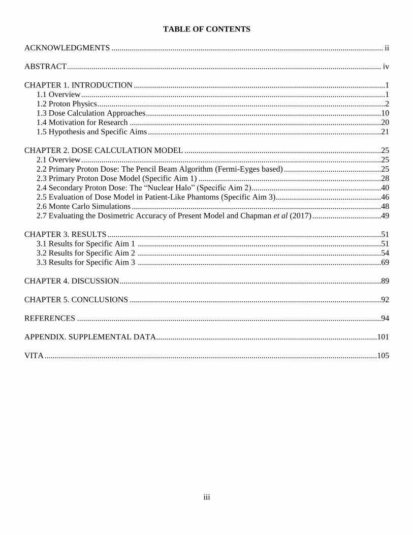
TABLE OF CONTENTS
ACKNOWLEDGMENTS ...................................................................................................................................... ii
ABSTRACT ........................................................................................................................................................... iv
CHAPTER 1. INTRODUCTION ............................................................................................................................1
1.1 Overview ......................................................................................................................................................1
1.2 Proton Physics ..............................................................................................................................................2
1.3 Dose Calculation Approaches ....................................................................................................................10
1.4 Motivation for Research ............................................................................................................................20
1.5 Hypothesis and Specific Aims ...................................................................................................................21
CHAPTER 2. DOSE CALCULATION MODEL .................................................................................................25
2.1 Overview ....................................................................................................................................................25
2.2 Primary Proton Dose: The Pencil Beam Algorithm (Fermi-Eyges based) ................................................25
2.3 Primary Proton Dose Model (Specific Aim 1) ..........................................................................................28
2.4 Secondary Proton Dose: The “Nuclear Halo” (Specific Aim 2) ................................................................40
2.5 Evaluation of Dose Model in Patient-Like Phantoms (Specific Aim 3) ....................................................46
2.6 Monte Carlo Simulations ...........................................................................................................................48
2.7 Evaluating the Dosimetric Accuracy of Present Model and Chapman et al (2017) ..................................49
CHAPTER 3. RESULTS .......................................................................................................................................51
3.1 Results for Specific Aim 1 ........................................................................................................................51
3.2 Results for Specific Aim 2 ........................................................................................................................54
3.3 Results for Specific Aim 3 ........................................................................................................................69
CHAPTER 4. DISCUSSION .................................................................................................................................89
CHAPTER 5. CONCLUSIONS ............................................................................................................................92
REFERENCES ......................................................................................................................................................94
APPENDIX. SUPPLEMENTAL DATA.............................................................................................................101
VITA ....................................................................................................................................................................105

iv
ABSTRACT
Pencil beam algorithms (PBAs) are often utilized for dose calculation in proton therapy treatment planning
because they are fast and accurate under most conditions. However, as discussed in Chapman et al (2017), the
accuracy of a PBA can be limited under certain conditions because of two major assumptions: (1) the central-
axis semi-infinite slab approximation; and, (2) the lack of material dependence in the nuclear halo model. To
address these limitations, we transported individual protons using a class II condensed history Monte Carlo and
added a novel energy loss method that scaled the nuclear halo equation in water to arbitrary geometry. Our
results indicated significant reductions in primary dose difference distal to laterally finite slab heterogeneities
(~15%) compared to our previous model. Furthermore, our improved nuclear halo model decreased the
distance-to-agreement (DTA) of the 1% isodose lines near heterogeneities by ~2-7 mm, and resulted in
significant in-field improvement for deep air slabs (~2% improvement in total dose at the peak). Evaluation of
both of these improvements in more clinically relevant geometries revealed an improved DTA of the 1%
isodose line (~0.3-3 mm) and a reduction of maximum dose near the peak (18-27% reduced to 6-15%). Overall,
the two modeling improvements made in this work have resulted in a dose model with significantly higher dose
calculation accuracy across a wide range of particularly challenging geometries.

1
CHAPTER 1. INTRODUCTION
1.1 Overview
Proton therapy has gained widespread appeal and implementation into numerous external beam radiation
treatment facilities. As of July 2017, the Particle Therapy Cooperative Group (PTCOG) reported sixty-four
proton therapy facilities in operation and sixty-three either under construction or in the planning stages
worldwide (PTCOG 2017). This development is attributed to the dosimetric benefits offered by protons,
including: a sharp lateral penumbra, a narrow Bragg peak that can be modulated to arbitrary width, and a finite
range, beyond which there is clinically insignificant dose. As will be shown, these dosimetric properties result
from the physical interactions between protons and matter.
As interest in proton therapy continues, there has been a trend toward improving the precision of these
treatments. For instance, the proton range (a critical factor for planning a patient treatment) is subject to
uncertainties in imaging, patient setup, beam delivery and dose calculation. The specific parameters that define
each of these aspects of patient care are typically managed using computer-based treatment planning systems
(TPS). A TPS is used to evaluate the dose distribution in several beam configurations, and identify the
configuration resulting in optimal tumor and non-tumor dose. However, the extent to which dose conforms to
the tumor or spares normal tissue is limited by the previously mentioned uncertainties. Therefore, reducing the
uncertainties of any one of these aspects directly results in a more conformal plan.
An essential component for the quality of a radiotherapy treatment plan is the accuracy of the dose
calculation model. Although the clinical advantages of more accurate dose calculations have not been fully
quantified, studies have shown that 5% changes in dose can result in 10-20% changes in tumor control
probability (TCP), or up to 20-30% changes in normal tissue complication probabilities (NTCP) (Stewart and
Jackson 1975, Goiten and Busse 1975, Orton et al 1984). Thus, maximizing the accuracy of dose calculations in
treatment planning potentially translates directly to both improved tumor control and a reduction in incidence
and / or severity of side effects.
2
Paganetti (2012) published a comprehensive study on this matter and posited reducing uncertainties in
the proton range would allow a reduction of the treatment volume, permitting better utilization of the dosimetric
advantages inherent to protons. In some cases, reducing some of these uncertainties will likely require the
development of new technologies – such as replacing the now standard photon-based computerized tomography
(CT) imaging technologies with proton-based solutions. Reduction of uncertainties in beam delivery and patient
setup may require new procedures. However, Paganetti estimated that the largest uncertainties in the range were
due to the analytical approximations used in current dose calculation technologies, amounting to ~+/-3% (1.5
standard deviations); he further speculated that the uncertainties in this category could be reduced to ~+/-0.2%
using a dose calculation tool that more realistically models proton transport and interaction physics, especially
in inhomogeneous regions.
An additional critical component that needs to be included in any proton dose calculation model is the
dose resulting from secondary particles generated in nonelastic nuclear interactions (Pedroni et al 2005). The
physical basis for this phenomenon will be discussed in a later section, but it has been shown that neglecting
this effect in a proton dose model may result in systematic errors for small fields (~10-15%), depending on the
size of the target volume (Pedroni et al 2005, Soukup et al 2005).
Thus, the literature indicates higher accuracy proton dose calculation algorithms would improve treatments
and better utilize the dosimetric advantages inherent to proton therapy. Additionally, the increasing focus on
conformal treatments places emphasis on developing higher accuracy dose calculations algorithms. All of these
considerations will be further expanded on in the following sections.
1.2 Proton Physics
In this section, we consider the subset of interaction physics important for dose calculations in proton
therapy. To facilitate discussion, this overview will be divided into three broad categories: energy loss, scatter,
and nuclear interactions. Furthermore, emphasis will be on interactions resulting in the beneficial dosimetric
properties previously mentioned, as well as concepts and equations relevant to discussion in proceeding
sections. Detailed coverage of proton interactions in matter is available in the literature (Chu et al 1993, Pedroni

3
et al 1995, Lomax 2009, ICRU 1998, ICRU 2007, Newhauser et al 2015). In the sections that follow on dose
calculation, discussion of dose models is broadly separately into two categories: “primary” and “secondary”
(sometimes called “nuclear halo”) dose. “Primary” dose is used to refer to dose due to protons which were
present at the start of the simulation (i.e., those protons that originate from the beam). As such, these protons are
the ones that encounter energy loss interactions (section 1.2.1), multiple Coulomb scatter (MCS) (section 1.2.2)
and larger angle scatter events, and fluence loss in nonelastic nuclear interactions (section 1.2.3). However, the
“primary” dose term is based on analytical functions which cannot fully characterize all such events (for
instance, the scatter model is based on a Gaussian, which is not capable of quantifying all large angle scatter
events). The intention of the “secondary” dose term is to model dose due to secondary protons created in
nonelastic nuclear interactions; however, events that are not adequately modeled by the primary term are also
inherently accounted for in the secondary term since the total dose is fit to Monte Carlo data in water (see
Chapter 2).
1.2.1 Energy Loss
As protons traverse matter, their energy is reduced by numerous inelastic interactions with atomic
electrons. The electrons are ionized in these interactions, depositing energy mostly in local tissue, which results
in absorbed dose. The proton’s large mass relative to that of the electron (1,832 times larger) results in
negligible deflections during these events so that protons trajectories are very closely approximated by straight
lines (see Figure 1.1); for this reason, energy loss can be quantified without considerations of scatter. These
frequent energy loss events that protons encounter in matter results in a continual decrease in energy. After a
proton has insufficient energy for further transport into matter, the proton stops, resulting in a finite range that is
a function of the incident energy. Protons can also lose energy in elastic interactions with the atomic nucleus,
however, this energy loss mechanism only becomes an important contribution to the overall dose at low
energies, toward the end of range. In this work, energy loss via nuclear elastic interactions was not an important
effect to model because it did not result in any difference in terms of the proton range. A less significant form of
energy loss (negligible in therapeutic scenarios) is called Bremsstrahlung, meaning “braking radiation,” in

4
which the proton is deflected by the nucleus and the kinetic energy lost in this process is carried off by a photon
to deposit dose in a remote area.
Figure 1.1. Protons lose energy mainly via inelastic Coulomb interactions with atomic electrons. Modified from
Newhauser et al (2015).
The large number of protons in a therapeutic beam and the statistical nature of interaction cross sections
infers that energy loss events are amenable to statistical treatment. Therefore, the energy loss rate, also called
the linear stopping power, is defined as the ratio of the differential mean energy loss to depth in the material of
interest. A more convenient expression of the energy loss rate is the mass stopping power, which is independent
of the mass density. The linear stopping power is indicated by 𝑆, and the mass stopping power makes the
density independence explicit, 𝑆/𝜌. The stopping power is often further subdivided into electronic and nuclear
stopping powers; the electronic stopping power characterizes energy loss events with atomic electrons whereas
the nuclear stopping power characterizes energy loss due to elastic interactions with the nucleus. As mentioned
previously, the nuclear stopping power was not included in the new dose model discussed in this work. In fact,
Gottschalk et al (2015) states that in a model such as ours, it is conceptually incorrect to include the nuclear
stopping power.
Numerous formulations have been presented for the linear electronic stopping power (Bragg and
Kleeman 1905, Bohr 1915, and Bethe 1930 and Bloch 1933), but the most accurate formulation, called the
Bethe-Bloch formula (Bethe 1930, Bloch 1933), takes relativistic and quantum mechanical considerations into
effect and has the following form,
𝑆
𝜌=
−𝑑𝐸
𝜌𝑑𝑥=
4𝜋𝑁𝐴𝑟𝑒2𝑚𝑒𝑐2
𝛽2
𝑍
𝐴[ln
2𝑚𝑒𝑐2𝛾2𝛽2
𝐼− 𝛽2 −
𝛿
2−
𝐶
𝑍], (1)

5
where 𝑁𝐴 = 6.022𝑥1023 𝑚𝑜𝑙−1 is Avogadro’s number, 𝑟𝑒 = 2.818𝑥10−13 𝑐𝑚 is the classical electron radius,
𝑚𝑒𝑐2 = 0.511 𝑀𝑒𝑉 is the rest mass of an electron, 𝛽 is the ratio of the velocity of the proton to the speed of
light, 𝑍 is the atomic number and A is the atomic weight of the material of interest, 𝛾 = (1 − 𝛽2)−1/2, 𝐼 is the
mean excitation potential of the material, 𝛿 is a density correction due to shielding of remote electrons by local
electrons, and 𝐶 is a shell correction term.
The energy loss rate is inversely proportional to 𝛽2, which implies an infinitely high and infinitesimally
narrow peak as 𝛽 approaches zero; this results in the monoenergetic Bragg peak that is characteristic of proton
beams. However, stochastic variations in proton energy loss (energy straggling) (Bohr 1948) result in slight
changes in proton path lengths (range straggling). The overall effect of range straggling is a broadening of the
Bragg peak that increases with increasing depth. For instance, a proton stopping power computation by Berger
et al (2005) resulted in the range straggling evident in Figure 1.2. Energy straggling theories for thick (Bohr
1915), intermediate (Landau 1944), and thin slabs of material (Vavilov 1957) have been characterized. The
simplest formulation is by Bohr (1915), in which the energy straggling is modeled as a Gaussian. Further
simplifications of Bohr’s theory have been presented as parameterizations of the RMS width of the Gaussian
based on range (Chu et al 1993).
Figure 1.2. Computed linear stopping power in liquid water vs. proton energy (Berger et al 2005).
A consequence of protons traveling in nearly straight lines is the near equivalence of the proton range
and average proton pathlength. The assumption that protons lose energy continuously is referred to as the
continuous slowing-down approximation (CSDA), which is often used in dose calculation models. Using the

6
CSDA, the proton range is calculated by integrating the reciprocal of the linear stopping power as a function of
energy. Additionally, using the CSDA, energy loss over discrete distances Δ𝑥 is calculated using the product of
the linear stopping power and Δ𝑥.
As a final point, equation (1) provides a theoretical framework for calculating stopping power, but it is
often more convenient to obtain stopping power values from readily available databases that perform all the
computations needed. Although there are certain dose calculation models that actually compute equation (1) for
a large number of particles, it is typically more convenient and less resource-intensive to use a tool such as
PSTAR (Berger et al 2005) or SRIM (Ziegler et al 2012). For example, PSTAR is an online tool that calculates
stopping power (electronic, nuclear, total) and range (CSDA, projected) for a database of pre-determined
materials and user-selected energies. Similarly, SRIM calculates ion stopping power and range values in several
biological materials and for a wide range of energies.
1.2.2 Scatter
Protons near the atomic nucleus may encounter a repulsive force due to the positive charge of the
nucleus. This elastic Coulomb interaction deflects the proton away from the nucleus (Figure 1.3). In this
interaction, the proton energy loss is negligible, and the deflection angle tends to be small. For this reason,
scatter may be quantified without considering energy loss. Like the energy loss rate, it is typically more
convenient to express scatter in a stochastic form.
Figure 1.3. Protons are deflected mainly via elastic Coulomb interactions with atomic nuclei. Modified from
Newhauser et al (2015).
Individual proton scatter events in the vicinity of an atomic nucleus tend to be very small; however, as
protons proceed through the medium, the accumulation of a large number of these deflections has a larger
impact on the lateral displacement. Because there are a large number of small scatter events and because of the
statistical nature of this phenomenon, it can be quantified using the central limit theorem. Thus, the probability
7
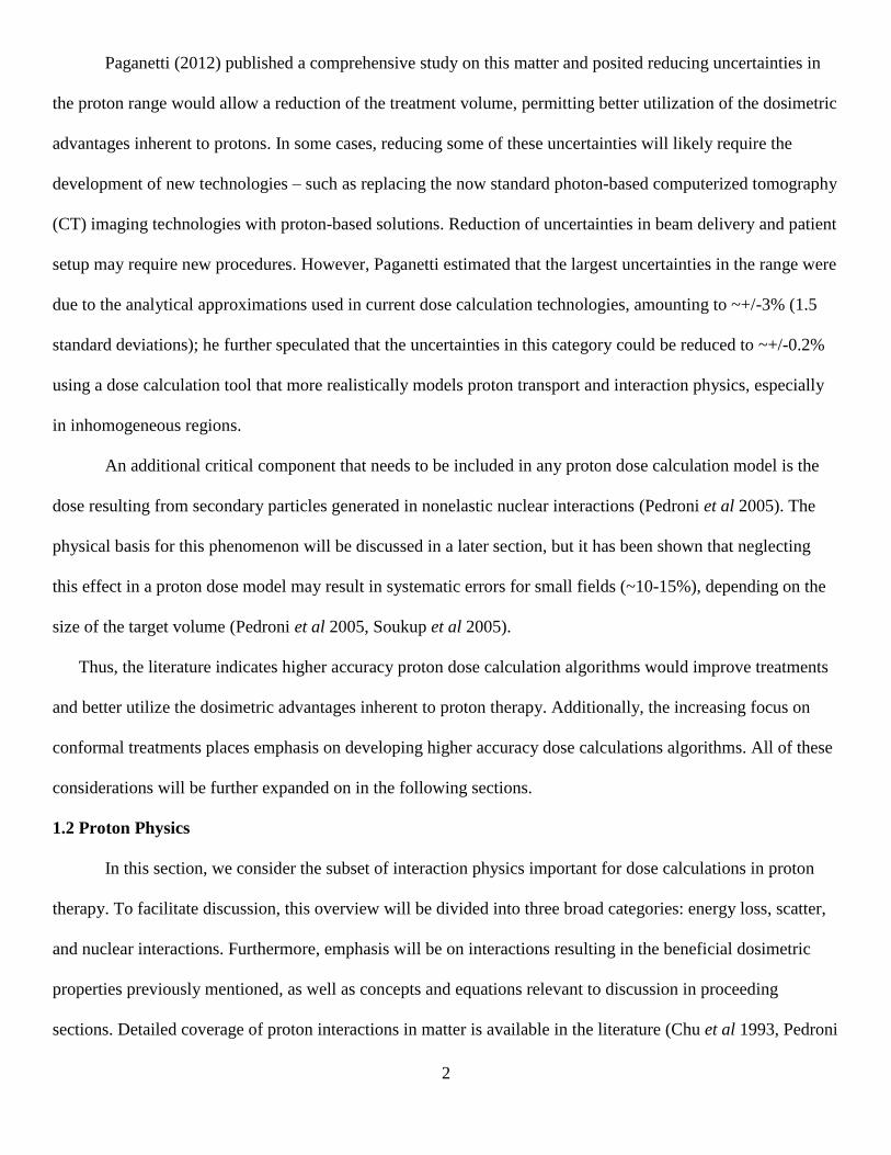
density describing what is called multiple Coulomb scatter (MCS) angles is modeled by a statistical distribution,
typically a Gaussian. MCS is the primary interaction that determines the sharpness of the lateral penumbra.
MCS relies on, and is derived from an accurate model of single scatter, which according to Rutherford
(1911) can be calculated using
𝜉(𝜒) =𝑑𝜎
𝑑Ω= 𝑍𝑟𝑒
2(𝑚𝑒𝑐2/𝛽𝜌)2
4 sin4(𝜒/2), (2)
where 𝑑𝜎 is the differential cross section for scattering into solid angle 𝑑Ω, and 𝜒 is the single scattering angle.
In equation (2), the Rutherford dependence is roughly 𝜒-4. The true mathematical form for scatter, therefore,
should approach 𝜒-4 at large angles. Moliere’s scatter theory (Bethe 1953) includes all these effects, as well as
scatter events intermediate to MCS and single scatter, called plural scattering. For that reason, and because
Moliere theory has been demonstrated to have excellent agreement with measurements (Gottschalk et al 1993),
it is considered the most accurate scatter theory. However, Moliere theory also requires numerous calculations,
including numerical integrations that could be potentially time-consuming depending on the material
composition of the calculation geometry. For that reason, a Gaussian approximation is typically preferred.
Regardless of the statistical distribution used to model MCS, the characteristic scattering angle must be
determined. For this purpose, a differential quantity is defined that can be integrated to determine the mean
squared scattering angle of a group of protons in an absorber. Integrating the characteristic angle of the single
scattering distribution, the linear angular scattering power is derived,
𝑇 =𝑑⟨𝜒2⟩
𝑑𝑥=
∫ 𝜒2𝜉(𝜒) 2𝜋𝜒 𝑑𝜒𝜒𝑚𝑎𝑥
𝜒𝑚𝑖𝑛
∫ 𝜉(𝜒) 2𝜋𝜒 𝑑𝜒𝜒𝑚𝑎𝑥
𝜒𝑚𝑖𝑛
, (3)
where the denominator evaluates to unity. 𝜒𝑚𝑎𝑥 and 𝜒𝑚𝑖𝑛 are determined by considering the
finite size of the nucleus for large angles and screening of the nuclear field for small angles (more details
available in Rossi and Griesen 1941). Similar to the mass stopping power, this quantity can also be calculated
independent of mass density so that the mass scattering power is given by T/𝜌. There are several scattering
power formulae available for protons (Gottschalk 2010). When using scattering power in a dose calculation
8
model, the spatial RMS width is often more useful than the scattering power. The various moments of the
scattering power can be calculated according to Fermi-Eyges theory (Eyges 1948),
𝜎𝑗2(𝑥) =
1
2∫ (𝑥 − 𝑥′)j 𝑇(��(𝑥′)) 𝑑𝑥′
𝑥
0
, (4)
where j=0 gives the sigma of the angular scattering Gaussian distribution, j=1 is the covariance, and j=2 gives
the sigma of the spatial scattering Gaussian distribution.
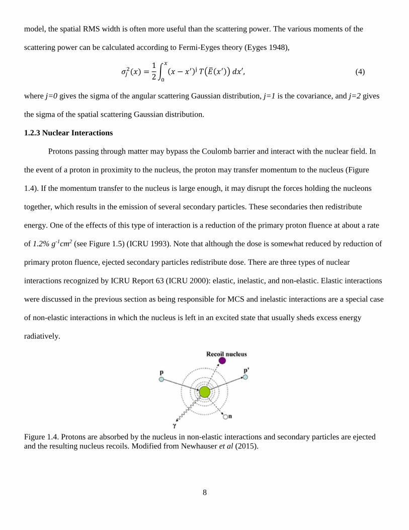
1.2.3 Nuclear Interactions
Protons passing through matter may bypass the Coulomb barrier and interact with the nuclear field. In
the event of a proton in proximity to the nucleus, the proton may transfer momentum to the nucleus (Figure
1.4). If the momentum transfer to the nucleus is large enough, it may disrupt the forces holding the nucleons
together, which results in the emission of several secondary particles. These secondaries then redistribute
energy. One of the effects of this type of interaction is a reduction of the primary proton fluence at about a rate
of 1.2% g-1cm2 (see Figure 1.5) (ICRU 1993). Note that although the dose is somewhat reduced by reduction of
primary proton fluence, ejected secondary particles redistribute dose. There are three types of nuclear
interactions recognized by ICRU Report 63 (ICRU 2000): elastic, inelastic, and non-elastic. Elastic interactions
were discussed in the previous section as being responsible for MCS and inelastic interactions are a special case
of non-elastic interactions in which the nucleus is left in an excited state that usually sheds excess energy
radiatively.
Figure 1.4. Protons are absorbed by the nucleus in non-elastic interactions and secondary particles are ejected
and the resulting nucleus recoils. Modified from Newhauser et al (2015).

9
Figure 1.5. Primary proton fluence is reduced at a rate of about 1.2% g-1cm2. Data shown in water. From
Newhauser et al (2015).
The cross section for non-elastic nuclear interactions in oxygen is shown in Figure 1.6. This figure
shows that the cross section is zero up until a threshold of a few MeV, which is referred to as the Coulomb
barrier because it is the energy needed to overcome the repulsive Coulombic force of the nucleus. The cross
section also levels off around energies exceeding 100 MeV. The Evaluated Nuclear Data File (Chadwick et al
2011) database provides a repository for these cross sections.
Figure 1.6. Total proton non-elastic nuclear cross section in oxygen vs incident proton energy. From Chadwick
et al (2011).
In these non-elastic interactions, energy is carried away from the interaction site by secondary particles.
The secondaries in these interactions include short-range charged particles, and long-range neutral particles.
The energy carried off by long-range neutral secondaries either exits the target completely or is redistributed;

10
for this reason, the energy deposited in the Bragg peak is lowered (Gottschalk 2004). Figure 1.7 shows how the
Bragg peak value is lowered as a result of these neutral particles carrying off some of the incident proton
energy. The short-range charged secondaries resulting from non-elastic nuclear events carry off low energies
relative to the incident proton and scatter out into a faint halo of secondary dose (Pedroni et al 2005); for this
reason, proton beams are said to exhibit a “nuclear halo” (Pedroni et al 2005).
Figure 1.7. Monte Carlo calculations of the Bragg peak with nuclear reactions turned off (dashed) and the actual
Bragg peak (solid) (Berger 1993) for a 160 MeV beam in water.
1.3 Dose Calculation Approaches
Monte Carlo (MC) dose models have long been considered the gold standard for dose calculations
(Schaffner et al 1999, Paganetti et al 2008, Schuemann et al 2014, Schuemann et al 2015). Indeed, the MC
approach has been shown to provide higher dose calculation accuracy than analytical models (Titt et al 2008,
Koch et al 2008, Newhauser et al 2008, Paganetti et al 2008, Schuemann et al 2014, Schuemann et al 2015),
but this also requires increased computational resources and longer calculation times that limit its widespread
application in routine treatment planning. For instance, in one study using the MC code Monte-Carlo N-Particle
eXtended (MCNPX) (Pelowitz 2011), Taddei et al (2009) simulated a typical three-beam proton lung cancer
treatment that required 5,000 hours on a single central processing unit. Although advances in computer
hardware and parallel processing techniques (especially those involving graphical processing units (GPUs))
have resulted in faster computation times for general purpose MC codes, this would still require specialized

11
hardware and increased costs that many cancer clinics would be reluctant to adopt. Additionally, GPUs have a
highly vectorized architecture which is not well suited for parallel processing of independent particle transport.
Finally, GPU-based general purpose Monte Carlo would likely still result in long calculation times in certain
applications, such as four-dimensional treatment plans and inverse planning (Keall et al 2004, Jeraj et al 2002,
Jeraj et al 1999). For these reasons, dose calculation models that strike a balance between speed and accuracy
have been the focus in the literature.
Typically, analytical proton dose models used in commercial treatment planning systems (TPS) are
based on pencil beam algorithms (PBA) (Petti 1992, Russell et al 1995, Hong et al 1996, Deasy 1998,
Schneider et al 1998, Schaffner et al 1999, Szymanowski and Oelfke 2002, Ciangaru et al 2005, Schaffner
2008, Westerly et al 2013, Chapman et al 2017, Inaniwa et al 2017), which segments a broad beam into many
smaller composite beams (called “pencil beams”). These proton dose models typically follow the formalism of
the electron dose model developed by Hogstrom et al (1981). Computation speed is an important factor in
calculation of radiotherapy treatment plans because it accommodates high patient throughput, and repeated
calculations needed during plan optimization and plan adjustment. Thus, PBAs are typically used because they
achieve a balance between accuracy and computation speed. However, the speed of PBAs is achieved mainly
through approximations of the underlying physical interactions that ultimately limits the accuracy of this class
of algorithms. It can be instructive to examine some of the more commonly used approximations and the
circumstances under which their accuracy decreases.
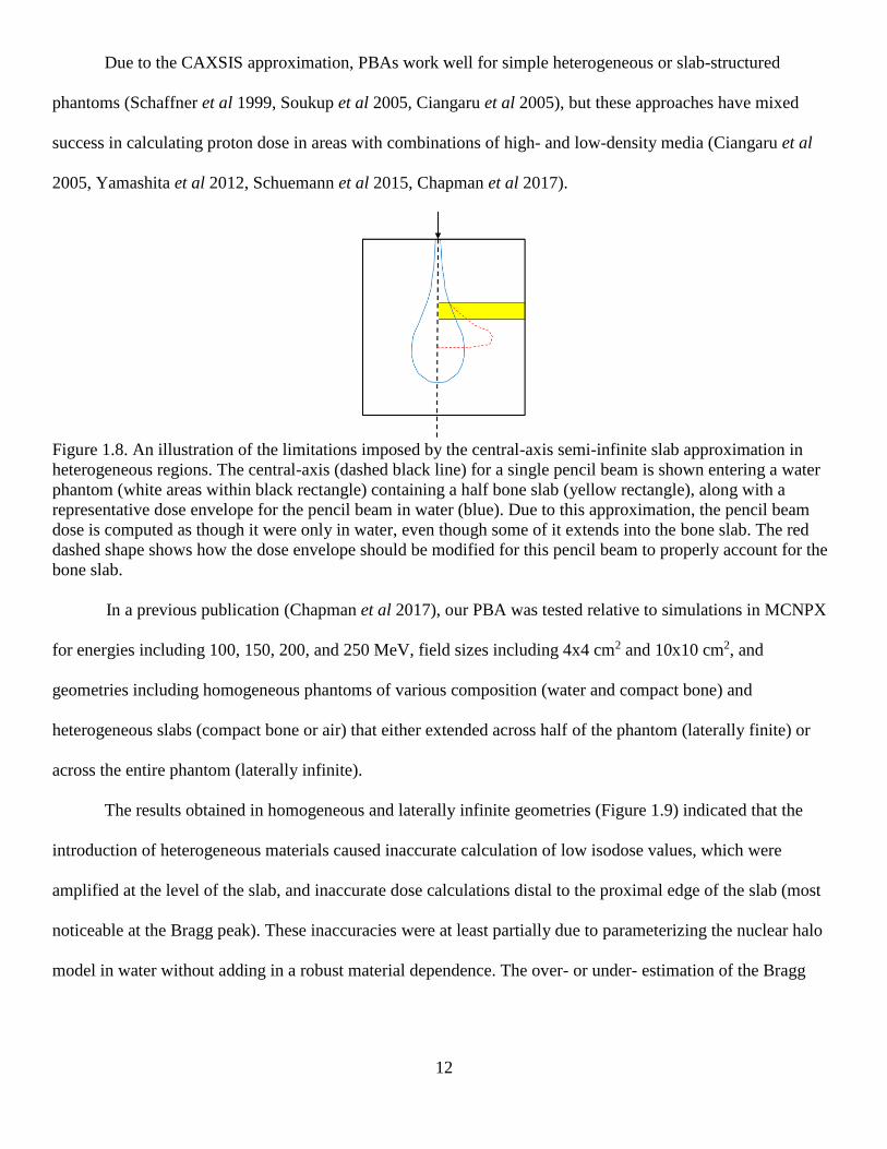
One approximation that has become customary in PBAs is the central-axis semi-infinite slab (CAXSIS)
approximation (Hogstrom et al 1981). In this approximation, materials encountered by the central-axis of each
pencil beam are considered to be laterally infinite homogeneous slabs. To illustrate the limitation this imposes,
consider a pencil beam with its central-axis originating in water with enough lateral scatter at a given depth to
spread part of the pencil beam distribution into an adjacent material of differing composition. In this example,
the CAXSIS approximation would be used to model those particles that extend into the adjacent material as
though they were in water, even though they are not (Figure 1.8).
12
Due to the CAXSIS approximation, PBAs work well for simple heterogeneous or slab-structured
phantoms (Schaffner et al 1999, Soukup et al 2005, Ciangaru et al 2005), but these approaches have mixed
success in calculating proton dose in areas with combinations of high- and low-density media (Ciangaru et al
2005, Yamashita et al 2012, Schuemann et al 2015, Chapman et al 2017).
Figure 1.8. An illustration of the limitations imposed by the central-axis semi-infinite slab approximation in
heterogeneous regions. The central-axis (dashed black line) for a single pencil beam is shown entering a water
phantom (white areas within black rectangle) containing a half bone slab (yellow rectangle), along with a
representative dose envelope for the pencil beam in water (blue). Due to this approximation, the pencil beam
dose is computed as though it were only in water, even though some of it extends into the bone slab. The red
dashed shape shows how the dose envelope should be modified for this pencil beam to properly account for the
bone slab.
In a previous publication (Chapman et al 2017), our PBA was tested relative to simulations in MCNPX
for energies including 100, 150, 200, and 250 MeV, field sizes including 4x4 cm2 and 10x10 cm2, and
geometries including homogeneous phantoms of various composition (water and compact bone) and
heterogeneous slabs (compact bone or air) that either extended across half of the phantom (laterally finite) or
across the entire phantom (laterally infinite).
The results obtained in homogeneous and laterally infinite geometries (Figure 1.9) indicated that the
introduction of heterogeneous materials caused inaccurate calculation of low isodose values, which were
amplified at the level of the slab, and inaccurate dose calculations distal to the proximal edge of the slab (most
noticeable at the Bragg peak). These inaccuracies were at least partially due to parameterizing the nuclear halo
model in water without adding in a robust material dependence. The over- or under- estimation of the Bragg

13
peak resulted from scaling the absorbed dose describing the nuclear halo to materials of interest using only a
ratio of stopping powers rather than explicitly modeling the production and transport of secondary protons.
Figure 1.9. Isodose comparisons between MC (dashed) and PBA (solid) for a 250 MeV, 4x4 cm2 beam incident
on a water phantom with a 5 cm slab. Both compact bone (yellow) slabs at the surface (a) and at z=30 cm (b)
are shown, along with air slabs (blue) at the surface (c) and at z=30 cm. Pass-rates within 2% dose difference or
1 mm distance-to-agreement were 100% (both (a) and (c)), 99.5% (b), and 93.2% (d). Isodose lines shown are
1, 2, 5, 10, 20, 30, 40, 50, 60, 70, 80, 90, and 100%. All pixels within the 1% isodose line were evaluated using
our 2% or 1 mm criteria, and regions that failed this criteria are indicated in red.
For the laterally finite slab evaluations (Figure 1.10), the accuracy of the PBA worsened as the slab
depth increased. The failures in these types of geometries were due to the CAXSIS approximation, and
agreement worsened with depth simply because the scatter increases, and the pencil beam envelope was
therefore larger at deeper depths, which resulted in more laterally distant points inaccurately attributed to the
material encountered along the pencil beam central-axis (refer to Figure 1.8). For all deeply placed slabs, the
PBA was not able to model dose perturbations caused by the sharp material interface between the
heterogeneous slab and water. For a field incident upon the edge of a laterally finite slab, this resulted in the
appearance of two hot spots and two cold spots distal to the slab heterogeneity.
With the accuracy limitations of some analytical approaches and speed limitations of MC approaches,
there is interest in developing new approaches that can, perhaps, achieve a more favorable balance between the
two. One approach is called the pencil beam redefinition algorithm (PBRA), originally described for electrons
14
by Shiu et al (1991). In the original Fermi-Eyges (Eyges 1948) based electron PBA (Hogstrom et al 1981),
Hogstrom et al realized that electrons were scattering in air before reaching the field-defining plane where the
pencil beams were modeled. Their solution was to mathematically redefine the pencil beams at the beam-
defining plane, which allowed modeling of scatter both in air and in patient, without the scatter in air overtaking
scatter in the patient. The PBRA was an extension of this original idea, where pencil beams were redefined
every 1 cm in depth. The PBRA has also been applied to protons (Egashira et al 2013) but required GPU
implementation because the lateral dose grid size had to be very small to accommodate the small proton scatter
angles, which would result in slow calculation times on a standard CPU implementation. Discrete ordinate
calculation models, which directly evaluates variants of the Boltzmann transport equation on a grid, (Sandison
et al 2000) have also been described in the literature.
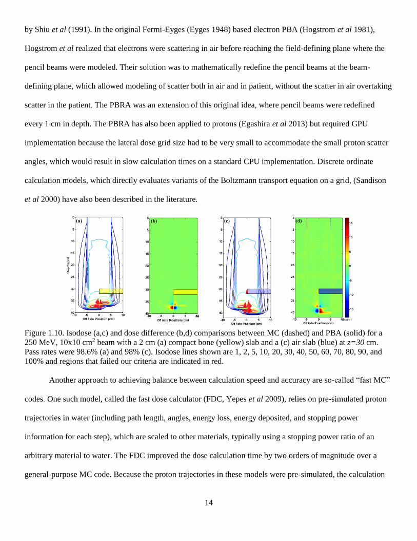
Figure 1.10. Isodose (a,c) and dose difference (b,d) comparisons between MC (dashed) and PBA (solid) for a
250 MeV, 10x10 cm2 beam with a 2 cm (a) compact bone (yellow) slab and a (c) air slab (blue) at z=30 cm.
Pass rates were 98.6% (a) and 98% (c). Isodose lines shown are 1, 2, 5, 10, 20, 30, 40, 50, 60, 70, 80, 90, and
100% and regions that failed our criteria are indicated in red.
Another approach to achieving balance between calculation speed and accuracy are so-called “fast MC”
codes. One such model, called the fast dose calculator (FDC, Yepes et al 2009), relies on pre-simulated proton
trajectories in water (including path length, angles, energy loss, energy deposited, and stopping power
information for each step), which are scaled to other materials, typically using a stopping power ratio of an
arbitrary material to water. The FDC improved the dose calculation time by two orders of magnitude over a
general-purpose MC code. Because the proton trajectories in these models were pre-simulated, the calculation

15
speed of this type of approach was fast but required processing an extremely large dataset that was best utilized
in a graphical processing unit (GPU) environment (Yepes et al 2010).
Recently, the FDC was validated in water for proton scanning beams (Yepes et al 2016a), with greater
than 99% of points over 23 patients within 2% or 2 mm. The FDC was also validated for use in intensity
modulated proton therapy (IMPT) (Yepes et al 2016b) for 23 patient cases and more than 99% of the voxels in
all patients were within 2% or 2 mm. Finally, the FDC was compared to dose calculated by the Eclipse
treatment planning system (Varian Medical Systems) for 525 patients (Yepes et al 2018). Out of these 525
patient cases, the FDC was shown to under-predict Eclipse by more than 10% for 4 patient cases and by more
than 15% for 2 patient cases, highlighting some potentially clinically significant dose differences in Eclipse.
However, the FDC does not include a nuclear halo model, which could result in dose errors for high energy
beams (Pedroni et al 2005).
In VMCpro (Fippel and Soukup 2004), protons were transported individually, step by step through the
calculation geometry, and sampled interaction step lengths using a cross section previously described by
Kawrakow (2000). Secondary particles and delta electrons were also individually transported. Excellent
agreement was reported along the central-axis of pencil beam simulations (1% or 0.5 mm) between VMCpro
and the general-purpose MC codes FLUKA (Ferrari et al 2005) and GEANT 4 (Agostinelli et al 2003) in
homogeneous phantoms of various materials (adult soft tissue and skeleton), demonstrating high accuracy in the
electromagnetic and nuclear models they used for those specific geometries. In a water phantom containing a
bone-lung interface heterogeneity, however, they noted an under-prediction of dose by a few percent, mostly
stemming from parameterization of their MCS scattering power only on mass density, and the inaccuracies
caused by that approximation were magnified by the low density of lung. Another potential cause for this under-
prediction is the absence of material dependence in their secondary dose model.
Despite these limitations, considerable speedup was observed in VMCpro (168 seconds) compared to
general purpose MC codes (~35 times faster than GEANT 4 (99 mins) and ~13 times faster than FLUKA (37
mins)) for a 150-MeV pencil beam in the lung-bone inhomogeneous geometry mentioned previously. Given this

16
computation time, however, VMCpro would still be too time consuming for broad beam calculations, which
would require the transport of several such pencil beams. Furthermore, the stochastic method used to transport
secondary protons that characterize the nuclear halo is subject to statistical fluctuations and increase the
calculation time beyond analytical methods.
Jia et al (2012) developed the gPMC, which implemented the Fippel and Soukup (2004) model on GPU.
The gPMC had calculation times on the order of 6-22 seconds and for 30 patient cases, accuracy was within 1%
or 1 mm for 94% of points within the 10% isodose line. Agreement below the 10% isodose line was not
reported. They also noted that the 1% or 1 mm agreement stated did not apply to geometries with low-density
air regions. Jia et al (2012) used the same simplified, material-independent implementation of the nuclear halo
as Fippel and Soukup (2004). However, this model did result in 1-2% underestimation in target for prostate
cancer cases (Giantsoudi et al 2015). Recently, Qin et al (2016) described the next iteration of this model,
gPMC 2.0, which for a prostate cancer case increased the number of pixels within 1% or 1 mm from 82.7%
(gPMC 1.0) to 93.1% (gPMC 2.0). However, they did not some differences in secondary proton dose when
compared to TOPAS (Perl et al 2012, Testa et al 2013). Souris et al (2016) described a multi-core
implementation of Fippel and Soukup (2004) and showed that their model agreed with GEANT4 (Agostinelli et
al 2003) within 2% or 1 mm. Calculation times in this model were below 25 seconds for 107 protons with initial
energy 200 MeV.
Tourovsky et al (2005) described a fast MC model that reduced the subset of interaction physics to the
main interactions needed for dose calculation (i.e., energy loss, scatter, nuclear interactions). This approach
retained most of the accuracy of general purpose MC while reducing the required time to calculate dose. In the
fourteen patient treatment plans tested, the Tourovsky et al (2005) model resulted in nearly 90% of voxels
within +/-5% agreement. Furthermore, comparing range calculations of their model to a proton radiograph
system, it was shown that the differences in range were mostly between -5% to 2% and differences in range
spread were between -1% to 3.5%. As demonstrated by Sawakuchi et al (2008), MCS within heterogeneities is
the main contributor to the degradation of the distal edge of the Bragg peak, thus the small differences in range

17
and range spread in the Tourovsky et al (2005) model indicate that primary protons were transported accurately
in heterogeneous geometries. Finally, for a typical treatment, this model required 20 minutes of calculation
time.
Although the comparisons between radiograph measurements and range calculations in Tourovsky et al
(2005) seem to indicate that the MCS model is accurate in heterogeneous geometries, the model nonetheless is
configured in a way that limits accuracy in such cases. Additionally, there were several implementation details
of their model that lent itself to inefficient calculations. For instance, they used a constant transport step size (~2
mm) in order to achieve reasonable dose calculation times. Near the Bragg peak, this step size is likely too
coarse to adequately sample the rapidly changing stopping power in this area. This limitation could be the
primary explanation for the wide range of dose differences and the long tail observed in their range difference
histogram. Secondly, the geometries used to test the model have not fully probed the underlying accuracy of
their dose model in heterogeneous tissue. For instance, the continuous changes of heterogeneities in CT
geometries, the overlapping spot beams of various sizes and energies delivered from multiple angles, the large
PTVs treated, and the wide range of materials (from air to Titanium) somewhat average out the inaccuracies
that may be present under simpler conditions. Finally, their nuclear halo model was overly simplistic because it
lacked material dependence and was based on a single Gaussian, which Li et al (2012) showed was insufficient
for modeling the full lateral extent of the nuclear halo.
1.3.1 The Nuclear Halo
The concept of a “nuclear halo” of dose resulting from non-elastic nuclear interactions has been known
to be an important contribution to proton dose for over a decade, with the first publication in this area by
Pedroni et al (2005). In fact, Pedroni et al (2005) and Soukup et al (2005) demonstrated that the lack of a
nuclear halo in a proton dose model could result in significant dose errors up to 10-15%, depending on the size
of the target volume; therefore, the nuclear halo has a non-negligible effect on the proton dose distribution.
Several models for the nuclear halo have been described in the literature, but unfortunately the physics of this
phenomenon has only been studied in modest detail.

18
Despite the lack of knowledge in the physics of the nuclear halo, general purpose Monte Carlo
(Agostinelli et al 2003, Ferrari et al 2005, Pelowitz 2011), which typically rely on the Bertini intranuclear
cascade model (Bertini et al 1968) for calculating the dose due to non-elastic nuclear interactions, have been
shown to agree well with measured data (Polf 2007, Kimstrand et al 2008, Titt et al 2008, Randeniya et al
2009). Some Fast Monte Carlo (FMC) models (Fippel and Soukup 2004, Jia et al 2012, Qin et al 2016, Souris
et al 2016) have also been described, which use data from ICRU Report 63 (ICRU 2000) to stochastically
transport secondary particles. However, because these FMCs transport primary protons and multiple types of
secondary particles, many of them require parallel computing implementations (graphics processing units or
multi-core central processing units) in order to achieve reasonable calculation times for clinical use.
Because stochastically-based nuclear halo models increase the calculation time, analytical models could
be used to calculate nuclear halo dose instead to achieve a balance of speed and accuracy. Pedroni et al (2005)
published the first analytical nuclear halo model, which used two Gaussians to model the fluence: one to
account for MCS and another which was empirically fit to account for the nuclear halo. This same nuclear halo
model was used in Tourovsky et al (2005). However, Li et al (2012) showed that a single Gaussian is not
sufficient for modeling the lateral profile of the nuclear halo out to low isodose values.
Poor modeling of the nuclear halo could be somewhat countered by use of the so-called field-size factor,
which forces the calculated dose to equal the measured dose at the center of a given field. Li et al (2012)
described a model that reduced the field size factor correction by up to 50% compared to Gaussian models,
which more realistically matched the lateral falloff of the nuclear halo as indicated by MC simulations. Their
approach was to replace the single Gaussian that was typically used in PBAs with a weighted sum of both a
Gaussian and a Cauchy-Lorentz term. Their model was parameterized in water and the results were only
presented in a homogeneous water phantom. An extension of the Li et al (2012) model was implemented by
Chapman et al (2017) in their PBA.
Despite the large number of publications on the nuclear halo (Pedroni et al 2005, Soukup et al 2005,
Sawakuchi et al 2010a, Sawakuchi et al 2010b, Sawakuchi et al 2010c, Zhang et al 2011, Peeler and Titt 2012,

19
Clasie et al 2012, Anand et al 2012, Li et al 2012, Zhu et al 2013, Inaniwa et al 2016, Chapman et al 2017),
none have resulted in a complete understanding of the physics in these interactions. Some of these studies rely
on the parameterization introduced in Pedroni et al (2005), and all1 of them apply a weighting factor to the
planar integrated depth dose (PIDD) to model the energy loss for secondary particles in the nuclear halo;
therefore, these models only used a one-dimensional calculation for estimating energy loss of secondary
particles in the nuclear halo.
Recently, Gottschalk et al (2015) published the most detailed nuclear halo model to date, highlighting
the physics and overall form of the nuclear halo for a 177-MeV proton beam in water. In his paper, Gottschalk
et al (2015) took issue with the use of PIDDs in prior literature, arguing that the PIDD inherently includes both
electronic and nuclear stopping power. Gottschalk et al (2015) noted that significant excess dose resulted from
these prior models near mid range (particularly, Pedroni et al 2005), and attributed that to the inclusion of
nuclear stopping power. He further stated that dose on the central-axis of a single pencil beam should not
include dose deposited by secondary particles, which is inherently included in the nuclear stopping power.
Therefore, energy loss modeling in current nuclear halo models is inaccurate.
Another limitation of all prior analytical nuclear halo models in the literature is the lack of robust
material dependence. In fact, all prior analytical models used the effective depth in water, a one-dimensional
calculation, to scale the nuclear halo to other materials. In a previous study (Chapman et al 2017), which also
relied on the effective depth in water, we demonstrated that significant dose differences resulted distal to thick
heterogeneities near the end of range, particularly air slabs. These dose differences were attributed to the lack of
robust material dependence in the nuclear halo model. Note that Inaniwa et al (2016) introduced an additional
scaling factor to scale the nuclear halo to non-water materials, but this factor was constant for each material;
therefore, this correction is inadequate to correct for the errors observed below heterogeneities in Chapman et al
(2017) because it is independent of slab thickness or proximity of the heterogeneity to the end of range.
1 Chapman et al (2017) uses a parameterization based on the central-axis of a broad field, which is mathematically equivalent to the
planar integrated depth dose by the reciprocity relationship (ICRU 1984).
20
1.4 Motivation for Research
Because general purpose MC dose models are not yet clinically viable due to the long calculation times
required and because analytical models have limited dosimetric accuracy in some cases, much of the literature
on proton dose models has been focused on development of fast Monte Carlo codes. Current fast Monte Carlo
dose models result in high dosimetric accuracy and calculation times less than a minute but model the nuclear
halo either by neglecting it entirely (Yepes et al 2008, Yepes et al 2010, Yepes et al 2016a, Yepes et al 2016b,
Yepes et al 2018), relying on overly simplistic modeling (Tourovsky et al 2005), or using stochastic transport
which increases calculation time (Fippel and Soukup 2004, Jia et al 2012, Qin et al 2016, Souris et al 2016).
It is our opinion that the best balance of accuracy and speed for proton dose calculations may be achieved using
a stochastic model for “primary” interactions (i.e., multiple Coulomb scatter and continuous energy loss from
protons which have not been removed from the primary beam) and an analytical model for the “nuclear halo”,
provided the physics of the nuclear halo could be modeled in more detail. A stochastic model for the primary
term would remove the dependence on the central-axis approximation, which should improve dosimetric
accuracy in heterogeneous geometries. An analytically-based nuclear halo model would reduce calculation time
relative to stochastic models because it does not require the transport of additional particles. The accuracy of
such a model is dependent on the validity of the approximations made.
Gottschalk et al (2015) has published the most detailed, physics-based model on the nuclear halo in
water to date, but the physics of the nuclear halo is still not sufficiently well understood to yield accurate
calculations in some situations. For instance, Chapman et al (2017) showed that neglecting material dependence
in the nuclear halo resulted in large dose differences distal to thick heterogeneities, which could potentially be
clinically relevant. The physics of material dependence in the nuclear halo has not been well studied and a
better understanding would likely yield more accurate analytical dose calculation models. Thus, there is limited
but cautionary evidence (Chapman et al 2017) suggesting that the nuclear halo may result in large dose errors in
some cases, but the clinical significance is not well understood.

21
In this work, we discuss a stochastically based primary dose model and a novel method for adding
robust material dependence to an analytically calculated nuclear halo. Our novel method relied on an improved
energy loss calculation that scaled the secondary particle dose resulting from the nuclear halo along all three
Cartesian axes, rather than just the typical one-dimensional scaling along depth. This improvement also
removes the central-axis approximation from the nuclear halo term, which previous analytical nuclear halo
models neglected.
1.5 Hypothesis and Specific Aims
The hypothesis of this work is that a proton dose calculation algorithm can be developed that results in
100% of points below heterogeneities within 3% dose difference or 1 mm distance-to-agreement compared to
Monte Carlo simulations. Furthermore, dose difference distal to slab heterogeneities will be within +/-5% in
laterally finite geometries and within +/-3% in laterally infinite geometries.
The hypothesis was tested for the following conditions:
1. 250 MeV monoenergetic beam and a spread-out Bragg peak with 5 cm of range modulation.
2. Rectangular field size (4x4 cm2).
3. Heterogeneities composed of two materials (air, compact bone), and various depths (z=10, 20, 30 cm)
and thicknesses (2, 4, 5 cm).
The hypothesis implies development of a dose model that achieves improved accuracy for proton dose
calculations compared to our previous model (Chapman et al 2017). The Specific Aims that follow detail the
development and evaluation of such a model, in incremental steps. In Specific Aim 1, the focus is on
developing a high accuracy primary proton dose calculation, and the increase in accuracy is demonstrated
relative to a three-dimensional extension of a pencil beam algorithm, using Monte Carlo data as the standard of
comparison. Specific Aim 2 details the improvements made to our previous nuclear halo model, and focus is on
the increase in accuracy attained from these improvements relative to the previous nuclear halo model. In
Specific Aim 3, the composite dose model (primary + secondary) is evaluated against Monte Carlo simulations
in heterogeneity configurations modeled after anatomy encountered in typical clinical scenarios.

22
1.5.1 Specific Aim 1: Develop and implement a dose calculation algorithm to address the limitations
imposed by the central-axis semi-infinite slab approximation
A primary dose calculation algorithm, similar to the model by Tourovsky et al (2005), was developed
and implemented. This model applied a slab-based approximation (from Z to Z+∆Z) to individual proton
transport that used Monte Carlo simulations and analytical equations, permitting high dose calculation accuracy.
This model was compared to both a three-dimensional extension of the Chapman et al (2017) pencil beam
algorithm and Monte Carlo simulations using MCNPX version 2.7e (Pelowitz 2011), which served as the
standard of comparison for both algorithms.
Specific Aim 1 had the following milestones:
1. Demonstrate 3% dose difference or 1 mm distantance-to-agreement in the primary dose only between
the present model and MC for 100% of points under the following conditions
a. Monoenergetic 250 MeV beam.
b. Rectangular field size (4x4 cm2).
c. Homogeneous water phantom.
d. Geometries with deep (z=30 cm), thick (4 cm) laterally finite heterogeneies of varying
composition (air and compact bone).
2. For the same conditions in (1) for Specific Aim 1, examine dose distal to slab heterogeneities and
demonstrate dose difference in the present model compared to MC within +/-5%.
1.5.2 Specific Aim 2: Develop and implement a methodology to include material dependence in the
nuclear halo
A novel, simple method for estimating energy lost by secondary protons resulting from the nuclear halo
is introduced, which permits lateral scaling in addition to the one-dimensional depth scaling of the water-based
nuclear halo model in Chapman et al (2017). The novel, simple nuclear halo model in the present work was
added to the primary dose model from Specific Aim 1 and compared against MC simulations. To demonstrate
the improved modeling in the present work, comparisons were made between the improved nuclear halo model
and the previous model (Chapman et al 2017).

23
Specific Aim 2 had the following milestones:
1. Demonstrate 3% dose difference or 1 mm distance-to-agreement in the total dose between the present
model and MC for 100% of points under the following conditions:
a. Monoenergetic 250 MeV beam.
b. Rectangular field size (4x4 cm2).
c. Thick (2, 4, 5 cm), laterally infinite heterogeneities at various depths (z=10, 20, 30 cm) of
varying composition (air and compact bone).
2. For the same conditions in (1) for Specific Aim 2, examine dose distal to slab heterogeneities and
demonstrate dose difference in the present model compared to MC within +/-3%.
1.5.3 Specific Aim 3: Quantify improvements made in Specific Aims 1 and 2 in geometries with complex
heterogeneities
The dose model developed in Specific Aims 1 and 2 was evaluated in various geometries intended to
model anatomy encountered in clinically-relevant scenarios.
Specific Aim 3 had the following milestones:
1. Demonstrate 3% dose difference or 1 mm distance-to-agreement in the total dose between the present
model and MC for 100% of points under the following conditions:
a. Monoenergetic 100 MeV and 250 MeV beam and a spread-out Bragg peak with 5 cm of range
modulation.
a. Rectangular field size (4x4 cm2).
b. Various geometries, including:
i. 2 cm wide by 2 cm thick checkerboard pattern (alternating air and compact bone).
ii. Prostate phantom, including femoral head (2 cm radius circle of compact bone) and
rectum (ellipse of air).
iii. Paranasal phantom, including numerous compact bone and air heterogeneities and a
convex skin surface.

24
2. For the same conditions in (1) for Specific Aim 3, examine dose distal to heterogeneities and
demonstrate dose difference in the present model compared to MC within +/-5%.
25
CHAPTER 2. DOSE CALCULATION MODEL
2.1 Overview
In this chapter, the new dose calculation model developed in this work is presented. This dose model
was designed primarily to resolve the two categories of errors reported in Chapman et al (2017): (1) those
caused by the pencil-beam central-axis approximation and (2) those caused by neglecting material-dependence
in the nuclear halo model. To study these two issues in isolation and find appropriate correction strategies, the
present model started with the same two-component dose equation as that from Chapman et al (2017):
𝐷𝑇𝑂𝑇𝐴𝐿(𝑋𝑖, 𝑌𝑗 , 𝑍𝑘) = 𝐷𝑃(𝑋𝑖, 𝑌𝑗 , 𝑍𝑘) + 𝐷𝑆(𝑋𝑖, 𝑌𝑗 , 𝑍𝑘), (5)
where the first term accounts for the “primary” effects on the beam due to energy loss and Coulombic scatter
(i.e., MCS and continuous energy loss) from protons which have not been removed from the primary beam, and
the second term accounts for the “nuclear halo” of dose deposited by secondary protons and other particles
created in non-elastic nuclear interactions. The nuclear halo term in equation (5), 𝐷𝑆(𝑋𝑖, 𝑌𝑗 , 𝑍𝑘), can also
account for the remaining over- or under-estimated scatter of primary protons in the primary term. Dose terms
in equation (5) were computed on a dose grid with 1x1x1 mm3 resolution, whose coordinates (𝑋𝑖, 𝑌𝑗 , 𝑍𝑘) we
specify using grid indices (𝑖, 𝑗, 𝑘). This nomenclature facilitates discussion of primary transport in the fast
Monte Carlo model because it makes the indices of the dose grid (𝑖, 𝑗, 𝑘) calculation point explicit. The
uppercase nomenclature is used for all variables pertaining to the dose grid, whereas lowercase variables are
used for variables pertaining to individual protons or pencil beams.
2.2 Primary Proton Dose: The Pencil Beam Algorithm (Fermi-Eyges based)
Before discussing the improved primary dose model, we examine how the pencil beam algorithm from
Chapman et al (2017) was extended to three dimensions. To avoid extraneous detail and to keep focus on the
improvements made in the present model, only modifications made to the primary pencil beam dose equation
are presented. Further details relevant to the pencil beam algorithm can be found in Chapman et al (2017).
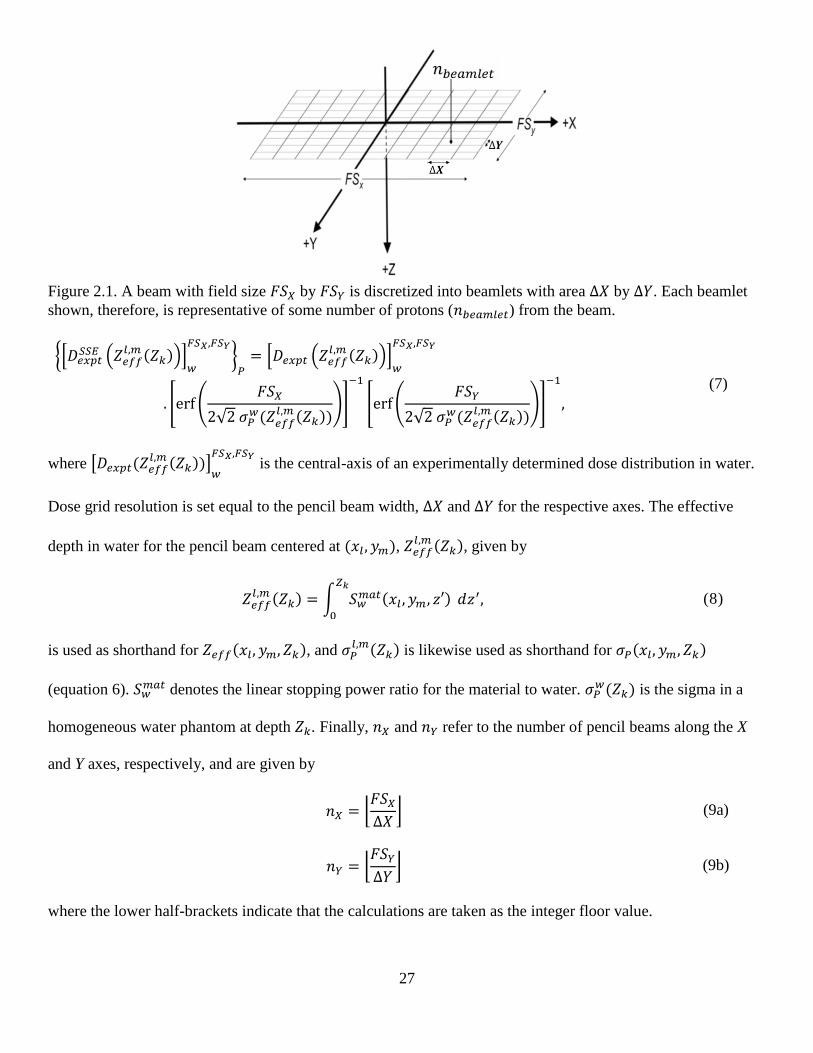
The pencil beam algorithm (PBA) began by segmenting the broad, monoenergetic beam at the field-
defining plane into a number of mathematically deconstructed pencil beams of area ∆𝑋 by ∆𝑌 (Figure 2.1). For
26
the laterally uniform 4x4 cm2 fields that were used in our model, each pencil beam therefore modeled some
number of protons, 𝑛𝑏𝑒𝑎𝑚𝑙𝑒𝑡, from the beam. Transport was then accomplished by applying Fermi-Eyges theory
(Eyges 1948) to each of these pencil beams. It can be shown that under these conditions, primary dose to
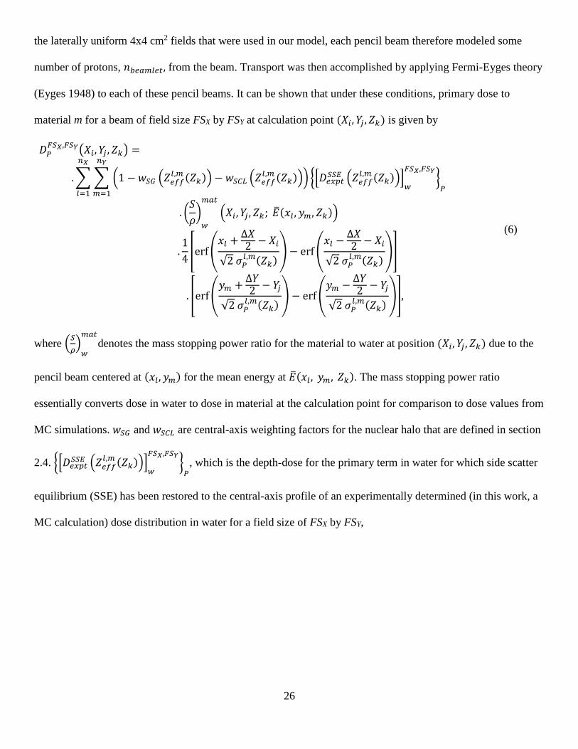
material m for a beam of field size FSX by FSY at calculation point (𝑋𝑖, 𝑌𝑗 , 𝑍𝑘) is given by
𝐷𝑃𝐹𝑆𝑋,𝐹𝑆𝑌(𝑋𝑖, 𝑌𝑗 , 𝑍𝑘) =
. ∑ ∑ (1 − 𝑤𝑆𝐺 (𝑍𝑒𝑓𝑓𝑙,𝑚 (𝑍𝑘)) − 𝑤𝑆𝐶𝐿 (𝑍𝑒𝑓𝑓
𝑙,𝑚 (𝑍𝑘)))
𝑛𝑌
𝑚=1
{[𝐷𝑒𝑥𝑝𝑡𝑆𝑆𝐸 (𝑍𝑒𝑓𝑓
𝑙,𝑚 (𝑍𝑘))]𝑤
𝐹𝑆𝑋,𝐹𝑆𝑌
}𝑃
𝑛𝑋
𝑙=1
. (𝑆
𝜌)
𝑤
𝑚𝑎𝑡
(𝑋𝑖, 𝑌𝑗 , 𝑍𝑘; ��(𝑥𝑙 , 𝑦𝑚, 𝑍𝑘))
.1
4[erf (
𝑥𝑙 +∆𝑋2 − 𝑋𝑖
√2 𝜎𝑃𝑙,𝑚(𝑍𝑘)
) − erf (𝑥𝑙 −
∆𝑋2 − 𝑋𝑖
√2 𝜎𝑃𝑙,𝑚(𝑍𝑘)
)]
. [erf (𝑦𝑚 +
∆𝑌2 − 𝑌𝑗
√2 𝜎𝑃𝑙,𝑚(𝑍𝑘)
) − erf (𝑦𝑚 −
∆𝑌2 − 𝑌𝑗
√2 𝜎𝑃𝑙,𝑚(𝑍𝑘)
)],
(6)
where (𝑆
𝜌)
𝑤
𝑚𝑎𝑡
denotes the mass stopping power ratio for the material to water at position (𝑋𝑖, 𝑌𝑗 , 𝑍𝑘) due to the
pencil beam centered at (𝑥𝑙, 𝑦𝑚) for the mean energy at ��(𝑥𝑙 , 𝑦𝑚, 𝑍𝑘). The mass stopping power ratio
essentially converts dose in water to dose in material at the calculation point for comparison to dose values from
MC simulations. 𝑤𝑆𝐺 and 𝑤𝑆𝐶𝐿 are central-axis weighting factors for the nuclear halo that are defined in section
2.4. {[𝐷𝑒𝑥𝑝𝑡𝑆𝑆𝐸 (𝑍𝑒𝑓𝑓
𝑙,𝑚 (𝑍𝑘))]𝑤
𝐹𝑆𝑋,𝐹𝑆𝑌
}𝑃
, which is the depth-dose for the primary term in water for which side scatter
equilibrium (SSE) has been restored to the central-axis profile of an experimentally determined (in this work, a
MC calculation) dose distribution in water for a field size of FSX by FSY,
27
Figure 2.1. A beam with field size 𝐹𝑆𝑋 by 𝐹𝑆𝑌 is discretized into beamlets with area ∆𝑋 by ∆𝑌. Each beamlet
shown, therefore, is representative of some number of protons (𝑛𝑏𝑒𝑎𝑚𝑙𝑒𝑡) from the beam.
{[𝐷𝑒𝑥𝑝𝑡𝑆𝑆𝐸 (𝑍𝑒𝑓𝑓
𝑙,𝑚 (𝑍𝑘))]𝑤
𝐹𝑆𝑋,𝐹𝑆𝑌
}𝑃
= [𝐷𝑒𝑥𝑝𝑡 (𝑍𝑒𝑓𝑓𝑙,𝑚 (𝑍𝑘))]
𝑤
𝐹𝑆𝑋,𝐹𝑆𝑌
. [erf (𝐹𝑆𝑋
2√2 𝜎𝑃𝑤(𝑍𝑒𝑓𝑓
𝑙,𝑚 (𝑍𝑘)))]
−1
[erf (𝐹𝑆𝑌
2√2 𝜎𝑃𝑤(𝑍𝑒𝑓𝑓
𝑙,𝑚 (𝑍𝑘)))]
−1
, (7)
where [𝐷𝑒𝑥𝑝𝑡(𝑍𝑒𝑓𝑓𝑙,𝑚 (𝑍𝑘))]
𝑤
𝐹𝑆𝑋,𝐹𝑆𝑌 is the central-axis of an experimentally determined dose distribution in water.
Dose grid resolution is set equal to the pencil beam width, ∆𝑋 and ∆𝑌 for the respective axes. The effective
depth in water for the pencil beam centered at (𝑥𝑙 , 𝑦𝑚), 𝑍𝑒𝑓𝑓𝑙,𝑚 (𝑍𝑘), given by
𝑍𝑒𝑓𝑓𝑙,𝑚 (𝑍𝑘) = ∫ 𝑆𝑤
𝑚𝑎𝑡(𝑥𝑙 , 𝑦𝑚, 𝑧′)𝑍𝑘
0
𝑑𝑧′, (8)
is used as shorthand for 𝑍𝑒𝑓𝑓(𝑥𝑙, 𝑦𝑚, 𝑍𝑘), and 𝜎𝑃𝑙,𝑚(𝑍𝑘) is likewise used as shorthand for 𝜎𝑃(𝑥𝑙, 𝑦𝑚, 𝑍𝑘)
(equation 6). 𝑆𝑤𝑚𝑎𝑡 denotes the linear stopping power ratio for the material to water. 𝜎𝑃
𝑤(𝑍𝑘) is the sigma in a
homogeneous water phantom at depth 𝑍𝑘. Finally, 𝑛𝑋 and 𝑛𝑌 refer to the number of pencil beams along the X
and Y axes, respectively, and are given by
𝑛𝑋 = ⌊𝐹𝑆𝑋
∆𝑋⌋ (9a)
𝑛𝑌 = ⌊𝐹𝑆𝑌
∆𝑌⌋ (9b)
where the lower half-brackets indicate that the calculations are taken as the integer floor value.
28
2.3 Primary Proton Dose Model (Specific Aim 1)
The primary dose model in the present work is a class II condensed history Monte Carlo algorithm.
Proton transport started from the field-defining plane and continued to depth in the patient. At the field-defining
plane, the broad beam is discretized into beamlets of area ∆𝑋 by ∆𝑌 (Figure 2.2). Note that for this model we
refer to the discretized areas as “beamlets” to distinguish them from the PBA, where we called them “pencil
beams.” Furthermore, by “beamlets” we do not mean to imply that is equivalent to a physical beam spot, but
that it is a mathematically deconstructed portion of the broad beam. In this model, transport is carried out
proton-by-proton. Because this method of transport does not model groups of protons simultaneously, the
central-axis approximation is no longer needed, and the systematic modeling errors therein are eliminated (see
section 1.3).
2.3.1 Initial Beam Characteristics
The beams used in the primary dose model were subject to the following assumptions: (1) the beam at
the surface of the phantom is parallel; (2) the beam arrives parallel to the Z-axis; and (3) there is no air gap
between the beam-defining-plane and the phantom surface (i.e., beamlets were defined directly on the phantom
surface). These approximations have a few consequences. Notably, because the beam is modeled directly on the
phantom surface and because the beam is parallel, there is no need to include a phase space model or perform
beam divergence and field size corrections. For simplicity, we designed the dose model irrespective of any
commercially available initial beam configuration. Adaptation of the model to relax these assumptions would be
straightforward.
The beam in the primary dose model had the following user-defined parameters: (1) number of particles
(NPS), which sets the initial number of protons (see section 2.3.4); (2) incident nominal energy (Enom), which is
used to calculate energy-specific parameters needed by the dose calculation; (3) rectangular field size (FSX and
FSY), which sets the lateral bounds of the beam; and, (4) sigma of the initial energy distribution (𝜎𝐸), which sets
the bounds of variation on energies randomly selected at the beam-defining plane.
29
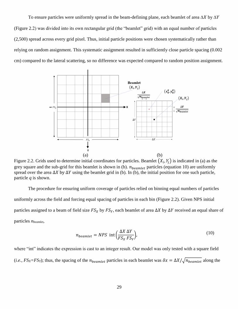
To ensure particles were uniformly spread in the beam-defining plane, each beamlet of area 𝑋 by 𝑌
(Figure 2.2) was divided into its own rectangular grid (the “beamlet” grid) with an equal number of particles
(2,500) spread across every grid pixel. Thus, initial particle positions were chosen systematically rather than
relying on random assignment. This systematic assignment resulted in sufficiently close particle spacing (0.002
cm) compared to the lateral scattering, so no difference was expected compared to random position assignment.
(a) (b)
Figure 2.2. Grids used to determine initial coordinates for particles. Beamlet (𝑋𝑖, 𝑌𝑗) is indicated in (a) as the
grey square and the sub-grid for this beamlet is shown in (b). 𝑛𝑏𝑒𝑎𝑚𝑙𝑒𝑡 particles (equation 10) are uniformly
spread over the area ∆𝑋 by ∆𝑌 using the beamlet grid in (b). In (b), the initial position for one such particle,
particle q is shown.
The procedure for ensuring uniform coverage of particles relied on binning equal numbers of particles
uniformly across the field and forcing equal spacing of particles in each bin (Figure 2.2). Given NPS initial
particles assigned to a beam of field size 𝐹𝑆𝑋 by 𝐹𝑆𝑌, each beamlet of area ∆𝑋 by ∆𝑌 received an equal share of
particles nbeamlet,
𝑛𝑏𝑒𝑎𝑚𝑙𝑒𝑡 = 𝑁𝑃𝑆 int (∆𝑋 ∆𝑌
𝐹𝑆𝑋 𝐹𝑆𝑌), (10)
where “int” indicates the expression is cast to an integer result. Our model was only tested with a square field
(i.e., FSX=FSY); thus, the spacing of the 𝑛𝑏𝑒𝑎𝑚𝑙𝑒𝑡 particles in each beamlet was 𝛿𝑥 = ∆𝑋/√𝑛𝑏𝑒𝑎𝑚𝑙𝑒𝑡 along the

30
X-axis, and 𝛿𝑦 = ∆𝑌/√𝑛𝑏𝑒𝑎𝑚𝑙𝑒𝑡 along Y. The final equations for initial coordinates of particle q within
beamlet (i, j) are therefore given by
𝑥0𝑞 = 𝑋𝑖 −
∆𝑋
2+ 𝑛1 𝛿𝑥, 𝑛1 = 1,2, … , √𝑛𝑏𝑒𝑎𝑚𝑙𝑒𝑡,
(11a)
𝑦0𝑞 = 𝑌𝑗 −
∆𝑌
2+ 𝑛2 𝛿𝑦, 𝑛2 = 1,2, … , √𝑛𝑏𝑒𝑎𝑚𝑙𝑒𝑡,
(11b)
where the lowercase variables 𝑥0𝑞 and 𝑦0
𝑞 refer to the initial position of the particle at the phantom surface (note
that typically 𝑥𝑘𝑞 and 𝑦𝑘
𝑞 are used, but at the beam-defining plane, k=0), and the uppercase variables 𝑋𝑖 and 𝑌𝑗
refer to center coordinates of pixel (i, j). Furthermore, pixel spacing in the dose grid is indicated by ∆𝑋 and ∆𝑌.
Finally, each proton at the beam-defining plane was initialized with an energy randomly sampled from a
Gaussian to model energy straggling, given by
𝐺(𝐸)𝑑𝐸 =1
√2𝜋 𝜎𝐸
exp [−(𝐸 − 𝐸𝑛𝑜𝑚)2
2 𝜎𝐸2 ] 𝑑𝐸. (12)
To generate the independent random variable needed to sample from equation (12), the Box-Mueller transform
(Box and Mueller 1958) was used. This approach takes two independent, random uniform random variables
(𝑈1, 𝑈2), on the range (0,1) and transforms them to two independent, normal random variables (𝑁1, 𝑁2), again
on the range (0,1). Thus, according to the Box-Mueller, transform,
𝑁1 = √−2 ln(𝑈1) cos(2𝜋 𝑈2), (13a)
𝑁2 = √−2 ln(𝑈1) sin(2𝜋 𝑈2). (13b)
Because (𝑁1, 𝑁2) are independent, normal random variables (i.e., continued sampling would yield a distribution
with a mean value of zero and unity variance), (𝑁1, 𝑁2) can be transformed to (𝐺1, 𝐺2) (i.e., two independent,
random Gaussian samples from equation 12) using
𝐺1 = 𝐸𝑛𝑜𝑚 + 𝜎𝐸𝑁1, (14a)
𝐺2 = 𝐸𝑛𝑜𝑚 + 𝜎𝐸𝑁2, (14b)
where 𝐺1 and 𝐺2 are two independent, random Gaussian samples from equation (12). This approach was
verified to reproduce the expected distribution using multiple test simulations.
31
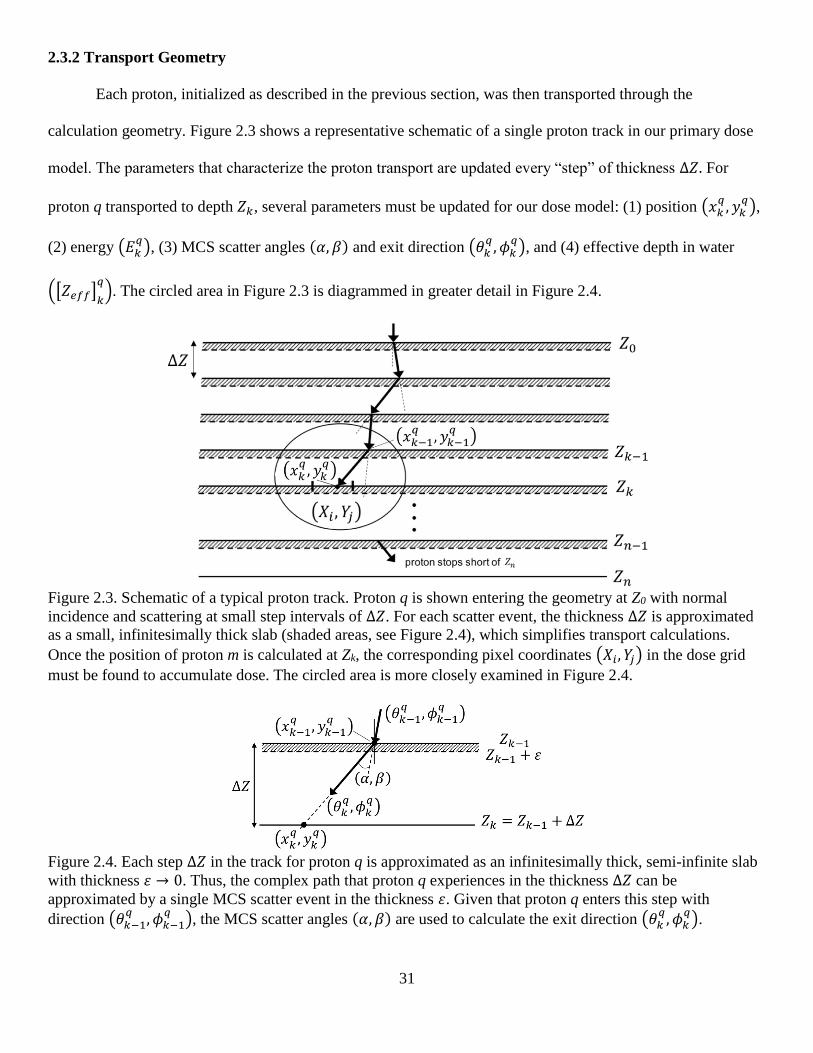
2.3.2 Transport Geometry
Each proton, initialized as described in the previous section, was then transported through the
calculation geometry. Figure 2.3 shows a representative schematic of a single proton track in our primary dose
model. The parameters that characterize the proton transport are updated every “step” of thickness ∆𝑍. For
proton q transported to depth 𝑍𝑘, several parameters must be updated for our dose model: (1) position (𝑥𝑘𝑞 , 𝑦𝑘
𝑞),
(2) energy (𝐸𝑘𝑞), (3) MCS scatter angles (𝛼, 𝛽) and exit direction (𝜃𝑘
𝑞 , 𝜙𝑘𝑞), and (4) effective depth in water
([𝑍𝑒𝑓𝑓]𝑘
𝑞). The circled area in Figure 2.3 is diagrammed in greater detail in Figure 2.4.
Figure 2.3. Schematic of a typical proton track. Proton q is shown entering the geometry at Z0 with normal
incidence and scattering at small step intervals of ∆𝑍. For each scatter event, the thickness ∆𝑍 is approximated
as a small, infinitesimally thick slab (shaded areas, see Figure 2.4), which simplifies transport calculations.
Once the position of proton m is calculated at Zk, the corresponding pixel coordinates (𝑋𝑖, 𝑌𝑗) in the dose grid
must be found to accumulate dose. The circled area is more closely examined in Figure 2.4.
Figure 2.4. Each step ∆𝑍 in the track for proton q is approximated as an infinitesimally thick, semi-infinite slab
with thickness 휀 → 0. Thus, the complex path that proton q experiences in the thickness ∆𝑍 can be
approximated by a single MCS scatter event in the thickness 휀. Given that proton q enters this step with
direction (𝜃𝑘−1𝑞 , 𝜙𝑘−1
𝑞 ), the MCS scatter angles (𝛼, 𝛽) are used to calculate the exit direction (𝜃𝑘𝑞 , 𝜙𝑘
𝑞).

32
One of the most important considerations in a dose model is the determination of the locations to deposit
dose. For each proton track, this information is given by the position of the proton for each step in the track. In
an arbitrary step of the track, proton q enters with position (𝑥𝑘−1𝑞 , 𝑦𝑘−1
𝑞 ) at depth 𝑍𝑘−1 and at depth 𝑍𝑘, the
position is given by
𝑥𝑘𝑞 = 𝑥𝑘−1
𝑞 + ∆Z tan 𝜃𝑘𝑞 cos 𝜙𝑘
𝑞 , (15a)
𝑦𝑘𝑞 = 𝑦𝑘−1
𝑞 + ∆Z tan 𝜃𝑘𝑞 sin 𝜙𝑘
𝑞 . (15b)
This updated position depends on the exit direction (𝜃𝑘𝑞 , 𝜙𝑘
𝑞) for this step. For this transport step, the proton
may experience numerous scatter events that result in a complex path. To address this problem, we
approximated the slab as an infinitesimally small (휀 → 0), semi-infinite slab (Figure 2.4) located near the
entrance to the slab (𝑍𝑘−1 + 휀), which allows the use of thin-target multiple Coulomb scatter (MCS) theory.
Thus, in each step of the proton trajectory, the scatter is calculated using MCS theory, which we specify using
spherical angles (α, β). As can be seen in Figure 2.4, due to the infinitesimal slab, the exit direction is a function
of both the entrance direction (𝜃𝑘−1𝑞 , 𝜙𝑘−1
𝑞 ) and the MCS scatter angles (α, β) with respect to the entrance
direction, such that
𝜃𝑘𝑞 = cos−1{cos 𝛼 cos 𝜃𝑘−1
𝑞 + sin 𝛼 cos 𝛽 sin 𝜃𝑘−1𝑞 }, (16a)
𝜙𝑘𝑞 = tan−1 {
cos 𝛼 sin 𝜃𝑘−1𝑞 sin 𝜙𝑘−1
𝑞 − sin 𝛼[cos 𝛽 cos 𝜃𝑘−1𝑞 sin 𝜙𝑘−1
𝑞 − sin 𝛽 cos 𝜙𝑘−1𝑞 ]
cos 𝛼 sin 𝜃𝑘−1𝑞 cos 𝜙𝑘−1
𝑞 − sin 𝛼 [cos 𝛽 cos 𝜃𝑘−1𝑞 cos 𝜙𝑘−1
𝑞 + sin 𝛽 sin 𝜙𝑘−1𝑞 ]
}, (16b)
where the ~ over the arc-tangent operation indicates that the result is returned in the proper quadrant (most
software packages refer to this function as atan2). Equations (16a-b) describe both the angles leaving the
current slab and the angles entering the next slab, i.e. proton q drifts from 𝑍𝑘−1 + 휀 to 𝑍𝑘−1 + ∆𝑍.
In order to quantify primary scatter angles within the slab (α, β), it is necessary to assume that the
particles follow some distribution. In this model, we use a Gaussian to sample the polar angle:
𝑓(𝛼) =
𝛼
𝜎𝛼2
exp [−𝛼2
2 𝜎𝛼2
]. (17)

33
Using the conservation of probability to relate this Gaussian with a uniformly distributed random number (0,1),
it can be shown that the polar scattering angle 𝛼 can be sampled using the following equation:
𝛼 = 𝜎𝛼√−2 ln(𝑈𝛼), (18)
where 𝑈𝛼 is an independent uniformly distribution random number over the interval [0, 1]. Furthermore,
according to MCS theory, 𝜎𝛼 can be calculated in the following way
𝜎𝛼
2(𝑋𝑖, 𝑌𝑗 , 𝑍𝑘) =1
2 𝑇(𝐸𝑘
𝑚) (∆𝑍
cos 𝜃𝑘𝑚), (19)
where 𝑇 is the linear angular scattering power (explained in the next section). Finally, azimuthal symmetry
gives
𝛽 = 2𝜋 𝑈𝛽 , (20)
where 𝑈𝛽 is an independent uniformly distributed random number over the interval [0,1].
Having found all the geometric parameters necessary to calculate the position of proton q at depth 𝑍𝑘,
(𝑥𝑘𝑞 , 𝑦𝑘
𝑞), the corresponding coordinates of the pixel in the dose grid, (𝑋𝑖, 𝑌𝑗), are found (see circled area in
Figure 2.3). For 𝑋𝑖 −∆𝑋
2≤ 𝑥𝑘
𝑞 ≤ 𝑋𝑖 +∆𝑋
2 and 𝑌𝑗 −
∆𝑌
2≤ 𝑦𝑘
𝑞 ≤ 𝑌𝑗 +∆𝑌
2, the primary dose contribution of proton q
to (𝑋𝑖 , 𝑌𝑗 , 𝑍𝑘) is given by
[𝐷(𝑋𝑖, 𝑌𝑗 , 𝑍𝑘)]
𝑃= [𝐷(𝑋𝑖, 𝑌𝑗 , 𝑍𝑘)]
𝑃+
1
∆𝑋 ∆𝑌 cos 𝜃𝑘𝑞
𝑆𝑚𝑎𝑡
𝜌(𝐸𝑘
𝑞) 𝐶 ([𝑍𝑒𝑓𝑓]𝑘
𝑞; 𝐸0
𝑞), (21)
where the ‘P’ subscript indicates that this refers to primary dose only, and [𝐷(𝑋𝑖, 𝑌𝑗 , 𝑍𝑘)]𝑃
on the right-hand
side refers to the previous value of [𝐷(𝑋𝑖, 𝑌𝑗 , 𝑍𝑘)]𝑃
. 𝐶 ([𝑍𝑒𝑓𝑓]𝑘
𝑞; 𝐸0
𝑞) is the correction factor for all remaining
unmodeled physics, including the fluence loss due to nonelastic nuclear interactions (section 2.3.3), 𝑆𝑚𝑎𝑡/𝜌 is
the mass stopping power in the material, 𝐸𝑘𝑞 refers to the energy of proton q at depth 𝑍𝑘, and 𝜃𝑘
𝑞 is the polar
spherical angle of the proton track from the beam axis in a spherical coordinate system.

34
2.3.3 Selection of Parameters
In this section, the focus will be on the selection of those parameters that describe physical interactions
of the proton. As mentioned in Chapter 1, there are three major categories of interactions that need to be
included in a proton dose calculation model for the primary beam: (1) energy loss, (2) scatter, and (3) fluence
loss of primary protons due to nonelastic nuclear interactions.
Energy loss for primary protons in our dose model is calculated using the continuous slowing down
approximation (CSDA), which for proton q at depth 𝑍𝑘, is calculated using
𝐸𝑘𝑞 ≈ 𝐸𝑘−1
𝑞 − (∆𝑍
cos 𝜃𝑘𝑞) 𝑆𝑚𝑎𝑡(𝐸𝑘−1
𝑞 ), (22)
where 𝐸𝑘−1𝑞
refers to the energy of the proton at depth 𝑍𝑘−1 and 𝐸𝑘𝑞 is the energy at 𝑍𝑘, and 𝑆𝑚𝑎𝑡 is the stopping
power of the material at (𝑋𝑖, 𝑌𝑗 , 𝑍𝑘) and at energy 𝐸𝑘−1𝑞 . Note that equation (22) is approximate because the
linear stopping power at energy 𝐸𝑘−1𝑞
is used rather than the average stopping power over the step. Another
measure of energy loss is the effective depth in water, given by
[𝑍𝑒𝑓𝑓]𝑘
𝑞= [𝑍𝑒𝑓𝑓]
𝑘−1
𝑞+ (
∆𝑍
cos 𝜃𝑘𝑞) 𝑆𝑤
𝑚𝑎𝑡(𝐸𝑘−1𝑞 ), (23)
where 𝑆𝑤𝑚𝑎𝑡 refers to the ratio of the linear collisional stopping power in the material at (𝑋𝑖, 𝑌𝑗 , 𝑍𝑘) to the linear
collisional stopping power in water at energy 𝐸𝑘−1𝑞
.
The equations for both 𝐸𝑘𝑞 and [𝑍𝑒𝑓𝑓]
𝑘
𝑞 require accurate determination of stopping power data. The
required stopping powers in water were looked up from a table of values calculated before proton transport took
place. This approach was preferred over using databases, such as SRIM (Ziegler et al 2012), because the
computation of tabular data was based on an analytical formula (equation 25) which allowed variable energy
resolution. To compute the stopping power table for water, three additional user-defined parameters are
required: the maximum energy (Emax), the energy resolution (fE), and the cutoff energy (Ecut). The energy array
is then calculated using
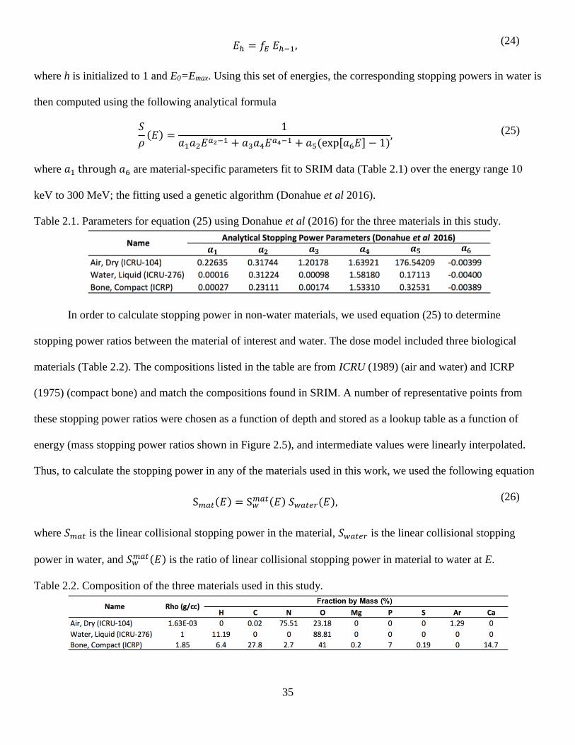
35
𝐸ℎ = 𝑓𝐸 𝐸ℎ−1, (24)
where h is initialized to 1 and E0=Emax. Using this set of energies, the corresponding stopping powers in water is
then computed using the following analytical formula
𝑆
𝜌(𝐸) =
1
𝑎1𝑎2𝐸𝑎2−1 + 𝑎3𝑎4𝐸𝑎4−1 + 𝑎5(exp[𝑎6𝐸] − 1), (25)
where 𝑎1 through 𝑎6 are material-specific parameters fit to SRIM data (Table 2.1) over the energy range 10
keV to 300 MeV; the fitting used a genetic algorithm (Donahue et al 2016).
Table 2.1. Parameters for equation (25) using Donahue et al (2016) for the three materials in this study.
In order to calculate stopping power in non-water materials, we used equation (25) to determine
stopping power ratios between the material of interest and water. The dose model included three biological
materials (Table 2.2). The compositions listed in the table are from ICRU (1989) (air and water) and ICRP
(1975) (compact bone) and match the compositions found in SRIM. A number of representative points from
these stopping power ratios were chosen as a function of depth and stored as a lookup table as a function of
energy (mass stopping power ratios shown in Figure 2.5), and intermediate values were linearly interpolated.
Thus, to calculate the stopping power in any of the materials used in this work, we used the following equation
S𝑚𝑎𝑡(𝐸) = S𝑤𝑚𝑎𝑡(𝐸) 𝑆𝑤𝑎𝑡𝑒𝑟(𝐸), (26)
where 𝑆𝑚𝑎𝑡 is the linear collisional stopping power in the material, 𝑆𝑤𝑎𝑡𝑒𝑟 is the linear collisional stopping
power in water, and 𝑆𝑤𝑚𝑎𝑡(𝐸) is the ratio of linear collisional stopping power in material to water at E.
Table 2.2. Composition of the three materials used in this study.
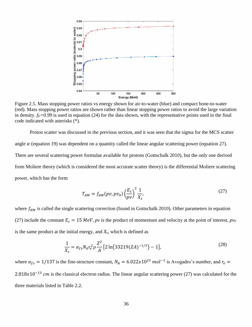
36
Figure 2.5. Mass stopping power ratios vs energy shown for air-to-water (blue) and compact bone-to-water
(red). Mass stopping power ratios are shown rather than linear stopping power ratios to avoid the large variation
in density. fE=0.99 is used in equation (24) for the data shown, with the representative points used in the final
code indicated with asterisks (*).
Proton scatter was discussed in the previous section, and it was seen that the sigma for the MCS scatter
angle 𝛼 (equation 19) was dependent on a quantity called the linear angular scattering power (equation 27).
There are several scattering power formulae available for protons (Gottschalk 2010), but the only one derived
from Moliere theory (which is considered the most accurate scatter theory) is the differential Moliere scattering
power, which has the form
𝑇𝑑𝑀 = 𝑓𝑑𝑀(𝑝𝑣, 𝑝𝑣0) (𝐸𝑠
𝑝𝑣)
2 1
𝑋𝑠,
(27)
where 𝑓𝑑𝑀 is called the single scattering correction (found in Gottschalk 2010). Other parameters in equation
(27) include the constant 𝐸𝑠 = 15 𝑀𝑒𝑉, pv is the product of momentum and velocity at the point of interest, pv0
is the same product at the initial energy, and Xs, which is defined as
1
𝑋𝑠= 𝛼𝑓𝑠𝑁𝐴𝑟𝑒
2𝜌𝑍2
𝐴{2 ln(33219(𝑍𝐴)−1/3) − 1},
(28)
where 𝛼𝑓𝑠 = 1/137 is the fine-structure constant, 𝑁𝐴 = 6.022𝑥1023 𝑚𝑜𝑙−1 is Avogadro’s number, and 𝑟𝑒 =
2.818𝑥10−13 𝑐𝑚 is the classical electron radius. The linear angular scattering power (27) was calculated for the
three materials listed in Table 2.2.

37
The last major interaction that needs to be discussed for this primary dose model is the fluence loss of
primary protons resulting from non-elastic nuclear interactions. This interaction is not calculated while the
proton is transported, unlike the previously mentioned proton track parameters. Instead, fluence loss is handled
using tabular data obtained from Monte Carlo simulations. This approach allows a simple, computationally
inexpensive table lookup to determine fluence loss for the primary beam. This approach results in a reduced
subset of physical interactions in our model, which is one of the primary reasons that our model is fast. In
contrast, general purpose MC include an extensive set of interaction types that often result in long calculation
times. Modeling fluence loss with tabular data in our model also improves computational efficiency over dose
models with stochastic nuclear halos (Fippel and Soukup 2004, Jia et al 2012, Qin et al 2016, Souris et al
2016), which relied on evaluating cross sections and stochastic secondary proton transport. This approach was
also more computationally efficient than the analytical nuclear halo approach by Tourovsky et al (2005), which
also relied on evaluating cross section data.
The procedure for characterizing fluence loss required two simulations: (1) simulation of the primary
proton dose (i.e., no nuclear halo included) at point (𝑋𝑖, 𝑌𝑗 , 𝑍𝑘) for beam with incident energy 𝐸0 in water using
our present model, [𝐷𝑃𝑤(𝑋𝑖, 𝑌𝑗 , 𝑍𝑘; 𝐸0)]
𝑃𝑀, and (2) an MCNPX simulation of the total dose under the same
conditions, [𝐷𝑇𝑜𝑡𝑤 (𝑋𝑖, 𝑌𝑗 , 𝑍𝑘; 𝐸0)]
𝑀𝐶. To calculate fluence loss using these datasets, however, the beam must be
sufficiently broad to not be impacted by loss of side-scatter equilibrium, so that scatter is not accounted for
twice; thus, we instead equated the integral doses [𝐼𝐷𝐷𝑇𝑜𝑡𝑤 (𝑍𝑘; 𝐸0)]𝑀𝐶 =
∫ ∫ [𝐷𝑇𝑜𝑡𝑤 (𝑋𝑖, 𝑌𝑗 , 𝑍𝑘; 𝐸0)]
𝑀𝐶𝑌′ 𝑑𝑋′𝑑𝑌′
𝑋′ and [𝐼𝐷𝐷𝑃
𝑤(𝑍𝑘; 𝐸0)]𝑃𝑀 = ∫ ∫ [𝐷𝑇𝑜𝑡𝑤 (𝑋𝑖, 𝑌𝑗 , 𝑍𝑘; 𝐸0)]
𝑃𝑀𝑌′ 𝑑𝑋′𝑑𝑌′
𝑋′.
Thus, 𝐶(𝑍𝑘; 𝐸0), the fluence loss correction factor, is given by
𝐶(𝑍𝑘; 𝐸0) =[𝐼𝐷𝐷𝑇𝑜𝑡
𝑤 (𝑍𝑘; 𝐸0)]𝑀𝐶
[𝐼𝐷𝐷𝑇𝑜𝑡𝑤 (𝑍𝑘; 𝐸0)]𝑃𝑀
. (29)
After 𝐶(𝑍𝑘; 𝐸0) has been calculated, a number of representative points are chosen as a function of depth and
stored as a lookup table for energy E0 in the primary dose model program, giving the discrete distribution

38
𝐶∗(𝑍𝑘; 𝐸0). A plot showing both 𝐶∗(𝑍𝑘; 250 MeV) and 𝐶(𝑍𝑘; 250 MeV) is in Figure 2.6. Using the same
procedure, 𝐶∗(𝑍𝑘; 𝐸0) was calculated for two nominal energies 𝐸0 = {100, 250} 𝑀𝑒𝑉, and intermediate
energies are calculated by linear interpolation over nominal energy. Note that in equation (21), we use
𝐶 ([𝑍𝑒𝑓𝑓]𝑘
𝑞; 𝐸0
𝑞); thus, the correction factor is scaled to the material of interest by the effective depth in water.
Thus, for the primary fluence loss, we still relied on a one-dimensional scaling based on the effective depth in
water.
Figure 2.6. Plot comparing 𝐶(𝑍𝑘; 250 MeV) (black) and 𝐶∗(𝑍𝑘; 250 MeV) (red *).
2.3.4 Statistical Requirements
The primary dose model follows individual proton tracks over discrete steps in the phantom, which is
expected to produce more accurate dose calculations compared to a purely analytical approach, such as a pencil
beam algorithm (PBA). However, it is necessary to impose requirements on the number of particles simulated in
order to ensure a desired level of statistical accuracy. The required number of protons per pixel in the beam-
defining plane to achieve a desired statistical percentage accuracy of u% is given by:
𝑛𝑏𝑒𝑎𝑚𝑙𝑒𝑡 = (𝑢/100)−2. (30)
In this model, a statistical accuracy of 2% was used, yielding 2,500 particles per pixel in the beam-defining
plane; hence, for a broad beam with field size FSX by FSY and XY dose grid resolution ∆𝑋 by ∆𝑌, the total
number of particles required is

39
𝑁𝑃𝑆 = (𝑢/100)−2
𝐹𝑆𝑋 𝐹𝑆𝑌
∆𝑋 ∆𝑌. (31)
An additional factor that must be taken into consideration is how the stopping power is sampled.
Because we are using the CSDA to calculate stopping power, the precision of this calculation is inherently
limited by the finite step size. For example, using a constant step size, it is possible to adequately sample the
slowly varying entrance region of the stopping power curve, yet miss the rapidly changing features of the peak
(reference Figure 1.2). One early approach we had to this problem involved ensuring the percent difference in
linear stopping power between consecutive steps did not exceed some chosen percentage, which was typically
set to 5%. However, we found that this adaptive step size calculation required excessive calculation time, so we
instead chose to calculate on a grid using 0.1 cm steps from the surface to 77% of the range in water, with the
step size decreasing to 0.025 cm steps beyond that. Selection of the value for the step size change (77%) was
based on repeated simulations in water over a wide energy range (100-250 MeV) by comparing the agreement
between the simulation of the present model and MC data. In these repeated simulations, the threshold depth for
the change in step size was varied; ultimately, 77% of the range in water was selected as a compromise between
agreement at the peak and extended calculation time due to the finer grid spacing in the depth direction.
Additionally, in this calculation, a form of Geiger’s rule was used to calculate range based on the nominal
energy of the beam, as in 𝑅0𝑤(𝑐𝑚) = 2.2𝑥10−3(𝐸0(𝑀𝑒𝑉))1.77 in water. Despite the use of the variable step size
in our transport, the final dose was still accumulated in a dose grid with constant step size ∆𝑍 = 0.1 𝑐𝑚.
2.3.5 Description of Evaluation Geometries
Our previous study showed that one of the major effects impacting the accuracy of analytical dose
calculations was the CAXSIS approximation, which is particularly important for the primary proton dose
calculation. The primary dose calculation presented in this chapter is intended to solve the limitations of the
CAXSIS approximation. Thus, to assess the performance of the model we examined those geometries where the
limitations of the CAXSIS approximation were found to be the most severe.

40
The evaluation scenarios focused on the highest energy (250 MeV), a rectangular field size (4x4 cm2), and
deep (Z=30 cm), thick (4 cm) heterogeneous slabs. As in our previous study, we tested the range of materials
found in patient data by evaluating our model in both compact bone and air slabs. The slabs only extended over
half of the calculation geometry because that is the most challenging scenario for the CAXSIS approximation.
An evaluation in homogeneous water was also tested to ensure that our model could still calculate in simple
geometries.
2.4 Secondary Proton Dose: The “Nuclear Halo” (Specific Aim 2)
In this section, we discuss the nuclear halo equation in the Chapman et al (2017) model (hereafter, the
“original” model) and the modeling improvements made in the present work to achieve higher dosimetric
accuracy in heterogeneous geometries. The original dose model only calculated the nuclear halo in water and
scaled to other materials by using a simple one-dimensional effective depth calculation along the pencil-beam
central-axis. In discussing how to improve the modeling of the material dependence in the nuclear halo, we note
that the three following effects would ideally be incorporated into the model: (1) scaling dose in water to dose
in the material of interest at the calculation point; (2) energy loss of the scattered secondary particles throughout
the geometry; and (3) number of secondary protons produced, which is a function of both primary proton
energy and material. Our solution in Specific Aim 2 addresses the first two of these effects (section 2.4.2). The
specifics of how these improvements were added into the nuclear halo model are discussed in section 2.4.3.
2.4.1 Chapman et al (2017) Nuclear Halo Equation
In a previous publication (Chapman et al 2017), we presented the original nuclear halo model that was
used in our proton dose pencil beam algorithm (PBA). The equation used for the nuclear halo was modeled
empirically with coefficients determined by fitting the model to MC simulations of lateral dose profiles of a
0.1x0.1 cm2 pencil beam of protons in water. It was found that the best fit was obtained by a sum of a Gaussian
and a modified Cauchy-Lorentz term:
𝐷𝑆𝐹𝑆𝑋,𝐹𝑆𝑌(𝑋𝑖, 𝑌𝑗 , 𝑍𝑘) = 𝐷𝑆𝐺
𝐹𝑆𝑋 ,𝐹𝑆𝑌(𝑋𝑖, 𝑌𝑗 , 𝑍𝑘) + 𝐷𝑆𝐶𝐿𝐹𝑆𝑋,𝐹𝑆𝑌(𝑋𝑖, 𝑌𝑗 , 𝑍𝑘), (32)

41
where 𝐷𝑆𝐹𝑆𝑋 ,𝐹𝑆𝑌 is the total secondary dose for the field size FSX by FSY. The remaining two terms have the
following form:
𝐷𝑆𝐺𝐹𝑆𝑋,𝐹𝑆𝑌(𝑋𝑖, 𝑌𝑗 , 𝑍𝑘) =
∑ ∑ 𝑤𝑆𝐺 (𝑍𝑒𝑓𝑓𝑙,𝑚 (𝑍𝑘))
𝑛𝑌
𝑚=1
{[𝐷𝑒𝑥𝑝𝑡𝑆𝑆𝐸 (𝑍𝑒𝑓𝑓
𝑙,𝑚 (𝑍𝑘))]𝑤
𝐹𝑆𝑋,𝐹𝑆𝑌
}𝑆𝐺
. (𝑆
𝜌)
𝑤
𝑚𝑎𝑡
(𝑋𝑖, 𝑌𝑗 , 𝑍𝑘; ��(𝑥𝑙 , 𝑦𝑚, 𝑍𝑘))
𝑛𝑋
𝑙=1
.1
4[erf (
𝑥𝑙 +∆𝑋2 − 𝑋𝑖
√2 𝜎𝑆𝐺𝑙,𝑚 (𝑍𝑒𝑓𝑓
𝑙,𝑚 (𝑍𝑘))) − erf (
𝑥𝑙 −∆𝑋2 − 𝑋𝑖
√2 𝜎𝑆𝐺𝑙,𝑚 (𝑍𝑒𝑓𝑓
𝑙,𝑚 (𝑍𝑘)))]
. [erf (𝑦𝑚 +
∆𝑌2 − 𝑌𝑗
√2 𝜎𝑆𝐺𝑙,𝑚 (𝑍𝑒𝑓𝑓
𝑙,𝑚 (𝑍𝑘))) − erf (
𝑦𝑚 −∆𝑌2 − 𝑌𝑗
√2 𝜎𝑆𝐺𝑙,𝑚 (𝑍𝑒𝑓𝑓
𝑙,𝑚 (𝑍𝑘)))],
(33a)
𝐷𝑆𝐶𝐿𝐹𝑆𝑋,𝐹𝑆𝑌(𝑋𝑖, 𝑌𝑗 , 𝑍𝑘) =
∑ ∑ 𝑤𝑆𝐶𝐿 (𝑍𝑒𝑓𝑓𝑙,𝑚 (𝑍𝑘))
𝑛𝑌
𝑚=1
{[𝐷𝑒𝑥𝑝𝑡𝑆𝑆𝐸 (𝑍𝑒𝑓𝑓
𝑙,𝑚 (𝑍𝑘))]𝑤
𝐹𝑆𝑋,𝐹𝑆𝑌
}𝑆𝐶𝐿
. (𝑆
𝜌)
𝑤
𝑚𝑎𝑡
(𝑋𝑖, 𝑌𝑗 , 𝑍𝑘; ��(𝑥𝑙 , 𝑦𝑚, 𝑍𝑘))
𝑛𝑋
𝑙=1
.1
4[atan (
𝑥𝑙 +∆𝑋2 − 𝑋𝑖
𝜎𝑆𝐶𝐿𝑙,𝑚 (𝑍𝑒𝑓𝑓
𝑙,𝑚 (𝑍𝑘))) − atan (
𝑥𝑙 −∆X2 − 𝑋𝑖
𝜎𝑆𝐺𝑙,𝑚 (𝑍𝑒𝑓𝑓
𝑙,𝑚 (𝑍𝑘)))]
. [atan (𝑦𝑚 +
∆𝑌2 − 𝑌𝑗
𝜎𝑆𝐺𝑙,𝑚 (𝑍𝑒𝑓𝑓
𝑙,𝑚 (𝑍𝑘))) − atan (
𝑦𝑚 −∆Y2 − 𝑌𝑗
𝜎𝑆𝐺𝑙,𝑚 (𝑍𝑒𝑓𝑓
𝑙,𝑚 (𝑍𝑘)))] ,
(33b)
where 𝑤𝑆𝐺 , 𝑤𝑆𝐶𝐿, 𝜎𝑆𝐺 , and 𝜎𝑆𝐶𝐿 are left as free parameters of the model. 𝑛𝑋 and 𝑛𝑌 refer to the number of pencil
beams along the X and Y axes, respectively. Note the inclusion of the mass stopping power ratio, (𝑆
𝜌)
𝑤
𝑚𝑎𝑡
,
addresses the need for calculating dose in the material of interest at the calculation point. Additionally,
𝜎𝑆𝐺𝑙,𝑚 (𝑍𝑒𝑓𝑓
𝑙,𝑚 (𝑍𝑘)) and 𝜎𝑆𝐶𝐿𝑙,𝑚 (𝑍𝑒𝑓𝑓
𝑙,𝑚 (𝑍𝑘)) are used as shorthand for 𝜎𝑆𝐺 (𝑥𝑙 , 𝑦𝑚, 𝑍𝑒𝑓𝑓𝑙,𝑚 (𝑍𝑘)) and,
𝜎𝑆𝐶𝐿 (𝑥𝑙 , 𝑦𝑚, 𝑍𝑒𝑓𝑓𝑙,𝑚 (𝑍𝑘)) respectively. The side-scatter equilibrium corrections for the central-axis terms were
given by
{[𝐷𝑒𝑥𝑝𝑡𝑆𝑆𝐸 (𝑍𝑒𝑓𝑓
𝑙,𝑚 (𝑍𝑘))]𝑤
𝐹𝑆𝑋,𝐹𝑆𝑌
}𝑆𝐺
= [𝐷𝑒𝑥𝑝𝑡 (𝑍𝑒𝑓𝑓𝑙,𝑚 (𝑍𝑘))]
𝑤
𝐹𝑆𝑋,𝐹𝑆𝑌
erf [𝐹𝑆𝑋
2√2 𝜎𝑆𝐺𝑤 (𝑍𝑒𝑓𝑓
𝑙,𝑚 (𝑍𝑘))]
−1
erf [𝐹𝑆𝑌
2√2 𝜎𝑆𝐺𝑤 (𝑍𝑒𝑓𝑓
𝑙,𝑚 (𝑍𝑘))]
−1
,
(34a)

42
{[𝐷𝑒𝑥𝑝𝑡𝑆𝑆𝐸 (𝑍𝑒𝑓𝑓
𝑙,𝑚 (𝑍𝑘))]𝑤
𝐹𝑆𝑋,𝐹𝑆𝑌
}𝑆𝐶𝐿
= [𝐷𝑒𝑥𝑝𝑡 (𝑍𝑒𝑓𝑓𝑙,𝑚 (𝑍𝑘))]
𝑤
𝐹𝑆𝑋,𝐹𝑆𝑌
atan [𝐹𝑆𝑋
2 𝜎𝑆𝐶𝐿𝑤 (𝑍𝑒𝑓𝑓
𝑙,𝑚 (𝑍𝑘))]
−1
atan [𝐹𝑆𝑌
2 𝜎𝑆𝐶𝐿𝑤 (𝑍𝑒𝑓𝑓
𝑙,𝑚 (𝑍𝑘))]
−1
.
(34b)
A least-squares fit was performed in water to determine the free parameters in the model as a function of
depth. For all proton energies used in this study, the MC data from simulations of a 0.1x0.1 cm2 pencil beam in
water was used to parameterize the nuclear halo model. The MC data was calculated on a 0.025x0.025 cm2 grid
and spanned large lateral distances (+/- 10 cm off-axis) to characterize the off-axis distributions.
For the fitting procedure, MCNPX (Pelowitz 2011) simulations were used to generate a 0.1x0.1 cm2
pencil beam of protons in water for two initial energies (100 and 250 MeV). Because the initial field size of
0.1x0.1 cm2 was small compared to the lateral scattering of the pencil beam at depth, these simulations were
treated as a single pencil beam; thus, the free parameters of our model were fit to equations 32-34 with 𝑥𝑙 =
𝑦𝑚 = 0, 𝑛𝑥 = 𝑛𝑦 = 1, 𝑍𝑒𝑓𝑓𝑙,𝑚 (𝑍𝑘) = 𝑍𝑘, 𝜎𝑆𝐺
𝑙,𝑚 = 𝜎𝑆𝐺𝑤 , 𝜎𝑆𝐶𝐿
𝑙,𝑚 = 𝜎𝑆𝐶𝐿𝑤 , and (
𝑆
𝜌)
𝑤
𝑚𝑎𝑡
= 1.
2.4.2 Improved Energy Loss Calculation
Although material dependence was included to some extent in the equations presented in the previous
section, Chapman et al (2017) indicated that a more robust material dependence would further improve
agreement with MC simulations.
The prior nuclear halo model (equations 32-34) only accounted for energy loss along the central-axis of
the pencil beam via the effective depth in water. Because we are trying to model the energy loss of secondary
protons, which lose energy over more complex paths than the pencil-beam central-axis, we instead used a
water-equivalent calculation from the pencil beam at its origin to the point of interest. Figure 2.7(a) illustrates
the proposed scenario in an example phantom that includes a bone slab in an otherwise homogeneous water
geometry. To avoid cumbersome three-dimensional diagrams, we use the polar variable R to indicate transverse
distance from the central-axis of the pencil beam; the more conventional Cartesian X and Y parameters can be
easily obtained from this value.
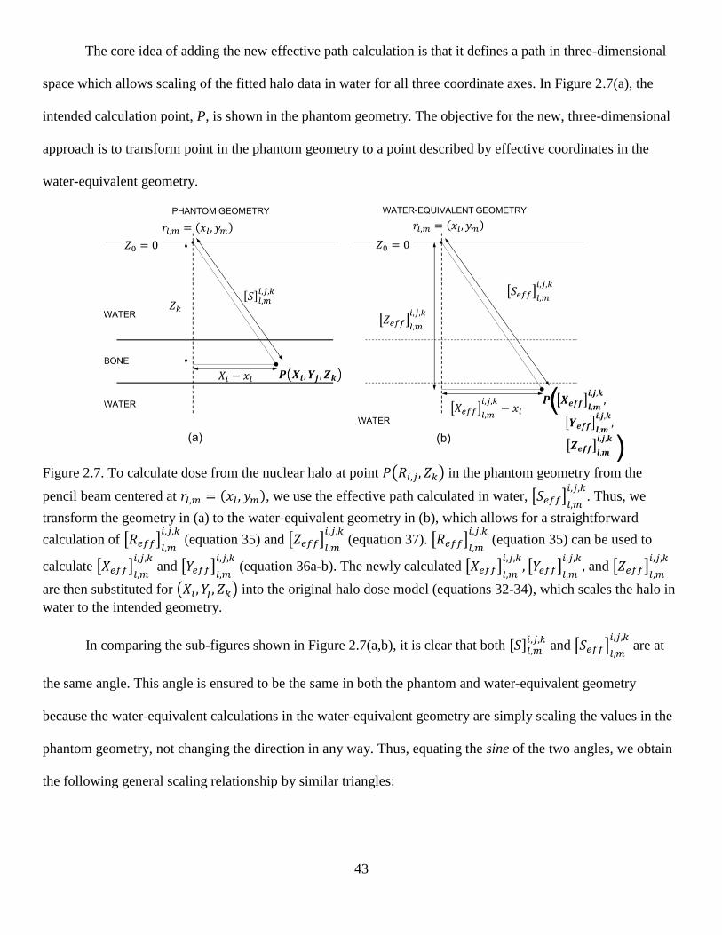
43
The core idea of adding the new effective path calculation is that it defines a path in three-dimensional
space which allows scaling of the fitted halo data in water for all three coordinate axes. In Figure 2.7(a), the
intended calculation point, P, is shown in the phantom geometry. The objective for the new, three-dimensional
approach is to transform point in the phantom geometry to a point described by effective coordinates in the
water-equivalent geometry.
Figure 2.7. To calculate dose from the nuclear halo at point 𝑃(𝑅𝑖,𝑗, 𝑍𝑘) in the phantom geometry from the
pencil beam centered at 𝑟𝑙,𝑚 = (𝑥𝑙, 𝑦𝑚), we use the effective path calculated in water, [𝑆𝑒𝑓𝑓]𝑙,𝑚
𝑖,𝑗,𝑘. Thus, we
transform the geometry in (a) to the water-equivalent geometry in (b), which allows for a straightforward
calculation of [𝑅𝑒𝑓𝑓]𝑙,𝑚
𝑖,𝑗,𝑘 (equation 35) and [𝑍𝑒𝑓𝑓]
𝑙,𝑚
𝑖,𝑗,𝑘 (equation 37). [𝑅𝑒𝑓𝑓]
𝑙,𝑚
𝑖,𝑗,𝑘 (equation 35) can be used to
calculate [𝑋𝑒𝑓𝑓]𝑙,𝑚
𝑖,𝑗,𝑘 and [𝑌𝑒𝑓𝑓]
𝑙,𝑚
𝑖,𝑗,𝑘 (equation 36a-b). The newly calculated [𝑋𝑒𝑓𝑓]
𝑙,𝑚
𝑖,𝑗,𝑘, [𝑌𝑒𝑓𝑓]
𝑙,𝑚
𝑖,𝑗,𝑘, and [𝑍𝑒𝑓𝑓]
𝑙,𝑚
𝑖,𝑗,𝑘
are then substituted for (𝑋𝑖, 𝑌𝑗 , 𝑍𝑘) into the original halo dose model (equations 32-34), which scales the halo in
water to the intended geometry.
In comparing the sub-figures shown in Figure 2.7(a,b), it is clear that both [𝑆]𝑙,𝑚𝑖,𝑗,𝑘
and [𝑆𝑒𝑓𝑓]𝑙,𝑚
𝑖,𝑗,𝑘 are at
the same angle. This angle is ensured to be the same in both the phantom and water-equivalent geometry
because the water-equivalent calculations in the water-equivalent geometry are simply scaling the values in the
phantom geometry, not changing the direction in any way. Thus, equating the sine of the two angles, we obtain
the following general scaling relationship by similar triangles:

44
[𝑅𝑒𝑓𝑓]𝑙,𝑚
𝑖,𝑗,𝑘= [
𝑆𝑒𝑓𝑓
𝑆]
𝑙,𝑚
𝑖,𝑗,𝑘
(𝑅𝑖,𝑗 − 𝑟𝑙,𝑚) + 𝑟𝑙,𝑚, (35)
where the subscript (𝑙, 𝑚) indicates that the variable is calculated along a path originating at the pencil beam
centered at (𝑥𝑙, 𝑦𝑚) (at the phantom surface) and terminating at grid position (𝑋𝑖, 𝑌𝑗 , 𝑍𝑘). Note that [𝑆𝑒𝑓𝑓
𝑆]
𝑙,𝑚
𝑖,𝑗,𝑘
is
equivalent to [𝑆𝑒𝑓𝑓]𝑙,𝑚
𝑖,𝑗,𝑘[𝑆]𝑙,𝑚
𝑖,𝑗,𝑘⁄ .
As with the polar angle, the azimuthal angle is also preserved in transforming the phantom geometry to
the water-equivalent geometry. Therefore, the ratios between polar coordinate R and Cartesian coordinates (X,
Y) are also preserved. As a result, it is possible to transform equation (35) into the following expressions:
[𝑋𝑒𝑓𝑓]𝑙,𝑚
𝑖,𝑗,𝑘= [
𝑆𝑒𝑓𝑓
𝑆]
𝑙,𝑚
𝑖,𝑗,𝑘
(𝑋𝑖 − 𝑥𝑙) + 𝑥𝑙 ,
(36a)
[𝑌𝑒𝑓𝑓]𝑙,𝑚
𝑖,𝑗,𝑘= [
𝑆𝑒𝑓𝑓
𝑆]
𝑙,𝑚
𝑖,𝑗,𝑘
(𝑌𝑗 − 𝑦𝑚) + 𝑦𝑚.
(36b)
The scaling along Z has a slightly different form since the origin for all [𝑆]𝑙,𝑚𝑖,𝑗,𝑘
are at the phantom surface,
[𝑍𝑒𝑓𝑓]𝑙,𝑚
𝑖,𝑗,𝑘= [
𝑆𝑒𝑓𝑓
𝑆]
𝑙,𝑚
𝑖,𝑗,𝑘
𝑍𝑘. (37)
Note that this is not the same as 𝑍𝑒𝑓𝑓𝑙,𝑚 (𝑍𝑘) (equation (8)), which is the effective depth in water as calculated
along the central-axis of the pencil beam at (𝑥𝑙 , 𝑦𝑚). [𝑍𝑒𝑓𝑓]𝑙,𝑚
𝑖,𝑗,𝑘 is the effective scaling along the Z-axis, as
determined by equation (37).
In the special case of laterally infinite heterogeneities, both [𝑆𝑒𝑓𝑓]𝑙,𝑚
𝑖,𝑗,𝑘 and 𝑍𝑒𝑓𝑓
𝑙,𝑚 (𝑍𝑘) are scaled at the
same rates because they traverse the same geometry; thus, [𝑆𝑒𝑓𝑓
𝑆]
𝑙,𝑚
𝑖,𝑗,𝑘
in equations (35-37) can be replaced with
𝑍𝑒𝑓𝑓𝑙,𝑚 (𝑍𝑘)/𝑍𝑘. Substitution of 𝑍𝑒𝑓𝑓
𝑙,𝑚 (𝑍𝑘)/𝑍𝑘instead of [𝑆𝑒𝑓𝑓
𝑆]
𝑙,𝑚
𝑖,𝑗,𝑘
in equations (35-37) is equivalent to invoking the
CAXSIS approximation in equations (35-37).
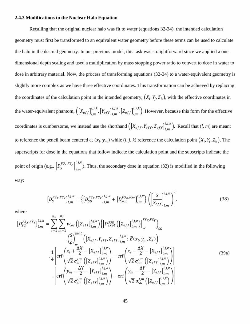
45
2.4.3 Modifications to the Nuclear Halo Equation
Recalling that the original nuclear halo was fit to water (equations 32-34), the intended calculation
geometry must first be transformed to an equivalent water geometry before these terms can be used to calculate
the halo in the desired geometry. In our previous model, this task was straightforward since we applied a one-
dimensional depth scaling and used a multiplication by mass stopping power ratio to convert to dose in water to
dose in arbitrary material. Now, the process of transforming equations (32-34) to a water-equivalent geometry is
slightly more complex as we have three effective coordinates. This transformation can be achieved by replacing
the coordinates of the calculation point in the intended geometry, (𝑋𝑖, 𝑌𝑗 , 𝑍𝑘), with the effective coordinates in
the water-equivalent phantom, ([𝑋𝑒𝑓𝑓]𝑙,𝑚
𝑖,𝑗,𝑘, [𝑌𝑒𝑓𝑓]
𝑙,𝑚
𝑖,𝑗,𝑘, [𝑍𝑒𝑓𝑓]
𝑙,𝑚
𝑖,𝑗,𝑘). However, because this form for the effective
coordinates is cumbersome, we instead use the shorthand ([𝑋𝑒𝑓𝑓, 𝑌𝑒𝑓𝑓 , 𝑍𝑒𝑓𝑓]𝑙,𝑚
𝑖,𝑗,𝑘). Recall that (l, m) are meant
to reference the pencil beam centered at (𝑥𝑙 , 𝑦𝑚) while (i, j, k) reference the calculation point (𝑋𝑖, 𝑌𝑗 , 𝑍𝑘). The
superscripts for dose in the equations that follow indicate the calculation point and the subscripts indicate the
point of origin (e.g., [𝐷𝑆
𝐹𝑆𝑥,𝐹𝑆𝑦]𝑙,𝑚
𝑖,𝑗,𝑘
). Thus, the secondary dose in equation (32) is modified in the following
way:
[𝐷𝑆𝐹𝑆𝑋,𝐹𝑆𝑌]
𝑙,𝑚
𝑖,𝑗,𝑘= {[𝐷𝑆𝐺
𝐹𝑆𝑋,𝐹𝑆𝑌]𝑙,𝑚
𝑖,𝑗,𝑘+ [𝐷𝑆𝐶𝐿
𝐹𝑆𝑋,𝐹𝑆𝑌]𝑙,𝑚
𝑖,𝑗,𝑘} ([
𝑆
𝑆𝑒𝑓𝑓]
𝑙,𝑚
𝑖,𝑗,𝑘
)
2
, (38)
where
[𝐷𝑆𝐺𝐹𝑆𝑋,𝐹𝑆𝑌]
𝑙,𝑚
𝑖,𝑗,𝑘= ∑ ∑ 𝑤𝑆𝐺 ([𝑍𝑒𝑓𝑓]
𝑙,𝑚
𝑖,𝑗,𝑘) {[𝐷𝑒𝑥𝑝𝑡
𝑆𝑆𝐸 ([𝑍𝑒𝑓𝑓]𝑙,𝑚
𝑖,𝑗,𝑘)]
𝑤
𝐹𝑆𝑋,𝐹𝑆𝑌
}𝑆𝐺
𝑛𝑦
𝑚=1
𝑛𝑥
𝑙=1
. (𝑆
𝜌)
𝑤
𝑚𝑎𝑡
([𝑋𝑒𝑓𝑓, 𝑌𝑒𝑓𝑓 , 𝑍𝑒𝑓𝑓]𝑙,𝑚
𝑖,𝑗,𝑘; ��(𝑥𝑙, 𝑦𝑚, 𝑍𝑘))
.1
4[erf (
𝑥𝑙 +∆𝑋2 − [𝑋𝑒𝑓𝑓]
𝑙,𝑚
𝑖,𝑗,𝑘
√2 𝜎𝑆𝐺𝑙,𝑚 ([𝑍𝑒𝑓𝑓]
𝑙,𝑚
𝑖,𝑗,𝑘)
) − erf (𝑥𝑙 −
∆𝑋2 − [𝑋𝑒𝑓𝑓]
𝑙,𝑚
𝑖,𝑗,𝑘
√2 𝜎𝑆𝐺𝑙,𝑚 ([𝑍𝑒𝑓𝑓]
𝑙,𝑚
𝑖,𝑗,𝑘)
)]
. [erf (𝑦𝑚 +
∆Y2 − [𝑌𝑒𝑓𝑓]
𝑙,𝑚
𝑖,𝑗,𝑘
√2 𝜎𝑆𝐺𝑙,𝑚 ([𝑍𝑒𝑓𝑓]
𝑙,𝑚
𝑖,𝑗,𝑘)
) − erf (𝑦𝑚 −
∆𝑌2 − [𝑌𝑒𝑓𝑓]
𝑙,𝑚
𝑖,𝑗,𝑘
√2 𝜎𝑆𝐺𝑙,𝑚 ([𝑍𝑒𝑓𝑓]
𝑙,𝑚
𝑖,𝑗,𝑘)
)]
(39a)

46
[𝐷𝑆𝐶𝐿𝐹𝑆𝑋,𝐹𝑆𝑌]
𝑙,𝑚
𝑖,𝑗,𝑘= ∑ ∑ 𝑤𝑆𝐶𝐿 ([𝑍𝑒𝑓𝑓]
𝑙,𝑚
𝑖,𝑗,𝑘) {[𝐷𝑒𝑥𝑝𝑡
𝑆𝑆𝐸 ([𝑍𝑒𝑓𝑓]𝑙,𝑚
𝑖,𝑗,𝑘)]
𝑤
𝐹𝑆𝑋,𝐹𝑆𝑌
}𝑆𝐶𝐿
𝑛𝑦
𝑚=1
𝑛𝑥
𝑙=1
. (𝑆
𝜌)
𝑤
𝑚𝑎𝑡
([𝑋𝑒𝑓𝑓, 𝑌𝑒𝑓𝑓 , 𝑍𝑒𝑓𝑓]𝑙,𝑚
𝑖,𝑗,𝑘; ��(𝑥𝑙, 𝑦𝑚, 𝑍𝑘))
.1
4[atan (
𝑥𝑙 +∆𝑋2 − [𝑋𝑒𝑓𝑓]
𝑙,𝑚
𝑖,𝑗,𝑘
𝜎𝑆𝐶𝐿𝑙,𝑚 ([𝑍𝑒𝑓𝑓]
𝑙,𝑚
𝑖,𝑗,𝑘)
) − atan (𝑥𝑙 −
∆𝑋2 − [𝑋𝑒𝑓𝑓]
𝑙,𝑚
𝑖,𝑗,𝑘
𝜎𝑆𝐶𝐿𝑙,𝑚 ([𝑍𝑒𝑓𝑓]
𝑙,𝑚
𝑖,𝑗,𝑘)
)]
. [atan (𝑦𝑚 +
∆𝑌2 − [𝑌𝑒𝑓𝑓]
𝑙,𝑚
𝑖,𝑗,𝑘
𝜎𝑆𝐶𝐿𝑙,𝑚 ([𝑍𝑒𝑓𝑓]
𝑙,𝑚
𝑖,𝑗,𝑘)
) − atan (𝑦𝑚 −
∆𝑌2 − [𝑌𝑒𝑓𝑓]
𝑙,𝑚
𝑖,𝑗,𝑘
𝜎𝑆𝐶𝐿𝑙,𝑚 ([𝑍𝑒𝑓𝑓]
𝑙,𝑚
𝑖,𝑗,𝑘)
)].
(39b)
Note that for effective path calculations taking place in water (equivalently, [𝑆𝑒𝑓𝑓]𝑙,𝑚
𝑖,𝑗,𝑘= [𝑆]𝑙,𝑚
𝑖,𝑗,𝑘), all effective
coordinates are simply equal to the coordinates of the calculation point in the intended geometry (i.e., equations
35-37 with [𝑆𝑒𝑓𝑓]𝑙,𝑚
𝑖,𝑗,𝑘= [𝑆]𝑙,𝑚
𝑖,𝑗,𝑘), so [𝐷𝑆
𝐹𝑆𝑋,𝐹𝑆𝑌]𝑙,𝑚
𝑖,𝑗,𝑘= 𝐷𝑆
𝐹𝑆𝑋 ,𝐹𝑆𝑌(𝑋𝑖, 𝑌𝑗 , 𝑍𝑘), which reduces equation (38) to
equation (32), the original nuclear halo equation.
2.4.4 Description of Evaluation Geometries
We evaluated geometries with laterally infinite slabs of both compact bone and air. As with the primary
proton dose evaluations, we used the highest energy (250 MeV), a rectangular field size (4x4 cm2), and deep,
thick slabs. Variations in slab depth (z = 10, 20, 30 cm) and thickness (2, 4, 5 cm) were also explored to ensure
the new nuclear halo model applied to a wide range of geometries.
2.5 Evaluation of Dose Model in Patient-Like Phantoms (Specific Aim 3)
Recall that in Specific Aim 1, evaluation geometries were selected to test the improvements over the
CAXSIS approximation that is part of all PBAs. Only primary dose was calculated to eliminate influence from
the nuclear halo model. In Specific Aim 2, we selected evaluation geometries which eliminated the error from
the CAXSIS approximation so the improvement in accuracy was indicative of the improved nuclear halo model.
In Specific Aim 3, we compared dose between the present model (equation 38), original model (equation
32), and MCNPX simulations. Geometries used for comparisons in this Aim featured laterally finite
heterogeneities and included dose from both the primary and secondary dose terms. Furthermore, the overall

47
goal in Specific Aim 3 is to characterize the dose accuracy levels achievable by the present model and the prior
model in simple “patient-like” phantoms, where heterogeneities are meant to mimic some of the anatomical
features one might find in a typical treatment scenario.
2.5.1 Checkerboard Phantom (2 cm x 2 cm)
The checkerboard phantom was designed with alternating 2 cm wide by 2 cm thick air / compact bone
slabs. This sort of heterogeneity configuration could potentially be found in the sinus region of the head, where
many small bones and air cavities are adjacent to one another. The schematic for the 2 cm x 2 cm checkerboard
phantom is shown in Figure 2.8 below.
2.5.2 Prostate Phantom
We designed a prostate phantom by focusing on the major heterogeneities typically encountered in these
treatments: the femoral head and the rectum. We approximated the femoral head as a 2 cm radius sphere
centered at Z = 19 cm and composed of compact bone (see Table 2.2). The theoretical prostate planning target
volume (PTV) was also designed as a 2 cm radius sphere which was centered at Z = 29 cm (the material of the
“PTV” was assigned to water). Finally, the rectum was modeled as an ellipsoid with a major axis of 2.98 cm
and a minor axis of 1.71 cm. The rectum heterogeneity was also centered at Z = 29 cm and was assigned to air
(Table 2.2). The full schematic for the prostate phantom is shown in Figure 2.9 below.
Figure 2.8. Geometry for the 2 cm x 2 cm checkerboard phantom. The phantom consists of 2 cm wide by 2 cm
thick alternating slabs of air (blue) and compact bone (yellow).
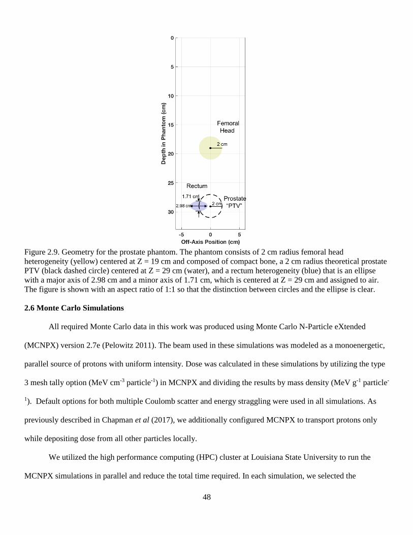
48
Figure 2.9. Geometry for the prostate phantom. The phantom consists of 2 cm radius femoral head
heterogeneity (yellow) centered at Z = 19 cm and composed of compact bone, a 2 cm radius theoretical prostate
PTV (black dashed circle) centered at Z = 29 cm (water), and a rectum heterogeneity (blue) that is an ellipse
with a major axis of 2.98 cm and a minor axis of 1.71 cm, which is centered at Z = 29 cm and assigned to air.
The figure is shown with an aspect ratio of 1:1 so that the distinction between circles and the ellipse is clear.
2.6 Monte Carlo Simulations
All required Monte Carlo data in this work was produced using Monte Carlo N-Particle eXtended
(MCNPX) version 2.7e (Pelowitz 2011). The beam used in these simulations was modeled as a monoenergetic,
parallel source of protons with uniform intensity. Dose was calculated in these simulations by utilizing the type
3 mesh tally option (MeV cm-3 particle-1) in MCNPX and dividing the results by mass density (MeV g-1 particle-
1). Default options for both multiple Coulomb scatter and energy straggling were used in all simulations. As
previously described in Chapman et al (2017), we additionally configured MCNPX to transport protons only
while depositing dose from all other particles locally.
We utilized the high performance computing (HPC) cluster at Louisiana State University to run the
MCNPX simulations in parallel and reduce the total time required. In each simulation, we selected the

49
appropriate number of initial histories needed for statistical uncertainties below 1%, which was typically
200x106 histories. The typical time required for one of these simulations was about 72 hours on 128 processors
(9,216 processor-hours).
The PBA (section 2.2) was commissioned using simulated dose distributions from a model of a
simplified proton therapy beamline in MCNPX. This approach was previously verified (Koch et al 2005 and
Newhauser et al 2007). Specifically for the PBA, the central-axis percent depth dose (PDD) was extracted for
two energies (100 and 250 MeV) and a field size of 4x4 cm2, which provided the required [𝐷𝑒𝑥𝑝𝑡(𝑧)]𝑤
𝐹𝑆𝑋,𝐹𝑆𝑌 in
section 2.2. As mentioned in section 2.3.3, the correction factors needed for intial energies (100 and 250 MeV),
𝐶(𝑍𝑘; 𝐸0), also required MC simulations. Finally, MC simulations were used both to parameterize the nuclear
halo model (as discussed previously in Knutson et al 2012) and as the standard of comparison for both the
previous model and the present model in the geometries selected for evaluation.
2.7 Evaluating the Dosimetric Accuracy of Present Model and Chapman et al (2017)
Dose calculated by the present model (“PM”) was compared with the original, Chapman et al (2017)
model (“OM”), using MCNPX data (“MC”) as the gold standard for monoenergetic (100 and 250 MeV) beams
and a spread-out Bragg peak with 5 cm of range modulation with a 4x4 cm2 field size. Dose for each model was
normalized to the maximum dose in a homogeneous water phantom for the same incident beam, which gave the
relative dose
[𝑅𝐷𝐹𝑆𝑋,𝐹𝑆𝑌(𝑋𝑖, 𝑌𝑗 , 𝑍𝑘)]𝑃𝑀
= 100 .[𝐷
𝐹𝑆𝑋,𝐹𝑆𝑌(𝑋𝑖, 𝑌𝑗 , 𝑍𝑘)]𝑃𝑀
[𝐷𝑤𝐹𝑆𝑋,𝐹𝑆𝑌(0, 0, 𝑍𝑚𝑎𝑥)]
𝑃𝑀
, (40a)
[𝑅𝐷𝐹𝑆𝑋,𝐹𝑆𝑌(𝑋𝑖, 𝑌𝑗 , 𝑍𝑘)]𝑂𝑀
= 100 .[𝐷
𝐹𝑆𝑋,𝐹𝑆𝑌(𝑋𝑖, 𝑌𝑗 , 𝑍𝑘)]𝑂𝑀
[𝐷𝑤𝐹𝑆𝑋,𝐹𝑆𝑌(0, 0, 𝑍𝑚𝑎𝑥)]
𝑂𝑀
, (40b)
[𝑅𝐷𝐹𝑆𝑋,𝐹𝑆𝑌(𝑋𝑖, 𝑌𝑗 , 𝑍𝑘)]𝑀𝐶
= 100 .[𝐷
𝐹𝑆𝑋,𝐹𝑆𝑌(𝑋𝑖, 𝑌𝑗 , 𝑍𝑘)]𝑀𝐶
[𝐷𝑤𝐹𝑆𝑋,𝐹𝑆𝑌(0, 0, 𝑍𝑚𝑎𝑥)]
𝑀𝐶
, (40c)

50
where the subscripts (PM, OM, and MC) refer to the present model, original model, and MCNPX simulations,
respectively. 𝐷𝑤𝐹𝑆𝑋,𝐹𝑆𝑌 is used to specify dose in a homogeneous water phantom, and 𝑍𝑚𝑎𝑥 is the depth along the
central-axis at which the dose is maximum in the homogeneous water phantom. We compared all three models
(PM, OM, and MC) using various geometries (chapter 3), and used the percentage of pixels passing 3% dose
difference of 1 mm distance-to-agreement (DTA) as a measure of the improvements in the PM compared to the
OM. Dose difference between MC and dose model X (meant as a generic label for either ‘PM’ or ‘OM’) was
calculated using
∆𝑅𝐷𝑀𝐶−𝑋𝐹𝑆𝑋,𝐹𝑆𝑌 = [𝑅𝐷𝐹𝑆𝑋,𝐹𝑆𝑌(𝑋𝑖, 𝑌𝑗 , 𝑍𝑘)]
𝑀𝐶− [𝑅𝐷𝐹𝑆𝑋,𝐹𝑆𝑌(𝑋𝑖, 𝑌𝑗 , 𝑍𝑘)]
𝑋. (41)
Distance-to-agreement was calculated using the method by Ju et al (2008).

51
CHAPTER 3. RESULTS
In this chapter, results are presented for each of the three aims in this work. Each section provides comparisons
detailing the relative performance of three dose calculation approaches: (1) the model in the present work
(hereafter referred to as the “present model,” or “PM”); (2) the Chapman et al (2017) PBA (hereafter referred to
as the “original model,” or “OM”); and, (3) the Monte Carlo data that is used as the standard of comparison for
PM and OM, denoted “MC” for this chapter. All data presented in this chapter compared dose between PM,
OM, and MC.
The comparisons in this chapter are mostly based on the percentage of points that pass the 3% or 1 mm
criteria set in the hypothesis. It should be further noted that most of these “pass rate” calculations are only tested
on points that are below the distal edge of the last major heterogeneity and also within 1% isodose line (the
“distal slab area”); this approach was chosen because the largest dosimetric differences between PM and OM
are expected below the distal edge of the slab heterogeneity. Another geometry (5 cm bone slab at z = 30 cm)
calculated the pass rate below the proximal slab edge and within the 1% isodose line because this particular slab
covered most of the Bragg peak. Additional metrics for determining agreement between dose models include
dose difference maps and histograms in the distal slab area, central-axis and lateral profiles, and the distance-to-
agreement (DTA) of the 1% isodose lines.
3.1 Results for Specific Aim 1
For all of the results that follow for Specific Aim 1, all calculation approaches (PM, OM, and MC) were
limited to primary dose only. Results are presented as inter-comparisons between these three models in a
homogeneous water phantom, laterally finite compact bone / air slab phantoms, for a monoenergetic (250 MeV)
beam. Table 3.1 summarizes the results for this aim.
Table 3.1. Results for homogenous water and laterally finite slabs. Columns in the table indicate the percentage
of points passing our criteria of 3% or 1 mm.

52
3.1.1 Homogeneous Water Phantom
Our results for Specific Aim 1 begin with a homogeneous water geometry. For this phantom, a 250 MeV
beam with a field size of 4x4 cm2 was used. Figure 3.1 shows isodose comparisons of dose calculated using the
PM relative to MC and dose calculated by the OM relative to MC. In both cases, 100.0% of points passed our
criteria of 3% or 1 mm. Some statistical noise is evident at the 30% isodose line for the PM, but this could be
reduced by using a higher number of initial protons (106 were used in this case). Central-axis (Figure 3.2) and
lateral profiles at the depth of maximum dose (Figure 3.3) are also shown. Agreement was excellent between all
models in water.
3.1.2 Laterally Finite Slabs
For laterally finite slabs (compact bone and air) of 4 cm thickness at z=30 cm extending from x=0 cm to
the right phantom edge, we tested a 250 MeV, 4x4 cm2 beam and compared the results between PM, OM, and
MC. For the compact bone case (Figure 3.4), 98.0% of points calculated by the PM were within 3% or 1 mm of
MC calculations. In contrast, the agreement between the OM and MC was 69.0%. The improvement of the PM
in addressing the limitations associated with the CAXSIS approximation is evident comparing the dose
difference maps and histograms in Figure 3.5. The PM, which is not limited by the CAXSIS approximation,
models the deposition of proton dose in a more physically realistic way than the OM.
We also compared the lateral profiles at z=34.5 cm (Figure 3.6) for all three calculation models (PM,
OM, MC). We found that the PM matched the MC profile to within +0.5% and -3.0% dose difference and it is
visually evident in Figure 3.6(a) that the PM correctly modeled primary dose changes due to the water-bone
interface near the slab. Because the OM was based on the CAXSIS approximation, inaccurate pencil beam
modeling near the slab edge (x=0 cm) averaged out the dose between all the contributing pencil beams,
resulting in dose differences within +8.5% and -13.5%.

53
(a) (b)
Figure 3.1. Primary dose calculation for a 250 MeV, 4x4 cm2 beam in water, shown using (a) PM (solid) vs MC
(dashed), and (b) OM (solid) and MC (dashed). 100.0% of points in both (a) and (b) satisfied 3% or 1 mm.
Isodose lines shown include 1, 2, 5, 10, 20, 30, 40, 50, 70, 90, and 100 %.
(a) (b)
Figure 3.2. Central-axis depth dose profiles for the homogeneous water geometry (Figure 3.1). Data shown
using (a) PM (solid) vs MC (dashed), and (b) OM (solid) vs MC (dashed). The red plot in each panel indicates
dose difference in this profile. The dose difference in (a) is within +1.0% to -3.0% and (b) within +/-1.0% for
all points.
For the laterally finite air slab case (Figure 3.7), 99.5% of points calculated by the PM were within 3%
or 1 mm of MC. In contrast, agreement between OM and MC was 69.5%. As with the bone slab, the PM
overcomes limitations imposed by the CAXSIS approximation in the OM, which is evident comparing the dose
difference maps and histograms in Figure 3.8.
WATER WATER
WATER WATER

54
Off-Axis Position (cm) Off-Axis Position (cm)
(a) (b)
Figure 3.3. Lateral dose profiles at the depth of maximum dose for the homogeneous water geometry (Figure
3.1). Data shown using (a) PM (solid) vs MC (dashed), and (b) OM (solid) vs MC (dashed). The red plot in
each panel indicates dose difference in this profile. The dose difference in (a) is within +/-1.5% and in (b) is
within +/-0.5%.
In comparing the lateral profiles at z=34.5 cm (Figure 3.9) for all three calculation models (PM, OM,
MC), we found that the PM matched the MC profile to within +1.0% and -2.0% dose difference and it is
visually evident in Figure 3.9(a) that the PM correctly modeled primary dose changes due to the water-air
interface near the slab. Because the OM was based on the CAXSIS approximation, the convolution of multiple,
inaccurate pencil beams near the slab edge (x=0 cm) averaged out the dose between all the contributing pencil
beams, resulting in dose differences within +2.0% and -5.0%.
3.2 Results for Specific Aim 2
For all of the results that follow for Specific Aim 2, all calculation approaches (PM, OM, and MC)
included both primary and secondary dose (i.e., total dose). The presentation of results for Specific Aim 2 here
are broken down into thin (2 cm) and thick (4, 5 cm) slab sections (additional comparisons are shown in the
Appendix). The general trend observed was improvement in low isodose lines for all slabs, and in-field
improvement for deep slabs only. For this reason, the figures in this section will only feature deep slabs (z = 30
cm).
WATER WATER
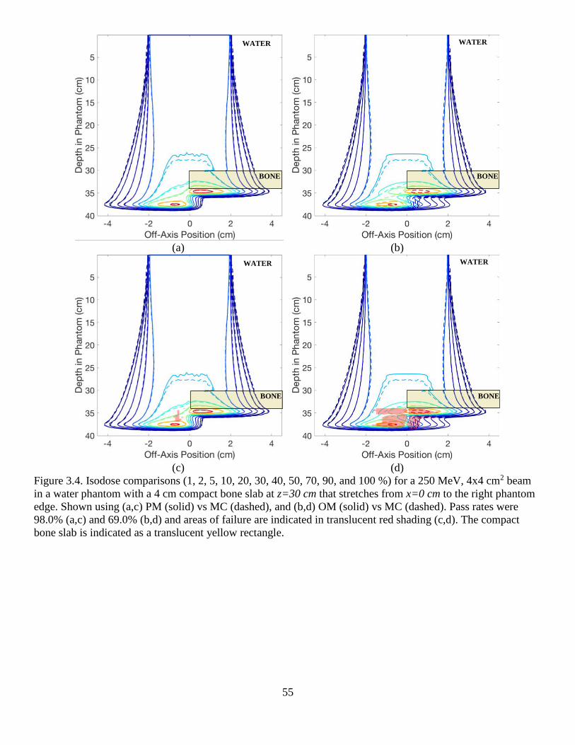
55
(a) (b)
(c) (d)
Figure 3.4. Isodose comparisons (1, 2, 5, 10, 20, 30, 40, 50, 70, 90, and 100 %) for a 250 MeV, 4x4 cm2 beam
in a water phantom with a 4 cm compact bone slab at z=30 cm that stretches from x=0 cm to the right phantom
edge. Shown using (a,c) PM (solid) vs MC (dashed), and (b,d) OM (solid) vs MC (dashed). Pass rates were
98.0% (a,c) and 69.0% (b,d) and areas of failure are indicated in translucent red shading (c,d). The compact
bone slab is indicated as a translucent yellow rectangle.
WATER WATER
BONE BONE
WATER WATER
BONE BONE
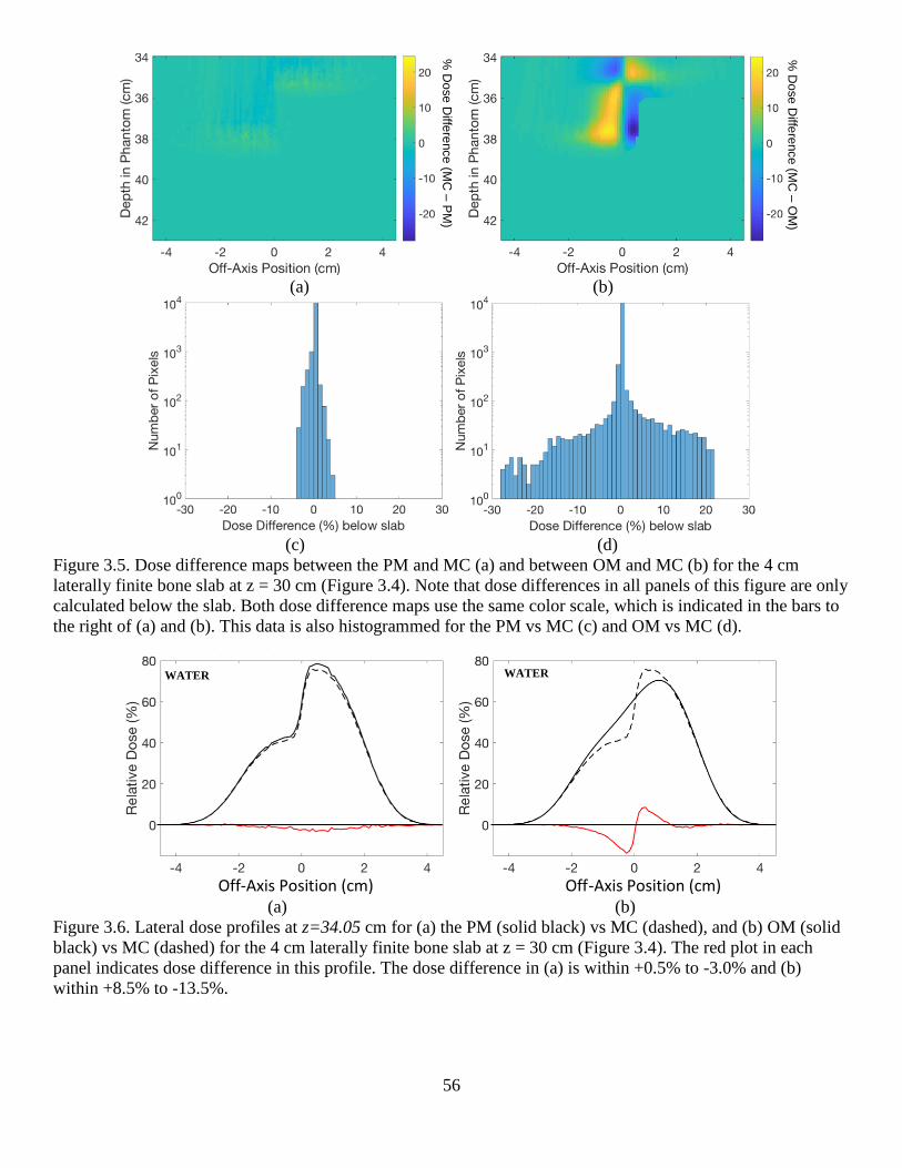
56
(a) (b)
(c) (d)
Figure 3.5. Dose difference maps between the PM and MC (a) and between OM and MC (b) for the 4 cm
laterally finite bone slab at z = 30 cm (Figure 3.4). Note that dose differences in all panels of this figure are only
calculated below the slab. Both dose difference maps use the same color scale, which is indicated in the bars to
the right of (a) and (b). This data is also histogrammed for the PM vs MC (c) and OM vs MC (d).
Off-Axis Position (cm) Off-Axis Position (cm)
(a) (b)
Figure 3.6. Lateral dose profiles at z=34.05 cm for (a) the PM (solid black) vs MC (dashed), and (b) OM (solid
black) vs MC (dashed) for the 4 cm laterally finite bone slab at z = 30 cm (Figure 3.4). The red plot in each
panel indicates dose difference in this profile. The dose difference in (a) is within +0.5% to -3.0% and (b)
within +8.5% to -13.5%.
% D
ose
Diffe
rence (M
C –
OM
)
% D
ose
Diffe
rence (M
C –
PM
)
WATER WATER
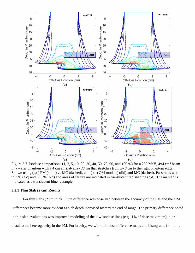
57
(a) (b)
(c) (d)
Figure 3.7. Isodose comparisons (1, 2, 5, 10, 20, 30, 40, 50, 70, 90, and 100 %) for a 250 MeV, 4x4 cm2 beam
in a water phantom with a 4 cm air slab at z=30 cm that stretches from x=0 cm to the right phantom edge.
Shown using (a,c) PM (solid) vs MC (dashed), and (b,d) OM model (solid) and MC (dashed). Pass rates were
99.5% (a,c) and 69.5% (b,d) and areas of failure are indicated in translucent red shading (c,d). The air slab is
indicated as a translucent blue rectangle.
3.2.1 Thin Slab (2 cm) Results
For thin slabs (2 cm thick), little difference was observed between the accuracy of the PM and the OM.
Differences became more evident as slab depth increased toward the end of range. The primary difference noted
in thin slab evaluations was improved modeling of the low isodose lines (e.g., 1% of dose maximum) in or
distal to the heterogeneity in the PM. For brevity, we will omit dose difference maps and histograms from this
WATER WATER
AIR AIR
WATER WATER
AIR AIR
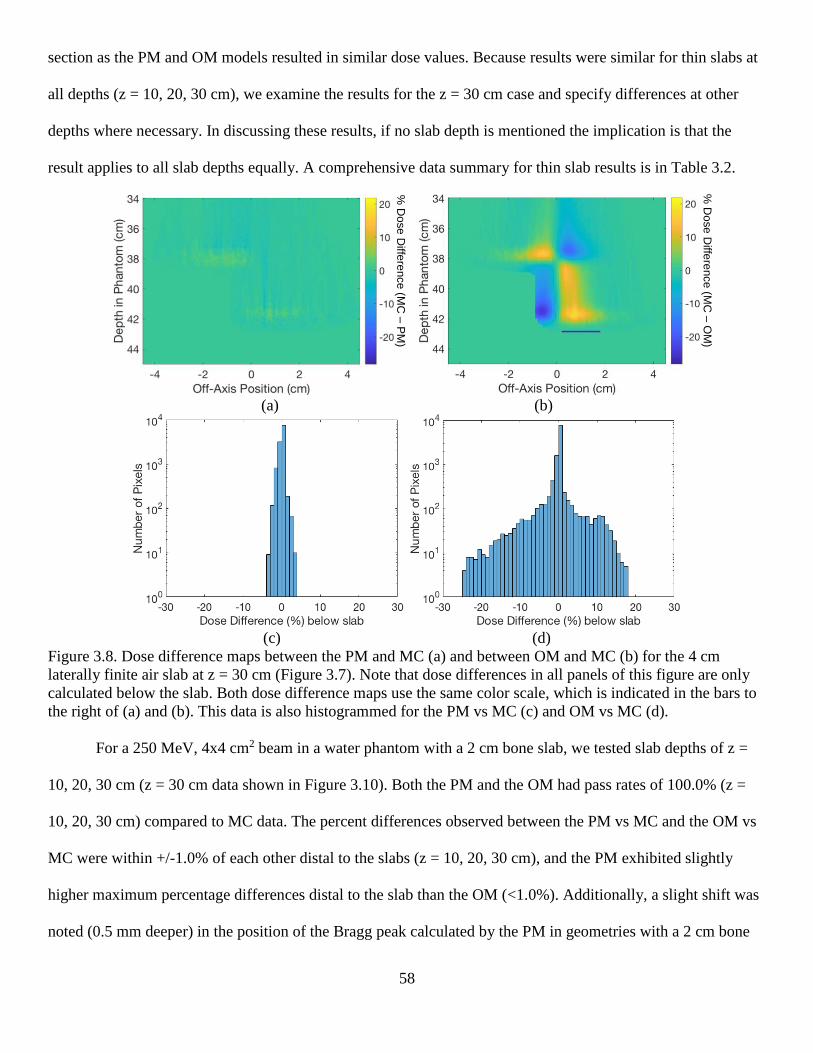
58
section as the PM and OM models resulted in similar dose values. Because results were similar for thin slabs at
all depths (z = 10, 20, 30 cm), we examine the results for the z = 30 cm case and specify differences at other
depths where necessary. In discussing these results, if no slab depth is mentioned the implication is that the
result applies to all slab depths equally. A comprehensive data summary for thin slab results is in Table 3.2.
(a) (b)
(c) (d)
Figure 3.8. Dose difference maps between the PM and MC (a) and between OM and MC (b) for the 4 cm
laterally finite air slab at z = 30 cm (Figure 3.7). Note that dose differences in all panels of this figure are only
calculated below the slab. Both dose difference maps use the same color scale, which is indicated in the bars to
the right of (a) and (b). This data is also histogrammed for the PM vs MC (c) and OM vs MC (d).
For a 250 MeV, 4x4 cm2 beam in a water phantom with a 2 cm bone slab, we tested slab depths of z =
10, 20, 30 cm (z = 30 cm data shown in Figure 3.10). Both the PM and the OM had pass rates of 100.0% (z =
10, 20, 30 cm) compared to MC data. The percent differences observed between the PM vs MC and the OM vs
MC were within +/-1.0% of each other distal to the slabs (z = 10, 20, 30 cm), and the PM exhibited slightly
higher maximum percentage differences distal to the slab than the OM (<1.0%). Additionally, a slight shift was
noted (0.5 mm deeper) in the position of the Bragg peak calculated by the PM in geometries with a 2 cm bone
% D
ose
Diffe
rence (M
C –
OM
)
% D
ose
Diffe
rence (M
C –
PM
)

59
slab compared to MC. In Figure 3.11, the OM overestimates dose immediately proximal to the peak and
underestimates dose at the peak. Lateral profiles below the distal edge of the slab (z = 32.5 cm) are shown in
Figure 3.12.
Off-Axis Position (cm) Off-Axis Position (cm)
(a) (b)
Figure 3.9. Lateral dose profiles at z=34.5 cm for (a) the PM (solid black) vs MC (dashed), and (b) OM (solid
black) vs MC (dashed) for the 4 cm laterally finite air slab at z = 30 cm (Figure 3.7). The red plot in each panel
indicates dose difference in this profile. The dose difference in (a) is within +1.0% to -2.0% and (b) within
+2.0% to -5.0%.
Table 3.2. Results for thin (2 cm) compact bone and air slabs. Columns in the table indicate the percentage of
points passing our criteria of 3% or 1 mm, and the improvement (negative values: worsening) in the DTA of the
1% isodose line (calculated by subtracting the DTA of the OM vs MC from the DTA of the PM vs MC).
The DTA of the 1% isodose line at the distal edge of the bone slab between the PM and MC improved
by 3.9 mm (z = 10 cm), 2.1 mm (z = 20 cm), or 1.5 mm (z = 30 cm) relative to the DTA between the OM and
MC. The DTA improvement at all depths further downstream was between 0.6 and 4.2 mm (z = 10 cm),
between 0.6 and 2.7 mm (z = 20 cm), or between 1.6 and 1.9 mm (z = 30 cm). The improved DTA at the 1%
WATER WATER
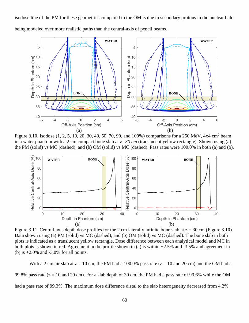
60
isodose line of the PM for these geometries compared to the OM is due to secondary protons in the nuclear halo
being modeled over more realistic paths than the central-axis of pencil beams.
(a) (b)
Figure 3.10. Isodose (1, 2, 5, 10, 20, 30, 40, 50, 70, 90, and 100%) comparisons for a 250 MeV, 4x4 cm2 beam
in a water phantom with a 2 cm compact bone slab at z=30 cm (translucent yellow rectangle). Shown using (a)
the PM (solid) vs MC (dashed), and (b) OM (solid) vs MC (dashed). Pass rates were 100.0% in both (a) and (b).
(a) (b)
Figure 3.11. Central-axis depth dose profiles for the 2 cm laterally infinite bone slab at z = 30 cm (Figure 3.10).
Data shown using (a) PM (solid) vs MC (dashed), and (b) OM (solid) vs MC (dashed). The bone slab in both
plots is indicated as a translucent yellow rectangle. Dose difference between each analytical model and MC in
both plots is shown in red. Agreement in the profile shown in (a) is within +2.5% and -3.5% and agreement in
(b) is +2.0% and -3.0% for all points.
With a 2 cm air slab at z = 10 cm, the PM had a 100.0% pass rate (z = 10 and 20 cm) and the OM had a
99.8% pass rate (z = 10 and 20 cm). For a slab depth of 30 cm, the PM had a pass rate of 99.6% while the OM
had a pass rate of 99.3%. The maximum dose difference distal to the slab heterogeneity decreased from 4.2%
WATER
BONE
WATER
BONE
WATER BONE WATER BONE

61
(OM vs MC) to 2.8% (PM vs MC) (z = 10 cm), 4.5% (OM vs MC) to 2.4% (PM vs MC) (z = 20 cm), and 7.4%
(OM vs MC) to 5.6% (PM vs MC) (z = 30 cm). Furthermore, for the 2 cm air slab at z = 10 cm, improvement of
the 1% isodose line in the slab (6.6 mm DTA) caused a downstream overestimation of the 1% isodose line (0.3-
6.5 mm DTA). When this slab was placed at z = 20 cm, there was a 4.5 mm DTA improvement in the slab for
the 1% isodose lines and a downstream overestimation of 0.6-3.2 mm. Finally, placing the 2 cm air slab at z =
30 cm (Figure 3.13), the improvement of the 1% isodose lines in the slab (3.1 mm DTA) was observed distal to
the slab and was improved by 0.4-2.6 mm further downstream. The improved DTA at the 1% isodose line at the
distal edge of the PM for these geometries compared to the OM is due to secondary protons in the nuclear halo
being modeled over more realistic paths than the central-axis of pencil beams. However, the PM had worse
agreement in the DTA of the 1% isodose line further downstream. This was probably due to neglecting the
changes due to heterogeneities in the number of secondary particles produced from non-elastic nuclear
interactions. Interestingly, the worsened DTA in the 1% isodose line distal to the air slab was not observed for
the same 4 cm air slab at z = 30 cm. This may be due to low scatter out of the pencil beam central-axis below
the slabs at z = 10 cm and 20 cm compared to the high scatter at z = 30 cm. The scatter at z = 10 cm and 20 cm
is perhaps not large enough to re-establish side scatter and charged particle equilibrium.
Off-Axis Position (cm) Off-Axis Position (cm)
(a) (b)
Figure 3.12. Lateral dose profiles taken at z = 32.5 cm for the 2 cm laterally infinite bone slab at z = 30 cm
(Figure 3.10). Data shown using (a) PM (solid) vs MC (dashed), and (b) OM (solid) vs MC (dashed). The red
plot in each panel indicates dose difference in this profile. Agreement in the profile shown in (a) is within
+1.5% to -0.5% and agreement in (b) is +1.0% and -0.5% for all points.
WATER WATER
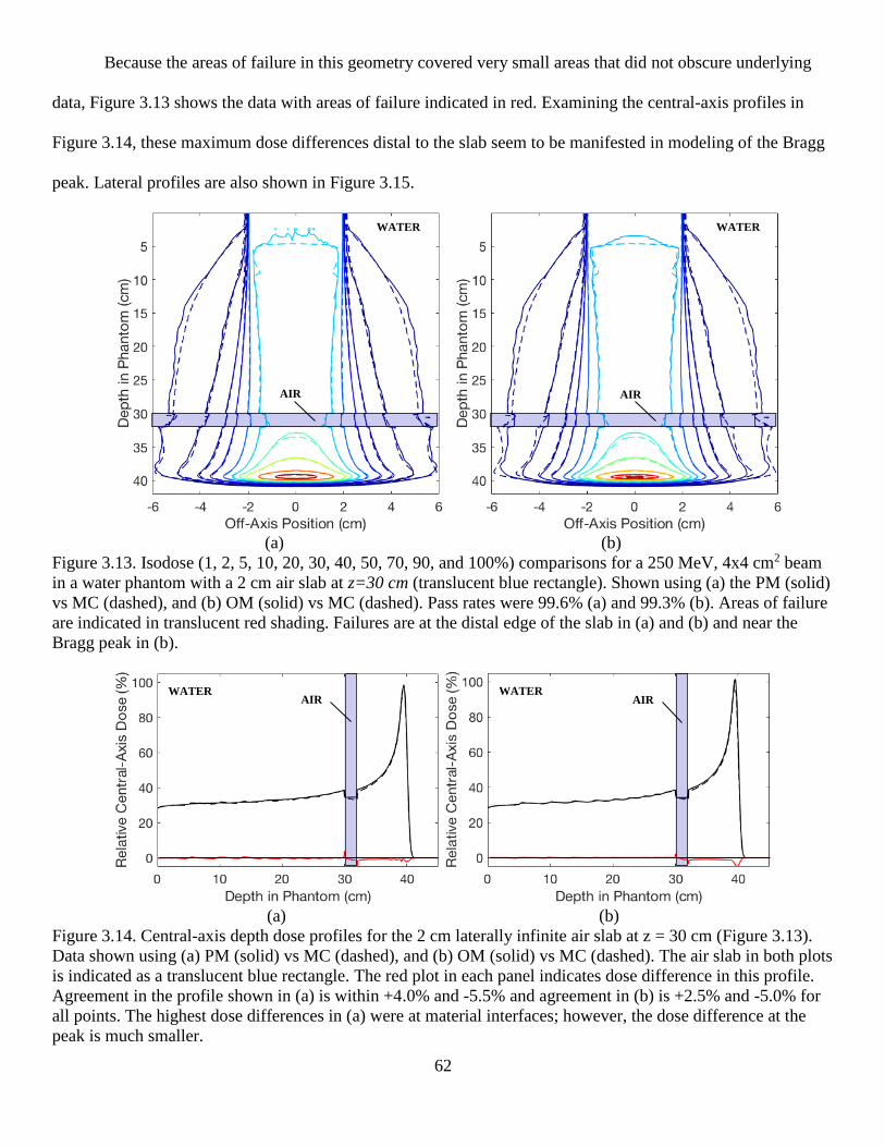
62
Because the areas of failure in this geometry covered very small areas that did not obscure underlying
data, Figure 3.13 shows the data with areas of failure indicated in red. Examining the central-axis profiles in
Figure 3.14, these maximum dose differences distal to the slab seem to be manifested in modeling of the Bragg
peak. Lateral profiles are also shown in Figure 3.15.
(a) (b)
Figure 3.13. Isodose (1, 2, 5, 10, 20, 30, 40, 50, 70, 90, and 100%) comparisons for a 250 MeV, 4x4 cm2 beam
in a water phantom with a 2 cm air slab at z=30 cm (translucent blue rectangle). Shown using (a) the PM (solid)
vs MC (dashed), and (b) OM (solid) vs MC (dashed). Pass rates were 99.6% (a) and 99.3% (b). Areas of failure
are indicated in translucent red shading. Failures are at the distal edge of the slab in (a) and (b) and near the
Bragg peak in (b).
(a) (b)
Figure 3.14. Central-axis depth dose profiles for the 2 cm laterally infinite air slab at z = 30 cm (Figure 3.13).
Data shown using (a) PM (solid) vs MC (dashed), and (b) OM (solid) vs MC (dashed). The air slab in both plots
is indicated as a translucent blue rectangle. The red plot in each panel indicates dose difference in this profile.
Agreement in the profile shown in (a) is within +4.0% and -5.5% and agreement in (b) is +2.5% and -5.0% for
all points. The highest dose differences in (a) were at material interfaces; however, the dose difference at the
peak is much smaller.
WATER
AIR
WATER
AIR
AIR AIR WATER WATER

63
Off-Axis Position (cm) Off-Axis Position (cm)
(a) (b)
Figure 3.15. Lateral dose profiles taken at z = 32.5 cm for the 2 cm laterally infinite air slab at z = 30 cm
(Figure 3.13). Data shown using (a) PM (solid) vs MC (dashed), and (b) OM (solid) vs MC (dashed). The red
plot in each panel indicates dose difference in this profile. Agreement in the profiles shown in (a) and (b) are
within 0.5% to -1.5%.
3.2.2 Thick Slab (4, 5 cm) Results
For a 250 MeV, 4x4 cm2 beam in a water phantom with a 4 cm bone slab, we tested slab depths of z =
10, 20, 30 cm. Both the PM and OM had pass rates of 100.0% (z = 10, 20 cm) and for z = 30 cm, the PM had a
pass rate of 100.0% whereas the OM had a pass rate of 98.6% compared to MC. The percent dose difference
between the PM and MC was within +/-2.5% of the dose difference between the OM vs MC distal to the slabs
(z = 10, 20, 30 cm). A slight shift was noted (1 mm deeper) in the position of the Bragg peak (z = 10, 20 cm)
calculated by the PM in geometries with a 4 cm bone slab compared to MC. However, for a 4 cm bone slab at z
= 30 cm (Figure 3.16), the PM better matched dose at the Bragg peak compared to the OM (by 1.6%). A
summary of all data for thick slabs is in Table 3.3.
To understand the differences between PM and OM in this geometry, Figure 3.17 shows dose difference
maps and histrograms for PM-MC (Figure 3.17(a,c)) and OM-MC (Figure 3.17(b,d)). In Figure 3.17,
differences are evident between the PM and OM both laterally and in depth. The lateral dose differences in the
OM can be attributed to accounting for material-dependence using the one-dimensional effective depth, as this
approach inherently neglects broadening of the secondary protons. In contrast, the PM accounts for the
broadening of secondary particles both by virtue of calculating effective (x, y) coordinates, and by the inverse-
square factor. As a result of the OM neglecting broadening, dose differences are extended over larger areas
WATER WATER

64
compared to the same dose difference values in the PM. For instance, the +2.0% dose difference between OM
and MC (Figure 3.17(b)) are distributed over a wider area compared to the +2.0% dose difference between PM
and MC (Figure 3.17(a)). This is also evident by examining the dose difference bin extending from 1.0% to
2.0% in Figure 3.17(c,d). Additionally, the DTA for the 1.0% isodose line at the distal edge of the bone slab
between the PM and MC decreased by 2.5 mm (z = 10 cm), 2.3 mm (z = 20 cm), or 2.4 mm (z = 30 cm)
compared to the DTA between the OM and MC. The DTA improvement further downstream was 0.7 to 3.1 mm
(z = 10 cm), 0.9 to 2.3 mm (z = 20 cm), or 2.2 to 2.4 mm (z = 30 cm). Thus, secondary proton broadening
impacted dose at far off-axis values as well.
Table 3.3. Results for thick (4 and 5 cm) compact bone and air slabs. Columns in the table indicate the
percentage of points passing our criteria of 3% dose difference or 1 mm distance-to-agreement, and the
improvement (negative values: worsening) in the DTA of the 1% isodose line (calculated by subtracting the
DTA of the OM vs MC from the DTA of the PM vs MC).
Differences between the PM and OM were also observed along the central-axis (Figure 3.18).
Comparing the central-axis plots for the PM and OM relative to MC, it is clear that distal to the slab
heterogeneity, the PM better matches MC than the OM. For instance, at the Bragg peak, the PM had a dose
difference of -0.2%. In contrast, the OM had a dose difference of +1.8% at the Bragg peak. Note that along the
central-axis (x = y = 0), equations (36A-B) do not result in [𝑋𝑒𝑓𝑓]𝑙,𝑚
𝑖,𝑗,𝑘= [𝑌𝑒𝑓𝑓]
𝑙,𝑚
𝑖,𝑗,𝑘= 0, because these effective
coordinates are functions of pencil beam position (𝑥𝑙, 𝑦𝑚). Thus, the PM results in differences along depth,
including the central-axis, compared to the OM. The inverse-square factor in equation 38 is an additional factor

65
that contributes to differences between PM and OM along depth. Lateral profiles for this geometry are shown in
Figure 3.19.
(a) (b)
Figure 3.16. Isodose (1, 2, 5, 10, 20, 30, 40, 50, 70, 90, and 100%) comparisons for a 250 MeV, 4x4 cm2 beam
in a water phantom with a 4 cm compact bone slab at z=30 cm (translucent yellow rectangle). Shown using (a)
the PM (solid) vs MC (dashed), and (b) OM (solid) vs MC (dashed). Pass rates were 100.0% (a) and 98.6% (b).
Areas of failure are indicated in translucent red shading. Failures are near the high dose area in (b).
For a 5 cm bone slab at z = 30 cm, the results were similar to those for the 4 cm bone slab at z = 30 cm.
The pass rates in this geometry were 99.4% (PM) vs 99.0% (OM) (Figure 3.20). We also examined dose
difference maps and histograms (Figure 3.21) below the proximal edge of the slab. The PM was found to
improve the dose difference at the Bragg peak compared to the OM (by ~8%) (Figure 3.22). Additionally, the
DTA of the 1% isodose line at z = 34 cm of the bone slab between the PM and MC improved by 2.9 mm
relative to the DTA between OM and MC. We chose to compare the DTA of the 1% isodose line at z = 34 cm
because the distal edge of the slab is beyond the Bragg peak.
For a 250 MeV, 4x4 cm2 beam in a water phantom with a 4 cm air slab, we tested slab depths of z = 10,
20, 30 cm. Both the PM and the OM had pass rates of 99.6% compared to MC for the slab at z = 10 cm. At z =
20 cm, the pass rate was 99.6% for the PM and 99.0% for the OM. With the air slab at z = 30 cm (Figure 3.23),
the pass rate seen was 98.6% (PM) vs 85.6% (OM). There are significantly higher areas of failure using the OM
for this geometry (4 cm air slab at z = 30 cm) compared to the OM in the 4 cm bone slab geometry. The reason
WATER
BONE
WATER
BONE

66
for this disparity includes the negligible energy loss and scatter across air slabs of a few cm (i.e., 𝑆𝑤𝑎𝑖𝑟 and the
scattering power in air are both very small) whereas the energy loss and scatter across bone slabs are greater
than in water. Thus, in the OM, the halo dose at the distal edge of the air slab is nearly equal to the halo dose at
the proximal edge of the air slab (by virtue of their effective depths being nearly equal), regardless of slab
thickness (for thicknesses up to a few cm). The low scattering power in air slabs causes each pencil beam in the
OM to be transported across the air slab along the central-axis of the pencil beam, and there is loss of side
scatter and charged particle equilibrium. The PM model transports particles over more complex paths because
dose calculated by the PM at the distal edge of the air slab is a function of the relative position between the
central-axis of each pencil beam and the calculation point of interest and is further scaled by the inverse-square
factor.
(a) (b)
(c) (d)
Figure 3.17. Dose difference maps between the PM and MC (a) and between OM and MC (b) for the 4 cm
laterally infinite bone slab at z = 30 cm (Figure 3.16). Note that dose differences in all panels of this figure are
only calculated below the slab. Both dose difference maps use the same color scale, which is indicated in the
bars to the right of (a) and (b). This data is also histogrammed for the PM vs MC (c) and OM vs MC (d).
% D
ose
Diffe
rence (M
C –
OM
)
% D
ose
Diffe
rence (M
C –
PM
)

67
(a) (b)
Figure 3.18. Central-axis depth dose profiles for the 4 cm laterally infinite bone slab at z = 30 cm (Figure 3.16).
Data shown using (a) PM (solid) vs MC (dashed), and (b) OM (solid) vs MC (dashed). The bone slab in both
plots is indicated as a translucent yellow rectangle. The red plot in each panel indicates dose difference in this
profile. Agreement in the profile shown in (a) is within +2.5% and -2.0% and agreement in (b) is +3.5% and -
2.5% for all points.
Off-Axis Position (cm) Off-Axis Position (cm)
(a) (b)
Figure 3.19. Lateral dose profiles taken at z = 34.5 cm for the 4 cm laterally infinite bone slab at z = 30 cm
(Figure 3.16). Data shown using (a) PM (solid) vs MC (dashed), and (b) OM (solid) vs MC (dashed). The red
plot in each panel indicates dose difference in this profile. Agreement in the profiles are within 1.5% to -1.0%
(a) or 3.5% to -0.5% (b).
As with the bone slab, the OM resulted in dose differences extended over larger areas compared to
equivalent dose differences in the PM (Figure 3.24). However, the dose difference for the OM in the distal slab
area (Figure 3.24(b)) is systematically underestimated. For instance, the -2.0% to 0.0% dose difference between
the PM and MC (Figure 3.24(a)) in this area increased to a consistent -4.0% to -5.0% dose difference between
the OM and MC (Figure 3.24(b)). This underesimation is also seen in Figure 3.25(b). Note that in the central-
axis profile of Figure 3.25(a), the PM significantly improves dosimetric agreement distal to the slab.
WATER BONE WATER BONE
WATER WATER

68
(a) (b)
Figure 3.20. Isodose (1, 2, 5, 10, 20, 30, 40, 50, 70, 90, and 100%) comparisons for a 250 MeV, 4x4 cm2 beam
in a water phantom with a 5 cm compact bone slab at z=30 cm (translucent yellow rectangle). Shown using (a)
the PM (solid) vs MC (dashed), and (b) OM (solid) vs MC (dashed). Pass rates were 99.4% (a) and 99.0% (b).
Areas of failure are indicated in translucent red shading. Failures were near the distal edge of the Bragg peak in
(a) and at the Bragg peak in (b).
The DTA for the 1% isodose line at the distal edge of the air slab between the PM and OM decreased by
1.9 mm (z = 10 cm), 2.2 mm (z = 20 cm), and 6.7 mm (z = 30 cm) compared to the DTA between the OM and
MC. Beyond the distal edge of the slab, the DTA of the 1% isodose line between the PM and MC was
overestimated by 2.4 to 8.5 mm (z = 10 cm) compared to the DTA between the OM and MC. For the slab at z =
20 cm, the DTA of the 1% isodose line between the PM and MC beyond the distal edge of the slab ranged from
values that overestimated the DTA by 2.8 mm to improvements of 3.4 mm compared to the DTA between the
OM and MC. For the slab at z = 30 cm, the DTA of the 1% isodose line between the PM and MC beyond the
distal edge of the slab improved by 2.4 to 7.6 mm (z = 30 cm) compared to the DTA between the OM and MC.
Thus, the broadening of secondary protons accounted for in the PM impacted dose at far off-axis values.
For a 5 cm air slab at z = 30 cm, the results were similar to those for the 4 cm air slab at z = 30 cm. The
pass-rates in this geometry were 94.6% for the PM and 78.5% for the OM (Figure 3.26). Dose difference maps
and histograms are shown in Figure 3.27. Maximum dose differences were at the Bragg peak (Figure 3.28).
Lateral profiles are shown in Figure 3.29.
WATER
BONE
WATER
BONE

69
(a) (b)
(c) (d)
Figure 3.21. Dose difference maps between the PM and MC (a) and between OM and MC (b) for the 5 cm
laterally infinite bone slab at z = 30 cm (Figure 3.20). Note that dose differences in all panels of this figure are
only calculated below the slab. Both dose difference maps use the same color scale, which is indicated in the
bars to the right of (a) and (b). This data is also histogrammed for the PM vs MC (c) and OM vs MC (d).
The DTA of the 1% isodose line at the distal edge of the bone slab between the PM and MC improved
by 6.2 mm relative to the DTA between OM and MC. Beyond the slab, the DTA improvement of the 1%
isodose lines was 2.2 to 6.0 mm.
3.3 Results for Specific Aim 3
For all of the results that follow for Specific Aim 3, all calculation approaches (PM, OM, and MC)
included both primary and secondary dose (i.e., total dose). The results include calculations in a 2 cm x 2 cm
checkerboard phantom, a prostate phantom, and a paranasal phantom. All geometries were tested using
monoenergetic beams, and the checkerboard and prostate phantoms additionally tested a SOBP beam. A
summary for all the data for Specific Aim 3 is in Table 3.4.
% D
ose
Diffe
rence (M
C –
OM
)
% D
ose
Diffe
rence (M
C –
PM
)

70
(a) (b)
Figure 3.22. Central-axis depth dose profiles for the 5 cm laterally infinite bone slab at z = 30 cm (Figure 3.20).
Data shown using (a) PM (solid) vs MC (dashed), and (b) OM (solid) vs MC (dashed). The bone slab in both
plots is indicated as a translucent yellow rectangle. The red plot in each panel indicates dose difference in this
profile. Agreement in the profile shown in (a) is within +2.5% and -0.5% and agreement in (b) is +10.5% and -
1.0% for all points.
3.3.1 Checkerboard Phantom (2 cm x 2 cm)
For a 250 MeV, 4x4 cm2 beam in our 2 cm x 2 cm checkerboard phantom, pass rates were 99.0% (PM)
vs 84.0% (OM) (Figure 3.31). Additionally, dose difference maps and histograms are shown in Figure 3.32. To
better evaluate how well the PM improved compared to the limitations imposed by the CAXSIS approximation
in the OM, we observed depth dose profiles (x = +/- 1 cm) and a lateral dose profile just below the checkered
slab configuration (z = 34.05 cm). Comparing the depth dose profiles at x = -1 cm for both models (Figure
3.33), the PM is shown to agree within +3.0% and -4.5% relative to MC, whereas the OM agrees within +3.0%
to -10.5% of MC; furthermore, the -10.5% percent difference seen with the OM is at the peak. At x = 1 cm
(Figure 3.33), the depth profile shows a similar result: the PM percent differences range from +4.0% to -3.0%
and the OM ranges from +2.0% to -12.5%, again with the -12.5% at the peak. These differences are mostly due
to the CAXSIS approximation applied to the OM whereas the PM is not dependent on this approximation. To a
lesser extent, these differences are impacted by the differences in material-dependence of the nuclear halo
between the PM and OM.
WATER BONE WATER BONE

71
(a) (b)
(c) (d)
Figure 3.23. Isodose (1, 2, 5, 10, 20, 30, 40, 50, 70, 90, and 100%) comparisons for a 250 MeV, 4x4 cm2 beam
in a water phantom with a 4 cm air slab at z=30 cm (translucent blue rectangle). Shown using (a,c) the PM
(solid) vs MC (dashed), and (b,d) OM (solid) vs MC (dashed). Pass rates were 98.6% (a,c) and 85.6% (b,d).
Areas of failure are indicated in translucent red shading.
From the lateral profile comparisons (Figure 3.34), it can be seen that the PM accounted for the interface
between bone and air heterogeneities whereas the OM smoothed out the dose at the interfaces. The percent
difference for this profile in the PM was within +5.5% to -2.0% whereas the OM was within +3.5% to -5.0%.
The DTA of the 1% isodose line between the PM and MC in the checkered slabs improved by 0.5 mm, and
further downstream improved by 0.84 to 0.85 mm relative to the DTA between OM and MC.
WATER
AIR
WATER
AIR
WATER
AIR
WATER
AIR
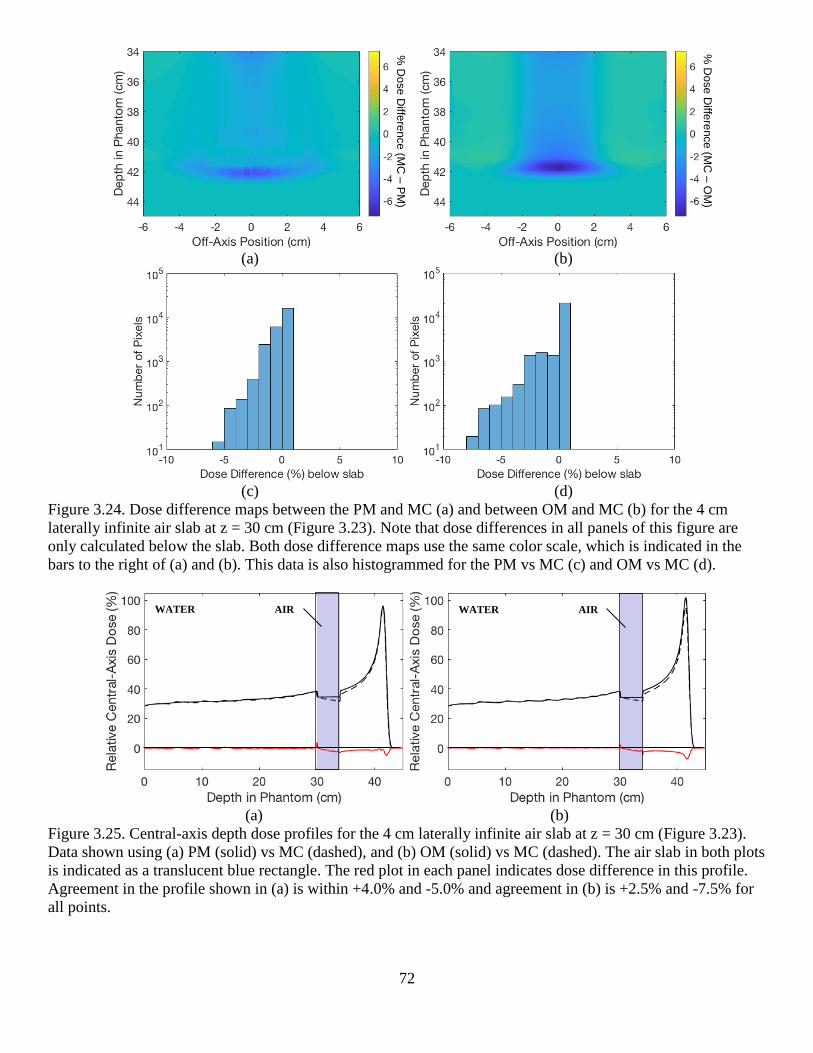
72
(a) (b)
(c) (d)
Figure 3.24. Dose difference maps between the PM and MC (a) and between OM and MC (b) for the 4 cm
laterally infinite air slab at z = 30 cm (Figure 3.23). Note that dose differences in all panels of this figure are
only calculated below the slab. Both dose difference maps use the same color scale, which is indicated in the
bars to the right of (a) and (b). This data is also histogrammed for the PM vs MC (c) and OM vs MC (d).
(a) (b)
Figure 3.25. Central-axis depth dose profiles for the 4 cm laterally infinite air slab at z = 30 cm (Figure 3.23).
Data shown using (a) PM (solid) vs MC (dashed), and (b) OM (solid) vs MC (dashed). The air slab in both plots
is indicated as a translucent blue rectangle. The red plot in each panel indicates dose difference in this profile.
Agreement in the profile shown in (a) is within +4.0% and -5.0% and agreement in (b) is +2.5% and -7.5% for
all points.
% D
ose
Diffe
rence (M
C –
OM
)
% D
ose
Diffe
rence (M
C –
PM
)
WATER AIR WATER AIR
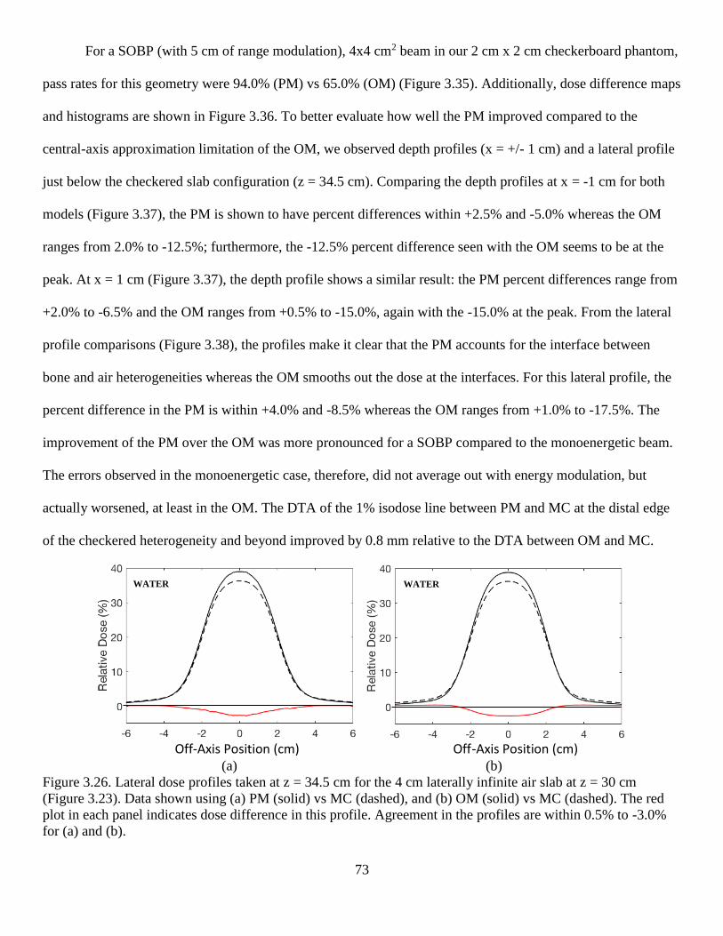
73
For a SOBP (with 5 cm of range modulation), 4x4 cm2 beam in our 2 cm x 2 cm checkerboard phantom,
pass rates for this geometry were 94.0% (PM) vs 65.0% (OM) (Figure 3.35). Additionally, dose difference maps
and histograms are shown in Figure 3.36. To better evaluate how well the PM improved compared to the
central-axis approximation limitation of the OM, we observed depth profiles (x = +/- 1 cm) and a lateral profile
just below the checkered slab configuration (z = 34.5 cm). Comparing the depth profiles at x = -1 cm for both
models (Figure 3.37), the PM is shown to have percent differences within +2.5% and -5.0% whereas the OM
ranges from 2.0% to -12.5%; furthermore, the -12.5% percent difference seen with the OM seems to be at the
peak. At x = 1 cm (Figure 3.37), the depth profile shows a similar result: the PM percent differences range from
+2.0% to -6.5% and the OM ranges from +0.5% to -15.0%, again with the -15.0% at the peak. From the lateral
profile comparisons (Figure 3.38), the profiles make it clear that the PM accounts for the interface between
bone and air heterogeneities whereas the OM smooths out the dose at the interfaces. For this lateral profile, the
percent difference in the PM is within +4.0% and -8.5% whereas the OM ranges from +1.0% to -17.5%. The
improvement of the PM over the OM was more pronounced for a SOBP compared to the monoenergetic beam.
The errors observed in the monoenergetic case, therefore, did not average out with energy modulation, but
actually worsened, at least in the OM. The DTA of the 1% isodose line between PM and MC at the distal edge
of the checkered heterogeneity and beyond improved by 0.8 mm relative to the DTA between OM and MC.
Off-Axis Position (cm) Off-Axis Position (cm)
(a) (b)
Figure 3.26. Lateral dose profiles taken at z = 34.5 cm for the 4 cm laterally infinite air slab at z = 30 cm
(Figure 3.23). Data shown using (a) PM (solid) vs MC (dashed), and (b) OM (solid) vs MC (dashed). The red
plot in each panel indicates dose difference in this profile. Agreement in the profiles are within 0.5% to -3.0%
for (a) and (b).
WATER WATER
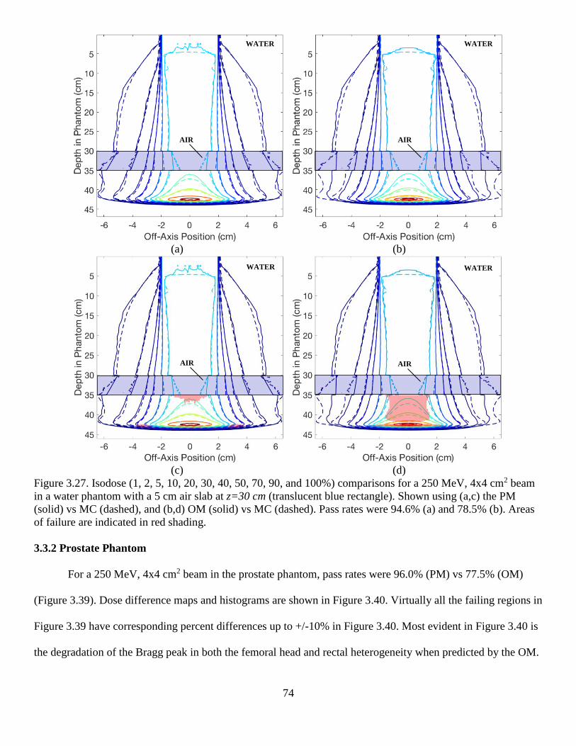
74
(a) (b)
(c) (d)
Figure 3.27. Isodose (1, 2, 5, 10, 20, 30, 40, 50, 70, 90, and 100%) comparisons for a 250 MeV, 4x4 cm2 beam
in a water phantom with a 5 cm air slab at z=30 cm (translucent blue rectangle). Shown using (a,c) the PM
(solid) vs MC (dashed), and (b,d) OM (solid) vs MC (dashed). Pass rates were 94.6% (a) and 78.5% (b). Areas
of failure are indicated in red shading.
3.3.2 Prostate Phantom
For a 250 MeV, 4x4 cm2 beam in the prostate phantom, pass rates were 96.0% (PM) vs 77.5% (OM)
(Figure 3.39). Dose difference maps and histograms are shown in Figure 3.40. Virtually all the failing regions in
Figure 3.39 have corresponding percent differences up to +/-10% in Figure 3.40. Most evident in Figure 3.40 is
the degradation of the Bragg peak in both the femoral head and rectal heterogeneity when predicted by the OM.
WATER
AIR
WATER
AIR
WATER
AIR
WATER
AIR
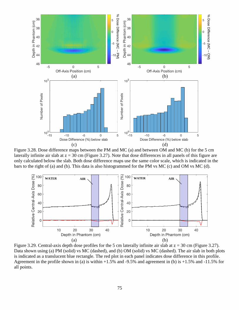
75
(a) (b)
(c) (d)
Figure 3.28. Dose difference maps between the PM and MC (a) and between OM and MC (b) for the 5 cm
laterally infinite air slab at z = 30 cm (Figure 3.27). Note that dose differences in all panels of this figure are
only calculated below the slab. Both dose difference maps use the same color scale, which is indicated in the
bars to the right of (a) and (b). This data is also histogrammed for the PM vs MC (c) and OM vs MC (d).
(a) (b)
Figure 3.29. Central-axis depth dose profiles for the 5 cm laterally infinite air slab at z = 30 cm (Figure 3.27).
Data shown using (a) PM (solid) vs MC (dashed), and (b) OM (solid) vs MC (dashed). The air slab in both plots
is indicated as a translucent blue rectangle. The red plot in each panel indicates dose difference in this profile.
Agreement in the profile shown in (a) is within +1.5% and -9.5% and agreement in (b) is +1.5% and -11.5% for
all points.
% D
ose
Diffe
rence (M
C –
OM
)
% D
ose
Diffe
rence (M
C –
PM
)
WATER AIR WATER AIR

76
Off-Axis Position (cm) Off-Axis Position (cm)
(a) (b)
Figure 3.30. Lateral dose profiles taken at z = 35.05 cm for the 5 cm laterally infinite air slab at z = 30 cm
(Figure 3.27). Data shown using (a) PM (solid) vs MC (dashed), and (b) OM (solid) vs MC (dashed). The red
plot in each panel indicates dose difference in this profile. Agreement in the profiles are within 0.5% to -3.5%
for (a) and (b).
Table 3.4. Results for evaluation geometries in Specific Aim 3. Columns in the table indicate the percentage of
points passing our criteria of 3% or 1 mm, and the improvement (negative values: worsening) in the DTA of the
1% isodose line (calculated by subtracting the DTA of the OM vs MC from the DTA of the PM vs MC).
To better evaluate how well the PM improved compared to the central-axis approximation limitation of
the OM, we observed a central-axis profile and a lateral profile just below the rectal heterogeneity (z = 30 cm).
Comparing the central-axis profiles for both models (Figure 3.41), the PM is shown to have percent differences
within +1.5% and -5.0% whereas the OM ranges from +9.5% to -15.5%; furthermore, there is significant
degradation in the Bragg peak by the OM. From the lateral profile comparisons (Figure 3.42), it is clear that the
PM accounts for the interface between the air heterogeneity of the rectum and water, whereas the OM smooths
out the dose at the interfaces. For this lateral profile, the percent difference in the PM is within +1.0% and -
0.5% whereas the OM ranges from +1.0% to -1.5%.
Additionally, the DTA of the 1% isodose line between the PM and MC distal to both the femoral head
and rectum heterogeneity (z = 30.05 cm) improved by 2.1 mm relative to the DTA between OM and MC.
Further downstream, the DTA of the 1% isodose line improved between 0.9 mm to 2.7 mm.
WATER WATER
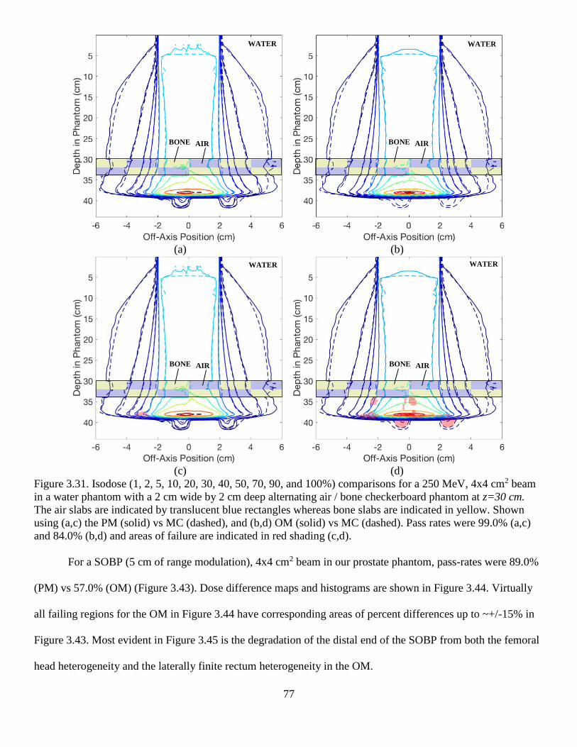
77
(a) (b)
(c) (d)
Figure 3.31. Isodose (1, 2, 5, 10, 20, 30, 40, 50, 70, 90, and 100%) comparisons for a 250 MeV, 4x4 cm2 beam
in a water phantom with a 2 cm wide by 2 cm deep alternating air / bone checkerboard phantom at z=30 cm.
The air slabs are indicated by translucent blue rectangles whereas bone slabs are indicated in yellow. Shown
using (a,c) the PM (solid) vs MC (dashed), and (b,d) OM (solid) vs MC (dashed). Pass rates were 99.0% (a,c)
and 84.0% (b,d) and areas of failure are indicated in red shading (c,d).
For a SOBP (5 cm of range modulation), 4x4 cm2 beam in our prostate phantom, pass-rates were 89.0%
(PM) vs 57.0% (OM) (Figure 3.43). Dose difference maps and histograms are shown in Figure 3.44. Virtually
all failing regions for the OM in Figure 3.44 have corresponding areas of percent differences up to ~+/-15% in
Figure 3.43. Most evident in Figure 3.45 is the degradation of the distal end of the SOBP from both the femoral
head heterogeneity and the laterally finite rectum heterogeneity in the OM.
WATER
AIR BONE
WATER
AIR BONE
WATER
AIR BONE
WATER
AIR BONE

78
(a) (b)
(c) (d)
Figure 3.32. Dose difference maps between the PM and MC (a) and between OM and MC (b) for the
checkerboard phantom (Figure 3.31). Note that dose differences in all panels of this figure are only calculated
below the slab. Both dose difference maps use the same color scale, which is indicated in the bars to the right of
(a) and (b). This data is also histogrammed for the PM vs MC (c) and OM vs MC (d).
To better evaluate how well the PM improved compared to the central-axis approximation limitation of
the OM, we observed a central-axis profile and a lateral profile below the rectal heterogeneity and below the
distal 90% line of the SOBP (z = 31.75 cm). Comparing the central-axis profiles for both models (Figure 3.45),
the PM is shown to have percent differences within +1.5% and -6.0% whereas the OM ranges from +2.5% to -
28%; furthermore, there is degradation of the Bragg peak as calculated by the OM. From the lateral profile
comparisons (Figure 3.46), it is clear that the PM accounts for the interface between the rectal edge and water,
whereas the OM smooths out the dose at interfaces. For the lateral profile, the percent difference in the PM is
within +3.5% and -5.5% whereas the OM ranges from +1.0% to -5.0%. Most of the differences between the PM
and OM are due to limitations imposed by the CAXSIS approximation and a lack of material dependence for
the nuclear halo term.
% D
ose
Diffe
rence (M
C –
OM
)
% D
ose
Diffe
rence (M
C –
PM
)
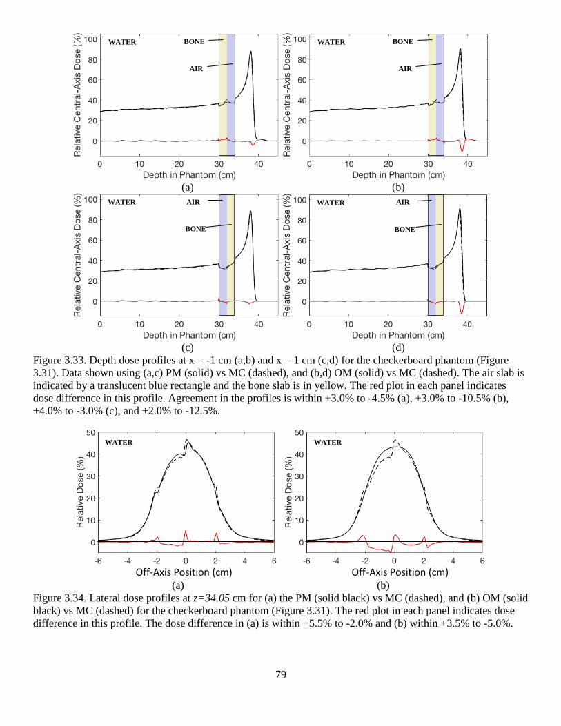
79
(a) (b)
(c) (d)
Figure 3.33. Depth dose profiles at x = -1 cm (a,b) and x = 1 cm (c,d) for the checkerboard phantom (Figure
3.31). Data shown using (a,c) PM (solid) vs MC (dashed), and (b,d) OM (solid) vs MC (dashed). The air slab is
indicated by a translucent blue rectangle and the bone slab is in yellow. The red plot in each panel indicates
dose difference in this profile. Agreement in the profiles is within +3.0% to -4.5% (a), +3.0% to -10.5% (b),
+4.0% to -3.0% (c), and +2.0% to -12.5%.
Off-Axis Position (cm) Off-Axis Position (cm)
(a) (b)
Figure 3.34. Lateral dose profiles at z=34.05 cm for (a) the PM (solid black) vs MC (dashed), and (b) OM (solid
black) vs MC (dashed) for the checkerboard phantom (Figure 3.31). The red plot in each panel indicates dose
difference in this profile. The dose difference in (a) is within +5.5% to -2.0% and (b) within +3.5% to -5.0%.
WATER
AIR
BONE WATER
AIR
BONE
WATER
BONE
AIR WATER
BONE
AIR
WATER WATER

80
Additionally, the results indicated that the DTA of the 1% isodose line between the PM and MC distal to
both the femoral head and rectum heterogeneity (z = 30.05 cm) improved by 2.9 mm relative to the DTA
between OM and MC. Further downstream, the DTA of the 1% isodose line between the PM and MC was
overestimated by up to 1.3 mm but reached improvements up to 7.2 mm.
(a) (b)
(c) (d)
Figure 3.35. Isodose (1, 2, 5, 10, 20, 30, 40, 50, 70, 90, and 100%) comparisons for a SOBP (216-236 MeV in 2 MeV
steps (5 cm of range modulation)), 4x4 cm2 beam in a water phantom with a 2 cm wide by 2 cm deep alternating air /
bone checker phantom at z=30 cm. The air slabs are indicated by translucent blue rectangles whereas bone slabs are
indicated in yellow. Shown using (a,c) the PM (solid) vs MC (dashed), and (b,d) OM (solid) vs MC (dashed). Pass rates
were 94.0% (a,c) and 65.0% (b,d) and areas of failure are indicated in red shading (c,d).
WATER
AIR BONE
WATER
AIR BONE
WATER
AIR BONE
WATER
AIR BONE
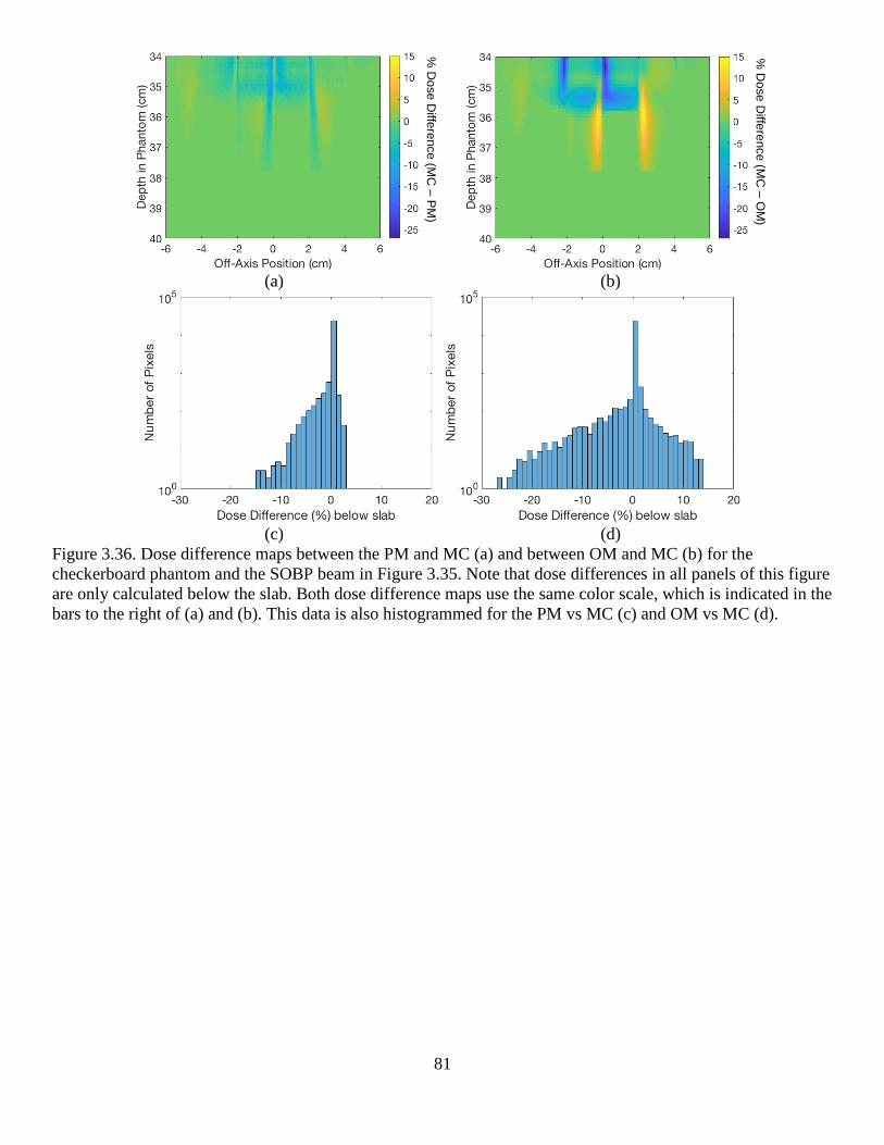
81
(a) (b)
(c) (d)
Figure 3.36. Dose difference maps between the PM and MC (a) and between OM and MC (b) for the
checkerboard phantom and the SOBP beam in Figure 3.35. Note that dose differences in all panels of this figure
are only calculated below the slab. Both dose difference maps use the same color scale, which is indicated in the
bars to the right of (a) and (b). This data is also histogrammed for the PM vs MC (c) and OM vs MC (d).
% D
ose
Diffe
rence (M
C –
OM
)
% D
ose
Diffe
rence (M
C –
PM
)

82
(a) (b)
(c) (d)
Figure 3.37. Depth dose profiles at x = -1 cm (a,b) and x = 1 cm (c,d) for the checkerboard phantom and the
SOBP beam in Figure 3.35. Data shown using (a,c) PM (solid) vs MC (dashed), and (b,d) OM (solid) vs MC
(dashed). The air slab is indicated by a translucent blue rectangle and the bone slab is in yellow. The red plot in
each panel indicates dose difference in this profile. Agreement in the profiles is within +2.5% to -5.0% (a),
+2.0% to -12.5% (b), +2.0% to -6.5% (c), and +0.5% to -15.0% (d).
Off-Axis Position (cm) Off-Axis Position (cm)
(a) (b)
Figure 3.38. Lateral dose profiles at z=34.5 cm for (a) the PM (solid black) vs MC (dashed), and (b) OM (solid
black) vs MC (dashed) for the geometry in Figure 3.35. The red plot in each panel indicates dose difference in
this profile. The dose difference in (a) is within +4.0% to -8.5% and (b) within +1.0% to -17.5%.
WATER
BONE
AIR WATER
BONE
AIR
WATER
AIR
BONE WATER
AIR
BONE
WATER WATER
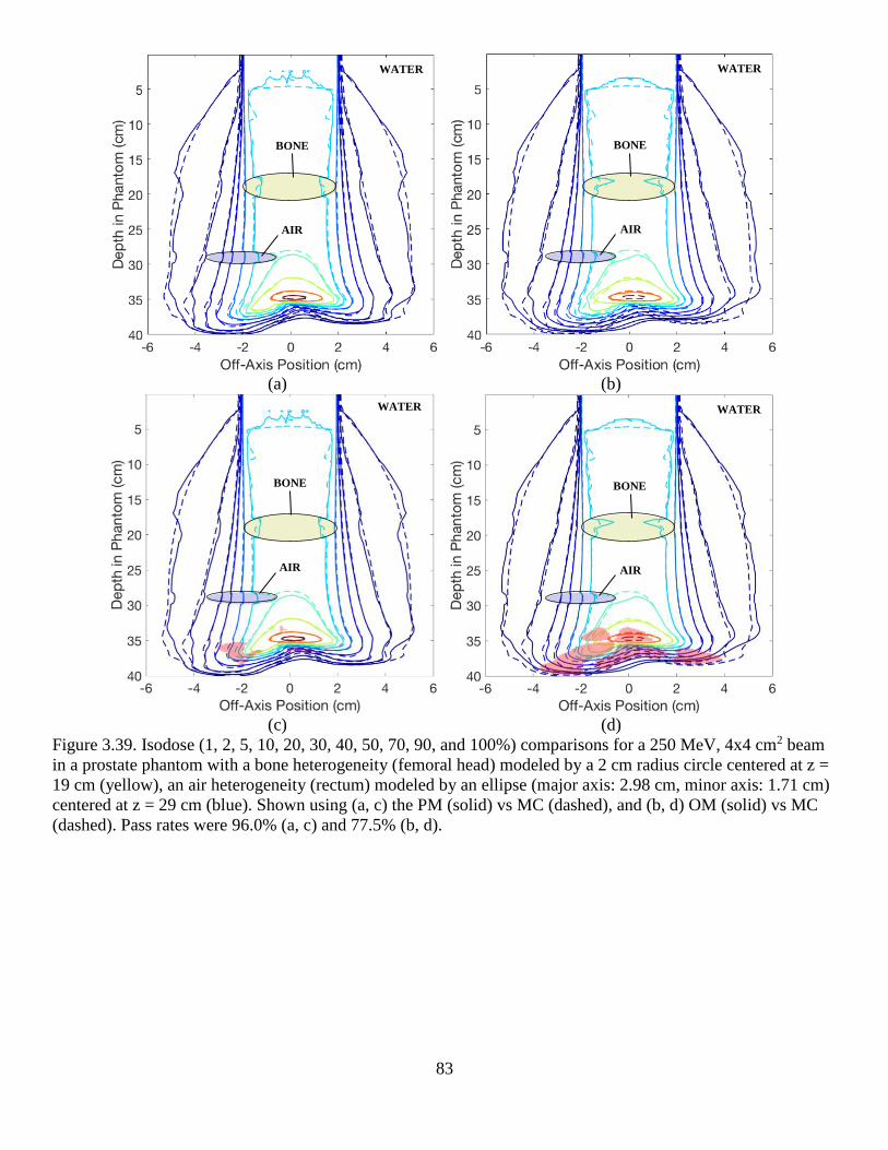
83
(a) (b)
(c) (d)
Figure 3.39. Isodose (1, 2, 5, 10, 20, 30, 40, 50, 70, 90, and 100%) comparisons for a 250 MeV, 4x4 cm2 beam
in a prostate phantom with a bone heterogeneity (femoral head) modeled by a 2 cm radius circle centered at z =
19 cm (yellow), an air heterogeneity (rectum) modeled by an ellipse (major axis: 2.98 cm, minor axis: 1.71 cm)
centered at z = 29 cm (blue). Shown using (a, c) the PM (solid) vs MC (dashed), and (b, d) OM (solid) vs MC
(dashed). Pass rates were 96.0% (a, c) and 77.5% (b, d).
WATER
AIR
BONE
WATER
AIR
BONE
WATER
AIR
BONE
WATER
AIR
BONE

84
(a) (b)
(c) (d)
Figure 3.40. Dose difference maps between the PM and MC (a) and between OM and MC (b) for the prostate
phantom (Figure 3.39). Note that dose differences in all panels of this figure are only calculated below the slab.
Both dose difference maps use the same color scale, which is indicated in the bars to the right of (a) and (b).
This data is also histogrammed for the PM vs MC (c) and OM vs MC (d).
(a) (b)
Figure 3.41. Central-axis depth dose profiles for the prostate phantom (Figure 3.39). Data shown using (a) PM
(solid) vs MC (dashed), and (b) OM (solid) vs MC (dashed). The femoral head heterogeneity in both plots is
indicated as a translucent yellow. The red plot in each panel indicates dose difference in this profile. Agreement
in the profile shown in (a) is within +1.5% and -5.0% and agreement in (b) is +9.5% and -15.5% for all points.
% D
ose
Diffe
rence (M
C –
OM
)
% D
ose
Diffe
rence (M
C –
PM
)
WATER BONE WATER BONE
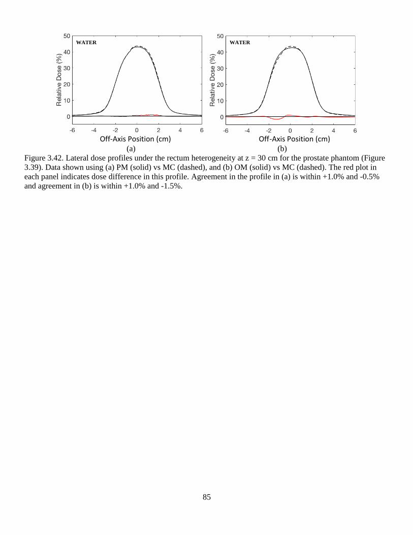
85
Off-Axis Position (cm) Off-Axis Position (cm)
(a) (b)
Figure 3.42. Lateral dose profiles under the rectum heterogeneity at z = 30 cm for the prostate phantom (Figure
3.39). Data shown using (a) PM (solid) vs MC (dashed), and (b) OM (solid) vs MC (dashed). The red plot in
each panel indicates dose difference in this profile. Agreement in the profile in (a) is within +1.0% and -0.5%
and agreement in (b) is within +1.0% and -1.5%.
WATER WATER

86
(a) (b)
(c) (d)
Figure 3.43. Isodose (1, 2, 5, 10, 20, 30, 40, 50, 70, 90, and 100%) comparisons for a SOBP (216-236 MeV) in
2 MeV steps (5 cm of range modulation)), 4x4 cm2 beam in a prostate phantom with a bone heterogeneity
(femoral head) modeled by a 2 cm radius circle centered at z = 19 cm (yellow), an air heterogeneity (rectum)
modeled by an ellipse (major axis: 2.98 cm, minor axis: 1.71 cm) centered at z = 29 cm (blue). Shown using
(a,c) PM (solid) vs MC (dashed), and (b,d) OM (solid) vs MC (dashed). Pass rates were 89.0% (a,c) and 57.0%
(b,d).
WATER
AIR
BONE
WATER
AIR
BONE
WATER
AIR
BONE
WATER
AIR
BONE
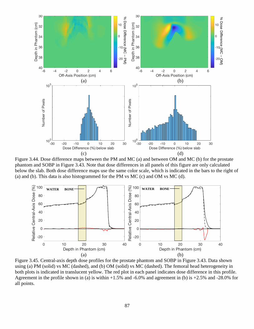
87
(a) (b)
(c) (d)
Figure 3.44. Dose difference maps between the PM and MC (a) and between OM and MC (b) for the prostate
phantom and SOBP in Figure 3.43. Note that dose differences in all panels of this figure are only calculated
below the slab. Both dose difference maps use the same color scale, which is indicated in the bars to the right of
(a) and (b). This data is also histogrammed for the PM vs MC (c) and OM vs MC (d).
(a) (b)
Figure 3.45. Central-axis depth dose profiles for the prostate phantom and SOBP in Figure 3.43. Data shown
using (a) PM (solid) vs MC (dashed), and (b) OM (solid) vs MC (dashed). The femoral head heterogeneity in
both plots is indicated in translucent yellow. The red plot in each panel indicates dose difference in this profile.
Agreement in the profile shown in (a) is within +1.5% and -6.0% and agreement in (b) is +2.5% and -28.0% for
all points.
% D
ose
Diffe
rence (M
C –
OM
)
% D
ose
Diffe
rence (M
C –
PM
)
WATER BONE WATER BONE

88
Off-Axis Position (cm) Off-Axis Position (cm)
(a) (b)
Figure 3.46. Lateral dose profiles under the rectum heterogeneity at z = 31.75 cm for the prostate phantom and
SOBP in Figure 3.43. Data shown using (a) PM (solid) vs MC (dashed), and (b) OM (solid) vs MC (dashed).
The red plot in each panel indicates dose difference in this profile. Agreement in the profile in (a) is within
+3.5% and -5.5% and agreement in (b) is within +1.0% and -5.0%.
WATER WATER
89
CHAPTER 4. DISCUSSION
In this work, we developed a stochastic dose calculation model that eliminated the CAXSIS approximation in
calculating primary dose (Specific Aim 1) and added material-dependence to the calculation of the nuclear halo
of secondary protons (Specific Aim 2).
Removing the CAXSIS approximation in our primary transport model was shown to significantly reduce
dose difference below laterally finite heterogeneities compared to the previous model (Chapman et al 2017),
and robust material-dependence in the nuclear halo resulted in significant improvements in the dose difference
below laterally infinite heterogeneities compared to the previous one-dimensional implementation. Overall,
resulting dose differences and distances-to-agreement were shown to improve agreement with Monte Carlo data
in a wide variety of geometries (Specific Aims 1, 2, and 3) compared to Chapman et al (2017).
Our study provided new insight into the basic physics of material-dependence in the nuclear halo.
Transport of secondary particles through heterogeneities was shown to be more accurately modeled by the
material dependent nuclear halo in this work compared to the original, one-dimensional implementation. This
improvement resulted in decreased dose differences using the present model compared to the original model.
Our results strongly suggest that robust material dependence in the nuclear halo will be important in
heterogeneous patient anatomy. For instance, a rectal heterogeneity in a prostate treatment plan for a large
patient could have a diameter on the order of 4-5 cm, which our results indicate would cause significant dose
errors beyond the heterogeneity using the original model.
In our previous study (Chapman et al 2017), we reported large dose differences between the PBA and
Monte Carlo calculations in volumes downstream of thick heterogeneities, particularly air slabs.
Correspondingly, the improvement of the present model relative to the PBA was most significant following
large air heterogeneities.
Dose differences calculated by the present geometry indicated higher accuracy compared to the
Tourovsky et al (2005) model. For instance, in all geometries, 88.0%, 97.0%, and 99.7% of points calculated by
the present model were within +/-2%, +/-5%, and +/-10%, respectively. In contrast, the Tourovsky et al (2005)
90
model resulted in 69.0%, 93.0%, and 98.0% of points within +/-2%, +/-5%, and +/-10%, respectively. While the
geometries tested in this work were not completely analogous to those of Tourovsky (their evaluations were in
patient data), both models were designed primarily to eliminate the central-axis semi-infinite slab
approximation and were tested in geometries challenging for this approximation. We attribute that additional
accuracy achieved by our model to the improvements we made in the material-dependence added to the nuclear
halo and the reduced step size toward the end of range.
In the most recent publication on the fast dose calculator (FDC) by Yepes et al (2018), over 525 patient
cases were examined. It was shown that the Eclipse TPS, based on a pencil beam algorithm, over-estimated the
maximum dose by 10-15% in some patient cases compared to the FDC. These results are consistent with our
observations in the patient-like phantoms that we studied, especially those using a SOBP (10-20%).
Jia et al (2012) reported that greater than 98.7% of the points in all geometries were within 2% or 2 mm
(above the 10% dose level), except for geometries with low-density air regions. Agreement below the 10%
isodose level was not reported. Our work showed a distinct improvement in the distance-to-agreement of the
1% isodose line below heterogeneities. The nuclear halo implementation in Fippel and Soukup (2004) and Jia et
al (2012) was limited to water.
Souris et al 2016 stated that their model was within 2% or 1 mm of GEANT 4, which is higher accuracy
than we were able to achieve (3% or 1 mm compared to MCNPX). However, Souris et al 2016 relied on a
complex physical model, including stochastic transport for secondary protons characterizing the nuclear halo,
which necessitated a multi-core implementation to achieve reasonable calculation times. Though our model did
not achieve the levels of accuracy stated in Souris et al (2016), we think that our model strikes a good balance
between speed and accuracy without requiring a multi-core or GPU implementation.
The model in this work has some limitations. Evaluations were performed in simple geometries, which
was intentional to characterize the underlying transport physics. It could be argued that our evaluations were not
tested in clinically realistic geometries, like voxellized patient anatomy. However, this is not a major limitation
because in the example geometries that we studied, we carefully selected them to be severe tests. Because our

91
evaluations were inherently more sensitive than what would be encountered in patient geometry, we expect that
dose errors from our model in patient anatomy would be smaller than what was observed in the geometries in
this work. Thus, limiting our study to simple geometries was also a strength.
Many of the limitations in the present model could be resolved by ensuring agreement between stopping
power calculations in the present model and MC and incorporating a material-dependent range straggling
correction. Addition of both of these features to the model in this work would improve the dose differences
even further, especially in areas distal to the depth of maximum dose. Another significant addition that should
be made is including changes in secondary proton production as a function of material and energy. The present
model neglected this effect; however, MCNPX output files indicated changes in the number of secondary
particles produced due to non-elastic nuclear interactions in heterogeneities compared to water. In addition to
the suggested modeling improvements, future work in this area should perform evaluations in patient data.
Finally, one remaining topic of discussion is the calculation time of the present model compared to
general purpose Monte Carlo. This dissertation has largely been focused on presenting the improved accuracy
of this model, but that presentation is predicated on calculating dose in a shorter timeframe than general-
purpose Monte Carlo calculations. Using our 2.3GHz Intel Core i5 based system, a monoenergetic 250 MeV,
4x4 cm2 field calculated in water for the model developed in this work required 5.6 minutes, or 0.09 processor-
hours. In contrast, MCNPX simulations used 256 parallel 2.6 GHz 8-Core Sandy Bridge Xeon 64-bit processors
to calculate this same geometry in about 42.3 minutes, or 180.5 processor-hours. Thus, our model achieved
significant speedup compared with MCNPX. Calculation times for our dose model in other geometries varied
mainly with the initial number of protons and the resolution of the dose grid.
92
CHAPTER 5. CONCLUSIONS
In this work, we have detailed approaches to improving both the primary and nuclear halo components of a
proton dose model, with the aims of reducing the two sources of errors observed in Chapman et al (2017): (1)
the central-axis semi-infinite slab approximation; and, (2) the lack of material dependence in the nuclear halo
model. In Specific Aim 1, we introduced a primary dose model that was stochastically based to reduce errors
due to the central-axis approximation. The simplified approach to predict fluence loss of primary protons and
particle transport enabled our model to reduce calculation times without sacrificing much accuracy relative to a
general-purpose Monte Carlo code. In Specific Aim 2, we presented an improved energy loss calculation
method that allowed transformation of the calculation geometry to an equivalent water phantom in three
dimensions. This method allowed transformation of the original nuclear halo equation (Chapman et al 2017) for
any desired calculation geometry. In Specific Aim 3, we compared our improved primary and nuclear halo dose
model with Monte Carlo simulations from MCNPX in three patient-like phantoms. Contrasting our improved
primary and nuclear halo dose model against the PBA (Chapman et al 2017) showed the amount of
improvement our new model achieved.
The hypothesis of this work was found to be false: the present model did not result in 100% of points
passing our 3% or 1 mm criteria for each geometry that we tested. However, we did see improved pass rates for
the present model compared to the PBA in virtually every case. Furthermore, dose differences between the
present model and MC distal to heterogeneities sometimes exceeded 5% (laterally finite) and 3% (laterally
infinite). It was seen that some systematic differences between stopping power data in MCNPX vs the present
model for compact bone resulted in a shift of the Bragg peak. The present model also overestimated Bragg peak
dose, which was further amplified by both the effective lateral distance calculation and the inverse square factor
introduced in the improved energy loss calculation in Specific Aim 2. These confounding factors are likely the
reason that we were not able to achieve dose differences less than 3% distal to laterally infinite heterogeneities
in all cases. However, dose difference between the present model and MC distal to air slabs was reduced
compared to the dose difference between the PBA and MC. Most significantly, in-field improvements, as well
93
as improvement in distance-to-agreement of the 1% isodose line, were observed for depths distal to deep (z = 30
cm), thick (4, 5 cm) air slabs.
Given the improvements and limitations observed in our work, future work in this area would benefit
from investigating approaches to include changes in secondary particle production due to heterogeneities. Any
model implementing this effect should include a fast and reliable approach to performing the additional energy
loss calculations needed as this could result in a significant slowdown. Additionally, any future models would
benefit from ensuring identical stopping power data between both the calculation model and the standard of
comparison. Systematic differences between the two in our study likely contributed to the 0.5-1 mm
discrepancy observed in Bragg peaks distal to compact bone heterogeneities. Finally, incorporating a material-
dependent range straggling correction would likely address small differences in the Bragg peak that were
observed in Specific Aim 2.
Overall, our results indicate significant improvement in dose calculation accuracy compared to our
previous PBA (Chapman et al 2017) and suggest that these improvements will be dosimetrically important in
heterogeneous patient anatomy. We attribute this additional accuracy to the improvements our model made to
removing dependence on the central-axis semi-infinite slab approximation and the improved energy loss
calculation that added in a material-dependence to the nuclear halo model.

94
REFERENCES
Agostinelli S., Allison J., Amako K., and Apostolakis J., 2003. Geant4 – a simulation toolkit. Nucl. Instrum.
Methods A., 506, 250-303.
Anand A., Sahoo N., Zhu X.R., Sawakuchi G.O., Poenisch F., Amos R.A., Ciangaru G., Titt U., Suzuki K.,
Mohan R., and Gillin M.T., 2012. A procedure to determine the planar integral spot dose values of proton pencil
beam spots. Med. Phys., 39, 891-900.
Berger, M.J., 1993. Penetration of proton beams through water I. Depth dose distribution, spectra and LET
distribution. NISTIR 5226.
Berger, M.J., Coursey, J.S., Zucker, M.A., and Chang J., 2005. ESTAR, PSTAR, and ASTAR: Computer
Programs for Calculating Stopping-Power and Range Tables for Electrons, Protons, and Helium Ions (version
1.2.3). [Online] Available: http://physics.nist.gov/Star [2011, September 14], National Institute of Standards and
Technology, Gaithersburg, MD.
Bertini H.W., et. al., 1968. Nucl. Instr. and Meth., 66.
Bethe, H.A., 1930. Zur theorie des durchgangs schneller korpuskularstrahlen durch materie. Ann. Phys., 5, 324-
400.
Bethe, H.A., 1953. Moliere’s theory of multiple scatting. Phys. Rev., 89, 1256-66.
Bloch, F., 1933. Zur bremsung rasch bewegter teilchen beim durchgang durch materie. Ann. Phys., 16, 285-320.
Bohr, N., 1915. On the decrease of velocity of swiftly moving electrified particles in passing through matter.
Phil. Mag., 30, 581-612.
Bohr, N., 1948. The penetration of atomic particles through matter. K. Dan. Vidensk. Selsk. Mat. Fys. Medd.,
18(8), 1-144.
Box G.E.P. and Muller M.E., 1958. A Note on the Generation of Random Normal Deviates. The Annals of
Mathematical Statistics., 29(2), 610-11.
Bragg W. and Kleemen R., 1905. On the alpha particles of radium and their loss of range in passing through
various atoms and molecules. Phil. Mag., 10, 318-40.
Chadwick, M.B. et al, 2011. ENDF/B-VII.1 Nuclear data for science and technology: cross sections,
covariances, fission product yields and decay data. Nuclear Data Sheets, 112, 2887-996.
Chapman, J.W., Knutson N.C., Fontenot J.D., Newhauser W.D., and Hogstrom K.R., 2017. Evaluating the
accuracy of a three-term pencil beam algorithm in heterogeneous media. Phys. Med. Biol., 62, 1172-91.
Chu W.T., Ludewigt B.A., and Renner T.R., 1993. Instrumentation for treatment of cancer using proton and
light-ion beams. Rev. Sci. Instrum., 65, 2055-2122.
Ciangaru G., Polf J.C., Bues M., and Smith A.R., 2005. Benchmarking analytical calculations of proton doses in
heterogeneous matter. Med. Phys., 32(12), 3511-23.
95
Clasie B., Depauw N., Fransen M., Goma C., Panahandeh H.R., Seco J., Flanz J.B., and Kooy H.M., 2012.
Golden beam data for proton pencil-beam scanning. Phys. Med. Biol., 57, 1147-58.
Deasy, J.O., 1998. A proton dose calculation algorithm for conformal therapy simulations based on Moliere’s
theory of lateral deflections. Med. Phys., 32(12), 3511-23.
Donahue W., Newhauser W.D., and Ziegler J.F., 2016. Analytical model for ion stopping power and range in
therapeutic energy interval for beams of hydrogen and heavier ions. Phys. Med. Biol., 61(17), 6570-84.
Egashira Y., Nishio T., Hotta K., Kohno R., and Uesaka M., 2013. Application of the pencil-beam redefinition
algorithm in heterogeneous media for proton beam therapy. Phys. Med. Biol., 58, 1169-84.
Eyes, L., 1948. Multiple scattering with energy loss. Phys. Rev., 74, 1534-35.
Ferrari A., Fasso A., Ranft J., and Sala P., 2005. FLUKA: a multi-particle transport code. CERN, SLAC-R-773.
Fippel M., 1999. Fast Monte Carlo dose calculation for photon beams based on the VMC electron algorithm.
Med. Phys., 26, 1466-75.
Fippel M. and Soukup M., 2004. A Monte Carlo dose calculation algorithm for proton therapy. Med. Phys.,
31(8), 2263-73.
Giantsoudi D., Schuemann J, Jia X., Dowdell S., Jian S., and Paganetti H., 2015. Validation of a GPU-based
Monte Carlo code (gPMC) for proton radiation therapy: clinical cases study. Phys. Med. Biol., 60, 2257-69.
Goiten M. and Busse J., 1975. Immobilization error: Some theoretical considerations. Radiology, 117, 407-12.
Gottschalk B., Koehler A.M., Schneider R.J., Sisterson J.M., and Wagner M.S., 1993. Multiple Coulomb
scattering of 160 MeV protons. Nucl. Instrum. Meth. B74, 467-90.
Gottschalk, B., 2004. Passive Beam Spreading in Proton Radiation Therapy. Unpublished book. Available:
http://physics.harvard.edu/~gottschalk.
Gottschalk, B., 2010. On the scattering power of radiotherapy protons. Med. Phys., 37(1), 352-67.
Gottschalk B., Cascio E.W., Daartz J., Wagner M.S., 2015. On the nuclear halo of a proton pencil beam
stopping in water. Phys. Med. Biol., 60, 5627-54.
Hogstrom K.R., Mills M.D., and Almond P.R., 1981. Electron beam dose calculations. Phys. Med. Biol., 26,
445-59.
Hong L., Goiten M., Bucciolini M., Comiskey R., Gottschalk B., Rosenthal S., Serago C., and Urie M., 1996. A
pencil beam algorithm for proton dose calculations. Phys. Med. Biol., 41, 1305-1330.
ICRP, 1975. Report on the Task Group on Reference Man, Publication 23, International Commission on
Radiological Protection, Elmsford, New York. (Oxford: Pergamon Press)
ICRU, 1984. Radiation dosimetry: electron beams with energies between 1 and 50 MeV, Report 35,
International Commission on Radiation Units and Measurements, Washington, D.C. (Oxford: Oxford
University Press)

96
ICRU, 1989. Tissue substitutes in radiation dosimetry and measurement, Report 44, International Commission
on Radiation Units and Measurements, Washington, D.C. (Oxford: Oxford University Press)
ICRU, 1993. Stopping powers and ranges for protons and alpha particles, Report 46, International Commission
on Radiation Units and Measurements, Washington, D.C. (Oxford: Oxford University Press)
ICRU, 1998, Clinical proton dosimetry – part I: beam production, beam delivery and measurement of absorbed
dose, Report 59, International Commission on Radiation Units and Measurements, Washington, D.C. (Oxford:
Oxford University Press)
ICRU, 2000. Nuclear data for neutron and proton radiotherapy and for radiation protection, Report 63,
International Commission on Radiation Units and Measurements, Washington, D.C. (Oxford: Oxford
University Press)
ICRU, 2007. Prescribing, recording, and reporting proton-beam therapy, Report 78, International Commission
on Radiation Units and Measurements, Washington, D.C. (Oxford: Oxford University Press)
Inaniwa T., Kanematsu N., Sato S., and Kohno R., 2016. A dose calculation algorithm with correction for
proton-nucleus interactions in non-water materials for proton radiotherapy treatment planning. Phys. Med. Biol.,
61, 67-89.
Inaniwa T., Kanematsu N., Noda K., and Kamada T., 2017. Treatment planning of intensity modulated
composite particle therapy with dose and linear energy transfer optimization. Phys. Med. Biol., 62, 5180-97.
Jeraj R. and Keall P., 1999. Monte Carlo-based inverse treatment planning. Phys. Med. Biol., 44, 1885-96.
Jeraj R., Keall P.J., and Siebers J.V., 2002. The effect of dose calculation accuracy on inverse treatment
planning. Phys. Med. Biol., 7, 391-407.
Jia X., Schuemann J., Paganetti H., and Jiang S.B., 2012. GPU-based fast Monte Carlo dose calculation for
proton therapy. Phys. Med. Biol., 57, 7783-97.
Ju T. and Simpson T., 2008. Geometric interpretation of the gamma dose distribution comparison technique:
Interpolation-free calculation. Med. Phys., 35(3), 879-87.
Kawrakow I., 2000. Accurate condensed history Monte Carlo simulation of electron transport, I. EGSnrc, the
new EGS4 version. Med. Phys., 27, 485-98.
Keall P.J., Siebers J.V., Joshi S., and Mohan R., 2004. Monte Carlo as a four-dimensional radiotherapy
treatment-planning tool to account for respiratory motion. Phys. Med. Biol., 49, 3639-48.
Kimstrand P., Tilly N., Ahnesjo A., and Traneus E., 2008. Experimental test of Monte Carlo proton transport at
grazing incidence in GEANT4, FLUKA and MCNPX. Phys. Med. Biol., 53, 1115-29.
Knutson N., 2012. Evaluation of a proton pencil beam algorithm for dose calculations in heterogeneous media.
Master’s Thesis, Louisiana State University, Baton Rouge, Louisiana.
Koch N. and Newhauser W., 2005. Virtual commissioning of a treatment planning system for proton therapy of
ocular cancers. Radiat. Prot. Dosim., 115, 159-63.
97
Koch N., Newhauser W.D., Titt U., Gombos D., Coombes K., and Starkschall G., 2008. Monte Carlo
calculations and measurements of absorbed dose per monitor unit for the treatment of uveal melanoma with
proton therapy. Phys. Med. Biol., 53, 1581-94.
Landau, L., 1944. On the energy loss of fast particles by ionization. J. Phys. (USSR), 8, 201-5.
Li Y., Zhu R.X., Sahoo N., Anand A., and Zhang X., 2012. Beyond Gaussians: a study of single-spot modeling
for scanning proton dose calculations. Phys. Med. Biol., 57, 983-97.
Lomax, A.J., 2009. Charged particle therapy: the physics of interaction. Cancer J., 15, 285-91.
Newhauser W.D., Fontenot J., Zheng Y., Polf J., Titt U, Koch N., Zhang X., and Mohan R., 2007. Monte Carlo
simulations for configuring and testing an analytical proton dose-calculation algorithm. Phys. Med. Biol., 52,
4569-84.
Newhauser W.D., et. al., 2008. Monte Carlo proton radiation therapy planning calculations. Trans. Am. Nucl.
Soc., 99, 63-4.
Newhauser W.D. and Zhang R., 2015. The physics of proton therapy. Phys. Med. Biol., 60, R155.
Orton C.G., Mondalek P.M., Spicka J.T., Herron D.S., and Andres L.I., 1984. Lung corrections in photon beam
treatment planning: are we ready? Int. J. Radiat. Oncol. Biol. Phys., 10, 2191-99.
Paganetti H., Jiang H., Parodi K., Slopsema R., and Engelsman R., 2008. Clinicial implementation of full
Monte Carlo dose calculation in proton beam therapy. Phys. Med. Biol., 53, 4825-53.
Paganetti H., 2012. Range uncertainties in proton therapy and the role of Monte Carlo simulations. Phys. Med.
Biol., 57, R99-117.
Pedroni E., Bacher R., Blattmann H., Bohringer T., Coray A., Lomax A., Lin S., Munkel G., Scheib S.,
Schneider U., and Tourovsky A., 1995. The 200 MeV proton therapy project at the Paul Scherrer Institute:
Conceptual design and practical realization. Med. Phys., 22(1), 37-53.
Pedroni E., Scheib S., Bohringer T., Coray A., Grossman M., Lin S. and Lomax A., 2005. Experimental
characterization of physical modeling of the dose distribution of scanned pencil beam. Phys. Med. Biol., 50,
541-61.
Peeler C.R. and Titt U., 2012. Monte Carlo study of radial energy deposition from primary and secondary
particles for narrow and large proton beamlet source models. Phys. Med. Biol., 57, 3785-92.
Pelowitz, D.B. (ed), 2011. MCNPX™ User’s Manual, Version 2.7.0. (Los Alamos, NM: Los Alamos National
Laboratory).
Perl J., Shin J., Schuemann J., Faddegon B., and Paganetti H., 2012. TOPAS: an innovative proton Monte Carlo
platform for research and clinical applications. Med. Phys., 39, 6818-37.
Petti, P.L., 1992. Differential-pencil-beam dose calculations for charged particles. Med. Phys., 19(1), 137-49.
Polf J.C., Harvey M., Titt U., Newhauser W.D., and Smith A.R., 2007. Initial beam size study for passive
scatter proton therapy: I. Monte Carlo verification. Med. Phys., 34, 4213-8.

98
PTCOG, 2017. Particle therapy facilities in operation. [Online] Avaialable:
http://ptcog.web.psi.ch/ptcentre.html (Particle Therapy Co-Operative Group).
Qin N., Botas P., Giantsoudi D., Schuemann J., Tian Z., Jian S.B., Paganetti H., and Jia X., 2016. Recent
developments and comprehensive evaluations of a GPU-based Monte Carlo package for proton therapy. Phys.
Med. Biol., 61, 7347-62.
Randeniya S.D., Taddei P.J., Newhauser W.D., and Yepes P., 2009. Intercomparison of Monte Carlo Radiation
Transport Codes MCNPX, GEANT4, and FLUKA for simulating proton radiotherapy of the eye. Nucl.
Technol., 168, 810-4.
Rossi B. and Griesen K., 1941. Cosmic-Ray Theory. Rev. Mod. Phys., 12, 240-309.
Russell K.R., Grussell E., and Montelius A., 1995. Dose calculations in proton beams: range straggling
corrections and energy scaling. Phys. Med. Biol., 40, 1031-1043.
Rutherford, E., 1911. The scattering of and particles by matter and the structure of the atom. Phil. Mag., 21,
669-88.
Sandison G.A., Chetsov A.V., 2000. Proton loss model for therapeutic beam dose calculations. Med. Phys.,
27(9), 2133-45.
Sawakuchi G.O., Titt U., Mirkovic D., and Mohan R., 2008. Desnity heterogeneities and the influence of
multiple Coulomb and nuclear scatterings on the Bragg peak distal edge of proton therapy beams. Phys. Med.
Biol., 53, 4605-19.
Sawakuchi G.O., Zhu X.R., Poenisch F., Suzuki K., Ciangaru G., Titt U., Anand A., Mohan R., Gillin M.T., and
Sahoo N., 2010a. Experimental characterization of the low-dose envelope of spot scanning proton beams. Phys.
Med. Biol., 55, 3467-78
Sawakuchi G.O., Mirkovic D., Perles L.A., Sahoo N., Zhu X.R., Ciangaru G., Suzuki K., Gillin M.T., Mohan
R., and Titt U., 2010b. An MCNPX Monte Carlo model of a discrete spot scanning proton beam therapy nozzle.
Med. Phys., 37, 4690-70
Sawakuchi G.O., Titt U., Mirkovic D., Ciangaru G., Zhu X.R., Sahoo N., Gillin M.T., and Mohan R., 2010c.
Monte Carlo investigation of the low-dose envelope from scanned proton pencil beams. Phys. Med. Biol., 55,
711-21
Schaffner B., Pedroni E., and Lomax A., 1999. Dose calculation models for proton treatment planning using a
dynamic beam delivery system: an attempt to include density heterogeneity effects in the analytical dose
calculation. Phys. Med. Biol., 44, 27-41.
Schaffner B., 2008. Proton dose calculation based on in-air fluence measurements. Phys. Med. Biol., 53, 1545-
62
Schneider U., Schaffner B., Lomax A.J., Pedroni E., and Tourvosky A., 1998. A technique for calculating range
spectra of charged particle beams distal to thick inhomogeneities. Med. Phys., 25, 457-63.

99
Schuemann J., Dowdell S., Grassberger C., Min C.H., and Paganetti H., 2014. Site-specific range uncertainties
caused by dose calculation algorithms for proton therapy. Phys. Med. Biol., 59, 4007-31.
Schuemann J., Giantsoudi D., Grassberger C., Moteabbed M., Min C.H., and Paganetti H., 2015. Assessing the
clinical impact of approximations in analytical dose calculations for proton therapy. Int. J. Radiat. Oncol., 92,
1157-64.
Shiu A.S. and Hogstrom K.R., 1991. Pencil-beam redefinition algorithm for electron dose distributions. Med.
Phys., 18(1), 7-18.
Soukup M., Fippel M., and Alber M., 2005. A pencil beam algorithm for intensity modulated proton therapy
derived from Monte Carlo simulations. Phys. Med. Biol., 59, 5089-104.
Szymanowski H. and Oelfke U., 2002. Two-dimensional pencil beam scaling: an improved proton dose
algorithm for heterogeneous media. Phys. Med. Biol., 47(18), 3313-30.
Souris K. and Lee J.A., 2016. Fast multipurpose Monte Carlo simulation for proton therapy using multi- and
many-core CPU architectures. Med. Phys., 43(4), 1700-12.
Stewart J.G. and Jackson A.W., 1975. The steepness of the dose response curve both for tumor cure and normal
tissue injury. Laryngoscope, 85, 1107-11.
Taddei P.J., Fontenot J.D., Zheng Y., Mirkovic D., Lee A.K., Titt U., and Newhauser W.D., 2008. Reducing
stray radiation dose to patients receiving passively scattered proton radiotherapy for prostate cancer. Phys. Med.
Biol., 53, 2131-47.
Testa M, Schuemann J., Lu H.M., Shin J., Faddegon B., Perl J., and Paganetti H., 2013. Experimental validation
of the TOPAS Monte Carlo system for passive scattering proton therapy. Med. Phys., 40, 121719.
Titt U., Sahoo N., Ding X., Zheng Y., Newhauser W.D., Zhu X.R., Polf J.C., Gillin M.T. and Mohan R., 2008.
Assessment of the accuracy of an MCNPX-based Monte Carlo simulation model for predicting three-
dimensional absorbed dose distributions. Phys. Med. Biol., 53, 4455-79.
Tourovksy A., Lomax A.J., Schneider U., and Pedroni E., 2005. Monte Carlo dose calculation for spot scanned
proton therapy. Phys. Med. Biol., 50, 971-81.
Vavilov, P.V., 1957. Ionization losses of high-energy heavy particles. Sov. Phys. JETP, 5, 749-51.
Westerly D.C., Mo X., Tome W.A., Mackie T.R., and Deluca P.M., 2013. A generalized 2D pencil beam
scaling algorithm for proton dose calculation in heterogeneous slab geometries. Med. Phys., 40, 061706.
Yamashita T., Akagi T. Aso T., Kimura A., and Sasaki T., 2012. Effect of inhomogeneity in a patient’s body on
the accuracy of the pencil beam algorithm in comparison to Monte Carlo. Phys. Med. Biol., 57, 7673-88.
Yepes P., Randenjya S., Taddei P.J., and Newhauser W.D., 2009. A track-repeating algorithm for fast Monte
Carlo dose calculations of proton radiotherapy. Nucl. Technol., 168, 736-40.
Yepes P., Mirkovic D., and Taddei P.J., 2010. A GPU implementation of a track-repeating algorithm for proton
radiotherapy dose calculations. Phys. Med. Biol., 55, 7107-7120.
100
Yepes P., Guan F., Kerr M., Randeniya S., Li Y., Bronk L., Liu A., Mirkovic D., Sahoo N., Titt U., Anand A.,
and Mohan R., 2016a. Validation of a track-repeating algorithm versus measurements in water for proton
scanning beams. Biomed. Phys. Eng. Express., 2, 037002.
Yepes P., Eley J., Liu A., Mirkovic D., Randeniya S., Titt U., and Mohan R., 2016b. Validation of a track
repeating algorithm for intensity modulated proton therapy: clinical cases study. Phys. Med. Biol., 61, 2633-45.
Yepes P., Adair A., Grosshans D., Mirkovic D., Poenisch F., Titt U., Wang Q., and Mohan R., 2018.
Comparison of Monte Carlo and analytical dose computations for intensity modulated proton therapy. Phys.
Med. Biol., 63, 045003.
Zhang X., Liu W., Li Y., Li X., Quan M., Mohan R., Anand A., Sahoo N., Gillin M., and Zhu X.R., 2011.
Paramaterization of multiple Bragg curves for scanning proton beams using simulationeous fitting of multiple
curves. Phys. Med. Biol., 56, 7725-35.
Zhu X.R., Poenisch F., Lii M., Sawakuchi G.O., Titt U., Bues M., Song X., Zhang X., Li Y., Ciangaru G., Li
H., Taylor M.B., Suzuki K., Mohan R., Gillin M.T., and Sahoo N., 2013. Commissioning dose computation
models for spot scanning proton beams in water for a commercially available treatment planning system. Med.
Phys., 40, 041723.
Ziegler J.F., Biersack J.P., and Ziegler M.D., 2012. SRIM: The Stopping and Range of Ions in Matter (Chester,
MD.: SRIM Co.).

101
APPENDIX. SUPPLEMENTAL DATA
(a) (b)
Figure A.1. Isodose (1, 2, 5, 10, 20, 30, 40, 50, 70, 90, and 100%) comparisons for a 250 MeV, 4x4 cm2 beam
in a water phantom with a 2 cm compact bone slab at z=10 cm that stretches across the entire width of the
phantom. Shown using (a) sbMC (solid) vs MC (dashed), and (b) Chapman et al (2017) model (solid) and MC
(dashed). Pass rates were 100% (a) and 100% (b). The bone slab is indicated as a translucent yellow rectangle.
(a) (b)
Figure A.2. Isodose (1, 2, 5, 10, 20, 30, 40, 50, 70, 90, and 100%) comparisons for a 250 MeV, 4x4 cm2 beam
in a water phantom with a 2 cm air slab at z=10 cm that stretches across the entire width of the phantom. Shown
using (a) sbMC (solid) vs MC (dashed), and (b) Chapman et al (2017) model (solid) and MC (dashed). Pass
rates were 99.8% (a) and 99.8% (b). The air slab is indicated as a translucent blue rectangle.

102
(a) (b)
Figure A.3. Isodose (1, 2, 5, 10, 20, 30, 40, 50, 70, 90, and 100%) comparisons for a 250 MeV, 4x4 cm2 beam
in a water phantom with a 2 cm compact bone slab at z=20 cm that stretches across the entire width of the
phantom. Shown using (a) sbMC (solid) vs MC (dashed), and (b) Chapman et al (2017) model (solid) and MC
(dashed). Pass rates were 100% (a) and 100% (b). The bone slab is indicated as a translucent yellow rectangle.
(a) (b)
Figure A.4. Isodose (1, 2, 5, 10, 20, 30, 40, 50, 70, 90, and 100%) comparisons for a 250 MeV, 4x4 cm2 beam
in a water phantom with a 2 cm air slab at z=20 cm that stretches across the entire width of the phantom. Shown
using (a) sbMC (solid) vs MC (dashed), and (b) Chapman et al (2017) model (solid) and MC (dashed). Pass
rates were 99.8% (a) and 99.8% (b). The air slab is indicated as a translucent blue rectangle.

103
(a) (b)
Figure A.5. Isodose (1, 2, 5, 10, 20, 30, 40, 50, 70, 90, and 100%) comparisons for a 250 MeV, 4x4 cm2 beam
in a water phantom with a 4 cm bone slab at z=10 cm that stretches across the entire width of the phantom.
Shown using (a) sbMC (solid) vs MC (dashed), and (b) Chapman et al (2017) model (solid) and MC (dashed).
Pass rates were 100% in (a) and (b). The bone slab is indicated as a translucent yellow rectangle.
(a) (b)
Figure A.6. Isodose (1, 2, 5, 10, 20, 30, 40, 50, 70, 90, and 100%) comparisons for a 250 MeV, 4x4 cm2 beam
in a water phantom with a 4 cm air slab at z=10 cm that stretches across the entire width of the phantom. Shown
using (a) sbMC (solid) vs MC (dashed), and (b) Chapman et al (2017) model (solid) and MC (dashed). Pass
rates were 99.6% (a) and 99.6% (b). The air slab is indicated as a translucent blue rectangle.
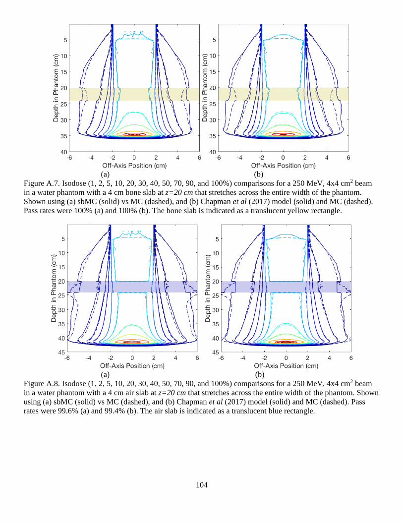
104
(a) (b)
Figure A.7. Isodose (1, 2, 5, 10, 20, 30, 40, 50, 70, 90, and 100%) comparisons for a 250 MeV, 4x4 cm2 beam
in a water phantom with a 4 cm bone slab at z=20 cm that stretches across the entire width of the phantom.
Shown using (a) sbMC (solid) vs MC (dashed), and (b) Chapman et al (2017) model (solid) and MC (dashed).
Pass rates were 100% (a) and 100% (b). The bone slab is indicated as a translucent yellow rectangle.
(a) (b)
Figure A.8. Isodose (1, 2, 5, 10, 20, 30, 40, 50, 70, 90, and 100%) comparisons for a 250 MeV, 4x4 cm2 beam
in a water phantom with a 4 cm air slab at z=20 cm that stretches across the entire width of the phantom. Shown
using (a) sbMC (solid) vs MC (dashed), and (b) Chapman et al (2017) model (solid) and MC (dashed). Pass
rates were 99.6% (a) and 99.4% (b). The air slab is indicated as a translucent blue rectangle.

105
VITA
John Chapman was born in Lake Charles, Louisiana, in 1984. He was raised in Westlake, Louisiana, and
graduated from Westlake High School in May of 2002. Since 2004, he earned a Bachelor of Science in
Electrical Engineering degree with a minor in mathematics at Louisiana State University, and in 2012, he
earned a Master of Science in Medical Physics at Louisiana State University. In the summer of 2018, he will
enroll in the medical physics residency program at Washington University in St. Louis to further his clinical
exposure in preparation for a career as an academic clinical medical physicist.


![Towards a novel small animal proton irradiation platform ... · extensive Monte Carlo simulations using the FLUKA code (version 2011.2x-5, [11,12]). Additional imaging modalities](https://img.pdfslide.us/doc/110x75/60c8ea91993214639b4aac50/towards-a-novel-small-animal-proton-irradiation-platform-extensive-monte-carlo.jpg)