DEVELOPMENT OF A SIMULTANEOUS DESIGN FOR ...d-scholarship.pitt.edu/9737/1/Gokhan_Nuri_Mehmet_2007.pdfDEVELOPMENT OF A SIMULTANEOUS DESIGN FOR SUPPLY CHAIN PROCESS FOR THE OPTIMIZATION

DEVELOPMENT OF A SIMULTANEOUS DESIGN FOR SUPPLY CHAIN PROCESS FOR THE OPTIMIZATION OF THE PRODUCT DESIGN AND SUPPLY CHAIN

CONFIGURATION PROBLEM

by

Nuri Mehmet Gökhan

B.S., Istanbul Technical University, 2001

M.S., Sabanci University, 2003

Submitted to the Graduate Faculty of

the School of Engineering in partial fulfillment

of the requirements for the degree of

Doctor of Philosophy

University of Pittsburgh

2007

ii

UNIVERSITY OF PITTSBURGH

SCHOOL OF ENGINEERING

This dissertation was presented

by

Nuri Mehmet Gökhan

It was defended on

September 14, 2007

and approved by

Kim LaScola Needy, PhD, Associate Professor, Department of Industrial Engineering

Bryan A. Norman, PhD, Associate Professor, Department of Industrial Engineering

Brady Hunsaker, PhD, Assistant Professor, Department of Industrial Engineering

Michael R. Lovell, PhD, Professor, Department of Industrial Engineering

Robert J. Ries, PhD, Research Assistant Professor, Department of Civil and Environmental

Engineering

Dissertation Director: Kim LaScola Needy, Ph.D., Associate Professor, Department of

Industrial Engineering

iii

Copyright © by Nuri Mehmet Gökhan 2007

iv

This research investigates the development of a process for Design for Supply Chain (DFSC) – a

process that aims to reduce the product life cycle costs, improve product quality, improve

efficiency, and improve profitability for all partners in the supply chain (SC). It focuses on

understanding the impacts and benefits of incorporating the SC configuration problem into the

product design phase. As the product design establishes different requirements on the

manufacturability, cost, and similar parameters, the SC is also closely linked to product design

decisions and impacted by them. This research uniquely combines the impacts of the product

design and price decisions on the product demand and the impacts of the SC decisions on cost,

lead time, and demand satisfaction.

The developed mathematical models are aimed at economically managing the SC for

product design and support not only product design, but also redesign associated with process

improvements and design changes in general. This research suggests development of a proactive

approach to product design allowing impacts to the SC to be predicted in advance and resolved

more quickly and economically. It presents two product and SC design approaches. The

sequential approach examines the design of a product followed by the SC design where the

simultaneous approach considers both the product and SC designs concurrently. By utilizing

Mixed Integer Programming and a Genetic Algorithm, this research studies various research

questions which examine modeling preferences and essential performance metrics, impacts of

DEVELOPMENT OF A SIMULTANEOUS DESIGN FOR SUPPLY CHAIN PROCESS FOR THE OPTIMIZATION OF THE PRODUCT DESIGN AND SUPPLY

CHAIN CONFIGURATION PROBLEM

Nuri Mehmet Gökhan, PhD

University of Pittsburgh, 2007

v

using a sequential versus simultaneous design approach on these performance metrics, the

robustness of the resulting SC design, and relative importance of the product and SC design on

the profits. To answer these questions, different models are developed, tested with illustrative

data, and the results are analyzed.

The test results and industry experts’ validations conclude that the developed DFSC

models add significant value to the product design procedure resulting in a useful decision

support tool. The results indicate that the simultaneous DFSC approach captures the complex

interactions between the product and supply chain decisions, improving the overall profit of a

product across its life cycle.

Keywords: Design for Supply Chain, Product Design, Supply Chain, Simultaneous

Optimization, Mixed Integer Programming, Heuristics, Genetic Algorithm.

vi

TABLE OF CONTENTS

PREFACE ................................................................................................................................. XIII

NOTATION ................................................................................................................................ XV

1.0 INTRODUCTION ........................................................................................................ 1

1.1 MOTIVATION ...................................................................................................... 2

1.2 PROBLEM STATEMENT .................................................................................... 5

1.3 RESEARCH QUESTIONS ................................................................................... 8

1.4 CONTRIBUTION ............................................................................................... 11

1.5 OVERVIEW OF THE DISSERTATION ........................................................... 12

2.0 LITERATURE REVIEW .......................................................................................... 14

2.1 PROBLEM TYPES ............................................................................................. 15

2.1.1 Product Design Models ................................................................................. 15

2.1.2 Supply Chain Models .................................................................................... 19

2.1.3 Product Design and Supply Chain Combined Models ................................. 22

2.2 MODEL FORMULATION ................................................................................. 28

2.3 SOLUTION METHODOLOGIES ...................................................................... 33

2.4 SUMMARY ......................................................................................................... 37

3.0 PROBLEM FORMULATION .................................................................................. 40

3.1 PROBLEM DEFINITION ................................................................................... 40

vii

3.2 PRELIMINARY MODELS ................................................................................. 53

3.3 COMPLETE MODEL FORMULATION ........................................................... 58

3.4 REDUCED MODELS ......................................................................................... 69

3.5 MODEL ASYMPTOTIC SIZE ANALYSIS ...................................................... 71

4.0 SOLUTION METHODOLOGY .............................................................................. 77

4.1 DETERMINISTIC OPTIMIZATION METHODOLOGIES .............................. 77

4.1.1 Overview ....................................................................................................... 77

4.1.2 Performance on the Preliminary Models ...................................................... 79

4.2 HEURISTICS AND META HEURISTICS ........................................................ 82

4.2.1 Overview ....................................................................................................... 82

4.2.2 Performance on the Preliminary Models ...................................................... 86

4.3 SELECTED SOLUTION METHODOLOGIES AND IMPLEMENTATION ... 96

4.3.1 Mixed Integer Programming ......................................................................... 97

4.3.2 Genetic Algorithm ........................................................................................ 98

4.4 SOLUTION TECHNIQUES COMPLEXITY ANALYSIS .............................. 107

5.0 COMPUTATIONAL RESULTS ............................................................................ 110

5.1 PERFORMANCE TESTS ON COMPLETE AND REDUCED MODELS ..... 110

5.1.1 Mixed Integer Programming ....................................................................... 111

5.1.2 Genetic Algorithms ..................................................................................... 114

5.1.3 Comparative Analysis ................................................................................. 117

5.2 PROBLEM AND MODEL VALIDATION ...................................................... 128

5.3 ANSWERS TO RESEARCH QUESTIONS ..................................................... 132

5.3.1 Performance Metrics and Modeling Preferences ........................................ 133

viii

5.3.2 Simultaneous versus Sequential Approach ................................................. 142

5.3.3 Combining Product and Supply Chain Design ........................................... 155

6.0 CONCLUSIONS AND FUTURE RESEARCH .................................................... 159

6.1 SUMMARY AND CONCLUSIONS ................................................................ 159

6.2 EXTENSIONS FOR DFSC MODELS AND SOLUTION METHODS .......... 162

APPENDIX A. MODEL LINEARIZATION SCHEMA ...................................................... 166

APPENDIX B. REDUCED DFSC MODELS ........................................................................ 173

APPENDIX C. PRELIMINARY GA PARAMETER TEST RESULTS ............................. 179

APPENDIX D. REDUCED GA SUB-MODELS .................................................................... 180

BIBLIOGRAPHY ..................................................................................................................... 183

ix

LIST OF TABLES

1. Performance measures for supply chain management (adapted from [56]) ............................. 32

2. Summary of number of variables and constraints in different models ..................................... 75

3. Numerical illustration of model asymptotic size of different models ...................................... 76

4. Illustrative test problem data for the preliminary models ......................................................... 80

5. MIP cost minimization model preliminary run results ............................................................. 81

6. MIP lead time minimization model preliminary run results ..................................................... 81

7. Genetic Algorithm cost minimization model preliminary run results ...................................... 91

8. Genetic Algorithm lead time minimization model preliminary run results .............................. 91

9. Tabu Search cost minimization model preliminary run results ................................................ 94

10. Tabu Search lead time minimization model preliminary run results ...................................... 95

11. Summary of number of variables and constraints in GA sub-models .................................. 102

12. Numerical illustration of model asymptotic size of GA sub-models ................................... 103

13. Complete and reduced DFSC problem instances for performance testing ........................... 111

14. MIP results for the complete DFSC model........................................................................... 112

15. MIP results for the reduced DFSC model – 1....................................................................... 113

16. MIP results for the reduced DFSC model – 2....................................................................... 113

17. GA results for the complete DFSC model ............................................................................ 115

x

18. GA results for the reduced DFSC model – 1 ........................................................................ 116

19. GA results for the reduced DFSC model – 2 ........................................................................ 117

20. MIP results for the complete and reduced DFSC models..................................................... 133

21. GA results for the complete and reduced DFSC models ...................................................... 134

22. Customer satisfaction values of component design alternatives – cordless phone .............. 137

23. Parameter estimation error test results .................................................................................. 139

24. Parameter estimation error test results by using the base case solution ............................... 141

25. Customer satisfaction values of component design alternatives – desktop computer ......... 144

26. Simultaneous and sequential approach results for the cordless phone example .................. 147

27. Simultaneous and sequential approach results for the desktop computer example .............. 148

28. Simultaneous and sequential approach results with alternative sequential procedure ......... 151

29. Optimal solutions of simultaneous and sequential approaches – desktop computer ............ 152

30. Revenue, costs, and lead time results of the cordless phone example .................................. 153

31. Revenue, costs, and lead time results of the desktop computer example ............................. 153

32. Product design and supply chain decisions for the cordless phone example ....................... 156

33. Product design and supply chain decisions for the desktop computer example ................... 157

xi

LIST OF FIGURES

1. Actions affecting life cycle cost (adapted from [34]) .................................................................. 3

2. Sequential and simultaneous product and supply chain design processes .................................. 7

3. The Kano model (adapted from [9] and [29]) ........................................................................... 16

4. Design phase in the product life cycle ....................................................................................... 41

5. The proposed DFSC Procedure ................................................................................................. 43

6. Chromosome structure of the Genetic Algorithm for the preliminary models ......................... 87

7. Chromosome structure of the Genetic Algorithm for complete and reduced models ............... 99

8. Progress of the MIP and the GA for the complete DFSC model (instance 1) ........................ 118

9. Progress of the MIP and the GA for the reduced DFSC model – 1 (instance 1) .................... 119

10. Progress of the MIP and the GA for the reduced DFSC model – 2 (instance 1) .................. 119

11. Progress of the MIP and the GA for the complete DFSC model (instance 2) ...................... 120







xii






23. The sequential approach procedure based on separate time periods ..................................... 146

24. The sequential approach procedure based on the optimization over all time periods .......... 150

xiii

PREFACE

Though only my name appears on the cover of this dissertation, a great many people have

contributed to its production. I owe my gratitude to all those people who have made this

dissertation possible and because of whom my graduate experience has been one that I will

cherish forever.

I would like to express my deepest gratitude to my advisor and mentor, Dr. Kim L.

Needy for her endless guidance, support, patience, and direction throughout my dissertation

research, as well as other studies. I have been amazingly fortunate to have an advisor who gave

me the freedom to explore on my own and at the same time the guidance to recover when my

steps faltered. Without her support and inspiration, I would not be able to accomplish what I

have done. I would also like to thank her for her enthusiasm, sincere advice, and invaluable

suggestions that guided me through countless difficulties in all aspects of my life.

I am also grateful to my committee members, Drs. Bryan Norman, Brady Hunsaker,

Robert Ries, and Michael Lovell for their support, help, and guidance throughout my research. I

would like to thank them for advising me in making this dissertation more accurate and more

solid.

I would like to thank University of Pittsburgh’s NSF Center for e-Design and Drs. Bart

O. Nnaji and Michael Lovell for providing me the opportunity to work under the Center’s

xiv

support throughout my research. I would also like to thank industry experts who provided

invaluable input and feedback for my dissertation.

I gladly express my gratitude to the wonderful Industrial Engineering staff, Richard

Brown, Minerva Pilachowski, Nora Siewiorek, Lisa Bopp, and Chalice Zavada for providing

support and help during my long years at Pitt. I want to express my sincere thanks to Richard and

Nora not only for their enthusiasm but also for all the coffee that kept me awake all the time.

I am very grateful to all my friends in the Department who always supported me and

created a joyful work environment. I would like to thank Özlem Arısoy, Görkem Saka, Mehmet

Can Demirci, Melissa Bilec, Natasa Vidic, Mustafa Baz, Pınar Yıldırım, Murat Kurt, Korhan

Turhan, Osman Özaltın, Erin Claypool, Burhaneddin Sandıkçı, Gillian Nicholls, Chen Li,

Shengnan Wu, Oscar, and Guiping for their support and friendship. I would like to express my

gratitude especially to Halil Bayrak and J.P. Lai for their invaluable input in my dissertation and

support in many ways. Final thanks go to the cheerful group of Zeynep Erkin, Sakine Batun, Işıl

Öndeş, Gözde İçten, Anıl Yılmaz, and Alp Şekerci!

I am forever indebted to my wonderful parents, Hale and Ülgür, and to my dear sister

Gökçe for believing in me and for their unconditional support and encouragement. This work

would never be the same without them.

Finally, I am very grateful to my amazing wife and best friend, Şebnem, for her endless

love, patience, absolute support, and for helping me keep my life in proper perspective and

balance. I am very indebted to her for sharing all my troubles during hard times and for her

enthusiasm that helped me overcome so many problems.

Thank you all…

xv

NOTATION

Sets i, k ∈ I : Sets of components from component 1 to component P

Sets j, l ∈ J : Sets of suppliers from 1 to S

Set αi ∈ Ai: Set of design alternatives of component i

Set t ∈ T : Set of time periods

Set n ∈ N : Set of binary factorization elements of lead time – demand

multiplication

P: Total number of components used in the product (|I | = P)

S: Total number of available suppliers (|J | = S)

Ai: Number of design alternatives for component i (|Ai| = Ai)

T: Number of time periods (each representing a product life cycle

phase) (|T | = T)

N: Number of lead time – demand binary variables (γ and δ) that cover all

possible LT1t × Demand1t values in a binary representation (|N | = N)

cijαit1, cijαit

2: Unit manufacturing costs of component i at supplier j for production

levels 1 and 2 for component design αi at time period t

xvi

Capacityijαit1, Capacityijαit

2: Total production capacity of supplier j for component i for

production levels 1 and 2 for component design αi at time period t

Netwcojl: Fixed supply chain network costs between suppliers j and l

Relationik: Number of components k required to manufacture component i

ptijαit: Production time of design αi of component i at supplier j in time

period t

valiαit: Value of design αi of component i for the demand in time period t (%

of total contribution)

Tportcostjklαkt: Unit transportation cost of design αk of component k from supplier l

to j in period t

ω1t, ω2t, ω3t: Allowed values that price can take in time period t

ht: Unit inventory holding cost of the final product in time period t

β1, β2: Demand function coefficients

timemultipliert: A parameter value in order to adjust demand value according to the

time period t (based on what life cycle phase t is)

periodlengtht: Length of the time period t (in the same units with lead time)

zssratio: Z-value from the normal distribution corresponding to the given

safety stock ratio (ssratio)

ρ1, ρ2: Constant coefficients of variation for demand over lead time and

lead time, respectively

Mcapiαit: Total available capacity for design αi of component i in time period t

over all suppliers (∑=

+P

jtijtij ii

CapacityCapacity1

21αα )

xvii

Mdem: Maximum potential demand over all periods (calculated by using

maximum of timemultipliert and lowest pricet with υt=1)

xijαit1, xijαit

2: Total production amount of component i at supplier j for production

levels 1 and 2 for component design αi at time period t

pricet: Price of the final product in time period t

yjl: 1, if suppliers j and l have a direct relationship; 0, otherwise

aijαit: 1, if supplier j fulfills its level 1 capacity with design αi of

component i in time period t; 0, otherwise

ujklαkt: Total amount of design αk of component k manufactured at supplier l

and transported to supplier j in time period t

πiαit: 1, if design αi of component i is selected for time period t; 0,

otherwise

υt: Total value of the final product design for time period t (between 0

and 1, calculated by a constraint in the model)

Demandit: Total demand for component i at time period t

φ1t: 1, if price values are increased to ω2t; 0, otherwise

φ2t: 1, if price values are increased to ω3t; 0, otherwise

λ1t, λ2t: Variables that reflects pricing decision onto demand generation via

φ1t, φ2t, and υ in time period t

τt+: 1, if demand > total production; 0, otherwise

τt-: 1, if total production > demand; 0, otherwise

kt+: Equal to demand, if demand > total production; 0, otherwise

kt-: Equal to total production, if total production > demand; 0, otherwise

xviii

ψ1t, ψ2t, ψ3t, ψ4t: Control variables that link pricing decisions and demand or total

production values for revenue calculation in time period t

LTit: Total lead time for component i in time period t

LTintt: LT1t value rounded up to the nearest integer

ptimeit: Maximum production time for component i in time period t

γnt: 1, if nth binary factor for LT1t is selected for time period t; 0,

otherwise

δnt: A variable to reflect lead time-demand multiplication via binary

factorization in time period t

1

1.0 INTRODUCTION

This research focuses on understanding the impacts and proposed benefits of incorporating the

supply chain configuration problem into the product design phase analogous to the Design for

Manufacturability (DFM) concept introduced in the 1980s where manufacturing processes of a

product are taken into account in the product design phase. Academic studies and industry

experiences show the benefits of incorporating different aspects of the production phase into the

product design process. As the product design establishes different requirements on the

manufacturability, assembly, cost, and similar parameters that have significant impacts on the

later phases of the product’s life cycle, supply chain is also very closely linked to product design

decisions and impacted by these decisions. Therefore, the same benefits that are suggested with

other Design for X approaches are also applicable for the Design for Supply Chain (DFSC)

concept. Different Design for X approaches consider the impacts of the product design on

various concepts such as cost, assembly, environment, and supply chain separately. However,

since there would only be a single product design, its impacts on these various issues would be

cumulative that is a product design may be optimized for minimum cost or easy assembly but

this same design may not be the optimal decision for the environment or supply chain issues.

Although in a perfect case, all of these problems would be combined and solved concurrently,

each of these problems is very complex and needs to be studied in detail before being combined.

In this research, the Design for Supply Chain approach is investigated to quantify and understand

2

the impacts of the product design on the supply chain performance. The proposed benefits of the

DFSC are investigated by utilizing a mathematical programming approach in order to quantify

these proposed benefits.

The developed mathematical programming model is structured in a way to optimize

product design and supply chain decisions with an aim of maximizing profits throughout the

product’s life cycle. At the same time, this model allows for further investigation of the proposed

benefits of incorporating supply chain decisions into the product design phase by providing the

opportunity to exclude supply chain related decisions and evaluate the impacts of this exclusion.

The model includes widely known product and supply chain design aspects, and has also been

validated by industry experts. This ensures that the model captures important design parameters

that are being used in the industry and is as realistic as possible.

While this model is designed to be very realistic by considering primary product design

and supply chain performance parameters, it tends to be mathematically very complex and hard

to solve. Therefore, this research also aims to evaluate different solution techniques such as

deterministic optimization procedures, heuristics, and their combinations in order to find optimal

or near-optimal solutions quickly.

1.1 MOTIVATION

Research studies demonstrate that the average discrete manufacturer realizes a 12% reduction in

time-to-value, a 20% reduction in development costs, and a 7% reduction in manufacturing costs

by collaborating with the supply chain early in the design process [32]. Most benefits of

collaboration among supply chain (SC) partners lie in the design phase of the product lifecycle,

3

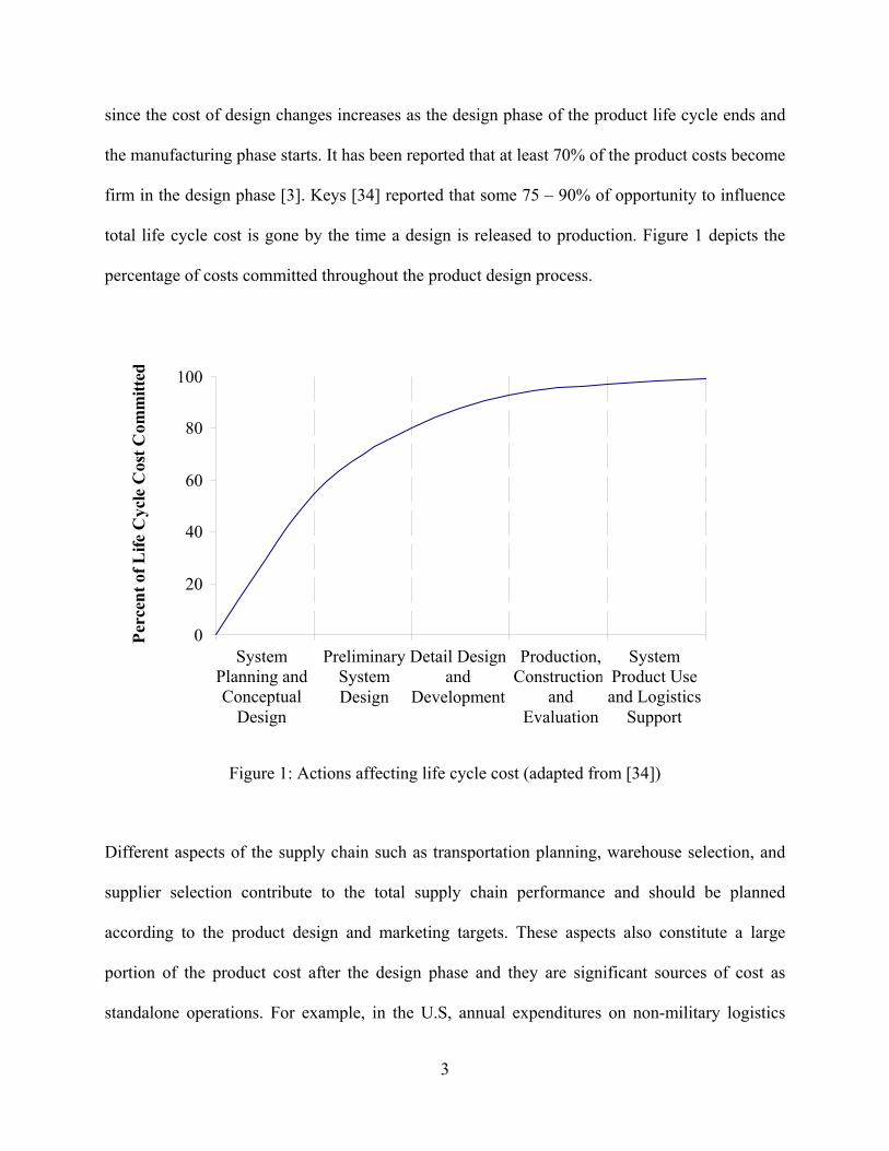
since the cost of design changes increases as the design phase of the product life cycle ends and

the manufacturing phase starts. It has been reported that at least 70% of the product costs become

firm in the design phase [3]. Keys [34] reported that some 75 – 90% of opportunity to influence

total life cycle cost is gone by the time a design is released to production. Figure 1 depicts the

percentage of costs committed throughout the product design process.

Figure 1: Actions affecting life cycle cost (adapted from [34])

Different aspects of the supply chain such as transportation planning, warehouse selection, and

supplier selection contribute to the total supply chain performance and should be planned

according to the product design and marketing targets. These aspects also constitute a large

portion of the product cost after the design phase and they are significant sources of cost as

standalone operations. For example, in the U.S, annual expenditures on non-military logistics

0

20

40

60

80

100

SystemPlanning andConceptual

Design

PreliminarySystemDesign

Detail Designand

Development

Production,Construction,

andEvaluation

SystemProduct Useand Logistics

Support

Perc

ent o

f Life

Cyc

le C

ost C

omm

itted

System Planning and Conceptual

Design

Preliminary System Design

Detail Design and

Development

Production, Construction,

and Evaluation

System Product Use and Logistics

Support

4

represented over 11% of the Gross National Product in 1995 [55]. A decade later in 2005, the

total logistics costs total around $1.3 trillion, still representing 10% of the Gross National

Product [19]. Therefore, the proposed benefits of designing the supply chain within the product

design or redesign lifecycle phases present huge impacts on both the cost and other performance

measures of the supply chain and success of the product. In this research, a product’s success is

defined as its ability to generate enough demand and to satisfy this demand via the associated

supply chain during its life cycle period. For example, a product could be considered as

successful if its life cycle spans as long as planned, if it attracts targeted demand at the targeted

markets, if it adds value to the company and its brand, and if it satisfies customers, therefore

generating expected profits.

This research aims to investigate the impacts and proposed benefits of incorporating the

supply chain configuration problem into the product design phase. The motivation behind the

study is that proposed benefits could be understood and considered by managers when

conceptual ideas are supported with case studies to include quantitative analysis and performance

metrics. This research investigates the formulation of advanced and complex product design and

supply chain models with the investigation of several solution techniques to solve these models

in a timely manner with optimal or near-optimal results. Here, product design models aim to

solve product design selection, pricing, and similar problems; where supply chain models are

mainly developed to design the supply chain by selecting suppliers and setting the relations

between them.

5

1.2 PROBLEM STATEMENT

In the complex business environment of the current technology era, it is recognized that not

paying enough attention to product design might potentially result in financial losses due to

demand generation problems. In this context, demand generation is used to define how attractive

a product design is in terms of creating demand. In other words, it is the ability of a product

design to generate demand by satisfying customer expectations. As the supply and therefore the

competition among the companies for the limited market demand increases, the product design

gains more importance for demand generation. However, the product design impacts not only the

demand generation, but also the manufacturing processes, cost, quality, and lead time. The

product design affects the associated supply chain directly with its requirements including, but

not limited to manufacturing, transportation, quality, quantity, production schedule, material

selection, production technologies, production policies, regulations, and laws. From a broad

perspective, the success of the supply chain depends on the product design and the capabilities of

the supply chain, but the reverse is also true, the success of the product depends on the supply

chain which produces it. Since the product design dictates multiple requirements on the supply

chain as mentioned previously, it is clear that once a product design is completed, it would

determine the structure of the supply chain, limiting the flexibility of the engineers to generate

and evaluate different supply chain alternatives. Furthermore, constructing an optimal supply

chain is a key for the success of the product because of its impacts to cost, quality, and schedule.

In this research, the impacts of the product design and redesign on the supply chain structure is

studied with an aim at quantifying those impacts so that they can be used in the product design

phase to better understand the tradeoffs between the benefits and costs of the different supply

chain alternatives. The problem that the product design engineers and managers face in the

6

product design phase is to pick the “best” design among several alternatives in order to generate

the targeted profits or benefits. This “best” design is decided generally based on its potential for

demand generation in the industry. Thus the “best” product design would be the design which

satisfies the customer requirements at the utmost level. Therefore, there is always an option to

select the “best” possible product design and then optimize the supply chain for this fixed

product design. In this research context, from the total profit point of view, the “best” product

design would be the one that sacrifices (if necessary) some demand attractiveness for better

supply chain performance so that the total profits (as a combination of both generated demand

and supply chain performance) are maximized. Since the design decisions generate many

constraints regarding manufacturing and supply chain requirements, the design alternatives need

to be studied and compared considering their impacts to the supply chains. Broadly speaking, in

addition to “always selecting the best possible design” approach (without regard to the supply

chain design), there are two different approaches for product and supply chain design integration

namely sequential and simultaneous as depicted in Figure 2.

The sequential approach, which is widely applied in industry, suggests that product

design should be completed based on customer, marketing, and management requirements

independently from analyzing the supply chain impacts. After the design is completed, the

supply chain should be generated and then examined for its performance. If the supply chain

performance is not within desirable limits, the product design should be revised until a

satisfactory supply chain performance is achieved. However, as it will be further explained and

studied in Chapter 3.0, this approach very likely leads to a suboptimal product and supply chain

design configuration due to solving each problem separately. Even after an optimal product

design is created for customer and company requirements, subsequent changes to the component

7

and part designs to achieve a better performing supply chain may lead to a non-optimal product

and supply chain design.

Figure 2: Sequential and simultaneous product and supply chain design processes

In contrast, a simultaneous product and supply chain design would overcome these

shortcomings. The proposed approach uses not only customer, marketing, and management

requirements necessary for the product design, but it also incorporates supplier information. With

this approach, the cyclic procedure of designing a product, generating the supply chain,

Sequential Product and Supply Chain Design

Simultaneous Product and Supply Chain Design

Data input (customer, marketing, management requirements)

Data input (customer, marketing, management requirements, supplier

information)

Design product and components Design product and component alternatives and generate associated supply chain (SC)

Generate the supply chain (SC) and evaluate its performance

Satisfied with SC performance?

Finalize the product and SC design.

Finalize the product and SC design.

Satisfied with product design & SC performance?

Yes

No

Yes

No Satisfied with

product design? No

Yes

8

evaluating the supply chain, and redesigning the product is reduced in many cases to a single

iteration. However, the costs and time requirements associated with determining or designing

several components at once need to be considered for the simultaneous approach. The main

tradeoff between the sequential and simultaneous approach would be designing several

component alternatives at once for the simultaneous approach versus launching a non-optimal

product design - supply chain combination which might lead to lower profits with the sequential

approach.

The problem addressed in this research is about picking the “optimal” product design by

evaluating its impacts on the demand generation and supply chain network requirements. Briefly,

developed models evaluate and compare the product design alternatives to select the optimal one

which maximizes the company’s profit by generating more demand and supplying this demand

with high quality products in a timely manner and with less cost.

1.3 RESEARCH QUESTIONS

This research investigates the development of a process for Design for Supply Chain [52] - a

process that aims to drastically reduce the product life cycle costs (including design, production,

and logistic costs), improve product quality, improve efficiency, and improve profitability for all

partners in the supply chain. It presents supply chain models aimed at economically managing

the supply chain for product design and supports not only product design, but also redesign

associated with process improvements and design changes in general. It suggests development of

a proactive approach to product design and design change allowing impacts to the supply chain

to be predicted in advance and resolved more quickly and economically.

9

A typical example of DFSC is the automotive OEM with multi-tier suppliers and

corresponding product data and information transfers to facilitate supply chain profitability.

OEM's can focus on core competencies and optimize intellectual assets while outsourcing

processes that are integral to their finished products [8]. Another objective of DFSC is to elevate

the supply chain to the level of a design and development partner to create a ripple effect of

benefits consistent with an OEM's primary objectives - quality and time to market [1]. It would

also help to eliminate the "bullwhip effect" [48] (cascading rise in inventory and financial

bottlenecks due to unanticipated changes to product design).

By utilizing mathematical programming and heuristics on the DFSC models, this research

specifically aims to answer four major research questions by studying several related sub-

questions:

1. Which product design / supply chain performance metrics should be included in the

model?

This question inquires which performance metrics should be considered in the model since each

additional metric would increase the complexity of the model. This research investigates impacts

of different performance metrics on the complexity and quality of the solution techniques.

Benefits and costs of adding new metrics to the model are analyzed.

1.1. How much computational complexity does a performance metric add to the model?

1.2. Are there specific performance metrics (such as cost and lead time) that should always

be considered in the model?

1.3. How does the performance of the solution techniques differ by adding another

performance metric to the model?

10

2. How do the performance metrics differ for the product design and the associated

supply chain for the simultaneous and sequential approaches?

This question asks whether the simultaneous approach would impact the final product design and

supply chain configuration that would have been selected by the sequential approach. It also

examines which supply chain performance metrics would differ by using the simultaneous

approach and whether any of these metrics would be improved.

2.1. Does the simultaneous approach provide a less costly product design and supply chain

through the product’s life cycle?

2.2. Does the simultaneous approach create a supply chain that has minimum lead time?

2.3. To what level does the simultaneous approach modify the product design that is

optimized for customer preferences?

2.4. Does the non-optimal product design (according to customer preferences) pay for itself

through better supply chain performance?

3. How robust is the supply chain to product design changes?

The underlying idea is that there would not be any significant differences between different

supply chains for a given product design. This question is explored by studying different supply

chain configurations for a given product design and measuring both their forecasted and realized

long-term performances.

3.1. Do product design changes result in a change to the number of suppliers?

3.2. Do product design changes result in a change in the number of tiers in the supply chain?

3.3. Do product design changes result in a change of the actual suppliers?

3.4. How sensitive is the supply chain to product design changes, i.e., what level of

magnitude of changes result in a change to the supply chain?

11

3.5. Does the simultaneous design approach provide a more robust supply chain structure

than the sequential approach?

4. What is the relative importance of the product design and the supply chain design on

the product success (thus on the profits)?

This idea questions whether the design team of the product should only concentrate on the

demand generation potential of the product design rather than considering its impacts on the

supply chain, assuming effects of the supply chain performance on demand generation is

negligible when compared to those of the product design itself. This question is studied by

comparing the impacts of the product design and the supply chain performance on profit.

4.1. How does optimal product design differ when supply chain structure is considered in

addition to customer preferences than when it is not considered?

4.2. How much impact does the product design and supply chain have on the product’s

success (profits)?

1.4 CONTRIBUTION

This research makes several significant contributions. First, a significant addition to the existing

DFSC research is provided by combining the product design and supply chain decisions into a

single framework which optimizes the decisions simultaneously. This research aims to fill in the

gap in the DFSC literature which lacks explicit consideration and integration of marketing and

product design decisions and manufacturing and supply chain decisions. The previous academic

studies concentrated on the integration of the product differentiation point or product Bill of

12

Materials requirements to the supply chain optimization models, and hence lack any assessment

of impacts of these decisions on the customer demand and satisfaction. This research uniquely

addresses both the demand and manufacturing aspects of a product and it employs well-

established product design and supply chain performance metrics.

The second contribution of this dissertation is that the developed models are not limited

to certain industries or products but rather they are generic and can be used virtually for any type

of product in any manufacturing industry.

The third contribution of this dissertation is that it investigates and provides insight about

possible solution procedures, including Mixed Integer Programming and Genetic Algorithm, and

their benefits to the solving these complex DFSC models. Detailed computational tests and

illustrative examples provide a clear assessment of both solution methodologies. In addition, this

dissertation evaluates alternative modeling preferences and assesses the performance of different

solution methodologies for these alternative models. Furthermore, the presented analyses provide

insight into the modeling and algorithmic / computation complexity issues.

Finally, this dissertation provides an important assessment from different industry experts

across various industries and includes these experts’ validation and suggestions for further work.

1.5 OVERVIEW OF THE DISSERTATION

In this dissertation, Chapter 2 provides a summary of the relevant literature that is related to

product and supply chain decision problems. The first section in this chapter describes separate

product design and supply chain design studies followed by an explanation of the research that

investigated a combination of product and supply chain design similar to the DFSC approach.

13

The following sections concentrate on mathematical model formulations and solution techniques

used for these separate and combined problems. A summary of the literature is provided in the

last section.

The mathematical model formulation is given in Chapter 3. The detailed problem

description in the first section is followed by preliminary mathematical models in the second

section. The third and fourth sections describe the complete DFSC model formulation and

reduced DFSC models used to investigate research questions, respectively. The last section

provides a model asymptotic size analysis for the described models.

Brief history and capabilities of deterministic optimization methods and relevant

heuristics are given in the first and second sections of Chapter 4. This chapter also provides a

comparison of these methods’ performance on the preliminary models in the relevant

subsections. Finally, a complexity analysis of these solution methods is provided.

Chapter 5 concentrates on the computational results first by analyzing how different

solution techniques perform for the described models. The second section is the problem and

model validation and it includes the industry experts’ assessments, comments, and revisions

about the significance of the problem, the mathematical model structure and assumptions, and

finally the computational results. The last section in this chapter addresses research questions and

provides answers for these questions based on the computational results.

Chapter 6, the last chapter, presents a summary of the findings and concluding remarks.

The second section provides future work both in extending the DFSC models and studying other

solution techniques.

14

2.0 LITERATURE REVIEW

Examination of the scholarly literature shows growing interest in supply chain problems and the

relationships between the product design and supply chains as the potential impacts of supply

chain decisions become more tractable, understandable, and easy to evaluate. Since the World

War II era, there has been a growing interest in supply chain planning to increase efficiency and

performance of supply chains. At the same time, product design and customer satisfaction

interactions have gained increasing interest by researchers working in both design engineering

and marketing. With the advancements in problem modeling and solution techniques, limited

supply chain and product design problems are extended to capture more realistic aspects of these

problems. In the last two decades, combining these two important and interacting problems

continues to draw attention both by academia and industry.

This literature review provides a summary of these efforts that are aimed at modeling and

solving product design and customer satisfaction problems, supply chain problems, and their

combinations. The literature review section is organized into three sections, namely problem

types (Section 2.1), model formulation (Section 2.2), and solution methodologies (Section 2.3).

Although several studies consider modeling, solution, or problem aspects collectively, they are

presented within the literature survey according to their main contributions.

15

2.1 PROBLEM TYPES

As this research examines a combination of product design and supply chain design problems,

these two separate problems need to be comprehended. The product design problems often tend

to be studied within the marketing and industrial engineering domains as they relate to the

demand generation context of this research. On the other hand, supply chain problems are more

widely studied within the industrial engineering optimization area although the majority of the

research still concentrates on logistics aspects. Relevant studies to these different problem types

are presented.

2.1.1 Product Design Models

The product design, along with price, advertising, and other market variables, is always

considered one of the most important variables that impact demand. As each product is sold to

satisfy certain customer needs, the product design addresses these needs by providing different

features via different components. Each different component design satisfies these customer

needs to a different degree. For example, car tires mainly satisfy customers’ needs for good road

traction and a smooth ride. However, different tire thread designs such as dry or snow road

threads fully satisfy these needs in the corresponding road conditions. Therefore, using a dry

road thread on a car to be sold in a market with many snowy days would satisfy customers’

needs partially, resulting in lower demand.

As an important effort in conceptualizing the interaction between the product design and

satisfaction of customers’ needs, the Kano model, given in Figure 3, examines degree of

16

achievement by the product design against the customer satisfaction. It defines three major areas

of customer satisfaction and their relationship to products features.

Figure 3: The Kano model (adapted from [9] and [29])

According to the Kano model, the straight line represents expected performance measures from a

product design. These expectations are usually expressed by the customers so the designers know

what they need to provide as product features. The exciters or innovative design features are not

expected by the customers and therefore are not expressed. Thus, if they are not achieved, they

do not result in loss of customer satisfaction, however when they are provided, they provide

extraordinary positive impact on customer satisfaction. On the opposite, basic design features are

not expressed by the customers even though they are expected from a product design. Safety and

Customer satisfaction

Degree of achievement

Unexpected - innovative (unspoken)

Expected (unspoken)

Expected (spoken) Exciters

Basic

Performance

17

reliability features are usually in this category. Satisfaction of these basic expectations normally

do not result in customer satisfaction, instead they only prevent customer dissatisfaction.

In order to quantify the relationship between product design and satisfaction of

customers’ needs, various models have been studied in the literature. In the robust design process

context, Taguchi developed a “quality loss function” that evaluates the level of the dissatisfaction

of customers’ needs (and value) when a product component’s design is different than its ideal

specifications [21]. Although Taguchi developed more than 68 loss functions, the most widely

used function, which is called nominal-the-best type given in (1.1), quantifies loss of customer

value when a component design, y, varies from its targeted ideal value, τ. The quality loss

coefficient, k, is assumed or determined by an expert and depends on the product or market and

is defined in monetary values [9].

2)( τ−= ykL (1.1)

Another important approach is Value Engineering (VE) which was developed at General Electric

during World War II. In this approach, the value of a component (and consequently its design) is

defined as the ratio of its function to its cost. Although VE does not necessarily evaluate the

satisfaction of customers’ needs by the product component’s design, it is widely used in industry

to eliminate non-value added costs in product designs [17][18] and it is often required by the

U.S. Department of Defense and NASA of their contractors [5].

Quality Function Deployment (QFD), which was developed by Dr. Shigeru Mizuno in

1972 and first applied in Mitsubishi in Japan, is “a planning tool to fulfill customer expectations”

[9]. QFD is widely used to make design tradeoff decisions between component alternatives [17].

In this method, customers’ needs (WHATs) are transformed into design specifications (HOWs)

by design engineers in the first step. Next, the relationships between customers’ needs and design

18

specifications are determined. Following these assessments, competing products’ specifications

are also added into the relationship matrix, representing strengths and weaknesses of the

proposed product design alternatives. In later steps, customers’ priorities on these features and

associated technical difficulties to manufacture these designs are assessed. In conclusion, QFD

provides a structured method to evaluate the satisfaction level of customers’ needs via features

proposed by the product design alternatives. An extensive literature survey of Chan and Wu [12]

suggests that QFD is widely used to collect and translate and to satisfy customers’ needs.

As another effort to quantify the customer satisfaction and the product design

interactions, Martin and Ishii [47] studied impacts of design variety on the customer satisfaction

and manufacturing processes. In parallel to the QFD method, they developed an index called

Variety Voice of the Customer (V2OC), which is a measure of the importance of the component

to the customer, as well as the heterogeneity of the market with respect to that component. In this

method, if a component is ranked with low V2OC value, then it is suggested that this component

design is standardized for cost reduction. However, a high V2OC rating suggests that the

corresponding component is of critical value for customer satisfaction and therefore should be

designed to satisfy different customer requirements.

Although there is an extensive literature of product design and its impacts on customer

satisfaction (and consequently demand generation), a brief overview of important studies and

concepts are presented. These studies suggest different methods can be employed to map

customers’ needs to design specifications. They also suggest that various methods can be used to

quantify impacts of satisfaction of customers’ needs on the demand. However, despite the

existence of different methods, it should be noted that the product design and demand generation

19

relationship is an important issue and it needs to be quantified in a structured way to the extent

possible to represent the complex interaction.

2.1.2 Supply Chain Models

A supply chain, which is defined as “consisting of all parties involved, directly or indirectly, in

fulfilling a customer request” [13], is a continuously evolving part of a company’s production

process and plays a critical role in the profitability of a product and the company. A supply chain

starts with the raw material procurement and includes all tiers of suppliers that manufacture

product components, production facilities that utilize manufacturing and assembly operations,

warehouses and distribution centers, retailers, customers, and post-sales service centers. In this

research, the supply chain configuration problem focuses on a segment of the supply chain

beginning with the raw material procurement and ending with the final product manufacturing or

assembly. Chopra and Meindl [13] suggest that toward the customer’s request fulfillment

objective, a supply chain not only includes manufacturing and transportation of products but also

consists of marketing, new product development, distribution, finance, and customer service.

Within this definition, a supply chain is considered a vital part of a product’s life cycle which

starts with customers’ needs and ends only after the last customer service is completed,

representing a time horizon longer than the actual selling period of a product. Obviously, each of

many parts that constitutes a supply chain brings important planning challenges and these

problems are widely studied by academicians.

From an academic perspective, interest in supply chain problems has begun almost with

the first operations research studies in the World War II era that examined transportation,

scheduling, and facility location problems. As one of the earliest studies, in 1959, Hanssmann

20

[31] modeled material procurement, production, and distribution with an aim of optimizing the

level of inventory and selecting optimal inventory locations. In 1960, Clark and Scarf [14]

developed a model to optimize purchasing decisions from different echelons of a supply chain,

each having a different level of available inventory and different lead times. The supply chain

has gained more attention from academic and industry beginning in the mid 1970’s by studying

different solution techniques for supply chain problems as explained in section 2.3. In the

1980’s, several studies concentrated on inventory optimization and economic order quantity

determination problems [55]. These, mainly single vendor and single buyer models are extended

to capture multi-vendor, multi-buyer, and multi-period cases in the 1990’s [55]. However until

the mid 1990’s, supply chain models often concentrated on single subproblems, such as

inventory planning and buyer-vendor coordination. Later studies are aimed toward combining

these subproblems into larger but more realistic complete supply chain models. For example,

Cohen and Lee [16] formulated their model beginning with the material procurement, then

production, and concluding with the product distribution portions of the supply chain and used a

series of linked, approximate submodels, and heuristics optimization to solve the problem. They

introduced stochastic demand and lead time parameters into the model and suggested different

heuristic solution procedures for material control, production, stockpile inventory, and

distribution submodels that constitutes the final supply chain model when combined.

In parallel to these operational supply chain problems, strategic supply chain planning

and supply chain network design problems are also widely studied within the engineering and

business literatures. One of the initial papers that proposed a model and an efficient solution

technique for specific kinds of supply chain problems was dated back to 1974 in which the

authors modeled a static distribution system to optimize the locations of intermediate distribution

21

facilities between plants and customers [24]. This paper reports significant computational time

gains by employing Bender’s Decomposition technique and having solutions within one or two

tenths of one percent of the global optimum. Viswanadham and Raghavan [60] investigated

performance of different supply chain networks under two different production planning and

control policies, namely make-to-stock and assemble-to-order systems. Truong and Azadivar

[56] developed a model to design the network of a supply chain that addresses supplier selection,

distribution center location, inventory planning, and production orders. Cakravista et al. [10]

developed a two-stage supply chain planning model which performs supplier selection based on

supplier bids and determines optimal manufacturing and logistics functions. Talluri and Baker

[54] developed a multi-phase model that evaluates each supplier’s production efficiency and

incorporates this analysis into supply chain network design problem. Their model also optimizes

production assignments to selected suppliers. Wu and O’Grady [64] developed a methodology to

improve design of a supply chain network for multi-criteria in a constrained environment. Ding

et al. [20] developed a supplier selection model that incorporates uncertainties emerging from

demand, production, and distribution parts of a supply chain. Vidal and Goetschalckx [58]

presented a mathematical model that maximizes the after tax profit of a multinational company

by using transfer prices (prices a company’s different departments charge for semi-products

within the company) and the allocation of transportation costs as explicit decision variables. This

selection of studies represent the wide spectrum of the challenges that are directly associated

with the supply chain problems in today’s global business environment.

Thomas and Griffin [55] surveyed different supply chain models at operational and

strategic levels both in academic and business literatures and stressed the lack of life cycle and

inventory obsolescence constraints in the supply chain models. They stated that these problems

22

can partially be attributed to the supply chain structure and design. They also reported the

importance of adding new objectives into the models due to current business trends. For

example, they suggest including environmental regulations, and incorporating important

macroeconomic parameters, such as currency exchange rates, which becomes more important

with the movement towards globalization and outsourcing. Lambert and Cooper [36] stress that

in today’s supply chain management problems; marketing decisions also play a significant role.

Customer relationship management, demand management, and product development and

commercialization are all vital parts of the supply chain management problems. Additionally, in

parallel to the globalization, supply chain problems become far more complicated than classical

logistics problems with the integration of long-term strategic supplier relations and marketing

aspects.

These selected studies represent emerging interests from more than six decades of supply

chain research. As the trend shows, the current interests in supply chain research are more

focused on developing complicated, thus realistic, models as conceptual combinations of

previously studied sub-models with the addition of emerging industry needs. Similarly

development of different solution techniques that can provide good solutions in acceptable time

for larger models has also gained more importance as realistic models challenge existing, well-

established solution techniques currently in use.

2.1.3 Product Design and Supply Chain Combined Models

Although supply chain management and decision models are widely studied in the literature, the

Design for Supply Chain concept is specifically addressed in several studies. The term Design

23

for Supply Chain Management (DFSCM) is first used by Lee and Billington [41] in an inventory

planning problem within a supply chain review study. The authors stated that

A lot has been written on design for manufacturability, for assembly, for quality, for producibility, and for serviceability. To this list we would add "design for supply chain management." Thus product designs should be evaluated not only on functionality and performance but also on the resulting costs and service implications that they would have throughout the product's supply chain. The same applied to process designs. [[41], p.11]

In another study, Lee [40] suggested that changing the mind-set of the design teams and

quantification of benefits of the DFSCM are the most important and significant obstacles for

implementation.

Keys [34] discussed the Design for Life Cycle concept that he described as the

combination of all design efforts including but not limited to manufacturability, assembly, cost,

quality, customer support logistics, and supply chain. He suggested that it is very important to

keep the focus on the product life cycle since today “the planning of new products includes

second, third, etc., generation product follow-on’s, where the support to and through product

lives must be a part of an integrated life cycle strategy.”

In a study by Lee and Sasser [44], Hewlett-Packard’s (HP) new product line, called

Rainbow, was used to study an analytical DFSC model which incorporates stochastic demand

with lead time decisions, service level targets, and inventory, stockout, and shipment costs in

order to decide on the optimal product differentiation point. The authors provided analytical

solutions for the model for different product life cycle phases as well as for different design

alternatives. The importance of the study is that it was done using real data and the results were

validated after the product launch over the product life cycle. Another important contribution is

that all the modeling and analysis was done during the product design phase, which differs from

the majority of supply chain related studies that try to optimize the supply chain for products past

24

the design phase. Although these authors studied a supply chain configuration problem, they did

not incorporate supplier selection and thus associated uncertain quality, lead time, and capacity

problems. In another study completed at HP, Lee and Billington [42] reported HP’s new

approach to modeling and optimizing its SC policies which adds distribution, market, and

product specifications into the available inventory modeling efforts. They explained the positive

impacts of the new approach which suggests incorporating all related divisions of the company,

key suppliers, and key customers into the SC design decisions and developing product-based

supply chains. They listed four key company requirements as the basis for their model: “(1)

benchmarking inventory and service tradeoffs; (2) assessing the impact of uncertainties on

operational performance; (3) analyzing what-if questions for different scenarios and operating

characteristics; and (4) evaluating product design impacts on the supply chain, that is, predicting

how the supply chain would perform under different product and process design alternatives”

([42], pp. 47). Lee, in his several studies, introduced and used similar terms that constitute parts

of the DFSCM concept. Design for Localization (or interchangeably Design for Customization

[43]) concentrates on delaying the customization of a product’s design for different local market

segments. In relation, the Design for Flexible Manufacture [39] concept is introduced that aims

to increase part commonality and interchangeable subassemblies to help reduce inventory costs

and to ease supplier management. Finally, Design for Logistics [39] aims to design products so

that they can be transported easily in a cost effective manner. However, all these concepts that

add up to the DFSCM concept introduced by Lee and his colleagues, mainly focus on delaying

product customization to reduce inventory and designing products for effective packaging and

transportation. In these studies, the product design – customer demand interactions were not

included, hence customer demand – supply chain performance relations were not evaluated.

25

Another extensive DFSC study has been conducted by Arntzen et al. [2] at Digital

Equipment Corporation (DEC), that led to a term which they coined Global Supply Chain Model

(GSCM). The GSCM is a large mixed-integer linear programming model (MIP) that minimizes

cost or lead times (or both) for different echelons of the supply chain and time periods with

requirements of meeting the estimated demand, using limited capacities, and restrictions on local

content and offset trade. The cost structure of the model included fixed and variable production

costs, inventory costs, and distribution costs including taxes, duties, and duty drawback. The

model was developed to support product development at DEC for about 20 new products. It was

used to design the supply chain during the product design phase and reported savings of US $1.4

billion in four years with around a 500% productivity increase. However, the GSCM uses a

combined objective function (weighted average of cost and lead time) and the objective function

is limited to these two objectives. Furthermore, the fixed demand assumption is one of the major

drawbacks of the model. The solution technique is a branch and bound algorithm with

introduction of penalties for violating constraints to save computation time. The authors reported

around a one minute solution time for problems with 2,000 to 6,000 constraints and 5,000 to

20,000 variables, with a few hundred of these variables being binary.

The impacts of different product life cycle phases and the type of product on the structure

of the associated supply chain are reported to be unavoidable and necessary factors to be

included in the modeling efforts in the literature. Fisher [23] stressed two distinct types of

products, namely functional and innovative; and two related supply chain functions, physical

(transforming raw material to an end product and concentrating mainly on cost reduction) and

market mediation (ensuring the variety of products reaching the marketplace matches what

consumers want to buy and concentrating mainly on lead time reduction). He gives examples of

26

Campbell’s Soup as a functional product with predictable demand (so use a physical supply

chain with cost reducing strategy) and Sport Obermeyer’s line as an innovative product with

unpredictable demand (so use market mediation supply chain with uncertainty reduction

techniques, such as getting orders earlier).

Wang et al. [61] suggested three types of products: innovative, functional, and hybrid and

three categories of supply chains: lean supply chain (that focuses on lean manufacturing and cost

reductions), agile supply chain (that aims to provide flexible and fast manufacturing to reduce

lead time), and hybrid supply chain (that aims to capture both aspects of lean and agile supply

chains). They used Analytic Hierarchy Process (AHP) and linear programming (LP) in a supplier

selection model for solution procedures where suppliers are ranked with AHP and selected by

using LP and preemptive goal programming in order to develop the desired supply chain (lean,

agile, or hybrid) for the given product type (innovative, functional, or hybrid). The supply chain

performance is measured by using the Supply-Chain Operations Reference model (SCOR),

which is “a process reference model that has been developed and endorsed by the Supply-Chain

Council as the cross-industry standard diagnostic tool for supply-chain management” [53].

Although this approach does not require extensive computational resources, the necessity of

expert knowledge for AHP, setting goals and SCOR evaluations are major implementation

drawbacks. Yet, expanding this solution technique as a multi-objective solution procedure which

considers several objectives at the same time both in AHP and goal programming phases would

be challenging, yet necessary for a better supplier selection model.

Fandel and Stammen [22] developed a mathematical model to fix the product program

and the extended supply chain network. In this study, they modeled investment decisions on

product development projects between alternative products to compare product life cycles with

27

their development and recycling strategies. Their model evaluated impacts of these decisions on

the supply chain network and aimed to develop the optimal product development and supply

chain network strategy to maximize overall profits. Although their model includes recycling

performance of the supply chain and allows selection of different product alternatives, they did

not explicitly consider the impacts of the product design on customer satisfaction and demand.

Moreover, due to extensive size of the developed model, they did not provide an efficient

solution methodology for large, real life problems.

Graves and Willems [30] developed a supply chain network model for a new product that

selects suppliers and assigns production orders. However, this model assumes that the product

design is finalized. Despite this drawback, this model provides opportunities by accounting for

time-to-market costs and allowing multiple sourcing of a product component.

Lamothe et al. [37] studied a product family selection and supply chain network design

problem, similar to the proposed DFSC concept. In their study, the authors suggested a Generic

Bill of Materials (G-BOM), which is a flexible Bill of Materials in terms of satisfying customers’

needs. In this study, different product family variants are associated with different market

segments. A market segment is considered to be satisfied by at least the corresponding product

variant or by a better product variant. Within this demand satisfaction perspective, the model

aimed at minimizing total supply chain costs that come from variable manufacturing,

transportation, and inventory decisions and fixed facility opening and transpiration line opening

costs. Although the study models selection of better product variants for satisfaction of better

market segments, it does not take the impacts of product design on the demand and market share

into account. With an aim of cost minimization, the authors did not include the demand

generation problem associated with the product design and pricing decisions. They have also

28

excluded economies of scale and international taxes and duties for simplification purposes. This

study is an example of the growing interest in academia for modeling product design and supply

chain interactions. Although this study precisely models product design and supply chain

relations, its main drawback is the lack of explicit modeling of the impacts of product design on

the product demand. Since the changing product demand may require different supply chains,

overlooking the product design - demand interaction may result in a non-optimal supply chain

network. Authors, in this study, also used an open-close decision structure to select suppliers and

incur associated fixed costs which limits the model to capture the increasing nature of these costs

with higher levels of interactions between supplier pairs.

2.2 MODEL FORMULATION

During the development of supply chain modeling efforts, academicians expanded the problem

formulations so that initially ignored issues that complicate the problem are added for more

realistic problem formulations. Yet, mathematical problem formulation is still a challenge for

researchers since formulation is a primary driver of solution techniques and ultimately the

complexity of the problem and solution time as well. Incorporating stochastic, nonlinear, or

qualitative objectives, parameters, and variables into the formulation helps to develop more

realistic models although it is usually harder to solve these formulations computationally and

often requires long computational time or sacrifices from solution quality. The formulation is

also closely linked to the problem studied since it describes what decisions will be made and

what constraints will be considered.

29

Beamon [7] provides a detailed survey of research studies in multi-stage supply chain

modeling and divides supply chain models into four categories: (1) deterministic analytical, (2)

stochastic analytical, (3) economic, and (4) simulation models. She also defines performance

measures for supply chains in two groups: (1) qualitative (customer satisfaction, flexibility,

information and material flow integration, effective risk management, and supplier

performance), and (2) quantitative (a) based on cost (cost minimization, sales maximization,

profit maximization inventory investment minimization, and return on investment

maximization), and (b) based on customer responsiveness (fill rate maximization, product

lateness minimization, customer response time minimization, lead time minimization, and

function duplication minimization). She also provides a list of frequently considered supply

chain model variables which includes product / distribution scheduling, inventory levels, number

of stages (echelons), distribution center assignments to customer, product assignment to plants,

relationships between suppliers and buyers, product differentiation step specification, and

number of product types held in inventory. She stresses the importance of using multi-objectives

for realistic supply chain modeling and also including demand variance and related bullwhip

effect problems. Although it is a very detailed paper about supply chain modeling aspects, it does

not specify any solution techniques or discuss the implications of the model parameters on

solution techniques.

Viswanadham and Raghavan [60] pointed out that a portion of the supply chain may

operate under a push policy while the rest may operate under a pull policy and stressed that this

transition point is called a decoupling point. They also suggested four different supply chain

structures: (1) serial, (2) divergent, (3) convergent, and (4) network structure. They emphasized

five analytical techniques for modeling supply chain problems and measuring performance

30

including (1) series–parallel graphs, (2) Markov chains, (3) Petri nets, (4) queuing networks, and

(5) system dynamics. They implemented a stochastic Petri net approach using a Stochastic Petri

Net Package (SPNP) to calculate the total cost of inventory and backorders under Make-to-Stock

(MTS) and Assemble-to-Order (ATO) policies and studied the decoupling point problem.

However, their work concentrated on cost aspects of the MTO or ATO policies only and their

assumption that all variables were exponentially distributed requires further research in order to

observe results for different distributions as well as their impacts on other performance measures,

such as lead times or production quality.

Lee and Kim [45] developed a model for multi-product, multi-period, multi-shop

production and distribution to satisfy the retailer’s demand in given time periods. They proposed

a hybrid solution technique which combines analytic methods with a simulation modeling

approach to capture the stochastic nature of operation times in the supply chain. The objective of

their model is to minimize the overall cost that includes production, transportation, inventory,

and shortage costs, subject to inventory and operation time constraints. They incorporated

machining and distribution time parameters from simulation results into the analytical model and

proposed an iterative solution approach. This problem formulation only focused on the

production and subsequent distribution questions without considering the front-end portion of the

process namely raw material and vendor inputs. Despite the use of simulation, they also did not

include stochastic demand aspects and removed backlog approaches which are often necessary

for realistic supply chain models. In a related effort, Kim et al. [35] proposed a nonlinear model

that optimizes production quantities for the final product and its components that are outsourced

to different suppliers. They included capacity constraints for the manufacturer and suppliers and

used a probabilistic demand function. The nonlinear model is transformed into two linear models

31

by using Karush-Kuhn Tucker (KKT) conditions, thus an iterative approach is developed to find

the “global” optimum. The objective function of maximizing profits is optimized for expected

demand values and considered for a single period in which both the manufacturing and sales take

place. The lead time and delivery delays are ignored and all the production and assembly

processes are assumed to be in a single period. Despite these drawbacks, the model and solution

technique provides a good example for cost oriented manufacturing and outsourcing decision

problems for existing product designs. Lamothe et al. [37] modeled their product family and

supply chain network design problem as a Mixed Integer Programming problem. Their model

included G-BOM, product flow, shipping, inventory, and supplier capacity constraints often

requiring the use of binary variables to represent open-close type decisions. However, they stress

that they avoided integer variables for lead time representation given that lead times are

significantly shorter than the modeled planning time periods.

Truong and Azadivar [56] described a methodology developed for an optimal supply

chain configuration and proposed a hybrid solution procedure for the problem combining

heuristics and simulation. They listed several performance measures for supply chain models

which are grouped into quantitative and qualitative sections. Table 1 lists these performance

measures.

Wu and O’Grady [64] used a network-based approach, called Extended Trans-Nets,

which represents the design of the supply chain as an abstract network with ‘AND’ and ‘OR’

nodes. They stated that this approach allows different designs of the supply chain to be modeled

and analyzed. However, this approach cannot identify improvements in the design of supply

chain by its nature and, similar to a system simulation, different designs should be entered by the

end user or another algorithm.

32

Table 1: Performance measures for supply chain management (adapted from [56])

Performance Measure Description Based on cost or profit

Cost It is most widely used and cost is minimized for the entire supply chain.

Return on Investment Maximize the ratio of net profit to capital. Based on responsiveness to customers

Fill rate Maximize the fraction of customer orders filled on time.

Customer response time Minimize the amount of time required from order placement to delivery to customer.

Product lateness Minimize the amount of time between promised delivery time and actual delivery time.

Qualitative performance measures

Customer satisfaction The degree to which customers (internal or external) are satisfied with the product received.

Flexibility The degree to which the supply chain can respond to random fluctuations in the demand pattern.

Effective risk management The degree to which effects of inherent risks that come from the relationships within the supply chain are minimized.

Weber et al. [62] provided a literature search with 74 papers about supply chain vendor selection

problems and stated that manufacturing cost, lead time, product quality, supplier capacity, and

supplier location are the criteria most often used as primary decision factors.

Although there are various kinds of supply chain models with different objectives and

variables, the most common problem formulation shown in the literature aims to minimize cost

under specific capacity constraints. However, in order to develop more realistic models in

response to industry’s needs, multi-objective formulations are required and the formulations

should capture the dynamic, stochastic, and structural aspects (such as push and pull strategies)

inherent in the supply chains. Recent studies also mention the introduction of more stochastic

elements into the model, necessitating the use of combinations of established solution techniques

or development of new ones.

33

2.3 SOLUTION METHODOLOGIES

Although there have been rapid computational technological developments in optimization

methods in the last 20 years, there remains a need for more realistic and thus complicated models

demanding even more powerful and timely solution techniques. It is why this area remains one

of the main interests of the academic community. The supply chain problem is specifically one

of these complex problems that requires new solution procedures because of the need to combine

several different subproblems, such as distribution, location and allocation, transportation, and

production planning in order to address the supply chain solution in its entirety. These

subproblems were modeled and solved as independent problems initially because of the lack of

computational resources and extensive data gathering tools as well as industry’s interest in fast

solutions for smaller problems. As the military and industry needs grew, academic researchers

initially worked on modeling smaller supply chain subproblems with an aim of finding optimal

solutions for them as fast as possible. However, the literature trends show that handling these

subproblems separately leads to suboptimal solutions for the supply chain as a whole since the

interdependency between them is extremely high, making it almost impossible to combine the

results to get the “one” optimal solution for the entire supply chain. The changes in the industry’s

priorities towards solving broader, thus more complex problems in addition to the impacts of

globalization, requires more academic studies that model and solve large and complex problems

which are combinations of these subproblems. The technological developments in computing

power and existing knowledge about these subproblems make both modeling and solving these

large problems easier and help to reach optimum results.

Supply chain problems are usually multi-objective problems with conflicting objectives

since realistic problems introduce several objectives at once. Usually, all of these objectives are

34

very important to construct a profitable supply chain. For example, ignoring optimization of lead

times and focusing only on the production costs provide a minimum cost supply chain, but it

does not ensure profitability due to potentially long lead times resulting in stockouts. Despite

their advances on single objective optimization, pure mathematical optimization techniques do

not seem to handle the multi-objective problems well unless some modifications are introduced

into the model, such as weighing/ranking objectives or penalizing solutions for poor objective

values. The heuristic solution techniques, which are based on the concept of rapidly moving the

solution space towards the best objective by moving to better solutions at each step, are more

widely used to solve the supply chain problems because of their reasonable computational time

requirements for an acceptably good solution and their flexibility to be fit into different kinds of

problems.

Vidal and Goetschalckx [59] presented an extensive literature survey of global supply

chain optimization models with an emphasis on the use of MIP models and solution techniques.

They suggested that although complex interactions in the supply chain can be straightforwardly

captured by these models, a framework that can represent quantitative and qualitative decision

variables is necessary. Unfortunately, an established and widely accepted supply chain modeling

structure does not exist.

Coello [15] provides an extensive review of the use of heuristic-based optimization

techniques for multi-objective problems, including weighted average of objectives, goal

programming, ε-constraint method, Vector Evaluated Genetic Algorithm (VEGA) methodology,

using genders in GA for objectives, weighted min-max approach, and multiple-objective GA. He

states strengths and weaknesses of each of these approaches and suggests different problems

suitable for them. However, he criticizes the crucial implementation of weighing solutions to

35

combine them into a single objective for pure mathematical optimization because of its

drawbacks including the requirement of determining proper weights and lack of generating

proper Pareto optimal solutions in the presence of non-convex search spaces. The stochastic

nature of the supply chain which is a result of uncertainty of demand, quality, production and

transportation times, and long term planning requirements, is also identified in the literature as a

barrier for optimizing objectives with deterministic parameter values. Although both

mathematical and heuristic-based solution algorithms use deterministic parameters, the

evaluation of the proposed optimal supply chain structure is done with simulation to capture the

impacts of those uncertainties. The simulation aims to capture the state of the system in the long

term with use of stochastic parameters. Of the biggest advantages of the simulation is its

unlimited capacity of introducing stochastic elements and constructing a true representation of

the analyzed system. These aspects make simulation a perfect tool to examine the long term

consequences of complex supply chain decisions which are usually made using uncertain

information.

Vergara et al. [57] developed a heuristic Evolutionary Algorithm (EA) for scheduling the

part processes within the suppliers and setting the synchronized delivery cycle time for the

supply chain. They compared the results with enumeration of all solutions and showed that the

heuristic solution provides optimal or near-optimal solutions faster than enumeration methods as

the problem size gets larger. Aytug et al. [4] reviewed the use of a Genetic Algorithm (GA),

which is a specific type of EA, to solve production and operations management problems, such

as loading, scheduling, facility layout, line balancing, and production planning. The review

suggests a rapid increase in heuristic implementations in the last two decades. Several

implementation experiments resulted in refined and better heuristic applications that are capable

36

of providing good solutions in reasonable computational times. Aytug et al. also stressed that

more advanced modeling and implementation techniques and developments in applications of

heuristics could be used to solve a wide range of problems. For example, improved solution

encoding techniques provide faster heuristic procedures for very complex or large problems

since they save computational time by representing solutions in more compact memory.

Truong and Azadivar [56] stated that finding the optimal strategy for a single supply

chain would be hard since different components of the supply chain have different, conflicting

objectives and the supply chain is a dynamic system that evolves over time. They grouped the

supply chain configurations into two categories: (1) structural decisions (location, capacity, and

transportation) and (2) coordination decisions (supplier selection, partnerships, inventory

ownership, information sharing, demand forecasting, production plans, etc.). They stressed the

interactions between all these decisions and the need for considering all at the same time. Their

proposed solution algorithm was a hybrid algorithm consisting of a GA (that picks structural

variables in particular), MIP (solving for coordination decisions) and simulation (to evaluate the

supply chain for random events). Their experiments with illustrative examples showed that this

approach performed better than a pure GA application and a random sampling approach in terms

of both solution quality and solution time. Nevertheless, further testing with larger instances

would be beneficial to observe the quality of the solution procedure, since the authors generated

a single-product supply chain with few supplier alternatives and a total of 12 production stages.

The model is solved for a single period and single objective (cost minimization) for an existing

product. The multi-period, multi-product extension of the model is needed for a more realistic

application and multi-objective optimization exists as a challenge for this kind of hybrid solution

algorithm.

37

Wu and O’Grady [64] developed a Constraint-Based Genetic Algorithm (CBGA) which

feeds possible supply chain network design alternatives into the developed Extended Trans-Nets

supply chain model. However, complex supply chain model representation of Extended Trans-

Nets requires too much computer memory. In addition, the CBGA uses a weighted average of

multiple objectives in order to evaluate a solution’s fitness which diminishes the benefits of

developing a multi-objective model.

Lourenco [46] surveyed application of metaheuristics in various kinds of supply chain

models, including product design, inventory planning, and supply chain network design. She

suggests that their modularity, easy implementation, easy updating, and adaptation to new

situations combined with simulation and decision support systems make metaheuristics an

important solution method for solving large scale supply chain network problems.

In parallel to the developments in problem formulations, combinations of several solution

techniques (e.g., deterministic optimization techniques, simulation, heuristics, and system

dynamics) are more commonly used to solve these large supply chain models. The introduction

of stochastic or nonlinear elements and the growing size of the real-world supply chain models

(i.e., more variables and parameters due to globalization and outsourcing) requires hybrid

solution methods to be utilized to ensure quality solutions with reasonable computational times.

2.4 SUMMARY

The provided literature review summarizes how the research interests of different disciplines are

focused on the product design and supply chain problems through the past six decades. In

addition to the growing interests in these two distinct problems, in the last two decades, it is also

38

acknowledged that interactions of these two problems propose important research challenges as

the industry needs grow with the globally marketed products and global supply chains.

Different proposed methods try to quantify product design and customer satisfaction

relationship. However, these methods often capture the relationship partially due to the highly

qualitative nature of the customer behavior. Development of more realistic concepts and methods

in establishing the quantitative representation of this interaction is still a significant research

challenge.

On the other hand, because of its more quantitative nature, supply chain problems are

often modeled in a more structured way. However, although different supply chain models are

proposed and even implemented in industry cases, the lack of a consensus on supply chain

modeling is still a major drawback. A more significant problem with the supply chain research is

that the models tend to be very large for real cases and thus it is very hard to find optimal or even

acceptable solutions within adequate time limits. In this case, heuristics and metaheuristics are

good candidates as alternative solution techniques when one does not want to compromise from

the realistic models. These heuristics are still being developed and improved and finding suitable

and fast heuristics for various supply chain problems is still an important research area.

Finally, there has not been a significant progress in Design for Supply Chain research

after the mid 1990’s until the last couple of years which is now a more challenging task due to

the global scale of the product design and supply chain problems. Up to this time, the DFSC

models were geared more towards optimizing the supply chain policies and the product

differentiation and product family decisions without considering marketing aspects of the

product design. Therefore, the modeling of impacts of the product design on customer

satisfaction (thus on the product demand) and incorporating the design of the supply chain (not

39

only supply chain policies but the actual suppliers and their connections) still poses a significant

research problem.

In this research, the product design is looked at both from the marketing and the

production perspectives and its interactions with the customer satisfaction and the supply chain

performance are investigated. The impacts of product demand and various supply chain

performance metrics are captured and translated into financial metrics. In addition, different

solution techniques including deterministic optimization and heuristics are investigated and their

performances are analyzed. In brief, this research aims to fill in the gap by combined modeling

of product design – demand generation, supply chain – demand satisfaction, and product design

– supply chain performance interactions as well as investigating efficient solution techniques.

40

3.0 PROBLEM FORMULATION

In this section, the DFSC problem formulation, which is based on the literature and industry

experts’ reviews, is presented. Following the detailed problem definition, the preliminary models

used in the early steps of the solution method analysis are discussed. Next, the complete

mathematical notation and formulation is given. In the subsequent sections, the reduced

mathematical models from the complete formulation are provided with a brief asymptotic size

analysis of the models.

3.1 PROBLEM DEFINITION

This research targets DFSC problems to find optimal product and supply chain design decisions

within the product design alternative and supplier selection contexts. DFSC considers

constructing the optimal supply chain configuration and product design simultaneously, so that

impacts of the supply chain on the selected objectives are optimized during the product life

cycle.

The product design phase begins with design requirements and ends with a product

description [65]. It can be grouped into four parts: (1) conceptual design phase (usually where a

hypothetical design and product function alternatives are created rather than actual detailed

drawings are developed), (2) physical design phase (where general features and design

41

specifications of the product are determined and drawn as well as some prototyping), (3) detailed

design phase (where single components of the product are designed in detail and tested for

satisfactory functionality), and (4) final design phase (where the component and final product

designs are tested, finalized, and documented). Figure 4 illustrates the details of the design phase

within the product life cycle. These design phases are not explicitly distinct and they contain

feedforward and feedback loops between these phases since each phase creates inputs for the

subsequent phases and undesired results in any phase require adjustments in the previous phases.

Figure 4: Design phase in the product life cycle

For a new product, the design phase generally uses customer expectations and marketing goals of

the company as inputs for the conceptual phase. With these inputs, the main functions of the

product are determined. For example, a car manufacturer may decide to launch a new car and the

marketing team decides on the targeted customers. The demand for a new product, complaints

about the performance of an existing product, or the failure due to malfunctions of an existing

Conceptual Design

Physical Design

Detailed Design

Final Design

Design Production Divestment

42

product can trigger a new product design. At this point, it should be noted that the product design

phase is also applicable for redesigning an existing product. This redesign process would not be

too different than designing a completely new product other than shorter time requirements

especially for the conceptual phase due to existing knowledge. The customer expectations are

usually used in the conceptual design phase to define the broad scope of design requirements,

such as how powerful, or how technologically advanced the product should be. The pricing

requirements are also determined in this phase in general, leading to a Target Costing (TC)

procedure to determine an acceptable cost for the final product.

In this research, it is assumed that the product’s main function, the general product

definition, customer expectations, and the customers’ assessments about functions of the

components are known. Therefore, the market research efforts to understand what customers

require and how they value each available feature related to new or redesigned products are not

modeled. Instead, this information is assumed to be already known and used as an input for the

DFSC model.

With these assumptions, the problem is defined to be selecting the “optimal” product

design. This optimal design is aimed at achieving maximum profit by generating desired demand

through satisfying customer needs and by utilizing the supply chain optimally. Here, an optimal

supply chain is defined to have lower cost with acceptable lead time and to provide high quality

products. Obviously, the demand generation and satisfaction are not only functions of a product

design, but also significant outcomes of the supply chain performance thus leading to the DFSC

concept. Figure 5 illustrates the proposed DFSC procedure.

43

Figure 5: The proposed DFSC Procedure

Define main product (aim of the

product)

Use VE to determine the customer requirements /

possible pricing information

Use TC to determine a product cost

Determine product components

Use VE to set component

specifications / TC for component costs

Identify suppliers given the component cost and

specifications

Obtain supplier bids

Evaluate the bids and build supplier network

Develop shipping relationships b/w

suppliers (variable costs)

Develop information relationships b/w

suppliers (fixed costs)

Redesign component alternatives

Evaluate SC cost, reliability, flexibility,

performance, etc.) Satisfied w/ cost & perf?

Start production

Yes

No

Design component alternatives

Key: SC: Supply Chain TC: Target Costing VE: Value Engineering

44

The proposed DFSC procedure starts with the definition of the main product. Based on this

decision, Value Engineering, market surveying, and similar tools are utilized to understand how

much value each product feature would add to the product from the customer point of view. This

information is later used in deciding among product design alternatives. At the same time,

product definition, value assessment, and market survey results are combined to develop a

possible pricing range for the final product. Given that price range and company’s profit goals, a

target product cost is established. In the next step, by employing customer preferences and

proposed features of the product, different product components are determined. Subsequently,

customer value assessment and target cost information is distributed among these product

components. For example, initial customer surveys for a car design may suggest a certain value

for the safety of the car. However, this value needs to be distributed among several components

related to safety such as braking systems, traction controls, airbags, and seat belts either by

industry experts or again by customer survey methods. In the next step, different design

alternatives for each component are designed. These design alternatives might be actual different

geometric component designs or may consist of different design tolerances, different materials,

and regional customization options. In parallel to the design alternatives development, potential

suppliers are searched. For each component design, supplier’s capabilities, capacity, cost, lead

time, and quality information is collected. Finally, the proposed DFSC approach optimizes the

product and supply chain designs concurrently by balancing demand generated by the product

design and demand satisfied through the associated supply chain. The details of different

modeling assumptions and concepts captured by the model formulation are explained below.

45

Objective Function

Since the developed DFSC model aims to balance the product and supply chain designs,

different objectives can be sought. In the literature, the supply chain optimization models mostly

aim to minimize total cost of the supply chain [7]. However, in reality, a company’s final

objective from a product would always be to generate maximum profit by creating demand for

this product through marketing and then by satisfying this demand through manufacturing and

sales. Fandel [22] suggests that “as a component of strategic planning, strategic supply chain

management is focused towards the goals and tasks of company policy. The main goal of

strategic supply chain management is to achieve profit maximization.” In their simultaneous

product and supply chain design study, Lamothe et al. [37] stressed that when market shares (and

demand) depend on the product configuration (options chosen), the eventual objective needs to

be profit maximization. Since the DFSC models developed in this research consider both

marketing and manufacturing decisions towards creating and satisfying the demand, the final

objective is selected to be overall profit maximization throughout the product’s life cycle.

Marketing Mix Assumptions

In terms of marketing mix decisions, price and product (as product design) are modeled

since they are the most relevant decision variables in profit maximization. For simplification

purposes and in support of the main objective of understanding product and supply chain design

interactions, impacts of product placing and promotion are excluded.

Product Design’s Impacts on the Demand and Supply Chain

In this research, the product design plays three important roles. The first one is that the

value of each component alternative design is added to determine the final value of the product.

The total demand for the product is positively correlated to the value of the product design thus a

46

better product design would increase the demand or vice versa. In order to quantify the

customers’ needs and value assessments, each product component is given a value between 0 and

1. These component values add up to 1, representing a percentage of the corresponding

component’s value satisfying the customers’ needs. For example, a computer basically consists

of a motherboard-CPU, a hard disk, a monitor, memory, and other peripherals. If the monitor is

valued at 20% importance by customers then it would be valued as 0.2 in the model. The

remaining components’ values would sum up to 80% (or 0.8 in the model). Within each

component, several design alternatives are considered. Each of these alternatives has different

values with a maximum of the value of the component itself. For example, an LCD monitor may

be valued at 20% (0.2) due to its better view quality and smaller size where a CRT monitor may

be valued at 10% (0.1) due to its old technology and larger space requirements. The important

point here is that a design alternative’s value should never exceed the maximum value of the

component itself (20% for a monitor in the example). In this model, all component designs are

assumed to be compatible with each other allowing the model to select the product designs

without any restrictions. However, for a given time period only one design alternative for each

component can be selected since concurrent selection of different design alternatives would

mean different products at the end and would require a multi-product model. At the same time, it

is assumed that there is no correlation between the value of a component design and the

associated supplier manufacturing and transportation costs and lead times. This implies that a

higher valued component design may cost less than a less valued component design to

manufacture or transport. For example, a (high valued) LCD monitor takes less space than a

regular (low valued) CRT monitor resulting in lower transportation costs.

47

The second role of the product design is that it limits supplier alternatives for the supply

chain network since each component design alternative may not be manufactured by each

supplier. Within the same computer design example, an LCD monitor design would result in a

different suppliers set than a CRT monitor since an LCD is an advanced technology and still may

not be manufactured by some suppliers.

Obsolescence

Finally the third role of the product design is that, by utilizing different component

alternative values over the time periods, it captures the impacts of the obsolescence which is an

important product design performance metric in today’s fast paced business environment. For

example, a high valued component design for the initial time periods might have a lower design

value for the later time periods. Since this value is directly linked with the product’s demand

generation potential, a lower value represents lower demand due to obsolescence of the particular

component design. It should be noted that in this model obsolescence is also captured by

diminishing supplier capacities over the time periods for certain component design alternatives.

For example, in a year, a supplier may have half the capacity it has today for a particular

component alternative due to unavailability of raw materials, lower profitability for the supplier,

and market competition. Therefore, the model captures obsolescence both by accounting for

reduction in demand and reduction in supply as the component design alternative becomes

obsolete.

The Demand Function and Demand Assumptions

As it is stated that price and product (as product design) factors of the marketing mix are

used in the model, the demand function consists of their interactions. Various functions are used

in the marketing, economy, and engineering literatures to represent price – demand relationship

48

including linear, polynomial, exponential, logistic, etc. In this research, a quadratic function is

used to relate the pricing decisions to the demand since it captures the changing price elasticity

of the demand for different pricing ranges without complicating the mathematical model.

The impact of the product design on the demand is assumed to be linearly correlated

(positive) with the product design value. According to this approach, the maximum design value,

1, generates the maximum demand where any lower product design value reduces the demand in

a linear fashion. For example, a product design value of 0.5 would generate half of the maximum

demand.

A third element of the demand function is the time period itself, where the demand

occurs. This element helps capture the impacts of different product life cycle phases on the

demand such as having a lower demand during the introduction period and a higher demand

during the product maturity phase given that same price levels and product design features are

provided in each period.

The interaction of these three elements (price, product design, and time period) is

assumed to impact the demand in a combined way. Therefore, each element’s impact is

multiplied toward the final demand calculation, leading to a non-linear demand function due to a

quadratic price function and multiplication of price and design value variables. A demand

function linearization schema is provided in Appendix section A.2.

Supply Chain Performance Metrics

For the supply chain planning models, Weber [62] suggested that manufacturing cost,

lead time, product quality, supplier capacity, and supplier location are the criteria most often

used as primary decision factors. Together with the industry experts’ opinions (see Section 5.2),

primary supply chain criteria are selected to be manufacturing, inventory, and transportation

49

costs, lead time, and supplier capacity. Quality of each supplier is assumed to be at least at a

certain level that they are considered in the planning. Therefore, an assumption of the model is

that all the available suppliers meet the quality specifications of a particular component or they

are not considered for being candidates and have a zero capacity for that particular component.

Supplier locations are also not explicitly modeled for simplification; however the impacts of the

location on the transportation costs and lead times are captured by supplier specific information.

Other than these two main aspects, the supplier location impacts are mostly qualitative in nature

such as risks and opportunities. Although these measures can be added into the model later, they

do not have a direct impact on the product and supply chain design interaction and thus are not

included.

Economies of Scale Structure and Assumptions

The supplier manufacturing costs are included as unit costs incurred per item

manufactured. These costs change for selected component design alternatives, suppliers, and

time periods. In addition, supplier capacities may differ for each time period, for the component

design alternative, and for different suppliers. In order to capture the impacts of the economies of

scale, which suggests lower unit manufacturing costs for larger order sizes, the supplier

capacities and manufacturing costs are divided into two levels. Up to the first supplier capacity

level (which would represent a partial use of the total capacity), a relatively higher unit

manufacturing cost is incurred per unit. Only if this level 1 capacity is fully utilized, then

additional units that fall into level 2 capacity would be charged a lower unit manufacturing cost.

This model representation captures the concept of reducing per unit manufacturing costs with

higher capacity utilization. It should be noted that the economies of scale factor in this model is

50

only related to unit manufacturing costs and has no impact on transportation and supply chain

network costs and lead times.

Transportation Structure and Assumptions

In this model, different transportation costs are incurred for different directions of flow

between suppliers, for different component alternative designs, and for different time periods.

This structure helps to capture different import / export taxes applied by countries. For example,

if a country (or region) only applies import taxes and omits export taxes, then it would cost less

to receive from that country than to send to that country. In addition, this structure allows the

same components to be manufactured by different suppliers and transported to various higher-

tiered suppliers independently. Briefly, components are not required to be transported from / to a

single supplier and any number of suppliers can manufacture the same component and transport

to a single supplier or different suppliers.

Lead Time Concept and Assumptions

As one of the important supply chain performance metrics, lead times are considered as

the summation of a components’ and its predecessors’ production times. Lead times are assumed

to include both production and transportation times. Each lead time is defined for a component

design alternative from a supplier for a given time period. However, lead times are assumed to be

given for predetermined batch sizes and they only depend on the supplier capacity utilization. In

lead time calculations, specific times of the suppliers are not considered in calculating the final

lead time and instead, the longest time of the all suppliers (relative to the supplier capacity

utilization) is assumed as a component’s lead time. This means production is assumed to

continue only when all the required components are delivered. Partial deliveries from different

suppliers with shorter lead times are not accounted toward a component’s final lead time.

51

Inventory Calculations and Assumptions

The lead time information is not directly modeled in the objective function but rather its

impacts on the inventory costs are used. Total inventory cost for a time period is approximated

by assuming that final product inventory is held by the main manufacturer at a level that ensures

a certain level of demand is satisfied during the lead time period. This demand satisfaction level

is given by the end user and corresponding safety stock levels depend on this satisfaction level.

Therefore, longer lead times results in higher safety stock levels driving inventory costs higher.

By this representation, the model captures a lead time minimization objective via an inventory

cost minimization perspective. In order to capture the variability of the demand and lead time in

a deterministic model, it is assumed that demand and lead time have constant coefficients of

variations (ρ1 and ρ2, respectively) thus higher lead time (and demand) values result in higher

variations. Moreover, for simplification purposes and to keep a linear model, demand variability

is removed from the inventory calculations (ρ1=0).

Time Periods in the Model

As this model aims to optimize product and supply chain design at a strategic (long term)

level, time periods are considered to be product life cycle phases. These phases often last for

months or even years. Therefore, this strategic level model does not deal with production

scheduling and short term inventory planning problems.

Supply Chain Network Costs

Another important supply chain cost driver is the initial investment costs of the supply

chain network. These costs include supplier certification, training, computer and communication

network infrastructure (including computer software investments), and other initial, one-time

fixed costs. Although the qualitative preferences over certain suppliers (such as supplier

52

preference weights) are not explicitly modeled, the model captures some of these cost-based

preferences by accounting for different supply chain network costs. For example, a strategic

supplier, which the company has had business with, would have significantly lower supply chain

network costs since minimal certification or communication investments would be required for a

new product. These costs are modeled in a way that when there is a direct relationship between

any two suppliers, the associated supply chain network costs are incurred. The direct relationship

between two suppliers is defined to exist only if a sub-component is transported from one of the

suppliers to the other one. These direct relationships are represented in a one-way fashion,

therefore they illustrate that only the sub-component supplier is linked to the upper tier and the

corresponding costs are incurred. For an upper-tier supplier to be linked to the lower-tier

supplier; it must supply another sub-component to this supplier and this would remove the

hierarchy between them, making them both at the same tier. It should be noted that although

these supply chain network costs are one-time fixed costs, they are not modeled as facility

opening-closing costs which is widely used in the literature. The open-close decision structure

limits the model to incur these costs once if a supplier is used regardless of its relationships’

complexity within the supply chain. The benefit of this modeling structure is that it allows

different supply chain network costs to be incurred helping to capture cases like excluding

certification costs for an already certified supplier. It also helps model different costs for each

supplier if it has a complex relationship with many of the suppliers.

53

3.2 PRELIMINARY MODELS

In order to test proposed deterministic optimization and heuristic solution techniques, two

preliminary mathematical models are developed. Total cost and lead time are the two primary

performance measures that are used in this preliminary analysis. Although other secondary

performance measures are mentioned in the literature, only total cost and lead time are used in

the preliminary problem formulation stage since this stage aims to evaluate performance of

different solution techniques rather than developing the complete DFSC model. The product

design, pricing decisions, and their impacts on the demand generation are also excluded in the

preliminary modeling stage.

In the preliminary analysis, the total cost is considered to have two parts: (1) total

production costs (e.g., setup, material, and labor costs) and (2) total supply chain network costs.

Total production costs are assumed to be varying by production quantity and they are given per

unit. For simplicity reasons transportation, distribution, inventory holding, and similar

production costs are excluded in this stage. Total supply chain network costs are assumed to be

fixed costs that are charged independent of the number of units produced by the main

manufacturer or its suppliers. It is assumed that there would be a network (relation) between any

supplier pairs (or between the supplier and the main manufacturer) for any directly related

components that are manufactured by them. Direct relation between components is defined to

occur when one of the components directly goes into the assembly of the other component in the

Bill of Material (BOM). For example, if a metal component is directly assembled into a car body

without going through any other process (e.g., painting, press, or welding), then there exists a

direct relation between the metal component and the car body. Therefore, a network cost is

incurred between the manufacturers of this metal segment and car body. It should be noted that

54

any supplier who manufactures a component that is used in several other components has

network relations with all these manufacturers. However, if a supplier supplies more than one

component for another supplier or the manufacturer, the network costs are incurred only once,

since these costs are assumed to include initial inspection, training, communication network

implementation, and similar one time initial costs. The primary difference of this preliminary

supply chain network representation from the method described in the problem definition

(section 3.1) is that suppliers are assumed to have a network connection when they manufacture

any two directly related components regardless of whether these components are actually

transported between them for manufacturing.

With respect to the lead time minimization model, the lead times are assumed to be fixed

and independent of the supplier’s capacity utilization in the preliminary analysis. Since the

transportation aspect is also excluded in the preliminary modeling stage, the lead time values do

not include transportation times but only consists of production times.

Cost minimization model

In this model, the cost is minimized subject to demand satisfaction, economies of scale, capacity

limitations, and supply chain network generation constraints. The parameters and variables are as

follows:

Parameters:

Sets i ∈ I : Sets of components from component 1 (final product) to component P

Sets j ∈ J : Sets of suppliers from 1 (the main manufacturer) to S

P: Total number of components used in the product (|I | = P)

S: Total number of available suppliers (|J | = S)

cij1, cij

2: Unit manufacturing costs of component i at supplier j for production levels 1 and 2

55

Capacityij1, Capacityij

2: Total production capacity of supplier j for component i for production

levels 1 and 2.

Demandi: Total demand for component i

Netwcojl: Fixed supply chain network costs between suppliers j and l

Relationik: Number of components k required to manufacture component i

Variables:

xij1, xij

2: Total production amount of component i at supplier j for production levels 1 and 2

zij: 1, if component i is manufactured by supplier j; 0, otherwise

yjl: 1, if suppliers j and l have a direct relationship; 0. otherwise

aij: 1, if supplier j does not fulfill its level 1 capacity with component i; 0, otherwise

Equation (2.1) is the objective function that consists of total production and supply chain

network costs. The first part of the equation is the total production costs that is the summation of

level 1 and level 2 production costs of components at each supplier. The second part of the

equation is the summation of total network costs incurred over all possible supplier relation

pairs. The first constraint (equation 2.2) ensures that the total production of each component

}1,0{,,,0,

)(,0|,,,1,,,

)(

..

)(min

21

22

11

111

21

1 11 1

2211

∈≥

≠>∀≤−+∀≤∀≥∀≤

∀≥+

++

∑

∑∑∑∑

=

= == =

ijjlijijij

ikjlklij

ijijij

ijijij

ijijij

S

jiijij

S

j

S

ljljl

P

i

S

jijijijij

ayzxx

ljRelationlkjiyzzjiaCapacityxjiaCapacityxjizCapacityx

iDemandxx

ts

Netwcoyxcxc (2.1)

(2.2)

(2.3)(2.4)(2.5)

(2.6)

(2.7)

Demand satisfaction constraint

Capacity and economies of scale constraints

Supply chain generation constraint

56

satisfies the demand of this component. Equations (2.3), (2.4), and (2.5) serve both as capacity

and economies of scale constraints. While equations (2.3) and (2.5) limit the production of each

component with the related supplier’s capacity limitations for different production levels,

equation (2.4) determines the value of the aij variable by checking whether level 1 production

capacity is fulfilled. Unless this level 1 capacity is fully utilized, the aij variable prohibits use of

any level 2 capacity by interacting in equation (2.5). Equation (2.3) also controls the zij variable

by forcing it to be 1 when a production quantity is assigned to supplier j for component i.

Equation (2.6) is used to capture the network relationships within the supply chain by ensuring

that the yjl variable gets a value 1 when suppliers j and l manufacture directly related components

so that appropriate network relation costs are incurred in the objective function. Equation (2.7)

defines the structure of the variables.

Lead time minimization model

In this model, the total time required to manufacture the final product (lead time) is minimized

subject to demand and capacity constraints. The same variables and parameters as used in the

cost minimization model apply, with the addition of the following:

Parameter:

ptij: Production time of component i at supplier j

Variables:

LTi: Total lead time for component i

ptimei: Maximum production time for component i

57

The objective function (equation 3.1) minimizes the lead time of component 1 (LT1), which is

defined as the main product. Equation (3.2) ensures the demand for each component is satisfied

where equations (3.3), (3.4), and (3.5) limit the production levels according to the capacity limits

and dictate proper use of the economies of scale concept as described with the cost minimization

model. Equation (3.6) ensures that production time of component i is selected as the maximum

of all production times of component i among all suppliers that manufacture this component.

This is necessary to capture the impact of selecting the supplier with longer lead times, since in

general manufacturing a batch of product starts after its components arrives. Thus, if one supplier

takes longer to deliver a component than another supplier, the production waits for the supplier

with the longer lead time. The next constraint (3.7) defines the lead time of a component (LTi) as

the summation of this component’s production time and the maximum of related component’s

lead time values (since basically lead time values are based on production times). Equation (3.8)

ensures that lead time of a component is at least equal to its production time. It can be suggested

that equation (3.7) already includes equation (3.8), but to reduce the number of constraints in the

model, equation (3.8) is defined only for those component pairs that have a direct relationship. In

}1,0{,;0,,,

00

0|,,,,

)(

..min

21

1

22

11

111

21

1

∈≥

>∀=∀∀≥>∀+≥>∀≥

∀≤∀≥∀≤

∀≥+∑=

ijijiiijij

ikii

ikiki

ijijiji

ijijij

ijijij

ijijij

S

jiijij

azLTptimexx

ik for Relationi|ptimeLToni,k|RelatiptimeLTLT

CapacityjizptptimejiaCapacityxjiaCapacityxjizCapacityx

iDemandxx

tsLT (3.1)

(3.2)

(3.3)(3.4)

(3.6)(3.7)(3.8)

(3.9)

(3.5)


Capacity and economiesof scale constraints

Lead time calculation constraints

58

this case, equation (3.8) is required to capture the lead and production time relation for the

components that do not have any components used in them. Finally, equation (3.9) defines the

structure of the variables.

Reduced cost minimization model

In addition to these preliminary models, another model is used to optimally assign the production

orders within the heuristic optimization procedure. This model is an MIP model that minimizes

total production costs without considering supply chain network costs. Therefore, this model is

actually a subset of the equations given in the cost minimization model. This model is given

below with the variable and parameter definitions as defined previously.

The solution techniques test results based on these preliminary models are given in sections 4.1.2

and 4.2.2.

3.3 COMPLETE MODEL FORMULATION

The complete DFSC model as presented here is based on the conditions and assumptions

explained in problem definition (section 3.1). This model aims to maximize the total profit over

}1,0{,,0,

,,,

)(

..

)(min

21

22

11

111

21

1 1

2211

∈≥

∀≤∀≥∀≤

∀≥+

+

∑

∑∑

=

= =

ijijijij

ijijij

ijijij

ijijij

S

jiijij

P

i

S

jijijijij

azxx

jiaCapacityxjiaCapacityxjizCapacityx

iDemandxx

ts

xcxc (4.1)

(4.2)

(4.3)(4.4)

(4.5)

(4.6)


Capacity and economies of scale constraints

59

the product’s life cycle by selecting component design alternatives, prices, and supplier

production and transportation quantities. The product demand, supply chain network structure,

and inventory levels are also calculated. Obsolescence and economies of scale concepts are

captured via different constraints. For the completeness of the model, all used parameters and

variables (including ones that were used in preliminary models) are listed below:

Parameters:

• Sets i ∈ I : Sets of components from component 1 (final product) to component P

• Sets j ∈ J : Sets of suppliers from 1 (the main manufacturer) to S

• Set αi ∈ Ai: Set of design alternatives of component i

• Set t ∈ T : Set of time periods

• Set n ∈ N : Set of binary factorization elements of lead time – demand multiplication

• P: Total number of components used in the product (|I | = P)

• S: Total number of available suppliers (|J | = S)

• Ai: Number of design alternatives for component i (|Ai| = Ai)

• T: Number of time periods (each representing a product life cycle phase) (|T | = T)

• N: Number of lead time – demand binary variables (γ and δ) that cover all possible LT1t ×

Demand1t values in a binary representation (|N | = N)

• cijαit1, cijαit

2: Unit manufacturing costs of component i at supplier j for production levels 1 and

2 for component design αi at time period t

• Capacityijαit1, Capacityijαit

2: Total production capacity of supplier j for component i for

production levels 1 and 2 for component design αi at time period t

60

• Netwcojl: Fixed supply chain network costs between suppliers j and l

• Relationik: Number of components k required to manufacture component i

• ptijαit: Production time of design αi of component i at supplier j in time period t

• valiαit: Value of design αi of component i for the demand in time period t (% of total

contribution)

• Tportcostjklαkt: Unit transportation cost of design αk of component k from supplier l to j in

period t

• ω1t, ω2t, ω3t: Allowed values that price can take in time period t

• ht: Unit inventory holding cost of the final product in time period t

• β1, β2: Demand function coefficients

• timemultipliert: A parameter value in order to adjust demand value according to the time

period t (based on what life cycle phase t is)

• periodlengtht: Length of the time period t (in the same units with lead time)

• zssratio: z-value from the normal distribution corresponding to the given safety stock ratio

(ssratio)

• ρ1, ρ2: Constant coefficients of variation for demand over lead time and lead time,

respectively

• Mcapiαit: Total available capacity for design αi of component i in time period t over all

suppliers (∑=

+P

jtijtij ii

CapacityCapacity1

21αα )

• Mdem: Maximum potential demand over all periods (calculated by using maximum of

timemultipliert and lowest pricet with υt=1)

61

Variables:

• xijαit1, xijαit

2: Total production amount of component i at supplier j for production levels 1 and

2 for component design αi at time period t

• pricet: Price of the final product in time period t

• yjl: 1, if suppliers j and l have a direct relationship; 0, otherwise

• aijαit: 1, if supplier j fulfills its level 1 capacity with design αi of component i in time period t;

0, otherwise

• ujklαkt: Total amount of design αk of component k manufactured at supplier l and transported

to supplier j in time period t

• πiαit: 1, if design αi of component i is selected for time period t; 0, otherwise

• υt: Total value of the final product design for time period t (between 0 and 1, calculated by a

constraint in the model)

• Demandit: Total demand for component i at time period t

• φ1t: 1, if price values are increased to ω2t; 0, otherwise

• φ2t: 1, if price values are increased to ω3t; 0, otherwise

• λ1t, λ2t: Variables that reflects pricing decision onto demand generation via φ1t, φ2t, and υ in

time period t

• τt+: 1, if demand > total production; 0, otherwise

• τt-: 1, if total production > demand; 0, otherwise

• kt+: Equal to demand, if demand > total production; 0, otherwise

• kt-: Equal to total production, if total production > demand; 0, otherwise

62

• ψ1t, ψ2t, ψ3t, ψ4t: Control variables that link pricing decisions and demand or total production

values for revenue calculation in time period t

• LTit: Total lead time for component i in time period t

• LTintt: LT1t value rounded up to the nearest integer

• ptimeit: Maximum production time for component i in time period t

• γnt: 1, if nth binary factor for LT1t is selected for time period t; 0, otherwise

• δnt: A variable to reflect lead time-demand multiplication via binary factorization in time

period t

The complete DFSC model is described below:

Objective Function

The objective of this model is to maximize the total profit throughout the product’s life cycle.

Two components of the total profit are total revenue and total cost and total profit is defined as

Total Profit = Total Revenue – Total Cost

Since the model is not restricted to satisfy all the demand, the Total Revenue would be

Total Revenue = Price x Satisfied Demand

where,

Satisfied Demand = min(Demand, Total Production)

Since both demand and production amounts are variables in the model, for the Total Revenue

calculation, a linearization schema is developed. The details of this linearization are given in

Appendix section A.1. According to this schema, Total Revenue over the product’s life cycle is

(5.1)∑=

−+ +−++−++=T

tttttttttttt kkRevenueTotal

1421331121 ))(())(()( ψψωωψψωωω

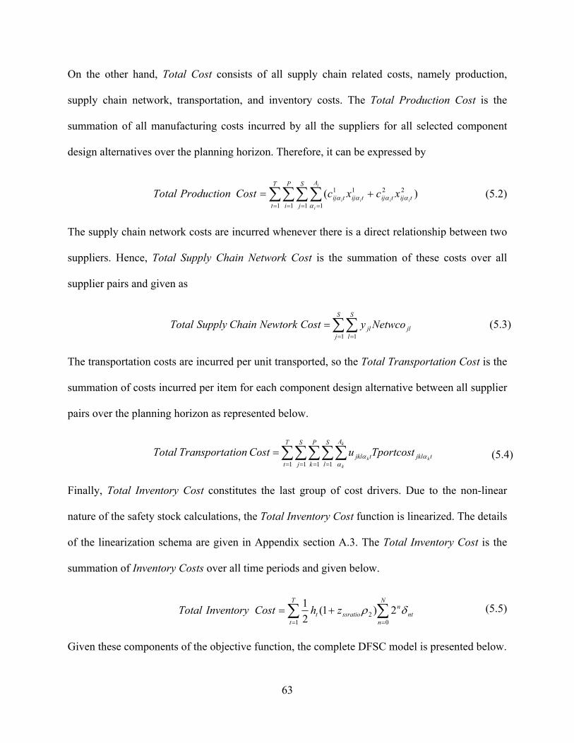
63

On the other hand, Total Cost consists of all supply chain related costs, namely production,

supply chain network, transportation, and inventory costs. The Total Production Cost is the

summation of all manufacturing costs incurred by all the suppliers for all selected component

design alternatives over the planning horizon. Therefore, it can be expressed by

The supply chain network costs are incurred whenever there is a direct relationship between two

suppliers. Hence, Total Supply Chain Network Cost is the summation of these costs over all

supplier pairs and given as

The transportation costs are incurred per unit transported, so the Total Transportation Cost is the

summation of costs incurred per item for each component design alternative between all supplier

pairs over the planning horizon as represented below.

Finally, Total Inventory Cost constitutes the last group of cost drivers. Due to the non-linear

nature of the safety stock calculations, the Total Inventory Cost function is linearized. The details

of the linearization schema are given in Appendix section A.3. The Total Inventory Cost is the

summation of Inventory Costs over all time periods and given below.

Given these components of the objective function, the complete DFSC model is presented below.

(5.5)∑ ∑= =

+=T

t

N

nnt

nssratiot zhCostInventoryTotal

1 02 2)1(

21 δρ

(5.2)∑∑∑∑= = = =

+=T

t

P

i

S

j

A

tijtijtijtij

i

i

iiiixcxcCostProductionTotal

1 1 1 1

2211 )( α

αααα

(5.3)∑∑= =

=S

j

S

ljljl NetwcoyCostNewtorkChainSupplyTotal

1 1

(5.4)∑∑∑∑∑= = = =

=T

t

S

j

P

k

S

l

A

tjkltjkl

k

k

kkTportcostuCosttionTransportaTotal

1 1 1 1

α

αα

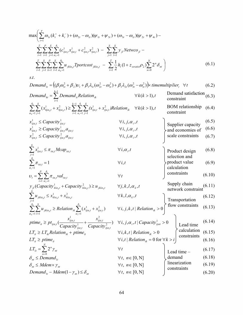
64

(6.3)

(6.1)

(6.2)

(6.4)

(6.5)

⎟⎠

⎞+−

−−+

−⎜⎝

⎛+−++−++

∑ ∑∑∑∑∑∑

∑∑∑∑∑∑

∑

= == = = = =

= == = = =

=

−+

T

t

N

nnt

nssratiot

T

t

S

j

P

k

S

l

A

tjkltjkl

S

j

S

ljljl

T

t

P

i

S

j

A

tijtijtijtij

T

tttttttttttt

zhTportcostu

Netwcoyxcxc

kk

k

k

kk

i

i

iiii

1 02

1 1 1 1 1

1 11 1 1 1

2211

1421331121

2)1(21

)(

))(())(()(max

δρ

ψψωωψψωωω

ααα

ααααα

( )

tkkRelation)x(xxx

tkkRelationDemandDemand

tliertimemultipDemandts

ik

k

i

A

α

S

jtijαtijα

A S

jtkjtkj

ikitkt

tttttttttt

i

i

ii

k

k

kk),1()(

),1(

)()()(..

1

1 1 1

21

1 1

21

1-k

1i

21

2321

21

22112

2111

>∀+≥+

>∀=

∀×−+−++=

∑∑∑∑∑

∑−

= = == =

=

ααα

ωωλβωωλβυβωβ

tval

ti

,tiMcapx

P

i

A

titit

A

ti

ititi

S

jtij

i

i

ii

i

i

i

iii

∀=

∀=

∀≤

∑∑

∑

∑

= =

=

=

1 1

1

1

1

,1

,

ααα

αα

ααα

πυ

π

απ

tjiaCapacityxtjiaCapacityxtjiCapacityx

itijtijtij

itijtijtij

itijtij

iii

iii

ii

,,,,,, ,,,

22

11

11

ααα

ααα

ααα

αα

∀≤∀≥∀≤

0|,,,)(

,,,

,,,, )(

1

21

1 1

21

1

21

>∀+≥

∀+≤

∀≥+

∑∑∑

∑

== =

=

ik

A

tijtijik

A S

ltjkl

ktkltkl

S

jtjkl

ktjkltkltkljl

RelationtkjixxRelationu

tlkxxu

tlkjuCapacityCapacityy

i

i

ii

k

k

k

kkk

kkk

ααα

αα

ααα

ααα

α

α

ikRelationtiptimeLTRelationtkiptimeRelationLTLT

CapacitytjiCapacity

xCapacity

xptptime

ikitit

ikitikktit

tijitij

tij

tij

tijtijit

i

i

i

i

i

>∀=∀≥>∀+≥

>∀+≥

for 0|,0|,,

0|,,,)( 12

2

1

1

αα

α

α

αα α

N][0, , )1(N][0, ,N][0, ,

2

1

1

01

∈∀≤−−∈∀×≤∈∀≤

∀=∑=

ntMdemDemandntMdemntDemand

tLT

ntntt

ntnt

tnt

N

nnt

nt

δγγδ

δ

γ

(6.6)

(6.7)

(6.8)

(6.9)

(6.10)

(6.11)

(6.12)

(6.13)

(6.14)

(6.15)(6.16)

(6.17)(6.18)(6.19)

(6.20)


BOM relationship constraint

Supplier capacity and economies of scale constraints

Product design selection and product value calculation constraints

Supply chain network constraint

Transportation flow constraints

Lead time calculation constraints

Lead time – demand linearization constraints

65

}1,0{,,,,,,,

0,,,,,,,,,,,,,,,

)(

)(

1

)(

)(

}2,1{,1}2,1{, }2,1{,

1

21

43212121

114

112

1124

4

113

111

1113

3

22

22

2

11

11

1

11

11

1 1

21

11

11

1 1

21

11

1

1

1 1

21

111

11 1

21

11

11

21

1

1

1

1

1

1

1

1

1

1

1

1

1

1

1

1

1

1

1

1

1

1

1

1

1

1

11

1

1

1

1

1

11

1

1

11

1

1

11

1

1

1

∈

≥

∀+≤+

∀≤

∀≤

∀+≤+

∀≤

∀≤∀+≤+∀≤∀≤∀+≤+∀≤∀≤

∀+≤++

∀≤

∀+≤

∀+≤+∀≤∀≤∀≤+

∀+−≥

∀−+≥

∈∀+≤+∈∀≤∈∀≤

∀≤+

−+

−+

=

−

=

=

−=

−

=

=

−

+

+

+

+=

−

=

−

= =

=

−−

= =

−

++

++

+

−+= =

−

= ==

+

∑∑

∑

∑∑

∑

∑∑∑∑

∑

∑∑

∑∑

∑∑∑

nttttttijjlti

nttktttttttttitittjkltijtij

A

ttt

A

tt

A

ttt

tt

A

ttt

A

tt

A

ttt

tt

ttt

tt

tt

ttt

tt

tt

A

tt

A

tt

A S

jtjtj

A

ttt

A S

jtjtjt

ttt

tt

tt

tt

A S

jtjtjtt

t

A S

jtjtj

A

tt

qttqt

tqt

qtqt

tt

ii

kii

ay

DemandkkptimeLTuxx

tMcapkMcap

tMcap

tk

tMcapkMcap

tMcap

tktMdemkMdemtMdemtktMdemkMdemtMdemtk

tMcapkMcapxx

tMcapk

txxk

tMdemkMdemDemandtMdemktDemandkt

txxDemandMdem

tDemandxxMcap

qtqtqt

t

γφφττπ

δυψψψψλλ

ψφ

φψ

ψ

ψφ

φψ

ψψφ

φψψ

ψφφψ

ψ

τ

τ

ττ

ττ

τ

τ

λυφυλφλφφ

αα

ααα

αα

αα

αα

αα

αα

αα

αα

αα

ααα

αα

ααα

ααα

ααα

αα

(6.21)(6.22)(6.23)(6.24)

(6.25)

(6.26)

(6.27)(6.28)(6.29)(6.30)

(6.31)

(6.32)

(6.33)

(6.34)(6.35)(6.36)(6.37)(6.38)(6.39)(6.40)

(6.41)

(6.42)

(6.43)

(6.44)

(6.45)

(6.46)

66

Equation (6.2) calculates the demand of the final product (component 1) for each time period

based on selected component design alternatives, price, and the time period adjustment

parameter. The original demand function in non-linear form is given below.

Since equation (7.1) is non-linear due to multiplication of the price and υ variables, a

linearization schema is presented in Appendix section A.2. Equation (6.3) does not necessarily

constrain the feasible region, but instead is used to evaluate the demand for each selected

component alternative design based on the demand for the final product and Bill of Materials

data. Similarly, equation (6.4) makes sure that each component that is assembled into another

one is manufactured in at least an amount required by the Bill of Materials data. The difference

between these two equations is that equation (6.4) constrains the minimum manufacturing

quantity of a component where equation (6.3) only calculates the demand for this component but

does not enforce any limits on the manufacturing amounts. Equations (6.5), (6.6), and (6.7)

establish supplier capacity limits and an economies of scale structure as explained in preliminary

models. The next three constraints incorporate the product design decisions into the model. The

first constraint (6.8) ensures that only selected component alternative designs (for which πiαit = 1)

are manufactured. The second product design constraint (6.9) requires that exactly one

component design alternative is selected for each component in each time period. The last

product design constraint (6.10) is used to calculate total value of the final product based on

component design alternative selections. The supply chain network design is set up by the

equation (6.11) by making sure that two suppliers are linked (that is yjl = 1) if any transportation

occurs between them (that is ujklαkt > 0) for a component. Equation (6.12) guarantees that the

total amount of a component transported from a supplier is at most the manufactured quantity by

tttt liertimemultippriceDemand ××+= υββ )( 22

11 (7.1)

67

this supplier. The next constraint (6.13) makes sure that for a component manufactured at a

certain supplier, all required subcomponents are transported to this supplier from other suppliers.

Equations (6.14) through (6.17) are used to calculate the lead times. Equation (6.14), similar to

the equation (3.6) described in the preliminary models, makes sure that the production time of a

component is at least equal to the longest time it takes for manufacturing this component among

all the suppliers that manufacture this particular component. This constraint is necessary since it

is assumed that the production of a component starts only after all of its subcomponents are

delivered to the manufacturer. Therefore, the longest production time among all of a

component’s suppliers is defined as the production time of this component. However, different

from the preliminary modeling, in this complete model it is assumed that production time data

(ptijαit) is given for the total capacity of the supplier, hence the final production time of a

component at a particular supplier is determined relative to the capacity utilization of this

supplier. For example, if a supplier states that it takes 10 days to manufacture the complete batch

in full capacity utilization, then the model decides that the production time of this component at

this supplier would be 5 days if half the capacity is used. Equations (6.15) and (6.16) are used to

calculate the final lead time of a component in the same fashion described in the preliminary

models where the former constraint (only defined for components which have subcomponents)

ensures that the lead time of a component is equal to the summation of its own manufacturing

time and the maximum lead time of its subcomponents. The latter constraint is used only for the

components which do not have any subcomponents to make sure that their final lead time is at

least equal to their production times. In the lead time constraints set, the last equation (6.17) is

used to represent the final lead time of the main product with binary variables for inventory cost

linearization described in Appendix section A.3.

68

Constraints (6.18) through (6.45) are used for linearization of the model and do not

impose any actual limits on the product and supply chain design. Equations (6.18), (6.19), and

(6.20) ensure that δnt variables take values to truly represent demand – lead time multiplication in

a binary format. Similarly, while equation (6.21) ensures that only one of the second or third

price levels is selected, the following three equations ((6.22), (6.23), and (6.24)) ensure that the

λ1t and λ2t variables take correct values to capture price and product design value multiplications.

In order to calculate the satisfied demand, which is the minimum of demand and total

production, equations (6.25), (6.26), and (6.27) control the τt+ and τt

- variable values to represent

whether the demand or the total production is larger. Based on these τt+ and τt

- values, kt+ and kt

-

variables take the minimum of the demand or the total production via equations (6.28) through

(6.33). The following ten constraint sets, equations (6.36) through (6.45), control the ψ variables

that are used in revenue calculation and described in revenue linearization in section A.1 of the

Appendix. Finally, equation (6.46) establishes the required variable types and bounds.

This complete DFSC model formulation defines all of the considered problem aspects

under the stated assumptions. Therefore, this model is used as the base formulation to investigate

research questions. However, this research not only investigates the proposed DFSC concept but

it also focuses on different modeling practices and the tradeoffs between solution performance

and model features. As the complete DFSC model is very large and complex, despite the

simplification by linearization of the model, it requires too much computational time and power

to optimize. In addition, this model entails several parameters that sometimes companies cannot

estimate easily. Therefore, different reduced models are developed to investigate the impacts of

certain concepts on the value of the model and solution time and quality. The following section

(3.4) provides different models that are derived from the developed complete DFSC model.

69

3.4 REDUCED MODELS

As stated in the research question 1, this research aims to investigate the importance of different

product design and supply chain performance metrics in real industry cases as well as their

impacts on modeling the DFSC problems and impacts on the performance of the solution

techniques. Therefore, to investigate impacts of different performance metrics, different reduced

DFSC models are developed. These models are based on the developed complete DFSC model

and they are developed by removing some model features, changing some assumptions, or both.

These models are presented below and the differences from the complete model are explained.

The impacts of these changes on the validation of the model and performance of the solution

techniques are discussed in sections 5.2 and 5.3.1, respectively.

Initially, the economies of scale concept is removed from the complete model resulting in

the reduced DFSC model 1. Although this is a widely used concept both in industry and

academia in supply chain modeling, for simplification purposes, it is usually modeled by using

piecewise linear functions with only a couple of segments as in the complete DFSC model.

Therefore, the actual representation of the economies of scale concept is often only an

approximation in order to keep the models linear. In addition, the unit manufacturing cost data is

often estimated for a long-term planning in such models thus it involves a significant amount of

uncertainty. Moreover, demanding more detailed cost data based on the capacity utilization of

the suppliers only amplifies this uncertainty. Briefly, the first reduced model investigates the

impacts of removing the economies of scale concept from the DFSC modeling. It is assumed that

using an average unit manufacturing cost (thus having a less realistic model) is a reasonable

trade off for the increased uncertainty due to more detailed data requirements for the economies

of scale modeling.

70

In the complete DFSC model, the economies of scale were introduced by dividing the

supplier capacities into two different levels and using an associated two-level unit manufacturing

cost structure. This representation drives constraints given in equations (6.6) and (6.7) and also

requires the introduction of a binary variable, aijαit, to control the proper application of the

concept. As a result, removing the economies of scale concept eliminates these two constraints

and the corresponding binary variable. In addition, since the production quantities at each

supplier are no longer divided into two levels, the second level manufacturing quantity variable,

xijαit2, and the second level capacity parameter, Capacityijαit

2, are no longer necessary. As it is

discussed in the model asymptotic size analysis section (3.5), these changes significantly reduce

the number of variables and constraints. The mathematical formulation of the reduced DFSC

model – 1 is given in Appendix B.1.

In the reduced DFSC model 2, the impacts of removing the lead time (and thus inventory)

from the complete DFSC model are investigated. This reduced model is based on the complete

DFSC model therefore it utilizes the economies of scale concept. When the lead time concept is

removed, only the direct cost related supply chain performance metrics remain in the model. As

it is discussed in the model validation section (5.2), the lead time data is often hard to collect or

estimate compared to the cost data. In addition, supply chain costs are usually determined and

fixed for a period through contractual agreements where the lead time depends on the actual

daily operations and varies greatly. Although contracts may oblige supply chain partners to

perform within certain lead time limits via penalties or other sanctions, it is still very hard for

companies to estimate a true lead time for a supply chain in the long-term. Furthermore, the

inventory levels highly depend on the inventory keeping and product ordering policies. The

variability of the lead time and demand also requires certain assumptions as discussed in the

71

complete model formulation section (3.3) such as constant coefficient of variation and linearly

changing average inventory levels. Therefore, it may be preferable to neglect inventory and lead

time concepts in the initial planning stage and consider them separately in a later phase of the

supply chain planning process to save from the model solution time and achieve the optimal

solution. The impacts of removing the inventory and lead time concepts on the model and

solution quality are discussed in section 5.3.1 in detail. The mathematical formulation of the

reduced DFSC model – 2 is given in Appendix B.2.

In the complete DFSC model, the lead time and inventory cost concepts require several

binary (γnt, δnt) and continuous (LTit, ptimeit) variables. In addition, removing lead time and

inventory concepts makes the related parameters (ptijαit, ht, periodlengtht, zssratio, ρ1, ρ2)

redundant. Finally, constraints (6.14) through (6.20) and the inventory cost calculation in the

objective function, which is given in equation (5.5), can be removed from the model. The

significance of the removal of these variables and constraints are discussed in section 3.5.

3.5 MODEL ASYMPTOTIC SIZE ANALYSIS

In this section, an asymptotic size analysis of the preliminary, complete, and reduced models is

provided. This analysis summarizes the changes in the number of variables and number of

constraints, as well as the expected performance of the solution techniques.

Preliminary Models

The complexity of the proposed models increases not only by the number of product components

and suppliers, but also with the interactions between them. For the cost minimization model, the

number of variables is equal to 4(PS)+S2, where P is the number of components and S is the

72

number of total suppliers. 2PS of these variables are binary, where the rest are non-negative

continuous variables. The number of supply chain generation constraints depends on the direct

relationships between the components therefore only an upper bound can be calculated. The

maximum number of total constraints is equal to P(PS2+3S+1).

For the lead time minimization model, the number of variables is equal to 4PS+2P,

where 2PS of these variables are binary. The number of constraints is based on the relationships

between the components, and between components and suppliers. Therefore, an upper bound for

the total number of constraints is P(P+4S+2).

As shown above for both models, the number of variables and constraints increase

significantly when the number of components or suppliers is increased.

Complete DFSC Model

Among the developed models, the complete model captures all the described concepts and

assumptions, making it the most complex model in terms of variables, constraints, and their

interactions. By using the model’s set notation, the total number of the variables in the complete

DFSC model can be expressed as S2+T(13+2N+3P+[(PAi)(1+3S+S2)]), where T is number of

time periods, Ai is total number of design alternatives for the component i, and N is number of

lead time – demand binary variables. Therefore, the number of variables in this model increases

linearly with the number of components, number of time periods, number of lead time – demand

binary variables, and number of design alternatives per component when one of them is

increased and the others are constant. However, the number of variables increases with the

square of the number of available suppliers when the number of other variables is constant;

hence this parameter has the most significant impact on the model size.

S2+T(4+N+[(PAi)(1+S)]) of these variables are binary and this shows that the number of

73

available suppliers is critical as the binary variables increase the solution time significantly more

than continuous variables. It should be noted that among all variables, the number of xijαit1, xijαit

2,

ujklαkt, πiαit, yjl, and aijαit variables, which were described in section 3.3, highly depends on the

model set sizes and their interactions, where the number of ujklαkt and yjl variables increases with

the square of the number of available suppliers, significantly increasing the model size.

Similar to the preliminary models, the exact number of constraints in the complete DFSC

model depends on the parameter values which define component – supplier relationships, Bill of

Material information, and component design alternatives. An upper bound on the constraints is

equal to T(30+3N+P[4+P+PS+Ai(1+5S+S2)]), which suggests that the total number of

constraints significantly depends on the number of time periods. This is due to the structure of

the model to capture the total life cycle of the product based on life cycle phases rather than

using short time periods for tactical or operational planning.

The model analysis suggests that the complete DFSC model size highly depends not only

on the size of the parameter sets but also on the interactions between these sets. Therefore, each

problem instance differs by size and complexity and larger problems may have significantly

fewer constraints due to relatively simpler Bill of Materials or component – supplier interactions.

Reduced Models

In the first reduced model, where the economies of scale concept is removed, the total number of

variables is reduced by 2PSAiT to S2+T(13+2N+3P+[(PAi)(1+S+S2)]). The significance of this

reduction is from the fact that PSAiT of these variables are binary, promising a significant

reduction in solution times. In addition, with the removal of the economies of scale concept, the

upper limit on the total number of constraints is reduced by 2PSAiT due to elimination of

74

equations (6.6) and (6.7). It should be noted that although the reduction in the number of

constraints is important, having fewer binary variables notably reduces the solution space.

With the exclusion of lead time and inventory cost concepts, the second reduced model

employs 2T(P+N) less variables than the complete DFSC model. This reduction eliminates a

total of TN binary variables (γnt) which is less than the binary variable reduction in the first

reduced model. In terms of constraint reduction, the second reduced model cuts

T(3N+P+P2+PSAi) constraints by purging equations (6.14) through (6.20). The total reduction in

the number of constraints is less than the same reduction in the first reduced model provided that

the P<SAi condition is true. It should be noted that this condition would hold in almost all real

cases unless the majority of the considered components are manufactured by a very small set of

suppliers. This analysis suggests that the first reduced model reduces more variables and

constraints suggesting a shorter solution time as compared to the second reduced model. Section

5.3.1 specifically addresses the solution quality and time performances of the reduced models.

Table 2 summarizes the total number of variables and maximum number of constraints

possible for each developed model.

75

Table 2: Summary of number of variables and constraints in different models

Number of Variables

Number of Integer Variables Number of Constraints

Preliminary Models Preliminary cost minimization model 4PS+S2 2PS+S2 P(PS2+3S+1)

Preliminary lead time minimization model 4PS+2P 2PS P(P+4S+2)

Preliminary reduced cost minimization model 4PS 2PS 3PS+P

DFSC MIP Models

Complete DFSC model S2+

T(13+2N+3P+ [(PAi)(1+3S+S2)])

S2+T(4+N+ PAi[1+S])

30T+3NT+ PT[4+P+PS+Ai(1+5S+S2)]

Reduced DFSC model – 1 S2+

T(13+2N+3P+ [(PAi)(1+S+S2)])

S2+ T(4+N+PAi)

30T+3NT+ PT[4+P+PS+Ai(1+3S+S2)]

Reduced DFSC model – 2 S2+

T(13+P+ [(PAi)(1+3S+S2)])

S2+T(4+ PAi[1+S])

30T+ PT[3+PS+Ai(1+4S+S2)]

In order to illustrate the significance of the reductions in the number of variables and constraints,

Table 3 summarizes these values for all different models based on a problem instance with 10

components, 3 design alternatives for each component, 15 suppliers, 4 time periods, and 8 lead

time – demand binary variables.

76

Table 3: Numerical illustration of model asymptotic size of different models

Number of Variables

Number of Integer Variables Number of Constraints

Preliminary Models Preliminary cost minimization model 825 525 22,960

Preliminary lead time minimization model 620 300 720

Preliminary reduced cost minimization model 600 300 460

DFSC MIP Models

Complete DFSC model 32,981 2,193 42,896

Reduced DFSC model – 1 29,381 393 39,296

Reduced DFSC model – 2 32,837 2,161 40,560

This numerical illustration presents a 10.92% reduction in number of variables for the reduced

DFSC model – 1 and 0.44% reduction for the second reduced DFSC model. More importantly,

the reduction in the number of binary variables, which challenge and lengthen the solution

procedures, is 1,800 for the first reduced model and 32 for the second reduced model.

77

4.0 SOLUTION METHODOLOGY

In order to solve the developed MIP models, a deterministic optimization method (branch and

bound) and different metaheuristics are investigated. This chapter provides a brief history of

these methods followed by the details of specific implementations for this research. Finally, their

performance test results on the preliminary test models are presented.

4.1 DETERMINISTIC OPTIMIZATION METHODOLOGIES

4.1.1 Overview

Deterministic optimization methodologies include all varieties of solution techniques that are

aimed toward solving the problems that only involve deterministic parameters and variables.

Problem formulations that only include continuous variables and linear functions are solved by

using Linear Programming (LP), which was mainly developed during World War II and evolved

by incorporation of fast and optimal guaranteed solution methods such as the Simplex

Algorithm. For a problem to be formulated as an LP, it should satisfy four assumptions [63]. The

first one is the linearity assumption that states each of the variable’s contribution to any equation

in the model is constant and these contributions are additive, therefore prohibiting any

interactions (including multiplication and division) of the variables. The second assumption

78

(divisibility) states that all of the variables in the model are continuous. The third assumption is

certainty which requires all the model parameters are to be known constants, thus it assumes that

the model is solved under perfect information. The final assumption is that the model has a

single objective which is optimized under the other assumptions. However, many real problem

cases violate the divisibility assumption by requiring either all or some of the variables to take

integer values. When all of a model’s variables are required to take integer values, this model

formulation is called Integer Programming (IP). On the other hand, when models engage both

continuous and integer variables, they are named as Mixed Integer Programming formulations.

The MIP problems are usually very hard to solve effectively compared to the LP

problems. However, certain methods are developed to accelerate the solution procedures (e.g.,

branch and bound, cutting plane, branch and cut, delayed column generation) and save time over

the enumeration of all possible integer solutions. Since this research does not evaluate nor use all

of these methods, only the branch and cut method is discussed in detail. The branch and cut

method is actually a combination of branch and bound and cutting plane methods. The branch

and bound method, first introduced by Land and Doig [38] in 1960, aims to shrink the search

space for the problem by pruning unpromising search space regions thus saving computational

time. The underlying process of this method is that after the initial LP relaxation of the problem

is solved, the solution space is divided into smaller sub-solution spaces (branching). During this

process, a solution tree is constructed to keep track of which solutions (nodes) have which

variables at the integer values and the objective values of these solutions. Within the process, the

time savings come from pruning the unpromising branches of the tree instead of spending time

on these solutions as in the complete enumeration. By keeping track of each node’s best possible

solution value, as an upper (or lower) bound, other nodes that have worse bounds can be

79

removed from the search space. The cutting plane method, first introduced by Gomory [28] in

1963, aims to add new specially structured constraints (cuts) to the original model in order to

eliminate the non-integer optimal solution for the initial model relaxation. These cuts are

constructed in a special formation so that they do not remove any feasible integer solutions from

the search space when eliminating the current non-integer solution. The branch and cut method

used in this research is a combination of branch and bound and cutting plane methods, where

during the branch and bound algorithm, relevant cuts are introduced to further reduce the

solution space size.

The most significant feature of solving LP and MIP problems by the mentioned methods

is that finding the optimal solutions to these problems is guaranteed, provided one exists.

However, MIP problems are usually very hard to solve to the optimal value due to the drastically

increasing solution space size for larger problems. In this case, the specially structured solution

procedures such as heuristics and metaheuristics need to be considered. Their details are

discussed in section 4.2. The following section provides the computational test results of the

described MIP branch and bound solution procedure on the preliminary models.

4.1.2 Performance on the Preliminary Models

In order to perform tests on the performance of MIP and metaheuristics, five different illustrative

problem instances are generated randomly for the preliminary models. Table 4 shows detailed

information about each of these problem instances.

80

Table 4: Illustrative test problem data for the preliminary models

Problem Instance

Number of Components

Number of Suppliers

Number of Components per

Supplier 1 5 10 1-3 2 10 20 1-4 3 25 50 1-7 4 50 100 1-14 5 100 200 1-19

For all instances, unit manufacturing costs (that suppliers charge per component produced) are

selected randomly based on a uniform distribution (here to referred as uniform-randomly) from a

[10-100] interval for the first production level and from a [1-70] interval for the second

production level. However, the second level cost is forced to be less than or equal to the first

level cost to ensure the economies of scale concept is considered. Similarly, first and second

level capacity values for each component-supplier pair are selected uniform-randomly having the

second level capacity larger than or equal to the first level capacity. For all instances, lead times

are distributed uniform-randomly from a [100-1,000] interval. SC network costs are again

selected uniform-randomly from a [10,000-1,000,000] interval.

The MIP solution technique is utilized by using the CPLEX® optimization software to

optimize each model separately. CPLEX® uses a robust branch and cut algorithm to solve MIP

models optimally in a short time period, however MIP models tend to increase in size

significantly as the number of variables increases making the solution procedure very time

consuming. The behavior of the MIP solution techniques for small and large models is tested and

the results and the performance of the solution procedure is analyzed.

All CPLEX® runs are completed on the Microsoft Windows® XP platform on a computer

with an Intel® Pentium 4 3.06 GHz CPU and 1 GB of RAM.

81

The cost minimization and lead time minimization models are solved by using default

CPLEX® parameters as the base case. Table 5 shows the results of the cost minimization runs

where Table 6 reports results of the lead time minimization runs. Problem instance 4 in the cost

minimization model and problem instance 5 in the lead time minimization model cannot be

solved to the optimal value due to memory limitations. Therefore, the best found integer

solutions are reported.

Table 5: MIP cost minimization model preliminary run results

Problem Instance

Final Integer Solution ($)

Relative Optimality Gap*

Solution Time (in seconds)

1 21,769,159 0.00 % 0.11 2 56,899,401 0.00 % 0.21 3 46,931,986 0.00 % 2,457.76 4 81,096,271 16.18 % 494,246.30 5 381,543,320 0.00 % 113,737.19

* Relative optimality gap is the percentage of the gap between the best known integer solution and the best possible integer solution (a lower bound).

Table 6: MIP lead time minimization model preliminary run results

Problem Instance

Final Integer Solution (hr.)

Relative Optimality Gap*


1 2,704 0.00 % 0.13 2 3,381 0.00 % 0.13 3 1,695 0.00 % 5.59 4 2,193 0.00 % 228.69 5 3,108 11.03 % 102,465.21

* Relative optimality gap is the percentage of the gap between the best known integer solution and the best possible integer solution (a lower bound).

The MIP results show that as the problem size gets larger, the solution time increases

significantly. The time increase is more significant in the cost minimization model due to its high

dependency on the relationships between the components and suppliers as described in the model

82

complexity section. However, the cost minimization model results show that both the solution

quality and the solution times depend on the exact problem instance values in addition to the

problem instance size. For example, problem instance 4 cannot be solved to the optimal value in

more than 5 days and is stopped due to memory limitations where the largest problem instance

(5) can be solved to the optimal point in 1.5 days.

4.2 HEURISTICS AND META HEURISTICS

As specified before, the time to solve a MIP problem with branch and cut method increases

significantly as the problem size gets larger. In this case, heuristics and metaheuristics present an

important alternative to the deterministic optimization methods.

4.2.1 Overview

Heuristics, in general, can be defined as special algorithms which are designed to solve a

problem much faster than the traditional optimization methods, occasionally by guaranteeing an

optimal solution or sometimes by providing an approximation limit to the real optimal solution.

It should be noted that this approximation limit may be infinite, meaning that no guaranteed

optimality approximation is provided by the heuristic. In this sense, heuristics are often designed

specifically for a problem (and formulation) and they exploit the problem structure to efficiently

come up with good solutions in a shorter time (e.g., Nearest Neighborhood Algorithm for

Traveling Salesman Problems and Dijkstra’s Algorithm for Shortest Path Problems). However,

this special design of the algorithm for a particular problem limits its applicability on other

83

problems. In addition, some heuristics are not always developed to optimize a problem but to

find a feasible solution very quickly. Especially for large combinatorial optimization problems,

MIP techniques may stall even before finding a feasible solution, encouraging the use of

heuristics.

Metaheuristics, alternatively, are special types of heuristics that are applicable to a wide

range of problems and they are not limited by the problem structure and formulation. However,

metaheuristics often utilize some randomness in the search process. In addition, metaheuristics

usually move in the search space by utilizing specially designed operations to evaluate a portion

of the search space to come up with a good solution quickly. In general, a particular solution

quality cannot be guaranteed for metaheuristics. There exist various metaheuristics for different

types of problems but the most common ones include Genetic Algorithm (GA), Tabu Search

(TS), Simulated Annealing (SA), Ant Colony Optimization (ACO), and Greedy Algorithm

(GrA).

The application of different metaheuristics on the supply chain problems are discussed in

section 2.3. In this research, GA and TS are selected as candidate metaheuristics for the DFSC

problem since they are the commonly used techniques and their performances are known to be

very good for these types of problems. Initially, these metaheuristics are evaluated by using the

preliminary model formulations. A brief history of these methods and their application details are

given below.

Genetic Algorithm

The Genetic Algorithm was initially developed by Holland and his associates at the University of

Michigan in the 1970s [33]. The GA has a biological basis. In brief, the GA imitates the

operations of Darwin’s Theory of Evolution such as crossover and mutation, to find the optimal

84

solution (even though it is not guaranteed). The main idea behind the algorithm is to reach a

“good” solution by employing these operations on an initial set of solutions, namely an initial

population. The individual solutions, which as a set constitute a population, are called

chromosomes. Each chromosome represents a solution for the problem and therefore is encoded

to represent a particular solution. Encoding is an important issue for the GA since it dictates how

the algorithm advances by limiting the search space and determining the structure of certain GA

operators. The chromosomes are often encoded by using binary values for yes – no, open – close

and similar decisions or by using integer and/or real numbers to represent real values that the

corresponding problem variables could take. Every following generation after the first one is

generated by creating new offspring by applying crossover to two selected parent chromosomes

from the previous generation and sometimes also letting the best ones live without performing

crossover (elitist approach). Mutation is used to partly modify the old generation’s individuals or

the newly created offspring in order to diverse the search. The GA has certain advantages over

other search and optimization methods which are its ability to search the solution space

extensively without being stuck on a local optimal point and being computationally beneficial

especially for large problem instances. However, its major drawback is that it does not guarantee

a global optimal solution which is common for metaheuristics in general. For further detailed

information about GA, refer to Goldberg [27].

Tabu Search

Tabu Search is a metaheuristics solution algorithm that employs a memory structure that defines

the way the algorithm moves through the search space. Attributed to Fred Glover [25][26], it was

originally developed two decades ago. Since then, several refinements have been made to the

algorithm making it more powerful. The main idea of TS is to keep track of previous moves in

85

the solution space and diversify the search by encouraging the search process to move to

unexplored regions of the solution space by preventing going back to previous steps. This is

implemented by a so called “tabu list” which consists of changes made to the solutions in the

previous steps. Whenever the algorithm searches for another solution, it is blocked from

considering previous solutions as alternatives, thus it is forced to move to an unexplored region

of the solution space.

As a first step in a TS procedure, solutions are defined and coded into a solution array

similar to the chromosome concept in the GA. The structure of the solution array is very

important since it determines the possible operations to be utilized on it. Another important TS

concept is “neighborhood” which defines the set of all solutions that lie near the current solution.

Each solution is considered to be within the neighborhood of the current solution if it can be

reached directly from the current solution by an operation called a “move.” Therefore, move and

neighborhood are closely related terms and setting one help dictate the other.

In general, the TS algorithm starts by picking a solution randomly from the solution

space. After evaluating the objective value for that solution, it evaluates objective values of all

feasible solutions within the neighborhood of the current solution and moves to the “best” one in

the neighborhood. After a new current solution is fixed, the previous move operation is added

into the tabu list thus preventing the algorithm from evaluating the previous solution as a

candidate for the next step. As the algorithm moves through the solution space in this manner,

the tabu list fills and many moves become prevented. The usual application is to set a limit for

the number of tabu moves, so after a certain number of iterations, the oldest move is removed

from the list and it is allowed to be examined again. Although the TS algorithm has a tendency to

pick a solution with a better objective function value than the current one on every iteration, the

86

tabu list may prevent it from doing so. Therefore, the algorithm is sometimes forced to move to a

worse solution which helps diversifying the search and preventing being stuck in a local optima.

In addition to the tabu list, which keeps track of last moves thus called “short term

memory,” some “long term memory” concepts are also popular in the TS. The long term

memory generally uses the frequencies of solution segments (attributes), e.g., how many times a

solution segment occurs in the search. This type of memory is used to employ “diversification,”

which aims to force the algorithm to search a wider area by selecting less frequently used

attributes or “intensification” which compels the algorithm to focus on a particular region by

urging more frequently used attributes. It should be noted that there are many extensions and

variations used in TS applications to improve the solution process. For further details of TS

concepts, refer to Glover and Laguna [26].

4.2.2 Performance on the Preliminary Models

In this research, the GA and TS algorithms are coded in Visual Basic by using Microsoft Visual

Studio® 6.0 and run on the same hardware as described in MIP performance testing on the

preliminary models.

Genetic Algorithm

In a GA, genes, which are elements within a chromosome, can take different values (called

alleles) such as continuous, integer, or binary numbers. They define the structure of a

chromosome and therefore have drastic impacts on the behavior, the solution quality, and

computational time of the algorithm. In the preliminary testing implementation of the GA, the

chromosomes represent the solutions with binary genes. Each chromosome represents a complete

solution of the problem where all possible component–supplier pairs are decided to be active (in

87

use) or inactive. Each gene of the chromosome corresponds to a component – supplier pair and

an allele value (1 or 0) of the gene represents the status of the corresponding pair; 1, being an

active pair and 0, an inactive pair. Figure 6 depicts an illustrative chromosome structure.

Component – Supplier Relationship p1-s1 p1-s2 p2-s1 … … pp-ss-2 pp-ss-1 pp-ss 1 = used pair 0 = unused pair 1 1 0 … … 0 1 0

Figure 6: Chromosome structure of the Genetic Algorithm for the preliminary models

It should be noted that only the possible component – supplier pairs are included in the

chromosome structure hence only available suppliers for manufacturing a component are listed

under this particular component’s section. For example, a chromosome structure for a problem

set can be as comp1-supplier2, comp1-supplier5, comp2-supplier3, comp2-supplier6, etc.

The GA solution procedure begins with creation of the initial population. For the next

steps, new generations are created by applying two major genetic operators and additional

procedures. After copying a certain number of best solutions to the next generation directly

(elitist selection rule), new solutions are created by a crossover operator which selects two

parents (two solutions from the previous generation) according to a roulette wheel selection rule.

In this rule, all solutions have a certain probability of being selected as parents which is

distributed according to the objective value of the solution, called the fitness value. Then a cut

point is selected randomly based on a uniform distribution (hereafter referred to as

uniform-randomly) and the offspring is created by copying the genes from the first parent up to

the cut point and copying the rest from the second parent. With a certain probability, these new

88

solutions are mutated, which means some genes of the solution are randomly flipped from 1 to 0

or vice versa making any part – supplier pair active or inactive. This mutation procedure adds

diversity to the populations and helps prevent being trapped in local optimal solution spaces or

early convergence.

Since the defined problem has some constraints, crossover and mutation procedures may

lead to infeasible solutions because of their random altering nature. Therefore, a repair

procedure, that eliminates the infeasibility of a solution, is employed. Due to the structure of the

chromosome and genetic operators, infeasibility can only occur in a segment of a chromosome

that corresponds to a single particular part whose genes either come from different parents or are

mutated. For that part’s chromosome segment, the repair procedure uniform-randomly selects

genes to change their value into 1 (to use more suppliers to satisfy the demand) until infeasibility

is removed. Although this procedure disturbs the exact replication of parents’ structures, it has a

small impact in the solutions since only a single segment among many is repaired and major

chromosome structures of parents are preserved.

Finally, an immigration concept is employed to ensure the diversity of the population to

search a wider solution space and prevent convergence to local optimal solutions. In this

procedure, a certain percent of the population is randomly generated instead of being created by

using individuals from the previous generation in reference to immigration in nature. If no

improvements are observed in the last certain number of generations, the population is “kicked”

where after elitist chromosomes are copied, the rest of the population is created randomly similar

to the immigration concept. In this case, crossover and mutation operators are not used for the

new population. The algorithm terminates either when convergence is determined (very small or

no improvements are noted after a certain number of generations) or an iteration limit is reached.

89

The preliminary GA application solves for the cost and lead time minimization objectives. The

pseudo-code of the GA implementation is given below.

Preliminary GA Pseudo-code:

Create initial population Until stopping criteria is met Copy elitist chromosomes to next generation Create immigrant chromosomes for the next generation Until population size is filled Select two parents according to the roulette wheel rule Cross subsections of the chromosomes Decide to mutate or not If mutate, then randomly perturb the solution; else, continue Do Calculate fitness values of the chromosomes If the best solution is not changed for certain number of generations, then kick

population Do Check stopping criteria is met, if yes, then terminate; else, continue

The GA requires several parameters to be adjusted before the final testing to reach the maximum

performance since the behavior of the GA depends on these parameters. For the preliminary

analysis, problem instance 3 with 25 components and 50 suppliers is selected for the parameter

adjustment tests since it is not only complex enough to see different results for different

parameter settings, but also manageable in size to perform many test runs. The analyzed

parameters consist of population size, maximum number of generations, percentage of number of

elitist chromosomes, and percentage of immigrating chromosomes. The mutation rate also needs

to be adjusted for each run, but a special structure, which starts with lower mutation rates

(between 0.01 and 0.2) and increases as the algorithm proceeds up to a predetermined high value

(between 0.5 and 0.8), is used. Although high mutation rates may disturb the similarity of

successive generations, initial performance tests suggest increasing mutation rates provides more

diversity and helps to prevent local optimal results. In addition to mutation rate changes, another

90

operation that reduces the number of active component – supplier pairs is also included into the

mutation operation. By this addition, when a new component – supplier pair is activated by the

mutation operator, other active pairs for this component are removed keeping the solution

feasible. Therefore, mutation rates are not explicitly analyzed within this parameter adjustment

test sets. Each parameter setting combination has been run for five times for the parameter tests

since the GA is a random algorithm. Performance results are reported in Appendix C. The results

suggest that the number of maximum generations has the largest impact on the solution quality

(despite increasing computation times) followed by population size. It is intuitive that increasing

both the population size and the number of generations results in better solutions and longer

computational times since this allows the algorithm to search more solutions in the solution

space. However, these test results suggest that increasing the number of generations adds more

value to the search than increasing the population size. Therefore, different numbers of

generations and population sizes were used for different problem instances, with a preference of

increasing the number of generations.

For the percentage of elitist and immigration chromosomes, their impacts on the solution

quality is not as significant, although a higher immigration chromosome percentage increases the

solution time more than the percentage of elitist chromosomes. This is also intuitive in the sense

that immigrating chromosomes are newly created while elitist chromosomes are exact copies

from the previous generation, thus it takes more time to create a new feasible solution than

copying an existing one. As the final parameter set, the percentage of elitist chromosomes is set

at 5% where the immigration percentage is set at 1%. Table 7 reports results of the GA runs for

five preliminary problem instances for the cost minimization problem and Table 8 reports the

GA run results for the lead time minimization problem for five preliminary problem instances.

91

Table 7: Genetic Algorithm cost minimization model preliminary run results

Problem Instance

Population Size

Number of Generations

Best Objective

($)

Solution time (in seconds)

Relative Gap*

Solution Time Gap**

1 100 50 21,769,159 41 0.00 % 99.73 % 100 50 58,098,429 57 2.06 % 99.63 % 2 100 200 58,700,381 249 3.07 % 99.92 % 200 250 57,474,011 636 1.00 % 99.97 % 100 1,000 54,389,653 3,389 13.71 % 27.48 % 3 100 5,000 49,263,967 18,966 4.73 % 87.04 % 200 5,000 49,553,641 38,692 5.29 % 93.65 % 100 50 144,734,979 614 43.97 % -80,394.14 % 4 200 250 135,448,500 5,992 40.13 % -8,148.44 % 100 1,000 91,306,584 12,520 11.18 % 3,847.65 % 20 355 474,948,397 3,100 19.76 % -3,568.94 % 5 25 1,000 414,122,894 11,212 7.87 % -914.42 % 100 355 455,809,970 26,643 16.29 % -326.89 %

* Relative gap is the percentage of the gap between the best known CPLEX® solution and the best GA solution. (Negative values show a better objective function value for the GA.) ** Solution time gap measures compare how long the CPLEX® run lasts relative to the GA run. (Negative values show shorter solution times for the GA.) *** Bold values indicate a better objective value or a shorter solution time for the GA.

Table 8: Genetic Algorithm lead time minimization model preliminary run results

Problem Instance

Population Size


Best Objective

(hr)


Relative Gap*

Solution Time Gap**

1 100 50 2,704 1.29 0.00 % 98.79 % 2 100 50 3,381 7.12 0.00 % 98.79 % 3 200 250 1,841 54.60 7.93 % 95.55 % 4 250 1,000 2,601 112.18 15.68 % 59.22 % 5 200 1,000 3,457 540.75 -12.70 % -18,848.72 %

* Relative gap is the percentage of the gap between the best known CPLEX® solution and the best GA solution. (Negative values show a better objective function value for the GA.) ** Solution time gap measures compare how long the CPLEX® run lasts relative to the GA run. (Negative values show shorter solution times for the GA.) *** Bold values indicate a better objective value or a shorter solution time for the GA.

The GA results suggest that for smaller problem instances, the MIP solutions can achieve

optimal solutions in a shorter time. Yet, for larger problem instances, the GA can find better

92

solutions than the MIP more quickly. The benefits of the GA are more significant with the cost

minimization model where the number of nodes in the branch & cut procedure of CPLEX®

increases significantly. Although not shown on the tables, it should also be noted that the GA can

find a feasible solution for any problem instance in less than one second, whereas the MIP

procedure spends time on the order of ten minutes to find the first feasible solution for larger

instances such as 4 and 5. Another important point is that the benefits of the GA diminish in the

long term in the sense that after a certain amount of time, the GA reports fewer improvements

where the MIP procedure would eventually find the optimal solution. These results are intuitive

since after a near-optimal solution is found, it takes a longer time to find a better solution

because of the random search aspects of the GA.

Tabu Search

In this research, the solution array of the problem is defined as a binary array, with each element

corresponding to a component – supplier pair similar to the chromosome structure of the GA

application. The move operator is selected to change one array element’s value from 0 to 1 or

vice versa on each iteration. As a result, the neighborhood is defined as the solutions that either

have one more or one less active component – supplier pair. However, changing an array

element from 1 to 0, thus making this pair inactive, may lead to an infeasible solution. In this

case, these infeasible solutions are determined and are not considered as candidate solutions for

future moves. After a move is completed, the changed array element is added to the tabu list to

prevent its use in future moves. However, even if a move is on the tabu list, solutions reachable

through this move are still evaluated since an “aspiration criterion” is implemented. With this

concept, if a tabu move leads to a solution with an objective value that is better than any known

93

objective value so far, then this tabu move is allowed as an exception, thus preventing missing

good opportunities in the solution space.

The TS algorithm keeps track of the best known solutions and when a solution better than

the best one is not found for a certain number of iterations, it changes the current solution to the

best known and clears the tabu list. With this long term memory application, branching towards

worse regions of the solution space is stopped after some point and a fresh search is initiated

from the best known point without any prevented moves by emptying the tabu list. If no

improvement is noticed after a certain number of iterations (convergence) or a predetermined

iteration limit is reached, the algorithm terminates.

Two main parameters of the TS, the tabu list size and the number of iterations limit,

mainly determine the behavior of the algorithm. Therefore, these parameters are changed

according to the size of the problem instance. All given values represent the starting tabu list size

since the tabu list size is not fixed throughout the search. According to this policy, the tabu list

size increased when a cycling between previous solutions occurs and it is reduced when no

improvements are noted for a certain number of iterations. The number of iterations limit defines

the maximum iterations allowed, however when the algorithm cannot improve the solution for a

predetermined number of iterations, it is terminated. The preliminary TS application is able to

minimize for both cost and lead time objectives. The pseudo-code of the TS implementation is

given below.

94

TS Pseudo-code: Create initial solution Until stopping criteria is met Apply move to each solution array element and evaluate the objective value If a tabu move has better objective than known so far apply aspiration, else set the

non-tabu solution with best objective value as the new solution Add changed solution array element to the tabu list Update tabu list by removing oldest tabu move If the best solution is not changed for a certain number of iterations then set best

solution so far as current solution Do Check stopping criteria is met, if yes, then terminate; else, continue

For the five preliminary problem instances, Table 9 reports the results and the performance of the

TS algorithm for the cost minimization model. The lead time minimization model results and

performance are shown in Table 10.

Table 9: Tabu Search cost minimization model preliminary run results

Problem Instance

Tabu List Size

Number of Iterations

Best Objective ($)


Relative Gap*

Solution Time Gap**

1 20 100 21,769,159 0.19 0.00 % 42.11 % 2 50 250 56,899,401 22.93 0.00 % 99.08 % 3 50 250 52,150,368 434.17 10.01 % -466.08 % 4 50 250 133,883,711 2,100.41 39.43 % -23,430.94 % 5 50 250 689,614,166 23,734.02 44.67 % -379.22 %

* Relative gap is the percentage of the gap between the best known CPLEX® solution and the best TS solution. (Negative values show a better objective function value for the TS.) ** Solution time gap measures compare how long the CPLEX® run lasts relative to the TS run (Negative values show shorter solution times for the TS). *** Bold values indicate a better objective value or a shorter solution time for the TS.

95

Table 10: Tabu Search lead time minimization model preliminary run results

Problem Instance

Tabu List Size

Number of

Iterations

Best Objective

(hr)


Relative Gap*

Solution Time Gap**

1 20 100 2,704 0.17 0.00 % 23.53 % 2 20 100 3,381 0.25 0.00 % 48.00 % 3 20 500 1,706 27.04 0.64 % 79.33 % 4 50 1,000 2,193 630.15 0.00 % 63.71 % 5 50 200 4,717 1,144.32 36.02 % -8,854.24 %

* Relative gap is the percentage of the gap between the best known CPLEX® solution and the best TS solution. (Negative values show a better objective function value for the TS.) ** Solution time gap measures compare how long the CPLEX® run lasts relative to the TS run (Negative values show shorter solution times for the TS). *** Bold values indicate a better objective value or a shorter solution time for the TS.

The TS lead time minimization results suggest that it performs very well for smaller instances

and its performance is also good for the largest instance. However, for the middle-sized

instances, it finds the optimal solution in a longer time compared to MIP solutions. This is a

result of the defined neighborhood search policy in which the number of neighboring solutions

increases extensively with the number of components and suppliers. However, due to the

structure of the lead time problem, many neighboring solutions are degenerate, therefore the TS

spends too much time searching different solutions with the same objective value. When

compared to the GA, where the number of objective function calculations are fixed by the

population size and degenerate solutions are very rare through crossover operations, the TS

spends time on degenerate solutions and this causes worse computational time performance

especially around a local optimal solution. In summary, GA outperforms TS as the problem size

gets larger.

For the cost minimization problem, the TS performs well with the smaller instances,

however with larger instances, solving the reduced cost minimization model for each candidate

96

solution reduces the performance. It should also be noted that the number of neighboring

solutions drastically increases with the larger problem instances. When compared to the GA,

increasing the number of objective function calculations due to the problem size rather than

having a fixed number of objective function calculations makes the GA preferable for larger

problem instances. On the other hand, the TS outperforms the CPLEX® for the large instances by

reaching good solutions in a shorter time although it takes longer to improve the solution for the

TS than for the CPLEX®. This suggests complex neighborhood and extensive objective function

value evaluation procedures of the TS results in diminishing benefits during the search procedure

resulting in a better performance than the MIP but a worse performance as compared to the GA.

These results suggest that none of the methods dominates another for all instances and

each has certain time or solution quality advantages and disadvantages. However, in the long

run, as the problem sizes gets larger, the GA starts to perform better compared to other methods.

4.3 SELECTED SOLUTION METHODOLOGIES AND IMPLEMENTATION

Based on the performance analyses of the different solution techniques on the preliminary

models, the complete and reduced DFSC models are solved by using the MIP branch and cut

method and the GA. The MIP guarantees finding the optimal solution and performs very good

for smaller problem instances in particular. However, for larger problem instances, extensive

search tree size creates a memory problem and finding the optimal solution takes very long. In

such cases, the GA is used to quickly find good, near-optimal solutions. The implementation

details of both the MIP and the GA are given below.

97

4.3.1 Mixed Integer Programming

As described in the preliminary modeling section (4.1.1), the MIP branch and cut method utilizes

the CPLEX® software. In order to solve MIP models, CPLEX® provides various options,

including branching and node selection strategies, probing and cut generation alternatives,

stopping criteria choices, etc. In order to select the best CPLEX® parameter set, an automated

parameter tuning process, developed by Baz et al. [6], is utilized. In this process, a specifically

designed program, Selection Tool for Optimization Parameters (STOP), works by solving a

practically solvable size of the optimization model under different solver options in a structured

way. First, a set of initial runs under different options were completed. Different solver options

in these initial runs were selected by pairwise coverage; however STOP also allows the user to

select these parameters randomly or by a greedy heuristic. Following that, a machine learning

process based on regression trees (as artificial neural networks being another option) is employed

to select optimization parameters for further runs. For CPLEX®, the investigated optimization

parameters consist of MIP emphasis (preference of concentrating on finding the optimal solution,

a feasible solution, or their combination), node selection (strategy for selecting a node for

exploration), branching variable selection (strategy for selecting a variable to branch on at each

node), dive type (an option to look for the children nodes with probing before selecting the

node), fractional cuts, and Mixed Integer Rounding (MIR) cuts. The results of 64 runs with

various solver parameter combinations with problem instances with five to six components and

suppliers did not show any significant solution time difference over the default solver

parameters. The default CPLEX® option for most of these parameters is for automatic selection

and adjustment during the branch and cut procedure. The only two exceptions (that are not

automatically adjusted during the branch and cut process) are the node selection strategy and the

98

MIP emphasis parameters. However, changing these parameters from their default values did not

have a significant impact on the solution time. In summary, all MIP computational tests are run

by using the default CPLEX® parameters.

4.3.2 Genetic Algorithm

In order to solve the complete and reduced DFSC models, the GA progresses by deciding on two

key problem variables, the price levels (pricet) and the component design alternative selections

(πiαit) in each time period. Therefore, each GA chromosome has two main segments, one for

price and another for design selection variables. The complete GA chromosome structure is

given in Figure 7. According to this structure, the price segment has T genes, each corresponding

to a pricing decision for a time period. These genes may get values changing from 1 to the

number of pricing levels allowed by the problem instance. For example, if three price levels are

considered for the models, then these genes may be valued as 1, 2, or 3. It should be noted that,

since there are no assumptions in the model limiting selection of price values for different time

periods, any gene can take any of these allowed values independent of each other without

causing any infeasibility.

In the component design selection segment of the chromosome, each gene corresponds to

a selected – not selected decision for a component design alternative in a time period. Therefore,

the genes are valued as 1 if the corresponding component design alternative is selected for the

particular time period (i.e., πiαit = 1) or as 0 if this component design alternative is not selected

(i.e., πiαit = 0). However, due to the constraint given in equation (6.9), these genes’ values depend

on each other for the representation of a feasible solution. Since only one design alternative can

99

be selected for each component in each time period, only one of the genes may be 1 for a given

i,t parameter value pair.

Figure 7: Chromosome structure of the Genetic Algorithm for complete and reduced models

The GA algorithm starts by creating the initial population. This is done uniform-randomly

selecting a price value and component design alternatives for each time period. Since only one

design alternative is selected for each component in each time period, initial chromosomes

always correspond to feasible solutions.

Following the initial population, new generations are created by applying two major

genetic operators and additional procedures. After copying a certain percentage of the best

solutions to the next generation directly (elitist selections rule), new solutions are created by a

crossover operator which selects two parents (two solutions from the previous generation)

according to a roulette wheel selection rule (based on their fitness values) as described in the

preliminary GA procedure. Then, for the crossover procedure, first two new offsprings are

created. For the pricing decision in each time period, one of the two parents’ gene values is

selected with a higher probability (0.7 in this research) given to the parent with the better fitness

value. These genes are then copied to the first offspring. The other offspring’s price value for this

time period is selected by the same procedure. After the price segment crossover is completed,

Price segment

Component design selection segment c1 c2 c3 Components

t1 t2

t3

t1 t2 t3 t1 t2 t3 t1 t2 t3 Time periods

α1

α2

α1

α2

α1

α2

α1

α2

α3

α1

α2

α3

α1

α2

α3

α1

α2

α1

α2

α1

α2

Design alternatives

1 3 2 1 0 0 1 1 0 0 1 0 1 0 0 0 0 1 0 1 0 1 0 1 Gene values

100

the component design alternatives segment crossover is utilized. For each component, a parent

(again the first parent with higher probability equal to 0.7) is selected for the first offspring and

the other parent is assigned to the second offspring. Within each selected component, for each

time period, again one of the parents is randomly selected by assigning a much higher probability

(0.95 in this research) to the previously selected parent. In order to avoid a repair function as

explained in section 4.2.2, all of the component alternatives’ gene values are copied from the

selected parent so that the crossover procedure always produces a feasible offspring. This

crossover procedure mostly maintains each parent’s gene structure via iteratively reducing the

probability of selecting different parents from the component level to the time period level but

selection of different parents for a component’s different time periods is not completely

eliminated.

After both offspring are formed with crossover, with a certain probability, these new

chromosomes are mutated. The mutation is done separately for the pricing and component

alternative selection segments. For the pricing segment, the price of a uniform-randomly selected

time period is changed to another allowed price level with equal selection probabilities for other

price levels. In the component design alternative segment, a component, and then a time period is

uniform-randomly selected for mutation. Within this time period, the already selected component

alternative design (which has a gene value of 1) is unselected by flipping the corresponding gene

value to 0. Among all other design alternatives, one is uniform-randomly picked and its gene

value is flipped to 1 from 0 to select this design alternative. Therefore, this mutation procedure is

ensured to keep feasibility of the offspring while providing some diversity to the GA procedure.

The GA algorithm terminates either when a convergence is determined (no improvements are

noted after a certain number of generations) or a time limit is reached.

101

Within the GA procedure, each chromosome’s fitness value (objective function value) is

evaluated. Since the GA only picks the price and component design alternatives, the rest of the

variables (production amounts, supplier selection, transportation flows, lead times, supply chain

network, and economies of scale) need to be optimized for the given GA selections. Therefore,

after each chromosome is completely produced (either by initial random selection, or by

crossover and mutation), CPLEX® is called to optimize other decisions via solving a smaller

DFSC model, suited for the GA application. The GA model for the complete DFSC model is

given below in equations (8.1) through (8.23) where corresponding GA models for the reduced

DFSC models are listed in Appendix D. These GA models are based on their MIP counterparts

and they follow the same notation and variables as well as same concepts and constraints.

However, there are small modifications on these sub-models in order to reflect the GA decisions.

Since the GA algorithm selects price and component design alternatives, the complete

DFSC is modified. Pricet, πiαit, and Demandit variables of the complete DFSC model are still

used in this GA sub-model but they are defined as parameters. Since two components of the

demand function (price and product design) are selected by the GA, the demand values can be

computed by the GA and inputted to the CPLEX® model. Due to the use of these variables as

parameters, the linearization schemas are not employed in this model. Price – satisfied demand

multiplication in the revenue function and demand – lead time multiplication in the inventory

cost calculations do not introduce any nonlinearity for this model. Therefore, linearization related

variables including υt, φ1t, φ2t, λ1t, λ2t, ψ1t, ψ2t, ψ3t, ψ4t, δnt, and γnt are removed from the model.

The only newly introduced variable to this GA sub-model is LTintt which is used in

inventory cost calculations instead of the LT1t variable as presented in the complete DFSC

model. This addition ensures that the final lead time value used for inventory cost calculations is

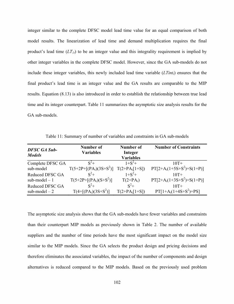
102

integer similar to the complete DFSC model lead time value for an equal comparison of both

model results. The linearization of lead time and demand multiplication requires the final

product’s lead time (LT1t) to be an integer value and this integrality requirement is implied by

other integer variables in the complete DFSC model. However, since the GA sub-models do not

include these integer variables, this newly included lead time variable (LTintt) ensures that the

final product’s lead time is an integer value and the GA results are comparable to the MIP

results. Equation (8.13) is also introduced in order to establish the relationship between true lead

time and its integer counterpart. Table 11 summarizes the asymptotic size analysis results for the

GA sub-models.

Table 11: Summary of number of variables and constraints in GA sub-models

DFSC GA Sub-Models

Number of Variables

Number of Integer

Variables

Number of Constraints

Complete DFSC GA sub-model

S2+ T(5+2P+[(PAi)(3S+S2)]

1+S2+ T(2+PAi[1+S])

10T+ PT[2+Ai(1+5S+S2)+S(1+P)]

Reduced DFSC GA sub-model – 1

S2+ T(5+2P+[(PAi)(S+S2)]

1+S2+ T(2+PAi)

10T+ PT[2+Ai(1+3S+S2)+S(1+P)]

Reduced DFSC GA sub-model – 2

S2+ T(4+[(PAi)(3S+S2)]

S2+ T(2+PAi[1+S])

10T+ PT[1+Ai(1+4S+S2)+PS]

The asymptotic size analysis shows that the GA sub-models have fewer variables and constraints

than their counterpart MIP models as previously shown in Table 2. The number of available

suppliers and the number of time periods have the most significant impact on the model size

similar to the MIP models. Since the GA selects the product design and pricing decisions and

therefore eliminates the associated variables, the impact of the number of components and design

alternatives is reduced compared to the MIP models. Based on the previously used problem

103

example (see section 3.5), with 10 components, 3 design alternatives for each component, 15

suppliers, 4 time periods, and 8 lead time – demand binary variables, Table 12 illustrates the

number of variables and constraints in the GA sub-models.

Table 12: Numerical illustration of model asymptotic size of GA sub-models

DFSC GA Sub-Models Number of Variables

Number of Integer Variables

Number of Constraints

Complete DFSC GA sub-model 32,725 2,154 42,840

Reduced DFSC GA sub-model – 1 29,125 354 39,240

Reduced DFSC GA sub-model – 2 32,641 2,153 40,400

The GA illustration does not show a significant reduction either in the number of variables nor in

the number of constraints compared to the MIP illustration (Table 3). The performance tests of

the MIP and GA solution techniques (section 5.1) discuss as the significance of these reductions

in number of variables and constraints and their impact on the solution performance.

104

}1,0{,,,,,

integer; & 0 ;0,,,,,,,

)(

)(

1

)(

)(

for 0|,0|,,

0|,,,)(

0|,,,)(

,,,

,,,,)(,,,,,,,,,

,

),1( )(

..

)1(21

)()(max

21

11

11

1 1

21

11

11

1 1

21

11

1

1

1 1

21

111

11 1

21

11

11

1

12

2

1

11

21

1 1

21

1

21

22

11

111

1

1

1 1 1

21

1 1

21

1112

1 1 1 1

1 11 1 1 1

2211

1

1

1

1

1

1

1

1

1

11

1

1

1

1

1

11

1

1

11

1

1

11

1

1

1

∈

≥≥

∀+≤++

∀≤

∀+≤

∀+≤+∀≤∀≤∀≤+

∀+−≥

∀−+≥

∀≥>∀=∀≥

>∀+≥

>∀+≥

>∀+≥

∀+≤

∀≥+∀≤∀≥∀≤

∀≤

>∀+≥+

⎟⎟⎠

⎞++

+⎜⎜⎝

⎛++−⎟

⎠

⎞⎜⎝

⎛+

−+

−+

=

−

=

−

= =

=

−−

= =

−

++

++

+

−+= =

−

= ==

+

== =

=

=

−

= = == =

== = = =

= == = = ==

−+

∑∑∑∑

∑

∑∑

∑∑

∑∑∑

∑∑∑

∑

∑

∑∑∑∑∑

∑∑∑∑∑∑

∑∑∑∑∑∑∑

tttijjlti

tktttitittjkltijtij

A

tt

A

tt

A S

jtjtj

A

ttt

A S

jtjtjt

ttt

tt

tt

tt

A S

jtjtjtt

t

A S

jtjtj

A

tt

tt

ikitit

ikitikktit

tijitij

tij

tij

tijtijit

ik

A

tijtijik

A S

ltjkl

ktkltkl

S

jtjkl

ktjkltkltkljl

itijtijtij

itijtijtij

itijtij

ititi

S

jtij

ik

k

i

A

α

S

jtijαtijα

A S

jtkjtkj

T

tttssratiot

T

t

S

j

P

k

S

l

A

tjkltjkl

S

j

S

ljljl

T

t

P

i

S

j

A

tijtijtijtij

T

tttt

ii

kii

i

i

i

i

i

i

i

ii

k

k

k

kkk

kkk

iii

iii

ii

iii

i

i

ii

k

k

kk

k

k

kk

i

i

iiii

ay

LTintDemandkkptimeLTuxx

tMcapkMcapxx

tMcapk

txxk

tMdemkMdemDemandtMdemτktDemandkt

txxDemandMdem

tDemandxxMcap

tLTLTintikRelationtiptimeLT

RelationtkiptimeRelationLTLT

CapacitytjiCapacity

xCapacity

xptptime


tlkxxu

tlkjuCapacityCapacityytjiaCapacityxtjiaCapacityxtjiCapacityx

,tiMcapx

tkkRelation)x(xxx

ts

LTintDemandzhTportcostu

Netwcoyxcxckkprice

ττπ

τ

τ

τ

ττ

τ

τ

α

α

αααα

απ

ρ

αα

ααα

αα

αα

ααα

αα

ααα

ααα

ααα

αα

αα

α

α

αα

ααα

αα

ααα

ααα

ααα

ααα

αα

ααα

ααα

ααα

ααααα

(8.3)

(8.1)

(8.2)

(8.4)(8.5)(8.6)(8.7)

(8.8)

(8.9)

(8.10)

(8.11)(8.12)(8.13)

(8.14)

(8.15)

(8.16)(8.17)(8.18)(8.19)

(8.20)

(8.21)

(8.22)

(8.23)

105

The complete pseudo-code of the GA implementation is given below.

Complete GA Pseudo-code:

Create initial population Until stopping criteria is met Copy elitist chromosomes to next generation Until population size is filled Select two parents according to the roulette wheel rule For each offspring For each time period Select one of the parents (higher probability given to the parent with better fitness value) Copy the corresponding gene value Next time period Next offspring For each offspring For each component Select a parent (with higher probability given to the first parent) For each time period Select a parent (higher probability given to the assigned parent) Copy gene values for this component and time period Next time period Next component Next offspring Decide to mutate or not If mutate Randomly perturb the pricing for a time period Randomly perturb a component design alternative selection End if Do Calculate fitness values of the chromosomes Do Check stopping criteria is met, if yes, then terminate; else, continue

Since the GA is a random search algorithm, different parameters impact the solution time and

quality and different runs may produce different results. A parameter tuning test based on the

preliminary models is explained in section 4.2.2. The rule of thumb suggests that increasing

population size and number of generations would yield better solutions (with the expense of

longer solution times) since more of the solution space will be searched. The preliminary

analyses also support this outcome. On the other hand, increasing mutation probability and

106

percentage of elitist chromosomes have different impacts on the solution quality and time. A

higher mutation rate endangers the survival of the good chromosomes (or chromosome

segments) by randomly altering the genes too frequently. However, a low mutation rate would

not help to diversify the population since the crossover operation always picks the genes from

the existing gene structures. Therefore, for a balanced diversification and preservation of the

population, a dynamic mutation rate is used [50]. According to this, the GA starts with a low

mutation rate since the algorithm is more likely to improve the best-known solution during the

early generations. However, as the best-known solution improves and the search progresses to

later generations, it takes longer to find a better solution due to the random nature of the

algorithm. In these phases, a larger mutation rate helps to diversify the population by random

perturbation of the chromosomes [11].

In addition to the mutation, survival of the elitist chromosome helps to exploit the

best-known solutions to find better solutions within the neighborhood. According to this concept,

a predetermined percentage of the best chromosomes of the population survives (copied

unchanged) to the next generation based on their fitness values. This procedure ensures that a

population always contains the best-known solutions and it survives until a better one is found.

Since, according to the roulette wheel selection rule, a chromosome with a better fitness value is

more likely to be selected for crossover, the elitist approach also guides the algorithm to make

more use of the best-known solutions. However, a too high elitist percentage risks the diversity

of the population by filling the new generation with too many of the chromosomes from the

previous generations. A too low percentage would lead to loss of good chromosomes and thus

the algorithm cannot exploit the good chromosomes to the possible extent. Therefore, the

percentage of the elitist chromosomes for larger populations is increased. According to this

107

approach, a small population size would keep only a small percentage of the elitist chromosomes

where more of these good solutions can be kept and exploited when larger populations are

maintained.

4.4 SOLUTION TECHNIQUES COMPLEXITY ANALYSIS

Preliminary Model Solution Techniques

Most of the MIP models, especially which do not satisfy specific conditions (e.g., with integer

right hand side values or with a totally unimodular constraint matrix) tend to be NP-hard. In

addition, most of the supply chain problems are modeled as MIP models. Although the

complexity of the developed DFSC models is not explicitly proven, like most non-trivial supply

chain models, it is expected that these models are NP-hard. The performance of the solution

techniques discussed in sections 4.1.2 and 4.2.2 suggest that it is significantly harder to solve the

developed DFSC models as these models grow in size and they do not guarantee a polynomial

time solution. In addition, for the CPLEX® MIP solver, the complexity of the solution algorithm

depends on the relaxed linear programming solution (with the fractional values of integer

variables) and the relationships between the components and suppliers.

Both of the heuristic algorithms evaluated in preliminary modeling (GA and TS) start

with creating feasible solutions by fixing variables. This process takes O(PS) computational time

where O denotes an asymptotic upper bound for the time of the process. It should be noted that

in the GA, the number of chromosomes is equal to the population size for a single generation

(thus the process takes O(pop_size × PS)) where the TS generates only a single solution at each

108

iteration. After the initial solution set is created, the GA uses three operations to create the next

generation:

1) copying elitist chromosomes (O(#elitist × PS)),

2) creating immigrating chromosomes (O(#immigrating × PS)), and

3) crossover and mutation (O(#crossover × PS)).

Therefore, each generation of the GA lasts O(pop_size × PS), and for a given number of

generations, the GA takes O(#generations × pop_size × PS) time.

On the other hand, the TS investigates each neighboring solution of the current one by

flipping a single bit every time. Thus the search takes O(PS) computational time. The move

operation picks the best flip and moves to this solution which takes O(1) time since only a single

bit is changed in each move. As a result, for a given iteration limit, the TS algorithm takes

O(#iterations × PS) time. However, since both algorithms employ a CPLEX® MIP solution

procedure to calculate the objective function by using branch and cut and simplex algorithms,

neither algorithm is guaranteed to run in polynomial time suggesting a significant increase in

solution times as the problem sizes increases.

Complete and Reduced Model Solution Techniques

Similar to the preliminary models, the complete and reduced DFSC model solution obtained by

using the branch and cut technique depends on the interactions between components and

suppliers (thus on the problem instance) and the problem size. Since the branch and bound tree

would grow as the problem size gets larger, it increases the solution time. However, the growth

of the solution tree size cannot be analytically determined since it depends on the initial

relaxation results, the number of integer variables, and the problem instance itself. The model

complexity analysis proposes that the number of binary variables is S2+T(4+N+[(PAi)(1+S)]) in

109

the complete DFSC model therefore an upper bound on the size of the branch and bound solution

tree would be 2S2+T(4+N+[(PAi)(1+S)]).

The GA solution procedure starts with creating an initial population which selects

component design alternatives and prices for each time period. This process takes O(PAiT) time

therefore it is polynomial. For the creation of the following generations, the elitist chromosome

copying and crossover procedures take O(pop_size × PAiT) time in total, since each of these

procedures requires copying each gene to a new offspring. However, the number of iterations

(generations) the GA will use is not known since it depends on the improvements from one

generation to the next. In addition, each chromosome’s fitness value is calculated by another

branch and cut algorithm to solve for the remaining variables. In conclusion, since the number of

generations changes randomly for each GA run and the branch and cut algorithm is not

polynomial, the GA eventually cannot run in polynomial time.

110

5.0 COMPUTATIONAL RESULTS

In this section, the computational results are presented. The first section reports on the

performance of the MIP and GA solution techniques on the complete and reduced DFSC models.

The solution quality and solution time are reported with a comparative analysis. The following

section concentrates on the research questions stated in section 1.3. Each research question is

investigated and the behavior of the models, solution techniques, and results are discussed. The

third section summarizes the validity of the models and the results via academic literature survey

and industry experts’ views.

5.1 PERFORMANCE TESTS ON COMPLETE AND REDUCED MODELS

The performance of the MIP and GA solution techniques are discussed in this section. In order to

evaluate their performances, five complete DFSC model instances are created randomly. Table

13 shows the number of components and available suppliers used in these problem instances.

Similar to the preliminary modeling, these instances grow in size to evaluate the performance of

the solution methods for different problem sizes.

111

Table 13: Complete and reduced DFSC problem instances for performance testing

Problem Instance Number of Components Number of all Suppliers 1 4 6 2 6 9 3 8 12 4 10 15 5 16 24

For all five instances, four time periods are considered. Each time period in the model

corresponds to a product life cycle phase, namely introduction, growth, maturity, and decline as

suggested by Perreault and McCarthy [49].

In these problem instances, the number of design alternatives for each component is

uniform-randomly selected between 1 and 3. For the Bill of Materials relationships, a

uniform-random assignment is followed where any number of a component between zero and

five may be required by another component. It should be noted that if zero units of a component

are required by another component, it is not used. The production time for each component is

selected between 1 and 30 days uniform-randomly. By performing a presolve analysis for each

instance, the maximum lead time is determined to be less than 256 days (28 days) for each

instance. This bound necessitates eight binary lead time linearization variables (γnt) to be used for

these problem instances.

5.1.1 Mixed Integer Programming

For the performance testing of the branch and cut method, CPLEX® is utilized with the default

parameters as suggested by the STOP procedure described in section 4.3.1. For each problem

112

instance, the branch and cut algorithm is allowed to run for 48 hours (172,800 seconds) or until

the optimal solution is found (by a 0.01% optimality gap). The optimality gap measures the

relative ratio of the objective value of the best integer feasible solution found to the objective

value of the best possible solution (a bound) which is the best objective value of a node in the

MIP solution tree. When the optimality gap value is equal to zero, the obtained solution is

guaranteed to be the optimal one. Larger optimality gap values mean the true optimal solution is

between the solution obtained and the bound. For any optimality gap value other than zero, the

current solution may be the optimal solution but it is not guaranteed nor proven. Table 14 reports

the results of the MIP runs with the complete DFSC model instances.

Table 14: MIP results for the complete DFSC model

Problem Instance Optimality Gap Solution Time (sec.) 1 0.01% 150.69 2 20.61% 172,800.00 3 2,490.00% 172,800.00 4 92.01% 172,800.00 5 96.03% 172,800.00

The results show that although a feasible solution to the problem is found for every problem

instance, they cannot be solved to optimality with the given 48 hour time limit (except the

smallest instance). Another important result is that the solution quality depends not only on the

problem size but also on the problem instance as well. For example, the two largest problems (4

and 5) can be solved to around 90% optimality, but the third instance result is only within the

2,490% of the optimality bound. Therefore, the MIP solution progress cannot be easily

determined by only assessing the problem size. Moreover, the results show that the complete

DFSC is very complex and hard to solve even for small scale problems.

113

In order to further evaluate the performance of the MIP algorithm, the reduced DFSC

model – 1 is solved by using the same problem instances and with the same 48 hour time limit.

Table 15 summarizes the results.

Table 15: MIP results for the reduced DFSC model – 1

Problem Instance Optimality Gap Solution Time (sec.) 1 0.01% 36.89 2 0.01% 48,091.53 3 15.64% 172,800.00 4 36.60% 172,800.00 5 33.11% 172,800.00

The results show that the solution quality is increased for all instances compared to the complete

model. As suggested by the model complexity analysis, having fewer binary variables helps the

algorithm progress faster. These results still suggest that the solution quality degrades as the

problems get larger and solution time increases. However, compared to the complete model, the

algorithm finds better solutions in the same running time or even in a shorter time as seen in

problem instance 2.

In order to evaluate the performance of the MIP solution technique further, the reduced

DFSC model – 2 is solved by using the same problem instances. The results are shown in Table

16.

Table 16: MIP results for the reduced DFSC model – 2

Problem Instance Optimality Gap Solution Time (sec.) 1 0.01% 6.24 2 0.01% 7,023.81 3 0.01% 145,232.95 4 49.63% 172,800.00 5 16.34% 172,800.00

114

The reduced DFSC model – 2 MIP results show that, in general, the performance increase is

even better than the one for the reduced DFSC model – 1. Three of the five problem instances

could be solved to optimality and the largest problem is solved to less than a 17% optimality gap,

best among all three tests. However, the solution quality for the fourth instance is worse than that

of for the reduced DFSC model – 1. These results suggest that the performance of the MIP

solution algorithm is not necessarily correlated with the number of binary variables in the model

as the reduced DFSC model – 1 has fewer binary variables than the reduced DFSC model – 2.

The interactions between these variables are very important for faster reduction of the optimality

bound. However, in general, it is clear that the algorithm performance deteriorates as the

problems get larger.

5.1.2 Genetic Algorithms

In order to test the performance of the GA, the described five problem instances are solved for

both the complete and the reduced DFSC models. The GA procedure is allowed to run for 48

hours (the same limit applied to the MIP) or it is terminated when no improvements are noted in

20 consecutive generations. Initial test runs without the objective improvement termination

condition showed that once no improvements are noted for about 10 iterations, the GA often

cannot find a better solution. Therefore, setting the termination limit to 20 consecutive

generations without any improvements is reasonable. Each GA run is started with a 5% elitist

chromosome rate and a 1% mutation rate. However, according to the dynamic mutation rate

application, the mutation rate is increased by 1% when no improvements in the best-known

solution are noted for three consecutive generations. The solution quality (optimality gap) of the

GA is measured relatively to the final solution of the MIP technique. For example, if the MIP

115

finds the optimal solution and the GA does not, then there is an optimality gap for the GA

solution. The negative optimality gap values mean that the GA solution is worse than the MIP

solution (since the objective is to maximize the profit) where the positive values correspond to

the GA solutions which are better than the MIP solutions. Since the MIP guarantees an optimal

solution (if one exists), the GA can only find better solutions when the MIP runs are stopped due

to meeting the time limit before the optimal solution is found. The solution time gap values on

the other hand are different. The negative solution time gaps correspond to faster GA runs where

positive solution time gap values mean that it took the GA longer to achieve the reported results.

Table 17 summarizes the results of the GA with the complete DFSC model.

Table 17: GA results for the complete DFSC model

Problem Instance Objective Value Gap Solution Time Gap Solution Time (sec.) 1 0.00% 99.56% 300.72 2 -0.04% -99.83% 291.40 3 5.30% -74.33% 44,354.28 4 6.66% -98.54% 2,529.32 5 -18.53% -38.17% 106,841.33

* Bold values indicate a better objective value or a shorter solution time for the GA.

According to the results, the GA usually terminates before the MIP, except for the smallest

instance due to the requirement of searching for an extra 20 generations with no improvements.

Since the GA does not use any optimality bound information, these additional generations

increase the solution time even if the optimal solution is found as shown with the first problem

instance. Due to the random nature of the GA, a solution quality bound cannot be given.

However, results show that the GA finds the optimal solution for the smallest instance and it

finds better solutions than the MIP for the third and fourth problem instances. For the second and

the fifth (largest) problem instances, it cannot find a better solution than the MIP, suggesting a

116

highly random solution quality. However, the GA usually runs for shorter time periods compared

to the MIP and the solution quality is always less than 20% worse compared to the MIP.

Table 18 reports the results of the GA application for the reduced DFSC model – 1 where

the economies of scale concept is removed.

Table 18: GA results for the reduced DFSC model – 1

Problem Instance Objective Value Gap Solution Time Gap Solution Time (sec.) 1 0.00% 75.52% 64.75 2 0.00% -99.87% 60.13 3 5.72% -98.03% 3,396.70 4 4.00% -98.57% 2,465.88 5 -9.87% 0.00% 172,800.00

* Bold values indicate a better objective value or a shorter solution time for the GA.

The reduced DFSC model – 1 GA run results show that the GA performs better with the reduced

model as it finds the optimal solution for the first and second instances and finds better solutions

than the MIP for the third and fourth problem instances. For the largest instance, the solution

quality is less than 10% of the MIP where both algorithms terminate due to the time limit.

However, the GA runs are often shorter than the MIP runs except for the smallest instance where

the additional 20 generations requirement for termination adds extra time to the algorithm and

becomes significant. As the last performance test for the GA, results of the reduced DFSC model

– 2 are summarized in Table 19.

117

Table 19: GA results for the reduced DFSC model – 2

Problem Instance Objective Value Gap Solution Time Gap Solution Time (sec.) 1 0.00% 1,734.18% 114.45 2 0.00% -98.26% 122.39 3 -0.12% -70.66% 42,608.76 4 -4.64% -86.25% 23,767.98 5 -4.73% -66.87% 57,246.45

* Bold values indicate a shorter solution time for the GA.

The reduced DFSC model – 2 results show that the GA can find very good solutions (less than

5% worse than the MIP) in a relatively short time, except for the smallest instance due to the

termination requirement described before. In the worst case, for the largest problem instance, the

GA runs for nearly 16 hours where the MIP runs up to the 48 hour time limit.

5.1.3 Comparative Analysis

The final run results for the MIP and GA solution techniques only show the outcomes of the

individual runs within the allowed time limits. However, the progression of both solution

techniques are important to accurately compare their performances. For example, since the MIP

procedure tries to find the true optimal solution to the problem, it continues to run even after the

optimal solution is found to prove its optimality. On the other hand, the GA procedure terminates

regardless of the goodness of the solution and does not try to prove optimality or to provide any

optimality gap information. Therefore, the actual optimization process data is illustrated to

compare the behavior of each solution technique over the run-time.

For each of the problem instances, six different runs (MIP and GA runs for the complete

model and the reduced models 1 and 2) are illustrated on the following charts. The x-axis shows

the run time in a logarithmic scale where the y-axis shows the actual solution value. Since both

118

algorithms find a feasible solution with a positive objective value very quickly (in less than

0.05% of their total run times), the y-axis on the graphs only shows positive objective values for

clarity. The progress of both algorithms for the first problem instance is shown in Figure 8 for

the complete DFSC model, in Figure 9 for the reduced DFSC model – 1, and in Figure 10 for the

reduced DFSC model – 2.

0.00E+00

2.00E+07

4.00E+07

6.00E+07

8.00E+07

1.00E+08

1.20E+08

1.40E+08

1.60E+08

1.80E+08

0.01 0.10 1.00 10.00 100.00 1000.00

Time (seconds)

Obj

ectiv

e V

alue

MIP Complete GA Complete

Figure 8: Progress of the MIP and the GA for the complete DFSC model (instance 1)

119

0.00E+00

2.00E+07

4.00E+07

6.00E+07

8.00E+07

1.00E+08

1.20E+08

1.40E+08

1.60E+08

1.80E+08

0.01 0.1 1 10 100

Time (seconds)

Obj

ectiv

e V

alue

MIP Reduced 1 GA Reduced 1

Figure 9: Progress of the MIP and the GA for the reduced DFSC model – 1 (instance 1)

0.00E+00

5.00E+07

1.00E+08

1.50E+08

2.00E+08

2.50E+08

0.01 0.1 1 10 100 1000

Time (seconds)

Obj

ectiv

e V

alue



120

The algorithm progressions show that for this smallest problem instance, the MIP solves the

problem to the optimality for all models in a shorter time than the GA. The MIP dominates the

GA for the complete DFSC model and the reduced DFSC model -2. Although the GA finds a

better solution than the MIP initially for the reduced DFSC model – 1, the MIP outperforms the

GA by finding the optimal solution in a shorter time. The progression of both algorithms for the

second problem instance is shown in Figure 11 for the complete DFSC model, in Figure 12 for

the reduced DFSC model – 1, and in Figure 13 for the reduced DFSC model – 2.

0.00E+00

5.00E+07

1.00E+08

1.50E+08

2.00E+08

0.1 1 10 100 1000 10000 100000 1000000

Time (seconds)

Obj

ectiv

e V

alue



121

0.00E+00

5.00E+07

1.00E+08

1.50E+08

2.00E+08

0.01 0.1 1 10 100 1000 10000 100000

Time (seconds)

Obj

ectiv

e V

alue



0.00E+00

5.00E+07

1.00E+08

1.50E+08

2.00E+08

0.01 0.1 1 10 100 1000 10000

Time (seconds)

Obj

ectiv

e V

alue



122

For the second problem instance, as opposed to the first instance, the GA dominates the MIP for

all three models by finding the solutions with better objective values in a shorter time. The

progress of both algorithms for the third problem instance is shown in Figure 14 for the complete

DFSC model, in Figure 15 for the reduced DFSC model – 1, and in Figure 16 for the reduced

DFSC model – 2.

0.00E+00

1.00E+07

2.00E+07

3.00E+07

4.00E+07

5.00E+07

6.00E+07

7.00E+07

8.00E+07

9.00E+07

1 10 100 1000 10000 100000 1000000

Time (seconds)

Obj

ectiv

e V

alue



123

0.00E+00

1.00E+07

2.00E+07

3.00E+07

4.00E+07

5.00E+07

6.00E+07

7.00E+07

8.00E+07

9.00E+07

0.1 1 10 100 1000 10000 100000 1000000

Time (seconds)

Obj

ectiv

e V

alue



0.00E+00

2.00E+07

4.00E+07

6.00E+07

8.00E+07

1.00E+08

1.20E+08

0.01 0.1 1 10 100 1000 10000 100000 1000000

Time (seconds)

Obj

ectiv

e V

alue



124

For the third problem instance, the MIP finds better solutions in the beginning of each run;

however the GA finds either better or as good solutions and takes less time in the end. The GA

terminates before the MIP for all three models and actually the MIP cannot find as good

solutions as the GA within the time limit. For the fourth problem instance, the progress of both

algorithms is shown in Figure 17 for the complete DFSC model, in Figure 18 for the reduced

DFSC model – 1, and in Figure 19 for the reduced DFSC model – 2.

0.00E+00

5.00E+06

1.00E+07

1.50E+07

2.00E+07

2.50E+07

3.00E+07

3.50E+07

4.00E+07

4.50E+07

5.00E+07

1 10 100 1000 10000 100000 1000000

Time (seconds)

Obj

ectiv

e V

alue



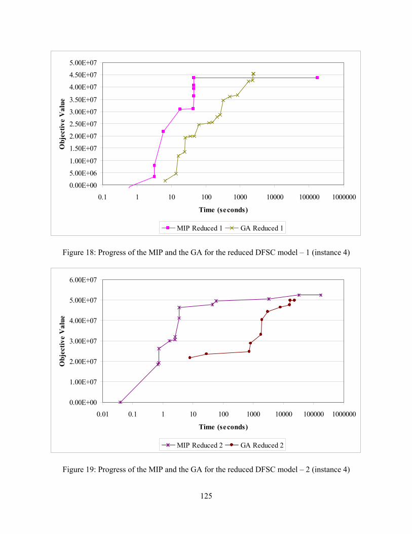
125

0.00E+00

5.00E+06

1.00E+07

1.50E+07

2.00E+07

2.50E+07

3.00E+07

3.50E+07

4.00E+07

4.50E+07

5.00E+07

0.1 1 10 100 1000 10000 100000 1000000

Time (seconds)

Obj

ectiv

e V

alue



0.00E+00

1.00E+07

2.00E+07

3.00E+07

4.00E+07

5.00E+07

6.00E+07

0.01 0.1 1 10 100 1000 10000 100000 1000000

Time (seconds)

Obj

ectiv

e V

alue



126

For the fourth problem instance, the results differ for different models. In the complete DFSC

model, the GA outperforms the MIP both in solution quality and time. For the reduced DFSC

model – 1, the GA finds a slightly better solution than the MIP; however the MIP finds a very

good solution in a much shorter time. For the reduced DFSC model – 2, the MIP outperforms the

GA by finding much better solutions very quickly. The GA terminates earlier than MIP due to

lack of any improvement in the solution quality before finding a solution as good as MIP did.

The progress of both algorithms for the fifth problem instance is shown in Figure 20 for the

complete DFSC model, in Figure 21 for the reduced DFSC model – 1, and in Figure 22 for the

reduced DFSC model – 2.

0.00E+00

5.00E+07

1.00E+08

1.50E+08

2.00E+08

2.50E+08

3.00E+08

3.50E+08

1 10 100 1000 10000 100000 1000000

Time (seconds)

Obj

ectiv

e V

alue



127

0.00E+00

5.00E+07

1.00E+08

1.50E+08

2.00E+08

2.50E+08

3.00E+08

1 10 100 1000 10000 100000 1000000

Time (seconds)

Obj

ectiv

e V

alue



0.00E+00

1.00E+08

2.00E+08

3.00E+08

4.00E+08

5.00E+08

6.00E+08

1 10 100 1000 10000 100000 1000000

Time (seconds)

Obj

ectiv

e V

alue



128

For the largest problem instance, the MIP procedure terminates due to the time limit before

proving the optimality of the solution. However, the GA cannot find a better solution for any of

the three models and is dominated by the MIP.

This comparative analysis of the both methods’ progressions suggests that neither one of

the methods dominates the other for all models or problem sizes. The results show that the GA

performs better for the mid-sized problem instances, but it is dominated by the MIP for the

smaller instances (due to the terminating conditions) and by the larger instances due to the

inherent difficulties that the GA encounters with a large solution space, i.e., a diminishing

probability of improving a good solution.

5.2 PROBLEM AND MODEL VALIDATION

The DFSC modeling concepts, assumptions, and results are discussed with three different

industry experts in order to get industry users’ input and validate the models. Some discussions

with the industry experts were conducted in the model development phase and their input is

incorporated into the models. Further discussions were aimed toward validating the models and

assessing the solution quality towards the end of the research. These experts currently work in

supply chain planning related tasks at their companies. The first expert works for a U.S.-based

company that specializes in sleep and respiratory solutions. The second expert’s company

manufactures electrical systems and components for automobiles, aircraft, and other industrial

equipment and is also based in the U.S. The third expert works in an international company

which manufactures electronics and provides electrical engineering solutions to diverse markets.

129

The discussions with these experts showed that none of the companies currently employ

an integrated DFSC procedure that simultaneously considers product and supply chain design

issues in the product design phase. However, both experts from the U.S.-based companies stated

that their companies are beginning to utilize more of the simultaneous approach and forsaking

the sequential approach. Yet, design teams still maintain primary responsibility for the design

process with only partial involvement from supply chain related groups although the

involvement by the supply chain groups is increasing. The third company expert stated that they

are currently using the sequential approach in all of their product designs.

The U.S.-based companies stated that their primary interest in the supply chain design

problems is cost reductions. In terms of the product design, the U.S.-based companies’ primary

concerns are the satisfaction of the regulations and customer specifications, followed by the

improvement of the customer attractiveness of the product. The third company stated that their

primary goal both in product and supply chain design is to satisfy specific quality levels required

by the customer regardless of its impacts on the cost and other measures. All three experts

confirm that the manufacturing, inventory, supply chain network, and transportation costs as well

as lead times and supplier capacity limitations are the most important factors for their decisions

in the supply chain design decisions. Other variables that they felt were of secondary importance

but were not included in these developed models include mainly more qualitative factors such as

working history with suppliers, strategic partnerships, number of distinct suppliers, certain risks

due to suppliers’ processes or location, increasing diversity, and suppliers’ company culture. All

three experts suggested that although these factors are important, they play a secondary role in

the supply selection procedure and are often considered as tie-breaking criteria. This suggests

130

that the developed DFSC models would be a valid and useful decision support tool utilizing the

most important industry criteria.

In terms of product design, experts suggest that they often change the component designs

several times in the product design phase to meet certain specifications and attract more

customers or to achieve a better supply chain performance as suggested by the sequential

approach. These design changes include, but are not limited to actual geometric design changes,

selection of different materials, and using different versions of components such as computer

chips. The impacts of these design changes on the demand and customer satisfaction are often

assessed by the marketing departments via expert knowledge and forecasting or by customer

surveys. Therefore, the industry experts suggest that the developed DFSC concept and models

may improve their product design procedures by reducing the number of product design change

iterations thus reducing the time to launch the product to the market.

The industry experts suggest that they usually have a considerable amount of information

about the potential price levels and demand in the product design phase so the pricing and

demand function data requirements of the DFSC models can be satisfied. They also acknowledge

that obsolescence plays an important role in their product and supply chain decisions and some

level of obsolescence information can be predicted for the DFSC models. Experts stated that cost

data such as supplier manufacturing costs and economies of scale information can be gathered

with relative ease. However, transportation and inventory costs can only be estimated with a

certain level of error due to their highly fluctuating nature. Similarly, suppliers’ lead time

information may be estimated with some error since it highly depends on the daily operations

and capacity utilization levels and may change over time. The initial supply chain network cost

concept and its importance is also validated by the industry experts and it is suggested that these

131

costs can be estimated since they are required only for the short term. In summary, the data

requirements of the DFSC model can be satisfied within a certain level of error, therefore the

experts suggested that the DFSC model would add value to their decision support systems.

The experts suggest that removing economies of scale or lead time and inventory

concepts from the model in order to be able to solve it or shorten the solution time would have

the least significant impact on the quality of the model. Since removing the economies of scale

concept (reduced DFSC model – 1) significantly reduces the number of binary variables (and

thus the model complexity) and it can easily be approximated via an average unit manufacturing

cost value, the experts suggest that it would be reasonable to set this concept aside in order to

improve the solution procedure. On the other hand, the removal of lead time and inventory

(reduced DFSC model – 2) is a more significant sacrifice making it a secondary choice for the

model reduction. The industry experts suggest avoiding some other model reduction suggestions

such as removing transportation costs or removing supplier capacity limitations since these

concepts add significant value to the models and the data can be estimated with relative

accuracy. Price and / or demand decisions, variations due to different product life cycle phases

(time periods), supply chain network costs, and product design’s impacts on the demand are the

most significant value adding and differentiating concepts of the DFSC models and therefore

should be kept even if they introduce complexity into the models.

As another suggestion to reduce the model complexity and improve the solution

procedures, the experts suggest that the models be solved for the most critical components of the

product (as opposed to the whole product) in terms of customer satisfaction, product

functionality, and cost and quality impacts. This would reduce the number of components in the

model and the number of suppliers to be considered. For example, an analytical analysis such as

132

Pareto analysis can be employed to identify the most critical components in terms of their impact

on the demand and their challenging requirements on the supply chain configuration. The experts

suggest that in most of their products, the number of components that they would consider as

critical is less than ten. Therefore, the developed illustrative problem instances can represent a

real case and show the complexity of the models even for the instance with few components and

suppliers.

In summary, after reviewing the models and illustrations in detail, the industry experts

liked the model and the underlying simultaneous optimization approach. They state that the

model requires extensive amount of data however the required data would already be gathered

for the product design and supplier selections. Therefore, they stated that they would use the

developed DFSC models and it would serve as a valuable decision support tool. The industry

experts also agreed that the model captures the most important product design and supply chain

variables. They also stressed that it would be useful to customize the models into their

company’s specific needs as further discussed in section 6.2 (extensions for the DFSC models).

5.3 ANSWERS TO RESEARCH QUESTIONS

In this research, the performance of the DFSC concept is examined via the stated major research

questions. This section provides detailed analysis and answers to the stated research questions.

133

5.3.1 Performance Metrics and Modeling Preferences

Research Question 1: Which product design / supply chain performance metrics should be

included in the model?

The first research question investigates which product design and supply chain

performance metrics should be included in the model in order to keep the models realistic and

representative of the real industry problems as well as simple enough to find high quality

solutions within acceptable time limits. The reduced DFSC models are used to investigate the

performance variations between different modeling preferences. The concepts to be removed

from the models are selected based on the model structure (to have significant impacts on the

model size and solution performance) and are validated by the industry experts as discussed.

The performance of both solution procedures for the complete and the reduced DFSC

models are summarized in Table 20 for the MIP and in Table 21 for the GA.

Table 20: MIP results for the complete and reduced DFSC models

Complete DFSC Model Reduced DFSC Model – 1 Reduced DFSC Model – 2 Problem Instance

Optimality Gap

Solution Time (sec.)

Optimality Gap


Optimality Gap


1 0.01% 150.69 0.01% 36.89 0.01% 6.242 20.61% 172,800.00 0.01% 48,091.53 0.01% 7,023.813 2,490.00% 172,800.00 15.64% 172,800.00 0.01% 145,232.954 92.01% 172,800.00 36.60% 172,800.00 49.63% 172,800.005 96.03% 172,800.00 33.11% 172,800.00 16.34% 172,800.00

134

Table 21: GA results for the complete and reduced DFSC models

Complete DFSC Model Reduced DFSC Model – 1 Reduced DFSC Model – 2 Problem Instance

Optimality Gap*


Optimality Gap*


Optimality Gap*


1 0.01% 300.72 0.01% 64.75 0.01% 114.452 20.68% 291.40 0.01% 60.13 0.01% 122.393 2,359.39% 44,354.28 9.38% 3,396.70 0.12% 42,608.764 80.11% 2,529.32 31.35% 2,465.88 56.91% 23,767.985 140.62% 106,841.33 47.69% 172,800.00 22.12% 57,246.45

* The optimality gap values measure the percent difference between the GA solution and the best bound value provided by the MIP for the corresponding MIP model. Note that this table does not compare the MIP and the GA results but it shows the performance variations for different models.

These results clearly show a performance increase for both solution procedures when the

complete DFSC is reduced. While the optimality gap is very large for problem instances other

than the smallest one (problem instance 1) with the complete model, both algorithms terminate

prior to finding an optimal solution due to the time limit or lack of improvements for a specified

time. On the other hand, both algorithms progress more rapidly and provide better optimality gap

values in a shorter time for the reduced models. Nevertheless, the solution techniques’

performances do not provide an apparent conclusion on how they differ for the two reduced

models. For the reduced DFSC model – 1, the MIP cannot prove the optimality of the solution

within the 48 hour time limit for the three largest problem instances although it improves the

optimality gap compared to the complete model. Similarly, the GA terminates in a shorter time

and provides a better optimality gap except for the largest instance where it reaches the time

limit. For the reduced DFSC model – 2, the optimality gap improvements over the complete

model are better for the problem instances 3 and 5 and worse for the instance 4 compared to the

first reduced model. Although the reduced DFSC model – 1 prunes more binary variables than

the second model and therefore is expected to improve both of the solution techniques, the

results suggest that the solution performance depends not only on the problem size (e.g., number

135

of component design alternatives, number of suppliers) and number of binary variables, but also

on the problem instance itself (e.g., Bill of Material complexity, actual cost and lead time

values). The differences in the interactions between the model variables due to the different

parameter values may help the first reduced model to be solved to a better solution than the

second reduced model or vice versa.

In summary, the results suggest that the reduced models can be solved to significantly

better solutions (to a lesser optimality gap value) in the same time period or even a shorter time

period and therefore become attractive alternatives to the complete DFSC when it cannot be

solved or the solution quality is not satisfactory. The loss of detailed information, such as

impacts of economies of scale or lead times, may be an acceptable tradeoff to allow for a better

solution performance. As industry experts agree, the economies of scale information can be

approximated by an average cost value and then can be evaluated after the model is solved and

the final product design and price are fixed. On the other hand, when the first reduced model

solutions are not satisfactory, lead time and inventory information can be removed as in the

second reduced model. However, the loss of this information is more significant in this model as

these concepts cannot be approximated with any other parameters remaining in the model.

Therefore, the second reduced model is only preferred when the complete and the first reduced

models cannot be solved. However, when the second reduced model is utilized, the results

should be further analyzed qualitatively by investigating the impacts of the simplifications to the

model.

In order to test the changes in the model solution and objective value with respect to the

parameter estimation errors, a sensitivity analysis is conducted. For these tests, a new problem

instance based on a simple cordless phone example is created. The cordless phone in this

136

example is assumed to consist of four components, namely a housing, battery, printed circuit

board, and antenna. This example is modeled with five components including the final assembly

of the cordless phone itself as another component. Although this final assembly is regarded as a

standalone component in order to capture supplier selection and cost aspects, it does not have

any design alternatives nor any customer satisfaction value. The remaining four components

have two design alternatives each and the customer satisfaction value of these designs change

over time to reflect obsolescence. There are four time periods in this example representing four

main product life cycle phases as described before. The customer satisfaction values of each

component over four time periods are given in Table 22. For this problem, five suppliers are

considered, with the first supplier being the final manufacturer and the only supplier available for

the final assembly.

137

Table 22: Customer satisfaction values of component design alternatives – cordless phone

Appearance Battery Life Signal Quality

Dialing Functions

Total

Total Value 40.0% 30.0% 15.0% 15.0% 100.0% Component Cordless Phone

0.0% 0.0% 0.0% 0.0% 0.0%

Housing

Design 1 30.0%-30.0%-30.0%-30.0%

4.0%-4.0%-4.0%-4.0%

34.0%-34.0%-34.0%-34.0%

Design 2 24.0%-24.0%-21.0%-18.0%

3.6%-3.2%-3.2%-2.8%

27.6%-27.2%-24.2%-20.8%

Battery

Lithium Ion 25.0%-25.0%-25.0%-25.0%

1.0%-1.0%-1.0%-1.0%

26.0%-26.0%-26.0%-26.0%

Ni-Cd 20.0%-17.5%-12.5%-7.5%

0.9%-0.9%-0.9%-0.9%

20.9%-18.4%-13.4%-8.4%

Printed Circuit Board

Design 1 5.0%-5.0%-5.0%-5.0%

6.0%-6.0%-6.0%-6.0%

11.0%-11.0%-11.0%-11.0%

22.0%-22.0%-22.0%-22.0%

Design 2 4.5%-4.5%-4.5%-4.5%

4.8%-4.8%-4.8%-4.8%

8.8%-7.7%-7.7%-5.5%

18.1%-17.0%-17.0%-14.8%

Antenna

Design 1 10.0%-10.0%-10.0%-10.0%

8.0%-8.0%-8.0%-8.0%

18.0%-18.0%-18.0%-18.0%

Design 2 9.0%-9.0%-9.0%-9.0%

5.6%-5.6%-5.6%-5.6%

14.6%-14.6%-14.6%-14.6%

* Four different values in the table correspond to component design values for four time periods. The time periods are ordered as |time period 1 – time period 2| in the table. time periods are ordered as |time period 3 – time period 4|

138

To test differences in the objective function and solution variables, first the initial problem with

the original parameter values (base case) is solved. Next, to represent estimation errors,

important parameter values are increased or decreased by 10% separately from the base case.

The tested parameters include supplier capacities (Capacityijαit1,2), unit manufacturing costs at

suppliers (cijαit1,2), production times at suppliers (ptijαit), supply chain network costs (Netwcojl),

transportation costs (Tportcostjklαkt), and demand function coefficients (β1, β2). Table 23 shows

the objective value of each scenario and whether the variables of supplier selection (supply chain

design), component alternatives selection (product design), and pricing differ from the base case.

All tests are conducted by using the MIP solution procedure by solving the complete DFSC

model therefore these tests capture all the described concepts and the solutions are proven to be

optimal. It should be noted that the aim of these tests is not to show how the actual solution

values change but rather to understand how much impact these estimation errors might have on

the primary product and supply chain designs. Therefore, the changes in the variables from the

base case primarily investigate whether another design or another supplier for a component is

selected and if the pricing decisions are changed. The pricing decisions are important since price

has a significant impact on the demand and may influence selection of different product or

supply chain designs.

139

Table 23: Parameter estimation error test results

Scenario Objective

Value (profit) ($)

Change from the Base Case Solution

Time (sec.) Product

Design Price ($)

Supply Chain Design

Base Case 85,462,662 - - - 16,606.92Supplier capacity (+10%) 88,765,433 Yes No Yes 2,954.48 Supplier capacity (-10%) 81,205,455 Yes No No 73,292.46Unit manufacturing cost (+10%) 82,818,261 No No Yes 21,108.20Unit manufacturing cost (-10%) 88,211,200 Yes No Yes 16,257.85Supplier production time (+10%) 83,693,537 No No Yes 38,170.30Supplier production time (-10%) 87,240,959 Yes No Yes 27,672.56Supply chain network cost (+10%) 83,955,662 No No No 14,514.36Supply chain network cost (-10%) 86,969,662 No No No 15,995.99Transportation cost (+10%) 84,263,290 No No No 45,424.48Transportation cost (-10%) 86,662,033 No No No 18,484.96Demand function coefficients (+10%) 100,850,314 Yes No Yes 32,361.29Demand function coefficients (-10%) 68,012,999 Yes No Yes 17,516.67

The results suggest that for this problem instance, underestimating the cost parameter values or

overestimating the supplier capacities and the demand function coefficients results in lower

profits due to increases in the realized costs or unexpected supplier capacity limitations and

lower realized demand. Estimation errors in the opposite directions result in higher profits due to

lower supply chain costs, higher demand, or more supplier production capacity.

A 10% estimation error in the supply chain network costs or in the transportation costs do

not change the preferred product design and supplier selection. However, estimation errors on

other parameters have different consequences and depend on the actual problem data and

interactions between the variables. For example, the demand function coefficients have a

significant impact on the profit value since they directly impact the demand and revenue rather

than the supply chain costs. An interesting result of these tests is that none of the scenarios

resulted in a change in the optimal price levels.

140

Since the product and supply chain design decisions are made before the parameter errors

are realized in a real life situation, additional sensitivity analysis is performed to further examine

the impact of these errors by further illustrating such an issue. In this case, instead of optimizing

the problem from the beginning with the new parameter values for each scenario, the optimal

solution for the base case is used with the new parameter values. The same product design

selections, supplier selections (thus supply chain network), and price values that are optimal for

the base case are kept the same for each scenario. The remaining decisions including production

and transportation quantities are optimized again. Table 24 shows the results of these tests. In the

second column of this table, the profit values for the scenarios are shown where the base case

scenario decisions are maintained. In the third column, the re-optimized profit results for each

scenario are given. It should be noted that these profit values are the same results as shown in

Table 23. The difference in the profit values when the base case solution is used and when the

problems are re-optimized is shown in the fourth column.

141

Table 24: Parameter estimation error test results by using the base case solution

Scenario

Objective Value with Base Case

Solution ($)

Objective Value with

Re-optimized Solution ($)

Change in the Objective Value

with Re-optimization ($)

Base Case 85,462,662 85,462,662 - Supplier capacity (+10%) 86,398,935 88,765,433 2,366,498 Supplier capacity (-10%) 81,069,890 81,205,455 135,565 Unit manufacturing cost (+10%) 82,818,261 82,818,261 - Unit manufacturing cost (-10%) 88,107,062 88,211,200 104,138 Supplier production time (+10%) 83,693,537 83,693,537 - Supplier production time (-10%) 87,218,392 87,240,959 22,567 Supply chain network cost (+10%) 83,955,662 83,955,662 - Supply chain network cost (-10%) 86,969,662 86,969,662 - Transportation cost (+10%) 84,263,290 84,263,290 - Transportation cost (-10%) 86,662,033 86,662,033 - Demand function coefficients (+10%) 93,583,581 100,850,314 7,266,733 Demand function coefficients (-10%) 65,926,952 68,012,999 2,086,047

The results show that the re-optimization improves the objective values for some scenarios.

However, since re-optimization cannot occur in real life, changes in the profit values while

maintaining the decisions made in the base case provide important clues of the impact of the

parameter estimation errors. The results showed that the increased and reduced supplier

capacities, lower manufacturing costs and production times, and changes in the demand function

coefficients have resulted in lower profits compared to the re-optimization results. This suggests

that these parameter estimation errors have significant impact on the profit and if the base case

decisions could be altered later in the product life cycle phases, higher profit values could be

obtained. For other scenarios, base case decisions resulted in the same profit value as the re-

optimization suggesting that the decisions based on the erroneous estimations for these

parameters would still be optimal when true parameter values are observed.

142

Nevertheless, these test results only provide a general idea about the significance of the

impacts of these parameter estimation errors. Yet, the impact of these parameter estimation

errors may be different for other problem instances depending on the interactions between these

parameters in the model. Another important result of these tests is that the solution time for these

problems may significantly change based on the actual parameter values. For this particular

problem instance, the solution time for different scenarios changed significantly from

approximately 45 minutes to 20 hours. The results suggest that supplier capacity values have the

most significant impact on the solution time. Increased supplier capacities significantly reduced

the solution time by providing enough capacity from the selected suppliers where reduced

capacities lengthen the solution time since the production amounts need to be distributed among

different suppliers for the optimal allocation.

5.3.2 Simultaneous versus Sequential Approach

Research Question 2: How do the performance metrics differ for the product design and

the associated supply chain for the simultaneous and sequential approaches?

The second research question investigates how sequential and simultaneous approaches

impact the product and supply chain design performance metrics. In order to investigate this

research question, two problem instances are tested since this research question aims to test the

main contribution of this dissertation and further insight from additional problem instances is

important. In addition to the previously described cordless phone example, a new problem

instance which is based on a desktop computer is introduced. In this example, the final product is

considered as a standalone component with no design alternatives and no design value. The

remaining five components are the motherboard & CPU, memory, hard disk, monitor, and

143

peripherals. The components’ design values are selected to be diminishing over four different

time periods to capture obsolescence impacts similar to the cordless phone example. The

customer satisfaction values of each component over four time periods are given in Table 25. For

this problem, seven suppliers are considered, as the first supplier being the final manufacturer

and the only supplier available for the final assembly.

144

Table 25: Customer satisfaction values of component design alternatives – desktop computer

Perform-ance

Ease of Use

Storage Capacity

Display Quality

Appear-ance Total

Total Value 50.0% 13.0% 10.0% 17.0% 10.0% 100.0% Component Desktop Computer

0.0% 0.0% 0.0% 0.0% 0.0%

Motherboard & CPU

2.5 GHz 35.0%-35.0%-35.0%-35.0%

5.0%-5.0%-5.0%-5.0%

40.0%-40.0%-40.0%-40.0%

2.0 GHz 30.0%-25.0%-20.0%-10.0%

4.0%-3.0%-2.0%-2.0%

34.0%-28.0%-22.0%-12.0%

Memory

1 GB 10.0%-10.0%-10.0%-10.0%

4.0%-4.0%-4.0%-4.0%

14.0%-14.0%-14.0%-14.0%

512 MB 7.0%-6.0%-4.0%-2.0%

3.0%-2.0%-2.0%-1.0%

10.0%-8.0%-6.0%-3.0%

Hard Disk

120 GB 5.0%-5.0%-5.0%-5.0%

8.0%-8.0%-8.0%-8.0%

13.0%-13.0%-13.0%-13.0%

60 GB 4.0%-4.0%-3.0%-1.0%

6.0%-6.0%-4.0%-1.0%

10.0%-10.0%-7.0%-2.0%

Monitor

19” LCD 3.0%-3.0%-3.0%-3.0%

8.0%-8.0%-8.0%-8.0%

5.0%-5.0%-5.0%-5.0%

16.0%-16.0%-16.0%-16.0%

19” CRT 2.0%-2.0%-1.0%-0.0%

6.0%-5.0%-3.0%-1.0%

2.0%-2.0%-0.0%-0.0%

10.0%-9.0%-4.0%-1.0%

Peripherals

Advanced 10.0%-10.0%-10.0%-10.0%

2.0%-2.0%-2.0%-2.0%

5.0%-5.0%-5.0%-5.0%

17.0%-17.0%-17.0%-17.0%

Standard 8.0%-8.0%-4.0%-4.0%

1.0%-1.0%-0.0%-0.0%

4.0%-3.0%-3.0%-2.0%

13.0%-12.0%-7.0%-6.0%

* Four different values in the table correspond to component design values for four time periods. The time periods are ordered as |time period 1 – time period 2| in the table. time periods are ordered as |time period 3 – time period 4|

145

In order to evaluate the differences between the sequential and simultaneous approaches as stated

in this research question, each problem instance (cordless phone and desktop computer

examples) is first solved with the simultaneous approach. Subsequently, each problem is solved

via the sequential approach. Since the product design value should be as high as possible

according to the sequential approach (as the design teams would prefer higher design values in a

sequential approach), the initial solution has been based on selecting the best design alternatives

for each component which would maximize the demand. After the complete DFSC model is

solved for this scenario, each component design is changed to a less preferred alternative

following a minimum loss of design value rule. This procedure aims to capture a real case where

a design team would compromise from a component’s design (to potentially reduce SC costs)

which would cause the minimum loss of total product design value, that is, the component with

the lowest impact on the demand. In order to truly capture the impact of the design change on the

demand, the design value loss is multiplied by the time multipliers which are used in the

complete DFSC model to represent each product life cycle phase’s impact on the demand. For

example, assume that the first two time multipliers which correspond to introduction and growth

phases of a product’s life cycle are equal to 1 and 2, respectively. This means that for the same

demand parameters (product design and price); the demand in the growth phase would be twice

the demand in the introduction phase. Therefore, the impact of the design value changes would

be more on the growth phase compared to the introduction phase. The described sequential

approach procedure is depicted in Figure 23.

146

Figure 23: The sequential approach procedure based on separate time periods

Moving through this procedure, several iterations are tested until no improvements on the total

profit is recorded. The simultaneous and sequential approaches are compared by first solving the

cordless phone example. For this example, the four time multipliers corresponding to four

different product life cycle phases are 1, 2, 3, and 1; respectively. Table 26 shows the result of

the simultaneous approach and summarizes the results of the sequential approach.

Find each component’s design value loss for each time period

Rank components in ascending order for their demand loss for each time period

Demand loss = Design value loss × timemultipliert

Select the lowest ranked component in the corresponding time period

Replace the best design alternative with a less valued design alternative

Calculate the maximum profit

Fix the design change at its lower valued alternative (current change accepted)

New profit > previous iteration’s profit?

Fix the design change at its higher valued alternative (current change rejected)

Select the next lowest ranked component in the corresponding time period

Yes

No

Last component in the ranked list?

Yes Terminate

No

147

In the first scenario, all components’ first designs are selected (best product design

possible). In each following scenario, the component design with the lowest impact on the

demand is changed to the second design alternative. The demand loss column shows the impact

of this design change on the demand. If the profit is increased with this design change, then this

change is accepted and subsequent scenarios include this change. If the change does not increase

the profit, then it is rejected and is not investigated in the subsequent scenarios.

Table 26: Simultaneous and sequential approach results for the cordless phone example

Scenario Component Time Period

Demand Loss Profit ($) Design Change

Accepted Simultaneous Approach 85,462,662 Sequential Approach

1 - - - 77,830,520 - 2 Antenna 1 3.4% 78,333,287 Yes 3 Antenna 4 3.4% 78,621,416 Yes 4 Printed Circuit Board 1 3.9% 78,951,870 Yes 5 Battery 1 5.1% 79,567,470 Yes 6 Housing 1 6.4% 79,626,229 Yes 7 Antenna 2 6.8% 82,127,598 Yes 8 Printed Circuit Board 4 7.2% 75,996,840 No 9 Printed Circuit Board 2 10.0% 82,878,307 Yes 10 Antenna 3 10.2% 85,462,662 Yes 11 Housing 4 13.2% 83,101,544 No 12 Housing 2 13.6% 83,856,203 No 13 Printed Circuit Board 3 15.0% 79,245,215 No 14 Battery 2 15.2% 85,032,936 No 15 Battery 4 17.6% 83,178,938 No 16 Housing 3 29.4% 83,048,751 No 17 Battery 3 37.8% 82,370,043 No

The sequential approach test results show that scenarios 2 through 10 (except scenario 8) result

in higher profit. Further design changes (scenarios 11 through 17) do not improve the profit from

the $85,462,662 level obtained in scenario 10. In this problem, scenario 10 of the sequential

148

approach finds the same profit as the simultaneous approach. In addition, the optimal solutions of

both approaches are the same, that is, they not only result in the same product design, but also

they select the same price levels and the same suppliers. In the second comparison of

simultaneous and sequential approaches, the desktop computer problem is solved by following

the same procedure described for the cordless phone example. For this example, the time

multipliers are 1, 1.2, 1.6, and 1; respectively for each product life cycle phase. Table 27 shows

the results of both design approaches.

Table 27: Simultaneous and sequential approach results for the desktop computer example

Scenario Component Time Period

Demand Loss Profit ($) Design Change

Accepted Simultaneous Approach 8,495,076,500 Sequential Approach

1 - - - 7,561,769,600 - 2 Hard Disk 1 3.0% 7,539,925,100 No 3 Hard Disk 2 3.6% 7,669,845,600 Yes 4 Peripherals 1 4.0% 7,648,320,500 No 5 Memory 1 4.0% 7,647,961,500 No 6 Peripherals 2 4.8% 7,795,946,900 Yes 7 Monitor 1 6.0% 7,747,072,600 No 8 Motherboard & CPU 1 6.0% 7,761,299,800 No 9 Memory 2 7.2% 7,798,211,400 Yes 10 Monitor 2 8.4% 7,815,327,500 Yes 11 Hard Disk 3 9.6% 7,313,069,500 No 12 Peripherals 4 11.0% 7,669,300,400 No 13 Hard Disk 4 11.0% 7,425,286,000 No 14 Memory 4 11.0% 7,659,417,200 No 15 Peripherals 3 12.8% 7,658,090,700 No 16 Memory 3 12.8% 7,679,607,300 No 17 Motherboard & CPU 2 14.4% 7,727,076,000 No 18 Monitor 4 15.0% 7,612,294,200 No 19 Monitor 3 19.2% 7,581,860,000 No 20 Motherboard & CPU 4 28.0% 7,413,139,300 No 21 Motherboard & CPU 3 28.8% 7,548,458,900 No

149

The results show that the sequential approach based on the previously described procedure

cannot find as high a profit value as the simultaneous approach for this problem example. Only

four out of the first ten scenarios could improve the profit value where none of the remaining

eleven scenarios could find a better objective value. Since the previously described sequential

approach procedure performs poorly, another procedure is also tested to represent the sequential

approach for this problem. Within this new procedure, the component with the lowest impact on

the demand is selected in a similar manner. However, instead of fixing its design selection at a

given time period, the problem is solved by releasing this component’s design selections for all

time periods and fixing other components at their best designs. For example, in the first scenario

of this procedure, the lowest total design loss over four time periods is for the hard disk

component. Therefore, all other components designs are fixed at their best; the design selections

for the hard disk are decided by the optimization process. If a higher profit is noted for this

problem, then these design decisions are fixed and the subsequent component’s design selections

are released. The new modified sequential approach procedure is depicted in Figure 24. Moving

through this procedure the sequential approach is tested and the results are shown in Table 28.

150

Figure 24: The sequential approach procedure based on the optimization over all time periods

Find each component’s total design value loss over all time periods

Rank components in ascending order for their total demand loss

Total demand loss = Σt(Design value loss × timemultipliert)

Select the lowest ranked component

Release related constraints to select component designs by optimization

Fix the design values selected by the optimization

Select the next lowest ranked component

Yes

Terminate

No Last component

in the ranked list with no profit

improvement?

Calculate the maximum profit

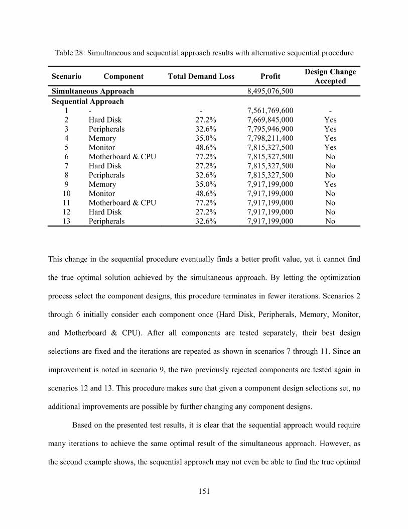
151

Table 28: Simultaneous and sequential approach results with alternative sequential procedure

Scenario Component Total Demand Loss Profit Design Change Accepted

Simultaneous Approach 8,495,076,500 Sequential Approach

1 - - 7,561,769,600 - 2 Hard Disk 27.2% 7,669,845,000 Yes 3 Peripherals 32.6% 7,795,946,900 Yes 4 Memory 35.0% 7,798,211,400 Yes 5 Monitor 48.6% 7,815,327,500 Yes 6 Motherboard & CPU 77.2% 7,815,327,500 No 7 Hard Disk 27.2% 7,815,327,500 No 8 Peripherals 32.6% 7,815,327,500 No 9 Memory 35.0% 7,917,199,000 Yes 10 Monitor 48.6% 7,917,199,000 No 11 Motherboard & CPU 77.2% 7,917,199,000 No 12 Hard Disk 27.2% 7,917,199,000 No 13 Peripherals 32.6% 7,917,199,000 No

This change in the sequential procedure eventually finds a better profit value, yet it cannot find

the true optimal solution achieved by the simultaneous approach. By letting the optimization

process select the component designs, this procedure terminates in fewer iterations. Scenarios 2

through 6 initially consider each component once (Hard Disk, Peripherals, Memory, Monitor,

and Motherboard & CPU). After all components are tested separately, their best design

selections are fixed and the iterations are repeated as shown in scenarios 7 through 11. Since an

improvement is noted in scenario 9, the two previously rejected components are tested again in

scenarios 12 and 13. This procedure makes sure that given a component design selections set, no

additional improvements are possible by further changing any component designs.

Based on the presented test results, it is clear that the sequential approach would require

many iterations to achieve the same optimal result of the simultaneous approach. However, as

the second example shows, the sequential approach may not even be able to find the true optimal

152

solution and be stuck with a worse solution. When the optimal prices and component design

selections are analyzed for both approaches (shown in Table 29), although there are only minor

component design and price differences the profit for the simultaneous approach is higher.

Nevertheless, all of these changes that constitute the optimal solution cannot always be

determined easily by the sequential approach. The iterative procedure, which the sequential

approach utilizes, may miss some alternatives as the interactions between different variables

make it hard to capture the profit improvements via an iterative approach. This example

illustrates the benefits of the simultaneous approach where all decisions are evaluated in a

combined structure, and better solutions are found compared to iteratively trying to improve the

solutions.

Table 29: Optimal solutions of simultaneous and sequential approaches – desktop computer

Component Design Selections Profit Time

Period 1 Time

Period 2 Time

Period 3 Time

Period 4 Simultaneous Approach 8,495,076,500 Motherboard & CPU 2 1 1 1 Memory 2 1 1 1 Hard Disk 2 2 1 1 Monitor 2 2 1 1 Peripherals 2 2 1 1 Price 400 400 400 400 Sequential Approach 7,917,199,000 Motherboard & CPU 1 1 1 1 Memory 1 1 1 1 Hard Disk 1 2 1 1 Monitor 1 2 1 1 Peripherals 1 2 1 1 Price 800 400 400 400

153

In order to further investigate the benefits of using the DFSC and the simultaneous approach, the

results of the simultaneous approach, sequential approach, and not using either of these methods

(only selecting the best product design and then optimizing the supply chain) are compared by

using both examples. Table 30 and Table 31 show the profit, revenue, total and detailed supply

chain costs, and final product’s lead time values for these three methods for the cordless phone

and desktop computer examples, respectively.

Table 30: Revenue, costs, and lead time results of the cordless phone example

Simultaneous Approach

Sequential Approach

Best Product Design

Profit ($) 85,462,662 85,462,662 77,830,520 Revenue ($) 156,014,344 156,014,344 168,000,000 Total Supply Chain Cost ($) 70,551,682 70,551,682 90,169,479 Manufacturing Cost ($) 26,444,006 26,444,006 32,052,857 Supply Chain Network Cost ($) 15,070,000 15,070,000 15,070,000 Transportation Cost ($) 11,993,713 11,993,713 16,193,142 Inventory Cost ($) 17,043,963 17,043,963 26,853,480 Lead Time* (days) 5-10-19-9 5-10-19-9 11-18-23-11 * Four different values in the table correspond to final product lead times in four time periods.

Table 31: Revenue, costs, and lead time results of the desktop computer example


Sequential Approach

Best Product Design

Profit ($) 8,495,076,500 7,917,199,000 7,561,769,600 Revenue ($) 13,945,540,000 12,850,180,000 12,940,800,000 Total Supply Chain Cost ($) 5,450,459,560 4,932,977,064 5,379,030,446 Manufacturing Cost ($) 4,351,615,400 3,936,897,800 4,273,806,900 Supply Chain Network Cost ($) 17,480,000 17,480,000 17,480,000 Transportation Cost ($) 693,433,690 634,276,890 703,595,610 Inventory Cost ($) 387,930,470 344,322,374 384,147,936 Lead Time* (days) 5-10-9-9 7-10-9-9 7-11-9-9 * Four different values in the table correspond to final product lead times in four time periods.

154

As stated before, both the simultaneous and the sequential approaches find the same optimal

solution for the cordless phone example. When these results are compared to the best product

design selection scenario, it is shown that these methods find a higher profit. Although the best

product design approach generates more demand and thus more revenue, both the simultaneous

and the sequential approaches find less costly supply chains and therefore have higher profits. It

is also shown that for this example, selecting the best product design would yield higher lead

times compared to the other two approaches, increasing the inventory costs significantly.

For the desktop computer example, the simultaneous approach finds the best solution,

followed by the sequential approach, and then by select the best product design scenario.

Changes in the price decisions impact the revenues for these approaches. The simultaneous

approach can satisfy more demand by better supplier selection at a lower price as compared to

the select the best product design scenario. Although more demand is created in the select the

best product design scenario, this high demand cannot be completely satisfied resulting in lower

revenue. The sequential approach has the lowest revenue since it cannot generate more demand

than the best product design scenario nor supports a lower price and higher demand satisfaction

as in the simultaneous approach. The results show that the simultaneous approach creates a more

costly supply chain (total supply chain cost in Table 31) in addition to its higher revenue

however it finds the maximum overall profit. For example, it finds a supply chain with shortest

lead times, but its higher demand causes higher inventory costs compared to other two

approaches.

In summary, the test results show that selecting the best component design alternatives

does not necessarily provide the maximum profit although it satisfies the customer’s needs at the

maximum level. The test results illustrate that selecting less valued component design

155

alternatives (via simultaneous or sequential method) may improve the performance and the

profits of the product throughout its life cycle. However, when one of these methods is selected

for improving the product design, the results indicate that the simultaneous approach finds better

solutions than the sequential approach and the sequential approach may not be able to achieve

the same solution. An additional benefit of using the simultaneous approach is that once it finds

the optimal solution, no further iterations are required. On the other hand for the sequential

approach, many iterations may be required where each time large optimization problems are

solved. Yet these iterations may not even improve the profit and the sequential approach may

terminate with a worse result.

The results suggest that the simultaneous approach does not necessarily reduce the total

supply chain costs or the product lead time, but it balances the cost with the revenue to find a

higher profit. Therefore, it helps to overcome the complex interactions between the revenue and

cost sides of the profit which is hard to analyze separately in a sequential approach. The

simultaneous approach also modifies the product design to achieve better performance in such a

way that the other approaches cannot do iteratively. The simultaneous approach may

compromise some customer satisfaction, however it accounts for the tradeoff of customer

satisfaction with a better supply chain performance.

5.3.3 Combining Product and Supply Chain Design

Research Question 3: How robust is the supply chain to product design changes?

The third research question investigates the robustness of the supply chain with respect to

the product design changes. In order to test the impacts of the product design on the supply

chain, both of the previously described cordless phone and the desktop computer examples’

156

resulting supply chains are analyzed. Table 32 shows the design selections and resulting supply

chains for the simultaneous approach and the best design approach for the cordless phone

example.

Table 32: Product design and supply chain decisions for the cordless phone example

Component Design Selections Selected Suppliers

Time Per. 1

Time Per. 2

Time Per. 3

Time Per. 4

Time Per. 1

Time Per. 2

Time Per. 3

Time Per. 4


Housing 2 1 1 1 3-4 1-3 1-3 1-3 Battery 2 1 1 1 5 4-5 4-5 5 Printed Circuit Board 2 2 1 1 2 2 2 2 Antenna 2 2 2 2 5 5 5 5 Price 40 40 40 40 Best Design Approach

Housing 1 1 1 1 1 1-3 1-3 1 Battery 1 1 1 1 4-5 5 4-5 4-5 Printed Circuit Board 1 1 1 1 2 2 2 2 Antenna 1 1 1 1 5 5 5 5 Price 40 40 40 40

The cordless phone example results show some changes in the supplier selection over time for

different component design selections. For the housing and battery components, some suppliers

are selected or unselected in the optimal solution depending on the demand and capacity

limitations. However, for the printed circuit board and antenna components, the same suppliers

are selected over all time periods although different designs were chosen for these components.

Table 33 presents the design selections and the supply chain alternatives for the desktop

computer example.

157

Table 33: Product design and supply chain decisions for the desktop computer example

Component Design Selections Selected Suppliers

Time Per. 1

Time Per. 2

Time Per. 3

Time Per. 4

Time Per. 1

Time Per. 2

Time Per. 3

Time Per. 4


Motherboard & CPU 2 1 1 1 2-3-7 2-3-7 2-3-7 2-7 Memory 2 1 1 1 2-5 1-2-5 1-2-5 2-5 Hard Disk 2 2 1 1 6 6 3-5-6 3-6 Monitor 2 2 1 1 3 3 3-4-5 3-5 Peripherals 2 2 1 1 7 7 2-6-7 6-7 Price 400 400 400 400 Best Design Approach

Motherboard & CPU 1 1 1 1 2-3 2-3-7 2-3-7 2-7 Memory 1 1 1 1 2-5 1-2-5 1-2-5 2-5 Hard Disk 1 1 1 1 6 3-5-6 3-5-6 3-5 Monitor 1 1 1 1 5 3-4-5 3-4-5 3-5 Peripherals 1 1 1 1 7 6-7 2-6-7 6-7 Price 800 400 400 400

The desktop computer example results show that the simultaneous approach selected different

suppliers for the hard disk and monitor components over time. The change in the supply chain is

a result of different demand due to design selections and related supplier capacities. It should

also be noted that although it is not explicitly modeled and implied in the objective function, the

simultaneous approach results generate a supply chain with fewer suppliers, which would reduce

the supply chain complexity in real industry applications.

As these example problems illustrate, different component design selections would

necessitate different supply chain designs as changing demand and price values would require

use of more supplier capacity or a less costly supplier in the optimal solution. These

requirements may necessitate new suppliers to be added to or some existing suppliers to be

removed from the supply chain as well as replacement of some suppliers by others to

158

accommodate new cost or capacity requirements. Although these examples do not explicitly

indicate any change in the supply chain tiers, real industry problems may require more

components to be added into the product bill of material depending on the component design

selections which may further result in new supply chain tiers.

Research Question 4: What is the relative importance of the product design and the supply

chain design on the product success (thus on the profits)?

The fourth research question investigates whether the product design or the supply chain

dominates each other’s impact on the product’s success and profits. The two examples’ test

results indicate a strong interdependence between the product design and the supply chain, and

that they both have significant impacts on the product’s profits. As shown in Table 30 for the

cordless phone example, sometimes it may be preferred to reduce the demand by selecting less

attractive component designs in order to reduce the supply chain costs and to maximize the

profit. However, due to strong interdependence, as shown in Table 31 for the desktop computer

example, it might be better to increase the demand by selecting better product designs so that

more revenue is generated although supply chain costs are increased. Therefore, the results

indicate that neither product design nor the supply chain dominate each other in terms of

significance of their impacts on the profit generation. This result stresses the importance of the

simultaneous approach as it aims to balance these two important aspects to maximize the profit

where overlooking either one (as shown in best product design approach results) may lead to

non-optimal results.

159

6.0 CONCLUSIONS AND FUTURE RESEARCH

This chapter highlights the findings of this research and summarizes the conclusions in the first

section. In the second section, further concepts, ideas, and opportunities which can be added to

extend the developed DFSC models are presented. This section also discusses further

enhancements to the presented solution techniques and alternative solution procedures.

6.1 SUMMARY AND CONCLUSIONS

In this dissertation, an optimization model which aims to maximize the profit of a product

throughout its life cycle by deciding its components’ design alternatives, the associated supply

chain, and price levels is presented. This DFSC model provides an opportunity to simultaneously

consider product design and supply chain decisions within the product design phase which would

replace the sequential approach that is commonly used in industry. The simultaneous approach

helps the decision makers to see the big picture and impacts of their decisions both in the short

and long term. It also provides an alternative approach for optimizing these decisions to achieve

better results which cannot always be accomplished by the sequential approach. Finally, the

simultaneous approach generally works faster than the sequential approach which may require

multiple iterations, thus it helps to finalize the product design and supply chain decisions earlier,

reducing product design time and product time-to-market.

160

The test results suggest that both the product design and the supply chain are important

decisions and both have significant impacts on a product’s profitability. Therefore, emphasis

must be placed on both aspects and neither one should be overlooked. The presented

simultaneous approach offers an analytical framework to achieve this balanced method where

both aspects are considered before any major decisions are made as it is very costly to change the

product design or supply chain decisions in the later phases of a product’s life cycle.

The computational test results further suggest that the DFSC models tend to be very

complex in nature due to very complicated relationships and interdependencies between product

design and supply chain variables. These models grow significantly in size as the number of

product components and the number of suppliers increase. According to the test results and

industry experts’ suggestions, the developed reduced DFSC models are attractive alternatives

where the full-scale complete DFSC models cannot be solved in reasonable times.

In terms of solution methodologies, the test results show that metaheuristics can be

utilized to improve the quality of the solutions for the DFSC models where they cannot be solved

easily by the deterministic optimization methodologies, such as the MIP. However, the test

results also show that the performance of both solution methodologies depends both on the

problem size and the complexity of the interactions between the problem parameters. Since the

MIP guarantees an optimal solution, it is the preferred solution methodology. However, when the

solution time becomes unreasonable due to the problem size and complexity, metaheuristics

(GA) become a good solution alternative.

According to the discussions with the industry experts and their model reviews, the

developed DFSC models would add important value to their product design processes and would

be a very useful decision support tool. The industry experts suggest that although further

161

extensions and customization of the DFSC models would increase their value, the developed

models are valid and show the underlying benefits of the simultaneous product and supply chain

design optimization approach. In terms of model applicability, the industry experts agree that the

DFSC model has diverse data requirements, yet this data is customarily gathered. Hence, the

DFSC model can be easily implemented and utilized with the data in hand.

This research provides a significant addition to the existing DFSC research by combining

the product design and supply chain decisions into a single framework which optimizes the

decisions simultaneously. This research aims to fill in the gap in the DFSC literature which lacks

explicit consideration and integration of marketing and product design decisions and

manufacturing and supply chain decisions. Both the demand and manufacturing aspects of a

product are addressed uniquely in this research and well-established product design and supply

chain performance metrics are employed. The generic DFSC models which are applicable to

virtually any type of product in any manufacturing industry are solved by utilizing Mixed Integer

Programming and Genetic Algorithm. Detailed computational tests and illustrative examples

provide a clear assessment of both solution methodologies. In addition, this dissertation evaluates

alternative modeling preferences and assesses the performance of different solution

methodologies for these alternative models. Furthermore, the presented analyses provide insight

into the modeling and algorithmic / computation complexity issues.

Finally, this dissertation provides an important assessment from different industry experts

across various industries and includes these experts’ validation and suggestions for further work.

162

6.2 EXTENSIONS FOR DFSC MODELS AND SOLUTION METHODS

The developed DFSC model aims to capture important decision variables which a product design

or supply chain expert would consider for a new product. However, it is certain that some

particular extensions of this model and further customizations would improve the quality of the

model and help it fit different products’ unique requirements. In this section, some additional

objectives, constraints, and concepts are presented.

Although a company’s main objective is usually profit maximization, some other

objectives might be pursued occasionally in order to achieve other goals. For example, when the

company wishes to penetrate into a new market with a new product design, its main objective

might be demand or market share maximization rather than maximization of profit. Although,

the main objective in the long term would still be profit maximization, this short term objective

to maximize demand may overrule the profit maximization objective and the company may even

allow a short term loss. Therefore, an important extension for the DFSC model would be

introduction of different objectives for different time periods to reflect changing priorities of a

company for a product. Introduction of different objectives for different time periods should not

be confused with a multi-objective formulation since these various objectives here are aimed to

be unique goals which vary in different time periods. In addition to the market share

maximization objective, some other important objectives include maximizing the reliability of

the supply chain and reducing the negative impacts of the product design and supply chain on the

environment. The maximization of the supply chain reliability is an important issue since

variations in supplier quality and lead times have significant impacts on the supply chain

performance and profitability in the later phases of the product life cycle. In addition, the product

design influences the environment by dictating material selection and certain manufacturing

163

processes. For example, using a plastic component may have a more negative impact on the

environment than using a metal component if the product is not recycled properly at the end of

its life cycle. A product design may also require certain manufacturing processes that have

harmful effects on the environment such as generating chemical waste. Therefore, minimizing

the harmful impacts of the product and supply chain design on the environment could be a good

extension for the DFSC models.

In addition to the changes in the objective function, the DFSC model can be extended by

adding or changing some constraints to capture other important concepts or requirements. For

example, as the industry experts stated, many companies make their supplier selections not only

by using the quantitative variables (such as cost and lead time) but they also consider some

qualitative metrics or constraints. The industry experts listed quality levels of suppliers, risks and

opportunities of a supplier, and previous business history with some suppliers as important

qualitative metrics. However, it would be beneficial to quantify these metrics by using a

structured methodology (such as Analytical Hierarchy Process) or using a surrogate measure

such as number of defective parts per million for the quality before they are introduced into the

DFSC model.

In terms of other quantitative constraints, the DFSC models can be improved by adding

specific supply chain network constraints that many companies consider. For example, these

constraints may include the requirement of using at least two distinct suppliers for the critical

parts, some minimum order quantities for certain suppliers, or some other constraints that are

related to outsourcing decisions and protection of intellectual property. For instance, it would be

an interesting extension to study the impact of different component design selections on the

164

protection of the intellectual property where some design alternatives cannot be manufactured by

the main company or by the domestic suppliers.

As today’s business environment involves complex decisions for outsourcing to overseas

and offshoring, the addition of related variables such as custom duty rates would also add

significant value to the DFSC models. Since these decisions often need to take the import and

export related issues and costs into account, the DFSC can easily capture these important aspects.

Some important variables identified by the industry experts include custom duty rates, taxation

variations in different countries, import / export quotas, additional transportation challenges such

as vessel capacity problems, and other risks related to other countries’ political and economical

circumstances. Some of these variables such as quotas and taxes are quantitative measures and

can be added into the DFSC models with relative ease. Yet, other variables such as economic or

political risks are qualitative in nature and require further assessment and need to be analytically

quantified for integration into the DFSC models. Expansion of the DFSC models to incorporate

these outsourcing and offshoring variables is important for global supply chain decisions and

would add value to the DFSC models.

Although the deterministic approach employed in this dissertation captures and estimates

the impacts of the most important supply chain performance criteria, the explicit modeling of the

stochastic elements would be another important extension. The demand and supply chain lead

time parameters (which are approximated by assuming constant coefficients of variation in this

dissertation) can be further analyzed by a stochastic modeling approach. The impacts of the

demand and the lead time on the profits can be investigated in detail through a simulation

analysis integrated within the optimization procedure. However, the additional computational

165

requirements associated with the simulation should be carefully weighed against the model

improvements.

166

APPENDIX A

MODEL LINEARIZATION SCHEMA

In this section, the linearization schemas that are developed to remove nonlinearities from the

mathematical model are described.

A.1 REVENUE LINEARIZATION

In order to represent the Total Revenue with linear equations, initially two sets of variables

(τt+, τt

- and kt+, kt

-) are introduced. As explained in their definition in section 3.3, these variables

are used to evaluate satisfied demand which is

)oduction, Total Pr(DemandemandSatisfiedD ttt 11min=

Based on their definitions, these variables take respective values as shown below.

⎩⎨⎧

=⇒==⇒=

>+

⎪⎩

⎪⎨⎧

+=⇒=

=⇒=+>

−−

++

= =

= =

−−

++

= =

∑∑

∑∑∑∑

0 0 1

,)(

)( 1

0 0 ,)(

11

1 1

21

11

1 1

21

111 1

21

111

1

111

1

111

1

111

tt

tttt

A S

jtjtj

A S

jtjtjtt

ttA S

jtjtjt

kτDemandkτ

thenDemandxxIf

xxkτ

kτthenxxDemandIf

ααα

αααα

αα

(A.1)

(A.2)

(A.3)

167

Since, according to the presented representation, kt+ and kt

- would take relevant demand or total

production values, revenue in each time period can be expressed as

))k(k(priceRevenue tttt−+ +×=

As described in section 3.1, a quadratic price – demand function can be expressed by

22

1 ββ += priceDemand

By using this function, the demand can be expressed as a function of price, product design

value, and time period adjustment parameter by

tttt liertimemultippriceDemand ××+= υββ )( 22

11

As the price is allowed to take discrete values (ω1t, ω2t, ω3t) in this model, the final price value in

each time period is expressed by

ttttttttprice 2131121 )()( φωωφωωω −+−+=

where, φ1t and φ2t variables control if price values are increased to ω2t and/or ω3t, respectively.

From equations (A.4) and (A.7), it can be concluded that regardless of the price levels, revenue

would at least be equal to )(1−+ + ttt kkω . Since the demand function is utilized in a separate

constraint in the model, a direct mathematical equation of the revenue and demand functions

does not exist. Therefore, having kt+ and kt

- take relevant demand or total production values via

separate constraints given in (6.30) and (6.33), it is not necessary to linearize the revenue

function with respect to price – product design value multiplication. However, an additional set

of variables (ψ1t, ψ2t, ψ3t, ψ4t) is introduced to represent revenue values for higher price levels.

The actual non-linear relations that these variables represent are given below

(A.4)

(A.5)

(A.6)

(A.7)

168

ttt

ttt

ttt

ttt

kkkk

24

13

22

11

φψ

φψ

φψ

φψ

×=

×=

×=

×=

−

−

+

+

Since constraints given in equations (6.34) through (6.45) force only one of the ψ values to take

a non-zero value, the revenue function can finally be expressed by

))(())(()( 421331121 tttttttttttt kkRevenue ψψωωψψωωω +−++−++= −+

Accordingly, Total Revenue would be expressed by

∑∑=

−+

=

+−++−++==T

tttttttttttt

T

tt kkRevenueRevenueTotal

1421331121

1))(())(()( ψψωωψψωωω

A.2 DEMAND LINEARIZATION

Since the quadratic price – demand function is given as

22

1 ββ += priceDemand

and the final price value in each time period is expressed by

ttttttttprice 2131121 )()( φωωφωωω −+−+=

the demand function becomes

( ) tttttttttt liertimemultipDemand ××+++−−= υβφωβφωβφφωβ 222311

22121

2111 )1(

since φ1t × φ2t = 0 is always true by definition and via equation (6.21).

(A.8)

(A.9)

(A.10)

(A.11)

(A.12)

(A.13)

169

In order to represent Demand1t as a linear equation, an additional set of variables (λ1t, λ2t) is

introduced to linearize price – product design value multiplication. The actual non-linear

relations that these variables represent are given below

ttt

ttt

υφλυφλ×=×=

22

11

By using the Demand1t function (A.13) and replacing φ × υ multiplications by λ variables, the

final Demand1t function becomes

( ) tttttttttt liertimemultipDemand ×−+−++= )()()( 21

2321

21

22112

2111 ωωλβωωλβυβωβ

A.3 INVENTORY COST LINEARIZATION

Since the developed model is at the strategic planning level, the inventory levels are calculated as

the average Safety Stock levels for each time period. Based on the inventory theory and wide

application in the literature, the Safety Stock level for a given customer satisfaction target under

stochastic demand and lead time is given as the following formula [49].

222 )( LDssratio DLzStockSafety σσ +=

where L is the average lead time, D is the average demand during the average lead time, and 2Lσ

and 2Dσ are the variances of the lead time and demand during the lead time, respectively.

The lead time values used in this research (LT1t) are given in actual true time units.

However, the demand values (Demand1t) are calculated for the entire product life cycle phase (t)

therefore, the average demand during the lead time is calculated byt

t

thperiodlengDemand1 , where

(A.14)

(A.15)

(A.16)

170

periodlengtht is the length of the time period t in the same units with lead time. Therefore, by

using the parameters and variables of the DFSC model, the Safety Stock in a time period can be

represented as

In this research, it is assumed that lead time and lead time demand have constant coefficients of

variation, which suggests that change in the variation of these variables is constant when their

average values are changed. The mathematical representations of ρ1 and ρ2 by using model

variables are given below.

1

1

t

t

Demand

thperiodlengDemandσρ =

t

LT

LTρ

12

σ=

By using ρ1 and ρ2 for coefficients of variation for lead time and demand over the lead time

respectively, the safety stock in a time period can be represented as

22

1

2111

21

222

21

2

212

11

ρρ

ρρ

+=

+=

tt

ttssratio

tt

t

t

ttssratiot

LTthperiodlengDemandLT

z

LTthperiodleng

Demandthperiodleng

DemandLTzStockSafety

Since the total inventory would be equal to the sum of the average lead time inventory kept and

safety stock, the Total Inventory in a time period is represented as

22

1

211111 ρ

ρ++=

tt

ttssratio

t

ttt LTthperiodleng

DemandLTz

thperiodlengDemandLT

InventoryTotal

Since this model calculates the demand at the strategic level, the lead time demand variation is

removed by assuming ρ1 = 0. Hence, the Total Inventory in a time period becomes

22

212

1 LTt

tDemandtssratiot thperiodleng

DemandLTzStockSafety σσ += (A.17)

(A.18)

(A.19)

(A.20)

(A.21)

171

)1( 211

21111 ρρ ssratio

t

tt

t

ttssratio

t

ttt z



zthperiodleng

DemandLTInventoryTotal +=+=

However, the lead time and demand multiplication makes this equation non-linear therefore a

linearization is provided. Since Demand1t is a continuous variable, LT1t is limited to take integer

values, given that production time data, ptijαit is integer and capacity utilization adjustments do

not strictly enforce proportional reductions in production times. Furthermore, the lead time

values are rounded up to the nearest integer value since it would be better to account for the

uncertainty for the worst case scenario. Given these assumptions, lead time values can be

represented as combinations of several binary variables (γnt) as shown in the following equation.

N][0, ,22...6432168420

65432101 ∈=++++++++= ∑=

nLTN

nnt

nnt

ntttttttt γγγγγγγγγ

It should be noted that based on the provided data, the number of γ variables (N) needs to be

estimated so that LT1t ≤ 2N is always true in order to keep the model feasible. By utilizing this

binary representation schema, lead time – demand multiplication becomes

tntn

tttttt

tttttttttt

Demand

DemandDemandDemandDemandDemandDemandDemandDemandLT

1

161514

1312111011

2

...643216 842

γ

γγγγγγγ

++++++++=

By the introduction of δnt variables, each of which corresponding to relative γntDemand1t

multiplications (i.e., N][0,each for 1 ∈= nDemand tntnt γδ ), the lead time - demand multiplication

is represented as

N][0, ,2

2...643216842

0

654321011

∈=

++++++++=

∑=

n

DemandLTN

nnt

n

ntn

ttttttttt

δ

δδδδδδδδ

In order to calculate Total Inventory Cost, the average inventory in a time period is assumed to

be half of the maximum inventory levels. This approach is widely used in the literature and is

(A.22)

(A.23)

(A.24)

(A.25)

172

based on the fact that the inventory is used over the lead time thus it is safe to assume that the

inventory decreases linearly with the time. Therefore, the average inventory level for a time

period can be adequately approximated as the half of the maximum inventory. Based on this

assumption, the Total Inventory Cost in a time period can be calculated as

)1(21

)1(21

211

211

ρ

ρ

ssratiottt

ssratiot

ttttt

zDemandLTh

zthperiodleng

DemandLThthperiodlengCostInventoryTotal

+=

+=

By using the lead time - demand linearization (A.25), the linear form of the Total Inventory Cost

in a time period, which is used in the objective function, becomes

∑=

+=8

02 2)1(

21

nnt

nssratiott zhCostInventoryTotal δρ

(A.26)

(A.27)

173

APPENDIX B

REDUCED DFSC MODELS

In this appendix, the two reduced DFSC model formulations, described in section 3.4, are

presented. It should be noted that the same notation used in the complete DFSC modeling is

employed.

B.1 REDUCED DFSC MODEL – 1

The following mathematical model is the reduced DFSC model that reflects the removal of

economies of scale concept from the complete model.

174

( )

t, nMdemDemandt, nMdemt, nDemand

tLT

ikRelationtiptimeLTRelationtkiptimeRelationLTLT

CapacitytjiCapacity

xptptime

RelationtkjixRelationu

tlkxu

tlkjuCapacityytjiCapacityx

tval

ti

,tiMcapx

tkkRelationxx



zhTportcostuNetwcoy

xckk

ntntt

ntnt

tnt

N

nnt

nt

ikitit

ikitikktit

tijitij

tijtijit

ik

A

tijik

A S

ltjkl

ktkl

S

jtjkl

ktjkltkljl

itijtij

P

i

A

titit

A

ti

ititi

S

jtij

ik

k

i

A

α

S

jtijα

A S

jtkj

ikitkt

tttttttttt

T

t

N

nnt

nssratiot

T

t

S

j

P

k

S

l

A

tjkltjkl

S

j

S

ljljl

T

t

P

i

S

j

A

tijtij

T

tttttttttttt

i

ii

i

i

i

k

k

k

kk

kk

ii

i

i

ii

i

i

i

iii

i

i

i

k

k

k

k

k

kk

i

i

ii

∀∈≤−−∀∈×≤∀∈≤

∀=

>∀=∀≥>∀+≥

>∀≥

>∀≥

∀≤

∀≥∀≤

∀=

∀=

∀≤

>∀≥

>∀=

∀×−+−++=

⎟⎟⎠

⎞+++

⎜⎜⎝

⎛+−+−++−++

∑

∑∑∑

∑

∑∑

∑

∑

∑∑∑∑∑

∑

∑ ∑∑∑∑∑∑∑∑

∑∑∑∑∑

=

== =

=

= =

=

=

−

= = == =

=

= == = = == =

= = = ==

−+

N][0,)1(N][0,N][0,

2

for 0|,0|,,

0|,,,

0|,,,

,,,

,,,,,,,

,1

,

),1(

),1(

)()()(..

2)1(21

))(())(()(max

1

1

01

11

11

1

1 1

1

1

1

111 1

1

1

1

1

1 1 1

1

1 1

1

1-k

1i

21

2321

21

22112

2111

1 02

1 1 1 11 1

1 1 1 1

11

1421331121

δγγδ

δ

γ

α

α

αα

πυ

π

απ


δρ

ψψωωψψωωω

αα

αα

αα

αα

αα

αα

αα

ααα

αα

ααα

αα

ααα

ααα

(A.29)

(A.28)

(A.30)

(A.31)

(A.32)

(A.33)

(A.34)

(A.35)

(A.36)

(A.37)

(A.38)

(A.39)

(A.40)(A.41)

(A.42)

(A.43)(A.44)(A.45)

175

(A.47)(A.46)

(A.48)(A.49)

(A.50)

(A.51)

(A.52)(A.53)(A.54)(A.55)

(A.56)

(A.57)

(A.58)

(A.59)(A.60)

(A.61)(A.62)(A.63)(A.64)(A.65)

(A.66)

(A.67)

(A.68)

(A.69)

(A.70)

(A.71)}1,0{,,,,,,

;0,,,,,,,,,,,,,,

1

}2,1{,1}2,1{, }2,1{,

1

21

4321211

114

112

1124

4

113

111

1113

3

22

22

2

11

11

1

11

11

1 1

11

11

1 1

11

1

1

1 1

111

11 1

11

11

21

1

1

1

1

1

1

1

1

1

1

1

1

1

1

1

1

1

1

1

1

1

1

1

1

1

1

1

1

1

1

1

1

1

1

1

1

1

1

1

1

1

1

∈

≥

∀+≤+

∀≤

∀≤

∀+≤+

∀≤

∀≤∀+≤+∀≤∀≤∀+≤+∀≤∀≤

∀+≤+

∀≤

∀≤

∀+≤+∀≤∀≤∀≤+

∀−≥

∀−≥

∈∀+≤+∈∀≤∈∀≤

∀≤+

−+

−+

=

−

=

=

−=

−

=

=

−

+

+

+

+=

−

=

−

= =

=

−−

= =

−

++

++

+

−+= =

−

= ==

+

∑∑

∑

∑∑

∑

∑∑∑∑

∑

∑∑

∑∑

∑∑∑

ntttttjlti

nttktttttttttitittjkltij

A

ttt

A

tt

A

ttt

tt

A

ttt

A

tt

A

ttt

tt

ttt

tt

tt

ttt

tt

tt

A

tt

A

tt

A S

jtj

A

ttt

A S

jtjt

ttt

tt

tt

tt

A S

jtjtt

t

A S

jtj

A

tt

qttqt

tqt

qtqt

tt

y

DemandkkptimeLTux

tMcapkMcap

tMcap

tk

tMcapkMcap

tMcap


tMcapkMcapx

tMcapk

txk


txDemandMdem

tDemandxMcap

qtqtqt

t

i

ki

γφφττπ

δυψψψψλλ

ψφ

φψ

ψ

ψφ

φψ

ψψφ

φψψ

ψφφψ

ψ

τ

τ

ττ

ττ

τ

τ

λυφυλφλφφ

α

αα

αα

αα

αα

αα

αα

αα

αα

αα

αα

αα

αα

αα

αα

αα

176

B.2 REDUCED DFSC MODEL – 2

The following mathematical model is the reduced DFSC model that reflects the removal of lead

time and inventory concepts from the complete model.

177

( )

0|,,,)(

,,,

,,,,)(,,,,,,,,,

,1

,

),1()(

),1(

)()()(..

)(

))(())(()(max

1

21

1 1

21

1

21

22

11

111 1

1

1

1

1

1 1 1

21

1 1

21

1-k

1i

21

2321

21

22112

2111

1 1 1 11 11 1 1 1

2211

1421331121

>∀+≥

∀+≤

∀≥+∀≤∀≥∀≤

∀=

∀=

∀≤

>∀+≥+

>∀=

∀×−+−++=

⎟⎟⎠

⎞+⎜⎜

⎝

⎛++

−+−++−++

∑∑∑

∑

∑∑

∑

∑

∑∑∑∑∑

∑

∑∑∑∑∑∑∑∑∑∑∑

∑

== =

=

= =

=

=

−

= = == =

=

= = = == == = = =

=

−+

ik

A

tijtijik

A S

ltjkl

ktkltkl

S

jtjkl

ktjkltkltkljl

itijtijtij

itijtijtij

itijtij

P

i

A

titit

A

ti

ititi

S

jtij

ik

k

i

A

α

S

jtijαtijα

A S

jtkjtkj

ikitkt

tttttttttt

T

t

S

j

P

k

S

l

A

tjkltjkl

S

j

S

ljljl

T

t

P

i

S

j

A

tijtijtijtij

T

tttttttttttt


tlkxxu


tval

ti

,tiMcapx

tkkRelation)x(xxx



TportcostuNetwcoyxcxc

kk

i

i

ii

k

k

k

kkk

kkk

iii

iii

ii

i

i

ii

i

i

i

iii

i

i

ii

k

k

kk

k

k

kk

i

i

iiii

ααα

αα

ααα

ααα

ααα

ααα

αα

ααα

αα

ααα

ααα

ααα

ααααα

α

αααα

πυ

π

απ


ψψωωψψωωω

(A.72)

(A.73)

(A.74)

(A.75)

(A.76)

(A.77)

(A.78)(A.79)(A.80)(A.81)

(A.82)

(A.83)

178

}1,0{,,,,,,

;0,,,,,,,,,,,,

)(

)(

1

)(

)(

}2,1{,1}2,1{, }2,1{,

1

21

43212121

114

112

1124

4

113

111

1113

3

22

22

2

11

11

1

11

11

1 1

21

11

11

1 1

21

11

1

1

1 1

21

111

11 1

21

11

11

21

1

1

1

1

1

1

1

1

1

1

1

1

1

1

1

1

1

1

1

1

1

1

1

1

1

1

11

1

1

1

1

1

11

1

1

11

1

1

11

1

1

1

∈

≥

∀+≤+

∀≤

∀≤

∀+≤+

∀≤

∀≤∀+≤+∀≤∀≤∀+≤+∀≤∀≤

∀+≤++

∀≤

∀+≤

∀+≤+∀≤∀≤∀≤+

∀+−≥

∀−+≥

∈∀+≤+∈∀≤∈∀≤

∀≤+

−+

−+

=

−

=

=

−=

−

=

=

−

+

+

+

+=

−

=

−

= =

=

−−

= =

−

++

++

+

−+= =

−

= ==

+

∑∑

∑

∑∑

∑

∑∑∑∑

∑

∑∑

∑∑

∑∑∑

tttttijjlti

tkttttttttttjkltijtij

A

ttt

A

tt

A

ttt

tt

A

ttt

A

tt

A

ttt

tt

ttt

tt

tt

ttt

tt

tt

A

tt

A

tt

A S

jtjtj

A

ttt

A S

jtjtjt

ttt

tt

tt

tt

A S

jtjtjtt

t

A S

jtjtj

A

tt

qttqt

tqt

qtqt

tt

ii

kii

ay

Demandkkuxx

tMcapkMcap

tMcap

tk

tMcapkMcap

tMcap


tMcapkMcapxx

tMcapk

txxk


txxDemandMdem

tDemandxxMcap

qtqtqt

t

φφττπ

υψψψψλλ

ψφ

φψ

ψ

ψφ

φψ

ψψφ

φψψ

ψφφψ

ψ

τ

τ

ττ

ττ

τ

τ

λυφυλφλφφ

αα

ααα

αα

αα

αα

αα

αα

αα

αα

αα

ααα

αα

ααα

ααα

ααα

αα

(A.85)(A.84)

(A.86)(A.87)

(A.88)

(A.89)

(A.90)

(A.91)(A.92)(A.93)(A.94)

(A.95)

(A.96)

(A.97)(A.98)(A.99)

(A.100)(A.101)(A.102)(A.103)

(A.104)

(A.105)

(A.106)

(A.107)

(A.109)

(A.108)

179

APPENDIX C

PRELIMINARY GA PARAMETER TEST RESULTS

Population Size


% Elitist Chromosomes

% Immigrating Chromosomes

Best Objective ($)


100 1,000 1 1 55,008,046 6,440.83 100 1,000 5 1 54,389,653 3,389.32 100 1,000 10 1 54,832,677 3,435.80 100 1,000 5 5 57,267,504 3,507.90 100 1,000 10 10 58,886,818 3,619.83 10 50 5 1 80,069,169 17.51 25 50 5 1 79,495,423 41.54 50 50 5 1 71,512,200 81.49

100 50 5 1 72,920,801 169.71 200 50 5 1 70,655,715 334.39 10 100 5 1 80,839,748 39.75 25 100 5 1 73,995,774 83.60 50 100 5 1 71,460,939 164.07

100 100 5 1 71,755,095 338.87 200 100 5 1 70,504,045 646.53 50 250 5 1 73,099,370 420.25

100 250 5 1 63,283,761 836.70 200 250 5 1 61,447,527 1,678.82 200 500 5 1 56,948,753 3,153.78 50 1,000 5 1 60,943,471 1,876.25

100 1,000 5 1 54,389,653 3,389.00 50 5,000 5 1 55,662,800 9,924.39

100 5,000 5 1 49,263,967 18,966.84 200 5,000 5 1 49,553,641 38,692.77

* Shaded areas represent tested parameter. (The rest of the parameters are kept constant.) ** Starting mutation rate is set at 5%.

180

APPENDIX D

REDUCED GA SUB-MODELS

This appendix presents the reduced MIP models that are used in the GA procedure. Both models

have fewer variables and constraints than the complete DFSC model and the corresponding GA

sub-models since linearization, economies of scale, and lead time (with inventory cost

calculation) variables are eliminated simultaneously.

D.1 REDUCED GA SUB-MODEL – 1

This model removes economies of scale concept from the presented GA sub-model.

181

}1,0{,,, integer; and 0 ;0,,,,,,

1

for 0|,0|,,

0|,,,

0|,,,

,,,

,,,,,,,

,

),1(

..

)1(21

)(max

1

11

11

1 1

11

11

1 1

11

1

1

1 1

111

11 1

11

11

1

11

11

1

1 1

1

1

1

111

1

1

1 1 1

1

1 1

1

112

1 1 1 1

1 11 1 1 1

11

1

1

1

1

1

1

1

1

1

1

1

1

1

1

1

1

1

1

1

1

1

1

1

1

1

∈≥≥

∀+≤+

∀≤

∀≤

∀+≤+∀≤∀≤∀≤+

∀−≥

∀−≥

∀≥>∀=∀≥

>∀+≥

>∀≥

>∀≥

∀≤

∀≥∀≤

∀≤

>∀≥

⎟⎟⎠

⎞++

+⎜⎜⎝

⎛+−⎟

⎠

⎞⎜⎝

⎛+

−+−+

=

−

=

−

= =

=

−−

= =

−

++

++

+

−+= =

−

= ==

+

== =

=

=

−

= = == =

== = = =

= == = = ==

−+

∑∑∑∑

∑

∑∑

∑∑

∑∑∑

∑∑∑

∑

∑

∑∑∑∑∑

∑∑∑∑∑∑

∑∑∑∑∑∑∑

ttjltitktttitittjkltij

A

tt

A

tt

A S

jtj

A

ttt

A S

jtjt

ttt

tt

tt

tt

A S

jtjtt

t

A S

jtj

A

tt

tt

ikitit

ikitikktit

tijitij

tijtijit

ik

A

tijik

A S

ltjkl

ktkl

S

jtjkl

ktjkltkljl

itijtij

ititi

S

jtij

ik

k

i

A

α

S

jtijα

A S

jtkj

T

t1ttssratiot

T

t

S

j

P

k

S

l

A

tjkltjkl

S

j

S

ljljl

T

t

P

i

S

j

A

tijtij

T

tttt

yLTintDemandkkptimeLTux

tMcapkMcapx

tMcapk

txk


txDemandMdem

tDemandxMcap

tLTLTintikRelationtiptimeLT

RelationtkiptimeRelationLTLT

CapacitytjiCapacity

xptptime

RelationtkjixRelationu

tlkxu

tlkjuCapacityytjiCapacityx

,tiMcapx

tkkRelationxx

ts

LTintDemandzhTportcostu

Netwcoyxckkprice

iki

i

ii

i

i

i

k

k

k

kk

kk

ii

iii

i

i

i

k

k

k

k

k

kk

i

i

ii

ττπ

τ

τ

ττ

ττ

τ

τ

α

α

αα

απ

ρ

ααα

αα

αα

αα

αα

αα

αα

αα

αα

αα

αα

αα

αα

αα

αα

αα

ααα

αα

ααα

ααα

(A.110)

(A.118)(A.119)

(A.111)

(A.112)

(A.113)(A.114)

(A.115)

(A.117)

(A.116)

(A.125)(A.126)

(A.120)

(A.121)

(A.122)

(A.124)(A.123)

(A.127)

(A.128)

(A.129)

182

D.2 REDUCED GA SUB-MODEL – 2

This model removes lead time and inventory cost concepts from the presented GA sub-model.

}1,0{,,,, ;0,,,,,

)(

)(

1

)(

)(

0|,,,)(

,,,

,,,,)(,,,,,,,,,

,

),1( )(

..

)()(max

21

11

11

1 1

21

11

11

1 1

21

11

1

1

1 1

21

111

11 1

21

11

11

1

21

1 1

21

1

21

22

11

111

1

1

1 1 1

21

1 1

21

1 1 1 1

1 11 1 1 1

2211

1

1

1

1

1

1

1

1

1

11

1

1

1

1

1

11

1

1

11

1

1

11

1

1

1

∈≥

∀+≤++

∀≤

∀+≤

∀+≤+∀≤∀≤∀≤+

∀+−≥

∀−+≥

>∀+≥

∀+≤

∀≥+∀≤∀≥∀≤

∀≤

>∀+≥+

⎟⎟⎠

⎞

+⎜⎜⎝

⎛++−⎟

⎠

⎞⎜⎝

⎛+

−+−+

=

−

=

−

= =

=

−−

= =

−

++

++

+

−+= =

−

= ==

+

== =

=

=

−

= = == =

= = = =

= == = = ==

−+

∑∑∑∑

∑

∑∑

∑∑

∑∑∑

∑∑∑

∑

∑

∑∑∑∑∑

∑∑∑∑∑

∑∑∑∑∑∑∑

tttijjltikttttjkltijtij

A

tt

A

tt

A S

jtjtj

A

ttt

A S

jtjtjt

ttt

tt

tt

tt

A S

jtjtjtt

t

A S

jtjtj

A

tt

ik

A

tijtijik

A S

ltjkl

ktkltkl

S

jtjkl

ktjkltkltkljl

itijtijtij

itijtijtij

itijtij

ititi

S

jtij

ik

k

i

A

α

S

jtijαtijα

A S

jtkjtkj

T

t

S

j

P

k

S

l

A

tjkltjkl

S

j

S

ljljl

T

t

P

i

S

j

A

tijtijtijtij

T

tttt

iikii

i

i

ii

k

k

k

kkk

kkk

iii

iii

ii

iii

i

i

ii

k

k

kk

k

k

kk

i

i

iiii

ayDemandkkuxx

tMcapkMcapxx

tMcapk

txxk

tMdemkMdemDemandtMdemτktDemandkt

txxDemandMdem

tDemandxxMcap


tlkxxu


,tiMcapx

tkkRelation)x(xxx

ts

Tportcostu

Netwcoyxcxckkprice

ττπ

τ

τ

τ

ττ

τ

τ

α

αααα

απ

ααααα

αα

αα

ααα

αα

ααα

ααα

ααα

αα

ααα

αα

ααα

ααα

ααα

ααα

αα

ααα

ααα

ααα

ααααα

(A.137)

(A.138)

(A.130)

(A.131)

(A.132)

(A.133)(A.134)

(A.136)(A.135)

(A.144)

(A.145)

(A.139)

(A.140)

(A.141)

(A.143)(A.142)

(A.146)

(A.147)

(A.148)

183

BIBLIOGRAPHY

[1] Alibre Inc., “Design Anywhere. Build Anywhere. The Opportunity in Global Manufacturing,” 2001, http://www.alibre.com.

[2] Arntzen, B. C., Brown, G. G., Harrison, T. P., Trafton, L. L., “Global Supply Chain Management at Digital Equipment Corporation,” Interfaces, Vol. 25, No. 1, pp. 69-93, 1995.

[3] Asiedu, Y., Gu, P., “Product Life Cycle Cost Analysis: State of the Art Review,” International Journal of Production Review, Vol. 36, No. 4, pp. 883 – 908, 1998.

[4] Aytug, H., Khouja, M., Vergara, F. E., “Use of Genetic Algorithms to solve Production and Operations Management Problems: A Review,” International Journal of Production Research, Vol. 41, No. 17, pp. 3955-4009, 2003.

[5] Babcock, D., L., Morse, L. C., Managing Engineering and Technology, 3rd Edition, Prentice Hall, Upper Saddle River, NJ, 2002.

[6] Baz, M., Brooks, J. P., Gosavi, A., Hunsaker, B., “Automated Tuning of Optimization Software Parameters,” Technical Report 2007-7, University of Pittsburgh Department of Industrial Engineering.

[7] Beamon, B. M., “Supply Chain Design and Analysis: Models and Methods,” International Journal of Production Economics, Vol. 55, No. 3, pp. 281-294, 1998.

[8] Berger, A. J., Gattorna, J. L., Supply Chain Cybermastery: Building high performance supply chains of the future, Gower Publishing Limited, Burlington, VT, 2001.

[9] Besterfield, D., H., Besterfield-Michna, C., Besterfield, G., H., Besterfield-Sacre, M., Total Quality Management, 3rd Edition, Prentice Hall, Upper Saddle River, NJ, 2003.

[10] Cakravista, A., Toha, I. S., Nakamura, N., “A Two-Stage Model for the Design of Supply Chain Networks,” International Journal of Production Economics, Vol. 80, No. 3, pp. 231-248, 2002.

[11] Chan, K. Y., Aydin, M. E., Fogarty, T. C., “Main effect fine-tuning of the mutation operator and the neighborhood function for uncapacitated facility location problems,” Soft Computing, Vol. 10, No. 11, pp. 1075-1090, 2006.

http://www.alibre.com/�

184

[12] Chan, L., Wu, M., “Quality Function Deployment: A Literature Review,” European Journal of Operational Research, Vol. 143, No. 3, pp. 463-497, 2002.

[13] Chopra, S., Meindl, P., Supply Chain Management: Strategy, Planning, and Operation, 2nd Edition, Pearson/Prentice Hall, Upper Saddle River, NJ, 2004.

[14] Clark, A. J., Scarf, H., “Optimal Policies for a Multi-Echelon Inventory Problem,” Management Science, Vol. 6, No. 4, pp. 475-490, 1960.

[15] Coello C. A., “A Comprehensive Survey of Evolutionary-Based Multiobjective Optimization Techniques,” Knowledge and Information Systems: An International Journal, Vol. 1, No. 3, pp. 269-308, 1999.

[16] Cohen, M. A., Lee, H. L., “Strategic Analysis of Integrated Production Distribution System: Models and Methods,” Operations Research, Vol. 36, No. 2, pp. 216-228, 1988.

[17] Cook, H., Wu, A., “On the Valuation of Goods and Selection of the best Design Alternative,” Research in Engineering Design, Vol. 13, No. 1, pp. 42-54, 2001.

[18] Cooper, R., Slagmulder, R., Target Costing and Value Engineering, Productivity Press, Portland, OR, 1997.

[19] Council of Supply Chain Management Professionals, “18th Annual Logistics State of Logistics Report,” 2006, available at http://cscmp.org.

[20] Ding, H., Benyoucef, L., Xie, X., “A Simulation Optimization Methodology for Supplier Selection Problem,”, International Journal of Integrated Manufacturing, Vol. 18, No. 2-3, pp. 210-224, 2005.

[21] Ealey, L. A., Quality by Design: Taguchi Methods and U.S. Industry, ASI Press, Dearborn, MI, 1988.

[22] Fandel, G., Stammen, M., “A General Model for Extended Strategic Supply Chain Management with Emphasis on Product Life Cycles including Development and Recycling,” International Journal of Production Economics, Vol. 89, No. 3, pp. 293-308, 2004.

[23] Fisher, M. L., “What is the Right Supply Chain for Your Product?,” Harvard Business Review, Vol. 75, No. 2, pp. 105-116, 1997.

[24] Geoffrion, A., M., Graves, G. W., “Multicommodity Distribution System Design by Bender’s Decomposition,” Management Science, Vol. 20, No. 5, pp. 822-844, 1974.

[25] Glover, F., “Future Paths for Integer Programming and Links to Artificial Intelligence,” Computers & Operations Research, Vol.13, No. 5, pp. 533-549, 1986.

[26] Glover, F. Laguna, M., “Tabu Search,” Chapter 3 in Modern Heuristic Techniques for Combinatorial Problems, Reeves, C., R. (ed.), Blackwell Scientific Publications, Oxford, UK, 1993.

http://cscmp.org/�

185

[27] Goldberg, D. E., Genetic Algorithms in Search, Optimization, and Machine Learning, Addison – Wesley, Reading, Mass, 1989.

[28] Gomory, R. E., “An Algorithm for Integer Solutions to Linear Programs,” Recent Advances in Mathematical Programming, R. L. Graves and P. Wolde (ed.), McGraw-Hill, New York, NY, 1963.

[29] Govers, C. P. M., “What and How About Quality Function Deployment (QFD),” International Journal of Production Economics, Vol. 46-47, No. 1, pp. 575-585, 1996.

[30] Graves, S. C., Willems, S. P., “Optimizing the Supply Chain Configuration for New Products,” Management Science, Vol. 51, No. 8, pp. 1165-1180, 2005.

[31] Hanssmann, F., “Optimal Inventory Location and Control in Production and Distribution Networks,” Operations Research, Vol. 7, No. 4, pp. 483-498, 1959.

[32] Hausman, W., Carison, R., Kouvelis, P., Supply Chain Seminars, 2001, http://www.supplychainseminars.com.

[33] Holland, J. H., Adaptation in Natural and Artificial Systems, University of Michigan Press, Ann Arbor., 1975.

[34] Keys, L. K., “System Life Cycle Engineering and DF’X’,” IEEE Transactions on Components, Hybrids, and Manufacturing Technology, Vol. 13, No. 1, pp. 83-93, 1990.

[35] Kim, B., Leung, J. M. Y., Park, K. T., Zhang, G., Lee, S., “Configuring a Manufacturing Firm’s Supply Network with Multiple Suppliers,” IIE Transactions, Vol.34, No. 8, pp. 663-677, 2002.

[36] Lambert, D., M., Cooper, M., C., “Issues in Supply Chain Management,” Industrial Marketing Management, Vol. 29, No. 1, pp. 65-83, 2000.

[37] Lamothe, J., Hadj-Hamou, K., Aldanondo, M., “An Optimization Model for Selecting a Product Family and Designing Its Supply Chain,” European Journal of Operational Research, Vol. 169, No. 3, pp. 1030-1047, 2006.

[38] Land, A. H., Doig, A. G., “An automatic method for solving discrete programming problems,” Econometrica, Vol. 28, No.3, pp. 497-520, 1960.

[39] Lee, H. L., “Effective Inventory and Service Management through Product and Process Redesign,” Operations Research, Vol. 44, No. 1, pp. 151-159, 1996.

[40] Lee, H. L., “Design for Supply Chain Management: Concepts and Examples,” Perspectives in Operations Management: Essays in Honor of Elwood S. Buffa, R. Sarin (ed.), Kluwer Academic, Boston, MA, pp. 45-65, 1993.

[41] Lee, H. L., Billington, C., “Managing Supply Chain Inventory: Pitfalls and Opportunities,” Sloan Management Review, Vol. 33, No. 3, pp. 65-73, 1992.

http://www.supplychainseminars.com/�

186

[42] Lee, H. L., Billington, C., “The Evolution of Supply-Chain Management Models and Practice at Hewlett-Packard,” Interfaces, Vol. 25, No. 5, pp. 42-63, 1995.

[43] Lee, H. L., Billington, C., Carter, B., “Hewlett-Packard gains control of inventory and service through design for localization,” Interfaces, Vol. 23, No. 4, pp. 1-11, 1993.

[44] Lee, H. L., Sasser, M. M., “Product Universality and Design for Supply Chain Management,” Production Planning & Control, Vol. 6, No. 3, pp. 270-277, 1995.

[45] Lee, Y. H., Kim, S. H., “Production – Distribution Planning in Supply Chain Considering Capacity Constraints,” Computers & Industrial Engineering, Vol. 43, No. 1, pp 169-190, 2002.

[46] Lourenco, H. R., “Supply Chain Management: An Opportunity for Metaheuristics,” UPF Economics and Business, Working Paper No. 538, 2001.

[47] Martin, M. V., Ishii, K., “Design for Variety: Development of Complexity Indices and Design Charts,” Proceedings of 1997 ASME Design Engineering Technical Conferences, Paper No. DETC97/DFM-4359, Sacramento, CA, September 1997.

[48] Mentzer, J. T., Supply Chain Management, Sage Publications Inc., Thousand Oaks, CA, 2001.

[49] Perreault, W. D., McCarthy, J. E., Essentials of Marketing: A Global-Managerial Approach, 8th Edition, Irwin/McGraw-Hill, Boston, MA, 2000.

[50] Revees, C. R., “A Genetic Algorithm for flowshop sequencing,” Computers and Operations Research, Vol. 22, No. 1, pp. 5-13, 1995.

[51] Simchi-Levi, D., Kaminsky, P., Simchi-Levi, E., Designing and Managing the Supply Chain, McGraw-Hill, New York, NY, 2000.

[52] Stanford Global Supply Chain Forum, http://www.stanford.edu/group/scforum/, 2001

[53] Supply-Chain Council, http://www.supply-chain.org, 2005.

[54] Talluri S., Baker, R. C., “A Multi-Phase Mathematical Programming Approach for Effective Supply Chain Design,” European Journal of Operational Research, Vol. 141, No. 3, pp. 544-558, 2002.

[55] Thomas, D. J., Griffin, P. M., “Coordinated Supply Chain Management,” European Journal of Operational Research, Vol. 94, No. 1, pp. 1-15, 1996.

[56] Truong, T. H., Azadivar, F., “Optimal Design Methodologies for Configuration of Supply Chains,” International Journal of Production Research, Vol. 43, No. 11, pp. 2217-2236, 2005.

http://www.stanford.edu/group/scforum/�

http://www.supply-chain.org/�

187

[57] Vergara, F. E., Khouja, M, Michalewicz, Z., “An Evolutionary Algorithm for Optimizing Material Flow in Supply Chains,” Computers & Industrial Engineering, Vol. 43, No. 3, pp. 407-421, 2002.

[58] Vidal, C. J, Goetschalckx, M., “A Global Supply Chain Model with Transfer Pricing and Transportation Cost Allocation,” European Journal of Operational Research, Vol. 129, No.1, pp. 134-158, 2001.

[59] Vidal, C. J, Goetschalckx, M., “Strategic Production-Distribution Models: A Critical Review with Emphasis on Global Supply Chain Models,” European Journal of Operational Research, Vol. 98, No. 1, pp. 1-18, 1997.

[60] Viswanadham, N., Raghavan, NR. S., “Performance Analysis and Design of Supply Chains: A Petri Net Approach,” Journal of the Operational Research Society, Vol. 51, No. 10, pp. 1158-1169, 2000.

[61] Wang, G., Huang, S. H., Dismukes, J. P., “Product-driven Supply Chain Selection Using Integrated Multi-Criteria Decision Making Methodology,” International Journal of Production Economics, Vol. 91, No.1, pp. 1-15, 2004.

[62] Weber, C., Current, J. R., Benton, W. C., “Vendor Selection Criteria and Methods,” European Journal of Operational Research, Vol. 50, No. 1, pp. 2-18, 1991.

[63] Winston, W. L., Operations Research: Applications and Algorithms, 3rd ed., Duxbury Press, Belmont, CA, 1994.

[64] Wu, T., O’Grady, P., “A Methodology for improving the Design of a Supply Chain,” International Journal of Computer Integrated Manufacturing, Vol. 17, No. 4, pp. 281-293, 2004.

[65] Zeng, Y., Gu, P., “A Science-Based approach to Product Design Theory Part I: Formulation and Formalization of Design Process,” Robotics and Computer Integrated Manufacturing, Vol. 15, No. 4, pp. 331-339, 1999.

Documents

DEVELOPMENT OF A SIMULTANEOUS DESIGN FOR ...d-scholarship.pitt.edu/9737/1/Gokhan_Nuri_Mehmet_2007.pdfDEVELOPMENT OF A SIMULTANEOUS DESIGN FOR SUPPLY CHAIN PROCESS FOR THE OPTIMIZATION