Development of a Simple Software Program Used for …file.scirp.org/pdf/JSIP20120400009_90416790.pdf · the Stark effect is the dominant broadening mechanism, in comparison to the

Journal of Signal and Information Processing, 2012, 3, 502-515 http://dx.doi.org/10.4236/jsip.2012.34063 Published Online November 2012 (http://www.SciRP.org/journal/jsip)

Development of a Simple Software Program Used for Evaluation of Plasma Electron Density in LIBS Experiments via Spectral Line Shape Analysis

Ashraf Mohmoud El Sherbini1,2, Abdel Aziz Saad Al Aamer1

1Department of Physics, Collage of Science, Al Imam Muhammad Ibn Saud Islamic University (AMISU), Al Riyadh, KSA; 2Laboratory of Lasers and New Materials, Department of Physics, Faculty of Science, Cairo University, Giza, Egypt. Email: [email protected] Received August 10th, 2012; revised September 14th, 2012; accepted September 28th, 2012

ABSTRACT

A Software program has been developed in order to perform a fast and reliable calculation to plasma electron density in laser induced breakdown spectroscopy (LIBS) experiments. This program is based on analyzing the emitted spectral line shape via utilizing facilities of the MatLab7® package to perform this task. This software can perform the following tasks; read the exported data file (*txt-format) from ICCD camera-software, specify the working wavelength of interest, removes the continuum emission component appeared under the line, calculates the spectral line intensity of the line, calculates the spectral shift of the line from the tabulated values, correct against spectral shift jitter at the peak emission, de-convoluting and extracting the different components contributing to the emitted line full width at half of the maxi-mum (FWHM) and finally calculates the plasma electron density. In this article we shall present the results of the test measurement of the plasma electron density utilizing spectral line shape analysis to the emitted Hα-line, Si I-line at 288.15 nm and O I-line at 777.2 nm at different camera delay times ranging from 1 to 5 μs. Keywords: Software; LIBS; Hα-Line; Electron Density; MatLab7®

1. Introduction

LIBS, is an acronym derived from the letter words of the statement “Laser Induced Breakdown Spectroscopy”[1]. It is a technique based on utilizing light emitted from plasma generated via interaction of a high power lasers with matter (solid, liquid or gases). Assuming that light emitted is sufficiently influenced by the characteristic parameters of the plasma, the analysis of this light yields considerable information about the elemental structure and the basic physical processes in plasma [2]. The thermodynamic state of plasma can be identified via two independent measurable parameters namely; electron density and temperature [2]. In the passive optical emis-sion spectroscopy (OES) mode, light analyzers (spectro-graphs or monochromators) with a graphical readout are employed to give the characteristic emission spectrum. A spectrum is the functional dependence of the output light spectral intensity (radiance) on the emission wavelength [3-5].

Among the OES methods proposed for the measure-ment electron density, the spectral broadening of emis-sion lines due to the Stark effect is the most widely use method [3]. This method is based on the assumption that

the Stark effect is the dominant broadening mechanism, in comparison to the Doppler and other broadening mecha-nisms (resonance and Van der Waals broadenings). The validity of this assumption was generally admitted in LIBS experiments and was justified in various studies [6].

Over the tremendous number of the recorded spectra under a variety of different experimental conditions, the extraction of the information’s from spectra provides a strong motivation to a fast and precise computer routine for calculation of plasma parameters. This informa-tion’s are generally stored in the spectral line width (FWHM) and the signal height (spectral radiance). The FWHM is a sensitive function of the Stark and other broadening mechanism, while the spectral radiance is sensitive to plasma temperature and/or elemental con-centration [7].

A computer programming used for spectral line shape analysis is not new, several authors have contributed by their work in this field, but the exact processing method were almost not clear which might lead to confusion [8-10]. Several software simulation programs based on different theories were developed to calculate the elec-tron density from the FWHM of the hydrogen lines at the

Copyright © 2012 SciRes. JSIP


503

Balmer series [11,12]. In this article we will present the results of using a

straight forward computer routine written in Matlab7® package used for fast and reliable calculation of the plasma electron number density. A spectral line shape analysis was adopted to extract the Lorentzian compo-nent of the emitted line FWHM. This software was ap-plied to different emitted spectral lines (Hα-line, Si I-line at 288.15 nm and O I-line at 777.2 nm) from plasmas formed via interaction of a high peak power laser with a plane solid target in open air.

2. Spectral Line Shape Analysis

2.1. Shape of Emitted Line

The emission spectral line shape is the functional relation between the spectral radiance over the wavelength range. This shape describes the distribution of the light around the central emission wavelength. It could be a Gaussian or Lorentzian, depending on the physical effect consid-ered on the emitting atom or ion [4,5].

The Gaussian line shape can be described by [5];

2

exp 2.7726 o

G

G A

(1a)

With Gaussian half width in (nm) can be expressed as;

7 kelvinnm 7.17 10 nm

amua

G oa

T

M (1b)

whereas, a is the atomic kinetic temperature, T aM is the atomic weight in the units of (amu).

These expressions describe the homogeneous distribu-tion of the spectral intensity around the line central wave-length o , with amplitude defined by factor A and

G is the FWHM. This distribution is best suited to describe Doppler-effect as well as the intrinsic instru-mental broadening with G is the measured spectro-graph bandwidth.

On the other hand, if the radiance across the line shape is not homogeneous, the distribution of the light around the central wavelength can be best described by the Lor-entzian function [5]:

2

0.15915

0.5s

o s

L

2

(2)

This FWHM s is a direct function of the physi-cal processes that can cause such broadening, e.g. Stark effect and/or pressure broadening.

In plasma spectroscopy the actual emission spectral line is often contains a combination of both Gaussian and Lorentzian shapes. This was attributed to the existence of

the different effects of plasma on the measured line shape e.g. Doppler effect, instrumental as well as the Stark ef-fect on the emitting species in the plasma. As a result, the measured line shape should be expressed as the convolu-tion between such effects, which is known as the Voigt line shape [5]:

; ,

; * ; d

G S

G S

V

G L

(3a)

This integration is nothing but the convolution func-tion between Gaussian and Lorentzian function, with a FWHM given by:

22

2 2s

V G

s (3b)

2.2. Measurement of Plasma Electron Density Utilizing Stark Broadening

For the hydrogenic lines appeared in normal LIBS ex-periments, the Stark effect was found as the dominant mechanism of spectral line broadening [7]. The theoreti-cal calculations of Stark broadening of hydrogenic lines parameters were described in detail in several texts [3-6]. For the linear Stark effect, this broadening manifest itself on form of a Lorentzian line shape having a FWHM

H , hence, the plasma electron density can be de-duced from the spectral broadening of the Hα-line utilizing the following expression [13];

3 2

12 3

1 2

HH 8.02 10 cms

en

(4)

In this expression 1 2 is the half width of the re-duced Stark profiles in Å, it is a weak function of elec-tron density and temperature through the ion-ion corre-lation and Debye-shielding correction and the velocity dependence of the impact broadening. Precise values of 1 2 for the Balmer series can be found in Ref. [14].

For an elements other than hydrogen and due to colli-sions with slow electrons and ions, the quadratic Stark effect acts on the half width at half maximum s . The electron density can be related to the Lorentzian spectral line half width by [7]:

1 1.75 1 0.75 es s ref

e

NA R

N (5a)

In this equation, s is the electron-impact (half) width, A is the ion broadening parameter, which is a measure of the relative importance of the collisions with ions in the broadening, s is the Stark broadening pa-


http://www.sciencedirect.com/science/article/pii/S0584854706000930#bib32


504

rameter. is the reference electron density, usually of the order of 1016 or 1017 cm−3, at which the parameters

refeN

s and A are calculated [7].

It is worth noting that, the Stark broadening of an iso-lated non-hydrogenic neutral atom spectral line and ion is mainly due to micro-fields produced by the slow elec-trons. As a consequence, the contribution of quasi-static ions can be neglected and hence Equation (5a) can be approximated to [7];

refs s e eN N (5b)

Unfortunately, the situation is not so simple because of the effect of self absorption by non-homogeneous plasma produced by the laser. This is often occur to the emitted spectral lines [15] and might lead to serious errors in the measured density values.

2.3. The Effect of Self Absorption on Line Shape

Self absorption acts to distort the line shape. It increases the line width and decreasing the spectral line intensity [6, 7]. It is originated mostly from the cooler boundary layer which contains most of population of the neutral atoms [6]. For a strong self absorption the line center may ex-hibits readily recognizable self-reversal [7].

Not very recently, a new method was developed by the author in order to quantify the effect of self absorption to emitted lines in terms of what is known as the coefficient of self absorption (SA) [16]. This coefficient at the line center o was originally defined as the ratio of the intensity (counts per sec) of a spectral line subjected to self absorption oI to that of the same line in the limit of negligible self absorption o oI and was ex-pressed as [5];

1 e ok

o

o o o

ISA

I k

(6a)

However, it was suggested that the same amount (SA) can be expressed on the form of relative spectral line widths of the Lorentzian components of the same line in a two quite different situations of self absorbed line

s to the case of negligible absorption so and therefore, Equation (6a) should reads[16];

1

0.56s

so

SA

(6b)

Knowing that the Lorentzian FWHM of any spectral line can be expressed in terms of the electron density

2 s en , then Equation (6b) can further be modified to express the coefficient of the self absorption in terms of the ratio of two electron density values. One is de-duced from the distorted line (which of course will yield larger apparent values) and the

other is the density of the electrons in the plasma as measured from an optically thin spectral line (The Hα-line in our case) . Then Equation (6b) can be modified to:

2 lins s en e

2so s en H

110.560.56 line

He

e

n

n

s

so

SA

(6c)

Equation (6c) indicates that the SA coefficient varies from 1 in case of perfectly optically thin line to the limit of zero in case of completely absorbed line [15].

Finally, one has to utilize Equation (6c) in order to cal-culate the amount of absorption (SA), and then use Equa-tion (6a) to get the corrected value of the spectral line intensity o oI .

3. Software Program

3.1. Program Orders to Extract Information from the Recorded Line Shape

1) Read the spectrum file data (as exported from cam-era software);

2) Plot the spectrum in a MatLab7 window; 3) Remove the continuum component under the whole

of spectrum; 4) Isolate the line of interest (working line); 5) Calculate the wavelength (λoexp) at the peak emis-

sion; 6) Calculate the spectral shift, from the tabulated

wavelength λoTh; 7) Measure the spectral line intensity (Signal height

and/or area under curve); 8) Measure the amount of continuum under this line

(Background); 9) Calculate the signal to background (continuum) ra-

tio; 10) Building up the necessary functions around this

λoexp; 11) Carrying out the necessary convolution between

theoretical functions to get the theoretical line shape (Voigt) around this λoexp;

12) Compare the theoretical Voigt function to the iso-lated measured line shape;

13) Use the necessary equations to calculate the elec-tron density;

14) Repeat the process of comparison until the best fit-ting is reached, then terminate and give output results;

15) For suspected lines calculate the amount of ab-sorption (SA).

3.2. Program Flowchart

As shown in Figure 1, we h ve started with reading the a




505

Figure 1. The program flow chart.

exported data from the ICCD camera, and then we feed the atomic data parameters (e.g. wavelength of interest, atomic weight, etc.) and the manual control parameters. Next, we have removed the continuum under the whole the spectrum via creating a new base line. Next we isolate the line of interest, and during this process we calculated the line intensity, and the amount of the continuum appeared under this line and the signal to background ration and also the central line wavelength at the peak of emission. Then, we have built up the required Voigt function via convolu-tion between the Lorentzian and Gauss functions and fi-nally we compare this function to the experimentally measured line shape extracting the Stark component that will be used to measure the electron density at the best fitting. The details of the program can be found at Table 1.

4. Results and Discussion

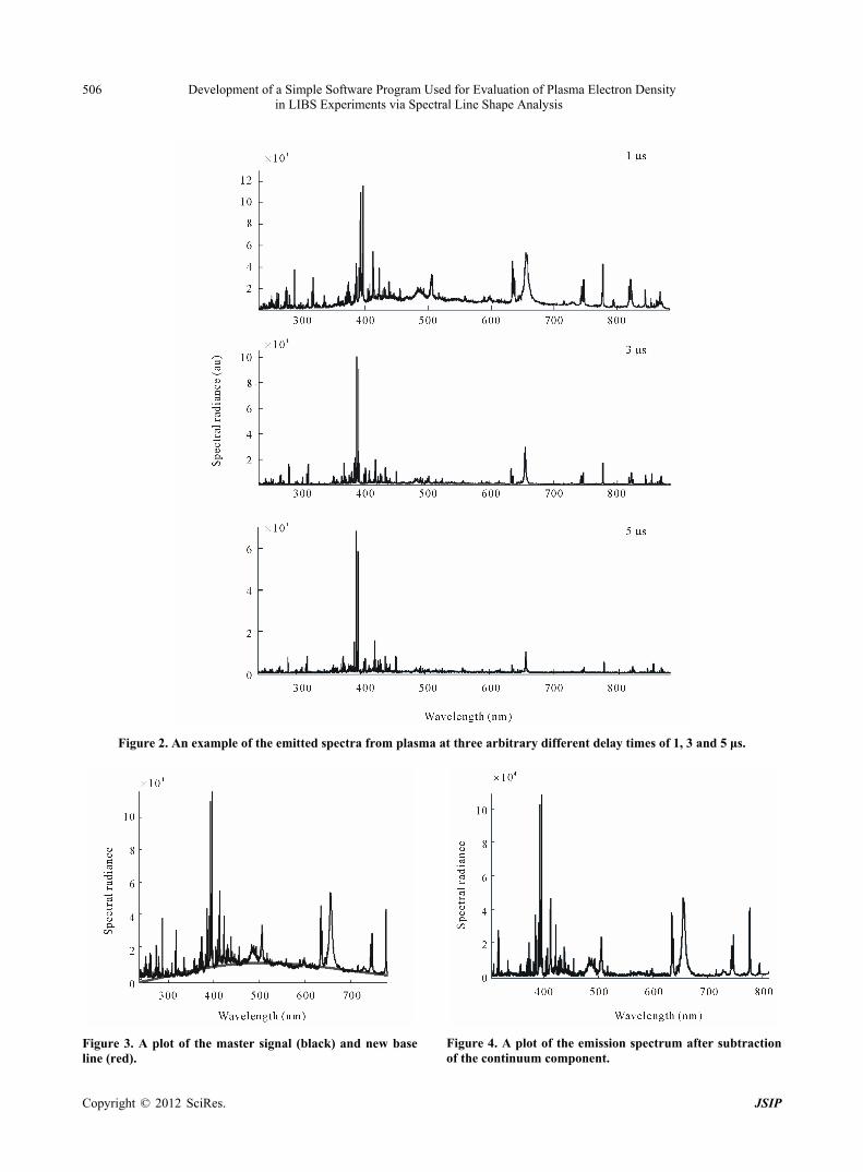
Figure 2 represents the master optical signals in the

range from 200 - 1000 nm as recorded by the ICCD cam-era program (KestrelSpec® 3.96) and plotted in a Mat-Lab7® window. These spectra were taken at a gate time of 1 μs and arbitrary delay times of 1, 3 and 5 μs.

One can notice the strong continuum component ap-peared under the whole the spectrum. This continuum is usually attributed to the free-free and free-bound transi-tions of the quasi free electrons in the plasma and should be removed before processing any optical signal. Also one can notice the decrease in the continuum level as the delay time increases from 1 to 5 μs.

Figure 3 shows the new base line plotted in red color, this line was created via fitting of the whole the spectrum (40001 pixels) to a polynomial function set at the 5th or-der. One can notice that for every region the cutting level should be manually adjusted. This can be done by the manual control set at program statement number 15. The clean spectrum after subtraction of the continuum is hown in Figure 4. s


506

Figure 2. An example of the emitted spectra from plasma at three arbitrary different delay times of 1, 3 and 5 μs.

Figure 3. A plot of the master signal (black) and new base line (red).

Figure 4. A plot of the emission spectrum after subtraction of the continuum component.



507

The isolated Hα-line in the master form (data pixel points) is shown at Figure 5. The signal analysis will be applied to this optical signal, first we will calculate the spectral radiance and then de-convolute the different con-tributions to the line FWHM. Peering in mind that the Stark width component will be used to evaluate the elec-tron density, hence, a comparison of this signal to a theoretically Voigt function will be applied.

On the other hand, Figure 6 shows a plot of the dif-ferent theoretical functions (Lorentzian and two Gaussian shapes) centered at the experimentally measured central emission wavelength (λoexp). It is worth noting that the

Figure 5. Shown is the isolated master optical emission sig-nal at the Hα-line.

Figure 6. A plot of the Lorentzian function (Drawn in black); the Gaussian function resulted from the instrumental broad-ening (drawn in red), the other Gaussian resulted from the Doppler-Effect is extremely small.

Gaussian functions can be attributed to the Doppler-effect as well as the instrumental bandwidth of the spectro- graph, while the Lorentzian component to the pressure or Stark effect. One can observe that either of the Gaussian components of the line is very small with respect to the Stark component in LIBS experiments, or hence the Doppler component can generally be neglected without too much error. Figure 7 shows the results of the com-parison of the theoretical Voigt line shape (Black curve) to the experimentally measured profile (red curve) at the best fitting.

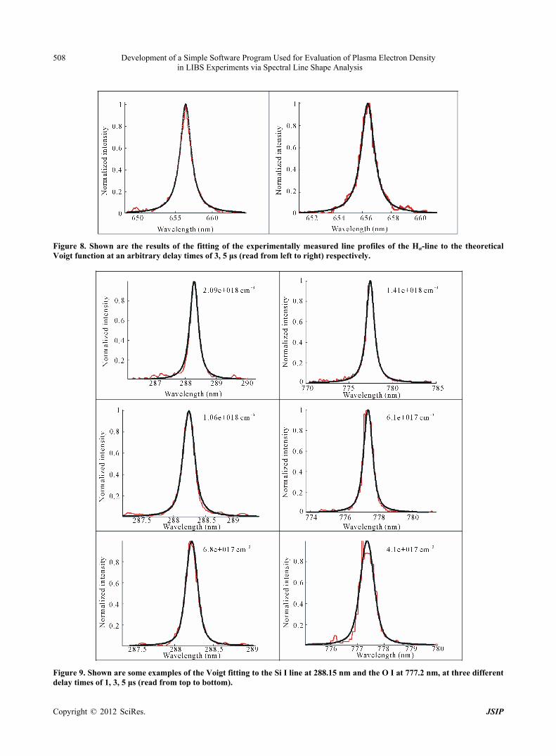
Figure 8 shows the results of fitting of the Voigt func-tion to the Hα-line profile at two arbitrary delay times of 3, 5 μs, respectively. The repeated application of the program at two different delay times yields ∆λStark = 1.76, 1.03 nm, respectively and hence an electron densities of 2.1 × 1017 and 9.5 × 1016 cm–3, respectively.

We have tested the program in order to evaluate the electron density from elements other than hydrogen, e.g. Si I at 288.15 nm and O I at 777.2 nm appeared in the same emission spectra. Noting that, the equation used to evaluate the electron density should be changed, i.e. in-stead of using Equation (4), one should use Equation (5b). The stark broadening parameters of the two lines are taken from tables at Ref. [4], at the given reference elec-tron density. At Figure 9 we give the results of the ap-plication of the program to the Si I and O I at three dif-ferent delay times namely at 1, 3, 5 μs together with the evaluated electron densities.

Finally, in order to realize the importance of the meas-urements of the electron densities utilizing different lines arising from plasma produced by laser, one should plot the variation of the electron density as inferred from dif-

Figure 7. An example of fitting the experimental line profile at the Hα-line (red curve) to the theoretical Voigt function Black curve). (




508

Figure 8. Shown are the results of the fitting of the experimentally measured line profiles of the Hα-line to the theoretical Voigt function at an arbitrary delay times of 3, 5 μs (read from left to right) respectively.

Figure 9. Shown are some examples of the Voigt fitting to the Si I line at 288.15 nm and the O I at 777.2 nm, at three different elay times of 1, 3, 5 μs (read from top to bottom). d


509

ferent lines. Figure 10 represents the results of the esti-mated electron density with delay time. From the figure one can conclude that the line at Si I suffering from opti-cal thickness while this is not the case of the O I at 777.2 nm. This is because one can notice the strong deviation of the electron density calculated from the Si I-line at 288.14 nm and the moderate deviation of the O I-line at 777.2 nm from the density as calculated from the Hα-line. This indicates that both lines are subjected to some self absorption.

With the help of expression (6c), after comparison of the calculate electron density from one line to the same amount as evaluated utilizing the Hα-line one can calcu-late the amount of optical thickness of the plasma at each line and correct the intensities of either line which lies after the scope of this article.

5. Conclusion

We have developed simple routine software used to evaluate the electron density utilizing the spectral line shape analysis to the light emitted from plasma. This routine is based on comparison of the measured line shape to a theoretically built Voigt function. This enables us to extract the stark component contribution to the line width, hence the calculation of the plasma electron den-sity. The electron density was evaluated utilizing differ-ent spectral lines emitted from the plasma under the same condition e.g. the Hα-line (that was used as a reference line in the measurement of the electron density) as well as Si I-line at 288.15 nm and the O I-line at the 777.2 nm.

Figure 10. A demonstration to the temporal variation of the finally calculated electron density utilizing the program with delay time, squares represent the calculated electron density from the Hα-line, triangles are the same density as measured from the O I line at 777.2 nm and the solid disks are the electron densities as calculated from the Si I-line at 288.15 nm.

The higher densities showed by lines other than hydro-gen was attributed to the presence of optical depth of the plasma to these lines.

6. Notations

1) In order to change the wavelength of interest (i.e. to apply the analysis to another line) one has to assign the new wavelength of interest at line number 4.

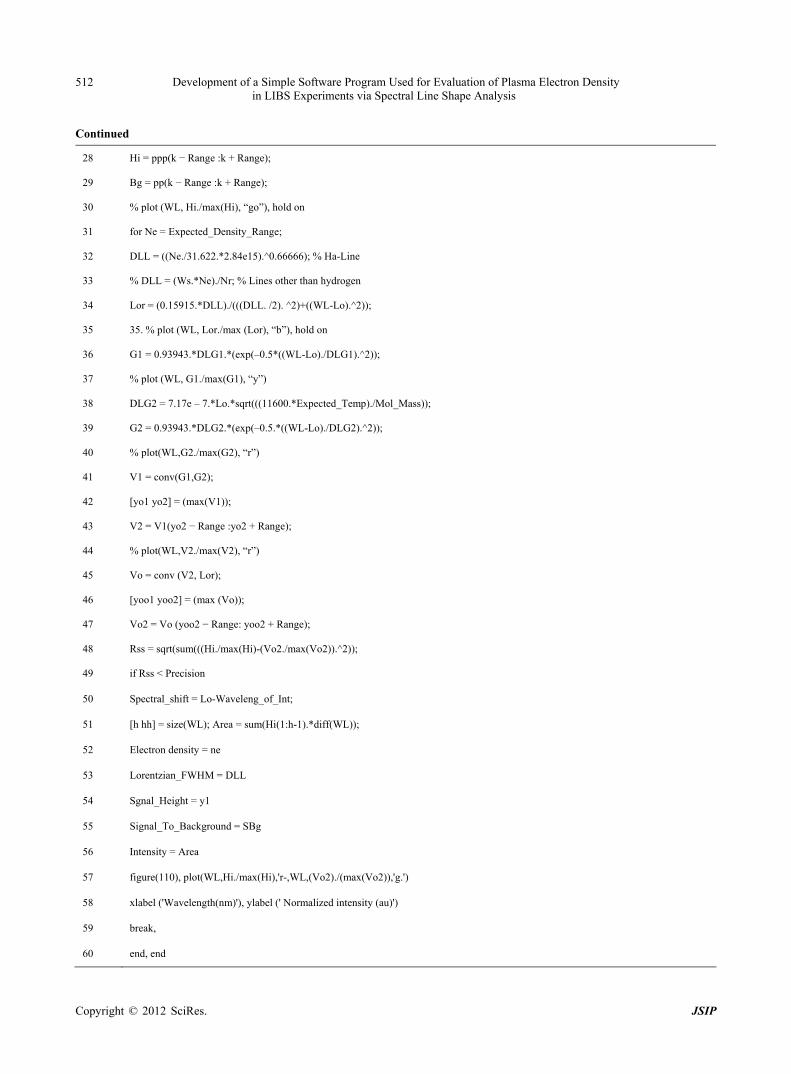
2) For lines other than the Hα-line, one has to use Equation 5(b) instead of Equation (4) and use line num-ber 33 instead of line number 32 (pause line 32 by using the % sign at the start of the line) together with assign-ment of the reference electron density (Nr) and Stark broadening parameter (ωs) at lines 11,12.

3) From our experience to handle the LIBS spectra under our condition of the laser energy and duration the expected temperature is almost around 1 eV and hence the Doppler FWHM is almost centered on 0.04 nm that can be neglected.

4) One more option that can enhance precision of the fitting is to change the value of the controllable precision parameter at line 16.

5) In order to examine somewhat line against the effect of absorption, one has to run the program two times in series. The first run to calculate the density utilizing the Hα-line, and the next to run the program to calculate the same density using the suspected line. Then the applica-tion of Equation (6c) will evaluate directly the amount of self absorption. If the SA value is found in the range (0.8 - 1) the line is considered as optically thin [15], lower val-ues of SA means that the lines is thick and need to be corrected.

6) The correction of spectral intensity against the ef-fect of self absorption can be carried using Equation (6a) in order to evaluate o oI .

7) Lines (13 - 16) completely enables one to control the fitting to the experimental line shape.

7. Acknowledgements

The experimental part utilized in the analysis was carried at the Laboratory of lasers and New Materials, Faculty of Science at Cairo University—Egypt under the supervi-sion of Prof. Th. M. EL Sherbini and Prof. S. H. Allam.

REFERENCES [1] A. F. M. Y. Haider and Z. H. Khan, “Determination of Ca

Content of Coral Skeleton by Analyte Additive Method Using the LIBS Technique,” Optics & Laser Technology, Vol. 44, No. 6, 2012, pp. 1654-1659. doi:10.1016/j.optlastec.2012.01.032

[2] W. Lochte-Holtgreven, “Plasma Diagnostics,” North Hol- land, Amsterdam, 1968.


http://dx.doi.org/10.1016/j.optlastec.2012.01.032


510

[3] H. R. Griem, “Plasma Spectroscopy,” McGrow-Hill, Inc., New York, 1964.

[4] H. R. Griem, “Spectral Line Broadening by Plasmas,” Academic Press, New York, 1974.

[5] H. J-Kunze, “Introduction to Plasma Spectroscopy,” Springer Series on Atomic, Optical and Plasma Physics, Vol. 56, Springer, New York, 2009.

[6] H. Amamou, A. Bois, B. Ferhat, R. Redon, B. Rossetto and P. Matheron, “Correction of the Self-Absorption for Reversed Spectral Lines: Application to Two Resonance Lines of Neutral Aluminum,” JQSRT, Vol. 77, No. 4, 2003, pp. 365-372. doi:10.1016/S0022-4073(02)00163-2

[7] N. Konjevic, “Plasma Broadening and Shifting of Non- Hydrogenic Spectral Lines: Present Status and Applica-tions,” Physics Reports, Vol. 316, No. 6, 1999, pp. 339- 401. doi:10.1016/S0370-1573(98)00132-X

[8] R. Žikić, M. A. Gigosos, M. Ivković, M. Á. González and N. Konjević, “A Program for the Evaluation of Electron Number Density from Experimental Hydrogen Balmer Beta Line Profiles,” Spectrochimica Acta Part B, Vol. 57, No. 5, 2002, pp. 987-998. doi:10.1016/S0584-8547(02)00015-0

[9] N. Konjević, M. Ivković and N. Sakan, “Hydrogen Bal- mer Lines for Low Electron Number Density Plasma Di-agnostics,” Spectrochimica Acta Part B, Vol. 76, 2012, pp. 16-26.

[10] C. Yubero, M. C. García and M. D. Calzada, “On the Use of the Hα Spectral Line to Determine the Electron Den-sity in a Microwave (2.45 GHz) Plasma Torch at Atmos-pheric Pressure,” Spectrochimica Acta Part B, Vol. 61, No. 5, 2006, pp. 540-544.

doi:10.1016/j.sab.2006.03.011

[11] W. Olchawa, “Computer Simulations of Hydrogen Spec-tral Line Shapes in Dense Plasmas,” JQSRT, Vol. 74, No. 4, 2002, pp. 417-429. doi:10.1016/S0022-4073(01)00262-X

[12] S.-K. Chan and A. Montaser, “Determination of Electron Number Density via Stark Broadening with an Improved Algorithm,” Spectrochimica Acta Part B, Vol. 448, No. 2, 1989, pp. 175-184.

[13] A. M. El Sherbini, H. Hegazy and Th. M. El Sherbini, “Measurement of Electron Density Utilizing the Hα-Line from Laser Produced Plasma in Air,” Spectrochimica Acta Part B, Vol. 61, No. 5, 2006, pp. 532-539. doi:10.1016/j.sab.2006.03.014

[14] P. Kepple and H. R. Griem, “Improved Stark Profile Cal-culations for the Hydrogen Lines Hα, Hβ, Hγ, and Hδ,” Physical Review, Vol. 173, No. 1, 1968, pp. 317-325. doi:10.1103/PhysRev.173.317

[15] A. M. EL Sherbini, A. M. Aboulfotouh, S. H. Allam and Th. M. EL Sherbini, “Diode Laser Absorption Measure-ments at the Hα-Transition in Laser Induced Plasmas on Different Targets,” Spectrochimica Acta Part B, Vol. 65, No. 12, 2010, pp. 1041-1046. doi:10.1016/j.sab.2010.11.004

[16] A. M. El Sherbini, Th. M. El Sherbini, H. Hegazy, G. Cristoforetti, S. Legnaioli, V. Palleschi, L. Pardini, A. Salvetti and E. Tognoni, “Evaluation of Self-Absorption Coefficients of Aluminum Emission Lines in Laser-In- duced Breakdown Spectroscopy Measurements,” Spec-trochimica Acta Part B, Vol. 60, No. 12, 2005, pp. 1573- 1579. doi:10.1016/j.sab.2005.10.011


http://dx.doi.org/10.1016/S0022-4073(02)00163-2

http://dx.doi.org/10.1016/S0370-1573(98)00132-X

http://dx.doi.org/10.1016/S0584-8547(02)00015-0

http://dx.doi.org/10.1016/j.sab.2006.03.011

http://dx.doi.org/10.1016/S0022-4073(01)00262-X


http://dx.doi.org/10.1103/PhysRev.173.317




511

Appendix A

Program statements in MatLab7®.

Table 1. Description to order at each line.

Line No. Order

01 close all, clear all

02 load filename.txt

03 L = filename (:, 1); I = filename (:, 2);

04 Waveleng_of_Int = 656.27; % in nm units

05 Expected_Temp = 1; % in eV units

06 Mol_Mass = 1; % Molecular mass in amu units

07 DLG1 = 0.12; % Instrumental Bandwidth in nm units

08 Ne_Step = 1e16; % in e/cm3 units

09 Expected_Density_Range = [1e16:Ne_Step:5e18]; % in e/cm3 units

10 fit _order = 5; % polynomial fitting order

11 Nr = 1e17; % Reference density in e/cm3 units

12 Ws = 0.0044; % Stark broadening parameter in nm units

13 Range = 1000; % Number of pixels to cover the line

14 Jitter _Shift = –35;

15 Cutting _Level = –3000;

16 Precision = 0.0000024;

17 p = polyfit (L, I, fit _order)

18 pp = Cutting_Level + polyval (p, L);

19 ppp = abs(I-pp);

%%%%%%%%%%%%%%%%%%%%%%%%%%%%%%%%%%%%%%%%%%%%%%%%%%%%%%%%%%%%%%%%

20 x1 = find (L == Waveleng_of_Int-1); x2 = find (L == Waveleng_of_Int + 1);

21 L1 = L(x1: x2);

22 [y1 y2] = max (ppp(x1: x2));

23 Lo = L1 (y2-Jitter_Shift);

24 [Y1 Y2] = max (pp(x1: x2));

25 SBg = y1/(Y1);

26 k = find(L == Lo);

27 WL = L(k − Range : k + Range);



512

Continued

28 Hi = ppp(k − Range :k + Range);

29 Bg = pp(k − Range :k + Range);

30 % plot (WL, Hi./max(Hi), “go”), hold on

31 for Ne = Expected_Density_Range;

32 DLL = ((Ne./31.622.*2.84e15).^0.66666); % Ha-Line

33 % DLL = (Ws.*Ne)./Nr; % Lines other than hydrogen

34 Lor = (0.15915.*DLL)./(((DLL. /2). ^2)+((WL-Lo).^2));

35 35. % plot (WL, Lor./max (Lor), “b”), hold on

36 G1 = 0.93943.*DLG1.*(exp(–0.5*((WL-Lo)./DLG1).^2));

37 % plot (WL, G1./max(G1), “y”)

38 DLG2 = 7.17e – 7.*Lo.*sqrt(((11600.*Expected_Temp)./Mol_Mass));

39 G2 = 0.93943.*DLG2.*(exp(–0.5.*((WL-Lo)./DLG2).^2));

40 % plot(WL,G2./max(G2), “r”)

41 V1 = conv(G1,G2);

42 [yo1 yo2] = (max(V1));

43 V2 = V1(yo2 − Range :yo2 + Range);

44 % plot(WL,V2./max(V2), “r”)

45 Vo = conv (V2, Lor);

46 [yoo1 yoo2] = (max (Vo));

47 Vo2 = Vo (yoo2 − Range: yoo2 + Range);

48 Rss = sqrt(sum(((Hi./max(Hi)-(Vo2./max(Vo2)).^2));

49 if Rss < Precision

50 Spectral_shift = Lo-Waveleng_of_Int;

51 [h hh] = size(WL); Area = sum(Hi(1:h-1).*diff(WL));

52 Electron density = ne

53 Lorentzian_FWHM = DLL

54 Sgnal_Height = y1

55 Signal_To_Background = SBg

56 Intensity = Area

57 figure(110), plot(WL,Hi./max(Hi),'r-,WL,(Vo2)./(max(Vo2)),'g.')

58 xlabel ('Wavelength(nm)'), ylabel (' Normalized intensity (au)')

59 break,

60 end, end



513

Appendix B

Program Statement Function

Line No Task Description

1 Close and clear any programs running at the Matlab working space

2 Load the data file (ASC II format)

3 Assign the wavelengths from 200 nm to 1000 nm with a step difference (resolution) of 0.02 nm per pixel, to single column matrix which is now contains 40,001 pixels, call it matrix-L. Also, assign the signal height at each wavelength to single column matrix which also contains 40001 pixels, call it matrix-I

Manual Control Parameters

4 Specify the working wavelength in nm units

5 State the expected electron temperature

6 State the molecular mass of atom or ion of the element that emits light in amu units

7 Assign the instrumental bandwidth as measured in units of nm

8 Assign the step in electron density range (PRECISION IN MEASURMENTS)

9 Assign the expected lower and higher density values with step as stated at line 8

10 Assign the order of the used polynomial function for fitting to the whole spectrum in order to create the new base line

11 For elements other than hydrogen, assign the reference electron density value

12 For elements other than hydrogen, state the Stark broadening parameters as taken from standard tables

Fitting Control Parameters

13 Assign the number of pixels that can cover the line to wings

14 Assign the number of pixels used to correct the peak wavelength against pulse jitter

15 State the amount of the manual cutting level (this may be changes from one line to the other in the same working spectrum)

16 State the precision needed for the fitting of spectral line to the Voigt function

Creation of New Base Line

17 Use the built-in polynomial function, fit the whole the spectrum to an order defined before at line number 10

18

At the best fit to the emission spectrum, evaluate the polynomial coefficients, this new pp function will act as the NEW BASE LINE. This new base line can be further detuned via addition or subtraction of a certain constant as mentioned before at the (Cutting Level) specified at line number 15. Upon detuning to this factor one can reach the best cutting level at the line wings, call the resulted new base function as matrix-pp. This matrix function is actually the continuum emission component, which is resulted mainly from the free-free and free-bound transition and should be subtracted before application of analysis to the line shape.

19 Subtract this new base (matrix-pp) from the master spectrum (matrix-I) to get a clean spectrum (matrix-ppp) without the unnecessary continuum component appeared under the line of interest.

Isolation of the Spectral Line of Interest

20 Utilizing the wavelength matrix (L), choose the pixel point “x1” that lie before the wanted line of interest and choose the pixel point “x2” lie after the line of interest

21 Create a single matrix of new wavelengths “starting from pixel number x1 and ended at pixel number x2” call this new wavelength region as matrix-L1

22 In the same range from pixels (x1: x2) find the maximum height (y1) from the matrix (ppp) without continuum, this is the line intensity in units of counts/sec and the corresponding pixel number y2 of the peak height

23 Calculate the wavelength corresponding to the pixel number y2 and call this wavelength as Lo (λoexp) taking into account any jitter in the peak wavelength

24 In the same range from pixels (x1: x2) find the maximum height from the matrix (pp) which represent the continuum intensity (Y1) in units of counts/sec



514

Continued

25 Calculate the signal to background (y1/Y1)

Built up the Necessary Theoretical Functions around λoexp

26 From the wavelength matrix L, find the pixel number (k) corresponding to λoexp

27 Create a new wavelength region centered around λoexp and extended by number of pixels specified previously by (Range—at line number 13)

28 Utilizing matrix (ppp) of signal heights and free from continuum, find the new heights in the same range corresponding to the new wavelength WL regime i.e. in the same region defined by statement range at line 13

29 Utilizing matrix (pp) of background continuum, fine the new heights in the same range corresponding to the new wavelength WL regime i.e. in the same region defined by statement range at line 13

30 Plot, if necessary, the experimental isolated line in the new range defined by new wavelength regime WL and the corresponding signal heights Hi

The Theoretical Functions 1. Lorentzian Function

31 With the help of the properties of the “FOR-loop” let the electron density Ne is the free running parameter according to values previously defined at line number 9, together with the precision step at line 8

32 For the hydrogen Hα-line only use equation 4 at the text to calculate the Lorentzian FWHM in nm

33 For lines other than the hydrogen Hα-line, use this equation 5b to calculate the Lorentzian FWHM in nm

34 Calculate the Lorentzian function according to line FWHM defined in the previous step

35 Plot, if necessary the theoretical Lorentzian function centered around λoexp in the new range defined by wavelengths WL and signal heights Hi

2. Gauss Function Resulted from the Instrumental Bandwidth

36 Calculate the Gauss function according to line FWHM defined line number 7

37 Plot, if necessary the theoretical Gauss function centered around λoexp in the new range defined by wavelengths WL and signal heights Hi

3. Gauss Function Resulted from the Doppler Effect

38 Calculate the line FWHM according to Doppler effect centered around λoexp in the new range defined by wavelengths WL and signal heights Hi at the expected electron temperature specified at line number 5

39 Calculate the Gauss function according to line FWHM defined in the previous step

40 Plot, if necessary the theoretical Gauss function centered around λoexp in the new range defined by wavelengths WL and signal heights Hi

4. Start Convolution between the Different Functions

41 Start with convolution between the two Gauss functions G1, G2

42 Calculate the pixel number corresponding to the maximum of the new function V1 and call this number as yo2

43 From this function V1 extract the required number of pixels just to cover the spectral line according to Range specified to line 13, call this function as V2

44 Plot, if necessary the theoretical V2 function centered around λoexp in the new range defined by wavelengths WL and signal heights Hi

5. Carry a Convolution between V2 and the Lorentzian Function

45 Convolute the two functions V2 and Lorentzian function (Lor), call new function as Vo

46 Calculate the pixel number corresponding to the maximum of the new function V1 and call this number as yoo2

47 From this function Vo extract the required number of pixels just to cover the spectral line according to Range specified to line 13, call this function as Vo2

48 Compare between the theoretically built normalized Voigt function (Vo20 and the experimentally normalized measured line profile Hi according to the principle of least square fitting method. Call the residual number as RSS

6. Utilizing the Conditional (IF-Statement)

49 If, the residual number at line 48 corresponding to the fitting, is lower than a certain level defined by order precision at line 16




515

Continued

50 Calculate the spectral shift

51 Evaluate the area under the experimentally measured profile

52 Evaluate the electron density at the best fit

53 Evaluate the Lorentzian FWHM in nm at the best fit

54 Evaluate the signal height at the best fit

55 Evaluate the background at the best fit

56 Evaluate the spectral intensity as area under curve at the best fit

56 Plot the final results of comparison between the theoretical function and the experimentally measured line profile

58 Break the loop

59 End the first loop started at line 49

60 End second loop started at line 31

Documents

Development of a Simple Software Program Used for …file.scirp.org/pdf/JSIP20120400009_90416790.pdf · the Stark effect is the dominant broadening mechanism, in comparison to the