Development of a seismic design procedure for metal building systems

UC San DiegoUC San Diego Electronic Theses and Dissertations

TitleDevelopment of a seismic design procedure for metal building systems

Permalinkhttps://escholarship.org/uc/item/3vp4k1pf

AuthorHong, Jong-Kook

Publication Date2007-01-01 Peer reviewed|Thesis/dissertation

eScholarship.org Powered by the California Digital LibraryUniversity of California

https://escholarship.org/uc/item/3vp4k1pf

https://escholarship.org

http://www.cdlib.org/

UNIVERSITY OF CALIFORNIA, SAN DIEGO

Development of A Seismic Design Procedure for Metal Building Systems

A Dissertation submitted in partial satisfaction of the requirements

for the degree Doctor of Philosophy

in

Structural Engineering

by

Jong-Kook Hong

Committee in charge:

Professor Chia-Ming Uang, Chair Professor David Benson Professor Enrique Luco Professor Sia Nemat-Nasser Professor Benson Shing

2007

Copyright

Jong-Kook Hong, 2007

All rights reserved.

iii

SIGNATURE PAGE

The Dissertation of Jong-Kook Hong is approved, and it is

acceptable in quality and form for publication on

microfilm:

Chair

University of California, San Diego

2007

iv

DEDICATION

To my wife, Ha-Jeong

and my daughter, Joanne

v

EPIGRAPH

Ignorance is not innocence, but sin.

- Robert Browning

vi

TABLE OF CONTENTS

SIGNATURE PAGE ..................................................................................................... iii

DEDICATION .............................................................................................................. iv

EPIGRAPH..................................................................................................................... v

TABLE OF CONTENTS .............................................................................................. vi

LIST OF ABBREVIATIONS ........................................................................................ x

LIST OF SYMBOLS..................................................................................................... xi

LIST OF FIGURES..................................................................................................... xiv

LIST OF TABLES .................................................................................................... xviii

ACKNOWLEDGEMENTS ........................................................................................ xix

VITA............................................................................................................................. xx

ABSTRACT OF THE DISSERTATION.................................................................... xxi

1 INTRODUCTION.................................................................................................. 1

1.1 Introduction .................................................................................................... 1

1.2 Current Seismic Design Philosophy............................................................... 2

1.3 Metal Building Systems ................................................................................. 4

1.4 Current Seismic Design Practice of Metal Buildings..................................... 5

1.5 Statement of Problem ..................................................................................... 6

1.6 Dissertation Outline and Chapter Summary................................................... 7

1.6.1 Chapter 1............................................................................................. 8

1.6.2 Chapter 2............................................................................................. 8

1.6.3 Chapter 3............................................................................................. 8

1.6.4 Chapter 4............................................................................................. 9

1.6.5 Chapter 5............................................................................................. 9

1.6.6 Chapter 6............................................................................................. 9

1.6.7 Chapter 7........................................................................................... 10

2 LITERATURE REVIEW..................................................................................... 13

2.1 Introduction .................................................................................................. 13

2.2 LRFD Strength Evaluation of Web-Tapered Members................................ 13

2.2.1 Axial Compressive Strength ............................................................. 13

2.2.2 Flexural Strength............................................................................... 16

2.2.3 Combined Axial Compression and Flexure ...................................... 18

2.2.4 Shear Strength................................................................................... 20

2.3 Metal Building Testing................................................................................. 22

vii

2.3.1 Forest and Murray (1982) ................................................................. 22

2.3.2 Hwang et al. (1989 and 1991)........................................................... 23

2.3.3 Sumner (1995) .................................................................................. 23

2.3.4 Heldt and Mahendran (1998) ............................................................ 24

2.3.5 Chen et al. (2006).............................................................................. 24

2.4 Finite Element Analysis ............................................................................... 25

2.4.1 Davids (1996).................................................................................... 25

2.4.2 Miller and Earls (2003 and 2005) ..................................................... 25

2.5 Summary and Conclusions ........................................................................... 26

3 CYCLIC TESTING OF A METAL BUILDING SYSTEM................................ 32

3.1 Introduction .................................................................................................. 32

3.2 Design of Test Building................................................................................ 32

3.2.1 Test Building..................................................................................... 32

3.2.2 Design Load ...................................................................................... 33

3.2.3 Governing Load Combination .......................................................... 34

3.3 Testing Program ........................................................................................... 35

3.3.1 General .............................................................................................. 35

3.3.2 Material Properties............................................................................ 36

3.3.3 Test Setup.......................................................................................... 36

3.3.4 Instrumentation ................................................................................. 37

3.3.5 Loading History ................................................................................ 38

3.4 Test Results .................................................................................................. 39

3.4.1 Gravity Load Test ............................................................................. 39

3.4.2 Cyclic Test ........................................................................................ 40

3.5 Overstrength of Test Frame.......................................................................... 44

3.6 Member Strength Correlation....................................................................... 44

3.7 Flange Brace Force....................................................................................... 46

3.8 Summary and Conclusions ........................................................................... 49

4 FINITE ELEMENT ANALYSIS OF TEST FRAME........................................ 117

4.1 Introduction ................................................................................................ 117

4.2 Finite Element Modeling Technique .......................................................... 117

4.2.1 General ............................................................................................ 117

4.2.2 Geometry and Element ................................................................... 117

4.2.3 Material Properties.......................................................................... 119

4.2.4 Gravity Load and Monotonic Push ................................................. 119

4.2.5 Post-Buckling Response ................................................................. 119

4.3 Correlation with Test Results ..................................................................... 120

viii

4.3.1 Gravity Load Analysis .................................................................... 120

4.3.2 Lateral Load Analysis ..................................................................... 121

4.4 Initial Geometric Imperfection ................................................................... 122

4.5 Summary and Conclusions ......................................................................... 122

5 DEVELOPMENT OF A SEISMIC DESIGN PROCEDURE ........................... 132

5.1 Introduction ................................................................................................ 132

5.2 Drift-Based Design Concept....................................................................... 132

5.3 System Overstrength Factor, Ωo................................................................. 134

5.4 Fundamental Period.................................................................................... 135

5.4.1 Design Seismic Base Shear............................................................. 135

5.4.2 T versus Ta....................................................................................... 136

5.4.3 Story Drift Evaluation..................................................................... 137

5.5 Influence of Damping................................................................................. 137

5.6 Influence of R-Factor.................................................................................. 138

5.7 Simplified Design Procedure...................................................................... 138


6 APPLICATIONS OF THE PROPOSED SEISMIC DESIGN PROCEDURE .. 148

6.1 Introduction ................................................................................................ 148

6.2 Case 1 (40 ft×12 ft)..................................................................................... 148

6.2.1 Step 1: Preliminary Design ............................................................. 148

6.2.2 Step 2: Compute Actual Fundamental Period, T ............................ 149

6.2.3 Step 3: Compute Ωo Based on the Revised Earthquake Load ........ 150

6.2.4 Step 4: Check Ωo/R Ratio................................................................ 151

6.2.5 Step 5: Connection Design.............................................................. 151

6.3 Case 2 (100 ft×20 ft)................................................................................... 151






6.4 Case 3 (150 ft×20 ft)................................................................................... 154






ix


7 SUMMARY AND CONCLUSIONS................................................................. 186

7.1 Summary..................................................................................................... 186

7.2 Conclusions ................................................................................................ 189

APPENDIX A. MEMBER STRENGTH CHECK OF TEST FRMAE ..................... 192

APPENDIX B. OVERSTRENGTH FACTOR OF EXAMPLE BUILDINGS.......... 205

APPENDIX C. PARAMETRIC STUDIES ON PANEL ZONE THICKNESS ........ 219

REFERENCES........................................................................................................... 228

x

LIST OF ABBREVIATIONS

AISC American Institute of Steel Construction,

AISI American Iron and Steel Institute,

ASCE American Society of Civil Engineers,

ASD Allowable Stress Design,

BSSC Building Seismic Safety Committee,

DCR Demand/Capacity Ratio,

DCRE Demand/Capacity Ratio under Earthquake Load,

DCRG Demand/Capacity Ratio under Gravity Load,

FEA Finite Element Analysis,

FEMA Federal Emergency Management Agency,

ICC International Code Council,

IBC International Building Code,

LRFD Load and Resistance Factor Design,

MBMA Metal Building Manufacturers Association,

OMF Ordinary Moment Frame,

SMF Special Moment Frame, and

UCSD University of California, San Diego.

xi

LIST OF SYMBOLS

Ag Area of cross-section,

Aw Area of web,

Cb Bending coefficient dependent on moment gradient,

Cd Displacement amplification factor,

Ceu Required strength to respond elastically,

Cs Code-specified seismic force level,

Cu Coefficient for upper limit of fundamental period,

Cv Shear coefficient,

Cy Ultimate strength level,

E Elastic modulus,

Fbγ Critical flexural stress,

Fcr Critical buckling stress,

Fsγ St. Venant’s term of critical flexural stress,

Fu Tensile stress,

Fwγ Warping term of critical flexural stress,

Fy Specified minimum yield stress,

Fye Design expected yield strength,

Fyw Web yield stress,

K Effective length factor for prismatic members,

Kγ Effective length factor for web-tapered members,

Lb Unbraced length of a segment,

Mn Nominal flexural strength,

Mnt Required flexural strength with no lateral translation,

Mlt Required flexural strength with lateral translation,

Mp Nominal plastic flexural strength,

Mu Required flexural strength,

Pn Nominal compressive strength,

xii

Pu Required axial strength,

Py Nominal tensile strength,

Q Slenderness member reduction factor,

Qa Slenderness member reduction factor for stiffened compression

members,

Qs Slenderness member reduction factor for unstiffened compression

elements,

Sa Spectral response acceleration,

SDS Design, 5 percent damped, spectral response acceleration parameter at

short periods,

SD1 Design, 5 percent damped, spectral response acceleration parameter at a

period of 1 second,

R Response modification factor,

Rμ System ductility reduction factor,

Sx′ Section modulus at larger member end,

T Actual fundamental period,

Ta Fundamental period by approximate method,

Vn Nominal shear strength,

Vu Required shear strength,

do Depth of beam at smaller end,

di Depth of beam at larger end,

h Tapered member length factor,

kv Web plate buckling coefficient,

g Acceleration of gravity,

ro Radius of gyration about strong axis,

roy Radius of gyration about weak axis,

ΔC Drift capacity,

ΔD Drift demand,

ΔS Drift at design seismic force level,

Ωo System overstrength factor,

xiii

δe Elastic story drift,

δs Inelastic story drift, plε Plastic strain,

γ Tapering ratio,

λ Section compactness ratio,

σtaper Stress of tapered member,

σ|0 Yield surface size as zero plastic strain, and

ξ Damping ratio.

xiv

LIST OF FIGURES

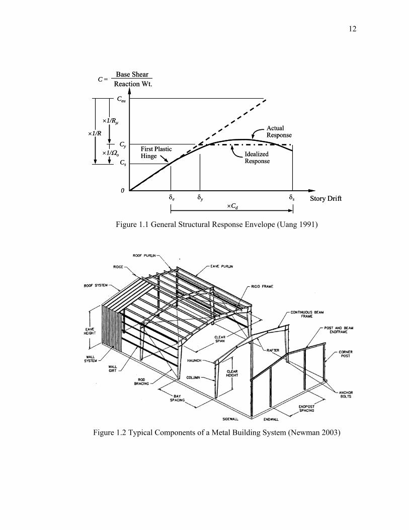
Figure 1.1 General Structural Response Envelope (Uang 1991) .................................12

Figure 1.2 Typical Components of a Metal Building System (Newman 2003)...........12

Figure 2.1 Tapered Beam Geometry and Presumed Loading (Lee et al. 1972) ...........29

Figure 2.2 Length Modification Factor (Lee et al. 1972).............................................30

Figure 2.3 Panel Zone Plate with Stiffener ..................................................................31

Figure 2.4 Tension Field in the Panel Zone .................................................................31

Figure 3.1 Elevation and Top View of Test Building ..................................................55

Figure 3.2 Sidewall Elevation ......................................................................................56

Figure 3.3 Column Base ...............................................................................................57

Figure 3.4 Design Wind Load ......................................................................................58

Figure 3.5 SAP Modeling Scheme ...............................................................................58

Figure 3.6 Force Demand under Governing Loading Combination.............................59

Figure 3.7 Test Building...............................................................................................60

Figure 3.8 Flange Brace ...............................................................................................61

Figure 3.9 Test Setup....................................................................................................62

Figure 3.10 Actuator-to-Column Connection Details ..................................................63

Figure 3.11 Column Base Connection Details .............................................................64

Figure 3.12 Instrumentation for Panel Zone, End Plate, and Column Base.................65

Figure 3.13 Gravity Load and Cyclic Load..................................................................66

Figure 3.14 Vertical Deflection at Midspan .................................................................67

Figure 3.15 Frame 1: Rotation Angle at Column Base ................................................67

Figure 3.16 Stress Distribution due to Gravity Load ...................................................68

Figure 3.17 Moment Diagram (Gravity Load Only) ....................................................69

Figure 3.18 Derived and Simplified Support Reactions (Gravity Load Only).............70

Figure 3.19 Frame 1: Axial Force and Bending Moment Diagrams (Gravity Load

Only).....................................................................................................................71


Only).....................................................................................................................72

xv

Figure 3.21 Frame 1: Behavior at 1.5% Drift...............................................................73

Figure 3.22 Frame 2: Behavior at 1.5% Drift...............................................................74

Figure 3.23 Lateral Buckling at South Column and Rafter of Frame 2 .......................75

Figure 3.24 Flange Brace Reinforcement and Addition after First 2% Drift ...............76

Figure 3.25 Flange Braces Added during 2% Drift Cycles..........................................77

Figure 3.26 Frame 1: Failure Mode at First Positive Excursion to 3% Drift ...............78

Figure 3.27 Frame 2: Failure Mode at First Positive Excursion to 3% Drift ...............78

Figure 3.28 Failure Mode at First Negative Excursion to 3% Drift .............................79

Figure 3.29 Base Shear versus Column Top Displacement .........................................80

Figure 3.30 Frame 1: Moment versus Panel Zone Shear Deformation........................81

Figure 3.31 Frame 2: Moment versus Panel Zone Shear Deformation........................82

Figure 3.32 Moment versus End-Plate Opening Displacement ...................................83

Figure 3.33 Frame 1: Measured Strains at Rafter Flanges (Positive Excursions)........84

Figure 3.34 Frame 1: Measured Strains at North Column (Positive Excursions) ........85

Figure 3.35 Frame 1: Measured Strains at South Column (Positive Excursions) ........86

Figure 3.36 Frame 1: Measured Strains at Rafter Flanges (Negative Excursions) ......87

Figure 3.37 Frame 1: Measured Strains at North Column (Negative Excursions) ......88

Figure 3.38 Frame 1: Measured Strains at South Column (Negative Excursions) ......89

Figure 3.39 Frame 2: Measured Strains at Rafter Flanges (Positive Excursions)........90

Figure 3.40 Frame 2: Measured Strains at North Column (Positive Excursions) ........91

Figure 3.41 Frame 2: Measured Strains at South Column (Positive Excursions) ........92

Figure 3.42 Frame 2: Measured Strains at Rafter Flanges (Negative Excursions) ......93

Figure 3.43 Frame 2: Measured Strains at North Column (Negative Excursions) ......94

Figure 3.44 Frame 2: Measured Strains at South Column (Negative Excursions) ......95

Figure 3.45 Load versus Measured Strain at Rod Braces ............................................96

Figure 3.46 Strain Deviation at 1.5% Drift ..................................................................97

Figure 3.47 Support Reactions of Frame 1 at Positive 2.6% Drift (Lateral Load Only)

..............................................................................................................................98

Figure 3.48 Measured Rotation Angle at Column Bases of Frame 1...........................99

Figure 3.49 Shear Force at South Column of Frame 1...............................................100

xvi

Figure 3.50 Internal Forces at Positive 2.6% Drift due to Lateral Load Only ...........101

Figure 3.51 Frame 1: Internal Forces at Positive 2.6% Drift due to Combined Loads

............................................................................................................................102


............................................................................................................................103

Figure 3.53 Support Reactions of Frame 1 at Negative 2.3% Drift (Lateral Load Only)

............................................................................................................................104

Figure 3.54 Internal Forces at Negative 2.3% Drift due to Lateral Load Only..........105

Figure 3.55 Frame 1: Internal Forces at Negative 2.3% Drift due to Combined Loads

............................................................................................................................106


............................................................................................................................107

Figure 3.57 Frame 1: Axial Force and Moment Interaction.......................................108

Figure 3.58 Frame 2: Axial Force and Moment Interaction.......................................109

Figure 3.59 South Rafter Strength Check at Positive 2.6% Drift...............................110

Figure 3.60 North Rafter Strength Check at Negative 2.3% Drift .............................111

Figure 3.61 Flange Brace Force on HSS Supporting Beam.......................................112

Figure 3.62 Flange Brace Angle Section (L2½×2½×3/16) ........................................112

Figure 3.63 Moment due to Axial Load at Flange Brace ...........................................113

Figure 3.64 Frame 1: Measured Strain at Flange Brace.............................................114

Figure 3.65 Frame 2: Measured Strain at Additional Flange Brace...........................116

Figure 4.1 ABAQUS Model of Test Frame (Loading in Positive Direction) ............125

Figure 4.2 First Eigen Buckling Mode Shape for Models 2 and 3.............................125

Figure 4.3 Stress-Strain Relationship (Mays 2000) ...................................................126

Figure 4.4 Typical Unstable Static Response (ABAQUS Inc. 2005).........................126

Figure 4.5 Normal Stress Comparison .......................................................................127

Figure 4.6 Flange Buckling Failure Mode of Model 1...............................................128

Figure 4.7 Lateral Buckling Failure Mode of Model 2 ..............................................128

Figure 4.8 Flange Local Buckling and Lateral Buckling Failure Mode of Model 3..129

Figure 4.9 Base Shear versus Lateral Displacement Comparison..............................129

xvii

Figure 4.10 Predicted Failure Mode of Model 4 ........................................................130

Figure 4.11 Global Response Comparison.................................................................130

Figure 4.12 Initial Imperfection Effect on Global Response .....................................131

Figure 5.1 Seismic Design Concept ...........................................................................144

Figure 5.2 Design Response Spectrum (ASCE 7-05) ................................................145

Figure 5.3 Prototype Building for Dynamic Test (Sockalingam 1988) .....................145

Figure 5.4 General Response Spectrum (FEMA 273)................................................146

Figure 5.5 General Design Procedure ........................................................................147

Figure 6.1 Case 1 (40 ft×12 ft) ...................................................................................164

Figure 6.2 Case 1: Demand/Capacity Ratio under Governing Load Combination....165

Figure 6.3 Case 1: Spectral Response Acceleration and Drift Demand.....................166

Figure 6.4 Case 1: Overstrength Factor for Building A .............................................167

Figure 6.5 Case 1: Overstrength Factor for Building B .............................................169

Figure 6.6 Case 1: Failure Mode and Drift Capacity Verification of Building A......171

Figure 6.7 Case 1: Failure Mode and Drift Capacity Verification of Building B ......172

Figure 6.8 Case 2 (100 ft×20 ft) .................................................................................173

Figure 6.9 Case 2: Demand/Capacity Ratio under Governing Load Combination....174

Figure 6.10 Case 2: Spectral Response Acceleration and Drift Demand...................175

Figure 6.11 Case 2: Overstrength Factor at Critical Segment....................................176

Figure 6.12 Case 2: Failure Mode and Drift Capacity Verification of Building A....177

Figure 6.13 Case 2: Failure Mode and Drift Capacity Verification of Building B ....178

Figure 6.14 Case 3 (150 ft×20 ft) ...............................................................................179

Figure 6.15 Case 3: Connection Details (Nucor Building Systems) ..........................180

Figure 6.16 Case 3: Demand/Capacity Ratio under Governing Load Combination..181

Figure 6.17 Case 3: Spectral Response Acceleration and Drift Demand...................182

Figure 6.18 Case 3: Overstrength Factor at Critical Segment....................................183

Figure 6.19 Case 3: Failure Mode and Drift Capacity Verification of Building A....184

Figure 6.20 Case 3: Failure Mode and Drift Capacity Verification of Building B ....185

xviii

LIST OF TABLES

Table 1.1 Design Coefficients and Factors for Steel Seismic Force-Resisting Systems

(ASCE 7-05).........................................................................................................11

Table 2.1 Section Properties at the Smaller End (Lee et al. 1972)...............................28

Table 3.1 Member Properties .......................................................................................51

Table 3.2 Design Load .................................................................................................52

Table 3.3 Mechanical Properties of Steel.....................................................................52

Table 3.4 Strength Check of Frame 1 at Positive 2.6% Drift.......................................53

Table 3.5 Strength Check of Frame 2 at Positive 2.6% Drift.......................................53

Table 3.6 Strength Check of Frame 1 at Negative 2.3% Drift .....................................54

Table 3.7 Strength Check of Frame 2 at Negative 2.3% Drift .....................................54

Table 4.1 ABAQUS Modeling Matrix .......................................................................124

Table 4.2 Initial Imperfection Amplitude Effect on Ultimate Load Prediction .........124

Table 5.1 Coefficient for Upper Limit on Calculated Period (ASCE 7-05)...............142

Table 5.2 Values of Approximate Period Parameters Ct and x (ASCE 7-05) ............142

Table 5.3 Dynamic Properties of a Metal Building from Free Vibration Tests

(Sockalingam 1988)............................................................................................143

Table 5.4 Damping Coefficients BS and B1 as a Function of Effective Damping β

(FEMA 273) .......................................................................................................143

Table 6.1 Design Loads for Case 1 (40 ft×12 ft)........................................................159

Table 6.2 Case 1: Section Properties – Building A ....................................................159

Table 6.3 Case 1: Section Properties – Building B ....................................................159

Table 6.4 Design Loads for Case 2 (100 ft×20 ft)......................................................160



Table 6.7 Design Loads for Case 3 (150 ft×20 ft)......................................................162



xix

ACKNOWLEDGEMENTS

Funding for this research was provided by Metal Building Manufacturers

Association (MBMA) and American Iron and Steel Institute (AISI); Dr. W. Lee

Shoemaker was the contract administrator. Nucor Building Systems Group provided

the test building and Butler Manufacturing Company provided the construction of the

test building. Mr. Scott Russell at Nucor Building Systems Group and Mr. Al

Harrold at Butler Manufacturing Company provided the design examples in Chapter 6.

The MBMA Seismic Research Steering Group consisted of Messrs. Scott Russell and

Al Harrold, Professors Michael Engelhardt and Donald White.

The testing was conducted in the Charles Lee Powell Structures Laboratories at

the University of California, San Diego. Assistance from Messrs. James Newell and

Hyoung-Bo Sim throughout the testing phase is much appreciated.

Professor Chia-Ming Uang has served as my advisor and mentor throughout

my graduate studies. His support and guidance have made this work possible.

xx

VITA

1999 Bachelor, Chonnam National University, Korea

2001 Master of Engineering, Chonnam National University, Korea

2001-2002 Visiting Researcher, Posco-Hyundai Project

2002-2007 Graduate Research Assistant, University of California, San Diego

2007 Doctor of Philosophy, University of California, San Diego

PUBLICATIONS

Technical Reports

Hong, J. K. and Uang, C. M. (2004), “Cyclic Testing of a Type of Cold-Formed Steel Moment Connections For Pre-Fabricated Mezzanines,” Report No. TR-04/03, Department of Structural Engineering, University of California, San Diego, La Jolla, CA.

Hong, J. K. and Uang, C. M. (2006), “Cyclic Performance Evaluation of Metal Building System with Web-Tapered Members,” Report No. SSRP-06/23, Department of Structural Engineering, University of California, San Diego, La Jolla, CA.

Conferences

Hong, J. K., Uang, C. M., and Wood, K. (2006), “Cyclic Behavior of Bolted Moment Connection for a Type of Cold-Formed Pre-Fabricated Mezzanines,” Proceedings, 8th U.S. National Conference on Earthquake Engineering, Earthquake Engineering Research Institute.

Hong, J. K. and Uang, C. M. (2006), “Cyclic Performance of Metal Building Frame,” Proceedings, International Symposium Commemorating the 10th Anniversary of Earthquake Engineering Society of Korea, Earthquake Engineering Society of Korea.

xxi

ABSTRACT OF THE DISSERTATION

Development of A Seismic Design Procedure for Metal Building Systems

by

Jong-Kook Hong

Doctor of Philosophy in Structural Engineering

University of California, San Diego, 2007

Professor Chia-Ming Uang, Chair

Metal building systems are widely used in low-rise (1- or 2-story) building

construction for economic reasons. Maximum cost efficiency is usually achieved

through optimization of steel weight and the fabrication process by adopting web-

tapered members and bolted end-plate connections. However, the cyclic behavior of

this kind of system has not been investigated, and no specific seismic design

guidelines are available in the United States. Based on both experimental and

analytical studies, this dissertation introduces a new design concept utilizing drift

evaluation, and proposes a seismic design procedure for metal building systems.

xxii

Full-scale cyclic testing on a metal building with web-tapered members

demonstrated that the system has high deformability, but little ductility. Proper

flange bracing was essential to prevent premature lateral-torsional buckling. Test

results also showed that the overstrength of this system was very high since the non-

seismic load combination governed the design. A correlation study indicated that the

failure modes corresponded well with the strength evaluation contained in the AISC

LRFD Specification.

Numerical simulation using the finite element analysis program ABAQUS

demonstrated that good correlations in both the failure mode and the system strength

characteristics could be achieved when a proper assumption on the initial geometric

imperfections was made. A parametric study showed that the best correlation was

found in the models with the first eigen buckling mode shape and an amplitude of

Lb/1000 as an initial imperfection (Lb = unbraced length).

A drift-based seismic design procedure was then developed. The design goal

is to ensure that the elastic drift capacity of the system is larger than the drift demand

with a sufficient margin. The drift capacity is calculated using the system

overstrength factor, and both drift capacity and demand are estimated utilizing the

actual fundamental period. The proposed factor of safety (= 1.4) partially reflects the

influence of low damping nature of metal buildings. Case studies using the proposed

design procedure indicated that metal frames with heavy walls (i.e., masonry or

concrete) based on the current design procedure are very vulnerable to collapse under

major earthquake events, but the impact to the design of typical metal buildings

without heavy wall attachments is insignificant.

1

1 INTRODUCTION

1.1 Introduction

FEMA 450: NEHRP Recommended Provisions for Seismic Regulations for

New Buildings and Other Structures (BSSC 2003) presents criteria for the design and

construction of structures to resist earthquake ground motions as follows:

1. For most structures, structural damage from the design earthquake ground

motion would be repairable although perhaps not economically so.

2. For essential facilities, it is expected that the damage from the design

earthquake ground motion would not be so severe as to preclude continued

occupancy and function of the facility.

The design basis is that individual members shall be provided with adequate

strength at all sections to resist the shear, axial forces, and moments determined in

accordance with FEMA 450, and connections shall develop the strength of the

connected members or the force indicated above. It is also advised that the design of

a structure shall consider the potentially adverse effect that the failure of a single

member, connection, or component of the seismic-force-resisting system would have

on the stability of the structure

Generally accepted seismic design philosophy for structural steel buildings is

to remain elastic under minor earthquake events and to provide stability without

collapse under strong earthquake events. To achieve this goal economically, the

lateral load is reduced to the reasonable level based on the assumption that the

inherent inelastic characteristics (i.e., plastic hinge formation, sufficient ductility,

2

system redundancy, etc.) could significantly contribute to resisting the earthquake

shaking.

However, there are cases that such assumption cannot be applied explicitly.

While the conventional steel buildings are multi-story and the prismatic compact

sections are used, metal building are low-rise (1-, or 2-story) and the web-tapered non-

compact (or slender) sections are usually adopted for economic reasons. Metal

buildings are a unique system and different approach is needed for the seismic design,

but the same methodology used for conventional steel buildings is accepted by

engineering professionals. In this chapter, the current seismic design practice of

metal buildings is discussed and the motivation for the development of a new seismic

design procedure for metal buildings is addressed. The dissertation outline and the

summary of each chapter then follow.

1.2 Current Seismic Design Philosophy

Historically, the response modification factors (R-factor) are established

empirically. A rational formula of the R-factor was first developed by Uang (1991):

R = RμΩo (1.1)

where Rμ is the system ductility reduction factor, and Ωo is the system overstrength

factor (see Figure 1.1Error! Reference source not found.). Rμ depends on the

ductility capacity of energy dissipating members and Ωo represents the ratio between

the ultimate strength level, Cy, of the system and the code-prescribed seismic force

level, Cs. Assuming the system has sufficient energy dissipation capacity, the

seismic force level, Ceu, which represents the required structural strength to respond

3

elastically during a major earthquake event, could be significantly reduced to Cs by

using the R-factor:

R

CC eu

s = (1.2)

Then, the elastic story drift, δe, can be computed from elastic structural analysis and

the displacement amplification factor, Cd, is used to estimate the inelastic design story

drift.

δs = Cd δe (1.3)

The basic concept of this procedure is that certain structural components are

designed as the structural fuses and detailed to respond in the inelastic range to

dissipate the seismic energy during a major earthquake event. However, the rest of

the components are designed to remain elastic under the maximum loads that can be

delivered by the structural fuses. This approach greatly simplifies the seismic design

process since the only elastic analysis is required even though the structure would

behave in the inelastic range. The R, Ωo, and Cd values for structural steel building

systems specified in the ASCE 7: Minimum Design Loads for Buildings and Other

Structures (ASCE 2005), hereinafter referred as the ASCE 7, are summarized in Table

1.1 and the seismic design procedure is well established in the AISC Seismic

Provisions for Structural Steel Buildings (AISC 2005), hereinafter referred as the

AISC Seismic Provisions.

4

1.3 Metal Building Systems

Today, metal building systems dominate the low-rise (1- or 2-story) non-

residential building construction in the United States with several advantages such as

cost efficiency, ability to long spanning, fast construction, and so on. Since the

primary cornerstone of metal building construction is to minimize the building cost,

the goal is usually achieved through optimization of steel weight and the fabrication

process by adopting the built-up I-shaped web-tapered primary framing members with

bolted end-plate connections and the cold-formed secondary structural members.

Figure 1.2 shows a typical framing system of a single-story metal building. The

system is supported by main frames forming a number of bays, and the secondary

framing members (i.e., purlins and girts) are located between the main frames to carry

the structural load to the main frames. Lateral stability is provided by rigid moment

resisting ability of main frames in the transverse direction and diagonal rod braces in

the longitudinal direction. Columns can be inserted in the middle of clear span for

optimum efficiency. Metal buildings are usually clad with metal panels; however,

hard walls (i.e., masonry and concrete walls) are increasingly used nowadays.

The structural design loads are dead (D), live (L), rain (R), snow (S), wind (W)

and earthquake (E) loads, and additionally collateral (C) load which accounts for a

specific type of dead load other than the permanent construction such as the weight of

mechanical ducts, sprinklers and future ceilings is considered. The design of metal

building systems is generally governed by non-seismic loads (i.e., gravity and wind

loads) since they are very light, and the design procedure for the web-tapered

members are presented in the AISC LRFD Specification (AISC 2001) and the AISC

5

ASD Specification (AISC 1989). When heavy attachments are installed, the

governing factor is often the seismic load; however, there are no seismic design

guidelines for this unique building system.

1.4 Current Seismic Design Practice of Metal Buildings

Since no seismic design procedure for metal building systems exists, the

industry takes advantage of all allowed code exceptions and options that frequently

result in lighter and more economical structures than are normally found in other types

of building construction (Bachman and Shoemaker 2004). In accordance with the

ASCE 7-05, single-story steel buildings up to a height of 65 ft (and with some dead

load restrictions) assigned to Seismic Design Category D, E, or F can be designed as

an Ordinary Steel Moment Frames (OMF) with R = 3½, Ωo = 3, and Cd = 3. OMF is

expected to withstand minimal inelastic deformations in their members and

connections when subjected to the forces resulting from the motions of the design

earthquake (AISC 2005) and the stringent slenderness requirements for both local

buckling and lateral buckling are not required, and therefore, non-compact or slender

elements are usually used.

The bolted end-plate connections shall be designed for the lesser of (1)

1.1RyMp (LRFD) or (1.1/1.5)RyMp (ASD) of the beam (rafter) or (2) the maximum

moment that can be delivered by the system (AISC 2005). Item (1) is routinely used

for the seismic design of multi-story conventional steel building, but the AISC Seismic

Provisions do not define how to determine item (2). Therefore, Seismic Design

Guide for Metal Building Systems (MBMA 2004) interprets it as three (= Ωo) times the

6

design earthquake forces at that location. The connection design procedure including

panel zone design follows the AISC/MBMA Design Guide 16: Flush and Extended

Multiple-Row Moment End-Plate Connections (AISC 2002).

1.5 Statement of Problem

Research that was conducted after the Northridge, California Earthquake in

1994 has made a significant improvement to the AISC Seismic Provisions (AISC

2005). The Northridge problem is mainly associated with the brittle fracture of

welded joints at beam-to-column welded moment connections in multi-story steel

buildings composed of (seismically) compact wide flange sections. However, the

design of metal building systems adopts the seismic design codes developed for

conventional steel buildings due to a lack of research. Despite that past earthquakes

have demonstrated good performance, the direct application is not reasonable to the

completely different building system and the adoption of stringent requirements in

seismic design provisions has also impacted the design and construction of this type of

system. Followings are the issues that can be discussed:

Plastic Hinge Formation: Metal building frames designed as OMFs use

member sections that significantly exceed the limiting slenderness ratio, λp,

(and thus the λps values for seismic design) for compact section specified in the

AISC Seismic Provisions (AISC 2005), it is questionable that a yield

mechanism through plastic hinge formation can be developed.

Location of Plastic Hinges: For prismatic wide-flange beams in conventional

multi-story construction, cyclic test data is abundant to establish the rule for

7

determining the plastic hinge location (FEMA 2000). However, since metal

buildings usually use the web-tapered members, both demand and capacity in

the section vary along member span, in turn, the location of plastic hinges is

not obvious even if the plastic hinge can be developed.

System Redundancy: Metal buildings are used in low-rise construction, mostly

singe-story, and the columns are designed as hinge based. In this case, the

system requires only two plastic hinges to form a yield mechanism.

Building Period Calculation: Fundamental period of the building is a very

important factor to determine the design base shear. Since the approximate

fundamental period, Ta, (ASCE 2005) is intended for the conventional multi-

story steel buildings, the application to the metal buildings is not appropriate.

Therefore, research is needed to address these issues before a seismic design

procedure for metal buildings can be developed.

1.6 Dissertation Outline and Chapter Summary

This dissertation begins with the general introduction and the problems of

current seismic design procedure for metal building systems, and a review of the past

studies follows. Chapters 3 and 4 discuss the experimental and analytical studies of a

typical metal building system. Chapters 5 and 6 introduce the new seismic design

concept for the metal building systems and demonstrate how to apply it with design

examples. Each chapter starts with background information, and a brief summary

follows.

8

1.6.1 Chapter 1

This chapter discusses the basic philosophy of current design and the current

seismic design application to metal building systems. The problems of the current

seismic design procedure for metal buildings are presented and the need for a new

design procedure is addressed. Then, the outline of the dissertation and the summary

of each chapter are provided.

1.6.2 Chapter 2

This chapter reviews the previous studies of metal building systems in three

points of view. The general design procedure for strength of the web-tapered

members is first addressed, and the testing of metal building follows. Then, the

numerical analysis method is discussed.

1.6.3 Chapter 3

This chapter describes the cyclic performance evaluation of a typical web-

tapered metal building system. Test results indicate that lateral buckling is the

governing failure mode and the system has little ductility with sudden strength

degradation, although it shows high deformability. The observed system

overstrength is very high compare to the design base shear since the metal building is

governed by non-seismic load combinations. The derived internal member forces

and corresponding failures from the testing correspond well with the code provisions

for strength evaluation of web-tapered members. Lateral force at flange brace is

measured up to 2.6% of the nominal yield strength of the rafter compression flange.

9

1.6.4 Chapter 4

This chapter addresses the finite element modeling techniques for correlation

with the test results. The analytical correlation studies indicate that the initial

geometric imperfection assumed in the frame is very important parameter to predict

the response accurately. A model without considering any initial imperfection

overestimates the system ultimate strength, and the predicted failure (flange local

buckling) is not consistent with that (lateral buckling) observed in the test. The

correlation on the lateral stiffness of the system is also improved when the semi-rigid

nature of the column base connection is considered in the model.

1.6.5 Chapter 5

This chapter introduces a new concept for seismic design of metal building

systems based on the observation from testing. Considering the elastic performance

only, the drift-based design procedure is developed. The drift capacity of the

building is calculated using inherent system overstrength and compared with the drift

demand. It is proposed to use the actual fundamental period, T, rather than the

approximated fundamental period, Ta, for the determination of both drift capacity and

demand.

1.6.6 Chapter 6

This chapter describes the application of the drift-based seismic design

procedure for a total of six examples. Case study indicates that the proposed design

procedure has little impact on the current design for typical frames, but not the cases

with heavy walls. In such cases, the increase of member size is required.

10

1.6.7 Chapter 7

This chapter summarizes the work presented in this dissertation and addresses

the original contributions to the seismic design of metal building. Then, the

dissertation ends with future work and concluding remarks.

11

Table 1.1 Design Coefficients and Factors for Steel Seismic Force-Resisting Systems (ASCE 7-05)

Seismic Force-Resisting System R Ωo Cd B. Building Frame Systems

1.Steel eccentrically braced frames, moment resisting connections at columns away from links 8 2 4

2.Steel eccentrically braced frames, non-moment-resisting, connections at columns away from links 7 2 4

3.Special steel concentrically braced frames 6 2 5 4.Ordinary steel concentrically braced frames 3¼ 2 3¼

C. Moment-Resisting Frame Systems 1. Special steel moment frames 8 3 5½ 2. Special steel truss moment frames 7 3 5½ 3. Intermediate steel moment frames 4½ 3 4 4. Ordinary steel moment frames 3½ 3 3

D. Dual Systems With Special Moment Frames Capable Of Resisting At Least 25% of Prescribed Seismic Forces

1. Steel eccentrically braced frames 8 2½ 4 2. Special steel concentrically braced frames 7 2½ 5½

E. Dual Systems With Intermediate Moment Frames Capable of Resisting At Least 25% of Prescribed Seismic Forces

1. Special steel concentrically braced 6 2½ 5 G. Cantilevered Column Systems Detailed To Conform To The Requirements For:

1. Special steel moment frames 2½ 1¼ 2½ 2. Intermediate steel moment frames 1½ 1¼ 1½ 3. Ordinary steel moment frames 1¼ 1¼ 1¼

H. Steel Systems Not Specifically Detailed For Seismic Resistance, Excluding Cantilever Column Systems 3 3 3

12

Ceu

Cy

Cs

0

×1/Rμ

×1/Ωo

×1/R

×Cd

δe δy δs

C =Base Shear

Reaction Wt.

Story Drift

Actual Response

Idealized Response

First Plastic Hinge

Ceu

Cy

Cs

0

×1/Rμ

×1/Ωo

×1/R

×Cd

δe δy δs

C =Base Shear

Reaction Wt.

Story Drift

Actual Response

Idealized Response

First Plastic Hinge

Figure 1.1 General Structural Response Envelope (Uang 1991)

Figure 1.2 Typical Components of a Metal Building System (Newman 2003)

13

2 LITERATURE REVIEW

2.1 Introduction

Research on the behavior of metal building systems, especially for seismic

applications, is very limited. This chapter reviews the previous available studies on

metal building systems in three areas. Section 2.2 examines the design basis for

strength evaluation of web-tapered members. Sections 2.3 and 2.4 summarize the

metal building testing and the finite element analysis studies.

2.2 LRFD Strength Evaluation of Web-Tapered Members

Tapered structural elements which have a continuously varying cross section

along their longitudinal axes were first proposed in 1950s for economic reasons.

Since the stiffness (i.e., axial, flexural, and torsional) of the member varies along the

length of the member, stability check of tapered members is complicated. Due to the

lack of understanding, extensive research was conducted at the State University of

New York (SUNY), Buffalo in the 1960s and their results formed the basis of the

current AISC ASD Specification (AISC 1989) and AISC LRFD Specification (AISC

2001) for web-tapered member strength evaluation.

2.2.1 Axial Compressive Strength

For the linearly tapered member [see Figure 2.1(a)], the depth at any distance z

from the smaller end can be expressed as

⎟⎠⎞

⎜⎝⎛ γ+=

lzdd oz 1 (2.1)

14

where do represents the smallest depth at z = 0, and γ represents the tapering ratio. In

terms of the depths at the ends of the member, the tapering ratio is defined by

1−=γo

l

dd

(2.2)

For a prismatic member, γ is equal to 0; for a member whose depth at the larger end is

three times of its smaller end, γ is equal to 2. The assumed loading condition for a

typical member is shown in Figure 2.1(b) (Lee et al. 1972; 1981).

Lee et al. (1972; 1981) adopted the principle of virtual displacement using five

smaller, singly tapered cross-sections (see Table 2.1) with other variables such as

member length, member ratio, tapering ratio, and eccentricity to obtain buckling

strength of web-tapered member since it was not practically possible to non-

dimensionalize the many parameters in tapered members. Two approaches for

deriving the buckling strength were possible. The first approach was to use a

multivariable curve fitting technique, starting from polynomial expressions containing

all the variables could be developed. Another approach was based on the assumption

that adequate design allowable stresses were available for prismatic members, and

these could be modified to handle the tapered problem by introducing a factor.

=γ ),,,,,( lttbdf wfo

section-crosssmallertheonbasedmemberprismaticofStrengthmembertaperedofStrength (2.3)

with the restriction that when γ = 0 (prismatic), f = 1.0.

The second approach was adopted because the designers were familiar with

AISC code formulas for prismatic members although modification factor was

15

introduced, and the factors should give the designer an intuitive feeling of the increase

in strength of the tapered member over its prismatic counterpart. Figure 2.2(a) shows

the basic idea of axial strength estimation.

Since buckling can occur about either the strong or weak axis of the member,

the function, f, in Eq. (2.3) is different for each case. Observing that the variation of

the weak-axis radius of gyration along the length was small (equal flanges), no

modification factor was considered:

2

2

)/( yotaper rl

Eπ=σ (weak axis) (2.4)

For strong axis buckling, the length modification was necessary and the factor,

g, was chosen (Lee et al. 1972):

2

2

)/g( otaper rl

Eπ=σ (strong axis) (2.5)

where g = 1.000 – 0.375γ + 0.080γ2(1.000-0.0775γ). This idea was further extended

to other boundary conditions and doubly tapered cross-sections, and the effective

length factor, Kγ, was developed by Lee et al. (1972; 1979; and 1981) and was adopted

by the AISC LRFD Specification (AISC 2001). The axial compressive strength can

then be calculated using the same principles for prismatic members.

crg FAP = (2.6)

where Ag is the cross-section area, and Fcr is the critical buckling stress at the smaller

end:

E

QFS yeff π

=λ (2.7)

16

ycr FQF eff )658.0(2λ= (λeff ≤ 1.5) (2.8)

yeff

cr FF ⎟⎟⎠

⎞⎜⎜⎝

⎛

λ= 2

877.0 (λeff > 1.5) (2.9)

where S = KL/roy (weak-axis buckling) and KγL/rox (strong-axis buckling), and Q =

slenderness member reduction factor to account for the effect of local buckling.

2.2.2 Flexural Strength

The same methodology for the flexural strength of prismatic members can be

applied to the limit states of flange local buckling and web local buckling. The

flexural strength for lateral-torsional buckling for tapered members was first

developed by Lee et al. (1972) and further extended by Morrell and Lee (1974).

The length modification factor, h, was introduced as shown in Figure 2.2(b).

The critical lateral buckling stress for a prismatic beam subjected to a uniform bending

moment is given by

4

4

2

21l

ECEIl

GJEIS

wyy

xcr

π+

π=σ (2.10)

where σcr = prismatic member elastic critical stress (ksi), Sx = strong-axis elastic

section modulus (in3), EIy = bending rigidity about weak-axis, GJ = St. Venant’s

torsional rigidity, l = unbraced length (in), and Cw = warping constant (in4). The

critical buckling stress for a tapered beam by introducing the length modification

factor, h, is then,

4

4

2

2

)()(1)(

hlECEI

hlGJEI

SSM woyooyo

xoxo

ocr

π+

π==σ γ (2.11)

17

where (σcr)γ = tapered member elastic critical stress (ksi), Sxo = strong-axis elastic

section modulus at smaller end (in3), EIyo = bending rigidity about weak-axis at

smaller end, GJo = St. Venant’s torsional rigidity at smaller end, h = tapered member

length modification factor, l = unbraced length (in), and Cwo = warping constant at

smaller end (in4). Solving the (2.11) for h yields

2

1

2

2

222

2

)(])[(

11)( ⎥

⎥

⎦

⎤

⎢⎢

⎣

⎡

⎥⎥⎦

⎤

⎢⎢⎣

⎡ σ++

σ

π= γ

γ o

oxocr

xocr

oyo

GKdS

SlGKEI

h (2.12)

Lee et al. (1972) used Eq. (2.12) for calculating the first four cross-sections

shown in Table 2.1 and found that the resulting values were quite dependent on the

tapering ratio [also see Galambos (1998)]. Excluding Sections II and IV in Table 2.1

since they were representatives of typical column sections, two different length

modification factors were introduced by curve fitting for thick and shallow sections

(Sections I and III) and thin and deep section (Section V).

f

os A

ldh γ+= 0230.000.1 (2.13)

To

w rlh γ+= 00385.000.1 (2.14)

This idea was accepted by code provisions and the design flexural strength of

tapered members for the limit state of lateral-torsional buckling in the AISC LRFD

Specification (AISC 2001) is calculated as

Mn = (5/3)Sx′Fbγ (2.15)

18

where Sx′ is the section modulus based on the larger end of the unbraced section under

consideration, and Fbγ is the critical flexural stress which consists of the St. Venant’s

term, Fsγ, and the warping term, Fwγ.

yy

ws

yb FF

FFB

FF 6.0

60.1

32

22≤

⎟⎟⎟

⎠

⎞

⎜⎜⎜

⎝

⎛

+−=

γγ

γ (2.16)

Unless Fbγ ≤ Fy/3, in which case

22γγγ += wsb FFBF (2.17)

In Eqs. (2.16) and (2.17),

fos

s AldhEF/

41.0=γ (2.18)

2)/(9.5

Toww rlh

EF =γ (2.19)

The factor B developed by Morrell and Lee (1974) accounts for the effect of the

moment gradient along the member length and acts as the Cb factor for the prismatic

members.

2.2.3 Combined Axial Compression and Flexure

For web-tapered members subjected to both compression and bending,

interaction of all unbraced segments should be evaluated as a beam-column in

accordance with Chapter H of the AISC LRFD Specification (AISC 2001) with some

modifications. The interaction of axial compression and flexure for prismatic

members shall be limited by the following equations:

19

0.198

≤⎟⎟⎠

⎞⎜⎜⎝

⎛φ

+φ nb

u

n

u

MM

PP

for 2.0≥φ n

u

PP

(2.20)

0.12

≤⎟⎟⎠

⎞⎜⎜⎝

⎛φ

+φ nb

u

n

u

MM

PP

for 2.0<φ n

u

PP

(2.21)

where Pu = required compressive strength (kips), Pn = nominal compressive strength

(kips), Mu = required flexural strength (kip-in), Mn = nominal flexural strength (kip-in),

φ = φc = resistance factor for compression (= 0.85), and φb = resistance factor for

flexure (= 0.90). Mu for beam-columns shall be determined from a second-order

elastic analysis or from the following approximate second-order analysis procedure:

ltntu MBMBM 21 += (2.22)

where Mnt = required flexural strength in member assuming there is no lateral

translation of the frame, Mlt = required flexural strength in member as a result of

lateral translation of the frame only. The amplification factors B1 and B2 are defined

as follows:

1)/1( 1

1 ≥−

=eu

m

PPC

B (2.23)

⎟⎟⎠

⎞⎜⎜⎝

⎛−

=

∑∑

2

2

1

1

e

u

PP

B (2.24)

where Pe1 and Pe2 are in-plane Euler buckling strength.

For tapered members, Pn and Pex shall be determined for the properties of the

smaller end using the appropriate effective length factors discussed in Section 2.2.1,

20

but Mu and Mn shall be determined for the larger end (Section 2.2.2). In addition, the

coefficient Cm in Eq. (2.23) is replaced by 'mC determine as follows:

(a) When the member is subjected to end moments which cause single curvature

bending and approximately equal computed moments at the ends:

2

' 3.01.00.1 ⎟⎟⎠

⎞⎜⎜⎝

⎛φ

+⎟⎟⎠

⎞⎜⎜⎝

⎛φ

+=exb

u

exb

um P

PP

PC (2.25)

(b) When the computed bending moment at the smaller end of the unbraced

length is equal to zero:

2

' 6.09.00.1 ⎟⎟⎠

⎞⎜⎜⎝

⎛φ

+⎟⎟⎠

⎞⎜⎜⎝

⎛φ

−=exb

u

exb

um P

PP

PC (2.26)

2.2.4 Shear Strength

Shear strength of tapered members is determined based on the shear yielding,

elastic buckling, or inelastic buckling of the web plate, and the same approach for

plate girder (Chapter G of the AISC LRFD Specification) can be made. For a

relatively thick web plate, the shear strength is governed by shear yielding. For a

relatively thin web plate, the elastic or inelastic buckling would control the shear

strength. Two different sets of equations (with tension field action and without

tension filed action) are given in Appendix G; however it is stated that tension filed

action strength is not permitted for web-tapered plate girders. Then, the nominal

shear strength is:

vwywn CAFV 6.0= (2.27)

where Aw = area of web plate and Cv = shear coefficient determined as follows:

21

(a) For yw

v

wyw

v

FEk

th

FEk

37.110.1 ≤≤ :

w

ywvv th

FEkC

/

/10.1= (2.28)

(b) For yw

v

w FEk

th 37.1> :

yww

vv Fth

EkC 2)/(

51.1= (2.29)

The web plate buckling coefficient, kv is given as

2)/(55ha

kv += (2.30)

except that kv shall be taken as 5.0 if a/h exceeds 3.0 or [260/(h/tw)]2, where a = clear

distance between transverse stiffeners.

Although tension field action of web-tapered members is not allowed in the

AISC LRFD Specification (AISC 2001), the AISC/MBMA Steel Design Guide No. 16

(AISC 2003) utilizes the tension field action in the panel zone based on research by

Murray (1986) and Young and Murray (1996). Major research finding is that all

limit states (elastic buckling, inelastic buckling, and post-buckling) are possible for

negative moment loading and the tension field action can be developed in the panel

zone with full depth stiffeners [see Figure 2.3(a)]. Figure 2.4 shows the tension field

action in a buckled web plate; tension field must be anchored at both ends (points A

and B) to develop the additional post-buckling strength. The tension field will not

anchor in a panel zone with partial depth stiffener [see Figure 2.3(b)]. Similarly, the

22

outside corner of the knee area does not have sufficient anchorage to fully develop

tension field action under positive moment. Therefore, the design shear strength of

panel zone with full depth stiffeners under negative moment can take advantage of the

tension field action, and the required shear strength is (see Figure 2.3)

2uu

uP

hM

V −= (2.31)

2.3 Metal Building Testing

2.3.1 Forest and Murray (1982)

A total of eight full-scale tests were conducted to determine the structural

strength and stiffness by Forest and Murray (1982) under five different combinations

of gravity and wind loads. The objectives of the testing was (1) to verify the existing

design procedures used by a metal building manufacturer to predict deflections and

strength, (2) to verify the design procedures established by Lee et al. (1981), and (3) to

determine bracing requirements for tapered steel members.

Test results showed that the measured sidesway deflections were consistently

less than predicted due to the assumption of column base hinge although the measured

vertical deflections were very accurate. The correlation with the procedures by Lee

et al. (1981) indicated that no consistent set of design rules which adequately predicted

frame strength for all loading combinations was found. Caution was recommended if

a flange brace is located at an unrestrained purlin, for instance, near a sky light, but no

specific suggestions were made. It was also noted that no failure was attributed to

the end-plate connections.

23

2.3.2 Hwang et al. (1989 and 1991)

Two shaking table test of 1/5-scale steel gable frames were conducted at the

State University of New York at Buffalo; the first frame incorporated prismatic

members (Hwang et al. 1989) and the second frame incorporated web-tapered

members (Hwang et al. 1991).

Test results of the first frame showed that the system had high deformability

(i.e., very flexible). The elastic behavior was noted up to 3% drift; recall the elastic

range of typical Special Moment Frames (SMFs) for multi-story construction is about

1% drift. Local buckling at column top was the governing failure mode. Test

results of the second frame indicated that energy dissipation capacity was much less

than that of the first frame due to lateral-torsional buckling of the rafter, even though

the wide-spread inelastic deformation was observed in the web-tapered members.

Therefore, it was concluded that strict requirement for lateral bracing is needed, but

no specific recommendation was given.

2.3.3 Sumner (1995)

Sumner (1995) investigated the behavior of rigid knee joints typically found in

single-story, rigid gable frames. A total of eight rafter-column subassemblages were

tested with three different types of loading; positive bending (two specimens),

negative bending (four specimens), cyclic (two specimens). The correlation study

with the AISC LRFD strength evaluation for web-tapered members was also conducted.

The failure mode for all test specimens was flange local buckling. The

correlation study showed that the AISC LRFD provisions for axial load and flexure

24

interaction equation was sufficiently accurate and corresponded well with the failure

locations, although the shear strength evaluation without tension filed action was too

conservative.

2.3.4 Heldt and Mahendran (1998)

Full-scale test with a two-bay steel portal frame building, which was designed

in accordance with the Australian building code and consisted of hollow flange beams,

was conducted by Heldt and Mahendran (1998) to study the system behavior under

gravity and wind loads.

Test showed that the failure of the secondary framing system such as purlin

and flange brace resulted in the failure of the building. No inelastic evidence up to

failure was noted and the system failed suddenly. Test results also indicated that

cladding with rod brace was effective in reducing the frame deflection and the

connection bolt tension force, either sung-tight or fully tensioned, did not make a large

difference on the deflection.

2.3.5 Chen et al. (2006)

An experimental study on non-compact prismatic H-shaped members and

frames subjected to cyclic loads was conducted by Chen et al. (2006).

Component test results showed that the ductile behavior was noted in the

hysteresis loop and the non-compact or slender section was able to sustain a certain

level of load after the ultimate load. Two-story frame tests demonstrated the plate

buckling and plastic deformation in the member as well as local buckling. It was

then concluded that the energy dissipation capacity of the system was small, but

25

enough. It was also recommended that the width-to-thickness (w/t) ratio or the

height-to-thickness (h/t) ratio be limited to ensure the ductility of non-compact

sections.

2.4 Finite Element Analysis

2.4.1 Davids (1996)

Finite element analysis using ABAQUS (HKS 1996) was conducted on an

unbraced segment which was composed of one tapered rafter welded to one prismatic

rafter and compared with the test data (Davids 1996). Initial geometric imperfection

was introduced by applying a small lateral load (either 0.001 kips or 0.01 kips) at the

web-bottom flange intersection at the welded splice. Riks method (Riks 1970) was

used to trace the non-linear equilibrium path.

Lateral-torsional buckling failure mode was predicted from the analysis while

flange local buckling was the governing failure mode from the test. Analysis results

also indicated that the predicted buckling loads were close to those from the test, but

lower. Correlation study with the AISC LRFD Specification showed that the

provisions concerning combined axial force and flexure are very accurate when the

flexural strength is controlled by flange local buckling.

2.4.2 Miller and Earls (2003 and 2005)

A parametric study was carried out by Miller and Earls (2003 and 2005) in the

pursuit of the revisions to the web-tapered member flexural design provision contained

in the AISC LRFD Specification. A simply supported tapered beam subjected to pure

bending (Prawel. et al. 1974) and rafter-to-column subassemblages (Sumner 1995)

26

were modeled and the effects of various cross-sectional proportions and beam

geometries on flexural ductility of web-tapered I-shaped beams were studied. For the

initial imperfection, the first buckling mode shape from a linearized eigen buckling

analysis was introduced with a maximum amplitude of Lb/500 for the beam model

based on the suggestion by Winter (1960) and Lb/1000 for the subassemblages.

It was determined that the buckling loads of the web-tapered beams are

somewhat insensitive to the change in the maximum imperfection amplitude of

between Lb/1200 and Lb/100. Analysis results demonstrated that the AISC LRFD

Specification is too conservative for compact section, but unconservative for non-

compact section. It was also observed that an ultra compact section is needed in

order to attain the plastic hinge.

2.5 Summary and Conclusions

The behavior of web-tapered members was investigated and the correlation

studies with the strength evaluation presented in the AISC LRFD Specification were

conducted through experimental tests and analytical works by previous researchrs.

Most of these studies were dealing with the non-seismic application. From the

experimental tests, the following conclusions can be made:

(1) Forest and Murray (1982) found no consistency with the strength prediction in

the design procedure while Sumner (1995) demonstrated a good agreement

with the AISC LRFD Specification.

(2) Although the system with web-tapered members exhibited the wide-spread

inelastic deformation, the energy dissipation capacity was much smaller than

27

that with prismatic members due to lateral-torsional buckling failure under

seismic load [Hwang et al. (1989 and 1991)].

(3) No inelastic deformation was noted up to the failure of the system [Heldt and

Mahendran (1998)]; on the other hand, the non-compact section was able to

sustain a certain level of load after the ultimate load and the plastic hinge could

be developed [Chen et al. (2006)].

From the analytical works, the following conclusions can be made:

(1) The predicted failure mode of a rafter with initial geometric imperfection by

applying a small lateral load was different from that from test although the

buckling load was close [Davids (1996)].

(2) Miller and Earls (2003 and 2005) showed good agreements with test results by

using the frist eigen buckling mode shape with an initial geometric

imperfection amplitude of Lb/500 and Lb/1000 for the beam segment and the

rafter-to-column subassembalges, respectively.

(3) Miller and Earls (2003 and 2005) pointed out the AISC LRFD Specification is

not conservative for compact sections, and that ultra compact sections (λ<<λps)

are required to ensure a required rotational capacity.

28

Table 2.1 Section Properties at the Smaller End (Lee et al. 1972)

I II III IV V

do (in.) 6.00 6.00 6.00 6.00 12.00 b (in.) 4.00 12.00 4.00 12.00 6.00 tf (in.) 0.25 0.25 0.75 0.75 0.25 tw (in.) 0.10 0.10 0.25 0.25 0.10

29

dodl = do(1+γ)

zl

dl

tf

tw

b

dz = do(1+ γ)zl do

dodl = do(1+γ)

zl

dodl = do(1+γ)

zl

dl

tf

tw

b

dz = do(1+ γ)zldz = do(1+ γ)zl dodo

(a) Tapered Member Geometry

P

Mo = αMl

P

Ml

yx

z

Vo

Vll

P

Mo = αMl

P

Ml

yx

z

Vo

Vll

(b) Presumed Loading

Figure 2.1 Tapered Beam Geometry and Presumed Loading (Lee et al. 1972)

30

P P

l

gl

P P

P P

l

P P

l

gl

P P

gl

P P

(a) Definition of the Length Modification Factor, g, for Columns

hl

Mo Mo

Moment Diagram

l

Mo = αMlMl

Moment Diagram

hl

Mo Mo

Moment Diagram

hl

Mo Mo

Moment Diagram

l

Mo = αMlMl

Moment Diagram

l

Mo = αMlMl

Moment Diagram

(b) Definition of the Length Modification Factor, h, for Beams

Figure 2.2 Length Modification Factor (Lee et al. 1972)

31

Pu

Vu

Mu

Panel Zone Plate

Full Depth Column Web

Stiffener

Pu

Vu

Mu

Panel Zone Plate

Full Depth Column Web

Stiffener

Vu

Mu

Pu

Panel Zone Plate

Partial Depth Column Web

Stiffener

Vu

Mu

Pu

Panel Zone Plate

Partial Depth Column Web

Stiffener

(a) Knee with Full Depth Stiffener (b) Knee with Partial Depth Stiffener

Figure 2.3 Panel Zone Plate with Stiffener

Tension FieldB

A

Tension FieldB

A

Figure 2.4 Tension Field in the Panel Zone

32

3 CYCLIC TESTING OF A METAL BUILDING SYSTEM

3.1 Introduction

The cyclic performance of a metal building system with web-tapered members

was evaluated at University of California, San Diego, through a full-scale cyclic

testing (Sections 3.2 through 3.4). Section 3.5 discusses the overstrength of the test

frame. Section 3.6 summarizes the correlation of test results with the current design

code provisions for strength evaluation of web-tapered members, and Section 3.7

presents lateral bracing force. The test results provides useful information for the

numerical correlation studies in Chapter 4.

3.2 Design of Test Building

3.2.1 Test Building

A metal building with a dimension of 60 ft wide by 20 ft long by 20 ft eave

height and a 0.5:12 roof pitch was designed in accordance with the International

Building Code (ICC 2003). The elevation and top view of the building with overall

dimensions are shown in Figure 3.1. The built-up singly-symmetric, doubly-tapered

rafters and singly-tapered columns were assembled through eight-bolt extended end-

plate moment connections; 1 in.-diameter A325 high-strength bolts were used for the

rafter-to-column connections and ¾ in.-diameter A325 high-strength bolts were used

for the rafter-to-rafter connections. One side of the building was clad with a metal

sidewall, while the other side was completely opened. The columns at the sidewall

side were laterally braced by girts at their outside flanges and by flange braces at their

33

inside flanges, whereas no lateral brace was added at the open side columns other than

diagonal rod braces (see Figure 3.2). The rafters were braced by purlins and flange

braces at their outside and inside flanges, respectively. The typical four-bolt base

plate detail with ¾ in.-diameter A307 Grade A anchor bolts was specified for all

column bases as shown in Figure 3.3. The member section properties are

summarized in Table 3.1.

3.2.2 Design Load

Table 3.2 summarizes the design loads. The gravity load was 7.5 psf, 20 psf,

and 30.1 psf for dead load, roof live load, and snow load, respectively. For wind load,

the basic wind speed of 85 mph was considered and the wind exposure category was B.

According to Section 6.5.12.2.2 of ASCE 7-02 (ASCE 2002), the wind pressure for

the main wind force-resisting system of low-rise buildings shall be determined by the

following equation (Method 2):

)]()[( pipfh GCGCqp −= (3.1)

where qh is the velocity pressure evaluated at mean roof height, h. GCpf and GCpi are

the external and internal pressure coefficients, respectively. Figure 3.4 shows the

design wind load based on the above equation.

The building was assumed to be located in San Bernardino, California, a high

seismic region, for earthquake load. The seismic design category was D, and the

response modification factor, R, of 3.5 for Ordinary Moment Frames was used.

Based on an SDS value of 1.035 at 0.12 second, an SD1 value of 0.600 at 1 second, the

34

approximate fundamental period (Ta) was 0.31 second for the building frame

according to ASCE 7-02:

31.0)20)(028.0( 8.0 === xnta hCT sec. (3.2)

Then, the seismic response coefficient, Cs, was determined to be 0.296 (= SDS/R) and

the design base shear, V, was 4.8 kips.

3.2.3 Governing Load Combination

According to Section 1605 of IBC 2003, the following load combinations for

Load and Resistance Factor Design (LRFD) were considered:

1.4D (3.3)

1.2D + 0.5(Lr or S) (3.4)

1.2D + 1.6(Lr or S) + 0.8W (3.5)

1.2D + 1.6W + 0.5(Lr or S) (3.6)

1.2D + 1.0E + 0.2S (3.7)

0.9D + (1.0E or 1.6W) (3.8)

where D, Lr, S, W, and E are dead load, roof live load, snow load, wind load and

earthquake load, respectively. In Eqs. (3.7) and (3.8), the earthquake load, E, can be

rewritten as Eh + 0.2SDSD = Eh + 0.207D, where Eh is the effect of horizontal seismic

forces.

To check the governing load combination, structural analysis considering

second order effects was conducted on the moment resisting frame in the transverse

direction by using the commercial finite element analysis software, SAP2000

(Computer and Structures 2005). The modeling scheme is shown in Figure 3.5; each

35

member was modeled as a series of prismatic beams which have the section property

at mid point between two nodes. Ideal hinges were considered at the column bases.

The largest axial force and moment were noted for the non-seismic load

combination in Eq. (3.5):

1.2D + 1.6S + 0.8W (3.9)

Figure 3.6 shows the axial force, shear, and bending moment diagram; the axial force

was 34.1 kips and the maximum moment was 3,370 kip-in in the column with a

sidewall. The axial force and the maximum moment was 32.3 kips and 3,110 kip-in,

respectively, in the column at open side. The maximum moment in the rafter was

3,284 kip-in. Strength check at three critical locations under the governing load

combination was performed (see APPENDIX A); the frame was optimally designed.

3.3 Testing Program

3.3.1 General

The test building is shown in Figure 3.7. The building was constructed at the

Charles Lee Powell Structures Laboratories at the University of California, San Diego

(UCSD) following the U.S. construction practices; all pre-fabricated members were

assembled through bolted end-plate moment connections. After the columns were

erected and braced by diagonal rod bracing, the rafters assembled on the ground were

lifted and connected to the columns with eight 1-in. diameter high-strength bolts.

Purlins, girts, and diagonal flange braces were then installed. Diagonal flange braces,

which had a long-slotted hole at both ends, were connected from the purlin or girt to

the inside flanges of rafters or columns with snug-tight ½-in. diameter high-strength

36

bolts (see Figure 3.8). The building was clad with roof panel and wall panel. Only

one sidewall was installed as designed such that the bracing effects on the column

could be studied.

3.3.2 Material Properties

ASTM A529 Grade 55 steel was specified for the flange and ASTM A1011

HSLAS Grade 55 Class 1 steel was specified for the web of the rafters and columns.

The material properties based on tensile coupon test results are summarized in Table

3.3. All materials except for the 5/16-in.×6-in. plate satisfied the ASTM

requirements; this plate had a yield strength (= 53.8 ksi) slightly lower than the ASTM

minimum specified value (= 55 ksi). A325 high-strength bolts were used for the end-

plate moment connections and the flange brace connections.

3.3.3 Test Setup

The overall test configuration and the top view of the test setup are shown in

Figure 3.9. The closed side, which had a sidewall, was located to face the north, and

the open side was located to face the south. Four 50-kip hydraulic actuators, one at

each top corner of the building, were used to provide lateral load.

Some modifications were made to the test building for testing purposes.

Figure 3.10 shows the details for the actuator-to-frame connection [also see Figure

3.8(c)]. A 1 in. thick actuator attachment plate was welded to the column outside

flange. In addition, two pairs of ¼ in. thick partial-height stiffeners were added to

the column to prevent flange local bending and web crippling from the actuator

concentrated forces.

37

Figure 3.11 shows the column base detail. The column base plates were

mounted on short sections of W14×176 reinforced with vertical stiffeners, and were

fully tightened with four ¾-in. diameter A325 high-strength bolts instead of using four

¾-in. diameter anchor rods. The W14×176 section was then fully tightened with six

1-in. diameter A325 high-strength bolts to the mounting plate, which was tied to the

reaction floor.

3.3.4 Instrumentation

A combination of displacement transducers, inclinometers, strain gage rosettes,

and uniaxial strain gages were used to measure global and local responses. A total of

eight inclinometers were installed on Frame 1 to measure the rotation angles at column

base, column top, panel zone, and rafter [see Figure 3.9(a)]. These rotation angles

can be used to investigate the column base behavior from the bolt configuration and

the connection behavior at the rafter-to-column bolted end-plate connection.

A total of 27 displacement transducers were used to measure the displacement

of the test building. Figure 3.9(b) shows the location of displacement transducers at

roof level; five displacement transducers at each frame were used to measure the

horizontal, transverse, and vertical displacements of both frames. In addition, the

panel zone deformation, the bolted end-plate opening displacement, the column base

plate uplift, etc., were monitored (see Figure 3.12). A total of 25 rosettes and 104

uniaxial strain gages were used to measure the strains at various locations.

38

3.3.5 Loading History

The test program consisted of two stages (gravity load test and cyclic load test).

In the first stage, the gravity load component according to the seismic load

combination specified in the IBC 2003 was applied before the actuators were

connected to the test building.

1.2D + 1.0E + 0.2S = 1.412D + 0.2S + 1.0Eh (3.10)

The gravity load component (1.407D + 0.2S) in Eq. (3.10) is equal to 16.57 psf, which

corresponds to 19.9 kips for a tributary floor area of 1200 ft2. Deducting the self

weight (= 6.7 kips) of the test building, an additional weight of 13.2 kips was added by

fastening gypsum wall boards and wood panels on top of the roof [see Figure 3.13(a)].

In the second stage for cyclic testing, the loading sequence for beam-to-column

moment connection test specified in Appendix S6.2 of the AISC Seismic Provisions

(AISC 2005) was used [see Figure 3.13(b)] since no guideline for the cyclic testing of

this kind of framing system exists. This loading sequence was controlled by story

drift angles. The loading history begins with six cycles each at 0.375%, 0.5%, and

0.75%. The next four cycles in loading sequence were at 1% drift, followed by two

cycles each at 2%, 3%, 4%, etc., until the test building fails. In the testing, the

displacement controlled loading was applied to the north columns based on the

measurements of the displacement transducers [see Figure 3.9(b)] and the forces read

from the north actuators were imposed to the south actuators such that the same forces

were acting on both sides of the columns. The direction of the arrows represents the

positive direction.

39

3.4 Test Results

3.4.1 Gravity Load Test

3.4.1.1 General

The global behavior was monitored at three different loading stages: 28%, 89%,

and 100% of the gravity load application. Figure 3.14 shows the vertical deflection

at midspan of each frame. The measured deflections at midspan were 0.22 in. and

0.24 in. for Frame 1 and Frame 2, respectively, when the full gravity load was applied.

Figure 3.15 shows the rotation angles measured from the inclinometers installed 1 ft

above the column bases of Frame 1. The measured rotation angles were 0.005 rad

and 0.0032 rad near the north and south column bases, respectively, when the full

gravity load was applied.

3.4.1.2 Recorded Responses

Figure 3.16 shows the stress distribution at the outside flanges due to the

imposed gravity load. The stress was calculated by multiplying the measured strain

by the Young’s modulus (E = 29,000 ksi). Larger stresses were noted at both ends of

the rafters and the maximum stress was only of 3.3 ksi. Since strain gage readings

indicated that the frames remained elastic under gravity load, the moment could be

calculated by multiplying the stress by the elastic section modulus. The moment

distribution is shown in Figure 3.17. The moments at column bases were estimated

by linear extrapolation. Together with the rotation angles measured from the

inclinometers at Frame 1, the equivalent rotational stiffnesses were computed to be

12,000 kip-in/rad and 12,500 kip-in/rad at north and south column bases, respectively.

40

Axial and shear force distributions in the frames could be estimated as follows.

(Recall that the frames are indeterminate to the first degree.) Assuming that the

frame and the loading were symmetric, the vertical reaction at each column was a half

of the applied gravity load. Knowing the moments at the both ends of the columns

(see Figure 3.17), the column shear (i.e., horizontal reaction) could be derived from

statics. The resulting reactions are shown in Figure 3.18. Note that the horizontal

reactions in each frame have opposite sign but slightly different magnitudes. Thus, a

simplification for horizontal reactions was made such that horizontal force equilibrium

is satisfied.

Moment diagrams thus constructed can be further verified by measurements.

Since the frames were extensively instrumented with strain gages, moments that were

computed from gage readings based on basic beam theory at a number of locations in

the frames are also shown in Figures 3.19 and 3.20. Good correlation is observed in

the column and in the negative bending regions of the rafter. The stiffening effect in

the positive region of the rafter due to the addition of gypsum wall boards and wood

panels on the roof might have caused reduced strain readings.

3.4.2 Cyclic Test

3.4.2.1 Observed Behavior

The test structures remained practically elastic at low drift levels. Figures

3.21 and 3.22 show the observed frame behavior at 1.5% drift. No visual evidence of

local yielding or lateral buckling in the rafter or column was noted. Lateral buckling

with the maximum amplitudes of 2.5 in. and 2.0 in. at the column and rafter,

41

respectively, on the south side (without sidewall) of Frame 2 was observed on the first

positive excursion to 2% drift (see Figure 3.23), while Frame 1 did not show any sign

of buckling. On the north side (with a sidewall), no lateral buckling was observed

until the completion of first cycle at 2% drift.

It was noted during testing that flange braces for the rafters were not effective

in preventing lateral buckling because these braces were connected to the bottom

flange by snug-tight bolt in a long-slotted hole (see Figure 3.8). It was then decided

to weld each existing brace to the brace connection plate after the completion of the

first 2% drift cycle [see Figure 3.24(a)]. Furthermore, one flange brace was added to

the south side of Frame 2 to brace the column [see Figure 3.24(b)]; an HSS3×3×1/8

section was also added to serve as the support for the upper end of the brace.

During the second cycle at 2% drift, the rafter in the south side of Frame 2 still

experienced minor lateral buckling due to the existence of a permanent (i.e., residual)

deformation from the previous cycle. Upon the completion of the second cycle, two

flange braces were added before an extra cycle at 2% drift was applied: one at the top

of the south column in Frame 1 and the other one at the buckled region of the south

rafter in Frame 2 (see Figure 3.25). Such strengthening was effective to prevent

lateral buckling during the additional (third) cycle at 2% drift.

Both frames failed during the first excursion to 3% drift. On the positive

excursion at 3% drift, south rafter of Frame 1 and south column of Frame 2

experienced lateral buckling almost simultaneously (see Figures 3.26 and 3.27), which

was accompanied by a sudden drop of the applied load. The different failure mode in

these two frames was related to the strengthening that was introduced to the test

42

building during the 2% drift cycles. Rafter buckling in Frame 1 corresponded to the

location where one additional flange brace was added to Frame 2 [see Figure 3.25(c)].

On the other hand, the increased lateral strength of the rafter due to the addition of two

flange braces in Frame 2 forced the column buckling instead. But a significant

amount of axial force developed in these two flange braces, as evidenced from the

crippling of the purlin web and the permanent bending deformation of the HSS

supporting beam in Figure 3.27(b).

On the negative excursion to 3% drift, the north rafters in both frames buckled

laterally as shown in Figure 3.28(a). At the almost same time, the south columns

also experienced significant lateral buckling at their outside flanges [see Figure

3.28(b)]. The north columns, which were braced by girts and flange braces, did not

buckle. The strength degradation of the test building was significant and the test was

then stopped.

3.4.2.2 Global Behavior

Figure 3.29 shows that the overall global responses of both frames were similar.

The elastic behavior was noted up to 2% drift. The sudden strength degradation

during the 3% drift cycle was due to lateral buckling failure of the web-tapered

members; the story drifts at failure were 2.6% and 2.3% in the positive and negative

excursions, respectively. The maximum lateral loads measured were 44.68 kips for

Frame 1 and 44.05 kips for Frame 2, which were significantly higher than the design

base shear (= 4.8 kips). Overstrength of the test frame would be discussed further in

Section 3.5. The strength reduction was about 25% in the positive excursion and

43

about 45% in the negative excursion. Since south columns also experienced lateral

buckling when the north rafters buckled, the strength degradation was more significant

in the negative excursion than that in the positive excursion.

The average shear deformation of the column-to-rafter panel zone can be

computed from the measurements of two diagonally placed displacement transducers

[see Figure 3.12(a)]. The moment versus panel zone shear deformation relationships

are shown in Figures 3.30 and 3.31, all four panel zones practically remained in the

elastic region throughout the test. The opening at one bolted end-plate connection

was monitored by a displacement transducer [see Figure 3.12(b)]. Figure 3.32 shows

that the gap opening is negligibly small.

3.4.2.3 Strain Profile

Figures 3.33 through 3.44 show the measured strain profiles along the rafter

and column flanges of both frames. Dotted lines representing the yield strain, εy,

based on tensile coupon test results are also added in the plots. The first general

observation is that, up to 3% drift, both rafters and columns were strained below εy,

unless members experienced lateral buckling. Second, rafters were strained closer to

εy than columns. The measured strains of rod braces at north and south ends were

negligible as shown in Figure 3.45.

Lateral buckling of the south portion of Frame 2 was visually observed at 2%

drift. But gage readings indicated that such buckling started during the 1.5% drift

cycle. This is evident from the deviation of readings from two strain gages that were

placed on the inside flange of the rafter near the connection region (see Figure 3.46).

44

3.5 Overstrength of Test Frame

As was briefly mentioned in the previous section, the measured maximum base

shear of test frame was much higher than the design base shear. The system

overstrength was 9.31 (= 44.68 kips/4.8 kips) and 9.18 (= 44.05 kips/4.8 kips) for

Frame 1 and Frame 2, respectively (see Figure 3.29). These values are more than

three times the system overstrength for OMFs (Ωo = 3) specified in the design code

(IBC 2003).

Since the governing load was the non-seismic load combination and the

seismic load was small due to the light weight nature of the system, the test building

had high inherent reserve strength under earthquake load. The fact explains why this

system showed good performance in the past earthquake.

3.6 Member Strength Correlation

The axial force and moment produced by the lateral load only was calculated at

incipient failure (i.e., at +2.6% drift) in the positive drift direction (see Figure 3.47).

The moment at column bases of Frame 1 was estimated by multiplying the rotation

angles from the inclinometers, I4 and I8 (see Figure 3.48), by the rotational stiffness

derived from gravity load test (see Section 3.4.1).

Figure 3.49 shows the procedure used to calculate the shear force (= 22.9 kips)

at south column of Frame 1 indicated in Figure 3.47. Three rosettes were installed at

2 ft above from the column base; the shear stresses at failure were calculated by

multiplying the shear strains by the shear modulus (G = 11,150 ksi). The shear

forces were then calculated by multiplying the shear stresses by the web area of the

45

section. The average of three shear forces was 22.9 kips. Once this column shear is

determined, the remaining three reactions of the frame were calculated from statics;

second-order effect was considered in determining these reactions. Figure 3.47(a)

shows that the procedure resulted in two horizontal reactions with a very similar

magnitude; a simplification was thus made such that these two horizontal reactions are

equal. These same reactions were also assumed for Frame 2 because it was not as

fully instrumented as Frame 1.

Figure 3.50 shows the axial force and the bending moment diagram based on

the simplification. From beam theory, available moments derived from strain gage

readings are also added in the figure for comparison purposes. Good correlation

justifies the simplification made in constructing the internal force distributions.

The internal forces from the gravity load and the lateral load were then

superimposed to obtain the internal forces (see Figures 3.51 and 3.52). Based on

these force diagrams, each unbraced segment was checked as a beam-column

according to Chapter H of the AISC LRFD Specification (AISC 2001). The strength

check results are summarized in Tables 3.4 and 3.5.

Following the same procedure, the reaction for each frame at incipient failure

in the negative drift direction (i.e., at -2.3% drift) were calculated. But the

simplification was not made because the shear forces (21.83 kips vs. 14.45 kips)

derived in the north and south columns were quite different, probably due to a force

redistribution because the south column in Frame 2 was weakened due to lateral

buckling in the previous excursion (see Figure 3.53). Figures 3.54 through 3.56

46

show the internal force diagrams, and the results of strength check are summarized in

Tables 3.6 and 3.7.

For columns, the strength check data are also presented in the form of P-M

interaction in Figures 3.57 and 3.58. It is first observed that the axial loads were very

low and these columns behaved more like a flexural member. Second, the column

C4, which was not braced by the sidewall, had the highest demand/capacity (D/C)

ratio (= 1.18) at +2.6% drift; this is consistent with the observed lateral buckling in the

south column of Frame 2. Third, the D/C ratios of the three unbraced segments (C1,

C2, and C3) of the north columns were between 0.61 and 1.0.

The axial load in the rafter was even smaller. Therefore, all the unbraced

segments are treated as a flexural member and the D/C ratios are presented in Figures

3.59 and 3.60. At +2.6% drift, only the unbraced segment R2 in the south rafter of

Frame 1 buckled laterally, which was consistent with the highest D/C ratio calculated

for this segment. Due to the addition of a flange brace at this location during the 2%

drift cycles, the D/C ratios of segments R2A and R2B in Frame 2 are less than that of

segment R2 in Frame 1 (see Figure 3.59). At -2.3% drift, the D/C ratios of segment

R2 in the north rafter of both frames are the highest (see Figure 3.60); which is

consistent with the observed lateral buckling in the test.

3.7 Flange Brace Force

Figure 3.24(b) shows one of the two flange braces that were added to

strengthen the rafter of Frame 2. The HSS3×3×1/8 beam supporting the upper end of

the brace showed a permanent deformation at the end of the test, indicating that a

47

plastic hinge at the midspan was formed. Such information can be used to estimate

the axial force developed in the flange brace. Figure 3.61 shows the model, where

the HSS beam is subjected to a bi-axial bending due to the 45-degree brace

concentrated force at the midspan. Using the interaction formula specified in

Chapter H of the AISC LRFD Specification (AISC 2001):

1=+pz

z

py

y

MM

MM

(3.11)

where Mpy and Mpz correspond to the plastic moment of the HSS section about the y

and z axes, respectively, the horizontal component of the bracing force, F, was

calculated to be 2.38 kips, which corresponded to 2.6% of the nominal yield strength

of the rafter bottom flange.

In addition, strains at two flange braces (one existing flange brace for Frame 1

and one added flange brace for Frame 2) were measured. Using the strain gage

readings, the flange brace force was calculated from basic beam theory. The flange

brace section (L2½×2½×3/16) is shown in Figure 3.62; the cross section properties are

given in the AISC LRFD Specification (AISC 2001):

A = 0.901 in2, I1 = I2 = 0.535 in4, ry = 0.482 in.

Iy = A×ry2= 0.2093 in4, Iz = I1 + I2 − Iy = 0.8607 in4

Since the axial force acted at A, which was the connection bolt location, the

induced stress at any location is

zI

MyI

MAP

z

z

y

y ++=σ (3.12)

48

Moments due to the axial force and eccentricity are M1 = 0.563P and M2 = 0.593P

about axes 1 and 2, respectively [see Figure 3.63(a)]. The moments acting on the

principal axes are

PMMM y 0214.0sincos 21 −=θ−θ= (3.13)

PMMM z 8176.0cossin 21 =θ+θ= (3.14)

as shown in Figure 3.63(b).

The distance from any point, say B, on the section to the principal axes is (see

Figure 3.62).

θ+θ= cossin 21 ddy (3.15)

θ−θ= sincos 21 ddz (3.16)

Based on the above equations, the axial force, P, acing on the flange brace can be

calculated.

Figure 3.64 shows the gage readings of one flange brace in Frame 1. It was

judged that gage S97 had a more reliable measurement than the other gages. With

this gage, the derived brace axial force at incipient failure (+2.6% drift) was 1.72 kips

(tension). Figure 3.65 shows the reading of one strain gage for a flange brace that

was added during the 2% drift cycles. At incipient failure (+2.6% drift), the

calculated brace axial force was 3.07 kips (compression).

To summarize, the horizontal component of the above two flange brace forces

was 1.22 kips and 2.17 kips, or 1.3% and 2.4% of the nominal yield strength of the

rafter bottom flange. Together with the data derived from Eq. (3.11) for the brace

49

placed at the top end of a column, it is observed that the horizontal component of the

flange brace force varied from 1.3% to 2.6% of the yield strength of the rafter flange.


The test building, 60 ft wide by 20 ft long by 20 ft eave high and with a 0.5:12

roof pitch, was composed of two nominally identical frames with web-tapered

members. Major findings from the testing follow.

(1) Member stresses due to the imposed gravity load were relatively small ( ≈ 3

ksi).

(2) The dominant failure mode of the test frame under cyclic loading was lateral

buckling. Both rafter and column on the side without a sidewall experienced

buckling at 2% drift due to a lack of sound lateral bracing to the bottom flange

of the rafter. Such premature buckling was probably caused by the slippage

at the flange brace connection. Proper detailing is needed to avoid slippage.

(3) Such premature lateral buckling was prevented during the subsequent 2% drift

cycles by (i) welding the flange brace to the brace connection plate directly to

avoid any slippage, and (ii) adding additional flange braces to strengthen the

rafter.

(4) The test frame experienced lateral buckling at 2.6% drift in the first positive

excursion to 3% drift. Rafter buckled in one frame that was previously

strengthened by adding one additional flange brace. Strengthening of the

other frame with two additional flange braces forced the lateral buckling to

occur in the column instead of the rafter.

50

(5) Lateral buckling at 2.3% drift during the subsequent negative excursion to 3%

drift occurred in the rafters of both frames. Flange braces and girts that

existed on the other side of the test building with a sidewall were effective to

prevent column lateral buckling.

(6) The reserve strength of the building was very high; the overstrength was 9.31

and 9.18 for Frame 1 and Frame 2, respectively.

(7) The system showed little ductility, while its deformability in the elastic range

( ≈ 2% drift) was significantly larger than that ( ≈ 1% drift) in conventional

moment-resisting frames. The strength degradation was significant upon

lateral buckling.

(8) Internal forces derived from measurements and corresponding failure modes

correlated well with the AISC LRFD Specification (AISC 2001) for strength

evaluation of web-tapered members.

(9) The horizontal component of the flange brace force ranged from 1.3% to 2.6%

of the nominal yield strength of the rafter compression flange.

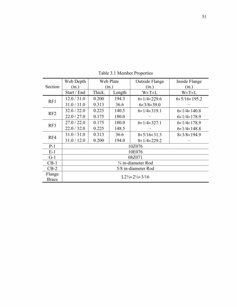
51

Table 3.1 Member Properties

Web Depth (in.)

Web Plate (in.)

Outside Flange (in.)

Inside Flange (in.) Section

Start / End Thick. Length W×T×L W×T×L 12.0 / 31.0 0.200 194.3 6×1/4×229.6 6×5/16×195.2 RF1 31.0 / 31.0 0.313 36.6 6×3/8×39.0 – 32.0 / 22.0 0.225 140.5 6×1/4×319.1 6×1/4×140.8 RF2 22.0 / 27.0 0.175 180.0 – 6×1/4×178.9 27.0 / 22.0 0.175 180.0 6×1/4×327.1 6×1/4×178.9 RF3 22.0 / 32.0 0.225 148.5 – 6×1/4×148.8 31.0 / 31.0 0.313 36.6 8×5/16×31.3 8×3/8×194.9 RF4 31.0 / 12.0 0.200 194.0 8×1/4×229.2 –

P-1 10Z076 E-1 10E076 G-1 08Z071

CB-1 ¾ in-diameter Rod CB-2 5/8 in-diameter Rod

Flange Brace L2½×2½×3/16

52

Table 3.2 Design Load

Load Type Detail Data Dead Load 2.5 psf

Collateral Load 3.0 psf Dead Load Frame Self Weight 2.0 psf

Live Load Roof Live Load 20.0 psf Snow Load Snow Load 30.1 psf

Wind Speed 85 mph Wind Exposure B Wind Load

Importance Factor 1.0 Site Location San Bernardino

Importance Factor 1.0 Seismic Design Category D

R 3.5 Earthquake Load

Cs 0.296

Table 3.3 Mechanical Properties of Steel

Member Fy (ksi) Fu (ksi) Elongation (%) 1/4×8 57.9 (63.4) 80.5 (85.6) 26 (21) 3/8×8 57.7 (58.4) 79.1 (77.5) 25 (20) 5/16×6 53.8 (59.1) 80.7 (84.2) 23 (22)

Flange

1/4×6 59.2 (61.2) 81.1 (80.4) 23 (22) 0.175”-thk. 64.2 (56.7) 77.4 (75.7) 26 (27) 0.2”-thk. 61.1 (61.0) 76.4 (79.0) 29 (31) Web

0.225”-thk. 65.4 (62.0) 79.3 (71.0) 27 (25) 1 Values based on tensile coupon test results 2 Values in parentheses based on Certified Mill Test Reports

53

Table 3.4 Strength Check of Frame 1 at Positive 2.6% Drift

Segment Pu Pn Py Pu/Pn Mu Mno Mni Mu/Mn UnityC1 +9.2 190 311 0.03 1477 2491 2672 0.58 0.61 C2 +9.2 220 403 0.02 2963 3243 3788 0.91 0.92 C3 +9.2 224 477 0.02 3724 3755 4348 0.99 1.00

Col

umn

C4 -15.8 165 427 0.10 4430 2869 3939 1.13 1.18 R1 -1.4 233 581 0.01 4430 4080 4080 1.09 1.10 R2 -1.3 194 483 0.01 4018 3376 3376 1.19 1.20 R3 -0.8 162 405 0.01 2483 2623 2623 0.95 0.96 R4 -0.4 193 435 0.00 945 2820 2820 0.34 0.34 S.

Raf

ter

R5 -0.0 201 452 0.00 219 2868 2868 0.08 0.08 1 Unit: kips and kip-in

Table 3.5 Strength Check of Frame 2 at Positive 2.6% Drift

Segment Pu Pn Py Pu/Pn Mu Mno Mni Mu/Mn UnityC1 +9.2 190 311 0.03 1462 2491 2672 0.59 0.61 C2 +9.2 220 403 0.02 2960 3243 3788 0.91 0.92 C3 +9.2 224 477 0.02 3729 3755 4348 0.99 1.00

Col

umn

C4 -15.8 165 427 0.10 4289 2869 3939 1.09 1.14 R1 -1.3 233 581 0.01 4289 4080 4080 1.05 1.06

R2A -1.2 230 532 0.01 3952 3797 3797 1.04 1.05 R2B -1.0 230 483 0.00 3234 3645 3645 0.89 0.89 R3 -0.7 160 405 0.00 2417 2623 2623 0.92 0.92 R4 -0.4 192 435 0.00 886 2820 2820 0.31 0.31 S.

Raf

ter


54

Table 3.6 Strength Check of Frame 1 at Negative 2.3% Drift

Segment Pu Pn Py Pu/Pn Mu Mno Mni Mu/Mn UnityC1 -13.4 190 311 0.07 1700 2491 2672 0.64 0.68 C2 -13.4 220 403 0.06 3384 3243 3788 0.89 0.92 C3 -13.4 224 477 0.06 4266 3755 4348 0.98 1.01

Col

umn

C4 +6.8 165 427 0.02 2218 2869 3939 0.77 0.78 R1 -5.1 233 581 0.02 4266 4080 4080 1.05 1.06 R2 -5.0 194 483 0.03 4006 3304 3304 1.21 1.23 R3 -4.5 162 405 0.03 2817 2623 2623 1.07 1.09 R4 -4.1 193 435 0.02 1524 2820 2820 0.54 0.55 N

. Raf

ter


Table 3.7 Strength Check of Frame 2 at Negative 2.3% Drift

Segment Pu Pn Py Pu/Pn Mu Mno Mni Mu/Mn UnityC1 -13.4 190 311 0.07 1714 2491 2672 0.64 0.68 C2 -13.4 220 403 0.06 3386 3243 3788 0.89 0.92 C3 -13.4 224 477 0.06 4261 3755 4348 0.98 1.01

Col

umn

C4 +6.8 165 427 0.02 2269 2869 3939 0.79 0.80 R1 -5.0 233 581 0.02 4261 4080 4080 1.04 1.05 R2 -4.9 194 483 0.02 3999 3304 3304 1.21 1.22 R3 -4.5 162 405 0.03 2801 2623 2623 1.07 1.09 R4 -4.1 193 435 0.02 1499 2820 2820 0.53 0.54 N

. Raf

ter


55

16'-6

11/

16"

16'-7

1/1

6"

4'-6"4@5'

1'-4"

18'-1

5/1

6"

7'-6

"6'

6'-6

"20

'

10"

8"60'

Flange Brace

RF1

AB

Side W

all

RoofRoof

4'-2 5/16"4'-6"4@5'

1'-4"

4'-2 5/16"12"

1/2"

RF2RF3

RF4

C4

C1

C2

C3

R1R2R3R4

R5

R4R3R2R1

Unbraced Segment

(a) Elevation

60'

B A

[Cen

ter-

to-C

ente

r]

[Out

-to-O

ut]

20'

20'-8

"

X-B

raci

ng

P-1

CB-2

CB-2

P-1

P-1P-1

X-B

raci

ng

CB-2

CB-2

CB-2 CB-2

(b) Top View

Figure 3.1 Elevation and Top View of Test Building

56

7'-6

"6'

6'-6

"

20'

G-1

G-1

E-1

CB-1 CB-1

(a) Line A

20'

CB-1 CB-1

E-1

(b) Line B

Figure 3.2 Sidewall Elevation

57

Side Wall

8”4”

4”

12-5

/8”

8”

4”

0.375” Thk

φ3/4”

Side Wall

8”4”

4”

12-5

/8”

8”

4”

0.375” Thk

φ3/4”

4”4”

12-5

/8”

8”

4”

0.375” Thk

φ3/4”

4”4”

12-5

/8”

8”

4”

0.375” Thk

φ3/4”

(a) Line A (b) Line B

Figure 3.3 Column Base

58

151.3 p/f 239.3 p/f

60.5

p/f

129.

3 p/

f

151.3 p/f 239.3 p/f

60.5

p/f

129.

3 p/

f

(a) Positive Internal Pressure

52.3 p/f 140.3 p/f

159.

5 p/

f

30.3

p/f

52.3 p/f 140.3 p/f

159.

5 p/

f

30.3

p/f

(b) Negative Internal Pressure

Figure 3.4 Design Wind Load

Figure 3.5 SAP Modeling Scheme

59

(a) Axial Force Diagram (kips)

(b) Shear Force Diagram (kips)

2111

33703110

2111

33703110

(c) Bending Moment Diagram (kip-in)

Figure 3.6 Force Demand under Governing Loading Combination

60

Figure 3.7 Test Building

61

Rafter

Purlin

Flange Braceφ1/2"

2'-4 1/2" or 3'-6"

1.25"

(L2.5X2.5X3/16)

Girt

Column

(L2.5X2.5X3/16)φ1/2"

Flange Brace

1.25"

2'-4 1/2" or 3'-6"

(a) Rafter Flange Brace (b) Column Flange Brace

Purlin

Rafter

Column

Girt

Flange Brace

Purlin

Rafter

Column

Girt

Flange Brace

(c) Flange Brace Installation

Figure 3.8 Flange Brace

62

Reaction Floor

60’

20’

Load Frame

Rea

ctio

n W

all

50-kip Hydraulic Actuator


II I

I I

I II

I Inclinometer

Reaction Floor

60’

20’

Load Frame

Rea

ctio

n W

all



II I

I I

I II

I Inclinometer

(a) Elevation

60’

20’

Rea

ctio

n W

all

Frame 1

Frame 2

Vertical DisplacementDisplacement Transducer

N60’

20’

Rea

ctio

n W

all

Frame 1

Frame 2

Vertical DisplacementDisplacement Transducer

N

(b) Top View

Figure 3.9 Test Setup

63

ActuatorAttachment Plate

Column

Rafter

AA50-kip Actuator

Roof

View A-A

Wall

Column

50-kip Actuator

Existing Stiffeners

Existing Stiffeners

1/4

1/4

1/4"-Stiffeners (A36)

3''

3''

Stiffeners

North Side

11-3/4''

2-1/8'' 16''

Ø1-1/8"

2-1/8''

11-3

/4''

4-1/

8''

20''

5/16

4-1/

8''

2''

15'' 1/2''1/2''

PL1''X15''X3''

16''

2''

16''

2-1/

2''

1/2''1/2''

¼”-Stiffener

Actuator Attachment Plate

Figure 3.10 Actuator-to-Column Connection Details

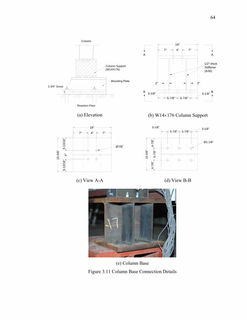
64

Column

Reaction Floor

Mounting Plate

Column Support (W14X176)

1-3/4'' Grout

4''

3-1/8''5-7/8''

7'' 7''

18''

3-1/8''5-7/8''

2" 2"

1/2"-thickStiffener(A36)

A

B

A

B

(a) Elevation (b) W14×176 Column Support

15-5

/8'' 5-

13/1

6''

4''

5-13

/16'

'

7'' 7''

18''

4''

Ø7/8"

5-7/

8''

Ø1-1/8''

3-1/8''5-7/8'' 5-7/8''

3-1/8''

15-5

/8''

4-7/

8''

4-7/

8''

(c) View A-A (d) View B-B

(e) Column Base

Figure 3.11 Column Base Connection Details

65

(a) Panel Zone

(b) End Plate (c) Column Base

Figure 3.12 Instrumentation for Panel Zone, End Plate, and Column Base

66

Wood Panel Screwing Top View after Gravity Load Application

(a) Gravity Load Application

0 10 20 30 40 50 60 70

-0.06

-0.04

-0.02

0.0

0.02

0.04

0.06

-10

-5

0

5

10

Step

Sto

ry D

rift A

ngle

(rad

)

Dis

plac

emen

t (in

.)

(b) AISC Loading Sequence

Figure 3.13 Gravity Load and Cyclic Load

67

0 20 40 60 80 1000.0

0.05

0.10

0.15

0.20

0.25

Def

lect

ion

(in)

Applicaiton of Gravity Load (%)

Frame 1Frame 2

Figure 3.14 Vertical Deflection at Midspan

0 20 40 60 80 100-0.6

-0.4

-0.2

0.0

0.2

0.4

0.6

Rot

atio

n A

ngle

(X 1

/100

0 ra

d)


I4I8

NI8 I4

I4I8

0 20 40 60 80 100-0.6

-0.4

-0.2

0.0

0.2

0.4

0.6

Rot

atio

n A

ngle

(X 1

/100

0 ra

d)


I4I8

NI8 I4

I4I8

Figure 3.15 Frame 1: Rotation Angle at Column Base

68

-4 0 4Stress (ksi)

-4 0 4Stress (ksi)

-4-2024

Stre

ss (k

si)

N

-4 0 4Stress (ksi)

-4 0 4Stress (ksi)

-4-2024

Stre

ss (k

si)

-4 0 4Stress (ksi)

-4 0 4Stress (ksi)

-4-2024

Stre

ss (k

si)

N

(a) Frame 1

N

-4 0 4Stress (ksi)

-4 0 4Stress (ksi)

-4-2024

Stre

ss (k

si)

N

-4 0 4Stress (ksi)

-4 0 4Stress (ksi)

-4-2024

Stre

ss (k

si)

(b) Frame 2

Figure 3.16 Stress Distribution due to Gravity Load

69

N

400 0 400Moment (kip-in)

400 0 400Moment (kip-in

40 60

4002000

200400

Mom

ent (

kip-

in)

N


400 0 400Moment (kip-in

40 60

4002000

200400

Mom

ent (

kip-

in)

(a) Frame 1

N



4002000

200400

Mom

ent (

kip-

in)

3182 N



4002000

200400

Mom

ent (

kip-

in)

3182

(b) Frame 2

Figure 3.17 Moment Diagram (Gravity Load Only)

70

N*40 kip-in *60 kip-in

*241 kip-in *213 kip-in

6.6 kips

H = 1.41 kips H = 1.37 kips

V = 3.3 kips V = 3.3 kips



6.6 kips

H = 1.4 kips H = 1.4 kips


Derived

* Indicating values derived from measurements

Simplified



6.6 kips

H = 1.41 kips H = 1.37 kips




6.6 kips





6.6 kips

H = 1.41 kips H = 1.37 kips




6.6 kips



Derived


Simplified

(a) Frame 1



6.6 kips

H = 1.35 kips H = 1.22 kips




6.6 kips



Derived


Simplified



6.6 kips

H = 1.35 kips H = 1.22 kips




6.6 kips





6.6 kips

H = 1.35 kips H = 1.22 kips




6.6 kips



Derived


Simplified

(b) Frame 2

Figure 3.18 Derived and Simplified Support Reactions (Gravity Load Only)

71

3.3(C)

0.0(C)

0.4(C)

0.8(C)

1.3(C)

1.4(C)

0.8(C)

0.0(C)

0.4(C)

0.8(C)

0.8(C)

1.3(C)

1.4(C)

3.3(C)

N

3.3(C)

0.0(C)

0.4(C)

0.8(C)

1.3(C)

1.4(C)

0.8(C)

0.0(C)

0.4(C)

0.8(C)

0.8(C)

1.3(C)

1.4(C)

3.3(C)

N

3.3(C)

0.0(C)

0.4(C)

0.8(C)

1.3(C)

1.4(C)

0.8(C)

0.0(C)

0.4(C)

0.8(C)

0.8(C)

1.3(C)

1.4(C)

3.3(C)

NN

3.3(C)

0.0(C)

0.4(C)

0.8(C)

1.3(C)

1.4(C)

0.8(C)

0.0(C)

0.4(C)

0.8(C)

0.8(C)

1.3(C)

1.4(C)

3.3(C)

N

3.3(C)

0.0(C)

0.4(C)

0.8(C)

1.3(C)

1.4(C)

0.8(C)

0.0(C)

0.4(C)

0.8(C)

0.8(C)

1.3(C)

1.4(C)

3.3(C)

N

3.3(C)

0.0(C)

0.4(C)

0.8(C)

1.3(C)

1.4(C)

0.8(C)

0.0(C)

0.4(C)

0.8(C)

0.8(C)

1.3(C)

1.4(C)

3.3(C)

NNNNN

(a) Axial Force Diagram

6(6)

106(89)

218(222)

40

237

81(56)

197(191)

217

35(28)60

225(294)34(87)

237(84) 128(60)108(42) 260(137)

205(230)

217(141)

14(72)231 210

Values in parenthesis are derived from gage readings.

N6(6)

106(89)

218(222)

40

237

81(56)

197(191)

217

35(28)60

225(294)34(87)

237(84) 128(60)108(42) 260(137)

205(230)

217(141)

14(72)231 210


NNNN

(b) Bending Moment Diagram


Only)

72

3.3(C)

0.0(C)

0.4(C)

0.8(C)

1.2(C)

1.3(C)

0.8(C)

0.0(C)

0.4(C)

0.8(C)

0.8(C)

1.2(C)

1.3(C)

3.3(C)

N

3.3(C)

0.0(C)

0.4(C)

0.8(C)

1.2(C)

1.3(C)

0.8(C)

0.0(C)

0.4(C)

0.8(C)

0.8(C)

1.2(C)

1.3(C)

3.3(C)

N

3.3(C)

0.0(C)

0.4(C)

0.8(C)

1.2(C)

1.3(C)

0.8(C)

0.0(C)

0.4(C)

0.8(C)

0.8(C)

1.2(C)

1.3(C)

3.3(C)

NN

3.3(C)

0.0(C)

0.4(C)

0.8(C)

1.2(C)

1.3(C)

0.8(C)

0.0(C)

0.4(C)

0.8(C)

0.8(C)

1.2(C)

1.3(C)

3.3(C)

N

3.3(C)

0.0(C)

0.4(C)

0.8(C)

1.2(C)

1.3(C)

0.8(C)

0.0(C)

0.4(C)

0.8(C)

0.8(C)

1.2(C)

1.3(C)

3.3(C)

N

3.3(C)

0.0(C)

0.4(C)

0.8(C)

1.2(C)

1.3(C)

0.8(C)

0.0(C)

0.4(C)

0.8(C)

0.8(C)

1.2(C)

1.3(C)

3.3(C)

NNNNN


52(52)

59(76)

168(168)

82

186

92(98)

195(195)

212

2(2)31

160(190) (72)

232(110) 123(7)

(25)

291(110)

211(140)

283(98)

19(113)168

32174

214


N

52(52)

59(76)

168(168)

82

186

92(98)

195(195)

212

2(2)31

160(190) (72)

232(110) 123(7)

(25)

291(110)

211(140)

283(98)

19(113)168

32174

214


52(52)

59(76)

168(168)

82

186

92(98)

195(195)

212

2(2)31

160(190) (72)

232(110) 123(7)

(25)

291(110)

211(140)

283(98)

19(113)168

32174

214


NNNN



Only)

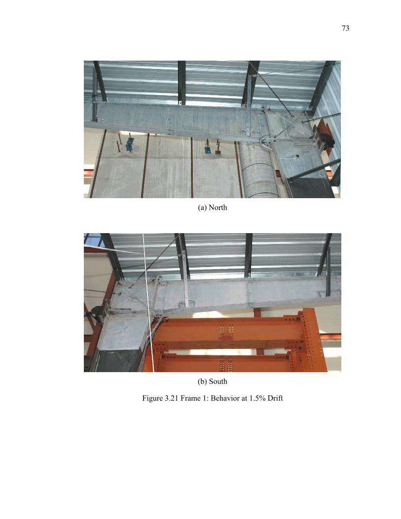
73

(a) North

(b) South

Figure 3.21 Frame 1: Behavior at 1.5% Drift

74

(a) North

(b) South

Figure 3.22 Frame 2: Behavior at 1.5% Drift

75

(b) Column

(a) Lateral Buckling (c) Rafter

Figure 3.23 Lateral Buckling at South Column and Rafter of Frame 2

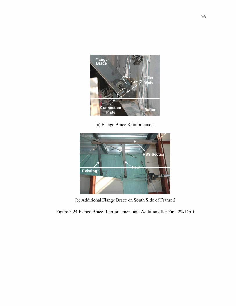
76

Rafter

Flange Brace

Fillet Weld

Connection Plate Rafter

Flange Brace

Fillet Weld

Connection Plate

(a) Flange Brace Reinforcement

HSS Section

NewExisting

HSS Section

NewExisting

(b) Additional Flange Brace on South Side of Frame 2

Figure 3.24 Flange Brace Reinforcement and Addition after First 2% Drift

77

Existing

Added after 1st Cycle

Added after 2nd Cycle

HSS SectionExisting

Added after 1st Cycle


HSS Section


ExistingHSS Section


ExistingHSS Section

(a) Frame 2 (b) Frame 1

N

Frames 1 and 2Frame 2

Additional Flange Brace

N

Frames 1 and 2Frame 2

Additional Flange Brace

(c) Location of Additional Flange Braces

Figure 3.25 Flange Braces Added during 2% Drift Cycles

78

(b) Close-up View

(a) South Rafter Lateral Buckling

Figure 3.26 Frame 1: Failure Mode at First Positive Excursion to 3% Drift

(b) Overload of Brace Support

(a) South Column Lateral Buckling

Figure 3.27 Frame 2: Failure Mode at First Positive Excursion to 3% Drift

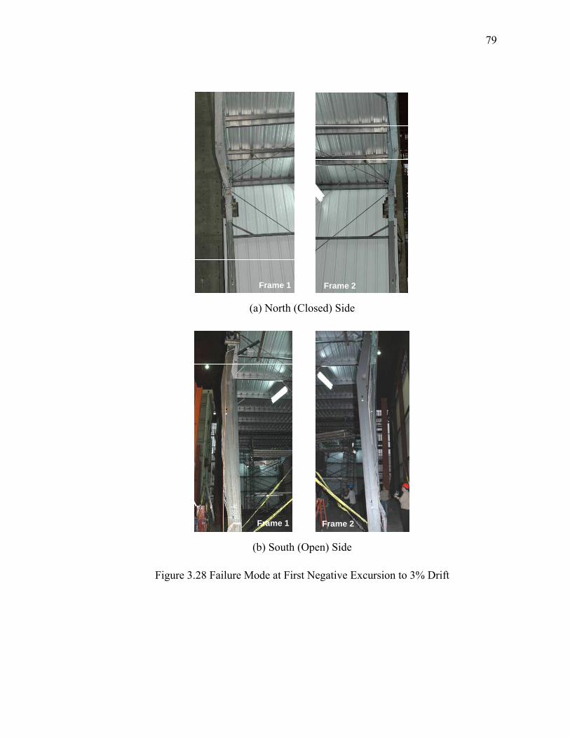
79

Frame 1 Frame 2Frame 1 Frame 2 (a) North (Closed) Side

Frame 1 Frame 2Frame 1 Frame 2 (b) South (Open) Side

Figure 3.28 Failure Mode at First Negative Excursion to 3% Drift

80

-8 -6 -4 -2 0 2 4 6 8

-40

-20

0

20

40

Column Top Displacement (in.)

Bas

e S

hear

(kip

s)

-0.04 -0.02 0.0 0.02 0.04Story Drift Ratio

Design Base Shear

-8 -6 -4 -2 0 2 4 6 8

-40

-20

0

20

40


Bas

e S

hear

(kip

s)


Design Base Shear

(a) Frame 1

-8 -6 -4 -2 0 2 4 6 8

-40

-20

0

20

40


Bas

e S

hear

(kip

s)


Design Base Shear

-8 -6 -4 -2 0 2 4 6 8

-40

-20

0

20

40


Bas

e S

hear

(kip

s)


Design Base Shear

(b) Frame 2

Figure 3.29 Base Shear versus Column Top Displacement

81

-0.004 -0.002 0.0 0.002 0.004

-4

-2

0

2

4

-1.0 -0.5 0.0 0.5 1.0

Shear Strain

Mom

ent (

X 1

000

kip-

in)

Normalized Shear Strain

(a) North Panel Zone

-0.004 -0.002 0.0 0.002 0.004

-4

-2

0

2

4

-1.0 -0.5 0.0 0.5 1.0

Shear Strain

Mom

ent (

X 1

000

kip-

in)


(b) South Panel Zone

Figure 3.30 Frame 1: Moment versus Panel Zone Shear Deformation

82

-0.004 -0.002 0.0 0.002 0.004

-4

-2

0

2

4

-1.0 -0.5 0.0 0.5 1.0

Shear Strain

Mom

ent (

X 1

000

kip-

in)


(a) North Panel Zone

-0.004 -0.002 0.0 0.002 0.004

-4

-2

0

2

4

-1.0 -0.5 0.0 0.5 1.0

Shear Strain

Mom

ent (

X 1

000

kip-

in)


(b) South Panel Zone

Figure 3.31 Frame 2: Moment versus Panel Zone Shear Deformation

83

RafterPanel Zone

L25

RafterPanel Zone

L25

N

Frame 1

RafterPanel Zone

L25

RafterPanel Zone

L25

N

Frame 1 [see Figure 3.12(b)]

(a) Location

-0.10 -0.05 0.0 0.05 0.10

-4

-2

0

2

4

Opening Displacement (in.)

Mom

ent (

X 1

000

kip-

in)

(b) Response

Figure 3.32 Moment versus End-Plate Opening Displacement

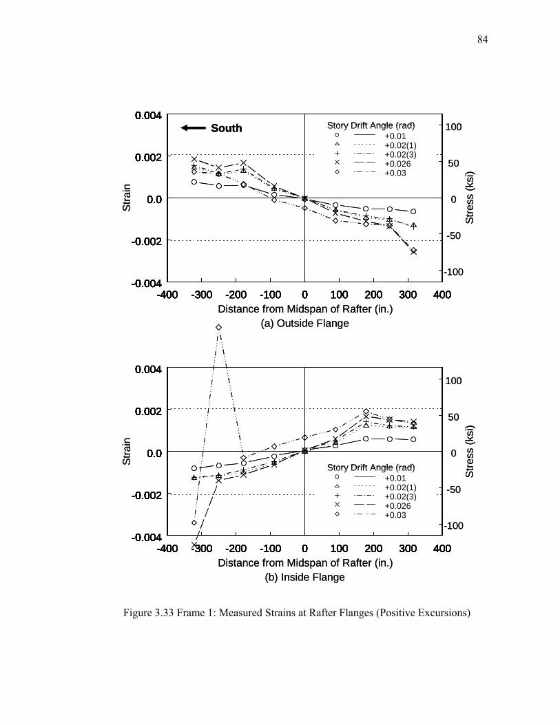
84

-400 -300 -200 -100 0 100 200 300 400-0.004

-0.002

0.0

0.002

0.004

-400 -300 -200 -100 0 100 200 300 400-0.004

-0.002

0.0

0.002

0.004

-400 -300 -200 -100 0 100 200 300 400-0.004

-0.002

0.0

0.002

0.004

-400 -300 -200 -100 0 100 200 300 400-0.004

-0.002

0.0

0.002

0.004

-400 -300 -200 -100 0 100 200 300 400-0.004

-0.002

0.0

0.002

0.004St

rain

Distance from Midspan of Rafter (in.)

Stre

ss (k

si)

(a) Outside Flange

-100

-50

0

50

100+0.01+0.02(1)+0.02(3)+0.026+0.03

Story Drift Angle (rad)

-400 -300 -200 -100 0 100 200 300 400-0.004

-0.002

0.0

0.002

0.004

-400 -300 -200 -100 0 100 200 300 400-0.004

-0.002

0.0

0.002

0.004

-400 -300 -200 -100 0 100 200 300 400-0.004

-0.002

0.0

0.002

0.004

-400 -300 -200 -100 0 100 200 300 400-0.004

-0.002

0.0

0.002

0.004

-400 -300 -200 -100 0 100 200 300 400-0.004

-0.002

0.0

0.002

0.004

Stra

in


Stre

ss (k

si)

(b) Inside Flange

-100

-50

0

50

100

+0.01+0.02(1)+0.02(3)+0.026+0.03


South

-400 -300 -200 -100 0 100 200 300 400-0.004

-0.002

0.0

0.002

0.004

-400 -300 -200 -100 0 100 200 300 400-0.004

-0.002

0.0

0.002

0.004

-400 -300 -200 -100 0 100 200 300 400-0.004

-0.002

0.0

0.002

0.004

-400 -300 -200 -100 0 100 200 300 400-0.004

-0.002

0.0

0.002

0.004

-400 -300 -200 -100 0 100 200 300 400-0.004

-0.002

0.0

0.002

0.004St

rain


Stre

ss (k

si)

(a) Outside Flange

-100

-50

0

50

100+0.01+0.02(1)+0.02(3)+0.026+0.03


-400 -300 -200 -100 0 100 200 300 400-0.004

-0.002

0.0

0.002

0.004

-400 -300 -200 -100 0 100 200 300 400-0.004

-0.002

0.0

0.002

0.004

-400 -300 -200 -100 0 100 200 300 400-0.004

-0.002

0.0

0.002

0.004

-400 -300 -200 -100 0 100 200 300 400-0.004

-0.002

0.0

0.002

0.004

-400 -300 -200 -100 0 100 200 300 400-0.004

-0.002

0.0

0.002

0.004

Stra

in


Stre

ss (k

si)

(b) Inside Flange

-100

-50

0

50

100

+0.01+0.02(1)+0.02(3)+0.026+0.03


SouthSouth

Figure 3.33 Frame 1: Measured Strains at Rafter Flanges (Positive Excursions)

85

-0.004 -0.002 0.0 0.002 0.0040

50

100

150

200

-0.004 -0.002 0.0 0.002 0.0040

50

100

150

200

-0.004 -0.002 0.0 0.002 0.0040

50

100

150

200

-0.004 -0.002 0.0 0.002 0.0040

50

100

150

200

-0.004 -0.002 0.0 0.002 0.0040

50

100

150

200D

ista

nce

from

Col

umn

Bas

e (in

.)

Strain

Stress (ksi)

(a) Outside Flange

-100 -50 0 50 100

+0.01+0.02(1)+0.02(3)+0.026+0.03


-0.004 -0.002 0.0 0.002 0.0040

50

100

150

200

-0.004 -0.002 0.0 0.002 0.0040

50

100

150

200

-0.004 -0.002 0.0 0.002 0.0040

50

100

150

200

-0.004 -0.002 0.0 0.002 0.0040

50

100

150

200

-0.004 -0.002 0.0 0.002 0.0040

50

100

150

200

Dis

tanc

e fro

m C

olum

n B

ase

(in.)

Strain

Stress (ksi)

(b) Inside Flange

-100 -50 0 50 100

+0.01+0.02(1)+0.02(3)+0.026+0.03


Figure 3.34 Frame 1: Measured Strains at North Column (Positive Excursions)

86

-0.004 -0.002 0.0 0.002 0.0040

50

100

150

200

-0.004 -0.002 0.0 0.002 0.0040

50

100

150

200

-0.004 -0.002 0.0 0.002 0.0040

50

100

150

200

-0.004 -0.002 0.0 0.002 0.0040

50

100

150

200

-0.004 -0.002 0.0 0.002 0.0040

50

100

150

200D

ista

nce

from

Col

umn

Bas

e (in

.)

Strain

Stress (ksi)

(a) Outside Flange

-100 -50 0 50 100

+0.01+0.02(1)+0.02(3)+0.026+0.03


-0.004 -0.002 0.0 0.002 0.0040

50

100

150

200

-0.004 -0.002 0.0 0.002 0.0040

50

100

150

200

-0.004 -0.002 0.0 0.002 0.0040

50

100

150

200

-0.004 -0.002 0.0 0.002 0.0040

50

100

150

200

-0.004 -0.002 0.0 0.002 0.0040

50

100

150

200

Dis

tanc

e fro

m C

olum

n B

ase

(in.)

Strain

Stress (ksi)

(b) Inside Flange

-100 -50 0 50 100

+0.01+0.02(1)+0.02(3)+0.026+0.03


Figure 3.35 Frame 1: Measured Strains at South Column (Positive Excursions)

87

South

-400 -300 -200 -100 0 100 200 300 400-0.004

-0.002

0.0

0.002

0.004

-400 -300 -200 -100 0 100 200 300 400-0.004

-0.002

0.0

0.002

0.004

-400 -300 -200 -100 0 100 200 300 400-0.004

-0.002

0.0

0.002

0.004

-400 -300 -200 -100 0 100 200 300 400-0.004

-0.002

0.0

0.002

0.004

-400 -300 -200 -100 0 100 200 300 400-0.004

-0.002

0.0

0.002

0.004St

rain


Stre

ss (k

si)

(a) Outside Flange

-100

-50

0

50

100

-0.01-0.02(1)-0.02(3)-0.023-0.03


-400 -300 -200 -100 0 100 200 300 400-0.004

-0.002

0.0

0.002

0.004

-400 -300 -200 -100 0 100 200 300 400-0.004

-0.002

0.0

0.002

0.004

-400 -300 -200 -100 0 100 200 300 400-0.004

-0.002

0.0

0.002

0.004

-400 -300 -200 -100 0 100 200 300 400-0.004

-0.002

0.0

0.002

0.004

-400 -300 -200 -100 0 100 200 300 400-0.004

-0.002

0.0

0.002

0.004

Stra

in


Stre

ss (k

si)

(b) Inside Flange

-100

-50

0

50

100-0.01-0.02(1)-0.02(3)-0.023-0.03


SouthSouth

-400 -300 -200 -100 0 100 200 300 400-0.004

-0.002

0.0

0.002

0.004

-400 -300 -200 -100 0 100 200 300 400-0.004

-0.002

0.0

0.002

0.004

-400 -300 -200 -100 0 100 200 300 400-0.004

-0.002

0.0

0.002

0.004

-400 -300 -200 -100 0 100 200 300 400-0.004

-0.002

0.0

0.002

0.004

-400 -300 -200 -100 0 100 200 300 400-0.004

-0.002

0.0

0.002

0.004St

rain


Stre

ss (k

si)

(a) Outside Flange

-100

-50

0

50

100

-0.01-0.02(1)-0.02(3)-0.023-0.03


-400 -300 -200 -100 0 100 200 300 400-0.004

-0.002

0.0

0.002

0.004

-400 -300 -200 -100 0 100 200 300 400-0.004

-0.002

0.0

0.002

0.004

-400 -300 -200 -100 0 100 200 300 400-0.004

-0.002

0.0

0.002

0.004

-400 -300 -200 -100 0 100 200 300 400-0.004

-0.002

0.0

0.002

0.004

-400 -300 -200 -100 0 100 200 300 400-0.004

-0.002

0.0

0.002

0.004

Stra

in


Stre

ss (k

si)

(b) Inside Flange

-100

-50

0

50

100-0.01-0.02(1)-0.02(3)-0.023-0.03


Figure 3.36 Frame 1: Measured Strains at Rafter Flanges (Negative Excursions)

88

-0.004 -0.002 0.0 0.002 0.0040

50

100

150

200

-0.004 -0.002 0.0 0.002 0.0040

50

100

150

200

-0.004 -0.002 0.0 0.002 0.0040

50

100

150

200

-0.004 -0.002 0.0 0.002 0.0040

50

100

150

200

-0.004 -0.002 0.0 0.002 0.0040

50

100

150

200D

ista

nce

from

Col

umn

Bas

e (in

.)

Strain

Stress (ksi)

(a) Outside Flange

-100 -50 0 50 100

-0.01-0.02(1)-0.02(3)-0.023-0.03


-0.004 -0.002 0.0 0.002 0.0040

50

100

150

200

-0.004 -0.002 0.0 0.002 0.0040

50

100

150

200

-0.004 -0.002 0.0 0.002 0.0040

50

100

150

200

-0.004 -0.002 0.0 0.002 0.0040

50

100

150

200

-0.004 -0.002 0.0 0.002 0.0040

50

100

150

200

Dis

tanc

e fro

m C

olum

n B

ase

(in.)

Strain

Stress (ksi)

(b) Inside Flange

-100 -50 0 50 100

-0.01-0.02(1)-0.02(3)-0.023-0.03


Figure 3.37 Frame 1: Measured Strains at North Column (Negative Excursions)

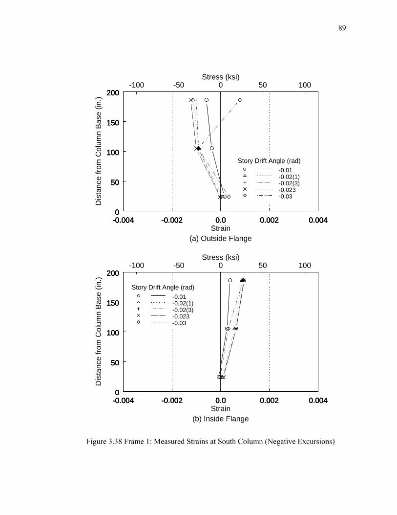
89

-0.004 -0.002 0.0 0.002 0.0040

50

100

150

200

-0.004 -0.002 0.0 0.002 0.0040

50

100

150

200

-0.004 -0.002 0.0 0.002 0.0040

50

100

150

200

-0.004 -0.002 0.0 0.002 0.0040

50

100

150

200

-0.004 -0.002 0.0 0.002 0.0040

50

100

150

200D

ista

nce

from

Col

umn

Bas

e (in

.)

Strain

Stress (ksi)

(a) Outside Flange

-100 -50 0 50 100

-0.01-0.02(1)-0.02(3)-0.023-0.03


-0.004 -0.002 0.0 0.002 0.0040

50

100

150

200

-0.004 -0.002 0.0 0.002 0.0040

50

100

150

200

-0.004 -0.002 0.0 0.002 0.0040

50

100

150

200

-0.004 -0.002 0.0 0.002 0.0040

50

100

150

200

-0.004 -0.002 0.0 0.002 0.0040

50

100

150

200

Dis

tanc

e fro

m C

olum

n B

ase

(in.)

Strain

Stress (ksi)

(b) Inside Flange

-100 -50 0 50 100

-0.01-0.02(1)-0.02(3)-0.023-0.03


Figure 3.38 Frame 1: Measured Strains at South Column (Negative Excursions)

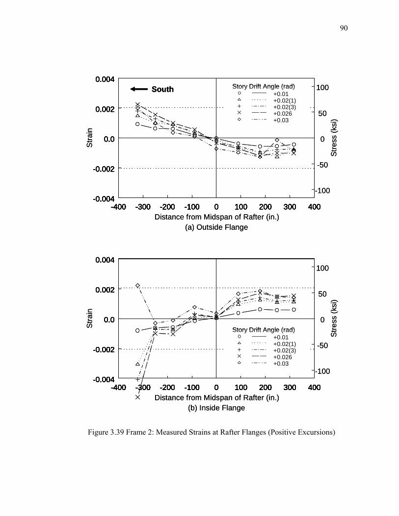
90

South

-400 -300 -200 -100 0 100 200 300 400-0.004

-0.002

0.0

0.002

0.004

-400 -300 -200 -100 0 100 200 300 400-0.004

-0.002

0.0

0.002

0.004

-400 -300 -200 -100 0 100 200 300 400-0.004

-0.002

0.0

0.002

0.004

-400 -300 -200 -100 0 100 200 300 400-0.004

-0.002

0.0

0.002

0.004

-400 -300 -200 -100 0 100 200 300 400-0.004

-0.002

0.0

0.002

0.004St

rain


Stre

ss (k

si)

(a) Outside Flange

-100

-50

0

50

100+0.01+0.02(1)+0.02(3)+0.026+0.03


-400 -300 -200 -100 0 100 200 300 400-0.004

-0.002

0.0

0.002

0.004

-400 -300 -200 -100 0 100 200 300 400-0.004

-0.002

0.0

0.002

0.004

-400 -300 -200 -100 0 100 200 300 400-0.004

-0.002

0.0

0.002

0.004

-400 -300 -200 -100 0 100 200 300 400-0.004

-0.002

0.0

0.002

0.004

-400 -300 -200 -100 0 100 200 300 400-0.004

-0.002

0.0

0.002

0.004

Stra

in


Stre

ss (k

si)

(b) Inside Flange

-100

-50

0

50

100

+0.01+0.02(1)+0.02(3)+0.026+0.03


SouthSouth

-400 -300 -200 -100 0 100 200 300 400-0.004

-0.002

0.0

0.002

0.004

-400 -300 -200 -100 0 100 200 300 400-0.004

-0.002

0.0

0.002

0.004

-400 -300 -200 -100 0 100 200 300 400-0.004

-0.002

0.0

0.002

0.004

-400 -300 -200 -100 0 100 200 300 400-0.004

-0.002

0.0

0.002

0.004

-400 -300 -200 -100 0 100 200 300 400-0.004

-0.002

0.0

0.002

0.004St

rain


Stre

ss (k

si)

(a) Outside Flange

-100

-50

0

50

100+0.01+0.02(1)+0.02(3)+0.026+0.03


-400 -300 -200 -100 0 100 200 300 400-0.004

-0.002

0.0

0.002

0.004

-400 -300 -200 -100 0 100 200 300 400-0.004

-0.002

0.0

0.002

0.004

-400 -300 -200 -100 0 100 200 300 400-0.004

-0.002

0.0

0.002

0.004

-400 -300 -200 -100 0 100 200 300 400-0.004

-0.002

0.0

0.002

0.004

-400 -300 -200 -100 0 100 200 300 400-0.004

-0.002

0.0

0.002

0.004

Stra

in


Stre

ss (k

si)

(b) Inside Flange

-100

-50

0

50

100

+0.01+0.02(1)+0.02(3)+0.026+0.03


Figure 3.39 Frame 2: Measured Strains at Rafter Flanges (Positive Excursions)

91

-0.004 -0.002 0.0 0.002 0.0040

50

100

150

200

-0.004 -0.002 0.0 0.002 0.0040

50

100

150

200

-0.004 -0.002 0.0 0.002 0.0040

50

100

150

200

-0.004 -0.002 0.0 0.002 0.0040

50

100

150

200

-0.004 -0.002 0.0 0.002 0.0040

50

100

150

200D

ista

nce

from

Col

umn

Bas

e (in

.)

Strain

Stress (ksi)

(a) Outside Flange

-100 -50 0 50 100

+0.01+0.02(1)+0.02(3)+0.026+0.03


-0.004 -0.002 0.0 0.002 0.0040

50

100

150

200

-0.004 -0.002 0.0 0.002 0.0040

50

100

150

200

-0.004 -0.002 0.0 0.002 0.0040

50

100

150

200

-0.004 -0.002 0.0 0.002 0.0040

50

100

150

200

-0.004 -0.002 0.0 0.002 0.0040

50

100

150

200

Dis

tanc

e fro

m C

olum

n B

ase

(in.)

Strain

Stress (ksi)

(b) Inside Flange

-100 -50 0 50 100

+0.01+0.02(1)+0.02(3)+0.026+0.03


Figure 3.40 Frame 2: Measured Strains at North Column (Positive Excursions)

92

-0.004 -0.002 0.0 0.002 0.0040

50

100

150

200

-0.004 -0.002 0.0 0.002 0.0040

50

100

150

200

-0.004 -0.002 0.0 0.002 0.0040

50

100

150

200

-0.004 -0.002 0.0 0.002 0.0040

50

100

150

200

-0.004 -0.002 0.0 0.002 0.0040

50

100

150

200D

ista

nce

from

Col

umn

Bas

e (in

.)

Strain

Stress (ksi)

(a) Outside Flange

-100 -50 0 50 100

+0.01+0.02(1)+0.02(3)+0.026+0.03


-0.004 -0.002 0.0 0.002 0.0040

50

100

150

200

-0.004 -0.002 0.0 0.002 0.0040

50

100

150

200

-0.004 -0.002 0.0 0.002 0.0040

50

100

150

200

-0.004 -0.002 0.0 0.002 0.0040

50

100

150

200

-0.004 -0.002 0.0 0.002 0.0040

50

100

150

200

Dis

tanc

e fro

m C

olum

n B

ase

(in.)

Strain

Stress (ksi)

(b) Inside Flange

-100 -50 0 50 100

+0.01+0.02(1)+0.02(3)+0.026+0.03


Figure 3.41 Frame 2: Measured Strains at South Column (Positive Excursions)

93

South

-400 -300 -200 -100 0 100 200 300 400-0.004

-0.002

0.0

0.002

0.004

-400 -300 -200 -100 0 100 200 300 400-0.004

-0.002

0.0

0.002

0.004

-400 -300 -200 -100 0 100 200 300 400-0.004

-0.002

0.0

0.002

0.004

-400 -300 -200 -100 0 100 200 300 400-0.004

-0.002

0.0

0.002

0.004

-400 -300 -200 -100 0 100 200 300 400-0.004

-0.002

0.0

0.002

0.004St

rain


Stre

ss (k

si)

(a) Outside Flange

-100

-50

0

50

100

-0.01-0.02(1)-0.02(3)-0.023-0.03


-400 -300 -200 -100 0 100 200 300 400-0.004

-0.002

0.0

0.002

0.004

-400 -300 -200 -100 0 100 200 300 400-0.004

-0.002

0.0

0.002

0.004

-400 -300 -200 -100 0 100 200 300 400-0.004

-0.002

0.0

0.002

0.004

-400 -300 -200 -100 0 100 200 300 400-0.004

-0.002

0.0

0.002

0.004

-400 -300 -200 -100 0 100 200 300 400-0.004

-0.002

0.0

0.002

0.004

Stra

in


Stre

ss (k

si)

(b) Inside Flange

-100

-50

0

50

100-0.01-0.02(1)-0.02(3)-0.023-0.03


SouthSouth

-400 -300 -200 -100 0 100 200 300 400-0.004

-0.002

0.0

0.002

0.004

-400 -300 -200 -100 0 100 200 300 400-0.004

-0.002

0.0

0.002

0.004

-400 -300 -200 -100 0 100 200 300 400-0.004

-0.002

0.0

0.002

0.004

-400 -300 -200 -100 0 100 200 300 400-0.004

-0.002

0.0

0.002

0.004

-400 -300 -200 -100 0 100 200 300 400-0.004

-0.002

0.0

0.002

0.004St

rain


Stre

ss (k

si)

(a) Outside Flange

-100

-50

0

50

100

-0.01-0.02(1)-0.02(3)-0.023-0.03


-400 -300 -200 -100 0 100 200 300 400-0.004

-0.002

0.0

0.002

0.004

-400 -300 -200 -100 0 100 200 300 400-0.004

-0.002

0.0

0.002

0.004

-400 -300 -200 -100 0 100 200 300 400-0.004

-0.002

0.0

0.002

0.004

-400 -300 -200 -100 0 100 200 300 400-0.004

-0.002

0.0

0.002

0.004

-400 -300 -200 -100 0 100 200 300 400-0.004

-0.002

0.0

0.002

0.004

Stra

in


Stre

ss (k

si)

(b) Inside Flange

-100

-50

0

50

100-0.01-0.02(1)-0.02(3)-0.023-0.03


Figure 3.42 Frame 2: Measured Strains at Rafter Flanges (Negative Excursions)

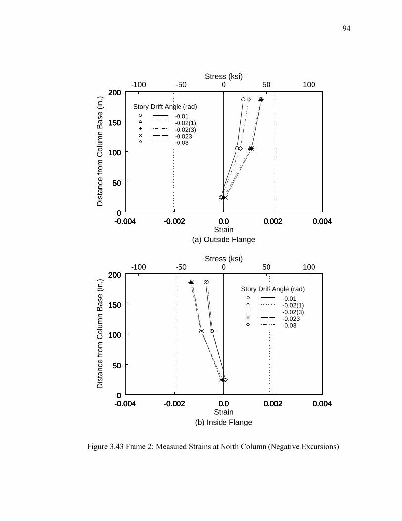
94

-0.004 -0.002 0.0 0.002 0.0040

50

100

150

200

-0.004 -0.002 0.0 0.002 0.0040

50

100

150

200

-0.004 -0.002 0.0 0.002 0.0040

50

100

150

200

-0.004 -0.002 0.0 0.002 0.0040

50

100

150

200

-0.004 -0.002 0.0 0.002 0.0040

50

100

150

200D

ista

nce

from

Col

umn

Base

(in.

)

Strain

Stress (ksi)

(a) Outside Flange

-100 -50 0 50 100

-0.01-0.02(1)-0.02(3)-0.023-0.03


-0.004 -0.002 0.0 0.002 0.0040

50

100

150

200

-0.004 -0.002 0.0 0.002 0.0040

50

100

150

200

-0.004 -0.002 0.0 0.002 0.0040

50

100

150

200

-0.004 -0.002 0.0 0.002 0.0040

50

100

150

200

-0.004 -0.002 0.0 0.002 0.0040

50

100

150

200

Dis

tanc

e fro

m C

olum

n Ba

se (i

n.)

Strain

Stress (ksi)

(b) Inside Flange

-100 -50 0 50 100

-0.01-0.02(1)-0.02(3)-0.023-0.03


Figure 3.43 Frame 2: Measured Strains at North Column (Negative Excursions)

95

-0.004 -0.002 0.0 0.002 0.0040

50

100

150

200

-0.004 -0.002 0.0 0.002 0.0040

50

100

150

200

-0.004 -0.002 0.0 0.002 0.0040

50

100

150

200

-0.004 -0.002 0.0 0.002 0.0040

50

100

150

200

-0.004 -0.002 0.0 0.002 0.0040

50

100

150

200D

ista

nce

from

Col

umn

Base

(in.

)

Strain

Stress (ksi)

(a) Outside Flange

-100 -50 0 50 100

-0.01-0.02(1)-0.02(3)-0.023-0.03


-0.004 -0.002 0.0 0.002 0.0040

50

100

150

200

-0.004 -0.002 0.0 0.002 0.0040

50

100

150

200

-0.004 -0.002 0.0 0.002 0.0040

50

100

150

200

-0.004 -0.002 0.0 0.002 0.0040

50

100

150

200

-0.004 -0.002 0.0 0.002 0.0040

50

100

150

200

Dis

tanc

e fro

m C

olum

n Ba

se (i

n.)

Strain

Stress (ksi)

(b) Inside Flange

-100 -50 0 50 100

-0.01-0.02(1)-0.02(3)-0.023-0.03


Figure 3.44 Frame 2: Measured Strains at South Column (Negative Excursions)

96

Figure 3.45 Load versus Measured Strain at Rod Braces

97

N

Frame 2 S87 S88

A

A

Section A-A

N

Frame 2 S87 S88S87 S88

A

A

Section A-A

(a) Location

-0.004 -0.002 0.0 0.002 0.004-0.004

-0.002

0.0

0.002

0.004

Strain S87

Stra

in S

88

Normalized Strain

Nor

mal

ized

Stra

in

-1 0 1

-1

0

1

2nd Cycle of 1% Drift1st Cycle of 1.5% Drift

(b) Strain Comparison

Figure 3.46 Strain Deviation at 1.5% Drift

98

N*411.39 kip-in

*22.34 kips

*H = 22.9 kips

V = 12.48 kips


*22.34 kips

*435.66 kip-in

*H = 22.9 kips

V = 12.48 kips

N*411.39 kip-in

*22.34 kips

*H = 22.9 kips

V = 12.48 kips


*22.34 kips

*435.66 kip-in

*H = 22.9 kips

V = 12.48 kips (a) Derived

N*411.39 kip-in

*22.34 kips

H = 22.34 kips

V = 12.48 kips

*22.34 kips

*435.66 kip-in

H = 22.34 kips

V = 12.48 kips

N*411.39 kip-in

*22.34 kips

H = 22.34 kips

V = 12.48 kips

*22.34 kips

*435.66 kip-in

H = 22.34 kips

V = 12.48 kips (b) Simplification

Figure 3.47 Support Reactions of Frame 1 at Positive 2.6% Drift (Lateral Load Only)

99

NI8 I4NI8 I4

(a) Location of Inclinometers

-0.04 0.0 0.04

-40

-20

0

20

40

Bas

e S

hear

(kip

s)

Rotation Angle (rad)

(b) I8 (c) I4

Figure 3.48 Measured Rotation Angle at Column Bases of Frame 1

100

2'R20 R21 R22

South Column of Frame 1

-20 -10 0 10-40

-20

0

20

40

Shear =-24 kips

Bas

e S

hear

(kip

s)

Shear Force (kips) (a) Location (b) R20

-20 -10 0 10-40

-20

0

20

40

Shear =-24.57 kips

Bas

e S

hear

(kip

s)

Shear Force (kips)

-20 -10 0 10-40

-20

0

20

40

Shear =-20.16 kipsB

ase

She

ar (k

ips)

Shear Force (kips)

(c) R21 (d) R22

Figure 3.49 Shear Force at South Column of Frame 1

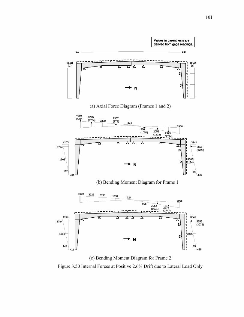
101

12.48(C)

0.0 0.0

12.48(T)


12.48(C)

0.0 0.0

12.48(T)


N

12.48(C)

0.0 0.0

12.48(T)


12.48(C)

0.0 0.0

12.48(T)


NNNN

(a) Axial Force Diagram (Frames 1 and 2)

132

1963

3794

411

4103

1866(2174)

3656(3228)

3941

85436

4060(4334)

3225(2704)

1357(978)

906(1051) 2052

(1523)

2390324

3906

2979(2744)

N132

1963

3794

411

4103

1866(2174)

3656(3228)

3941

85436

4060(4334)

3225(2704)

1357(978)

906(1051) 2052

(1523)

2390324

3906

2979(2744)

NNN

(b) Bending Moment Diagram for Frame 1

132

1963

3794

411

4103

1866

3656(3072)

3941

85436

4060 3225 1357

2979(2747)

9062052(1621)

2390324

3906

N132

1963

3794

411

4103

1866

3656(3072)

3941

85436

4060 3225 1357

2979(2747)

9062052(1621)

2390324

3906

NNN

(c) Bending Moment Diagram for Frame 2

Figure 3.50 Internal Forces at Positive 2.6% Drift due to Lateral Load Only

102

N

R1 R2 R3 R4 R515.78

C4

C1

C2

C3

R3 R2 R1(C) 9.18(T)

9.18(T)

9.18(T)

1.4(C)

1.3(C)

0.8(C)

0.4(C)

0.0(C)

0.0(C)

0.4(C)0.8

(C)1.3(C)1.4

(C)

0.8(C)

0.8(C)

R4

N

R1 R2 R3 R4 R515.78

C4

C1

C2

C3

R3 R2 R1(C) 9.18(T)

9.18(T)

9.18(T)

1.4(C)

1.3(C)

0.8(C)

0.4(C)

0.0(C)

0.0(C)

0.4(C)0.8

(C)1.3(C)1.4

(C)

0.8(C)

0.8(C)

R4

N

R1 R2 R3 R4 R5 R4 R3 R2 R1

C4

C1

C2

C3

N

R1 R2 R3 R4 R515.78

C4

C1

C2

C3

R3 R2 R1(C) 9.18(T)

9.18(T)

9.18(T)

1.4(C)

1.3(C)

0.8(C)

0.4(C)

0.0(C)

0.0(C)

0.4(C)0.8

(C)1.3(C)1.4

(C)

0.8(C)

0.8(C)

R4

N

R1 R2 R3 R4 R515.78

C4

C1

C2

C3

R3 R2 R1(C) 9.18(T)

9.18(T)

9.18(T)

1.4(C)

1.3(C)

0.8(C)

0.4(C)

0.0(C)

0.0(C)

0.4(C)0.8

(C)1.3(C)1.4

(C)

0.8(C)

0.8(C)

R4

N

R1 R2 R3 R4 R5 R4 R3 R2 R1

C4

C1

C2

C3

NNNN

R1 R2 R3 R4 R5 R4 R3 R2 R1

C4

C1

C2

C3


4018945

937

22692194430

2483

1972161 2335

R1 R2 R3 R4 R5

451

4430

C4

1477

2963

3724

376

C1

C2

C3

R4 R3 R2 R1

35033724

N

R1 R2 R3 R4 R5 R4 R3 R2 R1

C4

C1

C2

C3

4018945

937

22692194430

2483

1972161 2335

R1 R2 R3 R4 R5

451

4430

C4

1477

2963

3724

376

C1

C2

C3

R4 R3 R2 R1

35033724

N

R1 R2 R3 R4 R5 R4 R3 R2 R1

C4

C1

C2

C3

NNN

R1 R2 R3 R4 R5 R4 R3 R2 R1

C4

C1

C2

C3



103

N

R1 R2 R3 R4 R515.78

C4

C1

C2

C3

R4 R3 R2 R1(C) 9.18(T)

9.18(T)

9.18(T)

1.3(C)

1.2(C)

0.8(C)

0.4(C)

0.0(C)

0.0(C)

0.4(C)0.8

(C)1.2(C)1.3

(C)

0.8(C)

0.8(C)

R2A R2B

N

R1 R2 R3 R4 R515.78

C4

C1

C2

C3

R4 R3 R2 R1(C) 9.18(T)

9.18(T)

9.18(T)

1.3(C)

1.2(C)

0.8(C)

0.4(C)

0.0(C)

0.0(C)

0.4(C)0.8

(C)1.2(C)1.3

(C)

0.8(C)

0.8(C)

R2A R2B

N

R1R3 R4 R5 R4 R3 R2 R1

C4

C1

C2

C3R2A R2B

N

R1 R2 R3 R4 R515.78

C4

C1

C2

C3

R4 R3 R2 R1(C) 9.18(T)

9.18(T)

9.18(T)

1.3(C)

1.2(C)

0.8(C)

0.4(C)

0.0(C)

0.0(C)

0.4(C)0.8

(C)1.2(C)1.3

(C)

0.8(C)

0.8(C)

R2A R2B

N

R1 R2 R3 R4 R515.78

C4

C1

C2

C3

R4 R3 R2 R1(C) 9.18(T)

9.18(T)

9.18(T)

1.3(C)

1.2(C)

0.8(C)

0.4(C)

0.0(C)

0.0(C)

0.4(C)0.8

(C)1.2(C)1.3

(C)

0.8(C)

0.8(C)

R2A R2B

N

R1R3 R4 R5 R4 R3 R2 R1

C4

C1

C2

C3R2A R2B

N

R1R3 R4 R5 R4 R3 R2 R1

C4

C1

C2

C3R2A R2B


R1 R2 R3 R4 R5

R2A R2B

C4

C1

C2

C3

R4 R3 R2 R1

493

4289

4289

3952 (3234) 2417 2203 886 183221 983

2156 23303497

3729

3729

2960

1462

405

N

R1R3 R4 R5 R4 R3 R2 R1

C4

C1

C2

C3R2A R2BR1 R2 R3 R4 R5

R2A R2B

C4

C1

C2

C3

R4 R3 R2 R1

493

4289

4289

3952 (3234) 2417 2203 886 183221 983

2156 23303497

3729

3729

2960

1462

405

N

R1R3 R4 R5 R4 R3 R2 R1

C4

C1

C2

C3R2A R2B

N

R1R3 R4 R5 R4 R3 R2 R1

C4

C1

C2

C3R2A R2B



104

N*371kip-in

*18.14 kips

*H = 14.45kips

V = 10.1 kips


*18.14 kips

*345 kip-in

H = 21.83 kips

V = 10.1 kips

N*371kip-in

*18.14 kips

*H = 14.45kips

V = 10.1 kips


*18.14 kips

*345 kip-in

H = 21.83 kips

V = 10.1 kips Figure 3.53 Support Reactions of Frame 1 at Negative 2.3% Drift (Lateral Load Only)

105

10.1(T)

10.1(C)

3.7(C)

3.7(C)

N

10.1(T)

10.1(C)

3.7(C)

3.7(C)

NN

10.1(T)

10.1(C)

3.7(C)

3.7(C)

N

10.1(T)

10.1(C)

3.7(C)

3.7(C)

NNNNN


1965

3745

4049

183345

1831 26629654049

3335

2455

371

24551687 934

20

N1965

3745

4049

183345

1831 26629654049

3335

2455

371

24551687 934

20

NNN


Figure 3.54 Internal Forces at Negative 2.3% Drift due to Lateral Load Only

106

N

R1 R2 R3 R4 R5 13.4

C4

C1

C2

C3

R3 R2 R1 (C)6.8(T)

5.1(C)

5.0(C)

4.5(C)

4.1(C)

3.7(C)

3.7(C)

4.1(C)4.5

(C)5.0(C)

5.1(C)

4.5(C)

4.5(C)

R4

N

R1 R2 R3 R4 R5 13.4

C4

C1

C2

C3

R3 R2 R1 (C)6.8(T)

5.1(C)

5.0(C)

4.5(C)

4.1(C)

3.7(C)

3.7(C)

4.1(C)4.5

(C)5.0(C)

5.1(C)

4.5(C)

4.5(C)

R4

N

R1 R2 R3 R4 R5 R4 R3 R2 R1

C4

C1

C2

C3

N

R1 R2 R3 R4 R5 13.4

C4

C1

C2

C3

R3 R2 R1 (C)6.8(T)

5.1(C)

5.0(C)

4.5(C)

4.1(C)

3.7(C)

3.7(C)

4.1(C)4.5

(C)5.0(C)

5.1(C)

4.5(C)

4.5(C)

R4

N

R1 R2 R3 R4 R5 13.4

C4

C1

C2

C3

R3 R2 R1 (C)6.8(T)

5.1(C)

5.0(C)

4.5(C)

4.1(C)

3.7(C)

3.7(C)

4.1(C)4.5

(C)5.0(C)

5.1(C)

4.5(C)

4.5(C)

R4

N

R1 R2 R3 R4 R5 R4 R3 R2 R1

C4

C1

C2

C3

NNNN

R1 R2 R3 R4 R5 R4 R3 R2 R1

C4

C1

C2

C3


331

2218

1700

3384

4266

405

22182100

197

1524 2817

1093

5514266

4006877

C4

C1

C2

C3

R1 R2 R3 R4 R5 R4 R3 R2 R1

N

R1 R2 R3 R4 R5 R4 R3 R2 R1

C4

C1

C2

C3

331

2218

1700

3384

4266

405

22182100

197

1524 2817

1093

5514266

4006877

C4

C1

C2

C3

R1 R2 R3 R4 R5 R4 R3 R2 R1

N

R1 R2 R3 R4 R5 R4 R3 R2 R1

C4

C1

C2

C3

NNN

R1 R2 R3 R4 R5 R4 R3 R2 R1

C4

C1

C2

C3



107

N

R1 R2 R3 R4 R5 13.4

C4

C1

C2

C3

R4 R3 R2 R1 (C)6.8(T)

5.0(C)

4.9(C)

4.5(C)

4.1(C)

3.7(C)

3.7(C)4.1

(C)4.5(C)4.9

(C)5.0(C)

4.5(C)

4.5(C)

R2A R2B

N

R1 R2 R3 R4 R5 13.4

C4

C1

C2

C3

R4 R3 R2 R1 (C)6.8(T)

5.0(C)

4.9(C)

4.5(C)

4.1(C)

3.7(C)

3.7(C)4.1

(C)4.5(C)4.9

(C)5.0(C)

4.5(C)

4.5(C)

R2A R2B

N

R1R3 R4 R5 R4 R3 R2 R1

C4

C1

C2

C3R2A R2B

N

R1 R2 R3 R4 R5 13.4

C4

C1

C2

C3

R4 R3 R2 R1 (C)6.8(T)

5.0(C)

4.9(C)

4.5(C)

4.1(C)

3.7(C)

3.7(C)4.1

(C)4.5(C)4.9

(C)5.0(C)

4.5(C)

4.5(C)

R2A R2B

N

R1 R2 R3 R4 R5 13.4

C4

C1

C2

C3

R4 R3 R2 R1 (C)6.8(T)

5.0(C)

4.9(C)

4.5(C)

4.1(C)

3.7(C)

3.7(C)4.1

(C)4.5(C)4.9

(C)5.0(C)

4.5(C)

4.5(C)

R2A R2B

N

R1R3 R4 R5 R4 R3 R2 R1

C4

C1

C2

C3R2A R2B

N

R1R3 R4 R5 R4 R3 R2 R1

C4

C1

C2

C3R2A R2B


289

2269

1714

3386

4261

376

22692080

263

1499 2801

1087

5324261

3999

1627

848

C4C3

C2

C1

R1 R2A R2B R3 R4 R5 R4 R3R1R2

N

R1R3 R4 R5 R4 R3 R2 R1

C4

C1

C2

C3R2A R2B

289

2269

1714

3386

4261

376

22692080

263

1499 2801

1087

5324261

3999

1627

848

C4C3

C2

C1

R1 R2A R2B R3 R4 R5 R4 R3R1R2

N

R1R3 R4 R5 R4 R3 R2 R1

C4

C1

C2

C3R2A R2B

N

R1R3 R4 R5 R4 R3 R2 R1

C4

C1

C2

C3R2A R2B



108

NC1

C2

C3

C4

R1 R2 R3 R4 R5 R4 R3 R2 R1

NC1

C2

C3

C4

R1 R2 R3 R4 R5 R4 R3 R2 R1

(a) Location

0.0 0.5 1.0 1.5-2.0

-1.5

-1.0

-0.5

0.0

0.5

1.0

1.5+2.6%-2.3%+2.6%–2.3%

0.0 0.5 1.0 1.5-2.0

-1.5

-1.0

-0.5

0.0

0.5

1.0

1.5+2.6%-2.3%+2.6%–2.3%

Mu/Mn

P u/P

n

0.0 0.5 1.0 1.5-2.0

-1.5

-1.0

-0.5

0.0

0.5

1.0

1.5+2.6%-2.3%+2.6%–2.3%

0.0 0.5 1.0 1.5-2.0

-1.5

-1.0

-0.5

0.0

0.5

1.0

1.5+2.6%-2.3%+2.6%–2.3%

Mu/Mn

P u/P

n

0.0 0.5 1.0 1.5-2.0

-1.5

-1.0

-0.5

0.0

0.5

1.0

1.5

Mu/Mn

P u/P

n

0.0 0.5 1.0 1.5-2.0

-1.5

-1.0

-0.5

0.0

0.5

1.0

1.5

Mu/Mn

P u/P

n

(b) Segment C1 (c) Segment C2

0.0 0.5 1.0 1.5-2.5-2.0-1.5-1.0-0.50.00.51.01.5

Mu/Mn

P u/P

n

0.0 0.5 1.0 1.5-2.5-2.0-1.5-1.0-0.50.00.51.01.5

Mu/Mn

P u/P

n

0.0 0.5 1.0 1.5-2.5-2.0-1.5-1.0-0.50.00.51.01.5

Mu/Mn

P u/P

n

0.0 0.5 1.0 1.5-2.5-2.0-1.5-1.0-0.50.00.51.01.5

Mu/Mn

P u/P

n

(d) Segment C3 (e) Segment C4

Figure 3.57 Frame 1: Axial Force and Moment Interaction

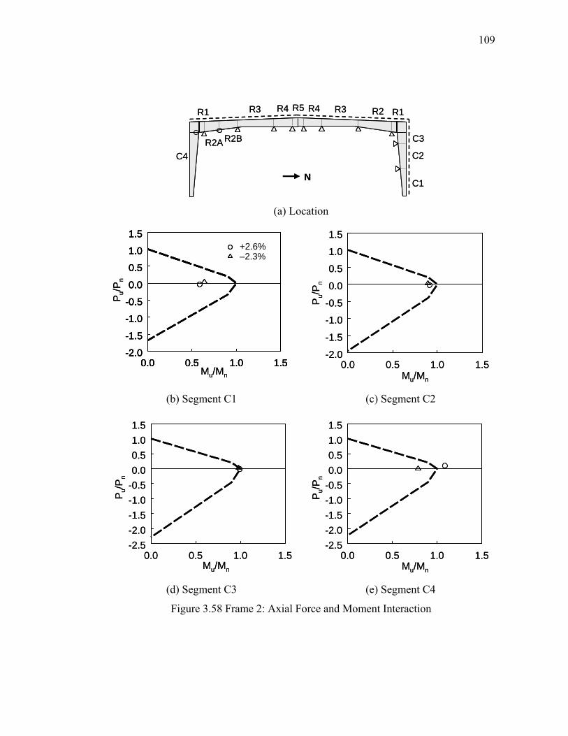
109

NC1

C2

C3

C4

R1 R3 R4 R5 R4 R3 R2 R1

R2AR2B

NC1

C2

C3

C4

R1 R3 R4 R5 R4 R3 R2 R1

R2AR2B

(a) Location

Mu/Mn

P u/P

n

0.0 0.5 1.0 1.5-2.0

-1.5

-1.0

-0.5

0.0

0.5

1.0

1.5+2.6%-2.3%+2.6%–2.3%

0.0 0.5 1.0 1.5-2.0

-1.5

-1.0

-0.5

0.0

0.5

1.0

1.5+2.6%-2.3%+2.6%–2.3%

Mu/Mn

P u/P

n

0.0 0.5 1.0 1.5-2.0

-1.5

-1.0

-0.5

0.0

0.5

1.0

1.5+2.6%-2.3%+2.6%–2.3%

0.0 0.5 1.0 1.5-2.0

-1.5

-1.0

-0.5

0.0

0.5

1.0

1.5+2.6%-2.3%+2.6%–2.3%

Mu/Mn

P u/P

n

0.0 0.5 1.0 1.5-2.0

-1.5

-1.0

-0.5

0.0

0.5

1.0

1.5

Mu/Mn

P u/P

n

0.0 0.5 1.0 1.5-2.0

-1.5

-1.0

-0.5

0.0

0.5

1.0

1.5

(b) Segment C1 (c) Segment C2

Mu/Mn

P u/P

n

0.0 0.5 1.0 1.5-2.5-2.0-1.5-1.0-0.50.00.51.01.5

Mu/Mn

P u/P

n

0.0 0.5 1.0 1.5-2.5-2.0-1.5-1.0-0.50.00.51.01.5

Mu/Mn

P u/P

n

0.0 0.5 1.0 1.5-2.5-2.0-1.5-1.0-0.50.00.51.01.5

Mu/Mn

P u/P

n

0.0 0.5 1.0 1.5-2.5-2.0-1.5-1.0-0.50.00.51.01.5

(d) Segment C3 (e) Segment C4

Figure 3.58 Frame 2: Axial Force and Moment Interaction

110

Mu/M

n

R1

R2

R3

R4

R5

0.0

0.5

1.0

1.5

Mu/M

n

R1

R2

R3

R4

R5

0.0

0.5

1.0

1.5

(a) Frame 1

Mu/M

n

R1

R2A

R2B R3

R4

R5

0.0

0.5

1.0

1.5

Mu/M

n

R1

R2A

R2B R3

R4

R5

0.0

0.5

1.0

1.5

(b) Frame 2

Figure 3.59 South Rafter Strength Check at Positive 2.6% Drift

111

Mu/M

n

R1

R2

R3

R4

R5

0.0

0.5

1.0

1.5

Mu/M

n

R1

R2

R3

R4

R5

0.0

0.5

1.0

1.5

(a) Frame 1

Mu/M

n

R1

R2

R3

R4

R5

0.0

0.5

1.0

1.5

Mu/M

n

R1

R2

R3

R4

R5

0.0

0.5

1.0

1.5

(b) Frame 2

Figure 3.60 North Rafter Strength Check at Negative 2.3% Drift

112

P

P y

z

Flange Brace

P

1372[54”]

P

P y

z

Flange Brace

P

1372[54”]

54”P

P y

z

Flange Brace

P

1372[54”]

P

P y

z

Flange Brace

P

1372[54”]

54”

F

F

FP

P y

z

Flange Brace

P

1372[54”]

P

P y

z

Flange Brace

P

1372[54”]

54”P

P y

z

Flange Brace

P

1372[54”]

P

P y

z

Flange Brace

P

1372[54”]

54”

F

F

F

Figure 3.61 Flange Brace Force on HSS Supporting Beam

C1

2

A

0.68

7

0.687z

y

0.593

0.56

3

θ

(= 45°)

zy

B

C1

2

A

0.68

7

0.687z

y

0.593

0.56

3

θ

(= 45°)

zy

B

Figure 3.62 Flange Brace Angle Section (L2½×2½×3/16)

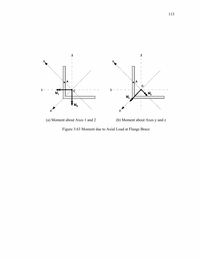
113

C1

2

A

z

y

M1

M2

C1

2

A

z

y

M1

M2

C1

2

A

z

y

M1

M2

C1

2

A

z

y

M1

M2

Mz

My

C1

2

A

z

y

Mz

My

C1

2

A

z

y

Mz

My

C1

2

A

z

y

Mz

My

C1

2

A

z

y

(a) Moment about Axes 1 and 2 (b) Moment about Axes y and z

Figure 3.63 Moment due to Axial Load at Flange Brace

114

NN

Purlin

Rafter

Bracing Angle

Purlin

Rafter

Bracing Angle

S97

S98 S99

0.5

0.5 0.5

2.5

2.5

0.1875

0.18

75

S97

S98 S99

0.5

0.5 0.5

2.5

2.5

0.1875

0.18

75

(a) Location

-400 -200 0 200 400

-40

-20

0

20

40

Microstrain

Bas

e S

hear

(kip

s)

(b) Strain Gage S97

Figure 3.64 Frame 1: Measured Strain at Flange Brace

115

-400 -200 0 200 400

-40

-20

0

20

40

Microstrain

Bas

e S

hear

(kip

s)

(c) Strain Gage S98

-400 -200 0 200 400

-40

-20

0

20

40

Microstrain

Bas

e S

hear

(kip

s)

(d) Strain Gage S99

Figure 3.64 Frame 1: Measured Strain at Flange Brace (continued)

116

NNN

Purlin

RafterBracing Angle

HSS Support

Purlin

RafterBracing Angle

HSS Support

2.5

2.5 S104

1.25

0.1875

0.18

75

2.5

2.5 S104

1.25

0.1875

0.18

75

(a) Location

-400 -200 0 200 400

-40

-20

0

20

40

Microstrain

Bas

e S

hear

(kip

s)

(b) Strain Gage S104

Figure 3.65 Frame 2: Measured Strain at Additional Flange Brace

117

4 FINITE ELEMENT ANALYSIS OF TEST FRAME

4.1 Introduction

A correlation study with the test results was performed using nonlinear finite

element analysis. Section 4.2 addresses the modeling technique used in this study.

Models predicted global and local behaviors of the frame and their correlation with

test results is presented in Section 4.3. The effect of initial geometric imperfection

through a parametric study is discussed in Section 4.4. The findings in this chapter

are used to provide proper modeling techniques for this type of building system in

Chapter 6.

4.2 Finite Element Modeling Technique

4.2.1 General

Finite element models that simulate geometry and material properties of the

test frames were created using the software ABAQUS (ABAQUS Inc. 2005). The

results of the finite element analysis complement the laboratory testing and provide

additional insight and information on the test frame behavior.

4.2.2 Geometry and Element

The ABAQUS model is shown in Figure 4.1; rather than modeling the entire

building explicitly, only one frame was modeled since the two frames were nominally

identical. A total of four models were generated considering the column base

boundary condition, initial geometric imperfection, and additional flange braces

installed during testing (see Table 4.1). The column base was modeled as either a

118

hinge support or a semi-rigid connection adopting a rotational spring with an average

spring constant value of 12,250 kip-in/rad obtained from the test. Initial geometric

imperfection with the first buckling mode shape from a linearized eigen buckling

analysis was employed for Models 2 through 4 with the amplitude of Lb/1000 (= 0.12

in.) based on the findings from Miller and Earls (2003 and 2005). For Models 2 and

3, the imperfection was introduced in the south rafter to simulate failure at positive

2.6% drift (see Figure 4.2). For Model 4, the imperfection was introduced in the

south column by applying an 1-in. displacement in the out-of-plane direction at the

end plate-to-continuity plate joint as well as in the north rafter using the first eigen

buckling mode shape to simulate failure of Frame 2 at negative 2.3% drift. While the

first three models represent the original test frame, two additional lateral braces for the

rafter in Model 3 were added to represent the strengthened Frame 2 in Model 4 (see

Figure 3.25). To incorporate the brace effect in the model, the out-of-plane

deformation was fully restrained at the purlin, girt, and flange brace locations.

Bolted end-plate connection was assumed rigid based on the test results (see Figure

3.32) and the associated surface interaction between end plates was not considered.

Residual stresses were not considered in this study and the slippage of flange braces

due to the use of long-slotted holes was also ignored.

Quadrilateral 4-node shell elements, ABAQUS S4R, with 6 degrees of

freedom per node (three translational and three in-plane rotations) were used. A

reduced integration scheme with one Gauss point in the center of each element was

used for computational efficiency. The mesh was refined in the connection region

and convergence studies were performed to ensure the mesh refinement was sufficient.

119

4.2.3 Material Properties

A tri-linear stress-strain relationship was utilized for the models as shown in

Figure 4.3 (Mays 2000). Typical steel properties (E = 29,000 ksi, Poisson’s ratio =

0.3) were used in the model to describe the elastic material properties, and the yield

strength, Fy, of 55 ksi and the tensile strength, Fu, of 70 ksi was assumed. The

plasticity in the models was based on a von Mises yield surface and associated flow

rule. The plastic hardening was defined by an isotropic hardening law. The

isotropic hardening component of the model defines the equivalent stress as a function

of the equivalent plastic strain (ABAQUS Inc. 2005).

)1(0

0 plbeQ ε−∞ −+σ=σ (4.1)

where σ|0 is the yield surface size as zero plastic strain, Q∞ and b are additional

material parameters, and plε is the plastic strain.

4.2.4 Gravity Load and Monotonic Push

The gravity load (= 16.57 psf) was first applied at the purlin locations as

concentrated loads based on their tributary areas. Monotonic lateral load was then

applied at column tops, to which the actuators were attached, up to failure; the positive

loading (north to south) was applied to Models 1 through 3, while the negative loading

(south to north) was imposed to Model 4.

4.2.5 Post-Buckling Response

It is often necessary to obtain nonlinear static equilibrium solutions for

unstable problems, where the load-displacement response can exhibit the type of

behavior shown in Figure 4.4. This is the case for the test frame since the system is

120

characterized by a sudden strength degradation due to lateral buckling failure (see

Figure 3.29). The modified Riks algorithm (Riks 1970; Crisfleld 1981; and Powell

and Simpson 1981) was then used; this solution scheme was selected in order to trace

the post-buckling range of the response. The load and/or the displacement may

decrease as the solution evolves during periods of the response. It is assumed that

the loading is proportional; that is the load magnitude varies with a single scalar

parameter. In addition, it is assumed that the response is reasonably smooth so that

sudden bifurcations do not occur.

The essence of the method is that the solution is viewed as the discovery of a

single equilibrium path in a space defined by the nodal variables and the loading

parameter. Development of the solution requires that it traverses the path as far as

required. The basic algorithm remains the Newton method; therefore, at any time

there will be a finite radius of convergence (ABAQUS Inc. 2005).

4.3 Correlation with Test Results

4.3.1 Gravity Load Analysis

Gravity load analysis was first performed. The predicted vertical deflection

at midspan of the frame was 0.31 in. for all models. Note the measured deflections,

0.22 in. and 0.24 in. in Frames 1 and 2, respectively, was less. Normal stress

distribution in all models was also similar and the maximum stress at both rafter ends

was less than 4 ksi. Figure 4.5 showed the normal stress comparison with the test

results. Good correlation was indicated at both rafter ends and column tops but some

deviations were observed in the midspan of the rafter. That is probably due to the

121

stiffening effect from the roof panel and the attached wood panels used for the gravity

load [see Figure 3.13(a)] at such low stress level.

4.3.2 Lateral Load Analysis

The analyses were halted at 7.8%, 3.9%, and 4.6% drift in Models 1, 2, and 3,

respectively, due to a numerical convergence problem associated with buckling. The

analysis of Model 1 which represented a perfectly straight condition showed flange

local buckling at the narrowest sections of the rafter (see Figure 4.6), while the

observed failure mode in the test was lateral buckling. On the other hand, Models 2

and 3 exhibited lateral buckling failure of the rafter (see Figures 4.7 and 4.8), although

flange local buckling followed in Model 3.

Base shear versus lateral displacement of each model was compared with the

recorded response in Figure 4.9. Model 1 did not capture the failure point and the

predicted ultimate load was much higher than that from test, while Models 2 and 3

predicted the failure location and ultimate load with sufficient accuracy. Lateral

stiffness of Model 3 was very close to the measured value due to the inclusion of

rotational spring at column base. Models 1 and 2 predicted a lesser lateral stiffness

because of the ideal hinge assumption at column base.

The analysis of Model 4 was halted at negative 3.6% drift due to a numerical

convergence problem. The analysis results provided a reasonable prediction of the

failure mode and the ultimate strength (see Figures 4.10 and 4.11). The predicted

ultimate strength in the negative excursion is similar to the measured peak strength in

the positive excursion. Since the test frame first experienced lateral buckling in the

122

positive excursion at 3% drift, a reduced ultimate strength in the subsequent negative

excursion is expected.

4.4 Initial Geometric Imperfection

A parametric study on the effect of initial geometric imperfection was carried

out with Model 3. First eigen buckling mode shape shown in Figure 4.2 was used as

an imperfection with the variation of the maximum amplitude, and the predicted

ultimate load was compared with that measured from test.

Regardless of the amplitude, lateral buckling failure mode (see Figure 4.8) was

predicted as long as the initial geometric imperfection was introduced. Global

responses shown in Figure 4.12 indicated that the ultimate load prediction was not

sensitive to the scaling factor of between Lb/500 and Lb/5000, and corresponded well

with the test data. Table 4.2 summarizes the predicted load and the error of each

considered case.


Finite element analysis of the test frame was conducted using the software

ABAQUS (ABAQUS Inc. 2005). First buckling mode shape from the linearized

eigen buckling analysis was employed to simulate initial geometric imperfection. To

overcome the convergence problems associated with post-buckling in thin structure,

modified Riks method was adopted.

(1) All models predicted a vertical deflection at midspan which is about 35%

larger than the measured value under gravity load. That is probably due to

123

the strengthening effect from the roof panel and the attached wood panel

(gravity load) which was not considered in the models.

(2) The model without an initial geometric imperfection predicted a different

failure mode (flange local buckling) and the ultimate load was much higher

than the measured.

(3) Models with an initial imperfection corresponded well with the test results in

terms of the buckling failure mode and the ultimate load capacity.

(4) For lateral stiffness and ultimate load, the model with a rotational spring at

column base predicted most accurately, but the results from the model with an

ideal hinge at column base was also acceptable when an initial geometric

imperfection was introduced.

(5) A parametric study showed that the acceptable range of initial imperfection

amplitude was between Lb/500 and Lb/5000; the most accurate prediction was

obtained with an amplitude of Lb/1000 for the cases considered.

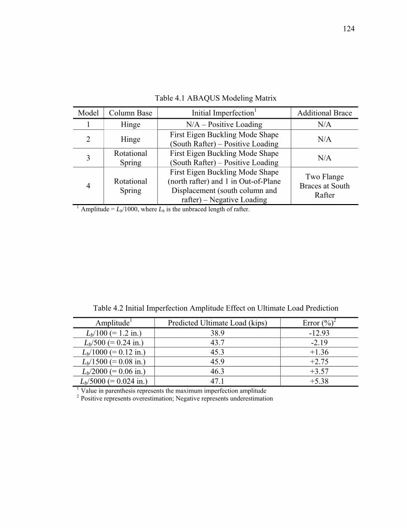
124

Table 4.1 ABAQUS Modeling Matrix

Model Column Base Initial Imperfection1 Additional Brace 1 Hinge N/A – Positive Loading N/A

2 Hinge First Eigen Buckling Mode Shape (South Rafter) – Positive Loading N/A

3 Rotational Spring

First Eigen Buckling Mode Shape (South Rafter) – Positive Loading N/A

4 Rotational Spring

First Eigen Buckling Mode Shape (north rafter) and 1 in Out-of-Plane Displacement (south column and

rafter) – Negative Loading

Two Flange Braces at South

Rafter 1 Amplitude = Lb/1000, where Lb is the unbraced length of rafter.

Table 4.2 Initial Imperfection Amplitude Effect on Ultimate Load Prediction

Amplitude1 Predicted Ultimate Load (kips) Error (%)2 Lb/100 (= 1.2 in.) 38.9 -12.93 Lb/500 (= 0.24 in.) 43.7 -2.19 Lb/1000 (= 0.12 in.) 45.3 +1.36 Lb/1500 (= 0.08 in.) 45.9 +2.75 Lb/2000 (= 0.06 in.) 46.3 +3.57 Lb/5000 (= 0.024 in.) 47.1 +5.38

1 Value in parenthesis represents the maximum imperfection amplitude 2 Positive represents overestimation; Negative represents underestimation

125

U1 = 0

U2, U3 = 0

U2, U3 = 0

2

13

N

U1 = 0U1 = 0

U2, U3 = 0

U2, U3 = 0

2

13

2

13

NN

U1 = 0

U2, U3 = 0

U2, U3 = 0

2

13

N

U1 = 0U1 = 0

U2, U3 = 0

U2, U3 = 0

2

13

2

13

NN

Figure 4.1 ABAQUS Model of Test Frame (Loading in Positive Direction)

Figure 4.2 First Eigen Buckling Mode Shape for Models 2 and 3

126

εy 3.5εy

Fy

Fu

ε

σ

E

εy 3.5εy

Fy

Fu

ε

σ

E

Figure 4.3 Stress-Strain Relationship (Mays 2000)

Figure 4.4 Typical Unstable Static Response (ABAQUS Inc. 2005)

127

Test DataModel 1

N

-4 0 4Stress (ksi)

-4 0 4Stress (ksi)

-4-2024

Stre

ss (k

si)

Test DataModel 1Test DataModel 1

N

-4 0 4Stress (ksi)

-4 0 4Stress (ksi)

-4-2024

Stre

ss (k

si)

(a) Frame 1

N

-4 0 4Stress (ksi)

-4 0 4Stress (ksi)

-4-2024

Stre

ss (k

si)

Test DataModel 1

N

-4 0 4Stress (ksi)

-4 0 4Stress (ksi)

-4-2024

Stre

ss (k

si)

Test DataModel 1Test DataModel 1

(b) Frame 2

Figure 4.5 Normal Stress Comparison

128

Figure 4.6 Flange Buckling Failure Mode of Model 1

Figure 4.7 Lateral Buckling Failure Mode of Model 2

129

Figure 4.8 Flange Local Buckling and Lateral Buckling Failure Mode of Model 3

-10 -5 0 5 10-60

-40

-20

0

20

40

60


Bas

e S

hear

(kip

s)


TestModel 1Model 2Model 3

Figure 4.9 Base Shear versus Lateral Displacement Comparison

130

Figure 4.10 Predicted Failure Mode of Model 4

-10 -5 0 5 10-60

-40

-20

0

20

40

60


Bas

e S

hear

(kip

s)


TestModel 4

Figure 4.11 Global Response Comparison

131

-10 -5 0 5 10-60

-40

-20

0

20

40

60


Bas

e S

hear

(kip

s)


-10 -5 0 5 10

-60

-40

-20

0

20

40

60


Bas

e S

hear

(kip

s)


(a) Lb/100 (b) Lb/500

-10 -5 0 5 10-60

-40

-20

0

20

40

60


Bas

e S

hear

(kip

s)


-10 -5 0 5 10

-60

-40

-20

0

20

40

60


Bas

e S

hear

(kip

s)


(c) Lb/1000 (d) Lb/1500

p p ( )

-10 -5 0 5 10-60

-40

-20

0

20

40

60


Bas

e S

hear

(kip

s)


-10 -5 0 5 10

-60

-40

-20

0

20

40

60


Bas

e S

hear

(kip

s)


(e) Lb/2000 (f) Lb/5000

Figure 4.12 Initial Imperfection Effect on Global Response

132

5 DEVELOPMENT OF A SEISMIC DESIGN PROCEDURE

5.1 Introduction

A new seismic design procedure based on story drift was developed for metal

building systems. Section 5.2 addresses the general concept of the new procedure.

Sections 5.3 and 5.4 discuss important design parameters that are used in the approach.

The effects of the damping ratio (ξ) and the response modification factor (R-factor) are

investigated in Sections 5.5 and 5.6. Section 5.7 presents the simplified seismic

design procedure considering the drift capacity and demand of metal buildings.

5.2 Drift-Based Design Concept

It was shown in the cyclic test of a metal building in Chapter 3 that the system

has little ductility; the behavior of the system was characterized by the elastic response

and sudden strength degradation as soon as the ultimate load was reached (see Figure

3.29). Test results also demonstrated that the strength evaluation for web-tapered

members specified in the code provisions (AISC 2001) is sufficiently accurate. For

the development of a new seismic design procedure, it is then assumed that the system

behaves elastically, but fails once any one of the members reaches its strength based

on the code provisions.

Figure 5.1 shows the general idea of the new seismic design procedure.

Consider the governing earthquake load combination, which is usually governed by

Eq. (3.7):

1.2D + f1L + f2S + 1.0E (5.1)

133

where the first three terms represent the gravity load effect, and the last term

represents the earthquake load effect. In a routine design the most critical unbraced

segment based on the above earthquake load combination can be identified.

Consider the axial-flexural interaction domain of this critical member, the yield

surface based on the AISC LRFD Specification (AISC 2001) is

0.198

≤φ

+φ n

u

n

u

MM

PP

when 2.0≥φ n

u

PP

(5.2)

0.12

≤φ

+φ n

u

n

u

MM

PP

when 2.0<φ n

u

PP

(5.3)

The gravity load effect can be represented by vector OA, and the eqrthquake

load effect is represented by vector AB. Representing these load effects in the form

of demand-capacity ratio (DCR), the DCRs for both the gravity load (i.e., DCRG) and

the earthquake load (i.e., DCRE) are shown in Figure 5.1(a). If the vector AB is

scaled by a multiplier Ωo such that point B is on the yield surface, the critical member

has reached its strength and the frame fails. This multiplier, which can be easily

calculated in the design process, is defined as the system overstrength. That is, Ωo is

a multiplier for the code specified design base shear such that the collapse limit state

of the frame reached.

Figure 5.1(b) shows the corresponding base shear versus story drift

relationship. The required elastic earthquake force, ED, specified in IBC (point D) is

reduced by the response modification factor, R, to the code prescribed design

earthquake force level, Eh, (point B). Since the frame lacks ductility, the response is

linear elastic until the critical member reaches its strength limit state (point C).

134

Recall that the system overstrength Ωo represents the ratio between the strength levels

at C and B. Therefore, the story drift capacity, ΔC, of the frame can also be

calculated as follows:

ΔC = ΩoΔS (5.4)

The goal of this design procedure is to ensure that the story drift capacity, ΔC,

is larger than the elastic drift demand, ΔD, due to ED by a certain safety margin.

Further discussions regarding the evaluation of the story drift and the base shear are

given in Section 5.4.3.

5.3 System Overstrength Factor, Ωo

The system overstrength factor, Ωo, is one of the most important parameters to

be calculated in this design procedure. Since the design of this type of building

system is typically governed by non-seismic load combinations, the system can have a

sufficient reserve of strength for the earthquake load combination. It was shown

from the cyclic test that the system overstrength factor was 9.31 and 9.18 for Frames 1

and 2, respectively (see Section 3.5). Test results also indicated that failure in the

most critical unbraced member resulted in a significant strength loss at the system

level. Hence, the overstrength factor of the critical component is the key parameter

to determining the system behavior.

In order to identify the critical segment, a strength check is required based on

the axial and flexural interaction, and the overstrength factor is calculated as shown in

Figure 5.1(a) for each unbraced segment. Since the DCR for each unbraced segment

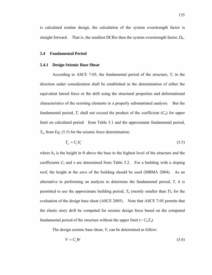
135

is calculated routine design, the calculation of the system overstrength factor is

straight forward. That is, the smallest DCRis then the system overstrength factor, Ωo.

5.4 Fundamental Period

5.4.1 Design Seismic Base Shear

According to ASCE 7-05, the fundamental period of the structure, T, in the

direction under consideration shall be established in the determination of either the

equivalent lateral force or the drift using the structural properties and deformational

characteristics of the resisting elements in a properly substantiated analysis. But the

fundamental period, T, shall not exceed the product of the coefficient (Cu) for upper

limit on calculated period from Table 5.1 and the approximate fundamental period,

Ta, from Eq. (5.5) for the seismic force determination:

xnta hCT = (5.5)

where hn is the height in ft above the base to the highest level of the structure and the

coefficients Ct and x are determined from Table 5.2. For a building with a sloping

roof, the height at the eave of the building should be used (MBMA 2004). As an

alternative to performing an analysis to determine the fundamental period, T, it is

permitted to use the approximate building period, Ta (mostly smaller than T), for the

evaluation of the design base shear (ASCE 2005). Note that ASCE 7-05 permits that

the elastic story drift be computed for seismic design force based on the computed

fundamental period of the structure without the upper limit (= CuTa)

The design seismic base shear, V, can be determined as follow:

WCV s= (5.6)

136

where Cs is the seismic response coefficient and W is the effective seismic weight.

The seismic response coefficient, Cs, can be determined by dividing the spectral

response acceleration, Sa, from the design response spectrum shown in Figure 5.2 by

the response modification factor, R.

5.4.2 T versus Ta

Study on dynamic characteristics of metal buildings is very limited.

Sockalingam (1988) conducted a vibration test on a single-story metal building (see

Figure 5.3); the prototype building was composed of web-tapered rafters and

columns, and had a dimension of 130 ft wide by 60 ft long by 22 ft eave high.

Three frames (two end frames and one middle frame) were spaced at 30 ft and a

gravity column was located at mid-span of each frame. The free vibration test

results are summarized in Table 5.3. The measured average frequency for the first

mode was about 1.1 Hz, which corresponded to the fundamental period of 0.9 second.

If the fundamental period of the prototype building is estimated based on

ASCE 7-05, Ta is 0.33 second [= (0.028)(22)0.8]. The approximate method

underestimates the fundamental period with an error of almost 300%, and in turn,

results in a much higher design base shear. Since the Ta formula in ASCE 7-05 is

developed for conventional multi-story buildings and is merely a function of the

building height [see Eq. (5.5)], the direct application of Ta to the low-rise metal

buildings is not reasonable. Actual period of the frame should always be calculated

in the proposed seismic design procedure. The upper limit (CuTa) on calculated

period is also not applicable for the seismic design of metal buildings.

137

5.4.3 Story Drift Evaluation

In conventional seismic design of multistory frames when inelastic action is

expected, the design story drift (i.e., maximum inelastic drift) is calculated by

multiplying ΔS in Figure 5.1(b) by a deflection amplification factor, Cd. Since metal

buildings investigated are expected to remain elastic and the frames can be modeled as

a single-degree-of-freedom system, the well-known relationship between maximum

displacement (i.e., spectral displacement) and spectral acceleration can be used

(Chopra 2001):

gSTaD ××⎟

⎠⎞

⎜⎝⎛

π=Δ

2

2 (5.7)

where T is the computed (actual) fundamental period, Sa is the spectral response

acceleration (see Figure 5.2), and g is the acceleration of gravity.

5.5 Influence of Damping

The design base shear in ASCE 7 is determined utilizing the spectral response

acceleration, Sa, based on a damping ratio (ξ) of 5%. When a building has a damping

ratio of other than 5%, the use of code-specified spectral acceleration results in an

unrealistic design base shear. In such case, Sa needs to be adjusted to reflect the

actual damping ratio and the guideline for the adjustment of the spectral response

acceleration is defined in FEMA 273 (BSSC 1997).

Figure 5.4 shows the general response spectrum, and the damping coefficients

(BS and B1) are summarized in Table 5.4. If a damping ratio of 2%, for instance, is

considered, the damping coefficients are 0.8 for both BS and B1. Then, Sa is increased

138

by 1/0.8 (= 1.25) and the corresponding design base shear is 25% higher than that

from 5% damping.

It is conceived that the damping ratio of metal buildings is relatively low

compare to that (5%) generally assumed for conventional steel buildings.

Sockalingam (1988) showed that the damping ratio is between 2.3% and 2.8% for the

first mode from free vibration tests on a metal building (see Table 5.3). Assuming

the damping ratio of a typical metal building is 2.5%, the coefficients of BS and B1 are

0.83 from linear interpolation and then, the design base shear is increased by 20% (=

1/0.83).

5.6 Influence of R-Factor

Moment frames in metal buildings are typically designed as Ordinary Moment

Frames (OMFs) with an R-factor of 3.5 (ASCE 2005). Consider the linear relation

provided in this design procedure as shown in Figure 5.1(b). If the value of R is

reduced by half, Eh and ΔS are doubled. But the system overstrength factor, Ωo, is

also reduced by half, which results in the same ΔC value. This observation is also

true if the value of R is doubled. Therefore, this design procedure is independent of

the R value due to the canceling effect from linear relation.

5.7 Simplified Design Procedure

Based on the background information discussed in Sections 5.2 through 5.6,

the proposed seismic design procedure for metal buildings follows (see Figure 5.5):

139

STEP 1 − Perform preliminary frame design based on IBC and consider all load

combinations.

In this step, the response modification factor R = 3.5 and the approximated

fundamental period (Ta = Cthnx) are assumed for seismic design.

STEP 2 − Compute the actual fundamental period:

gkWT π= 2 (5.8)

where W = effective weight (kips)

g = acceleration of gravity (= 386.4 in/sec2)

k = frame lateral stiffness (kip/in), which can be obtained from a static load

analysis in Step 1.

STEP 3 − Re-compute the earthquake load and calculate the system overstrength

factor.

Revise the earthquake load based on the actual fundamental period, T, without an

upper limit (= CuTa) and determine the system overstrength factor, Ωo [see Figure

5.1(a)].

STEP 4 − Check if the frame has sufficient margin of safety against collapse:

.4.1≥ΩR

o (5.9)

A re-design is needed if the above requirement is not satisfied

Note that Ωo/R in Eq. (5.9) equals the ratio between the story drift capacity and

demand:

140

R

ooS

D

C Ω=ΩΔ=

ΔΔ

(5.10)

A safety factor of 1.4 is recommended. This value also includes the effect of lower

damping of the frame which is not considered in routine design.

STEP 5 − Connection design.

The seismic force for the connection design is based on the seismic force from Step 3

multiplied by 1.4R.


A drift-based seismic design procedure was developed for metal buildings.

The design procedure assumes that the frame will respond elastically, and that the

failure occurs when any one of the members reaches its ultimate strength. The

design goal is to make sure that the drift capacity, ΔC, of the system is larger than the

drift demand, ΔD, by a sufficient margin, which is assured, by checking if the

calculated system overstrength factor, Ωo, is larger than the response modification

factor, R, by a factor of safety (= 1.4).

(1) The system overstrength factor, Ωo, of the critical component is one of the

most important parameters in this procedure. The system overstrength factor

in a member is the multiplier to the design earthquake load effect such that the

strength limit state (buckling) is reached.

(2) The actual fundamental period, T, should be used to calculate both the

earthquake load and the story drift. The use of T, instead of the approximated

141

fundamental period, Ta, reflects not only the actual earthquake force but also

the actual overstrength for the drift determination.

(3) The current design provisions utilize 5% damping although the actual damping

ratio of metal buildings is less (≈ 2 to 3%); the proposed factor of safety (= 1.4)

partially reflects the non-conservative nature of the current design provisions

for metal building design.

(4) The proposed design procedure is independent of the R value due to the

canceling effect from linear relationship. Using an R value of 3.5 is

appropriate for preliminary design. The adequacy of such design is then

verified by the proposed design procedure.

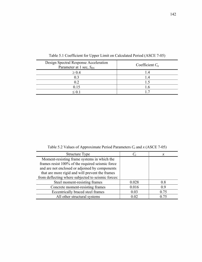
142

Table 5.1 Coefficient for Upper Limit on Calculated Period (ASCE 7-05)

Design Spectral Response Acceleration Parameter at 1 sec, SD1

Coefficient Cu

≥ 0.4 1.4 0.3 1.4 0.2 1.5 0.15 1.6 ≤ 0.1 1.7

Table 5.2 Values of Approximate Period Parameters Ct and x (ASCE 7-05)

Structure Type Ct x Moment-resisting frame systems in which the

frames resist 100% of the required seismic force and are not enclosed or adjoined by components that are more rigid and will prevent the frames

from deflecting where subjected to seismic forces:

Steel moment-resisting frames 0.028 0.8 Concrete moment-resisting frames 0.016 0.9 Eccentrically braced steel frames 0.03 0.75

All other structural systems 0.02 0.75

143

Table 5.3 Dynamic Properties of a Metal Building from Free Vibration Tests (Sockalingam 1988)

Loaded Frame Mode Applied Force (lb) Frequency (Hz) Damping (%) 15.5 1.162 2.31 42.0 1.133 2.78 First 50.2 1.117 2.84

Second 41.0 2.670 N/A Middle

Third 74.4 3.681 9.13 First 50.2 1.117 2.80 End Second 41.0 2.670 0.61

Table 5.4 Damping Coefficients BS and B1 as a Function of Effective Damping β (FEMA 273)

Effective Damping β (percentage of critical)1 BS B1

< 2 0.8 0.8 5 1.0 1.0 10 1.3 1.2 20 1.8 1.5 30 2.3 1.7 40 2.7 1.9

> 50 3.0 2.0 1. The damping coefficient should be based on linear interpolation for effective damping

values other than those given.

144

Pu/φ

Pn

Mu/φMn

DCRG

DCRE

Ωo(DCRE)

O

AB

C

Ωo = AC/ABDCR = Demand/Capacity Ratio

Yield SurfaceP

u/φP

n

Mu/φMn

DCRG

DCRE

Ωo(DCRE)

O

AB

C

Ωo = AC/ABΩo = AC/ABDCR = Demand/Capacity Ratio

Yield Surface

(a) P-M Interaction

∆S ∆D ∆C

ED

Eh

×1/R

E (Base Shear)

∆

×Ωo

(Demand) (Capacity)

A

B

C

DE

last

ic L

imit

∆S ∆D ∆C

ED

Eh

×1/R

E (Base Shear)

∆

×Ωo

(Demand) (Capacity)

A

B

C

DE

last

ic L

imit

(b) Base Shear versus Story Drift

Figure 5.1 Seismic Design Concept

145

SDS

SD1Sa =

SD1⋅TL

T2

Sa =SD1T

To Ts 1.0 TLPeriod, T (sec)

Spec

tral R

espo

nse

Acc

eler

atio

n, S

a(g

) SDS

SD1Sa =

SD1⋅TL

T2

Sa =SD1T

To Ts 1.0 TLPeriod, T (sec)

Spec

tral R

espo

nse

Acc

eler

atio

n, S

a(g

)

Figure 5.2 Design Response Spectrum (ASCE 7-05)

30 ft30 ft

27 ft

22 ft 65 ft

65 ft3@ 4 ft – 2 in

3 ft – 9 in

12@ 5 ft3 ft – 8 in

30 ft30 ft

27 ft

22 ft 65 ft

65 ft3@ 4 ft – 2 in

3 ft – 9 in

12@ 5 ft3 ft – 8 in

Figure 5.3 Prototype Building for Dynamic Test (Sockalingam 1988)

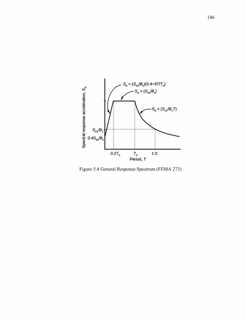
146

0.2To To 1.0Period, T

Spec

tral r

espo

nse

acce

lera

tion,

Sa

Sa = (Sxs/Bs)(0.4+3T/To)

Sx1/B1

0.4Sxs/Bs

Sa = (Sxs/Bs)

Sa = (Sx1/B1T)

0.2To To 1.0Period, T

Spec

tral r

espo

nse

acce

lera

tion,

Sa

Sa = (Sxs/Bs)(0.4+3T/To)

Sx1/B1

0.4Sxs/Bs

Sa = (Sxs/Bs)

Sa = (Sx1/B1T)

Figure 5.4 General Response Spectrum (FEMA 273)

147

STEP 2:Compute actual period


gkWT π= 2

STEP 1:Preliminary design

R = 3.5


R = 3.5

STEP 3:Compute Ωo based on revised earthquake load


STEP 4:FS = Ωo/R ≥ 1.4


Increasemember

size

Increasemember

size

No

EndEnd

Yes

STEP 5:Connection design

based on 1.4R


based on 1.4R



gkWT π= 2


R = 3.5


R = 3.5





Increasemember

size

Increasemember

size

No

EndEnd

Yes


based on 1.4R


based on 1.4R

Figure 5.5 General Design Procedure

148

6 APPLICATIONS OF THE PROPOSED SEISMIC DESIGN PROCEDURE

6.1 Introduction

This chapter demonstrates the application of the drift-based seismic design

procedure developed in Chapter 5. Three cases (40 ft wide by 12 ft eave height, 100

ft wide by 20 ft eave height, and 150 ft wide by 20 ft eave height) with frame spacing

of 25 ft were considered (Sections 6.2 to 6.4). Each case consists of two example

buildings assumed to be located in a high seismic region but with either high wind

(Building A) or low wind (Building B) regions. All buildings were first designed in

accordance with IBC 2006 (ICC 2006), which corresponded to the preliminary design

(Step 1 of the procedure in Section 5.7). The impact of the proposed seismic design

procedure on the current design practice is presented (Section 6.5).

6.2 Case 1 (40 ft×12 ft)

6.2.1 Step 1: Preliminary Design

Two example buildings with a dimension of 40 ft width by 12 ft eave height by

25 ft frame spacing and a roof pitch of 2:12 were designed by Nucor Building Systems

as shown in Figure 6.1. One side of the building was clad with a metal wall while

the other side was opened completely. The design loads are summarized in Table

6.1; the assumed wind loads were 85 mph and 120 mph for Building A and Building B,

respectively, and the wind exposure category C was considered for both buildings.

The governing load combinations according to IBC 2006 were the non-seismic load

combinations:

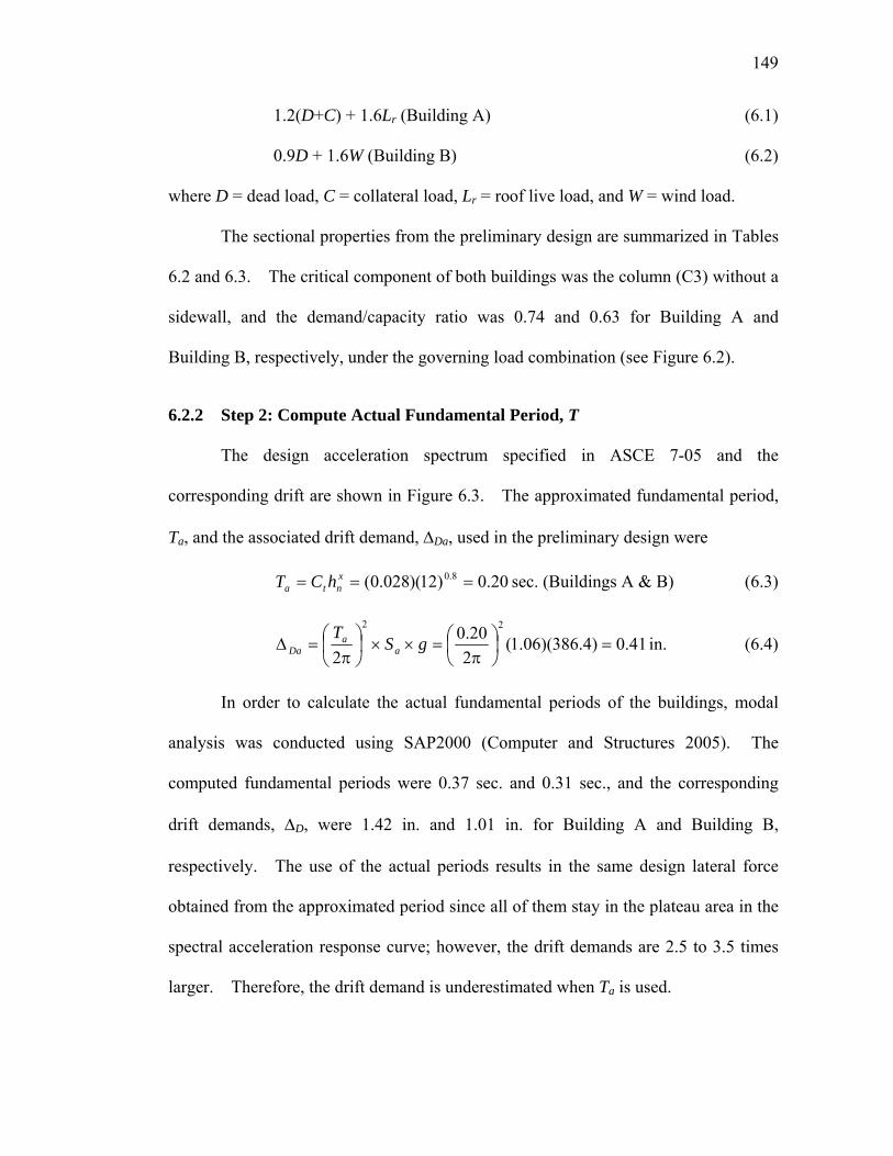
149

1.2(D+C) + 1.6Lr (Building A) (6.1)

0.9D + 1.6W (Building B) (6.2)

where D = dead load, C = collateral load, Lr = roof live load, and W = wind load.

The sectional properties from the preliminary design are summarized in Tables

6.2 and 6.3. The critical component of both buildings was the column (C3) without a

sidewall, and the demand/capacity ratio was 0.74 and 0.63 for Building A and

Building B, respectively, under the governing load combination (see Figure 6.2).

6.2.2 Step 2: Compute Actual Fundamental Period, T

The design acceleration spectrum specified in ASCE 7-05 and the

corresponding drift are shown in Figure 6.3. The approximated fundamental period,

Ta, and the associated drift demand, ΔDa, used in the preliminary design were

20.0)12)(028.0( 8.0 === xnta hCT sec. (Buildings A & B) (6.3)

41.0)4.386)(06.1(220.0

2

22

=⎟⎠⎞

⎜⎝⎛

π=××⎟

⎠⎞

⎜⎝⎛

π=Δ gS

Ta

aDa in. (6.4)

In order to calculate the actual fundamental periods of the buildings, modal

analysis was conducted using SAP2000 (Computer and Structures 2005). The

computed fundamental periods were 0.37 sec. and 0.31 sec., and the corresponding

drift demands, ΔD, were 1.42 in. and 1.01 in. for Building A and Building B,

respectively. The use of the actual periods results in the same design lateral force

obtained from the approximated period since all of them stay in the plateau area in the

spectral acceleration response curve; however, the drift demands are 2.5 to 3.5 times

larger. Therefore, the drift demand is underestimated when Ta is used.

150

The drift at the design seismic force level, ΔS, are then 0.41 in. (= 1.42/3.5) and

0.29 in. (= 1.01/3.5) for Building A and Building B, respectively.

6.2.3 Step 3: Compute Ωo Based on the Revised Earthquake Load

Since the actual fundamental periods for both buildings induce the same

seismic loads used in their preliminary designs, it is unnecessary to revise the seismic

load to compute the overstrength factor, Ωo. For individual unbraced segment, the

overstrength factor should be computed based on the axial and flexural interaction (see

Figures 6.4 and 6.5). In the figures, 1.412(D+C) is the gravity portion and 1.0Eh is

the earthquake portion based on the following equation:

1.2(D+C) + 1.0E = 1.2(D+C) + 0.2SDS(D+C)+1.0Eh (6.5)

= 1.412(D+C) + 1.0Eh

where D = dead load, C = collateral load, Eh = horizontal seismic force.

The column (C3) without a sidewall for both buildings is the critical

component under the earthquake load combination; the critical component is the same

for the governing load combination and the earthquake load combination in this case,

but this is not always true. The system overstrength factor at segment C3 is 5.70 and

8.19 for Building A and Building B, respectively.

The corresponding drift capacities, ΔC, are 2.34 in. (= 0.41×5.70) for Building

A and 2.38 in. (= 0.29×8.19) for Building B. These estimated drift capacities are

further verified using ABAQUS (ABAQUS Inc. 2005) based on the findings in

Chapter 4. The predicted failure mode and the drift capacity corresponded well with

the estimations in this procedure (see Figures 6.6 and 6.7). It is notable that plate

151

buckling developed in the panel zone of Building A provides the ductility in the

system (see Figure 6.6), although the inelastic behavior is not considered in this design

procedure. The potential for the development of a tension field action as a structural

fuse is discussed in Appendix C.

6.2.4 Step 4: Check Ωo/R Ratio

Based on the overstrength factor computed in Step 3, Ωo/R is 1.63 (= 5.70/3.5)

and 2.34 (= 8.19/3.5) for Building A and Building B, respectively. Both buildings

show Ωo/R ≥ 1.4; therefore, the drift capacity is larger than the drift demand with the

specified safety margin (= 1.4).

6.2.5 Step 5: Connection Design

Connection design (i.e., end-plate moment connection, panel zone) is based on

the seismic force obtained in Step 3 multiplied by 1.4R (= 4.9) in accordance with the

design code provisions:

1.412(D+C) + 1.4R(Eh) = 1.412(D+C) + 4.9Eh (6.6)

6.3 Case 2 (100 ft×20 ft)


Two buildings with a dimension of 100 ft width by 20 ft eave height by 25 ft

frame spacing with a roof pitch of 1:12 were designed by Butler Manufacturing

Company (see Figure 6.8). Both buildings were symmetric for their mid-spans.

The sides were clad with metal walls. The considered design loads are summarized

152

in Table 6.4. The governing load combinations were the non-seismic load

combinations:

1.2D + 1.6Lr (Building A) (6.7)

0.9D + 1.6W (Building B) (6.8)

Tables 6.5 and 6.6 summarize the sectional properties of both buildings. The

high demand/capacity ratios under the governing load combinations indicate that the

buildings were optimally designed (see Figure 6.9). The unbraced segment C2 was

the critical component, and the D/C ratio was 1.00 and 0.95 for Building A and

Building B, respectively.


The fundamental period from the approximate method presented in ASCE 7-05

is 31.0)20)(028.0( 8.0 === xnta hCT sec. and the corresponding drift demand is 0.94 in.

for both buildings (see Figure 6.10). The actual fundamental periods, T, from the

modal analysis using SAP2000 are 0.65 sec. and 0.56 sec., and the drift demands

adopting the obtained T are then 3.80 in. and 3.07 in. for Building A and Building B,

respectively. Therefore, the use of Ta results in the underestimation at 25% to 30%

level of the actual drift demand.

The drift, ΔS, are 1.09 in. (= 3.80/3.5) and 0.88 in. (= 3.07/3.5) for Building A

and Building B, respectively.


Figure 6.10(a) shows the spectral response acceleration, Sa, at Ta stays in the

plateau portion (= 1.00g). The Sa at T from Building B is in the descending portion

153

(= 0.92g) while it is located in the plateau portion (= 1.00g) at T from Building A.

Since the design base shear is determined based on the seismic response coefficient, Cs

(= Sa/R), shown in Eq. (5.6), the reduction of the seismic force by a factor of 0.92 (=

0.92g/1.00g) is necessary for Building A for the computation of Ωo.

The critical component under the earthquake load combination [Eq. (6.8)] of

both buildings is the segment R4 and the system overstrength factor is 4.90 and 7.29

for Building A and Building B, respectively (see Figure 6.11). The overstength

factors of all unbraced segments are summarized in Appendix B. Note the segment

C2 was the critical component under the governing load combination for both

buildings (Section 6.3.1).

1.2D + 1.0E = 1.2D + 0.2SDSD+1.0Eh =1.4D + 1.0Eh (6.9)

The corresponding drift capacities, ΔC, are 5.34 in. (= 1.09×4.90) for Building

A and 6.42 in. (= 0.88×7.29) for Building B. The predicted failure mode and the drift

capacity from ABAQUS analysis are reasonably corresponded with those estimated

from this procedure (see Figures 6.12 and 6.13). Flange local buckling without

lateral buckling leads to the ductile behavior in Building A while the failure mode of

lateral buckling results in a sudden strength degradation in Building B. However, it

is very difficult to control the failure only by flange local buckling with no lateral

buckling under cyclic loading in this building system.


Based on the overstrength factor computed in Step 3, Ωo/R is 1.40 (= 4.90/3.5)

and 2.08 (= 7.29/3.5) for Building A and Building B, respectively. Both buildings

154

show Ωo/R ≥ 1.4; therefore, the drift capacity is larger than the drift demand with the

specified safety margin (= 1.4).


Connection design is based on the seismic force obtained in Step 3 multiplied

by 1.4R (= 4.9):

1.4D + 1.4R(Eh) = 1.4D + 4.9Eh (6.10)

6.4 Case 3 (150 ft×20 ft)


Two buildings with a dimension of 150 ft width by 20 ft eave height by 25 ft

frame spacing were designed by Nucor Building Systems as shown in Figure 6.14;

Building A had a roof pitch of 1:12 while Building B had a roof pitch of 2:12.. Two

gravity columns were located in the middle of the span with a distance of 50 ft from

the two exterior columns. A full-height 8 in.-thick concrete wall was installed on

both sides of the buildings and the connection between the wall and the frame was

made at the knee area. The connection details for the wall-to-column and the interior

pipe column-to-rafter are shown in Figure 6.15.

The design loads are summarized in Table 6.7. The governing load

combination was the seismic load combination:

1.412(D+C) + 0.2S + 1.0Eh (Building A) (6.11)

1.412(D+C) + 1.0Eh (Building B) (6.12)

155

The sectional properties the buildings are summarized in Tables 6.8 and 6.9. The

critical segment was the exterior columns (unbraced segment C1) and the D/C ratio

was 0.93 and 1.08 for Building A and Building B, respectively (see Figure 6.16); the

D/C ratio larger than the unity (= 1.0) for Building B indicates that the building was

under designed.


The approximated fundamental period, Ta, is 0.31 sec. for both buildings,

which is the same for Case 2 (100 ft×20 ft); Eq. (5.5) totally depends on the height of

the building and results in the same fundamental period in the different buildings with

the same height. The corresponding drift demand based on Ta is 1.0 in. (see Figure

6.17).

The actual fundamental periods, T, from SAP2000 are 0.95 sec. and 0.90 sec.

for Building A and Building B, respectively. The spectral response accelerations

using T is located in the descending portion, and the corresponding drift demands are

6.26 in. and 5.97 in. for Building A and Building B, respectively. The drift demand

from Ta is significantly less than that from T (1.0 in. vs. 6.26 or 5.97 in.).

The drift, ΔS, are then1.79 in. (= 6.26/3.5) and 1.71 in. (= 5.79/3.5) for

Building A and Building B, respectively.


The seismic design loads can be reduced since both spectral response

accelerations, Sa, using T are located in the descending portion (0.71g for Building A,

0.75g for Building B) while Sa used for the preliminary design is in the plateau (=

156

1.06g) [see Figure 6.17(a)]. The reduction factor of the seismic force for the

computation of Ωo is 0.67 (= 0.71g/1.06g) and 0.71 (= 0.75g/1.06g) for Building A

and Building B, respectively.

The critical component of both buildings is the exterior column (segment C1)

and the system overstrength factor is 1.61 for Building A and 1.21 for Building B (see

Figure 6.18); the corresponding drift capacity is 2.88 in. (= 1.79×1.61) and 2.07 in. (=

1.71×1.21) for Building A and Building B, respectively. The overstrength factors for

all unbraced segments can be found in Appendix B.

The predicted failure mode and the global response from ABAQUS analysis

are shown in Figures 6.19 and 6.20. The predicted failure modes at exterior columns

correspond well with the critical component estimated in this procedure although the

predicted drift capacities are much larger than ΔC. That is because the interior

gravity columns are considered to be hinged at both top and bottom end connections in

the design, but the top connections in the ABAQUS models were generated as rigid

based on the connection drawing [see Figure 6.15(b)]. Therefore, the connections are

able to take some degrees of moment, which results in the moment redistribution of

the global system.


Ωo/R is less than 1.4 for both buildings [0.46 (= 1.61/3.5) and 0.35 (= 1.21/3.5)

for Building A and Building B, respectively]; the returning back to the design Step 2

with the increase of the member sizes is needed.

157


Once Step 4 is satisfied after repeating Steps 2 and 3, the connection design is

based on the seismic force obtained in the previous step (Step 3) multiplied by 1.4R (=

4.9).


This chapter demonstrats how to apply the drift-based seismic design

procedure developed in Chapter 5 with three cases (a total of six preliminary designed

buildings) by following the design procedure described in Section 5.7.

(1) The non-seismic load combination was the governing load combination for

Case 1 (40 ft×12 ft). The overstrngth factor, Ωo, of the critical component

under the earthquake load combination is 5.70 and 8.19 for Building A and

Building B, respectively. Ωo/R ≥ 1.4 is satisfied for both buildings; no re-

design is needed.

(2) The governing load combination was the non-seismic load combination for

both buildings in Case 2 (100 ft×20 ft). The fact the obtained Ωo/R is larger

than 1.4 for both buildings indicates that the buildings have enough drift

capacities to respond elastically under the earthquake event, and no designer-

design is needed.

(3) The earthquake load combination was the governing load combination due to

the use of the concrete walls for both buildings in Case 3 (150 ft×20 ft). In

this case, the increases of member size are required since the elastic drift

158

capacities are less than the elastic drift demands (Ωo/R is less than 1.4 for both

buildings).

(4) It is shown that metal frames with heavy hard walls based on the current

design procedure are vulnerable to collapse. However, the proposed seismic

design procedure does not affect the current design of typical metal buildings.

(5) The possibility for the use of the panel zone as a structural fuse is

demonstrated through the finite element analysis; the inelastic response

utilizing tension field action in the panel zone can be a good source to dissipate

the seismic energy in a stable manner.

159

Table 6.1 Design Loads for Case 1 (40 ft×12 ft)




85 mph (Building A) Wind Speed 120 mph (Building B) Wind Exposure C Wind Load

Importance Factor 1.0 Site Location California



Cs 0.303

Table 6.2 Case 1: Section Properties – Building A

Web Depth (in.)

Web Plate (in.)



Start / End Thick. Length W×T×L W×T×L RF1 12.0 / 18.0 0.125 124.6 5×1/4×124.6 5×1/4×124.6 RF2 15.0 / 15.0 0.15 217.0 5×1/4×217.0 5×1/4×217.0 RF3 15.0 / 15.0 0.15 217.0 5×1/4×217.0 5×1/4×217.0 RF4 18.0 / 12.0 0.125 124.6 5×1/4×124.6 5×1/4×124.6

* Fy = 55 ksi

Table 6.3 Case 1: Section Properties – Building B

Web Depth (in.)

Web Plate (in.)



Start / End Thick. Length W×T×L W×T×L RF1 12.0 / 20.0 0.15 119.8 5×1/4×119.8 5×1/4×119.8 RF2 20.0 / 12.0 0.15 214.9 5×1/4×214.9 5×1/4×214.9 RF3 12.0 / 20.0 0.15 214.9 5×1/4×214.9 5×1/4×214.9 RF4 20.0 / 12.0 0.15 119.8 5×1/4×119.8 5×1/4×119.8

* Fy = 55 ksi

160





85 mph (Building A) Wind Speed 120 mph (Building B) Wind Exposure C Wind Load




Cs 0.286

161


Web Depth (in.)

Web Plate (in.)



Start / End Thick. Length W×T×L W×T×L RF1 16.0 / 32.0 0.188 197.2 6×3/8×197.2 6×1/2×197.2

34.0 / 16.0 0.219 0.16

117.5 120.0 6×3/8×237.5 6×1/2×237.5

RF2 16.0 / 24.0 0.16

0.12 239.3 122.2 6×5/16×362.5 6×1/4×362.5

24.0 / 16.0 0.12 0.16

122.2 239.2 6×5/16×362.5 6×1/4×362.5

RF3 16.0 / 34.0 0.16

0.219 120.0 117.5 6×3/8×237.5 6×1/2×237.5

RF4 32.0 / 16.0 0.188 197.22 6×3/8×197.2 6×1/2×197.2 * Fy = 55 ksi


Web Depth (in.)

Web Plate (in.)




40.0 / 20.0 0.219 237.0 6×1/2×237.0 6×1/2×237.0 RF2

20.0 / 20.0 0.16 0.12

179.8 183.2

6×1/4×179.8 6×3/8×183.2

6×5/16×179.8 6×3/8×183.2

20.0 / 20.0 0.12 0.16

183.2 179.8

6×3/8×183.2 6×1/4×179.8

6×3/8×183.2 6×5/16×179.8 RF3

20.0 / 40.0 0.219 237.0 6×1/2×237.0 6×1/2×237.0 RF4 36.0 / 16.0 0.25 191.5 6×3/8×191.5 6×1/2×191.5

* Fy = 55 ksi

162



5.0 psf (Building A) Collateral Load 3.0 psf (Building B) Frame Self Weight 2.0 psf

Dead Load

Concrete Wall 55.0 psf Live Load Roof Live Load 12.0 psf

14.0 psf (Building A) Snow Load Snow Load 0.0 psf (Building B) 85 mph (Building A) Wind Speed 120 mph (Building B)

Wind Exposure C Wind Load




Cs 0.303

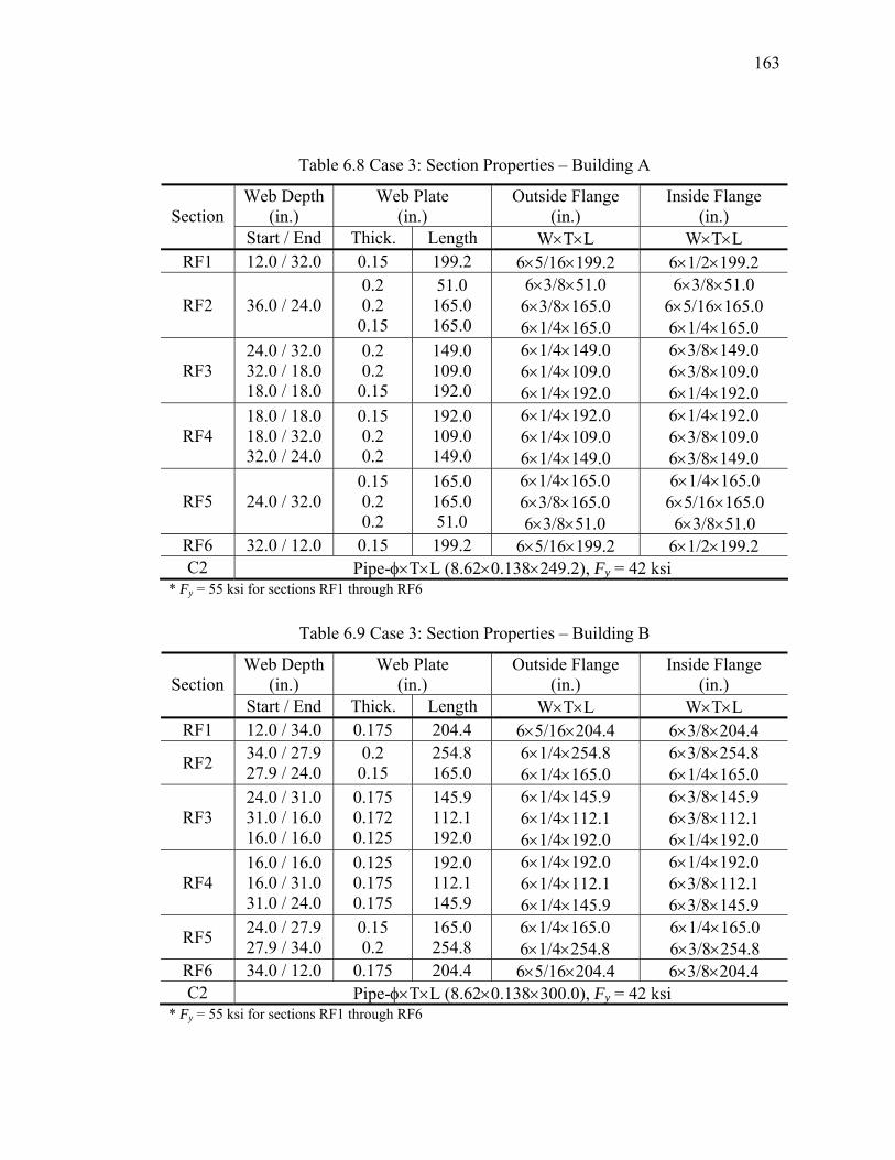
163


Web Depth (in.)

Web Plate (in.)




RF2 36.0 / 24.0 0.2 0.2 0.15

51.0 165.0 165.0

6×3/8×51.0 6×3/8×165.0 6×1/4×165.0

6×3/8×51.0 6×5/16×165.0 6×1/4×165.0

RF3 24.0 / 32.0 32.0 / 18.0 18.0 / 18.0

0.2 0.2 0.15

149.0 109.0 192.0

6×1/4×149.0 6×1/4×109.0 6×1/4×192.0

6×3/8×149.0 6×3/8×109.0 6×1/4×192.0

RF4 18.0 / 18.0 18.0 / 32.0 32.0 / 24.0

0.15 0.2 0.2

192.0 109.0 149.0

6×1/4×192.0 6×1/4×109.0 6×1/4×149.0

6×1/4×192.0 6×3/8×109.0 6×3/8×149.0

RF5 24.0 / 32.0 0.15 0.2 0.2

165.0 165.0 51.0

6×1/4×165.0 6×3/8×165.0 6×3/8×51.0

6×1/4×165.0 6×5/16×165.0 6×3/8×51.0

RF6 32.0 / 12.0 0.15 199.2 6×5/16×199.2 6×1/2×199.2 C2 Pipe-φ×T×L (8.62×0.138×249.2), Fy = 42 ksi

* Fy = 55 ksi for sections RF1 through RF6


Web Depth (in.)

Web Plate (in.)




RF2 34.0 / 27.9 27.9 / 24.0

0.2 0.15

254.8 165.0

6×1/4×254.8 6×1/4×165.0

6×3/8×254.8 6×1/4×165.0

RF3 24.0 / 31.0 31.0 / 16.0 16.0 / 16.0

0.175 0.172 0.125

145.9 112.1 192.0

6×1/4×145.9 6×1/4×112.1 6×1/4×192.0

6×3/8×145.9 6×3/8×112.1 6×1/4×192.0

RF4 16.0 / 16.0 16.0 / 31.0 31.0 / 24.0

0.125 0.175 0.175

192.0 112.1 145.9

6×1/4×192.0 6×1/4×112.1 6×1/4×145.9

6×1/4×192.0 6×3/8×112.1 6×3/8×145.9

RF5 24.0 / 27.9 27.9 / 34.0

0.15 0.2

165.0 254.8

6×1/4×165.0 6×1/4×254.8

6×1/4×165.0 6×3/8×254.8

RF6 34.0 / 12.0 0.175 204.4 6×5/16×204.4 6×3/8×204.4 C2 Pipe-φ×T×L (8.62×0.138×300.0), Fy = 42 ksi

* Fy = 55 ksi for sections RF1 through RF6

164

Flange Brace

122

3@60” 16”

45.9”90

”34

.6”

12 FT

40 FT

RF4R

F1RF2 RF3

C2

C1C3

R1

R2R3

R4 R5

R1R2R3

R4

Flange BraceFlange Brace

122

122

3@60” 16”

45.9”90

”34

.6”

12 FT

40 FT

RF4R

F1RF2 RF3

C2

C1C3

R1

R2R3

R4 R5

R1R2R3

R4

(a) Building 1

3@60” 16”

45.9”

90”

29.8

”

12 FT

40 FT

Flange Brace

122

RF4R

F1

RF2 RF3

C2

C1C3

R1

R2R3

R4 R5

R1R2R3

R4

3@60” 16”

45.9”

90”

29.8

”

12 FT

40 FT


122

122

RF4R

F1

RF2 RF3

C2

C1C3

R1

R2R3

R4 R5

R1R2R3

R4

(b) Building 2

Figure 6.1 Case 1 (40 ft×12 ft)

165

0.0 0.2 0.4 0.6 0.8 1.00.0

0.2

0.4

0.6

0.8

1.0C1C2C3

Mu/φMn

Pu/φ

Pn

D/C = 0.74

0.0 0.2 0.4 0.6 0.8 1.00.0

0.2

0.4

0.6

0.8

1.0C1C2C3

Mu/φMn

Pu/φ

Pn

D/C = 0.74

0.0 0.2 0.4 0.6 0.8 1.00.0

0.2

0.4

0.6

0.8

1.0R1R2R3R4R5

Mu/φMn

Pu/φ

Pn

0.0 0.2 0.4 0.6 0.8 1.00.0

0.2

0.4

0.6

0.8

1.0R1R2R3R4R5

Mu/φMn

Pu/φ

Pn

Column Rafter

(a) Building A

0.0 0.2 0.4 0.6 0.8 1.00.0

0.2

0.4

0.6

0.8

1.0C1C2C3

D/C = 0.63

Mu/φMn

Pu/φ

Pn

0.0 0.2 0.4 0.6 0.8 1.00.0

0.2

0.4

0.6

0.8

1.0C1C2C3

D/C = 0.63

Mu/φMn

Pu/φ

Pn

Mu/φMn

Pu/φ

Pn

0.0 0.2 0.4 0.6 0.8 1.00.0

0.2

0.4

0.6

0.8

1.0R1R2R3R4R5

Mu/φMn

Pu/φ

Pn

0.0 0.2 0.4 0.6 0.8 1.00.0

0.2

0.4

0.6

0.8

1.0R1R2R3R4R5

Column Rafter

(b) Building B

Figure 6.2 Case 1: Demand/Capacity Ratio under Governing Load Combination

166

0.0 0.5 1.0 1.5 2.00.0

0.5

1.0

1.5

Period, T (sec)

Spe

ctra

l Res

pons

e A

ccel

erat

ion,

Sa

(g)

SDS = 1.06g

T S=

0.63

7

T a=

0.20

T = 0.37 (Building A)T = 0.31 (Building B)

0.0 0.5 1.0 1.5 2.00.0

0.5

1.0

1.5

Period, T (sec)

Spe

ctra

l Res

pons

e A

ccel

erat

ion,

Sa

(g)

SDS = 1.06g

T S=

0.63

7

T a=

0.20


(a) Spectral Response Acceleration

0.0 0.5 1.0 1.5 2.00

2

4

6

8

10

12

Period, T (sec)

Drif

t (in

)

T a=

0.20


0.0 0.5 1.0 1.5 2.00

2

4

6

8

10

12

Period, T (sec)

Drif

t (in

)

T a=

0.20


(b) Drift Demand

Figure 6.3 Case 1: Spectral Response Acceleration and Drift Demand

167

Mu/φMn

P u/φ

Pn

0.0 0.2 0.4 0.6 0.8 1.00.0

0.2

0.4

0.6

0.8

1.0

Overstrength = 8.83

1.412(D+C)1.0Eh

Mu/φMn

P u/φ

Pn

0.0 0.2 0.4 0.6 0.8 1.00.0

0.2

0.4

0.6

0.8

1.0

Overstrength = 8.83

1.412(D+C)1.0Eh

Mu/φMn

P u/φ

Pn

0.0 0.2 0.4 0.6 0.8 1.00.0

0.2

0.4

0.6

0.8

1.0

Overstrength = 7.02

1.412(D+C)1.0Eh

Mu/φMn

P u/φ

Pn

0.0 0.2 0.4 0.6 0.8 1.00.0

0.2

0.4

0.6

0.8

1.0

Overstrength = 7.02

1.412(D+C)1.0Eh

Segment C1 Segment C2

Mu/φMn

P u/φ

Pn

0.0 0.2 0.4 0.6 0.8 1.00.0

0.2

0.4

0.6

0.8

1.0

Overstrength = 5.7

1.412(D+C)1.0Eh

Mu/φMn

P u/φ

Pn

0.0 0.2 0.4 0.6 0.8 1.00.0

0.2

0.4

0.6

0.8

1.0

Overstrength = 5.7

1.412(D+C)1.0Eh

Mu/φMn

P u/φ

Pn

0.0 0.2 0.4 0.6 0.8 1.00.0

0.2

0.4

0.6

0.8

1.0

Overstrength = 6.94

1.412(D+C)1.0Eh

Mu/φMn

P u/φ

Pn

0.0 0.2 0.4 0.6 0.8 1.00.0

0.2

0.4

0.6

0.8

1.0

Overstrength = 6.94

1.412(D+C)1.0Eh

Segment C3 Segment R1

Mu/φMn

P u/φ

Pn

0.0 0.2 0.4 0.6 0.8 1.00.0

0.2

0.4

0.6

0.8

1.0

Overstrength = 8.35

1.412(D+C)1.0Eh

Mu/φMn

P u/φ

Pn

0.0 0.2 0.4 0.6 0.8 1.00.0

0.2

0.4

0.6

0.8

1.0

Overstrength = 8.35

1.412(D+C)1.0Eh

Mu/φMn

P u/φ

Pn

0.0 0.2 0.4 0.6 0.8 1.00.0

0.2

0.4

0.6

0.8

1.0

Overstrength = 21.69

1.412(D+C)1.0Eh

Mu/φMn

P u/φ

Pn

0.0 0.2 0.4 0.6 0.8 1.00.0

0.2

0.4

0.6

0.8

1.0


1.412(D+C)1.0Eh

Segment R2 Segment R3

Figure 6.4 Case 1: Overstrength Factor for Building A

168

0.0 0.2 0.4 0.6 0.8 1.00.0

0.2

0.4

0.6

0.8

1.0

Overstrength = 99.7

1.412(D+C)1.0Eh

Mu/φMn

P u/φ

Pn

0.0 0.2 0.4 0.6 0.8 1.00.0

0.2

0.4

0.6

0.8

1.0

Overstrength = 99.7

1.412(D+C)1.0Eh

Mu/φMn

P u/φ

Pn

0.0 0.2 0.4 0.6 0.8 1.0

0.0

0.2

0.4

0.6

0.8

1.0


1.412(D+C)1.0Eh

Mu/φMn

P u/φ

Pn

0.0 0.2 0.4 0.6 0.8 1.00.0

0.2

0.4

0.6

0.8

1.0


1.412(D+C)1.0Eh

Mu/φMn

P u/φ

Pn


Figure 6.4 Case 1: Overstrength Factor for Building A (continued)

169

Mu/φMn

P u/φ

Pn

0.0 0.2 0.4 0.6 0.8 1.00.0

0.2

0.4

0.6

0.8

1.0

Overstrength = 9.63

1.412(D+C)1.0Eh

Mu/φMn

P u/φ

Pn

0.0 0.2 0.4 0.6 0.8 1.00.0

0.2

0.4

0.6

0.8

1.0

Overstrength = 9.63

1.412(D+C)1.0Eh

Mu/φMn

P u/φ

Pn

0.0 0.2 0.4 0.6 0.8 1.00.0

0.2

0.4

0.6

0.8

1.0

Overstrength = 9.13

1.412(D+C)1.0Eh

Mu/φMn

P u/φ

Pn

0.0 0.2 0.4 0.6 0.8 1.00.0

0.2

0.4

0.6

0.8

1.0

Overstrength = 9.13

1.412(D+C)1.0Eh


Mu/φMn

P u/φ

Pn

0.0 0.2 0.4 0.6 0.8 1.00.0

0.2

0.4

0.6

0.8

1.0

Overstrength = 8.19

1.412(D+C)1.0Eh

Mu/φMn

P u/φ

Pn

0.0 0.2 0.4 0.6 0.8 1.00.0

0.2

0.4

0.6

0.8

1.0

Overstrength = 8.19

1.412(D+C)1.0Eh

Mu/φMn

P u/φ

Pn

0.0 0.2 0.4 0.6 0.8 1.00.0

0.2

0.4

0.6

0.8

1.0

Overstrength = 9.23

1.412(D+C)1.0Eh

Mu/φMn

P u/φ

Pn

0.0 0.2 0.4 0.6 0.8 1.00.0

0.2

0.4

0.6

0.8

1.0

Overstrength = 9.23

1.412(D+C)1.0Eh


Mu/φMn

P u/φ

Pn

0.0 0.2 0.4 0.6 0.8 1.00.0

0.2

0.4

0.6

0.8

1.0


1.412(D+C)1.0Eh

Mu/φMn

P u/φ

Pn

0.0 0.2 0.4 0.6 0.8 1.00.0

0.2

0.4

0.6

0.8

1.0


1.412(D+C)1.0Eh

Mu/φMn

P u/φ

Pn

0.0 0.2 0.4 0.6 0.8 1.00.0

0.2

0.4

0.6

0.8

1.0


1.412(D+C)1.0Eh

Mu/φMn

P u/φ

Pn

0.0 0.2 0.4 0.6 0.8 1.00.0

0.2

0.4

0.6

0.8

1.0


1.412(D+C)1.0Eh


Figure 6.5 Case 1: Overstrength Factor for Building B

170

0.0 0.2 0.4 0.6 0.8 1.00.0

0.2

0.4

0.6

0.8

1.0


1.412(D+C)1.0Eh

Mu/φMn

P u/φ

Pn

0.0 0.2 0.4 0.6 0.8 1.00.0

0.2

0.4

0.6

0.8

1.0


1.412(D+C)1.0Eh

Mu/φMn

P u/φ

Pn

0.0 0.2 0.4 0.6 0.8 1.00.0

0.2

0.4

0.6

0.8

1.0


1.412(D+C)1.0Eh

Mu/φMn

P u/φ

Pn

0.0 0.2 0.4 0.6 0.8 1.00.0

0.2

0.4

0.6

0.8

1.0


1.412(D+C)1.0Eh

Mu/φMn

P u/φ

Pn


Figure 6.5 Case 1: Overstrength Factor for Building B (continued)

171

1

2

1

2

(a) Failure Mode

0 2 4 6 80

5

10

15

20

25

Displacement (in)

Bas

e S

hear

(kip

s)

Story Drift Ratio (rad)0.0 0.01 0.02 0.03 0.04 0.05 0.06

∆C1 2

Design Base Shear (= 2.4 kips)

0 2 4 6 80

5

10

15

20

25

Displacement (in)

Bas

e S

hear

(kip

s)


∆C1 2


(b) Drift Capacity

Figure 6.6 Case 1: Failure Mode and Drift Capacity Verification of Building A

172

(a) Failure Mode

0 2 4 6 80

10

20

30

Displacement (in)

Bas

e S

hear

(kip

s)


∆C


0 2 4 6 80

10

20

30

Displacement (in)

Bas

e S

hear

(kip

s)


∆C


(b) Drift Capacity

Figure 6.7 Case 1: Failure Mode and Drift Capacity Verification of Building B

173

9@60”47.9”

12.2”

90”

60” 4

7.3”

20 FT

100 FTFlange Brace

121

RF4R

F1

C2

C1

R1 R2

R3 R4 R5 R6 R7

RF2 RF3

CL

9@60”47.9”

12.2”

90”

60” 4

7.3”

20 FT

100 FTFlange BraceFlange Brace

121

121

RF4R

F1

C2

C1

R1 R2

R3 R4 R5 R6 R7

RF2 RF3

CL

(a) Building A

20 FT

9@60”47.9”12.2”

54” 6

0”41

.5”

100 FT36”

Flange Brace

121

RF4R

F1

C2

C1

R1 R2

R3 R4 R5 R6 R7

RF2 RF3

CL

20 FT

9@60”47.9”12.2”

54” 6

0”41

.5”

100 FT36”


121

121

RF4R

F1

C2

C1

R1 R2

R3 R4 R5 R6 R7

RF2 RF3

CL

(b) Building B


174

Mu/φMn

Pu/φ

Pn

0.0 0.2 0.4 0.6 0.8 1.00.0

0.2

0.4

0.6

0.8

1.0C1C2

D/C = 1.00

0.0 0.2 0.4 0.6 0.8 1.00.0

0.2

0.4

0.6

0.8

1.0C1C2

D/C = 1.00

Mu/φMn

Pu/φ

Pn

0.0 0.2 0.4 0.6 0.8 1.00.0

0.2

0.4

0.6

0.8

1.0C1C2

D/C = 1.00

0.0 0.2 0.4 0.6 0.8 1.00.0

0.2

0.4

0.6

0.8

1.0C1C2

D/C = 1.00

Mu/φMn

Pu/φ

Pn

0.0 0.2 0.4 0.6 0.8 1.00.0

0.2

0.4

0.6

0.8

1.0R1R2R3R4R5R6R7

0.0 0.2 0.4 0.6 0.8 1.00.0

0.2

0.4

0.6

0.8

1.0R1R2R3R4R5R6R7

Mu/φMn

Pu/φ

Pn

0.0 0.2 0.4 0.6 0.8 1.00.0

0.2

0.4

0.6

0.8

1.0R1R2R3R4R5R6R7

0.0 0.2 0.4 0.6 0.8 1.00.0

0.2

0.4

0.6

0.8

1.0R1R2R3R4R5R6R7

Column Rafter

(a) Building A

Mu/φMn

Pu/φ

Pn

0.0 0.2 0.4 0.6 0.8 1.00.0

0.2

0.4

0.6

0.8

1.0C1C2

D/C = 0.95

0.0 0.2 0.4 0.6 0.8 1.00.0

0.2

0.4

0.6

0.8

1.0C1C2

D/C = 0.95

Mu/φMn

Pu/φ

Pn

0.0 0.2 0.4 0.6 0.8 1.00.0

0.2

0.4

0.6

0.8

1.0C1C2

D/C = 0.95

0.0 0.2 0.4 0.6 0.8 1.00.0

0.2

0.4

0.6

0.8

1.0C1C2

D/C = 0.95

Mu/φMn

Pu/φ

Pn

0.0 0.2 0.4 0.6 0.8 1.00.0

0.2

0.4

0.6

0.8

1.0R1R2R3R4R5R6R7

0.0 0.2 0.4 0.6 0.8 1.00.0

0.2

0.4

0.6

0.8

1.0R1R2R3R4R5R6R7

Mu/φMn

Pu/φ

Pn

0.0 0.2 0.4 0.6 0.8 1.00.0

0.2

0.4

0.6

0.8

1.0R1R2R3R4R5R6R7

0.0 0.2 0.4 0.6 0.8 1.00.0

0.2

0.4

0.6

0.8

1.0R1R2R3R4R5R6R7

Column Rafter

(b) Building B


175

0.0 0.5 1.0 1.5 2.00.0

0.5

1.0

1.5

Period, T (sec)

Spe

ctra

l Res

pons

e A

ccel

erat

ion,

Sa

(g)

SDS = 1.00g

T S=

0.60

T a=

0.31

T = 0.56 (Building B)T = 0.65 (Building A)

0.0 0.5 1.0 1.5 2.00.0

0.5

1.0

1.5

Period, T (sec)

Spe

ctra

l Res

pons

e A

ccel

erat

ion,

Sa

(g)

SDS = 1.00g

T S=

0.60

T a=

0.31



0.0 0.5 1.0 1.5 2.00

2

4

6

8

10

12

Period, T (sec)

Drif

t (in

)

T a=

0.31


0.0 0.5 1.0 1.5 2.00

2

4

6

8

10

12

Period, T (sec)

Drif

t (in

)

T a=

0.31


(b) Drift Demand


176

Mu/φMn

P u/φ

Pn

0.0 0.2 0.4 0.6 0.8 1.00.0

0.2

0.4

0.6

0.8

1.0

Overstrength = 4.9

1.4D1.0Eh

Mu/φMn

P u/φ

Pn

0.0 0.2 0.4 0.6 0.8 1.00.0

0.2

0.4

0.6

0.8

1.0

Overstrength = 4.9

1.4D1.0Eh

(a) Building A – Segment R4

0.0 0.2 0.4 0.6 0.8 1.00.0

0.2

0.4

0.6

0.8

1.0

Overstrength = 7.25

1.4D1.0Eh

Mu/φMn

P u/φ

Pn

0.0 0.2 0.4 0.6 0.8 1.00.0

0.2

0.4

0.6

0.8

1.0

Overstrength = 7.25

1.4D1.0Eh

Mu/φMn

P u/φ

Pn

(b) Building B – Segment R4

Figure 6.11 Case 2: Overstrength Factor at Critical Segment

177

(a) Failure Mode

0 2 4 6 8 10 12 140

10

20

30

Displacement (in)

Bas

e S

hear

(kip

s)


∆C

No Lateral Buckling


0 2 4 6 8 10 12 140

10

20

30

Displacement (in)

Bas

e S

hear

(kip

s)


∆C

No Lateral Buckling


(b) Drift Capacity


178

1

2

1

2

(a) Failure Mode

0 2 4 6 8 10 12 140

10

20

30

40

Displacement (in)

Bas

e S

hear

(kip

s)


∆C

Lateral Buckling

12


0 2 4 6 8 10 12 140

10

20

30

40

Displacement (in)

Bas

e S

hear

(kip

s)


∆C

Lateral Buckling

12


(b) Drift Capacity


179

14@60”46.5”

16”

20 FT

50 FT 50 FT 50 FT

121

Flange Brace8”-thk. Concrete Wall

RF6R

F1

C2C1

R1

R2

R3

RF2 RF4

R4

R5 R7

R6 R8

R9 R11

R10 R12

R13

R14

R15

R16

CL

RF3

RF5

14@60”46.5”

16”

20 FT

50 FT 50 FT 50 FT

121

121

Flange Brace8”-thk. Concrete WallFlange Brace8”-thk. Concrete Wall8”-thk. Concrete Wall

RF6R

F1

C2C1

R1

R2

R3

RF2 RF4

R4

R5 R7

R6 R8

R9 R11

R10 R12

R13

R14

R15

R16

CL

RF3

RF5

(a) Building 1

14@60”

55.1” 122

16”

20 FT

50 FT 50 FT 50 FT


RF6R

F1

C2C1

R1

R2

R3

RF2 RF4

R4

R5 R7

R6 R8

R9 R11

R10 R12

R13

R14

R15

R16

CL

RF3

RF5

14@60”

55.1” 122

122

16”

20 FT

50 FT 50 FT 50 FT


RF6R

F1

C2C1

R1

R2

R3

RF2 RF4

R4

R5 R7

R6 R8

R9 R11

R10 R12

R13

R14

R15

R16

CL

RF3

RF5

(b) Building 2


180

(a) Wall-to-Frame at Knee Area

FLANGE BRACE(LOCATION MAY VARY PER DESIGN)

BOLT SIZE AND QUANTITY WILL VARY

3 1/2” DEEP AND SEAT STANDARD ON JOIST

ROOF STEEL LINE (PURLINS)ROOF STEEL LINE (JOIST)

STIFFENER

STANDARD INTERIOR PIPE COLUMN – INTERIOR “H”SHAPE BUILT-UP COLUMNS ARE ALSO AVAILABLE

FLANGE BRACE(LOCATION MAY VARY PER DESIGN)

BOLT SIZE AND QUANTITY WILL VARY

3 1/2” DEEP AND SEAT STANDARD ON JOIST

ROOF STEEL LINE (PURLINS)ROOF STEEL LINE (JOIST)

STIFFENER

STANDARD INTERIOR PIPE COLUMN – INTERIOR “H”SHAPE BUILT-UP COLUMNS ARE ALSO AVAILABLE

(b) Pipe-to-Rafter

Figure 6.15 Case 3: Connection Details (Nucor Building Systems)

181

0.0 0.2 0.4 0.6 0.8 1.00.0

0.2

0.4

0.6

0.8

1.0

C1C2

Mu/φMn

Pu/φ

Pn

D/C = 0.93

0.0 0.2 0.4 0.6 0.8 1.00.0

0.2

0.4

0.6

0.8

1.0

C1C2

Mu/φMn

Pu/φ

Pn

D/C = 0.93

0.0 0.2 0.4 0.6 0.8 1.00.0

0.2

0.4

0.6

0.8

1.0

C1C2

Mu/φMn

Pu/φ

Pn

D/C = 1.08

0.0 0.2 0.4 0.6 0.8 1.00.0

0.2

0.4

0.6

0.8

1.0

C1C2

Mu/φMn

Pu/φ

Pn

D/C = 1.08

Column Column

0.0 0.2 0.4 0.6 0.8 1.00.0

0.2

0.4

0.6

0.8

1.0R1R2R3R4R5R6R7R8

Mu/φMn

Pu/φ

Pn

0.0 0.2 0.4 0.6 0.8 1.00.0

0.2

0.4

0.6

0.8

1.0R1R2R3R4R5R6R7R8

Mu/φMn

Pu/φ

Pn

0.0 0.2 0.4 0.6 0.8 1.00.0

0.2

0.4

0.6

0.8

1.0R1R2R3R4R5R6R7R8

Mu/φMn

Pu/φ

Pn

0.0 0.2 0.4 0.6 0.8 1.00.0

0.2

0.4

0.6

0.8

1.0R1R2R3R4R5R6R7R8

Mu/φMn

Pu/φ

Pn

Mu/φMn

Pu/φ

Pn

0.0 0.2 0.4 0.6 0.8 1.00.0

0.2

0.4

0.6

0.8

1.0R9R10R11R12R13R14R15R16

Mu/φMn

Pu/φ

Pn

0.0 0.2 0.4 0.6 0.8 1.00.0

0.2

0.4

0.6

0.8

1.0R9R10R11R12R13R14R15R16

0.0 0.2 0.4 0.6 0.8 1.00.0

0.2

0.4

0.6

0.8

1.0R9R10R11R12R13R14R15R16

Mu/φMn

Pu/φ

Pn

0.0 0.2 0.4 0.6 0.8 1.00.0

0.2

0.4

0.6

0.8

1.0R9R10R11R12R13R14R15R16

Mu/φMn

Pu/φ

Pn

Rafter Rafter

(a) Building A (b) Building B


182

0.0 0.5 1.0 1.5 2.00.0

0.5

1.0

1.5

Period, T (sec)

Spe

ctra

l Res

pons

e A

ccel

erat

ion,

Sa

(g)

T S=

0.63

7

T a=

0.31


SDS = 1.06g

0.0 0.5 1.0 1.5 2.00.0

0.5

1.0

1.5

Period, T (sec)

Spe

ctra

l Res

pons

e A

ccel

erat

ion,

Sa

(g)

T S=

0.63

7

T a=

0.31


SDS = 1.06g


0.0 0.5 1.0 1.5 2.00

2

4

6

8

10

12

Period, T (sec)

Drif

t (in

)

T a=

0.31


0.0 0.5 1.0 1.5 2.00

2

4

6

8

10

12

Period, T (sec)

Drif

t (in

)

T a=

0.31


(b) Drift Demand


183

Mu/φMn

Pu/φ

Pn

0.0 0.2 0.4 0.6 0.8 1.00.0

0.2

0.4

0.6

0.8

1.0

Overstrength = 1.61

1.412(D+C)1.0Eh

1.412(D+C) + 0.2S1.0Eh

Mu/φMn

Pu/φ

Pn

0.0 0.2 0.4 0.6 0.8 1.00.0

0.2

0.4

0.6

0.8

1.0

Overstrength = 1.61

1.412(D+C)1.0Eh

Mu/φMn

Pu/φ

Pn

0.0 0.2 0.4 0.6 0.8 1.00.0

0.2

0.4

0.6

0.8

1.0

Overstrength = 1.61

1.412(D+C)1.0Eh

1.412(D+C) + 0.2S1.0Eh1.412(D+C) + 0.2S1.0Eh1.412(D+C) + 0.2S1.0Eh

(a) Building A – Segment C1

Mu/φMn

P u/φ

Pn

0.0 0.2 0.4 0.6 0.8 1.00.0

0.2

0.4

0.6

0.8

1.0

Overstrength = 1.21

1.412(D+C)1.0Eh

Mu/φMn

P u/φ

Pn

0.0 0.2 0.4 0.6 0.8 1.00.0

0.2

0.4

0.6

0.8

1.0

Overstrength = 1.21

1.412(D+C)1.0Eh

(b) Building B – Segment C1

Figure 6.18 Case 3: Overstrength Factor at Critical Segment

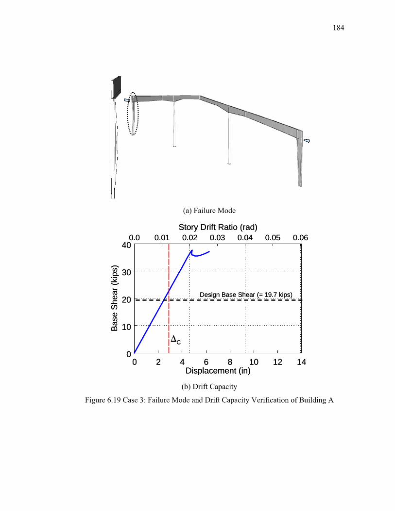
184

(a) Failure Mode

0 2 4 6 8 10 12 140

10

20

30

40

Displacement (in)

Bas

e S

hear

(kip

s)


∆C


0 2 4 6 8 10 12 140

10

20

30

40

Displacement (in)

Bas

e S

hear

(kip

s)


∆C


(b) Drift Capacity


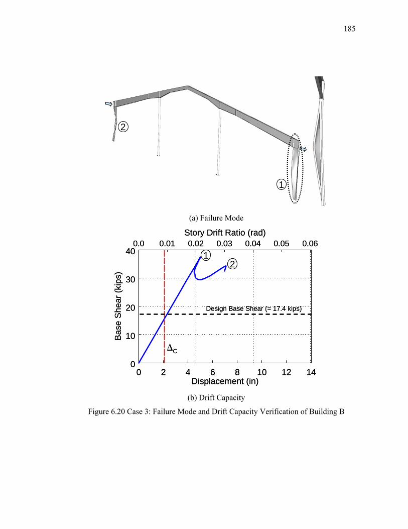
185

1

2

1

2

(a) Failure Mode

0 2 4 6 8 10 12 140

10

20

30

40

Displacement (in)

Bas

e S

hear

(kip

s)


∆C


12

0 2 4 6 8 10 12 140

10

20

30

40

Displacement (in)

Bas

e S

hear

(kip

s)


∆C


12

(b) Drift Capacity


186

7 SUMMARY AND CONCLUSIONS

7.1 Summary

Metal building systems are widely used in low-rise (1- or 2-story) building

construction in the United States. The primary cornerstone of metal building

construction is to minimize the building cost through optimization of the steel weight

and the fabrication process; the web-tapered I-shaped built-up sections are usually

used and for ease of construction the bolted end-plate moment connections are

adopted.

The design of this type of structural system is typically governed by the non-

seismic load combinations such as gravity and wind loads. For seismic design in

accordance with the International Building Code (ICC 2006), the system is designed

as an Ordinary Moment Frames (OMFs); the stringent slenderness requirements for

both local buckling and lateral buckling are not required, and therefore, non-compact

or slender elements are usually used. It is highly questionable whether the plastic

moment of the member can be developed. Even if the plastic moment can be

developed, it is very difficult to determine the location of the plastic hinge since the

section properties are optimized along the member length with respect to moment

demand. No specific seismic design guideline is available for this type of system due

to lack of research.

Despite the fact that past earthquakes have demonstrated satisfactory

performance of light, single-story metal buildings with bolted end-plate moment

connections, the stringent seismic design requirements, mainly developed for multi-

187

story steel moment frames associated with brittle fracture of welded joints after the

1994 Northridge, California earthquake, have also impacted the seismic design of

metal building system. In addition, the growing use of heavy exterior walls (i.e.,

masonry or concrete) challenges the seismic performance of this system under major

earthquakes. The development of a seismic design procedure for metal buildings is

required.

In this research, a cyclic test of a full-scale metal building with web-tapered

members was conducted with the objects of (1) evaluating the cyclic performance, and

(2) providing test data for calibration of numerical simulation. Test building with a

dimension of 60 ft wide by 20 ft eave height by 20 ft bay spacing and a 0.5:12 roof

pitch was designed in accordance with IBC. One side of the building was clad with a

metal sidewall, while the other side was completely open. The roof was also covered

with the conventional metal roof panels. Non-seismic load combination (1.2D + 1.6S

+ 0.8W) was the governing load combination in the design. For testing purpose, the

gravity load component in the earthquake load combination was imposed on top of the

roof in the first stage using wood panels. In the second stage, cyclic loading was

applied according to the loading sequence for beam-to-column moment connections

specified in the AISC Seismic Provisions (AISC 2005) since no guideline for cyclic

testing of this kind of framing system exists. Correlation study of the test results

with the strength evaluations of web-tapered members specified in the AISC LRFD

Specification (AISC 2001) was conducted. Lateral bracing force in flange braces

was also evaluated.

188

Analytical correlation study with the test data was carried out using the finite

element analysis program, ABAQUS (ABAQUS 2005). Rather than modeling the

entire building explicitly, only one frame was modeled since the two frames in the test

were nominally identical. Gravity load was first applied at the purlin locations as

concentrated loads based on their tributary areas. Then monotonic lateral load was

applied at column tops, where actuators were attached in the experimental testing, up

to failure. The modified Riks algorithm was adopted to trace the post-buckling range

of response. Column base boundary conditions were investigated. Sensitivity study

on initial geometric imperfection was also conducted.

Together with the cyclic test and the analytical correlation study results, a drift-

based seismic design concept was introduced and a seismic design procedure for metal

building systems was proposed. Only elastic response of the system is considered up

to failure. The design goal is to ensure that the drift capacity of the system is larger

than the drift demand by a sufficient margin. Utilizing a linear relationship between

base shear and story drift, the proposed design procedure requires checking if the ratio

of the system overstrength factor (Ωo) to the response modification factor (R-factor) is

larger than a factor of safety (= 1.4). The overstrength factor of an unbraced segment

is the multiplier to the earthquake load component in the earthquake load combination

such that the strength limit state is reached. The system overstrength factor is then

the smallest value among the overstrength factors of all unbraced segments. The

factor of safety of 1.4 partially reflects the non-conservative nature of the current

design provisions for metal building design; IBC assumes a damping ratio of 5% for

determining earthquake load, while the damping ratio from field measurements is

189

about 2 to 3%. The actual fundamental period of the building, not the empirical

period given in IBC, should also be used to calculate both the earthquake load and the

story drift.

The impact of the proposed design procedure on the current design of metal

buildings was investigated through a series of case studies. Three cases (two without

heavy walls and one with heavy walls) were considered. The buildings were

designed based on IBC (ICC 2006). The dimensions were 40 ft wide by 12 ft eave

height, 100 ft wide by 20 ft eave height, and 150 ft wide by 20 ft eave height for Cases

1, 2 and 3, respectively, and a 25 ft bay spacing was assumed for all cases. Each case

consisted of two buildings assumed to be located in a high seismic region with either a

low wind (Building A) or high wind (Building B) region.

7.2 Conclusions

Major findings from the experimental testing of a full-scale metal building are:

(1) Gravity load effect (1.412D + 0.2S) of the test building was relatively small

and the maximum stress due to gravity load was 3 ksi.

(2) System showed high deformability (i.e., flexibility), but little ductility.

Elastic behavior was noted up to 2% drift. Non-ductile lateral buckling

failure occurred at 2.6% drift, accompanied by sudden strength degradation.

(3) Proper detailing of flange brace connection is required. Premature lateral

buckling at rafter and column at 2% drift excursion was observed. Buckling

in the subsequent 2% drift cycle was prevented by welding the flange brace to

the brace connection plate to avoid slippage.

190

(4) Internal member forces derived from measurements and associated failure

modes corresponded well with strength evaluation of web-tapered members in

the AISC LRFD Specification (AISC 2001).

(5) The horizontal component of the flange brace force ranged between 1.3% and

2.6% of the nominal yield strength of the rafter compression flange.

Major findings from the analytical correlation study are:

(1) Model assuming either ideal hinges or rotational springs at column bases

predicted 35% larger vertical deflection than the measured value from test

under gravity load. The strengthening effect from the roof panel and the

attached wood panel used for gravity load was not considered in the models.

(2) Proper assumption of initial geometric imperfection was essential to predict the

frame behavior. Good correlation with test results was observed in the

models with an initial imperfection using the first eigen buckling mode shape.

The model without an initial imperfection predicted the different failure mode

and the much higher ultimate load.

(3) A parametric study demonstrated that the best correlation was obtained by

adopting the first eigen buckling mode shape with an amplitude of Lb/1000,

where Lb is unbraced length of the member.

(4) A model with rotational springs at column bases, accounting for rotational

stiffness of the base plate connection, accurately predicted the response.

Results from a model with ideal hinges at the column bases were also

191

acceptable. Although lateral stiffness was slightly underestimated, ultimate

load and associated failure mode corresponded well with test results.

(5) The potential for the development of a tension field action as a structural fuse

is addressed. Inelastic plate buckling of panel zone provides system strength

and stability in the numerical simulation.

Major findings from the case study of the proposed seismic design procedure are:

(1) Metal buildings with heavy sidewalls following the current design practice are

vulnerable to collapse under major earthquake events. Since earthquake load

combinations usually govern the design of this class of metal buildings, larger

members are needed in accordance with the proposed procedure.

(2) The proposed seismic design procedure does not affect the current design of

typical metal buildings without heavy walls. The system has enough reserve

strength under earthquake load since non-seismic load combinations govern

the design.

192

APPENDIX A. MEMBER STRENGTH CHECK OF TEST FRMAE

The member strength was checked at three segments, C3, C4, and R2 [see

Figure 3.1(a)] in accordance with the Load and Resistance Factor Design Specification

(AISC 2001). Nominal yield strength of 55 ksi was used for the calculations.

A1. Unbraced Segment C3

General

The axial force, shear force, and moment were Pu = 34.1 kips, Vu = 16.7 kips, and Mu

= 3,370 kip-in, respectively (see Figure 3.6). Section properties were given as

follow:

− Inside flange: width (bfi) = 6 in., thickness (tfi) = 5/16 in.

− Outside flange: width (bfo) = 6 in., thickness (tfo) = ¼ in.

− Web: start (ho) = 27.41 in., end (h) = 31 in., thickness (tw) = 0.2 in.

− Unbraced length: Lx = 230 in., Ly = 68 in.

Check Axial Compressive Strength

Chapter E and Appendix F3 for web-tapered members of the 2001 LRFD

Specification is applicable.

a. Flange Local Buckling

342.01.137

4/

4===

woc th

k ; therefore, kc = 0.35.

69.855

35.02900064.064.0λ =×

==y

cr F

Ek

Since rfo

fo

tb

tb λ12

25.026

2>=

×== , the flange is slender.

193

89.1555

35.02900017.117.1 =×

=y

c

FEk

Since y

c

y

c

FEk

tbFEk

17.1/64.0 ≤< , c

ys Ek

FtbQ ⎟

⎠⎞

⎜⎝⎛−= 65.0415.1 .

The reduction factor for slender unstiffened element is Qs = 0.841.

b. Web Local Buckling

2.3455

2900064.049.1λ ===y

r FE

Since ho/tw = 137.1, the web is slender.

39.4524.31/2900049.1/49.1 ==fE < ho/tw = 137.1

where f is taken as φFcr with Fcr calculated based on Qa = 1.0. Sx = (KγL/r)x =

1.28×230/10.56 = 27.87 and Sy = (KL/r)y = 1.0×68/1.07 = 63.55. φ = 0.85.

88.0)λ(39.0)λ( =π

=<=π

=EFS

EFS yy

yeffyx

xeff .

Since 74.0841.088.0)λ( =×=Qyeff < 1.5, [ ] 76.36658.02

== yQ

cr FQF effλ ksi.

The effective width is determined as follow:

⎥⎦

⎤⎢⎣

⎡−=

fE

tbfEtbe )/(

34.0192.1

70.624.31

29000)1.137(

34.0124.31

29000)2.0(92.1 =⎥⎦

⎤⎢⎣

⎡−= in. < 27.41 in.

The reduction factor for the first iteration is Qa = 0.53.

194

φFcr based on Q = Qs×Qa =0.45 from the first iteration is 18.52 ksi, which is very

different from the assumed value of f (= 31.24 ksi). Using f = φFcr, after few

iterations, be = 8.12 in., Qa = 0.55, Q = 0.47, and φFcr = 20.63 ksi.

c. Nominal Compressive Strength

φPn = φFcrAg = 20.63×8.86 = 182.7 kips.

Check Flexural Strength

a. Classification

155=wth .0

wyb

u

yr t

hP

PFE

<=⎟⎠⎞

⎜⎝⎛

×−=⎟

⎟⎠

⎞⎜⎜⎝

⎛−= 8.124

3.4879.01.3474.01

55290007.574.0170.5λ

φ

where φb = 0.9, Py = AgFy = 487.3 kips. Since w

r th

<λ , the web is slender and

Chapter G for Plate Girders specified in the 2001 LRFD Specification is applicable.

b. Flange Local Buckling

6.93125.02

62

=×

==fi

fi

tb

tb

73.855

2900038.038.0λ ===yf

p FE

34.1835.0/55

2900035.1/

35.1λ ===cyf

r kFE

Since λp<λ<λr, 5.52λλλλ

211 =

⎥⎥⎦

⎤

⎢⎢⎣

⎡⎟⎟⎠

⎞⎜⎜⎝

⎛

−

−−=

pr

pyfcr FF ksi.

195

The bending strength reduction factor, Rpg, is determined as follow:

0.1968.07.53001200

1 ≤=⎟⎟⎠

⎞⎜⎜⎝

⎛−

+−=

yww

wPG F

Eth

aa

R

where 1031.3 ≤==fcfc

ww tb

hta (inside flange is in compression).

The nominal moment for flange local buckling is

φbMn = φbSxcRPGFcr= 0.9(86.79)(0.968) (52.5) = 3,971 kip-in.

b. Lateral-Torsional Buckling

The flexural strength of tapered flexural members for the limit state of lateral-

torsional buckling is specified in Appendix F3-4 of the 2001 LRFD Specification.

13.097.27

97.2756.31=

−=

−=

o

oL

ddd

γ and the radius of gyration, rTo,= 1.43 (based

on compression flange plus one-third of the compression web area).

7.10)875.1/()97.27)(68)(09.1(

)29000(41.0/

41.0===

foss ALdh

EF γ ksi.

24.75)]43.1/()68)(003.1[(

)29000(9.5)/(

9.522 ===

Toww rLh

EF γ ksi.

where 09.1/023.00.1 =+= fos ALdh γ , 003.1/00385.00.1 =+= Tow rLh γ .

The factor, B, considering the effect of moment gradient is determined as follow

[Case (b)]:

⎟⎟⎠

⎞⎜⎜⎝

⎛+−⎟⎟

⎠

⎞⎜⎜⎝

⎛++=

2

1

2

1 0.17.00.158.00.1b

b

b

b

ff

ff

B γ

13.18.388.280.1)13.0(7.0

8.388.280.158.00.1 =⎟

⎠⎞

⎜⎝⎛ −−⎟

⎠⎞

⎜⎝⎛ −+=

196

⎥⎥⎦

⎤

⎢⎢⎣

⎡

+−=

⎥⎥

⎦

⎤

⎢⎢

⎣

⎡

+−=

2222 )24.72()7.10()13.1(6551

32

61

32

γγ

γ

ws

yb

FFB

FF

= 32.74 ksi < 0.6Fy (= 33 ksi).

The nominal moment for lateral-torsional buckling is

φbMn = φb )74.32)(79.86)(3/5(9.0)3/5( ' =rbx FS γ = 4,262 kip-in,

where 'xS is the elastic section modulus of the larger end.

c. Nominal Flexural Strength

φbMn = 3,971 kip-in. (flange local buckling governs.)

Check P-M Interaction

2.0187.07.1821.34

<==φ n

u

PP

942.039713370

2187.0

2=+=

φ+

φ nb

u

n

u

MM

PP

< 1.0 (O.K.)

Check Shear Strength

Vu = 16.7 kips

Since [ ] 2601.13749.70/07.3 <⎥⎦

⎤⎢⎣

⎡=<=

w

oyw t

hFE ,

⎥⎦

⎤⎢⎣

⎡φ=φ 2)/(

52.4

wwvnv th

EAV

1.35)1.137(

)29000(52.4)2.0)(97.27(9.0 2 =⎥⎦

⎤⎢⎣

⎡= kips > Vu (O.K.)

A2. Unbraced Segment C4

197

General


= 3,110 kip-in, respectively. Section properties were given as follow:

− Inside flange: width (bfi) = 8 in., thickness (tfi) = 3/8 in.


− Web: start (ho) = 12 in., end (h) = 31 in., thickness (tw) = 0.2 in.




516.0604

/4

===wo

c thk

56.1055

516.02900064.064.0λ =×

==y

cr F

Ek

Since rfo

fo

tb

tb λ16

25.028

2>=


31.1955

516.02900017.117.1 =×

=y

c

FEk

Since y

c

y

c

FEk

tbFEk

17.1/64.0 ≤< , 785.065.0415.1 =⎟⎠⎞

⎜⎝⎛−=

c

ys Ek

FtbQ .


⎥⎥⎦

⎤

⎢⎢⎣

⎡=== 2.34

552900064.049.1λ

yr F

E < [ho/tw = 60]; the web is slender.

After few iterations, 09.5944.18/2900049.1/49.1 ==fE < ho/tw = 60

198

where Sx = (KγL/r)x = 1.40×230/5.37 = 60.0,

Sy = (KL/r)y = 1.0×230/1.90 = 121,

37.1)λ(83.0)λ( =π

=<=π

=EFS

EFS yy

yeffyx

xeff .

Then, be = 7.32 in., Qa = 0.873, Q = 0.685.

13.1685.037.1)λ( =×=Qyeff < 1.5, φ [ ] 68.18658.02

=φ= λy

Qcr FQF eff ksi.


φPn = φFcrAg = 18.68×7.4 = 138.2 kips.


a. Classification

155=wth .0

wyb

u

yr t

hP

PFE

<=⎟⎠⎞

⎜⎝⎛

×−=⎟

⎟⎠

⎞⎜⎜⎝

⎛

φ−= 3.122

4079.03.3274.01

55290007.574.0170.5λ


r th

<λ , the web is slender.


67.10375.02

82

=×

==fi

fi

tb

tb

73.855

2900038.038.0λ ===yf

p FE

34.1835.0/55

2900035.1/

35.1λ ===cyf

r kFE

199


211 =

⎥⎥⎦

⎤

⎢⎢⎣

⎡⎟⎟⎠

⎞⎜⎜⎝

⎛

−

−−=

pr

pyfcr FF ksi.

0.1981.07.53001200

1 ≤=⎟⎟⎠

⎞⎜⎜⎝

⎛−

+−=

yww

wPG F

Eth

aa

R


ww tb





50.163.12

63.1263.31=

−=

−=

o

oL

ddd

γ , rTo = 2.19.

91.5/

41.0==

foss ALdh

EF γ ksi., 79.13)/(

9.52 ==

Toww rLh

EF γ ksi.


34.150.125.00.1

75.125.00.1

75.1=

+=

+=

γB [Case (d)]

94.196

132

22=

⎥⎥

⎦

⎤

⎢⎢

⎣

⎡

+−=

γγ

γ

ws

yb

FFB

FF ksi ≤ 0.6Fy (= 33 ksi).


φbMn = )94.19)(6.117)(3/5(9.0)3/5( ' =φ γrbxb FS = 3,517 kip-in.


φbMn = 3,517 kip-in. (lateral-torsional buckling governs.)

Check P-M Interaction

200

2.0234.02.1383.32

>==φ n

u

PP

019.135173110

98234.0

98

=⎟⎠⎞

⎜⎝⎛+=

φ+

φ nb

u

n

u

MM

PP

≈ 1.0 (say O.K.)


Vu = 14.8 kips

Since [ ] 2603.10269.70/07.3 <⎥⎦

⎤⎢⎣

⎡=<=

w

oyw t

hFE ,

⎟⎟

⎠

⎞

⎜⎜

⎝

⎛φ=φ

w

ywwywvnv th

FEAFV

/

/45.26.0

3.7060

)55/29000(45.2)2.0)(63.12)(55)(6.0)(9.0( =⎟

⎟⎠

⎞⎜⎜⎝

⎛= kips > Vu. (O. K.)

A3. Unbraced Segment R2

General


= 2,111 kip-in, respectively. Section properties were given as follow:

− Inside flange: width (bfi) = 6 in., thickness (tfi) = ¼ in.


− Web: start (ho) = 23.01 in., end (h) = 30.38 in., thickness (tw) = 0.225 in.




201

396.03.102

4/

4===

woc th

k

25.955

396.02900064.064.0λ =×

==y

cr F

Ek

Since rfo

fo

tb

tb λ12

25.026

2>=


90.1655

396.02900017.117.1 =×

=y

c

FEk

Since y

c

y

c

FEk

tbFEk

17.1/64.0 ≤< , 875.065.0415.1 =⎟⎠⎞

⎜⎝⎛−=

c

ys Ek

FtbQ .


2.3455

2900064.049.1λ ===y

r FE

Since ho/tw = 102.3, the web is slender.

After few iterations, 41.5753.19/2900049.1/49.1 ==fE < ho/tw = 102.3

where Sx = (KγL/r)x = 0.79×356/8.81 = 31.9,

Sy = (KL/r)y = 1.0×110/1.05 = 104.8,

07.1)λ(44.0)λ( =π

=<=π

=EFS

EFS yy

yeffyx

xeff .

Then, be = 9.0 in., Qa = 0.614, Q = 0.538.

817.0583.007.1)λ( =×=Qyeff < 1.5, φ [ ] 40.19658.02

=φ= λy

Qcr FQF eff ksi.


φPn = φFcrAg = 19.40×8.2 = 159.1 kips.

202


a. Classification

0.135=wth

wyb

u

yr t

hP

PFE

<=⎟⎠⎞

⎜⎝⎛

×−=⎟

⎟⎠

⎞⎜⎜⎝

⎛

φ−= 7.126

7.4499.06.1774.01

55290007.574.0170.5λ


r th

<λ , the web is slender.


1225.02

62

=×

==fi

fi

tb

tb

73.855

2900038.038.0λ ===yf

p FE

34.1835.0/55

2900035.1/

35.1λ ===cyf

r kFE


211 =

⎥⎥⎦

⎤

⎢⎢⎣

⎡⎟⎟⎠

⎞⎜⎜⎝

⎛

−

−−=

pr

pyfcr FF ksi.

0.102.17.53001200

1 >=⎟⎟⎠

⎞⎜⎜⎝

⎛−

+−=

yww

wPG F

Eth

aa

R ; therefore, RPG = 1.0


ww tb





203

31.051.23

51.2388.30=

−=

−=

o

oL

ddd

γ , rTo = 1.38.

29.5)5.1/()51.23)(110)(30.1(

)29000(41.0/

41.0===

foss ALdh

EF γ ksi.

23.26)]38.1/()110)(011.1[(

)29000(9.5)/(

9.522 ===

Toww rLh

EF γ ksi.


⎟⎟⎠

⎞⎜⎜⎝

⎛+−⎟⎟

⎠

⎞⎜⎜⎝

⎛++=

2

1

2

1 0.17.00.158.00.1b

b

b

b

ff

ff

B γ

21.19.358.140.1)31.0(7.0

9.358.140.158.00.1 =⎟

⎠⎞

⎜⎝⎛ −−⎟

⎠⎞

⎜⎝⎛ −+= [Case (b)].

30.266

132

22=

⎥⎥

⎦

⎤

⎢⎢

⎣

⎡

+−=

γγ

γ

ws

yb

FFB

FF ksi < 0.6Fy (= 33 ksi).


φbMn = )30.26)(62.79)(3/5(9.0)3/5( ' =φ γrbxb FS = 3,141 kip-in.


φbMn = 3,141 kip-in. (lateral-torsional buckling governs.)

Check Unity

2.0107.01.159

6.17<==

φ n

u

PP

73.031412111

2107.0

2=+=

φ+

φ nb

u

n

u

MM

PP

(O.K.)


204

Vu = 30.9 kips

Since [ ] 2603.10249.70/07.3 <⎥⎦

⎤⎢⎣

⎡=<=

w

oyw t

hFE

⎥⎦

⎤⎢⎣

⎡φ=φ 2)/(

52.4

wwvnv th

EAV

63.59)3.102(

)29000(52.4)225.0)(51.23(9.0 2 =⎥⎦

⎤⎢⎣

⎡= kips > Vu (O.K.).

205

APPENDIX B. OVERSTRENGTH FACTOR OF EXAMPLE BUILDINGS

B1. Example Building – Case 2 (100 ft×20 ft)

B1.1 Building A

9@60”47.9”

12.2”

90”

60” 4

7.3”

20 FT

100 FTFlange Brace

121

RF4R

F1

C2

C1

R1 R2

R3 R4 R5 R6 R7

RF2 RF3

CL

9@60”47.9”

12.2”

90”

60” 4

7.3”

20 FT

100 FTFlange BraceFlange Brace

121

121

RF4R

F1

C2

C1

R1 R2

R3 R4 R5 R6 R7

RF2 RF3

CL

Figure B1 Case 2: Unbraced Segment Designation for Building A

Overstrength Factor under Earthquake Load Combination

Earthquake Load Combination = 1.4D + 1.0Eh

Mu/φMn

P u/φ

Pn

0.0 0.2 0.4 0.6 0.8 1.00.0

0.2

0.4

0.6

0.8

1.0


1.4D1.0Eh

Mu/φMn

P u/φ

Pn

0.0 0.2 0.4 0.6 0.8 1.00.0

0.2

0.4

0.6

0.8

1.0


1.4D1.0Eh

Mu/φMn

P u/φ

Pn

0.0 0.2 0.4 0.6 0.8 1.00.0

0.2

0.4

0.6

0.8

1.0

Overstrength = 7.85

1.4D1.0Eh

Mu/φMn

P u/φ

Pn

0.0 0.2 0.4 0.6 0.8 1.00.0

0.2

0.4

0.6

0.8

1.0

Overstrength = 7.85

1.4D1.0Eh


Figure B2 Case 2: Overstrength Factor of Building A

206

Mu/φMn

P u/φ

Pn

0.0 0.2 0.4 0.6 0.8 1.00.0

0.2

0.4

0.6

0.8

1.0


1.4D1.0Eh

Mu/φMn

P u/φ

Pn

0.0 0.2 0.4 0.6 0.8 1.00.0

0.2

0.4

0.6

0.8

1.0


1.4D1.0Eh

Mu/φMn

P u/φ

Pn

0.0 0.2 0.4 0.6 0.8 1.00.0

0.2

0.4

0.6

0.8

1.0


1.4D1.0Eh

Mu/φMn

P u/φ

Pn

0.0 0.2 0.4 0.6 0.8 1.00.0

0.2

0.4

0.6

0.8

1.0


1.4D1.0Eh


Mu/φMn

P u/φ

Pn

0.0 0.2 0.4 0.6 0.8 1.00.0

0.2

0.4

0.6

0.8

1.0

Overstrength = 9.74

1.4D1.0Eh

Mu/φMn

P u/φ

Pn

0.0 0.2 0.4 0.6 0.8 1.00.0

0.2

0.4

0.6

0.8

1.0

Overstrength = 9.74

1.4D1.0Eh

Mu/φMn

P u/φ

Pn

0.0 0.2 0.4 0.6 0.8 1.00.0

0.2

0.4

0.6

0.8

1.0

Overstrength = 4.9

1.4D1.0Eh

Mu/φMn

P u/φ

Pn

0.0 0.2 0.4 0.6 0.8 1.00.0

0.2

0.4

0.6

0.8

1.0

Overstrength = 4.9

1.4D1.0Eh


Mu/φMn

P u/φ

Pn

0.0 0.2 0.4 0.6 0.8 1.00.0

0.2

0.4

0.6

0.8

1.0


1.4D1.0Eh

Mu/φMn

P u/φ

Pn

0.0 0.2 0.4 0.6 0.8 1.00.0

0.2

0.4

0.6

0.8

1.0


1.4D1.0Eh

Mu/φMn

P u/φ

Pn

0.0 0.2 0.4 0.6 0.8 1.00.0

0.2

0.4

0.6

0.8

1.0


1.4D1.0Eh

Mu/φMn

P u/φ

Pn

0.0 0.2 0.4 0.6 0.8 1.00.0

0.2

0.4

0.6

0.8

1.0


1.4D1.0Eh


Figure B2 Case 2: Overstrength Factor of Building A (continued)

207

Mu/φMn

P u/φ

Pn

0.0 0.2 0.4 0.6 0.8 1.00.0

0.2

0.4

0.6

0.8

1.0


1.4D1.0Eh

Mu/φMn

P u/φ

Pn

0.0 0.2 0.4 0.6 0.8 1.00.0

0.2

0.4

0.6

0.8

1.0


1.4D1.0Eh

Segment R7

Figure B2 Case 2: Overstrength Factor of Building A (contimued)

208

B1.2 Building B

20 FT

9@60”47.9”12.2”

54” 6

0”41

.5”

100 FT36”

Flange Brace

121

RF4R

F1

C2

C1

R1 R2

R3 R4 R5 R6 R7

RF2 RF3

CL

20 FT

9@60”47.9”12.2”

54” 6

0”41

.5”

100 FT36”


121

121

RF4R

F1

C2

C1

R1 R2

R3 R4 R5 R6 R7

RF2 RF3

CL

Figure B3 Case 2: Unbraced Segment Designation for Building B


Earthquake Load Combination = 1.4D + 1.0Eh

Mu/φMn

P u/φ

Pn

0.0 0.2 0.4 0.6 0.8 1.00.0

0.2

0.4

0.6

0.8

1.0


1.4D1.0Eh

Mu/φMn

P u/φ

Pn

0.0 0.2 0.4 0.6 0.8 1.00.0

0.2

0.4

0.6

0.8

1.0


1.4D1.0Eh

Mu/φMn

P u/φ

Pn

0.0 0.2 0.4 0.6 0.8 1.00.0

0.2

0.4

0.6

0.8

1.0


1.4D1.0Eh

Mu/φMn

P u/φ

Pn

0.0 0.2 0.4 0.6 0.8 1.00.0

0.2

0.4

0.6

0.8

1.0


1.4D1.0Eh


Figure B4 Case 2: Overstrength Factor of Building B

209

Mu/φMn

P u/φ

Pn

0.0 0.2 0.4 0.6 0.8 1.00.0

0.2

0.4

0.6

0.8

1.0


1.4D1.0Eh

Mu/φMn

P u/φ

Pn

0.0 0.2 0.4 0.6 0.8 1.00.0

0.2

0.4

0.6

0.8

1.0


1.4D1.0Eh

Mu/φMn

P u/φ

Pn

0.0 0.2 0.4 0.6 0.8 1.00.0

0.2

0.4

0.6

0.8

1.0


1.4D1.0Eh

Mu/φMn

P u/φ

Pn

0.0 0.2 0.4 0.6 0.8 1.00.0

0.2

0.4

0.6

0.8

1.0


1.4D1.0Eh


0.0 0.2 0.4 0.6 0.8 1.00.0

0.2

0.4

0.6

0.8

1.0


1.4D1.0Eh

Mu/φMn

P u/φ

Pn

0.0 0.2 0.4 0.6 0.8 1.00.0

0.2

0.4

0.6

0.8

1.0


1.4D1.0Eh

Mu/φMn

P u/φ

Pn

0.0 0.2 0.4 0.6 0.8 1.0

0.0

0.2

0.4

0.6

0.8

1.0

Overstrength = 7.25

1.4D1.0Eh

Mu/φMn

P u/φ

Pn

0.0 0.2 0.4 0.6 0.8 1.00.0

0.2

0.4

0.6

0.8

1.0

Overstrength = 7.25

1.4D1.0Eh

Mu/φMn

P u/φ

Pn


0.0 0.2 0.4 0.6 0.8 1.00.0

0.2

0.4

0.6

0.8

1.0


1.4D1.0Eh

Mu/φMn

P u/φ

Pn

0.0 0.2 0.4 0.6 0.8 1.00.0

0.2

0.4

0.6

0.8

1.0


1.4D1.0Eh

Mu/φMn

P u/φ

Pn

0.0 0.2 0.4 0.6 0.8 1.0

0.0

0.2

0.4

0.6

0.8

1.0


1.4D1.0Eh

Mu/φMn

P u/φ

Pn

0.0 0.2 0.4 0.6 0.8 1.00.0

0.2

0.4

0.6

0.8

1.0


1.4D1.0Eh

Mu/φMn

P u/φ

Pn


Figure B4 Case 2: Overstrength Factor of Building B (continued)

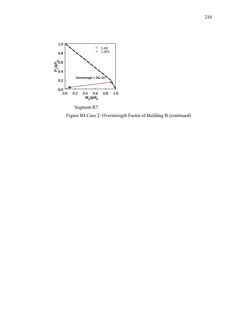
210

0.0 0.2 0.4 0.6 0.8 1.00.0

0.2

0.4

0.6

0.8

1.0


1.4D1.0Eh

Mu/φMn

P u/φ

Pn

0.0 0.2 0.4 0.6 0.8 1.00.0

0.2

0.4

0.6

0.8

1.0


1.4D1.0Eh

Mu/φMn

P u/φ

Pn

Segment R7


211

B2. Example Building – Case 3 (150 ft×20 ft)

B2.1 Building A

14@60”46.5”

16”

20 FT

50 FT 50 FT 50 FT

121


RF6R

F1

C2C1

R1

R2

R3

RF2 RF4

R4

R5 R7

R6 R8

R9 R11

R10 R12

R13

R14

R15

R16

CL

RF3

RF5

14@60”46.5”

16”

20 FT

50 FT 50 FT 50 FT

121

121


RF6R

F1

C2C1

R1

R2

R3

RF2 RF4

R4

R5 R7

R6 R8

R9 R11

R10 R12

R13

R14

R15

R16

CL

RF3

RF5

Figure B5 Case 3: Unbraced Segment Designation for Building A


Earthquake Load Combination = 1.412(D+C) + 0.2S + 1.0Eh

Mu/φMn

P u/φ

Pn

0.0 0.2 0.4 0.6 0.8 1.00.0

0.2

0.4

0.6

0.8

1.0

Overstrength = 1.61

1.412(D+C)1.0Eh

1.412(D+C) + 0.2S1.0Eh

Mu/φMn

P u/φ

Pn

0.0 0.2 0.4 0.6 0.8 1.00.0

0.2

0.4

0.6

0.8

1.0

Overstrength = 1.61

1.412(D+C)1.0Eh

Mu/φMn

P u/φ

Pn

0.0 0.2 0.4 0.6 0.8 1.00.0

0.2

0.4

0.6

0.8

1.0

Overstrength = 1.61

1.412(D+C)1.0Eh


Mu/φMn

P u/φ

Pn

0.0 0.2 0.4 0.6 0.8 1.00.0

0.2

0.4

0.6

0.8

1.0

Overstrength = 3.82

1.412(D+C)1.0Eh

1.412(D+C) + 0.2S1.0Eh

Mu/φMn

P u/φ

Pn

0.0 0.2 0.4 0.6 0.8 1.00.0

0.2

0.4

0.6

0.8

1.0

Overstrength = 3.82

1.412(D+C)1.0Eh

Mu/φMn

P u/φ

Pn

0.0 0.2 0.4 0.6 0.8 1.00.0

0.2

0.4

0.6

0.8

1.0

Overstrength = 3.82

1.412(D+C)1.0Eh



Figure B6 Case 3: Overstrength Factor of Building A

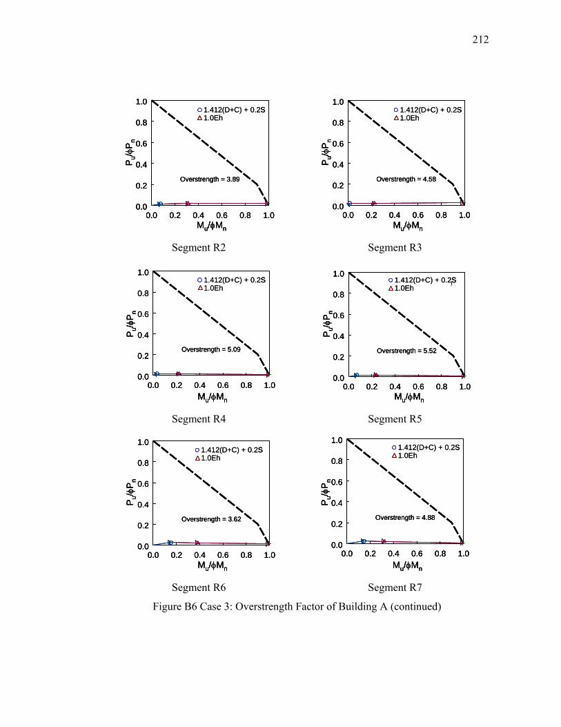
212

Mu/φMn

P u/φ

Pn

0.0 0.2 0.4 0.6 0.8 1.00.0

0.2

0.4

0.6

0.8

1.0

Overstrength = 3.89

1.412(D+C)1.0Eh

1.412(D+C) + 0.2S1.0Eh

Mu/φMn

P u/φ

Pn

0.0 0.2 0.4 0.6 0.8 1.00.0

0.2

0.4

0.6

0.8

1.0

Overstrength = 3.89

1.412(D+C)1.0Eh

Mu/φMn

P u/φ

Pn

0.0 0.2 0.4 0.6 0.8 1.00.0

0.2

0.4

0.6

0.8

1.0

Overstrength = 3.89

1.412(D+C)1.0Eh


Mu/φMn

P u/φ

Pn

0.0 0.2 0.4 0.6 0.8 1.00.0

0.2

0.4

0.6

0.8

1.0

Overstrength = 4.58

1.412(D+C)1.0Eh

1.412(D+C) + 0.2S1.0Eh

Mu/φMn

P u/φ

Pn

0.0 0.2 0.4 0.6 0.8 1.00.0

0.2

0.4

0.6

0.8

1.0

Overstrength = 4.58

1.412(D+C)1.0Eh

Mu/φMn

P u/φ

Pn

0.0 0.2 0.4 0.6 0.8 1.00.0

0.2

0.4

0.6

0.8

1.0

Overstrength = 4.58

1.412(D+C)1.0Eh



0.0 0.2 0.4 0.6 0.8 1.00.0

0.2

0.4

0.6

0.8

1.0

Overstrength = 5.09

1.412(D+C)1.0Eh

Mu/φMn

P u/φ

Pn

1.412(D+C) + 0.2S1.0Eh

0.0 0.2 0.4 0.6 0.8 1.00.0

0.2

0.4

0.6

0.8

1.0

Overstrength = 5.09

1.412(D+C)1.0Eh

Mu/φMn

P u/φ

Pn

0.0 0.2 0.4 0.6 0.8 1.00.0

0.2

0.4

0.6

0.8

1.0

Overstrength = 5.09

1.412(D+C)1.0Eh

Mu/φMn

P u/φ

Pn


0.0 0.2 0.4 0.6 0.8 1.0

0.0

0.2

0.4

0.6

0.8

1.0

Overstrength = 5.52

1.412(D+C)1.0Eh

Mu/φMn

P u/φ

Pn

1.412(D+C) + 0.2S1.0Eh

0.0 0.2 0.4 0.6 0.8 1.00.0

0.2

0.4

0.6

0.8

1.0

Overstrength = 5.52

1.412(D+C)1.0Eh

Mu/φMn

P u/φ

Pn

0.0 0.2 0.4 0.6 0.8 1.00.0

0.2

0.4

0.6

0.8

1.0

Overstrength = 5.52

1.412(D+C)1.0Eh

Mu/φMn

P u/φ

Pn



0.0 0.2 0.4 0.6 0.8 1.00.0

0.2

0.4

0.6

0.8

1.0

Overstrength = 3.62

1.412(D+C)1.0Eh

Mu/φMn

P u/φ

Pn

1.412(D+C) + 0.2S1.0Eh

0.0 0.2 0.4 0.6 0.8 1.00.0

0.2

0.4

0.6

0.8

1.0

Overstrength = 3.62

1.412(D+C)1.0Eh

Mu/φMn

P u/φ

Pn

0.0 0.2 0.4 0.6 0.8 1.00.0

0.2

0.4

0.6

0.8

1.0

Overstrength = 3.62

1.412(D+C)1.0Eh

Mu/φMn

P u/φ

Pn


0.0 0.2 0.4 0.6 0.8 1.0

0.0

0.2

0.4

0.6

0.8

1.0

Overstrength = 4.88

1.412(D+C)1.0Eh

Mu/φMn

P u/φ

Pn

1.412(D+C) + 0.2S1.0Eh

0.0 0.2 0.4 0.6 0.8 1.00.0

0.2

0.4

0.6

0.8

1.0

Overstrength = 4.88

1.412(D+C)1.0Eh

Mu/φMn

P u/φ

Pn

0.0 0.2 0.4 0.6 0.8 1.00.0

0.2

0.4

0.6

0.8

1.0

Overstrength = 4.88

1.412(D+C)1.0Eh

Mu/φMn

P u/φ

Pn




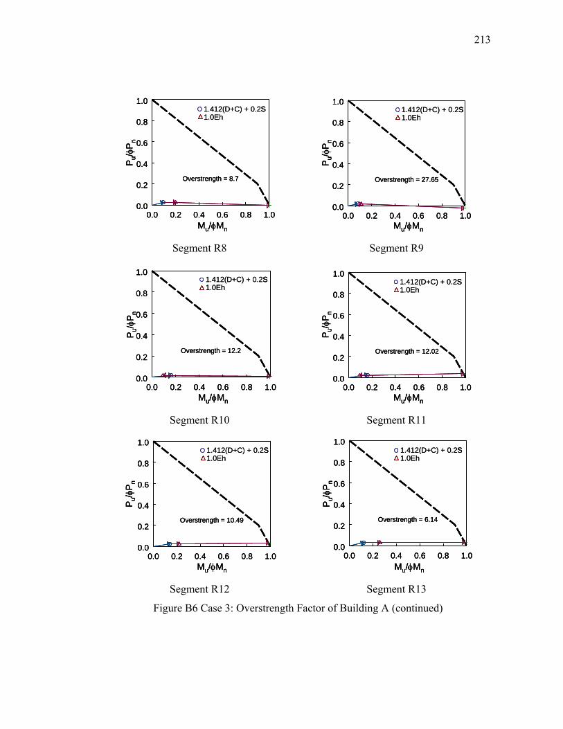
213

0.0 0.2 0.4 0.6 0.8 1.00.0

0.2

0.4

0.6

0.8

1.0

Overstrength = 8.7

1.412(D+C)1.0Eh

Mu/φMn

P u/φ

Pn

1.412(D+C) + 0.2S1.0Eh

0.0 0.2 0.4 0.6 0.8 1.00.0

0.2

0.4

0.6

0.8

1.0

Overstrength = 8.7

1.412(D+C)1.0Eh

Mu/φMn

P u/φ

Pn

0.0 0.2 0.4 0.6 0.8 1.00.0

0.2

0.4

0.6

0.8

1.0

Overstrength = 8.7

1.412(D+C)1.0Eh

Mu/φMn

P u/φ

Pn


Mu/φMn

P u/φ

Pn

0.0 0.2 0.4 0.6 0.8 1.00.0

0.2

0.4

0.6

0.8

1.0


1.412(D+C)1.0Eh

1.412(D+C) + 0.2S1.0Eh

Mu/φMn

P u/φ

Pn

0.0 0.2 0.4 0.6 0.8 1.00.0

0.2

0.4

0.6

0.8

1.0


1.412(D+C)1.0Eh

Mu/φMn

P u/φ

Pn

0.0 0.2 0.4 0.6 0.8 1.00.0

0.2

0.4

0.6

0.8

1.0


1.412(D+C)1.0Eh



0.0 0.2 0.4 0.6 0.8 1.00.0

0.2

0.4

0.6

0.8

1.0

Overstrength = 12.2

1.412(D+C)1.0Eh

Mu/φMn

P u/φ

Pn

1.412(D+C) + 0.2S1.0Eh

0.0 0.2 0.4 0.6 0.8 1.00.0

0.2

0.4

0.6

0.8

1.0

Overstrength = 12.2

1.412(D+C)1.0Eh

Mu/φMn

P u/φ

Pn

0.0 0.2 0.4 0.6 0.8 1.00.0

0.2

0.4

0.6

0.8

1.0

Overstrength = 12.2

1.412(D+C)1.0Eh

Mu/φMn

P u/φ

Pn


0.0 0.2 0.4 0.6 0.8 1.0

0.0

0.2

0.4

0.6

0.8

1.0


1.412(D+C)1.0Eh

Mu/φMn

P u/φ

Pn

1.412(D+C) + 0.2S1.0Eh

0.0 0.2 0.4 0.6 0.8 1.00.0

0.2

0.4

0.6

0.8

1.0


1.412(D+C)1.0Eh

Mu/φMn

P u/φ

Pn

0.0 0.2 0.4 0.6 0.8 1.00.0

0.2

0.4

0.6

0.8

1.0


1.412(D+C)1.0Eh

Mu/φMn

P u/φ

Pn



0.0 0.2 0.4 0.6 0.8 1.00.0

0.2

0.4

0.6

0.8

1.0


1.412(D+C)1.0Eh

Mu/φMn

P u/φ

Pn

1.412(D+C) + 0.2S1.0Eh

0.0 0.2 0.4 0.6 0.8 1.00.0

0.2

0.4

0.6

0.8

1.0


1.412(D+C)1.0Eh

Mu/φMn

P u/φ

Pn

0.0 0.2 0.4 0.6 0.8 1.00.0

0.2

0.4

0.6

0.8

1.0


1.412(D+C)1.0Eh

Mu/φMn

P u/φ

Pn


0.0 0.2 0.4 0.6 0.8 1.0

0.0

0.2

0.4

0.6

0.8

1.0

Overstrength = 6.14

1.412(D+C)1.0Eh

Mu/φMn

P u/φ

Pn

1.412(D+C) + 0.2S1.0Eh

0.0 0.2 0.4 0.6 0.8 1.00.0

0.2

0.4

0.6

0.8

1.0

Overstrength = 6.14

1.412(D+C)1.0Eh

Mu/φMn

P u/φ

Pn

0.0 0.2 0.4 0.6 0.8 1.00.0

0.2

0.4

0.6

0.8

1.0

Overstrength = 6.14

1.412(D+C)1.0Eh

Mu/φMn

P u/φ

Pn




214

0.0 0.2 0.4 0.6 0.8 1.00.0

0.2

0.4

0.6

0.8

1.0

Overstrength = 9.89

1.412(D+C)1.0Eh

Mu/φMn

P u/φ

Pn

1.412(D+C) + 0.2S1.0Eh

0.0 0.2 0.4 0.6 0.8 1.00.0

0.2

0.4

0.6

0.8

1.0

Overstrength = 9.89

1.412(D+C)1.0Eh

Mu/φMn

P u/φ

Pn

0.0 0.2 0.4 0.6 0.8 1.00.0

0.2

0.4

0.6

0.8

1.0

Overstrength = 9.89

1.412(D+C)1.0Eh

Mu/φMn

P u/φ

Pn


0.0 0.2 0.4 0.6 0.8 1.0

0.0

0.2

0.4

0.6

0.8

1.0


1.412(D+C)1.0Eh

Mu/φMn

P u/φ

Pn

1.412(D+C) + 0.2S1.0Eh

0.0 0.2 0.4 0.6 0.8 1.00.0

0.2

0.4

0.6

0.8

1.0


1.412(D+C)1.0Eh

Mu/φMn

P u/φ

Pn

0.0 0.2 0.4 0.6 0.8 1.00.0

0.2

0.4

0.6

0.8

1.0


1.412(D+C)1.0Eh

Mu/φMn

P u/φ

Pn



Mu/φMn

P u/φ

Pn

0.0 0.2 0.4 0.6 0.8 1.00.0

0.2

0.4

0.6

0.8

1.0

Overstrength = 76.1

1.412(D+C)1.0Eh

1.412(D+C) + 0.2S1.0Eh

Mu/φMn

P u/φ

Pn

0.0 0.2 0.4 0.6 0.8 1.00.0

0.2

0.4

0.6

0.8

1.0

Overstrength = 76.1

1.412(D+C)1.0Eh

Mu/φMn

P u/φ

Pn

0.0 0.2 0.4 0.6 0.8 1.00.0

0.2

0.4

0.6

0.8

1.0

Overstrength = 76.1

1.412(D+C)1.0Eh


Segment R16


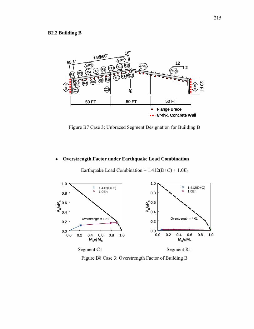
215

B2.2 Building B

14@60”

55.1” 122

16”20 FT

50 FT 50 FT 50 FT


RF6R

F1

C2C1

R1

R2

R3

RF2 RF4

R4

R5 R7

R6 R8

R9 R11

R10 R12

R13

R14

R15

R16

CL

RF3

RF5

14@60”

55.1” 122

122

16”20 FT

50 FT 50 FT 50 FT


RF6R

F1

C2C1

R1

R2

R3

RF2 RF4

R4

R5 R7

R6 R8

R9 R11

R10 R12

R13

R14

R15

R16

CL

RF3

RF5

Figure B7 Case 3: Unbraced Segment Designation for Building B


Earthquake Load Combination = 1.412(D+C) + 1.0Eh

Mu/φMn

P u/φ

Pn

0.0 0.2 0.4 0.6 0.8 1.00.0

0.2

0.4

0.6

0.8

1.0

Overstrength = 1.21

1.412(D+C)1.0Eh

Mu/φMn

P u/φ

Pn

0.0 0.2 0.4 0.6 0.8 1.00.0

0.2

0.4

0.6

0.8

1.0

Overstrength = 1.21

1.412(D+C)1.0Eh

Mu/φMn

P u/φ

Pn

0.0 0.2 0.4 0.6 0.8 1.00.0

0.2

0.4

0.6

0.8

1.0

Overstrength = 4.01

1.412(D+C)1.0Eh

Mu/φMn

P u/φ

Pn

0.0 0.2 0.4 0.6 0.8 1.00.0

0.2

0.4

0.6

0.8

1.0

Overstrength = 4.01

1.412(D+C)1.0Eh


Figure B8 Case 3: Overstrength Factor of Building B

216

Mu/φMn

P u/φ

Pn

0.0 0.2 0.4 0.6 0.8 1.00.0

0.2

0.4

0.6

0.8

1.0

Overstrength = 4.13

1.412(D+C)1.0Eh

Mu/φMn

P u/φ

Pn

0.0 0.2 0.4 0.6 0.8 1.00.0

0.2

0.4

0.6

0.8

1.0

Overstrength = 4.13

1.412(D+C)1.0Eh

Mu/φMn

P u/φ

Pn

0.0 0.2 0.4 0.6 0.8 1.00.0

0.2

0.4

0.6

0.8

1.0

Overstrength = 4.91

1.412(D+C)1.0Eh

Mu/φMn

P u/φ

Pn

0.0 0.2 0.4 0.6 0.8 1.00.0

0.2

0.4

0.6

0.8

1.0

Overstrength = 4.91

1.412(D+C)1.0Eh


0.0 0.2 0.4 0.6 0.8 1.00.0

0.2

0.4

0.6

0.8

1.0

Overstrength = 6.3

1.412(D+C)1.0Eh

Mu/φMn

P u/φ

Pn

0.0 0.2 0.4 0.6 0.8 1.00.0

0.2

0.4

0.6

0.8

1.0

Overstrength = 6.3

1.412(D+C)1.0Eh

Mu/φMn

P u/φ

Pn

0.0 0.2 0.4 0.6 0.8 1.00.0

0.2

0.4

0.6

0.8

1.0

Overstrength = 7.16

1.412(D+C)1.0Eh

Mu/φMn

P u/φ

Pn

0.0 0.2 0.4 0.6 0.8 1.00.0

0.2

0.4

0.6

0.8

1.0

Overstrength = 7.16

1.412(D+C)1.0Eh

Mu/φMn

P u/φ

Pn


0.0 0.2 0.4 0.6 0.8 1.00.0

0.2

0.4

0.6

0.8

1.0

Overstrength = 3.82

1.412(D+C)1.0Eh

Mu/φMn

P u/φ

Pn

0.0 0.2 0.4 0.6 0.8 1.00.0

0.2

0.4

0.6

0.8

1.0

Overstrength = 3.82

1.412(D+C)1.0Eh

Mu/φMn

P u/φ

Pn

0.0 0.2 0.4 0.6 0.8 1.0

0.0

0.2

0.4

0.6

0.8

1.0

M /M

Overstrength = 5.11

1.412(D+C)1.0Eh

Mu/φMn

P u/φ

Pn

0.0 0.2 0.4 0.6 0.8 1.00.0

0.2

0.4

0.6

0.8

1.0

M /M

Overstrength = 5.11

1.412(D+C)1.0Eh

Mu/φMn

P u/φ

Pn



217

0.0 0.2 0.4 0.6 0.8 1.00.0

0.2

0.4

0.6

0.8

1.0

Overstrength = 8.32

1.412(D+C)1.0Eh

Mu/φMn

P u/φ

Pn

0.0 0.2 0.4 0.6 0.8 1.00.0

0.2

0.4

0.6

0.8

1.0

Overstrength = 8.32

1.412(D+C)1.0Eh

Mu/φMn

P u/φ

Pn

0.0 0.2 0.4 0.6 0.8 1.0

0.0

0.2

0.4

0.6

0.8

1.0


1.412(D+C)1.0Eh

Mu/φMn

P u/φ

Pn

0.0 0.2 0.4 0.6 0.8 1.00.0

0.2

0.4

0.6

0.8

1.0


1.412(D+C)1.0Eh

Mu/φMn

P u/φ

Pn


0.0 0.2 0.4 0.6 0.8 1.00.0

0.2

0.4

0.6

0.8

1.0

Overstrength = 9.04

1.412(D+C)1.0Eh

Mu/φMn

P u/φ

Pn

0.0 0.2 0.4 0.6 0.8 1.00.0

0.2

0.4

0.6

0.8

1.0

Overstrength = 9.04

1.412(D+C)1.0Eh

Mu/φMn

P u/φ

Pn

0.0 0.2 0.4 0.6 0.8 1.0

0.0

0.2

0.4

0.6

0.8

1.0

Overstrength = 8.92

1.412(D+C)1.0Eh

Mu/φMn

P u/φ

Pn

0.0 0.2 0.4 0.6 0.8 1.00.0

0.2

0.4

0.6

0.8

1.0

Overstrength = 8.92

1.412(D+C)1.0Eh

Mu/φMn

P u/φ

Pn


0.0 0.2 0.4 0.6 0.8 1.00.0

0.2

0.4

0.6

0.8

1.0

Overstrength = 9.6

1.412(D+C)1.0Eh

Mu/φMn

P u/φ

Pn

0.0 0.2 0.4 0.6 0.8 1.00.0

0.2

0.4

0.6

0.8

1.0

Overstrength = 9.6

1.412(D+C)1.0Eh

Mu/φMn

P u/φ

Pn

0.0 0.2 0.4 0.6 0.8 1.0

0.0

0.2

0.4

0.6

0.8

1.0

Overstrength = 6.82

1.412(D+C)1.0Eh

Mu/φMn

P u/φ

Pn

0.0 0.2 0.4 0.6 0.8 1.00.0

0.2

0.4

0.6

0.8

1.0

Overstrength = 6.82

1.412(D+C)1.0Eh

Mu/φMn

P u/φ

Pn



218

Mu/φMn

P u/φ

Pn

0.0 0.2 0.4 0.6 0.8 1.00.0

0.2

0.4

0.6

0.8

1.0

Overstrength = 10.6

1.412(D+C)1.0Eh

Mu/φMn

P u/φ

Pn

0.0 0.2 0.4 0.6 0.8 1.00.0

0.2

0.4

0.6

0.8

1.0

Overstrength = 10.6

1.412(D+C)1.0Eh

0.0 0.2 0.4 0.6 0.8 1.0

0.0

0.2

0.4

0.6

0.8

1.0


1.412(D+C)1.0Eh

Mu/φMn

P u/φ

Pn

0.0 0.2 0.4 0.6 0.8 1.00.0

0.2

0.4

0.6

0.8

1.0


1.412(D+C)1.0Eh

Mu/φMn

P u/φ

Pn


0.0 0.2 0.4 0.6 0.8 1.00.0

0.2

0.4

0.6

0.8

1.0


1.412(D+C)1.0Eh

Mu/φMn

P u/φ

Pn

0.0 0.2 0.4 0.6 0.8 1.00.0

0.2

0.4

0.6

0.8

1.0


1.412(D+C)1.0Eh

Mu/φMn

P u/φ

Pn

Segment R16


219

APPENDIX C. PARAMETRIC STUDIES ON PANEL ZONE THICKNESS

Finite element analysis results of Building A of Case 1 indicated that the

system ductility could be provided by inelastic deformation of the panel zone (see

Figure 6.6); tension field action after panel zone plate buckling attributed to the stable

and ductile behavior of the system until failure. Parametric studies on the panel zone

thickness were performed to investigate the potential of utilizing panel zone

deformation as a structural fuse.

Case 1 and Case 3 (total four buildings) in Chapter 6 were considered.

ABAQUS models used for drift capacity verification were employed with the

variation of the panel zone thickness.

220

C1. Case 1

C1.1 Building A

(a) tpz = 0.15 in. (Building A)

(b) tpz = 0.14 in.

Figure C1 Case 1: Building A – Failure Mode

221

(c) tpz = 0.175 in.

Figure C1 Case 1: Building A – Failure Mode (continued)

0 2 4 6 80

5

10

15

20

25

Displacement (in)

Bas

e S

hear

(kip

s)


tpz = 0.15 in. (Building A)tpz = 0.14 in.tpz = 0.175 in.

Figure C2 Case 1: Building A – Global Response Comparison

222

C1.2Building B

(a) tpz = 0.175 in. (Building B)

(b) tpz = 0.14 in.

Figure C3 Case 1: Building B – Failure Mode

223

(c) tpz = 0.125 in.

Figure C3 Case 1: Building B – Failure Mode (continued)

0 2 4 6 80

10

20

30

Displacement (in)

Bas

e S

hear

(kip

s)


tpz = 0.175 in. (Building B)tpz = 0.14 in.tpz = 0.125 in.

Figure C4 Case 1: Building B – Global Response Comparison

224

C2. Case 3

C2.1 Building A

(a) tpz = 0.225 in. (Building A)

(b) tpz = 0.125 in.

Figure C5 Case 3: Building A – Failure Mode

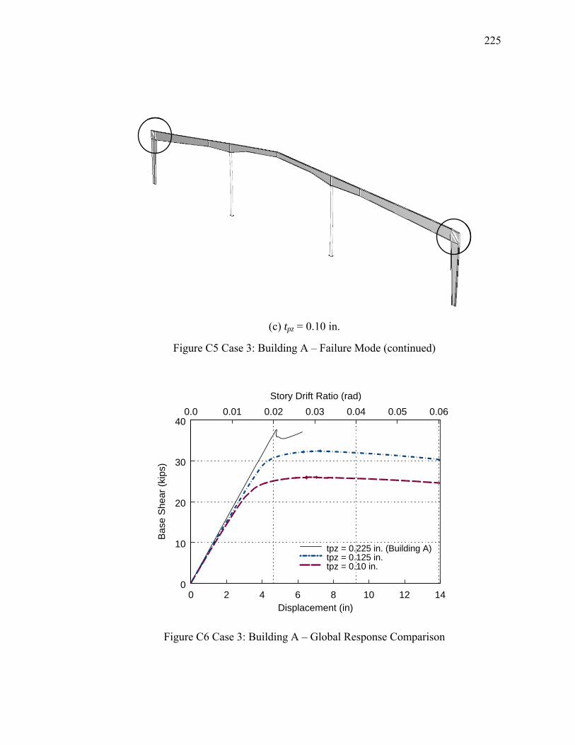
225

(c) tpz = 0.10 in.

Figure C5 Case 3: Building A – Failure Mode (continued)

0 2 4 6 8 10 12 140

10

20

30

40

Displacement (in)

Bas

e S

hear

(kip

s)


tpz = 0.225 in. (Building A)tpz = 0.125 in.tpz = 0.10 in.

Figure C6 Case 3: Building A – Global Response Comparison

226

C2.2Building B

(a) tpz = 0.225 in. (Building B)

(b) tpz = 0.125 in.

Figure C7 Case 3: Building B – Failure Mode

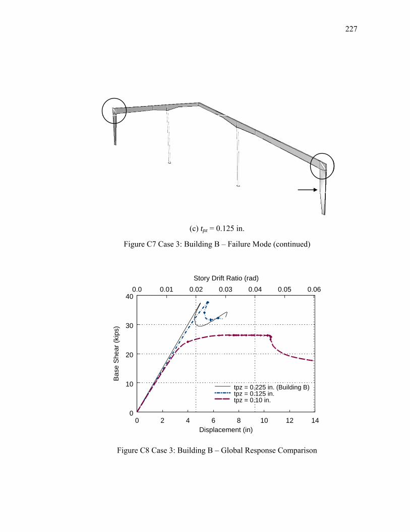
227

(c) tpz = 0.125 in.

Figure C7 Case 3: Building B – Failure Mode (continued)

0 2 4 6 8 10 12 140

10

20

30

40

Displacement (in)

Bas

e S

hear

(kip

s)


tpz = 0.225 in. (Building B)tpz = 0.125 in.tpz = 0.10 in.

Figure C8 Case 3: Building B – Global Response Comparison

228

REFERENCES

[1] ABAQUS. (2005). ABAQUS Standard Users Manual, Version 6.5, ABAQUS Inc. Providence, RI.

[2] AISC. (2002). AISC/MBMA Steel Design Guide 16: Flush and Extended Multiple-Row Moment End-Plate Connections, American Institute of Steel Construction, Chicago, IL.

[3] AISC. (1989). Manual of Steel Construction: Allowable Stress Design, Ninth Edition, American Institute of Steel Construction, Chicago, IL.

[4] AISC. (2001). Manual of Steel Construction: Load and Resistance Factor Design, Third Edition, American Institute of Steel Construction, Chicago, IL.

[5] AISC. (2005). Seismic Provisions for Structural Steel Buildings, American Institute of Steel Construction, Chicago, IL.

[6] ASCE. (2002). Minimum Design Loads for Buildings and Other Structures, ASCE 7-02, American Society of Civil Engineers, Reston, VA.

[7] ASCE. (2005). Minimum Design Loads for Buildings and Other Structures, ASCE 7-05, American Society of Civil Engineers, Reston, VA.

[8] Ashakul, A. and Murray, T. M. (2006). “LRFD versus ASD Frame Design Study,” Report No. CE/VPI-ST 02/02, Virginia Polytechnic Institute and State University, Blacksburg, VA.

[9] Bachman, R. E. and Shoemaker, W. L. (2004). “MBMA Seismic Design Guide for Metal Building Systems 2000 IBC,” CD Proceedings, 2004 ASCE Structures Congress, 1-8.

[10] Building Seismic Safety Committee. (1997). NEHRP Guidelines for the Seismic Rehabilitation of Buildings, FEMA 273, Federal Emergency Management Agency, Washington, D.C.

[11] Building Seismic Safety Committee. (2000). Recommended Seismic Design Criteria for New Steel Moment-Frame Buildings, EEMA 350, Federal Emergency Management Agency, Washington, D.C.

[12] Building Seismic Safety Committee. (2003). NEHRP Recommended Provisions for Seismic Regulations for New Buildings and Other Structures, FEMA 450, Federal Emergency Management Agency, Washington, D.C.

[13] Chen, Y., Wu, X., Tian, H., Zhao, J., and Ma, Y. (2006). “Experiment on Non-compact H-shaped Members and Frames Subjected to Cyclic Loads and the

229

Prediction of Capacities,” International Journal of Steel Structures, Korean Society of Steel Construction, 6(3), 215-226.

[14] Chopra, A. K. (2001). Dynamics of Structures: Theory and Applications to Earthquake Engineering, Second Edition, Prentice Hall, Upper Saddle River, NJ.

[15] Crisfleld, M. A. (1981). “A Fast Incremental/Iterative Solution Procedure That Handles Snap-through,” Computers and Structures, Vol.13, 55–62.

[16] Davids, D. B. (1996). LRFD Evaluation of Full-Scale Metal Building Rigid Frame Tests, Master Thesis, Virginia Polytechnic Institute and State University, Blacksburg, VA.

[17] Forest, R. and Murray, T. M. (1982). “Rigid Frame Studies,” Research Report No. FSEL/STAR 82-01, University of Oklahoma, Oklahoma City, OK.

[18] Galambos, T. V. (1998). Guide to Stability Design Criteria For Metal Structures, Fifth Edition, John Willey & Sons, Inc., New York, NY.

[19] Gil, H. and Yura, J. A. (1999). “Bracing Requirements of Inelastic Columns,” Journal of Constructional Steel Research, Elsevier, Vol.51. 1-19.

[20] Heldt, T. J. and Mahendran, M. (1998). “Full Scale Experiments of a Steel Portal Frame Building,” Journal of the Australian Institute of Steel Construction, Australian Institute of Steel Constructions, 32(4), 2-15.

[21] HKS. (1996). ABAQUS Standard Users Manual, Version 5.6, Hibbitt, Karlsson, and Sorensen Inc., Providence, RI.

[22] ICC. (2003). International Building Code. International Code Council, Inc., Whittier, CA.

[23] ICC. (2006). International Building Code. International Code Council, Inc., Whittier, CA.

[24] Lee, G. C., Chen, Y. C., and Hsu, T. L. (1979). “Allowable Axial Stress of Restrained Multi-Segment, Tapered Roof Girders,” Welding Research Council, Bulletin No. 248.

[25] Lee, G. C., Ketter R. L., and Hsu, T. L. (1981). The Design of Single Story Rigid Frames, Metal Building Manufacturers Association, Cleveland, OH.

[26] Lee, G. C. and Morrell, M. L. (1975). “Application of AISC Design Provisions for Tapered Members,” Engineering Journal, AISC, First Quarter, 1-13.

[27] Lee, G. C., Morrell, M. L., and Ketter, R. L. (1972). “Design of Tapered Members,” Welding Research Council, Bulletin No. 173.

230

[28] Mays, T. (2000). Application of the Finite Element Method to the Seismic Design and Analysis of Large Moment End-Plate Connections, Ph.D. Thesis, Virginia Polytechnic Institute and State University, Blacksburg, VA.

[29] MBMA. (2002). Metal Building Systems Manual, Metal Building Manufacturers Association, Cleveland, OH.

[30] MBMA. (2004). Seismic Design Guide for Metal Building Systems Based on the 2000 IBC, Metal Building Manufacturers Association, Cleveland, OH.

[31] Miller, B. S. and Earls, C. J. (2003). “Behavior of Web-Tapered Built-up I-Shaped Beams”, Report CE/ST 28, University of Pittsburgh, Pittsburgh, PA.

[32] Miller, B. S. and Earls, C. J. (2005). “On Moment Capacity and Flexural Ductility in Doubly Symmetric Web-Tapered I-Girders,” Engineering Journal, Third Quarter (2005), 123-141.

[33] Morrell, M. L. and Lee, G. C. (1974). “Allowable Stresses for Web-Tapered Beams with Lateral Restraints,” Welding Research Council, Bulletin No. 192.

[34] Murray, T. M. (1986). “Stability of Gable Frame Panel Zone Plates,” Proceedings of the Structural Stability Research Council Annual Technical Session, Structural Stability Research Council, 317-325.

[35] Newman, A (2003). Metal Building Systems: Design and Specifications, Second Editioin, McGraw-Hill, New York, NY.

[36] Nucor Building Systems website (http://www.nucorbuildingsystems.com).

[37] Powell, G. and Simons, J. (1981). “Improved Iterative Strategy for Nonlinear Structures,” International Journal for Numerical Methods in Engineering, Wiley InterScience, Vol. 17, 1455–1467.

[38] Prawel, S. P., Morrell, M. L. and Lee, G. C. (1974). “Bending and Buckling Strength of Tapered Structural Members,” Welding Research Journal Supplement, Vol.53, 75-84.

[39] Riks, E. (1970). “On the Numerical Solution of Snapping Problems in the Theory of Elastic Stability,” SUDAAR No. 401, Stanford University, Stanford, CA.

[40] SAP2000. (2005). SAP 2000 User’s Manual, Version 10.02, Computers and Structures Inc. Berkeley, CA.

[41] SEAOC. (1999). Recommended Lateral Force Requirements and Commentary, Seventh Edition, Structural Engineers Association of California, Sacramento, CA.

231

[42] Sockalingam, B. (1988). A Dynamic Test Procedure for Analyzing Low-Rise Metal Buildings, Master Thesis, Clemson University, Clemson, SC.

[43] Sumner, E., A. (1995). Experimental and Analytical Investigation of the LRFD Strength of Tapered Members, Master Thesis, Virginia Polytechnic Institute and State University, Blacksburg, VA.

[44] Uang, C. M. (1991). “Establishing R (or Rw) and Cd Factors for Building Seismic Provisions,” Journal of Structural Engineering, ASCE, Vol.117, No.1, 1991, 19-28.

[45] Winter, G. (1960). “Lateral Bracing of Columns and Beams,” Transactions, ASCE, Vol.125, 807-845.

[46] Young, J. and Murray, T. M. (1996). “Experimental Investigation of Positive Bending Moment Strength of Rigid Knee Connections,” Research Report No. CE/VPI-ST 9617, Department of Civil Engineering, Virginia Polytechnic Institute and State University, Blacksburg, VA.

[47] Yura, J. A. and Li, G. (2002). “Bracing Requirements for Inelastic Beams,” 2002 SSRC Annual Stability Conference, Structural Stability Research Council.

Documents

Development of a seismic design procedure for metal building systems