Univers

ity of

Cap

e Tow

n

Development of a Scaled Doubly-Fed Induction Generator for Assessment of Wind Power Integration Issues

Prepared by:

Name: Hossein Dehnavifard

Student Number: dhnhos001

Supervised by:

A/Prof Azeem Khan

Co-supervisor:

A/Prof Paul Barendse

Thesis submitted to the Department of Electrical Engineering, University of Cape Town, in complete fulfilment of the requirements for the degree of Doctor of Philosophy

November 2016

Department of Electrical Engineering

Faculty of Engineering & the Built Environment

University of Cape Town

The copyright of this thesis vests in the author. No quotation from it or information derived from it is to be published without full acknowledgement of the source. The thesis is to be used for private study or non-commercial research purposes only.

Published by the University of Cape Town (UCT) in terms of the non-exclusive license granted to UCT by the author.

Univers

ity of

Cap

e Tow

n

i

Declaration

This dissertation is submitted to the Department of Electrical Engineering, University of

Cape Town, in complete fulfilment of the requirements for the degree of Doctor of

Philosophy. It has not been submitted before for any degree or examination at this or

any other university. The author confirms that this thesis is based on his own work, save

for which is duly referenced. Portions of this work have been published in peer reviewed

journals and at referred international conference proceedings.

ii

Acknowledgements

The research in this thesis would have taken far longer to complete without the

encouragement from many others. It is a delight to acknowledge those who have

supported me over the last four years.

I wish to thank my parents for their love and encouragement, without whom I would

never have enjoyed so many opportunities.

I would like to thank my supervisor, Prof Mohamed A. Khan, for his guidance and relaxed,

thoughtful insight and also would like to thank my co-supervisor, Prof Paul Barendse, for

his support.

The days would have passed far more slowly without the support of my friends, at the

machine’s lab, whom I thank for putting up with my idiosyncrasies and for providing such

a rich source of conversation, education and entertainment.

I am thankful for the technical support of Mr. Chris Wozniak and Mr. Philip Titus during

my experimental tests in the machine’s lab.

iii

Abstract

Years of experience have been dedicated to the advancement of thermal power

plant technology, and in the last decade the investigation has focused on the wind

energy conversion system (WECS). Wind energy will play an important role in the

future of the energy market, due to the changing climate and the fossil fuel crisis.

Initially, wind energy was intended to cover a small portion of the energy market,

but in the long term it should compete with conventional fossil fuel power

generation.

The movement of the power system towards this new phenomena has to be

investigated before the wind energy share increases in the network. Therefore,

the wind energy integration issues serve as an interesting topic for authors to

improve the perception of integration, distribution, variability and power flow

issues. Several simulation models have been introduced in order to resolve this

issue, however, the variety in types of wind turbines and the network policies

result in these models having limited accuracy or being developed for specific

issues. The micro-machine is introduced in order to overcome the challenges of

simulation models and the costs involved in field tests. In the past, the grid

integration issue of large turbo-alternators was solved by the micro-machines. A

variety of tests are possible with the micro-machines and they also increase the

flexibility of the system. The increased accuracy as well as the ability to carry out

real-time analysis and compare actual field test data are strengths worth utilizing.

This project involves the designing and the prototyping of a scaled doubly-fed

induction generator (micro-DFIG). The machine is also analysed and tested. The

scaling of the micro-machine is achieved by means of a dimensional analysis,

which is a mathematical method that allows machines and systems to be down-

scaled by establishing laws of similitude between the reference model and its

scaled model. MATLAB/SIMULINK, Maxwell and Solid Work are employed to

achieve the objectives of this project.

iv

Table of Contents Declaration .......................................................................................................................... i

Acknowledgements ............................................................................................................ ii

Abstract ............................................................................................................................. iii

Table of Contents .............................................................................................................. iv

List of Figures ....................................................................................................................vii

List of Tables ...................................................................................................................... ix

1. Introduction .............................................................................................................. 10

1.1 The Wind Energy Conversion System Structure .............................................. 10

1.1.1 Tower and Foundation ............................................................................. 10

1.1.2 The Rotor .................................................................................................. 11

1.1.3 Drive Train ................................................................................................ 11

1.1.4 Generator ................................................................................................. 12

1.1.5 Nacelle and Yaw System .......................................................................... 12

1.1.6 Controls .................................................................................................... 13

1.2 Influence of Wind Power on the Power System .............................................. 13

1.3 Summary of Relevant Literature ...................................................................... 13

1.3.1 Micro-Machines ....................................................................................... 13

1.3.2 Dimensional Techniques .......................................................................... 14

1.3.3 Investigation of Wind Power Behaviour by Micro-Machines .................. 14

1.4 Aim and Objectives .......................................................................................... 15

1.5 Research Questions .......................................................................................... 15

1.6 Research Output and List of Publications ........................................................ 15

1.7 Organisation and Scientific Contribution of the Thesis ................................... 16

2. Induction Machine Design Consideration ................................................................ 19

2.1 Introduction ..................................................................................................... 19

2.2 Current Utilisation of Induction Machines ....................................................... 20

2.3 Essential Knowledge for Design of an Electrical Machine ............................... 22

2.4 Selection of Materials ...................................................................................... 22

2.4.1 Insulation .................................................................................................. 22

2.4.2 Laminations and Magnetic Material ........................................................ 23

2.4.3 Electrical Conductors ............................................................................... 24

2.5 The Induction Machine Design Process ........................................................... 24

2.5.1 Main Induction Machine’s Dimensions .................................................... 25

2.5.2 Standard Frames ...................................................................................... 26

2.5.3 Stator Structure of Induction Machines ................................................... 27

2.5.4 Rotor Structure of Induction Machines ................................................... 28

2.5.5 Airgap ....................................................................................................... 30

2.5.6 Winding Structure .................................................................................... 30

2.6 Cooling System and Thermal Modelling .......................................................... 33

2.6.1 Cooling System ......................................................................................... 33

2.6.2 Thermal Modelling ................................................................................... 34

2.7 Losses and Efficiency ........................................................................................ 35

2.8 Conclusion ........................................................................................................ 36

3. Wound Rotor Induction Machine Design ................................................................. 38

v

3.1 Introduction ..................................................................................................... 38

3.2 Stator Design .................................................................................................... 38

3.3 Rotor Design ..................................................................................................... 42

3.4 Magnetization Current ..................................................................................... 45

3.5 Reactances and Resistances ............................................................................. 48

3.6 Electrical Losses and Efficiency ........................................................................ 50

3.7 Analysis of the Reference-DFIG ........................................................................ 51

3.8 Conclusion ........................................................................................................ 54

4. Wind Energy Conversion System with a DFIG .......................................................... 55

4.1 Introduction ..................................................................................................... 55

4.2 Wind Energy System Output Power Trend ...................................................... 55

4.3 Wind Energy System Topologies ...................................................................... 56

4.4 Wind Turbine Components .............................................................................. 56

4.4.1 Gearbox .................................................................................................... 57

4.4.2 Converters ................................................................................................ 58

4.4.3 Generator ................................................................................................. 60

4.5 Analytical Result and Comparison.................................................................... 61

4.5.1 Analytical Results ..................................................................................... 61

4.5.2 Comparison .............................................................................................. 62

4.6 Conclusion ........................................................................................................ 64

5. Wind Power Integration Issues ................................................................................ 66

5.1 Introduction ..................................................................................................... 66

5.2 The Wind Farm in the Power System ............................................................... 66

5.3 Integration to the Power System ..................................................................... 68

5.4 The Effect of Wind Turbines on the Grid ......................................................... 69

5.5 The Network Impact on the Wind Turbine ...................................................... 70

5.6 Dynamic Performance of Wind Turbines ......................................................... 70

5.7 Aggregated Modelling of Large Wind Farms.................................................... 71

5.7.1 Aggregated Modelling Issues ................................................................... 71

5.7.2 A Single Machine Equivalent .................................................................... 72

5.8 Conclusion ........................................................................................................ 72

6. Dynamic Model of DFIG ........................................................................................... 73

6.1 Introduction ..................................................................................................... 73

6.2 Space Vectors in the Stator Reference Frame ................................................. 73

6.3 Transformations between the 3-phase and 2-phase Quantities ..................... 77

6.4 Transformations of Space Vectors between Different Reference Frames ...... 78

6.4.1 Rotor Reference Frame ............................................................................ 78

6.4.2 Synchronous Reference Frame ................................................................ 80

6.5 Dynamic Model of the Induction Machine in the Stationary Reference Frame

81

6.6 Dynamic Model of the Induction Machine in the Synchronous Reference Frame

85

6.7 Electromagnetic Torque Developed by the Induction Machine ...................... 87

6.8 d-q Modelling under Short-Circuit Condition .................................................. 89

6.9 Conclusion ........................................................................................................ 90

7. Micro-Machines and Scaling .................................................................................... 91

7.1 Introduction ..................................................................................................... 91

vi

7.2 Micro-Machine’s History .................................................................................. 91

7.3 Micro-Machine’s Applications in Wind Energy Conversion System ................ 92

7.4 Dimensional Analysis Techniques .................................................................... 93

7.5 The Scaled-DFIG ............................................................................................... 95

7.6 Conclusion ........................................................................................................ 98

8. Prototyping and Identification of micro-DFIG ........................................................ 101

8.1 The Prototyping Process ................................................................................ 101

8.2 Test’s Rig ........................................................................................................ 105

8.3 Identification of Equivalent Circuit Parameters ............................................. 105

8.3.1 No-Load Test .......................................................................................... 107

8.3.2 Blocked-Rotor Test ................................................................................. 109

9. Transient Response of the micro-DFIG .................................................................. 111

9.1 Introduction ................................................................................................... 111

9.2 The DFIG Operation Mode ............................................................................. 111

9.3 FEA Transient State Results ............................................................................ 112

9.4 The micro-DFIG Transient State Results ........................................................ 117

10. Conclusions and Recommendations ...................................................................... 128

10.1 Conclusions .................................................................................................... 128

10.2 Recommendations and Future Work ............................................................. 129

11. References .............................................................................................................. 131

12. Appendices ............................................................................................................. 146

Appendix A ................................................................................................................. 146

Appendix B ................................................................................................................. 153

Appendix C ................................................................................................................. 156

vii

List of Figures Fig. 1.1 Wind turbine components. ................................................................................. 11

Fig. 2.1 Estimated share of global electricity demand by end-use application in 2015.. 20

Fig. 2.2 Household motor energy consumption in terawatt-hours. ............................... 21

Fig. 2.3 IMs empirical stack aspect ratio versus number of pole pairs. .......................... 26

Fig. 2.4 Slot geometrics to locate coil windings: a) semi-closed, b) semi-open, c) open. 27

Fig. 2.5 Lap a) and wave b) single turn coils. .................................................................... 31

Fig. 2.6 Single-layer a) and double-layer b) coils (windings). ........................................... 32

Fig. 2.7 a) single stack magnetic core IMs with axial ventilations b) multiple stack

magnetic core IMs with axial and radial ventilations . .................................................... 33

Fig. 2.8 Thermal equivalent circuit for stator or rotor windings ...................................... 34

Fig. 3.1 Main flux path. .................................................................................................... 45

Fig. 3.2 Stator coil end connection. ................................................................................. 49

Fig. 3.3 Differential leakage Coefficient σd. .................................................................... 50

Fig. 3.4 The flux lines and the current densities in the stator and the rotor of the

reference-DFIG. ................................................................................................................ 52

Fig. 3.5 The flux densities in the stator and the rotor of the reference-DFIG................. 53

Fig. 3.6 The reference-DFIG 3-phase stator current. ...................................................... 53

Fig. 3.7 The reference-DFIG 3-phase stator voltage. ...................................................... 53

Fig. 4.1 Wind turbine rating growth. ............................................................................... 56

Fig. 4.2 Typical back-to-back arrangement of the converter circuits to control power flow.

.......................................................................................................................................... 60

Fig. 4.3 The stator current versus torque for machines A, B, C, D, E, and F. .................. 63

Fig. 4.4 The efficiency versus torque for machines A, B, C, D, E, and F. ......................... 64

Fig. 4.5 The torque versus slip for machines A, B, C, D, E, and F. ................................... 64

Fig. 4.6 The magnetization inductance versus voltage. .................................................. 65

Fig. 4.7 The stator and the rotor resistance versus voltage. ........................................... 65

Fig. 5.1 The grid connection of wind power. ................................................................... 67

Fig. 5.2 Illustrative power system. .................................................................................. 68

Fig. 6.1 The cross section of the stator and the rotor of 3 phase, 2-pole induction

machine. ........................................................................................................................... 74

Fig. 6.2 The 3-phases located with 120° displacement. .................................................. 75

Fig. 6.3 The balanced 3-phase stator currents. ............................................................... 75

Fig. 6.4 The space vectors for the stator current at ωt = 0. .......................................... 76

Fig. 6.5 The space vector for the stator current at ωt = π/3. ....................................... 77

Fig. 6.6 The final rotor current space vector relative to the stationary and rotor reference

frames. ............................................................................................................................. 79

Fig. 6.7 Final stator current space vector relative to the stationary and synchronous

reference frames. ............................................................................................................. 80

Fig. 6.8 Equivalent circuit representing the stator or rotor winding. ............................. 82

Fig. 6.9 Dynamic equivalent circuit of the d-axis in the stationary reference frame. ..... 84

Fig. 6.10 Dynamic equivalent circuit of the q-axis in the stationary reference frame. ... 84

Fig. 6.11 Dynamic equivalent circuit of the D-axis in the synchronous reference frame.

.......................................................................................................................................... 86

viii

Fig. 6.12 Dynamic equivalent circuit of the Q-axis in the synchronous reference frame.

.......................................................................................................................................... 86

Fig. 6.13 Forces acting on imaginary stator and rotor coils ............................................ 87

Fig. 7.1 The micro-DFIG flux lines and current densities in the stator and the rotor. .... 98

Fig. 7.2 The micro-DFIG flux current densities in the stator and the rotor. .................... 99

Fig. 7.3 The micro-DFIG 3-phase stator current. ............................................................. 99

Fig. 7.4 The micro-DFIG 3-phase stator voltage. ........................................................... 100

Fig. 8.1 The wound rotor induction motor’s parts are used for micro-DFIG ................ 102

Fig. 8.2 The prototyped stator, rotor and shaft of the micro-DFIG .............................. 102

Fig. 8.3 The micro-DFIG winding’s profile for a) the stator and b) the rotor. ............... 103

Fig. 8.4 Placement of windings into the micro DFGI’s slots. ......................................... 104

Fig. 8.5 The micro-DFIG’s a) schematic parts and b) the final assemble. ..................... 104

Fig. 8.6 The prototyped transformer to connect the micro-DFIG to the grid. .............. 105

Fig. 8.7 Set up for lab tests. ........................................................................................... 106

Fig.8.8 The flux lines is generated by a) the stator and b) the rotor coils. ................... 107

Fig. 8.9 The referred equivalent circuit of induction motor. ........................................ 108

Fig. 8.10 The equivalent circuit of the induction machine under the no-load condition.

........................................................................................................................................ 108

Fig. 8.11 The equivalent circuit of induction machine under the blocked-rotor condition.

........................................................................................................................................ 109

Fig. 9.1 The micro-DFIG assigned equivalent circuit. ..................................................... 113

Fig. 9.2 The reference DFIG FEA results a) rotor rotational speed b) electromagnetic

torque c) stator current d) stator voltage. ..................................................................... 115

Fig. 9.3 The scaled-DFIG FEA results a) rotor rotational speed b) electromagnetic torque

c) stator current d) stator voltage. ................................................................................. 117

Fig. 9.4 The scaled-DFIG test results a) rotor rotational speed b) electromagnetic torque

c) stator current d) stator voltage when the machine starts to operate. ...................... 119

Fig. 9.5 The scaled-DFIG test results a) rotor rotational speed b) electromagnetic torque

c) stator current d) stator voltage when the machine’s load increases. ....................... 120

Fig. 9.6 The scaled-DFIG FEA results a) rotor rotational speed b) electromagnetic torque

c) stator current d) stator voltage when the machine’s load increases. ....................... 122

Fig. 9.7 The scaled-DFIG rotational speed graph in, a) the experiment and b) FEA

simulation....................................................................................................................... 123

Fig. 9.8 The scaled-DFIG output power characteristics when speed increases, a) in the

experiment and b) in FEA simulation. ............................................................................ 124

Fig. 9.9 The scaled-DFIG stator current characteristics when speed increases, a) in the

experiment and b) in FEA simulation. ............................................................................ 125

Fig. 9.10 The scaled-DFIG stator voltage characteristics when speed increases, a) in the

experiment and b) in FEA simulation. ............................................................................ 126

Fig. 9.11 The thermal image of the micro-DFIG at full-load. ........................................ 127

ix

List of Tables Table 1.1 A comparison of different types of wind turbines. ...................................... 12

Table 2.1 Wind turbines’ suppliers of 70 percent of the market share. ...................... 21

Table 3.1 Outer to Inner Stator Diameter .................................................................... 39

Table 3.2 Lamination magnetization curve Bm(Hm). ................................................. 47

Table 3.3 The reference-DFIG specifications. .............................................................. 52

Table 4.1 Single-stage planetary gearbox modeling .................................................... 58

Table 4.2 Switches: maximum ratings and characteristics. ......................................... 58

Table 4.3 Back-to-back converter modeling. ............................................................... 60

Table 4.4 The comparison of analytical design features for a 736 kW generator. ...... 62

Table 7.1 Scaling factors. ............................................................................................. 93

Table 7.2 Scaling formula. ............................................................................................ 93

Table 7.3 Lipo’s scaling model parameters. ................................................................. 96

Table 7.4 Design parameter of the reference-DFIG details and the micro-DFIG. ....... 97

Table 7.5 The equivalent circuit parameters for the reference-DFIG and the micro-

DFIG. ...................................................................................................................... 97

Table 8.1 The details of 7.5kW wound rotor induction motor. ................................. 101

Table 8.2 The micro-DFIG winding details. ................................................................ 103

Table 8.3 The transformer’s detail. ........................................................................ 105

Table 8.4 The induction machine details under the no-load condition. .................... 108

Table 8.5 The induction machine details under the blocked-rotor condition. .......... 109

Table 8.6 The micro-DFIG equivalent circuit parameters. ......................................... 110

Table 9.1 Comparison of Parameters for the Reference and scaled DFIGs. .............. 113

10

1. Introduction

When a large scale of wind energy joins the grid, the main concern is to investigate

integration, distribution, transmission and power flow issues. Currently, digital

computing simulations are usually employed to research the above issues and have

improved in terms of computation speed and accuracy by employing advanced

computers. Although the computers are advanced, dynamic models are still required to

be simplified in order to maintain the balance between time, volume, and accuracy of

the simulations. The current power system models are too immature to investigate the

above problems, therefore, alternative methods are required. This thesis is in effort to

find better solutions for the wind energy challenges within the power system by

employing micro-machines.

1.1 The Wind Energy Conversion System Structure

A wind farm produces power by means of several interconnected wind turbines which

are located in a region with favourable wind conditions. The steady-state and dynamic

behaviour of a wind farm is determined by the aggregated characteristic responses of

individual wind turbines. A wind energy conversion system (WECS) structure is illustrated

to present a clear image of the source of dynamic behaviour of wind power [1], [2]. The

typical design of a wind turbine is a horizontal axis wind turbine. All components of this

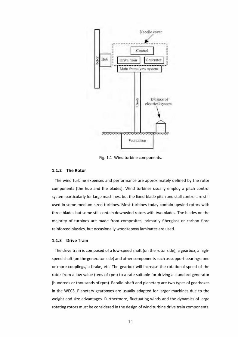
type of wind turbine are shown in figure 1.1 and are presented as follows.

1.1.1 Tower and Foundation

The generator, gearbox, etc. are located on the tower and its foundation. The free-

standing type using steel tubes, lattice towers, and concrete towers is the common

design currently in use. The properties of the wind farm are important when selecting

the type of tower. The minimum height of the tower is 20m, however, it is usually 1 to

1.5 times the rotor diameter. The tower stiffness must be considered in the design of the

wind turbine in order to minimize the vibrations between the rotor and the tower.

11

Fig. 1.1 Wind turbine components.

1.1.2 The Rotor

The wind turbine expenses and performance are approximately defined by the rotor

components (the hub and the blades). Wind turbines usually employ a pitch control

system particularly for large machines, but the fixed-blade pitch and stall control are still

used in some medium sized turbines. Most turbines today contain upwind rotors with

three blades but some still contain downwind rotors with two blades. The blades on the

majority of turbines are made from composites, primarily fiberglass or carbon fibre

reinforced plastics, but occasionally wood/epoxy laminates are used.

1.1.3 Drive Train

The drive train is composed of a low-speed shaft (on the rotor side), a gearbox, a high-

speed shaft (on the generator side) and other components such as support bearings, one

or more couplings, a brake, etc. The gearbox will increase the rotational speed of the

rotor from a low value (tens of rpm) to a rate suitable for driving a standard generator

(hundreds or thousands of rpm). Parallel shaft and planetary are two types of gearboxes

in the WECS. Planetary gearboxes are usually adapted for larger machines due to the

weight and size advantages. Furthermore, fluctuating winds and the dynamics of large

rotating rotors must be considered in the design of wind turbine drive train components.

12

1.1.4 Generator

In general, wind turbines are divided into variable-speed and constant-speed wind

turbines. If they drive at a constant or limited speed and connect directly to the grid, they

are known as constant-speed wind turbines. However, if they operate at variable speeds

with power electronic components, they are known as variable-speed wind turbines. The

grid connected wind turbines (constant-speed) usually make use of squirrel cage

induction generators (SCIG). Thus, these type of generators operate within a narrow

range of speeds, slightly higher than its synchronous speed. Rugged construction, low

cost, and ease of connection to an electrical network are the main advantages of this

type of machine.

Due to their ability to capture the maximum amount of power from the wind energy,

the variable-speed wind turbines are popular for utility-scale electrical power generation.

When used with suitable power electronic converters, either synchronous or induction

generators of either type can run at variable speed. The doubly-fed induction generators

(DFIGs) and the permanent magnet synchronous generators (PMSG) are popular for use

in variable-speed generators. Table 1.1 indicates a comparison of the features of

different types of wind turbines [3].

Table 1.1 A comparison of different types of wind turbines.

Type of generator SCIG DFIG PMSG

Aerodynamically Less efficient Efficient Efficient

Electrically Efficient Less efficient Less efficient

Gearbox Included Included None

Converter None Partial Full

Electrical Noise Noisy Less Noisy Less Noisy

Aerodynamic Noise Noisy Noisy Noisy

Design Simple Convectional Unconventional

Weight Heavy Heavy Heavy

Cost Normal Less Expensive Expensive

Speed Constant Speed Speed Range Variable Speed

1.1.5 Nacelle and Yaw System

The drive train components are placed in the main frame and the contents are

protected from the weather by the nacelle cover. The rotor shaft is aligned with the wind

by the yaw orientation system. The main frame is always connected to the tower with a

large bearing. An active yaw drive is always employed for upwind turbines and

13

sometimes is used with downwind turbines. It is composed of one or more yaw motors

which drives a pinion gear against a bull gear attached to the yaw bearing. An automatic

yaw control system with its wind sensor controls this mechanism. Yaw brakes are

sometimes used with this type of design to hold the nacelle in position when not yawing.

1.1.6 Controls

A wind turbine control system includes sensors, controllers, power amplifiers, etc.

Three properties are considered in the control system of the wind turbines: limiting the

input torque by the gearbox, maximizing the fatigue life of the structural components of

the wind turbine, and maximizing the power production.

1.2 Influence of Wind Power on the Power System

Voltage fluctuations, harmonics, reactive power, power peaks and in-rush current are

specifically considered in the grid power quality while the wind power integrates into the

power system. These issues can be caused by the wind turbine electrical components

such as the generator, transformer, etc., but also by the aerodynamic and mechanical

components such as the rotor and drive train. In this thesis, the wind generator’s

behaviour is investigated among WECS components, throughout.

1.3 Summary of Relevant Literature

1.3.1 Micro-Machines

Micro-machines were developed in the 1950s in order to generate empirical data [4].

They are designed by down-scaling large, utility-scale machinery. The prototyped micro-

machines are used for training and teaching purposes, developing a control system,

power system stability studies and the testing of theoretical assumptions and

approximations used in various analytical calculations. Recently, investigation of the

transient behaviours of power plant and power system have become the other additional

applications of the micro-machines [5], [6].

Due to the micro-machine’s capability to test under exact operating conditions, they

are used to research steady-state and transient phenomena in electrical power systems

even though the digital technology is advanced [7]–[12]. In fact, the time constant

regulators (TCRs) have been created in order to increase the simulation accuracy run by

the micro-machines under transient conditions [5], [13]. Simulated turbine generators

[14], parameter identification for generators and validation of digital models of power

system [15], [16] are also cited as applications of micro-machines.

14

1.3.2 Dimensional Techniques

Dimensional analysis is a critical technique in designing micro-machines. This technique

considers a relationship between the machine’s structures and its behaviour.

Dimensional analysis usually assists the scaling process to create scaling factors in order

to design a micro-machine. Scaling of a transformer is reported as first scaling by the

elementary physical approach [14]. The electric machines’ dynamic models are more

complex than transformers due to their structures. Therefore, the result of geometrical

scaling for electric machines is inaccurate. In [10], it is presented that physical similarities

between the reference machine and micro-machine does not guarantee similarity in the

machines’ characteristics under the same conditions. In addition, it is presented that

boundary and initial conditions also affect the size of the physical model in the scaling

process. In [8], operating under low temperatures is recommended in order to reduce

the complexity of the micro-machine by increasing the conductivity of the machine’s

conductors. The authors of this paper employed liquid nitrogen in order to achieve their

objective. In [12], it is reported that reduction in the machine’s size increases its losses

and the micro-machine’s characteristics are defined by its equivalent circuit parameters.

Therefore, the dynamic responses of micro-machine and reference machine will be the

same if the resistances and the reactances of both machines become equal in the per-

unit system. Brechten and his colleagues recommend a novel approach to developing

micro-machines by defining equations which describe relations between the micro-

machines and the reference machine. These defined equations are constrained by

geometrical infeasibility. A dynamic-response-control, known as Model Reference

Following Controller (MRFC), is developed in [12]. MRFC adapts two pulse width

modulators (PWMs) to feed the two rotor windings in order to control a micro-

synchronous machine.

1.3.3 Investigation of Wind Power Behaviour by Micro-Machines

It is known that synchronous generators have the major share in the electricity

generation within the power system. Their behaviours under various conditions have

been investigated for decades [17], [18]. While the wind energy in the power system

continually increases, the WECS usually uses variable speed generators with power

electric convertors such as DFIGs and PMSGs. The behaviour of these types of generators

require more research because they are new in the grid. Therefore, numerical modelling

has been employed to simulate and investigate the WECS’s behaviour under faulty

conditions [19]–[21]. However, these simulations can be heavy and time consuming

when they are based on the accurate model of the wind turbine. They can also lead to

15

lower accuracy of dynamic results when a simplified model of wind turbines is used. As

noted, the micro-machines can assist in investigating this new phenomena behaviour in

the grid. If the wind generators are scaled based on the relationship between the physical

dimensions and the machine’s behaviour under dynamic conditions, then the scaled-

generator or the micro-machine will behave in a similar manner under the same

conditions. In fact, the scaled-machine behaves the same as the reference machine under

the transient condition and its behaviour towards the grid can be researched with

acceptable accuracy and within reasonable time.

1.4 Aim and Objectives

Development of a scaled doubly-Fed induction generator for assessment of wind power

integration issues is the aim of the research and the objectives are as follows:

Develop a scaling methodology for a utility-scale DFIG.

Develop a design methodology for the detailed design of the scaled DFIG.

Analyse the design of the DFIGs with numerical techniques.

Prototype, test and compare the scaled machine’s performance to that of the

utility-scale DFIG.

Analyse specific grid integration issues with the laboratory-based system and

compare with results from actual and power system simulations.

1.5 Research Questions

The research questions related to the thesis are as follows:

How can a DFIG be down-scaled with inherent non-linear magnetic and electrical

properties?

How can a Micro-Machine be designed to have the same dynamic characteristics as

a utility-scale DFIG?

Which grid integration issues require more accurate models of DFIG systems than

those available in order to perform meaningful analysis?

Can a Micro-Machine be used to analyse specific grid integration issues with DFIGs

more accurately?

1.6 Research Output and List of Publications

The research output and list of publications are as follow:

Design, Prototype and Test a micro-DFIG.

16

H. Dehnavifard, M. Khan, and P. Barendse, “Development of a 5kW Scaled

Prototype of a 2.5 MW Doubly-Fed Induction Generator,” IEEE Trans. Ind. Appl.,

2016.

H. Dehnavifard, A. C. Wozniak, M. A. Khan, and P. S. Barendse, “Determination

of parameters of doubly-fed induction generators,” in 2016 XXII International

Conference on Electrical Machines (ICEM), pp. 2769–2774, 2016.

H. Dehnavifard, X. M. Hu, M. A. Khan, and P. S. Barendse, “Comparison between

a 2.5 MW DFIG and CDFIG in wind energy conversion systems,” in 2016 XXII

International Conference on Electrical Machines (ICEM), no. 3, pp. 238–244,

2016.

H. Dehnavifard, M. A. Khan, and P. Barendse, “Development of a 5kW scaled

prototype of a 2.5 MW Doubly-fed induction generator,” in 2015 IEEE Energy

Conversion Congress and Exposition (ECCE), 2015, pp. 990–996.

H. Dehnavifard, A. D. Lilla, M. A. Khan, and P. Barendse, “Design and optimization

of DFIGs with alternate voltage and speed ratings for wind applications,” in 2014

International Conference on Electrical Machines (ICEM), 2014, pp. 2008–2013.

A. D. Lilla, H. Dehnavifard, M. A. Khan, and P. Barendse, “Optimization of high

voltage geared permanent-magnet synchronous generator systems,” in 2014

International Conference on Electrical Machines (ICEM), 2014, pp. 1356–1362.

1.7 Organisation and Scientific Contribution of the Thesis

In this project, it is assumed that DFIGs are employed in the WECS. Therefore, a micro-

DFIG is developed to behave similarly to the utility-scale machine in order to investigate

wind power issues. To design a micro-DFIG, the dimensional analysis technique is

employed. This technique’s constraints are justified for DFIGs because of their specific

design. For instance, DFIGs have 3-phase windings on their rotor, as opposed to

synchronous machines. Finite Element methods (FEMs) are adapted to prove the

similarity of both machines’ behaviours under transient conditions. Finally, the machine

is prototyped and tested.

The thesis is completed as follows:

Chapter 1: Introduction

Chapter one defines the wind turbine and its components to present the effective

elements on output dynamic behaviour. It gives a literature survey on the micro-

machines and dimensional analysis. It also discusses micro-machine’s advantages in

order to investigate the wind energy in the power system.

17

Chapter 2: Induction Machine Design Considerations

Chapter two covers a literature review on induction machine design trends and focuses

on wound rotor induction machines. It includes market interest towards electrical

machines and in particular, wind generators. Also, it sheds light on unknown aspects of

machine design and is an effort to illustrate the important points regarding induction

machines. To conclude, it presents the areas which require further investigation.

Chapter 3: Wound Rotor Induction Machine Design

Chapter three explains the machine’s design theoretically with sizing equations and

empirical data. It also presents a reference DFIG analytical design along with its 2D finite

element analysis (FEA) simulation.

Chapter 4: Wind Energy Conversion System with DFIG

Chapter four describes a WECS component which includes DFIGs with different speeds

and voltages. It presents the cost and efficiency of the WECS’s components while the

generator voltage and speed change within a limit. It investigates a better DFIG

specification based on WECS’s cost and efficiency.

Chapter 5: Wind Power Integration Issues

Chapter five investigates the wind power integration issues. It describes how the power

system will react if there is a fault in wind power. It discusses the possibility of using the

micro-machines to develop a better understanding of the wind energy integration issues.

Chapter 6: Dynamic Model of DFIG

Chapter six presents the common mathematical modelling of induction machines. It

seeks to define the most important elements on transient behaviour of DFIGs by ignoring

time as a variable. These elements are considered in the dimensional analysis in order to

maintain the dynamic behaviour of the reference DFIG in the scaled-machine.

Chapter 7: Micro-Machines and Scaling

Chapter seven begins with a literature review about micro-machines and the scaling

process. It presents a dimensional analysis which is adjusted for wound rotor induction

machines. The micro-DFIG is presented in this chapter and ultimately, it is verified

through FEA.

18

Chapter 8: Prototyping and Identification of micro-DFIG

The process of the manufacturing of the micro-DFIG is illustrated in chapter eight. The

test rig is also discussed. At the end, the micro-DFIG is tested under blocked-rotor and

no-load condition to identify its equivalent circuit.

Chapter 9: Transient Response of micro-DFIG

In chapter nine, FEA is used to simulate the DFIGs under transient conditions through

various scenarios. The micro-machine is tested under similar conditions. The FEA and

experimental results are satisfactory and meet the objectives.

Chapter 10: Conclusion and Recommendations

The conclusions based on the FEA results and the micro-DFIG’s results at the transient-

state are made in chapter 10.

19

2. Induction Machine Design Consideration

Induction machines (IMs) are the most popular electric machines in industry. These

machines are rugged and do not require separate DC field power. They are very

economical, reliable, and are available in a wide power range, from fractional horse

power (FHP) to multi–megawatt capacity. Induction machine design, structural analysis,

efficiency and the state-of-the-art features are discussed in this chapter. The objective is

to review what has been accomplished in these years in terms of the design and

manufacturing of induction machines.

2.1 Introduction

IMs were invented with a wound rotor in 1889 and later using a squirrel cage rotor. As

with synchronous machines, induction machines have 3-phase windings on their stator.

Their rotor slots can be filled with 3-phase windings or by solid bars. These types of

electric machines are known to have robust construction, simple design and lower cost.

IMs can be operated at variable speeds, which is in contrast with synchronous machines.

Also, their connection process to the grid is relatively simple. They usually operate at a

low lagging power factor and often require power factor correction capacitors to improve

their operating power factor [22], [23].

Squirrel cage induction machines have their rotor slots filled by solid conductive bars.

These machines are the most common type of induction machines due to the simplicity

and robustness of their design and relatively low cost. This type is widely used in stand-

alone wind power generation schemes.

Wound rotor induction machines have 3-phase windings on the rotor and are

consequently more expensive and less robust than squirrel cage machines. Wound rotor

machines are preferred due to their ability to produce a high starting torque. If wound

rotor induction machines are fed through their rotor, they are called doubly-fed

induction machines. These machines can deliver power to the grid through their stator

and rotor [3], [24], [25]. In fact, this is an advantage of wound rotor that it has the ability

to extract rotor power but comes at the added cost of power electronics in the rotor

circuit [9], [22], [26]. An emerging application for doubly-fed induction generators (DFIGs)

are in wind energy conversion systems (WECSs). This is mainly due to its simplicity and

low cost in relation to competing wind generator technologies like the permanent

20

magnet synchronous generators (PMSGs) [1], [18], [27]. However, they require a gearbox

for low speed operation, particularly in wind energy applications [3], [9].

2.2 Current Utilisation of Induction Machines

Electric motors are the main energy conversion devices used in the modern world. In

developed countries, there are more than 3kW of installed electric motors per capita

[28]. Figure 2.1 shows the estimated share of global electricity demand by end-use

applications [29]. The figure shows that electric motors consume approximately 46% of

generated electricity in 2015. This means that if the efficiency of electric motors increases

by a small percentage on average, it will ultimately lead to significant energy savings. The

estimated number of electric motors installed in 2012 was 48.1 million units and this

estimate is expected to grow to approximately 60.8 million units by 2017 [30]. The ratings

of IMs vary from tens of watts to 400MW [3], [31]–[34].

Fig. 2.1 Estimated share of global electricity demand by end-use application in 2015.

As mentioned previously, induction motors are popular due to their rugged design and

moderate cost. Furthermore, they are typically connected directly to the grid through

protective devices such as relays and circuit breakers. In domestic applications, low

power induction motors are typically fed from a single-phase main supply. Home

appliances, account for approximately 79% of the residential energy consumption

globally, as shown in figure 2.2 [34]–[37].

Global revenue from the manufacturing of IMs was 250 million dollars in 2014 and it is

forecasted to be between 300 and 350 million dollars in 2017 [28]. In fact, the electric

motors market will grow by 40% by 2017. Moreover, IMs can be supplied through

converters to provide variable speed operation of motorised systems. In fact, more than

30% of the installed induction motors globally are powered through variable speed drives

21

[3]. The demand for variable speed drives has increased by 10% annually since 2010,

while the average annual growth in the electrical machines market was at a rate of 5%

over the same period [28]. It is predicted that more than half of the electric machines will

be controlled by a variable speed drive in the next decade, whilst IMs would dominate

up to 60% of the new market.

An emerging market for induction machines is in the wind energy sector, which has

been growing gradually since 1997. By the end of 2014, 423GW of electricity generated

was by wind farms in 80 countries, which primarily used induction generators. These

machines compete with permanent magnet generators in the market. There are,

however, no accurate market share details for different systems (DFIG and PMSG) due to

a lack of manufacturer information. Table 2.1 illustrates the wind generator suppliers by

their share market percentage for 2014.

Fig. 2.2 Household motor energy consumption in terawatt-hours.

Table 2.1 Wind turbines’ suppliers of 70 percent of the market share.

Manufacturer Generator types and drive train Market share (≅70%)

GE (US) IG1, DFIG2 PMSG3 11.8%

Vestas (Denmark) IG, DFIG PMSG 11.8%

Siemens (Germany) IG, DFIG PMSG 11%

Enercon (Germany) -- PMSG

EESG4 7.2%

Suzlon Group (India) IG, DFIG, SCIG5 -- 6.6%

Gamesa (Spain) IG, DFIG PMSG 6.4%

Goldwind (China) -- PMSG 6.0%

GuoDian United (China) IG, DFIG -- 3.5%

Sinovel (China) IG, DFIG -- 2.7%

Sewind (China) IG, DFIG PMSG 2.3%

1 Induction Generator 2 Doubly Fed Induction Generator 3 Permanent magnet synchronous Generator 4 Electrical excited synchronous generator 5 Squirrel Cage Induction Generator

22

2.3 Essential Knowledge for Design of an Electrical Machine

The design of an electrical machine involves the selection of electrical, magnetic and

insulation materials, and the detailed dimensioning of the magnetic circuit and electrical

circuits. This is carried out through detailed consideration of the design equations for the

specific machine under investigation. In general, there are a number of possible design

solutions that will meet the user specifications for the design, but it is the designer’s task

to find the optimum solution, which will be based on necessary trade-offs encountered

throughout the design process. The desired solution must have important features such

as high efficiency at rated speed, high power and torque density, tolerable temperature

rise, and ultimately low cost. Finally, the durability and reliability of the machine must be

considered in the design process. The manufacturing conditions form part of the design

challenges [3], [38], [39]. The design process also requires knowledge of the following

areas related to the machine type [40]:

National and international standards

Specifications (that deals with machine ratings, performance requirements etc., of

the consumer)

Cost of materials and labour

Manufacturing constraints

The desired design values will be achieved by iterative methods in order to overcome the

design complexities. Therefore, computers play an important role to evaluate aspects of

the design with sufficient accuracy throughout the design process. Moreover, laboratory

testing of a prototype can be used to validate the numerical results and assess if the

design specifications were achieved [41], [42].

2.4 Selection of Materials

Induction machines have magnetic circuits which permeate the revolving magnetic

fields, and also electric circuits which have alternating currents. The electric circuits have

a different purpose from the magnetic circuits, and are insulated from each other. The

magnetic, electric, and insulation materials are defined by their characteristics and their

losses [39], [43].

2.4.1 Insulation

Insulation materials are used to prevent short circuits between conductors, and

between conductors and the laminated cores in electrical machines. The insulation

material is selected based on the electrical circuit of the machine, but is required to be

23

compatible with the cooling system and the magnetic circuits of the machine. In fact, the

insulation helps to withstand inter-turn, phase-to-phase and phase-to-ground faults. In

the stator and rotor, the laminations are insulated from one-another by a special coating

which minimizes eddy current losses in the core. It is cited that bearing and shaft voltages

and currents are reduced by insulating the bearing housing. This helps to prevent

premature bearing damage. This is especially prevalent in PWM converter fed IMs, where

there are additional common mode high frequency capacitor currents [44]. In addition,

PWMs causes the applied current and voltage to become non-sinusoidal. This means the

current peaks result into raising the insulations’ temperature. The voltage peaks and the

voltage transient also causes the insulation stress. These effects will accelerate insulation

ageing [45]. Moreover, the insulation has to withstand the expected operating

temperature. There is a slow deterioration of insulation by internal chemical reactions

and contamination which causes cracks in the enamel, varnish or resin and thus reduces

the dielectric strength of the insulation [26], [46]. Flexible sheet materials such as

cellulose and polyester film proposed in [39], [47] are used to provide a slot to phase

insulation for class “A” temperatures. In high-temperature IMs (class “F”, “H”), glass cloth

paper treated with special varnish is used for a slot to phase insulation [32], [34], [39].

2.4.2 Laminations and Magnetic Material

The permanent magnet dipoles inside the material define the magnetic properties of

the material. As known, hysteresis is a property of magnetic materials which may cause

energy loss in electric machines. The alloys of iron, nickel, cobalt plus silicon-steels are

known as soft magnetic materials due to having low hysteresis. These materials include

micro-domains whose sizes are between 10–4 and 10–7m. When completely

demagnetized, these domains have random orientations and therefore the material has

zero remanence in all finite samples. The result of dipoles varies within the magnetic

material and creates B-H curves for each material [48]–[50]. Magnetic materials can be

categorised by their B-H curves.

Annealed iron (soft) is desirable to make a core for rotating machinery due to its high

level of a magnetic field tolerance (until 2.6 Tesla) without saturating. Soft iron can boost

the magnetic field concentration up to 50000 times more than air core. This material has

a high conductivity which causes high eddy current loss and undesirable heating. Two

methods are usually employed to decrease the conductivity of the iron: alloying with

silicon; and lamination [51].

Silicon-steel is an iron with up to 6.5% silicon and it is usually manufactured in a cold-

rolled with less than 2mm thickness [52]. The maximum thickness of lamination in the

24

electrical machines’ cores is 1mm [3]. The silicon-steel’s mechanical property depends

on its silicon concertation. Silicon ultimately reduces core losses by decreasing iron

conductivity. Basically, it decreases the induced eddy currents and narrows the hysteresis

loop. Then, the machine’s core will be laminated by the plates made of silicon-steel.

These laminations are coated to decrease conductivity between plates. The coating

protects the laminations from oxidation and acts as a lubricant while die cutting [34]. It

is reported for IMs of fundamental frequency up to 300Hz, that 0.5mm thick silicon steel

laminations lead to reasonable core losses of approximately 2 to 4W/kg at 1T and 50Hz.

For higher fundamental frequency, thinner laminations are required [52]–[54].

2.4.3 Electrical Conductors

In general, copper conductors are used for electrical machine windings. The type of

conductor, either circular or rectangular depends on the machine’s rating. Wound rotor

induction machines (WRIMs) have three phase windings on both their stator and rotor.

The size of the conductors in three phase windings depends on the current density. Also,

it is reported that current density affects the cooling system, service duty cycle, and the

targeted efficiency. The current density lies between 3.5 to 6A/mm2 for high efficiency

WRIMs. It is possible to twist several elementary conductors (6 to 8) in parallel to reduce

the skin effect to acceptable levels [23], [38], [55].

2.5 The Induction Machine Design Process

Several design approaches are available in literature, but majority start the process with

design specifications and pre-assigned values of flux densities and current densities.

Then, the stator bore diameter (𝐷𝑖𝑠), stack length (𝐿𝑖), number of stator and rotor slots,

stator outer diameter (𝐷out), stator and rotor slots’ dimensions are determined by

means of various approaches. Typically, the design algorithms iterate until an acceptable

efficiency and power factor have been achieved. If the results of the design process are

unsatisfactory, the whole process will be restarted from the initial state [3], [27], [31],

[39], [56], [57]. Due to the ability to simulate the geometric variations and irregularities,

saturations and eddy current effects with a high degree of accuracy, using finite element

method (FEM) to design electrical machines is popular. Radial flux machines are usually

simulated in 2D while axial flux machines require simulating in 3D to trace the flux lines

as well as the flux densities axially [19], [58]–[61]. In [21], the authors developed a finite

element (FE) based analysis by employing reduced models for both stator and rotor. This

model is fast and accurate enough that can be used for designing a large induction motor.

The optimization of the machine design is a multivariable and multimodal optimization

25

problem. Traditionally, a combination of analytical and empirical methods are used for

convectional design optimization. However, the emerging trend of design optimization is

based on FEM analysis combined in the optimisation loop. The evaluation of alternate

designs becomes simple and accurate by using FEM models. However, the simulation

time becomes lengthy when attempting to increase the accuracy of FEM calculations

[62], [63].

Madescu and Boldea present a practical nonlinear model which can be attached to the

industrial design tools for induction motors. Their main aim was to develop a two-

dimensional model which divides the machine into five circular cross-sectional domains

[57]. A canonical particle swarm optimization (PSO) technique is employed to develop a

fast and efficient multi-objective optimization design method for induction machines

[64]. Less design iterations are required in this method than traditional design methods.

Computer aided design (CAD) approach is presented for the design of an efficient and

compact DFIG. The designed DFIG is validated by means of finite element (FE) analysis.

The designed DFIG developed by the CAD program is then compared with a

conventionally designed DFIG of the same rating. The comparison involved the active

volume of the machine, airgap harmonics and efficiency at variable speeds [65], [66].

There appears to be a need for the development of better approaches for the design of

wound rotor induction machines, as most of the literature and commercial machine

design software focuses on squirrel cage IMs due to the interest of manufacturers.

2.5.1 Main Induction Machine’s Dimensions

Sizing equations for an electrical machine are presented in [22], [23], [26], [40]. The

authors describe various techniques to calculate the stator inner and outer diameters,

core length, equivalent slot dimensions, flux density as well as the number of poles. The

stator diameter and core length are the main dimensions of electric machines. There are

two different methods to calculate the length and diameter for IMs: 1- based on output

coefficient design concept (𝐶0) and 2- based on the rotor shear stress. The following

equation can be used to calculate the stator inner diameter (𝐷𝑖𝑠) for the machine [39],

[56]:

𝐷𝑖𝑠 = √𝑄

𝐿𝑖𝑛𝑠𝐶0 2.1

where 𝑝1 is the number of pole pairs, 𝑄 is the input power, 𝐿𝑖 stator length, 𝑛𝑠 is the

synchronous speed, and 𝐶0 is the output constant. Boldea and Lipo recommended the

rotor shear stress to calculate the inner stator diameter (𝐷𝑖𝑠) [25], [31]. Therefore,

26

𝐷𝑖𝑠 = √2×𝑇𝑒

𝜋×𝜆×𝑓𝑥𝑡

3 2.2

where 𝑇𝑒 is electromagnetic torque,𝜆 the aspect ratio and 𝑓𝑥𝑡 is the rotor shear stress for

induction generators. The aspect ratio is defined as the ratio of the stator length (𝐿𝑖) to

diameter (𝐷𝑖𝑠):

𝜆 =𝐿𝑖

𝐷𝑖𝑠 2.3

The ratio between the length and diameter of the machine will determine the power

factor and the cost of materials of IMs. In several references, methods are proposed to

ensure that the target operating characteristics are achieved [3], [9], [26], [39], [40], [67].

The authors propose that the ratio of stack length to pole pitch (𝐿

𝜆) may reduce costs if

(1.5 <𝐿

𝜆< 2), improve power factor if (1.0 <

𝐿

𝜆< 1.25), improve efficiency if (

𝐿

𝜆= 1.5),

and it is better to use (𝐿

𝜆= 1) in order to design DFIGs. The value of the ratio (

𝐿

𝜆) was

suggested to be between 0.6 and 2, depending on the size of the machine and the

characteristics desired. Figure 2.3 indicates the acceptable range for the stack aspect

ratio for the number of pole pairs [27]. It is reported that an increased stack length leads

to additional winding losses of up to 10 percent [24], [68], [69].

Fig. 2.3 IMs empirical stack aspect ratio versus number of pole pairs.

When choosing the diameter of the IM’s stator, the peripheral speed is considered. It is

suggested that the peripheral speed should not exceed about 30m/s [37], [70].

2.5.2 Standard Frames

Standard induction motor frames determine the overall mechanical structure of the

machine. The frame includes: the stator, bearings, end cover, and terminal box. It

provides safety, the ability to withstand twisting forces and shock when transmitting the

torque, as well as ventilation. Apart from a few special machines, the manufacturers of

27

all modern machines for industrial applications provide a series of standard frames which

cover a wide range of power ratings [71], [72]. As the airgap of an induction machines is

relatively small, the frame structure must be rigid in order to keep the stator and the

rotor concentric, otherwise, it can cause unbalanced magnetic pull [67], [72]. The frame

may be die-cast or fabricated. Machines with rating of approximately 50kW usually have

their frames die-cast in a strong silicon aluminium alloy and in some cases with the stator

core cast in. The process of die-casting has an advantage in that it facilitates the use of a

thicker cross-section frame in places where greater mechanical strength is required. The

die-cast frames do not require machining [34], [73]. The casing of small machines is

usually a single unit and comes on a base plate. The large-sized machines’ frames are

made up of a few steel plates. Depending on the design, the frame can be adapted and

modified. In machines with radial ventilating ducts, the stator core is placed inside the

frame on axial ribs, thereby providing an annular space for air between the core and the

frame [39], [43], [53].

2.5.3 Stator Structure of Induction Machines

The stator consists of a cylinder made of laminations. The stator laminations are packed

and placed into a frame. The stator core is laminated in segments for large machines in

order to avoid wasting steel. Depending on type of silicon-steel the outer arch length of

each segment can be between 0.3 and 0.8 m [74]. This will give an economical balance

between the cost of dies, the cost of assembly and the amount of left-over scrap material

after cutting the laminations from steel strips. Long cores are divided into a number of

stacks. Radial ventilating ducts are sandwiched between them for efficient cooling. The

width of a single stack of core should not exceed 0.5 to 0.6 m [39], [73], [75]. The slot

geometry is designed according to the IM’s power ratings. The slot geometry has an

important effect on the operating performance of IMs. The slots can be open or semi-

enclosed depending on the type of conductors (round or rectangular) (figure 2.4).

a b c

Fig. 2.4 Slot geometrics to locate coil windings: a) semi-closed, b) semi-open, c) open

[3].

28

Due to decreasing flux pulsation in the rotor tooth which increases core losses, only one

side (stator or rotor) is an open slot [76], [77]. The winding coils can be formed before

they are inserted into open-slots. The windings are more accessible when a need arises

for removing individual coils. In addition, decreasing the leakage reactance is one of the

merits of open slots. The coils must be formed after they are inserted in the semi-

enclosed slots. The semi-enclosed slots are used for the induction motor because they

result in smaller values of magnetizing current. As mentioned, the semi-enclosed slots

will have a lower tooth pulsation loss and a much quieter operation as compared to open

slots [78], [79]. Also, wedges are inserted at the openings of open-slots or semi-open-

slots to protect the windings from centrifugal forces and they are usually made up of

wood or Bakelite. It is recommended that a large number of narrow slots can minimize

tooth pulsation losses and noise in small IMs with open type slots [33]. It is reported in

various sources that in small IMs where round conductors are used, the tapered slot with

parallel sided tooth arrangement is useful, as it gives the maximum slot area for a

particular tooth flux density. In large and medium sized IMs, where strip conductors are

preferred, parallel sided slots with trapped teeth are used [3], [26], [79]. The large

number of stator slots will result in a small width of stator teeth, which may lead to the

teeth becoming mechanically weak. Moreover, the thin stator and rotor teeth may result

in excessive flux density levels in the teeth and higher iron losses. The narrow teeth would

be better to support at the radial ventilating ducts by welding the laminations [40], [70],

[80]. It is reported that having approximately equal tooth width and slot width would

help to have uniform flux density in the tooth. Also, the deep slots result in a large value

of leakage reactance [3], [25]. Moreover, the leakage reactance also increases if the

number of slots per pole per phase decreases, which in turn reduces the cost of the

winding due to the lower number of coils. On the other hand, the large number of slots

causes leakage flux and hence the leakage reactance decreases, which results in a higher

overload capacity. The cost also increases with a larger number of slots due to increasing

number of coils. Therefore, it is good practice to use as many slots as economically

possible [18], [27], [39]. Usually, the slot space factors in IMs lie between 0.25 and

0.4mm. High voltage machines have lower space factors due to the large thicknesses of

insulation [74], [78].

2.5.4 Rotor Structure of Induction Machines

The rotor core is laminated as a single plate in small machines and a segmental plate in

large machines. The rotor core pack is keyed to the shaft by a ring. The ring keeps the

plates together and the key transfers torque to the shaft and it usually makes the rotor

29

core skewed. The simplest way to reduce the harmonics is by skewing, which however

lowers the power factor and overload capacity of the machine. Therefore, it is better to

mention here that a large airgap length can decrease the harmonic torques, but it also

reduces the power factor and overload capacity on the IM [25], [40].

Depending on the size of the machine, radial and axial ventilating ducts are inserted in

the rotor to provide adequate air circulation. The number of radial ventilating ducts in

the rotor is usually equal to that of the stator [3], [18], [26], [39]. There are reports on

the relationship between rotor eccentricity and shaft arms and stiffeners. It has been

cited that if the rotor has not been placed on the shaft carefully or the shaft has not been

installed centrally (inside the stator), it will create a parasitic harmonic, vibration and

noise [3], [9], [22].

Generally, windings with an integer number of slots per pole per phase are used for the

rotor and cannot be equal to the number of slots per pole per phase in the stator.

Different policies are available in literature to select the number of slot per pole per

phase for each squirrel cage and wound rotor induction machines [18], [23], [81]. For

instance, it is recommended that the number of slots per pole per phase (q) must be an

integer in order to produce completely symmetrical windings in WRIMs. However, it is

recommended that fractional slot windings be used on the rotor for small WRIMs in order

to reduce the harmonic content of the airgap flux density [31], [39].

In order to achieve a small airgap in IMs, the shaft should be short and stiff. In fact, even

a small deflection would create noticeable irregularities in the airgap which would lead

to the production of an imbalanced magnetic pull. In the case of short shafts, the

diameter of bearings should be about two-thirds of the shaft maximum diameter [38],

[39]. Roller bearings are used for horizontal shaft machines and thrust bearings are used

for vertical shaft machines. The forces act radially in horizontal shaft machines while the

axial load acts downwards in vertical shaft machines. Radial loads in this case can be

caused either by the dynamic unbalance of the rotor or by the unbalanced magnetic pull

of the rotor towards the stator [3], [34], [43].

The slip rings are made up of either brass or phosphor bronze. They are pressed

together on the body of reinforced thermo-setting resin carried on a mild steel hub. The

slip rings are located either between the core and bearing or on the shaft extension.

When the slip rings are on the shaft extension, the shaft is made hollow to allow the

three connections from the rotor to the slip ring to pass through the bearings. The

brushless induction machine is designed to reduce the ohmic losses. Brushes are,

however, still used in modern machines [24], [39], [82]. Runcos and Mauricio investigated

a 350kW brushless doubly-fed 3-phase induction machine with its wound rotor circuit

30

connected to flat-plane rotary transformers. They reported the merits of eliminating

brushes and slip rings by means of rotary transformers. In addition, they presented a

rotary transformer design and demonstrated the operation of a 90-kW brushless doubly-

fed three phase IM [83]. The design and performance analysis of a medium-speed

brushless doubly-fed induction generation for a wind turbine drivetrain was investigated

by Abdi. It was shown that the medium speed brushless DFIG in combination with a two

stage gearbox, offers a low-cost, low-maintenance and more reliable drivetrain for wind

turbine applications [84].

2.5.5 Airgap

The length of the airgap in an induction machine should be mechanically as small as

possible in order to minimise the magnetizing current and improve the operating power

factor. A large airgap can reduce the flux pulsation loss, however, it creates a small

eccentricity and an unbalanced magnetic pull [24], [25], [48]. Several empirical equations

are presented to calculate the airgap length [25], [56]. Say suggested equation 2.4:

𝑔 = 0.2 + 2√𝐷𝑖𝑠. 𝑙𝑖 2.4

where 𝑔 is the airgap. Lipo presented a few methods and he ultimately derived equation

2.5:

𝑔 = 3 × 10−3𝜏 (2𝑝1)1

2 2.5

It is reported that a large airgap length would be better to facilitate cooling in induction

machines. The variation of reluctance in the path of the zig-zag leakage flux is the reason

for the noise in IMs. A large airgap length reduces the zig-zag leakage flux, which reduces

value of the leakage reactance as well as the noise level of the machine [22], [71], [75],

[85]. The flux density in the airgap should be moderate in order to limit the magnetizing

current, which will result in a poor power factor. However, in induction motors the flux

density in the airgap should be such that there is no saturation in any part of the magnetic

circuit. Moreover, a large flux density in the airgap causes high iron loss, thus reducing

the efficiency of the machine [48], [86].

2.5.6 Winding Structure

In general, the winding system is designed by assigning coils to the slots for different

phases, establishing the direction of currents in the coil sides, calculating the number of

turns for various coils, and finally sizing conductors for the slots. The number of coils is

determined by the number pole pairs and the number of phases. Moreover, a large

number of poles result in a poor power factor and also regulating the number of poles

31

can affect the magnetization current and the flux densities. Also, the number of turn per

coil is assigned based on the flux density in the airgap and the conductor size depends on

the operating current density. The large number of turns per coils produces a large

winding mmf, which decreases the overload capacity of IMs.

The number of turns per coil is calculated as follows:

𝑊1 =𝐾𝐸

𝑉𝑆𝑁√3

2√2𝑓𝑘𝑓𝐾𝑊1𝐵𝑔𝜏𝑙𝑖 2.6

where 𝐾𝐸 is the back 𝑒𝑚𝑓 factor (0.97 < 𝐾𝐸 < 0.98 ), 𝑉𝑆𝑁 is the stator phase voltage, 𝑓

is the frequency, 𝐾𝑊1 is the winding factor and 𝐵𝑔 is the assumed airgap flux density, and

𝑘𝑓 is filling factor. An important consideration in a three phase winding is to produce

equal resistance and leakage inductance per phase, in order to ensure a balanced

winding. The windings of electrical machines are restricted from movement in the radial

direction. The wire bands of rotors and solid bands (retaining rings) are methods that are

used for the carrying of rotor windings [87], [88].

Figure 2.5 illustrates lap and wave windings which are used for induction machines [3],

[25], [38], [74]. Single-layer windings employ full pitch coils (y = τ) to produce a

fundamental mmf with pole pitch “τ” and it would be practical to use an integer number

of slots per pole per phase. “y” is the number of slots which are covered. A single-layer

winding is appropriate for lower power IMs. Double-layer windings are shown in figure

2.6, which allow chorded (or fractional pitch) coils (y < τ) such that the end connections

of coils are shortened and thus copper loss is reduced.

a b

Fig. 2.5 Lap a) and wave b) single turn coils [3].

It is recommended that the double layer lap type winding with diamond-shaped coils is

generally used for stators and the use of single-layer mesh windings is suggested for small

machines with a small number of slots and having a large number of turns per phase. The

32

three phases of the winding can be connected in either star or delta, depending on the

starting methods to be employed [18], [25], [56], [74], [79].

a b

Fig. 2.6 Single-layer a) and double-layer b) coils (windings) [31].

Fractional slot windings with two pole symmetry (𝑞 =2𝑛+1

2) are investigated thoroughly

in [87]–[89], where the authors suggest that 𝑞 =3

2 for low power IMs. In general,

fractional slot windings reduces copper weight and space harmonic content in IMs.

Pole-changing windings have been considered since the sixties. A method known as

“the 3 equation principle” is presented in [90] for various pole count combinations. This

is also a kind of symmetric method with a well-defined methodology. Alternating the

number of poles in IMs is presented in [91]–[93] by changing the direction of the current

in the windings.

When sinusoidal three-phase currents are supplied to the stator windings of an ideal

machine, a sinusoidally distributed revolving mmf waveform is produced in the airgap of

the machine. If the coils of a winding were to be placed in the airgap (in a slot-less

machine) and distributed sinusoidally, then perfect sinusoidal distribution of mmfs would

be possible. However, the airgap in this scenario would be large and this leads to the low

power factor and efficiency [27], [39], [79], [94].

As known, the value of mmf depends on the size of the machine, the voltage of the

stator winding, the type of ventilation and the overload capacity desired. A medium

voltage high power machine is designed with a small value of Ampere-Turns [40], [79],

[87]. The voltage induced in the rotor is at its maximum when the rotor of the machine

is at rest. Therefore, to keep the rotor voltage at an acceptable level, the ratio of effective

stator to rotor turns must be properly selected [18], [25], [26]. For a wound rotor IM, the

rotor voltage on open circuit between the slip rings should not exceed 500 volts for small

machines. The voltage is limited to a low value to protect the operator from the machine

33

if the brush gear is not perfectly protected. Moreover, it is easier to insulate the rotor

windings with a low rotor voltage. The voltage in medium and large size machines can go

up to 4kV [39], [95].

2.6 Cooling System and Thermal Modelling

The cooling system is designed for the efficient transfer of heat from the electrical

machine’s housing to the surroundings of the machine. Thermal models are considered

when designing a cooling system. The thermal model of induction machines depends on

the level and location of the losses, machine geometry and the method of cooling.

Several thermal models have been recommended for IMs with regards to heat removal

methods, temperature distribution and insulation tolerance [3], [25], [39], [40], [56].

Some thermal considerations will be discussed in this section.

2.6.1 Cooling System

The cooling system of an IM can be either natural or forced, depending on the rating of

the IM. A natural air cooling system transfers the heat to the ambient air through a fan.

A forced cooling system is designed to transfer the heat to a secondary heat exchange

medium. In general, an air cooling system is preferred for electrical machines due to its

simplicity [39], [96], [97]. Ventilators ducts are radial channels that are located at the

regular interval along the axial length of the machine. Figure 2.7 shows the radial and

axial ventilating channels. Radial and radial-axial cooling ducts are usually recommended

for medium and large machines [24], [27], [98].

a

b

Fig. 2.7 a) single stack magnetic core IMs with axial ventilations b) multiple stack

magnetic core IMs with axial and radial ventilations [3].

It is reported in the literature that large machines can have a smaller rotor diameter as

well as better efficiency if they make use of an axial cooling system because their winding

resistances will be lower. This allows larger machines the ability to handle larger power

losses, without exceeding the thermal rating of the active materials used in the machine.

34

2.6.2 Thermal Modelling

Thermal circuit models and distributed models are described in [99], [100]. The

conduction method of heat transfer essentially implies that thermal energy flows from a

heat source to a heat sink. Generally, the heat source and the heat sink in IMs are

windings and the ambient air, respectively. In IMs, the thermal energy flow is defined

from the windings in the slots, through the conductor insulation and slot liner insulation,

to the laminated core teeth. Convection heat transfer takes place between the surface

of a solid body and a fluid. Convection depends on the velocity of the fluid, fluid

properties, the solid body geometry and orientation. IMs are designed with a frame

which has fins to allow heat transfer by convection. The insulated laminations reduces

the transfer of heat along the axial direction, which therefore enhances heat conduction,

convection, and radiation in a radial direction [3], [43], [98]. The conductor’s insulation is

designed for specific maximum temperatures. It is reported that the manufacturers test

IM by keeping it at locked rotor conditions in order to determine the max temperature

rise [43], [87]. A realistic thermal equivalent circuit for IMs at steady state and transient

conditions is proposed in figure 2.8.

Fig. 2.8 Thermal equivalent circuit for stator or rotor windings [101].

The authors investigated a thermal equivalent circuit with finite element analysis

software. The issue of heat flow in 2-dimensional coordinates is solved by using a finite

element formulation with arc-shaped elements in the r-θ plane of a cylindrical co-

ordinate system [102]. In 1995, Bellenda proposed a lumped parameters dynamic model

for the analysis of the thermal behaviour of the induction machine, based on the

machine’s geometrical dimensions. He presented an approach to estimate the thermal

behaviour of induction machines designed for the propulsion system of Electric Vehicles

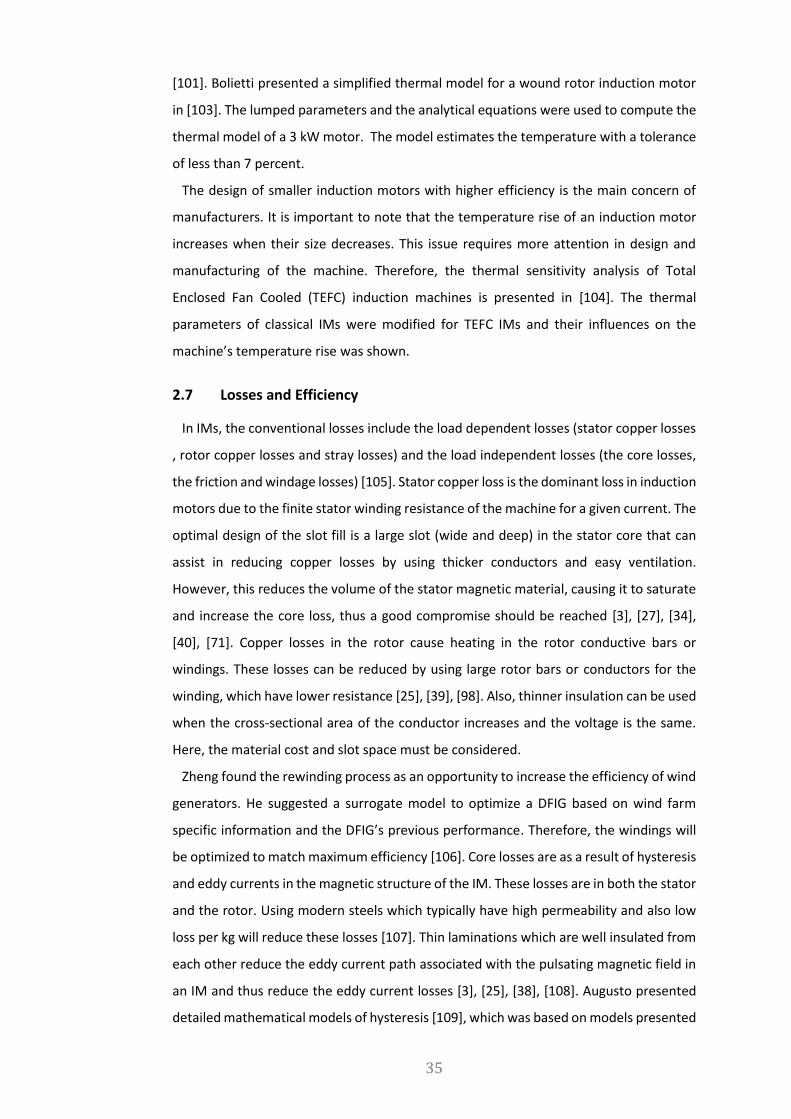
35

[101]. Bolietti presented a simplified thermal model for a wound rotor induction motor

in [103]. The lumped parameters and the analytical equations were used to compute the

thermal model of a 3 kW motor. The model estimates the temperature with a tolerance

of less than 7 percent.

The design of smaller induction motors with higher efficiency is the main concern of

manufacturers. It is important to note that the temperature rise of an induction motor

increases when their size decreases. This issue requires more attention in design and

manufacturing of the machine. Therefore, the thermal sensitivity analysis of Total

Enclosed Fan Cooled (TEFC) induction machines is presented in [104]. The thermal

parameters of classical IMs were modified for TEFC IMs and their influences on the

machine’s temperature rise was shown.

2.7 Losses and Efficiency

In IMs, the conventional losses include the load dependent losses (stator copper losses

, rotor copper losses and stray losses) and the load independent losses (the core losses,

the friction and windage losses) [105]. Stator copper loss is the dominant loss in induction

motors due to the finite stator winding resistance of the machine for a given current. The

optimal design of the slot fill is a large slot (wide and deep) in the stator core that can

assist in reducing copper losses by using thicker conductors and easy ventilation.

However, this reduces the volume of the stator magnetic material, causing it to saturate

and increase the core loss, thus a good compromise should be reached [3], [27], [34],

[40], [71]. Copper losses in the rotor cause heating in the rotor conductive bars or

windings. These losses can be reduced by using large rotor bars or conductors for the

winding, which have lower resistance [25], [39], [98]. Also, thinner insulation can be used

when the cross-sectional area of the conductor increases and the voltage is the same.

Here, the material cost and slot space must be considered.

Zheng found the rewinding process as an opportunity to increase the efficiency of wind

generators. He suggested a surrogate model to optimize a DFIG based on wind farm

specific information and the DFIG’s previous performance. Therefore, the windings will

be optimized to match maximum efficiency [106]. Core losses are as a result of hysteresis

and eddy currents in the magnetic structure of the IM. These losses are in both the stator

and the rotor. Using modern steels which typically have high permeability and also low

loss per kg will reduce these losses [107]. Thin laminations which are well insulated from

each other reduce the eddy current path associated with the pulsating magnetic field in

an IM and thus reduce the eddy current losses [3], [25], [38], [108]. Augusto presented

detailed mathematical models of hysteresis [109], which was based on models presented

36

by Mayergoys in [110]. Yanase proposed a simple method for predicting the magnetic

losses of electrical steel sheets in [111]. Pillay developed a model based on the three-

term loss separation formula to predict lamination losses in induction motors. This model

estimates the core losses by employing the flux density waveforms in different sections

of a machine from FEM. The model results are verified by measured data from an 11kW

induction machine [112]. The losses under an arbitrary induction waveform with or

without minor loops can be estimated by this method under sinusoidal excitation. A new

mathematical model of core losses in ferromagnetic steel, based on a minimal amount

of experimental data, is described in [113]. This new model has a hysteresis loss

coefficient that varies with frequency, eddy current coefficient and excess losses that are

a function of induction. The new model is validated successfully on a large number of

different samples of non-grain oriented fully and semi-processed steel alloys. Roy

illustrates a modelling technique to estimate the core losses for wound rotor induction

machine based on Mircea’s method [114]. It was shown that 10 to 20% of the total losses

are incurred in the magnetic materials of induction machines. The drag losses associated

with the rotor and fan, and the mechanical friction due to the motor bearing together

cause friction and windage loss. These losses are minimized by the good structural design

of the rotor and fan, such as proper bearing selection with appropriate lubrication.

Proper bearing alignment during assembly also helps to reduce these losses. If the

bearing are not well positioned, there may be increased losses and premature bearing

failure [105], [115].

Stray load losses are additional losses which are slightly more difficult to quantify and

model. The stray load loss causes an increase in temperature and consequently decreases

the torque of the machine. Some approximate equations for IMs have been presented in

the references to predict stray losses [108], [116]–[118]. The process of repair and

rewinding of electric machines affects the efficiency and particularly stray load loss. Cao

analysed this effect in [119], [120]. Sana presented analytical methods to calculate the

winding and the slotting effect on losses in a three phase induction machine in [121],

[122]. These methods allow for the distinction between contributions from the stator

and the rotor slot openings to the dynamic losses and, consequently, to the total iron

losses.

2.8 Conclusion

As mentioned, IMs are the most popular among electric motors used in industry today.

Moreover, a strong emerging application for IMs is in the wind energy sector. This

chapter outlined the important considerations associated with the design of induction

37

machines. In particular, the active materials and insulation properties were discussed.

The design and optimisation process of IMs were also considered in some detail. In

addition, different sections of IMs were introduced with their tasks in details. The

performance of IMs was also considered, in respect to losses, efficiency and thermal

behaviour. In conclusion, WRIMs’ design require more investigation to have better

efficiency due to their application in the WECSs.

38

3. Wound Rotor Induction Machine Design

The design considerations for induction machines were discussed in the previous

chapter. This chapter will describe the design algorithm by illustrating the sizing

equations and analytical calculations for the wound rotor induction generator (WRIG).

Three main operation modes are considered for the electromagnetic design in the

WRIGs: generator at the power grid, generator to the autonomous load and brushless AC

exciter (generator with rotor electric output). Here, the WRIG’s rotor is assumed to be

excited by a converter and the power can be delivered to the grid through either the

stator or rotor.

3.1 Introduction

A machine model, an optimized method and other objective functions with a computer

program are used to achieve the machine electromagnetic design. Electromagnetic

design factors of WRIGs are named as follows: stator and rotor cores sizing, stator and

rotor winding design, magnetization current calculation, equivalent circuit parameter

determination, and efficiency computation.

3.2 Stator Design

The interior diameter of the stator depends on a factor known as shear rotor stress (𝑓𝑥𝑡)

[25], [31], [38]. This shear rotor stress increases with torque and varies between 1.5 and

6N/cm2 [123]. The shear rotor stress is used to calculate the stator interior diameter (𝐷𝑖𝑠).

To calculate 𝐷𝑖𝑠, the electromagnetic torque has to be estimated at maximum speed on

the basis of the input power of the machine and expected efficiency. The electromagnetic

power (𝑆𝑔𝑁) is as follows:

𝑆𝑔𝑁 ≈𝑆𝑆𝑁 + 𝑆𝑅𝑁

𝜂𝑁 3.1

where,

𝑆𝑔𝑁: Electromagnetic power;

𝑆𝑆𝑁: Power on stator side at unity power factor;

𝑆𝑅𝑁: Power on rotor side at unity power factor;

𝜂𝑁: Expected efficiency;

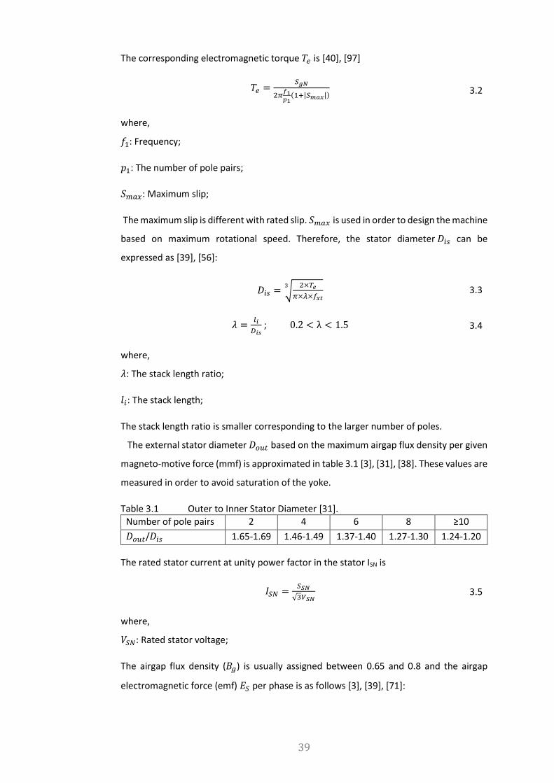
39

The corresponding electromagnetic torque 𝑇𝑒 is [40], [97]

𝑇𝑒 =𝑆𝑔𝑁

2𝜋𝑓1𝑝1

(1+|𝑆𝑚𝑎𝑥|) 3.2

where,

𝑓1: Frequency;

𝑝1: The number of pole pairs;

𝑆𝑚𝑎𝑥: Maximum slip;

The maximum slip is different with rated slip. 𝑆𝑚𝑎𝑥 is used in order to design the machine

based on maximum rotational speed. Therefore, the stator diameter 𝐷𝑖𝑠 can be

expressed as [39], [56]:

𝐷𝑖𝑠 = √2×𝑇𝑒

𝜋×𝜆×𝑓𝑥𝑡

3 3.3

𝜆 =𝑙𝑖

𝐷𝑖𝑠 ; 0.2 < λ < 1.5 3.4

where,

𝜆: The stack length ratio;

𝑙𝑖: The stack length;

The stack length ratio is smaller corresponding to the larger number of poles.

The external stator diameter 𝐷𝑜𝑢𝑡 based on the maximum airgap flux density per given

magneto-motive force (mmf) is approximated in table 3.1 [3], [31], [38]. These values are

measured in order to avoid saturation of the yoke.

Table 3.1 Outer to Inner Stator Diameter [31]. Number of pole pairs 2 4 6 8 ≥10

𝐷𝑜𝑢𝑡/𝐷𝑖𝑠 1.65-1.69 1.46-1.49 1.37-1.40 1.27-1.30 1.24-1.20

The rated stator current at unity power factor in the stator ISN is

𝐼𝑆𝑁 =𝑆𝑆𝑁

√3𝑉𝑆𝑁 3.5

where,

𝑉𝑆𝑁: Rated stator voltage;

The airgap flux density (𝐵𝑔) is usually assigned between 0.65 and 0.8 and the airgap

electromagnetic force (emf) 𝐸𝑆 per phase is as follows [3], [39], [71]:

40

𝐸𝑆 = 𝐾𝐸𝑉𝑆𝑁

√3 ; K𝐸 = 0.97 (0.97 < K𝐸 < 0.98) 3.6

where,

𝐾𝐸 : emf coefficient;

The pole pitch 𝜏 is calculated as follows:

𝜏 =𝜋𝐷𝑖𝑠

2𝑝1 3.7

The number of turns per phase is dependent on the emf per phase (𝐸𝑆), pole pitch (𝜏),

and winding factor (𝐾𝑊1). The fundamental winding factor is calculated as follows [3],

[25], [39]:

𝐾𝑊1 =𝑠𝑖𝑛

𝜋

6

𝑞1𝑠𝑖𝑛𝜋

6𝑞1

𝑠𝑖𝑛𝜋

2

𝑦

𝜏;

2

3≤

𝑦

𝜏≤ 1 3.8

where,

𝑞1: The number of slots per pole per phase in the stator, which an integer for an integral

slot winding machine.

𝑦

𝜏: The stator coil span/pole pitch ratio;

The number of turns (𝑊1) per phase is [3], [38]:

𝑊1 =𝐸𝑆

2√2𝑓1𝑊1𝐾𝑊1𝑎𝐵𝑔𝜏𝑙𝑖 3.9

Number of turns per coil (𝑛𝑐1) is calculated as follows:

𝑛𝑐1 =𝑊1

(2𝑝1𝑞1

𝑎1) 3.10

where, 𝑎1 is the number current paths in the stator winding.

The stator slot pitch (𝜏𝑆) is:

𝜏𝑆 =𝜋𝐷𝑖𝑠

𝑚 2𝑝1𝑞1 3.11

where,

𝑚: The number of phases;

The number of stator slots (𝑁𝑠) is:

𝑁𝑠 = 2𝑝1𝑞1𝑚 3.12

The stator conductor cross section (𝐴𝑐𝑜𝑠) is as follows:

41

𝐴𝑐𝑜𝑠 =𝐼𝑆𝑁

𝑎1.𝑗𝑐𝑜𝑠 3.13

where,

𝑗𝑐𝑜𝑠: The stator current density;

The cooling system and cross-section of the conductors depend on the selected current

densities in the stator and rotor of the machine. The useful slot area 𝐴𝑠𝑢 is:

𝐴𝑠𝑢 =𝑧1𝑛𝑐1𝐴𝑐𝑜𝑠

𝑘𝑓 3.14

where,

𝑧1: The number of layers per slot in the rotor;

𝑘𝑓: The slot fill factor;

In general, slot width (𝑊𝑆) is 45 to 50 percent of slot pitch for WRIGs. The rectangular

slot useful height (ℎ𝑆𝑈) is:

ℎ𝑆𝑈 =𝐴𝑠𝑢

𝑊𝑆 3.15

The airgap length (𝑔) is [3], [38], [39]:

𝑔 = (0.1 + 0.012√𝑆𝑆𝑁3 )10−3 3.16

If the flux density in the stator’s back iron (core) is assigned as 𝐵𝐶𝑆 then the height of the

stator back iron (ℎ𝐶𝑆) is:

ℎ𝐶𝑆 =𝐵𝑔𝜏

𝜋𝐵𝐶𝑆 3.17

The magnetically required outer diameter of the stator 𝐷𝑜𝑢𝑡𝑚 is

𝐷𝑜𝑢𝑡𝑚 = 𝐷𝑖𝑠 + 2(ℎ𝑆𝑈 + ℎ𝑆𝑊 + ℎ𝑐𝑠) 3.18

where,

ℎ𝑆𝑊 : The stator slot wedge, if used in the design;

As known, the flux and current density distribution in a conductor (or a group of

conductors) flowed by a.c. currents and surrounded by a magnetic core with some

airgaps can lead to skin effects. The skin effect increases the conductor’s effective

resistance at higher frequencies where the skin depth is smaller, as a result decreasing

the effective cross-section of the conductor. The skin effect factor is calculated using a

sequence of equations. Initially, it requires the calculation of a chording ratio, 𝛽 [3], [25],

[38]:

42

𝛽 = √𝜔1𝜇0𝜎𝑐𝑜

2

𝑎𝑐𝑒

𝑊𝑆 3.19

where,

𝛽: Chording ratio;

𝜔1: Angular speed;

𝜇0: Permeability of free space;

𝜎𝑐𝑜: Electrical conductivity;

𝑎𝑐𝑒: Conductor cross-sectional area;

The resistance (𝜑(𝜉)) and slot leakage inductance (𝜓(𝜉)) correction coefficients are

required to calculate the skin effect factor.

𝜑(𝜉) = 𝜉𝑠𝑖𝑛ℎ2𝜉+𝑠𝑖𝑛2𝜉

𝑐𝑜𝑠2ℎ𝜉−𝑐𝑜𝑠𝜉

𝜓(𝜉) = 2𝜉(𝑠𝑖𝑛ℎ𝜉+𝑠𝑖𝑛𝜉)

𝑐𝑜𝑠ℎ𝜉+𝑐𝑜𝑠𝜉

3.20

where, 𝜉 = 𝛽 × ℎ𝑐 and ℎ𝑐 is conductor thickness. Furthermore, skin effect coefficient

(𝐾𝑅𝑚𝑒) is [3], [27], [39]:

𝐾𝑅𝑚𝑒 = 𝜑(𝜉) +𝑚𝑒

2−1

3𝜓(𝜉) 3.21

where 𝑚𝑒 is the number of conductor strands. Furthermore, the additional skin effect

coefficient (𝐾𝑟𝑎𝑑) is [3], [25], [38]:

𝐾𝑟𝑎𝑑 = 4𝛽4. ℎ𝑐4(

𝑙𝑖

𝑙𝑡𝑢𝑟𝑛)2𝑛𝑐𝑛

2 (1+𝑐𝑜𝑠𝛾)2

4

𝛾 = (1 −𝑦

𝜏)

𝜋

2

3.22

where 𝑙𝑡𝑢𝑟𝑛 is the coil length. The total skin effect factor (𝐾𝑅) is [3], [25], [38]:

𝐾𝑅 = 1 + (𝐾𝑟𝑚𝑒 − 1)𝑙𝑖

𝑙𝑡𝑢𝑟𝑛+ 𝐾𝑟𝑎𝑑 3.23

The total skin effect factor is very important in the large machines due to their loss

calculations.

3.3 Rotor Design

The rotor design is based on maximum speed and power delivered, 𝑃𝑅𝑁, at the

maximum corresponding rotor voltage (𝑉𝑅𝑁 ≤ 𝑉𝑆𝑁). In addition, the unity power factor

in the stator is assumed to design the WRIG. Therefore, all the reactive power is provided

43

by the rotor. Consequently, the rotor also provides magnetization of the current in the

WRIG.

For 𝑉𝑅𝑁 = 𝑉𝑆𝑁 at 𝑆𝑚𝑎𝑥, the turns ratio between the rotor and stator 𝐾𝑅𝑆 is obtained

[3], [31] by considering equations 3.6 and 3.9 as follow:

𝐾𝑅𝑆 =𝑊2𝐾𝑊2

𝑊1𝐾𝑊1=

1

|𝑆𝑚𝑎𝑥| 3.24

where,

𝑊2: The rotor number of turns per phase;

𝐾𝑊2: The rotor winding factor;

The rated stator current referred to the rotor side (𝐼′𝑆𝑁) is:

𝐼′𝑆𝑁 =𝐼𝑆𝑁

𝐾𝑅𝑆 3.25

The rated magnetization current (𝐼′𝑚) depends on the machine power and the number

of poles. The referred magnetization current can be expressed as:

𝐼′𝑚 = 𝐾𝑚𝐼′𝑆𝑁 3.26

where, 𝐾𝑚 is the magnetization current coefficient and it varies between 0.1 and 0.3. The

magnetization current coefficient is initially assumed to calculate the rotor current,

however, it will ultimately be adjusted through the final calculation. The actual rotor

current (𝐼𝑅𝑁𝑅 ) at maximum slip is [3], [31]:

𝐼𝑅𝑁𝑅 = √𝐼′𝑆𝑁

2 + 𝐼′𝑚2 = 𝐼′𝑆𝑁√1 + 𝐾𝑚

2 3.27

The rotor power factor 𝑐𝑜𝑠𝜑2𝑁 is:

𝑐𝑜𝑠𝜑2𝑁 =𝑃𝑅𝑁

√3 𝑉𝑅𝑁𝐼𝑅𝑁𝑅 3.28

The rotor winding factor (𝐾𝑊2) is calculated similarly to the stator winding factor [3], [25],

[39].

𝐾𝑊2 =𝑠𝑖𝑛

𝜋

6

𝑞2𝑠𝑖𝑛𝜋

6𝑞2

𝑠𝑖𝑛𝜋

2

𝑦𝑅

𝜏 3.29

Where, 𝑞2 is the number of the rotor slots per pole per phase. Hence, the number of the

rotor slots (𝑁𝑟) is:

𝑁𝑟 = 2𝑝1𝑞2𝑚 3.30

The rotor turns per phase (𝑊2) is [3], [38]:

44

𝑊2 = 𝑊1𝐾𝑊1𝐾𝑅𝑆

𝐾𝑊2 3.31

The number of turns per coil (𝑛𝑐2) is:

𝑛𝑐2 =𝑊2

(2𝑝1𝑞2

𝑎2) 3.32

where 𝑎2 is the number of current paths in the rotor winding. Also, the rotor slot pitch

(𝜏𝑅) is calculated in a similar to stator slot pitch as:

𝜏𝑅 =𝜋𝐷𝑖𝑠

𝑚2𝑝1𝑞2 3.33

The rotor conductor cross-section (𝐴𝑐𝑜𝑟) is:

𝐴𝑐𝑜𝑟 =𝐼𝑅𝑁

𝑎2.𝑗𝑐𝑜𝑟 3.34

where, 𝑗𝑐𝑜𝑟 is the rotor current density. The rotor useful slot area (𝐴𝑟𝑢) is:

𝐴𝑟𝑢 =𝑧2𝑛𝑐2𝐴𝑐𝑜𝑟

𝑘𝑓 3.35

where,

𝑧2: The number of layers per slot in the rotor;

The rotor slot width (𝑊𝑅) is usually between 45% and 55% of the rotor slot pitch for

WRIGs. Then, the rotor slot’s height (ℎ𝑅𝑈) is:

ℎ𝑅𝑈 =𝐴𝑟𝑢

𝑊𝑅 3.36

The minimum rotor teeth width (𝑊𝑡𝑅𝑚𝑖𝑛) is [3], [25], [27], [39]:

𝑊𝑡𝑅𝑚𝑖𝑛 =𝜋(𝐷𝑖𝑠−2(𝑔+ℎ𝑅𝑈+ℎ𝑅𝑊))

𝑁𝑅− 𝑊𝑅 3.37

where, ℎ𝑅𝑊 is the rotor slot wedge. Then, the maximum rotor teeth flux density (𝐵𝑡𝑅𝑚𝑎𝑥)

is:

𝐵𝑡𝑅𝑚𝑎𝑥 =𝐵𝑔𝜏𝑅

𝑊𝑡𝑅𝑚𝑖𝑛 3.38

If 𝐵𝑐𝑟 is assigned as the rotor core flux density, the rotor back iron radial path (ℎ𝐶𝑅) is:

ℎ𝐶𝑅 =𝐵𝑔𝜏

𝜋𝐵𝑐𝑟 3.39

Consequently, the maximum shaft diameter (𝐷𝐼𝑅) is:

𝐷𝐼𝑅 = 𝐷𝐼𝑆 − 2(𝑔 + ℎ𝑅𝑈 + ℎ𝑅𝑊 + ℎ𝐶𝑅) 3.40

45

If the shaft diameter passes its maximum value, then the flux density increase in the rotor

core and rotor teeth. This results to increase in core loss and might also cause saturation

either in the rotor core or rotor teeth.

3.4 Magnetization Current

So far the stator and rotor designs are discussed. This section illustrates analytical

computations for the magnetization current. The flux path in the rotor and stator of a

typical wound rotor induction machine is shown in Figure 3.1. Applying Ampere’s Circuit

law along half of the contour of the main flux, yields the following [3], [25], [38]:

𝐹𝑚 = (𝐹𝐴𝐴′ + 𝐹𝐴𝐵 + 𝐹𝐵𝐶 + 𝐹𝐴′𝐵′ + 𝐹𝐵′𝐶′) 3.41

where,

𝐹𝐴𝐴′: The airgap mmf;

𝐹𝐴𝐵: The stator teeth mmf;

𝐹𝐵𝐶: The stator yoke mmf;

𝐹𝐴′𝐵′: The rotor teeth mmf;

𝐹𝐵′𝐶′: The rotor yoke mmf;

Fig. 3.1 Main flux path [31].

Carter’s coefficient is used to determine a modified effective airgap length due to the

effects of slot openings in a machine. The Carter’s coefficient for an induction machine is

the product of that for the stator and rotor of the machine, which can be expressed as

[3], [25], [38], [39]:

46

𝐾𝐶 = 𝐾𝐶1𝐾𝐶2 3.42

where, 𝐾𝐶1,𝐶2 =1

1−𝛾1,2𝑔

2𝜏𝑠,𝑟

and 𝛾1,2 =(

2𝑊𝑆′,𝑅′

𝑔)

2

5+2𝑊

𝑆′,𝑅′

𝑔

3.43

The equivalent slot openings, with magnetic wedges, 𝑊𝑆′ and 𝑊𝑅′ are:

𝑊𝑆′ =𝑊𝑆

𝜇𝑅𝑆 and 𝑊𝑅′ =

𝑊𝑅

𝜇𝑅𝑅 3.44

where, 𝜇𝑅𝑆 and 𝜇𝑅𝑅 are the relative permeabilities of the magnetic wedges associated

with the stator and rotor slots respectively. The airgap mmf can therefore be expressed

as [3], [25], [38], [39]:

𝐹𝐴𝐴′ = 𝑔𝐾𝐶𝐵𝑔

𝜇0 3.45

The flux densities in the stator core and teeth are required to calculate their respective

mmfs. The stator core flux density is assigned as 𝐵𝐶𝑆 and the flux density in the teeth

(𝐵𝑡𝑠) is:

𝐵𝑡𝑠 = 𝐵𝑔 ×𝜏𝑆

𝑊𝑡𝑠 3.46

Table 3.2 shows magnetization curve data of silicon-steel lamination at 50Hz with 0.5mm

thickness which it has 3.5% silicon. This lamination is simply used as an illustrative

example. From table 3.2, the field intensities for 𝐵𝑡𝑠 and 𝐵𝐶𝑆 can be determined. As a

result, the stator teeth (𝐹𝐴𝐵) and core (𝐹𝐵𝐶) mmfs are:

𝐹𝐴𝐵 = 𝐻𝑡𝑠(ℎ𝑠𝑢 + ℎ𝑠𝑤) 3.47

𝐹𝐵𝐶 ≈ 𝐻𝐶𝑆. 𝑙𝑐𝑠𝑎𝑣 3.48

where 𝐻𝐶𝑆 is selected from table 3.2 according to the stator core flux density and 𝑙𝑐𝑠𝑎𝑣 is

the average length of stator core flux path.

𝑙𝑐𝑠𝑎𝑣 ≈2

3

𝜋(𝐷𝑜𝑢𝑡−ℎ𝑐𝑠)

2.2𝑝1 3.49

The average rotor teeth flux density is required to calculate the mmf in the rotor tooth

portion. This can be expressed as follows:

𝐵𝑡𝑟𝑡 = 𝐵𝑔1 ×𝜏𝑅

𝑊𝑡𝑅 , 𝐵𝑡𝑅𝑚 = 𝐵𝑔1 ×

𝜏𝑅

𝑊𝑡𝑅𝑚 and 𝐵𝑡𝑅𝑏 = 𝐵𝑔1 ×

𝜏𝑅

𝑊𝑡𝑅

𝐵𝑡𝑅 =𝐵𝑡𝑅𝑡+𝐵𝑡𝑅𝑏+4𝐵𝑡𝑅𝑚

6

3.50

where,

47

𝐵𝑡𝑅𝑡: The top rotor tooth flux density;

𝐵𝑡𝑅𝑚: The middle rotor tooth flux density;

𝐵𝑡𝑅𝑏: The bottom rotor tooth flux density;

𝐻𝑡𝑟 is drived from table 3.2 and the rotor teeth mmf (𝐹𝐴′𝐵′) is:

𝐹𝐴′𝐵′ = 𝐻𝑡𝑟(ℎ𝑅𝑈 + ℎ𝑅𝑊) 3.51

The rotor back iron mmf is calculated similar to that of the stator core, as:

𝐹𝐵′𝐶′ = 𝐻𝐶𝑅 . 𝑙𝐶𝑅𝑎𝑣 3.52

where, 𝐻𝐶𝑅 is selected from table 3.2 according to rotor core flux density and 𝑙𝐶𝑅𝑎𝑣 is the

average length of the rotor core flux path [27], [31], [38]:

𝑙𝐶𝑅𝑎𝑣 =2

3

𝜋(𝐷𝑠ℎ𝑎𝑓𝑡+ℎ𝐶𝑅+0.01)

2.2𝑝1 3.53

the no-load rotor current (𝐼𝑅0) is [3], [31]:

𝐼𝑅0 = 𝐹𝑚𝜋.𝑝1

3𝑊2.𝐾𝑊2√2 3.54

Table 3.2 Lamination magnetization curve 𝐁𝐦(𝐇𝐦).

𝐵[𝑇] 𝐻[𝐴

𝑚] 𝐵[𝑇] 𝐻[

𝐴

𝑚]

0.05 22.8 1.05 237

0.1 35 1.1 273

0.15 45 1.15 310

0.2 49 1.2 356

0.25 57 1.25 417

0.3 65 1.3 482

0.35 70 1.35 585

0.4 76 1.4 760

0.45 83 1.45 1050

0.5 90 1.5 1340

0.55 98 1.55 1760

0.6 106 1.6 2460

0.65 115 1.65 3460

0.7 124 1.7 4800

0.75 135 1.75 6160

0.8 148 1.8 8270

0.85 162 1.85 11170

0.9 177 1.9 15220

0.95 198 1.95 22000

1.0 220 2.0 34000

48

As considered, the rated magnetization current is determined by assigning 𝐾𝑚. After

sizing the stator and the rotor, the magnetization mmf can be recalculated as follow:

𝐾𝑚 =𝐼𝑅0

𝐼𝑆𝑁′ 3.55

If the 𝐾𝑚 become greater than the assigned value, the design process requires to be

repeated by assigning new assumptions. However, the smaller 𝐾𝑚 leaves more room for

saturation in the stator teeth that can be used for the cooling system.

The saturation factor (𝐾𝑆) accounts for all iron mmfs as divided by the airgap mmf. The

saturation factor is expressed as follow:

𝐾𝑆 =𝐹𝐴𝐵+𝐹𝐵𝐶+𝐹

𝐴′𝐵′+𝐹𝐵′𝐶′

𝐹𝐴𝐴′ 3.56

For normal IMs, the saturation factor should be 𝐾𝑆 ≤ 1 and if it is 1 < 𝐾𝑆 < 1.6, then the

IM is mildly saturated [3].

3.5 Reactances and Resistances

The main WRIG parameters are the magnetization reactance 𝑋𝑚, the stator and rotor

resistance 𝑅𝑠 and 𝑅𝑟, and leakage reactances 𝑋𝑠𝑙 and 𝑋𝑟𝑙, referred to the stator. The

magnetization reactance expression is [25], [31], [38]:

𝑋𝑚 = 𝜔1 𝐿𝑚 3.57

where magnetization inductance (𝐿𝑚) is:

𝐿𝑚 =6𝜇0(𝑊1𝐾𝑊𝑆)2𝜏𝑙𝑖

𝜋2𝑝1𝑔𝐾𝐶(1+𝐾𝑆) 3.58

The stator resistance 𝑅𝑆 per phase is [3], [31], [39]:

𝑅𝑆 = 𝜌𝑐𝑜100°𝑊1.2

𝐴𝑐𝑜𝑠(𝑙𝑖 + 𝑙𝑓𝑠)

1

𝑎1 3.59

where, 𝑙𝑓𝑠 is the end winding length as shown in figure 3.2 and 𝜌𝑐𝑜100° is copper resistivity

at 100C°, which can be expressed as [31], [97]:

𝑙𝑓𝑠 = 2(𝑙𝑙 + 𝑙𝑙′) + 𝜋ℎ𝑠𝑡 = 2(𝑙𝑙 +𝛽𝑠𝜏

2𝑐𝑜𝑠𝛼) + 𝜋ℎ𝑡𝑠 and 𝛽𝑠 =

𝑦

𝜏 3.60

49

Fig. 3.2 Stator coil end connection [31].

The stator leakage reactance (𝑋𝑠𝑙) is:

𝑋𝑠𝑙 = 𝜔1𝐿𝑠𝑙 3.61

where 𝐿𝑠𝑙 is the stator leakage inductance [3], [25], [31].

𝐿𝑠𝑙 = 𝜇0(2𝑛𝑐1)2𝑙𝑖(𝜆𝑠 + 𝜆𝑒𝑛𝑑 + 𝜆𝑑𝑠)

𝑁𝑠

𝑚 𝑎12 3.62

The slot permeance coefficient (𝜆𝑠), the end connection permeance coefficient (𝜆𝑒𝑛𝑑)

and the differential leakage permeance coefficient (𝜆𝑑𝑠) are [3], [25], [31], [38]:

𝜆𝑠 =ℎ𝑠𝑢

3𝑊𝑠+

ℎ𝑠𝑤

𝑊𝑠′ 3.63

𝜆𝑒𝑛𝑑 = 0.34 𝑞1𝑙𝑓𝑠−0.64𝛽𝑠𝜏

𝑙𝑖 3.64

𝜆𝑑𝑠 = 0.9𝜏𝑠 (𝑞1 𝐾𝑊1)2 𝐾01

𝜎𝑑𝑠

𝐾𝐶 𝑔 3.65

where, 𝜎𝑑𝑠 is the stator differential leakage coefficient which depends on number of

slots per phase per pole and chording ratio 𝛽 as illustrated in figure 3.3. The term 𝜆𝑑𝑠

generally includes the zigzag leakage flux.

The rotor end connection length 𝑙𝑓𝑟 can be determined in a similarly manner to that of

the stator [3], [31], [38]:

𝑙𝑓𝑟 = 2(𝑙𝑙 +𝛽𝑟𝜏

2𝑐𝑜𝑠𝛼) + 𝜋(ℎ𝑅𝑈 + ℎ𝑅𝑊); 3.66

and the actual rotor resistance (𝑅𝑅𝑅) at 100C° is:

𝑅𝑅𝑅 = 𝜌𝑐𝑜100°

2.𝑊2

𝐴𝑐𝑜𝑟(𝑙𝑖 + 𝑙𝑓𝑟) 3.67

𝐿𝑟𝑙𝑅 is rotor leakage inductance is [3], [31], [38]:

𝐿𝑟𝑙𝑅 = 𝜇0(2𝑛𝑐2)

2𝑙𝑖(𝜆𝑆𝑅 + 𝜆𝑒𝑛𝑑𝑅 + 𝜆𝑑𝑅)𝑁𝑅

𝑚 3.68

50

Fig. 3.3 Differential leakage Coefficient 𝛔𝐝.

Similar to the stator, the rotor slot permeance coefficient (𝜆𝑆𝑅), end connection

permeance coefficient (𝜆𝑒𝑛𝑑𝑅) and differential leakage permeance coefficient (𝜆𝑑𝑅) are

as follows:

𝜆𝑆𝑅 =ℎ𝑅𝑈

3𝑊𝑅+

ℎ𝑅𝑊

𝑊𝑅′ 3.69

𝜆𝑒𝑛𝑑𝑅 = 0.34𝑞2𝑙𝑓𝑟−0.64𝛽𝑟𝜏

𝑙𝑖 3.70

𝜆𝑑𝑅 = 0.9𝜏𝑅 (𝑞2𝐾𝑊2)2𝐾02

𝜎𝑑𝑅

𝐾𝐶𝑔; 𝐾02 = 1 − 0.033(

𝑊𝑅′

𝑔𝜏𝑅); 3.71

where, the rotor differential leakage coefficient (𝜎𝑑𝑅) is determined the same as 𝜎𝑑𝑆 from

figure 3.3. Therefore, the actual rotor leakage reactance is:

𝑋𝑟𝑙𝑅 = 𝜔1𝐿𝑟𝑙

𝑅 3.72

The turns ratio (𝐾𝑅𝑆) can be used to transfer these value to the stator side. The rotor

resistance is usually larger than the stator resistance due to greater current density.

3.6 Electrical Losses and Efficiency

The equivalent circuit can be used to determine the power flow (depends on the

machine operating mode) and also calculate efficiency. Stator (𝑃𝑐𝑜𝑠), rotor (𝑃𝑐𝑜𝑟) and slip

rings (𝑃𝑠𝑟) losses are calculated as follows:

𝑃𝑐𝑜𝑠 = 3𝐾𝑅𝑅𝑆𝐼𝑆𝑁2 3.73

51

𝑃𝑐𝑜𝑟 = 3𝑅𝑅𝑅𝐼𝑅𝑁

2 3.74

𝑃𝑠𝑟 = 3𝑉𝑆𝑅𝐼𝑅𝑅 3.75

where,

𝑉𝑆𝑅: Voltage drop between the brush and slip-ring;

The stator and rotor core losses are calculated by means of classical core loss

formulations developed by Steinmetz. To calculate the stator fundamental core losses,

the stator teeth and back iron weight 𝐺𝑡𝑠 and 𝐺𝑐𝑠are required [3], [25], [31]:

𝐺𝑡𝑠 = {𝜋

4[(𝐷𝑖𝑠 + 2(ℎ𝑠𝑢 + ℎ𝑠𝑤))

2− 𝐷𝑖𝑠

2 ] − 𝑁𝑠 × (ℎ𝑠𝑢 + ℎ𝑠𝑤) × 𝑊𝑠} 𝑙𝑖𝛾𝑖𝑟𝑜𝑛 3.76

𝐺𝑐𝑠 ≈ 𝜋(𝐷𝑜𝑢𝑡 − ℎ𝑐𝑠) × ℎ𝑐𝑠 × 𝑙𝑖 × 𝛾𝑖𝑟𝑜𝑛 3.77

The fundamental core losses of the stator may be effected by mechanical machining.

These impacts are considered by using as 𝐾𝑡 (1.6 to 1.8) as tooth fudge factor and 𝐾𝑦 (1.3

to 1.4) as yoke fudge factor [3], [25], [31].

𝑃𝑖𝑟𝑜𝑛𝑠 = 𝑃10

50

(𝑓1

50)1.5

(𝐾𝑡𝐵𝑡𝑠2 𝐺𝑡𝑠 + 𝐾𝑦𝐵𝑐𝑠

2 𝐺𝑐𝑠) 3.78

The rotor core losses may be calculated in a similar manner [3], [31], [38].

The stray load losses include the surface and pulsation additional core losses (𝑃𝑎𝑑).

These losses depend on the ratio of the slot opening on the airgap in the stator and in

the rotor. These losses can be counted as 5% of the stator rated power. Thus, the total

electrical losses (∑𝑃𝑒) are:

∑𝑃𝑒 = 𝑃𝑐𝑜𝑠 + 𝑃𝑐𝑜𝑟 + 𝑃𝑖𝑟𝑜𝑛𝑠 + 𝑃𝑖𝑟𝑜𝑛𝑟 + 𝑃𝑎𝑑 + 𝑃𝑠𝑟 3.79

The mechanical losses (friction and windage losses) are negligible, however, they can

count less than 5% of the total power.

The electrical efficiency is:

𝜂𝑒 =𝑃𝑆𝑁+𝑃𝑅𝑁

𝑃𝑆𝑁+𝑃𝑅𝑁+∑𝑃𝑒 3.80

3.7 Analysis of the Reference-DFIG

The main design equations of a wound rotor induction generator were presented in the

preceding sections of this chapter. Several approaches can be used to conduct analytical

design of the machine. In this section, a reference machine is presented with

specifications in table 3.3 from [31]. The design details of the reference-DFIG are

illustrated in appendix A. Ansys Maxwell 2D is used to validate the design of the machine.

52

The rotor of the machine is assumed to be excited by a converter and the rated speed is

assumed to be 1750rpm.

Table 3.3 The reference-DFIG specifications.

Specification Symbol Quantity

Power[MW] 𝑃 2.5

Efficiency[%] ɳ 95.8

Voltage[V] 𝑉𝑆𝑁 690

Poles 2. 𝑝1 4

Phase 𝑚 3

Synchronous Speed[rpm] 𝑛1𝑁 1500

Frequency[Hz] 𝑓1 50

Maximum Slip 𝑆𝑚𝑎𝑥 ±0.25

Electromagnetic power[MW] 𝑆𝑔𝑁 =𝑃

0.96 2.604

Stator power[MW] 𝑆𝑆𝑁 2

Rotor power[MW] 𝑆𝑅𝑁 = 𝑆𝑆𝑁|𝑆𝑚𝑎𝑥| 0.5

The current densities, flux lines, and flux densities are illustrated in figures 3.4 and 3.5,

respectively.

Fig. 3.4 The flux lines and the current densities in the stator and the rotor of the reference-DFIG.

The mean current densities in the stator and rotor are assigned as 6.5𝐴/𝑚𝑚2 and

8𝐴/𝑚𝑚2 respectively, based on normal air cooling system. The mean stator and rotor

flux density are 1.8𝑇 and 1.5𝑇, respectively. The DFIG’s behaviour is defined according

its stator’s outputs. The 3-phase stator current and voltage graphs are shown in figures

3.6 and 3.7. The peak current and voltage are approximately 1000A and 690V in steady-

state, respectively.

53

Fig. 3.5 The flux densities in the stator and the rotor of the reference-DFIG.

Fig. 3.6 The reference-DFIG 3-phase stator current.

Fig. 3.7 The reference-DFIG 3-phase stator voltage.

54

3.8 Conclusion

The main design equations of a wound rotor induction machine were presented in this

chapter. This included the sizing detailed design equations, loss calculations and

equivalent circuit parameters. The design of a reference-DFIG is presented and validated

by means of numerical finite element analysis (FEA). The reference-DFIG will be used in

the reminder of the thesis to design and then compare with the micro-DFIG.

55

4. Wind Energy Conversion System with a DFIG

The design algorithm and sizing equations have been presented in the previous chapter.

As noted, the design algorithm begins with several assumptions according to the initial

specifications. Therefore, it is important to uncover the optimum specifications of the

generator such as voltage, speed, and rated power in the wind energy conversion system

(WECS). This chapter begins by illustrating the trends of wind generators output power

since they have been manufactured in order to picture their current status. Then, it

continues by discussing the advantages and disadvantages of different speeds (different

number of poles) and voltages (low and medium voltages) of the WECS components to

discover the optimum alternatives at present.

4.1 Introduction

It is evident that direct-drive generators are ideal for the wind energy system due to

the challenges caused by the drive-train in terms of cost and efficiency for the system.

However, research in the area of direct-drive DFIGs has shown that the technology is not

feasible for wind applications due to winding constraints of the design [31]. In addition,

wind generators can connect to the grid without transformers if they can generate the

power at medium voltage or even high voltage. This will decrease the current value and

reduce the generator copper losses, which will improve the efficiency of WECS [1], [124],

[125]. Consequently, the question will arise regarding which combination is best if it is

possible to design and prototype each part of the WECS (generator, gearbox, converter,

etc.).

4.2 Wind Energy System Output Power Trend

Wind turbines are available with horizontal and vertical axes in the market. The trend

of wind turbines output power from 1980 to 2014 is shown in figure 4.1. The figure

indicates commercial turbines in utility‐scale, land‐based, and offshore wind farms. It also

presents that a typical land‐based turbine has a rating of between 1.5 MW and 1.8 MW,

and offshore turbines have a rating from 3.6 to 5.0 MW, in 2005. Wind generators on a

scale of 7.5 to 10 MW are considered for offshore projects more recently. Ultimately, it

shows that the structural cost of wind turbines encourage manufacturers to prototype

wind generators with larger output power over time [126].

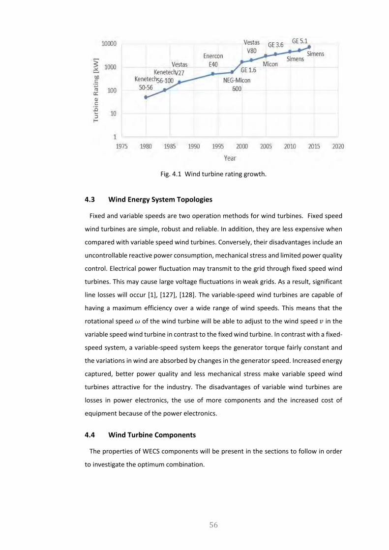
56

Fig. 4.1 Wind turbine rating growth.

4.3 Wind Energy System Topologies

Fixed and variable speeds are two operation methods for wind turbines. Fixed speed

wind turbines are simple, robust and reliable. In addition, they are less expensive when

compared with variable speed wind turbines. Conversely, their disadvantages include an

uncontrollable reactive power consumption, mechanical stress and limited power quality

control. Electrical power fluctuation may transmit to the grid through fixed speed wind

turbines. This may cause large voltage fluctuations in weak grids. As a result, significant

line losses will occur [1], [127], [128]. The variable-speed wind turbines are capable of

having a maximum efficiency over a wide range of wind speeds. This means that the

rotational speed 𝜔 of the wind turbine will be able to adjust to the wind speed 𝑣 in the

variable speed wind turbine in contrast to the fixed wind turbine. In contrast with a fixed-

speed system, a variable-speed system keeps the generator torque fairly constant and

the variations in wind are absorbed by changes in the generator speed. Increased energy

captured, better power quality and less mechanical stress make variable speed wind

turbines attractive for the industry. The disadvantages of variable wind turbines are

losses in power electronics, the use of more components and the increased cost of

equipment because of the power electronics.

4.4 Wind Turbine Components

The properties of WECS components will be present in the sections to follow in order

to investigate the optimum combination.

57

4.4.1 Gearbox

The wind turbine’s rotor turn speed is low, thus, its drive train includes a gearbox which

will justify the input speed in order to achieve the rated operation speed of the generator.

It is important to avoid under-designing the gearbox and adjust the design according to

its operating conditions. The gearbox is usually heavy and expensive compared to the

other components of the wind turbine. Gearboxes are divided into two basic types for

WECS: (1) parallel-shaft gearboxes and (2) planetary gearboxes [1], [129]–[131]. Parallel

gearboxes have two or more parallel shafts which carry the gears. For instance, a single-

stage parallel gearbox has two shafts which each have a gear. These shafts are known as

low-speed and high-speed shafts. The gear on the low-speed shaft is larger than that of

the high-speed shaft. Moreover, the low-speed shaft is usually connected to the rotor

and the high-speed shaft to the generator in the WECS. On the other hand, planetary

gearboxes have coaxial input and output shafts. In this gearbox, the loads on each gear

are reduced because there are multiple pairs of gear teeth meshing at any time. It causes

the gearbox to be relatively light and compact. A planet carrier includes at least 3

identical small gears which are stiffly connected to the lower speed shaft. These small

gears are known as planet in the career and they are assembled on short-shaft. These

planets mesh with a large-diameter internal or ring gear and a small-diameter sun gear.

The sun gear is connected to a high-speed shaft [132]. Ultimately, the gearbox is designed

to have a lower cost. Hence, the number of stages in a gearbox is important, primarily

because it affects the size, weight, and in the end, the cost of the gearbox. Also, the

maintenance of the gearbox becomes more difficult when the number of stages

increases. The gearbox’s cost should not cause a reduction in the reliability of the

gearbox. A single-stage planetary gear configuration is considered in this chapter.

𝐺𝑔𝑒𝑎𝑟 = 3.2𝑇𝑚 𝐹𝑠 𝐹𝑤

1000

4.1

Where Tm is the output torque of gearbox (N.m) and Fs is the service factor considering

surface damage and failure in metal fatigue. The weight factor Fw is given as [133]:

𝐹𝑤 =1

𝑍+

1

𝑍 𝑟𝑤+ 𝑟𝑤 + 𝑟𝑤

2 + 0.41 + 𝑟𝑤

𝑍× (𝑟𝑟𝑎𝑡𝑖𝑜 − 1)2

4.2

Where Z in the planetary wheel number in the stage; the wheel ratio 𝑟𝑤 =𝑟𝑟𝑎𝑡𝑖𝑜

2− 1 ,

and 𝑟𝑟𝑎𝑡𝑖𝑜 is single-stage gear ration. The cost of a single-stage gearbox 𝐶𝑔𝑒𝑎𝑟 is roughly

estimated by the weight 𝐺𝑔𝑒𝑎𝑟 and specific cost 𝑐𝑔𝑒𝑎𝑟 as [133]:

𝐶𝑔𝑒𝑎𝑟 = 𝑐𝑔𝑒𝑎𝑟 𝐺𝑔𝑒𝑎𝑟 4.3

The losses in a gearbox can be divided into two different parts: these include gear teeth

losses and bearing losses, which depend on the rotational speed. The main losses in a

58

gear box are proportional to the shaft speed.

𝑃𝑔𝑒𝑎𝑟 = 𝑘𝑔 𝑃𝑁

𝑛𝑟

𝑛𝑟𝑁

4.4

Where 𝑘𝑔 is a constant for the speed-dependent losses (in this case, it is 1.5 % for single-

stage gearbox), 𝑃𝑁 is the rated power of wind turbines, 𝑛𝑟𝑁 is the rated rotor speed.

Table 4.1 shows the coefficients for a single-stage gearbox.

Table 4.1 Single-stage planetary gearbox modeling

Single-stage gearbox

Gearbox service factor Fs 1.25

Planet wheel number Z 8

Cost per weight 𝑐𝑔𝑒𝑎𝑟 [$/kg] 8

Losses percentage at the rated power 𝑘𝑔 1.5%

4.4.2 Converters

Today, variable-speed wind turbine generator systems may use many different types of

converters. The power converters are a combination of basic elements such as diodes

and electronic switches, such as conventional or switchable thyristors and transistors.

The converters are characterized as either grid-commutated or self-commutated

converters [134]. A thyristor is a common type of grid-commutated converter. It is highly

reliable and well-priced, but it generates current harmonics and consumes reactive

power. Typical self-commutated converters consist of either gate turn-off (GTO)

thyristors or transistors. The advantage of self-commutated converters is their high

switching frequencies. Harmonics can be filtered out more easily and thus their

disturbances to the network can be reduced to low levels [135], [136]. As indicated in

table 4.2, the common switching frequency of an IGBT is between 2 and 20 kHz. In

contrast, GTO converters are limited to about 1kHz [137], [138].

Table 4.2 Switches: maximum ratings and characteristics.

Switch type

GTO6 IGCT7 BJT8 MOSFET9 IGBT10

Voltage [V] 6000 6000 1700 1000 6000

Current [A] 4000 2000 1000 28 1200

Switching frequency [kHz] 0.2-1 1-3 0.5-5 5-100 2-20

Drive requirements High Low Medium Low Low

Self-commutated converters are divided into current source converters (CSCs) and

voltage source converters (VSCs). These converters are able to control both the

6 Gate Turn-Off 7 Integrated Gate Commutated Thyristors 8 Bipolar Junction Transistors 9 Metal Oxide Semiconductor Field Effect Transistors 10 Insulated Gate Bipolar Transistors

59

frequency and the voltage. VSCs and CSCs are able to provide smooth switched voltage

and current waveforms, respectively. They can be used with different policies: six-step,

pulse amplitude modulated (PAM) or pulse width modulated (PWM). By using the PWM

technique, the low-frequency harmonics are eliminated and the frequency of the first

higher-order harmonics lie at approximately the switching frequency of the inverter or

rectifier. Generally, a power electronic system is adapted to adjust the generator voltage

and frequency in the variable-speed wind turbine. The system includes devices such as

soft-starters, rectifiers, inverters and frequency converters. There are various methods

to merge a rectifier and an inverter into a frequency converter. There are five applicable

technologies for controlling variable speed machines: back-to-back, multilevel, tandem,

matrix and resonant.

It is clear that the back-to-back converter configuration is fitted to current WECSs

(figure 4.2). However, the control strategy is gradually moving toward the matrix and

multilevel converter. The back-to-back PWM converter of a DFIG consists of a rotor-side

voltage converter (RSC) and a grid-side converter (GSC) [139]. With the rotor-side

converter, it is possible to control the torque or the speed of the DFIG as well as the

power factor at the stator terminals, while the main objective for the grid-side converter

is to keep the DC-link voltage constant regardless of the magnitude and direction of the

rotor power. The grid-side converter works at the grid frequency and the rotor-side

converter works at different frequencies, depending on the wind speed [140]. The matrix

converters are better in terms of efficiency and lifetime compared to back-to-back

converters with the DC link capacitor [141], [142]. However, protection in a fault

situation, higher conduction losses, and the limitation of the output voltage converter

are the disadvantages of the matrix converter [143], [144].

The losses of the converter can be divided into switching losses and conducting losses.

The switching losses of the switches are the turn-on and turn-off losses. For the diode

the switching losses mainly consist of turn-off losses, i.e., reverse-recovery energy. The

turn-on and turn-off losses for the switches and the reverse-recovery energy loss for a

diode can be found from data sheets. The conducting losses arise from the current

through the transistors and diodes [8]. Here, the losses of converter is calculated as

follow:

𝑃𝑐𝑜𝑛𝑣𝑁 = 𝑘𝑐 𝑃𝑁 4.5

The converter cost can also be calculated by their cost coefficient which varies by the

market rate. Table 4.3 illustrates the converter coefficient which is employed in this

chapter.

60

Table 4.3 Back-to-back converter modeling.

Converter coefficients

Converter losses percentage kc 3%

Specific cost of power electronic system [$/kW] 28

Specific cost of sub electrical system [$/kW] 38

4.4.3 Generator

Several types of generators may be used in wind turbines such as the squirrel cage

induction generator (SCIG), the wound rotor induction generator (WRIG) or the

synchronous generator and the permanent magnet synchronous generator (PMSG).

However, the PMSGs and the doubly-fed Induction generators (DFIGs) dominate the

market due to their many advantages.

Fig. 4.2 Typical back-to-back arrangement of the converter circuits to control power

flow.

PMSGs are suggested for use in wind turbines because of their property of self-excitation,

which allows an operation at a high power factor and a high efficiency [145]. The

efficiency is higher in the permanent magnet (PM) machines than in IMs, as the excitation

is provided without any energy supply. Permanent magnet materials are rare and as a

result, they are expensive. Also, it is difficult to work with permanent magnets materials

due to their sensitivity to heat, shock and stress. PM machines are required to be driven

by a full-scale converter in order to adjust their voltage and frequency to the grid, which

ultimately will increase the cost. The disadvantage of the PMSGs is the difficulty during

start-up, synchronization and voltage regulation [18], [146]. Also, their synchronous

nature can cause a very stiff performance in the case of an external short-circuit and

unsteady wind speed [147].

As mentioned earlier, the DFIG consists of a WRIG with the stator windings directly

connected to the constant-frequency 3-phase grid and with the rotor windings mounted

61

to a bidirectional back-to-back IGBT voltage source converter. The capability of

controlling the reactive power as well as controlling active and reactive power separately

are the DFIG’s advantages. The DFIGs are also able to deal with active power and reactive

power through their rotor by the grid-side converter as well as their stator. However, the

grid-side converter might become costly for a weak grid with voltage fluctuations

because they are designed based on the maximum slip in order to transfer an amount of

reactive power between the grid and the DFIG. Thus, the cost of the converter increases

when the speed range becomes wider. The DFIG requires slip rings which decrease its

efficiency [1], [148].

4.5 Analytical Result and Comparison

4.5.1 Analytical Results

A 736 kW, 4 pole, 4 kV, delta-connected wound rotor induction generator (WRIG) was

adapted from [3]. The WRIG is redesigned and optimized by means of an analytical design

algorithm and optimized with a genetic-algorithm. The design and optimization

procedure was validated by providing specifications for a machine similar to that

presented in [3]. The reference design and that of [3] are presented in table 4.2. It shows

five alternative wind generator designs (A, B, D, E, and F) which were generated by the

above mentioned design and optimization procedure. These designs are variations of the

reference design (c) and details for comparison are provided in table 4.2. In particular,

output power is the same, but the number of the poles and output voltages are different.

Table 4.2 includes three sections for comparison, namely the generator specifications,

system weight and components costs. The generator specifications present details of the

DFIGs designs such as bore diameter, axial length, airgap diameter, slot dimensions, etc.

As shown, the bore diameter increases when the speed decreases. This is expected since

the rated torque must increase with a drop in rated speed. This is achieved by increasing

the airgap diameter, since 𝑇~𝐷2 𝐿. The system weight shows the mass of the different

parts of the machine such as the stator, rotor, and gearbox. The copper mass of the

winding reduces when voltage increases and speed decreases. The gearbox weight

increases when speed reduces and the insulation expense will increase with voltage. The

last part of table 4.2 shows the cost of the wind generator and efficiency of the machines.

The active material cost increases along with the active material mass when the speed

decreases and voltage increases. In table 4.2, the initial cost showed wind turbine

installation, winding, and cables expense generally. The cables in the low-voltage (LV)

system contain simple insulation materials but they are more complicated for medium

voltage (MV) systems. These cables have a coated copper and a variety of insulations.

62

Moreover, the terminations of these MV cables are more difficult than that of LV cables

and are usually performed by higher skilled labour. However, the total cost impact on

installation and maintenance of these cables is minor and covered in the initial costs.

Moreover, the annual energy was calculated based on the gearbox’s maintenance,

generator insulation failure and an average wind profile.

Table 4.4 The comparison of analytical design features for a 736 kW generator.

Generator System

Machine name A B C D E F

Synchronous speed n [rpm] 1800 (4 poles) 900 (8 poles)

Voltage (on stator)[V] 690 2000 4000 690 2000 4000

Airgap diameter [m] 0.0015 0.0015 0.0015 0.0025 0.0025 0.0025

Bore diameter [m] 0.581 0.565 0.472 0.663 0.839 0.795

Outer diameter [m] 0.894 0.856 0.75 0.911 1.07 1.02

Inner diameter [m] 0.344 0.337 0.261 0.5 0.65 0.62

Axial length [m] 0.285 0.34 0.361 0.396 0. 310 0.37

Stator slot height [m] 0.0529 0.0684 0.075 0.0529 0.0629 0.693

Stator slot width [m] 0.02 0.01 0.01 0.02 0.01 0.01

Stator tooth width [m] 0.0307 0.0147 0.011 0.0089 0.0083 0.0073

Rotor slot height [m] 0.0404 0.0379 0.0417 0.0393 0.0390 0.0392

Rotor slot width [m] 0.021 0.105 0.105 0.021 0.105 0.105

Rotor tooth width [m] 0.0547 0.019 0.014 0.0221 0.0113 0.0102

System Weight

Stator’s Iron [kg] 808 695 713 585 869.5 781

Rotor’s Iron [kg] 404 327 294 255 426 545

Stator’s Copper [kg] 1.2 0.37 0.271 0.991 0.393 0.221

Rotor’s Copper [kg] 4.2 1.87 1.66 3.44 1.52 1.24

Single-stage gearbox [kg] 402 403.2 401.2 810.5 812.65 812.65

Total weight [kg] 1619 1427 1410 1655 2110 2140

Component Cost

Generator active material [$] 6840 6230 6550 7300 7520 7810

Initial [$] 18310 15960 12690 25530 20120 17610

Annual Energy cost [$] 37570 37710 33640 36530 39770 38630

Total cost [$] 62720 59900 52880 69360 67410 64050

Efficiency % 93.1 94.1 95.2 93.8 95.6 93.6

Power factor 0.91 0.9 0.912 0.862 0.9 0.9

4.5.2 Comparison

Figure 4.3 shows the characteristics of the stator current versus the shaft torque. The

mechanical part of the generator involves the shaft torque. As seen in figure 4.3, the

torque is proportional to the stator current. Conversely, all machines have similar output

power and it would be more efficient to generate electricity at maximum torque in a

wider range of stator current in order to control output power. It is indicated that the

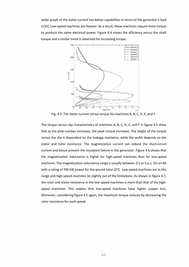
63

wider graph of the stator current has better capabilities in terms of the generator’s load

[135]. Low-speed machines are heavier. As a result, these machines require more torque

to produce the same electrical power. Figure 4.4 shows the efficiency versus the shaft

torque and a similar trend is observed for increasing torque.

Fig. 4.3 The stator current versus torque for machines A, B, C, D, E, and F.

The torque versus slip characteristics of machines A, B, C, D, E, and F in figure 4.5 show

that as the pole number increases, the peak torque increases. The height of the torque

versus the slip is dependent on the leakage reactance, while the width depends on the

stator and rotor resistance. The magnetization current can reduce the short-circuit

current and hence prevent the insulation failure in the generator. Figure 4.6 shows that

the magnetization inductance is higher for high-speed machines than for low-speed

machines. The magnetization inductance range is usually between 3.5 to 5 p.u. for an IM

with a rating of 700 kW power for the wound rotor [27]. Low-speed machines are in this

range and high-speed machines lie slightly out of the limitations. As shown in figure 4.7,

the rotor and stator resistance in the low-speed machines is more than that of the high-

speed machines. This implies that low-speed machines have higher copper loss.

Moreover, considering figure 4.5 again, the maximum torque reduces by decreasing the

rotor resistance for each speed.

64

Fig. 4.4 The efficiency versus torque for machines A, B, C, D, E, and F.

Fig. 4.5 The torque versus slip for machines A, B, C, D, E, and F.

4.6 Conclusion

Variations in the designs of a 736 kW induction machine are presented in this chapter.

Several aspects are compared and discussed for each design configuration. The MV

system achieves a significant capital cost advantage over the traditional LV system. In

particular, a substantial reduction in the cost of cables and transformers is observed for

MV systems compared to LV systems. The cost of converters also decreases dramatically

for MV machines. The perceived technical risk in the development of MV converter

systems is a concern for turbine manufacturers and operators. It is important to note that

many of the historic technical problems have been overcome in recent years by

technological advances. The weight of a gearbox increases dramatically with an increased

65

power rating of the turbine. In fact, the gearbox weight will scale approximately with the

cube of the radius, as does the weight of the rotor. Since planetary gearboxes are lighter

than parallel-shaft boxes, there is a weight advantage to be gained by using them.

Fig. 4.6 The magnetization inductance versus voltage.

Fig. 4.7 The stator and the rotor resistance versus voltage.

On the other hand, due to their greater complexity, they also cost more than would be

indicated by their reduced weight. Machines C and E are the most efficient of the high-

speed and low-speed machines, respectively. The results show that the quality of the

power generated by low-speed machines is better than that generated by high speed

machines. As a conclusion, it would be better to compromise between the quality,

efficiency and cost in different circumstances.

66

5. Wind Power Integration Issues

The main goal of the power system is to supply the network’s energy demand. In order

to increase the penetration of wind energy in the power system, due to green energy

obligations, it must adjust with power system conditions. Thus, the wind energy must

satisfy the system’s conditions before joining the network. The wind power fluctuates

naturally and its fluctuation will migrate to the power system with wind energy

integration. This chapter presents the wind energy integration issues with the

introduction of aggregated modelling to investigate these issues. The advantages and

disadvantages of the aggregation’s models are also presented. Finally, a single machine

equivalent is discussed.

5.1 Introduction

When nuclear energy was introduced to the market, integration posed a challenge due

to the inflexibility of nuclear energy. Hence, the flexibility of the system must be great

enough to add the nuclear source to the grid. Also, wind power is fairly new to the system

and more recently governments have made the decision to increase renewable energy

shares in the market, particularly wind energy, due to its advantages. The increasing wind

energy shares are evident with the current technology and do not require a major

redesign of the existing system. However, it is essential to predict the behaviour of wind

farms while integrating to the power system [36], [129], [130].

5.2 The Wind Farm in the Power System

The equation 5.1 indicates the voltages and the currents in a power system,

𝑣(𝑡) = 𝑉𝑀 cos(𝜔𝑡)

𝑖(𝑡) = 𝐼𝑀cos (𝜔𝑡 − 𝜃)

5.1

where,

𝑣(𝑡): Voltage;

𝑉𝑀: Maximum voltage;

𝜔 = 2𝜋𝑓;

𝑓 : Frequency;

𝑖(𝑡): Current;

67

𝐼𝑀: Maximum current;

𝜃: Phase shift between voltage and current.

The power can be calculated by the voltages and the currents as follows:

𝑝(𝑡) = 𝑣(𝑡)𝑖(𝑡) = 𝑉𝑀 cos(𝜔𝑡) 𝐼𝑀 cos(𝜔𝑡 − 𝜃)

= 𝑃[1 + cos(2𝜔𝑡)] + 𝑄 𝑠𝑖𝑚 (2𝜔𝑡)

5.2

where, P and Q represent active and reactive power, respectively. Essentially, the voltage

and the current waves must have a constant amplitude and 120° phase shift between

them to transfer 3-phase symmetric power to the grid. The impedance in all transmission

lines, cables and transformers in the feeding grid is represented by 𝑍 in figure 5.1. The

figure also indicates a local load at the point of connection of the wind farm [149].

Fig. 5.1 The grid connection of wind power.

𝑉1: RMS value of the voltage on the grid side;

𝑉2: RMS value of the voltage on the load side;

𝑃𝑤: Wind power active power;

𝑄𝑤: Wind power reactive power;

𝑃𝐿𝐷: Local load active power;

𝑄𝐿𝐷: Local load reactive power.

If there is a short-circuit failure at the wind farm connection point, then the short-circuit

power ( 𝑃𝑠𝑐) can be calculated through equations 5.3 and 5.4. The short-circuit increases

the current in the impedance 𝑍, while 𝑃𝑠𝑐 flows towards short-circuit point. It is important

to understand how the grid reacts.

𝑉1 − 𝑉2 = √3 𝑍. 𝐼 5.3

𝑃𝑠𝑐 =𝑉1

2

𝑍∗ 5.4

68

Under the normal conditions, the amount of current in impedance Z depends on the wind

energy generation due to its voltage (𝑉2) fluctuation. It must be recognized that there is

no space for wind energy in the weak system (with large impedance) as much as there is

for the stronger system (with small impedance) [150], [151]. As seen in equation 5.2, the

voltage 𝑉2 in figure 5.1 can be calculated as:

𝑉2 = {− 2𝑎1−𝑉1

2

2+ [(

2𝑎1−𝑉12

3) − (𝑎1

2 + 𝑎22)]

1

2}

1

2

5.5

where,

𝑎1: −𝑅(𝑃𝑊 − 𝑃𝐿𝐷) − 𝑋(𝑄𝑊 − 𝑄𝐿𝐷),

𝑎2: −𝑋(𝑃𝑊 − 𝑃𝐿𝐷) + 𝑅(𝑄𝑊 − 𝑄𝐿𝐷).

Equation 5.5 shows that the reactive power generation in the wind farm, 𝑄𝑊, has an

impact on the voltage 𝑉2. The local load and the feeding grid impedance are important

parameters in this incident.

5.3 Integration to the Power System

Figure 5.2 illustrates the power from the network (𝑃𝐺), industries and residential

demands (𝑃𝐷), and a wind power station that delivers power, 𝑃𝑊. The impedances

(𝑍1–𝑍3) represent the impedances in the transmission lines and transformers between

the different places in figure 5.2.

Fig. 5.2 Illustrative power system.

It is clear that the energy cannot disappear in the system. Therefore,

𝑃𝐺 = 𝑃𝐷 + 𝑃𝐿 − 𝑃𝑊 5.6

where,

𝑃𝐺: The power production in the grid side;

69

𝑃𝐷: The power consumption in the residential load;

𝑃𝐿: The electrical losses in the impedances;

𝑃𝑊: The wind energy.

The energy demands must be supplied by the power system. It is noted that the grid

power, wind energy and other power sources must be balanced against the energy

demands. Furthermore, the voltage level and the reactive power must be considered in

the transmission system. Hence, it is essential to investigate the dynamic behaviour of

wind farms in case of system faults in more detail.

5.4 The Effect of Wind Turbines on the Grid

Wind farms are located in remote areas and they connect to the grid through high-

voltage (HV) or medium-voltage (MV) distribution systems. Usually, the wind turbines

employ transformers and they may connect to the HV system. It is, however, often more

efficient sometimes to connect them directly by MV transmission lines to more nearby

loads. As mentioned, wind farms influence the steady-state voltage and reactive power

consumption of the network. The integrated wind power must respect the power

system’s rules which are as follows:

Steady-state voltage

The power system is designed to keep the voltage level as steady as possible. The

voltage variations of the system must be within the standard limits whenever the wind

turbines are directly connected to the MV system. These limits are set by the official wind

farm planning considerations [126], [152].

Reactive power consumption

The reactive power is an important factor in the power system. There is a demand for

reactive power from the reactive component operating in the network. The wind farms

also consume reactive power for their transformers and the transmit lines when they are

feeding active power to the grid. Reactive power consumption can decrease the power

factor at the conventional power stations [127]. It will increase in the classic constant

speed wind turbines (SCIG), as well as variable speed wind turbines (DFIG) with thyristor-

based converters. However, the wind turbines with IGBT-based converters (DFIG) will not

consume reactive power [3], [153], [154].

70

5.5 The Network Impact on the Wind Turbine

Weak grids may have an effect on aspects of the wind turbines such as performance,

safety, etc. [127], [152], [155]. These impacts are as follows:

Power performance

The wind turbine’s power performance can be affected by outages, frequency, and

voltage imbalance.

Safety

The safety of the wind turbine would be compromised when it is connected to weak

grids. For example, grid abnormalities in the voltage and the frequency may cause trip

relay and overheating of the generator.

Structural lifetime

The weak grid increases the mechanical stress on the wind turbine. Hence, the lifetime

of the mechanical components will be reduced.

Reactive power consumption

As stated above, wind farms trade the reactive power with the power system. This will

affect the power system and wind farms. So, it will influence the power factor of the wind

turbine.

5.6 Dynamic Performance of Wind Turbines

The regimen of energy generation has been changed by the WECS. Wind farms have

different characteristics from large power plants. Wind farms can recover and return to

being online within a few seconds following a disconnection due to mechanical failure.

On the other hand, thermal power stations require hours to be able to resynchronize

themselves to the network after a failure. One should also note that these types of

stations may contribute for several seconds substantially in a short-circuit in order to

ensure network protection and maintain voltage levels [156], [157]. Wherever wind

energy dominates in the local network and conventional generation from large power

stations is simultaneously reduced, significant voltage drops and frequency fluctuations

are more likely if the short-circuit capacity is reduced. This leads to both a voltage

instability and damage to the network protection systems. The understanding of the

dynamic behaviour of the wind turbines is vital in network failures in order to find the

new grid requirements and adjust the network regulation mechanism [1], [158].

71

5.7 Aggregated Modelling of Large Wind Farms

An aggregated model of a wind farm must consider each wind turbine individually, their

mutual interactions, the internal transmission lines and the wind farm grid connection. It

must also reduce the wind farm model and implement it in detailed models of the large

power system. The covering of these two issues is the main objective of an aggregated

model [18], [136]. An aggregated model is used to analyse the power system’s stability.

In this chapter, the focus is on the impact of a large wind farm on a large power system

which implies that a single machine can represent a large wind farm [159].

5.7.1 Aggregated Modelling Issues

As previously noted, the mutual interaction between wind turbines within a large wind

farm is considered by the aggregated model. The model is able to indicate the risk of

combing the electricity produced by different wind turbines within the wind farm [1]. A

grid disturbance from the external network may initiate the interaction problem within

the wind farm. Thus, a group of wind turbines might be separated from the others. The

potential of mutual interaction is higher amongst the wind turbines with converter-

controlled generators. Also, the issue of the wind turbines equipped with induction

generators and blade-angle control is cited [160], [161]. The aggregated model may assist

in designing the internal network of the wind farm and estimation of its reactive

compensation [162]. For large wind farms, analysing and investigating the control

coordination between control systems of wind turbines is possible by the wind farm’s

aggregated models [163]. Aggregated models of large wind farms can also be used to

evaluate relay settings during short-circuit faults or other disturbances in the internal

network of a wind farm. Instead of a complete model of all wind turbines, the behaviour

of the wind farm (at the point of common coupling to the grid) can be represented by an

equivalent model derived from the aggregation of wind turbines into an equivalent wind

turbine. A few aggregate wind farm models have been proposed in the literature,

reducing computational effort and simulation time during transient stability analysis. In

[136], a single-machine aggregate wind turbine model is developed for the entire wind

power plant. References [161] and [164] propose an equivalent model with constant

incoming wind speeds. An aggregate model is introduced in [165] which considers

variable incoming wind speeds. A method has been presented to separate wind farms for

parallel analysis in a super-computer and is given in [166]. The references are associated

with two issues. On one hand, some research is based on simplified wind turbine models

which lead to lower accuracy of dynamic results. On the other hand, some studies rely

on simplified wind models which may decrease the simulation time but will increase the

72

application difficulty in order to create a new set of equivalent wind turbines and their

variables whenever wind speed or wind direction change.

5.7.2 A Single Machine Equivalent

Whenever the power system falls into transient condition, the wind farm in the system

also gets affected. The wind turbines evidently will respond coherently to the transient

incident. It means the simulated behaviour of a wind turbine will be similar to the wind

farm dynamic response, if they both operate at the rated operational point of the wind

farm. The wind turbines with converters (DFIG and PMSG) would be at risk of a converter

blocking at the rated operation due to the machine and the grid-side converter currents

are being closest to their respective relay settings [136]. The arrangement of the control

system of converters must be considered within the wind farm to decrease the risk of

mutual interaction among the wind turbines. Therefore, the analysis of voltage stability

for a wind farm can be done simply by a single machine equivalent [159], [167]. To show

a single wind turbine model as a wind farm, the power capacity of the wind farm will be

the power capacity of the equivalent machine and the power generated in the wind farm

will be equal to the power produced in the equivalent machine [1], [159]. The reactive

power of the equivalent machine is also zero at the connection point [168]. It is worth

noting that the dynamic behaviour of speed and voltage are separated because the active

and the reactive power controls are dependent on each other [136]. As known, the risk

of mutual interaction for PMSG and DFIG may be neglected if the converter tuning is

efficient [169].

5.8 Conclusion

In this chapter the basic integration issue is discussed. The main interest is shown on

the short-circuit failure nearby the wind farm due to the wind farm behaviour being

unknown which is explained and analysed with its effects on the grid. The aggregation is

introduced as a tool to solve the issue and it helps reduce the complexity of the issue. A

few aggregated models and their properties are presented. It is shown that they have

difficulties in analysing the wind energy in the power system due to their constraints. A

single machine is also considered to represent a wind farm in the system. However, it

appears that prototyping a single machine equivalent is not feasible.

73

6. Dynamic Model of DFIG

As previously noted, a dimensional analysis technique is required when designing a

micro-machine using a reference machine. This technique is justified by the objective of

the scaling process, which is to achieve similar behaviour in both machines under

transient conditions. Therefore, the scaling factors will essentially be defined by the

parameters which generate the machine’s behaviour. The d-q model of a DFIG under

normal and short-circuit conditions is presented in this chapter in order to disclose the

parameters in the steady and transient states.

6.1 Introduction

In general, illustrating the operation of 3-phase induction machines by an equivalent

circuit or number of equations is known as modelling. An accurate dynamic model of a

wind generator is required in order to do research on steady-state and transient

characteristics of wind energy systems. In other words, this model assists in the discovery

of effective parameters on the steady and transient behaviours of the machine under

transient conditions. Therefore, the relationship between the identified parameters and

the machine’s equivalent circuit elements must be taken into account in the scaling

process [3], [170].

6.2 Space Vectors in the Stator Reference Frame

An induction machine is illustrated in figure 6.1 to present the space vectors concept.

For simplicity, the stator will be analysed and then the same concept will be used for the

rotor. There are two assumptions necessary to explain this concept; firstly, each phase

winding is assumed to have only one turn and secondly, all vectors indicated in bold

letters and a superscript present a particular reference frame. The winding’s axis is

presented perpendicular to the plane in which the coil lies. The stator reference frames

(stationary) are:

𝑑𝑠: The direct axis aligned along the horizontal geometrical axes of the stator.

𝑞𝑠: The quadrature axis aligned along the vertical geometrical axes of the stator.

The direct axis is physically referenced along the axis of the phase-A winding of the stator.

Currents entering the coil ends marked A, B, C (in figure 6.1) have been defined as being

positive. The currents are negative when entering ends A’, B’ and C’ [170], [171]. Figure

6.2 illustrates that the phases are spatially displaced by 120°. If the currents entering the

74

coils are provided from the grid, with radian frequency 𝜔, the currents can be indicated

as follows:

𝑖𝑎𝑠(𝑡) = 𝐼𝑠 cos(𝜔𝑡) = 𝐼𝑠𝑅𝑒{𝑒𝑗𝜔𝑡} 6.1

𝑖𝑏𝑠(𝑡) = 𝐼𝑠 cos (𝜔𝑡 −2𝜋

3) = 𝐼𝑠𝑅𝑒 {𝑒

(𝑗𝜔𝑡−2𝜋

3)} 6.2

𝑖𝑐𝑠(𝑡) = 𝐼𝑠 cos (𝜔𝑡 +2𝜋

3) = 𝐼𝑠𝑅𝑒 {𝑒

(𝑗𝜔𝑡−2𝜋

3)} 6.3

where 𝐼𝑠 illustrates the magnitude of stator current. Figure 6.3 presents the currents over

two periods.

Fig. 6.1 The cross section of the stator and the rotor of 3 phase, 2-pole induction machine.

A magneto-motive force will be produced along the winding’s axis when the current flows

in a phase. These currents can be indicated as vectors in the winding’s axis direction. The

magnitude of the current vector is proportional to the instantaneous value of the current

while the direction lies along the axis of the winding. These arrangements are known as

space vectors [171]–[174]. Figure 6.4 presents the phase current space vectors (at 𝜔𝑡 =

0) with the resultant current space vector, which is gained by vector addition of the

instantaneous phase current space vectors.

75

Fig. 6.2 The 3-phases located with 120° displacement.

Fig. 6.3 The balanced 3-phase stator currents.

Each phase current space vector may also be presented in complex form and the final

gained.

𝑖𝑎𝑠 = 𝑖𝑎𝑠𝑒𝑗0, 𝑖𝑏𝑠 = 𝑖𝑏𝑠𝑒

𝑗2𝜋

3 , 𝑖𝑐𝑠 = 𝑖𝑐𝑠𝑒𝑗4𝜋

3 6.4

𝑖𝑠𝑠 = 𝑖𝑎𝑠 + 𝑖𝑏𝑠 + 𝑖𝑐𝑠 6.5

𝑖𝑠𝑠 =

3

2 𝐼𝑠𝑒

𝑗(𝜔𝑡) 6.6

76

At 𝜔𝑡 = 0;

𝑖𝑎𝑠(0) = 𝐼𝑠; 𝑖𝑏𝑠(0) = −1

2𝐼𝑠; 𝑖𝑐𝑠(0) = −

1

2𝐼𝑠 6.7

𝑖𝑠𝑠 = 𝐼𝑠𝑒

𝑗0 −1

2𝐼𝑠𝑒

𝑗2𝜋

3 −1

2 𝐼𝑠𝑒

𝑗4𝜋

3 6.8

𝑖𝑠𝑠 = 1.5 𝐼𝑠𝑒

𝑗0 6.9

which is presented in figure 6.4. At =𝜋

3 ;

𝑖𝑎𝑠 (𝜋

3) =

1

2𝐼𝑠; 𝑖𝑏𝑠 (

𝜋

3) =

1

2𝐼𝑠; 𝑖𝑐𝑠 (

𝜋

3) = −𝐼𝑠 6.10

𝑖𝑠𝑠 =

1

2𝐼𝑠𝑒

𝑗0 +1

2𝐼𝑠𝑒

𝑗2𝜋

3 − 𝐼𝑠𝑒𝑗4

𝜋

3 6.11

𝑖𝑠𝑠 = 1.5 𝐼𝑠𝑒

𝑗𝜋

3 6.12

which is indicated in figure 6.5. 𝜃𝑠 shows the angular position of the final stator current

space vector. It is clear from figures 6.4 and 6.5 that the final vector current is 1.5 I𝑠 and

rotates with angular frequency 𝜔.

Fig. 6.4 The space vectors for the stator current at 𝛚𝐭 = 𝟎.

The implication of space vectors can also be distributed to all other parameters (i.e.

voltage (v), flux linkage (𝜓), mmf, etc.) [170], [171]. This means that a 3-phase induction

machine is able to transform into an equivalent 2-phase induction machine through

space vectors.

77

𝑣𝑠𝑠 = 𝑣𝑎𝑠𝑒

𝑗0 𝑣𝑏𝑠𝑒𝑗2

𝜋

3𝑣𝑐𝑠𝑒𝑗4

𝜋

3 6.13

𝜓𝑠𝑠 = 𝜓𝑎𝑠𝑒

𝑗0 𝜓𝑏𝑠𝑒𝑗2

𝜋

3𝜓𝑐𝑠𝑒𝑗4

𝜋

3 6.14

6.3 Transformations between the 3-phase and 2-phase Quantities

Thus far, the complex plane of the stator currents of induction machines have been

presented. It is formed by the quadrature and direct axis. Using Euler’s Identity 𝑒𝑗𝜔𝑡 =

cos(𝜔𝑡) + 𝑗𝑠𝑖𝑛(𝜔𝑡), the resultant stator current space vector may be decomposed into

its quadrature and direct components. This is indicated below by substituting equation

6.4 into 6.5.

Fig. 6.5 The space vector for the stator current at 𝛚𝐭 = 𝛑/𝟑.

𝑖𝑠𝑠 = 𝑖𝑎𝑠𝑒

𝑗0 + 𝑖𝑏𝑠𝑒𝑗2

𝜋

3 + 𝑖𝑐𝑠𝑒𝑗4

𝜋

3 6.15

𝑖𝑠𝑠 = 𝑖𝑎𝑠[cos(0) + jsin(0)] + 𝑖𝑏𝑠 [cos (

2𝜋

3) + jsin (

2𝜋

3)] + 𝑖𝑐𝑠 [cos (

4𝜋

3) +

jsin (4𝜋

3)]

6.16

𝑖𝑠𝑠 = (𝑖𝑎𝑠 −

1

2𝑖𝑏𝑠 −

1

2𝑖𝑐𝑠) + 𝑗 (

√3

2𝑖𝑏𝑠 −

√3

2𝑖𝑐𝑠) 6.17

𝑖𝑠𝑠 = 𝑖𝑑𝑠 + 𝑗𝑖𝑞𝑠 6.18

This may be indicated in matrix form as follows:

78

[𝑖𝑑𝑠

𝑠

𝑖𝑞𝑠𝑠] = [

1 −1

2−

1

2

0√3

2−

√3

2

] [

𝑖𝑎𝑠

𝑖𝑏𝑠

𝑖𝑐𝑠

] 6.19

The derived expression is referred to as the Clarke Transform [171], [175]. The 3-phase

quantities were shown in the stator reference frame by the resulting matrix. The inverse

of the matrix above can easily be solved for and the expression in (6.20) is known as the

Inverse Clarke Transform [175].

[

𝑖𝑎𝑠

𝑖𝑏𝑠

𝑖𝑐𝑠

] =

[

2

30

−1

3

1

√3

−1

3−

1

√3]

[𝑖𝑑𝑠

𝑠

𝑖𝑞𝑠𝑠] 6.20

6.4 Transformations of Space Vectors between Different Reference Frames

𝑖𝑠𝑠 was referenced to a plane perpendicular to the rotor shaft and stationary to the

stator. It can, however, also be referenced to other planes, with their orthogonal axis

rotating at various speeds. For instance, the rotor reference frame will be explained as

follows:

6.4.1 Rotor Reference Frame

The rotor current frequency is proportional to the slip, as shown:

𝜔𝑠𝑙𝑖𝑝 = 𝑠𝜔 =𝑑𝜃𝑠𝑙𝑖𝑝

𝑑𝑡 6.21

𝑠 =

𝜔

𝑝1−𝜔𝑟

𝜔

𝑝1

6.22

𝜃𝑠𝑙𝑖𝑝: Slip angular position;

𝜔𝑠𝑙𝑖𝑝: Slip angular frequency;

𝜔𝑟: Rotor angular frequency;

𝑠: Slip;

𝑝1: Number of pole pairs;

The rotor reference frame is defined by having its real and imaginary axis aligned with

the vertical and horizontal geometrical axis of the rotor. The real axis (direct axis, 𝑑𝑟), is

physically referenced along the axis of the phase-A coil of the rotor. 𝜃0 is known as the

angular position (𝜃0 = ∫𝜔0 𝑑𝑡) and 𝜔0 is referred to as the angular speed at which the

rotor reference frame rotates relative to the stator reference frame (𝜔0 = 𝑝1𝜔𝑟). The

79

currents in the rotor result in a final current space vector, which is indicated 𝑖𝑟 (figure

6.6). 𝜃𝑠𝑙𝑖𝑝 is the angular position of 𝑖𝑟 relative to the rotor reference frame and may be

calculated from the slip frequency (i.e. 𝜃𝑠𝑙𝑖𝑝 = ∫𝜔𝑠𝑙𝑖𝑝 𝑑𝑡). The resultant rotor current

space vector relative to the rotor reference frame can be illustrated as follows:

𝑖𝑟𝑟 = 1.5 𝐼𝑟 𝑒

𝑗𝜃𝑠𝑙𝑖𝑝 6.23

where 𝐼𝑟 is magnitude of the rotor current. As noted, the angle change between the

stator and rotor reference frame must be included (figure 6.6). Thus using Euler’s

Identity, 𝑒𝑗𝜔𝑡 = cos(𝜔𝑡) + 𝑗𝑠𝑖𝑛(𝜔𝑡), the equivalent rectangular representation is:

𝑖𝑟𝑠 = 𝑖𝑟

𝑟𝑒𝑗𝜃0 = (𝑖𝑑𝑟𝑟 + j𝑖𝑞𝑟

𝑟 )(cos(𝜃0) + 𝑗𝑠𝑖𝑛(𝜃0)) = (𝑖𝑑𝑟𝑟 cos(𝜃0) −

𝑖𝑞𝑟𝑟 𝑠𝑖𝑛(𝜃0)) + 𝑗 (𝑖𝑞𝑟

𝑟 cos(𝜃0) + 𝑗𝑖𝑑𝑟𝑟 𝑠𝑖𝑛(𝜃0))

6.24

Representing the above in matrix form

[𝑖𝑑𝑟𝑠

𝑖𝑞𝑟𝑠 ] = [

cos (𝜃0) −sin (𝜃0)sin (𝜃0) cos (𝜃0)

] [𝑖𝑑𝑟𝑟

𝑖𝑞𝑟𝑟 ] 6.25

Fig. 6.6 The final rotor current space vector relative to the stationary and rotor reference frames.

The inverse of the above expression is as follows:

[𝑖𝑑𝑟𝑟

𝑖𝑞𝑟𝑟 ] = [

cos (𝜃0) sin (𝜃0)−sin (𝜃0) cos (𝜃0)

] [𝑖𝑑𝑟𝑠

𝑖𝑞𝑟𝑠 ] 6.26

80

6.4.2 Synchronous Reference Frame

Here, the purpose of transformation is to conveniently analyse behaviour of induction

machines. It is essential to convert AC quantities to DC quantities due to alternating

quantities being difficult to work with, and thus transformations to various reference

frames are required to enable the conversion. The synchronous reference frame rotates

at synchronous speed, 𝜔, and the direct axis is referenced along the peak of the flux

density in the airgap [170], [171]. The immediate angle shaped between the synchronous

reference and the stationary reference frame is 𝜔𝑡 (figure 6.7). The resultant stator

current space vector seems to rotate at 𝜔 and stationary when perceived from the

stationary reference frame and the synchronous reference respectively. It may then be

decomposed into its two time invariant components; in the direction of its real and

imaginary axes. The relationship between the synchronous and the stator reference

frames are as follows (the resultant stator current space vector in the synchronous

reference frame is 𝑖𝑠𝑒):

𝑖𝑠𝑠 = 𝑖𝑠

𝑒𝑒𝑗𝜔𝑡 6.27

𝑖𝑠𝑒 = 𝑖𝑠

𝑠𝑒−𝑗𝜔𝑡 6.28

Similarly,

Fig. 6.7 Final stator current space vector relative to the stationary and synchronous reference frames.

𝑣𝑠𝑠 = 𝑣𝑠

𝑒𝑒𝑗𝜔𝑡 6.29

81

𝜓𝑠𝑠 = 𝜓𝑠

𝑒𝑒𝑗𝜔𝑡 6.30

The equivalent rectangular co-ordinates are as follows:

𝑖𝑑𝑠𝑠 + 𝑗𝑖𝑞𝑠

𝑠 = (𝑖𝐷𝑠𝑒 + 𝑗𝑖𝑄𝑠

𝑒 )(cos(𝜔𝑡) + 𝑗𝑠𝑖𝑛(𝜔𝑡)) = (𝑖𝐷𝑠𝑒 cos(𝜔𝑡) −

𝑖𝑄𝑠𝑒 𝑠𝑖𝑛(𝜔𝑡)) + 𝑗 (𝑖𝐷𝑠

𝑒 sin(𝜔𝑡) + 𝑗𝑖𝑄𝑠𝑒 𝑐𝑜𝑠(𝜔𝑡))

6.31

𝑖𝐷𝑠𝑒 + 𝑗𝑖𝑄𝑠

𝑒 = (𝑖𝑑𝑠𝑠 + 𝑗𝑖𝑞𝑠

𝑠 )(cos(−𝜔𝑡) + 𝑗𝑠𝑖𝑛(−𝜔𝑡)) = (𝑖𝑑𝑠𝑠 cos(𝜔𝑡) −

𝑖𝑞𝑠𝑠 𝑠𝑖𝑛(𝜔𝑡)) + 𝑗 (−𝑖𝑑𝑠

𝑠 sin(𝜔𝑡) + 𝑗𝑖𝑞𝑠𝑠 𝑐𝑜𝑠(𝜔𝑡))

6.32

Representing the above in matrix form:

[𝑖𝐷𝑠𝑒

𝑖𝑄𝑠𝑒 ] = [

cos (𝜔𝑡) sin (𝜔𝑡)−sin (𝜔𝑡) cos (𝜔𝑡)

] [𝑖𝑑𝑠

𝑠

𝑖𝑞𝑠𝑠] 6.33

whereby the above expression is referred to as the Park Transform [167], [171]. The

inverse is:

[𝑖𝑑𝑠

𝑠

𝑖𝑞𝑠𝑠] = [

cos (𝜔𝑡) −sin (𝜔𝑡)sin (𝜔𝑡) cos (𝜔𝑡)

] [𝑖𝐷𝑠𝑒

𝑖𝑄𝑠𝑒 ] 6.34

which is known as the Inverse Park Transform. Thus the transformation between

different reference frames integrates the theory of relativity. The solution policy of the

problem determines the choice of the reference frame.

6.5 Dynamic Model of the Induction Machine in the Stationary Reference

Frame

The windings may be presented as interconnected resistor-inductor circuit elements in

induction machines. Figure 6.8 illustrates such a circuit while voltage, current and flux

vectors are employed instead of time variant ac signals [65], [171], [176], [177].

82

Fig. 6.8 Equivalent circuit representing the stator or rotor winding.

The stator winding voltage is represented as follows:

𝑣𝑠𝑠 = 𝑅𝑠𝑖𝑠

𝑠 +𝑑𝜓𝑠

𝑠

𝑑𝑡 6.35

The rotor winding voltage is represented as follows:

𝑣𝑟𝑟 = 𝑅𝑟𝑖𝑟

𝑟 +𝑑𝜓𝑟

𝑟

𝑑𝑡 6.36

The following substitutions refer the rotor equivalent equation to the stator,

𝑣𝑟𝑟 = 𝑣𝑟

𝑠𝑒−𝑗𝜃0 6.37

𝑖𝑟𝑟 = 𝑖𝑟

𝑠𝑒−𝑗𝜃0 6.38

𝜓𝑟𝑟 = 𝜓𝑟

𝑠𝑒−𝑗𝜃0 6.39

𝑑𝜓𝑟𝑟

𝑑𝑡=

𝑑(𝜓𝑟𝑠𝑒−𝑗𝜃0)

𝑑𝑡 6.40

Differentiation by parts, we get

𝑑𝜓𝑟𝑟

𝑑𝑡=

𝑑𝜓𝑟𝑠

𝑑𝑡𝑒−𝑗𝜃0 +

𝑑(𝑒−𝑗𝜃0)

𝑑𝑡𝜓𝑟

𝑠 =𝑑𝜓𝑟

𝑠

𝑑𝑡𝑒−𝑗𝜃0 − 𝑗

𝑑𝜃0

𝑑𝑡𝜓𝑟

𝑠𝑒−𝑗𝜃0 6.41

whereby,

𝜔0 =𝑑𝜃0

𝑑𝑡 6.42

thus,

𝑑𝜓𝑟𝑟

𝑑𝑡=

𝑑𝜓𝑟𝑠

𝑑𝑡𝑒−𝑗𝜃0 − 𝑗𝜔0𝜓𝑟

𝑠𝑒−𝑗𝜃0 = 𝑒−𝑗𝜃0 (𝑑𝜓𝑟

𝑠

𝑑𝑡− 𝑗𝜔0𝜓𝑟

𝑠) 6.43

Substituting equations 6.38, 6.39, 6.44 into equation 6.37, we get

83

𝑣𝑟𝑠𝑒−𝑗𝜃0 = 𝑅𝑟𝑖𝑟

𝑠𝑒−𝑗𝜃0 + 𝑒−𝑗𝜃0 (𝑑𝜓𝑟

𝑠

𝑑𝑡− 𝑗𝜔0𝜓𝑟

𝑠) 6.44

dividing by 𝑒−𝑗𝜃0

𝑣𝑟𝑠 = 𝑅𝑟𝑖𝑟

𝑠 +𝑑𝜓𝑟

𝑠

𝑑𝑡− 𝑗𝜔0𝜓𝑟

𝑠 6.45

Interchanging 𝑑

𝑑𝑡 with 𝑝

𝑣𝑠𝑠 = 𝑅𝑠𝑖𝑠

𝑠 + 𝑝𝜓𝑠𝑠 6.46

𝑣𝑟𝑠 = 𝑅𝑟𝑖𝑟

𝑠 + 𝜓𝑟𝑠(𝑝 − 𝑗𝜔0) 6.47

The flux vectors have to appear in terms of currents and inductances in order to express

the above voltage equations in terms of the stator and the rotor current vector. Thus, the

equations 6.46 and 6.47 will transfer as follows,

𝐿𝑙𝑠 : Leakage stator inductance

𝐿𝑙𝑟 : Leakage rotor inductance

𝐿𝑚 : Mutual inductance

whereby,

𝐿𝑠 = 𝐿𝑙𝑠 + 𝐿𝑚 6.48

𝐿𝑟 = 𝐿𝑙𝑟 + 𝐿𝑚 6.49

𝜓𝑠𝑠 = 𝐿𝑠𝑖𝑠

𝑠 + 𝐿𝑚𝑖𝑟𝑠 6.50

𝜓𝑟𝑠 = 𝐿𝑚𝑖𝑠

𝑠 + 𝐿𝑟𝑖𝑟𝑠 6.51

Substituting equations 6.50 and 6.51 into equations 6.46 and 6.47 respectively, the

voltages are expressed as follows:

𝑣𝑠𝑠 = (𝑅𝑠 + 𝑝𝐿𝑠) 𝑖𝑠

𝑠 + 𝑝𝐿𝑚𝑖𝑟𝑠 6.52

𝑣𝑟𝑠 = (𝑝 − 𝑗𝜔0)𝐿𝑚𝑖𝑠

𝑠 + (𝑅𝑟 + (𝑝 − 𝑗𝜔0)𝐿𝑟)𝑖𝑟𝑠 6.53

This can be re-written as follows:

𝑣𝑑𝑠𝑠 = (𝑅𝑠 + 𝑝𝐿𝑠)𝑖𝑑𝑠

𝑠 + 𝑝𝐿𝑚𝑖𝑑𝑟𝑠 6.54

𝑣𝑞𝑠𝑠 = (𝑅𝑠 + 𝑝𝐿𝑠)𝑖𝑞𝑠

𝑠 + 𝑝𝐿𝑚𝑖𝑞𝑟𝑠 6.55

𝑣𝑑𝑟𝑠 = 𝑝𝐿𝑚𝑖𝑑𝑠

𝑠 + 𝜔0𝐿𝑚𝑖𝑞𝑠𝑠 + (𝑅𝑟 + 𝑝𝐿𝑟)𝑖𝑑𝑟

𝑠 + 𝜔0𝐿𝑟𝑖𝑞𝑟𝑠 6.56

84

𝑣𝑞𝑟𝑠 = −𝜔0𝐿𝑚𝑖𝑑𝑠

𝑠 + 𝑝𝐿𝑚𝑖𝑞𝑠𝑠 − 𝜔0𝐿𝑟𝑖𝑞𝑟

𝑠 + (𝑅𝑟 + 𝑝𝐿𝑟)𝑖𝑑𝑟𝑠 6.57

This may be expressed in matrix form as follows:

[ 𝑣𝑑𝑠

𝑠

𝑣𝑞𝑠𝑠

𝑣𝑑𝑟𝑠

𝑣𝑞𝑟𝑠]

= [

𝑅𝑠 + 𝑝𝐿𝑠 00 𝑅𝑠 + 𝑝𝐿𝑠

𝑝𝐿𝑚 00 𝑝𝐿𝑚

𝑝𝐿𝑚 𝜔0𝐿𝑚

−𝜔0𝐿𝑚 𝑝𝐿𝑚

𝑅𝑟 + 𝑝𝐿𝑟 𝜔0𝐿𝑟

−𝜔0𝐿𝑟 𝑅𝑟 + 𝑝𝐿𝑟

]

[ 𝑖𝑑𝑠

𝑠

𝑖𝑞𝑠𝑠

𝑖𝑑𝑟𝑠

𝑖𝑞𝑟𝑠]

6.58

The two equivalent circuits below represent the d-axis and the q-axis of the equations

above.

Fig. 6.9 Dynamic equivalent circuit of the d-axis in the stationary reference frame.

where,

𝑣1 = −𝜔0(𝐿𝑟𝑖𝑞𝑟𝑠 + 𝐿𝑚𝑖𝑞𝑠

𝑠 ) 6.59

Fig. 6.10 Dynamic equivalent circuit of the q-axis in the stationary reference frame.

where,

𝑣2 = −𝜔0(𝐿𝑟𝑖𝑑𝑟𝑠 + 𝐿𝑚𝑖𝑑𝑠

𝑠 ) 6.60

85

6.6 Dynamic Model of the Induction Machine in the Synchronous Reference

Frame

So far, the equivalent circuit and the modelling equations of the induction machine in

the stationary reference frame have been given. Using equations 6.27, 6.29 and 6.30 (i.e.

mapping 𝑣𝑠𝑠, 𝑖𝑠

𝑠, 𝜓𝑠𝑠 from the stationary reference frame to the synchronous reference

frame), substituting into equations 6.46 and 6.47[65], [170], [171], [176].

𝑣𝑠𝑒𝑒𝑗𝜔𝑡 = 𝑅𝑠𝑖𝑠

𝑒𝑒𝑗𝜔𝑡 + 𝑝𝜓𝑠𝑒𝑒𝑗𝜔𝑡 6.61

𝑣𝑟𝑒𝑒𝑗𝜔𝑡 = 𝑅𝑟𝑖𝑟

𝑒𝑒𝑗𝜔𝑡 + 𝜓𝑟𝑒𝑒𝑗𝜔𝑡(𝑝 − 𝑗𝜔0) 6.62

Substituting 𝑝 with 𝑑

𝑑𝑡 and simplifying the stator equation,

𝑣𝑠𝑒𝑒𝑗𝜔𝑡 = 𝑅𝑠𝑖𝑠

𝑒𝑒𝑗𝜔𝑡 +𝑑(𝜓𝑠

𝑒𝑒𝑗𝜔𝑡)

𝑑𝑡

𝑣𝑠𝑒𝑒𝑗𝜔𝑡 = 𝑅𝑠𝑖𝑠

𝑒𝑒𝑗𝜔𝑡 +𝑑(𝜓𝑠

𝑒)

𝑑𝑡𝑒𝑗𝜔𝑡 +

𝑑(𝑒𝑗𝜔𝑡)

𝑑𝑡𝜓𝑠

𝑒

𝑣𝑠𝑒𝑒𝑗𝜔𝑡 = 𝑅𝑠𝑖𝑠

𝑒𝑒𝑗𝜔𝑡 +𝑑(𝜓𝑠

𝑒)

𝑑𝑡𝑒𝑗𝜔𝑡 + 𝑗𝜔𝜓𝑠

𝑒𝑒𝑗𝜔𝑡

∴ 𝑣𝑠𝑒 = 𝑅𝑠𝑖𝑠

𝑒 + (𝑝 + 𝑗𝜔)𝜓𝑠𝑒

6.63

Simplifying the rotor equation,

𝑣𝑟𝑒𝑒𝑗𝜔𝑡 = 𝑅𝑟𝑖𝑟

𝑒𝑒𝑗𝜔𝑡 +𝑑(𝜓𝑟

𝑒𝑒𝑗𝜔𝑡)

𝑑𝑡− 𝑗𝜔0𝜓𝑟

𝑒𝑒𝑗𝜔𝑡

𝑣𝑟𝑒𝑒𝑗𝜔𝑡 = 𝑅𝑟𝑖𝑟

𝑒𝑒𝑗𝜔𝑡 +𝑑(𝜓𝑟

𝑒)

𝑑𝑡𝑒𝑗𝜔𝑡 +

𝑑(𝑒𝑗𝜔𝑡)

𝑑𝑡𝜓𝑟

𝑒 − 𝑗𝜔0𝜓𝑟𝑒𝑒𝑗𝜔𝑡

𝑣𝑟𝑒𝑒𝑗𝜔𝑡 = 𝑅𝑟𝑖𝑟

𝑒𝑒𝑗𝜔𝑡 +𝑑(𝜓𝑟

𝑒)

𝑑𝑡𝑒𝑗𝜔𝑡 + 𝑗𝜔𝜓𝑟

𝑒𝑒𝑗𝜔𝑡 − 𝑗𝜔0𝜓𝑟𝑒𝑒𝑗𝜔𝑡

∴ 𝑣𝑟𝑒 = 𝑅𝑟𝑖𝑟

𝑒 + (𝑝 + 𝑗𝜔 − 𝑗𝜔0)𝜓𝑟𝑒

6.64

Since 𝜔𝑠𝑙𝑖𝑝 = 𝑠𝜔 = 𝜔 − 𝜔0,

𝑣𝑟𝑒 = 𝑅𝑟𝑖𝑟

𝑒 + (𝑝 + 𝑗𝜔𝑠𝑙𝑖𝑝)𝜓𝑟𝑒 6.65

Transforming equations 6.50 and 6.51 to the synchronous reference frame, the flux may

be expressed as follows;

𝜓𝑠𝑒 = 𝐿𝑠𝑖𝑠

𝑒 + 𝐿𝑚𝑖𝑟𝑒 6.66

𝜓𝑟𝑒 = 𝐿𝑚𝑖𝑠

𝑒 + 𝐿𝑟𝑖𝑟𝑒 6.67

Substituting into equations 6.63 and 6.64 the following is attained,

86

𝑣𝑠𝑒 = [𝑅𝑠 + (𝑝 + 𝑗𝜔)𝐿𝑠]𝑖𝑠

𝑒 + (𝑝 + 𝑗𝜔)𝐿𝑚𝑖𝑟𝑒 6.68

𝑣𝑟𝑒 = (𝑝 + 𝑗𝜔𝑠𝑙𝑖𝑝)𝐿𝑚𝑖𝑠

𝑒 + [𝑅𝑟 + (𝑝 + 𝑗𝜔𝑠𝑙𝑖𝑝)𝐿𝑟] 𝑖𝑟𝑒 6.69

and representing these in matrix form

[ 𝑣𝐷𝑠

𝑒

𝑣𝑄𝑠𝑒

𝑣𝐷𝑟𝑒

𝑣𝑄𝑟𝑒]

=

[ 𝑅𝑠 + 𝑝𝐿𝑠 −𝜔𝐿𝑠

𝜔𝐿𝑠 𝑅𝑠 + 𝑝𝐿𝑠

𝑝𝐿𝑚 −𝜔𝐿𝑚

𝜔𝐿𝑚 𝑝𝐿𝑚

𝑝𝐿𝑚 −𝜔𝑠𝑙𝑖𝑝𝐿𝑚

𝜔𝑠𝑙𝑖𝑝𝐿𝑚 𝑝𝐿𝑚

𝑅𝑟 + 𝑝𝐿𝑟 −𝜔𝑠𝑙𝑖𝑝𝐿𝑟

𝜔𝑠𝑙𝑖𝑝𝐿𝑟 𝑅𝑟 + 𝑝𝐿𝑟]

[ 𝑖𝐷𝑠

𝑒

𝑖𝑄𝑠𝑒

𝑖𝐷𝑟𝑒

𝑖𝑄𝑟𝑒]

6.70

The two equivalent circuits, shown below represent the above matrix.

Fig. 6.11 Dynamic equivalent circuit of the D-axis in the synchronous reference frame.

where

𝑣1 = 𝜔(𝐿𝑠𝑖𝑄𝑠𝑒 + 𝐿𝑚𝑖𝑄𝑟

𝑒 ) 6.71

𝑣2 = 𝜔𝑠𝑙𝑖𝑝(𝐿𝑟𝑖𝑄𝑟𝑒 + 𝐿𝑚𝑖𝑄𝑠

𝑒 ) 6.72

Fig. 6.12 Dynamic equivalent circuit of the Q-axis in the synchronous reference frame.

where

𝑣3 = −𝜔(𝐿𝑠𝑖𝐷𝑠𝑒 + 𝐿𝑚𝑖𝐷𝑟

𝑒 ) 6.73

87

𝑣4 = −𝜔𝑠𝑙𝑖𝑝(𝐿𝑟𝑖𝐷𝑟𝑒 + 𝐿𝑚𝑖𝐷𝑠

𝑒 ) 6.74

6.7 Electromagnetic Torque Developed by the Induction Machine

The resultant stator and rotor current vectors may each be represented by a single

fictitious coil (in figure 6.13) when the 3-phase winding transfers to a fictitious 2-phase

winding in the stationary reference frame (figure 6.5). Figure 6.13 illustrates the stator

magnetic flux by the dashed lines (Φ𝑟𝑠). The radius of the rotor is represented by 𝑟 while

the angle between the stator and rotor current vectors is 𝛼. An electromagnetic force (𝐹)

is cause by a crash between the stator coil flux and the rotor coil flux. The torque applied

on the rotor coil is caused by the force component, which lies perpendicular to the plane

of the coil [170]. The force is expressed as follows:

𝐹 = 𝐹′ sin(𝛼) 6.75

where,

𝐹′ = 𝐵. 𝑙. 𝑖. 𝑟 6.76

𝐵: Flux density of the magnetic field caused by the stator winding;

𝑙 : Length of the coil side;

The torque generated in both the coil sides is,

𝑇′ = 2𝐹. 𝑟 = 2𝐹′. sin(𝛼) . 𝑟 = 2𝑙. 𝑟. 𝐵𝑟𝑠𝑖𝑟sin (𝛼) 6.77

Fig. 6.13 Forces acting on imaginary stator and rotor coils [171].

Since the stator coil is a single turn, the flux density may be indicated in terms of the flux

linkage,

88

𝐵𝑟𝑠 =Φ𝑟𝑠

𝐴𝑟=

𝜓𝑟𝑠

2𝑙.𝑟 6.78

𝐴𝑟: Area occupied by the rotor coil.

Substituting this back into the torque equation,

𝑇′ = 𝜓𝑟𝑠𝑖𝑟 sin(𝛼) 6.79

whereby the flux linkage may be represented in terms of the stator current as follows,

𝜓𝑟𝑠 = 𝐿𝑚𝑖𝑠 6.80

substituting into the torque equation,

𝑇′ = 𝐿𝑚𝑖𝑠𝑖𝑟 sin(𝛼) 6.81

𝑠𝑖𝑛 (𝛼) is expressed in terms of the currents rectangular complex components,

sin(𝛼) = sin(𝜃𝑠 − 𝜃𝑟) = sin(𝜃𝑠) cos(𝜃𝑟) − cos(𝜃𝑠) sin(𝜃𝑟) =𝑖𝑞𝑠𝑠

𝑖𝑠

𝑖𝑑𝑟𝑠

𝑖𝑟−

𝑖𝑑𝑠𝑠

𝑖𝑠

𝑖𝑞𝑟𝑠

𝑖𝑟=

1

𝑖𝑠𝑖𝑟(𝑖𝑞𝑠

𝑠 𝑖𝑑𝑟𝑠 − 𝑖𝑑𝑠

𝑠 𝑖𝑞𝑟𝑠 )

6.82

The torque equation now appears in terms of the stator and rotor current complex

components when substituting into equation 6.81.

𝑇′ = 𝐿𝑚(𝑖𝑞𝑠𝑠 𝑖𝑑𝑟

𝑠 − 𝑖𝑑𝑠𝑠 𝑖𝑞𝑟

𝑠 ) 6.83

As shown, the analysis done thus far has been for an induction machine with 2-poles. A

machine with 2𝑝1 number of poles turns 𝑝1 times slower than the 2-poles machine.

Therefore, the developed torque must be 𝑝1 times to cover for the drop in speed (since

Power (𝑊) =Torque (𝑁.𝑚) × Speed(𝑟𝑎𝑑/𝑠)) for the same sized machine. The total

apparent power gained by the imaginary 2-phase model, is 2

3 times greater than the

actual apparent power of the machine[170], [171]. This is proven below.

𝑖𝑠 =3

2𝐼𝑠,𝑚𝑎𝑥 6.84

𝑣𝑠 =3

2𝑉𝑠,𝑚𝑎𝑥 6.85

𝑆′𝑠 = 𝑣𝑠𝑖𝑠 =9

4𝐼𝑠,𝑚𝑎𝑥𝑉𝑠,𝑚𝑎𝑥 6.86

The actual apparent power of the machine is,

𝑆′𝑠 = 3𝐼𝑠,𝑚𝑎𝑥

√2 𝑉𝑠,𝑚𝑎𝑥

√2 6.87

89

Thus, the actual power of the machine and the fictitious machine differs by a factor of 2

3

, which is compensated for by multiplying the torque by 3

2 . The resulting torque equation

is as follows:

𝑇 =𝑝

3𝐿𝑚(𝑖𝑞𝑠

𝑠 𝑖𝑑𝑟𝑠 − 𝑖𝑑𝑠

𝑠 𝑖𝑞𝑟𝑠 ) 6.88

Similarly the above may be proven for the transformation to the synchronous reference

frame in which the following torque equation will emerge;

𝑇 =𝑝

3𝐿𝑚(𝑖𝑄𝑠

𝑒 𝑖𝐷𝑟𝑒 − 𝑖𝐷𝑠

𝑒 𝑖𝑄𝑟𝑒 ) 6.89

6.8 d-q Modelling under Short-Circuit Condition

Here, the DFIG is considered to rotate at rated speed and its stator supplies an isolated

passive load (𝑅0 + 𝑗𝜔𝐿0) with constant voltage 𝑣𝑠. In addition, a frequency converter

with voltage phasor 𝑣𝑟 is connected to the rotor. It is assumed that the speed, the rotor

excitation voltage and the frequency remain unchanged. Vicatos used Laplace

transformation on equations (6.70), (6.89) and 𝑣𝑟𝑒2 = 𝑣𝑄𝑟

𝑒2 + 𝑣𝐷𝑟𝑒2 to deduce the

machine’s equations in Laplace mode. The d-q components of the stator and rotor

equations are obtained by reversing the Laplace transformation. Then, the d-q

components are retransformed to find the voltage as a function of time [178]. Ultimately,

the stator voltage equations are simplified by eliminating the terms with 𝑝 due to the

stator and the rotor flux linkage remaining constant at the moment of short-circuit. The

simplified voltage equation are as follow;

𝑣𝐷𝑠𝑒 = 𝑅𝑠𝑖𝐷𝑠

𝑒 − 𝜔𝐿𝑠𝑖𝑄𝑟𝑒 − 𝜔𝑖𝑚𝑖𝑄𝑟

𝑒 6.90

𝑣𝑄𝑠𝑒 = 𝜔𝐿𝑠𝑖𝐷𝑟

𝑒 + 𝑅𝑠𝑖𝑄𝑠𝑒 + 𝜔𝑖𝑚𝑖𝐷𝑟

𝑒 6.91

The d-q components of the rotor flux linkage are unchanged thus any stator current

variation will cause a change in the rotor current at the instant the short-circuit occurs.

𝑖𝐷𝑟𝑒 =

𝜓𝐷𝑟𝑒

𝐿𝑟−

𝐿𝑚

𝐿𝑟𝑖𝐷𝑠

𝑒 6.92

𝑖𝑄𝑟𝑒 =

𝜓𝑄𝑟𝑒

𝐿𝑟−

𝐿𝑚

𝐿𝑟𝑖𝑄𝑠

𝑒 6.93

As a result, the stator voltage can also be expressed as follows:

𝑣𝐷𝑠𝑒 = 𝑅𝑠𝑖𝐷𝑠

𝑒 − 𝜔𝑖𝑄𝑠𝑒 [𝐿𝑠 −

𝐿𝑚2

𝐿𝑟] − 𝜔𝐿𝑚

𝜓𝑄𝑟𝑒

𝐿𝑟 6.94

𝑣𝑄𝑠𝑒 = 𝑅𝑠𝑖𝑄𝑠

𝑒 + 𝜔𝑖𝐷𝑠𝑒 [𝐿𝑠 −

𝐿𝑚2

𝐿𝑟] + 𝜔𝐿𝑚

𝜓𝐷𝑟𝑒

𝐿𝑟 6.95

90

Ultimately, the short-circuit current and voltage are determined and the stator short-

circuit time constant can be calculated by 𝐿𝑠

𝑅𝑠 (1 −

𝐿𝑚2

𝐿𝑠 𝐿𝑟). The duration of the short-circuit

is short due to the small stator time constant. In the end, the transient behavior of the

DFIG is dependent on a few dominant parameters, which include time. The purpose of

this section was to identify the dominant parameters of the machine’s behavior, besides

time. As considered, time is eliminated in equations (6.94) and (6.95), which enable

identification of the other important parameters. The time constant is also important

because their dynamic behaviors must be similar in equal time frame.

6.9 Conclusion

This chapter has reviewed the dynamic modelling of an induction machine. The

dynamic modelling of the induction machine is critical in developing mathematical

simulations. Also, it presents the dynamic model’s parameter influence on the machine’s

behaviour. It would be useful to find a relationship between the mathematical model and

the physical model. Ultimately, the machine will be scaled based on these parameters to

have similarity in their behaviours in the next chapter.

91

7. Micro‐Machines and Scaling

Thus far, the induction machine design has been discussed and the effective

parameters of the DFIG in transient behaviour have been presented. The dimensional

analysis technique is presented in this chapter in order to design a micro-machine which

has the same behaviour as the reference machine. The identified parameters are used in

order to find the scaling factor and ultimately design the scaled machine.

7.1 Introduction

As mentioned, there is a demand in the WECS to understand and predict issues such as

integration, distribution, variability and power flow when a large scale of wind power is

added to the power system. The first option is a mathematical simulation, which is ideal

since the number of variables is large. However, the model simplification remains an

interesting research area although finding the balance between computation time and

result accuracy remains a challenge [1], [179]. The classic electric machine models have

many simplifying assumptions which will reduce the accuracy [17], [180]. Therefore, an

alternative technology is required to model the generator with its complexity and also

reduce the simulation time. Micro-machines were introduced for this exact reason, to

simulate complex operating phenomena associated with electric machines [65], [181].

Micro-machines are scaled prototypes of large utility-scale machinery. In the past,

apprentice training, analytical design testing, tuning and regulation of current and new

equipment were the reasons for the prototyping of micro-machines in the industry [7],

[8]. In addition, the micro-machines were used for academic purposes such as

confirmation of modes of specific systems and their specified parameters, simplification

of the machine’s structural parameters of specific elements, investigation of the power

system stability and performing theoretical assumptions and approximations used in

different analytical computations [9]–[11]. The micro-machines were attractive even

though the ability of digital computers progressed and their results in sub-transient,

transient and steady-state became more accurate. The advantage of micro-machines was

that the exact operating condition could be simulated, which was a method to verify

digitally computed results [4], [12].

7.2 Micro-Machine’s History

Micro-machines are scaled models of industrial-sized generators, usually used as a

component of a power system research bench. They were initially employed to be an

92

answer to the demand of empirical data amongst machine designers in the 1950s [182].

They were then used in the research of the transient behaviour of the power plant and

the power system. Time constant regulators (TCRs) have been designed for micro-

machines in order to improve their transient behaviour, which was their advantage

against digital simulations [6], [183]. Their applications included the simulation of turbine

generators, the creation of generator models, the determination of generated

parameters as well as the validation of digital models of electric power systems.

Furthermore, they have been used in the instruction (or teaching) of young engineers,

the investigation of the generator stability and its control system [9], [13].

7.3 Micro-Machine’s Applications in Wind Energy Conversion System

Micro-machines have the ability to validate the simulation of the integration of wind

plants. Problems that may be solved by micro-machines include the inaccuracy in the

mathematical modelling as well as the difficulty and cost involved in performing field

tests on actual power systems [14]. The advantages of micro-machines in WECS include

being easier to create a model, better model accuracy, the ability to carry out real-time

analysis, and the ability to compare the results of real-time tests. The opportunities to

use micro-machines in the WECS are as follows [181]:

The large generators are integrated at transmission level to the power system,

whilst the renewable energy sources (RESs) are usually integrated at the sub-

transmission level. This means that the network is considered an ideal infinite bus

at transmission level and the network would not be ideal at the sub-transmission

level. Hence, the grid power quality may affect the RESs’ behaviour in the system,

and these influences may be neglected in current simulation packages. The realistic

impact of the RESs on the system can be investigated by micro-machines.

Current digital simulations depend on mathematical models of power system

components. All of the usual influence in real components may not be involved in

the simulation model due to the complexity of the components. The software

manufacturers model the component slightly differently. This is why the designers

are required to validate their simulation with various packages.

There is a demand to validate the mathematical model experimentally, which is

made possible by the micro-machines.

As mentioned earlier, the electric machines are a complex phenomenon in the

power system. This is worsened if a converter is added as a control system. The

converters have their own dynamic behaviours which are not accurately modelled

93

in simulation packages. The micro-machines are able to be converted and tested

under real conditions.

7.4 Dimensional Analysis Techniques

An acceptable scaled model of an alternator must be similar to the real one in a few

parameters such as dynamic response and mechanical machine constants. In [7], a large

synchronous generator is modelled by a micro-alternator with a low kVA rating. Equality

in dynamic response is obtained by adding negative resistance on the rotor circuit. The

micro-machine presented in [184] is relatively large for kVA power range and the result

is not accurate enough. Equality in time constant and losses between the micro-machine

and the real machine were considered in [10]. Berchten and his colleagues expressed a

novel micro-machine model which adjusts eight of the transient and sub-transient

characteristic time constants of a doubly-fed machine (DFM) [12]. In this model, several

scaling factors link dimensions and also physical properties of the micro-machine to the

real machine by considering equality in the dynamic response. The scaling factors and

their definitions are shown in table 7.1.

Table 7.1 Scaling factors.

Scaling factors Physical properties

k For the machine diameter D, length L and slot width WS

α For the current density J

β For the flux density B

γ For the slot depth hSS

Δ For the airgap

The real machine dimension 𝑥∗ multiplied to the scaling factor will drive the micro-

machine dimension 𝑥. The scaling relationships of a micro-machine are represented by

the equations in table 7.2.

𝑥 = (𝑠𝑐𝑎𝑙𝑖𝑛𝑔 𝑓𝑎𝑐𝑡𝑜𝑟) × 𝑥∗ 7.1

Table 7.2 Scaling formula.

Quantity Relation No.

Current Coverage [A] 𝐴

𝐴∗ = 𝛼𝛾

kVA rating [VA] 𝑆

𝑆∗ = 𝑘3𝛼𝛽𝛾 7.2

Voltage Rating [V] 𝑈

𝑈∗ = 𝑘2𝛽

Normalizing Impedance [ohm] 𝑍𝐵

𝑍𝐵∗ =

𝑘𝛽

𝛼𝛾

Winding Resistance [p.u.] 𝑟

𝑟∗ =𝛼

𝑘𝛽 7.3

Leakage Reactance [p.u.] 𝑥𝜚

𝑥𝜚∗=

𝛼𝛾2

𝑘𝛽 7.4

Magnetizing Reactance [p.u.] 𝑥𝑎𝑑

𝑥𝑎𝑑∗=

𝑘𝛼𝛾

∆𝛽 7.5

Time Constant 𝑇

𝑇∗ = 𝛾2

94

These equations can be proven by substituting the scaling factor in the design equations

from chapter 3. For instance, equation (7.2) can be proven as follows:

The apparent power is,

𝑆 = 𝐷2𝐿𝑖𝑘𝑜𝑝𝑛𝑠 7.6

By substituting the specific electric loading and output coefficients in equation (7.6), S

can be expressed as:

𝑆 =11×10−3

𝜋𝐷𝐿𝑖𝑛𝑠𝐵𝑔𝐾𝑤𝑄𝑛𝑐𝐼𝑠 7.7

The stator current is then converted to the current density and slot area, so S can be

written as:

𝑆 =11×10−3

𝜋𝐷𝐿𝑖𝑛𝑠𝐵𝑔𝐾𝑤𝑍𝑐(𝐽𝑠ℎ𝑠𝑏𝑠𝑠) 7.8

The ratio of the output apparent power of the scaled-machine and that of the reference

machine is expressed in (7.9). Here, the reference machine’s number of conductors (Zc)

is also used for the scaled-machine (on the stator-side), so the scaling factors can be

substituted as shown in (7.9).

𝑆

𝑆∗ = 𝑘3𝛼𝛽𝛾 7.9

The equations in table 7.2 can be derived in the same manner as equation (7.2). These

equations build a dimensional relationship between a reference DFIG and micro-DFIG

with the scaling factor for each design detail such as terminal voltage and current.

In chapter 6, equations (6.94-6.95) show the winding resistance, leakage and

magnetizing reactances’ impact on the transient behaviour of the machine under short-

circuit conditions. The authors in [12] also derived the per-unit reactance and resistances

of the micro-machine in the steady-state and transient which are close to the real DFIG

to keep the dynamic response. Thus, equations (7.2-7.5) have been selected from table

7.2 in order for the micro-DFIG to prove that it performs like the real system. The

reference machine will be scaled to an equivalent micro-DFIG when equations (7.2-7.5)

are derived, based on ratio of the reference and micro DFIG parameters. Therefore, these

ratios 𝑟

𝑟∗ = 1,𝑥𝜚

𝑥𝜚∗ = 1,

𝑥𝑎𝑑

𝑥𝑎𝑑∗ = 1 will be assumed. Hence, the converted equations are

given in (7.10-7.13):

𝑘3𝛼𝛽𝛾 = 0.002 7.10

𝛼 = 𝑘𝛽 7.11

𝛼 𝛾2 = 𝑘 𝛽 7.12

95

𝑘 𝛼 𝛾 = ∆ 𝛽 7.13

The scaling factors respectively are 𝛼 =0.044

𝑘, 𝛽 =

0.045

𝑘2 , 𝛾 = 1 and ∆= 𝑘2. These factors

will define the characteristics of the scaled-DFIG. The geometric scaling factor k has to

validate equation (7.14) for the micro-machine in the kVA range:

𝜋𝐷∗𝑘 ≥ 𝑄(𝑏𝑠𝑠∗𝛾 + 𝑏𝑠𝑡

∗𝑘𝛽) 7.14

Equation (7.14) represents the fact that the circumference of the micro-machine (𝜋𝐷∗𝑘)

is equal to the sum of the slot width (𝑏𝑠𝑠∗𝛾) and the thickness of rotor tooth (𝑏𝑠𝑡

∗𝑘𝛽)

multiplied by the number of slots if the airgap flux density remains unchanged (𝛽 = 1).

Due to there being different scaling factors involved in scaling the slot width, the tooth

width and diameter, this equation evaluates the feasibility of the scaled-DFIG.

Lipo suggested a simple scaling process of designing new machines by using the details

of similar existing ones [25]. Alternative relations between two machines are proposed

to simplify the design of the new machine in table7.3. It indicates that the parameters of

the scaled-machine vary with length (𝑘𝑙) and diameter (𝑘𝐷) when the number of turns is

held constant and when the number of turns is changed to keep the terminal voltage

constant. Lipo also mentioned that the equality in the electrical time constant appeared

to have a similar dynamic response between the two machines. As shown in table 7.3,

the electrical time constant of the machine (transient and sub-transient) will increase by

a factor 𝑘𝐷2 when the resistance decreases and the inductance increases. The challenge

of this method is the large deviation for scaling a machine from MWs rating to kWs.

Hence, the model will not be accurate for a large difference between their ratings.

7.5 The Scaled-DFIG

As noted, two scaling models are introduced in this chapter. Berchten’s scaling

methodology is used in this thesis due to the inaccuracies in Lipo’s policy when dealing

with long distance scaling.

The design process usually begins with assumed values of the following initial design

parameters: airgap flux density, stator and rotor current densities, etc. The scaling

equations developed in this chapter are used in this thesis for the design of the scaled-

DFIG. The minimum geometrical scaling factor (k) is determined as 0.25 by keeping the

stator equivalent circuit parameters and magnetization reactance in per-unit system plus

using equation (7.14).

96

Table 7.3 Lipo’s scaling model parameters.

Parameter Proportionality Constant B, J and N Constant B, J and V

Voltage [V] 𝑉 ∝ 𝑁.𝐷. 𝑙 𝑘𝑙 . 𝑘𝐷 1

Turns 𝑁 1 1

𝑘𝑙 . 𝑘𝐷

Current [A] 𝐼 ∝𝐷2

𝑁 𝑘𝐷

2 𝑘𝑙 . 𝑘𝐷3

Power [W] 𝑉. 𝐼 𝑘𝑙 . 𝑘𝐷3 𝑘𝑙 . 𝑘𝐷

3

Resistance [Ω] 𝑅 ∝𝑁2. 𝑙

𝐷2 𝑘𝑙

𝑘𝐷2

1

𝑘𝑙 . 𝑘𝐷3

Losses [W] 𝑅. 𝐼2 𝑘𝑙 . 𝑘𝐷2 𝑘𝑙 . 𝑘𝐷

2

Magnetic Inductance [Ω] 𝐿𝑚 ∝𝑁2. 𝐴𝑚

𝑙𝑚𝑝𝑎𝑡ℎ 𝑘𝑙

1

𝑘𝑙 . 𝑘𝐷2

Leakage Inductance [Ω] 𝐿𝑙 ∝𝑁2. 𝐴𝑙

𝑙𝑙𝑝𝑎𝑡ℎ 𝑘𝑙

1

𝑘𝑙 . 𝑘𝐷2

Magnetizing Current [A] 𝐼𝑚 ∝𝑉

𝐿𝑚 𝑘𝐷 𝑘𝑙 . 𝑘𝐷

2

Magnetizing Field Energy 𝜔𝑚 ∝ 𝐿𝑚. 𝐼𝑚2 𝑘𝑙 . 𝑘𝐷

2 𝑘𝑙 . 𝑘𝐷2

Leakage Field Energy 𝜔𝑙 ∝ 𝐿𝑙 . 𝐼𝑙2 𝑘𝑙 . 𝑘𝐷

4 𝑘𝑙 . 𝑘𝐷4

Electrical Time Constant 𝜏𝑒 ∝𝐿𝑚

𝑅 𝑘𝐷

2 𝑘𝐷2

Breakdown Torque [N.m]

𝑇𝑝𝑘 ∝𝑉2

𝐿𝑙 𝑘𝑙 . 𝑘𝐷

2 𝑘𝑙 . 𝑘𝐷2

Power Density [VA/m3] 𝑉𝐴

𝑣𝑜𝑙𝑢𝑚𝑒 𝑘𝐷 𝑘𝐷

Temperature Rise [°C] 𝜃 ∝𝐼2 . 𝑅

𝐴𝑠𝑢𝑟𝑓𝑎𝑐𝑒 𝑘𝐷 𝑘𝐷

Power Factor 𝐼

𝐼𝑚 𝑘𝐷 𝑘𝐷

The scaled-DFIG design is then continued by calculating the rating parameters such as

output power, flux densities, current densities, stator diameter, airgap and slot

dimension. In the next step, the rest of the machine’s specifications such as rated voltage,

equivalent circuit parameters and breakdown torque will be calculated by the equations

in chapter 3. The current density and the airgap flux density were determined as

0.176A/m and 0.704T respectively, from the scaling process, which is clearly

unacceptable. With consideration of the scaling procedure, the rated voltage is justified

to have the desired current and stator slot fill factor (𝑘𝑓). The number of turns on the

rotor is also increased in order to improve the rotor tooth flux density and as a result the

airgap flux density. As previously noted, the number of relevant stator or rotor slots for

the scaled-DFIG is selected as half of the reference DFIG. This is to satisfy the slot width

scaling factor (𝛾) as well as to strengthen the teeth of the micro-machine in order to resist

against the rotational tension and stress. The airgap would be scaled to 0.1mm by 𝛥

which is not feasible. Thus, it is assumed as 1.6mm, similar to the reference DFIG.

Consequently, the scaled-DFIG cores, teeth and airgap flux densities are within the

acceptable margin which verifies the result of analytical design. An air cooling system is

considered for this machine. Table 7.4 illustrates the geometrical design details of the

scaled-DFIG.

97

Table 7.4 Design parameter of the reference-DFIG details and the micro-DFIG.

Parameters Reference Micro-DFIG

kVA rating [VA] 2.5 × 106 5000

Efficiency [%] 95.7 73

Current [A] 1673.5 72.2

Voltage [V] 690 30

Torque [N.m] 13270 32.5

Number of slots Sta. /Rot. 60/48 30/24

Number of turns Sta. /Rot. per phase 80/160 80/320

Diameter [mm] 520 130

Length [mm] 520 130

Airgap [mm] 1.6 1.6

Stator slot width [mm] 13.6 6.8

Stator slot depth [mm] 68.8 8.7

Rotor slot width [mm] 15 7.5

Rotor slot depth [mm] 52 13.4

Airgap flux density [T] 0.75 0.63

Stator core flux density [T] 1.5 1.6

Stator teeth flux density [T] 1.55 1.32

Rotor core flux density [T] 1.87 1.63

Rotor teeth flux density [T] 2.1 1.77

Stator current density [A/mm2] 6.5 6.5

Rotor current density [A/mm2] 8 10

Maxwell 2D and 3D are used to verify the micro-DFIG and table 7.5 also indicates the

equivalent circuit parameters.

Table 7.5 The equivalent circuit parameters for the reference-DFIG and the micro-DFIG.

Parameters Reference Micro-DFIG

Stator Resistance (Rs) [p.u.] 0.018 0.018

Stator Leakage Reactance (Ls)[p.u.] 0.346 0.349

Stator Time Constant [s] 0.0512 0.0493

Rotor Resistance (Rr)[p.u.] 0.022 0.133

Rotor Leakage Reactance (Lr)[p.u.] 0.4 0.526

Magnetization Reactance (Xm)[p.u.] 10.85 13. 5

The rated speed is assumed as 1750rpm and the rotor is excited through the converter.

As expected, the efficiency is decreased by the output power. The per-unit resistance and

per-unit reactance are approximately equal. The magnetization reactance is increased by

25 percent from the reference DFIG to the micro-DFIG. Their time constants are

approximately 50ms. Due to the increase in number of turns and the use of narrower

conductors, the rotor resistance and the rotor reactance are increased. The resultant flux

lines and current densities are indicated in figure 7.1. As seen, the average current

98

densities are about 6.5𝐴/𝑚𝑚2 and 10𝐴/𝑚𝑚2 in the stator and the rotor respectively.

Figure 7.2 shows the flux densities in the stator and the rotor cores. As shown above, the

flux densities are distributed across the whole cross-section’s area and they are not

saturated. The average flux densities are 1.3𝑁𝑚 in the stator teeth and 1.8𝑁𝑚 in the

rotor teeth. As mentioned in chapter 3, the stator outputs define the DFIG’s behaviour.

Figure 7.3 and 7.4 present the 3-phase stator current and the 3-phase stator voltage,

respectively. These graphs are related to a state where the machine’s speed is constant

at 1750rpm while it is connected to the grid. The electrical time constant is about 45ms.

Fig. 7.1 The micro-DFIG flux lines and current densities in the stator and the rotor.

7.6 Conclusion

The micro-machines and their merits were reviewed in this chapter, along with several

scaling processes. Here, Berchten’s scaling model was preferred due to its accuracy in

this case. The scaling equations in table 7.2 indicate the relationship between physical

elements and equivalent circuit parameters. In fact, the circuit parameters will ultimately

remain unchanged whenever the scaling factors (α, β and γ) are in unity. Therefore, the

number of turns, slot width and voltage are adjusted after scaling to keep these factors

in unity. Per-unit resistance and per-unit reactance are equal between the reference DFIG

and scaled-DFIG. However, the magnetization reactances are different due to the airgap

not having been scaled. The referenced DFIG is scaled to 5kW DFIG. The micro-DFIG has

been verified by Maxwell 2D and 3D.

99

Fig. 7.2 The micro-DFIG flux current densities in the stator and the rotor.

Fig. 7.3 The micro-DFIG 3-phase stator current.

100

Fig. 7.4 The micro-DFIG 3-phase stator voltage.

101

8. Prototyping and Identification of micro‐DFIG

In the previous chapter, the process of designing the micro-DFIG based on the reference

design has been discussed. The analytical design has been verified by Maxwell 2D and

3D. Maxwell has also been employed to certify the objective of the designed micro-DFIG.

In this chapter, the prototyping process is discussed and the equivalent circuit

parameters are determined.

8.1 The Prototyping Process

The machine is composed of various parts such as the shaft, slip rings, bearings, rotor,

and stator. These components are hosted in a casing. Here, the manufacturing process

begins with purchasing an old 7.5kW 3-phase motor (table 8.1). The machine’s frame and

the other parts such as the slip rings and bearings are used in order to reduce time and

cost. New cores and windings were prototyped and installed in the machine.

Table 8.1 The details of 7.5kW wound rotor induction motor.

Parameter Value

Power [kW] 7.5

Rated line voltage, [V] 220

Rated line current, [A] 27

Power factor 0.75

Rated speed [rpm] 1420

Frequency [Hz] 50

All of the parts (frame, fan, and slip rings) are employed from a purchased machine as

shown in figure 8.1. The outside stator diameter is smaller than the internal diameter of

the frame. Thus, it is increased to fit the stator core in the casing. The stator back iron

core will increase, however, it will not affect the micro-DFIG’s dynamic behaviour. This is

due to it not having an effect on the mentioned parameters in chapter 7 such as the

airgap flux density. It will only decrease the stator core flux density as well as increase

the volume of materials which is not cost efficient. The prototyped cores are shown in

figure 8.2. Appendix B presents the stator, the rotor, and the shaft sketches. SURA M530-

65A silicon-steel is employed to laminate the stator and the rotor cores. The thickness of

each lamination is 0.5mm. Appendix C better presents the details of the SURA M530-65A.

The laminations of the stator and the rotor cores are laser cut according to their sketches

and placed on the shaft. It is important to note that the key way is skewed on the shaft

in order to skew the rotor slots.

102

Fig. 8.1 The wound rotor induction motor’s parts are used for micro-DFIG

Fig. 8.2 The prototyped stator, rotor and shaft of the micro-DFIG

The winding details of the micro-DFIG are presented in table 8.2. Figure 8.3 illustrates the

stator and the rotor winding design. The windings were placed according to the profiles

(figure 8.4) and the micro-DFIG is assembled and baked in the oven (figure 8.5).

103

Table 8.2 The micro-DFIG winding details.

Parameter Stator Rotor

Turn per Coil 4 4

Winding Layers 2 2

Parallel Branches 2 1

Coil pitch 7 5

Number of strands 2 3

Wire diameter range[mm] 1.829 0.724

a)

b)

Fig. 8.3 The micro-DFIG winding’s profile for a) the stator and b) the rotor.

104

Fig. 8.4 Placement of windings into the micro DFGI’s slots.

a)

b)

Fig. 8.5 The micro-DFIG’s a) schematic parts and b) the final assemble.

105

8.2 Test’s Rig

A test bench is required in order to test the micro-DFIG. The output voltage of the

micro-DFIG is 3-phase 20.9 (phase voltage) volts, which is quite low. A transformer is

designed and prototyped to connect the micro-DFIG to the grid (figure 8.6). Table 8.3

illustrates the details of the transformer.

Fig. 8.6 The prototyped transformer to connect the micro-DFIG to the grid.

Table 8.3 The transformer’s detail.

Parameter Value

Power [kVA] 5.5

Primary voltage [V] 40

Primary current [A] 79

Secondary voltage [V] 380

Secondary current [A] 8.3

Yokogawa WT1800 is employed to capture data and California Instruments model MX30

is adapted as a power supply. Figure 8.7 shows the lab set-up for testing the micro-DFIG.

8.3 Identification of Equivalent Circuit Parameters

IEEE Standard 112 presents the procedure for testing IMs and for determining the

equivalent circuit parameters. DFIGs are also tested using IEEE Standard 112. These

machines have a slightly different design structure due to the presence of rotor windings.

In the testing, the number of coil turns is assumed to be equal for both the stator and

rotor but are in fact not equal. This assumption would decrease the accuracy of the

results [31], [106], [185].

106

Fig. 8.7 Set up for lab tests.

The stator is usually connected to the grid and induces magnetic fields on the rotor

winding. The magnetic fields are strong enough to produce electromagnetic torque. As a

classic wound rotor machine, the machine will behave similarly if the stator gets short-

circuited while the magnetic fields are being produced by the rotor coils. However, the

stator coils have fewer turns than the rotor coils in DFIGs, which causes weaker magnetic

fields and eventually weaker magnetic torque. In this chapter, Maxwell 2D is used to

investigate the DFIG while it is fed through the stator or the rotor coils. In figure 8.8, the

flux lines in the machine are seen. Figure 8.8a shows the flux lines when the DFIG is fed

through the stator windings and the rotor windings are short-circuited, while figure 8.8b

shows when the DFIG is fed through the rotor with the stator windings short-circuited.

As indicated by m1 and m2, the flux lines are stronger when the machine is fed through

the rotor. This is justified by the fact that the number of coil turns on the stator is less

than the rotor in order to produce sufficient electromagnetic fields in generator mode.

107

The FEA proves IEEE Standard 112 tests’ results would be more accurate for DFIGs if they

were fed through the rotor.

Here, the equivalent circuit parameters are measured while the machine works in the

motor mode at slip‘s’ and it is also assumed that the stator winding is short-circuited.

The equivalent circuit of the machine is shown in figure 8.9 when it is fed through the

rotor.

(a)

(b)

Fig.8.8 The flux lines is generated by a) the stator and b) the rotor coils.

8.3.1 No-Load Test

Figure 8.10 shows the equivalent circuit of the machine under the no-load condition. This

means that the measured power under the no-load condition is dissipated across two

components, the rotor core loss (𝑟𝑚) and the rotor copper loss (𝑟2). The value of 𝑟2 may

be measured directly from the rotor windings.

108

Fig. 8.9 The referred equivalent circuit of induction motor.

Fig. 8.10 The equivalent circuit of the induction machine under the no-load condition.

Therefore, 𝑟𝑚can be calculated easily as follows [186], [187]:

𝑟𝑚 =𝑣2

𝑃𝑖𝑛𝑝𝑢𝑡− 𝑟2 8.1

Also, the input reactive power is used by the magnetizing and the rotor winding

reactances. The magnetizing reactance is much greater than the rotor winding reactance,

thus

𝑋𝑚 =𝑣2

𝑄𝑖𝑛𝑝𝑢𝑡 8.2

The no-load condition data of the induction machine is shown in table 8.4.

Table 8.4 The induction machine details under the no-load condition. Rotor

Resistance [Ω]

Frequency [Hz]

Active power [kW]

Reactive power [kVar]

Speed [rpm]

Stator Voltage

[V]

Stator Current

[A]

p.f.

1.35 50 0.089 0.344 1490 182.5 1.94 0.25

Therefore, the airgap magnetization reactance (𝑥𝑚) is 97Ω and the core resistance is

375.5 Ω both on the rotor side.

109

8.3.2 Blocked-Rotor Test

The equivalent circuit is changed under the blocked-rotor (BR) condition as shown in

figure 8.11.

Fig. 8.11 The equivalent circuit of induction machine under the blocked-rotor condition.

It is possible to measure the referred stator resistance and it may be calculated as follows:

𝑟1′ =𝑣2

𝑃𝑖𝑛𝑝𝑢𝑡− 𝑟2 8.3

The total reactance is:

𝑥1′ + 𝑥2 =𝑣2

𝑄𝑖𝑛𝑝𝑢𝑡 8.4

Table 8.5 shows the equivalent circuit details at the blocked-rotor condition (slip=1).

Table 8.5 The induction machine details under the blocked-rotor condition. Stator

Resistance[Ω] Frequency

[Hz] Active power [kW]

Reactive power [kVar]

Speed [rpm]

Stator Voltage

[V]

Stator Current

[A]

p.f.

0.142 16 1.247 1.0995 0 68 14.1 0.75

Hence, the stator resistance (𝑟1) and the rotor resistance (𝑟2) in the rotor side are

0.142Ω and 1.35Ω, respectively. The total stator and rotor reactances is 4.2Ω which

means 𝑥2 = 𝑥1′ = 2.1𝛺. By referring to equations 3.63, 3.64 and 3.65, the accurate value

of the stator reactance is calculated as follow:

𝜆𝑠 =ℎ𝑠𝑢

3𝑊𝑠+

ℎ𝑠𝑤

𝑊𝑠′ = 3.84 , 𝜆𝑒𝑛𝑑 = 0.34 𝑞1

𝑙𝑓𝑠−0.64𝛽𝑠𝜏

𝑙𝑖= 3.34

𝜆𝑑𝑠 = 0.9𝜏𝑠 (𝑞1 𝐾𝑊1)2 𝐾01

𝜎𝑑𝑠

𝐾𝐶 𝑔= 5.157

8.5

𝐿𝑠𝑙 = 𝜇0(2𝑛𝑐1)2𝑙𝑖(𝜆𝑠 + 𝜆𝑒𝑛𝑑 + 𝜆𝑑𝑠)

𝑁𝑠

𝑚 𝑎12

= 3.22 × 10−4[𝐻] 8.6

𝑋𝑠𝑙 = 𝜔1𝐿𝑠𝑙 = 0.101[Ω] 8.7

110

and the rotor reactance is also calculated as follow:

𝜆𝑆𝑅 =ℎ𝑅𝑈

3𝑊𝑅+

ℎ𝑅𝑊

𝑊𝑅′ = 2.94 , 𝜆𝑒𝑛𝑑𝑅 = 0.34𝑞2

𝑙𝑓𝑟−0.64𝛽𝑅𝜏

𝑙𝑖= 1.23

𝜆𝑑𝑅 = 0.9𝜏𝑅 (𝑞2𝐾𝑊2)2𝐾02

𝜎𝑑𝑅

𝐾𝐶𝑔= 1.811

8.8

𝐿𝑟𝑙𝑟 = 𝜇0(2𝑛𝑐2)

2𝑙𝑖(𝜆𝑆𝑅 + 𝜆𝑒𝑛𝑑𝑅 + 𝜆𝑑𝑅)𝑁𝑅

𝑚= 0.0125 [𝐻] 8.9

𝑋𝑟𝑙𝑟 = 𝜔1𝐿𝑟𝑙

𝑟 = 3.93 [Ω] 8.10

Table 8.6 presents the micro-DFIG’s equivalent circuit parameters in per-unit system.

Table 8.6 The micro-DFIG equivalent circuit parameters. Stator

Resistance [p.u.]

Stator Reactance

[p.u.]

Rotor Resistance

[p.u.]

Rotor Reactance

[p.u.]

Magnetization Reactance

[p.u.]

Core Loss Resistance

[p.u.]

0.0194 0.351 0.185 0.538 13.26 51.36

111

9. Transient Response of the micro‐DFIG

In the previous chapters, the electrical machine’s design was expressed theoretically

and a reference-DFIG has been adapted. The effect of an optimum design in the WECS

has been expressed earlier, relatively. Also, the dynamic modelling of the machine and

the scaling policy are presented to indicate the impact of different parameters on the

machine’s behaviour. The reference-DFIG is scaled to maintain dynamic behaviour, in

both sub-transient and transient states. Ultimately, the micro-DFIG is designed and

prototyped. This chapter presents scenarios to compare the transient behaviour of the

reference-DFIG and micro-DFIG by employing Maxwell 3D. The micro-DFIG is also tested

under similar scenarios.

9.1 Introduction

The machine is required to be under transient conditions in order to display transient

behaviour. In electric machines, transient conditions may be defined as follows [31], [97]:

Prime mover torque variations for generator mode;

Load machine torque variations for motor mode;

Power grid faults for generator mode;

Electric load variation in stand-alone generator mode;

Speed and voltage, current amplitudes, power, torque, and frequency vary in time during

transient conditions, until they eventually stabilize to a new steady state. As noted, the

proposed scaled-DFIG and reference DFIG were simulated in Maxwell 3D. The simulations

were conducted in order to verify the analytical results of the scaling and design

methodology. In addition, FEA would be used to verify the objective of this investigation

regarding the dynamic response of the two DFIGs.

9.2 The DFIG Operation Mode

It is necessary to discuss the DFIG’s operation mode before presenting the transient

result. The grid-connected generators must produce power at constant voltage and

frequency. DFIGs can do this by adjusting the rotor current and frequency for varying

wind speeds. In addition, the voltage amplitude will remain steady as long as the specific

flux value remains constant [188]. The induced stator voltage frequency depends on the

rotor voltage frequency and its rotational speed:

112

𝑓𝑠 = 𝑓𝑟 + 𝑓𝑚 9.1

Where 𝑓𝑠 is the stator voltage frequency, 𝑓𝑟 is the rotor voltage frequency and 𝑓𝑚 is the

rotor mechanical frequency, which

𝑓𝑚 =𝑛𝑚×𝑝

120 9.2

The DFIG has two modes of operation depending on the rotational speed: sub-

synchronous and super-synchronous. The positive direction of power flow is expressed

as:

𝑃𝑠 = 𝑃𝑚 − 𝑃𝑟 9.3

Where 𝑃𝑚 is input mechanical power, 𝑃𝑠 and 𝑃𝑟 are the stator and the rotor power,

respectively. The rotor power may be calculated:

𝑃𝑟 = 𝑇𝑚(𝜔𝑚 − 𝜔𝑠) 9.4

Where, 𝑇𝑚 is mechanical torque and 𝜔𝑚 and 𝜔𝑠 are the mechanical and synchronous

speed, respectively. The angular velocity slip expression is:

𝑠𝜔𝑠 = 𝜔𝑠 − 𝜔𝑚 9.5

By substituting the slip expression into the rotor power expression, it will be:

𝑃𝑟 = −𝑠𝑃𝑠 9.6

The stator power as a function of the slip is given by:

𝑃𝑠 =𝑃𝑚

1 − 𝑠

9.7

Hence, the slip and the rotational speed of the rotor have an impact on the direction of

the power flow. Also, the slip polarity indicates weather the power is drawn or delivered

at the stator and the rotor terminals.

Here, the stator voltage frequency of the micro-DFIG is accurate in FEA results due to

its ability to excite the rotor with 8.5Hz at the rated slip (17%). However, the stator

voltage frequency is not 50Hz due to the inability of California Instruments to supply less

than 16Hz. Here, the rotor frequency is selected as 20Hz and the stator frequency

depends on the slip in the tests. By referring to table 7.2 and time constant formula

(𝐿𝑠

𝑅𝑠 (1 −

𝐿𝑚2

𝐿𝑠 𝐿𝑟)), this issue does not have effect on transient behaviour of the machine

while testing.

9.3 FEA Transient State Results

So far, the equivalent circuit parameters for the reference DFIG, the scaled-DFIG and

the prototyped-DFIG are shown in table 9.1. The efficiency is moderate, but expected for

the size of the scaled-DFIG. The efficiency of the prototyped DFIG is lower compared to

113

the reference DFIG due to the increased copper and iron losses in the prototyped

machine. The per-unit resistance and per-unit reactance are approximately equal.

Table 9.1 Comparison of Parameters for the Reference and scaled DFIGs.

Machine Reference DFIG Scaled-DFIG Prototyped Scaled-DFIG

Power [kW] 2500 5 5

Efficiency [%] 95.7 73 65

Voltage (line to line) [V] 690 30 36.7

Stator current [A] 1675 72 72

Torque [N.m] 13270 32 32

Stator Resistance (Rs) [p.u.] 0.018 0.018 0.0194

Stator Leakage Reactance (Xs) [p.u.] 0.346 0.349 0.351

Stator Time Constant [S] 0.0512 0.0493 0.0477

Rotor Resistance (Rr)[p.u.] 0.022 0.133 0.185

Rotor Leakage Reactance (Xr)[p.u.] 0.4 0.526 0.538

Magnetization Reactance (Xm)[p.u.] 10.85 13. 5 13.26

As expected, the magnetization reactance is increased by 25% from the reference DFIG

to the prototyped DFIG. The prototyped DFIG’s time constant is approximately 50ms.

Figure 9.1 shows the equivalent circuit which is assigned for the reference DFIG and

micro-DFIG in FEA. The circuit is only included on the stator side of DFIGs.

Fig. 9.1 The micro-DFIG assigned equivalent circuit.

The rotor side of the DFIGs is assumed to be connected to a converter and gets excited

through the grid. Therefore, the test scenario is as follows: the rotor excites through a

converter and suddenly the stator is connected directly to loads when it rotates at the

rated speed (1750rpm). Phase A of the reference machine and scaled-DFIG are connected

to the earth at 150ms. The dynamic behaviour of the DFIG and scaled-DFIG are shown in

figure 9.2 and figure 9.3. Figures 9.2a and 9.3a represent the fact that the reference DFIG

and the scaled-DFIG speeds are constant while the generators experience start-up and

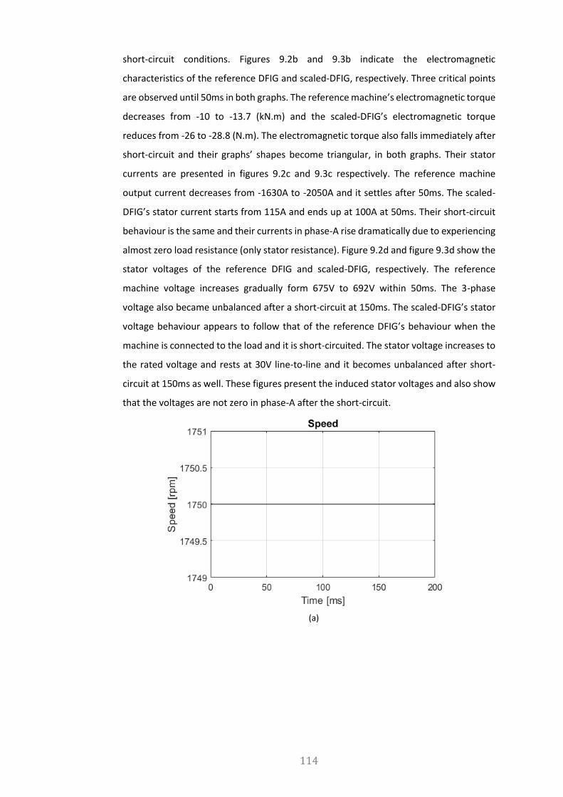
114

short-circuit conditions. Figures 9.2b and 9.3b indicate the electromagnetic

characteristics of the reference DFIG and scaled-DFIG, respectively. Three critical points

are observed until 50ms in both graphs. The reference machine’s electromagnetic torque

decreases from -10 to -13.7 (kN.m) and the scaled-DFIG’s electromagnetic torque

reduces from -26 to -28.8 (N.m). The electromagnetic torque also falls immediately after

short-circuit and their graphs’ shapes become triangular, in both graphs. Their stator

currents are presented in figures 9.2c and 9.3c respectively. The reference machine

output current decreases from -1630A to -2050A and it settles after 50ms. The scaled-

DFIG’s stator current starts from 115A and ends up at 100A at 50ms. Their short-circuit

behaviour is the same and their currents in phase-A rise dramatically due to experiencing

almost zero load resistance (only stator resistance). Figure 9.2d and figure 9.3d show the

stator voltages of the reference DFIG and scaled-DFIG, respectively. The reference

machine voltage increases gradually form 675V to 692V within 50ms. The 3-phase

voltage also became unbalanced after a short-circuit at 150ms. The scaled-DFIG’s stator

voltage behaviour appears to follow that of the reference DFIG’s behaviour when the

machine is connected to the load and it is short-circuited. The stator voltage increases to

the rated voltage and rests at 30V line-to-line and it becomes unbalanced after short-

circuit at 150ms as well. These figures present the induced stator voltages and also show

that the voltages are not zero in phase-A after the short-circuit.

(a)

115

(b)

(c)

(d)

Fig. 9.2 The reference DFIG FEA results a) rotor rotational speed b) electromagnetic torque c) stator current d) stator voltage.

116

(a)

(b)

(c)

117

(d)

Fig. 9.3 The scaled-DFIG FEA results a) rotor rotational speed b) electromagnetic torque c) stator current d) stator voltage.

The short-circuit scenario was performed to place the DFIGs under transient conditions

in Maxwell 3D. The reference-DFIG and the micro-DFIG circuits were shorted to earth at

150ms. It proves that their dynamic behaviours are similar in the transient state.

Therefore, the micro-DFIG design is acceptable.

9.4 The micro-DFIG Transient State Results

The experimental results are compared to FEA results for the scaled-DFIG, since

experimental results are not available for the reference DFIG. Therefore, the scaled-DFIG

is tested under the same conditions as the FEA simulation, however, the short-circuit

conditions were not tested due to concerns about safety of the operator and lab facilities.

As shown in figure 8.7, the micro-DFIG is excited by California Instruments and the stator

is connected to the load through the transformer. The prototyped DFIG is driven by a DC

motor. It is connected to a balance load on the stator through a transformer. A California

Instrument MX30 programmable power supply is connected to the rotor and acts as a

converter. The data is captured by means of a Yokogawa WT1800 power analyser.

In order to get the machine to its start-up condition, the machine is rotated until it gets

to 1800rpm while the stator is not connected to the load. The machine is tested by

suddenly connecting it to the load and the results are shown in figure 9.4. The speed is

reduced as presented in figure 9.4a. Figure 9.4b and 9.4c show an overshoot in the output

power and stator current at about 100ms because the electromagnetic fields of the rotor

and stator coils interact. In figure 9.4b, the electrical transient domain starts from about

108ms and it becomes steady at about 160ms. The stator current transient state in

phase-A starts from 102ms and it takes 53ms to reach steady-state.

118

(a)

(b)

(c)

119

(d)

Fig. 9.4 The scaled-DFIG test results a) rotor rotational speed b) electromagnetic torque c) stator current d) stator voltage when the machine starts to operate.

Figure 9.4d indicates that the stator voltage has increased to 38V as a result of

electromagnetic fields interacting and three peaks are observed from 100 to 153ms. The

results in figures 9.3 and 9.4 show that the scaled-DFIG and the prototyped DFIG behave

the same under the start-up condition. Figure 9.5 presents the results of the prototyped

DFIG when the load is increased by 30 percent.

(a)

120

(b)

(c)

(d)

Fig. 9.5 The scaled-DFIG test results a) rotor rotational speed b) electromagnetic torque c) stator current d) stator voltage when the machine’s load increases.

121

The load is increased from 3.8kW to 5.6kw when the rotational speed is 1800rpm. As a

result: sudden increasing the electromagnetic torque on the shaft, the output power

graph peaks at about 100ms while the rotational speed drops slightly until 133ms and

then starts to return to the initial speed. It can be observed that the electrical transient

domain is between 133ms and 185ms as shown in figure 9.5b. The output power

becomes constant after 185ms when it is 5.6kW at 303ms which is very close to output

power at 186ms. Figures 9.5c and 9.5d show the stator current and voltage

characteristics, respectively. The stator current characteristics have a similar behaviour

to the output power graph as opposed to the stator voltage. The electromagnetic fields

interaction causes a significant increase at about 100ms and its time constant is 50ms in

figures 9.5b and 9.5c. As expected, the stator voltage magnitude is constant in figure

9.5d. Figure 9.6 presents the result of simulation of the scaled-DFIG in FEA under the

same conditions as the previous test.

(a)

122

(b)

(c)

(d)

Fig. 9.6 The scaled-DFIG FEA results a) rotor rotational speed b) electromagnetic torque c) stator current d) stator voltage when the machine’s load increases.

The rotational speed is constant in figure 9.6a even when the load is added at 50ms. The

output power suddenly increases at 50ms and it reduces gradually to its steady-state

value at 100ms. Figure 9.6c illustrates three peaks from 50 to 93ms in the Phase-A stator

current. Figure 9.6d shows that the stator voltage magnitude is also steady. Figures 9.5

and 9.6 indicate that the scaled-DFIG and the prototyped DFIG have similar behaviours

while their loads increase. The rotational speed profiles in the test and the FEA simulation

are presented in figure 9.7a and 9.7b, respectively.

123

(a)

(b)

Fig. 9.7 The scaled-DFIG rotational speed graph in, a) the experiment and b) FEA simulation.

As noted, the speed ramps up between the operating points in the test but it is stepped

in the FEA. In fact, there is a delay in the speed increases in the test, while it is

instantaneous in the FEA simulation. Figure 9.8a and 9.8b present the output power of

the scaled-DFIG based on the rotational speed profiles.

124

(a)

(b)

Fig. 9.8 The scaled-DFIG output power characteristics when speed increases, a) in the experiment and b) in FEA simulation.

In the laboratory test, the speed increases twice between 165-200ms and 335-370ms.

The influence of the speed variations is evident in the output power graph within these

periods. The output power rises dramatically when the speed increases and it decreases

gradually after the rotational speed becomes constant in figure 9.8a. The FEA results

show that the output power increases quickly after the rotational speed is raised and it

becomes steady after about 45ms. The output power behaviour of the scaled-DFIG in the

laboratory test and the FEA simulation are similar. The stator current graph varies with

the rotational speed profile in the same manner as the output power. Figure 9.9 indicates

the stator current of the scaled-DFIG in the test and the FEA simulation.

125

(a)

(b)

Fig. 9.9 The scaled-DFIG stator current characteristics when speed increases, a) in the experiment and b) in FEA simulation.

Figures 9.9a shows that the electrical transient domains are between 205-257ms and

376-428ms. Three peaks can also be observed in each one. The stator current settles at

101.5A and 106.5A when the speed becomes steady in each step. Figure 9.9b shows the

current passes three peaks within 70-113ms and 130-175ms as it gradually reduces. The

stator voltage of the scaled-DFIG in the laboratory test and FEA are presented in figures

9.10a and 9.10b, respectively. As noted, the stator voltage is constant while the speed

varies.

126

(a)

(b)

Fig. 9.10 The scaled-DFIG stator voltage characteristics when speed increases, a) in the experiment and b) in FEA simulation.

Figure 9. 11 presents the temperature of cores and windings at full-load after running for

an hour.

127

Fig. 9.11 The thermal image of the micro-DFIG at full-load.

As seen above, the maximum temperature of rotor is 120℃, the slip rings are 100℃, and

the rest of the parts are less than 60℃. It proves that the cooling system of the machine

is capable to transferring the heat and protecting the insulations.

128

10. Conclusions and Recommendations

10.1 Conclusions

Based on the finding of this project, the following conclusion can be made:

1- Wound Rotor Induction Machine Design and Reference Design:

This dissertation has expressed the analytical design of the wound rotor induction

machine, following the literature review regarding induction machine design. The sizing

equations of the induction machine design have been illustrated and a reference design

was presented and verified in Maxwell 2D.

2- Investigation in the Wind Energy Conversion System with a DFIG:

The effect of various voltages and speeds has been investigated in the WECS with the

DFIG. The investigation was necessary in order to explore the DFIG’s design impact on

the cost and performance of the WECS. As a result, if there is an opportunity to redesign

a DFIG for the current WECS it would be reasonable to design it for a medium voltage

system.

3- Investigation in the Wind Energy Integration Issues

The penetration of the wind energy in the power system has been investigated to

illustrate their behaviours in the transient state. Then, the aggregation has been

introduced to develop a better understanding of the integration issues. The aggregated

models are introduced for specific issues but they present challenges as they are not

accurate. For instance, an accurate model is still required to predict the behaviour of

wind energy within the grid when there is a short-circuit. Furthermore, a single machine

equivalent is also discussed, but it is not feasible to be prototyped. Each power system

requires a specific model to accurately investigate the wind energy penetration within

sensible time.

4- Finding Critical Characteristics in Wound Rotor Induction Machine’s Transient

Behaviour:

The dynamic modelling of the induction machine has been expressed by a number of

equations to illustrate their transient behaviours. These equations have been transferred

to the stationary frame to decrease the model difficulty. These models have been

employed in FEA software to simulate the electrical machines mathematically. These

models theoretically can show the effective parameters on the dynamic behaviour of the

machine. These parameters can also be related to the machine’s geometry. This means

129

that the machine can be scaled while the reference and the scaled machine behave the

same during transient conditions.

5- Investigation in Dimensional Analysis and Micro-Machine’s Applications

The micro-machines have been expressed with their applications. They have been used

to solve the integration issues of the turbo-alternator. The dimensional analysis is also

discussed to design micro-machines. As the scaled wind generator would react the same

as the reference generator, it is feasible to employ them in solving the wind farm

integration issues.

6- Similarity Between Transient Behaviours’ of Reference DFIG and micro-DFIG

The mathematical modelling is adapted in order to identify the dominant parameters

in the equivalent circuit of the DFIG, which determines its behaviour. These equivalent

circuit elements must ultimately remain unchanged after the scaling process in order to

maintain the same behaviour of the reference machine and the scaled-DFIG. The scaling

process is outlined with the scaling factors and the scaling equation. Per-unit resistance

and per-unit reactance are kept equal between the reference DFIG and scaled-DFIG.

However, the magnetization reactances are different because the same airgap is used.

The reference DFIG and the scaled-DFIG are verified in the FEA and were tested under a

transient condition. The objective of the project was met, despite the efficiency of the

scaled-machine being less than the reference machine. The prototype DFIG was also

tested under the same transient conditions as FEA. There is a similarity between the FEA

and the prototype DFIG at the transient region. However, there are mechanical effects

which affect the test results of the prototype DFIG, which are not modelled in the FEA

(Maxwell), and hence not presented in the results, even though parameters, such as

inertia were implemented in the FEA software. The results show that the electrical

dynamic behaviour of the simulated and prototype scaled-DFIGs are similar, which

proves the objective of this investigation.

10.2 Recommendations and Future Work

Most of available FE software are facilitated to design squirrel cage induction machines

and they sometimes require complicated adjustments to simulate WRIMs. For instance

in the Flux, squirrel cage bars material must be replaced by copper and the machine

equivalent circuit also needs to justify simulating a WRIM while the rotor slots shape still

needs to be defined. Due to these challenges, Maxwell is employed to design wound

rotor induction machine in this project. However, Maxwell does not cover the mechanical

impacts of the machine (even though there are inertia variables that may be assigned).

130

Therefore, it is recommended to develop FE software for particularly wound rotor

machines since they are the popular wind generators.

Since a single machine is infeasible to simulate a wind farm and as result investigate the

wind integration issue, an ideal solution may be prototyping a laboratory based wind

farm using micro wind generators. The laboratory wind farm can include different types

of wind generators such as DFIG, SCIG, and PMSG. It should be capable of testing under

different wind profiles while it interacts with the grid (depends on where it is installed).

131

11. References

[1] T. Ackermann, Wind Power in Power Systems. John Wiley, 2005.

[2] J. G. Slootweg and E. de Vries, “Inside Wind Turbines - Fixed vs. Variable Speed,”

Renew. Energy World, pp. 30–40, 2003.

[3] I. Boldea and S. A. Nasar, The Induction Machines Design Handbook. CRC

Press/Taylor & Francis, 2010.

[4] R. Robert, “Micromachines and Microreseaux: Study of the Problems of Transient

Stability by the use of Models Similar Electromechanically to Existing Machines

and Systems,” in CIGRE, pp. 338–346, 1950.

[5] A. Rangekar, K. V. N. Rao, M. K. Gupta, and S. N. Saxena, “Development of Time

Constant Regulator for Micron-machine,” IEEE Trans. Ind. Electron., vol. IE-32,

1985.

[6] S. S. Kalsi and B. Adkins, “Transient Stability of Power Systems Containing both

Synchronous and Induction Machines,” Proc. IEE, vol. 118, no. 10, pp. 1467–1474,

1971.

[7] T. J. Hammons and A. J. Parsons, “Design of Microalternator for Power-System-

Stability Investigations,” Proc. Inst. Electr. Eng. UK, vol. 118, no. 10, p. 1421, 1971.

[8] M. J. Jefferies and A. Wright, “New Approach to Micromachine Construction,”

Proc. Inst. Electr. Eng. UK, vol. 117, no. 7, p. 1309, 1970.

[9] P. L. Alger, The Nature of Induction Machines. Gordon and Breach, 1965.

[10] V. A. Venikov and A. V Ivanov-Smolenski, “Developing Physical Models of Electrical

Systems,” Elektrichstro, pp. 1–10, 1955.

[11] C. M. Focken, Dimensional Methods and their Applications. London: Arnold, 1953.

[12] S. Berchten, K. Reichert, and E. Thaler, “Micromachine for Real-Time Generator

Simulation Design Limits and a Novel Solution with Adjustable Parameters,” IEEE

Trans. Energy Con., vol. 9, no. 12, pp. 38–39, 1989.

[13] D.W. Auckland and R. Shuttleworth, “Compensation Systems for a Micromachine

Model,” IEE Proc. C Gener. Transm. Distrib., vol. 128, no. 1, pp. 12–17, 1981.

[14] D. W. Auckland, R. Shuttleworth, and Y. A. A. Turki, “Micromachine Model for the

132

Simulation of Turbine Generators,” Transm. Distrib., vol. 134, no. 4, pp. 265–271,

1987.

[15] D. W. Auckland, S. M. L. Kabir, and R. Shuttleworth, “Generator Model for Power

System Studies,” Transm. Distrib., vol. 137, no. 6, pp. 383–390, 1990.

[16] D. Ruiz, T. I. Asiain, and D. Olguin, “Teaching and Research Laboratory Simulator

of Electric Power Systems,” in FIE ’99. 29th Annual Frontiers in Education

Conference, p. 11B6/8-11B6/14, 1999.

[17] C. Concordia, Synchronous Machines, Theory and Performance. New York, 1951.

[18] J. H. Walker, Large Synchronous Machines. Clarendon Press, 1981.

[19] B. R. Singla, S. Marwaha, and A. Marwaha, “Design and Transient Analysis of Cage

Induction Motor Using Finite Element Methods,” in 2006 International Conference

on Power Electronic, Drives and Energy Systems, pp. 1–5, 2006.

[20] L. Livadaru, A. Munteanu, A. Simion, and C.-G. Cantemir, “Design and finite

element analysis of high-density torque induction motor for traction

applications,” in 2015 9th International Symposium on Advanced Topics in

Electrical Engineering (ATEE), pp. 211–214, 2015.

[21] S. Williamson, “Implementation of finite-element analysis in a cage induction

motor electrical design program,” in Seventh International Conference on

Electrical Machines and Drives, pp. 57–61, 1995.

[22] R. Richter, “Electric Machines,” Bassel/Stuttgart: Verlag Birkhauser, 1954.

[23] P. L. Cochran, Polyphase Induction Motors. M. Dekker, 1989.

[24] P. L. Alger, Induction Machines, Their Behavior and Uses. Gordon and Breach,

1970.

[25] T. A. Lipo, Introduction to AC Machine Design. Wisconsin Power Electronics

Research Center, University of Wisconsin, 2004.

[26] E. S. Hamdi, Design of Small Electrical Machines, 1st ed. Chichester: Wiley, 1994.

[27] F. F. Tang and X., Induction Machine Design Handbook. Shanghai, China: China

Machine Press, 2002.

[28] Ca.mouser.com, “Mouser Electronics - Electronic Components Distributor.” 2016.

[29] “Wind Energy Foundation,” 2016. [Online]. Available:

133

http://windenergyfoundation.org/. [Accessed: 09-Jul-2016].

[30] “U.S. Motors,” 2016. [Online]. Available: http://www.usmotors.com/. [Accessed:

11-Apr-2016].

[31] I. Boldea, The Electric Generators Handbook. CRC/Taylor & Francis, 2006.

[32] I. Boldea, Linear Electric Machines, Drives, and Maglevs Handbook, 1st ed. Boca

Raton, Fla.: CRC Press, 2013.

[33] E. R. Laithwaite, Induction Machines for Special Purposes. Newnes, 1966.

[34] C. A. Gross, Electric Machines. CRC Press, 2007.

[35] R. J. Kerkman, G. L. Skibinski, D. W. Schlegel, and A. C. Drives;, “A.C. drives; Year

2000 and Beyond,” in Record of IEEE – APEC, 1999.

[36] P. Gipe, Wind Energy Comes of Age. Wiley, 1995.

[37] C. G. Veinott, Theory and Design of Small Induction Motors. McGraw-Hill, 1959.

[38] M. G. Say, The Performance and Design of Alternating Current Machines. Pitman,

1958.

[39] A. K. Sawhney, A Course in Electrical Machine Design. Dhanpat Rai and Sons, 1984.

[40] J. Pyrhonen, T. Jokinen, and V. Hrabovcova, Design of Rotating Electrical

Machines, 1st ed. .

[41] C. Kral, A. Haumer, M. Haigis, H. Lang, and H. Kapeller, “Comparison of a CFD

Analysis and a Thermal Equivalent Circuit Model of a TEFC Induction Machine

With Measurements,” IEEE Trans. Energy Con., vol. 24, no. 4, pp. 809–818, 2009.

[42] S. L. Ho and W. N. Fu, “Review and Future Application of Finite Element Methodes

in Induction Motors,” Electr. Mach. Power Syst., vol. 26, no. 2, pp. 111–125, 1998.

[43] S. A. Nasar, Handbook of Electric Machines. McGraw-Hill, 1987.

[44] A. H. Bonnett, “A Comparison Between Insulation Systems Available for PWM-

Inverter-Fed Motors,” IEEE Trans. Ind. Appl., vol. 33, no. 5, pp. 1331–1341, 1997.

[45] T. G. Arora, M. V. Aware, and D. R. Tutakne, “Effect of Pulse Width Modulated

Voltage on Induction Motor Insulation,” in 2012 7th IEEE Conference on Industrial

Electronics and Applications (ICIEA), pp. 2044–2048, 2012.

[46] G. Mugala, R. Eriksson, and P. Pettersson, “Comparing Two Measurement

134

Techniques for High Frequency Characterization of Power Cable Semiconducting

and Insulating Materials,” IEEE Trans. Dielectr. Electr. Insul., vol. 13, no. 4, pp. 712–

716, 2006.

[47] M. L. Miller, “Common Characterization Techniques for Insulating Materials Used

in Turbine Generators,” in EIC, 2007.

[48] M. Sawahata, K. Nishihama, H. Mikami, and T. Fujigaki, “Magnetic Flux Density

Analysis of Wound Rotor Induction Motor by Permeance Model,” in International

Conference on Electrical Machines and Systems (ICEM), 2009, pp. 1–6.

[49] M. Birkfeld and K. A. Hempel, “Calculation of the Magnetic Behaviour of Electrical

Steel Sheet Under Two Dimensional Excitation by Means of the Reluctance

Tensor,” IEEE Trans. Magn., vol. 33, no. 5, pp. 3757–3759, 1997.

[50] M. J. Hofmann and H.-G. Herzog, “Modeling Magnetic Power Losses in Electrical

Steel Sheets in Respect of Arbitrary Alternating Induction Waveforms: Theoretical

Considerations and Model Synthesis,” IEEE Trans. Magn., vol. 51, no. 2, pp. 1–11,

2015.

[51] J. Martinez-Roman, J. Perez-Cruz, M. Pineda-Sanchez, R. Puche-Panadero, J.

Roger-Folch, M. Riera-Guasp, and A. Sapena-Bano, “Electrical Machines

Laminations Magnetic Properties: A Virtual Instrument Laboratory,” IEEE Trans.

Educ., vol. 58, no. 3, pp. 159–166, Aug. 2015.

[52] M. Mochizuki, S. Hibino, and F. Ishibashi, “Application of 6.5% Silicon Steel Sheet

to Induction Motor and ITS Magnetic Properties,” Electr. Mach. Power Syst., vol.

22, no. 1, pp. 17–29, 1994.

[53] S. W. Cheong, E. J. Hilinski, and A. D. Rollett, “Grain Growth in a Low-Loss Cold-

Rolled Motor-Lamination Steel,” Met. Mat Trans A, vol. 34, no. 6, pp. 1321–1327,

2003.

[54] S. Sprague and D. Jones, “Using the New Lamination Steels Database in Motor

Design,” in Proceedings of SMMA, pp. 1–12, 2000.

[55] R. Kimmich, M. Doppelbauer, D. T. Pefers, J. G. Cowie, and E. F. Bruvn, “Die Cast

Copper Rotor Motors via Simple Substitution and Motor Redesign for Copper,” in

International Conference on Electrical Machines and Systems (ICEM), 2006.

[56] M. G. Say, Alternating Current Machines. Wiley, 1976.

[57] G. Madescu, I. Boldea, and T. J. E. Miller, “An Analytical Iterative Model (AIM) for

135

Induction Motor Design,” IEEE Trans. Ind. App., vol. 23, pp. 566–573, 1996.

[58] J. Wanjiku, M. A. Khan, P. S. Barendse, and P. Pillay, “Influence of Slot Openings

and Tooth Profile on Cogging Torque in Axial-Flux PM Machines,” IEEE Trans. Ind.

Electron., vol. 62, no. 12, pp. 7578–7589, Dec. 2015.

[59] O. O. Ogidi, P. S. Barendse, and M. A. Khan, “Detection of Static Eccentricities in

Axial-Flux Permanent-Magnet Machines With Concentrated Windings Using

Vibration Analysis,” IEEE Trans. Ind. Appl., vol. 51, no. 6, pp. 4425–4434, Nov.

2015.

[60] H. Dehnavifard, M. Khan, and P. Barendse, “Development of a 5kW Scaled

Prototype of a 2.5 MW Doubly-Fed Induction Generator,” IEEE Trans. Ind. Appl.,

2016.

[61] I. Daut, K. Anayet, and S. Tirapathy, “Design and modeling of induction motor

using opera 2D based on aluminum material,” in 2009 3rd International

Conference on Energy and Environment (ICEE), pp. 94–97, 2009.

[62] J.-S. Rho, C.-H. Lee, and H.-K. Jung, “Optimal Design of Ultrasonic Motor Using

Evolution Strategy and Finite Element Method,” Int. J. Appl. Electromagn. Mech.,

vol. 25, pp. 699–704, 2007.

[63] L. Jun-qing and W. Xi-mei, “FEM Analysis on Interturn Fault of Rotor Wingding in

DFIG,” in Electrical Machines and Systems, pp. 797–802, 2013.

[64] Y. Duan and R. G. Harley, “A Novel Method for Multiobjective Design and

Optimization of Three Phase Induction Machines,” IEEE Trans. Ind. App., vol. 47,

no. 4, pp. 1707–1715, 2011.

[65] L. Fan, Z. Miao, L. F. Miao, Z., L. Fan, Z. Miao, L. F. Miao, and Z., Modeling and

Analysis of Doubly Fed Induction Generator Wind Energy Systems. London:

Academic Press, 2015.

[66] G. I. Vakil and K. R. Rajagopal, “Computer Aided Design of a Compact Doubly-Fed

Induction Generator for Small Wind Power Application,” IEEE Trans. Ind. App., pp.

456–460, 2010.

[67] S. J. Chapman, Electric Machinery Fundamentals. McGraw-Hill, 1999.

[68] J. Martinez, A. Belahcen, and A. Arkkio, “3D Permeance Model of Induction

Machines Taking into Account Saturation Effects and its Connection with Stator

Current and Shaft Speed Spectra,” IET Electr. Power Appl., vol. 9, no. 1, pp. 20–29,

136

2015.

[69] J. R. Lopez, “The Effect of Induction Motor Design on Losses and Efficiency for

Adjustable Frequency Drives,” Conf. Rec. ISIE’94, pp. 214–219, 1994.

[70] W. L. Soong, G. B. Kliman, R. N. Johnson, R. A. White, and J. E. Miller, “Novel High-

Speed Induction Motor for a Commercial Centrifugal Compressor,” IEEE Trans.

Ind. Appl., vol. 36, no. 3, pp. 706–713, 2000.

[71] B. J. Chalmers and A. C. Williamson, A.C. Machines. Research Studies Press, 1991.

[72] P. C. Sen, Principles of Electric Machines and Power Electronics. John Wiley & Sons,

1997.

[73] T. L. Mthombeni, P. Pillay, and R. M. W. Strnat, “New Epstein Frame for

Lamination Core Loss Measurements Under High Frequencies and High Flux

Densities,” IEEE Trans. Energy Con., vol. 22, no. 3, pp. 614–620, 2007.

[74] O. Barre and B. Napame, “Fractional Slot Concentrated Windings: A New Method

to Manage the Mutual Inductance between Phases in Three-Phase Electrical

Machines and Multi-Star Electrical Machines,” Machines, vol. 3, no. 2, pp. 123–

137, 2015.

[75] B. Amin, Induction Motors. Springer, 2001.

[76] A. Boglietti, A. Cavagnino, and M. Lazzari, “Geometrical Approach to Induction

Motor Design,” in the 33rd Annual Conference of the IEEE Industrial Electronics

Society (IECON), pp. 149–156, 2007.

[77] D. H. Braymer and A. C. Roe, Rewinding Small Motors. McGraw-Hill, 1949.

[78] M. Cistelecan and E. Demeter, “New Three-Phase A.C. Windings with Low Spatial

Harmonic Content,” Rec. Electromotion Symp., pp. 98–100, 1997.

[79] K. Wilkinson, Rewinding Small Motors. Newnes, 1965.

[80] C. I. McClay and S. Williamson, “Influence of Rotor Skew on Cage Motor Losses,”

IEE Proc. - Electr. Power Appl., vol. 145, no. 5, p. 414, 1998.

[81] J. Staszak, “Determination of Slot Leakage Inductance for Three-Phase Induction

Motor Winding using an Analytical Method,” Arch. Electr. Eng., vol. 62, no. 4,

2013.

[82] H. F. Parshall and H. M. Hobart, Armature Windings of Electric Machines. D. Van

137

Nostrand Co, 1895.

[83] M. Ruviaro, F. Runcos, N. Sadowski, and I. M. Borges, “Analysis and Test Results

of a Brushless Doubly Fed Induction Machine With Rotary Transformer,” IEEE

Trans. Ind. Electron., vol. 59, no. 6, pp. 2670–2677, 2012.

[84] E. Abdi, M. R. Tatlow, R. A. McMahon, and P. J. Tavner, “Design and Performance

Analysis of a 6 MW Medium-Speed Brushless DFIG,” in Renewable Power

Generation Conference (RPG), pp. 1–4, 2013.

[85] D. M. Ionel, M. V Cistelecan, T. J. E. Miller, and M. I. McGilp, “A New Analytical

Method for the Computation of Airgap Reactances in Three-Phase Induction

Machines,” Rec. IEEE – IAS, Annu. Meet., vol. 1, pp. 65–72, 1998.

[86] T. Jokinen, “Flux Leakage,” 2008.

[87] H. Sequenz, “The Windings of Electric Machines,” in A.C. Machines, vol. 3, Vienna:

Springer Verlag, 1950.

[88] A. R. W. Broadway, “Part–Symmetrization of Three-Phase Windings,” IEEE Trans.

Ind. App., vol. 12, pp. 122–125, 1975.

[89] M. V Cistelecan and E. Demeter, “A Closer Approach of the Fractional Multilayer

Three-phase A.C. Windings,” Rec. Electromotion, vol. 1, p. 51-- 54., 1999.

[90] G. H. Rawcliffe, R. F. Burbidge, and W. Fong, “Induction-Motor Speed-Changing by

Pole-Amplitude Modulation,” Proc. IEE Part A Power Eng., vol. 105, no. 22, p. 411,

1958.

[91] H. Nam, S.-K. Jung, G.-H. Kang, J.-P. Hong, T.-U. Jung, and S.-M. Baek, “Design of

Pole-Change Single-Phase Induction Motor for House hold Appliances,” IEEE

Trans. Ind. App., vol. 40, no. 3, pp. 780–788, 2004.

[92] C. Zhang, J. Yang, X. Chen, and Y. Guo, “A New Design Principle for Pole-Changing

Winding-the Three-Equation Principle,” Electr. Mach. Power Syst., vol. 22, no. 2,

pp. 187–199, 1994.

[93] M. Poloujadoff, J. C. Mipo, and P. Siarry, “Designing 2 Pole and 2/4 Pole Windings

by the Simulated Annealing Method,” Electr. Mach. Power Syst., vol. 26, no. 10,

pp. 1059–1066, 1998.

[94] A. S. Langsdorf, “Air-Gap Flux in Induction Motors,” Trans. Am. Inst. Electr. Eng.,

vol. XXIV, pp. 919–931, 1905.

138

[95] A. Hughes, “New 3-Phase Winding of Low m.m.f. Harmonic Content,” Proc. Inst.

Electr. Eng. UK, vol. 117, no. 8, p. 1657, 1970.

[96] N. Bianchi, S. Bolognani, and F. Tonel, “Thermal Analysis of a Run-Capacitor Single-

Phase Induction Motor,” IEEE Trans. Ind. App., vol. 39, no. 2, pp. 457–465, 2003.

[97] I. Boldea and S. A. Nasar, Induction Machine Handbook. Boca Raton, Fla: CRC

Press, 1998.

[98] W. H. McAdams, Heat Transmission, 2nd ed. New York: McGraw Hill Inc., 1942.

[99] S. C. Mukhopadhyay and S. K. Pal, “Temperature Analysis of Induction Motors

using a Hybrid Thermal Model with Distributed Heat Sources,” J. Appl. Phys., vol.

83, no. 11, p. 6368, 1998.

[100] A. Boglietti, A. Cavagnino, M. Lazzari, and M. Pastorelli, “A Simplified Thermal

Model for Power Derating Prediction of TEFC Induction Motors,” Electr. Power

Components Syst., vol. 32, no. 7, pp. 701–723, 2004.

[101] G. Bellenda, L. Ferraris, and A.Tenconi, “A New Simplified Thermal Model for

Induction Motors for EVs Applications,” in Electrical Machines and Drives, pp. 11–

13, 1995.

[102] D. Staton, A. Boglietti, and A. Cavagnino, “Solving the More Difficult Aspects of

Electric Motor Thermal Analysis in Small and Medium Size Industrial Induction

Motors,” IEEE Trans. Energy Con., vol. 20, no. 3, pp. 620–628, 2005.

[103] A. Boglietti, A. Cavagnino, M. Popescu, and D. Staton, “Thermal Model and

Analysis of Wound-Rotor Induction Machine,” IEEE Trans. Ind. Electron., vol. 49,

no. 5, pp. 2078–2085, 2013.

[104] A. Boglietti, A. Cavagnino, and D. A. Staton, “TEFC Induction Motors Thermal

Models: A Parameter Sensitivity Analysis,” IEEE Trans. Ind. App., vol. 41, no. 3, pp.

756–763, 2005.

[105] N. Christofides, “Origins of Load Losses in Induction Motors with Cast Aluminium

Rotors,” Proc. Inst. Electr. Eng. UK, vol. 112, no. 12, p. 2317, 1965.

[106] Z. Tan, S. Member, X. Song, W. Cao, and S. Member, “DFIG Machine Design for

Maximizing Power Output Based on Surrogate Optimization Algorithm,” IEEE

Trans. Energy Convers., vol. 30, no. 3, pp. 1154–1162, 2015.

[107] W. A. Roshen, “Magnetic Losses for Non-Sinusoidal Waveforms Found in AC

139

Motors,” IEEE Trans. Power Electron., vol. 21, no. 4, pp. 1138–1141, 2006.

[108] A. A. Jimoh, Stray Load Losses in Induction Machines. National Library of Canada,

1987.

[109] A. Visintin, “Mathematical Models of Hysteresis,” phdthesis, University of Trieste,

2005.

[110] I. Mayergoyz, “Mathematical Models of Hysteresis,” IEEE Trans. Magn., vol. 22,

no. 5, pp. 603–608, 1986.

[111] S. Yanase, H. Kimata, Y. Okazaki, and S. Hashi, “A Simple Predicting Method for

Magnetic Losses of Electrical Steel Sheets under Arbitrary Induction Waveform,”

IEEE Trans. Magn., vol. 41, no. 11, pp. 4365–4367, 2005.

[112] M. J. Manyage, T. L. Mthombeni, P. Pillay, and A. Boglietti, “Improved Prediction

of Core Losses in Induction Motors,” in 2007 IEEE International Electric Machines

& Drives Conference, pp. 531–536, 2007.

[113] M. Popescu and D. M. Ionel, “A Best-Fit Model of Power Losses in Cold Rolled-

Motor Lamination Steel Operating in a Wide Range of Frequency and

Magnetization,” IEEE Trans. Magn., vol. 43, no. 4, pp. 1753–1756, 2007.

[114] K. Roy, D. Chatterjee, and A. K. Ganguli, “Modeling and Estimation of Core Losses

for Doubly-fed Wound Rotor Induction Machine,” in IEEE India Conference

(INDICON), pp. 1–4, 2010.

[115] E. M. Olin, “Determination of Power Efficiency of Rotating Electric Machines:

Summation of Losses Versus Input-Output Tests,” Proc. Am. Inst. Electr. Eng., vol.

31, no. 7, pp. 1287–1310, 1912.

[116] A. M. Odok, “Stray-Load Losses and Stray Torques in Induction Machines,” Trans.

Am. Inst. Electr. Eng. Part III Power Appar. Syst., vol. 77, no. 3, pp. 43–53, 1958.

[117] S. C. Englebretson, Induction Machine Stray Loss from Inter-Bar Currents. 2009.

[118] P. L. Alger, G. Angst, and E. J. Davies, “Stray-Load Losses in Polyphase Induction

Maclines,” Trans. Am. Inst. Electr. Eng. Part III Power Appar. Syst., vol. 78, no. 3,

pp. 349–355, 1959.

[119] W. Cao, K. J. Bradley, and J. Allen, “Evaluation of additional loss in induction

motors consequent on repair and rewinding,” in IEE Proc. Electr. Power Appl., pp.

1–6, 2006.

140

[120] W. Cao, K. J. Bradley, and A. Member, “Assessing the Impacts of Rewind and

Repeated Rewinds on Induction Motors : Is an Opportunity for Re-Designing the

Machine Being Wasted ?,” IEEE Trans. Ind. App., vol. 42, no. 4, pp. 958–964, 2006.

[121] N. David, D. C. Aliprantis, and S. Member, “Improved Efficiency of DFIG Wind

Energy Conversion Systems by Operating in the Rotor-Tied Configuration,” pp.

189–195, 2014.

[122] S. Jelassi, R. Romary, and J. F. Brudny, “Slot Design for Dynamic Iron Loss AC

Rotating Electrical Machine Reduction,” in IEEE Energy Conversion Congress and

Exposition (ECCE), pp. 563–569, 2010.

[123] T. A. Lipo, Introduction to AC Machine Design, Third. Madison, USA: Wisconsin

Power Electronics Research Center, University of Wisconsin, 2011.

[124] H. Dehnavifard, A. D. Lilla, M. A. Khan, and P. Barendse, “Design and optimization

of DFIGs with alternate voltage and speed ratings for wind applications,” in 2014

International Conference on Electrical Machines (ICEM), pp. 2008–2013, 2014.

[125] A. D. Lilla, H. Dehnavifard, M. A. Khan, and P. Barendse, “Optimization of high

voltage geared permanent-magnet synchronous generator systems,” in 2014

International Conference on Electrical Machines (ICEM), pp. 1356–1362, 2014.

[126] W. Erdman and M. Behnke, “Low Wind Speed Turbine Project Phase II : The

Application of Medium-Voltage Electrical Apparatus to the Class of Variable Speed

Multi-Megawatt Low Wind Speed Turbines Low Wind Speed Turbine Project

Phase II : The Application of Medium-Voltage Electrical A,” San Ramon, California,

techreport, 2014.

[127] A. Larsson, “The Power Quality of Wind Turbines,” phdthesis, Chalmers University

of Technology, 2000.

[128] F. Watanabe and T. Uchida, “Micro-siting of Wind Turbine in Complex Terrain:

Simplified Fatigue Life Prediction of Main Bearing in Direct Drive Wind Turbines,”

Wind Eng., vol. 39, no. 4, pp. 349–368, 2015.

[129] J. Manwell, Wind Energy Explained. John Wiley, 2001.

[130] T. Shanker, R. K. Singh, and M. Ieee, “Wind Energy Conversion System : A Review,”

2012.

[131] K. W. E. Cheng, J. K. Lin, Y. J. Bao, and X. D. Xue, “Review of the Wind Energy

Generating System,” 2011.

141

[132] A. Acakpovi and E. Ben Hagan, “A Wind Turbine System Model using a Doubly-Fed

Induction Generator (DFIG),” nternational J. Comput. Appl., vol. 90, no. 15, pp. 6–

11, 2014.

[133] Hui Li, Zhe Chen, and H. Polinder, “Optimization of Multibrid Permanent-Magnet

Wind Generator Systems,” IEEE Trans. Energy Convers., vol. 24, no. 1, pp. 82–92,

Mar. 2009.

[134] S. Heier, Grid Integration of Wind Energy Conversion Systems. Chichester, UK and

Kassel , Germany: John Wiley & Sons Ltd, 1998.

[135] P. J. Tavner, G. J. W. V Brussel, and F. Spinato, “Machine and Converter Reliabilities

in Wind Turbines,” in Proc. 3rd Power Electron. Mach. Drives (PEMD ), pp. 127–

130, 2006.

[136] V. Akhmatov, “Variable-speed Wind Turbines with Doubly-fed Induction

Generators, Part III: Model with the Back-to-back Converters,” Wind Eng., vol. 27,

no. 2, pp. 79–91, 2003.

[137] S. Muller, M. Deicke, and R. DeDoncker, “Adjustable Speed Generators for Wind

Turbines based on Doubly-fed Induction Machines and 4- Quadrant IGBT

Converters Linked to the Rotor,” IEEE Trans. Ind. App., vol. 2, 2000.

[138] Mohan N., T. M. Undeland, and W. P. Robbins, Power Electronics: Converters,

Applications and Design. Oxford, UK: Clarendon Press, 1989.

[139] P. Alemi and D.-C. Lee, “Power Loss Comparison in Two and Three-Level PWM

Converters,” in ECCE, 2011.

[140] W. Song, X. Feng, and K. M. Smedley, “A Carrier-Based PWM Strategy With the

Offset Voltage Injection for Single-Phase Three-Level Neutral-Point-Clamped

Converters,” IEEE Trans. Power Electron., vol. 28, no. 3, pp. 1083–1095, 2013.

[141] J. S. Kim and S. K. Sul, “New Control Scheme for AC–DC–AC converter without DC

link Electrolytic Capacitor,” in PESC’93, 1993, pp. 300–306.

[142] A. Schuster, “A Matrix Converter without Reactive Clamp Elements for an

Induction Motor Drive System,” in PESC’s, 1998, pp. 714–720.

[143] P. W. Wheeler and D. A. Grant, “A Low Loss Matrix Converter for AC Variable-

speed Drives,” in EPE 5th European Conference on Power Electronics and

Application, 1993, vol. 5, pp. 27–32.

142

[144] J. Rodriguez, L. Moran, A. Gonzalez, and C. Silva, “High Voltage Multilevel

Converter with Regeneration Capability,” in PESC’s 99, vol. 2, pp. 1077–1082.

[145] M. Alatalo, “Permanent Magnet Machines with Air Gap Windings and Integrated

Teeth Windings,” Sweden, techreport, 1996.

[146] A. J. Mitcham and N. Grum, “An Integrated LP Shaft Generator for the more

Electric Aircraft,” in IEE Coloquium on All Electric Aircraft, 1998, p. 8/1--8/9.

[147] “U.S. Small Wind Turbine Market: 2014 summary report,” New York, techreport,

2015.

[148] A. M. Alkandari, S. A. Soliman, and M. H. Abdel-rahman, “Steady State Analysis of

a Doubly Fed Induction Generator,” vol. 2011, no. September, pp. 393–400, 2011.

[149] A. Perdana, “Dynamic Models of Wind Turbines A Contribution towards the

Establishment of Standardized Models of Wind Turbines for Power System

Stability Studies,” phdthesis, CHALMERS UNIVERSITY OF TECHNOLOGY, 2008.

[150] M. Ali, I.-S. Ilie, J. V Milanovic, and G. Chicco, “Wind Farm Model Aggregation

Using Probabilistic Clustering,” IEEE Trans. Power Syst., vol. 28, no. 1, pp. 309–

316, 2013.

[151] B. Kivido, “Grid Integration of Wind Energy Systems,” phdthesis, University of

Cape Town, 2014.

[152] M. R. Islam and M. R. I. Sheikh, Enhancement of Power System Stability by Using

DFIG Based Wind Farm, 1st ed. Saarbrucken: LAP LAMBERT Academic Publishing,

2014.

[153] G. Abad, Doubly Fed Induction Machine. Wiley, 2011.

[154] H. Sterling, “Harmonic Field Effects in Induction Machines,” Electron. Power, vol.

23, no. 10, p. 841, 1977.

[155] L. Lin, “Effect of Wind Farm Based-on Wound Rotor Induction Generator on

Transient Characteristics of Transmission Grid,” 2009.

[156] V. Rana and M. A. Ansari, “Wind Farm Integration Effect on Electricity Market

Price,” in ECCE, pp. 349–354, 2013.

[157] S. Dakai, “Discussion of Wind Farm Integration in China,” techreport, 2005.

[158] G. Saccomando, J. Svensson, and A. Sannino, “Improving Voltage Disturbance

143

Rejection for Variable-Speed Wind Turbines,” IEEE Power Eng. Rev., vol. 22, no. 7,

p. 53, 2002.

[159] “An Aggregated Model of a Grid-connected, Large-scale, Offshore Wind Farm for

Power Stability Investigations Importance of Windmill Mechanical System,”

Electr. Power Energy Syst., vol. 24, no. 9, pp. 709–717, 2002.

[160] J. Juang and Y.-C. Huang, Intelligent Technologies and Engineering Systems.

Springer, 2013.

[161] F. Jurado, L. M. Ferna, and J. R. n Saenz, “Aggregated Dynamic Model for Wind

Farms with Doubly Fed Induction Generator Wind Turbines,” Renew. Energy, vol.

33, pp. 129–140, 2008.

[162] N. Jenkins, “Engineering Wind Farms,” Power Eng. J., vol. 4, pp. 53–60, 1993.

[163] J. R. Kristoffersen and P. Christiansen, “Horns Rev Offshore Wind Farm: Its Main

Controller and Remote Control System,” Wind Eng., vol. 27, no. 5, pp. 351–360,

2003.

[164] D. Yang, L. Ban, Z. Xiang, N. Du, B. Zheng, and Z. Wu, “An Aggregation Method of

Wind Farm Model for Electromagnetic Transient Simulation Analysis,” pp. 4–8,

2012.

[165] M. A. Chowdhury, N. Hosseinzadeh, M. M. Billah, and S. A. Haque, “Dynamic DFIG

Wind Farm Model with an Aggregation Technique,” in 6th International

Conference on Electrical and Computer Engineering ICECE 2010, no. December,

pp. 18–20, 2010.

[166] V. Akhmatov, “An Aggregated Model of a Large Wind Farm with Variable-speed

Wind Turbines Equipped with Doubly-fed Induction Generators,” Wind Eng. Press,

2004.

[167] S. J. G., S. W. H. de Haan, H. Polinder, and K. W., “Aggregated Modelling of Wind

Parks with Variable Speed Wind Turbines in Power System Dynamics Simulations,”

in the 14th Power Systems Computation Conference, 2002.

[168] P. Sørensen, B. Bak-Jensen, J. Kristian, A. D. Hansen, L. Janosi, and J. Bech, “Power

Plant Characteristics of Wind Farms,” in in Wind Power for the 21st Century, 2000.

[169] J. G. Slootweg, H. Polinder, and W. L. Kling, “Dynamic Modeling of a Wind Turbine

with Doubly Fed Induction Generator,” in IEEE Power Eng. Soc. Summer Meeting,

2001.

144

[170] A. Trzynadlowski, The Field Orientation Principle in Control of Induction Motors.

Kluwer Academic, 1994.

[171] P. S. Barendse, “Design and Implementation of Variable Speed Induction

Generator For Wind Energy System,” phdthesis, University of Cape Town, 2004.

[172] K. Hamann, “Field Orientated Control of an Induction Motor,” University of Cape

Town, 1999.

[173] P. M. Anderson and A. A. Fouad, Power System Control and Stability. IEEE Press,

2003.

[174] B. M. Wilamowski and J. D. Irwin, Power Electronics and Motor Drives. CRC Press,

2011.

[175] P. Vas, Sensorless Vector and Direct Torque Control. London: Oxford University

Press, 1998.

[176] C. Batlle, A. Dòria-Cerezo, and E. Fossas, “Modeling, Simulation and Control of a

Doubly-Fed Induction Machine,” Proc. Appl. Math. Mech., vol. 7, no. 1, pp.

3030003–3030004, 2007.

[177] J. B. Ekanayake, S. Member, L. Holdsworth, X. Wu, N. Jenkins, and S. Member,

“Dynamic Modeling of Doubly Fed Induction Generator Wind Turbines,” IEEE

Trans. POWER Syst., vol. 18, no. 2, pp. 803–809, 2003.

[178] S. Vicatos, A. Tegopoulos, M. S. Vicatos, J. A. Tegopoulos, S. Vicatos, and A.

Tegopoulos, “Transient State Analysis of a Doubly-Fed Induction Generator under

Three Phase Short Circuit,” IEEE Trans. Energy Con., vol. 6, no. 1, pp. 62–68, Mar.

1991.

[179] S. J. Chapman, Electric Machinery and Power System Fundamentals. McGraw-Hill,

2002.

[180] R. H. Park, “Two-Reaction Theory of Synchronous Machines Generalized Method

of Analysis-Part I & II,” Trans. Am. Inst. Electr. Eng., vol. 48, no. 3, pp. 716–727,

1929.

[181] R. Solomon, M. A. Khan, P. S. Barendse, P. Pillay, and K. A. Folly, “Review and

Application of Micromachines for Wind Energy Integration,” IEEE Int. Conf. Electr.

Mach., pp. 2151–2157, 2012.

[182] H. R and L. L. Freris, “Micromachine Simulation of Steam Power Plant,” Proc. IEE,

145

vol. 121, no. 6, p. 491499, 1974.

[183] M. E. Newton and B. W. Hogg, “Optimal Control of a Micro-Alternator System,”

IEEE Trans. Power Appar. Syst., vol. 95, no. 6, pp. 1822–1833, 1976.

[184] M. P. Kostenko and I. D. Ursav, “Electromagnetic Models of the Kyibyshew Power

Station,” Elektrichstro, vol. 8, pp. 781–795, 1955.

[185] S. H. Kia, H. Henao, S. Member, and G. Capolino, “Windings Monitoring of Wound

Rotor Induction Machines under Fluctuating Load Conditions,” pp. 3459–3465,

2011.

[186] “Induction Motor Laboratory.”

[187] Standards Coordinating Committee 21, “IEEE Standard Test Procedure for

Polyphase Induction Motors and Generators,” 2004.

[188] R. Pena, R. Cardenas, and G. Asher, “Overview of Control Systems for the

Operation of DFIGs in Wind Energy Applications,” in IECON 2013 - 39th Annual

Conference of the IEEE Industrial Electronics Society, pp. 88–95, 2013.

146

12. Appendices Appendix A

A reference DFIG is employed in chapter 3. Appendix A presents the reference DFIG’s

design details with relevant equations.

Table 1 The reference DFIG design details

Specification Formula Quantity

Power[MW] 𝑃 2.5

Efficiency[%] ɳ 95.8

Voltage[V] 𝑉𝑆𝑁 690

Poles 2. 𝑝1 4

Phase 𝑚 3

Speed[rpm] 𝑛1𝑁 1500

Frequency[Hz] 𝑓1 50

Max Slip 𝑆𝑚𝑎𝑥 ±0.25

Electromagnetic

power[MW] 𝑆𝑔𝑁 =

𝑃𝑜𝑤𝑒𝑟

0.96 2.604

Stator power[MW] 𝑆𝑆𝑁 2

Rotor power[MW] 𝑆𝑅𝑁 = 𝑆𝑆𝑁|𝑆𝑚𝑎𝑥| 0.5

Stator Design

Electromagnetic

Torque[kN.m] 𝑇𝑒 =

𝑆𝑔𝑁

2𝜋𝑓1𝑝1

(1 + |𝑆𝑚𝑎𝑥|) 13.27

The shear rotor stress

[N/cm2] 1.5 < 𝑓𝑥𝑡 < 6 6

Stack length ratio 𝜆 =𝑙𝑖

𝐷𝑖𝑠 ; 0.2 < 𝜆 < 1.5 1

Stator Internal

Diameter[m] 𝐷𝑖𝑠 = √

2 × 𝑇𝑒

𝜋 × 𝜆 × 𝑓𝑥𝑡

3

0.52

Stator Outer

Diameter[m] 𝐷𝑜𝑢𝑡 = 1.48 . 𝐷𝑖𝑠 0.796

Rated stator current[A] 𝐼𝑆𝑁 =𝑆𝑆𝑁

√3𝑉𝑆𝑁

1675.46

Airgap flux density[T] 𝐵𝑔1 0.75

Pole pitch[m] 𝜏 =𝜋𝐷𝑖𝑠

2𝑝1 0.4

Stator winding factor

𝐾𝑊1 =𝑠𝑖𝑛

𝜋6

𝑞1𝑠𝑖𝑛𝜋

6𝑞1

𝑠𝑖𝑛𝜋

2

𝑦

𝜏

𝑞1 = 5 (slot per pole per phase) 𝑦

𝜏 : the stator coil span/pole pitch ratio

2

3≤

𝑦

𝜏≤ 1

0.9097

147

Number turn per

current path (rough

calculation)

𝑊1𝑎 =

𝐾𝐸𝑉𝑆𝑁

√3

2√2𝑓1𝑊1𝐾𝑊1𝑎𝐵𝑔1𝜏𝑙𝑖

𝐾𝐸 = 0.97 (0.97 < 𝐾𝐸 < 0.98)

𝑎1 = 2 (current path)

19.32

Number of turn per coil 𝑛𝑐1 =𝑊1

(2𝑝1𝑞1

𝑎1) 2

Number turn 𝑊1 =2𝑝1

𝑎1𝑞1𝑛𝑐1 20

Stator slot pitch[m] 𝜏𝑠 =𝜋𝐷𝑖𝑠

𝑚2𝑝1𝑞1 0.0266

Stator number of slot 𝑁𝑠 = 2𝑝1𝑞1𝑚 60

Stator conductor cross

section[mm2]

𝐴𝑐𝑜𝑠 =𝐼𝑆𝑁

𝑎1. 𝑗𝑐𝑜𝑠

𝑗𝐶𝑂𝑆 = 6.5 [𝐴

𝑚𝑚2] (assumed current density)

128.88

Stator slot width[m] 𝑊𝑆 = 0.5 𝜏𝑠 0.01333

Stator useful slot

area[mm2]

𝐴𝑠𝑢 =2𝑛𝑐1𝐴𝑐𝑜𝑠

𝑘𝑓

𝑘𝑓 = 0.55 (assumed filling factor)

937

Stator useful slot

height[mm] ℎ𝑠𝑢 =

𝐴𝑠𝑢

1000 ∗ 𝑊𝑆 70.315

Arigap[mm] 𝑔 = (0.1 + 0.012√𝑆𝑆𝑛3 )10−3 1.6

Stator back iron core[m]

ℎ𝑐𝑠 =𝐵𝑔𝜏

𝜋𝐵𝑐𝑠

𝐵𝑐𝑠 = 1.55 [𝑇] (assumed stator core flux

density)

0.0637

Outer diameter[m] 𝐷𝑜𝑢𝑡𝑚 = 𝐷𝑖𝑠 + 2(ℎ𝑠𝑚 + ℎ𝑠𝑤 + ℎ𝑐𝑠) 0.7997~0.8

Cross section area of

elementary

conductor[mm2]

𝐴𝑐𝑜𝑠𝑒 =𝐴𝑐𝑜𝑠

4

Number of elementary conductor=4 32.2

Height of elementary

conductor[mm2]

ℎ𝑐𝑒 =𝐴𝑐𝑜𝑠𝑒

𝑎𝑐𝑒

𝑎𝑐𝑒 = 12[𝑚𝑚], (width of elementary

conductor)

𝑚𝑒 = 16 (number of layers elementary

conductors)

2.68

Skin Effect

Β[m-1]

𝛽 = √𝜔1𝜇0𝜎𝑐𝑜

2

𝑎𝑐𝑒

𝑊𝑆

𝜔1 = 2𝜋. 𝑓1

𝜇0 = 1.256 × 10−6

𝜎𝑐𝑜 = 4.3 × 107

69.64

ξ (unnamed in the

reference) 𝜉 = 𝛽 × ℎ𝑐𝑒 0.1866

148

Skin effect coefficient (for 16 layers elementary conductor)

𝐾𝑅𝑚𝑒 = 𝜑(𝜉) +𝑚𝑒

2 − 1

3𝜓(𝜉)

𝜑(𝜉) = 𝜉𝑠𝑖𝑛ℎ2𝜉 + 𝑠𝑖𝑛2𝜉

𝑐𝑜𝑠2ℎ𝜉 − 𝑐𝑜𝑠𝜉= 1

𝜓(𝜉) = 2𝜉(𝑠𝑖𝑛ℎ𝜉 + 𝑠𝑖𝑛𝜉)

𝑐𝑜𝑠ℎ𝜉 + 𝑐𝑜𝑠𝜉= 5.55 × 10−4

1.04675

Additional skin effect

𝐾𝑅𝑎𝑑 = 4𝛽4. ℎ𝑐𝑒4 (

𝑙𝑖𝑙𝑡𝑢𝑟𝑛

)2𝑛𝑐𝑛2

(1 + 𝑐𝑜𝑠𝛾)2

4

𝑙𝑡𝑢𝑟𝑛: coil turn length

𝛾 = (1 −𝑦

𝜏)𝜋

2= 0 (𝑓𝑜𝑟 𝑑𝑖𝑚𝑒𝑛𝑡𝑖𝑜𝑛𝑎𝑙 𝑐𝑜𝑖𝑙)

0.01847

Total skin effect factor 𝐾𝑅 = 1 + (𝐾𝑟𝑚𝑒 − 1)𝑙𝑠𝑡𝑎𝑐𝑘

𝑙𝑡𝑢𝑟𝑛+ 𝐾𝑅𝑎𝑑 1.03717

Rotor Design

Turn ration 𝐾𝑅𝑆 =𝑊2𝐾𝑊2

𝑊1𝐾𝑊1=

1

|𝑆𝑚𝑎𝑥| 4

Stator current reduced to rotor side[A]

𝐼′𝑆𝑁 =𝐼𝑆𝑁

𝐾𝑅𝑆 418.865

Rotor-reduced magnetizing current[A]

𝐼′𝑚 = 𝐾𝑚𝐼′𝑆𝑁 125.6595

Rotor current at max slip[A]

𝐼𝑅𝑁𝑅 = √𝐼′𝑆𝑁

2 + 𝐼′𝑚2 437.3

Rotor power factor 𝑐𝑜𝑠𝜑2𝑁 =𝑃𝑅𝑁

√3 𝑉𝑅𝑁𝐼𝑅𝑁𝑅

0.9578

Rotor winding factor 𝐾𝑊2 =

𝑠𝑖𝑛𝜋6

𝑞2𝑠𝑖𝑛𝜋

6𝑞2

𝑠𝑖𝑛𝜋

2

𝑦𝑅

𝜏

𝑞2 = 4 (Rotor slot per phase per pole)

0.925

Rotor number of slot 𝑁𝑟 = 2𝑝1𝑞2𝑚 48

Rotor turns per phase 𝑊2 = 𝑊1𝐾𝑊1𝐾𝑅𝑆

𝐾𝑊2 78.53~80

Number of turn per coil for rotor

𝑛𝑐2 =𝑊2

(2𝑝1𝑞2

𝑎2)

𝑎2 = 1 (rotor current path)

5

Rotor slot pitch[m] 𝜏𝑅 =𝜋𝐷𝑖𝑠

𝑚12𝑝1𝑞2 0.033805

Rotor conductor cross section[mm2]

𝐴𝑐𝑜𝑟 =𝐼𝑅𝑁

𝑎2. 𝑗𝑐𝑜𝑠

𝑗𝑐𝑜𝑟 = 8 [𝐴

𝑚𝑚2] (assumed current density)

43.4

Rotor slot width[m] 𝑊𝑅 = 0.45 𝜏𝑅 0.0152

Rotor useful slot area[mm2]

𝐴𝑟𝑢 =2𝑛𝑐2𝐴𝑐𝑜𝑟

𝑘𝑓

𝑘𝑓 = 0.55 (assumed filling factor)

789.09

Rotor useful slot height[mm]

ℎ𝑅𝑈 =𝐴𝑟𝑢

1000 ∗ 𝑊𝑅 51.913

149

Minimum rotor teeth width[mm]

𝑊𝑡𝑅𝑚𝑖𝑛 =𝜋(𝐷𝑖𝑠 − 2(𝑔 + ℎ𝑅𝑈 + ℎ𝑅𝑊))

𝑁𝑅

− 𝑊𝑅

11.42

Maximum rotor teeth flux density[T]

𝐵𝑡𝑅𝑚𝑎𝑥 =𝐵𝑔1𝜏𝑅

𝑊𝑡𝑅𝑚𝑖𝑛 2.22

Rotor back iron radial path[m]

ℎ𝐶𝑅 =𝐵𝑔𝜏

𝜋𝐵𝑐𝑟

𝐵𝑐𝑟 = 1.6[𝑇] (assumed rotor core flux

density)

0.0597~

0.06

Inner diameter[m] 𝐷𝐼𝑅 = 𝐷𝐼𝑆 − 2(𝑔 + ℎ𝑆𝑈 + ℎ𝑅𝑊 + ℎ𝐶𝑅) 0.287

Magnetization Current

Carter Coefficient

𝐾𝐶 = 𝐾𝐶1𝐾𝐶2

𝐾𝐶1,𝐶2 =1

1 − 𝛾1,2𝑔

2𝜏𝑠,𝑟

; 𝐾𝐶1 = 1.0826,𝐾𝐶2

= 1.04

𝛾1,2 =(2𝑊𝑆′,𝑅′

𝑔)2

5 +2𝑊𝑆′,𝑅′

𝑔

𝑊𝑆′ =𝑊𝑆

𝜇𝑅𝑆=

13.2

3= 4.066

𝑊𝑅′ =𝑊𝑅

𝜇𝑅𝑅=

15.2

5= 3.04

1.126

Airgap mmf [A.turns] 𝐹𝐴𝐴′ = 𝑔𝐾𝐶

𝐵𝑔1

𝜇0 1083.86

Stator teeth mmf [A.turns]

𝐹𝐴𝐵 = 𝐻𝑡𝑠(ℎ𝑠𝑢 + ℎ𝑠𝑤)

𝐵𝑡𝑠 = 𝐵𝑔1 ×𝜏𝑆

𝑊𝑡𝑠= 1.49[𝑇]

𝐻𝑡𝑠 = 1290 [𝐴/𝑚]

94.62

Stator back iron mmf [A.turns]

𝐹𝐵𝐶 ≈ 𝐻𝑐𝑠. 𝑙𝑐𝑠𝑎𝑣

(𝑙𝑐𝑠𝑤)𝐵𝐶 ≈2

3

𝜋(𝐷𝑜𝑢𝑡 − ℎ𝑐𝑠)

2.2𝑝1= 0.19266 𝑚

𝐻𝑐𝑠 = 1340[𝐴/𝑚]

258.17

Rotor teeth mmf [A.turns]

𝐹𝐴′𝐵′ = 𝐻𝑡𝑟(ℎ𝑅𝑈 + ℎ𝑅𝑊)

𝐵𝑡𝑟𝑡 = 𝐵𝑔1 ×𝜏𝑅

𝑊𝑡𝑅= 1.3629[𝑇]

𝐵𝑡𝑅𝑚 = 𝐵𝑔1 ×𝜏𝑅

𝑊𝑡𝑅𝑚= 1.69[𝑇]

𝐵𝑡𝑅𝑏 = 𝐵𝑔1 ×𝜏𝑅

𝑊𝑡𝑅= 2.2[𝑇]

𝐵𝑡𝑅 =𝐵𝑡𝑅𝑡 + 𝐵𝑡𝑅𝑏 + 4𝐵𝑡𝑅𝑚

6= 1.72[𝑇]

𝐻𝑡𝑟 = 5334 [𝐴/𝑚]

292.34

Rotor back iron mmf [A.turns]

𝐹𝐵′𝐶′ = 𝐻𝐶𝑅. 𝑙𝐶𝑅𝑎𝑣

𝑙𝐶𝑅𝑎𝑣 =2

3

𝜋(𝐷𝑠ℎ𝑎𝑓𝑡 + ℎ𝐶𝑅 + 0.01)

2.2𝑝1

= 0.19266 𝑚

𝐻𝐶𝑅 = 2460[𝐴/𝑚]

216.92

150

Total magnetization mmf [A.turns]

𝐹𝑚 =3𝑊2𝐾𝑊2𝐼𝑅0√2

𝜋𝑝1

= (𝐹𝐴𝐴′ + 𝐹𝐴𝐵 + 𝐹𝐵𝐶

+ 𝐹𝐴′𝐵′ + 𝐹𝐵′𝐶′

1946.40

No-load rotor current[A]

𝐼𝑅0 = 𝐹𝑚

𝜋. 𝑝1

3𝑊2. 𝐾𝑊2√2

𝐾𝑚 =𝐼𝑅0

𝐼𝑆𝑁′ = 0.09322

(compare it with assumed 𝐾𝑚)

39.05

Saturation factor[%] 𝐾𝑆 =𝐹𝐴𝐵 + 𝐹𝐵𝐶 + 𝐹𝐴′𝐵′ + 𝐹𝐵′𝐶′

𝐹𝐴𝐴′ 79

Reactances and Resistances

Magnetization Inductance[mH]

𝐿𝑚 =6𝜇0(𝑊1𝑎𝐾𝑊𝑆)

2𝜏𝑙𝑖𝜋2𝑝1𝑔𝐾𝐶(1 + 𝐾𝑆)

8.0428

Magnetization Reactance[Ω]

𝑋𝑚 = 𝜔1 𝐿𝑚 2.582

Base reactance[Ω] 𝑋𝑏 =𝑉𝑆𝑁

𝐼𝑆𝑁 0.238

Magnetization Reactance[p.u.]

𝑥𝑚 =𝑋𝑚

𝑋𝑏 10.85

Stator end connection[m]

𝑙𝑓𝑠 = 2(𝑙𝑙 + 𝑙𝑙′) + 𝜋ℎ𝑠𝑡

= 2(𝑙𝑙 +𝛽𝑠𝜏

2𝑐𝑜𝑠𝛼) + 𝜋ℎ𝑡𝑠

ll= 0.015 [m]

𝛽𝑠 =𝑦

𝜏=

12

15

ℎ𝑡𝑠 = 0.07035 [𝑚] (diameter of end

connection)

α=40°

0.668

Stator resistance[Ω] 𝑅𝑆 = 𝜌𝑐𝑜100°

𝑊1𝑎 . 2

𝐴𝑐𝑜𝑠(𝑙𝑖 + 𝑙𝑓𝑠)

1

𝑎1 0.429×10-2

Stator leakage inductance[mH]

𝐿𝑠𝑙 = 𝜇0(2𝑛𝑐1)2𝑙𝑖(𝜆𝑠 + 𝜆𝑒𝑛𝑑 + 𝜆𝑑𝑠)

𝑁𝑠

𝑚1𝑎12

The slot coefficient, 𝜆𝑠 =ℎ𝑠𝑢

3𝑊𝑠+

ℎ𝑠𝑤

𝑊𝑠′ = 7.852

The end connection coefficient,

𝜆𝑒𝑛𝑑 = 0.34𝑞1

𝑙𝑓𝑠 − 0.64𝛽𝑠𝜏

𝑙𝑖= 1.5143

The differential geometrical permeance

𝜆𝑑𝑠 = 0.9𝜏𝑠 (𝑞1𝐾𝑊1)2 𝐾01

𝜎𝑑𝑠

𝐾𝐶𝑔= 1.127

𝐾01 = 1 − 0.033(𝑊𝑆

′

𝑔𝜏𝑠) = 0.9873

0.257×10-3

Stator leakage reactance[Ω]

𝑋𝑠𝑙 = 𝜔1𝐿𝑠𝑙 0.0823

Rotor end connection[m]

𝑙𝑓𝑟 = 2(𝑙𝑙 +𝛽𝑟𝜏

2𝑐𝑜𝑠𝛼) + 𝜋(ℎ𝑅𝑈 + ℎ𝑅𝑊)

𝑙𝑙 = 0.015 [𝑚]

0.6375

151

𝛽𝑟 =𝑦

𝜏=

10

12

𝛼 = 40°

Rotor resistance[Ω] (reduced to rotor side)

𝑅𝑅𝑟 = 𝜌𝑐𝑜100°

𝑊2. 2

𝐴𝑐𝑜𝑟(𝑙𝑖 + 𝑙𝑓𝑠) 83.8×10-3

Rotor leakage inductance[mH] (reduced to rotor side)

𝐿𝑟𝑙𝑟 = 𝜇0(2𝑛𝑐2)

2𝑙𝑖(𝜆𝑆𝑅 + 𝜆𝑒𝑛𝑑𝑅 + 𝜆𝑑𝑅)𝑁𝑅

𝑚

The slot coefficient, 𝜆𝑠 =ℎ𝑅𝑈

3𝑊𝑅+

ℎ𝑅𝑊

𝑊𝑅′ =

2.1256

The end connection coefficient,

𝜆𝑒𝑛𝑑𝑅 = 0.34𝑞2

𝑙𝑓𝑟 − 0.64𝛽𝑅𝜏

𝑙𝑖= 1.1093

The differential geometrical permeance

𝜆𝑑𝑅 = 0.9𝜏𝑅 (𝑞2𝐾𝑊2)2 𝐾02

𝜎𝑑𝑅

𝐾𝐶𝑔= 1.413

𝐾02 = 1 − 0.033(𝑊𝑅

′

𝑔𝜏𝑅) = 0.994

4.858

Rotor leakage reactance[Ω] (reduced to rotor side)

𝑋𝑟𝑙𝑟 = 𝜔1𝐿𝑟𝑙

𝑟 1.525

Rotor resistance[Ω] 𝑅𝑅 =𝑅𝑅

𝑟

𝐾𝑅𝑆2 5.24×10-3

Rotor leakage inductance[mH]

𝐿𝑅𝑙 =𝐿𝑅𝑙𝑟

𝐾𝑅𝑆2 0.303

Rotor leakage reactance[Ω]

𝑋𝑅𝑙 =𝑋𝑅𝑙

𝑟

𝐾𝑅𝑆2 0.0953

Stator copper losses[kW]

𝑃𝑐𝑜𝑠 = 3 × 𝐾𝑅𝑅𝑆𝐼𝑆𝑁2 37.47

Rotor copper losses[kW]

𝑃𝑐𝑜𝑟 = 3 × 𝑅𝑅𝑟𝐼𝑅𝑁

2 48.075

Sliprings losses[kW] 𝑃𝑠𝑟 = 3𝑉𝑆𝑅𝐼𝑅

𝑟

The voltage drop along brushes is 𝑉𝑆𝑅 = 1𝑉 1.3119

Stator back iron weight[kg]

𝐺𝑐𝑠 ≈ 𝜋(𝐷𝑜𝑢𝑡 − ℎ𝑐𝑠) × ℎ𝑐𝑠 × 𝑙𝑖 × 𝛾𝑖𝑟𝑜𝑛 582

Stator teeth weight[kg]

𝐺𝑡𝑠 = {𝜋

4[(𝐷𝑖𝑠 + 2(ℎ𝑠𝑢 + ℎ𝑠𝑤))

2− 𝐷𝑖𝑠

2 ]

− 𝑁𝑠 × (ℎ𝑠𝑢 + ℎ𝑠𝑤)

× 𝑊𝑠} 𝑙𝑖𝛾𝑖𝑟𝑜𝑛

313.8

Stator core losses[kW]

𝑃𝑖𝑟𝑜𝑛𝑠 = 𝑃1050

(𝑓150

)1.5

(𝐾𝑡𝐵𝑡𝑠2 𝐺𝑡𝑠 + 𝐾𝑦𝐵𝑐𝑠

2 𝐺𝑐𝑠)

𝑃1050

= 3[𝑊

𝑘𝑔]

𝐾𝑡 = 1.6

𝐾𝑦 = 1.3

8.442

Rotor core losses[kW] 𝑃𝑖𝑟𝑜𝑛𝑟 < 𝑆𝑚𝑎𝑥2 𝑃𝑖𝑟𝑜𝑛𝑠 0.527

Total losses[kW]

∑𝑃𝑒 = 𝑃𝑐𝑜𝑠 + 𝑃𝑐𝑜𝑟 + 𝑃𝑖𝑟𝑜𝑛𝑠 + 𝑃𝑖𝑟𝑜𝑛𝑟 + 𝑃𝑎𝑑

+ 𝑃𝑠𝑟

𝑃𝑎𝑑𝑑 = 10 [𝑘𝑊]

101.2

152

Efficiency[%] 𝜂𝑒 =𝑃𝑆𝑁 + 𝑃𝑅𝑁

𝑃𝑆𝑁 + 𝑃𝑅𝑁 + ∑𝑃𝑒 95.8

153

Appendix B

The micro-DFIG’s structural profiles for the stator, the rotor and the shaft are presented

in Fig. 1, 2 and 3.

Figure 1 The micro-DFIG 2D and 3D stator sketch.

154

Figure 2 The micro-DFIG 2D and 3D rotor sketch.

155

Figure 3 The micro-DFIG 2D and 3D shaft sketch.

156

Appendix C

SURA M530-65A silicon-steel is used to laminate the micro-DFIG’s cores and the

lamination thickness is 0.5mm. Table 1 presents the loss details of SURA M530-65A

silicon-steel at 50Hz.

Table 2 SURA M530-65A silicon-steel loss details at 50Hz

Flux density[T] [W/kg] [VA/kg] [A/m]

0.1 0.02 0.08 39.2

0.2 0.11 0.23 53.2

0.3 0.23 0.41 62.9

0.4 0.38 0.62 71.5

0.5 0.56 0.86 79.8

0.6 0.76 1.14 88.5

0.7 0.98 1.46 97.8

0.8 1.24 1.82 108

0.9 1.53 2.25 120

1.0 1.85 2.76 134

1.1 2.12 3.41 156

1.2 2.62 4.28 195

1.3 3.07 5.65 271

1.4 3.63 8.66 466

1.5 4.26 18.46 1085

1.6 4.97 49.01 2750

1.7 5.59 115 5797

1.8 6.10 226 10270

Table 2 shows the magnetic details of SURA M530-65A silicon-steel.

Table 3 SURA M530-65A silicon-steel magnetic details

Magnetic polarization at 50Hz

H = 2500 A/m, [T] 1.59

H = 5000 A/m, [T] 1.68

H = 10000 A/m, [T] 1.79

Coercivity (DC) [A/m] 60

Relative permeability at 1.5 T 1110

Resistivity [μΩcm] 38

Yield strength [N/mm²] 285

Tensile strength [N/mm²] 430

Young’s modulus, RD11, [N/mm²] 190000

Young’s modulus, TD12, [N/mm²] 210000

Hardness HV5 (VPN) 145

11 Rolling Direction 12 Transverse Direction