Embed Size (px)
Citation preview

The University of MaineDigitalCommons@UMaine
Electronic Theses and Dissertations Fogler Library
12-2011
Development of a Scale Model Wind Turbine forTesting of Offshore Floating Wind TurbineSystemsHeather Rae Martin
Follow this and additional works at: http://digitalcommons.library.umaine.edu/etd
Part of the Civil Engineering Commons, Electro-Mechanical Systems Commons, and the EnergySystems Commons
This Open-Access Thesis is brought to you for free and open access by DigitalCommons@UMaine. It has been accepted for inclusion in ElectronicTheses and Dissertations by an authorized administrator of DigitalCommons@UMaine.
Recommended CitationMartin, Heather Rae, "Development of a Scale Model Wind Turbine for Testing of Offshore Floating Wind Turbine Systems" (2011).Electronic Theses and Dissertations. 1578.http://digitalcommons.library.umaine.edu/etd/1578

DEVELOPMENT OF A SCALE MODEL WIND TURBINE FOR TESTING OF
OFFSHORE FLOATING WIND TURBINE SYSTEMS
by
Heather Rae Martin
B.S. Civil and Environmental Engineering, 2009
A THESIS
Submitted in Partial Fulfillment of the
Requirements for the Degree of
Master of Science
(in Civil Engineering)
The Graduate School
The University of Maine
December, 2011
Advisory Committee:
Andrew J. Goupee, Research Assistant Professor of Mechanical Engineering, Advisor
Richard W. Kimball, Professor of Engineering, Maine Maritime Academy
William G. Davids, John C. Bridge Professor of Civil and Environmental Engineering

ii
THESIS ACCEPTANCE STATEMENT
On behalf of the Graduate Committee for Heather Martin I affirm that this
manuscript is the final and accepted thesis. Signatures of all committee members are on
file with the Graduate School at the University of Maine, 42 Stodder Hall, Orono, Maine.
Chair’s Name, & Title Date

iii
© 2011 Heather R. Martin
All Rights Reserved

LIBRARY RIGHTS STATEMENT
In presenting this thesis in partial fulfillment of the requirements for an advanced
degree at The University of Maine, I agree that the Library shall make it freely available
for inspection. I further agree that permission for "fair use" copying of this thesis for
scholarly purposes may be granted by the Librarian. It is understood that any copying or
publication of this thesis for financial gain shall not be allowed without my written
permission.
Signature: Date:

DEVELOPMENT OF A SCALE MODEL WIND TURBINE FOR TESTING OF
OFFSHORE FLOATING WIND TURBINE SYSTEMS
By Heather Rae Martin
Thesis Advisor: Dr. Andrew Goupee
An Abstract of the Thesis Presented in Partial Fulfillment of the Requirements for the
Degree of Master of Science (in Civil Engineering)
December, 2011
This thesis presents the development of a 1/50th scale 5 MW wind turbine
intended for wind and wave basin model testing of commercially viable floating wind
turbine structures. The design is based on a popular 5 MW wind turbine designed by the
National Renewable Energy Laboratory (NREL) commonly utilized in numerical
modeling efforts. The model wind turbine is to accompany generic floating model
platforms for basin model testing. The ultimate goal of the model development testing
program is to collect data for validating various floating wind turbine simulation codes
such as those developed by NREL.
This thesis will present an overview of the model testing program and detailed
information on the scaling methodology, design and physical characterization of the final
wind turbine model. The discussion of scaling methodology will include a presentation
of scaling relationships used to ensure loads and forces controlling global motions and
internal reactions are properly scaled during basin model testing. Particular attention is
paid to Reynolds number effects that control the aerodynamic performance of a wind
turbine model. Design methods, final designs and all instrumentation and components of
the 1/50th scale model are disclosed with additional discussion concerning special

fabrication techniques and component testing where applicable. Finally, physical
characterization and wind turbine performance results from analytical analyses and basin
model test data are provided and compared to determine the overall effectiveness of the
created model wind turbine for basin model testing.

iv
ACKNOWLEDGEMENTS
I would like to express sincere gratitude to the Department of Energy (Grants
DE-EE0002981, DE-EE0003278) and the National Science Foundation (Grant IIP-
0917974) for seeing the benefit and potential of this research project’s initiative and
providing the resources that made this project possible. Also I would like to give special
recognition to the individuals at the National Renewable Energy Lab who provided the
basis for this thesis and had a strong hand in promoting research and development of
floating wind turbine technology in the United States.
The research team at the AEWC Advanced Structures and Composites Center
and Maine Maritime Academy are the driving force that brought this research initiative
to the University of Maine and gave me the opportunity to work on this state-of-the-art
research project. Those at the AEWC I would like to thank include Habib Dagher for the
vision and drive to pursue deepwater offshore wind in Maine, my advisor Andrew
Goupee for his excellent insight, ability to clarify complicated problems and
contribution to this thesis, Robert Lindyberg for his leadership and guidance, Anthony
Viselli for his constant dedication and helpfulness, Eulan Patterson for his many hours
of work and dedication to the project’s success, Shawn Eary, Joel Gibbs, and Thomas
Snape for their engineering solutions and technical lab know-how, and finally Rachel
Joyce and Jacob Ward for their model fabrication efforts. I would also like to thank
Professor William Davids for his contribution to this work as well as the remainder of
the civil engineering faculty for their many hours preparing the present and future
generation of engineers. Those I would like to thank at Maine Maritime Academy

v
include Richard Kimball, my thesis committee member, for his invaluable knowledge
and guidance on the model design and testing effort, professors Barbara Fleck and Lynn
Darnell for their efforts and support, and students Armand Boero, Colt Stewart, Joel
Walker and Daniel Woods for their design and testing work on the model wind turbine
and original wind machine.
I also want to take the opportunity to express gratitude to those outside academia
who provided top quality work to make this project possible. Much appreciation is
directed towards to Ryan Beaumont and Curtis Libby of R. M. Beaumont Corp. for their
work and patience when building and troubleshooting the model instrumentation system,
James Bryant, John Belding, and Zach Belding from Advanced Manufacturing Center
for their flexibility and high quality work on the wind turbine model components and the
blade mold, and James Alexander and machinists from Alexander’s Machine and
Welding for their reliability, excellent work and quick turn around on model
components. Additionally, I am grateful for the direction given by the wave-basin
modeling teams at Technip and MARIN which was crucial for the success of the
modeling effort.
And last but certainly not least (cliché, but true), a warm and deep-rooted thank
you goes to my family and friends for their continuous support over the duration of this
research project and my academic career. Your enduring support truly makes all the
difference.

vi
TABLE OF CONTENTS
ACKNOWLEDGEMENTS ............................................................................................... iv
LIST OF TABLES ............................................................................................................. ix
LIST OF FIGURES ............................................................................................................. x
LIST OF NOMENCLATURE ......................................................................................... xiii
LIST OF ABBREVIATIONS AND ACRONYMS .......................................................... xv
CHAPTER 1. INTRODUCTION ........................................................................................ 1
1.1. Motivation ............................................................................................................... 1
1.2. Background ............................................................................................................. 4
1.3. Objective ................................................................................................................. 7
CHAPTER 2. SCALING METHODOLOGY AND APPLICATION ............................. 12
2.1. Methodology ......................................................................................................... 12
2.1.1. Scaling Relationships and Parameters ........................................................... 13
2.1.2. Discussion of Parameters Particular to Floating Wind Turbines ................... 15
2.1.3. Reynolds Number Effects .............................................................................. 19
2.1.4. Overview ........................................................................................................ 27
2.2. Target Scale Model Parameters ............................................................................. 29
CHAPTER 3. MODEL WIND TURBINE DESIGN AND FABRICATION .................. 34
3.1. Nacelle and Hub .................................................................................................... 34
3.1.1. Instrumentation and Housings ....................................................................... 35
3.1.2. Pitch Control .................................................................................................. 40

vii
3.1.3. Rotor Hub....................................................................................................... 42
3.1.4. Mass ............................................................................................................... 43
3.2. Data Acquisition and Controls .............................................................................. 44
3.3. Blade Design ......................................................................................................... 47
3.3.1. Geometry........................................................................................................ 47
3.3.2. Structural Analysis ......................................................................................... 55
3.3.3. Structural Design and Fabrication ................................................................. 58
3.4. Tower Design ........................................................................................................ 62
3.5. Full Assembly ........................................................................................................ 67
CHAPTER 4. MODEL CHARACTERIZATION AND PERFORMANCE
RESULTS ............................................................................................... 69
4.1. Physical Characterization ...................................................................................... 69
4.2. Blade Structural Testing ........................................................................................ 76
4.3. Wind Turbine Performance ................................................................................... 81
CHAPTER 5. CONCLUSION .......................................................................................... 93
5.1. Overview of Design and Results ........................................................................... 93
5.2. Future Work .......................................................................................................... 98
5.3. Conclusions ......................................................................................................... 100
APPENDIX A. INSTRUMENTATION AND CONTROLS SPECIFICATIONS ........ 102
APPENDIX B. SHOP DRAWINGS OF THE NACELLE, HUB AND TOWER ........ 104
APPENDIX C. BLADE GEOMETRY, SCRIPTS AND INPUT FILES ...................... 111

viii
APPENDIX D. CHARACTERIZATION INFORMATION AND DATA ................... 153
BIBLIOGRAPHY ........................................................................................................... 157
BIOGRAPHY OF THE AUTHOR ................................................................................. 161

ix
LIST OF TABLES
Table 2.1. Established scaling factors for floating wind turbine model testing. ........... 15
Table 2.2. Full scale NREL 5 MW properties and target model scale properties. ........ 31
Table 2.3. Maximum internal reactions of NREL’s ITI Energy Barge at full and
model scale, used to select model instrumentation. ..................................... 32
Table 3.1. List of nacelle sensors and components with individual weights. ............... 36
Table 3.2. Final mass of model nacelle major components, excluding blades. ............ 43
Table 3.3. Final non-dimensional geometry of NREL 5 MW reference wind
blade. ............................................................................................................ 50
Table 3.4. Mechanical properties of blade composite material,
Sprint ST-94/RC200T. ................................................................................. 59
Table 3.5. Comparison of target and model tower properties. ...................................... 65
Table 4.1. Physical properties of the model wind turbine at full scale. ........................ 71
Table 4.2. Measured tower bending natural frequencies of the model wind
turbine with a fixed base and placed on the TLP, spar and semi-
submersible platforms at full scale. ............................................................. 75
Table 4.3. Non-dimensional geometry of a simple low-Reynolds number wind
blade. ............................................................................................................ 90
Table A.1. Nacelle sensor and component specifications. ........................................... 102
Table A.2. Data acquisition and control equipment specifications. ............................. 103
Table D.1. Model tower distributed properties including cable mass. ......................... 153
Table D.2. Model tower distributed properties excluding cable mass. ........................ 153

x
LIST OF FIGURES
Figure 1.1. US offshore wind resource by region and depth for annual average
wind speeds above 7.0m/s. ........................................................................... 3
Figure 1.2. Illustration of significant loads effecting floating wind turbine
performance. ................................................................................................. 6
Figure 1.3. 1/50th scale floating platforms tested at MARIN. Clockwise from
left: OC3 Hywind spar-buoy, TLP, and semi-submersible. ......................... 8
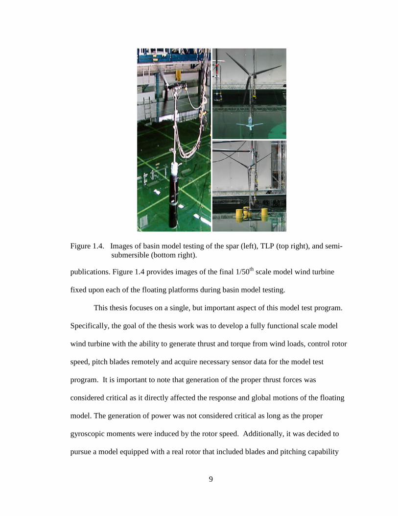
Figure 1.4. Images of basin model testing of the spar, TLP, and semi-
submersible. .................................................................................................. 9
Figure 2.1. Lift and drag coefficient as a function of angle of attack for a
NACA 64-618 airfoil section at r/R = 0.7 at model and full scale
wind conditions. ......................................................................................... 21
Figure 2.2. NACA 64-618 airfoil force diagrams at full and model conditions at
70% blade length. ....................................................................................... 23
Figure 2.3. Comparison of fluid flow effects at full and model scale conditions. ........ 25
Figure 3.1. Rendering of model nacelle and internal components with
dimensions given at model scale. ............................................................... 37
Figure 3.2. Image of fully instrumented model nacelle. ............................................... 38
Figure 3.3. Image of the pitch control assembly. .......................................................... 41
Figure 3.4. Image of the rotor hub. ................................................................................ 42
Figure 3.5. Control box with data acquisition and control equipment. ......................... 44
Figure 3.6. Image of cabling from the floating wind turbine model to the basin
carriage. ..................................................................................................... 45

xi
Figure 3.7. Labview GUI for data acquisition and controls. ......................................... 46
Figure 3.8. Flow chart of iterative method used to determine 2D airfoil geometry. ..... 49
Figure 3.9. Quadratic tip chord distribution. ................................................................. 52
Figure 3.10. Blade structural twist distribution and tip section interpolation. ................ 52
Figure 3.11. Comparison plot of documented and smoothed blade thickness
distribution. ................................................................................................. 53
Figure 3.12. Uniform trailing edge thickness of airfoils along blade span without
incorporating structural twist. ..................................................................... 54
Figure 3.13. 3D rendering of final model blade with sections number in
accordance with Table 3.3. ......................................................................... 55
Figure 3.14. Model blade mold components. .................................................................. 60
Figure 3.15. Fabrication procedure for model blade fabrication. .................................... 60
Figure 3.16. Blade laminate orientation. ......................................................................... 61
Figure 3.17. Carbon fiber model blade. ........................................................................... 62
Figure 3.18. Comparison of normalized tower mode shapes. ......................................... 66
Figure 3.19. Fully assembled fixed wind turbine model excluding cables. .................... 68
Figure 4.1. Degrees of freedom and reference frame for floating wind turbines. ......... 70
Figure 4.2. Normalized mode shapes for the model tower with cables and the
OC3 Hywind tower with 1st and 2nd order natural frequency values
provided at full scale. ................................................................................. 72
Figure 4.3. Image of a hammer test to determine model natural frequencies. .............. 73
Figure 4.4. Acceleration and PSD plots of a fixed and floating wind turbine on
the spar. ...................................................................................................... 74

xii
Figure 4.5. Cantilever bending test set up for 1/50th scale model blade. ..................... 77
Figure 4.6. Deflection along blade span at full scale under loading to induce a
maximum blade root bending moment scenario of 34,000 kN·m
from analytical predictions and test results of the model blade. ................ 78
Figure 4.7. Tip deflection as a function of blade root moment up to blade failure
for the model blade at full scale. ................................................................ 79
Figure 4.8. Induced stress along blade span at full scale under loading to induce
a maximum blade root bending moment scenario of 34,000 kN·m
from analytical predictions and test results of the model blade. ................ 80
Figure 4.9. Model wind turbine power and thrust coefficient performance curves
from fixed-base wind-only basin model testing data. ................................ 83
Figure 4.10. Performance curves for the NREL 5 MW wind turbine and model
turbine. ........................................................................................................ 84
Figure 4.11. Drela AG04 low-Reynolds number airfoil. ................................................ 88
Figure 4.12. Lift and drag coefficients of the NACA 64-618 airfoil under high and
low- Reynolds number conditions and of the Drela AG04 airfoil
under low-Reynolds number conditions. .................................................... 89
Figure 4.13. Power and thrust coefficient curves for the full scale, achieved
geo-sim at 1/50th scale, and redesigned 1/50th scale blade. ........................ 91
Figure B.1. Nacelle, hub and tower shop drawings. ..................................................... 104
Figure C.1. 2D geometry of model blade airfoil sections. .......................................... 111
Figure D.1. Acceleration and Power Spectral Density (PSD) plots from tower
hammer tests. ............................................................................................ 154

xiii
LIST OF NOMENCLATURE
a = axial induction factor
A = area
d = water depth
c/D = chord length to rotor
diameter ratio
c = chord length
C = wave celerity
CD = drag coefficient
CL = lift coefficient
CP = power coefficient
CT = thrust coefficient
df/dx = meanline slope
D = diameter
E = elastic modulus
f = wave frequency
fn = natural bending frequency
f(x) = meanline distribution
FD = drag force
FL = lift force
FQ = torque force
Fr = Froude number
FT = thrust force
g = acceleration due to gravity
G = shear modulus
Ho = angular momentum of rotor
Hz = hertz
I = area moment of inertia
J = mass moment of inertia
JT = polar moment of inertia
k = stiffness coefficient
kg = kilograms
L = length
m = meter
M = mass
MG = gyroscopic moment
N = Newton
Ncrit = laminar to turbulent
transition effect log factor
Pa = Pascal
Q = wave celerity to wind
speed ratio
R = radius
r/R = local radius/rotor radius
Re = Reynolds number
t = time unit
t/c = thickness to chord ratio
t(x) = thickness distribution
T = wave period
u = deflection
ua* = axial induced velocity
ut* = tangential induced
velocity
U = wind speed
v = fluid velocity
V* = resultant inflow
velocity
V = volt
W = watts

xiv
x/c = point location/chord
xp/c = pitch axis location/chord
y = neutral axis location
α = angle of attack
βi = resultant inflow angle
βn = boundary condition factor
λ = scale factor
μ = dynamic viscosity of a fluid
μm = micrometer
Ω = angular velocity of
rotor
ω = structural frequency
ψ = angular velocity
ρ = density
σ = stress
θp = blade pitch angle
Subscripts
m = denotes scale model
p = denotes full-scale
prototype
Unit Prefixes
μ = micro (×10-6)
m = milli (×10-3)
c = centi (×10-1)
k = kilo (×103)
M = mega (×106)
G = giga (×109)

xv
LIST OF ABBREVIATIONS AND ACRONYMS
2D two dimensional
CG center of gravity
DU Delft University
DAQ CompacDAQ Data Acquisition System
DOE Department of Energy
EMI electromagnetic interference
FA fore to aft
FAST An aeroelastic design code for horizontal axis wind turbines.
GUI graphical user interface
HAWT horizontal axis wind turbine
HDPE high-density polyethylene
ILS interlaminar shear strength
LAC Linear actuator control
MA3 Miniature Absolute Analogue
MIT Massachusetts Institute of Technology
NI National Instruments
NREL National Renewable Energy Lab
NWTC National Wind Technology Center
OC3 Offshore Code Comparison Collaboration
PSD power spectral density
RMP rotations per minute

xvi
SS side to side
SWL still water line
TLP Tension Leg Platform
TSR tip speed ratio
UC Davis University of California Davis
VI Virtual Instrument

1
CHAPTER 1. INTRODUCTION
Modern civilization in the United States has come to function and depend on
energy over the last century. Transportation, food production and agriculture,
households, businesses, industry and many other key societal functions are reliant on
energy to perform every-day tasks. However, over 75% of the United States’ (US)
primary energy production is from non-renewable, finite fossil fuels such as coal, oil, gas,
and natural gas (EIA, 2010). A major challenge facing future generations in the US and
around the world is to meet future energy demands by investing in new energy
production technologies especially those in the renewable energy sector (DOE, 2008).
An energy resource assessment made by the National Renewable Energy Lab (NREL)
has shown the US offshore wind resource has the potential to be a major renewable
energy contributor, yet technology to capture the vast majority of offshore wind, located
in waters over 60m deep, is currently in an early development stage (Schwartz, et al.,
2010). This thesis work is a primary component of an initial research effort consisting of
scale model testing for floating wind turbine technologies aimed at advancing technology
that efficiently captures offshore wind in deep-water environments. This introduction
will present the motivation and background for pursuing floating wind turbine technology
and the objective of the model testing research program.
1.1. MOTIVATION
The United States has a great opportunity to harness an indigenous abundant
renewable energy resource, offshore wind. In 2010, NREL estimated there to be over
4,000 GW of potential offshore wind energy found within 50 nautical miles of US

2
coastlines. The US Energy Information Association (EIA) reported the total annual US
electric energy generation in 2010 was 4.12 quadrillion kilowatt-hours or 940 GW (EIA,
2010), less than a quarter of the potential offshore wind resource. In addition, offshore
wind is the dominant ocean energy resource available in the US comprising 70% of the
total assessed ocean energy resource as compared to tidal and geothermal resources
(Musial, 2008). Through these assessments it is clear offshore wind could be a major
contributor to the US energy resource.
In particular, the Gulf of Maine is home to a significant portion of the US offshore
wind resource. Within the 50 nautical mile band extending from Maine’s coast resides an
estimated installed wind energy capacity of 156 GW of electricity (Schwartz, et al.,
2010). For comparison, Maine’s highest annual electric demand is 4.3 GW during the
summer months (EIA, 2011). Capturing 3.2% of Maine’s offshore wind total estimated
capacity, or 5 GW, would cover Maine’s peak energy demand and leave surplus energy
for potential distribution to surrounding political entities.
Many benefits to the US economy and environment would result if floating wind
turbine technology is commercialized. One benefit is that electric power from offshore
wind turbines could help increase US energy independence. In Maine, nearly 90% of the
energy used for home heating, electricity generation and transportation is derived from
fossil fuels leaving Maine citizens, like many US citizens, at the mercy of fluctuating and
inflating fossil fuel prices (Ocean Energy Task Force, 2009). Energy from offshore wind
has the potential to help control energy cost instability by providing clean electrons at a
predictable, reliable cost. Additionally, Maine’s billions of energy dollars exported
annually could be spent in a domestic market, helping to sustain local economies. Wind

3
power also has environmental benefits such as reduction of green house gas emissions
due to energy production that contribute to global warming (Serchuk, 2000). These are
only a few of the economic and environmental benefits that justify active pursuit of
onshore and offshore wind energy in the US.
The caveat to capturing offshore wind in the Gulf of Maine and much of the US
coast is deep water. Figure 1.1 illustrates that nearly 60% or 2,450 GW of the estimated
US offshore wind resource is located in water depths of 60m or more, (Musial, et al.,
2006). At water depths over 60m building fixed offshore wind turbine foundations, such
as those found in Europe, is likely economically unfeasible (Musial & Ram, 2010).
Therefore floating wind turbine technology is seen as the next best option to provide a
vessel for extraction of the majority of offshore wind energy in the US.
Figure 1.1. US offshore wind resource by region and depth for annual average wind speeds above 7.0m/s, (Musial & Ram, 2010). Reprinted with permission.
As of 2009 the US was a leading producer of wind energy in the world with over
35,000 MW of onshore wind energy production (DOE, 2010). Even so, there is still a

4
need to continue growth of wind energy production in the US in order to meet future
energy demand. As reported by the DOE, future wind energy growth should continue
onshore but also expand into offshore developments (2008). The DeepCwind
Consortium, lead by the University of Maine and supported by the DOE, NREL, and
several other private and public entities, is leading the US in deepwater floating wind
turbine development. Basin model testing of floating wind turbine platforms is an
essential part of the first phase of DeepCwind’s Maine Offshore Wind Plan established to
promote the development of 5 GW of offshore wind capacity in the Gulf of Maine by
2030 (University of Maine & James W. Sewall Company, 2011). Development of the
fully functional 1/50th scale 5 MW wind turbine, detailed in this thesis, was critical for
the completion of basin model testing and the progression of the Maine Offshore Wind
Plan. Furthermore, basin model testing provided real data to aid in improving and
validating fully-coupled simulation tools, discussed in subsequent sections, vital for
commercial design and development of floating wind turbine platforms.
1.2. BACKGROUND
In order to pursue commercial development of floating wind turbine technology a
validated aero-hydro-servo-elastic numerical model, or fully-coupled simulator, is needed
to accurately predict the dynamic system behavior to efficiently optimize floating
platform designs. Currently, there is only one prominent publicly available fully-coupled
simulator used to model the performance of floating wind turbines developed by NREL
(Jonkman & Buhl, 2007). NREL’s fully-coupled simulator was developed by interfacing
two wind industry-accepted simulation modules, FAST for servo-elastic simulation and
AeroDyn for aerodynamic simulation, and one oil and gas industry-accepted

5
hydrodynamic simulation code, WAMIT. However this tool has yet to be validated
against real data, and other coupled simulators such as Hydro Oil & Energy’s
SIMO/RIFLEX/HAWC (Neilsen, et al., 2006), Principal Power’s FastFloat (Cermelli, et
al., 2010), a rotor-floater-mooring coupled simulator developed at Texas A&M (Bae et
al., 2010), and MARIN’s aNySIM, (Gueydon & Xu, 2011) have limited information
currently published.
As of the writing of this thesis, there exists two commercial scale floating wind
turbines in the world, the Hywind spar-buoy by Statoil Hydro (2010) and the WindFloat
semi-submersible by Principle Power (2011). The Hywind spar-buoy floating platform
supports a 2.3 MW Siemens horizontal axis wind turbine (HAWT) and is heavily
instrumented to collect data of importance. However, the collected information is not
publicly available, and therefore, is of little use for parties interested in validating and
calibrating numerical analysis codes for floating wind turbines. Similarly, data collected
from WindFloat which supports a 2 MW HAWT wind turbine is also not currently
available. Other limited sources of data do exist for these two platforms, however, they
are derived from wave basin scale model testing.
Basin model testing is a refined science and is commonly used to test designs of
large scale offshore vessels and structures by the oil and gas industry, military, and
marine industries (Chakrabarti, 1994). A basin model test is ideal as it requires less time,
resources and risk than a full scale test while providing real and accurate data for model
validation. Additionally, wave basin testing is valuable as the environment can be
controlled. However even though wave basin testing is well refined in certain offshore

6
industries protocol for properly modeling the coupled wind and wave loads on a floating
wind turbine in a wave basin test environment has not been established.
Figure 1.2 illustrates the difficulty of quantifying all the complicated dynamics of
floating wind turbines. The significant loads on a floating wind turbine are characterized
by turbulent wind profiles, irregular wave loads, underwater currents and many other
complex factors. These varied environmental loads combined with fluid-structure
interaction, turbine performance and flexible member structural dynamics phenomena
make execution of an accurate scale model test a hearty challenge.
Figure 1.2. Illustration of significant loads effecting floating wind turbine performance, (Robinson & Musial, 2006). Reprinted with permission.
Despite the challenge, a few select floating wind turbine basin model tests have
been performed to the author’s knowledge. Principal Power Inc. tested a 1/67th scale

7
semi-submersible wind turbine platform, WindFloat (Cermelli, et al., 2010). Test results
were used to aid development of the first full scale WindFloat deployed in November,
2011 (Principle Power Inc., 2011). Also, test results were used as part of a proprietary
numerical model validation effort and proof of platform design performance. In 2006,
Hydro Oil & Energy conducted a 1/47th scale model test of a 5 MW spar-buoy floating
wind turbine at Marintek’s Ocean Basin Laboratory in Trondheim, Norway (Neilsen, et
al., 2006). Another basin test by WindSea of Norway was performed under Froude
scaled wind and waves at Force Technology on a 1/64.24th scale tri-wind turbine semi-
submersible platform (WindSea, 2011). These model tests provided valuable information
to respective stake holders and advanced knowledge of floating wind turbine dynamics.
However, methodologies and techniques used during these model tests have not been
thoroughly presented in the public domain. In addition, no test to date has made the
effort to create the high-quality wind environment required for simulating proper wind
turbine performance in a combined wind/wave test. Key differences between this basin
model test and those previously mentioned are that this model test program was
performed with fully-characterized Froude scaled wind loads, a fully functional model
wind turbine and findings of the test will be disseminated in the public domain.
1.3. OBJECTIVE
The primary goal of the basin model test program was to properly scale and
accurately capture real data of the rigid body motions and loads of different floating wind
turbine platform technologies and then compare data with numerical model results from
NREL’s aero-hydro-servo-elastic floating wind turbine simulator, or fully-coupled
simulator, for calibration and validation. Once the fully-coupled simulator is validated

8
against real data it could then be used with a much greater degree of confidence in design
processes for commercial development of floating offshore wind turbines.
To gain an array of test data for simulator comparison, three generic floating
platforms were tested during basin model testing: a semi-submersible, the OC3 Hywind
spar-buoy (Jonkman, 2010), and a tension leg platform (TLP) shown in Figure 1.3. The
models were tested under Froude scaled wind and wave loads, discussed further in
Chapter 2. The model platforms were built by MARIN and model testing was performed
at MARIN’s Offshore Basin in Wageningen, The Netherlands (2010). The three generic
platform designs are intended to cover the spectrum of currently investigated concepts,
each based on viable floating offshore structure technology. The designs, as well as their
accompanying performance data, will be made publicly available in proceeding
Figure 1.3. 1/50th scale floating platforms tested at MARIN. Clockwise from left: OC3 Hywind spar-buoy (left), TLP (top right), and semi-submersible (bottom right).
9
Figure 1.4. Images of basin model testing of the spar (left), TLP (top right), and semi-submersible (bottom right).
publications. Figure 1.4 provides images of the final 1/50th scale model wind turbine
fixed upon each of the floating platforms during basin model testing.
This thesis focuses on a single, but important aspect of this model test program.
Specifically, the goal of the thesis work was to develop a fully functional scale model
wind turbine with the ability to generate thrust and torque from wind loads, control rotor
speed, pitch blades remotely and acquire necessary sensor data for the model test
program. It is important to note that generation of the proper thrust forces was
considered critical as it directly affected the response and global motions of the floating
model. The generation of power was not considered critical as long as the proper
gyroscopic moments were induced by the rotor speed. Additionally, it was decided to
pursue a model equipped with a real rotor that included blades and pitching capability

10
over an actuator disk sized to achieve proper thrust forces under basin wind loads and a
rotating mass to emulate gyroscopic moments for a couple of reasons. First, data
collected from the real rotor allowed this research project to address unanswered
questions on wind turbine performance in a wave basin environment. Second, the pitch
capability of the model wind turbine will allow for future work to integrate active pitch
capability on the model and simulate irregular or extreme condition simulations such as
pitch mechanical failure where one blade is pitched while the other two are feathered. A
sized disk and simulated mass would not allow for collection of performance data as well
as provide a foundation for future basin model testing which could focus on blade
pitching options. Another important point is that the goal of the wind turbine model
design was to closely represent a full scale wind turbine. Numerical input files for the
fully coupled simulator of the final wind turbine model will be created in future research
efforts based on the characterization results presented in Chapter 4. In other words, a full
scale numerical model of the physical model at full scale will be used for fully-coupled
simulations. This thesis details the process and methods used to create the scale model
wind turbine used for basin model testing and provides results from wind turbine
characterization and performance testing.
From this scope of work, this thesis provides the following research contributions
to the scientific community:
1. Defining scaling methods and modeling techniques needed to perform accurate
wind/wave basin model tests of floating wind turbines.
2. Disclosing design details and characterization results of a 1/50th scale model of
the NREL 5 MW wind turbine for others to use for future model tests.

11
3. Providing clarification of Reynolds number effects on model wind turbine
performance under Froude scaled winds and provide methods that could be
employed to correct for undesired effects.
In short, this work provides a basis for future scale model wind turbines for basin model
testing of commercially viable floating wind turbine platforms.
The remaining structure of this thesis consists of four chapters. Chapter 2 presents
the utilized scaling methodology and established scaling laws with a discussion of
Reynolds number effects under Froude scaled conditions. Also presented in Chapter 2 are
the target 1/50th scale physical and mechanical parameters of the NREL 5 MW wind
turbine used to guide model design. Chapter 3 details the design and fabrication of the
model wind turbine. This chapter starts with the model nacelle design which includes
instrumentation selection, housing design, hub design and the blade pitch control method.
Following nacelle design is a description of the data acquisition and control system.
Model blade design and composite fabrication is then presented and the chapter is
concluded with the model tower design. Chapter 4 presents the characterization and
performance data of the model wind turbine during fix-based wind only basin model
testing as well as model blade structural testing results. In addition, this chapter provides
suggestions for future designs of wind turbines utilized in a Froude scaled wind
environment. Finally, Chapter 5 provides a conclusive overview of the methodology,
design, and characterization of the final 1/50th scale model test with suggestions for
future floating wind turbine basin model tests.

12
CHAPTER 2. SCALING METHODOLOGY AND APPLICATION
Proper scaling of a model and environmental conditions for scale model testing is
essential to complete a valid and reliable test. For floating wind turbine wind/wave
testing, proper scaling and modeling techniques have yet to be established. This chapter
will present and discuss the scaling relationships, scale factors, and modeling techniques
used to design and build the 1/50th scale wind turbine and platforms and establish
environmental conditions in the wave basin. In addition, target design values derived
from scaling methodology for the scale model wind turbine is also presented.
2.1. METHODOLOGY
In order to properly model the dynamic behavior of a floating wind turbine system
subjected to aerodynamic and hydrodynamic loading, an appropriate scaling
methodology must be used. A major challenge is overcoming the inability to
simultaneously maintain Froude and Reynolds numbers for a scaled floating wind turbine
experiment. In wind tunnel testing Reynolds number scaling is commonly used to
establish model parameters in order to properly represent the relationship of viscous and
inertial forces for a fluid flow, (Çengel and Cimbala, 2006). In wave basin testing Froude
number similitude is typically employed to properly scale the gravitational and inertial
properties of wave forces, the dominant external forces for a floating vessel or structure,
(Chakrabarti, 1994). In floating wind turbine testing maintaining Froude number was
preferred as all wave forcing and inertial effects were properly scaled. However, special
attention was paid to Reynolds-dependent phenomena in order to properly model the ratio
of wind to wave forces during basin model testing. In the following section, the Froude

13
scaling relationships used to design the 1/50th scale wind turbine model are presented
with further elaboration on parameters particular to floating wind turbine modeling.
Subsequently, a more detailed discussion of the consequences of Reynolds number
dissimilitude, particularly for wind turbine performance, is included.
2.1.1. Scaling Relationships and Parameters
In order to establish scale relationships, certain scaling laws must be followed. The
scaling relationships employed for modeling of floating offshore wind turbines are as
follows:
1. Froude number similitude is employed from prototype to scale model. Offshore
platform wave basin tests are typically scaled using Froude number and geometric
similarity. Although a Froude model does not scale all parameters properly the
dominant factor in the wave mechanics problem, inertia, is properly scaled
(Chakrabarti, 1994). For a floating wind turbine, this covers most properties of
interest which influence the global dynamic response of the system, excepting the
aerodynamic wind forces. Employing a Reynolds number scaling scheme,
common for model aerodynamic experiments, is impractical for a floating body
subjected to wave forcing. Therefore, Froude scaling is best suited for model
testing of floating wind turbines. The Froude number for a free surface wave is
waveCFrgL
= , (2.1)
where C is the wave celerity, or propagation speed, g is the local acceleration due
to gravity and L is a characteristic length. The scaling relationship maintained
from model scale to the full scale prototype is given as

14
p mFr Fr= , (2.2)
where p and m stand for prototype and model, respectively. Forces reliant on
Reynolds number, such as airfoil lift and drag are discussed in section 2.1.3.
2. Froude scaled wind is employed during basin model testing. If aerodynamic
turbine features are insensitive to Reynolds number, then the wind force to wave
force ratio from prototype to model scale is maintained by utilizing Froude scaled
wind and can be shown as
windUFrgL
= . (2.3)
An alternative, yet consistent, way to represent Froude scaled wind is by
maintaining the ratio of wind speed to wave celerity from model to full scale. This
ratio is identified by the variable Q and defined as
UQC
= , (2.4)
where U is the wind inflow velocity and C is the wave celerity.
3. The wind turbine tip speed ratio, TSR, is to be maintained from prototype to scale
model. TSR is computed as
RTSR
UΩ
= , (2.5)
where Ω is the rotor rotational speed, R is the blade tip radius and U is the wind
inflow velocity. Maintaining TSR ensures that the turbine rotational speed as well
as any system excitation frequencies resulting from rotor imbalance or
aerodynamic interaction with the tower will scale properly. In addition,
maintaining TSR will yield properly scaled turbine thrust forces and rotor torque

15
in conjunction with a Froude scaled wind environment, assuming a low
dependence on Reynolds number for the wind turbine airfoil section lift and drag
coefficients. Maintaining TSR between the prototype and model is given as
p mTSR TSR= . (2.6)
By following these scaling relationships, the scale factors shown in Table 2.1
were obtained to characterize a scaled floating wind turbine. Additional parameters can
be found in Chakrabarti (1994).
Table 2.1. Established scaling factors for floating wind turbine model testing.
Parameter Unit(s) Scale Factor Length (e.g. displacement, wave height and length) L λ Area L2 λ2 Volume L3 λ3 Density M/ L3 1
Mass M λ3 Time (e.g. wave period) T λ0.5 Frequency (e.g. rotor rotational speed, structural) T-1 λ-0.5
Velocity (e.g. wind speed, wave celerity) LT-1 λ0.5 Acceleration LT-2 1
Force (e.g. wind, wave, structural) MLT-2 λ3 Moment (e.g. structural, rotor torque) ML2T-2 λ4 Power ML2T-3 λ3.5 Stress ML-1T-2 λ Mass moment of inertia ML2 λ5 Area moment of inertia L4 λ4
2.1.2. Discussion of Parameters Particular to Floating Wind Turbines
By employing the scaling relationships shown previously, the following additional
parameters, not related to Reynolds number, yet relevant to a floating wind turbine
response were found to scale correctly from prototype to model.

16
The relationships shown in Table 2.1 are valid for both deep and shallow waves.
Wave celerity is dependent on the relative depth which is the ratio of water depth, d, to
wave length, L. The expression for wave celerity according to Main (1999) is
tanh(2 )2gL dC
Lπ
π= , (2.7)
and applies for all water depths. In shallow water where the relative depth, d/L
approaches 0, tanh(2πd/L) approaches 2πd/L. For deep water where the relative depth is
greater than 0.5, tanh(2πd/L) approaches 1 simplifying the equation to the often
recognized deep water expression,
2gLCπ
= . (2.8)
For a proper Froude scaled experiment, both L and d are each scaled by λ maintaining
the depth ratio and hyperbolic tangent term in Equation 2.7 from prototype to model
scale. Therefore, it is evident that wave celerity in deep to shallow water waves is scaled
the same. The scale factor for wave celerity is determined with Equation 2.8, where
wave length, L, is scaled by λ resulting in a celerity scale factor of λ0.5 which is consistent
with the scale factor for velocity given in Table 2.1.
In order to attain proper scaling of system dynamics, the ratio of the rotor rotation
speed to wave frequency must scale in the same manner. By using the scale factor for
frequency given in Table 2.1, the model wave frequency, fm, is found by
m pf fλ= . (2.9)
The turbine rotor rotational frequency scale factor is found by combining equations 2.5
and 2.6 and implementing scale factors for velocity and length from Table 2.1 to form

17
1
1m p
p p
pp
RRU U
λ
λ
ΩΩ= ,
(2.10)
which yields
m pλΩ = Ω . (2.11)
Therefore, rotor rotational frequency scales in the same fashion as other frequencies such
as the wave frequency shown in Equation 2.9.
Gyroscopic moments induced by rotor rotation on a floating turbine can occur in
both the yaw and pitch motions of a floating wind turbine structure. It is important to
replicate these effects during basin model testing to acquire accurate test data.
Gyroscopic moment, MG, of a fixed wind turbine is a function of angular velocity, ψ, and
angular momentum of the rotor, Ho, (Manwell, et al., 2002) and is of the form
G oM Hψ= , (2.12)
where rotor angular momentum is computed as
oH J= Ω , (2.13)
where J is the mass moment of inertia of the rotor about the rotor shaft axis. By applying
scale factors from Table 2.1 to rotor angular velocity ψ, rotor rotational frequency Ω, and
rotor mass moment of inertia J, the following relationships are prescribed
m pψ λψ= , m pλΩ = Ω , 5
1m pJ J
λ= .
(2.14 – 2.16)
Substituting Equations 2.14 through 2.16 in Equation 2.12 gives

18
23
1 1( )( )( )( )Gm p p p pM m rλψ λλ λ
= Ω ,
yielding
4
1Gm pM M
λ= . (2.17)
Therefore, if the gyroscopic and mass properties of the rotor are scaled correctly yielding
a Froude scale consistent value for J, the gyroscopic moment scales consistently with the
scale factors listed in Table 2.1 and is maintained in a Froude scaled model.
Proper scaling of structural deformation modes and vibration characteristics are of
particular importance in order to accurately model key structural dynamics behavior. By
following established scaling relationships and the scale parameters listed in Table 2.1,
the frequency of structural vibration scales as
m pω λω= . (2.18)
Delving further, the frequency of lateral vibration for a homogenous prismatic Euler-
Bernoulli beam (e.g. see Rao, 2004) is of the form
3nEILL m
ω β= , (2.19)
where βn is dependent on beam end boundary conditions, L is the member length, E is the
modulus of elasticity, I is the cross-section area moment of inertia, and m is the member
mass. By following the mass, length, and frequency scaling requirements given in Table
2.1 the scaling relationship for the bending stiffness, EI, can be determined by
rearrangement of variables which is shown as

19
3 3 3 3
( )( )( )
p pmm p
m m m m
E IEIL m L m
ω λω λλ λ
= = = ,
yielding
5
1( )m p pEI E Iλ
= . (2.20)
The same procedure was applied for determining the scaling relationship for other
stiffnesses, such as axial stiffness, EA, and torsional rigidity, GJT, which were found to
scale by λ3 and λ5 respectively. The aforementioned procedures for scaling stiffness
quantities is outlined because achieving a Froude scale stiffness involves a combination
of scaling dimensions and also scaling material moduli. This is difficult as often times the
materials used for model fabrication have similar material densities and moduli as the
prototype materials. Therefore, the combination of material density, stiffness and
geometry are usually tuned together to achieve the gross dimensions, mass properties,
and stiffness of the model component in design. This method was used to design the
model tower discussed in Chapter 3.
2.1.3. Reynolds Number Effects
While many quantities scale consistently with Froude number scaling, there are
limitations due to Reynolds number effects. Reynolds number quantifies the viscous and
inertial qualities of fluid flow and is expressed as (e.g. see Çengal and Cimbala, 2006)
Re vLρ
µ= , (2.21)
where ρ is the fluid density, v is the mean velocity of the object relative to the fluid, μ is
the dynamic viscosity and L is the fluid length of travel of interest. Reynolds number is

20
typically employed in aerodynamic modeling and wind tunnel testing of airfoil sections,
wings, wind turbines, and more (Çengel & Cimbala, 2006) where maintaining the viscous
and inertial properties of fluid flow is critical. As this model test utilized Froude number
similitude, Reynolds number similitude is not maintained. Therefore, forces heavily
reliant on Reynolds number such as lift and drag on wind blade airfoils would not scale
properly during basin model testing. As a fully functional wind turbine was desired for
basin testing, the effect of Froude scaled wind on the performance of the turbine needed
to be understood so that corrections could be made to improve testing procedures.
Under Froude scaled conditions, the wind speed and blade Reynolds number were
reduced from prototype to model scale. For the 1/50th scale model test a full scale 11 to
12 m/s wind speed reduced to less than 2 m/s and the Reynolds number at 70% blade
radius found with Equation 2.21 decreased from 11.5×10⁶ (turbulent flow) to 35×103
(laminar flow). The drastic change in Reynolds number resulted in a significant change
in the lift and drag behavior for airfoil sections of the geo-sim wind blade employed
during basin model testing. The model blade emulated the geometry of a full scale 5 MW
wind blade designed for high-Reynolds number turbulent flow as opposed to the low-
Reynolds number flow experienced during the wind/wave basin. Note that a full
description of the blade geometry is provided in Chapter 3. During basin model testing,
generated torque and thrust were lower than required. Therefore, wind speeds during
basin testing were increased to ensure proper thrust forces. However the power
coefficient, which depicts the power captured by the turbine relative to the available
power in the wind flow, was still low. In this section, an aerodynamic analyses of a
NACA 64-618 airfoil at 70% the blade length of the NREL 5 MW blade, used for the

21
model wind turbine and detailed in Chapter 3, was performed to clarify the Reynolds
number effects on a Froude scaled wind turbine model. A full description of wind
turbine performance results from basin testing is presented in Chapter 4.
Fluid flow behavior analysis over the NACA 64-618 airfoil was performed with
XFOIL (Drela, 1989) under full scale and model operational conditions. XFOIL is freely
available high-order panel code incorporating a fully-coupled viscous/inviscid interaction
method designed specifically for airfoil analysis. At full scale conditions, an operational
wind speed of 11.4m/s and a rotor speed of 12.1 rpm was used yielding a Reynolds
number of 11.5×10⁶. Model conditions consisted of a wind speed of 20.8 m/s and rotor
speed of 12.7 rpm (2.94 m/s 90 rpm model scale) which yielded a Reynolds number of
35×103. In XFOIL the laminar to turbulent transition effect log factor, Ncrit, was set to 9
at both full and model scale for consistency as this is the number used for standard wind
tunnels analysis (Drela, 1989). Figure 2.1 displays some of the results from the XFOIL
Figure 2.1. Lift and drag coefficient as a function of angle of attack for a NACA 64-618 airfoil section at r/R = 0.7 at model and full scale wind conditions.
-10 0 10 20-1
-0.5
0
0.5
1
1.5
2
α (deg)
CL
Full ScaleModel Scale
-10 0 10 200
0.05
0.1
0.15
0.2
0.25
α (deg)
CD

22
analysis through lift and drag coefficients over a range of angles of attack, α. As can be
seen in this figure, the relatively thick NACA 64-618 airfoil section exhibits low lift and
high drag in model conditions as opposed to full scale conditions.
The resulting forces per unit length of the wind blade using information from the
XFOIL analysis are illustrated with airfoil force diagrams in Figure 2.2 at full scale
conditions and model conditions transformed to full scale. The top diagram is generic
with exaggerated magnitudes for axial and tangential induced velocities, ua* and ut*, as
well as the angle of attack, α, for clarity. Induced velocities were found with an AeroDyn
analysis using the lift and drag coefficient inputs from the XFOIL analyses. AeroDyn
utilizes Blade Element Momentum (BEM) theory (e.g. see Moriarty & Hansen, 2005) to
calculate wind turbine aerodynamic loads. To calculate induced velocities, BEM theory
assumes a pressure loss, or momentum loss, through the rotor plane on the blade
elements. The momentum loss and resulting wake creates induced velocities which effect
the magnitude and angle of attack of the resulting inflow, V*, on the airfoil. In Figure 2.2
the induced velocities are shown as vectors, which contribute to the actual wind flow
magnitude and direction experienced by the airfoil, V*. The resulting lift and drag forces
per unit of blade length, FL and FD, are the major forces of interest in airfoil and hydrofoil
analysis as they produce the final torque and thrust forces, FQ and FD, shown in Figure
2.2. Lift and drag forces are found with the following equations:
21
2L LF V cCρ= , (2.13)
21
2D DF V cCρ= , (2.14)

23
Figure 2.2. NACA 64-618 airfoil force diagrams at full and model conditions at 70% blade length.
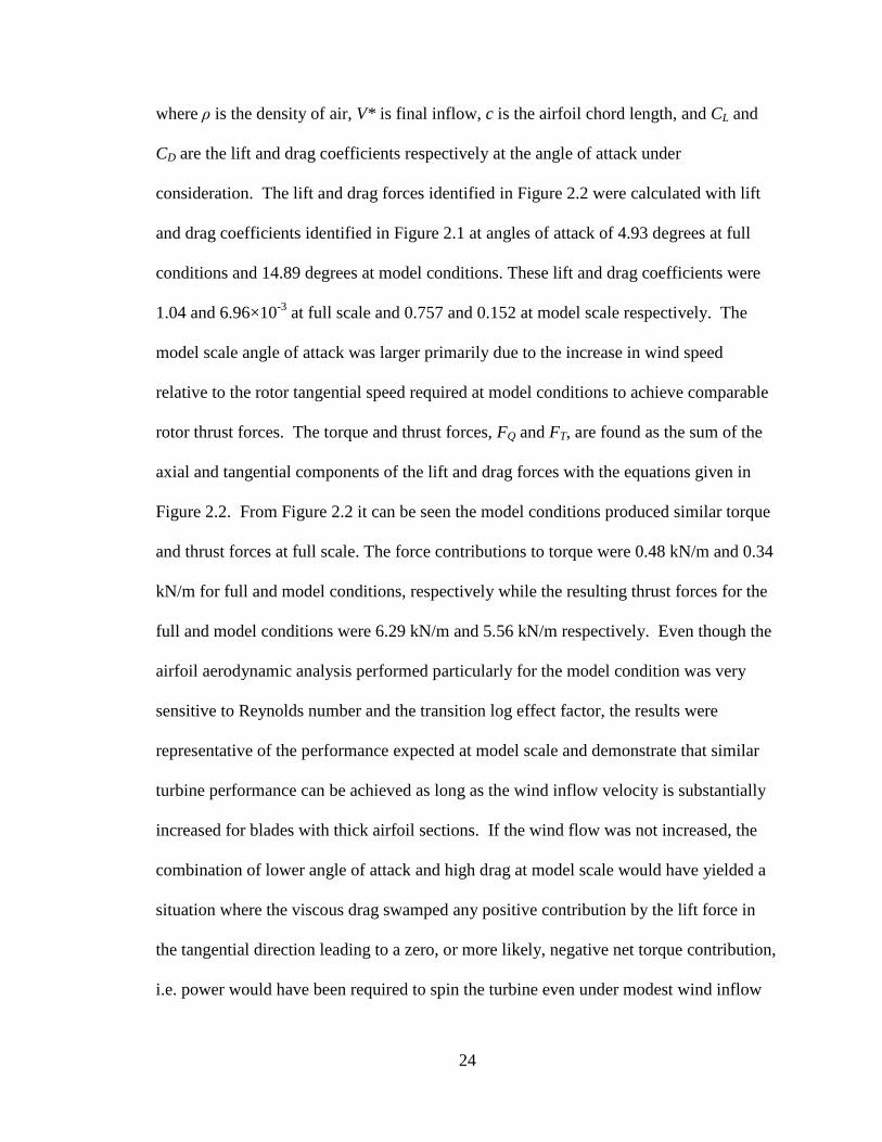
24
where ρ is the density of air, V* is final inflow, c is the airfoil chord length, and CL and
CD are the lift and drag coefficients respectively at the angle of attack under
consideration. The lift and drag forces identified in Figure 2.2 were calculated with lift
and drag coefficients identified in Figure 2.1 at angles of attack of 4.93 degrees at full
conditions and 14.89 degrees at model conditions. These lift and drag coefficients were
1.04 and 6.96×10⁻³ at full scale and 0.757 and 0.152 at model scale respectively. The
model scale angle of attack was larger primarily due to the increase in wind speed
relative to the rotor tangential speed required at model conditions to achieve comparable
rotor thrust forces. The torque and thrust forces, FQ and FT, are found as the sum of the
axial and tangential components of the lift and drag forces with the equations given in
Figure 2.2. From Figure 2.2 it can be seen the model conditions produced similar torque
and thrust forces at full scale. The force contributions to torque were 0.48 kN/m and 0.34
kN/m for full and model conditions, respectively while the resulting thrust forces for the
full and model conditions were 6.29 kN/m and 5.56 kN/m respectively. Even though the
airfoil aerodynamic analysis performed particularly for the model condition was very
sensitive to Reynolds number and the transition log effect factor, the results were
representative of the performance expected at model scale and demonstrate that similar
turbine performance can be achieved as long as the wind inflow velocity is substantially
increased for blades with thick airfoil sections. If the wind flow was not increased, the
combination of lower angle of attack and high drag at model scale would have yielded a
situation where the viscous drag swamped any positive contribution by the lift force in
the tangential direction leading to a zero, or more likely, negative net torque contribution,
i.e. power would have been required to spin the turbine even under modest wind inflow

25
speeds. While increasing the wind speeds ‘tuned’ the net thrust and torque forces
somewhat, this was not an ideal situation since the available power from the model wind
inflow, at least for the example given, is six times greater than available power from the
full scale inflow. Therefore, the geo-sim model rotor power efficiency will be
approximately an order of magnitude lower due to the inability to achieve the target
levels of torque at the right environmental conditions.
Figure 2.3 provides some insight into the low lift and high drag airfoil coefficients
at the model scale Reynolds numbers which lead to poor turbine performance. The figure
compares the displacement thickness of the boundary layer, as well as the laminar to
turbulent transition and separation location along the NACA 64-618 airfoil for the full
Figure 2.3. Comparison of fluid flow effects at full and model scale conditions.
0 0.2 0.4 0.6 0.8 1-0.1
0
0.1
0.2
0.3Full Scale Condition
0 0.2 0.4 0.6 0.8 1-0.1
0
0.1
0.2
0.3Model Condition at Full Scale
xTr Top
xTr Bottom
Separation
Re = 11.5x10⁶
Re = 35.7x10³

26
and model condition Reynolds numbers. As shown in Figure 2.3, at the full scale
condition the boundary layers are very thin with a majority of the upper and the last 45%
of the lower surface boundary layers turbulent. No separation of the flow occurs at full
scale and the total displacement thickness at the trailing edge is quite small, leading to
low drag. At model sale, the displacement thickness is drastically larger, especially on
the suction side of the airfoil. In addition, the plot in Figure 2.2 indicates that the flow is
separated in the laminar region near the top leading edge of the blade. The end result is
an enormous wake for the model scale airfoil which creates a large, virtual projected area
perpendicular to the inflow field which drastically increases the drag of the airfoil. In
addition, the poorly organized flow does not yield an optimal pressure distribution about
the airfoil perimeter resulting in a diminished lift coefficient for a given angle of attack.
As noted earlier, the low lift and high drag coefficients resulting from the flow field
changes shown in Figure 2.3 necessitate higher wind inflow velocities in order to create
properly scaled thrust and torque values for typical megawatt-scale wind turbine rotors
with thick airfoil sections required to achieve adequate structural bending stiffness.
Reynolds number dependent phenomena do not apply to wind turbine
aerodynamics alone. Hydrodynamic drag forces on submerged bodies due to currents
and waves are also function of Reynolds number. In small Froude models simulated
waves and currents will have a lower Reynolds number than the prototype conditions
causing the model drag coefficient to increase. This problem, for both the hydrodynamic
and aerodynamic instances can be improved by “tripping” the laminar flow to become
turbulent at the bow of the structure or leading edge of a wind blade for example. A
common and effective approach to trip the fluid flow is to place studs or roughened

27
material along the aforementioned areas (Chakrabarti, 1994). In general, this technique
can remedy most hydrodynamic issues experienced in Froude scale wave basin tests.
While improvements are made to wind turbine performance with this technique, testing
results given in Chapter 4 will later demonstrate that the method is insufficient by itself to
completely correct wind turbine performance.
A final Reynolds dependent quantity is the Strouhal number which characterizes
vortex shedding of fluid flow past an immersed body (White, 1999). Due to a
dependency on Reynolds number, Strouhal number is also not precisely modeled in a
Froude scaled model (Chakrabarti, 1994). However, according to White (1999), for bluff
bodies the Strouhal number is a weak function of Reynolds number and is approximately
0.2 for cylinders over a wide range of Reynolds numbers. With respect to
hydrodynamics, the spar-buoy, semi-submersible and TLP models tested consist
primarily of cylinders near the water surface where wave particle motion is the largest.
In general, Strouhal number similitude for wave based tests and for this test program is
not a concern.
2.1.4. Overview
The aforementioned scaling relationships properly maintain the dominant model
characteristics and wave forces that greatly influence rigid body motions and structural
loads of a floating wind turbine model. Utilizing Froude number similitude ensures mass
properties of the model and inertia properties relating to hydrodynamics are maintained.
By producing high fidelity Froude scaled wind in the basin the ratio of wind and wave
forces acting on the structure are maintained from full to model scale as long as Reynolds
dependence of airfoil coefficients is weak, which is not always the case and must be

28
corrected if found to be true. Also by maintaining TSR in conjunction with Froude scaled
winds, the rotor frequency and any resulting excitations are scaled properly. These
relationships ensure that global response of the floating model wind turbine will be well
captured in wind/wave basin model testing.
As noted earlier, certain forces reliant on Reynolds number are not maintained
using this methodology and require special attention when performing these tests. It is
important to note that Reynolds number discrepancy is a common occurrence with wave
basin testing of offshore structures. Certain corrections can be used to overcome
Reynolds number effects such as the use of turbulence inducers on the model where drag
forces are more prominent, such a wind blade’s leading edge, a tower face and platform
hull. In addition alterations to blade or hull geometry may be required to better simulate
the full scale response in the model test. For example, it is not uncommon for ship lifting
bodies to be altered in size at the model scale to emulate the full scale drag and lift force
condition in a Froude scaled towing test.
For this model test program a geo-sim of the NREL 5 MW wind turbine blade
was used for basin model testing. Performance results presented in Chapter 4 show that a
geo-sim was not an ideal means of achieving the desired performance for torque and
thrust, the latter more critical to capture properly in order to simulate the global motion
response of the floating system. The previous sections gave insight into the physical
reasons which produce the lack of turbine performance of a geo-sim blade. As discussed
in previous sections, the low model condition Reynolds numbers drastically alter the flow
characteristics around the thick wind turbine airfoil sections yielding poor lift and drag
coefficients as compared to full scale. For future model testing it would be beneficial to

29
design a model wind blade to better emulate the full scale performance at the low
Reynolds number condition of the Froude scale model test. A basic example of a low-
Reynolds number condition blade is presented in Chapter 4 for comparison against the
performance results of the geo-sim model blade subjected to Froude scaled winds. Even
considering the Reynolds number dependent pitfalls, the wave and wind turbine thrust
forces that control global motions and loads of a floating wind turbine model can be
maintained with a Froude scaling architecture, albeit often with a bit of tuning.
2.2. TARGET SCALE MODEL PARAMETERS
This section provides the basis and method used to establish target parameters or
characteristics of the model wind turbine used to guide the design of the final model. The
subsequent paragraphs provide discussion on the selection of the full scale wind turbine
emulated during wind/wave basin testing, determination of the appropriate scale factor,
and establishment of the final scale mechanical properties and dimensions of the model.
The scale model wind turbine is based on the commercial scale 5 MW reference
wind turbine from the National Renewable Energy Lab, NREL, (Jonkman, et al., 2009).
The NREL 5 MW reference wind turbine is a theoretical three bladed HAWT, a common
commercial wind turbine configuration, that has been established for the purpose of
offshore wind turbine analytical studies. This wind turbine was chosen because it is an
open-source design and has been heavily utilized in coupled numerical modeling of
various floating wind turbine concepts similar to those this test program is aiming to
validate. However the NREL 5 MW wind turbine is only theoretical and not all
dimensions and specifications required for fabrication were readily available posing an
interesting challenge to the model design and fabrication effort.

30
All the model wind turbine components, such as the wind blades, nacelle and hub
are based on descriptions of the NREL 5 MW wind turbine. The model tower is based on
the OC3 Hywind tower (Jonkman, 2010) which is 10 m shorter than the reference NREL
5 MW tower to account for the increased freeboard of the OC3 Hywind spar-buoy
floating platform. The OC3 Hywind tower base was located 10 m above the still water
line (SWL) also allowing for the semi-submersible and TLP to have a reasonable 10 m of
freeboard at the tower-platform interface. Model testing and fabrication was simplified
by using one turbine and tower model for all three platforms.
A model scale factor of 1/50th, or λ = 50, was chosen based on basin capacity and
construction feasibility. Using a scale factor greater than 50 would have severely reduced
the feasibility of building properly scaled wind turbine blades due to tight weight
constrictions which is discussed in detail shortly. Also, using smaller models in a basin
model test would reduce the accuracy of the test as most wave basins have difficulty
creating the diminutive waves required for experiments of a very small scale. While a
larger model would potentially perform better, a scale factor less than 50 would greatly
increase the model rotor size as well as the size and cost of wind machine specially
designed and built to deliver high quality winds in the basin for this test program. Lastly,
model design and early fabrication commenced prior to wave basin selection. At that
time, a larger model would have severely restricted the number of potential wave basins
world-wide that could perform the model tests due to basin dimension limitations.
Overall, a 1/50th scale factor was found to be a suitable choice.
Utilizing the scaling relationships and parameters previously discussed, the target
model parameters given in Table 2.2 were established. While certain design parameters

31
Table 2.2. Full scale NREL 5 MW properties and target model scale properties.
Property Full Scale 1/50th Scale
Power 5 MW 5.7 W
Blades mass 17,740 kg 0.14 kg
Blade length 61.5 m 1.23 m
Hub mass 56,780 kg 0.45 kg
Nacelle mass 240,000 kg 1.92 kg
Tower top mass (hub, 3 blades and nacelle) 350,000 kg 2.80 kg
Hub radius 1.50 m 0.03 m
Rotor diameter, D 126 m 2.52 m
Tower mass 249,718 kg 1.998 kg
Tower height 77.6 m 1.55 m
Tower CG (% from tower base) 43.0 % 43.0 %
Tower 1st bending natural frequency 0.478 Hz 3.378 Hz
Tower top diameter 3.78 m 0.08 m
Tower base diameter 6.5 m 0.13 m
were straight forward to achieve physically, several presented interesting engineering
challenges. The NREL 5 MW full scale wind blade is 61.5 m in length with a mass of
17,710 kg. When scaled by 1/50th the blade was reduced to 1.23 m in length with a mass
of 0.14 kg, which was extremely light relative to its size. Selection and use of
appropriate materials and fabrication techniques was critical in order to ensure the model
wind blade emulated the appropriate geometry and ultra-light mass requirement while
possessing adequate strength to resist loading during wind/wave basin model testing.
Design of the nacelle was also a unique engineering challenge as a motor assembly, all
necessary sensors and components and a durable housing needed to collectively weigh
1.92 kg at the 1/50th scale. Detailed discussion of the design, component selection,

32
and fabrication methods for the 1/50th scale model wind turbine used to overcome these
design challenges and others is provided in Chapter 3.
In order to size the sensors and motor needed for the model turbine, reasonable
estimates of the range of forces, moments, and the rotor torque needed to be established.
To do so extreme values of these reactions were taken from a suite of numerical
simulations performed with the NREL 5 MW wind turbine mated to the ITI Energy
Barge platform model (Jonkman, 2007). Simulations of the ITI Energy Barge floating
wind turbine exhibited the highest internal force and moment reactions due to poor
platform stability and excessive wave loads as compared to the OC3 Hywind Spar and
MIT/NREL TL, (Jonkman & Matha, 2009). Thus, the barge internal reactions were used
to identify appropriate instrumentation as the magnitudes of these reactions would have
been the maximum expected during basin model testing. Table 2.3 shows the internal
forces and moments at the tower top as well as the rotor torque at full and model scale
used to appropriately select the model motor and sensors. Specifics on the sensors, motor,
and controls utilized on the model wind turbine is discussed in Chapter 3.
Table 2.3. Maximum internal reactions of NREL’s ITI Energy Barge at full and model scale, used to select model instrumentation.
Maximum Reaction Full Scale 1/50th Scale
Rotor Torque 10,700 kN·m 1.710 N·m
Power 6.05 MW 6.84 W
Force – tower top – x (surge) 8,560 kN 68.5 N
Force – tower top – y (sway) 1,880 kN 15.0 N
Force – tower top – z (heave) 6,080 kN (compressive) 48.6 N (compressive)
Moment – tower top – x (pitch) 11,900 kN·m 1.90 N·m
Moment – tower top – y (roll) 38,900 kN·m 6.22 N·m
Moment – tower top – z (yaw) 21,600 kN·m 3.46 N·m

33
The values from Tables 2.2 and 2.3 provided the target parameters used to base
the design of scale model wind turbine. Throughout the design process, these target
design values remained constant and used to judge accuracy by which the model wind
turbine emulated full scale characteristics. Many of these target values provided many
technical challenges throughout the design process which is presented in the following
chapter.

34
CHAPTER 3. MODEL WIND TURBINE DESIGN AND FABRICATION
This chapter details the design and fabrication of a 1/50th scale model HAWT
based on target parameters of the NREL 5 MW reference wind turbine established in
Chapter 2. In addition to meeting the target parameters that control global motions and
dynamic such as system mass, inertia, etc., this model design included a fully-functional
turbine and rotor with rotational speed and pitch control capability. The structure of this
chapter is as follows: key components and sensors located in or near the wind turbine
nacelle will be presented first followed by the design of the nacelle enclosures that
housed sensors and served as a connection point for the motor, turbine drive shaft, rotor,
pitch control components and tower. Selection of the blade pitch control equipment and
the final rotor hub design will then be presented followed by a description of the data
acquisition system and control software wired to the model wind turbine during basin
testing. A detailed description of the final blade geometry and wind blade fabrication
process developed to manufacture ultra light yet stiff composite model wind blades will
then be discussed. Finally, the final model tower design will be presented as well as final
adjustments and modifications made to the fully assembled model wind turbine.
3.1. NACELLE AND HUB
Similar to a typical full scale upwind HAWT, the model nacelle included the
enclosures/housings, sensors, components and motor assembly located at the top of the
tower and downwind of the wind turbine rotor. The hub provided a connection between
the blades and main drive shaft and was designed to incorporate pitch control. A major
design challenge was meeting the nacelle target weight of 1.92 kg model scale, which

35
needed to include the motor assembly, sensors, pitching mechanism, rotor drive shaft and
supportive enclosures. Another challenge was meeting the hub weight requirement of
0.45 kg model scale. This section will present instrumentation selection, enclosure or
housing design, pitch control design and rotor hub design.
3.1.1. Instrumentation and Housings
Considerations for selection of instrumentation included data input range and
accuracy as well as physical size and weight of the sensor. Data necessary to collect
during basin model testing included generated torque, rotor rotational position, nacelle
accelerations and tower-top forces and moments. The model wind turbine was also
designed to function as a fixed-speed, fixed-pitch machine. During model testing at
MARIN the rotor speeds and blade pitch were set to prescribed values based on the wind
environment being tested. To maintain rotor speed a small gearbox and servo-motor with
an internal encoder was included on the model. The pitch control mechanism which
could vary the blade pitch range approximately 90 degrees is detailed in the following
section. The sensors and components chosen were compact, light weight and provided
high resolution data rates. Sensors and components are identified in Figure 3.2 and
additional information including individual weights can be found in Table 3.1. Further
specifications are provided in Appendix A.
The nacelle enclosure was designed to satisfy the connection requirements for the
selected sensors and components. The final nacelle enclosure consisted of two housings:
the bearing housing and the torque tube as shown in Figure 3.1. The bearing housing,
upwind of the torque tube, was designed to house the rotor position encoder and pitch
actuator. The analog encoder was to be placed up-wind of the torque transducer to ensure

36
Table 3.1. List of nacelle sensors and components with individual weights.
Component Manufacturer Mass (g)
MA3 Analog Encoder US Digital 10
L12 Linear Actuator Firgelli Inc. 34 T2 Precision Rotary Torque Transducer Interface Inc. 180
6-Axis Force and Moment Sensor
Advanced Mechanical Testing Inc. (AMTI) 100
Gyro Enhanced Orientation Sensor (6-axis accelerometer) MicroStrain 74
Parker Rotary Servo Motor Parker Motion 712
20:1 Gearhead Parker/Bayside 385
rotor position data was captured with little interference from the torque transducer. The
analog encoder was chosen due to its light weight and high resolution output, however
the single shaft design could not be placed directly on the main drive shaft. Therefore, the
bearing housing was designed to support the encoder externally while accommodating
1:1 acetyl miter gears to transfer the rotational speed from the main drive shaft to the
encoder as shown in Figure 3.1. In an effort to keep weight down, the bearing housing
was made of aluminum and four large holes were bored on each face parallel to the
centerline of the drive shaft to reduce weight. The downwind face of the bearing housing
hosted a welded aluminum flange to provide a mechanical connection to the torque tube.
The torque transducer required isolation from any axial, lateral or angular
motions which resulted in the unique housing for the sensor, coined the torque tube. The
stiff torque tube supported the torque transducer with bellows couplings to ensure clean
torque data was collected. As an extra precaution to protect the torque transducer from
thrust, thrust bearings and shaft collars were placed before and after the bearing housing
prior to the upwind bellows coupling. The two shaft collars also held the rotor drive

37
Figu
re 3
.1.
Ren
derin
g of
mod
el n
acel
le a
nd in
tern
al c
ompo
nent
s with
dim
ensi
ons g
iven
at m
odel
scal
e.

38
Figu
re 3
.2.
Imag
e of
fully
inst
rum
ente
d m
odel
nac
elle
.

39
shaft in place which facilitated mechanical disassembly and assembly of the unit. Internal
bearings and couplings for the torque tube arrangement are shown in Figure 3.1.
The torque tube itself was designed as a hollow aluminum cylinder to house the
torque transducer and bellows couplings and to ensure proper alignment with the motor
and rotor drive shafts as well as provide a stiff and light weight enclosure. Aluminum
flanges with bolt attachments were welded on either end of the torque tube to provide
mechanical connections for the motor/gearbox combination and the bearing housing.
Bolted connections were used throughout the model design, as opposed to welded or
epoxy bonds, to allow for assembly and disassembly of the model nacelle and provided
access to internal sensors components as needed. Detailed drawings of the bearing
housing and torque tube can be found in Appendix B.
The nacelle’s tower attachment point was located such that the vertical center line
of the tower and 6-axis force gauge intersected the CG of the model nacelle along the
drive shaft axis. Balancing the nacelle and rotor on the tower was important to ensure the
entire model did not tilt due to weight imbalance when placed on a floating platform
during basin model testing. Also, the nacelle and rotor were not angled atop the tower in
the pitch axis during basin testing, as is often done in commercial wind turbines to
facilitate greater blade to tower clearance. However if an angled nacelle and rotor is
desired, the model could be easily modified to accommodate the change. The tower
attachment bracket consisted of an aluminum channel with the web welded flush to the
bottom of the torque tube and a set of slotted bolt holes in either flange. Two aluminum
angles with standard bolt holes had one face mated with positioned with one face mated
to either side of the channel and one face flush with the 6-axis gauge mouthing plate. The

40
channel slotted bolt holes allowed for lateral adjustment of the tower center line upwind
and downwind of the nacelle.
3.1.2. Pitch Control
The ability to control blade pitch on the model wind turbine was important to
more accurately model real wind turbine performance. For basin model testing at
MARIN, remotely adjusting pitch between tests and fixing pitch during tests was the
immediate goal. Remote pitch adjustment was desired as manual adjustment would
disrupt the floating wind turbine test set up and take up valuable and costly time in the
wave basin. Even though the model had remote adjustment of pitch between test the
model was also designed to incorporate active pitch control for future model testing.
The pitch control assembly, shown in Figure 3.3, partially consisted of a L12
Firgelli mini linear actuator connected to a modified RC helicopter swash plate. The
swash plate translated along the drive shaft with a retrofitted linear bearing and permitted
independent rotation between the rotor and actuator with a ball bearing. The swash-plate
outer bearing was connected to the linear actuator while the inner bearing was connected
to three rigid links that spun in sync with the rotor. To remove rotational slack between
the rotor and swash-plate inner bearing from the rigid link ball connections, a linkage arm
was pinned to the hub shaft collar and the inner bearing. Each rigid link was connected
to a ball pin on the bottom of each blade bearing cup as shown in Figure 3.3. As the
swash plate actuated in a linear path along the main turbine shaft, the rigid links would
translate the motion into an angular rotation to adjust the pitch angle on each blade
equally. The radial position of the ball pin on the blade support hubs was chosen to
ensure that the blades were able to pitch from zero to ninety degrees with the actuator

41
Figure 3.3. Image of the pitch control assembly.
stroke length available. The blade pitch angle was calibrated with the linear actuator
stroke length prior to wind-wave basin testing. Pitch calibration consisted of measuring
blade pitch manually from the blade tip and correlating the angle with the stroke length of
the actuator. During basin testing, a certain pitch angle was reached by commanding the
actuator to a certain stroke length using the information established from pre-basin testing
calibration.
The pitching mechanism was successful for the purpose of this basin model test
program, however it is important to note there were difficulties with this pitch design.
Due to extensive testing, the small actuator did experience difficulties resisting thrust
loads on the wind blades. A small plastic female sleeve for the actuator worm gear
deformed during testing and caused slack in the system. Due to the created slack the
actuator needed to be fully retracted and then actuated in the upwind direction for every
pitch adjustment to remove slack and to ensure the correct pitch angle was achieved.
Also, the small rigid links between the swash plate and blade ends were not as durable as
Hub shaft collar
Swash-plate outer bearing
Linear actuator
Blade connector
Main drive shaft
Steel hub
Rigid links
Swash-plate inner bearing
Linkage arm

42
desired. In general, it is recommended this pitch mechanism design be revisited and
improved for future testing, especially if active pitch control is pursued.
3.1.3. Rotor Hub
The model rotor hub supported three model blades and permitted each blade the freedom
of rotation about each blade pitch axis. The rotor hub consisted of three aluminum
bearing cups, three hollow steel rods, and a steel central hub as shown in Figure 3.4.
Steel was chosen for the rods and hub to provide extra rigidity while aluminum was
chosen for the bearing cups to reduce weight. The steel hub incorporated a female
connection to the rotor drive shaft and was fixed with an aluminum shaft collar as shown
in Figure 3.3.
Figure 3.4. Image of the rotor hub.
Each bearing cup was held on the hollow steel supports with retaining rings
positioned above and below the cup. Nylon flanged bushings provided a bearing surface
Aluminum bearing cup
Hollow central
steel support
Steel central hub
Blade connector

43
between the bearing cups and the steel supports to allow for low friction rotation about
the blade pitch axes. The base of each bearing cup included a blade connector for the
attachment of the rigid links connected to the inner bearing of the swash plate. The large
outer diameter of the bearing cup was designed to fit tightly within the composite blade
root end with allowances for blade base aluminum band thickness and blade material
thickness. Specifics on the blade material composition will be discussed in Section 3.3.
Detailed drawings of the rotor hub are provided in Appendix B.
3.1.4. Mass
The final masses of the model nacelle and hub are listed in Table 3.2. The nacelle
mass includes hardware, enclosures, the motor assembly, pitch control components, and
sensors excluding the 6-axis force gauge. The 6-axis force gauge is included in the mass
distribution of the tower . The hub mass includes the hub assembly described previously.
Table 3.2. Final mass of model nacelle major components, excluding blades.
Component Full Scale Mass (kg) 1/50th Scale Mass (g)
Nacelle 274,900 2,200
Hub 72,880 583.0
Total 347,800 2,783
The final total nacelle and hub mass was higher than the target sum mass of
296,780 kg given in Table 2.2. At model scale, the final nacelle mass was 2.78 kg which
was found to be acceptable after removing all excess material possible and considering
the amount of equipment and capability included in the nacelle. To accommodate the
heavy nacelle, alterations were made to the final tower design and are detailed in section
3.4.

44
3.2. DATA ACQUISITION AND CONTROLS
All data acquisition hardware and controllers were fastened in an industrial control panel
enclosure, or control box, separate of the floating model. Major equipment consisted of a
power supply, a data acquisition system, motor controller, and pitch actuator circuit
board. Figure 3.5 labels the major components of the control box. Further details on the
control box hardware can be found in Appendix A. UMaine and MMA collaborated to
select the hardware and controllers while R.M. Beaumont Inc. built and wired the control
box.
Figure 3.5. Control box with data acquisition and control equipment.
The torque sensor, 6-axis force gauge, accelerometer, analog encoder and linear
actuator were connected to the control box via CAT5e shielded cable. The motor was
connected by 4-wire cable with braided shielding. The selected cabling worked
appropriately for transmitting signals, however the cables selected were physically robust
adding unwanted stiffness and mass to the system. To correct for cable addition, the
Data acquisition 4-slot Chassis
and input modules
Rhino 24 V, 5 V, and 12 V Power Supply
Merlin Gerin Protection
Circuit Breaker
Copley Xenus XTL Digital Servo Drive EMI Filter Linear Actuator Control Circuit Board (Encased) Power switch

45
cable stiffness was quantified from data collected from basin tests and will be included in
later numerical code validation efforts. While the cables worked adequately for basin
testing it is recommended that slender, flexible basin specific cables be identified as early
as possible in the development of a scale model to maximize test quality.
Figure 3.6. Image of cabling from the floating wind turbine model to the basin carriage.
Labview was used to collect, filter, and record data from the NI CompacDAQ
data acquisition chassis as well as send command signals through the DAQ to the Copley
motor controller. The Copley Xenus motor controller maintained an RPM set-point
by changing the input power to the motor based on feedback from the motor position
encoder. The controller accepted a RPM set-point from an analog command signal. The
controller was configured to accept a command signal from ±10 V, where 0 V = 0 RPM,
and ±10 V = max rated RPM, in opposite directions. The NI9263 output module sent the
analog controller command signal based on the slider setting in a custom VI. The pitch
linear actuator was controlled by a separate computer program, Firgelli’s LAC
Cables
included along model tower.

46
Configuration Utility (2011). A screen shot of the Labview VI is shown in Figure 3.7.
R. M. Beaumont Corp. wrote and calibrated the Labview interface with all hardware.
Figure 3.7. Labview GUI for data acquisition and controls.
The control computer running Labview and the LAC utility was positioned near
the control box on a basin carriage near the floating model to reduce the length of the
USB connection. User control was performed in the basin control room approximately 20
m away from the control box and basin carriage. This was facilitated with an Ethernet
cable that ran from the main computer to the control room computer to allow for Remote
Desktop control of the main computer. This set up allowed the data acquisition system to
be close to the model without lengthening sensor and power cables.
Data was collected from the turbine and platform instrumentation in parallel by
UMaine and Marin respectively. To synchronize the two data streams, a simple 0-5 V
saw-tooth signal was generated by Marin and collected by both systems in addition to a
start and stop signal. A more robust challenge was removing noise and interference
47
between the Marin and UMaine electrical systems. Electromagnetic interference (EMI)
generated in the sensors by the motor was eliminated by connecting the motor Copley
Zenus motor controller, shields, and enclosure to earth ground with a flat braided
grounding strap. In addition, high-density polyethylene (HDPE) washers and sleeves
were used to electrically isolate Marin sensors from the motor chassis. Finally, a line
filter was used to eliminate noise on the 220 V/50 Hz supply to the Copley Xenus. Once
the systems were collecting data cleanly all data acquisition ran smoothly for the full five
weeks of the test program. For simplicity a single data acquisition system is
recommended for future tests to reduce set-up time and ease troubleshooting and
calibration complications.
3.3. BLADE DESIGN
The model blade geometry and mass properties are based on the NREL 5 MW
reference wind turbine blade. Accurate representation of the full scale blade geometry
was chosen due to initial views that alteration of the geometry would come under scrutiny
from the wind turbine scientific community. Scaled mass properties were maintained to
capture proper inertial and gravitational effects during wind/wave basin model tests. The
following sections detail the formation of the blade geometry, structural design,
fabrication method and qualitative analysis of structural response.
3.3.1. Geometry
The model blade is a geo-sim, or a geometric copy, of the 5 MW NREL reference
wind turbine blade. A geo-sim from full to model scale was chosen as the NREL blade
geometry was publicly available and utilized for simulations in the NREL coupled

48
floating wind turbine simulator. This allowed for a greater impact of the floating turbine
tests on the scientific community as this particular blade geometry was familiar to many
in the floating wind turbine research field. However, gathering blade geometry data was
not entirely straightforward as the NREL blade was well documented with regard to
aerodynamic characteristics, yet there were information gaps related to the physical blade
geometry. Much of the blade geometry work involved finding valid information from
appropriate sources, such as Delft University (Timmer, 2009), and using appropriate
interpolations to generate an accurate and fair wind blade.
Information used from the NREL 5 MW wind turbine documentation (Jonkman, et
al. 2009) included the hub and rotor diameters, chord length, c, blade section structural
twist or pitch angle distribution, θp, and airfoil type distribution along the blade span. At
model scale the rotor diameter, Dr, was 2.52 m and the hub diameter, Dh, was 0.06 m
yielding a model blade length at 1.23 m model scale or 61.5 m full scale. Information on
blade tip geometry beyond 61.33m from the hub center was not specified except for
section pitch angle. Aside from the cylindrical blade root all non-dimensional 2D airfoil
geometries and blade pitch axis locations were obtained through other sources and is
detailed in following paragraphs.
All DU and NACA 64-618 airfoil surface coordinates were shared by Delft
University (Timmer, 2009) as Cartesian coordinates. An iterative numerical method,
illustrated by a flow chart shown in Figure 3.8, was used to calculate mean-line and
thickness information from each airfoil as only the Cartesian surface coordinates were
available. Airfoil mean-line and thickness information allowed for thickness adjustments
as needed without severely disrupting the aerodynamic properties of the airfoils.

49
Figure 3.8. Flow chart of iterative method used to determine 2D airfoil geometry.
Adjustments to thickness necessary for creating a manufacturable blade geometry,
especially near the trailing edge are discussed below. There were 200 sets of Cartesian
surface points for the NACA 64-618 airfoil and 400 sets for the DU airfoils. To reduce
upload time and processing power needed to generate a digital model blade surface, 25
sets of mean line and thickness data was generated per airfoil. Cosine spacing along the
airfoil chord length was used to preserve curvature at the leading and trailing edges. The
resulting non-dimensional meanline and thickness data sets and plots for each airfoil can
be found in Appendix C.
The final geometry of the NREL 5 MW blade is provided in Table 3.3 in non-
dimensional terms. Information provided in Table 3.3 includes all interpolations and

50
Table 3.3. Final non-dimensional geometry of NREL 5 MW reference wind blade.
Source Section Number Airfoil r/R c/D θp t/c xp/c
NREL documented
sections
1 Cylinder1 0.024 0.028 13.308 1.000 0.500
2 Cylinder1 0.031 0.028 13.308 1.000 0.500
Extracted sections from
UCDavis model.
3 Cylinder2 0.054 0.029 13.302 0.930 0.478
4 Cylinder3 0.088 0.031 13.308 0.780 0.449
5 Cylinder4 0.137 0.033 13.308 0.610 0.423
NREL documented
sections
6 DU 40 0.187 0.036 13.308 0.477 0.375
7 DU 35 0.252 0.037 11.480 0.383 0.375
8 DU 35 0.317 0.035 10.162 0.331 0.375
9 DU 30 0.382 0.034 9.011 0.290 0.375
10 DU 25 0.447 0.032 7.795 0.260 0.375
11 DU 25 0.512 0.030 6.544 0.238 0.375
12 DU 21 0.577 0.028 5.361 0.219 0.375
13 DU 21 0.642 0.026 4.188 0.202 0.375
14 NACA 64-618 0.707 0.024 3.125 0.180 0.375
15 NACA 64-618 0.772 0.022 2.319 0.180 0.375
16 NACA 64-618 0.837 0.020 1.526 0.180 0.375
17 NACA 64-618 0.892 0.018 0.863 0.180 0.375
18 NACA 64-618 0.935 0.017 0.370 0.180 0.375
19 NACA 64-618 0.978 0.011 0.106 0.180 0.375
Interpolated sections
(tip geometry)
20 NACA 64-618 0.983 0.010 0.082 0.180 0.375
21 NACA 64-618 0.988 0.009 0.060 0.180 0.375
22 NACA 64-618 0.992 0.008 0.040 0.180 0.375
23 NACA 64-618 0.995 0.006 0.023 0.180 0.375
24 NACA 64-618 0.998 0.005 0.010 0.180 0.375
25 NACA 64-618 0.999 0.003 0.003 0.180 0.375
26 NACA 64-618 1.000 0.002 0.000 0.180 0.375

51
extrapolation information discussed in subsequent paragraphs. The non-dimensional
terms detailing the blade geometry consist of the local radius over total rotor radius, r/R,
airfoil chord length over total rotor diameter, c/D, airfoil structural twist angle, θp,
maximum airfoil thickness over airfoil chord length, t/c and airfoil pitch axis location
over airfoil chord length, xp/c.
Another useful source of information was the UC Davis NREL 5 MW 3D surface
plot (van Dam, 2010). This accurate surface plot was not solely used as the model blade
basis due to unrealistic sharp trailing edge geometry and an inability to easily control
airfoil thickness adjustments. However, three UC Davis airfoil sections between the
circular blade root and first DU airfoil, DU40, were extracted from the UC Davis plot and
used in the final model blade geometry. These sections, though different, are labeled as
Cylinder2 through Cylinder4 in Table 3.3. These sections are named as such since the
model for the NREL 5 MW wind turbine models this section aerodynamically as a
cylinder, even though the geometries are not cylindrical. These three sections were used
over this particular region to ensure accurate geometry was preserved between the
cylindrical and airfoil sections near the blade root. The UC Davis blade was also used to
numerically extract airfoil blade pitch axis locations, xp/c. Extracted values for the pitch
axis location were found to be very similar to the DOWEC 6MW blade pitch axis
(Kooijman, et al. 2003), which formed the basis of the NREL 5 MW reference wind
blade. The final blade pitch axis values are detailed in Table 3.3.
The chord length and structural twist angle of the blade tip sections 20 through 28
of Table 3.3 were extrapolated. A quadratic curve was used to generate the tip chord
distribution to create a rounded blade tip as shown in Figure 3.9. Tip structural twist

52
angles were interpolated from the NREL structural twist distribution using a cubic
hermite interpolating polynomial (Lancaster & Šalkauskas, 1986). The structural twist
interpolation is illustrated in Figure 3.10. Matlab scripts and functions used to determine
the tip chord and structural twist distributions are located in Appendix C. Through
visual inspection of prototype, 1/130th scale 3D printed blades, it was found that the
original blade thickness distribution as computed from the NREL 5 MW Reference
turbine documentation did not result in a fair, or smooth, blade. Therefore, the final blade
thickness distribution was smoothed using another cubic hermite interpolating
Figure 3.9. Quadratic tip chord distribution.
Figure 3.10. Blade structural twist distribution and tip section interpolation.
0.975 0.98 0.985 0.99 0.995 1 1.0050
0.002
0.004
0.006
0.008
0.01
0.012
r/R
c/D
Selected Chord Lengths
0 0.1 0.2 0.3 0.4 0.5 0.6 0.7 0.8 0.9 10
2
4
6
8
10
12
14
r/R
θ p, (
°)
NREL Structural TwistInterpolation
0.98 0.99 10
0.050.1
r/R
θ p, (
°)

53
polynomial to obtain a fair blade. Figure 3.11. shows the original thickness distribution
of the NREL blade and the smoothed thickness distribution. Figure 3.11 does not
incorporate trailing edge thickness adjustments which are discussed in the following
paragraph. The smoothed thickness distribution was reviewed and deemed suitable by
NREL research staff and used for the final blade geometry. The thickness smoothing
scripts made with Matlab and inputs can be found in Appendix C.
Figure 3.11. Comparison plot of documented and smoothed blade thickness distribution.
A uniform trailing edge thickness along the blade length was incorporated into the
final geometry as the NACA-64-618 airfoil and DU airfoils possessed sharp trailing
edges making 3D surface generation difficult and model blade fabrication infeasible.
Therefore, a wedge technique was used to increase the thickness of each airfoil linearly,
starting with zero thickness at the leading edge and increasing to maximum thickness at
the trailing edge. The wedge technique allowed increase in trailing edge thickness while
preserving airfoil surface geometry. A thickness of 2 mm was estimated prior to blade
composite material selection to allow for two layers of composite material to meet at the
trailing edge. The trailing edge thickness of blade tip sections were slightly decreased
from the uniform trailing edge thickness in an effort to preserve the small tip airfoil
0 0.1 0.2 0.3 0.4 0.5 0.6 0.7 0.8 0.9 10
0.2
0.4
0.6
0.8
1
r/R
t/c
DocumentedInterpolation

54
section geometries. Figure 3.12 shows the blade airfoils sections with structural twist
angles of zero to clearly show the uniform trailing edge thickness along the blade length.
The final non-dimensional airfoil thickness values, t/c, including smoothed thickness and
trailing edge thickness are listed in Table 3.3.
Figure 3.12. Uniform trailing edge thickness of airfoils along blade span without incorporating structural twist.
Combining all the resources and interpolations previously described resulted in a
fair and constructible 1/50th scale NREL 5 MW wind blade, shown in Figure 3.13.
OpenProp, an open-source propeller and turbine design software suite (Epps & Kimball,
2010) was used as a guide to write a source code for generating the final blade surface
coordinates with all interpolations and thickness adjustments incorporated. MATLAB
was used for all interpolation functions and to write all parts of the blade input file
needed to create a 3D blade surface in Solidworks (2010). The blade sections were
assembled manually to create the final blade input file, SWBladeInput.txt whereas a
-0.02 0 0.02 0.04 0.06 0.08-0.04
-0.03
-0.02
-0.01
0
0.01
0.02
0.03
0.04
x
y
r/R = 0.18651r/R = 0.25159r/R = 0.31667r/R = 0.38175r/R = 0.44683r/R = 0.5119r/R = 0.57698r/R = 0.64206r/R = 0.70714r/R = 0.77222r/R = 0.8373r/R = 0.89153r/R = 0.93492r/R = 0.97831r/R = 0.98313r/R = 0.98772r/R = 0.99183r/R = 0.99527r/R = 0.99785r/R = 0.99946r/R = 1

55
SolidWorks import macro available with OpenProp was used to create the 3D blade
surface. Figure 3.13 is a rendering of the final SolidWorks model with called out section
numbers. The geometry generating source code and the final blade input file can be
found in Appendices C.2 and C.3 respectively.
Figure 3.13. 3D rendering of final model blade with sections number in accordance with
Table 3.3. Dimensions are model scale.
Throughout the design process, several iterations of the NREL blade were built in
SolidWorks and 3D printed for visual inspection. Most of the interpolations, such as
smoothing of blade thickness were incorporated after these inspections were done. The
SolidWorks model was also used for fabrication of the 1/50th scale clam shell mold used
for composite blade fabrication presented in section 3.3.3.
3.3.2. Structural Analysis
As a precursor to basin model testing, a basic structural analysis was performed
on the composite model blade to ensure low stresses and small deformations would occur

56
during basin model testing. In addition to ensuring blade strength, elimination of blade
flexibility was desired to reduce the number of variables in model testing. The analysis
to confirm design objectives were met was performed with the loading conditions of a
modified scaled extreme environmental condition. A simplistic loading scenario in the
flap-wise direction (perpendicular to the chord length of the tip airfoil section) was used
as it would produce the largest deflection estimate. This was deemed sensible since the
aerodynamic loads on a wind turbine blade are oriented such that their primary effect is
flap-wise bending. In addition, the area moment of inertia along the blade length in the
flap-wise direction is much less than the edge-wise direction, (except at the blade root)
and therefore flap-wise deflection was considered critical. In an effort to get an estimate
of the blade deflection, a simple cantilever bean analysis using Euler-Bernoulli beam
theory, was performed to estimate maximum stress and deflection as a function of span.
This analysis was performed on a simplified version of the blade geometry, where there
was no structural twist of blade sections along the blade span as shown in Figure 3.11 and
airfoil camber was removed such that the product inertia of the sections were zero.
Nonetheless, the blade geometry was non-prismatic resulting in the use of equations 3.1
and 3.2 from Gere (2006), to perform the analysis.
( ) ( )( )
( )M x y xx
I xσ = , (3.1)
( )( )( )
M xu xEI x
= ∫∫ . (3.2)
The moment as a function of span, M(x), was modeled linearly where maximum
moment occurred at the fixed blade root and there was zero moment at the blade tip. This
bending moment distribution corresponded to a point load at the tip of the cantilever
57
beam which was not necessarily representative of a realistic wind turbine loading
scenario. However, this approach was conservative and placed a greater internal bending
moment in the outer half of the blade span than would normally be achieved in a real
loading scenario. As the outer sections were the thinnest, they were the most flexible and
yielded larger axial stresses for a given internal moment compared to the thicker, more
robust inner foil sections. For this particular analysis, a maximum blade root moment of
5.44 Nm was used which was scaled down from a full scale maximum blade root moment
of 34,000 kN·m computed from an extreme condition simulation of the NREL 5 MW
reference wind turbine supported by the floating ITI Energy barge (Jonkman, 2007).
Similar to scaled maximum internal forces and moments discussed in section 2.2, results
from the ITI Energy Barge were used as this platform was found to have the worst
performance in fully-coupled simulations of any previously conducted floating wind
turbine foundation concepts, the others being the OC3 Hywind Spar and the MIT/NREL
TLP (Jonkman & Matha, 2009). Therefore, a maximum blade root moment of 34,000
kN·m was seen as very conservative as each of the actual platforms tested in this program
were more refined and better performing than the ITI Energy Barge. The area moment of
inertia, I(x), and the largest distance to the neutral axis, y(x), were based on the simplified
blade geometry described previously with wall thickness equal to 0.55 mm, the
measured final thickness of the model composite blades discussed in the subsequent
section.
The analysis showed the model blade reactions under scaled extreme conditions
to be minimal. The maximum stress located at r/R = 70.7%, or 0.86 m model scale, from
the blade root was 8.55 MPa, which was 0.016% of the Sprint ST-94 compressive

58
capacity of 53 GPa. The maximum blade deformation at the tip was found to be 5.5 mm
model scale or 0.28 m full scale assuming an axial material modulus of 54.12 GPa, as
given in Table 3.4. The predicted maximum deflection was only 2.0% of the maximum
blade deflection of 13.9 m determined from a fully-coupled simulation of the ITI Energy
barge under sea-state conditions, (Jonkman, 2007). These results gave confidence that the
model blade was very stiff and would easily resist loading during basin model testing.
Therefore, the model blade was predicted to have more than enough strength to resist
failure during basin testing and that deflections during basin testing would be negligible.
To verify the structural analysis results presented here, a point loaded cantilever bending
test was conducted on a model wind blade. The test procedure and a discussion of results
are presented in Chapter 4.
3.3.3. Structural Design and Fabrication
The focus of the model blade structural design was to achieve a very light wind
turbine blade while building a structure that replicated the complicated blade geometry
outlined in section 3.3.1. Due to the strict weight requirement, material choice quickly
steered towards a carbon fiber epoxy resin composite with very light and stiff material
properties. Early in the design process it was decided to not scale blade stiffness.
Scaling blade stiffness would have been extremely challenging due to difficulties with
simultaneously sourcing materials with appropriately scaled stiffnesses that would
emulate full scale construction architectures and fit the target weight budget. Also, as
mentioned previously, manufacturing a stiff blade in lieu of a flexible one reduced the
number of variables to consider during basin model testing. In addition, capturing global
performance was the main priority over blade deformation, rotor dynamics, and higher-

59
order aeroelastic effects. The chosen material for blade layup was Sprint ST-94/RC200T
(Gurit, 2011), a pre-pregnated woven carbon fiber resin epoxy composite. The material
properties for the chosen composite is given in Table 3.4. This material was selected as it
was designed specifically for composite mold fabrications and its material properties fit
the light weight and high stiffness requirements required of the model blade.
Table 3.4. Mechanical properties of blade composite material, Sprint ST-94/RC200T.
Material Property Value Composite Weight 0.200 kg/m2
Fiber Volume Fraction 0.44
Cure Ply thickness 0.253 mm
Tensile Modulus 54.12 GPa
Compressive Modulus 53.04 GPa
In-Plane Shear Modulus 3278 MPa
Longitudinal ILS Modulus 2980 MPa
Based on a 1/50th scale SolidWorks model of the wind blade described in section
3.3.1, the blade surface area was found to be 0.19 m2 . Using the surface area and the
composite weight listed in Table 3.4, it was found that two layers of Sprint ST-94
creating the blade surface shell would result in a blade mass under 0.10 kg and
undershoot the target scaled mass of 0.14 kg per blade. A lighter blade was ideal as this
weight allowed room for additional material in complex hub components of the model.
A bladder-mold fabrication method (Lokocz, 2010) was used to build a hollow
carbon fiber model wind blade. The final 1/50th scale SolidWorks blade model was
inverted to design a complex clam-shell aluminum mold containing the model wind blade
profile as shown in Figure 3.14. The mold consisted of three major components: the
major clam-shell halves containing the blade profile, two end plates to close the mold

60
root end, and a full end plate with an air connection adapter. Much of the mold design
and all machine tooling was done by the Advanced Manufacturing Center at UMaine.
Figure 3.14. Model blade mold components.
Prior to blade fabrication, the newly-made clam-shell blade mold was treated with
a Frekote Mold Release system (Henkel, 2010) which allowed for the clean removal of a
cured blade. The fabrication procedure is illustrated in Figure 3.15 with the images
numbered by order of operation. Image 1 shows two layers of Sprint ST-94 that were cut
Figure 3.15. Fabrication procedure for model blade fabrication.
to size and laid one after another in one half of the clam-shell mold’s blade profile. Each
layer was cut to start at the trailing edge, wrap around the leading edge and meet back at

61
the trailing edge along the blade length yielding only one material seam along the trailing
edge. The two laminate layers were oriented in the same manner such that the fibers were
parallel and perpendicular to the flat blade root end as shown in Figure 3.16. In common
composites terminology, the 0/90 woven fabric laminate lay-up can be represented as
[0/90]2f.
Figure 3.16. Blade laminate orientation.
Referring back to Figure 3.15, a custom latex bladder sized to fit inside the blade
profile and manufactured by Piercan USA Inc. (2010) was then laid on top of the open
composite laminates shown in image 2. The laminate layers were then folded over the
bladder and sealed along the trailing edge as shown in image 3. The second mold half
was then placed on top of the composite/bladder envelope and bolted down. Image 4
shows a 1 mm thick by 1.5 cm wide aluminum ring being slid into the open root end of
the mold with the laminate located between the ring and bladder. The aluminum ring was
machined to closely match the diameter of the blade end designed to provide a rigid
attachment point at the blade root. A set of end plates were then bolted onto the open end
of the mold to close the mold and provide a flush face for the blade root to but up against
while curing. Image 5 shows the end plates bolted to the mold with yellow adhesive
which secured the bladder flange and sealed the air connection once the outer end plate,
0˚
90˚

62
with an air supply valve, was attached. The fully closed mold is shown in image 6. After
the air connection was inspected and found sealed the mold was then cured for 12 hours
at 85 ˚C.
After cure completion the air supply was disconnected and mold allowed to cool.
Once the mold was at handling temperature, the end plates were removed and the bladder
released. The mold halves were then separated with the built in pry bolts and the blade
released. After removal, excess resin and carbon was removed from the blade via
scouring and sanding. Finally, through holes were drilled in the blade root aluminum
band which allowed for a bolted blade to hub connection. A completed blade is shown in
Figure 3.17.
Figure 3.17. Carbon fiber model blade.
The bladder-mold fabrication procedure proved to be very successful. Fifteen of
nineteen blades produced possessed complete and fair geometries. Out of the fifteen, the
average blade weight was 0.130 kg model scale or 16250 kg full scale undershooting the
full scale target mass of 17740 kg. The lighter blades helped to reduce the mass of the
entire wind turbine model which was beneficial due to the higher weight of the nacelle
design and additional mass from data cables, as will be further discussed in Chapter 4.
3.4. TOWER DESIGN
The model tower was designed with intentions of emulating the dynamic behavior
of the OC3 Hywind tower (Jonkman, 2010) which is 10 m shorter than the NREL 5 MW

63
reference wind turbine tower (Jonkman, et al., 2009) . The designs of the TLP, spar-buoy
and semi-submersible platforms each possessed 10 m of freeboard to ensure the rotor
centerline sat at 90m above the SWL for all three platforms.
Through preliminary tower design efforts it was clear that achieving all scaled
structural and dynamic parameters for the model was extremely difficult. Composite
fiber-reinforced nylon was found to have the necessary scaled stiffness, however
extrusion of a custom sized, hollow, non-tapered tower would have been time consuming
and expensive. Therefore, certain tower properties and considerations were prioritized
over others to achieve the most important tower characteristics that would ensure that the
tower emulated the full scale tower dynamic response. These parameters were prioritized
as follows:
1. Length
2. Tower mass
3. First natural bending frequency & mode shape
4. Center of gravity
5. Ease and cost of fabrication
As the overall mass of the entire wind turbine model was considered critical
compared to the individual tower mass and the nacelle and rotor final masses were
already deemed to be as light as possible, the target tower mass was reduced in order to
accommodate the over-weight nacelle. The target tower mass was reduced from 2.0 kg
listed in Table 2.1 to 1.12 kg in order to meet an overall wind turbine mass of 4.80 kg.
The tower material selected was aluminum due to its relatively low cost, light
weight and low stiffness; each of these traits being desirable for the scale model

64
construction. To determine the final design the tower height was fixed while an iterative
method was used to size the tower diameters to achieve the target mass and CG. The
tower diameter sizes were chosen from readily available aluminum tubing sizes to lower
cost of fabrication. Once a sample design was established, the 1st bending frequency and
the associated mode shape were found and compared with the full scale 1st bending
frequency and mode using BModes. BModes is an open source NREL beam finite
element model (Bir, 2008) used to determine the natural frequencies and associated mode
shapes of blades and towers, including towers on floating (compliant) foundations. The
tower design process described previously was iterated until a tower design was found
with comparable full scale structural and dynamic properties to the OC3 Hywind tower.
The final design consisted of two sections of 2024 aluminum alloy hollow rod.
The top section consisted of a 25.40 mm OD and 20.57 mm ID diameter rod at 129.9 cm
long with 7.620 cm of length, model scale, dedicated to a fit inside the bottom tower
section. The bottom section consisted of a 33.66 mm OD and 25.40 mm ID diameter rod
at 24.13 cm in length, model scale. Inside the bottom tower section was a solid 12.70 mm
seat to fix the vertical position of the top section starting at 7.620 cm from the tower top.
Below the seat the remainder of the bottom section was bored hollow. The base of the
bottom section also incorporated a welded base plate with a bolt hole pattern that
provided a connection between the tower and floating platforms. Slots were cut at the top
of both tower sections which were paired with shaft collars to affix tower sections, allow
for manual yaw adjustment, and provide an easy method of assembly and disassembly.
Also included in the tower design and analysis was the 6-axis force gauge and its
associating aluminum adapter which was made to fit inside the top tower while allowing
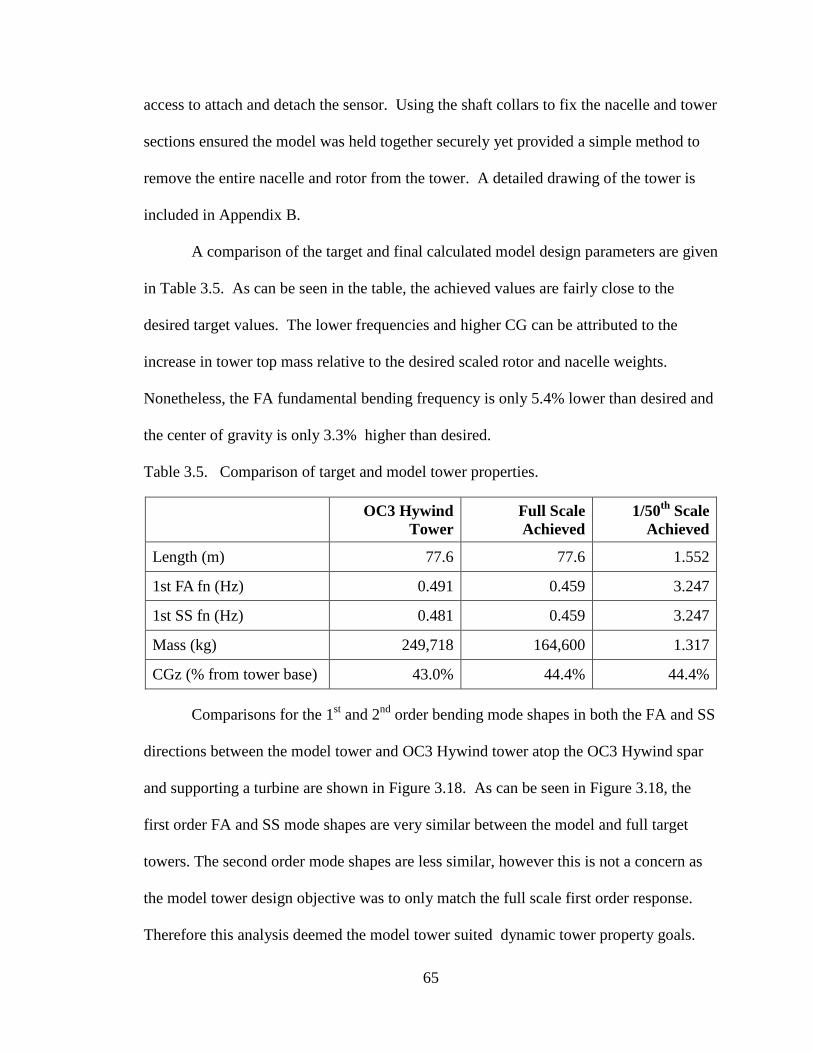
65
access to attach and detach the sensor. Using the shaft collars to fix the nacelle and tower
sections ensured the model was held together securely yet provided a simple method to
remove the entire nacelle and rotor from the tower. A detailed drawing of the tower is
included in Appendix B.
A comparison of the target and final calculated model design parameters are given
in Table 3.5. As can be seen in the table, the achieved values are fairly close to the
desired target values. The lower frequencies and higher CG can be attributed to the
increase in tower top mass relative to the desired scaled rotor and nacelle weights.
Nonetheless, the FA fundamental bending frequency is only 5.4% lower than desired and
the center of gravity is only 3.3% higher than desired.
Table 3.5. Comparison of target and model tower properties.
OC3 Hywind Tower
Full Scale Achieved
1/50th Scale Achieved
Length (m) 77.6 77.6 1.552
1st FA fn (Hz) 0.491 0.459 3.247
1st SS fn (Hz) 0.481 0.459 3.247
Mass (kg) 249,718 164,600 1.317
CGz (% from tower base) 43.0% 44.4% 44.4%
Comparisons for the 1st and 2nd order bending mode shapes in both the FA and SS
directions between the model tower and OC3 Hywind tower atop the OC3 Hywind spar
and supporting a turbine are shown in Figure 3.18. As can be seen in Figure 3.18, the
first order FA and SS mode shapes are very similar between the model and full target
towers. The second order mode shapes are less similar, however this is not a concern as
the model tower design objective was to only match the full scale first order response.
Therefore this analysis deemed the model tower suited dynamic tower property goals.

66
Figure 3.18. Comparison of normalized tower mode shapes.
-1 0 1 2 3 4 50
0.1
0.2
0.3
0.4
0.5
0.6
0.7
0.8
0.9
1
Nor
mal
ized
Tow
er L
engt
h
-1 0 1 2 3 4 50
0.1
0.2
0.3
0.4
0.5
0.6
0.7
0.8
0.9
1
Normalized deflection
Nor
mal
ized
Tow
er L
engt
h
SS1 ModelSS2 ModelSS1 OC3SS2 OC3
FA1 ModelFA2 ModelFA1 OC3FA2 OC3
SS1 (Hz) SS2 (Hz) Model: 0.4592 3.0222 OC3: 0.4814 2.0520
FA1 (Hz) FA2 (Hz) Model: 0.4592 2.9900 OC3: 0.4909 2.5560

67
A final and important comment refers to the tower diameter which was not
properly modeled due to limitations previously discussed. The final model tower
diameter was only 26.9% of the largest scaled maximum tower diameter. However, this
was deemed to be a minor issue. In fact, it was seen as potentially advantageous. The
current NREL simulator does not have a means to simulate the aerodynamic interaction
between the tower and the rotor blades as they pass by. Therefore, a smaller tower is
desirable as it minimizes this aerodynamic interaction making the data better suited for
code validation studies.
3.5. FULL ASSEMBLY
As a precaution in case of damage or failure, two model wind turbines were built
in parallel. Both models were shipped to MARIN for basin model testing, however only
one was used for the duration of the test program. The fully assembled final model wind
turbine, without data cables and a hub cover, is pictured on the following page in Figure
3.19.

68
Figure 3.19. Fully assembled fixed wind turbine model excluding cables.

69
CHAPTER 4. MODEL CHARACTERIZATION AND PERFORMANCE
RESULTS
This chapter presents results from physical characterization tests, blade structural
tests, and turbine performance data of the fully assembled and functional model wind
turbine with a fixed base. First, characterization of the mechanical and mass properties
of the model wind turbine will be presented. Second, blade structural testing and results
are presented and compared to the predicted values from the structural analysis discussed
in Chapter 3. A second analysis of the model tower dynamic response will also be
presented as the mass of the system increased from the original design due to the addition
of heavy instrumentation cables. Lastly, performance data from fixed-based wind-only
basin testing will be presented for the model rotor with original blades and for blades
with a roughened leading edge. The collected performance data will then be compared to
target performance curves and suggestions for a future model blade design will be given.
4.1. PHYSICAL CHARACTERIZATION
The final physical properties of the model wind turbine including the data cables
with a fixed base and mounted to each of the floating platforms was determined at
MARIN prior to floating wind turbine basin model testing. This data, in conjunction with
numerical estimates, was used to determine properties pertaining to the tower, turbine and
data cables exclusive of a floating platform. For all testing, a consistent reference frame
was used to properly identify all model properties and motions. Figure 4.1 illustrates the
floating wind turbine reference frame for positive x, y, and z axes as well as the 6-degrees
of freedom, these being surge, sway, heave, roll, pitch and yaw. The origin for this

70
Figure 4.1. Degrees of freedom and reference frame for floating wind turbines.
reference frame was taken at the intersection of the tower centerline and the still water
plane surface or still water line (SWL). The center of gravity of the wind turbine in the x,
y and z axis were determined by string suspension tests. Values for radius of gyration for
the entire wind turbine model including a floating platform were determined using bifilar
swing tests. Radius of gyration for the wind turbine model alone was obtained via a
combination of numerical estimates for the tower, nacelle and data cables and swing tests
for the rotor. The complete mass properties of the wind turbine model were checked
against the difference between MARIN’s reported masses of the entire systems and
platforms alone. The final values for mass, CG, and radius of gyration of the model wind
turbine with and without cables is given in Table 4.1.

71
Table 4.1. Physical properties of the model wind turbine at full scale.
Property Without Cables With Cables
Mass (kg) 561,750 699,400
CGx (m) 0 0
CGy (m) 0 0
CGz (m) 76.7 71.2
rx (m) 27.8 27.3
ry (m) 27.8 27.3
rz (m) 9.2 8.2
Rotor mass (kg) 122,225 122,225
rrotor (m) 19.3 19.3
A second analysis of the tower natural frequency and associated mode shapes was
performed due to the additional mass of the data cables employed during basin model
testing. In the analysis, the cable mass was modeled as an even distribution down the
tower length equal to 1,774 kg/m. Similar to the tower analysis discussed in Chapter 3,
the analysis utilized the specialized beam finite element package BModes (Bir, 2008) as a
basis to determine the natural frequency and mode shapes of the OC3 Hywind tower and
model tower. Each tower was modeled using approximately 200 beam finite elements.
The OC3 Hywind tower geometry varied linearly from a wide tower base to a more
narrow tower top and required a unique mass and stiffness matrix for each element. The
model tower, which does not taper but includes uniform sections, utilized nine different
uniform cross-section element, and hence many of the finite elements possessed similar
properties in the analysis of the model tower. The distributed properties used to generate
the segment mass and stiffness matrices for the model tower include segment mass
density, bending stiffness, axial stiffness and torsional stiffness. Tables of the distributed
properties for the model tower with and without cables are provided in Appendix D. For

72
Figure 4.2. Normalized mode shapes for the model tower with cables and the OC3
Hywind tower with 1st and 2nd order natural frequency values provided at full scale.
-1 0 1 2 3 4 50
0.1
0.2
0.3
0.4
0.5
0.6
0.7
0.8
0.9
1
Normalized deflection
Nor
mal
ized
Tow
er L
engt
h
-1 0 1 2 3 4 50
0.1
0.2
0.3
0.4
0.5
0.6
0.7
0.8
0.9
1
Nor
mal
ized
Tow
er L
engt
h
FA1 ModelFA2 ModelFA1 OC3FA2 OC3
SS1 ModelSS2 ModelSS1 OC3SS2 OC3
SS1 (Hz) SS2 (Hz) Model: 0.4523 2.7450 OC3: 0.4814 2.0520
FA1 (Hz) FA2 (Hz) Model: 0.4521 2.7210 OC3: 0.4909 2.5560

73
comparison, the OC3 Hywind tower distributed properties can be found in Jonkman,
(2010). The analyses modeled the model tower top with a free boundary supporting a
mass and inertia representing the nacelle and rotor and the tower base supporting a mass
and inertia emulating the compliant OC3 Hywind spar-buoy as well as a stiffness matrix
which represented restoring terms from the mooring system and hydrostatics. These
conditions were the same as those chosen in the earlier design efforts of Section 3.4.
Analysis results are shown in Figure 4.2. with the first and second order normalized mode
shapes for the OC3 Hywind and model towers in both FA and SS directions. By
comparing these mode shapes one can see the first order mode shapes between the model
and OC3 towers are very similar for both the FA and SS directions. The second order
bending mode shapes vary significantly between the model and prototype, much like the
results from the original tower analysis discussed in Chapter 3. However, this was not a
concern as emulating the second order mode shapes was not a primary goal of this
research initiative.
Experimental determination of the tower model natural frequencies was done with
hammer tests prior to wind/wave testing. Hammer tests were executed by exciting the
model with an impulse force, as shown in Figure 4.3, and recording resulting
Figure 4.3. Image of a hammer test to determine model natural frequencies.

74
accelerations at three locations along the tower. These locations were at z = 8.3 m, 49.5
m, and 81.7 m. Excitation was applied in both the x and y directions along the tower
length to determine the FA and SS natural frequencies. Figure 4.4 displays the FA time-
domain acceleration plots and the frequency-domain power spectral density
(PSD)acceleration plots at z = 49.5 m for both the fixed wind turbine model and the
floating wind turbine fixed to the spar-buoy. The PSDs were determined by using
traditional Fast Fourier transform (FFT) techniques (e.g. see O'Neil, 2003). The peaks on
the PSDs identify the system natural frequencies. For the fixed wind turbine the first
significant peak indicates a first FA natural frequency of 0.29 Hz. For the floating wind
turbine on spar-buoy the first large peak, which is at a very low frequency, represents the
rigid body
Figure 4.4. Acceleration and PSD plots of a fixed and floating wind turbine on the spar.
surge natural frequency for the floating system. The second peak represents the first FA
natural frequency of the entire floating system which is 0.43 Hz. The remaining
acceleration and PSD plots at mid height (z = 49.5 m) for FA and SS excitations are
0 1 2 3 4 5-50
0
50Wind Turbine Fixed
m/s
2
Time (s)0 1 2 3 4 5
-50
0
50Floating Wind Turbine on Spar-buoy
Time (s)
m/s
2
0 0.5 1 1.5 20
.05
.1
Frequency (Hz)
PS
D (m
/s2 )
2 /H
z
0 0.5 1 1.5 20
0.01
0.02
PS
D (m
/s2 )
2 /H
z
Frequency (Hz)
Platform surge
2nd fn1st fn1st fn2nd fn

75
given in Appendix D for all the platform types considered. The first and second order FA
and SS natural frequencies for all foundation types considered are listed in Table 4.2.
Table 4.2. Measured tower bending natural frequencies of the model wind turbine with a fixed base and placed on the TLP, spar and semi-submersible platforms at full scale.
Natural frequency (Hz)
1st FA 1st SS 2nd FA
Wind turbine alone 0.29 0.29 1.24
Wind turbine placed on TLP 0.28 0.29 1.16
Wind turbine placed on spar-buoy 0.43 0.44 1.29
Wind turbine placed on semi-submersible 0.35 0.38 1.26
The natural frequency values given in Table 4.2 line up well with analysis results
given in Figure 4. Figure 4.2 provides tower bending natural frequencies for the model
wind turbine tower on the spar only, where the FA and SS first order frequencies were
both 0.452 Hz. These predicted values were 5.1% and 2.7% higher than the measured
values, respectively. The discrepancy, though small, may be attributed to a number of
factors. The finite element analysis assumed rigid tower to platform and tower to nacelle
connections which, in reality, are not perfectly rigid. Also, imperfect characterization of
the tower structural properties and exclusion of gravity effects in the finite element
analysis would yield lower estimates of the bending natural frequencies better aligning
predictions with data. Nonetheless, the model wind turbine and tower yielded similar
physical and dynamic response properties as compared to the target OC3 Hywind tower
design. The total system weight including data cables was a modest 16.6% larger than
the target value and the fundamental FA tower bending frequency with the wind turbine

76
placed on the spar was 0.43 Hz, or 12.2% lower than the target value of 0.491 Hz. The
CG of the model tower including cable weight was at 46.9% the total tower height
resulting in a 9.1% difference between the final and target CG location of 43%.
4.2. BLADE STRUCTURAL TESTING
To complement the structural analysis presented in Chapter 3, a cantilever bending
test was performed to gather data on deflections and strains along the blade length under
loading. The purpose of the structural test was to prove that the model blade possessed
significant strength and exhibited minimal deflection under the most severe Froude
scaled wind conditions utilized during wind/wave basin model testing. All loads were
applied at the tip as it simplified the blade loading logistics during the test and created a
more severe shear force and bending moment distribution along the blade length than
would be expected in operation for a given blade root moment. Loading conditions used
for the test were done such that the resulting blade root moment was equivalent to the
resulting blade root moment from theoretical loading scenarios. All tests were conducted
such that bending occurred about the compliant, or flap, axis of the blade. In the
following discussion, note that all dimensions and loads are given at full scale.
The cantilever test set up is shown in Figure 4.5. Three string-pots were used to
measure the transverse deflection along the blade span. String pots were placed at the tip
and at the third points of the blade span, i.e. at 20.5 m, 41.0 m, 61.5 m from the root. Six
strain gauges were used, three along the top or pressure side and three along the bottom
or suction side starting at the blade root and placed at third points along the blade span or
at 0 m, 20.5 m and 41.0 m from the blade root. All gauges were oriented such that the
only axial strain was recorded. Load application occurred at 60 m from the blade root

77
Figure 4.5. Cantilever bending test set up for 1/50th scale model blade.
and was performed using measured weights for simplicity. Digital control over load
application via actuators and load cells would have been the preferred method of load
application, however the resolution of available lab equipment was not high enough to
apply the small scaled loads needed for the cantilever test. Therefore, weight data was
taken manually and paired with strain and deflection data collected with Labview.
Two types of tests were performed: one at operational loads and the other with
loads leading to blade failure. For operational testing, mass was added in increments of
15,250 kg up to a total load of 137,250 kg. A mass of 57,776 kg was needed at the load
location to create the maximum root moment of 34,000 kN·m which was determined in
Chapter 3. Figure 4.6 illustrates the deflection along the blade span under a blade root
moment of 34,000 kN·m from predicted structural analysis results discussed in Section
3.3.2 and structural test data. From this figure it can be seen the test tip deflection of
0.416 m was larger than the predicted deflection of 0.280 m. What is more important is
that the test deflection of 0.416 m was only 3% of the maximum tip deflection of 13.9 m
POINT LOAD LOCATION
STRINGPOTS
STRAIN GAUGES (TOP & BOTTOM)

78
computed by Jonkman from a fully-coupled simulation with the same 34,000 kN·m blade
root moment. With this data it was found that the model blade stiffness was over 33
times more stiff than the prescribed NREL 5 MW reference wind turbine blades.
Therefore the model blade achieved the high stiffness desired for basin testing as the peak
deflections found via analysis and testing were both minimal compared to the NREL
result. The discrepancy between the test and the analysis can be attributed to the
simplified Euler-Bernoulli analysis model which ignored shear deflection, bend-twist
coupling and three-dimensional effects such as ovalization of the blade cross-sections.
Figure 4.6. Deflection along blade span at full scale under loading to induce a maximum blade root bending moment scenario of 34,000 kN·m from analytical predictions and test results of the model blade.
As noted earlier, a second cantilever test was performed to determine the model
blade failure strength. This was done to ensure that the blade strength greatly exceeded
the strength required to resist aerodynamic loads during floating wind/wave basin model
testing. The results of this test are displayed in Figure 4.7 where tip deflection is plotted
as a function of blade root moment. The blade root moment shown in Figure 4.7 was
calculated by multiplying the applied load by the load location relative to the root and
adding the self-weight of the blade multiplied by the blade CG location which was
identified at 38% of the blade length from the root from a knife edge test.
0 10 20 30 40 50 60-1
-0.5
0
0.5
Full blade span, [m]
Def
lect
ion,
u [m
]
Test DataPrediction

79
Figure 4.7. Tip deflection as a function of blade root moment up to blade failure for the
model blade at full scale.
The last data point taken prior to blade failure is shown with an “×” in Figure 4.7.
Also the gray area of Figure 4.7 represents the range of blade root moments that are
expected during basin model testing with the maximum being 34,000 kN·m. As can be
seen by this figure, the model blade failure point is well beyond the expected operating
range which indicates that the blade is sufficiently strong to endure all wind/wave basin
model testing. The second structural test also demonstrated that blade failure was a result
of buckling and not material failure. Once the load was removed post failure, the blade
restored itself to its original configuration. The location of buckling failure or peak stress
occurred at a relatively thin blade section, at least for the NREL blade, at approximately
two-thirds of the blade length from the blade root under a load of 2,506 kN.
The location of buckling failure was found to be in close proximity with the
location of maximum stress under operational conditions determined from test data and
predicted stress values from the analysis discussed in Section 3.3.2. Strain gauge data
taken along the bottom, or compressive side, of the blade is shown in Figure 4.8 and
compared to predicted stress values determined from the structural analysis provided in
0 2 4 6 8 10 12 14 16
x 104
0
0.5
1
1.5
2
2.5
Root moment, [kN-m]
Tip
defle
ctio
n, [m
]
Test DataTest failure
Rangeduringtesting.
3.4

80
Figure 4.8. Induced stress along blade span at full scale under loading to induce a maximum blade root bending moment scenario of 34,000 kN·m from analytical predictions and test results of the model blade.
Section 3.3.2. Stress values from strain data were computed simply with Hooke’s law by
multiplying the recorded axial strain by the composite compressive elastic modulus of
54.10 GPa. Analysis results showed a maximum stress of 427.7 MPa at 43.0 m from the
blade root while test data reported a maximum stress of 450.4 MPa at 41.0 m from the
blade root. While no strength information is available for this material from the
manufacturer, no material failure is expected during operation since typical strength
values in compression for woven carbon epoxy composites are expected to be
approximately twice the maximum stress values from Figure 4.8 (e.g. see Daniel & Ishai,
2006).
The differences of the predicted and test values given in Figure 4.8 are due to the
crude analysis method used in Section 3.3.2 where anisotropic material properties were
not considered and a simplified blade geometry was modeled. In addition, the
information recorded by the strain gauges may be mildly altered by the presence of the
woven material structure. Additionally test strain data was limited as data was collected
0 10 20 30 40 50 60 70-100
0
100
200
300
400
500
Full blade span, [m]
Stre
ss, σ
[M
Pa]
Test DataPrediction

81
at three discrete points along the blade span and the maximum stress most likely occurred
in a location not equipped with a strain gauge. As a result, the information provided n
Figure 4.8 has considerable room for error due to the test and analysis procedures.
However, the purpose of the analysis and test was to prove beyond a reasonable doubt
that the model blade possessed high stiffness and adequate strength to resist deflection
and failure during basin model testing. The information provided in both the analysis and
test data has achieved this purpose even with the simplified procedures employed.
Overall, it is evident that the model blade met not only the design goals of a very high
bending stiffness, but also exhibited sufficient strength to easily resist any wind loading
during basin model testing.
4.3. WIND TURBINE PERFORMANCE
In addition to building an accurately scaled model wind turbine to achieve proper
dynamic response during basin model testing, the fully functional model wind turbine
was also built to emulate the functions of a real wind turbine and produce power and
thrust from Froude scaled winds during basin model testing. As discussed in Chapter 3,
the model blade geometry was scrutinized to produce a clean and accurate geo-sim of the
NREL 5 MW reference wind blade. During assimilation of the blade geometry, it was
anticipated that the geo-sim blade would perform comparably with the full scale blade
performance. This was predicated on the notion that the primary lift forces, for small
angles of attack, were not heavily reliant on Reynolds number and that the increase in
drag would be moderate and in line with flat plate calculations. However, the discussion
on Reynolds number effects in Chapter 2 clearly indicates that the lift and drag
coefficients are significantly affected by Reynolds number, especially for the thick foil

82
sections used for the model blade. The performance data taken during basin model
testing reflects the influence of low Reynolds number wind airflow on airfoil behavior,
and therefore, wind turbine performance. The remainder of this section will present and
discuss the performance data taken during fixed-based wind turbine testing.
Performance data collected during initial wind/wave basin model testing showed a
lack of generated torque and thrust when compared to expected values. While not
completely understood at the time, laminar separation was suspected as the cause of the
altered airfoil performance which was later confirmed with the analysis presented in
Chapter 2. Therefore, during basin model testing a decision was made to increase the
wind speeds to help increase model turbine performance and more specifically match full
scale and model scale thrust values which significantly influence the coupled motions of
the floating wind turbines. An example of the effect of the increased wind speed is
detailed Chapter 2 where wind speed was increased from 11.4 m/s to 20.8 m/s, these
speeds corresponding to the rated thrust condition.
Performance data is presented in subsequent text as the power coefficient, CP, and
thrust coefficient, CT, which are computed as
312
PPCU Aρ
= , (4.1)
212
TTCU Aρ
= , (4.2)
where ρ is the density of air, U is the wind inflow speed and A is the total swept area of
the HAWT rotor. P is the generated power determined from model torque data
multiplied by the rotor rotational speed and T is the generated thrust determined by x-axis

83
force data taken at the tower top. The power coefficient is a ratio of the generated power
to the available power of the wind inflow. Similarly the torque coefficient is the ratio of
generated thrust to a basic quantity representing potential wind force (Manwell, et al.,
2002). The power and thrust coefficients were used to provide a clean and concise way to
analyze the performance of a wind turbine design.
Figure 4.9 provides the normalized power and thrust coefficient curves generated
from the fixed-based model wind turbine performance data. These performance curves
were generated with a blade pitch setting of 6.4 degrees as this pitch angle was found to
produce the highest power response for the turbine during basin model testing. As is
Figure 4.9. Model wind turbine power and thrust coefficient performance curves from
fixed-base wind-only basin model testing data.
shown by Figure 4.9 the peak values for CP and CT were very low at 0.038 and 0.25
respectively. Typically a full scale peak value of CP would be approximately 0.45 and a
full scale value of CT around 0.9 at an operational TSR of roughly 7. For this
performance test, data was collected up to a TSR of 4.6 as maximum CP was achieved at a
TSR of 3.9. In addition, since the wind speed was increased while rotor speed was
0 1 2 3 4 50
0.01
0.02
0.03
0.04
0.05
TSR
CP
0 1 2 3 4 50
0.05
0.1
0.15
0.2
0.25
0.3
TSR
CT

84
maintained, the range of possible TSR values the model could operate through was
diminished. Due to rotor speed safety limitations, the aforementioned maximum TSR of
4.6 could not be surpassed to collect data at an ideal full scale TSR of roughly 7. The
range of tested TSRs aside, these low CP and CT values were attributed to low lift and
high drag coefficients for the model blade airfoil sections due to the low Reynolds
number conditions experienced during wind/wave basin model testing. As detailed in
section 2.1.3, the geo-sim model blade utilized thicker high-Reynolds number airfoils
which performed poorly at model scale wind inflow and rotor speeds.A comparison of
the data performance curves from Figure 4.9 and the desired performance curves are
shown in Figure 4.10. The desired full scale performance curves are provided for a blade
pitch angle of zero and 6.4 degrees and are labeled as Full 0 and Full 6.4 respectively.
Note that the target turbine blade pitch angle was zero degrees as this yields the
Figure 4.10. Performance curves for the NREL 5 MW wind turbine and model turbine.
0 2 4 6 8 100
0.1
0.2
0.3
0.4
0.5
0.6
0.7
0.8
0.9
TSR
Ct
0 2 4 6 8 100
0.05
0.1
0.15
0.2
0.25
0.3
0.35
0.4
0.45
0.5
TSR
Cp
Model SmoothModel RoughFull 0Full 6.4

85
maximum performance coefficient under full scale conditions.. However, the model
achieved maximum performance at a blade pitch of 6.4 degrees. Hence the full scale
performance curve of 6.4 degrees is shown to illustrate the maximum achievable
performance for this blade at that pitch angle. The result for the shift in maximum
performance of the model blade from the expected zero degrees to 6.4 degrees is a result
of drastically altered lift and drag coefficients at the low Reynolds number, as discussed
in Section 2.1.3. Referring back to Figure 4.9, the model performance curve is labeled as
Model Smooth, which will be elaborated upon in subsequent text. By comparing these
performance curves, it can be seen that the model wind turbine did not produce the torque
and thrust behavior desired during basin model testing. Note that the model thrust
coefficient curve was significantly closer to desired behavior than the power performance
curve and hence required a modest increase in wind speed (see Equation 4.2) to maintain
full scale thrust. The very low power coefficient lends evidence to the fact that the model
did not yield sufficient torque to create properly scaled power, even when wind speeds
were increased by 80% to match the desired thrust. Nonetheless, the thrust and not the
torque, is the main aerodynamic load which contributes to the floating system global
motions and dynamics and was the more important parameter to maintain. In addition to
closely modeling the appropriate thrust forces, the proper model wind turbine rotor
rotational speed was utilized during basin model testing which when coupled with the
near target rotor inertia, yielded the correct gyroscopic dynamic effects. Aside from the
thrust correction and achieving the correct gyroscopic dynamic effects, the increased
wind speed could have negative effects and reduce the representative accuracy of the
model wind turbine as compared to the expected full scale behavior. For example,
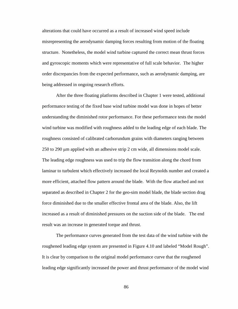
86
alterations that could have occurred as a result of increased wind speed include
misrepresenting the aerodynamic damping forces resulting from motion of the floating
structure. Nonetheless, the model wind turbine captured the correct mean thrust forces
and gyroscopic moments which were representative of full scale behavior. The higher
order discrepancies from the expected performance, such as aerodynamic damping, are
being addressed in ongoing research efforts.
After the three floating platforms described in Chapter 1 were tested, additional
performance testing of the fixed base wind turbine model was done in hopes of better
understanding the diminished rotor performance. For these performance tests the model
wind turbine was modified with roughness added to the leading edge of each blade. The
roughness consisted of calibrated carborundum grains with diameters ranging between
250 to 290 μm applied with an adhesive strip 2 cm wide, all dimensions model scale.
The leading edge roughness was used to trip the flow transition along the chord from
laminar to turbulent which effectively increased the local Reynolds number and created a
more efficient, attached flow pattern around the blade. With the flow attached and not
separated as described in Chapter 2 for the geo-sim model blade, the blade section drag
force diminished due to the smaller effective frontal area of the blade. Also, the lift
increased as a result of diminished pressures on the suction side of the blade. The end
result was an increase in generated torque and thrust.
The performance curves generated from the test data of the wind turbine with the
roughened leading edge system are presented in Figure 4.10 and labeled “Model Rough”.
It is clear by comparison to the original model performance curve that the roughened
leading edge significantly increased the power and thrust performance of the model wind

87
turbine, primarily above a TSR of 4. The drastic jump in performance around this TSR is
likely a result of the changing Reynolds number. As the rotor speed, or TSR, was the
dominant contributor to airfoil section speed, and hence Reynolds number, the low TSR
regions possessed a blade that was almost entirely experiencing laminar separation. At
the higher TSRs, or higher Reynolds number, the flow began to reattach on the outer
blade airfoil sections which produced appreciable lift and low to moderate drag and
resulted in drastically increased rotor performance. Even though it would have been
desirable to do so, TSR values beyond 4.9 were not tested as a result of a rotor speed limit
of 15.5 rpm (110 rpm model scale) set on the control system for safety purposes. As the
CP curve was still increasing at the largest tested TSR it is very likely peak CP was in
excesses of the 0.16 value shown. Even so, a CP of 0.16 was still 420% higher than the
turbine performance with a smooth blade leading edge. As a result of this testing, it is
clear that careful attention should be made to model blade surface treatment in order to
maximize turbine performance in the Froude scaled environment of a wind/wave basin
model test.
Even though leading edge roughness helped increase performance, future wind
turbine testing under Froude scaled winds will benefit by using a low-Reynolds number
specific wind blade geometry. While the blade geometry will likely not represent the full
scale architecture, the blade should be designed to increase torque output, match full
scale CT curves, and if possible closely match the change in total blade lift force with
respect to blade pitch. The first two points will ensure that the global mean forces on the
structure are maintained in a Froude scale environment, while the second will help
maintain the effect of turbine damping forces due to either changing wind speeds or

88
global motion of the floating wind turbine structure. In the following paragraphs an
example of a Froude scale specific model wind turbine blade geometry is presented. To
simplify the design process, emphasis was placed only on creating a simple geometry that
matched the CT curve in the vicinity of operational TSR (approximately 7) and maximized
the peak value of the CP curve.
The example redesign of the model wind blade began with the selection of a low-
Reynolds number airfoil which for this example is the Drela AG04 low-Reynolds specific
airfoil (Drela, 1995). The AG04 geometry is provided in Figure 4.11 where it is clearly
evident that the airfoil is very thin and therefore not as susceptible to laminar separation
Figure 4.11. Drela AG04 low-Reynolds number airfoil.
as many of the NREL 5 MW blade thick airfoil sections at the low model scale Reynolds
numbers. Lift and drag coefficients of the Drela AG04 and NACA 64-618 airfoils
determined by an XFOIL analysis are provided in Figure 4.12. As can be seen in Figure
4.12 it is clear that the AG04 airfoil showed significantly larger lift coefficient and lower
drag coefficient than the NACA 64-618 airfoil at the low Reynolds number of 35.7×10³
for operational angles of attack between zero and ten degrees. This was a drastic
improvement, however it is important to note that is difficult to create an airfoil that will
achieve the same high lift and very low drag of the full scale high Reynolds number
condition at these low Reynolds numbers.
-0.1 -0.05
0 0.05 0.1
0 0.2 0.4 0.6 0.8 1
Drela AG04 Airfoil

89
Figure 4.12. Lift and drag coefficients of the NACA 64-618 airfoil under high and low- Reynolds number conditions and of the Drela AG04 airfoil under low-Reynolds number conditions.
Using the AG04 lift and drag information of Figure 4.12 in the NREL FAST
package and manually adjusting the blade chord and twist distributions, a reasonably well
performing low-Reynolds number blade was achieved. A description of the blade is
given in Table 4.1. Comparing the new blade and the blade of Table 3.3, one can see that
the new blade had some unique differences as compared to the NREL 5 MW blade. First,
the inner sections, which are now airfoils instead of cylinders, were rotated a great deal
further so that the root sections produced lift and would not stall. Also, note that the
chord is 25% longer along the entire length of the blade as compared to the original
configuration of Table 3.3. This is to make up for the diminished lift force resulting from
the slightly smaller lift coefficient. The increase in chord raises the lift force to nearly the
same value as expected at full scale. Lastly, it is evident that the new blade is very thin
throughout the length of blade and does not possess any thick sections which will
-10 0 10 20-1
-0.5
0
0.5
1
1.5
2
α [deg]
CL
-10 0 10 200
0.05
0.1
0.15
0.2
0.25
α [deg]C
D
NACA 64-618,Re: 11.5x10⁶
NACA 64-618,Re: 35.7x10³
Drela AG04,Re: 35.7x10³
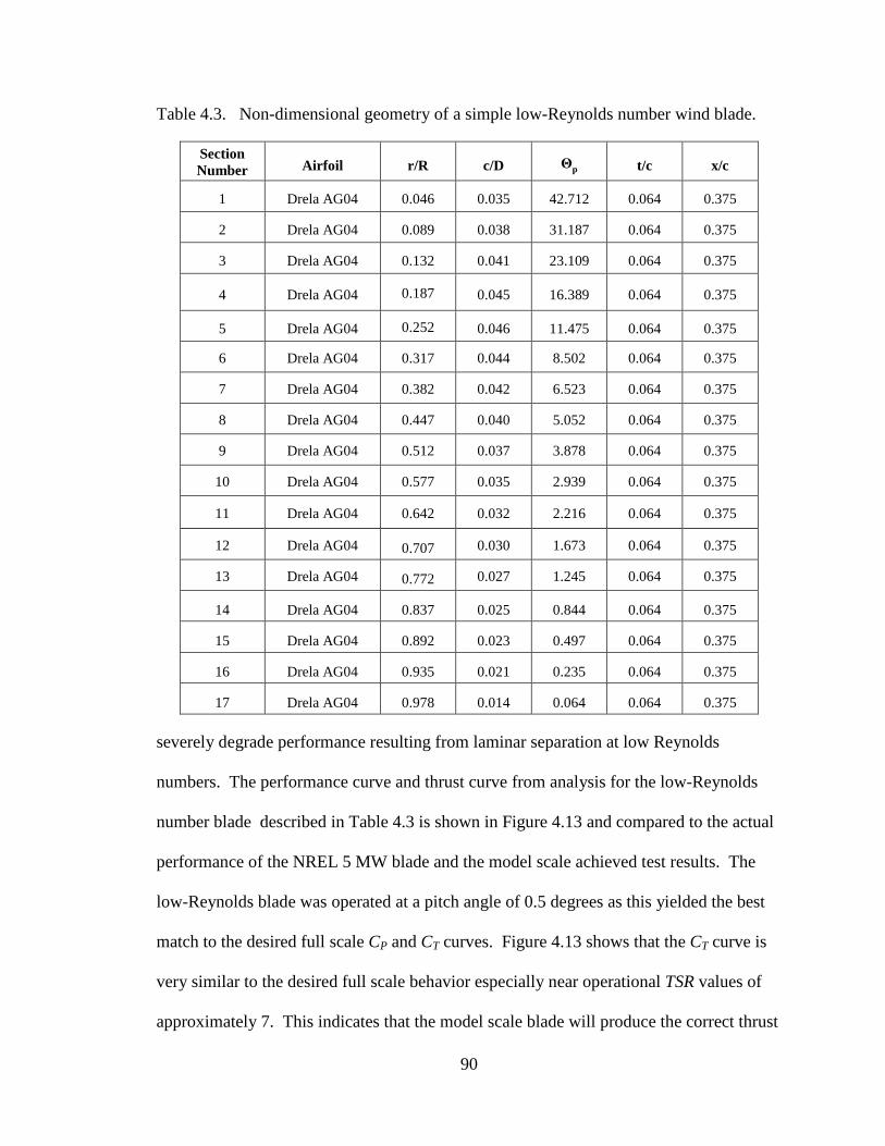
90
Table 4.3. Non-dimensional geometry of a simple low-Reynolds number wind blade.
Section Number Airfoil r/R c/D Θp t/c x/c
1 Drela AG04 0.046 0.035 42.712 0.064 0.375
2 Drela AG04 0.089 0.038 31.187 0.064 0.375
3 Drela AG04 0.132 0.041 23.109 0.064 0.375
4 Drela AG04 0.187 0.045 16.389 0.064 0.375
5 Drela AG04 0.252 0.046 11.475 0.064 0.375
6 Drela AG04 0.317 0.044 8.502 0.064 0.375
7 Drela AG04 0.382 0.042 6.523 0.064 0.375
8 Drela AG04 0.447 0.040 5.052 0.064 0.375
9 Drela AG04 0.512 0.037 3.878 0.064 0.375
10 Drela AG04 0.577 0.035 2.939 0.064 0.375
11 Drela AG04 0.642 0.032 2.216 0.064 0.375
12 Drela AG04 0.707 0.030 1.673 0.064 0.375
13 Drela AG04 0.772 0.027 1.245 0.064 0.375
14 Drela AG04 0.837 0.025 0.844 0.064 0.375
15 Drela AG04 0.892 0.023 0.497 0.064 0.375
16 Drela AG04 0.935 0.021 0.235 0.064 0.375
17 Drela AG04 0.978 0.014 0.064 0.064 0.375
severely degrade performance resulting from laminar separation at low Reynolds
numbers. The performance curve and thrust curve from analysis for the low-Reynolds
number blade described in Table 4.3 is shown in Figure 4.13 and compared to the actual
performance of the NREL 5 MW blade and the model scale achieved test results. The
low-Reynolds blade was operated at a pitch angle of 0.5 degrees as this yielded the best
match to the desired full scale CP and CT curves. Figure 4.13 shows that the CT curve is
very similar to the desired full scale behavior especially near operational TSR values of
approximately 7. This indicates that the model scale blade will produce the correct thrust

91
in a proper, and unaltered, Froude scale environment. The CP curve, while much better,
is still not the same as the full scale curve. This is due primarily to the inevitable increase
in airfoil drag at low Reynolds numbers which detracts almost directly from the wind
turbine power generation, or torque. Achieving a peak final value of over 0.35,
especially with peak efficiency occurring at the correct TSR, is most likely the best one
can expect under Froude scaling circumstances.
Figure 4.13. Power and thrust coefficient curves for the full scale, achieved geo-sim at 1/50th scale, and redesigned 1/50th scale blade.
Overall, the performance of the geo-sim model wind blade did not closely match
the desired performance values due to Reynolds number dependent alterations in airfoil
section lift and drag coefficients. The addition of roughness along the geo-sim blade
leading edge helped increase performance drastically, however data collection did not
cover the range of desired TSR values due to instrumentation limitations and the
maximum CP was not believed to be achieved. Nonetheless, it is advised for future
model tests to treat the leading edge of model blades in addition to designing a low-
Reynolds number specific wind blade to best match the desired performance results in a
Froude scale test. The previous design example presented is a good starting place from
0 2 4 6 8 100
0.1
0.2
0.3
0.4
0.5
0.6
0.7
0.8
0.9
TSR
CT
0 2 4 6 8 100
0.05
0.1
0.15
0.2
0.25
0.3
0.35
0.4
0.45
0.5
TSR
CP
Desired Full Scale
Redesigned 1/50th
Original 1/50th

92
which to further optimize the blade geometry to best achieve scaled aerodynamic
performance. Even though the NREL 5 MW geo-sim did not yield the correct turbine
performance under strictly Froude scale winds, the additional testing results and design
efforts presented here indicate that a suitable wind turbine can be constructed to more
closely match the target performance values under Froude scaled winds.
93
CHAPTER 5. CONCLUSION
The purpose of this work was to design, build and characterize a fully-functional
1/50th scale model wind turbine based on the NREL 5 MW reference wind turbine for the
purpose of wind/wave basin model testing of commercially viable offshore floating wind
turbine concepts. Unlike other known floating wind turbine wind/wave basin model
tests, this program subjected the floating model wind turbine to fully characterized
Froude scaled wind with the goal to produce torque, thrust, and gyroscopic forces that a
real wind turbine would experience. Aside from turbine performance, the functional scale
model wind turbine was designed to be mounted to three scale floating platforms via a
flexible tower which experienced additional forcing from scaled wave environments in
order to study the global motions and dynamic response of the entire system. The end
goal of the scale model development testing program was to collect data for validation of
fully-coupled servo-aero-hydro-elastic simulation codes, such NREL’s fully-coupled
simulator, as no such data currently exists. This goal was ultimately met in large part due
to the work outlined in this thesis which details and characterizes the fully functional
scale model wind turbine and tower utilized in wind/wave basin testing.
5.1. OVERVIEW OF DESIGN AND RESULTS
Overall, the physical model performed well throughout the duration of the model
test program. More specifically, the model nacelle, hub, sensors, and components suited
their purpose and met the needs of the basin model test program. No part of the bearing
housing, torque tube or hub malfunctioned throughout the five week basin model test
program. Nonetheless, improvements could still be made in future design iterations.

94
One design improvement involves the use of materials better suited to resist a
humid and dynamic environment for manufactured components. Mid-way through basin
model testing, the nacelle was disassembled and certain components cleaned of
potentially harmful rust accumulation. This can be avoided in future testing if rust
resistant materials or coatings were used for critical components, particularly those
possessing mating surfaces with other parts . For the wind turbine model described in
this thesis, not all components of the hub and nacelle were manufactured from these types
of materials in order to keep project costs in check. The blade pitch control assembly
also satisfied the needs for this model test program, however the linkages and the actuator
were not as durable as desired in order to resist the accumulation of joint slop caused by
continuous loading throughout five weeks of double shift basin model testing. As a
result, these components were periodically checked and replaced as needed throughout
the test program. In short, there is appreciable room for improvement of the pitch control
assembly design if the system is to be employed for future testing. This is especially true
if active blade pitch control would be a major part of future testing. For the wind/wave
basin test program, just the periodic remote operation of the blade pitch system in
between tests was enough to develop the aforementioned slop issues, therefore
continuous actuation of the system will be far more demanding, requiring an increase in
system robustness. Lastly, the final nacelle weight was still higher than the target weight.
Further reduction of the nacelle weight would be another area suitable for improvement.
Potential ways to reduce weight further would be truncating the torque tube and/or
removing more material from the bearing housing. However, the majority of the nacelle
and hub mass was located in the motor and gearbox assembly. Therefore, finding an
95
alternate, smaller motor with the similar capability as the Parker Motion BE164D may be
the cleanest and best weight loss solution for the nacelle.
Regarding the physical properties of the entire model wind turbine, the total mass
of the model was 16.5% larger than the target value which was primarily due to the
additional mass from the chosen instrumentation cables. Even though the model tower
weight described in Chapter 4 was 34% less than the target weight in order to
accommodate the heavy nacelle, the inclusion of the instrumentation cables affixed to the
length of the tower caused the final tower mass to be 21% greater than the target tower
mass which was not ideal. Nonetheless, the model tower dynamic response analysis,
which included the additional cable mass, mass from the model nacelle and inertia and
stiffness of the floating spar-buoy, yielded dynamic characteristic results very near the
target values. The fundamental bending frequencies and mode shapes for FA and SS
motion of the model tower were within 12.4% of the full scale target values, a
discrepancy deemed suitable for the needs of the wind/wave basin model testing
program.
Aside from the blade aerodynamic performance, the quality and stiffness of the
carbon fiber model blades exceeded design goals. The bladder-mold fabrication produced
high quality, ultra-light hollow composite model blades consistently and reliably. Due to
these successes, it is highly recommended that the bladder-mold fabrication method be
used for future composite model blades and other lightweight model components. The
structural analysis results and accompanying test data proved that the model blade
possessed the desired high stiffness and more than adequate strength to resist deflections

96
under extreme wind/wave basin loading conditions meeting the established blade design
goals.
Due to the difficulty of achieving target performance of a model wind turbine
under Froude scaled winds, much of this research effort was focused on understanding
and identifying the most appropriate method to capture appropriate aerodynamic forces.
During the pre-basin testing design efforts, crude flat plate viscous flow calculations led
to the assumption that the model turbine performance would represent full scale wind
turbine performance at low angles of attack with a geo-sim of the NREL 5 MW blade
under Froude scaled wind. However, the geo-sim blade utilized thick high-Reynolds
number airfoils which are required in real machines to provide adequate bending
strength. As the Froude scaled wind conditions in the basin were of a very low-Reynolds
number relative to the full scale wind conditions, the performance of the high-Reynolds
number airfoil geometries used in the blade design suffered resulting in a model rotor
performance that was much poorer than expected with low thrust and power generation.
Therefore, basin wind speeds were increased by 80% as a result of the diminished thrust
coefficient of the rotor. While this adjustment captured the correct thrust vital for
properly modeling the coupled global response of the floating wind turbine system, the
generated power and torque were still low.
Further investigation with XFOIL analyses of the NACA 64-618 airfoil sections
utilized in the model blade showed that the diminished performance was due to laminar
separation of the fluid flow near the leading edge of the suction side of the airfoil at the
low model scale Reynolds numbers. This laminar separation caused the formation of a
large wake in the rotor plane perpendicular to the wind inflow which decreased lift

97
coefficients and increased drag coefficients, resulting in low aerodynamic thrust and
torque. To gather performance data on the model wind turbine as a function of TSR,
fixed-base wind only tests were performed with Froude scaled winds increased by 80% to
match full scale rated thrust conditions. Data from these tests confirmed the XFOIL
analysis and characterized the model turbine with low thrust coefficients and severely
low power coefficient as a function of TSR compared to target performance.
Due to suspicion of laminar separation over the blade surface, a second round of
fixed-based wind only basin model testing was performed with roughness added to the
leading edge of each blade to trip the flow over the airfoil sections from laminar to
turbulent to prevent laminar separation. The performance data presented from these tests
showed power and thrust generation was greatly improved with the simple addition of
leading edge roughness, especially at higher TSR values. However, the test could not be
performed over the range of desired TSRs due to instrumentation limitations, and hence,
the incomplete test was unable to record the maximum power coefficient.
In addition to adding leading edge roughness it was found through analysis that
improved performance could be achieved through a redesign of the model blade
geometry by incorporating low-Reynolds number airfoils. By utilizing low Reynolds
number airfoils, such as was done in the example blade provided in Chapter 4, the model
wind turbine performance has the potential to achieve closer performance values under
Froude scaled winds as compared to the desired target performance from the full scale
wind turbine. The provided redesigned Froude scale blade illustrated the great potential
of using a modified turbine geometry to replicate full scale turbine performance,
particularly in the magnitude and shape of the thrust coefficient curve in the vicinity of

98
the turbine operating range. However, while not ideal, the geo-sim blade used for this
model test did attain the appropriate thrust forces that greatly affect the critical system
global responses of the entire floating wind turbine model by increasing wind inflow
velocities.
5.2. FUTURE WORK
The work described in this thesis is hoped to provide a foundation for the
development of future floating wind turbine basin model tests. That said, there is
certainly room for future improvements and additional model testing. A first suggestion
for future work is to complete the performance curves of the wind turbine model with
leading edge roughness by performing another fixed-base wind-only test and removing
system rotational speed limitations such that the model would operate at higher TSRs. A
completed performance curve would help characterize the extent to which leading edge
roughness can help improve the model wind turbine performance under Froude scale
winds. In addition, another series of performance testing with varying grain size of the
roughness material would also be useful information to help establish recommendations
for ideal blade leading edge treatments for future model testing.
Another area of future work would involve a re-design of the model wind blade
geometry to closely achieve target performance values, especially those for thrust. Unlike
the wind blade used for this model, using low-Reynolds number airfoils for the blade
design will help improve wind turbine performance under Froude scaled winds, likely
more than can be achieved by the addition of leading edge roughness alone. This is not to
suggest that a revised blade geometry should ignore leading edge roughness, as the
optimal model scale blade designs will likely make use of both strategies. The low-

99
Reynolds number wind blade design given in Chapter 4 illustrated potential blade
redesign techniques and provided a starting place for a new blade design. However, it is
important to note the example redesigned blade has not been fully optimized with regard
to best mimicking the performance behavior of the NREL 5 MW reference wind turbine
blade under Froude scale winds. Once a more optimal blade has been established and
built, another round of fixed-base wind only testing should be performed to capture
performance data and generate new power and thrust coefficient curves. Subsequently,
target and collected performance curves can be compared and further iteration of the
design procedure executed until no further improvement can be realized.
While beyond the scope of the initial floating wind turbine model test program,
future wind/wave basin model tests may want to include active blade pitch control
functionality to the model wind turbine as the effect of active pitch control on global
system response is an important research topic. To do so, the current nacelle design
should be retrofitted to accommodate new hardware for active pitch control as the
actuator and components used for this test program do not exhibit as much durability as
initial estimates would expect for this type of application. One design suggestion is to
incorporate separate mini-servo motors on the nacelle or within the blade roots which
receive command signals in parallel to actuate pitching of the wind blades. This
arrangement has the potential to be more robust and creates greater test flexibility, such
as the possibility to study cutting edge individual blade pitch schemes. However, three
mini servo motors are likely to be heavier than the small L12 Firgelli actuator employed
in the design outlined in Chapter 3. However, this could be compensated for with weight
reduction in some of the other nacelle and blade components. In addition to different

100
actuators, it is highly recommended that thicker, more stiff linkages or another more
robust manner of connecting the blades to the actuator or servo motors be used to make
the pitch control assembly more durable.
A final but important improvement in future model wind turbine designs is the
inclusion of lighter, less stiff cables to connect the model sensors and motor to the control
box. It is advised to specify and obtain cables well in advance of basin model testing as
specialty cables may need to be ordered and/or created. Having the appropriate cables
and including them in the original wind turbine design would reduce complications
related to testing and analysis.
5.3. CONCLUSIONS
In conclusion, the 1/50th scale wind turbine model met the critical design
requirements to execute a successful wind/wave basin floating wind turbine model test.
In retrospect, the chosen scale factor of 50 was an appropriate scale factor. A larger scale
factor was not desirable as it would have been difficult to create the small wave
environments, would have worsened Reynolds number dependent issues with the wind
turbine, and created near impossible model weight targets to achieve during design and
fabrication. A smaller scale factor would have increased the model size and improved
test accuracy, however mooring line length would have become a limiting factor with
respect to the basin size. Also, a smaller scale factor would have increased the size and
cost even more so of the wind machine built for this test program. Therefore, a scale
factor of 50 was suitable for this test program.
The forces and turbine properties that dictate the global motions and structural
response of the wind turbine model were in the vicinity of target values. The model

101
turbine power generation target was not ideally attained, however achieving the
appropriate power generation was considered secondary to achieving the appropriate
thrust forces which affect the global motions and structural response of the entire turbine.
The performance data presented here was for a fixed wind turbine and it would be likely
that performance of the floating wind turbine model would have diminished slightly due
to changes in the relative turbine wind inflow angle resulting from the moving rotor
plane. Maximizing energy capture for a moving turbine is a significant reason to pursue
future floating wind turbine basin model testing with active pitch control.
The test data taken from the wind/wave basin model test can now be compared to
outputs from fully-coupled numerical simulations employing the wind turbine model
characterized in this thesis for various code calibration and validation efforts. The
information provided in this thesis is intended to help refine the science of basin model
testing of floating wind turbine systems and guide future testing endeavors. Overall, it is
believed that the planned numerical code validation efforts which utilize data generated
from this model wind turbine will help boost future development and commercialization
of floating wind turbine technology in the United States and aid in ensuring future energy
security with a sustainable, renewable and abundant domestic resource: offshore wind.

102
APPENDIX A. INSTRUMENTATION AND CONTROLS SPECIFICATIONS
Component Manufacturer Part Number Signal Type Notes
Analog Encoder US Digital MA3-A10-125-B
10-bit Analog
Absolute output
Linear Actuator Firgelli Inc. L12-30-210-P L12-30-100-P USB/RS232
210 &100 gear ratios used for comparison
T2 Precision Rotary Torque Transducer
Interface Inc. T2-10Nm TTL Signal
6-Axis Force and Moment Sensor
Advanced Mechanical Testing Inc. (AMTI)
FS6-500 Analog
Gyro Enhanced Orientation Sensor (6-Axis Accelerometer)
MicroStrain 3DM-GX1 16-bit Analog Output
Parker Rotary Servo Motor Parker Motion BE164D-J-
NFON Encoder TTL
10:1 Gearhead Parker/Bayside NE23-010 N/A
Table A.1. Nacelle sensor and component specifications.

103
Component Manufacturer Part Number Notes
CompactDAQ data acquisition 4-slot chassis
National Instruments NI cDAQ-9174 Collect and distribute
signals
32-Ch Analog Input Module
National Instruments NI 9205 Torque and encoder input
4-Ch Analog Output Module
National Instruments NI 9263 Motor controller output
(2) 4-Ch Simultaneous Bridge Modules
National Instruments NI 9237
6-axis gauge inputs, module 1: forces, module 2: moments
Xenus XTL Digital Servo Drive (Motor controller)
Copley Controls XTL-230-40 Motor controller
Linear Actuator Control Board Firgelli LAC
24V, 12V, 5V Power Supplies Rhino
PSC-24-060 PSC-12-015 PSC-05-012
24 V: Motor, motor controller, CompactDAQ and modules, 12V: torque transducer, 6-axis accelerometer 5V: linear actuator and MA3 encoder
Protective Circuit Breaker Merlin Gerin Multi 9 System
C60a
EMI Filter Delta Electronics, Inc. 03DBAG5
Table A.2. Data acquisition and control equipment specifications.

104
APPENDIX B. SHOP DRAWINGS OF THE NACELLE, HUB AND TOWER
A
PPE
ND
IX B
. SH
OP
DR
AW
ING
S O
F T
HE
NA
CE
LL
E, H
UB
AN
D T
OW
ER
Figu
re B
.1.
Nac
elle
, hub
and
tow
er sh
op d
raw
ings
.

105
Figu
re B
.1.
Nac
elle
, hub
and
tow
er sh
op d
raw
ings
.

106
Figu
re B
.1.
Nac
elle
, hub
and
tow
er sh
op d
raw
ings
.

107
Figu
re B
.1.
Nac
elle
, hub
and
tow
er sh
op d
raw
ings
.
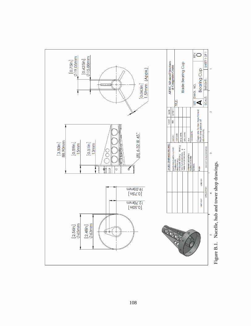
108
Figu
re B
.1.
Nac
elle
, hub
and
tow
er sh
op d
raw
ings
.

109
Figu
re B
.1.
Nac
elle
, hub
and
tow
er sh
op d
raw
ings
.

110
Figure B.1. Nacelle, hub and tower shop drawings.

111
APPENDIX C. BLADE GEOMETRY, SCRIPTS AND INPUT FILES
Airfoil 2D Geometry
Figure C.1. 2D geometry of model blade airfoil sections.
DU40_ft.txt x/c t(x)/c f(x)/c df/dx(x) 0.0000000e+000 0.0000000e+000 0.0000000e+000 0.0000000e+000 4.2775693e-003 6.5574565e-002 -2.1947304e-005 -5.2558510e-003 1.7037087e-002 1.3030746e-001 -9.3769328e-005 -6.1730149e-003 3.8060234e-002 1.9257545e-001 -2.4239301e-004 -6.1551191e-003 6.6987298e-002 2.5140694e-001 -3.8404680e-004 -1.3437045e-002 1.0332333e-001 3.0411757e-001 -1.2620890e-003 -3.7250904e-002 1.4644661e-001 3.4795068e-001 -3.5382102e-003 -5.8231119e-002 1.9561929e-001 3.8119878e-001 -6.7071413e-003 -6.9467781e-002 2.5000000e-001 4.0118076e-001 -1.0786923e-002 -4.8887020e-002 3.0865828e-001 4.0383509e-001 -1.2000894e-002 2.4752771e-002 3.7059048e-001 3.8946486e-001 -7.4960820e-003 8.1475871e-002 4.3473690e-001 3.6147338e-001 -1.6891405e-003 9.1424304e-002 5.0000000e-001 3.2266322e-001 4.3371165e-003 8.8714308e-002 5.6526310e-001 2.7636500e-001 9.8904004e-003 7.9057419e-002 6.2940952e-001 2.2684946e-001 1.4581258e-002 6.5330014e-002 6.9134172e-001 1.7793445e-001 1.8161053e-002 4.7751685e-002 7.5000000e-001 1.3256259e-001 2.0403724e-002 2.4641268e-002 8.0438071e-001 9.3162842e-002 2.1058515e-002 -5.8035382e-003 8.5355339e-001 6.1468238e-002 1.9979716e-002 -4.3141196e-002 8.9667667e-001 3.8095720e-002 1.7317499e-002 -8.4759338e-002 9.3301270e-001 2.2307767e-002 1.3532745e-002 -1.3239803e-001 9.6193977e-001 1.2861082e-002 9.0525666e-003 -1.8959529e-001 9.8296291e-001 8.4015601e-003 4.5362428e-003 -2.4378830e-001 9.9572243e-001 6.8818589e-003 1.2013367e-003 -2.7605560e-001 1.0000000e+000 6.7328195e-003 -5.7549180e-007 -1.2433734e-001
0 0.1 0.2 0.3 0.4 0.5 0.6 0.7 0.8 0.9 1-0.4
-0.3
-0.2
-0.1
0
0.1
0.2
0.3
x
DU 40
Original Surface PointsUsed Surface Points MeanlineThickness

112
Figure C.1. 2D geometry of model blade airfoil sections.
DU35_ft.txt x/c t(x)/c f(x)/c df/dx(x) 0.0000000e+000 0.0000000e+000 0.0000000e+000 0.0000000e+000 4.2775693e-003 4.8927993e-002 9.1954304e-006 2.9659318e-004 1.7037087e-002 9.9531343e-002 -5.7549326e-005 -9.8170325e-003 3.8060234e-002 1.5124297e-001 -4.2278906e-004 -2.5697786e-002 6.6987298e-002 2.0267030e-001 -1.4974896e-003 -4.7526594e-002 1.0332333e-001 2.5082022e-001 -3.6979376e-003 -7.1347353e-002 1.4644661e-001 2.9300639e-001 -7.3268356e-003 -9.1164110e-002 1.9561929e-001 3.2647609e-001 -1.2202809e-002 -1.0172065e-001 2.5000000e-001 3.4726079e-001 -1.7888436e-002 -6.4674839e-002 3.0865828e-001 3.4930360e-001 -1.9159013e-002 3.2568070e-002 3.7059048e-001 3.3359988e-001 -1.3596048e-002 9.7913620e-002 4.3473690e-001 3.0607222e-001 -6.7777316e-003 1.0450527e-001 5.0000000e-001 2.7080946e-001 -7.6098097e-005 9.7164152e-002 5.6526310e-001 2.3106279e-001 5.9047352e-003 8.4510896e-002 6.2940952e-001 1.8971897e-001 1.0876206e-002 6.9655969e-002 6.9134172e-001 1.4913949e-001 1.4721010e-002 5.3165636e-002 7.5000000e-001 1.1129800e-001 1.7344308e-002 3.2898225e-002 8.0438071e-001 7.8030057e-002 1.8537255e-002 5.6866081e-003 8.5355339e-001 5.0975388e-002 1.8094335e-002 -2.9255421e-002 8.9667667e-001 3.0942875e-002 1.6067005e-002 -6.9628890e-002 9.3301270e-001 1.7434329e-002 1.2844518e-002 -1.1739099e-001 9.6193977e-001 9.5777834e-003 8.7876940e-003 -1.7814122e-001 9.8296291e-001 6.2487983e-003 4.4635663e-003 -2.3728206e-001 9.9572243e-001 5.4281400e-003 1.1912642e-003 -2.7295846e-001 1.0000000e+000 5.5022424e-003 5.6982911e-009 -1.2332963e-001
0 0.1 0.2 0.3 0.4 0.5 0.6 0.7 0.8 0.9 1-0.4
-0.3
-0.2
-0.1
0
0.1
0.2
0.3
x
DU 35
Original Surface PointsUsed Surface Points MeanlineThickness

113
Figure C.1. 2D geometry of model blade airfoil sections.
DU30_ft.txt x/c t(x)/c f(x)/c df/dx(x) 0.0000000e+000 0.0000000e+000 0.0000000e+000 0.0000000e+000 4.2775693e-003 3.7041889e-002 8.1015611e-006 -4.6049904e-003 1.7037087e-002 7.6120742e-002 -2.9800761e-004 -2.9450453e-002 3.8060234e-002 1.1886290e-001 -1.1062690e-003 -4.4301956e-002 6.6987298e-002 1.6289490e-001 -2.6208662e-003 -5.7911742e-002 1.0332333e-001 2.0552560e-001 -4.9785828e-003 -6.9039506e-002 1.4644661e-001 2.4413292e-001 -8.1683385e-003 -7.4742832e-002 1.9561929e-001 2.7561296e-001 -1.1887072e-002 -7.0195904e-002 2.5000000e-001 2.9573339e-001 -1.5377807e-002 -3.0746791e-002 3.0865828e-001 2.9905848e-001 -1.5065289e-002 4.4426199e-002 3.7059048e-001 2.8666265e-001 -9.7572763e-003 9.3009282e-002 4.3473690e-001 2.6301000e-001 -3.3058899e-003 9.9364728e-002 5.0000000e-001 2.3218412e-001 3.0987442e-003 9.3910684e-002 5.6526310e-001 1.9736391e-001 8.9519141e-003 8.3689438e-002 6.2940952e-001 1.6091538e-001 1.3942232e-002 6.9904979e-002 6.9134172e-001 1.2508289e-001 1.7799778e-002 5.1860153e-002 7.5000000e-001 9.1932451e-002 2.0262538e-002 2.7380904e-002 8.0438071e-001 6.3383650e-002 2.1015272e-002 -5.2195415e-003 8.5355339e-001 4.0824815e-002 1.9911075e-002 -4.4712933e-002 8.9667667e-001 2.4609131e-002 1.7141173e-002 -8.7957078e-002 9.3301270e-001 1.4090995e-002 1.3218776e-002 -1.3433622e-001 9.6193977e-001 8.1651951e-003 8.7251310e-003 -1.8612875e-001 9.8296291e-001 5.5636416e-003 4.3417621e-003 -2.3445172e-001 9.9572243e-001 4.7845628e-003 1.1493143e-003 -2.6405823e-001 1.0000000e+000 4.7901264e-003 -8.4435508e-008 -1.1898120e-001
0 0.1 0.2 0.3 0.4 0.5 0.6 0.7 0.8 0.9 1-0.4
-0.3
-0.2
-0.1
0
0.1
0.2
0.3
x
DU 30
Original Surface PointsUsed Surface Points MeanlineThickness

114
Figure C.1. 2D geometry of model blade airfoil sections.
DU25_ft.txt x/c t(x)/c f(x)/c df/dx(x) 0.0000000e+000 0.0000000e+000 0.0000000e+000 0.0000000e+000 4.2775693e-003 3.4202940e-002 -5.1153001e-005 -2.0608527e-002 1.7037087e-002 6.7728247e-002 -6.4333267e-004 -4.7436786e-002 3.8060234e-002 1.0333986e-001 -1.6761413e-003 -4.1954312e-002 6.6987298e-002 1.3825644e-001 -2.6042565e-003 -2.2440996e-002 1.0332333e-001 1.7122747e-001 -2.9795108e-003 -3.2085344e-003 1.4644661e-001 2.0069533e-001 -2.7535452e-003 1.1492139e-002 1.9561929e-001 2.2474636e-001 -1.8378837e-003 2.5032065e-002 2.5000000e-001 2.4156278e-001 -9.1079363e-005 3.7469316e-002 3.0865828e-001 2.4941372e-001 2.4451586e-003 4.4108090e-002 3.7059048e-001 2.4657077e-001 5.2337957e-003 4.6189699e-002 4.3473690e-001 2.3281770e-001 8.2739319e-003 5.4141844e-002 5.0000000e-001 2.0955174e-001 1.2255468e-002 6.5244563e-002 5.6526310e-001 1.7915448e-001 1.6790056e-002 6.9455134e-002 6.2940952e-001 1.4468295e-001 2.1243682e-002 6.3497902e-002 6.9134172e-001 1.0963617e-001 2.4821597e-002 4.5123127e-002 7.5000000e-001 7.7652377e-002 2.6765732e-002 1.3034267e-002 8.0438071e-001 5.1442631e-002 2.6460741e-002 -3.0403919e-002 8.5355339e-001 3.2203996e-002 2.3863207e-002 -7.8951308e-002 8.9667667e-001 1.9400121e-002 1.9470511e-002 -1.2774674e-001 9.3301270e-001 1.1930122e-002 1.4036239e-002 -1.7217559e-001 9.6193977e-001 8.0667540e-003 8.5348024e-003 -2.0591094e-001 9.8296291e-001 5.8995410e-003 3.9656019e-003 -2.2585233e-001 9.9572243e-001 4.5493346e-003 1.0179258e-003 -2.3629166e-001 1.0000000e+000 4.1680451e-003 -3.9100670e-007 -1.0536030e-001
0 0.1 0.2 0.3 0.4 0.5 0.6 0.7 0.8 0.9 1
-0.3
-0.2
-0.1
0
0.1
0.2
0.3
x
DU 25
Original Surface PointsUsed Surface Points MeanlineThickness

115
Figure C.1. 2D geometry of model blade airfoil sections.
DU21_ft.txt x/c t(x)/c f(x)/c df/dx(x) 0.0000000e+000 0.0000000e+000 0.0000000e+000 0.0000000e+000 4.2775693e-003 2.9290634e-002 2.1645552e-004 5.5713592e-002 1.7037087e-002 5.7171630e-002 1.1218650e-003 6.7369141e-002 3.8060234e-002 8.5786716e-002 2.4138097e-003 6.0580760e-002 6.6987298e-002 1.1421848e-001 4.1314984e-003 5.9850325e-002 1.0332333e-001 1.4135627e-001 6.3276892e-003 5.9021542e-002 1.4644661e-001 1.6582953e-001 8.8002396e-003 5.6207663e-002 1.9561929e-001 1.8614406e-001 1.1500810e-002 5.4438397e-002 2.5000000e-001 2.0091800e-001 1.4432237e-002 5.2929691e-002 3.0865828e-001 2.0881617e-001 1.7475252e-002 4.9088698e-002 3.7059048e-001 2.0864034e-001 2.0333099e-002 4.0744363e-002 4.3473690e-001 1.9965937e-001 2.2587902e-002 3.2143847e-002 5.0000000e-001 1.8209038e-001 2.4486045e-002 2.7626625e-002 5.6526310e-001 1.5785266e-001 2.6193900e-002 2.4388393e-002 6.2940952e-001 1.2987365e-001 2.7646078e-002 1.7665399e-002 6.9134172e-001 1.0109065e-001 2.8442772e-002 3.0448671e-003 7.5000000e-001 7.4521340e-002 2.8075854e-002 -2.1747461e-002 8.0438071e-001 5.2223797e-002 2.6112167e-002 -5.5160982e-002 8.5355339e-001 3.5103389e-002 2.2552682e-002 -9.1633710e-002 8.9667667e-001 2.2960697e-002 1.7873279e-002 -1.2718206e-001 9.3301270e-001 1.4900952e-002 1.2680372e-002 -1.5848741e-001 9.6193977e-001 9.7346020e-003 7.7371466e-003 -1.8349345e-001 9.8296291e-001 6.4489801e-003 3.6869068e-003 -2.0492106e-001 9.9572243e-001 4.4655498e-003 9.7723269e-004 -2.2450760e-001 1.0000000e+000 3.7960897e-003 -5.2714042e-007 -1.0113921e-001
0 0.1 0.2 0.3 0.4 0.5 0.6 0.7 0.8 0.9 1
-0.3
-0.2
-0.1
0
0.1
0.2
0.3
0.4
x
DU 21
Original Surface PointsUsed Surface Points MeanlineThickness

116
Figure C.1. 2D geometry of model blade airfoil sections.
NACA_ft.txt x/c t(x)/c f(x)/c df/dx(x) 0.0000000e+000 0.0000000e+000 0.0000000e+000 0.0000000e+000 4.2775693e-003 2.6553072e-002 -2.3949415e-006 1.3829899e-002 1.7037087e-002 5.0001579e-002 7.2174641e-004 7.7804219e-002 3.8060234e-002 7.3096404e-002 3.0866209e-003 1.1770161e-001 6.6987298e-002 9.5861079e-002 6.6988548e-003 1.2053392e-001 1.0332333e-001 1.1741418e-001 1.0880493e-002 1.0730649e-001 1.4644661e-001 1.3706976e-001 1.5109942e-002 9.0193195e-002 1.9561929e-001 1.5403784e-001 1.9102871e-002 7.3725337e-002 2.5000000e-001 1.6748167e-001 2.2662446e-002 5.8487166e-002 3.0865828e-001 1.7649808e-001 2.5652233e-002 4.4374572e-002 3.7059048e-001 1.7988768e-001 2.7969209e-002 3.1036321e-002 4.3473690e-001 1.7503222e-001 2.9536512e-002 1.8181153e-002 5.0000000e-001 1.6219929e-001 3.0307939e-002 5.5587147e-003 5.6526310e-001 1.4422493e-001 3.0262070e-002 -7.0823963e-003 6.2940952e-001 1.2295329e-001 2.9405536e-002 -1.9939289e-002 6.9134172e-001 1.0017464e-001 2.7776817e-002 -3.3233133e-002 7.5000000e-001 7.7618932e-002 2.5442143e-002 -4.7298814e-002 8.0438071e-001 5.6692175e-002 2.2492010e-002 -6.2494055e-002 8.5355339e-001 3.8606660e-002 1.9052435e-002 -7.9354625e-002 8.9667667e-001 2.4135989e-002 1.5274697e-002 -9.8657381e-002 9.3301270e-001 1.3509143e-002 1.1351433e-002 -1.2192152e-001 9.6193977e-001 6.5303625e-003 7.5033541e-003 -1.5086316e-001 9.8296291e-001 2.5523596e-003 4.0592187e-003 -2.0813133e-001 9.9572243e-001 5.3710290e-004 1.0604577e-003 -2.4467500e-001 1.0000000e+000 0.0000000e+000 0.0000000e+000 -1.7363690e-001
0 0.1 0.2 0.3 0.4 0.5 0.6 0.7 0.8 0.9 1
-0.3
-0.2
-0.1
0
0.1
0.2
0.3
0.4
x
NACA 64-618
Original Surface PointsUsed Surface Points MeanlineThickness

117
Blade Geometry Source Code
Tip_section_distribution.m % --- Script to generate and interpolate blade tip information.--- % H. Martin % 11/6/10 % Identify tip airfoil locations along blade length: n = 8; % Number of sections -1: r = zeros(1,n); for i = 0:n-1 r(i+1) = cosd(90*(i/(n-1))); % Cosine spacing from 1 to 0 end r = fliplr(r); % Reverse spacing to 0 to 1. r = r*(63-61.6333); % Range r = [0:1.1.3667] % ------------------ Tip chord distribution: -------------------------- c = tip_c_dist(r); % Quadratic function see below c(end) = 0.200; c_nd = c./126; % Non-dimensional chord,c/D % where D = 126m full scale % Full quatratic distribution: dist = [0:1.3667/100:1.3667]; disty = tip_c_dist(dist); dist_roR = (dist+61.6333)/63; % Plot chord distribution of each section and full distribution: figure(1) plot(dist_roR, disty./126); hold on roR = (r+61.6333)/63; plot(roR,c_nd, 'or'); legend('Quadratic Distribution','Selected chord lengths') xlabel('r/R') ylabel('c/D') % ------------------- Tip pitch distribution: ------------------------- % Find pitch angle (theta_p) of each blade section based on NREL given % distribution: load NREL_5MWBlade.txt % Table 2-1 of (Jonkman, 2009) roR = NREL_5MWBlade(:,1); % BlFract theta = NREL_5MWBlade(:,3); % StrcTwst roR_tip = roR(45:end); theta_tip = theta(45:end); roR_tip_cos = (r+61.6333)/63; % Cosine spacing tip span locations. % Interpolate pitch angle based on established distribution: theta_tip_ext = pchip(roR_tip, theta_tip, roR_tip_cos'); % Plot full distribution figure(2) NREL1 = plot(roR, theta, '.-'); hold on

118
Interp = plot(roR_tip_cos, theta_tip_ext, 'ro'); legend('NREL StrcTwst','Pchip interpolation') xlabel('r/R'); ylabel('\theta_p, (°)'); % Zoom in on tip section distribution figure(3) NREL = plot(roR_tip, theta_tip, '.-'); hold on Interp = plot(roR_tip_cos, theta_tip_ext, 'ro'); legend('NREL StrcTwst','Pchip interpolation') axis tight xlabel('r/R'); ylabel('\theta_p, (°)'); tip_c_dist.m function c = tip_c_dist(y) % Function to project a quadratic chord distribution % H. Martin % 11/6/10 % % The quadratic form, y = a(c-0.200)^2 + 1.3667 was used where: % y = location along blade span % c = chord length % % and y = 0, c = 0.200 and % y = 1.3667, c = 1.419 % % gives: a = (1.3667/(1.419-0.200)^2); c = sqrt((1.3667-y)/a) + 0.200;
SmoothThickness.m % ---Script to calculate new airfoil thickness distribution and % generate a fair blade. % % A. Goupee and H. Martin % 11/15/11 % Load original airfoil geometry: R = 1.23; o = load('rRto.txt'); % [r/R, t/c] - r/R from Table 3.1, % t/c from NREL distribution. c = load('c.txt'); % Full scale chord length. c = c/50; % [c] model scale. % Create array to base spline: n = 100; ta = linspace(0,1,n); xa = linspace(0.1685,0.8696,n); % Cubic Hermite spline: p0 = 0.05078; % Starting point m0 = -0.09; % Starting tangent

119
p1 = 0.01084; % Ending point m1 = -0.021; % Ending tangent for i = 1:n; t = ta(i); ra(i) = (2*t^3-3*t^2+1)*p0+(t^3-2*t^2+t)*m0+(-2*t^3+3*t^2)*p1+(t^3-t^2)*m1; end; xi = o(6:13,1).*R; % Section to focus smoothing, model scale xi_n = o(6:13,1); % " " " ", non-dimensional % Extrapolated thickness along cubic spline ri = interp1(xa,ra,xi,'pchip'); ci = c(6:13); % Chords along section ri_n = ri./ci; % Non-dimensional thickness % Generate comparison plot of original thickness and spline thickness: figure(1), clf plot(o(:,1),o(:,2),'.-') % non-dimensional NREL distribution hold on plot(xi./R,ri./ci,'r*') % non-dimensional extrapolation % plot(xa,ra,'r') xs = [o(5,1);xi_n;o(14,1)]; rs = [o(5,2);ri_n;o(14,2)]; plot(xs,rs,'r') legend('Original thickness','Cubic spline interpolation') % title('Section thickness vs span location') xlabel('r/R'); ylabel('t/c') ProjectAirfoil.m % Project airfoils along blade span with correct pitch, chord, % thickness, and pitch axis origin. % H. Martin % 11/16/11 % % Updates: % 11/22/10 - Incorporate thickness, meanline values instead of x % and y surface point values: % 11/24/10 - Incorporated thickness smoothing along length close all % ---- Generate and load base information -------------------------- num_coord = 49; % # surface points/airfoil Np = 25; % To make 49 points total. lambda = 50; % Scale factor % Load full scale blade properties: (Table 3.1 w/ D = 126 m) load BladeProps.txt % Define properties in model scale r = BladeProps(:,1)/lambda; % [m] Span location c = BladeProps(:,2)/lambda; % [m] Chord length theta = BladeProps(:,3); % [deg] Pitch angle
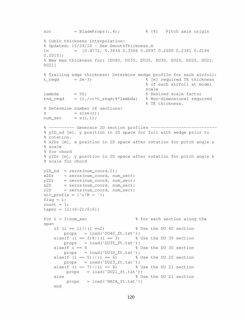
120
xoc = BladeProps(:,4); % [%] Pitch axis origin % Cubic thickness interpolation: % Updated: 11/24/10 - See SmoothThickness.m tn = [0.4772, 0.3834 0.3306 0.2897 0.2600 0.2381 0.2194 0.2015]; % New max thickness for: [DU40, DU35, DU35, DU30, DU25, DU25, DU21, DU21] % Trailing edge thickness: Determine wedge profile for each airfoil: t_reqd = 2e-3; % [m] required TE thickness
% of each airfoil at model scale
lambda = 50; % Desired scale factor tnd_reqd = (1./c)*t_reqd;%*lambda; % Non-dimensional required
% TE thickness. % Determine number of sections: s = size(r); num_sec = s(1,1); % ---------- Generate 2D section profiles -------------------------- % y2D_nd [m], y position in 2D space for foil with wedge prior to % rotation. % x2Dr [m], x position in 2D space after rotation for pitch angle & % scale % for chord % y2Dr [m], y position in 2D space after rotation for pitch angle & % scale for chord y2D_nd = zeros(num_coord,1); x2Dr = zeros(num_coord, num_sec); y2Dr = zeros(num_coord, num_sec); x2D = zeros(num_coord, num_sec); y2D = zeros(num_coord, num_sec); str_prefix = 'r/R = '; flag = 1; count = 1; taper = [2:(6-2)/6:6]; for i = 1:num_sec % for each section along the span if (i == 1)||(i ==2) % Use the DU 40 section props = load('DU40_ft.txt'); elseif (i == 3)%||(i == 3) % Use the DU 35 section props = load('DU35_ft.txt'); elseif i == 4 % Use the DU 30 section props = load('DU30_ft.txt'); elseif (i == 5)||(i == 6) % Use the DU 25 section props = load('DU25_ft.txt'); elseif (i == 7)||(i == 8) % Use the DU 21 section props = load('DU21_ft.txt'); else % Use the DU 21 section props = load('NACA_ft.txt'); end

121
Np = max(size(props)); x1 = props(:,1); t = props(:,2); % Incorporate thickness smoothing for DU foils: if (i >= 1) && (i <= 8) t = tn(i)/max(t).*t; end to(i) = max(t); f = props(:,3); dfdx = props(:,4); t_final(i) = max(t); for j = 1:Np % for EA point along the chord x2D_u(j) = x1(j) - (t(j)/2)*sin(atan(dfdx(j))); % 2D upper
% surface x x2D_l(j) = x1(j) + (t(j)/2)*sin(atan(dfdx(j))); % 2D lower
% surface x y2D_u(j) = f(j) + (t(j)/2)*cos(atan(dfdx(j))); % 2D upper
% surface y y2D_l(j) = f(j) - (t(j)/2)*cos(atan(dfdx(j))); % 2D lower
% surface y end % Combine coordinates: x2D_nd = zeros(Np*2-1,1); y2D_nd1 = zeros(Np*2-1,1); x2D_nd(1:Np) = flipud(x2D_u'); x2D_nd(Np+1:Np*2-1) = x2D_l(2:end)'; y2D_nd1(1:Np) = flipud(y2D_u'); y2D_nd1(Np+1:Np*2-1) = y2D_l(2:end)'; % Implement wedge: for j = 1:Np if i <= 15
% Upper surface y2D_nd(j) = y2D_nd1(j) + x2D_nd(j)*(tnd_reqd(i)/2 -
y2D_nd1(1)); % Lower surface y2D_nd(j+Np-1) = y2D_nd1(j+Np-1) - x2D_nd(j+Np-
1)*(tnd_reqd(i)/2 + y2D_nd1(end)); else
% tip geometry: % Upper surface y2D_nd(j) = y2D_nd1(j) +
x2D_nd(j)*(tnd_reqd(i)/(taper(count)) - y2D_nd1(1));
% Lower surface y2D_nd(j+Np-1) = y2D_nd1(j+Np-1) - x2D_nd(j+Np-
1)*(tnd_reqd(i)/(taper(count)) + y2D_nd1(end));
end end if i > 15; count = count+1; end

122
% Implement chord length x2D(:,i) = c(i).*(x2D_nd - xoc(i)); y2D(:,i) = c(i).*y2D_nd; % Implement pitch angle: % rotated 2D upper and lower surface x x2Dr(:,i) = x2D(:,i)*cosd(theta(i)) - y2D(:,i)*sind(theta(i)); % rotated 2D upper and lower surface y y2Dr(:,i) = x2D(:,i)*sind(theta(i)) + y2D(:,i)*cosd(theta(i)); % Build legend string for plots: str_legend(flag)=strcat(str_prefix,num2str(r(i)/(63/lambda))); flag = flag + 1; clear x2D_nd y2D_nd1 y2D_nd end % Plot pitched and unpitched sections: figure(1) plot(x2Dr,y2Dr, '.-') title('Rotated 2D DU Sections') legend(str_legend,'location','northwest'); axis equal figure(3) plot(x2D,y2D, '.-') title('Unrotated 2D Sections') legend(str_legend,'location','northwest'); axis equal % ------------------ Project Airfoils 3D coordinates ----------------------- % X3D [m], X position in 3D space (corresponds to y position in 2D % space) % Y2D [m], Y position in 3D space % Z3D [m], Z position in 3D space X3D = zeros(num_coord, num_sec); Y3D = zeros(num_coord, num_sec); Z3D = zeros(num_coord, num_sec); % for i = 1:num_sec % for each section along the span for j = 1:num_sec % for each section along the span
for i = 1:num_coord % for each point along the upper and % lower surfaces
X3D(i,j) = r(j)*(pi/180)*tand(theta(j)) + y2Dr(i,j); Y3D(i,j) = r(j)*sind((180/pi)*x2Dr(i,j)/r(j)); Z3D(i,j) = r(j)*cosd((180/pi)*x2Dr(i,j)/r(j)); end end % Plot projected airfoils: figure(2) plot3(X3D, Y3D, Z3D, '.-')

123
axis equal legend(str_legend,'location','northwest'); % -------- Create SolidWorks File:---------------------------------- % This creates the SectionCurves for the DU40-NACA64 airfoil % section, or Sections 6-26 filename = 'NREL_Blade'; filename_SolidWorks = strcat(filename,'_SolidWorks.txt'); fid = fopen(filename_SolidWorks,'w'); fid2 = fopen('DeepCwind.txt','w'); % Prop Parameters at beginning of file Z = 3; fprintf(fid,'%g, ' ,num_coord); fprintf(fid,'%g, ' ,num_sec); fprintf(fid,'%g,\n',Z); % Output curves defining each 2D section along the span % for each section along the span for j = 1:num_sec fprintf(fid,strcat('SectionCurve',num2str(j+5),',\n')); % for each point along the suction and pressure surfaces % (trailing edge -> leading edge -> trailing edge, close the curve) for i = 1:num_coord % fprintf(fid,'%f,%f,%f,\n',X3D(i,j),Y3D(i,j),Z3D(i,j)); fprintf(fid2,'%f,%f,%f,\n',X3D(i,j),Y3D(i,j),Z3D(i,j)); %Reprint 1st and last sections if i == 1 fprintf(fid,'%f,%f,%f,\n',X3D(i,j),Y3D(i,j),Z3D(i,j)); fprintf(fid2,'%f,%f,%f,\n',X3D(i,j),Y3D(i,j),Z3D(i,j)); elseif i == num_coord fprintf(fid,'%f,%f,%f,\n',X3D(i,j),Y3D(i,j),Z3D(i,j)); fprintf(fid2,'%f,%f,%f,\n',X3D(i,j),Y3D(i,j),Z3D(i,j)); else end end end %Tip Curves: for j = num_sec fprintf(fid,strcat('TipSectionCurve',num2str(j+5),',\n')); for i = 1:num_coord fprintf(fid,'%f,%f,%f,\n',X3D(i,j),Y3D(i,j),Z3D(i,j)) end for i = 1:Np-1 fprintf(fid,'%f,%f,%f,\n',X3D(i+1,j),Y3D(i+1,j),Z3D(i+1,j)); fprintf(fid,'%f,%f,%f,\n',tip(-i,1),tip(s(1,1)-i,2),... tip(s(1,1) - i,3)); end end

124
Solidworks Blade Input File
SWBladeInput.txt 26, 25, 3, SectionCurve1, 0.000000,0.035000,0.030000, 0.004387,0.034724,0.030000, 0.008704,0.033900,0.030000, 0.012884,0.032542,0.030000, 0.016861,0.030671,0.030000, 0.020572,0.028316,0.030000, 0.023959,0.025514,0.030000, 0.026968,0.022310,0.030000, 0.029551,0.018754,0.030000, 0.031669,0.014902,0.030000, 0.033287,0.010816,0.030000, 0.034380,0.006558,0.030000, 0.034931,0.002198,0.030000, 0.034931,-0.002198,0.030000, 0.034380,-0.006558,0.030000, 0.033287,-0.010816,0.030000, 0.031669,-0.014902,0.030000, 0.029551,-0.018754,0.030000, 0.026968,-0.022310,0.030000, 0.023959,-0.025514,0.030000, 0.020572,-0.028316,0.030000, 0.016861,-0.030671,0.030000, 0.012884,-0.032542,0.030000, 0.008704,-0.033900,0.030000, 0.004387,-0.034724,0.030000, 0.000000,-0.035000,0.030000, -0.004387,-0.034724,0.030000, -0.008704,-0.033900,0.030000, -0.012884,-0.032542,0.030000, -0.016861,-0.030671,0.030000, -0.020572,-0.028316,0.030000, -0.023959,-0.025514,0.030000, -0.026968,-0.022310,0.030000, -0.029551,-0.018754,0.030000, -0.031669,-0.014902,0.030000, -0.033287,-0.010816,0.030000, -0.034380,-0.006558,0.030000, -0.034931,-0.002198,0.030000, -0.034931,0.002198,0.030000, -0.034380,0.006558,0.030000, -0.033287,0.010816,0.030000, -0.031669,0.014902,0.030000, -0.029551,0.018754,0.030000, -0.026968,0.022310,0.030000, -0.023959,0.025514,0.030000, -0.020572,0.028316,0.030000, -0.016861,0.030671,0.030000, -0.012884,0.032542,0.030000, -0.008704,0.033900,0.030000, -0.004387,0.034724,0.030000, 0.000000,0.035000,0.030000, SectionCurve2, 0.000000,0.035000,0.039200, 0.004387,0.034724,0.039200, 0.008704,0.033900,0.039200, 0.012884,0.032542,0.039200, 0.016861,0.030671,0.039200,

125
0.020572,0.028316,0.039200, 0.023959,0.025514,0.039200, 0.026968,0.022310,0.039200, 0.029551,0.018754,0.039200, 0.031669,0.014902,0.039200, 0.033287,0.010816,0.039200, 0.034380,0.006558,0.039200, 0.034931,0.002198,0.039200, 0.034931,-0.002198,0.039200, 0.034380,-0.006558,0.039200, 0.033287,-0.010816,0.039200, 0.031669,-0.014902,0.039200, 0.029551,-0.018754,0.039200, 0.026968,-0.022310,0.039200, 0.023959,-0.025514,0.039200, 0.020572,-0.028316,0.039200, 0.016861,-0.030671,0.039200, 0.012884,-0.032542,0.039200, 0.008704,-0.033900,0.039200, 0.004387,-0.034724,0.039200, 0.000000,-0.035000,0.039200, -0.004387,-0.034724,0.039200, -0.008704,-0.033900,0.039200, -0.012884,-0.032542,0.039200, -0.016861,-0.030671,0.039200, -0.020572,-0.028316,0.039200, -0.023959,-0.025514,0.039200, -0.026968,-0.022310,0.039200, -0.029551,-0.018754,0.039200, -0.031669,-0.014902,0.039200, -0.033287,-0.010816,0.039200, -0.034380,-0.006558,0.039200, -0.034931,-0.002198,0.039200, -0.034931,0.002198,0.039200, -0.034380,0.006558,0.039200, -0.033287,0.010816,0.039200, -0.031669,0.014902,0.039200, -0.029551,0.018754,0.039200, -0.026968,0.022310,0.039200, -0.023959,0.025514,0.039200, -0.020572,0.028316,0.039200, -0.016861,0.030671,0.039200, -0.012884,0.032542,0.039200, -0.008704,0.033900,0.039200, -0.004387,0.034724,0.039200, 0.000000,0.035000,0.039200, SectionCurve3, 0.008492,0.035901,0.067978, 0.008005,0.036013,0.067986, 0.007512,0.036100,0.067995, 0.005924,0.036303,0.068019, 0.005323,0.036356,0.068026, 0.002795,0.036453,0.068048, -0.000627,0.036255,0.068061, -0.004309,0.035627,0.068050, -0.009796,0.033878,0.067984, -0.014660,0.031459,0.067880, -0.020261,0.027460,0.067714, -0.026100,0.021313,0.067490, -0.030193,0.014655,0.067293, -0.033082,0.005978,0.067069, -0.033745,-0.001970,0.066965, -0.032366,-0.010689,0.067191,

126
-0.029581,-0.017444,0.067381, -0.026355,-0.022330,0.067537, -0.022006,-0.026869,0.067700, -0.018732,-0.029366,0.067796, -0.015449,-0.031295,0.067873, -0.012883,-0.032474,0.067920, -0.011015,-0.033170,0.067950, -0.009208,-0.033727,0.067976, -0.008620,-0.033883,0.067984, -0.008041,-0.034028,0.067992, -0.007457,-0.034158,0.067999, -0.006860,-0.034282,0.068007, -0.004986,-0.034594,0.068027, -0.004335,-0.034678,0.068033, -0.001597,-0.034886,0.068050, 0.002110,-0.034801,0.068053, 0.006092,-0.034239,0.068028, 0.011981,-0.032456,0.067944, 0.017101,-0.029841,0.067829, 0.022768,-0.025406,0.067659, 0.028230,-0.018579,0.067450, 0.031623,-0.011387,0.067272, 0.033521,-0.002401,0.067065, 0.033347,0.005495,0.066974, 0.031295,0.013855,0.067213, 0.028290,0.020203,0.067407, 0.025112,0.024765,0.067559, 0.021016,0.029018,0.067714, 0.017997,0.031384,0.067799, 0.014998,0.033241,0.067866, 0.012663,0.034403,0.067909, 0.010964,0.035106,0.067939, 0.009456,0.035635,0.067964, 0.008977,0.035780,0.067971, 0.008492,0.035901,0.067978, SectionCurve4, 0.009688,0.040955,0.113521, 0.009270,0.041053,0.113524, 0.008848,0.041107,0.113529, 0.008423,0.041120,0.113538, 0.007995,0.041092,0.113546, 0.007469,0.041041,0.113554, 0.004670,0.040567,0.113600, 0.000980,0.039437,0.113659, -0.004388,0.036873,0.113707, -0.010103,0.033042,0.113686, -0.015955,0.027956,0.113611, -0.021580,0.021601,0.113529, -0.025837,0.014999,0.113482, -0.029229,0.006436,0.113452, -0.030505,-0.001502,0.113454, -0.029916,-0.010361,0.113527, -0.027743,-0.017338,0.113581, -0.024925,-0.022418,0.113618, -0.020934,-0.027112,0.113653, -0.017877,-0.029652,0.113673, -0.014212,-0.031877,0.113692, -0.011295,-0.033146,0.113704, -0.009108,-0.033856,0.113712, -0.008585,-0.033999,0.113714, -0.008073,-0.034129,0.113716, -0.008073,-0.034129,0.113716, -0.007554,-0.034242,0.113718,

127
-0.007020,-0.034349,0.113719, -0.006472,-0.034447,0.113721, -0.005908,-0.034537,0.113722, -0.004737,-0.034694,0.113725, -0.001546,-0.034872,0.113729, 0.004273,-0.034236,0.113726, 0.010688,-0.032029,0.113709, 0.015544,-0.029084,0.113683, 0.020788,-0.024171,0.113636, 0.025600,-0.016806,0.113561, 0.028448,-0.009301,0.113494, 0.029943,-0.000151,0.113431, 0.029734,0.007813,0.113419, 0.028082,0.016329,0.113497, 0.024546,0.025523,0.113580, 0.020963,0.031431,0.113600, 0.017553,0.035465,0.113582, 0.014111,0.038474,0.113550, 0.011735,0.040054,0.113532, 0.011275,0.040319,0.113529, 0.010897,0.040526,0.113528, 0.010508,0.040707,0.113524, 0.010106,0.040855,0.113521, 0.009688,0.040955,0.113521, SectionCurve5, 0.011074,0.046815,0.166769, 0.010662,0.046912,0.166770, 0.010241,0.046994,0.166771, 0.009867,0.046967,0.166782, 0.009479,0.046757,0.166798, 0.009027,0.046495,0.166811, 0.006681,0.044961,0.166881, 0.003663,0.042633,0.166958, -0.000734,0.038733,0.167012, -0.005595,0.033985,0.166993, -0.010854,0.028419,0.166927, -0.016230,0.021991,0.166862, -0.020608,0.015586,0.166831, -0.024516,0.007372,0.166817, -0.026518,-0.000311,0.166825, -0.026973,-0.009067,0.166874, -0.025752,-0.016177,0.166908, -0.023654,-0.021513,0.166926, -0.020293,-0.026578,0.166938, -0.017533,-0.029365,0.166943, -0.014079,-0.031807,0.166946, -0.011252,-0.033172,0.166949, -0.009107,-0.033911,0.166952, -0.008592,-0.034058,0.166953, -0.008087,-0.034189,0.166953, -0.008087,-0.034189,0.166953, -0.007574,-0.034298,0.166954, -0.007045,-0.034396,0.166955, -0.006502,-0.034484,0.166956, -0.005944,-0.034563,0.166957, -0.004784,-0.034699,0.166959, -0.001630,-0.034756,0.166963, 0.004053,-0.033709,0.166971, 0.010099,-0.030832,0.166977, 0.014455,-0.027298,0.166971, 0.018892,-0.021758,0.166946, 0.022686,-0.013934,0.166892, 0.024787,-0.006283,0.166841,

128
0.025771,0.002829,0.166798, 0.025508,0.010699,0.166794, 0.024267,0.019182,0.166853, 0.021835,0.028611,0.166917, 0.019432,0.035003,0.166922, 0.017110,0.039678,0.166885, 0.014664,0.043477,0.166828, 0.012876,0.045655,0.166792, 0.012518,0.046039,0.166787, 0.012218,0.046346,0.166784, 0.011879,0.046564,0.166775, 0.011485,0.046717,0.166769, 0.011074,0.046815,0.166769, SectionCurve6, 0.015066,0.054739,0.228536, 0.015066,0.054739,0.228536, 0.015090,0.054397,0.228617, 0.015193,0.053219,0.228895, 0.015379,0.051278,0.229337, 0.015655,0.048596,0.229920, 0.016039,0.045188,0.230614, 0.016566,0.041065,0.231384, 0.017236,0.036251,0.232187, 0.018017,0.030819,0.232970, 0.018854,0.024881,0.233679, 0.019666,0.018567,0.234265, 0.020350,0.012024,0.234692, 0.020767,0.005446,0.234937, 0.020788,-0.000914,0.234998, 0.020382,-0.006754,0.234903, 0.019734,-0.011200,0.234733, 0.018795,-0.014829,0.234532, 0.016999,-0.019108,0.234222, 0.014414,-0.023427,0.233829, 0.011293,-0.027198,0.233421, 0.007732,-0.030176,0.233055, 0.004010,-0.032109,0.232796, 0.000301,-0.033211,0.232641, -0.003366,-0.033560,0.232591, -0.006897,-0.033149,0.232650, -0.010252,-0.031985,0.232813, -0.013397,-0.030088,0.233066, -0.016249,-0.027486,0.233387, -0.018781,-0.024318,0.233738, -0.020967,-0.020854,0.234073, -0.022676,-0.016917,0.234390, -0.023755,-0.012407,0.234672, -0.023998,-0.006884,0.234899, -0.022714,-0.000058,0.235000, -0.019979,0.006292,0.234916, -0.016665,0.011582,0.234714, -0.012834,0.016536,0.234417, -0.008688,0.021280,0.234035, -0.004476,0.025881,0.233571, -0.000425,0.030342,0.233033, 0.003275,0.034630,0.232434, 0.006456,0.038709,0.231790, 0.009000,0.042537,0.231118, 0.010864,0.046040,0.230446, 0.012102,0.049101,0.229813, 0.012796,0.051616,0.229261, 0.013063,0.053495,0.228830, 0.013109,0.054656,0.228556,

129
0.013099,0.055102,0.228449, 0.013099,0.055102,0.228449, SectionCurve7, 0.013685,0.056520,0.311921, 0.013685,0.056520,0.311921, 0.013719,0.056158,0.311986, 0.013846,0.054947,0.312202, 0.014051,0.052957,0.312545, 0.014319,0.050217,0.312997, 0.014654,0.046753,0.313533, 0.015079,0.042590,0.314126, 0.015588,0.037762,0.314743, 0.016152,0.032347,0.315345, 0.016730,0.026450,0.315895, 0.017262,0.020196,0.316356, 0.017665,0.013718,0.316703, 0.017830,0.007189,0.316918, 0.017657,0.000831,0.316999, 0.017127,-0.005094,0.316959, 0.016397,-0.009849,0.316847, 0.015520,-0.013904,0.316695, 0.014026,-0.018450,0.316463, 0.011889,-0.022953,0.316168, 0.009306,-0.026912,0.315856, 0.006343,-0.030105,0.315567, 0.003234,-0.032308,0.315349, 0.000146,-0.033686,0.315205, -0.002899,-0.034296,0.315139, -0.005820,-0.034126,0.315158, -0.008587,-0.033179,0.315259, -0.011172,-0.031472,0.315434, -0.013509,-0.029030,0.315668, -0.015570,-0.025975,0.315934, -0.017343,-0.022534,0.316198, -0.018738,-0.018566,0.316456, -0.019628,-0.014002,0.316691, -0.019856,-0.008488,0.316886, -0.018801,-0.001802,0.316995, -0.016431,0.004572,0.316967, -0.013526,0.010128,0.316838, -0.010181,0.015442,0.316624, -0.006582,0.020595,0.316330, -0.002943,0.025618,0.315963, 0.000539,0.030487,0.315531, 0.003702,0.035153,0.315045, 0.006402,0.039565,0.314521, 0.008537,0.043669,0.313978, 0.010073,0.047387,0.313438, 0.011064,0.050609,0.312934, 0.011586,0.053237,0.312498, 0.011746,0.055190,0.312159, 0.011737,0.056391,0.311944, 0.011710,0.056841,0.311862, 0.011710,0.056841,0.311862, SectionCurve8, 0.012069,0.054531,0.395256, 0.012069,0.054531,0.395256, 0.012100,0.054174,0.395305, 0.012212,0.053009,0.395463, 0.012386,0.051100,0.395714, 0.012595,0.048479,0.396044, 0.012843,0.045171,0.396435, 0.013139,0.041207,0.396866,

130
0.013476,0.036631,0.397315, 0.013829,0.031523,0.397753, 0.014164,0.025982,0.398153, 0.014439,0.020107,0.398493, 0.014598,0.014004,0.398754, 0.014577,0.007810,0.398924, 0.014317,0.001705,0.398996, 0.013802,-0.004043,0.398980, 0.013168,-0.008632,0.398907, 0.012468,-0.012371,0.398808, 0.011251,-0.016620,0.398654, 0.009447,-0.021022,0.398446, 0.007258,-0.024905,0.398222, 0.004805,-0.028102,0.398009, 0.002249,-0.030503,0.397832, -0.000234,-0.032082,0.397708, -0.002548,-0.032863,0.397644, -0.004651,-0.032873,0.397643, -0.006618,-0.032135,0.397704, -0.008541,-0.030682,0.397819, -0.010425,-0.028570,0.397976, -0.012255,-0.025874,0.398160, -0.013945,-0.022638,0.398357, -0.015408,-0.018850,0.398554, -0.016516,-0.014477,0.398737, -0.017028,-0.009007,0.398898, -0.016129,-0.002407,0.398993, -0.013854,0.003701,0.398983, -0.011153,0.008997,0.398899, -0.008180,0.014132,0.398750, -0.005093,0.019198,0.398538, -0.002039,0.024184,0.398266, 0.000864,0.029037,0.397942, 0.003507,0.033680,0.397576, 0.005783,0.038042,0.397182, 0.007591,0.042069,0.396776, 0.008888,0.045692,0.396375, 0.009713,0.048818,0.396002, 0.010120,0.051360,0.395681, 0.010196,0.053245,0.395431, 0.010135,0.054401,0.395274, 0.010091,0.054825,0.395215, 0.010091,0.054825,0.395215, SectionCurve9, 0.010642,0.052220,0.478157, 0.010642,0.052220,0.478157, 0.010677,0.051876,0.478194, 0.010797,0.050767,0.478313, 0.010976,0.048949,0.478503, 0.011190,0.046455,0.478751, 0.011437,0.043315,0.479046, 0.011720,0.039559,0.479370, 0.012028,0.035231,0.479708, 0.012338,0.030395,0.480039, 0.012619,0.025147,0.480342, 0.012837,0.019592,0.480601, 0.012947,0.013841,0.480801, 0.012901,0.008015,0.480933, 0.012656,0.002260,0.480995, 0.012170,-0.003205,0.480989, 0.011484,-0.007871,0.480936, 0.010654,-0.011854,0.480854, 0.009410,-0.015908,0.480737,

131
0.007741,-0.019918,0.480587, 0.005811,-0.023487,0.480426, 0.003740,-0.026478,0.480271, 0.001647,-0.028805,0.480137, -0.000336,-0.030422,0.480037, -0.002092,-0.031326,0.479979, -0.003660,-0.031452,0.479971, -0.005113,-0.030862,0.480009, -0.006578,-0.029620,0.480087, -0.008136,-0.027694,0.480202, -0.009710,-0.025132,0.480343, -0.011206,-0.021970,0.480498, -0.012520,-0.018223,0.480655, -0.013503,-0.013884,0.480800, -0.013893,-0.008719,0.480921, -0.013126,-0.002862,0.480991, -0.011283,0.002727,0.480992, -0.008978,0.007858,0.480936, -0.006408,0.012886,0.480827, -0.003730,0.017855,0.480668, -0.001070,0.022730,0.480463, 0.001448,0.027455,0.480216, 0.003707,0.031970,0.479936, 0.005593,0.036221,0.479634, 0.007025,0.040150,0.479321, 0.007992,0.043680,0.479013, 0.008548,0.046716,0.478726, 0.008776,0.049172,0.478480, 0.008779,0.050980,0.478291, 0.008703,0.052086,0.478172, 0.008659,0.052486,0.478128, 0.008659,0.052486,0.478128, SectionCurve10, 0.009132,0.049443,0.560825, 0.009132,0.049443,0.560825, 0.009178,0.049118,0.560853, 0.009320,0.048081,0.560943, 0.009527,0.046372,0.561087, 0.009788,0.044021,0.561276, 0.010107,0.041065,0.561500, 0.010485,0.037537,0.561747, 0.010910,0.033468,0.562004, 0.011368,0.028905,0.562257, 0.011823,0.023938,0.562491, 0.012233,0.018698,0.562689, 0.012530,0.013334,0.562842, 0.012657,0.007987,0.562943, 0.012552,0.002767,0.562993, 0.012140,-0.002314,0.562995, 0.011316,-0.007194,0.562954, 0.010119,-0.011693,0.562879, 0.008674,-0.015748,0.562780, 0.007053,-0.019362,0.562667, 0.005330,-0.022492,0.562551, 0.003585,-0.025082,0.562441, 0.001880,-0.027134,0.562346, 0.000237,-0.028655,0.562270, -0.001265,-0.029586,0.562222, -0.002731,-0.029761,0.562213, -0.004111,-0.029256,0.562239, -0.005427,-0.028151,0.562296, -0.006777,-0.026315,0.562385, -0.008001,-0.023759,0.562498,

132
-0.009018,-0.020575,0.562624, -0.009771,-0.016866,0.562747, -0.010179,-0.012694,0.562857, -0.010168,-0.008153,0.562941, -0.009689,-0.003392,0.562990, -0.008725,0.001501,0.562998, -0.007260,0.006540,0.562962, -0.005315,0.011597,0.562881, -0.003048,0.016512,0.562758, -0.000646,0.021233,0.562599, 0.001681,0.025741,0.562411, 0.003724,0.030036,0.562198, 0.005318,0.034101,0.561966, 0.006400,0.037881,0.561724, 0.007018,0.041280,0.561485, 0.007263,0.044195,0.561263, 0.007279,0.046542,0.561073, 0.007218,0.048259,0.560928, 0.007168,0.049304,0.560837, 0.007145,0.049678,0.560804, 0.007145,0.049678,0.560804, SectionCurve11, 0.007626,0.046406,0.643328, 0.007626,0.046406,0.643328, 0.007675,0.046101,0.643350, 0.007823,0.045132,0.643419, 0.008043,0.043536,0.643529, 0.008320,0.041341,0.643674, 0.008652,0.038582,0.643845, 0.009032,0.035293,0.644034, 0.009446,0.031506,0.644230, 0.009878,0.027265,0.644423, 0.010298,0.022653,0.644602, 0.010671,0.017787,0.644755, 0.010943,0.012801,0.644873, 0.011067,0.007819,0.644953, 0.010993,0.002941,0.644993, 0.010662,-0.001817,0.644997, 0.009976,-0.006398,0.644968, 0.008968,-0.010637,0.644912, 0.007749,-0.014477,0.644838, 0.006381,-0.017909,0.644751, 0.004925,-0.020892,0.644662, 0.003450,-0.023371,0.644576, 0.002010,-0.025343,0.644502, 0.000619,-0.026808,0.644443, -0.000657,-0.027714,0.644404, -0.001912,-0.027918,0.644396, -0.003101,-0.027485,0.644414, -0.004246,-0.026482,0.644456, -0.005430,-0.024801,0.644523, -0.006515,-0.022452,0.644609, -0.007427,-0.019515,0.644705, -0.008115,-0.016081,0.644800, -0.008509,-0.012207,0.644884, -0.008542,-0.007977,0.644951, -0.008171,-0.003524,0.644990, -0.007384,0.001072,0.644999, -0.006168,0.005816,0.644974, -0.004534,0.010591,0.644913, -0.002619,0.015250,0.644820, -0.000585,0.019738,0.644698, 0.001382,0.024030,0.644552,

133
0.003097,0.028115,0.644387, 0.004416,0.031970,0.644207, 0.005284,0.035540,0.644020, 0.005746,0.038738,0.643836, 0.005889,0.041474,0.643665, 0.005840,0.043672,0.643520, 0.005739,0.045277,0.643409, 0.005666,0.046255,0.643339, 0.005636,0.046603,0.643314, 0.005636,0.046603,0.643314, SectionCurve12, 0.006278,0.043478,0.725699, 0.006278,0.043478,0.725699, 0.006338,0.043194,0.725716, 0.006505,0.042294,0.725769, 0.006753,0.040811,0.725854, 0.007075,0.038771,0.725965, 0.007465,0.036202,0.726098, 0.007920,0.033141,0.726244, 0.008432,0.029624,0.726396, 0.008981,0.025704,0.726545, 0.009539,0.021456,0.726683, 0.010071,0.016977,0.726802, 0.010513,0.012367,0.726895, 0.010793,0.007706,0.726959, 0.010815,0.003062,0.726994, 0.010501,-0.001498,0.726998, 0.009841,-0.005857,0.726976, 0.008902,-0.009909,0.726932, 0.007756,-0.013608,0.726873, 0.006464,-0.016915,0.726803, 0.005080,-0.019782,0.726731, 0.003671,-0.022149,0.726663, 0.002304,-0.023995,0.726604, 0.001016,-0.025302,0.726560, -0.000151,-0.026008,0.726535, -0.001263,-0.026144,0.726530, -0.002290,-0.025687,0.726546, -0.003166,-0.024626,0.726583, -0.004000,-0.023020,0.726635, -0.004751,-0.020855,0.726701, -0.005379,-0.018186,0.726773, -0.005854,-0.015072,0.726844, -0.006128,-0.011558,0.726908, -0.006154,-0.007712,0.726959, -0.005899,-0.003623,0.726991, -0.005350,0.000617,0.727000, -0.004507,0.004974,0.726983, -0.003366,0.009407,0.726939, -0.001992,0.013825,0.726869, -0.000506,0.018139,0.726774, 0.000949,0.022284,0.726658, 0.002225,0.026218,0.726527, 0.003213,0.029901,0.726385, 0.003873,0.033283,0.726238, 0.004239,0.036291,0.726094, 0.004381,0.038851,0.725961, 0.004390,0.040903,0.725848, 0.004348,0.042401,0.725762, 0.004305,0.043312,0.725709, 0.004284,0.043637,0.725689, 0.004284,0.043637,0.725689, SectionCurve13,

134
0.005005,0.040513,0.807985, 0.005005,0.040513,0.807985, 0.005064,0.040249,0.807998, 0.005230,0.039414,0.808039, 0.005478,0.038040,0.808105, 0.005799,0.036148,0.808192, 0.006185,0.033767,0.808295, 0.006629,0.030931,0.808409, 0.007121,0.027676,0.808526, 0.007639,0.024049,0.808642, 0.008160,0.020122,0.808750, 0.008655,0.015980,0.808842, 0.009071,0.011713,0.808915, 0.009348,0.007394,0.808966, 0.009403,0.003086,0.808994, 0.009169,-0.001151,0.808999, 0.008632,-0.005211,0.808983, 0.007855,-0.008996,0.808950, 0.006896,-0.012460,0.808904, 0.005810,-0.015565,0.808850, 0.004643,-0.018264,0.808794, 0.003450,-0.020501,0.808740, 0.002291,-0.022253,0.808694, 0.001196,-0.023503,0.808659, 0.000201,-0.024193,0.808638, -0.000749,-0.024351,0.808633, -0.001632,-0.023956,0.808645, -0.002391,-0.022998,0.808673, -0.003119,-0.021530,0.808713, -0.003781,-0.019542,0.808764, -0.004344,-0.017081,0.808820, -0.004781,-0.014204,0.808875, -0.005050,-0.010948,0.808926, -0.005110,-0.007377,0.808966, -0.004934,-0.003572,0.808992, -0.004509,0.000386,0.809000, -0.003838,0.004459,0.808988, -0.002915,0.008609,0.808954, -0.001795,0.012751,0.808900, -0.000579,0.016801,0.808826, 0.000611,0.020694,0.808735, 0.001644,0.024386,0.808632, 0.002425,0.027838,0.808521, 0.002923,0.031000,0.808406, 0.003168,0.033805,0.808293, 0.003226,0.036189,0.808190, 0.003179,0.038097,0.808102, 0.003100,0.039489,0.808036, 0.003036,0.040336,0.807994, 0.003008,0.040635,0.807979, 0.003008,0.040635,0.807979, SectionCurve14, 0.003899,0.037503,0.890210, 0.003899,0.037503,0.890210, 0.003960,0.037246,0.890221, 0.004146,0.036479,0.890253, 0.004383,0.035214,0.890304, 0.004701,0.033474,0.890371, 0.005102,0.031285,0.890451, 0.005580,0.028681,0.890538, 0.006121,0.025702,0.890629, 0.006696,0.022398,0.890718, 0.007263,0.018821,0.890801,

135
0.007780,0.015033,0.890873, 0.008194,0.011100,0.890931, 0.008453,0.007094,0.890972, 0.008508,0.003087,0.890995, 0.008278,-0.000840,0.891000, 0.007764,-0.004613,0.890988, 0.007055,-0.008170,0.890963, 0.006197,-0.011448,0.890926, 0.005230,-0.014389,0.890884, 0.004197,-0.016939,0.890839, 0.003144,-0.019040,0.890797, 0.002130,-0.020640,0.890761, 0.001225,-0.021717,0.890735, 0.000434,-0.022337,0.890720, -0.000382,-0.022539,0.890715, -0.001170,-0.022227,0.890723, -0.001793,-0.021318,0.890745, -0.002281,-0.019884,0.890778, -0.002673,-0.018031,0.890818, -0.002986,-0.015791,0.890860, -0.003228,-0.013185,0.890902, -0.003391,-0.010242,0.890941, -0.003463,-0.007006,0.890972, -0.003425,-0.003530,0.890993, -0.003252,0.000126,0.891000, -0.002870,0.003900,0.890991, -0.002292,0.007735,0.890966, -0.001608,0.011574,0.890925, -0.000874,0.015358,0.890868, -0.000146,0.019025,0.890797, 0.000526,0.022513,0.890716, 0.001102,0.025763,0.890627, 0.001552,0.028716,0.890537, 0.001859,0.031319,0.890449, 0.002026,0.033521,0.890369, 0.002071,0.035281,0.890301, 0.002031,0.036563,0.890249, 0.001940,0.037349,0.890217, 0.001902,0.037612,0.890206, 0.001902,0.037612,0.890206, SectionCurve15, 0.003085,0.034474,0.972389, 0.003085,0.034474,0.972389, 0.003144,0.034239,0.972397, 0.003324,0.033537,0.972422, 0.003556,0.032377,0.972461, 0.003868,0.030784,0.972513, 0.004261,0.028779,0.972574, 0.004731,0.026394,0.972642, 0.005263,0.023666,0.972712, 0.005828,0.020639,0.972781, 0.006391,0.017362,0.972845, 0.006909,0.013891,0.972901, 0.007334,0.010285,0.972946, 0.007619,0.006610,0.972978, 0.007715,0.002932,0.972996, 0.007550,-0.000676,0.973000, 0.007122,-0.004147,0.972991, 0.006511,-0.007422,0.972972, 0.005761,-0.010443,0.972944, 0.004908,-0.013156,0.972911, 0.003988,-0.015510,0.972876, 0.003046,-0.017453,0.972843,
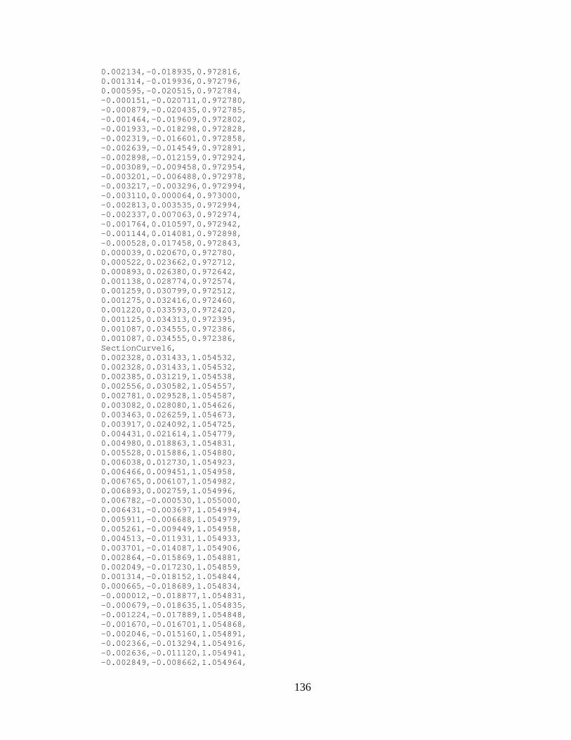
136
0.002134,-0.018935,0.972816, 0.001314,-0.019936,0.972796, 0.000595,-0.020515,0.972784, -0.000151,-0.020711,0.972780, -0.000879,-0.020435,0.972785, -0.001464,-0.019609,0.972802, -0.001933,-0.018298,0.972828, -0.002319,-0.016601,0.972858, -0.002639,-0.014549,0.972891, -0.002898,-0.012159,0.972924, -0.003089,-0.009458,0.972954, -0.003201,-0.006488,0.972978, -0.003217,-0.003296,0.972994, -0.003110,0.000064,0.973000, -0.002813,0.003535,0.972994, -0.002337,0.007063,0.972974, -0.001764,0.010597,0.972942, -0.001144,0.014081,0.972898, -0.000528,0.017458,0.972843, 0.000039,0.020670,0.972780, 0.000522,0.023662,0.972712, 0.000893,0.026380,0.972642, 0.001138,0.028774,0.972574, 0.001259,0.030799,0.972512, 0.001275,0.032416,0.972460, 0.001220,0.033593,0.972420, 0.001125,0.034313,0.972395, 0.001087,0.034555,0.972386, 0.001087,0.034555,0.972386, SectionCurve16, 0.002328,0.031433,1.054532, 0.002328,0.031433,1.054532, 0.002385,0.031219,1.054538, 0.002556,0.030582,1.054557, 0.002781,0.029528,1.054587, 0.003082,0.028080,1.054626, 0.003463,0.026259,1.054673, 0.003917,0.024092,1.054725, 0.004431,0.021614,1.054779, 0.004980,0.018863,1.054831, 0.005528,0.015886,1.054880, 0.006038,0.012730,1.054923, 0.006466,0.009451,1.054958, 0.006765,0.006107,1.054982, 0.006893,0.002759,1.054996, 0.006782,-0.000530,1.055000, 0.006431,-0.003697,1.054994, 0.005911,-0.006688,1.054979, 0.005261,-0.009449,1.054958, 0.004513,-0.011931,1.054933, 0.003701,-0.014087,1.054906, 0.002864,-0.015869,1.054881, 0.002049,-0.017230,1.054859, 0.001314,-0.018152,1.054844, 0.000665,-0.018689,1.054834, -0.000012,-0.018877,1.054831, -0.000679,-0.018635,1.054835, -0.001224,-0.017889,1.054848, -0.001670,-0.016701,1.054868, -0.002046,-0.015160,1.054891, -0.002366,-0.013294,1.054916, -0.002636,-0.011120,1.054941, -0.002849,-0.008662,1.054964,

137
-0.002993,-0.005958,1.054983, -0.003053,-0.003051,1.054996, -0.003003,0.000011,1.055000, -0.002781,0.003177,1.054995, -0.002398,0.006397,1.054981, -0.001926,0.009624,1.054956, -0.001412,0.012805,1.054922, -0.000899,0.015889,1.054880, -0.000428,0.018823,1.054832, -0.000030,0.021555,1.054780, 0.000269,0.024035,1.054726, 0.000458,0.026219,1.054674, 0.000540,0.028066,1.054627, 0.000531,0.029539,1.054586, 0.000465,0.030611,1.054556, 0.000368,0.031266,1.054537, 0.000329,0.031486,1.054530, 0.000329,0.031486,1.054530, SectionCurve17, 0.001731,0.028891,1.122962, 0.001731,0.028891,1.122962, 0.001785,0.028695,1.122967, 0.001948,0.028112,1.122982, 0.002163,0.027147,1.123006, 0.002454,0.025820,1.123037, 0.002819,0.024150,1.123074, 0.003256,0.022165,1.123115, 0.003751,0.019894,1.123158, 0.004280,0.017374,1.123200, 0.004810,0.014644,1.123239, 0.005307,0.011751,1.123273, 0.005729,0.008744,1.123300, 0.006035,0.005676,1.123320, 0.006183,0.002601,1.123331, 0.006110,-0.000421,1.123334, 0.005816,-0.003333,1.123329, 0.005365,-0.006086,1.123318, 0.004793,-0.008629,1.123301, 0.004128,-0.010916,1.123281, 0.003402,-0.012905,1.123260, 0.002649,-0.014551,1.123240, 0.001913,-0.015810,1.123223, 0.001246,-0.016665,1.123210, 0.000655,-0.017165,1.123203, 0.000034,-0.017345,1.123200, -0.000581,-0.017129,1.123203, -0.001091,-0.016450,1.123214, -0.001515,-0.015363,1.123229, -0.001879,-0.013952,1.123247, -0.002196,-0.012242,1.123267, -0.002471,-0.010247,1.123287, -0.002696,-0.007992,1.123306, -0.002862,-0.005509,1.123320, -0.002952,-0.002839,1.123330, -0.002944,-0.000026,1.123334, -0.002779,0.002884,1.123330, -0.002467,0.005846,1.123319, -0.002073,0.008815,1.123299, -0.001639,0.011743,1.123273, -0.001206,0.014581,1.123239, -0.000809,0.017281,1.123201, -0.000477,0.019794,1.123160, -0.000233,0.022076,1.123117,

138
-0.000086,0.024085,1.123076, -0.000034,0.025781,1.123038, -0.000060,0.027135,1.123006, -0.000134,0.028119,1.122982, -0.000231,0.028720,1.122967, -0.000269,0.028921,1.122962, -0.000269,0.028921,1.122962, SectionCurve18, 0.001301,0.026066,1.177712, 0.001301,0.026066,1.177712, 0.001351,0.025890,1.177715, 0.001501,0.025365,1.177727, 0.001701,0.024496,1.177745, 0.001970,0.023301,1.177770, 0.002310,0.021799,1.177798, 0.002715,0.020012,1.177830, 0.003174,0.017968,1.177863, 0.003665,0.015699,1.177895, 0.004159,0.013241,1.177926, 0.004623,0.010636,1.177952, 0.005021,0.007928,1.177973, 0.005314,0.005163,1.177989, 0.005464,0.002391,1.177998, 0.005416,-0.000334,1.178000, 0.005167,-0.002964,1.177996, 0.004776,-0.005449,1.177987, 0.004274,-0.007747,1.177975, 0.003688,-0.009815,1.177959, 0.003044,-0.011615,1.177943, 0.002374,-0.013104,1.177927, 0.001718,-0.014246,1.177914, 0.001121,-0.015021,1.177904, 0.000591,-0.015477,1.177898, 0.000032,-0.015644,1.177896, -0.000525,-0.015455,1.177899, -0.000992,-0.014846,1.177906, -0.001385,-0.013869,1.177918, -0.001727,-0.012599,1.177933, -0.002030,-0.011059,1.177948, -0.002297,-0.009263,1.177964, -0.002523,-0.007230,1.177978, -0.002697,-0.004993,1.177989, -0.002804,-0.002586,1.177997, -0.002825,-0.000048,1.178000, -0.002705,0.002577,1.177997, -0.002453,0.005251,1.177988, -0.002127,0.007931,1.177973, -0.001765,0.010575,1.177953, -0.001402,0.013138,1.177927, -0.001071,0.015576,1.177897, -0.000797,0.017846,1.177865, -0.000599,0.019906,1.177832, -0.000486,0.021718,1.177800, -0.000455,0.023249,1.177771, -0.000492,0.024470,1.177746, -0.000569,0.025356,1.177727, -0.000662,0.025897,1.177715, -0.000699,0.026079,1.177711, -0.000699,0.026079,1.177711, SectionCurve19, 0.001073,0.017735,1.232538, 0.001073,0.017735,1.232538, 0.001106,0.017615,1.232540,

139
0.001206,0.017259,1.232545, 0.001338,0.016668,1.232553, 0.001516,0.015856,1.232564, 0.001740,0.014835,1.232577, 0.002007,0.013621,1.232591, 0.002310,0.012232,1.232605, 0.002634,0.010690,1.232620, 0.002959,0.009020,1.232633, 0.003263,0.007249,1.232645, 0.003521,0.005408,1.232654, 0.003708,0.003528,1.232661, 0.003798,0.001643,1.232665, 0.003752,-0.000211,1.232666, 0.003571,-0.002000,1.232664, 0.003294,-0.003692,1.232660, 0.002942,-0.005257,1.232655, 0.002534,-0.006666,1.232648, 0.002088,-0.007892,1.232641, 0.001625,-0.008907,1.232634, 0.001173,-0.009686,1.232628, 0.000764,-0.010215,1.232624, 0.000401,-0.010527,1.232621, 0.000020,-0.010642,1.232620, -0.000361,-0.010515,1.232621, -0.000685,-0.010103,1.232625, -0.000962,-0.009439,1.232630, -0.001209,-0.008576,1.232636, -0.001431,-0.007530,1.232643, -0.001633,-0.006309,1.232650, -0.001808,-0.004927,1.232656, -0.001951,-0.003405,1.232661, -0.002050,-0.001768,1.232665, -0.002091,-0.000042,1.232666, -0.002038,0.001744,1.232665, -0.001895,0.003564,1.232661, -0.001703,0.005388,1.232654, -0.001485,0.007188,1.232645, -0.001266,0.008933,1.232634, -0.001067,0.010592,1.232620, -0.000905,0.012137,1.232606, -0.000792,0.013539,1.232592, -0.000736,0.014773,1.232577, -0.000731,0.015814,1.232565, -0.000769,0.016645,1.232554, -0.000831,0.017248,1.232545, -0.000900,0.017615,1.232540, -0.000927,0.017739,1.232538, -0.000927,0.017739,1.232538, SectionCurve20, 0.001054,0.015934,1.238646, 0.001054,0.015934,1.238646, 0.001083,0.015826,1.238647, 0.001172,0.015506,1.238651, 0.001289,0.014975,1.238657, 0.001446,0.014246,1.238666, 0.001644,0.013329,1.238676, 0.001880,0.012238,1.238688, 0.002148,0.010990,1.238699, 0.002434,0.009605,1.238711, 0.002720,0.008104,1.238721, 0.002988,0.006514,1.238731, 0.003214,0.004860,1.238738, 0.003376,0.003171,1.238744,
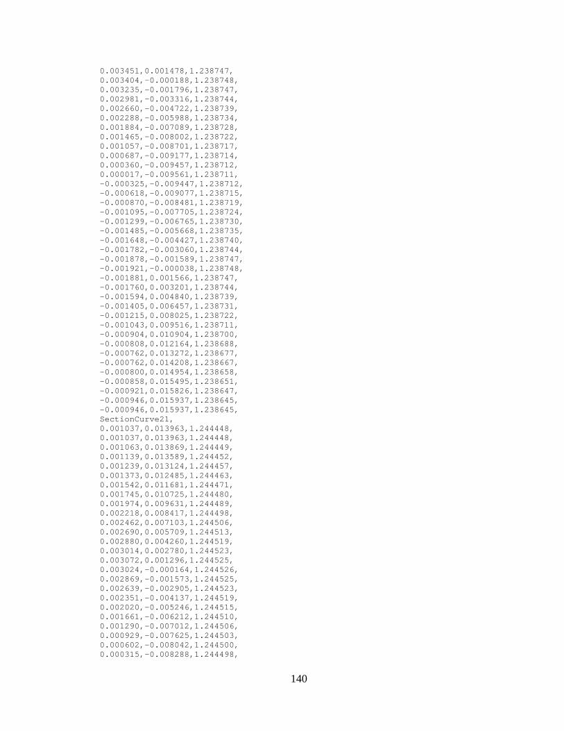
140
0.003451,0.001478,1.238747, 0.003404,-0.000188,1.238748, 0.003235,-0.001796,1.238747, 0.002981,-0.003316,1.238744, 0.002660,-0.004722,1.238739, 0.002288,-0.005988,1.238734, 0.001884,-0.007089,1.238728, 0.001465,-0.008002,1.238722, 0.001057,-0.008701,1.238717, 0.000687,-0.009177,1.238714, 0.000360,-0.009457,1.238712, 0.000017,-0.009561,1.238711, -0.000325,-0.009447,1.238712, -0.000618,-0.009077,1.238715, -0.000870,-0.008481,1.238719, -0.001095,-0.007705,1.238724, -0.001299,-0.006765,1.238730, -0.001485,-0.005668,1.238735, -0.001648,-0.004427,1.238740, -0.001782,-0.003060,1.238744, -0.001878,-0.001589,1.238747, -0.001921,-0.000038,1.238748, -0.001881,0.001566,1.238747, -0.001760,0.003201,1.238744, -0.001594,0.004840,1.238739, -0.001405,0.006457,1.238731, -0.001215,0.008025,1.238722, -0.001043,0.009516,1.238711, -0.000904,0.010904,1.238700, -0.000808,0.012164,1.238688, -0.000762,0.013272,1.238677, -0.000762,0.014208,1.238667, -0.000800,0.014954,1.238658, -0.000858,0.015495,1.238651, -0.000921,0.015826,1.238647, -0.000946,0.015937,1.238645, -0.000946,0.015937,1.238645, SectionCurve21, 0.001037,0.013963,1.244448, 0.001037,0.013963,1.244448, 0.001063,0.013869,1.244449, 0.001139,0.013589,1.244452, 0.001239,0.013124,1.244457, 0.001373,0.012485,1.244463, 0.001542,0.011681,1.244471, 0.001745,0.010725,1.244480, 0.001974,0.009631,1.244489, 0.002218,0.008417,1.244498, 0.002462,0.007103,1.244506, 0.002690,0.005709,1.244513, 0.002880,0.004260,1.244519, 0.003014,0.002780,1.244523, 0.003072,0.001296,1.244525, 0.003024,-0.000164,1.244526, 0.002869,-0.001573,1.244525, 0.002639,-0.002905,1.244523, 0.002351,-0.004137,1.244519, 0.002020,-0.005246,1.244515, 0.001661,-0.006212,1.244510, 0.001290,-0.007012,1.244506, 0.000929,-0.007625,1.244503, 0.000602,-0.008042,1.244500, 0.000315,-0.008288,1.244498,
141
0.000014,-0.008379,1.244498, -0.000287,-0.008279,1.244498, -0.000545,-0.007954,1.244501, -0.000769,-0.007432,1.244504, -0.000971,-0.006753,1.244508, -0.001154,-0.005929,1.244512, -0.001323,-0.004968,1.244516, -0.001472,-0.003880,1.244520, -0.001596,-0.002682,1.244523, -0.001688,-0.001393,1.244525, -0.001734,-0.000034,1.244526, -0.001707,0.001372,1.244525, -0.001610,0.002805,1.244523, -0.001473,0.004241,1.244519, -0.001316,0.005658,1.244513, -0.001157,0.007032,1.244506, -0.001014,0.008339,1.244498, -0.000899,0.009555,1.244489, -0.000822,0.010659,1.244480, -0.000788,0.011630,1.244472, -0.000793,0.012450,1.244464, -0.000830,0.013104,1.244457, -0.000883,0.013579,1.244452, -0.000941,0.013869,1.244449, -0.000963,0.013966,1.244448, -0.000963,0.013966,1.244448, SectionCurve22, 0.000773,0.011849,1.249652, 0.000773,0.011849,1.249652, 0.000795,0.011769,1.249653, 0.000861,0.011531,1.249655, 0.000948,0.011137,1.249658, 0.001065,0.010594,1.249663, 0.001213,0.009912,1.249669, 0.001389,0.009101,1.249675, 0.001588,0.008173,1.249681, 0.001801,0.007143,1.249688, 0.002015,0.006028,1.249693, 0.002214,0.004845,1.249699, 0.002383,0.003615,1.249703, 0.002504,0.002360,1.249706, 0.002560,0.001101,1.249708, 0.002526,-0.000138,1.249708, 0.002401,-0.001334,1.249707, 0.002212,-0.002464,1.249706, 0.001974,-0.003510,1.249703, 0.001698,-0.004451,1.249700, 0.001397,-0.005271,1.249697, 0.001086,-0.005949,1.249694, 0.000783,-0.006470,1.249691, 0.000508,-0.006824,1.249689, 0.000265,-0.007032,1.249688, 0.000010,-0.007110,1.249688, -0.000245,-0.007025,1.249688, -0.000463,-0.006750,1.249690, -0.000651,-0.006307,1.249692, -0.000819,-0.005730,1.249695, -0.000971,-0.005031,1.249698, -0.001110,-0.004216,1.249701, -0.001232,-0.003293,1.249704, -0.001333,-0.002276,1.249706, -0.001405,-0.001183,1.249707, -0.001439,-0.000030,1.249708,

142
-0.001410,0.001164,1.249707, -0.001322,0.002379,1.249706, -0.001199,0.003598,1.249703, -0.001061,0.004801,1.249699, -0.000920,0.005967,1.249694, -0.000794,0.007076,1.249688, -0.000691,0.008108,1.249682, -0.000621,0.009045,1.249675, -0.000588,0.009869,1.249669, -0.000589,0.010565,1.249663, -0.000617,0.011119,1.249659, -0.000661,0.011522,1.249655, -0.000708,0.011768,1.249653, -0.000727,0.011850,1.249652, -0.000727,0.011850,1.249652, SectionCurve23, 0.000613,0.009617,1.253999, 0.000613,0.009617,1.253999, 0.000630,0.009552,1.254000, 0.000684,0.009359,1.254001, 0.000755,0.009039,1.254003, 0.000850,0.008599,1.254007, 0.000970,0.008045,1.254010, 0.001114,0.007387,1.254014, 0.001276,0.006634,1.254018, 0.001450,0.005798,1.254023, 0.001624,0.004893,1.254026, 0.001787,0.003933,1.254030, 0.001925,0.002935,1.254033, 0.002023,0.001916,1.254035, 0.002070,0.000894,1.254036, 0.002043,-0.000112,1.254036, 0.001942,-0.001082,1.254036, 0.001790,-0.001999,1.254034, 0.001597,-0.002848,1.254033, 0.001374,-0.003612,1.254031, 0.001131,-0.004277,1.254029, 0.000879,-0.004828,1.254027, 0.000633,-0.005251,1.254025, 0.000410,-0.005538,1.254024, 0.000213,-0.005707,1.254023, 0.000006,-0.005770,1.254023, -0.000201,-0.005702,1.254023, -0.000377,-0.005478,1.254024, -0.000530,-0.005119,1.254026, -0.000666,-0.004651,1.254027, -0.000789,-0.004084,1.254029, -0.000902,-0.003422,1.254031, -0.001001,-0.002673,1.254033, -0.001083,-0.001848,1.254035, -0.001141,-0.000960,1.254036, -0.001168,-0.000024,1.254036, -0.001145,0.000944,1.254036, -0.001072,0.001931,1.254035, -0.000973,0.002920,1.254033, -0.000860,0.003896,1.254030, -0.000746,0.004842,1.254027, -0.000643,0.005742,1.254023, -0.000559,0.006580,1.254019, -0.000502,0.007340,1.254015, -0.000475,0.008009,1.254010, -0.000476,0.008574,1.254007, -0.000499,0.009024,1.254004,

143
-0.000534,0.009351,1.254001, -0.000573,0.009551,1.254000, -0.000587,0.009617,1.253999, -0.000587,0.009617,1.253999, SectionCurve24, 0.000505,0.007295,1.257273, 0.000505,0.007295,1.257273, 0.000519,0.007246,1.257273, 0.000559,0.007099,1.257274, 0.000612,0.006856,1.257275, 0.000683,0.006523,1.257277, 0.000772,0.006103,1.257279, 0.000879,0.005603,1.257282, 0.001001,0.005032,1.257284, 0.001130,0.004398,1.257286, 0.001260,0.003712,1.257289, 0.001380,0.002984,1.257290, 0.001482,0.002226,1.257292, 0.001554,0.001453,1.257293, 0.001587,0.000678,1.257294, 0.001564,-0.000084,1.257294, 0.001485,-0.000820,1.257294, 0.001367,-0.001516,1.257293, 0.001218,-0.002160,1.257292, 0.001047,-0.002740,1.257291, 0.000860,-0.003244,1.257290, 0.000668,-0.003662,1.257289, 0.000480,-0.003983,1.257288, 0.000310,-0.004201,1.257287, 0.000160,-0.004329,1.257287, 0.000003,-0.004377,1.257286, -0.000154,-0.004325,1.257287, -0.000289,-0.004156,1.257287, -0.000406,-0.003883,1.257288, -0.000510,-0.003528,1.257289, -0.000606,-0.003098,1.257290, -0.000693,-0.002596,1.257291, -0.000771,-0.002028,1.257292, -0.000835,-0.001402,1.257293, -0.000882,-0.000729,1.257294, -0.000906,-0.000019,1.257294, -0.000891,0.000716,1.257294, -0.000839,0.001464,1.257293, -0.000766,0.002215,1.257292, -0.000684,0.002955,1.257291, -0.000600,0.003673,1.257289, -0.000525,0.004356,1.257286, -0.000464,0.004991,1.257284, -0.000423,0.005568,1.257282, -0.000405,0.006075,1.257279, -0.000407,0.006504,1.257277, -0.000426,0.006845,1.257275, -0.000453,0.007093,1.257274, -0.000483,0.007244,1.257273, -0.000495,0.007295,1.257273, -0.000495,0.007295,1.257273, SectionCurve25, 0.000430,0.004913,1.259304, 0.000430,0.004913,1.259304, 0.000438,0.004880,1.259305, 0.000464,0.004781,1.259305, 0.000498,0.004617,1.259306, 0.000543,0.004393,1.259306,

144
0.000600,0.004110,1.259307, 0.000669,0.003774,1.259308, 0.000746,0.003389,1.259309, 0.000828,0.002962,1.259311, 0.000910,0.002500,1.259312, 0.000986,0.002009,1.259312, 0.001048,0.001500,1.259313, 0.001091,0.000979,1.259314, 0.001107,0.000457,1.259314, 0.001085,-0.000057,1.259314, 0.001026,-0.000552,1.259314, 0.000941,-0.001021,1.259314, 0.000836,-0.001455,1.259313, 0.000716,-0.001845,1.259313, 0.000587,-0.002185,1.259312, 0.000454,-0.002466,1.259312, 0.000325,-0.002682,1.259311, 0.000209,-0.002829,1.259311, 0.000107,-0.002915,1.259311, 0.000001,-0.002948,1.259311, -0.000105,-0.002913,1.259311, -0.000198,-0.002798,1.259311, -0.000278,-0.002615,1.259311, -0.000352,-0.002376,1.259312, -0.000419,-0.002086,1.259312, -0.000482,-0.001748,1.259313, -0.000539,-0.001365,1.259313, -0.000587,-0.000944,1.259314, -0.000624,-0.000491,1.259314, -0.000646,-0.000013,1.259314, -0.000642,0.000482,1.259314, -0.000613,0.000986,1.259314, -0.000570,0.001492,1.259313, -0.000520,0.001990,1.259312, -0.000470,0.002474,1.259312, -0.000424,0.002933,1.259311, -0.000388,0.003361,1.259310, -0.000365,0.003750,1.259308, -0.000357,0.004091,1.259307, -0.000362,0.004380,1.259306, -0.000377,0.004610,1.259306, -0.000398,0.004777,1.259305, -0.000419,0.004879,1.259305, -0.000427,0.004913,1.259304, -0.000427,0.004913,1.259304, SectionCurve26, 0.000375,0.002500,1.259998, 0.000375,0.002500,1.259998, 0.000379,0.002483,1.259998, 0.000390,0.002433,1.259998, 0.000404,0.002350,1.259998, 0.000422,0.002235,1.259998, 0.000446,0.002091,1.259998, 0.000474,0.001920,1.259999, 0.000505,0.001725,1.259999, 0.000539,0.001507,1.259999, 0.000571,0.001272,1.259999, 0.000600,0.001023,1.260000, 0.000622,0.000763,1.260000, 0.000633,0.000498,1.260000, 0.000631,0.000233,1.260000, 0.000609,-0.000029,1.260000, 0.000570,-0.000281,1.260000,

145
0.000517,-0.000520,1.260000, 0.000455,-0.000740,1.260000, 0.000386,-0.000939,1.260000, 0.000313,-0.001112,1.260000, 0.000240,-0.001255,1.259999, 0.000170,-0.001365,1.259999, 0.000108,-0.001440,1.259999, 0.000055,-0.001484,1.259999, 0.000000,-0.001500,1.259999, -0.000055,-0.001482,1.259999, -0.000104,-0.001424,1.259999, -0.000149,-0.001331,1.259999, -0.000191,-0.001209,1.259999, -0.000231,-0.001062,1.260000, -0.000270,-0.000890,1.260000, -0.000306,-0.000695,1.260000, -0.000339,-0.000480,1.260000, -0.000367,-0.000250,1.260000, -0.000388,-0.000006,1.260000, -0.000395,0.000245,1.260000, -0.000391,0.000502,1.260000, -0.000379,0.000759,1.260000, -0.000364,0.001013,1.260000, -0.000348,0.001259,1.259999, -0.000334,0.001493,1.259999, -0.000324,0.001710,1.259999, -0.000320,0.001908,1.259999, -0.000323,0.002082,1.259998, -0.000331,0.002229,1.259998, -0.000343,0.002346,1.259998, -0.000357,0.002431,1.259998, -0.000370,0.002483,1.259998, -0.000375,0.002500,1.259998, -0.000375,0.002500,1.259998, GuideCurve1, 0.000000,0.035000,0.030000, 0.000000,0.035000,0.039200, 0.008492,0.035901,0.067978, 0.009688,0.040955,0.113521, 0.011074,0.046815,0.166769, 0.015066,0.054739,0.228536, 0.013685,0.056520,0.311921, 0.012069,0.054531,0.395256, 0.010642,0.052220,0.478157, 0.009132,0.049443,0.560825, 0.007626,0.046406,0.643328, 0.006278,0.043478,0.725699, 0.005005,0.040513,0.807985, 0.003899,0.037503,0.890210, 0.003085,0.034474,0.972389, 0.002328,0.031433,1.054532, 0.001731,0.028891,1.122962, 0.001301,0.026066,1.177712, 0.001073,0.017735,1.232538, 0.001054,0.015934,1.238646, 0.001037,0.013963,1.244448, 0.000773,0.011849,1.249652, 0.000613,0.009617,1.253999, 0.000505,0.007295,1.257273, 0.000430,0.004913,1.259304, 0.000375,0.002500,1.259998, GuideCurve2, 0.026968,0.022310,0.030000,

146
0.026968,0.022310,0.039200, -0.004309,0.035627,0.068050, 0.000980,0.039437,0.113659, 0.003663,0.042633,0.166958, 0.016566,0.041065,0.231384, 0.015079,0.042590,0.314126, 0.013139,0.041207,0.396866, 0.011720,0.039559,0.479370, 0.010485,0.037537,0.561747, 0.009032,0.035293,0.644034, 0.007920,0.033141,0.726244, 0.006629,0.030931,0.808409, 0.005580,0.028681,0.890538, 0.004731,0.026394,0.972642, 0.003917,0.024092,1.054725, 0.003256,0.022165,1.123115, 0.002715,0.020012,1.177830, 0.002007,0.013621,1.232591, 0.001880,0.012238,1.238688, 0.001745,0.010725,1.244480, 0.001389,0.009101,1.249675, 0.001114,0.007387,1.254014, 0.000879,0.005603,1.257282, 0.000669,0.003774,1.259308, 0.000474,0.001920,1.259999, GuideCurve3, 0.031669,-0.014902,0.030000, 0.031669,-0.014902,0.039200, -0.029581,-0.017444,0.067381, -0.027743,-0.017338,0.113581, -0.025752,-0.016177,0.166908, 0.019734,-0.011200,0.234733, 0.016397,-0.009849,0.316847, 0.013168,-0.008632,0.398907, 0.011484,-0.007871,0.480936, 0.011316,-0.007194,0.562954, 0.009976,-0.006398,0.644968, 0.009841,-0.005857,0.726976, 0.008632,-0.005211,0.808983, 0.007764,-0.004613,0.890988, 0.007122,-0.004147,0.972991, 0.006431,-0.003697,1.054994, 0.005816,-0.003333,1.123329, 0.005167,-0.002964,1.177996, 0.003571,-0.002000,1.232664, 0.003235,-0.001796,1.238747, 0.002869,-0.001573,1.244525, 0.002401,-0.001334,1.249707, 0.001942,-0.001082,1.254036, 0.001485,-0.000820,1.257294, 0.001026,-0.000552,1.259314, 0.000570,-0.000281,1.260000, GuideCurve4, 0.004387,-0.034724,0.030000, 0.004387,-0.034724,0.039200, -0.008620,-0.033883,0.067984, -0.008073,-0.034129,0.113716, -0.008087,-0.034189,0.166953, -0.003366,-0.033560,0.232591, -0.002899,-0.034296,0.315139, -0.002548,-0.032863,0.397644, -0.002092,-0.031326,0.479979, -0.001265,-0.029586,0.562222,

147
-0.000657,-0.027714,0.644404, -0.000151,-0.026008,0.726535, 0.000201,-0.024193,0.808638, 0.000434,-0.022337,0.890720, 0.000595,-0.020515,0.972784, 0.000665,-0.018689,1.054834, 0.000655,-0.017165,1.123203, 0.000591,-0.015477,1.177898, 0.000401,-0.010527,1.232621, 0.000360,-0.009457,1.238712, 0.000315,-0.008288,1.244498, 0.000265,-0.007032,1.249688, 0.000213,-0.005707,1.254023, 0.000160,-0.004329,1.257287, 0.000107,-0.002915,1.259311, 0.000055,-0.001484,1.259999, GuideCurve5, -0.029551,-0.018754,0.030000, -0.029551,-0.018754,0.039200, 0.011981,-0.032456,0.067944, 0.010688,-0.032029,0.113709, 0.010099,-0.030832,0.166977, -0.023998,-0.006884,0.234899, -0.019856,-0.008488,0.316886, -0.017028,-0.009007,0.398898, -0.013893,-0.008719,0.480921, -0.010168,-0.008153,0.562941, -0.008542,-0.007977,0.644951, -0.006154,-0.007712,0.726959, -0.005110,-0.007377,0.808966, -0.003463,-0.007006,0.890972, -0.003201,-0.006488,0.972978, -0.002993,-0.005958,1.054983, -0.002862,-0.005509,1.123320, -0.002697,-0.004993,1.177989, -0.001951,-0.003405,1.232661, -0.001782,-0.003060,1.238744, -0.001596,-0.002682,1.244523, -0.001333,-0.002276,1.249706, -0.001083,-0.001848,1.254035, -0.000835,-0.001402,1.257293, -0.000587,-0.000944,1.259314, -0.000339,-0.000480,1.260000, GuideCurve6, -0.031669,0.014902,0.030000, -0.031669,0.014902,0.039200, 0.028290,0.020203,0.067407, 0.024546,0.025523,0.113580, 0.021835,0.028611,0.166917, 0.003275,0.034630,0.232434, 0.003702,0.035153,0.315045, 0.003507,0.033680,0.397576, 0.003707,0.031970,0.479936, 0.003724,0.030036,0.562198, 0.003097,0.028115,0.644387, 0.002225,0.026218,0.726527, 0.001644,0.024386,0.808632, 0.000526,0.022513,0.890716, 0.000039,0.020670,0.972780, -0.000428,0.018823,1.054832, -0.000809,0.017281,1.123201, -0.001071,0.015576,1.177897, -0.001067,0.010592,1.232620,

148
-0.001043,0.009516,1.238711, -0.001014,0.008339,1.244498, -0.000794,0.007076,1.249688, -0.000643,0.005742,1.254023, -0.000525,0.004356,1.257286, -0.000424,0.002933,1.259311, -0.000334,0.001493,1.259999, GuideCurve7, -0.004387,0.034724,0.030000, -0.004387,0.034724,0.039200, 0.008977,0.035780,0.067971, 0.010106,0.040855,0.113521, 0.011485,0.046717,0.166769, 0.013099,0.055102,0.228449, 0.011710,0.056841,0.311862, 0.010091,0.054825,0.395215, 0.008659,0.052486,0.478128, 0.007145,0.049678,0.560804, 0.005636,0.046603,0.643314, 0.004284,0.043637,0.725689, 0.003008,0.040635,0.807979, 0.001902,0.037612,0.890206, 0.001087,0.034555,0.972386, 0.000329,0.031486,1.054530, -0.000269,0.028921,1.122962, -0.000699,0.026079,1.177711, -0.000927,0.017739,1.232538, -0.000946,0.015937,1.238645, -0.000963,0.013966,1.244448, -0.000727,0.011850,1.249652, -0.000587,0.009617,1.253999, -0.000495,0.007295,1.257273, -0.000427,0.004913,1.259304, -0.000375,0.002500,1.259998, TipSectionCurve26, 0.000375,0.002500,1.259998, 0.000375,0.002500,1.259998, 0.000379,0.002483,1.259998, 0.000390,0.002433,1.259998, 0.000404,0.002350,1.259998, 0.000422,0.002235,1.259998, 0.000446,0.002091,1.259998, 0.000474,0.001920,1.259999, 0.000505,0.001725,1.259999, 0.000539,0.001507,1.259999, 0.000571,0.001272,1.259999, 0.000600,0.001023,1.260000, 0.000622,0.000763,1.260000, 0.000633,0.000498,1.260000, 0.000631,0.000233,1.260000, 0.000609,-0.000029,1.260000, 0.000570,-0.000281,1.260000, 0.000517,-0.000520,1.260000, 0.000455,-0.000740,1.260000, 0.000386,-0.000939,1.260000, 0.000313,-0.001112,1.260000, 0.000240,-0.001255,1.259999, 0.000170,-0.001365,1.259999, 0.000108,-0.001440,1.259999, 0.000055,-0.001484,1.259999, 0.000000,-0.001500,1.259999, -0.000055,-0.001482,1.259999, -0.000104,-0.001424,1.259999,

149
-0.000149,-0.001331,1.259999, -0.000191,-0.001209,1.259999, -0.000231,-0.001062,1.260000, -0.000270,-0.000890,1.260000, -0.000306,-0.000695,1.260000, -0.000339,-0.000480,1.260000, -0.000367,-0.000250,1.260000, -0.000388,-0.000006,1.260000, -0.000395,0.000245,1.260000, -0.000391,0.000502,1.260000, -0.000379,0.000759,1.260000, -0.000364,0.001013,1.260000, -0.000348,0.001259,1.259999, -0.000334,0.001493,1.259999, -0.000324,0.001710,1.259999, -0.000320,0.001908,1.259999, -0.000323,0.002082,1.259998, -0.000331,0.002229,1.259998, -0.000343,0.002346,1.259998, -0.000357,0.002431,1.259998, -0.000370,0.002483,1.259998, -0.000375,0.002500,1.259998, -0.000375,0.002500,1.259998, TipCurve1, 0.000375,0.002500,1.259998, -0.000375,0.002500,1.259998, TipCurve2, 0.000379,0.002483,1.259998, -0.000370,0.002483,1.259998, TipCurve3, 0.000390,0.002433,1.259998, -0.000357,0.002431,1.259998, TipCurve4, 0.000404,0.002350,1.259998, -0.000343,0.002346,1.259998, TipCurve5, 0.000422,0.002235,1.259998, -0.000331,0.002229,1.259998, TipCurve6, 0.000446,0.002091,1.259998, -0.000323,0.002082,1.259998, TipCurve7, 0.000474,0.001920,1.259999, -0.000320,0.001908,1.259999, TipCurve8, 0.000505,0.001725,1.259999, -0.000324,0.001710,1.259999, TipCurve9, 0.000539,0.001507,1.259999, -0.000334,0.001493,1.259999, TipCurve10, 0.000571,0.001272,1.259999, -0.000348,0.001259,1.259999, TipCurve11, 0.000600,0.001023,1.260000, -0.000364,0.001013,1.260000, TipCurve12, 0.000622,0.000763,1.260000, -0.000379,0.000759,1.260000, TipCurve13, 0.000633,0.000498,1.260000, -0.000391,0.000502,1.260000, TipCurve14,

150
0.000631,0.000233,1.260000, -0.000395,0.000245,1.260000, TipCurve15, 0.000609,-0.000029,1.260000, -0.000388,-0.000006,1.260000, TipCurve16, 0.000570,-0.000281,1.260000, -0.000367,-0.000250,1.260000, TipCurve17, 0.000517,-0.000520,1.260000, -0.000339,-0.000480,1.260000, TipCurve18, 0.000455,-0.000740,1.260000, -0.000306,-0.000695,1.260000, TipCurve19, 0.000386,-0.000939,1.260000, -0.000270,-0.000890,1.260000, TipCurve20, 0.000313,-0.001112,1.260000, -0.000231,-0.001062,1.260000, TipCurve21, 0.000240,-0.001255,1.259999, -0.000191,-0.001209,1.259999, TipCurve22, 0.000170,-0.001365,1.259999, -0.000149,-0.001331,1.259999, TipCurve23, 0.000108,-0.001440,1.259999, -0.000104,-0.001424,1.259999, TipCurve24, 0.000055,-0.001484,1.259999, -0.000055,-0.001482,1.259999, RootSectionCurve1, 0.000000,0.035000,0.030000, 0.004387,0.034724,0.030000, 0.008704,0.033900,0.030000, 0.012884,0.032542,0.030000, 0.016861,0.030671,0.030000, 0.020572,0.028316,0.030000, 0.023959,0.025514,0.030000, 0.026968,0.022310,0.030000, 0.029551,0.018754,0.030000, 0.031669,0.014902,0.030000, 0.033287,0.010816,0.030000, 0.034380,0.006558,0.030000, 0.034931,0.002198,0.030000, 0.034931,-0.002198,0.030000, 0.034380,-0.006558,0.030000, 0.033287,-0.010816,0.030000, 0.031669,-0.014902,0.030000, 0.029551,-0.018754,0.030000, 0.026968,-0.022310,0.030000, 0.023959,-0.025514,0.030000, 0.020572,-0.028316,0.030000, 0.016861,-0.030671,0.030000, 0.012884,-0.032542,0.030000, 0.008704,-0.033900,0.030000, 0.004387,-0.034724,0.030000, 0.000000,-0.035000,0.030000, -0.004387,-0.034724,0.030000, -0.008704,-0.033900,0.030000, -0.012884,-0.032542,0.030000, -0.016861,-0.030671,0.030000,
151
-0.020572,-0.028316,0.030000, -0.023959,-0.025514,0.030000, -0.026968,-0.022310,0.030000, -0.029551,-0.018754,0.030000, -0.031669,-0.014902,0.030000, -0.033287,-0.010816,0.030000, -0.034380,-0.006558,0.030000, -0.034931,-0.002198,0.030000, -0.034931,0.002198,0.030000, -0.034380,0.006558,0.030000, -0.033287,0.010816,0.030000, -0.031669,0.014902,0.030000, -0.029551,0.018754,0.030000, -0.026968,0.022310,0.030000, -0.023959,0.025514,0.030000, -0.020572,0.028316,0.030000, -0.016861,0.030671,0.030000, -0.012884,0.032542,0.030000, -0.008704,0.033900,0.030000, -0.004387,0.034724,0.030000, 0.000000,0.035000,0.030000, RootCurve1, 0.004387,0.034724,0.030000, -0.004387,0.034724,0.030000, RootCurve2, 0.008704,0.033900,0.030000, -0.008704,0.033900,0.030000, RootCurve3, 0.012884,0.032542,0.030000, -0.012884,0.032542,0.030000, RootCurve4, 0.016861,0.030671,0.030000, -0.016861,0.030671,0.030000, RootCurve5, 0.020572,0.028316,0.030000, -0.020572,0.028316,0.030000, RootCurve6, 0.023959,0.025514,0.030000, -0.023959,0.025514,0.030000, RootCurve7, 0.026968,0.022310,0.030000, -0.026968,0.022310,0.030000, RootCurve8, 0.029551,0.018754,0.030000, -0.029551,0.018754,0.030000, RootCurve9, 0.031669,0.014902,0.030000, -0.031669,0.014902,0.030000, RootCurve10, 0.033287,0.010816,0.030000, -0.033287,0.010816,0.030000, RootCurve11, 0.034380,0.006558,0.030000, -0.034380,0.006558,0.030000, RootCurve12, 0.034931,0.002198,0.030000, -0.034931,0.002198,0.030000, RootCurve13, 0.034931,-0.002198,0.030000, -0.034931,-0.002198,0.030000, RootCurve14, 0.034380,-0.006558,0.030000, -0.034380,-0.006558,0.030000,

152
RootCurve15, 0.033287,-0.010816,0.030000, -0.033287,-0.010816,0.030000, RootCurve16, 0.031669,-0.014902,0.030000, -0.031669,-0.014902,0.030000, RootCurve17, 0.029551,-0.018754,0.030000, -0.029551,-0.018754,0.030000, RootCurve18, 0.026968,-0.022310,0.030000, -0.026968,-0.022310,0.030000, RootCurve19, 0.023959,-0.025514,0.030000, -0.023959,-0.025514,0.030000, RootCurve20, 0.020572,-0.028316,0.030000, -0.020572,-0.028316,0.030000, RootCurve21, 0.016861,-0.030671,0.030000, -0.016861,-0.030671,0.030000, RootCurve22, 0.012884,-0.032542,0.030000, -0.012884,-0.032542,0.030000, RootCurve23, 0.008704,-0.033900,0.030000, -0.008704,-0.033900,0.030000, RootCurve24, 0.004387,-0.034724,0.030000, -0.004387,-0.034724,0.030000,

153
APPENDIX D. CHARACTERIZATION INFORMATION AND DATA
Cable Mass Excluded
Elevation [m]
Height Fraction
Mass [kg/m]
Fore-Aft Stiffness [N·m2]
Side-Side Stiffness [N·m2]
Torsional Stiffness [N·m2]
Extensional Stiffness [N]
10.00-10.31 0.000-0.004 53,897.6 1.12E+12 1.12E+12 8.55E+11 3.85E+12
10.31-18.54 0.004-0.110 2,825.2 1.12E+12 1.12E+12 8.55E+11 3.85E+12
18.54-21.56 0.110-0.149 4,034.2 1.37E+12 1.37E+12 1.04E+12 5.34E+12
21.56-22.26 0.149-0.158 14,270.4 1.37E+12 1.37E+12 1.04E+12 5.34E+12
22.26-81.63 0.158-0.923 1,209.0 2.49E+11 2.49E+11 1.89E+11 1.49E+12
81.63-82.87 0.923-0.939 3,354.7 2.49E+11 2.49E+11 1.89E+11 1.49E+12
82.87-83.49 0.939-0.947 10,047.6 2.49E+11 2.49E+11 1.89E+11 1.49E+12
83.49-84.42 0.947-0.959 8,659.9 2.49E+11 2.49E+11 1.89E+11 1.49E+12
84.42-87.6 0.959-1.000 3,937.0 1.10E+12 1.10E+12 8.40E+11 4.87E+12
Table D.1. Model tower distributed properties including cable mass.
Cable Mass Included
Elevation [m]
Height Fraction
Mass [kg/m]
Fore-Aft Stiffness [N·m2]
Side-Side Stiffness [N·m2]
Torsional Stiffness [N·m2]
Extensional Stiffness [N]
10.00-10.31 0.000-0.004 55,671.5 1.123E+12 1.123E+12 8.548E+11 3.853E+12
10.31-18.54 0.004-0.110 4599.0 1.123E+12 1.123E+12 8.548E+11 3.853E+12
18.54-21.56 0.110-0.149 5808.1 1.371E+12 1.371E+12 1.044E+12 5.342E+12
21.56-22.26 0.149-0.158 16,044.3 1.371E+12 1.371E+12 1.044E+12 5.342E+12
22.26-81.63 0.158-0.923 2982.9 2.485E+11 2.485E+11 1.892E+11 1.489E+12
81.63-82.87 0.923-0.939 5128.5 2.485E+11 2.485E+11 1.892E+11 1.489E+12
82.87-83.49 0.939-0.947 11,821.4 2.485E+11 2.485E+11 1.892E+11 1.489E+12
83.49-84.42 0.947-0.959 10,433.7 2.485E+11 2.485E+11 1.892E+11 1.489E+12
84.42-87.6 0.959-1.000 5710.8 1.104E+12 1.104E+12 8.404E+11 4.867E+12
Table D.2. Model tower distributed properties excluding cable mass.

154
Hammer Test Data Results
Figure D.1. Acceleration and Power Spectral Density (PSD) plots from tower hammer tests.
0 0.5 1 1.5 2 2.5 3 3.5 4 4.5 5-50
0
50
Time (s)
m/s
2
Fixed Wind Turbine AY MID
0 0.2 0.4 0.6 0.8 1 1.2 1.4 1.6 1.8 20
0.1
0.2
Frequency (Hz)
PS
D (m
/s2 )
2 /H
z
0 0.5 1 1.5 2 2.5 3 3.5 4 4.5 5-50
0
50
Time (s)
m/s
2
Floating Wind Turbine on Spar AY MID
0 0.2 0.4 0.6 0.8 1 1.2 1.4 1.6 1.8 20
0.005
0.01
0.015
0.02
Frequency (Hz)
PS
D (m
/s2 )
2 /H
z
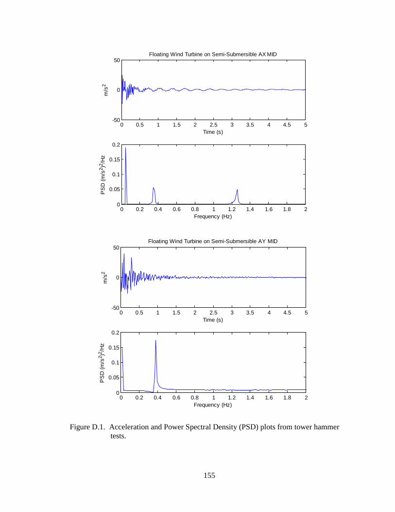
155
Figure D.1. Acceleration and Power Spectral Density (PSD) plots from tower hammer tests.
0 0.5 1 1.5 2 2.5 3 3.5 4 4.5 5-50
0
50
Time (s)
m/s
2
Floating Wind Turbine on Semi-Submersible AX MID
0 0.2 0.4 0.6 0.8 1 1.2 1.4 1.6 1.8 20
0.05
0.1
0.15
0.2
Frequency (Hz)
PS
D (m
/s2 )
2 /H
z
0 0.5 1 1.5 2 2.5 3 3.5 4 4.5 5-50
0
50
Time (s)
m/s
2
Floating Wind Turbine on Semi-Submersible AY MID
0 0.2 0.4 0.6 0.8 1 1.2 1.4 1.6 1.8 20
0.05
0.1
0.15
0.2
Frequency (Hz)
PS
D (m
/s2 )
2 /H
z

156
Figure D.1. Acceleration and Power Spectral Density (PSD) plots from tower hammer tests.
0 0.5 1 1.5 2 2.5 3 3.5 4 4.5 5-50
0
50
Time (s)
m/s
2
Floating Wind Turbine on TLP AX MID
0 0.2 0.4 0.6 0.8 1 1.2 1.4 1.6 1.8 20
0.2
0.4
Frequency (Hz)
PS
D (m
/s2 )
2 /H
z
0 0.5 1 1.5 2 2.5 3 3.5 4 4.5 5-50
0
50
Time (s)
m/s
2
Floating Wind Turbine on TLP AY MID
0 0.2 0.4 0.6 0.8 1 1.2 1.4 1.6 1.8 20
0.2
0.4
Frequency (Hz)
PS
D (m
/s2 )
2 /H
z

157
BIBLIOGRAPHY
Bae, Y. H., M. H. Kim, and Y. S. Shin. Rotor-floater-mooring Coupled Analysis of Mini-TLP-Type Offshore Floating Wind Turbines. Shanghai, China: OMAE 2010, 2010.
Bir, G. BModes - Software for Computing Rotating Blade Coupled Modes. NREL - National Wind Technology Center. Golden, 2008.
Çengel, Y.A., and J.M. Cimbala. Fluid Mechanics: fundamentals and applications - 1st ed. New York: McGraw-Hill, 2006.
Cermelli, C, A Aubault, D Roddier, and T McCoy. Qualification of a Semi-Submersible Floating Foundation for Multi-Megawatt Wind Turbines. Houston: Offshore Technology Conference, 2010.
Chakrabarti, S.K. Offshore Structure Modeling. Singapore: World Scientific Publishing Co. Pte. Ltd., 1994.
Daniel, I.M., and O. Ishai. Engineering Mechanics of Composite Materials. New York: Oxford University Press, 2006.
Department of Energy (DOE). "20% Wind Energy by 2030, Increasing WInd Energy's Contribution to U.S. Electricity Supply." 2008.
Department of Energy (DOE). 2009 Renewable Energy Data Book. Washington, DC: DOE, 2010.
Drela, M. "UIUC Applied Aerodynamics Group." UIUC Airfoil Data Site. 1995. http://www.ae.illinois.edu/m-selig/ads/coord_database.html (accessed 11 01, 2011).
Drela, M.. XFOIL: An Analysis and Design System for Low Reynolds Number Airfoils. University of Notre Dam: Conference on Low Reynolds number Airfoil Aerodynamics, 1989.
Energy Information Association (EIA). "State Energy Profiles: Maine." US Energy Information Association. May 16, 2011. http://www.eia.gov/state/state-energy-profiles-data.cfm?sid=ME#Consumption (accessed June 8, 2011).
Energy Information Association (EIA). "Total Energy: US Energy Information Administration." Primary Energy Production by Source, 1949-2009. August 19, 2010. http://www.eia.gov/totalenergy/data/annual/pdf/aer.pdf (accessed July 5, 2011).

158
Epps, B. P., and R.W. Kimball. "OpenProp v2.4 propeller/turbine design code." openprop.mit.edu. MIT. 2010. http://openprop.mit.edu (accessed October 03, 201).
Firgelli Technologies Inc. "Products, Firgelli." Firgelli Technologies inc. Web site. 2011. http://firgelli.com/products.php?id=16 (accessed July 13, 2011).
Gere, J.M. Mechanics of Materials. Canada: Thomson Learning, 2006.
Gueydon, S., and W. Xu. Floating Wind Turbine Motion Assessment. Kona, Hawaii: Oceans11 Conference, 2011.
Gurit. "ST 94 Single SPRINT." Gurit - SPRINT DATASHEETS - MARINE. 2011. http://www.gurit.com/files/documents/ST_94_v4.pdf (accessed 10 05, 2011).
Henkel. "Frekot Mold Release Solutions Guide." Henkel. 2010. http://www.henkelna.com/us/content_data/165094_LT4831_Frekote_Guide_10_6_Lo258132.pdf (accessed 10 10, 2011).
Jonkman, J. Definition of the Floating System for Phase IV of OC3. Golden, CO: NREL, 2010.
Jonkman, J. Dynamics Modeling and Loads Analysis of an Offshore Floating Wind Turbine. Golden, CO: NREL, 2007.
Jonkman, J., and D. Matha. Quantitative Comparison of the Responses of Three Floating Platforms. Golden, CO, CO: NREL, 2009.
Jonkman, J., and M. Buhl Jr. Development and Verification of a Fully Coupled Simulator for Offshore Wind Turbines. Golden, CO: National Renewable Energy Lab, 2007.
Jonkman, J., S. Butterfield, W. Musial, and G. Scott. Definition of a 5MW Reference Wind Turbine for Offshore System Development. Golden: NREL, 2009.
Kooijman, H.J.T., C Lindenburg, D. Winkelaar, and E.L. van der Hooft. DOWEC 6 MW Pre-Design. Energy Research Center of the Netherlands (ECN), 2003.
Lancaster, P., and K. Šalkauskas. Curve and Surface Fitting: An Introduction. London: Academic Press, 1986.
Lokocz, T. "Solid Mechanics of Cross Flow of Tidal Turbine Blades ." University of Maine. 2010. http://www.umaine.edu/mecheng/Peterson/Classes/Design/2009_10/Projects/TidalEnergy-TomLokocz/reports.html (accessed 10 10, 2011).
Main, I. G. Vibartions in Waves and Physics. 3. Cambridge: Cambridge University Press, 1999.

159
Manwell, J. F., J. G. McGowan, and A. L. Rogers. Wind Energy Explained: Theory, Design, and Application. West Sussex: John Wiley & Sons Ltd., 2002.
MARIN. DeepCwind Floating WInd Turbine Model Tests. Marin, 2011.
MARIN. "Marin: Offshore Basin." MARIN: Marine Research Institute Netherlands. July 19, 2010. http://www.marin.nl/web/Facilities-Tools/Basins/Offshore-Basin.htm (accessed August 10, 2011).
Moriarty, P.J., and A.C. Hansen. AeroDyn Theory Manual. Golden: NREL, 2005.
Musial, W. Status of Wave and Tidal Power Technologies for the United States. Technical Report, Golden, CO: NREL, 2008.
Musial, W., and B. Ram. Large-Scale Offshore Wind Power in the United States. Golden, CO: NREL, 2010.
Musial, W., S. Butterfield, and B. Ram. Energy from Offshore Wind. National Renewable Energy Lab, Houston, Texas: Offshore Technology Conference, 2006.
Neilsen, F G, T D Hanson, and B Skaar. Integrated Dynamic Analysis of Floating Offshore Wind Turbines. Hamburg: Hydro Oil & Energy, 2006.
Ocean Energy Task Force. "Final Report of the Ocean Energy Task Force to Governor John E. Baldacci." Maine State Planning Office, Augusta, 2009.
O'Neil, P.V. Advanced Engineering Mathematics. 5th Edition. Pacific Grove, CA: Brooks/Cole-Thomson Learning, Inc., 2003.
Piercan USA, Inc. "Composite bladder molding." Piercan USA, Inc. 2010. http://www.piercanusa.com/composite.html (accessed 11 05, 2011).
Principle Power Inc. "First WindFloat Sucessfully Deployed Offshore." November 30, 2011. http://www.principlepowerinc.com/news/press_PPI_WF_deployment.html (accessed December 2, 2011).
Rao, S. S. Mechanical Vibrations. 4. Upper Saddle River: Pearson Prentice Hall, 2004.
Robinson, M., and W. Musial. Offshore Wind Technology Overview. Presentation, NWTC, NREL, DOE, 2006.
Schwartz, M., D. Heimiller, S. Haymes, and W. Musial. Assessment of Offshore Wind Energy Resources for the Unites States. Technical Report, Golden, CO: NREL, 2010.
Serchuk, A. "The Environmental Imperative for Renewable Energy: An Update." Renewable Energy Policy Project (REPP), Washington, DC, 2000.
SolidWorks. SolidWorks Education Edition. Software. Dessault Systems. 2010.

160
Statoil Hydro. "Hywind Fact Sheet." Statoil.com. 2010. http://www.statoil.com/en/TechnologyInnovation/NewEnergy/RenewablePowerProduction/Offshore/Hywind/Downloads/Hywind%20Fact%20sheet.pdf (accessed September 15, 2011).
Timmer, N. "DOWEC blade airfoil data, (excel document)." Delft University of Technology, 2009.
University of Maine and James W. Sewall Company. "Maine Deepwater Offshore Wind Report." DeepCwind Consortium. Febuary 2011. http://deepcwind.org/docs/OfficialOffshoreWindReport-22311.pdf (accessed September 14, 2011).
van Dam, C.P., Chow, R. NREL 5MW [Blade] Description. University of California Davis, 2010.
White, F.M. Fluid Mechanics. 4. WCB McGraw-Hill, 1999.
WindSea. WindSea: Wave Basin. 2 2, 2011. http://www.windsea.com/movie/wave-basin/ (accessed June 8, 2011).

161
BIOGRAPHY OF THE AUTHOR
Heather Rae Martin was born in Presque Isle, Maine and raised in Caribou, Maine
up until sixth grade. She attended middle school and high school in Richmond, Maine
where she lived with her mother and stepfather, Deborah and Guy Cousins. Much of her
upbringing was also spent with her father and stepmother, Andy and Gina Martin, in
Frenchville and Madawaska, Maine.
After graduating from Richmond High School in 2005 as class valedictorian,
Heather attended the University of Maine where she was accepted into the Top-Scholar
Award program. During her sophomore year, she discovered an affinity for engineering
and decided to pursue a Bachelor of Science degree in Civil and Environmental
Engineering. In December 2009, Heather completed her Bachelor’s degree with summa-
cum laude honors and was selected as the Class of 2009 Outstanding Graduate of the
College of Engineering.
Heather has interned at the Stantec Inc. office in Scarborough, Maine as well as
with Kiewit Construction on the Willis Avenue Bridge Replacement in New York City.
In addition to her professional life, she also enjoys sports, outdoor activities, spending
time with her family and friends, traveling, cooking and of course laughing. In the
future, she hopes to continue to work and live in her home state, Maine.