Development of a Risk Based Model for use in Water Quality ...doras.dcu.ie/17516/1/Development_of_a_Risk_Based_Model_for_use… · Development of a Risk Based Model for use in Water

Development of a Risk Based

Model for use in Water Quality

Monitoring

By

Lisa Jones B.Sc. (Hons.)

A thesis submitted to Dublin City University in partial fulfilment of the

requirements for the award of

Doctor of Philosophy

Supervisor: Prof. Fiona Regan

Head of School: Prof. Conor Long

School of Chemical Sciences

Dublin City University

2012

ii

Authors Declaration

I hereby certify that this material, which I now submit for assessment on the programme of study

leading to the award of Doctor of Philosophy is entirely my own work, that I have exercised

reasonable care to ensure that the work is original, and does not to the best of my knowledge

breach any law of copyright, and has not been taken from the work of others save and to the

extent that such work has been cited and acknowledged within the text of my work.

Signed: _____________________(Lisa Jones)

ID No.: 58104330

Date: September 19th, 2012

iii

ABSTRACT

Modelling has recently emerged as an effective and efficient tool in the area of water quality

monitoring with new models taking in vast quantities of data and facilitating the development of

more targeted water monitoring programs. With the Water Framework Directive demanding that

monitoring requirements for a list of priority substances be met, achieving ‘good’ status in all

water bodies by 2015, there is a strong need for improved monitoring programmes.

In order to improve future monitoring programmes by making the process more ‘targeted’ a

simple risk-based model for the occurrence of priority substances in wastewater treatment plant

effluent was devised.

This model was developed through the collection of an extensive list of documents relating to

priority substances emission factors. These included wastewater treatment licence applications,

trade effluent licences, traffic data, rainfall data and census data. It was found that by relating

data from each of these sources to historic occurrence data it was possible to conceptualise

and develop to a model of risk of occurrence of priority substances. Validation of this model was

carried out using data from a 24 month sampling plan at 9 sites in two counties in Ireland.

This work has allowed for the compilation of a large dataset of emission factor and priority

substance occurrence in Ireland where none previously existed. For the first time a risk-based

model has been developed for Irish wastewater treatment plant effluents. Together the model

and dataset can be used by policy makers and inform the development of future priority

substance monitoring programmes.

iv

Glossary

Acronym Definition

ACN Acetonitrile

APHA American Public Health Association

AMPA Aminomethylphosphonic acid

AADT Annual average distance travelled

AA EQS Annual average environmental quality standard

AER Annual Environmental Report

AAS Atomic absorption spectroscopy

AED Atomic emission detection

BG Ballincollig

BN Bandon

BOD Biological oxygen demand

CE Capillary electrophoresis

CSO Central Statistics Office

CE Charleville

CAS number Chemical abstracts service registry number

COD Chemical oxygen demand

CY Clonakilty

CVAAS Cold vapour atomic absorption spectrometry

CIS Common Implementation Strategy

CIT Cork Institute of Technology

DEHP Di(2-ethylhexyl)phthalate

DDT Dichlorodiphenyltrichloroethane

DAD Diode array detection

DWF Dry weather flow

DCU Dublin City University

EF Effluent factors; These values are calculated as the inverse of

removal factors which are used for direct multiplication with loading

factors.

ECD Electron capture detection

EM Emission factors – sources of priority substances in a catchment,

i.e runoff, trade effluent, etc.

EI Electron impact

ESI Electrospray ionisation

ETAAS Electrothermal Atomic Absorption Spectrometry

EPA Environmental Protection Agency

EQS Environmental quality standard

EC European Commission

v

EEC European economic community

EU European Union

FY Fermoy

FAAS Flame atomic absorption spectroscopy

FID Flame ionization detector

FPD Flame photometric detection

FLD Fluorescence detection

GC Gas chromatography

GCMS Gas chromatography mass spectrometry

GIS Geographic information system

GFAAS Graphite furnace atomic absorption spectroscopy

HCV Heavy Commercial Vehicle

HPLC High performance liquid chromatography

HGAAS Hydride Generation Atomic Absorption Spectrometry

ICP Inductively coupled plasma

ICPAES Inductively coupled plasma atomic emission spectroscopy

ICPMS Inductively coupled plasma mass spectroscopy

ICPOES Inductively coupled plasma optical emission spectrometry

IDA Industrial development authority

IPPC Integrated Pollution Prevention and Control

IPA Isopropanol

LOD Limit of detection

LOQ Limit of quantitation

LC Liquid chromatography

LCMS Liquid chromatography mass spectrometry

LLE Liquid-liquid extraction

MW Mallow

MATLAB Matrix Laboratory (computing software)

MAC EQS Maximum allowable concentration environmental quality standard

MeOH Methanol

MW Molecular weight

NRA National Roads Authority

NPD Nitrogen-phosphorous detection

ND Not detected

NR Nutrient removal

PFT Picket fence thickener

PAH Polycyclic aromatic hydrocarbon

PS-DVB Polystyrene divinyl-benzene

PTFE Polytetrafluoroethylene

P.E. Population equivalent

vi

PDP Preceeding dry period

PS Priority substance

QGIS Quantum GIS - Open Source Geographic Information System

QFAAS Quartz Furnace Atomic Absorption Spectrometry

RAS Return activated sludge

RF Risk factor – value indicating the associated risk of occurrence of a

priority substance under certain conditions.

RY Ringaskiddy

RD Ringsend

RBD River basin district

SEPA Scottish environmental protection agency

SIM Selective ion monitoring

SBR Sequencing batch reactor

SPE Solid phase extraction

SOP Standard operating procedure

S.I. Statutory Instrument

SS Suspended solids

SD Swords

TSD Thermionic Sensitive Detection

TIC Total ion chromatograph

TSS Total suspended solids

TBT Tributyltin

UV Ultra-violet

VKT Vehicles kilometre travelled

VOC Volatile organic compound

WAS Waste activated sludge

WW Wastewater

WWTP Wastewater treatment plant

WFD Water Framework Directive

WWF Wet weather flow

vii

ACKNOWLEDGEMENTS

I would like to firstly acknowledge the funding and support provided by the EPA as part of the

Science, Technology, Research and Innovation for the Environment (STRIVE) Programme,

financed by the Irish Government under the National Development Plan 2007–2013.

I can’t thank my supervisor, Prof. Fiona Regan, enough for her guidance and encouragement.

This would not have been possible if not for her.

I wish to extend my gratitude to the technicians and my fellow researchers in the School of

Chemical Sciences at DCU who have provided invaluable support and assistance over the

course of this project, there are too many of you to name but you know who you are. Thank you

to our project partners in CIT and to Antoin and Dave for their help, work and advice.

A heartfelt thanks to the most supportive and patient lab/house-mates, and more importantly

friends, Chaps, Amy, Louise, Tony, Tim, and Rachel. I couldn’t have been luckier than when I

met you all. We’ve had many teas and chats together and will hopefully have many more.

Finally a very personal thank you to my family, my mom, dad, Rach and Garry who each

contributed their own special brand of love and support without which I would be nowhere.

Thank you.

viii

TABLE OF CONTENTS

AUTHORS DECLARATION ................................................................................................ II

ABSTRACT ................................................................................................................. III

GLOSSARY.................................................................................................................... IV

ACKNOWLEDGEMENTS .......................................................................................... VII

1. INTRODUCTION ................................................................................................. 1-1

1.1 EU WATER FRAMEWORK DIRECTIVE ................................................................. 1-2

1.2 PRIORITY AND HAZARDOUS SUBSTANCES .......................................................... 1-3

1.2.1 PESTICIDES .............................................................................................................. 1-7

1.2.2 POLYCYCLIC AROMATIC HYDROCARBONS (PAHS) .................................................. 1-9

1.2.3 METALS AND TRACE ELEMENTS .............................................................................1-12

1.3 MONITORING REQUIREMENTS OF THE WFD...................................................... 1-13

1.3.1 SURVEILLANCE MONITORING .................................................................................1-13

1.3.2 INVESTIGATIVE MONITORING ..................................................................................1-14

1.4 MODELLING AND THE WFD ............................................................................. 1-16

1.5 CONCLUSIONS ................................................................................................ 1-17

1.6 AIMS AND OBJECTIVES ................................................................................... 1-18

2. SITE SELECTION AND WASTE WATER TREATMENT PROCESSES ........... 2-19

2.1 INTRODUCTION ............................................................................................... 2-20


2.3 SITE SELECTIONS AND OVERVIEW ................................................................... 2-22

2.3.1 BALLINCOLLIG .........................................................................................................2-24

2.3.2 BANDON ..................................................................................................................2-26

2.3.3 CHARLEVILLE ..........................................................................................................2-28

2.3.4 CLONAKILTY............................................................................................................2-30

2.3.5 FERMOY ..................................................................................................................2-32

2.3.6 MALLOW .................................................................................................................2-34

2.3.7 RINGASKIDDY .........................................................................................................2-35

2.3.8 RINGSEND ..............................................................................................................2-36

2.3.9 SWORDS .................................................................................................................2-37

2.4 SAMPLING PLAN ............................................................................................. 2-39

2.5 CONCLUSION .................................................................................................. 2-41

3. SAMPLE PREPARATION AND STANDARD OPERATING PROCEDURES 3-42

ix

3.1 INTRODUCTION TO SAMPLE PREPARATION AND STANDARD OPERATING

PROCEDURES (SOPS) ............................................................................................... 3-43

3.1.1 SOLID PHASE EXTRACTION (SPE) .........................................................................3-45

3.1.2 SORBENT FORMATS ...............................................................................................3-46

3.1.3 TYPES OF SORBENTS .............................................................................................3-47

3.1.4 SPE METHOD DEVELOPMENT ..................................................................................3-49

3.1.5 OVERVIEW OF SPE METHOD DEVELOPMENT STEPS ................................................3-51

3.1.6 STANDARD OPERATING PROCEDURES ....................................................................3-51


3.3 SAMPLE PREPARATION FOR PAHS .................................................................. 3-53

3.3.1 CARTRIDGE SELECTION..........................................................................................3-54

3.3.2 SOLVENT SELECTION .............................................................................................3-55

3.4 SAMPLE PREPARATION FOR PESTICIDES .......................................................... 3-58

3.4.1 CARTRIDGE SELECTION..........................................................................................3-59

3.4.2 SOLVENT SELECTION .............................................................................................3-60

3.5 SAMPLE PREPARATION FOR METALS AND TRACE ELEMENTS ............................ 3-62

3.5.1 SOP .......................................................................................................................3-62

3.6 STANDARD OPERATING PROCEDURES ............................................................. 3-63

3.6.1 BRIEF OVERVIEW OF SOPS .....................................................................................3-64

3.6.2 OUTLINE OF SOP FOR PAHS.................................................................................3-64

3.6.3 OUTLINE OF SOP FOR PESTICIDES ........................................................................3-65

3.6.4 SAMPLE COLLECTION .............................................................................................3-66

3.6.5 SAMPLE PRESERVATION.........................................................................................3-66

3.6.6 TRANSPORTATION ..................................................................................................3-67

3.7 CONCLUSION .................................................................................................. 3-68

4. METHOD DEVELOPMENT ............................................................................... 4-69

4.1 INTRODUCTION ............................................................................................... 4-70

4.1.1 CHROMATOGRAPHIC SEPARATIONS .......................................................................4-70

4.1.2 POLYCYCLIC AROMATIC HYDROCARBONS .............................................................4-71

4.1.3 PESTICIDES ............................................................................................................4-74

4.1.4 METALS AND TRACE ELEMENTS .............................................................................4-77

4.1.5 METHOD DEVELOPMENT .........................................................................................4-79


4.3 PAH METHOD DEVELOPMENT ......................................................................... 4-81

4.3.1 HPLC METHOD ......................................................................................................4-81

4.3.2 GCMS METHOD .....................................................................................................4-84

x

4.3.3 FINAL PAH GCMS METHOD ..................................................................................4-92

4.4 PESTICIDE METHOD DEVELOPMENT ................................................................. 4-93

4.5 METALS AND TRACE ELEMENTS METHOD DEVELOPMENT ................................. 4-99

4.5.1 ICP-AES ................................................................................................................4-99

4.6 CONCLUSION ................................................................................................ 4-101

5. DEVELOPMENT OF A RISK-BASED MODEL ............................................... 5-102

5.1 INTRODUCTION ............................................................................................. 5-103

5.1.1 INTRODUCTION .................................................................................................... 5-103

5.1.1 REVIEW OF MODELLING APPROACHES FOR THESE PRIORITY SUBSTANCES ... 5-104

5.1.2 CASE STUDY: A SCOTTISH PERSPECTIVE ........................................................... 5-105

5.2 AIMS AND OBJECTIVES .................................................................................. 5-107

5.3 SCHEMATIC OF MODEL ................................................................................. 5-108

5.4 OVERVIEW OF DATA INPUT TO MODEL ........................................................... 5-109

5.5 DESIGN AND POPULATION OF MODEL ............................................................ 5-111

5.5.1 SELECTING AND CHARACTERISING THE AGGLOMERATION ................................. 5-112

5.5.2 LICENSED DISCHARGES ...................................................................................... 5-118

5.5.3 RAINFALL DATA ................................................................................................... 5-129

5.5.4 TRAFFIC DATA ..................................................................................................... 5-133

5.6 WWTP REMOVAL EFFICIENCIES AND CONCEPTUAL MODELLING ..................... 5-136

5.7 CONCLUSION ................................................................................................ 5-145

6. VALIDATION AND TESTING OF MODEL ...................................................... 6-146

6.1 AIMS AND OBJECTIVES .................................................................................. 6-147

6.2 BALLINCOLLIG .............................................................................................. 6-148

6.2.1 INTRODUCTION .................................................................................................... 6-148

6.2.2 PAHS................................................................................................................... 6-148

6.2.3 PESTICIDES ......................................................................................................... 6-150

6.2.4 METALS AND TRACE ELEMENTS .......................................................................... 6-151

6.3 BANDON ...................................................................................................... 6-152

6.3.1 INTRODUCTION .................................................................................................... 6-152

6.3.2 PAHS................................................................................................................... 6-153

6.3.3 PESTICIDES ......................................................................................................... 6-154


6.4 CHARLEVILLE ............................................................................................... 6-156

6.4.1 INTRODUCTION .................................................................................................... 6-156

6.4.2 PAHS................................................................................................................... 6-157

xi

6.4.3 PESTICIDES ......................................................................................................... 6-158


6.5 CLONAKILTY ................................................................................................ 6-160

6.5.1 INTRODUCTION .................................................................................................... 6-160

6.5.2 PAHS................................................................................................................... 6-161

6.5.3 PESTICIDES ......................................................................................................... 6-162


6.6 FERMOY ....................................................................................................... 6-164

6.6.1 INTRODUCTION .................................................................................................... 6-164

6.6.2 PAHS................................................................................................................... 6-165

6.6.3 PESTICIDES ......................................................................................................... 6-166


6.7 MALLOW ...................................................................................................... 6-168

6.7.1 INTRODUCTION .................................................................................................... 6-168

6.7.2 PAHS................................................................................................................... 6-169

6.7.3 PESTICIDES ......................................................................................................... 6-170


6.8 RINGASKIDDY ............................................................................................... 6-172

6.8.1 INTRODUCTION .................................................................................................... 6-172

6.8.2 PAHS................................................................................................................... 6-173

6.8.3 PESTICIDES ......................................................................................................... 6-174


6.9 RINGSEND .................................................................................................... 6-176

6.9.1 INTRODUCTION .................................................................................................... 6-176

6.9.2 PAHS................................................................................................................... 6-177

6.9.3 PESTICIDES ......................................................................................................... 6-178


6.10 SWORDS ...................................................................................................... 6-180

6.10.1 INTRODUCTION .................................................................................................. 6-180

6.10.2 PAHS ................................................................................................................ 6-181

6.10.3 PESTICIDES ....................................................................................................... 6-182

6.10.4 METALS AND TRACE ELEMENTS ........................................................................ 6-183

6.11 OVERVIEW OF RESULTS ................................................................................ 6-184

6.12 MODEL EVALUATION WITH COMPARISON OF 2 SITES ....................................... 6-191

6.13 APPLICATION OF MODEL ............................................................................... 6-195

6.14 CONCLUSION ................................................................................................ 6-197

xii

7. CONCLUSION ................................................................................................ 7-198

REFERENCES ...................................................................................................... 7-201

xiii

List of Figures

Figure 3-1 Schematic showing stages involved in SPE Method; A- Condition, B- Load,

C- Wash, D- Elute ..............................................................................................3-45

Figure 3-2 Overview of SPE sorbent selection procedure. ...........................................3-49

Figure 3-3 Overview of the steps involved in development and validation of the SPE

methods used in this project. ............................................................................3-51

Figure 3-4 Percentage recovery of each of the PAHs using the two preferred

cartridges. N=3. Naph = naphthalene. Ant = Anthracene. Fluor = fluoranthene.

Bb/k = benzo-b- and benzo-k-fluoranthene. Bap = benzo-a-pyrene. Ind =

indeno-1,2,3cd-pyrene. Bghi = Benzo-ghi-perylene. <LOD = below limit of

detection. ............................................................................................................3-55

Figure 3-5 Percentage recoveries of 2 PAHs using different elution solvents after

conditioning with MeOH and loading of a 1 mL spiked sample. N=3............3-56

Figure 3-6 Percentage recoveries of atrazine, dieldrin and chlorfenvinphos using

different elution solvents after conditioning with MeOH and loading of a spiked

sample. ...............................................................................................................3-60

Figure 3-7 Overview of SOPs followed in sampling and extraction. ............................3-64

Figure 4-1 Schematic of the steps involved in method development. .........................4-79

Figure 4-2 Naphthalene, 10 ppm, run on Agilent 1100 HPLC with UV detection at 220

nm. ......................................................................................................................4-82

Figure 4-3 Benzo-a-pyrene, 10 ppm, run on Agilent 1100 HPLC with UV detection at

220 nm (blue) and 253 nm (red).......................................................................4-83

Figure 4-4 Benzo-ghi-perylene, 10 ppm, run on Agilent 1100 HPLC with UV detection

at 220 nm (blue) and 253 nm (red). .................................................................4-83

Figure 4-5 Mass Spectrum of Naphthalene obtained using method described in Section

4.2.3 ....................................................................................................................4-85

Figure 4-6 Mass Spectrum of Benzo-g,h,i-perylene obtained using method described in

Section 4.2.3 ......................................................................................................4-85

Figure 4-7 Chromatogram showing separation of 8 priority PAHs by final PAH method

chosen for PAH analysis. A – Naphthalene, B – Anthracene, C –

Fluoranthene, D + E – Benzo-b/k-fluoranthene, F – Benzo-a-pyrene, G –

Indeno-1,2,3cd-pyrene, H – Benzo-ghi-perylene. Initial Temp: 55˚C. Initial

Time: 1.00 min. Rate: 25.00˚C/min. Final Temp: 310˚C. Final Time: 4.20 min.

Post time: 1.00 min. Run time: 15.40 min. Injection Volume: 5 µL. SIM Mode.

............................................................................................................................4-92

xiv

Figure 4-8 Mass Spectrum of Atrazine determined on a Hewlett Packard 6890 Series

GC, with a HP-5MS column from Agilent with mass selective detection. .....4-94

Figure 4-9 Mass Spectrum of Chlorfenvinphos determined on a Hewlett Packard 6890

Series GC, with a HP-5MS column from Agilent with mass selective detection.

............................................................................................................................4-95

Figure 4-10 Mass Spectrum of Dieldrin determined on a Hewlett Packard 6890 Series

GC, with a HP-5MS column from Agilent with mass selective detection. .....4-95

Figure 4-11 Chromatogram of 2 ppm pesticide mixture achieved using method Trial5

150111, detailed in text. Table 4-15 identifies each of these peaks and

summarises the most abundant ions in the mass spectra for each of these

peaks. .................................................................................................................4-97

Figure 5-1 Shows the prioritisation process developed to risk assess chemicals of

potential concern in Scotland. It summarises the risk assessment process in

terms of chemical hazard and environmental exposure. ............................ 5-105

Figure 5-2 Overview of the information required to populate the model and how this

information is related. LA = local authority, N = no, Y= yes, WW = DW = dry

weather, WW = wet weather, env = environmental, EFwwf = effluent factor for

wet weather flow, EFdwf = effluent factor for dry weather flow, Non-Lic Indus. =

non-licensed industry. .................................................................................... 5-108

Figure 5-3 Summary of data inputs to model. ............................................................. 5-109

Figure 5-4 Relationship of datasets to the Ringsend catchment. ............................. 5-110

Figure 5-5 Preliminary data obtained from agglomeration mapping. ........................ 5-112

Figure 5-6 Example of a catchment map attached to a wastewater effluent discharge

application for Ballincollig WWTP. This provides an outline of the catchment

that can be referenced to satellite imagery (Cork County Council 2007). . 5-113

Figure 5-7 After georeferencing a .pdf version of an agglomeration map the catchment

borders are clearly visible over the Google hybrid map. ............................. 5-114

Figure 5-8 By tracing out the agglomeration border using mapping tools it was possible

to calculate the internal area of each catchment. ........................................ 5-114

Figure 5-9 Map of the Ballincollig catchment (Cork County Council 2007). ............. 5-116

Figure 5-10 Map of Ringaskiddy catchment including sub-areas (Cork County Council

2007) ................................................................................................................ 5-116

Figure 5-11 Map of Ringsend catchment (Dublin City Council 2007)...................... 5-117

Figure 5-12 Overview of Licensed Discharges used as sources as data for populating

the model. ........................................................................................................ 5-118

Figure 5-13 Information included in the WWTP effluent discharge license applications

and AERs. ........................................................................................................... 120

xv

Figure 5-14 Google map showing rainfall monitoring stations in the Dublin area. The

WWTPs are indicated in red. ......................................................................... 5-130

Figure 5-15 Google map showing rainfall monitoring stations in the Cork area. The

WWTPs are indicated in pink. ....................................................................... 5-130

Figure 5-16 Overview of procedures involved in assigning risk factors using IPPC

licences as a sample source from the Ringsend catchment....................... 5-141

Figure 5-17 Outline on assigning risk based on IPPC licences in Ballincollig. ........ 5-142

Figure 5-18 From licence to risk factor for a petrol station in Ballincollig, Cork. ...... 5-143

Figure 6-1 Rainfall in the Ballincollig catchment in relation to SUM PAH and Pesticide

concentrations in WWTP effluent over the sampling period. ...................... 6-184

Figure 6-2 SUM PAH and Pesticide concentrations detected in the WWTP effluent in

Bandon over the sampling period. ................................................................ 6-185

Figure 6-3 SUM PAH and Pesticide concentrations detected in the Charleville WWTP

effluent over the sampling period. ................................................................. 6-185

Figure 6-4 SUM PAH and Pesticide concentrations detected in the WWTP effluent in

Clonakilty over the sampling period. ............................................................. 6-186

Figure 6-5 SUM PAH and Pesticide concentrations detected in effluent samples from

Fermoy WWTP over the sampling period. ................................................... 6-186

Figure 6-6 Rainfall in the Mallow catchment in relation to SUM PAH and Pesticide


Figure 6-7 Rainfall in the Ringaskiddy catchment in relation to SUM PAH and Pesticide


Figure 6-8 WWTP flow levels in the Ringsend catchment in relation to SUM PAH

concentrations in WWTP effluent over the sampling period for both WWF and

DWF conditions. ............................................................................................. 6-188

Figure 6-9 WWTP flow levels in the Ringsend catchment in relation to SUM Pesticide


DWF conditions. ............................................................................................. 6-189

Figure 6-10 WWTP flow levels in the Swords catchment in relation to SUM PAH


DWF conditions. ............................................................................................. 6-190

Figure 6-11 WWTP flow levels in the Swords catchment in relation to SUM Pesticide


DWF conditions. ............................................................................................. 6-190

xvi

List of Tables

Table 1-1 Annex X - List of priority substances in the field of water policy (European

Parliament 2000). ................................................................................................ 1-4

Table 1-2 Additions to original Priority Pollutant List by the Irish EPA (Irish EPA Oct.

2006) ..................................................................................................................... 1-5

Table 1-3 Other Relevant Pollutants/Hazardous Substances chosen based on the

WFD definition of a hazardous substance (Irish EPA Oct. 2006). .................. 1-6

Table 1-4 Largest group of compounds listed as priority pollutants in the WFD, mainly

pesticides. ............................................................................................................ 1-8

Table 1-5 Properties of PAHs listed as Priority Pollutants in the WFD. Log Kow is the

octanol/water partition coefficient value which indicates the solubility of the

chemical. Log Kow = (Nagpal 1993). ..................................................................1-10

Table 1-6 Properties of metals and trace elements listed as priority pollutants in the

WFD ....................................................................................................................1-12

Table 2-1 Overview of the WWTPs in this study. ..........................................................2-23

Table 2-2 Overview of Treatment Processes in operation at Ballincollig Wastewater

Treatment Plant. Data collected from EPA licensing application. .................2-25

Table 2-3 Overview of Treatment Processes in operation at Bandon Wastewater


Table 2-4 Overview of Treatment Processes in operation at Charleville Wastewater


Table 2-5 Overview of Treatment Processes in operation at Clonakilty Wastewater


Table 2-6 Overview of Treatment Processes in operation at Fermoy Wastewater


Table 2-7 Overview of Treatment Processes in operation at Mallow Wastewater


Table 2-8 Overview of Treatment Processes in operation at Ringsend Wastewater


Table 2-9 Overview of Treatment Processes in operation at Swords Wastewater


Table 2-10 Overview of Sampling Plan. Timeframe in which monthly samples were

collected. ............................................................................................................2-39

Table 2-11 Overview of sampling dates at nine WWTPs under study, with shaded

squares indicating samples collected. (Note: X indicates a period of intensive

sampling, samples taken every second day for a period of at least one week.)

............................................................................................................................2-40

xvii

Table 3-1 Comparison of the two most commonly used sample preparation methods in

environmental sample handling – SPE and LLE. ...........................................3-44

Table 3-2 Polarity and miscibility of commonly used solvents in SPE.........................3-50

Table 3-3 Recovery study of PAHs on SPE cartridges. Recoveries represent total SUM

PAH recovery using each cartridge. ................................................................3-54

Table 3-4 Overview of three method solvent combinations, (A, B, and C) evaluated for

use in the extraction of PAHs in wastewater. N=3..........................................3-57

Table 3-5 Recovery study of pesticides on SPE cartridges..........................................3-59

Table 3-6 Overview of three method solvent combinations (A, B and C) evaluated for

use in the extraction of pesticides in wastewater ............................................3-61

Table 3-7 Equipment and reagents required for the groups of priority pollutants

specified in the SOPs ........................................................................................3-63

Table 4-1 Method parameters of a selection of PAH studies with ‘PAHs’ column

indicating the number of PAHs included in the method for analysis. ............4-73

Table 4-2 Literature review of GC-based pesticide separation methods. ...................4-76

Table 4-3 Summary of studies carried out for trace element and metal analysis in

various matrices. ................................................................................................4-78

Table 4-4 Optimum wavelengths for both UV and fluorescence detection of PAHs ..4-81

Table 4-5 Peak areas and retention times for the PAHs at 95:5 MeOH:Water. N=3 .4-82

Table 4-6 List of priority PAHs with their molecular weights and mass spectrum ions.

Main ions are marked in bold. ..........................................................................4-84

Table 4-7 Selection of some of the methods evaluated for the determination of PAHs in

wastewater and method parameters. Not all methods are included as there

were only small differences between some methods. TIC = total ion

chromatogram. ...................................................................................................4-86

Table 4-8 Table of resolutions achieved using the methods outlined in Table 4-7 for

each PAH. Nap - naphthalene, Ant - anthracene, Flr -fluoranthene, BbF and

BkF - benzo-b- and benzo-k-fluoranthene, Bap – benzo-a-pyrene, Indeno –

indeno-1,2,3cd-pyrene, Bghi – Benzo-ghi-perylene. N=3 ..............................4-88

Table 4-9 Table of peak areas achieved using the methods outlined in Table 4-7 for

each of the 8 PAHs. Nap - naphthalene, Ant - anthracene, Flr -fluoranthene,

BbF and BkF - benzo-b- and benzo-k-fluoranthene, Bap – benzo-a-pyrene,

Indeno – indeno-1,2,3cd-pyrene, Bghi – Benzo-ghi-perylene. N=3 ..............4-89

Table 4-10 Calibration data and equation of the line for final PAH method for GCMS

used in this study. ..............................................................................................4-89

Table 4-11 Overview of limits of detection achieved for each PAH using the final

method. ...............................................................................................................4-90

xviii

Table 4-12 Results of injection volume study showing peak areas of each PAH against

injection volume. Optimum values are marked in bold. Naph - naphthalene,

Ant - anthracene, Flr -fluoranthene, BbF and BkF - benzo-b- and benzo-k-

fluoranthene, Bap – benzo-a-pyrene, Ind – indeno-1,2,3cd-pyrene, Bghi –

Benzo-ghi-perylene. N=3 ..................................................................................4-90

Table 4-13 Repeatability study showing the results of repeated injections of a 0.01 ppm

PAH mixture. Naph - naphthalene, Ant - anthracene, Flr -fluoranthene, BbF

and BkF - benzo-b- and benzo-k-fluoranthene, Bap – benzo-a-pyrene, Indeno

– indeno-1,2,3cd-pyrene, Bghi – Benzo-ghi-perylene. Ave. – average. StdDev

– standard deviation. RSD – relative standard deviation. N=3 ......................4-91

Table 4-14 Pesticides that are not suitable for direct GCMS analysis and citations from

the literature. ......................................................................................................4-93

Table 4-15 Summary of results of pesticide standards run using method Trial 5

150111.M showing each of the successfully separated pesticides, their

retention times and main ions present in the mass spectrums.*Pesticides not

included on this list: Glyphosate, Isoproturon, Mancozeb, Maneb, Mecoprop,

Nonylphenol, Thiram and Zineb. *Most abundant ions are highlighted in bold.

............................................................................................................................4-96

Table 4-16 Priority metals and trace elements and their optimised conditions for

analysis by ICPAES. * Denotes extra wavelength added by user, all solutions

were 1 ppm stock. .............................................................................................4-99

Table 5-1 Risk ranking scale applied to the data for the model. ............................... 5-111

Table 5-2 Calculating the total areas of each catchment. ......................................... 5-115

Table 5-3 Total area and urban area for each catchment. ........................................ 5-115

Table 5-4 WWTP and agglomeration characteristics, from WW effluent discharge

license applications. *From our calculations. NR – nutrient removal. R – river.

......................................................................................................................... 5-121

Table 5-5 A selection of information available for two of the nine sites from both the

WW License application (App.) and annual environmental report (AER). . 5-121

Table 5-6 Excel document wherein the population, P.E., Plant P.E., area of the

catchment, and flow data for each site were examined in order to determine

peak flows. ...................................................................................................... 5-123

Table 5-7 EPA waste license holders, their addresses, and risk factors and loading

factors for both direct input and runoff risks to the WWTP. LF – landfill, WTF –

waste transfer station, HW – hazardous waste facility, IWM – integrated waste

management facility. ...................................................................................... 5-124

Table 5-8 IPPC license holders, their addresses, and risk factors and loading factors

for both direct input and runoff risks. CL – chemical industry, FD – food and

drink facility, M – metals facility, OR – other activities. ............................... 5-125

xix

Table 5-9 Trade effluent license holders, their addresses and background data

gathered from the documents available on the EPA website. .................... 5-126

Table 5-10 Trade effluent license holders, their addresses, and risk factors and loading

factors for both direct input and runoff risks. FS – fuel station, HL – hotel, RL

– retail, FD – food. .......................................................................................... 5-127

Table 5-11 Part of an overall summary table of total direct inputs and possible surface

runoff values for each of the main groups of priority substances according to

the source of information (IPPC, EPA waste, and Local Authority Trade

effluent (LA-TE) licenses). These values are adjusted according to combined

drainage in the catchment. ............................................................................ 5-128

Table 5-12 A selection of rainfall monitoring stations in the Dublin and Cork areas. ..... 5-

129

Table 5-13 Rainfall stations within 5 km of the respective WWTPs.......................... 5-131

Table 5-14 Results of correlation study on rainfall stations located within a 5 km radius

of Ringsend WWTP, Swords WWTP and Ballincollig WWTP 2008-2010. 5-132

Table 5-15 Compilation of some of the NRA traffic counter data collected for one area.

This dataset provides information on daily traffic volume on a certain road for

each month of the year, with information also broken down into holiday traffic,

direction of traffic, and percentage heavy commercial vehicle (%HCV) traffic. 5-

133

Table 5-16 2004 Road Data from the NRA. In this table the catchment and road are

named and described in terms of road usage statistics. AADT - annual

average distance travelled in km. HCV - heavy commercial vehicle. Area

established is measured in hectare. ............................................................. 5-134

Table 5-17 Summary table showing traffic data gathered for each of the catchments in

the study. Each catchment is broken down into population, local traffic, traffic

distributions, types of vehicle, equivalent vehicles per kilometre travelled (eq

VKT), and an overall ranking of traffic loads for each WWTP in order from

most (1) to least (10). ..................................................................................... 5-135

Table 5-18 A selection of removal efficiencies for PSs according to literature review.

Level indicates the level of treatment with 1 being primary and 2 being

secondary treatment. ...................................................................................... 5-137

Table 5-19 Removal efficiencies for certain chemical and biological elements of

wastewater effluent in some WWTPs in Cork based on historic sampling data.

AER – Annual Environmental Report. APP – EPA Wastewater Discharge

license application. ......................................................................................... 5-138

Table 5-20 Final calculation of DWF risk factor for PAHs in Ballincollig .................. 5-144

Table 6-1 Dates of sample collections at Ballincollig WWTP. ................................... 6-148

xx

Table 6-2 Results of PAH analysis for Ballincollig WWTP. Results are compared to

their respective Maximum Allowable Concentration Environmental Quality

Standard (MAC EQS). All units are in µg L-1. ND = Not detected. Naph =

naphthalene. Ant = Anthracene. Fluor = fluoranthene. Bb/k = benzo-b- and

benzo-k-fluoranthene. Bap = benzo-a-pyrene. Ind = indeno-1,2,3cd-pyrene.

Bghi = Benzo-ghi-perylene. <LOD = below limit of detection. .................... 6-149

Table 6-3 Results of pesticide analysis for Ballincollig WWTP. Results are compared to


Standard (MAC EQS). All units are in µg L-1. ND = Not detected. *No MAC

EQS value available so taken as Annual Average EQS (AA EQS) for this

compound........................................................................................................ 6-150

Table 6-4 ICPMS results for samples collected at Ballincollig WWTP from June 2010 to

July 2011. Samples were analysed for 15 elements in a total of 10 samples.

Results are shown in μg L-1. Exceedances are marked in bold. ................ 6-151

Table 6-5 Dates of sample collections at Bandon WWTP. ........................................ 6-152

Table 6-6 Results of PAH analysis for Bandon WWTP. Results are compared to their

respective Maximum Allowable Concentration Environmental Quality Standard

(MAC EQS). All units are in µg L-1. ND = Not detected. Naph = naphthalene.

Ant = Anthracene. Fluor = fluoranthene. Bb/k = benzo-b- and benzo-k-

fluoranthene. Bap = benzo-a-pyrene. Ind = indeno-1,2,3cd-pyrene. Bghi =

Benzo-ghi-perylene. <LOD = below limit of detection. ................................ 6-153

Table 6-7 Results of pesticide analysis for Bandon WWTP. Results are compared to




compound........................................................................................................ 6-154

Table 6-8 ICPMS results for samples collected at Bandon WWTP from July 2010 to


Results are shown in μg L-1. Exceedances are marked in bold. ................ 6-155

Table 6-9 Dates of sample collections at Charleville WWTP. ................................... 6-156

Table 6-10 Results of PAH analysis for Charleville WWTP. Results are compared to






Table 6-11 Results of pesticide analysis for Charleville WWTP. Results are compared

to their respective Maximum Allowable Concentration Environmental Quality



compound........................................................................................................ 6-158

xxi

Table 6-12 ICPMS results for samples collected at Charleville WWTP from August

2010 to June 2011. Samples were analysed for 15 elements in a total of 4

samples. Results are shown in μg L-1. Exceedances of EQSs are marked in

bold. ................................................................................................................. 6-159

Table 6-13 Dates of sample collections at Clonakilty WWTP. .................................. 6-160

Table 6-14 Results of PAH analysis for Clonakilty WWTP. Results are compared to






Table 6-15 Results of pesticide analysis for Clonakilty WWTP. Results are compared to




compound........................................................................................................ 6-162

Table 6-16 ICPMS results for samples collected at Clonakilty WWTP from August 2010

to June 2011. Samples were analysed for 15 elements in a total of 4 samples.

Results are shown in μg L-1. Exceedances of EQSs are marked in bold. . 6-163

Table 6-17 Dates of sample collections at Fermoy WWTP. ...................................... 6-164

Table 6-18 Results of PAH analysis for Fermoy WWTP. Results are compared to their






Table 6-19 Results of pesticide analysis for Fermoy WWTP. Results are compared to




compound ........................................................................................................ 6-166

Table 6-20 ICPMS results for samples collected at Fermoy WWTP from July 2010 to


Results are shown in μg L-1. Exceedances of EQS levels are marked in bold.6-

167

Table 6-21 Dates of sample collections at Mallow WWTP. ....................................... 6-168

Table 6-22 Results of PAH analysis for Mallow WWTP. Results are compared to their




xxii



Table 6-23 Results of pesticide analysis for Mallow WWTP. Results are compared to




compound ........................................................................................................ 6-170

Table 6-24 ICPMS results for samples collected at Mallow WWTP from July 2010 to


Results are shown in μg L-1. .......................................................................... 6-171

Table 6-25 Dates of sample collections at Ringaskiddy WWTP. .............................. 6-172

Table 6-26 Results of PAH analysis for Ringaskiddy WWTP. Results are compared to






Table 6-27 Results of pesticide analysis for Ringaskiddy WWTP. Results are compared

to their respective Maximum Allowable Concentration Environmental Quality



compound........................................................................................................ 6-174

Table 6-28 ICPMS results for samples collected at Ringaskiddy WWTP from June

2010 to July 2011. Samples were analysed for 15 elements in a total of 9

samples. Results are shown in μg L-1. .......................................................... 6-175

Table 6-29 Dates of sample collections at Ringsend WWTP. ................................... 6-176

Table 6-30 Results of PAH analysis for Ringsend WWTP. Results are compared to






Table 6-31 Results of pesticide analysis for Ringsend WWTP. Results are compared to




compound ........................................................................................................ 6-178

Table 6-32 ICPMS results for samples collected at Ringsend WWTP. Samples were

analysed for 15 elements in a total of 34 samples. Results are shown in μg L -1.

EQS exceedances are marked in bold. ........................................................ 6-179

Table 6-33 Dates of sample collections at Swords WWTP. ...................................... 6-180

xxiii

Table 6-34 Results of PAH analysis for Swords WWTP. Results are compared to their






Table 6-35 Results of pesticide analysis for Swords WWTP. Results are compared to




compound........................................................................................................ 6-182

Table 6-36 ICPMS results for samples collected at Swords WWTP. Samples were

analysed for 15 elements in a total of 29 samples. Results are shown in μg L-1.

EQS exceedances are marked in bold. ........................................................ 6-183

Table 6-37 Summary of final risk values assigned to each of the four main groups of

PSs during periods of both dry weather flow (DWF) and wet weather flow

(WWF) for each of the sites included in this study. ..................................... 6-191

Table 6-38 Exceedances of priority substances at two WWTPs. ............................. 6-192

Table 6-39 Comparison of predicted risk to actual risk determined from sampling data

for two sites. .................................................................................................... 6-194

Table 6-40 Final risk rankings attributed to each site for the four main groups of WFD

priority substances under both WWF and DWF conditions. Dark green = low

risk. Light green = some risk. Yellow = moderate risk. Orange = high risk. Red

= very high risk. ............................................................................................... 6-195

Table 6-41 Ranking system converting risk factors to scale of risk of PS occurrence

under different conditions. LR – low risk. SR – some risk. MR – moderate risk.

HR – high risk. VHR – very high risk. ........................................................... 6-196

1-1

1. Introduction

1-2

1.1 EU Water Framework Directive

The pollution of water by chemicals and other pollutants affects all life on Earth as habitats and

ecosystems are disturbed, and biodiversity is reduced. There are many sources of pollutants in

water, including agriculture, industry, transportation and incineration (Lepom, Brown et al.

2009). Water has also been used for many years as a medium of waste discharge (Kocasoy,

Mutlu et al. 2008). Water pollutants can be transported over long distances, may be found in

remote areas, and can be found in the water many years after the substance has been banned

(Lepom, Brown et al. 2009). As society grows and becomes more affluent an increasing number

of pollutants and chemicals are released into the atmosphere and water (Kullenberg 1999).

Since the start of the new millennium more and more legislation has been put in place to try and

counteract the dramatic affects our activities are having on the world around us and the pursuit

for cleaner air, water and fuels is now of paramount importance. Although many efforts had

been made already in the area of environmental policy a significant step towards a cleaner

environment was taken in October 2000 when the European Parliament established the Water

Framework Directive (WFD) (European Parliament 2000). This document acts as a single piece

of legislation that covers rivers, lakes, groundwater and transitional (estuarine) and coastal

waters. The main objective of this directive is to attain ‘good’ status in water bodies that are

below ‘good’ status at present, as well as to retain ‘good’ or better status where it currently

exists, by 2015 (Irish EPA 2006). The WFD also aims to ‘achieve the elimination of priority

hazardous substances and contribute to achieving concentrations in the marine environment

near background values for naturally occurring substances with a list of priority hazardous

substances being defined and established by an amendment to the WFD in 2001 (European

Parliament 20 November 2001). In doing so the priority pollutants were legally defined as

‘substances identified in accordance with Article 16 (2) and listed in Annex X’ of the WFD and

were selected on the basis of ‘their significant risk to or via the aquatic environment’ using a

scientifically based methodology.

The amendment (European Parliament 20 November 2001) also states that ‘in accordance with

Article 1 (c) of Directive 2000/60/EC, the future reviews of the list of priority substances under

Article 16 (4) of that Directive will contribute to the cessation of emissions, discharges and

losses of all hazardous substances by 2020 by progressively adding further substances to the

list.’ As such, the list of priority substances was expanded to contain 41 substances in 2006

(Irish EPA 2006). This list was further expanded to contain 25 priority hazardous substances or

groups of substances which are defined as ‘substances or groups of substances that are toxic,

persistent and liable to bio-accumulate, and other substances or groups of substances which

give rise to an equivalent level of concern (Irish EPA 2006).

The levels of pollutants present in water bodies are most commonly judged against set

environmental quality standards (EQSs) that vary among different countries. These standards

dictate the maximum allowable concentrations (MAC EQS) or range of concentrations (Annual

1-3

Average or AA EQS) of specific pollutants allowed to ensure compliance with the EC guidelines.

Directive 2008/105/EC (European Parliament 2008) and S.I. 272 of 2009 (European Parliament

2009) define the latest EQS values for surface waters across Europe. The EU WFD was

transposed into Irish Law in 2003, (Irish EPA 2006) and as such these EQS values now form

the basis of priority substance water monitoring in Ireland.

1.2 Priority and Hazardous Substances

The list of priority pollutants was defined by Decision No. 2455/2001/EC (of the European

Parliament and of the Council of 20 November 2001 establishing the list of priority substances

in the field of water policy and amending Directive 2000/60/EC) with the selection of priority

pollutants being made ‘on the basis of their significant risk to or via the aquatic environment’

using a scientifically based methodology introduced in Article 16 (2) of Directive 2000/60/EC

(European Parliament 2000).

With regard to the control of priority pollutants, Decision No. 2455/2001/EC states that ‘specific

measures must be adopted at Community level against pollution of water by individual

pollutants or groups of pollutants presenting a significant risk to or via the aquatic environment,

including such risks to waters used for the abstraction of drinking water.’ These measures are

aimed at the progressive reduction of priority pollutants, with the ultimate aim of ‘achieving

concentrations in the marine environment approaching background values for naturally

occurring substances and close to zero for man-made synthetic substances.’ Therefore the list

of priority substances, including the priority hazardous substances, was established as Annex X

to Directive 2000/60/EC (European Parliament 2000).

It must also be noted that special rules apply to certain compounds that are naturally occurring,

where complete removal or cessation would be impossible; in these cases ‘measures should

aim at the cessation of emissions, discharges and losses into water of those priority hazardous

substances which derive from human activities.’

Finally, Decision No. 2455/2001/EC also states, ‘In accordance with Article 1(c) of Directive

2000/60/EC, the future reviews of the list of priority substances under Article 16 (4) of that

Directive will contribute to the cessation of emissions, discharges and losses of all hazardous

substances by 2020 by progressively adding further substances to the list’ as shown in Table

1-1.

1-4

Table 1-1 Annex X - List of priority substances in the field of water policy (European Parliament 2000).

CAS Number (1) Name of Priority Substance

(1) 15972-60-8 Alachlor

(2) 120-12-7 Anthracene

(3) 1912-24-9 Atrazine

(4) 71-43-2 Benzene

(5) N/a Brominated diphenylethers

(6) 7440-43-9 Cadmium and its compounds

(7) 85535-84-8 C10,13-chloralkanes

(8) 470-90-6 Chlorfenvinphos

(9) 2921-88-2 Chlorpyrifos

(10) 107-06-2 1,2-Dichloroethane

(11) 75-09-2 Dichloromethane

(12) 117-81-7 Di(2-ethylhexyl)phthalate (DEHP)

(13) 330-54-1 Diuron

(14) 115-29-7 Endosulfan

959-98-8 (alpha-Endosulfan)

(15) 206-44-0 Fluoranthene

(16) 118-74-1 Hexachlorobenzene

(17) 87-68-3 Hexachlorobutadiene

(18) 608-73-1 Hexachlorocyclohexane

58-89-9 (gamma-isomer, Lindane)

(19) 34123-59-6 Isoproturon

(20) 7439-92-1 Lead and its compounds

(21) 7439-97-6 Mercury and its compounds

(22) 91-20-3 Naphthalene

(23) 7440-02-0 Nickel and its compounds

(24) 25154-52-3 Nonylphenols

104-40-5 (4-(para)-nonylphenol)

(25) 1806-26-4 Octylphenols

140-66-9 (para-tert-octylphenol)

(26) 608-93-5 Pentachlorobenzene

(27) 87-86-5 Pentachlorophenol

(28) N/a Polyaromatic hydrocarbons

50-32-8 (Benzo(a)pyrene),

205-99-2 (Benzo(b)Fluoranthene),

191-24-2 (Benzo(g,h,i)perylene),

207-08-9 (Benzo(k)Fluoranthene),

193-39-5 (Indeno(1,2,3-cd)pyrene)

(29) 122-34-9 Simazine

1-5

(30) 688-73-3 Tributyltin compounds

36643-28-4 (Tributyltin-cation)

(31) 12002-48-1 Trichlorobenzenes

120-82-1 (1,2,4-Trichlorobenzene)

(32) 67-66-3 Trichloromethane (Chloroform)

(33) 1582-09-8 Trifluralin

In October 2006 the Irish EPA published Version 1.0 of a Water Framework Directive Monitoring

Programme(Irish EPA 2006). This document contained an Appendix 2.1, Surface Water

Parameters and Groundwater Parameters for Dangerous Substances Monitoring, wherein the

list of priority pollutants was expanded to contain a total of 41 priority substances, Table 1-2.

Table 1-2 Additions to original Priority Pollutant List by the Irish EPA (Irish EPA Oct. 2006)

Name CAS Number

34 DDT total N/a

para-para DDT 50-29-3

35 Aldrin 309-00-2

36 Endrin 60-57-1

37 Dieldrin 72-20-8

38 Isodrin 465-73-6

39 Carbon tetrachloride 56-23-5

40 Tetrachloroethylene 127-18-4

41 Trichloroethylene 79-01-6

Also included in Appendix 2.1 was a list of identified priority hazardous substances, which

means substances identified in accordance with Article 16(3) and (6) for which measures have

to be taken in accordance with Article 16(1) and (8), expanding the list of chemicals to 66, see

Article 2.29 of the Water Framework Directive (2000/60/EC of the European Parliament and of

the Council of 23 October 2000 establishing a framework for Community action in the field of

water policy) defines hazardous substances as ‘substances or groups of substances that are

toxic, persistent and liable to bio-accumulate, and other substances or groups of substances

which give rise to an equivalent level of concern.’ The identification of hazardous substances,

according to Decision No. 2455/2001/EC subsection (12), is said to require ‘consideration of the

selection of substances of concern in relevant Community legislation regarding hazardous

substances or relevant international agreements’ Table 1-3.

1-6

Table 1-3 Other Relevant Pollutants/Hazardous Substances chosen based on the WFD definition of a hazardous substance (Irish EPA Oct. 2006).

Number Substance CAS Number

42 Epichlorohydrin 106-89-8

43 Mecoprop 96-65-2

44 Pirimiphos-methyl 29232-93-7

45 Fenitrothion 122-14-5

46 Malathion 121-75-5

47 Epoxiconazole 135319-73-2

48 Glyphosate 1071-83-6

49 Nonylphenol ethoxylates 37340-60-6

50 Arsenic 7440-38-2

51 Zinc 7440-66-6

52 Copper 7440-50-8

53 Chromium 7440-47-3

54 Selenium 7782-49-2

55 Antimony 7440-36-0

56 Molybdenum 7439-98-7

57 Tin 7440-31-5

58 Barium 7440-39-3

59 Boron 7440-42-8

60 Vanadium 7440-62-2

61 Cobalt 7440-48-4

62 Fluoride 16984-48-8

63 Maneb 124727-38-2

64 Thiram 137-26-8

65 Mancozeb 8018'-01-7

66 Zineb 12122-67-7

Based on both usage and physic-chemical characteristics the priority and hazardous

substances above can be classified under the headings pesticides, polycyclic aromatic

hydrocarbons (PAHs), metals and trace elements and volatile organic compounds (VOCs). This

study focussed on the first three groups.

1-7

1.2.1 PESTICIDES

The largest group of compounds indicated in the WFD are the pesticides which have been used

increasingly as agriculture has developed e.g. in 2004 three agrochemical companies, which

together control the global market for pesticides, each logged sales of over $4 billion (Weber,

Smolka 2005) and in 2005 a study reports the industry sales of pesticides globally to be $31.19

billion (Galt 2008). It is as a result of this increase that widely used pesticides constitute

important water pollutants. A pesticide can be defined as ‘any substance or mixture of

substances intended for preventing, destroying, repelling, or mitigating any pest or weed’ and

they can be classified based on their physico-chemical properties, mode of action, period of

action, or by target. Pesticides are important in agriculture as the most cost-effective means of

pest and weed control, however overuse, mishandling or poor storage of pesticides can lead to

pollution of water bodies and the atmosphere (Bonnieux, Carpentier et al. 1998).

Pesticides enter river systems as either point sources or diffuse sources, with point sources

being certain locations on the body of water (e.g. sewage plants, sewer overflows and losses

due to bad management practices of farmers) and diffuse sources which are inputs along the

water course (e.g. drain-flow, deposition, runoff, drift and contribution through groundwater).

This makes pesticides especially relevant to water quality management and the regulation of

environmental risk as they impede the achievement of a good water quality status (Holvoet,

Seuntjens et al. 2007).

A study conducted by Pimentel et al. indicates that of the amount of pesticide applied to a crop

less than 0.1% actually reaches the target pest (Pimentel 1995) the rest can enter water

systems as either point source or diffuse pollution (Holvoet, Seuntjens et al. 2007). When

applied to the soil pesticides spend varying amounts of time in this matrix depending on how

strongly it is bound to the soil and how quickly the pesticide is degraded (Pimentel, Levitan

1986). Through the soil pesticides can leach into groundwater which then leads them to surface

waters where they can remain for long periods of time e.g. a study showed that some

organochlorine insecticides were detected in surface waters 20 years after they had been

banned (Arias-Estévez, López-Periago et al. 2008, Larson, Capel et al. 1997).

Holvoet et al. outlined the processes of pesticides in surface water which are diverse as they

can be transformed by complex photochemical, chemical and microbiological processes

including photolysis, volatilisation, sedimentation, sorption/desorption, biotransformation, re-

suspension, bio-accumulation and biodegradation (Holvoet, Seuntjens et al. 2007). These

processes are important to understand as they dictate how pesticides will travel in the

environment affecting soil, water and air pollution. Pesticide concentrations in environmental

samples are usually low with tolerance limits of around 0.1 µg L-1

in drinking waters (Irace-

Guigand, Aaron et al. 2004). In fact, the content of individual pesticides in drinking water is

limited to 0.1 mg L-1 (EEC 1980) this means that detection limits (LOD) of 0.1 mg L

-1 and lower

1-8

must be achieved by the methodology used preferably lower than four times this value in order

to reduce the possibility of false positive findings (Hernández, Sancho et al. 2001).

Table 1-4 Largest group of compounds listed as priority pollutants in the WFD, mainly pesticides.

Pesticide MW (g) GROUP Function

Alachlor 269.77 Chloroacetanilides Herbicide

Aldrin 364.91 Organochlorine Insecticide

Atrazine 215.68 Triazine Herbicide

Chlorfenvinphos 359.57 Organophosphorus Insecticide

Chlorpyrifos 350.59 Organophosphate Insecticide

DDT 354.49 Organochlorine Insecticide

DEHP 390.54 Phthalate Plasticiser

Dieldrin 380.91 Organochlorine Insecticide

Diuron 233.09 Phenyl ureas Herbicide

Endosulfan 406.93 Organochlorine Insecticide and Acaricide

Endrin 380.91 Organochlorine Insecticide and Rodenticide

Epichlorohydrin 92.53 Organochlorine and Epoxide Glycerol and epoxy resins synthesis

Fenitrothion 277.2 Organophosphate Insecticide

Glyphosate 169.08 Organophosphate Herbicide

Hexachlorobenzene 284.8 Chlorocarbon Fungicide

Hexachlorobutadiene 260.76 Chlorinated aliphatic diene Solvent

Isodrin 364.91 Organochlorine Insecticide

Isoproturon 206.28 Phenyl ureas Herbicide

Lindane 290.83 Organochlorine Insecticide and Rodenticide

Malathion 330.36 Organophosphorus Insecticide

Mancozeb 266.31 Dithiocarbamate Fungicide

Maneb 265.3 Dithiocarbamate Fungicide

Mecoprop 214.65 Phenoxy acids Herbicide

Nonylphenol 220.35 Polyalkyloxy Compound Adjuvant/surfactant

Pentachlorobenzene 250.34 Chlorinated aromatic hydrocarbon

Industrial

Pirimiphos Methyl 305.3 Organophosphorus Insecticide

Simazine 201.66 Triazine Herbicide

TBT 291.06 Organotin Antifoulant, Fungicide

Thiram 240.43 Dithiocarbamate Fungicide

Trichlorobenzene 181.45 Chlorocarbon Solvent

Trichloroethylene 131.39 Chlorocarbon Solvent

Trifluralin 335.28 Dinitroanilines Herbicide

Zineb 275.74 Dithiocarbamate Fungicide

1-9

1.2.2 POLYCYCLIC AROMATIC HYDROCARBONS (PAHS)

Polycyclic aromatic hydrocarbons (PAHs) are a group of both naturally occurring and man-

made chemicals which exist in over 100 different forms but are most commonly considered a

group of 16 which have been chosen as priority pollutants for their carcinogenicity and

mutagenicity (Graham, Allan et al. 2006, Countway, Dickhut et al. 2003, Berset, Ejem et al.

1999, Williamson, Petty et al. 2002). For the purpose of this study eight priority PAHs listed in

Annex X of the EU Water Framework Directive (2000/60/EC) have been focussed upon, Table

1-5.

Also known as fused-ring aromatics they are a class of organic compounds that consist of two

or more aromatic rings (Niimi, Palazzo 1986, Boehm 2005). The carcinogens and mutagens are

the PAHs with four or more rings in their structures, due to their metabolic transformation

capability (Luo, Mai et al. 2004). These are commonly found in airborne particulates, while the

PAHs with two or three rings are lighter and are generally associated with the gas phase

(Orecchio 2010).

1-10

Table 1-5 Properties of PAHs listed as Priority Pollutants in the WFD. Log Kow is the octanol/water partition coefficient value which indicates the solubility of the chemical. Log Kow = (Nagpal 1993). Priority PAH Molecular Weight Molecular

Formula

Structure Log

Kow

Anthracene 178.23 C14H10 4.5

Fluoranthene 202.25 C16H10 4.9

Naphthalene 128.17 C10H8 3.37

Benzo(a)pyrene 252.31 C20H12 6.06

Benzo(b)fluoranthene 252.31 C20H12 6.04

Benzo(g,h,i)perylene 276.33 C22H12

6.78

Benzo(k)fluoranthene 252.31 C20H12

6.21

Indeno (1,2,3-cd)pyrene 276.33 C22H12 6.58

(Ravindra, Sokhi and Van Grieken 2008) include domestic, mobile, industrial, agricultural, and

natural as the five major emission sources of PAHs. The main sources of PAHs in the

environment are anthropogenic as they are by-products of incomplete combustion, fossil fuel

combustion, coal gasification and liquification processes, waste incineration, petroleum

cracking, and in the production of coke, coal tar pitch, carbon black, and asphalt (Lebo, Zajicek

et al. 1992), (Wilcke 2000), (Budzinski, Garrigues et al. 1993). PAH’s may also be released into

marine environments via sewage, industrial wastewater, road runoff and street dust, and

through oil spills and ship traffic due to their presence in un-combusted petroleum (Countway,

Dickhut et al. 2003), (Graham, Allan et al. 2006). A study carried out by Lebo, Zajicek et al.

(1992) estimated that 230,000 metric tons/year of PAHs enter the environment globally from oil

1-11

and petroleum spills, direct discharges from industry and domestic sources, transportation and

biosynthesis.

PAHs are dangerous as pollutants as they are highly persistent in the environment due to their

physical and chemical stability, resistance to degradation at high temperatures and their

volatility (Berset, Ejem et al. 1999, Abad, Martínez et al. 2005). PAHs enter the environment

mainly in the gas phase and can remain in the atmosphere in both gas and particle phases

(Garban, Blanchoud et al. 2002), (Jaffrezo, Masclet et al. 1993). The particles can spend weeks

in the atmosphere before being deposited on land or in water (Sanders, Jones et al. 1993,

Orecchio 2007) while the more volatile gases take longer before deposition occurs. The

particles that are deposited on the water, although not very water soluble, (Harrison, Perry et al.

1975) pollute the water and become embedded in sediments (Sanders, Jones et al. 1993).

Some particles become trapped in the soil, which acts as a reservoir until they are volatilised

from the soil and redistributed in the environment where they can harm both humans and the

environment (Abad, Martínez et al. 2005).

1-12

1.2.3 METALS AND TRACE ELEMENTS

Metals and trace elements are found naturally occurring in the environment and as constituents

of the earth’s crust; (Naumann 1994, Terytze, Kördel et al. 1995) they have many uses, with

metals such as iron, copper and zinc widely used in industry. Elevated levels of trace elements

and metals in the environment are also as a result of human activities (municipal-, residential-

and traffic- related) (Alloway 1995, Thornton 1991). These pollutants are included on the list of

priority pollutants as they can accumulate in the environment and can lead to toxic effects in

humans, plants and animals alike, (Kavcar, Sofuoglu et al. 2009) however to date there is no

specific methodology to define the ecological danger of metals and the maximum allowable

concentration values for some trace elements (in water) is a cause for debate and the subject of

research in a number of countries (Tamasi, Cini 2004).

These pollutants can often take the form of particulates in the atmosphere that can be airborne

and be dispersed over large areas (Lawlor, Tipping 2003) or can be deposited on the planet’s

surface (Duzgoren-Aydin 2007, Sabin, Lim et al. 2006) where they can accumulate in water,

plants and topsoil and remain in the environment for a long time (Li, Poon et al. 2001). As well

as polluting the environment metals interfere with the water treatment process, as metal-

containing water is more difficult to recycle (Polat, Erdogan 2007).

Table 1-6 Properties of metals and trace elements listed as priority pollutants in the WFD

CAS number Substance Molecular Weight (g) Mol. formula

7439-92-1 Lead and its compounds 207.2 Pb

7439-97-6 Mercury and its compounds 200.59 Hg

7440-02-0 Nickel and its compounds 58.69 Ni

688-73-3 Tributyltin compounds 291.06 [CH3(CH2)3]3SnH

7440-38-2 Arsenic 74.92 As

7440-66-6 Zinc 65.39 Zn

7440-50-8 Copper 63.54 Cu

7440-47-3 Chromium 52 Cr

7440-49-2 Selenium 78.96 Se

7440-36-0 Antimony 121.75 Sb

7439-98-7 Molybdenum 95.94 Mo

7440-31-5 Tin 118.69 Sn

7440-48-4 Cobalt 58.93 Co

7440-62-2 Vanadium 50.94 V

7440-39-3 Barium 137.34 Ba

7440-42-8 Boron 10.81 B

16984-48-8 Fluoride 18.9 F

1-13

1.3 Monitoring Requirements of the WFD

In Ireland the national regulations implementing the WFD are the European Communities

(Water Policy) Regulations 2003 (S.I. No. 722 of 2003). According to Article 10 (1) of these

regulations the Environmental Protection Agency (EPA) shall prepare a water status-monitoring

programme in order to provide a clear and comprehensive overview of water status within each

of the seven river basin districts in the State (in accordance with articles 7 (1) and 8 of the

directive). River Basin Districts (RBDs) consist of river catchments or groups of catchments.

The EPA specifies the authorities by which the monitoring is carried out. The programme sets

out the ‘nature, frequency and extent’ of the monitoring to be implemented, to be in operation by

22 December 2006. For the general monitoring of water quality this programme will replace

existing national programmes.

The overall objectives of the monitoring programme are to achieve the objectives of the WFD,

as mentioned above. Thus, the monitoring programme:

Covers groundwater and surface waters: rivers, lakes, coastal and transitional waters;

Includes special sub-programmes for the protected areas included in the Register of

Protected Areas as defined in Article 6 of the WFD:

Includes artificial and heavily modified water bodies and these, apart from canals

monitoring programs (rivers, lakes or transitional and coastal waters).

In the WFD and Common Implementation Strategy (CIS) guidance documents three types of

monitoring are specified and described. These include: surveillance monitoring, operational

monitoring, and investigative monitoring.

The monitoring of surface waters is more detailed than for groundwater due to the requirement

to assess biological and hydro-morphological elements in surface waters to allow for the

assignation of ecological status.

1.3.1 SURVEILLANCE MONITORING

The objectives of Surveillance monitoring are:

To supplement and validate the impact assessment procedure detailed in Annex II of

the Directive;

The efficient and effective design of future monitoring programmed,

The assessment of long-term changes in natural conditions, and

The assessment of long-term changes resulting from widespread anthropogenic

activity.

According to the WFD, Surveillance Monitoring will be carried out at each monitoring site for a

one year period, a period which will be covered by a river basin management plan for:

parameters indicative of all biological quality elements, hydro-morphological elements, and

general physico-chemical qualities, priority list pollutants which are discharged into the river

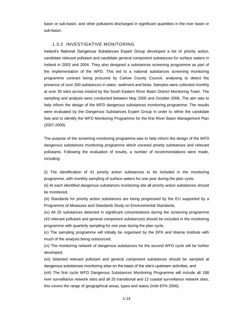
1-14

basin or sub-basin, and other pollutants discharged in significant quantities in the river basin or

sub-basin.

1.3.2 INVESTIGATIVE MONITORING

Ireland’s National Dangerous Substances Expert Group developed a list of priority action,

candidate relevant pollutant and candidate general component substances for surface waters in

Ireland in 2003 and 2004. They also designed a substances screening programme as part of

the implementation of the WFD. This led to a national substances screening monitoring

programme contract being procured by Carlow County Council, analysing to detect the

presence of over 200 substances in water, sediment and biota. Samples were collected monthly

at over 30 sites across Ireland by the South Eastern River Basin District Monitoring Team. The

sampling and analysis were conducted between May 2005 and October 2006. The aim was to

help inform the design of the WFD dangerous substances monitoring programme. The results

were evaluated by the Dangerous Substances Expert Group in order to refine the candidate

lists and to identify the WFD Monitoring Programme for the first River Basin Management Plan

(2007-2009).

The purpose of the screening monitoring programme was to help inform the design of the WFD

dangerous substances monitoring programme which covered priority substances and relevant

pollutants. Following the evaluation of results, a number of recommendations were made,

including:

(i) The identification of 41 priority action substances to be included in the monitoring

programme, with monthly sampling of surface waters for one year during the plan cycle,

(ii) At each identified dangerous substances monitoring site all priority action substances should

be monitored,

(iii) Standards for priority action substances are being progressed by the EU supported by a

Programme of Measures and Standards Study on Environmental Standards,

(iv) All 25 substances detected in significant concentrations during the screening programme

(43 relevant pollutant and general component substances) should be included in the monitoring

programme with quarterly sampling for one year during the plan cycle,

(v) The sampling programme will initially be organised by the EPA and Marine Institute with

much of the analysis being outsourced,

(vi) The monitoring network of dangerous substances for the second WFD cycle will be further

developed,

(vii) Selected relevant pollutant and general component substances should be sampled at

dangerous substances monitoring sites on the basis of the site’s upstream activities, and

(viii) The first cycle WFD Dangerous Substances Monitoring Programme will include all 188

river surveillance network sites and all 25 transitional and 12 coastal surveillance network sites,

this covers the range of geographical areas, types and status (Irish EPA 2006).

1-15

Section 58 of EPA Act of 1992 states that the EPA is required to collect and verify monitoring

results for all water supplies in Ireland covered by the Drinking Water Regulations. In order to

verify the information that has been submitted results must be collected on an annual basis

(from local authorities) and audits carried out on selected local authorities. As of March 2007

new powers and responsibilities have been assigned to the EPA in the area of drinking water

under the new Drinking Water Regulations published by the Department of Environment,

Heritage and Local Government.

In Ireland the safety of water supplies is determined by comparing the results of over 250,000

monitoring tests carried out on 945 public water supplies, 671 public group water schemes, 497

private group water schemes and 1284 small private supplies with the drinking water standards’

by the Irish EPA. In Ireland, surface waters account for 81.9% of the drinking water, followed by

groundwater (10.3%) and springs (7.8%) (Hayes,N.,Page,D.,Sweeney,L.,O’Leary,G. 2011).

1-16

1.4 Modelling and the WFD

The EQS directive (2008/105/EC) requires the concentrations of specific pollutants to not

exceed set thresholds. The targeted monitoring of these pollutants could confirm compliance to

EQSs with a high degree of certainty, which is why modelling would allow monitoring authorities

to know when threshold breaches are most likely to occur. The EU WFD was transposed into

Irish Law in 2003 (Irish EPA 2006) and as such these EQS values now form the basis of priority

substance water monitoring in Ireland. In order for future monitoring programmes to allow us to

meet the requirements established by the WFD the gaps in current knowledge must be

identified and where information is lacking for accurate emission factor data for a priority

substance or group of substances this must be gathered in order to produce truly representative

sampling results at the end of any monitoring campaigns.

1-17

1.5 Conclusions

The aquatic environment including lakes, rivers, ground water estuaries and coastal zones, is

vulnerable to changes induced by human activities. The WFD has listed a number of priority

and hazardous substances with environmental quality standards in place to limit the occurrence

of these pollutants in the environment. As new and emerging compounds are discovered and

incorporated into legislation and as current EQS values are lowered the need for robust and

reliable analytical methods, capable of reaching the necessary limits of detection, becomes

more pronounced. It is also important that strict standard operating procedures are in place and

adhered to for the handling, storage and analysis of samples collected in order to ensure the

integrity of the samples is preserved and that analytical results are of the highest standard.

The WFD aims to achieve and ensure “good quality status” of all European water bodies by

2015 and in setting such a goal poses a huge challenge in monitoring activities. While the

monitoring methods required are not specified the widely accepted method involves grab

sampling, which is the currently accepted method used for monitoring of priority pollutant

chemicals in our waters. Grab sampling is expensive and labour intensive and it identifies

compounds present at only a single point in time. Modelling is emerging as a useful tool for

informing monitoring programs with large databases revealing gaps in current knowledge and

highlighting areas for improvement.

The aim of this work is to use environmental modelling based on a wealth of data collected to

inform future targeted monitoring programmes and thus enable Ireland to meet the WFD

monitoring requirements. In this chapter available literature and statistical data that could be

used to inform targeted PS monitoring strategies is collated. The focus is on readily available

data relevant to major PS risk factors identified by conceptual modelling, and develop

appropriate indicators. These indicators are applied to nine WWTP agglomerations currently

being monitored in a PS study to predict the relative risk of elevated PS loading to receiving

waters across agglomerations and over time.

1-18

1.6 Aims and Objectives

The aim of this thesis is to detail the creation of an index of emission factors, a computer model,

based on both experimental data collected from the monitoring of priority pollutants in waste

water treatment plant effluent and data compiled on sources of these pollutants in the

environment. By monitoring both the emission factors and the actual levels of pollutants

released a model is created which will facilitate more informed water quality monitoring

programmes and will therefore help Ireland to meet European water quality deadlines and

levels.

Main project objectives:

- To design and populate a risk based model for the occurrence of priority substances in

wastewater;

- through the preparation of this model build a database of high quality information;

- to bring together many sources of relevant data on occurrence to one place;

- to develop simple methods for the extraction of priority substances in wastewater;

- to prepare standard operating procedures for the sampling handling, extraction and

analysis of samples to meet WFD requirements;

- to improve on current methods for the analysis of priority substances and

- to produce a final simple model that can inform future monitoring programmes.

2-19

2. Site Selection and

Waste Water Treatment

Processes

2-20

2.1 Introduction

In Ireland, as in many other countries, wastewater is an issue as water that has not been

adequately treated is being released back into the environment leading to increased pollution.

There are currently around 529 wastewater treatment facilities in the country (Monaghan,

Shannon et al. 2012). A recent report by the Irish EPA stated that for an average population

equivalent of 4.97 million 1% of wastewater received primary treatment, 78% received

secondary treatment (with 15% also receiving nutrient reduction), and 6% of wastewater was

untreated (Monaghan, Shannon et al. 2012). In Ireland the main piece of legislation governing

urban wastewater treatment is Council Directive 91/271/EEC which was adopted on 21 May

1991. This directive aims to counter the adverse effects of urban and industrial wastewater

discharges through the principles of planning, regulation, monitoring and information and

reporting on these discharges (EEC 1991).

The wastewater treatment process generally involves primary-, secondary- and sometimes

tertiary treatment (Radjenovic, Petrovic et al. 2007, Ren 2004). The primary treatment phase

incorporates the processes of screening, grit, fat, oil and grease removal, and settlement, with

the overall aim being the removal of solids from the wastewater stream. After this stage it is said

that 50 – 70% of suspended solids have now been removed, and that biological oxygen

demand, BOD, and bacterial count have been reduced by 20 – 50% and 25 – 75%, respectively

(Irish EPA 1997). Secondary treatment can follow and here the wastewater is subject to

biological treatment by microorganisms allowing organic matter removal and nitrification of the

wastewater thus reducing final nutrient levels in the wastewater (Radjenovic, Petrovic et al.

2007, Irish EPA 1997). This is followed by further settlement of the wastewater. Finally,

wastewater may be exposed to a tertiary level of treatment, usually chlorination or UV

treatment, (Radjenovic, Petrovic et al. 2007) which aims to disinfect the wastewater, removing

dissolved organics and inorganics, and suspended solids before final outflow (Ren 2004). It has

been shown that when a waste water treatment plant, WWTP, is functioning properly 90 – 95%

of pollutants can be eliminated before reintroduction of the water to the environment (Li, Jiku et

al. 2000).

Nutrient removal refers to the reduction of phosphorous and/or total nitrogen levels. This is

required where the receiving water body is deemed sufficiently “sensitive” - e.g. waters

susceptible to eutrophication. Since some algae can fix atmospheric nitrogen it is generally

accepted that phosphorus is the limiting nutrient in water. Phosphates occur in sewage effluents

due partly to human excretion and partly to their use in synthetic detergents. The principal

means of phosphorus removal is chemical precipitation, though removal can be incorporated

into primary or secondary treatment or may be added as a tertiary process. In raw wastewater

the predominant forms of nitrogen are organic nitrogen and ammonia. The most common

processes for removing ammonia are air stripping and biological nitrification/de-nitrification

(Cork County Council 2008).

http://eur-lex.europa.eu/LexUriServ/LexUriServ.do?uri=CELEX:31991L0271:EN:NOT

2-21


The aim of this chapter is to describe the selection of sites and the development of a sampling

plan which would cover a wide scope and encompass the characteristics of the majority of

WWTP sites across Ireland. This proved a challenge as varying levels of treatment, population

equivalents and source inputs need to be represented in the final model while also providing

temporal variation data of high quality to populate the model.

The objectives of this work include:

- providing a rationale for the selection of the nine sites chosen in this study;

- reviewing each of the sites and the processes at work in each plant;

- outlining the sampling plan to be adopted.

2-22

2.3 Site Selections and Overview

In order to make the final model of occurrence of priority pollutants in wastewater as

comprehensive as possible nine WWTPs in two different counties, Cork and Dublin, were

chosen. The rationale was to examine two well-populated counties, one with a high population

density and industrial input and the other with a more agricultural input.

Two large WWTPs in Dublin, Ringsend and Swords, and seven smaller scale WWTPs in Cork

were finally chosen. Each site caters for different population equivalents from close to 3000 in

Charleville to over 2.5 million in Ringsend. Different treatment processes are employed at the

different plants and each plant serves varying levels of domestic, industrial and agricultural

inputs. Table 2-1 gives an overview of the WWTPs included in this study, the population

equivalents they serve, the levels and types of treatments that are provided and the receiving

waters of the treated effluent most of which have been deemed ‘sensitive’ by the EPA.

As this project is a large-scale collaboration involving groups in two counties, tasks were divided

with Cork IT coordinating sampling efforts with Cork County Council, and DCU coordinating with

Fingal County Council for samples from Swords WWTP, and Dublin City Council and Celtic

Anglian Water for samples from Ringsend WWTP, as well as managing the project and

collaborating with the group in Cork.

2-23

Table 2-1 Overview of the WWTPs in this study.

WWTP

and Code

Treatment Type of

Treatment

Agglom.

PE

Plant PE Area

(Ha)

Receiving

Waters

Ballincollig

BG

Secondary PS, SS, AS

(Aeration Basin)

16,339 15,000 760 Freshwater

(R)

Bandon

BN

Secondary PS, AS (OD) 8178 20,000 458 Freshwater

(R)

Charleville

CE


(OD)

2,984 6,415 274 Freshwater

(R)

Clonakilty

CY


(OD)

7,500 -

15,000

15,000 750 Estuarine

Fermoy

FY

Secondary,

NR

PS, SS, AS

(OD; A-A-AT)

PR

5,800 12,960 394 Freshwater

(R)

Mallow

MW

Secondary,

NR

PS, SS, AS

(A-A-AT)

PR

7,091 12,000 595 Freshwater

(R)

Ringaskiddy

RY

None None 14,864 0 967 Estuarine

Ringsend

RD

Tertiary PS, SS, AS

(Sequencing

Batch Reactors)

U.V Disinfection

2,870,333 1,640,000 26,728 Estuarine

Swords

SD


(A-A-AT)

50,000 60,000 2,673 Estuarine

Table legend: Area = Area of catchment. PE = Population equivalent. (R) = River. PS = Primary

settlement. SS = Secondary Settlement. AS = Activated Sludge. PR = Phosphorous removal.

OD = Oxidation ditches. A-A-AT = Anaerobic-, anoxic- and aeration tanks. This information was

gathered from the EPA wastewater license applications of the respective WWTPs and from the

EPA Urban Wastewater Report, 2007.

Note: Ringaskiddy is listed as having a plant population equivalent of zero due to the lack of

treatment at this site. This site is located in an area with several pharmaceutical companies and

acts as a combined pumping system for this catchment.

2-24

2.3.1 BALLINCOLLIG

Ballincollig, as a growing town within the Cork Metropolitan area, has shown an increasing

population over recent censuses, with a population of 16,339 recorded in 2006 by the Central

Statistics Office, CSO. The Ballincollig catchment, as shown in Figure 5-9, covers an area of

760 km. This site represents a high population which is an expanding town near Cork city with

an agricultural hinterland. Contributions to the pollution load for the Ballincollig agglomeration

vary with daily, weekly and seasonal producers of effluent, with the main sources being the local

population, local industries, commercial and non-domestic users.

An old sewerage collection system originally linked a cavalry barracks to the north of the town

discharging to the west. As the original village extended and developed into a town a new trunk

sewer was laid. As new housing estates were built they discharged from the same trunk sewer

in Poulavone. After the establishment of the WWTP in Ballincollig the sewer network was

extended and pumping stations were established to facilitate transportation to the WWTP.

In 2006 an approximate non-domestic population equivalent of 8,200 was calculated, giving a

present total pollution load of 24,542 (Cork County Council 2009), while the hydraulic capacity is

now stated as 26,000 P.E., and the capacity of the plant for carbonaceous BOD removal is

~31,500PE (60g/h/d).

2.3.1.1 Overview

At the WWTP the sewage from local industries, collected via the public sewer, and domestic

waste arrive, by means of a number of pipes, at an inlet chamber upstream of the inlet works.

Table 2-2 gives a detailed overview of the specific treatment at the WWTP.

2-25

Table 2-2 Overview of Treatment Processes in operation at Ballincollig Wastewater Treatment Plant. Data collected from EPA licensing application.

Stage of Treatment Processes

Preliminary Screening of wastewater arriving at the plant is through two

mechanically raked coarse bar screens, 25 mm3.

Primary If the flow arriving at the plant exceeds 509 m3/hr the system in place to

handle the excess involves diversion, after screening, to the original

Primary Settling Tanks in the ‘old’ part of the plant, then on the to the

‘old’ Humus tanks until the inlet flows have reduced, allowing for the

diverted stream to be pumped back to the inlet. In the event of excess

storm water there is also an overflow weir which discharges to the outfall

pipe.

Grit is then removed from the stream by three constant velocity grit

channels, followed by a further fine screening step, 5 mm.

Secondary Secondary treatment occurs when the wastewater flows to a Carousel-

type activated sludge plant with a basin volume of approximately 9000

m3. The mixed liquor settles in three circular radial flow clarifiers, 2 old

clarifiers below ground level and a third ‘new’ clarifier above ground

level, constructed in 2008. The settled sludge (RAS) from the 2 old

clarifiers is returned to the aeration basin using 2 No. Archimedes screw

pumps and 1 No. pump. The settled sludge (RAS) from the third clarifier

is returned to the aeration basin by gravity. The excess sludge (WAS) is

pumped to the picket fence thickener (PFT) where it settles and

compacts. The floating scum on the clarifiers is removed via a scum box

and is pumped to the inlet works. The thickened sludge is pumped from

the bottom of the PFT to the centrifuge. The centrifuge dewaters and

further thickens the sludge prior to off-site disposal.

Discharge The treated effluent is discharged from the clarifiers via a weir to a

chamber. From this chamber it flows to a manhole on the north east of

the treatment plant site. From this manhole it is discharged to the river

Lee via the outfall pipe. There are two composite samplers in the

process; one at the inlet (flow proportional) and the other at the outlet

chamber from the clarifiers that is time based (Cork County Council -

Southern Division 2010).

2-26

2.3.2 BANDON

The WWTP in Bandon represents a low population and is located in Bandon southwest of Cork

City, the plant was upgraded in 1993, designed to treat a P.E. of 20,000, and is currently

treating a P.E. of 8,178. A combined sewerage system serves this agglomeration, with four

pump stations within the catchment: O’Mahony Avenue and Bridge Lane are local pump

stations; Watergate Street pump station pumps waste water flows from the north of the

catchment across the river to Glaslinn Road pump station.

Preliminary treatment is provided at the Glaslinn Road pump station consisting of coarse

screening, fine screening and grit removal. From Glaslinn Road wastewater is pumped to the

WWTP (Cork County Council 2008). The primary discharge is the treated effluent from the

WWTP which is discharged to the River Bandon via an open pipe at an average discharge

volume of 2370 m3/day. Secondary discharges flow to the River Bandon from the WWTP

overflow.

2.3.2.1 Overview

Table 2-3 gives a complete overview of the treatment processes employed at Bandon WWTP.

2-27

Table 2-3 Overview of Treatment Processes in operation at Bandon Wastewater Treatment Plant. Data collected from EPA licensing application.


Preliminary The preliminary treatment caters for flows of up to 480 L s-1

which

includes coarse screening and fine screening to 5mm in a ‘Screezer’ unit

which also incorporates screening dewatering and compaction. Grit

removal is provided for flows up to 200 L s-1

. Screenings and grit are

treated on site prior to disposal to landfill.

Flows of 156 L s-1

are pumped to the WWTP for treatment and excess

flows are discharged to the River Bandon.

Primary The WWTP was constructed in two stages and operates as two parallel

systems – a biological treatment plant with primary settlement and a

percolating filter system was constructed in the 1960s and an extended

aeration activated sludge plant with sludge thickening, partial

stabilisation and dewatering facilities was constructed in 1993. Primary

treatment comprises primary settlement in two horizontal flow settlement

tanks operating in parallel.

Secondary Settled sewage gravitates to a flow splitter chamber upstream of the

secondary treatment system. Flows up to 3 DWF (75 L s-1

) pass forward

to the secondary treatment system, an oxidation ditch.

A phosphate reduction system was installed in 1993 however is not

operational as the system depressed the pH of the waste water which

affected biological activity. Supernatant liquors from a gravity sludge

thickener and filtrate from a dewatering press are pumped to the

oxidation ditch, where they combine with incoming waste water and

receive full biological treatment with the main process stream. There is

also a facility to enable these flows to be pumped to the primary

settlement tank (Cork County Council 2008).

2-28

2.3.3 CHARLEVILLE

The treatment plant at Charleville is located in north Cork on the Limerick border and is

designed to cater for a P.E. of up to 15,000 although the 2006 census quotes a population for

Charleville of only 2,984. The industries in this agglomeration have separate WWTPs and for

the most part do not contribute to the flow in the foul sewer system. The surface water in

Charleville generally drains directly to the river, therefore not overloading the wastewater

treatment plant.

Charleville Wastewater Treatment Works was constructed on a green field site in the town land

of Ballincolly, to the north east of Charleville. The wastewater from Charleville town and

environs (274 Ha) is collected through a pipe network and flows by gravity to the wastewater

treatment plant in the town land of Ballincolly north–east of the town centre. The main source of

emissions is the 600mm diameter discharge pipe carrying the treated effluent from the

wastewater treatment plant to Charleville Stream. Charleville Stream flows along the eastern

boundary of the treatment plant (Cork County Council 2008).

2.3.3.1 Overview

Flows from Charleville town and environs flow by gravity to the treatment plant in Ballincolly. A

sludge return system is in operation to ensure an adequate level of mixed liquor suspended

solids. The system is flexible enough to ensure that sludge can be returned from the clarifiers to

the oxidation ditches and an adequate quantity of sludge can be pumped at all times. The mixed

liquor produced from the aeration system enters secondary clarifiers for the purpose of settling

sludge. The main treatment processes in operation at this WWTP are highlighted in Table 2-4.

2-29

Table 2-4 Overview of Treatment Processes in operation at Charleville Wastewater Treatment Plant. Data collected from EPA licensing application.


Preliminary A screen located within the inlet flume removes larger inorganic solid

material.

Primary Following screening, the inlet flume allows 510 m3/hr (6 DWF) to pass

into the splitter chamber. An overflow is located in the inlet flume to the

Charleville Stream.

Secondary The secondary treatment process is based on activated sludge system.

The aeration system at the plant is in the form of oxidation ditches. Each

oxidation ditch is 4500 m3 and contains 4 No. 7.0 m long rotors used to

ensure that sludge remains in suspension at all times. From the ditches,

the flow passes to the two clarifiers for the purpose of settling sludge.

Each clarifier is circular (160 m2) and equipped with a rotating bridge

sludge scraper, inlet, scum and sludge draw-off pipes, sludge return pipe

work, v-notch weir and a system to prevent scum entering the treated

effluent. The wastewater treatment system has two separate process

streams with provision to isolate each stream. At present only one

stream of the treatment plant is in use, as flows have not necessitated

the treatment plant to be used at full capacity.

Discharge The treated effluent flows to the outlet flume and is then discharged to

Charleville Stream through a 600 mm diameter outlet pipe. The liquid

discharge from a sludge-thickening tank is returned to the oxidation

ditch, and treated leachate is discharged to the main oxidation ditch and

treated as regular foul water.

2-30

2.3.4 CLONAKILTY

Clonakilty was an interesting choice for this study as development has generally increased in

recent years and there is high seasonal variation in population of this town due to tourism; a

winter population of approximately 7,500 P.E., and a summer loading of 15,000 P.E. Aside from

domestic inputs, the pollution load from this agglomeration arises from Shannonvale Chickens,

Clona Milk Dairies, Irish Yoghurts, Hotels, schools, a hospital, an abbatoir, a technology park,

etc. (Note: Shannonvale Chickens has its own treatment plant discharging treated effluent to the

public sewer.)

The wastewater in Clonakilty and its environs is collected in a partially combined foul and

surface water network consisting of both gravity and pumped systems. The central part of the

town gravitates in the partially combined system to the two main pump stations of the scheme -

Long Quay and Clarke Street. These then along with lnchydoney main pumping station pump

directly to the WWTP. There are other pumping stations on the outskirts of the town (Cork

County Council 2007).

2.3.4.1 Overview

The purpose of this plant is to remove solids and pollutant matter from sewage entering the

works, rendering the treated effluent suitable for discharge to a watercourse. Grit and other

materials are removed at the inlet works and an extended aeration process removes the main

pollutant matter prior to discharge to the harbour, Table 2-5.

2-31

Table 2-5 Overview of Treatment Processes in operation at Clonakilty Wastewater Treatment Plant. Data collected from EPA licensing application.


Preliminary A grit trap is currently in operation at the plant with a design flow

capacity of 0 – 180 L s-1

, a grit classifier was also recently installed. This

receives the grit from the grit trap and separates out the grit from other

materials and conveys the relatively dry grit into an adjacent wheelie bin

for removal to landfill.

In 2000 a mechanically brushed screen and Lisep unit (Haigh Ace Inlet

System) were installed. The largest model, 991, was installed in

Clonakilty and has a maximum capacity of 100 L s-1

. Acting as an

emergency bypass, a hand-operated penstock is located between the

screen and the inlet flumes at the inlet works. This penstock leads to a

backdrop manhole, which connects to the treatment plant outfall at the

easterly end of the site allowing bypass of plant in emergency situations.

Secondary After the screen outlet, the inlet channel splits into two channels 300 mm

wide. These channels were designed for a flow capacity of 51 L s-1

. The

divided flows are piped from here to the oxidation ditches. Extended

aeration is by means of 2 No. racetrack type oxidation ditches with 4 No.

rotors located midway along the length of each ditch as a means of

aeration. These ditches were designed for a much lower BOD loading

than the peak 15,000 P.E. that it serves in the summer. However, the

plant was designed for a higher hydraulic load of 6 DWF, whereas now

most plants are designed to take a hydraulic loading of 3 DWF. Recently

a further floating aerator was introduced into each ditch in order to

increase the amount of oxygen available for microorganisms to cater for

the increased loading.

The flow from the oxidation ditches is piped to the settling tanks. There

are 2 No. circular hopper-bottomed settling tanks currently in operation

as a means of secondary sedimentation. Sludge settles to the bottom of

these tanks and is returned to the lifting wheel chambers.

Discharge The supernatant liquid from the settling tanks is piped to the outlet

channel. The 400 mm outlet channel collects the treated effluent from

the settling tanks which then flows by gravity to the sea outfall.

2-32

2.3.5 FERMOY

The WWTP in Fermoy is located in the north-east of Cork City, on the banks of the River

Blackwater. The Fermoy catchment serves a total area of 394 hectares. The domestic

population of Fermoy has grown over the last three censuses with the most recent census

figures showing the town of Fermoy and environs having a population in excess of 5,800. The

Fermoy WWTP is designed for a population equivalent of 20,000 P.E. and BOD loading of

1,200 Kg/day. The wastewater in Fermoy is collected in a partially combined foul and separated

foul sewage drainage network. The wastewater drains from the town on both sides of the

Blackwater River; on the north side of the river wastewater drains to a pumping station at

Rathealy Road, which is then pumped across Fermoy Bridge to the main sewer. The

wastewater arising on the south side of the river drains directly to the WWTW.

The maximum hydraulic capacity of the Fermoy WWTP is 673 m3/h (2.3 DWF). In order to cope

with flows above 2.3 DWF, storm storage has been provided at the WWTW. The volume of

storm storage at the WWTW is approximately 1,126 m3. In the event that the storm water

holding tanks are filled and the storm continues, the storm water tanks are operated as a pre-

clarification tank without sludge removal. The overflow from the storm water storage tank is

connected to the final effluent outlet pipe.

The nature and quantities of foreseeable emissions from the wastewater works into the

receiving aqueous environment as well as identification of significant effects of the emissions on

the environment. The final effluent is discharged into the Blackwater River. At design capacity

the WWTW will discharge 7,140 m3/day to the river (Cork County Council 2007).

2.3.5.1 Overview

Table 2-6 details a breakdown of the treatment processes in operation at Fermoy WWTP.

2-33

Table 2-6 Overview of Treatment Processes in operation at Fermoy Wastewater Treatment Plant. Data collected from EPA licensing application.


Preliminary At the inlet pumps force the stream through 2 No. Mechanical screens

with an aerated grit and grease removal system and grit classifier.

Primary The existing WWTW were upgraded with an additional stream, therefore

the flow is split after the wastewater passes through the inlet works with

40% of the flow diverted to the existing wastewater treatment stream.

The remaining 60% is directed to a new treatment system.

Secondary The existing stream has an aeration phase (2 No. Oxidation ditches with

4 No. Surface aerators), a secondary settlement phase and return

activated sludge phase. The new stream has an anaerobic (1 No. Tank

with 3 No. Mixers), anoxic (1 No. Tank) and aeration phase (1 No. Tank

with fine bubble disc aeration), a secondary settlement phase and return

activated sludge phase. Ferric sulphate is also employed as a method of

phosphorus removal. Approximately 20% of this sludge is returned to the

aeration tank in order to maintain a sufficiently large microbial population

in the aeration tank and the remaining 80% is sent to the sludge

treatment processes. The sludge returned to the aeration process is

referred as the RAS (returned activated sludge) and that which is sent

directly to the sludge treatment processes is referred to as the WAS

(waste activated sludge).

Discharge Effluent is discharged into the Blackwater River.

2-34

2.3.6 MALLOW

The WWTP in Mallow is located in the north-east of Cork City, on the banks of the River

Blackwater. The Mallow catchment covers a total area of 595 hectares. The domestic

population of Mallow has grown with the most recent Census figures showing that Mallow Town

and environs now has a population in excess of 7,091. The Mallow WWTP is designed for a

P.E. of 18,000 with a BOD loading of 1,080 Kg/day.

The maximum hydraulic capacity of the Mallow WWTP is 556 m3/h (2.5 DWF). In order to cope

with flows above 2.5 DWF storm storage has been provided at the WWTW. The volume of

storm storage at the WWTW is approximately 1,012 m3. In the event that the storm water

holding tanks are filled and the storm continues, the storm water tanks are operated as a pre-

clarification tank without sludge removal. The overflow from the storm water storage tank is

connected to the final effluent outlet pipe.

The wastewater in Mallow is collected in a partially combined foul and separated foul sewage

drainage network. The wastewater drains from the town on both sides of the Blackwater River.

The wastewater drains to a pumping station at Mallow Bridge, which is then pumped to the

WWTP. At design capacity the WWTP will discharge 5,250 m3/day to the river (Cork County

Council 2007).

2.3.6.1 Overview

Table 2-7 details the waste treatment processes for Mallow, County Cork, with specific details

collected from the EPA licensing applications of the plant.

Table 2-7 Overview of Treatment Processes in operation at Mallow Wastewater Treatment Plant. Data collected from EPA licensing application.


Preliminary At the inlet pumps force the stream through 2 No. Mechanical screens

with an aerated grit and grease removal system and grit classifier.

Secondary The flow is split after the wastewater passes through the new inlet

works. 50% of the flow is diverted to the existing wastewater treatment

stream. The remaining 50% is directed to a new treatment system. The

existing stream has an aeration phase (2 No. Oxidation ditches with 2

No. Surface aerators), a secondary settlement phase and return

activated sludge phase. The new stream has an anaerobic (1 No. Tank

with 3 No. Mixers), anoxic (1 No. Tank) and aeration phase (1 No. Tank

with fine bubble disc aeration), a secondary settlement phase and return

activated sludge phase. Ferric sulphate is also employed as a method of

phosphorus removal.

2-35

2.3.7 RINGASKIDDY

The WWTP in Ringaskiddy is situated ca. 16 km from Cork City in the south west of the harbour

and is the location of a number of pharmaceutical companies. Discharges from the industries in

the area are governed by IPPC licences issued by the EPA. Treated effluent from a number of

industries in the area discharge into a common industrial development authority (IDA) trunk

sewer which flows by gravity through the Ringaskiddy screening plant and discharges into a

long pipe into the harbour. There is no WWTP serving this agglomeration only 6 Sewage

Pumping Stations with emergency overflows working for a P.E. of 97,556 as of the 2006

Census. Only 14,864 of this P.E. is the actual population of the agglomeration, while a number

of industries in this catchment are licensed to discharge effluent, providing a further P.E. of

licensed discharges to be estimated at 82,692. There are plans to develop this site further with

a WWTP due to begin construction at this site in 2016.

The agglomeration comprises a number of distinct areas linked by one sewer collection system.

The agglomeration is made up of the village of Crosshaven, the town of Carrigaline, the village

of Shanbally and also includes treated trade effluent from a number of industries in the

Ringaskiddy area. Wastewater collected in Crosshaven is pumped to the sewerage system in

Carrigaline. All wastewater collected in Carrigaline (including Crosshaven) is pumped through

the Coolmore Pumping Station at Church road, Carrigaline to a trunk sewer at Raheens, where

it is flows by gravity to the discharge point in Lower Cork Harbour. An underwater outfall pipe

discharges approximately 2.6 km from the shore at a depth of approximately 30 below sea level.

There is also a small collection system and pumping station in Shanbally village which conveys

effluent to the trunk sewer. This WWTP represents a treatment facility in a heavily industrialised

region with a high population.

2-36

2.3.8 RINGSEND

The Greater Dublin agglomeration served by the Ringsend plant includes all the areas of Dublin

City and South Dublin County Councils, and parts of Fingal, Dun Laoghaire, Rathdown and

Meath County Councils. The Ringsend catchment, Figure 5-11, includes a total area of 26728

hectare. The licence was issued by the EPA to all five contributory local authorities. The Greater

Dublin agglomeration is the largest agglomeration in Ireland, with a measured population

equivalent in 2010 of 2.45 million (maximum weekly average). Influent is composed of domestic

wastewater, commercial wastewater, licensed trade effluents, surface water from combined

sewers, surface water infiltration, groundwater infiltration, saline infiltration and tankered

wastewaters. The older parts of the network such as Dublin city center are drained on a

combined system that means both foul wastewater and storm water run-off from rainfall are

carried in the same system. The treated effluent is ultimately mixed with the cooling waters from

the ESB’s Poolbeg Generating plant, thus providing for further dilution of the effluent. Both flow

streams are then discharged together to the lower Liffey estuary. This data was collected from

the EPA Annual Environmental Report (AER) 2010 for Ringsend WWTP, Table 2-8.

Table 2-8 Overview of Treatment Processes in operation at Ringsend Wastewater Treatment Plant. Data collected from EPA licensing application.

Stage of

Treatment

Processes

Preliminary The wastewater passes through fine screens (6 mm) to remove paper, plastics

and large solids. Grit, fats, oil and grease are removed in special tanks.

Primary 12 primary treatment lamellae tanks allow 40% - 50% of the pollutants in the

wastewater to settle.

Secondary The settled wastewater is pumped to 24 Sequencing Batch Reactors (SBR’s) for

secondary treatment. Micro-organisms developed in the process are used to take

organic matter out of the wastewater, along with ammonia and nitrogen.

The SBR’s at Ringsend are the largest in the world and, uniquely, are contained in

a two story structure, due to site limitations. The 24 SBR’s are divided into 6 units,

built three on top of three. Each unit consists of 4 tanks, operating in sequence.

While one tank is filling with wastewater, a second is aerating wastewater with

oxygen to accelerate the natural biological secondary treatment. The third tank is

settling wastewater and the fourth tank is decanting treated wastewater to the

next treatment stage.

Tertiary The treated water receives tertiary treatment in the form of ultraviolet disinfection

Discharge The water receives tertiary treatment to meet Bathing Water Standards, before

being discharged into the Bay. Over 95% of the original pollutants have been

removed and the treated water is comparable to good quality river water (Dublin

City Council 2003).

2-37

2.3.9 SWORDS

The Swords agglomeration is centred on the town of Swords and covers nine square

kilometres. The Swords catchment covers a total area of 2673 hectares. The Swords plant is a

conventional aeration plant designed to cater for a P.E. of 60,000. The load for 2006 was

50,000 with main contribution to the agglomeration from domestic sources. There is some

contribution from the commercial activities in the town and there are also a number of

discharges from licensed trade effluent.

There are two river basins in the agglomeration area, the Ward and the Broadmeadow Rivers. A

number of storm water overflows and pumping station overflows, when operational, discharge to

these watercourses. The agglomeration drains by gravity to a treatment works on Spittal Hill

Road. The effluent from the plant is discharged to the Broadmeadow River slightly upstream of

the M1 Motorway crossing. As the Inner Broadmeadow Estuary is a designated sensitive area

under the Urban Wastewater Treatment Regulations nutrient reduction is also part of the

treatment process. There are two small treatment plants serving what were cottage schemes at

Toberburr and at Rowlestown, both of these schemes are to the west of Swords. Planned work,

expected to have been completed in 2008, would ensure that both plants would be replaced by

pumping stations and the necessary rising mains and gravity sewers would be laid to transfer

the sewage into the existing Swords scheme, where it would be treated in the Swords WWTP.

This data was collected from the EPA licence application forms (Fingal County Council 2007).

2.3.9.1 Overview

The treatment process consists of preliminary treatment, primary settlement, activated sludge

process and final settlement. The excess sludge is thickened, pasteurised, digested and

dewatered. A storm water holding tank is provided to deal with storm conditions. In the event of

a storm, the influent will be pumped through the inlet works and the preliminary treatment as

normal. The resultant influent is stored in the storm water tank where it allowed settling i.e. the

storm water tank acts as a primary tank. In the event of the storm conditions persisting the

screened and settled influent will overflow the storm water holding tank and discharge at the

primary discharge point.

2-38

Table 2-9 Overview of Treatment Processes in operation at Swords Wastewater Treatment Plant. Data collected from EPA licensing application.


Preliminary Influent to the plant is screened and grit, fats, oils and grease are

removed. Screenings and grit are washed and compacted prior to

disposal.

Primary The flow to the primary settlement tanks is split into three streams, the

existing treatment stream comprised of 2 circular tanks and two new

streams, comprising of two rectangular tanks. All settleable material is

separated in these tanks and pumped to the sludge treatment.

Secondary The activated sludge tanks consist of an anaerobic, an anoxic and an

aerobic zone for both biological phosphate removal and full nitrification

and de-nitrification. The aeration is carried out using a diffused air

system. Alum dosing is on standby for additional chemical phosphate

removal.

Discharge The final effluent and activated sludge are separated in the final

settlement tanks. The effluent is discharged to the Broadmeadow

Estuary (Fingal County Council 2004).

2-39

2.4 Sampling Plan

In order to populate the final model with valuable, comprehensive data, it was necessary to

devise a sampling plan that would provide as much detail on temporal and seasonal variability

as possible. This plan also needed to be flexible in order to facilitate sampling after an extreme

weather event and allow for the monitoring of the weather in such a way that samples

representative of both dry- and wet weather flow (DWF and WWF) could be acquired.

The rationale behind the sampling plan for the Dublin sites, Ringsend and Swords WWTPs, was

to collect monthly samples with periods of intensive sampling during two winter and two summer

periods. Effluent samples were collected at the same location for the same sample volumes,

and strictly employed SOPs were applied to all samples.

As the Cork samples were being provided by Cork Co. Council a much more flexible sampling

plan was put in place as this sampling was infrequent and it became much more difficult to

adhere to the SOPs. Up until April 2011 Cork samples were irregular therefore it was not

possible to conduct intensive sampling. From April to July 2011 monthly samples were received

from all sites and included intensive samples from the site in Ballincollig. Table 2-10 details the

specifics of the sampling plan including types of samples obtained, volumes and sample

breakdowns, as well as a clear overview of the sampling dates.

Table 2-10 Overview of Sampling Plan. Timeframe in which monthly samples were collected.

Site Sample Type Timeframe

(months)

Volume

(L)

Sample Breakdown

BG Grab 14 6.5

6 x 500 mL PAH analysis (3 filtered)

6 x 500 mL Pesticide analysis (3 filtered)

500 mL Metals analysis

BN Grab 13 6.5

CE Grab 12 6.5

CY Grab 4 6.5

FY Grab 13 6.5

MW Grab 13 6.5

RY Grab/ Composite 12 6.5

RD Grab 25 12.5 6 x 1 L PAH analysis (3 filtered)

6 x 1 L Pesticide analysis (3 filtered)

500 mL Metals analysis

SD Composite 20 12.5

*Note – The Cork samples for pesticide analysis were extracted in Cork IT following the same

SOPs. The composite sample from Swords was collected by an auto-sampler, which collected

100 mL per 1000 m3 flow through the plant. In Ringaskiddy the sample is part grab and part

composite in order to reach the necessary volumes required for our analyses.

2-40

Table 2-11 Overview of sampling dates at nine WWTPs under study, with shaded squares indicating samples collected. (Note: X indicates a period of intensive sampling, samples taken every second day for a period of at least one week.)

2009 2010 2011

Month J A S O N D J F M A M J J A S O N D J F M A M J J

BG X

BN

CE

CY

FY

MW

RY

RD X X X X X X

SD X X X X X X

2-41

2.5 Conclusion

This chapter has defined the nine sites chosen for this study, 7 sites in Cork and 2 sites in

Dublin. Each of the sites represents a different demographic, type of population and type of

treatment. The sampling plan devised allows for the evaluation of domestic, industrial and

agricultural inputs and emission factors while also affording the opportunity to compare levels

and styles of treatment and the removal efficiencies achieved by such.

Including Ringsend WWTP in the sampling plan has the added benefit of facilitating monitoring

of the largest WWTP in the country, serving the most heavily populated city, and operating well

over capacity, as can be seen in Table 2-1. This draws attention to an issue encountered during

the data collection stage of this project; the fact that different sources of the same data were

quoting different values for population equivalents and actual populations being served by each

plant. EPA waste licence applications made by the respective plants, annual environmental

reports (where available), and urban wastewater reports were shown to differ in the

fundamental area of P.E. served by the respective WWTPs. Where plants are undergoing

works, or being taken over by private companies it is important to have the correct P.E. values

as removal efficiencies of plants operating above capacity are severely reduced, thus leading to

increased levels of priority and hazardous substances being present in the WWTP effluent and

consequently being released back into the environment.

To conclude, this chapter has described the processes of site selection and sampling plan

development for this project. This was of paramount importance to the project as the final model

must be filled with high-quality data on a range of different sites under varying conditions.

3-42

3. Sample Preparation

and Standard

Operating Procedures

3-43

3.1 Introduction to Sample Preparation and Standard Operating

Procedures (SOPs)

Samples, from biological to environmental, are often not in a condition which would allow for

direct analysis to be carried out therefore a sample preparation step is necessary. This step

aims to ensure that the analyte(s) of interest is suitable for analysis after the step is complete.

This will generally involve ensuring that the analyte is free from interferences and in solution at

a concentration which will allow for its measurement or detection, it can also involve converting

the analyte to another form which would allow for easier separation and detection. These aims

can be achieved, depending on the original sample, through a number of techniques including

extraction, derivatization, homogenisation, filtration and pre-concentration (Luthria 2006).

An environmental sample, specifically wastewater, is non-homogenous containing dissolved

organic matter, particulates and will contain a wide range of substances of varying polarities.

Owing to the nature of these environmental samples sample preparation steps are required, i.e.

most water samples contain substances such as salts, humic acids and other humic substances

which can interfere with solid-phase extraction especially the determination of polar pesticides

(Ibáñez, Picó et al. 1998, Picó, Fernández et al. 2007). A good sample preparation step will

separate the analyte(s) of interest from these matrix constituents which could lead to analytical

interferences, leaving a clean, concentrated sample.

In the preparation of wastewater samples some of the most commonly used techniques involve

solid phase extraction (SPE) and liquid-liquid extraction (LLE). SPE facilitates sample extraction

and concentration while also minimising solvent consumption which is a big concern in

environmental labs. The trace nature of the analytes in question require that larger sample

volumes are collected and a sample preparation method which is capable of handling these

large volumes, resulting in a concentrated sample of the target analyte, must be chosen. Table

3-1 below compares SPE and LLE methods.

3-44

Table 3-1 Comparison of the two most commonly used sample preparation methods in environmental sample handling – SPE and LLE.

Solid Phase Extraction Liquid-Liquid Extraction

Little solvent consumption High solvent consumption

Cartridges and disks are disposable Heavy on glassware use – time consuming to

clean

Better recoveries Lower recoveries

No emulsions Emulsions

More versatile, more choice Chosen solvents must be immiscible

Cleaner extracts achievable

Can be automated Difficult to automate

Selective removal of interferences

3-45

3.1.1 SOLID PHASE EXTRACTION (SPE)

SPE was developed as a cheaper and more environmentally friendly alternative to liquid-liquid

extraction (LLE). Similar to LLE, SPE involves the partitioning of compounds between 2 phases.

The analytes (in liquid form) are placed in a small column or cartridge containing an appropriate

packing material where the analytes will have a stronger affinity for the solid packing than for

the sample matrix and the liquid sample is passed through this cartridge either by suction or by

positive pressure. The analytes are retained on the solid phase while many interferences are

washed out and are later removed by eluting with a solvent with a greater affinity for the

analytes (Huck, Bonn 2000).

The main procedure of SPE involves these steps:

- Activation of the sorbent by passing through an appropriate solvent (wetting)

- Removal of the activation solvent

- Sample introduction, and analytes retained on sorbent (retention step)

- Removal of interferences (washing)

- Analyte elution with stronger solvent

Figure 3-1 Schematic showing stages involved in SPE Method; A- Condition, B- Load, C- Wash, D- Elute

Different mechanisms of retention/elution are used and these are due to intermolecular forces

between the analytes and the active sites on the surface of the adsorbent and the matrix. In

SPE, another important parameter that must be controlled is known as the breakthrough

volume; this is the sample volume where the analyte starts to be eluted from the exit of the

cartridge and this value is a function of the chromatographic retention of analyte on the

particular sorbent, it can only be changed by altering the sorbent and increasing the sorbent

mass (Huck, Bonn 2000).

3-46

3.1.2 SORBENT FORMATS

With SPE the primary concern for analysts is sorbent choice, a choice that will solve their trace-

analysis problems, and so a key problem with SPE is method development. The solid-phase is

very important; for many years n-alkyl silica has been the universal SPE sorbent (Hennion

1999). It is also very important to obtain extracts free from matrix interferences in as few steps

as possible so selectivity is given a lot of consideration, the more selective the SPE step is, the

more sensitivity is obtained (Pichon 2000).

The two most common forms of SPE sorbents are as disks or cartridges. As described above

the extraction can be carried out in a sorbent-packed cartridge, or, it can be carried out on a

sorbent that is enmeshed in the inert matrix of a membrane-based extraction disk (Pichon

2000).

3.1.2.1 Cartridges

Cartridges contain different types and amounts of sorbent and they are also available in

different sizes (Masqué, Marcé et al. 1998). The main limitations associated with using

cartridges are restricted flow-rates and plugging of the top frit when analysing samples

containing suspended solids. Therefore if samples have not been previously filtered the use of

cartridges may be extremely slow and tedious (Hennion 1999). Other limitations are

encountered specifically when analysing water samples: tolerance to blockages is low and

channelling reduces the capacity to retain analytes. A solution to some of these problems would

involve the use of disks, yet cartridges are still the most popular as they use less solvent volume

than disks and also due to the fact that there is a limited commercial availability of sorbents for

disks compared to cartridges (Masqué, Marcé et al. 1998).

3.1.2.2 Disks

Disks are 0.5 mm thick membranes where the adsorbent is immobilized in a web of micro fibrils;

this allows higher flow-rates than SPE cartridges (Huck, Bonn 2000). Channelling effects are

also eliminated; however many of the same limitations still exist especially with samples

containing suspended matter (Hennion 1999). Disks are generally used when dealing with large

sample volumes and when the concentration of the analytes is low, e.g. trace analysis of

organic pollutants in water (Huck, Bonn 2000). The two main types of disks available are

Empore disks containing C18 or PS-DVB (Masqué, Marcé et al. 1998). The disks can be used

for extraction using one of three main processes: (i) pass the sample through the disk using a

vacuum source, the analytes are retained and then removed with a small volume of eluent, (ii)

suspend the membrane in the sample (liquid) for a specified period of time, allow to dry briefly in

air then directly detect the analytes using a solid state spectroscopic technique and (iii) similar

to (ii) except the analytes are desorbed by suspending the disk in a solvent and then detected in

the extract(Huck, Bonn 2000).

The main disadvantage of using disks rather than cartridges is the decrease in the breakthrough

volume, mainly for the more polar compounds, it is also for this reason that disks are used when

there is a strong interaction between the analyte and the sorbent(Masqué, Marcé et al. 1998).

3-47

3.1.3 TYPES OF SORBENTS

3.1.3.1 Chemically Bonded Reverse Phase Silica

The most common materials used as sorbents in SPE are the chemically bonded silica’s,

usually with C8 and C18 organic groups bonded to the surface of the porous silica. It is believed

that the more organic carbon bonded to the silica surface the better the sorbent. Manufacturers

use di- and tri-functional modifiers for the production of SPE sorbents due to the stability of the

bonded phase and the cost of production; this leads to polymeric bonded phases usually

containing 15-19% bonded carbon (Nawrocki, Da browska 2000).

Several types of modified silica’s are available commercially with different properties based on

percentage of carbon loading and the type of functional alkyl-silanes used for the bonding

(Hennion 1999). Among the modified silica’s while the C18 silica’s provide the greatest retention

they also trap the most interferences. Other options include cyclohexyl and phenyl phases, with

phenyl phases being shown to increase the retention of aromatic analytes. Cyanopropylsilica

and aminopropylsilica are polar phases that exhibit both polar and non-polar interactions.

Aminopropylsilica, when compared with a C18 sorbent, has achieved better detection and

quantification limits (Hennion 1999), however during the method development for the analysis of

PAHs it was found that C18 to be the most suitable for this sample group. Finally, selective

electron-donor- and electron-acceptor-bonded silica packing’s have been prepared specifically

for use with hydrophobic contaminants (Hennion 1999).

The main limitation of both reversed-phase silica sorbents and many of the polymeric sorbents

available is that they all require conditioning with a wetting solvent and cannot be allowed to dry

before the loading of an aqueous solvent (Hennion 1999).

3-48

3.1.3.2 Functionalised Polymers

This new generation of polymers (e.g. Strata-X from Phenomenez and Abselut from Varian) has

been designed to extract an extensive selection of analytes i.e. lipophilic, hydrophobic, acidic,

basic and neutral with a single cartridge with a simplified procedure since no conditioning is

required. These polymers have also been shown to provide a better wettability, and also

increase the extraction recoveries of polar compounds (Hennion 1999).

A main group of functionalized polymers used as sorbents are apolar poly(styrene–

divinylbenzene) copolymer sorbents. These resins are available in disposable cartridges, and

the highly cross-linked PS-DVB sorbents have the ability to trap very polar, non-polar and

ionized organic analytes (Hennion 1999). This ability of PS-DVB resins, such as Amberlite XAD-

type, of trapping more polar compounds than a typical C18 cartridge is one advantage, with

stability over pH range 1-14 being the other (Pichon 2000). Overall, it is believed that these

highly cross-linked PS-DVB sorbents are the sorbents to be selected for the extraction of very

polar analytes when large sample volumes are required (Hennion 1999). These cartridges are

the most widely used in the area of pesticide extraction. Through this study it was found that

polymeric sorbents proved sufficiently selective for our analytes, and removed many of the

interferences and matrix components, leaving clean samples for analysis.

3-49

3.1.4 SPE METHOD DEVELOPMENT

There are several steps involved in the development of a method for SPE. The first step is the

selection of an appropriate sorbent which will allow for the greatest sample recovery and the

best removal of interferences. Figure 3-2 below provides a schematic of factors that need to be

considered when selecting a SPE sorbent. Reverse phase sorbents are most suitable for

environmental applications in relation to water samples.

Figure 3-2 Overview of SPE sorbent selection procedure.

Sorbent mass and volume also have an important role as greater sorbent mass increases the

sorbent surface area in contact with the sample and increases the analyte capacity of the

sorbent which in turn affects the breakthrough volume. It must also be noted that silica-based

sorbents have lower sorbent surface area than polymeric sorbents and therefore have lower

analyte capacity per gram. A SPE method using a larger sorbent mass also uses higher

volumes of solvent.

Elution solvent strength in SPE is based on the polarity of the solvent and the nature of the

bonding between the analyte and the sorbent. Combinations of polar and non-polar solvents are

used in the conditioning, washing and elution stages of a SPE procedure. Table 3-2 below lists

the most commonly used solvents in SPE in order of their respective polarities. While some

solvents may prove stronger and therefore better for the elution of analytes it is important to

consider that some of these solvents are considered, themselves, as priority pollutants

according to the WFD, i.e. carbon tetrachloride and dichloromethane.

Aqueous

Water

Charged Neutral

Try reverse phase

Organics

Charged

Try reverse phase or ion

exchange

Neutral

Try reverse phase

Organic Is the sample matrix?

Is the analyte of interest more soluble in?

Is analyte?

Recommendation:

3-50

Table 3-2 Polarity and miscibility of commonly used solvents in SPE.

POLARITY SOLVENT Miscible in water?

Non-polar

Polar

Hexane

Isooctane

Carbon tetrachloride

Chloroform

Dichloromethane

Tetrahydrofuran

Diethyl ether

Ethyl acetate

Acetone

Acetonitrile

Isopropanol

Methanol

Water

Acetic acid

No

No

No

No

No

Yes

No

Poorly

Yes

Yes

Yes

Yes

Yes

Yes

3-51

3.1.5 OVERVIEW OF SPE METHOD DEVELOPMENT STEPS

There are a number of steps involved in the development and validation of an SPE method,

Figure 3-3. It is important that all steps are well optimised and validated before applying the final

method to actual samples.

Figure 3-3 Overview of the steps involved in development and validation of the SPE methods used in this project.

Through the application of the method outlined above the result is an optimized and validated

method of extraction for an analyte or group of analytes of interest.

3.1.6 STANDARD OPERATING PROCEDURES

In analysis the main source of imprecision and inaccuracy is the sample preparation step which

is often tedious and time-consuming. Steps must be taken to minimise the potential for error in

the analytical results and as such it is very important that standard operating procedures

(SOPs) are carefully established and strictly followed during all stages of sample handling from

collection through to analysis. As this work involved collaboration between two main project

partners it was important that SOPs were easily understood and followed by both parties to

ensure the integrity of the results.

Evaluate physical/chemical properties of analytes

Determine type of sorbent to be used and appropriate solvents

Evaluate different SPE brands for best recovery and sample clean up

Further evaluation using larger cartridges and sorbent bed volumes

Run different methods and optimise conditioning, washing and eluting

solvents

Run spiked samples to determine recoveries and breakthrough volumes

3-52


The aim of this chapter is to review sample preparation techniques and choose the most

suitable for the purposes of this study that would best allow the requirements of the WFD to be

met. As sample exchange between two research groups was also a factor it was necessary to

establish early on a strict set of SOPs and sample exchange procedures which would limit

inconsistencies in techniques and results between these groups.

The objectives are to:

- Introduce the concept of sample preparation,

- Highlight the importance of standard operating procedures (SOPs),

- Outline the theory of SPE and its applications within the scope of this study,

- Develop simple and fast methods for the multi-residue extraction of priority PAHs,

pesticides and metals,

- Describe the method development involved in the extraction of PAHs, pesticides and

metals and trace elements from a wastewater matrix and

- Summarise the SOPs adapted for use in this study.

3-53

3.3 Sample Preparation for PAHs

PAHs are hydrophobic compounds and are therefore easily extracted on typical reversed-phase

sorbents and C18 bonded silica is, by far, the most common (Portet-Koltalo, Oukebdane et al.

2007, Marcé, Borrull 2000, Sun, Littlejohn et al. 1998). Sargenti, McNair (1998) compared C18,

cyano and phenyl bonded silica sorbents and found that results for C18 were the most

acceptable, however, according to Kootstra, Straub et al. (1995) C8 material is better than C18

for extracting PAHs in both recoveries and reproducibilities. One main issue with these sorbents

is the presence of free silanol groups which result in non-reversed phase, or secondary,

interactions; the PAHs are strongly retained leading to low sample recoveries (Hagestuen,

Campiglia 1999). Through cartridge evaluation in this study it was found that Strata C18

cartridges resulted in the best recoveries and general performance for the WFD priority PAHs.

Other sorbents used include immuno-sorbents which have been applied to the selective

isolation of PAHs from complex environmental samples (Marcé, Borrull 2000) and Styrosorbs

MN-100 and MT-65. These styrosorbs are a type of hyper cross-linked polystyrene polymer

which have been successful sorbents for the pre-concentration of phenanthrene and

naphthalene (Nazarkina, Bulanova et al. 2001). Finally, SPE discs with a glass fibre matrix can

be used to reduce extraction times of PAHs compared to other extraction systems (Urbe, Ruana

1997). As mentioned there are limitations associated with both the use of cartridges and discs

for SPE, by pre-filtering the samples it was possible to avoid many of the clogging issues

associated with cartridge use and the samples were not limited by the lower breakthrough

volumes associated with the disc.

Owing to the non-polar nature of the PAHs and based on the literature a reversed phase

approach to SPE was selected. Reversed phase SPE involves the retention of non-polar

organic compounds from polar solutions such as water. Non-polar non-polar interactions occur

between the functional groups on the surface of the silica sorbent in the cartridge and the non-

polar analyte. To elute the PAHs a strong non-polar solvent is used to disrupt these bonds.

There were 2 main stages in the SPE method development for the PAHs - cartridge selection,

and solvent selection. First gas and liquid chromatographic methods were developed and these

were used to evaluate the cartridges and solvents chosen for SPE, this work is detailed in

Chapter 4.

3-54

3.3.1 CARTRIDGE SELECTION

Cartridge selection was an important process in the development of the PAH sample extraction

method. Table 3-3 shows the results of the preliminary PAH recovery study using 11

commercially available SPE cartridges. The aim of this study was to discover which SPE

cartridge would provide the best sample enrichment and highest recoveries for the priority

PAHs.

Spiked water samples (100 mL) were passed through the SPE cartridges listed, in triplicate,

under a vacuum, after conditioning using a basic method; 2 mL methanol (MeOH), 2 mL of

deionised (di) water. The cartridges were then washed with 2 further aliquots of deionised

water, dried with the vacuum, and PAHs were eluted using 2 mL acetonitrile (ACN) which was

evaporated down under nitrogen and reconstituted to 1 mL with ACN. Subsequent analysis was

carried out by HPLC-FLD detection and recoveries are listed in the table below, Table 3-3.

Table 3-3 Recovery study of PAHs on SPE cartridges. Recoveries represent total SUM PAH recovery using each cartridge.

Cartridge Sorbent Average Recoveries of Cartridges

N=3

Average Total

Recovery

1 2 3

Isolute TPH NH2 layer above C18 20.65% 74.80% 86.93% 60.79%

Bond Elut

ENV

Styrene divinyl

benzene polymer

6.30% 5.21% 7.44% 6.32%

Strata C18 C18 105.7% 107.38% 97.58% 103.52%

Bond Elut C18 C18 93.51% 132.33% 141.1% 122.30%

Isolute PAH

HC

NH2 layer above C18 20.73% 18.06% 21.89% 20.23%

Isolute C8 C8 12.90% 14.34% 6.87% 11.37%

Isolute C18 C18 58.32% 57.75% 53.09% 56.39%

Isolute C2 C2 22.85% 11.70% 17.16% 17.24%

Isolute ENV+ Hydroxylated

polystyrene-

divinylbenzene

copolymer

53.38% 54.51% 53.36% 53.75%

Strata C8 C8 9.96% 10.79% 12.66% 11.14%

From Table 3-3 several cartridges clearly demonstrate good sample enrichment with two also

providing sample enrichment. After investigation it was discovered that this enrichment was due

to breakthrough on the cartridges as the cartridges affected had sorbent beds of only 100mg.

Another issue was also evident from this preliminary study, although recoveries for Isolute

ENV+ seem acceptable for overall total percentage recovery there was no recovery of Benzo-a-

pyrene or Benzo-ghi-perylene only high recoveries of other compounds. These cartridges were

3-55

therefore ruled out as the goal was to achieve the highest possible recoveries for all eight

priority PAHS. From the preliminary study the top performing cartridges for all PAHs were

selected and re-evaluated at higher sorbent mass levels and a lower ‘spiked’ concentration.

The Isolute C18 and Strata C18 were found to be the most reliable cartridges when evaluated for

recoveries of all eight PAHs. Naphthalene, due to its volatility, had the lowest recovery for both

cartridges. The Strata cartridge out-performed the other cartridges for overall recoveries with

the Isolute cartridge found to be second best, Figure 3-4. These two cartridges were further

subjected to the solvent selection process in an attempt to further improve sample recoveries

and breakthrough volumes.

Figure 3-4 Percentage recovery of each of the PAHs using the two preferred cartridges. N=3. Naph = naphthalene. Ant = Anthracene. Fluor = fluoranthene. Bb/k = benzo-b- and benzo-k-fluoranthene. Bap = benzo-a-pyrene. Ind = indeno-1,2,3cd-pyrene. Bghi = Benzo-ghi-perylene. <LOD = below limit of detection.

3.3.2 SOLVENT SELECTION

Selection of appropriate and efficient solvents for use in this method was important to maintain

a high level of sample recovery. As mentioned in Section 3.1.1 there are several solvents

involved in the typical SPE procedure: conditioning, washing and eluting solvents. Optimisation

of each of these solvents leads to the most effective method. The literature was used as a

starting point in the method development.

A conditioning solvent in SPE should wet the sorbent making it activated towards the analyte(s)

in the sample. The cartridge must be kept in a conditioned state and not allowed to dry out

between conditioning and loading of sample. This is owing to drying leading to air pockets in the

sorbent bed which then reduces the interfacial contact between the sorbent and the sample.

Samples are retained on the sorbent by a number of mechanisms. In reverse phase SPE these

are hydrophobic interactions such as non-polar non-polar interactions and van der Waals or

dispersion interactions.

0

10

20

30

40

50

60

70

80

90

100

Naph. Ant. Fluor. Bb/k Bap Ind + Bghi

Isolute C18 Strata C18

Per

cen

tage

Rec

ove

ry

3-56

The sample is loaded in a strongly non-polar solvent, water. A wash step is also performed

using the same non-polar solvent, this allows for the elution of poorly retained interferences and

matrix constituents leaving the analytes of interest tightly bound to the sorbent. A strong elution

solvent, or mixture of solvents, is required to break the bonds and allow elution of the analyte.

Figure 3-5 Percentage recoveries of 2 PAHs using different elution solvents after conditioning with MeOH and loading of a 1 mL spiked sample. N=3.

The PAHs are nonpolar, and have been found to be strongly binding to SPE sorbents, see

Section 3.3, as such it was important to use strong eluting solvents, organic solvents. An elution

solvent should be strong enough to elute the analyte in as small a volume as possible. One of

the manufacturer recommended solvents from Phenomenex was a combination of

dichloromethane and acetonitrile (ACN) however as dichloromethane is also listed as a priority

pollutant the decision was made to evaluate ACN as well as other solvents. Figure 3-5 shows

the recoveries of naphthalene and benzo-ghi-perylene when eluted with different solvents using

the same method. Naphthalene and benzo-ghi-perylene were chosen as they represent the

spectrum of hydrophobicity of the PAHs in this study with naphthalene having the lowest Log

Kow value and benzo-ghi-perylene having the highest. From the study there was only a slight

difference in recoveries when using the more non-polar tetrahydrofuran (THF) compared to the

ACN. Owing to the nature of these two solvents and their handling and disposable in the lab

acetonitrile was chosen as the preferable elution solvent for this method. While other more non-

polar solvents could be used for elution a number, as mentioned earlier, are themselves listed

as priority substances and were therefore ruled out as candidates. Of the more non-polar

solvents toluene was mentioned most commonly in the literature in combination with acetonitrile

and other solvents and was thus investigated further.

Solvent combinations have been shown in Table 3-4. Presented are three different methods for

the SPE of PAHs each using strong eluting solvents, and resulting in a pre-concentration of

1000 when applied to our 1 L sample volumes. The solvent combinations were selected after

comparing methods listed in the literature and due to the non-polar nature of the PAHs. The

0

10

20

30

40

50

60

70

80

90

100

Tetrahydrofuran Acetonitrile Isopropanol Methanol

Naphthalene Benzo-ghi-perylene

Per

cen

tage

Rec

ove

ries

3-57

three methods in Table 3-4 were evaluated on both the Strata C18 and Isolute C18 cartridges

chosen after the cartridge evaluation study, Section 3.3.1. with final analysis by GC-MS.

Table 3-4 Overview of three method solvent combinations, (A, B, and C) evaluated for use in the extraction of PAHs in wastewater. N=3

SPE Methods

A B C

Conditioning:

6 mL MeOH

6 mL Water

Load 1 mL sample

Wash with 2 mL water

Dry cartridge under vacuum

Elute with ACN: Toluene (3:1)

Evaporate down with nitrogen

and reconstitute in 1 mL ACN

Conditioning:

2 mL ACN

2 mL MeOH

2 mL Water

Load 1 mL sample



Elute with 2 x 2 mL ACN



Conditioning:

2 mL MeOH

2 mL Toluene

2 mL Water

Load 1 mL sample



Elute with 2 mL ACN

1 mL Toluene



Of the three methods in Table 3-4 method B was chosen for it’s high overall recoveries,

achieving recoveries of over 70% for all PAHs using the Strata cartridge, including the

naphthalene which had exhibited some sample loss during the cartridge selection stage. This

method was also more environmentally friendly and avoided the use of toluene when compared

to the other two methods. When applied to a 1 L sample volume this method provides a 1000

times preconcentration factor allowing the method limits of detection to meet EU requirements.

3-58

3.4 Sample Preparation for Pesticides

The sorbents most commonly employed in pesticide analysis are chemically bonded silica

(usually C18 or C8) or styrene-divinylbenzene copolymers (PLRPs and Envichrom P).

Chemically bonded silicas have been shown to achieve high retention of non-polar and

moderately polar pesticides/compounds however they are not sufficient for polar samples. They

also show broad interfering peaks in UV chromatograms of water samples containing pesticides

due to co-extraction of interferences occurring at the low pH required for pesticide retention

(Moral, Sicilia et al. 2008) this is due to ionic interactions (Vigna, Morais et al. 2006). Another

problem with polar compounds is frequent poor reproducibility and recovery (Jiménez, Bernal et

al. 2001). Extraction and recovery of polar and non-polar herbicides has been achieved through

an increase in sorbent mass and/or by modification of the matrix (Wells, Yu 2000).

Styrene-divinylbenzene, as a copolymer, is a well-known hydrophobic solvent, shown to have

retentions equal to, or higher, than C18-bonded silica. Only apolar or moderately polar analytes

can be retained on PS-DVB (Ahmed 2001). Main examples of commercial polymeric SPE

sorbents are Strata-X, Oasis (poly(divinylbenzene-co-N-vinylpyrrolidone) and XAD (styrene-co-

divinylbenzene) (Vigna, Morais et al. 2006). Recoveries of polar compounds have been found to

be higher with PS-DVB than bonded silica although silica is hydrophilic the surface is

hydrophobic due to the presence of hydrocarbon chains so there is little surface contact with

aqueous solutions, whereas PS-DVB copolymers have a hydrophilic surface but also have

many aromatic sites which allow interactions with aromatic analytes (Masqué, Galia et al. 1998).

As outlined earlier in this chapter there are a number of steps involved in the SPE procedure

and thought must be given to the cartridges and solvents employed. Where C18 cartridges have

proven more suitable for non-polar separations with successes in the extraction of PAHs in

wastewater it is the polymeric adsorption media that have shown to retain a range of pesticides.

As with the PAHs a reversed phase approach is taken to the extraction of pesticides in

wastewater.

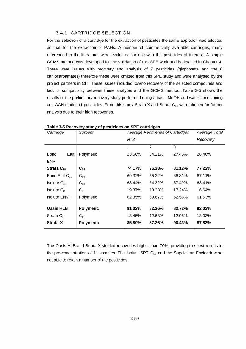
3-59

3.4.1 CARTRIDGE SELECTION

For the selection of a cartridge for the extraction of pesticides the same approach was adopted

as that for the extraction of PAHs. A number of commercially available cartridges, many

referenced in the literature, were evaluated for use with the pesticides of interest. A simple

GCMS method was developed for the validation of this SPE work and is detailed in Chapter 4.

There were issues with recovery and analysis of 7 pesticides (glyphosate and the 6

dithiocarbamates) therefore these were omitted from this SPE study and were analysed by the

project partners in CIT. These issues included low/no recovery of the selected compounds and

lack of compatibility between these analytes and the GCMS method. Table 3-5 shows the

results of the preliminary recovery study performed using a basic MeOH and water conditioning

and ACN elution of pesticides. From this study Strata-X and Strata C18 were chosen for further

analysis due to their high recoveries.

Table 3-5 Recovery study of pesticides on SPE cartridges

Cartridge Sorbent Average Recoveries of Cartridges

N=3

Average Total

Recovery

1 2 3

Bond Elut

ENV

Polymeric 23.56% 34.21% 27.45% 28.40%

Strata C18 C18 74.17% 76.38% 81.12% 77.22%

Bond Elut C18 C18 69.32% 65.22% 66.81% 67.11%

Isolute C18 C18 68.44% 64.32% 57.49% 63.41%

Isolute C2 C2 19.37% 13.33% 17.24% 16.64%

Isolute ENV+ Polymeric 62.35% 59.67% 62.58% 61.53%

Oasis HLB Polymeric 81.02% 82.36% 82.72% 82.03%

Strata C8 C8 13.45% 12.68% 12.98% 13.03%

Strata-X Polymeric 85.80% 87.26% 90.43% 87.83%

The Oasis HLB and Strata X yielded recoveries higher than 70%, providing the best results in

the pre-concentration of 1L samples. The Isolute SPE C18 and the Supelclean Envicarb were

not able to retain a number of the pesticides.

3-60

3.4.2 SOLVENT SELECTION

The second stage of evaluation for the extraction of pesticides in wastewater involved

evaluation of solvents for optimum extraction. The pesticides cover a range of non-polar to

moderately polar compounds as such it was important to use carefully tested eluting solvents.

As with the PAHs many of the organic solvents are also listed as priority substances and were

therefore ruled out for inclusion in the study.

Figure 3-6 shows the recoveries of atrazine, dieldrin and chlorfenvinphos when eluted with

different solvents using the same method. These compounds were chosen as they represent

the spectrum of hydrophobicity of the pesticides as well as the molecular size with

chlorfenvinphos the largest of the pesticides. From this study as well as the literature and

solvent handling/disposable considerations acetonitrile and isopropanol were further

investigated and found to achieve the highest recoveries for the pesticides when used together.

Figure 3-6 Percentage recoveries of atrazine, dieldrin and chlorfenvinphos using different elution solvents after conditioning with MeOH and loading of a spiked sample.

Table 3-6 outlines the three main solvent combinations used, A-C. Using GCMS analysis it was

found that method A gave the highest recoveries when run on the Strata-X cartridges and by

making the elution solvent a combination of ACN and IPA. This method has been evaluated by

other researchers and has been applied to all pesticide samples included in this study.

0

10

20

30

40

50

60

70

80

90

Toluene Acetonitrile Isopropanol Methanol IPA/ACN

Atrazine Dieldrin Chlorfenvinphos

Per

cen

tage

Rec

ove

ries

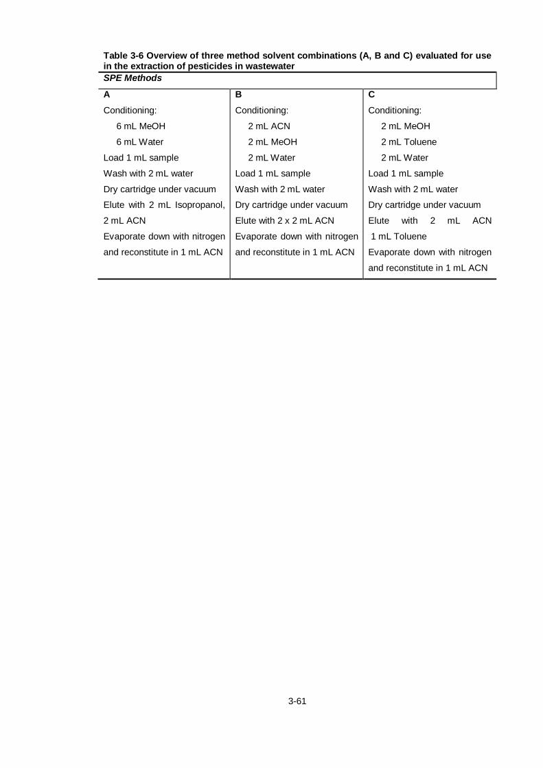
3-61

Table 3-6 Overview of three method solvent combinations (A, B and C) evaluated for use in the extraction of pesticides in wastewater

SPE Methods

A B C

Conditioning:

6 mL MeOH

6 mL Water

Load 1 mL sample



Elute with 2 mL Isopropanol,

2 mL ACN



Conditioning:

2 mL ACN

2 mL MeOH

2 mL Water

Load 1 mL sample






Conditioning:

2 mL MeOH

2 mL Toluene

2 mL Water

Load 1 mL sample



Elute with 2 mL ACN

1 mL Toluene



3-62

3.5 Sample Preparation for Metals and Trace Elements

For the metals and trace elements it was important to include as many of the priority and

hazardous substances as possible, without making the sampling, transportation and storage

procedures more difficult therefore one method of sample preparation could be applied to all

metals and trace element samples. Unlike the sample preparation procedures required for the

PAHs and pesticides a step is usually required to adapt the metals in the sample to the proper

form for the analytical methodology.

Through review of existing preparation methods, specifically the American Public Health

Association (APHA) guidelines (Eaton, Franson 2005) and EPA method 200.7 for the

determination of metals and trace elements in water and wastes by inductively coupled plasma

(ICP) it was clear that it would not be possible to use one method for all our analytes as different

metals required different pre-treatments, e.g. Mercury. It was then necessary to introduce a

method that would be as inclusive as possible and EPA method 200.7 outlined a sample

preparation for total dissolved metals which was deemed appropriate. This method would allow

for the preservation, preparation and analysis of 15 priority substances using one sample pre-

treatment method.

3.5.1 SOP

Samples were collected in PTFE bottles; this was to remove possible interferences with the

analysis of Boron, which could be encountered when collecting samples in borosilicate bottles.

After collection of the wastewater sample at the sampling site the pH of the water is adjusted to

below pH 2 using concentrated nitric acid (conc. HNO3). The APHA guidelines suggested the

use of nitric acid as it will adequately digest most samples and provides a suitable matrix for

ICP techniques.

When trying to determine total recoverable analytes a sample digestion step is required before

analysis. This is required for wastewater samples due to the particulates and suspended solids

in the water. While manual acid digestion of these samples is possible it is tedious and time

consuming and so microwave digestion was chosen as the final preparation step for the

samples. A Mars Express Instrument CEM Microwave Sample Preparation System was used.

The instrument was set to digest samples according to EPA Method 3015. This involved

measuring 45 mL of the acidified wastewater into the instrument sample tube and adding 5 mL

of conc. HNO3 bringing the total sample volume to 50 mL. The instrument autosampler has the

capacity for 16 samples at any one time, 15 samples and a blank. There are two stages to the

microwave digestion, ten minutes at 665W followed by 10 minutes at 290W, with a final 5

minute cool down setting. Samples were then filtered into plastic sample tubes to remove any

residual particulates which could become clogged in the ICP sample introduction system.

3-63

3.6 Standard Operating Procedures

In order to maintain strict quality control over the samples to ensure the integrity of the results it

was necessary to establish and employ a series of standard operating procedures (SOPs) to

cover all sample handling, from collection at the original site through to analysis in the lab.

These SOPs were prepared according to the American Public Health Association (APHA)

guidelines (Eaton, Franson 2005). As the samples were being collected for PAH, pesticide and

metals analysis, it was necessary to prepare three separate SOPs to cater for the different

requirements for both the stability and final analysis of the samples. The standard procedures

for sample preparation in the lab have been described in Sections 3.6.1, 3.6.2 and 3.6.3 below

and 3.5.1 above. The sampling materials required in order to follow the SOPs are listed in Table

3-7.

Table 3-7 Equipment and reagents required for the groups of priority pollutants specified in the SOPs

PAHs and Pesticides Metals and Trace Elements

Bucket

Shatterproof bottles (5 L) x 2, with TFE lined

screw cap lids

Polypropylene containers

Acetone

Deionised water

10% (v/v) dichloro-dimethylsilane in toluene

solution

Conc. HNO3 and an acid solution

Biohazard labels

Freezer box

Ice blocks

Gloves

Hard hat

The following sections outline the basic procedures that were followed covering all stages from

sample collection to storage.

3-64

3.6.1 BRIEF OVERVIEW OF SOPS

Presented in Figure 3-7 is an overview of the procedures followed in the sampling and

extraction of priority substances from wastewater as part of this study. Samples were collected

in triplicate and separated for pesticide, PAH and metals and trace elements analysis.

Figure 3-7 Overview of SOPs followed in sampling and extraction.

The SOPs are outlined in more details in the sections below.

3.6.2 OUTLINE OF SOP FOR PAHS

After developing a SPE method for the selective extraction of priority PAHs in wastewater the

following basic SOP was applied between project partners to ensure consistent sample

extraction procedures were carried out.

The collected samples of effluent were divided into 1 L/ 500 mL aliquots that were carefully

poured into 1 L silanised amber glass bottles. The SPE cartridges, 6 mL, 500 mg Strata-C18

cartridges from Phenomenex (California, USA), were labelled appropriately and were placed in

a SPE vacuum apparatus. SPE cartridges were conditioned with 2 mL acetonitrile followed by 2

mL methanol, and finally 2 mL of deionised water. Care was taken not to allow the cartridges to

dry. After conditioning the samples were loaded to the cartridges after which the cartridges were

rinsed with 2 x 2 mL deionised water and were allowed to vacuum dry. The SPE cartridges were

stored at -18 ˚C until needed. They were then defrosted and eluted with 2 x 2 mL acetonitrile.

This was evaporated down with nitrogen and reconstituted with 1 mL acetonitrile.

Prepare sampling equipment

Collect sample (1 L in Dublin, 500 mL in Cork. n=3)

Pesticide sample

Load sample on Strata X cartridge

Wash with water

Elute with ACN and IPA

Evaporate down and reconstitute in 1 mL ACN

Analyse by LCMS

PAH Sample

Load sample on C18 cartridge

Wash with water


Evaporate down and reconstitute in 1 mL ACN

Analyse by GCMS

Metals sample

Acidify to pH 2

Digest using microwave digestion

Analyse using ICPMS

3-65

3.6.3 OUTLINE OF SOP FOR PESTICIDES

The collected samples of effluent were divided into 1 L aliquots, which were carefully poured

into 1 L amber glass bottles. The solid phase extraction (SPE) cartridges, 6 mL, 500 mg Strata-

X cartridges from Phenomenex (California, USA), were labelled appropriately and were placed

in a SPE vacuum apparatus. SPE cartridges were conditioned with 6 mL methanol followed by

6 mL acetonitrile. Care was taken not to allow the cartridges to dry. After conditioning the

samples were loaded to the cartridges after which the cartridges were rinsed with 2 x 2 mL

deionised water and were allowed to vacuum dry. The SPE cartridges were frozen at -18 ˚C

until needed. They were then defrosted and eluted with 2 mL acetonitrile and 2 mL isopropanol.

This was evaporated down with nitrogen and reconstituted with 1 mL acetonitrile.

3-66

3.6.4 SAMPLE COLLECTION

For the priority PAHs and Pesticides prior to sampling all glass bottles used were silanised to

prevent adsorption of analytes to inner bottle walls which leads to loss of sample and lower

recoveries. Owing to the trace nature of these analytes this step was required as studies have

shown that this ‘deactivation’ of the glassware masks the polar Si-OH groups on the glass thus

decreasing its hydrophilicity. 5 L shatterproof glass bottle were taken and cleaned with detergent

followed by acetone and then rinsed with deionised water. A solution of 10 % (v/v) dichloro-

dimethylsilane in toluene is used to rinse the bottle. Finally, the bottle was rinsed with toluene

followed by methanol.

Note: All bottles were appropriately labelled as Biohazards and included details of sampling

location, time and date of collection, and initials of the sample collector. For metals and trace

elements the glass bottles were first acid rinsed - no silanisation was required.

3.6.4.1 Grab Samples

The majority of samples involved in this project were grab samples with only Swords and

Ringaskiddy providing composite samples. When collecting a grab sample the sampling bucket

was rinsed three times with the effluent at sampling point. The bucket was filled with wastewater

and used to fill the 5 L shatterproof bottles to the top, tapping the sides to remove air bubbles.

Bottle lids were tightened securely and bottles were transported back to the lab, keeping the

bottles in the dark to avoid exposure to light.

3.6.4.2 Composite Samples

When collecting the composite samples the bottles were given to the technicians at the

wastewater treatment plant. The technicians would then fill the bottles to capacity from the plant

auto-sampler. Finally after ensuring the bottle lids were tightened securely the bottles were

transported back to the lab, keeping the bottles in the dark to avoid exposure to light.

3.6.5 SAMPLE PRESERVATION

In order to preserve samples, after sample collection all metals samples were acidified to pH <2

with concentrated nitric acid (HNO3), this step is unique to the metals and trace elements. The

PAH and pesticide samples were preserved as described below.

3.6.5.1 Water Samples

Water samples, of minimum sample volume 600 mL, for shipping to the project partners were

stored in silanised amber bottles (or acid rinsed bottles for metals) or in dark conditions at 4˚C

for a maximum period of 7 days. After this time samples required extraction or analysis. No

further preservation was necessary. Samples arriving from Cork were to be extracted/digested

upon arrival.

3-67

3.6.5.2 Extracted and Digested Samples

Samples collected in Dublin were extracted immediately using the sample preparation methods

described earlier in this chapter. After extraction/digestion samples were stored in the dark at a

temperature of -18˚C. No further preservation was necessary.

3.6.6 TRANSPORTATION

If transporting samples a short distance samples were transported by car and were

extracted/digested within an hour of collection.

For long distance transportation i.e. between the Cork sites and Dublin, samples of water were

to be chilled and preserved at a temperature of 4ºC and maintained at that temperature from the

time of collection until analysis, in the dark or in amber bottles as PAHs and some pesticides

are known to be light sensitive, and must be appropriately labelled and sealed to maintain chain

of custody. Chain of custody forms were filled out and transported along with all samples

exchanged throughout the course of the project. Sample bottles were placed in an ice chest for

transport, this was filled with chopped or grated ice. Upon arrival samples were extracted

immediately. The ice chests were sealed first with biohazard tape and then cling film.

3-68

3.7 Conclusion

This chapter highlights the need for SOPs and quality control measures especially in the area of

environmental monitoring as chemicals are present in trace amounts and make for difficult

analysis. In large collaborative projects it is important to establish these standard procedures

between the different groups to maintain the same standard of sample handling and storage, as

such SOPs are not only prepared according to APHA guidelines, but also chain of custody

forms are in place which facilitate the tracking of all samples and any issues encountered, i.e.

leaking of sample during transport.

The nature of the sample to be collected immediately defines the need for sample preparation

procedures. In the case of WWTP effluent the presence of suspended solids, for example, is a

major factor to be considered when choosing a compatible preparation procedure. This chapter

summarises the process which should be followed when selecting and developing an

appropriate sample preparation method.

The trace nature of the priority pollutants in this type of sample must also be taken into account,

thus necessitating the procurement of larger sample volumes and large sorbent beds in the

SPE procedures to allow for the concentration of analytes to a workable range. Through the

procedures described in Chapter 4 it is possible to choose and develop three sample

preparation methods for the priority pesticides, PAHs and metals and trace elements listed in

the WFD.

To conclude this chapter has outlined the development of standard methods for the multiresidue

extraction of WFD priority substances from wastewater effluent. The methods described use

readily available equipment, are simple to use and allow for the requirements set out by the

WFD and EQS directive to be met.

4-69

4. Method Development

4-70

4.1 Introduction

4.1.1 CHROMATOGRAPHIC SEPARATIONS

High performance liquid chromatography (HPLC) and gas chromatography (GC) are very

popular analytical separation techniques. The basic principle involves the transportation of a

sample in a mobile phase (liquid in HPLC, gas in GC), through a solid stationary phase, which is

fixed in a thin column, and as the analyte elutes it is detected by a suitable detector. The

sample becomes partitioned based on affinity for either the solid or the mobile phase.

Components that are strongly retained on the stationary phase elute from the column more

slowly than those weakly retained by the stationary phase. These differences in mobility through

a column are the basis of separation. This method can be both quantitative and qualitative

(Skoog, Holler et al. 1998).

The stationary phase in HPLC is generally silica based and can be either reversed-phase or

normal-phase. In reversed-phase chromatography the stationary phase is nonpolar, and the

mobile phase is polar, the opposite is true for normal-phase chromatography. The type of

chromatography chosen is determined by the properties of the analyte. In reverse-phase

chromatography non-polar samples are more strongly retained, while polar samples are more

strongly retained in normal-phase chromatography. (Skoog, Holler and Nieman 1998) GC

employs mainly polymeric stationary phases and capillary columns 30-60m in length. In

chromatography the column diameter and length must be taken into account as they affect

separation efficiency and analysis times. The most commonly used columns in LC separations

are 100-250 mm long, with an internal diameter of 3-5 mm. Longer columns have longer

analysis times but better resolution, while shorter columns have shorter analysis times and lose

some resolution, the same theory applies to GC. Capillary columns are also popular in LC with

diameters of 0.05-0.3 mm they offer high separation and sensitivity, although they do require

long analysis times (Kostiainen, Kauppila 2009).

Coupled to a chromatographic instrument is a detection system that allows for the identification

of compounds as they elute from the column. Detection can use optical properties or physical

transformation of the analytes in order to visualize sample components. In chromatographic

analysis of PAHs and pesticides ultraviolet (UV), fluorescence and mass spectrometric

detection were found to commonly occur in the literature. A mass spectrometer, MS, is an

instrument, which separates moving ions on the basis of their mass-to-charge-ratios (m/z). This

involves a number of steps: atomization, ionisation, separating the ions formed on the basis of

their mass-to-charge-ratio, and counting the number of ions of each type. The m/z value is

generally equal to the mass of the ion as most ions formed are singly charged. (Skoog, Holler

and Nieman 1998) The final product of MS, is a mass spectrum, this is characteristic of a

certain compound and can be used for identification (Manahan 2000).

4-71

4.1.2 POLYCYCLIC AROMATIC HYDROCARBONS

Reverse phase columns can readily separate a number of PAHs isomers. Common solvents

used with these columns are acetonitrile-water or methanol-water combinations with gradient

elution. Generally fluorescent detectors are used in order to take advantage of the strong

fluorescence exhibited by many PAHs, and this method is still considered the most powerful

technique (comparable only to MS-SIM detection) in terms of sensitivity and selectivity. HPLC

techniques are preferred over GC methods in some instances as they allow the detection of

high-molecular mass PAHs which could undergo thermal decomposition at the high

temperatures required for GC analysis (Moret, Conte 2000, Peltonen, Kuljukka 1995). It was

found that the high-molecular weight priority PAHs were suitable for GCMS analysis, reaching

low limits of detection and improved separation over the HPLC-FLD method.

While liquid chromatography is commonly used in PAH analysis when coupled with

fluorescence or diode array detection, GC with flame ionization detector (FID) electron capture

detection (ECD) (Singh, Spassova et al. 1998) or MS based detection also have many

applications (Barco-Bonilla, Vidal et al. 2009, Gimeno, Altelaar et al. 2002, Peltonen, Kuljukka

1995, Brum, Netto 2009). Other forms of GC such as high resolution GC (HRGC) and capillary

GC(Barro, Regueiro et al. 2009, Poster, Schantz et al. 2006, Brum, Netto 2009) are also

common. The priority PAHs meet the main requirement for GC analysis, namely the ability to

volatilize within a given temperature range with most PAHs containing up to 24 carbon atoms

being eligible (Barton, Johnson et al. 1979). GC, as an analytical method, offers shorter analysis

times, low limits of detection and high resolution (Peltonen, Kuljukka 1995, Bjørseth, Dennis

1980). GC methods can also easily be adapted to meet the analyst’s needs with only slight

modifications – such as column, detector, temperature, and, in the case of MS, change in the

ionization mode.

The choice of column in GC analysis is important and stationary phases are being developed

with increasing levels of thermal stability, these being polymer based and producing more

reproducible chromatographic data (Peltonen, Kuljukka 1995). Separations are generally carried

out on cross-linked fused silica capillaries with slightly polar to non-polar sorbents; e.g. 5%

phenyl methyl silicone (Ratola, Lacorte et al. 2006) and methyl silicone, respectively, with the

former being most frequently used. These columns are robust and commonly commercially

available (De Boer, Law 2003). This is in contrast to special application columns with selective

stationary phases which are being developed by several analysts, e.g. the use of nematic liquid

crystal phases (De Boer, Law 2003). Capillary columns are the most widely used, favoured for

greater selectivity, sensitivity and resolution when compared to LC (Barro, Regueiro et al. 2009,

Poster, Schantz et al. 2006) and for their ability to highly resolve complex PAHs which form as a

result of inconsistent combustion processes (Peltonen, Kuljukka 1995, De Boer, Law 2003). As

with all GC analyses the column length is also an important parameter with 30 m being the most

common. Studies have been carried out to compare 30 m and 60 m column lengths

4-72

(Filipkowska, Lubecki et al. 2005) and the improved resolution of the 60 m length must be

weighed against the shorter run-times of the 30 m.

In the detection of PAHs fluorescence has been found to be a very sensitive and selective

method of detection when coupled to LC (Barco-Bonilla, Vidal et al. 2009) while MS has found

most applications in GC analysis. FID has also been applied to PAH analysis with finding that

the lack of sensitivity of this detector is incomparable to the MS which provides better selectivity,

more reliable results, analyte confirmation, and lower limits of detection (Barco-Bonilla, Vidal et

al. 2009). Another group, (Singh, Spassova et al. 1998) however, compared GC-MS to GC-ECD

finding ECD to be the more sensitive method, but though the use of selected ion monitoring

(SIM) the analyst can monitor only selected ions, increasing method selectivity with specific

compounds easily added to or removed from the SIM program and thus lower detection limits.

MS is generally used in the electron impact (EI) mode with selective ion monitoring (SIM)

(Valero-Navarro, Fernández-Sánchez et al. 2007, Crozier, Plomley et al. 2001, Ratola, Lacorte

et al. 2006, Bercaru, Ulberth et al. 2006). This method provides enhanced sensitivity (Barro,

Regueiro et al. 2009) and PAHs, mostly, yield strong molecular ions with little fragmentation in

this mode (De Boer, Law 2003).

4-73

Table 4-1 Method parameters of a selection of PAH studies with ‘PAHs’ column indicating the number of PAHs included in the method for analysis.

PAHs

Analysis Column Run

Time

(min)

Mode

16 GC-IT-MS DB-5ms 35 EI, SIM mode (Valero-Navarro, Fernández-

Sánchez et al. 2007)

17 GC-IT-MS DB-5ms 35 EI, SIM mode (Crozier, Plomley et al. 2001)

16 GCMS DB5–MS 34.2 EI, SIM mode (Bercaru, Ulberth et al. 2006)

16 GCMS n/a EI, TIM mode (Shimmo, Adler et al. 2002)

17 GCMS DB5MS 40 EI, SIM mode (Gmeiner, Stehlik et al. 1997)

16 GCMS HP 5MS 40 EI, SIM mode (Gaga, Tuncel 2004)

16 GCMS HP-DB

5MS

45 EI, SIM mode (Meudec, Dussauze et al. 2006)

17 GCMS DB-5 35 EI, SIM mode (Sprovieri, Feo et al. 2007)

16 GCMS DB-5MS 35 SIM mode (Cao, Wang et al. 2005)

15 GCMS HP-5 50 EI, SIM mode (Pérez, Farré et al. 2001)

12 GCFID CP-Sil 110 EI, SIM mode (Fernandes, Sicre 1999)

22 GCFID SE54 102 EI, SIM mode (Readman, Fillmann et al. 2002)

16 GCMS HP-5 SIM mode (Pérez, Guillamón et al. 2001)

15 GCMS HP-5MS

SV

32 SIM mode (Simon, Palme et al. 2006)

16 GCMS SPB-5 50 SIM mode (Wolska, Galer et al. 1999)

16 GCMS ZB 5 28 EI (Werres, Balsaa et al. 2009)

4-74

4.1.3 PESTICIDES

As the project was a collaboration between two research groups the task of method

development was shared with the other research group focussing on LCMS-based

methodologies, thus although LCMS is the preferred method for the analysis of pesticides in

wastewater the focus of this chapter is the development of a GC method for this multi-residue

analysis.

Some GC methods which are commonly implemented in the analysis of pesticides include

electron capture detection (ECD) (Concha-Graña, Fernández-Martínez et al. 2009) flame

photometric detection (FPD) (Yao, Jiang et al. 2001), nitrogen-phosphorous detection (NPD)

(Dugay, Miege et al. 1998) and atomic emission detection (AED) all of which are element-

selective detectors (Vinas, Campillo et al. 2002, Ahmed 2001), used because of the

heteroatoms contained in most pesticides, with AED being more sensitive due to its

multichannel ability which allows it to detect all elements, except helium, separately (Van Stee,

Leonards et al. 1999).

From Table 4-2 below it is clear that GC-ECD is a popularly used method and studies report low

limits of detection. Absolute detection limits of this model of detector are reported to be ca. 100

femtogram (fg) (De Boer, Law 2003) with a number of studies (Concha-Graña, Fernández-

Martínez et al. 2009, Boussahel, Bouland et al. 2002, Junior, Re-Poppi 2007) reporting low

limits of detection. These low levels allow for trace analysis which is important from an

environmental point of view as many potentially harmful contaminants present in water are only

at low concentrations and may go completely undetected without a method with trace analysis

capabilities. These same studies also reported good linearity’s using the ECD, whereas De

Boer and Law (2003) reported that poor linearity is a major drawback of the ECD making it

necessary to perform a method of multi-level calibration to solve this problem (De Boer, Law

2003). As an alternative to ECD, Guardia Rubio et al. (2007) found thermionic sensitive

detection (TSD) to be the more selective detection method although it is less commonly used as

a method of pesticide analysis (Guardia Rubio, Ruiz Medina et al. 2007).

FPD and NPD have also found many applications in the analysis of pesticides and as in Table

4-2 below both methods have been shown to achieve good linearities, limits of detection and

limits of quantification. Vassilakis et al. (1998) found GCNPD to produce poor resolution and

resorted to using LC-DAD to confirm the analysis (Vassilakis, Tsipi et al. 1998). In both gas- and

liquid chromatographic methods detection based on MS is a powerful method, providing

selective and sensitive analysis of pesticides (Planas, Puig et al. 2006) with the added benefit of

acquirement of structural information for the analyte (Vinas, Campillo et al. 2002). GC-tandem

MS (GC-MSMS) minimizes the level of clean-up required for complex environmental samples

due to its highly specific analyses, is easy to use, and is relatively low cost, however its

applications are limited to residue confirmation (Tahboub, Zaater et al. 2005, Bennett, Chung et

4-75

al. 1997) with single MS remaining the most commonly used method (Hada, Takino et al. 2000,

Natangelo, Tavazzi et al. 1999, McGowin, Adom et al. 2001).

In the GC analysis of pesticides fused-silica capillary columns are the most commonly

employed, facilitating the separation of many pesticides with similar characteristics. As

pesticides cover a large range of polarities this affects the choice of stationary phase with polar

pesticides such as the organophosphorous pesticides requiring polar sorbents e.g. DB 170

(Pang, Cao et al. 2006) and non-polar pesticides such as organochlorine pesticides requiring

non-polar sorbents e.g. DB-1 or DB-5 (Planas, Puig et al. 2006, Tahboub, Zaater et al. 2005). It

must also be noted that the non-polar stationary phases are generally considered more robust

(Ahmed 2001). Although many types of columns were evaluated in the methods below, (Table

4-2), the majority were fused silica capillary columns of 0.25 mm internal diameter (I.D.) and

0.25 μm film thickness with similar sorbents, and of 30 – 60 m in length, with the exception of

Hada et al. (2000) and Korenkova et al. (2003) who successfully used columns of 10 and 15 m

lengths, respectively. The results were both limits of detection and quantification in the ng L-1

region, and analysis times of 8-9 minutes. This is a major advantage in large-scale

environmental analysis when large sample numbers must be analysed at regular intervals,

however this method may result in reduced resolution, and selectivity (Hada, Takino et al. 2000,

Korenkova, Matisova et al. 2003).

Injection volume is also comparable in the studies included in Table 4-2 the majority of which

carried out sample injections of less than 4 µL with reasonable results with the exception of

(Concha-Graña, Fernández-Martínez et al. 2009) who used large sample injection volumes of

100 µL. They found this method to be comparable to both GCECD and GCMS and achieved

low limits of detection, between 0.3-25 ng L-1

, high recoveries, 69-107%, and finally very high

precision, 0.2-1.3%. When evaluating injection volumes as part of this priority substances work

it was found that injection volumes over 20 µL resulted in overloading of the column leading to

split peaks with shoulders and overall poor resolution.

4-76

Table 4-2 Literature review of GC-based pesticide separation methods.

Pests.

In

study.

Method Column Run

Time

(min)

Mode Reference

6 GC-MS HP-5MS 14 TIC (McGowin, Adom et al. 2001)

Mix GC–MS HP-5MS 35 Full scan (Pérez-Carrera, León et al. 2007)

32 GCMS DB-5 57 SIM (Planas, Puig et al. 2006)

21

GCECD DB-XLB n/a (Concha-Graña, Fernández-

Martínez et al. 2009)

GCECD DB-35 23.5 n/a

GCMS DB-XLB 60.3 SIM

Mix GCECD n/a 54.5 n/a (Vassilakis, Tsipi et al. 1998)

GCNPD n/a 52 n/a

GCMS HP-5 52 SIM

GCECD n/a 54.5 n/a

Mix GCECD PTE5 41 n/a (Boussahel, Bouland et al. 2002)

14 GCMSMS DB-5.625MS 36 Full Scan (Tahboub, Zaater et al. 2005)

18 GC-ECD VF-5MS 50 n/a (Junior, Re-Poppi 2007)

8 GCMS/MS DB-5-MS 36 n/a (Sauret-Szczepanski, Mirabel et

al. 2006)

12 GCNPD DB-5.625 37 n/a (Dugay, Miege et al. 1998)

17 GCMS HP-1 8.5 SIM (Hada, Takino et al. 2000)

15 GCMS HP-1MS 8 SIM (Korenkova, Matisova et al. 2003)

16

GC-ECD ZB-35 30 n/a (Mmualefe, Torto et al. 2009)

GC-

TOFMS

30 n/a

22 GCMS DB-5 MS 39 SIM ( uintana, Mart et al. 2001)

75 GCMS HP-5MS 60.5 SIM (de Almeida Azevedo, Lacorte et

al. 2000)

10 GC-IT-MS CP-Sil 8 CB 30 TIC, SIM (Maloschik, Ernst et al. 2007)

28 GC TSD

and ECD

CP-SIL 5CB

CP-SIL 8CB

34

23

n/a (Guardia Rubio, Ruiz Medina et

al. 2007)

12 GCMS DB-5MS 50 SIM (Wang, Zhao et al. 2007)

29 GCMS NB-5 35 SIM (Sasano, Hamada et al. 2000)

46 GC-IT-MS VF-5 MS 34.5 Full scan (Beceiro-González, Concha-

Graña et al. 2007)

21 GCMS DB-1701. 38 SIM (Chen, Yu et al. 2009)

8 GCMS DB-5MS 28 SIM (Silva, Aquino et al. 2008)

4-77


In the analysis of trace metals and metal coordination compounds GC and HPLC are the most

commonly used chromatographic techniques. Ion-pair chromatography is also rapidly gaining

popularity as are other reverse phase HPLC methods such as ion exchange HPLC and size-

exclusion HPLC. For example a size-exclusion ICP-MS system was set-up specifically to

analyse heavy metal complexes in natural aquatic samples, Wang, Lee (1997), and Jones-

Lepp, Momplaisir (2005) found LC-ESI-MS to be suitable for the analysis of organometallics

such as organotin, organoboron, and organoselenium. As with Jones-Lepp, Momplaisir (2005),

Reemtsma (2001) evaluated the use of LC-ESI-MS in the analysis of organometallic complexes

and found it efficient. It allows the identification of the organic compounds masked by signals

obtained for one element in LC-ICP-MS. In surface water a number of obstacles for the

detection of organometallics exist; sample enrichment is required due to their low

concentrations in natural environments, and there is limited stability of many organometallic

complexes.

Most chromatographic analyses of metals require use of a complexing agent during sample

preparation and these agents can produce high background interference, another method

involves sample pre-treatment using hydrolysis or derivatisation, which can suffer from

incomplete reactions. As mentioned above newer methods are used and these help to

overcome the issues associated with sample preparation: capillary electrophoresis (CE) with

indirect UV and direct absorbance detection, ICP-MS with micellar LC, and ion exchange LC-

ICP-MS (Jones-Lepp, Momplaisir 2005).

While there are chromatographic methods available for the analysis of metals and trace

elements it is inductively coupled plasma (ICP) based methods that are most common, i.e. ICP-

MS, and ICPAES (atomic emission spectroscopy) and these also allow for the low limits of

detection required by the WFD and EQS Directive to be met. This is highlighted in Table 4-3

which summarises a number of studies carried out in the area of metal and trace element

analysis in environmental matrices and the methods used by the various research groups.

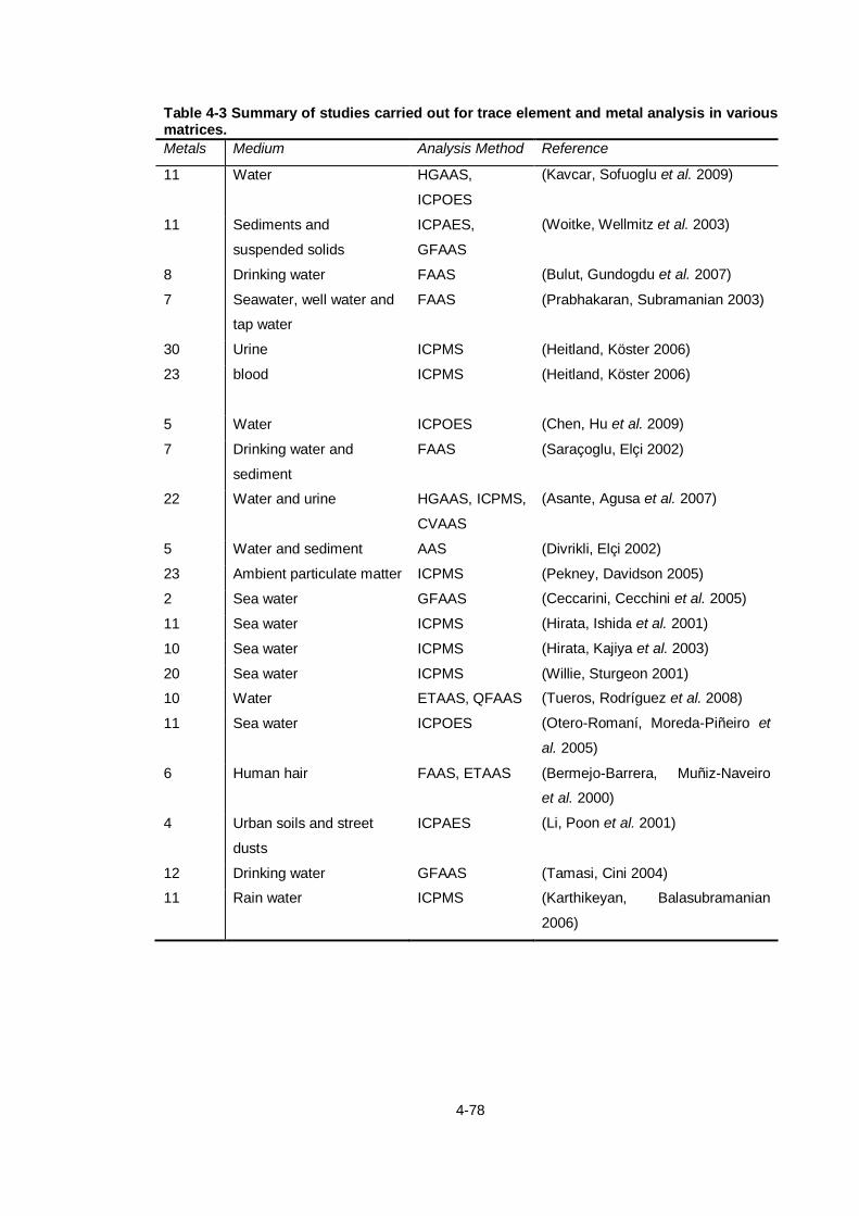
4-78

Table 4-3 Summary of studies carried out for trace element and metal analysis in various matrices.

Metals Medium Analysis Method Reference

11 Water HGAAS,

ICPOES

(Kavcar, Sofuoglu et al. 2009)

11 Sediments and

suspended solids

ICPAES,

GFAAS

(Woitke, Wellmitz et al. 2003)

8 Drinking water FAAS (Bulut, Gundogdu et al. 2007)

7 Seawater, well water and

tap water

FAAS (Prabhakaran, Subramanian 2003)

30 Urine ICPMS (Heitland, Köster 2006)

23 blood

ICPMS (Heitland, Köster 2006)

5 Water ICPOES (Chen, Hu et al. 2009)

7 Drinking water and

sediment

FAAS (Saraçoglu, Elçi 2002)

22 Water and urine HGAAS, ICPMS,

CVAAS

(Asante, Agusa et al. 2007)

5 Water and sediment AAS (Divrikli, Elçi 2002)

23 Ambient particulate matter ICPMS (Pekney, Davidson 2005)

2 Sea water GFAAS (Ceccarini, Cecchini et al. 2005)

11 Sea water ICPMS (Hirata, Ishida et al. 2001)

10 Sea water ICPMS (Hirata, Kajiya et al. 2003)

20 Sea water ICPMS (Willie, Sturgeon 2001)

10 Water ETAAS, QFAAS (Tueros, Rodríguez et al. 2008)

11 Sea water ICPOES (Otero-Romaní, Moreda-Piñeiro et

al. 2005)

6 Human hair FAAS, ETAAS (Bermejo-Barrera, Muñiz-Naveiro

et al. 2000)

4 Urban soils and street

dusts

ICPAES (Li, Poon et al. 2001)

12 Drinking water GFAAS (Tamasi, Cini 2004)

11 Rain water ICPMS (Karthikeyan, Balasubramanian

2006)

4-79

4.1.5 METHOD DEVELOPMENT

Method development is undertaken after the project has been specified and the medium

selected. Figure 4-1 below illustrates the steps involved in the method development process.

The first 3 steps involve the method development with the following steps outlining the stages of

method validation. It is important that methods used are robust, precise, reaching low limits of

detection and quantitation and have a good linear range.

Figure 4-1 Schematic of the steps involved in method development.

The method development steps outlined above where applied to the development of methods

for the analysis of all priority pesticides, PAHS and metals and trace elements listed in the

WFD. The VOCs were omitted from the process due to their volatile nature and inefficient

sample storage procedures. A fully developed method for the analysis of PAHs from wastewater

was taken further through the stages of method validation and all PAH sample analysis was

carried out in Dublin. The metals samples were sent away for analysis after sample preparation

procedures were carried out, as were the pesticide samples.

Define Performance Specification

Devise and develop experiments

Execute and evaluate results

Plan method validation experiments

Calibration, range and linearity

Precision and accuracy Robustness

Collate results

Apply validated method to real samples

4-80


The aim of this section is to develop methods for the analysis of WFD priority substances in

water. These are multiresidue methods that allow for the low levels of detection required by the

EQS directive.


- Review some the literature in relation to the analysis of priority PAHs, pesticides and

metals and trace elements.

- Describe the steps taken in the development of analytical methods.

- Improve on current methods of PAH analysis by reducing run-times.

- Detail method validation procedures followed.

4-81

4.3 PAH Method Development

4.3.1 HPLC METHOD

HPLC with ultraviolet (UV) and fluorescence detection (FLD) are the most common LC methods

for the analysis of the 8 WFD priority PAHs listed in Table 1-5. From the literature it was found

that most studies had found success with either methanol (MeOH) or acetonitrile (ACN) based

mobile phases as the PAHs are nonpolar and hydrophobic the columns found to be most

suitable were chemically bonded silica’s, C18. This echoes the results of the SPE method

development as the same basic principle is applied. All analysis was carried out on an Agilent

1100 HPLC with UV and FLD detection, and the column was a Supelco Supelcosil LC-18 HPLC

column (25 cm x 4.6 mm, 5 µm) (Sigma-Aldrich, Ireland). This method was designed as a

simple means of validating the SPE method during its development stages.

The first step involved the analysis of PAH standards by both UV and fluorescence in order to

determine optimum wavelengths for detector settings. The UV detector chosen could be set to 4

wavelengths simultaneously, therefore 200 nm, 220 nm, 253 nm, and 300 nm were selected, as

they would provide the best detection of the analytes. Table 4-4 lists the optimum detector

settings for the detection of the 8 priority PAHs.

Table 4-4 Optimum wavelengths for both UV and fluorescence detection of PAHs

Optimum Wavelengths

UV wavelength (nm) Fluorescence Wavelengths (nm)

Naphthalene 220 Em. 330 Ex. 220

Anthracene 253 Em. 370 Ex. 253

Fluoranthene 220 Em. 420 Ex. 235

Benzo-b-fluoranthene 253 Em. 420 Ex. 235

Benzo-k-fluoranthene 253 Em. 420 Ex. 235

Benzo-a-pyrene 253 Em. 420 Ex. 235

Benzo-ghi-perylene 253 Em. 420 Ex. 235

Indeno-1,2,3cd-pyrene 253 Em. 420 Ex. 235

In order to validate these wavelengths a simple analysis of 10 ppm standards of each of the

PAHs run using a mobile phase composed of 95 % MeOH and 5 % dionised water was carried

out. Figure 4-2 shows a 10 ppm naphthalene standard run using the method outlined at 220 nm.

A clear peak can be seen with no tailing effects.

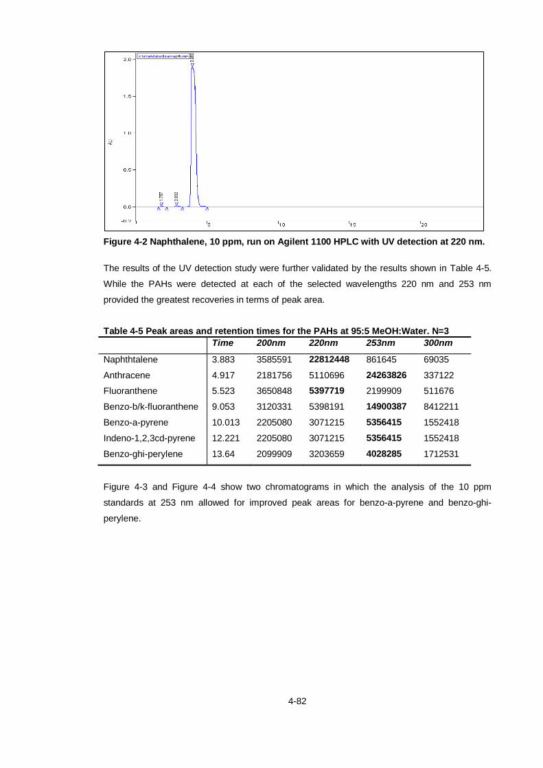
4-82

Figure 4-2 Naphthalene, 10 ppm, run on Agilent 1100 HPLC with UV detection at 220 nm.

The results of the UV detection study were further validated by the results shown in Table 4-5.

While the PAHs were detected at each of the selected wavelengths 220 nm and 253 nm

provided the greatest recoveries in terms of peak area.

Table 4-5 Peak areas and retention times for the PAHs at 95:5 MeOH:Water. N=3

Time 200nm 220nm 253nm 300nm

Naphthtalene 3.883 3585591 22812448 861645 69035

Anthracene 4.917 2181756 5110696 24263826 337122

Fluoranthene 5.523 3650848 5397719 2199909 511676

Benzo-b/k-fluoranthene 9.053 3120331 5398191 14900387 8412211

Benzo-a-pyrene 10.013 2205080 3071215 5356415 1552418

Indeno-1,2,3cd-pyrene 12.221 2205080 3071215 5356415 1552418

Benzo-ghi-perylene 13.64 2099909 3203659 4028285 1712531

Figure 4-3 and Figure 4-4 show two chromatograms in which the analysis of the 10 ppm

standards at 253 nm allowed for improved peak areas for benzo-a-pyrene and benzo-ghi-

perylene.

4-83

Figure 4-3 Benzo-a-pyrene, 10 ppm, run on Agilent 1100 HPLC with UV detection at 220 nm (blue) and 253 nm (red)

Figure 4-4 Benzo-ghi-perylene, 10 ppm, run on Agilent 1100 HPLC with UV detection at 220 nm (blue) and 253 nm (red).

After wavelength optimization the mobile phase composition was evaluated. From the literature

combinations of ACN:water and MeOH:water were most common and were found to achieve

good resolution and recoveries of PAHs. Therefore combinations and ratios of 95:5, 80:20,

75:25, and 50:50 each of ACN:Water and MeOH:Water were investigated. The 95:5

MeOH:Water proved to have the best resolution of samples. A simple method with 5 μL

injection volume, a 1 mL min-1

flow rate and overall 15 minute runtime was therefore used for

the validation of the PAH SPE method using the detection and mobile phase parameters

described above.

4-84

4.3.2 GCMS METHOD

For the method development by GCMS for PAHs in wastewater the first step was to run all

PAHs on the instrument using a basic single-step heating regime to determine relative retention

times and to allow the collection of mass spectra of each of the compounds. The main ions of

these mass spectra are listed in Table 4-6. 100 ppm solutions of each of the 8 priority PAHs

(Sigma-Aldrich) were prepared in methanol and 1 L aliquots were injected onto a Hewlett

Packard (HP 6890 Series GC) equipped with a DB5-MS (5% Poly (dimethylsiloxy) poly (1,4-bis

(dimethylsiloxy) phenylen) siloxane, 0.25 mm x 25 m x 0.25 µm) ultra-inert column (Agilent,

Ireland). An ultra-inert column was chosen due to issues with column bleed at the high

temperatures required to elute the higher molecular weight PAHs.

Table 4-6 List of priority PAHs with their molecular weights and mass spectrum ions. Main ions are marked in bold.

PAH Molecular weight (g) Main Ions

Naphthalene 128.17 128, 102, 98, 87, 64, 51

Anthracene 178.23 178, 152, 139,126,89,76,63

Fluoranthene 202.25 202, 174, 150, 101, 88, 75

Benzo-b-fluoranthene 252.31 281, 252, 224, 207, 126, 113, 100, 73

Benzo-k-fluoranthene 252.31 281, 252, 224, 207, 126, 113, 100

Benzo-a-pyrene 252.31 281, 252, 224, 207, 126, 113, 100, 73

Benzo-ghi-perylene 276.33 355, 276, 253, 207, 138, 124, 111, 96

Indeno-1,2,3cd-pyrene 276.33 276, 248, 207, 138, 112, 73

Figure 4-5 and Figure 4-6 are two examples of mass spectra obtained using the method

described above.

4-85

Figure 4-5 Mass Spectrum of Naphthalene obtained using method described in Section 4.2.3

Figure 4-6 Mass Spectrum of Benzo-g,h,i-perylene obtained using method described in Section 4.2.3

After the mass spectra and relative retention times were obtained for each of the 8 priority PAHs

various methods were evaluated, a selection of which are presented in

Table 4-7.

4-86

Table 4-7 Selection of some of the methods evaluated for the determination of PAHs in wastewater and method parameters. Not all methods are included as there were only small differences between some methods. TIC = total ion chromatogram.

GC Methods

Method No. Inlet temp. (°C) Injection Mode He Flow Initial

Temp (°C) Temp gradient (°C) MS mode Run time (min)

(mL min-1

)

# Rate Final temp. Final time

1 180 Splitless 1 80

1 40.00 143 0.00

TIC 38.98

2 10.00 150 2.00

3 10.00 170 0.00

4 30.00 230 2.00

5 1.00 250 2.00

6 50.00 310 5.00

4 180 Splitless 1 60 1 60.00 220 15.00

TIC 33.67 2 20.00 300 10.00

6 180 Splitless 1 60 1 60.00 280 5.00

TIC 18 2 60.00 300 7.00

9 260 Splitless 1.3 55 1 25.00 310 10.0 TIC 21.2

11 260 Splitless 1.3 55

1 25.00 290 0.50

TIC 18.83 2 20.00 260 2.00

3 35.00 310 3.00

14 260 Splitless 1.3 55 1 25.00 290 0.50

TIC 20.74 2 50.00 230 2.50

4-87

3 70.00 310 5.00

16 260 Splitless 1.3 55

1 40.00 290 0.50

TIC 16.02 2 60.00 230 2.50

3 70.00 310 1.00

4 10.00 320 2.00

22 300 splitless 1.3 55 1 25.00 320 5.00 TIC 16.6

25 300 splitless 1.3 55

1 35.00 280 1.00

TIC 19.05 2 25.00 220 1.00

3 45.00 320 5.00

26 300 splitless 1.3 55

1 35.00 300 1.00

TIC 20.76 2 35.00 200 1.50

3 50.00 320 4.00

27 300 splitless 1.3 55

1 35.00 280 1.00

TIC 17.5 2 25.00 220 0.00

3 60.00 320 5.00

29 300 splitless 1.3 55

1 35.00 260 0.00

TIC 13.69 2 60.00 220 0.50

3 60.00 320 4.00

34 300 splitless 1.3 55

1 25.00 260 1.00

TIC 18.12 2 60.00 190 0.50

3 60.00 325 4.00

4-88

For each of the methods listed in

Table 4-7 the resolutions of the separate PAHs were evaluated. Table 4-8 shows the results of

resolution studies for all PAHs for the selection of methods outlined in

Table 4-7. A value of 1.5 indicates perfect peak resolution, a value below this signifies poor

resolution while a value above indicates increasing resolution between peaks. Much difficulty

was encountered in peak separation, specifically poor resolution between benzo-b-fluoranthene

and benzo-k-fluoranthene which often co-eluted. Through contact with the Irish EPA it was

made clear that complete resolution of these peaks is not necessary as the EQS value that

applies is a SUM value of both peaks and not the individual peaks.

Table 4-8 Table of resolutions achieved using the methods outlined in Table 4-7 for each PAH. Nap - naphthalene, Ant - anthracene, Flr -fluoranthene, BbF and BkF - benzo-b- and benzo-k-fluoranthene, Bap – benzo-a-pyrene, Indeno – indeno-1,2,3cd-pyrene, Bghi – Benzo-ghi-perylene. N=3

Method 1 4 6 9 11 14 16 22 25 26 27 29 34

Nap. 81.3 33.2 30.4 53.5 34.1 45.1 42.2 63.5 0.0 41.2 44.3 40.0 55.4

Ant. 28.6 22.0 15.6 14.1 18.8 18.8 19.2 21.3 17.9 16.7 16.5 23.9 18.4

Flr. 94.8 70.7 55.1 36.9 44.0 93.8 94.3 47.8 122.5 23.0 94.5 39.7 89.3

Bbf. 1.3 0.9 0.7 0.6 0.6 0.7 0.8 0.6 0.9 1.0 0.8 0.8 0.8

Bkf. 12.4 7.6 7.5 5.8 6.3 5.0 6.6 6.2 6.0 5.7 20.0 6.3 5.3

Bap. 12.4 25.9 19.8 15.4 20.9 18.6 21.9 22.2 23.4 18.5 21.3 17.7 14.9

Bghi. 0.0 4.9 5.5 3.7 5.3 4.3 4.7 5.4 5.5 5.3 4.6 4.3 4.5

Indeno 0.0 4.9 5.5 3.7 5.3 4.3 4.7 5.4 5.5 5.3 4.6 4.3 4.5

The same methods were evaluated for peak area and the results are shown in Table 4-9. This

table shows the enhanced peak areas of the PAHs in some methods over others, a factor which

is very important due to the trace nature of the samples.

4-89

Table 4-9 Table of peak areas achieved using the methods outlined in Table 4-7 for each of the 8 PAHs. Nap - naphthalene, Ant - anthracene, Flr -fluoranthene, BbF and BkF - benzo-b- and benzo-k-fluoranthene, Bap – benzo-a-pyrene, Indeno – indeno-1,2,3cd-pyrene, Bghi – Benzo-ghi-perylene. N=3

PEAK AREA

Method Nap. Ant. Flr Bbf Bkf Bap Bghi Indeno

1 1.9E+06 2.1E+06 2.1E+06 6.8E+05 6.3E+05 3.8E+05 0.0E+00 0.0E+00

4 1.5E+06 1.5E+06 1.5E+06 6.2E+05 6.2E+05 4.3E+05 3.4E+05 2.3E+05

6 1.3E+06 1.5E+06 1.6E+06 6.3E+05 6.7E+05 4.2E+05 4.9E+05 1.5E+05

9 3.8E+07 7.4E+07 8.3E+07 3.1E+07 2.9E+07 2.1E+07 1.2E+07 6.0E+06

11 3.6E+07 3.6E+07 4.0E+07 5.1E+06 4.4E+06 2.4E+06 1.1E+06 6.6E+05

14 3.0E+07 4.1E+07 4.8E+07 8.9E+06 9.0E+06 5.1E+06 2.3E+06 1.1E+06

16 3.1E+07 4.0E+07 4.7E+07 9.8E+06 1.0E+07 5.7E+06 2.4E+06 1.2E+06

22 3.1E+07 2.9E+07 3.2E+07 1.4E+07 1.2E+07 7.7E+06 5.5E+06 2.5E+06

25 0.0E+00 4.3E+07 4.9E+07 1.6E+07 1.6E+07 1.0E+07 5.5E+06 3.2E+06

26 3.5E+07 3.9E+07 4.4E+07 1.4E+07 1.3E+07 1.0E+07 7.4E+06 3.7E+06

27 4.2E+07 4.5E+06 5.4E+07 2.2E+07 2.1E+07 1.5E+07 1.1E+07 5.0E+06

29 2.8E+07 2.3E+07 2.5E+07 1.7E+07 1.4E+07 1.0E+07 7.2E+06 3.4E+06

34 3.3E+07 3.2E+07 3.7E+07 1.8E+07 1.6E+07 1.4E+07 1.0E+07 4.6E+06

Through the studies outlined above and the compilation of data it was possible to examine the

results and determine a method which provided the optimum runtime, peak resolution and peak

area while also improving on current available methods. After evaluating many methods for the

separation of PAHs in wastewater a method with an initial temperature of 55°C, a ramp rate of

25°C min-1

to 310°C with an overall runtime of 15.40 minutes was chosen, Figure 4-7.

Calibration and robustness testing of this method was the next step after method development

and marked the beginning of method validation. 12-point calibration curves for each PAH has

been tabulated in Table 4-10 where good linearity and robustness was observed for each of the

PAH compounds tested in the project.

Table 4-10 Calibration data and equation of the line for final PAH method for GCMS used in this study.

PAH R2 Equation of the line

Naphthalene 0.99 Y=2,510,867.35 x

Anthracene 0.99 Y=2,581,790.81 x

Fluoranthene 0.99 y = 4,284,396.60 x

Benzo-b/k-fluoranthene 0.99 y = 6,799,501.45 x

Benzo-a-pyrene 0.99 y = 2,431,801.40 x

Indeno-1,2,3cd-pyrene 0.99 Y = 1,609,433.81 x

Benzo-ghi-perylene 0.99 Y = 2,075,531.72 x

4-90

The final overview of the limits of detection (LODs) achieved for each of the PAHs is listed in

Table 4-11.This table represents the limits of detection achieved using the GCMS method

alone, the pre-concentration factor offered by the SPE method allows for monitoring

requirements of the priority PAHs to be met. The LOQ was taken to be twice the LOD for each

compound.

Table 4-11 Overview of limits of detection achieved for each PAH using the final method.

PAH Method

LOD

(ppm)

LOD

(g L-1

)

Naphthalene 0.0001 0.1

Anthracene 0.0005 0.5

Fluoranthene 0.0001 0.1

Benzo-b/k-fluoranthene 0.0001 0.1

Benzo-a-pyrene 0.0005 0.5

Indeno-1,2,3cd-pyrene 0.0005 0.5

Benzo-ghi-perylene 0.0005 0.5

In order to validate the repeatability of the method an injection volume study was carried out to

determine the optimum injection volume of sample which would allow lower LODs without

diminishing overall method performance.

Table 4-12 Results of injection volume study showing peak areas of each PAH against injection volume. Optimum values are marked in bold. Naph - naphthalene, Ant - anthracene, Flr -fluoranthene, BbF and BkF - benzo-b- and benzo-k-fluoranthene, Bap – benzo-a-pyrene, Ind – indeno-1,2,3cd-pyrene, Bghi – Benzo-ghi-perylene. N=3

Injection

Volume (µL)

PEAK AREA

Naph. Ant. Flr. Bbf and BkF Bap. Bghi. Ind.

1 18460 7586 17022 18988 7970 7355 7292

2 25226 11084 31725 23289 9996 9554 10643

4 45067 18452 73574 49449 19329 13816 18705

5 77424 72729 218271 284882 108526 102868 80613

From Table 4-12 it can see that peak areas increased as injection volume increased yet there is

a point where tailing and peak splitting can begin interfering with resolution and general method

performance. In this study this point was reached at an injection volume of 8 µL. Therefore, after

completing this study 5 µL was chosen as the optimum injection volume for this method.

A repeatability study was carried out on this method whereby a series of injections of the same

concentration mixture, in this case 0.01 ppm, were carried out concurrently and peak areas

4-91

were recorded. All percentage relative standard deviation shown in Table 4-13 are below 5%

which is an acceptable precision margin for a method.

Table 4-13 Repeatability study showing the results of repeated injections of a 0.01 ppm PAH mixture. Naph - naphthalene, Ant - anthracene, Flr -fluoranthene, BbF and BkF - benzo-b- and benzo-k-fluoranthene, Bap – benzo-a-pyrene, Indeno – indeno-1,2,3cd-pyrene, Bghi – Benzo-ghi-perylene. Ave. – average. StdDev – standard deviation. RSD – relative standard deviation. N=3

Peak Area

Naph. Ant. Flr. Bap Bbf and BkF

Indeno Bghi

0.01ppm a 49694 26543 119716 79963 29615 23468 38426

0.01ppm b 52052 29036 118748 80761 33056 26057 42458

0.01ppm c 47383 27485 126777 78641 29944 25774 39728

0.01ppm d 50128 30327 124088 89060 32343 26150 42918

0.01ppm e 50677 28096 111634 84653 31701 25895 42530

Ave. 49986.8 28297.4 120192.6 82615.6 31331.8 25468.8 41212

StdDev 1704.9 1452.9 5789.9 4241.3 1500.4 1127.8 2010.2

RSD(%) 3.4 5.1 4.8 5.1 4.8 4.4 4.9

4-92

4.3.3 FINAL PAH GCMS METHOD

The final validated PAH method by GCMS is described below and is represented by the

chromatogram in Figure 4-7. This method allows for PAH levels below the set EQS values to be

quantified in one simple and fast method. Through the use of SIM mode it was possible to

detect PAH concentrations in complex wastewater samples after sample preparation.

Figure 4-7 Chromatogram showing separation of 8 priority PAHs by final PAH method chosen for PAH analysis. A – Naphthalene, B – Anthracene, C – Fluoranthene, D + E – Benzo-b/k-fluoranthene, F – Benzo-a-pyrene, G – Indeno-1,2,3cd-pyrene, H – Benzo-ghi-perylene. Initial Temp: 55˚C. Initial Time: 1.00 min. Rate: 25.00˚C/min. Final Temp: 310˚C. Final Time: 4.20 min. Post time: 1.00 min. Run time: 15.40 min. Injection Volume: 5 µL. SIM Mode.

A Hewlett Packard (HP 6890 Series GC) equipped with a DB5-MS (5% Poly (dimethylsiloxy)

poly (1,4-bis (dimethylsiloxy) phenylen) siloxane, 0.25 mm x 25 m x 0.25 µm) Ultra-Inert

capillary column (Agilent, Ireland) was used for analysis. The GC was connected to a mass

selective detector (MSD) (HP 5973 Series) operated in selected ion mode. Injection of 5 µL

sample was performed using the instrument autosampler. The carrier gas was helium. The oven

temperature program for the GC required injection at 55˚C (held for 1 min), increased at a rate

of 25˚C min-1

until the final temperature of 310˚C was reached (held for 4.20 min) giving an

overall runtime of 15.40 min. All samples were analysed in triplicate with procedural blanks

routinely analysed. The limits of quantification were determined as 10 times the noise level of

the chromatogram of a blank sample. A calibration range of 0.00001 – 1 ppm was achieved with

the mean correlation coefficients of the calibration curves greater than 0.99 for all compounds

indicating high linearity for this concentration range. Sample components were identified by

comparison of retention times and mass spectra with those of the standard mixture.

0

100000

200000

300000

400000

500000

600000

700000

800000

900000

1000000

Abundance

Time (min) 15

A

H G

F

D + E

C B

4-93

4.4 Pesticide Method Development

A simple method for the determination of priority pesticides was developed with the aim of

validating SPE studies for the extraction of these pesticides from a wastewater matrix. The 33

priority pesticides listed in the WFD, Section 1.2.1 and Table 4-15, were included in the method

development although the literature suggested that several would not be amenable to GC

analysis owing to their physical and chemical characteristics. These pesticides included

glyphosate and the six priority dithiocarbamate pesticides listed in Table 4-14.

Table 4-14 Pesticides that are not suitable for direct GCMS analysis and citations from the literature.

Pesticide Outcome of study Reference

Glyphosate Lists glyphosate as one of 134 pesticides found to

have no GC–MS peaks or for which sensitivity was

extremely low and did not meet requirements.

(Pang, Cao et al. 2006)

State that derivitisation is required prior to GCMS

analysis of glyphosate.

(Börjesson,

Torstensson 2000)

(Torres, Picó et al. 1996)

Isoproturon Isoproturon not thermally stable for direct GCMS

analysis.

(Camino-Sánchez,

Zafra-Gómez et al.

2011)

Describes the best method for isoproturon analysis to

be LC-MS/MS

(Pang, Cao et al.

2006)

Mancozeb This paper lists mancozeb as one of the pesticides not

compatible with GCMS

(Pang, Cao et al.

2006)

Suggest special pre-treatment required prior to GCMS

analysis.

(Armenta, Garrigues et al. 2005)

Maneb This paper lists maneb as one of the pesticides not


(Pang, Cao et al.

2006)

Mecoprop This paper details a preferred LCMS method for the

analysis of mecoprop.

(Klein, Alder 2003)

Thiram This paper lists thiram as one of the pesticides with

poor stability (Pang, Cao et al.

2006) Zineb This paper lists zineb as one of the pesticides not


Note: The dithiocarbamates have limited solubility in most organic solvents making them

difficult to analyse directly.

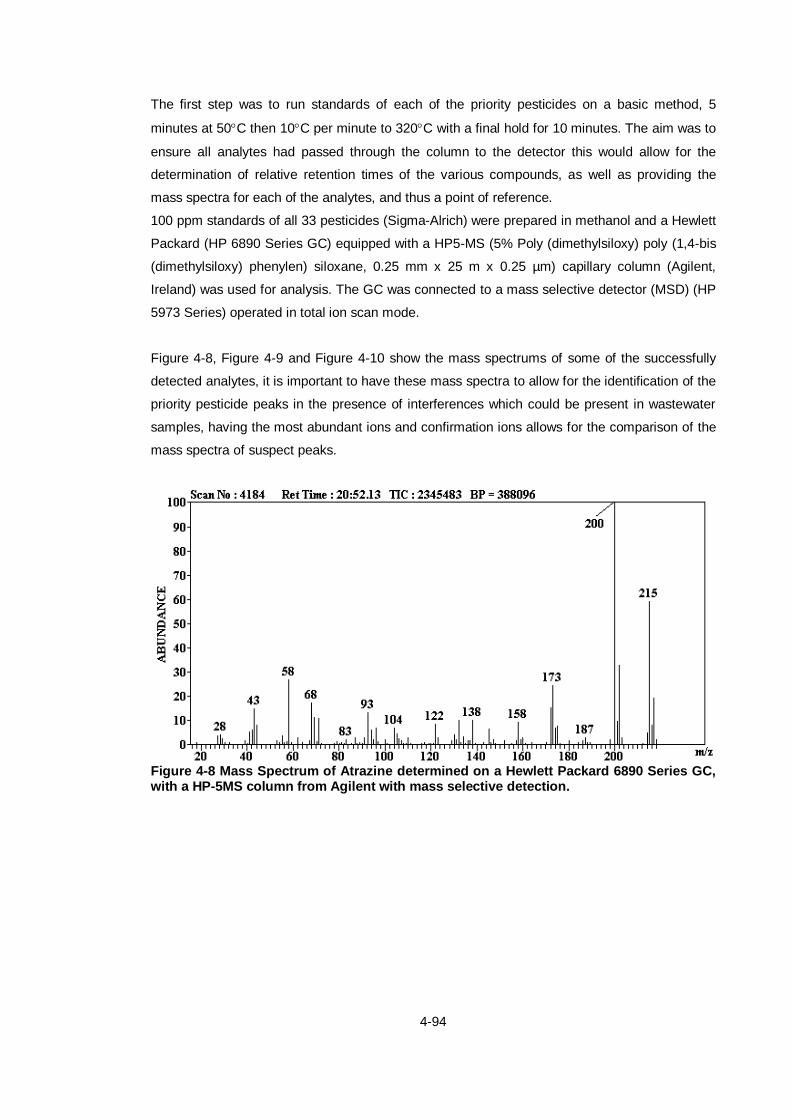
4-94

The first step was to run standards of each of the priority pesticides on a basic method, 5

minutes at 50C then 10C per minute to 320C with a final hold for 10 minutes. The aim was to

ensure all analytes had passed through the column to the detector this would allow for the

determination of relative retention times of the various compounds, as well as providing the

mass spectra for each of the analytes, and thus a point of reference.

100 ppm standards of all 33 pesticides (Sigma-Alrich) were prepared in methanol and a Hewlett

Packard (HP 6890 Series GC) equipped with a HP5-MS (5% Poly (dimethylsiloxy) poly (1,4-bis

(dimethylsiloxy) phenylen) siloxane, 0.25 mm x 25 m x 0.25 µm) capillary column (Agilent,

Ireland) was used for analysis. The GC was connected to a mass selective detector (MSD) (HP

5973 Series) operated in total ion scan mode.

Figure 4-8, Figure 4-9 and Figure 4-10 show the mass spectrums of some of the successfully

detected analytes, it is important to have these mass spectra to allow for the identification of the

priority pesticide peaks in the presence of interferences which could be present in wastewater

samples, having the most abundant ions and confirmation ions allows for the comparison of the

mass spectra of suspect peaks.

Figure 4-8 Mass Spectrum of Atrazine determined on a Hewlett Packard 6890 Series GC, with a HP-5MS column from Agilent with mass selective detection.

4-95

Figure 4-9 Mass Spectrum of Chlorfenvinphos determined on a Hewlett Packard 6890 Series GC, with a HP-5MS column from Agilent with mass selective detection.

Figure 4-10 Mass Spectrum of Dieldrin determined on a Hewlett Packard 6890 Series GC, with a HP-5MS column from Agilent with mass selective detection.

A summary of the successfully detected pesticides with their respective retention times and

main ions is presented in Table 4-15 below this does not include the pesticides highlighted in

Table 4-14 as they were not detected using the GCMS. The chromatogram that represents the

retention times and ions in Table 4-15 is shown in Figure 4-11.

4-96

Table 4-15 Summary of results of pesticide standards run using method Trial 5 150111.M showing each of the successfully separated pesticides, their retention times and main ions present in the mass spectrums.*Pesticides not included on this list: Glyphosate, Isoproturon, Mancozeb, Maneb, Mecoprop, Nonylphenol, Thiram and Zineb. *Most abundant ions are highlighted in bold.

Pesticide MW

(g)

Rt

(min)

Main Ions

Alachlor 269.77 24.24 269,237,224,188,160,146,132,117,91,77,45

Aldrin 364.91 25.62 364,329,293,263,250,220,186,101,91,79,66

Atrazine 215.68 20.869 215,200,173,158,138,92,68,58

Chlorfenvinphos 359.57 28.23

27.66

360,323,295,267,206,195,173,109,81,28

323,295,267,204,195,170,123,109,81,28

Chlorpyrifos 350.59 26.166 349,314,286,258,208,197,125,109,97

DDT 354.49 33.77 354,246,235,212,199,176,165,136,75

DEHP 390.54 35.319 390,279,167,149,113,71,57

Dieldrin 380.91 30.913 380,345,277,263,237,209,193,173,108,79

Diuron 233.09 28.08 232,187,159,124,72,44,28

Endosulfan 406.93 29.406 371,358,339,325,307,277,265,241,229,195,170,159,

85,69,31

Endrin 380.91 31.979 380,345,317,281,263,245,219,209,173,147,81,67

Epichlorohydrin 92.53 3.478 89,62,57,51,49,42,32,31,28,26

Fenitrothion 277.2 25.15 277,260,214,125,109,93,79,63,47

Hexachlorobenzene 284.8 20.191 284,249,214,177,142,107,71

Hexachlorobutadiene 260.76 12.425 260,225,190,153,141,118,83

Isodrin 364.91 26.996 364,329,293,263,193,147,111,91,66

Lindane 290.83 21.136 290,254,219,181,145,109,85,75,51

Malathion 330.36 25.728 285,256,211,173,158,143,125,101,93,79,63

Pentachlorobenzene 250.34 17.02 250,215,178,143,125,108,73

Pirimiphos Methyl 305.3 25.338 305,290,276,262,233,180,163,125,109,93

Simazine 201.66 20.66 201,186,173,158,145,138,132,123,96,85,68,55,44

TBT 291.06 18.819 291,269,213,177,155,121,57,41

Trichlorobenzene 181.45 11.76 180,145,109,74

Trichloroethylene 131.39 3.11 134,130,99,95,60,47,28

Trifluralin 335.28 19.504 335,306,290,264,248,43

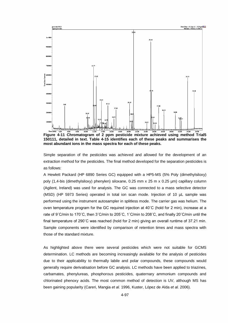
4-97

Figure 4-11 Chromatogram of 2 ppm pesticide mixture achieved using method Trial5 150111, detailed in text. Table 4-15 identifies each of these peaks and summarises the most abundant ions in the mass spectra for each of these peaks.

Simple separation of the pesticides was achieved and allowed for the development of an

extraction method for the pesticides. The final method developed for the separation pesticides is

as follows:

A Hewlett Packard (HP 6890 Series GC) equipped with a HP5-MS (5% Poly (dimethylsiloxy)

poly (1,4-bis (dimethylsiloxy) phenylen) siloxane, 0.25 mm x 25 m x 0.25 µm) capillary column

(Agilent, Ireland) was used for analysis. The GC was connected to a mass selective detector

(MSD) (HP 5973 Series) operated in total ion scan mode. Injection of 10 µL sample was

performed using the instrument autosampler in splitless mode. The carrier gas was helium. The

oven temperature program for the GC required injection at 40˚C (hold for 2 min), increase at a

rate of 9˚C/min to 170˚C, then 3˚C/min to 205˚C, 1˚C/min to 208˚C, and finally 20˚C/min until the

final temperature of 290˚C was reached (hold for 2 min) giving an overall runtime of 37.21 min.

Sample components were identified by comparison of retention times and mass spectra with

those of the standard mixture.

As highlighted above there were several pesticides which were not suitable for GCMS

determination. LC methods are becoming increasingly available for the analysis of pesticides

due to their applicability to thermally labile and polar compounds, these compounds would

generally require derivatisation before GC analysis. LC methods have been applied to triazines,

carbamates, phenylureas, phosphorous pesticides, quaternary ammonium compounds and

chlorinated phenoxy acids. The most common method of detection is UV, although MS has

been gaining popularity (Careri, Mangia et al. 1996, Kuster, López de Alda et al. 2006).

4-98

LC-MS has facilitated the analysis of ‘difficult’ pesticides in an efficient and selective manner;

these pesticides include quaternary ammonium compounds diquat and paraquat and the

phosphonic acid glyphosate and its major metabolite aminomethylphosphonic acid (AMPA)

(Hogendoorn, van Zoonen 2000). As such the project collaborators developed an LC-MS/MS

method for the analysis of the priority pesticides.

4-99

4.5 Metals and Trace Elements Method Development

4.5.1 ICP-AES

For the analysis of the priority metals and trace elements, Table 1-6, it was necessary to order a

custom reference standard. Elementec supplied an AccuTrace Custom Reference Standard

containing 1 g ml-1 of each of the 15 elements listed in Table 4-16. From this stock solution a

calibration curve was prepared. Analysis was carried out on a Liberty 220 ICP Emission

Spectrometer from Varian.

Prior to sample introduction there were a number of calibration steps that were be carried out

with this instrument. The optimum plasma viewing height, wavelength of analysis, and general

wavelength calibration of the instrument were set each day of analysis. As a starting point all

wavelengths were chosen according to those recommended by EPA Method 200.7. Multiple

wavelengths were available for each element with optimum wavelengths giving the higher

intensity readings and therefore making it possible to achieve lower limits of detection for these

elements.

Table 4-16 Priority metals and trace elements and their optimised conditions for analysis by ICPAES. * Denotes extra wavelength added by user, all solutions were 1 ppm stock.

Metal/Trace

Element

Symbol Optimised

Wavelength (nm)

Intensity at optimum

wavelength

Optimised

Viewing height

(mm)

Lead Pb 220.353 2305 4

Nickel Ni 231.604 1094 5

Arsenic As 193.696 465 4

Antimony Sb 206.833 593 4

Molybdenum* Mo 281.615 1702 4

Molybdenum Mo 203.844 1285 4

Chromium Cr 205.552 1411 4

Zinc Zn 213.856 4796 5

Copper Cu 324.754 2134 4

Tin Sn 189.926 948 5

Barium Ba 493.409 13406 4

Boron B 249.678 2779 4

Vanadium* V 309.311 1411 4

Vanadium V 292.402 538 4

Cadmium Cd 226.502 1146 5

Selenium Se 196.026 2591 5

Cobalt Co 228.616 1194 4

4-100

To begin all possible wavelengths were evaluated and generally the EPA recommended

wavelengths yielded superior results. However in the cases of molybdenum and vanadium a

secondary wavelength provided increased intensity and, as such, was chosen for addition to the

method. Some elements, i.e. arsenic, antimony, and tin, had low intensities at their optimum

wavelengths, making detection of low levels impossible for some concentrations. Table 4-16

lists the priority metals and trace elements with their respective optimum viewing heights and

wavelengths.

Calibration of the method was performed. The formula used to calculate volumes for the

calibration curve was: concentration required (ppm)/ concentration given (ppm in stock), by the

volume required, which was 50 mL. Stock solution was diluted to the mark with deionised water

as per EPA method 200.7 which outlines analysis of wastewater for metals and trace elements

using ICPAES. The lowest point on the calibration curve was selected after taking into account

the established EQS values for the metals and trace elements in question, these EQS values

can be found in S.I. 272 of 2009. As mentioned above, a number of elements were unsuitable

for this low level detection due to their poor wavelength intensity on this instrument.

This initial calibration was failed by the instrument as many of the lower concentrations were not

detected for some of the elements; this instrument is programmed to reject calibration where

standards do not increase, or the difference between standards is over 15%. The next step was

then to prepare some higher calibration standards, and so standards of 1, 0.5, and 0.1ppm were

added to the calibration.

The analysis of the metals and trace elements proved challenging due to the limitations of

current methods with only one available technique was suitable to meet the analytical

requirements for metals and trace elements outlined in the WFD, ICP-MS. ICPAES had been

evaluated for the analysis and was found not to achieve the limits of quantitation required,

therefore it was necessary to send samples to the accredited Centre for Microscopy and

Analysis lab for analysis by ICPMS. All samples were analysed for 15 priority metals and trace

elements at the ppb level, results are presented in Chapter 6.

4-101

4.6 Conclusion

This chapter gives an overview of methods commonly applied to the analysis of priority

substances in environmental matrices, citing many of the studies which were reviewed when

beginning the method development work. It was important to review these methods to

understand issues and problems encountered by other research groups so that the same issues

might be avoided.

The need for robust, quantitative methods is highlighted in the WFD. The process of selecting a

suitable analytical method has become much more difficult as there are currently a vast variety

of methods applicable to the analysis of priority substances. It is therefore necessary to define

analytical requirements very early in the stages of project development. Analytical and data

requirements must be defined to certain criteria including run times, ease of use of the method,

sample preparation requirements, precision and accuracy, and limits of detection and

quantitation. Where legislation is the driver for the research it is vital that those standards are

taken into account above all. In the case of the PAHs a number of approved methods were

available and were evaluated with GCMS proving to meet the project remit. By reducing the

runtime and improving resolution of the priority PAHs it was possible to achieve specifications

outlined in the WFD. This PAH method improved on runtime and limits of detection for reported

methods when used following the sample extraction method outlined in chapter 3.

With regard to the pesticide analysis most recent studies detail methods involving LCMS rather

than GCMS, and through this work it was found to be difficult to reach limits of detection near

the levels required and also difficulties were encountered with particular pre-treatment required

by some pesticides. In order to combat issues of incompatibility between pesticides and GCMS

analysis the project partners in Cork developed an LCMS method for the analysis of the

pesticides in wastewater.

5-102

5. Development of a

Risk-based Model

5-103

5.1 Introduction

5.1.1 INTRODUCTION

PSs originate from many sources, and are transferred to surface waters via a number of

pathways. Large installations may emit PSs originating from production processes directly into

surface waters, under licence from the EPA or Local Authorities. Gaseous emissions of PSs

from combustion and industrial sources may be deposited on surrounding land, and washed

into surface waters directly following precipitation (Sanders, Jones et al. 1993). Accidental or

deliberate dumping of waste materials onto land may also lead to runoff of PSs into surface

waters, or indirect contamination of surface waters via leaching into groundwater (Teijon,

Candela et al. 2010).

WWTPs are major potential point sources of priority pollutants that combine direct inputs from

domestic, industrial and commercial effluent with diffuse inputs from surface runoff of land-

deposited PSs. Sampling of PS concentrations in WWTP effluent under different conditions

(e.g. wet and dry weather) may offer insight into the sources of PSs (Gasperi, Garnaud et al.

2008). Furthermore, as major point sources of PS and following implementation of the Urban

Waste Water Treatment Directive, WWTPs offer strong opportunities for the effective control of

PS concentrations in surface waters through the implementation of management and

abatement options. Establishing the concentrations of priority pollutants in WWTP effluent is

important for the protection of public health.

There are a number of challenges that are encountered in the monitoring of these pollutants

including the establishment of standard methods for analysis and sample handling, setting

appropriate EQS values and developing methods which can reach the required LODs and

adapting to include new and emerging compounds as they are added to legislative monitoring

lists. When surveying work already completed and on going in this area two large studies were

identified as good examples of where modelling has facilitated the monitoring of these PSs in

the European arena. The SCOREPP project (Source Control Options for Reducing Emissions of

Priority Pollutants) had already surveyed a number of large European cities for the occurrence

of priority substance and also included a section on removal efficiencies of specific pollutants

from WWTPs that was particularly relevant to this study (Seriki, Gasperi et al. 2008). Also the

Scottish Environmental Protection Agency (SEPA) have developed an efficient monitoring tool

and have reported the detailed the process involved in establishing a model relating emission

factors to the occurrence of priority substances in surface waters (Clarke, Roberts et al. 2009).

5-104

5.1.1 REVIEW OF MODELLING APPROACHES FOR THESE PRIORITY

SUBSTANCES

In order to determine the most suitable approach to adopt when preparing a model for the

monitoring of emission factors for priority and hazardous substances it was first necessary to

evaluate some of the potential routes available. In a study by (Ahlman, Svensson 2005) a

simple GIS-based model is presented, SEWSYS, which uses basic process parameters

(deposition rates, accumulation time, flushing rates during rainfall) to predict storm water PS

concentrations. It focuses on land use including roof area and material type, road area, and

traffic volume. This model attributes most heavy metal and PAH loading to traffic (brake dust,

tyre wear, exhaust and road surface wear).

While this model provided valuable information on the type of data required and steps involved

in establishing a basic working model there were, however, many limitations which would have

to be overcome. The SEWSYS model is based on the MATLAB program, computing software,

while the aim of the current study is to base the model in a simpler program such as Excel. The

purpose of this is to make the model as user-friendly as possible while also not requiring

specialist knowledge in computer programming for use. Compared to the large number of

pollutants required for monitoring by the WFD the study by Ahlman et al. contains only 20

different substances (some organic pollutants, heavy metals and nutrients). As a much larger

pollutant set with more varying physical/chemical characteristics and emission sources is being

looked at in this study the SEWSYS model, while being a good stepping stone, would ultimately

need more work before being suitable for the purposes of this project. Also, while the

hydrological aspects of the SEWSYS model were well validated there were less reliable results

in the quality parts.

(De Keyser, Gevaert et al. 2010) generate a dynamic model capable of simulating the dynamic

release pattern of specific PSs. This model accounts for daily, weekly, and yearly patterns of

release, but is extremely data intensive (geographic and average load data required for every

source within a catchment), and the model was not tested on an actual catchment. Where

sufficient data are available, high-resolution parameter-based models provide an invaluable tool

to predict and understand temporal emission patterns, and to interpret (grab sampling)

monitoring data in the full context of dynamic relationships amongst various PS sources.

However, in Ireland at least, the current state of knowledge and data availability (e.g. emission

data from individual installations) is insufficient to support such models. In the first step towards

greater understanding of PS sources contributing to WWTP emissions, a simple risk-based

model that can be applied across catchments was proposed.

5-105

5.1.2 CASE STUDY: A SCOTTISH PERSPECTIVE

Case Study:

The most influential resource in the establishment of the model for this project was the

SEPA model which is further detailed in this case study.

A Scottish Perspective

SEPA evaluated over 400 priority and emerging substances in the initial stages of their

research. The steps taken in the formation of their chemical prioritisation tool are

detailed in Figure 5-1 below.

Figure 5-1 Shows the prioritisation process developed to risk assess chemicals of potential concern in Scotland. It summarises the risk assessment process in terms of chemical hazard and environmental exposure.

The prioritisation tool was developed in Microsoft Excel using a series of linked

spreadsheets which are both dynamic and interdependent – when one is changed the

others are automatically updated. This method allows for simpler data entry whilst

maintaining a transparent and consistent approach.

Extended universe of chemicals

Compiled from numerous drivers and obligations

Surface water universe of chemicals

Relevant list of candidates for prioritisation

Exposure assessment

Assign exposure score (0-5) based on source, usage

and/or monitoring data

Hazard assessment

Assign hazard score (0-5) based on persistence, bioaccumulation, toxicity and endocrine disruption

criteria

Overall risk score

(0-6)

Outputs

GIS mapping, inform State of Scotland’s Environment report, targeted monitoring, characterisation, designation of specific pollutants

5-106

Throughout the course of this work many documents and reports were reviewed and data

extracted and used to populate the model. This included 155 IPPC licenses, 62 waste discharge

licenses, 9 wastewater discharge applications including environmental impact statements and

historic sampling data for each of the sites, 11 annual environmental reports for the sites with

approved licenses, 872 trade effluent licences and data from 102 rainfall monitoring stations.

The data was compiled and the rainfall stations and WWTPs mapped. As well as these sources

of data, information was extracted from traffic counters, the CSO and the NRA. This data, while

not all presented within this chapter, is stored in a series of excel documents for submission to

the EPA. Chapter 6 continues with the population of the model and overall observations from

the model development and application process.

The data listed above was collected and analysed in full by the candidate. This data served to

populate the model and allow for the relation of emission factors to the occurrence of PSs and,

with the exception of the mathematical modelling, the candidate used this dataset as well as

collected experimental data to complete and validate the final model.

Risk scores (0–6) were calculated for each prioritised chemical as a function of their

hazard and occurrence in Scotland’s environment. Hazard scores were based on an

individual chemical’s environmental persistence and potential to bioaccumulate and

toxicity including endocrine disruption potential. Exposure was assessed for each

chemical in terms of monitoring data, point source emission data and usage information.

There is currently no definitive diffuse pollution element to the source assessment, though

the usage and monitoring assessments are relevant to both diffuse and point source

emissions.

A minimum of one robust source of exposure assessment data and one source of hazard

assessment data was required to complete the assessment. Any substance that did not

meet the minimum data requirements for either the exposure or hazard assessments was

assigned a risk score of zero, indicating insufficient information.

(Clarke, Roberts et al. 2009)

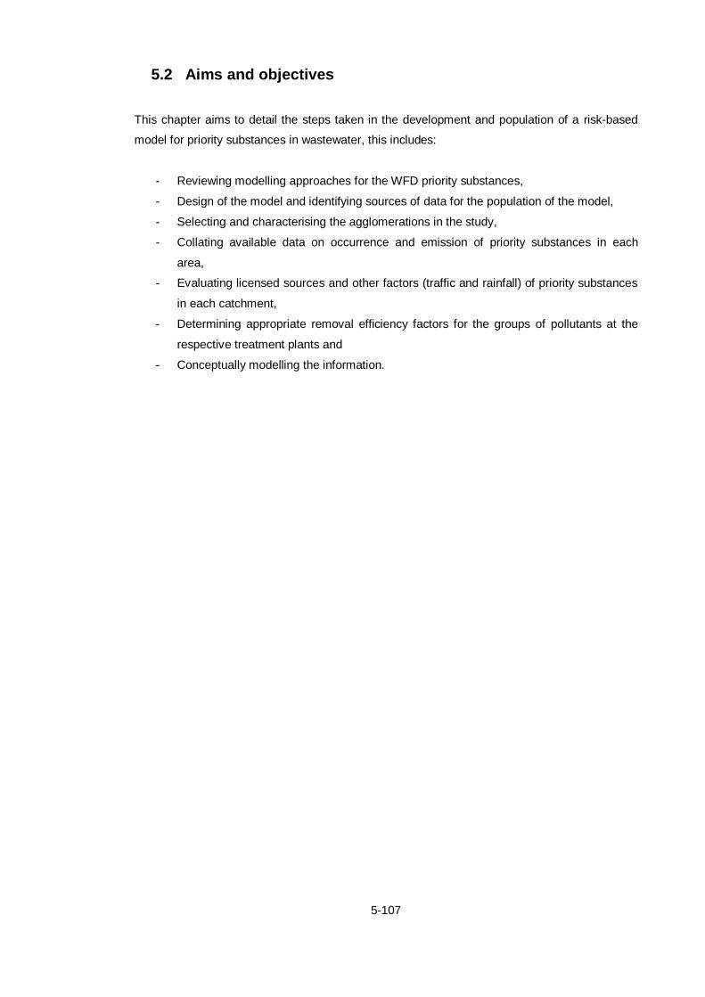
5-107

5.2 Aims and objectives

This chapter aims to detail the steps taken in the development and population of a risk-based

model for priority substances in wastewater, this includes:

- Reviewing modelling approaches for the WFD priority substances,

- Design of the model and identifying sources of data for the population of the model,

- Selecting and characterising the agglomerations in the study,

- Collating available data on occurrence and emission of priority substances in each

area,

- Evaluating licensed sources and other factors (traffic and rainfall) of priority substances

in each catchment,

- Determining appropriate removal efficiency factors for the groups of pollutants at the

respective treatment plants and

- Conceptually modelling the information.

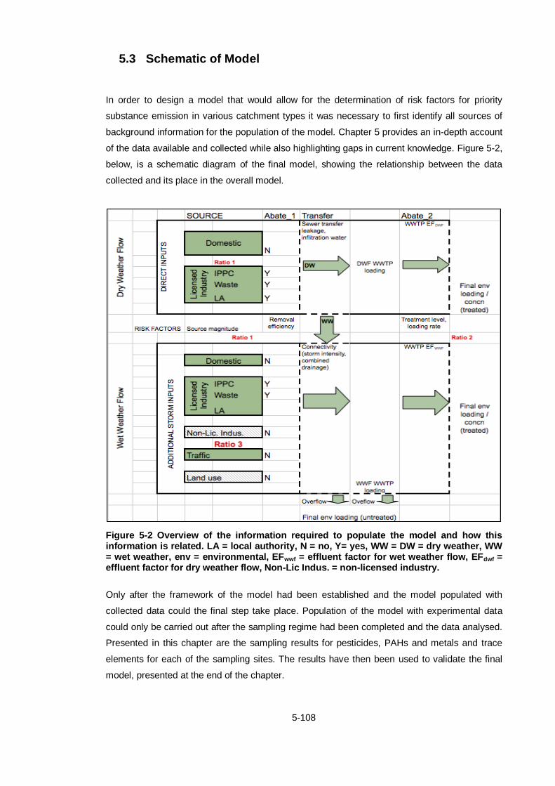
5-108

5.3 Schematic of Model

In order to design a model that would allow for the determination of risk factors for priority

substance emission in various catchment types it was necessary to first identify all sources of

background information for the population of the model. Chapter 5 provides an in-depth account

of the data available and collected while also highlighting gaps in current knowledge. Figure 5-2,

below, is a schematic diagram of the final model, showing the relationship between the data

collected and its place in the overall model.

Figure 5-2 Overview of the information required to populate the model and how this information is related. LA = local authority, N = no, Y= yes, WW = DW = dry weather, WW = wet weather, env = environmental, EFwwf = effluent factor for wet weather flow, EFdwf = effluent factor for dry weather flow, Non-Lic Indus. = non-licensed industry.

Only after the framework of the model had been established and the model populated with

collected data could the final step take place. Population of the model with experimental data

could only be carried out after the sampling regime had been completed and the data analysed.

Presented in this chapter are the sampling results for pesticides, PAHs and metals and trace

elements for each of the sampling sites. The results have then been used to validate the final

model, presented at the end of the chapter.

5-109

5.4 Overview of Data Input to Model

There were many sources of data drawn upon for the population of the model. Figure 5-3

depicts these sources of data and the number of each type of document evaluated.

Figure 5-3 Summary of data inputs to model.

As this model formed a web of information the relationship between data sources is more

clearly represented in Figure 5-4 using the Ringsend catchment as an example.

MODEL

IPPC Licenses (155)

Wastewater Discharge License Applications

(9)

Annual Environmental Reports (11)

Trade Effluent Licences

(872)

Waste Discharge Licenses

(62)

Experimental Data (164)

Traffic Data Census Data

Rainfall data (102)

5-110

Figure 5-4 Relationship of datasets to the Ringsend catchment.

Select Site:

Ringsend

Evaluate Wastewater Discharge Licence

Application

-historic data

-processes in use

-catchment map

Map plotted using GIS to determine catchment area

Collect rainfall monitoring data, plot stations on map, carry out statistical analysis

Historic data compiled to assess occurrence of

pollutants, flow through the plant

Flow relates to WWF and DWF differentiation

Determine processes in use at the plant - use to assess

removal efficiencies

Removal efficiencies used in the calculation of risk

factors

Collect licences

-IPPC

-Trade effluent

-Waste discharge

Evaluate risk of loading and runoff from each site based

on activities, volume and nature of historic discharge

data

Input risk and runoff data into the model

Collect traffic data and census data

Using the catchment maps calculate road area and population in the area

This relates to P.E. at the plant, surface runoff

calculations and PS loading from traffic

5-111

5.5 Design and Population of Model

In order to properly design a model for this project it was necessary to review current tools and

models used internationally. This involved reviewing existing modelling methods and

approaches taken by other research groups then deciding which format would best meet the

requirements of this project as well as the WFD. This choice was restricted by limitations in the

data available in Ireland. Data availability is a critical deciding factor in the design approach of

the model, which later impacts on the population of the model with available data. It was

important to both recognise and minimise the limitations of the model from the beginning.

In the design of the model the first draft involved a simple risk-based model. This was selected

as the most effective approach to demonstrating the need for targeted monitoring programs for

priority substances. The risk rankings enable both clear categorisation and ranking of various

emission factors of priority substances according to the associated risk of loading attributed to

each of those factors. The risk rankings are assigned based on collected data from a number of

sources in conjunction with the experimental results of our sampling campaign at each of the

sites included in the study. By relating the emission data to the actual determined levels in the

wastewater effluent it is possible to validate the risk rankings assigned within the model, or

indeed re-evaluate an assigned rank.

Table 5-1 Risk ranking scale applied to the data for the model.

Risk Ranking Description (high possibility of…)

0 No loading

1 Light loading

2 Significant loading

3 Substantial loading

4 Heavy loading

For the purpose of this project Microsoft Office Excel was chosen as the platform for this model

due to its simple user interface, widespread availability and as a low cost program that would be

receptive to large volumes of data.

5-112

5.5.1 SELECTING AND CHARACTERISING THE AGGLOMERATION

Sites in two counties in Ireland were selected for this study. The 9 sites were chosen on the

basis that a spread of varying population equivalents, levels and types of treatment, and input to

the treatment plants would best support a broad framework of knowledge from which to

construct a model, therefore the counties Dublin and Cork were chosen to best represent these

requirements. Figure 5-5 is a flow chart detailing the first steps taken towards creating and

populating the model.

Figure 5-5 Preliminary data obtained from agglomeration mapping.

To facilitate the preparation of a valuable tool to assist priority substance monitoring for this

study it was necessary to collect any available information related to each site in order to build

complete datasets. Included in the wastewater discharge license applications for each of the

treatment plants was an agglomeration map, i.e. Figure 5-6, a map for the Ballincollig WWTP

catchment, which shows the catchment area and any sub areas as well as grid references for

the treatment plants. Using this information it was possible to geo-reference each catchment

map to a Google hybrid layer, as shown in Figure 5-7 the catchment borders are plotted and

conversions are carried out in order to relate map distances to actual areas. This was carried

out using QGIS software, Figure 5-8.

Selection of Agglomerations

Collection of maps of catchments

Maps

•Plot areas and sub areas

•Use distance measuring tool to calculate area

•Evaluate agglomeration areas and determine % urban area

5-113

Figure 5-6 Example of a catchment map attached to a wastewater effluent discharge application for Ballincollig WWTP. This provides an outline of the catchment that can be referenced to satellite imagery (Cork County Council 2007).

In Figure 5-6 above the Ballincollig catchment is outlined on the map which was submitted to

the EPA as an attachment to the wastewater effluent discharge license application. In order to

convert this map to a usable map from which the catchment area can be calculated it was

necessary to perform a geo-referencing step. The latter refers to the selection of several points

along the catchment border and direct referencing to the same point on a hybrid map canvas.

As well as an overall catchment map the license applications can often also include maps of

sub-areas to the catchment, as in the case of Ringaskiddy, Figure 5-7 below, and maps

showing sampling points and maps showing sampling points referred to within the application.

Section 5.5.2 describes the typical information included in wastewater discharge license

applications.

5-114

Figure 5-7 After georeferencing a .pdf version of an agglomeration map the catchment borders are clearly visible over the Google hybrid map.

In Figure 5-7 above the original map of the Ballincollig catchment has been geo-referenced and

transposed onto a Google hybrid map layer. From this map the catchment border can be

outlined and extracted from the original pdf map and re-projected onto the Google map, 5-8

and Figure 5-9 below.

Figure 5-8 By tracing out the agglomeration border using mapping tools it was possible to calculate the internal area of each catchment.

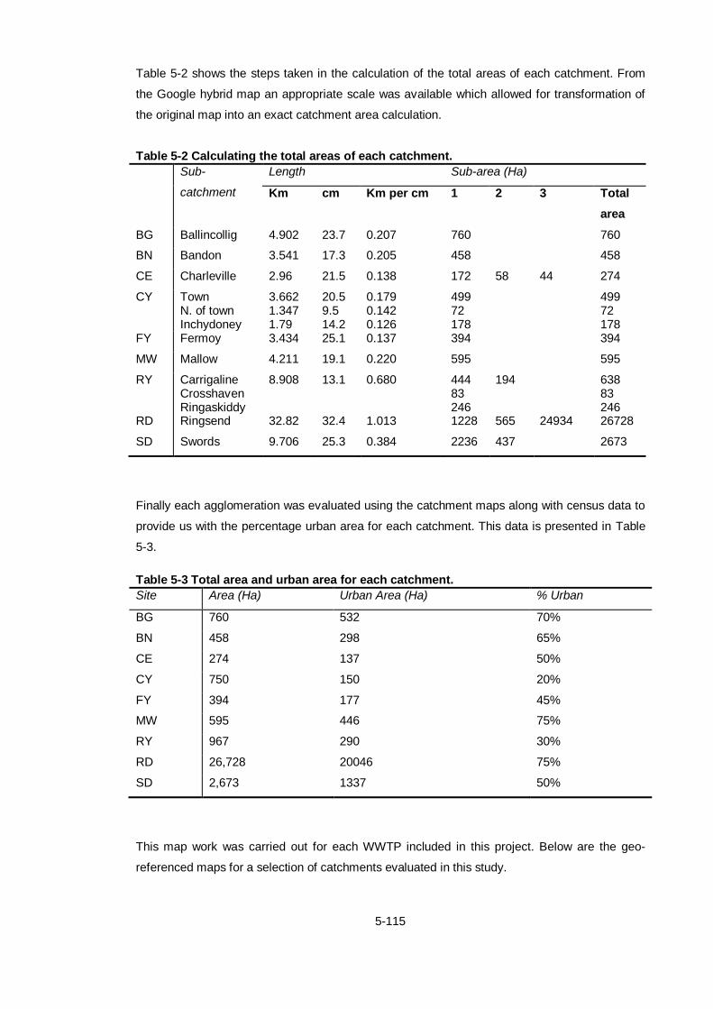
5-115

Table 5-2 shows the steps taken in the calculation of the total areas of each catchment. From

the Google hybrid map an appropriate scale was available which allowed for transformation of

the original map into an exact catchment area calculation.

Table 5-2 Calculating the total areas of each catchment.

Sub-

catchment

Length Sub-area (Ha)

Km cm Km per cm 1 2 3 Total

area

BG Ballincollig 4.902 23.7 0.207 760 760

BN Bandon 3.541 17.3 0.205 458 458

CE Charleville 2.96 21.5 0.138 172 58 44 274

CY Town N. of town Inchydoney

3.662 1.347 1.79

20.5 9.5 14.2

0.179 0.142 0.126

499 72 178

499 72 178

FY Fermoy 3.434 25.1 0.137 394 394

MW Mallow 4.211 19.1 0.220 595 595

RY Carrigaline Crosshaven Ringaskiddy

8.908

13.1

0.680

444 83 246

194 638 83 246

RD Ringsend 32.82 32.4 1.013 1228 565 24934 26728

SD Swords 9.706 25.3 0.384 2236 437 2673

Finally each agglomeration was evaluated using the catchment maps along with census data to

provide us with the percentage urban area for each catchment. This data is presented in Table

5-3.

Table 5-3 Total area and urban area for each catchment.

Site Area (Ha) Urban Area (Ha) % Urban

BG 760 532 70%

BN 458 298 65%

CE 274 137 50%

CY 750 150 20%

FY 394 177 45%

MW 595 446 75%

RY 967 290 30%

RD 26,728 20046 75%

SD 2,673 1337 50%

This map work was carried out for each WWTP included in this project. Below are the geo-

referenced maps for a selection of catchments evaluated in this study.

5-116

Figure 5-9 Map of the Ballincollig catchment (Cork County Council 2007).

Figure 5-10 Map of Ringaskiddy catchment including sub-areas (Cork County Council 2007)

5-117

Figure 5-11 Map of Ringsend catchment (Dublin City Council 2007).

Each of the catchments is described in more detail in Chapter 2.

5-118

5.5.2 LICENSED DISCHARGES

In order to populate the model with relevant, high quality data it was necessary to evaluate the

best possible sources of data. Having previously characterised the respective agglomerations,

Section 5.5.1, an evaluation of the significant sources of priority substances in each, beginning

with licensed emissions, was conducted. These emissions are broken down in Figure 5-12.

Figure 5-12 Overview of Licensed Discharges used as sources as data for populating the model.

Industrial installations performing listed activities above specified thresholds are licensed under

the EU Integrated Pollution Prevention and Control (IPPC) Directive. The Irish EPA makes

licence conditions and Annual Environmental Reports (AER) on emissions from these

installations publicly available. (However, the level of information provided on PS emissions was

found to vary across installations.) For the initial purposes of this risk-based model risk factors

were defined for each installation according to activity class and refined based on some

installation-specific information provided in the licences (whether or not discharge to sewers,

and surface water management). Sewer loading of PSs from licensed installations was

separated into direct sewer inputs and potential surface runoff inputs via combined drainage.

The same simple risk index scheme was applied to each installation in relation to each PS

group.

Waste management sites are also regulated by the EPA under Waste Licences. Local

authorities issue Trade Effluent licences to commercial premises discharging to sewers. These

licences typically contain little information, however the nature and number of each type of

discharge was used in the loading calculations for each catchment. Lists of commercial

installations were obtained from the relevant local authorities (excludes restaurants which are

licensed under separate fats, oils and greases licences, and were excluded from this study

owing to low PS emission risk relative to domestic loading). Sites were categorised based on

their primary activity (from internet searches where necessary), and loading risk factors were

estimated for each PS group for each activity category.

In all cases, site addresses (from EPA licences, and local authority license lists or the internet

for Trade Effluent licensees) were cross-referenced with agglomeration maps in order to

determine which, if any, WWTP agglomeration each sites feeds in to. To convert risk factors

into estimated loading factors for the risk model, loading is considered to be exponentially

Licensed Discharges

WW License Applications

EPA Waste Licenses

Annual Environmental Reports (AERs)

IPPC Licenses

Trade Effluent Licenses

5-119

related to the 4 risk factors, Table 5-1. This reflects the wide range of loading expected from

different licensed sources, with large IPPC sites for example discharging up to 100 times the

volume of commercial sites (albeit with more stringently monitored controls). Some degree of

emission abatement is in place for most licensed sites, and emission loading will often depend

on the effectiveness of the abatement methods (for runoff, this may depend on precipitation

intensity).

From our research it was found that not all businesses in the agglomeration have applied for

trade effluent licenses. They probably exclude a larger proportion of businesses in the small

agglomerations, where sites may not be linked to the sewer network. Some such sites (e.g.

garages) may still contribute to sewer PS loading via surface runoff (N.B. Some of these are

represented by surface runoff rankings attributed to waste licenses in the database). Sewer

loading of PSs from licensed installations was separated into direct sewer inputs and potential

surface runoff inputs via combined drainage.

This can also be a problem with other unlicensed sources such as car washes, Bed and

Breakfasts, shops, pubs, sporting facilities, etc., which are not taken into account. In 2008 it was

reported that pollution loads arising from commercial sources were underestimated in the

design at Ringsend WWTP, the same report estimated the actual contributed population

equivalent from these commercial sources to be 190,000 on top of the pollution load arriving at

Ringsend WWTP (Fehily 2008).

5.5.2.1 Waste Water Effluent Discharge License Applications and Annual

Environmental Reports (AERs)

While the maps were an important source of background information for the model one of the

greatest sources of information required for populating the model were the wastewater effluent

discharge license applications and the AERs for each of the plants. AERs are reports issued

annually for licenced WWTPs, they provide the most recent data on effluent quality and

standards as well as any changes made to the operation of the plant. Where available these

documents provided a wealth of information, as depicted in Figure 5-13.

120

Figure 5-13 Information included in the WWTP effluent discharge license applications and AERs.

WW License Applications and AERs

Types of treatment

Plant design

P.E Hydraulic capacity

Stormwater

Background of the area

Agglom. P.E. Historic Data

Sampling data Flow data Phys/chem

data

Levels of Treatment

Primary, Secondary or

Tertiary

5-121

Basic information on WWTPs and the agglomerations they serve in Ireland is provided in

documentation submitted to the EPA in applications for Waste Water Discharge Licences

(http://www.epa.ie), summarised in Table 5-4.

Table 5-4 WWTP and agglomeration characteristics, from WW effluent discharge license applications. *From our calculations. NR – nutrient removal. R – river.

WWTP Treatment Capacity

PE

Agglom. Pop. Area

(Ha)*

Receiving waters

BG Secondary 26,000 16,339 760 Freshwater-R

BN Secondary 20,000 6,200 458 Freshwater-R

CE Secondary 15,000 2,984 274 Freshwater-R

CY Secondary 6,067 7,500-15,000 750 Estuarine

FY Secondary, NR 20,000 5,800 394 Freshwater-R

MW Secondary, NR 18,000 7,091 595 Freshwater-R

RY None 0 14,864 967 Estuarine

RD Tertiary 1,640,000 1,200,000 26,728 Estuarine

SD Secondary, NR 60,000 50,000 2,673 Estuarine

Three critical factors were derived from available WWTP operational data to estimate the

equivalent level of treatment achieved by each WWTP under dry-weather flow (DWF) and wet-

weather flow (WWF) conditions:

- Level of treatment under normal operating conditions;

- DWF load factor;

- WWF load factor.

Table 5-5 A selection of information available for two of the nine sites from both the WW License application (App.) and annual environmental report (AER).

Report Conglomerate Testing

Date

TOTAL

Flow

m3/day

BOD

mg L-1

SS

mg L-1

COD

mg L-1

pH Ammonia

App. Ringaskiddy 8121 2406

kg/day

2810

kg/day

AER Ballincollig 9/1/08 7888 247 111

10/1/08 13148 819 789

7/2/08 5955 2.6 6 21 7.2 <1.0

6/3/08 4694 5.49 4 41 7.5 <1.0

3/4/08 3453 2.1 3 21

6/5/08 3406 <1.0 4 22 7.6 <1.0

Table 5-5 shows some of the information gathered from the WW license application and AER

for Ringaskiddy and Ballincollig WWTP. (The information available for Ringaskiddy is limited.)

As well as grid reference values and sampling dates the documents provide information on the

http://www.epa.ie/

5-122

population equivalent of the agglomeration which is broken down into domestic and licensed

contributions, as mentioned in Figure 5-13. This allows characterisation of the loading factors to

the plant to be carried out. Biological and hydraulic capacity of each plant is also included,

however the flow values are of the most value as these facilitate later calculations of base flow

through each plant, allowing for the distinction of WWF and DWF conditions in relation to

specific sampling results. The flow data also aids in the calculation of loading factors and can be

used to evaluate the performance of a particular plant specifically when it is operating above

capacity.

From the license applications and AERs a large dataset of historic sampling data was compiled.

Figure 5-9 shows a small selection of the historic sampling data gathered for the Ballincollig

catchment, wherein the sampling dates and plant flow volumes are compared to a number of

physical and chemical parameters of the plant.

In order to model PS loading, key risk indicators for both DWF and WWF conditions were

devised. Table 5-6 below shows the break down of each plant to show agglomeration

population (taken from census records), population equivalent (P.E.) (equivalent population of

the area including both domestic and licensed inputs)*, DWF levels, and peak flow (PF) levels at

pre-treatment (PF_PreT), at primary treatment (PF_1T) and at secondary treatment (PF_2T)

stages, where the information was available. From the license applications and AERs the

combined drainage area for each plant was also determined in broad ‘mostly’ or ‘partly’ terms,

therefore the assigned combined drainage factor values for each are shown below to be 0.75

for ‘mostly’ and 0.50 for ‘partly’. These factors are included in conceptual model calculations

discussed later in this chapter.

* Note: this value is generally taken from the license application except in the cases of Ringsend

WWTP and Charleville WWTP which were derived from estimated industrial flow BOD loading and adjustment using standard 16% estimate of industrial input, respectively.

This standard 16% estimate is derived from the National Urban Wastewater study published by the Department of the Environment, Community and Local Government in 2004 which states that industrial loadings are usually 16% of all domestic/residential loadings.

5-123

Table 5-6 Excel document wherein the population, P.E., Plant P.E., area of the catchment, and flow data for each site were examined in order to determine peak flows.

Site Level Agglom

pop.

Agglom

PE

Plant PE DWF PF_2T PF_1T Comb

Drain

m3 day

-1

BG 2 16,339 24,524 26,000 2,700 12,216 0.75

BN 2 6,200 8,178 20,000 2,160 6,480 13,478 0.75

CE 2 2,984 3,461 15,000 2,050 12,240 12,240 0.50

CY 2 11,250 13,050 6,067 1,469 8,813 8,813 0.50

FY 2,NR 5,800 12,000 20,000 3,200 16,152 0.50

MW 2,NR 7,091 8,226 18,000 5,338 13,344 0.50

RY 0 14,864 97,556 97,556 9,000 N/A N/A 0.50

RD 3 1,200,000 1,708,000 1,640,000 377,568 959,040 911,088 0.50

SD 2,NR 50,000 58,000 60,000 12,063 100% 0.75

For the Dublin sites larger datasets were available and were provided by the plant operators.

They supplied files detailing flow, storm water discharge and storage levels, standard

wastewater quality test results as well as some specific pollutant analysis results, specifically

those for heavy metals where the data was available. This data was relevant as the sampling

dates overlapped with those included in this project and allowed for comparative analysis

results as well as allowing the comparison of flow data from the plant to experimental results

from this project. This data was lacking for the Cork sites as there was no record of plant flow

levels other than those included in the license applications, therefore those values were used as

base levels, and average levels in later calculations.

5-124

5.5.2.2 EPA Waste Licenses

The EPA collects waste license information and this is made freely available on the Irish EPA

website (www.epa.ie). As part of this project all waste licenses available for each agglomeration

under study were collected. This enables risk factors and loading factors for both direct input

and runoff risk, Table 5-7 below, to be determined.

Taking a closer look at the EPA waste license applied for by Cork County Council Western

Division for a landfill facility called Derryconnell Landfill (marked with LF code in Table 5-7)

which feeds into Bandon WWTP it can be seen that risk factors for all PS from direct input were

assigned a value of 4, while runoff risk was assigned 0. These values were determined from the

evaluation of the waste license application and accompanying documents as found on the EPA

website (Irish EPA 2012).

Table 5-7 EPA waste license holders, their addresses, and risk factors and loading factors for both direct input and runoff risks to the WWTP. LF – landfill, WTF – waste transfer station, HW – hazardous waste facility, IWM – integrated waste management facility.

Code Plant Risk Factor

Direct Input Runoff Risk

PAH VOC HM Pest. PAH VOC HM Pest.

LF BN 4 4 4 4 0 0 0 0

WTF CY 2 2 2 1 2 2 2 2

HW FY 3 3 3 3 0 0 0 0

IWM RD 2 2 2 1 2 2 2 2

Loading Factor

Direct Input Direct Input


LF BN 54.6 54.6 54.6 54.6 0 0 0 0

WTF CY 7.4 7.4 7.4 2.7 7.4 7.4 7.4 7.4

HW FY 20.1 20.1 20.1 20.1 0 0 0 0

IWM RD 7.4 7.4 7.4 2.7 7.4 7.4 7.4 7.4

The website allows users to view the latest AERs for this site (2008, 2009, 2010), the original

application and the EPA review documents. The information in each of these documents was

evaluated and loading and risk factors were assigned. Included in the application document is

information on the nature of the facility, the quantity and nature of the waste, plant methods and

operating procedures, nature and impact of emissions, results of monitoring and sampling, the

recovery and treatment of waste and unauthorised of unexpected emissions. This data can be

verified through comparison to the latest AER which provides further information on current

waste quantities and composition, site capacity, any works at the site, continuous monitoring

systems and sampling results, and any environmental incidents or non-compliances.

5-125

This data was gathered and evaluated for each of the licensed waste facilities within each of the

catchments in this study, however there is always the issue of illegal dumping which is difficult

to take into account, therefore for the purposes of this study only licensed sources could be

included.

5.5.2.3 IPPC Licenses

As with the EPA waste licenses the IPPC licenses for each catchment were gathered and

evaluated as shown in Table 5-8 below. Each license application, along with any accompanying

documents, was reviewed and risk and loading factors for direct input and runoff risk were

attributed to each of the industries.

Take the Brewery, Chemical and Dairy Engineering Limited industry (marked as M in Table 5-8)

located in Charleville as an example. This industry has been IPPC licensed since 2005 and as

defined on the EPA website (http://www.epa.ie/terminalfour/ippc/ippc-view.jsp?regno=P0283-

02) as carrying out activities in boiler-making and the manufacture of reservoirs, tanks and other

sheet metal containers where the production area exceeds 500 square metres.

Table 5-8 IPPC license holders, their addresses, and risk factors and loading factors for both direct input and runoff risks. CL – chemical industry, FD – food and drink facility, M – metals facility, OR – other activities.




CL RD 2 4 2 2 1 1 1 0

FD BN 0 0 0 0 1 1 1 0

M CE 2 2 4 0 1 1 1 0

OR MW 1 3 3 0 1 1 1 0

Loading Factor



CL RD 7.4 54.6 7.4 7.4 2.7 2.7 2.7 0

FD BN 0 0 0 0 2.7 2.7 2.7 0

M CE 7.4 7.4 54.6 0 2.7 2.7 2.7 0

OR MW 2.7 20.1 20.1 0 7.4 7.4 7.4 7.4

Available documentation for this site includes AERs (2008, 2009, 2010) and licence application

documents. In the most recent AER for this site the only listed emissions to water/sewers are

rainwater to the field drain, clean water to the field drain (emptying clean tanks filled with water

for pressure testing), and office and canteen toilets connected to the mains sewerage system

(volumes not available).

Descriptions and quantities of disposed waste are also detailed in this report and as such this

industry is risk ranked for direct input of PAHs, VOCs and metals.

http://www.epa.ie/terminalfour/ippc/ippc-view.jsp?regno=P0283-02

http://www.epa.ie/terminalfour/ippc/ippc-view.jsp?regno=P0283-02

5-126

5.5.2.4 Trade Effluent Licenses

Trade effluent licenses and loading data were acquired for each of the agglomerations under

review. The licence information would provide a broad outline of industrial and commercial

inputs of specific PSs to the surface waters in the agglomeration based on the licensed

activities.

Lists of commercial installations were obtained from the relevant local authorities (this excluded

restaurants which are licensed under separate fats, oils and greases licenses, and were

excluded from this study owing to low PS emission risk relative to domestic loading). Sites were

categorised based on their primary activity (from internet searches where necessary), and

loading risk factors were estimated for each PS group for each activity category.

Table 5-9 Trade effluent license holders, their addresses and background data gathered from the documents available on the EPA website.

Limited information was available from the trade effluent licenses due to commercial sensitivity

issues therefore these sites were ranked based on their licensed activities within the catchment.

Table 5-9 above shows a condensed table of one of the Excel sheets detailing activities

associated with a number of licensed trade effluent discharges in the Ballincollig area. Any

available sampling data was also combined. The cumulative result of this data is seen in Table

5-10 below where risk and loading factors have been assigned.

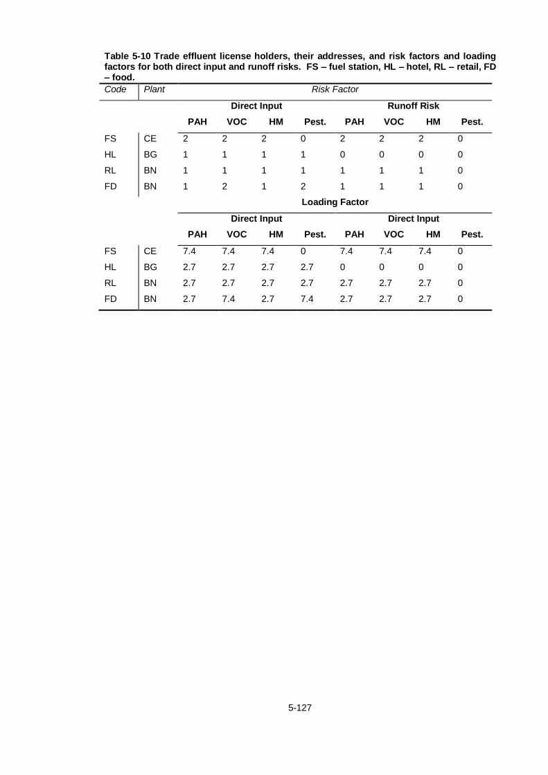
5-127

Table 5-10 Trade effluent license holders, their addresses, and risk factors and loading factors for both direct input and runoff risks. FS – fuel station, HL – hotel, RL – retail, FD – food.




FS CE 2 2 2 0 2 2 2 0

HL BG 1 1 1 1 0 0 0 0

RL BN 1 1 1 1 1 1 1 0

FD BN 1 2 1 2 1 1 1 0

Loading Factor



FS CE 7.4 7.4 7.4 0 7.4 7.4 7.4 0

HL BG 2.7 2.7 2.7 2.7 0 0 0 0

RL BN 2.7 2.7 2.7 2.7 2.7 2.7 2.7 0

FD BN 2.7 7.4 2.7 7.4 2.7 2.7 2.7 0

5-128

5.5.2.5 Summary of Licensed Sources

Hundreds of licence applications and supporting documents were gathered during the course of

this project, and any relevant data from each was identified, sorted and compiled into excel

databases, all of which are linked in an intricate web which contribute directly to the final model.

As numbers change as new AERs are submitted and as new information is available, the

documents are amenable to change and are programmed to adjust to the new data, Table 5-11.

Table 5-11 Part of an overall summary table of total direct inputs and possible surface runoff values for each of the main groups of priority substances according to the source of information (IPPC, EPA waste, and Local Authority Trade effluent (LA-TE) licenses).

These values are adjusted according to combined drainage in the catchment.

Site Licence DIRECT INPUT POSSIBLE SURFACE

RUNOFF INPUT

Comb.

Drain.

Area PAH VOC Metal Pest PAH VOC Metal Pest

BG IPPC n/a n/a n/a n/a n/a n/a n/a n/a 0.75

EPA

Waste

n/a n/a n/a n/a n/a n/a n/a n/a 0.75

LA-TE 38 38 38 8 26 26 26 0 0.75

TOTAL 38 38 38 8 26 26 26 0 0.75

BN IPPC 0 0 0 0 4 4 4 0 0.75

EPA

Waste

55 55 55 55 0 0 0 0 0.75

LA-TE 63 82 63 32 38 38 38 0 0.75

TOTAL 118 137 118 87 42 42 42 0 0.75

5-129

5.5.3 RAINFALL DATA

Rainfall in an area leads to increased flow through a WWTP, as water runs off buildings and

roads and enters the sewerage system before eventually making its way to the plant. This

creates a flushing effect at the plant, as this rainwater brings with it many pollutants that had

been present as street dust, pesticides on grass and fields, and airborne particulates. During

these periods of rainfall an increased flow reaches the plant, often pushing a plant above

capacity, and the stream is diverted to storm water overflow where the water can be released,

untreated, back into the effluent stream. Met Éireann were able to provide an extensive list of

rainfall monitoring stations nationwide, including grid references (Table 5-12) which allowed for

their mapping (Figure 5-14 and Figure 5-15).

Table 5-12 A selection of rainfall monitoring stations in the Dublin and Cork areas.

Station

number

Station Name River Catchment Grid

Reference

9523 Dublin (Blackrock College) Coastal O204297

1823 Dublin (Glasnevin) Tolka O150370

3923 Dublin (Merrion Square) Liffey O164335

1723 Dublin (Phoenix Park) Liffey O100361

2523 Dublin (Ringsend) On coast O189339

5102 Bandon (Hillview) Bandon W493547

3604 Carrigadrohid (Gen.Stn.) Lee W405720

6004 Carrigaline (Kilnagleary) Owenboy W740616

8606 Castlelyones (Ballymacsimon) Douglas-Bride W894899

5202 Clonakilty (Castleview) Argideen W429441

5-130

Figure 5-14 Google map showing rainfall monitoring stations in the Dublin area. The WWTPs are indicated in red.

Figure 5-15 Google map showing rainfall monitoring stations in the Cork area. The WWTPs are indicated in pink.

5-131

The rainfall data was used to assess the dry periods, rain intensity and rain duration and the

effect of meteorological conditions at the time of sampling. It is important to emphasise that the

model will just rank risk relative to average agglomerations - for dry weather flow and wet

weather flow. Further work is required to define meteorological relationships for more detailed

risk rankings, in particular to account for the preceding dry period.

After plotting the rainfall stations the next step was to determine which of the sites would give

the most accurate representation of the level of rainfall reaching the WWTPs. As there are a

number of rainfall monitoring stations in close proximity to each of the WWTPs it was required

that a study be carried out to discover which of the stations had the most representative values

in relation to the site. Sites within a 5 km radius of each of the sites were selected and statistical

analysis was carried out to determine the levels of correlation between the rainfalls measured at

each of the sites. This was determined using the Pearson correlation coefficient. If high

correlation was observed it would be possible to take the mean rainfall of the monitoring

stations when comparing to the flow through the plant, and, in turn, the detected pollutant levels.

Table 5-13 Rainfall stations within 5 km of the respective WWTPs.

WWTP Rainfall Stations within 5 km

Bandon Bandon (Hillview) 5102

Ballincollig Inishcarra (Gen.Stn.) 3704

Muskerry (Golf Club) 6104

Charleville Rathluirc (For.Stn.) 3706

Clonakilty Clonakilty (Castleview) 5202

Fermoy Moorepark 575

Mallow Mallow (Sewage Treatment Works) 6606

Mallow (Spa House) 7406

Ringaskiddy Carrigaline (Kilnagleary) 6004

Roches Point 1075 and 1004

Ringsend Dublin (Ringsend) 2523

Dublin (Simmonscourt) 7523

Dublin (Merrion Square) 3923

Dublin (Blackrock College) 9523

Swords Dublin Airport 532

Malahide Castle 1332

Table 5-13 gives an overview of the WWTPs and rainfall stations within 5 km of their locations.

In the cases of Bandon, Charleville, Clonakilty and Fermoy only one station was located within

this radius and so this would be representative alone of the rainfall at the plants. It must also be

noted that there was not enough information from the Carrigaline (Kilnagleary) station to

perform a correlation study.

5-132

Table 5-14 shows some of the results of these correlation studies. A value of 1 indicates full

correlation between datasets while a value above 0.8 indicates a strong correlation between the

two variables; therefore the aim was to achieve the highest possible correlations between

rainfall stations. For the Ringsend WWTP there are three rainfall stations in the area. After

analysis of the data it was shown that the greatest correlation was achieved between the

Ringsend and Merrion Square stations, correlation coefficient of 0.89307, with much lower

correlation between both sites and the Simmonscourt station, with correlation coefficients of

0.66615 and 0.68413 respectively.

Table 5-14 Results of correlation study on rainfall stations located within a 5 km radius of Ringsend WWTP, Swords WWTP and Ballincollig WWTP 2008-2010.

WWTP Rainfall Station Dublin

(Ringsend)

2523

Dublin Airport

532

Muskerry

(Golf Club)

6104

RD Dublin (Merrion Square) 0.89307

SD Malahide Castle 1332 0.89357

BG Inishcarra (Gen.Stn.) 3704 0.83284

Swords WWTP is represented by both Dublin Airport and Malahide Castle rainfall stations. After

comparing the two datasets an overall correlation coefficient of 0.89357 was achieved,

indicating that the mean rainfall of these two sites would be representative of rainfall in the area,

and thus rainfall reaching the WWTP. Ballincollig WWTP can also be represented by the mean

rainfall of its neighbouring rainfall stations as they have a correlation coefficient of 0.83284.

The final WWTP with more than one rainfall station nearby was Mallow WWTP, located near

both Mallow Spa House and Mallow Sewage Treatment Works rainfall stations. This correlation

study offered a very low correlation coefficient of only 0.37697, therefore data from both sites

could not be used when analysing the effluent data. In this situation it was fortunate as one of

the rainfall stations is located at the actual plant, allowing for the use of the Mallow Sewage

Treatment Works rainfall data for comparison to experimental results.

Following this statistical analysis it was clear which stations were representative of rainfall at

each of the WWTPs. For the Dublin and Swords sites, where detailed flow data was available, it

was possible to establish base flow levels and assign benchmarks above and below which dry

and wet weather flow conditions could be defined. For the Cork sites this definition relied on

flow data provided in the license applications. The flow data was evaluated in order to

determine a base level flow through the plant in relation to rainfall conditions at the time. This

allowed for the definition of WWF and DWF parameters for the Cork sites. For the final model

the separation of WWF and DWF results was necessary, therefore this was an important step.

5-133

5.5.4 TRAFFIC DATA

Traffic data obtained from National Roads Authority (NRA) as well as the Central Statistics

Office (CSO) was used in conjunction with mapping techniques which allowed for the

determination of average road usage in each catchment.

Table 5-15 Compilation of some of the NRA traffic counter data collected for one area. This dataset provides information on daily traffic volume on a certain road for each month of the year, with information also broken down into holiday traffic, direction of traffic, and percentage heavy commercial vehicle (%HCV) traffic.

Traffic Counter Data for "Poulavone N20-1" in year 2008, based on 365 days recorded data

Bank Holiday Directional Volumes in 2008 by number of vehicles

Month Jan Feb Mar Apr

Daily Volume 13330 14343 13613 15036

Holiday Easter (March) May

Date 21st 22

nd 23

rd 24

th 2

nd 3

rd 4

th 5

th

Southbound 6322 5333 3849 4175 9174 6301 4651 4618

Northbound 5586 4989 3658 4138 8251 5493 4432 4656

Average Hourly Directional Volumes on Weekdays (Monday - Friday) in 2008

Hour Ending 1 2 3 4 5 6 7 8

Southbound 44 24 21 14 13 33 110 350

Southbound

%HCV

1 2 2 6 8 6 6 5

Northbound 40 18 11 9 7 18 107 582

Northbound

%HCV

2 5 4 15 14 9 7 3

Average Hourly Directional Volumes on Saturdays in 2008

Hour Ending 1 2 3 4 5 6 7 8

Southbound 80 61 53 34 20 22 49 129

Southbound

%HCV

1 1 1 3 3 5 7 7

Northbound 67 48 39 25 13 14 44 127

Northbound

%HCV

1 2 2 4 5 9 11 5

Average Hourly Directional Volumes on Sundays in 2008

Hour Ending 1 2 3 4 5 6 7 8

Southbound 87 74 63 43 22 20 27 59

Southbound

%HCV

1 0 1 1 2 1 4 3

Northbound 65 58 46 31 13 12 27 60

Northbound

%HCV

1 1 1 2 2 3 1 1

5-134

Traffic-induced loading to WWTP (PAH, VOCs, HMs) should be largely proportional to traffic

volume within agglomeration combined drainage areas, as measured by Vehicle km Travelled

(VKT). Relevant available statistics are traffic flow on national roads in the vicinity of study

agglomerations, total VKT for different vehicle types 22 (National Roads Authority 2010) and

national VKT for six major road types (National Primary, National Secondary, Regional, Local

Primary, Local Secondary, Local Tertiary) (CSO 2009).

Table 5-16 2004 Road Data from the NRA. In this table the catchment and road are named and described in terms of road usage statistics. AADT - annual average distance travelled in km. HCV - heavy commercial vehicle. Area established is measured in hectare.

Catchment Location Year Aadt HCV% 2008

car aadt

2008

HCV aadt

Length km

RD N4 2003 46168 11.3 49029 7715 8.01

RD N7 2004 57734 15.1 56775 10856 4.6

RD N11 Fosters Ave 2004 48420 3.9 53897 2662 5.2

RD N81 After Tallaght

bypass

2004 30929 5.8 33747 2479 8.12

SD M1 N airport

interchange

2008 80232 7.2 74455 5361 3.13

BG N22 By-pass 2008 19982 5.6 18863 1056 3.4

Traffic was divided into two components: local traffic and through traffic. Local traffic was

considered to be a function of agglomeration population, and was calculated based on the

national average VKT per car on Regional and Local roads estimated to occur within urbanized

(i.e. WWTP agglomeration) areas – it was assumed that national average car ownership data

(CSO, 2009) translated into a ratio of 0.4 cars per capita in Dublin city, and 0.5 cars per capita

elsewhere in Ireland.

Local VKT within agglomerations was taken to equal the standard VKT per car (2359 km a-1;

2949 km a-1

in Dublin), or twice the agglomeration length if this was smaller (to bound traffic

volume by catchment size for smaller catchments). Local Heavy Commercial Vehicle (HCV)

traffic (lorries and buses) was calculated as a fixed ratio to car traffic based on CSO (2009)

data. A weighting factor of 3 was applied to HCV traffic to generate car-equivalent VKMs that

reflect higher PS deposition from HCVs (e.g. greater road wear and generation of brake dust,

higher fuel use. The estimated proportional area under combined drainage was multiplied by

agglomeration VKT to estimate the traffic-loading index for the catchment.

5-135

Table 5-17 Summary table showing traffic data gathered for each of the catchments in the study. Each catchment is broken down into population, local traffic, traffic distributions, types of vehicle, equivalent vehicles per kilometre travelled (eq VKT), and an overall ranking of traffic loads for each WWTP in order from most (1) to least (10).

Site Cars Heavy Commercial Vehicles

Local traffic

corrected

N-Rd

traffic-C

N-Rd traffic-P Local traffic N-Rd

traffic-C

N-Rd

traffic-P

BG 19,275,015 16,811,941 7,100,215 605,230

BN 5,095,151 18,294,390 1,876,868 1,324,682

CE 2,399,192 27,557,100 883,775 3,058,838

CY 5,134,615 11,325,335 1,891,406 1,018,271

FY 4,199,673 4,832,484 3,487,179 1,547,007 401,247 484,718

MW 6,847,523 2,089,568 23,298,954 2,522,378 156,718 2,073,607

RY 17,534,967 9,990,981 6,459,245 1,768,952

RD 1,415,632,449 956,110,597 521,467,533 96,861,695

SD 58,984,685 85,061,453 21,727,814 6,124,425

Pop. Comb.

Sewer

RELEVANT

CAR eq VKT

ADD CAR eq

VKT

CAR eq

vkm

Rank

Central AND

combined sewer

Peripheral AND

central non-

combined

C/C.A

BG 16,339 0.75 30,431,745 28,771,546 53,404 5

BN 6,200 0.75 24,745,644 8,248,548 72,087 3

CE 2,964 0.50 20,892,065 20,892,065 152,506 1

CY 11,250 0.50 5,404,416 19,784,564 14,415 10

FY 5,800 0.50 7,438,458 12,379,790 37,803 7

MW 7,091 0.50 8,487,189 38,006,963 28,530 8

RY 14,854 0.50 27,684,526 24,526,012 57,238 4

RD 1,200,000 0.50 1,490,017,524 2,736,713,206 111,496 2

SD 50,000 0.75 93,126,095 134,476,758 46,447 6

Through traffic was assumed to occur on N-roads within agglomeration boundaries. National

road traffic count data for points on N roads in the vicinity of agglomerations (NRA, 2009) were

multiplied by the length of the N-road within agglomeration boundaries to generate N-road VKT

for each agglomeration. N-roads were classified as peripheral to the agglomeration (e.g. bypass

roads) and central to the agglomeration. Peripheral roads were assumed to have independent

drainage systems, whilst central roads were assumed to have combined drainage according to

individual agglomeration proportional combined drainage estimates. For Dublin, where N-roads

radiate out of the centre and carry most commuter traffic to and from the city, through traffic was

assumed equal to traffic on radial M50 motorway. NRA data is reported as Annual Average

Daily Traffic (AADT) and % HCV, enabling car-eq. VKT to be calculated for each N road.

5-136

5.6 WWTP Removal Efficiencies and Conceptual Modelling

Wastewater treatment plants (WWTPs) can be major point source inputs of priority substances

to surface waters, and while many studies show that wastewater treatment removes 90-95% of

pollutants, this removal efficiency depends on a number of factors. In order to calculate the

loading of PSs attributed to the WWTPs it was first necessary to determine approximate

removal efficiencies for each of the pollutants within the respective plants.

This level is directly related to the operations at the plant, the input to the plant, the treatment

levels/types received by the water at each site, the handling of storm water and extreme

weather events and the ScorePP project, Seriki et al. (2008). Moore (2009) reported on

measured PS removal efficiencies at WWTPs, mainly based on secondary treatment with

activated sludge. For seven of the WWTPs considered in this study, removal efficiencies for

each group of PSs were approximated to average removal efficiencies for relevant PSs reported

by Seriki et al. (2008). Removal efficiencies used in the model calculations are detailed in Table

5-18 below.

5-137

Table 5-18 A selection of removal efficiencies for PSs according to literature review. Level indicates the level of treatment with 1 being primary and 2 being secondary treatment.

Removal efficiency (%)

Group Compound Data sources Level Primary

treatment

Secondary

treatment

VOC Benzene (Escalas, Guadayol et

al. 2003)

2 83%

VOC Benzene (Barbosa, Tandlich et

al. 2007)

2 99%

VOC Benzene (Parkerton 2001) 2 94%

VOC Chloroform (RDSE 2006) 72%

VOC AVERAGE 84%

PAH Naphthalene (RDSE 2006) 2 93%

PAH Anthracene RDSE (2006) 2 55%

PAH Fluoranthene (Busetti, Heitz et al.

2006)

2 73%

PAH Benzo(a)pyrene RDSE (2006) 2 50%

PAH Benzo(ghi)perylene RDSE (2006) 2 59%

PAH AVERAGE 77%

Pesticide Diuron (Lapertot, Pulgarín et

al. 2006)

2 10%

Pesticide Alachor (Zhu, Yan et al. 2006) 2 10%

Pesticide Isoproturon (Nitschke, Wilk et al.

1999)

2 10%

Pesticide Simazine (Meakins, Bubb et al.

1994)

1 10%

Pesticide Chlorfenvinphos (Gómez, Martínez

Bueno et al. 2007)

2 83%

PESTICIDE AVERAGE 57%

HM Lead compds (Buzier, Tusseau-

Vuillemin et al. 2006)

2 70%

HM Nickel compds Buzier et al. (2006) 2 50%

Phthalate ester DEHP (Fauser, Vikelsøe et

al. 2003)

2 96%

Alkyl phenolic

compound

Nonylphenols (Clara, Scharf et al.

2007)

2 57%

HM AVERAGE 67%

5-138

Table 5-19 Removal efficiencies for certain chemical and biological elements of wastewater effluent in some WWTPs in Cork based on historic sampling data. AER – Annual Environmental Report. APP – EPA Wastewater Discharge license application.

Report Area Test date Flow

(m3/day)

% REMOVAL EFFICIENCY

BOD

mg L-1

SS

mg L-1

COD

mg L-1

Ammonia

mg L-1

Total Phosphorous

mg L-1

AER BG 07/02/08 5955 49%

06/03/08 4694 99% 96% 60%

03/04/08 3453 45%

APP CY 19/09/07 2257 96% 100% 51%

24/10/07 2500 96% 95% 62% 59%

25/10/07 2064 100% 48% 96% -43%

APP CE 16/01/08 90% 53% 86% 37% 65%

14/02/08 10488 85% 69%

08/04/08 94% 58% 98% 83% 17%

After determining removal efficiencies for the three main groups of priority substances it was

possible to compile all data collected (licensed information, rainfall and traffic data and removal

data) into a functional model. The data was organised and tabulated as has been shown in this

chapter in such a way that excel functions could be applied between documents, forming a link

and allowing for easy updating or alteration of data.

Note: The VOCs were also evaluated in that a theoretical model based solely on collected data

was also developed.

5-139

5.6.1.1 Conceptual Modelling

Following the compilation of all relevant available data the conceptual model was developed.

This is the basis of the framework of the model and affords certain flexibility to the model with

regards to additions to the background data. Many calculations were derived as part of the

development of this model and are discussed and rationalised below.

WWTP load factors were calculated as a ratio of agglomeration PE loading to WWTP PE

capacity. For Clonakilty WWTP, with a calculated load factor of 2.2, DWF removal factors were

based on the assumption that half the flow received secondary treatment, and half received

primary treatment only. For WWTPs working in excess of or close to capacity, WW removal

factors were based on the assumption that overall removal efficiencies under high loading

conditions were equivalent to primary treatment removal efficiencies. Removal factors were

inversed into Effluent Factors (EF) for direct multiplication with loading factors.

The conceptual modelling of PS loading is to devise key risk indicators applicable under Dry

Weather Flow (DWF) and Wet Weather Flow (WWF) conditions. To convert risk factors into

estimated loading factors for the risk model, loading was considered to be exponentially related

to the 4 risk factors. This reflects the wide range of loading expected from different licensed

sources, with large IPPC sites for example discharging up to 100 times the volume of

commercial sites.

Loading to the environment from each WWTP under DWF can be expressed as DWF domestic

loading (population size) plus DWF industrial loading (total agglomeration PE), multiplied by

EFDWF.

[Eq.1] Risk of elevated DWF PS conc. = (IndustryDWF / popn) x EFDWF

Equation 1 can be further expanded as below:

[Eq.2] Risk of elevated DWF PS conc. = ((Agg_IndDWF / Nat_IndDWF) / (Agg_Pop / Nat_Pop)) x

EFDWF

Agg_IndDWF = Total industrial contributions from the agglomeration under dry weather flow

conditions. Taken from number of industrial licensed inputs in each

agglomeration.

Nat_IndDWF = Total national industrial contributions under dry weather flow conditions.

Taken from total number of industrial licensed inputs nationwide.

Agg_Pop = Total population loading for the agglomeration, this represents domestic

inputs.

Nat_Pop = Total national population loading.

EFDWF = Effluent factor under dry weather flow conditions.

5-140

Under WWF, WWTP loading is a function of DWF loading, plus WWF Domestic loading, plus

WWF Industrial loading, plus WWF traffic loading, plus WWF Land use loading, all multiplied by

EFWWF. Assuming that Industry and Transport sources are major contributors to WWTP PS

loading, then the risk of elevated PS concentrations can be simplified thus:

[Eq.3] Risk elevated WWF PS conc. = (IndustryDWF / Pop) + (IndustryCD / areaCD) +

(TrafficCD/areaCD) x PDP x EFWWF

PDP = Preceding Dry Period, should be linearly related to loading.

IndustryDWF = Total industrial loading under dry weather flow conditions.

Pop = Domestic population of the agglomeration.

IndustryCD = Total industrial loading in the combined drainage area.

areaCD = Total combined drainage area.

TrafficCD = Traffic loading in the combined drainage area.

EFWWF = Effluent factor under wet weather flow conditions.

Where specific data on lag time at the treatment plant and the effects of preceeding dry period

and storm water contributions have not been fully investigated a simpler equation is:

[Eq.4] Risk WWF conc. = (WWF Loading / WWF volume) x (1-REWWF)

WWF conc. = Risk of concentration of priority substances in WW effluent under wet weather

flow conditions.

REWWF = Removal efficiency under wet weather flow conditions.

Using the equations above with both collected data and the results of a 3-year sampling

campaign it was possible to produce a final model for the four main groups of priority

substances (pesticides, polycyclic aromatic hydrocarbons (PAHs), metals and trace elements

and volatile organic hydrocarbons (VOCs)).

5-141

5.6.1.2 Assigning Risk

Assigning risk values for different PSs under different conditions follows the procedure outlined

in Figure 5-16 and is used along with the conceptual modelling described in Section 5.6.1.1.

Figure 5-16 Overview of procedures involved in assigning risk factors using IPPC licences as a sample source from the Ringsend catchment.

Ringsend Catchment

IPPC Licences

Divide under headings based on activity i.e. chemicals, food and drink,

wood paper textiles

Overall number of each type of license is compared between sites. Average output

and area of industry is also detaied

General rankings between 0-4 are in place for industry based on activity, higher numberof each

industry adds to greater risk. Note: these values can be adjusted for industries

shown to have higher PS loadings

Collect data, compile under datasets in Excel

5-142

Using another example to illustrate assigning of risk values to the different catchments the site

of Ballincollig is expanded upon below, Figure 5-17.

Figure 5-17 Outline on assigning risk based on IPPC licences in Ballincollig.

To give a more specific example Figure 5-18 tracks a single trade effluent licence, for a petrol

station, from collection of the licence to the assignment of a risk factor.

Ballincollig

No IPPC licences therefore assigned risk for direct or possible runoff is zero

No EPA waste licences therefore assigned risk for direct or possible runoff is zero

7 Trade effluent licences, 5 of these are petrol stations which have a risk of 2 for loading of PAHs, metals and VOCs, 0 for pesticides

The SUM risk for each group of PSs from this site is multiplied by the combined drainage factor and this value is divided by the P.E. of the

catchment. This gives the industrial load factor used in the equations in Section 5.6.1.1.

This factor is combined with the WWF or DWF factor for the plant, the combined drainage of the catchment and the

removal efficiency (the effluent factor) which result in a final risk value

5-143

Figure 5-18 From licence to risk factor for a petrol station in Ballincollig, Cork.

The risk factor determined for the site described in Figure 5-18 is a single risk for a single site.

For a single petrol station the risk of PAH, VOC and metals and trace elements occurrence is 2

(per group) while pesticides are risked 0. When all trade effluent licences for Ballincollig have

been evaluated in this same manner the same procedure is carried out for waste discharge

licences and IPPC licences. As Ballincollig had no licences other than trade effluent this was the

simplest site to model. The SUM risk for each group of pollutants assigned from the 7 trade

effluent licences was used to calculate final risk. For example, the SUM PAH risk for Ballincollig

was 38, Table 5-20 shows how this number relates to the final DWF risk for PAHs in Ballincollig.

Topaz Irish Shell, Ballincollig Service Station

Collect trade effluent licence for this site. This provides limited information on the

output of PS from this site.

Due to the lack of emission data from this site a standard set of risk factors are applied for each group of PSs at this site based

on activity covered by the licence. For petrol stations the associated risk of loading for PAHs, VOCs and metals and trace elements is 2, while for pesticides the risk

is set at 0.

This is the ranking for one single trade effluent licensed site in Ballincollig. There are 7 trade effleunt licences in this

catchment which are ranked, as above, on one excel sheet.

The SUM risk for each group of PSs from this catchment is multiplied by the combined drainage factor and this value is divided by the P.E.

of the catchment. This gives the industrial load factor used in the equations in Section 5.6.1.1.

This factor is combined with the WWF or DWF factor for the plant, the combined drainage of the catchment and the removal efficiency (the effluent factor) which result

in a final risk value

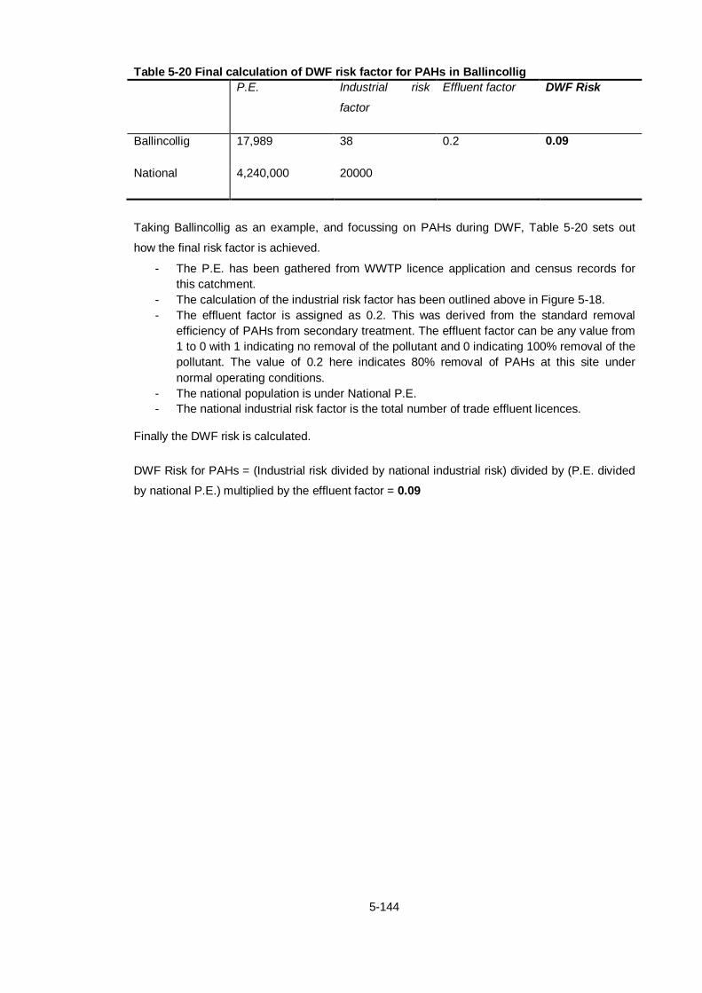
5-144

Table 5-20 Final calculation of DWF risk factor for PAHs in Ballincollig

P.E. Industrial risk

factor

Effluent factor DWF Risk

Ballincollig 17,989 38 0.2 0.09

National 4,240,000 20000

Taking Ballincollig as an example, and focussing on PAHs during DWF, Table 5-20 sets out

how the final risk factor is achieved.

- The P.E. has been gathered from WWTP licence application and census records for

this catchment.

- The calculation of the industrial risk factor has been outlined above in Figure 5-18.

- The effluent factor is assigned as 0.2. This was derived from the standard removal

efficiency of PAHs from secondary treatment. The effluent factor can be any value from

1 to 0 with 1 indicating no removal of the pollutant and 0 indicating 100% removal of the

pollutant. The value of 0.2 here indicates 80% removal of PAHs at this site under

normal operating conditions.

- The national population is under National P.E.

- The national industrial risk factor is the total number of trade effluent licences.

Finally the DWF risk is calculated.

DWF Risk for PAHs = (Industrial risk divided by national industrial risk) divided by (P.E. divided

by national P.E.) multiplied by the effluent factor = 0.09

5-145

5.7 Conclusion

This chapter highlighted the process followed in the establishment, development and population

of a risk-based model for the relation of emission factors to occurrence of priority and hazardous

substances in wastewater. This involved a review of modelling approaches that could be

adapted for the WFD priority substances. The model was then designed using identified

sources of data for the population of the model. Each site was characterised and sources of

information identified.

The information gathering was a continuous process with data tabulated as it became available.

Emission factors for the priority substances were evaluated by agglomeration and this data was

collated and used to populate the model. As no such model previously existed in Ireland no

single database of relevant information relating emission factors to PS occurrence was

available. Through the course of this project this dataset has been compiled and has been

made available to the Irish EPA for use in future monitoring programmes.

6-146

6. Validation and Testing

of Model

6-147

6.1 Aims and objectives

The aim of this chapter is to outline the population of the model with experimental data, using

this data to validate the theoretical risk assigned based on the literature.


- present the results of analysis for priority PAHs, pesticides and metals and trace

elements for the nine sites selected for study,

- provide an overview of these results in relation to WWF and DWF conditions,

- use the analytical results to validate the model with a focus on two sites for comparison,

- outline the basic use of the model and the application of this model to other sites.

6-148

6.2 Ballincollig

6.2.1 INTRODUCTION

At the Ballincollig site 16 samples were collected monthly over a sampling period that spanned

June 2010 through July 2011. Table 6-1 shows dates of sample collection at Ballincollig WWTP.

Of the sampling locations located in County Cork Ballincollig was the only site where it was

possible to carry out intensive sampling, with sampling carried out in June 2011. This section

will provide an overview of sampling results collected from this site providing information of

levels of PAHs, pesticides and metals and trace elements determined in the WWTP effluent

stream.

Table 6-1 Dates of sample collections at Ballincollig WWTP.

2010 2011

Sampling

Dates

24/06/2010

08/07/2010

25/08/2010

09/09/2010

28/10/2010

16/12/2010

18/01/2011

03/02/2011

03/03/2011

26/04/2011

17/05/2011

07/06/2011

27/06/2011

29/06/2011

01/07/2011

12/07/2011

6.2.2 PAHS

Presented in this section are the PAH results for Ballincollig WWTP, Table 6-2. All samples

were analysed for the eight priority PAHs listed in the WFD. Table 6-2 summarises the

occurrence and detected levels of each of the PAHs in the wastewater effluent samples

collected and analysed. The results are compared to the EQS levels applicable to the

respective PAHs.

6-149

Table 6-2 Results of PAH analysis for Ballincollig WWTP. Results are compared to their respective Maximum Allowable Concentration Environmental Quality Standard (MAC EQS). All units are in µg L

-1. ND = Not detected. Naph = naphthalene. Ant = Anthracene.

Fluor = fluoranthene. Bb/k = benzo-b- and benzo-k-fluoranthene. Bap = benzo-a-pyrene. Ind = indeno-1,2,3cd-pyrene. Bghi = Benzo-ghi-perylene. <LOD = below limit of detection.

Parameter Target EQS

µg L-1

Freq.

n=16

Range Percentile

Min. Max. 50 75 90

Naph. 1.2 16 5.44E-04

1.69E-03

8.72E-04

1.21E-03

1.42E-03

Ant. 0.1 16 <LOD 2.33E-02

6.89E-04

8.51E-04

1.32E-03

Fluor. 0.1 16 <LOD 1.89E-02

2.57E-04

3.35E-04

3.57E-04

Bb/k Σ=0.003 9 <LOD 4.02E-02

<LOD 2.85E-05

1.99E-02

Bap 0.05 8 <LOD 3.03E-02

2.41E-05

6.56E-03

1.83E-02

Ind + Bghi Σ=0.002 11 <LOD 4.21E-02

7.23E-05

1.91E-02

2.32E-02

Table 6-2 shows that naphthalene, anthracene and fluoranthene, the more water soluble PAHs

were detected in all samples collected, while the less water soluble, higher octanol/water

partition coefficient PAHs, were less frequently detected. Of these PAHs there were

exceedences of the EQS limits for the benzo-b/k-fluoranthene and the indeno-1,2,3cd-pyrene

and benzo-ghi-perylene (marked in bold in Table 6-2).

6-150

6.2.3 PESTICIDES

Presented in this section are the pesticide results for Ballincollig WWTP. All samples were

analysed for 14 of the priority pesticides listed in the WFD. Table 6-3 summarises the

occurrence and detected levels of each of the pesticides in the wastewater effluent samples


respective pesticides, where available.

Table 6-3 Results of pesticide analysis for Ballincollig WWTP. Results are compared to their respective Maximum Allowable Concentration Environmental Quality Standard (MAC EQS). All units are in µg L

-1. ND = Not detected. *No MAC EQS value available so

taken as Annual Average EQS (AA EQS) for this compound.

Parameter Target EQS µg L

-1

Freq. n=13

Range Percentile

Min. Max. 50 75 90

Alachlor 0.7 5 5.1E-02

1.3E-01

8.61E-02

9.78E-02

1.05E-01

Atrazine 2.00E+00

10 ND 2.1E-01

4.35E-02

1.48E-01

1.61E-01

Chlorfenvinphos 3.00E-01

9 3.0E-01

2.2E+00

7.89E-01

1.20E+00

1.73E+00

Diuron 1.8 13 <LOD 6.2E-01

2.06E-01

2.46E-01

3.45E-01

Malathion 7 ND 9.9E-01

1.36E-01

5.38E-01

8.52E-01

Simazine 4 9 1.5E-02

1.7E-01

5.67E-02

1.17E-01

1.26E-01

Fenitrothion 9 ND 7.8E-01

1.83E-01

3.30E-01

5.20E-01

Pirimiphos methyl 9 ND 6.9E-01

2.63E-01

4.50E-01

4.86E-01

Chlorpyrifos 0.1 3 ND 6.0E-02

2.16E-02

3.92E-02

4.98E-02

DEHP 1.3* 11 ND 1.4E+01

1.60E+00

2.01E+00

2.20E+00

Mecoprop 2 2.0E-02

3.4E-01

1.74E-01

2.46E-01

2.89E-01

Table 6-3 shows that eleven of the priority pesticides were detected in samples from Ballincollig

WWTP. Of these pesticides there were exceedences of the EQS limits for the chlorfenvinphos

and DEHP (marked in bold in Table 6-3). Of the thirteen samples collected at this site only

diuron was found to occur in all samples.

6-151


Ten samples collected at Ballincollig WWTP were microwave digested, stored and sent to the

Centre for Microscopic Analysis (CMA) in Trinity College Dublin for analysis by ICP-MS. The

analysis determined trace levels of 15 WFD priority metals and trace elements in the samples.

Presented in Table 6-4 below are the results of this analysis.

Table 6-4 ICPMS results for samples collected at Ballincollig WWTP from June 2010 to July 2011. Samples were analysed for 15 elements in a total of 10 samples. Results are shown in μg L

-1. Exceedances are marked in bold.

Parameter Target

EQS

Freq.

n=10

Range Percentile

µg L-1

Min. Max. 50 75 90

Boron 10 3.37

E+01 6.13

E+01 4.47

E+01 5.52

E+01 6.07

E+01

Vanadium 0

Chromium 0.6-4.7 4 1.37

E+00 3.63

E+00 1.86

E+00 2.42

E+00 3.14

E+00

Cobalt 0

Nickel 20 4 1.41

E+00 7.74

E+00 4.61

E+00 5.85

E+00 6.98

E+00

Copper 5.0-30 10 3.82

E+00 1.16

E+01 5.70

E+00 6.97

E+00 9.07

E+00

Zinc 8-100 10 4.03

E+01 7.08

E+01 5.67

E+01 6.08

E+01 6.48

E+01

Arsenic 20-25 0

Selenium 0

Molybdenum 0

Cadmium 0.08-0.25 0

Tin 0.0002 2 1.16

E+00 1.18

E+00 1.17

E+00 1.18

E+00 1.18

E+00

Antimony 1 1.15

E+00 1.15

E+00 1.15

E+00 1.15

E+00 1.15

E+00

Barium 9 2.23

E+00 1.09

E+01 3.10

E+00 7.39

E+00 1.05

E+01

Lead 7.2 2 1.05

E+00 2.21

E+01 1.16

E+01 1.68

E+01 2.00

E+01

According to Table 6-4 all samples collected were found to contain levels of trace elements with

Zinc present in the highest concentrations. Tin exceeded the EQS value in 2 of the 10 samples

with lead exceeding the EQS value in one sample.

6-152

6.3 Bandon

6.3.1 INTRODUCTION

At the Bandon site 10 samples were collected monthly over a sampling period that spanned

July 2010 through July 2011. Table 6-5 shows dates of sample collection at Bandon WWTP.

This section will provide an overview of sampling results collected from this site providing

information of levels of PAHs, pesticides and metals and trace elements determined in the

WWTP effluent stream.

Table 6-5 Dates of sample collections at Bandon WWTP.

2010 2011

Sampling

Dates

08/07/2010

12/08/2010

09/09/2010

28/10/2010

18/01/2011

10/02/2011

26/04/2011

17/05/2011

07/06/2011

12/07/2011

6-153

6.3.2 PAHS

Presented in this section are the PAH results for Bandon WWTP, Table 6-6. All samples were

analysed for the eight priority PAHs listed in the WFD. Table 6-6 summarises the occurrence

and detected levels of each of the PAHs in the wastewater effluent samples collected and

analysed. The results are compared to the EQS levels applicable to the respective PAHs.

Table 6-6 Results of PAH analysis for Bandon WWTP. Results are compared to their respective Maximum Allowable Concentration Environmental Quality Standard (MAC EQS). All units are in µg L




µg L-1

Freq.

n=10

Range Percentile

Min. Max. 50 75 90

Naph. 1.2 10 <LOD 2.92E-03

9.24E-04

1.02E-03

1.57E-03

Ant. 0.1 10 <LOD 1.10E-03

4.64E-04

7.11E-04

9.03E-04

Fluor. 0.1 9 <LOD 6.14E-04

3.10E-04

3.55E-04

4.57E-04

Bb/k Σ=0.003 7 <LOD 1.84E-04

0.00E+00

2.24E-05

6.28E-05

Bap 0.05 3 <LOD <LOD <LOD <LOD <LOD

Ind + Bghi Σ=0.002 4 <LOD <LOD <LOD <LOD <LOD

Table 6-6 shows that naphthalene and anthracene, the more water soluble PAHs, were

detected in all samples collected while the less water soluble, higher octanol/water partition

coefficient PAHs, were less frequently detected. None of the maximum detected levels were

above EQS limits for the PAHs.

6-154

6.3.3 PESTICIDES

Presented in this section are the pesticide results for Bandon WWTP, Table 6-7. All samples

were analysed for 14 of the priority pesticides listed in the WFD. Table 6-7 summarises the




Table 6-7 Results of pesticide analysis for Bandon WWTP. Results are compared to their respective Maximum Allowable Concentration Environmental Quality Standard (MAC EQS). All units are in µg L

-1. ND = Not detected. *No MAC EQS value available so taken as

Annual Average EQS (AA EQS) for this compound.

Parameter Target

EQS µg L-1

Freq.

n=10

Range Percentile

Min. Max. 50 75 90


1.3E-01

8.87E-02

9.89E-02

1.05E-01

Atrazine 2.00E+00

7 8.4E-03

4.2E-01

9.26E-02

1.67E-01

2.65E-01


6 5.5E-01

1.9E+00

9.96E-01

1.57E+00

1.79E+00

Diuron 1.8 10 5.0E-02

1.0E+00

2.46E-01

3.69E-01

4.79E-01

Malathion 5 ND 7.0E-01

2.86E-01

5.54E-01

6.00E-01


1.8E-01

6.90E-02

1.15E-01

1.60E-01

Fenitrothion 6 1.3E-02

6.4E-01

3.11E-01

3.71E-01

4.41E-01


2.26E-01

2.72E-01

3.32E-01


2.79E-02

3.74E-02

4.31E-02

DEHP 1.3* 9 2.0E-01

3.8E+01

1.85E+00

1.44E+01

1.94E+01

Mecoprop 1 4.1E-01

5.0E-01

4.45E-01

4.45E-01

4.45E-01

Table 6-7 shows that eleven of the priority pesticides were detected in samples from Bandon


and DEHP (marked in bold in Table 6-7). Of the ten samples collected at this site only diuron

was found to occur in all samples.

6-155


The results of ICP-MS analysis carried out on the 8 samples collected at Bandon WWTP are

presented in Table 6-8. All 8 samples showed the presence of trace elements, with highest

detected concentrations determined for Boron, Zinc and Copper.

Table 6-8 ICPMS results for samples collected at Bandon WWTP from July 2010 to July 2011. Samples were analysed for 15 elements in a total of 8 samples. Results are shown in μg L

-1. Exceedances are marked in bold.


Freq. n=8

Range Percentile

µg L-1

Min. Max. 50 75 90

Boron 8 4.50

E+01 1.34

E+02 6.86

E+01 8.84

E+01 1.09

E+02

Vanadium 1 1.32

E+00 1.32

E+00 1.32

E+00 1.32

E+00 1.32

E+00

Chromium 0.6-4.7 7 1.20

E+00 4.47

E+00 2.14

E+00 3.08

E+00 4.13

E+00

Cobalt 0

Nickel 20 8 2.46

E+00 1.08

E+01 3.47

E+00 6.57

E+00 1.08

E+01

Copper 5.0-30 8 1.83

E+01 4.68

E+01 3.40

E+01 3.94

E+01 4.19

E+01

Zinc 8-100 8 5.75

E+01 1.18

E+02 8.27

E+01 1.04

E+02 1.13

E+02

Arsenic 20-25 4 1.11

E+00 1.67

E+00 1.35

E+00 1.54

E+00 1.62

E+00

Selenium 1 1.32

E+00 1.32

E+00 1.32

E+00 1.32

E+00 1.32

E+00

Molybdenum 4 1.26

E+00 1.30

E+01 5.29

E+00 9.68

E+00 1.17

E+01

Cadmium 0.08-0.25 0

Tin 0.0002 7 1.51

E+00 6.47

E+00 2.02

E+00 3.87

E+00 5.91

E+00

Antimony 3 1.54

E+00 2.79

E+00 2.03

E+00 2.41

E+00 2.64

E+00

Barium 8 3.08E

+00 1.54

E+01 8.15

E+00 1.24

E+01 1.49

E+01

Lead 7.2 5 1.15

E+00 2.38

E+00 2.04

E+00 2.12

E+00 2.28

E+00

A high frequency of occurrence was noted for the boron, barium, copper, nickel and zinc. It was

also found that a number of exceedances of EQS values were detected with tin, copper and

zinc detected in high concentrations.

6-156

6.4 Charleville

6.4.1 INTRODUCTION

At the Charleville site 5 samples were collected monthly over a sampling period that spanned

August 2010 through July 2011. Table 6-9 shows dates of sample collection at Charleville

WWTP. This section will provide an overview of sampling results collected from this site

providing information of levels of PAHs, pesticides and metals and trace elements determined in

the WWTP effluent stream.

Table 6-9 Dates of sample collections at Charleville WWTP.

2010 2011

Sampling

Dates

25/08/2010

26/04/2011

17/05/2011

07/06/2011

12/07/2011

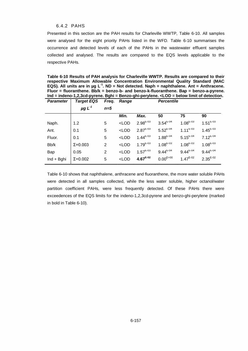
6-157

6.4.2 PAHS

Presented in this section are the PAH results for Charleville WWTP, Table 6-10. All samples




respective PAHs.

Table 6-10 Results of PAH analysis for Charleville WWTP. Results are compared to their respective Maximum Allowable Concentration Environmental Quality Standard (MAC EQS). All units are in µg L




µg L-1

Freq.

n=5

Range Percentile

Min. Max. 50 75 90

Naph. 1.2 5 <LOD 2.98E-03

3.54E-04

1.08E-03

1.51E-03

Ant. 0.1 5 <LOD 2.87E-03

5.52E-04

1.11E-03

1.45E-03

Fluor. 0.1 5 <LOD 1.44E-03

1.88E-04

5.15E-04

7.12E-04

Bb/k Σ=0.003 2 <LOD 1.79E-03

1.08E-03

1.08E-03

1.08E-03

Bap 0.05 2 <LOD 1.57E-03

9.44E-04

9.44E-04

9.44E-04

Ind + Bghi Σ=0.002 5 <LOD 4.67E-02

0.00E+00

1.47E-02

2.35E-02



partition coefficient PAHs, were less frequently detected. Of these PAHs there were

exceedences of the EQS limits for the indeno-1,2,3cd-pyrene and benzo-ghi-perylene (marked

in bold in Table 6-10).

6-158

6.4.3 PESTICIDES

Presented in this section are the pesticide results for Charleville WWTP, Table 6-11. All

samples were analysed for 14 of the priority pesticides listed in the WFD. Table 6-11

summarises the occurrence and detected levels of each of the pesticides in the wastewater

effluent samples collected and analysed. The results are compared to the EQS levels applicable

to the respective pesticides, where available.

Table 6-11 Results of pesticide analysis for Charleville WWTP. Results are compared to their respective Maximum Allowable Concentration Environmental Quality Standard (MAC EQS). All units are in µg L




µg L-1

Freq.

n=5

Range Percentile

Min. Max. 50 75 90

Atrazine 2 4 6.8E-03

1.2E-02

1.02E-02

1.14E-02

1.15E-02


1 1.8E+00

2.2E+00

1.96E+00

1.96E+00

1.96E+00

Diuron 1.8 5 3.4E-02

3.6E-01

5.65E-02

1.63E-01

2.72E-01

Malathion 1 4.8E-01

6.1E-01

5.41E-01

5.41E-01

5.41E-01


1.9E-01

1.82E-02

6.15E-02

1.33E-01


2.4E-01

1.74E-01

1.74E-01

1.74E-01

Pirimiphos methyl 1 2.1E-01

2.5E-01

2.28E-01

2.28E-01

2.28E-01

DEHP 1.3* 5 4.8E-01

1.1E+01

2.39E+00

3.87E+00

7.57E+00

Table 6-11 shows that 8 of the priority pesticides were detected in samples from Charleville


and DEHP (marked in bold in Table 6-11). Of the 5 samples collected at this site only diuron

and DEHP were found to occur in all samples.

6-159


Of the 4 samples collected at Charleville WWTP all were shown to contain some levels of

priority trace elements. From Table 6-12 it can be seen that highest detected levels were

determined for Copper, Zinc, Boron, Barium and Molybdenum.

Table 6-12 ICPMS results for samples collected at Charleville WWTP from August 2010 to June 2011. Samples were analysed for 15 elements in a total of 4 samples. Results are shown in μg L

-1. Exceedances of EQSs are marked in bold.

Parameter Target

EQS

Freq.

n=4

Range Percentile

µg L-1

Min. Max. 50 75 90

Boron 4

1.88E+01

5.50E+01

4.46E+01

5.20E+01

5.38E+01

Vanadium 2

1.06E+00 1.06E+00

1.06E+00

1.06E+00

1.06E+00

Chromium 0.6-4.7 1

1.57E+00 1.57E+00

1.57E+00

1.57E+00

1.57E+00

Cobalt 0

Nickel 20 3

1.12E+00 5.18E+00

2.06E+00

3.62E+00

4.56E+00

Copper 5.0-30 4

1.00E+01 1.93E+01

1.29E+01

1.45E+01

1.74E+01

Zinc 8-100 4

1.51E+01 3.67E+01

2.83E+01

3.52E+01

3.61E+01

Arsenic 20-25 1

1.18E+00 1.18E+00

1.18E+00

1.18E+00

1.18E+00

Selenium 0

Molybdenum 3

1.51E+01

2.49E+01

2.16E+01

2.33E+01

2.43E+01

Cadmium 0.08-0.25 0

Tin 0.0002 1

1.05E+00

1.05E+00

1.05E+00

1.05E+00

1.05E+00

Antimony 1

1.23E+00

1.23E+00

1.23E+00

1.23E+00

1.23E+00

Barium 4

3.25E+01

9.64E+01

7.79E+01

9.52E+01

9.59E+01

Lead 7.2 1

1.23E+00

1.23E+00

1.23E+00

1.23E+00

1.23E+00

Boron, barium, copper and zinc occurred in the highest frequency at this site with only tin

exceeding the EQS value.

6-160

6.5 Clonakilty

6.5.1 INTRODUCTION

At the Clonakilty site 4 samples were collected monthly over a sampling period that spanned

April through July 2011. Table 6-13 shows dates of sample collection at Clonakilty WWTP. This

section will provide an overview of sampling results collected from this site providing information

of levels of PAHs, pesticides and metals and trace elements determined in the WWTP effluent

stream.

Table 6-13 Dates of sample collections at Clonakilty WWTP.

2011

Sampling

Dates

26/04/2011

17/05/2011

07/06/2011

12/07/2011

6-161

6.5.2 PAHS

Presented in this section are the PAH results for Clonakilty WWTP, Table 6-14. All samples




respective PAHs.

Table 6-14 Results of PAH analysis for Clonakilty WWTP. Results are compared to their respective Maximum Allowable Concentration Environmental Quality Standard (MAC EQS). All units are in µg L




µg L-1

Freq.

n=4

Range Percentile

Min. Max. 50 75 90

Naph. 1.2 4 <LOD 1.67E-03

2.58E-04

3.86E-04

4.64E-04

Ant. 0.1 4 <LOD 7.60E-04

4.00E-04

4.47E-04

4.75E-04

Fluor. 0.1 4 <LOD 2.34E-04

4.79E-05

7.19E-05

8.63E-05

Bb/k Σ=0.003 0 ND ND 0.00E+00

0.00E+00

0.00E+00

Bap 0.05 0 ND ND 0.00E+00

0.00E+00

0.00E+00

Ind + Bghi Σ=0.002 0 ND ND 0.00E+00

0.00E+00

0.00E+00



partition coefficient PAHs, were not detected at all.

6-162

6.5.3 PESTICIDES

Presented in this section are the pesticide results for Clonakilty WWTP, Table 6-15. All samples





Table 6-15 Results of pesticide analysis for Clonakilty WWTP. Results are compared to their respective Maximum Allowable Concentration Environmental Quality Standard (MAC EQS). All units are in µg L




µg L-1

Freq.

n=4

Range Percentile

Min. Max. 50 75 90


3.2E-02

8.25E-03

1.47E-02

2.44E-02

Diuron 1.8 4 4.5E-03

3.2E-02

3.61E-02

4.46E-02

4.86E-02


3.2E-02

4.37E-03

4.56E-03

4.68E-03

DEHP 1.3* 4 4.5E-03

3.2E-02

6.31E+00

1.28E+01

2.39E+01

Table 6-15 shows that 4 of the priority pesticides were detected in samples from Clonakilty

WWTP. Of these pesticides there were no detected exceedences of the EQS limits. Of the 4

samples collected at this site only simazine was found not to occur in all samples, with atrazine,

diuron and DEHP detected in all samples.

6-163


Of the 4 samples collected at Clonakilty WWTP all were shown to contain some levels of priority

trace elements. From Table 6-16 it can be seen that highest detected levels were determined

for Copper, Zinc, Boron, Barium and Molybdenum.

Table 6-16 ICPMS results for samples collected at Clonakilty WWTP from August 2010 to June 2011. Samples were analysed for 15 elements in a total of 4 samples. Results are shown in μg L

-1. Exceedances of EQSs are marked in bold.

Parameter Target

EQS

Freq.

n=4

Range Percentile

µg L-1

Min. Max. 50 75 90

Boron 4 2.99E+01

1.26E+02

4.11E+01

6.77E+01

1.03E+02

Vanadium 2 5.29E+00

5.29E+00

5.29E+00

5.29E+00

5.29E+00

Chromium 0.6-4.7 1 1.29E+00

1.22E+01

6.74E+00

9.46E+00

1.11E+01

Cobalt 0 2.10E+00

2.10E+00

2.10E+00

2.10E+00

2.10E+00

Nickel 20 3 1.04E+00

1.18E+01

1.68E+00

4.50E+00

8.86E+00

Copper 5.0-30 4 6.82E+00

2.46E+02

1.24E+01

7.12E+01

1.76E+02

Zinc 8-100 4 1.69E+01

4.42E+02

5.40E+01

1.65E+02

3.31E+02

Arsenic 20-25 1 4.99E+00

4.99E+00

4.99E+00

4.99E+00

4.99E+00

Selenium 0 5.34E+00

5.34E+00

5.34E+00

5.34E+00

5.34E+00

Molybdenum 3 1.89E+00

2.94E+01

6.48E+00

1.80E+01

2.48E+01

Cadmium 0.08-0.25 0

Tin 0.0002 1 1.24E+01

1.24E+01

1.24E+01

1.24E+01

1.24E+01

Antimony 1 6.43E+00

6.43E+00

6.43E+00

6.43E+00

6.43E+00

Barium 4 2.66E+00

6.50E+01

5.01E+00

2.10E+01

4.74E+01

Lead 7.2 1 1.28E+01

1.28E+01

1.28E+01

1.28E+01

1.28E+01

High frequency of occurrence was observed for several of the metals and trace elements: bron,

nickel, copper, zinc and barium. There were also EQS exceedances detected for five of the

analytes as marked in bold in Table 6-16.

6-164

6.6 Fermoy

6.6.1 INTRODUCTION

At the Fermoy site 11 samples were collected monthly over a sampling period that spanned July

2010 through July 2011. Table 6-17 shows dates of sample collection at Fermoy WWTP. This



stream.

Table 6-17 Dates of sample collections at Fermoy WWTP.

2010 2011

Sampling

Dates

01/07/2010

05/08/2010

23/09/2010

28/10/2010

18/01/2011

03/02/2011

03/03/2011

26/04/2011

17/05/2011

07/06/2011

12/07/2011

6-165

6.6.2 PAHS

Presented in this section are the PAH results for Fermoy WWTP, Table 6-18. All samples were




Table 6-18 Results of PAH analysis for Fermoy WWTP. Results are compared to their respective Maximum Allowable Concentration Environmental Quality Standard (MAC EQS). All units are in µg L




µg L-1

Freq.

n=11

Range Percentile

Min. Max. 50 75 90

Naph. 1.2 11 <LOD 2.76E-03

7.90E-04

1.48E-03

1.79E-03

Ant. 0.1 8 <LOD 1.52E-03

3.92E-04

4.31E-04

4.75E-04

Fluor. 0.1 9 <LOD 2.56E-04

7.01E-05

1.14E-04

1.57E-04

Bb/k Σ=0.003 0 <LOD ND 0.00E+00

0.00E+00

0.00E+00

Bap 0.05 3 <LOD 2.07E-02

9.91E-03

1.49E-02

1.78E-02

Ind + Bghi Σ=0.002 3 <LOD 4.36E-03

0.00E+00

5.40E-04

8.64E-04


were detected in many of the samples collected, while the less water soluble, higher

octanol/water partition coefficient PAHs, were less frequently detected, with benzo-b/k-

fluoranthene not detected at all. Of these PAHs there were exceedences of the EQS limits for

the indeno-1,2,3cd-pyrene and benzo-ghi-perylene (marked in bold in Table 6-18).

6-166

6.6.3 PESTICIDES

Presented in this section are the pesticide results for Fermoy WWTP, Table 6-19. All samples





Table 6-19 Results of pesticide analysis for Fermoy WWTP. Results are compared to their respective Maximum Allowable Concentration Environmental Quality Standard (MAC EQS). All units are in µg L


Annual Average EQS (AA EQS) for this compound


µg L-1

Freq.

n=10

Range Percentile

Min. Max. 50 75 90


2.3E-01

7.03E-02

1.61E-01

2.05E-01

Atrazine 2.0 10 ND 5.3E-01

5.16E-02

1.16E-01

3.98E-01

Chlorfenvinphos 0.3 6 1.5E-01

2.2E+00

4.66E-01

1.44E+00

1.90E+00

Diuron 1.8 10 ND 8.3E-01

1.22E-01

1.95E-01

7.73E-01

Epoxiconazole 2 1.8E-03

2.0E-02

7.18E-03

9.81E-03

1.14E-02

Isoproturon 1.0 1 4.6E-03

1.3E-02

8.06E-03

8.06E-03

8.06E-03

Malathion 5 2.2E-03

4.3E-01

8.53E-02

1.22E-01

2.87E-01

Simazine 4.0 10 ND 4.5E-01

4.50E-02

8.33E-02

2.94E-01


6.6E-01

9.16E-02

2.12E-01

4.37E-01

Pirimiphos methyl 6 4.0E-03

8.0E-01

1.23E-01

2.08E-01

4.98E-01

Chlorpyrifos 0.1 4 2.6E-02

1.2E-01

6.11E-02

9.25E-02

9.87E-02

DEHP 1.3* 10 4.5E-01

1.7E+01

1.53E+00

1.98E+00

4.91E+00

Table 6-19 shows that 12 of the priority pesticides were detected in samples from Fermoy

WWTP. Of these pesticides there were exceedences of the EQS limits for the chlorfenvinphos,

chlorpyrifos and DEHP (marked in bold in Table 6-19). Of the ten samples collected at this site

only atrazine, diuron, simazine and DEHP were found to occur in all samples.

6-167


Of the 8 samples collected at Fermoy WWTP all were shown to contain some levels of priority



Table 6-20 ICPMS results for samples collected at Fermoy WWTP from July 2010 to July 2011. Samples were analysed for 15 elements in a total of 8 samples. Results are shown in μg L

-1. Exceedances of EQS levels are marked in bold.

Parameter Target

EQS

Freq.

n=4

Range Percentile

µg L-1

Min. Max. 50 75 90

Boron 4 5.04E+01

2.89E+02

1.54E+02

2.51E+02

2.72E+02

Vanadium 1

Chromium 0.6-4.7 2 1.28E+00

4.74E+00

2.91E+00

3.83E+00

4.37E+00

Cobalt 1

Nickel 20 4 1.58E+00

3.83E+00

2.17E+00

2.70E+00

3.38E+00

Copper 5.0-30 4 5.50E+00

2.69E+01

1.79E+01

2.24E+01

2.42E+01

Zinc 8-100 4 1.49E+01

8.11E+01

4.04E+01

5.21E+01

6.50E+01

Arsenic 20-25 1

Selenium 1


1.54E+01

6.00E+00

8.11E+00

1.20E+01

Cadmium 0.08-0.25 0

Tin 0.0002 1 6.63E+00

6.63E+00

6.63E+00

6.63E+00

6.63E+00

Antimony 1 1.50E+00

1.50E+00

1.50E+00

1.50E+00

1.50E+00

Barium 4 3.48E+00

1.60E+01

9.85E+00

1.18E+01

1.32E+01

Lead 7.2 1 1.13E+00 1.80E+00

1.47E+00

1.63E+00

1.73E+00

Barium, copper, zinc and boron had the highest frequency of detection with tin and chromium

exceeding their respective EQS levels.

6-168

6.7 Mallow

6.7.1 INTRODUCTION

At the Mallow site 12 samples were collected monthly over a sampling period that spanned July

2010 through July 2011. Table 6-21 shows dates of sample collection at Mallow WWTP. This



stream.

Table 6-21 Dates of sample collections at Mallow WWTP.

2010 2011

Sampling

Dates

08/07/2010

05/08/2010

23/09/2010

28/10/2010

24/11/2010

18/01/2011

17/02/2011

03/03/2011

26/04/2011

17/05/2011

07/06/2011

12/07/2011

6-169

6.7.2 PAHS

Presented in this section are the PAH results for Mallow WWTP, Table 6-22. All samples were




Table 6-22 Results of PAH analysis for Mallow WWTP. Results are compared to their respective Maximum Allowable Concentration Environmental Quality Standard (MAC EQS). All units are in µg L




µg L-1

Freq.

n=12

Range Percentile

Min. Max. 50 75 90

Naph. 1.2 12 <LOD 3.00E-03

5.93E-04

1.13E-03

1.87E-03

Ant. 0.1 9 <LOD 6.53E-04

3.05E-04

4.28E-04

5.53E-04

Fluor. 0.1 8 <LOD 7.36E-04

4.56E-05

1.58E-04

4.21E-04

Bb/k Σ=0.003 7 <LOD 3.12E-04

0.00E+00

6.54E-05

1.83E-04

Bap 0.05 4 <LOD 1.24E-03

0.00E+00

4.87E-04

7.78E-04

Ind + Bghi Σ=0.002 7 <LOD 7.13E-03

0.00E+00

2.40E-04

4.01E-03

Table 6-22 shows that the most water soluble PAH, naphthalene, was detected in all samples

collected, while the less water soluble, higher octanol/water partition coefficient PAHs, were less

frequently detected. Of these PAHs there were exceedences of the EQS limits for the benzo-

b/k-fluoranthene and the indeno-1,2,3cd-pyrene and benzo-ghi-perylene (marked in bold in

Table 6-22).

6-170

6.7.3 PESTICIDES

Presented in this section are the pesticide results for Mallow WWTP, Table 6-23. All samples





Table 6-23 Results of pesticide analysis for Mallow WWTP. Results are compared to their respective Maximum Allowable Concentration Environmental Quality Standard (MAC EQS). All units are in µg L


Annual Average EQS (AA EQS) for this compound


µg L-1

Freq.

n=12

Range Percentile

Min. Max. 50 75 90

Alachlor 0.7 6 ND 9.93E-02

5.16E-02

7.04E-02

8.18E-02

Atrazine 2.0 10 5.0E-03

1.9E-01

6.08E-02

1.12E-01

1.42E-01

Chlorfenvinphos 0.3 8 ND 1.9E+00

6.18E-01

8.90E-01

1.57E+00

Diuron 1.8 12 ND 4.8E-01

1.17E-01

2.08E-01

2.56E-01


1.9E-03

1.59E-03

1.71E-03

1.79E-03

Isoproturon 1.0 1 ND 2.2E-02

1.26E-02

1.26E-02

1.26E-02

Malathion 5 3.6E-02

4.0E-01

1.07E-01

1.78E-01

2.63E-01

Simazine 4.0 10 9.9E-03

2.2E-01

4.76E-02

1.01E-01

1.13E-01


5.0E-01

9.44E-02

1.71E-01

2.08E-01

Pirimiphos

methyl

8 ND 5.3E-01

1.24E-01

2.24E-01

2.51E-01


2.33E-02

2.87E-02

3.19E-02

DEHP 1.3* 12 ND 2.1E+01

1.20E+00

1.68E+00

2.05E+00

Table 6-23 shows that 12 of the priority pesticides were detected in samples from Mallow


and DEHP (marked in bold in Table 6-23). Of the 12 samples collected at this site only diuron

and DEHP were found to occur in all samples.

6-171


Of the 7 samples collected at Mallow WWTP all were shown to contain some levels of priority


for Copper, Zinc, Boron, Barium, Nickel and Molybdenum.

Table 6-24 ICPMS results for samples collected at Mallow WWTP from July 2010 to July 2011. Samples were analysed for 15 elements in a total of 7 samples. Results are shown in μg L

-1.

Parameter Target

EQS

Freq.

n=7

Range Percentile

µg L-1

Min. Max. 50 75 90

Boron 7

2.61E+01

9.01E+01

5.19E+01

7.36E+01

8.40E+01

Vanadium 1

1.78E+00

1.78E+00

1.78E+00

1.78E+00

1.78E+00

Chromium 0.6-4.7 4

1.06E+00

1.85E+00

1.57E+00

1.84E+00

1.84E+00

Cobalt 1

1.38E+00

1.38E+00

1.38E+00

1.38E+00

1.38E+00

Nickel 20 7

1.39E+00

4.55E+00

3.44E+00

4.20E+00

4.35E+00

Copper 5.0-30 7

5.38E+00

1.32E+01

1.05E+01

1.17E+01

1.30E+01

Zinc 8-100 7

6.61E+00

1.22E+02

3.83E+01

5.32E+01

8.27E+01

Arsenic 20-25 2

1.09E+00

1.24E+00

1.17E+00

1.20E+00

1.23E+00

Selenium 0

Molybdenum 4

1.89E+00

4.52E+00 2.59E+00

3.46E+00

4.10E+00

Cadmium 0.08-0.25 0

Tin 0.0002 1

2.00E+00

2.00E+00

2.00E+00

2.00E+00

2.00E+00

Antimony 0

Barium 7

3.52E+00

4.40E+01

9.03E+00

1.05E+01

2.46E+01

Lead 7.2 0

Five of the metals were found to occur in high frequency at the Mallow site with zinc and tin

exceeding EQS values.

6-172

6.8 Ringaskiddy

6.8.1 INTRODUCTION

At the Ringaskiddy site 12 samples were collected monthly over a sampling period that spanned

June 2010 through July 2011. Table 6-25 shows dates of sample collection at Ringaskiddy. This


of levels of PAHs, pesticides and metals and trace elements determined in the effluent stream.

As Ringaskiddy does not provide any level of treatment to the wastewater higher levels of

pollutants would be expected in the effluent stream when compared to the other Cork sites.

Table 6-25 Dates of sample collections at Ringaskiddy WWTP.

2010 2011

Sampling

Dates

15/06/2010

24/06/2010

01/07/2010

05/08/2010

09/09/2010

28/11/2010

24/02/2011

03/03/2011

26/04/2011

17/05/2011

07/06/2011

12/07/2011

6-173

6.8.2 PAHS

Presented in this section are the PAH results for Ringaskiddy WWTP, Table 6-26. All samples




respective PAHs.

Table 6-26 Results of PAH analysis for Ringaskiddy WWTP. Results are compared to their respective Maximum Allowable Concentration Environmental Quality Standard (MAC EQS). All units are in µg L

-1. ND = Not detected. Naph = naphthalene. Ant =

Anthracene. Fluor = fluoranthene. Bb/k = benzo-b- and benzo-k-fluoranthene. Bap = benzo-a-pyrene. Ind = indeno-1,2,3cd-pyrene. Bghi = Benzo-ghi-perylene. <LOD = below limit of detection.


µg L-1

Freq.

n=12

Range Percentile

Min. Max. 50 75 90

Naph. 1.2 12 <LOD 2.00E-02

3.58E-03

4.37E-03

1.13E-02

Ant. 0.1 12 <LOD 5.79E-02

8.38E-04

2.85E-03

2.53E-02

Fluor. 0.1 12 <LOD 5.75E-02

8.32E-03

2.21E-02

4.09E-02

Bb/k Σ=0.003 12 <LOD 5.48E-03

1.82E-04

3.85E-04

2.66E-03

Bap 0.05 10 <LOD 8.98E-03

3.51E-03

4.32E-03

4.47E-03

Ind + Bghi Σ=0.002 12 <LOD 4.91E-02

0.00E+00

1.17E-04

8.02E-03

Table 6-26 shows that all PAHs were found to occur in most of the samples analysed. Of these

PAHs there were exceedences of the EQS limits for the benzo-b/k-fluoranthene and the indeno-

1,2,3cd-pyrene and benzo-ghi-perylene (marked in bold in Table 6-26).

6-174

6.8.3 PESTICIDES

Presented in this section are the pesticide results for Ringaskiddy WWTP, Table 6-27. All





Table 6-27 Results of pesticide analysis for Ringaskiddy WWTP. Results are compared to their respective Maximum Allowable Concentration Environmental Quality Standard (MAC EQS). All units are in µg L



Parameter Target

EQS

Freq.

n=14

Range Percentile

µg L-1

Min. Max. 50 75 90

Alachlor 0.7 4 8.30E-03

6.93E-02

4.41E-02

5.25E-02

6.18E-02


1.6E-01

1.32E-01

1.48E-01

1.52E-01

Chlorfenvinphos 0.3 5 1.8E-01

2.0E+00

8.86E-01

1.02E+00

1.25E+00

Diuron 1.8 1 ND 4.1E-01

1.75E-01

2.19E-01

3.33E-01

Malathion 4 2.7E-02

5.9E-01

2.98E-01

3.03E-01

3.06E-01


1.2E-01

7.03E-02

1.03E-01

1.10E-01

Fenitrothion ND 8.9E-01

1.85E-01

3.44E-01

4.11E-01


3.13E-01

3.81E-01

4.57E-01

DEHP 1.3* 5 ND 3.1E+01

2.82E+00

5.90E+00

1.94E+01

Table 6-27 shows that 9 of the priority pesticides were detected in samples from Ringaskiddy


and DEHP (marked in bold in Table 6-27). Of the 14 samples collected at this site no single

pesticides was found to occur in all samples, rather each pesticide showed only low levels of

frequency of occurrence in the results.

6-175


Of the 9 samples collected at Ringaskiddy WWTP all were shown to contain some levels of

priority trace elements. From Table 6-28 it can be seen that higher levels of all trace elements

were determined in these samples when compared to those collected at the other sampling

sites, with notably high levels of Boron, Copper, Zinc, Molybdenum and Barium.

Table 6-28 ICPMS results for samples collected at Ringaskiddy WWTP from June 2010 to July 2011. Samples were analysed for 15 elements in a total of 9 samples. Results are shown in μg L

-1.

Parameter Target

EQS

Freq.

n=7

Range Percentile

µg L-1

Min. Max. 50 75 90

Boron 7

8.43E+01

5.56E+02

2.49E+02

3.35E+02

4.84E+02

Vanadium 1

1.04E+00

5.93E+00

1.57E+00

3.01E+00

4.00E+00

Chromium 0.6-4.7 4

2.45E+00

2.26E+01

3.87E+00

8.78E+00

1.21E+01

Cobalt 1

1.20E+00

4.74E+00

1.96E+00

2.35E+00

3.78E+00

Nickel 20 7

3.05E+00

2.36E+01

8.18E+00

1.79E+01

2.14E+01

Copper 5.0-30 7

2.11E+01

1.22E+02

4.36E+01

6.27E+01

9.00E+01

Zinc 8-100 7

4.97E+01

4.65E+02

1.14E+02

2.01E+02

3.25E+02

Arsenic 20-25 2

1.09E+00

3.85E+00

1.48E+00

1.84E+00

2.76E+00

Selenium 0

1.30E+00

3.75E+00

1.67E+00

2.52E+00

3.26E+00

Molybdenum 4

3.76E+00

4.43E+01

1.51E+01

2.99E+01

3.63E+01

Cadmium 0.08-0.25 0

Tin 0.0002 1

1.45E+00

9.38E+00

3.06E+00

5.46E+00

6.60E+00

Antimony 0

1.69E+00

6.99E+00

2.69E+00

3.77E+00

4.81E+00

Barium 7

8.32E+00

6.82E+01

1.37E+01

1.69E+01

4.17E+01

Lead 7.2 0

1.57E+00

9.62E+01

2.27E+00

1.57E+01

3.87E+01

This site had the highest percentage occurrence of metals of the Cork sites. Many of the metals

were found to occur at levels high above their EQS levels.

6-176

6.9 Ringsend

6.9.1 INTRODUCTION

At the Ringsend site 50 samples were collected monthly over a sampling period that spanned

July 2009 through July 2011. Table 6-29 shows dates of sample collection at Ringsend WWTP.

This section will provide an overview of sampling results collected from this site providing

information of levels of PAHs, pesticides and metals and trace elements determined in the

WWTP effluent stream. At the Ringsend site there were a number of periods of intensive

sampling carried out, with samples collected every second day during the winter and summer

months.

Table 6-29 Dates of sample collections at Ringsend WWTP.

2009 2010 2011

Sampling

Dates

16/07/2009

10/09/2009

15/10/2009

09/11/2009

11/11/2009

13/11/2009

15/11/2009

17/11/2009

19/11/2009

21/11/2009

23/11/2009

25/11/2009

27/11/2009

16/12/2009

20/01/2010

10/02/2010

15/03/2010

19/04/2010

25/05/2010

08/06/2010

09/06/2010

11/06/2010

13/06/2010

15/06/2010

17/06/2010

12/07/2010

14/07/2010

16/07/2010

18/07/2010

20/07/2010

22/07/2010

16/08/2010

28/09/2010

29/10/2010

15/12/2010

10/01/2011

12/01/2011

14/01/2011

10/02/2011

28/03/2011

14/04/2011

30/05/2011

27/06/2011

28/06/2011

05/07/2011

06/07/2011

08/07/2011

12/07/2011

13/07/2011

20/07/2011

6-177

6.9.2 PAHS

Presented in this section are the PAH results for Ringsend WWTP, Table 6-30. All samples




respective PAHs.

Table 6-30 Results of PAH analysis for Ringsend WWTP. Results are compared to their respective Maximum Allowable Concentration Environmental Quality Standard (MAC EQS). All units are in µg L



Parameter Target

EQS

Freq.

n=50

Range Percentile

µg L-1

Min. Max. 50 75 90

Naph. 1.2 50 <LOD 5.37E-02

2.29E-04

2.98E-03

2.18E-02

Ant. 0.1 50 <LOD 4.10E-02

2.00E-05

9.95E-03

2.96E-02

Fluor. 0.1 50 <LOD 2.49E-02

1.06E-05

1.25E-02

1.83E-02

Bb/k Σ=0.003 46 <LOD 1.51E-04

3.41E-06

6.05E-06

1.03E-05

Bap 0.05 43 <LOD 9.02E-03

5.42E-06

1.71E-03

5.68E-03

Ind + Bghi Σ=0.002 42 <LOD 5.74E-02

5.94E-06

8.21E-06

1.88E-05

Table 6-30 shows that the most water soluble PAHs, naphthalene, anthracene and

fluoranthene, were detected in all samples collected, while the less water soluble, higher

octanol/water partition coefficient PAHs, were slightly less frequently detected. Of these PAHs

there were exceedences of the EQS limits for the indeno-1,2,3cd-pyrene and benzo-ghi-

perylene (marked in bold in Table 6-30).

6-178

6.9.3 PESTICIDES

Presented in this section are the pesticide results for Ringsend WWTP, Table 6-31. All samples





Table 6-31 Results of pesticide analysis for Ringsend WWTP. Results are compared to their respective Maximum Allowable Concentration Environmental Quality Standard (MAC EQS). All units are in µg L


taken as Annual Average EQS (AA EQS) for this compound

Parameter Target

EQS

Freq.

n=36

Range Percentile

µg L-1

Min. Max. 50 75 90


1.35E-01

2.87E-01

3.57E-01


1.75E-01

2.74E-01

4.42E-01


2.12E+00

2.81E+00

3.43E+00

Diuron 1.8 36 ND 1.8E+00

2.11E-01

7.26E-01

9.72E-01

Isoproturon 1.0 10 ND 7.5E-03

2.65E-03

2.87E-03

3.65E-03

Malathion 18 ND 2.7E+00

6.48E-01

1.03E+00

1.60E+00

Simazine 4.0 24 ND 1.8E+00

2.46E-01

5.43E-01

7.37E-01

Fenitrothion 24 ND 3.8E+00

5.55E-01

1.11E+00

2.04E+00

Pirimiphos

methyl

26 ND 2.0E+00

1.86E-01

4.21E-01

8.67E-01


4.71E-02

8.44E-02

1.42E-01

DEHP 1.3* 25 ND 6.2E+00

5.77E-01

1.11E+00

1.76E+00

Table 6-31 shows that eleven of the priority pesticides were detected in samples from Ringsend

WWTP. Of these pesticides there were exceedences of the EQS limits for the alachlor,

chlorfenvinphos, diuron, chlorpyrifos and DEHP (marked in bold in Table 6-31). Of the 36

samples collected at this site only diuron was found to occur in all samples.

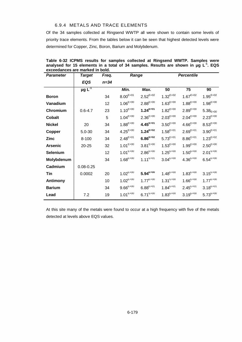
6-179


Of the 34 samples collected at Ringsend WWTP all were shown to contain some levels of

priority trace elements. From the tables below it can be seen that highest detected levels were

determined for Copper, Zinc, Boron, Barium and Molybdenum.

Table 6-32 ICPMS results for samples collected at Ringsend WWTP. Samples were analysed for 15 elements in a total of 34 samples. Results are shown in μg L

-1. EQS

exceedances are marked in bold.

Parameter Target

EQS

Freq.

n=34

Range Percentile

µg L-1

Min. Max. 50 75 90

Boron 34 8.00E+01

2.52E+02

1.32E+02

1.67E+02

1.95E+02

Vanadium 12 1.06E+00

2.88E+00

1.63E+00

1.88E+00

1.98E+00

Chromium 0.6-4.7 23 1.10E+00

1.24E+01

1.82E+00

2.89E+00

5.38E+00

Cobalt 5 1.04E+00

2.36E+00

2.03E+00

2.04E+00

2.23E+00

Nickel 20 34 1.88E+00

4.45E+01

3.50E+00

4.66E+00

8.53E+00

Copper 5.0-30 34 4.25E+00

1.24E+02

1.58E+01

2.69E+01

3.90E+01

Zinc 8-100 34 2.48E+01

6.86E+02

5.73E+01

8.86E+01

1.23E+02

Arsenic 20-25 32 1.01E+00

3.81E+00

1.53E+00

1.99E+00

2.50E+00

Selenium 12 1.01E+00

2.86E+00

1.25E+00

1.50E+00

2.01E+00


1.11E+01

3.04E+00

4.36E+00

6.54E+00

Cadmium 0.08-0.25

Tin 0.0002 20 1.02E+00

5.94E+00

1.48E+00

1.83E+00

3.15E+00

Antimony 10 1.02E+00

1.77E+00

1.31E+00

1.66E+00

1.77E+00

Barium 34 9.66E+00

6.88E+01

1.84E+01

2.45E+01

3.18E+01

Lead 7.2 19 1.01E+00

6.71E+00

1.83E+00

3.19E+00

5.73E+00

At this site many of the metals were found to occur at a high frequency with five of the metals

detected at levels above EQS values.

6-180

6.10 Swords

6.10.1 INTRODUCTION

At the Swords site 44 samples were collected monthly over a sampling period that spanned

November 2009 through July 2011. Table 6-33 shows dates of sample collection at Swords

WWTP. This section will provide an overview of sampling results collected from this site

providing information of levels of PAHs, pesticides and metals and trace elements determined in

the WWTP effluent stream. At the Swords site there were a number of periods of intensive

sampling carried out, with samples collected every second day during the winter and summer

months.

Table 6-33 Dates of sample collections at Swords WWTP.

2009 2010 2011

Sampling

Dates

17/11/2009

02/12/2009

04/12/2009

09/12/2009

11/12/2009

16/12/2009

18/12/2009

10/02/2010

15/03/2010

19/04/2010

31/05/2010

08/06/2010

09/06/2010

11/06/2010

14/06/2010

16/06/2010

18/06/2010

12/07/2010

14/07/2010

16/07/2010

19/07/2010

21/07/2010

23/07/2010

16/08/2010

18/08/2010

22/09/2010

29/10/2010

15/12/2010

09/01/2011

20/01/2011

21/01/2011

28/02/2011

28/03/2011

12/04/2011

30/05/2011

27/06/2011

28/06/2011

01/07/2011

05/07/2011

06/07/2011

08/07/2011

11/07/2011

13/07/2011

15/07/2011

6-181

6.10.2 PAHS

Presented in this section are the PAH results for Swords WWTP, Table 6-34. All samples were




Table 6-34 Results of PAH analysis for Swords WWTP. Results are compared to their respective Maximum Allowable Concentration Environmental Quality Standard (MAC EQS). All units are in µg L




µg L-1

Freq.

n=44

Range Percentile

Min. Max. 50 75 90

Naph. 1.2 44 <LOD 6.26E-02

5.54E-04

4.69E-03

1.43E-02

Ant. 0.1 44 <LOD 5.96E-02

6.24E-04

3.03E-02

4.48E-02

Fluor. 0.1 44 <LOD 3.42E-02

6.13E-04

1.73E-02

3.17E-02

Bb/k Σ=0.003 39 <LOD 2.55E-04

0.00E+00

1.46E-06

3.12E-06

Bap 0.05 36 <LOD 1.79E-02

6.80E-06

8.67E-03

1.78E-02

Ind + Bghi Σ=0.002 39 <LOD 9.20E-04

0.00E+00

2.69E-07

1.53E-06

Table 6-34 shows that the more water soluble PAHs, naphthalene, anthracene and

fluoranthene, were detected in all samples collected, while the less water soluble, higher

octanol/water partition coefficient PAHs, were slightly less frequently detected. Of these PAHs

there were no exceedences of the EQS limits detected.

6-182

6.10.3 PESTICIDES

Presented in this section are the pesticide results for Ballincollig WWTP, Table 6-35. All





Table 6-35 Results of pesticide analysis for Swords WWTP. Results are compared to their respective Maximum Allowable Concentration Environmental Quality Standard (MAC EQS). All units are in µg L


Annual Average EQS (AA EQS) for this compound.


µg L-1

Freq.

n=40

Range Percentile

Min. Max. 50 75 90


1.31E-01

2.47E-01

2.66E-01


2.77E-01

4.25E-01

5.26E-01


1.92E+00

3.79E+00

4.49E+00

Diuron 1.8 40 ND 1.4E+00

4.53E-01

9.88E-01

1.11E+00


2.9E-03

1.61E-03

2.24E-03

2.53E-03

Isoproturon 1.0 8 9.5E-04

3.9E-02

4.46E-03

6.23E-03

1.58E-02

Malathion 19 ND 2.0E+00

5.21E-01

8.83E-01

1.65E+00

Simazine 4.0 24 ND 1.2E+00

2.49E-01

4.78E-01

6.19E-01

Fenitrothion 29 ND 4.0E+00

8.04E-01

1.40E+00

2.78E+00

Pirimiphos methyl 28 ND 2.3E+00

5.48E-01

9.69E-01

1.53E+00


1.86E-02

3.67E-02

6.95E-02

DEHP 1.3* 33 ND 2.3E+00

3.22E-01

5.96E-01

6.81E-01

Table 6-35 shows that 12 of the priority pesticides were detected in samples from Swords

WWTP. Of these pesticides there were exceedences of the EQS limits for the chlorfenvinphos,

chlorpyrifos and DEHP (marked in bold in Table 6-35). Of the 40 samples collected at this site

only diuron was found to occur in all samples.

6-183


Of the 29 samples collected at Swords WWTP all were shown to contain some levels of priority



Table 6-36 ICPMS results for samples collected at Swords WWTP. Samples were analysed for 15 elements in a total of 29 samples. Results are shown in μg L

-1. EQS

exceedances are marked in bold.


Freq. n=29

Range Percentile

µg L-1

Min Max 50 75 90

Boron 29 3.84E+01

1.75E+02

7.64E+01

9.51E+01

1.03E+02

Vanadium 5 1.45E+00

6.32E+00

3.49E+00

3.94E+00

5.37E+00

Chromium 0.6-4.7 11 1.04E+00

6.54E+00

2.12E+00

3.07E+00

5.71E+00

Cobalt 3 1.11E+00

2.98E+00

1.17E+00

2.08E+00

2.62E+00

Nickel 20 29 1.22E+00

1.05E+01

2.52E+00

4.91E+00

5.98E+00

Copper 5.0-30 29 7.27E+00

3.14E+02

1.79E+01

2.87E+01

6.72E+01

Zinc 8-100 29 1.74E+01

3.05E+02

4.15E+01 9.98E+01

1.51E+02

Arsenic 20-25 6 1.03E+00

6.30E+00

1.64E+00

2.92E+00

4.80E+00

Selenium 7 1.04E+00

3.99E+00

1.26E+00

2.24E+00

3.16E+00


1.29E+01

1.86E+00

2.55E+00

3.75E+00

Cadmium 0.08-0.25 0

Tin 0.0002 6 1.06E+00

5.44E+00

2.74E+00

3.62E+00

4.54E+00

Antimony 5 1.04E+00

6.66E+00

1.25E+00

2.46E+00

4.98E+00

Barium 29 2.40E+00

1.29E+02

1.01E+01

1.55E+01

3.74E+01

Lead 7.2 11 1.48E+00

7.78E+00

2.48E+00

5.06E+00

6.81E+00

Chromium, copper, zinc, tin and lead were found to occur at levels above EQS values in the

Swords WWTP effluent.

6-184

6.11 Overview of Results

A total of 164 samples were collected from the 9 sites over the sampling period. In this section

the summaries of the analytical results obtained are presented, allowing for the evaluation of

each site based on the information. Along with results on the levels of occurrence of priority

PAHs, pesticides and metals and trace elements information on conditions at each site was

obtained where available.

Figure 6-1 Rainfall in the Ballincollig catchment in relation to SUM PAH and Pesticide concentrations in WWTP effluent over the sampling period.

In Ballincollig information on rainfall was available for the sampling period making it possible to

determine SUM levels of priority pesticides and PAHs at both dry and wet weather flow, Figure

6-1. No relationship between levels of PAHs and pesticides can discerned, with high PAH levels

occurring at different times than those of the pesticides.

0.00E+00

2.00E-02

4.00E-02

6.00E-02

8.00E-02

1.00E-01

1.20E-01

1.40E-01

0

2

4

6

8

10

12

14

24-Jun-10 24-Aug-10 24-Oct-10 24-Dec-10 24-Feb-11 24-Apr-11 24-Jun-11

Rainfall Sum PEST Sum PAH

Concentr

atio

n μ

g L

-1

Rain

fall

(mm

)

Ballincollig WWTP

6-185

Figure 6-2 SUM PAH and Pesticide concentrations detected in the WWTP effluent in Bandon over the sampling period.

In Bandon information on rainfall or flow was not available for the sampling period, therefore

PAH and pesticide levels are plotted over time in Figure 6-2. No relationship between levels of

PAHs and pesticides can discerned, with high PAH levels occurring at different times than those

of the pesticides.

Figure 6-3 SUM PAH and Pesticide concentrations detected in the Charleville WWTP effluent over the sampling period.

In Charleville information on rainfall or flow was not available for the sampling period, therefore

PAH and pesticide levels are plotted over time in Figure 6-3. There was no apparent

relationship between pesticide and PAH occurrence in the samples.

0.00E+00

5.00E-04

1.00E-03

1.50E-03

2.00E-03

2.50E-03

3.00E-03

0.00E+00

5.00E+00

1.00E+01

1.50E+01

2.00E+01

2.50E+01

3.00E+01

3.50E+01

4.00E+01

5/22/10 8/10/10 10/29/10 1/17/11 4/7/11 6/26/11 9/14/11

Sum PEST Sum PAH

Pesticid

e C

oncentr

ation μ

g L

-1

PA

H C

oncentr

ation μ

g L

-1

Bandon WWTP

0.00E+00

5.00E-03

1.00E-02

1.50E-02

2.00E-02

2.50E-02

3.00E-02

3.50E-02

4.00E-02

0.00E+00

2.00E+00

4.00E+00

6.00E+00

8.00E+00

1.00E+01

1.20E+01

5/22/10 9/19/10 1/17/11 5/17/11 9/14/11

Sum PEST Sum PAH

Pesticid

e C

oncentr

ation μ

g L

-1

PA

H C

oncentr

ation μ

g L

-1

Charleville WWTP

6-186

Figure 6-4 SUM PAH and Pesticide concentrations detected in the WWTP effluent in Clonakilty over the sampling period.

No information on rainfall or flow was available for the sampling period at Clonakilty WWTP,

therefore PAH and pesticide levels are plotted over time, Figure 6-4. No relationship between

levels of PAHs and pesticides can discerned, with high PAH levels occurring at different times

than those of the pesticides.

Figure 6-5 SUM PAH and Pesticide concentrations detected in effluent samples from Fermoy WWTP over the sampling period.

In Fermoy information on rainfall or flow was not available for the sampling period, therefore

PAH and pesticide levels are plotted over time in Figure 6-5. No relationship between levels of

PAHs and pesticides can discerned, with high PAH levels occurring at different times than those

of the pesticides.

0.00E+00

1.00E-04

2.00E-04

3.00E-04

4.00E-04

5.00E-04

6.00E-04

7.00E-04

8.00E-04

9.00E-04

1.00E-03

0.00E+00

5.00E+00

1.00E+01

1.50E+01

2.00E+01

2.50E+01

7-Apr-11 27-Apr-11 17-May-11 6-Jun-11 26-Jun-11 16-Jul-11

Sum PEST Sum PAH

Pesticid

e C

oncentr

ation μg L

-1

PA

H C

oncentr

ation μg L

-1

Clonakilty WWTP

0.00E+00

5.00E-03

1.00E-02

1.50E-02

2.00E-02

2.50E-02

0.00E+00

2.00E+00

4.00E+00

6.00E+00

8.00E+00

1.00E+01

1.20E+01

1.40E+01

5/22/10 8/10/10 10/29/10 1/17/11 4/7/11 6/26/11 9/14/11

Sum PEST Sum PAH

Pesticid

e C

oncentr

ation μg L

-

1

PA

H C

oncentr

ation μg L

-1

Fermoy WWTP

6-187

Figure 6-6 Rainfall in the Mallow catchment in relation to SUM PAH and Pesticide concentrations in WWTP effluent over the sampling period.

In Mallow information on rainfall was available for the sampling period, therefore PAH and

pesticide levels are plotted over time with rainfall superimposed, Figure 6-6, this allows for the

comparison between samples collected during wet and dry wither conditions. No relationship

between levels of PAHs and pesticides can discerned, with high PAH levels occurring at

different times than those of the pesticides.

Figure 6-7 Rainfall in the Ringaskiddy catchment in relation to SUM PAH and Pesticide concentrations in WWTP effluent over the sampling period.

In Ringaskiddy information on rainfall was available for the sampling period, therefore PAH and

pesticide levels are plotted over time with rainfall superimposed, Figure 6-7. This allows for the

0.00E+00

1.00E-03

2.00E-03

3.00E-03

4.00E-03

5.00E-03

6.00E-03

7.00E-03

8.00E-03

9.00E-03

0

5

10

15

20

25

8-Jul-10 8-Sep-10 8-Nov-10 8-Jan-11 8-Mar-11 8-May-11 8-Jul-11

Rainfall (mm) Sum PEST Sum PAH

Rain

fall

(mm

)

Concentr

atio

n μ

g L

-1

Mallow WWTP

0.00E+00

1.00E-02

2.00E-02

3.00E-02

4.00E-02

5.00E-02

6.00E-02

7.00E-02

8.00E-02

0

5

10

15

20

25

30

6/15/10 8/15/10 10/15/10 12/15/10 2/15/11 4/15/11 6/15/11

Rainfall (mm) Sum PEST Sum PAH

Rain

fall

(mm

)

Concentr

atio

n μg L

-1

Ringaskiddy WWTP

6-188

comparison between samples collected during wet and dry weather conditions. No relationship

between levels of PAHs and pesticides can be discerned, with high PAH levels occurring at

different times than those of the pesticides.

Information on rainfall was available for the sampling period in the Ringsend catchment

therefore PAH and pesticide levels are plotted over time with rainfall superimposed, Figure 6-8

and Figure 6-9. This allows for the comparison between samples collected during wet and dry

weather conditions. In order to evaluate results and characterise as occurring during ‘wet’ or

‘dry’ conditions it was necessary to plot rainfall against flow through the plant for the entire

sampling period. Then the relationship between rainfall and flow was assessed. In Ringsend

there was no delay between rainfall increase and flow increase. No relationship between levels

of PAHs and pesticides can discerned, with high PAH levels occurring at different times than

those of the pesticides.

Figure 6-8 WWTP flow levels in the Ringsend catchment in relation to SUM PAH concentrations in WWTP effluent over the sampling period for both WWF and DWF conditions.

In both Figure 6-8 and Figure 6-9 a sharp increase in the levels of detected PAHs was noted in

samples collected in June 2010. This increase coincided with an increase in the flow through

the plant at this time however past peaks had not had such a notable effect on the levels of

PAHs. From contact with technicians at the WWTP it was found that during this same time

period the plant had not been operating fully with the digesters not in operation. This in turn

reduces the removal efficiency of the plant for priority substances during this period of down-

time. While it is possible to compensate for this type of occurrence by reducing the removal

efficiency value and thus the effluent factor in modelling calculations it is important to note that

these periods of down-time must be recorded and reported so that appropriate monitoring

procedures can be put in place.

0

200000

400000

600000

800000

1000000

1200000

0.00E+00

1.00E-02

2.00E-02

3.00E-02

4.00E-02

5.00E-02

6.00E-02

7.00E-02

8.00E-02

26-Jun-09 4-Oct-09 12-Jan-10 22-Apr-10 31-Jul-10 8-Nov-10 16-Feb-11 27-May-11

Flow (m3/day) SUM PAH DWF SUM PAH WWF

Concentr

atio

n μg L

-1

Flo

w m

3/D

ay

Ringsend WWTP

6-189

Figure 6-9 WWTP flow levels in the Ringsend catchment in relation to SUM Pesticide concentrations in WWTP effluent over the sampling period for both WWF and DWF conditions.

In Swords WWTP information on rainfall and was available for the sampling period therefore

PAH and pesticide levels are plotted over time with rainfall superimposed, Figure 6-10 and

Figure 6-11. This allows for the comparison between samples collected during wet and dry

weather conditions. In order to evaluate results and characterise as occurring during ‘wet’ or

‘dry’ conditions it was necessary to plot rainfall against flow through the plant for the entire

sampling period. Then the relationship between rainfall and flow was assessed. In Swords there

was a 1-day delay between rainfall increases and flow increase, therefore this was taken into

account when judging WWF and DWF samples. No relationship between levels of PAHs and

pesticides can discerned with high PAH levels occurring at different times than those of the

pesticides.

0

200000

400000

600000

800000

1000000

1200000

0.00E+00

2.00E+00

4.00E+00

6.00E+00

8.00E+00

1.00E+01

1.20E+01

1.40E+01

26-Jun-09 4-Oct-09 12-Jan-10 22-Apr-10 31-Jul-10 8-Nov-10 16-Feb-11 27-May-11

Flow (m3/day) SUM Pest DWF SUM Pest WWF

Concentr

atio

n μg L

-1

Flo

w m

3/D

ay

Ringsend WWTP

6-190

Figure 6-10 WWTP flow levels in the Swords catchment in relation to SUM PAH concentrations in WWTP effluent over the sampling period for both WWF and DWF conditions.

Figure 6-11 WWTP flow levels in the Swords catchment in relation to SUM Pesticide concentrations in WWTP effluent over the sampling period for both WWF and DWF conditions.

0

5000

10000

15000

20000

25000

30000

0

0.02

0.04

0.06

0.08

0.1

0.12

0.14

14-Oct-09 22-Jan-10 2-May-10 10-Aug-10 18-Nov-10 26-Feb-11 6-Jun-11 14-Sep-11

Flow (m3/day) Sum PAH DWF Sum PAH WWF

Concentr

atio

n μg L

-1

Flo

w m

3/D

ay

Swords WWTP

0

5000

10000

15000

20000

25000

30000

0

2

4

6

8

10

12

14

16

14-Oct-09 22-Jan-10 2-May-10 10-Aug-10 18-Nov-10 26-Feb-11 6-Jun-11 14-Sep-11

Flow (m3/day) Sum Pest DWF Sum Pest WWF

Concentr

atio

n μg L

-1

Flo

w m

3/D

ay

Swords WWTP

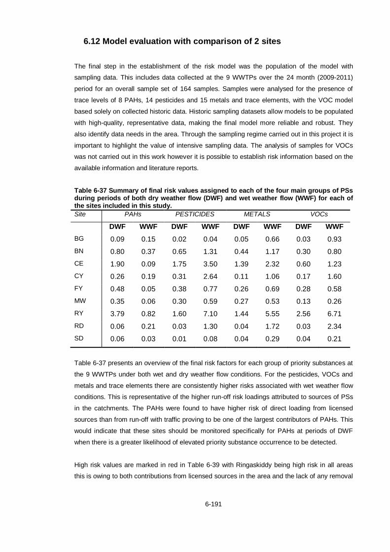
6-191

6.12 Model evaluation with comparison of 2 sites

The final step in the establishment of the risk model was the population of the model with

sampling data. This includes data collected at the 9 WWTPs over the 24 month (2009-2011)

period for an overall sample set of 164 samples. Samples were analysed for the presence of

trace levels of 8 PAHs, 14 pesticides and 15 metals and trace elements, with the VOC model

based solely on collected historic data. Historic sampling datasets allow models to be populated

with high-quality, representative data, making the final model more reliable and robust. They

also identify data needs in the area. Through the sampling regime carried out in this project it is

important to highlight the value of intensive sampling data. The analysis of samples for VOCs

was not carried out in this work however it is possible to establish risk information based on the

available information and literature reports.

Table 6-37 Summary of final risk values assigned to each of the four main groups of PSs during periods of both dry weather flow (DWF) and wet weather flow (WWF) for each of the sites included in this study.

Site PAHs PESTICIDES METALS VOCs

DWF WWF DWF WWF DWF WWF DWF WWF

BG 0.09 0.15 0.02 0.04 0.05 0.66 0.03 0.93

BN 0.80 0.37 0.65 1.31 0.44 1.17 0.30 0.80

CE 1.90 0.09 1.75 3.50 1.39 2.32 0.60 1.23

CY 0.26 0.19 0.31 2.64 0.11 1.06 0.17 1.60

FY 0.48 0.05 0.38 0.77 0.26 0.69 0.28 0.58

MW 0.35 0.06 0.30 0.59 0.27 0.53 0.13 0.26

RY 3.79 0.82 1.60 7.10 1.44 5.55 2.56 6.71

RD 0.06 0.21 0.03 1.30 0.04 1.72 0.03 2.34

SD 0.06 0.03 0.01 0.08 0.04 0.29 0.04 0.21

Table 6-37 presents an overview of the final risk factors for each group of priority substances at

the 9 WWTPs under both wet and dry weather flow conditions. For the pesticides, VOCs and

metals and trace elements there are consistently higher risks associated with wet weather flow

conditions. This is representative of the higher run-off risk loadings attributed to sources of PSs

in the catchments. The PAHs were found to have higher risk of direct loading from licensed

sources than from run-off with traffic proving to be one of the largest contributors of PAHs. This

would indicate that these sites should be monitored specifically for PAHs at periods of DWF

when there is a greater likelihood of elevated priority substance occurrence to be detected.

High risk values are marked in red in Table 6-39 with Ringaskiddy being high risk in all areas

this is owing to both contributions from licensed sources in the area and the lack of any removal

6-192

of pollutants at the sampling site which as yet provides no treatment and acts merely as a

pumping station.

By examining two of the sites more closely, Ballincollig in Cork and Ringsend in Dublin, it is

possible to validate the model making it applicable to any site. As no VOC analysis was carried

out that model is based entirely on historic, license and collected data.

Ballincollig and Ringsend were chosen as the sites to be included in this model validation step

as they represent both counties in the study, two different levels of treatment and removal

efficiency, two different types of input to the respective plants and were the sites with the most

available data for collection and population of the model. They are representative of the range

of conditions evaluated in the model. Specific flow data for each of these WWTPs allowed for a

clear distinction between WWF and DWF conditions whereas a number of the other sites did

not collect flow data sets and flow data was determined solely from weather conditions and

historic data. These facts made Ringsend and Ballincollig the most rational choices for the

validation study.

Table 6-38 Exceedances of priority substances at two WWTPs.

Ballincollig Ringsend

PAHs Benzo-b/k-fluoranthene and

indeno-1,2,3cd-pyrene/benzo-ghi-

perylene all exceed EQS in 90

percentile

indeno-1,2,3cd-pyrene/benzo-ghi-

perylene exceed EQS above 90

percentile

Pesticides Chlorfenvinphos and DEHP exceed

EQS in 50 percentile

Alachlor, DEHP, chlorfenvinphos,

diuron, and chlorpyrifos exceed EQS

in 90 percentile

Metals and Trace

Elements

Tin and lead exceed EQS above 50

percentile

Chromium, copper, zinc and tin

exceed EQS in 50 percentile

Nickel exceeds EQS in 90 percentile

A true comparison of the two sites can be demonstrated in Table 6-38 above. This table shows

detected exceedence of EQS values for specific pollutants from each group of pollutants by site.

The percentile of exceedence is also included to show the frequency of occurrence of these

high levels of PSs.

Ballincollig was found to have low risk attributed to all areas even during WWF while Ringsend

is classified as at risk of high levels of both pesticides and metals under the same conditions.

Breaking this down by group it is possible to rationale these results. First focussing on the PAHs

the results show that Ringsend was found to have higher frequency of occurrence for the WFD

6-193

priority PAHs than Ballincollig, and the WWF risk is corroborated by the maximum sum PAH

concentration detected during WWF which was only 2.06 x 10-02

at Ballincollig compared to 7.56

x 10-02

at Ringsend, the same was true for mean PAH concentrations. This result is expected

when taking into account the catchment characteristics, while Ringsend has over 200 licensed

sources of PSs that were evaluated for risk Ballincollig has only 7 trade effluent licenses, 4 of

which are petrol stations that are considered to be sources of PAHs making them the main

licensed sources of PAHs in that catchment. Also, in conjunction with the much lower population

in the Ballincollig catchment compared to the Ringsend catchment there is a higher level of

traffic contributing PAHs to Ringsend than site Ballincollig. However, when taking into account

notably high levels of occurrence, Table 6-38 shows that while there was a higher frequency of

occurrence of PAHs at Ringsend, there were more exceedences of EQS levels in Ballincollig.

The pesticides were risked higher at Ringsend for both WWF and DWF than Ballincollig. While

results show higher percentage occurrence of most pesticides at Ringsend results gave both

higher maximum sum pesticide concentration and average sum pesticide concentration at WWF

for Ballincollig. Table 6-38 shows that while Ballincollig has a higher level of EQS exceedence

for two pesticides, Ringsend has a greater range of pesticides exceeding EQS values in the 90

percentile of samples. Ballincollig, although covering a much smaller area than Ringend, has

both a higher combined drainage factor and a higher percentage nonurban area than Ringsend

(30% compared to 25%).

The issue with pesticide loading factors can be attributed to data gaps in this area, specifically

usage data and unlicensed sources. Large comprehensive datasets are needed which would

cover the usage statistics, import and purchasing of priority substances, especially pesticides,

as there are currently unexplained levels of banned substances occurring in Irish wastewaters.

For example pesticides such as atrazine and simazine were found to be present in a number of

samples collected at sites in both Dublin and Cork, substances which have been banned for

several years. Other pesticides such as alachlor and aldrin were also detected even though

these substances would have to be sourced from African or Mediterranean countries and would

not be expected to be found here in Ireland. It is discoveries such as these which lead us to

recommend that banned and obscure pollutants are not removed completely from current and

future monitoring programs as their continued presence in water systems must be noted and

steps to remediation taken. There are also potentially large sources of pesticides which are

unlicensed, e.g. golf courses apply pesticides but are not required to report usage of-, account

for disposal of- or potential run-off of pesticides from their greens leading to official loading

factors of zero. Through the development of this model it is observations such as these which

will facilitate the success of future monitoring programs.

The metals and trace elements risk assessments met expectations with Ringsend ranked as a

higher risk than Ballincollig. Ringsend shows both higher percentage frequency of occurrence

for the metals and trace elements, but also a wider variety of these substances than Ballincollig.

6-194

Table 6-38 shows results in agreement with the model with a number of metals found to exceed

EQS levels at a higher percentage occurrence in Ringsend than for Ballincollig. Ringsend also

covers a much larger catchment with a higher percent urban area than site 1 (75% compared to

70%). This catchment included 36 waste licenses, 66 IPPC licenses and 253 trade effluent

licenses, many of which are for laboratories, construction and machinery companies, the

transport industry and other sources which are highly ranked for loading of PSs.

Through the comparison of these sites the model has been found to be true to analytical results

from a strict sampling regime with results fitting the model created based on a large dataset of

licenses, annual environmental reports and historic data. The model can be further adapted and

is receptive to unlimited amounts of data making it amenable to continuous updating.

Table 6-39 Comparison of predicted risk to actual risk determined from sampling data for two sites.

6-195

6.13 Application of Model

The main application of this model is the use in identifying the risks of priority substance

occurrence at a site under both wet and dry weather conditions. This simple model can

therefore be used in the development of future monitoring programmes, reducing the need for

and cost of non-specific monitoring methods. Table 6-40 shows the final risk based model for

the occurrence of priority substances in wastewater. The rankings applied relate to the scale of

risk of occurrence of priority substances, Table 6-41. Green indicates a low risk of PS loading

during certain conditions with risk progressively increasing to a high risk of loading indicated in

red. The Ringaskiddy site has been ranked as very high risk owing to the lack of treatment of

the wastewater at this site.

Table 6-40 Final risk rankings attributed to each site for the four main groups of WFD priority substances under both WWF and DWF conditions. Dark green = low risk. Light green = some risk. Yellow = moderate risk. Orange = high risk. Red = very high risk.

Site PAHs PESTICIDES METALS VOCs


BG 0.09 0.15 0.02 0.04 0.05 0.66 0.03 0.93

BN 0.8 0.37 0.65 1.31 0.44 1.17 0.3 0.8

CE 1.9 0.09 1.75 3.5 1.39 2.32 0.6 1.23

CY 0.26 0.19 0.31 2.64 0.11 1.06 0.17 1.6

FY 0.48 0.05 0.38 0.77 0.26 0.69 0.28 0.58

MW 0.35 0.06 0.3 0.59 0.27 0.53 0.13 0.26

RY 3.79 0.82 1.6 7.1 1.44 5.55 2.56 6.71

RD 0.06 0.21 0.03 1.3 0.04 1.72 0.03 2.34

SD 0.06 0.03 0.01 0.08 0.04 0.29 0.04 0.21

Through the collection of data as described in chapter 5 it can be concluded that the same

ranking system can be applied to other catchments and can be used as a guidance document

for the monitoring of PSs in an area. By generating risk factors using the methods described the

scale outlined in Table 6-41 below can be used to evaluate the risks of occurrence of PSs at a

site under both wet and dry weather conditions.

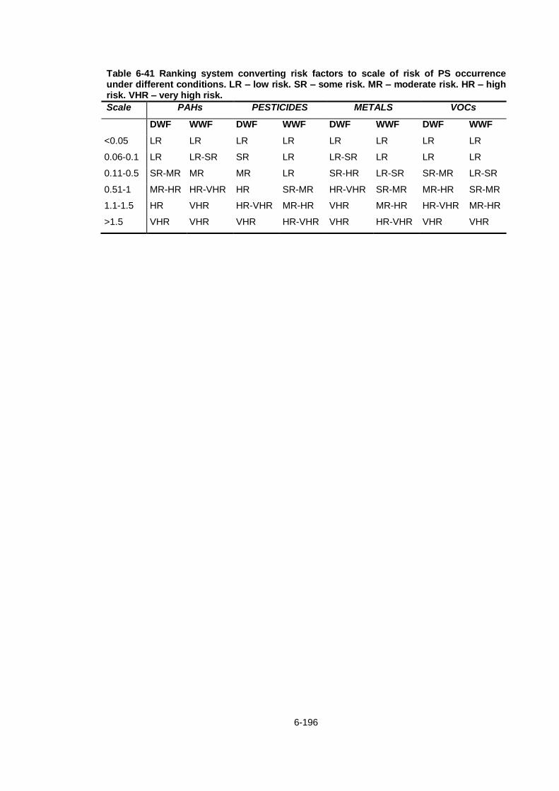
6-196

Table 6-41 Ranking system converting risk factors to scale of risk of PS occurrence under different conditions. LR – low risk. SR – some risk. MR – moderate risk. HR – high risk. VHR – very high risk.

Scale PAHs PESTICIDES METALS VOCs


<0.05 LR LR LR LR LR LR LR LR

0.06-0.1 LR LR-SR SR LR LR-SR LR LR LR

0.11-0.5 SR-MR MR MR LR SR-HR LR-SR SR-MR LR-SR

0.51-1 MR-HR HR-VHR HR SR-MR HR-VHR SR-MR MR-HR SR-MR

1.1-1.5 HR VHR HR-VHR MR-HR VHR MR-HR HR-VHR MR-HR

>1.5 VHR VHR VHR HR-VHR VHR HR-VHR VHR VHR

6-197

6.14 Conclusion

This chapter has continued on from the work detailed in chapter 5 and has presented the results

of sampling and analysis for each of the groups of priority substances at each of the nine

catchments included in the project. These samples were collected under different weather

conditions thus the weather conditions on the day of sampling as well the preceding days and

the subsequent effect on flow levels at the plant were all plotted and taken into account. This

allowed for the differentiation between samples collected under dry weather conditions and

those collected under wet weather conditions.

The collected data was statistically evaluated, the results of which are presented in this chapter.

This allowed for the data to be used to validate the theoretical model as outlined in chapter 5. A

thorough validation was carried out between the Ballincollig and Ringsend sites within this

chapter. Finally the model was simplified and a risk-scale legend was provided in Table 6-41

which can be directly applied to other sites for which this risk-based approach has been applied.

7-198

7. Conclusion

7-199

The development and implementation of targeted monitoring programmes for priority

substances in water is now more important than ever. Legislation has been put in place in the

form of the Water Framework Directive which has set a deadline of 2015 for all water bodies to

be of ‘good’ quality status. This thesis has examined the requirements of the WFD and the

associated list of priority substances. The chapters within the thesis identify and draw attention

to the current gaps in knowledge and provide a solution to monitoring issues in the form of a risk

based model. Throughout the course of this work 164 samples were collected. Each sample

was split and subjected to three different forms of sample preparation and analysis in triplicate.

This lead to the compilation of a database of thousands of chromatograms and mass spectra

which have each been statistically analysed and summarised. The time-consuming process of

simplifying the data resulted in a concise dataset in a format acceptable for input into the risk-

based model.

Chapters 1 and 2 summarise the legislation in the area of water quality in Ireland, specifically

the WFD and later amendments and statutory instruments. The project aims were outlined with

the main aim being the development of a risk-based model which could be used to inform

targeted monitoring programmes thus allowing Ireland to meet the water quality requirements of

the WFD. Wastewater input to surface waters is considered to be a major point source

contributor and was therefore selected as the medium to be studied. In order to accomplish this

task a database of sampling information representing sites across Ireland was required. This

involved the development of a strategic sampling plan which would provide information of

wastewater effluent quality over a large time-frame including periods of intensive sampling

which provides data on temporal variability in terms of pollutant concentrations. Site selection

was of prime importance as it was necessary to select a broad spectrum of sites covering a

span of population equivalents, input sources and levels of treatment. A well thought-out

sampling plan allowed for the achievement of these goals and nine different sites in both Dublin

and Cork were chosen.

After selecting the sampling sites and devising a sampling plan it was necessary to develop

methods for the extraction and analysis of the samples collected. Chapters 3 and 4 detail the

processes involved in method development and validation for the extraction and analysis of

priority PAHs, pesticides and metals and trace elements from a wastewater medium. It was

important that complete sample integrity was maintained throughout the process as high quality

data was required for the development of a model. Methods were selected based on extensive

literature review with due consideration given to extraction and analysis times and the

achievement of LODs sufficiently low to meet WFD and EQS requirements. Robust and reliable

multi-residue methods were developed with the PAH method by GCMS analysis improving on

current available methods in this area in terms of analysis times.

7-200

In chapter 5 the development and subsequent population of the model is presented. As with the

original aims of this project a database of information on emission factors, past priority

substance occurrence and other factors was built where no such database currently existed for

Ireland. This collection of data allowed for the identification of gaps in datasets and areas in

which the data was lacking and where this is a distinct need for improvement in the handling of,

storage of and access to complete datasets. An output of this project includes a report to the

EPA listing many recommendations in which improvements can be made to these identified

issues.

The creation of a framework for the model and population of the model was an on-going

process throughout the course of the project with the final stage being the inclusion of the

results of the 24 month sampling campaign. This data was thoroughly evaluated in terms of

emission factors and risk of loadings, both direct and indirect, at each of the sampling sites. The

results of this work are presented in chapter 6 in which analytical results for each group of

priority substances have been tabulated and statistically evaluated by sampling site. The data is

then compared and the final model is introduced. The results of three years of sampling and

data collection is a simple risk-based model which indicates the risk of occurrence of a group of

pollutants at a site under both wet and dry weather conditions.

This model is not restricted to only the sites included in this study, rather it allows for the

evaluation of any site. By implementing the same procedures as described, risk factors can be

attributed to any site where sufficient data is available. These risk factors can be directly used in

developing a monitoring strategy as they inform the analyst under which conditions specific

groups of priority substances will be a risk of occurring. Implementation of this model has the

potential to reduce the costs, both time and monetary, associated with currently employed non-

specific monitoring/sampling regimes which can often miss high levels of pollutants as they do

not take into account emission factors such as weather conditions.

To conclude, this work has achieved the aims to which it has set out. A validated risk-based

model has been prepared and a database of high-quality information has been created. This

database brings together information on emission factors and occurrence of WFD priority

substances and contains data from over 1000 licenses and reports as well as three years of

experimental data. Recommendations from this project will be used by policy-makers in the

implementation of future monitoring programmes and this work has improved on the current

state of knowledge on the relationship between emission factors and priority substance

occurrence in Ireland.

7-201

References

7-202

ABAD, E., MARTÍNEZ, K., PLANAS, C., PALACIOS, O., CAIXACH, J. and RIVERA, J., 2005. Priority organic pollutant assessment of sludges for agricultural purposes. Chemosphere, 61(9), pp. 1358-1369.

AHLMAN, S. and SVENSSON, G., 2005. SEWSYS - a tool for simulation of substance flows in urban sewer systems. ISSN 1650-3791; no 2005:11. Göteborg: Chalmers

University of Technology.

AHMED, F.E., 2001. Analyses of pesticides and their metabolites in foods and drinks. TrAC Trends in Analytical Chemistry, 20(11), pp. 649-661.

ALLOWAY, B.J., 1995. Heavy Metals in Soils. Springer.

ARIAS-ESTÉVEZ, M., LÓPEZ-PERIAGO, E., MARTÍNEZ-CARBALLO, E., SIMAL-GÁNDARA, J., MEJUTO, J.C. and GARCÍA-RÍO, L., 2008. The mobility and degradation of pesticides in soils and the pollution of groundwater resources. Agriculture, Ecosystems & Environment, 123(4), pp. 247-260.

ARMENTA, S., GARRIGUES, S. and DE LA GUARDIA, M., 2005. Solid sampling Fourier transform infrared determination of Mancozeb in pesticide formulations. Talanta, 65(4), pp. 971-979.

ASANTE, K.A., AGUSA, T., SUBRAMANIAN, A., ANSA-ASARE, O.D., BINEY, C.A. and TANABE, S., 2007. Contamination status of arsenic and other trace elements in drinking water and residents from Tarkwa, a historic mining township in Ghana. Chemosphere, 66(8), pp. 1513-1522.

BARBOSA, V.L., TANDLICH, R. and BURGESS, J.E., 2007. Bioremediation of trace organic compounds found in precious metals refineries’ wastewaters: A review of potential options. Chemosphere, 68(7), pp. 1195-1203.

BARCO-BONILLA, N., VIDAL, J., GARRIDO FRENICH, A. and ROMERO-GONZÁLEZ, R., 2009. Comparison of ultrasonic and pressurized liquid extraction for the analysis of polycyclic aromatic compounds in soil samples by gas chromatography coupled to tandem mass spectrometry. Talanta, 78(1), pp. 156-164.

BARRO, R., REGUEIRO, J., LLOMPART, M. and GARCIA-JARES, C., 2009. Analysis of industrial contaminants in indoor air: Part 1. Volatile organic compounds, carbonyl compounds, polycyclic aromatic hydrocarbons and polychlorinated biphenyls. Journal of Chromatography A, 1216(3), pp. 540-566.

BARTON, S.C., JOHNSON, N.D. and DAS, B.S., 1979. Final Report to Air Resourches Branch Canadian Ministry of Environment: A feasibility study of alternatives to high-volume sampling for labile constituents of atmospheric particulates.

Ontario, Canada.: Ontario Research Foundation.

BECEIRO-GONZÁLEZ, E., CONCHA-GRAÑA, E., GUIMARAES, A., GONÇALVES, C., MUNIATEGUI-LORENZO, S. and ALPENDURADA, M., 2007. Optimisation and validation of a solid-phase microextraction method for simultaneous determination of different types of pesticides in water by gas chromatography–mass spectrometry. Journal of Chromatography A, 1141(2), pp. 165-173.

BENNETT, D.A., CHUNG, A.C. and LEE, S.M., 1997. Multiresidue method for analysis of pesticides in liquid whole milk. Journal of AOAC International, 80(5), pp. 1065-1077.

7-203

BERCARU, O., ULBERTH, F., EMONS, H. and VANDECASTEELE, C., 2006. Accurate quantification of PAHs in water in the presence of dissolved humic acids using isotope dilution mass spectrometry. Analytical and bioanalytical chemistry, 384(5), pp. 1207-1213.

BERMEJO-BARRERA, P., MUÑIZ-NAVEIRO, O., MOREDA-PIÑEIRO, A. and BERMEJO-BARRERA, A., 2000. Experimental designs in the optimisation of ultrasonic bath–acid-leaching procedures for the determination of trace elements in human hair samples by atomic absorption spectrometry. Forensic science international, 107(1), pp.

105-120.

BERSET, J., EJEM, M., HOLZER, R. and LISCHER, P., 1999. Comparison of different drying, extraction and detection techniques for the determination of priority polycyclic aromatic hydrocarbons in background contaminated soil samples. Analytica Chimica Acta, 383(3), pp. 263-275.

BJØRSETH, A. and DENNIS, A.J., 1980. Polynuclear aromatic hydrocarbons:

chemistry and biological effects.[Lead abstract], .

BOEHM, P.D., 2005. Environmental Forensics. In: R.D. MORRISON PH.D., B.L.

MURPHY, ed, Burlington: Academic Press, pp. 313-337.

BONNIEUX, F., CARPENTIER, A. and WEAVER, R., 1998. Reducing soil contamination: economic incentives and potential benefits. Agriculture, Ecosystems & Environment, 67(2-3), pp. 275-288.

BÖRJESSON, E. and TORSTENSSON, L., 2000. New methods for determination of glyphosate and (aminomethyl)phosphonic acid in water and soil. Journal of

Chromatography A, 886(1–2), pp. 207-216.

BOUSSAHEL, R., BOULAND, S., MOUSSAOUI, K., BAUDU, M. and MONTIEL, A., 2002. Determination of chlorinated pesticides in water by SPME/GC. Water research,

36(7), pp. 1909-1911.

BRUM, D.M. and NETTO, A.D.P., 2009. Polycyclic aromatic hydrocarbons in Tripuí River, Ouro Preto, MG, Brazil. Journal of hazardous materials, 165(1-3), pp. 447-453.

BUDZINSKI, H., GARRIGUES, P., RADKE, M., CONNAN, J. and OUDIN, J.L., 1993. Thermodynamic calculations on alkylated phenanthrenes: geochemical applications to maturity and origin of hydrocarbons. Organic Geochemistry, 20(7), pp. 917-926.

BULUT, V.N., GUNDOGDU, A., DURAN, C., SENTURK, H.B., SOYLAK, M., ELCI, L. and TUFEKCI, M., 2007. A multi-element solid-phase extraction method for trace metals determination in environmental samples on Amberlite XAD-2000. Journal of

hazardous materials, 146(1), pp. 155-163.

BUSETTI, F., HEITZ, A., CUOMO, M., BADOER, S. and TRAVERSO, P., 2006. Determination of sixteen polycyclic aromatic hydrocarbons in aqueous and solid samples from an Italian wastewater treatment plant. Journal of Chromatography A,

1102(1–2), pp. 104-115.

BUZIER, R., TUSSEAU-VUILLEMIN, M., DIT MERIADEC, C.M., ROUSSELOT, O. and MOUCHEL, J., 2006. Trace metal speciation and fluxes within a major French

7-204

wastewater treatment plant: Impact of the successive treatments stages. Chemosphere, 65(11), pp. 2419-2426.

CAMINO-SÁNCHEZ, F.J., ZAFRA-GÓMEZ, A., PÉREZ-TRUJILLO, J.P., CONDE-GONZÁLEZ, J.E., MARQUES, J.C. and VÍLCHEZ, J.L., 2011. Validation of a GC–MS/MS method for simultaneous determination of 86 persistent organic pollutants in marine sediments by pressurized liquid extraction followed by stir bar sorptive extraction. Chemosphere, 84(7), pp. 869-881.

CAO, Z., WANG, Y., MA, Y., XU, Z., SHI, G., ZHUANG, Y. and ZHU, T., 2005. Occurrence and distribution of polycyclic aromatic hydrocarbons in reclaimed water and surface water of Tianjin, China. Journal of hazardous materials, 122(1), pp. 51-59.

CARERI, M., MANGIA, A. and MUSCI, M., 1996. Applications of liquid chromatography-mass spectrometry interfacing systems in food analysis: pesticide, drug and toxic substance residues. Journal of chromatography A, 727(2), pp. 153-184.

CECCARINI, A., CECCHINI, I. and FUOCO, R., 2005. Determination of trace elements in seawater samples by on-line column extraction/graphite furnace atomic absorption spectrometry. Microchemical journal, 79(1), pp. 21-24.

CHEN, D., HU, B. and HUANG, C., 2009. Chitosan modified ordered mesoporous silica as micro-column packing materials for on-line flow injection-inductively coupled plasma optical emission spectrometry determination of trace heavy metals in environmental water samples. Talanta, 78(2), pp. 491-497.

CHEN, S., YU, X., HE, X., XIE, D., FAN, Y. and PENG, J., 2009. Simplified pesticide multiresidues analysis in fish by low-temperature cleanup and solid-phase extraction coupled with gas chromatography/mass spectrometry. Food Chemistry, 113(4), pp.

1297-1300.

CLARA, M., SCHARF, S., SCHEFFKNECHT, C. and GANS, O., 2007. Occurrence of selected surfactants in untreated and treated sewage. Water research, 41(19), pp.

4339-4348.

CLARKE, R., ROBERTS, A. and CONRAD, A., 2009. Chemical prioritisation: ranking chemicals of concern to Scotland’s environment, Phase 1: Surface Waters. Scotland:

Scottish EPA.

CONCHA-GRAÑA, E., FERNÁNDEZ-MARTÍNEZ, G., FERNÁNDEZ-VILLARRENAGA, V., TURNES-CAROU, M., MUNIATEGUI-LORENZO, S., LÓPEZ-MAHÍA, P. and PRADA-RODRÍGUEZ, D., 2009. A study of large-volume on-column injection GC-ECD for the ultratrace analysis of organochlorine pesticides in water. Talanta, 78(3), pp.

764-771.

CORK COUNTY COUNCIL, 2009. Ballincollig and Environs Agglomeration Annual Environmental Report. Johnstown Castle Estate, County Wexford, Ireland:

Environmental Protection Agency.

CORK COUNTY COUNCIL, 2008-last update, Bandon Waste Water Discharge License Application [Homepage of Irish EPA], [Online]. Available:

http://www.epa.ie/licences/lic_eDMS/090151b28024f684.pdf2012].

http://www.epa.ie/licences/lic_eDMS/090151b28024f684.pdf

7-205

CORK COUNTY COUNCIL, 2008-last update, Charleville Waste Water Discharge License Application [Homepage of Irish EPA], [Online]. Available:

http://www.epa.ie/terminalfour/wwda/wwda-view.jsp?regno=D0204-012012].

CORK COUNTY COUNCIL, 2008. Fermoy Waste Licence Application. Ireland: Irish

EPA.

CORK COUNTY COUNCIL, 2007-last update, Ballincollig Waste Water Discharge License Application [Homepage of Irish EPA], [Online]. Available:


CORK COUNTY COUNCIL, 2007-last update, Clonakilty Waste Water Discharge License Application [Homepage of Irish EPA], [Online]. Available: http://www.epa.ie/terminalfour/wwda/wwda-view-filter.jsp?regno=D0051-

01&filter=b&docfilter=go2012].

CORK COUNTY COUNCIL, 2007-last update, Fermoy Waste Water Discharge License Application [Homepage of Irish EPA], [Online]. Available: http://www.epa.ie/terminalfour/wwda/wwda-view.jsp?regno=D0058-012012].

CORK COUNTY COUNCIL, 2007-last update, Mallow Waste Water Discharge License Application [Homepage of Irish EPA], [Online]. Available:


CORK COUNTY COUNCIL, 2007-last update, Ringaskiddy Waste Water Discharge License Application [Homepage of Irish EPA], [Online]. Available: http://www.epa.ie/terminalfour/wwda/wwda-view.jsp?regno=D0057-012012].

CORK COUNTY COUNCIL - SOUTHERN DIVISION, 2010. Ballincollig and Environs Agglomeration Annual Environmental Report January 2010-December 2010.

Johnstown Castle Estate, County Wexford, Ireland: Environmental Protection Agency.

COUNTWAY, R.E., DICKHUT, R.M. and CANUEL, E.A., 2003. Polycyclic aromatic hydrocarbon (PAH) distributions and associations with organic matter in surface waters of the York River, VA Estuary. Organic Geochemistry, 34(2), pp. 209-224.

CROZIER, P.W., PLOMLEY, J.B. and MATCHUK, L., 2001. Trace level analysis of polycyclic aromatic hydrocarbons in surface waters by solid phase extraction (SPE) and gas chromatography-ion trap mass spectrometry (GC-ITMS). Analyst, 126(11), pp.

1974-1979.

CSO, 2009. Central Statistics Office Yearly Report. Ireland: Central Statistics Office.

DE ALMEIDA AZEVEDO, D., LACORTE, S., VINHAS, T., VIANA, P. and BARCELÓ, D., 2000. Monitoring of priority pesticides and other organic pollutants in river water from Portugal by gas chromatography–mass spectrometry and liquid chromatography–atmospheric pressure chemical ionization mass spectrometry. Journal of chromatography A, 879(1), pp. 13-26.

DE BOER, J. and LAW, R.J., 2003. Developments in the use of chromatographic techniques in marine laboratories for the determination of halogenated contaminants and polycyclic aromatic hydrocarbons. Journal of Chromatography A, 1000(1), pp. 223-

251.

http://www.epa.ie/terminalfour/wwda/wwda-view.jsp?regno=D0204-01


http://www.epa.ie/terminalfour/wwda/wwda-view-filter.jsp?regno=D0051-01&filter=b&docfilter=go

http://www.epa.ie/terminalfour/wwda/wwda-view-filter.jsp?regno=D0051-01&filter=b&docfilter=go




7-206

DE KEYSER, W., GEVAERT, V., VERDONCK, F., DE BAETS, B. and BENEDETTI, L., 2010. An emission time series generator for pollutant release modelling in urban areas. Environmental Modelling & Software, 25(4), pp. 554-561.

DIVRIKLI, Ü and ELÇI, L., 2002. Determination of some trace metals in water and sediment samples by flame atomic absorption spectrometry after coprecipitation with cerium (IV) hydroxide. Analytica Chimica Acta, 452(2), pp. 231-235.

DUBLIN CITY COUNCIL, 2007-last update, Ringsend Waste Water Discharge License Application [Homepage of Irish EPA], [Online]. Available:


DUBLIN CITY COUNCIL, 2003. Ringsend (sbr) Wastewater Treatment Plant Overview.

Ireland: Dublin City Council.

DUGAY, J., MIEGE, C. and HENNION, M.C., 1998. Effect of the various parameters governing solid-phase microextraction for the trace-determination of pesticides in water. Journal of Chromatography A, 795(1), pp. 27-42.

DUZGOREN-AYDIN, N.S., 2007. Sources and characteristics of lead pollution in the urban environment of Guangzhou. Science of the Total Environment, 385(1-3), pp.

182-195.

EATON, A.D. and FRANSON, M.A.H., 2005. Standard methods for the examination of

water & wastewater. Amer Public Health Assn.

EEC, 1991. Council Directive of 21 May 1991 Concerning Urban Waste Water

Treatment (91/271/EEC). Directive edn. European Union: European Union.

EEC, 1980. Council Directive 80/788/EEC. L 229. European Union: Official Journal of

the European Communities.

ESCALAS, A., GUADAYOL, J.M., CORTINA, M., RIVERA, J. and CAIXACH, J., 2003. Time and space patterns of volatile organic compounds in a sewage treatment plant. Water research, 37(16), pp. 3913-3920.

EUROPEAN PARLIAMENT, 2009. S.I. No. 272 of 2009 European Communities Environmental Objectives (Surface Waters) Regulations. Statutory Instrument edn.

Ireland: .

EUROPEAN PARLIAMENT, 2008. Directive 2008/105/EC of the European Parliament

and of the Council of 16 December 2008. Directive edn. European Union: .

EUROPEAN PARLIAMENT, 2000. Directive 2000/60/EC of the European Parliament and of the Council of 23 October 2000 establishing a framework for Community action in the field of water policy. Articles 2(30) and 16(2). European Union: European

Parliament.

EUROPEAN PARLIAMENT, 20 November 2001. Decision No 2455/2001/EC of the European Parliament and of the Council of 20 November 2001 establishing the list of priority substances in the field of water policy and amending Directive 2000/60/EC.

European Union: European Parliament and of the Council of 20 November 2001.


7-207

FAUSER, P., VIKELSØE, J., SØRENSEN, P.B. and CARLSEN, L., 2003. Phthalates, nonylphenols and LAS in an alternately operated wastewater treatment plant—fate modelling based on measured concentrations in wastewater and sludge. Water research, 37(6), pp. 1288-1295.

FEHILY, B., 2008. A Review of and Report on Certain Matters Relating to Dublin City Council's Ringsend Wastewater Treatment Plant. Ireland: Department of the

Environment.

FERNANDES, M. and SICRE, M.A., 1999. Polycyclic aromatic hydrocarbons in the Arctic: Ob and Yenisei estuaries and Kara Sea shelf. Estuarine, Coastal and Shelf Science, 48(6), pp. 725-737.

FILIPKOWSKA, A., LUBECKI, L. and KOWALEWSKA, G., 2005. Polycyclic aromatic hydrocarbon analysis in different matrices of the marine environment. Analytica

Chimica Acta, 547(2), pp. 243-254.

FINGAL COUNTY COUNCIL, 2007-last update, Swords Waste Water Discharge License Application 2007, EPA website: [Homepage of Irish EPA], [Online]. Available:


FINGAL COUNTY COUNCIL, 2004. Swords Wastewater Treatment Works. Ireland:

Fingal County Council.

GAGA, E.O. and TUNCEL, S.G., 2004. Extraction and Analysis of Polycyclic Aromatic Hydrocarbons (PAHs) from rain samples, 4th Aegean Analytical Chemistry Days Congress, 29 Sept-3 Oct.2004 2004, pp. Proceedings Book 246.

GALT, R.E., 2008. Beyond the circle of poison: Significant shifts in the global pesticide complex, 1976–2008. Global Environmental Change, 18(4), pp. 786-799.

GARBAN, B., BLANCHOUD, H., MOTELAY-MASSEI, A., CHEVREUIL, M. and OLLIVON, D., 2002. Atmospheric bulk deposition of PAHs onto France: trends from urban to remote sites. Atmospheric Environment, 36(34), pp. 5395-5403.

GASPERI, J., GARNAUD, S., ROCHER, V. and MOILLERON, R., 2008. Priority pollutants in wastewater and combined sewer overflow. Science of the Total

Environment, 407(1), pp. 263-272.

GIMENO, R., ALTELAAR, A., MARCE, R. and BORRULL, F., 2002. Determination of polycyclic aromatic hydrocarbons and polycylic aromatic sulfur heterocycles by high-performance liquid chromatography with fluorescence and atmospheric pressure chemical ionization mass spectrometry detection in seawater and sediment samples. Journal of Chromatography A, 958(1), pp. 141-148.

GMEINER, G., STEHLIK, G. and TAUSCH, H., 1997. Determination of seventeen polycyclic aromatic hydrocarbons in tobacco smoke condensate. Journal of Chromatography A, 767(1), pp. 163-169.

GÓMEZ, M.J., MARTÍNEZ BUENO, M.J., LACORTE, S., FERNÁNDEZ-ALBA, A.R. and AGÜERA, A., 2007. Pilot survey monitoring pharmaceuticals and related compounds in a sewage treatment plant located on the Mediterranean coast. Chemosphere, 66(6), pp. 993-1002.


7-208

GRAHAM, M.C., ALLAN, R., FALLICK, A.E. and FARMER, J., 2006. Investigation of extraction and clean-up procedures used in the quantification and stable isotopic characterisation of PAHs in contaminated urban soils. Science of the total environment, 360(1), pp. 81-89.

GUARDIA RUBIO, M., RUIZ MEDINA, A., PASCUAL REGUERA, M. and FERNÁNDEZ DE CÓRDOVA, M., 2007. Multiresidue analysis of three groups of pesticides in washing waters from olive processing by solid-phase extraction-gas chromatography with electrón capture and thermionic specific detection. Microchemical journal, 85(2), pp. 257-264.

HADA, M., TAKINO, M., YAMAGAMI, T., DAISHIMA, S. and YAMAGUCHI, K., 2000. Trace analysis of pesticide residues in water by high-speed narrow-bore capillary gas chromatography–mass spectrometry with programmable temperature vaporizer. Journal of Chromatography A, 874(1), pp. 81-90.

HAGESTUEN, E.D. and CAMPIGLIA, A.D., 1999. New approach for screening polycyclic aromatic hydrocarbons in water samples. Talanta, 49(3), pp. 547-560.

HARRISON, R., PERRY, R. and WELLINGS, R., 1975. Polynuclear aromatic hydrocarbons in raw, potable and waste water. WATER RESEARCH, VOL 9, NO 4, P

331-346, APRIL 1975.2 FIG, 20 TAB, 147 REF., .

HAYES,N.,PAGE,D.,SWEENEY,L.,O’LEARY,G., 2011. The Provision and Quality of Drinking Water in Ireland: A Report for the Year 2010. Ireland: Irish Environmental

Protection Agency.

HEITLAND, P. and KÖSTER, H.D., 2006. Biomonitoring of 30 trace elements in urine of children and adults by ICP-MS. Clinica Chimica Acta, 365(1), pp. 310-318.

HEITLAND, P. and KÖSTER, H.D., 2006. Biomonitoring of 37 trace elements in blood samples from inhabitants of northern Germany by ICP–MS. Journal of trace elements

in medicine and biology, 20(4), pp. 253-262.

HENNION, M.C., 1999. Solid-phase extraction: method development, sorbents, and coupling with liquid chromatography. Journal of Chromatography A, 856(1), pp. 3-54.

HERNÁNDEZ, F., SANCHO, J., POZO, O., LARA, A. and PITARCH, E., 2001. Rapid direct determination of pesticides and metabolites in environmental water samples at sub-μg/l level by on-line solid-phase extraction-liquid chromatography–electrospray tandem mass spectrometry. Journal of Chromatography A, 939(1), pp. 1-11.

HIRATA, S., ISHIDA, Y., AIHARA, M., HONDA, K. and SHIKINO, O., 2001. Determination of trace metals in seawater by on-line column preconcentration inductively coupled plasma mass spectrometry. Analytica Chimica Acta, 438(1-2), pp.

205-214.

HIRATA, S., KAJIYA, T., TAKANO, N., AIHARA, M., HONDA, K., SHIKINO, O. and NAKAYAMA, E., 2003. Determination of trace metals in seawater by on-line column preconcentration inductively coupled plasma mass spectrometry using metal alkoxide glass immobilized 8-quinolinol. Analytica Chimica Acta, 499(1-2), pp. 157-165.

7-209

HOGENDOORN, E. and VAN ZOONEN, P., 2000. Recent and future developments of liquid chromatography in pesticide trace analysis. Journal of Chromatography A,

892(1), pp. 435-453.

HOLVOET, K., SEUNTJENS, P. and VANROLLEGHEM, P.A., 2007. Monitoring and modeling pesticide fate in surface waters at the catchment scale. Ecological Modelling,

209(1), pp. 53-64.

HUCK, C. and BONN, G., 2000. Recent developments in polymer-based sorbents for solid-phase extraction. Journal of Chromatography A, 885(1), pp. 51-72.

IBÁÑEZ, M., PICÓ, Y. and MAÑES, J., 1998. Improving the solid-phase extraction of “quat” pesticides from water samples: Removal of interferences. Journal of Chromatography A, 823(1), pp. 137-146.

IRACE-GUIGAND, S., AARON, J., SCRIBE, P. and BARCELÓ, D., 2004. A comparison of the environmental impact of pesticide multiresidues and their occurrence in river waters surveyed by liquid chromatography coupled in tandem with UV diode array detection and mass spectrometry. Chemosphere, 55(7), pp. 973-981.

IRISH EPA, Oct. 2006. Appendix, 2.1 Surface Water Parameters and Groundwater Parameters for Dangerous Substances Monitoring, IRISH WFD Monitoring

Programme. Ireland: Irish Environmental Protection Agency.

IRISH EPA, 2012, 2012-last update, Database of EPA Waste Discharge License Applications [Homepage of Irish EPA], [Online]. Available: http://www.epa.ie/terminalfour/waste/waste-view.jsp?regno=W0089-022011].

IRISH EPA, 2006. Irish Water Framework Directive Monitoring Programme V1.0. V1.0.

Ireland: EPA.

IRISH EPA, 1997. Wastewater Treatment Manuals, Primary, Secondary & Tertiary

Treatment. Ardcavan, Wexford, Ireland: Irish Environmental Protection Agency.

JAFFREZO, J.L., MASCLET, P., CLAIN, M., WORTHAM, H., BEYNE, S. and CACHIER, H., 1993. Transfer function of polycyclic aromatic hydrocarbons from the atmosphere to the polar ice--I. Determination of atmospheric concentrations at dye 3, Greenland. Atmospheric Environment.Part A.General Topics, 27(17-18), pp. 2781-

2785.

JIMÉNEZ, J., BERNAL, J., DEL NOZAL, M.J., TORIBIO, L. and ARIAS, E., 2001. Analysis of pesticide residues in wine by solid-phase extraction and gas chromatography with electron capture and nitrogen–phosphorus detection. Journal of

chromatography A, 919(1), pp. 147-156.

JONES-LEPP, T.L. and MOMPLAISIR, G.M., 2005. New applications of LC–MS and LC–MS< sup> 2</sup> toward understanding the environmental fate of organometallics. TrAC Trends in Analytical Chemistry, 24(7), pp. 590-595.

JUNIOR, J.L.R. and RE-POPPI, N., 2007. Determination of organochlorine pesticides in ground water samples using solid-phase microextraction by gas chromatography-electron capture detection. Talanta, 72(5), pp. 1833-1841.

http://www.epa.ie/terminalfour/waste/waste-view.jsp?regno=W0089-02

7-210

KARTHIKEYAN, S. and BALASUBRAMANIAN, R., 2006. Interlaboratory study to improve the quality of trace element determinations in rainwater. Analytica Chimica

Acta, 576(1), pp. 9-16.

KAVCAR, P., SOFUOGLU, A. and SOFUOGLU, S.C., 2009. A health risk assessment for exposure to trace metals via drinking water ingestion pathway. International journal

of hygiene and environmental health, 212(2), pp. 216-227.

KLEIN, J. and ALDER, L., 2003. Applicability of Gradient Liquid Chromatography with Tandem Mass Spectrometry to the Simultaneous Screening for About 100 Pesticides in Crops. Journal of AOAC International, 86(5), pp. 1015-1037.

KOCASOY, G., MUTLU, H.İ and AYLIN ZEREN ALAGÖZ, B., 2008. Prevention of marine environment pollution at the tourism regions by the application of a simple method for the domestic wastewater. Desalination, 226(1), pp. 21-37.

KOOTSTRA, P., STRAUB, M., STIL, G., VAN DER VELDE, E., HESSELINK, W. and LAND, C., 1995. Solid-phase extraction of polycyclic aromatic hydrocarbons from soil samples. Journal of chromatography A, 697(1), pp. 123-129.

KORENKOVA, E., MATISOVA, E. and SLOBODNÍK, J., 2003. Study on the feasibility of coupling large‐ volume injection to fast gas chromatography with mass spectrometric detection for analysis of organochlorine pesticides. Journal of separation

science, 26(12‐ 13), pp. 1193-1197.

KOSTIAINEN, R. and KAUPPILA, T.J., 2009. Effect of eluent on the ionization process in liquid chromatography-mass spectrometry. Journal of Chromatography A, 1216(4),

pp. 685-699.

KULLENBERG, G., 1999. Approaches to addressing the problems of pollution of the marine environment: an overview. Ocean & Coastal Management, 42(12), pp. 999-

1018.

KUSTER, M., LÓPEZ DE ALDA, M. and BARCELÓ, D., 2006. Analysis of pesticides in water by liquid chromatography-tandem mass spectrometric techniques. Mass

Spectrometry Review, 25(6), pp. 900-916.

LAPERTOT, M., PULGARÍN, C., FERNÁNDEZ-IBÁÑEZ, P., MALDONADO, M., PÉREZ-ESTRADA, L., OLLER, I., GERNJAK, W. and MALATO, S., 2006. Enhancing Biodegradability of Priority Substances (Pesticides) by Solar Photo-Fenton. Water

Research, 40(5), pp. 1086-1094.

LARSON, S.J., CAPEL, P.D. and MAJEWSKI, M.S., eds, 1997. Pesticides in Surface Waters - Distribution, rends, and governing factors In Gilliom, R.J. (Ed.), series of

pesticides in hydrologic system. Vol 3 edn. Chelsea, Michigan: Ann Arbor press.

LAWLOR, A. and TIPPING, E., 2003. Metals in bulk deposition and surface waters at two upland locations in northern England. Environmental Pollution, 121(2), pp. 153-

167.

LEBO, J., ZAJICEK, J., HUCKINS, J., PETTY, J. and PETERMAN, P., 1992. Use of semipermeable membrane devices for in situ monitoring of polycyclic aromatic hydrocarbons in aquatic environments. Chemosphere, 25(5), pp. 697-718.

7-211

LEPOM, P., BROWN, B., HANKE, G., LOOS, R., QUEVAUVILLER, P. and WOLLGAST, J., 2009. Needs for reliable analytical methods for monitoring chemical pollutants in surface water under the European Water Framework Directive. Journal of Chromatography A, 1216(3), pp. 302-315.

LI, H.Q., JIKU, F. and SCHRÖDER, H.F., 2000. Assessment of the pollutant elimination efficiency by gas chromatography/mass spectrometry, liquid chromatography–mass spectrometry and–tandem mass spectrometry: Comparison of conventional and membrane-assisted biological wastewater treatment processes. Journal of chromatography A, 889(1), pp. 155-176.

LI, X., POON, C. and LIU, P.S., 2001. Heavy metal contamination of urban soils and street dusts in Hong Kong. Applied Geochemistry, 16(11-12), pp. 1361-1368.

LI, X., POON, C. and LIU, P.S., 2001. Heavy metal contamination of urban soils and street dusts in Hong Kong. Applied Geochemistry, 16(11–12), pp. 1361-1368.

LUO, X., MAI, B., YANG, Q., FU, J., SHENG, G. and WANG, Z., 2004. Polycyclic aromatic hydrocarbons (PAHs) and organochlorine pesticides in water columns from the Pearl River and the Macao harbor in the Pearl River Delta in South China. Marine

pollution bulletin, 48(11), pp. 1102-1115.

LUTHRIA, D., 2006. Perspective - Significance of sample preparation in developing analytical methodologies for accurate estimation of bioactive compounds in functional foods. Journal of the Science of Food and Agriculture, 86, pp. 2266-2272.

MALOSCHIK, E., ERNST, A., HEGEDŰS, G., DARVAS, B. and SZÉKÁCS, A., 2007. Monitoring water-polluting pesticides in Hungary. Microchemical journal, 85(1), pp. 88-

97.

MANAHAN, S.E., 2000. Fundamentals of Environmental Chemistry. 2 edn. USA: CRC

Press.

MARCÉ, R. and BORRULL, F., 2000. Solid-phase extraction of polycyclic aromatic compounds. Journal of Chromatography A, 885(1), pp. 273-290.

MASQUÉ, N., GALIA, M., MARCÉ, R. and BORRULL, F., 1998. New chemically modified polymeric resin for solid-phase extraction of pesticides and phenolic compounds from water. Journal of Chromatography A, 803(1), pp. 147-155.

MASQUÉ, N., MARCÉ, R. and BORRULL, F., 1998. New polymeric and other types of sorbents for solid-phase extraction of polar organic micropollutants from environmental water. TrAC Trends in Analytical Chemistry, 17(6), pp. 384-394.

MCGOWIN, A.E., ADOM, K.K. and OBUBUAFO, A.K., 2001. Screening of compost for PAHs and pesticides using static subcritical water extraction. Chemosphere, 45(6-7),

pp. 857-864.

MEAKINS, N.C., BUBB, J.M. and LESTER, J.N., 1994. The behaviour of the s-triazine herbicides, atrazine and simazine, during primary and secondary biological waste water treatment. Chemosphere, 28(9), pp. 1611-1622.

MEUDEC, A., DUSSAUZE, J., JOURDIN, M., DESLANDES, E. and POUPART, N., 2006. Gas chromatographic–mass spectrometric method for polycyclic aromatic

7-212

hydrocarbon analysis in plant biota. Journal of Chromatography A, 1108(2), pp. 240-

247.

MMUALEFE, L.C., TORTO, N., HUNTSMAN-MAPILA, P. and MBONGWE, B., 2009. Headspace solid phase microextraction in the determination of pesticides in water samples from the Okavango Delta with gas chromatography-electron capture detection and time-of-flight mass spectrometry. Microchemical Journal, 91(2), pp. 239-244.

MONAGHAN, S., SHANNON, D., WALL, B. and O'LEARY, G., 2012. Focus on Urban

Waste Water Discharges in Ireland. Ireland: Irish Environmental Protection Agency.

MOORE, K., 2009. Using administrative data to estimate vehicle-kilometres for the

national vehicle fleet. Ireland: Central Statistics Office - Transport Statistics.

MORAL, A., SICILIA, M.D., RUBIO, S. and PÉREZ-BENDITO, D., 2008. Multifunctional sorbents for the extraction of pesticide multiresidues from natural waters. Analytica

Chimica Acta, 608(1), pp. 61-72.

MORET, S. and CONTE, L.S., 2000. Polycyclic aromatic hydrocarbons in edible fats and oils: occurrence and analytical methods. Journal of Chromatography A, 882(1), pp.

245-253.

NAGPAL, N.K., 1993, 1993-last update, Ambient Water Quality Criteria For Polycyclic Aromatic Hydrocarbons (PAHs), 2.0 PAHs and Their Characteristics [Homepage of Ministry of Environment, Lands and Parks Province of British Columbia], [Online].

Available: http://www.env.gov.bc.ca/wat/wq/BCguidelines/pahs/pahs-01.htm2009].

NATANGELO, M., TAVAZZI, S., FANELLI, R. and BENFENATI, E., 1999. Analysis of some pesticides in water samples using solid-phase microextraction–gas chromatography with different mass spectrometric techniques. Journal of

Chromatography A, 859(2), pp. 193-201.

NATIONAL ROADS AUTHORITY, 2010. National Roads Authority Report: National

Route Lengths as of 31/12/2009. Ireland: National Roads Authority.

NAUMANN, K., 1994. Natürlich vorkommende Organohalogene. Nachrichten aus Chemie, Technik und Laboratorium, 42(4), pp. 389-392.

NAWROCKI, J. and DA BROWSKA, A., 2000. Low-carbon silica sorbents for solid-

phase extraction. Journal of Chromatography A, 868(1), pp. 1-12.

NAZARKINA, S., BULANOVA, A. and LARIONOV, O., 2001. Solid-phase extraction of polycyclic aromatic hydrocarbons using polymer sorbents. Journal of Analytical

Chemistry, 56(4), pp. 348-350.

NIIMI, A. and PALAZZO, V., 1986. Biological half-lives of eight polycyclic aromatic hydrocarbons (PAHs) in rainbow trout (< i> Salmo gairdneri). Water research, 20(4),

pp. 503-507.

NITSCHKE, L., WILK, A., SCHÜSSLER, METZENER, G. and LIND, G., 1999. Biodegradation in Laboratory Activated Sludge Plants and Aquatic Toxicity of Herbicides. Chemosphere, 39(13), pp. 2313.

http://www.env.gov.bc.ca/wat/wq/BCguidelines/pahs/pahs-01.htm

7-213

ORECCHIO, S., 2010. Analytical method, pattern and sources of polycyclic aromatic hydrocarbons (PAHs) in the stone of the Temples of Agrigento (Italy). Journal of

hazardous materials, 176(1-3), pp. 339-347.

ORECCHIO, S., 2007. PAHs associated with the leaves of Quercus ilex L.: Extraction, GC-MS analysis, distribution and sources:: Assessment of air quality in the Palermo (Italy) area. Atmospheric Environment, 41(38), pp. 8669-8680.

OTERO-ROMANÍ, J., MOREDA-PIÑEIRO, A., BERMEJO-BARRERA, A. and BERMEJO-BARRERA, P., 2005. Evaluation of commercial C18 cartridges for trace elements solid phase extraction from seawater followed by inductively coupled plasma-optical emission spectrometry determination. Analytica Chimica Acta, 536(1–2), pp.

213-218.

PANG, G.F., CAO, Y.Z., ZHANG, J.J., FAN, C.L., LIU, Y.M., LI, X.M., JIA, G.Q., LI, Z.Y., SHI, Y.Q. and WU, Y.P., 2006. Validation study on 660 pesticide residues in animal tissues by gel permeation chromatography cleanup/gas chromatography–mass spectrometry and liquid chromatography–tandem mass spectrometry. Journal of


PARKERTON, T., 2001. A preliminary analysis of benzene fate in industrial wastewater treatment plants: implications for the EU existing substances risk assessment. 17 p.

CEFIC Aromatics Producers Association and CONCAWE.

PEKNEY, N.J. and DAVIDSON, C.I., 2005. Determination of trace elements in ambient aerosol samples. Analytica Chimica Acta, 540(2), pp. 269-277.

PELTONEN, K. and KULJUKKA, T., 1995. Air sampling and analysis of polycyclic aromatic hydrocarbons. Journal of Chromatography A, 710(1), pp. 93-108.

PÉREZ, S., FARRÉ, M., GARCÍA, M.J. and BARCELÓ, D., 2001. Occurrence of polycyclic aromatic hydrocarbons in sewage sludge and their contribution to its toxicity in the ToxAlert® 100 bioassay. Chemosphere, 45(6-7), pp. 705-712.

PÉREZ, S., GUILLAMÓN, M. and BARCELÓ, D., 2001. Quantitative analysis of polycyclic aromatic hydrocarbons in sewage sludge from wastewater treatment plants. Journal of Chromatography A, 938(1), pp. 57-65.

PÉREZ-CARRERA, E., LEÓN, V.M.L., PARRA, A.G. and GONZÁLEZ-MAZO, E., 2007. Simultaneous determination of pesticides, polycyclic aromatic hydrocarbons and polychlorinated biphenyls in seawater and interstitial marine water samples, using stir bar sorptive extraction-thermal desorption-gas chromatography-mass spectrometry. Journal of Chromatography A, 1170(1-2), pp. 82-90.

PICHON, V., 2000. Solid-phase extraction for multiresidue analysis of organic contaminants in water. Journal of Chromatography A, 885(1), pp. 195-215.

PICÓ, Y., FERNÁNDEZ, M., RUIZ, M.J. and FONT, G., 2007. Current trends in solid-phase-based extraction techniques for the determination of pesticides in food and environment. Journal of Biochemical and Biophysical Methods, 70(2), pp. 117-131.

PIMENTEL, D. and LEVITAN, L., 1986. Pesticides: amounts applied and amounts reaching pests. Bioscience, 36(2), pp. 86-91.

7-214

PIMENTEL, D., 1995. Amounts of pesticides reaching target pests: Environmental impacts and ethics. Journal of Agricultural and Environmental Ethics, 8(1), pp. 17-29.

PLANAS, C., PUIG, A., RIVERA, J. and CAIXACH, J., 2006. Analysis of pesticides and metabolites in Spanish surface waters by isotope dilution gas chromatography/mass spectrometry with previous automated solid-phase extraction: Estimation of the uncertainty of the analytical results. Journal of Chromatography A, 1131(1), pp. 242-

252.

POLAT, H. and ERDOGAN, D., 2007. Heavy metal removal from waste waters by ion flotation. Journal of hazardous materials, 148(1-2), pp. 267-273.

PORTET-KOLTALO, F., OUKEBDANE, K., ROBIN, L., DIONNET, F. and DESBÈNE, P., 2007. Quantification of volatile PAHs present at trace levels in air flow by aqueous trapping—SPE and HPLC analysis with fluorimetric detection. Talanta, 71(5), pp. 1825-

1833.

POSTER, D.L., SCHANTZ, M.M., SANDER, L.C. and WISE, S.A., 2006. Analysis of polycyclic aromatic hydrocarbons (PAHs) in environmental samples: a critical review of gas chromatographic (GC) methods. Analytical and bioanalytical chemistry, 386(4), pp.

859-881.

PRABHAKARAN, D. and SUBRAMANIAN, M., 2003. A new chelating sorbent for metal ion extraction under high saline conditions. Talanta, 59(6), pp. 1227-1236.

UINTANA, ., MART , I. and VENTURA, F., 2001. Monitoring of pesticides in drinking and related waters in NE Spain with a multiresidue SPE-GC–MS method including an estimation of the uncertainty of the analytical results. Journal of Chromatography A,

938(1), pp. 3-13.

RADJENOVIC, J., PETROVIC, M. and BARCELÓ, D., 2007. Advanced mass spectrometric methods applied to the study of fate and removal of pharmaceuticals in wastewater treatment. TrAC Trends in Analytical Chemistry, 26(11), pp. 1132-1144.

RATOLA, N., LACORTE, S., ALVES, A. and BARCELÓ, D., 2006. Analysis of polycyclic aromatic hydrocarbons in pine needles by gas chromatography–mass spectrometry: Comparison of different extraction and clean-up procedures. Journal of Chromatography A, 1114(2), pp. 198-204.

RDSE, 2006. Action Nationale de Recherche et de Réduction des Rejets de Substances Dangereuses dans l’Eau par les installations classées. 53 p. Rapport

d’étape.

READMAN, J., FILLMANN, G., TOLOSA, I., BARTOCCI, J., VILLENEUVE, J.P., CATINNI, C. and MEE, L., 2002. Petroleum and PAH contamination of the Black Sea. Marine pollution bulletin, 44(1), pp. 48-62.

REEMTSMA, T., 2001. The use of liquid chromatography-atmospheric pressure ionization-mass spectrometry in water analysis-Part I: Achievements. TrAC Trends in

Analytical Chemistry, 20(9), pp. 500-517.

REN, S., 2004. Assessing wastewater toxicity to activated sludge: recent research and developments. Environment international, 30(8), pp. 1151-1164.

7-215

SABIN, L.D., LIM, J.H., STOLZENBACH, K.D. and SCHIFF, K.C., 2006. Atmospheric dry deposition of trace metals in the coastal region of Los Angeles, California, USA. Environmental toxicology and chemistry, 25(9), pp. 2334-2341.

SANDERS, G., JONES, K.C. and HAMILTON-TAYLOR, J., 1993. A simple method to assess the susceptibility of polynuclear aromatic hydrocarbons to photolytic decomposition. Atmospheric Environment.Part A.General Topics, 27(2), pp. 139-144.

SARAÇOGLU, S. and ELÇI, L., 2002. Column solid-phase extraction with Chromosorb-102 resin and determination of trace elements in water and sediment samples by flame atomic absorption spectrometry. Analytica Chimica Acta, 452(1), pp. 77-83.

SARGENTI, S.R. and MCNAIR, H.M., 1998. Comparison of solid‐ phase extraction and supercritical fluid extraction for extraction of polycyclic aromatic hydrocarbons from drinking water. Journal of Microcolumn Separations, 10(1), pp. 125-131.

SASANO, R., HAMADA, T., KURANO, M. and FURUNO, M., 2000. On-line coupling of solid-phase extraction to gas chromatography with fast solvent vaporization and concentration in an open injector liner: Analysis of pesticides in aqueous samples. Journal of Chromatography A, 896(1), pp. 41-49.

SAURET-SZCZEPANSKI, N., MIRABEL, P. and WORTHAM, H., 2006. Development of an SPME–GC–MS/MS method for the determination of pesticides in rainwater: Laboratory and field experiments. Environmental pollution, 139(1), pp. 133-142.

SCOREPP, 2008-last update, European Initiatives: Source Control Options for Reducing Emissions of Priority Pollutants [Homepage of Euro-mediterranean Information System], [Online]. Available:

http://www.emwis.net/initiatives/fol060732/proj9501262012].

SERIKI, K., GASPERI, J., CASTILLO, L., SCHOLES, L., ERIKSSON, E., REVITT, M., MEINHOLD, J. and ATANASOVA, N., 2008. Priority pollutants behaviour in end of pipe wastewater treatment plants. Deliverable report, 5, pp. 1-91.

SHIMMO, M., ADLER, H., HYÖTYLÄINEN, T., HARTONEN, K., KULMALA, M. and RIEKKOLA, M.L., 2002. Analysis of particulate polycyclic aromatic hydrocarbons by on-line coupled supercritical fluid extraction-liquid chromatography-gas chromatography-mass spectrometry. Atmospheric Environment, 36(18), pp. 2985-

2995.

SILVA, M.G.D., AQUINO, A., DÓREA, H.S. and NAVICKIENE, S., 2008. Simultaneous determination of eight pesticide residues in coconut using MSPD and GC/MS. Talanta, 76(3), pp. 680-684.

SIMON, R., PALME, S. and ANKLAM, E., 2006. Single-laboratory validation of a gas chromatography–mass spectrometry method for quantitation of 15 European priority polycyclic aromatic hydrocarbons in spiked smoke flavourings. Journal of


SINGH, A.K., SPASSOVA, D. and WHITE, T., 1998. Quantitative analysis of polychlorinated biphenyls, organochlorine insecticides, polycyclic aromatic hydrocarbons, polychlorinated hydrocarbons and polynitrohydrocarbons in spiked samples of soil, water and plasma by selected-ion monitoring gas chromatography-

http://www.emwis.net/initiatives/fol060732/proj950126

7-216

mass spectrometry. Journal of Chromatography B: Biomedical Sciences and

Applications, 706(2), pp. 231-244.

SKOOG, HOLLER and NIEMAN, 1998. Principles of Instrumental Analysis. 5th edn.

USA: Brooks/Cole.

SPROVIERI, M., FEO, M.L., PREVEDELLO, L., MANTA, D.S., SAMMARTINO, S., TAMBURRINO, S. and MARSELLA, E., 2007. Heavy metals, polycyclic aromatic hydrocarbons and polychlorinated biphenyls in surface sediments of the Naples harbour (southern Italy). Chemosphere, 67(5), pp. 998-1009.

SUN, F., LITTLEJOHN, D. and DAVID GIBSON, M., 1998. Ultrasonication extraction and solid phase extraction clean-up for determination of US EPA 16 priority pollutant polycyclic aromatic hydrocarbons in soils by reversed-phase liquid chromatography with ultraviolet absorption detection1. Analytica Chimica Acta, 364(1-3), pp. 1-11.

TAHBOUB, Y.R., ZAATER, M.F. and AL-TALLA, Z.A., 2005. Determination of the limits of identification and quantitation of selected organochlorine and organophosphorous pesticide residues in surface water by full-scan gas chromatography/mass spectrometry. Journal of Chromatography A, 1098(1), pp. 150-155.

TAMASI, G. and CINI, R., 2004. Heavy metals in drinking waters from Mount Amiata (Tuscany, Italy). Possible risks from arsenic for public health in the Province of Siena. Science of the total environment, 327(1), pp. 41-51.

TEIJON, G., CANDELA, L., TAMOH, K., MOLINA-DÍAZ, A. and FERNÁNDEZ-ALBA, A., 2010. Occurrence of emerging contaminants, priority substances (2008/105/CE) and heavy metals in treated wastewater and groundwater at Depurbaix facility (Barcelona, Spain). Science of the Total Environment, 408(17), pp. 3584-3595.

TERYTZE, K., KÖRDEL, W., ALDAG, R., HANEL, J., HEIN, D., KELLER, E., KLEIN, M., KUHNT, G., MÜLLER-WEGENER, U. and SCHEUNERT, I., 1995. Detection and determination limits of priority organic pollutants in soil. Chemosphere, 31(4), pp. 3051-

3083.

THORNTON, I., 1991. Metal contamination of soils in urban areas. Soils in the urban

environment, , pp. 47-75.

TORRES, C.M., PICÓ, Y. and MAÑES, J., 1996. Determination of pesticide residues in fruit and vegetables. Journal of Chromatography A, 754(1–2), pp. 301-331.

TUEROS, I., RODRÍGUEZ, J., BORJA, A., SOLAUN, O., VALENCIA, V. and MILLÁN, E., 2008. Dissolved metal background levels in marine waters, for the assessment of the physico-chemical status, within the European Water Framework Directive. Science

of the Total Environment, 407(1), pp. 40-52.

URBE, I. and RUANA, J., 1997. Application of solid-phase extraction discs with a glass fiber matrix to fast determination of polycyclic aromatic hydrocarbons in water. Journal

of Chromatography A, 778(1), pp. 337-345.

VALERO-NAVARRO, A., FERNÁNDEZ-SÁNCHEZ, J., MEDINA-CASTILLO, A., FERNÁNDEZ-IBÁÑEZ, F., SEGURA-CARRETERO, A., IBÁÑEZ, J. and FERNÁNDEZ-GUTIÉRREZ, A., 2007. A rapid, sensitive screening test for polycyclic aromatic hydrocarbons applied to Antarctic water. Chemosphere, 67(5), pp. 903-910.

7-217

VAN STEE, L.L.P., LEONARDS, P.E.G., VREULS, R.J.J. and BRINKMAN, U.A.T., 1999. Identification of non-target compounds using gas chromatography with simultaneous atomic emission and mass spectrometric detection (GC-AED/MS): analysis of municipal wastewater. ANALYST-LONDON-SOCIETY OF PUBLIC

ANALYSTS THEN ROYAL SOCIETY OF CHEMISTRY-, 124, pp. 1547-1552.

VASSILAKIS, I., TSIPI, D. and SCOULLOS, M., 1998. Determination of a variety of chemical classes of pesticides in surface and ground waters by off-line solid-phase extraction, gas chromatography with electron-capture and nitrogen–phosphorus detection, and high-performance liquid chromatography with post-column derivatization and fluorescence detection. Journal of Chromatography A, 823(1), pp. 49-58.

VIGNA, C.R.M., MORAIS, L.S.R., COLLINS, C.H. and JARDIM, I.C.S.F., 2006. Poly (methyloctylsiloxane) immobilized on silica as a sorbent for solid-phase extraction of some pesticides. Journal of Chromatography A, 1114(2), pp. 211-215.

VINAS, P., CAMPILLO, N., L PEZ-GARC A, I., AGUINAGA, N. and HERNÁNDEZ-CÓRDOBA, M., 2002. Determination of pesticides in waters by capillary gas chromatography with atomic emission detection. Journal of Chromatography A, 978(1),

pp. 249-256.

WANG, P. and LEE, H., 1997. Recent applications of high-performance liquid chromatography to the analysis of metal complexes. Journal of Chromatography A,

789(1), pp. 437-451.

WANG, S., ZHAO, P., MIN, G. and FANG, G., 2007. Multi-residue determination of pesticides in water using multi-walled carbon nanotubes solid-phase extraction and gas chromatography-mass spectrometry. Journal of Chromatography A, 1165(1-2), pp.

166-171.

WEBER, C. and SMOLKA, S., 2005. Towards Pesticide Use Reduction in Germany.

Germany: Pestizid Aktions-Netzwerk e.V. (PAN Germany).

WELLS, M.J.M. and YU, L.Z., 2000. Solid-phase extraction of acidic herbicides. Journal of Chromatography A, 885(1), pp. 237-250.

WERRES, F., BALSAA, P. and SCHMIDT, T.C., 2009. Total concentration analysis of polycylic aromatic hydrocarbons in aqueous samples with high suspended particulate matter content. Journal of Chromatography A, 1216(12), pp. 2235-2240.

WILCKE, W., 2000. Synopsis polycyclic aromatic hydrocarbons (PAHs) in soil—a review. Journal of Plant Nutrition and Soil Science, 163(3), pp. 229-248.

WILLIAMSON, K.S., PETTY, J.D., HUCKINS, J.N., LEBO, J.A. and KAISER, E.M., 2002. HPLC-PFD determination of priority pollutant PAHs in water, sediment, and semipermeable membrane devices. Chemosphere, 49(7), pp. 703-715.

WILLIE, S. and STURGEON, R., 2001. Determination of transition and rare earth elements in seawater by flow injection inductively coupled plasma time-of-flight mass spectrometry. Spectrochimica Acta Part B: Atomic Spectroscopy, 56(9), pp. 1707-

1716.

7-218

WOITKE, P., WELLMITZ, J., HELM, D., KUBE, P., LEPOM, P. and LITHERATY, P., 2003. Analysis and assessment of heavy metal pollution in suspended solids and sediments of the river Danube. Chemosphere, 51(8), pp. 633-642.

WOLSKA, L., GALER, K., GÓRECKI, T. and NAMIESNIK, J., 1999. Surface water preparation procedure for chromatographic determination of polycyclic aromatic hydrocarbons and polychlorinated biphenyls. Talanta, 50(5), pp. 985-991.

YAO, Z., JIANG, G., LIU, J. and CHENG, W., 2001. Application of solid-phase microextraction for the determination of organophosphorous pesticides in aqueous samples by gas chromatography with flame photometric detector. Talanta, 55(4), pp.

807-814.

ZHU, J.H., YAN, X.L., LIU, Y. and ZHANG, B., 2006. Improving Alachlor Biodegradability by Ferrate Oxidation. Journal of hazardous materials, B135, pp. 94-

99.

Documents

Development of a Risk Based Model for use in Water Quality ...doras.dcu.ie/17516/1/Development_of_a_Risk_Based_Model_for_use… · Development of a Risk Based Model for use in Water