Development of a Relative Motion Facility forSimulations of Autonomous Air to Air Refuelling

Peter Thomas, Jon duBois, Tom RichardsonDepartment of Aerospace Engineering

University of BristolUK, BS8 1TR

{p.thomas, jon.dubois, thomas.richardson}@bristol.ac.uk

Abstract—The initial development and results of a comprehen-sive simulation and testing environment for autonomous air toair refuelling is presented. A thirteen degree of freedom relativemotion facility has been installed at the University of Bristolto support the design, testing, and validation of measurementsystems and autonomous control algorithms through hardwarein the loop simulations. Initially this facility is used to simulatethe ‘hook-up space’ in air to air refuelling. A real-time platformhandles the control of the manipulators in synchronisation withstreamed data generated by simulated kinematics. An air-to-airrefuelling simulation provides the kinematic data of a refuellingprobe and drogue, with the feedback loop made by the provi-sion of position measurements from proximity and vision-basedsensors. The synthetic environment is real-time and consistsof nonlinear models for the receiver and tanker, and accountsfor the additional dynamics of the probe and drogue. Datapackaging and delay compensation on the network between thereal-time platform and the robot controller is addressed in thispaper.

TABLE OF CONTENTS

1 INTRODUCTION . . . . . . . . . . . . . . . . . . . . . . . . . . . . . . . . . . 12 THE RELATIVE MOTION ROBOTICS FACILITY . 23 AIR TO AIR REFUELLING SIMULATION . . . . . . . . . 54 MANIPULATOR CONTROL . . . . . . . . . . . . . . . . . . . . . . . 85 EXPERIMENTAL RESULTS . . . . . . . . . . . . . . . . . . . . . . . 96 FUTURE WORK . . . . . . . . . . . . . . . . . . . . . . . . . . . . . . . . . . 117 CONCLUSIONS . . . . . . . . . . . . . . . . . . . . . . . . . . . . . . . . . . . 11

ACKNOWLEDGMENTS . . . . . . . . . . . . . . . . . . . . . . . . . . . 11REFERENCES . . . . . . . . . . . . . . . . . . . . . . . . . . . . . . . . . . . . 11BIOGRAPHY . . . . . . . . . . . . . . . . . . . . . . . . . . . . . . . . . . . . . 12

1. INTRODUCTIONAir to air refuelling (AAR) is predominately an endeavour toincrease endurance. Since the 1920s when the first AAR wasdemonstrated [1] only a few methods have been developedfor carrying out the transfer of fuel between aircraft. Thelooped-hose and wing-to-wing methods have been resignedto history leaving Flight Refuelling Limited’s probe-drogueand Boeing’s flying boom as the only two methods used incurrent AAR operations. Both of these methods have devel-oped within the scope of human-controlled flight, and nowpresent interesting challenges in the areas of control, poseestimation, and machine intelligence for unmanned systemsto replicate and ultimately improve performance.

With the increasing use of high-altitude, long endurance

978-1-4577-0557-1/12/$26.00 c⃝2012 IEEE.1 IEEEAC Paper #1423, Version 1.0, Updated 01/01/2012.

(HALE) UAVs in the foreseeable future an autonomous air toair refuelling (AAAR) capability is an inevitable necessity tosupport an expanded mission range. Other applications whereAAR would be an effective force multiplier are in aerialsearch and rescue and airborne communication relays. Andwhilst AAR is currently used almost exclusively in militaryscenarios there are potential cost savings to be made in airfreight by taking off with lower fuel stores (hence lowertake-off weight) and refuelling en-route; an idea proposedback in 1931 by Glover [2] but never pursued commercially.Recent works [3], [4] have revisited the ideas in the contextof modern operations. Looking towards the future, unmannedair freighters could benefit in this manner. ConsequentlyAAAR is a topic of much ongoing research that, amongstother aspects, entails integration of sensors that must meethigh bandwidth requirements for fast dynamic operation inclose proximity of other aircraft. The motion is relativeto the tanker, which ultimately becomes the reference pointfor all motion in the refuelling operation. The risks in the‘hook-up space’ (the region behind the tanker where couplingwith refuelling apparatus takes place) are significant and thecost of mistakes can be catastrophic. A proposed systemfor AAAR will require sufficiently rigorous testing to certifyits robustness and performance, for which hardware in theloop (HIL) facilities, that reduce the cost and risk from flighttesting, are ideally suited. Cobham Mission Equipment andthe University of Bristol are developing a Relative MotionRobotics (RMR) facility, based in the university’s AdvancedComposites Centre for Innovation and Science. The RMR fa-cility can function as a HIL facility to provide a cost effectiveresearch and trials capability for evolving technology. Previ-ous works in [5] and [6] used robot manipulators to simulateaircraft motion and refuelling boom movements to replicatethe AAAR scenario, albeit at a reduced scale. The RMRfacility employs two manipulators capable of supporting full-size refuelling apparatus with the capability to integrate poseestimation systems into a real-time control loop. In doing sothe suitability of vision systems, tracking algorithms, controlsystem designs, and refuelling hardware, that are mature intheir development can be tested in a safe and repeatableenvironment. The RMR is also capable of investigating widertechnology exploitation and utility to industry and academiafor relative motion work as well as supporting research intorobotic composites manufacture.

Generating a simulated refuelling environment that is suf-ficiently representative for HIL testing is not a trivial task[7], [8]. The hook-up space is a relatively compact environ-ment with complex interactions between aircraft, refuellingequipment, and aerodynamic effects from bow waves, wakevortices, and air turbulence. Over the last year we have beendeveloping and integrating a number of different aircraft andatmospheric models into a nonlinear, real-time simulation toprovide the synthetic environment for the RMR. The sim-ulation environment supports the research and development

1

Figure 1. Proposed layout of the relative motion robotics facility as a synthetic environment for air to air refuelling simulations.

part of this investigation as part of the wider ASTRAEAprogramme, and provides a model framework for testingand evaluating a number of different component models,control laws, and regulatory logic from several parties. It isdeveloped and maintained between Cobham Mission Equip-ment and the University of Bristol. Third party components,particularly the wake vortex model (which is calculated witha vortex lattice method, originating from the work describedin [9]) will not be addressed in this paper.

This paper describes the current work towards the develop-ment of the RMR as a HIL facility for AAAR. As such thereare two key areas addressed in this paper: the developmentand integration of the RMR facility, and the simulation envi-ronment the RMR aims to replicate. The paper is organisedas follows: firstly we discuss the layout of the RMR and itsconstituent parts, and describe the challenges and solutionsused to to interface the parts of the RMR, highlighting issuesof time delay compensation and communication flow. Nextwe summarise the AAR simulation environment and drawattention to the elements critical to the probe-drogue hook-up space. In Section 4 we explain the integration of thephysical and simulated systems, in terms of both executioncontrol and positional mappings. Lastly we present someexperimental results illustrating the challenges and successesin the development of the integrated RMR facility to date.

2. THE RELATIVE MOTION ROBOTICSFACILITY

The RMR is primarily intended for the modelling of relativemotion between bodies. The layout of the facility, as shownin Figure 1, is used here to create a synthetic environment forAAR to provide HIL testing capabilities for machine vision

and other sensor systems and algorithms towards autonomousrefuelling of aircraft. Simulation models of AAAR (alongwith control systems, sensor models and filters) are executedin real-time on a National Instruments PXIe-8133RT 1.73GHz control board mounted in a PXIe-1033 chassis. ThePXIe system is also runs a TCP/IP client for communicat-ing with the ABB IRC5 robot controller, and a supervisoryprocess responsible for transforming the output of the flightdynamics simulation to position command data suitable forthe two robot manipulators, in order to replicate the relativemotion between the aircraft or other apparatus used in therefuelling process. In addition, the supervisory process han-dles the execution control for the flight dynamics simulation,the downsampling of the position data, system performancemonitoring and communication timing and coordination, andsafety limits for the position demands.

The robotic cell comprises two ABB IRB6640 industrialrobots, designated R1 and R2, and having the performancecharacteristics as detailed in Table 1. R1 is secured to theground whilst R2 is mounted on a 7.7 m IRBT6004 track topermit translation of the robot base at a rate of 5.2 ft/s (1.6m/s). The addition of the track provides thirteen degrees offreedom motion. Actual refuelling hardware is used in the rig:a drogue is attached to the end of R1 and a refuelling probenozzle is mounted to the track-mounted R2 (Figure 2). In thisway the RMR can use the combination of joint rotations andmovement along the track to place the probe at positions andorientations anywhere in the operational envelope. SimilarlyR1 can translate and rotate the drogue to simulate turbulenceand motion of the drogue in flight.

The absolute operational envelope is a cylindrical workingarea of length 10 m and 2 m diameter, however practicaland safety limits imposed on the arm’s movements limits

2

Table 1. Performance characteristics for the IRB6640robots and the IRBT6004 track.

UnitMaximum acceleration 2 gMaximum relative velocity 6 m/sPose accuracy 0.16 mmPose repeatability 0.07 mmPose stabilisation time 0.36 sTrack length 7700 mmTrack maximum velocity 1.6 m/sTrack pose repeatability 0.08 mm

Reception

coupling

Canopy

RibsR1

Mounting

plate

R2

Nozzle

Probe

Mounting

plate

Track

Figure 2. The RMR cell mounted with refuelling drogue andprobe apparatus.

the nozzle tip and drogue’s position to inside the workingarea indicated in Figure 3. This provides an approach rangeof 6.5 metres with 1.5 m lateral and 2.6 m vertical motion.Coordinate frames can be defined in the robot controller andfor the work conducted here the position demands are definedrelative to a set of inertial axes aligned with the tanker bodyaxes, located at the end of the track nearest the drogue-carrying robot R1.

The flow of position information from the flight dynamicsmodel (FDM) simulations to the actual robot motion is illus-trated in Figure 4. Two physical devices are depicted (threeor more including the robots and track themselves, althoughin the discussion that follows they are included as part ofthe proprietary ABB system). The important elements arethe PXIe real-time controller and the IRC5 robot controller.The communication between these elements is by means of

Figure 3. RMR working area.

ethernet TCP/IP streams, carried over 100BASE-TX using aCategory 5 crossover cable.

The FDM simulation is shown in the bottom right corner; thecomplexity of this system is belied by its representation onthis diagram but is elaborated in Section 3. The simulationruns at 1 kHz on the real time Veristand Engine operatingsystem of the PXIe box. This operating system is capableof overseeing the deterministic execution of multiple models,or processes at defined rates. The primary control loopexecutes the FDM model and the supervisory process in turn,both at a rate of 1 kHz. At the start of each time stepfor a given process the data mappings into that process areread from the buffers, and when it executes, the outputs ofthe process are written to the buffers. The data mappingsbetween processes are referred to as channels, and this ishow information is exchanged between the processes on thePXIe. Critically, no data can be exchanged mid-way througha time step of a particular process. Note that the processescan be configured to run in parallel or consecutively, and inthe latter case the outputs of earlier processes will be availablefor later processes within the same time step. In the currentapplication the FDM is the first process to run each time step,and the position data from the FDM is made available tothe supervisor process. This data is passed as 64-bit doubleprecision floating point variables.

The supervisory process performs many tasks, including pro-viding execution control for the FDM, but its most criticaltask is to control the flow of data to and from the ABB IRC5controller. The key technical barrier is that while the FDMand supervisory process are both run in real time, and therobot motion can be controlled such that it meets positiondemands in deterministic time frames, the communicationprotocols do not mirror this determinism. On the IRC5 sideof the communications, the data transmission buffer and pro-cess/thread management is handled internally by proprietaryfirmware and very limited control can be exercised over theseprocesses. On the PXIe side of the communications, theso-called custom device process responsible for the TCP/IPtransmissions necessarily runs asynchronously with respectto the real time processes to avoid delaying any time steps inthe event of a delayed message from the IRC5 controller. Thedesign of the custom device will be described presently. Thesupervisory process controls the flow of data to and from theIRC5 controller using two sets of counters: the first set is usedto synchronise with the cycles of the IRC5 communicationloops and will be discussed shortly with reference to theTCP/IP custom device. The second set of counters are theCOMM and ACKN indices seen in Figure 4. These areused to orchestrate the motion commands send to the IRC5.The position demands from the FDM are sampled regularlyat 20 Hz using a timing pulse trigger to ensure a smoothmotion path definition. These are then placed into a FIFObuffer so that no position data will be omitted in the event ofcommunication delays. Each position dataset is sent to theIRC5 with a unique, sequential COMM (command) index.Once the position instruction has been completed on the IRC5it returns the corresponding ACKN (acknowledge) index.The receipt of this index by the supervisory process providesthe ACKN trigger used to send the next buffer entry. Ingeneral operation this buffer remains empty, with the positioninstructions being removed from the buffer in the same time-step that they are placed in it. It is nonetheless a necessaryfeature to prevent errors in the event of communication speedfluctuations.

The TCP/IP communications process on the PXIe is imple-

3

Figure 4. Position and control data flow between processes on the PXIe (real time) and IRC5 (proprietary robot) controllers

mented as a custom device in the Veristand Engine, runningasynchronously with respect to the real time processes, in-terfacing with the IRC5 controller on one side via a TCP/IPsocket and with the real-time supervisory process on theother side by means of 64-bit floating point data channels,read from and written to FIFO buffers in the shared memoryspace at the start and end of each custom device loop. Datareceived from the IRC5 includes measured positions derivedfrom the joint encoders, timing data used in the supervisorprocess to optimise position sampling timing, timestampsfor measured data, and control variables such as the ACKNindex and cycle synchronisation counter. Data sent to theIRC5 includes the position demands from the supervisoryprocess, the COMM index, the cycle synchronisation counterand the sampling time (currently held constant at 20 Hz). Thecommunications run faster than the 20 Hz position demands,to permit measurements to be recorded at a higher frequency.The asynchronous custom device runs as fast as it can, usingthe COMM/ACKN indices to trigger the motion instructionevents. The second set of counters, used to synchronisewith the IRC5 cycle and referred to as IRC5iteration andPXIiteration, ensure that the communications to and fro al-ways interleave the processing loops. That is, the supervisoryloop will always run once following the receipt of a messagefrom the IRC5 before a message is sent back to the IRC5,and vice versa for the motion control and measurement loopon the IRC5. This involves repeatedly looping followingreceipt of a TCP message until PXIiteration=IRC5iteration,indicating the supervisory process has processed the receiveddata, and only then sending a message back to the IRC5.Messages from the IRC5 controller are comprised of ASCIIstring representations of the numerical values, separated bycommas and terminated by a CRLF(0D0A) sequence. Thisis a legacy system and will be replaced in due course, but

the performance analysis in Section 5 illustrates that it doesnot impose a severe performance penalty. It does impact onthe precision of the data transmissions, but this does not havea real effect on the accuracy of the position demands andmeasurements. In contrast, the string parsing functions on theIRC5 are not well suited to processing long strings of numer-ical values and in this direction the values are now encodedas 32-bit floats, with big-endian bit ordering and little-endianbyte ordering, in a fixed-length message with start delimitingheader bytes. These can be efficiently reconstructed at theIRC5 end. The secondary responsibility of the custom deviceis for the logging of all data sent in each direction. This willinclude all available measured values as well as performanceand timing data, and demanded positions.

On the IRC5, the equivalent of the PXIe’s supervisor processis the motion planning and control process. This process ishandled by proprietary ABB firmware, and currently the onlymeans of influencing the process is to issue move instructionsfrom a high-level scripting code called RAPID. When a moveinstruction is issued, the motion planning process buffers theposition data and once the buffer contains sufficient positionsit constructs a smooth path, interpolating at the corners. Themove instruction contains position data as well as a time-step indicating the time the robot should take to complete themotion from the previous point to the new point. Providedthe buffer is replenished at the same rate the motions arecompleted, the planned path is iteratively updated to ensurea continuous motion. This buffering process introduces adelay between the FDM simulation and the robot motion(augmented to a small extent by the transmission times,message processing, and position filtering), and this delaymust be compensated for as described in Section 4. TheIRC5 controller is responsible for control of the electrical

4

TANKER

State demand

generator

Control

demand

generator

Trajectory

generator

Flight

dynamics

model

RECEIVER

State demand

generator

Control

demand

generator

Flight

dynamics

model

Hose

dynamics

model

Probe Model

Drogue

dynamics

model

Receiver states

Tanker states

DISTURBANCES

Air turbulence

Wake

turbulence

Sequence

logic

Tracking

algorithm

Bow wave

model

Drogue states

Probe states

Figure 5. Structure of the AAAR simulation environment. The grey paths indicate links yet to be implemented.

motor supply currents for driving the joints directly, and itis understood that this control is comprised of both feedbackand feedforward paths taking into account known propertiesof the robot limbs and the inertial properties of the mountedhardware to minimise overshoot, rise times and settling times.

The RAPID script loop which serves as the gateway to theIRC5 controller, mirroring the TCP/IP custom device on thePXIe, is independent of the motion planning, and needs onlyto supply motion instructions as they are made availableover the communications link. It performs a simple loop,repeatedly measuring poistions, recording timing informa-tion, sending these to the PXIe along with the ACKNindexand PXIiteration counters, and awaiting a response from thePXIe. Once a response is received, if the COMMindex hasincremented then a move instruction is executed and theACKNindex is adjusted. The loop then repeats.

The measurement data from the IRC5 can be received atrates of around 100 Hz under favourable conditions, butthe timing of the measurements is not regular and they canbe interrupted by the motion planning routines (which areapparently iterative algorithms that take indeterminate time toconverge). In addition, the measurements thus obtained makethe assumptions of zero backlash, accurate geometry models,and most importantly no structural flexibility. To providehigher fidelity measurements, accelerometers are mounted onthe manipulator plates to estimate the high frequency posi-tional data. Each robot uses a single triaxial accelerometerin conjunction with two more collocated transducers anda fourth, non-collocated device, to provide 6DOF acceler-ation measurements. The accelerometers are piezoelectriclow frequency IEPE devices, calibrated to ±5% gain at theextents of the range 0.5–1000 Hz. Signal conditioning anddata aquisition is performed on board the robots, with an

analogue pre-filter supplying a 50 kS/s analogue-to-digitalconversion, followed by digital signal processing and thendownsampling. An EtherCAT deterministic distributed mea-surement system is used to relay the measurements back tothe PXIe master device with system-wide jitter rated at lessthan 1 ms. Data fusion combines this high-frequency datawith the low-frequency measurements from the IRC5 usingcomplimentary filtering to provide a full-spectrum estimateof the robot manipulator motion.

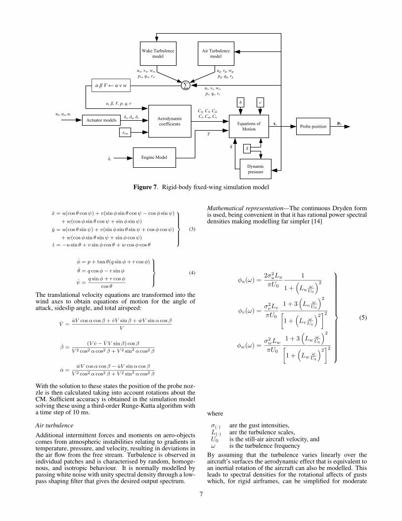
3. AIR TO AIR REFUELLING SIMULATIONSimulations are written in Mathworks’ Simulink environmentand compiled with the Simulink Coder (Real Time Work-shop) toolbox for use on the PXI platform using NationalInstruments’ Veristand target language compiler. Simula-tions cover the wider refuelling scenario in order to developand investigate control strategies, with the RMR specificallyproviding the HIL capability for the more complex hook-up space. The simulation environment (Figure 5) takes intoaccount:

1. Tanker trajectory demands and control, FCS and flightdynamics model.2. Models of the hose and drogue assembly3. Receiver navigation logic, FCS and flight dynamicsmodel.4. Atmospheric (gust and wake) disturbance models

The simulation structure is purposely modular such that on-going improvements to individual components can be madein parallel and swapped in, limiting the changes needed to thesimulation environment.

5

zp

xp

yp

yd

xd

zd

oa

θpψp

ϕp(xp, yp, zp)

axa

ya

za

Figure 6. Probe (p), drogue (d), and approach (a) axesdefinitions.

The purpose of the simulation, in the context of the RMRfacility, is to generate position and orientation informationfor the probe and drogue which can be replicated by themanipulators. To that end we define a set of axes systemsin Figure 6 which identifies the refuelling probe (p) andparadrogue (d) objects. The task in probe-drogue configuredAAR is to approach and couple the probe with the drogue toclose the refuel line. Consequently the probe must track andclose the range between it and the drogue, this described interms of the approach frame (a) which is coincident with thedrogue. The probe position is therefore described with thecoordinates (xp, yp, zp), relative to the origin oa.

Aircraft models

Both the receiver and tanker are rigid-body, six degrees offreedom objects having nonlinear aerodynamic behaviour inthe form of lookup data. The general schematic for the rigidbodies is illustrated in Figure 7. Reference commands fromthe guidance and navigation systems are used by the flightcontrol system to generate input commands to the actuatormodels. These in turn, along with the dynamic aircraft statesare used to generate the aerodynamic forces and moments onthe aircraft at the centre of mass (CM). Clearly the CM willvary throughout the refuelling process, primarily affecting thepitching moment of both receiver and tanker. However upto now we have assumed the variation will have a negligibleeffect on the performance of the flight control laws and haveused a fixed CM at 0.25c i.e. 25% from the leading edge of thewing’s mean aerodynamic chord. Future improvements to thesimulation will determine if this was a valid assumption: ithas already been suggested that that mass variation due to fueltransfer compounds the difficulties created by tanker waketurbulence [10]. A generic tanker flight dynamics modelis employed but the tanker dynamics are not critical to thesimulation - in simpler scenarios the tanker model has beenreplaced with a reference point moving at constant velocity.Two configurations for the receiver aircraft are used: an F-16 fighter jet and the conceptual Innovative Control Effectoraircraft.

A model for an F-16 unmanned jet fighter was derived fromthe data in [11], which itself is a reduced version from [12].The simplified model is valid for the aerodynamic rangeα ∈ [−10◦, 45◦], β ∈ [−30◦, 30◦], which is well within theflight regime for refuelling aircraft. Three first order lags withrate limits and saturations model the actuators similar to thoseused in [12]. Aerodynamic forces (X ,Y ,Z) and moment(L, M , N ) coefficients about the centre of mass (CM) arecalculated in the aerodynamic subsystem using the previous

time step aircraft states:

CX(α, q, δe) CY (α, β, p, r, δa, δr)

CZ(α, β, q, δe)

CL(α, β, p, r, δa, δr) CM (α, q, δe, CZ)

CN (α, β, p, r, δa, δr)

where α, β are the aerodynamic incidence and sideslip anglesand p, q, r are the rotational rates. The parameters δe, δa, andδr correspond to the elevator, aileron, and rudder deflections.Leading edge flaps and differential tail inputs are not used inthe model. The propulsive thrust is calculated through a lagin the power generated by the jet engine simulated with a firstorder transfer function.

A model for the conceptual Innovative Control Effector (ICE)[13] aircraft is used in addition to the F-16 to investigatecontrol challenges relevant to future aircraft configurations.The ICE is a tailless delta wing fixed-wing vehicle with a 65degree leading edge sweep and saw-tooth trailing edge. Thedesign for the ICE was driven by the need for a low radarcross section, hence the minimum vertical profile and controlsurface edges aligned with the external airframe edges. Yawcontrol is provided through multi-axis thrust vectoring (how-ever structural loads limit its operation to below 200 knots)and clamshells. Consequently a multitude of control effectorsare needed to enable the aircraft to operate with sufficientlateral command authority throughout its intended flight en-velope. Aerodynamic forces and moments on the CM aretabulated in a similar fashion to the F-16 model, dependingon the vehicle’s inertial velocity parameters through the air(α, β, p, q, r), and the magnitude of control defections foreach of the effectors.

For both F-16 and ICE models the aero-normalised forces andmoments are dimensionalised using the aircraft’s characteris-tic dimensions and the current dynamic pressure. The totalsum of both aerodynamic and propulsive forces and momentsis used to solve the standard equations of motion for a fixedwing aircraft. These equations relate the time derivative ofeach of the twelve primary states to the current state valuesand the forces and moments acting on the aircraft. If the sumof the forces and moments on the aircraft are expressed inthe form of Newton’s second law and subsequently integratedand transformed to the appropriate axes systems, the stateequations describing the six velocities (three translational andthree rotational) and six positions (again, a translational anda rotational triad) of the aircraft are obtained:

u = rv − qw − g sin θ +X + T

m

v = pq − ru+ g sinϕ cos θ +Y

m

u = qu− pv + g cosϕ cos θ +Z

m

(1)

p =pqIxz(Ix − Iy + Iz) + qr[Iz(Iy − Iz)− I2xz ] + Iz + Ixz

IxIz − I2xz

q =M + pr(Iz − Ix) + Ixz(r2 − p2)

Iy

r =pq[Ix(Ix − Iy) + I2xz ]− qrIxz(Ix − Iy + Iz) + Ixz + Ix

IxIz − I2xz

(2)

6

ur, vr, wr,

pr, qr, rr

uw, vw, ww,

pw, qw, rw

pp

α, β, V, p, q, r

xr

q

T

δt

ug, vg, wg,

pg, qg, rg

Engine Model

∑

CX, CY, CZ,

Cl, Cm, Cn

Probe position

Air Turbulence

model

δe, δa, δrActuator models

Equations of

Motion

Aerodynamic

coefficients

xcm

b c

S

ue, ua, ur

Wake Turbulence

model

α β V ← u v w

Dynamic

pressure

Figure 7. Rigid-body fixed-wing simulation model

x = u(cos θ cosψ) + v(sinϕ sin θ cosψ − cosϕ sinψ)

+ w(cosϕ sin θ cosψ + sinϕ sinψ)

y = u(cos θ sinψ) + v(sinϕ sin θ sinψ + cosϕ cosψ)

+ w(cosϕ sin θ sinψ + sinϕ cosψ)

z = −u sin θ + v sinϕ cos θ + w cosϕ cos θ

(3)

ϕ = p+ tan θ(q sinϕ+ r cosϕ)

θ = q cosϕ− r sinϕ

ψ =q sinϕ+ r cosϕ

cos θ

(4)

The translational velocity equations are transformed into thewind axes to obtain equations of motion for the angle ofattack, sideslip angle, and total airspeed:

V =uV cosα cosβ + vV sinβ + wV sinα cosβ

V

β =(V v − V V sinβ) cosβ

V 2 cos2 α cos2 β + V 2 sin2 α cos2 β

α =wV cosα cosβ − uV sinα cosβ

V 2 cos2 α cos2 β + V 2 sin2 α cos2 β

With the solution to these states the position of the probe noz-zle is then calculated taking into account rotations about theCM. Sufficient accuracy is obtained in the simulation modelsolving these using a third-order Runge-Kutta algorithm witha time step of 10 ms.

Air turbulence

Additional intermittent forces and moments on aero-objectscomes from atmospheric instabilities relating to gradients intemperature, pressure, and velocity, resulting in deviations inthe air flow from the free stream. Turbulence is observed inindividual patches and is characterised by random, homoge-nous, and isotropic behaviour. It is normally modelled bypassing white noise with unity spectral density through a low-pass shaping filter that gives the desired output spectrum.

Mathematical representation—The continuous Dryden formis used, being convenient in that it has rational power spectraldensities making modelling far simpler [14]

ϕu(ω) =2σ2

uLu

πU0

1

1 +(Lu

ωU0

)2

ϕv(ω) =σ2vLv

πU0

1 + 3(Lv

ωU0

)2

[1 +

(Lv

ωU0

)2]2

ϕw(ω) =σ2wLw

πU0

1 + 3(Lw

ωU0

)2

[1 +

(Lw

ωU0

)2]2

(5)

where

σ(·) are the gust intensities,L(·) are the turbulence scales,U0 is the still-air aircraft velocity, andω is the turbulence frequency

By assuming that the turbulence varies linearly over theaircraft’s surfaces the aerodynamic effect that is equivalent toan inertial rotation of the aircraft can also be modelled. Thisleads to spectral densities for the rotational affects of gustswhich, for rigid airframes, can be simplified for moderate

7

angles of attack [15]:

ϕp(ω) =σ2w

U0Lw

0.8(πLw

4b

) 13

1 +(

4bωπU0

)2

ϕq(ω) =−(

ωU0

)2

1 +(

3bωπU0

)2ϕv(ω)

ϕr(ω) =−(

ωU0

)2

1 +(

4bωπU0

)2ϕw(ω)

(6)

where b is the wingspan. Equations (5) and (6) are solvedin the time domain by transforming them into canonicalstate-space form so the turbulent velocity components can besummed to the aircraft’s inertial velocity parts prior to solvingthe equations of motion. For example, in the longitudinalaxes the axial and vertical gust perturbations (ug , wg) can bewritten and solved with

[susw1

sw2

]=

−U0

Lu0 0

0 0 1

0(

U0

Lw

)2

−2U0

Lw

[susw1

sw2

]+

[δu0δw

]

[ugwg

]=

σu

√2U0

πLu0 0

0 σw√π

(U0

Lw

) 32

σw

√3U0

πLw

[susw1

sw2

]

(7)

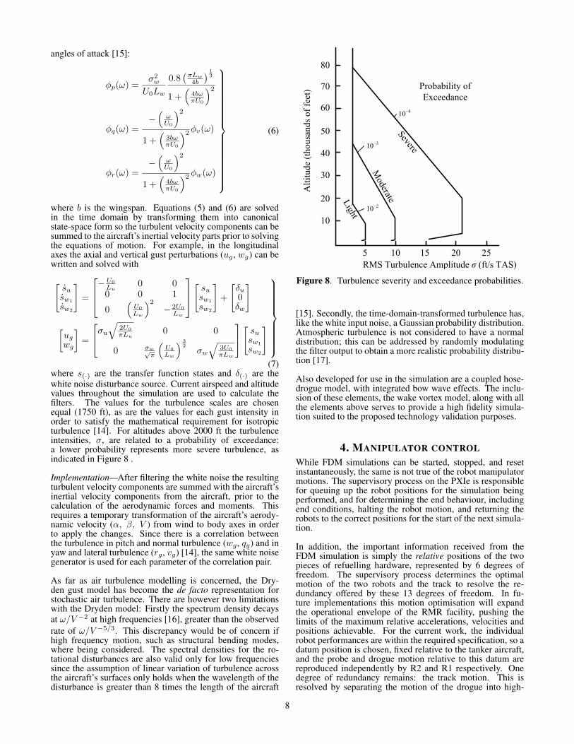
where s(·) are the transfer function states and δ(·) are thewhite noise disturbance source. Current airspeed and altitudevalues throughout the simulation are used to calculate thefilters. The values for the turbulence scales are chosenequal (1750 ft), as are the values for each gust intensity inorder to satisfy the mathematical requirement for isotropicturbulence [14]. For altitudes above 2000 ft the turbulenceintensities, σ, are related to a probability of exceedance:a lower probability represents more severe turbulence, asindicated in Figure 8 .

Implementation—After filtering the white noise the resultingturbulent velocity components are summed with the aircraft’sinertial velocity components from the aircraft, prior to thecalculation of the aerodynamic forces and moments. Thisrequires a temporary transformation of the aircraft’s aerody-namic velocity (α, β, V ) from wind to body axes in orderto apply the changes. Since there is a correlation betweenthe turbulence in pitch and normal turbulence (wg, qg) and inyaw and lateral turbulence (rg, vg) [14], the same white noisegenerator is used for each parameter of the correlation pair.

As far as air turbulence modelling is concerned, the Dry-den gust model has become the de facto representation forstochastic air turbulence. There are however two limitationswith the Dryden model: Firstly the spectrum density decaysat ω/V −2 at high frequencies [16], greater than the observedrate of ω/V −5/3. This discrepancy would be of concern ifhigh frequency motion, such as structural bending modes,where being considered. The spectral densities for the ro-tational disturbances are also valid only for low frequenciessince the assumption of linear variation of turbulence acrossthe aircraft’s surfaces only holds when the wavelength of thedisturbance is greater than 8 times the length of the aircraft

80

70

60

50

40

30

20

10

5 10 15 20 25

RMS Turbulence Amplitude σ (ft/s TAS)

Alt

itude

(thousa

nds

of

feet

) Probability of

Exceedance

10−2

10−3

10−4

Figure 8. Turbulence severity and exceedance probabilities.

[15]. Secondly, the time-domain-transformed turbulence has,like the white input noise, a Gaussian probability distribution.Atmospheric turbulence is not considered to have a normaldistribution; this can be addressed by randomly modulatingthe filter output to obtain a more realistic probability distribu-tion [17].

Also developed for use in the simulation are a coupled hose-drogue model, with integrated bow wave effects. The inclu-sion of these elements, the wake vortex model, along with allthe elements above serves to provide a high fidelity simula-tion suited to the proposed technology validation purposes.

4. MANIPULATOR CONTROLWhile FDM simulations can be started, stopped, and resetinstantaneously, the same is not true of the robot manipulatormotions. The supervisory process on the PXIe is responsiblefor queuing up the robot positions for the simulation beingperformed, and for determining the end behaviour, includingend conditions, halting the robot motion, and returning therobots to the correct positions for the start of the next simula-tion.

In addition, the important information received from theFDM simulation is simply the relative positions of the twopieces of refuelling hardware, represented by 6 degrees offreedom. The supervisory process determines the optimalmotion of the two robots and the track to resolve the re-dundancy offered by these 13 degrees of freedom. In fu-ture implementations this motion optimisation will expandthe operational envelope of the RMR facility, pushing thelimits of the maximum relative accelerations, velocities andpositions achievable. For the current work, the individualrobot performances are within the required specification, so adatum position is chosen, fixed relative to the tanker aircraft,and the probe and drogue motion relative to this datum arereproduced independently by R2 and R1 respectively. Onedegree of redundancy remains: the track motion. This isresolved by separating the motion of the drogue into high-

8

and low-frequency components; the robot axes are used toperform the high-frequency motion and the track moves therobot base to provide the low-frequency, quasi-static responseand give the probe its full longitudinal operational range.

As discussed in Section 2, there is an inevitable delay intro-duced by the motion planning stage in the IRC5 controller.This delay needs to be compensated using predictive con-trol to cast forward the simulation by the equivalent timestep. Approximations are inevitably introduced as a result,but previous studies in the context of structural-HIL-styletesting have shown that in continuous systems a reasonableapproximation can be obtained with a simple polynomialforward predictive capability [18], [19], [20]. This capa-bility is provided in the current implementation of the su-pervisory process. Future implementations will take intoaccount evaluations of the approaches presented by Chen andRicles [21] and may also take advantage of more traditionaldelay compensation methods such as Smith predictors. Thereis a trade off between temporal and spatial accuracy in themotion reproduced by the robots. Exploratory studies will bemade for the final version of this manuscript, quantifying thefidelity of the emulated motion and identifying the optimalpoint in the trade off.

The start point of the simulations is reached through a smoothtransition from the default starting position, 5500 mm directlyaft of the datum position (itself 500 mm aft of the droguecanopy starting position). This transition is effected with atriangular velocity profile to accelerate and decelerate uni-formly between the default and start positions. The simula-tion is paused throughout the transition and is commencedfrom a stationary pose at the start position. The end ofthe simulations is not currently detected by the supervisoryprocess, but instead safety limits are imposed on the relativepositions of the probe and drogue to ensure that the twopieces of hardware do not impact as the simulation progressesthrough the contact stage.

The robot system has three levels of safety provided asstandard: a set of physical joint limit stops and two levelsof software limits (for joint positions and tool centre point(TCP) cartesian positions). There is also a motion supervisionsystem which provides emergency stop behaviour in the eventof a collision. These safety measures are not comprehensive,however, and high-speed impact of the probe and drogueneed to be averted using higher-level control. Furthermore,to optimise motion paths in more advanced testing stages itwill be necessary to relax the restrictive joint limits currentlyin operation. This will require advanced safety control inthe supervisory process on the PXIe. In initial tests nocontact at all is required between the probe and drogue. As apreliminary safety measure, the probe tip is constrained suchthat it cannot move forward of the datum position, and thedrogue is similarly constrained such that it cannot move aft ofthe datum. To allow the execution of any simulation withoutthe need for abrupt halts the forward-aft motion of the probeis transformed using the following equation:

x2 = (x2 < xsafe) ? (x2) :

(xsafe

2− x2/xsafe

)(8)

where x2 is the demanded x-position for R2, x2 is therespective position from the simulation, and xsafe is thedistance at which the position modulation begins. The syntaxa?b : c denotes the C conditional operator. The output of thisfunction approaches zero smoothly and asymptotically as thedemanded position increases past xsafe, with a continuous

derivative at the point xsafe (and elsewhere). Behind xsafethe probe motion is mapped directly to the robot motion.An equivalent, negated, expression is derived for the droguemotion. A value of xsafe = −1000 is chosen arbitrarily forthe tests conducted here, where the value represents a distancemeasured in millimetres.

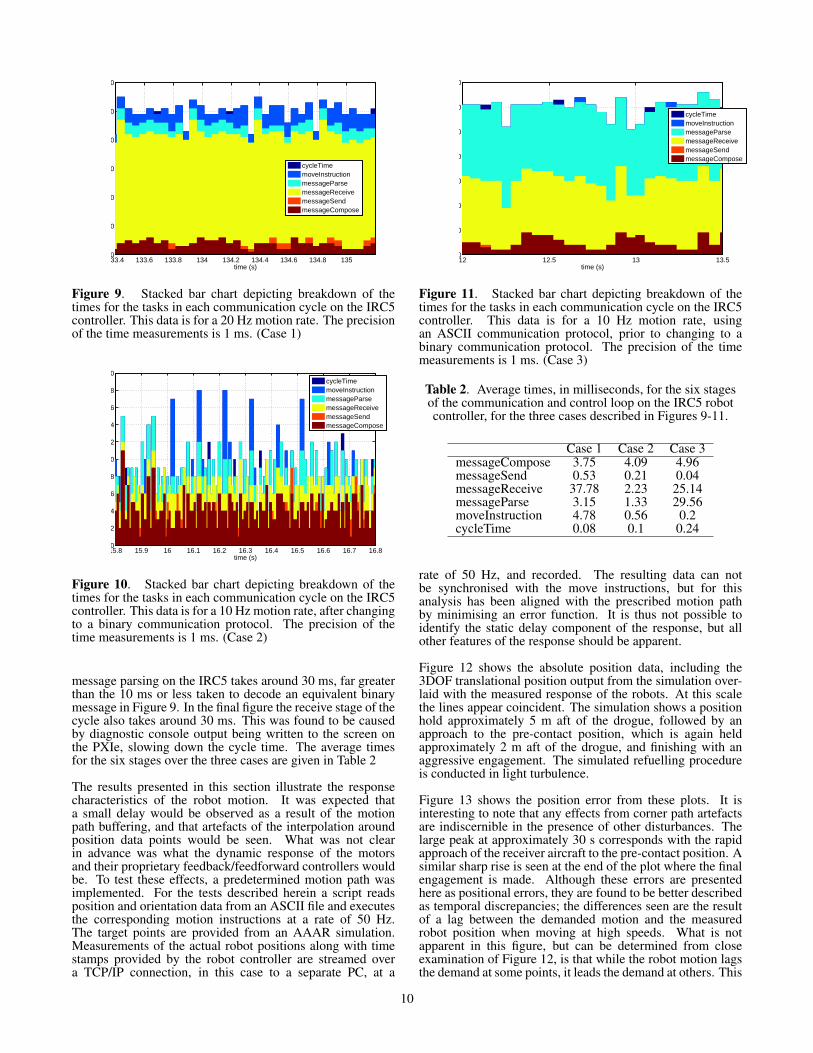
5. EXPERIMENTAL RESULTSSome timing data is now presented to illustrate the impor-tance of tuning the communication routes properly, and ofoptimising the algorithms. Firstly, Figure 9 shows the currentcase of a 20 Hz motion path update. The stacked bars indicatethe times that the respective tasks have taken on the IRC5controller for each time step. The total height of each baris proportional to its width, and represents the time for a fullcycle to complete. The precision of the measurements is 1 ms,which in some cases is too small to measure a time differencein some of the execution steps. The cycles are divided intosix stages: the messgaseCompose stage is where the mea-surement and timestamp data is aquired and sequenced intoa message ready for transmission from the IRC5 controller;the messageSend stage is where this message is sent over theTCP/IP link; the messageReceive stage is where the positiondemand and control data are revceived over the TCP/IP link;the messageParse stage is where the received message istranscribed into the appropriate variables on the controller;the moveInstruction stage is where the motion command isissued to the motion planning routines in the IRC5 controller,and finally the cycleTime stage is simply the time for thecycle to return to the beginning of the loop. The latter stagetakes negligible time but sometimes appears as a millisecondin the figures presented as an artefact of rounding errors.

In the case presented in Figure 9, the communication loopwas locked to the main cycle. That is, the only time thePXIe was sending messages to the IRC5 was when a motioncommand needed to be sent. Accordingly, every cycle takesapproximately 50 ms, corresponding to a 20 Hz cycle rate.It is by chance that the bottleneck in the case presented iswaiting for the latest sample to be buffered from the FDMsimulation by the supervisory process. That is why the IRC5time data indicates a large proportion of the cycle time isspent waiting to receive a message from the PXIe. If the timewas not allocated here, it would be spent waiting to bufferthe position data when the move instruction was executed inthe IRC5. It can be seen that the composition of the messagestring to send takes a comparable time to that taken to readthe binary message received from the PXIe.

Figure 10 shows an earlier test performed at 10 Hz. In thiscase, however, the communication cycle is not locked to theposition instruction cycle, and intermediate communicationsrelay measurements to the PXIe. In this case a standardcommunication cycle takes around 10 ms. The cycles wherea move instruction is received at the IRC5 can be seen, as thecycle takes longer, with the time taken to process the moveinstruction accounting for the difference. These cycles arespaced at approximately 0.1 s intervals as expected, and thetime spent processing the move command is the time neededto regulate the motion timing at the IRC5 end.

Finally, Figure 11 shows another example, but this time noposition data is sent (i.e. the COMM index remains at zero).In this case, however, the messages from the PXIe to the IRC5are encoded as ASCII strings of numeric values, requiringstring parsing on the IRC5. It can be seen here that the

9

133.4 133.6 133.8 134 134.2 134.4 134.6 134.8 1350

10

20

30

40

50

60

time (s)

cycleTimemoveInstructionmessageParsemessageReceivemessageSendmessageCompose

Figure 9. Stacked bar chart depicting breakdown of thetimes for the tasks in each communication cycle on the IRC5controller. This data is for a 20 Hz motion rate. The precisionof the time measurements is 1 ms. (Case 1)

15.8 15.9 16 16.1 16.2 16.3 16.4 16.5 16.6 16.7 16.80

2

4

6

8

10

12

14

16

18

20

time (s)

cycleTimemoveInstructionmessageParsemessageReceivemessageSendmessageCompose

Figure 10. Stacked bar chart depicting breakdown of thetimes for the tasks in each communication cycle on the IRC5controller. This data is for a 10 Hz motion rate, after changingto a binary communication protocol. The precision of thetime measurements is 1 ms. (Case 2)

message parsing on the IRC5 takes around 30 ms, far greaterthan the 10 ms or less taken to decode an equivalent binarymessage in Figure 9. In the final figure the receive stage of thecycle also takes around 30 ms. This was found to be causedby diagnostic console output being written to the screen onthe PXIe, slowing down the cycle time. The average timesfor the six stages over the three cases are given in Table 2

The results presented in this section illustrate the responsecharacteristics of the robot motion. It was expected thata small delay would be observed as a result of the motionpath buffering, and that artefacts of the interpolation aroundposition data points would be seen. What was not clearin advance was what the dynamic response of the motorsand their proprietary feedback/feedforward controllers wouldbe. To test these effects, a predetermined motion path wasimplemented. For the tests described herein a script readsposition and orientation data from an ASCII file and executesthe corresponding motion instructions at a rate of 50 Hz.The target points are provided from an AAAR simulation.Measurements of the actual robot positions along with timestamps provided by the robot controller are streamed overa TCP/IP connection, in this case to a separate PC, at a

12 12.5 13 13.50

10

20

30

40

50

60

70

time (s)

cycleTimemoveInstructionmessageParsemessageReceivemessageSendmessageCompose

Figure 11. Stacked bar chart depicting breakdown of thetimes for the tasks in each communication cycle on the IRC5controller. This data is for a 10 Hz motion rate, usingan ASCII communication protocol, prior to changing to abinary communication protocol. The precision of the timemeasurements is 1 ms. (Case 3)

Table 2. Average times, in milliseconds, for the six stagesof the communication and control loop on the IRC5 robotcontroller, for the three cases described in Figures 9-11.

Case 1 Case 2 Case 3messageCompose 3.75 4.09 4.96messageSend 0.53 0.21 0.04messageReceive 37.78 2.23 25.14messageParse 3.15 1.33 29.56moveInstruction 4.78 0.56 0.2cycleTime 0.08 0.1 0.24

rate of 50 Hz, and recorded. The resulting data can notbe synchronised with the move instructions, but for thisanalysis has been aligned with the prescribed motion pathby minimising an error function. It is thus not possible toidentify the static delay component of the response, but allother features of the response should be apparent.

Figure 12 shows the absolute position data, including the3DOF translational position output from the simulation over-laid with the measured response of the robots. At this scalethe lines appear coincident. The simulation shows a positionhold approximately 5 m aft of the drogue, followed by anapproach to the pre-contact position, which is again heldapproximately 2 m aft of the drogue, and finishing with anaggressive engagement. The simulated refuelling procedureis conducted in light turbulence.

Figure 13 shows the position error from these plots. It isinteresting to note that any effects from corner path artefactsare indiscernible in the presence of other disturbances. Thelarge peak at approximately 30 s corresponds with the rapidapproach of the receiver aircraft to the pre-contact position. Asimilar sharp rise is seen at the end of the plot where the finalengagement is made. Although these errors are presentedhere as positional errors, they are found to be better describedas temporal discrepancies; the differences seen are the resultof a lag between the demanded motion and the measuredrobot position when moving at high speeds. What is notapparent in this figure, but can be determined from closeexamination of Figure 12, is that while the robot motion lagsthe demand at some points, it leads the demand at others. This

10

0 10 20 30 40 50 60−1000

0

1000

2000

3000

4000

5000

6000

time (s)

posi

tion

(mm

)

x2simy2simz2simx2measy2measz2meas

Figure 12. Absolute positions from the simulated data andfrom the measured robot positions.

0 10 20 30 40 50 60−20

0

20

40

60

80

100

time (s)

posi

tion

erro

r (m

m)

x2y2z2

Figure 13. Position error for the robot motion relative to theprescribed simulation data motion path.

lead may not be a true lead, as the alignment of the two signalsin this case is not guaranteed, but it nonetheless points to avariable frequency response that may be characterised to theends of further improving the performance with an inverseapproach.

6. FUTURE WORKDevelopment of the RMR facility is ongoing and providesvarying levels of functionality even in development. Previoususes have included validation of simulation behaviour inquasi-real time and the evaluation of drogue-tracking algo-rithms recorded with a mid-range grey-scale camera. Futureprojects highlight the flexibility of the facility: these includevision-tracking of satellite systems for orbital docking controland various composites-based research projects. To achieve afully closed loop system the interface between the PXIe andthe a suitable vision sensor system will be established, andthe performance of the interface between the PXIe and IRC5robot controller will be fully characterised and managed.This will provide a complete HIL capability for evaluating

real sensor systems in a high fidelity refuelling simulationenvironment. Particular effort will be put into minimising theinevitable delays induced by the kinematic computations andimplementing delay compensation strategies.

In terms of the simulation model further areas of researchinclude better modelling the aerodynamic characteristics ofthe hose and drogue system, including nonlinear effects fromhose whip and any from the hose drum unit. The influence onmass variation on the flight mechanics of the receiver shouldbe addressed. At moderate levels of turbulence and in thepresence of the wake vortex the aeroelastic effects could bemodelled. The bending moments and loading forces on theextended probe could be investigated, which so far has beenassumed rigid. Similarly, aeroelastic effects on the droguecould be modelled and captured in the HIL simulation.

7. CONCLUSIONSAn overview of the Relative Motion Robotic (RMR) facil-ity at the University of Bristol, developed in collaborationwith Cobham Mission Equipment, has been given and theimportant considerations in implementation and performanceoptimisation have been discussed. Timing is critical instructural hardware in the loop simulations, and factors af-fecting performance in this regard have been described. Stepstaken to improve the performance and to push the limits ofthe equipment being used are documented, and preliminaryresults from a simulated air to air refuelling exercise havebeen presented. These results demonstrate the suitability ofthe facility for conducting advanced tests of aerial refuellinghardware and sensors for the purpose of developing auto-mated aerial refuelling capabilities. A high fidelity multi-entity flight dynamics model has been developed and theresults to date have highlighted key areas for investigationas being advanced delay compensation strategies and furthermotion response characterisation of the RMR to facilitateinverse feedforward control to improve on high speed motionreproduction.

ACKNOWLEDGMENTSThis work is funded by Cobham Mission Equipment as partof the ASTRAEA Programme. The ASTRAEA programmeis co-funded by AOS, BAE Systems, Cobham, EADS Cassid-ian, QinetiQ, Rolls-Royce, Thales, the Technology StrategyBoard, the Welsh Assembly Government and Scottish Enter-prise. Website: http://www.astraea.aero/

REFERENCES[1] R. K. Smith, Seventy-Five Years of Inflight Refueling:

Highlights, 1923-1998. United States GovernmentPrinting Office Superintendent of Documents, 1998.

[2] W. I. Glover, “Wings across the Atlantic,” PopularMechanics, vol. 55, no. 2, pp. 186–191, February 1931.

[3] M. A. Bennington and K. D. Visser, “Aerial refuelingimplications for commercial aviation,” Journal of Air-craft, vol. 42, no. 2, pp. 366–375, 2005.

[4] R. Nangia, “Operations and aircraft design towardsgreener civil aviation using air-to-air refuelling,” TheAeronautical Journal, vol. 110, pp. 705–721, November2006.

[5] L. Pollini, M. Innocenti, and R. Mati, “Vision algo-

11

rithms for formation flight and aerial refueling withoptimal marker labeling,” in AIAA Modeling and Sim-ulation Technologies Conference and Exhibit, August2005, pp. 1–15.

[6] W. R. Williamson, G. J. Glenn, V. T. Dang, J. L. Speyer,S. M. Stecko, and J. M. Takacs, “Sensor fusion appliedto autonomous aerial refueling,” Journal of Guidance,Control, and Dynamics, vol. 32, no. 1, pp. 262–275,2009.

[7] A. Dogan, S. Sato, and W. Blake, “Flight Control andSimulation for Aerial Refueling,” in AIAA Guidance,Navigation, and Control Conference and Exhibit, Au-gust 2005, pp. 1–15.

[8] J. Wang, V. Patel, Vijay, C. Cao, N. Hovakimyan, andE. Lavretsky, “Novel L1 adaptive control methodologyfor aerial refueling with guaranteed transient perfor-mance,” Journal of Guidance, Control, and Dynamics,vol. 31, no. 1, pp. 182–193, 2008.

[9] D. Saban, J. Whidborne, and A. Cooke, “Simulation ofwake vortex effects for uavs in close formation flight,”Aeronautical Journal, vol. 113, pp. 727–738, 2009.

[10] W. Mao and F. Eke, “A survey of the dynamics andcontrol of aircraf during aerial refueling,” NonlinearDynamics and Systems Theory, vol. 8, no. 4, pp. 375–388, 2008.

[11] B. L. Stevens and F. L. Lewis, Aircraft Control andSimulation, 2nd ed. John Wiley & Sons, USA, 2003.

[12] L. T. Nguyen, M. E. Ogburn, W. P. Gilbert, K. S.Kibler, P. W. Brown, and P. L. Deal, “Simulator study ofstall/post-stall characteristics of a fighter airplane withrelaxed longitudinal static stability,” NASA TP 1538,Washington, D. C., December 1979.

[13] K. M. Dorsett and D. R. Mehl, “Innovative controleffectors (ICE),” Wright-Patterson Airforce Base, Ohio,WL-TR-96-3043, January 1996.

[14] MIL-F-8785C, “Flying qualitites of piloted aircraft,”Department of Defense, USA, 1980.

[15] J. Roskam, Airplane Flight Dynamics and AutomaticFlight Controls. Roskam Aviation and EngineeringCorporation, 1979.

[16] S.-T. Wang and W. Frost, “Atmospheric turbulence sim-ulation techniques with application to flight analysis,”NASA CR 3305, 1980.

[17] C. G. Justus, C. W. Campbell, D. M. L., and D. L.Johnson, “New atmospheric turbulence model for shut-tle applications,” NASA TM 4168, 1990.

[18] J. du Bois, B. Titurus, and N. Lieven, “Transfer dynam-ics cancellation in real-time dynamic substructuring,”in International Conference on Noise and VibrationEngineering, ISMA2010, Leuven, Belgium, 2010.

[19] M. Wallace, D. Wagg, S. Neild, P. Bunniss, N. Lieven,and A. Crewe, “Testing coupled rotor blade-lag dampervibration using real-time dynamic substructuring,”Journal of Sound and Vibration, vol. 307, no. 3-5, pp.737–754, 2007.

[20] M. Wallace, D. Wagg, and S. Neild, “An adaptive poly-nomial based forward prediction algorithm for multi-actuator real-time dynamic substructuring,” Proceed-ings of the Royal Society A: Mathematical, Physical andEngineering Science, vol. 461, no. 2064, p. 3807, 2005.

[21] C. Chen and J. Ricles, “Analysis of actuator delay com-

pensation methods for real-time testing,” EngineeringStructures, vol. 31, no. 11, pp. 2643–2655, 2009.

BIOGRAPHY[

Peter Thomas is a member of theDynamics and Systems Research Groupat the University of Bristol where heis presently working on flight controlsystems and simulation for autonomousaerial refuelling. Previously he com-pleted his PhD at Cranfield University in2010, investigating applications of lowcost tools and techniques for flight test-ing and system identification of UAVs.

He received a MEng in Mechanical Engineering from War-wick University in 2006 and is an Associate Member of theIMechE. His research interests include flight dynamics sim-ulation, aircraft modelling and system identification, roboticbiomimetics, and control theory.

Jonathan DuBois studied as an un-dergraduate at the University of Bristoland the Kungliga Tekniska Hogskolanin Stockholm. He graduated with anMEng in Aerospace Engineering in 2002and after two years pursuing competitivesporting interests he returned to study fora PhD in Active Fuselage Response Sup-pression in Rotorcraft. In 2008 he spentthree months as a visiting academic at

the University of California, San Diego. Presently he is amember of the Dynamics and Systems research group andAgustaWestland Helicopters University Technology Centrein Vibration, working on the Rotor Embedded ActuatorTechnology programme. Jonathan’s research interests in-clude: Novel methods in parametric dynamic analyses, Ex-perimental parameter identification and Finite Element modelupdating problems, Eigenvalue curve veering, eigenvectorlocalisation, and modal coupling, Active and adaptive vibra-tion control, and Structural Health Monitoring Substructuringcontrol problems (hybrid numerical-hardware simulations)

Tom Richardson lectures Flight Me-chanics and Control in the AerospaceDepartment at Bristol University. Heobtained his first degree (MEng) fromthe Department at Bristol in 1998 andstayed on to undertake a PhD in Nonlin-ear Flight Mechanics. Awarded his PhDin 2002 he moved over to the Mechan-ical Engineering Department in Bristolas a Research Assistant. In June 2003 he

moved back to the Aerospace Department when he was ap-pointed to the Lectureship in Flight Mechanics. Dr Richard-son is a member of the Dynamics and Systems ResearchGroup. His principal research interest is control, rangingfrom classical flight control up to high-level decision-makingand autonomy. He has been a member of two GARTEURaction groups. In the first, (1999-2002) he was a member of ateam which addressed the problem of flight clearance usinga combination of Continuation and Optimisation methods.More recently he has been working with members from En-gineering Mathematics to address the problem of autonomywithin groups of unmanned air vehicles.

12