Embed Size (px)
Citation preview
Dottorato di ricerca in Scienza e Gestione dei Cambiamenti Climatici Scuola di dottorato in Global Change Science and Policy (ChangeS) Ciclo 23° (A.A. 2010 - 2011)
Development of a Regional Risk Assessment methodology for climate change impact assessment and management in coastal zones.
Sviluppo di una metodologia di Analisi di Rischio Regionale per l’analisi e la gestione degli impatti dei cambiamenti climatici nelle aree costiere. SETTORE SCIENTIFICO DISCIPLINARE DI AFFERENZA: CHIM/12
Tesi di dottorato di Silvia Torresan, matricola 955469 Coordinatore del Dottorato Tutore del dottorando Prof. Carlo Barbante Prof. Antonio Marcomini Co-tutore del dottorando
Dr. Andrea Critto
1
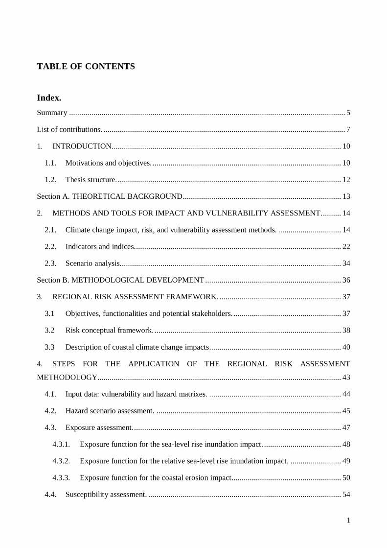
TABLE OF CONTENTS
Index.
Summary ........................................................................................................................................ 5
List of contributions. ....................................................................................................................... 7
1. INTRODUCTION. ................................................................................................................ 10
1.1. Motivations and objectives. ............................................................................................. 10
1.2. Thesis structure. .............................................................................................................. 12
Section A. THEORETICAL BACKGROUND .............................................................................. 13
2. METHODS AND TOOLS FOR IMPACT AND VULNERABILITY ASSESSMENT. ......... 14
2.1. Climate change impact, risk, and vulnerability assessment methods. ............................... 14
2.2. Indicators and indices. ..................................................................................................... 22
2.3. Scenario analysis............................................................................................................. 34
Section B. METHODOLOGICAL DEVELOPMENT ................................................................... 36
3. REGIONAL RISK ASSESSMENT FRAMEWORK. ............................................................ 37
3.1 Objectives, functionalities and potential stakeholders. ..................................................... 37
3.2 Risk conceptual framework. ............................................................................................ 38
3.3 Description of coastal climate change impacts................................................................. 40
4. STEPS FOR THE APPLICATION OF THE REGIONAL RISK ASSESSMENT
METHODOLOGY........................................................................................................................ 43
4.1. Input data: vulnerability and hazard matrixes. ................................................................. 44
4.2. Hazard scenario assessment. ........................................................................................... 45
4.3. Exposure assessment. ...................................................................................................... 47
4.3.1. Exposure function for the sea-level rise inundation impact. ...................................... 48
4.3.2. Exposure function for the relative sea-level rise inundation impact. ......................... 49
4.3.3. Exposure function for the coastal erosion impact...................................................... 50
4.4. Susceptibility assessment. ............................................................................................... 54

2
4.5. Risk assessment. ............................................................................................................. 56
4.6. Damage assessment. ....................................................................................................... 57
4.7. Regional Risk Assessment outputs. ................................................................................. 59
Section C. APPLICATION TO THE CASE STUDY AREA ......................................................... 61
5. DESCRIPTION AND CHARACTERIZATION OF THE CASE STUDY AREA. ................ 62
5.1. The North Adriatic coastal area. ...................................................................................... 62
5.2. Available dataset. ............................................................................................................ 64
6. THE MULTI-MODEL CHAIN APPLIED TO DEFINE CLIMATE CHANGE HAZARD
SCENARIOS IN THE NORTH ADRIATIC COASTAL AREA. .................................................. 66
6.1. Chain of numerical models applied to the North Adriatic Sea. ......................................... 66
6.2. Climate hazard. ............................................................................................................... 68
6.3. Sea-level rise hazard. ...................................................................................................... 69
6.4. Coastal erosion hazard. ................................................................................................... 69
6.5. Information available for the construction of hazard scenarios for the case study area. .... 70
7. APPLICATION OF THE REGIONAL RISK ASSESSMENT TO STUDY SEA-LEVEL RISE
AND COASTAL EROSION IMPACTS. ...................................................................................... 72
7.1. Input data: vulnerability and hazard matrixes. ................................................................. 72
7.2. Hazard scenarios assessment. .......................................................................................... 76
7.2.1. Sea-level rise hazard scenarios. ................................................................................ 76
7.2.2. Coastal erosion hazard scenarios. ............................................................................. 79
7.3. Exposure assessment. ...................................................................................................... 83
7.3.1. Sea-level rise and relative sea-level rise inundation impacts. .................................... 83
7.3.2. Coastal erosion impact. ............................................................................................ 86
7.4. Susceptibility assessment. ............................................................................................... 89
7.4.1. Sea-level rise and relative sea-level rise inundation impacts. .................................... 90
7.4.2. Coastal erosion impact. ............................................................................................ 90
7.5. Risk assessment. ............................................................................................................. 93
7.5.1. Sea-level rise and relative sea-level rise inundation impacts. .................................... 94
3
7.5.2. Coastal erosion impact. .......................................................................................... 100
7.6. Damage assessment. ..................................................................................................... 103
7.6.1. Sea-level rise and relative sea-level rise inundation impacts. .................................. 103
7.6.2. Coastal erosion impact. .......................................................................................... 112
Conclusions. ............................................................................................................................... 118
Bibliography. .............................................................................................................................. 120
AKNOWLEDGEMENTS ........................................................................................................... 129
APPENDIX I. Guidelines for the construction of the Vulnerability and Hazard matrixes. ........... 130
APPENDIX II. Guideline for the application of scores. ............................................................... 133
APPENDIX III. Guideline for the application of weights. ........................................................... 135
APPENDIX IV. Regional Risk Assessment maps for the analysis of sea-level rise, relative sea-level
rise and coastal erosion impacts in the North Adriatic coast......................................................... 137

4
A mia mamma…
…e a mio figlio Gianmarco.

5
Summary
Today there is new and stronger evidence that global warming is likely to have profound
impacts on coastal communities and ecosystems. Accelerated sea-level rise, increased storminess,
changes in water quality and coastal erosion as a consequence of global warming, are projected to
pose increasing threats to coastal population, infrastructure, beaches, wetlands, and ecosystems.
Coastal zones represent an irreplaceable and fragile ecological, economic and social resource that
need to be preserved from the increasing coastal resources depletion, conflicts between uses, and
natural ecosystems degradation. Accordingly, there is a growing importance of innovative
integrated and multidisciplinary approaches to support the preservation, planning and sustainable
management of coastal zones, considering the envisaged effects of global climate change.
Climate change impacts in coastal zones are very dependent on regional geographical and
environmental features, climate, and socio-economic conditions. Impact studies should therefore be
performed at the local or at most at the regional level. In order to provide effective information that
can assist coastal communities in planning sustainable adaptation measures to the effects of climate
change, the main aim of this thesis is to develop a GIS-based Regional Risk Assessment (RRA)
methodology for the integrated assessment of climate change impacts in coastal zones at the
regional scale. The main aim of the RRA is to evaluate and rank the potential impacts,
vulnerabilities and risks of climatic changes on coastal systems. Moreover the methodology allows
the identification of key vulnerable receptors in the considered region and of homogeneous
vulnerable and risk areas, that can be considered as homogeneous geographic sites for the definition
of adaptation and management strategies. The present thesis complies with the research activities of
the Euro-Mediterranean Centre for Climate Change (CMCC) and was implemented in a Decision
support System for Coastal climate change impact assessment (DESYCO).
In order to characterize climate related hazards and vulnerable receptors the RRA approach
integrates downscaled climate, circulation and wave models output for the construction of future
climate change scenarios and includes the analysis of site-specific physical, ecological and socio-
economic characteristics of the territory (e.g. coastal topography, geomorphology, presence and
distribution of vegetation cover, location of artificial protection).
The RRA methodology was applied to the coastal area of the North Adriatic sea, in order to
analyze the potential consequences of sea-level rise, relative sea-level rise inundation and coastal
erosion impacts on multiple coastal receptors (i.e. beaches, river mouths, wetlands, terrestrial
biological systems, protected areas, urban areas and agricultural areas) and compare the results
based on multiple climate change scenarios.

6
The main output of the analysis include exposure, susceptibility, risk and damage maps that
could be used to support coastal authorities in the implementation of sustainable planning and
management processes.
Exposure maps obtained for the permanent inundation impacts (i.e. sea-level rise and
relative sea-level rise) in 2100 allowing identification of coastal areas where the territory would be
more submerged by projected water levels (i.e. areas surrounding the Po River Delta and the
hinterland region between the Northern Venice lagoon and the Grado-Marano lagoons). Future
exposure scenarios of coastal erosion depict a worse situation in winter and autumn for the future
period 2070-2100 and highlight hot-spot exposure areas surrounding the Po River Delta.
Susceptibility maps highlighted that the receptors more susceptible to coastal erosion are the
beaches with about 94% of the territory identified by the very high and high susceptibility class.
Risk maps showed that receptors with very high risk scores for the sea-level rise impact are
wetlands, agricultural areas, protected areas and river mouths. The municipalities more interested
by potential loss of beaches due to relative sea-level rise inundation are Ariano nel Polesine, Porto
Viro, Porto Tolle, and Caorle. The receptors at higher risk for coastal erosion are the beaches where
the percentage of the territory with higher risk scores is about 72% in the winter, 21% in the spring,
14% in the summer and 41% in autumn.
Finally, the damage assessment phase showed that the receptors with by higher percentages
of the territory in the medium and high damage classes are wetlands, agricultural areas, protected
areas and river mouths for the sea-level rise inundation; beaches, wetlands and river mouths for the
coastal erosion impact.

7
List of contributions.
Published papers.
Torresan S., Critto A., Dalla Valle M., Harvey N., Marcomini, 2008. Assessing coastal
vulnerability to climate change: comparing segmentation at global and regional scales.
Sustainability Science, 3: 45-65.
Submitted papers.
Torresan S., Critto A., Rizzi J., Marcomini A., 2011. Assessment of coastal vulnerability to climate
change hazards at the regional scale: the case study of the North Adriatic sea. Accepted
by Natural Hazards and Earth System Sciences.
Iyalomhe F. Rizzi J. Torresan S., Gallina V. Critto A. Marcomini A., 2011. Inventory of GIS-
based Decision Support Systems addressing climate change impacts on coastal waters
and related inland watersheds, submitted to Climate Change, Intech, ISBN 980-953-
307-389-2.
Book Chapters.
Pasini S., Torresan S., Rizzi J., Critto A., Marcomini A., 2012. Analisi di rischio regionale in
supporto alla gestione degli acquiferi: concetti di base e applicazione nel progetto life+
trust. In: Autorità di bacino dei Fiumi Isonzo, Tagliamento, Livenza, Piave, Brenta-
Bacchiglione (Eds). Tool for regional scale assessment of grounwater storage
improvement in adaptation to climate change, in press.
Agostini P., Torresan S., Micheletti C., Critto A., 2009. Review of Decision Support Systems
devoted to the management of inland and coastal waters in the European Union. In:
Marcomini A., Suter G.W. II, Critto A. (Eds). Decision Support Systems for Risk Based
Management of Contaminated Sites. New York, Springer Verlag, pp 311- 329..
Carniel S., Sclavo M., Bergamasco A., Marcomini A. and Torresan S., 2009. Towards assessing
the Adriatic sea coastal vulnerability to regional climate change scenarios: preliminary
results. Volume Mare, CNR ed., in press.
Manuscripts in preparation.
Torresan S., Gallina V., Rizzi J., Critto A., Marcomini A., Regional Risk Assessment applied to
study Sea-Level Rise impacts in the North Adriatic Sea.
Torresan S., Rizzi J., Gallina V., Zabeo A., Critto A., Marcomini A., DESYCO: a decision support
system for the regional risk assessment of climate change impacts in coastal zones.
8
Proceedings of National and International conferences (extended abstracts).
Silvia Torresan, Jonathan Rizzi, Alex Zabeo, Sara Pasini, Valentina Gallina, Andrea Critto,
Antonio Marcomini, 2011. Climate change impacts on coastal areas: results from the
SALT, TRUST, CANTICO and PEGASO projects. Proceedings of the Tenth
International Conference on the Mediterranean Coastal Environment MEDCOAST, 25-
29 October 2011, Rhodes, Greece, Middle East Technical University, Ankara, Turkey,
in press.
Jonathan Rizzi, Silvia Torresan, Sara Pasini, Felix Iyalomhe, Andrea Critto, Antonio Marcomini,
2011. Application of a GIS-based Regional Risk Assessment methodology for the
sustainable use of groundwater. Results from the Life+ SALT project. Proceedings of
the 15st Italian National Conference ASITA , 15-18 novembre, Reggia di Colorno
(Parma). Italy, in press.
Torresan S., Critto A., Rizzi J., Zabeo Alex, Gallina V., Giove S., Marcomini A., “Risk-based
assessment of climate change impacts on coastal zones: the case study of the North
Adriatic Sea”. Invited paper at the conference Deltas in time of Climate Changes 2010,
Rotterdam, 29 September – 1 October 2010.
Rizzi J., Torresan S., Critto A., Zabeo A., Giove S., Marcomini A., 2010. “DESYCO: a Decision
Support System for the assessment of climate change impacts on coastal areas”,
Proceedings of the 14st Italian National Conference ASITA, 9 – 12 novembre 2010,
Fiera di Brescia, pp1-6.
Torresan S., Zabeo A., Rizzi J., Critto A., Pizzol L., Giove S., Marcomini A., 2010. “Risk
assessment and decision support tools for the integrated evaluation of climate change
impacts on coastal zones”. International Environmental Modelling and Software Society
(IEMSs), International Congress on Environmental Modelling and Software Modelling
for Environment’s Sake, Fifth Biennial Meeting, Ottawa, Canada David A. Swayne,
Wanhong Yang, A. A. Voinov, A. Rizzoli, T. Filatova (Eds.)
http://www.iemss.org/iemss2010/index.php?n=Main.Proceedings.
Zabeo A., Semenzin E., Torresan S., Gottardo S., Pizzol L., Rizzi J., Giove S., Critto A.,
Marcomini A., 2010. “Fuzzy logic based IEDSSs for environmental risk assessment and
management”. International Environmental Modelling and Software Society (IEMSs),
International Congress on Environmental Modelling and Software Modelling for
Environment’s Sake, Fifth Biennial Meeting, Ottawa, Canada David A. Swayne,
Wanhong Yang, A. A. Voinov, A. Rizzoli, T. Filatova (Eds.)
http://www.iemss.org/iemss2010/index.php?n=Main.Proceedings.
Rizzi J., Torresan S., Alberghi E., Critto A., Marcomini A., 2010. “Climate change regional
vulnerability assessment to support integrated coastal risk management”. In the
proceedings of the Gi4DM conference, Tourin, 2-4 February 2010.
Torresan S., Critto A., Tonino M.., Alberighi E., Pizzol L., Santoro F. and Marcomini A., 2009.
“Climate change risk assessment for coastal management.”. In Özhan, E. (Editor),
Proceedings of the Ninth International Conference on the Mediterranean Coastal
Environment, 10-14 November 2009, Sochi, Russia, MEDCOAST, Middle East
Technical University, Ankara, Turkey 91-102.
9
Torresan S., Critto A., Dalla Valle M., Harvey N. and Marcomini A., 2007. “A regional risk
assessment framework for climate change impacts evaluation in a coastal zone
management perspective”. In Özhan, E. (Editor), Proceedings of the Eighth
International Conference on the Mediterranean Coastal Environment, 13-17 November
2007, Alexandria, Egypt, MEDCOAST, Middle East Technical University, Ankara,
Turkey, vol 2, pp.741-752.
Torresan S., Critto A., Dalla Valle M., Marcomini A., 2007. “Use of GIS technologies to assess
vulnerability of coastal areas to climate change impacts”. Proceedings of the 11st
Italian National Conference ASITA , 6-9 November 2007,Torino, Italy, pp.1-6.
10
1. INTRODUCTION.
1.1. Motivations and objectives.
Coastal zones are considered key climate change hotspots worldwide (IPCC a, 2007; Voice et al.,
2006; EEA, 2010). The major expected impacts are associated with permanent inundation of low-
lying areas, increased flooding due to extreme weather events (e.g. storm surges), greater erosion
rates affecting beaches and cliffs (Nicholls and Cazenave, 2010; EC, 2005; EEA, 2006; Klein et al.,
2003). Furthermore, it is widely recognized that climate change can have far reaching consequences
on coastal surface and groundwater (e.g. saltwater intrusion), coastal ecosystems (e.g. wetlands and
biodiversity loss) marine biological communities and commercial species (Abuhoda and
Woodroffe, 2006; Wachenfeld et al, 2007; Nicholls, 2004; IPCC, 2008).
At the international level two main research communities are involved in the analysis of climate
change and climate variability impacts on coastal zones: the natural hazard and the climate change
communities.
According to the framework proposed by the natural hazard community (UN-ISDR, 2009), the
analysis of the likely impacts or risks related to coastal hazards involves the evaluation of two main
components: hazard (i.e. an event or phenomenon with the potential to cause harm such as loss of
life, social and economic damage or environmental degradation) and the system vulnerability (i.e.
the characteristics of a system that increase its susceptibility to the impact of climate induced
hazards). In this context, vulnerability is often expressed in a number of quantitative indices and is a
key step toward risk assessment and management (Romieu et al., 2010).
Within the climate change community, vulnerability is mainly defined as a function of three
components: exposure (i.e. the magnitude and rate of climate variations to which a system is
exposed); sensitivity (i.e. the degree to which a system could be affected by climate related stimuli),
and adaptive capacity (i.e. the ability of a system to adjust or to cope with climate-change
consequences) (IPCC a, 2007). Climate change vulnerability is also defined as a combination of
physical, environmental, social and economical factors whose assessment implies the integration of
multiple quantitative and qualitative data (Füssel and Klein, 2006). Moreover, it is considered as a
descriptor of the status of a system or community with respect to an imposed hazard (Kienberger et
al., 2009) and is related to a given location, sector or group (Hinkel and Klein, 2007).
The potential consequences of climate change on natural and human systems can be quantified in
terms of potential or residual impacts and risks, depending on the consideration of the adaptive
capacity component in the final assessment (Füssel and Klein, 2002).

11
Considering that climate change impacts and risks on coastal zones are very dependent on regional
geographical features, climate and socio-economic conditions, impact studies should be performed
at the local or at most at the regional/sub-national level (Torresan et al., 2009).
A relevant challenge is therefore to develop suitable approaches for the assessment of climate-
induced impacts at the regional scale, taking into account the best available geographical
information for the case study area, in order to highlight most critical regions and support the
definition of operational adaptation strategies.
The main aim of this thesis is therefore to develop a Regional Risk Assessment (RRA, Landis,
2005) methodology for the integrated assessment of potential climate change impacts on multiple
natural and human ecosystems (i.e. beaches, wetlands, protected areas, river mouths, urban and
agricultural areas and terrestrial biological systems). The methodology was developed in order to
support regional/sub-national assessments and provide suitable information to plan preventive
adaptation measures (e.g. construction of coastal defences, beach nourishment, planning and zoning
of coastal territory).
The RRA integrates numerical models output for the construction of future climate change
scenarios and considers bio-physical and socio-economic vulnerability indicators/ indices. In order
to analyse impacts at the regional spatial scale, the RRA employs downscaled climate, circulation
and morphodynamic models for the analysis of inundation and coastal erosion processes and
includes the analysis of site-specific physical, ecological and socio-economic characteristics of the
territory (e.g. coastal topography, geomorphology, presence and distribution of vegetation cover,
location of artificial protection). The method is based on Multi Criteria Decision Analysis (MCDA)
that includes a wide variety of methods for the evaluation and ranking of different alternatives,
considering all relevant aspects of a decision problem and involving many actors (Decision makers
as well as Experts) (Giove et al., 2009). It integrates expert judgments and stakeholder preferences
in order to aggregate quantitative and qualitative environmental and socio-economic indicators
representing the vulnerability of each coastal target to different climate induced hazards. The final
outcome of the analysis include the identification and ranking of homogeneous risk units for each
target of interest allowing the establishment of hotspot risk areas and defining priorities for
intervention.
The methodology was developed within the Euro-Mediterranean Centre for Climate Change
(CMCC, www.cmcc.it) in the frame of the CMCC-FISR project (2005-2010) funded by the Italian
Special Integrative Fund for Research (FISR). The North Adriatic coastal area was selected as case
study to test the RRA methodology and the main results of the analysis are presented and discussed
in this thesis. The structure of the thesis is outlined in the next paragraph.

12
1.2. Thesis structure.
This thesis is structured in three main sections: the first one (section A) illustrates the theoretical
background of this work; the second (section B) delineates the conceptual framework and the
methodology developed in the thesis; finally, the third section (section C) describes the application
of the methodology to the case study area of the North Adriatic coast.
Section A, focuses on the review of the state of the art concerning the main tools and methods
developed at the international level for the assessment of impacts, vulnerability and risks related to
climate change in coastal areas. Indicators and indices are also reviewed as useful tools to support
impact, vulnerability and risk assessment studies. Finally, an evaluation of the importance of
scenarios in climate change risk assessment and management is performed.
Section B is divided in two main chapters presenting the Regional Risk Assessment (RRA)
methodology developed in the thesis. Chapter 3 presents the risk conceptual framework and Chapter
4 describes the main steps for the application of the methodology (i.e. Hazard scenarios assessment;
Exposure assessment; Susceptibility assessment; Risk and Damage assessment).
Finally, Section C regards the application of proposed methodology to the coasts of the North
Adriatic Sea (Italy). It is composed of Chapter 7 presenting the results of the application of the RRA
to study sea-level rise and coastal erosion impacts and of Chapter 8 delineating the conclusions of
the work, where a summary of main findings and possible further investigations and
recommendations are presented.
13
Section A
THEORETICAL BACKGROUND

14
2. METHODS AND TOOLS FOR IMPACT AND VULNERABILITY
ASSESSMENT.
In the context of increasing concern about measured and envisaged impacts of climate change, the
development and the application of specific methods and tools for the assessment of vulnerability,
impacts and risks related to climate change is an increasing task. As far as coastal systems are
concerned, impact, risk and vulnerability assessment methodologies can support decision-makers in
a sustainable management of resources and in the implementation of appropriate adaptation
measures. Moreover, essential tools for the implementation of these methodologies are indicators
and indices used for monitoring climate variations, characterising spatial and temporal distributions
of stressors and drivers, identifying key vulnerable sectors and systems (IPPC a, 2007). Finally,
scenario analysis is widely considered as a key tool for impact and risk assessment (UKCIP, 2003)
and it is especially important where global changes are likely to occur and where there is high
uncertainty about the future.
As will be described in the following Paragraphs, the main aims of this Chapter are: 1) to review
current approaches developed at the international level for the assessment of impacts, vulnerability
and risks related to climate change in coastal areas; 2) to identify and compare potential indicators
and indices useful to support impact, vulnerability and risk assessments; 3) to explore the role of
scenarios analysis as a fundamental component of risk management and decision-making processes.
2.1. Climate change impact, risk, and vulnerability assessment methods.
This literature review analyses several relevant approaches developed by the scientific community
for the assessment of impacts, vulnerability and risk connected to climate change.
Starting from climate impact assessment methodologies, a first interesting approach is given by
Füssel (2002), who defines impact assessment as the practice of identifying and evaluating the
detrimental and beneficial consequences of climate change on natural and human systems.
Particularly, impact assessments evaluate the potential effects of several climate change scenarios,
including a (hypothetical) constant climate scenario, on one or more impact domains.
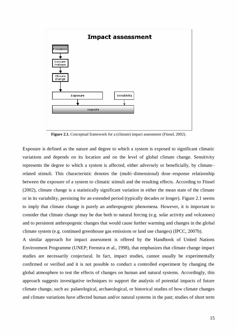
As depicted in Figure 2.1, climate impacts are a function of the exposure of a system to climatic
stimuli and of its sensitivity to these stimuli.
15
Figure 2.1. Conceptual framework for a (climate) impact assessment (Füssel, 2002).
Exposure is defined as the nature and degree to which a system is exposed to significant climatic
variations and depends on its location and on the level of global climate change. Sensitivity
represents the degree to which a system is affected, either adversely or beneficially, by climate–
related stimuli. This characteristic denotes the (multi–dimensional) dose–response relationship
between the exposure of a system to climatic stimuli and the resulting effects. According to Füssel
(2002), climate change is a statistically significant variation in either the mean state of the climate
or in its variability, persisting for an extended period (typically decades or longer). Figure 2.1 seems
to imply that climate change is purely an anthropogenic phenomena. However, it is important to
consider that climate change may be due both to natural forcing (e.g. solar activity and volcanoes)
and to persistent anthropogenic changes that would cause further warming and changes in the global
climate system (e.g. continued greenhouse gas emissions or land use changes) (IPCC, 2007b).
A similar approach for impact assessment is offered by the Handbook of United Nations
Environment Programme (UNEP; Feenstra et al., 1998), that emphasizes that climate change impact
studies are necessarily conjectural. In fact, impact studies, cannot usually be experimentally
confirmed or verified and it is not possible to conduct a controlled experiment by changing the
global atmosphere to test the effects of changes on human and natural systems. Accordingly, this
approach suggests investigative techniques to support the analysis of potential impacts of future
climate change, such as: palaeological, archaeological, or historical studies of how climate changes
and climate variations have affected human and/or natural systems in the past; studies of short term
16
climatic events (i.e. droughts and floods); studies of the impact of present day climate and climate
variability.
In addition to impact studies, vulnerability assessments are useful methodologies to investigate
climate change issues on ecological and human systems. In fact, they constitutes an extension of an
impact assessment and are aimed to: 1) produce information that helps to understand how a system
is potentially affected by and responds to a change in climatic conditions; 2) contribute to
policymaking by presenting this information to stakeholders; 3) recommend adaptation measures
and facilitate sustainable development Füssel (2002).
A key approach for vulnerability assessment is given by the IPCC in the third assessment report
(IPCC, 2001). According to this report, vulnerability is defined as the degree to which a system is
susceptible to, or unable to cope with, adverse effects of climate change, including climate
variability and extremes. Specifically, vulnerability is a function of the character, magnitude, and
rate of climate variation to which a system is exposed, its sensitivity and its adaptive capacity. The
combination of climate exposure and system sensitivity determine the potential impacts that would
be experienced in the absence of an adaptive response. Adaptive capacity is therefore a key
component of vulnerability assessments and can be planned or autonomous (IPCC, 2001).
A planned adaptation is a strategic change in anticipation of a variation in climate to increase the
capacity of a system to cope with (or avoid) the consequences of climate change. An autonomous
adaptation is the capacity of systems to improve their ability to cope over time as a reaction to
climate pressure.
In addition to the aforementioned components of a vulnerability assessment (i.e. exposure,
sensitivity and adaptive capacity), the Australian Government (2005) include two additional
aspects: adverse implications and potential to benefit. Adverse implications are an estimate of the
loss that could occur due to climate change impacts; potential to benefit is an estimate of the
potential benefit introduced by alternative adaptation options for sectors and/or regions.
As far as vulnerability assessment is concerned, Füssel (2006) presents a general framework with
two different generations.
The first generation is characterized by model and scenario-based analyses of potential impacts and
includes the following factors contributing to vulnerability: climate variability, non-climatic
determinants, evaluation of potential impacts in terms of their relevance to goods and services,
mitigation and adaptation measures to reduce adverse effects.
In this framework, mitigation refers to limiting global climate change through reducing the
emissions of greenhouse gases (GHGs) and enhancing their sinks, adaptation aims at moderating its
adverse effects through a wide range of system–specific actions.
17
The requirements for, and limitations to, implementing adaptation measures are more thoroughly
assessed in second–generation vulnerability assessments. A second-generation assessment requires
the involvement of social scientists in a multidisciplinary research group, a stronger participation of
stakeholders and, focuses more on adaptive capacity to reduce the adverse impacts of climate
variability and change.
In addition to impact and vulnerability assessment methods, risk assessment methodologies are
widely employed to evaluate the consequences of climate change on different natural and human
systems.
Jones and Boer (2005) describe two different major approaches to assess climate risk, a natural
hazards-based approach and a vulnerability-based approach. These two approaches are
complementary and can be developed separately or together.
The natural hazards-based approach to assess climate risk begins by characterising the climate
hazards and can be written as the product between the probability of climate hazard and
vulnerability. A hazard is an event with the potential to cause harm. Hazard is generally fixed at a
given level and used to estimate changing vulnerability over space and/or time. For example, a
flood of a given height or a storm with a given wind speed may increase in frequency of occurrence
over time, increasing the risk faced (assuming that vulnerability remains constant).
The vulnerability-based approach applies the conceptual framework of the coping range that
represent a climate range in which the outcomes of climate hazard are tolerable. Within the coping
range, a system or an activity is able to withstand stress without undergoing significant change.
Beyond this range the damages or losses are no longer tolerable and an identifiable group is said to
be vulnerable. The coping range provides a template that is particularly suitable for understanding
the relationship between climate hazards and society. The climatic stimuli and their responses for a
particular local activity or social grouping can be used to construct a coping range if sufficient
information is available. Risk can be assessed by calculating how often the coping range is
exceeded under given conditions. The method of assessing risk can range from qualitative to
quantitative. Qualitative methods can be carried out by building or using an existing conceptual
model of a specific coping range; quantitative methods will begin to assess the likelihood of
exceeding given criteria, such as critical threshold.
UKCIP (2003) gives a general definition of risk as the product of the probability or likelihood of
occurrence of hazard and the magnitude of a consequence. The consequence (or set of
consequences or impacts) is usually associated with exposure to a defined hazard, which is often
detrimental or harmful. Risk assessment is the structured analysis of hazards and impacts to provide
information for decisions; it usually relates to a particular exposure unit (i.e. individual, population,

18
infrastructure, building or environmental asset). The process usually proceeds by identifying
hazards, assessing the likelihoods and severities of impacts. Specifically, climate change risk
assessments attempt to define the consequences (or impact) of future climate on vulnerable or
climate-sensitive exposure units and receptors UKCIP (2003).
UN-ISDR (2009) provides another widely used approach in which risk is defined as the probability
of harmful consequences, or expected losses (deaths, injuries, property, livelihoods, economic
activity disrupted or environment damaged) resulting from interactions between natural or human-
induced hazards and vulnerable conditions. Hazard is considered as a potentially damaging physical
event (e.g. tropical cyclones, droughts, floods, storm surges); vulnerability is the combination of the
conditions determined by physical, social, economic, and environmental factors or processes, which
increase the susceptibility of a community to the impact of hazards.
Regional Risk Assessment (RRA) is another important approach for the assessment of impact and
environmental risk related to climate change.
RRA aims at providing a quantitative and systematic way to estimate and compare the impacts of
environmental problems that affect large geographic areas (Hunsaker et al., 1990). Moreover,
according to Landis and Wiegers (1997) and Landis (2005), RRA allow to consider many
environmental hazards which impact on large geographical areas (e.g. increased global CO2, ozone
depletion, global climate change, biodiversity loss) and take into account a wide range of sources
releasing a variety of stressors which can impact a multiplicity of assessment endpoints.
The main characteristic of the regional risk assessment is the complexity of the analysis caused by
the presence of multiple sources releasing multiple stressors which impact diverse receptors and the
regional scale of the analysis which requires the assessment and integration of a huge amount of
input data.
Accordingly, RRA becomes important when policymakers are called to face problems caused by a
multiplicity of sources of hazards, widely spread over a large area, which impact a multiplicity of
endpoint of regional interest. In fact, the limited economical resources don’t allow to plan
remediation strategies to reduce all the identified risk and it is necessary to classify risks and
prioritize the remediation actions.
Two different approaches are identified for the RRA: the first approach uses the traditional concepts
of ecological risk assessment but analyses exposure and response over a large area (Hunsaker et al.,
1990); the second approach uses ranking models to estimate the relative probability that some
environmental negative effects, caused by anthropological activity, can occur (Landis and Wiegers,
1997).
19
The first approach combines regional assessment methods and landscape ecology theory and
concerns the evaluation of the impacts which occur on population, species or ecosystem that are
widely dispersed over a region to estimate a regional hazard; uses regional models for exposure and
effect assessment, and probabilistic spatial models to support the risk quantification.
The RRA of the first approach includes 5 key steps: qualitative and quantitative description of the
source terms of the hazard; identification and description of the reference environment within which
effects are expected; selection of endpoints; estimation of spatiotemporal patterns of exposure by
using appropriate environmental transport models or available data and quantification of the
relationship between exposure in the modified environment (reference environment) and effects on
biota.
In the second approach proposed by Landis and Weigers (1997) the phases for the RRA are:
identification of the different sources, habitats and impacts; ranking the importance of the different
components of the risk assessment; spatial visualisation of the different components of the risk
assessment to verify if they overlap; relative risk estimation.
The main objectives of regional scale assessment are the evaluation of broader scale problems, their
contribution and influence on local scale problems as well as the cumulative effects of local scale
issues on regional endpoints in order to prioritize the risks present in the region of interest (Smith et
al., 2000) in order to prioritise and evaluate intervention and mitigation measures.
Impact, risk and vulnerability assessment concepts are essential to understand and compare national
and international case studies aimed at evaluate climate change impacts on coastal areas.
In fact, case studies often show differences not only associated with the type of coastal systems
analyzed, the aim of the study, and the spatial and temporal scale; but also concerning methods,
techniques, tools and scenarios employed in the analysis.
In accordance with Klein and Nicholls (1999) there are studies where natural-system vulnerability
is primary evaluated, and studies where socio-economic vulnerability related to climate change is
assessed. However, as defined by the authors natural-system and socioeconomic vulnerability are
related and interdependent, and proper analysis of socioeconomic vulnerability requires a prior
understanding of how the natural system would be affected.
An assessment of natural-system vulnerability at national level was performed by Silenzi et al.
(2002) and Gambolati and Teatini (2002). The aim of Silenzi et al. (2002) is to develop a
preliminary methodological guideline for the evaluation of the integrated hazard and risk of coastal
areas to relative sea-level changes. The method adopt a multidisciplinary approach for the territorial
analysis including geological, topographical, geomorphological, hydrological, geohydrological and
land use surveys, and use forecasts of ground level changes and accelerated beach erosion with
20
respect to sea-level rise. All data are processed through a Geographic Information System (GIS)
that performs the development of a provisional Digital Terrain Model (DTM), and allow the
construction of susceptibility, hazard and land use maps.
The aim of Gambolati and Teatini (2002) is to evaluate the morphodynamical evolution of the
Northern Adriatic coastal profile due to sea-level rise, storm surge and wave set-up, littoral
sediment transport and land subsidence. The predictions of each individual process is obtained
using IPCC global sea-level rise scenarios (Wigley and Raper, 1992), land subsidence, and
hydrodynamic and wave models. The outcome of numerical simulations are managed with a GIS
and then are interpolated with a Digital Elevation Model (DEM) in order to find out those lowlands
which are most likely to be flooded both permanently and occasionally, and to assess the expected
coastline regression during the decades to come. Moreover, in accordance with the methodology
developed by the United Nation Disaster Relief Office (UNDRO, 1995) an inundation risk factor is
defined. It depends on flooding hazard equal to the probability that a selected storm event occurs at
least once during a time interval; the economic value of the flooded area, and the relative damage
equal to the water elevation over the flooded area. The result is maps of the normalized risk factor
at present and in 2100 at regional and local scale.
Silenzi et al. (2002) and Gambolati and Teatini (2002) use GIS technologies in front of archiving,
organizing, and managing the data and for develop thematic map, but also to combine three-
dimensional terrain elevation models (DTM and DEM) with different sea-level rise scenarios. Both
studies attempt to assess the socioeconomic vulnerability using land use maps and risk analysis.
Additionally, there is a need to regionalize the scenarios to compare them with local data given by
the case study area. Natural climate variability on a regional basis comes out from a document of
the National Committee on Coastal and Ocean Engineering (NCCOE, 2004) that present a
methodology that considers the relative changes of climate change scenario modeling to key
environmental variables (i.e. mean sea-level, ocean currents and temperature, wind climate, wave
climate, rainfall/runoff, air temperature). Then possible effects on secondary variables of relevance
to local coastal and ocean engineering (i.e. local sea-level, currents, winds, waves, groundwater
level and quality, coastal flooding, foreshore stability, sediment transport, hydraulics of estuaries,
quality of coastal waters, ecology) are also considered. The likely interactions between the primary
and secondary variables are explored by means of an Impact Assessment Interaction Matrix.
Another interesting method is proposed by the National Oceanic and Atmospheric Administration
(NOAA, www.csc.noaa.gov/products/nchaz/startup.htm) that gives a step-by-step guideline for
assessing community vulnerability to environmental hazards. The aim is to develop and implement
a vulnerability assessment methodology that result in a foundation for identifying and prioritizing
21
community-based hazard mitigation activities. The initial steps focus on identifying hazard and
establishing relative priorities, identifying high potential impact areas for each hazard and assign
scores within risk consideration areas. After intersecting critical facilities categories (i.e. schools,
hospitals, police, utilities, communication, transportation) with high-risk areas, a societal and
economic analysis is performed. The societal analysis is made considering the categories of more
sensitive population (i.e. % households below poverty, % single parent with child families, %
housing units with no vehicle available); while economic analysis considers the major economic
sectors (i.e. agriculture, mining, construction, manufacturing, transportation and public utilities). An
environmental analysis identifies secondary hazard risk consideration sites (i.e. toxic release
inventory sites, solid waste facilities, oil facilities) and the last step is the mitigation opportunities
analysis. GIS technologies are used, primary to manage the large amount of data needed for the
analysis, and to conduct vulnerability assessment analysis and to visualize results. This approach is
not finalized on climate change, but it permits the analysis of multiple natural hazards such as
earthquakes and bushfire and flooding. Moreover, the methodology focuses on the analysis of
socioeconomic aspects and the environmental characteristics related to vulnerability of natural
resources (i.e. wetlands, significant habitat areas and fisheries nursery areas) are considered only in
the phase of the identification of secondary impacts.
Considering the socioeconomic vulnerability assessment, an innovative approach is proposed by the
Joint Research Centre (JRC) in Sagris et al. (2005). This method considers the actual state of the
socioeconomic system, and future demographic and economic trends using land use scenarios.
Moreover, this method demonstrate how integrated assessments of climate change effects can be
conducted at the local spatial scale, using sea-level rise scenarios regulated with regional climate
dynamics. Moreover, local DEM and GIS technologies are the basis to transform sea-level and
surge values into impact maps useful for a quantitative assessment in terms of territory affected.
The impact maps represent one of the main input to risk and vulnerability assessment.
Recent international vulnerability studies focus on conceptual frameworks related both on natural
and on socioeconomic system. For instance, a vulnerability assessment report of the Australian
coasts made by the Australian Greenhouse Office (Voice et al., 2006) primary identifies drivers and
stressors of climate change (i.e. sea-level rise, coastal erosion, frequency of extreme events), then
the preliminary impacts on natural and socioeconomic systems and, finally, the probable responses
to the negative effects. The report remarks that a full assessment of vulnerability requires
consideration of economic and social value of goods and services, infrastructure or ecosystems at
risk, combined with an assessment of resilience of the communities or ecosystems.
22
The last and most recent methodology for the assessment of vulnerability, impacts and risks is
proposed by the Sydney Coastal Councils Group (SCCG), partnered with CSIRO and working in
collaboration with University of the Sunshine Coast entitled Mapping Climate Change
Vulnerability in the Sydney Coastal Councils Groups (Preston, 2008). The aim of the project is to
assess and manage climate vulnerability in the Sydney region. The future climate of the SCCG
region is projected to be both warmer and drier. Meanwhile, sea-level rise is projected to increase
the risk of inundation and erosion of the SCCG coastline. Five areas of potential climate impacts
were selected for vulnerability assessment: extreme heat and human health effects, sea-level rise
and coastal hazards, extreme rainfall and urban storm water management, bushfire, and natural
ecosystems and assets. In conducting this vulnerability assessment, simple conceptual models
identifying the key processes and assumptions were developed for each of the above impact areas.
These models were subsequently utilised to select a broad range of indicators reflecting the three
components of vulnerability (exposure, sensitivity and adaptive capacity). These indicators were
integrated within GIS technologies to facilitate mapping of relative vulnerability. The resulting
regional vulnerability maps provide an indication of the relative vulnerability of different areas
within the SCCG to different climate change impacts.
From the studies proposed in this paragraph, it is clear that there is no a unique response for the
assessment of impacts, vulnerability and risks related to climate change in coastal zones.
Accordingly, there is the need to identify time by time an adequate method consistent with project
and research aims, and compatible with available technologies, tools, and dataset.
In the following paragraph, after a general introduction, a comparative analysis of indicators and
index useful to support the implementation of vulnerability, impact and risk methodologies will be
presented.
2.2. Indicators and indices.
In general terms, an indicator is a value that represents a phenomenon that cannot be directly
measured and may aggregate different types of data (Agostini et al. 2009). Indicators usually have
three relevant functions: they may reduce the number of parameters that normally would be
required to represent a situation; they may simplify the process of results communication to the
users; and they may quantify abstract concepts such as ecosystem health or biotic integrity that are
not measurable. In the field of environmental sciences, indicators are physical, chemical, biological
or socio-economic measures that best represent key elements of a complex ecosystem or
environmental issue (http://www.ozcoasts.org.au/glossary/def_i-l.jsp).
The Organisation for Economic Cooperation and Development (OECD, 1993), define an index as a
set of aggregated or weighted parameters or indicators. Moreover, the OECD (1993) proposed a
23
framework linking different indicators called the “Pressure-State-Response” (PSR) model, re-
elaborated later by the European Environmental Agency (EEA, 1995) in the “Driving-forces-
Pressure-State-Impact-Responses” (DPSIR) framework. Each of the five components of the DPSIR
framework can be analysed through the use of suitable indicators, in such a way that the complexity
of the environmental dynamics, without loosing its own flexibility, is well described (Agostini et
al., 2009).
Particularly, considering the effects related to climate change, indicators and indices are used for
monitoring climate variations, characterising spatial and temporal distributions of stressors and
drivers, identifying strategic vulnerability (IPCC, 2007a).
Generally, environmental indicators are divided in different categories concerning several sectors
and/or environmental problems. While the European Environmental Agency (EEA, 2004) identified
eight main categories of environmental indicators (i.e. atmosphere and climate, snow and ice,
marine ecosystems, terrestrial ecosystems and biodiversity, water, agriculture, economy and human
health), the Australian site for coastal assessment (http://www.ozcoasts.org.au/indicators/index.jsp)
proposes four main categories of indicators (i.e. coastal issues, biophysical indicators, pressure
indicators and coastal management indicators), which are then divided in further sub-groups (e.g.
declining water quality, climate change, habitat/species alterations). Accordingly, climate change is
not always considered as a main category for environmental indicators, rather it is a cross-cutting
theme of relevance for all the categories of environmental indicators.
Jones and Boer (2004), defined sustainability indicators that are related to thresholds indicating
reference values over which irreversible changes would happen, and use these indicators in order to
measure the risk for systems exposed to climate change.
In relation to the conceptual framework adopted, vulnerability indicators could reflect the outcome
of a defined climate hazard (e.g., monetary costs, human mortality, ecosystem damage, etc.) or the
state of a system prior to the occurrence of the hazard event (e.g., geomorphological, biological and
ecological features, population distribution, land use, economic condition, etc.) (Brooks 2003).
Moreover, according to Klein and Nicholls (1998) vulnerability is a multi-dimensional concept that
should be represented by an heterogeneous subset of biogeophysical, economical, institutional and
socio-cultural indicators.
The main aim of this paragraph is to identify and review indicators and indices that may be useful
for the analysis of impacts and risks related to climate change on coastal areas. Indicators and
indices will be classified based on their geophysical, biochemical, socio-economical characteristics
and will be compared and discussed considering their principal characteristics (e.g. objective, scale
of analysis) and based on the information reported in

24
Table 2.1.
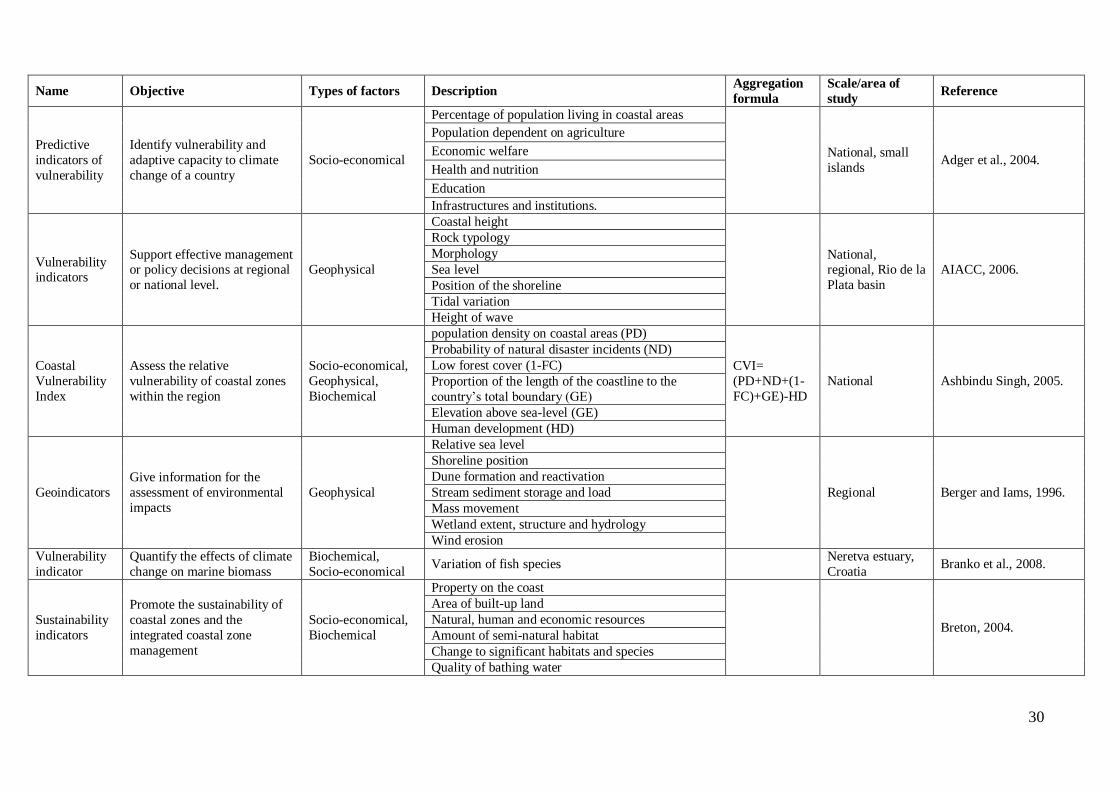
Table 2.1 allows an easy visualisation of reviewed indicators/indices and facilitate their comparison
based on the following criteria:
name given by the author;
objective of indicator or index;
types of factors considered in the indicator/indices (geophysical, biochemical, socio-
economical);
description of indicators or parameters considered in the indices;
spatial scale (local, regional, national and supranational);
reference.
Starting from the analysis of the “name” column of
Table 2.1, there are various examples of indicators/indices of vulnerability and sensitivity (i.e.
Adger et al., 2004; AIACC, 2006; Branko et al., 2008; Hinkel and Klein, 2007). However some
indicators are sustainability indicators (Breton, 2004) or environmental state indicators (EEA,
2005), and some others are referred to the DPSIR framework (i.e. Casazza et al., 2002; Marotta and
Vicinanza, 2001) or to physical and geophysical characteristics of coastal systems (i.e. Bryan et al.,
2001, Berger and Iams, 1996).
Considering the “Type of factors” column, while some authors propose indicators that consider
heterogeneous factors (i.e. geophysical and biochemical or geophysical and socio-economical),
others are focused on the analysis of a single type of factors (e.g. geophysical, biochemical or socio-
economic).
Among the broad category of geophysical indicators, Bryan et al. (2001) consider various physical
aspects of the coasts (e.g. elevation, exposure, aspect and slope) calculated at the regional scale
using GIS technologies in order to assess coastal vulnerability to sea-level rise in tide-dominated,
sedimentary coastal regions.
Berger and Iams (1996) use geoindicators to measure the magnitudes, frequencies, rates, or trends
of geological processes and phenomena that occur at or near Earth’s surface and that are significant
for assessing environmental change over periods of 100 years or less. Specifically, the following
geoindicators are identified for coastal zones: relative sea level, coastal subsidence and uplift,
shoreline position, coastal erosion, sediment transport and deposition, wind erosion, wetland extent,
structure and hydrology and can be used for the assessment of coastal vulnerability to climate
change.
25
In addition to geophysical indicators considering geological characteristics of the coast (i.e. coastal
height, rock typology, morphology and position of the shoreline), the report to Agency for the
Assessment of Impacts and Adaptations to Climate Change (AIACC, 2006) suggest to use
indicators regarding the main driving forces that affect coastal systems (e.g. sea level, tidal
variation, height of wave etc.). These indicators are used in order to orient scientific efforts toward
effective management or policy decisions at the regional or national level.
Within the category of vulnerability indicators, the U.S. Geological Survey (USGS, 2004) uses a
Coastal Vulnerability Index (CVI) to map the relative vulnerability of the coast to future sea-level
rise. The CVI scores different variables in terms of their physical contribution to sea-level rise
related coastal change. Considered variables are divided in geological variables (i.e.
geomorphology, historical shoreline change rate, regional coastal slope) and physical process
variables (i.e. relative sea-level rise, mean significant wave height, mean tidal range). In particular,
the geological variables take into account the shoreline’s relative resistance to erosion, long-term
erosion/accretion trend, and its susceptibility to flooding. The physical process variables contribute
to the inundation hazards of a particular section of coastline over time scales from hours to
centuries.
Another index-based approach is proposed by Schleupner (2005) with the Coastal Sensitivity Index
(CSI) that is aimed at the assessment of the sensitivity of the coast to flooding and erosion caused
by climate change and sea-level rise. To evaluate the probability of flooding and coastal erosion,
four categories that influence vulnerability are chosen: elevation and morphology of the coast,
erodibility, coastal exposition to the wind regime, and natural shelter of the coast. Relative
elevation, coastal morphology and erodibility represent geological/geomorphological characteristics
of coastal zones. Coastal exposition to the wind regime may affect coastal erosion and the
withdrawal of the coast. Natural shelter of the coastal segment have the function of natural
breakwaters along the coastline (i.e. coral reef, small islands, bays). Relative local subsidence and
elevation movements are added to these four categories.
As far as biochemical factors are concerned, the Australian society for the assessment and
monitoring of coastal areas (www.ozcoast.org.au) suggests the following indicators: algal blooms,
anoxic an hypoxic events, euthrophication, vector borne diseases, variation of terrestrial flora and
fauna, marine fauna, alloctone species presence. These indicators are used to explore coastal
ecosystem evolution, processes complexity, and information about ecosystem health.
Further biological indicators are proposed by Carlton and Battelle (2004) in order to assess the
economic impacts of climate change analysing the fish stock and its main characteristics (e.g.
species composition and habitat). Moreover, Branko et al. (2008) study the life cycles of new
26
species in the Eastern Adriatic coast in order to economically protect marine biomass to climate
change.
For the analysis of climate change impacts on plankton communities, Temnykh et al. (2008)
provide indicators regarding the variation of species composition of marine zooplankton in relation
to changes in water temperature; Gameiro and Brotas (2008) evaluate the variability of the
phytoplankton in the estuary in relation to multiple climatic drivers (i.e. temperature, wind, rainfall,
river flow, salinity).
Some indicators referred to biogeochemical factors are also provided by the European
Environmental Agency (EEA), in the State of Environment reports (EEA, 2005a,b). These
indicators concern the quality of bathing water, nutrient concentration in coastal, transition and
marine areas, and are important to evaluate the state of the environment.
Some authors, Casazza et al. (2002) and Marotta and Vicinanza (2001), analyse socio-economic
factors and apply the DPSIR framework in order to evaluate the environmental quality of Italian
coasts. The main driving-forces of this approach include population density, increase in population,
GDP distribution (agriculture, industry, services), tourism and coastal occupation but do not
explicitly include climate change forcings.
Adger et al. (2004) propose specific sub-set of indicators that enable a comparison of the
vulnerability and adaptive capacity of different systems, groups or regions to climate change. These
indicators are mostly related to socio-economic aspects and include the percentage of the national
population living in flood plains or in low-lying coastal areas, the assessment of population
immediately dependent on agriculture, the conditions of economic welfare, health, nutrition and
education, and finally the analysis of infrastructures and institutions.
Finally, several authors (Sorensen, 1997; Coastal Resources Center, 1996 and 1999; Hertin et al.,
2001; EEA, 2000) proposed some indicators in order to evaluate the effectiveness of Integrated
Coastal Zone Management (ICZM) policies and to monitor the results of this process (e.g. number
of ICZM activated, number of plan or strategies, stakeholder participation).
A specific set of indicators to study impacts of climate change in coastal zones is proposed by the
IPCC-Coastal Zone Management Subgroup (IPCC CZMS, 1992). These indicators are referred both
to socio-economic and to biochemical factors and include people potentially affected by climate
change impacts, people at risk, loss of capital, land loss, costs for prevention and adaptation
measures and wetland loss.
Breton (2004) defines sustainability indicators in order to promote the sustainability of coastal
zones and the development of ICZM strategies. These indicators concern both socio-economic
factors (i.e. demand for property on the coast, area of built-up land, human and economic assets at
27
risk) and geophysical/biochemical ones (e.g. amount of semi-natural habitat, change to significant
coastal and marine habitats and species, quality of bathing water, sea-level rise and extreme weather
conditions).
Voice et al. (2006) explain that a full assessment of vulnerability to climate change requires
consideration of the economic and social value of goods and services, infrastructure or ecosystems
at risk, combined with an assessment of vulnerable receptors to impacts such as sea-level rise, and
extreme weather events. Receptors to be considered in the analysis are both natural and human
ecosystems (i.e. beaches and dunes, estuaries, tidal wetlands, coral reefs, sea grasses, coastal
infrastructure, fisheries and aquaculture, tourism and health).
In order to support vulnerability studies related to climate change impacts in coastal zones, Hinkel
and Klein (2007) provide an integrated set of geophysical and socio-economical indicators at the
global scale, such as soil or sand loss, dune height, number of people in flooding risk areas, saline
intrusion areas, costs for adaptation and mitigation measures.
Also Travisi (2007) gives an heterogeneous set of indicators to define the costs for different climate
risk scenarios. These indicators include meteo-climate factors (i.e. temperature, precipitation),
environmental factors (i.e. natural areas, water resources, biodiversity), social factors (i.e. growth
rate and composition of the population, employment/unemployment rate, health), economic factors
(i.e. GDP, economic and technologic growth) and administrative factors (i.e. land planning,
resource management, prevention plans).
In order to assess the relative vulnerability of coastal zones within a region, Ashbindu Singh (2005)
considers the following indicators: population density in coastal areas, probability of natural
disaster incidents, percentage of vegetation cover, geographic exposure as the percentage of flat
land and the proportion of the length of the coastline to the country’s total boundary. Since the
original data are represented in non-comparable units, a formula is proposed to convert the data into
a set of equivalent indices. All the indicators are scaled between 0 and 1 using a scaling formula.
Once scaled, all the indicators are combined to produce a Coastal Vulnerability Index (CVI) applied
to assess the relative status (i.e. level of vulnerability) of coastal areas within each country
worldwide.
Finally, Torresan et al. (2008) adopt specific indicators to address climate-change related issues in
coastal zones and to identify vulnerable areas at the regional level. They include a heterogeneous
subset of indicators (i.e. coastal topography and slope, geomorphological characteristics, presence
and distribution of wetlands and vegetation cover, density of coastal population and number of
coastal inhabitants) that are referred to biophysical, ecological and socio-economical features of
coastal systems.
28
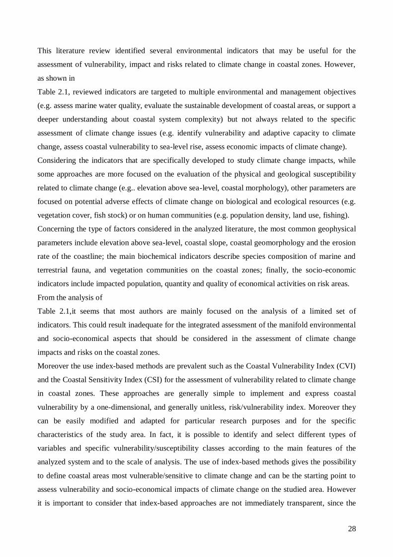
This literature review identified several environmental indicators that may be useful for the
assessment of vulnerability, impact and risks related to climate change in coastal zones. However,
as shown in
Table 2.1, reviewed indicators are targeted to multiple environmental and management objectives
(e.g. assess marine water quality, evaluate the sustainable development of coastal areas, or support a
deeper understanding about coastal system complexity) but not always related to the specific
assessment of climate change issues (e.g. identify vulnerability and adaptive capacity to climate
change, assess coastal vulnerability to sea-level rise, assess economic impacts of climate change).
Considering the indicators that are specifically developed to study climate change impacts, while
some approaches are more focused on the evaluation of the physical and geological susceptibility
related to climate change (e.g.. elevation above sea-level, coastal morphology), other parameters are
focused on potential adverse effects of climate change on biological and ecological resources (e.g.
vegetation cover, fish stock) or on human communities (e.g. population density, land use, fishing).
Concerning the type of factors considered in the analyzed literature, the most common geophysical
parameters include elevation above sea-level, coastal slope, coastal geomorphology and the erosion
rate of the coastline; the main biochemical indicators describe species composition of marine and
terrestrial fauna, and vegetation communities on the coastal zones; finally, the socio-economic
indicators include impacted population, quantity and quality of economical activities on risk areas.
From the analysis of
Table 2.1,it seems that most authors are mainly focused on the analysis of a limited set of
indicators. This could result inadequate for the integrated assessment of the manifold environmental
and socio-economical aspects that should be considered in the assessment of climate change
impacts and risks on the coastal zones.
Moreover the use index-based methods are prevalent such as the Coastal Vulnerability Index (CVI)
and the Coastal Sensitivity Index (CSI) for the assessment of vulnerability related to climate change
in coastal zones. These approaches are generally simple to implement and express coastal
vulnerability by a one-dimensional, and generally unitless, risk/vulnerability index. Moreover they
can be easily modified and adapted for particular research purposes and for the specific
characteristics of the study area. In fact, it is possible to identify and select different types of
variables and specific vulnerability/susceptibility classes according to the main features of the
analyzed system and to the scale of analysis. The use of index-based methods gives the possibility
to define coastal areas most vulnerable/sensitive to climate change and can be the starting point to
assess vulnerability and socio-economical impacts of climate change on the studied area. However
it is important to consider that index-based approaches are not immediately transparent, since the

29
final computed indices do not allow the user to understand the assumptions and evaluation that led
to its calculation. A clear explanation of the adopted methodology is therefore essential to support
the proper use of these methods (Ramieri et al., 2011).
Finally, as regards the scale of analysis, reviewed indicators/indices are defined at municipal, basin,
regional, national level or supranational/global scale. The definition of the scale analysis is a key
step for the application of indictors and is very dependent on the objective of the study and on data
availability.
.
30
Name Objective Types of factors Description Aggregation
formula
Scale/area of
study Reference
Predictive
indicators of
vulnerability
Identify vulnerability and
adaptive capacity to climate
change of a country
Socio-economical
Percentage of population living in coastal areas
National, small
islands Adger et al., 2004.
Population dependent on agriculture
Economic welfare
Health and nutrition
Education
Infrastructures and institutions.
Vulnerability indicators
Support effective management or policy decisions at regional
or national level.
Geophysical
Coastal height
National, regional, Rio de la
Plata basin
AIACC, 2006.
Rock typology
Morphology
Sea level
Position of the shoreline
Tidal variation
Height of wave
Coastal
Vulnerability
Index
Assess the relative
vulnerability of coastal zones
within the region
Socio-economical,
Geophysical,
Biochemical
population density on coastal areas (PD)
CVI=
(PD+ND+(1-
FC)+GE)-HD
National Ashbindu Singh, 2005.
Probability of natural disaster incidents (ND)
Low forest cover (1-FC)
Proportion of the length of the coastline to the
country’s total boundary (GE)
Elevation above sea-level (GE)
Human development (HD)
Geoindicators
Give information for the
assessment of environmental
impacts
Geophysical
Relative sea level
Regional Berger and Iams, 1996.
Shoreline position
Dune formation and reactivation
Stream sediment storage and load
Mass movement
Wetland extent, structure and hydrology
Wind erosion
Vulnerability
indicator
Quantify the effects of climate
change on marine biomass
Biochemical,
Socio-economical Variation of fish species
Neretva estuary,
Croatia Branko et al., 2008.
Sustainability
indicators
Promote the sustainability of
coastal zones and the
integrated coastal zone
management
Socio-economical,
Biochemical
Property on the coast
Breton, 2004.
Area of built-up land
Natural, human and economic resources
Amount of semi-natural habitat
Change to significant habitats and species
Quality of bathing water

31
Name Objective Types of factors Description Aggregation
formula
Scale/area of
study Reference
Sea-level rise
Extreme weather conditions
Coastal erosion and accretion
Physical
environmental
parameters
Assess coastal vulnerability to
sea-level rise Geophysical
Elevation land Statistical analysis, rank-
correlation
test, linear
regression
Regional,
Northern Spencer
Gulf
Bryan et al., 2001. Slope land
Exposure and orientation
Fishing
indicators
Assess economic impacts of
climate change
Biochemical,
Socio-economical Fish stock Regional
Carlton and Battelle,
2004.
DPSIR
indicators
Define environmental quality
of the coastal area Socio-economical
Population density
National, Italy
Casazza et al., 2002
Marotta and Vicinanza,
2001.
Increase in population
GDP distribution (agriculture, industry, services)
Tourism
Coastal occupation
Indicators of
the state of the
environment
Evaluate the state of marine
water Biochemical
Quality of bathing water
Europe EEA, 2005. Nutrient concentration in coastal, transition and
marine areas
Vulnerability
indicator
Measure human influence on
water ecosystems Biochemical Variability of phytoplankton
Tagus estuary,
Portugal
Gameiro and Brotas,
2008.
Vulnerability
indicators
Support vulnerability studies
related to impacts of climate
change on coastal zones
Geophysical, Socio-
economical
Soil or sand loss
Hinkel and Klein, 2007.
Dune height
Saline intrusion areas
Number of people in flooding risk areas
Costs for adaptation and mitigation measures
Vulnerability
indicators
Analyse the vulnerability of
coastal zones related to
climate change
Socio-economical,
Biochemical
People affected by impacts
Common
methodology
National,
regional, Holland,
Poland and
Germany
IPPC CZMS, 1992.
People at risk
Loss of capital
Land loss
Costs for prevention and adaptation measures
Wetland loss
Evaluation
measures of
climate risk
Measure the risk for systems
exposed to impacts of climate
change
Biochemical,
Socio-economical,
Geophysical
Salinity
National Jones and Boer, 2004. Mangroves
Planning for disasters/hazards
Infrastructure/economics

32
Name Objective Types of factors Description Aggregation
formula
Scale/area of
study Reference
Regional assessment planning
Critical thresholds for atolls
Coastal dynamics
Flooding and wetlands
Coastal
Sensitivity
Index (CSI)
Assess the sensitivity of the
coast to flooding and erosion
caused by climate change and
sea-level rise
Geophysical
Relative height of the coast
CSI=
(X1²+X2²+X3
²+X4²+Xn²) /
n
Caribbean region Schleupner, 2005
Morphology of the coast
Erodibility
Coastal exposition to the wind regime
Natural shelter of the coast
Subsidence
Elevation of the area
Sediment processes
Indicators for
the integrated
coastal zone
management
Evaluate the effectiveness of
ICZM policies and to monitor
the results
Socio-economical
Number of ICZM activated
Sorensen, 1997
Coastal Resources
Center, 1996 and 1999
Hertin et al. 2001.
Number of plan or strategies
Stakeholder participation
Vulnerability
indicator
Analyse the effects of
temperature change on water
ecosystem
Biochemical Species composition of zooplankton North-East zone
of The Black Sea Temnykh et al., 2008.
Regional
indicators of
coastal
vulnerability
Identify vulnerable areas at the
regional level
Geophysical,
Biochemical,
Socio-economical
Land of a particular elevation value
Regional, Veneto Torresan et al., 2008.
Slope
Geomorphological characteristics of the coast
Potential migration of wetlands
Vegetation cover
Density of coastal population
Number of coastal inhabitants
System
dimension
Define the costs for different
climate risk scenarios.
Estimate the cost of areas
exposed to a possible flooding
risk
Biochemical,
Geophysical,
Socio-economical
Natural area
Local, Piana di
Fondi (Lazio),
Piana di Sangro
(Abruzzo), Grado
and Marano
(FVG)
Travisi, 2007.
Biodiversity
Water resource
Rate of population growth
Composition of the population
Employment/unemployment rates

33
Name Objective Types of factors Description Aggregation
formula
Scale/area of
study Reference
Sanitary resources
GDP
Economical and technological growth
Land assessment planning
Methodologies for resources assessment
Existing prevention planning
Coastal
Vulnerability
Index (CVI)
Assess the rate of coastal
erosion/accretion and the
response of a coastline to sea-
level rise
Geophysical
Geomorphology (a)
CVI=
√[(a*b*c*d*e
*f)/6]
Regional USGS, 2004.
Historical shoreline change rate (b)
Regional coastal slope (c)
Relative sea-level rise (d)
Mean significant wave height (e)
Mean tidal range (f)
Coastal
vulnerability
factors
Quantify the vulnerability of
analysed systems to the
impacts related to climate
change
Geophysical,
Biochemical,
Socio-economical
Beaches and dune coasts
National,
Australia Voice et al., 2006.
Estuaries
Tidal wetlands
Water resources
Sea grasses
Coastal infrastructures
Fish and aquaculture
Tourism
Health
Coastal
indicators
Explore coastal ecosystem
evolution, processes
complexity, and information
about ecosystem health
Biochemical
Algal blooms
National,
Australia www.ozcoasts.org.au
Anoxic an hypoxic events
Euthrophication
Vector borne diseases
Variation of terrestrial flora and fauna
Marine fauna
Alloctone species presence
Table 2.1. Comparative analysis of indicators and indices found in literature for climate change impact, risk and vulnerability assessment.
34
2.3. Scenario analysis.
At the international level, scenarios are widely considered as a key tool for climate change risk assessment.
They are used to identify various sources and types of uncertainty associated with our knowledge of the
future, and as a tool to help analyzing the consequences of this uncertainty (UKCIP, 2003).
In general terms, scenarios describe plausible futures as a function of changes in major driving forces (i.e.,
the main determinants of change in a scenario), such as population growth, economic development or
technological change (DINAS-COAST, 2006). Accordingly, a scenario is a coherent, internally consistent,
and plausible description of a possible future state of the world (IPCC, 2007b). This kind of scenarios are
not predictions or forecasts (which indicate outcomes considered most likely), but are alternative images
without ascribed likelihoods of how the future might unfold. However they are widely used to assess future
developments in uncertain and complex conditions, to illustrate future conditions relative to main
environmental driving forces (e.g., in technology, agriculture or ecology) and to devise effective responses
by modifying current policies and decision making.
Scenarios can also be divided into exploratory (or descriptive) and normative (or prescriptive). The former
class includes scenarios describing the future according to known processes of change, or as extrapolations
of past trends (Carter et al., 2001); the latter considers scenarios describing a pre-specified future, either
optimistic, pessimistic, or neutral (Alcamo, 2001), and a set of actions that might be required to achieve (or
avoid) it. Such scenarios are often developed using an inverse modelling approach, by defining constraints
and then diagnosing plausible combinations of the underlying conditions that satisfy those constraints
(IPCC, 2007b).
As regards climate change inherent literature, in the Special Report on Emission Scenarios (SRES)
(Nakićenovićet al., 2000), the Intergovernmental Panel on Climate Change (IPCC) defined a set of
Emissions Scenarios that describe future and present-day global and regional emissions of Green House
Gases (GHG) and other pollutants (for example sulphur dioxide and carbon monoxide) which can influence
climate. The so called SRES scenarios are also based on storylines showing a set of possible conditions
relative to the main driving forces of environmental change (e.g., demography, economy, technology,
energy and agriculture). Specifically, the SRES storylines are structured in four major “families”, labeled
A1, A2, B1 and B2, each of which emphasizes a largely different set of social and economic ideals and they
are used to provide quantitative estimates of GHG and aerosol emissions from energy use, industrial
activities and land use.
For climate change risk assessment, two main types of scenarios are very useful: climate change and socio-
economic scenarios.
Scenarios of climate change represent uncertainty in future climate and are simply the predictions from
Global Climate Models (GCMs) or Regional Climate Models (RCMs). These models provide information
on future climate for a range of climate variables (e.g. air and water temperature, rainfall, wind circulation)
at a spatial resolution determined by the climate model (generally hundreds of kilometers a side for GCMs

35
and tens of kilometers a side for RCMs). The starting point for developing climate change scenarios is the
definition of scenarios of future emissions of the greenhouse gases and other pollutants that could affect
climate (e.g. SRES scenarios).
Socio-economic scenarios describe uncertainty in the future socioeconomic environment and provide
contextual socioeconomic descriptions allowing climate change risk to be judged against other sources of
risk (UKCIP, 2003). Each description of future world in the socio-economic scenario represents different
demographic, social, economic, technological, and environmental developments that diverge in increasingly
irreversible ways and result in different levels of (GHG) emissions.
Accordingly, each socio-economic scenario leads to a specific emissions scenario from which climate
scenarios can be generated.
Climate change scenarios provided by GCMs and RCMs are widely used to assess climate change at the
global and supra-national scale. However, the GCMs and RCMs outputs alone cannot assess the detailed
changes that may happen at the regional/local levels. Recently, there has been a lot of effort from the climate
community on the development of dynamical and statistical downscaling techniques to represent climate
change at local and regional scale, respectively. However, bridging the gap between the resolution of global
climate models and the local scale weather and microclimatic processes still represents a considerable
technical problem (STARDEX, 2005 http://www.cru.uea.ac.uk/projects/stardex/).
Moreover, most impact studies are done for spatial resolutions of the order of a few square kilometres. This
is much less than the horizontal areas of the GCMs and RCMs (i.e. from hundreds to tens of kilometres a
side), especially for regions of complex topography, coastal or island locations, and in regions of highly
heterogeneous land-cover (Wilby, 2004).
Consequently, climate scenarios usually investigate processes that happen at a geographical scale not useful
for coastal planners to study impacts regionally or locally. Therefore, methods are needed to bridge the gap
between the large scale of climate scenarios and the fine scale where local impacts happen as a consequence
of changed climate conditions.
In climate impact and risk assessment studies, a set of several significantly different scenarios can help in
bounding the uncertainty of the future. A good set of scenarios should include at least one or more negative
images of the future as well as a optimistic scenario assuming a successful future world.
36
Section B
METHODOLOGICAL DEVELOPMENT
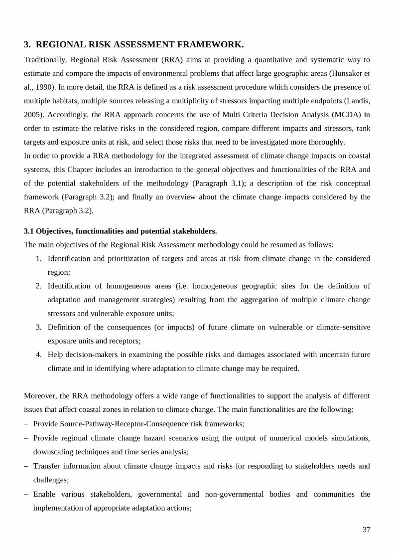
37
3. REGIONAL RISK ASSESSMENT FRAMEWORK.
Traditionally, Regional Risk Assessment (RRA) aims at providing a quantitative and systematic way to
estimate and compare the impacts of environmental problems that affect large geographic areas (Hunsaker et
al., 1990). In more detail, the RRA is defined as a risk assessment procedure which considers the presence of
multiple habitats, multiple sources releasing a multiplicity of stressors impacting multiple endpoints (Landis,
2005). Accordingly, the RRA approach concerns the use of Multi Criteria Decision Analysis (MCDA) in
order to estimate the relative risks in the considered region, compare different impacts and stressors, rank
targets and exposure units at risk, and select those risks that need to be investigated more thoroughly.
In order to provide a RRA methodology for the integrated assessment of climate change impacts on coastal
systems, this Chapter includes an introduction to the general objectives and functionalities of the RRA and
of the potential stakeholders of the methodology (Paragraph 3.1); a description of the risk conceptual
framework (Paragraph 3.2); and finally an overview about the climate change impacts considered by the
RRA (Paragraph 3.2).
3.1 Objectives, functionalities and potential stakeholders.
The main objectives of the Regional Risk Assessment methodology could be resumed as follows:
1. Identification and prioritization of targets and areas at risk from climate change in the considered
region;
2. Identification of homogeneous areas (i.e. homogeneous geographic sites for the definition of
adaptation and management strategies) resulting from the aggregation of multiple climate change
stressors and vulnerable exposure units;
3. Definition of the consequences (or impacts) of future climate on vulnerable or climate-sensitive
exposure units and receptors;
4. Help decision-makers in examining the possible risks and damages associated with uncertain future
climate and in identifying where adaptation to climate change may be required.
Moreover, the RRA methodology offers a wide range of functionalities to support the analysis of different
issues that affect coastal zones in relation to climate change. The main functionalities are the following:
Provide Source-Pathway-Receptor-Consequence risk frameworks;
Provide regional climate change hazard scenarios using the output of numerical models simulations,
downscaling techniques and time series analysis;
Transfer information about climate change impacts and risks for responding to stakeholders needs and
challenges;
Enable various stakeholders, governmental and non-governmental bodies and communities the
implementation of appropriate adaptation actions;
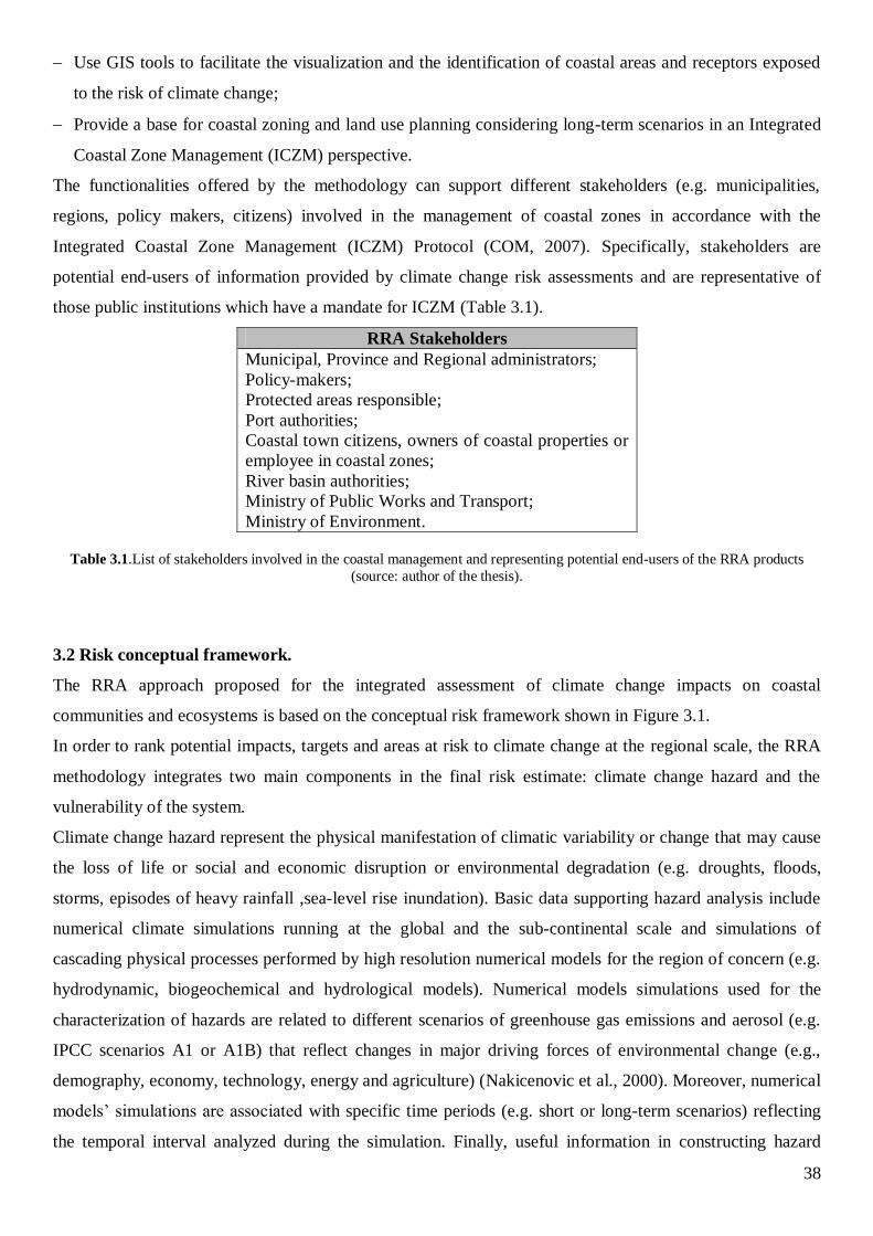
38
Use GIS tools to facilitate the visualization and the identification of coastal areas and receptors exposed
to the risk of climate change;
Provide a base for coastal zoning and land use planning considering long-term scenarios in an Integrated
Coastal Zone Management (ICZM) perspective.
The functionalities offered by the methodology can support different stakeholders (e.g. municipalities,
regions, policy makers, citizens) involved in the management of coastal zones in accordance with the
Integrated Coastal Zone Management (ICZM) Protocol (COM, 2007). Specifically, stakeholders are
potential end-users of information provided by climate change risk assessments and are representative of
those public institutions which have a mandate for ICZM (Table 3.1).
RRA Stakeholders
Municipal, Province and Regional administrators;
Policy-makers;
Protected areas responsible;
Port authorities;
Coastal town citizens, owners of coastal properties or
employee in coastal zones;
River basin authorities;
Ministry of Public Works and Transport;
Ministry of Environment.
Table 3.1.List of stakeholders involved in the coastal management and representing potential end-users of the RRA products
(source: author of the thesis).
3.2 Risk conceptual framework.
The RRA approach proposed for the integrated assessment of climate change impacts on coastal
communities and ecosystems is based on the conceptual risk framework shown in Figure 3.1.
In order to rank potential impacts, targets and areas at risk to climate change at the regional scale, the RRA
methodology integrates two main components in the final risk estimate: climate change hazard and the
vulnerability of the system.
Climate change hazard represent the physical manifestation of climatic variability or change that may cause
the loss of life or social and economic disruption or environmental degradation (e.g. droughts, floods,
storms, episodes of heavy rainfall ,sea-level rise inundation). Basic data supporting hazard analysis include
numerical climate simulations running at the global and the sub-continental scale and simulations of
cascading physical processes performed by high resolution numerical models for the region of concern (e.g.
hydrodynamic, biogeochemical and hydrological models). Numerical models simulations used for the
characterization of hazards are related to different scenarios of greenhouse gas emissions and aerosol (e.g.
IPCC scenarios A1 or A1B) that reflect changes in major driving forces of environmental change (e.g.,
demography, economy, technology, energy and agriculture) (Nakicenovic et al., 2000). Moreover, numerical
models’ simulations are associated with specific time periods (e.g. short or long-term scenarios) reflecting
the temporal interval analyzed during the simulation. Finally, useful information in constructing hazard

39
scenarios include the analysis of observations and time series of climate parameters and extreme events.
Based on the output provided by numerical models and/or time series analysis, it is possible to identify
hazard metrics (hk,s) that are the parameters used for the characterization of climate change hazard and
therefore for the construction of exposure scenarios.
The second main component of RRA is vulnerability, that, according to UN-ISDR (2009), is considered as a
multidisciplinary concept encompassing the site-specific characteristics of a community increasing its
sensitivity to hazards’ impacts (e.g. physical, social, economic, and environmental factors). More
specifically, in the RRA framework (Figure 3.1), vulnerability assessment requires the analysis of four main
categories of factors: susceptibility factors (sf), value factors (vf), attenuation factors (af) and pathway
factors (pf). sf are used to determine the susceptibility of a receptor to climate change hazards. Susceptibility
is mostly represented by geo-physical or ecological factors (e.g. geomorphology, sediment budget,
vegetation cover) and corresponds to the degree to which a receptor is affected, either adversely or
beneficially, by climate-related stimuli (IPCC, 2007a). Accordingly, sf denote the dose-response relationship
between the exposure of a receptor to climate stimuli and the resulting effects (Füssel and Klein, 2006). vf
identify relevant environmental and socio-economic values of the receptors that need to be preserved for the
interest of the community (e.g. land use, fishing areas, population density). af are elements that attenuate the
intensity of the hazard associated with an impact: for instance, an artificial structure (e.g. a dike) able to
reduce the hazard related to a storm surge flooding or to coastal erosion. Finally, pf stands for physical
characteristics of the receptors (e.g. elevation, distance from coastline) which determine the possibility that
climate change hazards would occur and therefore will support the identification of potential exposure areas.
Within the RRA methodology, af and pf are aggregated with hk,s which is provided by numerical models and
time series analysis through an exposure function that is used for the construction of exposure scenarios for
the final risk estimation. sf and vf are aggregated by means of Multi Criteria Decision Analysis (MCDA)
functions in order to have an estimation of the susceptibility to climate change and of the value of each
receptor to be used in the final estimate of risk and in the damage evaluation.
The proposed RRA methodology requires the management of a huge amount of heterogeneous parameters
regarding both climate change hazard analysis and vulnerability assessment. Geographic Information
Systems (GISs) are used to manage, manipulate, process, analyze, map and spatially organize data to
facilitate hazard, vulnerability and risk analysis. MCDA techniques are used to aggregate vulnerability and
hazard parameters in order to evaluate and rank targets, areas and risks from climate change at the regional
scale. Experts’ opinions and judgments are integrated, directly or indirectly, at each step of the RRA process
(i.e. from hazard characterization to risk assessment) and are particularly important for the selection of the
aggregation functions and in the assignment of weights and scores to risk assessment parameters.
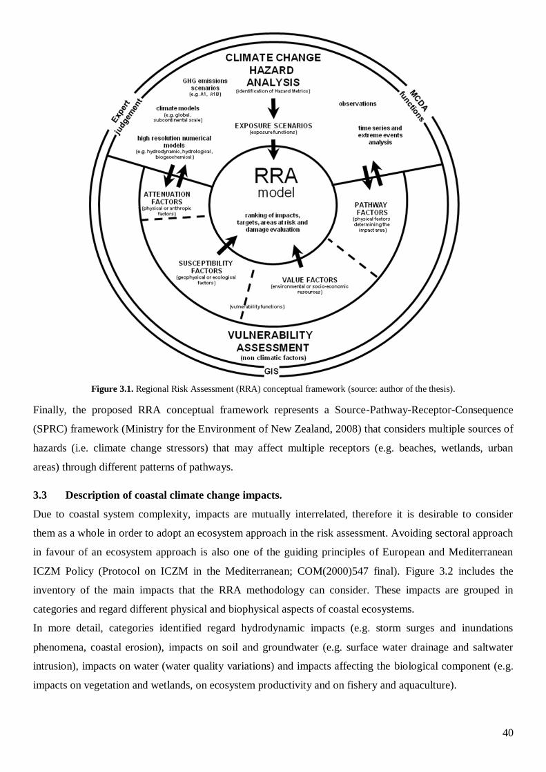
40
Figure 3.1. Regional Risk Assessment (RRA) conceptual framework (source: author of the thesis).
Finally, the proposed RRA conceptual framework represents a Source-Pathway-Receptor-Consequence
(SPRC) framework (Ministry for the Environment of New Zealand, 2008) that considers multiple sources of
hazards (i.e. climate change stressors) that may affect multiple receptors (e.g. beaches, wetlands, urban
areas) through different patterns of pathways.
3.3 Description of coastal climate change impacts.
Due to coastal system complexity, impacts are mutually interrelated, therefore it is desirable to consider
them as a whole in order to adopt an ecosystem approach in the risk assessment. Avoiding sectoral approach
in favour of an ecosystem approach is also one of the guiding principles of European and Mediterranean
ICZM Policy (Protocol on ICZM in the Mediterranean; COM(2000)547 final). Figure 3.2 includes the
inventory of the main impacts that the RRA methodology can consider. These impacts are grouped in
categories and regard different physical and biophysical aspects of coastal ecosystems.
In more detail, categories identified regard hydrodynamic impacts (e.g. storm surges and inundations
phenomena, coastal erosion), impacts on soil and groundwater (e.g. surface water drainage and saltwater
intrusion), impacts on water (water quality variations) and impacts affecting the biological component (e.g.
impacts on vegetation and wetlands, on ecosystem productivity and on fishery and aquaculture).
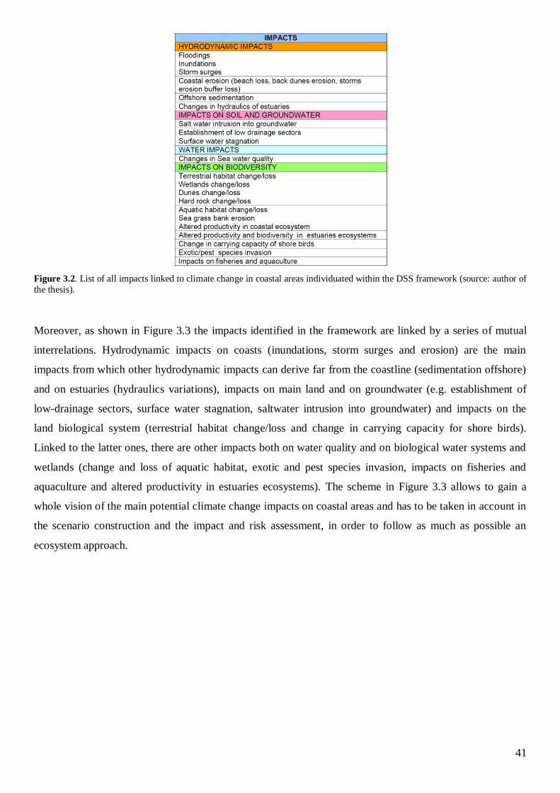
41
Figure 3.2. List of all impacts linked to climate change in coastal areas individuated within the DSS framework (source: author of
the thesis).
Moreover, as shown in Figure 3.3 the impacts identified in the framework are linked by a series of mutual
interrelations. Hydrodynamic impacts on coasts (inundations, storm surges and erosion) are the main
impacts from which other hydrodynamic impacts can derive far from the coastline (sedimentation offshore)
and on estuaries (hydraulics variations), impacts on main land and on groundwater (e.g. establishment of
low-drainage sectors, surface water stagnation, saltwater intrusion into groundwater) and impacts on the
land biological system (terrestrial habitat change/loss and change in carrying capacity for shore birds).
Linked to the latter ones, there are other impacts both on water quality and on biological water systems and
wetlands (change and loss of aquatic habitat, exotic and pest species invasion, impacts on fisheries and
aquaculture and altered productivity in estuaries ecosystems). The scheme in Figure 3.3 allows to gain a
whole vision of the main potential climate change impacts on coastal areas and has to be taken in account in
the scenario construction and the impact and risk assessment, in order to follow as much as possible an
ecosystem approach.
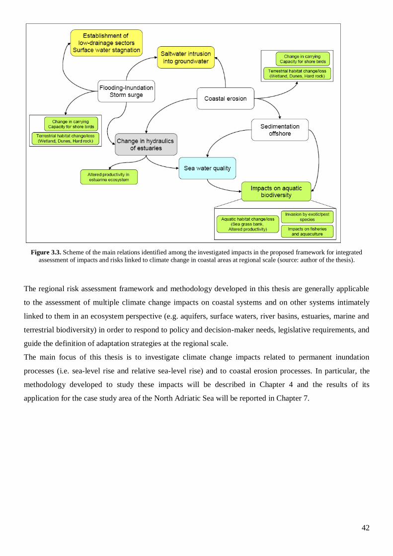
42
Figure 3.3. Scheme of the main relations identified among the investigated impacts in the proposed framework for integrated
assessment of impacts and risks linked to climate change in coastal areas at regional scale (source: author of the thesis).
The regional risk assessment framework and methodology developed in this thesis are generally applicable
to the assessment of multiple climate change impacts on coastal systems and on other systems intimately
linked to them in an ecosystem perspective (e.g. aquifers, surface waters, river basins, estuaries, marine and
terrestrial biodiversity) in order to respond to policy and decision-maker needs, legislative requirements, and
guide the definition of adaptation strategies at the regional scale.
The main focus of this thesis is to investigate climate change impacts related to permanent inundation
processes (i.e. sea-level rise and relative sea-level rise) and to coastal erosion processes. In particular, the
methodology developed to study these impacts will be described in Chapter 4 and the results of its
application for the case study area of the North Adriatic Sea will be reported in Chapter 7.

43
4. STEPS FOR THE APPLICATION OF THE REGIONAL RISK ASSESSMENT
METHODOLOGY.
The Regional Risk Assessment (RRA) methodology requires several steps for its application, as it is shown
in Figure 4.1.
Figure 4.1. Steps for the application of the Regional Risk Assessment methodology (source: author of the thesis).
The hazard and the vulnerability matrixes are used to collect all the input data needed to apply the RRA and
identify all the components contributing to the computation of risk in the case study area (i.e. stressors,
impacts and receptors) and their relationships (Paragraph 4.1). Specifically, the hazard matrix allows
identification of the stressors contributing in determining the investigated impacts and of the hazard metrics
which are then used to characterize climate change hazard within the Hazard scenario assessment phase. The
vulnerability matrix includes a subset of vulnerability factors representing physical, ecological and socio-
economic indicators of the analyzed system. Vulnerability factors are first classified in pathway, attenuation,
susceptibility and value factors and then employed in different stages of the RRA (i.e. exposure,
susceptibility, damage assessment phases).
The first step for the implementation of the RRA is the Hazard scenario assessment (Paragraph 4.3) that is
aimed at the characterization of climate change hazards that impact on a system. The second phase is the
exposure assessment (Paragraph 4.3) that aims at identifying and classifying areas where the hazard can be
in contact with the target (i.e. potential impacted areas). In this phase the hazard metrics can be normalized
through the assignation of scores and weights and are aggregated with the pathway and attenuation factors
using specific Exposure functions for each impact.
44
In order to provide an estimation of the susceptibility of the system to climate related hazards, the
Susceptibility assessment phase requires the aggregation of susceptibility factors that are first normalized
through the assignation of scores and weights and then aggregated by means of appropriate MCDA
functions (Paragraph 4.4). The following Risk assessment phase (Paragraph 4.5) is aimed at identifying and
classifying areas and targets at risk from different climate change impacts in the considered region.
Accordingly, risk assessment integrates the information about the exposure to a given climate change hazard
and about the susceptibility of a receptor to the examined hazard. Finally, the Damage assessment phase
(Paragraph 4.6) aggregates the results of the Risk assessment phase with the assessment of the
environmental and socio-economic value of a receptor, in order to provide a relative estimation of the
potential social, economic and environmental losses associated with targets and areas at risk in the case
study area (EC, 2007). The estimate of the receptors’ value is performed aggregating the value factors,
included in the vulnerability matrix and normalized through the assignation of scores and weights, by means
of MCDA functions. The following paragraphs will describe in more detail each step of the RRA
methodology.
4.1. Input data: vulnerability and hazard matrixes.
The first step for the implementation of the RRA methodology is the definition of the vulnerability and
hazard matrixes which are used to collect all the input data needed to apply the RRA and identify all the
components contributing to the computation of risk in the case study area (i.e. stressors, impacts and
receptors) and their relationships.
Two examples of generic vulnerability and hazard matrixes for the regional assessment of the risks caused
by climate change on coastal zones are reported in Appendix I. The main column of both vulnerability and
hazard matrixes is an inventory of the main potential climate change impacts affecting coastal zones. This
list include multiple interrelated impacts such as hydrodynamic impacts (e.g. storm surges and inundations
phenomena, coastal erosion), impacts on soil and groundwater (e.g. surface water drainage and saltwater
intrusion), impacts on water (water quality variations) and impacts affecting the biological component (e.g.
impacts on vegetation and wetlands, on ecosystem productivity and on fishery and aquaculture).
The vulnerability matrix reported in Table IA of Appendix I represents a guideline for the identification of
coastal receptors which could be affected by each climate change impact. Receptors represent important
features within the exposure unit, or system at risk. They are natural or anthropogenic systems of interest
due to ecological, economical, social reasons that are not equally affected by climate change hazards
(UKCIP, 2003). Moreover, each cell of the vulnerability matrix includes a subset of vulnerability factors
(i.e. pathway, attenuation, susceptibility and value factors) representing physical, ecological and socio-
economic parameters/indicators relevant for the assessment of vulnerability related to each climate change
impact. Pathway and attenuation factors are defined according to each climate change impact; susceptibility
factors are defined based on the impact and receptor considered in the assessment; value factors, instead, are
defined based on each specific receptor. A vulnerability factor can represent both a susceptibility and a value

45
characteristic of the same receptor as it can describe both the degree to which a receptor could be affected by
climate related stimuli, and relevant environmental and socio-economic values of the receptors that need to
be preserved for the interest of the community.
The hazard matrix reported in Table IB of Appendix I is a tool supporting the construction of climate change
hazard scenarios. In particular, a hazard matrix supports the user in the identification of those stressors that
contribute to determine the investigated impacts and of the hazard metrics which can be used to construct
hazard scenarios. Each climate change impact is caused by an ensemble of one or more stressors. A stressor
can be defined as the cause of environmental hazard which impacts large geographic areas and can create a
regional hazard to a population, species or ecosystems (Hunsaker et al., 1990). Each stressor can then be
characterized by one or more metrics that are quantitative measures of climate variables deriving from
statistical analysis of past measurement of weather, or from numerical models projections (UKCIP, 2003).
Hazard metrics are related to the considered impact and are variables that can change their values
considering different emission scenarios (e.g. A1B) and timeframes (e.g. 2070-2100). Vulnerability factors
are assumed as static values that represent the actual situation (reference scenario) and depend on the
intrinsic characteristics of the territory.
The general vulnerability and hazard matrixes reported in Appendix I are flexible tools that needs to be
adapted to the user purposes, to the specific case study context and according to the available data.
4.2. Hazard scenario assessment.
At the international level, hazard scenarios are widely considered as a key tool for climate change impact
and risk assessment (UKCIP, 2003).
Within the conceptual framework and the RRA methodology the hazard scenario assessment phase is aimed
at defining climate change hazards that impact on a system. Accordingly, climate change hazard scenarios:
i) determine the future conditions of hazard to climatic changes against which a system needs to adapt in
order to keep its ecological or socio-economical functions; ii) identify homogeneous hazard areas that may
result from the aggregation of multiple hazard metrics; iii) consider not only changes in the mean state of
climate but also changes in climate variability and extremes. Therefore, useful information for the hazard
scenario assessment phase can be derived from three main sources:
1) The output of high resolution impact models forced by downscaled climate models (e.g. the forecasts
derived from hydrodynamic models forced by regional climate models).
2) Climate scenario downscaling approaches (e.g. statistical and dynamical downscaling).
3) The analysis of past measurement of climate variables (e.g. statistical techniques of trend analysis, the use
of weather generator output or other model-derived output based on observed data, such as the analysis of
the return period of extreme storm surge events).
In the first source includes high resolution models (e.g. dedicated hydrodynamic, hydrologic or
biogeochemical models for the system of interest) that are nested with Global Climate Models (GCMs) and
46
Regional Climate Models (RCMs) in order to provide information about regional/local climate change
stressors.
The second source refers to climate scenario downscaling techniques in order to make a link between the
state of some variable representing a large scale and the state of some variable representing a much smaller
scale. This step often involves the nesting of a high-resolution limited area climate model to a RCM in order
to develop a local climate scenario. Finally, the third source regards the analysis of past measurement of
climate variables that can be an useful tool to provide regional/local information for hazard scenarios
construction in impact and risk assessment and in particular for the analysis of extreme events.
A key issue of the hazard assessment phase is to choose and use suitable statistics deriving from numerical
models and analysis of past measurement of climate variables in order to construct scenarios representing
potentially significant hazards related to climate change. Since models forecasts provide a huge amount of
model output for a detailed temporal resolution (i.e. every 6 hours, or every day or every month), the risk
assessor needs to define statistics which can properly describe the trend of the parameter under analysis, for
a reference period of typically 30 years (e.g. 2070-2100). Metrics provided by models are usually defined
according to their spatial and temporal domains. This implies that, for example, an average value may be
defined:
- spatially – at a point in time (an instantaneous spatial average);
- temporally – over a defined time interval (e.g. a 30-year average value for a particular global climate
model (GCM) or regional climate model (RCM) grid-box).
In general, examples of statistics associated with metrics for climate change risk assessment are (UKCIP,
2003):
mean or average, mode or median of values determined over a particular period;
cumulative (time-integrated) value;
the frequency or probability of particular values or events including percentiles,
the frequency or probability that values of variables will fall between particular bounds, or exceed a
particular (often extreme) threshold;
absolute maximum or minimum values that may be recorded, usually over a particular interval of time;
measures of variance, standard deviation or standard error, or more complete descriptions in terms of
probability distributions or functions.
Within the RRA methodology, the selected statistics representing hazard metrics associated with each
climate change impact are employed in the construction of hazard scenarios and then used in the Exposure
assessment phase (Paragraph 4.3) together with pathway and attenuation factors for the construction of
exposure maps.

47
4.3. Exposure assessment.
The exposure assessment phase is aimed at identifying and classifying areas where the hazard can be in
contact with the target (i.e. potential impacted areas) using Exposure functions.
The exposure functions Ek,s are defined for each climate change impact k and can be applied for different
hazard scenarios s that represents the spatial distribution of climate change hazards in a specific timeframe
(e.g. 2050, 2100) under specific emission scenario (e.g. IPCC SRES A1 or A2, Nakićenovićet al., 2000).
Moreover, within the RRA model, the Ek,s aggregates hazard metrics (hk,s), allowing the characterization of
the nature and magnitude of climate change related hazards, with attenuation factors (af) attenuating the
intensity of the hazard associated with an impact k and pathway factors (pf) determining the possibility of
contact between targets and climate change hazards.
Accordingly, the general Exposure function associated with an impact k and a scenario s is represented by
Equation 1:
Equation 1
where:
exposure score related to an impact k and a scenario s;
hk,s= hazard score related to the impact k and scenario s;
Atk= attenuation score related to the impact k;
Pk= pathway score related to the impact k.
The function F used in Equation 1 is defined according to the specific impact and can derive from scientific
literature or can be a MCDA function aimed at integrating the hazard metrics reported in the cells of the
hazard matrix (Appendix I, Table I B) and the attenuation and pathway factors reported in the cells of the
vulnerability matrix (Appendix I, Table I A).
The hazard metrics can be normalized with the assignation of scores and weights, if it is specifically
required in the Exposure function (e.g. in the Exposure function of the coastal erosion impact). Specifically,
hazard classes are related to hazard metrics and represent different intensity of hazard to climatic stressors
associated with each impact. Classes can be categorical (e.g. presence or absence of a particular indicator or
indicator type) or can derive from continuous data. In the first case, the classes and scores can be founded in
literature, or can be expressed by expert judgement. In the second case, classes can also be accomplished by
using some mathematical data based techniques such as dividing the frequency distribution for data into
quintiles. The set of the classes can be defined by the following mathematical definition
.
To each class, a score is assigned from a minimum value (i.e. 0) to a maximum value (i.e.1), with minimum
representing no hazard and the maximum value representing the higher class compared to the others
skE ,

48
(Preston et al., 2008). Finally, intermediate scores between 0 and 1 are assigned by experts following the
linguistic evaluations reported in Table II A of Appendix II. The set of the scores associate do hazard classes
can be defined by the following mathematical definition .
Moreover, weights (wi,k) can be assigned to hazard metrics to represent their relative importance in the
estimation of the exposure associated with each impact.
In more detail, with the aim to evaluate the relative importance of each hazard metric within each impact,
the expert assigns a set of weights in the range 0–1 according to the linguistic evaluations proposed in Table
III A. Hazard metrics denoted with an apex (‘) are metrics which have already been classified and weighted
according to the following equation for a general hazard metric hk,s:
h’k,s= si,k wi,k Equation 2
where:
h’k,s = weighted hazard metric;
si,k = score of the i-th hazard metric for the impact k;
wi,k = weight of the i-th hazard metric for the impact k.
In the following paragraphs, the exposure equations proposed to investigate the impacts related to Sea-Level
Rise (SLR), Relative Sea-Level Rise (RSLR) inundation and Coastal Erosion (CE) will be presented and
discussed. For impacts affecting the terrestrial environment (i.e. SLR, RSLR and CE) the exposure function
is used to project the information provided by sea water models inland.
Finally, it is important to highlight that the Exposure functions do not quantify the hazard related to climate
change in an absolute scale, on the contrary their objective is to establish a relative ranking within the
potential impacted areas and geographically define higher-exposed locations which could help to target
priority areas for the further risk and damage analyses.
4.3.1. Exposure function for the sea-level rise inundation impact.
SLR inundation impact is considered as the overflowing onto low-lying coastal areas caused by SLR. It
involves inundation of normally dry land by brackish or saline water (Smith and Ward, 1998) and doesn’t
include erosion phenomena due to SLR.
The main stressor considered in this impact is the SLR that can be defined as the increase of the sea level
both globally and locally over a period long enough to average out transient such as waves and tides (IPCC,
2007a). The correspondent hazard metric is the SLR water level defined as the height reached by the sea
over the considered “zero” elevation level: i.e. considering a SLR projection resulting from model output
and calculated according to a chosen IPCC SRES scenario (e.g. A1B, A2, Nakićenović et al., 2000).
The main pathway factor pf1 considered in this impact is the topography of the territory determining the
elevation of each cell of the case study area (i.e. the geographical unit defined for the spatial analysis) above
the mean sea level.

49
The objective of the Exposure function for the SLR inundation impact (Eslr,s) (Equation 3) is therefore to
determine and rank potential areas inundated by SLR based on the quantity of water staying at the top of
each cell according to the following equation:
Equation 3
where:
Eslr,s= exposure score related to SLR inundation impact in scenario s;
hslr,s= projection of sea-level rise water level according to scenario s (cm);
pf1= elevation of the cell (cm);
s1= threshold given by the decision maker. It represents the amount of water above a cell which generates
the maximum exposure (cm).
The hazard metric (hslr,s) corresponds to the metric SLR water level described before; the pathway factor
(pf1) represents the topography of the territory (i.e. the elevation of the cell) and determines if the considered
area can be reached by the hazard SLR or not. Finally, s1 is a threshold given by the decision maker (DM) in
order to normalize the value of the exposure function in the 0-1 range and to define the maximum water
quantity above each cell (e.g. 60 cm) over which the Exposure function assumes its maximum value. A DM
can therefore establish case by case what is the water level of tolerance for his community.
The Exposure function proposed for the SLR inundation impact permits to assign to each cell of the case
study area a score ranging between 0 (i.e. no exposure) and 1 (i.e. maximum exposure).If the cell is higher
than the SLR water level, the exposure score associated with the cell will be zero. On the contrary the
maximum exposure is defined if the amount of water above a cell is higher than the threshold provided by
DM. Values between 0 and 1 quantify the amount of water quantity staying at the top of each cell.
4.3.2. Exposure function for the relative sea-level rise inundation impact.
RSLR occurs where there is a local increase in the level of the ocean relative to the land, which might be due
to ocean rise and/or land level subsidence (IPCC, 2007a). Specifically, RLSR impact is considered as the
overflowing onto low-lying coastal areas caused by SLR and vertical land movements (i.e. subsidence and
uplift). In addition to the hazard metric and pathway factor used for the characterization of the SLR
inundation impact (Paragraph 4.3.1), this impact considers as pathway factor the vertical land movements
that can be defined as a gradual sinking or increasing of land with respect to its previous level
(http://www.nwrc.usgs.gov/fringe/glossary.html).
The objective of the Exposure function for the RSLR inundation impact (Equation 4) is to integrate SLR
model projections and literature data concerning the rate of subsidence/uplift of the case study area in order
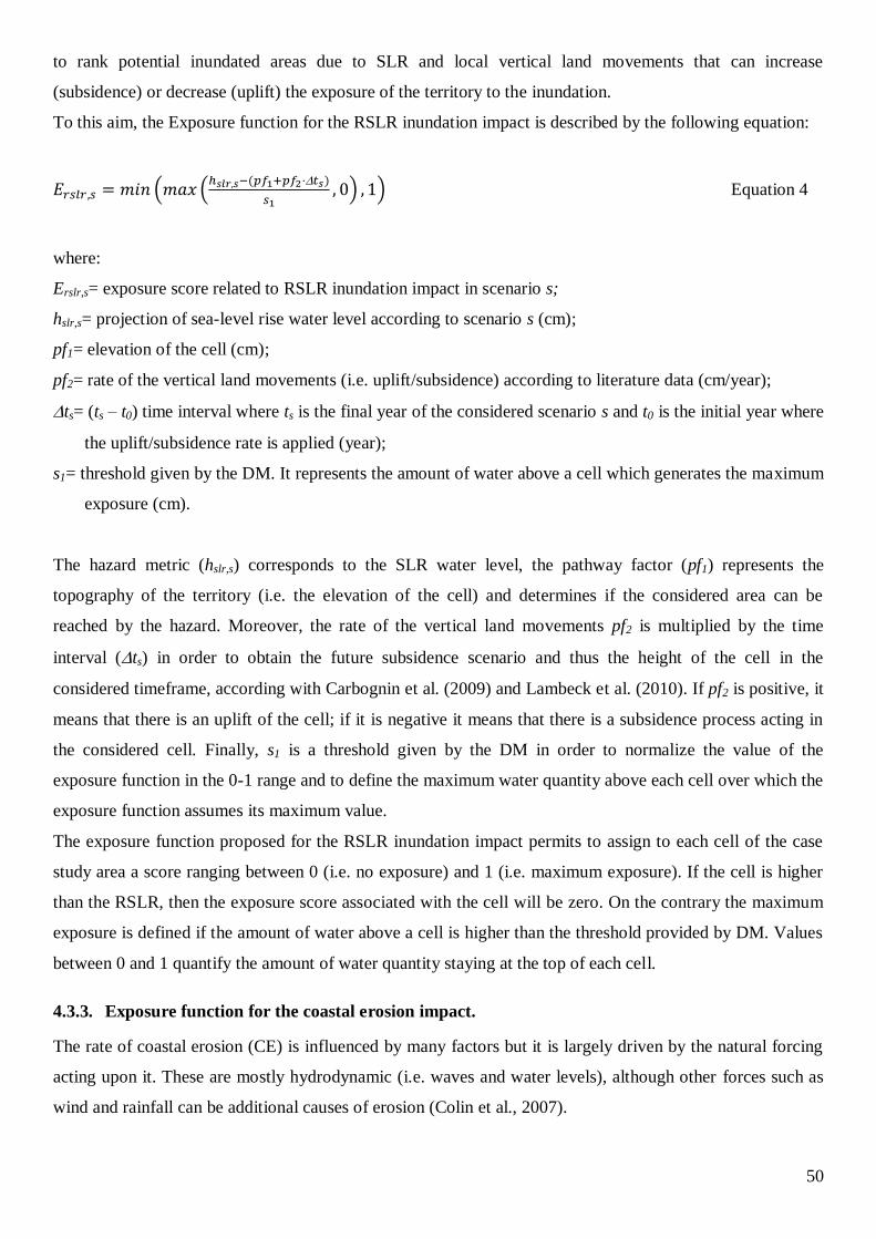
50
to rank potential inundated areas due to SLR and local vertical land movements that can increase
(subsidence) or decrease (uplift) the exposure of the territory to the inundation.
To this aim, the Exposure function for the RSLR inundation impact is described by the following equation:
Equation 4
where:
Erslr,s= exposure score related to RSLR inundation impact in scenario s;
hslr,s= projection of sea-level rise water level according to scenario s (cm);
pf1= elevation of the cell (cm);
pf2= rate of the vertical land movements (i.e. uplift/subsidence) according to literature data (cm/year);
ts= (ts – t0) time interval where ts is the final year of the considered scenario s and t0 is the initial year where
the uplift/subsidence rate is applied (year);
s1= threshold given by the DM. It represents the amount of water above a cell which generates the maximum
exposure (cm).
The hazard metric (hslr,s) corresponds to the SLR water level, the pathway factor (pf1) represents the
topography of the territory (i.e. the elevation of the cell) and determines if the considered area can be
reached by the hazard. Moreover, the rate of the vertical land movements pf2 is multiplied by the time
interval ( ts) in order to obtain the future subsidence scenario and thus the height of the cell in the
considered timeframe, according with Carbognin et al. (2009) and Lambeck et al. (2010). If pf2 is positive, it
means that there is an uplift of the cell; if it is negative it means that there is a subsidence process acting in
the considered cell. Finally, s1 is a threshold given by the DM in order to normalize the value of the
exposure function in the 0-1 range and to define the maximum water quantity above each cell over which the
exposure function assumes its maximum value.
The exposure function proposed for the RSLR inundation impact permits to assign to each cell of the case
study area a score ranging between 0 (i.e. no exposure) and 1 (i.e. maximum exposure). If the cell is higher
than the RSLR, then the exposure score associated with the cell will be zero. On the contrary the maximum
exposure is defined if the amount of water above a cell is higher than the threshold provided by DM. Values
between 0 and 1 quantify the amount of water quantity staying at the top of each cell.
4.3.3. Exposure function for the coastal erosion impact.
The rate of coastal erosion (CE) is influenced by many factors but it is largely driven by the natural forcing
acting upon it. These are mostly hydrodynamic (i.e. waves and water levels), although other forces such as
wind and rainfall can be additional causes of erosion (Colin et al., 2007).
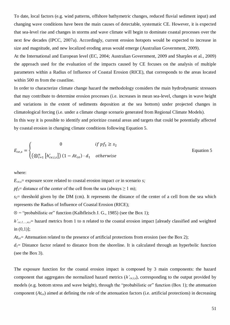
51
To date, local factors (e.g. wind patterns, offshore bathymetric changes, reduced fluvial sediment input) and
changing wave conditions have been the main causes of detectable, systematic CE. However, it is expected
that sea-level rise and changes in storms and wave climate will begin to dominate coastal processes over the
next few decades (IPCC, 2007a). Accordingly, current erosion hotspots would be expected to increase in
size and magnitude, and new localized eroding areas would emerge (Australian Government, 2009).
At the International and European level (EC, 2004; Australian Government, 2009 and Sharples et al., 2009)
the approach used for the evaluation of the impacts caused by CE focuses on the analysis of multiple
parameters within a Radius of Influence of Coastal Erosion (RICE), that corresponds to the areas located
within 500 m from the coastline.
In order to characterize climate change hazard the methodology considers the main hydrodynamic stressors
that may contribute to determine erosion processes (i.e. increases in mean sea-level, changes in wave height
and variations in the extent of sediments deposition at the sea bottom) under projected changes in
climatological forcing (i.e. under a climate change scenario generated from Regional Climate Models).
In this way it is possible to identify and prioritize coastal areas and targets that could be potentially affected
by coastal erosion in changing climate conditions following Equation 5.
Equation 5
where:
Ece,s= exposure score related to coastal erosion impact ce in scenario s;
pf3= distance of the center of the cell from the sea (always ≥ 1 m);
s2= threshold given by the DM (cm). It represents the distance of the center of a cell from the sea which
represents the Radius of Influence of Coastal Erosion (RICE);
= “probabilistic or” function (Kalbfleisch J. G., 1985) (see the Box 1);
h’ce,1,…,n,s= hazard metrics from 1 to n related to the coastal erosion impact [already classified and weighted
in (0,1)];
Atce= Attenuation related to the presence of artificial protections from erosion (see the Box 2);
d1= Distance factor related to distance from the shoreline. It is calculated through an hyperbolic function
(see the Box 3).
The exposure function for the coastal erosion impact is composed by 3 main components: the hazard
component that aggregates the normalized hazard metrics (h’ce,i,s), corresponding to the output provided by
models (e.g. bottom stress and wave height), through the “probabilistic or” function (Box 1); the attenuation
component (Atce) aimed at defining the role of the attenuation factors (i.e. artificial protections) in decreasing
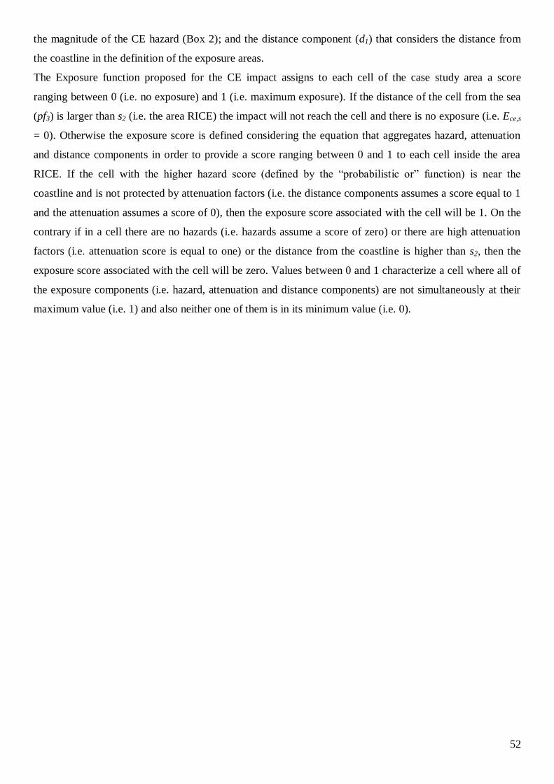
52
the magnitude of the CE hazard (Box 2); and the distance component (d1) that considers the distance from
the coastline in the definition of the exposure areas.
The Exposure function proposed for the CE impact assigns to each cell of the case study area a score
ranging between 0 (i.e. no exposure) and 1 (i.e. maximum exposure). If the distance of the cell from the sea
(pf3) is larger than s2 (i.e. the area RICE) the impact will not reach the cell and there is no exposure (i.e. Ece,s
= 0). Otherwise the exposure score is defined considering the equation that aggregates hazard, attenuation
and distance components in order to provide a score ranging between 0 and 1 to each cell inside the area
RICE. If the cell with the higher hazard score (defined by the “probabilistic or” function) is near the
coastline and is not protected by attenuation factors (i.e. the distance components assumes a score equal to 1
and the attenuation assumes a score of 0), then the exposure score associated with the cell will be 1. On the
contrary if in a cell there are no hazards (i.e. hazards assume a score of zero) or there are high attenuation
factors (i.e. attenuation score is equal to one) or the distance from the coastline is higher than s2, then the
exposure score associated with the cell will be zero. Values between 0 and 1 characterize a cell where all of
the exposure components (i.e. hazard, attenuation and distance components) are not simultaneously at their
maximum value (i.e. 1) and also neither one of them is in its minimum value (i.e. 0).
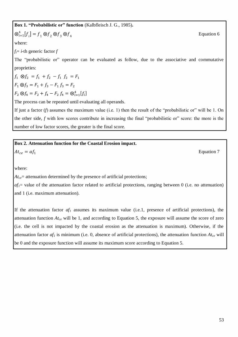
53
Box 1. “Probabilistic or” function (Kalbfleisch J. G., 1985).
Equation 6
where:
fi= i-th generic factor f
The “probabilistic or” operator can be evaluated as follow, due to the associative and commutative
proprieties:
The process can be repeated until evaluating all operands.
If just a factor (f) assumes the maximum value (i.e. 1) then the result of the “probabilistic or” will be 1. On
the other side, f with low scores contribute in increasing the final “probabilistic or” score: the more is the
number of low factor scores, the greater is the final score.
Box 2. Attenuation function for the Coastal Erosion impact.
Equation 7
where:
Atce= attenuation determined by the presence of artificial protections;
af1= value of the attenuation factor related to artificial protections, ranging between 0 (i.e. no attenuation)
and 1 (i.e. maximum attenuation).
If the attenuation factor af1 assumes its maximum value (i.e.1, presence of artificial protections), the
attenuation function Atce will be 1, and according to Equation 5, the exposure will assume the score of zero
(i.e. the cell is not impacted by the coastal erosion as the attenuation is maximum). Otherwise, if the
attenuation factor af1 is minimum (i.e. 0, absence of artificial protections), the attenuation function Atce will
be 0 and the exposure function will assume its maximum score according to Equation 5.

54
Box 3. Distance function.
The proposed distance function (d) assumes an hyperbolic trend according to the following equation:
Equation 8
where:
g= distance of the center of the cell from the sea (pf3) for the exposure to the coastal erosion (cm);
k= constant that defines the slope of the hyperbolic function;
b= s*t, where:
s= is a threshold given by DM. s2= represents the distance of the center of a cell from the sea which
represents the Radius of Influence of Coastal Erosion (RICE);
t = is a constant used in order to establish where to cut the hyperbolic function. For the exposure to the
coastal erosion t= 1.
In order to estimate potential risks associated with coastal erosion, the results of the exposure assessment
phase will be integrated with the susceptibility assessment that provides information about other relevant
factors contributing in determining coastal erosion impacts (e.g. lithology, geomorphology, littoral drift
rates, sediment budgets, coastal slope).
4.4. Susceptibility assessment.
The Susceptibility assessment phase is aimed at evaluating the degree to which the receptors could be
affected by a given climate change impact (e.g. SLR, SSF, CE) based on site-specific territorial information.
To this aim, the susceptibility assessment phase aggregates the susceptibility factors (sf) defined in the
vulnerability matrix using a Susceptibility function based on MCDA methods.
Since in the coastal territory a spatial unit (i.e. raster cell) can be characterized by two or more receptors
(e.g. a cell is both a beach and a protected area) the susceptibility function is applied to all the sf listed in the
vulnerability matrix for the considered impact k. In this way, if a cell is both a beach and protected area, its
susceptibility will be evaluated considering the contribution of all the sf related to the cell taken only once
time (i.e. the union of the sf related to receptors beach and protected areas). Moreover, it is assumed that a
given sf play the same role in determining the susceptibility of different receptors in relation to the analyzed
impact k (e.g. the vegetation cover has the same importance in determining the susceptibility of beaches and
protected areas to coastal erosion).
In order to apply the Susceptibility function that makes relative rankings of coastal areas and receptors more
sensitive to climate change impacts, the susceptibility factors (sf) must be classified, scored and weighted
taking into account the expert judgment. Specifically, susceptibility factor classes are determined by
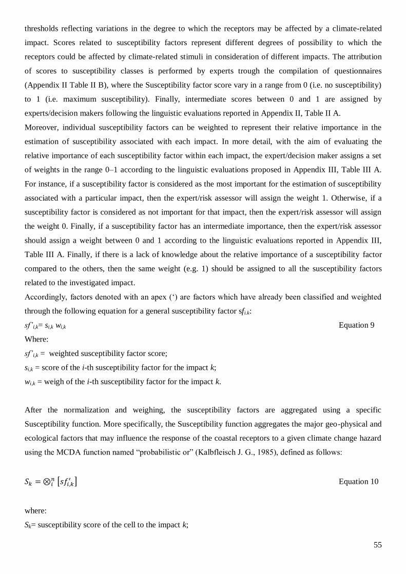
55
thresholds reflecting variations in the degree to which the receptors may be affected by a climate-related
impact. Scores related to susceptibility factors represent different degrees of possibility to which the
receptors could be affected by climate-related stimuli in consideration of different impacts. The attribution
of scores to susceptibility classes is performed by experts trough the compilation of questionnaires
(Appendix II Table II B), where the Susceptibility factor score vary in a range from 0 (i.e. no susceptibility)
to 1 (i.e. maximum susceptibility). Finally, intermediate scores between 0 and 1 are assigned by
experts/decision makers following the linguistic evaluations reported in Appendix II, Table II A.
Moreover, individual susceptibility factors can be weighted to represent their relative importance in the
estimation of susceptibility associated with each impact. In more detail, with the aim of evaluating the
relative importance of each susceptibility factor within each impact, the expert/decision maker assigns a set
of weights in the range 0–1 according to the linguistic evaluations proposed in Appendix III, Table III A.
For instance, if a susceptibility factor is considered as the most important for the estimation of susceptibility
associated with a particular impact, then the expert/risk assessor will assign the weight 1. Otherwise, if a
susceptibility factor is considered as not important for that impact, then the expert/risk assessor will assign
the weight 0. Finally, if a susceptibility factor has an intermediate importance, then the expert/risk assessor
should assign a weight between 0 and 1 according to the linguistic evaluations reported in Appendix III,
Table III A. Finally, if there is a lack of knowledge about the relative importance of a susceptibility factor
compared to the others, then the same weight (e.g. 1) should be assigned to all the susceptibility factors
related to the investigated impact.
Accordingly, factors denoted with an apex (‘) are factors which have already been classified and weighted
through the following equation for a general susceptibility factor sfi.k:
sf’i,k= si,k wi,k Equation 9
Where:
sf’i,k = weighted susceptibility factor score;
si,k = score of the i-th susceptibility factor for the impact k;
wi,k = weigh of the i-th susceptibility factor for the impact k.
After the normalization and weighing, the susceptibility factors are aggregated using a specific
Susceptibility function. More specifically, the Susceptibility function aggregates the major geo-physical and
ecological factors that may influence the response of the coastal receptors to a given climate change hazard
using the MCDA function named “probabilistic or” (Kalbfleisch J. G., 1985), defined as follows:
Equation 10
where:
Sk= susceptibility score of the cell to the impact k;

56
= “probabilistic or” function (see the Box 1);
= i
th susceptibility factor score related to the impact k (already classified and weighted in [0,1]).
Applying the “probabilistic or” function (Equation 10), if just a susceptibility factor (sf) assumes the
maximum value (i.e. 1) then the susceptibility score will be 1. On the other side, sf with low scores
contribute in increasing the final susceptibility score: the more is the number of low susceptibility factor
scores, the greater is the final susceptibility.
The susceptibility function is evaluated for each cell of the considered region aggregating all the sf’i,k of the
impact k. If a cell is comprised in two or more receptors, its susceptibility will result from the aggregation of
all the sf’i,k susceptibility factors taken only once.
In the RRA model the Susceptibility function is used in the Risk function in order to evaluate the risk score
associated with each receptor considered in the case study area as described in paragraph 4.5.
4.5. Risk assessment.
The Risk assessment phase is aimed at integrating information about the exposure to a given climate change
scenario and the territorial susceptibility, allowing identification and prioritization of coastal receptors and
areas at risk from different impacts related to climate change in the case study area.
Regional risk scores are not absolute predictions about the risks related to climate change. Rather they
provide relative classifications about areas and targets that are likely to be affected by climate change
impacts more severely than others in the same region.
According to the framework proposed by UN-ISDR (2009), which considers the risk as the product between
hazard (i.e. a potentially damaging event or activity) and vulnerability (i.e. conditions determined by
physical, social, economic, and environmental factors or processes, which increase the susceptibility of a
community to the impact of hazards), the general function for the estimation of the risk (Rk,s) related to a
impact k is the product between the exposure score Ek,s (representing the exposure associated with a given
climate change hazard scenario) and the susceptibility score (representing the degree to which a receptor is
affected by climate-related stimuli), according to the following equation:
Equation 11
where:
Rk,s= risk score related to an impact k and scenario s;
Ek,s= exposure score related with the impact k in scenario s, according to Equation 1;
Sk= susceptibility score to the impact k, according to Equation 6.
Risk score varies from 0 to 1, in which 0 means that in an area there is no risk (i.e. there is no exposure or no
sensitivity for the considered impact and scenario) and 1 means higher risk for the considered target/area in
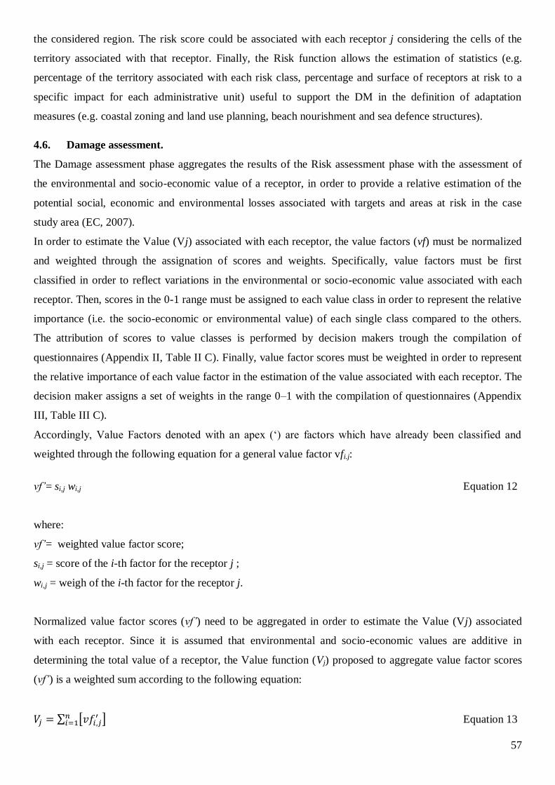
57
the considered region. The risk score could be associated with each receptor j considering the cells of the
territory associated with that receptor. Finally, the Risk function allows the estimation of statistics (e.g.
percentage of the territory associated with each risk class, percentage and surface of receptors at risk to a
specific impact for each administrative unit) useful to support the DM in the definition of adaptation
measures (e.g. coastal zoning and land use planning, beach nourishment and sea defence structures).
4.6. Damage assessment.
The Damage assessment phase aggregates the results of the Risk assessment phase with the assessment of
the environmental and socio-economic value of a receptor, in order to provide a relative estimation of the
potential social, economic and environmental losses associated with targets and areas at risk in the case
study area (EC, 2007).
In order to estimate the Value (Vj) associated with each receptor, the value factors (vf) must be normalized
and weighted through the assignation of scores and weights. Specifically, value factors must be first
classified in order to reflect variations in the environmental or socio-economic value associated with each
receptor. Then, scores in the 0-1 range must be assigned to each value class in order to represent the relative
importance (i.e. the socio-economic or environmental value) of each single class compared to the others.
The attribution of scores to value classes is performed by decision makers trough the compilation of
questionnaires (Appendix II, Table II C). Finally, value factor scores must be weighted in order to represent
the relative importance of each value factor in the estimation of the value associated with each receptor. The
decision maker assigns a set of weights in the range 0–1 with the compilation of questionnaires (Appendix
III, Table III C).
Accordingly, Value Factors denoted with an apex (‘) are factors which have already been classified and
weighted through the following equation for a general value factor vfi.j:
vf’= si,j wi,j Equation 12
where:
vf’= weighted value factor score;
si,j = score of the i-th factor for the receptor j ;
wi,j = weigh of the i-th factor for the receptor j.
Normalized value factor scores (vf’) need to be aggregated in order to estimate the Value (Vj) associated
with each receptor. Since it is assumed that environmental and socio-economic values are additive in
determining the total value of a receptor, the Value function (Vj) proposed to aggregate value factor scores
(vf’) is a weighted sum according to the following equation:
Equation 13

58
where:
Vj= value score of the receptor j;
fv’i,j = ith
value factor score related to the receptor j (already classified and weighted in [0,1]);
n= number of value factors.
The value function is aimed at identifying and classifying relevant environmental and socio-economic
values of the receptors that need to be preserved for the interest of the community (e.g. land use, fishing
areas). The Value score vary in a range from 0 to 1. The score 0 identifies the areas of a receptor that have
no relevant environmental or socio-economic value (i.e. the areas where the value associated with all the vf
is null). The score 1 identifies the areas of the analyzed receptor that are characterized by the higher
environmental or socio-economic value in the examined case study area. In the cases where there are no
available data to identify value factors for the investigated receptors, the value function cannot be calculated.
Since the value function aggregates scores and weights assigned by DM, the judgment would be subjective
and related to the interest of the DM. In order to obtain a consensus between DMs, Group Decision Theory
(Kiker et al., 2005) techniques could be applied to facilitate involvement, preference elicitation and
consensus evaluation. Finally, the value score (Vj) associated with each target j is integrated with relative
risk scores (Rk,s) estimated for each impact k and scenario s, through the following Damage function:
Equation 14
where:
Dj,k,s= damage score related to an impact k and a receptor j in the scenario s;
Rk,s= risk score related to impact k in scenario s, according to Equation 11;
Vj= value score of receptor j, according to Equation 13.
The Damage function vary from 0 to 1. It assumes the higher value when the risk is higher (i.e.1) and the
value score is higher, and assumes the minimum value (i.e. 0) when the risk and/or the value is 0. Finally, in
the other cases, the damage score assumes values in the range 0-1, allowing identification and prioritization
of the potential losses associated with targets and areas at risk in the considered region and supporting the
identification of areas which require prior adaptation actions to prevent impacts and risk related to climate
change.
The damage score is calculated for all the cells of the examined region where the receptor j is located. In
order to have an overall estimate of the damage associated with the receptor j for the impact k it is possible
to calculate some statistics (e.g. percentage of the receptor associated with each damage class, percentage
59
and surface of the receptor with higher damage scores for each administrative unit). These statistics can be
useful to support the DM in the definition and prioritization of adaptation measures.
4.7. Regional Risk Assessment outputs.
The main output of the RRA methodology include GIS-based exposure, susceptibility, risk and damage
maps that are calculated based on exposure, susceptibility, risk and damage functions described above.
These maps to establish relative priorities for intervention, to identify suitable areas for human settlements,
infrastructures and economic activities, and provide a basis for coastal zoning and land use planning.
All the hazard metrics and the vulnerability factors reported in Appendix I are represented in raster GIS
layers allowing analysis and visualization of their spatial distribution in the case study area. Thus, the
outputs of the risk assessment are also raster maps (i.e. cell based maps) representing the spatial distribution
of exposure, susceptibility, risk and damage in the examined coastal territory.
As shown in Figure 4.2, exposure maps identify and classify the areas where the hazard can be in contact
with the target (i.e. potential impacted areas) and derive from the aggregation of climate change hazard
scenarios (represented by single or multiple hazard metrics) with pathway and attenuation factors;
susceptibility maps represent the spatial distribution of environmental and socio-economic susceptibility
factors (e.g. land use, vegetation cover, coastal slope) and are derived from the aggregation of susceptibility
factors; risk maps identify and rank areas and receptors at risk from climate change related impacts in the
considered region; finally, damage maps derive from combination of risk and value functions and provide a
relative estimation of the potential social, economic and environmental losses.
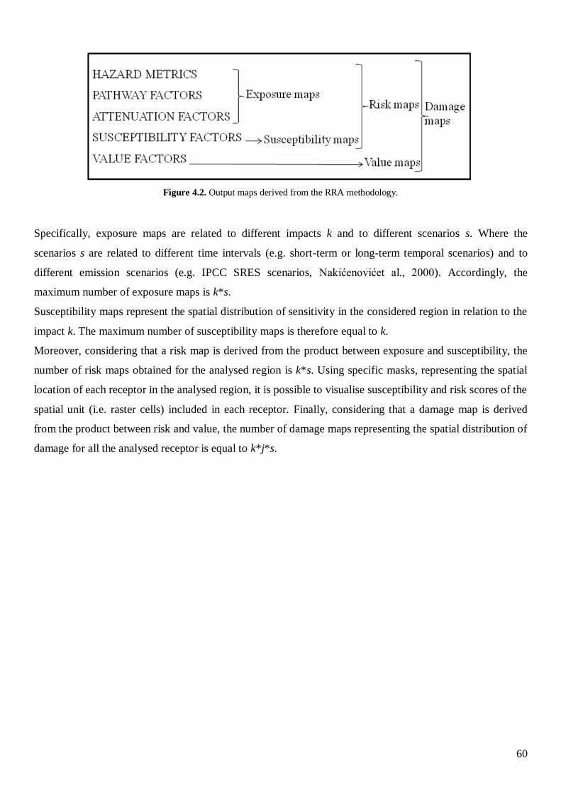
60
Figure 4.2. Output maps derived from the RRA methodology.
Specifically, exposure maps are related to different impacts k and to different scenarios s. Where the
scenarios s are related to different time intervals (e.g. short-term or long-term temporal scenarios) and to
different emission scenarios (e.g. IPCC SRES scenarios, Nakićenovićet al., 2000). Accordingly, the
maximum number of exposure maps is k*s.
Susceptibility maps represent the spatial distribution of sensitivity in the considered region in relation to the
impact k. The maximum number of susceptibility maps is therefore equal to k.
Moreover, considering that a risk map is derived from the product between exposure and susceptibility, the
number of risk maps obtained for the analysed region is k*s. Using specific masks, representing the spatial
location of each receptor in the analysed region, it is possible to visualise susceptibility and risk scores of the
spatial unit (i.e. raster cells) included in each receptor. Finally, considering that a damage map is derived
from the product between risk and value, the number of damage maps representing the spatial distribution of
damage for all the analysed receptor is equal to k*j*s.
61
Section C
APPLICATION TO THE CASE STUDY AREA
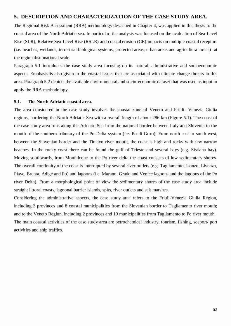
62
5. DESCRIPTION AND CHARACTERIZATION OF THE CASE STUDY AREA.
The Regional Risk Assessment (RRA) methodology described in Chapter 4, was applied in this thesis to the
coastal area of the North Adriatic sea. In particular, the analysis was focused on the evaluation of Sea-Level
Rise (SLR), Relative Sea-Level Rise (RSLR) and coastal erosion (CE) impacts on multiple coastal receptors
(i.e. beaches, wetlands, terrestrial biological systems, protected areas, urban areas and agricultural areas) at
the regional/subnational scale.
Paragraph 5.1 introduces the case study area focusing on its natural, administrative and socioeconomic
aspects. Emphasis is also given to the coastal issues that are associated with climate change threats in this
area. Paragraph 5.2 depicts the available environmental and socio-economic dataset that was used as input to
apply the RRA methodology.
5.1. The North Adriatic coastal area.
The area considered in the case study involves the coastal zone of Veneto and Friuli- Venezia Giulia
regions, bordering the North Adriatic Sea with a overall length of about 286 km (Figure 5.1). The coast of
the case study area runs along the Adriatic Sea from the national border between Italy and Slovenia to the
mouth of the southern tributary of the Po Delta system (i.e. Po di Goro). From north-east to south-west,
between the Slovenian border and the Timavo river mouth, the coast is high and rocky with few narrow
beaches. In the rocky coast there can be found the gulf of Trieste and several bays (e.g. Sistiana bay).
Moving southwards, from Monfalcone to the Po river delta the coast consists of low sedimentary shores.
The overall continuity of the coast is interrupted by several river outlets (e.g. Tagliamento, Isonzo, Livenza,
Piave, Brenta, Adige and Po) and lagoons (i.e. Marano, Grado and Venice lagoons and the lagoons of the Po
river Delta). From a morphological point of view the sedimentary shores of the case study area include
straight littoral coasts, lagoonal barrier islands, spits, river outlets and salt marshes.
Considering the administrative aspects, the case study area refers to the Friuli-Venezia Giulia Region,
including 3 provinces and 8 coastal municipalities from the Slovenian border to Tagliamento river mouth;
and to the Veneto Region, including 2 provinces and 10 municipalities from Tagliamento to Po river mouth.
The main coastal activities of the case study area are petrochemical industry, tourism, fishing, seaport/ port
activities and ship traffics.
63
Figure 5.1. The case study area: a) the Northern Adriatic Sea (adapted from google maps: maps.google.it); b) the coast of the
Veneto and Friuli Venezia Giulia regions (Italy).
On the whole, the Northern Adriatic Sea coast, comprises a very precarious coastal environment subject to
continuous morphological changes that can be appreciable even over short geological time scales
(Gambolati and Teatini, 2002). Moreover, erosion is still active in many areas both on the coastal sea floor
and on the beach since the beginning of the 20th century and especially after 1960 (Bondesan et al., 1995).
Many areas, particularly around the Po river Delta, are also located below the mean sea level and affected by
natural or man-induced subsidence (Pirazzoli, 2005). Furthermore, the municipality of Venice has been
experiencing an increase of high tide events with consequent flooding of the city (www.comune.venezia.it).
In Mediterranean sea rates of sea-level rise for the three longest tide-gauge stations ranged from 1.1 mm/yr
to 1.3 mm/yr (Tsimplis and Spencer, 1997). However, spatially the change is not uniform and in the North
Adriatic sea the observed sea level rate can vary from 1,2 mm/yr in Trieste to 2,5 mm/yr in Venice
(Antonioli et al., 2007).
Therefore, climate change and sea-level rise is a prominent issue for the case study area both considering the
vulnerability of fragile ecosystems such as coastal lagoons, and the concentration of cultural and socio-
economic values.
Even if in recent years several studies were produced to evaluate potential impacts of storm surge and sea-
level rise on the coasts of the Northern Adriatic sea (Bondesan et al., 1995; Gonella et al., 1998; Gambolati
and Teatini, 2002; Lionello, 2008), only few significant local sites (e.g. the lagoon of Venice) were
investigated with good detail. Existing studies were also often targeted to the analysis of specific physical
processes (e.g. morphological evolution of deltas and transitional environments in response to sea-level rise)
64
without considering other important factors contributing to coastal vulnerability to climate change such as
distribution of coastal assets, inhabitants and ecosystems (Fontolan, 2001; Seminara et al., 2005; Ferla et al.,
2007; Simeoni et al., 2007).
The complexity of the problems linked to climate change and the importance of natural and socioeconomic
aspects in the study area ask instead for a broader integrated approach.
Accordingly, the RRA methodology proposed in this thesis is an innovative approach not only with respect
to the spatial scale of analysis (e.g. the whole coastal area of the North Adriatic Sea), but also for the multi-
disciplinary and integrated approach that takes into account downscaled climate change processes (e.g. sea-
level rise, changes in currents and wave climate) to characterize climate change hazards at the regional
scale; and biogeophysical and socio-economic factors (e.g. altimetry, geomorphology, land use and
vegetation cover) to determine the susceptibility of the territory to climate change impacts and risks.
5.2. Available dataset.
The assessment of climate change impacts at the regional scale involves the collection of a huge amount of
data in order to characterize spatially the targets of the analysis (e.g. beaches, wetlands, agricultural areas
etc.) and define vulnerability indicators (i.e. susceptibility factors, attenuation factors, value factors and
pathway factors) to be included in the vulnerability matrix (paragraph 4.1). Consequently, a survey of
available information regarding physical, socio-economic and ecological features of the case study area was
performed for the North Adriatic coasts.
Available data were provided by various public institutions in graphic format or database, and include: a 5
meters Digital Elevation Model (DEM) supplied by Veneto Region and a 10 meters DEM supplied by Friuli
Venezia Giulia Region; the digital Corine Land Cover (CLC2000) database (e.g., wetlands, vegetation
cover, hydrological systems, dunes) (http://www.clc2000.sinanet.apat.it/cartanetclc2000/clc2000/prodotti.asp); a
list of Natura 2000 sites (i.e., ZPS and SIC areas) supplied by regional authorities; coastal data included in
the geographic coastal information system (e.g., coastal morphology, sediment budget, artificial protections)
implemented by the Italian Environmental Protection Agency (APAT, now called ISPRA;
http://www.mais.sinanet.apat.it); technical regional maps supplied by the Veneto and Friuli Regions
(www.regione.veneto.it /Ambiente+e+Territorio/; www.regione.fvg.it/rafvg/territorioambiente); and finally
administrative boundaries of coastal municipalities and provinces furnished by regional authorities.
For the assessment of coastal vulnerability to sea-level rise at the regional/sub-national scale it would be of
course preferable to use the higher spatial resolution and high vertical accuracy topographic datasets (i.e.
high resolution data obtained by Light Detection and Ranging techniques (LIDAR). However, this was not
totally feasible for the study area of concern, because only limited areas (i.e. the littoral zone of the Po River
Delta and of the Venice lagoon) hold a free access LIDAR database. Consequently, the present analysis was
done using the most detailed digital topographic dataset available for the whole coast of Veneto and Friuli
Venezia Giulia (i.e. DEM with a horizontal resolution of 5 and 10 m respectively). With future
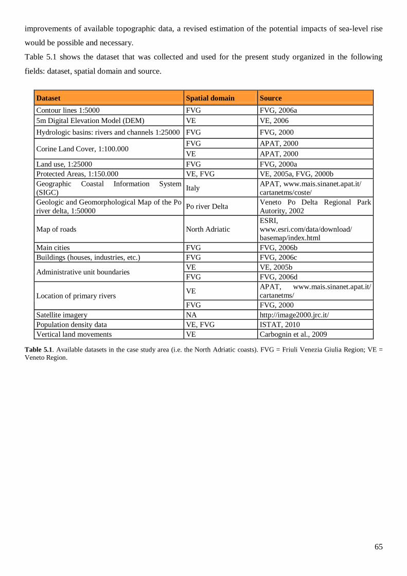
65
improvements of available topographic data, a revised estimation of the potential impacts of sea-level rise
would be possible and necessary.
Table 5.1 shows the dataset that was collected and used for the present study organized in the following
fields: dataset, spatial domain and source.
Dataset Spatial domain Source
Contour lines 1:5000 FVG FVG, 2006a
5m Digital Elevation Model (DEM) VE VE, 2006
Hydrologic basins: rivers and channels 1:25000 FVG FVG, 2000
Corine Land Cover, 1:100.000 FVG APAT, 2000
VE APAT, 2000
Land use, 1:25000 FVG FVG, 2000a
Protected Areas, 1:150.000 VE, FVG VE, 2005a, FVG, 2000b
Geographic Coastal Information System
(SIGC) Italy
APAT, www.mais.sinanet.apat.it/
cartanetms/coste/
Geologic and Geomorphological Map of the Po
river delta, 1:50000 Po river Delta
Veneto Po Delta Regional Park
Autority, 2002
Map of roads North Adriatic
ESRI,
www.esri.com/data/download/ basemap/index.html
Main cities FVG FVG, 2006b
Buildings (houses, industries, etc.) FVG FVG, 2006c
Administrative unit boundaries VE VE, 2005b
FVG FVG, 2006d
Location of primary rivers VE
APAT, www.mais.sinanet.apat.it/
cartanetms/
FVG FVG, 2000
Satellite imagery NA http://image2000.jrc.it/
Population density data VE, FVG ISTAT, 2010
Vertical land movements VE Carbognin et al., 2009
Table 5.1. Available datasets in the case study area (i.e. the North Adriatic coasts). FVG = Friuli Venezia Giulia Region; VE =
Veneto Region.

66
6. THE MULTI-MODEL CHAIN APPLIED TO DEFINE CLIMATE CHANGE
HAZARD SCENARIOS IN THE NORTH ADRIATIC COASTAL AREA.
This Chapter is aimed at describing the numerical models chain applied to study climate change impacts on
the coastal area of the North Adriatic Sea at the regional scale, the models involved in the chain and, finally,
at summarising the information provided by the models for the construction of climate change hazard
scenarios.
6.1. Chain of numerical models applied to the North Adriatic Sea.
In order to provide suitable information for the characterization of potentially significant hazard scenarios at
the regional scale and build climate change hazard maps to be used in the risk assessment, a chain of models
was set up for the study area of the North Adriatic Sea. The model chain was developed in the framework of
the CMCC-FISR project (www.cmcc.it) and includes different types and spatial scales of numerical models
simulating relevant circulation and morphodynamic processes recognized as influencing climate change
impacts on coastal areas. Starting from Global Climate Models (GCMs) and Regional Climate Models
(RCMs) representing the main atmosphere and ocean dynamics and covering large spatial domains (i.e. from
the global to the sub-continental scale), the chain of models includes a suite of higher resolution impact
models able to simulate ocean dynamics and circulation processes in coastal waters, with a spatial domain
ranging from the sub-national/regional to the local scale.
Models included in the models chain were supplied by partners involved in the CMCC-FISR project that
are: the National Institute of Geophysics and Volcanology (INGV) and the Marine Science Institute
(ISMAR) of the Italian National Research Council (CNR). Figure 6.1 represents the models chain applied
for the North Adriatic case study in its main components and interrelationships. As shown in Figure 6.1 the
model chain is forced by the IPCC SRES scenario A1B that provides the climate forcing in terms of
atmospheric concentrations of greenhouse gases (GHGs), ozone and aerosols (Nakićenović et al., 2000). The
A1B scenario belongs to the A1 storyline family, which describes a future world of very rapid economic
growth. In this potential future, global population peaks mid-century and declines thereafter, and new and
more efficient technologies are rapidly introduced. Moreover, the A1B scenario predicts carbon dioxide
emissions increasing until around 2050 and then decreasing, and it assumes a balanced emphasis between
fossil fuels and other energy sources. The A1B climate forcing represent the input for the GCM and the
nested RCM. The output of the RCM are used directly to construct downscaled climate hazard scenarios for
the case study area (i.e. scenarios of temperature, precipitation and wind variations) and then represent the
input for the suite of impact models running at higher resolution (i.e. from the Adriatic to the North Adriatic
scale). In Figure 6.1 the impact models are represented by hydrodynamic and wave models that are used to
investigate sea-level rise and coastal erosion hazards.

67
Figure 6.1. The multi-model chain applied to define climate change hazard scenarios in the North Adriatic coastal area. Names in
brackets refer to partners who applied each model.
In addition to the climate forcing (i.e. the output of GCMs and RCMs.), impact models employ also time
series analysis as input data. Specifically, in order to calibrate the model outputs and analyse the extreme
event trends the impact models use an observation dataset related to the reference period 1960-1990.
The construction of a model chain is an effective way to supply relevant information about climate forcing
and cascading processes ranging from the global/subcontinental scale to the regional/local scale. As shown
in Figure 6.1, the information provided by high resolution impact models is used to investigate climate
change hazards at a suitable spatial resolution for impact and risk assessment (i.e. from 5 km to 50 m) and
for a future temporal scenario (i.e. the thirty year period 2070-2100).
The models included in the model chain belong to the following main categories:
climate models (SXG, EBU-POM);
ocean and sea circulation models (SHYFEM, ROMS);
a wave model (SWAN).
The models included in the model chain were also classified according to the different hazard category
investigated (i.e. climate hazards, sea-level rise hazards and coastal erosion hazards). For each hazard
category, the following paragraphs will describe in more detail each model used in the model chain, its
specific characteristic and the outputs used for the construction of hazard scenarios at the regional/local
scale.

68
6.2. Climate hazard.
Models used for the characterization of climate hazard in the RRA are basically climate models that are
mathematical representations of the climate system based on the physical, chemical, and biological
properties of its components, their interactions and feedbacks (ukclimateprojections.defra.gov.uk). Global
Climate Models (GCMs) are three dimensional numerical models that solve the equations for fluid motion
and energy transfer around the globe and integrate these forward in time. Coupled Atmosphere-Ocean
Global Climate Models (AOGCM) are complex climate models which involve coupling comprehensive
three-dimensional atmospheric general circulation models within ocean general circulation models, with sea-
ice models and with models of land-surface processes (ukclimateprojections.defra.gov.uk).
In order to provide information at sub-continental level, Regional Climate Models (RCMs) are used to
model climate at a higher resolution for a finite area, driven by the boundary conditions of the GCM
(ukclimateprojections.defra.gov.uk). On the whole, climate models provide information about many climate
variables such as air and water temperature, wind and precipitation.
As shown in Figure 6.1, the climate models used in the model chain are: SINTEX-G (SXG) (Gualdi et al.,
2008) and EBU-POM (Djurdjevic and Rajkovic, 2007). The main aim of these models is providing
simulations of the evolution of climate variables at global and subcontinental scale respectively.
SXG is a global climate model with a remarkably high horizontal resolution, suitable to produce long
climate simulations and climate change projections (Gualdi et al. 2008). In particular, climate simulations of
the 20th and 21
st Centuries have been conducted, integrating the model with forcing agents, which include
greenhouse gases (CO2, CH4, N2O, and CFCs) and sulfate aerosols, as specified in the protocol for the
20C3M experiment and for the scenario experiments (e.g., A1B, A2, etc.) defined for the Intergovernmental
Panel on Climate Change (IPCC) simulations (Nakićenović et al., 2000). The model comprises the oceanic
component and the atmospheric component. The oceanic component is the reference version 8.2 of the
Océan Parallélisé (OPA; Madec et al. 1998) with the ORCA2 global ocean configuration. The resolution is
of about 2°x2°, with increased meridional resolutions to 0.5° near the equator, and 31 vertical levels, 10 of
which lie in the upper 100 m of the ocean. The atmospheric model component is the latest version of
ECHAM4 (Roeckner et al. 1996). ECHAM-4 considers variables like vorticity, divergence, temperature,
surface pressure, water vapour, clouds water. In particular, model outputs refer to seasonal total precipitation
values, wind velocity, seasonal change in temperature and evaporation. The spatial resolution of ECHAM-4
varies from about 600 to about 120 kilometres (Bauer and Wulfmeyer, 2009). This model is not used
directly in the Hazard Scenario Construction but is indispensable because its outputs are used as input for
the subcontinental climate model EBU-POM. In SINTEX-G, ECHAM-4 is implemented with a global
spatial resolution of about 120 km.
EBU-POM is a subcontinental ocean-atmosphere coupled model, built from the union of two models: EBU
(Eta Belgrade University) that deals with atmosphere at a spatial resolution of 0.125 degree (approximately
10 km) and 32 vertical levels, and POM (Princeton Ocean Models) that focuses on the ocean with a

69
horizontal resolution of 4 km and with 21 vertical levels (Djurdjevic and Rajković, 2007). In the integration
of these two components in the EBU-POM, energy and matter exchange and air/water interface have been
considered by means of an appropriate software that takes in account the differences in the respective spatial
resolution since the atmospheric component has a resolution roughly four times coarser than the oceanic
one. The output given by the EBU-POM is provided at a subcontinental scale, which includes the
Mediterranean Sea area with a spatial resolution of 0,25° (approximately 28 kilometres). EBU-POM outputs
produce climate hazard scenarios that are necessary as boundary conditions for higher spatial resolution
impact models as the circulation and wave models discussed below.
6.3. Sea-level rise hazard.
The model for the characterization of the sea-level rise hazard is the Shallow water Hydrodynamic Finite
Element Model (SHYFEM) (Umgiesser et al, 2004), used to solve hydrodynamic equations in environments
such as lagoons, coastal marine areas, estuaries and lakes. The model is made of several modules:
hydrodynamic, transport and diffusion, sediment transport, swell and an ecologic module. The modules used
in the model chain are the hydrodynamic and sediment and transport ones. The grid of SHYFEM is divided
in triangles whose detail level varies from some kilometres in the Adriatic sea to 50 metres in the Venice
lagoon (i.e. from the regional to the local scale).
The output for the hydrodynamic and sediment transport modules include water levels, current velocity,
water temperature and salinity, percentage of submerged areas (e.g. wetland areas) during storm phenomena,
bottom stress.
6.4. Coastal erosion hazard.
In order to define the coastal erosion hazard, the wave model Simulating WAves Nearshore (SWAN) and
the ocean and sea circulation model Regional Ocean Model System (ROMS) were used in the model chain.
SWAN is a wave movement model that works in the North Adriatic Sea and in Venice Lagoon (Booj et al,
1999). It is used to forecast waves trend on coastal environments since it is based on the wave movements in
deep waters, on the wind, the batimetry, currents and tides.
The input data of these model include a European wave phenomena set called ERA-40 (started in 1957 and
ended in 2002) produced for all European seas with a spatial resolution of 0,5° (approximately 56
kilometres).
As reported by Wolf et al. (2000), the SWAN model employs these input data to calculate the total number
of wave events and their significant heights, wave energy and frequency of occurrences, mean duration of
extreme wave events with certain intensity and the return period of extreme phenomena of the coastline.
Output parameters are calculated for the North Adriatic Sea with a spatial resolution that varies between 2
and 5 km. However, while for the thirty-year reference period (1960-1990) daily data are provided for the
whole model domain, for the future scenario (2070-2100) the outputs of SWAN were provided only for
several reference stations (i.e. 17 stations along the coastline) that are representative of the whole model
70
domain. All the outputs produced by the SWAN model are listed in Table 6.1 and can be used to determine
impacts in coastal system such as storm surge, flooding, coastal erosion and offshore sedimentation.
ROMS is a three-dimensional, free surface, terrain following numerical model that solves finite-difference
approximations of the Reynolds-averaged Navier-Stokes (RANS) equations using the hydrostatic and
Boussinesq assumptions with a split-explicit time stepping algorithm (Shchepetkin and McWilliams, 2005;
Haidvogel et al., 2008). More specifically, ROMS solves finite-difference approximations of the three-
dimensional Reynolds-averaged equations for conservation of mass, momentum, and heat using a two-
equation submodel for turbulent mixing (Sherwood et al., 2004). This model includes accurate and efficient
physical and numerical algorithms and several coupled models for biogeochemical, bio-optical, sediment,
and sea ice applications (https://www.myroms.org/).
As shown in Table 6.1 the output data of this model include: bottom stress along coastline and offshore, sea
water temperature and salinity, currents velocity. All the outputs are provided as daily data for the
simulations of the future scenario (i.e. 2070-2100) and the thirty-year reference period (i.e. 1960-1990).
ROMS data are available for the North Adriatic Sea on a model grid with a spatial resolution ranging from 2
to 5 km both for the reference and the future scenario. However, the same 17 reference stations of the
SWAN model were selected as representative of the whole model domain. This model can be used to
determinate impacts in a coastal zone such as coastal erosion, offshore sedimentation and water quality
variations. ROMS can run concurrently with SWAN (two-ways coupling) whereby currents influence the
wave field and waves affect the circulation. Via a two way nesting with SWAN model, ROMS considers
nearshore processes including wave-current interactions such as effects of wave breaking, sediment
morphology and a wetting and drying algorithm. The resulting integrated model is capable to predict coastal
circulation of water and sediments dynamics in many regions such as estuaries and from the shelf through
the surfzone and to assess scouring in the proximity of coastal structures (Carniel et al., 2007). In the models
chain, the output of the two integrated coupled models are forced with climate change forcing and include
metrics like wave energy and height, altered currents, bottom stress, temperature and salinity.
6.5. Information available for the construction of hazard scenarios for the case study area.
With the aim to support the hazard scenario construction and summarize available information provided by
the model chain, Table 6.1 summarizes the information provided by the North Adriatic multi-model chain
according to the following fields: the models name, category, domain and spatial resolution, the type of
hazard metrics provided as output of the models, and the investigated time scenario. Hazard metrics are the
main parameters used for the construction of hazard scenarios in the RRA methodology. As shown in the
spatial scale field, the model chain approach provided sufficiently detailed information (i.e. from 50 m to 5
km) for the characterization of climate change hazards at the regional/subnational scale. Within the RRA the
information summarized in Table 6.1 is used to construct climate change hazard scenarios that represent the
physical manifestation of climatic variability or change (e.g. changes in temperature and precipitation

71
patterns, sea-level rise inundation, wave storms) and have the potential to cause environmental or socio-
economic impacts.
Climate
change
hazard
Name Category Domain Spatial
resolution Hazard Metrics
Time
Scenario
Climate
hazard
SINTEX G Climate Model Global
Atmospheric
resolution 120
km
Oceanic
resolution 200
km
Air/sea temperature
2070-2100
Atmospheric pressure
Cloudiness
Rainfall
Relative humidity
Salinity
Winds
-
EBU-POM Climate Model Mediterranean
sea 28 km
Air/sea temperature
2070-2100
Atmospheric pressure
Cloudiness
Rainfall
Relative humidity
Salinity
Winds
Sea-level
rise hazard SHYFEM
Ocean and sea
Circulation
model
North Adriatic
sea 2.5 km-50 metres
Bottom stress
2070-2100
Salinity
Sea temperature
Submerged areas
Current velocity
Water levels
Coastal
erosion
hazard
SWAN
Ocean and
sea circulation
model
North Adriatic
sea
From 5 to 2 km
(17 reference
stations)
Wave energy
2070-2100 Wave direction
Wave height
Wave period
ROMS
Ocean and sea
circulation
model
Adriatic sea
From 5 to 2 km
(17 reference
stations)
Bottom stress
2070-2100 Salinity
Sea temperature
Water velocity
Table 6.1. Summary of information provided by the multi-model chain developed for the definition of climate change hazard
scenarios on North Adriatic coastal areas in order to support the construction of climate change hazard scenarios.
72
7. APPLICATION OF THE REGIONAL RISK ASSESSMENT TO STUDY SEA-
LEVEL RISE AND COASTAL EROSION IMPACTS.
This Chapter is aimed at describing the results obtained from the application of the Regional Risk
Assessment (RRA) methodology to study sea-level rise inundation and coastal erosion impacts in the coastal
zone of the North Adriatic sea.
According to the step by step procedure delineated Chapter 4, this Chapter describes the input data used in
the analysis (paragraph 7.1); the construction of hazard scenarios (paragraph 7.2); the identification of areas
potentially exposed to hazard (paragraph 7.3); the susceptibility assessment (paragraph 7.4); and finally the
relative risk assessment and damage estimate (paragraphs 7.5 and 7.6).
7.1. Input data: vulnerability and hazard matrixes.
As it is explained in Paragraph 4.1, the first step for the implementation of the RRA methodology is the
definition of the vulnerability and hazard matrixes which identifies all the components contributing to the
computation of risk in the case study area (i.e. stressors, impacts, receptors) and their relationships.
This paragraph presents the vulnerability and hazard matrixes constructed for the case study area of the
North Adriatic sea (Table 7.1 and Table 7.4). The matrixes were defined taking into account the main
features of the examined area (paragraph 5.1) and based on the available dataset for vulnerability and hazard
assessment (paragraphs 5.2 and 6.5).
The vulnerability factors included in the vulnerability matrix, classified into pathway, attenuation,
susceptibility and value factors, are described in Table 7.2. The selection of vulnerability factors was
performed taking into account the availability of homogeneous GIS data for the whole case study area
(Table 5.1). The receptors included in the vulnerability matrix are defined in Table 7.3. While the impacts
Sea-Level Rise (SLR) and Relative Sea-Level Rise (RSLR) inundation were considered to be relevant for all
the receptors included in the vulnerability matrix (i.e. inland and shoreline receptors), the Coastal Erosion
(CE) impact was analyzed only for the receptors that have the major potential to be affected by shoreline and
ocean dynamics (i.e. beaches, river mouths, wetlands and protected areas).
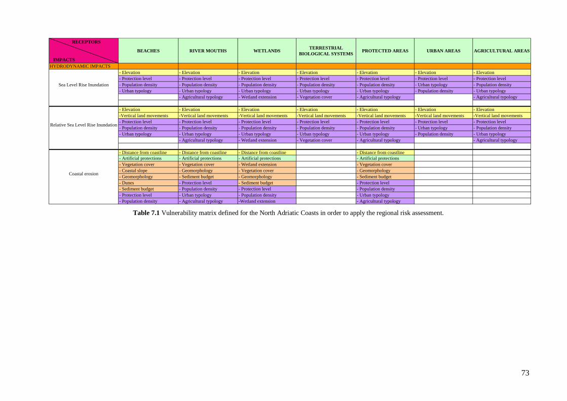
73
Table 7.1 Vulnerability matrix defined for the North Adriatic Coasts in order to apply the regional risk assessment.
RECEPTORS
IMPACTS
BEACHES RIVER MOUTHS WETLANDS TERRESTRIAL
BIOLOGICAL SYSTEMSPROTECTED AREAS URBAN AREAS AGRICULTURAL AREAS
HYDRODYNAMIC IMPACTS
- Elevation - Elevation - Elevation - Elevation - Elevation - Elevation - Elevation
- Protection level - Protection level - Protection level - Protection level - Protection level - Protection level - Protection level
- Population density - Population density - Population density - Population density - Population density - Urban typology - Population density
- Urban typology - Urban typology - Urban typology - Urban typology - Urban typology - Population density - Urban typology
- Agricultural typology - Wetland extension - Vegetation cover - Agricultural typology - Agricultural typology
- Elevation - Elevation - Elevation - Elevation - Elevation - Elevation - Elevation
-Vertical land movements -Vertical land movements -Vertical land movements -Vertical land movements -Vertical land movements -Vertical land movements -Vertical land movements
- Protection level - Protection level - Protection level - Protection level - Protection level - Protection level - Protection level
- Population density - Population density - Population density - Population density - Population density - Urban typology - Population density
- Urban typology - Urban typology - Urban typology - Urban typology - Urban typology - Population density - Urban typology
- Agricultural typology - Wetland extension - Vegetation cover - Agricultural typology - Agricultural typology
- Distance from coastline - Distance from coastline - Distance from coastline - Distance from coastline
- Artificial protections - Artificial protections - Artificial protections - Artificial protections
- Vegetation cover - Vegetation cover - Wetland extension - Vegetation cover
- Coastal slope - Geomorphology - Vegetation cover - Geomorphology
- Geomorphology - Sediment budget - Geomorphology - Sediment budget
- Dunes - Protection level - Sediment budget - Protection level
- Sediment budget - Population density - Protection level - Population density
- Protection level - Urban typology - Population density - Urban typology
- Population density - Agricultural typology -Wetland extension - Agricultural typology
Coastal erosion
Sea Level Rise Inundation
Relative Sea Level Rise Inundation
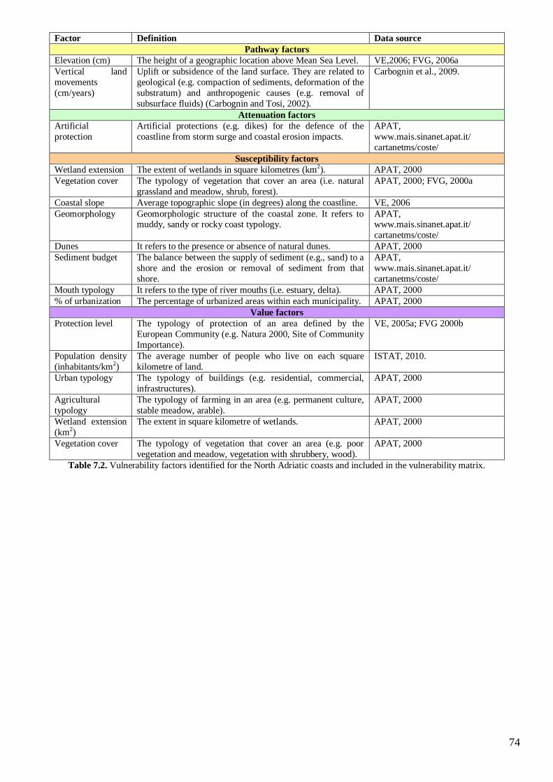
74
Factor Definition Data source
Pathway factors
Elevation (cm) The height of a geographic location above Mean Sea Level. VE,2006; FVG, 2006a
Vertical land
movements
(cm/years)
Uplift or subsidence of the land surface. They are related to
geological (e.g. compaction of sediments, deformation of the
substratum) and anthropogenic causes (e.g. removal of
subsurface fluids) (Carbognin and Tosi, 2002).
Carbognin et al., 2009.
Attenuation factors
Artificial
protection
Artificial protections (e.g. dikes) for the defence of the
coastline from storm surge and coastal erosion impacts.
APAT,
www.mais.sinanet.apat.it/
cartanetms/coste/
Susceptibility factors
Wetland extension The extent of wetlands in square kilometres (km2). APAT, 2000
Vegetation cover The typology of vegetation that cover an area (i.e. natural
grassland and meadow, shrub, forest).
APAT, 2000; FVG, 2000a
Coastal slope Average topographic slope (in degrees) along the coastline. VE, 2006
Geomorphology Geomorphologic structure of the coastal zone. It refers to muddy, sandy or rocky coast typology.
APAT, www.mais.sinanet.apat.it/
cartanetms/coste/
Dunes It refers to the presence or absence of natural dunes. APAT, 2000
Sediment budget The balance between the supply of sediment (e.g., sand) to a
shore and the erosion or removal of sediment from that
shore.
APAT,
www.mais.sinanet.apat.it/
cartanetms/coste/
Mouth typology It refers to the type of river mouths (i.e. estuary, delta). APAT, 2000
% of urbanization The percentage of urbanized areas within each municipality. APAT, 2000
Value factors
Protection level The typology of protection of an area defined by the
European Community (e.g. Natura 2000, Site of Community
Importance).
VE, 2005a; FVG 2000b
Population density
(inhabitants/km2)
The average number of people who live on each square
kilometre of land.
ISTAT, 2010.
Urban typology The typology of buildings (e.g. residential, commercial,
infrastructures).
APAT, 2000
Agricultural
typology
The typology of farming in an area (e.g. permanent culture,
stable meadow, arable).
APAT, 2000
Wetland extension
(km2)
The extent in square kilometre of wetlands. APAT, 2000
Vegetation cover The typology of vegetation that cover an area (e.g. poor
vegetation and meadow, vegetation with shrubbery, wood).
APAT, 2000
Table 7.2. Vulnerability factors identified for the North Adriatic coasts and included in the vulnerability matrix.

75
Receptor Definition Beaches This receptor analyzes beaches and the vegetation associated with them. Furthermore it analyzes natural and artificial protections to limitate impacts.
Sandy coastal areas are important for tourism, recreation and residential development (Voice et al 2006). Sand grade sediments are generally defined to be those predominantly
composed of grains ranging between 0.06 to 2.0 mm diameter (Pettijohn 1973). In the coastal environment, unconsolidated sediments within this grain size range are highly
mobile and small enough to be easily eroded and transported by waves, currents and winds that frequently act on most shorelines, in contrast to larger (pebble/cobble/boulder)
particles that are only moved by very energetic waves and hardly at all by wind (Sharples 2006).
River mouths This receptor includes estuaries and deltas. Specifically, it analyzes not only their morphological and ecological aspects but also the presence of artificial and natural
protections.
Estuaries are important receptors because they contain significant habitats including seagrasses, mudflats/sandflats, saltmarsh, reed, sedge and rush communities and provide
sheltered habitat, nursery and spawning areas for fish, crabs, prawns and shellfish (Voice et al 2006).
Delta is a landform where the mouth of a river flows into the sea. It builds up sediment outwards into the flat area which the river's flow encounters (as a deltaic deposit)
transported by the water and set down as the currents slow. Deltas present high biodiversity and significant habitats.
Wetland The wetland receptor includes coastal wetlands along with vegetation, animal life and artificial and natural protections located in wetlands areas. Wetland is an environment at the interface between truly terrestrial ecosystems and aquatic systems making them inherently different from each other yet highly dependent on
both. (Mitsch, 2007).
For the aims of this assessment the following categories were considered: inland wetlands, salt marshes and intertidal wetlands.
Terrestrial
biological
systems
This receptor includes animal and plant terrestrial life, their habitats and the ecological functions they provide. Specifically, terrestrial biodiversity encompasses the total
variety of life forms including plants, animals and micro-organisms and the processes and ecosystems they form (EPA,2002).
Protected
areas
This receptor includes areas with biological, morphological or historical sensitive aspects. Example of protected areas include: wetlands, marine areas, national parks, national
heritage. They provide tourism income, fisheries breeding and spawning grounds, ecosystem protection and protection of historical locations. (Voice et al 2006).
A protected area is defined as an area of land and/or sea especially dedicated to the protection and maintenance of biological diversity and of natural and associated cultural
resources, managed through legal or other effective means.
(UNEP-WCMC, http://www.unep-wcmc.org/protected_areas/index.htm).
Urban areas This receptor includes areas cover by countries, residential areas, commercial zones and industries. It includes areas in which a majority of the people are not directly
dependent on natural resource-based occupations (http://www.mhhe.com/biosci/pae/glossaryu.html). Specifically, it includes areas mainly occupied by dwellings and buildings
used by administrative/public utilities or collectivities, including their connected areas; areas mainly occupied by industrial activities of transformation and manufacturing,
trade, financial activities and services, transport infrastructures for road traffic and rail networks, airport installations, river and sea port installations, including their associated lands and access infrastructures; areas voluntarily created for recreational use (Bossard et al.,
2000)
Agricultural
areas
This receptor includes areas comprised of arable land, gardens and other perennial plants, meadows and natural pastures
(http://regionai.stat.gov.lt/en/savokos.html#Agricultural%20land). It includes: arable land (lands under a rotation system used for annually harvested plants and fallow lands,
which are permanently or not irrigated), permanent crops (all surfaces occupied by permanent crops, not under a rotation system), pastures (lands, which are permanently used
for fodder production) (Bossard et al., 2000).
Table 7.3. Description of the receptors included in the vulnerability matrix and identified as targets of the regional risk assessment methodology applied to the North Adriatic coast.
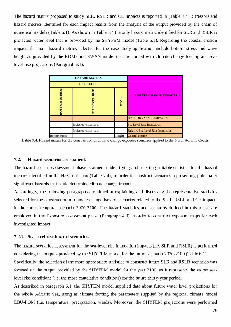
76
The hazard matrix proposed to study SLR, RSLR and CE impacts is reported in (Table 7.4). Stressors and
hazard metrics identified for each impact results from the analysis of the output provided by the chain of
numerical models (Table 6.1). As shown in Table 7.4 the only hazard metric identified for SLR and RSLR is
projected water level that is provided by the SHYFEM model (Table 6.1). Regarding the coastal erosion
impact, the main hazard metrics selected for the case study application include bottom stress and wave
height as provided by the ROMs and SWAN model that are forced with climate change forcing and sea-
level rise projections (Paragraph 6.1).
Table 7.4. Hazard matrix for the construction of climate change exposure scenarios applied to the North Adriatic Coasts.
7.2. Hazard scenarios assessment.
The hazard scenario assessment phase is aimed at identifying and selecting suitable statistics for the hazard
metrics identified in the Hazard matrix (Table 7.4), in order to construct scenarios representing potentially
significant hazards that could determine climate change impacts.
Accordingly, the following paragraphs are aimed at explaining and discussing the representative statistics
selected for the construction of climate change hazard scenarios related to the SLR, RSLR and CE impacts
in the future temporal scenario 2070-2100. The hazard statistics and scenarios defined in this phase are
employed in the Exposure assessment phase (Paragraph 4.3) in order to construct exposure maps for each
investigated impact.
7.2.1. Sea-level rise hazard scenarios.
The hazard scenarios assessment for the sea-level rise inundation impacts (i.e. SLR and RSLR) is performed
considering the outputs provided by the SHYFEM model for the future scenario 2070-2100 (Table 6.1).
Specifically, the selection of the more appropriate statistics to construct future SLR and RSLR scenarios was
focused on the output provided by the SHYFEM model for the year 2100, as it represents the worse sea-
level rise conditions (i.e. the more cautelative conditions) for the future thirty-year period.
As described in paragraph 6.1, the SHYFEM model supplied data about future water level projections for
the whole Adriatic Sea, using as climate forcing the parameters supplied by the regional climate model
EBU-POM (i.e. temperature, precipitation, winds). Moreover, the SHYFEM projections were performed
BO
TT
OM
ST
RE
SS
SE
A L
EV
EL
RIS
E
WA
VE
HYDRODYNAMIC IMPACTS
Projected water level Sea Level Rise Inundation
Projected water level Relative Sea Level Rise Inundation
Bottom stress Height Coastal erosion
CLIMATE CHANGE IMPACTS
HAZARD MATRIX
STRESSORS

77
imposing as boundary conditions at the Otranto strait two sea-level rise scenarios: a low sea-level rise
scenario equal to 20 cm and a high sea-level rise scenario equal to 45 cm. The boundary conditions at
Otranto were set considering the lowest and highest IPCC global sea-level rise projections for the year 2100
according to the emission scenario A1B (i.e. 21 cm and 48 cm respectively; IPCC, 2007b) and assuming a
linear sea-level rise trend for the future period 2070-2100.
The results of this assessment include two SLR hazard maps: a low sea-level rise scenario hazard map
representing the water levels projected by SHYFEM for the North Adriatic sea, according to a SLR at
Otranto equal to 20 cm (Figure 7.1); a high sea-level rise scenario hazard map representing the water levels
projected by SHYFEM for the North Adriatic sea, according to a SLR at Otranto equal to 45 cm (Figure 7.2.
As shown in Figure 7.1 and Figure 7.2. , most of the area of the North Adriatic Sea (i.e. from Po river Delta
to the Italy-Slovenia border) is characterised by a sea-level rise ranging from 0.164 m to 0.169 m for the low
sea-level rise map and from 0.414 m to 0.419 m for the high sea-level rise map. Accordingly, the maximum
range of variability is equal to 0.5 cm.

78
Figure 7.1. Hazard Map representing the Adriatic sea-level rise for the year 2100 (reference period 1960-1990). Sea-level changes
are simulated by the SHYFEM model according to a SLR at Otranto of 20 cm (low scenario).
Figure 7.2. Hazard Map representing the Adriatic sea-level rise for the year 2100 (reference period 1960-1990). Sea-level
changes are simulated by the SHYFEM model according to a SLR at Otranto of 45 cm (high scenario).
In order to determine a representative statistic to be used in the Exposure assessment phase for the SLR and
RSLR impacts (Paragraph 7.3), a specific analysis was performed only to water level values corresponding
to the dots adjoining to the shoreline of the case study area for the low and high hazard scenarios (Figure 7.1
and 7.2).
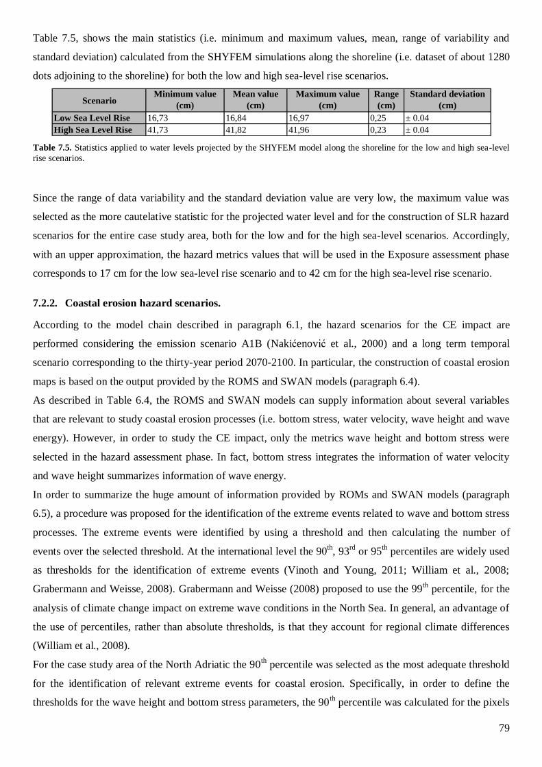
79
Table 7.5, shows the main statistics (i.e. minimum and maximum values, mean, range of variability and
standard deviation) calculated from the SHYFEM simulations along the shoreline (i.e. dataset of about 1280
dots adjoining to the shoreline) for both the low and high sea-level rise scenarios.
Table 7.5. Statistics applied to water levels projected by the SHYFEM model along the shoreline for the low and high sea-level
rise scenarios.
Since the range of data variability and the standard deviation value are very low, the maximum value was
selected as the more cautelative statistic for the projected water level and for the construction of SLR hazard
scenarios for the entire case study area, both for the low and for the high sea-level scenarios. Accordingly,
with an upper approximation, the hazard metrics values that will be used in the Exposure assessment phase
corresponds to 17 cm for the low sea-level rise scenario and to 42 cm for the high sea-level rise scenario.
7.2.2. Coastal erosion hazard scenarios.
According to the model chain described in paragraph 6.1, the hazard scenarios for the CE impact are
performed considering the emission scenario A1B (Nakićenović et al., 2000) and a long term temporal
scenario corresponding to the thirty-year period 2070-2100. In particular, the construction of coastal erosion
maps is based on the output provided by the ROMS and SWAN models (paragraph 6.4).
As described in Table 6.4, the ROMS and SWAN models can supply information about several variables
that are relevant to study coastal erosion processes (i.e. bottom stress, water velocity, wave height and wave
energy). However, in order to study the CE impact, only the metrics wave height and bottom stress were
selected in the hazard assessment phase. In fact, bottom stress integrates the information of water velocity
and wave height summarizes information of wave energy.
In order to summarize the huge amount of information provided by ROMs and SWAN models (paragraph
6.5), a procedure was proposed for the identification of the extreme events related to wave and bottom stress
processes. The extreme events were identified by using a threshold and then calculating the number of
events over the selected threshold. At the international level the 90th, 93
rd or 95
th percentiles are widely used
as thresholds for the identification of extreme events (Vinoth and Young, 2011; William et al., 2008;
Grabermann and Weisse, 2008). Grabermann and Weisse (2008) proposed to use the 99th percentile, for the
analysis of climate change impact on extreme wave conditions in the North Sea. In general, an advantage of
the use of percentiles, rather than absolute thresholds, is that they account for regional climate differences
(William et al., 2008).
For the case study area of the North Adriatic the 90th percentile was selected as the most adequate threshold
for the identification of relevant extreme events for coastal erosion. Specifically, in order to define the
thresholds for the wave height and bottom stress parameters, the 90th
percentile was calculated for the pixels
ScenarioMinimum value
(cm)
Mean value
(cm)
Maximum value
(cm)
Range
(cm)
Standard deviation
(cm)
Low Sea Level Rise 16,73 16,84 16,97 0,25 ± 0.04
High Sea Level Rise 41,73 41,82 41,96 0,23 ± 0.04
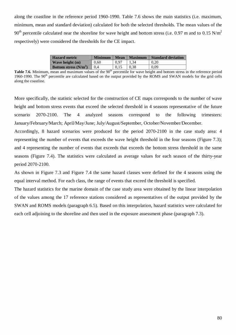
80
along the coastline in the reference period 1960-1990. Table 7.6 shows the main statistics (i.e. maximum,
minimum, mean and standard deviation) calculated for both the selected thresholds. The mean values of the
90th percentile calculated near the shoreline for wave height and bottom stress (i.e. 0.97 m and to 0.15 N/m
2
respectively) were considered the thresholds for the CE impact.
Hazard metric Minimum Mean Maximum Standard deviation
Wave height (m) 0,60 0,97 1,34 0,20
Bottom stress (N/m2) 0,4 0,15 0,38 0,09
Table 7.6. Minimum, mean and maximum values of the 90th percentile for wave height and bottom stress in the reference period
1960-1990. The 90th percentile are calculated based on the output provided by the ROMS and SWAN models for the grid cells
along the coastline.
More specifically, the statistic selected for the construction of CE maps corresponds to the number of wave
height and bottom stress events that exceed the selected threshold in 4 seasons representative of the future
scenario 2070-2100. The 4 analyzed seasons correspond to the following trimesters:
January/February/March; April/May/June; July/August/September, October/November/December.
Accordingly, 8 hazard scenarios were produced for the period 2070-2100 in the case study area: 4
representing the number of events that exceeds the wave height threshold in the four seasons (Figure 7.3);
and 4 representing the number of events that exceeds that exceeds the bottom stress threshold in the same
seasons (Figure 7.4). The statistics were calculated as average values for each season of the thirty-year
period 2070-2100.
As shown in Figure 7.3 and Figure 7.4 the same hazard classes were defined for the 4 seasons using the
equal interval method. For each class, the range of events that exceed the threshold is specified.
The hazard statistics for the marine domain of the case study area were obtained by the linear interpolation
of the values among the 17 reference stations considered as representatives of the output provided by the
SWAN and ROMS models (paragraph 6.5). Based on this interpolation, hazard statistics were calculated for
each cell adjoining to the shoreline and then used in the exposure assessment phase (paragraph 7.3).
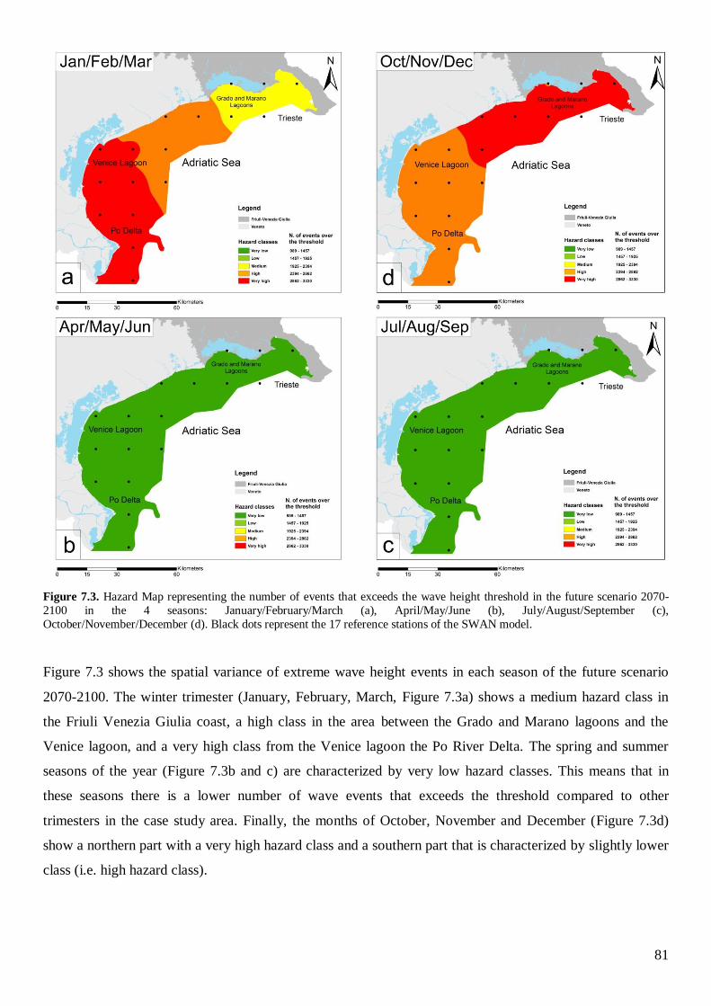
81
Figure 7.3. Hazard Map representing the number of events that exceeds the wave height threshold in the future scenario 2070-
2100 in the 4 seasons: January/February/March (a), April/May/June (b), July/August/September (c),
October/November/December (d). Black dots represent the 17 reference stations of the SWAN model.
Figure 7.3 shows the spatial variance of extreme wave height events in each season of the future scenario
2070-2100. The winter trimester (January, February, March, Figure 7.3a) shows a medium hazard class in
the Friuli Venezia Giulia coast, a high class in the area between the Grado and Marano lagoons and the
Venice lagoon, and a very high class from the Venice lagoon the Po River Delta. The spring and summer
seasons of the year (Figure 7.3b and c) are characterized by very low hazard classes. This means that in
these seasons there is a lower number of wave events that exceeds the threshold compared to other
trimesters in the case study area. Finally, the months of October, November and December (Figure 7.3d)
show a northern part with a very high hazard class and a southern part that is characterized by slightly lower
class (i.e. high hazard class).

82
Figure 7.4. Hazard Map representing the number of events that exceeds the bottom stress threshold in the future scenario 2070-
2100 in the 4 seasons: January/February/March (a), April/May/June (b), July/August/September (c),
October/November/December (d). Black dots represent the 17 reference stations of the ROMS model.
Figure 7.4 shows the spatial variance of extreme bottom stress events in the 4 seasons of the future scenario
2070-2100. The trimester April/May/June shows a very low hazard class, except for few parts that show the
low hazard class (Figure 7.4 b). The distribution of the classes for the other scenarios (Figure 7.4a, c and d)
is similar to the distribution discussed for the wave height hazard metric.
In order to identify areas potentially exposed to the CE impact, only the pixels along the coastline were
considered in the Exposure assessment phase (Paragraph 7.3). The projected number of extreme events (i.e.
wave and bottom stress events exceeding the threshold) that interests the coastline of the North Adriatic Sea
for the thirty-year future period 2070-2100 represent the hazard statistic that will be used in the Exposure
assessment phase (Paragraph 7.3.2).
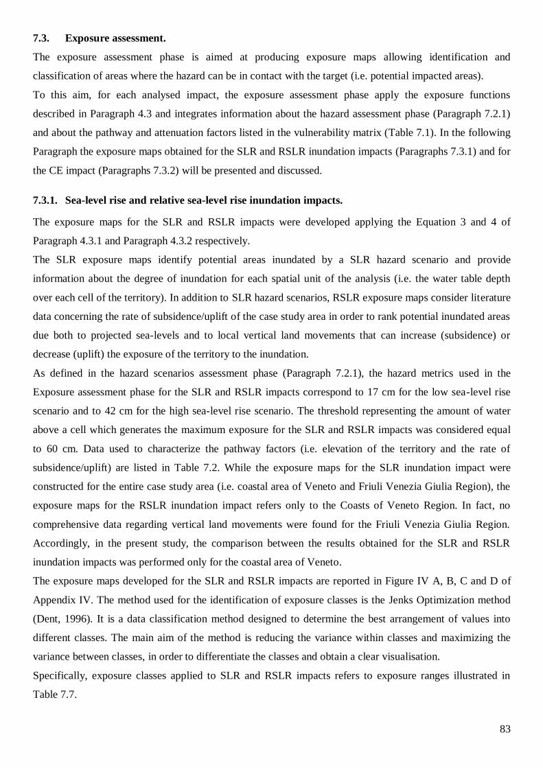
83
7.3. Exposure assessment.
The exposure assessment phase is aimed at producing exposure maps allowing identification and
classification of areas where the hazard can be in contact with the target (i.e. potential impacted areas).
To this aim, for each analysed impact, the exposure assessment phase apply the exposure functions
described in Paragraph 4.3 and integrates information about the hazard assessment phase (Paragraph 7.2.1)
and about the pathway and attenuation factors listed in the vulnerability matrix (Table 7.1). In the following
Paragraph the exposure maps obtained for the SLR and RSLR inundation impacts (Paragraphs 7.3.1) and for
the CE impact (Paragraphs 7.3.2) will be presented and discussed.
7.3.1. Sea-level rise and relative sea-level rise inundation impacts.
The exposure maps for the SLR and RSLR impacts were developed applying the Equation 3 and 4 of
Paragraph 4.3.1 and Paragraph 4.3.2 respectively.
The SLR exposure maps identify potential areas inundated by a SLR hazard scenario and provide
information about the degree of inundation for each spatial unit of the analysis (i.e. the water table depth
over each cell of the territory). In addition to SLR hazard scenarios, RSLR exposure maps consider literature
data concerning the rate of subsidence/uplift of the case study area in order to rank potential inundated areas
due both to projected sea-levels and to local vertical land movements that can increase (subsidence) or
decrease (uplift) the exposure of the territory to the inundation.
As defined in the hazard scenarios assessment phase (Paragraph 7.2.1), the hazard metrics used in the
Exposure assessment phase for the SLR and RSLR impacts correspond to 17 cm for the low sea-level rise
scenario and to 42 cm for the high sea-level rise scenario. The threshold representing the amount of water
above a cell which generates the maximum exposure for the SLR and RSLR impacts was considered equal
to 60 cm. Data used to characterize the pathway factors (i.e. elevation of the territory and the rate of
subsidence/uplift) are listed in Table 7.2. While the exposure maps for the SLR inundation impact were
constructed for the entire case study area (i.e. coastal area of Veneto and Friuli Venezia Giulia Region), the
exposure maps for the RSLR inundation impact refers only to the Coasts of Veneto Region. In fact, no
comprehensive data regarding vertical land movements were found for the Friuli Venezia Giulia Region.
Accordingly, in the present study, the comparison between the results obtained for the SLR and RSLR
inundation impacts was performed only for the coastal area of Veneto.
The exposure maps developed for the SLR and RSLR impacts are reported in Figure IV A, B, C and D of
Appendix IV. The method used for the identification of exposure classes is the Jenks Optimization method
(Dent, 1996). It is a data classification method designed to determine the best arrangement of values into
different classes. The main aim of the method is reducing the variance within classes and maximizing the
variance between classes, in order to differentiate the classes and obtain a clear visualisation.
Specifically, exposure classes applied to SLR and RSLR impacts refers to exposure ranges illustrated in
Table 7.7.
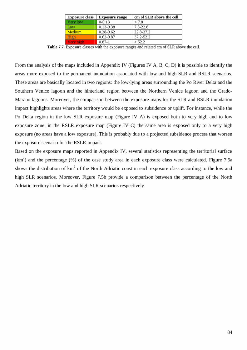
84
Exposure class Exposure range cm of SLR above the cell
Very low 0-0.13 < 7.8
Low 0.13-0.38 7.8-22.8
Medium 0.38-0.62 22.8-37.2
High 0.62-0.87 37.2-52.2
Very high 0.87-1 > 52.2
Table 7.7. Exposure classes with the exposure ranges and related cm of SLR above the cell.
From the analysis of the maps included in Appendix IV (Figures IV A, B, C, D) it is possible to identify the
areas more exposed to the permanent inundation associated with low and high SLR and RSLR scenarios.
These areas are basically located in two regions: the low-lying areas surrounding the Po River Delta and the
Southern Venice lagoon and the hinterland region between the Northern Venice lagoon and the Grado-
Marano lagoons. Moreover, the comparison between the exposure maps for the SLR and RSLR inundation
impact highlights areas where the territory would be exposed to subsidence or uplift. For instance, while the
Po Delta region in the low SLR exposure map (Figure IV A) is exposed both to very high and to low
exposure zone; in the RSLR exposure map (Figure IV C) the same area is exposed only to a very high
exposure (no areas have a low exposure). This is probably due to a projected subsidence process that worsen
the exposure scenario for the RSLR impact.
Based on the exposure maps reported in Appendix IV, several statistics representing the territorial surface
(km2) and the percentage (%) of the case study area in each exposure class were calculated. Figure 7.5a
shows the distribution of km2 of the North Adriatic coast in each exposure class according to the low and
high SLR scenarios. Moreover, Figure 7.5b provide a comparison between the percentage of the North
Adriatic territory in the low and high SLR scenarios respectively.
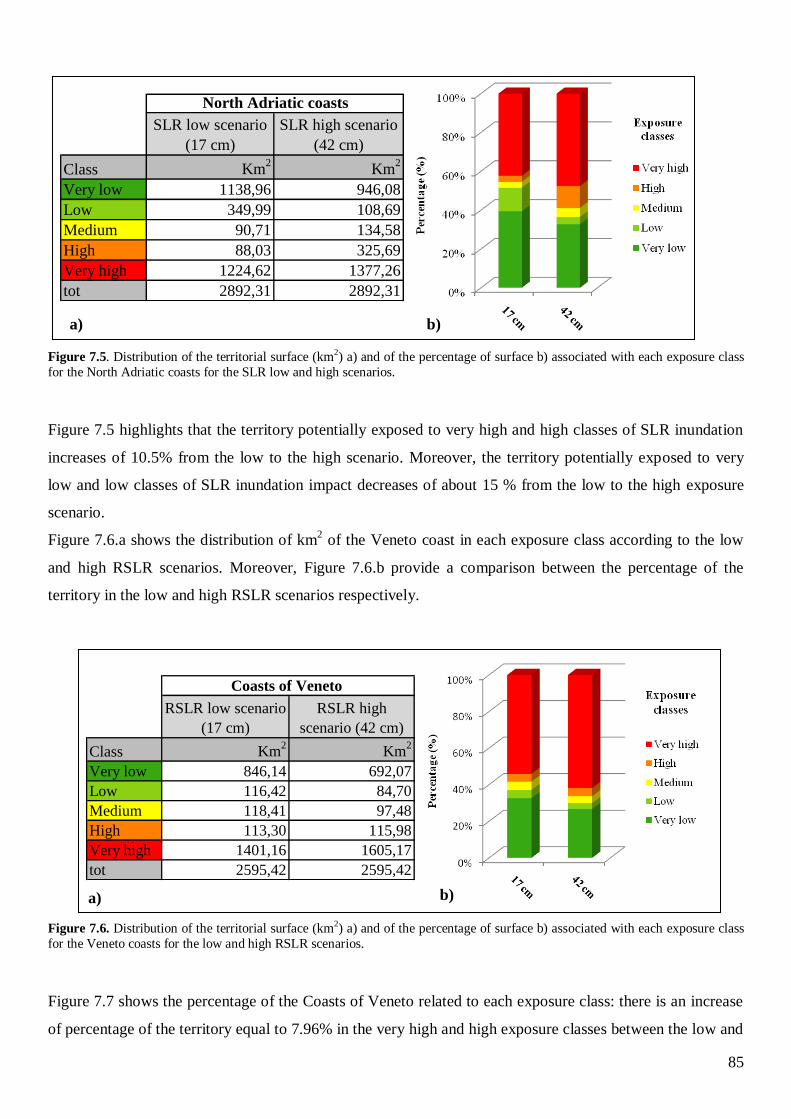
85
Figure 7.5. Distribution of the territorial surface (km2) a) and of the percentage of surface b) associated with each exposure class
for the North Adriatic coasts for the SLR low and high scenarios.
Figure 7.5 highlights that the territory potentially exposed to very high and high classes of SLR inundation
increases of 10.5% from the low to the high scenario. Moreover, the territory potentially exposed to very
low and low classes of SLR inundation impact decreases of about 15 % from the low to the high exposure
scenario.
Figure 7.6.a shows the distribution of km2 of the Veneto coast in each exposure class according to the low
and high RSLR scenarios. Moreover, Figure 7.6.b provide a comparison between the percentage of the
territory in the low and high RSLR scenarios respectively.
Figure 7.6. Distribution of the territorial surface (km2) a) and of the percentage of surface b) associated with each exposure class
for the Veneto coasts for the low and high RSLR scenarios.
Figure 7.7 shows the percentage of the Coasts of Veneto related to each exposure class: there is an increase
of percentage of the territory equal to 7.96% in the very high and high exposure classes between the low and
a) b)
SLR low scenario
(17 cm)
SLR high scenario
(42 cm)
Class Km2
Km2
Very low 1138,96 946,08
Low 349,99 108,69
Medium 90,71 134,58
High 88,03 325,69
Very high 1224,62 1377,26
tot 2892,31 2892,31
North Adriatic coasts
a) b)
RSLR low scenario
(17 cm)
RSLR high
scenario (42 cm)
Class Km2
Km2
Very low 846,14 692,07
Low 116,42 84,70
Medium 118,41 97,48
High 113,30 115,98
Very high 1401,16 1605,17
tot 2595,42 2595,42
Coasts of Veneto
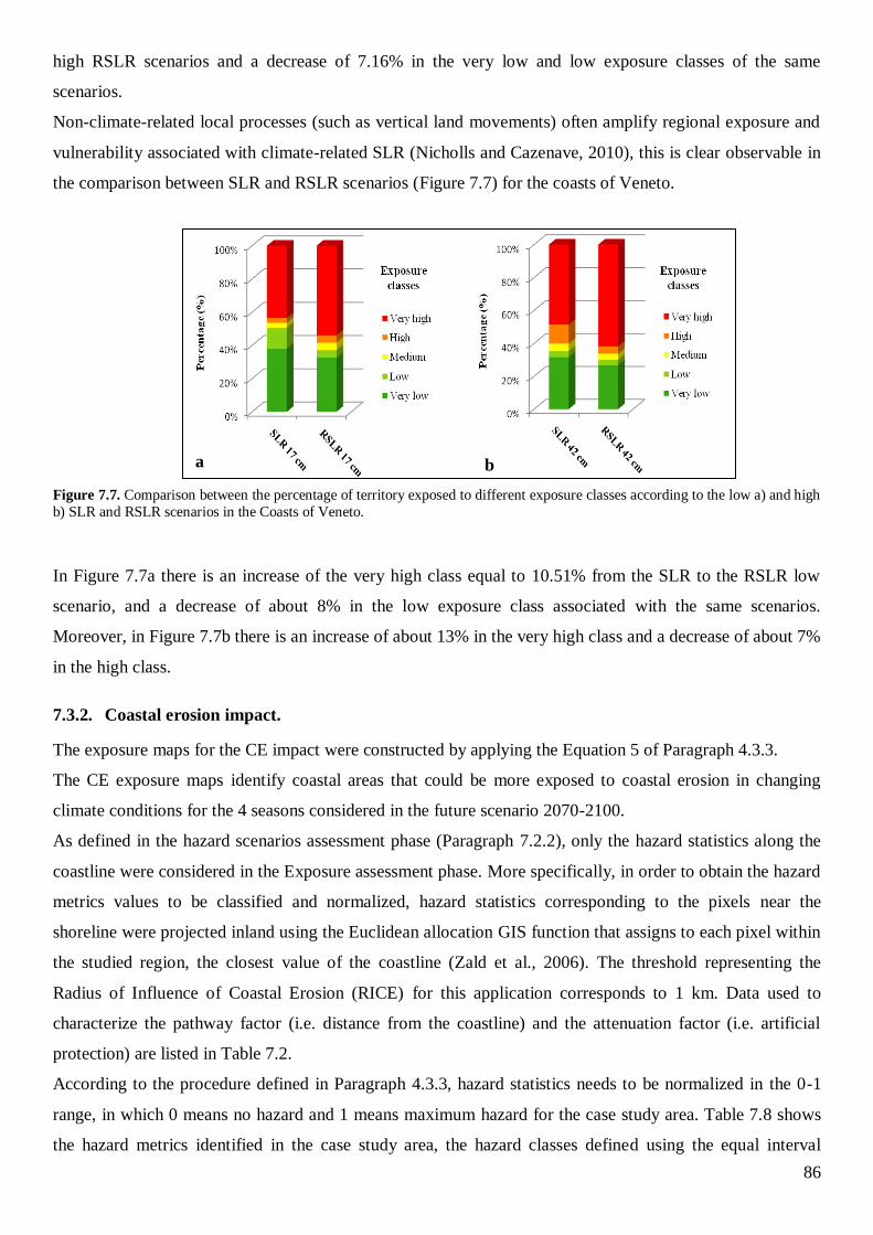
86
high RSLR scenarios and a decrease of 7.16% in the very low and low exposure classes of the same
scenarios.
Non-climate-related local processes (such as vertical land movements) often amplify regional exposure and
vulnerability associated with climate-related SLR (Nicholls and Cazenave, 2010), this is clear observable in
the comparison between SLR and RSLR scenarios (Figure 7.7) for the coasts of Veneto.
Figure 7.7. Comparison between the percentage of territory exposed to different exposure classes according to the low a) and high
b) SLR and RSLR scenarios in the Coasts of Veneto.
In Figure 7.7a there is an increase of the very high class equal to 10.51% from the SLR to the RSLR low
scenario, and a decrease of about 8% in the low exposure class associated with the same scenarios.
Moreover, in Figure 7.7b there is an increase of about 13% in the very high class and a decrease of about 7%
in the high class.
7.3.2. Coastal erosion impact.
The exposure maps for the CE impact were constructed by applying the Equation 5 of Paragraph 4.3.3.
The CE exposure maps identify coastal areas that could be more exposed to coastal erosion in changing
climate conditions for the 4 seasons considered in the future scenario 2070-2100.
As defined in the hazard scenarios assessment phase (Paragraph 7.2.2), only the hazard statistics along the
coastline were considered in the Exposure assessment phase. More specifically, in order to obtain the hazard
metrics values to be classified and normalized, hazard statistics corresponding to the pixels near the
shoreline were projected inland using the Euclidean allocation GIS function that assigns to each pixel within
the studied region, the closest value of the coastline (Zald et al., 2006). The threshold representing the
Radius of Influence of Coastal Erosion (RICE) for this application corresponds to 1 km. Data used to
characterize the pathway factor (i.e. distance from the coastline) and the attenuation factor (i.e. artificial
protection) are listed in Table 7.2.
According to the procedure defined in Paragraph 4.3.3, hazard statistics needs to be normalized in the 0-1
range, in which 0 means no hazard and 1 means maximum hazard for the case study area. Table 7.8 shows
the hazard metrics identified in the case study area, the hazard classes defined using the equal interval
b
)
a
)
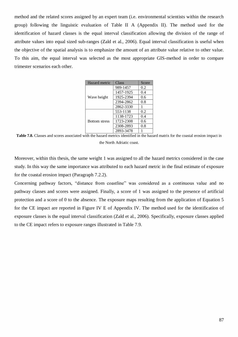
87
method and the related scores assigned by an expert team (i.e. environmental scientists within the research
group) following the linguistic evaluation of Table II A (Appendix II). The method used for the
identification of hazard classes is the equal interval classification allowing the division of the range of
attribute values into equal sized sub-ranges (Zald et al., 2006). Equal interval classification is useful when
the objective of the spatial analysis is to emphasize the amount of an attribute value relative to other value.
To this aim, the equal interval was selected as the most appropriate GIS-method in order to compare
trimester scenarios each other.
Hazard metric Class Score
Wave height
989-1457 0.2
1457-1925 0.4
1925-2394 0.6
2394-2862 0.8
2862-3330 1
Bottom stress
553-1138 0.2
1138-1723 0.4
1723-2308 0.6
2308-2893 0.8
2893-3478 1
Table 7.8. Classes and scores associated with the hazard metrics identified in the hazard matrix for the coastal erosion impact in
the North Adriatic coast.
Moreover, within this thesis, the same weight 1 was assigned to all the hazard metrics considered in the case
study. In this way the same importance was attributed to each hazard metric in the final estimate of exposure
for the coastal erosion impact (Paragraph 7.2.2).
Concerning pathway factors, “distance from coastline” was considered as a continuous value and no
pathway classes and scores were assigned. Finally, a score of 1 was assigned to the presence of artificial
protection and a score of 0 to the absence. The exposure maps resulting from the application of Equation 5
for the CE impact are reported in Figure IV E of Appendix IV. The method used for the identification of
exposure classes is the equal interval classification (Zald et al., 2006). Specifically, exposure classes applied
to the CE impact refers to exposure ranges illustrated in Table 7.9.
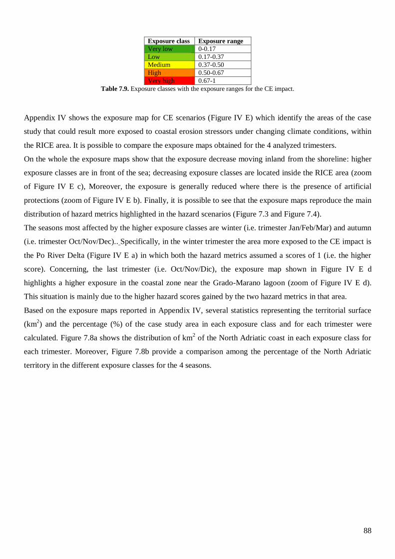
88
Exposure class Exposure range
Very low 0-0.17
Low 0.17-0.37
Medium 0.37-0.50
High 0.50-0.67
Very high 0.67-1
Table 7.9. Exposure classes with the exposure ranges for the CE impact.
Appendix IV shows the exposure map for CE scenarios (Figure IV E) which identify the areas of the case
study that could result more exposed to coastal erosion stressors under changing climate conditions, within
the RICE area. It is possible to compare the exposure maps obtained for the 4 analyzed trimesters.
On the whole the exposure maps show that the exposure decrease moving inland from the shoreline: higher
exposure classes are in front of the sea; decreasing exposure classes are located inside the RICE area (zoom
of Figure IV E c), Moreover, the exposure is generally reduced where there is the presence of artificial
protections (zoom of Figure IV E b). Finally, it is possible to see that the exposure maps reproduce the main
distribution of hazard metrics highlighted in the hazard scenarios (Figure 7.3 and Figure 7.4).
The seasons most affected by the higher exposure classes are winter (i.e. trimester Jan/Feb/Mar) and autumn
(i.e. trimester Oct/Nov/Dec).. Specifically, in the winter trimester the area more exposed to the CE impact is
the Po River Delta (Figure IV E a) in which both the hazard metrics assumed a scores of 1 (i.e. the higher
score). Concerning, the last trimester (i.e. Oct/Nov/Dic), the exposure map shown in Figure IV E d
highlights a higher exposure in the coastal zone near the Grado-Marano lagoon (zoom of Figure IV E d).
This situation is mainly due to the higher hazard scores gained by the two hazard metrics in that area.
Based on the exposure maps reported in Appendix IV, several statistics representing the territorial surface
(km2) and the percentage (%) of the case study area in each exposure class and for each trimester were
calculated. Figure 7.8a shows the distribution of km2 of the North Adriatic coast in each exposure class for
each trimester. Moreover, Figure 7.8b provide a comparison among the percentage of the North Adriatic
territory in the different exposure classes for the 4 seasons.
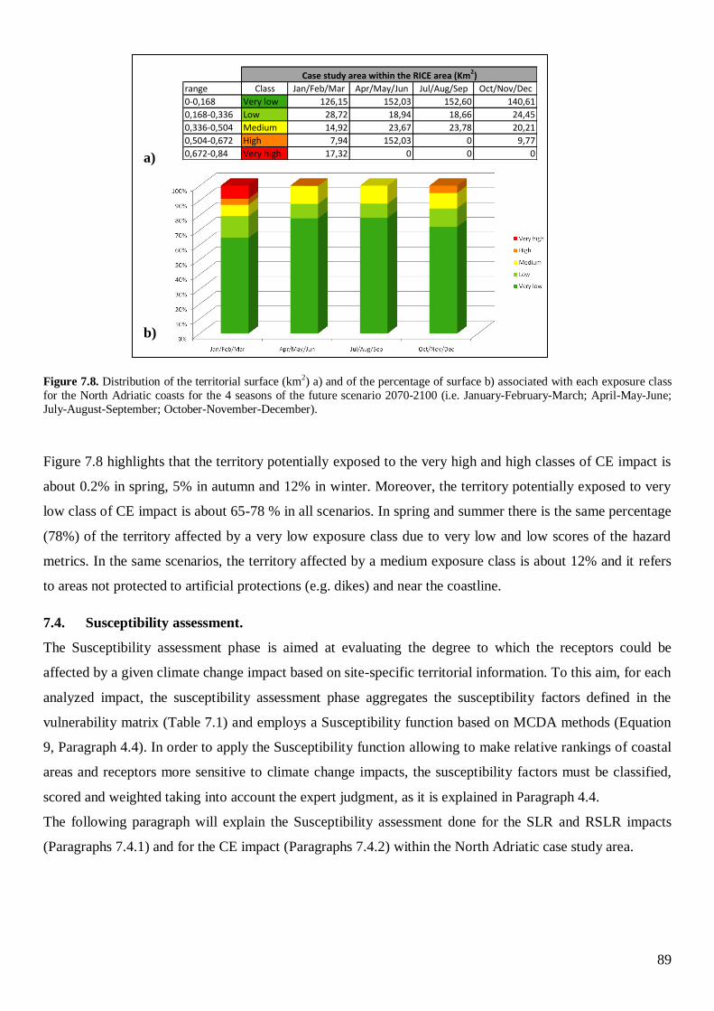
89
Figure 7.8. Distribution of the territorial surface (km2) a) and of the percentage of surface b) associated with each exposure class
for the North Adriatic coasts for the 4 seasons of the future scenario 2070-2100 (i.e. January-February-March; April-May-June;
July-August-September; October-November-December).
Figure 7.8 highlights that the territory potentially exposed to the very high and high classes of CE impact is
about 0.2% in spring, 5% in autumn and 12% in winter. Moreover, the territory potentially exposed to very
low class of CE impact is about 65-78 % in all scenarios. In spring and summer there is the same percentage
(78%) of the territory affected by a very low exposure class due to very low and low scores of the hazard
metrics. In the same scenarios, the territory affected by a medium exposure class is about 12% and it refers
to areas not protected to artificial protections (e.g. dikes) and near the coastline.
7.4. Susceptibility assessment.
The Susceptibility assessment phase is aimed at evaluating the degree to which the receptors could be
affected by a given climate change impact based on site-specific territorial information. To this aim, for each
analyzed impact, the susceptibility assessment phase aggregates the susceptibility factors defined in the
vulnerability matrix (Table 7.1) and employs a Susceptibility function based on MCDA methods (Equation
9, Paragraph 4.4). In order to apply the Susceptibility function allowing to make relative rankings of coastal
areas and receptors more sensitive to climate change impacts, the susceptibility factors must be classified,
scored and weighted taking into account the expert judgment, as it is explained in Paragraph 4.4.
The following paragraph will explain the Susceptibility assessment done for the SLR and RSLR impacts
(Paragraphs 7.4.1) and for the CE impact (Paragraphs 7.4.2) within the North Adriatic case study area.
range Class Jan/Feb/Mar Apr/May/Jun Jul/Aug/Sep Oct/Nov/Dec
0-0,168 Very low 126,15 152,03 152,60 140,61
0,168-0,336 Low 28,72 18,94 18,66 24,45
0,336-0,504 Medium 14,92 23,67 23,78 20,21
0,504-0,672 High 7,94 152,03 0 9,77
0,672-0,84 Very high 17,32 0 0 0
Case study area within the RICE area (Km2)
a)
b)
90
7.4.1. Sea-level rise and relative sea-level rise inundation impacts.
As highlighted in the vulnerability matrix (Table 7.1), for the specific analysis of SLR and RSLR inundation
impacts, no susceptibility factors were identified. In fact, it was assumed that a SLR/RSLR inundation event
affect all the receptors in the same way, causing a permanent loss of receptors’ sub-areas based only on the
elevation of the cells, Accordingly, each cell of the territory was considered to have the same maximum
susceptibility to SLR and RSLR impacts (i.e. susceptibility score equal to 1).
7.4.2. Coastal erosion impact.
In order to provide an estimation of the susceptibility of the system to the coastal erosion impact, the
susceptibility factors were normalized through the assignation of scores and weights and then aggregated
through the “probabilistic or” function (Paragraph 4.4).
Table 7.10 and Table 7.11 show the scores and weights provided by an expert team (i.e. environmental
scientists within the research group) to the susceptibility factors identified in the vulnerability matrix (Table
7.1). Scores and weights vary from 0 to 1, in which 0 means no susceptibility/importance and 1 means
maximum susceptibility/importance for the case study area. Table 7.10 shows the susceptibility factors
identified in the case study area, the susceptibility classes defined by qualitative or quantitative attributes
and the related scores (founded in literature or defined by the expert team).

91
SUSCEPTIBILITY
FACTOR CLASS SCORE
Vegetation cover
Poor vegetation and meadow 1
Vegetation with shrubbery 0.5
Forest 0.2
Coastal slope (degrees)
0 – 1,02 0.2
1,02 – 2,04 0.4
2,04 – 3,07 0.6
3,07 – 4,09 0.8
4,09 – 5,12 1
Geomorphology
Muddy coast 1
Sandy coast 0.5
Rocky coast 0.2
Dunes Absence 1
Presence 0.2
Sediment budget Advancing coast 0.2
Stable coast 0.5
Coast in erosion 1
Mouth-river typology Estuary 1
Delta 0.2
Wetland extension (km2)
0 – 19,9 1
19,9 – 39,8 0.8
39,8 – 59,8 0.6
59,8 – 79,7 0.4
79,7 – 99,6 0.2
% of urbanization
< 5% of the land occupied by urban and
industrial areas (per municipality) 0.2
5% and 10% of the land occupied by urban
and industrial areas (per municipality) 0.5
> 10% of the land occupied by urban and
industrial areas (per municipality) 1
Table 7.10. Classes and scores associated with the susceptibility factors identified in the vulnerability matrix for the coastal
erosion impact in the North Adriatic coast.
Table 7.11 shows the weights assigned by experts to each susceptibility factor in order to represent their
relative importance in the estimation of susceptibility associated with the impact CE.
SUSCEPTIBILITY FACTOR WEIGHT
Vegetation cover 0.6
Coastal slope (degrees) 0.8
Geomorphology 0.8
Dunes 0.6
Sediment budget 0.8
Mouth-river typology 0.5
Wetland extension (km2) 0.5
% of urbanization 0.4
Table 7.11. Weights associated with the susceptibility factors identified in the vulnerability matrix for the coastal erosion impact
in the North Adriatic coast.
Coastal slope, geomorphology and sediment budget gained the higher weights in the present assessment
since they represent geo-physical characteristics very important for the assessment of receptors’
susceptibility to coastal erosion, compared to other susceptibility factors. Vegetation cover and dunes are
considered slightly less important than the previous group of susceptibility factors and were assigned a
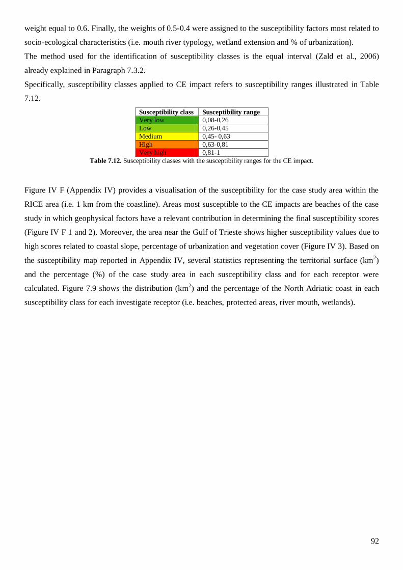
92
weight equal to 0.6. Finally, the weights of 0.5-0.4 were assigned to the susceptibility factors most related to
socio-ecological characteristics (i.e. mouth river typology, wetland extension and % of urbanization).
The method used for the identification of susceptibility classes is the equal interval (Zald et al., 2006)
already explained in Paragraph 7.3.2.
Specifically, susceptibility classes applied to CE impact refers to susceptibility ranges illustrated in Table
7.12.
Susceptibility class Susceptibility range
Very low 0,08-0,26
Low 0,26-0,45
Medium 0,45- 0,63
High 0,63-0,81
Very high 0,81-1
Table 7.12. Susceptibility classes with the susceptibility ranges for the CE impact.
Figure IV F (Appendix IV) provides a visualisation of the susceptibility for the case study area within the
RICE area (i.e. 1 km from the coastline). Areas most susceptible to the CE impacts are beaches of the case
study in which geophysical factors have a relevant contribution in determining the final susceptibility scores
(Figure IV F 1 and 2). Moreover, the area near the Gulf of Trieste shows higher susceptibility values due to
high scores related to coastal slope, percentage of urbanization and vegetation cover (Figure IV 3). Based on
the susceptibility map reported in Appendix IV, several statistics representing the territorial surface (km2)
and the percentage (%) of the case study area in each susceptibility class and for each receptor were
calculated. Figure 7.9 shows the distribution (km2) and the percentage of the North Adriatic coast in each
susceptibility class for each investigate receptor (i.e. beaches, protected areas, river mouth, wetlands).
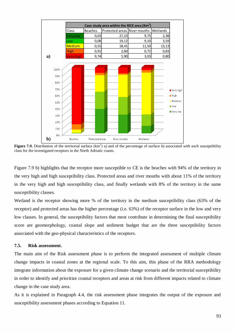
93
Figure 7.9. Distribution of the territorial surface (km2) a) and of the percentage of surface b) associated with each susceptibility
class for the investigated receptors in the North Adriatic coasts.
Figure 7.9 b) highlights that the receptor more susceptible to CE is the beaches with 94% of the territory in
the very high and high susceptibility class. Protected areas and river mouths with about 11% of the territory
in the very high and high susceptibility class, and finally wetlands with 8% of the territory in the same
susceptibility classes.
Wetland is the receptor showing more % of the territory in the medium susceptibility class (63% of the
receptor) and protected areas has the higher percentage (i.e. 63%) of the receptor surface in the low and very
low classes. In general, the susceptibility factors that most contribute in determining the final susceptibility
score are geomorphology, coastal slope and sediment budget that are the three susceptibility factors
associated with the geo-physical characteristics of the receptors.
7.5. Risk assessment.
The main aim of the Risk assessment phase is to perform the integrated assessment of multiple climate
change impacts in coastal zones at the regional scale. To this aim, this phase of the RRA methodology
integrate information about the exposure for a given climate change scenario and the territorial susceptibility
in order to identify and prioritize coastal receptors and areas at risk from different impacts related to climate
change in the case study area.
As it is explained in Paragraph 4.4, the risk assessment phase integrates the output of the exposure and
susceptibility assessment phases according to Equation 11.
Class Beaches Protected areas River mouths Wetlands
Very low 0,03 27,23 9,75 2,38
Low 0,08 19,12 9,10 3,59
Medium 0,55 18,41 11,50 13,13
High 0,91 2,60 0,72 0,83
Very high 9,74 5,90 3,03 0,80
Case study area within the RICE area (Km2)
a)
b)
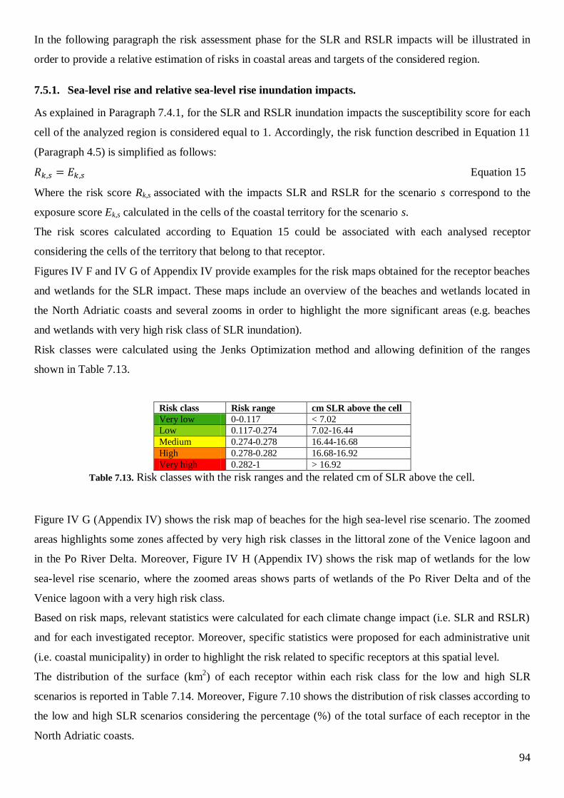
94
In the following paragraph the risk assessment phase for the SLR and RSLR impacts will be illustrated in
order to provide a relative estimation of risks in coastal areas and targets of the considered region.
7.5.1. Sea-level rise and relative sea-level rise inundation impacts.
As explained in Paragraph 7.4.1, for the SLR and RSLR inundation impacts the susceptibility score for each
cell of the analyzed region is considered equal to 1. Accordingly, the risk function described in Equation 11
(Paragraph 4.5) is simplified as follows:
Equation 15
Where the risk score Rk,s associated with the impacts SLR and RSLR for the scenario s correspond to the
exposure score Ek,s calculated in the cells of the coastal territory for the scenario s.
The risk scores calculated according to Equation 15 could be associated with each analysed receptor
considering the cells of the territory that belong to that receptor.
Figures IV F and IV G of Appendix IV provide examples for the risk maps obtained for the receptor beaches
and wetlands for the SLR impact. These maps include an overview of the beaches and wetlands located in
the North Adriatic coasts and several zooms in order to highlight the more significant areas (e.g. beaches
and wetlands with very high risk class of SLR inundation).
Risk classes were calculated using the Jenks Optimization method and allowing definition of the ranges
shown in Table 7.13.
Risk class Risk range cm SLR above the cell
Very low 0-0.117 < 7.02
Low 0.117-0.274 7.02-16.44
Medium 0.274-0.278 16.44-16.68
High 0.278-0.282 16.68-16.92
Very high 0.282-1 > 16.92
Table 7.13. Risk classes with the risk ranges and the related cm of SLR above the cell.
Figure IV G (Appendix IV) shows the risk map of beaches for the high sea-level rise scenario. The zoomed
areas highlights some zones affected by very high risk classes in the littoral zone of the Venice lagoon and
in the Po River Delta. Moreover, Figure IV H (Appendix IV) shows the risk map of wetlands for the low
sea-level rise scenario, where the zoomed areas shows parts of wetlands of the Po River Delta and of the
Venice lagoon with a very high risk class.
Based on risk maps, relevant statistics were calculated for each climate change impact (i.e. SLR and RSLR)
and for each investigated receptor. Moreover, specific statistics were proposed for each administrative unit
(i.e. coastal municipality) in order to highlight the risk related to specific receptors at this spatial level.
The distribution of the surface (km2) of each receptor within each risk class for the low and high SLR
scenarios is reported in Table 7.14. Moreover, Figure 7.10 shows the distribution of risk classes according to
the low and high SLR scenarios considering the percentage (%) of the total surface of each receptor in the
North Adriatic coasts.
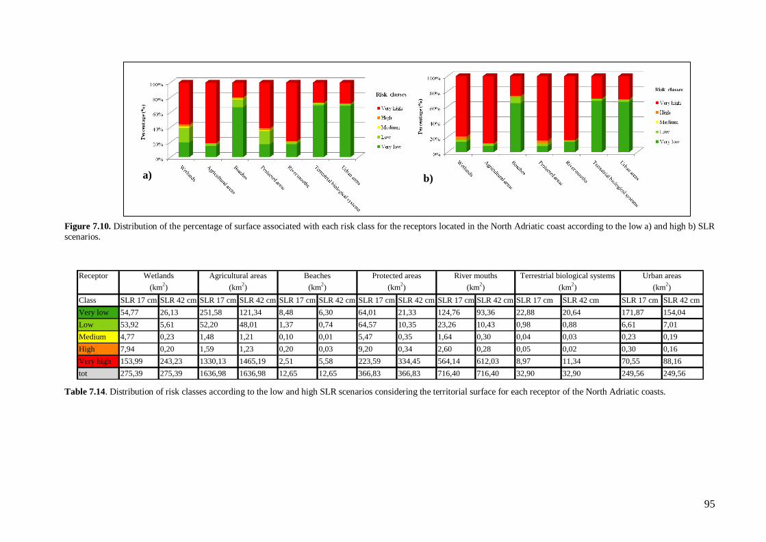
95
Figure 7.10. Distribution of the percentage of surface associated with each risk class for the receptors located in the North Adriatic coast according to the low a) and high b) SLR
scenarios.
Table 7.14. Distribution of risk classes according to the low and high SLR scenarios considering the territorial surface for each receptor of the North Adriatic coasts.
Receptor
Class SLR 17 cm SLR 42 cm SLR 17 cm SLR 42 cm SLR 17 cm SLR 42 cm SLR 17 cm SLR 42 cm SLR 17 cm SLR 42 cm SLR 17 cm SLR 42 cm SLR 17 cm SLR 42 cm
Very low 54,77 26,13 251,58 121,34 8,48 6,30 64,01 21,33 124,76 93,36 22,88 20,64 171,87 154,04
Low 53,92 5,61 52,20 48,01 1,37 0,74 64,57 10,35 23,26 10,43 0,98 0,88 6,61 7,01
Medium 4,77 0,23 1,48 1,21 0,10 0,01 5,47 0,35 1,64 0,30 0,04 0,03 0,23 0,19
High 7,94 0,20 1,59 1,23 0,20 0,03 9,20 0,34 2,60 0,28 0,05 0,02 0,30 0,16
Very high 153,99 243,23 1330,13 1465,19 2,51 5,58 223,59 334,45 564,14 612,03 8,97 11,34 70,55 88,16
tot 275,39 275,39 1636,98 1636,98 12,65 12,65 366,83 366,83 716,40 716,40 32,90 32,90 249,56 249,56
Urban areas
(km2)
Terrestrial biological systems
(km2)
Wetlands
(km2)
Agricultural areas
(km2)
Beaches
(km2)
Protected areas
(km2)
River mouths
(km2)
a) b)
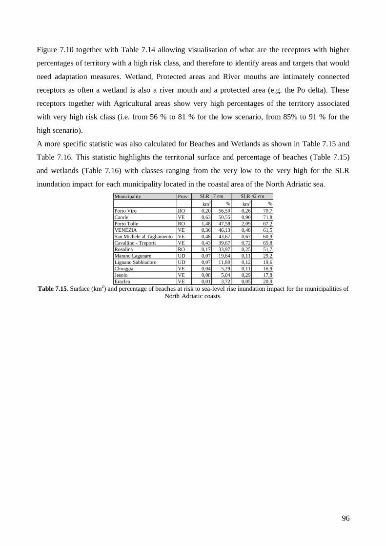
96
Figure 7.10 together with Table 7.14 allowing visualisation of what are the receptors with higher
percentages of territory with a high risk class, and therefore to identify areas and targets that would
need adaptation measures. Wetland, Protected areas and River mouths are intimately connected
receptors as often a wetland is also a river mouth and a protected area (e.g. the Po delta). These
receptors together with Agricultural areas show very high percentages of the territory associated
with very high risk class (i.e. from 56 % to 81 % for the low scenario, from 85% to 91 % for the
high scenario).
A more specific statistic was also calculated for Beaches and Wetlands as shown in Table 7.15 and
Table 7.16. This statistic highlights the territorial surface and percentage of beaches (Table 7.15)
and wetlands (Table 7.16) with classes ranging from the very low to the very high for the SLR
inundation impact for each municipality located in the coastal area of the North Adriatic sea.
Table 7.15. Surface (km2) and percentage of beaches at risk to sea-level rise inundation impact for the municipalities of
North Adriatic coasts.
Municipality Prov.
km2 % km
2 %
Porto Viro RO 0,20 56,50 0,26 70,7
Caorle VE 0,63 50,55 0,90 71,8
Porto Tolle RO 1,48 47,58 2,09 67,2
VENEZIA VE 0,36 46,13 0,48 61,5
San Michele al Tagliamento VE 0,48 43,67 0,67 60,9
Cavallino - Treporti VE 0,43 39,67 0,72 65,8
Rosolina RO 0,17 33,97 0,25 51,7
Marano Lagunare UD 0,07 19,64 0,11 29,2
Lignano Sabbiadoro UD 0,07 11,80 0,12 19,6
Chioggia VE 0,04 5,29 0,11 16,9
Jesolo VE 0,08 5,04 0,29 17,8
Eraclea VE 0,01 3,72 0,05 20,9
SLR 17 cm SLR 42 cm

97
Table 7.16. Surface (km2) and percentage of wetlands at risk to sea-level rise inundation impact for the municipalities
of the North Adriatic coasts.
About 70% of beaches would be lost for the SLR inundation impact (high scenario) in Porto Viro
and Caorle (Table 7.15). The percentage decrease to about 56% for the low SLR scenario. Rosolina
is the municipality with the higher surface at risk for wetlands receptor, with a percentage of the
territory at risk of 94.74% in the low SLR scenario and 97.12 % in the high SLR scenario (Table
7.16). As far as the RSLR impact is concerned, the distribution of the surface of each receptor (km2)
within each risk class for the low and high RSLR scenarios is reported in Table 7.17. Moreover,
Figure 7.11 shows the distribution of risk classes according to the low and high SLR scenarios
considering the percentage (%) of the total surface of each receptor in the Veneto coasts.
Municipality Prov.
km2
% km2
%
Rosolina RO 37,67 94,74 38,61 97,12
Jesolo VE 16,44 93,89 17,12 97,77
Campagna Lupia VE 32,50 92,36 33,70 95,76
Porto Viro RO 43,98 92,29 45,42 95,31
Carlino UD 0,51 90,01 0,53 93,67
Cavallino - Treporti VE 5,94 86,87 6,49 94,90
Latisana UD 0,89 84,52 0,98 93,10
VENEZIA VE 38,64 83,81 42,71 92,65
Codevigo PD 8,45 82,26 9,07 88,26
Porto Tolle RO 20,76 80,26 23,06 89,15
Musile di Piave VE 0,02 78,95 0,02 94,74
Caorle VE 7,46 77,90 9,08 94,77
Chioggia VE 8,39 74,18 9,84 87,05
Mira VE 17,03 72,10 18,97 80,33
Ariano nel Polesine RO 0,74 69,89 0,87 82,51
San Michele al Tagliamento VE 2,67 69,87 3,26 85,28
Precenicco UD 0,42 68,83 0,54 86,90
Quarto d'Altino VE 0,15 60,87 0,20 80,31
Marano Lagunare UD 5,18 58,51 6,87 77,58
Staranzano GO 0,72 54,43 0,86 65,14
Aquileia UD 0,17 51,82 0,20 61,57
Lignano Sabbiadoro UD 0,10 46,25 0,12 57,96
San Canzian d'Isonzo GO 0,03 42,27 0,04 70,10
Palazzolo dello Stella UD 0,02 36,47 0,03 58,82
Muzzana del Turgnano UD 0,01 33,33 0,01 63,64
Monfalcone GO 0,04 13,93 0,14 51,91
SLR 17 cm SLR 42 cm

98
Figure 7.11. Distribution of the percentage of surface associated with each risk class for the receptors located in the Veneto coast according to the low a) and high b) RSLR
scenarios.
Table 7.17. Distribution of risk classes according to the low and high RSLR scenarios considering the territorial surface for each receptor of the Coasts of Veneto.
Receptor
Class RSLR 17 cm RSLR 42 cm RSLR 17 cm RSLR 42 cm RSLR 17 cm RSLR 42 cm RSLR 17 cm RSLR 42 cm RSLR 17 cm RSLR 42 cm RSLR 17 cm RSLR 42 cm RSLR 17 cm RSLR 42 cm
Very low 35,64 14,68 123,09 32,47 4,11 3,09 31,18 3,98 79,51 59,20 13,06 11,22 136,39 118,95
Low 7,27 3,08 39,47 29,45 0,52 0,34 10,60 4,03 8,74 7,14 0,59 0,73 6,10 6,76
Medium 0,27 0,12 1,02 0,71 0,02 0,01 0,37 0,13 0,24 0,17 0,02 0,02 0,16 0,18
High 0,29 0,10 1,01 0,73 0,02 0,01 0,39 0,12 0,23 0,19 0,01 0,02 0,15 0,19
Very high 214,74 240,24 1316,91 1418,14 6,32 7,54 300,67 334,95 627,27 649,28 7,93 9,62 81,36 98,08
tot 258,21 258,21 1481,50 1481,50 10,98 10,98 343,22 343,22 715,99 715,99 21,61 21,60 224,17 224,17
Urban areas
(km2)
Terrestrial biological systems
(km2)
Wetlands
(km2)
Agricultural areas
(km2)
Beaches
(km2)
Protected areas
(km2)
River mouths
(km2)
a) b)

99
Figure 7.11 and Table 7.17, as presented for the SLR inundation impact, shows that Beaches, together with
Wetlands, Agricultural areas, Protected areas and River mouths are very impacted by RSLR, considering the
Coasts of Veneto.
Table 7.18. and Table 7.19. report the territorial surface and percentage of the territory of beaches and
wetland that would be lost in each municipality due to RSLR inundation impact.
Table 7.18. Surface (km2) and percentage of beaches at risk to relative sea-level rise inundation impact for the municipalities of
the Coasts of Veneto.
Table 7.19. Surface (km2) and percentage of wetlands at risk to Relative sea-level rise inundation impact for the municipalities of
the Coasts of Veneto.
The municipalities most at risk from RSLR considering beaches and wetlands are in the first lines of Table
7.18. and Table 7.19. Circa 98% of beaches would be lost for the RSLR inundation impact (low and high
scenarios) in Ariano nel Polesine that is the municipality with a higher risk. Rosolina is the municipality
with the higher risk for wetlands receptor, where almost all the wetlands would be lost in the low and high
RSLR scenarios.
Municipality Prov.
km2 % km
2 %
Ariano nel Polesine RO 0,05 98,73 0,05 98,73
Porto Viro RO 0,32 88,56 0,33 92,20
Porto Tolle RO 2,54 81,46 2,67 85,71
Rosolina RO 0,36 73,46 0,40 82,18
Caorle VE 0,83 66,10 0,92 73,35
San Michele al Tagliamento VE 0,61 55,64 0,76 69,16
Cavallino - Treporti VE 0,49 44,41 0,61 55,37
VENEZIA VE 0,23 29,03 0,28 36,61
Eraclea VE 0,05 23,50 0,09 39,26
Chioggia VE 0,12 17,92 0,19 28,60
Jesolo VE 0,21 13,14 0,40 24,98
RSLR 17 cm RSLR 42 cm
Municipality Prov.
km2
% km2
%
Rosolina RO 38,91 97,87 39,22 98,64
Jesolo VE 17,09 97,60 17,29 98,73
Caorle VE 9,26 96,70 9,53 99,43
Porto Viro RO 45,91 96,34 46,16 96,86
Porto Tolle RO 24,77 95,74 25,27 97,68
Musile di Piave VE 0,02 94,74 0,02 94,74
Cavallino - Treporti VE 6,34 92,73 6,61 96,65
Campagna Lupia VE 32,05 91,06 33,63 95,56
VENEZIA VE 41,12 89,19 43,21 93,74
Chioggia VE 9,88 87,41 10,39 91,88
Ariano nel Polesine RO 0,90 85,24 0,91 86,54
San Michele al Tagliamento VE 3,24 84,85 3,53 92,36
Quarto d'Altino VE 0,18 75,45 0,20 83,12
Mira VE 13,92 58,96 19,06 80,69
Eraclea VE 0,01 9,15 0,02 18,95
Marcon VE 0,00 0,92 0,06 10,69
RSLR 17 cm RSLR 42 cm
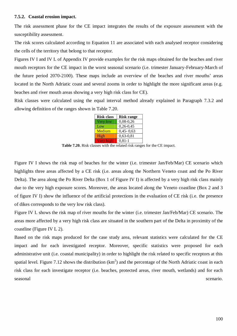
100
7.5.2. Coastal erosion impact.
The risk assessment phase for the CE impact integrates the results of the exposure assessment with the
susceptibility assessment.
The risk scores calculated according to Equation 11 are associated with each analysed receptor considering
the cells of the territory that belong to that receptor.
Figures IV I and IV L of Appendix IV provide examples for the risk maps obtained for the beaches and river
mouth receptors for the CE impact in the worst seasonal scenario (i.e. trimester January-February-March of
the future period 2070-2100). These maps include an overview of the beaches and river mouths’ areas
located in the North Adriatic coast and several zooms in order to highlight the more significant areas (e.g.
beaches and river mouth areas showing a very high risk class for CE).
Risk classes were calculated using the equal interval method already explained in Paragraph 7.3.2 and
allowing definition of the ranges shown in Table 7.20.
Risk class Risk range
Very low 0,08-0,26
Low 0,26-0,45
Medium 0,45- 0,63
High 0,63-0,81
Very high 0,81-1
Table 7.20. Risk classes with the related risk ranges for the CE impact.
Figure IV I shows the risk map of beaches for the winter (i.e. trimester Jan/Feb/Mar) CE scenario which
highlights three areas affected by a CE risk (i.e. areas along the Northern Veneto coast and the Po River
Delta). The area along the Po River Delta (Box 1 of Figure IV I) is affected by a very high risk class mainly
due to the very high exposure scores. Moreover, the areas located along the Veneto coastline (Box 2 and 3
of figure IV I) show the influence of the artificial protections in the evaluation of CE risk (i.e. the presence
of dikes corresponds to the very low risk class).
Figure IV L shows the risk map of river mouths for the winter (i.e. trimester Jan/Feb/Mar) CE scenario. The
areas more affected by a very high risk class are situated in the southern part of the Delta in proximity of the
coastline (Figure IV L 2).
Based on the risk maps produced for the case study area, relevant statistics were calculated for the CE
impact and for each investigated receptor. Moreover, specific statistics were proposed for each
administrative unit (i.e. coastal municipality) in order to highlight the risk related to specific receptors at this
spatial level. Figure 7.12 shows the distribution (km2) and the percentage of the North Adriatic coast in each
risk class for each investigate receptor (i.e. beaches, protected areas, river mouth, wetlands) and for each
seasonal scenario.
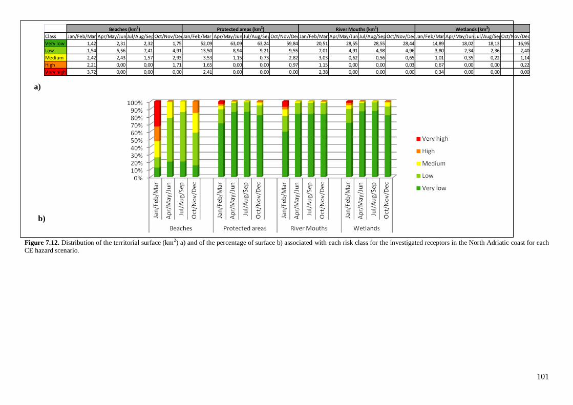
101
Figure 7.12. Distribution of the territorial surface (km2) a) and of the percentage of surface b) associated with each risk class for the investigated receptors in the North Adriatic coast for each
CE hazard scenario.
Class Jan/Feb/Mar Apr/May/Jun Jul/Aug/SepOct/Nov/DecJan/Feb/Mar Apr/May/Jun Jul/Aug/SepOct/Nov/DecJan/Feb/Mar Apr/May/Jun Jul/Aug/SepOct/Nov/Dec Jan/Feb/Mar Apr/May/Jun Jul/Aug/SepOct/Nov/Dec
Very low 1,42 2,31 2,32 1,75 52,09 63,09 63,24 59,84 20,51 28,55 28,55 28,44 14,89 18,02 18,13 16,95
Low 1,54 6,56 7,41 4,91 13,50 8,94 9,21 9,55 7,01 4,91 4,98 4,96 3,80 2,34 2,36 2,40
Medium 2,42 2,43 1,57 2,93 3,53 1,15 0,73 2,82 3,03 0,62 0,56 0,65 1,01 0,35 0,22 1,14
High 2,21 0,00 0,00 1,71 1,65 0,00 0,00 0,97 1,15 0,00 0,00 0,03 0,67 0,00 0,00 0,22
Very high 3,72 0,00 0,00 0,00 2,41 0,00 0,00 0,00 2,38 0,00 0,00 0,00 0,34 0,00 0,00 0,00
Beaches (km2) Protected areas (km2) River Mouths (km2) Wetlands (km2)
b)
a)

102
Figure 7.12 highlights that the receptor with the higher risk classes (i.e. very high, high and medium) is the
beach in the four investigated CE scenarios, this is due to the susceptibility score that is assumed by beaches
for the CE impact (see Paragraph 0). Specifically, the percentage surface of beaches with the higher risk
classes is about 72% in the first trimester, 21% in the second, 14% in the third and 41% in the fourth.
Moreover, the trimester Jan/Feb/Mar is the CE scenario in which the risk scores is the higher related to the
other trimesters, this is due to the high value of the hazard metrics (i.e. wave height and bottom stress in that
scenario (Paragraph 7.2.2).
A more specific statistic was also calculated for beaches and river mouths as shown in Table 7.21 and Table
7.22. This statistic highlights the territorial surface and percentage of beaches (Table 7.21) and river mouths
(Table 7.22) with very high and high risk classes in the RICE area of each municipality of the North Adriatic
sea.
Table 7.21. Surface (km2) and percentage of beaches surface at the higher risk to the CE impact for the municipalities of North
Adriatic coasts within the RICE area.
Table 7.22. Surface (km2) and percentage of river mouths surface at the higher risk to the CE impact for the municipalities of
North Adriatic coasts within the RICE area.
In the winter trimester (Jan/Feb/Mar), about the 92 % of beaches and 6-7% of river mouths result at higher
risk for the CE impact in Porto Viro and Rosolina (Table 7.21 and Table 7.22). Moreover, about 78 % of
beaches in Venice show higher risk related to the CE impact. Also Ariano nel Polesine, Chioggia, Porto
Tolle and Cavallino Treporti are characterized by high percentages of beaches (from 68 to 75%) at higher
risk for the CE impact. In the trimester Oct/Nov/Dic, Duino Aurisina would be the municipality most at risk
for the CE impact considering the beach receptor (i.e.100% of beaches at risk) followed by Lignano
Municipality PROV. Km2
% Km2
%
Porto Viro RO 0,26 92,65 0 0
Rosolina RO 0,41 92,31 0 0
Venezia VE 0,57 78,23 0 0
Ariano nel Polesine RO 0,04 74,68 0 0
Chioggia VE 0,50 72,26 0 0
Porto Tolle RO 1,88 70,36 0 0
Cavallino Treporti VE 0,72 67,89 0 0
Jesolo VE 0,68 43,33 0,26 16,69
Eraclea VE 0,08 37,54 0,08 37,54
Grado GO 0 0 0,21 30,81
San Michele al Tagliamento VE 0,30 28,17 0,30 28,17
Caorle VE 0,35 28,11 0,35 28,11
Lignano Sabbiadoro UD 0,07 13,10 0,37 70,60
Monfalcone GO 0 0 0,01 35,48
Duino Aurisina TS 0 0 0,02 100,00
Marano Lagunare UD 0 0 0,12 37,45
Jan/Feb/Mar Oct/Nov/Dic
Municipality PROV. Km2% Km2
%
Porto Tolle RO 2,30 16,43 0 0
Staranzano GO 0 0 0,02 12,69
Grado GO 0 0 0,01 11,96
Porto Viro RO 0,29 6,69 0 0
Rosolina RO 0,59 5,65 0 0
Ariano nel Polesine RO 0,06 5,49 0 0
Jan/Feb/Mar Oct/Nov/Dic

103
Sabbiadoro (70%). Table 7.22 highlights that the municipalities with a considerable percentage (16-12%) of
river mouths at higher risk for the CE impact are Porto Tolle, Staranzano and Grado in the winter and
autumn trimester respectively.
7.6. Damage assessment.
The Damage assessment phase aggregates the results of the Risk assessment phase (Paragraph 7.5) with the
assessment of the environmental and socio-economic value of a receptor, in order to provide a relative
estimation of the potential social, economic and environmental losses associated with targets and areas at
risk in the case study area (EC, 2007). Damage maps derive from the aggregation of risk maps and value
maps and are calculated using the damage function described in Paragraph 4.6.
In the following Paragraphs, the damage maps obtained for the SLR and RSLR impacts (Paragraph 7.6.1)
and for the CE impact (Paragraph 7.6.2) in the North Adriatic case study will be presented and discussed.
7.6.1. Sea-level rise and relative sea-level rise inundation impacts.
The first step required for the damage assessment phase is to estimate the value associated with each
receptor through a weighted sum (Equation 13). To this aim, it was necessary to classify and provide scores
and weights to the value factors identified in the vulnerability matrix (Table 7.1).
Table 7.23 shows the value classes and the related scores defined for the value factors identified for the
coastal receptors analysed in the case study area.

104
VALUE FACTOR CLASS SCORE
Protection level
National area 1
Regional area 0.5
Nature 2000 area 0.2
Urban typology
Residential building 1
Commercial building 0.5
Infrastructures 0.2
Agricultural typology
Permanent culture 1
Stable meadow 0.5
Arable 0.2
Wetland extension
(Km2)
0 – 19,9 0.2
19,9 – 39,8 0.25
39,8 – 59,8 0.5
59,8 – 79,7 0.75
79,7 – 99,6 1
Vegetation cover
Poor vegetation and meadow 0.2
Vegetation with shrubbery 0.5
Wood 1
Population density
< 100 inhabitants per municipality 0.2
100-300 inhabitants per
municipality 0.5
> 300 inhabitants per municipality 1
Table 7.23. Classes and scores associated with the value factors identified in the vulnerability matrix for the SLR and RSLR
impacts.
Individual value factors were scored in the 0-1 range following the linguistic evaluations reported in Table II
A (Appendix II).
According to the RRA methodology, the assignation of scores to value factors requires the involvement of
decision makers. However, in the present work, scores were assigned by a limited group of environmental
scientists, in order to do a preliminary test of the methodology. Moreover, within this thesis, the same
weight 1 was assigned to all the value factors considered in the case study. In this way the same importance
was attributed to each value factor in the final estimate of the value associated with each receptor. This is a
conservative approach to use in those cases where there is a lack of knowledge about the relative importance
of risk assessment parameters. For the cell composing each receptor, the value function aggregates the value
scores described in Table 7.14 thus obtaining one value map for each analysed receptor. In this way value
maps allow visualization of receptor sub-areas associated with each value class.
An example of value map obtained from the aggregation of the value factors for the receptor agricultural
areas is reported in Figure IV M of Appendix IV. The value map shows the distribution of the value classes
within the agricultural areas. The 60 % of the territory show a low value class due to the presence of factors
with lower value scores (e.g. Nature 2000 protected areas, commercial buildings, population density < 100
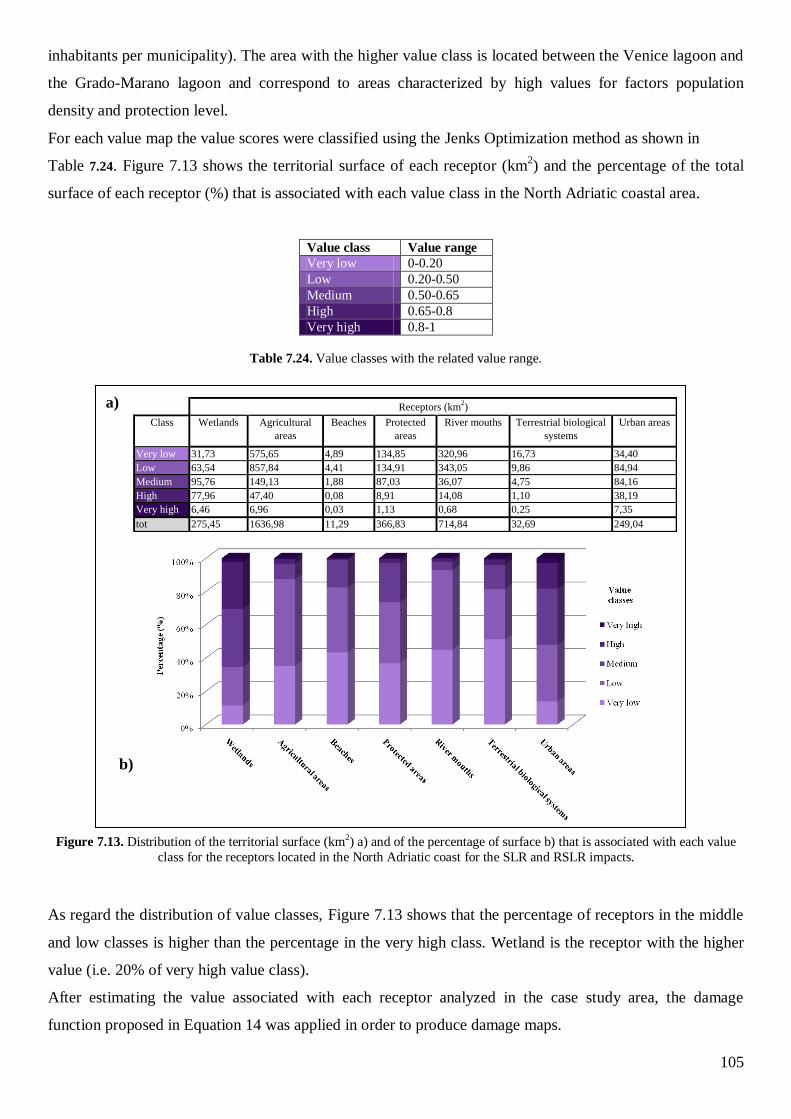
105
inhabitants per municipality). The area with the higher value class is located between the Venice lagoon and
the Grado-Marano lagoon and correspond to areas characterized by high values for factors population
density and protection level.
For each value map the value scores were classified using the Jenks Optimization method as shown in
Table 7.24. Figure 7.13 shows the territorial surface of each receptor (km2) and the percentage of the total
surface of each receptor (%) that is associated with each value class in the North Adriatic coastal area.
Value class Value range
Very low 0-0.20
Low 0.20-0.50
Medium 0.50-0.65
High 0.65-0.8
Very high 0.8-1
Table 7.24. Value classes with the related value range.
Figure 7.13. Distribution of the territorial surface (km2) a) and of the percentage of surface b) that is associated with each value
class for the receptors located in the North Adriatic coast for the SLR and RSLR impacts.
As regard the distribution of value classes, Figure 7.13 shows that the percentage of receptors in the middle
and low classes is higher than the percentage in the very high class. Wetland is the receptor with the higher
value (i.e. 20% of very high value class).
After estimating the value associated with each receptor analyzed in the case study area, the damage
function proposed in Equation 14 was applied in order to produce damage maps.
a)
b)
Very low 31,73 575,65 4,89 134,85 320,96 16,73 34,40
Low 63,54 857,84 4,41 134,91 343,05 9,86 84,94
Medium 95,76 149,13 1,88 87,03 36,07 4,75 84,16
High 77,96 47,40 0,08 8,91 14,08 1,10 38,19
Very high 6,46 6,96 0,03 1,13 0,68 0,25 7,35
tot 275,45 1636,98 11,29 366,83 714,84 32,69 249,04
Terrestrial biological
systems
Urban areasClass
Receptors (km2)
Wetlands Agricultural
areas
Beaches Protected
areas
River mouths

106
Figures IV N and IV O represent two examples of damage maps developed for agricultural and urban areas.
For the agricultural areas (Figure IV N) areas at higher damage are located near Jesolo (Figure IV N 1) and
near Campagna Lupia (located in the hinterland of Venice, Figure IV N 2) For the urban areas (Figure IV O)
high damage areas correspond to areas located near Jesolo (Figure IV O 1) and Porto Viro (Figure IV O 2),
In general, for the RSLR impact, areas at higher damage corresponds to areas where subsidence processes
are relevant (i.e. areas with higher risk scores). Moreover, these areas corresponds also to zones
characterized by higher value scores (i.e. areas with higher environmental or socio-economic value).
Damage scores were classified using the Jenks Optimization method and the ranges of scores associated
with each class is shown in Table 7.25.
Damage class Damage range
Very low 0-0.01
Low 0.01-0.13
Medium 0.13-0.28
High 0.28-0.41
Very high 0.41-1
Table 7.25. Damage classes with the related damage range.
The distribution of the surface of each receptor (km2) within each damage class for the low and high SLR
scenarios is reported in Table 7.26. Moreover, Figure 7.14 shows the distribution of damage classes
according to the low and high SLR scenarios considering the percentage (%) of the total surface of each
receptor in the North Adriatic coasts.

107
Figure 7.14. Distribution of the territorial percentage associated with each damage class according to the low a) and high b) SLR scenarios for the receptors located in the North
Adriatic coasts.
Table 7.26. Distribution of damage classes according to the low and high SLR scenarios considering the territorial surface for each receptor of the North Adriatic coasts.
Receptor
Class SLR 17 cm SLR 42 cm SLR 17 cm SLR 42 cm SLR 17 cm SLR 42 cm SLR 17 cm SLR 42 cm SLR 17 cm SLR 42 cm SLR 17 cm SLR 42 cm SLR 17 cm SLR 42 cm
Very low 63,09 48,66 732,59 642,67 9,56 8,37 180,46 159,71 384,53 364,28 28,13 26,76 173,16 155,44
Low 25,09 3,58 193,81 47,15 0,79 0,52 154,69 7,81 101,63 10,55 0,60 0,73 18,64 5,89
Medium 106,85 10,42 589,15 58,11 2,20 0,70 20,89 16,21 196,62 16,07 0,84 0,60 12,59 6,72
High 11,21 48,14 25,22 50,29 0,07 1,19 2,01 84,22 3,20 62,01 0,33 0,61 7,26 5,73
Very high 69,14 164,59 96,20 838,76 0,03 1,88 8,78 98,88 30,43 263,49 3,00 4,20 37,92 75,77
tot 275,39 275,39 1636,98 1636,98 12,65 12,65 366,83 366,83 716,40 716,40 32,90 32,90 249,56 249,56
Terrestrial biological
systems (km2)
Urban areas
(km2)
Wetlands
(km2)
Agricultural areas
(km2)
Beaches
(km2)
Protected areas
(km2)
River mouths
(km2)
a) b)
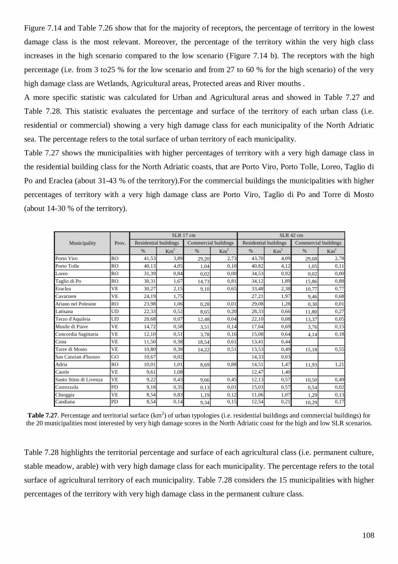
108
Figure 7.14 and Table 7.26 show that for the majority of receptors, the percentage of territory in the lowest
damage class is the most relevant. Moreover, the percentage of the territory within the very high class
increases in the high scenario compared to the low scenario (Figure 7.14 b). The receptors with the high
percentage (i.e. from 3 to25 % for the low scenario and from 27 to 60 % for the high scenario) of the very
high damage class are Wetlands, Agricultural areas, Protected areas and River mouths .
A more specific statistic was calculated for Urban and Agricultural areas and showed in Table 7.27 and
Table 7.28. This statistic evaluates the percentage and surface of the territory of each urban class (i.e.
residential or commercial) showing a very high damage class for each municipality of the North Adriatic
sea. The percentage refers to the total surface of urban territory of each municipality.
Table 7.27 shows the municipalities with higher percentages of territory with a very high damage class in
the residential building class for the North Adriatic coasts, that are Porto Viro, Porto Tolle, Loreo, Taglio di
Po and Eraclea (about 31-43 % of the territory).For the commercial buildings the municipalities with higher
percentages of territory with a very high damage class are Porto Viro, Taglio di Po and Torre di Mosto
(about 14-30 % of the territory).
Table 7.27. Percentage and territorial surface (km2) of urban typologies (i.e. residential buildings and commercial buildings) for
the 20 municipalities most interested by very high damage scores in the North Adriatic coast for the high and low SLR scenarios.
Table 7.28 highlights the territorial percentage and surface of each agricultural class (i.e. permanent culture,
stable meadow, arable) with very high damage class for each municipality. The percentage refers to the total
surface of agricultural territory of each municipality. Table 7.28 considers the 15 municipalities with higher
percentages of the territory with very high damage class in the permanent culture class.
% Km2 % Km
2 % Km2 % Km
2
Porto Viro RO 41,53 3,89 29,20 2,73 43,70 4,09 29,68 2,78
Porto Tolle RO 40,13 4,05 1,04 0,10 40,82 4,12 1,05 0,11
Loreo RO 31,39 0,84 0,02 0,00 34,53 0,92 0,02 0,00
Taglio di Po RO 30,31 1,67 14,73 0,81 34,12 1,89 15,86 0,88
Eraclea VE 30,27 2,15 9,10 0,65 33,48 2,38 10,77 0,77
Cavarzere VE 24,19 1,75 27,21 1,97 9,46 0,68
Ariano nel Polesine RO 23,98 1,06 0,28 0,01 29,08 1,28 0,30 0,01
Latisana UD 22,33 0,52 8,65 0,20 28,33 0,66 11,80 0,27
Terzo d'Aquileia UD 20,68 0,07 12,48 0,04 22,10 0,08 13,37 0,05
Musile di Piave VE 14,72 0,58 3,51 0,14 17,64 0,69 3,76 0,15
Concordia Sagittaria VE 12,10 0,51 3,78 0,16 15,08 0,64 4,14 0,18
Cona VE 11,50 0,38 18,54 0,61 13,41 0,44
Torre di Mosto VE 10,80 0,39 14,22 0,51 13,53 0,49 15,18 0,55
San Canzian d'Isonzo GO 10,67 0,02 14,33 0,03
Adria RO 10,01 1,01 8,69 0,88 14,51 1,47 11,93 1,21
Caorle VE 9,61 1,08 12,47 1,40
Santo Stino di Livenza VE 9,22 0,43 9,66 0,45 12,13 0,57 10,50 0,49
Correzzola PD 9,18 0,35 0,13 0,01 15,03 0,57 0,54 0,02
Chioggia VE 8,54 0,83 1,19 0,12 11,06 1,07 1,29 0,13
Candiana PD 8,54 0,14 9,34 0,15 12,54 0,21 10,29 0,17
SLR 17 cm SLR 42 cm
Residential buildings Commercial buildingsMunicipality Prov. Commercial buildingsResidential buildings
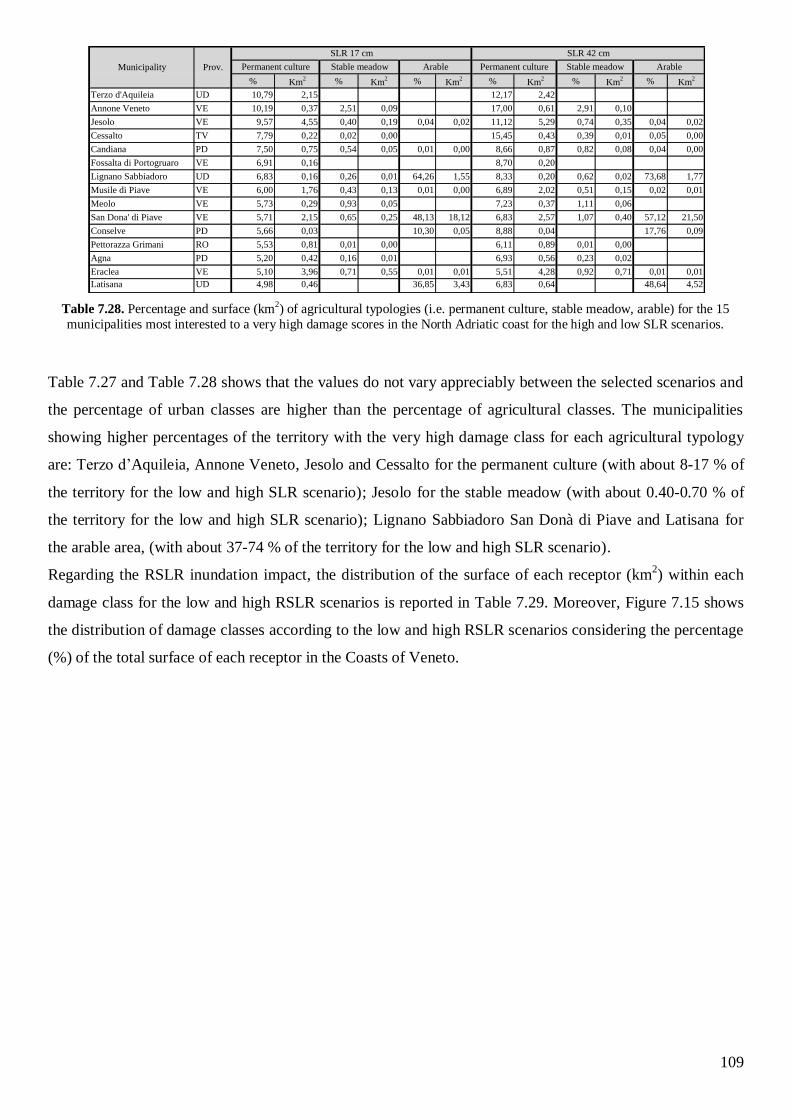
109
Table 7.28. Percentage and surface (km2) of agricultural typologies (i.e. permanent culture, stable meadow, arable) for the 15
municipalities most interested to a very high damage scores in the North Adriatic coast for the high and low SLR scenarios.
Table 7.27 and Table 7.28 shows that the values do not vary appreciably between the selected scenarios and
the percentage of urban classes are higher than the percentage of agricultural classes. The municipalities
showing higher percentages of the territory with the very high damage class for each agricultural typology
are: Terzo d’Aquileia, Annone Veneto, Jesolo and Cessalto for the permanent culture (with about 8-17 % of
the territory for the low and high SLR scenario); Jesolo for the stable meadow (with about 0.40-0.70 % of
the territory for the low and high SLR scenario); Lignano Sabbiadoro San Donà di Piave and Latisana for
the arable area, (with about 37-74 % of the territory for the low and high SLR scenario).
Regarding the RSLR inundation impact, the distribution of the surface of each receptor (km2) within each
damage class for the low and high RSLR scenarios is reported in Table 7.29. Moreover, Figure 7.15 shows
the distribution of damage classes according to the low and high RSLR scenarios considering the percentage
(%) of the total surface of each receptor in the Coasts of Veneto.
% Km2 % Km
2 % Km2 % Km
2 % Km2 % Km
2
Terzo d'Aquileia UD 10,79 2,15 12,17 2,42
Annone Veneto VE 10,19 0,37 2,51 0,09 17,00 0,61 2,91 0,10
Jesolo VE 9,57 4,55 0,40 0,19 0,04 0,02 11,12 5,29 0,74 0,35 0,04 0,02
Cessalto TV 7,79 0,22 0,02 0,00 15,45 0,43 0,39 0,01 0,05 0,00
Candiana PD 7,50 0,75 0,54 0,05 0,01 0,00 8,66 0,87 0,82 0,08 0,04 0,00
Fossalta di Portogruaro VE 6,91 0,16 8,70 0,20
Lignano Sabbiadoro UD 6,83 0,16 0,26 0,01 64,26 1,55 8,33 0,20 0,62 0,02 73,68 1,77
Musile di Piave VE 6,00 1,76 0,43 0,13 0,01 0,00 6,89 2,02 0,51 0,15 0,02 0,01
Meolo VE 5,73 0,29 0,93 0,05 7,23 0,37 1,11 0,06
San Dona' di Piave VE 5,71 2,15 0,65 0,25 48,13 18,12 6,83 2,57 1,07 0,40 57,12 21,50
Conselve PD 5,66 0,03 10,30 0,05 8,88 0,04 17,76 0,09
Pettorazza Grimani RO 5,53 0,81 0,01 0,00 6,11 0,89 0,01 0,00
Agna PD 5,20 0,42 0,16 0,01 6,93 0,56 0,23 0,02
Eraclea VE 5,10 3,96 0,71 0,55 0,01 0,01 5,51 4,28 0,92 0,71 0,01 0,01
Latisana UD 4,98 0,46 36,85 3,43 6,83 0,64 48,64 4,52
Municipality Prov.
SLR 17 cm SLR 42 cm
Permanent culture Stable meadow Arable Permanent culture Stable meadow Arable
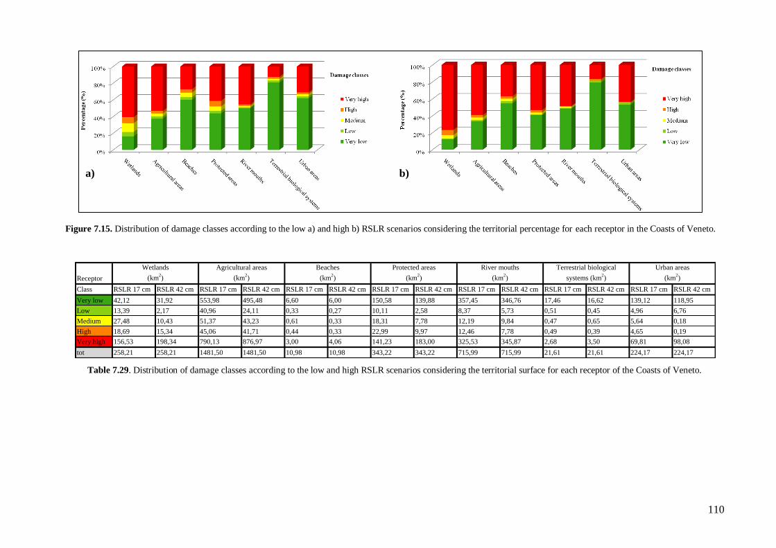
110
Figure 7.15. Distribution of damage classes according to the low a) and high b) RSLR scenarios considering the territorial percentage for each receptor in the Coasts of Veneto.
Table 7.29. Distribution of damage classes according to the low and high RSLR scenarios considering the territorial surface for each receptor of the Coasts of Veneto.
Receptor
Class RSLR 17 cm RSLR 42 cm RSLR 17 cm RSLR 42 cm RSLR 17 cm RSLR 42 cm RSLR 17 cm RSLR 42 cm RSLR 17 cm RSLR 42 cm RSLR 17 cm RSLR 42 cm RSLR 17 cm RSLR 42 cm
Very low 42,12 31,92 553,98 495,48 6,60 6,00 150,58 139,88 357,45 346,76 17,46 16,62 139,12 118,95
Low 13,39 2,17 40,96 24,11 0,33 0,27 10,11 2,58 8,37 5,73 0,51 0,45 4,96 6,76
Medium 27,48 10,43 51,37 43,23 0,61 0,33 18,31 7,78 12,19 9,84 0,47 0,65 5,64 0,18
High 18,69 15,34 45,06 41,71 0,44 0,33 22,99 9,97 12,46 7,78 0,49 0,39 4,65 0,19
Very high 156,53 198,34 790,13 876,97 3,00 4,06 141,23 183,00 325,53 345,87 2,68 3,50 69,81 98,08
tot 258,21 258,21 1481,50 1481,50 10,98 10,98 343,22 343,22 715,99 715,99 21,61 21,61 224,17 224,17
Terrestrial biological
systems (km2)
Urban areas
(km2)
Wetlands
(km2)
Agricultural areas
(km2)
Beaches
(km2)
Protected areas
(km2)
River mouths
(km2)
a) b)
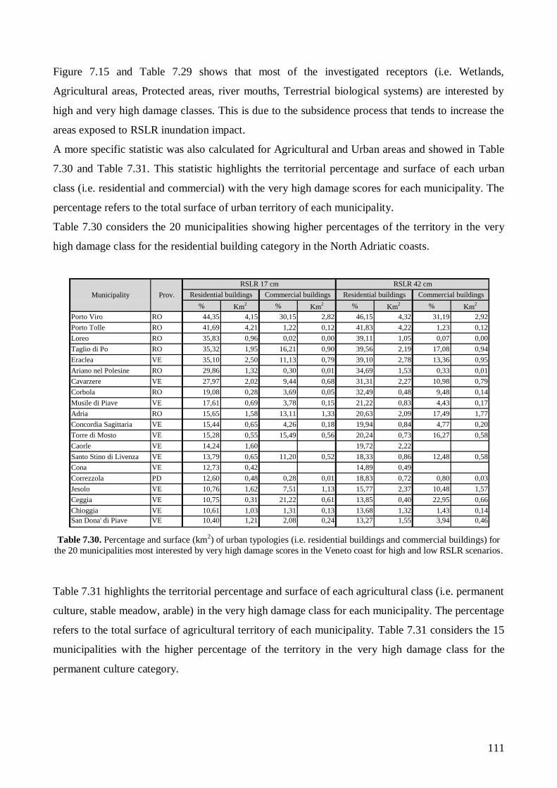
111
Figure 7.15 and Table 7.29 shows that most of the investigated receptors (i.e. Wetlands,
Agricultural areas, Protected areas, river mouths, Terrestrial biological systems) are interested by
high and very high damage classes. This is due to the subsidence process that tends to increase the
areas exposed to RSLR inundation impact.
A more specific statistic was also calculated for Agricultural and Urban areas and showed in Table
7.30 and Table 7.31. This statistic highlights the territorial percentage and surface of each urban
class (i.e. residential and commercial) with the very high damage scores for each municipality. The
percentage refers to the total surface of urban territory of each municipality.
Table 7.30 considers the 20 municipalities showing higher percentages of the territory in the very
high damage class for the residential building category in the North Adriatic coasts.
Table 7.30. Percentage and surface (km2) of urban typologies (i.e. residential buildings and commercial buildings) for
the 20 municipalities most interested by very high damage scores in the Veneto coast for high and low RSLR scenarios.
Table 7.31 highlights the territorial percentage and surface of each agricultural class (i.e. permanent
culture, stable meadow, arable) in the very high damage class for each municipality. The percentage
refers to the total surface of agricultural territory of each municipality. Table 7.31 considers the 15
municipalities with the higher percentage of the territory in the very high damage class for the
permanent culture category.
% Km2 % Km
2 % Km2 % Km
2
Porto Viro RO 44,35 4,15 30,15 2,82 46,15 4,32 31,19 2,92
Porto Tolle RO 41,69 4,21 1,22 0,12 41,83 4,22 1,23 0,12
Loreo RO 35,83 0,96 0,02 0,00 39,11 1,05 0,07 0,00
Taglio di Po RO 35,32 1,95 16,21 0,90 39,56 2,19 17,08 0,94
Eraclea VE 35,10 2,50 11,13 0,79 39,10 2,78 13,36 0,95
Ariano nel Polesine RO 29,86 1,32 0,30 0,01 34,69 1,53 0,33 0,01
Cavarzere VE 27,97 2,02 9,44 0,68 31,31 2,27 10,98 0,79
Corbola RO 19,08 0,28 3,69 0,05 32,49 0,48 9,48 0,14
Musile di Piave VE 17,61 0,69 3,78 0,15 21,22 0,83 4,43 0,17
Adria RO 15,65 1,58 13,11 1,33 20,63 2,09 17,49 1,77
Concordia Sagittaria VE 15,44 0,65 4,26 0,18 19,94 0,84 4,77 0,20
Torre di Mosto VE 15,28 0,55 15,49 0,56 20,24 0,73 16,27 0,58
Caorle VE 14,24 1,60 19,72 2,22
Santo Stino di Livenza VE 13,79 0,65 11,20 0,52 18,33 0,86 12,48 0,58
Cona VE 12,73 0,42 14,89 0,49
Correzzola PD 12,60 0,48 0,28 0,01 18,83 0,72 0,80 0,03
Jesolo VE 10,76 1,62 7,51 1,13 15,77 2,37 10,48 1,57
Ceggia VE 10,75 0,31 21,22 0,61 13,85 0,40 22,95 0,66
Chioggia VE 10,61 1,03 1,31 0,13 13,68 1,32 1,43 0,14
San Dona' di Piave VE 10,40 1,21 2,08 0,24 13,27 1,55 3,94 0,46
Municipality Prov.
RSLR 17 cm RSLR 42 cm
Commercial buildingsResidential buildings Residential buildings Commercial buildings

112
Table 7.31. Percentage and surface (km2) of agricultural typologies (i.e. permanent culture, stable meadow, arable) for
the 15 municipalities most interested by very high damage scores in the Veneto coast for high and low RSLR scenarios.
Table 7.30and Table 7.31 show that the values do not vary appreciably among the selected
scenarios and the percentage of urban classes characterized by high damage class are higher than
the percentage of agricultural classes characterized by the same damage class. Finally, the same
considerations emerged for the SLR can be remarked also for the RSLR inundation impact.
7.6.2. Coastal erosion impact.
As already explained for the SLR and RSLR inundation impacts in Paragraph 7.6.1, the first step of
the damage assessment phase is to classify and provide scores and weights to the value factors
identified in the vulnerability matrix (Table 7.1).
Table 7.32 shows the value classes and the related scores defined for the value factors identified for
the coastal receptors analysed in the case study area.
VALUE FACTOR CLASS SCORE
Protection level
National area 1
Regional area 0.5
Nature 2000 area 0.2
Population density
< 100 inhabitants per municipality 0.2
100-300 inhabitants per municipality 0.5
> 300 inhabitants per municipality 1
Agricultural typology
Arable 0.2
Stable 0.5
Permanent 1
Urban typology
Infrastructure 0.2
commercial 0.5
residential 1
Table 7.32. Classes and scores associated with the value factors identified in the vulnerability matrix for the CE impact.
% Km2 % Km
2 % Km2 % Km
2 % Km2 % Km
2
Motta di Livenza TV 22,64 0,11 39,59 0,19
Annone Veneto VE 20,24 0,73 3,17 0,11 25,98 0,93 3,78 0,14
Cessalto TV 19,51 0,54 0,77 0,02 0,07 0,00 27,89 0,77 1,09 0,03 0,09 0,00
Jesolo VE 11,07 5,27 0,75 0,36 0,04 0,02 12,17 5,79 1,56 0,74 0,04 0,02
Fossalta di
Portogruaro VE 8,62 0,20 10,05 0,23
Candiana PD 7,73 0,77 0,58 0,06 0,02 0,00 8,90 0,89 0,89 0,09 0,04 0,00
Noventa di Piave VE 7,06 0,10 1,20 0,02 17,69 0,26 10,15 0,15 3,23 0,05 28,96 0,42
Musile di Piave VE 6,99 2,05 0,55 0,16 0,03 0,01 7,86 2,31 0,74 0,22 0,04 0,01
San Dona' di Piave VE 6,83 2,57 1,23 0,46 59,99 22,58 8,20 3,09 1,55 0,58 68,99 25,97
Agna PD 6,71 0,54 0,21 0,02 8,06 0,65 0,33 0,03
Meolo VE 6,56 0,34 1,04 0,05 8,13 0,42 1,17 0,06
Portogruaro VE 6,48 1,65 0,72 0,18 8,26 2,11 0,98 0,25
Conselve PD 6,31 0,03 11,33 0,05 9,27 0,04 20,33 0,10
Pettorazza Grimani RO 6,09 0,89 0,01 0,00 6,32 0,92 0,01 0,00
Eraclea VE 5,67 4,41 0,99 0,77 0,01 0,01 5,99 4,65 1,13 0,87 0,01 0,01
Municipality Prov.
RSLR 17 cm RSLR 42 cm
Permanent culture Stable meadow Arable Permanent culture Stable meadow Arable
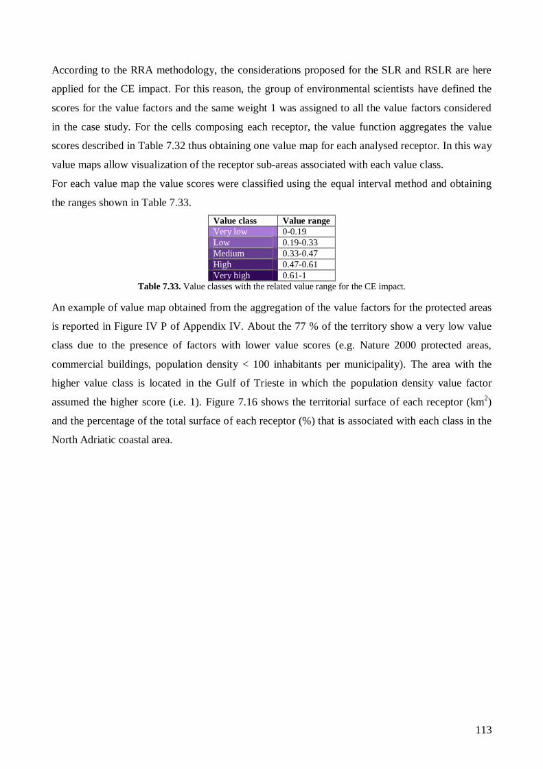
113
According to the RRA methodology, the considerations proposed for the SLR and RSLR are here
applied for the CE impact. For this reason, the group of environmental scientists have defined the
scores for the value factors and the same weight 1 was assigned to all the value factors considered
in the case study. For the cells composing each receptor, the value function aggregates the value
scores described in Table 7.32 thus obtaining one value map for each analysed receptor. In this way
value maps allow visualization of the receptor sub-areas associated with each value class.
For each value map the value scores were classified using the equal interval method and obtaining
the ranges shown in Table 7.33.
Value class Value range
Very low 0-0.19
Low 0.19-0.33
Medium 0.33-0.47
High 0.47-0.61
Very high 0.61-1
Table 7.33. Value classes with the related value range for the CE impact.
An example of value map obtained from the aggregation of the value factors for the protected areas
is reported in Figure IV P of Appendix IV. About the 77 % of the territory show a very low value
class due to the presence of factors with lower value scores (e.g. Nature 2000 protected areas,
commercial buildings, population density < 100 inhabitants per municipality). The area with the
higher value class is located in the Gulf of Trieste in which the population density value factor
assumed the higher score (i.e. 1). Figure 7.16 shows the territorial surface of each receptor (km2)
and the percentage of the total surface of each receptor (%) that is associated with each class in the
North Adriatic coastal area.

114
Figure 7.16. Distribution of the territorial surface (km2) a) and of the percentage of surface b) that is associated with each value class for the receptors located in the North Adriatic coasts for the coastal erosion impact.
Figure 7.16 shows that the territory percentage in the lower classes is higher than the percentage in
the very high class for beaches and protected areas. This is due to the wide presence of factors with
lower value scores (e.g. Nature 2000 protected areas, commercial buildings, population density <
100 inhabitants per municipality). For river mouths and wetlands the territory percentage in the
middle value class is higher than the percentage in the other value classes, due to the middle scores
that the value factors assumed in the case study area.
After estimating the value associated with each receptor analyzed in the case study area, the damage
function proposed in Equation 14 was applied in order to produce damage maps.
Damage scores were classified using the equal interval method and the ranges of scores associated
with each class is shown in Table 7.34.
Damage class Damage range
Very low 0-0.09
Low 0.09-0.18
Medium 0.18-0.27
High 0.27-0.36
Very high 0.36-0.45
Table 7.34. Damage classes with the related damage range for the CE impact.
Figures IV Q and IV R (Appendix IV) represent two examples of damage maps developed for
beaches and wetland. Figures IV Q and IV R highlights areas of beaches and wetlands affected by a
higher CE damage in the North Adriatic coast within the RICE area. The spatial distribution of the
Class Beaches Protected areas River mouths Wetlands
Very low 9,00 57,73 6,19 0,37
Low 2,23 11,79 10,72 9,07
Medium 0,15 4,56 15,51 10,02
High 0,04 0,48 0,41 0,64
Very high 0,00 0,15 1,21
Case study area within the RICE area (km2)
a)
b)
115
damage classes in the damage maps of Appendix IV shows that the study area is mostly interested
by the lower damage classes due to the the presence of factors with lower value scores.
Figure 7.17 shows the distribution (km2) and the percentage of the North Adriatic coast in each
damage class for each investigate receptor (i.e. beaches, protected areas, river mouth, wetlands) and
for each CE hazard scenario.

116
Figure 7.17. Distribution of the territorial surface (km2) a) and of the percentage of surface b) associated with each damage class for the investigated receptors in the North
Adriatic coast for each CE hazard scenario.
Class Jan/Feb/Mar Apr/May/Jun Jul/Aug/Sep Oct/Nov/Dec Jan/Feb/Mar Apr/May/Jun Jul/Aug/Sep Oct/Nov/Dec Jan/Feb/Mar Apr/May/Jun Jul/Aug/Sep Oct/Nov/Dec Jan/Feb/Mar Apr/May/Jun Jul/Aug/Sep Oct/Nov/Dec
Very low 7,62 11,01 11,01 10,05 70,52 73,00 73,00 71,78 27,45 31,84 31,84 31,75 18,18 20,27 20,27 19,57
Low 3,09 0,39 0,39 1,32 2,88 0,67 0,67 1,74 3,88 1,10 1,10 1,14 1,97 0,64 0,64 1,08
Medium 0,65 0,00 0,00 0,01 0,26 0,00 0,00 0,14 1,42 0,03 0,03 0,04 0,92 0,31 0,31 0,21
High 0,02 0,00 0,00 0,01 0,01 0,00 0,00 0,00 0,21 0,00 0,00 0,01 0,14 0,00 0,00 0,33
Very high 0,02 0,00 0,00 0,00 0,00 0,00 0,00 0,00 0,00 0,00 0,00 0,02 0,00 0,00 0,00 0,04
Beaches (km2) Protected areas (km
2) River Mouths (km
2) Wetlands (km
2)
a)
b)
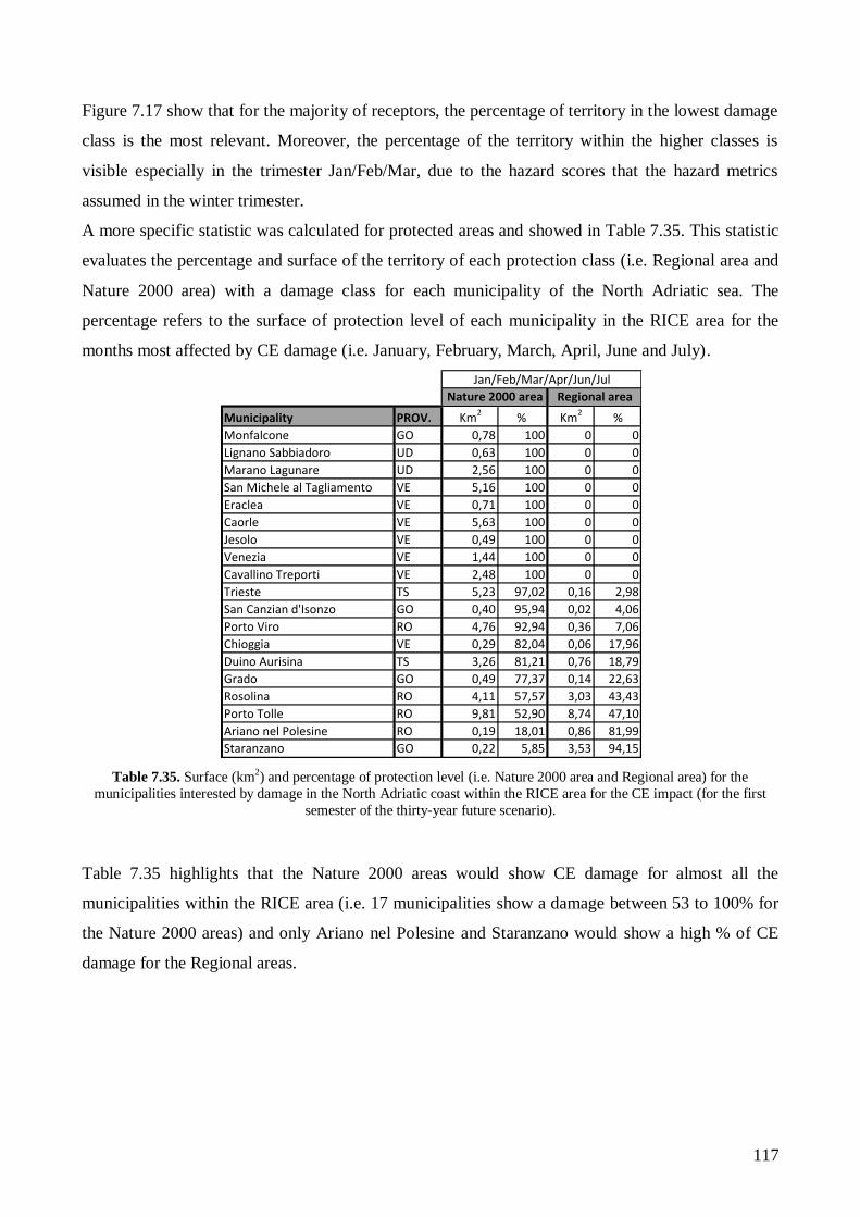
117
Figure 7.17 show that for the majority of receptors, the percentage of territory in the lowest damage
class is the most relevant. Moreover, the percentage of the territory within the higher classes is
visible especially in the trimester Jan/Feb/Mar, due to the hazard scores that the hazard metrics
assumed in the winter trimester.
A more specific statistic was calculated for protected areas and showed in Table 7.35. This statistic
evaluates the percentage and surface of the territory of each protection class (i.e. Regional area and
Nature 2000 area) with a damage class for each municipality of the North Adriatic sea. The
percentage refers to the surface of protection level of each municipality in the RICE area for the
months most affected by CE damage (i.e. January, February, March, April, June and July).
Table 7.35. Surface (km2) and percentage of protection level (i.e. Nature 2000 area and Regional area) for the
municipalities interested by damage in the North Adriatic coast within the RICE area for the CE impact (for the first
semester of the thirty-year future scenario).
Table 7.35 highlights that the Nature 2000 areas would show CE damage for almost all the
municipalities within the RICE area (i.e. 17 municipalities show a damage between 53 to 100% for
the Nature 2000 areas) and only Ariano nel Polesine and Staranzano would show a high % of CE
damage for the Regional areas.
Municipality PROV. Km2
% Km2
%
Monfalcone GO 0,78 100 0 0
Lignano Sabbiadoro UD 0,63 100 0 0
Marano Lagunare UD 2,56 100 0 0
San Michele al Tagliamento VE 5,16 100 0 0
Eraclea VE 0,71 100 0 0
Caorle VE 5,63 100 0 0
Jesolo VE 0,49 100 0 0
Venezia VE 1,44 100 0 0
Cavallino Treporti VE 2,48 100 0 0
Trieste TS 5,23 97,02 0,16 2,98
San Canzian d'Isonzo GO 0,40 95,94 0,02 4,06
Porto Viro RO 4,76 92,94 0,36 7,06
Chioggia VE 0,29 82,04 0,06 17,96
Duino Aurisina TS 3,26 81,21 0,76 18,79
Grado GO 0,49 77,37 0,14 22,63
Rosolina RO 4,11 57,57 3,03 43,43
Porto Tolle RO 9,81 52,90 8,74 47,10
Ariano nel Polesine RO 0,19 18,01 0,86 81,99
Staranzano GO 0,22 5,85 3,53 94,15
Jan/Feb/Mar/Apr/Jun/Jul
Nature 2000 area Regional area
118
Conclusions.
The thesis described the development of a Regional Risk Assessment (RRA) methodology for the
integrated assessment of climate change impacts in coastal zones at the regional scale and its
application to the case study of the North Adriatic coast in Italy.
Specifically, the RRA methodology was applied for the assessment and prioritization of targets and
areas at risks in relation to possible sea-level rise and erosion impacts, considering a climate change
scenario for the period 2070-2100 in the North Adriatic coastal area.
A strength of the proposed approach consists in the use of outputs coming from a multi-model chain
in order to gain information about the spatial and temporal distribution of climate change hazards at
the regional scale (e.g. sea-level rise projections, wave height and bottom stress). Moreover, the
originality of the approach consist in the use of Multi-Criteria Decision analysis (MCDA)
techniques in order to obtain relative rankings of targets and areas at risk in the examined coastal
territory and to identify homogeneous geographic sites for the definition of adaptation and
management strategies. Finally, the extensive use of Geographic Information Systems (GIS)
allowed a detailed analysis of the results and the estimation of several indicators and statistics for
key coastal targets and administrative units (e.g. km2 of beaches at higher risk for each coastal
municipality; percentage of residential buildings and commercial buildings with higher damage in
the considered region).
On the whole, the RRA outputs (i.e. exposure, susceptibility, risk and damage maps) and the related
indicators can be considered as a first-pass assessment for the spatial identification of areas and
targets at higher risk from climate change and for the definition of sustainable management options
at the regional (i.e. sub-national) scale.
In order to properly use the RRA results it is important to underline that the rankings produced by
the methodology are unit less numbers, expressed in qualitative classes (i.e. very high, high,
medium, low, very low), that judge the relative degree of risk and damage for the analyzed
receptors. Accordingly, regional risk and damage classifications do not provide absolute predictions
about the impacts of climate change, rather they are relative indices which provide information
about the sub-areas and targets within a region that are more likely to be affected by climate change
impacts than others.
For what concern the accuracy of the results coming from the risk assessment process, it should be
considered that the proposed methodology adequately takes into account the best available
geographical information at the regional scale, thus requiring a great effort to deal with a huge
amount of data at a detailed spatial resolution. Moreover, numerical models simulations used for the
construction of climate change hazard scenarios and exposure maps were validated through the

119
comparison with observed data for a control period (Gualdi et al., 2008, Djurdjevic and Rajkovic,
2008).
An important issue is related to the collection and organization of data coming from different
sources into homogeneous formats for the whole case study area. In fact, it was necessary to
perform a huge pre-processing phase in order to manage data with different geographic coordinate
systems and allow the GIS overlay and calculations. All this steps represent potential sources of
uncertainty and of geometrical errors in the final risk estimate.
Future improvements of the methodology can be obtained by eliciting more potential receptors and
extending their subset of vulnerability factors. Furthermore, the consistency of results provided by
the methodology can be properly tested trough a sensitivity analysis allowing the ascertainment of
how much the output of the assessment could be influenced by its input parameters (i.e. scores and
weights).
A relevant feature of the methodology is represented by its flexibility to manage input data (i.e.
raster or shape files) provided by different numerical models and vulnerability datasets. This
characteristic allows the methodology to be in principle applied at different spatial scales (i.e. from
the local to the national and supra-national scales) and to be updated with the analysis of new
climate change impacts on further ecosystems (e.g. groundwater, river basins, human health etc.).
Moreover, based on available data and models, the methodology could be improved considering not
only scenarios of climate change but also land use and population dynamics. It has also the potential
to be integrated with socio-economic models in order to obtain a quantitative estimation of damages
and losses associated with climate related impacts.
Finally, the proposed methodology can take advantage from the involvement of stakeholders early
in the process in order to improve the exchange of knowledge on relevant climate-related risks, to
identify well defined needs and data gaps at the regional to local scale, and better support decision
making processes in a climate service perspective.
120
Bibliography.
Abuodha P.A.O. and Woodroffe C.D., 2006. Assessing vulnerability of coast to climate change: a
review of approaches and their application to the Australian coast. University of Wollongong,
Faculty of Science Papers, Research Online.
Adger W. N., Brooks N., Bentham G., Agnew M. e Eriksen S., 2004. New indicators of
vulnerability and adaptive capacity. Tyndall Centre for Climate Change Research. Report 7.
Agostini P., Suter G. W. II, S. Gottardo, E. Giubilato, 2009. Indicators and endpoints for risk-based
decision process with decision support systems. In Marcomini A., Suter G.W. II, Critto A.
(Eds). Decision Support Systems for Risk Based Management of Contaminated Sites. Springer
Verlag, New York.
AIACC, 2006. Vulnerability and Adaptation of Estuarine Systems of the Río de la Plata. The
international START Secretariat 2000 Florida Avenue, NW Washington DC, USA.
Alcamo, J., 2001. In: Teresa, R. (Ed.), Scenarios as Tool for International Environmental
Assessment. European Environment-Agency, Copenhagen.
Antonioli F. and Silenzi S., 2007. Variazioni relative del livello del mare e vulnerabilità delle
pianure costiere italiane. Quaderni SGI 2 (2007).
Ashbindu Singh, 2005. Assessing coastal vulnerability. UNEP. 37 pp.
Australian Government, 2005. Climate change risk and vulnerability. Promoting an efficient
adaptation response in Australia. Report to the Australian Greenhouse Office, Department of
the Environment and Heritage.
Australian Government, 2009. Climate Change Risks to Australia’s Coast. A first pass national
assessment. ISBN: 978-1-921298-71-4.
Bauer, H.-S. and V. Wulfmeyer, 2009. Using a dynamical adjustment technique to validate the
representation of components of the water cycle in the ECHAM4 general circulation model – A
case study of an intense winter cyclone. Meteorol. Atmos. Phys. 104(3-4), 135-162,
DOI:10.1007/s00703-009-0018-7.
Berger A.R. e Iams W.J., 1996. The geoindicator concept and its application: An introduction. In:
Geoindicators – Assessing rapid environmental changes in earth systems. Pp. 1-14, A.A.
Balkema, Rotterdam. Branko G., Bartulovic V., Skaramuca B., 2008. Impact of recent
ichthyofauna changes on local fishery in the Neretva delta estuary, Croatia. International
Symposium, Lisbon. Pp 46.
Bondesan, A., Castiglioni, G.B., Elmi, C., Gabbianelli, G., Marocco, R., Pirazzoli, P.A. e Tomasin,
A., 1995. Coastal areas at risk from storm surges and sea-level rise in northeastern Italy. Journal
of Coastal Research: 11(4): 1354-1379.
121
Booij, N., Ris R. C. and Holthuijsen L. H., 1999. A third-generation wave model for coastal
regions, Part I: Model description and validation, J. Geophys. Res. Vol. 104, C4, pp.7649-7666.
Breton, 2004. State of the Coasts in Europe. Towards a EEA assessment report. Background paper.
European Environment Agency, Barcelona.
Brooks N., 2003. Vulnerability, risk and adaptation: a conceptual framework. Working paper 38,
Tyndall Centre for Climate Change Research, Norwich, UK, pp 20.
Bryan B., Harvey N., Belperio T., Bourman B., 2001. Distributed process modeling for regional
assessment of coastal vulnerability to sea-level rise. Kluwer Academic Publishers. Netherlands.
Pp 57-65.
Carbognin L., P. Teatini, A. Tomasin, L. Tosi, 2009. Global change and relative sea level rise at
Venice: what impact in term of flooding. Clim Dyn DOI 10.1007/s00382-009-0617-5.
Carlton D. Hunt, Ph. D. Battelle, 2004. Northwest Atlantic Coastal Indicators Workshop. Durham,
New Hampshire.
Carniel S., Vichi M., and M. Sclavo, 2007. Sensitivity of a coupled physical-biological model to
turbulence: high frequency simulations in a northern Adriatic station. Chemistry and Ecology,
23(2), pp. 157-175. DOI: 10.1080/02757540701197903.
Carter T.R., Parry M.L., Harasawa H. e Nishioka S., 1994. IPCC Technical Guidelines for
Assessing Climate Change Impacts and Adaptation. London, UK, IPCC.
Casazza G. C., Silvestri E., Spada, Melley A., 2002. Coastal environment in Italy: preliminary
approach using the “DPSIR Scheme” of indicators. In: Littoral 2002, The changing Coast.
EUROCOAST/EUCC (Ed. by EUROCOAST), pp. 541-549, Porto, Portugal.
Coastal Resources Center, 1999. Coastal Management Indicators. University of Rhode Island,
Coastal Resources Center, Narragansett, RI.
Colin R. T., E. P. Evans and E. C. Penning-Rowsell, 2007. Future flooding and coastal erosion
risks. Thomas Telford Publishing, Thomas Telford Ltd. ISBN: 978-0-7277-3449-5. Pp. 256.
COM(2007) 308 Brussels, 07.06.2007. Report to the European Parliament and the Council: An
evaluation of Integrated Coastal Zone Management (ICZM) in Europe.
Dent, B. D. 1996. Cartography: thematic map design. 4th edition. W.C. Brown/McGraw Hill,
Dubuque, Iowa.
DINAS-COAST CONSORTIUM, 2006: Dynamic Interactive Vulnerability Assessment. Users’
Manual.
Djurdjevic, V. and Rajkovic, B., 2008.Verification of a coupled atmosphere-ocean model using
satellite observations over the Adriatic Sea. Annal Geophysics, 26, 1935–1954.

122
EC, 2004. Living with coastal erosion in Europe: Sediment and Space for Sustainability. PART III
– Methodology for assessing regional indicators.
EC, 2005. Climate Change and the European Water Dimension A Report to the European Water
Directors. EU Report No. 21553., European Commission- Joint Research Centre (Publisher),
Ispra, Italy.
EC, 2007. ARMONIA project. Applied multi-risk mapping of natural hazards for impact
assessment. Deliverable 4.1.2. Report: Technical Glossary of a Multi Hazard Related
Vulnerability and Risk Assessment Language – Final version.
EEA, 2005a. The European environment - State and outlook 2005. State of Environment report No
1/2005.
EEA, 2005b. EEA core set of indicators – Guide. Technical report No 1/2005.
EEA, 2006. The changing faces of Europe's coastal areas. EEA Report No 6/2006. European
Environment Agency, Copenhagen. Available at: www.eea.europa.
eu/publications/eea_report_2006_6.
EEA, 2010. The European environment — state and outlook 2010. European Environment Agency,
Copenhagen.
Feenstra J.F., I. Burton, J.B. Smith, e R.S.J. Tol, 1998. Handbook on Methods for Climate Change
Impact Assessment and Adaptation Strategies, United Nations Environment Programme and
Institute for Environmental Studies, Free University of Amsterdam, Amsterdam.
Ferla M., Cordella M., Michielli L., Rusconi A., 2007. Long term variations on sea level and tidal
regime in the lagoon of Venice. Estuar Coast Shelf Sci 75(1–2):214–222.
Fontolan G, 2001. Risk of flooding: forecast and prevention plan. Province of Venice, Soil and
Civil Defence Unit, Trieste, pp 92.
Füssel H.M. and R.J.T. Klein, 2002. Assessing Vulnerability and Adaptation to Climate Change:
An Evolution of Conceptual thinking. Paper presented at the UNDP Expert Group Meeting on
“Integrating Disaster Reduction and Adaptation to Climate Change”, Havana, Cuba, 17-19 June
2002.
Füssel H.M.and Klein R.J.T., 2006. Climate change vulnerability assessments: an evolution of
conceptual thinking. Climatic Change 75:301-329.
Gambolati G., P. Teatini, 2002. GIS simulations of the inundation risk in the Coastal Lowlands of
the Northern Adriatic Sea. Math Comput Modell 35:963–972.
Gameiro C., Brotas V., 2008. Climatic drivers on phytoplankton temporal variability on Tagus
estuary, Portugal. International Symposium, Lisbon. Pag 36.

123
Giove
S., A. Brancia, F. K. Satterstrom, I. Linkov, 2009. Decision Support Systems and
Environment: Role of MCDA. A. Marcomini et al. (eds.), Decision Support Systems for Risk-
Based Management of Contaminated Sites, DOI 10.1007/978-0-387-09722-0_3. Springer
ScienceþBusiness Media, LLC 2009. Pp. 53-73.
Gonella M., P. Teatini, L. Tomasi and Gambolati G., 1998. Flood risk analysis in the Upper
Adriatic Sea due to storm surge, tide, waves, and natural and anthropic land subsidence, In
“CENAS-Coastline Evolution of the upper Adriatic Sea due to Sea Level Rise and Natural and
Anthropogenic Land Subsidence”. Gambolati G. (Ed.). Kluver Academic Publisher Dordrecht,
the Netherlands, 313-324.
Grabemann I., Weisse R., 2008. Climate change impact on extreme wave conditions in the North
Sea: an ensemble study. Ocean Dynamics (2008) 58:199–212 DOI 10.1007/s10236-008-0141-x.
Gualdi S., E. Scoccimarro, A. Navarra, 2008. Changes in Tropical Cyclone Activity due to Global
Warming: Results from a High-Resolution Coupled General Circulation Model. Journal of
Climate. 5204 Volume 21.
Haidvogel, D. B., H. Arango, W. P. Budgell, B. D. Cornuelle, E. Curchitser, E. Di Lorenzo, K.
Fennel, W. R. Geyer, A. J. Hermann, L. Lanerolle, J. Levin, J. C. McWilliams, A. J. Miller, A.
M. Moore, T. M. Powell, A. F. Shchepetkin, C. R. Sherwood, R. P. Signell, J. C. Warner, and J.
Wilkin, 2008. Ocean forecasting in terrain-following coordinates: Formulation and skill
assessment of the Regional Ocean Modeling System. Journal of Computational Physics,227,
3595-3624.
Hertin J., Berkhout F., Moll S., Olsthoorn X., Nocci G., Azzone G., Schepelmann P., 2001.
Indicators for monitoring integration of environment and sustainable development in enterprise
policy. Brighton, SPRU. Science and Technology Policy research, University of Sussex: 61 pp.
Hinkel J. e Klein R.J.T., 2007. Integrating Knowledge for Assessing Coastal Vulnerability to
Climate Change. In “Managing Coastal Vulnerability: an integrated approach” edited by L.
McFadden, R.J. Nicholls e E.Penning-Roswell. Elsevier Science, Amsterdam, 261 pp.
Hunsaker C. T., R. L. Graham, G. W. Suter II, R. V. O’Neill, L. W. Barnthouse, R. H. Gardner,
1990. Assessing ecological risk on a regional scale. Environmental Management 14: 325-332.
IPCC CZMS, 1992. A common methodology for assessing vulnerability to sea level rise. 2 revision.
Global Climate Change and the Rising Challenge of the sea. IPCC CZMS, the Hague, Ministry
of transport, public Works and water Managment, Appendix C.
IPCC, 2001. Third Assessment Report. The Scientific Basis. Working Group 1.
124
IPCC, 2007a. Climate Change 2007: Impacts, Adaptation and Vulnerability. Summary for
Policymakers. Contribution of Working Group II to the Fourth Assessment Report of the
Intergovernmental Panel on Climate Change, Geneva.
IPCC, 2007b. Climate Change 2007: The Physical Science Basis. Summary for Policymakers
Contribution of Working Group I to the Fourth Assessment Report of the Intergovernmental
Panel on Climate Change, Geneva.
IPCC, 2008. Climate change and water. Technical Paper VI. IPCC Secretariat, Geneva.
Jones R. and Boer R., 2004. Assessing Current Climate Risks, Technical paper 4 in "Adaptation
Policy Framework for Climate Change: Developing Strategies, Policies and Measured. Edited
by Bo Lim, Erika Spanger-Siegfried, Ian Burton, Elizabeth Malone, Saleemul Huq". Pp 91-
117.
Kalbfleisch J. G, 1985. Probability and Statistical Inference: Volume 1: Probability. Springer Texts
in Statistics-Sep 9, 1985.
Kienberger S, Lang S. and Zeil P., 2009. Spatial vulnerability units - Expert-based spatial modelling
of socio-economic vulnerability in the Salzach catchment, Austria. Natural Hazards and Earth
System Science, 9:779-788.
Kiker, G.A., Bridges, T.S., Varghese, A., Seager, T.P., Linkov, I., 2005. Application of
Multicriteria Decision Analysis in Environmental Decision Making, Integrated Environmental
Assessment and Management, vol.1 (2):95-108.
Klein R. J. T., Nicholls R. J. and Thomall F.,2003. Resilience to natural hazards: How useful is this
concept? Environmental Hazards 5 (2003) pp. 35–45.
Klein R.J.T. and Nicholls R.J., 1999. Assessment of Coastal Vulnerability to Climate Change.
Ambio, 28, n. 2. Pp 183-187.
Lambeck K., F. Antonioli, M. Anzidei, L. Ferranti, G. Leoni, G. Scicchitano, S. Silenzi, 2010. Sea
level change along the Italian coast during the Holocene and projections for the future.
Quaternary International xxx (2010) 1e8.
Landis W. G. and J. A. Weigers, 1997. Perspective: Design Considerations and Suggested
Approach for Regional and Comparative Ecological Risk Assessment. Human and Ecological
Risk Assessment: Vol. 3, No. 3, pp. 287-297.
Landis W. G., 2005. Regional scale ecological risk assessment. Using the relative risk model.
Edited by W. G. Landis. CRC PRESS.
Lionello P., Cogo S., Galati M.B. and Sanna A., (2008). The Mediterranean surface wave climate
inferred from future scenario simulations. Global and Planetary Change 63: pp 152–162.
125
Madec, G., P. Delecluse, M. Imbard, and C. Levy, 1998: OPA 8.1 Ocean General Circulation
Model reference manual. Institut Pierre-Simon Laplace Internal Rep. 11, 91 pp.
Marotta L., Vicinanza D., 2001. Indici di qualità ambientale nella gestione integrata della fascia
costiera. Studi Costieri: 4: 83-98.
Ministry for the Environment of New Zealand 2008. Coastal Hazards and Climate Change. A
Guidance Manual for Local Government in New Zealand. 2nd edition. Revised by Ramsay, D,
and Bell, R. (NIWA). Prepared for Ministry for the Environment. viii+127 p.
Nakićenovićet N., J. Alcamo, G. Davis, H.J.M. de Vries, J. Fenhann, S. Gaffin, K. Gregory, A.
Grubler, T.Y. Jung, T. Kram, E.L. La Rovere, L. Michaelis, S. Mori, T. Morita, W. Papper, H.
Pitcher, L. Price, K. Riahi, A. Roehrl, H-H. Rogner, A. Sankovski, M. Schlesinger, P. Shukla,
S. Smith, R. Swart, S. van Rooijen, N. Victor, and Z. Dadi, 2000: Special Report on Emissions
Scenarios. Intergovernmental Panel on Climate Change, Cambridge University Press,
Cambridge.
NCCOE, 2004. Guidelines for Responding to the Effects of Climate Change in Coastal and Ocean
Engineering. Engineers Australia 11 National Circuit, Barton ACT 2600.
Nicholls R. J. and Cazenave A., 2010. Sea-Level Rise and Its Impact on Coastal Zones. Science
328, 1517. DOI: 10.1126/science.1185782.
Nicholls R. J., 2004. Coastal flooding and wetland loss in the 21st century: changes under the SRES
climate and socio-economic scenarios. Global Environmental Change 14 (2004) pp. 69–86.
OECD, 1993. OECD core set of indicators for environmental performance reviews. OECD
Environment Monographs No. 83. OECD. Paris.
Pirazzoli P. A., 2005. A review of possible eustatic, isostatic and tectonic contributions in eight late-
Holocene relative sea-level histories from the Mediterranean area. Quaternary Science Reviews
24 (2005) 1989–2001.
Preston B.L., Smith T.F., Brooke C., Gorddard R., Measham T.G., Withycombe G., Mcinnes K.,
Abbs D., Beveridge B. and Morrison C., 2008. Mapping Climate Change Vulnerability in the
Sydney Coastal Councils Group. Prepared for the Sydney Coastal Councils Group.
Ramieri, E., Hartley A., Barbanti A., Duarte Santos F., Gomes A., Hilden M., Laihonen P.,
Marinova N., Santini M., 2011. Methods for assessing coastal vulnerability to climate change,
European Topic Centre on Climate Change Impacts, Vulnerability and Adaptation (ETC CCA)
Technical Paper, Bologna (IT) 93, October 2011.
Roeckner E., Oberhuber J. M., Bacher A., Christoph M. and Kirchner I., 1996. ENSO variability
and atmospheric response in a global coupled atmosphere-ocean GCM. Climate Dynamics,
12:737–754.
126
Romieu E., Welle T., Schneiderbauer S., Pelling M., Vinchon C., 2010. Vulnerability assessment
within climate change and natural hazard contexts: revealing gaps and synergies through coastal
applications. Sustainable Science 5:159–170.
Sagris V., L. Petrov, C. Lavalle, 2005. Towards an Integrated Assessment of Climate Change-
Induced Sea_Level Rise in the Baltic Sea: An Example for the City of Pӓrnu (Estonia).
European Comission, Joint Research Center.
Schleupner C., 2005. Spatial Analysis As Tool for Sensitivity Assessment of Sea Level Rise
Impacts on Martinique. Research Unit Sustainability and Global Change, Hamburg University
and Centre for Marine and Atmospheric Science. Working paper FNU-71.
Seminara G., Bolla Pittaluga M., Tambroni N., Garotta V., (2005). Open problems in modelling the
long-term morphodynamic evolution of the Venice Lagoon. In: Fletcher CA, Spencer T (eds)
Flooding and environmental challenges for Venice and its Lagoon: state of knowledge,
Cambridge University Press, New York, pp 369–378.
Sharples C., R. Mount and T. Pedersen, 2009. The Australian coastal smartline geomorphic and
stability map version 1: manual and data dictionary.
Shchepetkin A. F., McWilliams J. C., 2005. The regional oceanic modeling system (ROMS): a
split-explicit, free-surface, topography-following-coordinate oceanic model. Ocean Modelling
doi:10.1016/j.ocemod.2004.08.002.
Sherwood C. R., J. W. Book, S. Carniel, L. Cavaleri, J. Chiggiato, H. Das, J. D. Doyle, C. K.
Harris, A. W. Niedoroda, H. Perkins, P.-M. Poulain, J. Pullen, C. W. Reed, A. Russo, M. Sclavo,
R. P. Signell, P. Traykovski and J. C. Warner, 2004. Sediment dynamics in the Adriatic Sea
investigated with coupled models. Oceanography, 17(4), 58-69.
Shim J.P., Warkentin M., J.F. Courtney, D.J. Power, R. Sharda, C. Carlsson, 2002. Past, present and
future of decision support technology. Decis Supp Syst 33:111–126.
Silenzi S., Devoti S., Nisi M.F., Donatis M., Gallerini G., Aminti P., Pranzini E., Rossi L., 2002.
Integrated Hazard of Italian Coastal Plains with Respect to Relative Sea Level Rise: A Case
Study in Versilia Plain, Littoral 2002, The Changing Coast. EUROCOAST / EUCC, Porto –
Portugal. Ed. EUROCOAST – Portugal, ISBN 972-8558-09-0.
Simeoni U., Fontolan G., Tessari U., Corbau C., 2007. Domains of spit evolution in the Goro area,
Po Delta, Italy Geomorphology 86:332–348.
Smith K. and R. Ward, 1998. Floods: physical processes and human impacts. Ed. John Wiley,
Chichester 1998.
Smith, E.R., R. V. O’Neill, J.D. Wickham, K.B. Jones, L. Jackson, J.V. Kilaru, and R. Reuter,
2000. The U.S. EPA’s Regional Vulnerability Assessment Program: A Research Strategy for
127
2001 - 2006. U.S. Environmental Protection Agency, Office of Research and Development,
Research Triangle Park, NC.
Sorensen J., 1997. National and International Efforts at Integrated Coastal Management:
Definitions, Achievement, and Lessons. Coastal Management 25: pp 3-41.
Temnykh A. V., Melnikov V. V., Zagorodnyaya, 2008. Long term changes of zooplankton in the
coastal waters of the north-eastern Black Sea. International Symposium, Lisbon. Pp 34.
Torresan S., Critto A., Dalla Valle M., Harvey N. e Marcomini A., 2008. Assessing coastal
vulnerability to climate change: comparing segmentation at global and regional scales.
Sustainability Science, Springer. Pp 45.
Torresan, S., Critto, A., Tonino, M., Alberighi, E., Pizzol, L., Santoro, F., Marcomini, A., 2009.
Climate change risk assessment for coastal management. In Özhan, E. (Editor), Proceedings of
the Ninth International Conference on the Mediterranean Coastal Environment, 10-14 November
2009, Sochi, Russia, MEDCOAST, Middle East Technical University, Ankara, Turkey 91-102.
Travisi C., 2007. La valutazione dei costi del cambiamento climatico in aree costiere per la
definizione di strategie di adattamento: tre casi studio a confronto. Conferenza nazionale sui
Cambiamenti Climatici. Palermo.
Tsimplis M.N., Spencer N.E., 1997. Collection and analysis of monthly mean sea level data in the
Mediterranean and the Black Sea. J. Coast. Res. 13 (2), 534–544.
UKCIP, 2003. Climate adaptation: risk, uncertainty and decision-making. Robert Willows,
Richenda Connell (ed.). Pp166.
Umgiesser G., Melaku Canu D., Cucco A., Solidoro C., 2004. A finite element model for the
Venice Lagoon. Development, set up, calibration and validation. Journal of Marine Systems 51
(2004) 123– 145.
UN-ISDR (United Nations International Strategy for Disaster Reduction), 2009. Terminology:
Basic terms of disaster risk reduction.
USGS, 2004. Coastal Vulnerability Assessment of Olympic National Park to Sea-Level Rise, Open
File Report 04-1021, Electronic Book.
Vinoth J. and Young I. R., 2011. “Global Estimates of Extreme Wind Speed and Wave Height”.
American Meteorological Society. DOI: 10.1175/2010JCLI3680.1.
Voice M., Harvey N. e Walsh K., 2006. Vulnerability to Climate Change of Australia’s Coastal
Zone: Analysis of gaps in methods, data and system thresholds. Australian Greenhouse Office,
Department of the Environment and Heritage.
Wachenfeld D., Johnson J., Skeat A., Kenchington R., Marshall P. and Innes J.,2007. Chapter 1
Introduction to the Great Barrier Reef and climate change. In Climate Change and the Great
128
Barrier Reef, eds. Johnson JE and Marshall PA. Great Barrier Reef Marine Park Authority and
Australian Greenhouse Office, Australia.
Wigley T. M. L. and Raper S. C. B., 1992. Implications for climate and sea level of revised IPCC
emission scenarios. Nature, 357. Pp 293-300.
Wilby R. L., Charles S. P., Zorita E., Timbal B., Whetton P., Mearns L. O., 2000. Guidelines for
use of climate scenarios developed form statistical downscaling methods.
William J. Gutowski, Jr., Iowa State Univ., 2008. Observed Changes in Weather and Climate
Extremes. Weather and Climate Extremes in a Changing Climate Regions of Focus: North
America, Hawaii, Caribbean, and U.S. Pacific Islands. Eds. Thomas R. Karl, Gerald A. Meehl,
Christopher D. Miller, Susan J. Hassol, Anne M. Waple, and William L. Murray. Synthesis and
Assessment Product 3.3 Report by the U.S. Climate Change Science Program and the
Subcommittee on Global Change Research.
Wolf J., Hargreaves J.C. and Flather R.A., 2000. Shallow water wave modelling for the JERICHO
Project POL Report No. 57.
Zald A. E., Shelly S. and Wade T.,2006. A to Z GIS: An Illustrated Dictionary of Geographic
Information Systems. Articles (Libraries). Paper 144.

129
AKNOWLEDGEMENTS
I kindly thank prof. Antonio Marcomini and Dr. Andrea Critto for supervising my Ph.D. work from
the beginning to the end of the course. I thank also the Euro-Mediterranean Centre for Climate
Change (CMCC) for financial support and the Italian Special Integrative Fund for Research (FISR)
that funded the CMCC-FISR project.
I special thank my colleagues Valentina Gallina, Alex Zabeo, Jonathan Rizzi and Lisa Pizzol for the
helpful discussions and for the valuable contribution they provided to the CMCC-FISR project.
I thank also Prof. Silvio Giove for guiding the development of the MCDA procedures of the RRA
methodology and Filippo Corò for the implementation of the software DESYCO that was used for
producing risk maps.
I am grateful to Dr. Silvio Gualdi (CMCC) and to the colleagues of the National Research Council
(CNR) (Debora Bellafiore, Georg Umgiesser, Mauro Sclavo and Sandro Carniel) for the work done
in the CMCC-FISR project and especially for the provision of modeling outputs used in the
construction of climate change hazard scenarios. I also acknowledge Francesco Rianna, Enrico
Alberighi and Paolo Riccato for the help in data pre- and post-processing and Marco Tonino for
supporting the review of criteria and methods for hazard scenarios construction.
Finally, I thank all the public institutions that provided territorial data for the application of the
RRA methodology, and especially the Italian Environmental Protection Agency, the Veneto and
Friuli Venezia Giulia Regions.
A very special thank to Stefania and Yaella for continuous and sincere friendship during these
years.
My greatest thanks to my parents Patrizia and Ezio and to all my family that take care of Gianmarco
and supported me during difficulties. Thanks a lot also to Alberto and Gianmarco for living day by
day this adventure close to me and for supporting me right to the end.
130
APPENDIX I
Guidelines for the construction of the Vulnerability and Hazard matrixes.
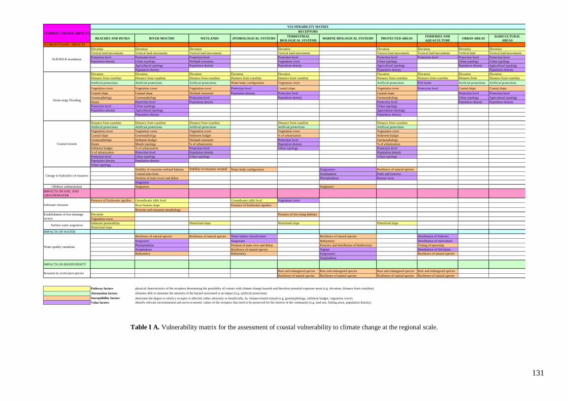
131
Table I A. Vulnerability matrix for the assessment of coastal vulnerability to climate change at the regional scale.
BEACHES AND DUNES RIVER MOUTHS WETLANDS HYDROLOGICAL SYSTEMSTERRESTRIAL
BIOLOGICAL SYSTEMSMARINE BIOLOGICAL SYSTEMS PROTECTED AREAS
FISHERIES AND
AQUACULTUREURBAN AREAS
AGRICULTURAL
AREAS
HYDRODYNAMIC IMPACTS
Elevation Elevation Elevation Elevation Elevation Elevation Elevation Elevation
Vertical land movements Vertical land movements Vertical land movements Vertical land movements Vertical land movements Vertical land movements Vertical land
movements
Vertical land movements
Protection level Protection level Protection level Protection level Protection level Protection level Protection level Protection level
Population density Urban typology Wetland extension Vegetation cover Urban typology Urban typology Urban typology
Agricultural typology Population density Population density Agricultural typology Population density Agricultural typology
Population density Population density Population density
Elevation Elevation Elevation Elevation Elevation Elevation Elevation Elevation Elevation
Distance from coastline Distance from coastline Distance from coastline Distance from coastline Distance from coastline Distance from coastline Distance from coastline Distance from
coastline
Distance from coastline
Artificial protections Artificial protections Artificial protections Water body configuration Vegetation cover Artificial protections Fish farms Artificial protections Artificial protections
Vegetation cover Vegetation cover Vegetation cover Protection level Coastal slope Vegetation cover Protection level Coastal slope Coastal slope
Coastal slope Coastal slope Wetland extension Population density Protection level Coastal slope Protection level Protection level
Geomorphology Geomorphology Protection level Population density Geomorphology Urban typology Agricultural typology
Dunes Protection level Population density Protection level Population density Population density
Protection level Urban typology Urban typology
Population density Agricultural typology Agricultural typology
Population density Population density
Distance from coastline Distance from coastline Distance from coastline Distance from coastline Distance from coastline
Artificial protections Artificial protections Artificial protections Artificial protections Artificial protections
Vegetation cover Vegetation cover Vegetation cover Vegetation cover Vegetation cover
Coastal slope Geomorphology Sediment budget % of urbanization Sediment budget
Geomorphology Sediment budget Wetland extension Protection level Geomorphology
Dunes Mouth typology % of urbanization Population density % of urbanization
Sediment budget % of urbanization Protection level Urban typology Protection level
% of urbanization Protection level Population density Population density
Protection level Urban typology Urban typology Urban typology
Population density Population density
Urban typology
Stability of estuarine wetland habitats Stability of estuarine wetland
habitats Water body configuration Seagraasses Resilience of natural species
Coastal plan-form Zooplankton Parks and reserves
Position of main rivers and deltas Phytoplankton Ramsar areas
Seagrasses
Offshore sedimentation Seagrasses Seagrasses
IMPACTS ON SOIL AND
GROUNDWATER
Presence of freshwater aquifers Groundwater table level Groundwater table level Vegetation cover
River bottom slope Presence of freshwater aquifers
Riverine and estuarine morphology
Elevation Presence of low-lying habitats
Vegetation cover
Substrate permeability Hinterland slope Hinterland slope Hinterland slope
Hinterland slope
IMPACTS ON WATER
Resilience of natural species Resilience of natural species Water bodies classification Resilience of natural species Distribution of fisheries
Seagrasses Seagrasses Bathymetry Distribution of mariculture
Phytoplankton Position of main river and deltas Presence and distribution of biodiveristy Timing of spawning
Zooplankton Resilience of natural species Tegnue Distribution of fish farms
Bathymetry Bathymetry Seagraasses Resilience of natural species
Zooplankton
IMPACTS ON BIODIVERSITY
Rare and endangered species Rare and endangered species Rare and endangered species Rare and endangered species
Resilience of natural species Resilience of natural species Resilience of natural species Resilience of natural species
Pathway factors
Attenuation factors
Susceptibility factors
Value factors
Invasion by exotic/pest species
Water quality variations
Establishment of low-drainage
sectors
Saltwater intrusion
Surface water stagnation
identify relevant environmental and socio-economic values of the receptors that need to be preserved for the interest of the community (e.g. land use, fishing areas, population density).
determine the degree to which a receptor is affected, either adversely or beneficially, by climate-related stimuli (e.g. geomorphology, sediment budget, vegetation cover).
physical characteristics of the receptors determining the possibility of contact with climate change hazards and therefore potential exposure areas (e.g. elevation, distance from coastline).
CLIMATE CHANGE IMPACTS
SLR/RSLR inundation
Storm surge Flooding
Coastal erosion
Change in hydraulics of estuaries
RECEPTORS
VULNERABILITY MATRIX
elements able to attenuate the intensity of the hazard associated to an impact (e.g. artificial protection).
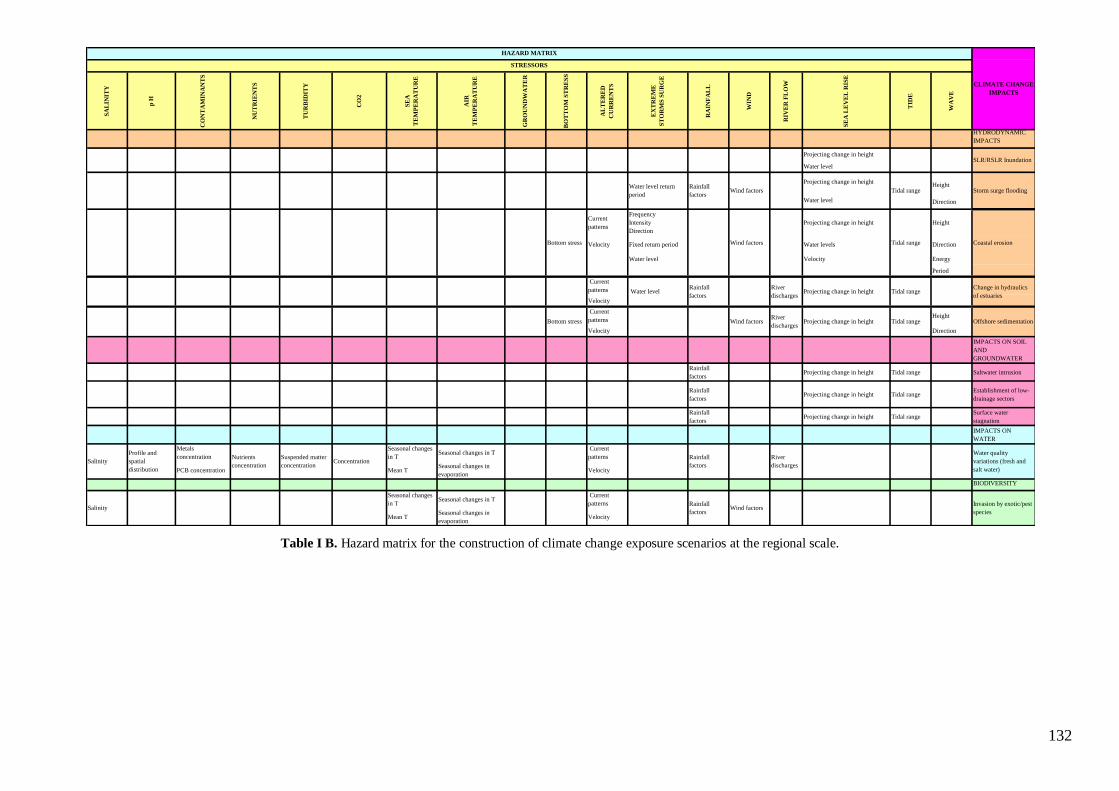
132
Table I B. Hazard matrix for the construction of climate change exposure scenarios at the regional scale.
SA
LIN
ITY
p H
CO
NT
AM
INA
NT
S
NU
TR
IEN
TS
TU
RB
IDIT
Y
CO
2
SE
A
TE
MP
ER
AT
UR
E
AIR
TE
MP
ER
AT
UR
E
GR
OU
ND
WA
TE
R
BO
TT
OM
ST
RE
SS
AL
TE
RE
D
CU
RR
EN
TS
EX
TR
EM
E
ST
OR
MS
SU
RG
E
RA
INF
AL
L
WIN
D
RIV
ER
FL
OW
SE
A L
EV
EL
RIS
E
TID
E
WA
VE
HYDRODYNAMIC
IMPACTS
Projecting change in height
Water level
Projecting change in height Height
Water level Direction
Current
patterns
Frequency
Intensity
Direction
Projecting change in height Height
Velocity Fixed return period Water levels Direction
Water level Velocity Energy
Period
Current
patterns
Velocity
Current
patternsHeight
Velocity Direction
IMPACTS ON SOIL
AND
GROUNDWATER
Rainfall
factorsProjecting change in height Tidal range Saltwater intrusion
Rainfall
factorsProjecting change in height Tidal range
Establishment of low-
drainage sectors
Rainfall
factorsProjecting change in height Tidal range
Surface water
stagnation
IMPACTS ON
WATER
Metals
concentration
Seasonal changes
in TSeasonal changes in T
Current
patterns
PCB concentration Mean TSeasonal changes in
evaporationVelocity
IMPACTS ON
BIODIVERSITY
Seasonal changes
in TSeasonal changes in T
Current
patterns
Mean TSeasonal changes in
evaporationVelocity
HAZARD MATRIX
CLIMATE CHANGE
IMPACTS
STRESSORS
Bottom stress Wind factors Tidal range Coastal erosion
Water levelRainfall
factors
River
dischargesProjecting change in height Tidal range
Change in hydraulics
of estuaries
Bottom stress Wind factorsRiver
dischargesProjecting change in height Tidal range Offshore sedimentation
Salinity
Profile and
spatial
distribution
Nutrients
concentration
Suspended matter
concentrationConcentration
Rainfall
factors
River
discharges
Water quality
variations (fresh and
salt water)
SalinityRainfall
factorsWind factors
Invasion by exotic/pest
species
Rainfall
factorsWind factors Tidal range
SLR/RSLR Inundation
Storm surge floodingWater level return
period

133
APPENDIX II
Guideline for the application of scores.

134
Linguistic Evaluation Scores (si,n) Most important class 1
Weakly less important class 0.8
Rather less important class 0.6
Strongly less important class 0.4
Less important class 0.2
No vulnerability/hazard 0
Table II A. Linguistic evaluations supporting the expert/decision maker in the assignation of relative scores to
vulnerability and hazard classes.
Factor Class Score (si,n)
Impact 1 Impact 2 Impact 3 ... Impact n Susceptibility factors
sf1 c1,1
c1,2
sf2
c2,1
c2,2
c2,3
sf3
c3,1
c3,2
...
c3,n
...
sfn
Hazard metrics
h1 c1,1
c1,2
h2
c2,1
c2,2
c2,3
h3
c3,1
c3,2
...
c3,n
...
hn
Table II B. Example of questionnaire to be administrated to experts for the assignation of relative scores to
susceptibility factors (sf) and hazard (h) classes.
Value Factor Class Score (si,n)
Receptor 1 Receptor 2 Receptor 3 … Receptor 4
vf1
c1,1
c1,2
c1,3
vf2 c2,1
c2,2
vf3
c3,1
c3,2
...
c3,n
… vfn
Table II C. Example of questionnaire to be administrated to decision makers for the assignation of relative scores to
value (vfn) classes.
135
APPENDIX III
Guideline for the application of weights.

136
Linguistic Evaluation Weights (wi,k) Most important vulnerability factor/hazard metric 1 Weakly less important vulnerability factor/hazard metric 0.8 Rather less important vulnerability factor/hazard metric 0.6 Strongly less important vulnerability factor/hazard metric 0.4 Demonstratively less important vulnerability factor/hazard metric 0.2 Not important vulnerability factor/hazard metric 0
Table III A. Linguistic evaluations supporting the expert/decision maker in the assignation of weights to vulnerability
factors and hazard metrics.
Susceptibility factors
Impacts i1 i2 i3 ... in
sf1 sf2 sf3 ... sfn
Hazard metrics
Impacts i1 i2 i3 ... in
h1 h2 h3 ... hn
Table III B. Example of questionnaire to be administrated to experts for the assignation of relative weights to
susceptibility factors (sf) and hazard metrics (h).
Value
factor Receptors
r1 r2 r3 ... rn vf1 vf2 vf3 ... vfn
Table III C. Example of questionnaire to be administrated to decision makers for the assignation of relative weights to
value factors (vfn).
137
APPENDIX IV
Regional Risk Assessment maps for the analysis of sea-level rise, relative sea-
level rise and coastal erosion impacts in the North Adriatic coast.

138
Figure IV A. Low exposure map for the sea-level rise inundation impact (projected water level of 17 cm) for the North
Adriatic coast.
Figure IV B. High exposure map for the sea-level rise inundation impact (projected water level of 42 cm) for the North
Adriatic coasts.
classes
classes
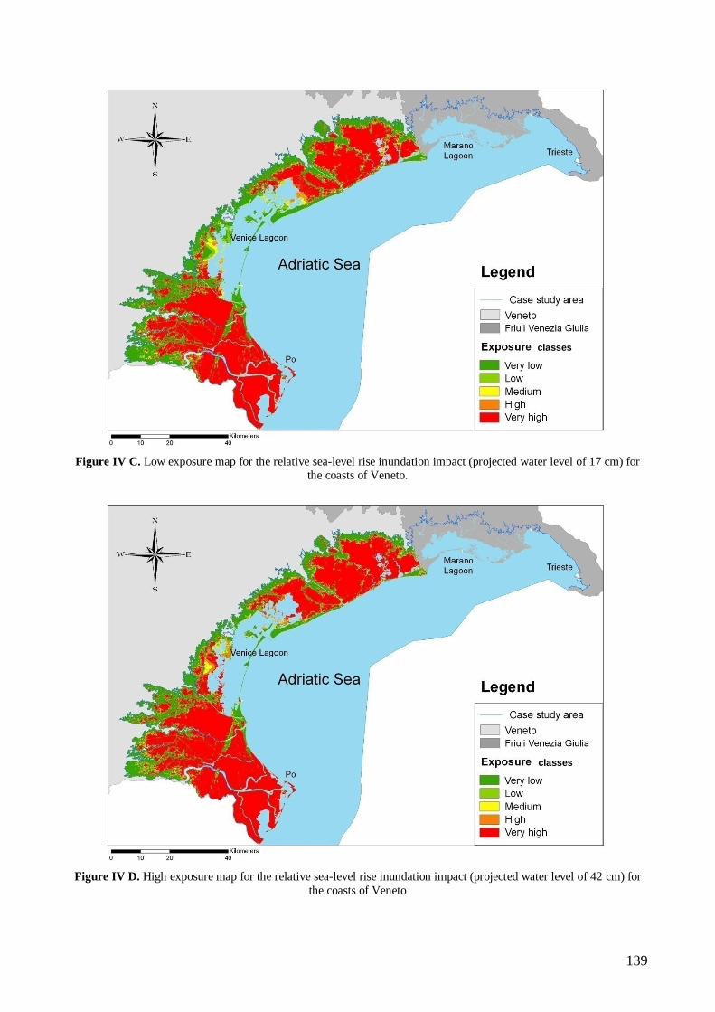
139
Figure IV C. Low exposure map for the relative sea-level rise inundation impact (projected water level of 17 cm) for
the coasts of Veneto.
Figure IV D. High exposure map for the relative sea-level rise inundation impact (projected water level of 42 cm) for
the coasts of Veneto
classes
classes
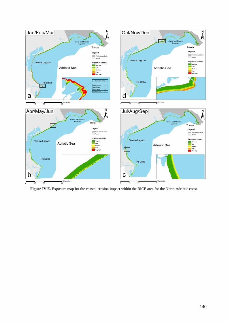
140
Figure IV E. Exposure map for the coastal erosion impact within the RICE area for the North Adriatic coast.

141
Figure IV F. Susceptibility map for the coastal erosion impact within the RICE area for the North Adriatic coast.

142
Figure IV G. Risk map of beaches for the high sea-level rise scenario (projected water level 42 cm) for the North
Adriatic coasts.
Figure IV H. Risk map of wetlands for the low sea-level rise scenario (projected water level of 17 cm) for the North
Adriatic coasts.
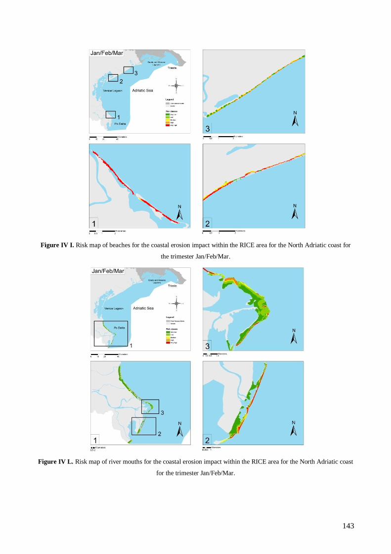
143
Figure IV I. Risk map of beaches for the coastal erosion impact within the RICE area for the North Adriatic coast for
the trimester Jan/Feb/Mar.
Figure IV L. Risk map of river mouths for the coastal erosion impact within the RICE area for the North Adriatic coast
for the trimester Jan/Feb/Mar.

144
Figure IV M. Value map for the agricultural areas receptor for the North Adriatic coasts for the sea-level rise and
relative sea-level rise impacts.
Figure IV N. Damage map of agricultural areas for the low relative sea-level rise scenario (projected water level of 17
cm) for the coasts of Veneto.
Jesolo
Campagna
Lupia

145
Figure IV O. Damage map of urban areas for the high relative sea-level rise scenario (projected water of 42 cm) for the
coasts of Veneto.
Figure IV P. Value map for the protected areas within the RICE area for the North Adriatic coast for the coastal
erosion impact.
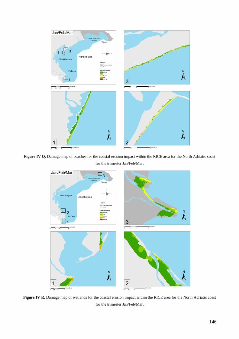
146
Figure IV Q. Damage map of beaches for the coastal erosion impact within the RICE area for the North Adriatic coast
for the trimester Jan/Feb/Mar.
Figure IV R. Damage map of wetlands for the coastal erosion impact within the RICE area for the North Adriatic coast
for the trimester Jan/Feb/Mar.