DEVELOPMENT OF A NOVEL FULLY COUPLED SOLVER IN … · DEVELOPMENT OF A NOVEL FULLY COUPLED SOLVER IN OPENFOAM: STEADY-STATE INCOMPRESSIBLE TURBULENT FLOWS IN ROTATIONAL REFERENCE

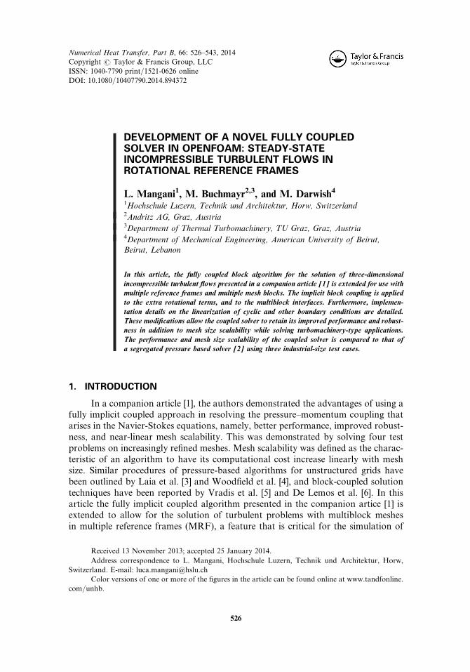
DEVELOPMENT OF A NOVEL FULLY COUPLEDSOLVER IN OPENFOAM: STEADY-STATEINCOMPRESSIBLE TURBULENT FLOWS INROTATIONAL REFERENCE FRAMES

L. Mangani1, M. Buchmayr2,3, and M. Darwish41Hochschule Luzern, Technik und Architektur, Horw, Switzerland2Andritz AG, Graz, Austria3Department of Thermal Turbomachinery, TU Graz, Graz, Austria4Department of Mechanical Engineering, American University of Beirut,Beirut, Lebanon

In this article, the fully coupled block algorithm for the solution of three-dimensional

incompressible turbulent flows presented in a companion article [1] is extended for use with

multiple reference frames and multiple mesh blocks. The implicit block coupling is applied

to the extra rotational terms, and to the multiblock interfaces. Furthermore, implemen-

tation details on the linearization of cyclic and other boundary conditions are detailed.

These modifications allow the coupled solver to retain its improved performance and robust-

ness in addition to mesh size scalability while solving turbomachinery-type applications.

The performance and mesh size scalability of the coupled solver is compared to that of

a segregated pressure based solver [2] using three industrial-size test cases.

1. INTRODUCTION

In a companion article [1], the authors demonstrated the advantages of using afully implicit coupled approach in resolving the pressure–momentum coupling thatarises in the Navier-Stokes equations, namely, better performance, improved robust-ness, and near-linear mesh scalability. This was demonstrated by solving four testproblems on increasingly refined meshes. Mesh scalability was defined as the charac-teristic of an algorithm to have its computational cost increase linearly with meshsize. Similar procedures of pressure-based algorithms for unstructured grids havebeen outlined by Laia et al. [3] and Woodfield et al. [4], and block-coupled solutiontechniques have been reported by Vradis et al. [5] and De Lemos et al. [6]. In thisarticle the fully implicit coupled algorithm presented in the companion artice [1] isextended to allow for the solution of turbulent problems with multiblock meshesin multiple reference frames (MRF), a feature that is critical for the simulation of

Received 13 November 2013; accepted 25 January 2014.

Address correspondence to L. Mangani, Hochschule Luzern, Technik und Architektur, Horw,

Switzerland. E-mail: [email protected]

Color versions of one or more of the figures in the article can be found online at www.tandfonline.

com/unhb.

Numerical Heat Transfer, Part B, 66: 526–543, 2014

Copyright # Taylor & Francis Group, LLC

ISSN: 1040-7790 print=1521-0626 online

DOI: 10.1080/10407790.2014.894372

526

turbomachinery applications. To preserve the convergence behavior and scalability,it is essential to use a fully implicit treatment for the multiblock interfaces,whether with conforming or nonconforming meshes. To this end, the implicitmultiblock procedure of Darwish et al. [7] was adopted. Since turbomachinery flowsare generally turbulent, the k–x SST turbulence model [8] is used with the coupledsolver.

In the remainder of the article the governing equations in a rotating referenceframe are first presented, then the key features of the MRF coupled solver aredetailed, namely, the implicit discretisation of the rotational terms, the arbitrarymesh interface (AMI) interblock interface, the cyclic patches, and other boundaryconditions. Finally, the performance and mesh scalability of the algorithm areevaluated for a variety of industrial turbomachinery applications.

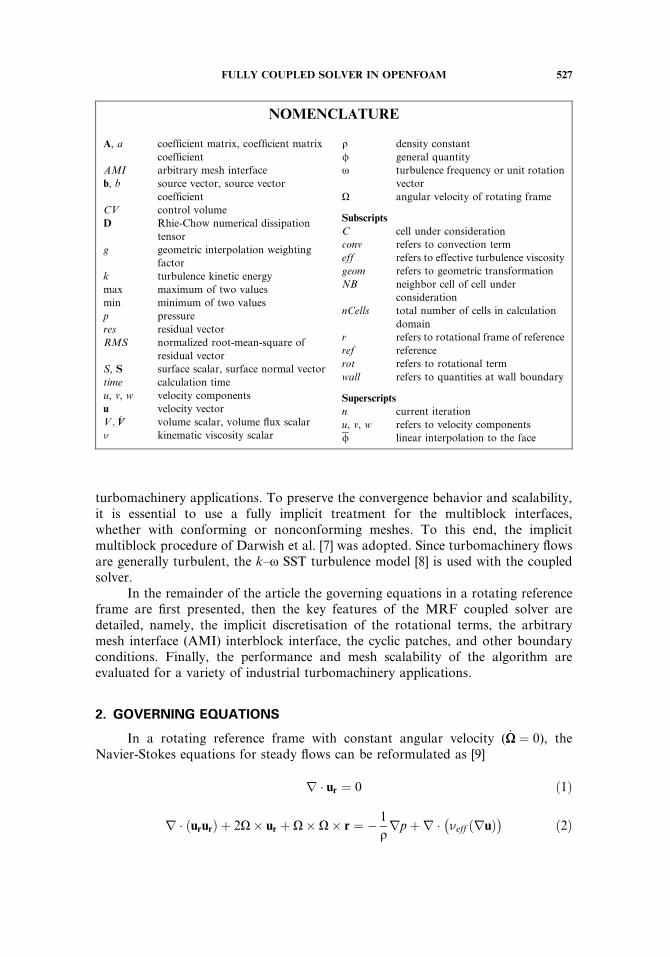
2. GOVERNING EQUATIONS

In a rotating reference frame with constant angular velocity ( _XX ¼ 0), theNavier-Stokes equations for steady flows can be reformulated as [9]

r � ur ¼ 0 ð1Þ

r � ururð Þ þ 2X� ur þ X� X� r ¼ � 1

qrpþr � neff ruð Þ

� �ð2Þ

NOMENCLATURE

A, a coefficient matrix, coefficient matrix

coefficient

AMI arbitrary mesh interface

b, b source vector, source vector

coefficient

CV control volume

D Rhie-Chow numerical dissipation

tensor

g geometric interpolation weighting

factor

k turbulence kinetic energy

max maximum of two values

min minimum of two values

p pressure

res residual vector

RMS normalized root-mean-square of

residual vector

S, S surface scalar, surface normal vector

time calculation time

u, v, w velocity components

u velocity vector

V ; _VV volume scalar, volume flux scalar

n kinematic viscosity scalar

q density constant

/ general quantity

x turbulence frequency or unit rotation

vector

X angular velocity of rotating frame

Subscripts

C cell under consideration

conv refers to convection term

eff refers to effective turbulence viscosity

geom refers to geometric transformation

NB neighbor cell of cell under

consideration

nCells total number of cells in calculation

domain

r refers to rotational frame of reference

ref reference

rot refers to rotational term

wall refers to quantities at wall boundary

Superscripts

n current iteration

u, v, w refers to velocity components

/ linear interpolation to the face

FULLY COUPLED SOLVER IN OPENFOAM 527

where X is the angular velocity of the rotating frame, and ur is the relative velocity inthe rotational system. The absolute or stationary frame velocity, u, is written

u ¼ ur þ X� r ð3Þ

In Eq. (2) the second and third terms are the Coriolis and centripetal forces, respectively.To facilitate the numerical discretization and resolution of these equations in

multiple rotating frames, the equations are re-cast in terms of the stationary, orabsolute, velocity [10], yielding

r � u ¼ 0 ð4Þ

r � uruð Þ þ X� u ¼ � 1

qrpþr � neff ruð Þ

� �ð5Þ

In Eq. (5) the effective kinematic viscosity is the sum of the laminar and turbulentkinematic viscosities (neff¼ nþ nt). The convecting flux is written in terms of the rela-tive velocity while the convected velocities are expressed in the stationary frame. Asin Eq. (3), the relation between the relative volume flux _VVr and absolute volume flux_VV can be written as

_VV ¼ _VVr þ X� rð Þ � Sf ð6Þ

In a rotational reference frame the k–x SST turbulence model becomes

r � ðurkÞ � r � ðnþ ntaKÞrk½ � ¼ 1

qPk � b�xk ð7Þ

r � ðurxÞ � r � ðnþ ntaxÞrx½ � ¼ C1Pk

mt� C2x

2 þ 2aeð1� F1Þx

rk � rx ð8Þ

In Eqs. (7) and (8) the effects of curvature or rotation [11, 12] are not accounted for.

3. DISCRETIZATION

With much of the details of the fully implicit coupling algorithm alreadypresented in the companion article [1], the focus of our numerical derivations ison the discretization of the key features of MRF flows. The starting point is theblock coefficient matrix derived in the companion article [1],

auuC auvC auwC aupCavuC avvC avwC avpCawuC awvC awwC awpCapuC apvC apwC appC

26664

37775 �

uC

vC

wC

pC

26664

37775

þXNB

auuNB auvNB auwNB aupNB

avuNB avvNB avwNB avpNB

awuNB awvNB awwNB awpNB

apuNB a

pvNB a

pwNB a

ppNB

26664

37775 �

uNB

vNB

wNB

pNB

26664

37775 ¼

buCbvCbwCbpC

26664

37775 ð9Þ

528 L. MANGANI ET AL.

The discretization of the rotational term, the linearization of some boundaryconditions such as the no-slip wall and the cyclic patch, and the implementationof the arbitrary mesh interfaces (Section 3.4) will now be detailed.

3.1. Rotational Term

In the momentum equation (5), the rotational term X� u is discretizedimplicitly by integrating it over a control volume and adding the resulting coefficientto the diagonal matrix, yielding

auvC;rot ¼ �Xz DV auwC;rot ¼ Xy DV

avuC;rot ¼ Xz DV avwC;rot ¼ �Xx DV

awuC;rot ¼ �Xy DV awvC;rot ¼ Xx DV

For convection in a rotational reference frame, the convecting flux is defined interms of the relative volume flux, thus the convection term coefficients become

auuC;conv ¼ j _VVn

r ; 0j auuNB;conv ¼ �j � _VVn

r ; 0javvC;conv ¼ j _VVn

r ; 0j avvNB;conv ¼ �j � _VVn

r ; 0jawwC;conv ¼ j _VVn

r ; 0j awwNB;conv ¼ �j � _VVn

r ; 0j

3.2. Moving-Wall Boundary Condition

Boundary conditions for coupled solvers do not differ from those of segregatedalgorithms. This is the case for both Dirichlet and von Neumann types of boundaryconditions. However, it is critical to ensure that the coefficients are linearized when-ever possible. This can be done in the coupled solver since the nondiagonal elementscan be resolved into the inter-equation coupling coefficients. This is illustrated forthe shear stress at moving walls.

At rotating walls the rotational volume flux _VVr over the boundary face is zero.Hence the contribution of the convection term in the momentum equations will bezero.

Following [13], the shear force reads

Fb;shear ¼ sb kSf k ð10Þ

with the shear stress at the boundary being

sbq¼ �n

quqn

ð11Þ

For moving-wall discretization this yields


sbq¼ �n

uk;C � uk;walld?

ð12Þ

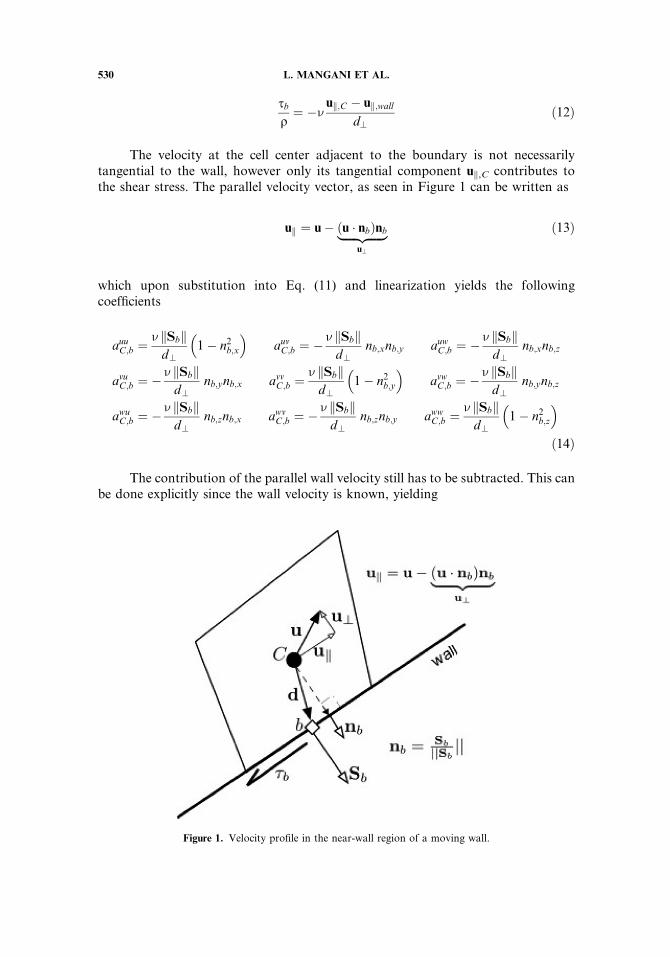
The velocity at the cell center adjacent to the boundary is not necessarilytangential to the wall, however only its tangential component uk,C contributes tothe shear stress. The parallel velocity vector, as seen in Figure 1 can be written as

uk ¼ u� ðu � nbÞnb|fflfflfflfflffl{zfflfflfflfflffl}u?

ð13Þ

which upon substitution into Eq. (11) and linearization yields the followingcoefficients

auuC;b ¼n kSbkd?

1� n2b;x

� �auvC;b ¼ � n kSbk

d?nb;xnb;y auwC;b ¼ � n kSbk

d?nb;xnb;z

avuC;b ¼ � n kSbkd?

nb;ynb;x avvC;b ¼n kSbkd?

1� n2b;y

� �avwC;b ¼ � n kSbk

d?nb;ynb;z

awuC;b ¼ � n kSbkd?

nb;znb;x awvC;b ¼ � n kSbkd?

nb;znb;y awwC;b ¼n kSbkd?

1� n2b;z

� �ð14Þ

The contribution of the parallel wall velocity still has to be subtracted. This canbe done explicitly since the wall velocity is known, yielding

Figure 1. Velocity profile in the near-wall region of a moving wall.


buC;b ¼n kSbkd?

uk;wall

bvC;b ¼n kSbkd?

vk;wall

bwC;b ¼n kSbkd?

wk;wall ð15Þ

3.3. Cyclic Boundary Conditions

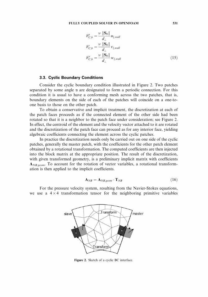
Consider the cyclic boundary condition illustrated in Figure 2. Two patchesseparated by some angle a are designated to form a periodic connection. For thiscondition it is usual to have a conforming mesh across the two patches, that is,boundary elements on the side of each of the patches will coincide on a one-to-one basis to those on the other patch.

To obtain a conservative and implicit treatment, the discretization at each ofthe patch faces proceeds as if the connected element of the other side had beenrotated so that it is a neighbor to the patch face under consideration; see Figure 2.In effect, the centroid of the element and the velocity vector attached to it are rotatedand the discretization of the patch face can proceed as for any interior face, yieldingalgebraic coefficients connecting the element across the cyclic patches.

In practice the discretization needs only be carried out on one side of the cyclicpatches, generally the master patch, with the coefficients for the other patch elementobtained by a rotational transformation. The computed coefficients are then injectedinto the block matrix at the appropriate position. The result of the discretization,with given transformed geometry, is a preliminary implicit matrix with coefficientsANB,geom. To account for the rotation of vector variables, a rotational transform-ation is then applied to the implicit coefficients.

ANB ¼ ANB;geom � TNB ð16Þ

For the pressure velocity system, resulting from the Navier-Stokes equations,we use a 4� 4 transformation tensor for the neighboring primitive variables

Figure 2. Sketch of a cyclic BC interface.


(u and p) that is based on the Rodriguez’ formula

TNB

¼

cðaÞþx2x½1�cðaÞ� xxxy½1�cðaÞ��xzsðaÞ xysðaÞþxxxz½1�cðaÞ� 0

xzsðaÞþxxxy½1�cðaÞ� cðaÞþx2y½1�cðaÞ� �xxsðaÞþxyxz½1�cðaÞ� 0

�xysðaÞþxxxz½1�cðaÞ� xxsðaÞþxyxz½1�cðaÞ� cðaÞþx2z ½1�cðaÞ� 0

0 0 0 1

266664

377775

ð17Þ

where x is the unit rotation vector and a is the rotation angle.

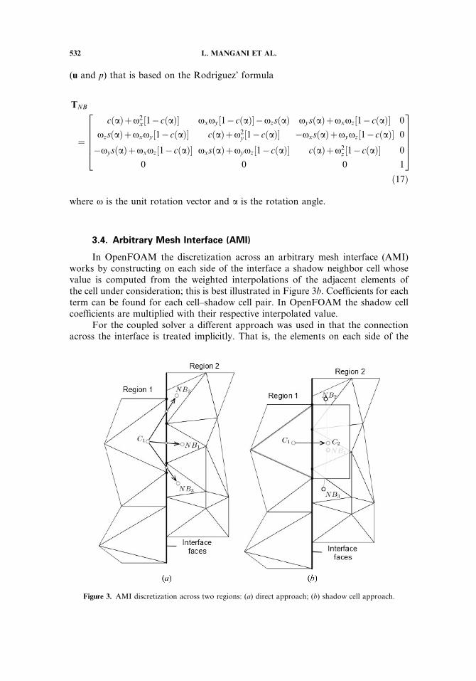
3.4. Arbitrary Mesh Interface (AMI)

In OpenFOAM the discretization across an arbitrary mesh interface (AMI)works by constructing on each side of the interface a shadow neighbor cell whosevalue is computed from the weighted interpolations of the adjacent elements ofthe cell under consideration; this is best illustrated in Figure 3b. Coefficients for eachterm can be found for each cell–shadow cell pair. In OpenFOAM the shadow cellcoefficients are multiplied with their respective interpolated value.

For the coupled solver a different approach was used in that the connectionacross the interface is treated implicitly. That is, the elements on each side of the

Figure 3. AMI discretization across two regions: (a) direct approach; (b) shadow cell approach.


interface are treated as directly connected through faces that are weightedsubsurfaces of their master surface, as seen in Figure 3a.

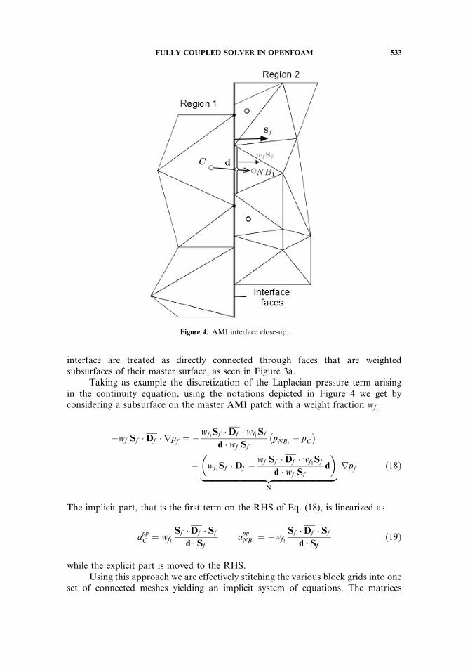
Taking as example the discretization of the Laplacian pressure term arisingin the continuity equation, using the notations depicted in Figure 4 we get byconsidering a subsurface on the master AMI patch with a weight fraction wf1

�wf1Sf �Df � rpf ¼ �wf1Sf �Df � wf1Sf

d � wf1SfpNB1

� pC� �

� wf1Sf �Df �wf1Sf �Df � wf1Sf

d � wf1Sfd

� |fflfflfflfflfflfflfflfflfflfflfflfflfflfflfflfflfflfflfflfflfflfflfflfflfflfflfflfflfflfflffl{zfflfflfflfflfflfflfflfflfflfflfflfflfflfflfflfflfflfflfflfflfflfflfflfflfflfflfflfflfflfflffl}

N

�rpf ð18Þ

The implicit part, that is the first term on the RHS of Eq. (18), is linearized as

appC ¼ wf1

Sf �Df � Sf

d � SfappNB1

¼ �wf1

Sf �Df � Sf

d � Sfð19Þ

while the explicit part is moved to the RHS.Using this approach we are effectively stitching the various block grids into one

set of connected meshes yielding an implicit system of equations. The matrices

Figure 4. AMI interface close-up.


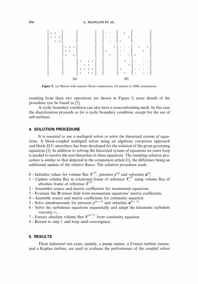
resulting from these two operations are shown in Figure 5; more details of theprocedure can be found in [7].

A cyclic boundary condition can also have a nonconforming mesh. In this casethe discretization proceeds as for a cyclic boundary condition, except for the use ofsub-surfaces.

4. SOLUTION PROCEDURE

It is essential to use a multigrid solver to solve the linearized system of equa-tions. A block-coupled multigrid solver using an algebraic correction approachand block-ILU smoothers has been developed for the solution of the given governingequations [1]. In addition to solving the linearized system of equations an outer loopis needed to resolve the non-linearities in these equations. The resulting solution pro-cedure is similar to that depicted in the companion article [1], the difference being anadditional update of the relative fluxes. The solution procedure reads

0 - Initialize values for volume flux _VVðnÞ, pressure p(n) and velocities u(n).

1 - Update volume flux in rotational frame of reference _VVðnÞr using volume flux of

absolute frame of reference _VVðnÞ.

2 - Assembles source and matrix coefficients for momentum equations.3 - Evaluate the D tensor field from momentum equations’ matrix coefficients.4 - Assemble source and matrix coefficients for continuity equation.5 - Solve simultaneously for pressure p(nþ 1) and velocities u(nþ 1).6 - Solve the turbulence equations sequentially and adapt the kinematic turbulent

viscosity nt.7 - Extract absolute volume flux _VV

ðnþ1Þfrom continuity equation.

8 - Return to step 1 and loop until convergence.

5. RESULTS

Three industrial test cases, namely, a pump runner, a Francis turbine runner,and a Kaplan turbine, are used to evaluate the performance of the coupled solver

Figure 5. (a) Matrix with interior block connections; (b) matrix in AMI connections.


under MFR conditions. A state-of-the-art OpenFOAM solver developed byCasartelli et al. [15] is used for comparison. For all tests, a k–x SST turbulencemodel is used and the simulation is considered converged when the normalizedroot-mean-square (RMS) residual for each field is smaller than 10�5. The evaluatedRMS is defined as

RMSð/Þ ¼

ffiffiffiffiffiffiffiffiffiffiffiffiffiffiffiffiffiffiffiffiffiffiffiffiffiffiffiffiffiffiffiffiffiffiffiffiffiffiffiffiffiffiffiffi1N

PNi¼0

res½/ðiÞ�=a//Cn o2

smaxð/; 0Þ �minð/; 0Þ ð20Þ

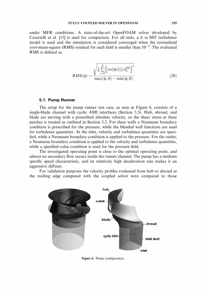
5.1. Pump Runner

The setup for the pump runner test case, as seen in Figure 6, consists of asingle-blade channel with cyclic AMI interfaces (Section 3.3). Hub, shroud, andblade are moving with a prescribed absolute velocity, so the shear stress at thesepatches is treated as outlined in Section 3.2. For these walls a Neumann boundarycondition is prescribed for the pressure, while the blended wall functions are usedfor turbulence quantities. At the inlet, velocity and turbulence quantities are speci-fied, while a Neumann boundary condition is applied to the pressure. For the outlet,a Neumann boundary condition is applied to the velocity and turbulence quantities,while a specified-value condition is used for the pressure field.

The investigated operating point is close to the optimal operating point, andalmost no secondary flow occurs inside the runner channel. The pump has a mediumspecific speed characteristic, and its relatively high deceleration rate makes it anaggressive diffuser.

For validation purposes the velocity profiles evaluated from hub to shroud atthe trailing edge computed with the coupled solver were compared to those

Figure 6. Pump configuration.


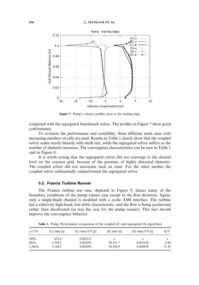
computed with the segregated benchmark solver. The profiles in Figure 7 show goodconformance.

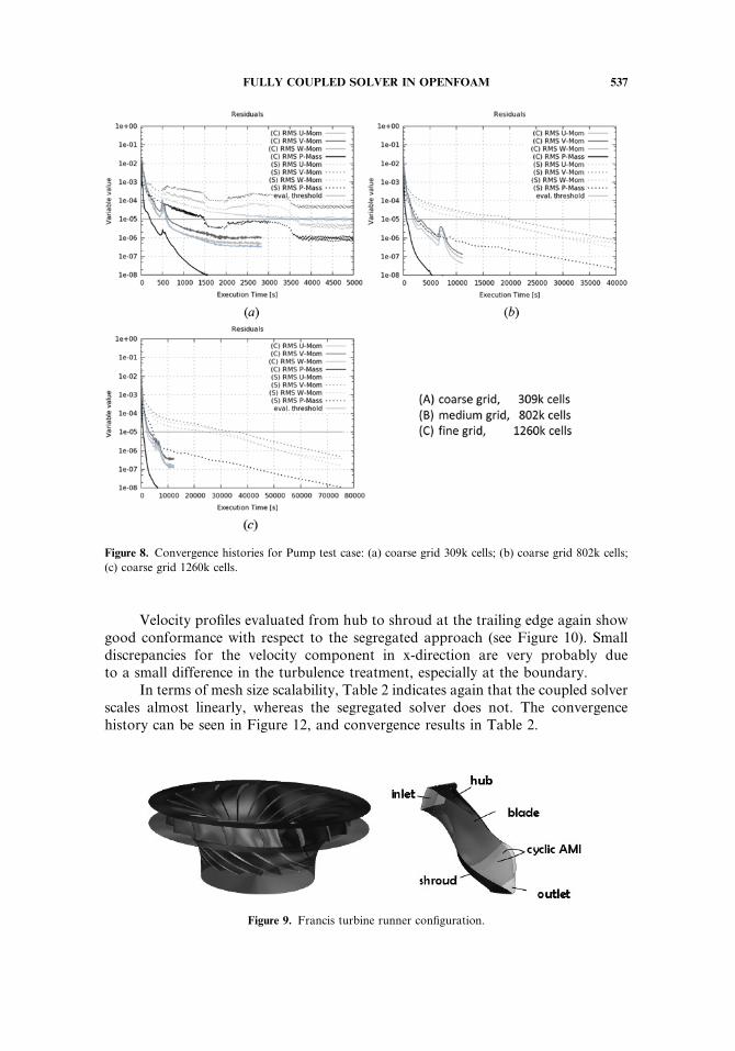
To evaluate the performance and scalability, three different mesh sizes withincreasing numbers of cells are used. Results in Table 1 clearly show that the coupledsolver scales nearly linearly with mesh size, while the segregated solver suffers as thenumber of elements increases. The convergence characteristics can be seen in Table 1and in Figure 8.

It is worth noting that the segregated solver did not converge to the desiredlevel on the coarsest grid, because of the presence of highly distorted elements.The coupled solver did not encounter such an issue. For the other meshes thecoupled solver substantially outperformed the segregated solver.

5.2. Francis Turbine Runner

The Francis turbine test case, depicted in Figure 9, shares many of theboundary conditions of the pump runner case except in the flow direction. Again,only a single-blade channel is modeled with a cyclic AMI interface. The turbinehas a relatively high-head, low-debit characteristic, and the flow is being acceleratedrather than decelerated (as was the case for the pump runner). This fact shouldimprove the convergence behavior.

Table 1. Pump: Performance comparison of the coupled (C) and segregated (S) algorithms

# CVs (C) time [s] (C) time=CV [s] (S) time [s] (S) time=CV [s] S=C

309 k 652.4 0.002111 x x x

802 k 2,399.2 0.002991 20,351.7 0.025250 8.48

1,260 k 3,144.5 0.002495 36,360.9 0.028858 11.56

Figure 7. Pump’s velocity profiles close to the trailing edge.


Velocity profiles evaluated from hub to shroud at the trailing edge again showgood conformance with respect to the segregated approach (see Figure 10). Smalldiscrepancies for the velocity component in x-direction are very probably dueto a small difference in the turbulence treatment, especially at the boundary.

In terms of mesh size scalability, Table 2 indicates again that the coupled solverscales almost linearly, whereas the segregated solver does not. The convergencehistory can be seen in Figure 12, and convergence results in Table 2.

Figure 9. Francis turbine runner configuration.

Figure 8. Convergence histories for Pump test case: (a) coarse grid 309k cells; (b) coarse grid 802k cells;

(c) coarse grid 1260k cells.


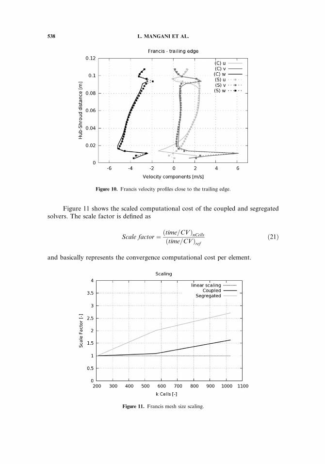
Figure 11 shows the scaled computational cost of the coupled and segregatedsolvers. The scale factor is defined as

Scale factor ¼ ðtime=CVÞnCellsðtime=CVÞref

ð21Þ

and basically represents the convergence computational cost per element.

Figure 11. Francis mesh size scaling.

Figure 10. Francis velocity profiles close to the trailing edge.


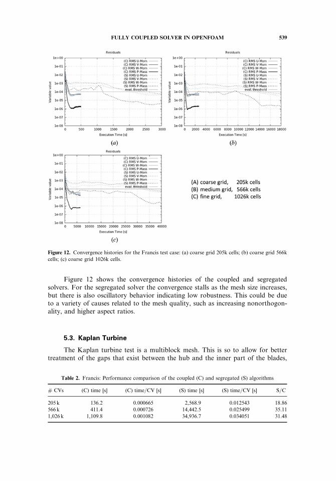
Figure 12 shows the convergence histories of the coupled and segregatedsolvers. For the segregated solver the convergence stalls as the mesh size increases,but there is also oscillatory behavior indicating low robustness. This could be dueto a variety of causes related to the mesh quality, such as increasing nonorthogon-ality, and higher aspect ratios.

5.3. Kaplan Turbine

The Kaplan turbine test is a multiblock mesh. This is so to allow for bettertreatment of the gaps that exist between the hub and the inner part of the blades,

Table 2. Francis: Performance comparison of the coupled (C) and segregated (S) algorithms


205 k 136.2 0.000665 2,568.9 0.012543 18.86

566 k 411.4 0.000726 14,442.5 0.025499 35.11

1,026 k 1,109.8 0.001082 34,936.7 0.034051 31.48

Figure 12. Convergence histories for the Francis test case: (a) coarse grid 205k cells; (b) coarse grid 566k

cells; (c) coarse grid 1026k cells.


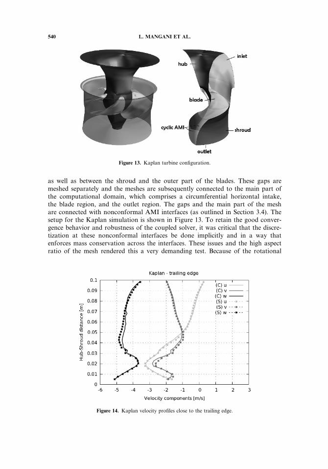
as well as between the shroud and the outer part of the blades. These gaps aremeshed separately and the meshes are subsequently connected to the main part ofthe computational domain, which comprises a circumferential horizontal intake,the blade region, and the outlet region. The gaps and the main part of the meshare connected with nonconformal AMI interfaces (as outlined in Section 3.4). Thesetup for the Kaplan simulation is shown in Figure 13. To retain the good conver-gence behavior and robustness of the coupled solver, it was critical that the discre-tization at these nonconformal interfaces be done implicitly and in a way thatenforces mass conservation across the interfaces. These issues and the high aspectratio of the mesh rendered this a very demanding test. Because of the rotational

Figure 13. Kaplan turbine configuration.

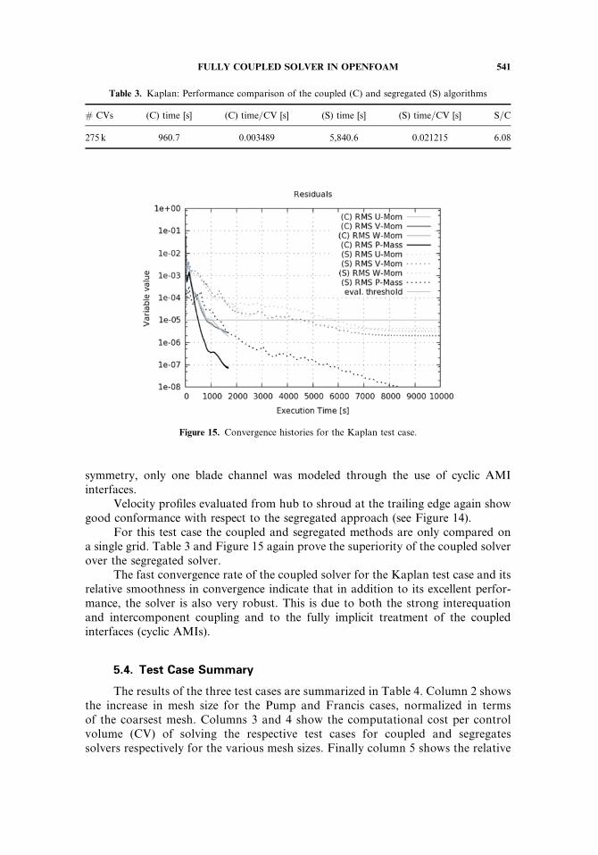
Figure 14. Kaplan velocity profiles close to the trailing edge.


symmetry, only one blade channel was modeled through the use of cyclic AMIinterfaces.

Velocity profiles evaluated from hub to shroud at the trailing edge again showgood conformance with respect to the segregated approach (see Figure 14).

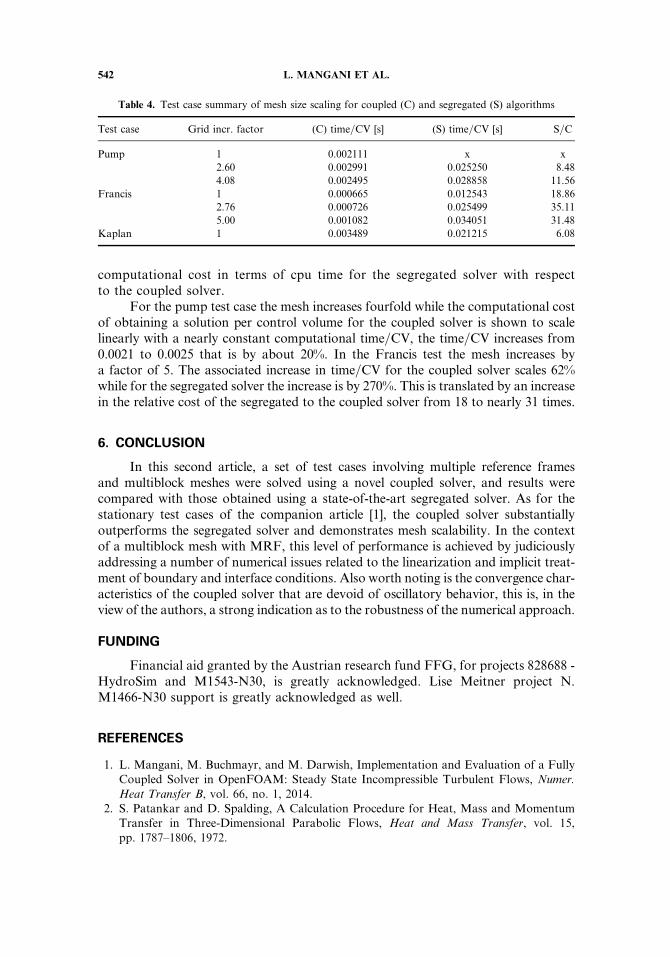
For this test case the coupled and segregated methods are only compared ona single grid. Table 3 and Figure 15 again prove the superiority of the coupled solverover the segregated solver.

The fast convergence rate of the coupled solver for the Kaplan test case and itsrelative smoothness in convergence indicate that in addition to its excellent perfor-mance, the solver is also very robust. This is due to both the strong interequationand intercomponent coupling and to the fully implicit treatment of the coupledinterfaces (cyclic AMIs).

5.4. Test Case Summary

The results of the three test cases are summarized in Table 4. Column 2 showsthe increase in mesh size for the Pump and Francis cases, normalized in termsof the coarsest mesh. Columns 3 and 4 show the computational cost per controlvolume (CV) of solving the respective test cases for coupled and segregatessolvers respectively for the various mesh sizes. Finally column 5 shows the relative

Table 3. Kaplan: Performance comparison of the coupled (C) and segregated (S) algorithms


275 k 960.7 0.003489 5,840.6 0.021215 6.08

Figure 15. Convergence histories for the Kaplan test case.


computational cost in terms of cpu time for the segregated solver with respectto the coupled solver.

For the pump test case the mesh increases fourfold while the computational costof obtaining a solution per control volume for the coupled solver is shown to scalelinearly with a nearly constant computational time=CV, the time=CV increases from0.0021 to 0.0025 that is by about 20%. In the Francis test the mesh increases bya factor of 5. The associated increase in time=CV for the coupled solver scales 62%while for the segregated solver the increase is by 270%. This is translated by an increasein the relative cost of the segregated to the coupled solver from 18 to nearly 31 times.

6. CONCLUSION

In this second article, a set of test cases involving multiple reference framesand multiblock meshes were solved using a novel coupled solver, and results werecompared with those obtained using a state-of-the-art segregated solver. As for thestationary test cases of the companion article [1], the coupled solver substantiallyoutperforms the segregated solver and demonstrates mesh scalability. In the contextof a multiblock mesh with MRF, this level of performance is achieved by judiciouslyaddressing a number of numerical issues related to the linearization and implicit treat-ment of boundary and interface conditions. Also worth noting is the convergence char-acteristics of the coupled solver that are devoid of oscillatory behavior, this is, in theview of the authors, a strong indication as to the robustness of the numerical approach.

FUNDING

Financial aid granted by the Austrian research fund FFG, for projects 828688 -HydroSim and M1543-N30, is greatly acknowledged. Lise Meitner project N.M1466-N30 support is greatly acknowledged as well.

REFERENCES

1. L. Mangani, M. Buchmayr, and M. Darwish, Implementation and Evaluation of a FullyCoupled Solver in OpenFOAM: Steady State Incompressible Turbulent Flows, Numer.Heat Transfer B, vol. 66, no. 1, 2014.

2. S. Patankar and D. Spalding, A Calculation Procedure for Heat, Mass and MomentumTransfer in Three-Dimensional Parabolic Flows, Heat and Mass Transfer, vol. 15,

pp. 1787–1806, 1972.

Table 4. Test case summary of mesh size scaling for coupled (C) and segregated (S) algorithms

Test case Grid incr. factor (C) time=CV [s] (S) time=CV [s] S=C

Pump 1 0.002111 x x

2.60 0.002991 0.025250 8.48

4.08 0.002495 0.028858 11.56

Francis 1 0.000665 0.012543 18.86

2.76 0.000726 0.025499 35.11

5.00 0.001082 0.034051 31.48

Kaplan 1 0.003489 0.021215 6.08


3. Y. G. Laia, An Unstructured Grid Method for a Pressure-Based Flow and Heat TransferSolver, Numer. Heat Transfer B, vol. 32, no. 3, pp. 267–281, 1997.

4. P. L. Woodfield, K. Suzuki, and K. Nakabe, Performance of a Three-Dimensional,Pressure-Based, Unstructured Finite-Volume Method for Low-Reynolds-NumberIncompressible Flow and Wall Heat Transfer Rate Prediction, Numer. Heat Transfer B,vol. 43, no. 5, pp. 403–423, 2003.

5. C. Vradis and K. J. Hammad, Strongly Coupled Block-Implicit Solution Technique forNon-Newtonian Convective Heat Transfer Problems, Numer. Heat Transfer B, vol. 33,no. 1, pp. 79–97, 1998.

6. M. J. S. de Lemos, Flow and Heat Transfer in Rectangular Enclosures Using a NewBlock-Implicit Numerical Method, Numer. Heat Transfer B, vol. 37, no. 4, pp. 489–508,2000.

7. M. Darwish, W. Geahchan, and F. Moukalled, Fully Implicit Coupling forNon-Matching Grids, Int. Conf. of Numerical Analysis and Applied Mathematics(ICNAAM 2010), Rhodos, Greece, pp. 47–50, 2010.

8. F. Menter, M. Kuntz, and R. Langtry, Ten Years of Industrial Experience with the SSTTurbulence Model, in K. Hanjalic et al. (eds.), Turbulance Heat and Mass Transfer 4,Begell House, Inc., 2003.

9. W. Hauger, W. Schnell, and D. Gross, Technische Mechanik 3, Springer-Verlag,Berlin, 2002.

10. C. Hirsch, Numerical Computation of Internal and External Flows, John Wiley, New York,

1991.11. A. Hellsten, Some Improvements in Menter’s K-Omega SST Turbulence Model, AIAA

Paper 98–2554, 1998.12. P. E. Smirnov and F. R. Menter, Sensitization of the SST Turbulence Model

to Rotation and Curvature by Applying the Spalart-Shur Correction Term, ASME J.Of Turbomachinery, vol. 131, 2009.

13. M. Darwish and F. Moukalled, A Review of Boundary Conditions and TheirImplementations in CFD Codes, Technical Report, 2000.

14. M. Darwish, W. Geahchan, and F. Moukalled, Fully Implicit Coupling for Non-Matching Grids, Numer. Heat Transfer, ICNAAM 2010, Crete, Greece, 2010.

15. E. Casartelli, L. Mangani, and S. Hug, Numerical Comparison Between Model andPrototype Flow in a Pump-Turbine Distributor, Int. Conf. and Exhibition InnovativeApproaches To Global Challenges, Bilbao, Spain, 2012.


Documents

DEVELOPMENT OF A NOVEL FULLY COUPLED SOLVER IN … · DEVELOPMENT OF A NOVEL FULLY COUPLED SOLVER IN OPENFOAM: STEADY-STATE INCOMPRESSIBLE TURBULENT FLOWS IN ROTATIONAL REFERENCE