1

International Journal of Computers In Industry, Vol 54, No 1, pp. 69-81, 2004.

Development of a novel 3D simulation modelling system for distributed

manufacturing

S. F. Qin

*, R. Harrison

**, A.A. West

**, D. K. Wright

Department of Design, Brunel University, Runnymede Campus, Surrey, TW20 0JZ, UK

**MSI Research Institute, Department of Mechanical & Manufacturing Engineering,

Loughborough University, Loughborough, LE11 3TU, UK

Abstract

This paper describes a novel 3D simulation modelling system for supporting our distributed

machine design and control paradigm with respect to simulating and emulating machine

behaviour on the Internet. The system has been designed and implemented using Java2D and

Java3D. An easy assembly concept of drag-and-drop assembly has been realised and implemented

by the introduction of new connection features (unified interface assembly features) between two

assembly components (modules). The system comprises a hierarchical geometric modeller, a

behavioural editor, and two assemblers. During modelling, designers can combine basic

modelling primitives with general extrusions and integrate CAD geometric models into simulation

models. Each simulation component (module) model can be visualised and animated in VRML browsers.

It is reusable. This makes machine design re-configurable and flexible. A case study example is given to

support our conclusions.

Keywords: simulation modelling, VRML modelling, connection features, virtual

manufacturing.

1 Introduction

Manufacturing enterprises face a number of overarching challenges: lowering the cost of

production, reducing lead-to-market time, and finding the means to incorporate a set of globally

* Corresponding author. Tel:+44-1784-431341; fax:+44-1784-439515. E-mail address: sheng.feng.qin@brunel.ac.uk

(S. Qin).

2

distributed partners within a distributed manufacturing environment. It has shown how these

challenges would be met effectively through the use of a more modular and reusable approach

[1,2,3] in machine design, testing, and implementation, and the use of a Web-based information

system [4,5,6]. Ideally, each module of a machine design should be rapidly verified with errors

and misconceptions identified as early as possible and a whole machine as an assembly of various

modules should then be analysed and tested virtually before being physically implemented.

Although various CAD/CAM systems are now widely used, properly integrated approaches to

machine design and control are still in their infancy and have not yet been established in industry

[7]. It is believed that integrated 3D geometric simulation and emulation techniques can be

applied to the optimisation of machine design and control logic testing. Although machine

designers and control system implementers are making use of isolated simulations [8] for the

optimisation of machine design, e.g., motion simulation, and for control logic testing, e.g.,

discrete event simulation, such isolated simulations could not support consistent modular and

reusable machine design. Recent studies [9,10] indicate that a visualisation and simulation system

might have the Internet as its backbone and Web technologies such as Java, HTML, VRML,

TCP/IP and Agents could be applied as its communication infrastructure, because a Web-based

system has a universal interface, uses open standards, and is globally supported.

This paper focuses on the development of a novel 3D simulation-modelling system for

supporting distributed modular manufacturing. It allows a machine control system to be

decomposed into a set of distributed components associated with different machine modules. It

makes the control logic an integral part of module design and machine design and allows the

remote visualisation of machine (or module) behaviour over the Internet by geographically

distributed engineering partners. Such remote visualisation is firmly supported by modular

simulation models developed within this system.

3

In this system, we classify simulation models into two categories: module simulation

models and machine simulation models. In order to create these two types of simulation models

simply and easily, new concepts of drag-and-drop assembling and connection features (unified

interface assembly features) are introduced in the system to develop two modelling tools, namely

module creator and module assembler. With these tools, designers can rapidly create module

simulation models integrated with control logic and interface assembly features. They can simply

assemble these models in a drag-and-drop manner.

Following this introduction, related work is briefly reviewed in Section 2. The prototype

system structure and design are given in Section 3 and 4. A case study example is discussed in

Section 5, and finally conclusions are drawn.

2 Related work

In our distributed applications, any complete machine is defined in a hierarchy in terms of

systems, sub-systems and modules. Each system consists of one or more sub-systems that are

each in turn made up of modules. The modules represent physical sub-assemblies of the machine

containing one or more elementary parts associated with motions and control logic and have

VRML simulation representations. Correspondingly, machine models are hierarchically made up

of module models. In this paper, we use a module or a module model to mean the same virtual

representation (model) of physical module.

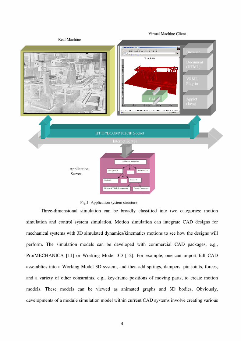
Our distributed application system uses the Internet as its backbone and Web technologies

such as HTML, VRML, and TCP/IP as its communication infrastructure structure (Fig. 1). A

machine and its control system design developed in the process definition environment (PDE) [7]

are located in the application server. Through a Web server, they can drive the real machine in the

workshop and the corresponding virtual machine (a VRML simulation model) in its client

windows. Design and development of a rapid 3D simulation modelling system is the focus of this

paper.

4

Three-dimensional simulation can be broadly classified into two categories: motion

simulation and control system simulation. Motion simulation can integrate CAD designs for

mechanical systems with 3D simulated dynamics/kinematics motions to see how the designs will

perform. The simulation models can be developed with commercial CAD packages, e.g.,

Pro/MECHANICA [11] or Working Model 3D [12]. For example, one can import full CAD

assemblies into a Working Model 3D system, and then add springs, dampers, pin-joints, forces,

and a variety of other constraints, e.g., key-frame positions of moving parts, to create motion

models. These models can be viewed as animated graphs and 3D bodies. Obviously,

developments of a module simulation model within current CAD systems involve creating various

A Machine Application

Sub-System 1 Sub-System N

Module1 Module N

…

Control Components Physical & VRML Representation

HTTP/DCOM/TCP/IP Socket

Browser

Document

(HTML)

VRML

Plug-in

Applet

(Java) EAI

Internet Server

Real Machine

Virtual Machine Client

Application

Server

Fig.1 Application system structure

5

CAD parts based on design features, creating CAD assemblies based on low-level assembly

constraints such as mate and align, and creating motion specifications based on the assemblies. It

is a time-consuming process and simulation models have no relations with control logic.

For control system simulation, the Virtual Workbench system described by Weyrich and

Drews in [13] used the professional modelling tool, Multigen II, for pre-processing of CAD data

and creating VRML-based simulation models by producing object hierarchies and levels of detail,

processing geometric objects and adding colour, material and texture to the objects.

Unfortunately, this system required an intensive manual pre-processing procedure. The use of

VRML-based simulations for virtual manufacturing applications has become increasingly

important. In order to build up VRML-based simulation models, CAD models in [14] from

various CAD packages were first translated into the International Graphics Exchange Standard

(IGES) form, and then translated to VRML files. Finally, a VRML editor was used for making an

assembly for animations. However, it was found that development of the VRML model in that

way required formidable effort and time, for example, if a part was modified in the CAD

packages, the engineers had to export the CAD models to VRML files again for re-assembly.

Actually, when a CAD model for a part or an assembly is exported to a VRML file, primitive

objects in the model will follow a flat hierarchical order. The objects will also be described in a

set of polygonal facets in a global co-ordinate system. Therefore, the various primitive objects

become inaccessible individually and the final VRML file may become too big to be suitable for

distributed applications. It seems clear that using and converting CAD data into simulation

models is a time-consuming procedure. Some efforts [15] were made to develop Web3D creation

tools, such as AC3D and mjbWorld, in order to easily create VRML-based [16] 3D visualization

models. But, they did not facilitate the assembly of modules.

3. Hierarchy of the simulation models

6

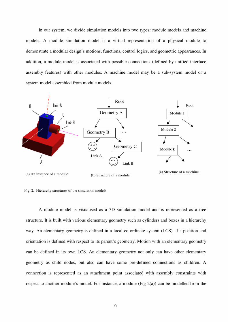
In our system, we divide simulation models into two types: module models and machine

models. A module simulation model is a virtual representation of a physical module to

demonstrate a modular design’s motions, functions, control logics, and geometric appearances. In

addition, a module model is associated with possible connections (defined by unified interface

assembly features) with other modules. A machine model may be a sub-system model or a

system model assembled from module models.

A module model is visualised as a 3D simulation model and is represented as a tree

structure. It is built with various elementary geometry such as cylinders and boxes in a hierarchy

way. An elementary geometry is defined in a local co-ordinate system (LCS). Its position and

orientation is defined with respect to its parent’s geometry. Motion with an elementary geometry

can be defined in its own LCS. An elementary geometry not only can have other elementary

geometry as child nodes, but also can have some pre-defined connections as children. A

connection is represented as an attachment point associated with assembly constraints with

respect to another module’s model. For instance, a module (Fig 2(a)) can be modelled from the

Fig. 2. Hierarchy structures of the simulation models

Module 1

Module 2

Module k

Root

…

(a) An instance of a module

(b) Structure of a module

(a) Structure of a machine

Geometry A

Geometry C

Geometry B …

Root

Link B

Link A

7

Base geometry A. The Base has a child of the geometry B (Slide), which can move on the top

face of the Base. The Slide has a child of the geometry C (Shaft), which can rotate about its axis.

The Slide also has a connection “Link A” at the centre of the top face, which links to a module

“A”. The Shaft has a connection “Link B” as well, which links to a module “B”. Connections are

geometrically represented as small spheres. The corresponding hierarchy structure is shown in

Fig. 2 (b).

A machine models can be defined by assembling module models in a hierarchical tree

structure (Fig. 2 (c)). A child module model can be assembled in a drag-and-drop manner. The

system will automatically match connections between the child module model and its parent

module model, and compute the assembly position of the child module with respect to its

connected geometry in the parent module. Comparing with traditional CAD assembly featuring

low-level constraints such as mate and align, this assembling process is simple.

4. The system design and implementation

The prototype system is a Java application. With it designers can rapidly create module

simulation models and assemble them into machine simulation models. The models can be

viewed as wireframe models in a Java2D window [17] and viewed as 3D rendering models in

a Java3D window [18]. The animated models can be checked in an embedded VRML

browser. In our modelling system, both VRML and Java3D were used to represent simulation

models. VRML formatted models are employed for the Web-based visualisations through a

suitable VRML Plug-in, e.g., Cosmo Player. The VRML models can be embedded into a

HTML file. The logic engine on the Web server can drive the simulation model remotely by

Java Script nodes in the HTML page through the VRML EAI interface mechanism (Fig. 1).

Java3D–based native simulation models are used for building up simulation databases,

because they are easy to maintenance and their sizes are small. Internally, both models are

derived from the same structure.

8

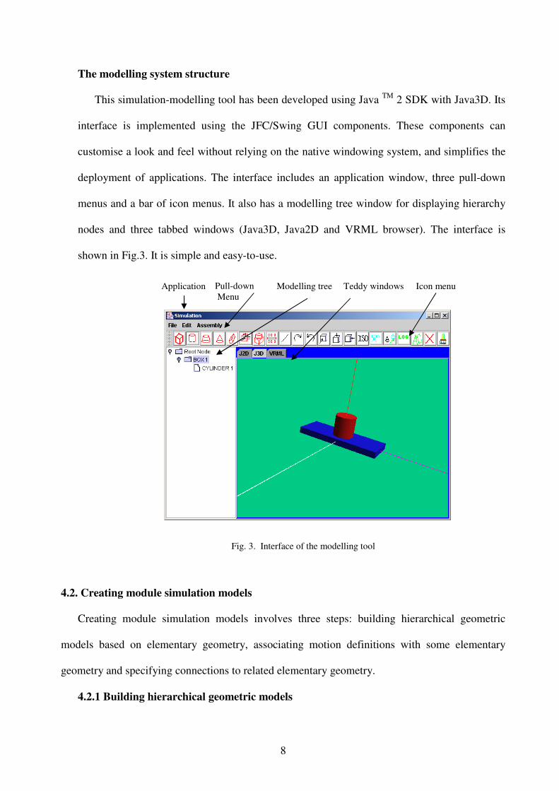
The modelling system structure

This simulation-modelling tool has been developed using Java TM

2 SDK with Java3D. Its

interface is implemented using the JFC/Swing GUI components. These components can

customise a look and feel without relying on the native windowing system, and simplifies the

deployment of applications. The interface includes an application window, three pull-down

menus and a bar of icon menus. It also has a modelling tree window for displaying hierarchy

nodes and three tabbed windows (Java3D, Java2D and VRML browser). The interface is

shown in Fig.3. It is simple and easy-to-use.

4.2. Creating module simulation models

Creating module simulation models involves three steps: building hierarchical geometric

models based on elementary geometry, associating motion definitions with some elementary

geometry and specifying connections to related elementary geometry.

4.2.1 Building hierarchical geometric models

Icon menu

Application Pull-down

Menu

Modelling tree Teddy windows

Fig. 3. Interface of the modelling tool

9

The hierarchical geometric modelling includes three steps. Elementary primitives are first

defined in their local co-ordinate systems. They are then positioned by specifying geometric

constraints with their parent geometry. Finally, they can be translated into desired positions by

shipping in their parent co-ordinate systems.

Local co-ordinate systems are defined to be consistent with VRML primitive definitions,

since our final simulation models are represented in the VRML format. This makes it easier to

transfer internal model definitions to a VRML file. The primitive definitions in their local co-

ordinate systems are shown in Fig. 4. The origins are in the centres of primitives. Primitives:

cones and truncated cones are defined in a similar way. Based on a local co-ordinate system,

an imaginary bounding box can be attached to each primitive. Its six faces are used as

constraint planes. The faces perpendicular to X-axis are called the right (on the right hand

side) and the left (on the left hand side) faces. In a similar way, the faces perpendicular to Y-

axis are called the top and the bottom faces. The faces associated with Z axis are named as the

front and the back faces.

In order to create module geometry, designers can interactively specify the sizes of the

primitive and position it. As an example, a box feature can be specified with sizes along three

dimensions in terms of length, depth and height. For the first geometry, it is located at the origin

of the default module co-ordinate system. Meanwhile, in the modelling tree window, the system

Y Y

Z Z

X X

Fig. 4. Primitive definition

10

will set up a “Root Node” as the root of the modelling tree and link the first geometry as its first

child node. In Fig 3, the first geometry (box) is linked to its parent (the root). After receiving the

first geometry, the designers need to select a parent node and then create its child node. Once a

parent node has been selected, the following nodes will become its children until a new parent

node is chosen. For a child primitive, if it is not directly linked to the root node, the designers can

input its sizes and specify a constraint by indicating its position relationships with its parent

bounding box in terms of attaching on the right or left faces, on the top or under the bottom, and

on the front and back faces. From this constraint, the system can determine transformation

parameters and attach the child geometry onto the centre of a specified face. For example, a

cylinder (Fig. 3) is attached on the top face of the box and located in the centre. The system uses

the centre of a constraint face as a default position, because the majority of assembly constraints

have central alignment relationships. Of course, child geometry can be edited into any position in

its parent co-ordinate system. To do so, a child node needs to be first selected and then the system

will display its parent co-ordinate system using three axis lines as in Fig. 3. With references to the

parent co-ordinate system, transformation parameters can be easily specified. Finally, the system

will update models. In this way, designers can easily build up a module model with desired

structures and geometry. Models can be displayed in the Java3D window with interactive

visualisation controls of dollying, tracking and tumbling. Using Java3D, these controls are much

easier to implement. The models can also be viewed as surface models in the Java2D graphics

window.

4.2.2 Defining motions

Based on a geometric model and its hierarchical tree, designers can interactively define

motions associated with the corresponding elementary geometry (parts). The motions can be

divided into general motions and state motions. The general motions can be described by position

translations or rotations. They are driven by actuators, e.g. motors. The state motions can be

11

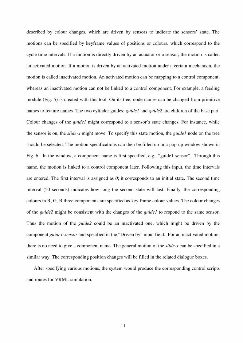
described by colour changes, which are driven by sensors to indicate the sensors’ state. The

motions can be specified by keyframe values of positions or colours, which correspond to the

cycle time intervals. If a motion is directly driven by an actuator or a sensor, the motion is called

an activated motion. If a motion is driven by an activated motion under a certain mechanism, the

motion is called inactivated motion. An activated motion can be mapping to a control component,

whereas an inactivated motion can not be linked to a control component. For example, a feeding

module (Fig. 5) is created with this tool. On its tree, node names can be changed from primitive

names to feature names. The two cylinder guides: guide1 and guide2 are children of the base part.

Colour changes of the guide1 might correspond to a sensor’s state changes. For instance, while

the sensor is on, the slide-x might move. To specify this state motion, the guide1 node on the tree

should be selected. The motion specifications can then be filled up in a pop-up window shown in

Fig. 6. In the window, a component name is first specified, e.g., “guide1-sensor”. Through this

name, the motion is linked to a control component later. Following this input, the time intervals

are entered. The first interval is assigned as 0; it corresponds to an initial state. The second time

interval (50 seconds) indicates how long the second state will last. Finally, the corresponding

colours in R, G, B three components are specified as key frame colour values. The colour changes

of the guide2 might be consistent with the changes of the guide1 to respond to the same sensor.

Thus the motion of the guide2 could be an inactivated one, which might be driven by the

component guide1-sensor and specified in the “Driven by” input field. For an inactivated motion,

there is no need to give a component name. The general motion of the slide-x can be specified in a

similar way. The corresponding position changes will be filled in the related dialogue boxes.

After specifying various motions, the system would produce the corresponding control scripts

and routes for VRML simulation.

12

Fig 6. Motion specifications

Fig.5. Motion definition

Guide1

Cutter-

base

Slide-Z

Base

Slide-X

Guide2

13

4.2.3 Specifying connections

Within a distributed manufacturing environment, module suppliers are likely to be

globally distributed. In a most possible scenario, a module manufacturer would provide

connection (assembly) information to his relevant manufacturing partners. Therefore,

assembly relations between modules, such as mating conditions, should be negotiated prior to

design and manufacturing a module. The assembly relationships can be pre-described as a

unified interface assembly feature (connection) associated with elementary geometry in

modules. Creating an assembly model (machine model) can be done automatically by

mapping the unified interface assembly features, rather than by interactively specifying

geometric constraints as in any commercial CAD systems. This would allow non-CAD users

to model a machine in a higher level. The use of the connection features provides designers

with a new paradigm for rapidly creating sub-systems or machines in a ‘drag-and-drop’

manner.

A connection (unified interface assembly feature) in this system is defined as a relatively

small sphere on a face of its elementary geometry. In order to define a connection, an

(a) Connect definition

Fig. 7 Connection and its constraints

(b) Implicit constraints

Om

Xm Lp

Op

Vp Np

Rp Xp

Yp

Zp

Ym

Zm

14

elementary geometry node is first selected, such as “cutter-base” in Fig.6. And then a

definition window can be activated (see Fig. 7(a)). In the window, designers can specify the

connection’s name, e.g., “cutter”, its locations (on the different attachment faces: the top, the

right, etc) and its relative positions to the centre of the attachment face. This information

provides the following assembly constraint information: positions, orientations and mating

planes. Positions can be described as the vector Lp in the local primitive co-ordinate system

(LCS) Op-Xp-Yp-Zp (Fig. 7(b)). The normal (Np) of the contacting face will serve as

orientations. Based on the normal vector Np and a unit vector Vp parallel to the Yp, a reference

vector Rp can be obtained by finding the cross product of vectors Np and Vp. Then a reference

plane is defined by the vector Np and Rp. Another orientation parameter can then be defined

by specifying a rotation angle β of the reference plane about the normal vector Np. If the

vector Np is parallel to the vector Vp, the vector Rp will then be assigned as a unit vector

parallel to the Zp axis. In this way, three assembly constraints are specified implicitly by

mating positions, mating attachment faces and mating reference planes. The local definitions:

Lp, Np and Rp can be transferred into the corresponding module’s co-ordinate system (MCS)

Om-Xm-Ym-Zm. As a result, the corresponding definitions: Lm, Nm, and Rm can be obtained. The

connection feature is displayed as a small sphere on the specified attachment face.

After specifying a module’s hierarchical geometry, motions, and connection features, the

final module definition can be displayed in the Java3D window (Fig. 8 (a)) and saved as the

native format in Java3D and as VRML format. The module can be checked over the Internet

as shown in Fig 8(b) or tested in the embedded VRML viewer window. If any thing is wrong,

modifications can be made easily.

15

4.3 Defining a sub-system or a machine

Defining a sub-system or a machine can be achieved by assembling modules or sub-systems.

A sub-system or a machine is a hierarchical assembly of modules or sub-systems. It has

differences from flatted CAD assemblies [19]. An assembly in CAD systems is based on

assembly constraints defined in global co-ordinate systems. Thus, assembly sequences are

commutable. In hierarchical assembly, every module is a hierarchical assembly of elementary

geometry. While assembling, the first module is aligned with the assembly default co-ordinate

system; another module may be loaded afterwards. The system will then search for relevant

connections by matching their names and solve the corresponding implicit assembly constraints

between a connection defined under its LCS in the current assembly and one defined in the MCS

associated with the next-module. The transformations will be automatically computed and the

next module will be treated as a child of the corresponding elementary geometry in its parent

module. In other word, hierarchical assembly is based on the transformation between a local co-

Fig. 8 Module Display

(a) Interface geometry (b) VRML module checking

16

ordinate system (LCS) and a global co-ordinate system (MCS). This is the reason for that a

connection must be defined in both its MCS and LCS. Assembly sequences are incommutable.

In this system, there are two ways of conducting assembly. One is based on modelling trees

(Fig. 2c). The system will automatically search a tree, match connections between a parent

module and a child module and assemble them hierarchically as shown the above. The other is

direct assembly based on modules defined in their VRML files. The next section will give more

details.

4.4 The VRML-based assembly

In a distributed engineering environment, modules in VRML files can support new

applications like design repository [20]. A module can be visualised and simulated over the

Internet. With this assembly tool, modules can also be easily assembled together into a sub-system

or a machine. Designers can assemble modules in a “drag-and-drop” way, avoiding to selecting

various low-level geometric elements, e.g., faces and edges, to specify assembly constraints as in

most commercial CAD systems.

In order to assembly VRML modules easily, we first analysed the VRML file structure and

developed an extended VRML format for containing our connections (unified interface assembly

features).

The extended VRML format contains an connection geometry description and its

constraints information group. The connection geometry (a sphere) description is defined as a

child node of its parent node in a VRML file. The constraint information group is represented as

a commentary group of VRML comment lines as shown below. It starts with the line “#Interface-

assembly-info” and ended with the line “#Interface-assembly-info-end”. In the body of this

group, each connection assembly feature is described in a sub-group of three lines. The first line

indicates the feature’s name. The second line contains assembly information in terms of local

positions (Lp,x , Lp,y and Lp,z) , normal directions (Np,x , Np,y and Np,z) , and relative rotation β about

17

the local normal; and the global positions and normal directions. The third line ends this sub-

group. If a module has more connection features, there will be more group information in the

body.

The connection geometry description is represented as a VRML transform node. An example is

shown below. It defines a sphere shape on the specified contacting face. The description starts

with the feature’s name. The translation and rotation nodes specify the positions of the sphere.

The internal rotation node is used for holding information about relative rotation about the local

normal. The shape node can be substituted by a module.

When assembling two modules in VRML files, the first file will be parsed to find the local

assembly information from commentary groups for connections. The second file will also be

parsed to find the global assembly information for connections. The system will then match two

connections and compute transformations. Afterwards, the system will create a sub-system file by

loading the first file in and changing the parameters in translation and rotation nodes within the

#Link_test

Transform {

translation 50.0 0.0 0.0

rotation 0 0 1 0

children [

Transform {

rotation 1.0 0.0 0.0 0.0

children [

Shape {

appearance Appearance {... }

geometry Sphere { 2 }

}

]

}

]

}

#Interface-assembly-info

#Linkpoint Name

#Linkpoint_info Lp,x Lp,y Lp,z Np,x Np,y Np,z β Global Lx Ly Lz Nx Ny Nz

#Endlinkpoint

#…

#Interface-assembly-info-end

18

matched connection geometry based on the corresponding assembly transformations and inserting

related contents from the second file into the shape node. Meanwhile, the global assembly

information from the second file will be modified under the sub-system co-ordinate system. In

this way, two sub-systems or modules can be assembled together easily.

4.5 Creating general extrusions

The use of various primitives may have some limitations on creating more complex geometric

models. In order to make geometric simulations to have more real appearances, the system

provides a tool to create general extrusions.

A general extrusion can be defined by a 2D cross section travelling along a 3D path. In the

VRML 2.0, a cross section of an extrusion is described in the X-Z co-ordinate plane. In order to

keep consistent with the VRML 2.0 and simplify definitions of extrusions, a general extrusion in

this system is defined by a 2D cross section in the X-Z plane and a 2D path in the X-Y plane. 2D

cross sections and paths can be either described interactively by entering a sequence of line

segments and arcs or inputting from DXF exchange files from commercial CAD packages.

Internally, cross sections and paths are represented as successive straight-line segments. After

obtaining a 2D cross section, e.g., one in Fig 9 (a) and a 2D path, e.g., one in Fig 9 (b), the

corresponding extrusion can be obtained and displayed in the java2D window (Fig 9 (c)) and in

the Java3D window (Fig 9 (d)). In the java2D window, designers can interactively specify

connections on selected facets. The extrusion can then be outputted as a special module and can

be assembled with another module or sub-system.

19

4.6 Integrating with CAD models

Apart from the creation of general extrusions, this system can integrate CAD models into its

modelling. Various CAD packages can be used for modelling a variety of complex parts and

output models into VRML files. Based on the CAD models, it is easy to find out information

about connection features in terms of positions and orientations. Afterwards, the VRML files of

the parts can be interactively edited to add connection features and then saved as special modules

like general extrusions. In this way, it is easy to include more complex parts’ models into

Fig. 9 General extrusions

(a) Cross section (b) Extrusion path section

(c) Surface model (d) Shaded model

20

simulation modelling. Integration of CAD packages can support different levels of details (LODs)

in the simulation models.

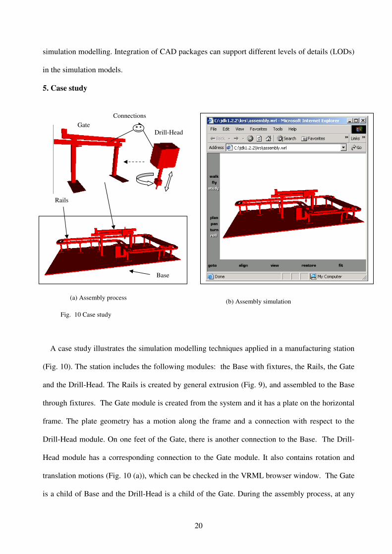
5. Case study

A case study illustrates the simulation modelling techniques applied in a manufacturing station

(Fig. 10). The station includes the following modules: the Base with fixtures, the Rails, the Gate

and the Drill-Head. The Rails is created by general extrusion (Fig. 9), and assembled to the Base

through fixtures. The Gate module is created from the system and it has a plate on the horizontal

frame. The plate geometry has a motion along the frame and a connection with respect to the

Drill-Head module. On one feet of the Gate, there is another connection to the Base. The Drill-

Head module has a corresponding connection to the Gate module. It also contains rotation and

translation motions (Fig. 10 (a)), which can be checked in the VRML browser window. The Gate

is a child of Base and the Drill-Head is a child of the Gate. During the assembly process, at any

Fig. 10 Case study

(b) Assembly simulation (a) Assembly process

Rails

Base

Connections

Gate Drill-Head

21

point, sub-systems can be tested. After finishing the assembly, the machine can be animated as

shown in Fig. 10 (b) to check its functions and design. Finally, the machine simulation model can

linked to a real distributed manufacturing system via the VRML EAI interface to emulate the

system as shown in Fig. 1.

6. Conclusion

The new 3D simulation modelling approach can support our distributed machine design and

control paradigm with respect to simulation and emulation of machine behaviour. Modules can be

rapidly modelled through primitives. Complex modules can be obtained by combining general

extrusions or integrating CAD models. The use of the connection features and the extended

VRML format makes the creation of sub-systems or machines quite simple. Designers can

visualise and animate modules in VRML browsers for checking and simply assemble modules in

a ‘drag-and-drop’ manner. This makes the component-based machine design more re-configurable

and flexible.

The current tool is a Java application and is easily to be converted into a Java Applet for Web-

based applications. This tool can also be further developed and applied into conceptual design

applications by adopting on-line sketching input [21].

Acknowledgements

The support of the EPSRC (GR/M83070 and GR/M53042), the Ford Motor Company Limited,

Cross-Hueller Limited, and the other collaborating companies in carrying out this research is

gratefully acknowledged. The authors also acknowledge the contributions of the research made by

other members of the MSI Research Institute.

Reference

22

1. Weston RH Reconfigurable component-based systems and the role of enterprise

engineering concepts. Computers in Industry 1999; 40(2):321-343.

2. Harrison R, AA West, RH Weston, Monfared RP. Distributed engineering of

manufacturing machines, Proc Instn Mech Engrs Part B 2000; 215: 217-231.

3. Harrison R., AA West, CD Wright. Integrating machine design and control, Int. J.

Computer Integrated Manufacturing 2000; 13(6):498-516.

4. Feldmann K, J Göhringer. Internet-based diagnosis of assembly system, Annals of the

CIRP 2000; 50:5-8.

5. Huang GQ, and KL Mak. Web-based design for manufacture and assembly, Computers in

Industry 1999; 38 (1): 17-30.

6. Shyamsundar N, R Gadh. Internet-based collaborative product design with assembly

features and virtual design spaces, Computer-Aided Design 2001; 33:637-651.

7. Harrison R, AA West. Component based paradigm for the design and implementation of

control systems in electronics manufacturing machinery, Journal of Electronic

Manufacturing 2000;10(1):1-17.

8. Kilingstam P, P Gullander. Overview of simulation tools for computer-aided production

engineering, Computers in Industry 1999; 38:173-186.

9. Hirukawa H, I Hara. Web-top robotics—using the World Wide Web as a platform for

building robotic systems, IEEE Robotics and Automation Magazine 2000; June: 40-45.

10. Stein MR. Interactive Internet artistry—painting on the World Wide Web with the

PumaPaint project, IEEE Robotics and Automation Magazine 2000; June: 28-32.

11. Parametric Technology Corporation, Pro/MECHANICA--Using Motion with

Pro/ENGINEERING, 1997.

12. Anon, Working Model, Http://www.workingmodel.com.

23

13. Weyrich M, P Drews. An interactive environment for virtual manufacturing: the virtual

workbench, Computers in Industry 1999; 38: 5-15.

14. Nidamarthi S, RH Allen, RD Sriram. Observation from supplementing the traditional

design process via Internet-based collaboration tools, Int. J., Computer Integrated

Manufacturing 2001; 14 (1):95-107.

15. The Web3d Repository, http://www.web3d.org/vrml/wb31.htm.

16. Hartman J, J Wernecke. The VRML 2.0 handbook-Building moving worlds on the Web,

Addison-Wesley Publishing. 1996.

17. Sun Mirocsystems, Inc., Java 2DTM API, http://java.sun.com/products/java-

media/2D/index.html

18. Sun Mirocsystems, Inc., Java3DTM API ,http://java.sun.com/products/java-media/3D/

19. Zeid I, CAD/CAM theory and practice, McGraw-Hill, 1991.

20. Szkman S., RD Sriram, C Bochenek, JW Raze, Senfaute J, Design repositories:

Engineering Design’s new knowledge, IEEE Intelligent System May/June 2000; 48- 55.

21. Qin S F, DK Wright, I. N Jordanov. A conceptual design tool: a sketch and fuzzy logic

based system, Proceedings of the Institution of Mechanical Engineering Part B, Journal of

Mechanical Engineer, 2001; 215:111-116.