Embed Size (px)
Citation preview
Health and Safety Executive
Development of a modelling tool for pesticide spray drift Phase 1: Data gathering and feasibility testing
Prepared by the Health and Safety Laboratory for the Health and Safety Executive 2006
RR498 Research Report

Health and Safety Executive
Development of a modelling tool for pesticide spray drift Phase 1: Data gathering and feasibility testing
Dr D A Rimmer, Dr P D Johnson & Dr A Kelsey Harpur Hill Buxton Derbyshire SK17 9JN
The project was originally conceived as having four phases and this document reports on phase 1. Work on phase 2 has commenced but phases 3 and 4 are presently in abeyance whilst work of a complimentary nature is being taken forward by others in response to the Royal Commission on Environmental Pollution report "Crop spraying and the health of residents and bystanders" (RCP, 2005).
The overall aim of the HSE project was to develop a robust computational modelling tool that would (a) assist HSE/FOD staff with the investigation of pesticide spraydrift incidents and (b) support enforcement action.
It was envisaged that the model would have been capable of working in two ways after an event:
• to predict spraydrift patterns using data on operating conditions obtained during the investigation; and
• to predict operating parameters or incident scenarios using deposition data obtained from samples of soil, vegetation or water taken from the investigation site.
In the latter case, any information on operating parameters obtained from the investigation would have facilitated the model and would have improved its accuracy and reliability.
It was anticipated that, if successfully developed, the tool would have been laptop based enabling HSE inspectors or Field Scientists to rapidly and consistently gather information and respond to complaints.
This report and the work it describes were funded by the Health and Safety Executive (HSE). Its contents, including any opinions and/or conclusions expressed, are those of the authors alone and do not necessarily reflect HSE policy.
HSE Books

© Crown copyright 2006
First published 2006
All rights reserved. No part of this publication may bereproduced, stored in a retrieval system, or transmitted inany form or by any means (electronic, mechanical,photocopying, recording or otherwise) without the priorwritten permission of the copyright owner.
Applications for reproduction should be made in writing to:Licensing Division, Her Majesty’s Stationery Office,St Clements House, 216 Colegate, Norwich NR3 1BQor by email to hmsolicensing@cabinetoffice.x.gsi.gov.uk
ii

i
ACKNOWLEDGEMENTS
The authors would like to thank HSE sponsors for funding and their input to the planning of this work.
We would also like to thank the subcontractors to Phase 1 of the project for their knowledgeable input: Mr. Richard Glass of the Central Science Laboratory (CSL), Professor Paul Miller of the Silsoe Research Institute (SRI) and Dr. Clare Butler-Ellis of the Pesticide Action Network (previously with SRI).
iii

iv

CONTENTS
1 INTRODUCTION......................................................................................... 1
2 WORK BY OTHERS ................................................................................... 3
3 DATA GATHERING.................................................................................... 43.1 CSL supplied data ................................................................................... 43.2 Data from other sources .......................................................................... 53.3 HSL data.................................................................................................. 53.4 Conclusions ............................................................................................. 7
4 ASSESSMENT OF MODELS ..................................................................... 84.1 Types of model ........................................................................................ 84.2 Development process ............................................................................ 104.3 Application – how would the tool be applied? ........................................ 114.4 Conclusions ........................................................................................... 11
5 SPRAY TRIALS ........................................................................................ 125.1 Results and discussion .......................................................................... 16
6 CONCLUSIONS........................................................................................ 29
7 APPENDICES........................................................................................... 307.1 Spray trial design ................................................................................... 307.2 Sampling positions ................................................................................ 317.3 Aerial line results ................................................................................... 377.4 Filter paper sampler results (kresoxim-methyl) ...................................... 407.5 Vegetation (grass) sampler results ........................................................ 447.6 Degradation (on grass) study results ..................................................... 567.7 Bystander (manequin) results................................................................ 597.8 Post-application exposure results.......................................................... 59
8 REFERENCES.......................................................................................... 60
v

vi
i
EXECUTIVE SUMMARY
Project Objectives
The overall aim of the project is to develop a robust computational modelling tool that will (a) assist HSE/FOD staff with the investigation of pesticide spraydrift incidents and (b) support enforcement action.
It is envisaged that the model would be capable of working in two ways after an event:
(1) to predict spraydrift patterns using data on operating conditions obtained during theinvestigation, and
(2) to predict operating parameters or incident scenarios using deposition data obtained from samples of soil, vegetation or water taken from the investigation site.
In the latter case any information on operating parameters obtained from the investigation would facilitate the model and would improve its accuracy and reliability.
If successfully developed, the tool will be laptop based, enabling HSE Inspectors or Field Scientists to rapidly and consistently gather information and respond to complaints. Ideally, the output would be graphic projections of measured and/or predicted exposures overlaid onto an accurate mapping package.
The project objectives are:
1. To determine the feasibility of using computational modelling for post event investigative purposes by employing a currently available model and evaluating it against new trial data, testing two significant variables.
2. Liase with other experts to gather available spray drift deposition data (and in a useable/transcribeable format) covering the many variables that affect spray drift.
3. If modelling can be demonstrated to work and suitable drift data are available, further evaluate and develop currently available models (if possible) and/or evaluate and develop two new models and decide which is most suited to predict deposition patterns of spray drift after a spray event.
4. If a suitable model can be developed, conduct a series of spray trials between 2004-6 totest and validate the model under a range of different spray conditions that are known to affect drift. Possible bystander exposure will be assessed.
5. To use the trial data to revise and develop the model further into a working tool that can be used for post event interpretation.
6. To standardise methodology and provide HSE with a computational tool for carrying out spraydrift investigations. It is intended that the tool will test compliance/adherence to the “Green Code” as well as providing scenario predictions.
Project phases
The project is planned four phases:
Phase I – Data gathering and feasibility testing – use existing data and models to test if this approach can predict observations from limited spray trials.
Phase II – Development of model. Creation of new model or adaption of an existing model for post-event predictive purposes.
vii
viii
Phase III – Validation of new model. Further spray trials to gather data to evaluate model and to refine it into a working tool.
Phase IV – Field testing. Application and testing of the tool during HSE investigations. Training and final delivery of product.
This report details the findings from Phase I.
Phase I Objectives
Project objectives 1 and 2 form the main objectives for phase I “Data gathering and feasibility testing”. Phase I will also:
• Continue to assess the potential for using grass as a sampler for determining post event drift deposition.
• Start to assess the potential for bystander exposure to occur (objective 4).
For the purposes of feasibility testing, trial/study variability needed to be tested. It was therefore decided that the trials should involve triplicate sprayings carried out under broadly similar conditions.
Main Findings
The main findings from the Phase I work are as follows:
Data gathering & spray trial 1. HSL has obtained a significant amount of existing data that covers ground-based
deposition gathered under a range of conditions involving variables that are known to influence spraydrift. The data, obtained from the Central Science Laboratory (CSL), covers trials carried out over many years. It represents probably the most complete set of independent data in the UK.
2. Based on agreed protocols, HSL conducted a comprehensive spray trial at the Silsoe Research Institute (SRI) in July 2004 to gather 3 additional data sets. A commercial fungicide mix (kresoxim methyl, epoxiconazole and fenpropimorph) was sprayed and ground based deposition (using kresoxim methyl as a marker) showed similar retrieval rates with the CSL supplied data gathered under similar conditions.
Grass sampling 3. Even though capture efficiency is lower than standard sampling devices, it has been
demonstrated that vegetation (grass) can be used as a surrogate sampler for drift investigation. However, if a matching in-field sample cannot be collected (likely scenario with growing crop), off target results would have to be related to an estimated in-field loading based on application rate information.
4. Post application degradation has been studied in grass samples and losses do not significantly alter normalised drift profiles over a 7-day period. Sampling and analysis can be undertaken for up to 14 days following an event, but consideration of subsequent weather conditions and the properties of active ingredients (i.e. vapour pressure, known degradation properties, etc.) must be taken into account before choosing this investigative route.
viii
ix
Computational modelling 5. Currently available computational and empirical models have been reviewed and UK
experts consulted (SRI) 6. The feasibility of employing such models for the interpretation (and prediction) of spray
drift events utilising ground deposition data has been demonstrated at a basic level (under ideal conditions).
7. The project does not aim to develop a modelling tool to predict bystander and large scale/long term exposures or resultant health effects. However, observations made during the course of this study may assist in identifying and defining other work to address these issues.
Potential for bystander exposure 8. Although very limited in scale, the results from mannequin tests during the trials have
shown that there is potential for bystander exposure to occur at distances of 12 metres or more from the intentionally sprayed area (i.e. boom end), even when spraying under acceptable conditions. The likelihood is that the pesticides involved in drift are more readily transported in the wind as very fine aerosol or vapour and gravitic deposition become less likely with distance. The results for fenpropimorph (most volatile of the 3 pesticides), which show a more gradual decrease in deposition over distance, support this hypothesis.
9. The results for fenpropimorph, which has a relatively high vapour pressure (3.5 mPa), have shown it to be transported by very different processes than for the other less volatile pesticides. Increased contamination levels compared to the other two pesticides have been observed at greater distances and heights. This indicates that existing marker/tracer generated drift data and associated models cannot be applied to pesticides that have higher vapour pressures.
10. There is potential for human exposure when walking through sprayed areas immediately following application. This may have implications for subsequent routes of exposure.
Associated tools 11. HSL have considered the potential for GIS mapping and GPS systems as tools to assist
in standardising investigative approaches for reported spraydrift incidents (Johnson et al, 2004).
Recommendations from this report
In the light of the Royal Commission on Environmental Pollution report “Crop spraying and the health of residents and bystanders” (RCEP, 2005), it is evident that this project addresses some of their recommended research needs. Within the scope of this project, HSL is interested in engaging and working with other researchers and stakeholders to further develop solutions for HSE enforcement needs, consistent with RCEP recommendations and the government response.
1. Phase II has already started and should be delivered according to the original project plan. Specifically, this will further assess and test modelling approaches for spray drift and consider options to develop them into a tool based on existing data.
2. The Phase II report will also provide a detailed statistical evaluation of the results contained in this report. This will help to verify the robustness of the data sets and hence of any derived modelling tool.
3. HSL specifically set out to investigate deposition of a range of pesticides with different physical properties. The results for fenpropimorph indicated that vapour transportation mechanisms are occurring rather than the standard spraydrift transport anticipated.
viii

x
Further work needs to be carried out to confirm the findings of this report and to consider the implications for spraying higher volatility pesticides.
4. Because of the potential for secondary exposure to pesticides from contact with treated areas, regulators should consider further work to investigate the secondary accumulation of pesticides in agricultural workers and field-adjacent households. This could follow on from a benchmarking study of levels in house dust in non-pesticide exposed households carried out in 2001 (Coldwell & Corns, 2001).
5. The authors will prepare appropriate research papers on the Phase I work for peer-reviewed publication.
6. The authors and HSE sponsors are aware that the RCEP report has led to an increased level of research being contracted with other UK organisations, and these could have implications for the delivery and relevance of a final tool (i.e. the direction of scientific development and regulatory policy may make the planned deliverables obsolete). Therefore, we will review the status of the project and consider if it is prudent to put the work on hold.
ix
1 INTRODUCTION
The Health and Safety Executive (HSE) has responsibilities under the Food and Environmental Protection Act and associated Control of Pesticides Regulations (FEPA/COPR) to investigate incidents where members of the public or their property may have been exposed to the off-target drift of pesticides. HSE specifically investigates incidents to establish compliance with the relevant legislation and not to confirm the cause of injury, ill health or other type of damage e.g. damage to the environment. HSE Inspectors will be looking for evidence that the duty holders (in particular the user of the pesticide) have taken all reasonably practicable precautions to protect the health of human beings and the environment. To carry out this duty Inspectors would need to obtain evidence of risk to human health or damage to the environment before taking enforcement action.
A significant proportion of the complaints alleging ill health from exposure to pesticides and the majority of environmental and other, non-health complaints have historically resulted from crop spraying activities and most of these have involved boom sprayers. Table 1 below summarises some of the data from the previous 7 years of HSE Pesticide Incident Reports.
Table 1. Spraydrift incident data involving boom spraying
Year Number of environmental complaints (% of total) Boom sprayer Air blast (orchard) sprayer
1996/7 77 (63%) 5 (4%) 1997/8 67 (74%) -1998/9 58 (73%)* -1999/2000 122 (72%)* (<4%) 2000/1 69 (66%) 3 (3%) 2001/2 68 (63%) 1 (1%) 2002/3 95 (61%) 6 (4%)
*Includes air assistance
Allegations of ill health resulting from accidental or inadvertent spraydrift of neighbours or bystanders together with an average 79 complaints per year alleging other failures to confine application of pesticides to the target crop (Table 1), constitute a significant area of concern for HSE. The complaints may have arisen from inappropriate spraying activities (i.e. in poor weather or without applying buffer zones), poor management [i.e. did not carry out a “Local Environmental Risk Assessment for Pesticides” (LERAP) or lack of notification to residents] or because of public sensitivities/concerns. Whatever the reasons, investigations are usually high profile, resource and time consuming and in many cases it is impossible to reach a viable conclusion and closure because of the absence of independent, objective evidence. Given the anxieties and sensitivities surrounding the use of pesticides, incident (complaint) investigations must be conducted in a professional and sensitive manner. HSE’s frontline inspection and enforcement arm, Field Operations Directorate (FOD), has always sought to use technical and scientific knowledge in support of pesticide incident investigations wherever appropriate and feasible.
Historically HSL has provided scientific support and advice to HSE investigations in the form of an analytical service to quantify pesticide residues in samples collected from incident sites and assistance with the interpretation of the resultant data. Previously, some basic spray trial work had been performed in 1993, primarily to look at the possibility of installing sampler arrays for situations where repeat incidents were alleged to be occurring (Rimmer et al, 1993).
1
As well as assessing a range of sampling devices (polypropylene tubes, pipe cleaners, filter paper and towelling), vegetation sampling and analysis was also performed. The results indicated that it was feasible to use vegetation analysis for post event investigation, but because a standardised trial design had not been agreed at this time, and sampling and analytical methodology not fully developed the results now have limited use.
While there is now considerable confidence in the HSL analytical service [methods are UKAS accredited and checked for quality (FAPAS)] and a standardised sampling protocol exists (White 1996), the interpretation of the findings remains limited (Rimmer et al, 1997). This is because of the very complex nature of the factors surrounding the spraying operation and the behaviour of airborne spray in any given situation. Such factors include weather conditions (wind speed and direction, temperature, humidity, etc.), spray quality (droplet size profile, application rate, etc.), sprayer movement (speed, direction, route, etc.), boom attributes (length, height, etc.) and local environment (crop height/type, boundary features, etc.). Additionally, because the investigations are nearly always conducted post-event, evidence may be unreliable and at best difficult to obtain.
In 2001, HSL carried out an initial literature survey (Hasan, 2002) to examine what work has been carried out on predictive modelling of pesticide spray drift and the factors that influence drift behaviour in real environments. Additionally it sought to gather experimental data that could be employed in the future to develop an in-house computational model that could assist FOD Inspectors with the post-event assessment of spraydrift incidents. The work carried out has successfully achieved the aims as far as the review of modelling applications and techniques are concerned, but it is evident that there is considerable experimental spray drift data that has yet to be gathered (Hasan, 2002). Moreover, the survey has shown that other researchers have not developed and validated computational models for the purposes of post-event incident investigation. A meeting held (at HSL on 20/8/03) between HSL, HSE, Silsoe Research Institute and DEFRA staff also confirmed this.
The proposed modelling tool would be most useful in helping to demonstrate that given the set of operating conditions as established by the investigation, spray drift away from the target area would or would not be likely to occur to such an extent that residents or bystanders would be likely to experience ill-health. Operating in this mode the model could reduce the need to take samples for analysis, resulting in a cumulative cost saving and payback of the capital invested in the original research. Additionally, it could offer the ability to support investigations where, for practical reasons, sampling and analysis cannot be undertaken [e.g. where samples may have degraded, or where appropriate sample media (i.e. grass) or positions are not available].
In the light of the RCEP report, it is essential that researchers in the regulatory governmental departments and private organisations work together to address the recommendations. The HSL authors are keen to do this and are willing to meet and discuss the current status of our work. HSL has a wealth of other skills and experience that can be applied to assist in addressing the risks to members of the public; these include environmental and biological measurement, medical assessment, computational toxicology and modelling, epidemiology, work psychology, risk assessment and management, field measurement, exposure control, occupational hygiene and field based scientists.
2

2 WORK BY OTHERS
Spray equipment manufacturers, government regulators and agricultural research institutes have performed a large amount of work in the UK and elsewhere (Ganzelmeier et al, 1995, Spray drift task force, 1997, van de Zande, 2004). Much of the work has been done to classify spray systems, optimise sprayer performance, improve the quality (efficacy) of spray application and to assist with the development of guidance [e.g. the “Green Code” (MAFF/HSE 1998) and the latest revision soon to be introduced, the “Code of Practice for the Safe Use of Plant Protection Products” (PSD, 2006)] and regulated risk management systems, e.g. LERAP (DEFRA, 2001). The systems for regulating pesticides involve government agencies, departments and their Ministers, the Advisory Committee on Pesticides (a statutory body set up by Ministers under section 16(7) of the Food and Environment Protection Act 1985 to advise on all matters relating to the control of pesticides), the biocides Consultative Committee as well as Committees and agencies within the European Union.
As stated, many government and industry scientists and engineers have been working on crop protection issues and the British Crop Protection Council (BCPC) has been an active facilitator in bringing researchers together to coordinate effort. Their role is to promote the development, use and understanding of effective and sustainable crop production practice.
As far as this project is concerned, the main UK researchers who have investigated spray quality and spraydrift factors from a regulatory perspective are:
• Central Science Laboratory (CSL), an Executive Agency of DEFRA. They have conducted much of the UK experimental field trial work funded by MAFF/DEFRA through PSD. This has been used to establish and validate the LERAP system (Glass et al, 2002).
• Silsoe Research Institute (SRI), a research organisation funded by the Biotechnology and Biological Sciences Research Council (BBSRC) to carry out basic and strategic research for the environmental, food and agricultural industries. They have been a leading player in the UK on experimental field trials, wind tunnel assessments and modelling developments, and have worked closely with CSL on field trial work funded by MAFF/DEFRA through PSD. Because a viable medium-long term business plan for SRI could not be developed, much of SRI has now closed down. Some staff and modelling expertise has been retained and transferred to The Arable Group (TAG), renamed as the Silsoe Spray Applications Unit.
Many other countries have conducted similar spray and spray drift work. The Dutch for example have conducted modelling and field-testing work that is reviewed in van de Zande, 2004, and the Germans have conducted a considerable amount of spraydrift data collection and modelling (Ganzelmeier et al, 1995)
In the US, the Spray drift task force was set up to consider spraydrift, but initially concentrated mainly on aerial spraying (developing the AgDrift model). Guidance does include boom sprayers, albeit using an empirical model based on less, though still a significant amount of, data than was collected for aerial application (Spray drift task force, 1997).
3
3.1
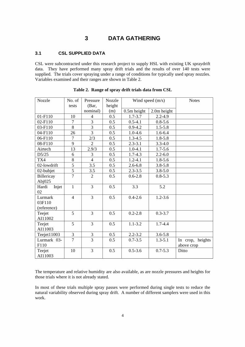
3 DATA GATHERING
CSL SUPPLIED DATA
CSL were subcontracted under this research project to supply HSL with existing UK spraydrift data. They have performed many spray drift trials and the results of over 140 tests were supplied. The trials cover spraying under a range of conditions for typically used spray nozzles. Variables examined and their ranges are shown in Table 2.
Table 2. Range of spray drift trials data from CSL
Nozzle No. of tests
Pressure (Bar,
Nozzle height
Wind speed (m/s) Notes
nominal) (m) 0.5m height 2.0m height 01-F110 10 4 0.5 1.7-3.7 2.2-4.9 02-F110 7 3 0.5 0.5-4.1 0.8-5.6 03-F110 8 3 0.5 0.9-4.2 1.5-5.8 04-F110 26 3 0.5 1.0-4.6 1.6-6.4 06-F110 7 2/3 0.5 1.3-4.5 1.8-5.8 08-F110 9 2 0.5 2.3-3.1 3.3-4.0 Airtech 13 2.9/3 0.5 1.0-4.1 1.7-5.6 D5/25 6 3 0.5 1.7-4.3 2.2-6.0 TX4 8 4 0.5 1.2-4.1 1.8-5.6 02-lowdrift 5 3.5 0.5 2.6-6.8 3.8-5.8 02-bubjet 5 3.5 0.5 2.3-3.5 3.8-5.0 Billericay Abj025
7 2 0.5 0.6-2.8 0.8-5.3
Hardi Injet 02
1 3 0.5 3.3 5.2
Lurmark 03F110 (reference)
4 3 0.5 0.4-2.6 1.2-3.6
Teejet AI11002
5 3 0.5 0.2-2.8 0.3-3.7
Teejet AI11003
5 3 0.5 1.1-3.2 1.7-4.4
Teejet11003 3 3 0.5 2.2-3.2 3.6-5.8 Lurmark 03F110
7 3 0.5 0.7-3.5 1.3-5.1 In crop, heights above crop
Teejet AI11003
10 3 0.5 0.5-3.6 0.7-5.3 Ditto
The temperature and relative humidity are also available, as are nozzle pressures and heights for those trials where it is not already stated.
In most of these trials multiple spray passes were performed during single tests to reduce the natural variability observed during spray drift. A number of different samplers were used in this work.
4
CSL have performed field trials to validate the use of wind tunnel data to assess the risk of spray drift from novel types of nozzles and to generate field data to allow validation of the reliability of pesticide users LERAP assessments.
The CSL data represents field scale data, collected under UK conditions. Spray drift data collected by CSL has been used in the validation and assessment of regulatory approaches to spray drift in the UK. HSL now have the full data set, stored as Excel spreadsheets.
3.2 DATA FROM OTHER SOURCES
There have been many other investigations into spray drift. Exact trial methodologies vary between trials.
The data published by Ganzelmeier et al (Ganzelmeier 1995), is frequently quoted. In these trials spraying occurred over an area, rather than from a single track as in the CSL trials. The area of the test plot was chosen so that drift from the furthest upwind track did not contribute to spray drift outside the application area. Only 16 trials were performed for field crops, however, and at least three replicates were performed for each trial.
The Spray drift task force in the USA performed trials for ground-based application on field crops. Again application occurred over an area, rather than from a single track. More significantly the closest drift measurements were made at 25’ (7.6m); in contrast the furthest CSL measurements were made at 12m.
These data sets therefore differ in the information available, and, do not cover the range of conditions and applications of the CSL data.
3.3 HSL DATA
Finally there is the data collected by HSL during the spray trials conducted during phase 1 of this project. The trial set up and data obtained are described more fully in Section 5 of this report. However, some comments about the data collected by HSL are made here.
The HSL trials used pesticides in the spray mixture. Most of the other data were obtained using non-pesticide marker additives (e.g. fluorescent or coloured dyes). Since the aim of the project is related to post-incident analysis, pesticides were used so that pesticide behaviour could be examined. Spray drift deposition data were collected on both filter papers and vegetation in the HSL trials. Samples taken after spraying will normally be limited to vegetation samples. None of the other data obtained from other sources include vegetation samples. The availability of both filter and vegetation samples in the HSL data allows comparison of the deposition data from the HSL trials with that from other sources. In Figure 1 the sample values from the CSL trial to provide field data to assess LERAP reliability, Run Ref. No. 02-18, are compared with data from the HSL degradation plot. The tests use the same nozzle and pressure, but are not directly equivalent as there were differences in both application and conditions. However, they do show similar retrieval rates.
5
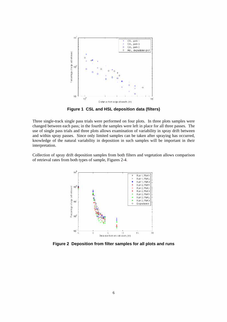
Figure 1 CSL and HSL deposition data (filters)
Three single-track single pass trials were performed on four plots. In three plots samples were changed between each pass; in the fourth the samples were left in place for all three passes. The use of single pass trials and three plots allows examination of variability in spray drift between and within spray passes. Since only limited samples can be taken after spraying has occurred, knowledge of the natural variability in deposition in such samples will be important in their interpretation.
Collection of spray drift deposition samples from both filters and vegetation allows comparison of retrieval rates from both types of sample, Figures 2-4.
Figure 2 Deposition from filter samples for all plots and runs
6
3.4
Figure 3 Deposition from all filter samples, log/log axes
Figure 4 All vegetation samples
Both the filter and vegetation data shows the natural variability that can occur in deposition from spray drift. The filter samples show the very high retrieval rates under the spray boom, while the vegetation samples show lower retrieval rates. Interpretation of deposition from vegetation samples needs consideration of both retrieval rates and variability.
CONCLUSIONS
Data from UK field trials of spray drift has been obtained from CSL. Comparison of the data collected by HSL indicates similar retrieval rates for samples. The data shows significant natural variability can occur in retrieval rates when spray drift occurs. Further statistical evaluations and comparisons of the HSL and CSL generated data will be made in the Phase 2 report.
7
4 ASSESSMENT OF MODELS
Models of spray drift have typically been developed for one of two purposes. One application has been for regulatory purposes, where a simple, frequently empirical, model is used to determine spray application conditions. An example of this is the LERAP approach used to determine how and when aquatic buffer zones can be modified (DEFRA, 2001). The other application has been research into spray drift management. A range of modelling techniques has been used to examine the effect varying parameter values have on spray drift. The information obtained from these models can then be used to develop approaches to management and reduction of spray drift. Models have been developed for this purpose because of the difficulty of controlling parameters during field trials and the limitations in the range and types of flow that can be examined in wind tunnels. The aims of this project differ from either of these purposes. It is the development of tools that can be used to examine the consequences of spraying where questions have subsequently been asked about the likelihood of spray drift having occurred. The requirements of models to address this problem will also differ.
In a previous review of spray drift modelling (Hasan et al, 2002) both boom and air-blast spraying were considered. In practice most UK spray drift incidents involve boom sprayers and it is these that are considered further here. Five different types of model were identified in the previous review: empirical, analytical, box, random walk and computational fluid dynamics (CFD). Of these, an approach based on use of a box model was identified as the most suitable to produce a tool for use by Inspectors. This choice was based both on the knowledge and expertise required of users and the time and computing resource necessary to produce results. Conversely the rejection of a random-walk model was based on the assumption that the time and computing resources necessary to perform a simulation would make it unsuitable in this application. However, if the use of a random-walk model could be separated from the application of a model in the field, then information obtained from running a random walk model could be used as the basis of a tool for investigating spray drift incidents. An approach that used random-walk simulations to generate a set of data on spray drift for the necessary parameter space and then statistically modelled this data to allow rapid use offers this possibility.
It has been demonstrated that existing research models can capture differences in behaviour as parameter values are varied but not necessarily predict absolute values of spray related quantities. Such models can be used in parametric studies to examine different approaches to improving spraying performance and reduction of spray drift. The results from such studies may subsequently be checked against further experimental measurements in either laboratory or the field. However, for this application the model uncertainty and natural variability will have to be examined when interpreting the results of modelling. Analysis of the data available post-incident will also have to consider how effects other than pure spray drift could affect the results.
TYPES OF MODEL
The different types of model identified (Hasan et al, 2002) are revisited here to identify their suitability for use in the development of a tool for investigating spray drift incidents.
8
4.1
4.1.1 Empirical e.g. LERAP and others
Empirical models are based on analysis of existing measurements. They do not have an underlying physical basis and great care would have to be taken if extrapolating beyond the limits of the data on which the model was based. The behaviour of interest would frequently be outside normal operation while the data used in model development are likely to have been collected for normal operation. They will probably be of limited utility in the investigation of spray drift incidents.
4.1.2 Analytical, box, random walk
These models are physically based. However, they make simplifications to the governing equations of fluid flow to allow solutions. This approach can be compared with the numerical solution of the full governing equations used in CFD, mentioned below. In practice a complete model may contain elements from more than one approach. In the Silsoe random walk model (Miller et al, 1996), the movement of droplets and air in the region of the nozzle is calculated using an analytical solution of this region developed by Ghosh and Hunt (Ghosh and Hunt, 1998), while beyond this region a Lagrangian, random walk, model of droplet movement is used. Thus the distinctions between these different types of model may in practice become blurred.
Perhaps the most important distinction in models that have been applied to spray drift is between Eulerian & Lagrangian approaches. In a Lagrangian model the movements of representative droplets are calculated directly; the resulting deposition and drift can then be obtained. Lagrangian calculations can simulate regions where rapid changes in concentration occur over length scales less than the local length scales of turbulence (Xu et al, 1997). However, Lagrangian simulations require calculation of the paths of many droplets involving significant computational effort. In a Eulerian model the droplets are treated as a cloud in a continuum calculation. The calculations performed are much cheaper but there is significant effort involved in the development and parameterisation of the model.
4.1.3 CFD modelling
In CFD the full governing equations of fluid flow are solved numerically. In atmospheric flows it would take too long to perform calculations resolving all the scales of fluid motion that are present, so the turbulance in the flow must still be modelled. CFD can in principle calculate both the full flow field and droplet movement from spray break-up to deposition. Droplet movement can be calculated using either a Eulerian or a Lagrangian approach. However, the cost of resolving all the required scales in a single calculation would be very high. The expertise required of users of CFD would also be an important limit to its application. In practice, a more likely and practical use of CFD would be to examine and obtain data on particular stages of the spray drift process. For example, modelling the interaction of air and droplets in the vicinity of the spraying vehicle, or the response of air and droplets to an obstacle in the drift region further down wind. The results of such calculations could then be used to provide information for the development of other models.
Limits to the range of applicability in empirical models limit their usefulness, while at the other extreme the cost and expertise necessary to use CFD limits its application. Between these, the physically based but simplified models offer the best approach to the requirements of this project. The use of a Lagrangian model to generate data with a statistical fit to the results to allow rapid calculations offers the most useful approach for this project.
9
4.2 DEVELOPMENT PROCESS
The suggested approach to development of the modelling tool is to separate running the spray drift model from the tool to be used by Inspectors. This would allow the use of a Lagrangian model, with relatively long run times, to generate data on spray drift. The data generated would then be fitted using a statistical model for rapid use.
The Silsoe Research Institute spray drift model already exists and is documented; appropriate models of the physics of spray drift are already incorporated. Use of this as the model for calculating spray drift would allow the use of a tool that has already been developed and documented. Any development and validation required would start from this basis rather than from scratch. In principle, use of this model is possible though the cost and license need to be determined. An alternative would be to write an equivalent model ourselves, preferably with advice from Paul Miller (formerly of SRI, now in The Arable Group). The basic idea of a Lagrangian spray drift model is not that complex. However, appropriate physics must be incorporated and modelled correctly and it must be demonstrated that this has been achieved. To produce a useful model the efficiency of the implementation must also be addressed. Development of a model from scratch would therefore involve considerable extra effort.
Development of the tool for investigating spray drift incidents would be in three stages:
• Comparison of the predictions of the Lagrangian model against CSL/HSL data. This may suggest modifications to be made to the Silsoe model.
• Generation of data for additional spraying scenarios, to provide a better ‘map’ of the results of spraying over the range of parameters considered important.
• Fit a statistical model to this data.
The statistical model would then provide a rapid method to calculate spray drift for given conditions.
As already noted from the field observations, there is considerable variability in pesticide deposition. The Lagrangian model and hence the statistical model would provide mean values for a given set of conditions. Characterisation of the expected variation in deposition, using statistical analysis, will therefore be an important part of any tool, to allow interpretation of any samples taken after an incident. Since the eventual aim is the provision of a tool to interpret actual spray drift applications, information on additional variation occurring in practice, as opposed to in field trials, is needed. The possibility that some of the future spray trials should be based on actual applications should be considered.
The most important parameters influencing spray drift are:
• Atmospheric conditions – wind speed and direction
• Spray conditions – boom height, spray quality and the use of adjuvants.
These will be the main parameters considered when developing the spray drift model. The influence of other parameters will also be considered (where possible and appropriate), for example, those influencing other possible transport mechanisms (e.g. vapour transport).
10
4.3 APPLICATION – HOW WOULD THE TOOL BE APPLIED?
The information available in any investigation will always be limited. Some time will have elapsed between the time when a possible incident occurred and the collection of vegetation samples to analyse for the presence of pesticide. The exact conditions at the time of spraying will not be known, typically meteorological data from the nearest Met Office station will be the best available information. There may also be questions about details of the pesticide application.
Vegetation samples can be used as indicators of the presence of pesticide, perhaps also indicating significant features of the spray application e.g. the position of the edge of the swath. However, natural variation in the transport and deposition of spray drift, combined with differences in vegetation and degradation of pesticides with time will lead to scatter in the results obtained. The limited numbers of samples that can be obtained and analysed would make it difficult to fit a model to sample data collected after an incident, and any prediction of source terms would contain significant uncertainty.
The approach suggested here is to use the available information about the application and conditions when spraying occurred to make predictions of spray deposition. The predictions could then be used to describe the likely spray drift behaviour; any available information on the distribution of pesticide from samples would then be interpreted in the light of the predictions.
4.4 CONCLUSIONS
An approach to development of a tool for investigating spray drift incidents has been described. The approach decouples the simulation of spray drift from the tool used to investigate spray drift incidents.
It is suggested that an existing model, that has successfully predicted spray drift, should be used to simulate spray drift. This model would be checked against the HSL and CSL data to check its predictive ability and the need for any further development considered. The use of an existing model would avoid the time and effort required to develop, check and document a new model. The data gathered will allow examination of the predictive ability of the model. In developing the model, issues raised in the RCEP report and by the data collected will be considered. In particular the possible effects of volatilisation on interpretation of post-incident data will be considered.
Once the suitability of the spray drift model had been determined a database of spray drift simulations covering the parameter space considered important would be generated. A statistical model would be fitted to this data to allow rapid calculation of spray drift behaviour. The nature of the statistical modelling used would be decided in conjunction with discussion of how a tool for investigating spray drift incidents would be used.
The modelling would predict mean quantities; interpretation of these predictions would have to consider the observed natural variability in deposition and sampling uncertainty in the data. Initial analysis of observations of the variation in deposition rates across the parameter space would give some indication of what levels of uncertainty would make it hard to distinguish whether predictions and observations differed. Application of the tool would determine practical usefulness and whether approaches to sampling could be developed to improve usefulness.
11

5 SPRAY TRIALS
Spray trials were conducted by HSL, with support from SRI, to collect data necessary to understand and interpret data from post-incident spray drift samples. The trials were made using pesticides rather than tracer compounds.
Vegetation is usually the only medium available for post-incident investigation work, and there is often a delay between the occurrence of the incident and the inspection/sampling visits. In the trails, grass samples (the most widespread vegetation available in most situations) were collected and samples were also taken of ground deposition onto filter papers, following standard protocols. This allows both comparisons of the retrieval rates for the different types of sample but also of the HSL data with that collected by others, to ensure that they are compatible. The effect of degradation of pesticide on the vegetation samples through time was also examined. In addition to the ground samples deposition onto mannequins and aerial lines was also investigated to allow comparison of bystander exposure with ground samples and to examine distribution with height.
SRI was sub-contracted under this project to provide a suitable trial site, agricultural boom sprayer (and operator), weather recording facilities (mast), and to input to the design and organisation/completion of the trials. The trial site provided was located on the large grass area in front of the main Institute building at the SRI site at Silsoe in Bedfordshire (see Figure 5).
conducted here
Spray trial
Figure 5 Map of SRI site showing spray trial location
The spray trials were finally conducted in July 2004, following 3 aborted attempts due to unfavourable weather conditions.
12
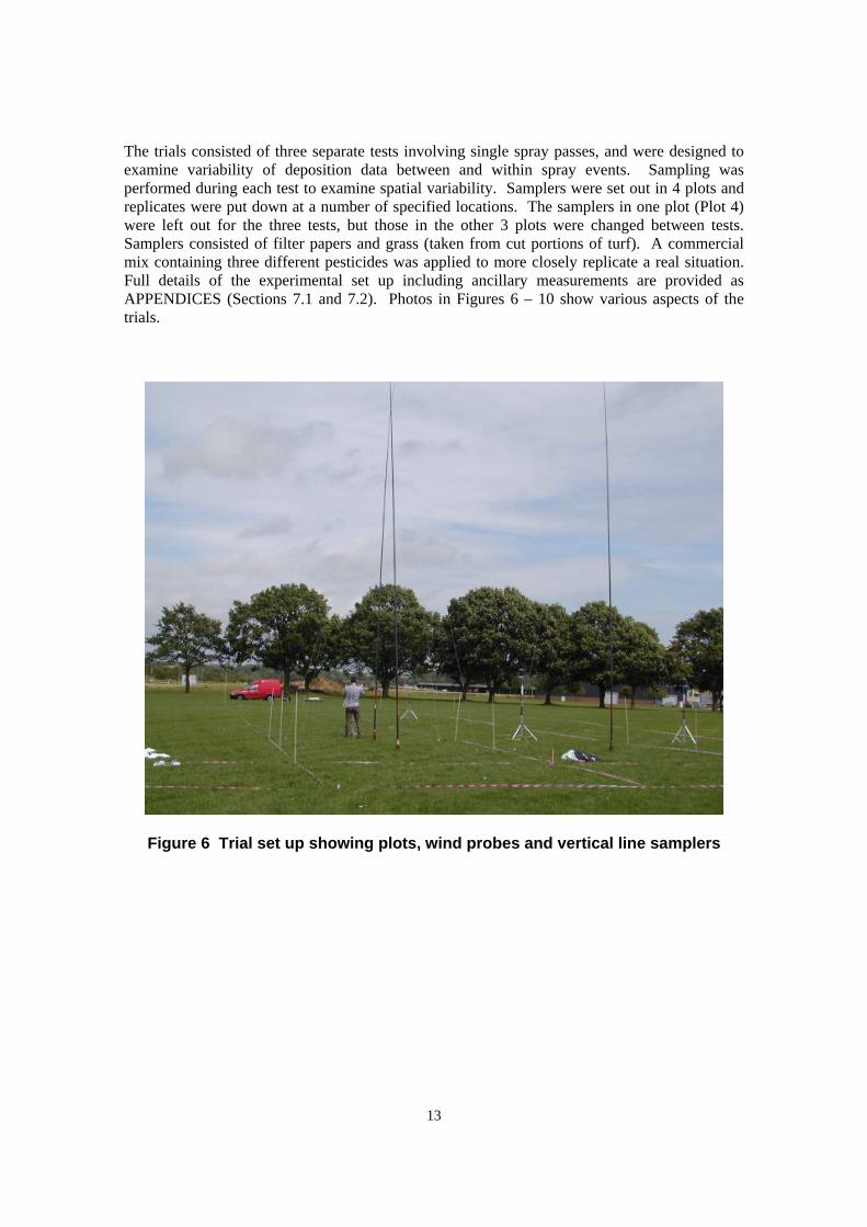
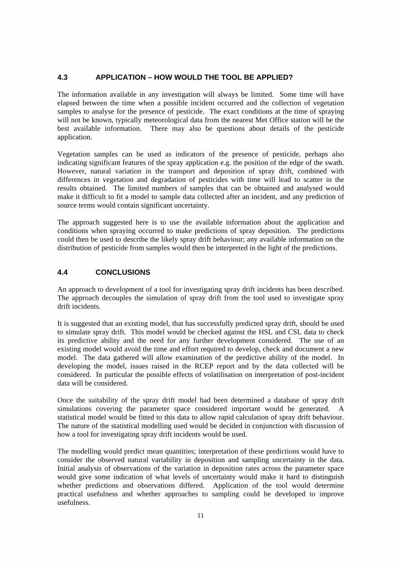
The trials consisted of three separate tests involving single spray passes, and were designed to examine variability of deposition data between and within spray events. Sampling was performed during each test to examine spatial variability. Samplers were set out in 4 plots and replicates were put down at a number of specified locations. The samplers in one plot (Plot 4) were left out for the three tests, but those in the other 3 plots were changed between tests. Samplers consisted of filter papers and grass (taken from cut portions of turf). A commercial mix containing three different pesticides was applied to more closely replicate a real situation. Full details of the experimental set up including ancillary measurements are provided as APPENDICES (Sections 7.1 and 7.2). Photos in Figures 6 – 10 show various aspects of the trials.
Figure 6 Trial set up showing plots, wind probes and vertical line samplers
13
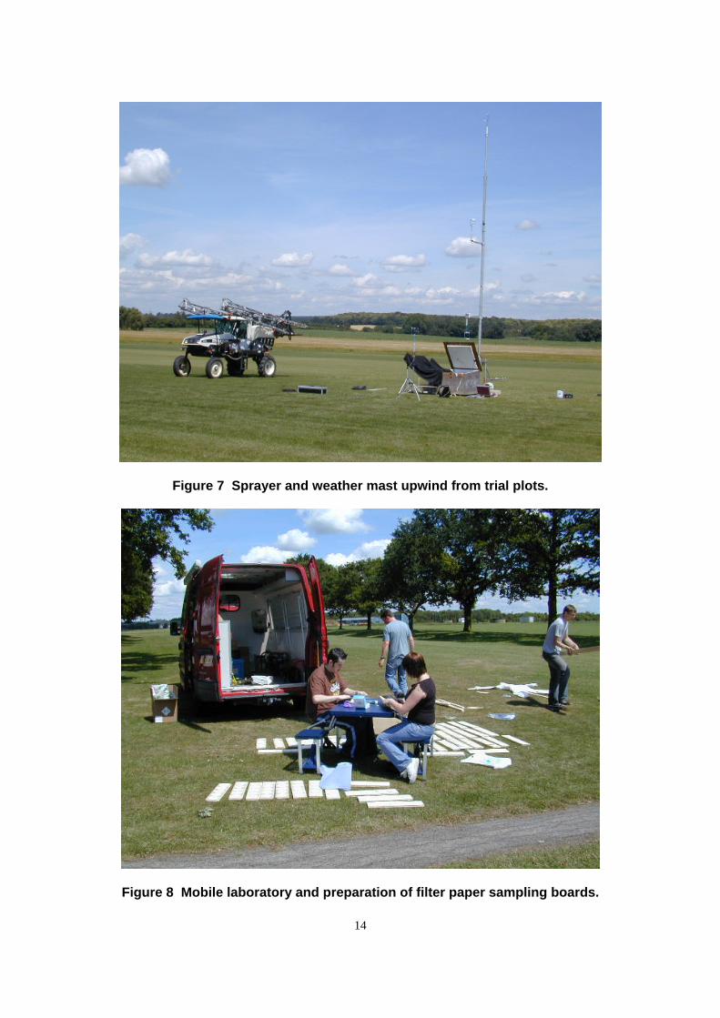
Figure 7 Sprayer and weather mast upwind from trial plots.
Figure 8 Mobile laboratory and preparation of filter paper sampling boards.
14

Figure 9 Sprayer operating past the plots, mannequins are set up in plot 4
Figure 10 Cutting grass samples from turfs taken from sprayed plots
15

While it was important to obtain comparable drift data using filter paper samplers, the trial also offered a good opportunity to more rigorously investigate the use of vegetation as a sampling medium. Vegetation is often the only sampling media available for post event spraydrift investigation. Because of the widespread availability, grass sampling has been the vegetation sample of choice (White 1996). As far as we are aware, this is the first time grass and filter paper samples have been directly compared using a robust and standardised methodology and approach.
Specifically the aims of the vegetation sampling and analysis were to: 1. Determine the feasibility of using vegetation as a surrogate-sampling device. 2. Validate the use of area sampling as opposed to weight sampling. 3. Allow comparison of sampler efficiencies and spray profiles. 4. Assess the effects of pesticide degradation (chemical breakdown, plant growth dilution
and metabolism and weathering) on spray profiles.
5.1 RESULTS AND DISCUSSION
Full trial results are detailed in the APPENDICES, Sections 7.3 to 7.10.
5.1.1 Recovery data
The most reliable data from the trials came from the analysis of the pesticide kresoxim-methyl; good recoveries were achieved from both the filter paper and vegetation samples. The data obtained from this pesticide can be directly compared with the data provided by CSL.
Due to the poor recovery of epoxiconazole and fenpropimorph (probably due to increased adsorption efficiency), filter paper deposition data has not been calculated. However, their recovery data from vegetation was found to be acceptable (mean recovery >70%) and hence, their results have been included in this report for broad comparison with those for kresoximmethyl. Tables 3 and 4, outline the recovery and limit of detection data obtained.
Table 3. Recovery data
Pesticide % Recovery from filter paper (Av ± SD)
% Recovery from grass (Av ± SD)
% Recovery from aerial lines
% Recovery from suits
Kresoxim-methyl 88.5 ±1.6 (n=4) 86.2 ± 4.1 (n=7) 149* 100
Epoxiconazole 17.6 72.4 ± 11.4 (n=7) 110 57 Fenpropimorph 27.3 83.0 ± 11.6 (n=6) 109 79
*The high recovery of kresoxim-methyl from the aerial is most likely to be a matrix enhancement effect caused during the analysis. Matrix matched standards are generally used to account for this, but this was not practicable for the aerial lines. The results are blank subtracted to attempt to ensure that any false positives caused by the matrix (the drift line) are negated.
16

Table 4. Limits of detection (LOD) data
Pesticide LOD filter paper LOD grass LOD aerial lines LOD suits Kresoxim-methyl 7 ng/filter 1.3 µg/kg 24 ng/m
Epoxiconazole - 3.5 µg/kg 18 ng/m
Fenpropimorph - 0.7 µg/kg 9 ng/m
5.1.2 Aerial line data
Analytical results for the deposition of the three pesticides on aerial lines are given in APPENDIX Sections 7.3.
Whereas the filter and turf samples give a measure of the distance travelled by the pesticide spray, the aerial lines show the distribution with height at a distance. There were three masts, each with two lines, placed at the positions shown in APPENDIX sections 7.1 and 7.2. All the lines were collected, by winding onto purpose built racks, and replaced after each pass of the sprayer. The 10m lines were then cut into 1m segments and analysed. That there were two masts at the same distance, 4m, from the sprayer enables us to look at the variation encountered over a single pass. The third mast was placed further back at 8m to show what happens to the spray plume over distance. This three dimensional view of the plume is essential when trying to model the spray drift.
The first observation is that there is a difference in the profiles produced by the three pesticides. Whereas kresoxim-methyl and epoxiconazole exhibits a steady decay, fenpropimorph levels off and starts to increase at the top of the mast. The profiles for mast one (plot 1, 4m) are shown in figure 11 (segment 1 is lowest and segment 10 highest); these plots are the average of both lines on the mast over all three runs. All the plots show a large drop in the level of pesticide between the first and second segments, 49% for kresoxim-methyl, 48% for epoxiconazole and 40% for fenpropimorph. For kresoxim-methyl and epoxiconazole there is then a reasonably consistent drop of approximately 50% for each consecutive segment. For fenpropimorph there is a consistent drop of around 10% for each further segment until it levels off at segment 8. These distribution patterns are repeated for the masts in the other two positions and can be taken as representative profiles.
The profiles obtained for kresoxim-methyl and epoxiconazole are generally what would have been expected as the spray is directed downwards and it is reasonable to assume that it would be most concentrated at lower heights. The shape of the profile for fenpropimorph is very distinct from the other two and is not so obviously explained. It is unlikely to be an artefact of the analysis as the results are both recovery and blank corrected and the effect is seen in all the sample sets. Taking into account the properties of the pesticides, the most notable difference is in the vapour pressure, effectively a measure of volatility of a compound. The values given in the Pesticides Manual (BCPC, 1997) are fenpropimorph 3.5 mPa, epoxiconazole <0.01 mPa and kresoxim-methyl 0.0023 mPa, making fenpropimorph by far the most volatile of the three pesticides. It is only conjecture at this stage, but it would not be unreasonable to assume that the fenpropimorph is volatilising and rising as a vapour to give the high levels found at the top of the mast. Given the wind conditions and close proximity to the boom end, it is likely that the vapour has originated from the 24 metre sprayed swath. This effect would not be observed for the other two compounds to the same degree, as they are less volatile, and would explain the difference in the shapes of the profiles. If this is the case then it has implications for analysis of incident data and development of any computational model and requires further investigation.
17

0
100
200
300
400
500
600
ii l
ipe
stic
ide
per s
egm
ent (
ng) fenprop morph
kresox m-methyepox conazole
1 2 3 4 5 6 7 8 9 10 Section of aerial line
Figure 11 Aerial line profiles for mast one averaged over three runs
In Figure 12, the variation between lines, masts and runs is illustrated. Kresoxim-methyl was chosen to demonstrate this because the variation in the data is slightly greater than for the other two pesticides, so it can be considered a worst-case scenario. The first chart shows the individual data points on both lines attached to the two masts from run 1. Similarly, the second and third charts show the equivalent data for runs 2 and 3. The observed variations are likely to be due to the number of variables that influence spray drift even under relatively controlled conditions
0
200
300
400
500
600
700
800
il (
ng)
line 1
line 2
line 1
line 2
100
Kres
oxm
-met
hy
run 1 mast 1
run 1 mast 1
run 1 mast 2
run 1 mast 2
1 2 3 4 5 6 7 8 9 10
Section of aerial line
0
200
300
400
500
600
il (
ng)
line 1
line 2
line 1
line 2
100
Kres
oxm
-met
hy
run 2 mast 1
run 2 mast 1
run 2 mast 2
run 2 mast 2
1 2 3 4 5 6 7 8 9 10
Section of aerial line
18
600
500
400
Kres
oxim
-met
hyl (
ng)
300
200
100
0
line 1
line 2
line 1
line 2
run 3 mast 1
run 3 mast 1
run 3 mast 2
run 3 mast 2
1 2 3 4 5 6 7 8 9 10
Section of aerial line
Figure 12 Individual aerial line data for kresoxim-methyl to show variation
There are few data points with which to carry out a full statistical study of the variation of the deposition but some simple observations can be made. It may be expected that the two lines from each mast would give the best agreement whilst the variation would increase when comparing two masts in the same run and would increase further when comparing two separate runs. This does not appear to be the case as there is clearly significant variation between the lines and the masts, whereas the agreement between individual runs appears to be good when the individual lines are averaged. The level of variation is likely to be the result of various factors e.g. gusting and boom movement. The data will however, give an indication of the ranges of data that are likely to result from a spraying pass and these can be built into a computational model.
The data for the individual masts for kresoxim-methyl, averaged over all three of the passes is shown in Figure 13. It can be seen that the profile of the chart is consistent but the results are not totally as expected. Mast 1 (plot 1, at 4 m distance) has a first section average of 291 ng compared with Mast 2 (plot 2, at 4 m distance) that averages 464 ng. Over the three runs these two values were expected to have averaged out to produce a closer match, but this is clearly not the case. It is possible that there is a systematic effect in each pass such as the boom height changing at the same point so as to give the variation between the two masts. Another point of note is that the results for mast 1 (plot 1, at 4 m distance) and mast 3 (plot 1, at 8 m distance) are very similar where it may be expected that the mast 3 values would be lower due to the plume tailing off. Another feature in the comparison of these two masts is that at there is no pesticide detected for the higher sections on mast 1 (or mast 2) but there is for mast 3; this would suggest that instead of dropping, the plume of spray is in fact still rising. The variation between masts 1 and 2 as well as masts 1 and 3 is repeated for epoxiconazole, which has a similar profile (see data Appendix, Section 7.3) to kresoxim-methyl. This would suggest that the effects are genuine.
For fenpropimorph, the comparisons are more in line with what would be expected (see data Appendix, Section 7.3). Mast 1 and mast 2 give very similar profiles in terms of shape and values, and mast 1 gives a similar profile in terms of shape to mast 3 but higher values. As has already been stated, the profile produced for fenpropimorph varies from those of the kresoximmethyl and epoxiconazole so the differences in the plume may be due to the different transport mechanisms that are occuring.
It is obvious that there are several questions arising from this data set and further work is required to investigate these.
19

350
300
ng) Mast 1
250l (200
m-m
ethy
150 i
100
Kres
ox
50
0 1 2 3 4 5 6 7 8 9 10
Section of aerial line
500
400 450
ng) Mast 2
350l (
300 250
m-m
ethy
200i
150
Kres
ox
100 50 0
1 2 3 4 5 6 7 Section of aerial line
8 9 10
350
300
ng) Mast 3
250l (
200
m-m
ethy
150 i
100
Kres
ox
50
0 1 2 3 4 5 6 7 8 9 10
Section of aerial line
Figure 13 Individual mast data for kresoxim-methyl averaged over three runs
20
5.1.3 Filter paper deposition results and evaluation
Analytical results for Kresoxim-methyl deposition on filter paper samplers are given in APPENDIX Section 7.4. As already stated, filter paper deposition for the other two pesticides was not calculated because of the low and variable recoveries achieved from this sampling media.
The filter data, expressed as a percentage of the theoretical application rate shows that a high (>90) percentage of the spray has been collected and recovered using this type of device.
Initial evaluation has shown that the filter paper trial data compares well with CSL supplied data. A brief analysis and overview has already been given in Section 3 of this report. This effectively means that all the data sets are robust and comparable and hence can be used to develop the modelling tool in Phase 2.
5.1.4 Grass deposition results and evaluation
Analytical results for the deposition of the three pesticides on grass samplers are given in APPENDIX Section 7.5.
The grass data for the intentionally sprayed area (-5 m), expressed as a percentage of the theoretical application rate shows that on average 34% (12.6% RSD) of the spray has been collected and recovered using grass as a sampler (Table 5). The considerably lower capture efficiency compared to the filter paper performance is probably due to the deposition of pesticide to the ground. When the grass results are expressed as a percentage of the filter depositions, further data on the capture efficiency of grass can be compared (Table 6) indicating an average 35.5% (14.6% RSD).
Table 5. Grass results (kresoxim-methyl) relative to theoretical application rate.
Grass results relative to the theoretical application rate (%) Distance Run 1 Run 2 Run 3 Degradation Mean ± SD
Minus 5 m 28 35.5 35 38 34.1 ± 4.3 (n=4)
Table 6. Grass results (kresoxim-methyl) relative to filter results.
Grass relative to filter paper results (%) Distance Run 1 Run 2 Run 3 Degradation Mean ± SD
Minus 5 m 0 m
25 33
37 39
38 32
39 41 35.5 ± 5.2 (n=8)
However, as shown in Table 7, there is a good correlation between the filter and vegetation deposition data when both data sets are normalised to the intentionally sprayed area. This demonstrates that, provided an in-field sample can be obtained and similar vegetation is collected using an area sampling method, then vegetation can be used as a surrogate sampler for post event drift investigation.
21

Table 7. Comparison of the filter and vegetation deposition data for kresoxim-methyl in plot 4 (3 sprayings), with normalised to the intentionally sprayed (-5 m) samples.
Distance Filter Vegetation Minus 5 m 100% 100%
0 m 29.7% 31% 4 m 0.5% 1.2% 8 m 0.2% 0.4%
Because of the relatively low variation in grass results (12 – 14% RSD) and good correlation with the filter data, it may be possible to use an assumed in-field grass deposition (35% of the theoretical application rate). This would then permit the normalisation of the outfield results to provide a spray profile for situations where grass samples cannot be collected. There are assumptions that would have to be tested in the further phases of work.
5.1.5 Grass degradation results and evaluation
Analytical results for the degradation of the three pesticides on grass samplers are given in APPENDIX Section 7.6.
Spraydrift complaints tend to be made several days after an event and there may be a further delay before sampling can take place. It is therefore important to consider the effects that the degradation may have on the drift profiles. Degradation of pesticide deposition can occur by a number of routes including:
• Plant metabolism. • Chemical degradation, for example due to pH effects, photo-degradation (sunlight), etc. • Physical dilution, for example due to plant growth. • Environmental losses, for example due to rain wash-off and evaporation.
The rate of degradation is very dependent on the pesticide itself. Some indicative information is available in publications such as the Pesticide Manual or from manufacturers, but this is sketchy. Where information is available, it is usually expressed as a half-life (time taken to reach half concentration) on a particular matrix.
The HSL field study set out to look at the degradation of the pesticides used under real deposition and weathering conditions, to see if there were any concentration effects on the degradation rates and to establish if the spray profiles were disrupted over time. Because of the prevailing weather conditions, the samples saw little or no rainfall during the two-week period of the study. The approximate half-lives found are compared with published data in Table 8.
Table 8. Comparison of HSL and published degradation information.
Pesticide Vapour pressure* Published half-life* HSL study half-life Kresoxim-methyl 2.3 x 10⁻³ mPa - 7 days
Epoxiconazole <10 x 10–3 mPa Extensive (plants) 3-4 months (soil)
14 days
fenpropimorph 3.5 mPa 3-7 days (cereals) <4 days
*Information from The Pesticide Manual
22
The HSL data does not conflict with the available published data. What is evident though, is that under the HSL experimental conditions, there may be a correlation between the half-life and the published vapour pressure (i.e. degradation was mainly driven by evaporative losses). Data supplied in MDHS 94 (HSE, 1999) show similar evaporative degradation profiles, albeit from different sampling media.
The effect of time (i.e. degradation) on the normalised (to intentionally sprayed area) spray profiles is illustrated for all 3 pesticides in Tables 9-11.
Table 9. Spray profiles for kresoxim-methyl on vegetation over time, with data normalised to the intentionally sprayed (-5 m) samples.
Distance 0 days 4 days 7 days 14 days Minus 5 m 100% 100% 100% 100%
0 m 31% 33% 35% 41% 4 m 1.2% 0.6% 0.3% 0.7%
Table 10. Spray profiles for epoxiconazole on vegetation over time, with data normalised to the intentionally sprayed (-5 m) samples.
Distance 0 days 4 days 7 days 14 days Minus 5 m 100% 100% 100% 100%
0 m 37% 37% 38% 46% 4 m 1.0% 1.2% 0.6% 0.8%
Table 11. Spray profiles for fenpropimorph on vegetation over time, with data normalised to the intentionally sprayed (-5 m) samples.
Distance 0 days 4 days 7 days 14 days Minus 5 m 100% 100% 100% 100%
0 m 90% 71% 73% 60% 4 m 24% 14% 9% 9%
The effects of degradation on the profiles (i.e. comparing % results between the different columns within each table) appear to have little impact on the profiles for kresoxim-methyl and epoxiconazole over a seven-day period and it still may be possible to use their profiles for indicative purposes for up to 14 days after an event. The profile for fenpropimorph changes significantly even after 4 days. This is not surprising given the variabilities introduced due to the short half-life observed for this pesticide. Clearly, if drift profiles are to be used for post event spraydrift investigation, some knowledge of an active ingredient’s stability must be known. Published half-lives and/or vapour pressures must be considered prior to commencing any enforcement monitoring (sampling and analysis).
Comparison of the data for the three pesticides also shows that there is an increased dose of fenpropimorph observed at 0 and 4 m distance compared to the other two. This is again indicative that other transport and deposition mechanisms may have occurred during the spray trials.
23
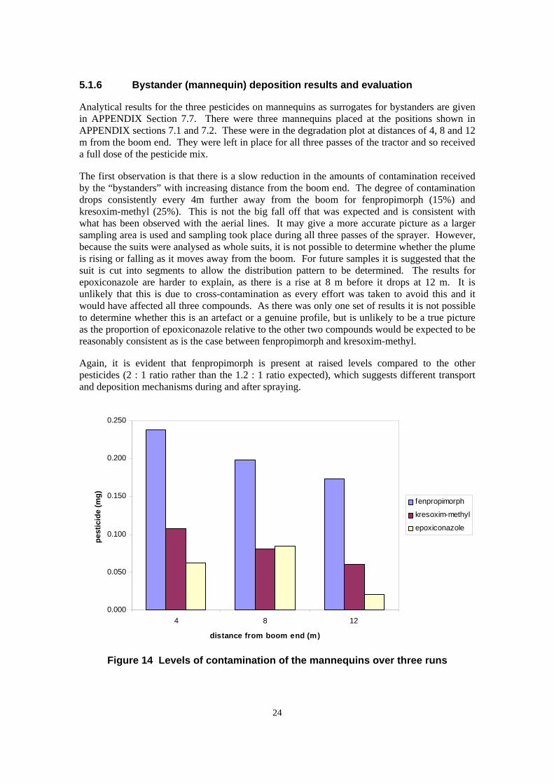
5.1.6 Bystander (mannequin) deposition results and evaluation pe
stic
ide
(mg)
Analytical results for the three pesticides on mannequins as surrogates for bystanders are given in APPENDIX Section 7.7. There were three mannequins placed at the positions shown in APPENDIX sections 7.1 and 7.2. These were in the degradation plot at distances of 4, 8 and 12 m from the boom end. They were left in place for all three passes of the tractor and so received a full dose of the pesticide mix.
The first observation is that there is a slow reduction in the amounts of contamination received by the “bystanders” with increasing distance from the boom end. The degree of contamination drops consistently every 4m further away from the boom for fenpropimorph (15%) and kresoxim-methyl (25%). This is not the big fall off that was expected and is consistent with what has been observed with the aerial lines. It may give a more accurate picture as a larger sampling area is used and sampling took place during all three passes of the sprayer. However, because the suits were analysed as whole suits, it is not possible to determine whether the plume is rising or falling as it moves away from the boom. For future samples it is suggested that the suit is cut into segments to allow the distribution pattern to be determined. The results for epoxiconazole are harder to explain, as there is a rise at 8 m before it drops at 12 m. It is unlikely that this is due to cross-contamination as every effort was taken to avoid this and it would have affected all three compounds. As there was only one set of results it is not possible to determine whether this is an artefact or a genuine profile, but is unlikely to be a true picture as the proportion of epoxiconazole relative to the other two compounds would be expected to be reasonably consistent as is the case between fenpropimorph and kresoxim-methyl.
Again, it is evident that fenpropimorph is present at raised levels compared to the other pesticides (2 : 1 ratio rather than the 1.2 : 1 ratio expected), which suggests different transport and deposition mechanisms during and after spraying.
0.250
0.200
0.150
0.100
0.050
0.000
4 8 12
i l
epoxi
fenpropimorph
kresox m-methy
conazole
distance from boom e nd (m)
Figure 14 Levels of contamination of the mannequins over three runs
24
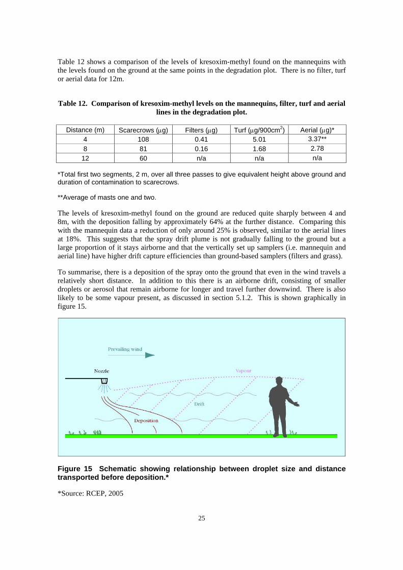
Table 12 shows a comparison of the levels of kresoxim-methyl found on the mannequins with the levels found on the ground at the same points in the degradation plot. There is no filter, turf or aerial data for 12m.
Table 12. Comparison of kresoxim-methyl levels on the mannequins, filter, turf and aerial lines in the degradation plot.
Distance (m) Scarecrows (µg) Filters (µg) Turf (µg/900cm2) Aerial (µg)* 4 108 0.41 5.01 3.37** 8 81 0.16 1.68 2.78
12 60 n/a n/a n/a
*Total first two segments, 2 m, over all three passes to give equivalent height above ground and duration of contamination to scarecrows.
**Average of masts one and two.
The levels of kresoxim-methyl found on the ground are reduced quite sharply between 4 and 8m, with the deposition falling by approximately 64% at the further distance. Comparing this with the mannequin data a reduction of only around 25% is observed, similar to the aerial lines at 18%. This suggests that the spray drift plume is not gradually falling to the ground but a large proportion of it stays airborne and that the vertically set up samplers (i.e. mannequin and aerial line) have higher drift capture efficiencies than ground-based samplers (filters and grass).
To summarise, there is a deposition of the spray onto the ground that even in the wind travels a relatively short distance. In addition to this there is an airborne drift, consisting of smaller droplets or aerosol that remain airborne for longer and travel further downwind. There is also likely to be some vapour present, as discussed in section 5.1.2. This is shown graphically in figure 15.
Figure 15 Schematic showing relationship between droplet size and distance transported before deposition.*
*Source: RCEP, 2005
25
The quantities of pesticides found on the mannequins into context it can be compared to the accepted operator exposure level (AOEL). For kresoxim-methyl this is 0.9 mg/kg body weight/day and assuming a body weight of 70kg gives an acceptable exposure of 63 mg/day. The dose received at 4 m was 108 µg and therefore less than 0.2% of the AOEL, dropping to around 0.1% at 12 m. However the pesticides used in this trial were primarily chosen because they were fungicides of low toxicity. If the pesticide had been, for example, chlorothalonil (AOEL 0.005 mg/kg body weight/day) and had been found at the same levels it would have equalled 31% of the AOEL at 4 m and 17% at 12 m. More toxic chemicals will obviously have a greater potential to do harm. In terms of LERAP, it is possible that a buffer zone could be reduced down to 1 m.
5.1.7 Potential for post application exposure
During the collection of samples, HSL staff wore personal protective equipment (PPE), which included coveralls, gloves and shoe covers. While the staffs work patterns were not systematically studied, the PPE samples were collected and analysed to provide some information on secondary exposure that can arise from casual contact with a treated area (i.e. walking through fields picking up items).
Analytical results for the potential post application exposure to the three pesticides are given in APPENDIX Section 7.8. These show that significant exposure can occur, and not unsurprisingly the main contamination is on the feet. The ranges of exposure for kresoximmethyl are 2 - 305 µg for the gloves, 0 - 954 µg for the boots and 0 - 242 µg for the suits.
The results could have significance for walkers if a sprayed area is not closed off, but also for people living adjacent to fields, if drift has occurred. The contamination may also have further implications in that it may be a route to transfer residues back into people’s homes. A recent HSE study showed that pesticides could accumulate in house dust (samples taken from vacuum cleaners) even for non-pesticide workers (Coldwell, 2001). Further work could be conducted to look at levels in house dust from the homes of pesticide workers or residents living close to sprayed fields.
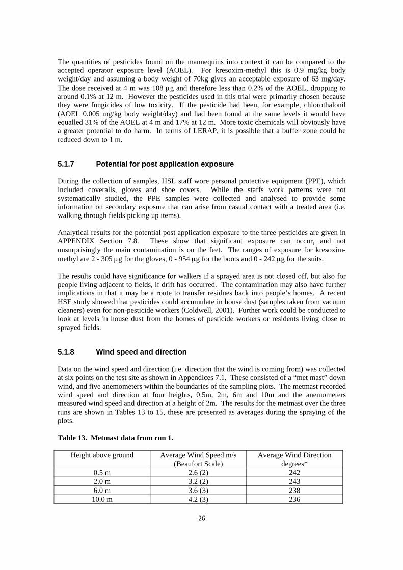
5.1.8 Wind speed and direction
Data on the wind speed and direction (i.e. direction that the wind is coming from) was collected at six points on the test site as shown in Appendices 7.1. These consisted of a “met mast” down wind, and five anemometers within the boundaries of the sampling plots. The metmast recorded wind speed and direction at four heights, 0.5m, 2m, 6m and 10m and the anemometers measured wind speed and direction at a height of 2m. The results for the metmast over the three runs are shown in Tables 13 to 15, these are presented as averages during the spraying of the plots.
Table 13. Metmast data from run 1.
Height above ground Average Wind Speed m/s (Beaufort Scale)
Average Wind Direction degrees*
0.5 m 2.6 (2) 242 2.0 m 3.2 (2) 243 6.0 m 3.6 (3) 238
10.0 m 4.2 (3) 236
26
Table 14. Metmast data from run 2.
Height above ground Average Wind Speed m/s (Beaufort Scale)
Average Wind Direction degrees*
0.5 m 3.0 (2) 242 2.0 m 3.3 (2) 247 6.0 m 4.2 (3) 238
10.0 m 4.8 (3) 236
Table 15. Metmast data from run 3.
Height above ground Average Wind Speed m/s (Beaufort Scale)
Average Wind Direction degrees*
0.5 m 3.2 (2) 243 2.0 m 3.6 (3) 252 6.0 m 4.6 (3) 242
10.0 m 5.2 (3) 240
*The test site was orientated at 65 degrees to magnetic north (i.e. the wind was blowing down the plots).
The results show a gradual increase in average wind speed throughout the day but never rose above 3 on the Beaufort scale, which means we had acceptable spraying conditions throughout the tests according to the green code (MAFF, 1998). The direction of the wind was also consistent and perpendicular to the tramlines throughout the day.
The results for the five anemometers are given in the same format in below in Tables 16 to 18. The five positions of the anemometers are shown in Appendices 7.1.
Table 16. Anemometer data from run 1.
Anemometer Average Wind Speed m/s (Beaufort Scale)
Average Wind Direction degrees*
A 3.4 (3) 237 B 3.4 (3) 236 C 4.2 (3) 247 E 3.4 (3) 239 G 3.3 (3) 237
Table 17. Anemometer data from run 2.
Anemometer Average Wind Speed m/s (Beaufort Scale)
Average Wind Direction degrees*
A 3.9 (3) 240 B 4.1 (3) 236 C 3.7 (3) 242 E 3.9 (3) 240 G 4.0 (3) 239
Table 18. Anemometer data from run 3. 27
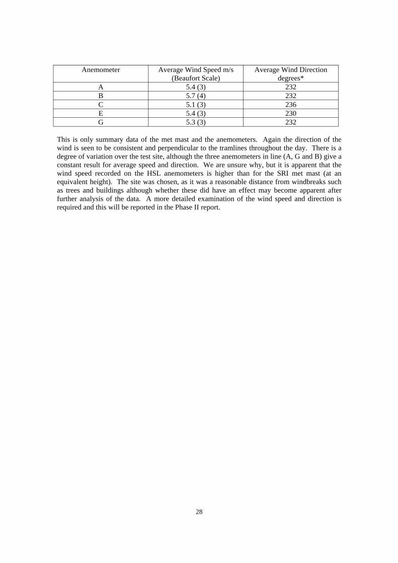
Anemometer Average Wind Speed m/s (Beaufort Scale)
Average Wind Direction degrees*
A 5.4 (3) 232 B 5.7 (4) 232 C 5.1 (3) 236 E 5.4 (3) 230 G 5.3 (3) 232
This is only summary data of the met mast and the anemometers. Again the direction of the wind is seen to be consistent and perpendicular to the tramlines throughout the day. There is a degree of variation over the test site, although the three anemometers in line (A, G and B) give a constant result for average speed and direction. We are unsure why, but it is apparent that the wind speed recorded on the HSL anemometers is higher than for the SRI met mast (at an equivalent height). The site was chosen, as it was a reasonable distance from windbreaks such as trees and buildings although whether these did have an effect may become apparent after further analysis of the data. A more detailed examination of the wind speed and direction is required and this will be reported in the Phase II report.
28
6 CONCLUSIONS
1. HSL has obtained a significant amount of existing data covering a range of conditions andinvolving variables that are known to influence spraydrift. The data, obtained from the Central Science Laboratory (CSL), covers trials carried out over many years. It represents probably the most complete set of independent data in the UK.
2. Based on agreed protocols, HSL conducted a comprehensive spray trial at the Silsoe Research Institute (SRI) in July 2004 to gather 3 additional data sets. The data obtained using a commercial fungicide mix (kresoxim methyl, epoxiconazole and fenpropimorph) compares well with the CSL supplied data.
3. Even though capture efficiency is lower than standard sampling devices, it has been demonstrated that vegetation (grass) can be used as a surrogate sampler for drift investigation. However, if a matching in-field sample cannot be collected (likely scenario with growing crop), off target results would have to be related to an estimated in-field loading based on the farmers/sprayers records for application rate.
4. Post application degradation has been studied in grass samples and losses do not appear to have significantly altered normalised drift profiles over a 7-day period for two of the three pesticides tested. It may be appropriate to carry out sampling and analysis to support enforcement action for up to 14 days following an event, but consideration of subsequent weather conditions and the properties of active ingredients (i.e. vapour pressure, known degradation properties, etc.) must be taken into account before doing this.
5. Currently available computational and empirical models have been reviewed and UK experts consulted (SRI)
6. The feasibility of employing such models for the interpretation (and prediction) of spray drift events utilising ground deposition data has been demonstrated at a basic level.
7. Although very limited in scale, the results from mannequin tests during the trials have shown that there is potential for bystander exposure to occur at distances of 12 metres or more, even when spraying under acceptable conditions. The likelihood is that the pesticides involved in drift are more readily transported in the wind as very fine aerosol or vapour and that gravitic deposition become less likely with distance. The results for fenpropimorph (most volatile of the 3 pesticides), which show a more gradual decrease in deposition over distance, support this hypothesis.
8. The results for fenpropimorph, which has a relatively high vapour pressure (3.5 mPa), have shown it to be transported by very different processes than for the other less volatile pesticides. Increased contamination levels compared to the other two pesticides have been observed at greater distances and heights. This indicates that existing marker/tracer generated drift data and associated models cannot be applied to pesticides that have higher vapour pressures.
9. The project is not aiming to develop a modelling tool to predict bystander and large scale/long term exposures or resultant health effects. However, observations made during the course of this study may assist in identifying and defining other work to address these issues.
10. There is potential for human exposure when walking through sprayed areas immediately following application. This may have implications for subsequent routes of exposure.
12. HSL have considered the potential for GIS mapping and GPS systems as tools to assist in standardising investigative approaches for reported spraydrift incidents (Johnson et al, 2004).
29
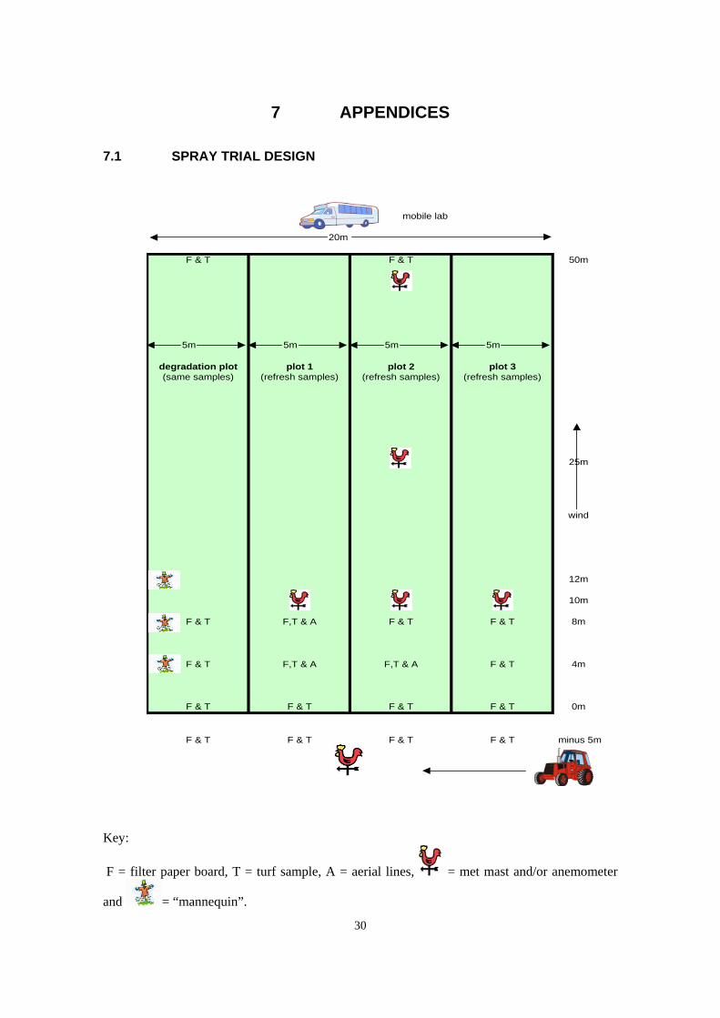
7.1
7 APPENDICES
SPRAY TRIAL DESIGN
mobile lab
20m
F & T F & T
5m 5m 5m 5m
degradation plot plot 1 plot 2 plot 3 (same samples) (refresh samples) (refresh samples) (refresh samples)
F & T F,T & A F & T F & T
F & T F,T & A F,T & A F & T
F & T F & T F & T F & T
50m
25m
wind
12m
10m
8m
4m
0m
F & T F & T minus 5m F & T F & T
Key:
F = filter paper board, T = turf sample, A = aerial lines, = met mast and/or anemometer
and = “mannequin”.
30
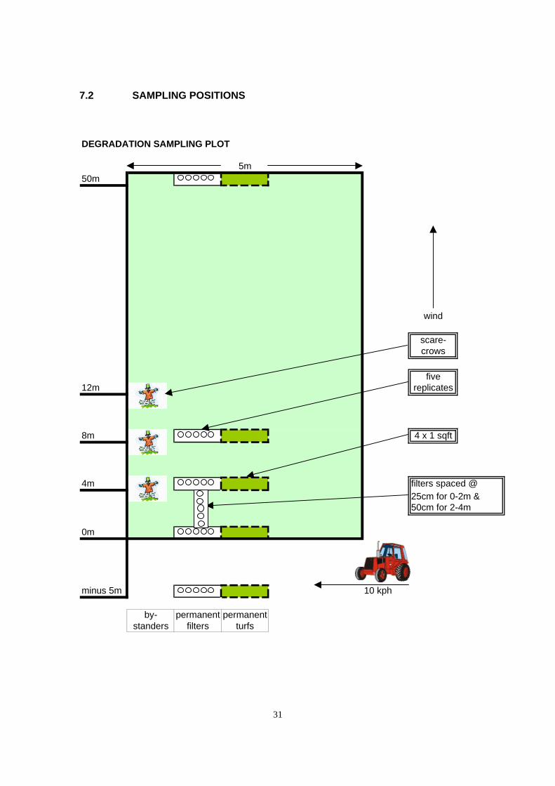
7.2 SAMPLING POSITIONS
DEGRADATION SAMPLING PLOT
5m 50m
crows
12m
8m
4m
0m
wind
scare
five replicates
4 x 1 sqft
filters spaced @ 25cm for 0-2m & 50cm for 2-4m
minus 5m 10 kph
by- permanent permanent standers filters turfs
31
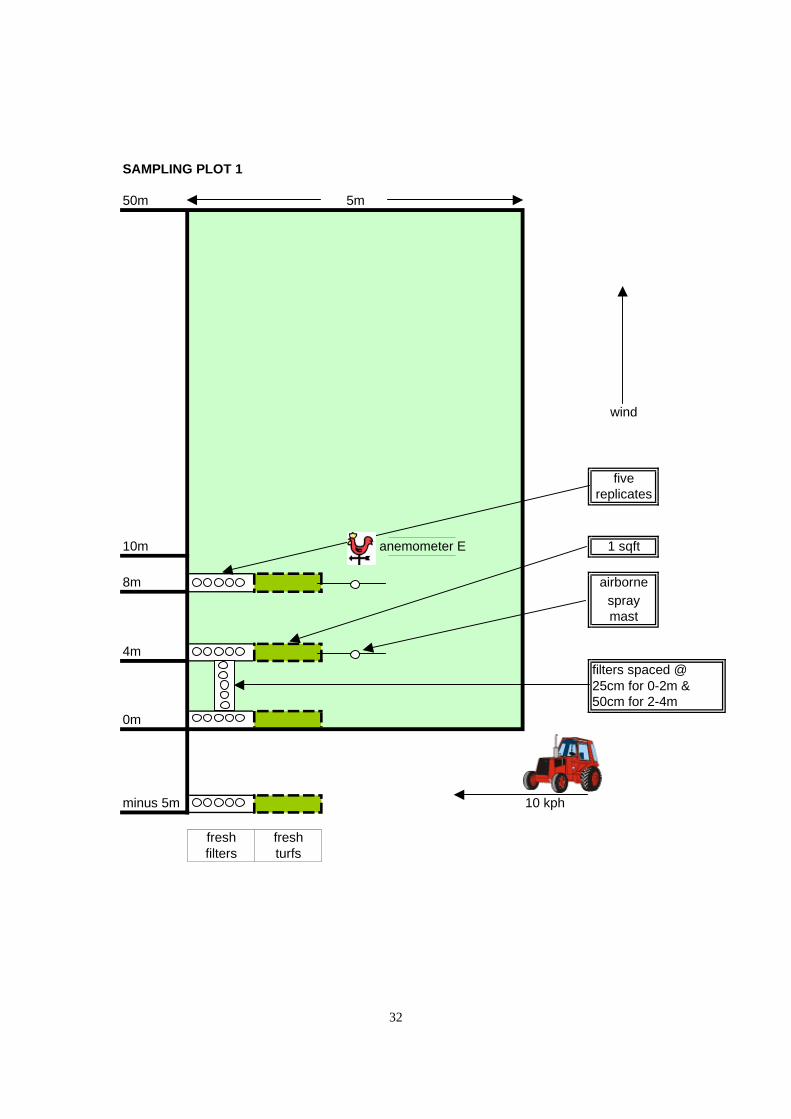
SAMPLING PLOT 1
50m
10m
8m spray
4m
0m
5m
wind
five replicates
anemometer E 1 sqft
airborne
mast
filters spaced @ 25cm for 0-2m & 50cm for 2-4m
minus 5m 10 kph
fresh fresh filters turfs
32
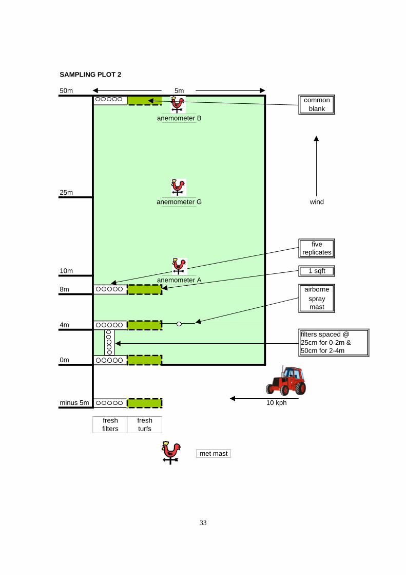
SAMPLING PLOT 2
50m
blank
25m
10m
8m spray
4m
0m
5m common
anemometer B
anemometer G wind
five replicates
1 sqft anemometer A
airborne
mast
filters spaced @ 25cm for 0-2m & 50cm for 2-4m
minus 5m 10 kph
fresh fresh filters turfs
met mast
33
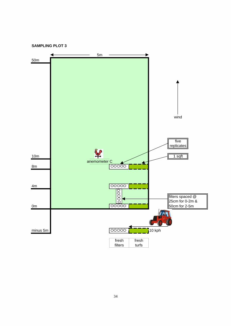
SAMPLING PLOT 3
5m 50m
10m
8m
4m
0m
wind
five replicates
1 sqft anemometer C
filters spaced @ 25cm for 0-2m & 50cm for 2-5m
minus 5m 10 kph
fresh fresh filters turfs
34

SPRAYING CONDITIONS
D 1 2 3 50m
0m
minus 5m
approx. wind direction
65o
N
335o
1. BASF MANTRA epoxiconazole, fenpropimorph & kresoxim methyl (125:150:125 g/l) 2. Tank mix = 333 ml in 180 l water applied at 180 l/ha 3. 03 conventional 110o flat fan nozzles at 3 bar 4. 8 kmph forward speed 5. Boom height 0.7m above grass 6. 24m sprayer 7. Spray times; pass 1 12:09:55-12:10:03
pass 2 13:18:29-13:18:38 pass 3 14:41:44-14:41:52
VEGETATION
1. Turfs approx. 1 sqft 2. Replaced in plots 1,2 & 3 after each pass 3. Remain in plot D for all three passes 4. Positioned at -5m, 0m, 4m & 8m for all plots (x4 for plot D) 5. "Blank" at 50m in plots D & 2 6. Degradation samples taken at t=0, t=4d, t=7d & t=14d 7. Turfs sampled by cutting grass 8. Samples kept in a cool box and transfered to a freezer at HSL 9. Degradation turfs kept on balcony at HSL, exposed to general weather conditions
DEVICES
1. 90mm dia. GF/A filters stapled flat on wooden planks 2. Replaced in plots 1,2 & 3 after each pass 3. Remain in degradation plot for all three passes 4. Positioned at -5m, 0m, 4m & 8m for all plots & "blanks" at 50m in plots D & 2 5. 5 replicates at each sampling point 6. Additional single samples every 25cm between 0 & 2m & every 50cm between 2 & 4m
35

7. At -5m, 3 filters were used at each point to prevent breakthrough, all 3 sampled 8. Plots 1& 2 had samples down the left hand side, plot 3 on the right and plot D central 9. Filters desorbed into 20ml cyclohexane on site and transferred to a freezer at HSL
OTHER SAMPLES
1. Tank mix (from nozzles) 2. Mannequins (Tyvek suits mounted onto wooden cross) at 4m, 8m & 12m in plot D 3. 2 x 11m drift lines (2 mm) at 4m in plots 1 & 2 & 8m in plot 1 4. Tyvek suits, gloves (nitrile & cotton) and over-boots worn during sample collection
PHYSICAL & INSTRUMENTAL MEASUREMENTS
1. 5 remote logging anemometers 2m high; Anemometer E at 10m in plot 1 Anemometer A at 10m in plot 2 Anemometer C at 10m in plot 3 Anemometer G at 25m in plot 2 Anemometer B at 50m in plot 2
2. 10 m met mast up-wind from sampling site 3. Videos & stills
36
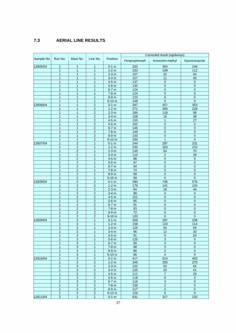
7.3 AERIAL LINE RESULTS
Sample No. Run No. Mast No. Line No. Position Corrected result (ng/device)
Fenpropimorph Kresoxim-methyl Epoxiconazole
12605/04 1 1 1 0-1 m 320 304 246 1 1 1 1-2 m 233 108 112 1 1 1 2-3 m 157 32 54 1 1 1 3-4 m 157 11 40 1 1 1 4-5 m 137 0 0 1 1 1 5-6 m 135 0 0 1 1 1 6-7 m 124 0 0 1 1 1 7-8 m 124 0 0 1 1 1 8-9 m 123 0 0 1 1 1 9-10 m 148 0 0
12606/04 1 1 2 0-1 m 397 457 353 1 1 2 1-2 m 271 300 228 1 1 2 2-3 m 184 118 98 1 1 2 3-4 m 158 16 38 1 1 2 4-5 m 155 1 27 1 1 2 5-6 m 162 0 0 1 1 2 6-7 m 145 0 0 1 1 2 7-8 m 149 0 0 1 1 2 8-9 m 133 0 0 1 1 2 9-10 m 230 1 0
12607/04 1 2 1 0-1 m 244 297 231 1 2 1 1-2 m 235 263 210 1 2 1 2-3 m 135 54 70 1 2 1 3-4 m 110 2 28 1 2 1 4-5 m 88 0 0 1 2 1 5-6 m 97 0 0 1 2 1 6-7 m 94 0 0 1 2 1 7-8 m 74 0 0 1 2 1 8-9 m 99 0 0 1 2 1 9-10 m 99 0 0
12608/04 1 2 2 0-1 m 390 746 576 1 2 2 1-2 m 179 141 134 1 2 2 2-3 m 94 18 44 1 2 2 3-4 m 89 0 0 1 2 2 4-5 m 101 0 0 1 2 2 5-6 m 85 0 0 1 2 2 6-7 m 91 0 0 1 2 2 7-8 m 93 0 0 1 2 2 8-9 m 72 0 0 1 2 2 9-10 m 133 0 0
12609/04 1 3 1 0-1 m 358 287 238 1 3 1 1-2 m 158 123 114 1 3 1 2-3 m 126 54 54 1 3 1 3-4 m 96 12 33 1 3 1 4-5 m 91 0 29 1 3 1 5-6 m 125 3 0 1 3 1 6-7 m 90 3 0 1 3 1 7-8 m 98 3 0 1 3 1 8-9 m 80 2 0 1 3 1 9-10 m 96 4 0
12610/04 1 3 2 0-1 m 417 514 403 1 3 2 1-2 m 346 355 275 1 3 2 2-3 m 152 53 64 1 3 2 3-4 m 125 20 41 1 3 2 4-5 m 111 7 29 1 3 2 5-6 m 118 6 0 1 3 2 6-7 m 116 3 0 1 3 2 7-8 m 136 2 0 1 3 2 8-9 m 117 2 0 1 3 2 9-10 m 125 5 0
12611/04 2 1 1 0-1 m 631 317 232
37
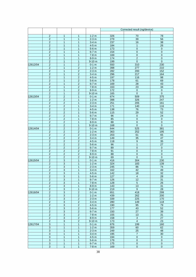
Corrected result (ng/device)
2 1 1 1-2 m 326 70 78 2 1 1 2-3 m 279 39 56 2 1 1 3-4 m 237 16 38 2 1 1 4-5 m 184 1 26 2 1 1 5-6 m 173 0 0 2 1 1 6-7 m 154 0 0 2 1 1 7-8 m 169 0 0 2 1 1 8-9 m 174 2 0 2 1 1 9-10 m 199 0 0
12612/04 2 1 2 0-1 m 550 310 230 2 1 2 1-2 m 398 277 210 2 1 2 2-3 m 282 200 152 2 1 2 3-4 m 296 217 164 2 1 2 4-5 m 197 116 98 2 1 2 5-6 m 178 61 69 2 1 2 6-7 m 169 28 43 2 1 2 7-8 m 163 23 34 2 1 2 8-9 m 172 0 0 2 1 2 9-10 m 165 0 0
12613/04 2 2 1 0-1 m 674 509 375 2 2 1 1-2 m 398 326 247 2 2 1 2-3 m 251 205 161 2 2 1 3-4 m 171 140 116 2 2 1 4-5 m 138 76 73 2 2 1 5-6 m 115 29 52 2 2 1 6-7 m 96 0 24 2 2 1 7-8 m 85 0 0 2 2 1 8-9 m 88 0 0 2 2 1 9-10 m 168 0 0
12614/04 2 2 2 0-1 m 644 525 381 2 2 2 1-2 m 363 252 195 2 2 2 2-3 m 203 61 65 2 2 2 3-4 m 149 35 47 2 2 2 4-5 m 118 9 35 2 2 2 5-6 m 96 1 27 2 2 2 6-7 m 89 0 0 2 2 2 7-8 m 91 0 0 2 2 2 8-9 m 88 0 0 2 2 2 9-10 m 69 0 0
12615/04 2 3 1 0-1 m 416 304 230 2 3 1 1-2 m 324 183 139 2 3 1 2-3 m 245 86 74 2 3 1 3-4 m 162 42 49 2 3 1 4-5 m 142 18 32 2 3 1 5-6 m 127 4 28 2 3 1 6-7 m 126 12 31 2 3 1 7-8 m 128 5 26 2 3 1 8-9 m 143 13 31 2 3 1 9-10 m 219 9 28
12616/04 2 3 2 0-1 m 651 418 299 2 3 2 1-2 m 439 262 200 2 3 2 2-3 m 339 225 170 2 3 2 3-4 m 280 149 118 2 3 2 4-5 m 190 95 79 2 3 2 5-6 m 177 43 52 2 3 2 6-7 m 150 27 39 2 3 2 7-8 m 155 13 31 2 3 2 8-9 m 158 3 27 2 3 2 9-10 m 173 4 23
12617/04 3 1 1 0-1 m 676 199 160 3 1 1 1-2 m 359 60 62 3 1 1 2-3 m 249 25 48 3 1 1 3-4 m 195 7 30 3 1 1 4-5 m 194 0 0 3 1 1 5-6 m 179 0 0 3 1 1 6-7 m 175 0 0 3 1 1 7-8 m 169 0 0
38
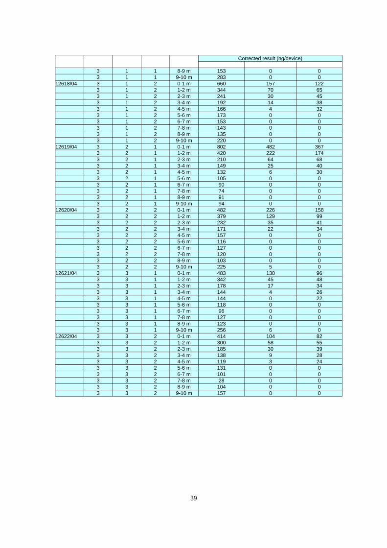
Corrected result (ng/device)
3 1 1 8-9 m 153 0 0 3 1 1 9-10 m 283 0 0
12618/04 3 1 2 0-1 m 660 157 122 3 1 2 1-2 m 344 70 65 3 1 2 2-3 m 241 30 45 3 1 2 3-4 m 192 14 38 3 1 2 4-5 m 166 4 32 3 1 2 5-6 m 173 0 0 3 1 2 6-7 m 153 0 0 3 1 2 7-8 m 143 0 0 3 1 2 8-9 m 135 0 0 3 1 2 9-10 m 220 0 0
12619/04 3 2 1 0-1 m 802 482 367 3 2 1 1-2 m 420 222 174 3 2 1 2-3 m 210 64 68 3 2 1 3-4 m 149 25 40 3 2 1 4-5 m 132 6 30 3 2 1 5-6 m 105 0 0 3 2 1 6-7 m 90 0 0 3 2 1 7-8 m 74 0 0 3 2 1 8-9 m 91 0 0 3 2 1 9-10 m 94 0 0
12620/04 3 2 2 0-1 m 482 226 158 3 2 2 1-2 m 379 129 99 3 2 2 2-3 m 232 35 41 3 2 2 3-4 m 171 22 34 3 2 2 4-5 m 157 0 0 3 2 2 5-6 m 116 0 0 3 2 2 6-7 m 127 0 0 3 2 2 7-8 m 120 0 0 3 2 2 8-9 m 103 0 0 3 2 2 9-10 m 225 5 0
12621/04 3 3 1 0-1 m 483 130 96 3 3 1 1-2 m 342 45 48 3 3 1 2-3 m 178 17 34 3 3 1 3-4 m 144 4 26 3 3 1 4-5 m 144 0 22 3 3 1 5-6 m 118 0 0 3 3 1 6-7 m 96 0 0 3 3 1 7-8 m 127 0 0 3 3 1 8-9 m 123 0 0 3 3 1 9-10 m 256 6 0
12622/04 3 3 2 0-1 m 414 104 82 3 3 2 1-2 m 300 58 55 3 3 2 2-3 m 185 30 39 3 3 2 3-4 m 138 9 28 3 3 2 4-5 m 119 3 24 3 3 2 5-6 m 131 0 0 3 3 2 6-7 m 101 0 0 3 3 2 7-8 m 28 0 0 3 3 2 8-9 m 104 0 0 3 3 2 9-10 m 157 0 0
39

7.4 FILTER PAPER SAMPLER RESULTS (KRESOXIM-METHYL)
Run 1 data
RUN 1 µg/filterDistance Sample detail Sample Numbers
Ave result lt % of APP* %RSD
Plot1 88.5 28.30 31.98 50.28 120.86 11.50 Plot2 88.5 25.90 29.27 46.01 110.61 8.00Minus
5m Plot3 88.5 24.40 27.57 43.35 104.21 8.70 Plot1 88.5 14.10 15.93 25.05 60.22 17.70 Plot2 88.5 12.60 14.24 22.39 53.81 6.600m Plot3 88.5 11.50 12.99 20.43 49.11 14.00 Plot1 12184/04 88.5 4.07 4.60 7.23 17.38 Plot2 12215/04 88.5 6.16 6.96 10.94 26.310.25m Plot3 12251/04 88.5 x x x x Plot1 12185/04 88.5 2.92 3.30 5.19 12.47 Plot2 12216/04 88.5 6.11 6.90 10.86 26.090.5m Plot3 12252/04 88.5 x x x x Plot1 12186/04 88.5 0.72 0.81 1.28 3.07 Plot2 12217/04 88.5 2.84 3.21 5.05 12.130.75m Plot3 12253/04 88.5 x x x x Plot1 12187/04 88.5 0.84 0.95 1.49 3.59 Plot2 12218/04 88.5 1.35 1.53 2.40 5.771m Plot3 12254/04 88.5 x x x x Plot1 12188/04 88.5 0.26 0.29 0.46 1.11 Plot2 12219/04 88.5 0.75 0.85 1.33 3.201.25m Plot3 12255/04 88.5 x x x x Plot1 12189/04 88.5 0.41 0.46 0.73 1.75 Plot2 12220/04 88.5 0.79 0.89 1.40 3.371.5m Plot3 12256/04 88.5 x x x x Plot1 12190/04 88.5 0.23 0.26 0.41 0.98 Plot2 12221/04 88.5 0.86 0.97 1.53 3.671.75m Plot3 12257/04 88.5 x x x x Plot1 12191/04 88.5 0.30 0.34 0.53 1.28 Plot2 12222/04 88.5 0.65 0.73 1.15 2.782m Plot3 12258/04 88.5 x x x x Plot1 12192/04 88.5 0.28 0.32 0.50 1.20 Plot2 12223/04 88.5 0.30 0.34 0.53 1.282.5m Plot3 12259/04 88.5 0.37 0.42 0.66 1.58 Plot1 12193/04 88.5 0.22 0.25 0.39 0.94 Plot2 12224/04 88.5 0.28 0.32 0.50 1.203m Plot3 12260/04 88.5 0.25 0.28 0.44 1.07 Plot1 12194/04 88.5 0.20 0.23 0.36 0.85 Plot2 12225/04 88.5 0.23 0.26 0.41 0.983.5m Plot3 12261/04 88.5 0.20 0.23 0.36 0.85 Plot1 88.5 0.10 0.11 0.18 0.43 20.50 Plot2 88.5 0.15 0.17 0.27 0.64 6.004m Plot3 88.5 0.22 0.25 0.39 0.94 14.70 Plot1 88.5 0.17 0.19 0.30 0.73 14.50 Plot2 88.5 0.05 0.06 0.09 0.21 16.008m Plot3 88.5 0.13 0.15 0.23 0.56 11.40
50m Plot2 88.5 0.00 0.00 0.00 0.00 LOD 88.5 0.01 0.01 0.01 0.03
% Recovery Corrected resu
g per hectare
12174-8/04 12205-9/04
12246-50/04 12179-83/04 12210-4/04
12246-50/04
12195-9/04 12226-30/04 12262-6/04 12200-4/04 12231-5/04
12267-71/04 12236-40/04
Footnotes
*Theoretical application rate (APP) for Kresoxim-methyl (125 g/l, mixed 333 ml to 180 l in water and sprayed at 180 l/ha) = 125*333/1000 = 41.6 g/ha.
-5m, 0m, 4m and 8m, %RSD figures are for 5 replicate samples.
40
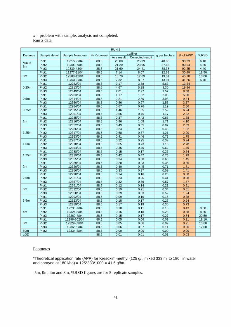
x = problem with sample, analysis not completed. Run 2 data
RUN 2 µg/filterDistance Sample detail Sample Numbers
Ave result lt % of APP* %RSD
Plot1 88.5 23.00 25.99 40.86 98.23 6.10 Plot2 88.5 21.20 23.95 37.66 90.54 4.60Minus
5m Plot3 88.5 21.60 24.41 38.38 92.25 4.40 Plot1 88.5 7.14 8.07 12.69 30.49 18.50 Plot2 88.5 10.70 12.09 19.01 45.70 10.000m Plot3 88.5 7.32 8.27 13.01 31.26 6.70 Plot1 12282/04 88.5 3.17 3.58 5.63 13.54 Plot2 12313/04 88.5 4.67 5.28 8.30 19.940.25m Plot3 12349/04 88.5 2.01 2.27 3.57 8.58 Plot1 12283/04 88.5 1.17 1.32 2.08 5.00 Plot2 12314/04 88.5 2.21 2.50 3.93 9.440.5m Plot3 12350/04 88.5 0.86 0.97 1.53 3.67 Plot1 12284/04 88.5 0.67 0.76 1.19 2.86 Plot2 12315/04 88.5 1.46 1.65 2.59 6.240.75m Plot3 12351/04 88.5 0.66 0.75 1.17 2.82 Plot1 12285/04 88.5 0.37 0.42 0.66 1.58 Plot2 12316/04 88.5 0.96 1.08 1.71 4.101m Plot3 12352/04 88.5 0.49 0.55 0.87 2.09 Plot1 12286/04 88.5 0.24 0.27 0.43 1.02 Plot2 12317/04 88.5 0.68 0.77 1.21 2.901.25m Plot3 12353/04 88.5 0.41 0.46 0.73 1.75 Plot1 12287/04 88.5 0.22 0.25 0.39 0.94 Plot2 12318/04 88.5 0.65 0.73 1.15 2.781.5m Plot3 12354/04 88.5 0.35 0.40 0.62 1.49 Plot1 12288/04 88.5 0.15 0.17 0.27 0.64 Plot2 12319/04 88.5 0.42 0.47 0.75 1.791.75m Plot3 12355/04 88.5 0.34 0.38 0.60 1.45 Plot1 12289/04 88.5 0.20 0.23 0.36 0.85 Plot2 12320/04 88.5 0.40 0.45 0.71 1.712m Plot3 12356/04 88.5 0.33 0.37 0.59 1.41 Plot1 12290/04 88.5 0.14 0.16 0.25 0.60 Plot2 12321/04 88.5 0.23 0.26 0.41 0.982.5m Plot3 12357/04 88.5 0.32 0.36 0.57 1.37 Plot1 12291/04 88.5 0.12 0.14 0.21 0.51 Plot2 12322/04 88.5 0.19 0.21 0.34 0.813m Plot3 12358/04 88.5 0.29 0.33 0.52 1.24 Plot1 12292/04 88.5 0.09 0.10 0.16 0.38 Plot2 12323/04 88.5 0.15 0.17 0.27 0.643.5m Plot3 12359/04 88.5 0.17 0.19 0.30 0.73 Plot1 88.5 0.10 0.11 0.18 0.43 9.80 Plot2 88.5 0.16 0.18 0.28 0.68 8.504m Plot3 88.5 0.15 0.17 0.27 0.64 20.50 Plot1 88.5 0.05 0.06 0.09 0.21 19.10 Plot2 88.5 0.05 0.06 0.09 0.21 10.608m Plot3 88.5 0.06 0.07 0.11 0.26 12.00
50m Plot2 88.5 0.00 0.00 0.00 0.00 LOD 88.5 0.01 0.01 0.01 0.03
% Recovery Corrected resu
g per hectare
12272-6/04 12303-7/04
12339-43/04 12277-81/04 12308-12/04 12344-8/04
12293-7/04 12324-8/04 12360-4/04
12298-302/04 12329-33/04 12365-9/04 12334-8/04
Footnotes
*Theoretical application rate (APP) for Kresoxim-methyl (125 g/l, mixed 333 ml to 180 l in water and sprayed at 180 l/ha) = 125*333/1000 = 41.6 g/ha.
-5m, 0m, 4m and 8m, %RSD figures are for 5 replicate samples.
41
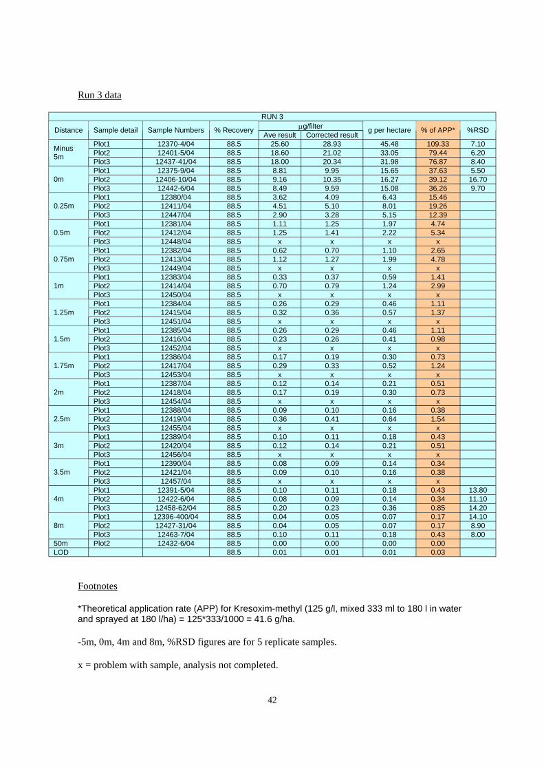
Run 3 data
Distance
Minus 5m
0m
0.25m
0.5m
0.75m
1m
1.25m
1.5m
1.75m
2m
2.5m
3m
3.5m
4m
8m
50m LOD
Sample detail
Plot1 Plot2 Plot3 Plot1 Plot2 Plot3 Plot1 Plot2 Plot3 Plot1 Plot2 Plot3 Plot1 Plot2 Plot3 Plot1 Plot2 Plot3 Plot1 Plot2 Plot3 Plot1 Plot2 Plot3 Plot1 Plot2 Plot3 Plot1 Plot2 Plot3 Plot1 Plot2 Plot3 Plot1 Plot2 Plot3 Plot1 Plot2 Plot3 Plot1 Plot2 Plot3 Plot1 Plot2 Plot3 Plot2
Sample Numbers
12370-4/04 12401-5/04
12437-41/04 12375-9/04
12406-10/04 12442-6/04 12380/04 12411/04 12447/04 12381/04 12412/04 12448/04 12382/04 12413/04 12449/04 12383/04 12414/04 12450/04 12384/04 12415/04 12451/04 12385/04 12416/04 12452/04 12386/04 12417/04 12453/04 12387/04 12418/04 12454/04 12388/04 12419/04 12455/04 12389/04 12420/04 12456/04 12390/04 12421/04 12457/04
12391-5/04 12422-6/04
12458-62/04 12396-400/04 12427-31/04 12463-7/04 12432-6/04
RUN 3 µg/filter% Recovery
Ave result Corrected result 88.5 25.60 28.93 88.5 18.60 21.02 88.5 18.00 20.34 88.5 8.81 9.95 88.5 9.16 10.35 88.5 8.49 9.59 88.5 3.62 4.09 88.5 4.51 5.10 88.5 2.90 3.28 88.5 1.11 1.25 88.5 1.25 1.41 88.5 x x 88.5 0.62 0.70 88.5 1.12 1.27 88.5 x x 88.5 0.33 0.37 88.5 0.70 0.79 88.5 x x 88.5 0.26 0.29 88.5 0.32 0.36 88.5 x x 88.5 0.26 0.29 88.5 0.23 0.26 88.5 x x 88.5 0.17 0.19 88.5 0.29 0.33 88.5 x x 88.5 0.12 0.14 88.5 0.17 0.19 88.5 x x 88.5 0.09 0.10 88.5 0.36 0.41 88.5 x x 88.5 0.10 0.11 88.5 0.12 0.14 88.5 x x 88.5 0.08 0.09 88.5 0.09 0.10 88.5 x x 88.5 0.10 0.11 88.5 0.08 0.09 88.5 0.20 0.23 88.5 0.04 0.05 88.5 0.04 0.05 88.5 0.10 0.11 88.5 0.00 0.00 88.5 0.01 0.01
g per hectare
45.48 33.05 31.98 15.65 16.27 15.08 6.43 8.01 5.15 1.97 2.22
x 1.10 1.99
x 0.59 1.24
x 0.46 0.57
x 0.46 0.41
x 0.30 0.52
x 0.21 0.30
x 0.16 0.64
x 0.18 0.21
x 0.14 0.16
x 0.18 0.14 0.36 0.07 0.07 0.18 0.00 0.01
% of APP*
109.33 79.44 76.87 37.63 39.12 36.26 15.46 19.26 12.39 4.74 5.34
x 2.65 4.78
x 1.41 2.99
x 1.11 1.37
x 1.11 0.98
x 0.73 1.24
x 0.51 0.73
x 0.38 1.54
x 0.43 0.51
x 0.34 0.38
x 0.43 0.34 0.85 0.17 0.17 0.43 0.00 0.03
%RSD
7.10 6.20 8.40 5.50
16.70 9.70
13.80 11.10 14.20 14.10 8.90 8.00
Footnotes
*Theoretical application rate (APP) for Kresoxim-methyl (125 g/l, mixed 333 ml to 180 l in water and sprayed at 180 l/ha) = 125*333/1000 = 41.6 g/ha.
-5m, 0m, 4m and 8m, %RSD figures are for 5 replicate samples.
x = problem with sample, analysis not completed.
42
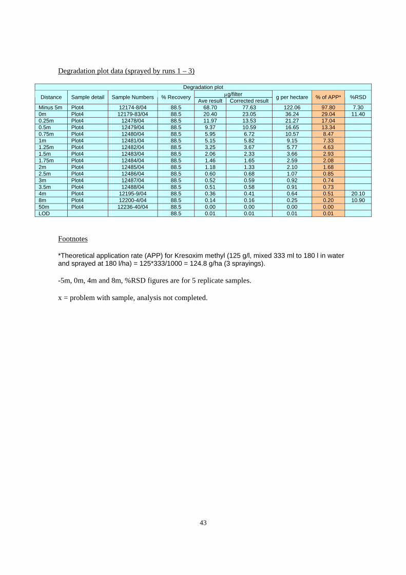
Degradation plot data (sprayed by runs 1 – 3)
Degradation plot µg/filterDistance Sample detail Sample Numbers
Ave result lt % of APP* %RSD
Minus 5m Plot4 88.5 68.70 77.63 122.06 97.80 7.30 0m Plot4 88.5 20.40 23.05 36.24 29.04 11.40 0.25m Plot4 12478/04 88.5 11.97 13.53 21.27 17.04 0.5m Plot4 12479/04 88.5 9.37 10.59 16.65 13.34 0.75m Plot4 12480/04 88.5 5.95 6.72 10.57 8.47 1m Plot4 12481/04 88.5 5.15 5.82 9.15 7.33 1.25m Plot4 12482/04 88.5 3.25 3.67 5.77 4.63 1.5m Plot4 12483/04 88.5 2.06 2.33 3.66 2.93 1.75m Plot4 12484/04 88.5 1.46 1.65 2.59 2.08 2m Plot4 12485/04 88.5 1.18 1.33 2.10 1.68 2.5m Plot4 12486/04 88.5 0.60 0.68 1.07 0.85 3m Plot4 12487/04 88.5 0.52 0.59 0.92 0.74 3.5m Plot4 12488/04 88.5 0.51 0.58 0.91 0.73 4m Plot4 88.5 0.36 0.41 0.64 0.51 20.10 8m Plot4 88.5 0.14 0.16 0.25 0.20 10.90 50m Plot4 88.5 0.00 0.00 0.00 0.00 LOD 88.5 0.01 0.01 0.01 0.01
% Recovery Corrected resu
g per hectare
12174-8/04 12179-83/04
12195-9/04 12200-4/04
12236-40/04
Footnotes
*Theoretical application rate (APP) for Kresoxim methyl (125 g/l, mixed 333 ml to 180 l in water and sprayed at 180 l/ha) = 125*333/1000 = 124.8 g/ha (3 sprayings).
-5m, 0m, 4m and 8m, %RSD figures are for 5 replicate samples.
x = problem with sample, analysis not completed.
43
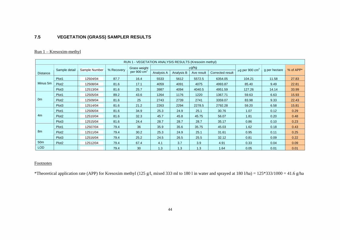
7.5 VEGETATION (GRASS) SAMPLER RESULTS
Run 1 – Kresoxim-methyl
Distance
Minus 5m
0m
4m
8m
50m LOD
Sample detail
Plot1 Plot2 Plot3 Plot1 Plot2 Plot3 Plot1 Plot2 Plot3 Plot1 Plot2 Plot3 Plot2
Sample Number
12504/04 12508/04 12513/04 12505/04 12509/04 12514/04 12506/04 12510/04 12515/04 12507/04 12511/04 12516/04 12512/04
RUN 1 - VEGETATION ANALYSIS RESULTS (Kresoxim methyl)
µg/kg% Recovery Grass weight
per 900 cm2 Analysis A Analysis B Ave result Corrected result
87.7 16.4 5533 5612 5572.5 6354.05 81.6 17.1 4059 4091 4075 4993.87 81.6 25.7 3987 4094 4040.5 4951.59 89.2 43.6 1264 1176 1220 1367.71 81.6 25 2743 2739 2741 3359.07 81.6 21.2 2263 2294 2278.5 2792.28 81.6 34.9 25.3 24.9 25.1 30.76 81.6 32.3 45.7 45.8 45.75 56.07 81.6 24.4 28.7 28.7 28.7 35.17 79.4 36 35.9 35.6 35.75 45.03 79.4 30.2 25.3 24.9 25.1 31.61 79.4 25.2 24.5 26.5 25.5 32.12 79.4 67.4 4.1 3.7 3.9 4.91 79.4 30 1.3 1.3 1.3 1.64
µg per 900 cm2
104.21 85.40
127.26 59.63 83.98 59.20 1.07 1.81 0.86 1.62 0.95 0.81 0.33 0.05
g per hectare
11.58 9.49
14.14 6.63 9.33 6.58 0.12 0.20 0.10 0.18 0.11 0.09 0.04 0.01
% of APP*
27.83 22.81 33.99 15.93 22.43 15.81 0.29 0.48 0.23 0.43 0.25 0.22 0.09 0.01
Footnotes
*Theoretical application rate (APP) for Kresoxim methyl (125 g/l, mixed 333 ml to 180 l in water and sprayed at 180 l/ha) = 125*333/1000 = 41.6 g/ha
44
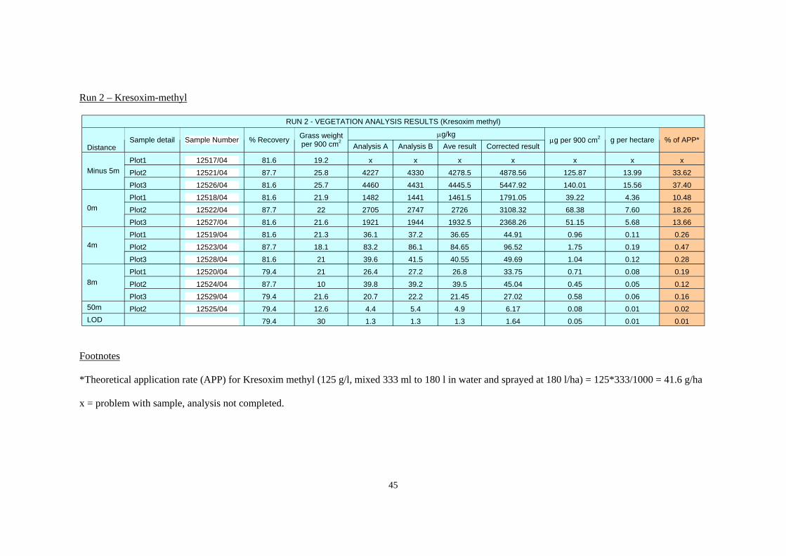
Run 2 – Kresoxim-methyl
Distance
Minus 5m
0m
4m
8m
50m LOD
Sample detail
Plot1 Plot2 Plot3 Plot1 Plot2 Plot3 Plot1 Plot2 Plot3 Plot1 Plot2 Plot3 Plot2
Sample Number
12517/04 12521/04 12526/04 12518/04 12522/04 12527/04 12519/04 12523/04 12528/04 12520/04 12524/04 12529/04 12525/04
RUN 2 - VEGETATION ANALYSIS RESULTS (Kresoxim methyl)
µg/kg% Recovery Grass weight
per 900 cm2 Analysis A Analysis B Ave result Corrected result
81.6 19.2 x x x x 87.7 25.8 4227 4330 4278.5 4878.56 81.6 25.7 4460 4431 4445.5 5447.92 81.6 21.9 1482 1441 1461.5 1791.05 87.7 22 2705 2747 2726 3108.32 81.6 21.6 1921 1944 1932.5 2368.26 81.6 21.3 36.1 37.2 36.65 44.91 87.7 18.1 83.2 86.1 84.65 96.52 81.6 21 39.6 41.5 40.55 49.69 79.4 21 26.4 27.2 26.8 33.75 87.7 10 39.8 39.2 39.5 45.04 79.4 21.6 20.7 22.2 21.45 27.02 79.4 12.6 4.4 5.4 4.9 6.17 79.4 30 1.3 1.3 1.3 1.64
µg per 900 cm2
x 125.87 140.01 39.22 68.38 51.15 0.96 1.75 1.04 0.71 0.45 0.58 0.08 0.05
g per hectare
x 13.99 15.56 4.36 7.60 5.68 0.11 0.19 0.12 0.08 0.05 0.06 0.01 0.01
% of APP*
x 33.62 37.40 10.48 18.26 13.66 0.26 0.47 0.28 0.19 0.12 0.16 0.02 0.01
Footnotes
*Theoretical application rate (APP) for Kresoxim methyl (125 g/l, mixed 333 ml to 180 l in water and sprayed at 180 l/ha) = 125*333/1000 = 41.6 g/ha
x = problem with sample, analysis not completed.
45
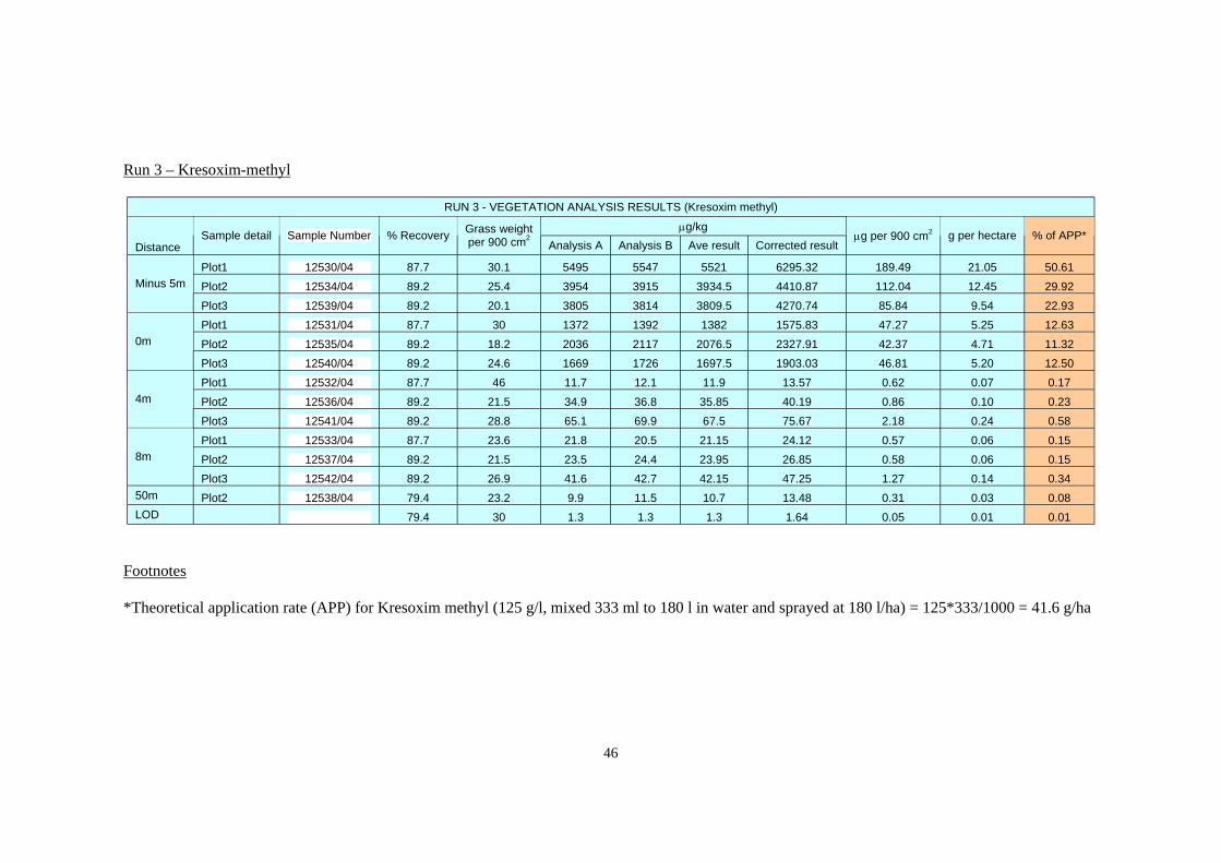
Run 3 – Kresoxim-methyl
Distance
Minus 5m
0m
4m
8m
50m LOD
Sample detail
Plot1 Plot2 Plot3 Plot1 Plot2 Plot3 Plot1 Plot2 Plot3 Plot1 Plot2 Plot3 Plot2
Sample Number
12530/04 12534/04 12539/04 12531/04 12535/04 12540/04 12532/04 12536/04 12541/04 12533/04 12537/04 12542/04 12538/04
RUN 3 - VEGETATION ANALYSIS RESULTS (Kresoxim methyl)
µg/kg% Recovery Grass weight
per 900 cm2 Analysis A Analysis B Ave result Corrected result
87.7 30.1 5495 5547 5521 6295.32 89.2 25.4 3954 3915 3934.5 4410.87 89.2 20.1 3805 3814 3809.5 4270.74 87.7 30 1372 1392 1382 1575.83 89.2 18.2 2036 2117 2076.5 2327.91 89.2 24.6 1669 1726 1697.5 1903.03 87.7 46 11.7 12.1 11.9 13.57 89.2 21.5 34.9 36.8 35.85 40.19 89.2 28.8 65.1 69.9 67.5 75.67 87.7 23.6 21.8 20.5 21.15 24.12 89.2 21.5 23.5 24.4 23.95 26.85 89.2 26.9 41.6 42.7 42.15 47.25 79.4 23.2 9.9 11.5 10.7 13.48 79.4 30 1.3 1.3 1.3 1.64
µg per 900 cm2
189.49 112.04 85.84 47.27 42.37 46.81 0.62 0.86 2.18 0.57 0.58 1.27 0.31 0.05
g per hectare
21.05 12.45 9.54 5.25 4.71 5.20 0.07 0.10 0.24 0.06 0.06 0.14 0.03 0.01
% of APP*
50.61 29.92 22.93 12.63 11.32 12.50 0.17 0.23 0.58 0.15 0.15 0.34 0.08 0.01
Footnotes
*Theoretical application rate (APP) for Kresoxim methyl (125 g/l, mixed 333 ml to 180 l in water and sprayed at 180 l/ha) = 125*333/1000 = 41.6 g/ha
46
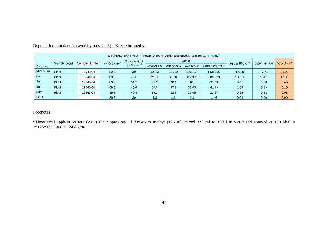
Degradation plot data (sprayed by runs 1 – 3) – Kresoxim-methyl
Distance Minus 5m 0m 4m 8m 50m LOD
Sample detail
Plot4 Plot4 Plot4 Plot4 Plot4
Sample Number
12543/04 12544/04 12545/04 12546/04 12547/04
DEGRADATION PLOT - VEGETATION ANALYSIS RESULTS (Kresoxim methyl)
µg/kg% Recovery Grass weight
per 900 cm2 Analysis A Analysis B Ave result Corrected result
89.3 30 12853 12710 12781.5 14312.99 89.3 46.6 2559 2620 2589.5 2899.78 89.9 51.2 85.9 90.1 88 97.89 89.3 40.4 36.9 37.2 37.05 41.49 89.3 40.4 19.3 22.8 21.05 23.57 89.3 30 1.3 1.3 1.3 1.46
µg per 900 cm2
429.39 135.13
5.01 1.68 0.95 0.04
g per hectare
47.71 15.01 0.56 0.19 0.11 0.00
% of APP*
38.23 12.03 0.45 0.15 0.08 0.00
Footnotes
*Theoretical application rate (APP) for 3 sprayings of Kresoxim methyl (125 g/l, mixed 333 ml to 180 l in water and sprayed at 180 l/ha) = 3*125*333/1000 = 124.8 g/ha.
47
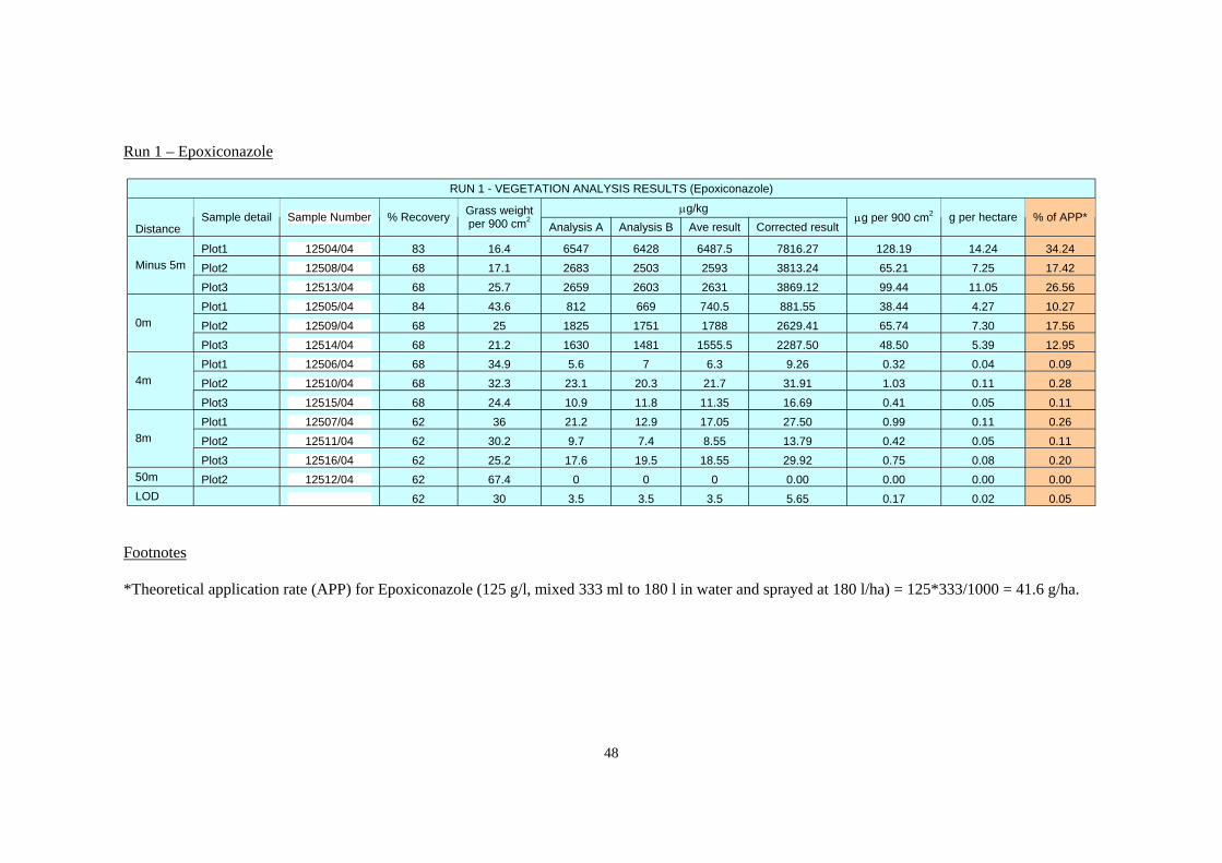
Run 1 – Epoxiconazole
Distance
Minus 5m
0m
4m
8m
50m LOD
Sample detail
Plot1 Plot2 Plot3 Plot1 Plot2 Plot3 Plot1 Plot2 Plot3 Plot1 Plot2 Plot3 Plot2
Sample Number
12504/04 12508/04 12513/04 12505/04 12509/04 12514/04 12506/04 12510/04 12515/04 12507/04 12511/04 12516/04 12512/04
RUN 1 - VEGETATION ANALYSIS RESULTS (Epoxiconazole)
µg/kg% Recovery Grass weight
per 900 cm2 Analysis A Analysis B Ave result Corrected result
83 16.4 6547 6428 6487.5 7816.27 68 17.1 2683 2503 2593 3813.24 68 25.7 2659 2603 2631 3869.12 84 43.6 812 669 740.5 881.55 68 25 1825 1751 1788 2629.41 68 21.2 1630 1481 1555.5 2287.50 68 34.9 5.6 7 6.3 9.26 68 32.3 23.1 20.3 21.7 31.91 68 24.4 10.9 11.8 11.35 16.69 62 36 21.2 12.9 17.05 27.50 62 30.2 9.7 7.4 8.55 13.79 62 25.2 17.6 19.5 18.55 29.92 62 67.4 0 0 0 0.00 62 30 3.5 3.5 3.5 5.65
µg per 900 cm2
128.19 65.21 99.44 38.44 65.74 48.50 0.32 1.03 0.41 0.99 0.42 0.75 0.00 0.17
g per hectare
14.24 7.25
11.05 4.27 7.30 5.39 0.04 0.11 0.05 0.11 0.05 0.08 0.00 0.02
% of APP*
34.24 17.42 26.56 10.27 17.56 12.95 0.09 0.28 0.11 0.26 0.11 0.20 0.00 0.05
Footnotes
*Theoretical application rate (APP) for Epoxiconazole (125 g/l, mixed 333 ml to 180 l in water and sprayed at 180 l/ha) = 125*333/1000 = 41.6 g/ha.
48

Run 2 – Epoxiconazole
Distance
Minus 5m
0m
4m
8m
50m LOD
Sample detail
Plot1 Plot2 Plot3 Plot1 Plot2 Plot3 Plot1 Plot2 Plot3 Plot1 Plot2 Plot3 Plot2
Sample Number
12517/04 12521/04 12526/04 12518/04 12522/04 12527/04 12519/04 12523/04 12528/04 12520/04 12524/04 12529/04 12525/04
RUN 2 - VEGETATION ANALYSIS RESULTS (Epoxiconazole) µg/kg
% Recovery Grass weight per 900 cm2
Analysis A Analysis B Ave result Corrected result
68 19.2 x x x x 83 25.8 2848 2812 2830 3409.64 68 25.7 2931 3097 3014 4432.35 68 21.9 1085 880 982.5 1444.85 83 22 2014 1838 1926 2320.48 68 21.6 1336 1248 1292 1900.00 68 21.3 14.5 14.2 14.35 21.10 83 18.1 45.5 46.5 46 55.42 68 21 16 21.1 18.55 27.28 62 21 12.3 11.7 12 19.35 83 10 25.3 16.9 21.1 25.42 62 21.6 18.5 17.9 18.2 29.35 62 12.6 0 0 0 0.00 62 30 3.5 3.5 3.5 5.65
µg per 900 cm2
x 87.97
113.91 31.64 51.05 41.04 0.45 1.00 0.57 0.41 0.25 0.63 0.00 0.17
g per hectare
x 9.77
12.66 3.52 5.67 4.56 0.05 0.11 0.06 0.05 0.03 0.07 0.00 0.02
% of APP*
x 23.50 30.43 8.45
13.64 10.96 0.12 0.27 0.15 0.11 0.07 0.17 0.00 0.05
Footnotes
*Theoretical application rate (APP) for Epoxiconazole (125 g/l, mixed 333 ml to 180 l in water and sprayed at 180 l/ha) = 125*333/1000 = 41.6 g/ha
x = problem with sample, analysis not completed.
49

Run 3 – Epoxiconazole
Distance
Minus 5m
0m
4m
8m
50m LOD
Sample detail
Plot1 Plot2 Plot3 Plot1 Plot2 Plot3 Plot1 Plot2 Plot3 Plot1 Plot2 Plot3 Plot2
Sample Number
12530/04 12534/04 12539/04 12531/04 12535/04 12540/04 12532/04 12536/04 12541/04 12533/04 12537/04 12542/04 12538/04
RUN 3 - VEGETATION ANALYSIS RESULTS (Epoxiconazole) µg/kg
% Recovery Grass weight per 900 cm2
Analysis A Analysis B Ave result Corrected result
83 30.1 3726 3467 3596.5 4333.13 84 25.4 2387 2495 2441 2905.95 84 20.1 2396 2659 2527.5 3008.93 83 30 1013 1036 1024.5 1234.34 84 18.2 963 1310 1136.5 1352.98 84 24.6 1199 1752 1475.5 1756.55 83 46 <LOD <LOD <LOD <LOD 84 21.5 13.1 16 14.55 17.32 84 28.8 41.3 49.7 45.5 54.17 83 23.6 14.2 7.6 10.9 13.13 84 21.5 16.1 12.9 14.5 17.26 84 26.9 34.5 23.3 28.9 34.40 62 23.2 0 0 0 0.00 62 30 3.5 3.5 3.5 5.65
µg per 900 cm2
130.43 73.81 60.48 37.03 24.62 43.21 <0.17 0.37 1.56 0.31 0.37 0.93 0.00 0.17
g per hectare
14.49 8.20 6.72 4.11 2.74 4.80
<0.02 0.04 0.17 0.03 0.04 0.10 0.00 0.02
% of APP*
34.84 19.71 16.15 9.89 6.58
11.54 <0.05 0.10 0.42 0.08 0.10 0.25 0.00 0.05
Footnotes
*Theoretical application rate (APP) for Epoxiconazole (125 g/l, mixed 333 ml to 180 l in water and sprayed at 180 l/ha) = 125*333/1000 = 41.6 g/ha
50
Degradation plot data (sprayed by runs 1 – 3) – Epoxiconazole
Distance Minus 5m 0m 4m 8m 50m LOD
Sample detail
Plot4 Plot4 Plot4 Plot4 Plot4
Sample Number
12543/04 12544/04 12545/04 12546/04 12547/04
RUN 3 - VEGETATION ANALYSIS RESULTS (Epoxiconazole) µg/kg
% Recovery Grass weight per 900 cm2
Analysis A Analysis B Ave result Corrected result
67 30 7260 7902 7581 11314.93 67 46.6 1763 1868 1815.5 2709.70 85 51.2 53.2 60.2 56.7 66.71 67 40.4 17.8 25.3 21.55 32.16 67 40.4 0 0 0 0.00 67 30 3 3 3 4.48
µg per 900 cm2
339.45 126.27
3.42 1.30 0.00 0.13
g per hectare
37.72 14.03 0.38 0.14 0.00 0.01
% of APP*
30.22 11.24 0.30 0.12 0.00 0.01
Footnotes
*Theoretical application rate (APP) for 3 sprayings of Epoxiconazole (125 g/l, mixed 333 ml to 180 l in water and sprayed at 180 l/ha) = 3*125*333/1000 = 124.8 g/ha.
51
Run 1 – Fenpropimorph
Distance
Minus 5m
0m
4m
8m
50m LOD
Sample detail
Plot1 Plot2 Plot3 Plot1 Plot2 Plot3 Plot1 Plot2 Plot3 Plot1 Plot2 Plot3 Plot2
Sample Number
12504/04 12508/04 12513/04 12505/04 12509/04 12514/04 12506/04 12510/04 12515/04 12507/04 12511/04 12516/04 12512/04
RUN 1 - VEGETATION ANALYSIS RESULTS (Fenpropimorph)
µg/kg% Recovery Grass weight
per 900 cm2 Analysis A Analysis B Ave result Corrected result
96 16.4 3953 3972 3962.5 4127.60 76 17.1 3533 3712 3622.5 4766.45 76 25.7 3780 4310 4045 5322.37 82 43.6 1396 1592 1494 1821.95 76 25 2148 2351 2249.5 2959.87 76 21.2 2298 2571 2434.5 3203.29 76 34.9 142 146 144 189.47 76 32.3 163 169 166 218.42 76 24.4 107 115 111 146.05 72 36 142 133 137.5 190.97 72 30.2 106 101 103.5 143.75 72 25.2 86 85 85.5 118.75 72 67.4 3.2 1.2 2.2 3.06 72 30 0.7 0.7 0.7 0.97
µg per 900 cm2
67.69 81.51
136.78 79.44 74.00 67.91 6.61 7.06 3.56 6.88 4.34 2.99 0.21 0.03
g per hectare
7.52 9.06
15.20 8.83 8.22 7.55 0.73 0.78 0.40 0.76 0.48 0.33 0.02 0.00
% of APP*
15.04 18.11 30.40 17.65 16.44 15.09 1.47 1.57 0.79 1.53 0.96 0.67 0.05 0.01
Footnotes
*Theoretical application rate (APP) for Fenpropimorph (150 g/l, mixed 333 ml to 180 l in water and sprayed at 180 l/ha) = 150*333/1000 = 49.95 g/ha.
52

Run 2 – Fenpropimorph
Distance
Minus 5m
0m
4m
8m
50m LOD
Sample detail
Plot1 Plot2 Plot3 Plot1 Plot2 Plot3 Plot1 Plot2 Plot3 Plot1 Plot2 Plot3 Plot2
Sample Number
12517/04 12521/04 12526/04 12518/04 12522/04 12527/04 12519/04 12523/04 12528/04 12520/04 12524/04 12529/04 12525/04
RUN 2 - VEGETATION ANALYSIS RESULTS (Fenpropimorph) µg/kg
% Recovery Grass weight per 900 cm2
Analysis A Analysis B Ave result Corrected result
76 19.2 x x x x 96 25.8 4052 4517 4284.5 4463.02 76 25.7 4749 4974 4861.5 6396.71 76 21.9 2747 2960 2853.5 3754.61 96 22 3506 3853 3679.5 3832.81 76 21.6 3103 3302 3202.5 4213.82 76 21.3 279.8 313.4 296.6 390.26 96 18.1 365.8 418.8 392.3 408.65 76 21 247.8 269.2 258.5 340.13 72 21 202.7 246.7 224.7 312.08 96 10 300.5 283.3 291.9 304.06 72 21.6 143.9 138.9 141.4 196.39 72 12.6 51.3 44.3 47.8 66.39 72 30 0.7 0.7 0.7 0.97
µg per 900 cm2
x 115.15 164.40 82.23 84.32 91.02 8.31 7.40 7.14 6.55 3.04 4.24 0.84 0.03
g per hectare
x 12.79 18.27 9.14 9.37
10.11 0.92 0.82 0.79 0.73 0.34 0.47 0.09 0.00
% of APP*
x 25.59 36.53 18.27 18.74 20.23 1.85 1.64 1.59 1.46 0.68 0.94 0.19 0.01
Footnotes
*Theoretical application rate (APP) for Fenpropimorph (150 g/l, mixed 333 ml to 180 l in water and sprayed at 180 l/ha) = 150*333/1000 = 49.95 g/ha.
x = problem with sample, analysis not completed.
53
Run 3 – Fenpropimorph
Distance
Minus 5m
0m
4m
8m
50m LOD
Sample detail
Plot1 Plot2 Plot3 Plot1 Plot2 Plot3 Plot1 Plot2 Plot3 Plot1 Plot2 Plot3 Plot2
Sample Number
12530/04 12534/04 12539/04 12531/04 12535/04 12540/04 12532/04 12536/04 12541/04 12533/04 12537/04 12542/04 12538/04
RUN 3 - VEGETATION ANALYSIS RESULTS (Fenpropimorph) µg/kg
% Recovery Grass weight per 900 cm2
Analysis A Analysis B Ave result Corrected result
96 30.1 3809 4007 3908 4070.83 82 25.4 4202 4357 4279.5 5218.90 82 20.1 4495 4465 4480 5463.41 96 30 2042 2174 2108 2195.83 82 18.2 4211 4372 4291.5 5233.54 82 24.6 2833 2862 2847.5 3472.56 96 46 110 118 114 118.75 82 21.5 523 565 544 663.41 82 28.8 452 474 463 564.63 96 23.6 186 219 202.5 210.94 82 21.5 230 277 253.5 309.15 82 26.9 276 325 300.5 366.46 72 23.2 59.4 54.6 57 79.17 72 30 0.7 0.7 0.7 0.97
µg per 900 cm2
122.53 132.56 109.81 65.88 95.25 85.43 5.46
14.26 16.26 4.98 6.65 9.86 1.84 0.03
g per hectare
13.61 14.73 12.20 7.32
10.58 9.49 0.61 1.58 1.81 0.55 0.74 1.10 0.20 0.00
% of APP*
27.23 29.46 24.40 14.64 21.17 18.98 1.21 3.17 3.61 1.11 1.48 2.19 0.41 0.01
Footnotes
*Theoretical application rate (APP) for Fenpropimorph (150 g/l, mixed 333 ml to 180 l in water and sprayed at 180 l/ha) = 150*333/1000 = 49.95 g/ha.
54
Degradation plot data (sprayed by runs 1 – 3) – Fenpropimorph
Distance Minus 5m 0m 4m 8m 50m LOD
Sample detail
Plot4 Plot4 Plot4 Plot4 Plot4
Sample Number
12543/04 12544/04 12545/04 12546/04 12547/04
RUN 3 - VEGETATION ANALYSIS RESULTS (Fenpropimorph) µg/kg
% Recovery Grass weight per 900 cm2
Analysis A Analysis B Ave result Corrected result
83 30 5849 5699 5774 6956.63 83 46.6 3251 3451 3351 4037.35 95 51.2 889 985 937 986.32 83 40.4 322 367 344.5 415.06 83 40.4 59.5 58.9 59.2 71.33 83 30 0.7 0.7 0.7 0.84
µg per 900 cm2
208.70 188.14 50.50 16.77 2.88 0.03
g per hectare
23.19 20.90 5.61 1.86 0.32 0.00
% of APP*
15.47 13.95 3.74 1.24 0.21 0.00
Footnotes
*Theoretical application rate (APP) for 3 sprayings of Fenpropimorph (150 g/l, mixed 333 ml to 180 l in water and sprayed at 180 l/ha) = 3*150*333/1000 = 149.85 g/ha.
55
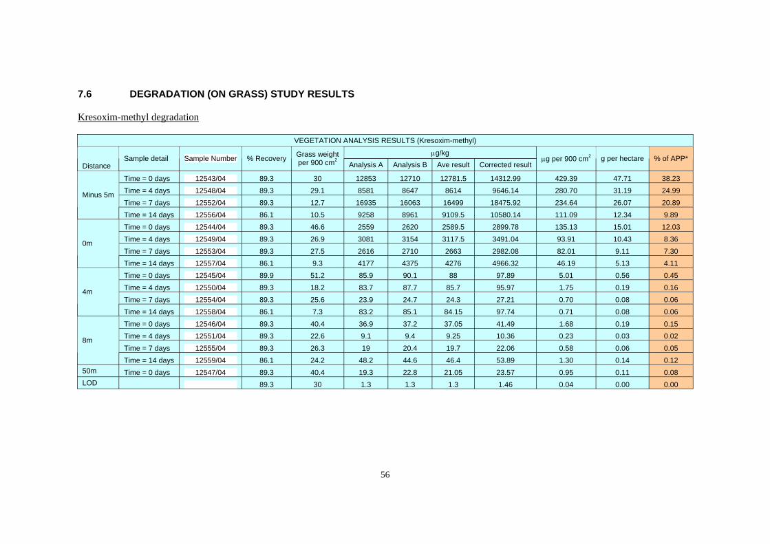
7.6 DEGRADATION (ON GRASS) STUDY RESULTS
Kresoxim-methyl degradation
Distance
Minus 5m
0m
4m
8m
50m LOD
Sample detail
Time = 0 days Time = 4 days Time = 7 days Time = 14 days Time = 0 days Time = 4 days Time = 7 days Time = 14 days Time = 0 days Time = 4 days Time = 7 days Time = 14 days Time = 0 days Time = 4 days Time = 7 days Time = 14 days Time = 0 days
Sample Number
12543/04 12548/04 12552/04 12556/04 12544/04 12549/04 12553/04 12557/04 12545/04 12550/04 12554/04 12558/04 12546/04 12551/04 12555/04 12559/04 12547/04
VEGETATION ANALYSIS RESULTS (Kresoxim-methyl)
µg/kg% Recovery Grass weight
per 900 cm2 Analysis A Analysis B Ave result Corrected result
89.3 30 12853 12710 12781.5 14312.99 89.3 29.1 8581 8647 8614 9646.14 89.3 12.7 16935 16063 16499 18475.92 86.1 10.5 9258 8961 9109.5 10580.14 89.3 46.6 2559 2620 2589.5 2899.78 89.3 26.9 3081 3154 3117.5 3491.04 89.3 27.5 2616 2710 2663 2982.08 86.1 9.3 4177 4375 4276 4966.32 89.9 51.2 85.9 90.1 88 97.89 89.3 18.2 83.7 87.7 85.7 95.97 89.3 25.6 23.9 24.7 24.3 27.21 86.1 7.3 83.2 85.1 84.15 97.74 89.3 40.4 36.9 37.2 37.05 41.49 89.3 22.6 9.1 9.4 9.25 10.36 89.3 26.3 19 20.4 19.7 22.06 86.1 24.2 48.2 44.6 46.4 53.89 89.3 40.4 19.3 22.8 21.05 23.57 89.3 30 1.3 1.3 1.3 1.46
µg per 900 cm2
429.39 280.70 234.64 111.09 135.13 93.91 82.01 46.19 5.01 1.75 0.70 0.71 1.68 0.23 0.58 1.30 0.95 0.04
g per hectare
47.71 31.19 26.07 12.34 15.01 10.43 9.11 5.13 0.56 0.19 0.08 0.08 0.19 0.03 0.06 0.14 0.11 0.00
% of APP*
38.23 24.99 20.89 9.89
12.03 8.36 7.30 4.11 0.45 0.16 0.06 0.06 0.15 0.02 0.05 0.12 0.08 0.00
56
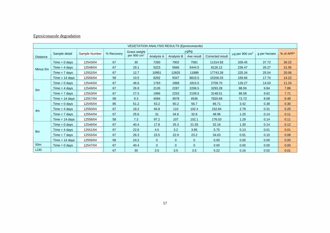
Epoxiconazole degradation
Distance
Minus 5m
0m
4m
8m
50m LOD
Sample detail
Time = 0 days Time = 4 days Time = 7 days Time = 14 days Time = 0 days Time = 4 days Time = 7 days Time = 14 days Time = 0 days Time = 4 days Time = 7 days Time = 14 days Time = 0 days Time = 4 days Time = 7 days Time = 14 days Time = 0 days
Sample Number
12543/04 12548/04 12552/04 12556/04 12544/04 12549/04 12553/04 12557/04 12545/04 12550/04 12554/04 12558/04 12546/04 12551/04 12555/04 12559/04 12547/04
% Recovery
67 67 67 58 67 67 67 58 85 67 67 58 67 67 67 58 67 67
VEGETATION ANALYSIS RESULTS (Epoxiconazole)
µg/kgGrass weight per 900 cm2
Analysis A Analysis B Ave result Corrected result
30 7260 7902 7581 11314.93 29.1 5223 5666 5444.5 8126.12 12.7 10951 12825 11888 17743.28 10.5 8292 9347 8819.5 15206.03 46.6 1763 1868 1815.5 2709.70 26.9 2126 2287 2206.5 3293.28 27.5 1966 2253 2109.5 3148.51 9.3 4094 4978 4536 7820.69
51.2 53.2 60.2 56.7 66.71 18.2 94.8 110 102.4 152.84 25.6 31 34.6 32.8 48.96 7.3 97.2 107 102.1 176.03
40.4 17.8 25.3 21.55 32.16 22.6 4.5 3.2 3.85 5.75 26.3 23.5 22.9 23.2 34.63 24.2 0 0 0 0.00 40.4 0 0 0 0.00 30 3.5 3.5 3.5 5.22
µg per 900 cm2
339.45 236.47 225.34 159.66 126.27 88.59 86.58 72.73 3.42 2.78 1.25 1.29 1.30 0.13 0.91 0.00 0.00 0.16
g per hectare
37.72 26.27 25.04 17.74 14.03 9.84 9.62 8.08 0.38 0.31 0.14 0.14 0.14 0.01 0.10 0.00 0.00 0.02
% of APP*
30.22 21.05 20.06 14.22 11.24 7.89 7.71 6.48 0.30 0.25 0.11 0.11 0.12 0.01 0.08 0.00 0.00 0.01
57

Fenpropimorph degradation
Distance
Minus 5m
0m
4m
8m
50m LOD
Sample detail
Time = 0 days Time = 4 days Time = 7 days Time = 14 days Time = 0 days Time = 4 days Time = 7 days Time = 14 days Time = 0 days Time = 4 days Time = 7 days Time = 14 days Time = 0 days Time = 4 days Time = 7 days Time = 14 days Time = 0 days
Sample Number
12543/04 12548/04 12552/04 12556/04 12544/04 12549/04 12553/04 12557/04 12545/04 12550/04 12554/04 12558/04 12546/04 12551/04 12555/04 12559/04 12547/04
% Recovery
83 83 83 66 83 83 83 66 95 83 83 66 83 83 83 66 83 83
VEGETATION ANALYSIS RESULTS (Fenpropimorph)
µg/kgGrass weight per 900 cm2
Analysis A Analysis B Ave result Corrected result
30 5849 5699 5774 6956.63 29.1 2302 2191 2246.5 2706.63 12.7 4840 4487 4663.5 5618.67 10.5 2835 2556 2695.5 4084.09 46.6 3251 3451 3351 4037.35 26.9 1749 1696 1722.5 2075.30 27.5 1614 1513 1563.5 1883.73 9.3 1950 1727 1838.5 2785.61
51.2 889 985 937 986.32 18.2 483 494 488.5 588.55 25.6 207 207 207 249.40 7.3 341 378 359.5 544.70
40.4 322 367 344.5 415.06 22.6 58.8 61.4 60.1 72.41 26.3 124 130 127 153.01 24.2 415 425 420 636.36 40.4 59.5 58.9 59.2 71.33 30 0.7 0.7 0.7 0.84
µg per 900 cm2
208.70 78.76 71.36 42.88
188.14 55.83 51.80 25.91 50.50 10.71 6.38 3.98
16.77 1.64 4.02
15.40 2.88 0.03
g per hectare
23.19 8.75 7.93 4.76
20.90 6.20 5.76 2.88 5.61 1.19 0.71 0.44 1.86 0.18 0.45 1.71 0.32 0.00
% of APP*
15.47 5.84 5.29 3.18
13.95 4.14 3.84 1.92 3.74 0.79 0.47 0.29 1.24 0.12 0.30 1.14 0.21 0.00
58

7.7
7.8
BYSTANDER (MANEQUIN) RESULTS
Sample No. Sample description Corrected result µg/device
Fenpropimorph Kresoxim-methyl Epoxiconazole 12560/04 scarecrow 4m 238 108 62 12561/04 scarecrow 8m 198 81 85 12562/04 scarecrow 12m 173 60 20
POST-APPLICATION EXPOSURE RESULTS
Sample No. Sample description Corrected result µg/device
Fenpropimorph Kresoxim-methyl Epoxiconazole 12560/04 scarecrow 4m 238 108 62 12561/04 scarecrow 8m 198 81 85 12562/04 scarecrow 12m 173 60 20 12563/04 gloves set 1a 6 5 0 12567/04 boots set 1a 439 0 0 12569/04 suit set 1a 48 5 0 12570/04 gloves set 1b 5 2 0 12574/04 boots set 1b 266 74 0 12576/04 suit set 1b 45 0 34 12577/04 gloves set 2a 6 5 0 12581/04 boots set 2a 481 954 0 12583/04 suit set 2a 101 34 0 12584/04 gloves set 2b 8 11 0 12588/04 boots set 2b 461 413 0 12590/04 suit set 2b 65 8 25 12591/04 gloves set 3a 11 96 5 12595/04 boots set 3a 890 0 0 12597/04 suit set 3a 74 42 23 12598/04 gloves set 3b 25 305 8 12602/04 boots set 3b 869 0 0 12604/04 suit set 3b 126 242 101
59

8 REFERENCES
Coldwell M and Corns H (2001); Background pesticide levels in house dust, HSL internal report OMS/2001/14.
DEFRA (2001), Horizontal boom sprayers: a step-by-step guide to reducing aquatic buffer zones in the arable sector (Local environment risk assessments for boom sprayers LERAP)
Ganzelmeier H, Rautmann D, Spangenberg R Streloke M, Herrmann M, Wenzelburger H-J and Walter H-F (1995); Studies on the spray drift of plant protection products: results of a test program carried out throughout the Federal Republic of Germany, Mitteilungen aus der Biologischen Bundesanstalt für Land- und Forstwirtschaft, Berlin-Dahlem. Heft 305.
Ghosh S and Hunt JCR (1998); Spray jets in a cross-flow, Journal of Gluid Mechanics 365, 109-136.
Glass CR, Mathers JJ, Harrington P, Gilbert AJ and Smith S (2002); Field validation of LERAP (and assessment of bystander contamination), CSL Report 1728/02/02.
Hasan R, Gobeau NCH and Rimmer DA (2002); Modelling pesticide drift during tractor-mounted spraying operations, HSL report CM/02/02.
HSE (1999); MDHS 94, Pesticides in air and/or on surfaces, ISBN 0-7176-1619-3
Johnson PD, Corns H, Coldwell and Higgins J (2004); Evaluation of analytical methods for pesticides and biocides 2003, HSL report OMS/2004/11.
MAFF/HSE (1998); Green Code – Code of practice for the safe use of pesticides on farms and holdings, MAFF Publications (now obtainable through Pesticides Safety Directorate, DEFRA) 1998.
Miller PCH, Butler Ellis MC and Tuck CR (1996); Entrained air and droplet velocities produced by agricultural flat-fan nozzles, Atomization and Sprays 6, 693-707.
PSD (due for publication in Feb 2006) - Code of Practice for the Safe Use of Plant Protection Products.
Rimmer DA, White J, Taylor M and Guiver R (1993); Sampling and analysis of pesticides from spraydrift incidents. Preliminary assessment of spray trials carried out in May 2003, HSL report IR/L/IA/93/9.
Rimmer DA, Johnson PD, White J and Douglas ND (1997); Evaluation of analytical methods to aid in the enforcement of FEPA/COPR: Final project report – 1997, HSL report IACS/97/14.
Royal Commission on Environmental Pollution (RCEP) report (2005); Crop Spraying and the Health of Residents and Bystanders.
Spray drift task force, US Government Publication (1997), A summary of ground application studies. URL = http://www.agdrift.com/PDF_FILES/ground.pdf
60

van de Zande JC, Michielsen JMGP, Stallinga H, Wenneker M, Heijne B (2004), Hedgerow filtration and barrier vegetation, International Conference on Pesticide Application for Drift Management, October 27-29, 2004, Waikoloa, Hawaii, 163-177.
White J (1996); Revised sampling protocol for spray drift investigations, HSL report IACS/96/4.
Xu ZG, Walklate PJ and Miller PCH (1997); Evaluation of a stochastic model for spray transport prediction from air-assisted sprayers, Aspects of Applied Biology 48, 195-200.
61

Published by the Health and Safety Executive 11/06

Health and Safety Executive
Development of a modelling tool for pesticide spray drift Phase 1: Data gathering and feasibility testing
The project was originally conceived as having four phases and this document reports on phase 1. Work on phase 2 has commenced but phases 3 and 4 are presently in abeyance whilst work of a complimentary nature is being taken forward by others in response to the Royal Commission on Environmental Pollution report "Crop spraying and the health of residents and bystanders" (RCP, 2005).
The overall aim of the HSE project was to develop a robust computational modelling tool that would (a) assist HSE/FOD staff with the investigation of pesticide spraydrift incidents and (b) support enforcement action.
It was envisaged that the model would have been capable of working in two ways after an event:
• to predict spraydrift patterns using data on operating conditions obtained during the investigation; and
• to predict operating parameters or incident scenarios using deposition data obtained from samples of soil, vegetation or water taken from the investigation site.
In the latter case, any information on operating parameters obtained from the investigation would have facilitated the model and would have improved its accuracy and reliability.
It was anticipated that, if successfully developed, the tool would have been laptop based enabling HSE inspectors or Field Scientists to rapidly and consistently gather information and respond to complaints.
This report and the work it describes were funded by the Health and Safety Executive (HSE). Its contents, including any opinions and/or conclusions expressed, are those of the authors alone and do not necessarily reflect HSE policy.
RR498
www.hse.gov.uk