DEVELOPMENT OF A HYBRID LBM-POTENTIAL FLOW

MODEL FOR NAVAL HYDRODYNAMICS

DEVELOPPEMENT D’UN MODELE HYBRIDE LBM-POTENTIEL

POUR L’HYDRODYNAMIQUE NAVALE

C.M. O’REILLY1,2, S.T. GRILLI1, J.C. HARRIS3, A. MIVEHCHI1,C.F. JANSSEN4, J.M. DAHL1

1 Dept. of Ocean Engineering, University of Rhode Island, Narragansett, RI 02882, USA2 Navatek Ltd., South Kingstown, RI 02879, USA3 LHSV, Ecole des Ponts, CEREMA, EDF R&D, Universite Paris-Est, Chatou, France4 Fluid Dynamics and Ship Theory Inst., Hamburg University of Technology (TUHH), Germany

coreilly@navatekltd.com

Summary

We report on the validation of a 3D hybrid model for naval hydrodynamics based on aperturbation method, where velocity and pressure are the sum of an inviscid flow with aviscous perturbation. The far- to near-field inviscid flows can be solved with a BEM, basedon potential flow theory and the near-field perturbation flow is solved with a NS modelbased on a Lattice Boltzmann Method (LBM). We give the model formulation and latestdevelopments in LES turbulence modeling, including a wall model. We validate these bysimulating flows over a flat plate for Re ∈ [3.7× 104; 1.2× 106], for which the plate frictioncoefficient agrees well with experiments. We also simulate the flow past a foil for Re = 3×106

and show good agreement of lift forces with experiments. Results obtained with the hybridmodel are nearly identical to those of the LBM alone, but with a smaller computationaldomain, demonstrating the benefits of this approach.

Resume

Nous presentons un modele hybride pour l’hydrodynamique navale, base sur une methodede perturbation decomposant la vitesse et la pression en la somme d’un ecoulement non-visqueux et d’une perturbation visqueuse. Les equations des champs lointain a proche sontresolues par une methode potentielle BEM et celles des ecoulements en champ proche par unmodele NS base sur la methode “Lattice Boltzmann” (LBM). Nous resumons la formulationdu modele et ses derniers developpements en modelisation LES de la turbulence avec un“wall model” (couche limite visqueuse-turbulente). Ceux-ci sont valides pour l’ecoulementsau dessus d’une plaque pour Re ∈ [3.7 × 104; 1.2 × 106] ; le coefficient de frottement sur laplaque est en bon accord avec l’experience. Nous simulons l’ecoulement autour d’un hydrofoilpour Re = 3× 106 et montrons un bon accord avec l’experience. Les resultats obtenus avecle modele hybride sont tres proches de ceux du modele LBM seul, mais pour un domaine decalcul plus petit, ce qui montre l’avantage de cette approche.

I – Introduction

The simulation of large ship motions and resistance in steep waves is typically perfor-med using linear or nonlinear potential flow solvers, usually based on a higher-order Boun-dary Element Method (BEM), with semi-empirical corrections introduced to account forviscous/turbulent effects. However in some cases, viscous/turbulent flows near the ship’shull and breaking waves and wakes must be accurately modeled to capture the salient phy-sics. Navier-Stokes (NS) solvers can and have been used to model such flows, but they arecomputationally expensive and often too numerically dissipative to model wave propagationover long distances.

Here, we detail the development of a 3D hybrid model, for solving naval hydrodynamicsproblems, based on a perturbation method (e.g., Alessandrini, 2007 ; Grilli, 2008 ; Harris andGrilli, 2012), in which both velocity and pressure are expressed as the sum of an inviscid (I)and a viscous perturbation (P) component. In this model, the far- to near-field inviscid flowis solved with a BEM, based on fully nonlinear potential flow (FNPF) theory, also referredto as Numerical Wave Tank (NWT), and the near-field perturbation flow is solved with aNS model, here implemented with a Lattice Boltzmann Method (LBM ; e.g., d’Humiereset al., 2002 ; Janssen, 2010 ; Janssen et al., 2010) including a Large Eddy Simulation of theturbulence (LES ; e.g., Krafczyk et al., 2003). Both the BEM and LBM models have separaterepresentations of the free surface (using an explicit Eulerian-Lagrangian time updating inthe former and a VOF method in the latter ; e.g., O’Reilly et al., 2015).

In the context of the hybrid perturbation method, the LBM is only applied to the near-field where viscous/turbulent effects matter, and its solution is forced by results of the NWTapplied to the entire domain. Hence the hybrid approach increases computational efficiencyrelative to traditional CFD solutions, in which the NS solver is applied to the entire domain.This was already demonstrated by Reliquet et al. (2014) based on different types of models,which were less efficient and optimized than those proposed here. Indeed, the NWT usedhere was the object of numerous developments over the past two decades (see Grilli et al.’s,2010 review to date). Its latest version was optimized with a Fast Multipole Method (FMM),based on the parallel ExaFMM library, and shown to achieve nearly linear scaling on largeCPU clusters (e.g., Harris et al., 2014 and Harris et al., in this conference). The LBMhas proved to be accurate and efficient for simulating a variety of complex fluid flow andfluid-structure interaction problems and, when implemented on a massively parallel GeneralPurpose Graphical Processor Unit (GPGPU) co-processor, it was also shown to achieve veryhigh efficiency (over 100 million node updates per second on a single GPGPU ; e.g., Janssen,2010 ; Janssen et al., 2013 ; Banari et al., 2014). In this respect, LBM developments in thiswork are based on the highly efficient, GPGPU-accelerated, Lattice Boltzmann solver ELBE(Janssen et al., 2015 ; www.tuhh.de/elbe), developed at TUHH, which features various LBMmodels, an on-device grid generator, higher-order boundary conditions, and the possibility ofspecifying overlapping nested grids. ELBE also includes the initial LBM perturbation modelbased on Janssen et al.’s (2010) approach (discussed later). Simple validations of the hybridLBM and LBM-LES approaches, for viscous and turbulent oscillatory boundary layers, werereported by O’Reilly et al. (2015) and Janssen et al. (2016).

In this paper, we focus on the development and validation of the hybrid NS-LBM solverapplied to the perturbation flow and, in this context, the modeling of turbulent flows by aLES, and by an accurate representation of boundary layers near solid boundaries without theneed for a refined discretization. We first summarize the principles of the LBM, in particularwhen using the more accurate Multiple Relaxation Time (MRT) method. We then detail theformulation of the perturbation method in the context of turbulent flows and show how the

standard LES equations are modified. The hybrid LBM-LES approach is then validated bysolving turbulent flows past a solid boundary and retrieving the “law of the wall”. Finally,the method is validated by computing the drag and lift coefficients of a hydrofoil at highReynolds number.

II – Methodology

II – 1 Lattice Boltzmann Method (LBM)

In the LBM, the macroscopic NS equations are modeled by solving an equivalent me-soscopic problem in which the fluid is represented by particles interacting over a (typicallyregular) lattice (or grid), through their distribution functions (DF) f(t,x, ξ), representingthe normalized probability to find a particle at location x at time t with velocity ξ ; themacroscopic hydrodynamic quantities (e.g., velocity, pressure,...) are defined as moments ofthe DFs.

The time evolution of discrete particle DFs is governed by the Boltzmann advection-collision equation,

DfαDt

=∂fα(t,x)

∂t+ eα · ∂fα(t,x)

∂x= Ωα +Bα (1)

in which eα denotes discrete particle velocities, Ωα is a collision operator describing inter-actions between particles, and Bα represents volume forces such gravity. Eq. (1) is discre-tized over a regular lattice, of grid spacing ∆x using n = 19 discrete particle velocities,which point in the directions of 18 neighboring particles from a given particle location ;thus : eα = 0, 0, 0; ±c, 0, 0; 0,±c, 0; 0, 0,±c; ±c,±c, 0; ±c, 0,±c; 0,±c,±c, forα = 0, ..., 18 (standard D3Q19 scheme). The constant velocity c =

√3cs is related to the

speed of sound cs.In the standard single relaxation time (SRT) LBM, Eq. (1) is discretized by finite diffe-

rences in space and time as,

fα(t +∆t,x+ eα∆t)− fα(t,x) = −1

τfα(x, t)− f eq

α (ρ,u)+B′α (2)

where f eqα (ρ,u) are equilibrium DFs, functions of the macroscopic fluid density ρ and velocity

u, ∆t is time step (with c = ∆x/∆t), and τ = 3ν/c2 + ∆t/2, a nondimensional relaxationtime (SRT) expressed as a function of fluid viscosity ν. LBM simulations are typically splitup into a local collision step, which locally drives the particle DFs to equilibrium, and apropagation step, during which the evolved DFs are advected. The hydrodynamic quantitiesare found as low order moments of the DFs,

ρ =

n∑

α=1

fα, ρu =

n∑

α=1

eαfα (3)

Applying a Chapman-Enskog expansion to Eq. (2) (see, e.g., Banari et al., 2014) yields,

f eqα (ρ,u) = wα

(

ρ+ ρo

(

3(u · eα)

c2+

9

2

(u · eα)2c4

− 3

2

u2

c2

))

(4)

for the LBM solution to satisfy the incompressible NS equations up to O(∆x2) and O(Ma2)errors, with Ma the Mach number ; ρo and ρ represent the average fluid density and a smallperturbation from that density, respectively, and wα are lattice dependent directional weightswith, w0 = 1/3, w1...6 = 1/18 and w7...18 = 1/36.

The collision step in Eq. (2) is a strictly local operation between neighboring latticenodes while the convective step simply propagates the particle distribution functions intheir discretized velocity directions eα. Unlike standard NS solvers used in CFD the LBMsolution does not require a pressure correction step as pressure is simply given by p = c2sρ.This locality of all LBM numerical operations makes it very well suited to massively parallelcomputations on a GPGPU.

d’Humieres et al. (2002) showed that more accurate and stable results can be obtained,particularly for high Reynolds numbers Re, using the multiple relaxation time (MRT) LBM.This method incorporates higher-order moments (i.e., hydrodynamic quantities and theirfluxes) into the solution, which have important physical significance (Lallemand and Lou2000) and will be useful to implement the LES in the LBM for turbulent flows (see below).In the MRT, the collision operator in the right hand side of Eq. (2) is replaced by (β =0, ..., 18; γ, δ = 0, ..., 15 ; repeated indices in equations mean an implicit summation),

Ωα = −M−1αγ Sγδ(Mβδfβ −meq

δ ) (5)

where Mαγ is the transformation matrix from DFs to moments, with fα = M−1αγ mγ and Sγδ

is a diagonal collision matrix of relaxation parameters, weighing different properties of thefluid (see references). Equilibrium moments meq

γ are derived from the f eqα (x, t) as,

meq0 = ρ, meq

3 = ρux, meq5 = ρuy, meq

7 = ρuz

meq1 = eeq = ρ0(u

2x + u2

y + u2z), meq

9 = 3peqxx = ρ0(2u2x − u2

y − u2z)

meq11 = peqzz = ρ0(u

2

y − u2

z), meq13 = peqxy = ρ0(uxuy)

meq14 = peqyz = ρ0(uyuz), meq

15 = peqxz = ρ0(uxuz) (6)

In the following, prime variables will denote non-dimensional variables where lengthshave been divided by a length scale λ, times by time scale τ , and mass by mass scale ;thus, c′ = cτ/λ = ∆x′/∆t′. The numerical solution in LBM models is typically stable fora mesh Courant number of 1, yielding, c′ = 1 ; one also typical assumes, λ = ∆x, thus∆x′ = 1 → ∆t′ = 1 ; finally the nondimensional viscosity reads, ν ′ = ντ/λ2. In LBMsimulations of flows at specified Mach and Reynolds numbers (Ma, Re), one thus finds,ν ′ = c′sℓ

′Ma/Re, to use in simulations, also given the physical length scale of the flow ℓ.

II – 2 Equations for the perturbation LBM

Here, we first recap the expressions of the NS perturbation method (Grilli, 2008 ; Har-ris and Grilli, 2012) and develop the corresponding LBM equations with MRT. In the NSperturbation approach, both the flow velocity and pressure are expressed as,

ui = uIi + uP

i with p = pI + pP (7)

where p = p+ ρgx3 − 2

3ρk denotes the perturbation dynamic pressure, with k the turbulent

kinetic energy. Recall that superscripts I denote irrotational flow quantities, with uIi = ∇iφ

I

satisfying Euler equations, and superscripts P represents perturbation flow quantities thatare driven by the inviscid flow fields. After applying this decomposition and substitutingEuler’s equations, the perturbation NS equations read,

∂uPi

∂xi

= 0 (8)

∂uPi

∂t+ uP

j

∂uPi

∂xj

= −1

ρ

∂pP

∂xi

+ (ν + νt)∂2uP

i

∂xj ∂xj

−(

∂uIi

∂xj

uPj + uI

j

∂uPi

∂xj

)

+ 2∂νt∂xj

Sij (9)

where ν and νt are kinematic molecular and turbulent viscosity, respectively, with the latterbeing expressed through the Smagorinsky method as,

νt = (CS∆)2|S|, with Sij = SPij + SI

ij =1

2

(

∂uPi

∂xj

+∂uP

j

∂xi

+∂uI

i

∂xj

+∂uI

j

∂xi

)

(10)

where CS is the Smagorinsky constant, ∆ a grid filtering length scale, and Sij the rate ofstrain tensor is the sum of components functions of the perturbation (SP

ij ) and inviscid (SIij)

velocity.Janssen et al. (2010) developed a perturbation LBM-LES with MRT solving Eqs. (7) to

(10), in which the “I-P” interactions terms were treated as volume forces through the B′α

terms of Eq. (2). Here, instead, we solve these equations, assuming the perturbation LBM-LES DFs are decomposed as, fα = f I

α+fPα and introduced in Eq. (2). Substracting from the

latter the LBM equation for the inviscid flow, we find,

fPα (t+∆t,x+eα∆t))−fP

α (t,x)) = −1

τfP

α (t,x)−f eqα (ρI+ρP ,uI+uP )+f eq,I

α (ρI ,uI) (11)

where the f eq,Iα (ρI ,uI) are expressed with Eq. (4) based on inviscid fields and satisfy,

n∑

α=1

f eq,Iα = 0,

n∑

α=1

eαifeq,Iα = ρou

Ii ,

n∑

α=1

eαieαjfeq,Iα = pIδij + ρou

Iiu

Ij (12)

The perturbation equilibrium DFs are then found as, f eq,Pα (ρP ,uP ,uI) = f eq

α (ρI + ρP ,uI +uP )− f eq,I

α (ρI ,uI),

f eq,Pα = wα

(

ρP + ρo

(

3uP · eα

c2s+

9

2

(eα · uP )2 + 2(eα · uP )(eα · uI)

c4s− 3

2

(uP )2

c2s

))

, (13)

which satisfy,

n∑

α=1

f eq,Pα = ρP ,

n∑

α=1

eαifeq,Pα = ρou

Pi ,

n∑

α=1

eαieαjfeq,Pα = pP δij + ρou

Iiu

Pj + ρou

Pi u

Ij + ρou

Pi u

Pj

(14)A rigorous Chapman-Enskog expansion would show that the perturbation NS Eqs. (7) to(10) are recovered when using these DFs. Note the interaction terms between the I and Pfields in Eqs. (13) and (14) expressing the inviscid flow forcing on the perturbation fields.

Extending this formulation to the MRT, assuming a collision operator expressed by Eq.(5), we find the equilibrium moments,

meq1 = eeq = ρ0((u

Px )

2 + (uPy )

2 + (uPz )

2 + 2uPx u

Ix + 2uP

y uIy + 2uP

z uIz)

meq9 = 3peqxx = ρ0(2(u

Px )

2 − (uPy )

2 − (uPz )

2 + 4uPx u

Ix − 2uP

y uIy − 2uP

z uIz)

meq11 = peqzz = ρ0((u

Py )

2 − (uPz )

2 + 2uPy u

Iy − 2uP

z uIz), meq

13 = peqxy = ρ0(uPx u

Py + uP

x uIy + uP

y uIx)

meq14 = peqyz = ρ0(u

Py u

Pz + uP

y uIz + uP

z uIy), meq

15 = peqxz = ρ0(uPx u

Pz + uP

x uIz + uP

z uIx)

(15)

Moments that are not listed above are unchanged from the standard MRT formulation.

II – 3 LES turbulence modeling with a LBM

Krafczyk et al. (2003) expressed the 2nd-order moments of the DFs as,

Pij =

n∑

α=1

eαieαjfα = c2sρoδij + ρouiuj −2c2s ρ

s2Sij (16)

where s2 is a relaxation rate for these moments, and showed that they are related to 2nd-order moments in the MRT, 3pxx, pzz, pxy, pyz, and pxz. The 1st and 2nd terms in Eq. (16)’sRHS are functions of flow quantities obtained through other moments of the DFs. Based onEq. (16), the rate of strain tensor can be expressed as,

Sij =s22c2sρ

c2sρ δij + ρuiuj − Pij =s22c2sρ

Qij (17)

where Qij are the terms in . Krafczyk et al. (2003) assumed that the Qij ’s are functionsof the non-equilibrium part of the DFs, fneq

α = fα − f eqα and provided their expressions as a

function of the 2nd-order MRT moments. Similar to LES Eq. (10), they then calculated theturbulent viscosity as,

νt = (CS∆)2|S| = s22c2sρ

(Cs∆)2|Q|, with |Q| =√

QijQij (18)

and expressed the relaxation rate of the 2nd-order moments as,

s2 =1

τ0 + τtwith τt =

1

2

(

√

τ 20 + 18(Cs∆)2|Q| − τ0

)

(19)

where τ0 is the relaxation time based on the molecular viscosity.When applying the LES to the perturbation LBM, the moments P P

ij are given by thelast Eq. (14), yielding an expression for the perturbation rate of strain tensor that featuresnonlinear interaction terms between the I and P fields,

SPij =

s22c2sρ

(

c2sρδij + ρouPi u

Pj + ρou

Iiu

Pj + ρou

Pi u

Ij − P P

ij

)

=s22c2sρ

QPij (20)

The rate of strain tensor for the total flow is thus given by,

Sij =s22c2sρ

QPij + SI

ij (21)

Therefore the |Q| term to use in LES Eqs. (18) and (19) in combination with the MRT LBMEqs. (11) to (15), is modified as follows,

|Q| =√

RijRij with Rij = QPij +

2c2sρos2

SIij (22)

where the QPij terms are computed with Eq. (20).

II – 4 LBM turbulent wall model

Typical naval hydrodynamics flows are fully turbulent, with Re > 106. Thus, the turbu-lent boundary layers (BL) near solid boundaries (e.g., ship hull) must be properly modeledin the LBM. Since resolving the BL in the LBM grid would be computationally prohibitive

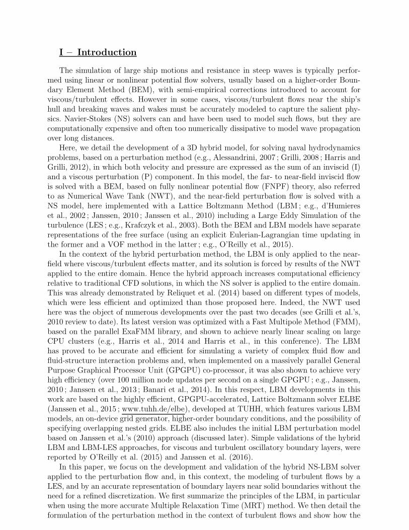
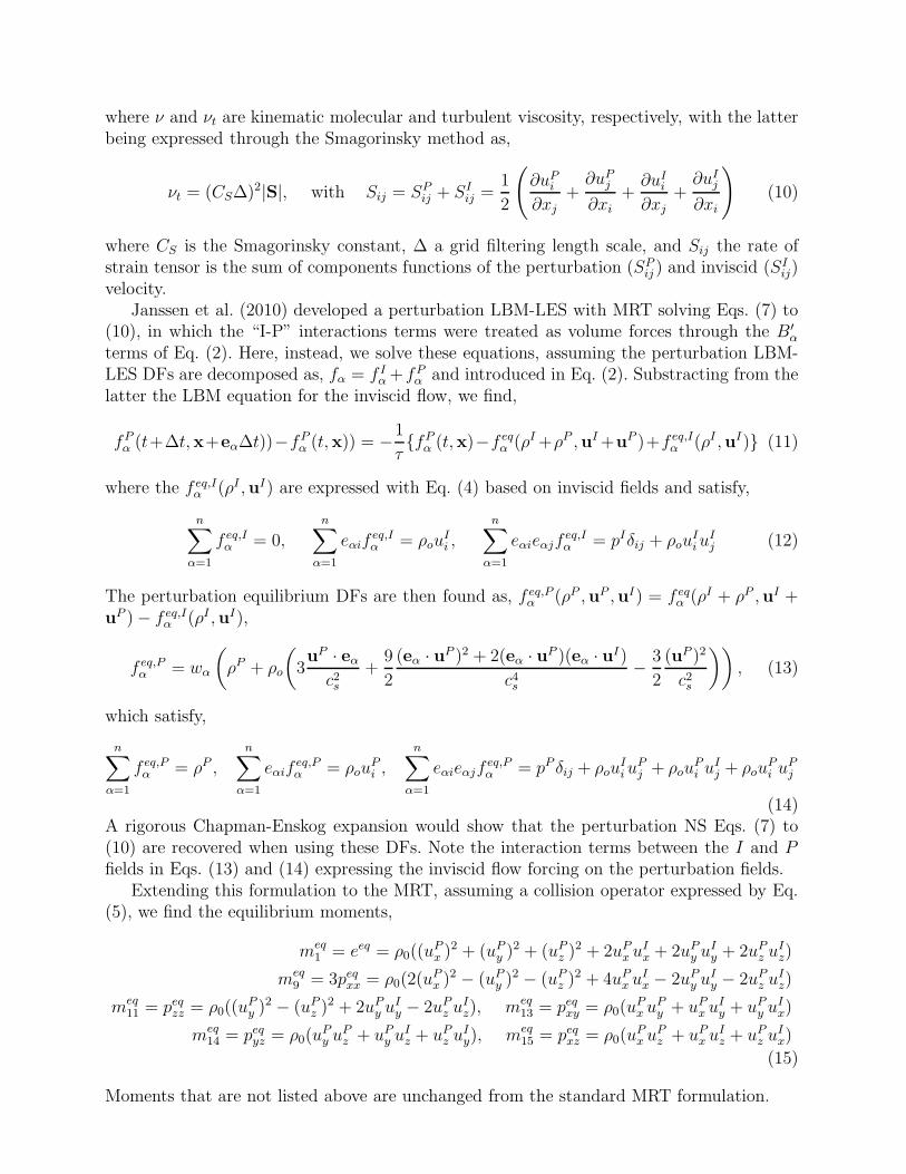
(a) (b) (c)

Figure 1 – Sketch of LBM flow reconstruction near a solid boundary (assumed 2D for simpli-city) : (a) known or computed variables ; (b) known (—–) and missing (- - - -) DF populations ;(c) variables in geometric calculations. Lattice points are marked by (•). [(a) and (b) fromMalaspinas and Sagaut (2014)]

(even with grid refinement through nesting such as done in ELBE), besides the LES of theflow, this requires using a proper wall model. Below, we describe the extension to the per-turbation LBM-LES of the method proposed by Malaspinas and Sagaut (2014), based on amacroscopic representation of the flow within the BL (i.e., on the LBM lattice). A thin layerapproximation is introduced, implying that the mean free flow is locally nearly parallel tothe solid boundary (i.e., wall) and statistically stationary ; it is also assumed that there is nohorizontal pressure gradient. In such conditions, the mean velocity profile can be found as afunction of the distance to the wall y from the semi-empirical equation proposed by Musker(1979), on the basis of experimentally validated logarithmic “laws of the wall” for the fullyturbulent upper BL, the viscous lower BL, and a transition layer based on experimentalmeasurements,

u(y+) = uτ

((

5.424 atan

(

2.0 y+ − 8.15

16.7

)

+ log10

(

(y+ + 10.6)9.6

(y+2 − 8.15 y+ + 86.0)2

)

− 3.52

)

(23)

where the friction velocity uτ and non-dimensional distance y+ are defined as

uτ =√

τw/ρ with y+ = yuτ

ν(24)

Malaspinas and Sagaut (2014) also express the turbulent eddy viscosity as

µt = κy+(

1− e−y+

26.0

)2∣∣

∣

∣

∂u

∂y

∣

∣

∣

∣

(25)

and κ is a constant chosen to be 0.384 based on experimental data.The “law of the wall” Eqs. (23) to (25) will be used to express the boundary condition at

a solid boundary in the LBM, where unknown DF’s are reconstructed on the lattice nodesbased on the macroscopic flow quantities, assuming ∆x ≫ δBL, with δBL the thickness ofthe viscous and transition sublayers in the BL. Let us define x1, x2, and n as the positionof the first and second off wall lattice nodes and the outward normal unit vector at thewall, respectively (Fig. 1). As is standard in most LBM wall boundary models, DF’s thatsatisfy eα · n < 0 (dashed populations seen in Fig. 1b) are assumed to be unknown after thecollision and propagation steps. To find the flow at x1 (labeled ρbc and ubc), these DFs arereconstructed using the velocity gradient at point 1 from the “law of the wall” combinedwith flow quantities calculated in the LBM at location x2. Thus, the DFs near the wall areconstructed as,

fα(x1, t) = f eqα (ρbc,ubc) + fneq

α

(

∂ubc

∂y

)

(26)

where f eqα is specified through Equations (2) and (13) for the standard LBM or the pertur-

bation LBM methods, respectively.Details of determining flow quantities ubc and ρbc at location x1 near the wall are discussed

below. The fneqα DFs are constructed as follows (Malaspinas and Saugat 2014),

fneqα

(

∂ubc

∂y

)

= −wαρ

c2sλν

3∑

i=1

3∑

j=1

eαieαj − c2sIijSij (27)

where λν is the laminar relaxation time and Iij is the identity matrix. While only validated inthe present applications for a flat solid boundary (wall), this method is intended to be usedfor general boundary geometries, for which a shift in reference frame is needed, such thatthe x-axis always points towards the local streamwise direction. Here, the prime variablesrepresent quantities shifted to a wall-normal reference frame (Fig. 1c), where location x2 isfound by projecting n along each lattice velocity at x1 ; we select the direction α with thelargest y′α value and find, x2 = x1+ eα∆t. The streamwise basis vector ex′ is then computedby assuming that x2 lies within the BL. Thus,

y′α =eα · −n

|eα|, with ex′ =

u2 − (u2 · n)n)|u2 − (u2 · n)n)|

(28)

In many LBM solid boundary schemes, the distance between the wall and the nearest latticepoint is assumed to be ∆x/2. Here, a new scheme based on Merkle et al. (2016) is used tomore accurately estimate this distance (see Fig. 1c). The calculation of y′α and wall dependentquantities may then be more accurately performed within the wall model.

Specifically, to evaluate u′bc, which depends on the wall shear stress τw, for each near-wall

lattice point, one numerically solves the implicit equation, u′2 = u(y′2, τw) where u′

2 = u2 · e′xand u(y′2, τw) is given by Musker’s Eqs. (23) and (24). A Newton scheme is used to thiseffect, which iterates over the τw value until convergence. Next ubc and µbc are solved forand Eq. (25) is used to specify the relaxation at boundary nodes, together with Eq. (19) andreplacing the turbulent shear stress τt calculated with the LES by the newly calculated valueτw. Finally, ρbc is calculated using the method originally proposed by Zou and He (1997),which reconstructs the flow density based on known DFs only,

ρbc =1

1 + ubc · n(2ρ+ + ρ0), with ρ0 =

∑

α∈α|eα·n=0

fα and ρ+ =∑

α∈α|eα·n>0

fα (29)

Equation (26) may now be applied to the unknown DFs (such as at point 2).When applying this turbulent wall model to the perturbation LBM, we reconstruct the

total flows, u2 and u′2 in Eq. (28) from u2 = uI

2 + uP2 , and solve the macroscopic (Musker)

equation to find ubc = uI1 + uP

1 . The equilibrium DFs in Eq. (26) are now those of Eq. (13).Finally, in Eq. (27) we now use SP

ij instead of Sij, so that only the perturbation componentis applied back to the DF’s.

II – 5 Hybrid-LBM force evaluation

The total force acting on a solid body is computed in the perturbation LBM as a li-near combination of the inviscid and perturbation forces, F = FI + FP , where the inviscidcontribution is evaluated through an integration over the body boundary ΓB of the knownpressure pI . The perturbation force is evaluated through the momentum exchange methodas,

FP =∑

α∈ΓB

Fα = − V

∆teαfα(t+∆t,x)− fα′(t,x) (30)

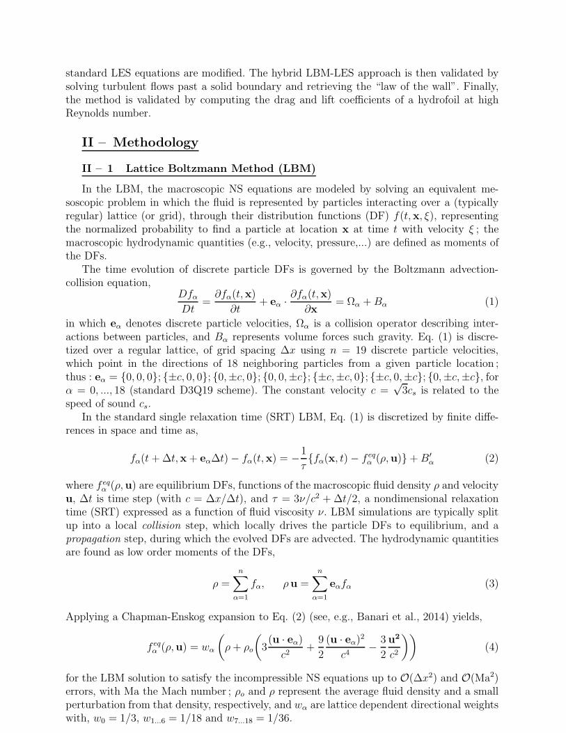
(a) (b)

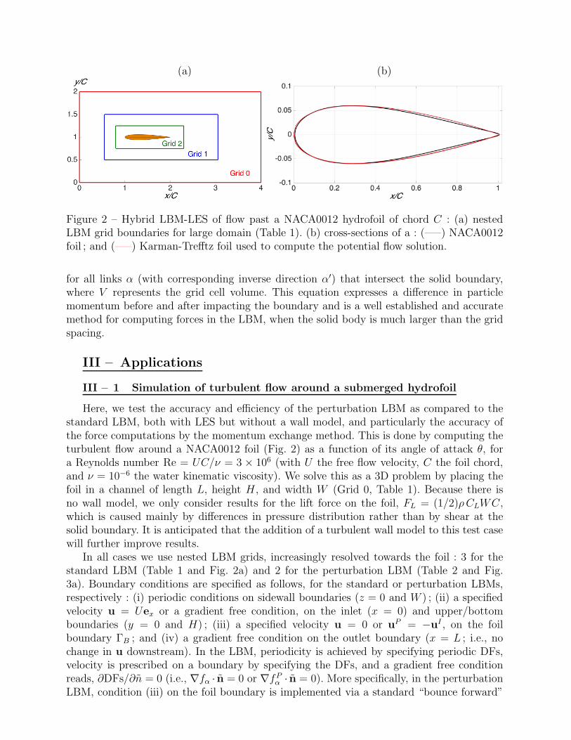
Figure 2 – Hybrid LBM-LES of flow past a NACA0012 hydrofoil of chord C : (a) nestedLBM grid boundaries for large domain (Table 1). (b) cross-sections of a : (—–) NACA0012foil ; and (—–) Karman-Trefftz foil used to compute the potential flow solution.

for all links α (with corresponding inverse direction α′) that intersect the solid boundary,where V represents the grid cell volume. This equation expresses a difference in particlemomentum before and after impacting the boundary and is a well established and accuratemethod for computing forces in the LBM, when the solid body is much larger than the gridspacing.

III – Applications

III – 1 Simulation of turbulent flow around a submerged hydrofoil

Here, we test the accuracy and efficiency of the perturbation LBM as compared to thestandard LBM, both with LES but without a wall model, and particularly the accuracy ofthe force computations by the momentum exchange method. This is done by computing theturbulent flow around a NACA0012 foil (Fig. 2) as a function of its angle of attack θ, fora Reynolds number Re = UC/ν = 3 × 106 (with U the free flow velocity, C the foil chord,and ν = 10−6 the water kinematic viscosity). We solve this as a 3D problem by placing thefoil in a channel of length L, height H , and width W (Grid 0, Table 1). Because there isno wall model, we only consider results for the lift force on the foil, FL = (1/2)ρCLWC,which is caused mainly by differences in pressure distribution rather than by shear at thesolid boundary. It is anticipated that the addition of a turbulent wall model to this test casewill further improve results.

In all cases we use nested LBM grids, increasingly resolved towards the foil : 3 for thestandard LBM (Table 1 and Fig. 2a) and 2 for the perturbation LBM (Table 2 and Fig.3a). Boundary conditions are specified as follows, for the standard or perturbation LBMs,respectively : (i) periodic conditions on sidewall boundaries (z = 0 and W ) ; (ii) a specifiedvelocity u = Uex or a gradient free condition, on the inlet (x = 0) and upper/bottomboundaries (y = 0 and H) ; (iii) a specified velocity u = 0 or uP = −uI , on the foilboundary ΓB ; and (iv) a gradient free condition on the outlet boundary (x = L ; i.e., nochange in u downstream). In the LBM, periodicity is achieved by specifying periodic DFs,velocity is prescribed on a boundary by specifying the DFs, and a gradient free conditionreads, ∂DFs/∂n = 0 (i.e., ∇fα · n = 0 or ∇fP

α · n = 0). More specifically, in the perturbationLBM, condition (iii) on the foil boundary is implemented via a standard “bounce forward”

Grid Number L/C W/C H/C ∆x/C NGrid 0 4.0 2.0 0.2 0.0182 293,040Grid 1 2.5 1.5 0.15 0.0913 556,416Grid 2 1.5 0.5 0.5 0.0045 892,416

Table 1 – Grid parameters of the large domain used in the initial tests of the regular andhybrid LBM-LES models, for the submerged hydrofoil test case (Figs. 3 and 5). Grid lengthis L, width W , height H , and hydrofoil chord length C. Total number of LBM points isN = 1, 741, 872.

Grid Number L/C W/C H/C ∆x/C NGrid 0 2.9 1.2 0.2 0.0081 1,404,000Grid 1 2.0 0.8 0.15 0.0040 3,984,000

Table 2 – Grid parameters of small domain used in convergence tests of the perturbationLBM-LES model for the submerged hydrofoil test case (Figs. 4 and 5). Grid length is L, widthW , height H , and hydrofoil chord length C. Total number of LBM points is N = 5, 388, 000.

scheme applied to the DFs after the collision and propagation steps,

fα′(x1, t) = fα(x1, t)− 2ρ0wα

eα · −uI

c2(31)

where direction α′ is opposite to direction α ; Eq. (31) is applied to all boundary nodes thatsatisfy the condition eα′ · n < 0.

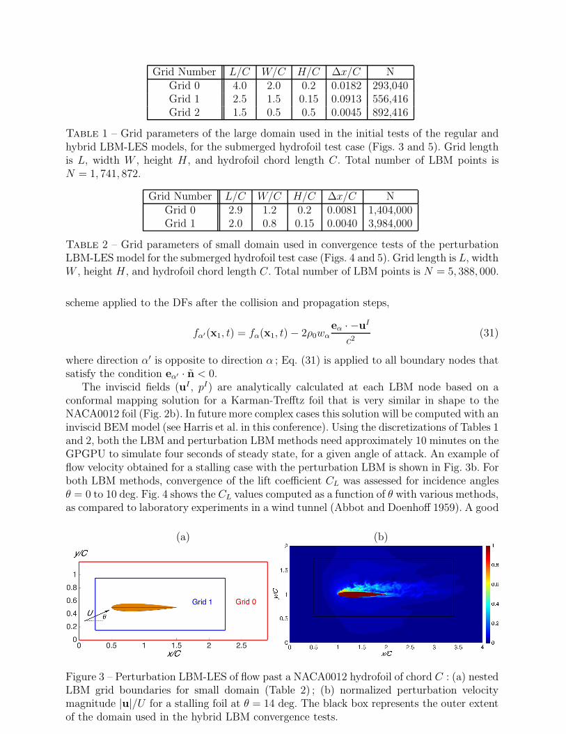
The inviscid fields (uI , pI) are analytically calculated at each LBM node based on aconformal mapping solution for a Karman-Trefftz foil that is very similar in shape to theNACA0012 foil (Fig. 2b). In future more complex cases this solution will be computed with aninviscid BEM model (see Harris et al. in this conference). Using the discretizations of Tables 1and 2, both the LBM and perturbation LBM methods need approximately 10 minutes on theGPGPU to simulate four seconds of steady state, for a given angle of attack. An example offlow velocity obtained for a stalling case with the perturbation LBM is shown in Fig. 3b. Forboth LBM methods, convergence of the lift coefficient CL was assessed for incidence anglesθ = 0 to 10 deg. Fig. 4 shows the CL values computed as a function of θ with various methods,as compared to laboratory experiments in a wind tunnel (Abbot and Doenhoff 1959). A good

(a) (b)

Figure 3 – Perturbation LBM-LES of flow past a NACA0012 hydrofoil of chord C : (a) nestedLBM grid boundaries for small domain (Table 2) ; (b) normalized perturbation velocitymagnitude |u|/U for a stalling foil at θ = 14 deg. The black box represents the outer extentof the domain used in the hybrid LBM convergence tests.

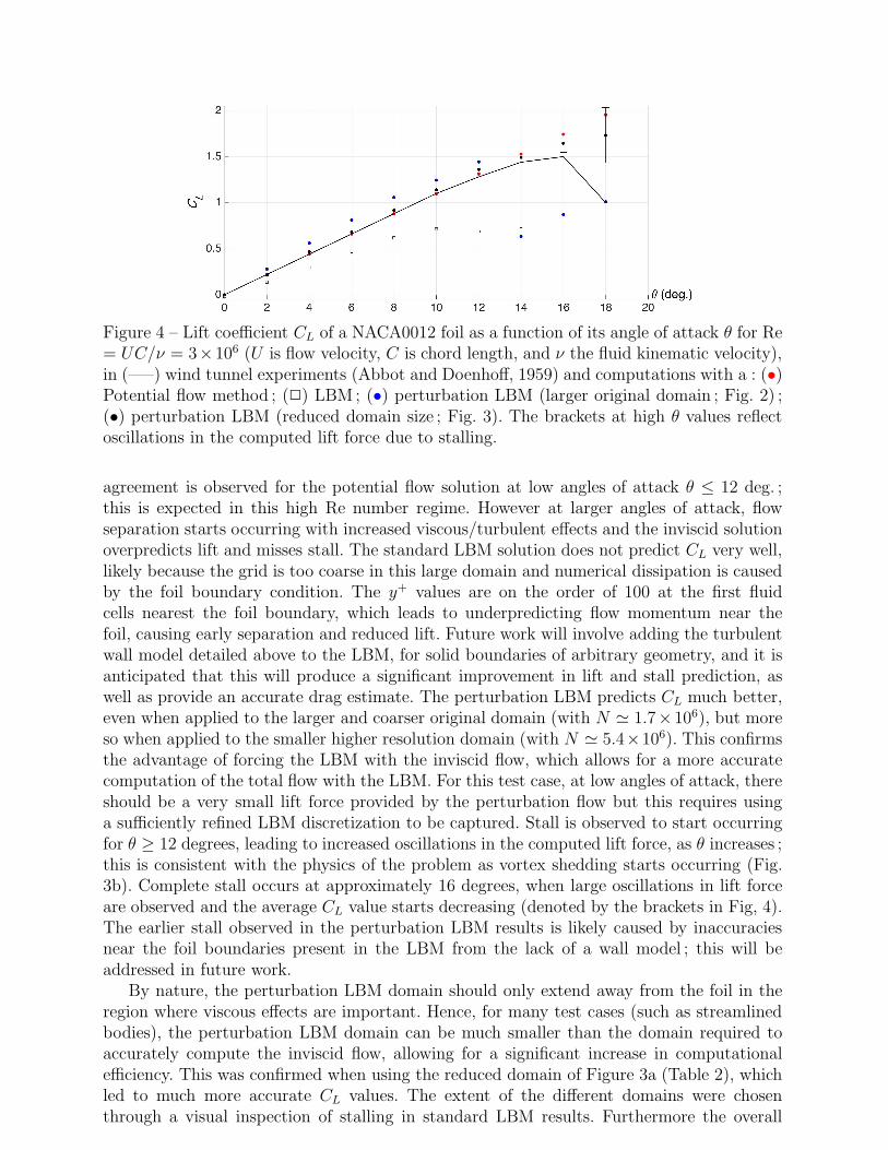
Figure 4 – Lift coefficient CL of a NACA0012 foil as a function of its angle of attack θ for Re= UC/ν = 3×106 (U is flow velocity, C is chord length, and ν the fluid kinematic velocity),in (—–) wind tunnel experiments (Abbot and Doenhoff, 1959) and computations with a : (•)Potential flow method ; () LBM ; (•) perturbation LBM (larger original domain ; Fig. 2) ;(•) perturbation LBM (reduced domain size ; Fig. 3). The brackets at high θ values reflectoscillations in the computed lift force due to stalling.

agreement is observed for the potential flow solution at low angles of attack θ ≤ 12 deg. ;this is expected in this high Re number regime. However at larger angles of attack, flowseparation starts occurring with increased viscous/turbulent effects and the inviscid solutionoverpredicts lift and misses stall. The standard LBM solution does not predict CL very well,likely because the grid is too coarse in this large domain and numerical dissipation is causedby the foil boundary condition. The y+ values are on the order of 100 at the first fluidcells nearest the foil boundary, which leads to underpredicting flow momentum near thefoil, causing early separation and reduced lift. Future work will involve adding the turbulentwall model detailed above to the LBM, for solid boundaries of arbitrary geometry, and it isanticipated that this will produce a significant improvement in lift and stall prediction, aswell as provide an accurate drag estimate. The perturbation LBM predicts CL much better,even when applied to the larger and coarser original domain (with N ≃ 1.7×106), but moreso when applied to the smaller higher resolution domain (with N ≃ 5.4×106). This confirmsthe advantage of forcing the LBM with the inviscid flow, which allows for a more accuratecomputation of the total flow with the LBM. For this test case, at low angles of attack, thereshould be a very small lift force provided by the perturbation flow but this requires usinga sufficiently refined LBM discretization to be captured. Stall is observed to start occurringfor θ ≥ 12 degrees, leading to increased oscillations in the computed lift force, as θ increases ;this is consistent with the physics of the problem as vortex shedding starts occurring (Fig.3b). Complete stall occurs at approximately 16 degrees, when large oscillations in lift forceare observed and the average CL value starts decreasing (denoted by the brackets in Fig, 4).The earlier stall observed in the perturbation LBM results is likely caused by inaccuraciesnear the foil boundaries present in the LBM from the lack of a wall model ; this will beaddressed in future work.

By nature, the perturbation LBM domain should only extend away from the foil in theregion where viscous effects are important. Hence, for many test cases (such as streamlinedbodies), the perturbation LBM domain can be much smaller than the domain required toaccurately compute the inviscid flow, allowing for a significant increase in computationalefficiency. This was confirmed when using the reduced domain of Figure 3a (Table 2), whichled to much more accurate CL values. The extent of the different domains were chosenthrough a visual inspection of stalling in standard LBM results. Furthermore the overall

(a) (b)

100

101

102

1030

5

10

15

20

25

30

35

40

45u+

y+

100

101

102

1030

5

10

15

20

25

30

35

40

45 u+

y+

(c) (d)

100

101

102

103

1040

10

20

30

40

50

y+

u+

105

1060

1

2

3

4

5

6x 10−3

Rem

Cf

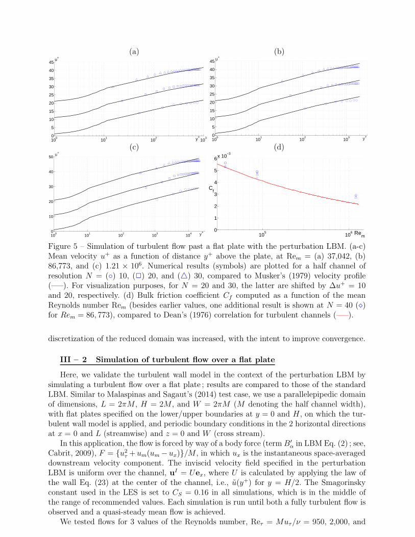
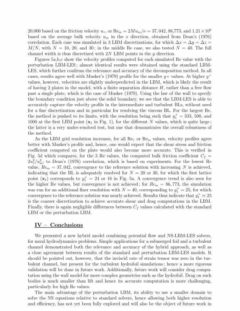
Figure 5 – Simulation of turbulent flow past a flat plate with the perturbation LBM. (a-c)Mean velocity u+ as a function of distance y+ above the plate, at Rem = (a) 37,042, (b)86,773, and (c) 1.21 × 106. Numerical results (symbols) are plotted for a half channel ofresolution N = () 10, () 20, and () 30, compared to Musker’s (1979) velocity profile(—–). For visualization purposes, for N = 20 and 30, the latter are shifted by ∆u+ = 10and 20, respectively. (d) Bulk friction coefficient Cf computed as a function of the meanReynolds number Rem (besides earlier values, one additional result is shown at N = 40 (⋄)for Rem = 86, 773), compared to Dean’s (1976) correlation for turbulent channels (—–).

discretization of the reduced domain was increased, with the intent to improve convergence.

III – 2 Simulation of turbulent flow over a flat plate

Here, we validate the turbulent wall model in the context of the perturbation LBM bysimulating a turbulent flow over a flat plate ; results are compared to those of the standardLBM. Similar to Malaspinas and Sagaut’s (2014) test case, we use a parallelepipedic domainof dimensions, L = 2πM , H = 2M , and W = 2πM (M denoting the half channel width),with flat plates specified on the lower/upper boundaries at y = 0 and H , on which the tur-bulent wall model is applied, and periodic boundary conditions in the 2 horizontal directionsat x = 0 and L (streamwise) and z = 0 and W (cross stream).

In this application, the flow is forced by way of a body force (term B′α in LBM Eq. (2) ; see,

Cabrit, 2009), F = u2τ + um(um−ux)/M , in which ux is the instantaneous space-averaged

downstream velocity component. The inviscid velocity field specified in the perturbationLBM is uniform over the channel, uI = Uex, where U is calculated by applying the law ofthe wall Eq. (23) at the center of the channel, i.e., u(y+) for y = H/2. The Smagorinskyconstant used in the LES is set to CS = 0.16 in all simulations, which is in the middle ofthe range of recommended values. Each simulation is run until both a fully turbulent flow isobserved and a quasi-steady mean flow is achieved.

We tested flows for 3 values of the Reynolds number, Reτ = Muτ/ν = 950, 2,000, and

20,000 based on the friction velocity uτ , or Rem = 2Mum/ν = 37, 042, 86,773, and 1.21×106

based on the average bulk velocity um in the x direction, obtained from Dean’s (1976)correlation. Each case was simulated in 3 LBM discretizations, for which ∆x = ∆y = ∆z =M/N , with N = 10, 20, and 30 ; in the middle Re case, we also tested N = 40. The fullchannel width is thus discretized with 2N LBM points in the y direction.

Figures 5a,b,c show the velocity profiles computed for each simulated Re value with theperturbation LBM-LES ; almost identical results were obtained using the standard LBM-LES, which further confirms the relevance and accuracy of the decomposition method. In allcases, results agree well with Musker’s (1979) profile for the smaller y+ values. At higher y+

values, however, velocities are slightly underperdicted in the LBM, which is likely the resultof having 2 plates in the model, with a finite separation distance H , rather than a free flowpast a single plate, which is the case of Musker (1979). Using the law of the wall to specifythe boundary condition just above the solid boundary, we see that the LBM-LES is able toaccurately capture the velocity profile in the intermediate and turbulent BLs, without needfor a fine discretization and in particular for resolving the viscous BL. For the largest Re,the method is pushed to its limits, with the resolution being such that y+1 = 333, 500, and1000 at the first LBM point (x1 in Fig. 1), for the different N values, which is quite large ;the latter is a very under-resolved test, but one that demonstrates the overall robustness ofthe method.

As the LBM grid resolution increases, for all Reτ or Rem values, velocity profiles agreebetter with Musker’s profile and, hence, one would expect that the shear stress and frictioncoefficient computed on the plate would also become more accurate. This is verified inFig. 5d which compares, for the 3 Re values, the computed bulk friction coefficient Cf =2u2

τ/u2m, to Dean’s (1976) correlation, which is based on experiments. For the lowest Re

value, Rem = 37, 042, convergence to the reference solution with increasing N is achieved,indicating that the BL is adequately resolved for N = 20 or 30, for which the first latticepoint (x1) corresponds to y+1 = 24 or 16 in Fig. 5a. A convergence trend is also seen forthe higher Re values, but convergence is not achieved ; for Rem = 86, 773, the simulationwas run for an additional finer resolution with N = 40, corresponding to y+1 = 25, for whichconvergence to the reference solution was nearly achieved. Results thus indicate that y+1 ≃ 25is the coarser discretization to achieve accurate shear and drag computations in the LBM.Finally, there is again negligible differences between Cf values calculated with the standardLBM or the perturbation LBM.

IV – Conclusions

We presented a new hybrid model combining potential flow and NS-LBM-LES solvers,for naval hydrodynamics problems. Simple applications for a submerged foil and a turbulentchannel demonstrated both the relevance and accuracy of the hybrid approach, as well asa close agreement between results of the standard and perturbation LBM-LES models. Itshould be pointed out, however, that the inviscid rate of strain tensor was zero in the tur-bulent channel, but present for the turbulent hydrofoil simulations ; hence a more rigorousvalidation will be done in future work. Additionally, future work will consider drag compu-tation using the wall model for more complex geometries such as the hydrofoil. Drag on suchbodies is much smaller than lift and hence its accurate computation is more challenging,particularly for high Re values.

The main advantage of the perturbation LBM, its ability to use a smaller domain tosolve the NS equations relative to standard solvers, hence allowing both higher resolutionand efficiency, has not yet been fully explored and will also be the object of future work in

which the far-field inviscid flow is more complex (e.g., irregular wave field). Finally, earlierwork by O’Reilly et al. (2015) has illustrated the standard LBM model’s (ELBE) ability toalso simulate free surface flows and free surface piercing bodies. We intend to extend theperturbation LBM method to simulating such problems, using fully non-linear free surfaceboundary conditions in which “I-P” interaction terms will appear.

V – Acknowledgements

C. O’Reilly, S. Grilli, A. Mivehchi and J. Dahl acknowledge support from grants N000141310687and N000141612970 of the Office of Naval Research (PM Kelly Cooper).

References

[1] Abbot, I.H., Von Doenhoff A.E. (1959) Theory of Wing Sections, Dover Pub., NewYork.

[2] Alessandrini, B. (2007). These d’Habilitation en Vue de Diriger les Recherches. EcoleCentrale de Nantes, Nantes.

[3] Banari A., Janssen C.F., and Grilli S.T. (2014). An efficient lattice Boltzmann multi-phase model for 3D flows with large density ratios at high Reynolds numbers. Comp.

and Math. with Applications, 68(12), 1819-1843.

[4] Cabrit, O. (2009) Direct simulations for wall modeling of multicomponent reactingcompressible turbulent flows. Phys. Fluids, 21, 055108.

[5] Dean, R. B., (1976) A single formula for the complete velocity profile in a turbulentboundary layer. J. Fluids Eng., 98(4), 723-726.

[6] Grilli, S.T. (2008) On the Development and Application of Hybrid Numerical Modelsin Nonlinear Free Surface Hydrodynamics. Keynote lecture in Proc. 8th Intl. Conf. on

Hydrodynamics (Nantes, France, 9/08) (P. Ferrant and X.B. Chen, eds.), pps. 21-50.

[7] Grilli, S.T., Dias, F., Guyenne, P., Fochesato, C. and F. Enet (2010) Progress InFully Nonlinear Potential Flow Modeling Of 3D Extreme Ocean Waves. Chapter 3in Advances in Numerical Simulation of Nonlinear Water Waves (ISBN : 978-981-283-649-6, edited by Q.W. Ma) (Vol. 11 in Series in Advances in Coastal and OceanEngineering). World Scientific Publishing Co. Pte. Ltd., pps. 75- 128.

[8] Guo Z., Zheng C., and Shi B. (2002). Discrete lattice effects on the forcing term in thelattice Boltzmann method. Phys. Rev., E65(4).

[9] Harris, J.C. and S.T. Grilli (2012). A perturbation approach to large-eddy simulationof wave-induced bottom boundary layer flows. Intl. J. Numer. Meth. Fluids, 68, 1,574-1,604.

[10] Harris J.C. and Grilli, S.T. (2014). Large eddy simulation of sediment transport overrippled beds. Nonlin. Process. Geophys., 21, 1,169-1,184.

[11] d’Humieres D., Ginzburg I., Krafczyk M., Lallemand P., and Luo L.-S. (2002) MultipleRelaxation-Time Lattice Boltzmann models in three-dimensions. Phil. Trans. RoyalSoc. London, A360, 437-451.

[12] Janssen C.F., S.T. Grilli and M. Krafczyk (2010) Modeling of Wave Breaking andWave-Structure Interactions by Coupling of Fully Nonlinear Potential Flow andLattice-Boltzmann Models. In Proc. 20th Offshore and Polar Engng. Conf. (ISOPE10,Beijing, China, June 20-25, 2010), pps. 686-693. Intl. Society of Offshore and PolarEngng.

[13] Janssen, C.F. (2010) Kinetic approaches for the simulation of non-linear free surface

flow problems in civil and environmental engng.. PhD thesis, Technical Univ. Braun-schweig.

[14] Janssen, C.F., S.T. Grilli and M. Krafczyk (2013) On enhanced non-linear free surfaceflow simulations with a hybrid LBM-VOF approach. Comp. and Math. with Applica-

tions, 65(2), 211-229.

[15] Janssen, C.F., D. Mierke, M Uberruck, S. Gralher, and T. Rung (2015) Validationof the GPU-accelerated CFD solver ELBE for free surface flow problems in civil andenvironmental engineering. Computation, 3(3),354-385.

[16] Janssen, C.F., Rung, T., Grilli S.T., O’Reilly C.M., (2016) An enhanced LBM-basedperturbation method (in preparation).

[17] Krafczyk M., Tolke J., Rank E., and Schulz M. (2001) Two-dimensional simulation offluid-structure interaction using Lattice Boltzmann methods. Comp. and Struct., 22,2,031-2,037.

[18] Krafczyk M., Tolke J., and Luo L.-S. (2003) Large eddy simulations with a multiple-relaxation-time LBE model. Intl. J. Modern Phys., 17, 33-39.

[19] Lallemand, P. and Luo, L.S. (2000) Theory of the Lattice Boltzmann Method : Dis-persion, dissipation, isotropy, Galilean invariance, and stability. Phys. Review, E61,6,546-6,562.

[20] Malaspinas, O., Sagaut, P., (2014) Wall model for large-eddy simulation based on thelattice Boltzmann method. J. Comp. Phys., 257, 25-40.

[21] Merkle, D., Janssen, C.F., (2016) Efficient calculation of sub-grid distances for higher-order boundary conditions in LBM (in preparation).

[22] Musker, A. (1979) Explicit expression for the smooth wall velocity distribution in aturbulent boundary layer. AIAA J., 17(6), 655-657.

[23] O’Reilly, C., Grilli, S.T., Dahl, J.M., Banari, A., Janssen, C.F., Shock, J.J. and M.Uberrueck. (2015) Solution of viscous flows in a hybrid naval hydrodynamic schemebased on an efficient Lattice Boltzmann Method. In Proc. 13th Intl. Conf. on Fast Sea

Transportation (FAST 2015 ; Washington D.C., September 1-4, 2015).

[24] Reliquet, G., A. Drouet, P.-E. Guillerm, L. Gentaz and P. Ferrant (2014). Simulationof wave-ship interaction in regular and irregular seas under viscous flow theory usingthe SWENSE method. In Proc. 30th Symp. Naval Hydrod. (Tasmania, 11/2014), 11pps.

[25] Succi, S. (2002) The lattice Boltzmann equation for fluid dynamics and beyond, OxfordScience Publications, Oxford.

[26] Zou Q., He X. (1997) On pressure and velocity boundary conditions for the latticeBoltzmann BGK model, Phys. Fluids, 9, 1,592-1,598.