Development of a human-tissue-like phantom for 3.0-T MRI

Yusuke Ikemoto and Wataru TakaoDepartment of Radiology, Okayama Kyokuto Hospital, Okayama, Okayama 703-8265, Japan

Keisuke Yoshitomi and Seiichiro OhnoCentral Division of Radiology, Okayama University Hospital, Okayama, Okayama 700-8558, Japan

Takashi HarimotoDepartment of Radiology, Kitagawa Hospital, Wake-gun, Okayama 709-0497, Japan

Susumu KanazawaDepartment of Radiology, Graduate School of Medicine, Dentistry and Pharmaceutical Sciences,Okayama University, Okayama, Okayama 700-8558, Japan

Koichi Shibuya, Masahiro Kuroda, and Hirokazu Katoa)

Department of Radiological Technology, Graduate School of Health Sciences, Okayama University, Okayama,Okayama 700-8558, Japan

(Received 18 April 2011; revised 29 September 2011; accepted for publication 6 October 2011;

published 31 October 2011)

Purpose: A 3.0-T MRI phantom having human-tissue-equivalent relaxation times was developed.

Methods: The ingredients of the phantom are carrageenan (for gelatinization), GdCl3 (as a

T1-relaxation modifier), agarose (as a T2-relaxation modifier), and NaN3 (as an antiseptic agent).

Numerous samples with varying concentrations of GdCl3 and agarose were prepared, and T1 and T2

were measured using 3.0-T MRI.

Results: Relaxation times of the phantom samples ranged from 395 to 2601 ms for T1 values and

29 to 334 ms for T2 values. Based on the measured results, empirical formulae were devised to

express the relationships between the concentrations of relaxation modifiers and relaxation times.

Conclusions: Adjustment of GdCl3 and agarose concentrations allows arbitrary setting of relaxa-

tion times, and the creation of a phantom that can mimic relaxation times of human-tissue. Carra-

geenan is considered the most suitable as a gelling agent for an MRI phantom, as it permits the

relatively easy and inexpensive production of a large phantom such as for the human torso, and

which can be easily shaped with a knife. VC 2011 American Association of Physicists in Medicine.

[DOI: 10.1118/1.3656077]

Key words: 3.0-T MRI, phantom, carrageenan, GdCl3, agarose

I. INTRODUCTION

The signal to noise ratio (SNR) and contrast to noise ratio

(CNR) of 3.0-T MRI are much greater than those of 1.5-T

MRI,1,2and thus 3.0-T MRI systems have gradually become

widely used in clinical settings. Benefits of 3.0-T MRI

include a shorter examination time, reduction of contrast

agent in MR angiography examinations, improved spatial re-

solution for biliary and pancreatic duct images, and

improved frequency resolution for MR spectroscopy exami-

nation.3 However, artifacts increase in 3.0-T MRI because of

increased magnetic susceptibility effects and chemical shift

effects, leading to a reduction of image contrast and prolon-

gation of scanning time. In addition, increased frequency of

RF magnetic fields due to the strengthening of the static

magnetic field from 1.5 T to 3.0 T induces adverse effects.

The specific absorption rate (SAR) in the human body from

RF magnetic fields at 3.0 T is approximately four times

greater than that at 1.5 T, making it necessary to set appro-

priate pulse sequences and flip angles to prevent burning

from the high SAR.4 Nonuniformity of MR images occurs in

3.0-T equipment due to attenuation and shortened wave-

length of the RF magnetic field passing through the human

body, induced by the high conductivity and permittivity of

the human body. Research to investigate and overcome these

problems raises the need of an MRI phantom having human-

tissue-equivalent relaxation times and dielectric properties.

A phantom’s T1 and T2 are modified by a static magnetic

field, while its conductivity and permittivity are dependent

on the frequency of applied RF magnetic fields. We previ-

ously successfully developed a phantom using carrageenan

gel (CAGN phantom), for use with 1.5-T MRI.5–9 In the

present study, we have now developed a new phantom hav-

ing human-tissue-equivalent relaxation times for 3.0-T MRI.

Numerous sample phantoms with varying amounts of T1 and

T2 relaxation modifiers were prepared, and the relaxation

times of each sample were measured. Based on these meas-

ured results, empirical formulae were obtained by the nonlin-

ear least-squares method, which showed the relationships

between the concentrations of the two modifiers and both T1

and T2 values. The creation of a human-tissue-like 3.0-T

phantom with two arbitrarily-set relaxation times is possible

with the appropriate blend of T1 and T2 modifiers according

to the empirical formulae.

6336 Med. Phys. 38 (11), November 2011 0094-2405/2011/38(11)/6336/7/$30.00 VC 2011 Am. Assoc. Phys. Med. 6336

Carrageenan, normally used as a low-cost food additive,

consists of saccharides extracted from red algae (seaweed).

These saccharides have molecular weights of 100 000–500

000, comprised mainly of galactose and 3,6-anhydrogalac-

tose. Carrageenan is a gelling material similar to agar though

relatively cheaper. While agarose10–12 and agar13,14 have

been widely used as gelling agents for MRI phantoms, the

benefits of carrageenan over other gels such as polysaccha-

ride or gelatin,15 include greater elasticity and strength,

being formable into a large and stable phantom, and having

an easily modified shape.5 In contrast to agarose, carra-

geenan has a little influence on T2, making possible a phan-

tom with a long T2 value.

II. MATERIALS AND METHODS

II.A. Sample preparation

Materials used for the phantoms were carrageenan

(KC-200S: Chuo Kasei Co., Ltd., Osaka, Japan) for gelati-

nization; GdCl3 (Sigma Chemical Corp., St. Louis, MO,

USA) as a T1 modifier; agarose (Type 1, #A-6013: Sigma

Chemical Corp., St. Louis, MO, USA) as a T2 modifier;

NaN3 (Katayama Chemical, Osaka, Japan) as an antisep-

tic; and, distilled water.5 Agarose was chosen as a T2

modifier as it affects that value in MRI. Conversely, carra-

geenan was selected as the gelling agent because it has

almost no impact on T2 values. As a control phantom, a

solution of NiCl2(Sigma Chemical Corp., St. Louis, MO)

was used.

The total weight of each sample was 100 g, including

distilled water. Sample size was limited by the total num-

ber of samples needed to evaluate more than 180 combina-

tions of T1 and T2 modifier concentrations necessary for

measuring the various relaxation times. Previous studies

have shown that phantom size is irrelevant due to the phan-

tom’s homogeneity.9 The concentrations of carrageenan

and NaN3 were fixed at 3 and 0.03 w/w%, respectively.

Based on previous reports, we used the lowest possible

concentration of carrageenan that would yield a phantom

physically strong enough to maintain its shape, and the

lowest possible concentration of NaN3 necessary to prevent

the occurrence of mold.5 The concentration of GdCl3ranged from 0 to 180 lmol/kg, while that of agarose ranged

from 0 to 2.0 w/w%.

All ingredients for each phantom were mixed together in

a Pyrex tube (diameter: 40 mm, height: 130 mm). The mix-

ture was then heated while being stirred in a hot water bath

at 90 �C to dissolve the carrageenan and agarose. This mix-

ture was then boiled in a microwave oven at 90–100 �C to

complete the dissolving of the agarose.9 Heating in the

microwave oven serves to prevent the occurrence of many

defects when imaging the phantom. Next, the mixture was

cooled to 25 6 1 for gelling purposes. Finally, each sample

phantom tube was sealed with a rubber stopper to prevent

water evaporation. For verification of MRI equipment set-

tings and the validity of our data, a 100 g control phantom

was prepared, consisting of NiCl2 solution set at 14 mmol/

kg.

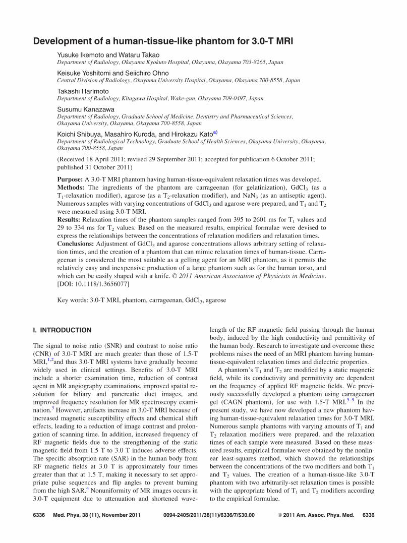
II.B. MRI measurement

Measurements of T1 and T2 were made using a 3.0-T

Magnetic Resonance Imager (Signa Excite HDx 3.0 T, GE

Healthcare ). The Pyrex tube containing the control phantom

was placed at the center of a custom-made acrylic case, and

18 Pyrex tubes, each containing a phantom sample, were

placed inside the case around the control. Figure 1(a) shows

an array of samples for measurement in which 18 sample

phantoms and 1 control at the center of the array are set in

the head coil. Figure 1(b) is an SE image of such an array,

obtained at TR¼ 15 000 ms, TE¼ 15 ms. An region-of-in-

terest (ROI) was identified on each sample, and T1 and T2

values were then calculated.

The samples and control were then scanned with an axial

projection using a head coil. The scan parameters were: slice

thickness, 10 mm; matrix, 256� 256; FOV, 220 mm; band

width, 6 15.63 kHz; and, number of acquisitions, 1. To com-

pare the relaxation times at 3.0 T with those at 1.5 T, previ-

ously reported pulse sequences5 were used here for

measuring T1 and T2 values . T1 was measured using the sat-

uration recovery method with a constant TE value of 15 ms

and TR values of 133, 167, 217, 300, 400, 533, 717, 950,

1683, 3000, 5283, 9317, and 15 000 ms. T2 was measured

using the spin echo method with a constant TR value of 10

000 ms and TE values of 15, 22, 29, 39, 52, 69, 93, 125, 167,

224, and 300 ms. Calculation of T1 and T2 values was per-

formed using “IMAGE J” by setting a ROI 20 mm in diameter

(448 pixels) in the center of each sample.

II.C. Examination of the relationship betweenconcentrations of modifiers and relaxation times

Based on the obtained data, and using methods previously

reported,5 the relationships between the concentrations of

the two modifiers and the two relaxation times were both for-

mulated using the nonlinear least-squares method (Gauss–-

Newton Method) installed in MATLABVR

(The MathWorks,

Inc., Natick).

III. RESULTS

III.A. Relaxation times of samples

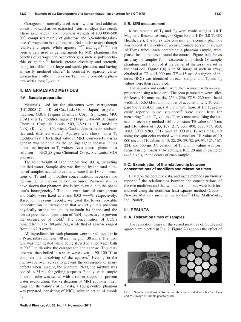
The relaxation times of the varied mixtures of GdCl3 and

agarose are plotted in Fig. 2. Figure 2(a) shows the effect of

FIG. 1. Sample phantoms within an acrylic case inserted in a head coil (a)

and MR image of sample phantoms (b).

6337 Ikemoto et al.: Development of a human-tissue-like phantom for 3.0-T MRI 6337

Medical Physics, Vol. 38, No. 11, November 2011

the GdCl3 and agarose concentrations on T1 and T2. Each

solid line corresponds to a different iso-agarose concentra-

tion, while each broken line indicates an iso-GdCl3 concen-

tration. T1 decreases with an increased GdCl3 concentration,

irrespective of the agarose concentration. T2 decreases with

an increased agarose concentration and further decreases

with the increase of the GdCl3 concentration. In Fig. 2(b),

the relaxation times for a range of human-tissues2,16–19have

been superimposed on our data. The range of relaxation

times obtained for our various samples fall within those of

most types of human-tissues.

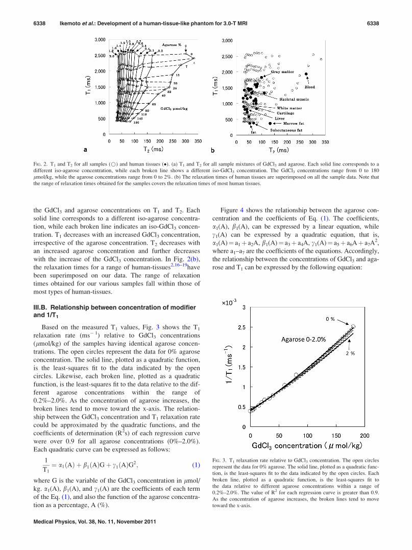
III.B. Relationship between concentration of modifierand 1/T1

Based on the measured T1 values, Fig. 3 shows the T1

relaxation rate (ms� 1) relative to GdCl3 concentrations

(lmol/kg) of the samples having identical agarose concen-

trations. The open circles represent the data for 0% agarose

concentration. The solid line, plotted as a quadratic function,

is the least-squares fit to the data indicated by the open

circles. Likewise, each broken line, plotted as a quadratic

function, is the least-squares fit to the data relative to the dif-

ferent agarose concentrations within the range of

0.2%–2.0%. As the concentration of agarose increases, the

broken lines tend to move toward the x-axis. The relation-

ship between the GdCl3 concentration and T1 relaxation rate

could be approximated by the quadratic functions, and the

coefficients of determination (R2s) of each regression curve

were over 0.9 for all agarose concentrations (0%–2.0%).

Each quadratic curve can be expressed as follows:

1

T1

¼ a1ðAÞ þ b1ðAÞGþ c1ðAÞG2; (1)

where G is the variable of the GdCl3 concentration in lmol/

kg. a1(A), b1(A), and c1(A) are the coefficients of each term

of the Eq. (1), and also the function of the agarose concentra-

tion as a percentage, A (%).

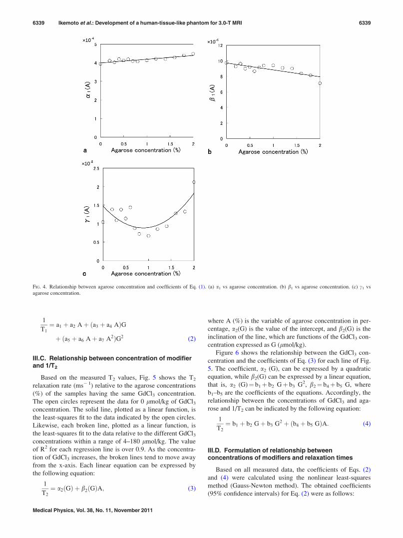
Figure 4 shows the relationship between the agarose con-

centration and the coefficients of Eq. (1). The coefficients,

a1(A), b1(A), can be expressed by a linear equation, while

c1(A) can be expressed by a quadratic equation, that is,

a1(A)¼ a1þ a2A, b1(A)¼ a3þ a4A, c1(A)¼ a5þ a6Aþ a7A2,

where a1–a7 are the coefficients of the equations. Accordingly,

the relationship between the concentrations of GdCl3 and aga-

rose and T1 can be expressed by the following equation:

FIG. 2. T1 and T2 for all samples (*) and human tissues (�). (a) T1 and T2 for all sample mixtures of GdCl3 and agarose. Each solid line corresponds to a

different iso-agarose concentration, while each broken line shows a different iso-GdCl3 concentration. The GdCl3 concentrations range from 0 to 180

lmol/kg, while the agarose concentrations range from 0 to 2%. (b) The relaxation times of human tissues are superimposed on all the sample data. Note that

the range of relaxation times obtained for the samples covers the relaxation times of most human tissues.

FIG. 3. T1 relaxation rate relative to GdCl3 concentration. The open circles

represent the data for 0% agarose. The solid line, plotted as a quadratic func-

tion, is the least-squares fit to the data indicated by the open circles. Each

broken line, plotted as a quadratic function, is the least-squares fit to

the data relative to different agarose concentrations within a range of

0.2%–2.0%. The value of R2 for each regression curve is greater than 0.9.

As the concentration of agarose increases, the broken lines tend to move

toward the x-axis.

6338 Ikemoto et al.: Development of a human-tissue-like phantom for 3.0-T MRI 6338

Medical Physics, Vol. 38, No. 11, November 2011

1

T1

¼ a1 þ a2 Aþ ða3 þ a4 AÞG

þ ða5 þ a6 Aþ a7 A2ÞG2 (2)

III.C. Relationship between concentration of modifierand 1/T2

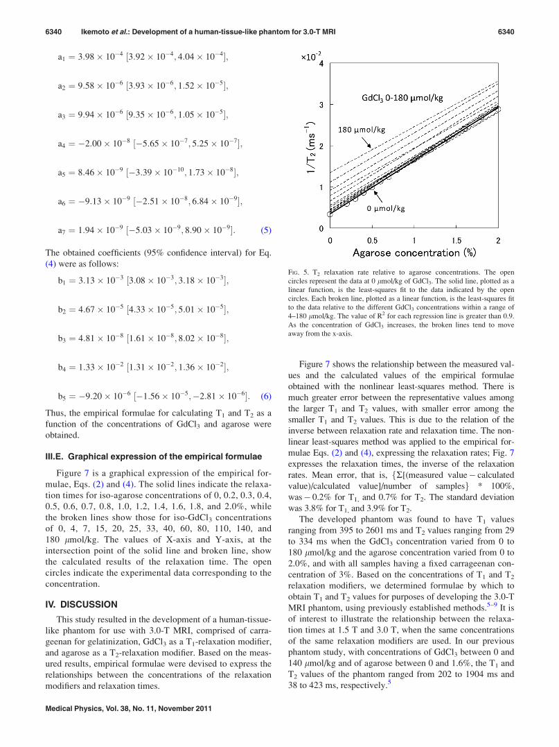
Based on the measured T2 values, Fig. 5 shows the T2

relaxation rate (ms� 1) relative to the agarose concentrations

(%) of the samples having the same GdCl3 concentration.

The open circles represent the data for 0 lmol/kg of GdCl3concentration. The solid line, plotted as a linear function, is

the least-squares fit to the data indicated by the open circles.

Likewise, each broken line, plotted as a linear function, is

the least-squares fit to the data relative to the different GdCl3concentrations within a range of 4–180 lmol/kg. The value

of R2 for each regression line is over 0.9. As the concentra-

tion of GdCl3 increases, the broken lines tend to move away

from the x-axis. Each linear equation can be expressed by

the following equation:

1

T2

¼ a2ðGÞ þ b2ðGÞA; (3)

where A (%) is the variable of agarose concentration in per-

centage, a2(G) is the value of the intercept, and b2(G) is the

inclination of the line, which are functions of the GdCl3 con-

centration expressed as G (lmol/kg).

Figure 6 shows the relationship between the GdCl3 con-

centration and the coefficients of Eq. (3) for each line of Fig.

5. The coefficient, a2 (G), can be expressed by a quadratic

equation, while b2(G) can be expressed by a linear equation,

that is, a2 (G)¼ b1þ b2 Gþ b3 G2, b2¼ b4þ b5 G, where

b1–b5 are the coefficients of the equations. Accordingly, the

relationship between the concentrations of GdCl3 and aga-

rose and 1/T2 can be indicated by the following equation:

1

T2

¼ b1 þ b2 Gþ b3 G2 þ ðb4 þ b5 GÞA: (4)

III.D. Formulation of relationship betweenconcentrations of modifiers and relaxation times

Based on all measured data, the coefficients of Eqs. (2)

and (4) were calculated using the nonlinear least-squares

method (Gauss-Newton method). The obtained coefficients

(95% confidence intervals) for Eq. (2) were as follows:

FIG. 4. Relationship between agarose concentration and coefficients of Eq. (1). (a) a1 vs agarose concentration. (b) b1 vs agarose concentration. (c) c1 vs

agarose concentration.

6339 Ikemoto et al.: Development of a human-tissue-like phantom for 3.0-T MRI 6339

Medical Physics, Vol. 38, No. 11, November 2011

a1 ¼ 3:98� 10�4 ½3:92� 10�4; 4:04� 10�4�;

a2 ¼ 9:58� 10�6 ½3:93� 10�6; 1:52� 10�5�;

a3 ¼ 9:94� 10�6 ½9:35� 10�6; 1:05� 10�5�;

a4 ¼ �2:00� 10�8 ½�5:65� 10�7; 5:25� 10�7�;

a5 ¼ 8:46� 10�9 ½�3:39� 10�10; 1:73� 10�8�;

a6 ¼ �9:13� 10�9 ½�2:51� 10�8; 6:84� 10�9�;

a7 ¼ 1:94� 10�9 ½�5:03� 10�9; 8:90� 10�9�: (5)

The obtained coefficients (95% confidence interval) for Eq.

(4) were as follows:

b1 ¼ 3:13� 10�3 ½3:08� 10�3; 3:18� 10�3�;

b2 ¼ 4:67� 10�5 ½4:33� 10�5; 5:01� 10�5�;

b3 ¼ 4:81� 10�8 ½1:61� 10�8; 8:02� 10�8�;

b4 ¼ 1:33� 10�2 ½1:31� 10�2; 1:36� 10�2�;

b5 ¼ �9:20� 10�6 ½�1:56� 10�5;�2:81� 10�6�: (6)

Thus, the empirical formulae for calculating T1 and T2 as a

function of the concentrations of GdCl3 and agarose were

obtained.

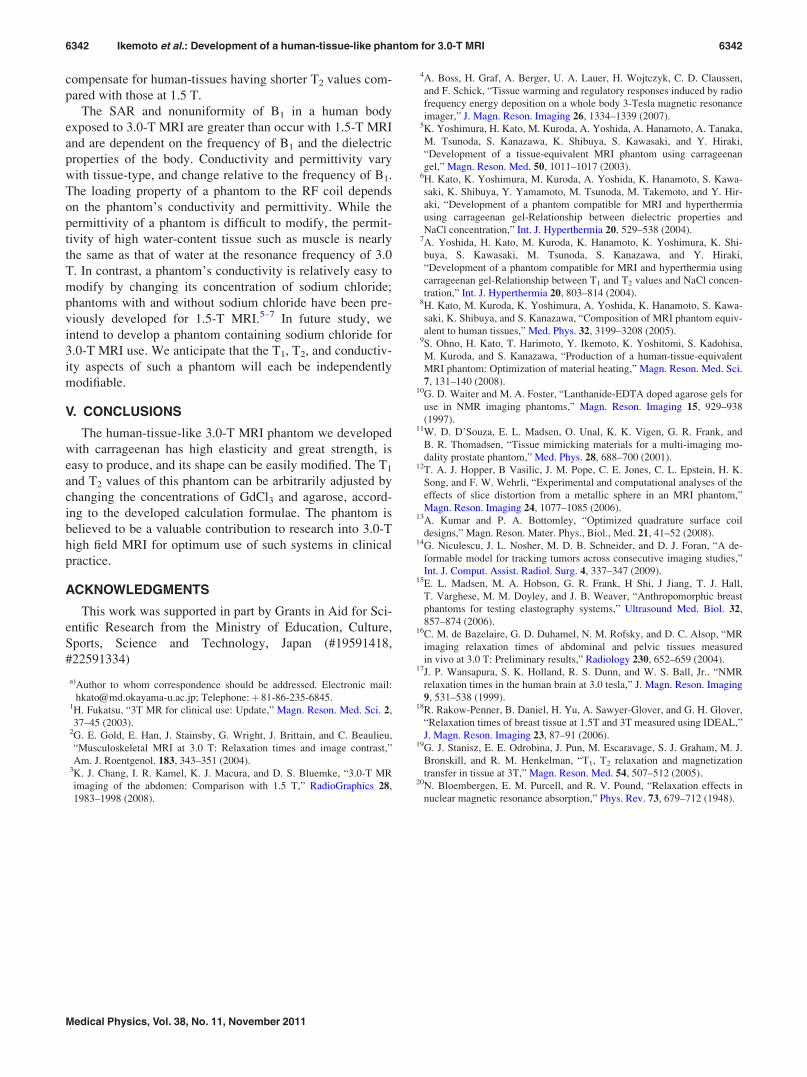
III.E. Graphical expression of the empirical formulae

Figure 7 is a graphical expression of the empirical for-

mulae, Eqs. (2) and (4). The solid lines indicate the relaxa-

tion times for iso-agarose concentrations of 0, 0.2, 0.3, 0.4,

0.5, 0.6, 0.7, 0.8, 1.0, 1.2, 1.4, 1.6, 1.8, and 2.0%, while

the broken lines show those for iso-GdCl3 concentrations

of 0, 4, 7, 15, 20, 25, 33, 40, 60, 80, 110, 140, and

180 lmol/kg. The values of X-axis and Y-axis, at the

intersection point of the solid line and broken line, show

the calculated results of the relaxation time. The open

circles indicate the experimental data corresponding to the

concentration.

IV. DISCUSSION

This study resulted in the development of a human-tissue-

like phantom for use with 3.0-T MRI, comprised of carra-

geenan for gelatinization, GdCl3 as a T1-relaxation modifier,

and agarose as a T2-relaxation modifier. Based on the meas-

ured results, empirical formulae were devised to express the

relationships between the concentrations of the relaxation

modifiers and relaxation times.

Figure 7 shows the relationship between the measured val-

ues and the calculated values of the empirical formulae

obtained with the nonlinear least-squares method. There is

much greater error between the representative values among

the larger T1 and T2 values, with smaller error among the

smaller T1 and T2 values. This is due to the relation of the

inverse between relaxation rate and relaxation time. The non-

linear least-squares method was applied to the empirical for-

mulae Eqs. (2) and (4), expressing the relaxation rates; Fig. 7

expresses the relaxation times, the inverse of the relaxation

rates. Mean error, that is, fR[(measured value� calculated

value)/calculated value]/number of samplesg * 100%,

was� 0.2% for T1, and 0.7% for T2. The standard deviation

was 3.8% for T1, and 3.9% for T2.

The developed phantom was found to have T1 values

ranging from 395 to 2601 ms and T2 values ranging from 29

to 334 ms when the GdCl3 concentration varied from 0 to

180 lmol/kg and the agarose concentration varied from 0 to

2.0%, and with all samples having a fixed carrageenan con-

centration of 3%. Based on the concentrations of T1 and T2

relaxation modifiers, we determined formulae by which to

obtain T1 and T2 values for purposes of developing the 3.0-T

MRI phantom, using previously established methods.5–9 It is

of interest to illustrate the relationship between the relaxa-

tion times at 1.5 T and 3.0 T, when the same concentrations

of the same relaxation modifiers are used. In our previous

phantom study, with concentrations of GdCl3 between 0 and

140 lmol/kg and of agarose between 0 and 1.6%, the T1 and

T2 values of the phantom ranged from 202 to 1904 ms and

38 to 423 ms, respectively.5

FIG. 5. T2 relaxation rate relative to agarose concentrations. The open

circles represent the data at 0 lmol/kg of GdCl3. The solid line, plotted as a

linear function, is the least-squares fit to the data indicated by the open

circles. Each broken line, plotted as a linear function, is the least-squares fit

to the data relative to the different GdCl3 concentrations within a range of

4–180 lmol/kg. The value of R2 for each regression line is greater than 0.9.

As the concentration of GdCl3 increases, the broken lines tend to move

away from the x-axis.

6340 Ikemoto et al.: Development of a human-tissue-like phantom for 3.0-T MRI 6340

Medical Physics, Vol. 38, No. 11, November 2011

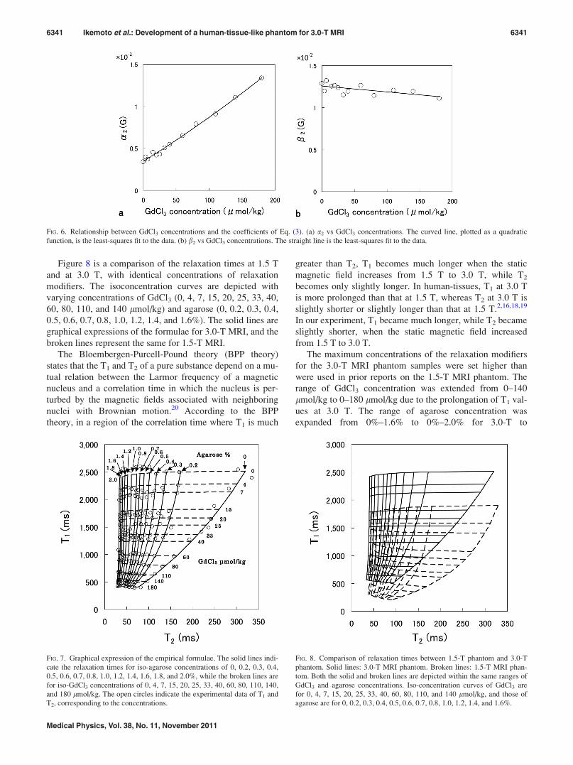
Figure 8 is a comparison of the relaxation times at 1.5 T

and at 3.0 T, with identical concentrations of relaxation

modifiers. The isoconcentration curves are depicted with

varying concentrations of GdCl3 (0, 4, 7, 15, 20, 25, 33, 40,

60, 80, 110, and 140 lmol/kg) and agarose (0, 0.2, 0.3, 0.4,

0.5, 0.6, 0.7, 0.8, 1.0, 1.2, 1.4, and 1.6%). The solid lines are

graphical expressions of the formulae for 3.0-T MRI, and the

broken lines represent the same for 1.5-T MRI.

The Bloembergen-Purcell-Pound theory (BPP theory)

states that the T1 and T2 of a pure substance depend on a mu-

tual relation between the Larmor frequency of a magnetic

nucleus and a correlation time in which the nucleus is per-

turbed by the magnetic fields associated with neighboring

nuclei with Brownian motion.20 According to the BPP

theory, in a region of the correlation time where T1 is much

greater than T2, T1 becomes much longer when the static

magnetic field increases from 1.5 T to 3.0 T, while T2

becomes only slightly longer. In human-tissues, T1 at 3.0 T

is more prolonged than that at 1.5 T, whereas T2 at 3.0 T is

slightly shorter or slightly longer than that at 1.5 T.2,16,18,19

In our experiment, T1 became much longer, while T2 became

slightly shorter, when the static magnetic field increased

from 1.5 T to 3.0 T.

The maximum concentrations of the relaxation modifiers

for the 3.0-T MRI phantom samples were set higher than

were used in prior reports on the 1.5-T MRI phantom. The

range of GdCl3 concentration was extended from 0–140

lmol/kg to 0–180 lmol/kg due to the prolongation of T1 val-

ues at 3.0 T. The range of agarose concentration was

expanded from 0%–1.6% to 0%–2.0% for 3.0-T to

FIG. 7. Graphical expression of the empirical formulae. The solid lines indi-

cate the relaxation times for iso-agarose concentrations of 0, 0.2, 0.3, 0.4,

0.5, 0.6, 0.7, 0.8, 1.0, 1.2, 1.4, 1.6, 1.8, and 2.0%, while the broken lines are

for iso-GdCl3 concentrations of 0, 4, 7, 15, 20, 25, 33, 40, 60, 80, 110, 140,

and 180 lmol/kg. The open circles indicate the experimental data of T1 and

T2, corresponding to the concentrations.

FIG. 8. Comparison of relaxation times between 1.5-T phantom and 3.0-T

phantom. Solid lines: 3.0-T MRI phantom. Broken lines: 1.5-T MRI phan-

tom. Both the solid and broken lines are depicted within the same ranges of

GdCl3 and agarose concentrations. Iso-concentration curves of GdCl3 are

for 0, 4, 7, 15, 20, 25, 33, 40, 60, 80, 110, and 140 lmol/kg, and those of

agarose are for 0, 0.2, 0.3, 0.4, 0.5, 0.6, 0.7, 0.8, 1.0, 1.2, 1.4, and 1.6%.

FIG. 6. Relationship between GdCl3 concentrations and the coefficients of Eq. (3). (a) a2 vs GdCl3 concentrations. The curved line, plotted as a quadratic

function, is the least-squares fit to the data. (b) b2 vs GdCl3 concentrations. The straight line is the least-squares fit to the data.

6341 Ikemoto et al.: Development of a human-tissue-like phantom for 3.0-T MRI 6341

Medical Physics, Vol. 38, No. 11, November 2011

compensate for human-tissues having shorter T2 values com-

pared with those at 1.5 T.

The SAR and nonuniformity of B1 in a human body

exposed to 3.0-T MRI are greater than occur with 1.5-T MRI

and are dependent on the frequency of B1 and the dielectric

properties of the body. Conductivity and permittivity vary

with tissue-type, and change relative to the frequency of B1.

The loading property of a phantom to the RF coil depends

on the phantom’s conductivity and permittivity. While the

permittivity of a phantom is difficult to modify, the permit-

tivity of high water-content tissue such as muscle is nearly

the same as that of water at the resonance frequency of 3.0

T. In contrast, a phantom’s conductivity is relatively easy to

modify by changing its concentration of sodium chloride;

phantoms with and without sodium chloride have been pre-

viously developed for 1.5-T MRI.5–7 In future study, we

intend to develop a phantom containing sodium chloride for

3.0-T MRI use. We anticipate that the T1, T2, and conductiv-

ity aspects of such a phantom will each be independently

modifiable.

V. CONCLUSIONS

The human-tissue-like 3.0-T MRI phantom we developed

with carrageenan has high elasticity and great strength, is

easy to produce, and its shape can be easily modified. The T1

and T2 values of this phantom can be arbitrarily adjusted by

changing the concentrations of GdCl3 and agarose, accord-

ing to the developed calculation formulae. The phantom is

believed to be a valuable contribution to research into 3.0-T

high field MRI for optimum use of such systems in clinical

practice.

ACKNOWLEDGMENTS

This work was supported in part by Grants in Aid for Sci-

entific Research from the Ministry of Education, Culture,

Sports, Science and Technology, Japan (#19591418,

#22591334)

a)Author to whom correspondence should be addressed. Electronic mail:

hkato@md.okayama-u.ac.jp; Telephone:þ 81-86-235-6845.1H. Fukatsu, “3T MR for clinical use: Update,” Magn. Reson. Med. Sci. 2,

37–45 (2003).2G. E. Gold, E. Han, J. Stainsby, G. Wright, J. Brittain, and C. Beaulieu,

“Musculoskeletal MRI at 3.0 T: Relaxation times and image contrast,”

Am. J. Roentgenol. 183, 343–351 (2004).3K. J. Chang, I. R. Kamel, K. J. Macura, and D. S. Bluemke, “3.0-T MR

imaging of the abdomen: Comparison with 1.5 T,” RadioGraphics 28,

1983–1998 (2008).

4A. Boss, H. Graf, A. Berger, U. A. Lauer, H. Wojtczyk, C. D. Claussen,

and F. Schick, “Tissue warming and regulatory responses induced by radio

frequency energy deposition on a whole body 3-Tesla magnetic resonance

imager,” J. Magn. Reson. Imaging 26, 1334–1339 (2007).5K. Yoshimura, H. Kato, M. Kuroda, A. Yoshida, A. Hanamoto, A. Tanaka,

M. Tsunoda, S. Kanazawa, K. Shibuya, S. Kawasaki, and Y. Hiraki,

“Development of a tissue-equivalent MRI phantom using carrageenan

gel,” Magn. Reson. Med. 50, 1011–1017 (2003).6H. Kato, K. Yoshimura, M. Kuroda, A. Yoshida, K. Hanamoto, S. Kawa-

saki, K. Shibuya, Y. Yamamoto, M. Tsunoda, M. Takemoto, and Y. Hir-

aki, “Development of a phantom compatible for MRI and hyperthermia

using carrageenan gel-Relationship between dielectric properties and

NaCl concentration,” Int. J. Hyperthermia 20, 529–538 (2004).7A. Yoshida, H. Kato, M. Kuroda, K. Hanamoto, K. Yoshimura, K. Shi-

buya, S. Kawasaki, M. Tsunoda, S. Kanazawa, and Y. Hiraki,

“Development of a phantom compatible for MRI and hyperthermia using

carrageenan gel-Relationship between T1 and T2 values and NaCl concen-

tration,” Int. J. Hyperthermia 20, 803–814 (2004).8H. Kato, M. Kuroda, K. Yoshimura, A. Yoshida, K. Hanamoto, S. Kawa-

saki, K. Shibuya, and S. Kanazawa, “Composition of MRI phantom equiv-

alent to human tissues,” Med. Phys. 32, 3199–3208 (2005).9S. Ohno, H. Kato, T. Harimoto, Y. Ikemoto, K. Yoshitomi, S. Kadohisa,

M. Kuroda, and S. Kanazawa, “Production of a human-tissue-equivalent

MRI phantom: Optimization of material heating,” Magn. Reson. Med. Sci.

7, 131–140 (2008).10G. D. Waiter and M. A. Foster, “Lanthanide-EDTA doped agarose gels for

use in NMR imaging phantoms,” Magn. Reson. Imaging 15, 929–938

(1997).11W. D. D’Souza, E. L. Madsen, O. Unal, K. K. Vigen, G. R. Frank, and

B. R. Thomadsen, “Tissue mimicking materials for a multi-imaging mo-

dality prostate phantom,” Med. Phys. 28, 688–700 (2001).12T. A. J. Hopper, B Vasilic, J. M. Pope, C. E. Jones, C. L. Epstein, H. K.

Song, and F. W. Wehrli, “Experimental and computational analyses of the

effects of slice distortion from a metallic sphere in an MRI phantom,”

Magn. Reson. Imaging 24, 1077–1085 (2006).13A. Kumar and P. A. Bottomley, “Optimized quadrature surface coil

designs,” Magn. Reson. Mater. Phys., Biol., Med. 21, 41–52 (2008).14G. Niculescu, J. L. Nosher, M. D. B. Schneider, and D. J. Foran, “A de-

formable model for tracking tumors across consecutive imaging studies,”

Int. J. Comput. Assist. Radiol. Surg. 4, 337–347 (2009).15E. L. Madsen, M. A. Hobson, G. R. Frank, H Shi, J Jiang, T. J. Hall,

T. Varghese, M. M. Doyley, and J. B. Weaver, “Anthropomorphic breast

phantoms for testing elastography systems,” Ultrasound Med. Biol. 32,

857–874 (2006).16C. M. de Bazelaire, G. D. Duhamel, N. M. Rofsky, and D. C. Alsop, “MR

imaging relaxation times of abdominal and pelvic tissues measured

in vivo at 3.0 T: Preliminary results,” Radiology 230, 652–659 (2004).17J. P. Wansapura, S. K. Holland, R. S. Dunn, and W. S. Ball, Jr.. “NMR

relaxation times in the human brain at 3.0 tesla,” J. Magn. Reson. Imaging

9, 531–538 (1999).18R. Rakow-Penner, B. Daniel, H. Yu, A. Sawyer-Glover, and G. H. Glover,

“Relaxation times of breast tissue at 1.5T and 3T measured using IDEAL,”

J. Magn. Reson. Imaging 23, 87–91 (2006).19G. J. Stanisz, E. E. Odrobina, J. Pun, M. Escaravage, S. J. Graham, M. J.

Bronskill, and R. M. Henkelman, “T1, T2 relaxation and magnetization

transfer in tissue at 3T,” Magn. Reson. Med. 54, 507–512 (2005).20N. Bloembergen, E. M. Purcell, and R. V. Pound, “Relaxation effects in

nuclear magnetic resonance absorption,” Phys. Rev. 73, 679–712 (1948).

6342 Ikemoto et al.: Development of a human-tissue-like phantom for 3.0-T MRI 6342

Medical Physics, Vol. 38, No. 11, November 2011