Embed Size (px)
Citation preview
Development of a high-cadence,high-precision solar imaging
polarimeter with application to the FSPprototype
Der Fakultät für Elektrotechnik, Informationstechnik, Physikder Technischen Universität Carolo-Wilhelmina zu Braunschweig
zur Erlangung des Grades einesder Ingenieurwissenschaften (Dr.-Ing.)
genehmigte Dissertation
von Francisco Andrés Iglesiasaus Mendoza, Argentinien
eingereicht am: 12. April 2016mündliche Prüfung am: 29. April 2016
1. Referent: Prof. Dr.-Ing. Harald Michalik2. Referent: Prof. Dr. Sami K. Solanki
Druckjahr: 2016

Bibliografische Information der Deutschen Nationalbibliothek
Die Deutsche Nationalbibliothek verzeichnet diese Publikation in derDeutschen Nationalbibliografie; detaillierte bibliografische Datensind im Internet über http://dnb.d-nb.de abrufbar.
Cover: High-cadence, MOMFBD-restored measurement of a solar poreacquired with the FSP (top and bottom left). The Grey scale in the normal-ized Stokes V ranges from −23 to 10%. FSP modulator (top right) and thepnCCD camera (bottom right). Cover by www.behance.net/birpip
ISBN 978-3-944072-50-0
uni-edition GmbH 2016http://www.uni-edition.de© Francisco Andrés Iglesias
This work is distributed under aCreative Commons Attribution 3.0 License
Printed in Germany

Vorveröffentlichungen der Dissertation
Teilergebnisse aus dieser Arbeit wurden mit Genehmigung der Fakultät für Elektrotech-nik, Informationstechnik, Physik, vertreten durch den Betreuer der Arbeit, in folgendenBeiträgen vorab veröffentlicht:
Publikationen
Iglesias, F. A., Feller, A., Nagaraju, K. and Solanki, S, K., 2016, High-resolution,high-sensitivity, ground-based solar spectropolarimetry with a new fast imagingpolarimeter, Astronomy and Astrophysics, Volume 590, A89.
Iglesias, F. A., Feller, A. and Nagaraju, K., 2015, Smear correction of highly-variable, frame-transfer-CCD images with application to polarimetry, Applied Op-tics, Volume 54, Issue 19, p. 5970.
Tagungsbeiträge
Iglesias, F. A., Feller, A., Nagaraju, K. and Solanki, S, K., 2016, Fast Solar Po-larimeter: Prototype characterization and first results, ASP Conference Series,Volume 504, p. 325.
Feller, A., Iglesias, F. A., Nagaraju, K., Solanki, S. K. and Ihle, S., 2014, Fast SolarPolarimeter: Description and First Results, ASP Conference Series, Volume 489,p. 271.
iii


To my family and María Belén Tomaselli


Contents
List of Figures xii
List of Tables xiii
Summary xvi
Kurzfassung xviii
1 Introduction 11.1 Objectives . . . . . . . . . . . . . . . . . . . . . . . . . . . . . . . . . . 31.2 Outline . . . . . . . . . . . . . . . . . . . . . . . . . . . . . . . . . . . 4
2 Background 72.1 Introduction to solar spectropolarimetry . . . . . . . . . . . . . . . . . . 7
2.1.1 Description of polarized light and its transformations . . . . . . . 72.1.2 Generation and transformation of polarized light . . . . . . . . . 102.1.3 Solar spectropolarimetry . . . . . . . . . . . . . . . . . . . . . . 162.1.4 Data requirements in high-resolution solar polarimetry . . . . . . 17
2.2 Solar polarimeters . . . . . . . . . . . . . . . . . . . . . . . . . . . . . . 202.2.1 Measurement technique . . . . . . . . . . . . . . . . . . . . . . 202.2.2 Polarization modulators . . . . . . . . . . . . . . . . . . . . . . 232.2.3 Wavelength discrimination . . . . . . . . . . . . . . . . . . . . . 252.2.4 Scientific cameras . . . . . . . . . . . . . . . . . . . . . . . . . 27
2.3 Polarimetric effects of atmospheric seeing and image motion . . . . . . . 322.3.1 Description of atmospheric seeing and image motion . . . . . . . 322.3.2 Polarimetric effects in the different modulation schemes . . . . . 362.3.3 Image restoration . . . . . . . . . . . . . . . . . . . . . . . . . . 40
3 High-cadence, ground-based polarimetry 453.1 Main properties of a high-cadence polarimeter . . . . . . . . . . . . . . . 45
3.1.1 Camera requirements . . . . . . . . . . . . . . . . . . . . . . . . 473.1.2 Polarization modulator requirements . . . . . . . . . . . . . . . . 50
3.2 The Fast Solar Polarimeter Prototype . . . . . . . . . . . . . . . . . . . . 513.2.1 Cameras used in ground-based polarimeters: state-of-the-art . . . 523.2.2 System overview . . . . . . . . . . . . . . . . . . . . . . . . . . 54
vii

Contents
4 Characterization and optimization of an FLC-based polarization modulator 594.1 Main design features . . . . . . . . . . . . . . . . . . . . . . . . . . . . 594.2 Efficiencies optimization . . . . . . . . . . . . . . . . . . . . . . . . . . 62
4.2.1 Step 1: FLCs characterization . . . . . . . . . . . . . . . . . . . 634.2.2 Step 2: First optimization and SRs characterization . . . . . . . . 664.2.3 Step 3: Final optimization and results . . . . . . . . . . . . . . . 67
4.3 Polarimetric calibration . . . . . . . . . . . . . . . . . . . . . . . . . . . 684.3.1 Spatial dependence . . . . . . . . . . . . . . . . . . . . . . . . . 704.3.2 Spectral dependence . . . . . . . . . . . . . . . . . . . . . . . . 714.3.3 Modulation frequency dependence . . . . . . . . . . . . . . . . . 724.3.4 Thermal dependence . . . . . . . . . . . . . . . . . . . . . . . . 73
5 Characterization and optimization of a pnCCD camera for fast imaging po-larimetry 755.1 Design and specifications . . . . . . . . . . . . . . . . . . . . . . . . . . 75
5.1.1 pnCCD sensor and readout electronics . . . . . . . . . . . . . . . 765.1.2 pnCCD camera . . . . . . . . . . . . . . . . . . . . . . . . . . . 77
5.2 Camera-modulator synchronization and camera calibration . . . . . . . . 785.2.1 Frame transfer model . . . . . . . . . . . . . . . . . . . . . . . . 805.2.2 Frame transfer correction . . . . . . . . . . . . . . . . . . . . . . 83
5.3 Gain and linearity . . . . . . . . . . . . . . . . . . . . . . . . . . . . . . 865.4 Camera noise . . . . . . . . . . . . . . . . . . . . . . . . . . . . . . . . 89
5.4.1 Common mode correction . . . . . . . . . . . . . . . . . . . . . 895.4.2 Total camera noise . . . . . . . . . . . . . . . . . . . . . . . . . 915.4.3 Exposure time stability . . . . . . . . . . . . . . . . . . . . . . . 915.4.4 Readout and quantization noise . . . . . . . . . . . . . . . . . . 925.4.5 Dark noise, offset and dynamic range . . . . . . . . . . . . . . . 92
5.5 Photon-noise limited regime . . . . . . . . . . . . . . . . . . . . . . . . 93
6 First light measurements 976.1 Data acquisition and reduction . . . . . . . . . . . . . . . . . . . . . . . 97
6.1.1 Intensity calibration . . . . . . . . . . . . . . . . . . . . . . . . 976.1.2 Polarimetric calibration . . . . . . . . . . . . . . . . . . . . . . . 996.1.3 Frame accumulation and polarimetric normalization . . . . . . . 996.1.4 Instrumental polarization . . . . . . . . . . . . . . . . . . . . . . 1006.1.5 Image restoration with MOMFBD . . . . . . . . . . . . . . . . . 101
6.2 Measurements in spectrograph mode . . . . . . . . . . . . . . . . . . . . 1036.2.1 Low SNR regime: Second solar spectrum of Ca I . . . . . . . . . 104
6.3 Measurements in filtergraph mode . . . . . . . . . . . . . . . . . . . . . 1046.3.1 Low SNR regime: Fe I scan of the quiet sun . . . . . . . . . . . . 1056.3.2 High SNR regime: Fe I scan of an active region . . . . . . . . . . 109
6.4 Performance evaluation . . . . . . . . . . . . . . . . . . . . . . . . . . . 1106.4.1 pnCCCd camera issues . . . . . . . . . . . . . . . . . . . . . . . 1106.4.2 Image restoration and signal amplitude . . . . . . . . . . . . . . 1136.4.3 Polarimetric sensitivity . . . . . . . . . . . . . . . . . . . . . . . 1156.4.4 Measurements of the magnetically insensitive 557.6 nm line . . . 116
viii

Contents
6.4.5 Spatial resolution and seeing induced crosstalk . . . . . . . . . . 118
7 Concluding remarks and prospects 1237.1 The Fast Solar Polarimeter II . . . . . . . . . . . . . . . . . . . . . . . . 125
Acronyms 128
Nomenclature 133
Bibliography 135
Acknowledgements 145
Curriculum Vitae and publications 148
ix


List of Figures
1.1 Examples of solar activity and its effects on Earth . . . . . . . . . . . . . 2
2.1 Processes that can generate or modify polarization . . . . . . . . . . . . . 102.2 Example of scattering polarization signals in the solar atmosphere . . . . 132.3 Example of Zeeman polarization signals in a sunspot . . . . . . . . . . . 152.4 Remote diagnosis of the solar atmosphere using ground-based, spectropo-
larimetric measurements . . . . . . . . . . . . . . . . . . . . . . . . . . 172.5 Intrinsic trade-offs in high-resolution, solar spectropolarimetry . . . . . . 202.6 Basic architecture of a scientific camera . . . . . . . . . . . . . . . . . . 282.7 Comparison between CMOS and CCD image sensors . . . . . . . . . . . 282.8 Measured power spectrum of seeing-induced image motion . . . . . . . . 372.9 Simulated SIC considering high-order aberrations and the AO effect . . . 41
3.1 Rolling shutter implications in high-cadence polarimetry. . . . . . . . . . 493.2 Comparison of the frame rate and modulation frequency of the solar po-
larimeters listed in Table 3.2 . . . . . . . . . . . . . . . . . . . . . . . . 553.3 Components of the FSP . . . . . . . . . . . . . . . . . . . . . . . . . . . 563.4 Retardance dispersion of the achromatic QWP in the PSG of FSP . . . . . 56
4.1 FSP modulator package. . . . . . . . . . . . . . . . . . . . . . . . . . . 604.2 Sensitivity of the total polarimetric efficiency to variations in the FLCs
switching angles and the retardances of all components. . . . . . . . . . . 634.3 FLCs characterization results. . . . . . . . . . . . . . . . . . . . . . . . 654.4 Measured and modeled FSP polarimetric efficiencies. . . . . . . . . . . . 684.5 Example FSP calibration measurements. . . . . . . . . . . . . . . . . . . 704.6 Spatial variation of the FSP modulation matrix due to errors during cali-
bration. . . . . . . . . . . . . . . . . . . . . . . . . . . . . . . . . . . . 724.7 Measured dispersion of the FSP modulation matrix. . . . . . . . . . . . . 734.8 Measured variation of the FSP polarimetric efficiencies with modulation
frequency. . . . . . . . . . . . . . . . . . . . . . . . . . . . . . . . . . . 744.9 Measured modulator housing temperature. . . . . . . . . . . . . . . . . . 74
5.1 pnCCD sensor used in FSP . . . . . . . . . . . . . . . . . . . . . . . . . 785.2 pnCCD camera system used in FSP . . . . . . . . . . . . . . . . . . . . 795.3 Frame transfer and camera-modulator synchronization. . . . . . . . . . . 815.4 Errors in the desmeared images due to uncertainties in the final condition 845.5 Error propagation in the desmearing algorithm . . . . . . . . . . . . . . . 85
xi

List of Figures
5.6 Frame transfer artifact correction. . . . . . . . . . . . . . . . . . . . . . 865.7 Measured pnCCD camera gain. . . . . . . . . . . . . . . . . . . . . . . . 875.8 Measured pnCCD non-linearities. . . . . . . . . . . . . . . . . . . . . . 885.9 Polarimetric errors introduced by second order non-linearities and resid-
ual offsets in the pnCCD camera. . . . . . . . . . . . . . . . . . . . . . . 895.10 Common mode artifact correction . . . . . . . . . . . . . . . . . . . . . 915.11 Measured readout plus residual common mode noise of the pnCCD camera. 935.12 Bias frame of the pnCCD camera. . . . . . . . . . . . . . . . . . . . . . 945.13 Integration time versus total camera noise . . . . . . . . . . . . . . . . . 95
6.1 Frame accumulation and polarimetric normalization . . . . . . . . . . . . 1006.2 FSP setup during the first light measurements with the VTT echelle spec-
trograph. . . . . . . . . . . . . . . . . . . . . . . . . . . . . . . . . . . . 1046.3 Ca I second solar spectrum measured with Fast Solar Polarimeter (FSP). . 1066.4 FSP setup during the first light measurements with the TESOS filtergraph
at the VTT. . . . . . . . . . . . . . . . . . . . . . . . . . . . . . . . . . 1076.5 Quiet Sun scan of the Fe I 630.2 nm spectral line. . . . . . . . . . . . . . 1086.6 MOMFBD restored quiet Sun scan of the Fe I 630.2 nm spectral line. . . . 1096.7 Active region scan of the Fe I 630.2 nm spectral line measured with FSP. . 1116.8 MOMFBD-restored active region scan of Fe I spectral line. . . . . . . . . 1126.9 Detail of the MOMFBD-restored active region scan of the Fe I 630.2 nm
spectral line. . . . . . . . . . . . . . . . . . . . . . . . . . . . . . . . . . 1136.10 Effects of FSP cadence and duty cycle on image restoration. . . . . . . . 1156.11 Measurements of the non-magnetic 557.6 nm line. . . . . . . . . . . . . . 1176.12 Seeing induced crosstalk in normalized Stokes Q images. . . . . . . . . . 1206.13 Measured artifact level in individual Stokes Q measurements. . . . . . . . 1216.14 Effects of the modulation frequency, duty cycle and image restoration on
the SIC level. . . . . . . . . . . . . . . . . . . . . . . . . . . . . . . . . 122
xii
List of Tables
2.1 Basic camera characteristics and performance specifications . . . . . . . 302.2 Comparison of the main properties of CMOS and CCD sensors . . . . . . 31
3.1 Summary of the most relevant properties of a ground-based polarimeterthat aims for high-sensitivity and high spatial resolution . . . . . . . . . . 46
3.2 Comparison of the detector-related properties for eight state-of-the-art,full-stokes, ground-based, solar polarimeters working in the visible partof the spectrum. . . . . . . . . . . . . . . . . . . . . . . . . . . . . . . . 53
4.1 Measured FLCs dispersion constants . . . . . . . . . . . . . . . . . . . . 644.2 Measured FLCs switching time . . . . . . . . . . . . . . . . . . . . . . . 664.3 Measured SRs dispersion constants . . . . . . . . . . . . . . . . . . . . . 674.4 Properties of the optical components in FSP modulator . . . . . . . . . . 674.5 Sensitivity of the total polarimetric efficiency to variations in the position
angles. . . . . . . . . . . . . . . . . . . . . . . . . . . . . . . . . . . . . 684.6 Example FSP modulation matrix. . . . . . . . . . . . . . . . . . . . . . . 694.7 Maximum allowed variations of the modulation matrix elements. . . . . . 714.8 Variation of the FSP modulation matrix with modulation frequency. . . . 744.9 Simulated thermal variation of the FSP modulation matrix. . . . . . . . . 74
6.1 Different approaches to restore FSP data with MOMFBD. . . . . . . . . . 1026.2 Data specification of the Ca I second solar spectrum measured with FSP . 1056.3 Data specification for the Fe I scan of the quiet sun measured with FSP . . 1076.4 Data specification for active region scan in Fe I measured with FSP . . . . 110
xiii

Summary
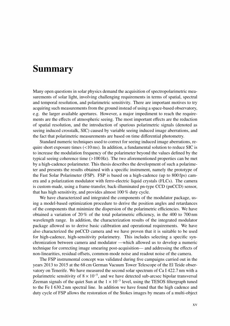
Many open questions in solar physics demand the acquisition of spectropolarimetric mea-surements of solar light, involving challenging requirements in terms of spatial, spectraland temporal resolution, and polarimetric sensitivity. There are important motives to tryacquiring such measurements from the ground instead of using a space-based observatory,e.g. the larger available apertures. However, a major impediment to reach the require-ments are the effects of atmospheric seeing. The most important effects are the reductionof spatial resolution, and the introduction of spurious polarimetric signals (denoted asseeing induced crosstalk, SIC) caused by variable seeing induced image aberrations, andthe fact that polarimetric measurements are based on time differential photometry.
Standard numeric techniques used to correct for seeing induced image aberrations, re-quire short exposure times (<10 ms). In addition, a fundamental solution to reduce SIC isto increase the modulation frequency of the polarimeter beyond the values defined by thetypical seeing coherence time (>100 Hz). The two aforementioned properties can be metby a high-cadence polarimeter. This thesis describes the development of such a polarime-ter and presents the results obtained with a specific instrument, namely the prototype ofthe Fast Solar Polarimeter (FSP). FSP is based on a high-cadence (up to 800 fps) cam-era and a polarization modulator with ferro-electric liquid crystals (FLCs). The camerais custom-made, using a frame-transfer, back-illuminated pn-type CCD (pnCCD) sensor,that has high sensitivity, and provides almost 100 % duty cycle.
We have characterized and integrated the components of the modulator package, us-ing a model-based optimization procedure to derive the position angles and retardancesof the components that minimize the dispersion of the polarimetric efficiencies. We haveobtained a variation of 20 % of the total polarimetric efficiency, in the 400 to 700 nmwavelength range. In addition, the characterization results of the integrated modulatorpackage allowed us to derive basic calibration and operational requirements. We havealso characterized the pnCCD camera and we have proven that it is suitable to be usedfor high-cadence, high-sensitivity polarimetry. This includes selecting a specific syn-chronization between camera and modulator —which allowed us to develop a numerictechnique for correcting image smearing post-acquisition— and addressing the effects ofnon-linearities, residual offsets, common-mode noise and readout noise of the camera.
The FSP instrumental concept was validated during five campaigns carried out in theyears 2013 to 2015 at the 68 cm German Vacuum Tower Telescope of the El Teide obser-vatory on Tenerife. We have measured the second solar spectrum of Ca I 422.7 nm with apolarimetric sensitivity of 8 × 10⁻⁵, and we have detected sub-arcsec bipolar transversalZeeman signals of the quiet Sun at the 1 × 10⁻³ level, using the TESOS filtergraph tunedto the Fe I 630.2 nm spectral line. In addition we have found that the high cadence andduty cycle of FSP allows the restoration of the Stokes images by means of a multi-object
xv

Summary
multi-frame blind deconvolution, using only the narrow-band science data, consisting ofindividual short exposure (2.5 ms) frames with low signal to noise ratio. We have studiedthe residual level of seeing induced crosstalk (SIC) using non-modulated filtergraph mea-surements. At a modulation frequency of 100 Hz, if no image restoration is used, SIC isbelow the 7 × 10⁻⁵ noise level after averaging ∼8 min of quiet-Sun Stokes images. On theother hand, after restoring 1.16 min of the same measurements, we found traces of SIC atthe noise level of 4 × 10⁻⁴ only in the edges of the images, where the performance of theadaptive optics and image restoration are reduced due to seeing anisoplanatism.
The techniques and methods studied and/or developed in this work are of relevancefor any project addressing the development of high-cadence, high-sensitivity imaging po-larimetry.
xvi
Kurzfassung
Viele offene Fragen in der Sonnenphysik erfordern Spektropolarimetrie mit hohen An-forderungen an die räumliche, spektrale und zeitliche Auflösung, sowie an die polarimetri-sche Genauigkeit. Es gibt gute Argumente warum man solche Messungen an bodenge-bundenen Teleskopen durchführt und nicht im Weltraum, z.B. wegen der größeren Aper-tur von bodengebundenen Teleskopen. Ein Nachteil von bodengebundenen Beobachtun-gen ist allerdings der Einfluss von atmosphärischer Turbulenz (Seeing). Seeing beein-trächtigt die räumliche Auflösung und verursacht falsche Polarisationssignale, sogenann-ten Seeing Induced Crosstalk (SIC). Der SIC ist bedingt durch eine zeitliche Änderungder optischen Aberrationen während der Polarisationsmessung, welche ihrerseits auf einerzeitlichen Abfolge von differenziellen Intensitätsmessungen beruht.
Typische numerische Algorithmen zur Korrektur von seeingbedingten Aberrationenverlangen nach Einzelbildern mit kurzen Belichtungszeiten (< 10 ms). Darüber hinausbesteht eine grundlegende Lösung für das Problem des SIC darin das Polarimeter beiModulationsperioden unterhalb der typischen Korrelationszeitskala des Seeings zu be-treiben. Dies entspricht Modulationsfrequenzen oberhalb von 100 Hz. Alle die genanntenAnforderungen können durch ein schnelles Polarimeter erfüllt werden. Diese Disserta-tion beschreibt die Entwicklung eines schnellen Polarimeters sowie die Resultate die mitdem Prototypen des "Fast Solar Polarimeter" (FSP) erzielt wurden. Das FSP besteht auseiner schnellen (bis zu 800 fps) Kamera und einem Polarisationsmodulator aus ferroelek-trischen Flüssigkristallen (FLCs). Die Kamera ist eine Spezialanfertigung basierend aufeinem rückseitenbeleuchteten pn-Typ CCD (pnCCD) Sensor mit Frame Transfer. DieserSensor hat eine sehr hohe Empfindlichkeit und ermöglicht den Betrieb bei einem Arbeits-zyklus von nahezu 100 %.
Die Komponenten des Modulators wurden einzeln charakterisiert und mit Hilfe einesModells in Bezug auf Positionswinkel und Verzögerungen dahingehend optimiert, dasseine möglichst hohe und achromatische polarimetrische Effizienz erreicht wird. Es isthierbei gelungen, die Schwankung der gesamten polarimetrischen Effizienz über denspektralen Arbeitsbereich von 400 bis 700 nm unterhalb von 20 % zu halten. Darüberhinaus hat die sorgfältige Charakterisierung des Modulators es erlaubt, die Anforderun-gen an dessen Kalibration und Betriebsstabilität zu definieren, welche eingehalten wer-den müssen, um die angestrebte polarimetrische Genauigkeit zu erreichen. Des Weiterenwurde die pnCCD Kamera charakterisiert und es konnte gezeigt werden, dass diese in derTat geeignet ist für schnelle Polarimetrie mit der geforderten Genauigkeit. Die Arbeitenin Bezug auf die Kamera beinhalteten weiter eine Optimierung der Synchronisierungmit dem Modulator sowie die Ausarbeitung und die Verifizierung eines Algorithmus zurnumerischen Korrektur der durch den Frame Transfer verursachten Bildverschmierung.Weiter wurde der Einfluss von verschiedenen kamerabezogenen Effekten auf die Polari-
xvii

Kurzfassung
sationsmessung untersucht: Nichtlinearität, residuale Offsets, sowie Common-Mode undAusleserauschen.
Fünf Beobachtungskampagnen haben es erlaubt das FSP Konzept zu validieren. DieseKampagnen wurden in den Jahren 2013-2015 am deutschen 68 cm Vakuum-Turm-Teleskop(VTT) des Teide Observatoriums auf Teneriffa durchgeführt. Am Gitterspektrographendes VTT wurde unter anderem das Streupolarisationsspektrum (das sogenannte zweiteSonnenspektrum) der Ca I 422.7 nm Spektralline mit einer polarimetrischen Empfind-lichkeit von 8 × 10⁻⁵ gemessen. Am TESOS Filtergraphen des VTT wurden unter an-derem die schwachen (Amplitude um 1 × 10⁻³), kleinskaligen (< 1 Bogensekunde) hori-zontalen Magnetfelder der ruhigen Sonne mittels des transversalen Zeeman Effekts inder Fe I 630.2 nm Spektralline gemessen. Weiter konnte gezeigt werden, dass die hoheKadenz und der hohe Arbeitszyklus des FSP die Rekonstruktion von Stokes Bildern mithoher Qualität erlauben. Dabei werden, im Gegensatz zu anderen Instrumenten inde-rien ein zusätzlicher Breitbandkanal zum Einsatz kommt, nur die schmalbandigen undkurzzeitig belichteten (2.5 ms) Bilder der pnCCD Kamera des FSP verwendet. Auf dieseWeise können differentielle Fehler zwischen zwei unterschiedlichen Bildkanälen aus-geschlossen werden. Die Rekonstruktion basiert auf dem "Multi-Object Multi-FrameBlind Deconvolution" (MOMFBD) Algorithmus.
Bei einer Modulationsfrequenz von 100 Hz, und ohne Bildrekonstruktion, liegt dieAmplitude des SIC unterhalb des Rauschlevels von 7 × 10⁻⁵, welcher nach einer Integra-tionszeit von etwa 8 min in der ruhigen Sonne erreicht wurde. Andererseits, nach Bild-rekonstruktion eines Datensatzes aus der gleichen Beobachtung, entsprechend einer Inte-grationszeit von 1.16 min, wurden Signaturen von SIC knapp oberhalb des Rauschlevelsvon 4 × 10⁻⁴ beobachtet. Allerdings ist der SIC hier auf die Randbereiche der StokesBilder beschränkt wo die Güte der adaptiven Optik und der Bildrekonstruktion wegenAnisoplanatismus und Randeffekten eingeschränkt ist.
Die Techniken und Methoden die in dieser Dissertation studiert und in der Praxiserprobt wurden sind von allgemeiner Bedeutung für Projekte, die sich mit hochgenauerbildgebender Polarimetrie mit hoher Kadenz beschäftigen.
xviii
1 Introduction
Even though the Sun is a common, middle-aged star, it is very special to human kind. Ourhome planet lies within the realm of the Sun. This is true not only from a gravitationalpoint of view —with more than 99.8 % of the solar system mass concentrated in its star(Woolfson 2000)— but also in terms of energy flow. The Sun has provided the majority ofthe Earth’s energy input uninterruptedly during billions of years, allowing among othersthings the evolution of life as we know it.
Our host star is also special from an astronomical point of view, it is the only star thatwe can resolve, even in a very demanding definition of the term. State-of-the-art observa-tories can reach a spatial resolution that corresponds to only 5 × 10⁻⁵ of the solar diameterapproximately (some 70 km!). The ability to investigate and in particular to image the finedetails of the Sun, has radically changed the early human conception of a static and quietstar. Our present understanding involves a highly dynamic and active Sun, with manyphenomena that span a wide range of temporal, spatial and energetic scales. From themore regular eleven-years cycle of the sunspots (see, e.g. Solanki 2003) to the unpre-dictable coronal mass ejections (see Fig. 1.1), and the fast (tens of minutes) solar flares(Stix 2002, Ch. 9). This diverse solar activity strongly influences the vicinity of Earth,including its magnetosphere and upper atmosphere. Such an influence became sociallyrelevant with the advent of electricity-based and specially space-based technologies, pro-moting among others the development of the space weather sciences (Bothmer and Daglis2007, Ch. 2). The effects of solar activity include not only the beautiful polar auroras (seeFig.1.1), but also more harmful phenomena such as the injection of high-energy parti-cles in low orbits, which can damage spacecrafts, artificial satellites or hazard astronautsduring spacewalks; the induction of electric currents in long power lines or oil pipes lo-cated in high-latitude regions, which can destroy transformers or sensing and protectionsystems; the interference of satellite or aircraft communication; and the interruption orperformance reduction of global navigation systems (Bothmer and Daglis 2007).
The main driver of the solar activity is the Sun’s magnetic field (Stix 2002, Ch.8), therefore a detailed study of its generation and interaction with solar matter, is ofparamount importance to both general society and to the scientific community. Giventhe large distances and very hazardous conditions of the near-sun environment, in-situmeasurements of magnetic fields in the solar surface, or lower atmosphere, are not yetpossible. As a result, remote sensing tools have been developed to estimate the solarmagnetic fields from Earth or near-Earth space using a combination of spectropolarimet-ric measurements of the incoming solar light and polarized radiative transfer theory (seee.g. del Toro Iniesta 2003). The solar magnetic fields extend along spatial scales that rangefrom tens of km to hundreds of Mm; change in time intervals that can last few seconds toseveral years; and have strengths ranging from tens to thousands of Gauss (Stix 2002, Ch.
1
1 Introduction
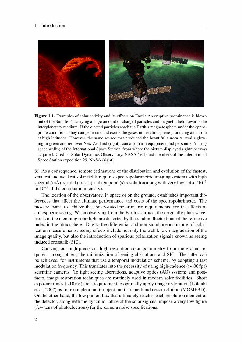
Figure 1.1. Examples of solar activity and its effects on Earth: An eruptive prominence is blownout of the Sun (left), carrying a huge amount of charged particles and magnetic field towards theinterplanetary medium. If the ejected particles reach the Earth’s magnetosphere under the appro-priate conditions, they can penetrate and excite the gases in the atmosphere producing an auroraat high latitudes. However, the same source that produced the beautiful aurora Australis glow-ing in green and red over New Zealand (right), can also harm equipment and personnel (duringspace walks) of the International Space Station, from where the picture displayed rightmost wasacquired. Credits: Solar Dynamics Observatory, NASA (left) and members of the InternationalSpace Station expedition 29, NASA (right).
8). As a consequence, remote estimations of the distribution and evolution of the fastest,smallest and weakest solar fields requires spectropolarimetric imaging systems with highspectral (mÅ), spatial (arcsec) and temporal (s) resolution along with very low noise (10−3
to 10−5 of the continuum intensity).The location of the observatory, in space or on the ground, establishes important dif-
ferences that affect the ultimate performance and costs of the spectropolarimeter. Themost relevant, to achieve the above-stated polarimetric requirements, are the effects ofatmospheric seeing. When observing from the Earth’s surface, the originally plain wave-fronts of the incoming solar light are distorted by the random fluctuations of the refractiveindex in the atmosphere. Due to the differential and non simultaneous nature of polar-ization measurements, seeing effects include not only the well known degradation of theimage quality, but also the introduction of spurious polarization signals known as seeinginduced crosstalk (SIC).
Carrying out high-precision, high-resolution solar polarimetry from the ground re-quires, among others, the minimization of seeing aberrations and SIC. The latter canbe achieved, for instruments that use a temporal modulation scheme, by adopting a fastmodulation frequency. This translates into the necessity of using high-cadence (>400 fps)scientific cameras. To fight seeing aberrations, adaptive optics (AO) systems and post-facto, image restoration techniques are routinely used in modern solar facilities. Shortexposure times (∼10 ms) are a requirement to optimally apply image restoration (Löfdahlet al. 2007) as for example a multi-object multi-frame blind deconvolution (MOMFBD).On the other hand, the low photon flux that ultimately reaches each resolution element ofthe detector, along with the dynamic nature of the solar signals, impose a very low figure(few tens of photoelectrons) for the camera noise specifications.
2
1.1 Objectives
In this way, the development of high-precision, high-resolution solar polarimeters isstrongly coupled to the development of fast, low-noise detectors. Moreover, only recenttechnological developments in complementary metal-oxide-semiconductor (CMOS) sen-sors or charge-coupled devices (CCDs) and their readout electronics, have allowed us toget close to the performance requirements derived from the most demanding open ques-tions in modern solar spectropolarimetry.
1.1 ObjectivesAll the main goals of this thesis are related to the instrumental challenges that arise duringthe development of a state-of-the-art, ground-based, solar polarimeter. A particular focusis on the relatively unexplored case of high-cadence solar polarimetry, by means of thedevelopment and validation of a specific instrument: The prototype of the FSP. The maingoals of this work are:
(g1) Integration, characterization and optimization of a polarization modulator basedon ferro-electric liquid crystals (FLCs), to be used for fast modulation and high-resolution polarimetry.
(g2) Characterization and optimization of a custom-made, pn-type CCD (pnCCD) cam-era to be used in high-cadence polarimetry.
(g3) Integration, testing and validation of the FSP as a complete system.
(g4) Application of image restoration to high-cadence polarimetric data, to improve spa-tial resolution and signal to noise ratio (S NR).
The most important questions that arise from the above-described goals, involve theevaluation of the effects introduced by the pnCCD camera, never used in visible polarime-try before; and the FLC-based modulator on the polarimeter’s performance. The principalcontributions of the author are related to the quantification of such effects and the devel-opment of the necessary criteria and techniques to mitigate them when relevant. Sincea measurement instrument can only accomplish its purpose when all its components areworking properly and in harmony, from hardware to software, there is in addition a set ofsecondary tasks that need to be carried out when trying to fulfill the listed objectives. Themost relevant contributions derived from this thesis are enumerated below.
(c1) Measurement and analysis of the properties of an FLC-based, polarization modula-tor and optimization of its polarimetric efficiencies in a high-cadence regime. Thisincludes the derivation of calibration requirements from the spatial, thermal, spectraland temporal characterization of the modulation matrix. Also the application of amodel-based optimization procedure during design and assembly in oder to obtainwide-band polarimetric efficiencies. (c1) is related to (g1) and (g3).
(c2) Measurement and analysis of the relevant properties of a pnCCD camera and selec-tion of a camera-modulator synchronization strategy. This involves the quantifica-tion of the polarimetric artifacts introduced by the camera, as well as of the effectsof the camera noise properties on the instrumental performance. This contribution
3
1 Introduction
includes: (a) the selection of a camera-modulator synchronization strategy; (b) thedevelopment of a novel technique to numerically correct the smearing artifacts dueto the shutter-less operation of frame transfer sensors, for the case of highly-variablescenes; and (c) analysis of the common mode artifact correction. (c2) is related to(g2) and (g3).
(c3) Integration and validation of the FSP as a complete system. This includes the devel-opment of the reduction pipeline that implements all the calibration steps, derivedfrom the results in (c1) and (c2), necessary to obtain science ready data. It alsoimplies executing the relevant tasks, e.g. integration with post focus-instruments,required to acquire the first light measurements at the solar telescope; as well as theevaluation of the results to quantify the instrumental performance. (c4) is related to(g3).
(c4) First restoration of high-cadence, spectropolarimetric data by means of a MOMFBD.This involves the application of MOMFBD to spectropolarimetric data that havean exposure time (2.5 ms) shorter than the decorrelation time of day-time seeing(∼20 ms), near 100 % duty cycle (DC) and very low sensor noise (∼4.9 e−rms); aregime not reachable with others solar polarimeters. (c5) is related to (g4).
1.2 OutlineThe rest of the manuscript is organized as follows:
Chapter 2 reviews the fundamental concepts relevant to the subjects presented in thisthesis. It covers the basics of solar imaging polarimetry, including polarizedlight characterization and generation, a brief overview of remote solar atmo-spheric diagnosis and a detailed description of the main components of solarpolarimeters. A limited introduction to atmospheric seeing and its polarimet-ric effects is also given here. Finally the problem of solar image restorationby means of a MOMFBD is briefly presented.
Chapter 3 firstly discusses the case of high-cadence, solar polarimetry by detailing itsmain advantages, challenges and the derived requirements on the modula-tor package and the scientific camera used to obtain high-resolution, high-sensitivity observations from the ground. Secondly, the FSP is presented in-cluding its science goals and main specifications in order to point out its prosand cons with respect to other state-of-the-art, ground-based, solar polarime-ters that also operate in the visible part of the spectrum.
Chapter 4 details the development of an FLC-based polarization modulator package thatoperates at 100 Hz modulation frequency, and is optimized to obtain balancedand achromatic polarimetric efficiencies in the 400 nm to 700 nm wavelengthrange. Mechanical, optical, thermal and dynamical design descriptions andcharacterization results are presented. The latter are used to define calibrationrequirements and to develop the data reduction routines in Chapter 6.
4

1.2 Outline
Chapter 5 presents the characterization and optimization of a pnCCD camera to be usedfor high-cadence, solar polarimetry. After a review of the camera design andstructure, a given modulator-camera synchronization strategy is selected todevelop a numeric technique to correct for frame transfer artifacts. The cam-era noise, gain and dark current are measured and its impact on polarimetricprecision is evaluated. Additionally, the common mode artifact is analyzedand its correction discussed.
Chapter 6 describes some of the first-light measurements, carried out with FSP at the68 cm Vacuum Tower Telescope (VTT), and discusses its results. Firstly,the main aspects of the data reduction pipeline developed by the author arepresented. Secondly, a brief discussion of the different approaches to applyMOMFBD to the high-cadence data, is presented. Thirdly, three observa-tional results are shown for spectrograph and filtergraph modes. Finally, theperformance and limitations of FSP are discussed after estimating the resid-ual SIC, and reporting the results of the measurements of the non-magnetic557.6 nm absorption line.
Chapter 7 summarizes the main contributions and results of the thesis. A short descrip-tion of the second phase of the FSP project is also given.
5

2 Background
The development of a solar polarimeter requires understanding the synergy of differenttopics, including the physics of polarized light, the engineering behind the main devicesthat allow measuring polarization and the post-facto treatment of the raw data. This chap-ter reviews these topics, in order to establish the necessary terminology and definitions,required to present the work developed in the rest of the thesis.
Section 2.1 introduces the formalism needed to describe quasi-monochromatic, par-tially polarized light and the natural mechanisms, relevant to solar physics, that generateit. Additionally, it briefly describes the usage of polarimetry in modern solar physicsand what are the typical data requirements and challenges that arise from it. Section 2.2details the different measurement techniques and the components that form an imagingsolar spectropolarimeter, including the polarization modulator, the scientific camera andthe wavelength discriminator. The polarimetric effects of the atmospheric seeing and im-age motion, crucial for ground based instruments, are addressed in section 2.3. Where,in addition, the problem of restoring seeing-degraded solar images is briefly discussed;focusing on a particular technique, namely MOMFBD.
2.1 Introduction to solar spectropolarimetry
2.1.1 Description of polarized light and its transformations
Measuring polarization of light implies characterizing the behavior of the electric fieldvector as the wave propagates. For the case of a transversal —the propagation modein free space— monochromatic wave, such a behavior is described by the well knownpolarization ellipse (see e.g. Goldstein 2003, Ch. 3). Moreover, only three real parametersare required to completely define the polarization ellipse, namely, the amplitude of the twocomponents of the electric field (E) that are orthogonal to the propagation direction, andthe phase difference between them.
However, the amplitude-based description mentioned above, is not complete, e.g. itcan not describe unpolarized light, and has limited practical relevance. The main reasonsof the latter are (a) that monochromatic (strictly time and space periodic) waves do notexist in nature; (b) that the optical electric field describes a full ellipse in time-scalesthat are too short to access with current detection technology (see below); and (c) thatdevices capable of quantifying optical radiation are sensitive to the field volume energy(∝| E |2) and not to its amplitude. Due to the aforementioned reasons, a description of thepolarization of polychromatic (in particular quasi-monochromatic) radiation, in terms ofobservable (measurable) quantities is required. Such a formalism was introduced by G.
7
2 Background
G. Stokes in 1852, and is summarized below.The x component of the complex electric field, Ex, belonging to a quasi-monochromatic1,
transversal, plane wave propagating in the z direction; can be expressed as a monochro-matic, plane wave that is slowly modulated in amplitude as follows
Ex(z, t) = [ξx(t)eiδx(t)]ei(kz−ω0t), (2.1)
where t is time, i the imaginary unit, ω0 the mean frequency, k the wave number; and ξx(t)and δx(t) are the module and phase of the complex modulating function —that determinesthe spectral content of the wave— respectively.
Since in practice a polarimetric measurement requires a time interval that is muchlonger than the mean period (or the coherence time) of the optical wave, a temporal av-erage of the polarization ellipse will be actually registered during any experiment, e.g.the mean period is 1.6 × 10⁻¹⁵ s for a mean wavelength of 500 nm. After applying sucha temporal average, the equation of the polarization ellipse can be expressed in terms ofmeasurable quantities as (see e.g. Goldstein 2003, Ch. 4)
I2 ≥ Q2 + U2 + V2, (2.2)
where,
I = 〈ExE∗x〉 + 〈EyE∗y〉 = 〈ξ2x(t)〉 + 〈ξ
2y(t)〉, (2.3)
Q = 〈ExE∗x〉 − 〈EyE∗y〉 = 〈ξ2x(t)〉 − 〈ξ
2y(t)〉, (2.4)
U = 〈ExE∗y〉 + 〈EyE∗x〉 = 2〈ξx(t)ξy(t) cos(δ(t))〉, (2.5)
V = i(〈ExE∗y〉 − 〈EyE∗x〉) = 2〈ξx(t)ξy(t) sin(δ(t))〉, (2.6)
δ = δx − δy and 〈〉 denotes the average operation. Note that we have dropped the depen-dences on t and z in Ex and Ey for clarity. However, we preserved the temporal depen-dence in all the ξ and δ, to empathize that the wave is not monochromatic and thus it canbe partially polarized2.
The four terms introduced in Eq. 2.2, the so called Stokes parameters, are quadraticforms of the electric filed and thus have units of intensity, i.e. they are the measurableaspects of the polarization ellipse. They are refereed to as Stokes I parameter, that givesthe total intensity of the beam; Stokes Q parameter, that gives the amount of linear 0°or 90° polarization; Stokes U parameter, that gives the amount of linear 45° or −45°polarization; and Stokes V parameter, that gives the amount of right or left handed circularpolarization. The Stokes parameters are usually arranged in the so called Stokes vector(S) as follows
S = [I,Q,U,V]T = [S 0, S 1, S 2, S 3]T , (2.7)1With a spectral bandwidth negligible compared to its mean frequency.2Since the measured signal is the result of the incoherent average of many uncorrelated photons (which
are always totally polarized), it can present zero polarization —i.e. there is no statistical preference for anypolarization state— or partial polarization. The latter means that, after averaging the polarization state ofall the considered photons, a fraction of them (given by the polarization degree) are not canceled out. Suchan incoherent superposition, can not be described by the Jones calculus because the Jones vectors preservethe phases of the individual photons, and thus their average is equivalent to the coherent superposition (seee.g. Stenflo 1994, Ch. 2 for a definition of Jones calculus).
8
2.1 Introduction to solar spectropolarimetry
where the superscript T denotes the transpose. In Eq. 2.6, we have also introducedan alternative notation of S, i.e. using S 0, S 1, S 2 and S 3; both notations shall be usedindistinguishably across the manuscript.
The Stokes formalism provides a concise representation of unpolarized (Q = U =
V = 0), partially polarized (I2 > Q2 + U2 + V2) and totally polarized (I2 = Q2 + U2 + V2)light. Moreover, it readily describes the polarization state (S) of a beam resulting from thecombination of two uncorrelated beams (S(0) and S(1)) as a simple addition (S = S(0)+S(1)).
The modification of the polarization state of a beam, resulting from its interactionwith matter, can be conveniently expressed as a linear transformation of the initial Stokesvector, S(0), defined by a 4 × 4 Mueller matrix (M) as follows3
S = MS(0). (2.8)
If N of such a transformations —each defined by Mn, with n ∈ 0, 1, ...,N − 1 and n = 0being the first one applied— act on a beam with initial Stokes vector S(0), the resultingpolarization state, S, is given by
S =
( 0∏n=N−1
Mn
)S(0). (2.9)
To facilitate the interpretation of a physically meaningful M, let us differentiate itselements in terms of its diattenuation 3-vector (h), polarizance 3-vector (v) and 3 × 3rotation matrix (R). Following del Toro Iniesta (2003), we can re-write Eq. 2.8 as
g[1p
]= M0,0
[1 hT
v R
] [1
p(0)
], (2.10)
where M0,0 is the first element of M, the polarization vector (p) is defined as
p =
[QI,
UI,
VI
]T
= [q, u, v]T with 0 ≤| p |≤ 1, (2.11)
and g is the gain of the optical system. In Eq. 2.11, we have also introduced an alternativenotation of p using the short forms for the normalized Stokes parameters, namely q, u andv.
A given 4 × 4 matrix is a Mueller matrix if it defines a transformation that is closedin the Stokes vectors space, i.e. if the S obtained from Eq. 2.8 satisfies Eq. 2.2. To doso, M0,0 ≥ 0 to ensure a positive output intensity for an unpolarized (p(0) = 0, also callednatural) input; h has to belong to the Poincaré sphere4 to ensure I/I(0) ≥ 0 ; and v has tobelong to the Poincaré sphere because p = v for a natural input.
A useful Mueller matrix is the one that produces a rotation of the reference frame inthe transversal plane of the wave, i.e. it does not modify circular polarization values (V).
3This matrix approach, introduced by Hans Mueller in 1940s, satisfactorily describes the polarimet-ric effects of most of the optical components found in solar telescopes, spectrographs and polarimeters.Moreover it also sets the basis for the description of the polarimetric effects of stellar atmospheres.
4A unitary sphere introduced by Henri Poincaré to visually represent the polarization state of a beam,and simplify the calculus of its modifications when interacting with polarizing elements (see e.g. Goldstein2003, Ch. 12).
9
2 Background
For a rotation of an angle θ, measured counterclockwise from the Stokes Q direction, sucha matrix is defined as (del Toro Iniesta 2003)
Mrot(θ) =
1 0 0 00 c2 s2 00 −s2 c2 00 0 0 1
, (2.12)
where c2 = cos(2θ) and s2 = sin(2θ). Note that, Mrot is a R4 rotation matrix, i.e.
MrotMTrot = MT
rotMrot = 1, where 1 is the identity matrix. After rotation, the new Stokesvector and Mueller matrix are given by
S = MrotS(0) and M = MTrotM
(0)Mrot (2.13)
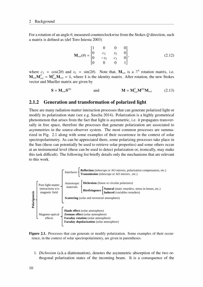
2.1.2 Generation and transformation of polarized lightThere are many radiation-matter interaction processes that can generate polarized light ormodify its polarization state (see e.g. Sascha 2014). Polarization is a highly geometricalphenomenon that arises from the fact that light is asymmetric, i.e. it propagates transver-sally in free space, therefore the processes that generate polarization are associated toasymmetries in the source-observer system. The most common processes are summa-rized in Fig. 2.1 along with some examples of their occurrence in the context of solarspectropolarimetry. As can be appreciated there, some polarizing processes take place inthe Sun (these can potentially be used to retrieve solar properties) and some others occurat an instrumental level (these can be used to detect polarization or, ironically, may makethis task difficult). The following list briefly details only the mechanisms that are relevantto this work.
Pola
rige
nesi
s
Magneto-optical effects
Interfaces
Anisotropicmaterials
Scattering (solar and terrestrial atmosphere)
Pure light-matterinteractions w/o magnetic field
Hanle effect (solar atmosphere)Zeeman effect (solar atmosphere)Faraday rotation (solar atmosphere)Faraday depolarization (solar atmosphere)
Dichroism (linear or circular polarizers)
Birefringence
Reflection (telescope or AO mirrors, polarization compensators, etc.)Transmission (telescope or AO mirrors , etc.)
Natural (static retarders, stress in lenses, etc.)Induced (variables retarders)
Figure 2.1. Processes that can generate or modify polarization. Some examples of their occur-rence, in the context of solar spectropolarimetry, are given in parentheses.
1. Dichroism (a.k.a diattenuation), denotes the asymmetric absorption of the two or-thogonal polarization states of the incoming beam. It is a consequence of the
10
2.1 Introduction to solar spectropolarimetry
anisotropic electric properties of a material, and is commonly used to manufacturepolarizers. In particular, a partial linear polarizer has a high transmittance, k0 , ofthe E component that is parallel to its optical axis; and a lower transmittance, k90 ,of the orthogonal component. Denoting α = k0
2 + k902, β = (k0
2− k90
2)/α andγ = 2k0k90/α; the polarimetric action of a partial linear polarizer, with its opticalaxis forming an angle θ relative to the Stokes Q direction, can be characterized byits Mueller matrix, Mppol, as follows (del Toro Iniesta 2003)
Mppol(θ, k0 , k90) =α
2
1 βc2 βs2 0βc2 c2
2 + γs22 (1 − γ)s2c2 0
βs2 (1 − γ)s2c2 s22 + γc2
2 00 0 0 γ
. (2.14)
If k0 = 1 and k90 = 0, Mppol reduces to the case of an ideal linear polarizer withMueller matrix Mpol, given by
Mpol(θ) =12
1 c2 s2 0c2 c2
2 s2c2 0s2 s2c2 s2
2 00 0 0 0
. (2.15)
Note that, a perfect linear polarizer produces a linearly polarized output beam forany value of the input Stokes vector, i.e. v , 0 and the last row of Mpol is null. Thesame device can also be used as a linear polarization analyzer, i.e. its h producesan output Stokes I, that is sensitive to the values of Stokes Q and U of the inputbeam (see Sect. 2.2.1).
2. Birefringence is a consequence of the anisotropic electric response (refractive in-dex) of a given material, i.e. the dielectric tensor written in the principal frame ofreference, is a 3 × 3 diagonal matrix with different diagonal elements. If only twoout of the three principal refractive indexes of the dielectric tensor are equal, thematerial is called uniaxial. Disc-shaped optical components made of uniaxial ma-terials, are typically characterized by the position angle of its optical axis (θ) and aretardance (δ) given by
δ = 2π(no − ne)thick
λ, (2.16)
where thick is the geometrical thickness of the disc; no and ne are the ordinary (cor-responding to the two directions perpendicular to the optical axis) and extraordinary(corresponding to the direction of the optical axis) refractive indexes respectively;and λ is the wavelength of the wave in vacuum (del Toro Iniesta 2003, Ch. 4). Whenlight hits normally such a device, the component of the E that is perpendicular tothe optical axis experiences a phase lag with respect to the component parallel to itgiven by δ, modifying in this way the polarization state of the beam.
Birefringence can be natural or induced, and is commonly exploited to manufac-ture retarders. Natural birefringence appears in materials that are formed by non-isotropic crystals, such as Calcite, LiNbO3 (uniaxial) or mica (biaxial) (Goldstein2003, Ch. 24). Birefringence may be induced or modified, i.e. the values of δ or
11
2 Background
θ can be changed using electric fields (as in an FLC or nematic LC) or pressurewaves (as in piezo-elastic crystals). Regardles of its kind, the polarimetric action ofa retarder can be characterized for a given δ and θ using its Mueller matrix, Mret,given by (del Toro Iniesta 2003)
Mret(θ, δ) =
1 0 0 00 c2
2 + s22 cos(δ) [1 − cos(δ)]s2c2 −s2 sin(δ)
0 [1 − cos(δ)]s2c2 s22 + c2
2 cos(δ) c2 sin(δ)0 s2 sin(δ) −s2 sin(δ) cos(δ)
. (2.17)
If δ = π/2, the retarder is called a quarter-wave plate (QWP). Analogously, ifδ = π, the retarder is called a half-wave plate (HWP). Note that, a linear retarderdoes not modify the polarization degree of a beam, i.e. v = h = 0, it only introducesa rotation of the incoming p, i.e. the matrix R is a R3 rotation matrix.
3. Scattering polarization is produced when an incident, anisotropic radiation field isscattered by matter (Goldstein 2003, Ch. 20). The phenomenon can be understoodin terms of classical electrodynamics by assuming that the scattering material iscomposed of elemental electric dipoles (representing e.g. the electrons, atomicnuclei, molecules, etc.) that are excited by the incoming transversal waves, andreradiate only in directions perpendicular to their longitudinal axes. For the case ofThomson and Rayleigh scattering, the polarization state of the beam scattered at anangle θ relative to the propagation direction of the incoming beam, can be obtainedusing the Mueller matrix of the process (Goldstein 2003, Ch. 20)
Msca(θ) = κsca
1 + cos2(θ) sin2(θ) 0 0
sin2(θ) 1 + cos2(θ) 0 00 0 2 cos(θ) 00 0 0 2 cos(θ)
, (2.18)
where Stokes Q is defined perpendicular to the plane of scattering and κsca is aconstant independent of the wavelength of the incoming beam (λ) for Thomsonscattering, or, a function proportional to 1/λ4 for Rayleigh scattering. Since thepolarizance vector of Msca is not null, the scattering process acts as a polarizer,i.e. the scattered light will be linearly polarized even for the case of unpolarizedincoming radiation. The polarization degree depends on the scattering angle, beingzero for forward (θ = 0°) and backwards (θ = 180°) scattering, and maximum forθ = 90°.
The Earth’s atmosphere is anisotropically illuminated by the distant Sun, as a conse-quence, molecular Rayleigh scattering produces not only a blue —see the resultingStokes I parameter for an unpolarized input in Eq 2.18— but also a linearly polar-ized sky. Fortunately the net sky polarization in the direction of the Sun (θ = 0°) isvery low and can be neglected when doing solar polarimetry from the ground.
Scattering polarization takes place also in the solar atmosphere due to the anisotropicradiation field, i.e. the incident light has a preferred radial direction, giving rise to anet linear polarization signal predominantly oriented parallel to the solar limb (seee.g. Stenflo 2013). Since the scattering angle viewed by a distant observer tends
12
2.1 Introduction to solar spectropolarimetry
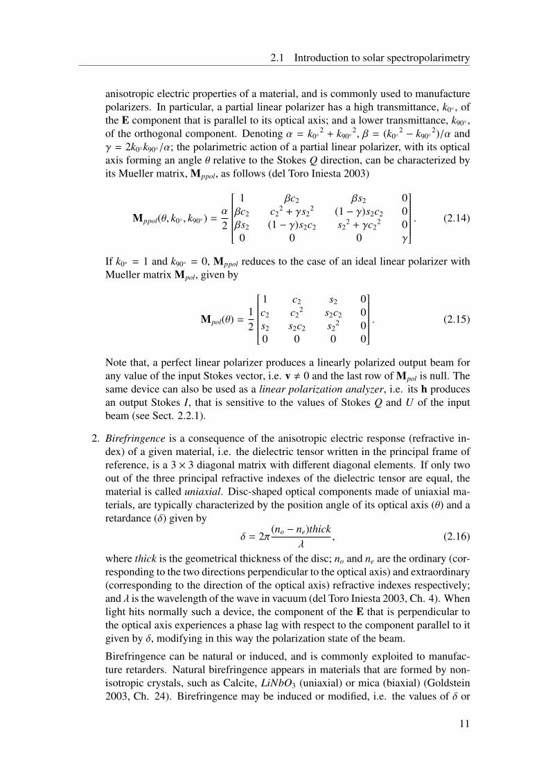
to 90° towards the solar limb, the larger scattering polarization signals are foundthere. However, even the largest signals are relatively small (∼10−3 ) due to the av-eraged contribution of a wide range of scattering angles and other quantum effectsintroduced by the scattering in bound-bound transitions of atoms (that deviate fromthe dipole approximation given above, Stenflo 2013). A spectral atlas of Stokes Q/Idue to scattering polarization near the solar limb, presents a behavior that stronglydiffers from the intensity solar spectrum. Therefore, it is usually refereed to as thesecond solar spectrum (Stenflo and Keller 1997), see Fig. 2.2.
422.4 422.5 422.6 422.7 422.8 422.9λ [nm]
0.0
0.2
0.4
0.6
0.8
1.0
I/Ic
422.4 422.5 422.6 422.7 422.8 422.9λ [nm]
0.0
0.5
1.0
1.5
2.0
2.5
3.0
Q/I
[%]
Figure 2.2. Example of scattering polarization signals in the solar atmosphere. The upper panelshows a portion of the normalized intensity spectrum recorded near the solar limb. The light isalso linearly polarized due to scattering in the solar atmosphere, as the Stokes Q/I measurementspresented in the lower panel exemplify. The spectral behavior of both signals is so different, thatthe bottom case is usually referred to as the second solar spectrum. These measurements arepart of a full spectral atlas that covers the visible and UV ranges published by Gandorfer (2000,2002, 2005).
4. Hanle effect. The presence of a magnetic field (B) modifies the scattering polariza-tion process. This can be partially understood as a randomization of the elementaldipoles orientations between the excitation and emission stages, that derives in thereduction of the resulting net linear polarization. The Hanle effect —which mayalso produce a rotation of the plane of polarization (Hanle 1924)— can be used toprobe the solar magnetic fields in certain spectral lines (Stenflo 1982).
5. The Zeeman effect refers to the splitting of the energy levels of an atom due to theinfluence of an external B (see e.g. del Toro Iniesta 2003, Ch. 8 and referencestherein) . An energy level with total angular momentum quantum number j, splitsin to (2 j + 1) sub-levels, each with a different magnetic quantum number (m). Theenergy difference between the sub-levels is proportional to | B | and the magneticsensitivity of the level, the so called Landé factor. When light interacts with matter,an absorption or emission spectral line is formed if the electrons of the constituent
13
2 Background
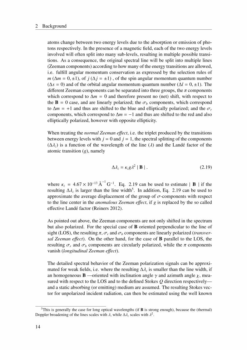
atoms change between two energy levels due to the absorption or emission of pho-tons respectively. In the presence of a magnetic field, each of the two energy levelsinvolved will often split into many sub-levels, resulting in multiple possible transi-tions. As a consequence, the original spectral line will be split into multiple lines(Zeeman components) according to how many of the energy transitions are allowed,i.e. fulfill angular momentum conservation as expressed by the selection rules ofm (∆m = 0,±1), of j (∆ j = ±1) , of the spin angular momentum quantum number(∆s = 0) and of the orbital angular momentum quantum number (∆l = 0,±1). Thedifferent Zeeman components can be separated into three groups, the π componentswhich correspond to ∆m = 0 and therefore present no (net) shift, with respect tothe B = 0 case, and are linearly polarized; the σb components, which correspondto ∆m = +1 and thus are shifted to the blue and elliptically polarized; and the σr
components, which correspond to ∆m = −1 and thus are shifted to the red and alsoelliptically polarized, however with opposite ellipticity.
When treating the normal Zeeman effect, i.e. the triplet produced by the transitionsbetween energy levels with j = 0 and j = 1, the spectral splitting of the components(∆λz) is a function of the wavelength of the line (λ) and the Landé factor of theatomic transition (g), namely
∆λz = κzgλ2 | B | . (2.19)
where κz = 4.67 × 10⁻¹³ Å−1
G−1. Eq. 2.19 can be used to estimate | B | if theresulting ∆λz is larger than the line width5. In addition, Eq. 2.19 can be used toapproximate the average displacement of the group of σ-components with respectto the line center in the anomalous Zeeman effect, if g is replaced by the so calledeffective Landé factor (Reiners 2012).
As pointed out above, the Zeeman components are not only shifted in the spectrumbut also polarized. For the special case of B oriented perpendicular to the line ofsight (LOS), the resulting π, σr and σb components are linearly polarized (transver-sal Zeeman effect). On the other hand, for the case of B parallel to the LOS, theresulting σr and σb components are circularly polarized, while the π componentsvanish (longitudinal Zeeman effect).
The detailed spectral behavior of the Zeeman polarization signals can be approxi-mated for weak fields, i.e. where the resulting ∆λz is smaller than the line width, ifan homogeneous B —oriented with inclination angle γ and azimuth angle χ, mea-sured with respect to the LOS and to the defined Stokes Q direction respectively—and a static absorbing (or emitting) medium are assumed. The resulting Stokes vec-tor for unpolarized incident radiation, can then be estimated using the well known
5This is generally the case for long optical wavelengths (if B is strong enough), because the (thermal)Doppler broadening of the lines scales with λ, while ∆λz scales with λ2.
14
2.1 Introduction to solar spectropolarimetry
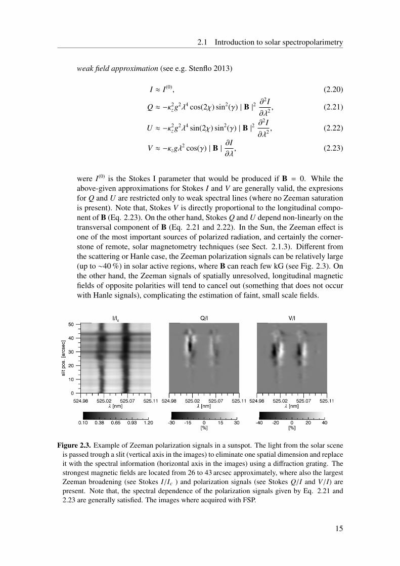
weak field approximation (see e.g. Stenflo 2013)
I ≈ I(0), (2.20)
Q ≈ −κ2z g2λ4 cos(2χ) sin2(γ) | B |2
∂2I∂λ2 , (2.21)
U ≈ −κ2z g2λ4 sin(2χ) sin2(γ) | B |2
∂2I∂λ2 , (2.22)
V ≈ −κzgλ2 cos(γ) | B |∂I∂λ, (2.23)
were I(0) is the Stokes I parameter that would be produced if B = 0. While theabove-given approximations for Stokes I and V are generally valid, the expresionsfor Q and U are restricted only to weak spectral lines (where no Zeeman saturationis present). Note that, Stokes V is directly proportional to the longitudinal compo-nent of B (Eq. 2.23). On the other hand, Stokes Q and U depend non-linearly on thetransversal component of B (Eq. 2.21 and 2.22). In the Sun, the Zeeman effect isone of the most important sources of polarized radiation, and certainly the corner-stone of remote, solar magnetometry techniques (see Sect. 2.1.3). Different fromthe scattering or Hanle case, the Zeeman polarization signals can be relatively large(up to ∼40 %) in solar active regions, where B can reach few kG (see Fig. 2.3). Onthe other hand, the Zeeman signals of spatially unresolved, longitudinal magneticfields of opposite polarities will tend to cancel out (something that does not occurwith Hanle signals), complicating the estimation of faint, small scale fields.
Figure 2.3. Example of Zeeman polarization signals in a sunspot. The light from the solar sceneis passed trough a slit (vertical axis in the images) to eliminate one spatial dimension and replaceit with the spectral information (horizontal axis in the images) using a diffraction grating. Thestrongest magnetic fields are located from 26 to 43 arcsec approximately, where also the largestZeeman broadening (see Stokes I/Ic ) and polarization signals (see Stokes Q/I and V/I) arepresent. Note that, the spectral dependence of the polarization signals given by Eq. 2.21 and2.23 are generally satisfied. The images where acquired with FSP.
15
2 Background
2.1.3 Solar spectropolarimetry
Solar spectropolarimetry refers to the measurement of the polarization state of solar lightas function of its wavelength. In general, the aim of these kind of measurements is thequantification of different physical variables of interest in the Sun, particularly in its at-mosphere. Many such variables, most notably the solar magnetic field, are of crucialimportance to understand the solar dynamics and the plethora of phenomena that arisefrom the Sun and influence the whole solar system (see Ch. 1). Therefore solar spec-tropolarimetry is a key resource to solar system sciences such as Solar physics, planetarysciences and Earth climate.
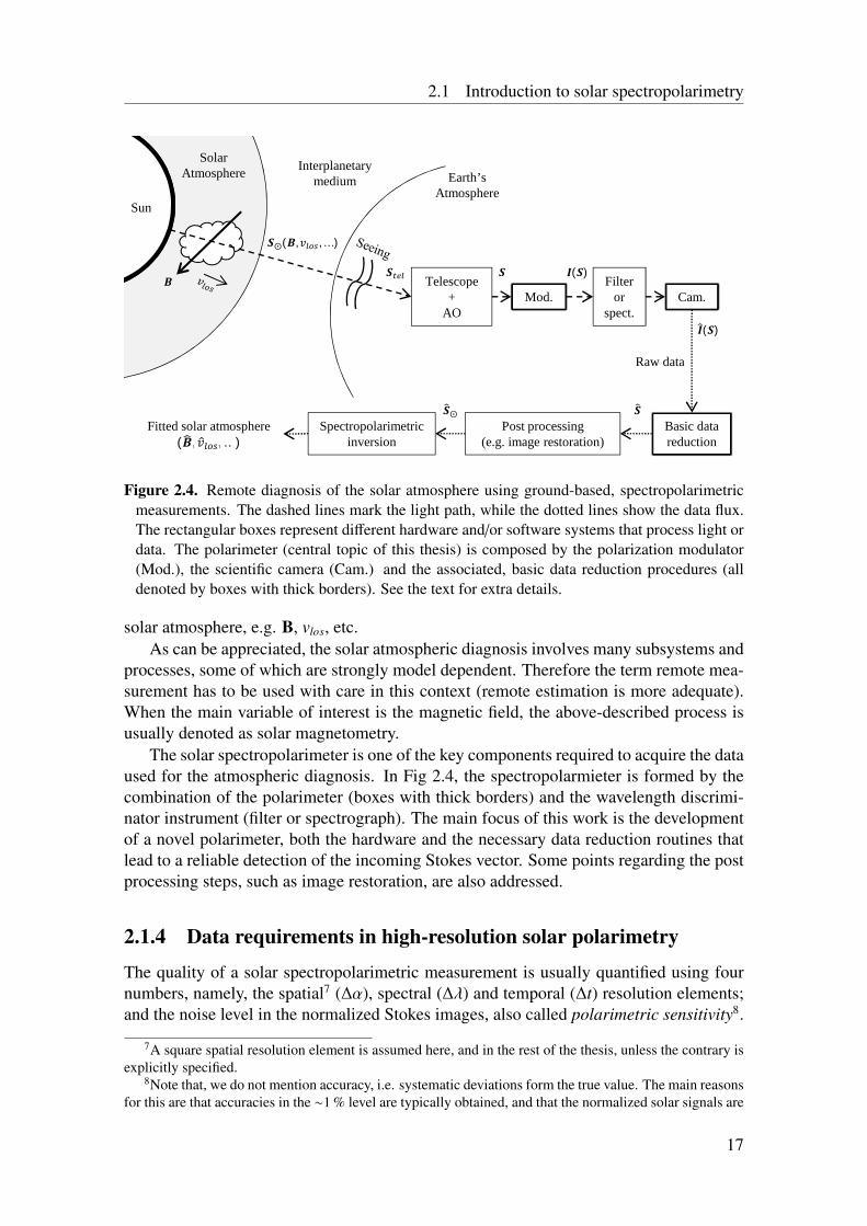
The above-mentioned measurement and analysis procedure, usually denoted as atmo-spheric diagnosis, is summarized by the sketch presented in Fig. 2.4, for the specificcase in which ground-based observations are employed. The light radiated from the baseof the solar photosphere6 (assumed to be unpolarized) interacts with the material of thesolar atmosphere. For visible and infra red (IR) wavelengths, the majority of absorptionspectral lines are formed by interactions with the plasma of the photosphere and lowerchromosphere. Further absorption and emission spectral lines are also formed higher inthe chromosphere and in the corona, mostly in the ultra violet (UV) and shorter wave-lengths.When radiation leaves the solar atmosphere, it carries information about the envi-ronment, e.g. magnetic field, line of sight velocity of the plasma (vlos), etc., in which thespectral lines are formed. Such an information is imprinted in the polarization state of thelight and its spectral dependence (denoted with Stokes vector S), thanks to the Zeeman,Doppler and Hanle effects among others (see Sect 2.1.2).
After traveling through the optically thin interplanetary medium, light reaches theEarth’s atmosphere. There, atmospheric seeing aberrates the solar image, resulting in areduction of spatial resolution and other issues (see Sect. 2.3.1). The aberrated solarscene, Stel, is then observed with a ground-based telescope, usually equipped with an AOsystem to partially correct the seeing effects. The polarimeter receives light, S, at thescientific focus of the telescope, that may differ from Stel due to spurious instrumentalpolarization. The first block of the polarimeter, performs a modulation in order to encodethe incoming polarization information in fluctuations of its output intensity (denoted asI(S)). The intensities are then recorded by a scientific camera (denoted as I(S) ), afterprevious selection of the desired spectral range by means of a wavelength discriminationsystem, e.g. a filter or a spectrograph.
Once the raw data is acquired, a first set of basic reduction steps, e.g. demodulation,are applied to retrieve the best possible estimation of S, S. Additional processing of thedata is also done to eliminate the telescope and AO polarimetric effects, and further reducethe seeing aberrations, in order to recover S. The estimated solar signal, S, is used inthe last step to perform a spectropolarimetric inversion. The latter provides, through aniterative model-fitting process, a quantitative estimation of the physical variables at the
6The solar atmosphere is divided in four layers. The lowest, photosphere, a few hundred km thick layerwhich defines the visible surface of the star, i.e. the effective temperature at the photosphere (∼5778 K) isequal to the temperature of a black body radiating the same total energy as the Sun. Above the photospherelies the chromosphere, which extends for some 2000 km and presents a small temperature increase (from4000 to 7000 K approximately). In between the chromosphere and the 1 MK corona, there is a thin tran-sition region that presents also an abrupt decrease in density (see e.g. Stix 2002, Ch. 4 and 9 for extradetails).
16
2.1 Introduction to solar spectropolarimetry
SolarAtmosphere
Sun
푩
Earth’sAtmosphere
Interplanetary medium
Telescope+
AOMod.
Filteror
spect.
Basic data reduction
Post processing(e.g. image restoration)
Spectropolarimetric inversion
Fitted solar atmosphere (푩, 푣 , … )
Cam.
푺⨀(푩,푣 , … )
푺⨀
푺 푰(푺)
Raw data
푺
푺
푰(푺)
Figure 2.4. Remote diagnosis of the solar atmosphere using ground-based, spectropolarimetricmeasurements. The dashed lines mark the light path, while the dotted lines show the data flux.The rectangular boxes represent different hardware and/or software systems that process light ordata. The polarimeter (central topic of this thesis) is composed by the polarization modulator(Mod.), the scientific camera (Cam.) and the associated, basic data reduction procedures (alldenoted by boxes with thick borders). See the text for extra details.
solar atmosphere, e.g. B, vlos, etc.As can be appreciated, the solar atmospheric diagnosis involves many subsystems and
processes, some of which are strongly model dependent. Therefore the term remote mea-surement has to be used with care in this context (remote estimation is more adequate).When the main variable of interest is the magnetic field, the above-described process isusually denoted as solar magnetometry.
The solar spectropolarimeter is one of the key components required to acquire the dataused for the atmospheric diagnosis. In Fig 2.4, the spectropolarmieter is formed by thecombination of the polarimeter (boxes with thick borders) and the wavelength discrimi-nator instrument (filter or spectrograph). The main focus of this work is the developmentof a novel polarimeter, both the hardware and the necessary data reduction routines thatlead to a reliable detection of the incoming Stokes vector. Some points regarding the postprocessing steps, such as image restoration, are also addressed.
2.1.4 Data requirements in high-resolution solar polarimetry
The quality of a solar spectropolarimetric measurement is usually quantified using fournumbers, namely, the spatial7 (∆α), spectral (∆λ) and temporal (∆t) resolution elements;and the noise level in the normalized Stokes images, also called polarimetric sensitivity8.
7A square spatial resolution element is assumed here, and in the rest of the thesis, unless the contrary isexplicitly specified.
8Note that, we do not mention accuracy, i.e. systematic deviations form the true value. The main reasonsfor this are that accuracies in the ∼1 % level are typically obtained, and that the normalized solar signals are
17
2 Background
The latter is equal to the noise to signal ratio (NS R) of the corresponding intensity images,divided by the so called polarimetric efficiencies (see Sect. 2.2.1 for a definition), thus weuse the NS R in the following analysis. In addition, we consider here only polarimetersthat are able to measure the full Stokes vector.
Many open questions in modern solar physics impose challenging requirements onthe current and upcoming solar telescopes and spectropolarimeters (Kleint and Gandorfer2015). Four examples of such questions that particularly push the instrumental limits aresummarized in the following list.
• Quantification of the horizontal component of the faint —with a mean strength of∼100 G— quiet Sun B of the photosphere. The latter is crucial to determine whetherthe small-scale fields are more horizontal or vertical, or more importantly, if thequiet Sun magnetic fields dominate the total magnetic flux of the Sun (Almeida andGonzaléz 2011).
• Quantification of the turbulent B. The limited spatial resolution of current obser-vations, plus the cancellation effect of the Zeeman signals when the magnetic fieldis randomly oriented, put the Hanle effect in an advantage point to diagnose small-scale turbulent fields (possibly related to the quiet Sun fields of the previous point).The latter requires the detection of the faint scattering polarization signals (see sect.2.1.2) at small spatial scales (Trujillo Bueno et al. 2004).
• Quantification and structure of the faint chromospheric B. The fields at the chromo-sphere are generally weaker, and the spectral line selection is more limited in termsof Landé factors, than in the photosphere. The latter results in faint Zeeman signalswhich also change faster due to the larger chromospheric sound speed (Kleint andGandorfer 2015).
• Polarimetry of fast events, such as flares, require spectropolarimeters that can per-form full-Stokes measurements within a second (Kleint and Gandorfer 2015).
Clearly, not all the aforementioned examples (and other open questions not mentionedhere) impose the same specifications on the required spectropolarimetric data. However,it is possible to define rough values for the instrumental requirements that characterizemost of the state-of-the-art (or under development), high-resolution, high-sensitivity solarspectropolarimeteres. These are, ∆αgoal ∼ 0.2 arcsec, ∆λgoal ∼ 20 mÅ and NS Rgoal ∼
10−4. The definition of ∆tgoal is more case dependent, because it is strongly related to theachievable NS R and ∆α, this is detailed below.
There are intrinsic trade-offs that arise from the data requirements specified above,these are related to the fact that high-resolution imaging of dynamic solar signals is photonstarved (see e.g. Stenflo 1999). Let us consider the detection, at a given wavelength (λ0),of a polarimetric feature that evolves only spatially on the solar surface with an angularspeed v; using a resolution element [∆α,∆t,∆λ] and aiming for a given NS R. In orderto avoid spatial smearing, the detection should be faster that the time the feature takes tocross one spatial resolution element, i.e. the maximum measurement time is limited by
∆t ≤ ∆α/v. (2.24)
also small and quantified relative to the nearest unpolarized continuum portion of the spectrum. Thus, inthe absence of artifacts and assuming typical instrumental polarization (<5 %); the noise level becomes therelevant quantity to determine the minimum detectable signal.
18
2.1 Introduction to solar spectropolarimetry
Note that we have neglected any other phenomenon that may lead to a reduction of thespatial resolution, most notably the atmospheric seeing (see Sect 2.3.1).
On the other hand, assuming the instrument is photon noise (Np) limited9, the mini-mum time required to reach the desired NS R is related to the effective photon flux illumi-nating the detector (Φ) by
∆t ≥ 12/(NS R2Φ∆α2), (2.25)
where we have assumed, for simplicity, ideal polarimetric efficiencies for the modulator(equal to 1/
√3, see Sect. 2.2.1), ideal quantum efficiency (QE) for the detector, and
that the image is critically sampled, i.e. the angular pixel size is half the angular spatialresolution. An estimation of Φ, given in terms of the solar spectral irradiance (Γ)10 andtelescope aperture (D), is
Φ = κΦΓλ20D
2 photon s−1 arcsec−2, (2.26)
where κΦ = 273.33 photon J−1 nm−1 arcsec−2, and we have assumed a resolving power of250 000 (∆λ = 20 mÅ at λ0 = 500 nm) and a total throughput of the system of 10 %.
Under the afore mentioned assumptions, Eq. 2.24 to 2.26, define a limit for the pos-sible combinations of ∆α and NS R that can be simultaneously satisfied, given a D and aλ0, namely
NS R ≥( 12vκΦΓλ2
0D2∆α3
)1/2
. (2.27)
Fig. 2.5 shows plots of the minimum NS R, defined by Eq. 2.27, versus ∆α for differentD and λ0, using v = 10 km s−1 (which corresponds roughly to the sound speed in the solarphotosphere). The values for NS Rgoal and ∆αgoal are identified by a black circle. Let ustake as an example the case of D = 1.5 m (the approximate value for the biggest solartelescopes currently in operation) and λ0 = 500 nm . Here, even when the diffraction limitof the telescope allows resolving features of 0.2 arcsec, the spatial smearing due to evolu-tion makes this only possible for a maximum integration time of 14.5 s. The latter in turn,imposes NS R > 3 × 10⁻⁴, due to the photo collecting power of the considered aperture.Therefore, the measurement regime defined by NS Rgoal and ∆αgoal can not be reachedwith a 1.5 m telescope. Only an increase in D, e.g. to the 4 m of the largest solar telescopeto operate in the near future, can (barely) allow the acquisition of such a measurement.We have to point out that the present analysis is based on the assumption that only a sin-gle long exposure measurement is acquired, or equivalently, that many short-exposuresmeasurements are blindly accumulated in order to reduce NS R. Other techniques, e.g.feature-tracking-based averaging, may be used to minimize spatial smearing due to thesignal evolution, i.e. to obtain a better dependence of NS R vs. ∆t than that given by Eq.2.25.
9This means that the dominant noise source in the images is the Poissonian shot noise —with meanvalue 〈Np〉 and variance σp
2 = 〈Np〉— associated to the photo-electrons generation in the detector.10In the following example, we use the values of the ground spectral irradiance, with units of
J s−1 m−2 nm−1, reported in http://rredc.nrel.gov/solar/spectra/am1.5/astmg173/astmg173.html
19
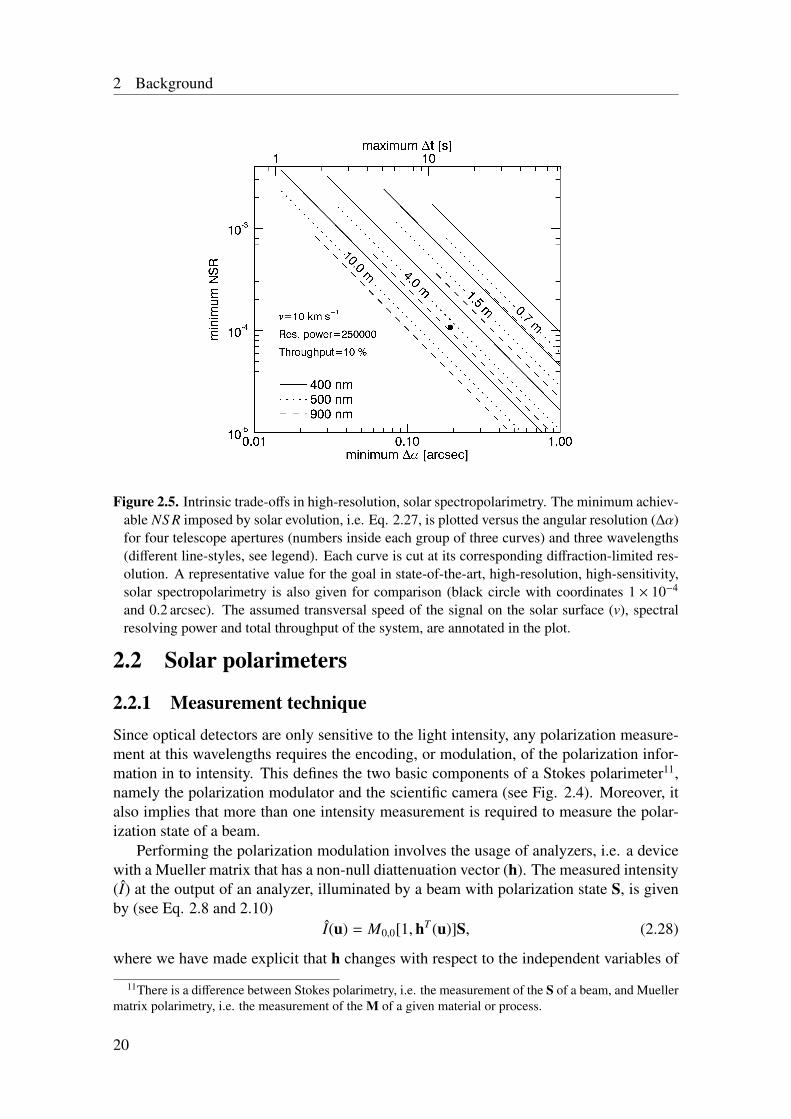
2 Background
Figure 2.5. Intrinsic trade-offs in high-resolution, solar spectropolarimetry. The minimum achiev-able NS R imposed by solar evolution, i.e. Eq. 2.27, is plotted versus the angular resolution (∆α)for four telescope apertures (numbers inside each group of three curves) and three wavelengths(different line-styles, see legend). Each curve is cut at its corresponding diffraction-limited res-olution. A representative value for the goal in state-of-the-art, high-resolution, high-sensitivity,solar spectropolarimetry is also given for comparison (black circle with coordinates 1 × 10⁻⁴
and 0.2 arcsec). The assumed transversal speed of the signal on the solar surface (v), spectralresolving power and total throughput of the system, are annotated in the plot.
2.2 Solar polarimeters
2.2.1 Measurement techniqueSince optical detectors are only sensitive to the light intensity, any polarization measure-ment at this wavelengths requires the encoding, or modulation, of the polarization infor-mation in to intensity. This defines the two basic components of a Stokes polarimeter11,namely the polarization modulator and the scientific camera (see Fig. 2.4). Moreover, italso implies that more than one intensity measurement is required to measure the polar-ization state of a beam.
Performing the polarization modulation involves the usage of analyzers, i.e. a devicewith a Mueller matrix that has a non-null diattenuation vector (h). The measured intensity(I) at the output of an analyzer, illuminated by a beam with polarization state S, is givenby (see Eq. 2.8 and 2.10)
I(u) = M0,0[1,hT (u)]S, (2.28)
where we have made explicit that h changes with respect to the independent variables of
11There is a difference between Stokes polarimetry, i.e. the measurement of the S of a beam, and Muellermatrix polarimetry, i.e. the measurement of the M of a given material or process.
20
2.2 Solar polarimeters
the modulation (u), and so does the measured I. To obtain an analyzer that has an outputintensity sensitive to the four Stokes parameters of the input, one or many retarders (seeEq. 2.17) followed by a linear polarizer (see Eq. 2.14) need to be used, i.e. the analyzerhas Mana = Mppol(θret)Mret(θppol, δ) for the case of a single retarder. As a consequence, thebasic variables that can be modified in order to change h(u), and produce the modulation,are the retardances (δ) and the position angles (θret and θppol).
In general, h will be restricted to a finite set of discrete values, the so called modulationstates, defined at different u, i.e. u ∈ u0,u1, ...,uNmod−1. In this case, a full polarimetricmeasurement requires the synchronous acquisition of Nmod intensity measurements, oneper each modulation state, that can be collected in a vector I = [I0, I1, ..., INmod−1], givenby
I = OS, (2.29)
where the modulation matrix (O) is
O =
1 hT (u0)1 hT (u1)...
...1 hT (uNmod−1)
, (2.30)
and we have assumed that S does not change with u, and that M0,0 = 1 because its valuedoes not affect the measured p.
In order to solve the linear system given by Eq. 2.29 and retrieve the full S, at leastfour independent measurements are needed (Nmod = 4). Such a solution can be expressedas
S = DI, (2.31)
where, ideally, the demodulation matrix (D) is given by D = O−1 and is exactly known.In practice this is not the case due to imperfect calibration and noise among others, that isthe reason to differentiate between the measured Stokes vector, S, and the true S.
Error propagation in Eq. 2.31, leads to the definition of the useful polarimetric ef-ficiencies vector (ε); which has elements ε i, that are related to the elements of D, Di, j,through (Collados 1999)
ε i =1√
Nmod∑Nmod−1
j=0 D2i, j
=σ/√
Nmod
σi, (2.32)
where i ∈ 0, 1, 2, 3, σ is the uncertainty in the measured I (assuming the same value forall its components) and σi is the uncertainty in the measured S i. Note that, the ε definedabove quantifies how the noise obtained by simply averaging the Nmod measurements,σ/√
Nmod, compares to the noise in the retrieved Stokes parameter, σi. The latter allowsthe comparison of the noise properties in different modulation schemes, i.e. systems withdifferent Nmod. The total polarimetric efficiency is defined as,
ε total =
√ε2
1 + ε22 + ε2
3. (2.33)
21
2 Background
The relevant quantities when doing solar polarimetry, are the uncertainties in the nor-malized Stokes parameters, these are given by
σ2i/0 =
− S i
S20
σ0
2
+
(1
S 0σi
)2
≈
(1
S 0σi
)2
, (2.34)
where the approximation was done assuming S i/S 0 << 1, as is the case for many solartargets (see Sect. 2.1.2). Replacing Eq. 2.32 in 2.34, we get that σi/0 is given by the NS Rin the averaged Nmod elements of I, 〈I〉, scaled by the polarimetric efficiency
σi/0 ≈1
ε i√
Nmod
σ
S 0≈
1ε i
σ/√
Nmod
〈I〉, (2.35)
where we have used the fact that, for the weakly polarized scene assumed, S 0 ≈ 〈I〉.An ideal analyzer has | h(u) |= 1. Any given modulation scheme that uses ideal
components would reach a maximum ε ideal that satisfies,
ε ideal,0 = 1 and√ε2
ideal,1 + ε2ideal,2 + ε2
ideal,3 = 1. (2.36)
Or, equivalently, it has an associated polarimetric efficiencies matrix,
A = OT O, (2.37)
that is diagonal, with the main diagonal equal to Nmodε ideal (del Toro Iniesta and Colla-dos 2000). Note that, Eq. 2.36 implies that the efficiencies of an ideal and balancedmodulator, i.e. with equal efficiencies in Stokes Q, U and V , are
εbal =
[1,
1√
3,
1√
3,
1√
3
]. (2.38)
Ideal modulators can not be achieved in practice, because the analyzer elements arenot perfect retarders and polarizers. In this case, Eq. 2.36 does not hold and matrix A isnot diagonal. The latter gives a general guide to design efficient modulators, namely, themore diagonal the matrix A is, the closer is the system to its ideal behavior.
Finally, the definition of ε given in Eq. 2.32, allows responding to the question of whatis the best D to use in Eq. 2.31 when Nmod > 4, and thus the system given by Eq. 2.29becomes overdetermined. If the maximization of the resulting ε is the driving criterion,then D has to fulfill (del Toro Iniesta and Collados 2000)
D = (OT O)−1OT = AOT . (2.39)
Of particular interest is the fact that, computing D using Eq. 2.39, is equivalent to itsderivation using the singular value decomposition (SVD) method (see e.g. Press et al.2007b, Ch. 2.6) to find the pseudo-inverse of O (Collados 1999). This is because SVDminimizes the sum of the squared coefficients of D and thus maximizes the ε.
22
2.2 Solar polarimeters
2.2.2 Polarization modulatorsDepending on which are the independent variables used to modulate the output intensityof the polarization analyzer, different instrumental concepts can be envisioned (see e.g.del Toro Iniesta 2003, Ch. 4). The list below describes the main modulation techniquesemployed in solar polarimeters, including the technologies used to implement them.
1. Temporal modulation: In this case u = t (see Eq. 2.28), thus the different intensitymeasurements are acquired at different instants of time. If the time interval betweenconsecutive intensity measurements is 1/( fmodNmod), then we call fmod the modula-tion frequency. The temporal modulation can be implemented using the followingdevices.
(a) Rotating retarder: If the retarder of the analyzer is motorized, it can be rotatedat a fixed angular speed, say ω. This produces a linear variation of the posi-tion angle of its optical axis with time, i.e. θret(t) = ωt, and thus a temporalmodulation of the analyzer diattenuation vector. Rotating retarders have beenwidely used in the first generations of ground-based, imaging polarimeters.However, moving parts restrict the maximum fmod and, in combination withmisalignments, produce image wobbling that can severely harm spatial reso-lution (Stenflo 1994, Ch. 13). The are, however, some techniques to reducewobbling that had lead to rotating-retarder polarimeters that can achieve highspatial resolution, e.g. Lites et al. (2013).
(b) Electro-optical retarder: These are devices with induced birefringence (seeSect. 2.1.2) that allow a controlled modification of their δ or θret by the appli-cation of an external electric field (del Toro Iniesta 2003, Ch. 4). The mostcommonly used for solar polarimetry are:
• Piezo-elastic modulators (PEMs, Stenflo and Povel 1985) are made of apiece of glass in which a standing acoustic wave is established, by meansof an electro-acoustic transducer, at the resonance frequency (∼50 kHz)of the glass plate. This produces a continuous temporal modulation of theδ at the same frequency, while keeping the θret fixed. They can be usedin the vacuum UV and IR (Stenflo 1994, Ch. 13). A full-Stokes, PEM-based modulator, which requires the synchronization of two PEMs, hasnot been achieved in practice due to frequency stability issues, see e.g.Gandorfer (1999).• Nematic liquid crystals can be confined in a thin layer between two glass
plates to form a variable retarder. The application of an external voltagemodifies the aspect ration of the individual birefringent crystals (see Sect.2.1.2) allowing for slow ( fmod ≈ 20 Hz), continuous modulation of thedevice δ (del Toro Iniesta 2003, Ch.). Crystal-based devices whose δ canbe controlled, such as nematic liquid crystals, are usually called liquidcrystal variable retarders (LCVRs).• Ferro-electric liquid crystals can also be contained in thin layers to pro-
duce variable retarders. Here the external filed imposed produces the re-orientation of the uniaxial birefringent crystals, which modifies θret of the
23
2 Background
device between two positions, that differ Θ≈45° from each other (wereΘ is called the FLC switching angle). δ is controlled by the thickness ofthe layer (∼2 µm), which can be tuned to produce a half-wave plate at agiven central wavelength, λ0 (Gandorfer 1999). Two FLCs can be usedin combination with two static retarders (SRs) to efficiently modulate thefull Stokes vector up to fmod ≈ 1 kHz, in the visible portion of the spec-trum (from 400 to 700 nm approximately, see Gandorfer 1999). Such adesign has been adopted in many current solar polarimeters.The wavelength dependence of δ in FLCs is considerable, and has beenstudied by Gisler et al. (2003). They proposed the following model forthe dispersion law of birefringence, at a given temperature and expressedin fractions of λ
δ(λ) =
(δ0λ0 −
Cλ2
0
)1λ
+Cλ3 , (2.40)
where C is the dispersion constant and δ0 is the retardance value at thecentral wavelength, λ0, e.g. equal to 0.5 and 0.25 for ideal half-wave andquarter-wave plates respectively.Both δ and Θ are temperature (T ) dependent in FLCs. The latter is thestronger effect and can be modeled by (Gisler et al. 2003)
Θ(T ) = CT1
√CT2 − T , (2.41)
where CT1 and CT2 are two constants.
2. Spatial modulation: In this case u = x (see Eq. 2.28), therefore the different inten-sity measurements are acquired simultaneously at different positions. This type ofmodulators can be implemented by means of the following two devices.
(a) Birefringent plate: If a block of birefringent material is cut in such a waythat its optical axis forms an oblique angle with respect to an incident beam,it will produce a separation of such a beam in one ordinary and one extraor-dinary component (see Sect. 2.1.2). While the ordinary ray is not deviatedfrom the incident direction, the extraordinary is refracted at an oblique angle.The latter leads to the formation of two rays at the output of the block (delToro Iniesta 2003, Ch. 4). The two most commonly used devices are theSavart plate, where two birefringent plates are properly placed to separate theincoming beam into two output rays that experience the same phase lag andhave parallel propagation directions; and the Wollaston plate were the outputbeams have different output angles. The polarimetric action of both devicescan be modeled by two Mueller matrices, one per output ray, that correspondto two linear polarizers with orthogonal optical axes (antiparallel h and v).Therefore, they form spatial modulators, that can be used to illuminate differ-ent sections of a single detector simultaneously due to the small separation ofthe output beams. The Savart plate is used close to the detector (focal plane)while the Wollaston plate is used in collimated setups (close to a pupil).
(b) Polarizing beam splitter: Discrete spatial modulation can also be achievedwith a block of birefringent material, that has been cut diagonally and stuck
24
2.2 Solar polarimeters
back using a special cement. The refractive index of the cement produces totalreflexion of the ordinary beam that is deviated orthogonally from the incidentdirection. The extraordinary beam is refracted in the diagonal interface con-tinuing its propagation with unaffected direction. The polarimetric action ofsuch a beam splitter is modeled by two Mueller matrices, one for each outputray, that correspond to two linear polarizers with orthogonal optical axes (an-tiparallel h and v). The polarizing beam splitter can be used together with twodetectors, or a single detector plus the appropriate optics, to record simultane-ously two orthogonal polarization states.
3. Spatio-temporal modulation: A combination of temporal and spatial modulation isapplied in the dual beam and beam exchange techniques.
(a) Dual beam: In this common scheme (Lites 1987, Collados 1999), a tempo-ral modulator is followed by a double birefringent plate or a polarizing beamsplitter. Two simultaneous measurements with orthogonal polarization are ac-quired for every state of the temporal modulator (using either two cameras ortwo parts of the same sensor). After the appropriate combination of the simul-taneous measurements, the SIC can be reduced provided that beam imbalancesare controlled (see Sect. 2.3.2).
(b) Beam exchange: Same as the dual beam, except that, an extra measurement isacquired after exchanging the beams that reach the two cameras.This reducesthe effects of beam imbalances with respect to the dual beam technique (seeSect. 2.3.2). For example, Bianda et al. (1998) use a manually-rotated half-wave plate in combination with a polarizing beam splitter to implement thebeam exchange. They simultaneously image Stokes I+Q and I-Q on differentsections of a single sensor. After this first exposure, they manually rotatethe retarder to switch the polarization states of the output beams and exposeagain. Similar implementations can be done using electro-optical retarderssuch as FLCs in order to increase the temporal modulation frequency.
2.2.3 Wavelength discriminationMost of the physical phenomena that modify the polarization of light are strongly wave-length dependent (see Sect. 2.1.2). In particular, accurate measurements of solar Zeemanor scattering polarization signals, require resolving spectral features that are much nar-rower than the width of a single absorption or emission line, i.e. 1 Å. As a consequence,the device used for wavelength discrimination along with the polarimeter (see Fig. 2.4) isof paramount importance.
There are three solutions developed to solve the fundamental problem of imaging thetwo spatial plus one spectral dimensions in to a bi-dimensional intensity detector. Themain difference between them is what dimensions are simultaneously imaged, and whichare multiplexed in time. This affects the properties of the resulting data, i.e. simultane-ity, resolution, field of view (FOV) and spectral range. Any of the three approaches canbe combined with a temporally or spatially modulated polarimeter to form a spectropo-larimeter. In the former case, the simultaneity in the dimension that is time-multiplexed
25
2 Background
is diminished, due to the time the polarimeter takes to acquire all the modulation states.For this and other reasons, some of the requirements for wavelength discriminators aregenerally stricter if they are used for spectropolarimetry than those used for simple spec-troscopy, e.g. duty cycle. Further details on each of the three solutions, as they areimplemented in solar spectropolarimeters, are given below.
1. Spectrograph + slit based scanner: In this case the spectral dimension, includingone or more spectral lines, plus one of the spatial dimensions are simultaneouslyimaged on the detector. Thus the remaining spatial dimension is multiplexed intime. This is typically accomplished by first selecting an unidimensional regionfrom the FOV using a slit12. The light from the slit is then fed to a spectrograph inorder to produce an image containing the spectral plus spatial information along theslit. To acquire the remaining spatial information, the slit is moved in discrete stepsto scan the FOV (see e.g. Beck et al. 2005a and Sankarasubramanian et al. 2004 fortwo solar applications). Solar spectrograph-based systems are usually built usingechelle diffraction gratings 13 and have high resolving power (up to 800 000, Ken-tischer et al. 1998). On the other hand, the resulting data is not spatially coherent. Itfollows that moving or extended signals may not be properly sampled, that the re-sulting spatial resolution is usually worse than with the other approaches (due to thelimited accuracy of the scanning system) and that each slit exposure is affected bya different realization of the atmospheric seeing (see Sect. 2.3.1). The latter greatlycomplicates any post-facto restoration of the acquired images (see Sect. 2.3.3).
2. Tunable filtergraph: Using a tunable filter, both spatial dimensions can be simulta-neously imaged on the detector. In order to obtain the spectral information, the filterhas to be successively re-tuned in discrete wavelength steps. Generally less than 20points are recorded per spectral line (Kentischer et al. 1998). For that reason, thedetection of spectrally complex signals is commonly done with spectrograph-basedsystems. On the other hand, the spatial coherence of the data acquired with a fil-tergraph allows a better study of moving solar signals that are spatially extended,as well as allowing the application of post-facto image restoration to improve thespatial resolution in ground-based observatories. The most common tunable fil-ters used in high-resolution spectropolarimeters use one or multiple Fabry-Pérotetalons14 (e.g. Bello González and Kneer 2008 and Martínez Pillet et al. 2011) be-cause they can be tuned in a short time (<1 s, Kentischer et al. 1998) and provide
12The slit thickness corresponds typically to the diffraction limit of the telescope.13A diffraction grating is a dispersive element that features a periodic (with spacing d) distribution of N
thin grooves. The achievable resolving power of the grating is given by Nm, were m is the interferenceorder. Analogously, the angle of dispersion for a wavelength λ0 and normal incidence, is arcsin(mλ0/d).Therefore, observing at high orders is desirable, however, only a fraction of the incoming light is put in anygiven order. To solve this issue, and allow spectroscopy of faint sources, an echelle grating has speciallyshaped grooves that ensure that most of the incoming light is output to a given high (e.g. 1000) order (Bornand Wolf 1999, Ch. 8).
14A Fabry-Pérot etalon is a resonant cavity formed by two highly parallel (λ/200) reflecting surfaces. Thetransmission spectrum presents periodic resonance peaks every ∆λFS R, the so called free spectral range. Thefull-width at half maximum (∆λFWHM) is related to the reflectivity (re f ) by ∆λFWHM/∆λFS R = π
√re f /(1−
re f ), i.e. the higher the re f , the better the finesse or separation of the transmission peaks. The location of thepeaks can be changed by re-tunning the etalon, i.e. modifying the separation between the reflective surfacesusing piezoelectric actuators. Errors in the cavity thickness produce random shifts of the transmission
26
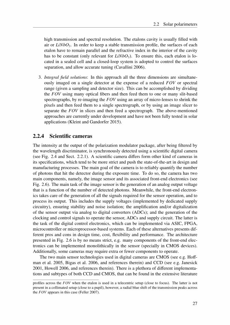
2.2 Solar polarimeters
high transmission and spectral resolution. The etalons cavity is usually filled withair or LiNbO3. In order to keep a stable transmission profile, the surfaces of eachetalon have to remain parallel and the refractive index in the interior of the cavityhas to be constant (only relevant for LiNbO3). To ensure this, each etalon is lo-cated in a sealed cell and a closed-loop system is adopted to control the surfacesseparation, and allow accurate tuning (Cavallini 2006).
3. Integral field solutions: In this approach all the three dimensions are simultane-ously imaged on a single detector at the expense of a reduced FOV or spectralrange (given a sampling and detector size). This can be accomplished by dividingthe FOV using many optical fibers and then feed them to one or many slit-basedspectrographs, by re-imaging the FOV using an array of micro-lenses to shrink thepixels and then feed them to a single spectrograph, or by using an image slicer toseparate the FOV in slices and then feed a spectrograph. The above-mentionedapproaches are currently under development and have not been fully tested in solarapplications (Kleint and Gandorfer 2015).
2.2.4 Scientific camerasThe intensity at the output of the polarization modulator package, after being filtered bythe wavelength discriminator, is synchronously detected using a scientific digital camera(see Fig. 2.4 and Sect. 2.2.1). A scientific camera differs form other kind of cameras inits specifications, which tend to be more strict and push the state-of-the-art in design andmanufacturing processes. The main goal of the camera is to reliably quantify the numberof photons that hit the detector during the exposure time. To do so, the camera has twomain components, namely, the image sensor and its associated front-end electronics (seeFig. 2.6). The main task of the image sensor is the generation of an analog output voltagethat is a function of the number of detected photons. Meanwhile, the front-end electron-ics takes care of the generation of all the signals required for the sensor operation, and toprocess its output. This includes the supply voltages (implemented by dedicated supplycircuitry), ensuring stability and noise isolation; the amplification and/or digitalizationof the sensor output via analog to digital converters (ADCs); and the generation of theclocking and control signals to operate the sensor, ADCs and supply circuit. The latter isthe task of the digital control electronics, which can be implemented via ASIC, FPGA,microcontroller or microprocessor-based systems. Each of these alternatives presents dif-ferent pros and cons in design time, cost, flexibility and performance. The architecturepresented in Fig. 2.6 is by no means strict, e.g. many components of the front-end elec-tronics can be implemented monolithically in the sensor (specially in CMOS devices).Additionally, some cameras may require extra or fewer components to operate.
The two main sensor technologies used in digital cameras are CMOS (see e.g. Hoff-man et al. 2005, Bigas et al. 2006, and references therein) and CCD (see e.g. Janesick2001, Howell 2006, and references therein). There is a plethora of different implementa-tions and subtypes of both CCD and CMOS, that can be found in the extensive literature
profiles across the FOV when the etalon is used in a telecentric setup (close to focus). The latter is notpresent in a collimated setup (close to a pupil), however, a radial blue shift of the transmission peaks acrossthe FOV appears in this case (Feller 2007).
27
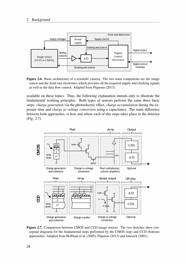
2 Background
Image sensor(CCD or CMOS)
Digital control
electronicsA/D
Power supply
Supply voltages
Analog outputs
Clocking and control
Supply control
Digital output
Digital control interface
Clocking and control
Front-end electronics
Figure 2.6. Basic architecture of a scientific camera. The two main components are the imagesensor and the front end electronics which provides all the required supply and clocking signalsas well as the data flow control. Adapted from Piqueras (2013).
available on these topics. Thus, the following explanation intends only to illustrate thefundamental working principles. Both types of sensors perform the same three basicsteps: charge generation via the photoelectric effect, charge accumulation during the ex-posure time and charge to voltage conversion using a capacitance. The main differencebetween both approaches, is how and where each of this steps takes place in the detector(Fig. 2.7).
Output
np
p+
poly
select
bus
reset
MOSdiode
...
CDS
A/D
ArrayPixel
Charge generation and collection
Charge to voltage conversion
Pixel multiplexing / column amplifiers
Sensor output
np
p+
reset
MOSdiode
CDS
A/D
ArrayPixel
Charge generation and collection
Charge to voltage conversion
C
Charge transfer
e-
Φ3Φ2Φ1
e-
Off-chip
CMO
SCC
D
Optional
Optional
Figure 2.7. Comparison between CMOS and CCD image sensors. The two sketches show con-ceptual diagrams for the fundamental steps performed by the CMOS (top) and CCD (bottom)approaches. Adapted from Hoffman et al. (2005), Piqueras (2013) and Janesick (2001).
28
2.2 Solar polarimeters
CMOS sensors perform the charge generation, collection and conversion to voltagewithin a single pixel. Further signal processing steps, such as amplification or multi-sampling15, can be also embedded to produce an active pixel structure. The voltages of thematrix are then read by multiplexing each pixel to common buffers, which are terminatedin amplifiers. The detailed addressing process, number of buffers and amplifiers, dependson the specific sensor design. Further stages, used to implement CDS and to allocate theADCs, can be optionally placed at the sensor level.
On the other hand, CCDs perform only the charge generation and accumulation stepson the pixel level. As a consequence, the charges need to be transfered row-wise, using theshift-register structure of the sensor, after every exposure. At the end of the columns, thecharges are typically loaded in a transversal register that shifts them towards the readoutnode —where the charge to voltage conversion and amplification occur— one pixel at atime. Multiple transversal registers and/or output channels are also commonly used toincrease the readout speed.
Before performing any comparison between the performances of the CCD and CMOStechnologies; let us collect and define in Table 2.1, the camera characteristics and perfor-mance specifications that will be used during the rest of this thesis.
The spectral range of the QE in CCDs is mostly limited to that of silicon16, i.e. typ-ically from 300 to 1100 nm plus the x-rays, provided that proper anti-reflective coatingsare applied. CMOS devices can have an extended working rage due to the possibility ofusing a non-silicon layer as photosensitive material, connected —usually using iridium orindium bumps— to a silicon layer where the readout integrated circuitry of each pixel islocated. Such an hybrid CMOS can be sensitive up to 10 µm (Hoffman et al. 2005).
If the sensor is front illuminated, the gate structure, electrodes and other circuitry (inCMOS) present there, reduce the FF. The spectral response is also limited in this case,mainly because short wavelengths (<400 nm) are strongly absorbed an reflected by thepoly-silicon gate structure (Janesick 2001, Sect 1.2.2.1). To increase the UV response,the gate can be coated with a phosphor (that re-radiates at longer wavelengths) or a backilluminated sensor can be employed. The latter option is very efficient because in additiona 100 % FF can be reached. However, back illumination requires thinning the sensorsubstrate (to allow the photons reaching the collecting area near the gate) and a morecomplicated manufacturing process (Janesick 2001, Sect. 1.1.2).
The literature is full of good comparisons between the properties of CMOS and CCDtechnologies, e.g. Janesick et al. (2006, 2007), Magnan (2003). Some of the most im-portant differences between the two technologies are summarized in Table 2.2. We havehighlighted using italics the sensor properties that are more relevant to ground-based so-lar polarimetry. These will be discussed in detail in the following chapters, particularly
15 Fixed pattern noise (FPN) —mostly due to dark current non-uniformity (DCNU, see Table 2.1)— isone of the main disadvantages in CMOS devices; because of the manufacturing-induced differences in thecircuitry of each pixel. An effective way to reduce FPN and reset noise (due to the kTC noise of the sensecapacitance and reset pulse feed-through) in CMOS and CCD sensors, is sampling the pixel signal multipletimes during the readout. One of the simplest way to do the latter is correlated double sampling (CDS),here the sensing node is sampled twice. A first time after the reset and the second time after the exposure isfinished. The two samples are then subtracted to eliminate low frequency noise and any offset, producingessentially a band-pass effect (Hoffman et al. 2005, Janesick 2001).
16Some CCDs have been produced using Germanium, they have an extended spectral response up to1.6 µm. However, they present other issues like large dark currents (Janesick 2001, Sect. 1.2.2.1).
29

2 Background
Parameter Symbol Unit Definition and responsible components or processes
Sensor area Ncol×Nrow pixel2 The sensor area and aspect ratio are defined during thedesign stage.
Pixel area Apixel µm2 The total area occupied by each pixel is defined duringthe design stage.
Frame rate FR fps ; Hz Number of frames that can be read out per second. Itis influenced by the readout electronics, ADCs and thecharge transfer speed (in CCDs).
Duty cycle DC % Equal to the product of the frame rate and the exposuretime. It is affected by the readout electronics and shutterstrategy.
ADC resolution Nadc bit Length of the ADC word.
Sensitivity QE × FF % The filling factor (FF, ratio of the photosensitive to thetotal area of the pixel) is mainly influenced by the designsof the pixel (gate size, extra circuitry, etc.) and sensor(back or front illuminated, routing, etc.). The QE (frac-tion of incident photons that produce photo-electrons) isgiven by the photosensitive material and anti-reflectivecoating among others.
Non-linearity NL % Quantifies how much the sensor output deviates from alinear function of the exposure time. Mainly influencedby the pixel structure and readout electronics.
Full well charge FWC e− The amount of electrons that can be collected by a pixelbefore it saturates, i.e. its output does not increase withan increase of the exposure time. It is determined by thepixel and sensor structure as well as the readout electron-ics.
Conversion gain G DN /e− Number of digital counts produced per each photo-electron. Mostly given by the sensing node capacity,readout electronics and ADCs. Generally configurable.
Dark current id e− s−1 Flux of thermal charges created in the sensor. The sensortemperature, pixel size and material strongly influence itsvalue.
Dark currentnon-uniformity
DCNU % Pixel to pixel variations of the id after calibration. Mainlygiven by the manufacturing tolerances and readout cir-cuitry. It is an additive noise source.
Photon responsenon-uniformity
PRNU % Pixel to pixel variations of the photon response (G, QE,etc.) after calibration (multiplicative noise). Given by themanufacturing tolerances and readout circuitry.
Read out noiserms value
σro e−rms Noise in a zero-exposure frame. Given mostly by thereadout circuitry.
Quantizationnoise rms value
σadc e−rms Quantization plus other noise sources introduced by theADCs. It is an important contributor to σro. Given byNadc and the ADCs circuitry.
Dark noise rmsvalue
σd e−rms Poissonian noise produced by id.
Table 2.1. Basic camera characteristics and performance specifications. The last column givesa short definition and a summary of the main responsible components or processes for eachfeature. See e.g. Janesick (2001) for more detailed definitions.
30

2.2 Solar polarimeters
in Sect. 3.1.1 and Ch. 5. Note that, CCDs tend to perform typically better in the sensorproperties that are determinant for low-light scientific imaging (such as high-resolution,solar spectropolarimetry).
Property CCD CMOS
Noise(1) Typically lower due to the lowdark current and readout noise.
Higher, e.g. the quality of thereadout circuits in each pixelproduce higher FPN and resetnoise.
Linearity Better. Worse, due to the signal depen-dence of the readout circuit gain.
Sensitivity Higher Lower.
Shutter Mechanical or electronic snap-shot (frame transfer or interline).
Electronic snapshot or rollingshutter.
Cost Higher Lower. Benefits from computerCMOS industry.
Mass/size Higher. Lower. Monolithic integrationof much of the front-end elec-tronics is possible.
Powerconsump-tion
Higher. Needs many, relativelyhigh voltages for charge transfer-ring.
Lower. Only a single CMOSvoltage is required.
Radiationtolerance
Lower due to the creation ofcharge traps.
Higher because no charge trans-fer is needed.
Heritage Long heritage (since 1975) spe-cially in the scientific commu-nity.
Serious competitors since the90’s. Very strong growth inrecent years due to the pushof massive commercial applica-tions.
Misc. No built-in signal processing.May suffer form smearing, pixelblooming and charge transfer in-efficiency.
Only a single clock is needed.Random or selective readout ispossible.
1 The root mean squared (rms) value of the total camera noise, σcam, is equal to√σro
2 + σd2.
Table 2.2. Comparison of the main properties of CMOS and CCD sensors. The properties high-lighted in italic are more critical for ground-based solar polarimetry.
The CMOS architecture has in principle many advantages with respect to the CCDapproach, e.g. built-in signal processing capabilities. However, CCDs have been superiorin overall still image quality, and thus the preferred option in many scientific applications,since their first astronomical usages in the mid 70’s. Up to recently, the noise, sensitiv-ity and dynamic range of state-of-the-art scientific CCDs, could not be simultaneouslyachieved by CMOS sensors (Bigas et al. 2006). This is mainly due to the quality and
31
2 Background
size of the readout circuits that the CMOS manufacturing process can achieve within thereduced space of a single pixel. Regardless of this, CMOS sensors have made their way(since the early 90’s) into many commercial and scientific applications that benefit fromits advantages; most notably low power consumption and radiation tolerance (of particularimportance in space-based imaging systems, see e.g. Piqueras 2013).
In the last decade, the synergy between the manufacturing processes of CMOS sensorsand other massive commercial industries (personal computers, mobile devices, etc.) haveproduced enormous improvements in some sensor parameters that are critical for scien-tific applications (sensitivity and noise). Sometimes reaching and surpassing the mostdemanding CCD benchmarks (Janesick et al. 2013). Nowadays the performance differ-ence between the two technologies is narrow and is getting narrower every year. Thehuge variety of sensors design, configurations and performances; make any weighing be-tween the CCD and CMOS solutions strongly dependent on the application, manufactureravailability and budget, even within the scientific imaging sector.
2.3 Polarimetric effects of atmospheric seeing and imagemotion
The location of the solar observatory strongly influences the properties of the resultingspectropolarimetric data. Space-based observatories can, among others, detect portionsof the spectrum absorbed by Earth’s atmosphere (such as the UV regime); observe the Sun24 hours uninterruptedly (in some cases); and avoid the image aberrations introduced byatmospheric seeing. On the other hand, they suffer from serious disadvantages includinghigh monetary cost, lack of flexibility to upgrade or repair the instruments, and usuallydo not contain state-of-the-art technology by the time of launch (Kleint and Gandorfer2015).
A particularly important difference between ground and space-based observatories,is the available aperture size. As discussed in Sect. 2.1.4, the collecting power of thetelescope presents a fundamental limitation to the simultaneous angular resolution andS NR that can be achieved when imaging a dynamic solar signal (see Fig. 2.5). In thisrespect, the larger apertures of ground-based telescopes (currently 1.6 m versus the 0.5 min space) provide them with an advantage position. Such a difference will be even moreprominent in the near future, when the 4 m DKIST telescope under construction in Hawaii(e.g. Elmore et al. 2014) sees first light. In order to fully exploit the high S NR and spatialresolution achievable by such large apertures, new instrumental techniques —that furtherreduce the image aberrations and polarimetric effects introduced by atmospheric seeing—are required.
2.3.1 Description of atmospheric seeing and image motionIf an initially plane monochromatic wave propagates downwards through an atmosphericlayer of thickness ∆h, located at an altitude h0, it will experience a complex disturbance(U) —i.e. each component of the incoming E is multiplied by U17— given by (e.g. Saha
17Note that, the seeing disturbance do not contemplate variations of the amplitude. For polarimetry thisis not an issue because (a) the air attenuation is small, (b) the portion of the sky covered by the FOV is small
32
2.3 Polarimetric effects of atmospheric seeing and image motion
2007, Sect. 5.3.1)U(r, t) = eiδ(r,t), (2.42)
were the phase shifts (δ) are
δ(r, t) =2πλ
∫ h0+∆h
h0
n(r, t, h)dh, (2.43)
n denotes the refractive index, t the time and r the bi-dimensional position vector onthe plane of the considered layer. The random fluctuations of n induce the same kindof variations in δ, which in turn aberrates (deforms) the wavefront that would reach anyground-based telescope. The consequent reduction in image quality is called seeing (seee.g. Saha 2007, Ch. 5).
The detailed process of image degradation by seeing is complicated and its descrip-tion out of the scope of this thesis. However, two aspects are critical to ground-basedpolarimetry and in particular to the FSP project. Firstly, the instrumental requirementsneeded to reduce seeing induced spurious signals (see Sect. 3.1), are based on the tempo-ral behavior of δ. Secondly, many image restoration techniques, such as the MOMFBD(see Sect 2.3.3), are based on a linear shift invariant model of the seeing degradation.Because of these, we only describe below some basic concepts necessary to understandhow seeing is characterized, and what are the limitations and properties of the imagedegradation model.
The random spatial and temporal fluctuations of n, are produced by the inhomo-geneities of the temperature (dominant effect in solar observations), pressure and humidityof the gases that compose the atmosphere. The source of the inhomogeneities are convec-tion cells, wind shear and other hydrodynamic instabilities. The spatial dimensions of thefluctuations span a wide range, from the outer scale of the turbulence (tens of meters) toits inner scale (in the mm or cm level). The energy is transported towards the small scales,by the successive breaking of larger structures into smaller eddies. This scale-invariantprocess can be quantitatively described using the Kolmogorov turbulence theory.
Roddier (1981), based on the works of (Tatarski 1961) and others, combined the Kol-mogorov theory with a plane-parallel atmosphere, composed of many independent thinlayers, to derive the spatial correlational properties of U at the telescope aperture. Thelatter can be conveniently specified using the spatial coherence function of U, expressedin terms of the Fried parameter (r0, Fried 1966), as follows (e.g. Saha 2007, Sect. 5.4.2)
〈U(r0)U∗(r0 + r)〉 = e−3.44(|r|/r0)5/3, (2.44)
were ∗ denotes the complex conjugate. The r0, a.k.a coherence length, is a measure of theseeing quality and scales as
r0 ∝ λ6/5. (2.45)
Equation 2.44 can be used to derive the spatial power spectrum of δ, D, due to Kol-mogorov turbulence,
D(k) = 0.023r0−5/3 | k |−11/3, (2.46)
resulting in negligible spatial variations of the attenuation and (c) a fast variation of such a flat attenuationwould only produce a modification in the polarimetric offset (thus not affecting the signal value relative tothe continuum).
33
2 Background
where k is the spatial frequencies vector.The temporal behavior of δ, due to the contribution of many dynamic atmospheric
layers, is difficult to derive. A common approach due to Taylor (1938), is to consider asingle phase screen (with spatial properties given by Eq. 2.46), that is frozen and movesat the local wind speed v. Then, the temporal statistics of the resulting δ at the ground,are governed by the seeing coherence time (τ0), which relates to r0 through
τ0 ≈r0
v∝ λ6/5. (2.47)
The total imaging action of the seeing, can be reasonably modeled by a stochastic,linear-space-invariant system. The space invariance only holds if the FOV is smallerthan the seeing isoplanatic patch, i.e. the circular area of the sky enclosed by the seeingisoplanatic angle (φ0). The φ0 relates to r0 according to (e.g Saha 2007, Sect. 5.4.4)
φ0 ∝r0
h0∝ λ6/5, (2.48)
where h0 is the mean effective height of the turbulence layer. As a consequence, we canwrite the image degradation process due to the action of both seeing and the telescope, inthe spatial Fourier domain, as follows
I(k, t) = Hatm+tel(k, t)I(k), (2.49)
were Hatm+tel(k, t) is the instantaneous optical transfer function (OTF) of the seeing plustelescope18, and I(k, t) and I(k) are the spatial Fourier transform of Stokes I (images) atthe focus of the telescope and the Sun, respectively (refer to Fig 2.4). Note that the solarscene is assumed to be constant for the present analysis.
The above-introduced statistical properties of the seeing, translate in to properties ofHatm+tel(k, t). According to the observing regime —defined by the telescope aperture (D)and the exposure time (te)— we can distinguish the following cases (all assuming a FOVsmaller than the isoplanatic patch, and a quasi-monochromatic observation):
1. D << r0: By definition, r0 is equivalent to the maximum diameter of a circularaperture that would be able to operate at the diffraction limit19. Therefore, theachievable spatial resolution in this case, is not limited by the seeing but by thediffraction limit of the telescope, namely 1.22λ/D approximately. Typical values ofr0, for day time seeing in astronomical sites at λ = 500 nm, can be in the order of5 cm for very bad conditions and 30 cm for excellent conditions.
2. D >> r0 and te >> τ0: In this long exposure regime, the measured image (degradedboth by blurring and image motion) can be obtained by computing the average overmany independent seeing realizations in Eq. 2.49 (e.g. Saha 2007, Sect. 5.4.1), i.e.
〈I(k, t)〉 = 〈Hatm+tel(k, t)〉I(k). (2.50)
18In the rest of this section we assume no AO is present in the beam19More precisely, the rms error of the wavefront, in a circular area of diameter r0 at the ground, is
approximately 1 rad or λ/6.
34
2.3 Polarimetric effects of atmospheric seeing and image motion
Roddier (1981) showed that
〈Hatm+tel(k, t)〉 = Hatmle(k)H tel(k), (2.51)
were Hatmle(k) is the long-exposure OTF of the seeing and H tel(k) the (constant)telescope OTF. Moreover, he proved that Hatmle(k) reduces to a Gaussian OTFgiven by the Fourier transform of the complex disturbance coherence function (Eq.2.44). Thus, the width of Hatmle(k) only depends on the overall seeing conditions,r0. Since D >> r0, the maximum achievable spatial resolution is seeing-limited to1.22λ/r0 approximately20, i.e. 〈Hatm+tel(k, t)〉 → Hatmle(k). Note that if D << r0, asin the first case, then 〈Hatm+tel(k, t)〉 → H tel(k).
3. D >> r0 and te << τ0: In this short exposure regime, image motion does notcontribute to the seeing-induced aberrations. The remaining degradation is usuallycalled image blurring. The measured image can be computed using a single real-ization ofHatm+tel(k, t) in Eq. 2.49 (frozen seeing condition). SinceHatm+tel(k, t) israndom, the seeing effect is studied on the energy spectral density of the measuredimage, i.e. (Roddier 1981)
〈| I(k, t) |2〉 = 〈| Hatm+tel(k, t) |2〉 | I(k) |2 . (2.52)
Different from the long-exposure case, the short-exposure 〈| Hatm+tel(k, t) |2〉 has nosimple analytical expression. This was studied by Korff (1973), who proved that〈| Hatm+tel(k, t) |2〉 has an asymptotic behavior that extends to the high-frequenciesup to the diffraction limit of H tel(k). The latter, i.e. that seeing-aberrated, short-exposure images retain the spatial information up to the diffraction limit, is thebase of the post-facto image restoration techniques. Korff (1973) also found thatthe low-frequency part of 〈| Hatm+tel(k, t) |2〉 corresponds to the long exposure〈Hatm+tel(k, t)〉 when an image motion compensator is used. Thus, image motionis the main responsible of the contrast reduction in the low spatial frequencies oflong-exposure images. Moreover, the variance of the wavefront errors in radianssquared, reduces from 1.03 (D/r0)5/3 to 0.134 (D/r0)5/3 after complete tip-tilt cor-rection (Judge et al. 2004).
As explained above, the ratio te/τ0 is critical to the spatial resolution that large tele-scopes (>50 cm) can reach in the presence of seeing. It is also critical to the level ofspurious polarization signals introduced by the seeing (see Sect 2.3.2). Typically, τ0 forday-time seeing is 10 to 50 ms (Löfdahl et al. 2007). Unfortunately, modern solar spec-tropolarimetry requires S NR values that can not be achieved with te << 50 ms, in anyof the currently available solar telescopes. Note that the latter imposes a trade-off be-tween S NR and spatial resolution that is in general more strict than the one imposed bythe mere evolution of the solar signal, i.e. Eq 2.27 (see also Fig. 2.5). To work withlonger te and preserve the spatial resolution, either the seeing-induced aberrations haveto be compensated before the long-exposure image is acquired (path adopted by the AOcommunity); or many short-exposure images has to be acquired and the seeing-inducedaberrations removed post-facto before accumulating them (path adopted by the numericimage restoration community).
20This is the reason to define the image degradation as the ratio D/r0.
35
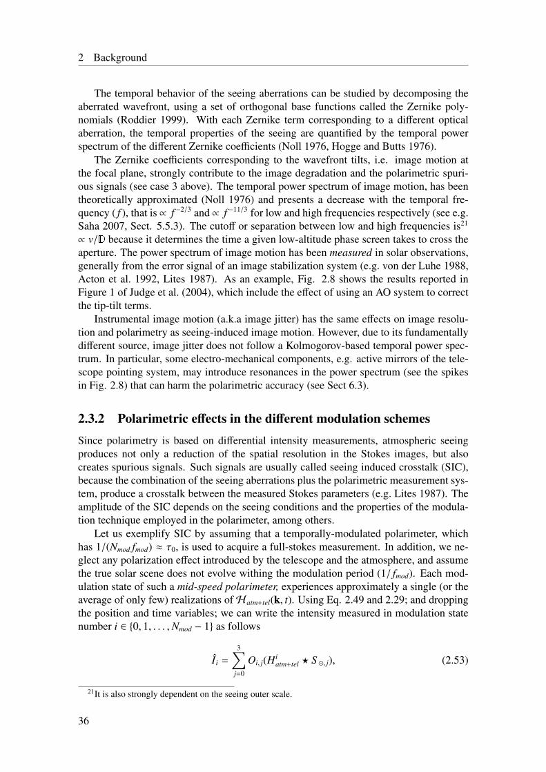
2 Background
The temporal behavior of the seeing aberrations can be studied by decomposing theaberrated wavefront, using a set of orthogonal base functions called the Zernike poly-nomials (Roddier 1999). With each Zernike term corresponding to a different opticalaberration, the temporal properties of the seeing are quantified by the temporal powerspectrum of the different Zernike coefficients (Noll 1976, Hogge and Butts 1976).
The Zernike coefficients corresponding to the wavefront tilts, i.e. image motion atthe focal plane, strongly contribute to the image degradation and the polarimetric spuri-ous signals (see case 3 above). The temporal power spectrum of image motion, has beentheoretically approximated (Noll 1976) and presents a decrease with the temporal fre-quency ( f ), that is ∝ f −2/3 and ∝ f −11/3 for low and high frequencies respectively (see e.g.Saha 2007, Sect. 5.5.3). The cutoff or separation between low and high frequencies is21
∝ v/D because it determines the time a given low-altitude phase screen takes to cross theaperture. The power spectrum of image motion has been measured in solar observations,generally from the error signal of an image stabilization system (e.g. von der Luhe 1988,Acton et al. 1992, Lites 1987). As an example, Fig. 2.8 shows the results reported inFigure 1 of Judge et al. (2004), which include the effect of using an AO system to correctthe tip-tilt terms.
Instrumental image motion (a.k.a image jitter) has the same effects on image resolu-tion and polarimetry as seeing-induced image motion. However, due to its fundamentallydifferent source, image jitter does not follow a Kolmogorov-based temporal power spec-trum. In particular, some electro-mechanical components, e.g. active mirrors of the tele-scope pointing system, may introduce resonances in the power spectrum (see the spikesin Fig. 2.8) that can harm the polarimetric accuracy (see Sect 6.3).
2.3.2 Polarimetric effects in the different modulation schemesSince polarimetry is based on differential intensity measurements, atmospheric seeingproduces not only a reduction of the spatial resolution in the Stokes images, but alsocreates spurious signals. Such signals are usually called seeing induced crosstalk (SIC),because the combination of the seeing aberrations plus the polarimetric measurement sys-tem, produce a crosstalk between the measured Stokes parameters (e.g. Lites 1987). Theamplitude of the SIC depends on the seeing conditions and the properties of the modula-tion technique employed in the polarimeter, among others.
Let us exemplify SIC by assuming that a temporally-modulated polarimeter, whichhas 1/(Nmod fmod) ≈ τ0, is used to acquire a full-stokes measurement. In addition, we ne-glect any polarization effect introduced by the telescope and the atmosphere, and assumethe true solar scene does not evolve withing the modulation period (1/ fmod). Each mod-ulation state of such a mid-speed polarimeter, experiences approximately a single (or theaverage of only few) realizations ofHatm+tel(k, t). Using Eq. 2.49 and 2.29; and droppingthe position and time variables; we can write the intensity measured in modulation statenumber i ∈ 0, 1, . . . ,Nmod − 1 as follows
Ii =
3∑j=0
Oi, j(Hiatm+tel ? S , j), (2.53)
21It is also strongly dependent on the seeing outer scale.
36
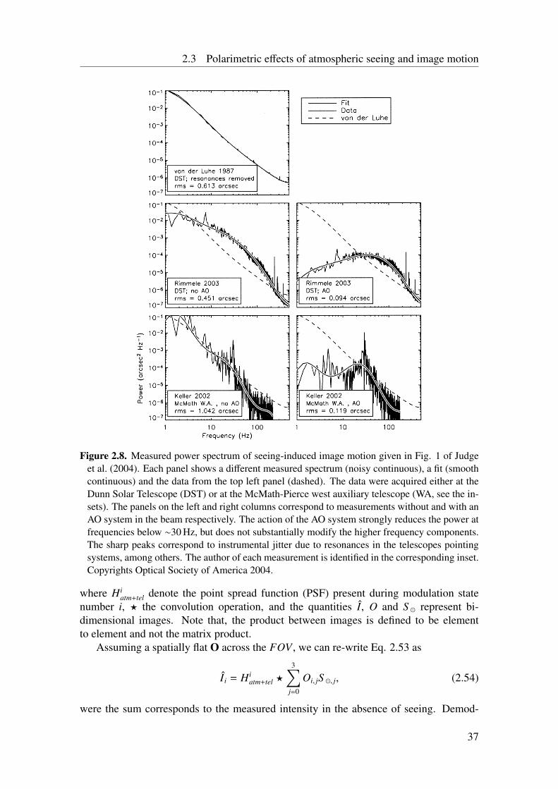
2.3 Polarimetric effects of atmospheric seeing and image motion
Figure 2.8. Measured power spectrum of seeing-induced image motion given in Fig. 1 of Judgeet al. (2004). Each panel shows a different measured spectrum (noisy continuous), a fit (smoothcontinuous) and the data from the top left panel (dashed). The data were acquired either at theDunn Solar Telescope (DST) or at the McMath-Pierce west auxiliary telescope (WA, see the in-sets). The panels on the left and right columns correspond to measurements without and with anAO system in the beam respectively. The action of the AO system strongly reduces the power atfrequencies below ∼30 Hz, but does not substantially modify the higher frequency components.The sharp peaks correspond to instrumental jitter due to resonances in the telescopes pointingsystems, among others. The author of each measurement is identified in the corresponding inset.Copyrights Optical Society of America 2004.
where Hiatm+tel denote the point spread function (PSF) present during modulation state
number i, ? the convolution operation, and the quantities I, O and S represent bi-dimensional images. Note that, the product between images is defined to be elementto element and not the matrix product.
Assuming a spatially flat O across the FOV , we can re-write Eq. 2.53 as
Ii = Hiatm+tel ?
3∑j=0
Oi, jS , j, (2.54)
were the sum corresponds to the measured intensity in the absence of seeing. Demod-
37
2 Background
ulating Eq. 2.54 using Eq. 2.31, and assuming a flat D across the FOV , we obtain thefollowing measured Stokes vector elements
S mid,k =
Nmod−1∑i=0
Hiatm+tel ?
3∑j=0
Dk,iOi, jS , j
, (2.55)
were k ∈ 0, 1, 2, 3.If the polarimeter used is a fast polarimeter, i.e. with 1/ fmod << τ0, then we can
assume the Hiatm+tel are the same for all the Nmod modulation states, i.e. Hi
atm+tel = H0atm+tel.
In this case, the measurement corresponds just to the aberrated version of the true S ,k,i.e. from Eq. 2.55
S f ast,k = H0atm+tel ?
Nmod−1∑i=0
3∑j=0
Dk,iOi, jS , j = H0atm+tel ? S ,k. (2.56)
Note that, generally both S mid,k and S f ast,k differ in a given spatial position from S ,k.Nonetheless, the nature of the errors is very different. S f ast,k results from the linear filter-ing of S ,k and thus, it cannot contain spatial frequency components that are not present inthe original solar scene. The latter is not true for S mid,k. For example, consider the simplecase of a solar scene with a spatially-non-flat Stokes I and a flat polarization vector —asthe one detected in non-magnetic solar spectral lines— here S(r) = S ,0(r)[1, κ1, κ2, κ3]T
were κ1, κ2 and κ3 are constants ∈ R. The measured polarization vector, using a fastpolarimeter, is in this case flat and equals to the solar value, i.e.
S f ast,k
S f ast,0=
H0atm+tel ? κkS ,0
H0atm+tel ? S ,0
= κk, (2.57)
On the other hand, the S mid,k/S mid,0 are non-flat and contain spurious polarization signals.The latter are introduced because S ,0 is also non-flat, i.e. there is crosstalk from StokesI to p.
Another modulation regime that we can consider is the one reached by a slow po-larimeter, i.e. one with 1/(Nmod fmod) >> τ0. In this case, each modulation state wouldexperience a long-exposure PSF, which would tend to be all similar given constant see-ing conditions (see case 2 in Sect 2.3.1). As a consequence, the resulting SIC reduceswith respect to the mid-speed case. However, this gain comes at the expense of a strongreduction in spatial resolution.
The SIC reduction by the usage of a dual beam system, as well as the effect of beamimbalances, can be easily understood using the examples given in Collados (1999). Let usdenote the two simultaneous intensity measurements obtained with a dual-beam system—e.g. one formed by an ideal circular polarization analyzer, a polarizing beam splitterand two independent cameras denoted up (u) and down (d)— as follows
Iu(t0) = g(I + ∆Iatm) + g(V + ∆Vatm), (2.58)
Id(t0) = (g + ∆g)(I + ∆Iatm) − (g + ∆g)(V + ∆Vatm), (2.59)
were ∆Iatm and ∆Vatm represent the seeing-induced errors in a particular spatial location,and ∆g is the uncertainty in the gain table determination after a flat fielding procedure.
38
2.3 Polarimetric effects of atmospheric seeing and image motion
The measured Stokes I and V are then,
Idbeam = Iu(t0) + Id(t0) = (2g + ∆g)(I + ∆Iatm) − ∆g(V + ∆Vatm), (2.60)
Vdbeam = Iu(t0) − Id(t0) = (2g + ∆g)(V + ∆Vatm) − ∆g(I + ∆Iatm). (2.61)
If the dual beam system is perfectly balanced, i.e. ∆g = 0, the crosstalks I ↔ Vdisappear (last terms in Eq. 2.60 and 2.61) and the measured Stokes parameters are justthe aberrated versions of the true values. On the other hand, given that typically V << I(see Sect. 2.1.2), even a small ∆g can severely diminish the polarimetric accuracy (see e.g.Stenflo and Povel 1985, Keller et al. 1994). In particular, since the last term on the rightside of Eq. 2.60 can be neglected, the crosstalk introduced in Vdbeam/Idbeam is ∆g/(2g+∆g)which can easily be >0.1 % for large sensors. In the above-presented analysis, we haveneglected beam imbalances due to the wrong registration (co-alignment) of the beams onthe sensors. The latter represent a strong limiting factor of the polarimetric accuracy indual beam systems, particularly in the presence of strong spatial gradients of the signals(Lites 1987).
The last modulation scheme to analyze is the beam exchange. Assuming the same dualbeam system that was used to acquire the measurements given in Eq. 2.58 and 2.59, isnow used to take two extra measurements but exchanging the beams of the two detectors,we get
Iu(t1) = g(I + ∆I′atm) − g(V + ∆V ′atm), (2.62)
Id(t1) = (g + ∆g)(I + ∆I′atm) + (g + ∆g)(V + ∆V ′atm), (2.63)
were we have assumed that both gains have not changed from t0 → t1 and denoted withprimes the new values of the seeing induced signals. The measured Stokes signals cannow be obtained by the following combination of the four intensity measurements,
Ibeamex = Iu(t0) + Id(t0) + Iu(t1) + Id(t1), (2.64)
Vbeamex = Iu(t0) − Id(t0) − Iu(t1) + Id(t1), (2.65)
that result in
Ibeamex = (2g + ∆g)(I + ∆Iatm + ∆I′atm) + ∆g(∆Vatm − ∆V ′atm), (2.66)
Vbeamex = (2g + ∆g)(V + ∆Vatm + ∆V ′atm) + ∆g(∆I′atm − ∆Iatm). (2.67)
The crosstalk terms in Eq. 2.66 and 2.67 are now only dependent on the small seeing-induced signals. In particular, the error introduced by the last term of Eq. 2.67, can bekept lower than in the dual beam case, i.e. ∆g(∆I′atm − ∆Iatm)/Ibeamex < 0.1 %.
A detailed quantitative study of the SIC, when using a rotating wave-plate as modula-tor, was introduced by Lites (1987). He developed a formalism to include only the effectsof image motion by assuming the change in the true Stokes vector, due to seeing, is givenby the gradient in the true Stokes I times the image displacement. This allows the compu-tation of the crosstalk values among all the Stokes parameters, using the measured powerspectrum of seeing-induced image motion. Lites (1987) considered both single and dualbeam setups, and obtained the fundamental results exemplified above, namely
• The SIC increases linearly with the rms image motion.
39
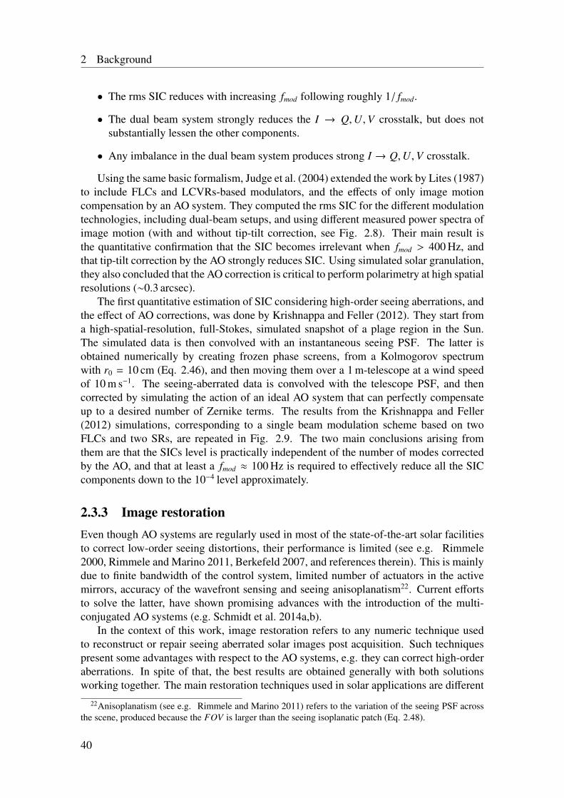
2 Background
• The rms SIC reduces with increasing fmod following roughly 1/ fmod.
• The dual beam system strongly reduces the I → Q,U,V crosstalk, but does notsubstantially lessen the other components.
• Any imbalance in the dual beam system produces strong I → Q,U,V crosstalk.
Using the same basic formalism, Judge et al. (2004) extended the work by Lites (1987)to include FLCs and LCVRs-based modulators, and the effects of only image motioncompensation by an AO system. They computed the rms SIC for the different modulationtechnologies, including dual-beam setups, and using different measured power spectra ofimage motion (with and without tip-tilt correction, see Fig. 2.8). Their main result isthe quantitative confirmation that the SIC becomes irrelevant when fmod > 400 Hz, andthat tip-tilt correction by the AO strongly reduces SIC. Using simulated solar granulation,they also concluded that the AO correction is critical to perform polarimetry at high spatialresolutions (∼0.3 arcsec).
The first quantitative estimation of SIC considering high-order seeing aberrations, andthe effect of AO corrections, was done by Krishnappa and Feller (2012). They start froma high-spatial-resolution, full-Stokes, simulated snapshot of a plage region in the Sun.The simulated data is then convolved with an instantaneous seeing PSF. The latter isobtained numerically by creating frozen phase screens, from a Kolmogorov spectrumwith r0 = 10 cm (Eq. 2.46), and then moving them over a 1 m-telescope at a wind speedof 10 m s−1. The seeing-aberrated data is convolved with the telescope PSF, and thencorrected by simulating the action of an ideal AO system that can perfectly compensateup to a desired number of Zernike terms. The results from the Krishnappa and Feller(2012) simulations, corresponding to a single beam modulation scheme based on twoFLCs and two SRs, are repeated in Fig. 2.9. The two main conclusions arising fromthem are that the SICs level is practically independent of the number of modes correctedby the AO, and that at least a fmod ≈ 100 Hz is required to effectively reduce all the SICcomponents down to the 10−4 level approximately.
2.3.3 Image restorationEven though AO systems are regularly used in most of the state-of-the-art solar facilitiesto correct low-order seeing distortions, their performance is limited (see e.g. Rimmele2000, Rimmele and Marino 2011, Berkefeld 2007, and references therein). This is mainlydue to finite bandwidth of the control system, limited number of actuators in the activemirrors, accuracy of the wavefront sensing and seeing anisoplanatism22. Current effortsto solve the latter, have shown promising advances with the introduction of the multi-conjugated AO systems (e.g. Schmidt et al. 2014a,b).
In the context of this work, image restoration refers to any numeric technique usedto reconstruct or repair seeing aberrated solar images post acquisition. Such techniquespresent some advantages with respect to the AO systems, e.g. they can correct high-orderaberrations. In spite of that, the best results are obtained generally with both solutionsworking together. The main restoration techniques used in solar applications are different
22Anisoplanatism (see e.g. Rimmele and Marino 2011) refers to the variation of the seeing PSF acrossthe scene, produced because the FOV is larger than the seeing isoplanatic patch (Eq. 2.48).
40
2.3 Polarimetric effects of atmospheric seeing and image motion
Figure 2.9. Simulated SIC considering high-order aberrations and the AO effect, given in Fig.7 of Krishnappa and Feller (2012). Each panel shows the SIC (vertical axes) between twoStokes parameters (indicated in the titles), versus the number of Zernike terms compensatedby the AO (horizontal axes), for different modulation frequencies (different line-styles). Themodulation frequencies in all panels are 2.14 (continuous), 29.9 (dotted), 98.2 (dashed), and200.7 Hz (dashed-dotted). Copyrights Optical Society of America 2012.
variants of MOMFBD (see Löfdahl 2002, for a review) and speckle imaging (SI, Kellerand von der Luehe 1992).
Independently of the technique used, the model assumed for the image degradationdue to seeing is linear and space-invariant (Eq. 2.49). Since neither the true solar scene(object) nor the degradation function (seeing plus telescope PSF) are known, many in-dependent measurements of the same (constant) object are required to constrain the esti-mations. In order to preserve the spatial information up to the telescope diffraction limit,such measurements need to have te < τ0, in daylight typically te ∼ 10 ms. The spaceinvariance means that only images with a FOVs smaller that the seeing isoplanatic patch(see Eq. 2.48) can be restored. To deal with larger FOVs, the scene is usually divided insmaller patches that are restored independently.
Both MOMFBD and SI present pros and cons. Three important disadvantages of SIare (a) it does not work properly when an AO is in the beam, because it modifies theseeing statistical properties; (b) it does not allow the estimation of the degradation func-tions; and (c) it requires at least ∼100 statistically independent measurements of the sameobject, which is difficult when considering fast evolving solar signals. On the other hand,MOMFBD requires much more computing time and perform worse with low contrast data(Löfdahl et al. 2007). The first restorations of the data acquired with FSP has been carriedout using MOMFBD, thus we detail here only this technique.
The multi-frame blind deconvolution (MFBD) problem implies recovering a time-invariant object, I, using only many aberrated and noisy measurements, Ii, were i ∈
41
2 Background
0, 1, . . . ,N f rm−1. Dropping the spatial frequency variable, we can write in the spatialFourier domain (following Van Noort et al. 2005)
Ii = Hiatm+telI +N i, (2.68)
were N i is the Fourier transform of withe noise, the OTFs can be obtained from
Hiatm+tel = F | F −1
Pi |2, (2.69)
and F denotes the Fourier transform operator. The generalized pupil function, Pi, can beobtained from the telescope pupil transmission function (D) and the pupil phase (δi), asfollows
Pi = Deiδi . (2.70)
The δi describe the seeing-aberrated wavefronts. They are parametrized to reduce thenumber of free variables, using the following finite orthogonal expansion
δi = δ0,i +
Nmode−1∑m=0
κi,mΩi,m, (2.71)
were Nmode denote the number of modes used, κi,m are the expansion coefficients andΩi,m are the orthogonal basis functions, i.e. Zernike polynomials for the tilts terms andatmospheric Karhunen-Loéve modes23 for the blurring effects. The δ0,i is used to includeany know phase difference (diversity) with respect to another channel (see below).
The simultaneous estimation of both object and aberrations is achieved by the iterativeminimization of an error metric with respect to all the coefficients κ= κi,m (note that κis different from the spatial frequency vector k). The simplest metric and the fastestimplementation, are obtained for Gaussian noise (Van Noort et al. 2005). In this case, themetric (L) can be simplified to the least square difference between the measured Ii andthe estimated ones (Paxman et al. 1996), i.e.
L(κ) =∑
k
N f rm−1∑i=0
| Ii |2 −|∑N f rm−1
i=0 I∗i H
iatm+tel |
2∑N f rm−1i=0 | H
iatm+tel |
2 +γ
, (2.72)
were Hiatm+tel are the estimated OTFs and γ is the regularization term of a simple Wiener
deconvolution24. Note that Eq. 2.72 does not explicitly include the unknown object25, I,and thus after minimization all theH i
atm+tel are known (we call this, the wavefront sensingstep). The derivation of the estimated object can be done after the wavefront sensing inan separate deconvolution step.
23A set of optimal basis functions, that minimize the mean squared error in the truncated expansion ofa random process. The expansion coefficients are independent random variables, while the basis functionsare orthogonal and continuous (Roddier 1990).
24 A wiener filter has a spectral response, Hwiener(k), that allows the best estimation, i.e. minimizes themean squared error, of a random image from its blurred version. If the blurring function is H(k), thenHwiener(k) = 1/H(k)× | H(k) |2 /(| H(k) |2 +γ(k)). γ(k) is a regularization factor, used to avoid noiseamplification, given by the ratio of the noise and signal power spectra (see e.g. Saha 2007).
25The second term inside the parentheses in Eq. 2.72 corresponds to the estimated version of the firstterm. Note it resembles the convolution of the estimated object and the estimated OTFs, where the formeris in turn obtained from a Wiener deconvolution of the measurements using the estimated OTFs.
42
2.3 Polarimetric effects of atmospheric seeing and image motion
Multiple objects can be recorded at the same time, e.g. by simultaneously imag-ing the same solar scene using different filters in each channel. Additionally, more thanone channel can be used to image the same object with different diversity δ0,i (phase di-versity). The restoration of each object, I, j with j ∈ 0, 1, . . . ,Nob j−1, constitutes anindependent MFBD problem (Eq. 2.72). Nonetheless, any known relationship among theobjects, can be translated to an equality constraint among the corresponding free coeffi-cients, κ j, to make the simultaneous restoration a better conditioned problem. The latteris the MOMFBD approach, developed by Löfdahl (2002) and implemented as a freeware,highly-parallel, C++ code by Van Noort et al. (2005). A MOMFBD implies then, theminimization of the weighted sum of the individual metrics (Eq. 2.72) of all the objects,namely
Lmo(κmo) =
Nob j−1∑j=0
κob j, jL j(κ j), (2.73)
were κob j, j are the individual weights.Typical wide band (WB) solar scenes require at least ∼5 frames to run a MFBD. On
the other hand, narrow band (NB) data require an increased number of frames to obtain agood restoration, due to the low S NR (Löfdahl et al. 2007). Another solution to restoreNB data, is to record a simultaneous WB channel. After acquisition, both channels can bejointly restored by running a two-object MOMFBD. The latter, provided that, sub-pixelco-alignment is performed and the aberrations in both channels are the same or have afixed, know relationship (Van Noort et al. 2005).
43

3 High-cadence, ground-basedpolarimetry
As seen in Ch. 2, the reduction of SIC and the implementation of image restoration,are critical for any ground-based polarimeter that aims to reach simultaneously high po-larimetric sensitivity and high spatial resolution (a regime demanded by many challeng-ing open questions in modern solar physics, see Sect. 2.1.4). To reduce SIC a high-modulation frequency is required. In addition, an efficient implementation of imagerestoration demands short exposure times. A high DC and low noise are also needed,to reach the desired S NR as fast as possible and avoid the spatial smearing produced bysolar evolution and seeing. These basic requirements can be met by a high-cadence po-larimeter, i.e. one that can acquire a large amount of Stokes images per second. Thedevelopment of the prototype of an instrument that aims for such a regime, is the centraltopic of this thesis.
The present chapter begins by summarizing the general properties that define such ahigh-cadence polarimeter, based on the concepts introduced in Ch. 2. These are then usedto explore the requirements of the camera and the polarization modulator, in order to pon-der in a nutshell the different available technologies (Sect. 3.1). From the analysis above,it is found that the camera is generally the bottle neck of a high-cadence polarimeter. Thisis further explored by comparing the different cameras used in eight state-of-the-art, so-lar polarimeters that work in the visible part of the spectrum (Sect. 3.2.1). Within sucha comparison, the prototype of the FSP is introduced, as a novel solar polarimeter thatworks in an unexploited regime of high cadence, low noise and high DC. An overview ofFSP is given in Sect. 3.2, including an enumeration of its main constituent components.
As seen in Sect. 2.1.3, the IR and UV regimes are very important to diagnose the solaratmosphere, most notably the transition region and the chromosphere. In spite of this, therest of this work focuses only on visible-polarimetry (from 400 to 700 nm approximately)in which almost all spectropolarimetric measurements have been carried out, due to arichness of Zeeman sensitive lines, allowing detailed diagnostics of the solar magneticfield. It is also the regime targeted by the FSP project. Some of the contents presented inthis chapter have been literally published in Iglesias et al. (2016).
3.1 Main properties of a high-cadence polarimeterBased on the concepts and criteria introduced in Ch. 2, we have collected in Table 3.1, thethe most relevant properties that define a ground-based polarimeter that simultaneouslyaims for high-polarimetric sensitivity and high spatial resolution.
45
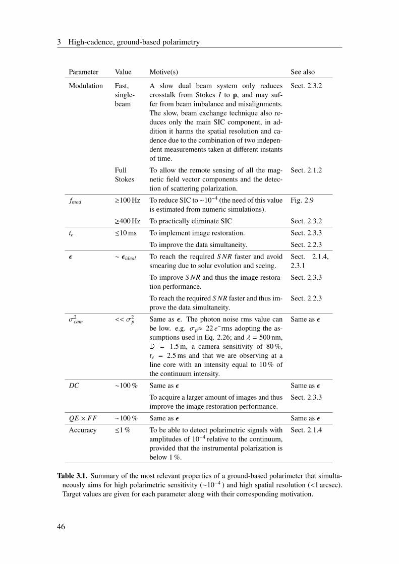
3 High-cadence, ground-based polarimetry
Parameter Value Motive(s) See also
Modulation Fast,single-beam
A slow dual beam system only reducescrosstalk from Stokes I to p, and may suf-fer from beam imbalance and misalignments.The slow, beam exchange technique also re-duces only the main SIC component, in ad-dition it harms the spatial resolution and ca-dence due to the combination of two indepen-dent measurements taken at different instantsof time.
Sect. 2.3.2
FullStokes
To allow the remote sensing of all the mag-netic field vector components and the detec-tion of scattering polarization.
Sect. 2.1.2
fmod ≥100 Hz To reduce SIC to ∼10−4 (the need of this valueis estimated from numeric simulations).
Fig. 2.9
≥400 Hz To practically eliminate SIC Sect. 2.3.2
te ≤10 ms To implement image restoration. Sect. 2.3.3
To improve the data simultaneity. Sect. 2.2.3
ε ∼ εideal To reach the required S NR faster and avoidsmearing due to solar evolution and seeing.
Sect. 2.1.4,2.3.1
To improve S NR and thus the image restora-tion performance.
Sect. 2.3.3
To reach the required S NR faster and thus im-prove the data simultaneity.
Sect. 2.2.3
σ2cam << σ2
p Same as ε. The photon noise rms value canbe low. e.g. σp≈ 22 e−rms adopting the as-sumptions used in Eq. 2.26; and λ = 500 nm,D = 1.5 m, a camera sensitivity of 80 %,te = 2.5 ms and that we are observing at aline core with an intensity equal to 10 % ofthe continuum intensity.
Same as ε
DC ∼100 % Same as ε Same as ε
To acquire a larger amount of images and thusimprove the image restoration performance.
Sect. 2.3.3
QE × FF ∼100 % Same as ε Same as ε
Accuracy ≤1 % To be able to detect polarimetric signals withamplitudes of 10−4 relative to the continuum,provided that the instrumental polarization isbelow 1 %.
Sect. 2.1.4
Table 3.1. Summary of the most relevant properties of a ground-based polarimeter that simulta-neously aims for high polarimetric sensitivity (∼10−4 ) and high spatial resolution (<1 arcsec).Target values are given for each parameter along with their corresponding motivation.
46
3.1 Main properties of a high-cadence polarimeter
The fast modulation and a short exposure time detailed in Table 3.1, can be fulfilledonly by a high-cadence polarimeter. For the rest of this work, we use the term fast po-larimeter as a synonym of high-cadence polarimeter.
3.1.1 Camera requirementsThe general polarimeter properties given in Table 3.1, impose a first set of constraints onthe camera specifications. The two most demanding parameters for a large sensor are theFR and σcam. The former is determined by which of the following two strategies is usedto register the different modulation states (Stenflo 2013, Ch. 13):
• Synchronous readout: Where each modulation state is recorded by the camera in anindividual frame. Thus, FR is determined by fmod through:
FR = Nmod fmod. (3.1)
• Asynchronous readout: Where many modulation states are recorded in a singleframe. This was firstly implemented by Povel et al. (1990) in the successful ZurichIMaging POLarimeter (ZIMPOL). This is, up to date, the only polarimeter thatworks with modulation frequencies in the 10 kHz regime. ZIMPOL has seen manyimprovements since its first version, and proved capable of carrying out measure-ments with very-high sensitivity (∼10−5 ) although only at low spatial resolution(see Sect. 3.2.1), using a spectrograph as wavelength discriminator (see Ramelliet al. 2010, for an overview).
The heart of the ZIMPOL system is a specially modified CCD sensor. In the full-Stokes version, which employs an FLC-based modulator with Nmod = 4, three out offour rows of the sensor are shielded, so they are not photosensitive and can be usedas charge storage. During operation, the modulator is synchronized with the chargetransfer of the CCD, allowing the accumulation of the signals of the individualmodulation states in independent rows. Since the charge transfer can be done in theµs regime, the modulation frequency is basically limited by the modulator. In thisway, the sensor readout is decoupled from fmod allowing to have FR << fmod.
The ZIMPOL concept presents clear disadvantages regarding the resulting FR, DC,and pixel shape and size. These make the system not suitable for high spatial reso-lution applications (see Sect. 3.2.1).
Assuming that a synchronous readout is employed, we enumerate in the following list,the main camera properties that critically affect the performance of a fast polarimeter. Weinclude also representative values for each parameter, only to guide the discussion of theirimplications on the camera technology selection. The first four points are derived fromthe figures given in Table. 3.1, the rest are obtained from other considerations (specifiedin each case).
1. FR ≥ 400 fps : Necessary to achieve a fmod≥100 Hz with Nmod =4 (Eq. 3.1), whichis the minimum required to measure the full S (Sect. 2.2.1). This value of FR alsoguarantees te<10 ms. Note we do not consider the case of fmod≥400 Hz given in
47
3 High-cadence, ground-based polarimetry
Table 3.1. This is because the minimum resulting FR, i.e. ≥ 1600 fps, can not beachieved —simultaneously with the noise, sensor size and DC specifications listedbelow— even by state-of-the-art technology on scientific cameras (see e.g. Sect.3.2.1).
2. σcam < 7 e−rms : Imposed for the polarimeter to be photon-noise limited (see Sect.5.5), i.e.
σ2cam < 0.1σ2
p. (3.2)
In most of the scientific cameras —provided that no strict power consumption con-straints are imposed— the σd can be reduced to very low levels by cooling thesensor. Assuming this —and considering that the imposed te is short, further reduc-ing the number of dark electrons— the σro becomes the main contributor to σcam.The latter is what discourages the usage of commercial high-speed (>kHz) cameras,to do high-resolution solar polarimetry1.
Moreover, the lack (until very recently) of scientific cameras with the FR, DC,sensor size and σcam specifications enumerated here; has led to the fact that mostof the high-sensitivity, ground-based polarimeters currently in operation, still makeuse of the slow dual beam technique for SIC suppression (see Sect. 3.2.1).
3. DC∼100 %: In addition to the motives given in Table 3.1, note that, the smaller theDC the more strict the noise requirements of the camera become, i.e. for a givenFR the σp per frame decreases with the DC, making it more difficult to fulfill Eq.3.2.
Given the high FR imposed, an almost ∼100 % duty cycle can be obtained in largesensors (see below) only if they have the ability to read while they continue inte-grating. Such a characteristic is implemented only in full-frame-transfer or interlineCCDs (Hoslst 1998) —by means of dedicated charge storage areas in the sensor—and in specific CMOS sensors that can store the signal in the readout node of eachpixel (e.g. Lauxtermann and Leipold 2011).
4. QE ×FF∼100 %: This implies keeping FF=100 % and maximizing QE in the 400to 700 nm wavelength range. Note that the former discourages the usage of interlineCCDs or CMOS devices with complex circuitry inside the pixel structure2.
5. Shutter type = Snapshot: In order to keep the DC as high as possible, the cameraneeds to be exposed during most of the duration of each modulation cycle. Thisimplies that te ≈ 1/(Nmod fmod), therefore, the exposure of all the pixels of the sensorhas to be in phase. If not, the pixels that are readout later may accumulate some
1This is, however, the solution adopted in the high-cadence polarimeter at the Japanese Solar Flare Tele-scope (Hanaoka 2004, Hanaoka et al. 2003). This polarimeter uses a small (260×260 pixels), commercialcamera (DALSA-CA-D6-256) that can run at 955 fps. The sensor operates at ambient temperature and haslarge readout noise (not reported). The main difference with respect to the regime aimed at in Table 3.1, isthat the photon flux, and thus the σp are higher, relaxing the requirement on σro imposed by Eq. 3.2.
2With these kind of devices a FF=100 % can still be obtained by utilizing a micro-lenses array, in oderto focus the incoming light only in the photosensitive areas of each pixel. This solution presents, however,other drawbacks including misalignments between pixels and micro-lenses, and the associated increase instraylight.
48
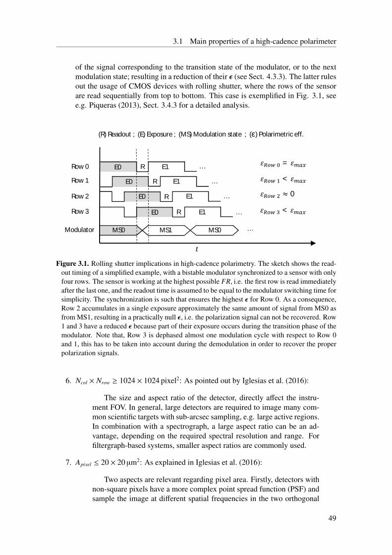
3.1 Main properties of a high-cadence polarimeter
of the signal corresponding to the transition state of the modulator, or to the nextmodulation state; resulting in a reduction of their ε (see Sect. 4.3.3). The latter rulesout the usage of CMOS devices with rolling shutter, where the rows of the sensorare read sequentially from top to bottom. This case is exemplified in Fig. 3.1, seee.g. Piqueras (2013), Sect. 3.4.3 for a detailed analysis.
R
(R) Readout ; (E) Exposure ; (MS) Modulation state ; (ε) Polarimetric eff.
R
R
R
MS0
…
…
…
…
MS1
E0
E0
Row 0
E0
E0
E1
E1
E1
E1
휀 = 휀
휀 ≈ 0
휀 < 휀
휀 < 휀
푡
Row 1
Row 2
Row 3
Modulator MS0 …
Figure 3.1. Rolling shutter implications in high-cadence polarimetry. The sketch shows the read-out timing of a simplified example, with a bistable modulator synchronized to a sensor with onlyfour rows. The sensor is working at the highest possible FR, i.e. the first row is read immediatelyafter the last one, and the readout time is assumed to be equal to the modulator switching time forsimplicity. The synchronization is such that ensures the highest ε for Row 0. As a consequence,Row 2 accumulates in a single exposure approximately the same amount of signal from MS0 asfrom MS1, resulting in a practically null ε, i.e. the polarization signal can not be recovered. Row1 and 3 have a reduced ε because part of their exposure occurs during the transition phase of themodulator. Note that, Row 3 is dephased almost one modulation cycle with respect to Row 0and 1, this has to be taken into account during the demodulation in order to recover the properpolarization signals.
6. Ncol × Nrow ≥ 1024 × 1024 pixel2: As pointed out by Iglesias et al. (2016):
The size and aspect ratio of the detector, directly affect the instru-ment FOV. In general, large detectors are required to image many com-mon scientific targets with sub-arcsec sampling, e.g. large active regions.In combination with a spectrograph, a large aspect ratio can be an ad-vantage, depending on the required spectral resolution and range. Forfiltergraph-based systems, smaller aspect ratios are commonly used.
7. Apixel ≤ 20 × 20 µm2: As explained in Iglesias et al. (2016):
Two aspects are relevant regarding pixel area. Firstly, detectors withnon-square pixels have a more complex point spread function (PSF) andsample the image at different spatial frequencies in the two orthogonal
49
3 High-cadence, ground-based polarimetry
dimensions, further complicating the image restoration process. Sec-ondly, the pixel size has to match the required spatial sampling of the—ideally diffraction limited— image. As a consequence, large pixelsmay require re-imaging setups of unpractical dimensions, which can alsointroduce further optical aberrations.
Small and square pixels are an advantage, the figure given here is just a referenceadopted from the typical values used in current solar facilities (see Sect. 3.2.1).
8. NENOB≥ 11 ENOB: This is imposed to have a very low quantization noise (Hoslst1998, Sect. 4.2.5), e.g.
σ2adc =
(2Nadc−NENOB
G√
12
)2
≤ 0.1σ2cam, (3.3)
where NENOB is the ADC effective number of bits (ENOB), which is smaller thanthe ADC resolution (Nadc), because it includes both the quantization noise and thecontributions from the non-ideal circuitry of the ADC (IEEE 2001). Here we haveassumed 2Nadc/G = 15 000 e− due to the short exposure times involved (see σp inTable 3.1).
9. NL < 1 %: Non-linearities in the camera introduce spurious polarimetric signals(Keller 1996). The amplitude of such artifacts is proportional to the NL and tothe instrumental polarization level. The figure given here, is required to ensurethe artifact level is ∼10−4 when the instrumental offset is ∼10−2 , see Sect. 5.3 forfurther details.
From the above-detailed properties, note that σcam, QE × FF and NL are amongthe critical camera specifications. Since typically CCDs outperform CMOS sensors insuch parameters (see Table 2.2), most of the high-sensitivity, ground-based polarimeterscurrently in operation employ CCD cameras (Sect. 3.2.1).
3.1.2 Polarization modulator requirementsIn the following list we enumerate the main requirements of the polarization modula-tor derived from Table 3.1, along with their implications on the modulation technologyselection.
1. fmod≥100 Hz: Out of the available modulation technologies listed in Sect. 2.2.2,only the FLCs and PEMs allow to modulate above 100 Hz. However the very highmodulation frequency of the PEMs rules out any demodulation by means of syn-chronous readout.
2. Full stokes modulation: A full-Stokes modulator based on PEMs has proven diffi-cult to implement, because it requires two PEMs oscillating at the same frequency.Such a configuration is very sensitive to external perturbations (e.g. small temper-ature mismatches of the crystals) and thus the required phase stability can not beachieved (Gandorfer 1999).
50
3.2 The Fast Solar Polarimeter Prototype
On the other hand, full-stokes modulators based on FLCs have been successfullyused in many solar polarimeters for slow (e.g. Keller et al. 2003) and in two casesfor fast (Hanaoka 2004, Ramelli et al. 2010) modulation. Furthermore, FLCs canbe purchased with high optical quality, and are long lasting and stable, providedUV degradation and temperature issues are controlled (see Sect. 2.2.2).
3. Nmod = 4: Modulation schemes with larger Nmod produce Stokes images with largerS NR (del Toro Iniesta 2003, Sect. 5.2). On the other hand, the camera FR scaleslinearly with Nmod (Eq. 3.1). Since the minimum FR imposed on the camera bythe SIC considerations is already a strict requirement (see point 2 in Sect. 3.1.1),the smallest value possible for Nmod that allows to measure the full S should beadopted3, i.e. 4 (Sect. 2.2.1).
4. ε ∼ ε ideal: Modulators based on two FLCs (Nmod=4) can provide ε total > 80 %,usually by means of a modulator design optimized for efficiency across a broadspectral working range (Gisler 2005, Tomczyk et al. 2010).
5. ts << 2.5 ms: Since for a fast polarimeter the DC has to be as high as possible,the camera is likely to be exposed during both the stable states of the modulator, aswell as during the transition between stable states. Thus, in order to ensure high ε,the modulator switching time (ts) should be kept short (see Sect. 4.3.3), i.e.
ts <<1
Nmod fmod. (3.4)
To compute the figure given here, we assumed Nmod = 4 and fmod=100 Hz. A typicalvalue for ts in FLCs is ∼70 µs (see Sect. 4.2.1).
Note that, considering the requirements specified above, an FLC-based polarizationmodulator is the best candidate to be employed in a full-Stokes, fast polarimeter.
3.2 The Fast Solar Polarimeter PrototypeThe goal of the FSP project is the development of a ground-based, high-cadence po-larimeter that can operate as close as possible to the regime detailed in Table 3.1, in orderto acquire high-spatial-resolution and high-polarimetric-sensitivity measurements of thesolar light in the visible part of the spectrum. The main science questions that the FSPproject will seek to address include, among others, those listed in Sect. 2.1.4. Conse-quently the main design driving parameters are a target sensitivity of 10−4 and sub-arcsecspatial resolution (reachable only with spectropolarimetric data that is optimized for postacquisition restoration).
Based on the arguments presented in Sect. 3.1.1, it can be clearly seen that the mostchallenging component, required to develop such a fast polarimeter, is the camera. FSP isconceived around a novel, custom-made pnCCD camera that can provide high FR and low
3Note that, this discourages the usage of a rotating waveplate as a modulator, even if a fast rotation ofthe disk can be achieved. For example, the polarimeter developed by Hanaoka (2012) uses a plate rotatingat 25 s−1 that has Nmod = 8. Thus it can only reach a fmod = 50 Hz with a detector that has FR=400 fps.
51
3 High-cadence, ground-based polarimetry
σcam. In addition, following the arguments given in Sect. 3.1.2, an FLC-based polarizationmodulator is employed.
The FSP project started in 2012 and is divided in two stages. The first one involvesthe development of a prototype polarimeter, that uses a pnCCD camera that has a small(264 × 264 pixel2) sensor, FR ≤ 800 Hz and σcam = 4.9 e−rms; in a single beam con-figuration. The camera was manufactured by PNSensor GmbH. The principal goals ofthe prototype stage are (a) to asses the suitability of the pnCCD technology for its us-age in high-cadence, high-sensitivity polarimetry at visible wavelengths; (b) to developan FLC-based modulator that can provide at least fmod ≥ 100 Hz and ε tot ≥ 80 % in the400 to 700 nm wavelength range; and (c) to obtain the measurements required to evaluatethe instrumental concept and its polarimetric performance. Including, most notably, theresidual SIC level when operating at fmod = 100 Hz. The main focus of this thesis is thedevelopment of such a prototype, hereafter denote simply as FSP.
The know-how acquired with FSP shall be used to face the second stage of the project,hereafter referred to as FSP II (Sect. 7.1), which implies the development of a scienceready polarimeter using a camera with a larger pnCCD sensor (1024 × 1024 pixel2) thatcan run at FR ≤ 400 Hz. Such a sensor, and its associated electronics, is currently beingdeveloped by the MPG Semiconductor Lab. The modulator package will be the same asemployed in FSP, with the difference that the larger sensor area will allow the implemen-tation of a high-cadence, dual-beam setup, never tested in solar polarimetry before.
3.2.1 Cameras used in ground-based polarimeters: state-of-the-artTo better allocate the working regime of FSP among the rest of the ground-based solarpolarimeters, we present in Table 3.2 (adapted from Iglesias et al. 2016), the main cameraproperties for the following eight state-of-the-art polarimeters that work in the visible partof the spectrum 4: IBIS (Cavallini 2006); VIP (Beck et al. 2010); CRISP (Scharmer et al.2008, de la Cruz Rodríguez et al. 2015); DLSP on phase II (Sankarasubramanian et al.2004, 2006); SPINOR (Socas-Navarro et al. 2006) ; FSP and ZIMPOL-3 (Ramelli et al.2010, 2014). We include, in addition, the targeted properties of FSP II (see Sect. 7.1).
All the cameras listed in Table 3.2 are based on CCD sensors that have square pixels.The only exception to the latter is ZIMPOL-3, which has a pixel aspect ratio of 4 to 1 anda long dimension (90 µm) nearly six times larger than the most common value (<16 µm).ZIMPOL-3 uses a sensor with three out of four rows covered. This demands attaching a
4As explained in Iglesias et al. (2016):
We excluded from this list the SOLIS/VSM (Keller et al. 2003) although is an interestingexample of early high-cadence polarimetry. The initial idea of the project in 1998 was touse a pair of custom made, 1024x1024, Sarnoff VCCD1024H cameras which had, 18x18µm2 pixel area, 46 e−rms readout noise and 300 fps frame rate (Keller 1998). Howeverthe system was never delivered by the manufacturer, forcing the VSM team to select aninterim camera, with the Rockwell HyViSI-1024 model being chosen. The cameras weremodified to have 256x1024 pixels, a 92 fps frame rate and have been operative since 2003(Harvey et al. 2004). Due to variable-dark levels, inter-quadrant crosstalk and readout noiseissues, among others, VSM was updated in 2010 to use a pair of commercial Sarnoff 1M100cameras (Balasubramaniam and Pevtsov 2011) similar to the ones used in SPINOR, hencethe exclusion from our list.
52
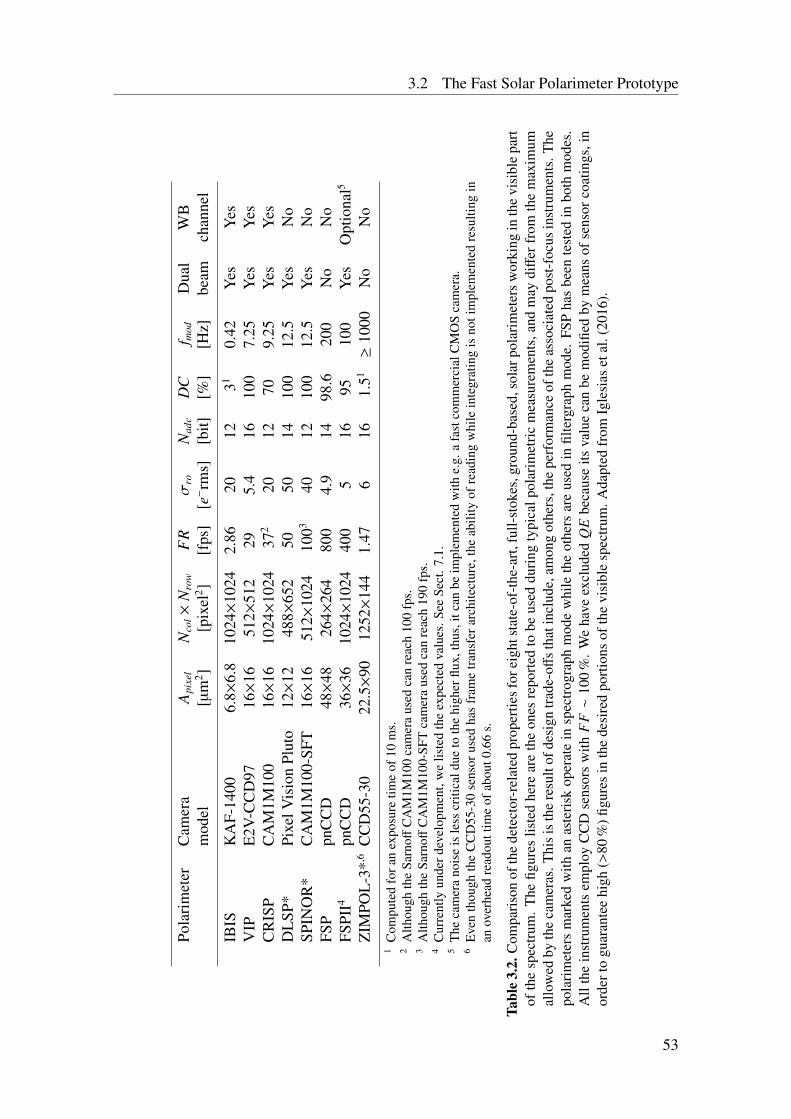
3.2 The Fast Solar Polarimeter Prototype
Pola
rim
eter
Cam
era
Api
xel
Nco
l×
Nro
wF
Rσ
roN
adc
DC
f mod
Dua
lW
Bm
odel
[µm
2 ][p
ixel
2 ][f
ps]
[e−rm
s][b
it][%
][H
z]be
amch
anne
l
IBIS
KA
F-14
006.
8×6.
810
24×
1024
2.86
2012
310.
42Y
esY
esV
IPE
2V-C
CD
9716×
1651
2×51
229
5.4
1610
07.
25Y
esY
esC
RIS
PC
AM
1M10
016×
1610
24×
1024
372
2012
709.
25Y
esY
esD
LSP
*Pi
xelV
isio
nPl
uto
12×
1248
8×65
250
5014
100
12.5
Yes
No
SPIN
OR
*C
AM
1M10
0-SF
T16×
1651
2×10
2410
0340
1210
012
.5Y
esN
oFS
Ppn
CC
D48×
4826
4×26
480
04.
914
98.6
200
No
No
FSPI
I4pn
CC
D36×
3610
24×
1024
400
516
9510
0Y
esO
ptio
nal5
ZIM
POL
-3*,6
CC
D55
-30
22.5×
9012
52×
144
1.47
616
1.51≥
1000
No
No
1C
ompu
ted
fora
nex
posu
retim
eof
10m
s.2
Alth
ough
the
Sarn
offC
AM
1M10
0ca
mer
aus
edca
nre
ach
100
fps.
3A
lthou
ghth
eSa
rnoff
CA
M1M
100-
SFT
cam
era
used
can
reac
h19
0fp
s.4
Cur
rent
lyun
derd
evel
opm
ent,
we
liste
dth
eex
pect
edva
lues
.See
Sect
.7.1
.5
The
cam
era
nois
eis
less
criti
cald
ueto
the
high
erflu
x,th
us,i
tcan
beim
plem
ente
dw
ithe.
g.a
fast
com
mer
cial
CM
OS
cam
era.
6E
ven
thou
ghth
eC
CD
55-3
0se
nsor
used
has
fram
etr
ansf
erar
chite
ctur
e,th
eab
ility
ofre
adin
gw
hile
inte
grat
ing
isno
tim
plem
ente
dre
sulti
ngin
anov
erhe
adre
adou
ttim
eof
abou
t0.6
6s.
Tabl
e3.
2.C
ompa
riso
nof
the
dete
ctor
-rel
ated
prop
ertie
sfo
reig
htst
ate-
of-t
he-a
rt,f
ull-
stok
es,g
roun
d-ba
sed,
sola
rpol
arim
eter
sw
orki
ngin
the
visi
ble
part
ofth
esp
ectr
um.
The
figur
eslis
ted
here
are
the
ones
repo
rted
tobe
used
duri
ngty
pica
lpol
arim
etri
cm
easu
rem
ents
,and
may
diff
erfr
omth
em
axim
umal
low
edby
the
cam
eras
.Thi
sis
the
resu
ltof
desi
gntr
ade-
offs
that
incl
ude,
amon
got
hers
,the
perf
orm
ance
ofth
eas
soci
ated
post
-foc
usin
stru
men
ts.T
hepo
lari
met
ers
mar
ked
with
anas
teri
skop
erat
ein
spec
trog
raph
mod
ew
hile
the
othe
rsar
eus
edin
filte
rgra
phm
ode.
FSP
has
been
test
edin
both
mod
es.
All
the
inst
rum
ents
empl
oyC
CD
sens
ors
with
FF∼
100
%.
We
have
excl
uded
QE
beca
use
itsva
lue
can
bem
odifi
edby
mea
nsof
sens
orco
atin
gs,i
nor
dert
ogu
aran
tee
high
(>80
%)fi
gure
sin
the
desi
red
port
ions
ofth
evi
sibl
esp
ectr
um.A
dapt
edfr
omIg
lesi
aset
al.(
2016
).
53
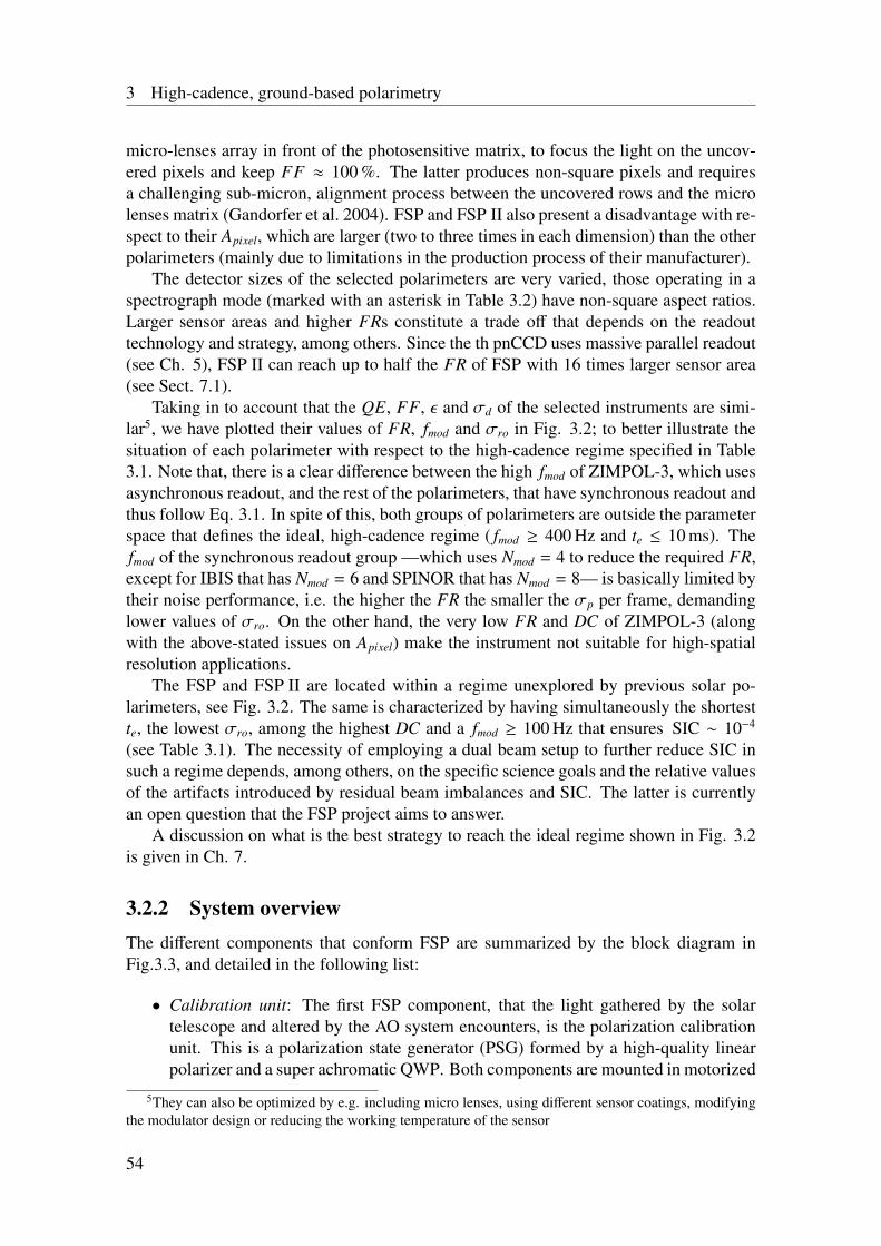
3 High-cadence, ground-based polarimetry
micro-lenses array in front of the photosensitive matrix, to focus the light on the uncov-ered pixels and keep FF ≈ 100 %. The latter produces non-square pixels and requiresa challenging sub-micron, alignment process between the uncovered rows and the microlenses matrix (Gandorfer et al. 2004). FSP and FSP II also present a disadvantage with re-spect to their Apixel, which are larger (two to three times in each dimension) than the otherpolarimeters (mainly due to limitations in the production process of their manufacturer).
The detector sizes of the selected polarimeters are very varied, those operating in aspectrograph mode (marked with an asterisk in Table 3.2) have non-square aspect ratios.Larger sensor areas and higher FRs constitute a trade off that depends on the readouttechnology and strategy, among others. Since the th pnCCD uses massive parallel readout(see Ch. 5), FSP II can reach up to half the FR of FSP with 16 times larger sensor area(see Sect. 7.1).
Taking in to account that the QE, FF, ε and σd of the selected instruments are simi-lar5, we have plotted their values of FR, fmod and σro in Fig. 3.2; to better illustrate thesituation of each polarimeter with respect to the high-cadence regime specified in Table3.1. Note that, there is a clear difference between the high fmod of ZIMPOL-3, which usesasynchronous readout, and the rest of the polarimeters, that have synchronous readout andthus follow Eq. 3.1. In spite of this, both groups of polarimeters are outside the parameterspace that defines the ideal, high-cadence regime ( fmod ≥ 400 Hz and te ≤ 10 ms). Thefmod of the synchronous readout group —which uses Nmod = 4 to reduce the required FR,except for IBIS that has Nmod = 6 and SPINOR that has Nmod = 8— is basically limited bytheir noise performance, i.e. the higher the FR the smaller the σp per frame, demandinglower values of σro. On the other hand, the very low FR and DC of ZIMPOL-3 (alongwith the above-stated issues on Apixel) make the instrument not suitable for high-spatialresolution applications.
The FSP and FSP II are located within a regime unexplored by previous solar po-larimeters, see Fig. 3.2. The same is characterized by having simultaneously the shortestte, the lowest σro, among the highest DC and a fmod ≥ 100 Hz that ensures SIC ∼ 10−4
(see Table 3.1). The necessity of employing a dual beam setup to further reduce SIC insuch a regime depends, among others, on the specific science goals and the relative valuesof the artifacts introduced by residual beam imbalances and SIC. The latter is currentlyan open question that the FSP project aims to answer.
A discussion on what is the best strategy to reach the ideal regime shown in Fig. 3.2is given in Ch. 7.
3.2.2 System overviewThe different components that conform FSP are summarized by the block diagram inFig.3.3, and detailed in the following list:
• Calibration unit: The first FSP component, that the light gathered by the solartelescope and altered by the AO system encounters, is the polarization calibrationunit. This is a polarization state generator (PSG) formed by a high-quality linearpolarizer and a super achromatic QWP. Both components are mounted in motorized
5They can also be optimized by e.g. including micro lenses, using different sensor coatings, modifyingthe modulator design or reducing the working temperature of the sensor
54
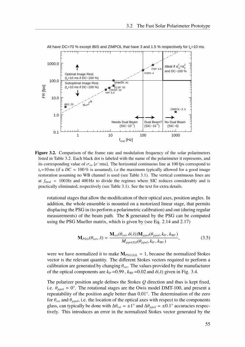
3.2 The Fast Solar Polarimeter Prototype
All have DC>70 % except IBIS and ZIMPOL that have 3 and 1.5 % respectively for te=10 ms.
IBIS: 20
VIP: 5.4CRISP: 20
DLSP: 50
SPINOR: 40
FSP: 4.9
FSPII: 4
ZIMPOL−3: 6
Optimal Image Rest.(te<10 ms if DC~100 %)
Suboptimal Image Rest.(te>10 ms if DC~100 %)
Needs Dual Beam(SIC~10
−2)
No Dual Beam
Ideal if σ2
ro<σ2
p
and DC~100 %
(SIC~0)Dual Beam?(SIC~10
−4)
1 10 100 1000fmod [Hz]
0.1
1.0
10.0
100.0
1000.0
FR
[fps
]
N mod=4
Figure 3.2. Comparison of the frame rate and modulation frequency of the solar polarimeterslisted in Table 3.2. Each black dot is labeled with the name of the polarimeter it represents, andits corresponding value of σro [e−rms]. The horizontal continuous line at 100 fps correspond tote=10 ms (if a DC ≈ 100 % is assumed), i.e the maximum typically allowed for a good imagerestoration assuming no WB channel is used (see Table 3.1). The vertical continuous lines areat fmod = 100 Hz and 400 Hz to divide the regimes where SIC reduces considerably and ispractically eliminated, respectively (see Table 3.1). See the text for extra details.
rotational stages that allow the modification of their optical axes, position angles. Inaddition, the whole ensemble is mounted on a motorized linear stage, that permitsdisplacing the PSG in (to perform a polarimetric calibration) and out (during regularmeasurements) of the beam path. The S generated by the PSG can be computedusing the PSG Mueller matrix, which is given by (see Eq. 2.14 and 2.17)
MPS G(θret, λ) =Mret(θret, δ(λ))Mppol(θppol, k0 , k90)
Mppol,0,0(θppol, k0 , k90), (3.5)
were we have normalized it to make MPS G,0,0, = 1, because the normalized Stokesvector is the relevant quantity. The different Stokes vectors required to perform acalibration are generated by changing θret. The values provided by the manufacturerof the optical components are k0=0.99 , k90=0.02 and δ(λ) given in Fig. 3.4.
The polarizer position angle defines the Stokes Q direction and thus is kept fixed,i.e. θppol = 0°. The rotational stages are the Owis model DMT-100, and present arepeatability of the position angle better than 0.01°. The determination of the zerofor θret and θppol, i.e. the location of the optical axes with respect to the componentsglass, can typically be done with ∆θret = ±1° and ∆θppol = ±0.1° accuracies respec-tively. This introduces an error in the normalized Stokes vector generated by the
55
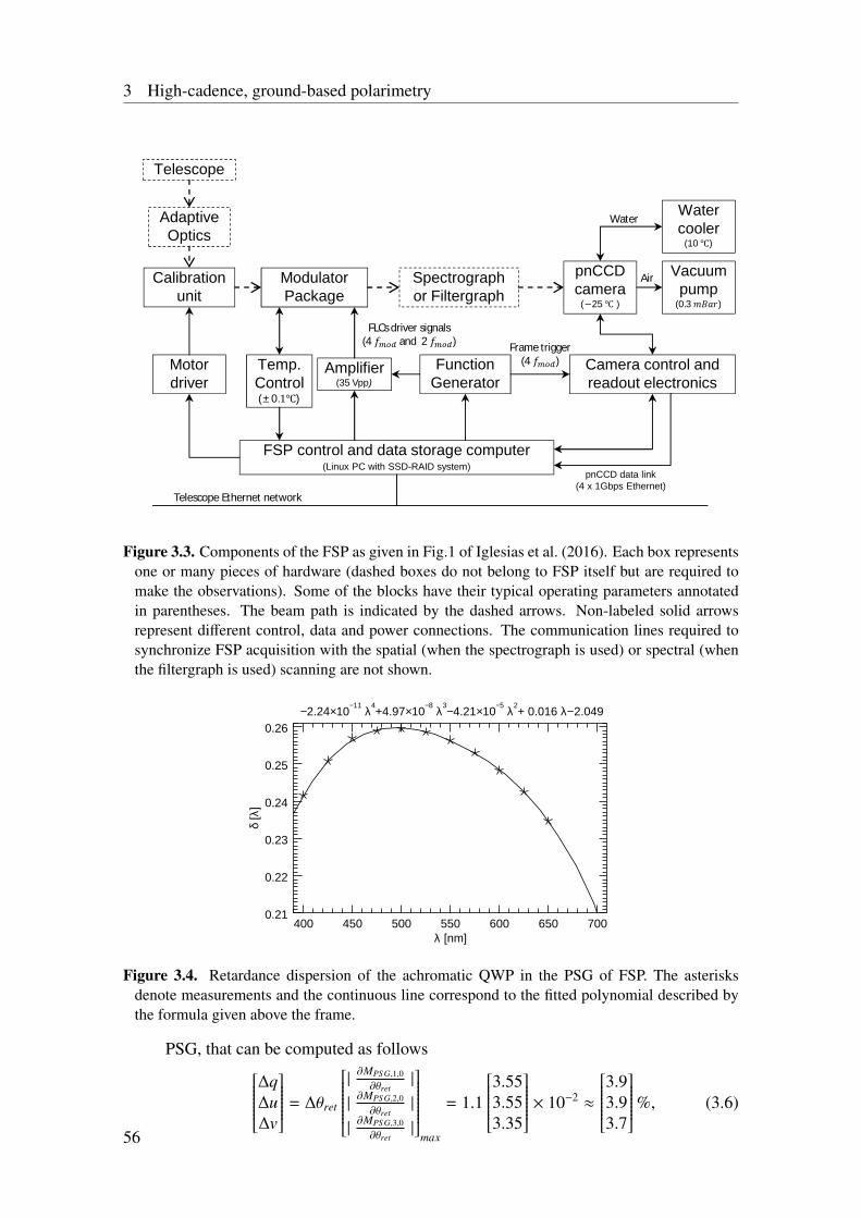
3 High-cadence, ground-based polarimetry
Telescope
Adaptive Optics
ModulatorPackage
Spectrograph or Filtergraph
pnCCD camera
(−25 )
Motor driver
Calibration unit
Camera control and readout electronics
FSP control and data storage computer(Linux PC with SSD-RAID system)
Amplifier(35Vpp)
FunctionGenerator
Water cooler
(10)
Vacuum pump
(0.3푚퐵푎푟)
Temp. Control(±0.1)
pnCCD data link (4 x 1Gbps Ethernet)
Water
Air
Telescope Ethernet network
Frame trigger (4푓 )
FLCs driver signals(4푓 and 2푓 )
Figure 3.3. Components of the FSP as given in Fig.1 of Iglesias et al. (2016). Each box representsone or many pieces of hardware (dashed boxes do not belong to FSP itself but are required tomake the observations). Some of the blocks have their typical operating parameters annotatedin parentheses. The beam path is indicated by the dashed arrows. Non-labeled solid arrowsrepresent different control, data and power connections. The communication lines required tosynchronize FSP acquisition with the spatial (when the spectrograph is used) or spectral (whenthe filtergraph is used) scanning are not shown.
−2.24×10⁻¹¹
λ4+4.97×10
−8 λ3−4.21×10
−5 λ2
+ 0.016 λ−2.049
400 450 500 550 600 650 700λ [nm]
0.21
0.22
0.23
0.24
0.25
0.26
δ [λ
]
Figure 3.4. Retardance dispersion of the achromatic QWP in the PSG of FSP. The asterisksdenote measurements and the continuous line correspond to the fitted polynomial described bythe formula given above the frame.
PSG, that can be computed as follows∆q∆u∆v
= ∆θret
|∂MPS G,1,0
∂θret|
|∂MPS G,2,0
∂θret|
|∂MPS G,3,0
∂θret|
max
= 1.1
3.553.553.35
× 10−2 ≈
3.93.93.7
%, (3.6)
56
3.2 The Fast Solar Polarimeter Prototype
where we have used Eq. 2.8 and 3.5, replaced the above-given values for δ, k0 andk90 , considered a full rotation of the QWP and assumed the input of the PSG isweakly and polarized.
• Modulator package: After the calibration unit, the beam encounters the FSP mod-ulator package, which is located as early as possible in the beam path to minimizethe polarimetric influence of the other optical components, most notably the wave-length discriminator. The modulator is temperature controlled and driven with ana-log voltage signals, provided by an Agilent 33502A two-channel amplifier (fixedgain of 5). Further details on the modulator are given in Ch. 4.
• pnCCD camera: The modulated intensities, after being filtered by the wavelengthdiscriminator, are recorded using the pnCCD camera. In order to reduce the darkcurrent, the sensor is cooled down to −25 C by means of a peltier thermoelectriccooler module, and a closed water circuit (Julabo F25-ED with an operating rangefrom −28 to 100° and an accuracy of ±0.03°). In order to avoid condensation, thesensor housing is evacuated to 0.3 mbar. Further details on the camera are given inCh. 5.
• Function generator: Both the modulator switching and the camera readout are trig-gered in synchronization by a single Agilent 33522A, 30 MHz function generator.Even though FSP can modulate at 200 Hz, most of the measurements were obtainedat 100 Hz because that is the fmod of FSP II, and thus the main regime that the pro-totype was designed to explore.
• Control computer: The instrument is controlled by a single Linux-based PC. Thecontrol computer is used (a) to configure the function generator, amplifier and cam-era to acquire the desired measurement; (b) to control the motorized calibrationunit; (c) to record the house keeping data from the camera housing and temperatureof the modulator; and (d) to record the output data of the camera. Due to the highdata rate, 780 Mbit s−1 at 800 fps, the data is transfered by four dedicated 1 Gbit s−1
Ethernet connections in parallel and recorded in the control computer using a SSD-based RAID system.
57

4 Characterization and optimizationof an FLC-based polarizationmodulator
The modulator package is one of the key elements of the polarimeter because its perfor-mance influences the polarimetric sensitivity and accuracy. In order to guarantee highmodulation frequency and polarimetric efficiencies, special considerations have to betaken into account during the design and optimization of the modulator package.
This chapter details the development process of the FLC-based modulator used inFSP. Section 4.1 presents a description of the main design features. The optimizationprocedure, followed to obtain a balanced and achromatic set of polarimetric efficiencies,is detailed in Sect. 4.2 including the main characterization results of the FLCs and SRsused in the modulator. Finally, Sect. 4.3 describes the polarimetric calibration procedure—including its limitations (Sect. 4.3.1)— along with the measured behavior of the modu-lation matrix with respect to changes in the wavelength (Sect. 4.3.2) and modulation fre-quency (Sect. 4.3.3). In addition, the measured thermal properties of the FLCs are used tosimulate the modulation matrix temperature dependence (Sect. 4.3.4). These results areutilized among others to derive the modulation frequency and temperature stabilizationrequirements, as well as to define how frequently a calibration needs to be performed.
The result of this chapter are fundamental to the development of the data reductionpipeline of the instrument, briefly described in Chapter 6. Some of the contents presentedhere have been published in Iglesias et al. (2016).
4.1 Main design featuresThe FSP modulator has a design similar to the SOLIS/VSM modulator (Keller et al.2003). It is composed of two bistable FLCs (FLC1 and FLC2), two SRs (SR1 andSR2)and a polarizer beam splitter cube employed as linear analyzer (see Sect. 2.2.2). The maincharacteristics of the modulator can be appreciated in Fig. 4.1 and are listed below:
• Housing: The modulator housing is made of a good thermal conductor (the mainblock is CuZn39Pb3 − 2.0380 − MS 58) and has large mass (7845.7 g). This is toprovide high thermal inertia and low gradients, in order to facilitate the thermalcontrol of the optical elements (see Sect. 4.3.4). The maximum dimensions of themodulator, including the rotational stage and the beam splitter cube, are 133.2 ×125.0 × 234.2 mm. The optical aperture is 22 mm.
59
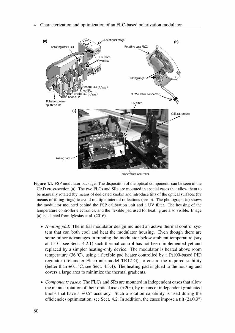
4 Characterization and optimization of an FLC-based polarization modulator
Knob FLC1 (4푓 )Knob SR1
Knob FLC2 (2푓 )
Polarizer beam-splitter cube
Entrance window
Knob SR2
Rotating case FLC1 Rotating case FLC2
Tilting rings
(a) (b)
(c)
UV filter
Calibration unit
Temperature controller
Heating pad
FLC2 electric connector
Rotational stage
Figure 4.1. FSP modulator package. The disposition of the optical components can be seen in theCAD cross-section (a). The two FLCs and SRs are mounted in special cases that allow them tobe manually rotated (by means of dedicated knobs) and introduce tilts of the optical surfaces (bymeans of tilting rings) to avoid multiple internal reflections (see b). The photograph (c) showsthe modulator mounted behind the FSP calibration unit and a UV filter. The housing of thetemperature controller electronics, and the flexible pad used for heating are also visible. Image(a) is adapted from Iglesias et al. (2016).
• Heating pad: The initial modulator design included an active thermal control sys-tem that can both cool and heat the modulator housing. Even though there aresome minor advantages in running the modulator below ambient temperature (sayat 15 C, see Sect. 4.2.1) such thermal control has not been implemented yet andreplaced by a simpler heating-only device. The modulator is heated above roomtemperature (36 C), using a flexible pad heater controlled by a Pt100-based PIDregulator (Telemeter Electronic model TR12-G), to ensure the required stability(better than ±0.1 C, see Sect. 4.3.4). The heating pad is glued to the housing andcovers a large area to minimize the thermal gradients.
• Components cases: The FLCs and SRs are mounted in independent cases that allowthe manual rotation of their optical axes (±20°), by means of independent graduatedknobs that have a ±0.5° accuracy. Such a rotation capability is used during theefficiencies optimization, see Sect. 4.2. In addition, the cases impose a tilt (2±0.3°)
60
4.1 Main design features
to each component in order to avoid having parallel surfaces between componentsthat can produce interference fringes due to multiple internal reflections.
• Entrance window: The 25 mm entrance window has an anti-reflection coating (VIS0° [425-675nm]) that presents a reflectance lower than 0.3 % in the 400 to 700 nmwavelength range, and has a sharp increase below 400 nm. The latter contributes toreduce the UV radiation reaching the FLCs, which is further diminished by the UVfilter placed before the modulator1.
• Beam splitter cube: In FSP only the transmitted beam of the 25 mm polarizer beamsplitter cube is used. Regarding its polarimetric action, it is equivalent to that ofa partial linear polarizer (see Sect. 2.2.2) with k0=0.99 and k90=0.02 in the 440to 650 nm wavelength range. The position of the beam splitter optical axis is keptparallel to the Stokes Q direction defined by the PSG. This angle can be modifiedby the modulator rotational stage, which is an Owis model DT100-D53 that has anaccuracy of ±30 arcsec.
Neglecting the effect of the entrance window, the polarimetric action of the modulatorcan be modeled by its Mueller matrix (see Eq. 2.14 and 2.17),
M(l′) =MPPOLMS R2MFLC2MS R1MFLC1
MPPOL,0,0, (4.1)
were l′ = [θFLC1, θS R1, θFLC2, θS R2, δFLC1, δS R1, δFLC2, δS R2, k0 , k90 ,Θ′FLC1,Θ
′FLC2]T and all
the position angles are measured counter clockwise from θPPOL = 0° (see Sect. 4.1).We adopt Eq. 2.40 to model the retardance dispersion of the FLCs and the SRs. EachFLC has two positions of its optical axis. We define θFLC1 and θFLC2 for the positionwhere the optical axis is closer to 0°. Θ′FLC1 and Θ′FLC2 are the relative deviations of theFLCs optical axes measured counter clockwise from θFLC1 and θFLC2 respectively. Thedeviations are either 0° or the value of the switching angles (ΘFLC1 and ΘFLC2). The fourpossible combinations of the FLCs states define the modulation scheme, with Nmod=4 andthe following 4 × 4 modulation matrix (see Eq. 2.30)
O(l) =
1 hT ([. . . , 0° , 0° ]T )1 hT ([. . . ,ΘFLC1,ΘFLC2]T )1 hT ([. . . , 0° ,ΘFLC2]T )1 hT ([. . . ,ΘFLC1., 0° ]T )
, (4.2)
were the vector l contains all the relevant modulator parameters
l = [λ, θFLC1, θS R1, θFLC2, θS R2, δ0FLC1, δ0S R1, δ0FLC2, δ0S R2, λ0FLC1, λ0S R1,
λ0FLC2, λ0S R2,CFLC1,CS R1,CFLC2,CS R2, k0 , k90 ,ΘFLC1,ΘFLC2]T . (4.3)
Note that FLC1 is driven at twice the frequency of FLC2 (see Fig. 3.3). For futurereference we assume all the wavelengths in l are expressed in nm, all the angles in deg,all the δ0 in fractions of λ and all the C in nm3.
1UV radiation is energetic enough to dissociate the organic molecules that from the liquid crystal, per-manently degrading its polarimetric properties.
61
4 Characterization and optimization of an FLC-based polarization modulator
The two main performance features relevant to the modulator design are the achiev-able polarimetric sensitivity and accuracy. The first limiting factor of the polarimetricaccuracy is the quality of the polarimetric calibration, i.e. what are the errors when esti-mating the true O(l). Such errors, are further increased with any significant variation ofl between the calibration and the actual science measurement. Therefore, the sensitivityof O(l) to some of the parameters in l determines important calibration requirements toensure an accuracy better than 1 %, see Sect. 4.3.
If a good accuracy is obtained, the maximization of the polarimetric sensitivity —proportional to the ε(l) derived from D(l), see Eq. 2.35— becomes the most importantdriver of the modulator design, see Sect. 4.2.
4.2 Efficiencies optimization
The polarimetric response of the modulator components is strongly wavelength depen-dent, particularly for the FLCs. Therefore, the maximization (optimization) of ε(l) can bedone as follows:
• Optimization for a narrow spectral range: Which has the advantage that typicallylarger ε(l) can be obtained. This implies, however, that observations at other wave-lengths have either very low ε(l) or require a modification of the modulator. Thelatter implies exchanging some of the optical components and/or readjusting all theposition angles.
• Optimization for an achromatic response: This approach seeks to have simultane-ously the maximum ε(l) and the flattest dispersion. Even if, for a narrow spectralrange the achromatic modulator may present lower ε(l), it allows multi-wavelengthobservations —either simultaneous or sequentially deferred— without the need ofany modification.
Since the main FSP science goals demand vector-polarimetric observations across thewhole optical range, an achromatic and balanced modulator was selected, i.e. with a goalε(l) → εbal in the 400 to 700 nm wavelength range. The balance of the efficiencies (seeEq. 2.38) implies that no preference is given for circular or linear polarization, e.g. due tothe longitudinal and traversal Zeeman effects respectively. In spite of this, the adjustmentof the components position angles was designed to allow a fast and accurate modification.This was done to permit a minor optimization in case a specific scientific program requireshigher or unbalanced ε(l) in a narrow spectral range. The latter feature has, however, notbeen utilized in FSP yet.
The FLCs and SRs properties strongly affect the resulting ε(l) (see Fig. 4.2). Inaddition, the manufacturing tolerances of the components can be large, in particular forthe FLCs (e.g. ∆δ0FLC = ±10 %), and the retardance dispersion parameters can not beprecisely controlled in the manufacturing process. To minimize the effect of such man-ufacturing tolerances in the modulator design, we applied the procedure described in thefollowing three sections.
62
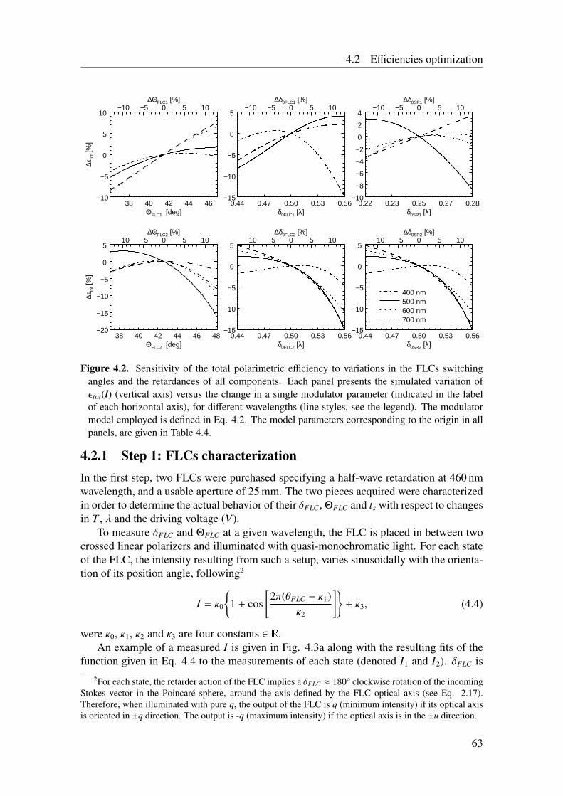
4.2 Efficiencies optimization
38 40 42 44 46ΘFLC1 [deg]
−10
−5
0
5
10
∆εto
t [%
]
−10 −5 0 5 10∆ΘFLC1 [%]
0.44 0.47 0.50 0.53 0.56δ0FLC1 [λ]
−15
−10
−5
0
5−10 −5 0 5 10
∆δ0FLC1 [%]
38 40 42 44 46 48ΘFLC2 [deg]
−20
−15
−10
−5
0
5
∆εto
t [%
]
−10 −5 0 5 10∆ΘFLC2 [%]
0.44 0.47 0.50 0.53 0.56δ0FLC2 [λ]
−15
−10
−5
0
5−10 −5 0 5 10
∆δ0FLC2 [%]
0.22 0.23 0.25 0.27 0.28δ0SR1 [λ]
−10
−8
−6
−4
−2
0
2
4−10 −5 0 5 10
∆δ0SR1 [%]
0.44 0.47 0.50 0.53 0.56δ0SR2 [λ]
−15
−10
−5
0
5−10 −5 0 5 10
∆δ0SR2 [%]
400 nm500 nm600 nm700 nm
Figure 4.2. Sensitivity of the total polarimetric efficiency to variations in the FLCs switchingangles and the retardances of all components. Each panel presents the simulated variation ofεtot(l) (vertical axis) versus the change in a single modulator parameter (indicated in the labelof each horizontal axis), for different wavelengths (line styles, see the legend). The modulatormodel employed is defined in Eq. 4.2. The model parameters corresponding to the origin in allpanels, are given in Table 4.4.
4.2.1 Step 1: FLCs characterizationIn the first step, two FLCs were purchased specifying a half-wave retardation at 460 nmwavelength, and a usable aperture of 25 mm. The two pieces acquired were characterizedin order to determine the actual behavior of their δFLC, ΘFLC and ts with respect to changesin T , λ and the driving voltage (V).
To measure δFLC and ΘFLC at a given wavelength, the FLC is placed in between twocrossed linear polarizers and illuminated with quasi-monochromatic light. For each stateof the FLC, the intensity resulting from such a setup, varies sinusoidally with the orienta-tion of its position angle, following2
I = κ0
1 + cos
[2π(θFLC − κ1)
κ2
]+ κ3, (4.4)
were κ0, κ1, κ2 and κ3 are four constants ∈ R.An example of a measured I is given in Fig. 4.3a along with the resulting fits of the
function given in Eq. 4.4 to the measurements of each state (denoted I1 and I2). δFLC is2For each state, the retarder action of the FLC implies a δFLC ≈ 180° clockwise rotation of the incoming
Stokes vector in the Poincaré sphere, around the axis defined by the FLC optical axis (see Eq. 2.17).Therefore, when illuminated with pure q, the output of the FLC is q (minimum intensity) if its optical axisis oriented in ±q direction. The output is -q (maximum intensity) if the optical axis is in the ±u direction.
63
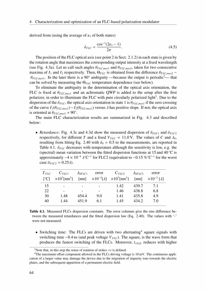
4 Characterization and optimization of an FLC-based polarization modulator
derived from (using the average of κ3 of both states)
δFLC =cos−1(2κ3 − 1)
2π. (4.5)
The position of the FLC optical axis (see point 2 in Sect. 2.1.2) in each state is given bythe rotation angle that maximizes the corresponding output intensity at a fixed wavelength(see Fig. 4.3a). Let us call such angles θFLC,max1 and θFLC,max2, taken for two consecutivemaxima of I1 and I2 respectively. Then, ΘFLC is obtained from the difference θFLC,max2 −
θFLC,max1. In the later there is a 90° ambiguity —because the output is periodic2— thatcan be solved by measuring the ΘFLC temperature dependence (see below).
To eliminate the ambiguity in the determination of the optical axis orientation, theFLC is fixed at θFLC,max1 and an achromatic QWP is added to the setup after the firstpolarizer, in order to illuminate the FLC with pure circularly polarized light3. Due to thedispersion of the δFLC, the optical axis orientation in state 1 is θFLC,max1 if the zero crossingof the curve I1(θFLC,max1)− I2(θFLC,max1) versus λ has positive slope. If not, the optical axisis oriented at θFLC,max1 + 90°.
The main FLC characterization results are summarized in Fig. 4.3 and describedbelow:
• Retardance: Fig. 4.3c and 4.3d show the measured dispersion of δFLC1 and δFLC2
respectively, for different T and a fixed VFLC = 11.0 V. The values of C and λ0,resulting from fitting Eq. 2.40 with δ0 = 0.5 to the measurements, are reported inTable 4.1. δFLC decreases with temperature although the sensitivity is low, e.g. the(spectral) mean variation between the fitted dispersion functions at 15 and 40 C isapproximately −4 × 10⁻⁴ λC−1 for FLC2 (equivalent to −0.15 %C−1 for the worstcase δFLC2 = 0.25λ).
T FLC CFLC1 λ0FLC1 error CFLC2 λ0FLC2 error[C] ×107[nm3] [nm] ×10−3[λ] ×107[nm3] [nm] ×10−3 [λ]
15 - - - 1.42 439.7 7.122 - - - 1.46 438.8 6.830 1.48 454.4 9.0 1.41 435.8 4.940 1.44 451.9 6.1 1.45 434.2 7.0
Table 4.1. Measured FLCs dispersion constants. The error columns give the rms difference be-tween the measured retardances and the fitted dispersion law (Eq. 2.40). The values with ‘-’were not measured.
• Switching time: The FLCs are driven with two alternating4 square signals withswitching time ∼8.4 ns (and peak voltage VFLC). The square, is the wave form thatproduces the fastest switching of the FLCs. Moreover, tsFLC reduces with higher
3Note that, in this step the sense of rotation of stokes +v is defined.4The maximum offset component allowed in the FLCs driving voltage is 10 mV. The continuous appli-
cation of a larger value may damage the device due to the migration of impurity ions towards the electricplates, and the subsequent apparition of a permanent electric field.
64
4.2 Efficiencies optimization
VFLC2=11.0 [V]
400 450 500 550 600 650 700λ [nm]
0.2
0.3
0.4
0.5
0.6
0.7
δ FC
L2 [λ
]
VFLC1=11.0 [V]
400 450 500 550 600 650 700λ [nm]
0.2
0.3
0.4
0.5
0.6
0.7
δ FC
L1 [λ
]
λ=515 [nm] ; TFLC1=36 [°C] ; VFLC1=17.5 [V]
0 50 100 150 200θFLC1 [deg]
0.0
0.2
0.4
0.6
0.8
1.0
1.2
1.4
Nor
m. I
VFLC2=11.0 [V]
400 450 500 550 600 650 700λ [nm]
0
1
2
3
4
ΘF
LC2−
ΘF
LC2(
700)
[deg
]
λ=700 [nm]; VFLC2=11.0 [V]
15 20 25 30 35 40TFLC2 [°C]
40
41
42
43
ΘF
LC2(
700
nm)
[deg
]
VFLC1=11.0 [V]
400 450 500 550 600 650 700λ [nm]
0
1
2
3
4
5
ΘF
LC1
− Θ
FLC
1(70
0 nm
) [d
eg]
λ=700 [nm]; VFLC1=11.0 [V]
15 20 25 30 35 40TFLC1 [°C]
38
39
40
41
42
ΘF
LC1(
700
nm)
[deg
]
λ=460 [nm] ; TFLC2=TFLC1=30 [°C]
4 6 8 10 12 14VFLC [V]
30
32
34
36
38
40
42
44
ΘF
LC [d
eg]
TFLC2=40°C
TFLC2=40°C
TFLC1=15°C
TFLC1=22°C
TFLC1=30°C
TFLC1=40°C
I1I2
TFLC2=30°C
TFLC2=40°C
65.1λ3−0.31 λ2
+5.0x10⁻⁴λ
Meas.
2.71(262.00−TFLC2)0.5
TFLC1=15°C
TFLC1=22°C
TFLC1=30°C
TFLC1=40°C
91.9λ3−0.46 λ2
+7.9x10⁻⁴λ
Meas.
2.64(252.41−TFLC1)0.5
FLC2FLC1
(a) (b)
(c) (d)
(e) (f)
(g) (h)
Figure 4.3. FLCs characterization results. The measurement conditions are specified in the titleof each panel. (a) Variation of the output intensity versus position angle for both states of FLC1(asterisks), along with the resulting fits of Eq. 4.4 (see legend). (b) Switching angle versusdriving voltage for both FLCs (see legend). Retardance dispersion at different temperatures(see legends) for FLC2 (c) and FLC1 (d). Switching angle dispersion at different temperatures(see legends) for FLC2 (e) and FLC1 (f). In both cases the value of the switching angles atλ = 700 nm has been subtracted. The latter are shown in (g) and (h) for FLC2 and FLC1respectively, along with the fitted temperature variation laws. See the text for extra details.
65
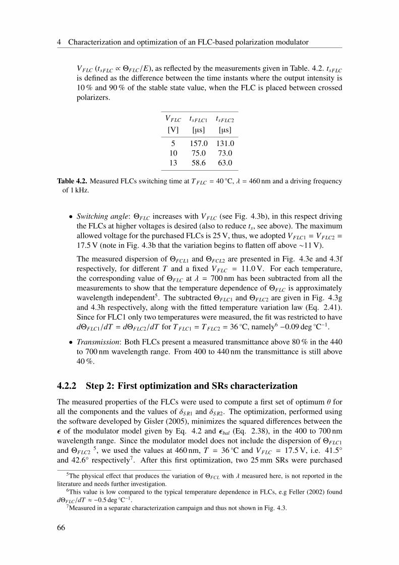
4 Characterization and optimization of an FLC-based polarization modulator
VFLC (tsFLC ∝ ΘFLC/E), as reflected by the measurements given in Table. 4.2. tsFLC
is defined as the difference between the time instants where the output intensity is10 % and 90 % of the stable state value, when the FLC is placed between crossedpolarizers.
VFLC tsFLC1 tsFLC2
[V] [µs] [µs]
5 157.0 131.010 75.0 73.013 58.6 63.0
Table 4.2. Measured FLCs switching time at T FLC = 40 C, λ = 460 nm and a driving frequencyof 1 kHz.
• Switching angle: ΘFLC increases with VFLC (see Fig. 4.3b), in this respect drivingthe FLCs at higher voltages is desired (also to reduce ts, see above). The maximumallowed voltage for the purchased FLCs is 25 V, thus, we adopted VFLC1 = VFLC2 =
17.5 V (note in Fig. 4.3b that the variation begins to flatten off above ∼11 V).
The measured dispersion of ΘFCL1 and ΘFCL2 are presented in Fig. 4.3e and 4.3frespectively, for different T and a fixed VFLC = 11.0 V. For each temperature,the corresponding value of ΘFLC at λ = 700 nm has been subtracted from all themeasurements to show that the temperature dependence of ΘFLC is approximatelywavelength independent5. The subtracted ΘFLC1 and ΘFLC2 are given in Fig. 4.3gand 4.3h respectively, along with the fitted temperature variation law (Eq. 2.41).Since for FLC1 only two temperatures were measured, the fit was restricted to havedΘFLC1/dT = dΘFLC2/dT for T FLC1 = T FLC2 = 36 C, namely6 −0.09 deg C−1.
• Transmission: Both FLCs present a measured transmittance above 80 % in the 440to 700 nm wavelength range. From 400 to 440 nm the transmittance is still above40 %.
4.2.2 Step 2: First optimization and SRs characterizationThe measured properties of the FLCs were used to compute a first set of optimum θ forall the components and the values of δS R1 and δS R2. The optimization, performed usingthe software developed by Gisler (2005), minimizes the squared differences between theε of the modulator model given by Eq. 4.2 and εbal (Eq. 2.38), in the 400 to 700 nmwavelength range. Since the modulator model does not include the dispersion of ΘFLC1
and ΘFLC25, we used the values at 460 nm, T = 36 C and VFLC = 17.5 V, i.e. 41.5°
and 42.6° respectively7. After this first optimization, two 25 mm SRs were purchased
5The physical effect that produces the variation of ΘFCL with λ measured here, is not reported in theliterature and needs further investigation.
6This value is low compared to the typical temperature dependence in FLCs, e.g Feller (2002) founddΘFLC/dT ≈ −0.5 deg C−1.
7Measured in a separate characterization campaign and thus not shown in Fig. 4.3.
66
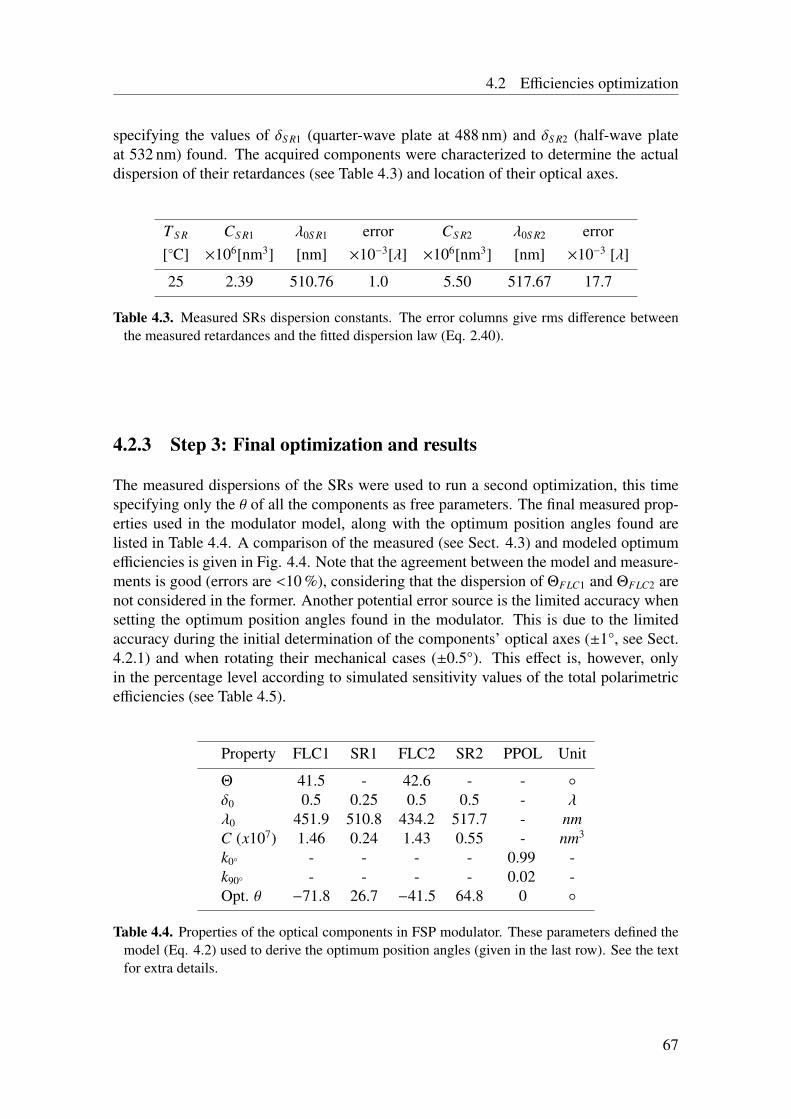
4.2 Efficiencies optimization
specifying the values of δS R1 (quarter-wave plate at 488 nm) and δS R2 (half-wave plateat 532 nm) found. The acquired components were characterized to determine the actualdispersion of their retardances (see Table 4.3) and location of their optical axes.
T S R CS R1 λ0S R1 error CS R2 λ0S R2 error[C] ×106[nm3] [nm] ×10−3[λ] ×106[nm3] [nm] ×10−3 [λ]
25 2.39 510.76 1.0 5.50 517.67 17.7
Table 4.3. Measured SRs dispersion constants. The error columns give rms difference betweenthe measured retardances and the fitted dispersion law (Eq. 2.40).
4.2.3 Step 3: Final optimization and results
The measured dispersions of the SRs were used to run a second optimization, this timespecifying only the θ of all the components as free parameters. The final measured prop-erties used in the modulator model, along with the optimum position angles found arelisted in Table 4.4. A comparison of the measured (see Sect. 4.3) and modeled optimumefficiencies is given in Fig. 4.4. Note that the agreement between the model and measure-ments is good (errors are <10 %), considering that the dispersion of ΘFLC1 and ΘFLC2 arenot considered in the former. Another potential error source is the limited accuracy whensetting the optimum position angles found in the modulator. This is due to the limitedaccuracy during the initial determination of the components’ optical axes (±1°, see Sect.4.2.1) and when rotating their mechanical cases (±0.5°). This effect is, however, onlyin the percentage level according to simulated sensitivity values of the total polarimetricefficiencies (see Table 4.5).
Property FLC1 SR1 FLC2 SR2 PPOL Unit
Θ 41.5 - 42.6 - -
δ0 0.5 0.25 0.5 0.5 - λλ0 451.9 510.8 434.2 517.7 - nmC (x107) 1.46 0.24 1.43 0.55 - nm3
k0 - - - - 0.99 -k90 - - - - 0.02 -Opt. θ −71.8 26.7 −41.5 64.8 0
Table 4.4. Properties of the optical components in FSP modulator. These parameters defined themodel (Eq. 4.2) used to derive the optimum position angles (given in the last row). See the textfor extra details.
67
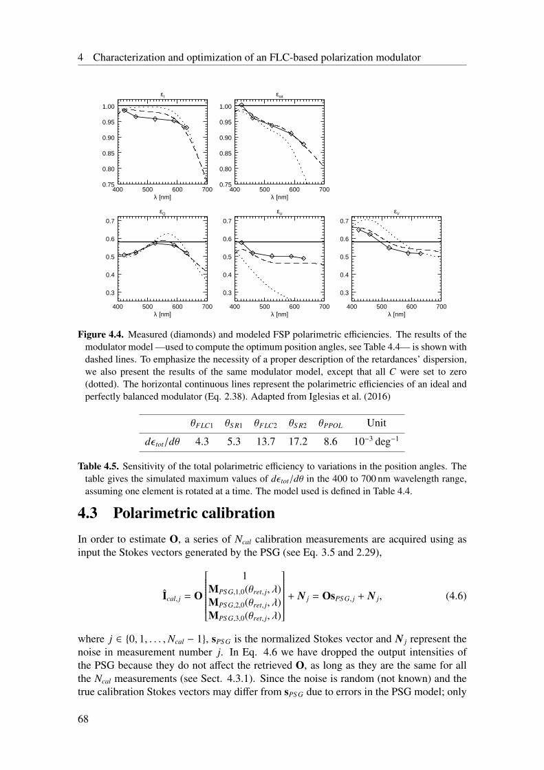
4 Characterization and optimization of an FLC-based polarization modulator
εI
400 500 600 700λ [nm]
0.75
0.80
0.85
0.90
0.95
1.00
εQ
400 500 600 700λ [nm]
0.3
0.4
0.5
0.6
0.7
εU
400 500 600 700λ [nm]
0.3
0.4
0.5
0.6
0.7
εV
400 500 600 700λ [nm]
0.3
0.4
0.5
0.6
0.7
εtot
400 500 600 700λ [nm]
0.75
0.80
0.85
0.90
0.95
1.00
Figure 4.4. Measured (diamonds) and modeled FSP polarimetric efficiencies. The results of themodulator model —used to compute the optimum position angles, see Table 4.4— is shown withdashed lines. To emphasize the necessity of a proper description of the retardances’ dispersion,we also present the results of the same modulator model, except that all C were set to zero(dotted). The horizontal continuous lines represent the polarimetric efficiencies of an ideal andperfectly balanced modulator (Eq. 2.38). Adapted from Iglesias et al. (2016)
θFLC1 θS R1 θFLC2 θS R2 θPPOL Unit
dε tot/dθ 4.3 5.3 13.7 17.2 8.6 10−3 deg−1
Table 4.5. Sensitivity of the total polarimetric efficiency to variations in the position angles. Thetable gives the simulated maximum values of dεtot/dθ in the 400 to 700 nm wavelength range,assuming one element is rotated at a time. The model used is defined in Table 4.4.
4.3 Polarimetric calibrationIn order to estimate O, a series of Ncal calibration measurements are acquired using asinput the Stokes vectors generated by the PSG (see Eq. 3.5 and 2.29),
Ical, j = O
1
MPS G,1,0(θret, j, λ)MPS G,2,0(θret, j, λ)MPS G,3,0(θret, j, λ)
+ N j = OsPS G, j + N j, (4.6)
where j ∈ 0, 1, . . . ,Ncal − 1, sPS G is the normalized Stokes vector and N j represent thenoise in measurement number j. In Eq. 4.6 we have dropped the output intensities ofthe PSG because they do not affect the retrieved O, as long as they are the same for allthe Ncal measurements (see Sect. 4.3.1). Since the noise is random (not known) and thetrue calibration Stokes vectors may differ from sPS G due to errors in the PSG model; only
68
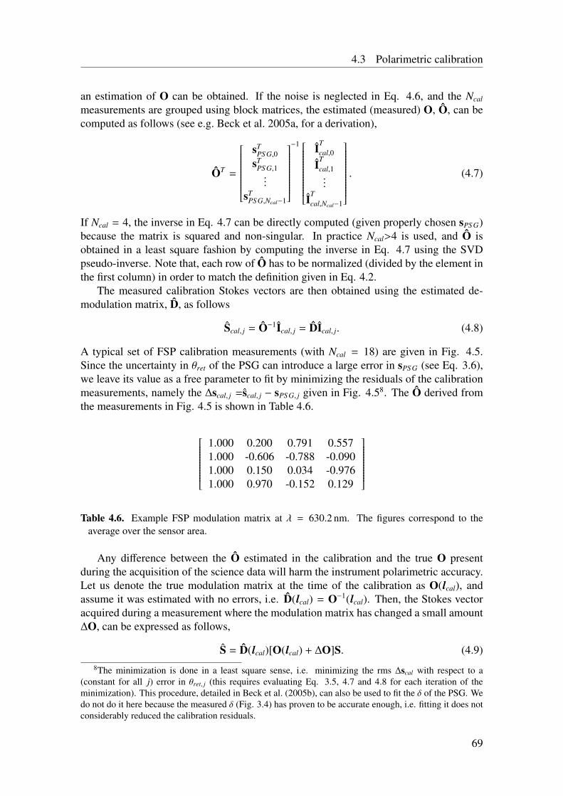
4.3 Polarimetric calibration
an estimation of O can be obtained. If the noise is neglected in Eq. 4.6, and the Ncal
measurements are grouped using block matrices, the estimated (measured) O, O, can becomputed as follows (see e.g. Beck et al. 2005a, for a derivation),
OT =
sT
PS G,0sT
PS G,1...
sTPS G,Ncal−1
−1
ITcal,0
ITcal,1...
ITcal,Ncal−1
. (4.7)
If Ncal = 4, the inverse in Eq. 4.7 can be directly computed (given properly chosen sPS G)because the matrix is squared and non-singular. In practice Ncal>4 is used, and O isobtained in a least square fashion by computing the inverse in Eq. 4.7 using the SVDpseudo-inverse. Note that, each row of O has to be normalized (divided by the element inthe first column) in order to match the definition given in Eq. 4.2.
The measured calibration Stokes vectors are then obtained using the estimated de-modulation matrix, D, as follows
Scal, j = O−1Ical, j = DIcal, j. (4.8)
A typical set of FSP calibration measurements (with Ncal = 18) are given in Fig. 4.5.Since the uncertainty in θret of the PSG can introduce a large error in sPS G (see Eq. 3.6),we leave its value as a free parameter to fit by minimizing the residuals of the calibrationmeasurements, namely the ∆scal, j =scal, j − sPS G, j given in Fig. 4.58. The O derived fromthe measurements in Fig. 4.5 is shown in Table 4.6.
1.000 0.200 0.791 0.5571.000 -0.606 -0.788 -0.0901.000 0.150 0.034 -0.9761.000 0.970 -0.152 0.129
Table 4.6. Example FSP modulation matrix at λ = 630.2 nm. The figures correspond to the
average over the sensor area.
Any difference between the O estimated in the calibration and the true O presentduring the acquisition of the science data will harm the instrument polarimetric accuracy.Let us denote the true modulation matrix at the time of the calibration as O(lcal), andassume it was estimated with no errors, i.e. D(lcal) = O−1(lcal). Then, the Stokes vectoracquired during a measurement where the modulation matrix has changed a small amount∆O, can be expressed as follows,
S = D(lcal)[O(lcal) + ∆O]S. (4.9)8The minimization is done in a least square sense, i.e. minimizing the rms ∆scal with respect to a
(constant for all j) error in θret, j (this requires evaluating Eq. 3.5, 4.7 and 4.8 for each iteration of theminimization). This procedure, detailed in Beck et al. (2005b), can also be used to fit the δ of the PSG. Wedo not do it here because the measured δ (Fig. 3.4) has proven to be accurate enough, i.e. fitting it does notconsiderably reduced the calibration residuals.
69
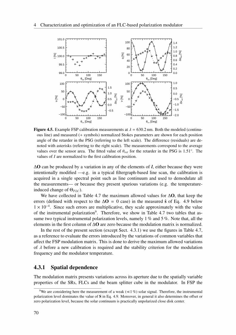
4 Characterization and optimization of an FLC-based polarization modulator
0 50 100 150θret [Deg]
99.0
99.5
100.0
100.5
101.0
I [%
]
0 50 100 150θret [Deg]
0
20
40
60
80
100
q [%
]
0.0
0.2
0.4
0.6
0.8
1.0
1.2
1.4
∆qca
l [%
]
0 50 100 150θret [Deg]
−100
−50
0
50
100
u [%
]
−0.5
0.0
0.5
1.0
1.5
∆uca
l [%
]0 50 100 150
θret [Deg]
−100
−50
0
50
100
v [%
]
−2.0
−1.5
−1.0
−0.5
0.0
0.5
1.0
∆vca
l [%
]
Figure 4.5. Example FSP calibration measurements at λ = 630.2 nm. Both the modeled (continu-ous line) and measured (+ symbols) normalized Stokes parameters are shown for each positionangle of the retarder in the PSG (referring to the left scale). The difference (residuals) are de-noted with asterisks (referring to the right scale). The measurements correspond to the averagevalues over the sensor area. The fitted value of θret for the retarder in the PSG is 1.51°. Thevalues of I are normalized to the first calibration position.
∆O can be produced by a variation in any of the elements of l, either because they wereintentionally modified —e.g. in a typical filtergraph-based line scan, the calibration isacquired in a single spectral point such as line continuum and used to demodulate allthe measurements— or because they present spurious variations (e.g. the temperature-induced change of ΘFLC).
We have collected in Table 4.7 the maximum allowed values for ∆O, that keep theerrors (defined with respect to the ∆O = 0 case) in the measured s of Eq. 4.9 below1 × 10−4. Since such errors are multiplicative, they scale approximately with the valueof the instrumental polarization9. Therefore, we show in Table 4.7 two tables that as-sume two typical instrumental polarization levels, namely 1 % and 5 %. Note that, all theelements in the first column of ∆O are zero because the modulation matrix is normalized.
In the rest of the present section (except Sect. 4.3.1) we use the figures in Table 4.7,as a reference to evaluate the errors introduced by the variations of common variables thataffect the FSP modulation matrix. This is done to derive the maximum allowed variationsof λ before a new calibration is required and the stability criterion for the modulationfrequency and the modulator temperature.
4.3.1 Spatial dependenceThe modulation matrix presents variations across its aperture due to the spatially variableproperties of the SRs, FLCs and the beam splitter cube in the modulator. In FSP the
9We are considering here the measurement of a weak (1 %) solar signal. Therefore, the instrumentalpolarization level dominates the value of S in Eq. 4.9. Moreover, in general it also determines the offset orzero polarization level, because the solar continuum is practically unpolarized close disk center.
70
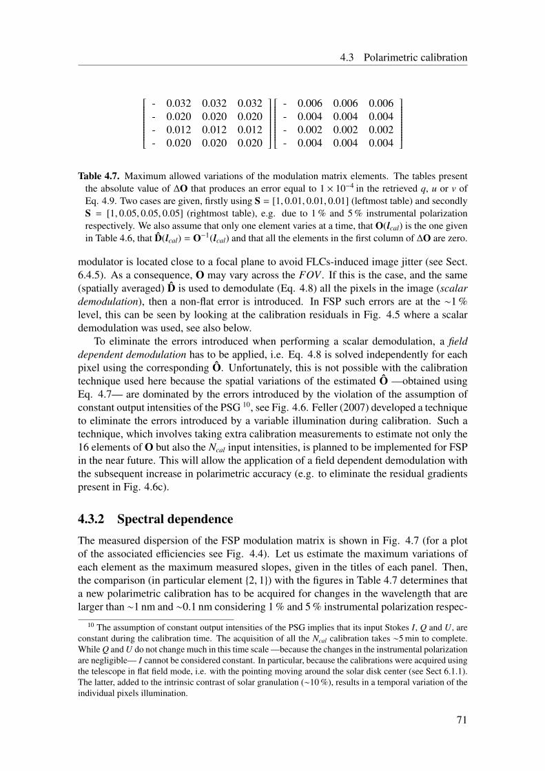
4.3 Polarimetric calibration
- 0.032 0.032 0.032- 0.020 0.020 0.020- 0.012 0.012 0.012- 0.020 0.020 0.020
- 0.006 0.006 0.006- 0.004 0.004 0.004- 0.002 0.002 0.002- 0.004 0.004 0.004
Table 4.7. Maximum allowed variations of the modulation matrix elements. The tables present
the absolute value of ∆O that produces an error equal to 1 × 10⁻⁴ in the retrieved q, u or v ofEq. 4.9. Two cases are given, firstly using S = [1, 0.01, 0.01, 0.01] (leftmost table) and secondlyS = [1, 0.05, 0.05, 0.05] (rightmost table), e.g. due to 1 % and 5 % instrumental polarizationrespectively. We also assume that only one element varies at a time, that O(lcal) is the one givenin Table 4.6, that D(lcal) = O−1(lcal) and that all the elements in the first column of ∆O are zero.
modulator is located close to a focal plane to avoid FLCs-induced image jitter (see Sect.6.4.5). As a consequence, O may vary across the FOV . If this is the case, and the same(spatially averaged) D is used to demodulate (Eq. 4.8) all the pixels in the image (scalardemodulation), then a non-flat error is introduced. In FSP such errors are at the ∼1 %level, this can be seen by looking at the calibration residuals in Fig. 4.5 where a scalardemodulation was used, see also below.
To eliminate the errors introduced when performing a scalar demodulation, a fielddependent demodulation has to be applied, i.e. Eq. 4.8 is solved independently for eachpixel using the corresponding O. Unfortunately, this is not possible with the calibrationtechnique used here because the spatial variations of the estimated O —obtained usingEq. 4.7— are dominated by the errors introduced by the violation of the assumption ofconstant output intensities of the PSG 10, see Fig. 4.6. Feller (2007) developed a techniqueto eliminate the errors introduced by a variable illumination during calibration. Such atechnique, which involves taking extra calibration measurements to estimate not only the16 elements of O but also the Ncal input intensities, is planned to be implemented for FSPin the near future. This will allow the application of a field dependent demodulation withthe subsequent increase in polarimetric accuracy (e.g. to eliminate the residual gradientspresent in Fig. 4.6c).
4.3.2 Spectral dependenceThe measured dispersion of the FSP modulation matrix is shown in Fig. 4.7 (for a plotof the associated efficiencies see Fig. 4.4). Let us estimate the maximum variations ofeach element as the maximum measured slopes, given in the titles of each panel. Then,the comparison (in particular element 2, 1) with the figures in Table 4.7 determines thata new polarimetric calibration has to be acquired for changes in the wavelength that arelarger than ∼1 nm and ∼0.1 nm considering 1 % and 5 % instrumental polarization respec-
10 The assumption of constant output intensities of the PSG implies that its input Stokes I, Q and U, areconstant during the calibration time. The acquisition of all the Ncal calibration takes ∼5 min to complete.While Q and U do not change much in this time scale —because the changes in the instrumental polarizationare negligible— I cannot be considered constant. In particular, because the calibrations were acquired usingthe telescope in flat field mode, i.e. with the pointing moving around the solar disk center (see Sect 6.1.1).The latter, added to the intrinsic contrast of solar granulation (∼10 %), results in a temporal variation of theindividual pixels illumination.
71
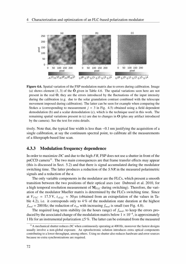
4 Characterization and optimization of an FLC-based polarization modulator
(a)
0 50 100 150 200pixel
0
50
100
150
200
250pi
xel
(b)
0 50 100 150 200pixel
(c)
0 50 100 150 200pixel
−0.11−0.10
−0.09−0.08
−0.070.09 0.10 0.11 0.12 0.13 0.14 0.09 0.10 0.11 0.12 0.13 0.14
Figure 4.6. Spatial variation of the FSP modulation matrix due to errors during calibration. Image(a) shows element 1, 3 of the O given in Table 4.6. The spatial variations seen here are notpresent in the real O, they are the errors introduced by the fluctuations of the input intensityduring the calibration (e.g. due to the solar granulation contrast combined with the telescopemovement imposed during calibration). The latter can be seen for example when comparing theStokes u (corresponding to measurement j = 3 in Fig. 4.5) obtained using a field dependentdemodulation (b) and a scalar demodulation (c), which is the technique used in this work. Theremaining spatial variations present in (c) are due to changes in O (plus any artifact introducedby the camera). See the text for extra details.
tively. Note that, the typical line width is less than ∼0.1 nm justifying the acquisition of asingle calibration, at say the continuum spectral point, to calibrate all the measurementsof a filtergraph-based line scan.
4.3.3 Modulation frequency dependenceIn order to maximize DC and due to the high FR, FSP does not use a shutter in front of thepnCCD camera11. The two main consequences are that frame transfer effects may appear(this is discussed in Sect. 5.2) and that there is signal accumulated during the modulatorswitching time. The latter produces a reduction of the S NR in the measured polarimetricsignals and a reduction of the ε.
The only variable components in the modulator are the FLCs, which present a smoothtransition between the two positions of their optical axes (see Dubreuil et al. 2010, fora high temporal resolution measurement of MFLC during switching). Therefore, the vari-ation of the modulator Mueller matrix is determined by the FLCs switching time. Sinceat VFLC = 17.5 V, tsFLC ≈ 50 µs (obtained from an extrapolation of the values in Ta-ble 4.2), i.e. it corresponds only to 4 % of the modulation state duration at the highestfmod = 200 Hz; the reduction of ε tot with increasing fmod is small (see Fig. 4.8).
The required long term stability (in the hours range) of fmod, to keep the errors pro-duced by the associated change of the modulation matrix below 1 × 10⁻⁴, is approximately1 Hz for an instrumental polarization ≤5 %. The latter can be estimated from the measured
11A mechanical shutter reduces DC when continuously operating at 400 Hz, moreover the fastest designsusually involve a non-global exposure. An optoelectronic solution introduces extra optical componentscontributing to a lower throughput, among others. Using no shutter also reduces hardware and error sourcesbecause no extra synchronizations are required.
72
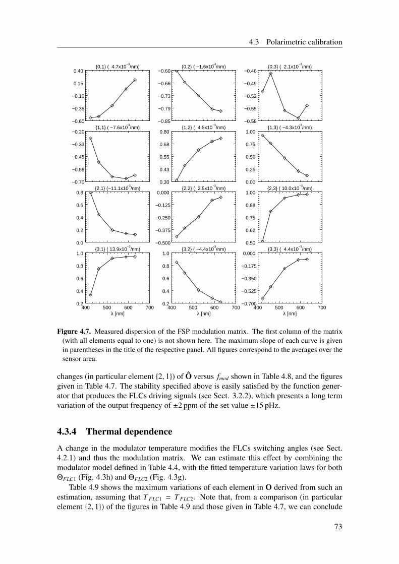
4.3 Polarimetric calibration
0,1 ( 4.7x10⁻³
/nm)
−0.60
−0.35
−0.10
0.15
0.400,2 ( −1.6x10
−3/nm)
−0.85
−0.79
−0.73
−0.66
−0.600,3 ( 2.1x10
−3/nm)
−0.58
−0.55
−0.52
−0.49
−0.46
1,1 ( −7.6x10⁻³
/nm)
−0.70
−0.58
−0.45
−0.33
−0.201,2 ( 4.5x10
−3/nm)
0.30
0.43
0.55
0.68
0.801,3 ( −4.3x10
−3/nm)
0.00
0.25
0.50
0.75
1.00
2,1 (−11.1x10⁻³
/nm)
0.0
0.2
0.4
0.6
0.82,2 ( 2.5x10
−3/nm)
−0.500
−0.375
−0.250
−0.125
0.0002,3 ( 10.0x10
−3/nm)
0.50
0.62
0.75
0.88
1.00
3,1 ( 13.9x10⁻³
/nm)
400 500 600 700λ [nm]
0.2
0.4
0.6
0.8
1.03,2 ( −4.4x10
−3/nm)
400 500 600 700λ [nm]
0.2
0.4
0.6
0.8
1.03,3 ( 4.4x10
−3/nm)
400 500 600 700λ [nm]
−0.700
−0.525
−0.350
−0.175
0.000
Figure 4.7. Measured dispersion of the FSP modulation matrix. The first column of the matrix(with all elements equal to one) is not shown here. The maximum slope of each curve is givenin parentheses in the title of the respective panel. All figures correspond to the averages over thesensor area.
changes (in particular element 2, 1) of O versus fmod shown in Table 4.8, and the figuresgiven in Table 4.7. The stability specified above is easily satisfied by the function gener-ator that produces the FLCs driving signals (see Sect. 3.2.2), which presents a long termvariation of the output frequency of ±2 ppm of the set value ±15 pHz.
4.3.4 Thermal dependence
A change in the modulator temperature modifies the FLCs switching angles (see Sect.4.2.1) and thus the modulation matrix. We can estimate this effect by combining themodulator model defined in Table 4.4, with the fitted temperature variation laws for bothΘFLC1 (Fig. 4.3h) and ΘFLC2 (Fig. 4.3g).
Table 4.9 shows the maximum variations of each element in O derived from such anestimation, assuming that T FLC1 = T FLC2. Note that, from a comparison (in particularelement 2, 1) of the figures in Table 4.9 and those given in Table 4.7, we can conclude
73
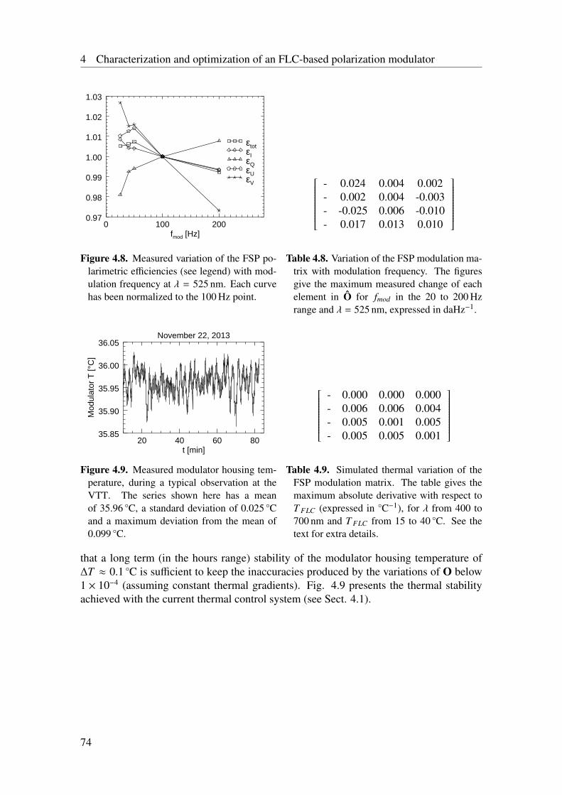
4 Characterization and optimization of an FLC-based polarization modulator
0 100 200fmod [Hz]
0.97
0.98
0.99
1.00
1.01
1.02
1.03
εtotεIεQεUεV
Figure 4.8. Measured variation of the FSP po-larimetric efficiencies (see legend) with mod-ulation frequency at λ = 525 nm. Each curvehas been normalized to the 100 Hz point.
- 0.024 0.004 0.002- 0.002 0.004 -0.003- -0.025 0.006 -0.010- 0.017 0.013 0.010
Table 4.8. Variation of the FSP modulation ma-
trix with modulation frequency. The figuresgive the maximum measured change of eachelement in O for fmod in the 20 to 200 Hzrange and λ = 525 nm, expressed in daHz−1.
November 22, 2013
20 40 60 80t [min]
35.85
35.90
35.95
36.00
36.05
Mod
ulat
or T
[°C
]
Figure 4.9. Measured modulator housing tem-perature, during a typical observation at theVTT. The series shown here has a meanof 35.96 C, a standard deviation of 0.025 Cand a maximum deviation from the mean of0.099 C.
- 0.000 0.000 0.000- 0.006 0.006 0.004- 0.005 0.001 0.005- 0.005 0.005 0.001
Table 4.9. Simulated thermal variation of the
FSP modulation matrix. The table gives themaximum absolute derivative with respect toT FLC (expressed in C−1), for λ from 400 to700 nm and T FLC from 15 to 40 C. See thetext for extra details.
that a long term (in the hours range) stability of the modulator housing temperature of∆T ≈ 0.1 C is sufficient to keep the inaccuracies produced by the variations of O below1 × 10−4 (assuming constant thermal gradients). Fig. 4.9 presents the thermal stabilityachieved with the current thermal control system (see Sect. 4.1).
74
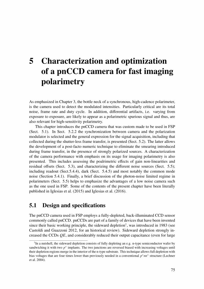
5 Characterization and optimizationof a pnCCD camera for fast imagingpolarimetry
As emphasized in Chapter 3, the bottle neck of a synchronous, high-cadence polarimeter,is the camera used to detect the modulated intensities. Particularly critical are its totalnoise, frame rate and duty cycle. In addition, differential artifacts, i.e. varying fromexposure to exposure, are likely to appear as a polarimetric spurious signal and thus, arealso relevant for high-sensitivity polarimetry.
This chapter introduces the pnCCD camera that was custom made to be used in FSP(Sect. 5.1). In Sect. 5.2.2 the synchronization between camera and the polarizationmodulator is selected and the general expression for the signal acquisition, including thatcollected during the shutter-less frame transfer, is presented (Sect. 5.2). The latter allowsthe development of a post-facto numeric technique to eliminate the smearing introducedduring frame transfer, in the presence of strongly polarized sources. A characterizationof the camera performance with emphasis on its usage for imaging polarimetry is alsopresented. This includes assessing the poalrimetric effects of gain non-linearities andresidual offsets (Sect. 5.3), and characterizing the different noise sources (Sect. 5.5);including readout (Sect.5.4.4), dark (Sect. 5.4.5) and most notably the common modenoise (Section 5.4.1). Finally, a brief discussion of the photon-noise limited regime inpolarimeters (Sect. 5.5) helps to emphasize the advantages of a low noise camera suchas the one used in FSP. Some of the contents of the present chapter have been literallypublished in Iglesias et al. (2015) and Iglesias et al. (2016).
5.1 Design and specificationsThe pnCCD camera used in FSP employs a fully-depleted, back-illuminated CCD sensorcommonly called pnCCD. pnCCDs are part of a family of devices that have been inventedsince their basic working principle, the sideward depletion1, was introduced in 1983 (seeCastoldi and Guazzoni 2012, for an historical review). Sideward depletion strongly in-creased the CCDs QE, and considerably reduced their output capacitance (even for large
1In a nutshell, the sideward depletion consists of fully depleting an e.g. n-type semiconductor wafer bysandwiching it with two p+ implants. The two junctions are reversed biased with increasing voltages untiltheir depletion regions merge in the interior of the n-type substrate. This technique allows full depletion withbias voltages that are four times lower than previously needed in a conventional p+nn+ structure (Lechneret al. 2004).
75
5 Characterization and optimization of a pnCCD camera for fast imaging polarimetry
area devices) among others. The later, in addition, particularly pushed the development ofhigh-performance readout electronics that has low σro and high FR, including, the veryimportant introduction of the on-chip amplifier.
The first pnCCD was demonstrated in 1988 for X-ray spectroscopy (Strueder et al.1988). Since then, many of the most successful developments and applications of this kindof sensors to astrophysics, have been done at the Max Planck institute for extraterrestrialphysics and the semiconductor lab of the Max Planck Society, initially together withPNSensor GmbH. They developed the first versions of the pnCCD sensor and readoutASIC —the CMOS amplifier and multiplexer (CAMEX)— employed in FSP, for X-rayimaging in the successful XMM-Newton space mission launched in 1999 (Strueder et al.2000). Further improvements were made for another X-ray application in space on boardof the ROSITA mission (Meidinger et al. 2003). The high QE and FR with low σro of theabove-named pnCCD systems, have also promoted their usage for imaging in optical andnear IR wavelengths since 2006 (Hartmann et al. 2006). Particularly suitable applicationswere found in astronomy either as main imager or as wavefront sensor for AO systems(see Ihle et al. 2012, and references therein).
The above-named benefits on FR and σro of the pnCCD (further detailed below),are clearly in line with the camera requirements of a high-cadence solar polarimeter (seeSect. 3.1.1). The latter has triggered the development of FSP, which constitutes the firstapplication of a pnCCD to solar polarimetry.
5.1.1 pnCCD sensor and readout electronicsThe basic internal structure of the three-phase pnCCD sensor used in the FSP camerais presented in Figs. 5.1a and b. The main detector features, that are most relevant toits application in a high-cadence polarimeter, are enumerated below. See Table 3.2 forfurther detector properties, and also Ihle et al. (2008) and Hartmann et al. (2006).
1. Fully depleted, back illuminated pnCCD: The fully depleted volume of the sen-sor increases its QE in the whole optical range. The photocharges generated byhigher energy photons (with short penetration depths) are more likely to reach theaccumulation region —located at the electron potential minimum at around 8 µmof the front side— because the bulk of the sensor is devoid of free charges for re-combination and the electric field in its interior is large. This permits having aback illuminated device with thicker substrate (compared to usual CCDs), whichin turn greatly improves the efficiency in detecting lower energy photons (withhigh penetration depths). The back illumination also allows to reach FF = 100 %;to avoid etaloning in applications with very narrow spectral bandwidth, like solarspectropolarimetry; and to have a thin and homogeneous entrance window whichhas low absorption and —along with the reduced reflectivity when depositing anti-reflecting coatings on it— contributes to further increase the QE in the blue (seeFig. 5.1c). The buried transfer channel contributes to a low charge transfer ineffi-ciency (<5 × 10⁻⁵). In addition, the fully depleted volume and large pixels, amongother properties, allow the sensor to reach FWC up to 1 × 10⁵ e− (although thisis not a critical parameter because modern solar polarimetry is generally photonstarved, see Sect 2.1.4).
76
5.1 Design and specifications
2. Column parallel readout and split frame transfer architecture: The sensor presentschannel parallel readout, i.e. every semi-column has independent readout circuitry(see below) and is read in parallel. The readout is split and each half of the lightsensitive area is quickly transfered to a shielded frame storage after each exposure(see Sect. 5.2 for further details on this process). The two above-named technolo-gies (plus the fast readout of the CAMEX, see below) allow the sensor to reachsimultaneously high FR and DC (see Table 3.2).
3. On chip amplifiers plus CAMEX readout ASICs: Each semi-column of the sensorends in a low-noise, on-chip JFET amplifier. The output of each on-chip amplifieris in turn bonded to a single channel of the readout ASICs, the CAMEX (see Her-rmann et al. 2008, Hartmann et al. 2006). Each CAMEX has 132 readout channelsthat are read in parallel and then multiplexed to two analog serial outputs (64 chan-nels per output). A single readout channel of the CAMEX is conformed amongothers by (a) a current source to bias the pnCCD on-chip amplifier; (b) a first JFETlow noise amplification stage; (c) a second amplification stage, with 8-fold cor-related double sampling for noise reduction2; (d) a sampling and hold stage thatallows starting the amplification of the next CCD row while the multiplexing ofthe current row is still in progress (further increasing the FR); and (e) a serializer.The CAMEX also features fully programmable gains and digital to analog convert-ers and reference voltages, for the internal generation of the bias voltages of eachstage (eliminating the need of many external power supply lines). The above-namedcharacteristics of the readout CAMEX plus the low noise figures of the on-chip am-plifier (possible due to the low output capacitance of the fully depleted channel) arethe main causes of the very low σro (Sect. 5.4.4) and NL (Sect. 5.3).
4. Others: The light sensitive area of the CCD sensor in FSP is small3, i.e. Ncol ×
Nrow=248 × 256 pixel2 (see point 6 in Sect 3.1.1). Note that, 8 additional columnsand 4 rows are covered by an aluminum shield in each side of the light sensitivearea. The shielded columns are used to filter the common mode artifact (see Sect.5.4.1). The shielded rows help to prevent stray light in the adjacent rows of theframe storage areas. The image area of the sensor is 12.7 × 12.7 mm2.
5.1.2 pnCCD cameraAn overview of the pnCCD camera system, including housing, main connections andassociated readout electronics rack is given in Fig. 5.2 (see Ihle et al. 2012, for a de-scription of a similar system). The sensor is located in an evacuated compartment of thecamera housing, and is cooled down using two two-stage Peltier elements that are pre-cooled using a cool water circuit. The maximum dimensions of the camera housing are170 × 165.8 × 227.9 mm. The 8 analog outputs of the CAMEX are connected to one
2This means that the output of the first amplifier stage is sampled eight times after the reset, and anothereight times after the charges are read. The samples before and after the reset are then subtracted one to oneand the eight resulting values averaged to form the output signal, see also footnote 15 in Sect. 2.2.4.
3We used Ncol × Nrow=264 × 264 pixel2 in Table 3.2 because this are the amount of pixels read in everyexposure.
77
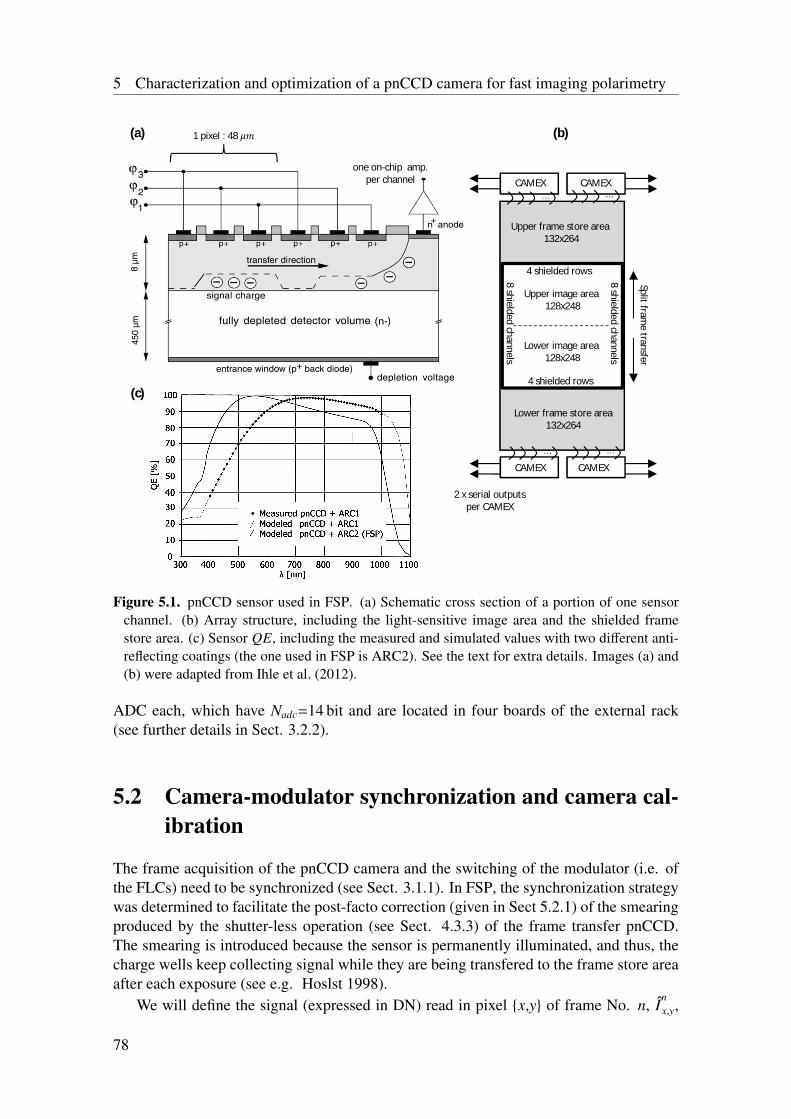
5 Characterization and optimization of a pnCCD camera for fast imaging polarimetry
CAMEX CAMEX
CAMEX CAMEX
Upper frame store area132x264
Lower frame store area132x264
Upper image area128x248
Lower image area128x248
Split frame transfer
8 shielded channels
8 shielded channels
4 shielded rows
4 shielded rows
2 x serial outputsper CAMEX
… …
… …
one on-chip amp.per channel
1 pixel : 48 ߤ(a) (b)
(c)
Figure 5.1. pnCCD sensor used in FSP. (a) Schematic cross section of a portion of one sensorchannel. (b) Array structure, including the light-sensitive image area and the shielded framestore area. (c) Sensor QE, including the measured and simulated values with two different anti-reflecting coatings (the one used in FSP is ARC2). See the text for extra details. Images (a) and(b) were adapted from Ihle et al. (2012).
ADC each, which have Nadc=14 bit and are located in four boards of the external rack(see further details in Sect. 3.2.2).
5.2 Camera-modulator synchronization and camera cal-ibration
The frame acquisition of the pnCCD camera and the switching of the modulator (i.e. ofthe FLCs) need to be synchronized (see Sect. 3.1.1). In FSP, the synchronization strategywas determined to facilitate the post-facto correction (given in Sect 5.2.1) of the smearingproduced by the shutter-less operation (see Sect. 4.3.3) of the frame transfer pnCCD.The smearing is introduced because the sensor is permanently illuminated, and thus, thecharge wells keep collecting signal while they are being transfered to the frame store areaafter each exposure (see e.g. Hoslst 1998).
We will define the signal (expressed in DN) read in pixel x,y of frame No. n, Inx,y,
78
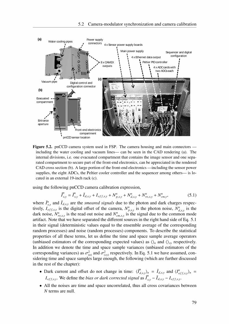
5.2 Camera-modulator synchronization and camera calibration
(a)
(b)
(c)
Sequencer and digital configuration4 x Ethernet data output
8 x CAMEX outputs
Water cooling pipes
Vacuum pipe Digital control and configuration connector
Power supply connectors
pnCCD sensor location
Entrance aperture
Front-end electronics compartment
Evacuated compartment
4 x Sensor power supply boards
Main power supply
Peltier PID controller
4 x ADC cards with two ADCs each
Figure 5.2. pnCCD camera system used in FSP. The camera housing and main connectors —including the water cooling and vacuum lines— can be seen in the CAD rendering (a). Theinternal divisions, i.e. one evacuated compartment that contains the image sensor and one sepa-rated compartment to secure part of the front-end electronics, can be appreciated in the renderedCAD cross section (b). A large portion of the front-end electronics —including the sensor powersupplies, the eight ADCs, the Peltier cooler controller and the sequencer among others— is lo-cated in an external 19-inch rack (c).
using the following pnCCD camera calibration expression,
Inx,y = In
x,y + Id,x,y + Io f f ,x,y + Nnp,x,y + Nn
d,x,y + Nnro,x,y + Nn
cm,y, (5.1)
where Inx,y and Id,x,y are the smeared signals due to the photon and dark charges respec-
tively, Io f f ,x,y is the digital offset of the camera, Nnp,x,y is the photon noise, Nn
d,x,y is thedark noise, Nn
ro,x,y is the read out noise and Nncm,x,y is the signal due to the common mode
artifact. Note that we have separated the different sources in the right hand side of Eq. 5.1in their signal (deterministic values equal to the ensemble average of the correspondingrandom processes) and noise (random processes) components. To describe the statisticalproperties of all these terms, let us define the time and space sample average operators(unbiased estimators of the corresponding expected values) as 〈〉n and 〈〉xy respectively.In addition we denote the time and space sample variances (unbiased estimators of thecorresponding variances) as σ2
(n) and σ2(xy) respectively. In Eq. 5.1 we have assumed, con-
sidering time and space samples large enough, the following (which are further discussedin the rest of the chapter):
• Dark current and offset do not change in time: 〈Ind,x,y〉n = Id,x,y and 〈In
o f f ,x,y〉n =
Io f f ,x,y. We define the bias or dark corrected signal as Inx,y − Id,x,y − Io f f ,x,y.
• All the noises are time and space uncorrelated, thus all cross covariances betweenN terms are null.
79
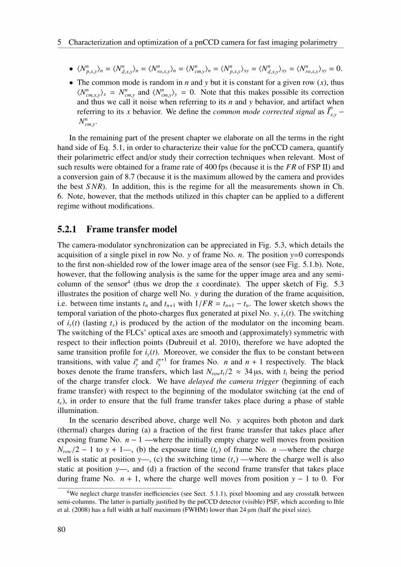
5 Characterization and optimization of a pnCCD camera for fast imaging polarimetry
• 〈Nnp,x,y〉n = 〈Nn
d,x,y〉n = 〈Nnro,x,y〉n = 〈Nn
cm,y〉n = 〈Nnp,x,y〉xy = 〈Nn
d,x,y〉xy = 〈Nnro,x,y〉xy = 0.
• The common mode is random in n and y but it is constant for a given row (x), thus〈Nn
cm,x,y〉x = Nncm,y and 〈Nn
cm,y〉y = 0. Note that this makes possible its correctionand thus we call it noise when referring to its n and y behavior, and artifact whenreferring to its x behavior. We define the common mode corrected signal as I
nx,y −
Nncm,y.
In the remaining part of the present chapter we elaborate on all the terms in the righthand side of Eq. 5.1, in order to characterize their value for the pnCCD camera, quantifytheir polarimetric effect and/or study their correction techniques when relevant. Most ofsuch results were obtained for a frame rate of 400 fps (because it is the FR of FSP II) anda conversion gain of 8.7 (because it is the maximum allowed by the camera and providesthe best S NR). In addition, this is the regime for all the measurements shown in Ch.6. Note, however, that the methods utilized in this chapter can be applied to a differentregime without modifications.
5.2.1 Frame transfer modelThe camera-modulator synchronization can be appreciated in Fig. 5.3, which details theacquisition of a single pixel in row No. y of frame No. n. The position y=0 correspondsto the first non-shielded row of the lower image area of the sensor (see Fig. 5.1.b). Note,however, that the following analysis is the same for the upper image area and any semi-column of the sensor4 (thus we drop the x coordinate). The upper sketch of Fig. 5.3illustrates the position of charge well No. y during the duration of the frame acquisition,i.e. between time instants tn and tn+1 with 1/FR = tn+1 − tn. The lower sketch shows thetemporal variation of the photo-charges flux generated at pixel No. y, iy(t). The switchingof iy(t) (lasting ts) is produced by the action of the modulator on the incoming beam.The switching of the FLCs’ optical axes are smooth and (approximately) symmetric withrespect to their inflection points (Dubreuil et al. 2010), therefore we have adopted thesame transition profile for iy(t). Moreover, we consider the flux to be constant betweentransitions, with value in
y and in+1y for frames No. n and n + 1 respectively. The black
boxes denote the frame transfers, which last Nrowtt/2 ≈ 34 µs, with tt being the periodof the charge transfer clock. We have delayed the camera trigger (beginning of eachframe transfer) with respect to the beginning of the modulator switching (at the end ofte), in order to ensure that the full frame transfer takes place during a phase of stableillumination.
In the scenario described above, charge well No. y acquires both photon and dark(thermal) charges during (a) a fraction of the first frame transfer that takes place afterexposing frame No. n − 1 —where the initially empty charge well moves from positionNrow/2 − 1 to y + 1—, (b) the exposure time (te) of frame No. n —where the chargewell is static at position y—, (c) the switching time (ts) —where the charge well is alsostatic at position y—, and (d) a fraction of the second frame transfer that takes placeduring frame No. n + 1, where the charge well moves from position y − 1 to 0. For
4We neglect charge transfer inefficiencies (see Sect. 5.1.1), pixel blooming and any crosstalk betweensemi-columns. The latter is partially justified by the pnCCD detector (visible) PSF, which according to Ihleet al. (2008) has a full width at half maximum (FWHM) lower than 24 µm (half the pixel size).
80
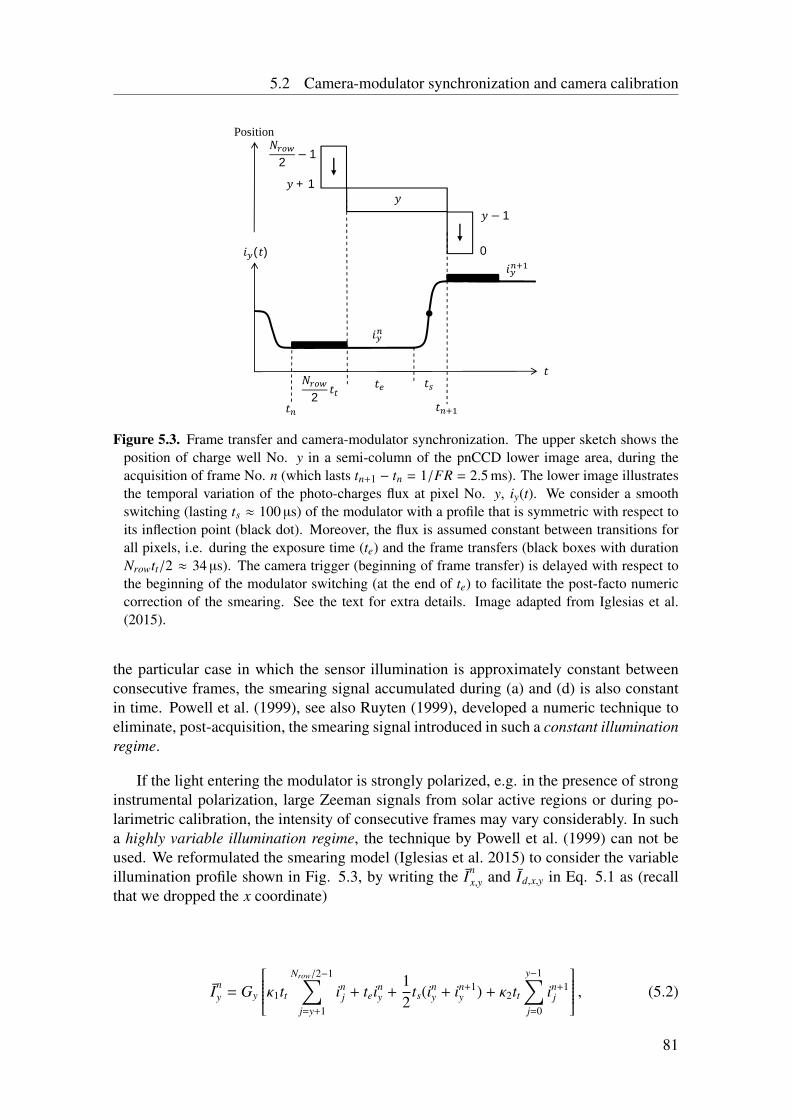
5.2 Camera-modulator synchronization and camera calibration
푡
푖 (푡)
푡
푖
푡푁2 푡
푡 푡
푦
푁2 − 1
푦 + 1
푦 − 1
0
Position
푖
Figure 5.3. Frame transfer and camera-modulator synchronization. The upper sketch shows theposition of charge well No. y in a semi-column of the pnCCD lower image area, during theacquisition of frame No. n (which lasts tn+1 − tn = 1/FR = 2.5 ms). The lower image illustratesthe temporal variation of the photo-charges flux at pixel No. y, iy(t). We consider a smoothswitching (lasting ts ≈ 100 µs) of the modulator with a profile that is symmetric with respect toits inflection point (black dot). Moreover, the flux is assumed constant between transitions forall pixels, i.e. during the exposure time (te) and the frame transfers (black boxes with durationNrowtt/2 ≈ 34 µs). The camera trigger (beginning of frame transfer) is delayed with respect tothe beginning of the modulator switching (at the end of te) to facilitate the post-facto numericcorrection of the smearing. See the text for extra details. Image adapted from Iglesias et al.(2015).
the particular case in which the sensor illumination is approximately constant betweenconsecutive frames, the smearing signal accumulated during (a) and (d) is also constantin time. Powell et al. (1999), see also Ruyten (1999), developed a numeric technique toeliminate, post-acquisition, the smearing signal introduced in such a constant illuminationregime.
If the light entering the modulator is strongly polarized, e.g. in the presence of stronginstrumental polarization, large Zeeman signals from solar active regions or during po-larimetric calibration, the intensity of consecutive frames may vary considerably. In sucha highly variable illumination regime, the technique by Powell et al. (1999) can not beused. We reformulated the smearing model (Iglesias et al. 2015) to consider the variableillumination profile shown in Fig. 5.3, by writing the In
x,y and Id,x,y in Eq. 5.1 as (recallthat we dropped the x coordinate)
Iny = Gy
κ1tt
Nrow/2−1∑j=y+1
inj + tein
y +12
ts(iny + in+1
y ) + κ2tt
y−1∑j=0
in+1j
, (5.2)
81
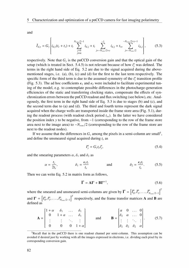
5 Characterization and optimization of a pnCCD camera for fast imaging polarimetry
and
Id,y = Gy
id,y(te + ts) + tt
Nrow/2−1∑j=0j,m
id, j + tt
−1∑j=−Nrow/2+y
id, j + tro
−Nrow/2+y−1∑j=−Nrow/2
id, j
, (5.3)
respectively. Note that Gy is the pnCCD conversion gain and that the optical gain of thesetup (which is treated in Sect. 5.4.5) is not relevant because of how in
y was defined. Theterms in the right hand side of Eq. 5.2 are due to the signal acquired during the above-mentioned stages, i.e. (a), (b), (c) and (d) for the first to the last term respectively. Thespecific form of the third term is due to the assumed symmetry of the in
y transition profile(Fig. 5.3). The ad hoc coefficients κ1 and κ2 were included to facilitate experimental tun-ing of the model, e.g. to contemplate possible differences in the photocharge-generationefficiencies of the static and transferring clocking states, compensate the effects of syn-chronization errors between the pnCCD readout and flux switching (see below), etc. Anal-ogously, the first term in the right hand side of Eq. 5.3 is due to stages (b) and (c), andthe second term due to (a) and (d). The third and fourth terms represent the dark signalacquired when the charge wells are transported inside the frame store area (Fig. 5.1), dur-ing the readout process (with readout clock period tro). In the latter we have consideredthe position index y to be negative, from −1 (corresponding to the row of the frame storearea next to the image area) to −Nrow/2 (corresponding to the row of the frame store arenext to the readout nodes).
If we assume that the differences in Gy among the pixels in a semi-column are small5,and define the unsmeared signal acquired during te as
Iny = Gytein
y , (5.4)
and the smearing parameters α, δ1 and δ2 as
α =ts
2te, δ1 =
κ1tt
teand δ2 =
κ2tt
te. (5.5)
Then we can write Eq. 5.2 in matrix form as follows,
In= AIn + BIn+1, (5.6)
where the smeared and unsmeared semi-columns are given by In=
[In
0, In1, . . . , I
nNrow/2−1
]T
and In =[In
0, In1, . . . , I
nNrow/2−1
]Trespectively, and the frame transfer matrices A and B are
defined as
A =
1 + α δ1 . . . δ1
0 1 + α . . . δ1...
.... . .
...0 0 0 1 + α
and B =
α 0 . . . 0δ2 α . . . 0...
.... . .
...δ2 δ2 δ2 α
. (5.7)
5Recall that in the pnCCD there is one readout channel per semi-column. This assumption can beavoided if desired just by working with all the images expressed in electrons, i.e. dividing each pixel by itscorresponding conversion gain.
82
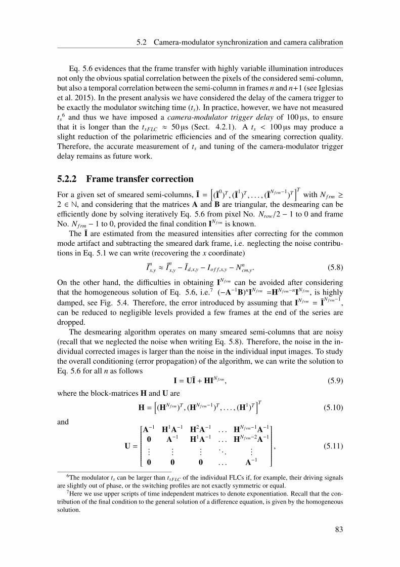
5.2 Camera-modulator synchronization and camera calibration
Eq. 5.6 evidences that the frame transfer with highly variable illumination introducesnot only the obvious spatial correlation between the pixels of the considered semi-column,but also a temporal correlation between the semi-column in frames n and n+1 (see Iglesiaset al. 2015). In the present analysis we have considered the delay of the camera trigger tobe exactly the modulator switching time (ts). In practice, however, we have not measuredts
6 and thus we have imposed a camera-modulator trigger delay of 100 µs, to ensurethat it is longer than the tsFLC ≈ 50 µs (Sect. 4.2.1). A ts < 100 µs may produce aslight reduction of the polarimetric efficiencies and of the smearing correction quality.Therefore, the accurate measurement of ts and tuning of the camera-modulator triggerdelay remains as future work.
5.2.2 Frame transfer correctionFor a given set of smeared semi-columns, I =
[(I0)T , (I1)T , . . . , (IN f rm−1)T
]Twith N f rm ≥
2 ∈ N, and considering that the matrices A and B are triangular, the desmearing can beefficiently done by solving iteratively Eq. 5.6 from pixel No. Nrow/2 − 1 to 0 and frameNo. N f rm − 1 to 0, provided the final condition IN f rm is known.
The I are estimated from the measured intensities after correcting for the commonmode artifact and subtracting the smeared dark frame, i.e. neglecting the noise contribu-tions in Eq. 5.1 we can write (recovering the x coordinate)
Inx,y ≈ I
nx,y − Id,x,y − Io f f ,x,y − Nn
cm,y. (5.8)
On the other hand, the difficulties in obtaining IN f rm can be avoided after consideringthat the homogeneous solution of Eq. 5.6, i.e.7 (−A−1B)nIN f rm =HN f rm−nIN f rm , is highlydamped, see Fig. 5.4. Therefore, the error introduced by assuming that IN f rm = IN f rm−1,can be reduced to negligible levels provided a few frames at the end of the series aredropped.
The desmearing algorithm operates on many smeared semi-columns that are noisy(recall that we neglected the noise when writing Eq. 5.8). Therefore, the noise in the in-dividual corrected images is larger than the noise in the individual input images. To studythe overall conditioning (error propagation) of the algorithm, we can write the solution toEq. 5.6 for all n as follows
I = UI + HIN f rm , (5.9)
where the block-matrices H and U are
H =[(HN f rm)T , (HN f rm−1)T , . . . , (H1)T
]T(5.10)
and
U =
A−1 H1A−1 H2A−1 . . . HN f rm−1A−1
0 A−1 H1A−1 . . . HN f rm−2A−1
......
.... . .
...
0 0 0 . . . A−1
, (5.11)
6The modulator ts can be larger than tsFLC of the individual FLCs if, for example, their driving signalsare slightly out of phase, or the switching profiles are not exactly symmetric or equal.
7Here we use upper scripts of time independent matrices to denote exponentiation. Recall that the con-tribution of the final condition to the general solution of a difference equation, is given by the homogeneoussolution.
83
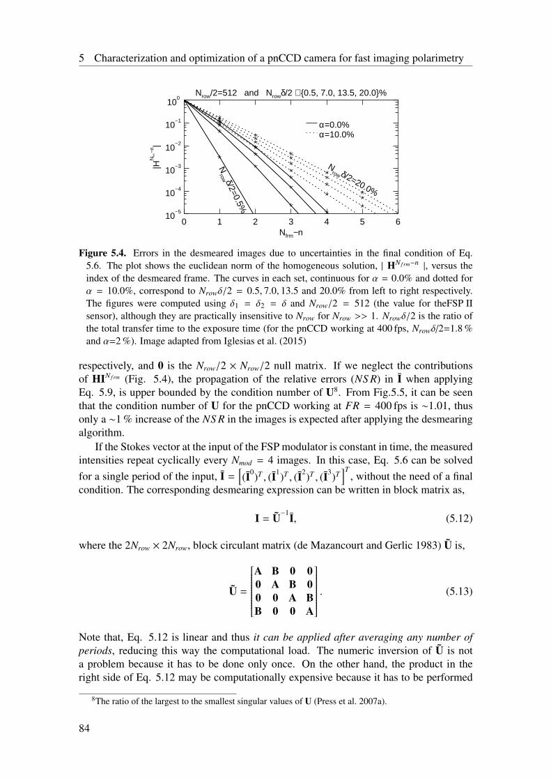
5 Characterization and optimization of a pnCCD camera for fast imaging polarimetry
Nrow/2=512 and Nrowδ/2 ∈ 0.5, 7.0, 13.5, 20.0%
0 1 2 3 4 5 6Nfrm−n
10−5
10−4
10−3
10−2
10−1
100
|HN
frm−n
|
Nrow δ/2=0.5%
Nrow δ/2=20.0%
α=0.0%α=10.0%
Figure 5.4. Errors in the desmeared images due to uncertainties in the final condition of Eq.5.6. The plot shows the euclidean norm of the homogeneous solution, | HN f rm−n |, versus theindex of the desmeared frame. The curves in each set, continuous for α = 0.0% and dotted forα = 10.0%, correspond to Nrowδ/2 = 0.5, 7.0, 13.5 and 20.0% from left to right respectively.The figures were computed using δ1 = δ2 = δ and Nrow/2 = 512 (the value for theFSP IIsensor), although they are practically insensitive to Nrow for Nrow >> 1. Nrowδ/2 is the ratio ofthe total transfer time to the exposure time (for the pnCCD working at 400 fps, Nrowδ/2=1.8 %and α=2 %). Image adapted from Iglesias et al. (2015)
respectively, and 0 is the Nrow/2 × Nrow/2 null matrix. If we neglect the contributionsof HIN f rm (Fig. 5.4), the propagation of the relative errors (NS R) in I when applyingEq. 5.9, is upper bounded by the condition number of U8. From Fig.5.5, it can be seenthat the condition number of U for the pnCCD working at FR = 400 fps is ∼1.01, thusonly a ∼1 % increase of the NS R in the images is expected after applying the desmearingalgorithm.
If the Stokes vector at the input of the FSP modulator is constant in time, the measuredintensities repeat cyclically every Nmod = 4 images. In this case, Eq. 5.6 can be solvedfor a single period of the input, I =
[(I0)T , (I1)T , (I2)T , (I3)T
]T, without the need of a final
condition. The corresponding desmearing expression can be written in block matrix as,
I = U−1I, (5.12)
where the 2Nrow × 2Nrow, block circulant matrix (de Mazancourt and Gerlic 1983) U is,
U =
A B 0 00 A B 00 0 A BB 0 0 A
. (5.13)
Note that, Eq. 5.12 is linear and thus it can be applied after averaging any number ofperiods, reducing this way the computational load. The numeric inversion of U is nota problem because it has to be done only once. On the other hand, the product in theright side of Eq. 5.12 may be computationally expensive because it has to be performed
8The ratio of the largest to the smallest singular values of U (Press et al. 2007a).
84
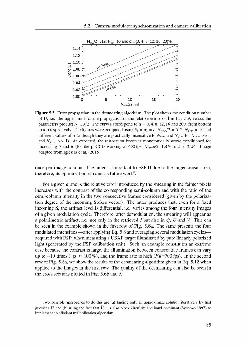
5.2 Camera-modulator synchronization and camera calibration
Nrow/2=512, Nfrm=10 and α ∈ 0, 4, 8, 12, 16, 20%
0 5 10 15 20Nrowδ/2 [%]
1.00
1.02
1.04
1.06
1.08
1.10
1.12
1.14
Con
d(U
)α=20%
α=0%
Figure 5.5. Error propagation in the desmearing algorithm. The plot shows the condition numberof U, i.e. the upper limit for the propagation of the relative errors of I in Eq. 5.9, versus theparameters product Nrowδ/2. The curves correspond to α = 0, 4, 8, 12, 16 and 20% from bottomto top respectively. The figures were computed using δ1 = δ2 = δ, Nrow/2 = 512, N f rm = 10 anddifferent values of α (although they are practically insensitive to Nrow and N f rm for Nrow >> 1and N f rm >> 1). As expected, the restoration becomes monotonically worse conditioned forincreasing δ and α (for the pnCCD working at 400 fps, Nrowδ/2=1.8 % and α=2 %). Imageadapted from Iglesias et al. (2015)
once per image column. The latter is important to FSP II due to the larger sensor area,therefore, its optimization remains as future work9.
For a given α and δ, the relative error introduced by the smearing in the fainter pixelsincreases with the contrast of the corresponding semi-column and with the ratio of thesemi-column intensity in the two consecutive frames considered (given by the polariza-tion degree of the incoming Stokes vector). The latter produces that, even for a fixedincoming S, the artifact level is differential, i.e. varies among the four intensity imagesof a given modulation cycle. Therefore, after demodulation, the smearing will appear asa polarimetric artifact, i.e. not only in the retrieved I but also in Q, U and V . This canbe seen in the example shown in the first row of Fig. 5.6a. The same presents the fourmodulated intensities —after applying Eq. 5.8 and averaging several modulation cycles—acquired with FSP, when measuring a USAF target illuminated by pure linearly polarizedlight (generated by the FSP calibration unit). Such an example constitutes an extremecase because the contrast is large, the illumination between consecutive frames can varyup to ∼10 times (| p |≈ 100 %), and the frame rate is high (FR=700 fps). In the secondrow of Fig. 5.6a, we show the results of the desmearing algorithm given in Eq. 5.12 whenapplied to the images in the first row. The quality of the desmearing can also be seen inthe cross sections plotted in Fig. 5.6b and c.
9Two possible approaches to do this are (a) finding only an approximate solution iteratively by firstguessing I0 and (b) using the fact that U−1
is also block circulant and band dominant (Vescovo 1997) toimplement an efficient multiplication algorithm.
85
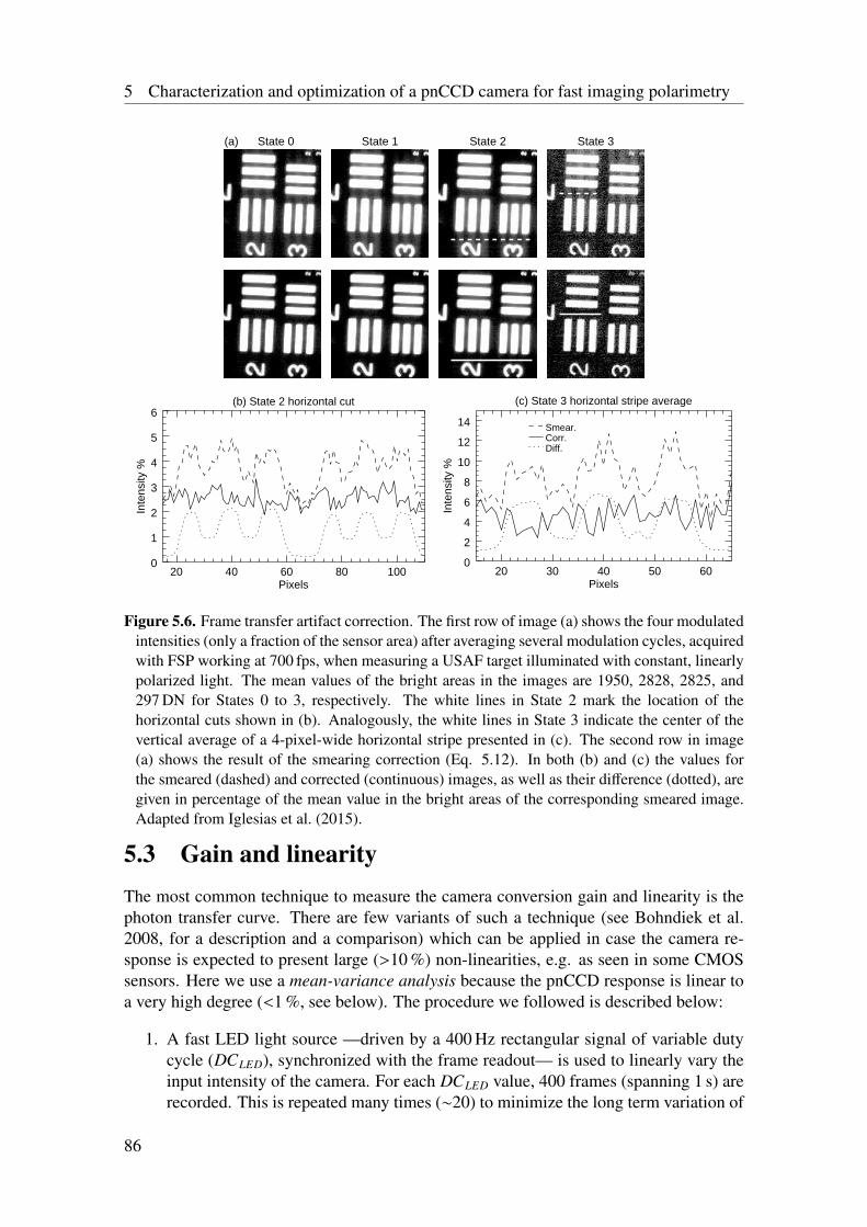
5 Characterization and optimization of a pnCCD camera for fast imaging polarimetry
(a) State 0 State 1 State 2 State 3
(b) State 2 horizontal cut
20 40 60 80 100Pixels
0
1
2
3
4
5
6
Inte
nsity
%
(c) State 3 horizontal stripe average
20 30 40 50 60Pixels
0
2
4
6
8
10
12
14
Inte
nsity
%
Smear.Corr.Diff.
Figure 5.6. Frame transfer artifact correction. The first row of image (a) shows the four modulatedintensities (only a fraction of the sensor area) after averaging several modulation cycles, acquiredwith FSP working at 700 fps, when measuring a USAF target illuminated with constant, linearlypolarized light. The mean values of the bright areas in the images are 1950, 2828, 2825, and297 DN for States 0 to 3, respectively. The white lines in State 2 mark the location of thehorizontal cuts shown in (b). Analogously, the white lines in State 3 indicate the center of thevertical average of a 4-pixel-wide horizontal stripe presented in (c). The second row in image(a) shows the result of the smearing correction (Eq. 5.12). In both (b) and (c) the values forthe smeared (dashed) and corrected (continuous) images, as well as their difference (dotted), aregiven in percentage of the mean value in the bright areas of the corresponding smeared image.Adapted from Iglesias et al. (2015).
5.3 Gain and linearityThe most common technique to measure the camera conversion gain and linearity is thephoton transfer curve. There are few variants of such a technique (see Bohndiek et al.2008, for a description and a comparison) which can be applied in case the camera re-sponse is expected to present large (>10 %) non-linearities, e.g. as seen in some CMOSsensors. Here we use a mean-variance analysis because the pnCCD response is linear toa very high degree (<1 %, see below). The procedure we followed is described below:
1. A fast LED light source —driven by a 400 Hz rectangular signal of variable dutycycle (DCLED), synchronized with the frame readout— is used to linearly vary theinput intensity of the camera. For each DCLED value, 400 frames (spanning 1 s) arerecorded. This is repeated many times (∼20) to minimize the long term variation of
86
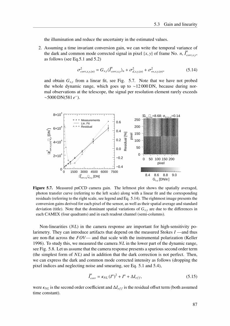
5.3 Gain and linearity
the illumination and reduce the uncertainty in the estimated values.
2. Assuming a time invariant conversion gain, we can write the temporal variance ofthe dark and common mode corrected signal in pixel x, y of frame No. n, I
ncorr,x,y,
as follows (see Eq.5.1 and 5.2)
σ2corr,x,y,(n) = Gx,y〈I
ncorr,x,y〉n + σ2
d,x,y,(n) + σ2ro,x,y,(n), (5.14)
and obtain Gx,y from a linear fit, see Fig. 5.7. Note that we have not probedthe whole dynamic range, which goes up to ∼12 000 DN, because during nor-mal observations at the telescope, the signal per resolution element rarely exceeds∼5000 DN(581 e−).
0 1500 3000 4500 6000 7500⟨I^n
corr,x,y⟩n,x,y [DN]
0
2×10⁴
4×10⁴
6×10⁴
8×10⁴
⟨σ2 co
rr,x
,y,(
n)⟩ x,
y [D
N2 ]
−0.4
−0.2
0.0
0.2
0.4
0.6R
esid
ual [
%]
⟨Gx,y⟩x,y=8.68; σG,(x,y)=0.14
0 50 100 150 200pixel
0
50
100
150
200
250
pixe
l
MeasurementsLin. FitResidual
8.4 8.6 8.8 9.0Gx,y [DN/e−]
Figure 5.7. Measured pnCCD camera gain. The leftmost plot shows the spatially averaged,photon transfer curve (referring to the left scale) along with a linear fit and the correspondingresiduals (referring to the right scale, see legend and Eq. 5.14). The rightmost image presents theconversion gains derived for each pixel of the sensor, as well as their spatial average and standarddeviation (title). Note that the dominant spatial variations of Gx,y are due to the differences ineach CAMEX (four quadrants) and in each readout channel (semi-columns).
Non-linearities (NL) in the camera response are important for high-sensitivity po-larimetry. They can introduce artifacts that depend on the measured Stokes I —and thusare non-flat across the FOV— and that scale with the instrumental polarization (Keller1996). To study this, we measured the camera NL in the lower part of the dynamic range,see Fig. 5.8. Let us assume that the camera response presents a spurious second order term(the simplest form of NL) and in addition that the dark correction is not perfect. Then,we can express the dark and common mode corrected intensity as follows (dropping thepixel indices and neglecting noise and smearing, see Eq. 5.1 and 5.4),
Incorr = κNL (In)2 + In + ∆Io f f , (5.15)
were κNL is the second order coefficient and ∆Io f f is the residual offset term (both assumedtime constant).
87
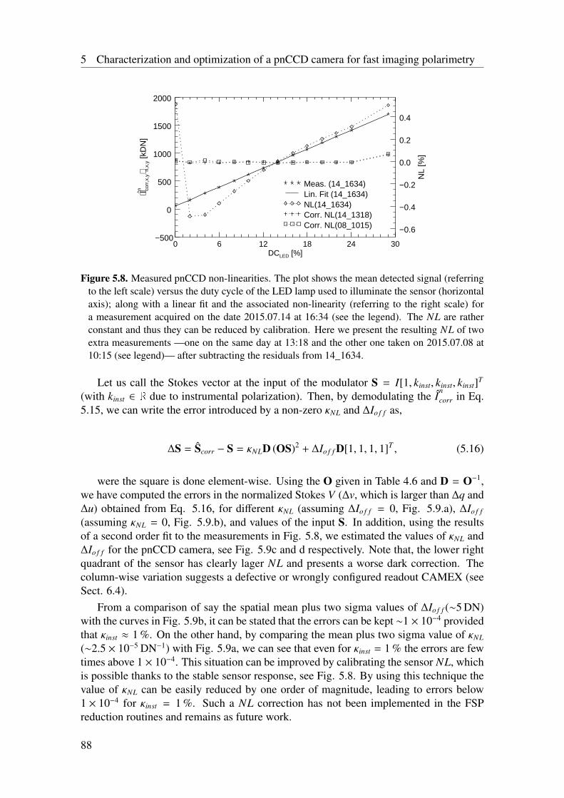
5 Characterization and optimization of a pnCCD camera for fast imaging polarimetry
0 6 12 18 24 30DCLED [%]
−500
0
500
1000
1500
2000
⟨I^n corr
,x,y⟩ n,
x,y
[kD
N]
−0.6
−0.4
−0.2
0.0
0.2
0.4
NL
[%]
Meas. (14_1634)Lin. Fit (14_1634)NL(14_1634)Corr. NL(14_1318)Corr. NL(08_1015)
Figure 5.8. Measured pnCCD non-linearities. The plot shows the mean detected signal (referringto the left scale) versus the duty cycle of the LED lamp used to illuminate the sensor (horizontalaxis); along with a linear fit and the associated non-linearity (referring to the right scale) fora measurement acquired on the date 2015.07.14 at 16:34 (see the legend). The NL are ratherconstant and thus they can be reduced by calibration. Here we present the resulting NL of twoextra measurements —one on the same day at 13:18 and the other one taken on 2015.07.08 at10:15 (see legend)— after subtracting the residuals from 14_1634.
Let us call the Stokes vector at the input of the modulator S = I[1, kinst, kinst, kinst]T
(with kinst ∈ R due to instrumental polarization). Then, by demodulating the Incorr in Eq.
5.15, we can write the error introduced by a non-zero κNL and ∆Io f f as,
∆S = Scorr − S = κNLD (OS)2 + ∆Io f f D[1, 1, 1, 1]T , (5.16)
were the square is done element-wise. Using the O given in Table 4.6 and D = O−1,we have computed the errors in the normalized Stokes V (∆v, which is larger than ∆q and∆u) obtained from Eq. 5.16, for different κNL (assuming ∆Io f f = 0, Fig. 5.9.a), ∆Io f f
(assuming κNL = 0, Fig. 5.9.b), and values of the input S. In addition, using the resultsof a second order fit to the measurements in Fig. 5.8, we estimated the values of κNL and∆Io f f for the pnCCD camera, see Fig. 5.9c and d respectively. Note that, the lower rightquadrant of the sensor has clearly lager NL and presents a worse dark correction. Thecolumn-wise variation suggests a defective or wrongly configured readout CAMEX (seeSect. 6.4).
From a comparison of say the spatial mean plus two sigma values of ∆Io f f (∼5 DN)with the curves in Fig. 5.9b, it can be stated that the errors can be kept ∼1 × 10⁻⁴ providedthat κinst ≈ 1 %. On the other hand, by comparing the mean plus two sigma value of κNL
(∼2.5 × 10⁻⁵ DN−1) with Fig. 5.9a, we can see that even for κinst = 1 % the errors are fewtimes above 1 × 10⁻⁴. This situation can be improved by calibrating the sensor NL, whichis possible thanks to the stable sensor response, see Fig. 5.8. By using this technique thevalue of κNL can be easily reduced by one order of magnitude, leading to errors below1 × 10−4 for κinst = 1 %. Such a NL correction has not been implemented in the FSPreduction routines and remains as future work.
88
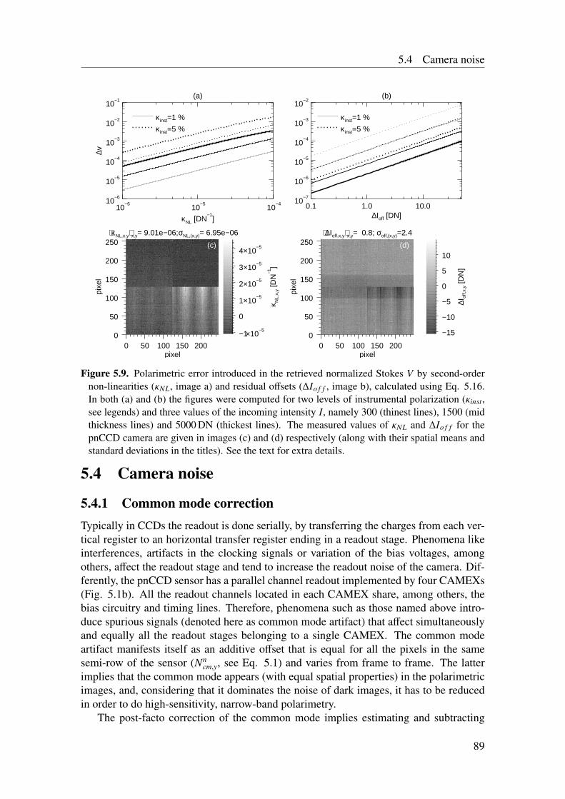
5.4 Camera noise
⟨κ NL,x,y⟩x,y= 9.01e−06; σNL,(x,y)= 6.95e−06
0 50 100 150 200pixel
0
50
100
150
200
250
pixe
l
⟨∆Ioff,x,y⟩x,y= 0.8; σoff,(x,y)=2.4
0 50 100 150 200pixel
0
50
100
150
200
250
pixe
l
(a)
10−6
10−5
10−4
κNL [DN−1
]
10−6
10−5
10−4
10−3
10−2
10−1
∆v(b)
0.1 1.0 10.0∆Ioff [DN]
10−7
10−6
10−5
10−4
10−3
10−2
κ inst=1 %
κ inst=5 %
κ inst=1 %
κ inst=5 %
−1×10⁻⁵
0
1×10⁻⁵
2×10⁻⁵
3×10⁻⁵
4×10⁻⁵
κ NL,
x,y
[DN
−1]
−15
−10
−5
0
5
10
∆Iof
f,x,y [D
N]
(c) (d)
Figure 5.9. Polarimetric error introduced in the retrieved normalized Stokes V by second-ordernon-linearities (κNL, image a) and residual offsets (∆Io f f , image b), calculated using Eq. 5.16.In both (a) and (b) the figures were computed for two levels of instrumental polarization (κinst,see legends) and three values of the incoming intensity I, namely 300 (thinest lines), 1500 (midthickness lines) and 5000 DN (thickest lines). The measured values of κNL and ∆Io f f for thepnCCD camera are given in images (c) and (d) respectively (along with their spatial means andstandard deviations in the titles). See the text for extra details.
5.4 Camera noise
5.4.1 Common mode correctionTypically in CCDs the readout is done serially, by transferring the charges from each ver-tical register to an horizontal transfer register ending in a readout stage. Phenomena likeinterferences, artifacts in the clocking signals or variation of the bias voltages, amongothers, affect the readout stage and tend to increase the readout noise of the camera. Dif-ferently, the pnCCD sensor has a parallel channel readout implemented by four CAMEXs(Fig. 5.1b). All the readout channels located in each CAMEX share, among others, thebias circuitry and timing lines. Therefore, phenomena such as those named above intro-duce spurious signals (denoted here as common mode artifact) that affect simultaneouslyand equally all the readout stages belonging to a single CAMEX. The common modeartifact manifests itself as an additive offset that is equal for all the pixels in the samesemi-row of the sensor (Nn
cm,y, see Eq. 5.1) and varies from frame to frame. The latterimplies that the common mode appears (with equal spatial properties) in the polarimetricimages, and, considering that it dominates the noise of dark images, it has to be reducedin order to do high-sensitivity, narrow-band polarimetry.
The post-facto correction of the common mode implies estimating and subtracting
89
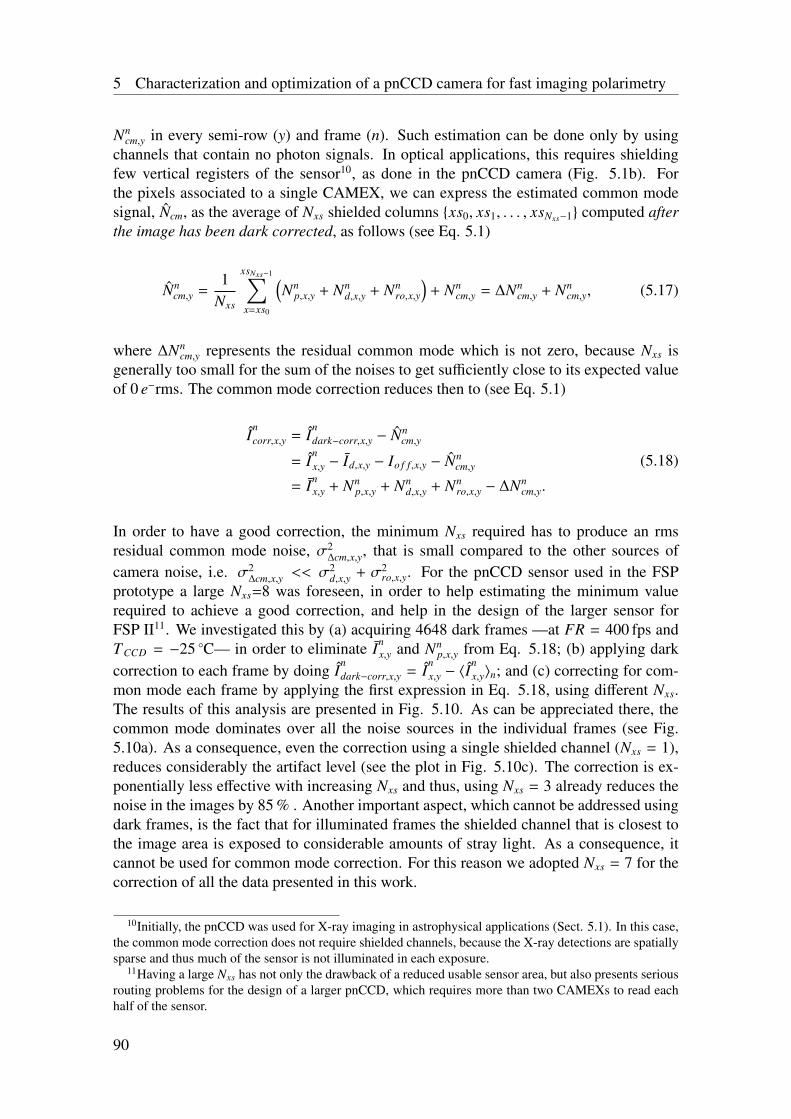
5 Characterization and optimization of a pnCCD camera for fast imaging polarimetry
Nncm,y in every semi-row (y) and frame (n). Such estimation can be done only by using
channels that contain no photon signals. In optical applications, this requires shieldingfew vertical registers of the sensor10, as done in the pnCCD camera (Fig. 5.1b). Forthe pixels associated to a single CAMEX, we can express the estimated common modesignal, Ncm, as the average of Nxs shielded columns xs0, xs1, . . . , xsNxs−1 computed afterthe image has been dark corrected, as follows (see Eq. 5.1)
Nncm,y =
1Nxs
xsNxs−1∑x=xs0
(Nn
p,x,y + Nnd,x,y + Nn
ro,x,y
)+ Nn
cm,y = ∆Nncm,y + Nn
cm,y, (5.17)
where ∆Nncm,y represents the residual common mode which is not zero, because Nxs is
generally too small for the sum of the noises to get sufficiently close to its expected valueof 0 e−rms. The common mode correction reduces then to (see Eq. 5.1)
Incorr,x,y = I
ndark−corr,x,y − Nn
cm,y
= Inx,y − Id,x,y − Io f f ,x,y − Nn
cm,y
= Inx,y + Nn
p,x,y + Nnd,x,y + Nn
ro,x,y − ∆Nncm,y.
(5.18)
In order to have a good correction, the minimum Nxs required has to produce an rmsresidual common mode noise, σ2
∆cm,x,y, that is small compared to the other sources ofcamera noise, i.e. σ2
∆cm,x,y << σ2d,x,y + σ2
ro,x,y. For the pnCCD sensor used in the FSPprototype a large Nxs=8 was foreseen, in order to help estimating the minimum valuerequired to achieve a good correction, and help in the design of the larger sensor forFSP II11. We investigated this by (a) acquiring 4648 dark frames —at FR = 400 fps andTCCD = −25 C— in order to eliminate In
x,y and Nnp,x,y from Eq. 5.18; (b) applying dark
correction to each frame by doing Indark−corr,x,y = I
nx,y − 〈I
nx,y〉n; and (c) correcting for com-
mon mode each frame by applying the first expression in Eq. 5.18, using different Nxs.The results of this analysis are presented in Fig. 5.10. As can be appreciated there, thecommon mode dominates over all the noise sources in the individual frames (see Fig.5.10a). As a consequence, even the correction using a single shielded channel (Nxs = 1),reduces considerably the artifact level (see the plot in Fig. 5.10c). The correction is ex-ponentially less effective with increasing Nxs and thus, using Nxs = 3 already reduces thenoise in the images by 85 % . Another important aspect, which cannot be addressed usingdark frames, is the fact that for illuminated frames the shielded channel that is closest tothe image area is exposed to considerable amounts of stray light. As a consequence, itcannot be used for common mode correction. For this reason we adopted Nxs = 7 for thecorrection of all the data presented in this work.
10Initially, the pnCCD was used for X-ray imaging in astrophysical applications (Sect. 5.1). In this case,the common mode correction does not require shielded channels, because the X-ray detections are spatiallysparse and thus much of the sensor is not illuminated in each exposure.
11Having a large Nxs has not only the drawback of a reduced usable sensor area, but also presents seriousrouting problems for the design of a larger pnCCD, which requires more than two CAMEXs to read eachhalf of the sensor.
90
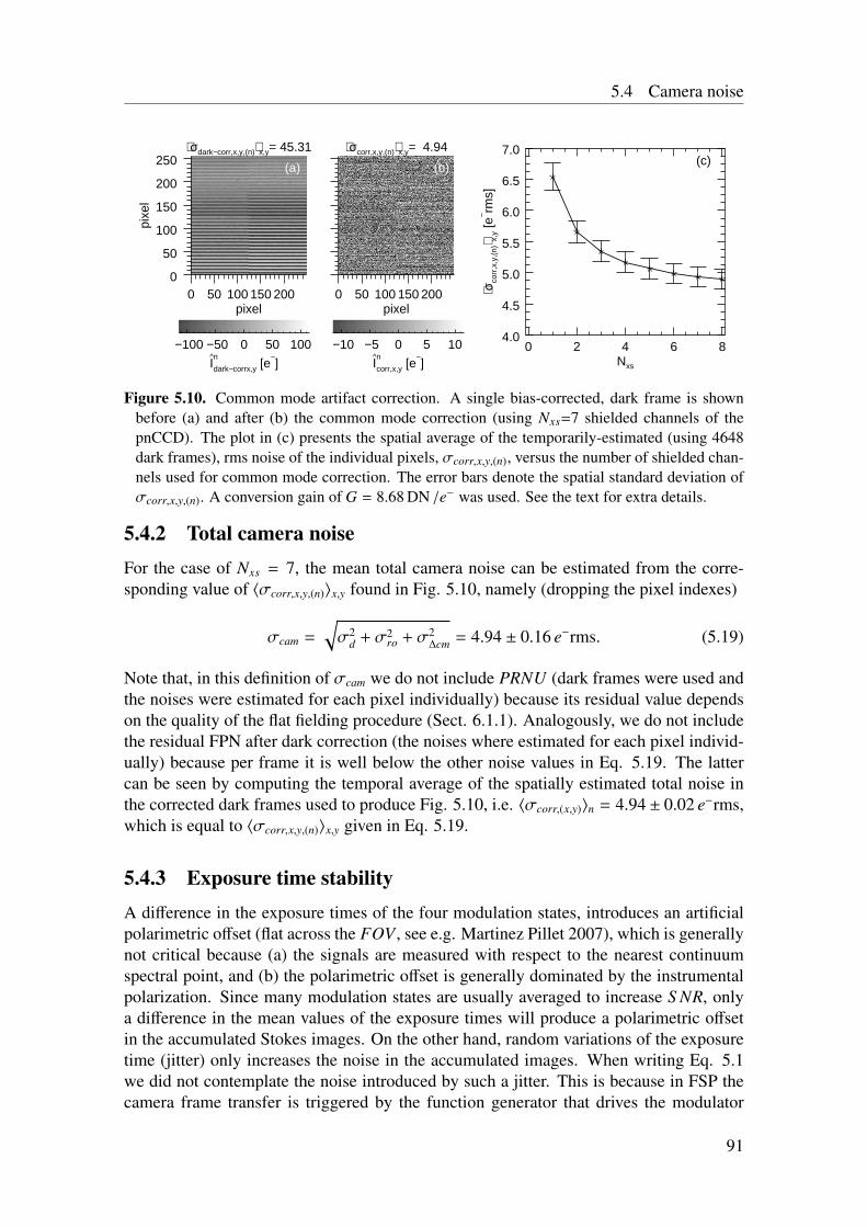
5.4 Camera noise
⟨σdark−corr,x,y,(n)⟩x,y= 45.31
0 50 100 150 200pixel
0
50
100
150
200
250pi
xel
⟨σcorr,x,y,(n)⟩x,y= 4.94
0 50 100 150 200pixel
0 2 4 6 8Nxs
4.0
4.5
5.0
5.5
6.0
6.5
7.0
⟨σco
rr,x
,y,(
n)⟩ x,
y [e
− rms]
−100 −50 0 50 100
I^n
dark−corrx,y [e−]
−10 −5 0 5 10
I^n
corr,x,y [e−]
(a) (b) (c)
Figure 5.10. Common mode artifact correction. A single bias-corrected, dark frame is shownbefore (a) and after (b) the common mode correction (using Nxs=7 shielded channels of thepnCCD). The plot in (c) presents the spatial average of the temporarily-estimated (using 4648dark frames), rms noise of the individual pixels, σcorr,x,y,(n), versus the number of shielded chan-nels used for common mode correction. The error bars denote the spatial standard deviation ofσcorr,x,y,(n). A conversion gain of G = 8.68 DN /e− was used. See the text for extra details.
5.4.2 Total camera noiseFor the case of Nxs = 7, the mean total camera noise can be estimated from the corre-sponding value of 〈σcorr,x,y,(n)〉x,y found in Fig. 5.10, namely (dropping the pixel indexes)
σcam =
√σ2
d + σ2ro + σ2
∆cm = 4.94 ± 0.16 e−rms. (5.19)
Note that, in this definition of σcam we do not include PRNU (dark frames were used andthe noises were estimated for each pixel individually) because its residual value dependson the quality of the flat fielding procedure (Sect. 6.1.1). Analogously, we do not includethe residual FPN after dark correction (the noises where estimated for each pixel individ-ually) because per frame it is well below the other noise values in Eq. 5.19. The lattercan be seen by computing the temporal average of the spatially estimated total noise inthe corrected dark frames used to produce Fig. 5.10, i.e. 〈σcorr,(x,y)〉n = 4.94 ± 0.02 e−rms,which is equal to 〈σcorr,x,y,(n)〉x,y given in Eq. 5.19.
5.4.3 Exposure time stabilityA difference in the exposure times of the four modulation states, introduces an artificialpolarimetric offset (flat across the FOV , see e.g. Martinez Pillet 2007), which is generallynot critical because (a) the signals are measured with respect to the nearest continuumspectral point, and (b) the polarimetric offset is generally dominated by the instrumentalpolarization. Since many modulation states are usually averaged to increase S NR, onlya difference in the mean values of the exposure times will produce a polarimetric offsetin the accumulated Stokes images. On the other hand, random variations of the exposuretime (jitter) only increases the noise in the accumulated images. When writing Eq. 5.1we did not contemplate the noise introduced by such a jitter. This is because in FSP thecamera frame transfer is triggered by the function generator that drives the modulator
91

5 Characterization and optimization of a pnCCD camera for fast imaging polarimetry
(see Sect. 3.2.2), which is very stable (see Sect. 4.3.3). Each frame of the pnCCD cameracarries a 1 µs accuracy time stamp. For example, in a series of 28426 frames acquiredwith FR=400 fps, we measured a mean frame acquisition period (time difference betweenconsecutive time stamps) of 2.500 ms with a standard deviation of 2.53 µs.
5.4.4 Readout and quantization noiseThe noise in common-mode-corrected, dark frames —temporally estimated for each pixelusing many frames— can be decomposed as follows
σ2corr,x,y,(n) = σ2
d,x,y,(n) + σ2ro,x,y,(n) + σ2
∆cm,x,y,(n)
= G2x,yid,x,y
[te + ts + tt (Nrow − y) + troy
]+ σ2
ro,x,y,(n) + σ2∆cm,x,y,(n)
= G2x,yid,x,yttot + σ2
ro,x,y,(n) + σ2∆cm,x,y,(n),
(5.20)
where we have used the last equality in Eq.5.18 (assuming Inx,y = 0); and Eq. 5.3, assuming
that id,x,y of the pixels in a single column are approximately the same. ttot is the totallifetime of the charge wells during each acquisition, which depends on the y coordinateof the considered pixel. The most common technique to measure the readout noise of thecamera involves acquiring many ’zero-exposures’ frames, i.e. with ttot short enough tomake the dark noise contribution (first term in the right hand side of Eq. 5.20) negligible.Note that, in frame transfer CCDs, the minimum possible ttot is tt (Nrow − y) + troy. Forcameras with large σro,x,y,(n), fast readout and frame transfer (small tro and tt), usuallythe minimum ttot is small enough to allow and accurate measurement of σro,x,y,(n). In thepnCCD, however, this is not the case and thus we measured σro,x,y,(n) by acquiring frameswith the charge transfer direction reversed, i.e. no charges are deposited in the readoutcapacitance. This is practically equivalent to do ttot = 0 ms at the expense of loosing anydependence of σro,x,y,(n) on y. The latter is not a problem because each semi-column of thesensor has its own readout channel. We acquired 1000 frames in such a reversed transfermode for different frame rates, and computed σcorr,x,y,(n) =
(σ2
ro,x,y,(n) + σ2∆cm,x,y,(n)
)1/2, see
Fig. 5.11. Note that, σcorr,x,y,(n) does not depend on FR because the readout is done at afixed frequency (tro is constant).
The ADCs used to digitalize the anlog outputs of the CAMEX have a resolution ofNadc = 14 bit with NENOB = 10 ENOB. Therefore, the contribution of the quantizationnoise (see Eq. 3.3) to the readout noise is small, i.e. Nadc=0.53 e−rms for a conversiongain of G=8.68 DN /e−.
5.4.5 Dark noise, offset and dynamic rangeComparing the measured mean value of σcorr,x,y,(n) at FR=400 fps shown in Fig. 5.11 withEq. 5.19, it is evident that the total camera noise is dominated by the readout (plus residualcommon mode) noise for the normal working temperature of TCCD = −25 C. Moreover,a rough estimation of the dark noise in this regime is
√4.94 − 4.93 = 0.31 e−rms. Since
the total lifetime of the charge wells (ttot, see Eq. 5.20) depends on the y (row) coordinate,and tro (∼8.66 µs) is larger than tt (∼0.26 µs), the pixels located near the center of theimage will accumulate on average more dark charges.
92

5.5 Photon-noise limited regime
⟨σcorr,x,y,(n)⟩x,y=4.93; σcorr,x,y,(n)(x,y)=0.17
0 50 100 150 200pixel
0
50
100
150
200
250pi
xel
200 400 600 800FR [fps]
4.6
4.8
5.0
5.2
⟨σco
rr,x
,y,(
n)⟩ x,
y [e
− rms]
4.4 4.6 4.8 5.0 5.2 5.4σcorr,x,y,(n) [e
−rms]
Figure 5.11. Measured readout plus residual common mode noise of the pnCCD camera. Theleftmost image shows the temporally-estimated noise in 1000, common-mode and bias correcteddark frames. The frames were acquired at a frame rate of FR=400 fps, and with the chargetransfer direction reversed in order to avoid any contribution from thermal charges. The sameprocedure was repeated for different FR, the resulting mean values of the noises are shown inthe rightmost plot. See the text for extra details.
A typical bias frame used for dark correction at FR=400 fps is presented in Fig. 5.12,including its time stability. From the latter it can be seen that the bias of the lower right(LR) quadrant presents a slightly worse time stability than the upper left quadrant (UL,which is similar to the other quadrants), i.e. the standard deviations of the curves for LRand UL are 7.6 and 5.3 DN respectively. This may be the reason for the increased residualoffsets detected in the LR quadrant in Fig. 5.9d, although its confirmation requires furtherinvestigation. Note that the bias frame shown in Fig. 5.12 presents few (∼ 16) hot pixels(with values from 300 up to 3000 DN above the spatial mean). The source of such pixelshas not been identified, however, they are filtered out during data reduction.
Using the spatial mean value of the bias frame given in Fig. 5.12, 〈Indark,x,y〉n,x,y, and
the previously found G=8.68 DN /e− and σcam=4.94 e−rms; we can estimate the dynamicrange per frame of the pnCCD camera to be
(2Nadc − 〈I
ndark,x,y〉n,x,y
)/(Gσcam) = 285.
5.5 Photon-noise limited regimeAs discussed in Sect. 2.1.4, solely the photon-noise imposes severe constraints on theachievable S NR when doing high-resolution, imaging spectropolarimetry of dynamic so-lar signals. Therefore, reducing any noise contribution from the camera or modulator isvery important. To illustrate this, let us express the required number of Stokes images(Nstk, i.e. four times the number of intensity frames) that need to be averaged, in orderto achieve a desired noise level in the normalized Stokes parameter i ∈ I, q, u, v (σi) asfollows
Nstk =κint
ε2i Nmodσ
2i 〈I
n〉n
(1 +
σ2cam
σ2p
), (5.21)
where κint = 1 e−; 〈In〉n is expressed in e−, i.e. we redefined 〈In
〉n → 〈In〉n/G (see
93
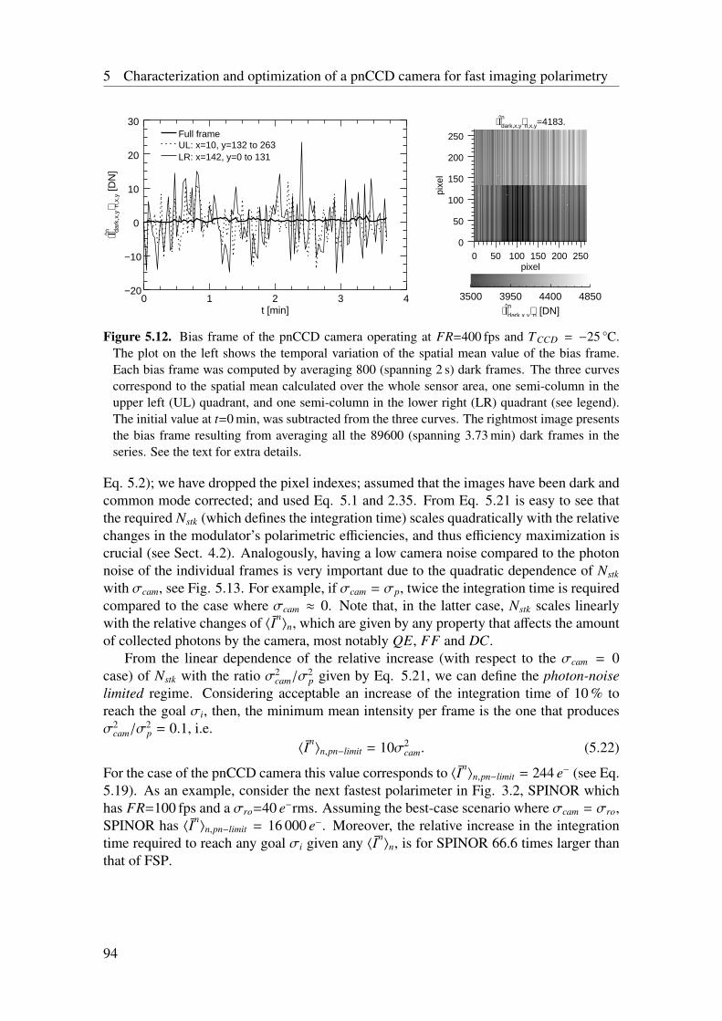
5 Characterization and optimization of a pnCCD camera for fast imaging polarimetry
0 1 2 3 4t [min]
−20
−10
0
10
20
30⟨I^n da
rk,x
,y⟩ n,
x,y
[DN
]⟨I^n
dark,x,y⟩n,x,y=4183.
0 50 100 150 200 250pixel
0
50
100
150
200
250
pixe
l
Full frameUL: x=10, y=132 to 263LR: x=142, y=0 to 131
3500 3950 4400 4850⟨I^n
dark,x,y⟩n [DN]
Figure 5.12. Bias frame of the pnCCD camera operating at FR=400 fps and TCCD = −25 C.The plot on the left shows the temporal variation of the spatial mean value of the bias frame.Each bias frame was computed by averaging 800 (spanning 2 s) dark frames. The three curvescorrespond to the spatial mean calculated over the whole sensor area, one semi-column in theupper left (UL) quadrant, and one semi-column in the lower right (LR) quadrant (see legend).The initial value at t=0 min, was subtracted from the three curves. The rightmost image presentsthe bias frame resulting from averaging all the 89600 (spanning 3.73 min) dark frames in theseries. See the text for extra details.
Eq. 5.2); we have dropped the pixel indexes; assumed that the images have been dark andcommon mode corrected; and used Eq. 5.1 and 2.35. From Eq. 5.21 is easy to see thatthe required Nstk (which defines the integration time) scales quadratically with the relativechanges in the modulator’s polarimetric efficiencies, and thus efficiency maximization iscrucial (see Sect. 4.2). Analogously, having a low camera noise compared to the photonnoise of the individual frames is very important due to the quadratic dependence of Nstk
with σcam, see Fig. 5.13. For example, if σcam = σp, twice the integration time is requiredcompared to the case where σcam ≈ 0. Note that, in the latter case, Nstk scales linearlywith the relative changes of 〈In
〉n, which are given by any property that affects the amountof collected photons by the camera, most notably QE, FF and DC.
From the linear dependence of the relative increase (with respect to the σcam = 0case) of Nstk with the ratio σ2
cam/σ2p given by Eq. 5.21, we can define the photon-noise
limited regime. Considering acceptable an increase of the integration time of 10 % toreach the goal σi, then, the minimum mean intensity per frame is the one that producesσ2
cam/σ2p = 0.1, i.e.
〈In〉n,pn−limit = 10σ2
cam. (5.22)
For the case of the pnCCD camera this value corresponds to 〈In〉n,pn−limit = 244 e− (see Eq.
5.19). As an example, consider the next fastest polarimeter in Fig. 3.2, SPINOR whichhas FR=100 fps and a σro=40 e−rms. Assuming the best-case scenario where σcam = σro,SPINOR has 〈In
〉n,pn−limit = 16 000 e−. Moreover, the relative increase in the integrationtime required to reach any goal σi given any 〈In
〉n, is for SPINOR 66.6 times larger thanthat of FSP.
94
5.5 Photon-noise limited regime
σi=1×10⁻³
; εi=1/√ 3
0 10 20 30 40 50σcam [e
−rms]
0.1
1.0
10.0
100.0
Inte
grat
ion
time
[min
]
10 e
−
25 e−
50 e−
100 e−
200 e−
500 e−
1000 e−
Figure 5.13. Integration time required to achieve a noise level of 1 × 10⁻³ in the normalizedStokes images, versus the total camera noise for different intensity levels (〈In
〉n, annotated overeach continuous curve). Note that the vertical axis is in logarithmic scale. The figures werecomputed using Eq. 5.21, assuming a frame rate of 400 fps and the parameters shown in the title(note that for a given frame rate, the integration time is independent of Nmod). The horizontaldotted line indicates the typical lifetime of solar granulation (5 min). As an example, in the VTTwe obtained (working at the diffraction limit) a 〈In
〉n of ∼12 and ∼300 e− for the line core of CaI 422.7 nm and the continuum near Fe I 630.2 nm respectively (see Ch. 6). See also Table 3.2for typical values of σro (which generally dominates σcam) in solar polarimeters.
95

6 First light measurements
After integration of the main FSP components in the laboratory, the instrumental conceptwas tested in five first-light campaigns. These were carried out using the 68 cm, GermanVTT located in El Tedie observatory, Tenerife, between the years 2013 and 2015.
The present chapter describes some of the results of such observations, along with themost relevant tasks that were carried out in order to obtain the final data sets. The empha-sis is put on the data reduction pipeline (Section 6.1), for the reason that its realizationrequires understanding the main components of the system and thus, is in close relation-ship with the results obtained in Chapters 4 and 5. One example observation is givenfor FSP working in spectrograph mode (Section 6.2) and two for the case of filtergraph(Section 6.3). In addition, we present the results of the firsts applications of MOMFBDto filtergraph-based FSP measurements, including a short overview of the different waysin which the restoration of the data can be approached. The results of the presented mea-surements are used to asses the performance of the polarimeter, including the achievedpolarimetric sensitivity and residual levels of SIC (Section 6.4). Some of the contents ofthe present chapter have been published in Iglesias et al. (2016).
6.1 Data acquisition and reductionIn the following sections we describe in a nutshell the most important data reduction steps,required to process FSP data. The same steps are applied for measurements carried outwith a spectrograph or with a filtergraph unless explicitly stated. A typical measurementinvolves the acquisition of (a) science measurements, with modulated intensities I; (b)flat field measurements, with modulated intensities I f lat; (c) dark measurements, with in-tensities Idark ; and (d) polarimetric calibration measurements, with modulated intensitiesIcal.
6.1.1 Intensity calibrationThe first step involves the calibration of the modulated intensities acquired with thepnCCD camera. This requires the following
1. Science data acquisition: Given a goal noise in the normalized Stokes vectors ofthe science images, σ, the required number of Stokes measurements (Nstk) can bederived from Eq. 5.21.
2. Missing frames and phase detection: Since the synchronization of camera and mod-ulator is crucial to allow the demodulation of the acquired intensities, every single
97
6 First light measurements
missing frame has to be carefully identified (using the time stamps, see Sect. 5.4.3)and the full modulation cycle removed. Another critical aspect is the definition ofwhich of the four modulation states is considered the first one. Such a first state hasto be the same in all data sets, including the calibration measurements. One draw-back of the pnCCD camera design was that the identification of the modulationstates corresponding to each frame was not implemented. Therefore a workaroundthat includes an initial overexposure was used. This issue was taken into consider-ation when designing the new FSP II camera.
3. Dark correction: Before or after the science images have been acquired, the darkmeasurements are carried out. The number of dark frames required, N f rm−dark, canbe computed from σcam/
√N f rm−dark << σ and Eq. 5.19. Then, the science images
are dark corrected by doing Incorr0,x,y = I
nx,y − 〈I
ndark,x,y〉n (see Eq. 5.1).
4. Common mode correction: Each frame is common mode corrected by applying Eq.5.18. After this, the shielded channels of the sensor are cropped from all frames toobtain I
ncorr1,x,y.
5. Frame transfer correction: The smearing is eliminated from each modulation state(set of four intensity frames) by applying Eq. 5.12 to each column of I
ncorr1,x,y. This
results in the desmeared intensities Incorr2,x,y. Note that Eq. 5.12 assumes a periodic
signal, i.e. a constant input Stokes vector. If this is not the case, Eq. 5.6 has to beused (iteratively solved) instead.
6. Flat fielding: The acquisition of the flat field is done by randomly moving thetelescope in a quiet region of the Sun, around the same longitude as the scienceobservations, and disabling the AO correction. Since the telescope motion has afixed velocity, the faster the camera, the more frames have to be acquired to en-sure the proper smearing of the solar structures in the background. From a noisepoint of view, the number of flat frames required, N f rm− f lat, can be obtained from√
(σcam2 + I f lat)/N f rm− f lat << σ, where I f lat is the mean intensity in the flat images.
The corrected (after undergoing steps 2 to 5) flat field data, Inf lat−corr2,x,y, are used
to eliminate the spatial variations of the gain table in the science data by doingI
ncorr3,x,y = I
ncorr2,x,y ∗ 〈I
nf lat−corr2,x,y〉n,x,y/〈I
nf lat−corr2,x,y〉n. This procedure takes into ac-
count both the spatial variations of the detector G and the optical gain of the setup.In addition, since the average of all frames (independently of the modulation state)of I
nf lat−corr2,x,y is used, no polarized components of the flat field can be corrected
using this technique. When using a spectrograph, the spectral lines are present inthe flat field1 complicating the correction of the pixels located in the lines. To copewith this, the spectral lines are numerically removed from 〈I
nf lat−corr2,x,y〉n by interpo-
lating in the wavelength dimension. When observing with a multi-etalon filtergraphin telecentric configuration (Sect. 2.2.3), as for the measurements presented in Sect.6.2, the flat field is usually dominated by the etalons errors. Therefore we acquireand apply an independent flat field for each spectral point. Given a spatially con-stant spectral content of the incoming intensity during flat fielding, variations in
1Moving the spectral lines out of the FOV implies retuning the spectrograph setup which would modifythe flat field and produce an erroneous correction.
98
6.1 Data acquisition and reduction
the etalon cavities (optical path length) and reflectance across their aperture, pro-duce a spatial variation of the transmission profiles. The transmission profile ofthe multi-etalon setup can vary in amplitude, width and spectral location. Whileall these phenomena produce a spatial fluctuation of the output intensity, the flatfielding process described above can correct only for local changes of the ampli-tude and not for spectral shifts of the transmission profiles. The latter, however, arehigher-order errors that can be corrected in an extra step (not described here, seede la Cruz Rodríguez et al. 2015) if required.
7. Image restoration: In this step, the modulated intensities ( Incorr3,x,y) can be option-
ally restored by using a MOMFBD, this is detailed in Sect. 6.1.5. Note that the flatfielding procedure described in the previous step, only affects the resulting StokesI images. Thus it could also be applied after the polarimetric demodulation onlyon Stokes I. We have done it in the 6th step, however, because it is required if theintensity images are restored before demodulation.
6.1.2 Polarimetric calibrationThe polarimetric calibration is done as explained in Sect. 4.3. We typically recordNcal = 18 independent calibration inputs, see Fig. 4.5. When working with a filter-graph, the calibration is acquired in the nearest continuum spectral position (see Sect.4.3.2) and with the telescope moving in flat field mode, to ensure an unpolarized and flatinput for the PSG. This, however, contributes to increasing the input intensity fluctua-tions (see foot note 10 on Sect. 4.3.1), which complicates the implementation of a fielddependent demodulation, see Sect 4.3.1. When working with a spectrograph, the cali-bration is performed covering the same spectral range as the science data. The spectrallines are excluded (due to the low S NR) when computing the spatial mean to obtain ascalar demodulation matrix (Sect 4.3.1). The estimated demodulation matrix, D, is usedto demodulate the science data by doing Sx,y = DIcorr3,x,y for each modulation cycle.
6.1.3 Frame accumulation and polarimetric normalizationAfter demodulation, the Nstk Stokes images acquired are normalized (Eq. 2.11) and accu-mulated to reduce noise. The accumulation and normalization operations do not commuteand thus an order of application has to be selected. Considering Stokes Q, the two pos-sible options are 〈Q
nx,y/I
nx,y〉n and 〈Q
nx,y〉n/〈I
nx,y〉n. Out of these two options, only the latter
is an asymptotically (for Nstk → ∞) unbiased estimator for the ratio of the expectationvalues, Qx,y/Ix,y (see Fig. 6.1). The second order approximation to the expected value ofboth estimators is (see van Kempen and van Vliet 2000),
E
⟨ Qnx,y
Inx,y
⟩n
=Qx,y
Ix,y+ κbias and E
〈Qnx,y〉n
〈Inx,y〉n
=Qx,y
Ix,y+κbias
Nstk, (6.1)
where κbias = (Qx,y1[DN] − σ2Q,I,x,y)/I
2x,y, E represents the expectation value operator and
σ2Q,I,x,y is the covariance between Qx,y and Ix,y. Note that Ix,y is in the denominator of κbias,
this produces a crosstalk from Stokes I which is spatially non-flat and increases for shortexposure times.
99
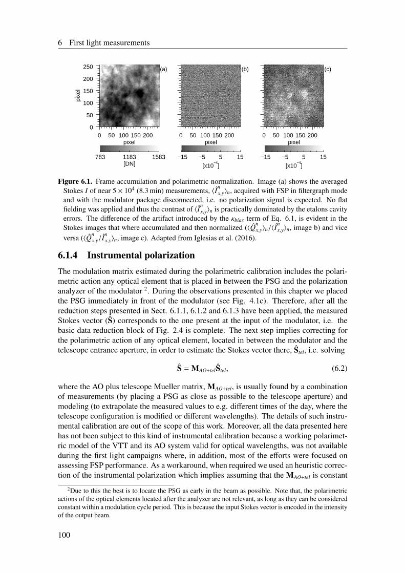
6 First light measurements
0 50 100 150 200pixel
0
50
100
150
200
250
pixe
l
0 50 100 150 200pixel
0 50 100 150 200pixel
783 1183 1583[DN]
−15 −5 5 15
[x10−4
]
−15 −5 5 15
[x10−4
]
(a) (b) (c)
Figure 6.1. Frame accumulation and polarimetric normalization. Image (a) shows the averagedStokes I of near 5 × 10⁴ (8.3 min) measurements, 〈In
x,y〉n, acquired with FSP in filtergraph modeand with the modulator package disconnected, i.e. no polarization signal is expected. No flatfielding was applied and thus the contrast of 〈In
x,y〉n is practically dominated by the etalons cavityerrors. The difference of the artifact introduced by the κbias term of Eq. 6.1, is evident in theStokes images that where accumulated and then normalized (〈Qn
x,y〉n/〈Inx,y〉n, image b) and vice
versa (〈Qnx,y/I
nx,y〉n, image c). Adapted from Iglesias et al. (2016).
6.1.4 Instrumental polarizationThe modulation matrix estimated during the polarimetric calibration includes the polari-metric action any optical element that is placed in between the PSG and the polarizationanalyzer of the modulator 2. During the observations presented in this chapter we placedthe PSG immediately in front of the modulator (see Fig. 4.1c). Therefore, after all thereduction steps presented in Sect. 6.1.1, 6.1.2 and 6.1.3 have been applied, the measuredStokes vector (S) corresponds to the one present at the input of the modulator, i.e. thebasic data reduction block of Fig. 2.4 is complete. The next step implies correcting forthe polarimetric action of any optical element, located in between the modulator and thetelescope entrance aperture, in order to estimate the Stokes vector there, Stel, i.e. solving
S = MAO+telStel, (6.2)
where the AO plus telescope Mueller matrix, MAO+tel, is usually found by a combinationof measurements (by placing a PSG as close as possible to the telescope aperture) andmodeling (to extrapolate the measured values to e.g. different times of the day, where thetelescope configuration is modified or different wavelengths). The details of such instru-mental calibration are out of the scope of this work. Moreover, all the data presented herehas not been subject to this kind of instrumental calibration because a working polarimet-ric model of the VTT and its AO system valid for optical wavelengths, was not availableduring the first light campaigns where, in addition, most of the efforts were focused onassessing FSP performance. As a workaround, when required we used an heuristic correc-tion of the instrumental polarization which implies assuming that the MAO+tel is constant
2Due to this the best is to locate the PSG as early in the beam as possible. Note that, the polarimetricactions of the optical elements located after the analyzer are not relevant, as long as they can be consideredconstant within a modulation cycle period. This is because the input Stokes vector is encoded in the intensityof the output beam.
100
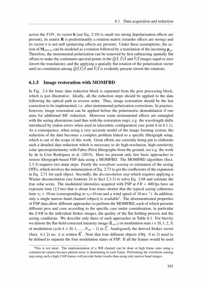
6.1 Data acquisition and reduction
across the FOV , its vector h (see Eq. 2.10) is small (no strong depolarization effects arepresent), its matrix R is predominantly a rotation matrix (retarder effects are strong) andits vector v is not null (polarizing effects are present). Under these assumptions, the ac-tion of MAO+tel can be modeled as a rotation followed by a translation of the incoming ptel.Therefore, the instrumental polarization can be removed by first subtracting spatially flatoffsets to make the continuum spectral points in the Q/I, U/I and V/I images equal to zero(invert the translation); and the applying a spatially flat rotation of the polarization vectoruntil no correlation among Q/I,U/I and V/I is evidently present (invert the rotation).
6.1.5 Image restoration with MOMFBD
In Fig. 2.4 the basic data reduction block is separated from the post processing block,which is just illustrative. Ideally, all the reduction steps should be applied to the datafollowing the optical path in reverse order. Thus, image restoration should be the lastcorrection to be implemented, i.e. after instrumental polarization corrections. In practice,however, image restoration can be applied before the polarimetric demodulation if oneaims for additional SIC reduction. Moreover some instrumental effects are entangledwith the seeing aberrations (and thus with the restoration step), e.g. the wavelength shiftsintroduced by etalon errors when used in telecentric configuration (see point 6 in 6.1.1).As a consequence, when using a very accurate model of the image forming system, thereduction of the data becomes a complex problem linked to a specific filtergraph setup,which is out of the scope of this work. Great efforts are currently being put to elaboratesuch a detailed data reduction which is necessary to do high-resolution, high-sensitivitysolar spectropolarimetry with Fabry-Pérot filtergraphs from the ground, see e.g. the workby de la Cruz Rodríguez et al. (2015). Here we present only few basic approaches torestore filtergraph-based FSP data using a MOMFBD. The MOMFBD algorithm (Sect.2.3.3) requires two main steps. Firstly the wavefront sensing or estimation of the seeingOTFs, which involves the minimization of Eq. 2.73 to get the coefficients of the expansionin Eq. 2.71 for each object. Secondly, the deconvolution step which requires applying aWiener deconvolution (see footnote 24 in Sect 2.3.3) to solve Eq. 2.68 and estimate thetrue solar scene. The modulated intensities acquired with FSP at FR = 400 fps have anexposure time (2.5 ms) that is about four times shorter that the typical seeing coherencetime τ0 ≈ 10 ms (corresponding to r0=10 cm and a wind speed of 10 m s−1). In addition,only a single narrow-band channel (object) is available3. The aforementioned propertiesof FSP data allow different approaches to perform the MOMFBD, each of which presentsdifferent pros and cons according to the specific case under consideration, in particularthe S NR in the individual Stokes images, the quality of the flat fielding process and theseeing conditions. We describe only three of such approaches in Table 6.1. For brevitywe denote the flat-field-corrected intensity image (Icorr3) in modulation state i ∈ 0, 1, 2, 3of modulation cycle k ∈ 0, 1, . . . ,Nstk − 1 as I
ki . Analogously the derived Stokes vector
(Sect. 6.1.2) no. k is written Sk. Note that four different objects (Obj. 0 to 3) need to
be defined to separate the four modulation states of FSP. If all the frames would be used
3This is not ideal. The implementation of a WB channel can be done at high frame rates using acommercial camera because photon noise is dominating in each frame. Performing the wavefront sensingstep using such a high S NR frames will provide better results than using only narrow band images.
101
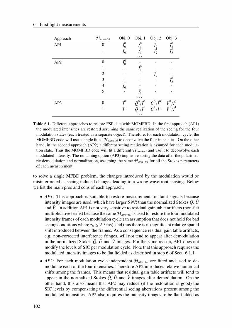
6 First light measurements
Approach Hatm+tel Obj. 0 Obj. 1 Obj. 2 Obj. 3
AP1 0 I00 I0
1 I02 I0
31 I1
0 I11 I1
2 I13
. . .
AP2 0 I00 - - -
1 - I01 - -
2 - - I02 -
3 - - - I03
4 I10 - - -
5 - I11 - -
. . .
AP3 0 I0 Q0/I0 U0
/I0 V0/I0
1 I1 Q1/I1 U1
/I1 V1/I1
. . .
Table 6.1. Different approaches to restore FSP data with MOMFBD. In the first approach (AP1)the modulated intensities are restored assuming the same realization of the seeing for the fourmodulation states (each treated as a separate object). Therefore, for each modulation cycle, theMOMFBD code will use a single fittedHatm+tel to deconvolve the four intensities. On the otherhand, in the second approach (AP2) a different seeing realization is assumed for each modula-tion state. Thus the MOMFBD code will fit a different Hatm+tel and use it to deconvolve eachmodulated intensity. The remaining option (AP3) implies restoring the data after the polarimet-ric demodulation and normalization, assuming the same Hatm+tel for all the Stokes parametersof each measurement.
to solve a single MFBD problem, the changes introduced by the modulation would bemisinterpreted as seeing induced changes leading to a wrong wavefront sensing. Belowwe list the main pros and cons of each approach.
• AP1: This approach is suitable to restore measurements of faint signals becauseintensity images are used, which have larger S NR than the normalized Stokes Q, Uand V . In addition AP1 is not very sensitive to residual gain table artifacts (non-flatmultiplicative terms) because the sameHatm+tel is used to restore the four modulatedintensity frames of each modulation cycle (an assumption that does not hold for badseeing conditions where τ0 ≤ 2.5 ms), and thus there is no significant relative spatialshift introduced between the frames. As a consequence residual gain table artifacts,e.g. non-corrected interference fringes, will not tend to appear after demodulationin the normalized Stokes Q, U and V images. For the same reason, AP1 does notmodify the levels of SIC per modulation cycle. Note that this approach requires themodulated intensity images to be flat fielded as described in step 6 of Sect. 6.1.1.
• AP2: For each modulation cycle independent Hatm+tel are fitted and used to de-modulate each of the four intensities. Therefore AP2 introduces relative numericalshifts among the frames. This means that residual gain table artifacts will tend toappear in the normalized Stokes Q, U and V images after demodulation. On theother hand, this also means that AP2 may reduce (if the restoration is good) theSIC levels by compensating the differential seeing aberrations present among themodulated intensities. AP2 also requires the intensity images to be flat fielded as
102
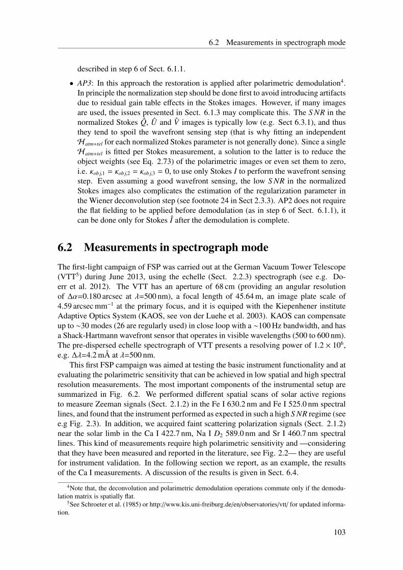
6.2 Measurements in spectrograph mode
described in step 6 of Sect. 6.1.1.
• AP3: In this approach the restoration is applied after polarimetric demodulation4.In principle the normalization step should be done first to avoid introducing artifactsdue to residual gain table effects in the Stokes images. However, if many imagesare used, the issues presented in Sect. 6.1.3 may complicate this. The S NR in thenormalized Stokes Q, U and V images is typically low (e.g. Sect 6.3.1), and thusthey tend to spoil the wavefront sensing step (that is why fitting an independentHatm+tel for each normalized Stokes parameter is not generally done). Since a singleHatm+tel is fitted per Stokes measurement, a solution to the latter is to reduce theobject weights (see Eq. 2.73) of the polarimetric images or even set them to zero,i.e. κob j,1 = κob j,2 = κob j,3 = 0, to use only Stokes I to perform the wavefront sensingstep. Even assuming a good wavefront sensing, the low S NR in the normalizedStokes images also complicates the estimation of the regularization parameter inthe Wiener deconvolution step (see footnote 24 in Sect 2.3.3). AP2 does not requirethe flat fielding to be applied before demodulation (as in step 6 of Sect. 6.1.1), itcan be done only for Stokes I after the demodulation is complete.
6.2 Measurements in spectrograph modeThe first-light campaign of FSP was carried out at the German Vacuum Tower Telescope(VTT5) during June 2013, using the echelle (Sect. 2.2.3) spectrograph (see e.g. Do-err et al. 2012). The VTT has an aperture of 68 cm (providing an angular resolutionof ∆α=0.180 arcsec at λ=500 nm), a focal length of 45.64 m, an image plate scale of4.59 arcsec mm−1 at the primary focus, and it is equiped with the Kiepenhener instituteAdaptive Optics System (KAOS, see von der Luehe et al. 2003). KAOS can compensateup to ∼30 modes (26 are regularly used) in close loop with a ∼100 Hz bandwidth, and hasa Shack-Hartmann wavefront sensor that operates in visible wavelengths (500 to 600 nm).The pre-dispersed echelle spectrograph of VTT presents a resolving power of 1.2 × 10⁶,e.g. ∆λ=4.2 mÅ at λ=500 nm.
This first FSP campaign was aimed at testing the basic instrument functionality and atevaluating the polarimetric sensitivity that can be achieved in low spatial and high spectralresolution measurements. The most important components of the instrumental setup aresummarized in Fig. 6.2. We performed different spatial scans of solar active regionsto measure Zeeman signals (Sect. 2.1.2) in the Fe I 630.2 nm and Fe I 525.0 nm spectrallines, and found that the instrument performed as expected in such a high S NR regime (seee.g Fig. 2.3). In addition, we acquired faint scattering polarization signals (Sect. 2.1.2)near the solar limb in the Ca I 422.7 nm, Na I D2 589.0 nm and Sr I 460.7 nm spectrallines. This kind of measurements require high polarimetric sensitivity and —consideringthat they have been measured and reported in the literature, see Fig. 2.2— they are usefulfor instrument validation. In the following section we report, as an example, the resultsof the Ca I measurements. A discussion of the results is given in Sect. 6.4.
4Note that, the deconvolution and polarimetric demodulation operations commute only if the demodu-lation matrix is spatially flat.
5See Schroeter et al. (1985) or http://www.kis.uni-freiburg.de/en/observatories/vtt/ for updated informa-tion.
103

6 First light measurements
Telescope
KAOS
Slit Echelle Spectrograph
pnCCD camera
ModulatorPackage
Reimaging optics
Calibrationunit
Figure 6.2. FSP setup during the first light measurements with the VTT echelle spectrograph.The boxes denote the main components located in the beam path (marked with dashed arrows).The boxes with continuous borders belong to FSP. The two photographs show the real devicesassociated to some of the boxes (indicated with continuous arrows). These include the modulatorpackage (left photo) vertically mounted on top of the box containing the spectrograph entranceslit, and the pnCCD camera (right photo) mounted at an output port of the echelle spectrograph.
6.2.1 Low SNR regime: Second solar spectrum of Ca ITo record the second solar spectrum of Ca I, the slit was located near the solar limb —atµ ≈ 0.156— were the scattering signals are stronger (Sect. 2.1.2). In addition, we orientedthe slit (which matched the Stokes Q orientation of FSP) tangential to the solar limb inorder to maximize the Stokes Q signal. As mentioned in Sect. 6.2, we aimed for highspectral but low spatial resolution which allowed us to use long integration times in orderto explore the high polarimetric sensitivity regime of FSP7. Therefore, a large spatialsampling (∆αsamp) was used, see Table 6.2. Moreover KAOS was not correcting thewavefronts because the low contrast near the limb does not allow its proper functioning.The measured values of scattering polarization and the achieved polarimetric sensitivityare presented in Fig. 6.3.
6.3 Measurements in filtergraph modeFiltergraph-based measurements are the main goal of FSP because high spatial resolutionin combination with high sensitivity are required when trying to estimate the smallest and
6µ is equal to the cosine of the angle between the LOS and the normal of the solar surface.7Since the gradient in Stokes I images is large due to the presence of the absorption spectral lines, the
system is sensitive to instrumental image motion which can introduce polarimetric crosstalk. The highmodulation frequency of FSP helps to reduce such a crosstalk.
104
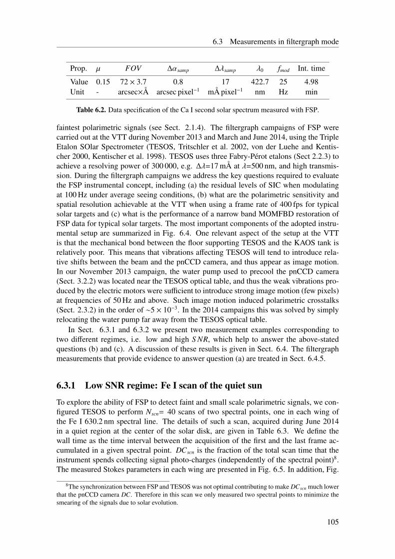
6.3 Measurements in filtergraph mode
Prop. µ FOV ∆αsamp ∆λsamp λ0 fmod Int. time
Value 0.15 72 × 3.7 0.8 17 422.7 25 4.98Unit - arcsec×Å arcsec pixel−1 mÅ pixel−1 nm Hz min
Table 6.2. Data specification of the Ca I second solar spectrum measured with FSP.
faintest polarimetric signals (see Sect. 2.1.4). The filtergraph campaigns of FSP werecarried out at the VTT during November 2013 and March and June 2014, using the TripleEtalon SOlar Spectrometer (TESOS, Tritschler et al. 2002, von der Luehe and Kentis-cher 2000, Kentischer et al. 1998). TESOS uses three Fabry-Pérot etalons (Sect 2.2.3) toachieve a resolving power of 300 000, e.g. ∆λ=17 mÅ at λ=500 nm, and high transmis-sion. During the filtergraph campaigns we address the key questions required to evaluatethe FSP instrumental concept, including (a) the residual levels of SIC when modulatingat 100 Hz under average seeing conditions, (b) what are the polarimetric sensitivity andspatial resolution achievable at the VTT when using a frame rate of 400 fps for typicalsolar targets and (c) what is the performance of a narrow band MOMFBD restoration ofFSP data for typical solar targets. The most important components of the adopted instru-mental setup are summarized in Fig. 6.4. One relevant aspect of the setup at the VTTis that the mechanical bond between the floor supporting TESOS and the KAOS tank isrelatively poor. This means that vibrations affecting TESOS will tend to introduce rela-tive shifts between the beam and the pnCCD camera, and thus appear as image motion.In our November 2013 campaign, the water pump used to precool the pnCCD camera(Sect. 3.2.2) was located near the TESOS optical table, and thus the weak vibrations pro-duced by the electric motors were sufficient to introduce strong image motion (few pixels)at frequencies of 50 Hz and above. Such image motion induced polarimetric crosstalks(Sect. 2.3.2) in the order of ∼5 × 10⁻³. In the 2014 campaigns this was solved by simplyrelocating the water pump far away from the TESOS optical table.
In Sect. 6.3.1 and 6.3.2 we present two measurement examples corresponding totwo different regimes, i.e. low and high S NR, which help to answer the above-statedquestions (b) and (c). A discussion of these results is given in Sect. 6.4. The filtergraphmeasurements that provide evidence to answer question (a) are treated in Sect. 6.4.5.
6.3.1 Low SNR regime: Fe I scan of the quiet sun
To explore the ability of FSP to detect faint and small scale polarimetric signals, we con-figured TESOS to perform Nscn= 40 scans of two spectral points, one in each wing ofthe Fe I 630.2 nm spectral line. The details of such a scan, acquired during June 2014in a quiet region at the center of the solar disk, are given in Table 6.3. We define thewall time as the time interval between the acquisition of the first and the last frame ac-cumulated in a given spectral point. DCscn is the fraction of the total scan time that theinstrument spends collecting signal photo-charges (independently of the spectral point)8.The measured Stokes parameters in each wing are presented in Fig. 6.5. In addition, Fig.
8The synchronization between FSP and TESOS was not optimal contributing to make DCscn much lowerthat the pnCCD camera DC. Therefore in this scan we only measured two spectral points to minimize thesmearing of the signals due to solar evolution.
105
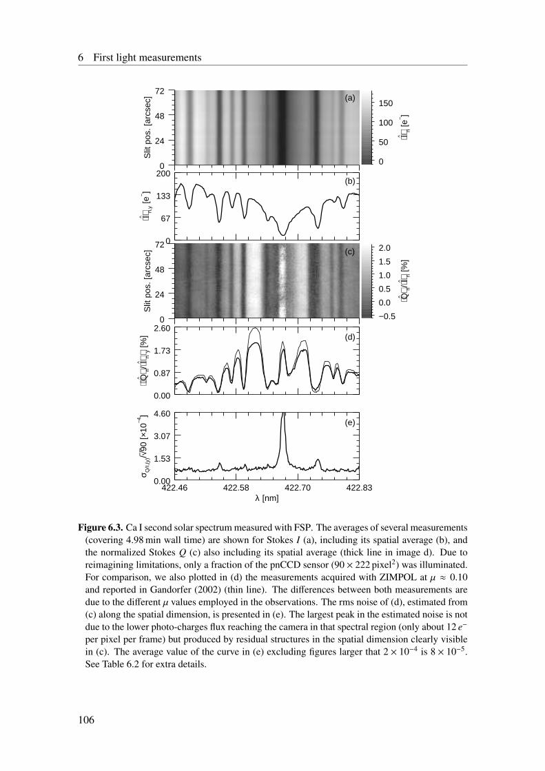
6 First light measurements
0
24
48
72
Slit
pos
. [ar
csec
]
0
24
48
72
Slit
pos
. [ar
csec
]
0
67
133
200
⟨I^ ⟩ n,y
[e− ]
0.00
0.87
1.73
2.60
⟨⟨Q ^ ⟩ n/
⟨I^ ⟩ n⟩y
[%]
422.46 422.58 422.70 422.83λ [nm]
0.00
1.53
3.07
4.60
σ Q/I,
(y)/√
90
[×10
−4]
0
50
100
150
⟨I^ ⟩ n [e
− ]
−0.5
0.0
0.5
1.0
1.5
2.0
⟨Q ^ ⟩ n/
⟨I^ ⟩ n [%
]
(a)
(b)
(c)
(d)
(e)
Figure 6.3. Ca I second solar spectrum measured with FSP. The averages of several measurements(covering 4.98 min wall time) are shown for Stokes I (a), including its spatial average (b), andthe normalized Stokes Q (c) also including its spatial average (thick line in image d). Due toreimagining limitations, only a fraction of the pnCCD sensor (90 × 222 pixel2) was illuminated.For comparison, we also plotted in (d) the measurements acquired with ZIMPOL at µ ≈ 0.10and reported in Gandorfer (2002) (thin line). The differences between both measurements aredue to the different µ values employed in the observations. The rms noise of (d), estimated from(c) along the spatial dimension, is presented in (e). The largest peak in the estimated noise is notdue to the lower photo-charges flux reaching the camera in that spectral region (only about 12 e−
per pixel per frame) but produced by residual structures in the spatial dimension clearly visiblein (c). The average value of the curve in (e) excluding figures larger that 2 × 10⁻⁴ is 8 × 10⁻⁵.See Table 6.2 for extra details.
106
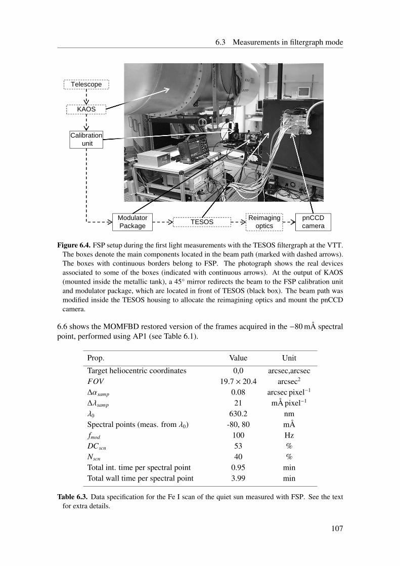
6.3 Measurements in filtergraph mode
Telescope
KAOS
TESOS pnCCD camera
ModulatorPackage
Reimaging optics
Calibrationunit
Figure 6.4. FSP setup during the first light measurements with the TESOS filtergraph at the VTT.The boxes denote the main components located in the beam path (marked with dashed arrows).The boxes with continuous borders belong to FSP. The photograph shows the real devicesassociated to some of the boxes (indicated with continuous arrows). At the output of KAOS(mounted inside the metallic tank), a 45° mirror redirects the beam to the FSP calibration unitand modulator package, which are located in front of TESOS (black box). The beam path wasmodified inside the TESOS housing to allocate the reimagining optics and mount the pnCCDcamera.
6.6 shows the MOMFBD restored version of the frames acquired in the −80 mÅ spectralpoint, performed using AP1 (see Table 6.1).
Prop. Value Unit
Target heliocentric coordinates 0,0 arcsec,arcsecFOV 19.7 × 20.4 arcsec2
∆αsamp 0.08 arcsec pixel−1
∆λsamp 21 mÅ pixel−1
λ0 630.2 nmSpectral points (meas. from λ0) -80, 80 mÅfmod 100 HzDCscn 53 %Nscn 40 %Total int. time per spectral point 0.95 minTotal wall time per spectral point 3.99 min
Table 6.3. Data specification for the Fe I scan of the quiet sun measured with FSP. See the textfor extra details.
107
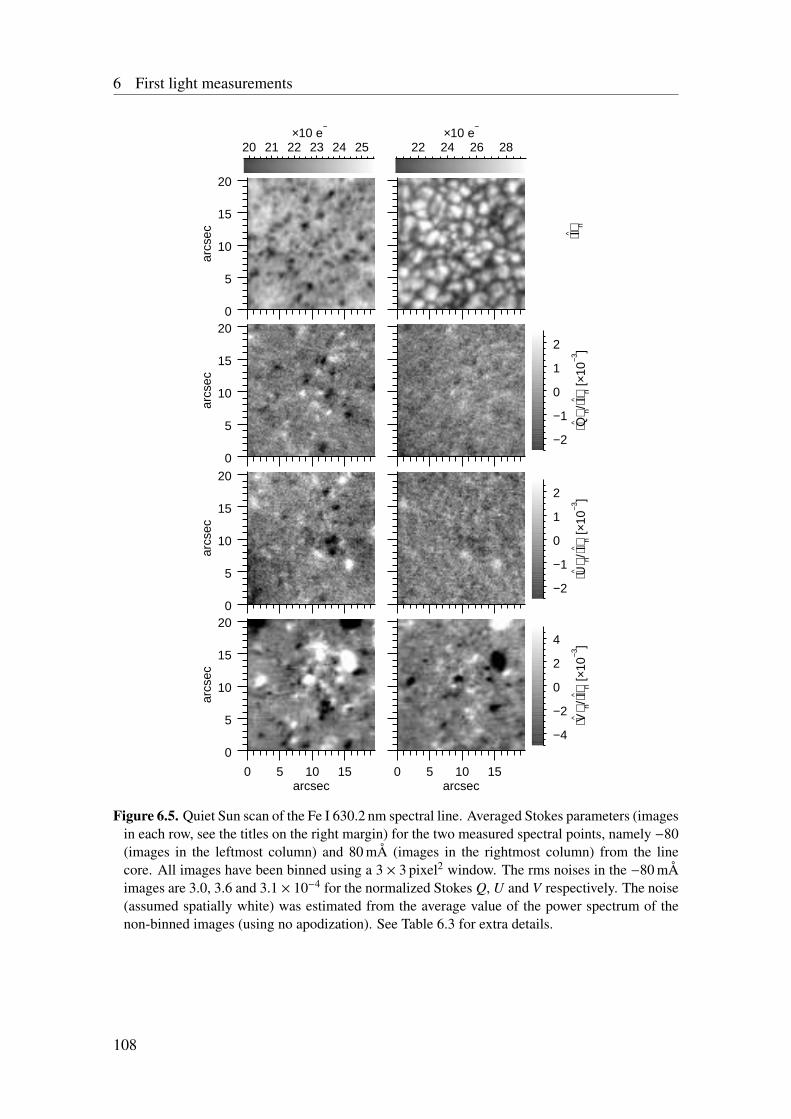
6 First light measurements
0
5
10
15
20
arcs
ec
0
5
10
15
20
arcs
ec
0
5
10
15
20
arcs
ec
0 5 10 15arcsec
0
5
10
15
20
arcs
ec
0 5 10 15arcsec
20 21 22 23 24 25×10 e
−
22 24 26 28×10 e
−
−2
−1
0
1
2
⟨Q ^ ⟩ n/
⟨I^ ⟩ n [×
10−3
]−2
−1
0
1
2
⟨U ^ ⟩ n/
⟨I^ ⟩ n [×
10−3
]
−4
−2
0
2
4
⟨V ^ ⟩ n/
⟨I^ ⟩ n [×
10−3
]⟨I^ ⟩ n
Figure 6.5. Quiet Sun scan of the Fe I 630.2 nm spectral line. Averaged Stokes parameters (imagesin each row, see the titles on the right margin) for the two measured spectral points, namely −80(images in the leftmost column) and 80 mÅ (images in the rightmost column) from the linecore. All images have been binned using a 3 × 3 pixel2 window. The rms noises in the −80 mÅimages are 3.0, 3.6 and 3.1 × 10⁻⁴ for the normalized Stokes Q, U and V respectively. The noise(assumed spatially white) was estimated from the average value of the power spectrum of thenon-binned images (using no apodization). See Table 6.3 for extra details.
108
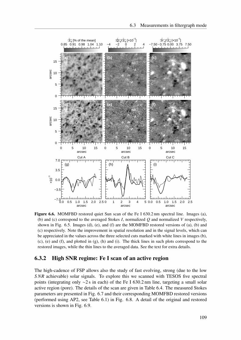
6.3 Measurements in filtergraph mode
(a)
0
5
10
15
arcs
ec
(b)
A
(c)
BC
(d)
0 5 10 15arcsec
0
5
10
15
arcs
ec
(e)
A
0 5 10 15arcsec
(f)
BC
0 5 10 15arcsec
Cut A
(g)
0.0 0.5 1.0 1.5 2.0 2.5arcsec
−7.0
−3.5
0.0
3.5
7.0
×10−3
Cut B
(h)
0 1 2 3 4 5arcsec
Cut C
(i)
0.0 0.5 1.0 1.5 2.0 2.5arcsec
0.85 0.91 0.98 1.04 1.10⟨I^⟩n [% of the mean]
−4 −2 0 2 4⟨Q ^ ⟩n/⟨I
^⟩n [×10−3
]−7.50 −3.75 0.00 3.75 7.50
⟨V ^ ⟩n/⟨I^⟩n [×10
−3]
Figure 6.6. MOMFBD restored quiet Sun scan of the Fe I 630.2 nm spectral line. Images (a),(b) and (c) correspond to the averaged Stokes I, normalized Q and normalized V respectively,shown in Fig. 6.5. Images (d), (e), and (f) are the MOMFBD restored versions of (a), (b) and(c) respectively. Note the improvement in spatial resolution and in the signal levels, which canbe appreciated in the values across the three selected cuts marked with white lines in images (b),(c), (e) and (f), and plotted in (g), (h) and (i). The thick lines in such plots correspond to therestored images, while the thin lines to the averaged data. See the text for extra details.
6.3.2 High SNR regime: Fe I scan of an active region
The high-cadence of FSP allows also the study of fast evolving, strong (due to the lowS NR achievable) solar signals. To explore this we scanned with TESOS five spectralpoints (integrating only ∼2 s in each) of the Fe I 630.2 nm line, targeting a small solaractive region (pore). The details of the scan are given in Table 6.4. The measured Stokesparameters are presented in Fig. 6.7 and their corresponding MOMFBD restored versions(performed using AP2, see Table 6.1) in Fig. 6.8. A detail of the original and restoredversions is shown in Fig. 6.9.
109
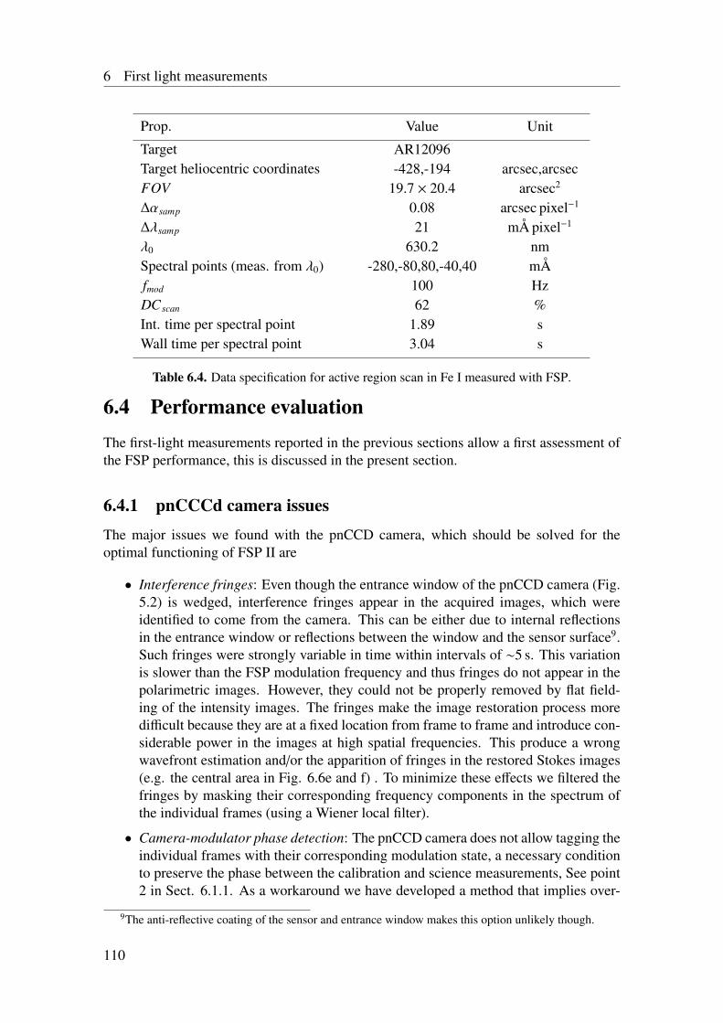
6 First light measurements
Prop. Value Unit
Target AR12096Target heliocentric coordinates -428,-194 arcsec,arcsecFOV 19.7 × 20.4 arcsec2
∆αsamp 0.08 arcsec pixel−1
∆λsamp 21 mÅ pixel−1
λ0 630.2 nmSpectral points (meas. from λ0) -280,-80,80,-40,40 mÅfmod 100 HzDC scan 62 %Int. time per spectral point 1.89 sWall time per spectral point 3.04 s
Table 6.4. Data specification for active region scan in Fe I measured with FSP.
6.4 Performance evaluationThe first-light measurements reported in the previous sections allow a first assessment ofthe FSP performance, this is discussed in the present section.
6.4.1 pnCCCd camera issues
The major issues we found with the pnCCD camera, which should be solved for theoptimal functioning of FSP II are
• Interference fringes: Even though the entrance window of the pnCCD camera (Fig.5.2) is wedged, interference fringes appear in the acquired images, which wereidentified to come from the camera. This can be either due to internal reflectionsin the entrance window or reflections between the window and the sensor surface9.Such fringes were strongly variable in time within intervals of ∼5 s. This variationis slower than the FSP modulation frequency and thus fringes do not appear in thepolarimetric images. However, they could not be properly removed by flat field-ing of the intensity images. The fringes make the image restoration process moredifficult because they are at a fixed location from frame to frame and introduce con-siderable power in the images at high spatial frequencies. This produce a wrongwavefront estimation and/or the apparition of fringes in the restored Stokes images(e.g. the central area in Fig. 6.6e and f) . To minimize these effects we filtered thefringes by masking their corresponding frequency components in the spectrum ofthe individual frames (using a Wiener local filter).
• Camera-modulator phase detection: The pnCCD camera does not allow tagging theindividual frames with their corresponding modulation state, a necessary conditionto preserve the phase between the calibration and science measurements, See point2 in Sect. 6.1.1. As a workaround we have developed a method that implies over-
9The anti-reflective coating of the sensor and entrance window makes this option unlikely though.
110
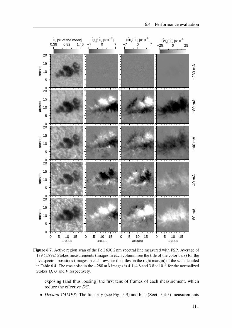
6.4 Performance evaluation
0
5
10
15
20
arcs
ec
0
5
10
15
20
arcs
ec
0
5
10
15
20
arcs
ec
0
5
10
15
20
arcs
ec
0 5 10 15arcsec
0
5
10
15
20
arcs
ec
0 5 10 15arcsec
0 5 10 15arcsec
0 5 10 15arcsec
0.38 0.92 1.46⟨I^⟩n [% of the mean]
−7 0 7⟨Q ^ ⟩n/⟨I
^⟩n [×10−2
]−7 0 7
⟨U ^ ⟩n/⟨I^⟩n [×10
−2]
−25 0 25⟨V ^ ⟩n/⟨I
^⟩n [×10−2
]
−28
0 m
Å−
80 m
Å−
40 m
Å40
mÅ
80 m
Å
Figure 6.7. Active region scan of the Fe I 630.2 nm spectral line measured with FSP. Average of189 (1.89 s) Stokes measurements (images in each column, see the title of the color bars) for thefive spectral positions (images in each row, see the titles on the right margin) of the scan detailedin Table 6.4. The rms noise in the −280 mÅ images is 4.1, 4.8 and 3.8 × 10⁻³ for the normalizedStokes Q, U and V respectively.
exposing (and thus loosing) the first tens of frames of each measurement, whichreduce the effective DC.
• Deviant CAMEX: The linearity (see Fig. 5.9) and bias (Sect. 5.4.5) measurements
111
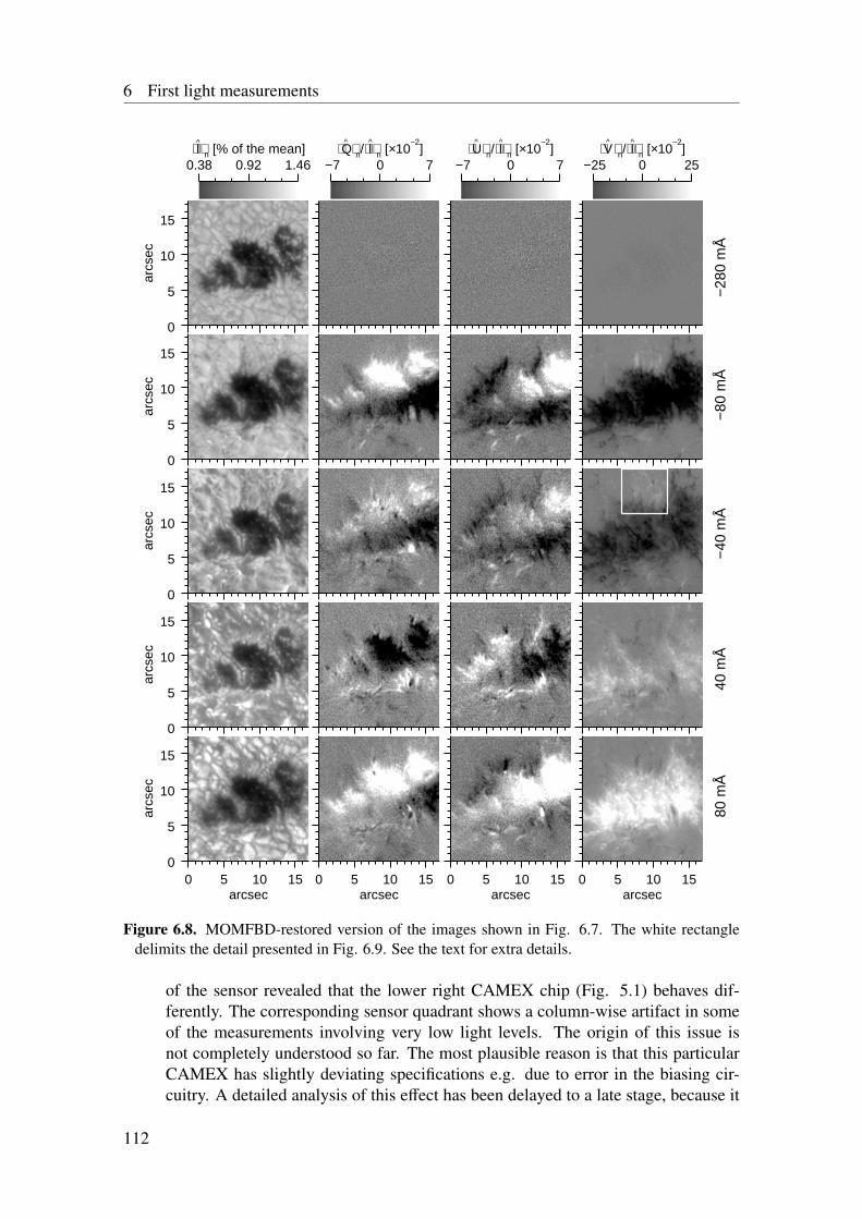
6 First light measurements
0
5
10
15
arcs
ec
0
5
10
15
arcs
ec
0
5
10
15
arcs
ec
0
5
10
15
arcs
ec
0 5 10 15arcsec
0
5
10
15
arcs
ec
0 5 10 15arcsec
0 5 10 15arcsec
0 5 10 15arcsec
0.38 0.92 1.46⟨I^⟩n [% of the mean]
−7 0 7⟨Q ^ ⟩n/⟨I
^⟩n [×10−2
]−7 0 7
⟨U ^ ⟩n/⟨I^⟩n [×10
−2]
−25 0 25⟨V ^ ⟩n/⟨I
^⟩n [×10−2
]
−28
0 m
Å−
80 m
Å−
40 m
Å40
mÅ
80 m
Å
Figure 6.8. MOMFBD-restored version of the images shown in Fig. 6.7. The white rectangledelimits the detail presented in Fig. 6.9. See the text for extra details.
of the sensor revealed that the lower right CAMEX chip (Fig. 5.1) behaves dif-ferently. The corresponding sensor quadrant shows a column-wise artifact in someof the measurements involving very low light levels. The origin of this issue isnot completely understood so far. The most plausible reason is that this particularCAMEX has slightly deviating specifications e.g. due to error in the biasing cir-cuitry. A detailed analysis of this effect has been delayed to a late stage, because it
112
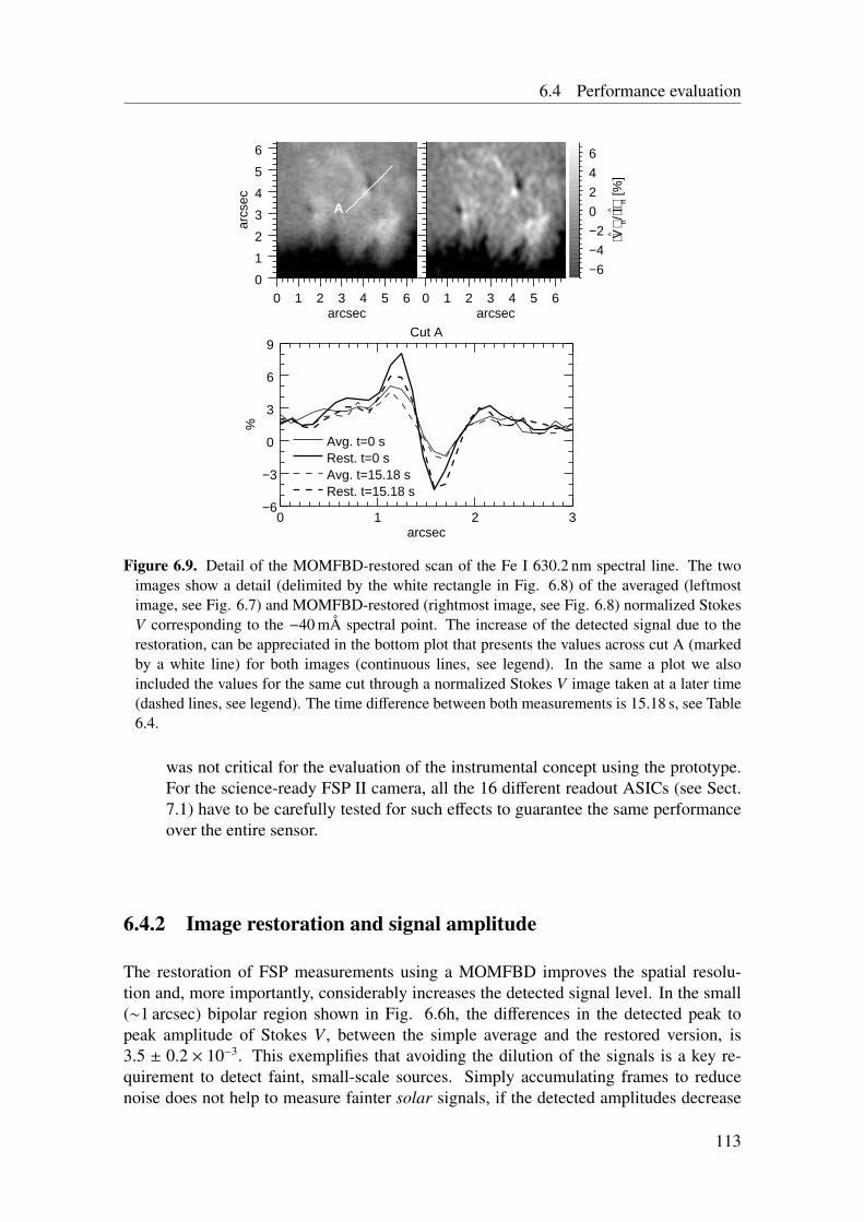
6.4 Performance evaluation
A
0 1 2 3 4 5 6arcsec
0
1
2
3
4
5
6
arcs
ec
0 1 2 3 4 5 6arcsec
Cut A
0 1 2 3arcsec
−6
−3
0
3
6
9
%
Avg. t=0 sRest. t=0 sAvg. t=15.18 sRest. t=15.18 s
−6
−4
−2
0
2
4
6
⟨V ^ ⟩ n/
⟨I^ ⟩ n [%
]
Figure 6.9. Detail of the MOMFBD-restored scan of the Fe I 630.2 nm spectral line. The twoimages show a detail (delimited by the white rectangle in Fig. 6.8) of the averaged (leftmostimage, see Fig. 6.7) and MOMFBD-restored (rightmost image, see Fig. 6.8) normalized StokesV corresponding to the −40 mÅ spectral point. The increase of the detected signal due to therestoration, can be appreciated in the bottom plot that presents the values across cut A (markedby a white line) for both images (continuous lines, see legend). In the same a plot we alsoincluded the values for the same cut through a normalized Stokes V image taken at a later time(dashed lines, see legend). The time difference between both measurements is 15.18 s, see Table6.4.
was not critical for the evaluation of the instrumental concept using the prototype.For the science-ready FSP II camera, all the 16 different readout ASICs (see Sect.7.1) have to be carefully tested for such effects to guarantee the same performanceover the entire sensor.
6.4.2 Image restoration and signal amplitude
The restoration of FSP measurements using a MOMFBD improves the spatial resolu-tion and, more importantly, considerably increases the detected signal level. In the small(∼1 arcsec) bipolar region shown in Fig. 6.6h, the differences in the detected peak topeak amplitude of Stokes V , between the simple average and the restored version, is3.5 ± 0.2 × 10⁻³. This exemplifies that avoiding the dilution of the signals is a key re-quirement to detect faint, small-scale sources. Simply accumulating frames to reducenoise does not help to measure fainter solar signals, if the detected amplitudes decrease
113
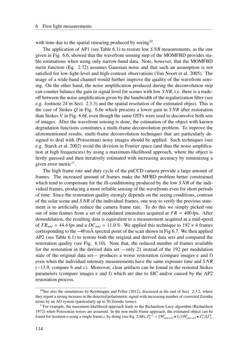
6 First light measurements
with time due to the spatial smearing produced by seeing10.The application of AP1 (see Table 6.1) to restore low S NR measurements, as the one
given in Fig. 6.6, showed that the wavefront sensing step of the MOMFBD provides sta-ble estimations when using only narrow-band data. Note, however, that the MOMFBDmerit function (Eq. 2.72) assumes Gaussian noise and that such an assumption is notsatisfied for low-light-level and high-contrast observations (Van Noort et al. 2005). Theusage of a wide-band channel would further improve the quality of the wavefront sens-ing. On the other hand, the noise amplification produced during the deconvolution stepcan counter balance the gain in signal level for scenes with low S NR, i.e. there is a trade-off between the noise amplification given by the bandwidth of the regularization filter (seee.g. footnote 24 in Sect. 2.3.3) and the spatial resolution of the estimated object. This isthe case of Stokes Q in Fig. 6.6e which presents a lower gain in S NR after restorationthan Stokes V in Fig. 6.6f, even though the same OTFs were used to deconvolve both setsof images. After the wavefront sensing is done, the estimation of the object with knowndegradation functions constitutes a multi-frame deconvolution problem. To improve theaforementioned results, multi-frame deconvolution techniques that are particularly de-signed to deal with (Poissonian) noisy images should be applied. Such techniques (seee.g. Starck et al. 2002) avoid the division in Fourier space (and thus the noise amplifica-tion at high frequencies) by using a maximum-likelihood approach, where the object isfirstly guessed and then iteratively estimated with increasing accuracy by minimizing agiven error metric11.
The high frame rate and duty cycle of the pnCCD camera provide a large amount offrames. The increased amount of frames make the MFBD problem better constrainedwhich tend to compensate for the ill-conditioning produced by the low S NR of the indi-vidual frames, producing a more reliable sensing of the wavefronts even for short periodsof time. Since the restoration quality strongly depends on the seeing conditions, contrastof the solar scene and S NR of the individual frames, one way to verify the previous state-ment is to artificially reduce the camera frame rate. To do this we simply picked oneout of nine frames from a set of modulated intensities acquired at FR = 400 fps. Afterdemodulation, the resulting data is equivalent to a measurement acquired at a mid-speedof FRmid = 44.4 fps and a DCmid = 11.0 %. We applied this technique to 192 × 4 framescorresponding to the −40 mÅ spectral point of the scan shown in Fig 6.7. We then appliedAP2 (see Table 6.1) to restore both the original and derived data sets and compared therestoration quality (see Fig. 6.10). Note that, the reduced number of frames availablefor the restoration in the derived data set —only 21 instead of the 192 per modulationstate of the original data set— produces a worse restoration (compare images e and f)even when the individual intensity measurements have the same exposure time and S NR(∼13.9, compare b and c). Moreover, clear artifacts can be found in the restored Stokesparameters (compare images e and f) which are due to SIC and/or caused by the AP2restoration process.
10See also the simulations by Krishnappa and Feller (2012), discussed at the end of Sect. 2.3.2, wherethey report a strong increase in the detected polarimetric signal with increasing number of corrected Zerniketerms by an AO system (particularly up to 30 Zernike terms).
11For example, the maximum-likelihood approach leads to the Richardson-Lucy algorithm (Richardson1972) when Poissonian noises are assumed. In the non multi-frame approach, the estimated object can befound for iteration n using a single frame,i, by doing (see Eq. 2.68), In+1
= [H∗atm+tel?Ii/(H iatm+tel?I
n)]In
.
114
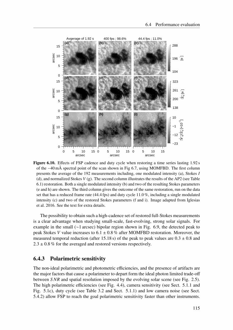
6.4 Performance evaluation
Avgerage of 1.92 s(a)
0
5
10
15
arcs
ec
400 fps ; 98.6%(b)
44.4 fps ; 11.0%(c)
(d)
0
5
10
15
arcs
ec
(e) (f)
(g)
0 5 10 15arcsec
0
5
10
15
arcs
ec
(h)
0 5 10 15arcsec
(i)
0 5 10 15arcsec
104
196
288
[e− ]
138
200
261
323
⟨I^ ⟩ n [e
− ]
−23
−12
−1
10
⟨V ^ ⟩ n/
⟨I^ ⟩ n [×
10−2
]
Figure 6.10. Effects of FSP cadence and duty cycle when restoring a time series lasting 1.92 sof the −40 mÅ spectral point of the scan shown in Fig 6.7, using MOMFBD. The first columnpresents the average of the 192 measurements including, one modulated intensity (a), Stokes I(d), and normalized Stokes V (g). The second column illustrates the results of the AP2 (see Table6.1) restoration. Both a single modulated intensity (b) and two of the resulting Stokes parameters(e and h) are shown. The third column gives the outcome of the same restoration, run on the dataset that has a reduced frame rate (44.4 fps) and duty cycle 11.0 %, including a single modulatedintensity (c) and two of the restored Stokes parameters (f and i). Image adapted from Iglesiaset al. 2016. See the text for extra details.
The possibility to obtain such a high-cadence set of restored full-Stokes measurementsis a clear advantage when studying small-scale, fast-evolving, strong solar signals. Forexample in the small (∼1 arcsec) bipolar region shown in Fig. 6.9, the detected peak topeak Stokes V value increases to 6.1 ± 0.8 % after MOMFBD restoration. Moreover, themeasured temporal reduction (after 15.18 s) of the peak to peak values are 0.3 ± 0.8 and2.3 ± 0.8 % for the averaged and restored versions respectively.
6.4.3 Polarimetric sensitivity
The non-ideal polarimetric and photometric efficiencies, and the presence of artifacts arethe major factors that cause a polarimeter to depart form the ideal photon limited trade-off
between S NR and spatial resolution imposed by the evolving solar scene (see Fig. 2.5).The high polarimetric efficiencies (see Fig. 4.4), camera sensitivity (see Sect. 5.1.1 andFig. 5.1c), duty cycle (see Table 3.2 and Sect. 5.1.1) and low camera noise (see Sect.5.4.2) allow FSP to reach the goal polarimetric sensitivity faster than other instruments.
115
6 First light measurements
These are the main properties that permitted the detection of the small-scale (0.24 arcsecspatial sampling), quiet-Sun signals with a sensitivity of ∼3.5 × 10⁻⁴ after integrating0.95 min (about a fifth of the typical solar granulation life-time) with a flux of only about230 e− pixel−1 frame, see Fig. 6.5. The detection was further improved by the increase insignal levels obtained by image restoration. On the other hand the main potential sourcesof artifacts are the modulator and the polarimetric calibration procedure, the pnCCD cam-era and the residual levels of SIC. We found that the modulator and calibration artifactscan be suppressed to the level of 1 × 10⁻⁴, provided that the instrumental polarization levelis not larger than ∼1 % (see Sect. 4.3). Analogously, we found that the pnCCD cameraintroduces no major polarimetric artifact besides those mentioned in Sect. 6.4.1 (see Sect.5.2 and 5.3). These statements are further supported by the results reported in Sect 6.4.5and the low-spatial-resolution measurements of the second solar spectrum given in Fig.6.3. The latter reach a polarimetric sensitivity of ∼8 × 10⁻⁵ in the spatially-averaged, nor-malized Stokes Q, without clear signs of instrumental artifacts and with good agreementwith the ZIMPOL results.
6.4.4 Measurements of the magnetically insensitive 557.6 nm lineIn order to estimate the level of SIC, no solar signal has to be present in the Stokesimages12. One of the best ways to achieve this is by measuring polarization in magneticlines with null Landé factor to ensure the absence of Zeeman signals. If, in addition, atarget located near the center of the solar disk is chosen, the scattering polarization signalsare also practically ruled out, resulting in flat Stokes Q, U and V images with non-zerooffsets due to instrumental polarization. The combination of a non-flat Stokes I with sucha flat Q, U and V in this kind of measurement, makes it ideal to detect any SIC from StokesI to Q, U and V . We measured the Fe I 557.6 nm line (which has g=0) in a quiet regionof the Sun during a short campaign in April 2015. Such measurements are presented inFig. 6.11. As can be appreciated in the Stokes images of row (c), there is a clear artifactaffecting Stokes Q and U. Such an artifact is not present in the measurements given inrow (a), which were acquired under the same conditions, except that the modulator wasdisconnected. The latter means that no actual modulation is taking place and thus nopolarimetric signal should be measured. The actual source of the aforementioned artifacthas not been identified and remains as future work. In spite of this we list and discussbelow the main possible sources.
• Modulator induced image motion: The combination of a non-normal beam inci-dence on the FLCs (see the tilting rings in Fig. 4.1) and a change in their refractiveindex, between the two states of their optical axes, introduces a deflection of theoutput beam. Such a deflection may produce in turn image motion which is syn-chronized with the frame acquisition, and thus any derived artifact will be system-atically repeated every modulation cycle appearing even after accumulating manyStokes images. Modulation induced image motion has been reported to appear inother polarimeters (see e.g. Hanaoka 2006). One solution to this problem is tolocate the modulator package near a focal plane in order to minimize the image
12For example in measurements of the quiet Sun, both SIC an transversal Zeeman signals tend to appearnear the borders of the granules where the gradient of Stokes I is maximum.
116
6.4 Performance evaluation
0
5
10
15
arcs
ec
0
5
10
15
arcs
ec
0
5
10
15
arcs
ec
0 5 10 15arcsec
0
5
10
15
arcs
ec
0 5 10 15arcsec
0 5 10 15arcsec
0 5 10 15arcsec
0.65 0.96 1.27⟨I^⟩n [% of the mean]
−3 0 3⟨Q ^ ⟩n/⟨I
^⟩n [×10−3
]−3 0 3
⟨U ^ ⟩n/⟨I^⟩n [×10
−3]
−3 0 3⟨V ^ ⟩n/⟨I
^⟩n [×10−3
]
(a)
(b)
(c)
(d)
Figure 6.11. Measurements of the non-magnetic 557.6 nm line. (a) ∼10 s average acquired withthe modulation disconnected. (b) ∼10 s average acquired with the modulation running. (c) sameas (b) after subtracting from each image its smoothed version (using a 40×40 pixel2 window). (d)same as (c) except that the images where realigned before the polarimetric demodulation, usingsub-pixel cross-correlation among consecutive frames. Such a realignment reduced the temporalpower spectrum of the Stokes Q and U time series, by approximately one order of magnitude.The original plate scale of the images is 0.08 arcsec pixel−1 in both directions, however they havebeen binned using a 2 × 2 pixel2 window. The standard deviations of the normalized Stokes Q,U and V images in row (a), are 1.2, 1.4 and 1.3 × 10⁻³ respectively.
motion introduced by the beam deflection13. We have not quantified the beam de-flection, if any, introduced by the FSP modulator package. However the artifactsseen in row (c) of Fig. 6.11 are not likely to be produced by this effect because thecenter of the modulator was located at only ∼15 cm from a focal plane (<< than the
13In principle image motion can not be eliminated because the two FLCs in the modulator can not be inthe same focal plane at the same time.
117
6 First light measurements
telescope focal length of 45 m); the realignment of the images before demodulationshown in row (d), does not considerably reduce the artifact level; and no artifact isvisible at the same level in the measurements presented in Fig. 6.5.
• SIC: Another possible source of the artifacts seen in row (c) of Fig. 6.11 is residualseeing induced crosstalk. This option is unlikely because of the following. Firstly,note that the measurements acquired with the modulation package disconnectedare still sensitive to these effects, i.e. the only difference with respect to a regularmeasurement is that O does not depend on i in Eq. 2.53. However, the artifacts arenot present in the images shown in row (a). Secondly, the correlation coefficientsof the Stokes Q, U and V images in row (c) with respect to the Stokes I image,are larger (-0.28, 0.23 and -0.05 respectively) than the correlation coefficients ofthe absolute values of the same Stokes Q, U and V with respect to the modulus ofthe gradient of Stokes I (-0.03, 0.01 and -0.01 respectively). In case of SIC, theopposite is expected. Finally, the realignment of the images before demodulationshown in row (d), does not considerably reduce the artifact level (which also rulesout jitter induced crosstalk due to e.g. a resonance peak in the residual motion ofthe AO tip-tilt correction mirror).
• Stray light: A third potential source of the artifacts under discussion is the presenceof stray light. This means that the measured Stokes vector, Sstray is the sum of thevector measured in absence of stray light, S, plus a spatially uncorrelated term dueto possibly polarized stray light, ∆S. We can write the measured normalized Stokesparameter k ∈ Q,U,V as follows,
S stray,k
S stray,0=
11 + ∆S 0/S 0
(S k
S 0+
∆S k
S 0
). (6.3)
Note that, even if the stray light is unpolarized (∆S k = 0) it will introduce crosstalkfrom Stokes I in the Q, U and V images, by means of the multiplicative term inthe right side of Eq. 6.3. Such a crosstalk can explain the artifacts in row (c)of Fig. 6.11 which correlate with Stokes I (see the previous bullet). Moreovera wavelength-dependent polarized stray light term, can also account for the largescale gradients seen in row (d) which are not present in the measurements acquiredat other wavelengths.
6.4.5 Spatial resolution and seeing induced crosstalk
The present section has been extracted from Iglesias et al. 2016 with minor changes andan adapted notation.
Quantifying the amplitude of SIC in narrow-band, diffraction-limit-sampled, Stokesimages recorded at high modulation frequency, is difficult because the artifact is normallyhidden by the photon noise and any possible solar signal. Moreover if image averaging isused to reduce photon noise, the SIC artifact is smeared and thus its level also reduces, seeSect. 2.3 and e.g. Lites 1987, Hanaoka 2004. Let us discriminate the spatially estimatedpower in the image of the normalized Stokes parameter i ∈ Q,U,V, after averaging Nstk
118
6.4 Performance evaluation
measurements as follows,
σ2tot(i,Nstk, fmod, Irms) =
σ2i
Nstk+ σ2
art(i,Nstk, fmod, Irms) + σ2sig(i,Nstk), (6.4)
where we have neglected any fixed pattern noise that cannot be reduced by image av-eraging. σi = (σcam
2 + σp2)1/2/(ε i
√Nmod〈I〉) is the noise in the individual normalized
Stokes images (see Eq. 2.35) ; σart(i,Nstk, fmod, Irms) includes the power due to SICand other artifacts (see below) in Stokes parameter i, where we made explicit its de-pendence with respect to Nstk, to the modulation frequency, fmod, and to the rms con-trast values of the Stokes I images averaged, Irms; and σsig(i,Nstk) is the averaged sig-nal power of the actual solar scene. To be able to reliably detect solar polarimetric sig-nals, one needs to obtain after averaging, a value of the signal to artifact and noise ratio,S ANR(i,Nstk) = σsig(i,Nstk)/[σ2
i /(Nstk) + σ2art(i,Nstk, fmod, Irms)]1/2, that is large enough
given a predefined criterion. Note that the above-described approach is of practical rele-vance only for the cases where the portion of the FOV covered by signal and by artifactare similar, so that their spatial rms values are equally representative of their peaks values.
As an application of the above-expressed ideas, let us consider the case of quiet Sunmeasurements, of particular importance for FSP given its science goals. One way toachieve σsig(i,Nstk) = 0 in Eq. 6.4 and still be sensitive to SIC, is to use measurementsacquired with the modulator package deactivated (see Sect. 6.4.5). In addition, since SICnot only depends on modulation frequency, but also on the instantaneous seeing condi-tions and contrast of the solar scene (Judge et al. 2004); we use the following procedureto reduce the influence of the latter two. We start with a set of 45989 (7.66 min wall time)quiet Sun measurements acquired at 100 Hz with the FSP modulator package deactivated.We then derived two new sets that have modulation frequencies of 20 and 11.1 Hz, bypicking one out of five and one out of nine frames respectively, from the set of measuredintensities at 100 Hz (as done in Sect. 6.4.2). After demodulation, the 20 and 11.1 Hz datasets are equivalent to measurements taken at those frequencies with duty cycles of 19.7and 11 % respectively. The advantages of this method are that practically the same solarscene, seeing conditions and values of σi are present in the three data sets. The measuredvalues for Stokes I and normalized Stokes Q corresponding to the original and derivedmeasurements are shown in Fig. 6.12 for different values of Nstk. The qualitative resultsalso apply to Stokes U and V , which are not presented here.
Firstly, note that SIC is evident in the single measurements, i.e. Nstk=1, of the 20and 11.1 Hz cases (images c and d respectively) while not being above the noise levelfor the 100 Hz image (b). Moreover, the artifact tends to have larger amplitudes towardsthe borders of the FOV because the AO corrections of the wavefront are worse awayfrom the system’s locking point —located approximately at the center of the image—due to seeing anisoplanatism (see Sect. 2.3.3). The reduction of the SIC with increasingmodulation frequency, can be also appreciated in Fig. 6.13, where the artifact level in theindividual Stokes Q measurements,
σart(Q, 1, fmod, Irms) =
√σ2
tot(Q, 1, fmod, Irms) − σ2Q, (6.5)
is plotted for all the frames —thus including a variety of instantaneous seeing conditions—in the three data sets versus Stokes I rms contrast. To obtain the artifact level, we as-sume it can only introduce power at spatial frequencies that are below the diffraction
119
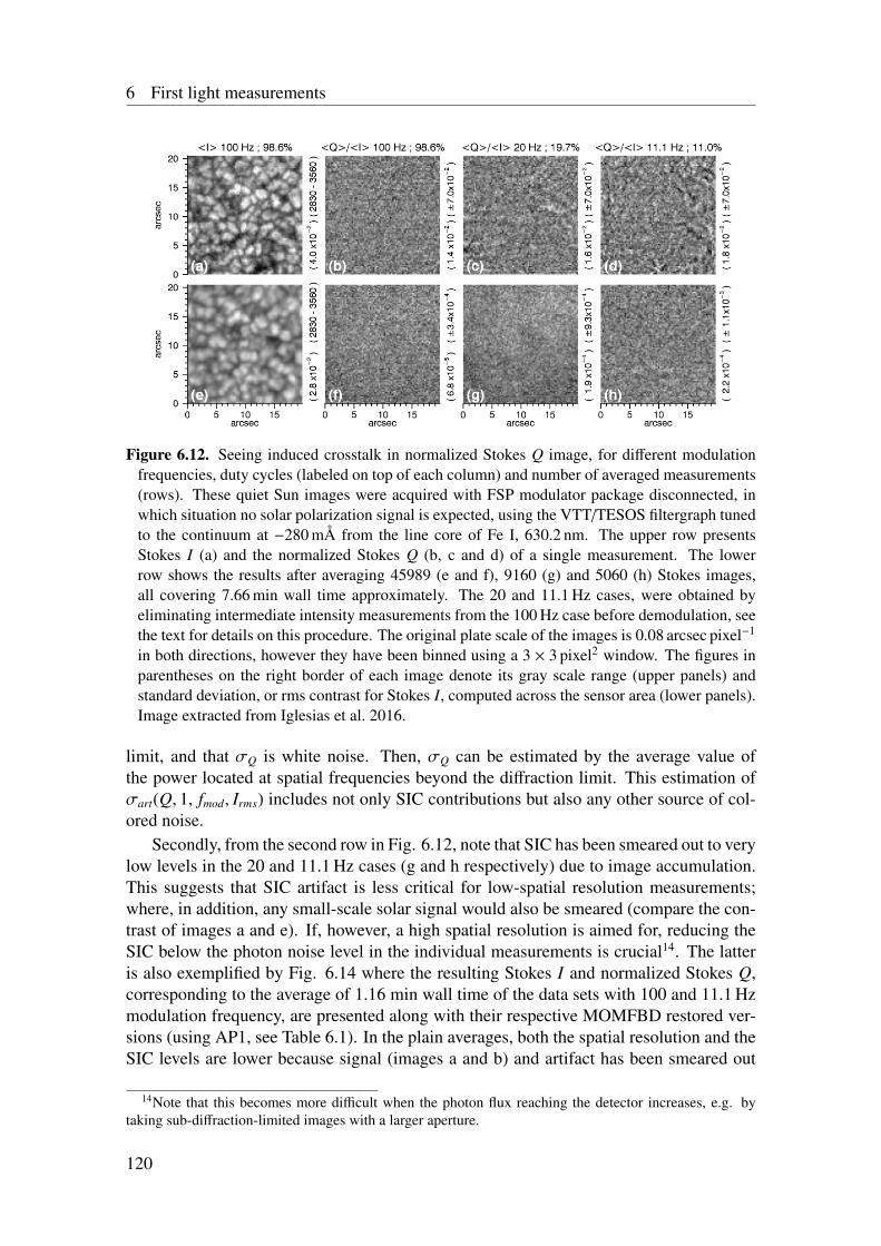
6 First light measurements
Figure 6.12. Seeing induced crosstalk in normalized Stokes Q image, for different modulationfrequencies, duty cycles (labeled on top of each column) and number of averaged measurements(rows). These quiet Sun images were acquired with FSP modulator package disconnected, inwhich situation no solar polarization signal is expected, using the VTT/TESOS filtergraph tunedto the continuum at −280 mÅ from the line core of Fe I, 630.2 nm. The upper row presentsStokes I (a) and the normalized Stokes Q (b, c and d) of a single measurement. The lowerrow shows the results after averaging 45989 (e and f), 9160 (g) and 5060 (h) Stokes images,all covering 7.66 min wall time approximately. The 20 and 11.1 Hz cases, were obtained byeliminating intermediate intensity measurements from the 100 Hz case before demodulation, seethe text for details on this procedure. The original plate scale of the images is 0.08 arcsec pixel−1
in both directions, however they have been binned using a 3 × 3 pixel2 window. The figures inparentheses on the right border of each image denote its gray scale range (upper panels) andstandard deviation, or rms contrast for Stokes I, computed across the sensor area (lower panels).Image extracted from Iglesias et al. 2016.
limit, and that σQ is white noise. Then, σQ can be estimated by the average value ofthe power located at spatial frequencies beyond the diffraction limit. This estimation ofσart(Q, 1, fmod, Irms) includes not only SIC contributions but also any other source of col-ored noise.
Secondly, from the second row in Fig. 6.12, note that SIC has been smeared out to verylow levels in the 20 and 11.1 Hz cases (g and h respectively) due to image accumulation.This suggests that SIC artifact is less critical for low-spatial resolution measurements;where, in addition, any small-scale solar signal would also be smeared (compare the con-trast of images a and e). If, however, a high spatial resolution is aimed for, reducing theSIC below the photon noise level in the individual measurements is crucial14. The latteris also exemplified by Fig. 6.14 where the resulting Stokes I and normalized Stokes Q,corresponding to the average of 1.16 min wall time of the data sets with 100 and 11.1 Hzmodulation frequency, are presented along with their respective MOMFBD restored ver-sions (using AP1, see Table 6.1). In the plain averages, both the spatial resolution and theSIC levels are lower because signal (images a and b) and artifact has been smeared out
14Note that this becomes more difficult when the photon flux reaching the detector increases, e.g. bytaking sub-diffraction-limited images with a larger aperture.
120
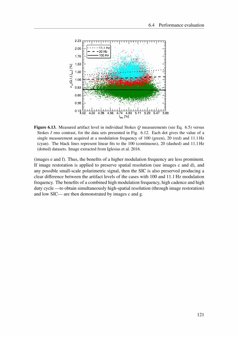
6.4 Performance evaluation
Figure 6.13. Measured artifact level in individual Stokes Q measurements (see Eq. 6.5) versusStokes I rms contrast, for the data sets presented in Fig. 6.12. Each dot gives the value of asingle measurement acquired at a modulation frequency of 100 (green), 20 (red) and 11.1 Hz(cyan). The black lines represent linear fits to the 100 (continuous), 20 (dashed) and 11.1 Hz(dotted) datasets. Image extracted from Iglesias et al. 2016.
(images e and f). Thus, the benefits of a higher modulation frequency are less prominent.If image restoration is applied to preserve spatial resolution (see images c and d), andany possible small-scale polarimetric signal, then the SIC is also preserved producing aclear difference between the artifact levels of the cases with 100 and 11.1 Hz modulationfrequency. The benefits of a combined high modulation frequency, high cadence and highduty cycle —to obtain simultaneously high-spatial resolution (through image restoration)and low SIC— are then demonstrated by images c and g.
121
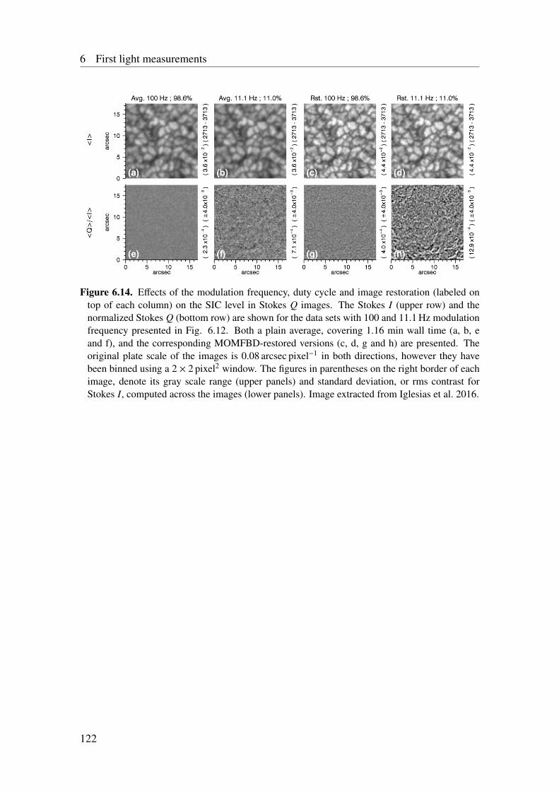
6 First light measurements
Figure 6.14. Effects of the modulation frequency, duty cycle and image restoration (labeled ontop of each column) on the SIC level in Stokes Q images. The Stokes I (upper row) and thenormalized Stokes Q (bottom row) are shown for the data sets with 100 and 11.1 Hz modulationfrequency presented in Fig. 6.12. Both a plain average, covering 1.16 min wall time (a, b, eand f), and the corresponding MOMFBD-restored versions (c, d, g and h) are presented. Theoriginal plate scale of the images is 0.08 arcsec pixel−1 in both directions, however they havebeen binned using a 2 × 2 pixel2 window. The figures in parentheses on the right border of eachimage, denote its gray scale range (upper panels) and standard deviation, or rms contrast forStokes I, computed across the images (lower panels). Image extracted from Iglesias et al. 2016.
122
7 Concluding remarks and prospects
In this thesis we have tackled the instrumental challenges that arise when developing aground-based, high-cadence solar polarimeter. This work is focused on a specific in-strument, the prototype of the FSP. However many of the methods and techniques weemployed or developed, are of relevance to high-cadence polarimetry in general.
Any practical polarimeter that aims to measure the full Stokes vector (a requirementto e.g. remotely probe the full magnetic field vector), employs a form of temporal mod-ulation. Therefore, we started by summarizing the main effects of atmospheric seeingon temporally-modulated imaging polarimetry, namely the reduction of spatial resolutionand the introduction of SIC. After describing the cons of the dual-beam (beam imbal-ances), beam-exchange (extra measurements required) and asynchronous-readout solu-tions, we derived the most important properties of a single-beam, synchronous polarime-ter that aims to reduce SIC and optimize image restoration. These properties were trans-lated in to a set of general requirements for the camera and modulator, that were in turnused to evaluate the pros and cons of the different available technologies. This showedthat based on reliability, performance and technology maturity an FLC-based modulatoris the best current alternative for full-Stokes, high-cadence modulation. In addition, itshowed that the bottle neck of a synchronous polarimeter are the frame rate and noise ofthe scientific camera employed.
The latter motivated the development of the FSP prototype, which is described inthis work. We have integrated, characterized and optimized an FLC based polarizationmodulator, supporting the fact that a model-based design procedure can be satisfactorilyused to obtain achromatic polarimetric efficiencies. By comparing the required stabilityof the modulation matrix with the characterization results, we derived the calibration re-quirements in terms of the maximum changes allowed in wavelength, modulator housingtemperature, and driving frequency. In addition we characterized a custom-made pnCCDcamera never used in polarimetry before, and proved its suitability to do high-cadence,high-sensitivity solar polarimetry from the ground. We selected a specific synchronizationbetween camera and modulator, which allowed us to develop an accurate model of the im-age acquisition including the signals acquired during the shutter-less frame transfers, andthe strong variations on the sensor illumination that can be present when doing polarime-try. The latter was used to develop a numeric technique for correcting image smearingpost-acquisition. The main properties of the pnCCD camera where characterized and itspolarimetric effects addressed when relevant. These include the effects of non-linearity,residual offsets, common-mode noise (where the minimum number of channels for thecorrection was derived) and readout noise.
We have preformed all the necessary steps to acquire the first-light measurements ofthe integrated FSP prototype at the VTT solar telescope. These include the development
123
7 Concluding remarks and prospects
of the reduction routines and acquisition of measurements working with both a spec-trograph and filtergraph. These measurements allowed us to asses the suitability of theFSP instrumental concept. We found that the superior sensitivity, noise, duty cycle ofthe pnCCD camera, together with the high polarimetric efficiencies of the modulator arecrucial to acquire the extremely photon-starved measurements required by many sciencecases. In addition, the high cadence and duty cycle of FSP proved crucial to allow therestoration of the images by means of a MOMFBD, using only narrow-band data whichhave low S NR. The restoration improved not only the spatial resolution of the Stokesimages, but also increased the signal levels. With FSP we measured scattering polariza-tion with a polarimetric sensitivity of 8 × 10⁻⁵, and detected sub-arcsec bipolar patches oflinear polarization at the 1 × 10⁻³ level using the TESOS filtergraph.
We studied the residual level of SIC using non-modulated filtergraph measurements.We found that at a modulation frequency of 100 Hz, if no image restoration is used, SICis below the 7 × 10⁻⁵ noise level after averaging ∼8 min of quiet-Sun Stokes images.If the signal is preserved by using a MOMFBD restoration, then SIC is also preservedincreasing its level. After restoring 1.16 min of quiet-Sun measurements acquired withFSP, we found artifacts at the 4 × 10⁻⁴ noise level only in the edges of the images wherethe AO performance is reduced due to seeing anisoplanatism.
There are a set of open questions and tasks that arise from the above-mentioned work,and demand further investigation during the next phase of the FSP project. We list themost relevant below.
• The dispersion of the FLC’s switching angles that we measured should be verifiedand, in the positive case, included in the modulator model.
• Reducing the instrumental polarimetric offset is crucial to lower the level of theartifacts introduced by various camera and modulator related effects (e.g. detec-tor non-linearities, instability of the modulation matrix, etc.). A simple option tocompensate the instrumental offsets is to modify the exposure times of the differentmodulation cycles. This solution will be implemented in FSP II.
• The calibration procedure has to be modified to contemplate variations of the inputillumination, in order to allow the implementation of a spatially-dependent demod-ulation.
• The calibration of the pnCCD non-linearities has to be implemented.
• The tuning of the camera-modulator triggering delay has to be done.
• The synchronization between FSP and the scanning feature of the post focus instru-ment, has to be optimized in order to fully exploit the high duty cycle of FSP.
• The modulator induced jitter, if any, should be properly characterized to asseswhether the modulator can be used further away from a focal plane, which wouldreduce the variation of the modulation matrix across the FOV and may be advanta-geous in terms of physical constraints for specific setups.
• The source of the observed artifacts in the 556.7 nm line should be identified inorder to allow a more accurate estimation of the residual SIC levels.
124
7.1 The Fast Solar Polarimeter II
• Multi-frame deconvolution algorithms that are better than a Wiener filter to decon-volve very low S NR images, have to be investigated in order to improve the imagerestoration results.
Let us end this section by discussing Fig. 3.2. As can be appreciated there, the idealregime in terms of SIC reduction corresponds to a modulation frequency, fmod, beyond400 Hz. Reaching such a high fmod with a synchronous, full-Stokes polarimeter impliesoperating the camera at least at a FR=1600 fps. This solution is clearly not desirable be-cause the resulting very low photon noise would impose a serious constraint on the camerareadout noise, in order to be photon noise limited. Moreover, there is no clear advantagein terms of image restoration because the exposure time (∼0.6 ms) is much shorter thanthe typical 10 ms coherence time of the seeing. In this sense trying to further push the syn-chronous approach beyond FSP II does not look like a good alternative. A better solutionshould be trying to implement an asynchronous polarimeter using a different techniquethan that used in ZIMPOL in order to reach fmod ≥ 400 Hz while keeping FR=100 fps,a low readout noise and a high QE, FF and DC. A promising technology to implementthis alternative solution are the active pixel sensors where the charges corresponding tothe different modulation states can be accumulated separately within the pixel structure.One version of such detectors, the DEPFET/Infinipix, are currently being investigated atthe semiconductor lab of the Max Planck Society in collaboration with the Max Planckinstitute for Solar System Research. Note that many science cases do not require reachingthe ideal regime discussed above. Therefore many highly demanded measurements canstill be done if the residual SIC can be reduced to about 1 × 10⁻⁴, as done with FSP forspecific conditions.
7.1 The Fast Solar Polarimeter IIThe next phase in the FSP project, FSP II, implies the development of a science-ready po-larimeter. The modulator package and calibration unit used in the prototype will be alsoemployed in FSP II. The camera will be replaced by a larger 1024 × 1024 pixel2 pnCCD(see Table 3.2 for details) currently under development at the semiconductor lab of theMax Planck Society. The camera will provide a larger FOV while keeping the 100 Hzmodulation frequency and low noise. To achieve this, 16 readout ASIC of a new type areused, the so called VERITAS-1 (Porro et al. 2013). The larger FOV allows the imple-mentation of a high-cadence, dual-beam system which has never been operated before.If no beam exchange is used, the performance of the dual-beam setup strongly dependson the ability of the flat fielding procedure to effectively suppress beam imbalances. Inaddition the larger image size increases the data rate from 47 to 800 MBs−1. This woulddemand the creation of data mining routines and the optimization of data reduction algo-rithms (e.g. smearing correction) in order to minimize processing time and storage. Oneimportant aspect related to the latter is the necessity of storing all the recorded frames,which is strongly determined by the selected image restoration approach.
125


Acronyms
ADC Analog to digital converter (p. 27)AO Adaptive optics (p. 2)ASIC Application specific integrated circuit (p. 27)CAMEX CMOS amplifier and multiplexer (p. 76)CCD Charge-coupled device (p. 3)CDS Correlated double sampling (p. 29)CMOS Complementary metal-oxide-semiconductor (p. 3)ENOB Effective number of bits (p. 50)FLC Ferro-electric liquid crystal (p. 3)FPGA Field programmable gates array (p. 27)FPN Fixed pattern noise (p. 29)FSP Fast Solar Polarimeter (p. xii)FSP II Fast solar polarimeter II (p. 52)FWHM Full width at half maximum (p. 80)HWP Half-wave plate (p. 12)IR Infra red (p. 16)JFET Junction field-effect transistor (p. 77)KAOS Kiepenhener institute Adaptive Optics System (p. 103)LC Liquid crystal (p. 12)LCVR Liquid crystal variable retarder (p. 23)LED Light emitting diode (p. 86)LOS Line of sight (p. 14)MFBD Multi-frame blind deconvolution (p. 41)MOMFBD Multi-object multi-frame blind deconvolution (p. 2)NB Narrow band (p. 43)OTF Optical transfer function (p. 34)PEM Piezo-elastic modulator (p. 23)pnCCD Pn-type CCD (p. 3)PSF Point spread function (p. 37)PSG Polarization state generator (p. 54)QWP Quarter-wave plate (p. 12)rms Root mean squared (p. 31)SI Speckle imaging (p. 41)SIC Seeing induced crosstalk (p. xvi)SR Static retarder (p. 24)SVD Singular value decomposition (p. 22)TESOS Triple Etalon SOlar Spectrometer (p. 105)
127

Acronyms
UV Ultra violet (p. 16)VTT Vacuum Tower Telescope (p. 5)WB Wide band (p. 43)ZIMPOL Zurich IMaging POLarimeter (p. 47)
128

Nomenclature
1 Identity matrix of the appropriate dimensions (p. 10)A Polarimetric efficiencies matrix (p. 22)A First frame transfer matrix coefficient (p. 82)α Frame transfer coefficient (p. 82)Apixel Pixel area (p. 30)B Magnetic field (p. 13)B Second frame transfer matrix coefficient (p. 82)c2 Short form for cos(2θ) (p. 10)C Coefficient in the dispersion law of the FLC retardance (p. 24)χ Azimuthal angle of the magnetic field vector defined with respect to the Stokes Q
direction (p. 14)CT1 First coefficient in the temperature dependence law of the FLC switching angle
(p. 24)CT2 Second coefficient in the temperature dependence law of the FLC switching angle
(p. 24)D Demodulation matrix (p. 21)D Demodulation matrix element (p. 21)D Telescope aperture (p. 19)D Telescope pupil transmission function (p. 42)DC Duty cycle (p. 4)DCscn Scan duty cycle (p. 105)DCNU Dark current non-uniformity (p. 29)∆ Used to denote an interval or change in a quantity (p. 14)δ Phase of a wave (p. 8)δ Retardance (p. 11)δ Frame transfer coefficient (p. 82)∆λ Spectral resolution (p. 17)∆α Angular resolution (p. 17)∆t Temporal resolution (p. 17)∆λz Zeeman splitting (p. 14)E Electric field (p. 7)E Electric field component (p. 8)ε Polarimetric efficiencies vector (p. 21)ε Polarimetric efficiency (p. 21)E Expected value operator (p. 99)f Temporal frequency (p. 36)FF Filling factor (p. 30)
129

Nomenclature
fmod Modulation frequency (p. 23)FOV Field of view (p. 25)FR Frame rate (p. 30)F Fourier transform operator (p. 42)FWC Full well charge (p. 30)G Conversion gain (p. 30)g Landé factor of an atomic transition (p. 14)g Gain of an optical system (p. 9)γ Wiener filter parameter (p. 42)γ Inclination angle of the magnetic field vector defined with respect to the line of
sight (p. 14)Γ Solar spectral irradiance (p. 19)H Point spread function (p. 37)h Diattenuation vector (p. 9)H Optical transfer function (p. 34)h Altitude (p. 32)H Matrix coefficient of the homogeneous solution of the frame transfer equation
(p. 83)D Measured or estimated demodulation matrix (p. 69)O Measured or estimated modulation matrix (p. 69)s Measured or estimated normalized Stokes vector (p. 69)I Measured or estimated Stokes I parameter (p. 16)I Measured or estimated vector of intensities (p. 21)Ncm Measured or estimated common mode artifact (p. 90)Q Measured or estimated Stokes Q parameter (p. 99)S Measured or estimated Stokes vector element (p. 21)S Measured or estimated Stokes vector (p. 16)U Measured or estimated Stokes U parameter (p. 101)V Measured or estimated Stokes V parameter (p. 39)i Charges flux produced in a CCD (p. 80)I Stokes I parameter (p. 8)I Smeared Stokes I parameter (p. 79)I Vector of smeared Stokes I parameters (p. 82)id Dark current (p. 30)I Fourier transform of Stokes I (p. 34)Io f f Digital offset of the camera (p. 79)I Vector of intensities (p. 82)j Total angular momentum quantum number (p. 13)k Wave number (p. 8)k0 Transmittance of a partial linear polarizer along its optical axis (p. 11)k90 Transmittance of a partial linear polarizer along a direction orthogonal to its opti-
cal axis (p. 11)κ Used for general proportionality constants or coefficients (p. 12)κ A vector of constants κ (p. 42)k Spatial frequencies vector (p. 34)L Error metric (p. 42)
130

Nomenclature
l Vector containing the modulator parameters (p. 61)λ Wavelength (p. 11)l Orbital angular momentum quantum number (p. 14)M Mueller matrix (p. 9)M Mueller matrix element (p. 9)µ Cosine of the angle between the LOS and the normal of the solar surface (p. 104)N Noise (p. 79)n Refractive index (p. 33)n Discrete time or frame number (p. 78)N Fourier transform of the noise (p. 42)N Set of the integers numbers (p. 83)Nadc ADC resolution (p. 30)Ncal Number of calibration measurements (p. 68)Ncm Signal due to the common mode artifact (p. 79)Ncol Number of columns of an image sensor (p. 30)Nd Dark noise (p. 79)ne Extraordinary refractive index (p. 11)NENOB ADC effective number of bits (p. 50)N f rm Number of frames (p. 42)NL Non-linearity (p. 30)Nmod Number of modulation states (p. 21)Nmode Number of modes used in a MFBD (p. 42)no Ordinary refractive index (p. 11)Nob j Number of objects used in a MOMFBD (p. 43)Np Photon noise (p. 19)Nro Read out noise (p. 79)Nrow Number of rows of an image sensor (p. 30)Nscn Number of scans (p. 105)NS R Noise to signal ratio (p. 18)Nstk Number of Stokes frames (p. 93)N Noise vector (p. 68)Nxs Number of shielded channels used for common mode correction (p. 90)O Modulation matrix (p. 21)O Modulation matrix element (p. 37)Ω Orthogonal basis functions used in a MFBD (p. 42)ω Angular temporal frequency (p. 8)P Generalized pupil function (p. 42)p Polarization vector (p. 9)π Principal Zeeman component (p. 14)Φ Photon or photo-electron flux (p. 19)φ0 Seeing isoplanatic angle (p. 34)PRNU Photon response non-uniformity (p. 30)q Short form for Q/I (p. 9)Q Stokes Q parameter (p. 8)QE Quantum efficiency (p. 19)R Rotation matrix (p. 9)
131

Nomenclature
r0 Fried parameter (p. 33)R Set of the real numbers (p. 10)r Bi-dimensional position vector (p. 33)S Stokes vector (p. 8)S 0 Alternative form for Stokes I parameter (p. 9)S 1 Alternative form for Stokes Q parameter (p. 9)s Normalized Stokes vector (p. 68)S 2 Alternative form for Stokes U parameter (p. 9)s2 Short form for sin(2θ) (p. 10)S 3 Alternative form for Stokes V parameter (p. 9)S Stokes vector element (p. 37)σ Standard deviation or rms value (p. 21)σb Blue Zeeman component (p. 14)σr Red Zeeman component (p. 14)σadc Quantization noise rms value (p. 30)σcam Total camera noise rms value (p. 31)σd Dark noise rms value (p. 30)σp Photon noise rms value (p. 19)σro Read out noise rms value (p. 30)S NR Signal to noise ratio (p. 3)T Temperature (p. 24)t Time (p. 8)τ0 Seeing coherence time (p. 34)te Exposure time (p. 34)θ Scattering angle relative to the propagation direction of the incoming beam (p. 12)θ Position angle of the optical axis of a given optical component relative to the
Stokes Q direction (p. 11)θ Rotation angle of a reference frame rotation (p. 10)Θ FLC switching angle (p. 24)tro Period of the CCD charge readout clock (p. 82)ts Switching time (p. 51)tt Period of the CCD charge transfer clock (p. 80)ttot Total life time of the charge wells in the pnCCD (p. 92)u Short form for U/I (p. 9)U Stokes U parameter (p. 8)U Matrix coefficient of the particular solution of the frame transfer equation (p. 83)U Matrix coefficient of the periodic solution of the frame transfer equation (p. 84)v Short form for V/I (p. 9)V Stokes V parameter (p. 8)v Speed (p. 18)V Voltage (p. 63)v Polarizance vector (p. 9)vlos Line of sight velocity (p. 16)x Horizontal position or column number (p. 78)ξ Modulus of the complex modulating amplitude of a quasi-monochromatic wave
(p. 8)
132

Nomenclature
xs Horizontal position or column number of the shielded pnCCD channels (p. 90)y Vertical position or row number (p. 78)
133


Bibliography
Acton, D. S., Sharbaugh, R. J., Roehrig, J. R., Tiszauer, D., 1992, Wave-front tilt powerspectral density from the image motion of solar pores, Applied Optics, 31, 4280–4284
Almeida, J. S., Gonzaléz, M. M., 2011, The magnetic fields of the quiet sun, in ASPconference Series, (Eds.) J. Kuhn, et al., vol. 437, p. 451
Balasubramaniam, K. S., Pevtsov, A., 2011, Ground-based synoptic instrumentation forsolar observations, in Solar Physics and Space Weather Instrumentation IV, vol. 8148,pp. 09–18
Beck, C., Schlichenmaier, R., Collados, M., Bellot Rubio, L., Kentischer, T., 2005a, A po-larization model for the German Vacuum Tower Telescope from in situ and laboratorymeasurements, Astronomy and Astrophysics, 443, 1047–1053
Beck, C., Schmidt, W., Kentischer, T., Elmore, D., 2005b, Polarimetric Littrow Spectro-graph - instrument calibration and first measurements, Astronomy and Astrophysics,437, 1159–1167
Beck, C., Bellot Rubio, L. R., Kentischer, T. J., Tritschler, A., del Toro Iniesta, J. C., 2010,Two-dimensional solar spectropolarimetry with the KIS/IAA visible imaging polarime-ter, Astronomy and Astrophysics, 520, A115
Bello González, N., Kneer, F., 2008, Narrow-band full Stokes polarimetry of small struc-tures on the Sun with speckle methods, Astronomy and Astrophysics, 480, 265–275
Berkefeld, T., 2007, Solar adaptive optics, in Modern solar facilities - advanced solarscience, (Eds.) F. Kneer, K. G. Puschmann, A. D. Wittmann, p. 107
Bianda, M., Solanki, S. K., Stenflo, J. O., 1998, Hanle depolarisation in the solar chro-mosphere, Astronomy and Astrophysics, 331, 760–770
Bigas, M., Cabruja, E., Forest, J., Salvi, J., 2006, Review of CMOS image sensors,Microelectronics Journal, 37, 433 – 451, ISSN 0026-2692
Bohndiek, S. E., Cook, E. J., Arvanitis, C. D., Olivo, A., Royle, G. J., Clark, A. T.,Prydderch, M. L., Turchetta, R., Speller, R. D., 2008, A CMOS active pixel sensorsystem for laboratory- based x-ray diffraction studies of biological tissue, Physics inMedicine and Biology, 53, 655–672
Born, M., Wolf, E., 1999, Principles of Optics
135
Bibliography
Bothmer, V., Daglis, I. A., 2007, Space Weather: Physics and Effects, EnvironmentalSciences, Springer-Verlag Berlin Heidelberg
Castoldi, A., Guazzoni, C., 2012, Sideward depletion: A novel detector family pushes theperformance of the integrated front end to new heights, Solid-State Circuits Magazine,IEEE, 4, 46–54, ISSN 1943-0582
Cavallini, F., 2006, IBIS: a new post-focus instrument for solar imaging spectroscopy,Solar Physics, 236, 415–439
Collados, M., 1999, High resolution spectropolarimetry and magnetography, in ThirdAdvances in Solar Physics Euroconference: Magnetic Fields and Oscillation, (Eds.)B. Schmieder, A. Hofmann, J. Staude, vol. 184 of ASP Conference Series, pp. 3–22
de la Cruz Rodríguez, J., Löfdahl, M. G., Sutterlin, P., Hillberg, T., Rouppe van der Voort,L., 2015, CRISPRED: A data pipeline for the CRISP imaging spectropolarimeter, ApJ
de Mazancourt, T., Gerlic, D., 1983, The inverse of block-circulant matrix, IEEE Trans-actions on Antennas and Propagation, AP-31, 808–810
del Toro Iniesta, J. C., 2003, Introduction to Spectropolarimetry, Cambridge UniversityPress
del Toro Iniesta, J. C., Collados, M., 2000, Optimum Modulation and Demodulation Ma-trices for Solar Polarimetry, Applied Optics, 39, 1637–1642
Doerr, H.-P., Kentischer, T. J., Steinmetz, T., Probst, R. A., Franz, M., Holzwarth, R.,Udem, T., Hänsch, T. W., Schmidt, W., 2012, Performance of a laser frequency combcalibration system with a high-resolution solar echelle spectrograph, in Modern Tech-nologies in Space- and Ground-based Telescopes and Instrumentation II, vol. 8450 ofSPIE, p. 84501G
Dubreuil, M., Rivet, S., Le Jeune, B., Dupont, L., 2010, Time-resolved switching analysisof a ferroelectric liquid crystal by snapshot Mueller matrix polarimetry, Optics Letters,35, 1019
Elmore, D. F., Rimmele, T., et al., 2014, The Daniel K. Inouye Solar Telescope first lightinstruments and critical science plan, in Society of Photo-Optical Instrumentation Engi-neers (SPIE) Conference Series, vol. 9147 of Society of Photo-Optical InstrumentationEngineers (SPIE) Conference Series, p. 7
Feller, A., 2002, Achromatic Polarization Modulation with Ferroelectric Liquid Crystals,Diploma thesis, ETH Zurich
Feller, A., 2007, Instrument System for Imaging Spectro-Polarimetry, Ph.D. thesis, ETHZurich
Fried, D. L., 1966, Optical Resolution Through a Randomly Inhomogeneous Mediumfor Very Long and Very Short Exposures, Journal of the Optical Society of America(1917-1983), 56, 1372
136
Bibliography
Gandorfer, A., 2000, The Second Solar Spectrum: A high spectral resolution polarimetricsurvey of scattering polarization at the solar limb in graphical representation. VolumeI: 4625 Å to 6995 Å
Gandorfer, A., 2002, The Second Solar Spectrum: A high spectral resolution polarimetricsurvey of scattering polarization at the solar limb in graphical representation. VolumeII: 3910 Å to 4630 Å
Gandorfer, A., 2005, The Second Solar Spectrum: A high spectral resolution polarimetricsurvey of scattering polarization at the solar limb in graphical representation. VolumeIII: 3160 Å to 3915 Å
Gandorfer, A. M., 1999, Ferroelectric retarders as an alternative to piezoelastic modula-tors for use in solar stokes vector polarimetry, Optical Engineering, 38, 1402–1408
Gandorfer, A. M., Steiner, H. P. P. P., Aebersold, F., Egger, U., Feller, A., Gisler, D.,Hagenbuch, S., Stenflo, J. O., 2004, Solar polarimetry in the near UV with the ZurichImaging Polarimeter ZIMPOL II, Astronomy and Astrophysics, 422, 703–708
Gisler, D., 2005, Instrumentierung für hochpräzise Vektorpolarimetrie in der Astronomie,Ph.D. thesis, ETH-Zurich
Gisler, D., Feller, A., Gandorfer, A. M., 2003, Achromatic liquid crystal polarisationmodulator, in Polarimetry in Astronomy, (Ed.) S. Fineschi, vol. 4843 of Society ofPhoto-Optical Instrumentation Engineers (SPIE) Conference Series, pp. 45–54
Goldstein, D., 2003, Polarized Light, Revised and Expanded, Optical Engineering, CRCPress, second edn.
Hanaoka, Y., 2004, Ferroelectric Liquid Crystal Polarimeter for High-cadence Hα Imag-ing Polarimetry, Solar Physics, 222, 265–278
Hanaoka, Y., 2006, High-Precision Imaging Polarimetry in the Hα Line, in AstronomicalSociety of the Pacific Conference Series, (Eds.) R. Casini, B. W. Lites, vol. 358 ofAstronomical Society of the Pacific Conference Series, p. 185
Hanaoka, Y., 2012, Polarimeter with a high-speed rotating waveplate for the solar ob-servation, in Society of Photo-Optical Instrumentation Engineers (SPIE) ConferenceSeries, vol. 8446 of Society of Photo-Optical Instrumentation Engineers (SPIE) Con-ference Series, p. 70
Hanaoka, Y., Noguchi, M., Sakurai, T., Ichimoto, K., 2003, High-Speed Hα Camera andthe Real-Time Image Processing System for Solar Observations, in Innovative Tele-scopes and Instrumentation for Solar Astrophysics, (Eds.) S. L. Keil, S. V. Avakyan,vol. 4853 of Society of Photo-Optical Instrumentation Engineers (SPIE) ConferenceSeries, pp. 576–583
Hanle, W., 1924, Über magnetische Beeinflussung der Polarisation der Resonanzfluo-reszenz, Zeitschrift fur Physik, 30, 93–105
137
Bibliography
Hartmann, R., Buttler, W., Gorke, H., Herrmann, S., Holl, P., Meidinger, N., Soltau,H., Strüder, L., 2006, A high-speed pnCCD detector system for optical applications,Nuclear Instruments and Methods in Physics Research A, 568, 118–123
Harvey, J. W., Keller, C., Cole, L., Roy, T., Jaksha, D., 2004, High-speed camerasand solar observing, in Telescopes and Instrumentation for Solar Astrophysics, (Eds.)S. Fineschi, M. A. Gummin, vol. 5171 of Proceedings of the SPIE, pp. 258–268
Herrmann, S., Buttler, W., Hartmann, R., Meidinger, N., Porro, M., Strueder, L., 2008,Camex readout asics for pnccds, in Nuclear Science Symposium Conference Record,2008. NSS ’08. IEEE, pp. 2952–2957, ISSN 1095-7863
Hoffman, A., Loose, M., Suntharalingam, V., 2005, CMOS Detector Technology, Exper-imental Astronomy, 19, 111–134
Hogge, C. B., Butts, R. R., 1976, Frequency spectra for the geometric representation ofwavefront distortions due to atmospheric turbulence, IEEE Transactions on Antennasand Propagation, 24, 144–154
Hoslst, G. C., 1998, CCD Arrays Cameras and Displays, chap. 3.3.3, SPIE Optical Engi-neering Press
Howell, S. B., 2006, Handbook of CCD Astronomy
IEEE, 2001, IEEE Standard for Terminology and Test Methods for Analog-To-DigitalConverters, IEEE Std 1241-2000, pp. i–
Iglesias, F. A., Feller, A., Nagaraju, K., 2015, Smear correction of highly variable, frame-transfer CCD images with application to polarimetry, Applied Optics, 54, 5970
Iglesias, F. A., Feller, A., Nagaraju, K., Solanki, S, K., 2016, High-resolution, high-sensitivity, ground-based solar spectropolarimetry with a new fast imaging polarimeter,Astronomy and Astrophysics, 590, A89
Ihle, S., Hartmann, R., Downing, M., Struder, L., Deiries, S., Gorke, H., Hermann, S.,Kanbach, G., Papamasturakis, J., Soltau, H., Stefanescu, A., 2008, Optical test resultsof fast pnccds, in Nuclear Science Symposium Conference Record, 2008. NSS ’08.IEEE, pp. 3351–3356, ISSN 1095-7863
Ihle, S., Ordavo, I., Bechteler, A., Hartmann, R., Holl, P., Liebel, A., Meidinger, N.,Soltau, H., Strüder, L., Weber, U., 2012, A compact high-speed pnCCD camera foroptical and x-ray applications, in Society of Photo-Optical Instrumentation Engineers(SPIE) Conference Series, vol. 8453 of Society of Photo-Optical Instrumentation En-gineers (SPIE) Conference Series, p. 1
Janesick, J., Andrews, J. T., Elliott, T., 2006, Fundamental performance differences be-tween CMOS and CCD imagers: Part 1, in Society of Photo-Optical InstrumentationEngineers (SPIE) Conference Series, vol. 6276 of Society of Photo-Optical Instrumen-tation Engineers (SPIE) Conference Series, p. 0
138
Bibliography
Janesick, J., Andrews, J., Tower, J., Grygon, M., Elliott, T., Cheng, J., Lesser, M., Pinter,J., 2007, Fundamental performance differences between CMOS and CCD imagers: PartII, in Society of Photo-Optical Instrumentation Engineers (SPIE) Conference Series,vol. 6690 of Society of Photo-Optical Instrumentation Engineers (SPIE) ConferenceSeries, p. 3
Janesick, J. R., 2001, Scientific charge-coupled devices
Janesick, J. R., Elliott, T., Andrews, J., Tower, J., Pinter, J., 2013, Fundamental perfor-mance differences of CMOS and CCD imagers: part V, in Society of Photo-OpticalInstrumentation Engineers (SPIE) Conference Series, vol. 8659 of Society of Photo-Optical Instrumentation Engineers (SPIE) Conference Series, p. 2
Judge, P. G., Elmore, D. F., Lites, B. W., Keller, C. U., Rimmele, T., 2004, Evaluation ofseeing-induced cross talk in tip-tilt-corrected solar polarimetry, Appl. Opt., 43, 3817–3828
Keller, C., 1996, Recent progress in imaging polarimetry, in Solar Polarization, (Eds.)J. Stenflo, K. Nagendra, pp. 243–252, Springer Netherlands, ISBN 978-94-010-6586-3
Keller, C. U., 1998, SOLIS: a modern facility for synoptic solar observations, in AdvancedTechnology Optical/IR Telescopes VI, vol. 3352, pp. 732–741
Keller, C. U., von der Luehe, O., 1992, Solar speckle polarimetry, Astronomy and Astro-physics, 261, 321–328
Keller, C. U., Deubner, F.-L., Egger, U., Fleck, B., Povel, H. P., 1994, On the strength ofsolar intra-network fields, Astronomy and Astrophysics, 286, 626–634
Keller, C. U., Harvey, J. W., the SOLIS Team, 2003, The SOLIS Vector-Spectromagnetograph, in Solar polarization 3, vol. 307 of ASP Conference Series, p. 13
Kentischer, T. J., Schmidt, W., Sigwarth, M., Uexkuell, M. V., 1998, TESOS, a doubleFabry-Perot instrument for solar spectroscopy, Astronomy and Astrophysics, 340, 569–578
Kleint, L., Gandorfer, A., 2015, Prospects of solar magnetometry - from ground and inspace, Space Science Review
Korff, D., 1973, Analysis of a method for obtaining near-diffraction-limited informationin the presence of atmospheric turbulence, Journal of the Optical Society of America(1917-1983), 63, 971
Krishnappa, N., Feller, A., 2012, Precision in ground-based solar polarimetry: simulatingthe role of adaptive optics, Appl. Opt., 51, 7953–7961
Lauxtermann, S., Leipold, D., 2011, Backside Illuminated CMOS Snapshot Shutter Im-ager on 50 um Thick High Resistivity Silicon, in 2011 INTERNATIONAL IMAGESENSOR WORKSHOP, p. 32
139
Bibliography
Lechner, P., Hartmann, R., Holl, P., Lutz, G., Meidinger, N., Porro, M., Richter, R.,Schaller, G., Schopper, F., Soltau, H., Strüder, L., Treis, J., 2004, State-of-the-art silicondetectors for X-ray spectroscopy, in International Centre for Diffraction Data 2004,Advances in X-ray Analysis, vol. 47
Lites, B., Akin, D., Card, G., Cruz, T., Duncan, D. W., Edwards, C. G., Elmore, D. F.,Hoffmann, C., Katsukawa, Y., Katz, N., Kubo, M., Ichimoto, K., Shimizu, T., Shine,R. A., Streander, K. V., Suematsu, A., Tarbell, T. D., Title, A. M., Tsuneta, S., 2013,The Hinode Spectro-Polarimeter, Solar Physics, 283, 579–599
Lites, B. W., 1987, Rotating waveplates as polarization modulators for stokes polarimetryof the sun: evaluation of seeing-induced crosstalk errors, Appl. Opt., 26, 3838–3845
Löfdahl, M. G., 2002, Multi-frame blind deconvolution with linear equality constraints, inImage Reconstruction from Incomplete Data II, (Eds.) J. Bones, M. Fiddy, R. Millane,vol. 4792, pp. 146–155
Löfdahl, M. G., van Noort, M., Denker, C., 2007, Solar image restoration, in ModernSolar Facilities - Advanced Solar Science, (Eds.) F. Kneer, K. G. Puschmann, A. D.Wittmann, Universitätsverlag, Göttingen
Magnan, P., 2003, Detection of visible photons in CCD and CMOS: A comparative view,Nuclear Instruments and Methods in Physics Research A, 504, 199–212
Martinez Pillet, V., 2007, Instrumental Approaches to Magnetic and Velocity Measure-ments in and out of the Ecliptic Plane, in ESA Special Publication, vol. 651 of ESASpecial Publication
Martínez Pillet, V., del Toro Iniesta, J., Ávarez-Herrero, A., et al., 2011, The imagingmagnetograph experiment (IMaX) for the sunrise balloon-borne solar observatory, So-lar Physics, 268, 57–102, ISSN 0038-0938
Meidinger, N., Bonerz, S., Braeuninger, H. W., Eckhardt, R., Englhauser, J., Hartmann,R., Hasinger, G., Holl, P., Krause, N., Lutz, G., Pfeffermann, E., Richter, R. H., Soltau,H., Strueder, L., Truemper, J. E., 2003, Frame store PN-CCD detector for the ROSITAmission, in X-Ray and Gamma-Ray Telescopes and Instruments for Astronomy., (Eds.)J. E. Truemper, H. D. Tananbaum, vol. 4851 of Society of Photo-Optical Instrumenta-tion Engineers (SPIE) Conference Series, pp. 1040–1047
Noll, R. J., 1976, Zernike polynomials and atmospheric turbulence, Journal of the OpticalSociety of America (1917-1983), 66, 207–211
Paxman, R. G., Seldin, J. H., Loefdahl, M. G., Scharmer, G. B., Keller, C. U., 1996, Eval-uation of Phase-Diversity Techniques for Solar-Image Restoration, The AstrophysicalJournal, 466, 1087
Piqueras, J., 2013, Design and optimization of a space camera with application to the PHIsolar magnetograph, Ph.D. thesis, International Max Planck Research School for SolarSystem Science
140

Bibliography
Porro, M., Bianchi, D., et al., 2013, Veritas: A 128-channel asic for the readout of pnccdsand depfet arrays for x-ray imaging, spectroscopy and xfel applications, IEEE Trans-actions on Nuclear Science, 60, 446–455
Povel, H., Aebersold, H., Stenflo, J. O., 1990, Charge-coupled device image sensor as ademodulator in a 2-D polarimeter with a piezoelastic modulator, Applied Optics, 29,1186–1190
Powell, K., Chana, D., Fish, D., Thompson, C., 1999, Restoration and frequency analysisof smeared CCD images, Applied Optics, 38, 1343–1347
Press, W. H., Teukolsky, S. A., Vetterling, W. T., Flannery, B. P., 2007a, NumericalRecipes 3rd Edition: The Art of Scientific Computing, chap. 2.6, p. 69, CambridgeUniversity Press
Press, W. H., Teukolsky, S. A., Vetterling, W. T., Flannery, B. P., 2007b, NumericalRecipes 3rd Edition: The Art of Scientific Computing, Cambridge University Press
Ramelli, R., Balemi, S., Bianda, M., Defilipps, I., Gamma, L., Hagenbuch, S., Rogantini,M., Steiner, P., J., S. O., 2010, ZIPOL-3: a poweful solar polarimeter, in Proc. SPIE7735, Ground-based and Airborne Instrumentation for Astronomy III
Ramelli, R., Gisler, D., Bianda, M., Bello Gonzalez, N., Berdyugina, S., Soltau, D.,2014, First successful deployment of the zimpol-3 system at the gregor telescope, inGround-based and Airborne Instrumentation for Astronomy V, (Eds.) S. K. Ramsay,I. S. McLean, H. Takami, vol. 9147 of Proc. of SPIE, pp. 3G1–3G8
Reiners, A., 2012, Observations of cool-star magnetic fields, Living Reviews in SolarPhysics, 9
Richardson, W. H., 1972, Bayesian-Based Iterative Method of Image Restoration, Journalof the Optical Society of America (1917-1983), 62, 55
Rimmele, T., Marino, J., 2011, Solar adaptive optics, Living Rev. Solar Phys., 8
Rimmele, T. R., 2000, Solar adaptive optics, in Adaptive Optical Systems Technology,(Ed.) P. L. Wizinowich, vol. 4007 of Society of Photo-Optical Instrumentation Engi-neers (SPIE) Conference Series, pp. 218–231
Roddier, F., 1981, The effects of atmospheric turbulence in optical astronomy, Progressin optics. Volume 19. Amsterdam, North-Holland Publishing Co., 1981, p. 281-376.,19, 281–376
Roddier, F. (Ed.), 1999, Adaptive Optics in Astronomy, Cambridge University Press
Roddier, N., 1990, Atmospheric wavefront simulation using Zernike polynomials, OpticalEngineering, 29, 1174–1180
Ruyten, W., 1999, Smear correction for frame transfer charged-coupled-device cameras,Optics Letters, 24, 878–880
141
Bibliography
Saha, S. K., 2007, Diffraction-Limited Imaging with Large and Moderate Telescopes
Sankarasubramanian, K., Lites, B., Gullixson, C., Elmore, D., Hegwer, S., Streander, K.,Rimmele, T., Fletcher, S., Gregory, S., Richards, K., Rousset, E., 2004, The DiffractionLimited Spectro-Polarimeter: A new instrument for high resolution solar polarimetry.,in Telescopes and Instrumentation for Solar Astrophysics, (Eds.) S. Fineschi, M. A.Gummin, vol. 5171, pp. 207–218
Sankarasubramanian, K., Lites, B., Gullixson, C., Elmore, D., Hegwer, S., Streander, K.,Rimmele, T., Fletcher, S., Gregory, S., Sigwarthc, M., 2006, The diffraction limitedspectro-polarimeter, in Solar Polarization 4, (Eds.) R. Casini, B. W. Lites, vol. 358 ofASP Conference Series
Sascha, T., 2014, Polarization and polarimetry: A review, Journal of The Korean Astro-nomical Society, 47, 15–39
Scharmer, G., Narayan, G., Hillberg, T., de la Cruz Rodríguez, J., Löfdahl, M. G., Kisel-man, D., Sutterlin, P., van Noort, M., Lagg, A., 2008, CRISP spectropolarimetric imag-ing of penumbral fine structure, ApJ, 689, L69–L72
Schmidt, D., Berkefeld, T., Heidecke, F., Fischer, A., von der Lühe, O., Soltau, D., 2014a,GREGOR MCAO looking at the Sun, in Society of Photo-Optical Instrumentation En-gineers (SPIE) Conference Series, vol. 9148 of Society of Photo-Optical Instrumenta-tion Engineers (SPIE) Conference Series, p. 1
Schmidt, D., Gorceix, N., Zhang, X., Marino, J., Coulter, R., Shumko, S., Goode, P.,Rimmele, T., Berkefeld, T., 2014b, The multi-conjugate adaptive optics system of theNew Solar Telescope at Big Bear Solar Observatory, in Society of Photo-Optical Instru-mentation Engineers (SPIE) Conference Series, vol. 9148 of Society of Photo-OpticalInstrumentation Engineers (SPIE) Conference Series, p. 2
Schroeter, E. H., Soltau, D., Wiehr, E., 1985, The German solar telescopes at the Obser-vatorio del Teide, Vistas in Astronomy, 28, 519–525
Socas-Navarro, H., Elmore, D., Pietarila, A., Darnell, A., Lites, B., Tomczyk, S., Heg-wer, S., 2006, SPINOR: visible and infrared spectro-polarimetry at the national solarobservatory, Solar Physics, 235, 55–73
Solanki, S., 2003, Sunspots: An overview, Astronomy and Astrophysics Review, 11, 153–286
Starck, J. L., Pantin, E., Murtagh, F., 2002, Deconvolution in Astronomy: A Review, ThePublications of the Astronomical Society of the Pacific, 114, 1051–1069
Stenflo, J., 1982, The Hanle effect and the diagnostics of turbulent magnetic fields in thesolar atmosphere, Solar Physics, 80, 209–226
Stenflo, J., 1994, Solar Magnetic Fields, vol. 189 of Astrophysics and Space ScienceLibrary, Springer Netherlands, ISBN 978-90-481-4387-0
142
Bibliography
Stenflo, J., 1999, Solar magnetism and the second solar spectrum: Future directions, inPolarization, (Eds.) K. N. Nagendra, J. O. Stenflo, vol. 243 of Astrophysics and SpaceScience Library, pp. 1–16
Stenflo, J., 2013, Solar magnetic fields as revealed by Stokes polarimetry, Astronomy andAstrophysics Review, 21, 66
Stenflo, J., Keller, C., 1997, The second solar spectrum. A new window for diagnosticsof the Sun., Astronomy and Astrophysics, 321, 927–934
Stenflo, J. O., Povel, H., 1985, Astronomical polarimeter with 2-d detector arrays, Appl.Opt., 24, 3893–3898
Stix, M., 2002, The Sun, Astronomy and Astrophysics Library, Springer Berlin Heidel-berg, second edn.
Strueder, L., Lutz, G., Sterzik, M., Holl, P., Kemmer, J., 1988, First tests with fullydepleted pn-CCD’s, IEEE Transactions on Nuclear Science, 35, 372–376
Strueder, L., Meidinger, N., Pfeffermann, E., Hartmann, R., Braeuninger, H. W., Reppin,C., Briel, U. G., Hippmann, H., Kink, W., Hauff, D., Krause, N., Aschenbach, B.,Hartner, G. D., Dennerl, K., Haberl, F., Stoetter, D., Kemmer, S., Truemper, J. E., Lutz,G., Richter, R. H., Solc, P., Eckhardt, R., Kendziorra, E., Kuster, M., von Zanthier, C.,Holl, P., Viehl, A., Krisch, S., Kemmer, J., Soltau, H., 2000, X-ray pn-CCDs on theXMM Newton Observatory, in X-Ray Optics, Instruments, and Missions III, (Eds.)J. E. Truemper, B. Aschenbach, vol. 4012 of Society of Photo-Optical InstrumentationEngineers (SPIE) Conference Series, pp. 342–352
Tatarski, V. I., 1961, Wave Propagation in Turbulent Medium, McGraw-Hill
Taylor, G. I., 1938, The Spectrum of Turbulence, Proceedings of the Royal Society ofLondon Series A, 164, 476–490
Tomczyk, S., Casini, R., de Wijn, A. G., Nelson, P. G., 2010, Wavelength-diverse polar-ization modulators for stokes polarimetry, Appl. Opt., 49, 3580–3586
Tritschler, A., Schmidt, W., Langhans, K., Kentischer, T., 2002, High-resolution solarspectroscopy with TESOS - Upgrade from a double to a triple system, Solar Physics,211, 17–29
Trujillo Bueno, J., Shchukina, N., Asensio Ramos, A., 2004, A substantial amount ofhidden magnetic energy in the quiet Sun, Nature, 430, 326–329, astro-ph/0409004
van Kempen, G., van Vliet, L., 2000, Mean and variance of ratio estimators used in fluo-rescence ratio imaging, Cytometry, 39, 300–305, ISSN 1097-0320
Van Noort, M., Der Voort, L., LÃufdahl, M., 2005, Solar image restoration by useof multi-frame blind de-convolution with multiple objects and phase diversity, SolarPhysics, 228, 191–215, ISSN 0038-0938
143

Bibliography
Vescovo, R., 1997, Inversion of block-circulant matrices and circular array approach,IEEE Transactions on Antennas and Propagation, 45, 1565–1567
von der Luehe, O., Kentischer, T., 2000, High spatial resolution performance of a triplefabry-pérot filtergraph, Astronomy and Astrophysics Supplement Series, 146, 499–506
von der Luehe, O., Soltau, D., Berkefeld, T., Schelenz, T., 2003, Kaos: Adaptive opticssystem for the vacuum tower telescope at teide observatory
von der Luhe, O., 1988, Measurements of characteristics of image motion with a solarimage stabilizing device, Astronomy and Astrophysics, 205, 354–360
Woolfson, M., 2000, The origin and evolution of the solar system, Astronomy and Geo-physics, 41, 12
144

Acknowledgements
This PhD thesis results from the work I have carried out during the past years at the Max-Planck-Institute for Solar System Research, in Göttingen, Germany. Numerous peoplehave supported me along this path.
First I would like to thank Prof. Harald Michalik who generously accepted me as aPhD student and gave me valuable feedback to shape this thesis. I am also in debt withProf. Sami K. Solanki for his support and efficient guidance. In addition, I would like tothank the members of the SLAM group for contributing to create such a great workingand learning environment. Special thanks go to Alex Feller, who mentored me duringthis years and taught me almost everything I know about solar polarimetry, always withthe kindness that characterizes him. I have carried out this work within the InternationalMax Planck Research School in Solar System Science (IMPRS), efficiently coordinatedby Sonja Schuh to whom I am also grateful. Finally, I would like to acknowledge HebeCremades for making possible my admission to the IMPRS. I dedicate this thesis to myfriends, family and to my beloved partner María Belén Tomaselli: Thank you for almosta decade of the finest companionship, I love you.
145


Curriculum Vitae and publications
Name Francisco Andrés IglesiasDate of birth 7 November 1984Place of birth Mendoza (Argentine)E-Mail [email protected]
Education
1998-2003 Instituto técnico ENET N5 (Argentine)Mechanical technician
2004-2010 Universidad Teconlógica Nacional, FRM (Argentine)Electronics technician
2004-2012 Universidad Teconlógica Nacional, FRM (Argentine)Dipl.-Ing. in Electronics. Thesis: Implementation of a fastKalman filter core in FPGA
2012-2016 Technische Universität Braunschweig (Germany)PhD thesis under the International Max Planck Research School(IMPRS) on Solar System Science
Publications
Iglesias, F. A., Feller, A., Nagaraju, K. and Solanki, S, K., 2016, High-resolution,high-sensitivity, ground-based solar spectropolarimetry with a new fast imagingpolarimeter, Astronomy and Astrophysics, Volume 590, A89
Iglesias, F. A., Feller, A. and Nagaraju, K., 2015, Smear correction of highly-variable, frame-transfer-CCD images with application to polarimetry, Applied Op-tics, Volume 54, Issue 19 p. 5970.
Cremades, H., Iglesias, F. A., St. Cyr, O. C.; Xie, H., Kaiser, M. L. and Gopal-swamy, N., 2015, Low-Frequency Type-II Radio Detections and Coronagraph DataEmployed to Describe and Forecast the Propagation of 71 CMEs/Shocks, SolarPhysics, Volume 290, Issue 9, pp.2455-2478.
Iglesias, F. A., Feller, A., Nagaraju, K. and Solanki, S, K., 2016, Fast Solar Po-larimeter: Prototype characterization and first results, ASP Conference Series,Volume 504, p. 325.
Feller, A., Iglesias, F. A., Nagaraju, K., Solanki, S. K. and Ihle, S., 2014, Fast SolarPolarimeter: Description and First Results, ASP Conference Series, Volume 489,p. 271
147

Curriculum Vitae and publications
Iglesias, F. A., and Demmaties, D., 2013, Kalman filter core implementation inFPGA, edUTecNe Ed. in http://www.edutecne.utn.edu.ar
Selected conference contributions
Iglesias, F. A., Feller, A., Nagaraju, K. and Solanki, S. K., 2014, The Fast SolarPolarimeter, Poster, Polarimetric Techniques and Technology workshop, Leiden(Netherlands )
Iglesias, F. A., Feller, A., Nagaraju, K., Solanki, S. K. and Ihle, S., 2013, Designand performance characterization of the Fast Solar Polarimeter, Poster, SPW7,Kunming (China)
Cremades, H., Iglesias, F. A., St Cyr, O. C., Kaiser, M. L., Xie, H. and Quirk, C.A., 2011, A Descriptive-Predictive Model of CME Propagation based on Multi-Instrument Data, AGU fall Meeting 2011, San Francisco (USA)
Iglesias F. A., Generale, S., Noguera, A. and Generale, N., 2011, Estimation of thecoverage area of a UHF antenna in a complex environment through the softwareRadio Mobile and validation with in situ measurements, Poster, 6 EnIDI, Mendoza(Argentina)
Iglesias, F. A., Cremades, H., St. Cyr, O., C., Kaiser, M.,2009, Space weather andCMEs kinematic in the inner corona. 5 EnIDI. Mendoza (Argentina)
148