Development of a General-Purpose Component-based ...etheses.whiterose.ac.uk/13825/2/Thesis_gang.pdf · Department of Civil and Structural Engineering Development of a General-Purpose

`

Department of Civil and Structural Engineering

Development of a General-Purpose Component-based Connection Element

for Structural Fire Analysis A thesis submitted in partial fulfilment of the requirements for the degree of Doctor of Philosophy

Gang Dong

Supervised by Professor Ian Burgess & Dr Buick Davison

August 2016

i

Summary

In fire, elevated temperatures undermine the resistance of structural materials, which leads to steel-framed buildings being subject to very large deformations. Elevated temperatures also cause the affected members to expand, and subsequent cooling induces contraction and recovery of strength. Because of the irreversible nature of plastic straining this causes extremely complex force combinations in connections. Connections which are traditionally idealized as “pinned” or “rigid” in design actually display considerable semi-rigid behaviour, which may contribute to the structure’s survival during and after an internal fire.

It will be necessary in future for structural engineers to understand how joints perform in fire, which has been emphasized by a series of case studies, including the official forensic reports on buildings of the New York World Trade complex which collapsed during the “9/11” events in 2001. Eventually, advances in analysis, testing and design codes must allow engineers to design structures which will survive fires without experiencing disproportionate collapse.

This PhD study describes the development of a general component-based connection element, which has been implemented in the Vulcan software in order to enable modelling of the robustness and ductility of the connections in fire scenarios. The component-based method which has been adopted is generally accepted as an efficient intermediate way of treating the behaviour of connections in small-deflection ambient-temperature design of semi-rigid frameworks, which is included in Eurocode 3 Part 1.8. This has been developed in the course of several projects at the University of Sheffield towards high-temperature large-deflection representation of connections in a series of stages, including the characterization of individual components, joint testing and component assembly for some conventional connection types. The RFCS-funded project COMPFIRE, of which this work forms a part, extended the data-set to an innovative connection type, the reverse channel, which offers the prospect of greatly enhanced ductility as a way of improving structural robustness in fire. The new data derives from both structural furnace testing and detailed Finite Element analyses. Used in combination with the “static/dynamic” solver in Vulcan, the use of the general-purpose component-based connection element has been demonstrated in studies of the performance, including progressive collapse, of planar steel frames in fire scenarios.

The development should allow engineers to identify local failure of joints, and to predict the subsequent failure of the remaining structure, in analytical design. This will enable vulnerable areas to be identified in the structure and their design details to be amended in order to produce a building which is more robust in fire.

ii

Table of Contents

Summary ..................................................................................................................................... i

List of figures ............................................................................................................................. vi

List of tables ............................................................................................................................ xiv

Chapter 1. Introduction...................................................................................................... 1

1.1 Background of fire engineering ................................................................................... 1

1.2 Recent major structural fire events ............................................................................ 1

1.2.1 Full scale fire tests at Cardington (1995-96 and 2003) ........................................ 1

1.2.2 World Trade Centre, 2001 ................................................................................... 3

1.3 Performance-based design ......................................................................................... 5

Chapter 2. Literature review of research on modelling of semi-rigid joints in fire ........... 7

2.1 Joint material properties at elevated temperature .................................................... 8

2.2 Semi-rigid joint definition ......................................................................................... 10

2.3 Evolution of analysis methods for semi-rigid joints .................................................. 11

2.3.1 Mathematical expressions – curve-fit models ................................................... 11

2.3.2 Finite element models ....................................................................................... 13

2.3.3 The ‘component method’ .................................................................................. 13

2.4 The COMPFIRE project .............................................................................................. 20

2.5 Conclusion ................................................................................................................. 22

2.6 Research motivations ................................................................................................ 23

2.7 Research aim, objectives and methodologies .......................................................... 23

2.7.1 Aim of research .................................................................................................. 23

2.7.2 Detailed objectives............................................................................................. 24

2.7.3 Methodologies ................................................................................................... 24

iii

Chapter 3. Development of component models for reverse channel connections ........ 25

3.1 Plastic hinge method ................................................................................................. 25

3.2 Yu’s T-stub model (Yu, 2009) .................................................................................... 27

3.2.1 When strain ԑm is lower than yield strain ԑy ( ym ,

refer to Figure 17) ........ 28

3.2.2 When strain ԑm is higher than yield strain ԑy but lower than ultimate strain ԑu (

umy , refer to Figure 17)) .................................................................................. 28

3.2.3 When strain ԑm is higher than ultimate strain ԑu ( um ,refer to Figure 17)

29

3.2.4 Strain energy ...................................................................................................... 30

3.3 Development of the component model for reverse channel under tension ........... 31

3.3.1 Straight-line plastic hinge mechanism ............................................................... 33

3.3.2 Bolt pull-out ‘cone’ model mechanism .............................................................. 35

3.4 Validation of the plastic hinge model for reverse channel under tension ............... 38

3.4.1 Preliminary finite element simulation ............................................................... 39

3.4.2 Selected tests conducted by the University of Manchester .............................. 44

3.4.3 Selected tests conducted at The University of Coimbra.................................... 46

3.4.4 Further parametric studies ................................................................................ 49

3.5 Development of the plastic hinge model for reverse channel under compression . 73

3.5.1 Failure modes ..................................................................................................... 74

3.5.2 Plastic hinge mechanisms .................................................................................. 75

3.5.3 Further parametric studies ................................................................................ 77

3.6 Conclusion ................................................................................................................. 93

Chapter 4. Development of a general-purpose component-based connection element

95

4.1 Identification of the active components ................................................................... 97

iv

4.2 Development of the user-defined connection element ........................................... 99

4.2.1 Assembly of components ................................................................................. 100

4.2.2 Tension component ......................................................................................... 102

4.2.3 Effective Force/Displacement curve of a component at constant temperature

103

4.2.4 Unloading with changing temperatures .......................................................... 105

4.2.5 Typical tension bolt row ................................................................................... 106

4.2.6 Compression spring row .................................................................................. 109

4.2.7 Solution process of Vulcan ............................................................................... 110

4.2.8 Incorporation of the user-defined connection element into Vulcan .............. 112

4.2.9 The static/dynamic Vulcan solver. ................................................................... 115

4.2.10 Preliminary application of the user-defined connection element in examples

117

4.3 Development of the connection element for flush endplate connection .............. 131

4.3.1 Adopted component model ............................................................................. 132

4.3.2 Comparison with flush endplate joint tests ..................................................... 140

4.4 Development of the connection element for reverse channel connection ........... 145

4.4.1 Comparison with reverse channel joint tests .................................................. 145

4.5 Conclusion ............................................................................................................... 153

Chapter 5. Application of the component-based element to COMPFIRE connections . 155

5.1 Small-scale fire test ................................................................................................. 155

5.2 Dynamic modelling of failure process in connection .............................................. 160

Chapter 6. Discussion, Conclusion and Further Recommendations .............................. 166

6.1 Summary ................................................................................................................. 166

6.2 Recommendations for further work ....................................................................... 167

v

6.2.1 Generalization of the component model ........................................................ 167

6.2.2 Joint zone ......................................................................................................... 169

References ............................................................................................................................. 171

Appendix A Input of connection element in Vulcan .............................................................. 178

<CONNECTION DATA > .......................................................................................................... 181

<CONNECTION TEMP PATTERN> ........................................................................................... 188

Appendix B Example of Vulcan input ..................................................................................... 189

vi

List of figures

Figure 1: Cardington test building prior to the concreting of the floors ................................... 2

Figure 2: Fin-plate connection failure in Cardingotn test ........................................................ 3

Figure 3: Typical floor plan of WTC building 7 (NIST, 2008) ...................................................... 4

Figure 4: Reduction factors for yiled strength relationship of steel at elevated temperatures

(CEN, 2005b) .............................................................................................................................. 9

Figure 5: Reduction factors for Young’s modulus relationship of steel at elevated

temperatures (CEN, 2005b) ....................................................................................................... 9

Figure 6: Reduction factors for strength relationship of bolts at elevated temperatures (CEN,

2005b) ........................................................................................................................................ 9

Figure 7: Different forms of curve-fitting representation of joints characteristics (Al-Jabri,

2008) ........................................................................................................................................ 11

Figure 9: Failure mechanism 1 ................................................................................................. 14

Figure 10: failure mechanism2 ................................................................................................ 14

Figure 11: Force-displacement curve after Tschemmernegg et al (Block, 2006a) .................. 15

Figure 12: Spring model of a flush endplate connection (a) and equivalent model (b) after

Leston-Jones (Block, 2006a) .................................................................................................... 16

Figure 13: Typical component-based connection assembly (Simões da Silva, 2001) ............. 17

Figure 15: Joint test setup (schematic) by Yu (2011) ............................................................... 19

Figure 16: (a) Endplate and (b) reverse-channel connections to composite columns (Huang,

2012) ........................................................................................................................................ 21

Figure 17: illustration of shear effect on plastic hinge moment capacity ............................... 26

Figure 18: Stress blocks of a plastic hinge (Yu, 2009a) ............................................................ 27

Figure 18: Material property model ........................................... Error! Bookmark not defined.

Figure 20: Plastic hinge mechanisms ....................................................................................... 32

Figure 21: Straight yield line plastic hinge mechanism (RCT 8) (RFCS, 2012a). ...................... 32

vii

Figure 22: Circular yield line pattern and plastic hinge mechanism (RCT3) (RFCS, 2012a). .... 32

Figure 22: Plastic hinge mechanisms .......................................... Error! Bookmark not defined.

Figure 23: Bending moment diagram for single-span frame. .................................................. 33

Figure 25: Plastic hinge rotations ............................................................................................ 34

Figure 28: Circular plastic hinge strain energy calculation ...................................................... 36

Figure 28: Displacement measurements for the component model validation. .................... 39

Figure 29: Manchester componest test setup (RFCS, 2012a) ................................................. 40

Figure 30: Manchester componest test rig arrangement (RFCS, 2012a) ................................ 40

Figure 31: detailed view of tested channels in a Manchester component test (RFCS, 2012a)

.................................................................................................................................................. 41

Figure 32: FE model of Manchester RCT-7 test 9 (3D view) ................................................... 41

Figure 33: FE model of Manchester RCT-7 test 9 (side view) ................................................. 42

Figure 34: Mancheser RCT-7 test preliminary model deformed shape 1 ............................... 42




Figure 38: Mancheser RCT-7 test preliminary FE model .vs. test results ................................ 45

Figure 40: Post-test photograph of Manchester test RCT-7 (RFCS, 2012a). .......................... 46

Figure 41: reverse channel under tension component model and bolt pull-out model

validation against Coimbra tests.............................................................................................. 48

Figure 43: RC-in-Tension component model: parametric studies (Tests1-3) .......................... 57



Figure 46: RC-in-Tension component model: parametric studies (Tests21-28) ...................... 59


viii









Figure 56: Tensile parametric Test 8 deformed shape by FEA ................................................ 64

Figure 57: Tension parametric Test 8: strain contours by FEA ................................................ 65

Figure 58: typical formation of straight line plastic hinge mechanism ................................... 66

Figure 59: Comparison of leg length on RC-in-Tension component model ........................... 67

Figure 60: Bolt separation effects on one bolt row in tension; FEA results (Tests 1-12). ....... 67

Figure 61: Effect of reverse channel thickness (tube-cut) in the parametric study (tension

cases) ........................................................................................................................................ 68

Figure 62: parametric study; PFC compared with tube-cut channels (tension). ..................... 69

Figure 63: Parametric studies on group effect (tension, FE results). ...................................... 70

Figure 64: Comparison of bolt pull-out limits. ......................................................................... 72

Figure 65: Plastic hinge rotations (I) ........................................................................................ 74

Figure 66: Plastic hinge rotations (II) ....................................................................................... 74

Figure 66: Reverse channel under compression (Plastic Hinge Mechanism 1). ...................... 76

Figure 67: Reverse channel under compression (Plastic Hinge Mechanism 2). ...................... 76

Figure 71: RC-in-Compression component model: parametric studies (Tests 5-8) ................ 78

Figure 72: RC-in-Compression component model: parametric studies (Tests 9-12) .............. 79

Figure 73: RC-in-Compression component model: parametric studies (Tests 21-24) ............ 79

ix


Figure 75:RC-in-Compression component model: parametric studies (Tests 37-40) ............. 80

Figure 76:RC-in-Compression component model: parametric studies (Tests 41-44) ............. 81











Figure 87: Compression parametric study Test 1 deformed shape by FEA. ............................ 86

Figure 88: Compression parametric study Test 1 strain contours by FEA ............................... 87

Figure 89: Compression parametric study Test 48 deformed shape by FEA ........................... 87

Figure 90: Compression parametric study test 48 strain contour by FEA ............................... 88

Figure 91: Leg length (H) effect on one bolt in compression parametric strudy: FEA results

(Tests 1-12) .............................................................................................................................. 89

Figure 92: Bolt separation effect (a) on one bolt in compression parametric study FEA results

(Tests 1-12) .............................................................................................................................. 90

Figure 93: Endplate thickness effects on reverse channel in compression parametric study

FEA results (Tests 1-12 & 37-48) .............................................................................................. 91

Figure 94: FEA images of compression parametric study tests 4 and 40 ................................ 91

Figure 95: Effect of reverse channel thickness effect in the parametric study ....................... 92

Figure 96: parametric study PFC VS. Tube-cut (compression) ................................................ 92

x

Figure 97: post-yield hardening in the compression parametric study .................................. 93

Figure 98: Component assembly for endplate connection (Burgess, 2009) ........................... 95

Figure 99: Component-based connection element development procedure. ........................ 97

Figure 100: Endplate connection active component (Burgess, 2009) ..................................... 98

Figure 102: Active component in reverse channel joints. ....................................................... 99

Figure 104: Component assembly and beam-end shear panel (Block, 2006) ....................... 101

Figure 105: Illustration of gaps in a reverse channel connection .......................................... 102

Figure 106: Schematic component assembly for the column-face connection (Block 2006).

................................................................................................................................................ 102

Figure 110: Typical tension component F/D curve ................................................................ 104

Figure 111: Unloading at changing temperatures ................................................................. 105

Figure 111: Typical tension component F/D curve for bolt in tension .................................. 107

Figure 112: T-stub test picture (Spyrou, 2002) ...................................................................... 107

Figure 113: T-stub deformed shapes at different testing stages .......................................... 108

Figure 114: Typical tension bolt row force/displacement curve ........................................... 109

Figure 115: Typical compression component force/displacement behaviour ...................... 109

Figure 116: Newton-Raphson iterative procedure ................................................................ 111

Figure 117: interaction between connection element and Vulcan ....................................... 113

Figure 118: Connection element local coordinate system .................................................... 113

Figure 120: component failure causing structural collapse .................................................. 116

Figure 121: procedure of connection failure modelling ........................................................ 117

Figure 122: Isolated beam with connection elements, without axial restraint. ................... 118

Figure 123: Isolated beam with connection elements, with hinged end, fixed in position. . 118

Figure 124: 2D subframe. ....................................................................................................... 119

Figure 125: 2D “rugby goal-post” frame. .............................................................................. 119

xi

Figure 126: Analysed endplate connection details. ............................................................... 120

Figure 127: Typical tension component Force/Displacement (F/D) curve -assumptions at 20○

C. ............................................................................................................................................ 121

Figure 128: Typical Component F/D curves at different temperatures. ............................... 121

Figure 129: Capacity reduction factors for all the components. ........................................... 122

Figure 130: Ductility factor for tension component. ............................................................ 122

Figure 131: Bolt row forces for Case 1 (5-bolt-row case) [load 10kN/m]. ............................ 123

Figure 132: Spring row and connection horizontal movements for Case 1 (5-bolt-row case)

[load 10kN/m]. ....................................................................................................................... 123

Figure 134: Spring row and connection horizontal movement Case 1 (3-bolt-row case) [load

10kN/m]. ................................................................................................................................ 124

Figure 136: Beam mid-span deflections for Case 2 [load 10kN/m]. ...................................... 126

Figure 137: Spring row and connection horizontal movement Case 2 [load 10kN/m]. ........ 126

Figure 140: Beam deflection with cooling from 800°C for Case 2 [load 10kN/m]. ............... 128

Figure 141: Component force for Case 3 [load 10kN/m]. ..................................................... 129

Figure 142: Spring row and connection horizontal movement for Case 3 [load 10 kN/m]. . 129

Figure 144: Spring row and connection horizontal movement Case 4 [load 10 kN/m]. ....... 130

Figure 146: Equivalent T-stub (one bolt row) ........................................................................ 133

Figure 149: Effective tension bolt row F/D curve in an endplate connection ....................... 137

Figure 150: Simplification of component model F/D, curve (a) ............................................ 137

Figure 151: Simplification of component model F/D, curve (b) ............................................ 138

Figure 152: Simplification of component model F/D, curve (c) ............................................. 138

Figure 153: T-stub geometry .................................................................................................. 139

Figure 154: Joint test setup by Yu (2011) .............................................................................. 140

Figure 156: Model setup ........................................................................................................ 142

Figure 157: EP_20_35_04-02-08_8mm ................................................................................. 143

xii

Figure 158: EP_20_35_05-02-08 ............................................................................................ 143

Figure 159:EP_20_55_28-02-08 ............................................................................................. 143

Figure 160: EP_450_35_23-11-07 .......................................................................................... 143

Figure 161: EP_450_45_23-10-07 .......................................................................................... 143

Figure 162: EP_450_55_19-02-08 .......................................................................................... 143

Figure 163: EP_550_35_11-12-07_8mm ............................................................................... 144

Figure 164: EP_550_35_17-12-07_15mm ............................................................................. 144

Figure 165: EP_550_35_27-11-07 .......................................................................................... 144

Figure 166: EP_550_45_16-10-07 .......................................................................................... 144

Figure 167: EP_550_55_13-02-08 .......................................................................................... 144

Figure 168: EP_650_35_30-11-07 .......................................................................................... 144

Figure 169: EP_650_45_19-10-07 .......................................................................................... 144

Figure 170: EP_650_55_15_02_08 ........................................................................................ 144

Figure 171: CCFT-RC200_550_55_10-01-2011 side view after test ...................................... 146

Figure 172: CCFT-RC200_550_55_10-01-2011 top view after test ....................................... 147

Figure 173: SCFT-RC200_550_55_04-01-2011 side view after test ...................................... 147

Figure 174: SCFT-RC200_550_55_04-01-2011 side view 2 after test ................................... 148

Figure 175: SCFT-RC200_550_55_04-01-2011 top view after test ....................................... 148

Figure 177: SCFT-RC200_550_55_04-01-2011. ..................................................................... 151

Figure 178: 3. CCFT-RC250_550_55_1-10-2010. ................................................................... 152

Figure 179: 4. SCFT-RC250_550_55_15-09-2010. ................................................................. 152

Figure 180: 5. CCFT-UKPFC230_550_55_06-08-2010. ........................................................... 152

Figure 181: 6. SCFT-UKPFC230_550_55_02-07-2010. ........................................................... 152

Figure 182: 7. CCFT-UKPFC230_20_55_03-03-2011. ............................................................. 152

Figure 183: 8. SCFT-UKPFC230_20_55_24-01-2011. ............................................................. 152

xiii

Figure 184: 9 .CCFT-UKPFC200_550_55_17-09-2010. ........................................................... 152

Figure 185: 10. SCFT-UKPFC200_550_55_08-07-2010. ......................................................... 152

Figure 186: Comparison of predicted failure loads against test results. ............................... 153

Figure 187: Setup of the subframe tests at Manchester ...................................................... 156

Figure 188: Applied loading in subframe test ........................................................................ 156

Figure 189: Thermocouple locations in tests TD1 (RFCS, 2012) ............................................ 156

Figure 190: Subframe model of Manchester test TD1. ......................................................... 157

Figure 191: TD1 temperatures ............................................................................................... 158

Figure 192: TD1 beam mid-span deflection. .......................................................................... 159

Figure 193: Connection axial force-temperature relationships ............................................ 160

Figure 194: Subframe in parametric study. ........................................................................... 161

Figure 196: Axial forces of spring rows against connection temperature ............................. 162

Figure 198: Beam end rotation against connection temperature. ........................................ 163

Figure 199: Column top deflection against connection temperature. .................................. 163

Figure 200: Heated structure – initial stage. ......................................................................... 164

Figure 201: Connection fractured (710°C). ............................................................................ 164

Figure 202: Column buckling at 960°C . ................................................................................. 165

Figure 203: Generalized component assumption. ................................................................. 168

Figure 204: Stops for a component. ...................................................................................... 169

Figure 205: Stops for a complete spring row. ........................................................................ 169

Figure 206: Component based joint array. ............................................................................ 170

xiv

List of tables

Table 1: Structural steel material reduction factors at elevated temperatures (CEN, 2005b) . 8

Table 2: Bolt material strength reduction factors at elevated temperatures (CEN, 2005b) ..... 8

Table 3: Connection type definitions in EC3 Part 1-8 (CEN, 2005b) ........................................ 10

Table 4: Material properties in Manchester component test RCT7 ........................................ 45

Table 5: Reverse channel component tests conducted by the University of Coimbra ........... 47

Table 6: Component model parametric study List 1 ............................................................... 50




Table 10: Component model parametric study List 5 ............................................................. 54



Table 13: RC-in-tension test bolt pull-out limit calculation by AISC & CIDECT ........................ 72

Table 14: RC-in-tension bolt pull-out limit calculation by bolt pull-out model ....................... 73

Table 15: list of characterized component models ............................................................... 132

Table 16: Failure modes for the T-stub (Spyrou, 2002) ......................................................... 134

Table 17: Selected list of isolated flush endplate joint tests ................................................. 141

Table 18: Simplified material properties for endplate tests .................................................. 142

Table 19: Isolated joint tests performed at Sheffield within COMPFIRE. .............................. 146

Table 20: Material properties for isolated reverse channel joint tests. ................................ 150

Table 21: Failure modes in the validations against joint tests. ............................................. 151

Table 22: simplification of temperature curves ..................................................................... 157

Table 23: Material properties ................................................................................................ 158

xv

1

Chapter 1. Introduction

1.1 Background of fire engineering

Purkiss (2007) defines Fire safety engineering as ‘the application of scientific and

engineering principles to the effects of fire, in order to reduce the loss of life and damage to

property, by quantifying the risks and hazards involved and providing an optimal solution to

the application of preventive or protective measures’.

People expect their homes and workplaces to be immune from unwanted fires, which cause

many property losses and deaths each year. If fire can be prevented or extinguished in time,

fire deaths and property losses can be eliminated. This requires multi-disciplinary efforts,

integrating many different fields of science and engineering.

However, some fires will always happen. There are many strategies for preventing fire or

reducing its impact. Combustible material can be kept under proper management to reduce

the occurrence of ignition. The occupants can be warned instantly by fire detection.

Sufficient fire-escapes allow occupants to be evacuated efficiently. Fire damage can also be

restricted by containment. Automatically activated sprinklers have shown their capability of

controlling or extinguishing fires. The proper selection, design and use of these strategies or

combinations of them are vital in fire engineering.

In particular, structural fire engineers are involved in the specification of passive fire

protection: thermal effects of fires on structures, designing members capable of resisting

thermal effects, and controlling fire spread. All these attempts are intended to ensure that

the building maintains its stability for an appropriate period. The following sections will

introduce some major events in structural fire engineering.

1.2 Recent major structural fire events

Interest in structural fire engineering has led to much recent development. The following

will identify two key events during the last 20 years. Some indications have come from these

events that joints are potentially the weakest parts of a structure (Burgess, 2007).

1.2.1 Full scale fire tests at Cardington (1995-96 and 2003)

The purpose of the tests at Cardington was to investigate the behaviour of a real structure

under real fire conditions and to collect data that would allow computer programs for the

2

analysis of structures in fire to be verified. The tested structures included an eight-storey

steel-framed composite building (Newman, 2006), a seven-storey reinforced concrete

building (Bailey, 2002) and a six-storey timber-framed building (TF, 2000). Newman et al.

(2006) summarized the observed behaviour in the tests on the steel/concrete frame (shown

in Figure 1).

Figure 1: Cardington test building prior to the concreting of the floors

The structure generally performed very well and maintained overall structural stability,

although the construction materials weakened with increasing temperature. The results of

these tests show the difference between the performance of single unrestrained members

in standard fire tests and the performance of the whole building in fire. In a real building

structure, its performance is subject to both interactions and changes in load-carrying

mechanism. This is considerably beyond what is seen in the simple standard fire test. For

example, the Cardington tests demonstrated the ability of a composite floor slab to develop

tensile membrane action (Bailey, 2000a and b). This has been adopted by engineers to

reduce the cost of fire protection.

The connection fractures observed in the Cardington tests also called attention to the fact

that the axial force in a connection is as important as its weakening material properties in

fire.

3

There were a series of tests on the steel/concrete frame. In Test 1 a restrained secondary

beam was heated by a purpose-built gas-fired furnace. This 9m span beam was heated over

its middle 8m region. Its connections were left relatively cool. By visual inspection at the

end of this test, the partial-depth end-plate connections at both ends had partly fractured.

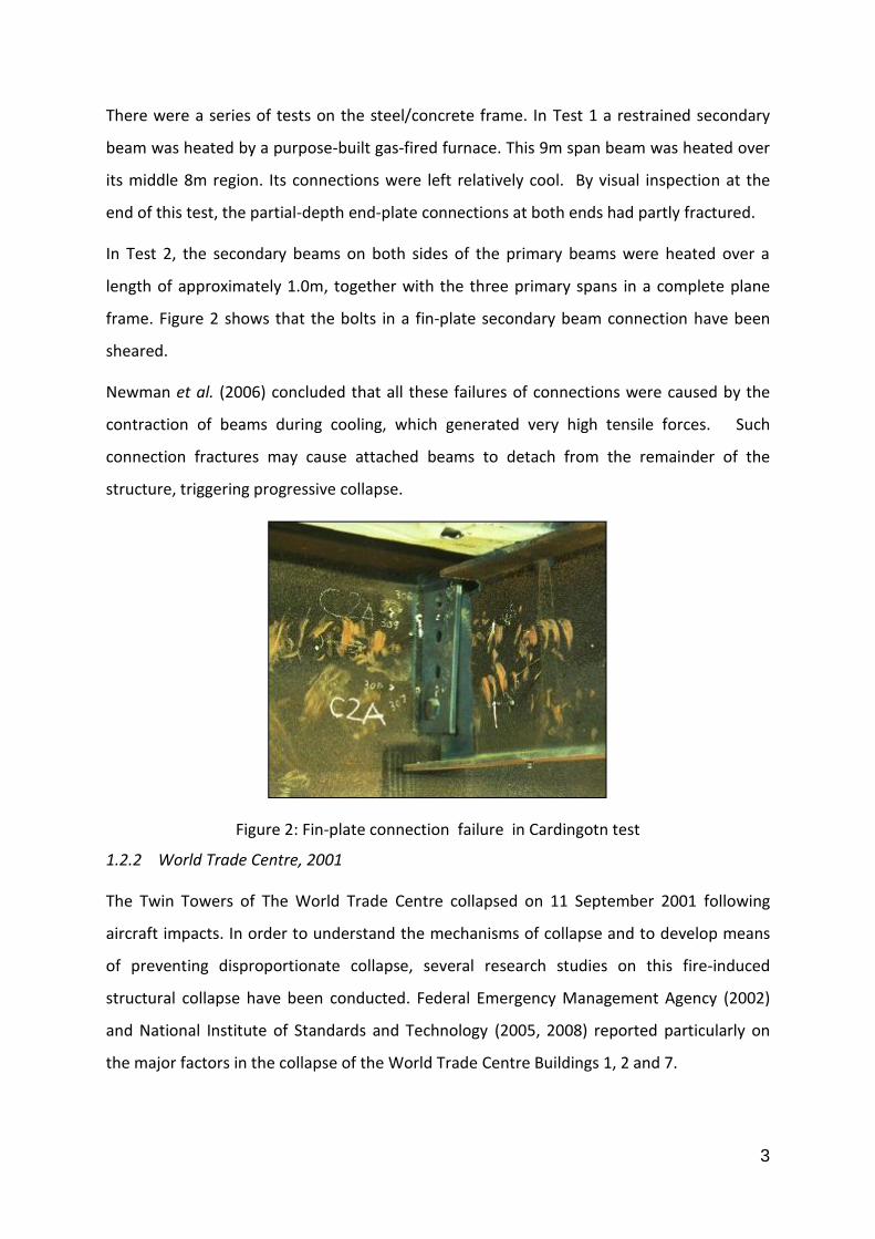
In Test 2, the secondary beams on both sides of the primary beams were heated over a

length of approximately 1.0m, together with the three primary spans in a complete plane

frame. Figure 2 shows that the bolts in a fin-plate secondary beam connection have been

sheared.

Newman et al. (2006) concluded that all these failures of connections were caused by the

contraction of beams during cooling, which generated very high tensile forces. Such

connection fractures may cause attached beams to detach from the remainder of the

structure, triggering progressive collapse.

Figure 2: Fin-plate connection failure in Cardingotn test

1.2.2 World Trade Centre, 2001

The Twin Towers of The World Trade Centre collapsed on 11 September 2001 following

aircraft impacts. In order to understand the mechanisms of collapse and to develop means

of preventing disproportionate collapse, several research studies on this fire-induced

structural collapse have been conducted. Federal Emergency Management Agency (2002)

and National Institute of Standards and Technology (2005, 2008) reported particularly on

the major factors in the collapse of the World Trade Centre Buildings 1, 2 and 7.

4

In particular, Building 7 of the World Trade Centre is deemed to have undergone progressive

collapse due to the failure of key connections joining primary beams to columns. Particular

attention is drawn to the connection of primary beams to Column 79 on Floors 12-14 as the

probable leading factor in the collapse (See Figure 3) these primary beams (44/79)

supported several protected secondary beams with long spans, on one side only, with very

few secondary beams attached on the opposite side. These secondary beams were heated

over a long period to temperatures between 500°C and 600°C during the fire. In order to

restrain the secondary beams from expanding by about 100mm the primary beam would

have needed connections which were extremely strong in horizontal shear. In the event,

large horizontal forces were generated at these connections, which had only been designed

against gravity load. The locating bolts at this connection had so little shear resistance that

they were easily fractured by the horizontal shear forces produced by restrained expansion

of the secondary beams; and the primary beam was separated from Column 79. This

separation would have sequentially happened on adjacent lower floors, thus depriving

Column 79 of horizontal support from these floors and facilitating its buckling and collapse.

In the process of collapse of the floors immediately involved, the falling cumulative mass of

these superstructures would generate large dynamic forces, which the lower structure could

not resist.

Figure 3: Typical floor plan of WTC building 7 (NIST, 2008)

5

1.3 Performance-based design

Until recently, most design against fire has been based on the simple ‘deemed-to-satisfy’

prescriptive building codes. This prescriptive approach is based on experiences accumulated

through many years in the light of past fire incidents (Wang, 2013). Since it is simple to put

into practice, and has displayed a generally satisfactory level of fire safety, the prescriptive

approach has been very extensively used to specify fire strategies. However, design codes

based on various aspects of performance have not been extensive enough in scope to be

able to cover all cases. Designers also have little or no opportunity to take a rational

engineering approach to the conduct of fire safety design. The final alternative is a fully

performance-based approach to design, based on the basic principles of fire science, heat

transfer and structural mechanics, and aims to provide information on how an integrated

building performs under a wide range of ignition scenarios (Custer, 1997).

In 1991, the Building Regulations in England and Wales changed from prescriptive to

performance-based requirements. The statutory requirement is that ‘the building shall be

designed and constructed so that, in the event of fire, its stability will be maintained for a

reasonable period’. Practical guidance was also given by Approved Document B, which

amplifies the Building Regulations, as ‘A fire safety engineering approach that takes into

account the total fire safety package can provide an alternative approach to fire safety’.

In performance-based design, any fire strategy can be adopted by fire engineers, when they

wish to, and are able to, verify against the agreed fire safety goals. The whole performance

of the building under fire is assessed, in the context of both the active fire safety systems

and passive fire protection, and the performance of the structure. Variations from the

acceptable solutions which offer greater cost savings or other benefits can be assessed.

With a correct level of safety plus cost saving, the building’s marketing potential is therefore

increased, and it will attract a higher income.

In order to allow designers to develop structures which perform well in fires, a trustworthy

method is to model the frame using global nonlinear finite element (FE) analysis, which

takes account of changing temperatures temperature-dependent material properties and

thermal expansion characteristics. With this method, designers are able to develop

sufficiently robust connection and structural configurations. This can give more confidence

6

about the actual structural behaviour in a fire rather than the supposedly conservative

protections given by a series of arbitrary rules.

Projects world-wide, such as the China Central Television (CCTV) building in Beijing, have

started to use this fire engineering approach to justify the sufficiency of their prescriptive

fire protection (Luo, 2005). The application of performance-based design has not only great

potential for improving structural safety but also for cutting whole-life cost.

7

Chapter 2. Literature review of research on modelling of semi-rigid joints in fire

The importance of joints in fire in general has been highlighted in the previous chapter. To

accurately predict the behaviour of steel frames in fire, it is essential to include the effects

of connection behaviour, particularly the combined effect of axial force, co-existent large

rotation and the reductions of strength and stiffness with elevated temperatures.

One approach to such a problem is to conduct full-scale or isolated fire testing. In 1976,

CTICM (Kruppa, 1976) conducted the first experimental fire tests on joints, which showed

that the deformation of other elements preceded bolt failure. Since it was intended to

investigate the performance of high-strength bolts at elevated temperatures, the

performance of the joint as a whole was not presented. Lawson (1990) also conducted a set

of moment-rotation joint tests in fire to measure the residual structural continuity afforded

by beam-to-column joints at elevated temperatures. The tested joint types included

extended endplate, flush end plate and double-sided web cleat. Non-composite, composite

and shelf angle floor beams were considered in this study. All the joint rotations reached

over 6O. The tests verified the rotational plastic capacity of joints in fire, which could retain

up to two-thirds of the ambient design moment capacity at the test temperatures. He also

stated that the composite action in fire contributed to the joints’ moment capacity, which

could be estimated on basis of the combined moment capacities of the bare steel joint and

the reinforced concrete slab. A simple rule was also proposed by Lawson to design simply

supported beams, taking into account the moment transferred via joints in fire. These early

attempts provided some important information for joint modelling during the early stages

of the development of performance-based structural fire engineering. However, these tests

supplied insufficient data to present the moment-rotation characteristics of the joints, and

totally ignored the effects of large axial restraint forces. Since that era, a large number of

more focused experimental tests have been conducted to understand various aspects of the

behaviour of joints in fire. However, such furnace testing is so expensive that it cannot

economically produce a sufficiently large database of results for direct practical design

purposes.

8

The alternative approach is to create numerical models to simulate the joints’ behaviour in

fire. This chapter will concentrate on previous developments in the modelling of semi-rigid

joints at ambient and elevated temperatures.

2.1 Joint material properties at elevated temperature

The material of which a joint is composed will degrade with elevated temperature. EC3 Part

1-2 (CEN 2005c) summarizes the relationships between the Young’s modulus of steel and its

yield strength at elevated temperatures. These reduction factors are included in Table 1 and

Table 2, and also plotted in Figure 4 to Figure 6.

Table 1: Structural steel material reduction factors at elevated temperatures (CEN, 2005b)

Steel temperature (°C)

Yields strength reduction factor

Young's modulus reduction factor

20 1.000 1.000

100 1.000 1.000

200 1.000 0.900

300 1.000 0.800

400 1.000 0.700

500 0.780 0.600

600 0.470 0.310

700 0.230 0.130

800 0.110 0.090

900 0.060 0.068

1000 0.040 0.045

1100 0.020 0.023

1200 0.000 0.000

Table 2: Bolt material strength reduction factors at elevated temperatures (CEN, 2005b)

Temperature (°C) Strength reduction factor for bolts

20 1.000

100 0.968

150 0.952

200 0.935

300 0.903

400 0.775

500 0.550

600 0.220

700 0.100

800 0.067

900 0.033

1000 0.000

9

Figure 4: Reduction factors for yiled strength relationship of steel at elevated temperatures (CEN, 2005b)

Figure 5: Reduction factors for Young’s modulus relationship of steel at elevated temperatures (CEN, 2005b)

Figure 6: Reduction factors for strength relationship of bolts at elevated temperatures (CEN,

2005b)

0

0.1

0.2

0.3

0.4

0.5

0.6

0.7

0.8

0.9

1

0 200 400 600 800 1000 1200

Yie

lds

str

en

gth

re

du

cti

on

fa

cto

r

Temperature (OC)

0

0.1

0.2

0.3

0.4

0.5

0.6

0.7

0.8

0.9

1

0 200 400 600 800 1000 1200

Yo

un

g's

mo

du

lus r

ed

ucti

on

facto

r

Temperature (OC)

0

0.1

0.2

0.3

0.4

0.5

0.6

0.7

0.8

0.9

1

0 200 400 600 800 1000

Str

en

gth

re

du

cti

on

fa

cto

r fo

r b

olt

s

Temperature (OC)

10

2.2 Semi-rigid joint definition

It is generally acknowledged that semi-rigid design of steel frames can result in efficiency,

lightness and economical design (Astaneh, 1989). When the connections are designed as

semi-rigid, a certain amount of moment is allowed to transfer from the beam-ends to the

columns, which reduces the mid-span bending moments in the beams (Anderson, 1987). As

a direct result, it is possible to reduce the internal beam cross-sections. Compared to pinned

connection, the provision of semi-rigid connection stiffness also helps the columns to resist

buckling.

Based on a joint’s rotational stiffness, EC3 Part 1-8 (CEN (2005b)) classifies joints as semi-

rigid, pinned or rigid (see Table 3).

Table 3: Connection type definitions in EC3 Part 1-8 (CEN, 2005b)

Connection type Definition

Pinned Effectively released in terms of rotational constraint. Can transfer

internal forces, but will not develop considerable moments.

Rigid Effectively continuous. Has sufficient rotational stiffness to

transfer both forces and moments.

Semi-rigid Lies between the pinned and rigid connection types. The

interaction between members is based on the design moment-

rotation characteristics of the joint.

As explained in the previous chapter, the effects of joint behaviour are so influential on the

distribution of internal forces and moments within a structure in a fire scenario that they

should be taken into account in structural analysis in fire. The deformations at fire

temperatures can be several orders of magnitude higher than those used in ambient-

temperature semi-rigid design, and so the high-strain properties of connection components

become dominant compared with initial stiffnesses.

11

2.3 Evolution of analysis methods for semi-rigid joints

The early work on semi-rigid joint models has been summarized by Nethercot and Zandonini

(1989). This summary will not be repeated here.

The incorporation of semi-rigid behaviour, both axially and rotationally, within global

structural analysis for fire cases, is important. In fire, the connections are subjected to high

axial forces and large deformations, due to the thermal expansion/contraction of beams and

degradation of their material strengths and stiffness.

In general, there are three different ways of modelling semi-rigid joints (Al-Jabri, 2008):

1. Mathematical expressions – curve-fit models;

2. Finite element models;

3. Component-based methods.

2.3.1 Mathematical expressions – curve-fit models

The curve-fit model uses a numerical form (generally polynomial) to represent the moment-

rotation relationship of a joint, which is based on experimental test data. Figure 7 illustrates

that the joint’s behaviour can be represented by different forms of curve-fitting. It can be

implemented in analytical models such as finite element models. In order to consider the

effects of various parts within the joint, such as bolts, welding and plates, the moment-

rotation relationship is generally complicated, and has to be non-linear. Typical

mathematical representations include bi-linear, tri-linear and multi-linear curves.

Figure 7: Different forms of curve-fitting representation of joints characteristics (Al-Jabri, 2008)

12

EI-Rimawi (1997) made an initial attempt to use a curve-fitting method to model joint

behaviour in fire. A simple equation with three parameters using a Ramberg-Osgood

expression (1943) was proposed in the following form.

n

B

M

A

M

01.0 (2.1)

where the relationship between joint rotation () and moment (M) are defined by the

temperature-dependent parameters A, B and n. The parameters A and B respectively

represent the joint’s stiffness and strength, and n defines the sharpness of the “knee” in the

curve. This model was extended further by Leston-Jones (1997) and Al-Jabri (1999), to a

model which was capable of closely representing a joint’s rotational stiffness and strength

with increasing temperature. Figure 8 shows that the curve-fit model could even be

extended to combine two separate moment-rotation expressions to cope with connections,

such as flexible endplate connections, which have two stages of moment-rotation

behaviour: before and after contact of the beam flange with column flange.

Figure 8: Moment-rotation-temperature curves for a typical flexible end plate joint (Al-Jabri, 2008)

In general, these models predict a joint’s rotational behaviour with reasonable accuracy.

Since these models are developed on the basis of isolated joints subject only to moment

and rotation, they are limited in application to cases where the effect of axial restraint due

to thermal expansion/contraction is not critical, and where axial forces superposed on

moments are not likely to be serious. However, as discussed in the previous chapter, the

axial force due to thermal expansion/contraction can cause connection failure and trigger

13

progressive collapse. Therefore, global analysis for performance-based design using the

curve-fit model cannot represent the structural global behaviour with reasonable accuracy.

2.3.2 Finite element models

The finite element method (FEM) is a powerful tool to investigate joint behaviour in fire.

Since Liu (1994, 1996, 1998a and 1998b) made the first attempt to model joint behaviour at

elevated temperature, several authors have developed various methods considering

geometrical and material nonlinearity.

As Al-Jabri et al. (2008) summarized, finite element models can provide good comparisons

against tests on joints in fire. It is a reliable technique, and enables a wider range of

parameters to be investigated than is possible in rather complex and expensive tests.

However, the cost in terms of time is an obstacle to its practical application in structural fire

engineering design.

2.3.3 The ‘component method’

EC3 Part 1-8 defines the component method as a design method, in which a joint is

modelled as an assembly of basic components, to specify the structural properties of joints

in frames of any type. Jaspart (2000) illustrated the component method by analogy with the

finite element method, in which each component is equivalent to one finite element in the

FE method. It must be emphasized that all of the above work was done as part of the

development of semi-rigid ambient-temperature design methods for steel frames, and is

therefore restricted to small rotations, elastic rotational stiffness and plastic capacity. It

completely ignores large deflections, axial force and component fracture; all of these are

vital for progressive collapse analysis in fire.

The component method was originated by Zoetemeijer (1974). A simple analytical method

for the behaviour of T-stubs, as a common element in conventional steel connections, was

developed. This method took into account the plasticity of the flanges and bolts. Two

different collapse mechanisms were defined based on the determining factor: bolt facture

and flange plate collapse. Accordingly, a number of yield line patterns were specified

(examples are shown in Figure 9 and Figure 10). An ‘effective length’ for a T-stub was

calculated on the basis of a number of yield line patterns. This method was validated by a

14

series of tests. These yield line patterns have been included in so-called ‘Green book’ (SCI,

1997), and EC3-1.8 (CEN, 2005b).

Figure 9: Failure mechanism 1

Figure 10: failure mechanism2

After that, Tschemmernegg et al. (1987) improved the component method. He investigated

the behaviour compression zone in the column web. A series of tests focused on welded and

bolted bare-steel endplate joints. The axial column loading was included in some of these

tests. He proposed the component-method as a way of determining analytically the

nonlinear moment-rotation relationships, in terms of initial stiffness and plastic capacity, for

joints (both welded and bolted) in structural steel frames (shown in Figure 11). This

development incorporated the most important features of the component method: the

joint is composed of several zones, each of which is represented by a non-linear spring.

15

Figure 11: Force-displacement curve after Tschemmernegg et al (Block, 2006a)

The component method has subsequently been developed by Jaspart (2000, who

summarized the development of component-based models into three steps:

Identification of the active components

Evaluation of the mechanical characteristics of each individual basic component

Assembly of the components

Jaspart listed the relevant components for an extended end-plate connection. Each of the

basic components has its own definition of strength and stiffness, in tension, compression

or shear. The effects of interaction were also considered within a given component when

subject to the coexistence of compression (or tension) and shear. This interaction is likely to

reduce the component’s strength and stiffness, and to affect its force-displacement curve.

Jaspart (2000) also pointed out that the component method could be suitable for the

characteristics of joints subjected to extreme loading conditions such as earthquake or fire.

The component-based method has been included in EC3 Part 1-8 as a standard tool to

calculate semi-rigid joint behaviour. Compared either with the time consumed in setting-up

FE models or in the prohibitive expense of fire tests, the component method is a relatively

easy way for structural engineers to predict the joint capacity by hand, and also to offer an

intermediate method to model semi-rigid joints within global nonlinear structural analysis

software.

Leston-Jones (1997) conducted a programme of moment-rotation-temperature experiments

on typical flush end-plate connections, covering a range of temperatures. Both bare-steel

and composite arrangements were considered. A spring-stiffness rotational model (shown

16

in Figure 12) was developed to represent connection degradation at high temperatures. The

model was designed for two bolt row flush endplate connection, considering endplate in

bending (epb), column flange in bending (cfb), column web in compression (cwc), and bolt

in tension (bt). Similar to Eurocode, an equivalent bolt row was adopted to deal with the

connection with more than one bolt row. A tri-linear curve was used for each component.

Sensitivity studies were then carried out to investigate of the influence of connection

response on frame behaviour in fire.

(a)

(b)

Figure 12: Spring model of a flush endplate connection (a) and equivalent model (b) after Leston-Jones (Block, 2006a)

Al-Jabri (1999) extended Leston-Jones’s experimental programme from small section sizes

to larger beam and column sections, and concentrated more fully on composite

connections. Using the same principles as Leston-Jones, he developed a component-based

model to represent his flush endplate connection tests at elevated temperatures. He

extended this model for the partial-depth endplate connection, and achieved a good match

with the tests. Once again this work was purely rotational.

Simões da Silva et al. (2001) proposed a purely rotational component model for bare steel

flush end-plate joints (shown in Figure 13). The model was designed to assess the moment

resistance and rotational stiffness of a joint at both ambient and elevated temperatures.

The components were defined in compliance with EN 1993-1-8. For elevated-temperature

cases, the material strength and modulus reduction factors given in EN 1993-1-2 were

adopted. In validations against Al-Jabri’s tests, a global temperature correction factor (equal

17

to 0.925 experiment) was necessary in order to achieve good agreement between the tests

and the model.

Figure 13: Typical component-based connection assembly (Simões da Silva, 2001)

Spyrou (2002) conducted a series of furnace tests to identify the degradation of the

characteristics of T-stubs in tension, and column webs under compression, at elevated

temperatures. Detailed finite element studies were also conducted. Based on these tests

and finite element models, component models for end-plate/flange T-stubs under tension,

and column webs under compression, were developed for modelling of the behaviour of

steel-to-steel connections at elevated temperature. The influence of axial forces on joint

response and overall frame behaviour was highlighted. Both tensile and compressive axial

forces are recognised as reducing the rotational ductility of joints, and therefore limit the

ductility of the structural frame. In the fire scenario, the axial force effect will be even more

distinct. Hence, in order to provide with acceptable accuracy, it is necessary for the

component-based model to include the axial force effect.

Sokol et al (2003) developed three nonlinear springs and assembled them to simulate the

Cardington fire test No.7, in order to study structural integrity. The three springs

respectively represented tension, compression and shear within the connection. This study

showed reasonably good agreement during the heating phase of the structure, but

experienced some difficulty in representing the cooling phase.

18

Block (2004a, 2004b, 2005a, 2005b,2006a, 2006b, 2007, 2013a and 2013b) focused on the effect

of axial pre-compression in columns, due to superstructure loading, on the behaviour of the

column-web compression zone of steel-to-steel end-plate connections. Both furnace tests

and finite element modelling were conducted, and simplified component models were

developed, from the basis of Spyrou’s component model, including the column web under

compression. A component-based connection element (Figure 14) was developed and

simulated in the Vulcan research code, and this was partly validated.

Figure 14: Block’s (2006a) component assembly for end-plate connection.

A collaborative EPSRC project (EP/C5109841/1) conducted by the Universities of Sheffield

and Manchester investigated the robustness of connections in fire conditions (Yu et al.,

2008a, 2008b, 2009a,2009b, 2009c, 2009d and 2011; Hu et al., 2009, Dai et al., 2009a,

2009b, 2010a and 2010b). The tested connections encompassed four typical beam-column

connections: fin-plate, flush end-plate, flexible end-plate and web-cleat. A selection of

connections under inclined forces (Figure 15), as well as structural subframes, was tested to

very high deformation, and in some cases to destruction, at temperatures up to 650°C. Yu

(2011) also conducted numerical investigations of the tested connections. On the basis of

Compression springs (column web)

One set of tension springs per bolt row (T-stubs, bolts)

Shear spring (bolts)Zero length

i j

19

the yield-line method, Yu (2009) developed a component model for the T-stub, which

considers both geometry and material nonlinearity.

Figure 15: Joint test setup (schematic) by Yu (2011)

Santiago et al. (2008a, and 2008b, 2009 and 2010) conducted experimental and numerical

studies of six steel subframes under natural fire conditions. The objective was to investigate

joint behaviour under combined bending moment and the axial force developed during a

natural fire. The study focused on three types of connection: header plate, flush end-plate,

and extended end-plate. It was intended to investigate the influence of connection type on

the behavior of steel sub-structures in fire. The experimental investigation highlighted the

fact that the large tensile forces and reversal of connection moment during the cooling

stage can cause failure of bolted joints.

Jones (2008, 2009, 2010a and 2010b), conducted a series of ambient- and elevated-

temperature tests on fin-plate connections to tubular columns. These included fin plates

under tension (tying) and shear force, and reverse channel legs under shear. After these

tests and extensive numerical simulations had been achieved, a component-based method

for the tensile behaviour of fin plate connections to concrete-filled rectangular steel tubular

columns was developed.

Furnace

Load Jack

Reaction frame

20

Taib (2012) created an integrated component-based element for fin-plate connections

under fire conditions. The development was based on Sarraj’s (2007) development of a

realistic FE model for fin plate connections in fire. The component-based element considers

the influence of both vertical and horizontal forces at bolt rows, as well as incorporating

unloading and cooling properties.

2.4 The COMPFIRE project

COMPFIRE was one of the latest joints-in-fire projects, and particularly considered the

behaviour and design of joints to composite columns for improved robustness in fire. This

project (RFCS, 2009) involved a number of academic research groups and industrial

partners, namely

University of Coimbra

Czech Technical University

DESMO

Luleå Technical University

University of Sheffield

University of Manchester

TATA Steel Tubes (Europe)

This project coincided with the author’s PhD studies, and supplied extensive and useful test

and numerical data.

The aim of this project was to provide an integrated approach to the practical application of

performance-based fire engineering design to composite structures, taking account of joint

performance under natural fire conditions, including the cooling phase. The main objective

was to develop a comprehensive component-based design methodology for joints to

composite columns. The composite joints (Figure 16) under investigation were traditional

flush endplate and the novel semi-rigid reverse channel connections. These were applied to

connections between steel beams (UB306x165x40 shown in Figure 16) and two types of

composite column; concrete-filled tubular (CFT, SHS 224.5x8 in Figure 16b) and partially-

encased H-section (PE, 254x254x89 UC in Figure 16a) columns. The reverse-channel

connection possesses very high rotational capacity without compromising its ultimate

strength under ambient-temperature gravity load.

21

Figure 16: (a) Endplate and (b) reverse-channel connections to composite columns (Huang, 2012)

The project included a number of tests on complete joints, numerical and analytical studies

of components, whole connection assemblies and structural subframes. The project

included seven work packages:

1. Joint thermal behaviour and modelling: this package was intended to investigate the

temperature distributions within the joints in both standard and real fire scenarios.

2. Component behaviour: A comprehensive set of reverse channel component test data

was gathered by the Universities of Manchester and Coimbra. The University of

Sheffield conducted 20 isolated-joint tests. Based on these data, Luleå Technical

University performed simulations using finite element modelling, and expanded the

test data. The University of Sheffield developed simplified models to predict the

load-deflection curves of reverse channel components at both ambient and elevated

temperatures.

3. Component-based joint modelling: The component models developed in Work

Package 2 were assembled and validated against the isolated joint tests in Work

Package 2.

4. Fire tests on subframes: The Universities of Manchester and Coimbra conducted a

total of 11 subframe tests to assess the complicated behaviour between the

composite joint and the surrounding structural element under different fire

(b) (a)

22

exposure conditions, including an investigation of how the connections behave

during the cooling phase of a fire event.

5. Integrated FE modelling: This work package used both standard finite element

analysis, and finite element analysis incorporating a simplified component-based

method, to model the subframe tests conducted in Work Package 4.

6. Demonstration fire tests: Two fire tests on a complete composite structure under

natural fire conditions were conducted, in order to provide experimental data and to

demonstrate impact of joints with improved detailing on structural fire robustness.

7. Development of practical design guides: Based on the previous work package, a

practical method was developed to predict composite joint behaviour under fire.

The project data was intended to be used to develop a general component-based

connection element, to enable global non-linear structural programs to model the whole

structure, including the behaviour of connections. The test data would also be used to

validate the component-based connection element.

2.5 Conclusion

The component-based method provides an intermediate approach, using the minimum of

computational effort, while retaining the key characteristics of connection behaviour and

offering acceptable predictions of frame behaviour.

The above developments by Zoetemeijer, Tchemmernegg and Jaspart were intended for

semi-rigid steel connections at ambient temperature against normal design loads. The

elastic and yield material properties were considered. The initial elastic rotational stiffness

was captured. However, this cannot be used for large deflection, or for material non-

linearity at elevated temperature.

The main aim of the research by Leston-Jones, Al-Jabri and Simões da Silva was to develop

moment-rotation-temperature characteristics of joints. However, in the wake of

observations from both accidental fires and full-scale fire tests at Cardington, the effect of

axial force has also risen considerably in importance.

The developments by Spyrou, Sokol, Block , Jones and Taib were limited to one connection

type, either flush endplate or fin plate connections.

23

2.6 Research motivations

Observations from the full-scale fire tests at Cardington and the collapse of buildings of the

World Trade Centre in 2001 have raised concerns that joints are potentially the weakest

parts of a structure (Burgess, 2007). Due to the combination of thermal and mechanical

effects caused by heating, the resultant forces on joints (in addition to vertical shear) are

complicated and vary, from pure moment, to moment and compression, and eventually to

almost pure tension. Additionally, the connections are subjected to large rotations.

Therefore, engineers must take into account the complexity of actions on the connections,

and their response, when designing structures that will perform well in a fire. The

incorporation of realistic connection behaviour within global nonlinear finite element

programs is important, as it allows designers to be clear about the actual structural

behaviour and to ensure the adequacy of the connections in terms of robustness and

ductility.

However, incorporation of realistic joint behaviour in the structural analysis is problematic.

The test data is limited, and can only reveal how the connections work in fire to a certain

extent, as testing is expensive and there is a wide range of joint types. Although general

finite element packages can predict the behaviour of connections with a good degree of

accuracy, the modelling of connections to obtain this behaviour is prohibitively detailed, and

therefore expensive, in practical design situations.

It would be ideal to create a general component-based representation of the ‘connection

zone’ at the column-face of a beam-to-column joint. This requires the minimum of

computational effort, while retaining the key characteristics of connection behaviour and

offering acceptable predictions of frame behaviour. It enables engineers to predict the

behaviour of connections within a structure in fire, to track the progressive collapse

sequence, and to design robust structures based on performance-based principles.

2.7 Research aim, objectives and methodologies

2.7.1 Aim of research

This PhD research is intended to develop component-based connection elements for two

connection types: flush endplate and reverse channel connections, and to demonstrate

their use in case studies.

24

2.7.2 Detailed objectives

The research activities are:

Identification of the active components;

Development of component models;

Component assembly;

Tests on connection element.

Running demonstration cases as examples of application.

2.7.3 Methodologies

Based on the joint test and detailed finite element analysis, both flush endplate and reverse

channel connections are divided into several zones, called active component zones, which

either contribute to the joint deformation, or limit the joint capacity.

These active components will each be represented by a lateral spring. This spring is

termpature-dependent and defined with failure criteria. For flush endplate, Spyrou (2002),

Block (2004a, 2004b, 2005a, 2005b, 2006a, 2006b, 2007, 2013a and 2013b), and Yu (2008a,

2008b, 2009a, 2009b, 2009c, 2009d and 2011) have developed the models for some of the

key components, including T-stub in tension, and column web under compression. For

reverse channel connections, the component models for reverse channel under

tension/compression were needed.

In order to enable global (frame analysis) nonlinear structural software to model the

structure taking into account the semi-rigid joint behaviour in fire, it is essential to assemble

these component models using rigid links. Yu’s isolated joint tests and the COMPFIRE

project provided comprehensive data to validate this development.

25

Chapter 3. Development of component models for reverse channel connections

The reverse channel itself is clearly one of the key components of the reverse channel

connection. In order to build up the component-based connection element for the reverse

channel connection, a force-displacement relationship was developed on the basis of the

plastic hinge method. In addition, a bolt pull-out limit derived from a ‘cone model’ (also

called the ‘bolt pull-out model’) was developed. A series of component tests and whole-joint

tests were conducted in the COMPFIRE project, and these provided experimental data

which helped to characterise the behaviour of reverse channel connections under tension.

Based on these tests, an extensive FEA parametric study was simulated by the COMPFIRE

partner at Luleå, which was intended to facilitate the investigation of all the possible

behaviour of reverse channels under tension/compression and validation of the component

models for the reverse channel under tension and compression.

3.1 Plastic hinge method

The reverse channel supports tensile and compressive loads, primarily through bending

action. Therefore, the plastic theory of structures (Horne, 1971) can be used to deal with

the behaviour of the reverse channel under tension or compression beyond the elastic limit,

with particular emphasis on the failure load. With material properties which degrade either

as a result of increasing temperature and/or increasing loading, plastic hinges will gradually

form at the most highly stressed points in the reverse channel. Material and geometric

nonlinearities are considered, but the effects of shear and axial forces on the plastic hinges

are neglected, because their effects on the bending capacity will be small.

Bhatt (1999) explained the effect of shear force on the ultimate bending capacity, and

characterised the effect as:

2/75.01 pp QQMM

(3.1)

in which Mp is the section’s plastic moment capacity, where the plastic hinge forms; Qp is

the plastic shear capacity; Q is the shear force and M is the moment. In order to assess the

effects of shear on the bending capacity, the following is a quick assessment (shown in

figure 17), considering 150mm long plastic hinge with 12mm plate thickness. The maximum

shear used the maximum tensile resistance based on an 8.8 M20 bolt.

26

Plate thickness (where the plastic hinge forms) mmt p 12

Plate length (where the plastic hinge forms) mmLp 12

Tensile area per M20 bolt: 2245mmAt

(Owens, 1989)

Tension strength of per M20 bolt pt: 2560

mm

Npt

(BSI, 2001)

Tension capacity of M20 bolt: kN

ApP tt

t 2.1371000

The maximum shear is limited by the bolt tension capacity. Therefore,

kNPQ t 2.137max

The plastic shear force is

kN

LtfQ

ppy

p 3693

The plastic moment capacity reduction factor is

%3.10max

75.0

2

Qp

Qr

Figure 17: illustration of shear effect on plastic hinge moment capacity

tp

F (based on M12 bolt tensile capacity)

Assumed plastic

hinge location

Lp

27

This plastic moment capacity reduction factor can be ignored in the derivation of the

component’s force-displacement curve, but can be taken into account as a design safety

factor in later practice.

According to the energy-balance principle, the external work is equal to the internal work

absorbed in plastic deformation of the hinges:

321 PHPHPH WWWF (3.2)

Where is the external work done by the applied load F in moving through a displacement

δ, and WPH1, WPH2 andWPH3 are the internal plastic work components due to rotations of the

plastic hinges PH1, PH2 and PH3.

A three-phase elastic-plastic material property model (Figure 18) is assumed, similar to that

used by Yu (2009) for T-stub models. The details of Yu’s derivation are documented in 3.2.

Figure 18: Stress blocks of a plastic hinge (Yu, 2009a)

3.2 Yu’s T-stub model (Yu, 2009)

Yu (2009) developed a component model for T-stubs (shown in Figure 19) in fire on the basis

of the energy method. The development of the current component model for reverse

channel connections under tension and compression uses Yu (2009)’s approach to calculate

the strain energy within the plastic hinge. This part will include Yu’s derivation in calculating

the plastic hinge energy.

m

x

u

yf

uf

c2 c1

y

c1

28

Figure 19: Yu’s (2009) mechanism for T-stub

The assumed material model is shown in Figure 18, as a typical elastic-plastic three-phase

characteristic. The calculation of strain energy is divided into three possibilities when the

strain (ԑm) within the plastic hinge reaches the different stages.

3.2.1 When strain ԑm is lower than yield strain ԑy ( ym ,

refer to Figure 18)

Stress is

mt

xE

2

(3.3)

Where E is the Young’s modulus, x is the distance to the plate centre line, and t is the plate

thickness

The moment at the plastic hinge

xdxt

xEBeM m

t

ff 2

0 22

(3.4)

meff E

tBM

3

1

22

2

(3.5)

Where Beff is the effective width of the plastic hinge.

3.2.2 When strain ԑm is higher than yield strain ԑy but lower than ultimate strain ԑu

( umy , refer to Figure 18))

21

tc

m

y

(3.6)

29

The stress can be written as

1

1

2

2

cxt

xEf

cxt

xE

ymty

m

(3.7)

Where Et is the tangent Young’s modulus. The moment at the plastic hinge is

xdx

t

xEfxdx

t

xEBM

t

cymtym

c

beff

2

0 222

(3.8)

2

32

6

1

2

1

3

1

22

m

y

tytmteff EEEEEt

BM

(3.9)

3.2.3 When strain ԑm is higher than ultimate strain ԑu ( um ,refer to Figure 18)

22

tc

m

u

(3.10)

The stress is

2

2

1

2

2

cxf

cxt

xEf

cxt

xE

u

ymty

m

(3.11)

The moment M is

xdxfxdx

t

xEfxdx

t

xEBeM

t

cu

c

cymtym

c

ff

2

0 2

2

1

1

222

(3.12)

Therefore,

2332

2

2

2

1

3

1

6

1

2

11

2

1

22 uuutyuyt

m

ueff fEEEft

BM

(3.13)

30

3.2.4 Strain energy

The curvature of the cross-section is2t

m . This assumes the length of the plastic hinge is

t, the rotation of the plastic hinge is

m

tm dx

t

2

20

(3.14)

Factor 2

02

2

tBM eff

(3.15)

The moment M is simplified into

ym :

EMM6

10

(3.16)

umy :

2

3

03

2

2

1

6

1

y

tytt EEEEEMM

(3.17)

um :

2332

202

1

3

1

6

1

2

14

2

1uuutyuytu fEEEfMM

(3.18)

The rotational energy generated at the yield line is calculated by

0

MdWph (3.19)

ym

2

12

1EWph

(3.20)

um :

y

y

dEEEEEdEWy

tyttph2 2

32

0 3

2

2

1

6

1

6

1

2

3

2

3

2

2

1

12

1y

y

ytt EEE

(3.21)

31

um :

u

u

y

y

dfEEEf

dEEEEEdEW

uuutyuytu

y

tyttph

2

2332

2

2

2 2

32

0

2

1

3

1

6

1

2

14

2

1

3

2

2

1

6

1

6

1

233222

2

1

3

1

6

1

2

142

2

12 uuutyuytuuyyutut fEEEfEEE

(3.22)

3.3 Development of the component model for reverse channel under tension

Following the flush endplate connection, the reverse channel was introduced between the

composite column face and endplate. Since the reverse channel is relatively flexible, the

connection deformation can be large, which itself may limit the connection’s capacity.

Hence, it is necessary to implement a component model to represent the reverse channel in

the connection element. The following two sections will develop the component model for

reverse channels under tension and compression.

The component model developed for the reverse channel under tension adopts the plastic

hinge mechanism method to calculate the force/displacement curve. By investigation of the

component tests conducted in COMPFIRE (RFCS, 2012a), a reverse channel under tension

may form two combined plastic hinge mechanisms:

A ‘cone’ with a circular plastic hinge around the bolt head (Figure 20a).

Straight line plastic hinges (Figure 20b)

Both of the plastic hinge mechanisms are identified in the component test in Figure 21

Figure 22. In the straight-line plastic hinge mechanism, 6 plastic hinges form. The tops of the

two legs are moved slightly towards each other by the bending deformation in the web.

The ‘circular’ plastic hinge is due to the bolt head being pulled-out from the bolt hole in the

reverse channel web. The conical wall is under circumferential tension, and a circular plastic

hinge forms at the bottom of the cone due to the rotation of the cone wall.

32

a) Circular yield line

at the base of the

b) Straight yield line

pattern

Figure 22: Circular yield line pattern and plastic hinge mechanism (RCT3) (RFCS, 2012a).

Figure 21: Straight yield line plastic hinge mechanism (RCT 8) (RFCS, 2012a).

Figure 20: Plastic hinge mechanisms

33

3.3.1 Straight-line plastic hinge mechanism

For the straight-line plastic hinge mechanism, the reverse channel works similarly to a

single-span portal frame. From the bending moment diagram (shown in Figure 23), three

plastic hinges (PH1, PH2 and PH3) gradually form. Figure 24 shows straight-line plastic hinge

locations for two types of reverse channel: a parallel-flange rolled channel (PFC) and a

channel cut from a structural hollow-section rectangular tube. PH1 is assumed to be at the

edge of the bolt head. PH2 and PH3 are respectively on the legs near the root of the tube-

cut and on the web of the PFC near to the root. This is because the maximum moment

happens at the intersection of web and leg, but the PFC and tube-cut sections have different

local wall thicknesses; the PFC has a thicker leg, and a gradually-changing thickness in the

root area. PH3 is at the bottom of the reverse channel leg. In order to allow sufficient space

to install the bolts on-site, it is considered that the minimum clear distance between the

reverse channel leg and bolt head should be 1.5 times the bolt diameter.

Figure 23: Bending moment diagram for single-span frame.

Based on the plastic hinge method (Figure 25), the rotations of the plastic hinges for a PFC

are calculated as:

0

30

2

0

2

1

cosarcsin

mm

mhh

(3.23)

312 (3.24)

0

2

0

2

10

3

cosarcsin

mh

mmm

(3.25)

PP

34

Figure 24: Reverse channel under tension: plastic hinge locations.

For the channel cut from tube, the plastic hinge rotations are calculated as:

ho

tf

roottw

mo

tf

roottw

m

m

PH1 PH2 PH3

h

h

m= (L-2n)/2-tf-rh-tw/2

mo= 0.8*root

m= (L-2n)/2-tf-rh-tw/2

ho= root+tw/2

L

L

2n

2n

Bolt head

radius: rh

Bolt head

radius: rh

PH1 PH2 PH3

b) PFC

a) Cut tube

θ0

h

m

h0

θ3

θ2

θ1

δ

F

θ3

θ2

F

δ

θ1

θ0

m0

h

m

Figure 25: Plastic hinge rotations

35

22

0

030

01

cos1arcsin

mh

hhh

(3.26)

312 (3.27)

0

10

22

0

3

cosarcsin

hh

mhm

(3.28)

3.3.2 Bolt pull-out ‘cone’ model mechanism

The bolt pull-out ‘cone’ model (Figure 26) is a simplified model used to calculate the local

deformation of the reverse channel web around a bolt hole before the bolt is pulled out.

The work done by the bolt tension force is assumed to be absorbed only by deformation of

the reverse channel web; the effect of stress concentrations, cracking around the bolt hole

and the non-uniform contact between the reverse channel and the bolt head are beyond

the scope of this analysis. Equating the internal absorbed work (Wtotal) to the external work

done:

FWtotal (3.29)

The internal work (Wtotal) in the ’cone model’ includes the absorbed energy in the circular

plastic hinge (Wcircular), and the strain energy due to the circumferential stretching of the

cone wall (Wstrip).

stripcircularotalt WWW (3.30)

36

Figure 26: Circular plastic hinge strain energy calculation

For the cone wall under tension, the average width of this area (rave) is

2/22

mm

dRrave (3.31)

In this equation, the d is the bolt shank diameter, and 2mm is the clearance between the

bolt hole and the bolt shank.

The average section area is:

wtd

RA

2

2 (3.32)

Where tw is the reverse channel web thickness.

The average cone wall radius is:

222

dRRrave

(3.33)

The average length of the cone wall is:

avestrip rL 2 (3.34)

The rotation of the circular plastic hinge is:

2/arctan

mdR

(3.35)

Average cone wall radius rave

Circular plastic hinge

dm/2

2R

θ

2R

0.8*root

Circular plastic hinge

Average cone wall radius rave: R-(R-d/2-2)/2r

Circular plastic hinge bolt head

bolt head

Circular plastic hinge cone wall under tension

δ

R-rave

37

Where dm is the mean of the dimensions of the bolt head across the points and across the

flats.

The average elongation of the cone wall is:

stripavestrip LrRRL cos2 (3.36)

The initial axial stiffness is:

stripL

EAk

(3.37)

The tangent stiffness is:

strip

TT

L

AEk

(3.38)

The Yield resistance is:

AfF yy (3.39)

The ultimate resistance is:

AfF uu (3.40)

The axial deformation along the bolt pull-out direction at the yield load is:

kFL yy (3.41)

The axial deformation at the ultimate load is:

Tyuyu kFFLL (3.42)

The work absorbed at a given bolt head movement (

ustripustripUyuUy

y

ustripyystripystripTy

y

ystripstrip

strip

LLLLFLLFFk

F

LLLLLLLkFk

F

LLLk

W

　　　　

　　　

　　　　　　　　　　　　　　　　　　

2

1

2

22

1

2

2

1

2

2

2

(3.43)

Figure 26 shows the principles of the rotation calculation for Wcircular, where

38

42

2

py

pcircular

tfRMW (3.44)

When the bolt is pulled out (Figure 28), the cone wall rotation (θ at unit of radians) reaches

its maximum (θmax):

22

2arccosmax dR

dR m

(3.45)

The bolt head maximum movement (δmax) is:

maxmax sin22

dR

(3.46)

Therefore, the Force (F) is:

totalWF max

(3.47)

Accordingly, the bolt pull-out limit (Fmax) is:

xma

totalWF

max,

max

(3.48)

Figure 27: Cone model for bolt pull-out limit.

3.4 Validation of the plastic hinge model for reverse channel under tension

A wide-ranging validation was performed using a series of tests and FEA simulations on

reverse channels of various geometries for ambient and elevated temperatures. In

COMPFIRE (RFCS, 2012a), a set of component tests on reverse channels under tension were

Dm/2

θmax

2R

δmax

39

performed by the Universities of Manchester and Coimbra with the aim of providing

experimental data to characterize the behaviour of the reverse channel under tension.

Following the test setup, the preliminary finite element model was simulated by the author

using ABAQUS, to investigate the reverse channel under tension behaviour. Based on the

tests in COMPFIRE, a further intensive FEA parametric study was conducted by Luleå

Technical University to investigate all possible modes of behaviour (RFCS, 2012a).

All the test and analysis results are represented as force/displacement curves (using the

measurements shown in Figure 28). The force is the total reaction force at the base of the

reverse channel, and the displacement is the movement measured at the bolt. In order to

investigate the ‘cone model’ contribution (the displacement due to the bolt being pulled

through the bolt hole), a force/displacement curve is also plotted for some of the tests, for

which the deformation is the local displacement of the bolt.

Figure 28: Displacement measurements for the component model validation.

3.4.1 Preliminary finite element simulation

While the University of Manchester was conducting the reverse channel component test

(shown in Figure 29), a preliminary finite element model was created to investigate the

behaviour of the reverse channel under tension. This preliminary finite element model was

general in nature, but was particularly focused on Test 7 (RCT 7).

Total force

Displacement for bolt pull out model

Displacement for

component model

40

Figure 29: Manchester componest test setup (RFCS, 2012a)

Figure 30: Manchester componest test rig arrangement (RFCS, 2012a)

To conduct the component tests, the University of Manchester designed the test rig which is

shown in Figure 30. This consisted of two side columns providing reaction forces for two

opposed channels (shown in Figure 31). The tensile force on the channels was applied via

hydraulic jack, supported by the top cross-beam.

41

Figure 31: detailed view of tested channels in a Manchester component test (RFCS, 2012a)

Figure 32 shows the FE model setup, which was created using ABAQUS Dynamic/Explicit. It

adopted the methodology and material properties in Yu (2008b). All the elements used the

element type C3D8R, which are 8-noded solid (brick) elements. Figure 33 shows a sectional

view of the FE model. In order to save computation time, boundary conditions representing

an axis of symmetry were applied. A fixed boundary was applied at the reverse channel leg,

and vertical movement was applied at the top of the bolt. In order to simulate the contact

between bolt head and the channel web, a 1mm gap was initially assumed.

Figure 32: FE model of Manchester RCT-7 test 9 (3D view)

UKPFC 230x90x32

bolt

Vertical movement applied

150mm

42

Figure 33: FE model of Manchester RCT-7 test 9 (side view)

Figure 34 shows the deformed channel at a relatively early stage of the analysis. The dashed

line shows the straight-line idealisation of the plastic hinge mechanism. The channel leg is

rotating inwards, and has one plastic hinge near to its bottom. One of the plastic hinges is

located at the inner side of the bolt head; another plastic hinge is located near to the root

radius on the channel flange. The bolt shank comes into contact with the bolt hole inner

side, and is slightly bent, which is also shown in the 3D view (Figure 35).

Figure 34: Mancheser RCT-7 test preliminary model deformed shape 1

Fixed

Symmetry boundary

45mm

1mm gap

PH1

PH2

PH3

43


Figure 36 shows the deformations at the end of the simulation, after the bolt has

completely pulled out. The bolt hole is then conical, which is also highlighted in Figure 37.


Figure 38 shows a comparison of the force/displacement predictions against the test results.

The force plotted is the total reaction at the reverse channel leg base, and the displacement

is the upward movement of the bolt head.

44


The Force/Displacement (F/D) curve from the Finite element model starts from 1mm, at

which the assigned gap between the bolt head and channel web is fully closed and contact

force is transmitted. The F/D curve from the FE model is nearly of the same shape as that

given by the test. The peak reaction force occurs when the bolt has very nearly been pulled

out. The predicted bolt pull-out limit from the ABAQUS model is also very close to that

experienced in the test. This comparison at least partly validates the FE model. The detailed

information given by the FE model shows the process of bolt pull-out, and the gradual

combination of deformation from the “straight-line” plastic hinge mechanism and the local

“cone” model representing bolt pull-out.

It can be summarized from Figure 38 that, if the initial gap imposed in the FE model is

closed-up, the experimental and modelling curves very nearly coincide, although the peak

load in the test produces a very sudden drop-off in force, probably because the test setup is

not sufficiently stiff to allow a gradual negative-stiffness path to be stable.

3.4.2 Selected tests conducted by the University of Manchester

One test result (RCT7) from Manchester, which measured the reverse channel deformation,

can be used directly for component model validation. The key parameters are shown in

Table 4.

45

Table 4: Material properties in Manchester component test RCT7

The force-displacement relationship for the reverse channel (RCT7) given by the component

model is compared with the test data in Figure 39.

The bolt pull-out model’s contribution to the deflection is shown in green, and the total

component model deflection is shown in blue. The component model clearly successfully

captures the stage at which the first plastic hinge forms. After the formation of the first

plastic hinge, the component’s stiffness is reduced considerably. This is because, beyond

this stage, the reverse channel web contributes most to the overall component model

deformation.

Figure 38: Mancheser RCT-7 test preliminary FE model .vs. test results

Figure 39 includes local deformation of the bolt hole at any applied force level. When the

bolt is nearly pulled out, the local deformation contributes about two thirds of the

component deformation. This can be seen from the test photograph (shown as Figure 40).

The final deformed shape combines the straight-line plastic hinge mechanism and the cone

model around the bolt hole, both of which are highlighted on Figure 40.

Test No. Element

Coupon

position

Thickness

(mm)

E

(N/mm2)

Et

(N/mm2)

fy

(N/mm2)

fu

(N/mm2)

Web 7.5 190190.4 6035 442.11 669.48

Flange 14 186669.9 6008 416.21 643.142

UKPFC

230x90x32RCT-7

0

50

100

150

200

0 10 20 30 40 50 60

Fo

rce o

n e

ach b

olt (kN

)

Displacement at the bolt central line (mm)

RCT-7

Test

Abaqus model

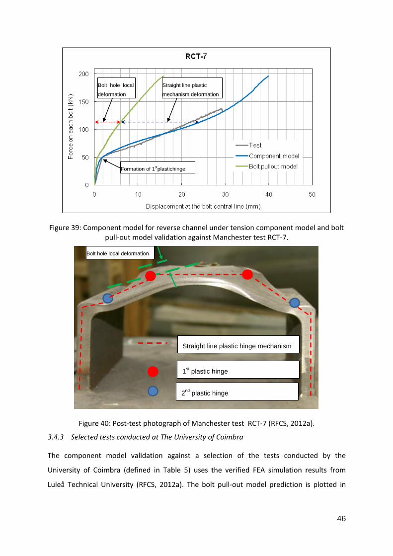
46

Figure 39: Component model for reverse channel under tension component model and bolt pull-out model validation against Manchester test RCT-7.

Figure 40: Post-test photograph of Manchester test RCT-7 (RFCS, 2012a).

3.4.3 Selected tests conducted at The University of Coimbra

The component model validation against a selection of the tests conducted by the

University of Coimbra (defined in Table 5) uses the verified FEA simulation results from

Luleå Technical University (RFCS, 2012a). The bolt pull-out model prediction is plotted in

Straight line plastic hinge mechanism

Bolt hole local deformation

Formation of 1stplastichinge

1st plastic hinge

2nd

plastic hinge

Bolt hole local

deformation

Straight line plastic

mechanism deformation

47

Figure 41 to show the contribution that local bolt hole deformation makes at each applied

force level.

Table 5: Reverse channel component tests conducted by the University of Coimbra

Test N.

Reverse channel section

section type applied load

Test Temp (°C)

Steel grade h(mm) tw(mm) tf(mm)

1 202x90x7 Welded Tension 20 S275 202 7 15



15 200x90x8 Cut tube Tension 20 S355 200 8 8



18 UPN200 Rolled Tension 20 S275 200 8.5 11.5

In tests 1, 2, 3 and 18 (shown in Figure 41), the bolt pull-out model prediction is close to that

of the component model, which means that the reverse channel is relatively stiff.

In the Coimbra component tests, the bolt separation was 85mm with M24 bolts. The

reverse channels in tests 1, 2, 3 and 18 have thicker legs, Therefore, the bolt head is close to

the reverse channel’s root zone. As the result of this, the straight plastic hinge mechanism

has barely formed, and the bolt pull-out model dominates.

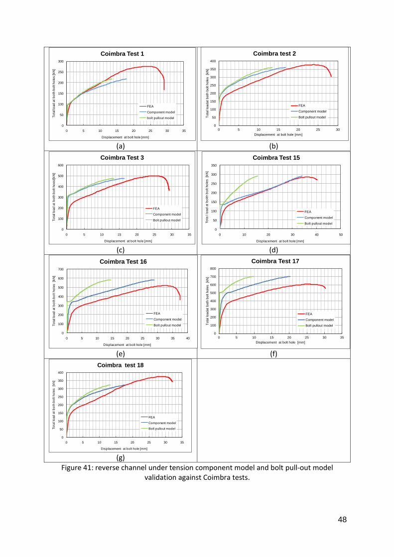
48

(a)

(b)

(c)

(d)

(e)

(f)

(g)

Figure 41: reverse channel under tension component model and bolt pull-out model validation against Coimbra tests.

0

50

100

150

200

250

300

0 5 10 15 20 25 30 35

To

tal l

oad

at

bo

th b

olt h

ole

s [kN

]

Displacement at bolt hole [mm]

Coimbra Test 1

FEA

Component model

bolt pullout model

0

50

100

150

200

250

300

350

400

0 5 10 15 20 25 30

Tota

l lo

adat

both

bolt h

ole

s

[kN

]


Coimbra test 2

FEA

Component model

Bolt pullout model

0

100

200

300

400

500

600

0 5 10 15 20 25 30 35

To

tal l

oad

at

bo

th b

olt h

oesl[kN

]


Coimbra Test 3

FEA

Component model

Bolt pullout model

0

50

100

150

200

250

300

350

0 10 20 30 40 50

To

ta l

load

at

bo

lth b

olt h

ole

s [k

N]


Coimbra Test 15

FEA

Component model

Bolt pullout model

0

100

200

300

400

500

600

700

0 5 10 15 20 25 30 35 40

To

tal l

oad

at

bo

th b

olt h

ole

s [k

N]


Coimbra Test 16

FEA

Component model

Bolt pullout model

0

100

200

300

400

500

600

700

800

0 5 10 15 20 25 30 35

To

tal lo

ad

at

both

bolt h

ole

s

[kN

]


Coimbra Test 17

FEA

Component model

Bolt pullout model

0

50

100

150

200

250

300

350

400

0 5 10 15 20 25 30 35

To

tal l

oad

at

bo

th b

olt h

ole

s [k

N]


Coimbra test 18

FEA

Component model

Bolt pullout model

49

3.4.4 Further parametric studies

The COMPFIRE component tests provide a good opportunity to validate the component

model. The following parametric study aims to expand the component test data further to

investigate the reverse channel behaviour at both ambient and elevated temperatures. All

the parametric FEA analyses were conducted by Tim Heistermann from Luleå University of

Technology.

Table 6 to Table 12 list the parametric study simulations. The SHS 350x8 cut-tube section,

with leg length 90mm (‘h’ shown in Figure 42) is selected as a benchmark. Two general types

of reverse channel (PFC and tube-cut) are considered. All the tests are analysed for both

tension and compression cases.

Figure 42: Reverse channel parametric studies layout (showing three bolt rows)

For the tension tests, analyses were intended to carry on up to bolt pull-out. As the bolt

pull-out limit was beyond the specification of this parametric study, these FEA results do not

necessarily show the maximum resistance, and were often stopped due to solution

convergence problems. From this parametric study, the general locations and formation of

plastic hinges in the reverse channel under tension/compression can be identified at

intermediate stages of loading, using the strain contours. This identification is difficult to

capture accurately from experimental component tests.

h t f

L

root t w

30

30

75 150 150 75

a

Endplate

Elevation Top view

Bolt

Bolt hole

50

Table 6: Component model parametric study List 1

No

te

on

e b

olt

ro

w

tem

p

(○C

)

20

20

20

20

20

20

20

20

20

20

20

20

dis

tan

ce

bet

wee

n

bo

lt r

ow

s (m

m)

15

0

15

0

15

0

15

0

15

0

15

0

15

0

15

0

15

0

15

0

15

0

15

0

a1(m

m)

90

90

90

15

0

15

0

15

0

21

0

21

0

21

0

27

0

27

0

27

0

Bo

lt

row

s

1

1

1

1

1

1

1

1

1

1

1

1

Bo

lt S

ize

(mm

)

20

20

20

20

20

20

20

20

20

20

20

20

End

pla

te S

ize

Thic

knes

s

(mm

)

20

20

20

20

20

20

20

20

20

20

20

20

Len

gth

(mm

)

15

0

15

0

15

0

15

0

15

0

15

0

15

0

15

0

15

0

15

0

15

0

15

0

Wid

th

(mm

)

15

0

15

0

15

0

21

0

21

0

21

0

27

0

27

0

27

0

33

0

33

0

33

0

Rev

erse

Ch

ann

el

Len

gth

bef

f(m

m)

15

0

15

0

15

0

15

0

15

0

15

0

15

0

15

0

15

0

15

0

15

0

15

0

Ro

ot

(mm

)

12

/8

12

/8

12

/8

12

/8

12

/8

12

/8

12

/8

12

/8

12

/8

12

/8

12

/8

12

/8

Leg

Thic

knes

s

tf(m

m)

8

8

8

8

8

8

8

8

8

8

8

8

Leg

Len

gth

H(m

m)

60

90

12

0

60

90

12

0

60

90

12

0

60

90

12

0

Flan

ge

Thic

knes

s

tw(m

m)

8

8

8

8

8

8

8

8

8

8

8

8

Flan

ge

Len

gth

L(m

m)

35

0

35

0

35

0

35

0

35

0

35

0

35

0

35

0

35

0

35

0

35

0

35

0

Sect

ion

35

0X

8 (

cut)

35

0X

8 (

cut)

35

0X

8 (

cut)

35

0X

8 (

cut)

35

0X

8 (

cut)

35

0X

8 (

cut)

35

0X

8 (

cut)

35

0X

8 (

cut)

35

0X

8 (

cut)

35

0X

8 (

cut)

35

0X

8 (

cut)

35

0X

8 (

cut)

NO

.

1

2

3

4

5

6

7

8

9

10

11

12

51


no

te

two

bo

lt r

ow

s

thre

e b

olt

ro

ws

on

e b

olt

ro

w a

t el

evat

ed

tem

per

atu

re

tem

p

(○C

)

20

20

20

20

20

20

20

20

45

0

45

0

55

0

55

0

dis

tan

ce

bet

wee

n

bo

lt r

ow

s (m

m)

15

0

15

0

15

0

15

0

15

0

15

0

15

0

15

0

15

0

15

0

15

0

15

0

a1(m

m)

90

15

0

21

0

27

0

90

15

0

21

0

27

0

15

0

21

0

15

0

21

0

Bo

lt

row

s

2

2

2

2

3

3

3

3

1

1

1

1

Bo

lt S

ize

(mm

)

20

20

20

20

20

20

20

20

20

20

20

20

End

pla

te S

ize

Thic

knes

s (m

m)

20

20

20

20

20

20

20

20

20

20

20

20

Len

gth

(m

m)

30

0

30

0

30

0

30

0

45

0

45

0

45

0

45

0

15

0

15

0

15

0

15

0

Wid

th

(mm

)

15

0

21

0

27

0

33

0

15

0

21

0

27

0

33

0

21

0

27

0

21

0

27

0

Rev

erse

Ch

ann

el

Len

gth

b

eff(

mm

)

30

0

30

0

30

0

30

0

45

0

45

0

45

0

45

0

15

0

15

0

15

0

15

0

Ro

ot

(mm

)

12

/8

12

/8

12

/8

12

/8

12

/8

12

/8

12

/8

12

/8

12

/8

12

/8

12

/8

12

/8

Leg

Thic

knes

s

tf(m

m)

8

8

8

8

8

8

8

8

8

8

8

8

Leg

Len

gth

H(m

m)

90

90

90

90

90

90

90

90

90

90

90

90

Flan

ge

Thic

knes

s

tw(m

m)

8

8

8

8

8

8

8

8

8

8

8

8

Flan

ge

Len

gth

L(m

m)

35

0

35

0

35

0

35

0

35

0

35

0

35

0

35

0

35

0

35

0

35

0

35

0

Sect

ion

35

0X

8 (

cut)

35

0X

8 (

cut)

35

0X

8 (

cut)

35

0X

8 (

cut)

35

0X

8 (

cut)

35

0X

8 (

cut)

35

0X

8 (

cut)

35

0X

8 (

cut)

35

0X

8 (

cut)

35

0X

8 (

cut)

35

0X

8 (

cut)

35

0X

8 (

cut)

NO

.

13

14

15

16

17

18

19

20

21

22

23

24

52


no

te

on

e b

olt

ro

w a

t

elev

ated

te

mp

erat

ure

thre

e b

olt

ro

ws

at e

leva

ted

te

mp

erat

ure

tem

p

(○C

)

65

0

65

0

75

0

75

0

45

0

45

0

55

0

55

0

65

0

65

0

75

0

75

0

dis

tan

ce

bet

wee

n

bo

lt r

ow

s (m

m)

15

0

15

0

15

0

15

0

15

0

15

0

15

0

15

0

15

0

15

0

15

0

15

0

a1(m

m)

15

0

21

0

15

0

21

0

15

0

21

0

15

0

21

0

15

0

21

0

15

0

21

0

Bo

lt

row

s

1

1

1

1

3

3

3

3

3

3

3

3

Bo

lt S

ize

(mm

)

20

20

20

20

20

20

20

20

20

20

20

20

End

pla

te S

ize

Thic

knes

s (m

m)

20

20

20

20

20

20

20

20

20

20

20

20

Len

gth

(m

m)

15

0

15

0

15

0

15

0

15

0

15

0

15

0

15

0

15

0

15

0

15

0

15

0

Wid

th

(mm

)

21

0

27

0

21

0

27

0

21

0

27

0

21

0

27

0

21

0

27

0

21

0

27

0

Rev

erse

Ch

ann

el

Len

gth

b

eff(

mm

)

15

0

15

0

15

0

15

0

15

0

15

0

15

0

15

0

15

0

15

0

15

0

15

0

Ro

ot

(mm

)

12

/8

12

/8

12

/8

12

/8

12

/8

12

/8

12

/8

12

/8

12

/8

12

/8

12

/8

12

/8

Leg

Thic

knes

s

tf(m

m)

8

8

8

8

8

8

8

8

8

8

8

8

Leg

Len

gth

H(m

m)

90

90

90

90

90

90

90

90

90

90

90

90

Flan

ge

Thic

knes

s

tw(m

m)

8

8

8

8

8

8

8

8

8

8

8

8

Flan

ge

Len

gth

L(m

m)

35

0

35

0

35

0

35

0

35

0

35

0

35

0

35

0

35

0

35

0

35

0

35

0

Sect

ion

35

0X

8 (

cut)

35

0X

8 (

cut)

35

0X

8 (

cut)

35

0X

8 (

cut)

35

0X

8 (

cut)

35

0X

8 (

cut)

35

0X

8 (

cut)

35

0X

8 (

cut)

35

0X

8 (

cut)

35

0X

8 (

cut)

35

0X

8 (

cut)

35

0X

8 (

cut)

NO

.

25

26

27

28

29

30

31

32

33

34

35

36

53


no

te

end

pla

te

thic

knes

s ef

fect

tem

p

(○C

)

20

20

20

20

20

20

20

20

20

20

20

20

dis

tan

ce

bet

wee

n

bo

lt r

ow

s (m

m)

15

0

15

0

15

0

15

0

15

0

15

0

15

0

15

0

15

0

15

0

15

0

15

0

a1(m

m)

90

90

90

15

0

15

0

15

0

21

0

21

0

21

0

27

0

27

0

27

0

Bo

lt

row

s

1

1

1

1

1

1

1

1

1

1

1

1

Bo

lt S

ize

(mm

)

20

20

20

20

20

20

20

20

20

20

20

20

End

pla

te S

ize

Thic

knes

s (m

m)

10

10

10

10

10

10

10

10

10

10

10

10

Len

gth

(m

m)

15

0

15

0

15

0

15

0

15

0

15

0

15

0

15

0

15

0

15

0

15

0

15

0

Wid

th

(mm

)

15

0

15

0

15

0

21

0

21

0

21

0

27

0

27

0

27

0

33

0

33

0

33

0

Rev

erse

Ch

ann

el

Len

gth

b

eff(

mm

)

15

0

15

0

15

0

15

0

15

0

15

0

15

0

15

0

15

0

15

0

15

0

15

0

Ro

ot

(mm

)

12

/8

12

/8

12

/8

12

/8

12

/8

12

/8

12

/8

12

/8

12

/8

12

/8

12

/8

12

/8

Leg

Thic

knes

s

tf(m

m)

8

8

8

8

8

8

8

8

8

8

8

8

Leg

Len

gth

H(m

m)

60

90

12

0

60

90

12

0

60

90

12

0

60

90

12

0

Flan

ge

Thic

knes

s

tw(m

m)

8

8

8

8

8

8

8

8

8

8

8

8

Flan

ge

Len

gth

L(m

m)

35

0

35

0

35

0

35

0

35

0

35

0

35

0

35

0

35

0

35

0

35

0

35

0

Sect

ion

35

0X

8 (

cut)

35

0X

8 (

cut)

35

0X

8 (

cut)

35

0X

8 (

cut)

35

0X

8 (

cut)

35

0X

8 (

cut)

35

0X

8 (

cut)

35

0X

8 (

cut)

35

0X

8 (

cut)

35

0X

8 (

cut)

35

0X

8 (

cut)

35

0X

8 (

cut)

NO

.

37

38

39

40

41

42

43

44

45

46

47

48

54


no

te

RC

Th

ickn

ess

1

tem

p

(○C

)

20

20

20

20

20

20

20

20

20

20

20

20

dis

tan

ce

bet

wee

n

bo

lt r

ow

s (m

m)

15

0

15

0

15

0

15

0

15

0

15

0

15

0

15

0

15

0

15

0

15

0

15

0

a1(m

m)

90

90

90

15

0

15

0

15

0

21

0

21

0

21

0

27

0

27

0

27

0

Bo

lt

row

s

1

1

1

1

1

1

1

1

1

1

1

1

Bo

lt S

ize

(mm

)

20

20

20

20

20

20

20

20

20

20

20

20

End

pla

te S

ize

Thic

knes

s (m

m)

20

20

20

20

20

20

20

20

20

20

20

20

Len

gth

(m

m)

15

0

15

0

15

0

15

0

15

0

15

0

15

0

15

0

15

0

15

0

15

0

15

0

Wid

th

(mm

)

15

0

15

0

15

0

21

0

21

0

21

0

27

0

27

0

27

0

33

0

33

0

33

0

Rev

erse

Ch

ann

el

Len

gth

b

eff(

mm

)

15

0

15

0

15

0

15

0

15

0

15

0

15

0

15

0

15

0

15

0

15

0

15

0

Ro

ot

(mm

)

15

/10

15

/10

15

/10

15

/10

15

/10

15

/10

15

/10

15

/10

15

/10

15

/10

15

/10

15

/10

Leg

Thic

knes

s

tf(m

m)

10

10

10

10

10

10

10

10

10

10

10

10

Leg

Len

gth

H(m

m)

60

90

12

0

60

90

12

0

60

90

12

0

60

90

12

0

Flan

ge

Thic

knes

s

tw(m

m)

10

10

10

10

10

10

10

10

10

10

10

10

Flan

ge

Len

gth

L(m

m)

35

0

35

0

35

0

35

0

35

0

35

0

35

0

35

0

35

0

35

0

35

0

35

0

Sect

ion

35

0X

8 (

cut)

35

0X

8 (

cut)

35

0X

8 (

cut)

35

0X

8 (

cut)

35

0X

8 (

cut)

35

0X

8 (

cut)

35

0X

8 (

cut)

35

0X

8 (

cut)

35

0X

8 (

cut)

35

0X

8 (

cut)

35

0X

8 (

cut)

35

0X

8 (

cut)

NO

.

49

50

51

52

53

54

55

56

57

58

59

60

55


no

te

RC

Th

ickn

ess

2

tem

p

(○C

)

20

20

20

20

20

20

20

20

20

20

20

20

dis

tan

ce

bet

wee

n

bo

lt r

ow

s (m

m)

15

0

15

0

15

0

15

0

15

0

15

0

15

0

15

0

15

0

15

0

15

0

15

0

a1(m

m)

90

90

90

15

0

15

0

15

0

21

0

21

0

21

0

27

0

27

0

27

0

Bo

lt

row

s

1

1

1

1

1

1

1

1

1

1

1

1

Bo

lt S

ize

(mm

)

20

20

20

20

20

20

20

20

20

20

20

20

End

pla

te S

ize

Thic

knes

s (m

m)

20

20

20

20

20

20

20

20

20

20

20

20

Len

gth

(m

m)

15

0

15

0

15

0

15

0

15

0

15

0

15

0

15

0

15

0

15

0

15

0

15

0

Wid

th

(mm

)

15

0

15

0

15

0

21

0

21

0

21

0

27

0

27

0

27

0

33

0

33

0

33

0

Rev

erse

Ch

ann

el

Len

gth

b

eff(

mm

)

15

0

15

0

15

0

15

0

15

0

15

0

15

0

15

0

15

0

15

0

15

0

15

0

Ro

ot

(mm

)

18

/12

18

/12

18

/12

18

/12

18

/12

18

/12

18

/12

18

/12

18

/12

18

/12

18

/12

18

/12

Leg

Thic

knes

s

tf(m

m)

12

12

12

12

12

12

12

12

12

12

12

12

Leg

Len

gth

H(m

m)

60

90

12

0

60

90

12

0

60

90

12

0

60

90

12

0

Flan

ge

Thic

knes

s

tw(m

m)

12

12

12

12

12

12

12

12

12

12

12

12

Flan

ge

Len

gth

L(m

m)

35

0

35

0

35

0

35

0

35

0

35

0

35

0

35

0

35

0

35

0

35

0

35

0

Sect

ion

35

0X

8 (

cut)

35

0X

8 (

cut)

35

0X

8 (

cut)

35

0X

8 (

cut)

35

0X

8 (

cut)

35

0X

8 (

cut)

35

0X

8 (

cut)

35

0X

8 (

cut)

35

0X

8 (

cut)

35

0X

8 (

cut)

35

0X

8 (

cut)

35

0X

8 (

cut)

NO

.

61

62

63

64

65

66

67

68

69

70

71

72

56


no

te

PFC

.VS.

tu

be-

cut

(all

the

tub

e-

cut

sect

ion

are

in

ven

ted

fo

r

com

par

iso

n)

1

tem

p

(○C

)

20

20

20

20

20

20

20

20

20

20

20

20

dis

tan

ce

bet

wee

n

bo

lt r

ow

s (m

m)

15

0

15

0

15

0

15

0

15

0

15

0

15

0

15

0

15

0

15

0

15

0

15

0

a1(m

m)

90

90

90

90

90

90

90

90

90

90

90

90

Bo

lt

row

s

1

1

1

1

1

1

1

1

1

1

1

1

Bo

lt S

ize

(mm

)

20

20

20

20

20

20

20

20

20

20

20

20

End

pla

te S

ize

Thic

knes

s (m

m)

20

20

20

20

20

20

20

20

20

20

20

20

Len

gth

(m

m)

15

0

15

0

15

0

15

0

15

0

15

0

15

0

15

0

15

0

15

0

15

0

15

0

Wid

th

(mm

)

20

0

20

0

20

0

20

0

20

0

20

0

20

0

20

0

25

0

25

0

25

0

25

0

Rev

erse

Ch

ann

el

Len

gth

b

eff(

mm

)

15

0

15

0

15

0

15

0

15

0

15

0

15

0

15

0

15

0

15

0

15

0

15

0

Ro

ot

(mm

)

12

10

.5/7

12

11

.25

/7.

5

12

8/1

2

12

13

.5/9

15

14

.25

/9.

5

15

16

.5/1

1

Leg

Thic

knes

s

tf(m

m)

14

7

14

7.5

14

8

15

.5

9

17

.5

9.5

19

11

Leg

Len

gth

H(m

m)

90

90

90

90

90

90

90

90

10

0

10

0

10

0

10

0

Flan

ge

Thic

knes

s

tw(m

m)

7

7

7.5

7.5

8

8

9

9

9.5

9.5

11

11

Flan

ge

Len

gth

L(m

m)

20

0

20

0

23

0

23

0

26

0

26

0

30

0

30

0

38

0

38

0

43

0

43

0

Sect

ion

PFC

20

0x9

0x3

0

20

0x7

(cu

t)

PFC

23

0x9

0x3

2

23

0x7

.5 (

cut)

PFC

26

0x9

0x3

5

26

0x8

(cu

t)

PFC

30

0x9

0x4

1

30

0x9

(cu

t)

PFC

3

80

x10

0x5

4

38

0x9

.5(c

ut)

PFC

4

30

X1

00x6

4

43

0x1

1(c

ut)

NO

.

73

74

75

76

77

78

79

80

81

82

83

84

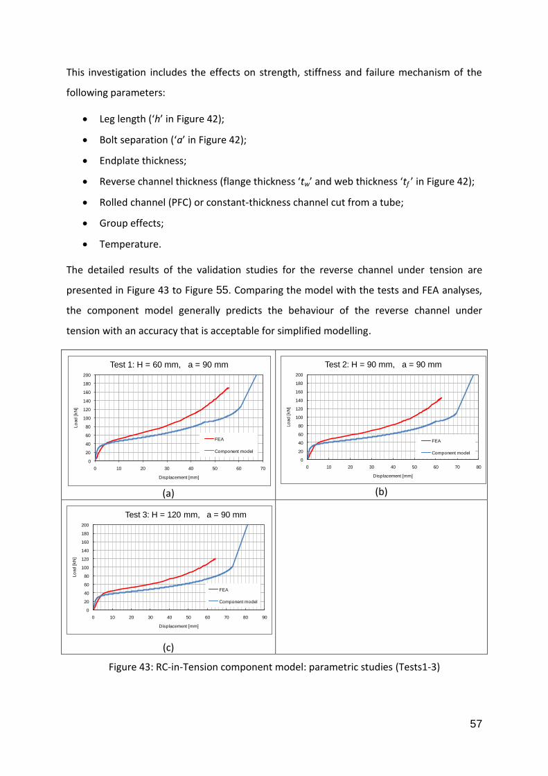
57

This investigation includes the effects on strength, stiffness and failure mechanism of the

following parameters:

Leg length (‘h’ in Figure 42);

Bolt separation (‘a’ in Figure 42);

Endplate thickness;

Reverse channel thickness (flange thickness ‘tw’ and web thickness ‘tf ’ in Figure 42);

Rolled channel (PFC) or constant-thickness channel cut from a tube;

Group effects;

Temperature.

The detailed results of the validation studies for the reverse channel under tension are

presented in Figure 43 to Figure 55. Comparing the model with the tests and FEA analyses,

the component model generally predicts the behaviour of the reverse channel under

tension with an accuracy that is acceptable for simplified modelling.

(a)

(b)

(c)

Figure 43: RC-in-Tension component model: parametric studies (Tests1-3)

0

20

40

60

80

100

120

140

160

180

200

0 10 20 30 40 50 60 70

Lo

ad

[kN

]

Displacement [mm]

Test 1: H = 60 mm, a = 90 mm

FEA

Component model

0

20

40

60

80

100

120

140

160

180

200

0 10 20 30 40 50 60 70 80

Lo

ad

[kN

]

Displacement [mm]

Test 2: H = 90 mm, a = 90 mm

FEA

Component model

0

20

40

60

80

100

120

140

160

180

200

0 10 20 30 40 50 60 70 80 90

Lo

ad

[kN

]

Displacement [mm]

Test 3: H = 120 mm, a = 90 mm

FEA

Component model

58



(a)

(b)

(c)

(a)

(b)

(c)

0

50

100

150

200

250

300

350

0 10 20 30 40 50 60 70

Lo

ad

[kN

]

Displacement [mm]

Test 4: H = 60 mm, a = 150 mm

FEA

Component model

0

50

100

150

200

250

300

350

0 10 20 30 40 50 60 70 80

Lo

ad

[kN

]

Displacement [mm]

Test 5: H = 90 mm, a = 150 mm

FEA

Component model

0

50

100

150

200

250

300

350

0 10 20 30 40 50 60 70 80 90

Lo

ad

[kN

]

Displacement [mm]

Test 6: H = 120 mm, a = 150 mm

FEA

Component model

0

50

100

150

200

250

300

350

0 10 20 30 40 50

Lo

ad

[kN

]

Displacement [mm]

Test 7: H = 60 mm, a = 210 mm

FEA

Component model

0

50

100

150

200

250

300

350

0 10 20 30 40 50

Lo

ad

[kN

]

Displacement [mm]

Test 8: H = 90 mm, a = 210 mm

FEA

Component model

0

50

100

150

200

250

300

350

0 10 20 30 40 50

Lo

ad

[kN

]

Displacement [mm]

Test 9: H = 90 mm, a = 210 mm

FEA

Component model

59

(a)

(b)

(c)

(d)

(e)

(f)

(g)

(f)


0

50

100

150

200

250

300

350

0 10 20 30 40 50 60 70 80

Lo

ad

[kN

]

Displacement [mm]

Test 21: 350x8 (cut), a=150 mm, 450 C

FEA

Component model

Bolt pullout model0

50

100

150

200

250

300

0 10 20 30 40 50 60

Lo

ad

[kN

]

Displacement [mm]

Test 22: 350x8 (cut), a=210 mm, 450 C

FEA

Component model

Bolt pullout model

0

50

100

150

200

250

0 10 20 30 40 50 60 70 80

Lo

ad

[kN

]

Displacement [mm]

Test 23: 350x8 (cut), a=150 mm, 550 C

FEA

Component model

Bolt pulllout model

0

20

40

60

80

100

120

140

160

180

200

0 10 20 30 40 50 60

Lo

ad

[kN

]

Displacement [mm]

Test 24: 350x8 (cut), a=210 mm, 550 C

FEA

Component model

Bolt pullout model

0

20

40

60

80

100

120

140

0 10 20 30 40 50 60 70 80

Lo

ad

[kN

]

Displacement [mm]

Test 25: 350x8 (cut), a=150 mm, 650 C

FEA

Component model

Bolt pullout model

0

20

40

60

80

100

120

0 10 20 30 40 50 60

Lo

ad

[kN

]

Displacement [mm]

Test 26: 350x8 (cut), a=210 mm, 650 C

FEA

Component model

Bolt pullout model

0

10

20

30

40

50

60

0 10 20 30 40 50 60 70 80

Lo

ad

[kN

]

Displacement [mm]

Test 27: 350x8 (cut), a=150 mm, 750 C

FEA

Component model

Bolt pullout model

0

10

20

30

40

50

60

0 10 20 30 40 50 60

Lo

ad

[kN

]

Displacement [mm]

Test 28: 350x8 (cut), a=210 mm, 750 C

FEA

Component model

Bolt pullout model

60

(a)

(b)

(c)


(a)

(b)

(c)


0

100

200

300

400

500

600

0 10 20 30 40 50 60 70 80 90

Lo

ad

[kN

]

Displacement [mm]

H = 60 mm, a = 90 mm

Test 49

Component model

Bolt pullout model

0

100

200

300

400

500

600

0 20 40 60 80 100

Lo

ad

[kN

]

Displacement [mm]

H = 90 mm, a = 90 mm

Test 50

Component model

Bolt pullout model

0

100

200

300

400

500

600

0 20 40 60 80 100 120

Lo

ad

[kN

]

Displacement [mm]

H = 120 mm, a = 90 mm

Test 51

Component model

Bolt pullout model

0

50

100

150

200

250

300

350

400

450

500

0 10 20 30 40 50 60 70

Lo

ad

[kN

]

Displacement [mm]

H = 60 mm, a = 150 mm

Test 52

Component model

Bolt pullout model

0

50

100

150

200

250

300

350

400

450

500

0 10 20 30 40 50 60 70 80

Lo

ad

[kN

]

Displacement [mm]

H = 90 mm, a = 150 mm

Test 53

Component model

Bolt pullout model

0

50

100

150

200

250

300

350

400

450

500

0 10 20 30 40 50 60 70 80

Lo

ad

[kN

]

Displacement [mm]

H = 120 mm, a = 150 mm

Test 54

Component model

Bolt pullout model

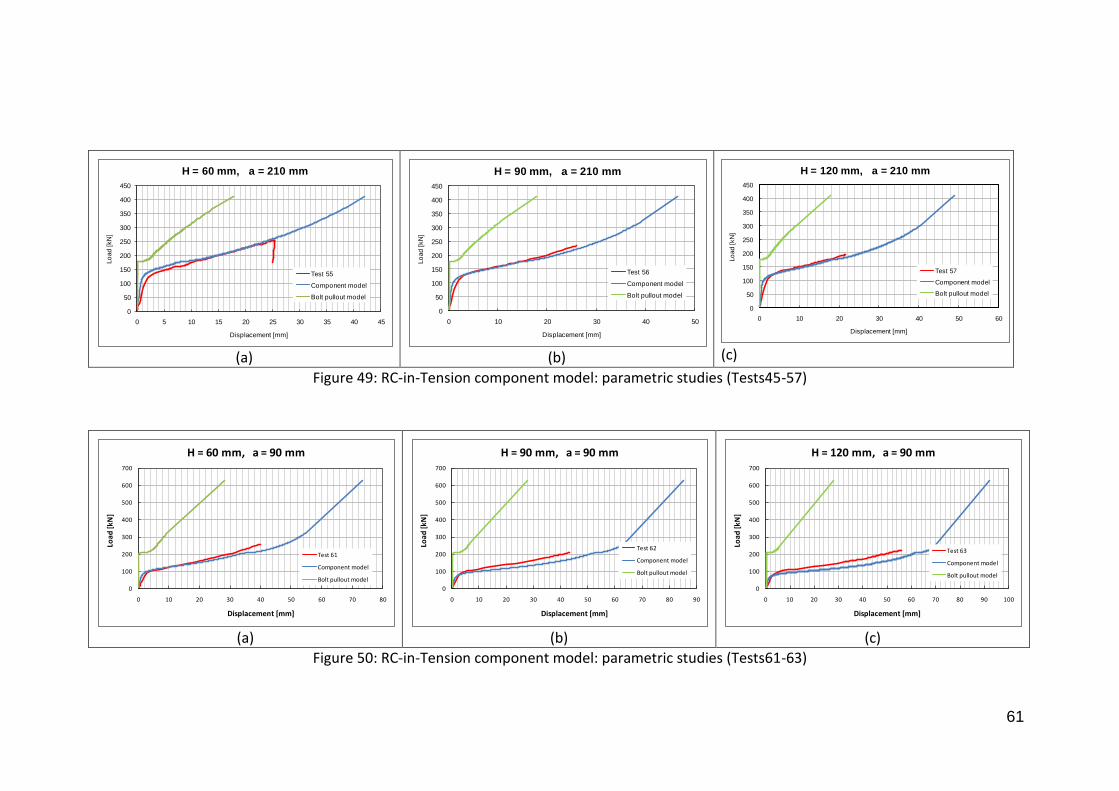
61

(a)

(b) (c)


(a)

(b)

(c)


0

50

100

150

200

250

300

350

400

450

0 5 10 15 20 25 30 35 40 45

Lo

ad

[kN

]

Displacement [mm]

H = 60 mm, a = 210 mm

Test 55

Component model

Bolt pullout model

0

50

100

150

200

250

300

350

400

450

0 10 20 30 40 50

Lo

ad

[kN

]

Displacement [mm]

H = 90 mm, a = 210 mm

Test 56

Component model

Bolt pullout model

0

50

100

150

200

250

300

350

400

450

0 10 20 30 40 50 60

Lo

ad

[kN

]

Displacement [mm]

H = 120 mm, a = 210 mm

Test 57

Component model

Bolt pullout model

0

100

200

300

400

500

600

700

0 10 20 30 40 50 60 70 80

Load

[kN

]

Displacement [mm]

H = 60 mm, a = 90 mm

Test 61

Component model

Bolt pullout model

0

100

200

300

400

500

600

700

0 10 20 30 40 50 60 70 80 90

Load

[kN

]

Displacement [mm]

H = 90 mm, a = 90 mm

Test 62

Component model

Bolt pullout model

0

100

200

300

400

500

600

700

0 10 20 30 40 50 60 70 80 90 100

Load

[kN

]

Displacement [mm]

H = 120 mm, a = 90 mm

Test 63

Component model

Bolt pullout model

62

(a)

(b)

(c)


(a)

(b)

(c)


0

100

200

300

400

500

600

700

0 10 20 30 40 50 60 70

Load

[kN

]

Displacement [mm]

H = 60 mm, a = 150 mm

Test 64

Component model

Bolt pullout model

0

100

200

300

400

500

600

700

0 10 20 30 40 50 60 70

Load

[kN

]

Displacement [mm]

H = 90 mm, a = 150 mm

Test 65

Component model

Bolt pullout model

0

100

200

300

400

500

600

700

0 10 20 30 40 50 60 70 80

Load

[kN

]

Displacement [mm]

H = 120 mm, a = 150 mm

Test 66

Component model

Bolt pullout model

0

100

200

300

400

500

600

0 5 10 15 20 25 30 35 40

Load

[kN

]

Displacement [mm]

H = 60 mm, a = 210 mm

Test 67

Component model

Bolt pullout model

0

100

200

300

400

500

600

0 5 10 15 20 25 30 35 40 45 50

Load

[kN

]

Displacement [mm]

H = 90 mm, a = 210 mm

Test 68

Component model

Bolt pullout model

0

100

200

300

400

500

600

0 5 10 15 20 25 30 35 40 45 50

Load

[kN

]

Displacement [mm]

H = 120 mm, a = 210 mm

Test 69e

Component model

Bolt pullout model

63

(a)

(b)

(c)

(d)


(a)

(b)

(c)

(d)


0

50

100

150

200

250

0 5 10 15 20 25

Load

[kN

]

Displacement [mm]

PFC 200x90x30

Test 73

Component model

Bolt pullout model

0

50

100

150

200

250

300

0 5 10 15 20 25 30 35 40 45

Load

[kN

]

Displacement [mm]

200x7 (cut)

Test 74

Component model

Bolt pullout model

0

50

100

150

200

250

300

0 5 10 15 20 25 30 35 40 45

Load

[kN

]

Displacement [mm]

PFC 230x90x32

Test 75

Component model

Bolt pullout model

0

50

100

150

200

250

300

0 10 20 30 40 50 60

Load

[kN

]

Displacement [mm]

230x7.5 (cut)

Test 76

Component model

Bolt pullout model

0

50

100

150

200

250

300

350

0 10 20 30 40 50 60

Load

[kN

]

Displacement [mm]

PFC 260x90x35

Test 77

Component model

Bolt pullout model

0

50

100

150

200

250

300

350

0 10 20 30 40 50 60 70

Load

[kN

]

Displacement [mm]

260x8 (cut)

Test 78

Component model

Bolt pullout model

0

50

100

150

200

250

300

350

400

450

0 10 20 30 40 50 60 70 80

Load

[kN

]

Displacement [mm]

PFC 300x90x41

Test 79

Component model

Bolt pullout model

0

50

100

150

200

250

300

350

400

450

0 10 20 30 40 50 60 70 80

Load

[kN

]

Displacement [mm]

300x9 (cut)

Test 80

Component model

Bolt pullout model

64

(a)

(b)

(c)

(d)


3.4.4.1 Plastic hinge mechanism

Figure 56 shows the deformed shape from the tension parametric study based on Test 8.

The FE analysis has supplied detailed data on the component behaviour. Figure 57 displays

strain contours from this test, captured from an ABAQUS output video. These are the

principal plastic strains in various parts of the reverse channel connections. The notation 11

indicates the principal bending strain, 22 is the strain in the orthogonal direction to 11. The

video clearly shows how the plastic hinges form, and their locations. It is obvious that the

three plastic hinges are located near to bolt holes, reverse channel roots, and legs.

Figure 56: Tensile parametric Test 8 deformed shape by FEA

0

50

100

150

200

250

300

350

400

450

500

0 20 40 60 80 100

Load

[kN

]

Displacement [mm]

PFC 380x100x54

Test 81

Component model

Bolt pullout model

0

100

200

300

400

500

600

0 20 40 60 80 100 120

Load

[kN

]

Displacement [mm]

380x9.5 (cut)

Test 82

Component model

Bolt pullout model

0

100

200

300

400

500

600

700

0 20 40 60 80 100 120

Load

[kN

]

Displacement [mm]

PFC 430x100x64

Test 83

Component model

Bolt pullout model

0

100

200

300

400

500

600

700

0 20 40 60 80 100 120

Load

[kN

]

Displacement [mm]

430x11 (cut)

Test 84

Component model

Bolt pullout model

65

(a) leg Pe22 inner (b) leg Pe22 outer

(c) max principal strain

(d) plate pe11 top

(e) web pe11 bottom

(f) web pe11 top

Figure 57: Tension parametric Test 8: strain contours by FEA

3.4.4.2 Ambient temperature

The ambient-temperature cases 1 to 9 are shown in Figure 43 to Figure 45. Generally, the

force-displacement curve of the reverse channel (called the ‘component model’) shows the

typical three stages (shown in Figure 58):

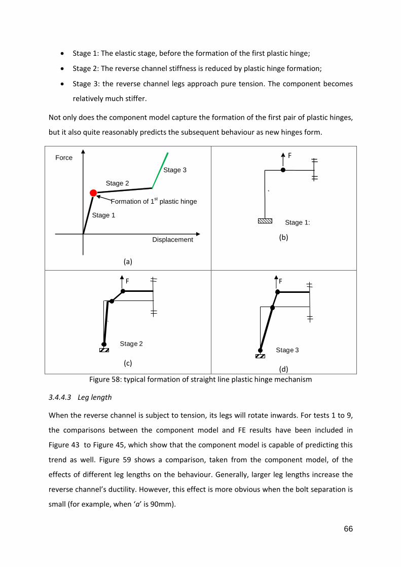
66

Stage 1: The elastic stage, before the formation of the first plastic hinge;

Stage 2: The reverse channel stiffness is reduced by plastic hinge formation;

Stage 3: the reverse channel legs approach pure tension. The component becomes

relatively much stiffer.

Not only does the component model capture the formation of the first pair of plastic hinges,

but it also quite reasonably predicts the subsequent behaviour as new hinges form.

(a)

(b)

(c)

(d)

Figure 58: typical formation of straight line plastic hinge mechanism

3.4.4.3 Leg length

When the reverse channel is subject to tension, its legs will rotate inwards. For tests 1 to 9,

the comparisons between the component model and FE results have been included in

Figure 43 to Figure 45, which show that the component model is capable of predicting this

trend as well. Figure 59 shows a comparison, taken from the component model, of the

effects of different leg lengths on the behaviour. Generally, larger leg lengths increase the

reverse channel’s ductility. However, this effect is more obvious when the bolt separation is

small (for example, when ‘a’ is 90mm).

F

Stage 2

F

Stage 3

Stage 1

Stage 2

Stage 3

Displacement

Force

Formation of 1st plastic hinge

F

Stage 1:

67

(a)

(b)

(c)

Figure 59: Comparison of leg length on RC-in-Tension component model

(a)

(b)

(c)

Figure 60: Bolt separation effects on one bolt row in tension; FEA results (Tests 1-12).

0

20

40

60

80

100

120

140

160

180

200

0 10 20 30 40 50 60 70 80 90

Lo

ad

[kN

]

Displacement [mm]

Summary: H = 60-120 mm, a = 90 mm

Test 1: H=60mm

Test 2: H=90mm

Test 3: H=120mm

0

50

100

150

200

250

300

350

0 10 20 30 40 50 60 70 80 90

Lo

ad

[kN

]

Displacement [mm]

Summary: H = 60-120 mm, a = 150 mm

Test 4: H=60mm

Test 5: H=90mm

Test 6: H=120mm

0

50

100

150

200

250

300

350

0 10 20 30 40 50

Lo

ad

[kN

]

Displacement [mm]

Summary: H = 90 mm, a = 210 mm

Test 7: H=60mm

Test 8: H=90mm

Test 9: H=120mm

0

50

100

150

200

250

300

350

400

0 10 20 30 40 50 60 70 80 90

Lo

ad

[kN

]

Displacement [mm]

Summary: H = 60 mm, a = 90-210 mm

Test 1: a=90mm

Test 4: a=150mm

Test 7: a=210mm

0

50

100

150

200

250

300

0 10 20 30 40 50 60 70 80

Lo

ad

[kN

]

Displacement [mm]

Summary: H = 90 mm, a = 90-210 mm

Test 2: a=90mm

Test 5: a=150mm

Test 8: a=210mm

0

20

40

60

80

100

120

140

160

180

200

0 10 20 30 40 50 60 70 80 90

Lo

ad

[kN

]

Displacement [mm]

Summary: H = 120 mm, a = 90-210 mm

Test 3: a=90mm

Test 6: a=150mm

Test 9: a=210mm

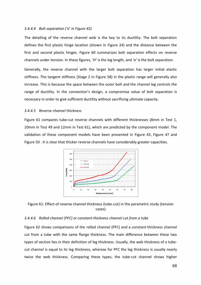
68

3.4.4.4 Bolt separation (‘a’ in Figure 42)

The detailing of the reverse channel web is the key to its ductility. The bolt separation

defines the first plastic hinge location (shown in Figure 24) and the distance between the

first and second plastic hinges. Figure 60 summarizes bolt separation effects on reverse

channels under tension. In these figures, ‘H’ is the leg length, and ‘a’ is the bolt separation.

Generally, the reverse channel with the larger bolt separation has larger initial elastic

stiffness. The tangent stiffness (Stage 2 in Figure 58) in the plastic range will generally also

increase. This is because the space between the outer bolt and the channel leg controls the

range of ductility. In the connection’s design, a compromise value of bolt separation is

necessary in order to give sufficient ductility without sacrificing ultimate capacity.

3.4.4.5 Reverse channel thickness

Figure 61 compares tube-cut reverse channels with different thicknesses (8mm in Test 1,

10mm in Test 49 and 12mm in Test 61), which are predicted by the component model. The

validation of these component models have been presented in Figure 43, Figure 47 and

Figure 50 . It is clear that thicker reverse channels have considerably greater capacities.

Figure 61: Effect of reverse channel thickness (tube-cut) in the parametric study (tension cases)

3.4.4.6 Rolled channel (PFC) or constant-thickness channel cut from a tube

Figure 62 shows comparisons of the rolled channel (PFC) and a constant-thickness channel

cut from a tube with the same flange thickness. The main difference between these two

types of section lies in their definition of leg thickness. Usually, the web thickness of a tube-

cut channel is equal to its leg thickness, whereas for PFC the leg thickness is usually nearly

twice the web thickness. Comparing these types, the tube-cut channel shows higher

0

100

200

300

400

500

600

0 10 20 30 40 50 60 70 80

Load

[kN

]

Displacement [mm]

Test 1

Test 49

Test 61

69

ductility, due to its thinner legs. Therefore, in choosing between channels with the same

capacity, the tube-cut section would be recommended.

(a)

(b)

(c)

(d)

(e)

(f)

Figure 62: parametric study; PFC compared with tube-cut channels (tension).

3.4.4.7 Group effects

Figure 63 presents a comparison of group effects seen in the tensile parametric studies

using detailed FE analysis. Tests 2, 5, 8 and 11 are single-bolt-row cases, Tests 14, 17, 20 and

23 are two-bolt-row cases and Tests 26, 29, 32 and 35 are three-bolt-row cases. The

distance between multiple bolt rows is 150mm in all these tests. The force is the total

reaction force at the bottom of the reverse channel. The deformation shown in Figure 63 for

0

50

100

150

200

250

0 5 10 15 20 25 30 35 40

Loa

d [

kN

]

Displacement [mm]

Test 73

Test 74

0

50

100

150

200

250

300

0 5 10 15 20 25 30 35 40 45 50

Loa

d [

kN

]

Displacement [mm]

Test 75

Test 76

0

50

100

150

200

250

300

350

0 10 20 30 40 50 60 70

Load

[kN

]

Displacement [mm]

Test 77

Test 78

0

50

100

150

200

250

300

350

400

450

0 10 20 30 40 50 60 70 80

Load

[kN

]

Displacement [mm]

Test 79

Test 80

0

100

200

300

400

500

600

0 20 40 60 80 100 120

Loa

d [

kN

]

Displacement [mm]

Test 81

Test 82

0

100

200

300

400

500

600

700

0 20 40 60 80 100 120

Load

[kN

]

Displacement [mm]

Test 83

Test 84

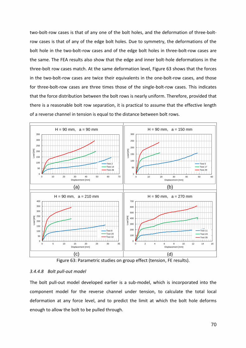
70

two-bolt-row cases is that of any one of the bolt holes, and the deformation of three-bolt-

row cases is that of any of the edge bolt holes. Due to symmetry, the deformations of the

bolt hole in the two-bolt-row cases and of the edge bolt holes in three-bolt-row cases are

the same. The FEA results also show that the edge and inner bolt-hole deformations in the

three-bolt row cases match. At the same deformation level, Figure 63 shows that the forces

in the two-bolt-row cases are twice their equivalents in the one-bolt-row cases, and those

for three-bolt-row cases are three times those of the single-bolt-row cases. This indicates

that the force distribution between the bolt rows is nearly uniform. Therefore, provided that

there is a reasonable bolt row separation, it is practical to assume that the effective length

of a reverse channel in tension is equal to the distance between bolt rows.

(a)

(b)

(c)

(d)

Figure 63: Parametric studies on group effect (tension, FE results).

3.4.4.8 Bolt pull-out model

The bolt pull-out model developed earlier is a sub-model, which is incorporated into the

component model for the reverse channel under tension, to calculate the total local

deformation at any force level, and to predict the limit at which the bolt hole deforms

enough to allow the bolt to be pulled through.

0

50

100

150

200

250

300

350

0 10 20 30 40 50 60 70

Loa

d [

kN

]

Displacement [mm]

H = 90 mm, a = 90 mm

Test 2

Test 14

Test 26

0

50

100

150

200

250

300

0 10 20 30 40 50 60

Load [

kN

]

Displacement [mm]

H = 90 mm, a = 150 mm

Test 5

Test 17

Test 29

0

50

100

150

200

250

300

350

400

0 5 10 15 20 25 30 35

Load [

kN

]

Displacement [mm]

H = 90 mm, a = 210 mm

Test 8

Test 20

Test 32

0

100

200

300

400

500

600

700

0 2 4 6 8 10 12 14 16

Load [

kN

]

Displacement [mm]

H = 90 mm, a = 270 mm

Test 11

Test 23

Test 35

71

The AISC limiting force (AISC, 2005) Rn for bolt pull-out through the wall of a hollow

structural section is given by

uwn tfdR 85.0 (3.49)

Where dw is the average diameter of the bolt head, t is the tube wall thickness and fu is the

ultimate strength of the hollow structural section’s steel.

The corresponding CIDECT limit (Jaspart, 2005) for punching of a single bolt through a tube

wall, Fpunch,cp, is:

0

,3 M

yc

mcppunch

tfdF

(3.50)

Table 13 and Table 14 show the predicted bolt pull-out limits using the AISC, CIDECT and the

current bolt pull-out models on the component tests. Figure 64 shows the comparison of

these bolt pull-out limits. Generally, the CIDECT limit is the highest, and AISC is the most

conservative for design purposes. With a proper design safety factor, the bolt pull-out

model can be used safely in practical connection design.

3.4.4.9 Temperature

The component model is also tested for elevated-temperature situations (shown in Figure

46). The component model prediction is higher than the FE, especially at the kink created by

the formation of first plastic hinge (refer to Figure 58) .This is because the component model

only considers the energy absorbed by the yielding of the material at the plastic hinge

locations, and neglects the gradual reduction of elastic stiffness with temperature. The

mainly-elastic zones between plastic hinge locations also deform and store strain energy.

Therefore, the component model’s predictions will be stiffer, particularly in the early stages

of deformation, and at elevated temperatures, when the modulus of steel degrades more

quickly than the yield strength. However, the component model still predicts the higher-

deflection and pull-out limit behaviour reasonably.

72

Table 13: RC-in-tension test bolt pull-out limit calculation by AISC & CIDECT

test list Test (kN)

Bolt head dia (mm)

Bolt shank dia (mm)

tf (mm)

Yield strength (N/mm2)

Ultimate strength (N/mm2)

tem (°C)

AISC Limit (kN)

CIDECT (kN)

Man

ches

ter

RCT1 95 32.3 20 5.5 325 594 20 89.6 104.7

RCT2 43 32.3 20 5.5 203 203 550 30.7 65.5

RCT3 13 32.3 20 5.5 55 55 750 8.3 17.8

RCT4 96 32.3 20 5.5 325 594 20 89.6 104.7

RCT5 41 32.3 20 5.5 203 203 550 30.7 65.5

RCT6 12 32.3 20 5.5 55 55 750 8.3 17.8

Co

imb

ra

Test 1 135 38.8 24 7.0 287 581 20 134.1 141.4

Test 2 174 38.8 24 10.0 287 581 20 191.6 202.0

Test 3 251 38.8 24 12.0 287 581 20 229.9 242.4

Test 7 78 38.8 24 10.0 179 179 550 59.2 126.2

Test 8 97 38.8 24 12.0 179 179 550 71.0 151.5

Test 11 20 38.8 24 10.0 49 49 750 16.1 34.3

Test 12 23 38.8 24 12.0 49 49 750 19.3 41.2

Test 15 140 38.8 24 8.0 347 420 20 110.8 195.4

Test 16 238 38.8 24 10.0 516 592 20 195.2 363.1

Test 17 295 38.8 24 12.0 471 540 20 213.7 397.8

Test 18 200 38.8 24 8.5 344 605 20 169.6 205.8

Test 19 67 38.8 24 8.5 215 215 550 60.3 128.6

Test 20 21 38.8 24 8.5 58 58 750 16.4 35.0

Test 21 100 37.0 20 6.0 96 255 550 48.1 38.6

Figure 64: Comparison of bolt pull-out limits.

0

50

100

150

200

250

300

350

400

0 50 100 150 200 250 300 350 400

Dif

fere

nt b

olt p

ullo

ut lim

it (kN

)

Test (kN)

CIDECT/Test

AISC/Test

Cone model/Test

73

Table 14: RC-in-tension bolt pull-out limit calculation by bolt pull-out model

test list

Test (kN)

bolt pull-out model

R (mm) θ Δ

rave (mm) εr εy εu Wstrip Wθ Wtotal

F (kN)

Man

ches

ter

RCT1 95 20.4 1.04 7.25 16.2 0.128 0.002 0.040 329834 327649 657483 91

RCT2 43 20.4 1.04 7.25 16.2 0.128 0.002 0.002 121243 204780 326023 45

RCT3 13 20.4 1.04 7.25 16.2 0.128 0.004 0.004 32811 55700 88511 12

RCT4 96 20.4 1.04 7.25 16.2 0.128 0.002 0.040 329834 327649 657483 91

RCT5 41 46.4 0.50 16.38 29.2 0.071 0.002 0.040 492728 222197 714925 44

RCT6 12 46.4 0.50 16.38 29.2 0.071 0.003 0.003 133189 60438 193627 12

Co

imb

ra

Test 1 135 33.8 0.76 13.59 23.9 0.113 0.001 0.155 918625 564519 1483143 109

Test 2 174 36.3 0.71 14.55 25.15 0.107 0.001 0.155 1457339 1162596 2619935 180

Test 3 251 36.3 0.71 14.55 25.15 0.107 0.001 0.155 1748807 1674138 3422944 235

Test 7 78 36.3 0.71 14.55 25.15 0.107 0.002 0.002 672320 726622 1398943 96

Test 8 97 36.3 0.71 14.55 25.15 0.107 0.002 0.002 806785 1046336 1853121 127

Test 11

20 36.3 0.71 14.55 25.15 0.107 0.003 0.003 181949 197641 379591 26

Test 12

23 36.3 0.71 14.55 25.15 0.107 0.003 0.003 218339 284603 502943 35

Test 15

140 43.1 0.62 16.89 28.55 0.095 0.002 0.044 1576153 930269 2506423 148

Test 16

238 39.5 0.66 15.69 26.75 0.101 0.002 0.049 2448107 2121136 4569243 291

Test 17

295 35.9 0.72 14.40 24.95 0.108 0.002 0.067 2285664 2742991 5028656 349

Test 18

200 34.3 0.75 13.79 24.15 0.112 0.002 0.178 1233626 999283 2232909 162

Test 19

67 34.3 0.75 13.79 24.15 0.112 0.002 0.002 622708 624552 1247260 90

Test 20

21 34.3 0.75 13.79 24.15 0.112 0.004 0.004 168392 169878 338271 25

Test 21

100 44.2 0.65 19.40 28.1 0.116 0.001 0.137 629675 154984 784659 40

3.5 Development of the plastic hinge model for reverse channel under compression

When the reverse channel is subject to compression, its mechanical model is similar to that

under tension. The flange is subject to bending. The legs are under compression, which is

opposite to the channel under tension. Since the stiffness of flange under bending is less

than the legs under compression, the two ends of flange will rotate inwards. The plastic

hinges at the tops of the two legs are moved slightly away from each other by the bending

deformation of the web (shown in Figure 65 and Figure 66). Since the legs are subject to

compression, Plastic Hinges 2 (PH2 shown in Figure 68 and Figure 69) will move from the

channel web to the reverse channel legs.

74

Figure 65: Plastic hinge rotations (I)

Figure 66: Plastic hinge rotations (II)

3.5.1 Failure modes

For a reverse channel under compression, there are four possible “failure” modes:

1. Large deformation of the reverse channel in a plastic hinge mechanism, leading to

contact of the web of the reverse channel with the column flange/face. The detail of

the plastic hinge mechanism is explained in 3.5.2.

2. Web fracture, by punching-through of the endplate (Figure 67). This can be

estimated simply by applying the material shear strength over the punch perimeter

area, although this assumes that failure is simultaneous around the perimeter.

3wypunching tcfF (3.51)

Where fy is the reverse channel yield strength, c is the perimeter of the punching

shear area, and tw is the reverse channel web thickness.

3. Leg buckling, in which the buckling force for a leg is based on the Perry-Robertson

method (Coates, 1988) for an effective length factor of between 0.5 (fixed-fixed) and

0.7 (fixed-hinged). Conservatively, the latter is more reasonable. Since there is no

information about the actual geometric imperfection level in the channel’s flanges

the original formula based on tests in the 1920s (Robertson 1925) seems as

justifiable as the more recent formulae, for example those included in Eurocode 3

(CEN, 2005a).

θ0

m

h0

θ3

θ2

θ1 δ

F

h

θ3

θ2

θ1 δ

F

θ3

θ2

θ1 δ

F

θ3

θ2

θ1

δ

F

(a) (b) (c)

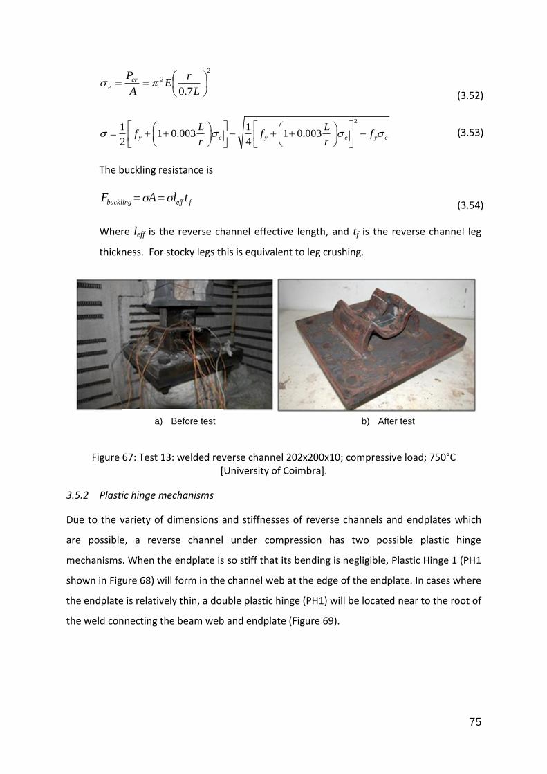
75

2

2

7.0

L

rE

A

Pcr

e (3.52)

2

1 11 0.003 1 0.003

2 4y e y e y e

L Lf f f

r r

(3.53)

The buckling resistance is

feffbuckling tlAF (3.54)

Where leff is the reverse channel effective length, and tf is the reverse channel leg

thickness. For stocky legs this is equivalent to leg crushing.

Figure 67: Test 13: welded reverse channel 202x200x10; compressive load; 750°C [University of Coimbra].

3.5.2 Plastic hinge mechanisms

Due to the variety of dimensions and stiffnesses of reverse channels and endplates which

are possible, a reverse channel under compression has two possible plastic hinge

mechanisms. When the endplate is so stiff that its bending is negligible, Plastic Hinge 1 (PH1

shown in Figure 68) will form in the channel web at the edge of the endplate. In cases where

the endplate is relatively thin, a double plastic hinge (PH1) will be located near to the root of

the weld connecting the beam web and endplate (Figure 69).

b) After test a) Before test

76

Figure 68: Reverse channel under compression (Plastic Hinge Mechanism 1).

Figure 69: Reverse channel under compression (Plastic Hinge Mechanism 2).

The rotations in the two modes may be calculated (Figure 65 and Figure 66) from:

(( ( (

√

) (3.55)

(3.56)

(√

) (3.57)

(3.58)

Figure 66 shows the rotation direction of each plastic hinge within the reverse channel.

When θ1 is less than θ0, then θ1, θ2 and θ3 increase with the displacement (δ) (Figure 66 a).

When θ1 is larger than θ0, the θ3 rotation will change direction. Accordingly, the mechanism

will change and the channel resistance will enhance. In order to simplify the model, the

component model will continue its analysis until θ1 is equal to θ0. The force is assumed to

stay constant after this point, until the reverse channel reaches its maximum allowable

deformation under compression.

ho=root+tw/2

hoho

PH1

PH2h

PH3h

L L

tf

roottw

tf

roottw

m lem

m=(l-le-tf-tw)/2

ho=root+tw/2

m=(l-le-tf-tw)/2

le

tb

tw

h

L

ho

m

tf

root

sww

ho=root+tw/2

m=(l-tb-2*sww-tw -tf)/2

sww

tw

PH1

PH2

PH3

PH4

h

L

ho

m

tf

roottb

ho=root+tw/2

m=(l-tb-2*sww-tw -tf)/2

le le

77

3.5.3 Further parametric studies

During the COMPFIRE project, intensive parametric studies (listed in Table 6 to Table 12)

were conducted by Luleå Technical University using ABAQUS. The aim was to expand the

component test data, in order to investigate the reverse channel behaviour more

extensively at both ambient and elevated temperatures. The detail of this parametric study

is included in 3.4.4.

The detailed results of the validation studies for the reverse channel under compression are

presented from Figure 70 to Figure 86. In general, by comparing the model with the tests

and FEA analyses, the component model is seen to be able to predict the behaviour of the

reverse channel under compression; the remainder of this section is a discussion of the

parameters considered in this study:

Plastic hinge mechanism

Leg length

Bolt separation

Endplate thickness

Reverse channel thickness

Rolled channel (PFC) or constant thickness channel cut from a tube

Post yield hardening in the reverse channel under compression

78

(a)

(b)

(c)

(d)

Figure 70: RC-in-Compression component model: parametric studies (Tests 1-4)

(a)

(b)

(c)

(d)


0

10

20

30

40

50

60

70

80

0 10 20 30 40 50 60 70 80

Load

[kN

]

Displacement [mm]

H = 60 mm, a = 90 mm

Test 1

Component model

0

10

20

30

40

50

60

0 20 40 60 80 100

Load

[kN

]

Displacement [mm]

H = 90 mm, a = 90 mm

Test 2

Component model

0

10

20

30

40

50

60

0 20 40 60 80 100 120 140

Load

[kN

]

Displacement [mm]

H = 120 mm, a = 90 mm

Test 3

Component model

0

10

20

30

40

50

60

70

80

90

0 10 20 30 40 50 60 70

Load

[kN

]

Displacement [mm]

H = 60 mm, a = 150 mm

Test 4

Component model

0

10

20

30

40

50

60

70

80

90

0 20 40 60 80 100

Load

[kN

]

Displacement [mm]

H = 90 mm, a = 150 mm

Test 5

Component model

0

10

20

30

40

50

60

70

80

90

0 20 40 60 80 100 120 140

Load

[kN

]

Displacement [mm]

H = 120 mm, a = 150 mm

Test 6

Component model

0

20

40

60

80

100

120

140

160

180

0 10 20 30 40 50 60 70

Load

[kN

]

Displacement [mm]

H = 60 mm, a = 210 mm

Test 7

Component model

0

20

40

60

80

100

120

140

160

180

0 10 20 30 40 50 60 70

Load

[kN

]

Displacement [mm]

H = 60 mm, a = 210 mm

Test 7

Component model

79

(a)

(b)

(c)

(d)


(a)

(b)

(c)

(d)


0

20

40

60

80

100

120

140

160

180

0 20 40 60 80 100 120 140

Loa

d [

kN

]

Displacement [mm]

H = 120 mm, a = 210 mm

Test 9

Component model

0

20

40

60

80

100

120

140

160

180

200

0 10 20 30 40 50 60 70

Loa

d [

kN

]

Displacement [mm]

H = 60 mm, a = 270 mm

Test 10

Component model

0

20

40

60

80

100

120

140

160

180

200

0 20 40 60 80 100

Load

[kN

]

Displacement [mm]

H = 90 mm, a = 270 mm

Test 11

Component model

0

20

40

60

80

100

120

140

160

180

200

0 20 40 60 80 100 120 140

Load

[kN

]

Displacement [mm]

H = 120 mm, a = 270 mm

Test 12

Component model

0

10

20

30

40

50

60

70

0 20 40 60 80 100

Load

[kN

]

Displacement [mm]

350x8 (cut), a=150 mm, 450°C

Test 21

Component model

0

20

40

60

80

100

120

140

0 20 40 60 80 100

Load

[kN

]

Displacement [mm]

350x8 (cut), a=210 mm, 450°C

Test 22

Component model

0

5

10

15

20

25

30

35

40

45

50

0 20 40 60 80 100

Load

[kN

]

Displacement [mm]

350x8 (cut), a=150 mm, 550°C

Test 23

Component model

0

10

20

30

40

50

60

70

80

90

100

0 20 40 60 80 100

Load

[kN

]

Displacement [mm]

350x8 (cut), a=210 mm, 550°C

Test 24

Component model

80

(a)

(b)

(c)

(d)


(a)

(b)

(c)

(d)

Figure 75:RC-in-Compression component model: parametric studies (Tests 37-40)

0

5

10

15

20

25

30

0 20 40 60 80 100

Load

[kN

]

Displacement [mm]

350x8 (cut), a=150 mm, 650°C

Test 25

Component model

0

10

20

30

40

50

60

0 20 40 60 80 100

Load

[kN

]

Displacement [mm]

350x8 (cut), a=210 mm, 650°C

Test 26

Component model

0

2

4

6

8

10

12

14

0 20 40 60 80 100

Load

[kN

]

Displacement [mm]

350x8 (cut), a=150 mm, 750°C

Test 27

Component model

0

5

10

15

20

25

30

0 20 40 60 80 100

Load

[kN

]

Displacement [mm]

350x8 (cut), a=210 mm, 750°C

Test 28

Component model

0

10

20

30

40

50

60

70

80

90

0 20 40 60 80 100 120

Load

[kN

]

Displacement [mm]

H = 60 mm, a = 90 mm

Test 37

Component model

0

10

20

30

40

50

60

70

0 20 40 60 80 100 120

Load

[kN

]

Displacement [mm]

H = 90 mm, a = 90 mm

Test 38

Component model

0

10

20

30

40

50

60

0 20 40 60 80 100 120 140

Load

[kN

]

Displacement [mm]

H = 120 mm, a = 90 mm

Test 39

Component model

0

10

20

30

40

50

60

70

80

0 20 40 60 80 100 120 140

Load

[kN

]

Displacement [mm]

H = 60 mm, a = 150 mm

Test 40

Component model

81

(a)

(b)

(c)

(d)

Figure 76:RC-in-Compression component model: parametric studies (Tests 41-44)

(a)

(b)

(c)

(d)


0

10

20

30

40

50

60

70

80

0 20 40 60 80 100 120

Load

[kN

]

Displacement [mm]

H = 90 mm, a = 150 mm

Test 41

Component model

0

10

20

30

40

50

60

70

80

0 20 40 60 80 100 120 140

Load

[kN

]

Displacement [mm]

H = 120 mm, a = 150 mm

Test 42

Component model

0

20

40

60

80

100

120

0 20 40 60 80 100 120

Load

[kN

]

Displacement [mm]

H = 60 mm, a = 210 mm

Test 43

Component model

0

10

20

30

40

50

60

70

80

90

100

0 20 40 60 80 100 120 140 160

Load

[kN

]

Displacement [mm]

H = 90 mm, a = 210 mm

Test 44

Component model

0

10

20

30

40

50

60

70

80

90

0 20 40 60 80 100 120 140

Load

[kN

]

Displacement [mm]

H = 120 mm, a = 210 mm

Test 45

Component model

0

20

40

60

80

100

120

0 20 40 60 80 100 120

Load

[kN

]

Displacement [mm]

H = 60 mm, a = 270 mm

Test 46

Component model

0

10

20

30

40

50

60

70

80

90

0 20 40 60 80 100

Load

[kN

]

Displacement [mm]

H = 90 mm, a = 270 mm

Test 47

Component model

0

10

20

30

40

50

60

70

80

90

0 20 40 60 80 100 120 140

Load

[kN

]

Displacement [mm]

H = 120 mm, a = 270 mm

Test 48

Component model

82

(a)

(b)

(c)

(d)


(a)

(b)

(c)

(d)


0

10

20

30

40

50

60

70

80

90

100

0 10 20 30 40 50 60 70

Load

[kN

]

Displacement [mm]

H = 60 mm, a = 90 mm

Test 49

Component model

0

10

20

30

40

50

60

70

80

90

0 20 40 60 80 100

Load

[kN

]

Displacement [mm]

H = 90 mm, a = 90 mm

Test 50

Component model

0

10

20

30

40

50

60

70

80

90

0 20 40 60 80 100 120 140

Load

[kN

]

Displacement [mm]

H = 120 mm, a = 90 mm

Test 51

Component model

0

20

40

60

80

100

120

140

160

0 10 20 30 40 50 60 70

Load

[kN

]

Displacement [mm]

H = 60 mm, a = 150 mm

Test 52

Component model

0

20

40

60

80

100

120

140

160

0 20 40 60 80 100

Load

[kN

]

Displacement [mm]

H = 90 mm, a = 150 mm

Test 53

Component model

0

20

40

60

80

100

120

140

160

0 20 40 60 80 100 120 140

Load

[kN

]

Displacement [mm]

H = 120 mm, a = 150 mm

Test 54

Component model

0

50

100

150

200

250

0 10 20 30 40 50 60 70 80

Load

[kN

]

Displacement [mm]

H = 60 mm, a = 210 mm

Test 55

Component model

0

50

100

150

200

250

0 20 40 60 80 100

Load

[kN

]

Displacement [mm]

H = 90 mm, a = 210 mm

Test 56

Component model

83

(a)

(b)

(c)

(d)


(a)

(b)

(c)

(d)


0

50

100

150

200

250

0 20 40 60 80 100 120 140

Load

[kN

]

Displacement [mm]

H = 120 mm, a = 210 mm

Test 57

Component model

0

50

100

150

200

250

0 10 20 30 40 50 60 70

Load

[kN

]

Displacement [mm]

H = 60 mm, a = 270 mm

Test 58

Component model

0

50

100

150

200

250

0 20 40 60 80 100

Load

[kN

]

Displacement [mm]

H = 90 mm, a = 270 mm

Test 59

Component model

0

50

100

150

200

250

0 20 40 60 80 100 120 140

Load

[kN

]

Displacement [mm]

H = 120 mm, a = 270 mm

Test 60

Component model

0

20

40

60

80

100

120

140

160

0 5 10 15 20

Load

[kN

]

Displacement [mm]

H = 60 mm, a = 90 mm

Test 61

Component model

0

20

40

60

80

100

120

140

0 5 10 15 20 25

Load

[kN

]

Displacement [mm]

H = 90 mm, a = 90 mm

Test 62

Component model

0

20

40

60

80

100

120

140

0 5 10 15 20 25

Load

[kN

]

Displacement [mm]

H = 120 mm, a = 90 mm

Test 63

Component model

0

50

100

150

200

250

0 10 20 30 40 50 60 70

Load

[kN

]

Displacement [mm]

H = 60 mm, a = 150 mm

Test 64

Component model

84

(a)

(b)

(c)

(d)


(a)

(b)

(c)

(d)


0

50

100

150

200

250

0 20 40 60 80 100

Load

[kN

]

Displacement [mm]

H = 90 mm, a = 150 mm

Test 65

Component model

0

50

100

150

200

250

0 20 40 60 80 100 120 140

Load

[kN

]

Displacement [mm]

H = 120 mm, a = 150 mm

Test 66

Component model

0

50

100

150

200

250

0 10 20 30 40 50 60 70

Load

[kN

]

Displacement [mm]

H = 60 mm, a = 210 mm

Test 67

Component model

0

50

100

150

200

250

0 20 40 60 80 100

Load

[kN

]

Displacement [mm]

H = 90 mm, a = 210 mm

Test 68

Component model

0

50

100

150

200

250

300

0 20 40 60 80 100 120 140

Load

[kN

]

Displacement [mm]

H = 120 mm, a = 210 mm

Test 69

Component model

0

50

100

150

200

250

300

0 10 20 30 40 50 60 70

Load

[kN

]

Displacement [mm]

H = 60 mm, a = 270 mm

Test 70

Component model

0

50

100

150

200

250

300

0 20 40 60 80 100

Load

[kN

]

Displacement [mm]

H = 90 mm, a = 270 mm

Test 71

Component model

0

50

100

150

200

250

0 20 40 60 80 100 120 140

Load

[kN

]

Displacement [mm]

H = 120 mm, a = 270 mm

Test 72

Component model

85

(a)

(b)

(c)

(d)


(a)

(b)

(c)

(d)


0

50

100

150

200

250

300

350

400

450

500

0 10 20 30 40 50 60 70 80 90 100

Load

[kN

]

Displacement [mm]

PFC 200x90x30)

Test 73

Component model

0

50

100

150

200

250

300

350

400

0 10 20 30 40 50 60 70 80 90 100

Load

[kN

]

Displacement [mm]

200x7 (cut)

Test 74

Component model

0

50

100

150

200

250

300

350

400

450

0 10 20 30 40 50 60 70 80 90 100

Load

[kN

]

Displacement [mm]

PFC 230x90x32

Test 75

Component model

0

50

100

150

200

250

300

350

0 20 40 60 80 100

Load

[kN

]

Displacement [mm]

230x7.5 (cut)

Test 76

Component model

0

50

100

150

200

250

300

350

400

0 20 40 60 80 100

Load

[kN

]

Displacement [mm]

PFC 260x90x35

Test 77

Component model

0

50

100

150

200

250

0 20 40 60 80 100

Load

[kN

]

Displacement [mm]

260x8 (cut)

Test 78

Component model

0

50

100

150

200

250

300

350

0 10 20 30 40 50 60 70 80 90 100

Load

[kN

]

Displacement [mm]

PFC 300x90x41

Test 79

Component model

0

20

40

60

80

100

120

140

160

180

0 10 20 30 40 50 60 70 80 90 100

Load

[kN

]

Displacement [mm]

300x9 (cut)

Test 80

Component model

86

(a)

(b)

(c)

(d)


3.5.3.1 Plastic hinge mechanism

The FE analysis has supplied detailed data on the component behaviour. Figure 87 and

Figure 89 show the deformed shapes for the parametric compression Tests1 and 48. Their

strain contours are shown in Figure 88 and Figure 90; these clearly show the plastic hinge

locations. They illustrate the two types of plastic hinge mechanism, which have been

discussed in 3.5.2.

Figure 87: Compression parametric study Test 1 deformed shape by FEA.

0

50

100

150

200

250

0 10 20 30 40 50 60 70 80 90 100

Load

[kN

]

Displacement [mm]

PFC 380x100x54

Test 81

Component model

0

20

40

60

80

100

120

140

0 10 20 30 40 50 60 70 80 90 100

Load

[kN

]

Displacement [mm]

380x9.5 (cut)

Test 82

Component model

0

50

100

150

200

250

0 20 40 60 80 100 120

Load

[kN

]

Displacement [mm]

PFC 430x100x64

Test 83

Component model

0

20

40

60

80

100

120

0 10 20 30 40 50 60 70 80 90 100

Load

[kN

]

Displacement [mm]

430x11 (cut)

Test 84

Component model

87

Figure 88: Compression parametric study Test 1 strain contours by FEA

Figure 89: Compression parametric study Test 48 deformed shape by FEA

web_pe11_top

web_pe11_bottom

max_principal_strain

plate_pe11_top

leg_pe22_inner

leg_pe22_outer

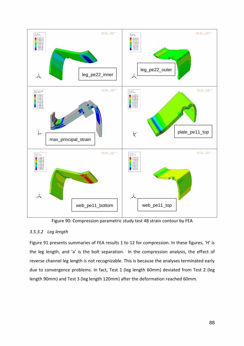
88

Figure 90: Compression parametric study test 48 strain contour by FEA

3.5.3.2 Leg length

Figure 91 presents summaries of FEA results 1 to 12 for compression. In these figures, ‘H’ is

the leg length, and ‘a’ is the bolt separation. In the compression analysis, the effect of

reverse channel leg length is not recognizable. This is because the analyses terminated early

due to convergence problems. In fact, Test 1 (leg length 60mm) deviated from Test 2 (leg

length 90mm) and Test 3 (leg length 120mm) after the deformation reached 60mm.

leg_pe22_inner leg_pe22_outer

max_principal_strain

plate_pe11_top

web_pe11_bottom web_pe11_top

89

(a)

(b)

(c)

(d)

Figure 91: Leg length (H) effect on one bolt in compression parametric strudy: FEA results (Tests 1-12)

3.5.3.3 Bolt separation (‘a’ in Figure 42)

Figure 92 shows a summary of bolt separation effects on reverse channels under both

tension and compression. In these figures, ‘H’ is the leg length, and ‘a’ is the bolt separation.

Since bolt edge distance is constant in this study, larger bolt separations imply larger

endplate width. The larger bolt separation (wider endplate) will increase the elastic

stiffness. This is similar to the tension cases, where the bolt separation defines the plastic

hinge locations. Therefore, a reasonable bolt separation is necessary to increase the

connection ductility.

0

10

20

30

40

50

60

70

80

0 10 20 30 40 50 60 70 80

Load

[kN

]

Displacement [mm]

H = 60-120 mm, a = 90 mm

Test 1: H=60mm

Test 2: H=90mm

Test 3: H=120mm

0

10

20

30

40

50

60

70

80

90

0 5 10 15 20 25 30 35

Load

[kN

]

Displacement [mm]

H = 60-120 mm, a = 150 mm

Test 4: H=60mm

Test 5: H=90mm

Test 6: H=120mm

0

20

40

60

80

100

120

140

160

180

0 5 10 15 20 25 30 35 40 45

Load

[kN

]

Displacement [mm]

H = 60-120 mm, a = 210 mm

Test 7: H=60mm

Test 8: H=90mm

Test 9: H=120mm

0

20

40

60

80

100

120

140

160

180

200

0 10 20 30 40 50 60

Load

[kN

]

Displacement [mm]

H = 60-120 mm, a = 270 mm

Test 10: H=60mm

Test 11: H=90mm

Test 12: H=120mm

90

(a)

(b)

(c)

Figure 92: Bolt separation effect (a) on one bolt in compression parametric study FEA results (Tests 1-12)

3.5.3.4 Endplate thickness

Figure 93 shows a comparison of FEA results for one-bolt-row cases with different endplate

thicknesses (10mm and 20mm). Except for cases with 90 mm bolt separation, the thinner

endplate shows greater ductility. This is because the thinner endplate changes from plastic

hinge Mechanism 1 to plastic hinge Mechanism 2 (shown in Figure 68 and Figure 69).Figure

94 shows the deformed shape and the different plastic hinge locations.

3.5.3.5 Reverse channel thickness

Figure 95 compares reverse channels with different thicknesses (8mm in Test 1, 10mm in

Test 49 and 12mm in Test 61). Similarly to the tension cases, the stiffness will be increased

considerably with a thicker reverse channel.

0

20

40

60

80

100

120

140

160

180

200

0 10 20 30 40 50 60 70 80

Load

[kN

]

Displacement [mm]

H = 60 mm, a = 90-270 mm

Test 1:a=90mm

Test 4: a=150mm

Test 7: a=210mm

Test 10:a=270mm

0

20

40

60

80

100

120

140

160

180

200

0 10 20 30 40 50 60 70

Load

[kN

]

Displacement [mm]

H = 90 mm, a = 90-270 mm

Test 2: a=90mm

Test 5: a=150mm

Test 8: a=210mm

Test 11: a=270mm

0

20

40

60

80

100

120

140

160

180

200

0 10 20 30 40 50 60 70

Load

[kN

]

Displacement [mm]

H = 120 mm, a = 90-270 mm

Test 3: a=90mmTest 6: a=150mmTest 9: a=210mmTest 12: a=270mm

91

(a)

(b)

(c)

(d)

Figure 93: Endplate thickness effects on reverse channel in compression parametric study FEA results (Tests 1-12 & 37-48)

Test 4

Test 40

Figure 94: FEA images of compression parametric study tests 4 and 40

3.5.3.6 Rolled channel (PFC) or constant thickness channel cut from a tube

Figure 96 shows the comparison of the rolled channel (PFC) at a constant-thickness channel

cut from a tube, which have different definition of leg thickness. Similar to the tension

cases, the tube-cut section with thinner legs shows the higher ductility.

0

10

20

30

40

50

60

70

80

90

0 20 40 60 80 100 120

Load

[kN

]

Displacement [mm]

H = 60-120 mm, a = 90 mm

Test 37: H=60mm

Test 38: H=90mm

Test 39: H=120mm

Test 1: H=60mm

Test 2: H=90mm

Test 3: H=120mm

0

10

20

30

40

50

60

70

80

90

0 20 40 60 80 100 120 140

Load

[kN

]

Displacement [mm]

H = 60-120 mm, a = 150 mm

Test 40: H=60mm

Test 41: H=90mm

Test 42: H=120mm

Test 4: H=60mm

Test 5: H=90mm

Test 6: H=120mm

0

20

40

60

80

100

120

140

160

180

0 20 40 60 80 100 120 140 160

Load

[kN

]

Displacement [mm]

H = 60-120 mm, a = 210 mm

Test 43: H=60mmTest 44: H=90mmTest 45: H=120mmTest 7: H=60mmTest 8: H=90mmTest 9: H=120mm

0

20

40

60

80

100

120

140

160

180

200

0 20 40 60 80 100 120

Load

[kN

]

Displacement [mm]

H = 60-120 mm, a = 270 mm

Test 10: H=60mmTest 11: H=90mmTest 12: H=120mmTest 46: H=60mmTest 47: H=90mmTest 48: H=120mm

92

Figure 95: Effect of reverse channel thickness effect in the parametric study

(a)

(b)

(c)

(d)

(e)

(f)

Figure 96: parametric study PFC VS. Tube-cut (compression)

0

20

40

60

80

100

120

140

0 10 20 30 40 50 60 70 80Lo

ad [

kN]

Displacement [mm]

Test 1Test 49Test 61

0

50

100

150

200

250

300

350

400

450

500

0 5 10 15 20 25 30 35 40 45 50

Load

[kN

]

Displacement [mm]

Test 73

Test 74

0

50

100

150

200

250

300

350

400

450

0 5 10 15 20 25 30 35 40 45

Load

[kN

]

Displacement [mm]

Test 75

Test 76

0

50

100

150

200

250

300

350

400

0 10 20 30 40 50

Load

[kN

]

Displacement [mm]

Test 77

Test 78

0

50

100

150

200

250

300

350

0 10 20 30 40 50 60

Load

[kN

]

Displacement [mm]

Test 79

Test 80

0

50

100

150

200

250

0 10 20 30 40 50 60 70

Load

[kN

]

Displacement [mm]

Test 81

Test 82

0

50

100

150

200

250

0 20 40 60 80 100 120

Load

[kN

]

Displacement [mm]

Test 83

Test 84

93

3.5.3.7 Post yield hardening in the reverse channel under compression

Figure 97 presents the FE analysis results for the compression parametric study (single-bolt-

row cases). The cases with wider endplate (a = 210 and 270 mm) show post-yield hardening

after the plastic hinges form. This is because the reverse channel leg in compression is

relatively stiff at the beginning. At large deformation it starts to show its contribution, as

‘post-yield hardening’ happens. In order to simplify the calculation, this post-yield hardening

is excluded from this development.

(a)

(b)

(c)

Figure 97: post-yield hardening in the compression parametric study

3.6 Conclusion

Based on the plastic hinge method, the component models for the reverse channel under

tension and compression have been developed. In particular, a bolt pull-out limit has been

derived from a ‘cone model’ (also called ‘bolt pull-out model’). The COMPFIRE project has

supplied comprehensive test and FE data to characterise the behaviour of the reverse

channel under tension. Parametric studies are carried out hereafter to investigate the

reverse channel behaviour. These studies will show that the component models are capable

of reasonably representing the reverse channel behaviour, and that they are ready to be

0

20

40

60

80

100

120

140

160

180

200

0 10 20 30 40 50 60 70 80

Load

[kN

]

Displacement [mm]

H = 60 mm, a = 90-270 mm

Test 1:a=90mm

Test 4: a=150mm

Test 7: a=210mm

Test 10:a=270mm

0

20

40

60

80

100

120

140

160

180

200

0 10 20 30 40 50 60 70

Load

[kN

]

Displacement [mm]

H = 90 mm, a = 90-270 mm

Test 2: a=90mm

Test 5: a=150mm

Test 8: a=210mm

Test 11: a=270mm

0

20

40

60

80

100

120

140

160

180

200

0 10 20 30 40 50 60 70

Load

[kN

]

Displacement [mm]

H = 120 mm, a = 90-270 mm

Test 3: a=90mmTest 6: a=150mmTest 9: a=210mmTest 12: a=270mm

94

implemented within the component based connection element, to model the reverse

channel connection behaviour in fire.

95

Chapter 4. Development of a general-purpose component-based connection element

Over the past 30 years the components which can be assembled to represent ambient-

temperature small-deflection moment-rotation behaviour of common connection types

(mainly flush and extended endplate connections) have been investigated by researchers all

around the world, and a number of component models have been developed. Figure 13

shows the component-based connection assembly by Simões da Silva (2001) for the flush

endplate joint.

These researches have taken place in the context of the development of semi-rigid design

principles (embodied in Eurocode 3 Part 8 (CEN, 2005b)) for steel and composite structural

frameworks. Figure 98 shows another assembly which is consistent with Eurocode 3 Part

1.8, by Burgess (2009).

Figure 98: Component assembly for endplate connection (Burgess, 2009)

The previous research objectives have been rather limited. The component-based

connection models have been used only to calculate the elastic rotational stiffnesses of

connections, and their moment capacity; they do not need to include strain-reversal

properties, fracture of individual components or the effects of elevated temperatures. In

Column web

tension

Column flange

bending

Bolttension

End plate bending

Beam web tension

Beam flangeColumn web

compression

Column web

shear

Hogging

Moment

96

contrast, the component-based connection models which are intended to be used in

structural numerical modelling of framed building structures under fire conditions have to

deal with the net compressive forces and distortions caused by restrained thermal

expansion of beams, as well as the tensile forces and distortions caused by catenary action

of the same beams at much higher temperatures, when the strength of steel has been

greatly degraded.

Block (2006a) has summarized the procedure to develop a mechanical model into three

steps, which are shown Figure 99Figure .

Step 1 Identification of the active components: Active components are those which either

contribute to the deformation of a joint or limit its strength.

Step 2 Specification of the component characteristics: In order to extend material properties

to the fire case, each component’s behaviour needs to be analysed at elevated

temperatures using F.E. studies and experiments, and described with a simplified analytical

model.

Step 3 Assembly of the active joint components: If the behaviour of the individual

components is known, it is possible to assemble them in a stiffness model and to represent

the joint as a joint finite element. Each component is represented as a translational spring

interconnected by rigid links. The joint’s overall performance in fire will then be modelled.

This procedure is very flexible. It can consider any types of joint, either bolted or welded. In

order to model the connection constitutive behaviour in fire, some specific effects such as

component fracture, progressive failure of component can be introduced.

Component models which can be assembled to model both flush endplate and reverse

channel connections under tension and compression at elevated temperatures, including

their ultimate (or fracture) conditions, have been developed and characterized by the

author as a part of the COMPFIRE project. These components can be assembled to model

various connection specifications.

97

Figure 99: Component-based connection element development procedure.

In this chapter, the key components for flush endplate and reverse channel connections are

identified. On the basis of the flush endplate connection, the assembly of an appropriate

number of components within a general-purpose component assembly is generalized to

represent connections of different specifications, and this is built into the Vulcan software.

In this expandable assembly, the tension and compression components are represented

using non-linear force/displacement curves, which are defined by the user. This is actually a

component-based connection element with flexible access, and is called a user-defined

connection element. Beyond this, several of the adopted component models are reviewed

and incorporated into the general-purpose component assembly to form connection

elements for both the flush endplate and the reverse channel connection types.

4.1 Identification of the active components

Table 6.1 in EC3 Part 1.8 lists the basic components for endplate joints:

column web panel in shear

column web in transverse compression

column web in transverse tension

Step 2 Specification of the component characteristics

Step 3 Assembly of the component

Step 1 Identification of the active component

98

column flange in bending,

end-plate in bending,

flange cleat in bending

beam or column flange and web in compression,

beam web in tension

plate in tension or compression

bolt in shear

bolts in bearing

Welds

These active components are also shown in Figure 100.

Figure 101 lists the active components which are considered within the connection element

under this development.

Beam web Column web

Beam flange web Column web

Compression

Beam web

Column web Column flange

End plate

Tension bolts

Tension

Slip

Figure 100: Endplate connection active component (Burgess, 2009)

99

Figure 101: Zones of structural action in endplate joints (Spyrou, 2002).

Based on the experiments conducted in COMPFIRE (Huang, 2013a, 2013b) and FE studies

(RFCS, 2012a), the zones of structural action for the reverse channel connection are

identified in Figure 102.

Figure 102: Active component in reverse channel joints.

4.2 Development of the user-defined connection element

The user-defined connection element is a component-based connection element developed

from the assembly of a number of components, which follows the distribution of key

components in the flush endplate connection (Figure 100). Users are allowed to define the

Bolt in tension

Endplate in bending

M

Column web in compression

Reverse channel in compression

Endplate in bending

M

Bolt in tension

Reverse channel in bending

Column flange in bending

100

basic behaviour of all components at ambient temperature as non-linear

force/displacement curves. Reduction factors are applied to the material properties of these

in order to define the component behaviour at elevated temperatures. The following

sections will cover:

Basic assumptions for the structural properties of each tension/compression

component,

How to combine these tension components in series into one effective “bolt-row”

spring,

How to assemble these spring rows as a connection element,

How to fit this connection element into Vulcan to deal with the structural behaviour

of buildings at elevated temperatures, including progressive collapse.

4.2.1 Assembly of components

Figure 103 depicts the general-purpose component assembly of a simple two-bolt-row

endplate connection, together with the action of the adjacent shear panel towards the end

of the beam. Figure 104 illustrates how this component-based connection element and

shear panel can deform in response to the combination of axial force, shear force and

moment which can happen during a fire.

In order to tackle the changing force combination during a fire, gaps (shown in Figure 105)

are utilised in Figure 103 and Figure 104. Figure 106 uses a reverse channel connection as an

example to illustrate the function of these gaps. The gap between a compression spring row

and a rigid face is designed to represent the space between the reverse channel and the

beam endplate. Once these are in contact, the compression spring row is activated, which

ensures that it only works under compressive force. The gaps between the rigid links above

bolt springs in tension (explained in detail in 4.2.5) are formed and increased when the

bolt’s plastic deformation breaks the contact between the mating plate surfaces. However,

the bolt does not act in compression, which is transferred directly by the contact between

the reverse channel (or column) face and endplate springs.

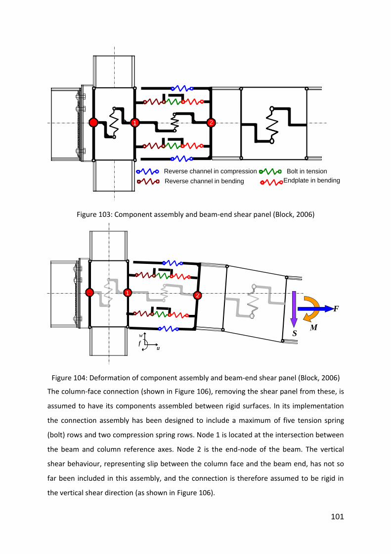
101

Figure 103: Component assembly and beam-end shear panel (Block, 2006)

Figure 104: Deformation of component assembly and beam-end shear panel (Block, 2006)

The column-face connection (shown in Figure 106), removing the shear panel from these, is

assumed to have its components assembled between rigid surfaces. In its implementation

the connection assembly has been designed to include a maximum of five tension spring

(bolt) rows and two compression spring rows. Node 1 is located at the intersection between

the beam and column reference axes. Node 2 is the end-node of the beam. The vertical

shear behaviour, representing slip between the column face and the beam end, has not so

far been included in this assembly, and the connection is therefore assumed to be rigid in

the vertical shear direction (as shown in Figure 106).

` 1 2

Endplate in bending

Bolt in tensionReverse channel in compression

Reverse channel in bending

` 1

uf

u

w

f

F

S

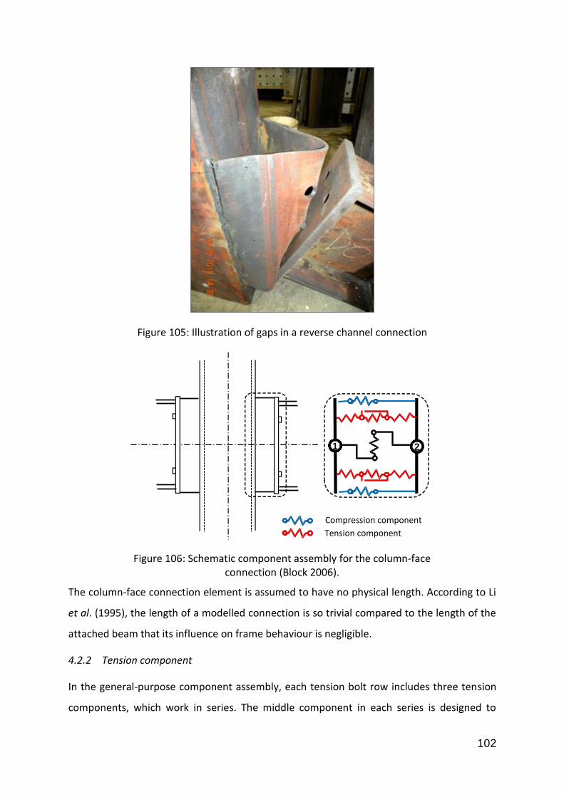
102

Figure 105: Illustration of gaps in a reverse channel connection

The column-face connection element is assumed to have no physical length. According to Li

et al. (1995), the length of a modelled connection is so trivial compared to the length of the

attached beam that its influence on frame behaviour is negligible.

4.2.2 Tension component

In the general-purpose component assembly, each tension bolt row includes three tension

components, which work in series. The middle component in each series is designed to

Figure 106: Schematic component assembly for the column-face connection (Block 2006).

Tension component Compression component

2 1

103

represent the bolt in tension, and how this is represented will be explained in detail later.

The other two tension components in a bolt row represent the column flange in tension and

the endplate in tension for flush endplate connections, or the reverse channel in tension

and endplate in tension for reverse channel connections. Each tension component’s

Force/Displacement behaviour is represented by a multi-linear curve without any

‘descending’ (negative stiffness) part. A typical multi-linear curve (Figure 107) consists of 5

intersections, which can be expanded if more are required, to plot relevant aspects of the

component behaviour. In Figure 107, Point 5 represents the ‘ultimate strength’, at which

point the component has its maximum resistance and deformation. Beyond the ultimate

strength, the component is deemed to be fractured. If Point 5 is reached, the whole spring

row in which this component is located will be ‘switched off’, and is not recoverable. It will

not contribute to the joint’s stiffness or robustness in the subsequent analysis.

Figure 107: Typical tension component force/displacement behaviour

4.2.3 Effective Force/Displacement curve of a component at constant temperature

When a component carries a force it may become inelastic, and will then have irreversible

deformation (‘residual deformation’) when its force is reduced to zero. In this development,

the classic Masing rule (Gerstle, 1988) is employed for this ‘memory effect’. Based on the

Masing rule the unloading curve is the original loading curve doubled in scale and rotated by

180°.

If the initial loading curve (Block, 2006) is represented by:

Point 2

Point 3

Point 4

Point 5 (ultimate) )

Displacement

Fo

rce

Point 1

Fracture

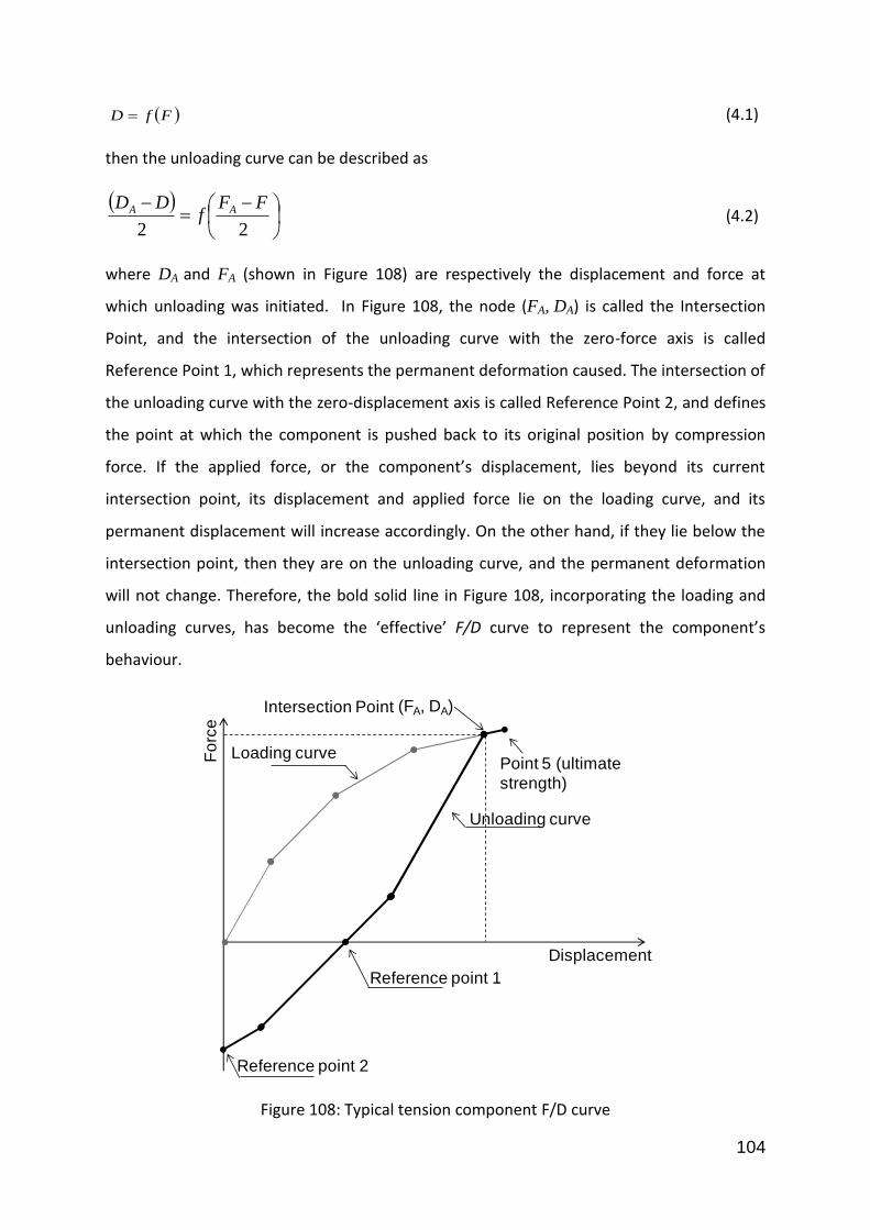
104

(4.1)

then the unloading curve can be described as

(4.2)

where DA and FA (shown in Figure 108) are respectively the displacement and force at

which unloading was initiated. In Figure 108, the node (FA, DA) is called the Intersection

Point, and the intersection of the unloading curve with the zero-force axis is called

Reference Point 1, which represents the permanent deformation caused. The intersection of

the unloading curve with the zero-displacement axis is called Reference Point 2, and defines

the point at which the component is pushed back to its original position by compression

force. If the applied force, or the component’s displacement, lies beyond its current

intersection point, its displacement and applied force lie on the loading curve, and its

permanent displacement will increase accordingly. On the other hand, if they lie below the

intersection point, then they are on the unloading curve, and the permanent deformation

will not change. Therefore, the bold solid line in Figure 108, incorporating the loading and

unloading curves, has become the ‘effective’ F/D curve to represent the component’s

behaviour.

Figure 108: Typical tension component F/D curve

FfD

22

FFf

DD AA

Displacement

(FA, DA)

Fo

rce

Reference point 1

Intersection Point

Unloading curve

Loading curve

Reference point 2

Point 5 (ultimate

strength)

105

4.2.4 Unloading with changing temperatures

When a component is heated in a fire, its F/D curve is temperature-dependent and the

temperature is continuously changing during the fire. Therefore, the ‘Reference Point’

concept is introduced to locate the unloading curve. Block (2006) describes the principle of

the ‘Reference Point’ concept as ‘plastic strain which is not affected by a temperature

variation’. Therefore, the component’s permanent deformation is assumed not to change

when only its temperature changes. When moving to the next temperature step, the

component’s current permanent deformation is that saved from the last step, and will be

updated at the end of each calculation step.

Figure 109: Unloading at changing temperatures

Figure 111 explains how this concept is implemented in Vulcan. Reference Point 1 is

updated at the end of the step at temperature T1, on the basis of the applied force and the

component’s Force/Displacement (F/D) curve. When moving to the next step (temperature

T2), the unloading curve will be plotted on the basis of the component’s new F/D curve.

Therefore the new unloading curve will be located by starting from a point on the new

Fo

rce

Displacement

T1

T2

(F2, D2)

Reference point 1

T1< T2

F1> F2

D2> D1

(F1, D1)

106

loading curve, passing through Reference Point 1 from the previous step (temperature T1).

Finally, the effective F/D curve is formed for this temperature T2.

4.2.5 Typical tension bolt row

In the calculation process for this connection element, the three components in each

tension bolt row are combined into one effective spring at each temperature step (Figure

110). The force-displacement curves of the tension bolt rows are used to define the

connection’s local force and stiffness. After the global analysis reaches a converged stable

equilibrium (explained in 4.2.7), the forces in the tension bolt rows are established, and the

displacements of each tension component are calculated; these are then output in order to

help the user to evaluate the state of the connection. The related information, such as each

component’s permanent deformation, is then updated.

In accordance with the principle of springs working in series, the force stays the same in

each spring within a spring row. The maximum resistance of the effective spring is defined

by the weakest spring in this series. The forces at all the points in all the components’ F/D

curves are sorted in increasing order, and any force above the weakest component’s

ultimate resistance is ignored. At each force level, the effective spring’s displacement is the

aggregate of all the components’ displacements under the corresponding force level. When

calculating each component’s deformation, the unloading curve will be used if the force is

below that at the previously established intersection point.

Figure 110: Assembly of the individual tension components in a tension bolt row

The middle component in each tension bolt row is allocated to the bolt in tension. This is

only able to transfer tension force. Figure 111 illustrates the typical effective

force/displacement curve for a bolt in tension, for which there is no Reference Point 2

(Figure 108). This is because the bolt does not take compression force in either the flush

endplate connection or the reverse channel connection. In compression, the left- and right-

hand components will contact directly to transfer the force.

=

F

D

Unloading curve

+ +

+ +

F

D

F

D

F

D

Unloading curve

107

The endplate connection is now used to explain this principle. In this connection, the three

tension components in each tension bolt row include the column flange under bending, the

bolt in tension and the endplate in bending, are represented by two T-stub components.

Figure 112 illustrates this as a picture of a T-stub tension test.

Figure 111: Typical tension component F/D curve for bolt in tension

Figure 112: T-stub test picture (Spyrou, 2002)

Figure 113 shows the deformed shapes of the T-stub at various stages of a sequence of axial

force. The applied force starts with increasing tension, which reduces to zero, changes to

compression, reduces to zero again, and finally changes to tension.

Fo

rce

Point 5 (ultimate strength)

Unloading curve

Intersection Point (FA,DA)

Reference Point 1Displacement

108

Figure 113: T-stub deformed shapes at different testing stages

The typical tension bolt row Force/Displacement (F/D) curve consists of four parts (Figure

114): tension, bolt plastic deformation, compression, and residual compression. Each part

may be used at different stages of a fire.

The ‘tension part’ (Figure 113 a, b and c) shows all three components in parallel under

tension. Two T-stub flanges are subject to bending, while two bolts are under tension.

The ‘bolt recovery of plastic deformation part’(Figure 113 d) represents the stage between

the ‘tension’ and ‘compression’ parts, during which the applied tension reduces to zero, and

the deformed endplate and column flange have not yet come into contact. As the bolt-in-

tension component does not work under compression, the tension spring row’s stiffness is

zero after this. The plastic deformation of the bolt is residual and irrecoverable, even during

the reloading which is shown in Figure 113 g, h and f.

The ‘compression part’ (Figure 113 e and f) represents the state when the plastically

deformed endplate and column flange are pushed back until their centres come into

contact.

a b c

d e f

g h i

109

The ‘residual compression’ part (Figure 113 f) is based on the assumption that the tension

bolt row can transfer a certain amount of compression force. However, as the parts of the

connection represented by the compression spring group are much stiffer than this, most of

the compression force will be transferred by the compression spring group.

Figure 114: Typical tension bolt row force/displacement curve

4.2.6 Compression spring row

A compression component characteristic is represented by 3 intersection points, which can

be increased if necessary (Figure 115). A compression component will be ‘switched off’

under tension force, when its stiffness contribution is zero and it transfers zero tension

force. Point 3 is the ultimate strength point beyond which no change of force occurs.

Figure 115: Typical compression component force/displacement behaviour

Displacement

Point 2

Point 1

Fo

rce

Point 3

Fo

rce

Residual compression

Compression

Bolt plastic deformation

Tension

Displacement

110

4.2.7 Solution process of Vulcan

Since the general-purpose component assembly has now been developed, consideration of

the effects of interaction at connections within frames under elevated temperatures can be

addressed, once it has been incorporated into the global nonlinear finite element software

Vulcan. The principles and procedure are also applicable to other type of connection and

can be incorporated into other finite element packages.

Vulcan is a nonlinear finite element analysis software for structural fire engineering. When

modelling a discrete structure, the whole structural system is represented with a large

number of elements. A joint will be modelled as a 2-noded connection element. The whole

structure forms a global system with global coordinates, while each element forms an

internal system with its own local coordinates.

After applying loadings, such as temperature, force and/or deformation, a structure may

stay stable, or lose its stability and collapse. A stable structure retains equilibrium of internal

and external forces, compatibility of internal and external deformations, and its defined

constitutive relationships between internal force and deformation (Izzuddin, 2005). Vulcan

is intended to track the equilibrium, while retaining its compatibility and constitutive

relationships, which are represented by the following three equations:

}{][}{ fTP T (4.3)

This equation represents the equilibrium of internal and external forces. {P} is the vector of

applied forces based in global coordinates, and {f} is the vector of internal forces based in

local coordinates. [T] is the geometric transformation matrix between the global and local

coordinates.

}]{[}{ UTd (4.4)

This equation matches the internal and external deformations. {d} is the internal

deformation vector based in local coordinates, and {U} is the external deformation vector

based in global coordinates

}]{[}{ dkf (4.5)

111

This equation relates the internal force to deformation using the constitutive relationships.

{f} is the vector of internal forces based in local coordinates. The local stiffness matrix [k] is

variable, due to both geometrical and material nonlinearities.

For linear elastic analysis, the unknown {U} can be determined for a given {P}:

}]{[}{ UKP (4.6)

where

]][[][][ TkTK T (4.7)

The commonly used Newton-Raphson iterative technique (Sun, 2012) is adopted to achieve

a converged solution. In the load control method, equilibrium states are hunted for various

load levels defined by (λ1,.., λi...., λn). An unknown equilibrium state corresponding to λi is

obtained through an iterative procedure, which starts from the last known equilibrium state

in the load level λi-1 and consisted of steps. It should be noted that Vulcan has both static

and dynamic solvers; the following is an illustration of procedure on the basis of static

solver. In the static solver, the rates of inertial effects from the change of loading and

temperature are ignored. The relationship between static and dynamic solver will be

included in 4.2.9. The following is the calculation process to find the equilibrium at load

level “P1” on the basis of load level “P0”. This procedure is also shown in Figure 116.

Load

Displacement

G1 1

ΔPi

K0

ki

ΔU2 Step λi

Step λi-1

Iteration between load steps

ΔU3 ΔU1

U0 U1

P0

P1

Figure 116: Newton-Raphson iterative procedure

112

1. Calculate incremental {ΔP} from load level P0 to load level P1.

2. Using the stiffness [K0] on the last step, solve the incremental global displacement

}{][}{ 1

0 PKU i

(4.8)

3. Update the global nodal displacement

}{}{}{ 01 iUUU (4.9)

4. Update the global nodal forces

}{}{}{ 01 PPP (4.10)

5. Update the local element displacement

}]{[}{ 11 UTd (4.11)

6. Calculate the global internal force

}]{[}{ 11 fTR (4.12)

7. Calculate the out of balance forces {Gi}={Ri}-{Pi}

}{}{}{ 111 PRG (4.13)

8. If G1 does not meet with the convergence criteria, the above calculation will repeat.

The stiffness will be calculated for the next step. The iteration will be carried on,

until the convergence criteria is met.

4.2.8 Incorporation of the user-defined connection element into Vulcan

Within Vulcan, this new connection element is attached to the existing subroutine, called

SEMIJO, which is specified for the existing simpler spring elements and which Block (2006a)

also used for his connection element. In each calculation step (or load/displacement step),

the connection element receives the necessary incremental displacement vector from

SEMIJO and returns the tangent stiffness matrix and force vector (shown in Figure 117).

113

Block (2006) first derived the tangent stiffness matrix ( '

cK ) of the connection element,

shown as Equation 4.14. Based on the element local axis, a node has total six Degrees of

Freedom (DOF), including x, y, z, xx (rotation about x-axis), yy (rotation about y-axis) and zz

(rotation about z-axis). The x-axis is the axial direction of the connection. The y- and z-axes

are the shear directions of the connection. The connection element local coordinate system

is also illustrated in Figure 118. Accordingly, the tangent stiffness matrix will be 12x12. The

out-of-plane and torsional DOF are assumed to be connected rigidly and without

interaction, because these are currently under development and are in any case of relatively

minor importance in steel or composite building structures.

Vulcan Connection element

Tangent stiffness matrix

Force

Incremental displacement

Node 2

Node 1

Z

Y X

Z

Y X

Figure 117: interaction between connection element and Vulcan

Figure 118: Connection element local coordinate system

114

0000000000

00000000

0000000000

0000000000

0000000000

00000000

0000000000

00000000

0000000000

0000000000

0000000000

00000000

'

55

'

51

'

55

'

51

'

33

'

33

'

15

'

11

'

15

'

11

'

55

'

51

'

55

'

51

'

33

'

33

'

15

'

11

'

15

'

11

'

KKKK

KK

KKKK

KKKK

KK

KKKK

KC

(4.14)

in which

2

1

'

,

1

'

,

'

11

i

iC

n

i

iT kkK

(4.15)

2

1

'

,,

1

'

,,

'

51

'

15

i

iCiC

n

i

iTiT klklKK

(4.16)

''

33 skK (4.17)

2

1

'

,

2

,

1

'

,

2

,

'

55

i

iCiC

n

i

iTiT klklK

(4.18)

In which the subscripts ‘T’ and ‘C’ represent components working in tension or compression,

and n is the number of bolt rows. The subscript ‘s’ denotes a shear component.

K11 represents the axial stiffness under the axial force in axis-x shown in Figure 118. K15 is

the axial stiffness in axis x under the bending about the y-axis. K33 is the shear stiffness in

axis z under shear in z direction. K55 is the bending stiffness about axis y under the bending

about axis y.

However, the static solver only converges on the ascending part (positive stiffness) of the

force-displacement curve. The change to a descending part, with negative stiffness or

unstable equilibrium, will lead to a numerical singularity and is beyond the static solver’s

115

capacity. It will stop the analysis without accurately predicting the failure of the whole

structure. At that time, a dynamic solver is necessary, which is included in 4.2.9.

4.2.9 The static/dynamic Vulcan solver.

As a key part of performance-based structural design, the structural engineering should

ensure that the possibility of disproportionate structural collapse in fire is avoided.

Scenario-based non-linear finite element modelling of the structure is necessary for the

performance-based structural fire engineering building design, particularly for large and

complex buildings. Therefore, the numerical modelling must be capable of predicting the

real structural behaviour, not only before the first loss of structural stability, but also from

the local instability to total collapse.

The following takes the connection as an example. One component failure in a connection,

such as fracture of a bolt, may indeed trigger a progressive structural collapse, but does not

in itself constitute failure of the whole structure. Generally, a component failure will cause

the structure to lose its stability temporarily, as other components and members of the

structure share the redistributed internal forces. After the load path is re-formed in this

way, it is possible for the structure to re-stabilize. This is a common phenomenon in

experimental testing under load-control, where the force-deflection trace is saw-toothed

because of a sequence of releases of internal force as local fractures occur. When

equilibrium cannot be achieved between the external loading and the redistributed internal

forces, a more widespread structural collapse occurs. Figure 119 shows schematically the

situation in terms of applied force and deflection when part of the structure reaches its

peak load capacity. Since the load level remains constant the deflection accelerates

dynamically, and will become extremely high unless a re-stabilized configuration is found.

The figure shows the initial quasi-static equilibrium path, followed by a dynamic phase

which re-stabilizes and once again becomes quasi-static. Figure 120 shows the alternative

(or eventual) situation, when no re-stabilization is found and a real structural collapse

occurs.

116

Figure 119: Loss of stability and re-stabilization of structure.

Figure 120: component failure causing structural collapse

Figure 121 shows the general flowchart for modelling of a structure and its connections,

including its failure sequence. Generally a quasi-static analysis solver is used, up to the point

at which the first component fails. From this point the dynamic solver is activated to track

the motion of the structure. If stability is not regained, this initiates a cascade of failures of

the other components, leading to complete detachment of the members.

Stable region

Unstable region

Load

Deflection

Stable region

δre-st

δcrit

Pcrit

Dynamic

Load

Co

llapse

Structu

re with

ou

t fractu

red co

mp

on

ent

Deflectio

n

Component fracture

Intact structure

117

Figure 121: procedure of connection failure modelling

4.2.10 Preliminary application of the user-defined connection element in examples

The development of the general-purpose connection element was intended to cope with

reverse channel and flush endplate connections, in which the component characterizations

will be defined internally on the basis of connection geometries, temperature development

and temperature-dependent material properties. However, the connection element also

allows the definition of component behaviour by users, which is called the user-defined

connection element. The force-displacement curves and the temperature-dependent

strength and modulus reduction factors for the components are required for the input. The

element provides a tool to investigate the interaction between connections and the

adjacent connected structure, and to understand the demands posed by the structure on its

connections.

The user-defined connection element has been successfully incorporated into Vulcan. In

order to test its functioning in limited subframe examples rather than in more extensive

structural frames, four cases were created to test the element:

Case 1: Isolated beam with connection elements, without axial restraint (Figure

122)

Case 2: Isolated beam with connection elements, with axial restraint (Figure 123)

Case 3: 2D subframe (Figure 124)

Case 4: 2D “rugby goal-post” frame (Figure 125)

Read in data for new step (Such as temperature)

Static analysis

Failed component is deleted

Numerical singularity?

- Re-stabilized?

YES

NO

NO

Connected member detached

YES A component reaches

its limit ?

Explicit Dynamic analysis NO

YES

118

All these cases were analysed with the static-dynamic solver, using different connection

details, and the results were compared with those obtained using idealized rigid and pinned

connections. The connection behaviour in the cooling phase of the fire has also been

examined.

In all of these test cases the beam section was 254x102UKB22, and the column was

203x203UKC71. The beam endplate thickness was 12mm and the steel grade was S275. No

out-of-plane deflection was allowed. The joint details (Figure 127) were designed to test the

connection elements’ full capacity for 3 and 5 bolt rows, of which the lowest would normally

be considered to act only in shear.

The component behaviour (Figure 127) for both arrangements was based on a set of

derivations from earlier studies (Hu et al., 2007 and Yu et al., 2009). In order to consider the

components’ behaviour at elevated temperatures, reduction factors and ductility factors

(Figure 128, Figure 129 and Figure 130 respectively) were temporarily introduced to reduce

the ambient-temperature resistance and to increase the ductility at high temperatures.

Figure 122: Isolated beam with connection elements, without axial restraint.

Figure 123: Isolated beam with connection elements, with hinged end, fixed in position.

W= 10kN/m

UB 254X102X225500 mm

W= 10kN/m

UB 254X102X22

5500 mm

119

Figure 124: 2D subframe.

Figure 125: 2D “rugby goal-post” frame.

3500 m

m

UB 254X102X22

5500 mm2750 mm 2750 mm

3500 m

m

350

0 m

m

UB 254X102X22

5500 mm

3500

mm

120

Figure 126: Analysed endplate connection details.

27

130

76 27

55

50

27.5

72.5

55

(a)

Top compression spring row

1st tension bolt row

2nd tension bolt row

3rd tension bolt row

Bottom compression spring row

27

130

76 27

55

145

30

30

30

30

30

(b)



2nd

tension bolt row


Bottom compression spring row

4th tension bolt row


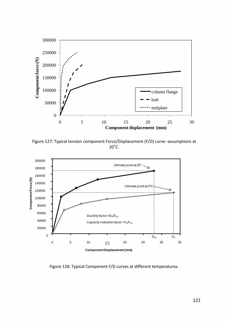
121

Figure 127: Typical tension component Force/Displacement (F/D) curve -assumptions at 20○C.

Figure 128: Typical Component F/D curves at different temperatures.

0

50000

100000

150000

200000

250000

300000

0 5 10 15 20 25 30

Co

mp

on

ent fo

rce

(N)

Component displacement (mm)

column flange

bolt

endplate

0

20000

40000

60000

80000

100000

120000

140000

160000

180000

200000

0 5 10 15 20 25 30 35

Co

mp

on

en

t Fo

rce (N

)

Component Displacement (mm)

Ultimate point at 20°

Ultimate point at θ°C

D20 Dθ

Ductility factor =Dθ/D20

Capacity reduction factor =Fθ/F20

122

Figure 129: Capacity reduction factors for all the components.

Figure 130: Ductility factor for tension component.

Case 1: Isolated beam with connection elements, without axial restraint

Case 1 was tested for mid-span deflections against cases with the ends both perfectly

restrained laterally, but allowed to move axially and unrestrained against rotation. Figure

131 plots the bolt row forces against steel temperature for the 5-bolt-row case. The forces

in the bolt rows all start reducing beyond 500°C, while the spring row deformations are

noticeably increasing in Figure 132. From the output file, the fracture of the first tension

bolt row triggers a progressive structural failure, since the remaining components cannot

resist the applied load.

0

0.2

0.4

0.6

0.8

1

1.2

0 200 400 600 800 1000 1200 1400

Fact

or

Temperature ( C)

bolt

T-stub& compression zone

0

0.5

1

1.5

2

2.5

3

3.5

0 500 1000 1500

Fact

or

Temperature ( C)

bolt ductility factor

t-stub ductility factor

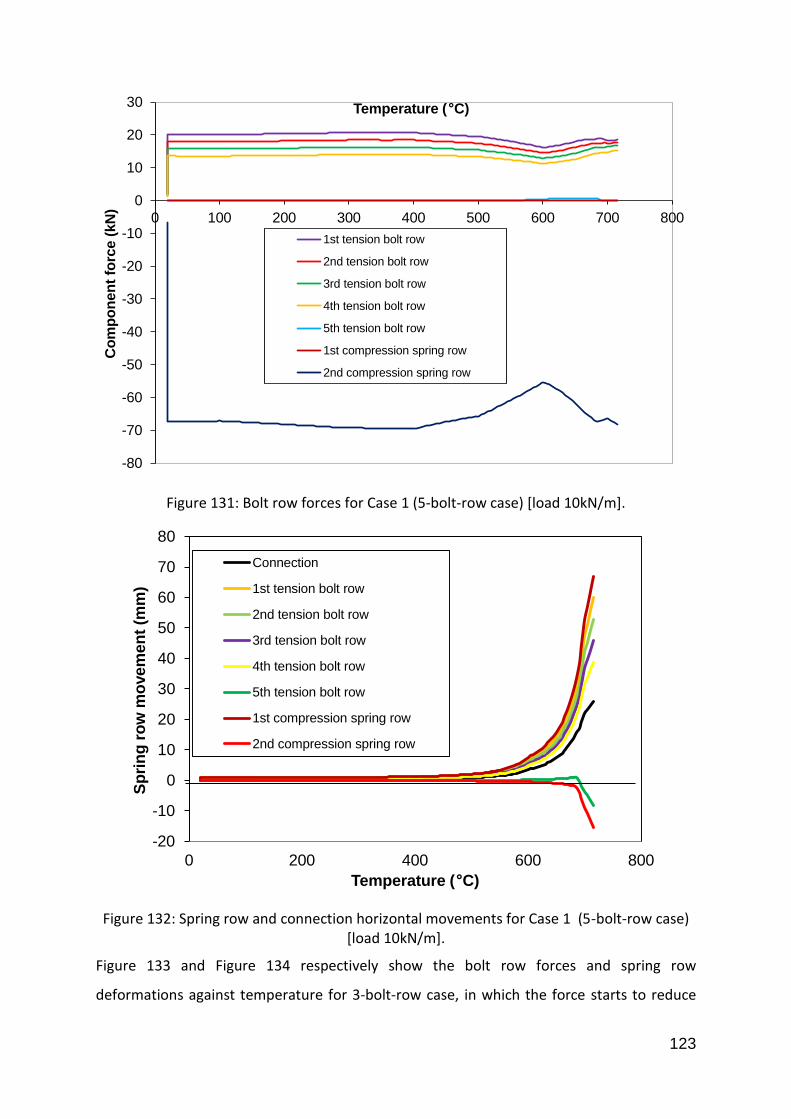
123

Figure 131: Bolt row forces for Case 1 (5-bolt-row case) [load 10kN/m].

Figure 132: Spring row and connection horizontal movements for Case 1 (5-bolt-row case) [load 10kN/m].

Figure 133 and Figure 134 respectively show the bolt row forces and spring row

deformations against temperature for 3-bolt-row case, in which the force starts to reduce

-80

-70

-60

-50

-40

-30

-20

-10

0

10

20

30

0 100 200 300 400 500 600 700 800

Co

mp

on

en

t fo

rce (

kN

)Temperature ( C)






1st compression spring row

2nd compression spring row

-20

-10

0

10

20

30

40

50

60

70

80

0 200 400 600 800

Sp

rin

g r

ow

mo

vem

en

t (m

m)

Temperature ( C)

Connection








124

beyond 400°C, while the spring row deformation starts increasing sharply. It can also be

seen from Figure 135 that, in both of the connection element cases, deflections lie between

those for the perfectly rigid and pinned cases. Logically, the 5-bolt-row connection is stiffer

than the 3 bolt row connection and also has higher resistance.

Figure 133: Bolt row force for case 1 (3-bolt-row case) [load 10kN/m].

Figure 134: Spring row and connection horizontal movement Case 1 (3-bolt-row case) [load

10kN/m].

-70

-60

-50

-40

-30

-20

-10

0

10

20

30

0 100 200 300 400 500 600 700 800

Co

mp

on

en

t fo

rce

(k

N)

Temperature ( C)






-10

0

10

20

30

40

50

60

0 200 400 600 800

Spri

ng

row

mo

vem

ent

(mm

)

Temperature ( C)

Connection






125

Figure 135: Beam mid-span deflections for Case 1 [load 10kN/m].

Case 2: Isolated beam with connection elements, with axial restraint

In Case 2, the deflections for the rigid and pinned connections (Figure 136) come very close

at high temperatures (above 600°C), when the beam is in the catenary stage and is under

nearly pure tension; this is logical for a case with fixed ends. It is also noticeable that the

deflection of the beam with connection elements initially lies between those of the beams

with rigid and pinned connections. Above 685°C, the beam with connection elements has a

larger deflection than either of the rigid or pinned cases. This happens because catenary

action causes a net shortening of the beam which is greater than the thermal expansion,

and some of this net shortening can be accommodated by extension of the bolt rows. The

bolt row deflections, together with the net movement of the beam end, are shown in Figure

137, and illustrate this point.

-2500

-2000

-1500

-1000

-500

0

0 200 400 600 800

De

fle

cti

on

(m

m)

Temperature (0C)

5 bolt row

3 bolt row

Fixed

Pinned

126

Figure 136: Beam mid-span deflections for Case 2 [load 10kN/m].

Figure 137: Spring row and connection horizontal movement Case 2 [load 10kN/m].

Figure 138 shows how the connection element deals with the combination of forces in the

joint when the beam is heated in Case 2. In the initial stage, the top 4 tension bolt rows and

the bottom (2nd) compression spring row work to resist the beam-end rotation due to the

applied load. After the beam is heated it starts to expand, and the connection experiences a

combination of compression and bending, at which stage all the top 4 tension bolt rows are

gradually ‘switched off’ as the tension force in the top of the section is offset by the thermal

-1200

-1000

-800

-600

-400

-200

0

0 200 400 600 800 1000 1200

Defl

ecti

on

(m

m)

Temperature (OC)

Connection element 5 bolt rowFixed

Pinned

-50

0

50

100

150

200

250

0 200 400 600 800 1000

Spri

ng

row

mo

vem

ent

(mm

)

Temperature ( C)

Connection








127

expansion. Once all the tension bolt rows have temporarily stopped working, the top

compression spring row starts to work together with the bottom compression spring, and

the whole section is under compression. With the temperature increasing further, the

beam’s deflection increases sharply and the top 4 tension bolt rows progressively replace

the top compression spring row in resisting the combination of compression force and

moment. Above 600°C, the beam progressively develops catenary tension and reduces its

bending action. Eventually all the 5 tension bolt rows are working and both of the

compression spring rows are ‘switched off’. The initial failure is at the first tension bolt row,

and the remaining components cannot then resist the applied load.

Figure 138: Component force for Case 2 [load 10kN/m].

In Case 2, the assembly was examined during cooling (Figure 139 and Figure 140). In Figure

140 the simulation was stopped due to the fracture of the bolt in the first tension bolt row,

which was determined from the Vulcan output file.

-350

-300

-250

-200

-150

-100

-50

0

50

0 100 200 300 400 500 600 700 800 900 1000

Co

mp

on

en

t fo

rce

(kN

)

Temperature ( C)








128

Figure 139: Beam deflection with cooling from 750°C for Case 2 [load 10kN/m].

Figure 140: Beam deflection with cooling from 800°C for Case 2 [load 10kN/m].

Case 3: 2D subframe

Figure 141 and Figure 142 respectively show component forces and displacements in Case 3.

It follows the same trend as Case 2, in which the 5 tension bolt rows and 2 compression

spring rows switch on/off in sequence while the beam is heated up and expands. About

above 550°C, the beam progressively develops catenary tension and reduces its bending

action. Eventually all the 5 tension bolt rows are working, and both of the compression

spring rows are ‘switched off’. The first failure is at the first tension bolt row, after which

the remaining components cannot resist the applied load.

-600

-500

-400

-300

-200

-100

0

0 200 400 600 800

defl

ecti

on

(m

m)

Temperature (OC)

Connection element

Rigid

Pinned

-700

-600

-500

-400

-300

-200

-100

0

0 200 400 600 800 1000

Defl

ecti

on

(m

m)

Temperature (OC)

Connection element

Rigid

Pinned

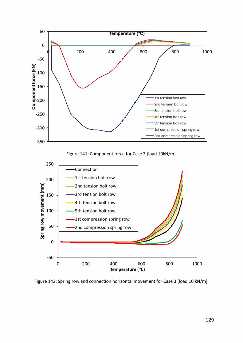
129

Figure 141: Component force for Case 3 [load 10kN/m].

Figure 142: Spring row and connection horizontal movement for Case 3 [load 10 kN/m].

-350

-300

-250

-200

-150

-100

-50

0

50

0 200 400 600 800 1000

Co

mp

on

en

t fo

rce

(k

N)

Temperature ( C)








-50

0

50

100

150

200

250

0 200 400 600 800 1000

Spri

ng

row

mo

vem

ent

(mm

)

Temperature ( C)

Connection








130

Case 4: 2D “rugby goal-post” frame

Figure 143 and Figure 144 respectively show the component forces and displacements in

Case 4. Case 4 is similar to case 1. The top four tension bolt rows work until the first tension

bolt fails, triggering the connection failure.

Figure 143: Component force for Case 4 [load 10 kN/m].

Figure 144: Spring row and connection horizontal movement Case 4 [load 10 kN/m].

-120

-100

-80

-60

-40

-20

0

20

40

0 200 400 600 800 1000

Co

mp

on

en

t fo

rce

(k

N)

Temperature ( C)







-50

0

50

100

150

200

250

0 200 400 600 800 1000

Spri

ng

row

mo

vem

ent

(mm

)

Temperature ( C)

Connection








131

Summary

The main differences and similarities shown by the four cases outlined above lie in their

degrees of beam-end restraint in the axial and rotational degrees of freedom. In particular,

Cases 1 and 4 have limited axial restraint stiffness, whereas Cases 2 and 3 have very high

axial restraint. Figure 145 shows one aspect (the mid-span deflection) of the effects of these

boundary conditions in the 4 cases. The mid-span deflections of Cases 2 and 3 are nearly

overlapped. The deflections of the isolated beam without axial restraint (Case 1) and the 2D

“Rugby goal-post” frame (Case 4) are close, and increase sharply above 600°C. Both Cases 1

and 4 initially deflect very little, since very low axial forces do not induce thermal buckling of

the beam, whereas the cases with high axial restraint very rapidly induce sufficient axial

force because of their restraint to thermal expansion. However, the same axial restraint

equilibrates catenary tension, which acts to control the deflections at high temperatures,

when the less restrained cases are capable of “run-away” deflection because their

mechanisms mainly consist of bending. Case 4 can generate some axial tension at high

deflections because of the elastic and plastic resistance to pull-in of the two columns, and it

can be seen that the “run-away” is much less rapid than that of the simple beam in Case 1.

Figure 145: The heated beam’s mid-span deflection for 4 cases [load 10 kN/m]

4.3 Development of the connection element for flush endplate connection

The preliminary applications of the user-defined connection element have shown that it is

feasible to use component-based connection elements in numerical modelling of structural

-1200

-1000

-800

-600

-400

-200

0

0 200 400 600 800 1000

Defl

ecti

on

(m

m)

Temperature (OC)

Isolated beam with connection elements without axial restraint

Isolated beam with connection elements with axial restraint

2D subframe

2D goal post f rame

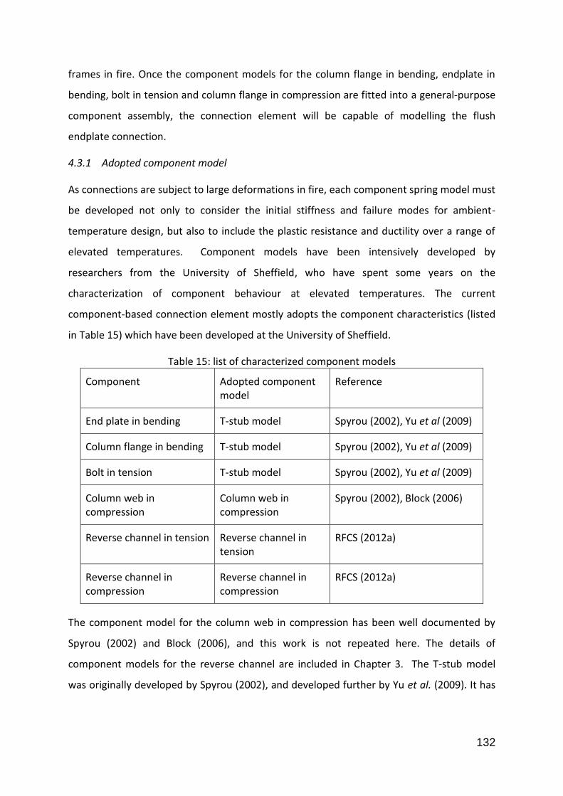
132

frames in fire. Once the component models for the column flange in bending, endplate in

bending, bolt in tension and column flange in compression are fitted into a general-purpose

component assembly, the connection element will be capable of modelling the flush

endplate connection.

4.3.1 Adopted component model

As connections are subject to large deformations in fire, each component spring model must

be developed not only to consider the initial stiffness and failure modes for ambient-

temperature design, but also to include the plastic resistance and ductility over a range of

elevated temperatures. Component models have been intensively developed by

researchers from the University of Sheffield, who have spent some years on the

characterization of component behaviour at elevated temperatures. The current

component-based connection element mostly adopts the component characteristics (listed

in Table 15) which have been developed at the University of Sheffield.

Table 15: list of characterized component models

Component Adopted component model

Reference

End plate in bending T-stub model Spyrou (2002), Yu et al (2009)

Column flange in bending T-stub model Spyrou (2002), Yu et al (2009)

Bolt in tension T-stub model Spyrou (2002), Yu et al (2009)



Spyrou (2002), Block (2006)

Reverse channel in tension Reverse channel in tension

RFCS (2012a)



RFCS (2012a)

The component model for the column web in compression has been well documented by

Spyrou (2002) and Block (2006), and this work is not repeated here. The details of

component models for the reverse channel are included in Chapter 3. The T-stub model

was originally developed by Spyrou (2002), and developed further by Yu et al. (2009). It has

133

been validated against a series of component tests. In order to fit into the component

assembly, these T-stub models were combined.

4.3.1.1 Previous development of the T-stub model

In the endplate connection’s tension zone, the three tension components (bolt in tension,

endplate in bending and column flange in bending) are equivalent to the two T-stubs (shown

in Figure 146), connected by bolts.

The behaviour of the T-stub has been widely investigated over the past thirty years, both

experimentally and theoretically, even if most of this research has been for relatively small

deflections. Coelho (2004) summarised the earlier works by Zoetemeijer (1974), Packer et

al.(1977), Yee et al. (1986), Jaspart (1991), Bursi et al. (1997), Faella et al. (1998), Gebbeken

et al. (1999), Swanson et al. (2000) and Piluso et al.(2001). These works have been

selectively included in EC3 Part 1.8 (CEN, 2005b). In particular, the development by

Zoetemeijer includes the basic principles of the component methods. It is the most

important among these developments and is even now broadly applied throughout Europe.

Figure 146: Equivalent T-stub (one bolt row)

Zoetemeijer (1974) derived his T-stub model based on the yield-line principle; this can be

used to assess the ultimate plastic resistance of the T-stub. It assumed that the plastic

deformation is large enough to allow the adoption of the most favourable static equilibrium

condition. The three classic failure mechanisms considered are illustrated in Table 16. For

134

each collapse mechanism, the resistance can be calculated from the equilibrium in the

plastic condition, taking into account any prying force which exists. The resistance of the T-

stub is the smallest of those from these collapse mechanisms. Zoetemeijer also successfully

introduced the concept of effective length (of the T-stub in the dimension perpendicular to

the plane of the “T”) for design purposes. The effective length is the equivalent length of the

flange plate which contributes to load transmission; it does not have to be the physical

length of the plate, or the inter-bolt-row spacing.

Table 16: Failure modes for the T-stub (Spyrou, 2002)

Failure mode 1:

First plastic hinge forms in the T-stub flange

Bolt yielding

Bolt fracture

Failure mode 2:

First plastic hinge forms in the T-stub flange

Second plastic hinge forms in the T-stub flange

Bolt yielding

Bolt fracture

Failure mode 3:

Bolt yielding

Bolt fracture

135

4.3.1.2 The development of the T-stub model at the University of Sheffield

Two component models have been verified against tests, and can be used to represent the

tension component behaviour at elevated temperatures.

Spyrou (2002) tested a large number of bolted T-stub assemblies at elevated temperatures,

and their force-displacement characteristics were measured. Spyrou developed a simplified

analytical model on the basis of classic beam theory, corresponding to the three possible

collapse mechanisms (Table 16). In Block’s (2006) connection element, Spyrou’s

formulations were used to simulate separately the endplate in tension and the column

flange in tension. The T-stub’s effective length was defined as shown in ‘Joints in Steel

Construction: Moment connections’ (SCI, 1997).

Spyrou’s derivation included two identical T-stubs with four bolts. The model gives

acceptable results, and is straightforward to use for the prediction of the tension zone

behaviour at elevated temperatures. However, in Spyrou’s model the prediction of the

formation of the second plastic hinge is slightly conservative, because the location of the

second plastic hinge is considered to be at the bolt centre line. In reality, the T-stubs can be

held together by sufficiently stiff bolts, and can only form a hinge at the edge of the bolt

head or nut. On the other hand, in the case of one sufficiently thick T-stub flange, working

with a relatively small bolt, the bolt can also rotate due to the very stiff and strong T-stub

flange. Therefore, the second plastic hinge’s location is dependent upon the relative

strengths of the plate and bolt.

Yu (2009a) developed a yield-line model in accordance with the plastic work principle

(Figure 19).

boltPHPH WWWF 21 (4.19)

In the above equation, the work ( ) done by the applied force F is equal to the sum of the

rotational plastic work of the two plastic hinges plus the tensile work in distortion of the

bolts. In Yu’s model, three-phase elastic-plastic material models are assumed for both the T-

stub flange and the bolt. The bolt reaches necking after it has reached its ultimate strength.

The model considers material and geometric nonlinearities (Error! Reference source not

found.), which enable the component failure to be precisely captured. The validations

against both finite element models and tests at ambient and elevated temperatures have

F

136

shown that this model represents the behaviour of T-stubs very well. Yu’s model is also easy

to implement within the component assembly for endplate connections.

4.3.1.3 Revised component model for T-stub

This section will focus on how the tension component T-stub is characterised and built into

the assembly. The general assembly (Error! Reference source not found.) considers the

three tension components in a row to be working in series, and consequently the same

force is present in all the components in a bolt row. The active tension components in the

endplate connection are the column flange in bending, the bolt in tension and the endplate

in bending, which are represented by the T-stub model (discussed in 4.3.1.2). However, due

to prying action, the force in the bolt can differ from that which it applies to either of the

two flanges. In order to implement the T-stub model in the general component assembly

(Figure 103), the bolt in tension is included in the weaker side of two T-stubs (that with

lower maximum resistance). Figure 147 shows typical force/displacement curves for both

the T-stub flanges and whole T-stub. The plotted force is the applied force, and the

displacements for the column flange and the pair of T-stub flanges are (δ-δb) and δ

respectively (as illustrated in Figure 19). Therefore, the effective F/D curve for each tension

bolt row (Figure 148) consists of the sum of the deflections from an effective F/D curve for

the weaker side of the whole T-stub and an effective F/D curve from its stronger side.

Figure 147: Force/displacement curves plotted by the T-stub model

Displacement

Fo

rce

F/D curve for T-stub flange

F/D curve for the

whole T-stub

137

Figure 148: Effective tension bolt row F/D curve in an endplate connection

In order to efficiently model component behaviour and capture the failure, the component-

based connection element adopted to represent the T-stub is a combination of Spyrou’s and

Yu’s component models. Yu’s yield line model is used to compute the Force/Displacement

curve and to capture the failure point. As it is time consuming to consider such a detailed

F/D characteristic in each component within the connection element, the F/D curve (shown

in Figure 149) has been simplified and divided uniformly to be represented by just 5 points

(nodes 1 to 5) connected by straight lines. As the initial stiffness is a basic element of the

component-based connection element’s prediction, this is calculated on the basis of

Spyrou’s T-stub model. Figure 150 shows that Node 2 is relocated at the intersection

between the line representing the initial stiffness and the extended Line 2. A typical

simplified curve is shown in Figure 151.

Figure 149: Simplification of component model F/D, curve (a)

Displacement

Fo

rce

Ef fective F/D

curve for the

whole T-stub

Displacement

Fo

rce

Ef fective F/D

curve for the T-

stub f lange

Stronger side Weaker side

+= Tension bolt row’s

effective F/D curveF

orc

e

Node 1

Node 3

Displacement

Node 4Node 5

Node 2

Line 1

Line 2

Line 3Line 4

138

Figure 150: Simplification of component model F/D, curve (b)

Figure 151: Simplification of component model F/D, curve (c)

The geometry of a T-stub is shown in Figure 152.

The initial bolt stiffness (Kb) is given by:

b

sbb

L

AEK (4.20)

Where Lb is the effective bolt length, Eb is the Young’s modulus of the bolt, and As is the bolt

shank area.

Node 1

Node 3

Displacement

Fo

rce

Movement of Node 2

Node 4Node 5

Initial stif fness

Extended Line 2

Node 1

Node 3

Displacement

Fo

rce

Node 2

Node 4Node 5

139

Figure 152: T-stub geometry

The whole T-stub deformation (δ) is:

(4.21)

Where is the T-stub flange deformation and is the bolt deformation. The ratio of bolt

force (Fbolt) to the total T-stub force (F) is developed by Spyrou (2002) and given by:

3848

2

2246

1

1216

1

3223

32

DhnlnmnDhn

EIK

nnL

EI

F

F

e

b

e

bolt (4.22)

Where E is the T-stub Young’s modulus; , is the effective width of the T-

stub flange and tf is the T-stub flange thickness. F is the tension force applied to the T-stub,

and Fbolt is the bolt tension force.

The initial stiffness of the T-stub (Spyrou,2002) is

24462448

122333nDhLmmL

EIEI

LK

eee (4.23)

The initial stiffness of the T-stub flange (Spyrou,2002) is

b

f

KK

K

1

1 (4.24)

0.8r

n

Dh

m

F

L e

F bolt F bolt

b

f

140

4.3.2 Comparison with flush endplate joint tests

The connection element was validated (Table 17) against the flush endplate joint tests,

which were conducted by Yu in the collaborative EPSRC project (EP/C5109841/1) conducted

by the Universities of Sheffield and Manchester. This project investigated the robustness of

connections in fire conditions (Yu et al., 2008a, 2008b, 2009a, 2009b, 2009c, 2009d and

2011; Hu et al., 2009, Dai et al., 2009a, 2009b, 2010a and 2010b). Yu’s connection tests

focused on high-temperature structural behaviour of components and assemblies under

combined tying and shearing forces. A large number of connections (shown in Figure 153

and Figure 154) were tested to destruction under inclined forces, at temperatures up to

650°C. The tested connections cover four typical beam-column connection types, including

the flush endplate connection (listed in Table 17).

Figure 153: Joint test setup by Yu (2011)

Load jack

Reaction frame

Electrical furnace

Macalloy bars

Tested

connection

Reaction frame

Support beam

α

Furnace bar

Link bar

Jack bar

141

Figure 154: Joint test side view by Yu (2011)

Table 17: Selected list of isolated flush endplate joint tests

Test ID

Endplate

thickness

(mm)

Initial

angle

Number of

bolt rows

Temperature

(°C)

EP_20_35_04-02-08_8mm 8 35 3 20

EP_20_35_05-02-08 20 35 3 20

EP_20_55_28-02-08 20 55 3 20

EP_450_35_23-11-07 20 35 3 450

EP_450_45_23-10-07 20 45 3 450

EP_450_55_19-02-08 20 55 3 450

EP_550_35_11-12-07_8mm 8 35 3 550

EP_550_35_17-12-07_15mm 15 35 3 550

EP_550_35_27-11-07 20 35 3 550

EP_550_45_16-10-07 20 45 3 550

EP_550_55_13-02-08 20 55 3 550

EP_650_35_30-11-07 20 35 3 650

EP_650_45_19-10-07 20 45 3 650

EP_650_55_15-02-08 20 55 3 650

4.3.2.1 Material properties

The material properties of the endplate connection tests at ambient and elevated

temperatures were summarized by Yu et al. (2011), and are listed in Table 18.

142

Table 18: Simplified material properties for endplate tests

Temperature (°C) 20 450 550 650

Column

and

beam

Yield stress (N/mm2) 357 176 106 63

Ultimate stress (N/mm2) 568 300 211 105

Young’s modulus (N/mm2) 176000 82900 63050 32450

Second modulus (N/mm2) 1062 532 398 137

Endplate Yield stress (N/mm2) 293 145 87 52




Bolt Yield stress (N/mm2) 677 341 135 49




4.3.2.2 Model setup

Figure 155 shows how the tests were set up, and the form in which they were modelled in

Vulcan. The bars (heavy black lines between hinges) were assumed to be rigid.

Figure 155: Model setup

4.3.2.3 Results

Comparison between the component-based connection element and tests (furnace-bar

force versus the connection rotation) are presented in Figure 156 to Figure 169. In general,

the connection element is in satisfactory agreement with the test results, especially if its

simplicity compared with comparable Finite Element models is recalled. The prediction of

?

Furnace bar Link bar

Jack bar

Force

143

initial stiffness given by the element matches that from the tests. More importantly, in the

context of robustness analysis, the element also captures the maximum resistance

conditions well enough, and in most cases conservatively. The modelling results have been

plotted until one component is predicted to fracture, so that the curves show the peak

capacities; the experimental curves show the full extent of each test. In some tests failure

occurred; others were stopped in order to protect the furnace from damage.

Figure 156: EP_20_35_04-02-08_8mm

Figure 157: EP_20_35_05-02-08

Figure 158:EP_20_55_28-02-08

Figure 159: EP_450_35_23-11-07

Figure 160: EP_450_45_23-10-07

Figure 161: EP_450_55_19-02-08

0

50

100

150

200

250

300

350

400

0 1 2 3 4 5 6 7 8 9 10

Fo

rce in

oven b

ar

(kN

)

Connection roation( )

Test

Connection element

0

50

100

150

200

250

300

350

400

0 1 2 3 4 5 6 7 8 9 10

Fo

rce in

oven b

ar

(kN

)

Rotation (°)

Connection element

Test

0

50

100

150

200

250

300

350

400

0 1 2 3 4 5 6 7 8 9 10

Fo

rce in

oven b

ar

(kN

)

Rotation (°)

Connection element

Test

0

50

100

150

200

250

0 1 2 3 4 5 6 7 8 9

Fo

rce in

oven b

ar

(kN

)

Rotation (°)

Connection element

Test

0

50

100

150

200

250

0 1 2 3 4 5 6 7 8 9

Fo

rce in

oven b

ar

(kN

)

Rotation (°)

Test

Connection element

0

50

100

150

200

250

0 1 2 3 4 5 6 7 8 9

Fo

rce in

oven b

ar

(kN

)

Rotation (°)

Connection element

Test

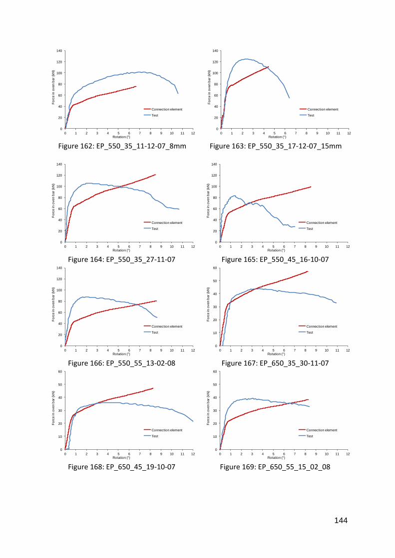
144

Figure 162: EP_550_35_11-12-07_8mm

Figure 163: EP_550_35_17-12-07_15mm

Figure 164: EP_550_35_27-11-07

Figure 165: EP_550_45_16-10-07

Figure 166: EP_550_55_13-02-08

Figure 167: EP_650_35_30-11-07

Figure 168: EP_650_45_19-10-07

Figure 169: EP_650_55_15_02_08

0

20

40

60

80

100

120

140

0 1 2 3 4 5 6 7 8 9 10 11 12

Fo

rce in

oven b

ar

(kN

)

Rotation (°)

Connection element

Test

0

20

40

60

80

100

120

140

0 1 2 3 4 5 6 7 8 9 10 11 12

Fo

rce in

oven b

ar

(kN

)

Rotation (°)

Connection element

Test

0

20

40

60

80

100

120

140

0 1 2 3 4 5 6 7 8 9 10 11 12

Fo

rce in

oven b

ar

(kN

)

Rotation (°)

Connection element

Test

0

20

40

60

80

100

120

140

0 1 2 3 4 5 6 7 8 9 10 11 12

Fo

rce in

oven b

ar

(kN

)

Rotation (°)

Connection element

Test

0

20

40

60

80

100

120

140

0 1 2 3 4 5 6 7 8 9 10 11 12

Fo

rce in

oven b

ar

(kN

)

Rotation (°)

Connection element

Test

0

10

20

30

40

50

60

0 1 2 3 4 5 6 7 8 9 10 11 12

Fo

rce in

oven b

ar

(kN

)

Rotation (°)

Connection element

Test

0

10

20

30

40

50

60

0 1 2 3 4 5 6 7 8 9 10 11 12

Fo

rce in

oven b

ar

(kN

)

Rotation (°)

Connection element

Test

0

10

20

30

40

50

60

0 1 2 3 4 5 6 7 8 9 10 11 12

Fo

rce in

oven b

ar

(kN

)

Rotation (°)

Connection element

Test

145

4.4 Development of the connection element for reverse channel connection

The component characterizations reported previously in Chapter 3 have been built-into

Vulcan, and are accessible to the general-purpose element model. The component model

for reverse channel connections was developed in the COMPFIRE project, and this enabled

20 tests under axial force and moment to be carried out and compared with analysis. It is

therefore possible to validate the connection element for reverse channel connections

against the joint tests conducted in the COMPFIRE project.

4.4.1 Comparison with reverse channel joint tests

As part of COMPFIRE, the University of Sheffield performed 20 constant-temperature tests

on isolated joints to Concrete-Filled-Tube (CFT) and Partially-Encased (PE) H-section columns

under different combinations of axial and shear forces and moments. These isolated joint

tests provided valuable experimental data to identify the behaviour of the composite joint

and validate the component-based element under conditions which combine a number of

bolt rows, working together in the context of a fairly general form of joint distortion, in

contrast to the isolated bolt-row tests carried out at Manchester and Coimbra. Table 19

shows the list of 14 of the Sheffield joint tests which have been used in the following

validation.

The test setup was similar to the flush endplate tests (shown schematically in Figure 155).

Selected test photos are shown from Figure 170 to Figure 174. The geometry of the

individual test specimens is well documented in RFCS (2009) and is therefore not repeated

here.

146

Table 19: Isolated joint tests performed at Sheffield within COMPFIRE.

No ID Column Temp Connection type

1 CCFT-RC200_550_55_10-01-2011 CFT 550 RC cut from SHS 200X6

2 SCFT-RC200_550_55_04-01-2011 CFT 550 RC cut from SHS 200X6

3 CCFT-RC250_550_55_1-10-2010 CFT 550 RC cut from SHS 250X8

4 SCFT-RC250_550_55_15-09-2010 CFT 550 RCcut from SHS 250X8

5 CCFT-UKPFC230_550_55_06-08-2010 CFT 550 UKPFC230x90x32

6 SCFT-UKPFC230_550_55_02-07-2010 CFT 550 UKPFC230x90x32







13 PE-UKPFC150_550_55_13-01-2011 P/E* 550 UKPFC150x75x18

14 PE-UKPFC150_650_55_19-01-2011 P/E* 650 UKPFC150x75x18

*Partially-encased H-section column

Figure 170: CCFT-RC200_550_55_10-01-2011 side view after test

147

Figure 171: CCFT-RC200_550_55_10-01-2011 top view after test

Figure 172: SCFT-RC200_550_55_04-01-2011 side view after test

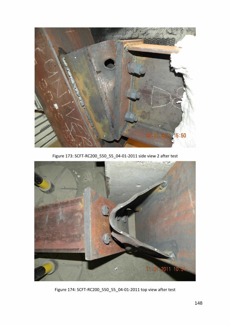
148

Figure 173: SCFT-RC200_550_55_04-01-2011 side view 2 after test

Figure 174: SCFT-RC200_550_55_04-01-2011 top view after test

149

4.4.1.1 Material properties

The component characterizations used within the component-based connection element

use three-stage elastic-plastic material properties at ambient temperature, defined by the

“yield” and “ultimate” strength points. After the ultimate strength point is reached, the

stress values are assumed to stay constant, and the strain is allowed to increase without

limit from this point.

The bolt material properties are the same as those in the endplate joint tests (shown in

Table 18). The steel material properties (Table 20) at ambient temperature use the average

values from the coupon test results. The temperature-dependent yield strength and elastic

modulus reduction factors given in EC3 part 1-2 are employed to partially define the

material properties at elevated temperatures. The ultimate strength is assumed to be

reached at a strain of 0.04 at both ambient and elevated temperatures. In order to calculate

the ultimate strength at elevated temperature (above 400°C), the tangent modulus is

assumed to be100N/mm2 at all temperatures.

150

Table 20: Material properties for isolated reverse channel joint tests. Test ID Yield stress

(N/mm2) Ultimate

stress (N/mm2)

Young’s modulus (N/mm2)

Tangent modulus (N/mm2)

Temp. (°C )

Reverse channel

1 CCFT-RC200_550

247 251 125557 100 550

2 SCFT-RC200_550

245 249 125612 100 550

3 CCFT-RC250_550

247 251 125557 100 550

4 SCFT-RC250_550

245 249 125612 100 550 5 CCFT-UKPFC230_550

225 228 84964 100 550

6 SCFT- UKPFC230_550

225 229 108401 100 550 7 CCFT-UKPFC230_20

365 543 114333 4691 20

8 SCFT- UKPFC230_20

368 546 189685 4674 20 9 CCFT-UKPFC200_550

186 190 98448 100 550


186 190 98448 100 550

11 CCFT-UKPFC180_550

183 187 126501 100 550


174 178 98339 100 550

Endplate 1 CCFT-RC200_550

269 273 97659 100 550 2 SCFT-RC200_550

269 273 97659 100 550

3 CCFT-RC250_550

269 273 97659 100 550

4 SCFT-RC250_550

269 273 97659 100 550

5 CCFT-UKPFC230_550

269 273 97659 100 550 6 SCFT- UKPFC230_550

269 273 97659 100 550

7 CCFT-UKPFC230_20

430 617 214635 4905 20

8 SCFT- UKPFC230_20

430 617 214635 4905 20

9 CCFT-UKPFC200_550

269 273 97659 100 550 10 SCFT- UKPFC200_550

269 273 97659 100 550

11 CCFT-UKPFC180_550

269 273 97659 100 550


269 273 97659 100 550

Beam 1 CCFT-RC200_550

359 512 234268 4041 550 2 SCFT-RC200_550

359 512 234268 4041 550

3 CCFT-RC250_550

359 512 234268 4041 550

4 SCFT-RC250_550

359 512 234268 4041 550

5 CCFT-UKPFC230_550

359 512 234268 4041 550


359 512 234268 4041 550 7 CCFT-UKPFC230_20

359 512 234268 4041 20

8 SCFT- UKPFC230_20

359 512 234268 4041 20

9 CCFT-UKPFC200_550

359 512 234268 4041 550


359 512 234268 4041 550 11 CCFT-UKPFC180_550

359 512 234268 4041 550


359 512 234268 4041 550

4.4.1.2 Results

The plots of the furnace-bar force against connection rotation for Tests 1 to 10 are shown in

Error! Reference source not found. to Error! Reference source not found..

Table 21 shows the failure mode in each case. Both the adopted AISC limit and the current

bolt pull-out model limit are seen to be safe for design purposes. The connection element

151

using the CIDECT limit reasonably predicts the maximum resistance against the test results.

It also successfully predicts the failure mode, except in Tests 9 and 10. However, since the

predicted maximum resistance is close to that in the test, the prediction of failure mode can

be sensitive to various factors, such as material properties and test specimen dimensions.

The validation summary plot (Figure 185) also shows that the connection element with the

bolt pull-out model is capable of modelling the reverse channel connection failure capacities

for design purposes.

Table 21: Failure modes in the validations against joint tests. No Name Test Failure mode Connection element prediction

Pull-out model

AISC CIDECT

1 CCFT-RC200_550_55_10-01-2011 No failure (Technical limitation)

Pull-out Pull-out Tensile fracture

2 SCFT-RC200_550_55_04-01-2011 Pull-out Pull-out Pull-out Pull-out 3 CCFT-RC250_550_55_1-10-2010 No failure (Technical

limitation) Tensile fracture

Pull-out Tensile fracture

4 SCFT-RC250_550_55_15-09-2010 Tensile fracture Tensile fracture

Pull-out Tensile fracture

5 CCFT-UKPFC230_550_55_06-08-2010 Tensile fracture Pull-out Pull-out Tensile fracture

6 SCFT-UKPFC230_550_55_02-07-2010 Tensile fracture Pull-out Pull-out Tensile fracture

7 CCFT-UKPFC230_20_55_03-03-2011 Technical limitation Pull-out Pull-out Pull-out 8 SCFT-UKPFC230_20_55_24-01-2011 Pull-out Pull-out Pull-out Pull-out

9 CCFT-UKPFC200_550_55_17-09-2010 Tensile fracture Pull-out Pull-out Pull-out

10 SCFT-UKPFC200_550_55_08-07-2010 Tensile fracture Pull-out Pull-out Pull-out

Figure 175: CCFT-RC200_550_55_10-01-

2011.

Figure 176: SCFT-RC200_550_55_04-01-

2011.

0

20

40

60

80

100

120

140

160

180

0 5 10 15 20 25

Fo

rce

(kN

)

Rotation ( )

Test

Connection element

0

20

40

60

80

100

120

140

160

180

0 5 10 15 20 25

Fo

rce

(kN

)

Rotation ( )

Test

Connection element

152

Figure 177: 3. CCFT-RC250_550_55_1-10-

2010.

Figure 178: 4. SCFT-RC250_550_55_15-09-

2010.

Figure 179: 5. CCFT-UKPFC230_550_55_06-08-

2010.

Figure 180: 6. SCFT-UKPFC230_550_55_02-07-

2010.

Figure 181: 7. CCFT-UKPFC230_20_55_03-

03-2011.

Figure 182: 8. SCFT-UKPFC230_20_55_24-

01-2011.

Figure 183: 9 .CCFT-UKPFC200_550_55_17-

09-2010.

Figure 184: 10. SCFT-UKPFC200_550_55_08-

07-2010.

0

20

40

60

80

100

120

140

160

180

0 5 10 15 20 25

Fo

rce

(kN

)

Rotation ( )

Test

Connection element

0

20

40

60

80

100

120

140

160

180

0 5 10 15 20 25

Fo

rce

(kN

)

Rotation ( )

Test

Connection element

0

20

40

60

80

100

120

140

160

180

0 5 10 15 20 25

Fo

rce

(kN

)

Rotation ( )

Test

Connection element

0

20

40

60

80

100

120

140

160

180

0 5 10 15 20 25

Fo

rce

(kN

)

Rotation ( )

Test

Connection element

0

20

40

60

80

100

120

140

160

180

200

220

240

260

280

0 3 6 9 12 15

Fo

rce

(kN

)

Rotation ( )

Test

Connection element

0

20

40

60

80

100

120

140

160

180

200

220

240

260

280

0 3 6 9 12 15

Fo

rce

(kN

)

Rotation ( )

Test

Connection element

0

20

40

60

80

100

120

140

160

180

0 5 10 15 20 25

Fo

rce

(kN

)

Rotation ( )

Test

Connection element

0

20

40

60

80

100

120

140

160

180

0 5 10 15 20 25

Fo

rce

(kN

)

Rotation ( )

Test

Connection element

153

Figure 185: Comparison of predicted failure loads against test results.

4.5 Conclusion

The component-based connection element has been developed. The approach is consistent

with EC3 Part 1-8, in which the connection is divided into several effective lateral non-linear

springs, which are assembled with rigid links to represent the semi-rigid connection. The

reduced material properties at elevated temperature are also taken into account. The

proposed connection element has been implemented within Vulcan to model joints at

elevated/cooling temperatures. Validation against experimental results at ambient and

elevated temperature has been carried out. The connection element has shown that it can

model with adequate accuracy the nonlinear temperature-dependent response of two

connection types (endplate and reverse channel connection) under generalised loading

conditions, including unloading (deflection reversal) whenever this occurs. For the reverse

channel connection, the predictions of the component model, including the simple sub-

model representing bolt pull-out, are close to the test results, and can be used for practical

design analysis. Due to the simplification of component model, the force/rotation curves do

not match as perfectly as general detailed finite element modelling, and there may be scope

for improvements particularly to the pull-out model. Some factors, such as the precise

locations of plastic hinges, are at present too complicated for the component model to take

into account accurately, and some further development may be able to optimize these.

0

50

100

150

200

250

300

0 100 200 300

Co

nnectio

n e

lem

ent

(kN

)

Test (kN)

154

However, as an intermediate method at the present time, the component-based connection

element balances reasonable accuracy with great advantages in computing and setup time

costs. It allows engineers to model the connection in fire efficiently without losing too much

accuracy.

155

Chapter 5. Application of the component-based element to COMPFIRE connections

This chapter concerns the use of the general-purpose component-based connection

element in the analysis of steel-framed buildings in fire. It is firstly applied in the modelling

of a subframe test conducted at Manchester as part of the COMPFIRE project. A 2D model

will be used to show how, when used in combination with the static-dynamic solver, the

connection element is capable of modelling the progressive failure of connections in a plane

multi-storey frame. The results show how the behaviour of steel joints in fire conditions can

be modelled using component-based joint models.

5.1 Small-scale fire test

Within the scope of the COMPFIRE project, researchers at the University of Manchester

completed four fire tests (RFCS, 2012). These were intended to investigate the complex

behaviour of reverse channel connections within simple structural frameworks under

different fire scenarios, including their behaviour during the cooling phase. The tests were

designed to investigate the effects of both rotational and axial restraint on the rotations and

thermal expansions and contractions of the beam, including local yielding and buckling, and

overall catenary action. Comparing the results from modelling against the subframe test

results shows that the component-based connection element is capable of modelling the

whole range of joint behaviour.

The Manchester experimental layout is shown Figure 186. Two hydraulic jacks, manually

pumped, were used with the objective of applying equal constant vertical forces to the

beam. The target was to maintain a 40kN load at each jack; this was generally achieved, as

shown in Figure 187. The reaction forces were measured by load cells installed at the bases

of the columns. A total of 34 thermocouples (shown in Figure 188) were used to monitor the

temperature development during and after the tests.

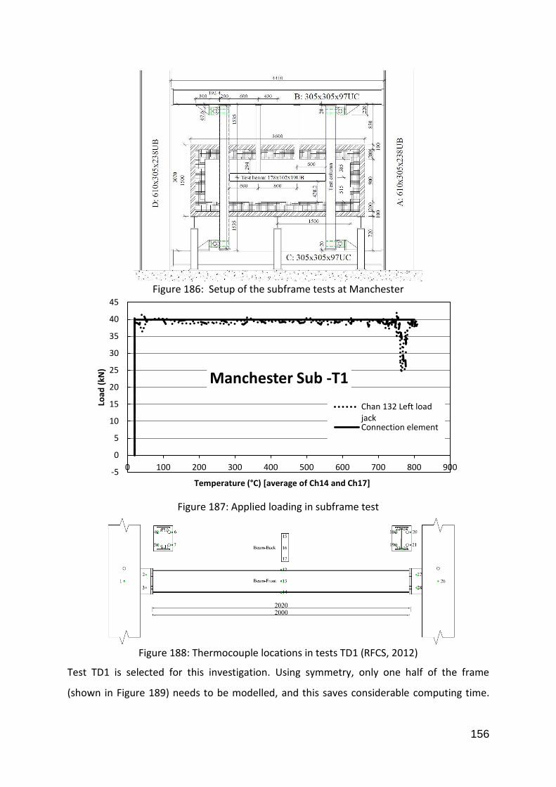
156

Figure 186: Setup of the subframe tests at Manchester

Figure 187: Applied loading in subframe test

Figure 188: Thermocouple locations in tests TD1 (RFCS, 2012)

Test TD1 is selected for this investigation. Using symmetry, only one half of the frame

(shown in Figure 189) needs to be modelled, and this saves considerable computing time.

-5

0

5

10

15

20

25

30

35

40

45

0 100 200 300 400 500 600 700 800 900

Load

(kN

)

Temperature (°C) [average of Ch14 and Ch17]

Manchester Sub -T1

Chan 132 Left loadjackConnection element

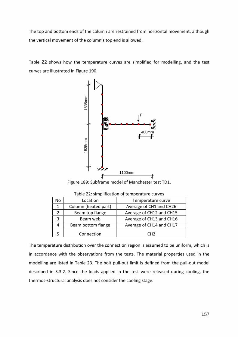
157

The top and bottom ends of the column are restrained from horizontal movement, although

the vertical movement of the column’s top end is allowed.

Table 22 shows how the temperature curves are simplified for modelling, and the test

curves are illustrated in Figure 190.

Figure 189: Subframe model of Manchester test TD1.

Table 22: simplification of temperature curves

No Location Temperature curve

1 Column (heated part) Average of CH1 and CH26

2 Beam top flange Average of CH12 and CH15

3 Beam web Average of CH13 and CH16

4 Beam bottom flange Average of CH14 and CH17

5 Connection CH2

The temperature distribution over the connection region is assumed to be uniform, which is

in accordance with the observations from the tests. The material properties used in the

modelling are listed in Table 23. The bolt pull-out limit is defined from the pull-out model

described in 3.3.2. Since the loads applied in the test were released during cooling, the

thermos-structural analysis does not consider the cooling stage.

1535m

m1535m

m

1100mm

400mm

F

158

Figure 190: TD1 temperatures

Table 23: Material properties

End plate & beam Bolt Tube section

Yield stress (N/mm2)) 293 677 357

Ultimate stress (N/mm2) 492 998 568

Young’s modulus (N/mm2 149000 210000 176000

Tangent modulus (N/mm2) 1002 1629 1062

Figure 191 shows the beam mid-span deflection-temperature curve; the temperature

shown is the average test value in the beam’s bottom flange (average of Channels 14 and

17, shown in Figure 188).

0

100

200

300

400

500

600

700

800

900

1000

0 20 40 60 80 100 120 140 160

Tem

pera

utr

e (

ºC)

Time (Min)

TD1-Temperatures

Beam top flange

Beam web

Beam bottom flange

Column

Connection

159

Figure 191: TD1 beam mid-span deflection.

The deflection of the beam predicted by Vulcan modelling including the connection element

initially lies close to the test result. Above 700°C, this deflection begins to rise sharply. At

745°C, both of the tension bolt rows failed, due to reaching the bolt pull-out limit (170kN)

defined by the pull-out model. The maximum deflection is 220 mm at 745°C. If the bolt pull-

out limit is that defined by CIDECT (Jaspart, 2005) it fails at the same temperature, but due

to bolt fracture, given a maximum bolt tensile resistance of 190kN. The failure type actually

identified in the test was bolt thread-stripping, which is one of the ways in which bolts can

fail in tension.

Figure 192 presents the connection axial force-temperature results; again the temperature

shown is the average test value in the beam bottom flange. The axial force shown for the

test results is the sum of the reaction forces recorded by the load cells. The left-hand load

cells are Channels 128 and 129, and the right-hand load cells are Channels 130 and 131.

Figure 192 shows that the beam’s axial compression force initially increases, due to the

restraint provided by the connections and columns to thermal expansion of the beam, but

gradually reduces and changes to tension as the beam’s deflection increases sharply and

enters the catenary stage. The axial force given by the modelling is generally slightly higher

than the test results.

-500

-450

-400

-350

-300

-250

-200

-150

-100

-50

0

0 100 200 300 400 500 600 700 800 900

Be

am m

id-d

efl

ect

ion

(m

m)

[ch

13

6]

temperature (°C)[average of ch14 and ch17]

Manchester Sub -T1

Test

Connection element

160

Figure 192: Connection axial force-temperature relationships

5.2 Dynamic modelling of failure process in connection

As described above, the connection element has been implemented within the Vulcan

research code with the static-dynamic solver. The progressive failure of a connection can

therefore be simulated. In order to demonstrate the capacity of the procedure, a

progressive collapse analysis of a 2-D structural frame is carried out in the following section.

The geometry of the 3-span composite 2D subframe can be seen in Figure 193. The beam

span (L) is 6 metres, and the floor height is 3.5 metres. It is assumed that the fire happens in

the middle bay. The temperatures of the heated connections are assumed to be the same,

and identical to that of the beam, and the temperatures of the heated columns are each

half of that of the heated beam. The beam size is 305x165x40UB. The column is

SHS400x400x16 concrete-filled with C30 concrete. The uniform line load on the beam is

27.8 kN/m. The effect of upper floors is represented by an axial compression force of

8000kN per column. The connections used are reverse channel connections, one of which is

shown in Figure 194. The reverse channel is a cutting from a 250x10 tube, cut with a 90 mm

leg length. The M20 bolts used are Grade 8.8. The leg length of the fillet welds is 8mm. The

structural steel generally used is S355, except for the endplates which are S275. Because of

the symmetry of the model, only half of the structure needs to be modelled.

-80

-60

-40

-20

0

20

40

60

80

0 100 200 300 400 500 600 700 800 900

Co

nn

ect

ion

axi

al f

orc

e (

kN)

temperature (°C)[average of ch14+ch17]

Manchester Sub -T1

128+129 Axial force on the left

130+131 Axial force on the right

Connection element

161

Figure 193: Subframe in parametric study.

Figure 194: Reverse channel connection used in the parametric study.

Figure 195 shows the axial forces, generated by the Vulcan analysis, in the different

component spring rows within the heated connections against the connection

temperatures. The heated connections fracture at 710°C.

L L L

H

H

F F F F

0.5 T

1.0T

0.5 T

200

60

90 55 55

15

90

75


2n tension bolt row



Bottom compression spring rowpresspringrow

162

Figure 195: Axial forces of spring rows against connection temperature

Figure 196 plots the heated connections’ component axial (normal) forces against their

equal beam end rotations. It can be seen that the sequence of fracture of the tension bolt

rows starts from the top tension bolt row and ends with the bottom row.

Figure 196: Axial forces of spring rows against beam end rotation

These three tension bolt rows fracture when the beam end rotation reaches 18.61, 19.41

and 24. After all the bolt rows have fractured, the beam is completely detached from the

columns.

Figure 197 plots the beam rotation against the heated connection’s temperature. The

analysis continues until buckling of the column occurs at a higher temperature.

-150

-100

-50

0

50

100

0 200 400 600

Axi

al f

orc

e (

kN)

Temperature (OC)

1st tension boltrow

2nd tension boltrow

3rd tension boltrow

top compressionrow

bottomcompression row

-150

-100

-50

0

50

100

0 5 10 15 20 25

Axi

al f

orc

e (

kN)

Rotation at beam end (deg)

bottom compression row




top compression row

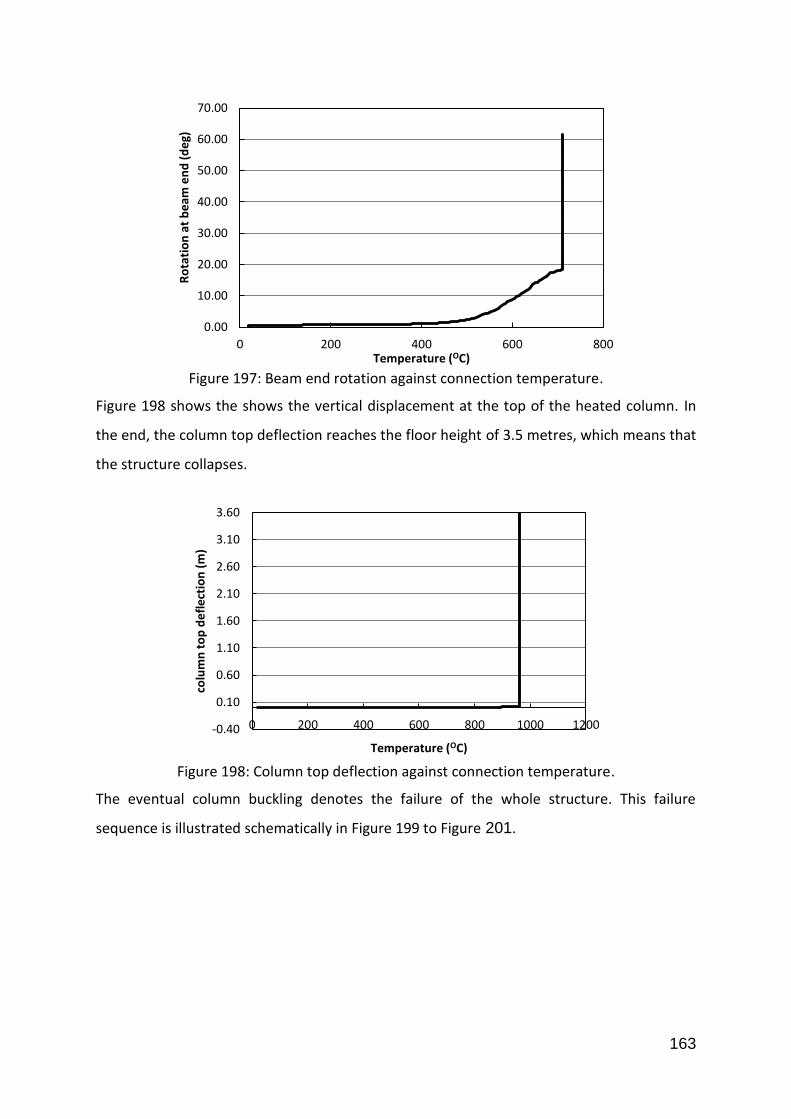
163

Figure 197: Beam end rotation against connection temperature.

Figure 198 shows the shows the vertical displacement at the top of the heated column. In

the end, the column top deflection reaches the floor height of 3.5 metres, which means that

the structure collapses.

Figure 198: Column top deflection against connection temperature.

The eventual column buckling denotes the failure of the whole structure. This failure

sequence is illustrated schematically in Figure 199 to Figure 201.

0.00

10.00

20.00

30.00

40.00

50.00

60.00

70.00

0 200 400 600 800

Ro

tati

on

at

be

am e

nd

(d

eg)

Temperature (OC)

-0.40

0.10

0.60

1.10

1.60

2.10

2.60

3.10

3.60

0 200 400 600 800 1000 1200

colu

mn

to

p d

efl

ect

ion

(m

)

Temperature (OC)

164

Figure 199: Heated structure – initial stage.

Figure 200: Connection fractured (710°C).

165

Figure 201: Column buckling at 960°C .

This modelling has demonstrated that analysis with a combination of the component-based

connection element with the static-dynamic solver is capable of simulating the progressive

fracture of spring rows within connections as temperatures rise. It also shows the structural

behaviour beyond connection fracture until final structural collapse occurs.

166

Chapter 6. Discussion, Conclusion and Further Recommendations

6.1 Summary

The traditional idealizations of joints in steel frames, as either ‘pinned’ or ‘rigid’, were for

many years assumed to describe their actual behaviour in fire. It was only after observations

from the Cardington fire test series, followed by very prominent fire-induced events such as

the collapse of three of the World Trade Centre buildings in 2001, which engineers and

researchers realized fully that the connections could be the most vulnerable parts of a

structure when fire happens. Connections can be seen to behave differently in fire and at

ambient temperature. The material properties of steel plate and bolts both degrade with

increasing temperature. However, because of the combination of this weakening with the

partially restrained thermal expansions and contractions, particularly of long-span beams,

the connections can be subjected to large axial forces. Taking into account the large

rotations to which the connections are subjected at high temperatures, the senses of these

axial forces may change during the fire. Therefore, it is necessary for designers to

comprehend how structures can really behave, when deciding how to analyse them with

acceptable accuracy and reasonable efficiency in terms of time and cost.

The component-based method is an intermediate and efficient way of modelling the

behaviour of connections, within the framework of a global finite element analysis which is

computationally efficient compared with detailed FE modelling. This thesis has addressed

the creation of a general-purpose component-based representation of the column-face

“connection” zone, as an element which has two external nodes but can internally contain

any number of rows of components with temperature-dependent properties, including both

force-reversal and failure. The principles of its development are applicable to different

connection types and to implementation in different software packages.

The development began with the creation of a flush endplate connection element, and was

then extended to the reverse channel connection. For both connection types the key

components, which limit the connection capacity or contribute to the joint deformation,

were identified at the start. The component characterization for endplate connections has

generally adopted the models previously developed by Spyrou (2002), Block (2006), and Yu

(2009a). The component models for the reverse channel were developed by the author

167

during the course of the COMPFIRE project. The assembled component-based connection

elements were also validated against the isolated joint tests carried out by Yu in a previous

Sheffield project.

In the course of this work the general-purpose connection element has been implemented

within the software Vulcan, which has been equipped with a static-dynamic solution process

in a parallel project. The coming-together of these two development threads has created a

software tool, albeit still at the level of research code, which should allow engineers to

identify the local failures of the joints, and to predict the subsequent failure sequence of the

remaining structure. Engineers should henceforward be able to identify the vulnerable parts

of a structure in scenario-based analyses, and to modify their designs in order to produce a

building which will perform robustly in different fire cases.

6.2 Recommendations for further work

Due to the limited amount of time available for postgraduate research, this PhD study

cannot cover everything. The advantages of the component-based connection element have

been shown above. The following are issues which follow-on from the work done, which

should be considered in future research work.

6.2.1 Generalization of the component model

Specific component-based models have been applied to various types of connection: web-

cleat, fin plate and flush endplate etc. Although these connections are different, the

application of the component-based element principle is the same. This has been well-

established during this development process, in which the basic assumptions were made in

the context of flush endplate connections and subsequently extended to the reverse

channel. This is an illustration that the connection element can be generalized further, and it

is apparent that all bolted connections have certain common features; “tension”

components (which may act in compression under some circumstances) tend to be chained

in series at the levels of bolt-holes, with additional compression components which never

act in tension, generally located where the top or bottom flange of the beam member

contacts the column face, possibly through an endplate. In order to develop the generalized

component-based connection element, it is necessary for the component assembly to

168

accommodate different component characteristics, and to have the capability to switch

on/off any component or spring rows under certain conditions.

Firstly, the component behaviour needs to be generalized, and then the deflections of the

number of components in each spring row can easily be added. Figure 202 is a sketch

showing the proposed generalized component behaviour, across all four tension and

compression quadrants. The unloading follows the Masing rule (Gerstle, 1988). Each

component has descending (negative-stiffness) parts from both the tension and

compression zones.

Figure 202: Generalized component assumption.

Figure 203 shows the concept of ‘stops’ within a component; there can be limits to the

permissible ranges of both tension and compression. When a limit is reached, the

component can become completely rigid.

Figure 204 illustrates the concept of ‘stops’ for a complete spring row. These can make the

spring row switch on/off according to certain limits, and can cope with both tension and

compression. Therefore, the extra spring rows can be easily built up.

Displacement

Forc

e

F/D curve

Descending partUnloading curve

Tension zone

Compression zone

169

Figure 203: Stops for a component.

Figure 204: Stops for a complete spring row.

6.2.2 Joint zone

EC3 Part 1.8 points out that it is necessary to take into account not only the rotational

deformation of a connection but also the shear deformation of the web panel. EC3 1.8 also

requires classification of both the connection (at the column-face) and joint (the whole

region near a beam-end). A ‘joint’ therefore logically includes the connection plus web shear

panels. Web shear panels may exist within both the column web in the region of the beam

connections, and in the beam web near to the end of the beam.

A 4-noded shear panel element can be proposed to represent the column web behaviour,

whereas the beam web naturally forms a 2-noded shear panel element (Figure 205). The

column-face connection element defined in this thesis is then located between the column

web shear panel and the beam shear panel elements. The column web element connects to

Compression limit reached

Tension limit reached

Compression

Tension

170

the upper and lower beam-column elements representing the continuous column. The

beam web shear panel element is located between the column-face connection element

and the end of the beam element.

Figure 205: Component based joint array.

` 1

uf

u

w

f

F

S

3

4

171

References

Al-Jabri K.S. (1999), “The behaviour of steel and composite beam-to-column connections in fire”, PhD Thesis, University of Sheffield.

Al-Jabri K.S., Davison J.B. and Burgess I.W. (2008), “Performance of Beam-to-Column Joints in Fire-A Review”, Fire Safety Journal, 43 (1), pp. 50-62.

AISC (2005) Steel Construction Manual.American Institute of Steel Construction INC.

Astaneh A. (1989). “Demand and Supply of Ductility in Steel Shear Connections”, Journal of Constructional Steel Research 14, pp.1-19.

Bailey C.G. and Moore D.B. (2000a), “The Structural Behaviour of Steel Frames with Composite Floor Slabs Subjected to Fire: Part1: Theory”, The Structural Engineer, 78(11), pp. 19-27.

Bailey C.G. and Moore D.B. (2000b), “The Structural Behaviour of Steel Frames with Composite Floor Slabs Subjected to Fire: Part 2: Design”, The Structural Engineer, 78(11), pp. 28-33.

Bailey C.G. (2002), “Holistic Behaviour of Concrete Buildings in Fire”, Proceedings of the Institution of Civil Engineers, 152(3), pp.199-212.

Bhatt, P (1999). ‘Structures’. Longman Group United Kingdom.

Block, F.M., Burgess, I.W. and Davison, J.B.(2004a), ‘Numerical and Analytical Studies of Joint Component Behaviour in Fire’, Paper S7-4, Third International Workshop on Structures in Fire, Ottawa, Canada, (May) pp 383-395.

Block, F.M., Davison, J.B., Burgess, I.W. and Plank, R.J. (2004b), 'A Component Approach to Modelling Steelwork Connections in Fire: Behaviour of Column Webs in Compression', Proc. ASCE Structures Congress, Nashville, (May)) ISBN 0-7844-0700-2.

Block, F.M., Davison, J.B., Burgess, I.W. and Plank, R.J.(2005a),'High-Temperature Experiments on Joint Components', 4thEuropean Conference on Steel Structures, Maastricht, Netherlands.

Block, F.M., Davison, J.B., Burgess, I.W. and Plank, R.J.(2005b),'High-Temperature Experiments on Joint Component Behaviour', ICASS '05, Shanghai, China.

Block, F.M. (2006a), 'Development of a Component-Based Finite Element for Steel Beam-to-Column Connections at Elevated Temperatures',PhD thesis, University of Sheffield.

Block, F.M., Burgess, I.W., Davison, J.B.and Plank, R.J. (2006b), 'A Component-Based Approach for Modelling the Effect of Fire on Steel Joints', 19th Australasian Conference on the Mechanics of Structures and Materials, Canterbury, New Zealand.

172

Block, F.M., Davison, J.B., Burgess, I.W. and Plank, R.J. (2007), ‘The Development of a Component-Based Connection Element for Endplate Connections in Fire’, Fire Safety Journal, 42 pp 498–506.

Block, F.M., Davison, J.B., Burgess, I.W. and Plank, R.J.(2013a), ‘Principles of a Component-Based Connection Element for the Analysis of Steel Frames in Fire’, Engineering Structures, 49 pp 1059–1067.

Block, F.M., Davison, J.B., Burgess, I.W. and Plank, R.J.(2013b), ‘The Treatment of Cooling and Deformation-Reversal in Component-Based Connection Elements for the Analysis of Steel Frames in Fire’, Journal of Constructional Steel Research, 86 pp54–65.

Burgess I.W. (2007), “Connection Modelling in Fire”,Proc. COST C26 Workshop Urban Habitat Constructions under Catastrophic Events, Prague, pp. 25-34.

Burgess I.W. (2009), “Robustness of Composite Multi-Storey Buildings in Fire”, PowerPoint slides for the presentation in Tsinghua University at October 2009.

Bursi OS, and Jaspart JP. (1997). Benchmarks for finite element modelling of bolted steel connections. J Construct Steel Res;43(1):17–42.

Case J. and Chilver A.H. (1959) ‘Strength of Materials’. Edward Arnold (Publishers) LTD.

CEN (2005a), “BS EN1993-1-1:2005: Eurocode 3: Design of steel structures, Part 1.1: General rules and rules for buildings”, European Committee for Standardization, Brussels.

CEN (2005b), “BS EN1993-1-8:2005: Eurocode 3: Design of steel structures, Part 1.8: Design of Joints”, European Committee for Standardization, Brussels.

CEN (2005c), “BS EN1993-1-2:2005: Eurocode 3: Design of steel structures, Part 1.2: Structural Fire Design”, European Committee for Standardization, Brussels.

Coates R.C., Coutie M.G. and Kong F.K. (1988), “Structural Analysis” (third edition). Chapman & Hall.

Custer R.L.P., and Meacham B.J. (1997), “Introduction to Performance-based Fire Safety”, Society of Fire Protection Engineers and National Fire Protection Association.

Dai X.-H., Wang Y.-C.and Bailey C. G. (2009a), “An experimental study of structural behaviour of joints in restrained steel frames in fire”, Proc. Int.Conf. Applications of Structural Fire Engineering. Prague, ed.Wald, F.,Kallerova, P., Chlouba, J., pp. 350-355.

Dai X.-H., Wang Y.-C.and Bailey C. G. (2009b), “Effects of Partial Fire Protection on Temperature Development in Steel Joints Protected by Intumescent Coating”, Fire Safety Journal., 44, pp. 376-386.

Dai X.-H., Wang Y.-C. and Bailey C. G. (2010a), “A Simple Method to Predict Temperatures in Steel joints With Partial Intumescent Coating Fire Protection”, Journal of Fire Technology, 46, pp. 19-35.

173

Dai X.-H., Wang Y.-C. and Bailey C. G. (2010b), “Numerical Modelling of Structural Fire Behaviour of Restrained Steel Beam_Column Assemblies using Typical Joint Types”, Engineering Structures, 32, pp. 2337-2351.

El-Rimawi J.A., Burgess I.W. and Plank R.J. (1997), “The Influence of Connection Stiffness on the Behaviour of Steel Beams in Fire”. Journal of Constructional Steel Research, 43(1-3), pp. 1–15.

Faella C, Piluso V, Rizzano G. (1998). Experimental analysis of bolted connections: snug versus preloaded bolts. J Struct Eng ASCE;124(7):765–74.

Federal Emergency Management Agency (FEMA) (2002), “World Trade Centre Building Performance Study: Data Collection, Preliminary Observations and Recommendations”, FEMA Technical Report 403, Federal Emergency Management Agency, Washington, DC, USA.

Gebbeken N, and Wanzek T. (1999). Benchmark experiments for numerical simulations of T-stubs. In: Virdi KS, editor. Numerical simulation of semi-rigid connections by the finite element method. COST C1,Report of working group 6—Numerical simulation, Brussels;. p. 61–70.

Gerstle, K.H., (1988), “Effect of Connections on Frames”, Journal of Constructiona lSteel Research, 10, pp. 241-267.

Grantham R., Enjily V., Milner M., Bullock M.G.andPittsT.F. (2000),“Multi-Storey Timber Frame Buildings: A Design Guide”, BREPress, Garston.

Horne, M.R. (1971) ‘Plastic Theory of Structures’. Thomas Nelson and Sons Ltd. pp5-32.

Hu Y., Davison J.B., Burgess I.W. and Plank R.J., “Component Modelling of Flexible End-plate Connections in Fire”, International Journal of Steel Structures,9, (2009) pp. 29-38.

Huang, S.S., Davison, J.B. and Burgess (2013a), I.W., 'High-Temperature Tests on Joints to Steel and Partially-Encased H-Section Columns', Journal of Constructional Steel Research, 80 pp 243-251.

Huang, S.S., Davison, J.B. and Burgess (2013b), I.W., 'Experiments on Reverse-Channel Connections at Elevated Temperatures', Engineering Structures. 49 pp 973-982.

Izzudin BA (2005), “Finite Element Analysis Hand-out for MSc structural steel”.

Jaspart JP. (1991). Etude de la semi-rigidite des noeuds poutre-colonne et son influence sur la resistance et la stabilite des ossatures en acier. Ph.D. Thesis. University of Lie`ge, Lie`ge; [in French].

Jaspart J.-P. (2000), “General Report: Session on Connections” Journal of Constructional Steel Research, 55, pp.69-89.

Jaspart, J.-P., Pietrapertosa C., Weynand K., Busse E., and Klinkhammer R. (2005), “Development of a Fully Consistent Design Approach for Bolted and Welded Joints in

174

Building Frames and Trusses between Steel Members Made of Hollow and/or Open Sections: Application of the Component Method”. CIDECT Research Project 5BP, Draft final report – Volume 1: Practical design guide.

Jones M. and Wang Y.-C. (2008), “Experimental Studies and Numerical Analysis of the Shear Behaviour of Fin Plate Connections to Tubular Columns at Ambient and Elevated Temperatures”, Steel and Composite Structures: An International Journal, 8(3), pp. 179-200.

Jones M.H. (2009), “Tensile and Shear Behaviour of Fin-Plate Connections to Hollow and Concrete-Filled Steel Tubular Columns at Ambient and Elevated Temperatures”, PhD thesis, University of Manchester.

Jones M.H. and Wang Y.-C. (2010a), “Shear and Bending Behaviour of Fin Plate Connection to Concrete-Filled Rectangular Steel Tubular Column – Development of a Simplified Calculation Method”, Journal of Constructional Steel Research, http://dx.doi.org/10.1016/j.jcsr.2010.10.006

Jones M.H. and Wang Y.-C. (2010b), “Tying Behaviour of Fin Plate Connection to Concrete-Filled Rectangular Steel Tubular Column: Development of a Simplified Calculation Method”, Journal of Constructional Steel Research, 66, pp. 1-10, doi:10.1016/j.jcsr.2009.07.011

Kruppa J. (1976), “Resistance en Feudes Assemblages par Boulons”, CTICM Report, Document No. 1013-1, Centre Technique Industrial de la Construction Metallique, St. Remy les Chevreuse, France, 1976. *English translation available:“Fire Resistance of Joints with High Strength Bolts

Lawson R.M. (1990), “Behaviour of Steel Beam-to-Beam Connections in Fire”, The Structural Engineer,68(14), pp. 263-71.

Leston-Jones L.C. (1997), “The Influence of Semi-Rigid Connections on the Performance of Steel Framed Structures in Fire”, PhD Thesis, University of Sheffield.

Li, T.Q., Choo, B.S. and Nethercot, D.A. (1995), ‘Connection Element Method for the Analysis of Semi-rigid Frames’, Journal of Constructional Steel Research, 32, pp. 143-171.

Liu T.C.-H.and Morris L.J. (1994),“Theoretical Modelling of Steel Bolted Connections under Fire Exposure”,Proceedings of the International Conference on Computational Mechanics, Hong Kong.

Liu T.C.-H. (1996),“Finite Element Modelling of Behaviour of Steel Beams and Connections in Fire”, Journal of Constructional Steel Research,35(3), pp.181–99.

Liu T.C.-H. (1998a),“Effect of Connection Flexibility on Fire Resistance of Steel Beams”, Journal of Constructional Steel Research, 45(1), pp. 99–118.

Liu T.C.-H (1998b),“Three-dimensional Modelling of Steel/Concrete Composite Connection Behaviour in Fire.’ Journal of Constructional Steel Research,46(1-3), pp. 319–20.

175

Liu T.C.-H. (1999),“Moment–Rotation–Temperature Characteristics of Steel/Composite Connections”. Journal of Structural Engineering,125(10), pp. 1188–97.

Luo M.-C., Yin Y.-Z., Lamont S., and Lane B. (2005), “Eastern Solutions Focus: Building Design”, Fire Engineering Journal and Fire Protection (FEJ FP), pp.29-31.

National Institute of Standards and Technology (NIST) (2005), “Federal Building and Fire Safety Investigation of the World Trade Centre Disaster: Final Report of the National Construction Safety Team on the Collapse of the World Trade Centre Towers (Draft)”, NIST Report NCSTAR 1(Draft), Gaithersburg, MD, USA.

National Institute of Standards and Technology (NIST) (2008), “Federal Building and Fire Safety Investigation of the World Trade Centre Disaster: Structural Response and Probable Collapse Sequence of World Trade Centre Building 7”, NIST Report NCSTAR 1-9(2), Gaithersburg, MD, USA.

Nethercot, D.A., and Zandonini, R. (1989), “Methods of Prediction of Joint Behaviour: Beam-to-Column Connections”, Structural Connections, Stability and Strength, Narayanan, R., ed., Elsevier Applied Science Publishers, pp. 23-62, London.

Newman G.M., Robinson J.T., and Bailey C.G. (2006), “Fire Safe Design: A New Approach to Multi-Storey Steel-Frame Buildings”, 2nd ed., SCI Publication P288, Steel Construction Institute, Ascot, UK.

Packer JA and Morris LJ. (1977). A limit state design method for the tension region of bolted beam-to-column connections. Struct Eng;55(10):446–58.

Piluso V, Faella C, and Rizzano G. (2001). Ultimate behavior of bolted T-stubs. II: Model validation. J Struct Eng ASCE;127(6):694–704.

Purkiss J.A. (2007), “Fire Safety Engineering Design of Structures”,2nd ed., Butterworth-Heinemann.

Ramberg, W., and Osgood, W.R. (1943), “Description of Stress-Strain Curves by Three Parameters”, National Advisory Committee for Aeronautics, Technical Report 902.

RFCS (2009),“COMPFIRE – Design of joints to composite columns for improved fire robustness”, Research Fund for Coal and Steel, Grant agreement n RFSR-CT-2009-00021, European Commission, Brussels,2009.

RFCS (2012a) Deliverable 3 (D3) Report on simplified structural behaviour of components Research Fund for Coal and Steel, Grant agreement n° RFSR-CT-2009-00021, European Commission, Belgium.

RFCS (2012b) Deliverable 4 (D4) Report on Simplified Structural Behaviour of Components, Research Fund for Coal and Steel, Grant agreement n° RFSR-CT-2009-00021, European Commission, Belgium.

176

Robertson, A. (1925), “The strength of struts”. Selected Engineering Paper No. 28.. Institution of Civil Engineers.

Santiago A., Simões da Silva L., Vila Real P. and Veljkovic M.(2008a), “Numerical Study of a Steel SubframeinFire”, Computers and Structures, 86(15-16), pp. 1619-1632.

Santiago A., Simões da Silva L., Vaz G., Vila Real P. and Gameiro Lopes A. (2008b), “Experimental Investigation of the Behaviour of a Steel Subframeunder a Natural Fire”, International Journal of Steel and Composite Structures, 8(3), pp. 243-264.

Santiago A., Simões da Silva L., Vila Real P., Gameiro Lopes A. and Vaz G. (2009), “Experimental Evaluation of the Influence of Connection Typology on the Behaviour of Steel Structures under Fire’, Engineering Journal AISC, 46(2), pp. 81-98.

Santiago A., Simões da Silva L. and Vila Real P.(2010), “Numerical Modelling of the Influence of Joint Typologies on the 3D Behaviour of a Steel Subframe under a Natural Fire”,Fire Technology,46, pp. 49–65.

SCI (1997). Joints in Steel Construction: Moment Connections”, The Steel Construction Institute. pp 7-49.

Simões da Silva L., Santiago A. and Vila Real P. (2001), “A Component Model for the Behaviour of Steel Joints at Elevated Temperatures’, Journal of Constructional Steel Research, 57, pp. 1169-1195.

Sokol Z., Wald F.,Pultar M. andBeneš M. (2003),“Numerical Simulation of Cardington Fire Test on Structural Integrity”, Proceedings of the International Conference, Mathematical and Computer Modelling in Science and Engineering”CTUPrague,pp. 339-343. ISBN 80-7015-912-X.

Spyrou S. (2002), “Development of a component-based model of steel beam-to-column joints at elevated temperatures”, PhD Thesis, University of Sheffield.

Sun, R.R. (2012), ‘Numerical Modelling for Progressive Collapse of Steel Frame Structures in Fire’, PhD Thesis, University of Sheffield.

Swanson JA, and Leon RT. (2000). Bolted steel connections: tests on T-stub components. J Struct Eng ASCE;126(1):50–6.

Taib, M.(2012), 'The Performance of Steel Framed Structures with Fin-Plate Connections in Fire', PhD thesis, University of Sheffield, July 2012.

Tschemmernegg, F., Tautschnig, A., Klein, H., Braun, Ch. and Humer, Ch. (1987), “ZurNachgiebigkeit von Rahmenknoten – Teil 1” (Semi-rigid joints of frame structures Vol. 1– in German), Stahlbau 56, Heft 10, S. 299-306.

TF(2000), Grantham R, Enjily v, Milner M, Bullock M, G Pitts. Multi-story Timber Frame Buildings: A Design Guide, BRE Press, Garston.

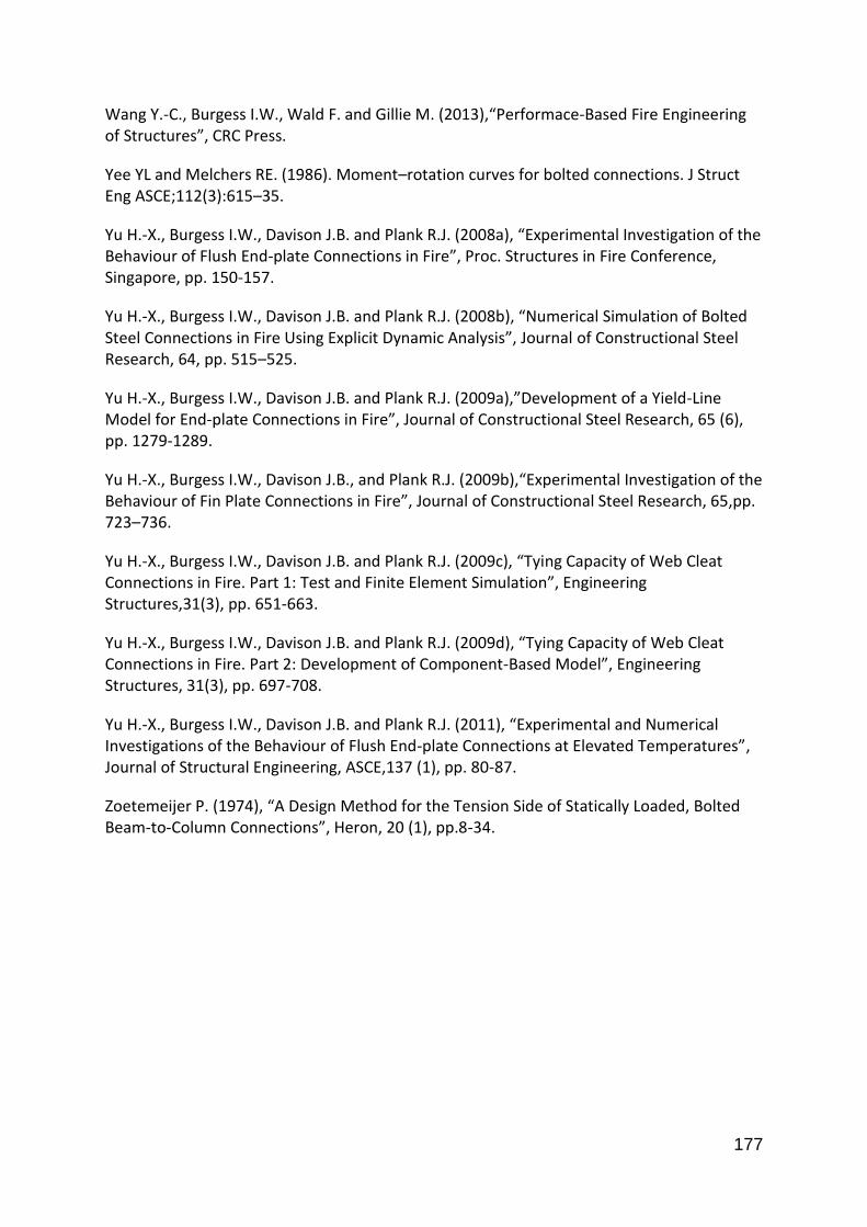
177

Wang Y.-C., Burgess I.W., Wald F. and Gillie M. (2013),“Performace-Based Fire Engineering of Structures”, CRC Press.

Yee YL and Melchers RE. (1986). Moment–rotation curves for bolted connections. J Struct Eng ASCE;112(3):615–35.

Yu H.-X., Burgess I.W., Davison J.B. and Plank R.J. (2008a), “Experimental Investigation of the Behaviour of Flush End-plate Connections in Fire”, Proc. Structures in Fire Conference, Singapore, pp. 150-157.

Yu H.-X., Burgess I.W., Davison J.B. and Plank R.J. (2008b), “Numerical Simulation of Bolted Steel Connections in Fire Using Explicit Dynamic Analysis”, Journal of Constructional Steel Research, 64, pp. 515–525.

Yu H.-X., Burgess I.W., Davison J.B. and Plank R.J. (2009a),”Development of a Yield-Line Model for End-plate Connections in Fire”, Journal of Constructional Steel Research, 65 (6), pp. 1279-1289.

Yu H.-X., Burgess I.W., Davison J.B., and Plank R.J. (2009b),“Experimental Investigation of the Behaviour of Fin Plate Connections in Fire”, Journal of Constructional Steel Research, 65,pp. 723–736.

Yu H.-X., Burgess I.W., Davison J.B. and Plank R.J. (2009c), “Tying Capacity of Web Cleat Connections in Fire. Part 1: Test and Finite Element Simulation”, Engineering Structures,31(3), pp. 651-663.

Yu H.-X., Burgess I.W., Davison J.B. and Plank R.J. (2009d), “Tying Capacity of Web Cleat Connections in Fire. Part 2: Development of Component-Based Model”, Engineering Structures, 31(3), pp. 697-708.

Yu H.-X., Burgess I.W., Davison J.B. and Plank R.J. (2011), “Experimental and Numerical Investigations of the Behaviour of Flush End-plate Connections at Elevated Temperatures”, Journal of Structural Engineering, ASCE,137 (1), pp. 80-87.

Zoetemeijer P. (1974), “A Design Method for the Tension Side of Statically Loaded, Bolted Beam-to-Column Connections”, Heron, 20 (1), pp.8-34.

178

Appendix A Input of connection element in Vulcan

Vulcan is a finite element analysis (FEA) program, which has been developed particularly for

the analysis of building structures in fire situation. This component-based connection

element is currently implemented in its FORTRAN version. The following table shows the

format of the part of the data input file for the connection elements. The remaining

structural information input is included in the latest Input explanation for the Vulcan

software.

For the connection element, there are two definitions:

Connection data: informs Vulcan about the connection geometries, locations, and

material properties.

Connection Temperature (TEMP) Pattern: informs Vulcan about the connection

temperature distribution.

The following is the general connection element input format. The variables are explained in

the following two tables.

<CONNECTION DATA >

Block 1: (compulsory input for every connection type)

Numcontype

Contype iendtype inumrow

Block 2: (optional input only for flush endplate connection type)

Contype internal imajorminor iec3bolt iductile ductmul

Contype endwidth ednthick endheight colroot endweld enddist coldist

Contype washerdia washerthick boltarea bolthethick nutthick

Contype d0 d1 d2 d3 d4 d5 d6 d7

179

Contype endym endfy colfanym colfanfy boltym boltfy boltfu endfu colfu endet colet boltet

Contype colwebym colwebfy colflanfy

Block 3: (optional input only for reverse channel connection type)

Contype internal imajorminor iec3bolt iductile ductmul ipull-out



Contype d0 d1 d2 d3 d4 d5 d6 d7


Contype colwebym colwebfy colflanfy

Contype revym revfy revfu revet

Contype revwebth revlegth revweble revlegle revroot revlegweld

Block 4: (optional input only user defined connection)

Contype capacityfac ductilityfac

Subblock1:

Contype c1f1 c1f2 c1f3 c1d1 c1d2 c1d3 1ccapfaccfy 1cducfaccfy


Contype 1t1f1 1t1f2 1t1f3 1t1f4 1t1f5 1t1d1 1t1d2 1t1d3 1t1d4 1t1d5 1t1capfaccfy

1t1ducfaccfy


1t2ducfaccfy


1t3ducfaccfy


1t4ducfaccfy


1t5ducfaccfy

180

………….

Subblock5:


3t1ducfaccfy


3t2ducfaccfy


3t3ducfaccfy


3t4ducfaccfy


3t5ducfaccfy

<CONNECTION TEMP PATTERN>

Numtemppat

Temppat tendtemp1 tcolflantemp1 tbolttemp1





Temppat ccolwebtemp1 ccolflantemp1


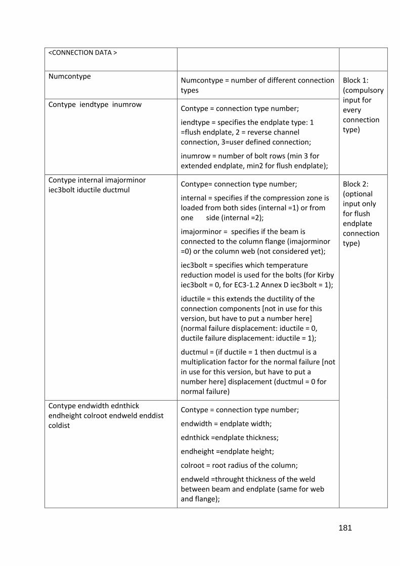
181

<CONNECTION DATA >

Numcontype Numcontype = number of different connection types

Block 1: (compulsory input for every connection type)

Contype iendtype inumrow Contype = connection type number;

iendtype = specifies the endplate type: 1 =flush endplate, 2 = reverse channel connection, 3=user defined connection;

inumrow = number of bolt rows (min 3 for extended endplate, min2 for flush endplate);


Contype= connection type number;

internal = specifies if the compression zone is loaded from both sides (internal =1) or from one side (internal =2);

imajorminor = specifies if the beam is connected to the column flange (imajorminor =0) or the column web (not considered yet);

iec3bolt = specifies which temperature reduction model is used for the bolts (for Kirby iec3bolt = 0, for EC3-1.2 Annex D iec3bolt = 1);

iductile = this extends the ductility of the connection components [not in use for this version, but have to put a number here] (normal failure displacement: iductile = 0, ductile failure displacement: iductile = 1);

ductmul = (if ductile = 1 then ductmul is a multiplication factor for the normal failure [not in use for this version, but have to put a number here] displacement (ductmul = 0 for normal failure)

Block 2: (optional input only for flush endplate connection type)


Contype = connection type number;

endwidth = endplate width;

ednthick =endplate thickness;

endheight =endplate height;

colroot = root radius of the column;

endweld =throught thickness of the weld between beam and endplate (same for web and flange);

182

enddist = edge distance of the bolt holes in the endplate (measured from center holes);

coldist = edge distance of the bolt holes in column flange (measured from center holes);



Washerdia = outer diameter of the washer;

washerthick = washer thickness;

boltarea = stress area of the bolts;

bolthethick = thickness of the bolt head;

nutthick = thickness of the nut;

Contype d0 d1 d2 d3 d4 d5 d6 d7 Contype = connection type number;

d0 = vertical distance from the centre of the beam to the upper edge of the endplate;

d1 = vertical distance from the centre of the beam to the first bolt row ;

d2 = vertical distance from the centre of the beam to the 2nd bolt row;

d3 = vertical distance from the centre of the beam to the 3rd bolt row;

d4 = vertical distance from the centre of the beam to the 4th bolt row;


d6 = vertical distance from the centre of the beam to the upper edge of the reverse channel [this version only considers the endplate and reverse channel have the same length];

d7 = vertical distance from the centre of the beam to the lower edge of the reverse channel [negative];



Endym = young’s modulus of endplate;

Endfy = yield stress of endplate ;

colfanym = young’s modulus of column flange;

colfanfy =yield stress of column flange;

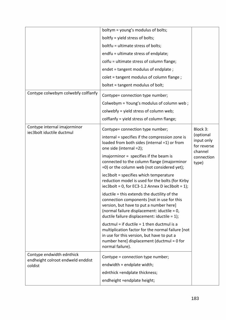
183

boltym = young’s modulus of bolts;

boltfy = yield stress of bolts;

boltfu = ultimate stress of bolts;

endfu = ultimate stress of endplate;

colfu = ultimate stress of column flange;

endet = tangent modulus of endplate ;

colet = tangent modulus of column flange ;

boltet = tangent modulus of bolt;

Contype colwebym colwebfy colflanfy Contype= connection type number;

Colwebym = Young’s modulus of column web ;

colwebfy = yield stress of column web;

colflanfy = yield stress of column flange;



internal = specifies if the compression zone is loaded from both sides (internal =1) or from one side (internal =2);

imajorminor = specifies if the beam is connected to the column flange (imajorminor =0) or the column web (not considered yet);

iec3bolt = specifies which temperature reduction model is used for the bolts (for Kirby iec3bolt = 0, for EC3-1.2 Annex D iec3bolt = 1);

iductile = this extends the ductility of the connection components [not in use for this version, but have to put a number here] (normal failure displacement: iductile = 0, ductile failure displacement: iductile = 1);

ductmul = if ductile = 1 then ductmul is a multiplication factor for the normal failure [not in use for this version, but have to put a number here] displacement (ductmul = 0 for normal failure).

Block 3: (optional input only for reverse channel connection type)



endwidth = endplate width;

ednthick =endplate thickness;

endheight =endplate height;

184

colroot = root radius of the column;

endweld =throught thickness of the weld between beam and endplate (same for web and flange);

enddist = edge distance of the bolt holes in the endplate (measured from center holes);

coldist = edge distance of the bolt holes in column flange (measured from center holes);



Washerdia = outer diameter of the washer;

washerthick = washer thickness;

boltarea = stress area of the bolts;

bolthethick = thickness of the bolt head;

nutthick = thickness of the nut;

Contype d0 d1 d2 d3 d4 d5 d6 d7 Contype = connection type number;

d0 = vertical distance from the centre of the beam to the upper edge of the endplate;

d1 = vertical distance from the centre of the beam to the first bolt row ;

d2 = vertical distance from the centre of the beam to the 2nd bolt row;

d3 = vertical distance from the centre of the beam to the 3rd bolt row;



d6 = vertical distance from the centre of the beam to the upper edge of the reverse channel [this version only considers the endplate and reverse channel have the same length];

d7 = vertical distance from the centre of the beam to the lower edge of the reverse channel [negative];



Endym = young’s modulus of endplate;

185

Endfy = yield stress of endplate ;

colfanym = young’s modulus of column flange;

colfanfy =yield stress of column flange;

boltym = young’s modulus of bolts;

boltfy = yield stress of bolts;

boltfu = ultimate stress of bolts;

endfu = ultimate stress of endplate;

colfu = ultimate stress of column flange;

endet = tangent modulus of endplate ;

colet = tangent modulus of column flange ;

boltet = tangent modulus of bolt;

Contype colwebym colwebfy colflanfy Contype= connection type number;

Colwebym = Young’s modulus of column web ;

colwebfy = yield stress of column web;

colflanfy = yield stress of column flange;

Contype revym revfy revfu revet Contype = connection type number;

Revym = reverse channel young’s modulus;

Revfy = reverse channel yield stress;

Revfu = reverse channel ultimate stress;

Revet = reverse channel tangent modulus;

Contype revwebth revlegth revweble revlegle revroot revlegweld

Revwebth = reverse channel web thickness;

Revlegth =reverse channel leg thickness;

Revweble = reverse channel web length;

Revlegle = reverse channel leg length;

Revroot = reverse channel root;

Revlegweld = throught thickness of welding at reverse channel leg.

Block 4: (optional input only user Line 1:

CXfY: compression component (column flange

Block 4: (optional

186

defined connection)

Contype capacityfac ductilityfac

Subblock1:



Contype 1t1f1 1t1f2 1t1f3 1t1f4 1t1f5 1t1d1 1t1d2 1t1d3 1t1d4 1t1d5 1t1capfaccfy 1t1ducfaccfy





………….

Subblock5:




under compression) force.

X = 1,2; 1 top compression row; 2 bottom compression row;

Y = 1,2,3; 3 nodes for each typical tension component;

The first node must be zero for each compression curve

CXdY: compression component (column flange under compression) deformation.


Y = 1,2,3; 3 nodes for each typical tension component;

The first node must be zero for each compression curve

Xccapfaccfy = capacity reduction factor for the compression component (column web under compression) at the top compression row


Xcducfaccfy = ductility factor for the compression component at the top compression row


XtYfZ: tension component (column flange under compression) force.

X = 1,2,3; 1: column flange under bending; 2: bolt in tension; 3: endplate in bending.

Y = 1,2,3,4,5; tension bolt row number;

Z = node number. Each tension component is represented by 5node. The first node is zero

XtYcapfaccfy = capacity reduction factor for the tension component at the Xth tension bolt row



XtYducfaccfy = ductility factor for the tension

input only user defined connection)***

187



component at the Xth tension bolt row



{CONNECTION DATA}

188


Numtemppat

Numtemppat = number of different connection temperature pattern (currently only consider 1);


Temppat = connection temperature pattern number;

Tendtempn = temperature multiplier for endplate at height of nth bolt row;

Tcolflantempn=temperature multiplier for column flange at height of nth bolt row;

Tbolttempn = temperature multiplier for bolt at height of nth bolt row;






Tempat = connection temperature pattern number;

Ccolwebtem1 = temperature multiplier for column web at height of upper beam flange;

Ccolflantemp1=temperature multiplier for column flange at height of upper beam flange;


Temppat = connection temperature pattern number;

Ccolwebtem1 = temperature multiplier for column web at height of lower beam flange;

Ccolflantemp1=temperature multiplier for column flange at height of lower beam flange;

{CONNECTION TEMP PATTERN}

189

Appendix B Example of Vulcan input

In order to explain how to write the Vulcan connection element input data, the input for an

endplate connection (test EP_20_35_04-02-08_8mm) is taken as an example. The joint test

details are included in 4.3.2 .

<HEADER>

EP_20_35_04-02-08_8mm

{HEADER}

<VERSION>

6

{VERSION}

<PROGRAM CONTROL>

0 0 0

1.000 1.000

1 0.000 0.000 0.0003 1.000

5000 0

{PROGRAM CONTROL}

<STRUCTURE INFORMATION>

15 9 9 4 0 0

100 0.000 1 13

3 2 1 1

{STRUCTURE INFORMATION}

<NODAL GEOMETRY>

1 0 0 0

190

2 61.69703308 0 28.76945836

3 242.9589738 0 113.2922886

4 424.2209146 0 197.8151189

5 475.929427 0 193.4046499

6 527.6379395 0 188.9941809

7 537.4860202 0 187.257717

8 762.5146637 0 147.5795166

9 987.5433073 0 107.9013162

10 997.391388 0 106.1648523

11 1007.367029 0 105.4672948

12 1139.998164 0 96.19291908

13 1282.60494 0 86.22098586

14 1347.100215 0 -35.13170352

15 1696.809043 0 -176.4282593

{NODAL GEOMETRY}

<NEW BEAM SECTION>

1 1 1

1

1

1

3 3 1 1

357 176000 0.3

357 176000 0.3

3560000 20500000 0.3

191

275 210000 0.3

-30 0.25 0.2

1 2 1 1 1

303.4 165 165 10.2 10.2 6.0 8 5 5

2 2 2 1 1

260.3 256.3 256.3 17.3 17.3 10.3 8 5 5

3 1 3 1 1

25 25 5 5

5 0 0 5 0 0

5 0 5 5 0 0

5 5 5 5 5 5

5 0 5 5 5 0

5 0 0 5 0 0

4 4 4 4 4

4 4 4 4 4

4 4 4 4 4

4 4 4 4 4

4 4 4 4 4

{NEW BEAM SECTION}

<MEMBER DATA>

1 1 0 0

1 1 2 9 1 1 2 1 0 180

2 7 0 0

192

2 2 4 3 0 1 1 1 1 0 0

3 7 0 0

3 4 6 5 0 1 1 1 1 0 0

4 1 0 0

4 6 7 3 3 3 1 1 0 180

5 7 0 0

5 7 9 8 0 3 1 1 1 0 0

6 1 0 0

6 9 10 3 3 1 1 1 0 180

7 1 0 0

7 10 11 3 3 1 1 1 0 180

8 7 0 0

8 11 13 12 0 3 1 1 1 0 0

9 7 0 0

9 10 15 14 0 3 1 1 1 0 0

{MEMBER DATA}

<CONNECTION DATA>

193

1

1 1 3

1 1 0 0 0 0

1 200 8 323.4 12.7 8 55 83.15

1 37 3 314.156 13 16

1 161.7 101.7 31.7 -101.7 0 0

1 149000 293 176000 357 210000 677 998 492 568

1002 1062 1629

1 176000 357 357

{CONNECTION DATA}


1

1 1.0 1.0 1.0

1 1.0 1.0 1.0

1 1.0 1.0 1.0

1 1.0 1.0 1.0

1 1.0 1.0 1.0

1 1.0 1.0

1 1.0 1.0

{CONNECTION TEMP PATTERN}

<BOUNDARY CONDITIONS>

1 111111

2 10101

194

3 10101

4 10101

5 10101

6 10101

7 10101

8 10101

9 10101

10 10101

11 10101

12 10101

13 111101

14 10101

15 110101

0 0

{BOUNDARY CONDITIONS}

<JOINT LOADS>

15 0 0 -500000 0 0 0

0 0 0 0 0 0 0

{JOINT LOADS}

<DISPLAY DEFLECTIONS>

5

1 2 4 6 15

{DISPLAY DEFLECTIONS}

195

<DISPLAY FORCES>

5

1 2 5 8 9

{DISPLAY FORCES}

<DISPLAY CONNECTIONS>

4

1 4 6 7

{DISPLAY CONNECTIONS}

<TEMPERATURE DATA>

1 1 20

1 0 20

{TEMPERATURE DATA}

{END OF FILE}

.

Documents

Development of a General-Purpose Component-based ...etheses.whiterose.ac.uk/13825/2/Thesis_gang.pdf · Department of Civil and Structural Engineering Development of a General-Purpose