Development of a Fully Vectorized Potential Flow Solver1144406/FULLTEXT01.pdf · Matrix Laboratory (Matlab) ... ary layer e ect need not to be considered. ... (FDM) is based on the

IN DEGREE PROJECT MECHANICAL ENGINEERING,SECOND CYCLE, 30 CREDITS

, STOCKHOLM SWEDEN 2017

Development of a Fully Vectorized Potential Flow Solver

WENYUAN YU

KTH ROYAL INSTITUTE OF TECHNOLOGYSCHOOL OF ENGINEERING SCIENCES

ii

Acknowledgements

Sincere gratitude is expressed to Romain Gojon for supervising my work,and to Mihai Mihaescu for examining it.

I would like to thank my friend and colleague Alessandro who gave mea lot of support and disguised with me during thesis period. I wouldalso like to thank Marcus who helped me a lot on Swedish translation.Thank Song Chen for giving me a lot of instruction on power point mak-ing and thesis defence.

In the end, I thank Department of Mechanics for giving me access tofacilities.

Wenyuan Yu Master’s thesis

Contents

1 Introduction 1

1.1 Background . . . . . . . . . . . . . . . . . . . . . . . . . 1

1.2 Objectives and achievements . . . . . . . . . . . . . . . . 2

2 Characteristics of the solver 5

2.1 Characteristics of flow . . . . . . . . . . . . . . . . . . . . 5

2.1.1 Review of thermodynamics . . . . . . . . . . . . . 5

2.1.2 Inviscid flow . . . . . . . . . . . . . . . . . . . . . 6

2.1.3 Irrotational flow . . . . . . . . . . . . . . . . . . . 7

2.2 Equations for flow case . . . . . . . . . . . . . . . . . . . . 7

2.2.1 Euler equation . . . . . . . . . . . . . . . . . . . . 7

2.2.2 Potential flow equation . . . . . . . . . . . . . . . 7

2.3 Finite difference scheme for spatial derivation . . . . . . . 8

2.3.1 Standard multi-point stencil scheme . . . . . . . . 8

2.3.2 Dissipation . . . . . . . . . . . . . . . . . . . . . . 9

2.3.3 Dispersion . . . . . . . . . . . . . . . . . . . . . . . 10

2.3.4 Optimized multi-point stencil scheme . . . . . . . 11

2.3.5 Boundary scheme . . . . . . . . . . . . . . . . . . . 13

2.4 Finite difference scheme for time derivation . . . . . . . . 15

2.4.1 Euler method . . . . . . . . . . . . . . . . . . . . . 15

2.4.2 Low storage Runge-Kutta algorithms . . . . . . . . 16

2.5 Mesh build . . . . . . . . . . . . . . . . . . . . . . . . . . 16

2.5.1 Structured grid . . . . . . . . . . . . . . . . . . . . 17

2.5.2 Body-fitted grids . . . . . . . . . . . . . . . . . . . 17

3 Case description and setup 21

3.1 Scheme testing case . . . . . . . . . . . . . . . . . . . . . 21

3.2 2D-pulse case . . . . . . . . . . . . . . . . . . . . . . . . . 23

3.2.1 Case description . . . . . . . . . . . . . . . . . . . 23

3.2.2 Analytical solution . . . . . . . . . . . . . . . . . . 26

3.2.3 Establish Euler Equation . . . . . . . . . . . . . . 27

3.2.4 Jacobian transformation on Euler equation . . . . 29

3.2.5 Potential equation . . . . . . . . . . . . . . . . . . 30

3.2.6 Jacobian transformation on potential equation . . 31

iii

iv CONTENTS

3.2.7 Analytical and numerical results for Jacobian ele-ments . . . . . . . . . . . . . . . . . . . . . . . . . 32

3.2.8 Boundary conditions . . . . . . . . . . . . . . . . . 333.3 Airfoil section case . . . . . . . . . . . . . . . . . . . . . . 35

3.3.1 Building 2D airfoil section . . . . . . . . . . . . . . 353.3.2 Case description . . . . . . . . . . . . . . . . . . . 373.3.3 Building O-type configuration domain and Jaco-

bian transformation . . . . . . . . . . . . . . . . . 393.3.4 Establish potential equations . . . . . . . . . . . . 423.3.5 Boundary conditions . . . . . . . . . . . . . . . . . 43

4 Results and conclusions 454.1 Scheme testing case . . . . . . . . . . . . . . . . . . . . . 454.2 2D pulse case . . . . . . . . . . . . . . . . . . . . . . . . . 48

4.2.1 Euler solver . . . . . . . . . . . . . . . . . . . . . . 504.2.2 Potential solver . . . . . . . . . . . . . . . . . . . . 524.2.3 Influence of Runge-Kutta method . . . . . . . . . . 544.2.4 Time consumed by different solvers . . . . . . . . . 55

5 Conclusions 57


Chapter 1

Introduction

1.1 Background

Computational Fluid dynamic(CFD) has become an important tool foraeronautical application. Different numerical algorithms solving Navier-Stokes equations have been developed to convert groups of partial differ-ential equations (PDEs) to groups of algebraic equations. Most of thesealgorithms reduce PDEs to ordinary differential equations through spa-tial and temporal discretisation.

As one of the most commonly used spatial discretization methods, finitedifference method has been developed since the early stages of aero-nautical CFD to meet the requirement of high order of accuracy, lowdispersion and low dissipation. As a result, different numerical schemesare designed to optimize dispersion and dissipation properties in theFourier space for large wavenumber. Available optimized finite differ-ences are for instance the explicit dispersion-relation-preserving schemeof Tam and Webb [1] or the compact schemes of Lele[2]. When cod-ing these finite difference schemes, the common method is to use loopcommand. In the present work, the loop command will be replaced byvector operation to build the schemes. Generally, vectorization methodhas three advantages[3]:(1) Appearance: Vectorized mathematical code appears more like themathematical expressions found in textbooks, making the code easier tounderstand.(2) Less Error Prone: Without loops, vectorized code is often shorter.Fewer lines of code mean fewer opportunities to introduce programmingerrors.(3) Performance: Vectorized code often runs much faster than the cor-responding code containing loops.

Matrix Laboratory (Matlab) is one of the ideal platforms for operationsinvolving matrices and vectors. Since the early stages of development,

1

2 CHAPTER 1. INTRODUCTION

Matlab has become a multifunctional mathematical tool to solve systemsof algebraic equations. In this manuscript, considering the advantagesof Matlab on vectorization, the solvers will be established with Matlablanguage.

Based on the Navier-Stokes equations, different solvers have been de-veloped for different specific fluid. Although in the natural world, theinviscid and non-heat conduction fluid does not exist, viscosity and heatconduction are sometimes so small that they can be neglected in someproblems. Once neglecting these two effects, Navier-Stokes equationswill be simplified and transformed into Euler equations. As viscosityterms are accompanied with second order PDEs in Navier-Stokes equa-tions, neglecting viscosity indicates that Euler equations are much eas-ier to be linearized. Adding irrotational fluid condition to Euler equa-tions, potential flow equation can be set up. Potential flow model isthe simplest description on inviscid compressible flow, as it has onlyone unkonwn in the PDE equation.[10] Velocities of three directions inCartesian coordinate can be expressed in the derivative form and otherunknowns such as temperature, pressure and density can be derivedfrom thermodynamic equations.

1.2 Objectives and achievements

In this manuscript, both Euler solver and potential solver will be builton Matlab platform. 4th and 6th order of Runge-Kutta method will beused for temporal discretisation and different multi-point center differ-ence schemes will be used on spatial discretisation. Both of these solverswill be used to solve a 2D flow case.

Center finite difference is the basic method in this paper for spatial dis-cretization. In general, except the schemes that will be used adjacent tothe boundary points, center finite difference schemes will be used on themain mesh points. Depending on the requirement of order of accuracyand optimization, different multi-point stencil schemes will be built inMatlab in the form of matrix. As a result, solving PDEs is actually op-erating matrices in Matlab. Standard schemes and optimized schemeswill be tested with 1D linear convection equation before applying themto the solvers.

In 2D-pulse case, the rectangular domain will be transformed into awavy domain and as a result Jacobian transformation method will betested.

Results from different schemes will be compared with the analytical so-lution in two dimensional pulse case. Besides, results from two different


CHAPTER 1. INTRODUCTION 3

solvers will also be compared.

The multi-point stencil schemes built in matrix will not only be used onthe main PDEs, but also on the Jacobian transformation, while calcu-lating the relation of coordinates between real domain and the compu-tational domain. The Jacobian transformation will be derived both inEuler and potential solver, and the results from the transformed meshwill be compared with the results from original mesh.

Radiation and wall boundary conditions will be considered while solvingpulse and airfoil problems and far field boundary condition will be con-sidered in airfoil case. Keeping 2nd order of accuracy at the boundary,the relative equations or operating matrix will be derived for both Eulerand Potential solver.

Master’s thesis Wenyuan Yu

4 CHAPTER 1. INTRODUCTION


Chapter 2

Characteristics of the solver

The basic steps to build a solver include:(1) Definition of the working fluid.(2) Solver equations based on the NS equations and hypotheses.(3) Building the meshes needed to discretize the PDEs.(4) Temporal and spatial discretisation.(5) Verification of the solver using test case for which analytical solutionexists.

This chapter will give a brief introduction on the knowledges that willbe used in different steps.

2.1 Characteristics of flow

2.1.1 Review of thermodynamics

With the standard atmosphere condition, for most gases, the distancebetween two particles is more than 10 molecular diameter[4]. The idealgas hypothesis can be used:

P = ρRT (2.1)

Further limiting the condition, the gas will be regarded as perfect gasin this paper, giving the equation:

e = CvT (2.2)

h = CpT (2.3)

where e is internal energy per unit mass and h is enthalpy per unit mass,indicating both e and h are only a function of temperature T. With thedefinition of enthalpy:

h = e+ pV (2.4)

5

6 CHAPTER 2. CHARACTERISTICS OF THE SOLVER

the relation:

Cv − Cp = R (2.5)

could be derived.

Define specific heat ratio γ = CvCp

, we could derive:

Cp =γR

γ − 1(2.6)

Cv =R

γ − 1(2.7)

Combine function 2.1, 2.2 and 2.7, we can derive:

p = ρ(γ − 1)e (2.8)

Define the total enthalpy as H0,

H0 = h+U2

2= CpT0 +

U2

2(2.9)

Substitute equation 2.6 into equation 2.9,we obtain:

H0 =γRT0

γ − 1+

U2

2(2.10)

Another hypothesis in this manuscript is that the flow is isentropic,indicating:

p2

p1= (

ρ2

ρ1)γ

= (T2

T1)

γγ−1

(2.11)

Define the sound velocity as a, with isentropic condition, we could derive:

a2 =∂p

∂ρ(2.12)

Deriving further:

a =√γRT (2.13)

2.1.2 Inviscid flow

In this manuscript, viscosity is not considered, which indicates the bound-ary layer effect need not to be considered. This simplification makes itpossible to use both Euler and potential equation to analyse the sameproblem.


CHAPTER 2. CHARACTERISTICS OF THE SOLVER 7

2.1.3 Irrotational flow

A flow is irrotational if curl of velocity v is zero:

∇× v = 0

.

It is a precondition to analyse potential flow.

2.2 Equations for flow case

2.2.1 Euler equation

Without viscosity, the Navier-Stokes equations become the Euler equa-tion whose conservative form is:

∂U

∂t+∇ · F = Q (2.14)

in which,

U = {ρ, ρu,E}T (2.15)

u = {u, v, w},E =1

2ρ(ρ+

u2

2)

F = {ρu, ρu · u + P I, (E + P )u− k∆T}T

and Q is source term. In this case, source term Q is 0.

2.2.2 Potential flow equation

Potential flow method can only be used to solve irrotational flow prob-lems. In many compressible flow application, the real flow field is closeto be irrotational [5] so that potential flow equation becomes a tool.With the single dependent variable, potential flow equation combinescontinuity, momentum and energy equation into one equation.

For irrorational flow, ∇ × V = 0, scalar function φ(x, y, z) is definedsuch that

V = ∆φ (2.16)

is called velocity potential. In Cartesian coordinate,

u =∂φ

∂xi, v =

∂φ

∂yj, w =

∂φ

∂zk



2.3 Finite difference scheme for spatial deriva-tion

Finite difference method (FDM) is based on the properties of Taylorexpansion. For a given function u(x), the Taylor expansion of u is:

u(x+ ∆x) = u(x) + ∆x∂u

∂x+

∆x2

2

∂2u

∂x2+ ...+

∆xn

n!

∂nu

∂xn(2.17)

It is the simplest method to apply on structured meshes, especially theuniform meshes, to solve differential equations.

The derivative of u can be expressed in:

ux =∂u

∂x= lim

x→0

u(x+ ∆x)− u(x)

∆x(2.18)

If ∆x is very small but finite, the right-hand side expression is an ap-proximation of ux.The truncation error could be reduced by reducing∆x, namely grid size in the real CFD case, but it will take more effortsto compute. The power of ∆x left by Taylor expansion is called theorder accuracy, which depends on the selected scheme.

In this article, center difference schemes are mostly used while backwardand forward biased difference schemes are applied on the border adja-cent points. This will be discussed in the subsection 2.3.5.

2.3.1 Standard multi-point stencil scheme

We assume subscript i as the step number and u as a flux which needto be solved in one dimension case. The Taylor expansion indicates:

ui+1 = ui + ∆x∂u

∂x|i +

∆x2

2

∂2u

∂x2+ ...+

∆xn

n!

∂nu

∂xn(2.19)

In a similar way, the flux N steps away from position i can be expressed:

ui+N = ui +N∆x∂u

∂x|i +

(N∆x)2

2

∂2u

∂x2|i +...+

(N∆x)n

n!

∂nu

∂xn|i (2.20)

If terms with ∆xn−1 could be cancelled, the maximum power of leftterms is O(∆xn), and n is the order of accuracy. To meet the require-ment on the order of accuracy, multi-point stencil schemes are needed.Theoretically, the more points put in the stencil, the higher the order ofaccuracy.

For central difference scheme, a total number of points of 2N+1 is usedwith N the number of points on the left and right side of the original



point (i=0), indicating the standard center difference scheme is 2N th

order of accuracy.

∂u

∂x|i=0=

1

∆x

j=N∑j=−N

aju(x0 + j∆x) (2.21)

In order to make the order of accuracy of the scheme to be 2N, the termsbefore O(∆x2N ) needed to cancelled. Remembering the equation 2.20,the flux -N steps away from position i can be expressed:

ui−N = ui −N∆x∂u

∂x|i +

(N∆x)2

2

∂2u

∂x2|i +...+ (−1)n

(N∆x)n

n!

∂nu

∂xn|i

The rest terms ui−j and ui+j can be derived in the same way. The co-efficients aj from equation 2.21 can be obtained by substituting all theterms. Then except term ∂u

∂x , the sum of coefficients before all the termsare equal to 0. As a result, to cancel the terms before O(∆x2N ), weneed 2N+1 equations, that is 2N+1 points in the scheme.

In this manuscript, 3 points, 5 points, 7 points, 9 points and 11 pointsstencil schemes are used. The coefficients aj for each stencil scheme areshown below:

XXXXXXXXXXXschemecoefficient

ai−4 ai−3 ai−2 ai−1 ai ai+1 ai+2 ai+3 ai−4

3 points stencil −12 0 1

2

5 points stencil 112

−812 0 8

12−112

7 points stencil −160

960

−4560 0 45

60−960

160

9 points stencil 3840

−32840

168840

−672840 0 672

840−168840

32840

−3840

Table 2.1: Coefficients for standard multi-point stencil

2.3.2 Dissipation

After the algebraic manipulations on the left side of Taylor series, wechange PDEs into the form of difference, the terms left on the right sideare called truncation errors which will make numerical solution differentfrom analytical solution. If the amplitude of numerical solution varieswith time compared with analytical solution, dissipation error appears.In the Taylor series, the odd order terms are dissipative terms.

Take a third order backward biased scheme for example:

∂u

∂x|i=

uj−2 − 6uj−1 + 3uj + 2uj = 1

6∆x



The above equation can be divided into antisymmetric and symmetricpart:

∂u

∂x|i=

uj−2 − 8uj−1 + 8uj+1 − uj+2 + uj−2 − 4uj−1 + 6uj − 4uj+1 + uj+2

12∆x

The order of accuracy for the antisymmetric part is four, while the sym-metric component approximates ∆x3uxxx

12 . This term is a third orderdissipative term and the source of dissipative error.

From the perspective of Taylor expansion, the dissipation error existsif the components are asymmetric (aj 6= a−j). Note that the antisym-metric portion of the first-derivative operator always has an even orderof accuracy, indicating that there is no dissipation for central differencescheme[6].

As in this manuscript, central difference scheme is the main algorithm,dissipative error will not be disguised.

2.3.3 Dispersion

With different wavenumber, different waves travel with different speed,which contributes to the dispersion. The source of dispersion is the oddterm from Taylor expansion. This will lead to the distortion of waves[7].

From the Fourier transformation point of view,

u = ueikx (2.22)

applying this to equation,

k∗∆x = 2

N∑i=1

ai sin(ik∆x) (2.23)

The dispersive error E is the difference between the modified wavenum-ber k∗ and exact wavenumber k[8].

E =

∫ π2

−π2

[k∆x− k∗∆x]2d(k∆x) (2.24)

k∆x relates to mesh resolution through points per wave length(PPW).It indicates that grid size could influence dispersive error.

From central finite difference operator perspective, there is no imaginarypart in wavenumber k∗, the real part of modified wave will cause a dif-ference between phase velocity and group velocity, which is the source



of dispersive error.

To minimize dispersive error E, optimized central difference schemeshave been developed[8]in order to minimize the dispersion error E. Theywill be presented in subsection 2.3.4.

2.3.4 Optimized multi-point stencil scheme

The order of accuracy is not the only factor that influences the accuracy,as mentioned in the above section, dispersive error should also be con-sidered while selecting the scheme. Generally, a good finite differencescheme should be low dissipative and dispersive on a wide bandwidth ofwave frequency.

Combining equation 2.24 and 2.23, we obtain:

E =

∫ π2

−π2

[k∆x− 2N∑i=1

ai sin(ik∆x)]

2

d(k∆x) (2.25)

From the perspective of minimum principle of function, to let E be aminimum,

∂E

∂aj= 0 (2.26)

Taking 7-point 4th order accuracy scheme as an example. To meet therequirement of 4th order, we need to use Taylor expansion on right sideof equation 2.21, and equating terms of order ∆x and terms of order∆x3. By doing this we have two equations for three unknowns (a1, a2,a3). Together with an equation 2.26, we can find three unknown coeffi-cients for optimized scheme.

From previous section, we know that the group velocity difference couldcause dispersion error. As a result, if the group velocity of the schemecan approximate the original equation, less dispersion error will appear.In the book of hristopher K. W. Tam [7], the group velocity of finite dif-

ference schemes are determined by ∂(k∗∆x)∂(kx) . To let scheme have a close

group velocity with original equation, ∂(k∗∆x)∂(kx) should be close to 1.

Figure 2.1 shows the ∂(k∗∆x)∂(kx) curve of the optimized 7-point stencil.



Figure 2.1: 4th order 7-point stencil[7]

From above figure we notice that ∂(k∗∆x)∂(kx) = 1 on the bandwidth range

of 0-0.4. This value is larger than 1 on the bandwidth of 0.4-1.1. Thisindicates the dispersion error still exists if the wavenumber is large, inorder to solve this issue, a η is set to integration equation of E.

E =

∫ η

0[k∆x− 2

N∑i=1

ai sin(ik∆x)]

2

d(k∆x) (2.27)

From figure 2.1, we set η = 1.1, and then obtain the coefficients aj withthe same method presented before.

In general, by lowering the order of accuracy, new coefficients for themulti-point stencil scheme are now available to optimize the dispersiveproperty.

In this paper, for optimized multi-point stencil schemes, the order ofaccuracy will be kept four, and the new coefficients for these stencils areshown in the table:XXXXXXXXXXXscheme

coefficientai−5 ai−4 ai−3 ai−2 ai−1 ai ai+1 ai+2 ai+3 ai−4 ai+5

7 points stencil -0.0208 0.1667 -0.77089 0 0.77089 -0.1667 0.0208

9 points stencil 0.00765 -0.0595 0.2447 -0.8416 0 0.8416 -0.2447 0.0595 -0.00765

11 points stencil -0.00248 0.02078 -0.09032 0.28651 -0.87276 0 0.87276 -0.28651 0.09032 -0.02078 0.00248

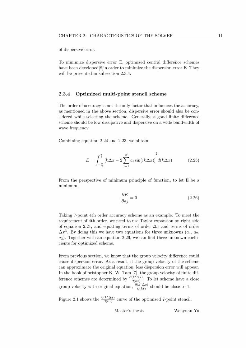
From the equation 2.23, the relation between effective wave numberk∗∆x and exact wave number k∆x for standard and optimized multi-point schemes are shown below:



Figure 2.2: Effective wave number versus exact wave number for differentfinite-difference schemes

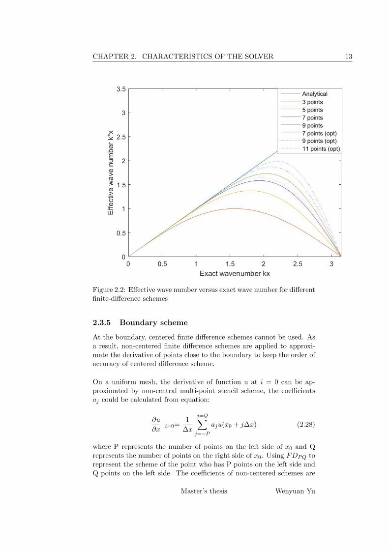
2.3.5 Boundary scheme

At the boundary, centered finite difference schemes cannot be used. Asa result, non-centered finite difference schemes are applied to approxi-mate the derivative of points close to the boundary to keep the order ofaccuracy of centered difference scheme.

On a uniform mesh, the derivative of function u at i = 0 can be ap-proximated by non-central multi-point stencil scheme, the coefficientsaj could be calculated from equation:

∂u

∂x|i=0=

1

∆x

j=Q∑j=−P

aju(x0 + j∆x) (2.28)

where P represents the number of points on the left side of x0 and Qrepresents the number of points on the right side of x0. Using FDPQ torepresent the scheme of the point who has P points on the left side andQ points on the left side. The coefficients of non-centered schemes are



shown in below tables:

coefficient ai−1 ai ai+1

FD02−32 2 -1

Table 2.2: 3 points stencil scheme

coefficient ai−2 ai−1 ai ai+1 ai+2

FD04−2512 4 -3 4

3−14

FD13−14

−56

32

−12

112

Table 2.3: 5 points stencil schemes

coefficient ai−3 ai−2 ai−1 ai ai+1 ai+2 ai+3

FD06−147

60 6 −152

203

−22560

65

−16

FD15−16

−7760

52

−53

56

−14

130

FD24130

−25

−712

43

−12

215

−160


coefficient ai−4 ai−3 ai−2 ai−1 ai ai+1 ai+2 ai+3 ai+4

FD08−2283

8406720840

−11760840

15680840

−14700840

9408840

−3920840

960840

−105840

FD17−105840

−1338840

2940840

−2940840

2450840

−1470840

588840

−140840

15840

FD2615840

−240840

−798840

1680840

−1050840

560840

−210840

48840

−5840

FD35−5840

60840

−420840

−378840

1050840

−420840

140840

−30840

3840


To ensure 4th order of accuracy, the point number of stencil should belarger than 5. In the present work [2], the coefficients for optimizedbiased finite difference close to border point are shown in the table:



coefficient ai−3 ai−2 ai−1 ai ai+1 ai+2 ai+3

FD06 -2.226 4.8278 -5.0014 3.9111 -2.1153 0.7189 -0.1153

FD15 -0.2129 -0.1603 2.0789 -1.287 0.6852 -0.2453 0.0417

FD24 0.0483 -0.4883 -0.3660 1.0480 -0.2893 0.0504 -0.0031

Table 2.6: 7 points stencil schemes (optimized)

coefficient ai−4 ai−3 ai−2 ai−1 ai ai+1 ai+2 ai+3 ai+4

FD08 -2.7179 7.464 -14 18.6667 -17.5001 11.2 -4.66667 1.143 -0.125

FD17 -0.125 -1.355 3.5 -3.5 2.9167 -1.75 0.7 0.1667 0.0179

FD26 0.0179 -0.2856 -0.95 2 1.25 0.6667 -0.25 0.0571 -0.006

FD35 -0.006 0.0714 -0.5 -0.45 1.25 -0.5 0.1667 -0.0357 0.00357

Table 2.7: 9 points stencil schemes(optimized)

coefficient ai−5 ai−4 ai−3 ai−2 ai−1 ai ai+1 ai+2 ai+3 ai−4 ai+5

FD010 -2.3916 5.8325 -7.6502 7.9078 -5.9226 3.0710 -1.0150 0.1700 0.00282 -0.0048 -0.000013

FD19 -0.18002 -1.23755 2.48473 -1.81032 1.11299 -0.48109 0.1266 -0.01551 0.0000216 0.00015645 -0.00000739

FD28 0.05798 -0.5361 -0.2641 0.9174 -0.169688 -0.02972 0.02968 -0.005222 -0.0001188 -0.000119 -0.0000201

FD37 -0.01328 0.11598 -0.61748 -0.27411 1.08621 -0.40295 0.131067 -0.028155 0.002596 0.000129 0

FD46 0.01676 -0.11748 0.411035 -1.13029 0.341436 0.556397 -0.08253 0.003566 0.001173 -0.000072 -0.00000035

Table 2.8: 11 points stencil schemes(optimized)

The coefficients for FDQP are antisymmetric to the coefficients in theabove tables.

2.4 Finite difference scheme for time derivation

2.4.1 Euler method

Euler method is the most common method used in time discretisationwhen solving PDEs. In this manuscript, forward Euler method is tested:

∂u

∂t= u(x, t) (2.29)

un+1 − un

∆t= u(x, tn) (2.30)

The equations indicates that the order of accuracy on time is only firstorder. To get higher order of accuracy, Runger-Kutta method will beused for time discretisation.



2.4.2 Low storage Runge-Kutta algorithms

Runge-Kutta scheme is one of the most common time marching algo-rithms which is based on Taylor expansions. In this manuscript, 4thorder (RK-4)and 6th order (RK-6) Runge-Kutta schemes will be used.To illustrate this method, we assume time step as ∆t and n as time level,F is a function of flux u.

∂u

∂t= F (u) (2.31)

The value of flux u at time step n is known, to find u of the next timestep (n+1), four (six) evaluation of derivative function F will be per-formed, it is called 4th (6th) order of Runge-Kutta (RK) scheme. Theseintermediate evaluations provide indirectly the high-order derivatives ofu so that a matching of high-order terms in a Taylor series. The generalform for a N-th order Runge-Kutta scheme is shown in the following:

un+1 = un +N∑j=1

wj∆tkj = un +N∑j=1

wj∆t∂jun

∂twj =

1

j!(2.32)

To reduce the storage requirement, low-storage Runge-Kutta algorithm[12] is used, it will take two storage locations per variable, illustratestandard explicit 4th order RK scheme as an example, the procedurebetween time level n and n+1 is:

u0 = un

for m=1,2,3,4

um = un + am∆tF (um−1) (2.33)

un+1 = u4

am =1

N −m+ 1, a1 =

1

4, a2 =

1

3, a3 =

1

2, a4 = 1

For 6th order RK scheme, the method is the same.

2.5 Mesh build

When setting up CFD simulation, building mesh is the first necessarystep. An appropriate grid distribution is a crucial factor to get sat-isfactory results. Different methods have been developed nowadays togenerate both structured and unstructured grids. This manuscript willemphasize on structured grid.



2.5.1 Structured grid

Structured grid is composed of groups of intersecting lines. There aretwo groups of lines for two dimensional mesh and three groups for threedimensional mesh. In structured mesh, the nodes defined by a certainalgorithm follow the repeated pattern. Every node is surrounded by aequal number of nodes.

Compared with unstructured mesh whose nodes are arbitrarily distributed,structured mesh requires less computational memory. Besides, the align-ment (e.g. grid lines align with streamlines) contributes to a better ac-curacy of the solver.

Ideally, the grids are cartesian distributed(Case described in section 3.2).This grid will be associated with the highest possible accuracy of thediscretized formulas. However, in most of real cases (such as the casesection 3.3), where curved solid walls exist, they are no longer alignedwith Cartesian lines. In this manuscript, body-fitted grid method isused to solve this problem.

Basically, the idea is to transform irregular body-fitted meshes(physicaldomain) into structured mesh(computational domain) so that finite dif-ference schemes can be applied.

2.5.2 Body-fitted grids

For most of CFD problems, the physical fluid domain does not havea regular geometry. It suggests that numerical schemes need greatergeometry flexibility[13]. Approximating the boundary by a series ofrectangular steps as shown in figure 2.3 would lead to significant errorsclose to the wall and large deficiencies in the predictions. A solutionto this issue is to use body-fitted grids which follow the boundary ofphysical domain. In this method, curvilinear grids are generated to fitthe body of geometry as much as possible. More complex method isused to keep the smoothness and continuity of the grids.



Figure 2.3: Comparison between normal and body-fitted grids [13]

As shown in the figure 2.3, the edges of grids are no longer aligned withCartesian coordinate (x1, x2), the finite difference over the grids will notbe straightforward. The physical domain needs to be transformed intoa normal computational domain with Jacobian matrix.

Two types of method can be used to generate body-fitted grids. Onesolution is to define a local orthogonal coordinate(η). This method con-sumes more time while generating orthogonal intersected grids, espe-cially the domain with complex geometry. Besides, it is also difficultto refine the grids. Another method is to define a non-orthogonal co-ordinate (η). This makes the mesh easier to generate, and avoids someof the problems of being forced to place grid lines where they are notneeded. However, this method is not suitable for complex geometry.If the geometry is complex, multi-block method will be used. In thismanuscript, the first method will be used in the ”flow over airfoil” caseand the second method will be used in the pulse case.

Depending on the orientation of the grid lines, various domain config-urations can be selected when using the first method. In this paper,O-mesh is selected.

To apply the numerical schemes mentioned in the previous section non-Cartesian coordinate mesh, we need to transform curvilinear coordinateinto Cartesian coordinate. In another word, the shape of physical do-main is not the computational domain, we need to use the Jacobian



matrix to complete the transformation.

Assuming the physical domain is two dimensional and its two axes are ξand η respectively and the corresponding computational domain is twodimensional and its two axes are x and y respectively. If the grid doesnot deform with time:

ξ = ξ(x, y), η = η(x, y) (2.34)

As a result, there is a one to one correspondence between the points ofphysical domain and the points of computational domain.

The chain-rule indicates:

∂

∂x=∂ξ

∂x

∂

∂ξ+∂η

∂x

∂

∂η(2.35)

∂

∂y=∂ξ

∂y

∂

∂ξ+∂η

∂y

∂

∂η(2.36)

When written in matrix form: ∂∂x

∂∂y

=

ξx ηx

ξy ηy

∂∂ξ

∂∂η

When discretizing in space, ∆x and ∆y are no longer constant, so weneed to use ∆ξ and ∆η as grid space steps. Define matrix j as :

J =

ξx ηx

ξy ηy

The previous matrix form will be written in the form: ∂

∂ξ

∂∂η

= J−1

∂∂x

∂∂y

In two dimensional case:

J−1 =

xξ yξ

xη yη

J = (J−1)

−1

Define |√g| = (xξyη − xηyη),

J = (J−1)−1

=1√g

yη −yξ−xη xξ



With above relations,the metrics (ξx,ηx,ξy,ηy) can be expressed withterms (xξ,xη,yξ,yη). The latter can be easily found in the computationaldomain.


Chapter 3

Case description and setup

3.1 Scheme testing case

Before applying different spatial discretization schemes to 2D-pulse caseand airfoil section case, we will test those scheme with a simple 1D linearconvection equation:

∂u

∂t+∂u

∂x= 0 (3.1)

Given the initial velocity disturbance:

u = sin(2πx

a∆x)exp(−ln(2)(

x

b∆x)2) (3.2)

In equation 3.2, parameters a and b are directly connected with the spec-tral contents of velocity disturbance. In this manuscript, two groups of(a, b) are used to test the scheme.

Problem 1:

a1 = 8, b1 = 3

Problem 2:

a2 = 4, b2 = 9

If we decompose signal (initial velocity disturbance) into a number ofdiscrete frequencies, we can obtain the normalised power spectral densityfigure shown below:

21

22 CHAPTER 3. CASE DESCRIPTION AND SETUP

Figure 3.1: Spectral contents of the initial disturbances for - - -Problem1 and —Problem 2

The figure3.1 indicates that the discrete frequencies of velocity distur-bance concentrate in a certain wavenumber (frequency). Compared withproblem 1, the concentrate wavenumber of problem 2 is larger. Remem-bering figure 2.2, the larger exact wavenumber is prone to produce dis-persive error. So problem 2 is prone to be dispersive and as a result has ahigher requirement on finite difference scheme compared with problem 1.

The initial small disturbance for these two problems are shown below:

Figure 3.2: Initial condition for problem 1 (left) and problem 2 (right)

In this 1D problem, discretize the domain into uniform dx, non-dimensionalizethe x coordinate by dividing dx, the velocity will propagate to theright. Setting time step as 100 and the disturbance will ideally arrive at


CHAPTER 3. CASE DESCRIPTION AND SETUP 23

xdx = 50.

Figure 3.3: Analytical solution for problem 1 (left)and problem 2 (right)at timestep=100

The results from different discretization schemes will be compared withthe analytical solution shown above, verifying the dispersive property ofschemes in the result chapter.

Notice 4th order Kutta-Runge method will be used on time discretizationfor these two problems.

3.2 2D-pulse case

In this section, an Euler solver and a potential solver will be built tosolve the pulse problem in rectilinear domain and wavy domain. Runge-Kutta method will be used for the discretization of time space and multi-point stencil center difference schemes will be used to dicretize in space.Results from all the shemes will be compared with analytical solutionin the result chapter.

3.2.1 Case description

Assume a small density (pressure) disturbance is imposed on a two-dimensional uniform mean flow in a rectilinear and wavy mesh domain.The whole domain is 50 ∗ 50 in size. Assume the uniform velocity u0 is



0.5 Mach number in x direction, the density and pressure is ρ0 and p0

respectively. The initial potential field is shown in fig.3.4.

Figure 3.4: Initial potential field for rectilinear and wavy domain

In the mid-point of domain, a density (pressure) pulse is applied, thepulse function is:

p′(x, y, 0) = ρ′ = εe−αβ2

(3.3)

ε is the amplitude of the pulse while β is the radial distance from theoriginal point, α is related to the half width of the Gaussian profile b [9]

α =In(2)

b2



β = (x− u0t)2 + y2

To some extent, coefficient b decides the exact wavenumber of originalequation. The smaller b will lead to a larger wave number and as a resultmakes dispersion more likely to appear. In this paper, b will be set as 1.5.

In order to make calculation simpler(non-dimensionalize), assume thesound velocity a0 = 1 and uniform density ρ0 = 1 recalling function 2.1and function 2.12, the uniform pressure p0 is :

p0 =ρ0

γ=

1

γ

both seeing fig.3.5 and fig.3.6,

Figure 3.5: Small disturbance on a rectangular domain



Figure 3.6: Small disturbance on a wavy domain

3.2.2 Analytical solution

There exists analytical solution for this pulse problem. This analyticalsolution will be used to compare with results from different numericalschemes in the result chapter.The analytical solution can be given witha Bessel function J0 order of zero:

p′(x, y, t) = ρ′(x, y, t) =ε

2α

∫ ∞0

e−ζ24α cos(ζt)J0(ζβ)ζdζ (3.4)

The analytical solution will be obtained from Matlab with integratemethod ’trapz ’. Picking out the solution in the middle line of the domain(y=0), the analytical solution is shown in below fig.3.7 and fig.3.8.



Figure 3.7: Analytical solution density pulse(y=0, u0=0)

Figure 3.8: Analytical solution density pulse(y=0, u0=0.5)

3.2.3 Establish Euler Equation

For a two-dimensional inviscid flow domain with no source term. Eulerequation can be written as:

∂ρ

∂t+∂ρu

∂x+∂ρv

∂y= 0 (3.5)



∂ρu

∂t+

∂

∂x(ρu2 + p) +

∂

∂y(ρuv) = 0 (3.6)

∂ρv

∂t+

∂

∂y(ρv2 + p) +

∂

∂x(ρuv) = 0 (3.7)

∂E

∂t+

∂

∂x(u(E + p)) +

∂

∂y(v(E + p)) = 0 (3.8)

where ρ is the density of the flow, u and v are the velocities in x and ydirection respectively in Cartesian coordinate, p is the pressure, E is thetotal energy per mass unit mass, E = ρ(e+ u2+v2

2 ), and e is the internalenergy per unit mass.

The equations above are the conservative form of the Euler equations,while written in convective form, the above equations change into:

∂ρ

∂t+ u

∂ρ

∂x+ ρ

∂u

∂x+ v

∂ρ

∂y+ ρ

∂v

∂y= 0 (3.9a)

∂u

∂t+ u

∂u

∂x+ v

∂u

∂y+

∂p

ρ∂x= 0 (3.9b)

∂v

∂t+ u

∂v

∂x+ v

∂v

∂y+

∂p

ρ∂y= 0 (3.9c)

∂e

∂t+ u

∂e

∂x+ v

∂e

∂y+p

ρ(∂u

∂x+∂v

∂y) = 0 (3.9d)

Recalling the function 2.8 and multiplying ρ on both sides of function3.9d, we can be obtain:

∂p

∂t+ u

∂p

∂x+ v

∂p

∂y+ p(γ − 1))(

∂u

∂x+∂v

∂y) = 0 (3.9)

Assume small pressure and density disturbance as p′ and ρ′ , small ve-locity disturbance in x and y direction as u′ and v′ respectively, then:

p = P0 + p′

ρ = ρ0 + ρ′

u = U0 + u′

v = V 0 + v′ = v′

Put these terms back to convective form of Euler equations, neglectingthe small terms, we can obtain:

∂U

∂t+∂E

∂x+∂F

∂y= H (3.10)



U =

ρ′

u′

v′

p′

,E =

ρ0u′ + ρ′u0

u0u′ + p′

ρ0

u0v′

u0p′ + γP0u′

,F =

ρ0v′

0

p′

ρ0

γp0v′

The term H on the right side of equation 3.10 represents distributedtime-dependent source which is zero in pulse case.

If equation3.10 is written in matrix form, it is easy to show that thereare four eigenvalues. These four eigenvalues indicate that the solution ofsmall disturbance Euler equation can be decomposed into entropy wave,vorticity wave and two modes of acoustic waves[7]. The entropy waveconsists of density pulse ρ′ alone, the vorticity wave consists of velocityfluctuation u′ and v′ alone, the acoustic wave involves fluctuation in allphysical variables.

3.2.4 Jacobian transformation on Euler equation

Assume the mesh is no longer uniform rectilinear, the mesh grid is shownbelow:

Figure 3.9: Wavy Mesh

The function for the mesh is:



ξ = ξ(x, y) = x+Acos(Wny); (3.11)

η = η(x, y) = y +Acos(Wnx) (3.12)

where A is the amplitude of wave equation and Wn is the angular fre-quency of wave of domain. As finite difference schemes can only beused in uniform mesh, the real domain will need to be transformed intocomputational domain with method introduced in the previous chap-ter. Based on chain-rule, equation 2.35, equation 2.36 and Jacobiantransform matrix,

∂E

∂x=

1

J(∂E

∂ξyη −

∂E

∂ηyξ)

∂F

∂y=

1

J(−∂F

∂ξxη +

∂F

∂ηxξ)

As the mesh does not change with time, the Euler equation 3.10 thenchanges into:

∂U

∂t+

1

J(∂E

∂ξyη −

∂E

∂ηyξ −

∂F

∂ξxη +

∂F

∂ηxξ) = 0 (3.13)

With this transformation, term E and F can be discretized with differentnumerical schemes.

3.2.5 Potential equation

The conservative form of continuity equation for potential flow is:

∂ρ

∂t+∂(ρφx)

∂x+∂(ρφy)

∂y= 0 (3.14)

Where u = φx = ∂φ∂x and v = φy = ∂φ

∂x .

The small disturbance precondition indicates that the total enthalpy H0

will be uniform in this case, based on the equation 2.10 and equation2.12,

H0 =γRT0

γ − 1+

U2

2=

a02

γ − 1+

(φx2 + φy

2)

2(3.15)

Given the condition a0 = 1 and u0 described in the previous section

H0 =1

γ − 1+u2

0

2(3.16)

Based on the momentum equation and equation 2.11, we could obtain:

ρ

ρ0= (1− (φx

2 + φy2)

2H0− φtH0

)

1γ−1

(3.17)



Impose a small disturbance ρ′ at the first time step, ρ = ρ0 + ρ′ andbased on the potential at the first time step, we obtain the potentialat next time step with equation 3.17, then put this new potential intoequation 3.15, we could find the density ρ at next time step, put it backto equation 3.17 and iterate in this way, we get the final result.

3.2.6 Jacobian transformation on potential equation

The function for the mesh in potential solver are equation 3.11 andequation 3.12. Transform continue equation3.14 into equation 3.18:

∂ρ

∂t+∂(ρU)

∂ξ+∂(ρV)

∂η= 0 (3.18)

in which U and V are contravariant velocities that need to be derived.The momentum and energy equation ( 3.17) will not be transformed.From the chain-rule equations and Jacobian transformation matrix:

(ρφx)

∂x=

1

J(∂(ρφx)

∂ξyη −

∂(ρφx)

∂ηyξ) (3.19)

(ρφy)

∂y=

1

J(−∂(ρφy)

∂ξxη +

∂(ρφy)

∂ηxξ) (3.20)

φx =∂φ

∂x=

1

J(∂φ

∂ξyη −

∂φ

∂ηyξ) (3.21)

φy =∂φ

∂y=

1

J(−∂φ

∂ξxη +

∂φ

∂ηxξ) (3.22)

Substitute equations 3.19, 3.20, 3.21 and 3.22 into equation 3.14, weobtain:

∂ρ

∂t+

1

J(∂(ρφx)

∂ξyη −

∂(ρφx)

∂ηyξ −

∂(ρφy)

∂ξxη +

∂(ρφy)

∂ηxξ) = 0 (3.23)

As f ′g = (fg)′ − g′f , assume∂(ρφx)∂ξ = f ′ and yη as g, then we obtain:

∂(ρφx)

∂ξyη =

∂(ρφxyη)

∂ξ− yηξ (3.24)

Similarly, we can obtain:

∂(ρφx)

∂ηyξ =

∂(ρφxyξ)

∂η− yξη (3.25)

∂(ρφy)

∂ξxη =

∂(ρφyxη)

∂ξ− xηξ (3.26)

∂(ρφy)

∂ηxξ =

∂(ρφyxξ)

∂η− xξη (3.27)



Substitute above equations back to equation 3.23, we obtain:

∂ρ

∂t+

1

J(∂(ρφxyη − ρφyxη)

∂ξ+∂(−ρφxyξ + ρφyxξ)

∂η) = 0 (3.28)

Assume

g11 = x2η + y2

η

g12 = g21 = xξxη + yξyη

g22 = x2ξ + y2

ξ

Substitute equation 3.21 and equation 3.22 into equation 3.28, we obtain:

∂ρ

∂t+

1

J2(∂ρ(g11φξ − g12φη)

∂ξ+∂ρ(g22φη − g21φξ)

∂η) = 0 (3.29)

As a result, the contravariant velocities U and V are:

U =g11φξ − g12φη

J2

V =g22φη − g21φξ

J2

respectively.

So when using potential solver on wavy meshes, the procedure is ba-sically the same with the rectilinear meshes, the difference is that twocontravariant velocities need to be calculated in the iteration.

3.2.7 Analytical and numerical results for Jacobian ele-ments

Equation 3.11 and equation 3.12 give the relation between the real wavydomain and the rectilinear computational domain. While calculatingJacobian matrix, we need to find the derivatives of ξ and η in Cartesiancoordinate, namely (ξx, ξy, ηx, ηy). As ξ(x, y) and η(x, y) are trigono-metric functions, the analytical solution for them can be easily found:

ξx = 1

ξy = −AWnsin(Wny)

ηx = −AWnsin(Wnx)

ηy = 1

To keep the order of accuracy of the solver, ξx, ξy, ηx, ηy will be calculatedwith the numerical finite difference scheme that will used to solve PDEs.In the below figure 3.10, the analytical solution and numerical solutionfor ξx, ξy, ηx, ηy will be compared with the form of Jacobian determinatecontour.



Figure 3.10: Analytical and numerical solution for Jacobian determinate

This figure indicates the difference between numerical and analyticalsolution when calculation Jacobian matrices is not significant. Definethe determinate of Jacobian matrix from numerical solution is J and thedeterminate of Jacobian matrix from analytical solution is Ja, the errorbetween them as EJ ,

EJ =√|J2 − J2

a | (3.30)

Through calculation, we can find E is an order of 10−5, this result alsoindicates that the difference between numerical and analytical Jacobianmatrices is not significant.

3.2.8 Boundary conditions

The computational domain is inevitable to be finite, which requires ar-tificial exterior boundary conditions. Two principles need to be focusedon: the external influence should be minimized and the reflection of out-going fluctuation should be avoided[13].

As discussed in the previous section, the linearized small disturbanceEuler equation supports three types of waves: entropy wave, vorticitywave and acoustic wave. The acoustic wave, which involves the fluctua-tion in all physical variables, will propagate and radiate in all direction.This leads to the radiation boundary condition that will be used in thepulse case.

The boundary condition for this pulse problem is shown in figure3.11,



Figure 3.11: Boudary Condition

For the small density(pressure)pulse,the information reaching wall bound-ary will be totally reflected, indicating a zero gradient gradient of smalldisturbance in the direction normal to the wall:

∂U

∂n= 0 (3.31)

in which n represents the direction vector. In terms of radiation bound-ary, the information reaching such a boundary will not be reflected,but will be allowed to leave the computational domain, indicating theoutgoing fluctuation at the radiation boundary should satisfy:

1

V (θ)

∂U

∂t+∂U

∂r+

U

2r= 0 (3.32)

in which r represents the radial direction and V (θ) can be obtained from:

V (θ) = u0cos(θ) + a0(1−M2sin2(θ))12

θ = actan(y

x)

From equation 3.31, we derive:

∂U

∂y=∂U

∂xtan(θ) (3.33)

To keep 2nd order of accuracy at the wall boundary, the discretizationscheme at the boundary y=-50 is:

Ui+1,1 −Ui−1,1

2∆x− 1

tan(θ)

−3Ui,1 + 4Ui,2 −Ui,3

2∆y= 0 (3.34)



Assume a = 12∆x and bi = 1

tan(θi)1

2∆y ,written the discretization schemein the form of matrix:

−3a− 3b1 4a −a−a −3b2 a. . .

. . .. . .

−a −3bn−1 a3a− 3bn −4a a

U1,1

U2,1...

Un−1,1

Un,1

= bi

U1,3 − 4U1,2

U2,3 − 4U2,2...

Un−1,3 − 4Un−1,2

Un,3 − 4Un,2

Notice in the first , second, last second and last rows, the schemes arenot centered finite difference schemes.

As for the radiation boundary, we just need to use the same discretiza-tion method on the equation3.32.

3.3 Airfoil section case

In this section, a series of NACA 4-digit symmetric airfoil generator isbuilt in Matlab. Depending on the shape of the symmetric airfoil sec-tion, an O-type elliptical mesh will be generated around the airfoil. Inorder to reduce the storage memory, only half of the computational do-main will be considered.

Potential solver will be used. As viscosity is not considered in thismanuscript, boundary layer effect will not be considered. The boundaryat the airfoil surface is wall condition and boundary far away from theairfoil will be set as far-field boundary.

3.3.1 Building 2D airfoil section

The airfoil generator has two inputs: name and number of points neededto draw the curve of airfoil. The airfoil will be built in the Cartesiancoordinate.

The airfoil that will be analysed in this manuscript is NACA-0012, indi-cating that the maximum thickness of airfoil is 12 percent of total chordlength. Set the chord length c=1, the maximum thickness Mt=0.12.The equation for the upper surface is airfoil is :

y =Mt

0.2(a0√x+ a1x+ a2x2 + a3x3 + a4x4) (3.35)

in which,

a0 = 0.2969

a1 = −0.1260



a2 = −0.3516

a3 = 0.2843

a4 = −0.1036

With equation 3.35, we got the curve for the half of airfoil NACA-0012with sharp trailing edge. In order to smoothen the body-fitted gridsclose to the trailing edge and to keep the shape of O-type mesh, thesharp trailing edge need to be replaced by small semi-circle trailing edge,shown in fig.3.13.

For the airfoil, the curve close to the leading edge and trailing edge ismore curvate, so instead of distributing evenly in x direction, the pointswill be distributed by the equation:

xi =1

2(1− cos(Ψi)) (3.36)

where Ψi = πin , n is the number of points used to build the upper surface

of airfoil.

The airfoil is shown in figure3.12

Figure 3.12: Airfoil NACA-0012

Zooming in and the trailing edge is shown below:



Figure 3.13: Trailing edge

3.3.2 Case description

The airfoil section we use in this paper is NACA-0012 which is a typicalsymmetric airfoil in ”flow over an airfoil” case. The angle of attack iszero in this case, indicating there is no lift force over the airfoil surface.Besides, as viscosity is also not considered in this manuscript, boundarylayer effects, e.g. separation and friction will also not be considered.

Assume the air flow around the airfoil with a uniform velocity. Thewhole computational domain is shown below:



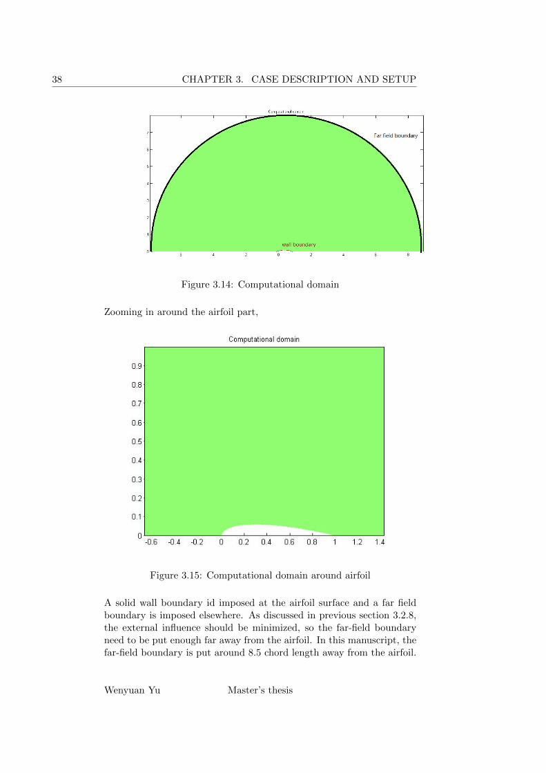
Figure 3.14: Computational domain

Zooming in around the airfoil part,

Figure 3.15: Computational domain around airfoil

A solid wall boundary id imposed at the airfoil surface and a far fieldboundary is imposed elsewhere. As discussed in previous section 3.2.8,the external influence should be minimized, so the far-field boundaryneed to be put enough far away from the airfoil. In this manuscript, thefar-field boundary is put around 8.5 chord length away from the airfoil.



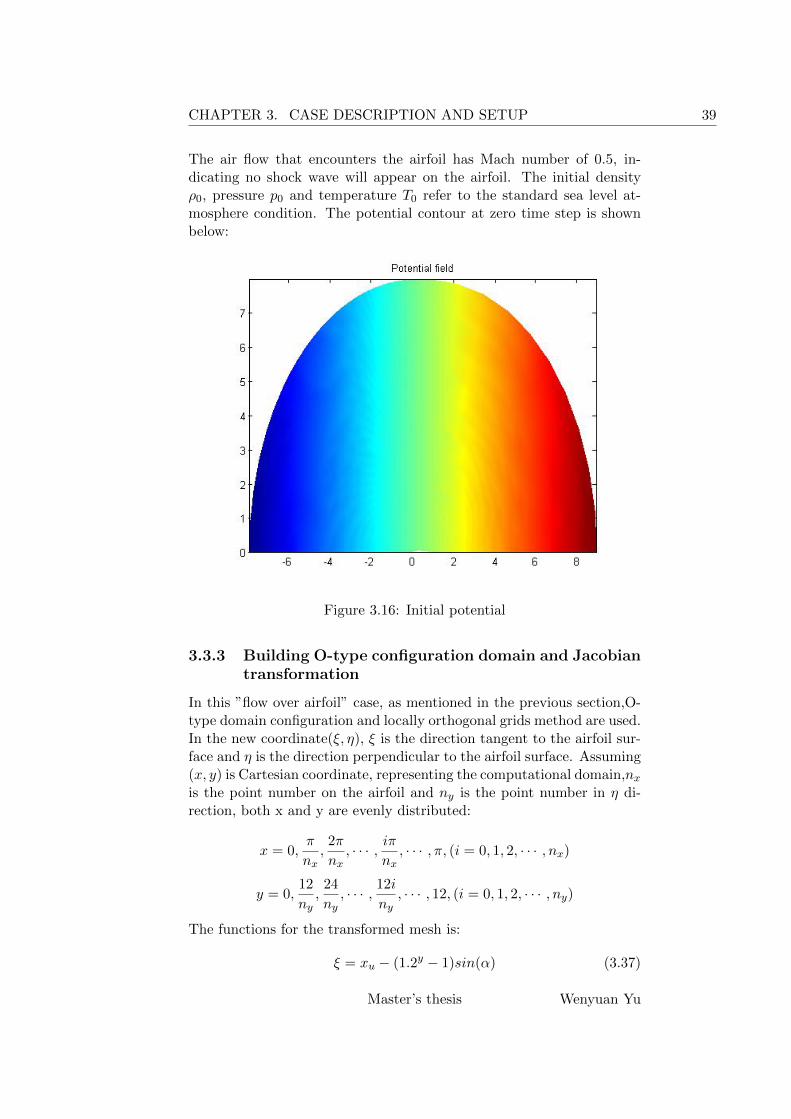
The air flow that encounters the airfoil has Mach number of 0.5, in-dicating no shock wave will appear on the airfoil. The initial densityρ0, pressure p0 and temperature T0 refer to the standard sea level at-mosphere condition. The potential contour at zero time step is shownbelow:

Figure 3.16: Initial potential

3.3.3 Building O-type configuration domain and Jacobiantransformation

In this ”flow over airfoil” case, as mentioned in the previous section,O-type domain configuration and locally orthogonal grids method are used.In the new coordinate(ξ, η), ξ is the direction tangent to the airfoil sur-face and η is the direction perpendicular to the airfoil surface. Assuming(x, y) is Cartesian coordinate, representing the computational domain,nxis the point number on the airfoil and ny is the point number in η di-rection, both x and y are evenly distributed:

x = 0,π

nx,2π

nx, · · · , iπ

nx, · · · , π, (i = 0, 1, 2, · · · , nx)

y = 0,12

ny,

24

ny, · · · , 12i

ny, · · · , 12, (i = 0, 1, 2, · · · , ny)

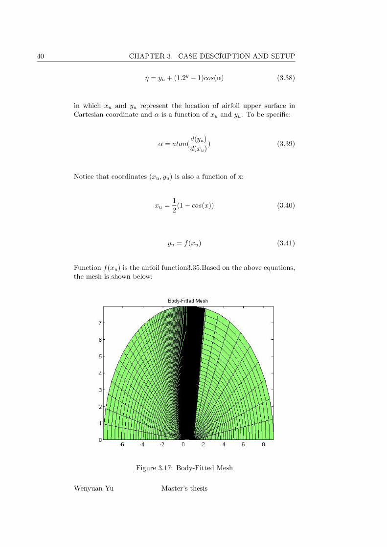
The functions for the transformed mesh is:

ξ = xu − (1.2y − 1)sin(α) (3.37)



η = yu + (1.2y − 1)cos(α) (3.38)

in which xu and yu represent the location of airfoil upper surface inCartesian coordinate and α is a function of xu and yu. To be specific:

α = atan(d(yu)

d(xu)) (3.39)

Notice that coordinates (xu, yu) is also a function of x:

xu =1

2(1− cos(x)) (3.40)

yu = f(xu) (3.41)

Function f(xu) is the airfoil function3.35.Based on the above equations,the mesh is shown below:

Figure 3.17: Body-Fitted Mesh



Figure 3.18: Mesh close to the airfoil

The method to build the Jacobian matrix has been disguised in the pre-vious section. The values (xξ, xη, yξ, yη) can be calculated with finitedifference schemes based on the relations 3.37 and 3.38. Once the Ja-cobian matrix is obtained, the physical domain can be transformed intoa regular computational domain where finite difference schemes can beused.

Figure 3.19: Physical domain for the airfoil case



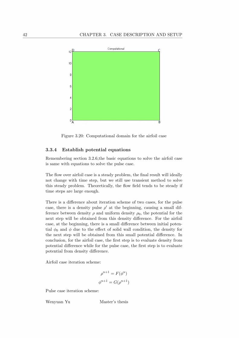
Figure 3.20: Computational domain for the airfoil case

3.3.4 Establish potential equations

Remembering section 3.2.6,the basic equations to solve the airfoil caseis same with equations to solve the pulse case.

The flow over airfoil case is a steady problem, the final result will ideallynot change with time step, but we still use transient method to solvethis steady problem. Theoretically, the flow field tends to be steady iftime steps are large enough.

There is a difference about iteration scheme of two cases, for the pulsecase, there is a density pulse ρ′ at the beginning, causing a small dif-ference between density ρ and uniform density ρ0, the potential for thenext step will be obtained from this density difference. For the airfoilcase, at the beginning, there is a small difference between initial poten-tial φ0 and φ due to the effect of solid wall condition, the density forthe next step will be obtained from this small potential difference. Inconclusion, for the airfoil case, the first step is to evaluate density frompotential difference while for the pulse case, the first step is to evaluatepotential from density difference.

Airfoil case iteration scheme:

ρn+1 = F (φn)

φn+1 = G(ρn+1)

Pulse case iteration scheme:



φn+1 = G(ρn)

ρn+1 = F (φn+1)

Function F and G depend on the selected discretization scheme on theequation 3.18 and equation 3.17 respectively.

3.3.5 Boundary conditions

As disguised in the case description section, at the external boundaryof domain, the flow field is assumed to be known. According to theequation [10],

φfarfield = U∞x +Γ

2πtan−1[

√1−M2tan(θ − α0)] + φ0 (3.42)

Γ is circulation around the airfoil. The term with circulation Γ is addedto revise the potential equation, due to the fact that potential flow isirrotational. As NACA-0012 is a symmetric airfoil and there is no angleof attack, the circulation Γ = 0. If assume φ0 = 0, the far-field potentialis:

φfarfield = U∞x (3.43)

As a result, to satisfy far-field boundary,referring to figure 3.20,

φDC = φfarfield = U∞x

Meanwhile, in order to satisfy the solid wall boundary condition at theairfoil surface, remembering

∂φ

∂n= 0

As direction of η is perpendicular to the upper surface of airfoil,we get:

∂φ

∂η= 0 (3.44)

To keep second order of accuracy, the biased finite difference scheme isused, φAB needed to be restricted:

φAB = 4φi,end−1 − 3φi,end−2 (3.45)




Chapter 4

Results and conclusions

In this chapter, the results from scheme testing case and 2D pulse casewill be presented. As solid wall boundary condition was not be able tobe coded in a correct way, the results for the airfoil section case was notobtained.

4.1 Scheme testing case

Setting time step as 100, plot the result from standard multi-pointscheme and analytical solution in the same figure, the results are shownbelow:

(a) Problem 1 (b) Problem 2

Figure 4.1: Standard 3 points stencil scheme

45

46 CHAPTER 4. RESULTS AND CONCLUSIONS







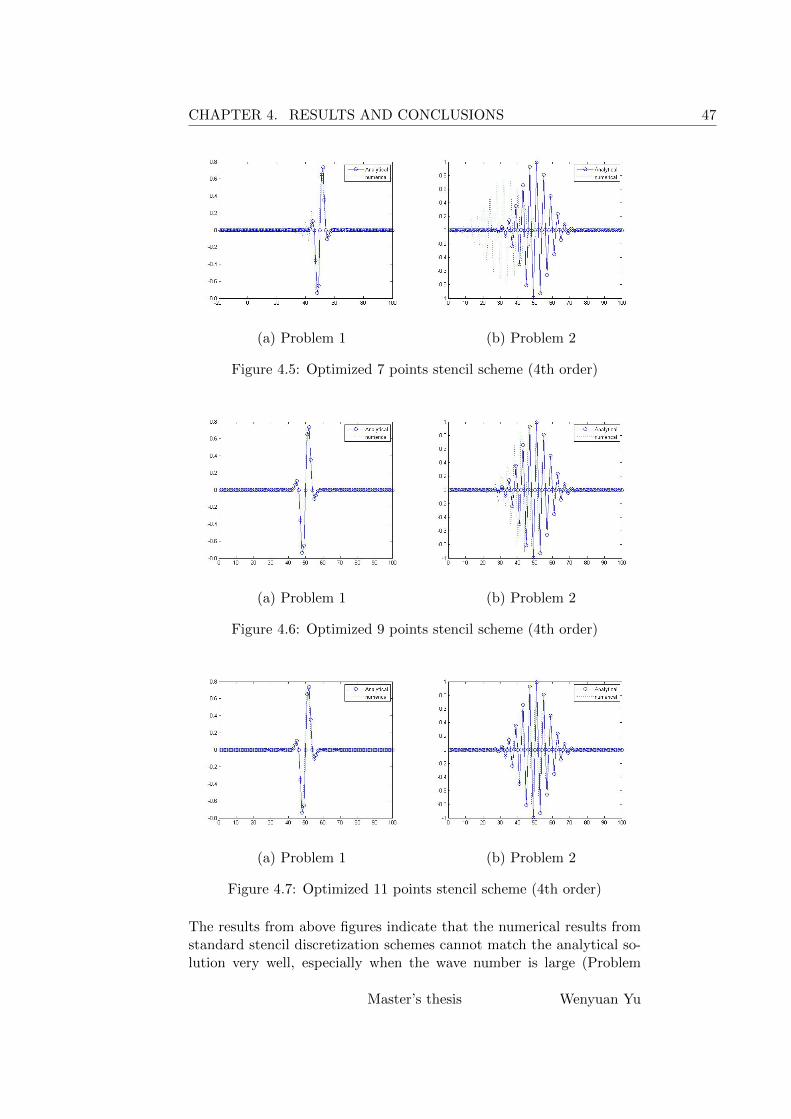
Keeping 4th order of accuracy and applying 7, 9, 11-point optimizedstencil schemes, the results are shown below:


CHAPTER 4. RESULTS AND CONCLUSIONS 47


Figure 4.5: Optimized 7 points stencil scheme (4th order)





The results from above figures indicate that the numerical results fromstandard stencil discretization schemes cannot match the analytical so-lution very well, especially when the wave number is large (Problem



2). With higher order of accuracy (fig4.4), the numerical solution couldmatch the analytical solution if the wave number k∗∆x is small.

Compared with standard stencil scheme, the 4th order optimized schemesobviously have better performances. The more points we put into thestencil, the better performance of the scheme, just as predicted fromfigure 2.2.

Define error as:

e = (∑

(unumerical − uexact)2/∑

uexact2)

12 (4.1)

XXXXXXXXXXXProblemscheme

3-point 5-point 7-point 9-point

e1 1.4126 1.2313 0.9790 0.8072e2 1.4170 1.3736 1.2979 1.1257

Table 4.1: Errors for the standard multi-point schemes

XXXXXXXXXXXProblemscheme

7-point 9-point 11-point

e1 0.5337 0.4440 0.4347e2 1.1529 0.9272 0.7976

Table 4.2: Errors for the 4th order optimized multi-point schemes

4.2 2D pulse case

This section will be separated into two subsections in which results fromEuler solver and potential solver will be presented respectively.

The evolution of the pulse in the physical domain is shown:



(a) nstep=0 (b) nstep=200


Figure 4.8: Evolution of the density pulse in rectilinear mesh

In the wavy mesh, the evolution of the density pulse is shown:





Figure 4.9: Evolution of the density pulse in wavy mesh

From above figures, we can conclude that results from rectilinear meshand wavy mesh is generally the same, indicating that the Jacobian trans-formation is correct.

To simplify the comparison with analytical solution and accelerate com-putation speed, the initial velocity u0(φ0) will be set as zero. The pulsewill as a result not move, but stay in the middle of domain and propa-gate in radial direction.

The numerical error will be calculated with equation:

Error =

√∫ ∫(panalytical − pnumerical)2dA∫ ∫

p2analyticaldA

(4.2)

Both analytical and numerical solution will be extracted at the y=0.The pressure profile from difference discretisation schemes will shown inthe same figure.

4.2.1 Euler solver

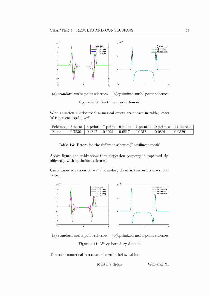
Using Euler equations on the rectilinear grid domain, the results areshown below:



(a) standard multi-point schemes (b)optimized multi-point schemes

Figure 4.10: Rectilinear grid domain

With equation 4.2,the total numerical errors are shown in table, letter’o’ represent ’optimized’,

Schemes 3-point 5-point 7-point 9-point 7-point-o 9-point-o 11-point-o

Error 0.7530 0.4347 0.1021 0.0917 0.0952 0.0891 0.0829

Table 4.3: Errors for the different schemes(Rectilinear mesh)

Above figure and table show that dispersion property is improved sig-nificantly with optimized schemes.

Using Euler equations on wavy boundary domain, the results are shownbelow:


Figure 4.11: Wavy boundary domain

The total numerical errors are shown in below table:




Error 0.7714 0.4046 0.1127 0.1023 0.1057 0.0996 0.0934

Table 4.4: Error from different schemes(wavy mesh)

The results from wavy mesh also indicates that optimized schemes con-tribute to a better dispersive property. Besides, comparing results fromtwo types of meshes, we can find that Jacobian transformation will pro-duce a small extra numerical errors.

To further prove the advantages of optimized schemes, we create a newinitial condition for the pulse case. Remembering the equation3.3, set-ting b as 1, indicating the pulse will have a larger wave number. Besides,the initial velocity u0 is set as 0.5 Mach. The results are shown below:


Figure 4.12: Rectilinear mesh domain(b=1,u0=0.5 Ma)

The total numerical errors are shown in the below table:


Error 1.4259 0.6474 0.1927 0.1321 0.1345 0.1260 0.1035

Table 4.5: Error from different schemes(Rectilinear mesh,b=1,u0=0.5Ma)

The figure and table indicate that the more points in the stencil, theless dispersion will the scheme behave.

4.2.2 Potential solver

Using potential equations on the rectilinear domain, the results areshown below:




Figure 4.13: Rectilinear mesh domain

The total numerical error from potential solver is shown in below table:Schemes 3-point 5-point 7-point 9-point 7-point-o 9-point-o 11-point-o

Error 0.6558 0.3226 0.3127 0.3142 0.3115 0.3128 0.3121

Table 4.6: Error from different schemes(Rectilinear mesh)

The results from figure and table show that potential solver will lead tosmall dispersive error compared with Euler equations, the accuracy ofpotential solver is generally lower than Euler equations. The optimizedschemes used on the potential solver will not produce higher accuracy.

Using potential solver on wavy boundary domain, the results are shownbelow:


Figure 4.14: Wavy boundary domain

The total numerical error from potential solver is shown in below table:




Error 0.6612 0.3272 0.3175 0.3183 0.3164 0.3176 0.3170

Table 4.7: Error from different schemes(wavy mesh)

Now setting b=1 and testing optimized scheme on potential solvers jusklike Euler solver, the results are shown below:


Figure 4.15: Rectilinear mesh domain(b=1)

The total numerical errors are shown in the below table:


Error 0.8726 0.4616 0.4215 0.4185 0.4167 0.4476 0.4176

Table 4.8: Error from different schemes(Rectilinear mesh,b=1)

The above figure and table shows that optimized schemes used on thepotential solver will not improve the dispersive property significantly.

4.2.3 Influence of Runge-Kutta method

In this section, we will change the order of Runge-Kutta method andfind out if the order of RK method has an effect on the final result.

We will select select optimized 7-point stencil scheme, and change theorder of RK method, compare the results from both Euler solver andpotential solver.



Figure 4.16: Optimized 9-point stencil scheme

Schemes 4th-RK-Euler 4th-RK-Potential 6th-RK-Euler 6th-RK-Potential

Error 0.0829 0.3115 0.0831 0.3113

Table 4.9: Optimized 9-point stencil scheme

Above figure and table show that the order of Rung-Kutta method hasno significant effect on the final results.

4.2.4 Time consumed by different solvers

In this section, a record on time consuming of different solvers will bepresented. Matlab functions ’tic’ and ’toc’ are used to record the time.Optimized 7-point and 9-point stencil schemes are selected to solve thesame problem based on Euler and potential solvers, the results are shownbelow:

XXXXXXXXXXXSchemeSolver

Euler Euler Jacobian Potential Potential Jocabian

7-point stencil 36.61 58.08 22.75 44.06

9-point stencil 39.01 61.3 24.07 46.22

7-point optimized stencil 36.71 58.07 23 44.79

9-point optimized stencil 39.14 60.03 24.3 46.83

Table 4.10: Time consumed by two solvers (second)

From table 4.10, we can conclude that Jacobian transformation is a pro-cess that consume a lot of time, while the number of points in the stencil



does not influence the time consuming significantly. Compared with Eu-ler solver, potential solver is much faster to solve the same equations.


Chapter 5

Conclusions

In this manuscript, centered different multi-points center difference schemesare built in form of matrices based on Matlab platform. To reducethe dispersion from center difference method, optimized multi-pointsschemes are used. While building these schemes, backward and forwardbiased finite schemes are also used close to the boundary. As being builtin the form of matrices, the spatial discretisation becomes a process ofvectorization. In temporal space, Runge-Kutta method is applied.

With discretisation method for spatial and time space, Euler equationsand potential equations are built in the form of matrices. Numericalsolution will then obtained from matrix and vector operation. Whilebuilding the solvers, the shape of physical domain is also considered. Ifthe physical domain is not a regular rectangular shape, Jacobian trans-formation matrix will be used to transform the complex coordinate intoa normal Cartesian coordinate.

Two cases are established based on Euler and potential solver. In 2Dpulse case, radiation boundary condition and solid wall boundary con-dition are considered. In the airfoil case, far-field boundary conditionand solid wall boundary condition are considered. In the airfoil case, adetailed description on how to build NACA airfoil meshes is presented.As there is something wrong with code on imposing boundary condi-tions, the results from airfoil case are not obtained. In 2D-pulse case,results from both solvers are obtained and are compared with analyticalsolution.

Through the comparison from 2D-Pulse case, the conclusions are drawn:(1) Potential solver is faster than Euler solver.(2) Euler solver is more accurate than Euler solver.(3) Potential solver is less sensitive to the exact wavenumber. Optimizedspatial discretisation schemes cannot improve the dispersion propertysignificantly in potential solver.

57

58 CHAPTER 5. CONCLUSIONS

(4) Euler solver is more sensitive to the exact wavenumber. Optimizedspatial discretisation schemes can improve the dispersion property sig-nificantly.(5) Jacobian transformation method will produce a small extra error onboth Euler and potential solvers.

Further work need to be done on revising the Matlab code for boundaryconditions. Besides, the Matlab code for airfoil mesh refinement need tobe developed. Once obtaining the results from airfoil case, the resultsshould be compared with the results from known solvers.


Bibliography

[1] C.K.W. Tam ”Computational aeroacoustics: issues and methods,AIAA J. 33 (10)(1995)” 1788–1796.

[2] C.K.W. Tam, J.C. Webb ”Dispersion-relation-preserving fi-nite difference schemes for computational acoustics, J. Comput.Phys(107)(1993) 261-281”

[3] ”Vectorization”.Documentation.Mathworks.2017.Web.

[4] John D. Anderson. ”Modern Compressible Flow with Historical Per-spective”. New York:McGraw-Hill,2003.

[5] Thomas H. Pulliam,David W. Zingg. ”Fundamental Algorithms inComputational Fluid Dynamics” New York: Springer, 2014.

[6] Julien,B.,Christophe,B. Olivier,M.(2006). ”Higher order,low disper-sive and low dissipative explicit schemes for multi-scale and bound-ary problems.” Lyon:Laboratoire de Me canique des Fluides etd’Acoustique

[7] Christopher K. W. Tam ”Computational Aeroacoustics a NewWavenumber Approach” USA:Florida State University,CambridgeUniversity press,2012.

[8] W. De Roeck,W. Desmet, M. Baelmans, P. Sas. ”An overview ofhigh-order finite difference schemes for computational aeroacoustics.”Leuven:K.U.Leuven, Department of Mechanical Engineering.

[9] P.Toth,A.Fritzsch,M.M.Lohasza. ”Application of ComputationalFluid Dynamics Softwares for 2D Acoustic Wave Propagation.” Bu-dapest:Department of Fluid Dynamics, Budapest University of Tech-nology and Economics,2008.

[10] C.Hirseh. ”Numerical Computation of Internal and External Flows(V OL2).” New York:John Wiley Sons,1994.

[11] Christophe Bogey,Christophe Bailly ”A family of low dispersiveand low dissipative explicit schemes for flow and noise computations”Lyon:Laboratoire de Me canique des Fluides et d’Acoustique,2003.

59

60 BIBLIOGRAPHY

[12] J.H.Williamson. ”Low Storage Runge-Kutta Schemes” England:Department of Computer Science, University of Reading,1979.

[13] T. J. Craft. ”Body-Fitted Grids” England: School of MechanicalAerospace and Civil Engineering,University of Manchester


www.kth.se

Documents

Development of a Fully Vectorized Potential Flow Solver1144406/FULLTEXT01.pdf · Matrix Laboratory (Matlab) ... ary layer e ect need not to be considered. ... (FDM) is based on the