Development of a Flame Spread Screening Tool for Fiber ... of a Flame Spread Screening Tool for Fiber Reinforced Polymers A Major Qualifying Project Report submitted to the Faculty

Development of a Flame Spread Screening Tool for Fiber Reinforced Polymers

A Major Qualifying Project Report

submitted to the Faculty of WORCESTER POLYTECHNIC INSTITUTE

in partial fulfillment of the requirements for the Degree of Bachelor of Science

By:

__________________________ Valerie Boutin

__________________________

Andrew Eng

__________________________ Michael Gorgone

__________________________

Matthew Guilfoyle

__________________________ Craig Mitchell

__________________________

Chelsea Tuttle

May 2012 Project number: NAD FM11

__________________________ Professor Nicholas A. Dembsey, Advisor

1-1

Table of Contents Table of Contents ............................................................................................................................. 1-1

1. Organization of this MQP ................................................................................................................... 1-5

2. Development of a Flame Spread Screening Tool for Fiber Reinforced Polymers for Interior

Applications................................................................................................................................................ 2-5

2.1. Abstract ...................................................................................................................................... 2-5

2.2. Introduction ............................................................................................................................... 2-5

2.3. Interior Finishes ......................................................................................................................... 2-6

2.4. Database .................................................................................................................................... 2-7

2.5. The Model ................................................................................................................................ 2-10

2.6. Tunnel Test Calibration Inputs ................................................................................................. 2-13

2.7. Room Corner Test Calibration Inputs ....................................................................................... 2-13

2.8. Results ...................................................................................................................................... 2-14

2.9. Conclusion and Recommendations.......................................................................................... 2-18

2.10. Nomenclature ...................................................................................................................... 2-18

2.11. References ........................................................................................................................... 2-18

3. Development of a Flame Spread Screening Tool for Fiber Reinforced Polymers for Interior

Applications.............................................................................................................................................. 3-19

3.1. Abstract .................................................................................................................................... 3-19

3.2. Introduction ............................................................................................................................. 3-20

3.3. Database .................................................................................................................................. 3-21

3.4. Cone ......................................................................................................................................... 3-22

3.5. Model ....................................................................................................................................... 3-23

3.6. Results ...................................................................................................................................... 3-25

3.7. Design ....................................................................................................................................... 3-28

3.8. Compartment Effects ............................................................................................................... 3-30

3.9. Conclusion ................................................................................................................................ 3-31

3.10. Nomenclature ...................................................................................................................... 3-31

3.11. References ........................................................................................................................... 3-32

4. Conclusion ........................................................................................................................................ 4-34

5. Acknowledgements .......................................................................................................................... 5-34

1-2

Appendix A Cone Calorimeter .................................................................................................... A-35

Appendix B Flame Spread Model Adaptations ............................................................................ B-36

Appendix C Flame Correlation ..................................................................................................... C-46

Appendix D Uncertainty ............................................................................................................. D-50

Appendix E NFPA 285 Review ..................................................................................................... E-52

Appendix F NFPA 286 Review ..................................................................................................... F-56

Appendix G ASTM E84 Review .................................................................................................... G-58

Appendix H Compartment Effect ................................................................................................ H-60

Appendix I International Building Code Review .......................................................................... I-63

Appendix J Cone: Heat Release Rate Histories ........................................................................... J-66

Appendix K Cone: Specific Extinction Area Histories ................................................................ K-107

Appendix L B-Parameter Analysis ............................................................................................. K-147

Appendix M Smoke Calculations ................................................................................................ K-158

List of Figures

Figure 2-1:Areas of a Building .................................................................................................................... 2-6

Figure 2-2: Baseline FRP ............................................................................................................................. 2-8

Figure 2-3: Sandwich Panel FRP ................................................................................................................. 2-8

Figure 2-4: HRRPUA of Baseline FRP at Variable Heat Fluxes .................................................................... 2-9

Figure 2-5: Baseline FRP time to Ignition vs Incident Heat Flux ................................................................ 2-9

Figure 2-6: Mowrer and Williamson Flame Spread Model ...................................................................... 2-10

Figure 2-7: Pyrolysis Front of Baseline FRP in Tunnel Test ...................................................................... 2-14

Figure 2-8: Room Corner Test Wall Configuration ................................................................................... 2-15

Figure 2-9: Room Corner Test Ceiling Configuration ............................................................................... 2-16

Figure 2-10: Baseline HRR Calibration Results With No Ceiling ............................................................... 2-16

Figure 2-11: Baseline HRR Calibration Results With Ceiling .................................................................... 2-16

Figure 3-1: Baseline FRP ........................................................................................................................... 3-21

Figure 3-2: FRP Sandwich Panel ............................................................................................................... 3-21

Figure 3-3: Repeat Runs of Baseline FRP at 50kW/m2 ............................................................................. 3-22

Figure 3-4: NFPA 285 Model Results Cores.............................................................................................. 3-26

Figure 3-5: NFPA 285 Model Results Fillers ............................................................................................. 3-26

Figure 3-6: NFPA 285 Model Results Aggregates ..................................................................................... 3-27

Figure 3-7: NFPA 285 Model Results Pigments ........................................................................................ 3-27

Figure 3-8: NFPA 285 Model Results Resin Changes ............................................................................... 3-28

1-3

Figure 3-9: Incident Heat Flux Distribution .............................................................................................. 3-29

Figure 3-10: Equivalent Screening Test Front View ................................................................................. 3-30

Figure 3-11: Equivalent Screening Test Top View .................................................................................... 3-30

List of Tables

Table 2-1: IBC Interior Finish Requirements .............................................................................................. 2-7

Table 2-2: FRP System Modifications ......................................................................................................... 2-8

Table 2-3: Model Inputs at 65kW/m2 ...................................................................................................... 2-10

Table 2-4: Calibration Inputs .................................................................................................................... 2-14

Table 2-5: Simulated Test Results ............................................................................................................ 2-17

Table 3-1: FRP System Modifications ....................................................................................................... 3-21

Table 3-2: Model Inputs at 65kW/m2 ...................................................................................................... 3-23

Table 3-3: NFPA 285 Inputs for Baseline System ..................................................................................... 3-25

Table 3-4: Compartment Effects .............................................................................................................. 3-31

2-5

1. Organization of this MQP This MQP is a compilation of two 15-page conference papers focusing on flame spread

modeling of fiber reinforced polymers. Chapter two is the first of the two papers and focuses on interior testing. Chapter three is the second of the papers and focuses on exterior testing as well as a capstone design exercise. Abstract and references are included with each respective chapter. The MQP also contains a series of appendices to cover material in a complexity not covered in the conference style paper.

2. Development of a Flame Spread Screening Tool for Fiber Reinforced

Polymers for Interior Applications

2.1. Abstract

The International Building Code (IBC) is often referenced in the United States to establish requirements for new construction. Based on performance criteria established in the IBC, interior finish materials are rated Class A, B, or C or pass/fail. The uses of materials are limited to particular building areas and applications according to their classification. To obtain a classification, materials must undergo full-scale standardized tests: Tunnel Test and Room Corner Test (ASTM E 84 or NFPA 286 respectively). The Tunnel Test is beneficial because it is less expensive to conduct, provides a greater range of classification, and is a traditional test in the field of fire protection. The Room Corner Test is advantageous because the conditions are more realistic and comparable to true fire scenarios. Both of these tests impose a potentially significant economic penalty for material development. Currently there is no IBC process for screening materials based on economical bench-scale standardized testing (ASTM E 1354) to assess materials performance in full-scale tests. Fiber reinforced polymers (FRPs) are of growing interest in building construction due to their customizability. An initial flame spread model was developed relating Cone Calorimeter (ASTM E 1354) test data to full-scale test scenarios in the Tunnel Test and Room Corner Test. The flame spread model is capable of screening new materials to suggest performance levels in full-scale testing based on material properties of FRP systems.

2.2. Introduction

Material developers are faced with the challenge of creating new materials that fit both an architect’s vision and the Authority Having Jurisdiction’s (AHJ’s) safety requirements. The International Building Code (IBC) [1] is often referenced in the United States by the AHJ to establish safety requirements for new construction. The IBC requires any new interior finish material to undergo a full-scale standardized test, either the Tunnel Test (ASTM E84) [2] (Appendix G) or the Room Corner Test (NFPA 286) [3] (Appendix F). The Tunnel Test will result in a classification (A, B, or C), and this classification will determine where the material can be used inside the building. The Room Corner Test results are reported as pass/fail. If the material passes it can be used virtually anywhere inside the building. These tests are both time

2-6

consuming and costly. If the desired result is not attained, the material developer must make changes and submit the material for retesting. Additional testing imposes a potentially significant economic penalty for material development. Currently, there is no process for screening materials based on the more economical bench-scale standardized tests such as the Cone Calorimeter (ASTM E 1354) [4] (Appendix A) to assess performance in full-scale tests.

This project studied the relationship between the material properties measured in the Cone Calorimeter of fiber reinforced polymers (FRPs) and their performance in full-scale tests. These materials are of growing interest in building construction due to their customizability. An initial flame spread model was developed relating Cone Calorimeter material properties to full-scale test scenarios in the Tunnel Test and Room Corner Test. The Tunnel Test model was based on previous work by Mowrer and Williamson [5] and the Room Corner Test model used this work in conjunction with Schebel’s work [6]. Fourteen FRP systems, each with a change in one component (e.g. resin type, aggregate type, etc.) were screened using the model.

In going forward, manufacturers will be able to use this initial model to screen materials relative to full-scale standardized test performance, and determine in which applications their material can be used. This will enable them to make changes to the material to obtain optimum performance without wasting time and resources on multiple full-scale tests.

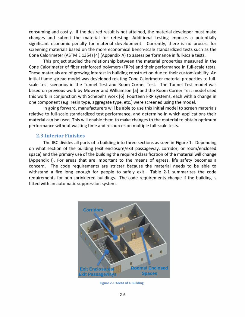
2.3. Interior Finishes

The IBC divides all parts of a building into three sections as seen in Figure 1. Depending on what section of the building (exit enclosure/exit passageway, corridor, or room/enclosed space) and the primary use of the building the required classification of the material will change (Appendix I). For areas that are important to the means of egress, life safety becomes a concern. The code requirements are stricter because the material needs to be able to withstand a fire long enough for people to safely exit. Table 2-1 summarizes the code requirements for non-sprinklered buildings. The code requirements change if the building is fitted with an automatic suppression system.

Corridors

Exit Enclosures/

Exit Passageways

Rooms/ Enclosed

Spaces

Figure 2-1:Areas of a Building

2-7

Table 2-1: IBC Interior Finish Requirements

2.4. Database

Fourteen (14) FRP systems provided by Kreysler & Associates were designed for interior applications. The Baseline FRP Figure 2-2 was a 0.06in (1.5mm) thick polymer concrete layer that contained a resin, alumina trihydrate, and sand aggregate. The substrate was a 0.1875in (4.8mm) layer consisting of a resin and 4 layers of glass in a chopped strand mat mixed in a glass to resin ratio range of 25:75 to 35:65 by weight. The resin used in both layers was Norsodyne with intumescent additives. The other FRP systems were modifications of the Baseline, each with one variation of a component: sand aggregate was replaced by specified fillers, the size of sand aggregate was altered, various pigments were added to the polymer concrete, and the surface layer was changed to Norsodyne without an aggregate and the substrate layer was changed to DCPD. Additionally, three FRP systems were sandwich panels Figure 2-2 with the Baseline FRP on the top face, varying materials in the core, and an identical substrate layer on the bottom face. A complete table of FRP systems can be seen in Table 2-2: FRP System .

Occupancy Example Exit Enclosures & Exit

Passageways Corridors

Rooms & Enclosed Spaces

Assembly-1 & Assembly 2

Theater & Restaurant A A B

Assembly-3, Assembly-4, & Assembly 5

Community Hall, Arena, & Stadium

A A C

Business, Educational, Mercantile, & Residential-1

Office, School, Retail Store, & Hotel

A B C

Residential-4 Assisted Living (6-15

people) A B B

Factory Millwork B C C

High Hazard Storage of Toxic

Materials A A B

Institutional-1 Assisted Living Facility A B B Institutional-2 Hospital A A B Institutional-3 Prison A A B Institutional-4 Child Daycare Facility A A B Residential-2 Apartment B B C

Residential-3 Adult Care Facility (<5

people) C C C

Storage Warehouse B B C

2-8

Figure 2-2: Baseline FRP

Figure 2-3: Sandwich Panel FRP

Table 2-2: FRP System Modifications

Filler Aggregate Pigment Resin Core

Bronze #0/30 White Norsodyne Plywood

Aluminum #0/60 Grey DCPD Balsa

#2/16 Beige Foam

Following ASTM E 1354 (See Appendix A), the fourteen FRP specimens were tested in the Cone Calorimeter to obtain bench-scale material properties. Incident heat fluxes of 25, 50, and 75kW/m2 were selected for testing. Various material properties were obtained including the heat release rate per unit area (HRRPUA), time to ignition (tf), and mass loss rate. Qualitative observations were made during the test to determine other parameters required for large-scale prediction (e.g. time to burn out). A database was developed to organize the information by specimen type and document each specimen’s characteristics. Typical variation in heat release rate caused by changes to the incident heat flux of the Cone is shown in Figure 2-4. A complete compilation of Cone data can be found in Appendix J and Appendix K.

2-9

Figure 2-4: HRRPUA of Baseline FRP at Variable Heat Fluxes

A significant drop in heat release rate was seen at an incident heat flux of 25kW/m2. This suggests that this value is near the minimum heat flux for ignition of the material. This is further illustrated by the significant increase in time to ignition at the lower heat flux as seen in Figure 2-5.

Figure 2-5: Baseline FRP time to Ignition vs Incident Heat Flux

The Database of inputs each system from the Cone Calorimeter is highlighted in Table 2-3. These inputs will be used in the Modeling Section below.

0

20

40

60

80

100

120

140

160

0 500 1000 1500

HR

RP

UA

(kW

/m2)

Time (s)

HRRPUA of Baseline FRP at Varying Heat Flux

25kW/m^2

50kW/m^2

75kW/m^2

0

100

200

300

400

0 20 40 60 80

Tim

e to

Ign

itio

n (

s)

Incident Heat Flux (kW/m2)

Baseline FRP Time to Ignition vs. Incident Heat Flux

2-10

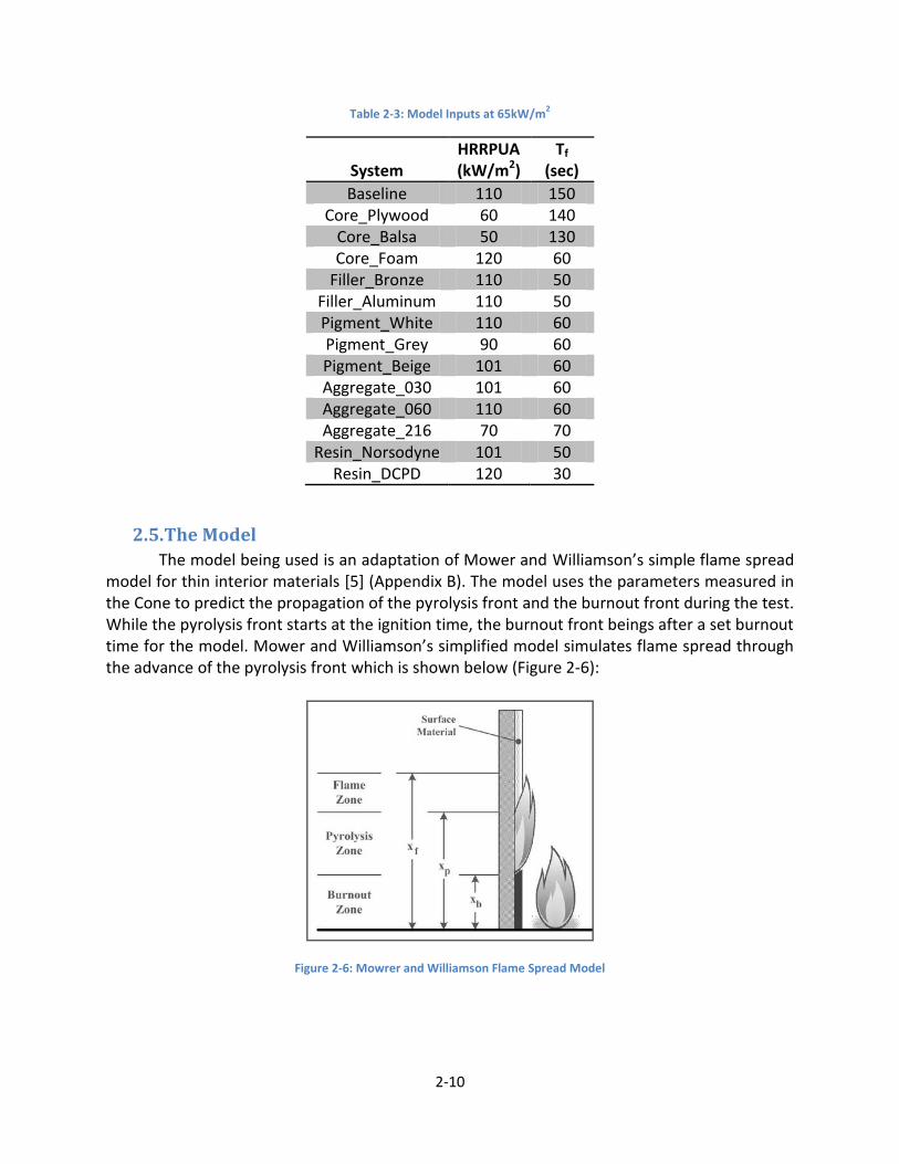
Table 2-3: Model Inputs at 65kW/m2

System

HRRPUA (kW/m2)

Tf (sec)

Baseline 110 150 Core_Plywood 60 140

Core_Balsa 50 130 Core_Foam 120 60

Filler_Bronze 110 50 Filler_Aluminum 110 50 Pigment_White 110 60 Pigment_Grey 90 60 Pigment_Beige 101 60 Aggregate_030 101 60 Aggregate_060 110 60 Aggregate_216 70 70

Resin_Norsodyne 101 50 Resin_DCPD 120 30

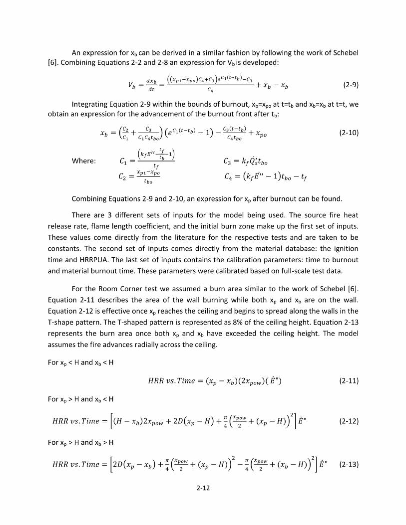
2.5. The Model

The model being used is an adaptation of Mower and Williamson’s simple flame spread model for thin interior materials [5] (Appendix B). The model uses the parameters measured in the Cone to predict the propagation of the pyrolysis front and the burnout front during the test. While the pyrolysis front starts at the ignition time, the burnout front beings after a set burnout time for the model. Mower and Williamson’s simplified model simulates flame spread through the advance of the pyrolysis front which is shown below (Figure 2-6):

Figure 2-6: Mowrer and Williamson Flame Spread Model

2-11

( ) ( )

(2-1)

The advancement of the pyrolysis front is based on flame height, pyrolysis height and ignition time. Once burnout begins this value is shown by:

( ) ( )

(2-2)

Mower and Williamson finish their derivation by integrating the equations within specific bounds to gain relationships for xp and xb. However, since the source fire plays a significant role in the flame spread of standardized tests, the equations have been adapted to incorporate the source fire. The driving force behind the model is the forward heating zone, represented by the flame length. The flame length is calculated using a linearized approximation suggested by Quintiere et. Al [7]. The flame length approximation before burnout therefor becomes:

(2-3)

A similar flame length approximation is used for times after burnout:

( ) (2-4)

Using the flame length approximation including the source fire, Equation 2-.1 can be rewritten using Equation 2-3 as:

( )

(2-5)

Using Equation 2-5, a relationship is derived for xp before burnout by integrating with the bounds of xp=xpo at t=0 and xp=xp at t=t. With these bounds Equation 2-5 can be integrated and rearranged:

(

)

(

)

(2-6)

According to Mower and Williamson [5], the flame spread can be expressed as the advancement of the pyrolysis zone, Vp-Vb. Combining Equations 2-1 and 2-2 with Equation 2-4, we get a relationship for the advancement of the pyrolysis zone after burnout begins, shown below:

( ) ( ) ( )

( )

(2-7)

Integrating Equation 2-7 with the bounds of xp-xb=xp1-xpo at t=tb and xp-xb= xp-xb at t=t a relationship between the pyrolysis zone and time can be seen below:

(( ) )

( )

(2-8)

2-12

An expression for xb can be derived in a similar fashion by following the work of Schebel [6]. Combining Equations 2-2 and 2-8 an expression for Vb is developed:

(( ) ) ( )

(2-9)

Integrating Equation 2-9 within the bounds of burnout, xb=xpo at t=tb and xb=xb at t=t, we obtain an expression for the advancement of the burnout front after tb:

(

) ( ( ) )

( )

(2-10)

Where: (

)

( )

Combining Equations 2-9 and 2-10, an expression for xp after burnout can be found.

There are 3 different sets of inputs for the model being used. The source fire heat

release rate, flame length coefficient, and the initial burn zone make up the first set of inputs.

These values come directly from the literature for the respective tests and are taken to be

constants. The second set of inputs comes directly from the material database: the ignition

time and HRRPUA. The last set of inputs contains the calibration parameters: time to burnout

and material burnout time. These parameters were calibrated based on full-scale test data.

For the Room Corner test we assumed a burn area similar to the work of Schebel [6].

Equation 2-11 describes the area of the wall burning while both xp and xb are on the wall.

Equation 2-12 is effective once xp reaches the ceiling and begins to spread along the walls in the

T-shape pattern. The T-shaped pattern is represented as 8% of the ceiling height. Equation 2-13

represents the burn area once both xp and xb have exceeded the ceiling height. The model

assumes the fire advances radially across the ceiling.

For xp < H and xb < H

( )( )( ) (2-11)

For xp > H and xb < H

[( ) ( )

(

( ))

] (2-12)

For xp > H and xb > H

[ ( )

(

( ))

(

( ))

] (2-13)

2-13

2.6. Tunnel Test Calibration Inputs

The input parameter xp0 represents the length of the initial pyrolysis zone in meters. For the Tunnel Test model it is taken as equal to 0.6m. This value was estimated for the Tunnel Test based on a heat flux map for ASTM E 84 [8], and the assumption that xp0 would represent an ignition length where the heat fluxes are above 30kW/m2, which is consistent with the observation in the Cone testing that the critical heat flux of the FRP systems is approximately 25kW/m2. The maximum heat flux from the heat flux map was approximately 44kW/m2. The average heat flux over the estimated 0.6m was 36kW/m2 which was rounded to 40kW/m2. The

input represents the heat release rate per unit area of the baseline FRP system at a characteristic heat flux composed of the source fire and the insult from wall flames. To obtain this characteristic heat flux, the value from the burner (40kW/m2) is added to 25kW/m2. The 25kW/m2 is the estimated heat flux from the burning specimen according to the wall [9]. This results in a total incident heat flux of 65kW/m2. From a graph of HRRPUA vs. heat flux from the Cone data, and the characteristic heat flux of 65kW/m2, an interpolated value for HRRPUA was 110kW. The same method of interpolation was used to calculate a time to ignition at a heat flux of 65kW/m2 (Similar to Figure 2-5). The input kf is a constant and the value 0.011 is used. This value is increased from the suggested 0.01 value due to the forced flow effects in the tunnel. Based on the work of Fernandez-Pello [10], forced flow increases the heat transfer between the flame and ceiling (this is further detailed in Appendix C). The inputs tb and tbo were calibration parameters adjusted during calibration. Ultimately both inputs were assigned a value of 60 seconds which yielded model results consistent with the actual full-scale test results. After 60 seconds the flame spread has advanced outside of the source fire heat affected zone. The model reflects this by neglecting the source fire after 60 seconds. All calibration inputs are outlined in Table 2-4.

2.7. Room Corner Test Calibration Inputs

In the room corner test, the initial burn zone is equal to 0.5m. This was estimated using the work of Williamson and Revenaugh [11]. The input kf is a flame length parameter. As outlined in Clearey and Quintiere’s paper [7] a value 0 .01 is used for buoyant flow. The input

represents the characteristic heat release per unit area which consists of the heat from the source fire to the wall and from the burning material to the wall. The value used was 85kW/m2. An approximate value of 60kW/m2 was used for the heat from the source fire to the wall. An additional 25kW/m2 was added to account for the heat from the burning material to the wall [9]. Since the cone data was only available for a maximum incident heat flux of 75kW/m2, these values were used. The time to ignition, tf, was selected based on the cone data at 75kW/m2. Similar to the tunnel test calibration, tb and tbo were calibration parameters adjusted during calibration. Ultimately, tbo was assigned a value of 400s, and tb was assigned a value of 60s, in order to yield the best fit from the model to the actual full-scale test results.

2-14

Table 2-4: Calibration Inputs

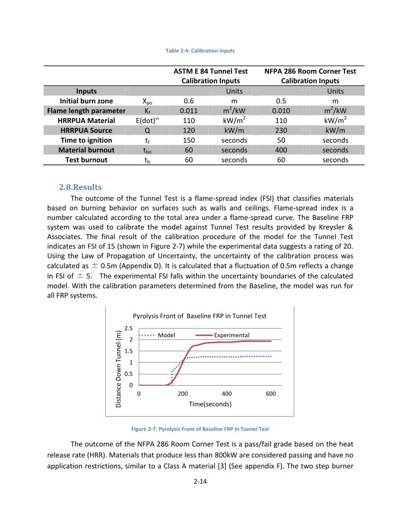
2.8. Results

The outcome of the Tunnel Test is a flame-spread index (FSI) that classifies materials based on burning behavior on surfaces such as walls and ceilings. Flame-spread index is a number calculated according to the total area under a flame-spread curve. The Baseline FRP system was used to calibrate the model against Tunnel Test results provided by Kreysler & Associates. The final result of the calibration procedure of the model for the Tunnel Test indicates an FSI of 15 (shown in Figure 2-7) while the experimental data suggests a rating of 20. Using the Law of Propagation of Uncertainty, the uncertainty of the calibration process was

calculated as ± 0.5m (Appendix D). It is calculated that a fluctuation of 0.5m reflects a change

in FSI of ± 5. The experimental FSI falls within the uncertainty boundaries of the calculated model. With the calibration parameters determined from the Baseline, the model was run for all FRP systems.

Figure 2-7: Pyrolysis Front of Baseline FRP in Tunnel Test

The outcome of the NFPA 286 Room Corner Test is a pass/fail grade based on the heat

release rate (HRR). Materials that produce less than 800kW are considered passing and have no

application restrictions, similar to a Class A material [3] (See appendix F). The two step burner

0

0.5

1

1.5

2

2.5

0 200 400 600

Dis

tan

ce D

ow

n T

un

nel

(m

)

Time(seconds)

Pyrolysis Front of Baseline FRP in Tunnel Test

Model Experimental

ASTM E 84 Tunnel Test

Calibration Inputs NFPA 286 Room Corner Test

Calibration Inputs

Inputs

Units Units Initial burn zone Xpo 0.6 m 0.5 m

Flame length parameter Kf 0.011 m2/kW 0.010 m2/kW HRRPUA Material E(dot)'' 110 kW/m2 110 kW/m2 HRRPUA Source Q 120 kW/m 230 kW/m Time to ignition tf 150 seconds 50 seconds

Material burnout tbo 60 seconds 400 seconds Test burnout tb 60 seconds 60 seconds

2-15

regime of 286 was used where the HRR of the burner starts at 40kW for 5 minutes followed

immediately by 160 kW for 10 minutes. The experimental room corner tests were not run in

exact accordance with NFPA 286. There were four tests each with variations. The first two tests

(one with the baseline FRP and one with the Norsodyne resin FRP) were run as screening tools.

Panels were placed vertically up the corner and horizontally across where the wall meets the

ceiling. In addition, two panels were placed on the ceiling. For the second two tests, these

ceiling panels were removed. These configurations can be seen in Figure 2-8 and Figure 2-9. For

a screening specimen to be considered valid, the pyrolysis zone cannot reach the end of the

panels. In these experiments, the ends of the specimens were reached indicating that further

flame spread would be expected and greater HRRs would be produced. These greater HRRs

indicate that the two FRP systems on the walls and ceiling will not pass a NFPA 286 test using a

full specimen. To simplify the model calibration, two additional experiments were conducted

using a constant burner HRR of 160kW for 10 minutes. In one experiment the Baseline FRP was

used with no ceiling panels, and in the other experiment the surface coating Norsodyne resin

FRP with ceiling panels was used. As with the Tunnel Test, this model was calibrated against the

Baseline and Norsodyne surface layer experimental results. The results of these two

experiments are shown in Figure 2-10 and Figure 2-11. The experimental results without the

ceiling (Figure 2-10) indicate a maximum HRR of 340kW (prior to compartment effect) while our

model suggests a maximum of 310kW. Using the Law of Propagation of Uncertainty, the

uncertainty of the calibration process was calculated as ± 40kW (Appendix D). The

experimental results for the test with a ceiling indicate a maximum heat release rate of

780kW/m2 while the model suggests a maximum of 2000kW/m2 with an uncertainty of ± 40kW.

Figure 2-8: Room Corner Test Wall Configuration

2-16

Figure 2-9: Room Corner Test Ceiling Configuration

Figure 2-10: Baseline HRR Calibration Results With No Ceiling

Figure 2-11: Baseline HRR Calibration Results With Ceiling

0

100

200

300

400

500

0 100 200 300 400 500 600

HR

R (

kW)

Time (seconds)

Heat Release Rate - Baseline Room Corner Test Without Ceiling

Model Experimental

0

500

1000

1500

2000

2500

0 100 200 300 400 500 600

HR

R (

kW)

Time (seconds)

Heat Release Rate - Baseline Room Corner Test With Ceiling

Model Experimental

2-17

Table 2-5: Simulated Test Results

ASTM E84 Tunnel Test NFPA 286 Room Corner

Test No Ceiling

NFPA 286 Room Corner Test

With Ceiling

Specimen FSI Class HRR (kW) Pass HRR (kW) Pass Baseline 15 A 310 Yes 2040 No

Bronze Filler 45 B 460 Yes 2690 No Al Filler 45 B 510 Yes 2740 No

0/30 Aggregate 30 B 480 Yes 2550 No 0/60 Aggregate 35 B 410 Yes 2300 No 2/16 aggregate 20 A 370 Yes 2100 No White Pigment 40 B 280 Yes 1310 No Grey Pigment 25 A 410 Yes 2120 No Beige Pigment 30 B 400 Yes 2300 No

Norsodyne Resin 40 B 420 Yes 2310 No

DCPD Resin* 180 20

C A

480 Yes 2550 No

Plywood Core 15 A 260 Yes 1380 No Balsa Core 15 A 350 Yes 2070 No Foam Core 15 A 290 Yes 1660 No

*DCPD Resin has two reported FSIs because there was a large discrepancy in the cone data for time to ignition*

As seen in Table 2-5, all of the FRP systems received an A or B classification in the Tunnel Test and passed the Room Corner Test if the FRP is not placed on the ceiling. If the FRP were to be used on the ceiling, the model predicts the specimen will not meet the passing requirements.

Even though all FRPs passed the tests, the different groups of systems performed

differently. Changing the fillers had a significant negative effect on HRR, with these systems

having an FSI of 45. This change from the baseline FSI of 15 is significant because it is exceeds

the bounds of uncertainty of our model. Changing the aggregates had a less significant effect,

with FSI values ranging from 20 to 35, but several of these are outside the bounds of our

uncertainty. Changing the pigments also had a less significant effect, with FSI values ranging

from 25 to 40, but several of these are outside the bounds of our uncertainty as well. The

addition of cores had little to no impact on the FSI. As seen in Table 2-5, there are similar

trends between tests within the groups of systems. The systems with different fillers had the

highest HRR, the ones with different pigments had the next highest HRR, the ones with the

different aggregate sizes had lower HRR, and the systems with the different cores had little to

no change in HRR. The screening tool was unable to accurately represent the systems with resin

changes the Norsodyne surface layer and the DCPD substrate layer because their initial burning

behaviors were outside the paradigm of model.

2-18

2.9. Conclusion and Recommendations

The recommendations of the team are that none of the FRP systems should be used on the ceiling. If a class A rating is desired, the FRPs with different fillers should not be used, and systems with different aggregate sizes or pigments should be carefully considered before use. The systems with added cores behave similarly to the Baseline FRPs and therefore should be able to be used in the same applications. During our analysis it was determined that the driving factor behind changes in performance was the time to ignition. The systems that ignited the quickest had the highest FSI in the Tunnel Test and the highest HRR in the Room Corner Test. This should be taken into consideration when analyzing different FRP systems. In conclusion, this project created a simple, easy to use flame spread model for different FRPs that gives a better indication of performance of the modified FRPs without spending money on full-scale testing. This allows manufacturers to know where different systems could be used in a building. In the future we hope the framework of this project can be used to facilitate further research.

2.10. Nomenclature

(HRRPUA)

( )

2.11. References

(1) International Building Code, 5th Edition.

(2) ASTM E 84, “Standard Test Method for Surface Burning Characteristics of Building

Materials,” ASTM International, West Conshohocken, PA

(3) NFPA 286, Standard Methods of Fire Tests for Evaluating Contribution of Wall and

Ceiling Interior Finish to Room Fire Growth, 2011 Edition

3-19

(4) ASTME E 1354, “Standard Test Method for Heat and Visible Smoke Release Rates for

Materials and Products Using an Oxygen Consumpiton Calorimeter,” ASTM

International, West Conshohocken, PA

(5) Mowrer, F.W., and Williamson, R.B.. “Flame Spread Evaluation for Thin Interior Finish

Materials”. Fire Safety Science-Proceedings of the Third International Symposium,

p. 689-698.

(6) Schebel, K., Dembsey, N.A., Meacham, B.J., Johann, M., Tubbs, J., and Alston, J. “Fire

Growth Simulation in Passenger Rail Vehicles Using a Simplified Flame Spread

Model Coupled with a CFD Fire Model”.

(7) Cleary, T.G., and Quintiere, J.G.. “A Framework for Utilizing Fire Property Tests”. Fire

Safety Science-Proceedings of the Third International Symposium, p. 647-656.

(8) Society of Fire Protection Engineering Handbook, 3rd edition: 2-14.59


(10) Fernandez-Pello, C., & Zhou, L. “Turbulent, Concurrent, Ceiling flame spread: The

Effect of Buoyancy.” Combustion and Flame 92:45-49 (1993).

(11) Williamson,R, Revenaugh, A “Ignition Sources in Room Fire Tests and Some

Implications for Flame Spread Evaluation”

3. Development of a Flame Spread Screening Tool for Fiber Reinforced

Polymers for Interior Applications

3.1. Abstract

The International Building Code (IBC) is often referenced in the United States to

establish requirements for new construction. Based on performance criteria, exterior cladding

materials are classified as pass or fail, and require a pass in order to be used on the exterior of a

building (with some exceptions listed in the IBC). To obtain this classification, materials must

undergo a full-scale standardized test, NFPA 285, which imposes an economic penalty for

materials development. Currently there is no process for screening materials based on

economical bench-scale standardized testing such as the Cone Calorimeter (ASTM E 1354) to

assess materials’ performance in full-scale tests.

This study investigated the relationship between bench-scale material properties of

various fiber reinforced polymers (FRPs) and their performance in full-scale tests. A flame

3-20

spread model was developed relating Cone Calorimeter (ASTM E 1354) test data to the full-

scale Multi Story Building Test (NFPA 285). Initial evaluation shows the model to be a useful

tool for screening materials. In going forward, manufacturers will be able to use this model to

screen materials relative to full-scale standardized test performance, and determine if their

material can be used. This will enable them to make changes to the material to obtain optimum

performance without wasting time and resources on multiple full-scale tests. Additionally, an

alternative test method was designed as a screening test for NFPA 285 using the dimensions of

a standard fire test compartment. The accessible test facility will enable more laboratories to

run the test and predict how the material will behave in the Multi Story Building Test.

3.2. Introduction

In the United States the International Building Code (IBC) [1], or similar adaptations, is

referenced to govern new construction projects. The IBC dictates where and how certain

materials can be used, and therefore influences decisions made by architects and contractors.

Specifically, it requires that exterior wall assemblies be tested in accordance with and comply

with the acceptance criteria of the test standard NFPA 285 [12] (Appendix E). However, the

Multi Story Building Test (NFPA 285) requires a large test facility as well as large testing

specimens, which limit the number of facilities that can conduct this test for material

developers. Due to this limitation and the potential economic penalty, when a developer is

ready to test his product, failure of NFPA 285 is extremely undesirable.

It was the goal of this project to develop a screening tool to predict behavior of

materials in the NFPA 285 test using bench-scale material properties obtained from a Cone

Calorimeter test (ASTM E 1354) [4] (Appendix A). Similar work has been done by the Building

Research Association of New Zealand (Branz) and is reported in Development of a vertical

channel test method for regulatory control of combustible exterior cladding system [13]. Branz

suggests an intermediate test, which would act as a screening test to larger scale exterior test

methods similar to NFPA 285. The initial model used as a screening tool was adapted from the

work done by Mowrer and Williamson [5] and was calibrated using the data from Chapter 2 -

Interior Finishes. When used correctly, the model is able to use input parameters derived from

cone calorimeter results to calculate the length of flame spread for a specific material in the

NFPA 285 test. The success of this model would allow material developers to run multiple

bench-scale tests to refine their materials before spending time, money, and resources on a

large-scale test such as NFPA 285.

Finally, this project designed an alternative test method for screening NFPA 285. This

Exterior Screening Test will provide data to determine whether or not a material will pass or fail

the NFPA 285 test. The test is developed to mimic the heat fluxes and flame spread associated

3-21

with NFPA 285 while using smaller room dimensions.

3.3. Database

The FRPs used for this project were provided by Kreysler and Associates. They are

designed for both interior and exterior use and can be modified to possess desired aesthetic

traits. The Baseline FRP (Figure 3-1) consists of a polymer concrete layer on the top face of a

substrate. The polymer concrete contains Norsodyne resin, alumina trihydrate, and sand

aggregate. The substrate contains Norsodyne resin with 4 layers of chopped strand mat glass.

There were thirteen other FRP systems, each with a change in one component. As portrayed in

Table 3-1: the sand aggregate was replaced by specified fillers, affecting the reflectivity of the

FRP; the size of the aggregate was varied, affecting the texture; and various pigments were

added to the polymer concrete, affecting the color. They also experimented with the resins in

the FRP. In one sample, the alumina trihydrate and sand aggregate were removed from the

polymer concrete, leaving the top layer a resin-rich surface of Norsodyne. This mimicked a gel

coat surface, which could have desirable characteristics to an architect. The final sample was

experimental: the substrate resin was replaced with a DCPD laminate resin, which is more

combustible then Norosdyne, to observe the fire protective properties of the Baseline polymer

concrete. Additionally, as shown in Figure 3-2, three FRP systems were sandwich panels, with

the Baseline FRP on the top face, varying cores in the middle, and an identical substrate layer

on the bottom face. These cores were added to increase strength and bending resistance.

Figure 3-1: Baseline FRP

Figure 3-2: FRP Sandwich Panel

Table 3-1: FRP System Modifications

Filler

• Bronze

• Aluminum

Aggregate

• #0/30

• #0/60

• #2/16

Pigment

• White

• Grey

• Beige

Resin

• Resin rich surface

• DCPD Laminate

Core

• Plywood

• Balsa

• Foam

3-22

3.4. Cone

The FRP systems were tested using the Cone Calorimeter in accordance with ASTM

E1354 (Appendix A) to create a material database of the 14 systems (Cone data found in

Appendix J). The material database contains information about these systems at three incident

heat fluxes: 25kW/m2, 50kW/m2, and 75kW/m2. Shown below (Figure 3-3) is the typical heat

release rate per unit area (HRRPUA) of the Baseline FRP system at 50kW/m2. Using the material

database, values can be interpolated at the desired incident heat flux. The material properties

used in the model come directly from the Cone data, including average ignition time and

average HRRPUA. Shown in Table 3-2, these parameters where taken at an incident heat flux of

65 kW/m2, which is consistent with the incident heat flux of NFPA 285.

Figure 3-3: Repeat Runs of Baseline FRP at 50kW/m2

-20

0

20

40

60

80

100

120

140

1 201 401 601 801 1001 1201 1401

kW/m

^2

Time (seconds)

Baseline FRP HRR 50kW/m2

Baseline 1

Baseline 2

Baseline 3

Baseline 4

3-23

Table 3-2: Model Inputs at 65kW/m2

System

HRRPUA (kW/m

2)

Tf (sec)

Baseline 110 150 Core_Plywood 60 140

Core_Balsa 50 130 Core_Foam 120 60

Filler_Bronze 110 50 Filler_Aluminum 110 50 Pigment_White 110 60 Pigment_Grey 90 60 Pigment_Beige 101 60 Aggregate_030 101 60 Aggregate_060 110 60 Aggregate_216 70 70

Resin_Norsodyne 101 50 Resin_DCPD 120 30

3.5. Model

The model being used is an adaptation of Mowrer and Williamson’s [5] simple flame

spread model for thin interior materials (for more information see Appendix B). The model uses

the parameters measured in the Cone to predict the propagation of the pyrolysis front and the

burnout front during the test. While the pyrolysis front starts at the ignition time, the burnout

front begins after a set burnout time for the model. Mowrer and Williamson’s simplified model

simulates flame spread through the advance of the pyrolysis front:

( ) ( )

(3-1)

The advancement of the pyrolysis front is based on the flame height, the pyrolysis

height and the ignition time. Once burnout begins this value is shown by:

( ) ( )

(3-2)

Mowrer and Williamson finish their derivation by integrating the equations within

specific bounds to gain relationships for xp and xb. However, since the source fire plays a

significant role in the flame spread of standardized tests, the equations have been adapted to

incorporate the source fire. The driving force behind the model is the forward heating zone,

represented by flame length. The flame length is calculated using a linearized approximation

suggested by Mowrer and Williamson [5]. The flame length approximation before burnout

therefore becomes:

(3-3)

A similar flame length approximation is used for times after burnout:

( ) (3-4)

3-24

Using the flame length approximation including the source fire, Equation 3-1 can be

rewritten using Equation 3-3 as:

( )

(3-5)

Using Equation 3-5, a relationship is derived for xp before burnout by integrating with

the bounds of x=xpo at t=0 and x=xp1 at t=tb. With these bounds, Equation 3-5 can be integrated

and rearranged:

(

)

(

)

(3-6)

According to Mowrer and Williamson [5], the flame spread can be expressed as the

advancement of the pyrolysis zone, Vp-Vb. Combining Equations 3-1 and 3-2 with Equation 3-4,

we get a relationship for the advancement of the pyrolysis zone after burnout begins, shown

below:

( ) ( ) ( )

( )

(3-7)

Integrating Equation 3-7 with the bounds of xp-xb=xp1-xpo at t=tb and xp-xb= xp-xb at t=t a

relationship between the pyrolysis zone and time can be seen below:

(( ) )

( )

(3-8)

An expression for xb can be derived in a similar fashion by following the work of Schebel

[6]. Combining Equations 3-2 and 3-8, an expression for Vb is developed:

(( ) ) ( )

(3-9)

Integrating Equation 3-9 within the bounds of burnout, xb=xpo at t=tb and xb=xb at t=t, we

obtain an expression for the advancement of the burnout front after tb:

(

) ( ( ) )

( )

(3-10)

Where: (

)

( )

Combining Equations 3-9 and 3-10, an expression for xp after burnout can be found.

There are 3 different sets of inputs for the model being used. The source fire heat

release rate, flame length correlation, and the initial burn zone make up the first set of inputs.

3-25

These values come directly from literature regarding NFPA 285 and are taken to be constants

for each test. The second set of inputs comes directly from the material database: the ignition

time and HRRPUA. The last set of inputs contains the calibration parameters: time to burnout

and material burnout time. These parameters were taken to be equal because of their nature

and were adjusted during the calibration process.

3.6. Results

The model was calibrated and simulates NFPA 285 based on the calibration process

used for NFPA 286 and ASTM E 84 (Chapter 2 – Interior Finishes) as well as information

presented by Ron Alpert [14]. The input parameters are shown in Table 3-3. The value of

75kW/m was used based on a flame length of 2.5ft on an inert wall, using the flame length

correlation shown in Equation 3.3. Since there is buoyant flow flame spread present in NFPA

285, the value of 0.01m2/kW is used for kf as suggested by Cleary [15]. Values of ignition time

and HRRUPA of the material can be interpolated at an incident heat flux of 65kW/m2 using the

data in the material database. Work by Ron Alpert [14] suggests an incident heat flux of

40kW/m2 from the source fire, and a value of 25kW/m2 is assumed for the flame heat flux

characteristic to the material itself. For NFPA 285, xpo was taken to be 1m based on the heat-

affected zone shown by Ron Alpert [14]. The reasoning behind this is that the source fire has a

flame length of 1m, and regardless of the material this 1-meter zone is affected. The flame

spread, which causes a pass or fail of NFPA 285, occurs above this zone. The last model inputs

are the calibration parameters, which were adjusted based on the test being simulated. Since

there was no full-scale testing results for the model to be calibrated against, these values were

taken to be 60 seconds (similar to the calibration process of ASTM E 84 in Chapter 2 – Interior

Finishes). This data came from the knowledge that the source fire was a driving force of the

flame spread in the heat-affected zone of the source fire. The source fire was turned off after

burnout began because it is believed that the source fire intensity is a main component of the

initial flame spread of the model but not significant above this zone. The uncertainty of the

model was calculated using the Law of Propagation of Uncertainty as described in Appendix D.

It was found that the uncertainty of the model results is +/- 1 foot. This uncertainty is consistent

with the uncertainty found in the Tunnel test and takes into account the change of input

parameters for NFPA 285.

Table 3-3: NFPA 285 Inputs for Baseline System

Input tf tb tbo xpo kf Value 150s 60s 60s 1m 110kW/m2 0.01m2/kW 75kW/m

3-26

The 14 FRP systems can be broken up into five different categories based on the

changes made to their composition. The five categories are: cores, fillers, aggregate, pigments,

and resin changes.

Figure 3-4: NFPA 285 Model Results Cores

Figure 3-5: NFPA 285 Model Results Fillers

0.00

1.00

2.00

3.00

4.00

5.00

6.00

7.00

8.00

9.00

10.00

0 200 400 600 800 1000 1200 1400 1600

Hei

ght

Ab

ove

Win

do

w (

ft)

Time (seconds)

Cores

Baseline

Plywood

Balsa

Foam

0.001.002.003.004.005.006.007.008.009.00

10.00

0 200 400 600 800 1000 1200 1400 1600Hei

ght

Ab

ove

Win

do

w (

ft)

Time (seconds)

Fillers

BaselineBronzeAluminum

3-27

Figure 3-6: NFPA 285 Model Results Aggregates

Figure 3-7: NFPA 285 Model Results Pigments

0.00

1.00

2.00

3.00

4.00

5.00

6.00

7.00

8.00

9.00

10.00

0 200 400 600 800 1000 1200 1400 1600

Hei

ght

Ab

ove

Win

do

w (

ft)

Time (seconds)

Aggregates

Baseline

030

060

216

0.00

1.00

2.00

3.00

4.00

5.00

6.00

7.00

8.00

9.00

10.00

0 200 400 600 800 1000 1200 1400 1600

Hei

ght

Ab

ove

Win

do

w (

ft)

Time (seconds)

Pigments

Baseline

White

Grey

Beige

3-28

Figure 3-8: NFPA 285 Model Results Resin Changes

In Figure 3-4 through Figure 3-8, the results can be seen for each category of FRPs. The

charts display the flame spread above the top of the window. It is observed that changes made

to the fillers of the polymer concrete will have the most negative effects on flame spread. It is

also observed that changing the core of the sandwich panel will have little to no effect since the

top face is the Baseline FRP. The aggregate and pigment changes experience various changes in

flame spread. The changes in resin have vastly different effects. Through data obtained in the

Tunnel Test Model (Chapter 2 – Interior Finishes), it was decided that these two FRP systems

were outside the paradigm of the NFPA 285 Model. This conclusion was consistent with the

erratic behavior of the FRPs in the Cone Calorimeter data reports. With the exception of the

DCPD resin change, all of the systems propagated to a distance below 10 feet. Therefore it is

predicted that these systems would pass an NFPA 285 standardized test.

3.7. Design

This project also designed a screening test method for NFPA 285 [12], the Standard Fire

Test Method for Evaluation of Fire Propagation Characteristics of Exterior Non-Load-Bearing

Wall Assemblies Containing Combustible Components. It was the goal of this test (Exterior

Screening Test) to be a screening test for the Multi Story Building Test, with smaller required

dimensions. A standard compartment is used for the test facilities (same as the one used in

NFPA 286 [3]), with one short wall removed. The specimen shall be 8 feet tall and 2 feet wide

0.00

1.00

2.00

3.00

4.00

5.00

6.00

7.00

8.00

9.00

10.00

0 200 400 600 800 1000 1200 1400 1600

Hei

ght

Ab

ove

Win

do

w (

ft)

Time (seconds)

Resin Changes

Baseline

Norsodyne

DCPD

3-29

and mounted on the middle of the other short wall. 1-inch steel angles shall be installed on

each side of the specimen. A slot burner shall be located along the width of the specimen. The

slot burner is constructed from a 2-foot long, 1-inch, schedule 40 steel pipe with a ½-inch slot

cut down the top (a mesh screen is placed below the slot to diffuse the gas). Gas shall be run

into both ends of the slot burner via two 90-degree elbows. Methane gas lines are installed at

each elbow, with flow controls on each side to ensure a balanced flame. The flame produced by

the slot burner will be no higher than 1ft from the floor of the room. This size flame will

produce a HRRPUW of 12kW/m as seen in the SFPE Handbook [16]. A radiant panel will be

located one inch behind the slot burner set at 35kW/m2, which takes into account the

absorptivity of the slot burner flame. This panel should be approximately 2ft wide and 3ft tall.

The predicted heat flux distribution of the Exterior Screening Test is shown in Figure 3-9 the

Exterior Screening Test attempts to mimic the upper 8ft of NFPA 285 by using the radiant panel

and slot burner to produce this heating regime in the standard compartment. The upper 8ft is

the focus of this test because it is the area where the flame spread will occur, and will

determine whether or not a material passes or fails. The slot burner will mimic the top of the

source fire and the radiant heat burner will add in the additional heat flux, which is lost by not

including the source fire. The test shall be run for 25 minutes in accordance with NFPA 285

disregarding the preheating of the room [3]. Figure 3-10 and Figure 3-11 show the layout of this

test with required dimensions.

Figure 3-9: Incident Heat Flux Distribution

3-30

Figure 3-10: Equivalent Screening Test Front View

Figure 3-11: Equivalent Screening Test Top View

3.8. Compartment Effects

Because this test is conducted within a partially enclosed compartment, it is necessary

to understand the impacts the compartment will have on the screening test specimen. The

following equation (3-14) and values (Table 3-4) were used to determine the change in the

upper gas layer from the ambient conditions. The change in temperature is estimated to be

72K, which gives an upper layer temperature of 367K.

3-31

(3-14)

Inputs ∆T Rho k Delta g A0 H0 Cp Q Tamb hk At

Values 72 1440 kg/m3

0.00028 kW/mK

0.05m 9.8m/s2 5m2 2m 1.05

kJ/kgK 90 kW

295 K

0.106 kW/mK

41.7 m2

Table 3-4: Compartment Effects

It can be observed that the compartment has a minimal effect on the wall specimen due

to the low increase in upper layer gas temperature. This method is developed by McCaffrey,

Quintiere, and Harkleroad in the SFPE Handbook [17] and is referenced in Appendix H.

3.9. Conclusion

While the model followed the same calibration procedures as the successful screening

models in Chapter 2, there are still many limitations involved. The model is only capable of

screening the vertical flame spread component of NFPA 285. It does not take into consideration

the horizontal flame spread, and overall temperature requirements for passing NFPA 285, nor

can it completely model the effect of the flashed over room as a source of heat flux as seen in

285. Another limitation is that there was no NFPA 285 test data for the 14 FRP systems to

compare and calibrate the model against. An area of future work would be to run NFPA 285

tests on the Baseline system (at least) in order to obtain a calibration.

As seen in the results, some FRP systems performed better than others. This is due to

the changes in components. These changes effect the time to ignition, which is the driving force

of how fast and far a flame front will propagate on a material. Therefore, it is suggested that

material developers focus on achieving longer times to ignition in order to have the best chance

of passing a Multi Story Building Test. Through the anaylsis of this model it is observed that

bench-scale material properties have a dominating affect on full-scale test performance.

3.10. Nomenclature

DTg = 480Q

gcpr¥T¥A0 H0

æ

è

çç

ö

ø

÷÷

23

hkAT

gcpr¥A0 H0

æ

è

çç

ö

ø

÷÷

-13

3-32

(HRRPUA)

( )

3.11. References

(1) International Building Code, 5th Edition.

(2) ASTM E 84, “Standard Test Method for Surface Burning Characteristics of Building

Materials,” ASTM International, West Conshohocken, PA

(3) NFPA 286, Standard Methods of Fire Tests for Evaluating Contribution of Wall and

Ceiling Interior Finish to Room Fire Growth, 2011 Edition

(4) ASTME E 1354, “Standard Test Method for Heat and Visible Smoke Release Rates for

Materials and Products Using an Oxygen Consumpiton Calorimeter,” ASTM

International, West Conshohocken, PA

(5) Mowrer, F.W., and Williamson, R.B.. “Flame Spread Evaluation for Thin Interior Finish

Materials”. Fire Safety Science-Proceedings of the Third International Symposium,

p. 689-698.

(6) Schebel, K., Dembsey, N.A., Meacham, B.J., Johann, M., Tubbs, J., and Alston, J. “Fire

Growth Simulation in Passenger Rail Vehicles Using a Simplified Flame Spread

Model Coupled with a CFD Fire Model”.

(7) Cleary, T.G., and Quintiere, J.G.. “A Framework for Utilizing Fire Property Tests”. Fire

Safety Science-Proceedings of the Third International Symposium, p. 647-656.



(10) Fernandez-Pello, C., & Zhou, L. “Turbulent, Concurrent, Ceiling flame spread: The

Effect of Buoyancy.” Combustion and Flame 92:45-49 (1993).

3-33

(11) Williamson,R, Revenaugh, A “Ignition Sources in Room Fire Tests and Some

Implications for Flame Spread Evaluation”

(12) NFPA 285, Standard Fire Test Method for Evaluation of Fire Propagation

Characteristics of Exterior Non-Load-Bearing Wall Assemblies Containing

Combustible Components, 2012 Edition

(13) Whiting, P.N. “Development of the Vertical Channel Test Method for Regulatory

Control Of Combustible Exterior Cladding Systems.” BRANZ Study Report No. 137.

(2005).

(14) Alpert, Ron. “Evaluation of Exterior Insulation and Finish System Fire Hazard for

Commercial Applications.” Journal of Fire Protection engineering, Vol. 12, Novemeber

2002, p. 245-256

(15) Cleary, T.G., and Quintiere, J.G.. “A Framework for Utilizing Fire Property Tests”.

Fire Safety Science-Proceedings of the Third International Symposium, p. 647-

656.

(16) Society of Fire Protection Engineering Handbook, 3rd edition: 2-14

(17) McCaffrey, Quintiere, and Harkleroad. Society of Fire Protection Engineering

Handbook, 3rd edition: 3

5-34

4. Conclusion This project succeeded in creating an initial flame spread modeling tool for FRPs that is

simple and easy to use. The model uses material properties from bench-scale tests to predict

behavior in full-scale tests within reasonable uncertainty. The full-scale tests modeled in this

project were the ASTM E84 Tunnel Test, the NFPA 286 Room Corner Test, and the NFPA 285

Multi Story Building Test. This is useful to materials developers because it allows them to have

a better idea of how their FRP systems will perform in expensive full-scale tests while only

needing to conduct economical bench-scale tests. This project is also significant because it will

serve as the base for future work in the field. Limitations of the model and various input

parameters will serve as a starting point for future work. Specific recommendations follow:

Additional full-scale test data to refine model calibration.

Further study of FRP intumescent behavior to better define material properties

such as time to ignition for use in model simulation.

Further study of how the flame spread model represents the forward heating

zone for materials with low heat release rates per unit area.

Refinement of the NFPA 285 compartment based screening test.

5. Acknowledgements We would like to thank Kreysler & Associates for their assistance in supplying the

materials necessary to complete our data collection. We would also like to thank Professor Dembsey for his time and guidance through the completion of this project. Finally, this project could not have been completed without Randy Harris and the staff of the WPI Fire lab.

A-35

Appendix A Cone Calorimeter

Cone Calorimeter

The cone calorimeter is a fire-testing instrument used to quantify the burn characteristics of small

test samples (100mm x 100mm per ASTM E1354). The main component is a conical radiant electrical

heater that simulates real fire development by producing a range of heat fluxes. The characteristics

measured by the cone calorimeter include:

Heat release rate per unit area

Cumulative heat released

Effective heat of combustion

Mass loss rate

Total mass loss

Smoke obscuration

While the results from cone calorimeter testing are determined on small specimens, they are an

accurate representation of the intended product in end use as long as all data obtained during edge

burning is disregarded. This test method is the starting point for the development of materials with

desirable fire resistant, flame retardant, and smoke suppressant properties.

Oxygen Consumption

Oxygen consumption calorimetry is the basis for determining heat characteristics of the sample.

Using an oxygen analyzer, the cone calorimeter determines the amount of oxygen consumed during the

burn. For every 1 kilogram of oxygen consumed during the burn, approximately 13.1*10^3 kilojoules of

heat are released (ASTM E1354-10a). Heat release rate per unit area and cumulative heat released are

calculated from this data.

Load Cell

The load cell is instrumental to cone calorimetry in that it provides data necessary to characterize

the burn sample. During the test, the sample is secured on the load cell which measures and records

mass every second. This data is compiled to calculate total mass loss and mass loss rate. Change in mass

and heat release rate are needed to calculate effective heat of combustion.

Products Of Combustion

Products of combustion are directed through a duct where a helium-neon laser, silicon photodiodes,

and reference detectors are positioned and programmed to measure smoke obscuration. The initial

intensity of the laser is recorded using a sample of clean air. This value is compared to the instantaneous

intensity measurements as the products of combustion flow through the duct. Changes in intensity

correlate to the density of the products of combustion.

B-36

Appendix B Flame Spread Model Adaptations

Mowrer and Williamson

Mowrer and Williamson used a simplified flame spread model in order to evaluate upward

flame spread. This model is used to evaluate the flame spread on thin lining materials which are adhered

to noncombustible substrates.

Assumptions

In Mowrer and Williamson’s flame spread model there are a number of assumptions which are

made. The first is that the heat flux is considered to be constant in the vicinity of the exposed area and

zero in the areas which are not exposed. The overall heat flux imposed on the wall by the wall flame is

treated as a constant value of approximately 25-30 kW/m2 in the pyrolysis and flame zones and zero in

the other areas. The external heat flux is assumed to be 50-60 kW/m2, which is based on the room fire

tests which are being considered. Once the wall fuel in the vicinity of the external ignition source burns

out, the external source no longer plays a role in the overall heat flux, and the additional wall fuel is

considered to be exposed only to the heat flux produced by the wall flame. The next assumption is that

a linearized flame length approximation is used. There are two models which are used to measure this,

one before burnout begins and one after burnout.

Nomenclature

E - Energy release (kJ)

- Energy release rate (kW) kpc - Thermal inertia [(kW/m2-K)2-s] k - Flame length parameter m - Mass (kg)

- Heat flux (kW/m2) t - Time (s) T - Temperature (K or C) V - Velocity (rn/s) x - Length parameter (m) Subscripts b - Burnout zone bo - Burning duration e - External f - Flame zone ig - Ignition p - Pyrolysis zone s - Surface

B-37

Superscripts ‘ Per unit length (m-1) ‘’ Per unit area (m-2)

Figure one is a schematic of the variables and measurements used in this model.

Equations

The equations which are used in the flame spread model are outlined and explained below.

(1) – Rate of pyrolysis front advance

( ) ( )

( ) ( )

In this model, the flame spread rate is defined as the rate of pyrolysis front advance. This is the change in the height of the pyrolysis zone (xp) over time.

(2) – Thermal model of heating an inert wall with constant properties

[

]

This formula defines the variable tf, which is used in equation (1). is defined as the thermal inertia, which is a property intrinsic to the material on the wall. tf is the time that the material takes to heat to the point where ignition is possible.

(3) – Rate of fuel burnout

B-38

( ) ( )

( ) ( )

In this formula, rate of fuel burnout is defined as the velocity of the burnout zone. This is the change in the height of the burnout zone (xb) over time.

(4) – Linearized flame length approximation before burnout

This formula defines the flame length before burnout begins, which is the area from the top of the pyrolysis zone to the top of the flame. Kf is a correlating factor used to approximate this. Cleary and

Quintiere suggest a value of .01m2/kW for kf. is the heat release rate per unit area.

(5) – Dimensionless flame length after burnout begins

( )

( )

This formula defines the flame length after burnout begins, which is the area from the top of the pyrolysis zone to the top of the flame. This formula adjusts for the fact that the flame is no longer at the floor level and is rising up the wall.

(6) – Using equation (4) for times t<tb, equation (1) can be written as:

(

)

(7) – Equation (6) can be integrated with the limits that x=xpo at t=0 and x=xp at t=t as:

(

)

∫

∫( )

( )

( )

B-39

(8) – After burnout begins, at times t>tb, the net rate of flame propagation can be expressed as the

difference between the pyrolysis front velocity and the burnout front velocity:

( ) ( )

( )

(9) – Solving equation (5) for xf and substituting it into equation (8), it can be rearranged to:

( )

( ) (

)

( ) ( )(

)

( ) ( ) (

(( ) )

)

(10) – Equation (9) can be integrated, with the limits of (xp-xb) = (xp1 – xpo) at t=tb and (xp – xb) = (xp –

xb) = (xp-xb) at time t=t, to yield the pyrolysis zone length at any time:

( ) ( ) (

(( ) )

)

∫ ( )

∫((( ) )

)

( )

(

(( ) )

)

( ) (

)

B-40

Schebel

Schebel applies the flame spread model which is presented in Mowrer and Williamson in order

to model flame spread in a train car. In this model Schebel makes a few more assumptions in order to

apply the model to his work

Assumptions

The first assumption which Schebel makes is that there is no preheating of the upper gas layer

caused by convection and radiation. The heat flux which is used in the cone calorimeter is used as both

the external heat flux as well as the wall flame heat flux. The areas of which are preheated and spread

pattern of the flame are based on an expected, predetermined burn pattern (shown below). Any lateral

spread across the walls is considered to be minimal and therefore it is neglected. However, a region of

wall along the ceiling will experience lateral flame spread. The depth of this region is estimated as .08h,

where h is the ceiling height. Mowrer and Williamson’s model is used to establish a pyrolysis area. With

this pyrolysis area and the expected burn areas, Heat Release Rates can be established.

Equations

Based on the assumptions made, HRR values are established using pyrolysis areas based on xp – xb, using

three different equations, based on whether the pyrolysis area is on the wall, the ceiling, or both.


( )( )( )


[( ) ( )

(

( ))

]

B-41


[ ( )

(

( ))

(

( ))

]

Where

Xpow = Initial source fire width

H = Ceiling Height

D = .08H (Representative T-shape depth)

Inputs

When doing his calculations, Schebel uses several inputs taken from Cone Calorimeter tests in order to

simplify the use of the Mowrer and Williamson flame spread model. The first variable taken from cone

testing data is the characteristic flame spread time, or tig. This simplifies the model by directly

incorporating parameters such as the ignition temperature and the thermal inertia. Schebel also based

his heat flux measurements off of data from Cone Calorimeter tests. He found that the pyrolysis zone

flame heat flux is 20 kW/m2 greater than the heat flux generated by the cone calorimeter. As another

simplification, Schebel assumes that the burnout time is the time of source fire burnout, and is taken to

be the burnout time observed in the Cone Calorimeter.

Application to other tests

The methods used by Schebel to adapt the Mowrer and Williamson flame spread model can be used to

adapt the model to other tests. The main difference between the tests will be the geometry used to

determine the HRR vs. Time.

ASTM E84 Tunnel test

The geometry of the Tunnel Test is similar to the geometry of the Schebel test before it reaches the

ceiling, except that the fire travels horizontally along a tunnel instead of vertically up a wall.

B-42

The critical heat fluxes of FRPs tested in the Cone Calorimeter were found to be approximately 25

kW/m2. Any distance along the graph with a heat flux above 30 kW/m2 was taken to be the initial burn

height to provide a margin of safety. This distance is approximately .6m down the tunnel. This is

confirmed to be reasonable when compared to the total length of the burner flame, which is

approximately 1.4m. For the purposes of the model, once this area ignites the source fire is to be

ignored.

( )( )( )

Where

W = Width of the tunnel (20in)

Xpo = .6m

NFPA 286 room corner test

The geometry in the room corner test is very similar to that in the Schebel test. The main difference is

that the fire travels up the corner of a room rather than a flat wall. This means that the width of the

burning wall area will be twice as wide, because there will be an area as wide as the source fire on both

walls. The initial heat release rate of the burner is 40 kW for the first 5 minutes and 160 kW for the next

10 minutes.


( )( )( )


B-43

[( ) ( )

(

( ))

]


[ ( )

(

( ))

(

( ))

]

Where

Xpow = Initial source fire width (in the room corner test the burner width is 12in)

H = Ceiling Height (in the room corner test the ceiling height is 8ft)


Xpo = .5m

ISO 9705 Room Corner Test

The geometry in the ISO 9705 room corner test is very similar to that in the Schebel test. The main

difference is that the fire travels up the corner of a room rather than a flat wall. This means that the

width of the burning wall area will be twice as wide, because there will be an area as wide as the source

fire on both walls. The initial heat release rate is 100kW for the first 10 minutes and 300 kW for the next

10 minutes.

B-44

Based on the heat flux maps shown above, the initial burn height is estimated to be the distance of the

highest heat flux (40-50 kW/m2) nearest to the burner. This height is approximately .45m. For the

purposes of the model it is assumed that once this area ignites the source fire is ignored.


( )( )( )


[( ) ( )

(

( ))

]


[ ( )

(

( ))

(

( ))

]

Where

Xpow = Initial source fire width (in the room corner test the burner width is 17cm)

H = Ceiling Height (in the room corner test the ceiling height is 2.4m)


Xpo = .45m

NFPA 285

The geometry of the NFPA 285 test is similar to the geometry of the Schebel test before it reaches the

ceiling, with the source fire width being the width of the window burner.

B-45

The critical heat fluxes of FRPs tested in the Cone Calorimeter were found to be approximately 25

kW/m2. Any distance along the NFPA 286 line on the graph with a heat flux above 30 kW/m2 was taken

to be the initial burn height to provide a margin of safety. This distance is approximately 1m. For the

purposes of the model, once this area ignites the source fire is to be ignored.

( )( )( )

Where

W = Width of the window burner (60in)

Xpo = 1m

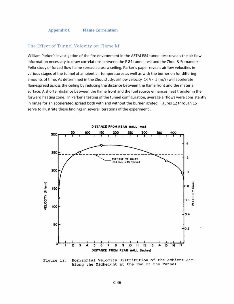
C-46

Appendix C Flame Correlation

The Effect of Tunnel Velocity on Flame kf

William Parker’s investigation of the fire environment in the ASTM E84 tunnel test reveals the air flow

information necessary to draw correlations between the E 84 tunnel test and the Zhou & Fernandez-

Pello study of forced flow flame spread across a ceiling. Parker’s paper reveals airflow velocities in

various stages of the tunnel at ambient air temperatures as well as with the burner on for differing

amounts of time. As determined in the Zhou study, airflow velocity 1< V < 5 (m/s) will accelerate

flamespread across the ceiling by reducing the distance between the flame front and the material

surface. A shorter distance between the flame front and the fuel source enhances heat transfer in the

forward heating zone. In Parker’s testing of the tunnel configuration, average airflows were consistently

in range for an accelerated spread both with and without the burner ignited. Figures 12 through 15

serve to illustrate these findings in several iterations of the experiment .

C-47

C-48

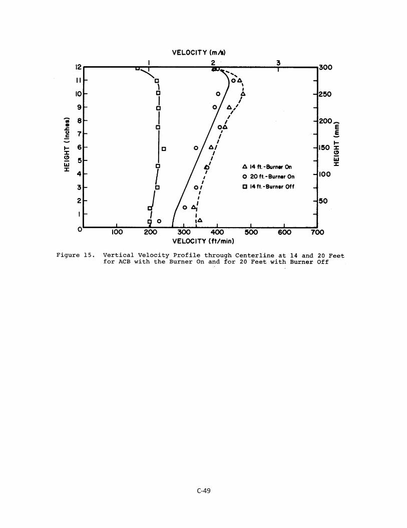
C-49

D-50

Appendix D Uncertainty

To determine the amount of uncertainty associated with the flame spread model the team conducted

an analysis using the Propagation of Uncertainty theory. This method states that the uncertainty of an

equation can be derived from the equation:

( ) √(

)

(

)

(

)

(1)

Is the partial differentiation of the equation f with respect to n, and s n

is the standard

deviation of the parameter n. Since the model uses a different equation once burnout begins, the

uncertainty must be calculated for both of these equations. Due to a lack of sufficient data, the

standard deviation ( ) values for each input parameter were determined by normalizing the

experimental data rather than a standard formula.

Algebraic Constants

(

)

( )

Before Burnout

(

( ) )

( )

(

( )

)(

)

( ) (2)

(

) (

)

( )

(3)

( ) √(

)

(

)

(1)

The resulting U(xp) value is the uncertainty of xp before burnout.

After Burnout

D-51

(

( )

(( ) ) )

(

)

( ) [

( ) ] (

)

(

)

( )

(( ) )

(

)

[

(

)

(

( ) )]

[

(( ) ) (

)]( (

)

) (

)

(

)

[

(

)(( ) )

] (

) (

(( ) ) ) (4)

(

(( ) ) )

(

)( )

(

) ( )

(

)

(( )

( ) )

(( ) )

[

( )

(

)

[(

( )

(

)

)(

( ) )

(

(( ) ) )(

)]

]

( (

)( )

)

[(( )( )

)(

(

)( )

)(

(

)(( ) )

)]

( ( )

(( ) ) ) (5)

( ) √(

)

(

)

(1)

The resulting U(xp) value is the uncertainty of xp after burnout.

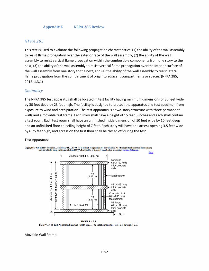
E-52

Appendix E NFPA 285 Review

NFPA 285

This test is used to evaluate the following propagation characteristics: (1) the ability of the wall assembly

to resist flame propagation over the exterior face of the wall assembly, (2) the ability of the wall

assembly to resist vertical flame propagation within the combustible components from one story to the

next, (3) the ability of the wall assembly to resist vertical flame propagation over the interior surface of

the wall assembly from one story to the next, and (4) the ability of the wall assembly to resist lateral

flame propagation from the compartment of origin to adjacent compartments or spaces. (NFPA 285,

2012: 1.3.1)

Geometry

The NFPA 285 test apparatus shall be located in test facility having minimum dimensions of 30 feet wide

by 30 feet deep by 23 feet high. The facility is designed to protect the apparatus and test specimen from

exposure to wind and precipitation. The test apparatus is a two-story structure with three permanent

walls and a movable test frame. Each story shall have a height of 15 feet 8 inches and each shall contain

a test room. Each test room shall have an unfinished inside dimension of 10 feet wide by 10 feet deep

and an unfinished floor-to-ceiling height of 7 feet. Each story will have one access opening 3.5 feet wide

by 6.75 feet high, and access on the first floor shall be closed off during the test.

Test Apparatus:

Movable Wall Frame:

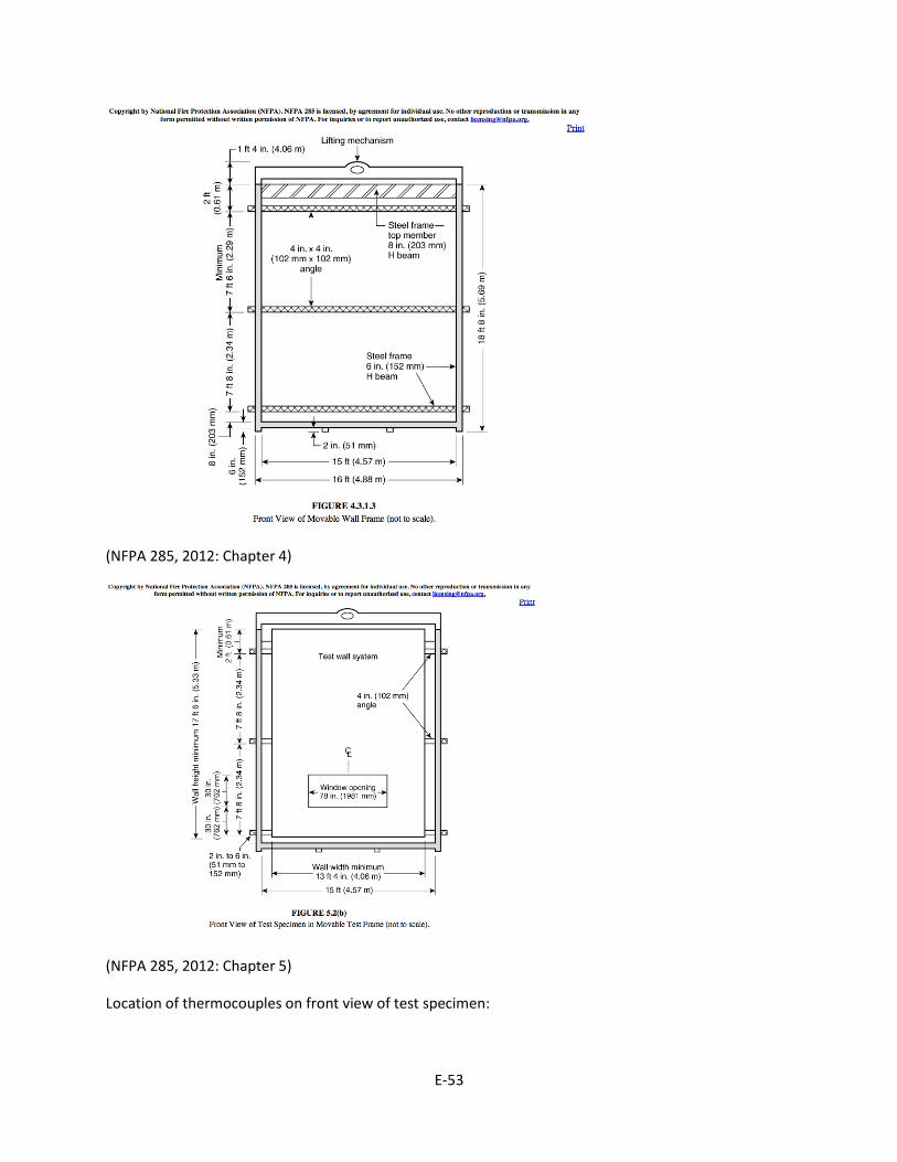
E-53

(NFPA 285, 2012: Chapter 4)

(NFPA 285, 2012: Chapter 5)

Location of thermocouples on front view of test specimen:

E-54

Fuel Package

The test requires two natural gas-fired burners: one placed inside the first-story test room and other

near the top of the first-story window opening of the test specimen. The burners shall be constructed of

nominal 2 in outside diameter steel pipe. (NFPA 285, 2012: 4.4)

Test Duration

Five minutes after ignition of the test room burner, the gas supply to the window burner shall be turned

on and burner ignited. Thirty minutes after ignition of the test room burner, the gas supply to both

burners shall be shut off. Residual burning on the test specimen shall not be extinguished until not less

than 10 minutes after the gas supply is shut off. Therefore the total test duration is at least 40 minutes

long. (NFPA 285, 2012: Chapter 8)

Thermal Insult

Room burner at 900kW, window burner at 400 kW

Pass/Fail Criteria

E-55

In order to pass the fire test, the specimen needs to meet the determined performance criteria during

the 30-minute fire exposure portion of the test in order to pass (NFPA 285, 2012: 10.2). The

performance criteria specifies that flame propagation on the exterior face of the test specimen shall not

occur either vertically or horizontally beyond the area of the flame plume impingement by the window

burner flames. NFPA 285 defines this propagation in Chapter 10. Additionally, flames shall not occur in

second-story test room, and the temperature in the second-story test room shall not exceed 500

degrees Fahrenheit above the ambient air temperature at beginning of test. Flames shall also not occur

beyond the intersection of the test specimen and the side walls of the test apparatus. (NFPA 285, 2012:

Chapter 10)

Types of Assemblies

NFPA 285 is designed to test exterior non-load-bearing wall assemblies and panels used as components

of curtain wall assemblies that are constructed using combustible materials or that incorporate

combustible components, and that are intended to be installed on buildings required to have exterior

walls of noncombustible construction (NFPA, 285, 2012: 1.1.1). Test specimens shall be at minimum 17.5

feet high and 13.3 feet wide. There shall be a window opening 30 inches high and 78 inches wide with a

sill height 30 inches above the top of the first-story test room slab. The specimen shall completely cover

the front face of the test apparatus expect for the window opening. (NFPA 285, 2012: Chapter 5)

Many different wall assembly systems can be tested using NFPA 285. Most assemblies contain some sort

of insulation at the core of the system protected by at least one layer of exterior material. An example is

extruded polystyrene insulation under various exterior finishes, including brick, stone, concrete, EIFS,

etc.

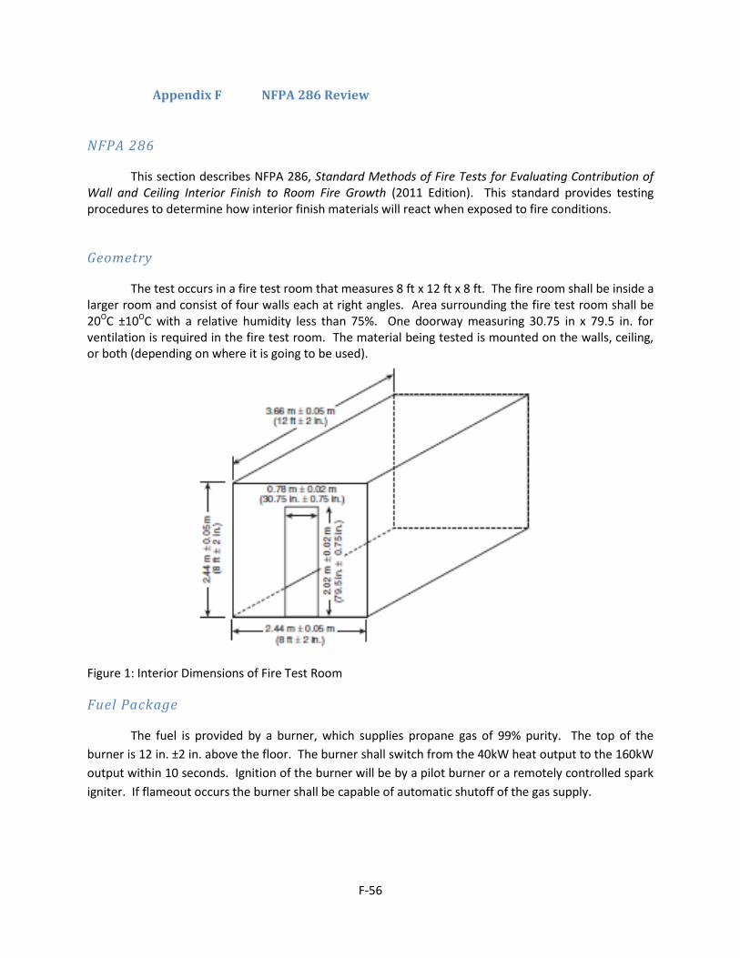
F-56

Appendix F NFPA 286 Review

NFPA 286

This section describes NFPA 286, Standard Methods of Fire Tests for Evaluating Contribution of Wall and Ceiling Interior Finish to Room Fire Growth (2011 Edition). This standard provides testing procedures to determine how interior finish materials will react when exposed to fire conditions.

Geometry

The test occurs in a fire test room that measures 8 ft x 12 ft x 8 ft. The fire room shall be inside a larger room and consist of four walls each at right angles. Area surrounding the fire test room shall be 20OC ±10OC with a relative humidity less than 75%. One doorway measuring 30.75 in x 79.5 in. for ventilation is required in the fire test room. The material being tested is mounted on the walls, ceiling, or both (depending on where it is going to be used).

Figure 1: Interior Dimensions of Fire Test Room

Fuel Package

The fuel is provided by a burner, which supplies propane gas of 99% purity. The top of the

burner is 12 in. ±2 in. above the floor. The burner shall switch from the 40kW heat output to the 160kW

output within 10 seconds. Ignition of the burner will be by a pilot burner or a remotely controlled spark

igniter. If flameout occurs the burner shall be capable of automatic shutoff of the gas supply.

F-57

Test Duration

The test is run for a total of fifteen minutes. The room is exposed to a heat release of 40 kW from the burner for 5 minutes, then a heat release of 160 kW for an additional ten minutes. The ignition is turned off after the ten minutes at 160 kW and the test is terminated (unless safety concerns make it necessary to terminate earlier).

Thermal Insult

40kW for 5 minutes, 160kW for an additional 10 minutes

Report Criteria

A material is assessed based on:

Incident heat flux on the center of the floor

Temperature of the gases in the upper part of the fire test room

Rate of heat release

Smoke release

Time to flashover A material is said to have passed if all of the following requirements are met:

During the 40 kW exposure:

Flames do not reach the ceiling During the 160 kW exposure:

Flames do not reach the outer extremity of the sample on any wall or ceiling

Flashover does not occur

Peak heat release rate never exceeds 800 kW

Total smoke released does not exceed 1000 m2 Flashover is said to occur when two of the following conditions have occurred:

Heat release rate exceeds 1 MW

Heat flux at the floor exceeds 20 kW/m2

Average upper layer temperature exceed 600oC

Flames exit doorway

Autoignition of a paper target on the floor occurs

Types of Specimen

This test is used for interior finish materials. Materials can be tested three different ways; on three

walls (if the material will only be used on the walls), on three walls and the ceiling (if the materials will

be used on the walls and ceiling), and only on the ceiling (for those materials only to be used on the

ceiling). The material being tested shall be mounted in the fire room as it would be mounted for actual

use. The material will be placed on panels and there will be two panels on the end wall, three panels on

each side wall, and three on the ceiling.

G-58

Appendix G ASTM E84 Review

ASTM E 84

This section describes ASTM E84 Standard Test Method for Surface Burning Characteristics of Building

Materials (2012 Edition). This is a standard for the comparative surface burning behavior of building

materials and applies to exposed surfaces such as walls and ceilings. The purpose of this test method is

to determine the relative burning behavior of the material based on flame spread along the sample as

well as smoke production. Results of this test provide comparative measurements of surface flame

spread and smoke density relative to red oak and fiber cement boards.

Geometry

A 24-ft long by 20-in wide specimen is secured as the ceiling (downward facing surface) in a fire test

chamber (17.75-in x 12.0-in x 25-ft).

Fuel Package

One end of the test chamber will have two gas burners directed upward, creating flames against the

surface of the test specimen. The two gas burners are spaced 12-in from the end of the test chamber

and 7 ½ +/- ½ in . below the specimen surface. The burners are fed by one gas inlet split in a tee section

to supply each burner.

An air intake shutter is located 54 +/- 5in. upstream of the burner. To provide the proper air turbulence

for combustion, six refractory fire bricks are located along the side wall of the chamber to provide

turbulence baffling.

Test Duration

The test is to run a total of 10 minutes from the ignition of the burners. The test may be concluded early

if the specimen is completely consumed in the fire area and no further progressive burning is evident

and the photoelectric cell reading has returned to the baseline. (section 8 procedure)

G-59

Pass/Fail Criteria

When the test is completed, flame spread distance vs time is plotted and the area under the curve is

calculated. In the event that the flame recedes during the test duration, a horizontal line is drawn from

the point of recession for the remainder of the test or until the flame front continues past the original

recession point. If the total area under the curve is less than or equal to 97.5, the area is multiplied by

.515 to obtain the flame spread index (FSI). FSI = 0.515 *AT. If the total area is greater than 97.5 the FSI

is calculated as 4900/(195-AT). The FSI is rounded to the nearest multiple of 5. (See ASTM E84 appendix

X2 for derivations)

Types of Assemblies

This test is designed to test building materials that will be used as finishing surfaces such as walls or

ceilings. The test assembly must be a downward facing surface in the ceiling position of the test

chamber. The test assembly or material has to be capable of mounting in this position by means of self-

support or holding in place by supports along the test surface or by securing the specimen from the

back. Specimen with supports exhibit lower flame spread index than those able to be tested without

additional support. Also materials with dripping and delaminating qualities severe enough to alter the

flame front will also display lower flame spread indexes.

H-60

Appendix H Compartment Effect

Because this test is conducted within a partially enclosed compartment, it is necessary to understand

the impacts the compartment will have on the fire temperatures. In this case, the fire starts about 2.4

meters below the ceiling. The hot products of combustion will create a plume, which will rise toward the

ceiling due to buoyancy. As it rises, the plume will draw in cooler air from the compartment, therefore

decreasing the temperature of the plume and increasing its volumetric flow rate. Upon reaching the

ceiling, the plume will spread out and form a hot gas layer that descends in the room with time.

Eventually this layer will reach the openings in the room where the hot gas will flow out of the room and

the outside air will flow into the room. This is known as the two layer or zone model and can be seen in

the figure below.

MQH Method

Many assumptions are made for this model. It is assumed that the only interchange between

the air in the lower part of the room and the hot upper gas layer is through the plume. It is also assumed

that the compositions and temperatures of each layer is uniform, and that the temperature of the upper

layer will always be greater than the lower layer. The basic governing principle used to calculate the

temperature in a compartment fire is the conservation of energy. It states that the energy added to the

upper layer by the fire is equal to the energy lost from the upper layer from radiation and convection

plus the energy convected out of the compartment openings. Throughout this test, flashover conditions

H-61

were never attained, this section focuses on predicting compartment fire temperatures for preflashover

fires. Specifically, the method of McCaffrey, Quintiere, and Harkleroad was used. These hand

calculations are an approximate solution that use a limiting set of assumptions for calculating the upper

gas layer temperature. Based on a simple conservation of energy equation and multiple substitutions,

the following power-law relationship can be used to solve for this change in temperature:

Heat Transfer Coefficient

As stated in the above assumptions, the heat transfer coefficient is determined based on the

thermal penetration time. The equation for calculating the thermal penetration time is as follows:

Consequently, the following equations are used to determine the heat transfer coefficient necessary for

the above analysis.

for times greater than the thermal penetration time.

for times less than or equal to the thermal penetration time.

Limitations

The following limitation exist for this method:

DTg = 480Q

gcpr¥T¥A0 H0

æ

è

çç

ö

ø

÷÷

23

hkAT

gcpr¥A0 H0

æ

è

çç

ö

ø

÷÷

-13

hk =k

d

hk =krc

t

æ

èç

ö

ø÷

12

tp =rc

k

æ

èç

ö

ø÷

d

2

æ

èç

ö

ø÷

2

H-62

The correlation holds for compartment upper layer gas temperatures up to approximately

600oC.

The correlation applies to steady-state as well as time-dependent fires as long as the transient

response is the wall conduction phenomenon.

The correlation is not applicable to rapidly developing fires in large enclosures in which

significant fire growth has occurred before the combustion products have exited the

compartment.

The energy release rate of the fire must be determined from data or other correlations.

The characteristic fire growth time and thermal penetration time of the room-lining materials

must be determined in order to evaluate the effective heat transfer coefficient.

The correlation is based on data from a limited number of experiments and does not contain

extensive data on ventilation-controlled fire nor data on combustible walls or ceilings. Most of

the fuel n the test fires was near the center of the room.

(SFPE Handbook, Third Edition: 3-6)

I-63

Appendix I International Building Code Review

Building Code Regulations

The interior wall and ceiling finish requirements are dependent on two main factors. The first is the type of building or “occupancy” as the building code refers to it and the second is where in the building the material is going. There are ten main types of building occupancies. The occupancy is determined based on the main use/purpose of the building. Some occupancies are further classified (as 1, 2, 3, etc.) based on a more specific use.

Types of Occupancies

The main occupancy types are:

Assembly (A)

Business (B)

Educational (E)

Factory (F)

High-Hazard (H)

Institutional (I)

Mercantile (M)

Residential (R)

Storage (S)

Utility and Miscellaneous (U) As described above, to determine a building’s occupancy classification the main purpose of the building is used. Some occupancies types are broken down further with sub-classes. For interior wall and ceiling finish requirements the sub-classes of Assembly, Institutional, and Residential impact the code requirements.

The building is considered an assembly occupancy when many people gather in the building for any reason (i.e. religious, social, awaiting transportation, food, drink, etc.). Since there are such a variety of buildings that fall under the assembly occupancy there are sub categories, A-1, A-2, A-3, A-4, and A-5. A-1 occupancies typically have fixed seating and are used for performance or viewing performance (i.e. movie theater). Buildings that are meant for the consumption of food or beverages are given an A-2 classification. A-3 occupancy is given to any other assembly type building except for those used for indoor or outdoor sporting events (i.e. place of religious worship, lecture hall, museum, pool hall, etc). Buildings that house indoor sporting events and have spectator seating are considered A-4 occupancies while structures used for outdoor sporting events are considered A-5 occupancies. Institutional occupancies are buildings in which people live or are cared for because of physical limitations (health or age), medical treatment, or because they “are detained for penal or correctional purposes”. The sub-classes of Institutional occupancies are I-1, I-2, I-3, I-4. An I-1 occupancy refers to a building in which people (more than 16) reside and are supervised. Personal care services are provided. Residents are capable of reacting to emergency situations without physical assistance (i.e. alcohol and drug centers, assisted living facilities, etc.). I-2 occupancies are buildings used for any type of 24 hour care (physical, mental, or custodial) of people who are not capable of responding to emergency situations on their own (i.e. child care facilities (more than 5 children under the age of 2 ½), hospitals, nursing homes, etc.). Buildings in which more than five people reside who are incapable of self preservation because of security restraints are considered I-3 occupancies (i.e. jails). I-4 occupancies are

I-64

buildings in which people, regardless of age are cared for (for less than 24 hours) by someone other than relatives/guardians. Residential occupancies are buildings in which people sleep in, but are not considered institutional occupancies. The sub-classes of Residential occupancies are R-1, R-2, R-3, and R-4. R-1 occupancies are building where people do not stay permanently (less than 30 consecutive days). These would include things like hotels or motels. R-2 occupancies are building in which more than two sleeping/dwelling units are present. The occupants tend to be permanent. This would include apartments, dormitories, fraternities, monasteries, etc. R-3 occupancies are building where the occupants are normally permanent but are not classified as R-1, R-2, R-4, or I. R-4 occupancies are building used for assisted living of more than 5 people but no more than 16. For Business, Educational, Factory, High-Hazard, Mercantile, Storage, Utility and Miscellaneous occupancies any sub-classes that may exist do not matter for the interior wall and ceiling finish requirements. A business occupancy is a building used as an office, for professional services, or other equivalent purposes (i.e. print shop, post office, educational occupancies above the 12th grade, etc.). An educational occupancy is a building used for educational purposes until the 12th grade. Factory assemblies are buildings used for any type or process in manufacturing excluding those classified as High-Hazard or Storage. This includes assembling, disassembling, fabricating, finishing, etc. High-Hazard occupancies are buildings used for the same purpose as a factory assembly except the materials being manufactured constitute physical or health hazards. Mercantile occupancies are comprised of buildings used for the display of goods for sale. Storage occupancies are buildings used for storage purposes. Utility and Miscellaneous buildings are those that cannot be classified under any other category.

Material Classifications and Building Areas

The International Building Code classifies materials based on results from ASTM E 84 or UL 723 testing. There are three different classifications, Class A, Class B, or Class C. The different classes are determined by the flame spread index and smoke-developed during the tests. The following table details the different classifications:

Class Flame Spread Index Smoke Developed Index

A 0-25 0-450

B 26-75 0-450

C 76-200 0-450

The code gives a minimum requirement. If the code says that a class B material is needed, then either a class A or class B material can be used. A class C material would not be allowed in that particular section of that type of occupancy. A class C requirement means a class A, B, or C material may be used. When the code says class A material is needed, only a class A material can be used.

Requirements for interior finishes depend on where in the building the material is going to be. The International Building Code divides buildings into three sections: exit enclosures, corridors, and rooms and enclosed spaces. The occupancy type will also affect the material requirements.

I-65

Class C materials

Class C materials are only permitted in exit enclosures in F, R-2, R-3, and S occupancies. They are permitted in corridors in B, E, M, R-1, R-4, I-1, F, R-2, R-3, and S occupancies. For rooms and enclosed spaces class C materials are allowed in all assembly and residential occupancies, B, E, M, H, F, S, I-1, and I-3 occupancies.

Class B Materials

Class B materials are permitted wherever class C materials are allowed as well as in exit enclosures in all assembly, B, E, M, R-1, R-4, H, I-1, I-2, and I-4 occupancies. They are permitted in corridors in all assembly, H, I-2, and I-4 occupancies. For rooms and enclosed spaces class B materials are allowed in I-2, and I-4 occupancies.

Class A Materials

Class A materials are permitted wherever class B and C materials are allowed as well as in exit enclosures in I-3 occupancies. They are permitted in corridors in I-3 occupancies.

Non-Sprinklered Buildings

All of the above requirements are assuming the building is sprinklered. If the occupancy is not protected by an automatic sprinkler system the interior finish requirements change. Essentially any area that had a class B requirement in a sprinklered building would require a class A material in a non-sprinklered building. Many class C requirements in sprinklered buildings become class B requirements for non-sprinklered buildings. All of the requirements are increased by a class in the exit enclosure sections for a non-sprinklered building. The only corridor requirement that does not increase in a non-sprinklered building is in the F occupancies. There were more requirements that remained the same for rooms and enclosed spaces for non-sprinklered buildings. These included A-3, A-3, A-4, A-5, B, E, M, R-1, F, I-2, I-4, R-2, S occupancies. No requirements changed for R-3 occupancies regardless of whether the building was sprinklered or not. There are no restrictions for U occupancies in a sprinklered or non-sprinklered building.

J-66

Appendix J Cone: Heat Release Rate Histories

25 kw/m2 Heat Release rate analysis

Thirteen FRP systems are analyzed in the context of heat release rate. This briefing highlights all thirteen

systems as well as groups the systems in terms of pigments, filler, gel, and aggregate composition for

comparison purposes.

Baseline FRP System

No gelcoat

Polymer concrete: Norsodyne H 81269 TF with 6% cobalt & DDM-9

Alumina Trihydrate: 10% of resin by weight

Sand: 150% of resin by weight, split evenly between #0/30 and #2/16

1-1/2 parts sand to 1 part resin

No pigment

Approximately 60 mil thickness (aggregate dependent)

3/16" single skin laminate: Norsodyne H 81269 TF with 6% cobalt & DDM-9

4 layers of 1.5 ounce chopped strand mat

Glass to resin ratio range: 25:75 to 35:65 by weight

System 1 – Addition of 1/2" plywood core & 3/16” rear skin (Note that core separation was observed in

several samples)

System 2 – Addition of 3/4" balsa core & 3/16” rear skin

System 3 – Addition of 1/2" polyurethane foam core & 3/16” rear skin

System 4 – Bronze filler instead of sand: 1 part bronze powder to 1 part resin by weight

System 5 – Aluminum filler instead of sand: 1 part aluminum powder to 2 parts resin by weight

System 6 – Straight Norsodyne H 81269 TF as gelcoat in place of resin based polymer concrete

System 7 – Addition of white pigment to polymer concrete

System 8 – Addition of grey pigment to polymer concrete

System 9 – Addition of beige pigment to polymer concrete

System 10 – #0/30 aggregate only



System 13 – DCPD Laminate resin (with 6 layers of glass) instead of Norsodyne

J-67

-10

-5

0

5

10

15

20

25

30

35

40

1 201 401 601 801 1001 1201 1401

kW/m

^2

Seconds

Baseline HRR 25kW/m2

Base

Base

Base

-10

0

10

20

30

40

50

60

1 501 1001

kW/m

^2

Seconds

Kreysler Sample 1 HRR 25 kW/m2

G

H

Baseline

J-68

-10

0

10

20

30

40

50

60

70

1 501 1001

kW/m

^2

Seconds

Kreysler Sample 2 HRR 25kW/m2

H

I

Baseline

-10

-5

0

5

10

15

20

25

30

35

1 501

kW/m

^2

Seconds


G

H

Baseline

J-69

-10

0

10

20

30

40

50

60

70

80

90

1 201 401 601

kW/m

^2

Seconds


H

I

Baseline

-20

0

20

40

60

80

100

1 201 401 601 801 1001 1201 1401

kW/m

^2

Seconds


G

H

Baseline

J-70

-10

0

10

20

30

40

50

60

1 201 401 601 801 1001 1201

kW/m

^2

Seconds


I

J

Baseline

-20

-10

0

10

20

30

40

50

60

70

80

90

1 201 401 601 801 1001 1201 1401 1601 1801 2001 2201 2401 2601 2801

kW/m

^2

Seconds


H

I

Baseline

J-71

-20

0

20

40

60

80

100

1 201 401 601 801 1001 1201 1401 1601 1801 2001 2201 2401 2601 2801 3001

kW/m

^2

Seconds


H

I

Baseline

-20

0

20

40

60

80

100

120

1 201 401 601 801 1001 1201 1401 1601 1801 2001

kW/m

^2

Seconds


G

H

Baseline

J-72

-10

0

10

20

30

40

50

60

70

80

90

1 201 401 601

kW/m

^2

Seconds


G

H

Baseline

-20

0

20

40

60

80

100

120

1 201 401 601 801

kW/m

^2

Seconds


G

H

Baseline

J-73

-10

0

10

20

30

40

50

60

1 201 401 601 801 1001

kW/m

^2

Seconds


G

H

Baseline

-20

0

20

40

60

80

100

120

1 201 401 601 801 1001 1201

kW/m

^2

Seconds


G

H

Baseline

J-74

-20

0

20

40

60

80

100

120

1 201 401 601 801 10011201140116011801200122012401260128013001

kW/m

^2

Seconds

Pigment HRR Comparisons 25kW/m2

(White) 7H

(Grey) 8H

(Beige) 9G

Baseline

-20

0

20

40

60

80

100

120

1 201 401 601

kW/m

^2

Seconds

Aggregate HRR Comparison 25kW/m2

(#0/30) 10G

(#0/60) 11G

(#2/16) 12G

Baseline

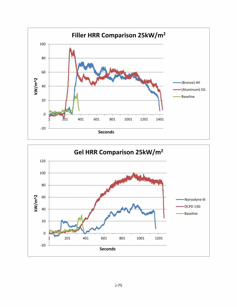
J-75

-20

0

20

40

60

80

100

1 201 401 601 801 1001 1201 1401

kW/m

^2

Seconds

Filler HRR Comparison 25kW/m2

(Bronze) 4H

(Aluminum) 5G

Baseline

-20

0

20

40

60

80

100

120

1 201 401 601 801 1001 1201

kW/m

^2

Seconds

Gel HRR Comparison 25kW/m2

Norsodyne 6I

DCPD 13G

Baseline

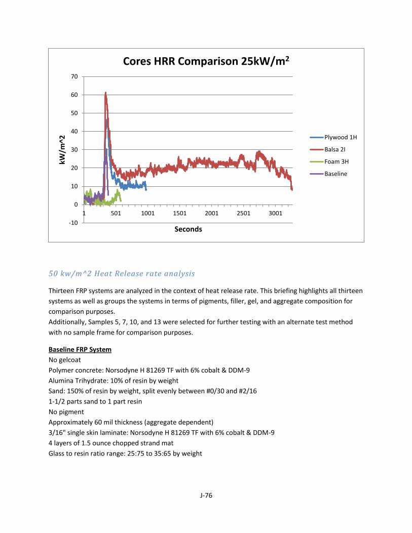
J-76

50 kw/m^2 Heat Release rate analysis




Additionally, Samples 5, 7, 10, and 13 were selected for further testing with an alternate test method

with no sample frame for comparison purposes.

Baseline FRP System

No gelcoat





No pigment





-10

0

10

20

30

40

50

60

70

1 501 1001 1501 2001 2501 3001

kW/m

^2

Seconds

Cores HRR Comparison 25kW/m2

Plywood 1H

Balsa 2I

Foam 3H

Baseline

J-77


several samples)













J-78

-20

0

20

40

60

80

100

120

140

1 201 401 601 801 1001 1201 1401

kW/m

^2

Seconds


Baseline 1

Baseline 2

Baseline 3

Baseline 4

-20

0

20

40

60

80

100

120

1 501 1001 1501 2001

kW/m

^2

Seconds


A

B

C

D

Baseline

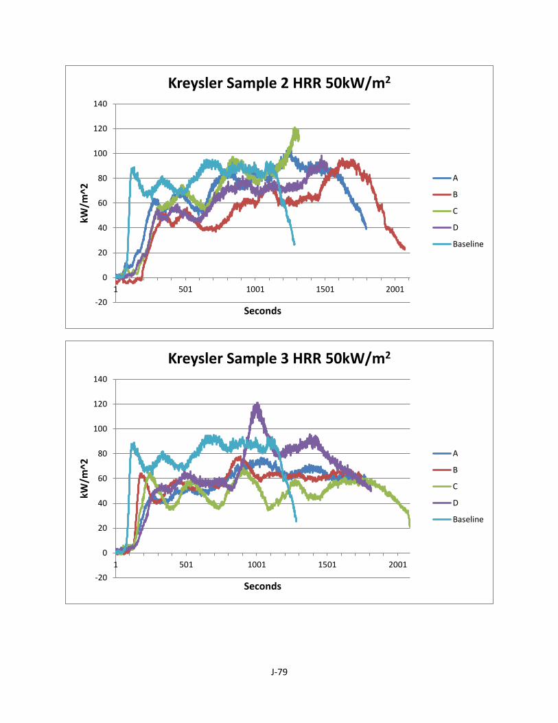
J-79

-20

0

20

40

60

80

100

120

140

1 501 1001 1501 2001

kW/m

^2

Seconds


A

B

C

D

Baseline

-20

0

20

40

60

80

100

120

140

1 501 1001 1501 2001

kW/m

^2

Seconds


A

B

C

D

Baseline

J-80

-20

0

20

40

60

80

100

120

140

160

1 201 401 601

kW/m

^2

Seconds


Baseline

D

E

-20

0

20

40

60

80

100

120

140

1 201 401 601 801

kW/m

^2

Seconds

Kreysler Sample 5 HRR/m2

Baseline

C

D

No Frame

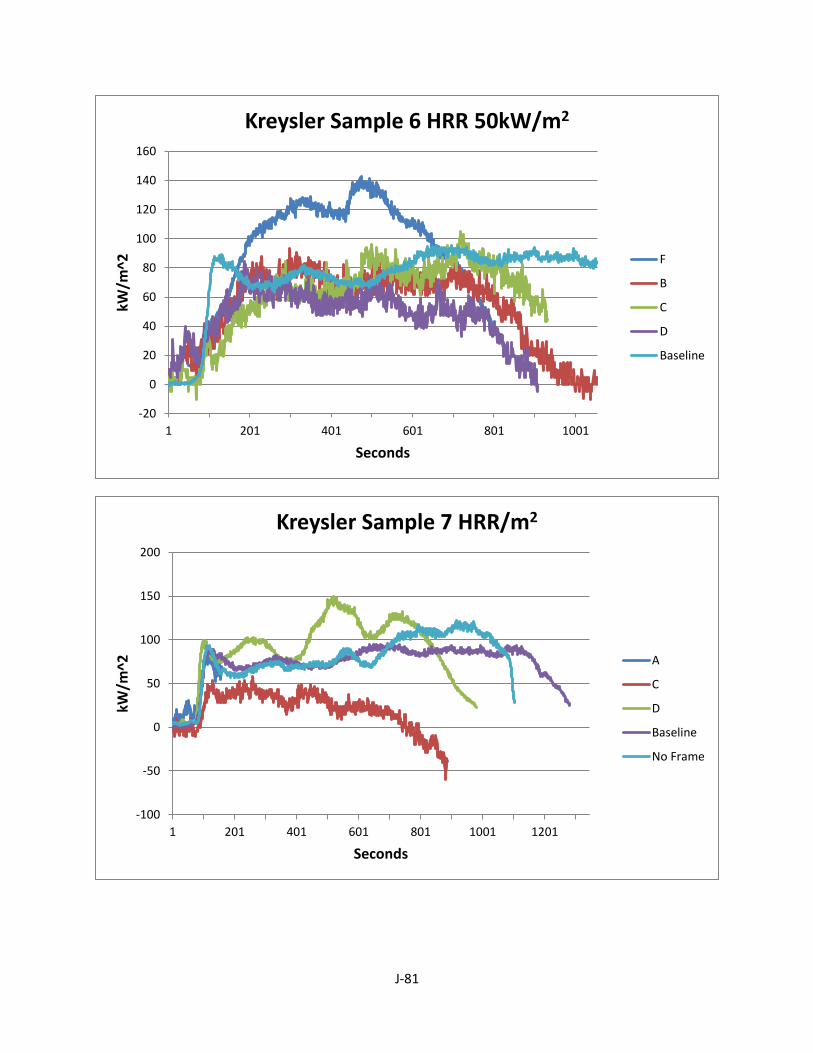
J-81

-20

0

20

40

60

80

100

120

140

160

1 201 401 601 801 1001

kW/m

^2

Seconds


F

B

C

D

Baseline

-100

-50

0

50

100

150

200

1 201 401 601 801 1001 1201

kW/m

^2

Seconds


A

C

D

Baseline

No Frame

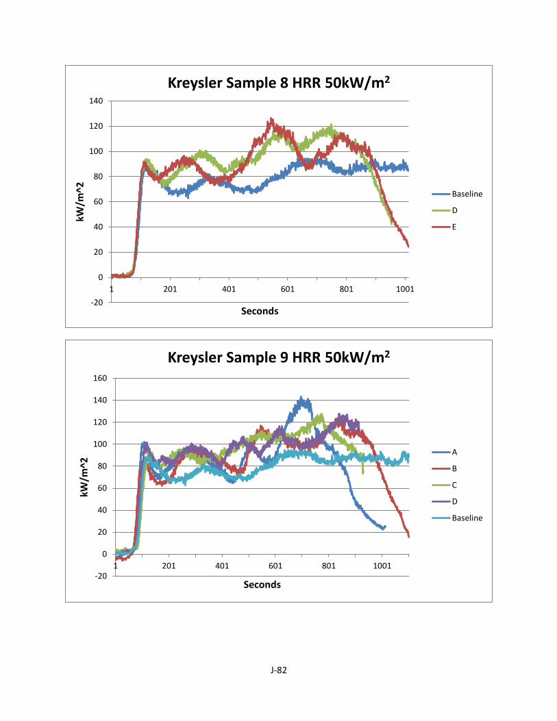
J-82

-20

0

20

40

60

80

100

120

140

1 201 401 601 801 1001

kW/m

^2

Seconds


Baseline

D

E

-20

0

20

40

60

80

100

120

140

160

1 201 401 601 801 1001

kW/m

^2

Seconds


A

B

C

D

Baseline

J-83

-20

0

20

40

60

80

100

120

140

1 201 401 601 801 1001 1201

kW/m

^2

Seconds


A

B

C

D

Baseline

No Frame

-20

0

20

40

60

80

100

120

140

1 201 401 601 801 1001 1201

kW/m

^2

Seconds


A

B

C

D

Baseline

J-84

-20

0

20

40

60

80

100

120

140

1 201 401 601 801 1001 1201

kW/m

^2

Seconds


B

C

Baseline

-50

0

50

100

150

200

1 201 401 601 801 1001 1201

kW/m

^2

Seconds


B

C

Baseline

No Frame

J-85

-20

0

20

40

60

80

100

120

140

160

1 201 401 601 801 1001

kW/m

^2

Seconds


(White) 7D

(Grey) 8D

(Beige) 9B

Baseline

-20

0

20

40

60

80

100

120

140

1 201 401 601 801 1001

kW/m

^2

Seconds


(#0/30) 10B

(#0/60) 11B

(#2/16) 12B

Baseline

J-86

-20

0

20

40

60

80

100

120

140

1 201 401 601

kW/m

^2

Seconds


(Bronze) 4D

(Aluminum) 5D

Baseline

-50

0

50

100

150

200

1 201 401 601 801 1001

kW/m

^2

Seconds


Norsodyne 6B

DCPD 13C

Baseline

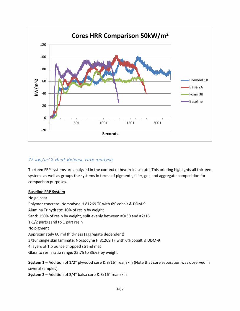
J-87

75 kw/m^2 Heat Release rate analysis




Baseline FRP System

No gelcoat





No pigment






several samples)


-20

0

20

40

60

80

100

120

1 501 1001 1501 2001

kW/m

^2

Seconds


Plywood 1B

Balsa 2A

Foam 3B

Baseline

J-88












J-89

-20

0

20

40

60

80

100

120

140

160

1 201 401 601 801 1001 1201 1401

kW/m

^2

Seconds


Base 3

Base 4

-20

0

20

40

60

80

100

120

140

160

1 501 1001 1501 2001

kW/m

^2

Seconds


E

F

Baseline

J-90

-50

0

50

100

150

200

1 501 1001

kW/m

^2

Seconds


E

F

Baseline

0

20

40

60

80

100

120

140

160

180

200

1 501 1001

kW/m

^2

Seconds


E

F

Baseline

J-91

0

50

100

150

200

250

1 201 401 601

kW/m

^2

Seconds


F

G

Baseline

0

20

40

60

80

100

120

140

160

180

200

1 201 401 601

kW/m

^2

Seconds


E

F

Baseline

J-92

0

20

40

60

80

100

120

140

160

180

200

1 201 401 601

kW/m

^2

Seconds


G

H

Baseline

0

20

40

60

80

100

120

140

160

180

200

1 201 401 601 801

kW/m

^2

Seconds


F

G

Baseline

J-93

-20

0

20

40

60

80

100

120

140

160

180

1 201 401 601

kW/m

^2

Seconds


F

G

Baseline

0

20

40

60

80

100

120

140

160

180

200

1 201 401 601

kW/m

^2

Seconds


E

F

Baseline

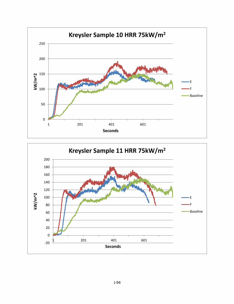
J-94

0

50

100

150

200

250

1 201 401 601

kW/m

^2

Seconds


E

F

Baseline

-20

0

20

40

60

80

100

120

140

160

180

200

1 201 401 601

kW/m

^2

Seconds


E

F

Baseline

J-95

-20

0

20

40

60

80

100

120

140

160

1 201 401 601 801

kW/m

^2

Seconds


E

F

Baseline

-50

0

50

100

150

200

250

1 201 401 601

kW/m

^2

Seconds


E

F

Baseline

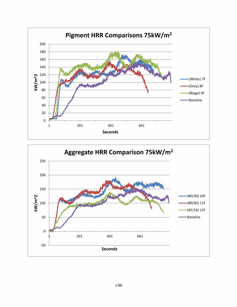
J-96

0

20

40

60

80

100

120

140

160

180

200

1 201 401 601

kW/m

^2

Seconds


(White) 7F

(Grey) 8F

(Beige) 9F

Baseline

-50

0

50

100

150

200

250

1 201 401 601

kW/m

^2

Seconds


(#0/30) 10F

(#0/60) 11F

(#2/16) 12F

Baseline

J-97

0

50

100

150

200

250

1 201 401 601

kW/m

^2

Seconds


(Bronze) 4F

(Aluminum) 5F

Baseline

0

50

100

150

200

250

1 201 401 601 801 1001

kW/m

^2

Seconds


Norsodyne 6G

DCPD 13F

Baseline

J-98

Heat Release rate analysis At variable heat flux




Baseline FRP System

No gelcoat





No pigment






several samples)


0

20

40

60

80

100

120

140

160

180

200

1 501 1001

kW/m

^2

Seconds


Plywood 1F

Balsa 2F

Foam 3F

Baseline

J-99












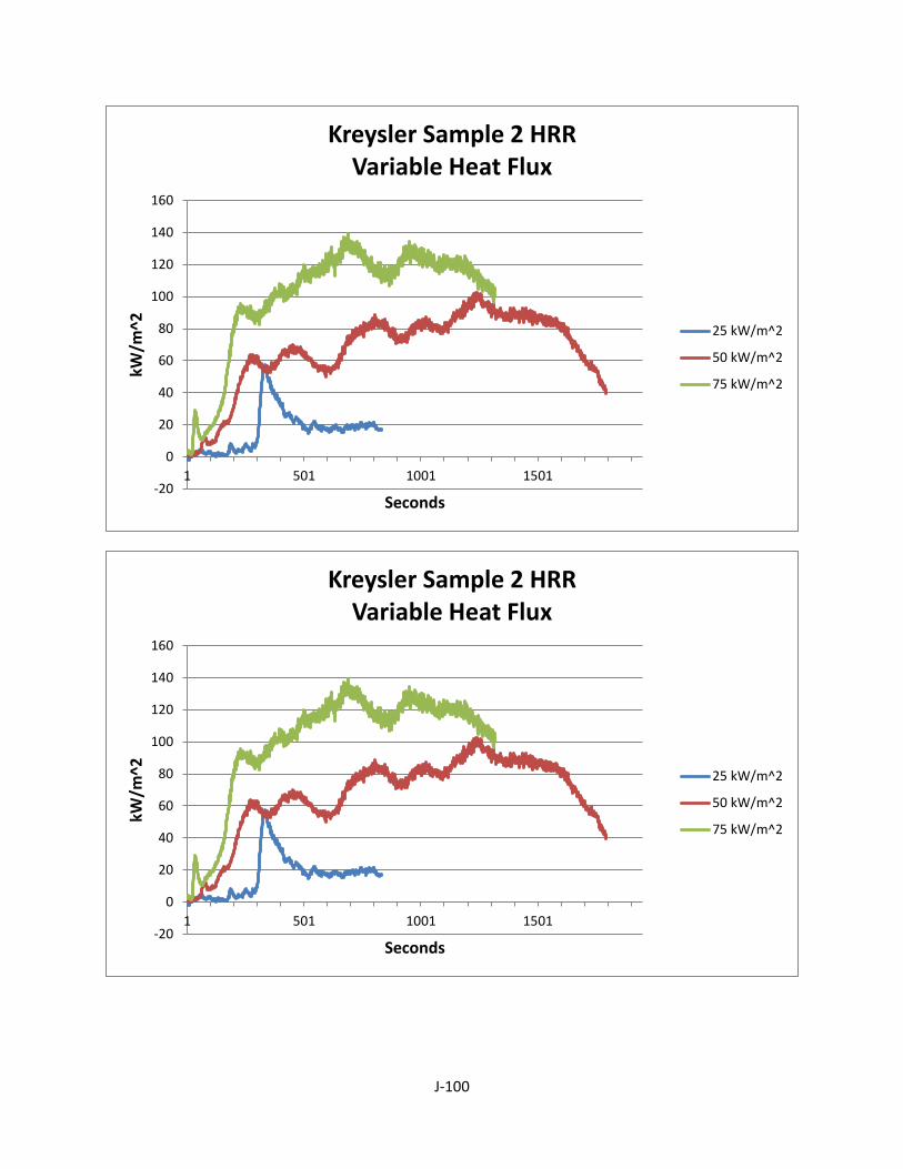
J-100

-20

0

20

40

60

80

100

120

140

160

1 501 1001 1501

kW/m

^2

Seconds

Kreysler Sample 2 HRR Variable Heat Flux

25 kW/m^2

50 kW/m^2

75 kW/m^2

-20

0

20

40

60

80

100

120

140

160

1 501 1001 1501

kW/m

^2

Seconds


25 kW/m^2

50 kW/m^2

75 kW/m^2

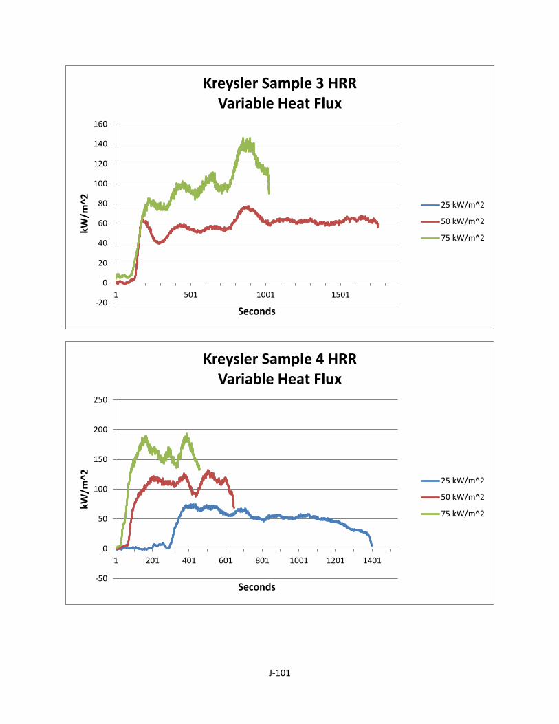
J-101

-20

0

20

40

60

80

100

120

140

160

1 501 1001 1501

kW/m

^2

Seconds


25 kW/m^2

50 kW/m^2

75 kW/m^2

-50

0

50

100

150

200

250

1 201 401 601 801 1001 1201 1401

kW/m

^2

Seconds


25 kW/m^2

50 kW/m^2

75 kW/m^2

J-102

-20

0

20

40

60

80

100

120

140

160

180

200

1 201 401 601 801 1001 1201 1401 1601

kW/m

^2

Seconds


25 kW/m^2

50 kW/m^2

75 kW/m^2

-50

0

50

100

150

200

1 201 401 601 801 1001

kW/m

^2

Seconds


25 kW/m^2

50 kW/m^2

75 kW/m^2

J-103

-20

0

20

40

60

80

100

120

140

160

180

200

1 501 1001 1501 2001 2501

kW/m

^2

Seconds


25 kW/m^2

50 kW/m^2

75 kW/m^2

-20

0

20

40

60

80

100

120

140

160

180

1 201 401 601 801 1001 1201 1401 1601 1801 2001 2201 2401 2601 2801

kW/m

^2

Seconds


25 kW/m^2

50 kW/m^2

75 kW/m^2

J-104

-20

0

20

40

60

80

100

120

140

160

180

1 201 401 601 801 1001 1201 1401 1601 1801 2001

kW/m

^2

Seconds


25 kW/m^2

50 kW/m^2

75 kW/m^2

0

20

40

60

80

100

120

140

160

180

1 201 401 601 801 1001 1201

kW/m

^2

Seconds


25 kW/m^2

50 kW/m^2

75 kW/m^2

J-105

-20

0

20

40

60

80

100

120

140

160

180

1 201 401 601 801

kW/m

^2

Seconds


25 kW/m^2

50 kW/m^2

75 kW/m^2

-20

0

20

40

60

80

100

120

140

1 201 401 601 801 1001

kW/m

^2

Seconds


25 kW/m^2

50 kW/m^2

75 kW/m^2

J-106

-50

0

50

100

150

200

250

1 201 401 601 801 1001 1201

kW/m

^2

Seconds


25 kW/m^2

50 kW/m^2

75 kW/m^2

K-107

Appendix K Cone: Specific Extinction Area Histories

Specific Extinction Area analysis – 25kW/M2

Thirteen FRP systems are analyzed in the context of specific extinction area. This briefing highlights all

thirteen systems as well as groups the systems in terms of pigments, filler, gel, and aggregate

composition for comparison purposes.

Baseline FRP System

No gelcoat





No pigment






several samples)













K-108

-0.2

-0.1

0

0.1

0.2

0.3

0.4

0.5

1 301

m^2

/g

Time (Seconds)

Baseline SEA at 25kW/m2

Baseline 5

Baseline 7

-0.8

-0.6

-0.4

-0.2

0

0.2

0.4

0.6

0.8

1

1 501 1001

m^2

/g

Time (s)

Kreysler Sample 1 SEA at 25kW/m2

G

H

Baseline

K-109

-0.6

-0.4

-0.2

0

0.2

0.4

0.6

0.8

1

1.2

1 501 1001 1501 2001 2501 3001

m^2

/g

Time (s)


H

I

Baseline

-0.6

-0.4

-0.2

0

0.2

0.4

0.6

1 501

m^2

/g

Time (s)


G

H

Baseline

K-110

-0.8

-0.6

-0.4

-0.2

0

0.2

0.4

0.6

0.8

1

1.2

1 201 401 601 801 1001 1201 1401

m^2

/g

Time (s)


H

I

Baseline

-0.8

-0.6

-0.4

-0.2

0

0.2

0.4

0.6

0.8

1

1.2

1 201 401 601 801 1001 1201 1401 1601

m^2

/g

Time (s)


G

H

Baseline

K-111

-1

-0.8

-0.6

-0.4

-0.2

0

0.2

0.4

0.6

0.8

1

1.2

1 201 401 601 801 1001 1201


I

J

Baseline

-2

-1.5

-1

-0.5

0

0.5

1

1.5

2

2.5

1 201 401 601 801 1001 1201 1401 1601 1801 2001 2201 2401 2601

m^2

/g

Time (s)


H

I

Baseline

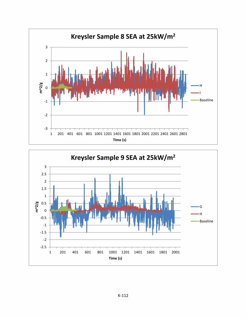
K-112

-3

-2

-1

0

1

2

3

1 201 401 601 801 1001 1201 1401 1601 1801 2001 2201 2401 2601 2801

m^2

/g

Time (s)


H

I

Baseline

-2.5

-2

-1.5

-1

-0.5

0

0.5

1

1.5

2

2.5

3

1 201 401 601 801 1001 1201 1401 1601 1801 2001

m^2

/g

Time (s)


G

H

Baseline

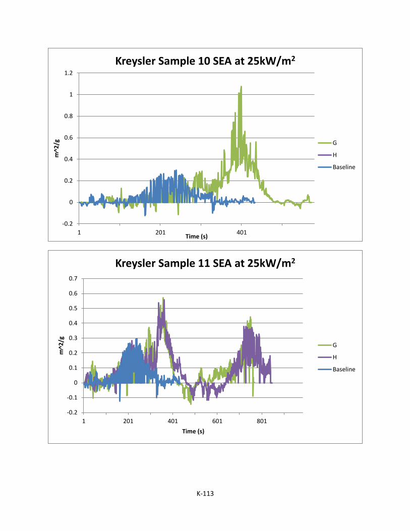
K-113

-0.2

0

0.2

0.4

0.6

0.8

1

1.2

1 201 401

m^2

/g

Time (s)


G

H

Baseline

-0.2

-0.1

0

0.1

0.2

0.3

0.4

0.5

0.6

0.7

1 201 401 601 801

m^2

/g

Time (s)


G

H

Baseline

K-114

-0.2

-0.1

0

0.1

0.2

0.3

0.4

1 201 401 601 801 1001

m^2

/g

Time (s)


G

H

Baseline

-0.5

0

0.5

1

1.5

2

2.5

1 201 401 601 801 1001 1201

m^2

/g

Time (s)


G

H

Baseline

K-115

-2.5

-2

-1.5

-1

-0.5

0

0.5

1

1.5

2

2.5

1 501 1001 1501 2001 2501 3001

m^2

/g

Time (s)

SEA Pigment Comparisons at 25kW/m2

(White) 7H

(Grey) 8H

(Beige) 9H

Baseline

-0.4

-0.2

0

0.2

0.4

0.6

0.8

1

1.2

1 201 401 601 801 1001

m^2

/g

Time (s)

SEA Aggregate Comparison at 25kW/m2

(#0/30) 10G

(#0/60) 11G

(#2/16) 12G

Baseline

K-116

-0.8

-0.6

-0.4

-0.2

0

0.2

0.4

0.6

0.8

1

1.2

1 201 401 601 801 1001 1201 1401

m^2

/g

Time (s)

SEA Filler Comparison at 25kW/m2

(Bronze)

(Aluminum)

Baseline

-1

-0.5

0

0.5

1

1.5

2

2.5

1 201 401 601 801 1001 1201

SEA Gel Comparison at 25kW/m2

Norsodyne 6

DCPD 13

Baseline

K-117

Specific Extinction Area analysis – 50kW /m2




Baseline FRP System

No gelcoat





No pigment






several samples)


-0.8

-0.6

-0.4

-0.2

0

0.2

0.4

0.6

0.8

1

1 201 401 601 801

m^2

/g

Time (s)

SEA Cores Comparison at 25kW/m2

Plywood 1G

Balsa 2H

Foam 3G

Baseline

K-118












K-119

-2

-1.5

-1

-0.5

0

0.5

1

1.5

2

1 301 601 901 1201

m^2

/g

Time (Seconds)

Baseline SEA 50kW/m2

Baseline 1

Baseline 2

Baseline 3

Baseline4

-0.8

-0.6

-0.4

-0.2

0

0.2

0.4

0.6

0.8

1

1.2

1 501 1001 1501 2001

m^2

/g

Time (s)

Kreysler Sample 1 SEA 50kW/m2

A

B

C

D

Baseline

K-120

-1

-0.8

-0.6

-0.4

-0.2

0

0.2

0.4

0.6

0.8

1 501 1001 1501 2001

m^2

/g

Time (s)


A

B

C

D

Baseline

-2

-1.5

-1

-0.5

0

0.5

1

1.5

2

2.5

1 501 1001 1501

m^2

/g

Time (s)


A

B

C

D

Baseline

K-121

-0.6

-0.4

-0.2

0

0.2

0.4

0.6

0.8

1

1.2

1 201 401 601

m^2

/g

Time (s)


Baseline

F

D

-0.8

-0.6

-0.4

-0.2

0

0.2

0.4

0.6

0.8

1 201 401 601 801

m^2

/g

Time (s)


Baseline

C

D

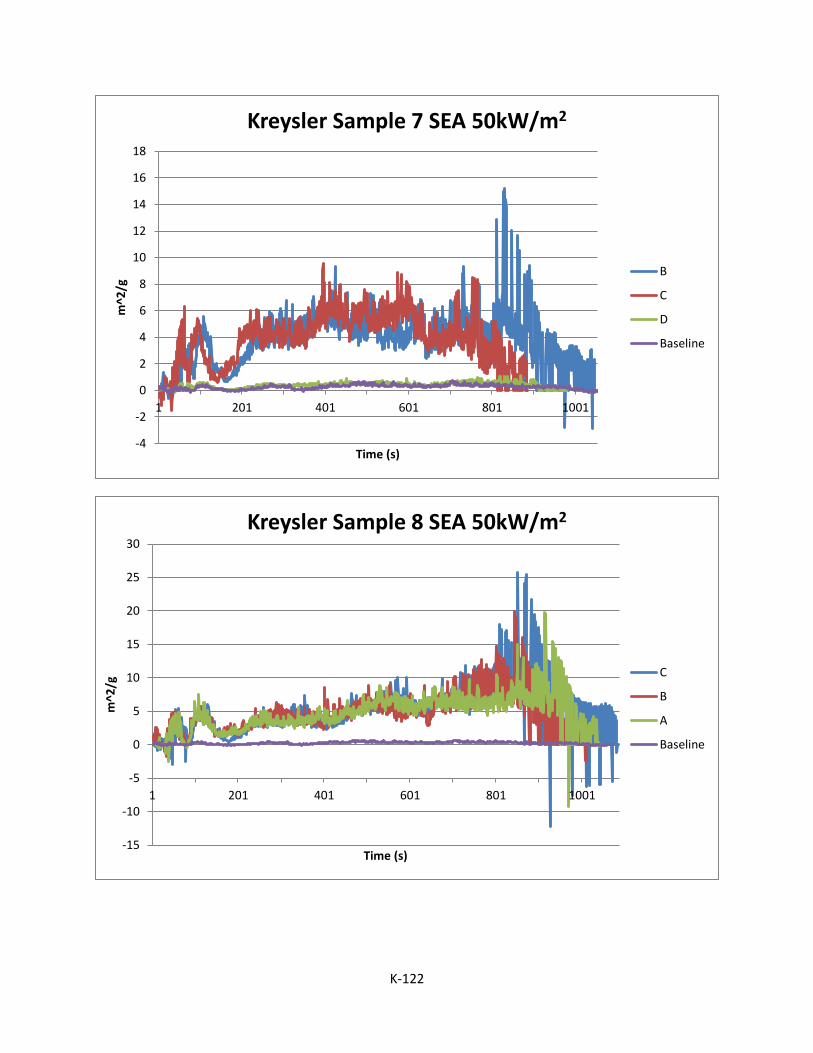
K-122

-4

-2

0

2

4

6

8

10

12

14

16

18

1 201 401 601 801 1001

m^2

/g

Time (s)


B

C

D

Baseline

-15

-10

-5

0

5

10

15

20

25

30

1 201 401 601 801 1001

m^2

/g

Time (s)


C

B

A

Baseline

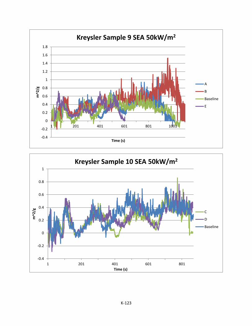
K-123

-0.4

-0.2

0

0.2

0.4

0.6

0.8

1

1.2

1.4

1.6

1.8

1 201 401 601 801 1001

m^2

/g

Time (s)


A

B

Baseline

E

-0.4

-0.2

0

0.2

0.4

0.6

0.8

1

1 201 401 601 801

m^2

/g

Time (s)


C

D

Baseline

K-124

-0.4

-0.2

0

0.2

0.4

0.6

0.8

1 201 401 601 801 1001

m^2

/g

Time (s)


C

D

Baseline

-0.8

-0.6

-0.4

-0.2

0

0.2

0.4

0.6

0.8

1

1 201 401 601 801 1001

m^2

/g

Time (s)


B

Baseline

K-125

-1

-0.5

0

0.5

1

1.5

2

1 201 401 601 801 1001

m^2

/g

Time (s)


C

D

Baseline

-15

-10

-5

0

5

10

15

20

25

1 201 401 601 801 1001

m^2

/g

Time (s)

Pigment SEA Comparisons 50kW/m2

(White) 7C

(Grey) 8A

(Beige) 9B

Baseline

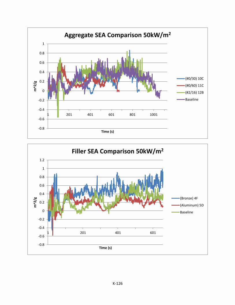
K-126

-0.8

-0.6

-0.4

-0.2

0

0.2

0.4

0.6

0.8

1

1 201 401 601 801 1001

m^2

/g

Time (s)

Aggregate SEA Comparison 50kW/m2

(#0/30) 10C

(#0/60) 11C

(#2/16) 12B

Baseline

-0.8

-0.6

-0.4

-0.2

0

0.2

0.4

0.6

0.8

1

1.2

1 201 401 601

m^2

/g

Time (s)

Filler SEA Comparison 50kW/m2

(Bronze) 4F

(Aluminum) 5D

Baseline

K-127

Specific Extinction Area analysis – 75kW




Baseline FRP System

No gelcoat





No pigment






several samples)


-0.6

-0.4

-0.2

0

0.2

0.4

0.6

0.8

1

1.2

1 501 1001 1501 2001

m^2

/g

Time (s)

Cores SEA Comparison 50kW/m2

Plywood 1B

Balsa 2A

Foam 3B

Baseline

K-128












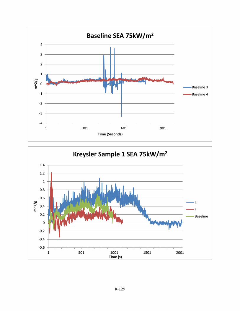
K-129

-4

-3

-2

-1

0

1

2

3

4

1 301 601 901

m^2

/g

Time (Seconds)

Baseline SEA 75kW/m2

Baseline 3

Baseline 4

-0.6

-0.4

-0.2

0

0.2

0.4

0.6

0.8

1

1.2

1.4

1 501 1001 1501 2001

m^2

/g

Time (s)


E

F

Baseline

K-130

-0.6

-0.4

-0.2

0

0.2

0.4

0.6

0.8

1

1.2

1 501 1001

m^2

/g

Time (s)


E

F

Baseline

-0.6

-0.4

-0.2

0

0.2

0.4

0.6

0.8

1

1.2

1 501 1001

m^2

/g

Time (s)


E

F

Baseline

K-131

-0.6

-0.4

-0.2

0

0.2

0.4

0.6

0.8

1

1.2

1.4

1.6

1 201 401 601

m^2

/g

Time (s)


F

G

Baseline

-1

-0.5

0

0.5

1

1.5

2

1 201 401 601 801

m^2

/g

Time (s)


E

F

Baseline

K-132

-0.4

-0.2

0

0.2

0.4

0.6

0.8

1

1.2

1 201 401 601 801 1001


G

H

Baseline

-1.5

-1

-0.5

0

0.5

1

1.5

2

1 201 401 601 801 1001

m^2

/g

Time (s)


F

G

Baseline

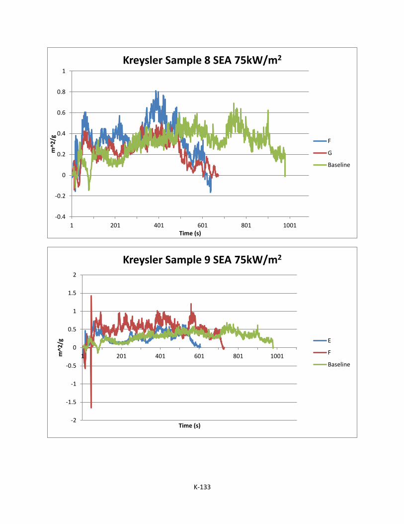
K-133

-0.4

-0.2

0

0.2

0.4

0.6

0.8

1

1 201 401 601 801 1001

m^2

/g

Time (s)


F

G

Baseline

-2

-1.5

-1

-0.5

0

0.5

1

1.5

2

1 201 401 601 801 1001m^2

/g

Time (s)


E

F

Baseline

K-134

-1

-0.5

0

0.5

1

1.5

2

1 201 401 601 801

m^2

/g

Time (s)


E

F

Baseline

-1

-0.5

0

0.5

1

1.5

2

1 201 401 601 801

m^2

/g

Time (s)


E

F

Baseline

K-135

-0.8

-0.6

-0.4

-0.2

0

0.2

0.4

0.6

0.8

1

1.2

1 201 401 601 801

m^2

/g

Time (s)


E

F

Baseline

-1.5

-1

-0.5

0

0.5

1

1.5

2

2.5

1 201 401 601 801 1001

m^2

/g

Time (s)


F

Baseline

E

K-136

-2

-1.5

-1

-0.5

0

0.5

1

1.5

2

1 201 401 601 801 1001

m^2

/g

Time (s)

Pigment SEA Comparisons 75kW/m2

(White) 7G

(Grey) 8G

(Beige) 9F

Baseline

-1

-0.5

0

0.5

1

1.5

2

1 201 401 601 801 1001

m^2

/g

Time (s)

Aggregate SEA Comparison 75kW/m2

(#0/30) 10E

(#0/60) 11F

(#2/16) 12E

Baseline

K-137

-0.6

-0.4

-0.2

0

0.2

0.4

0.6

0.8

1

1.2

1.4

1.6

1 201 401 601

m^2

/g

Time (s)

Filler SEA Comparison 75kW/m2

(Bronze) 4G

(Aluminum) 5E

Baseline

-1.5

-1

-0.5

0

0.5

1

1.5

2

2.5

1 201 401 601 801 1001

m^2

/g

Time (s)

Gel SEA Comparison 75kW/m2

Norsodyne 6

DCPD 13

Baseline 6.5229E-05

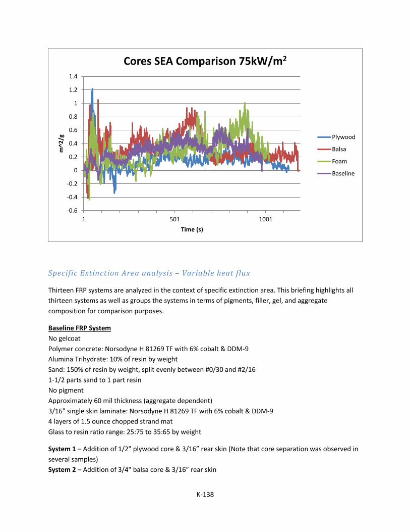
K-138

Specific Extinction Area analysis – Variable heat flux




Baseline FRP System

No gelcoat





No pigment






several samples)


-0.6

-0.4

-0.2

0

0.2

0.4

0.6

0.8

1

1.2

1.4

1 501 1001

m^2

/g

Time (s)

Cores SEA Comparison 75kW/m2

Plywood

Balsa

Foam

Baseline

K-139












K-140

-0.8

-0.6

-0.4

-0.2

0

0.2

0.4

0.6

0.8

1

1.2

1 501 1001 1501 2001

m^2

/g

Time (s)

Kreysler Sample 1 SEA Variable Heat Flux

25 kw/m^2

50 kW/m^2

75 kW/m^2

-0.6

-0.4

-0.2

0

0.2

0.4

0.6

0.8

1

1.2

1 501 1001 1501

m^2

/g

Time (s)


25 kw/m^2

50 kW/m^2

75 kW/m^2

K-141

-1

-0.5

0

0.5

1

1.5

2

1 501 1001 1501

m^2

/g

Time (s)


25 kw/m^2

50 kW/m^2

75 kW/m^2

-1

-0.5

0

0.5

1

1.5

2

1 201 401 601 801 1001 1201 1401

m^2

/g

Time (s)


25 kw/m^2

50 kW/m^2

75 kW/m^2

K-142

-0.8

-0.6

-0.4

-0.2

0

0.2

0.4

0.6

0.8

1

1.2

1 201 401 601 801 1001 1201 1401

m^2

/g

Time (s)


25 kw/m^2

50 kW/m^2

75 kW/m^2

-1

-0.5

0

0.5

1

1.5

1 201 401 601 801 1001 1201 1401

m^2

/g

Time (s)


25 kw/m^2

50 kW/m^2

75 kW/m^2

K-143

-1.5

-1

-0.5

0

0.5

1

1.5

2

1 501 1001 1501 2001 2501

m^2

/g

Time (s)


25 kw/m^2

50 kW/m^2

75 kW/m^2

-5

0

5

10

15

20

25

1 501 1001 1501 2001 2501

m^2

/g

Time (s)


25 kw/m^2

50 kW/m^2

75 kW/m^2

K-144

-2.5

-2

-1.5

-1

-0.5

0

0.5

1

1.5

2

2.5

3

1 201 401 601 801 1001 1201 1401 1601 1801 2001

m^2

/g

Time (s)


25 kw/m^2

50 kW/m^2

75 kW/m^2

-0.6

-0.4

-0.2

0

0.2

0.4

0.6

0.8

1

1.2

1 201 401 601 801

m^2

/g

Time (s)


25 kw/m^2

50 kW/m^2

75 kW/m^2

K-145

-1

-0.5

0

0.5

1

1.5

2

1 201 401 601

m^2

/g

Time (s)


25 kw/m^2

50 kW/m^2

75 kW/m^2

-0.8

-0.6

-0.4

-0.2

0

0.2

0.4

0.6

0.8

1

1 201 401 601 801 1001

m^2

/g

Time (s)


25 kw/m^2

50 kW/m^2

75 kW/m^2

K-146

-1.5

-1

-0.5

0

0.5

1

1.5

2

2.5

1 201 401 601 801 1001 1201

m^2

/g

Time (s)


25 kw/m^2

50 kW/m^2

75 kW/m^2

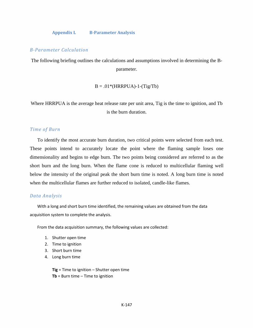
K-147

Appendix L B-Parameter Analysis

B-Parameter Calculation

The following briefing outlines the calculations and assumptions involved in determining the B-

parameter.

B = .01*(HRRPUA)-1-(Tig/Tb)

Where HRRPUA is the average heat release rate per unit area, Tig is the time to ignition, and Tb

is the burn duration.

Time of Burn

To identify the most accurate burn duration, two critical points were selected from each test.

These points intend to accurately locate the point where the flaming sample loses one

dimensionality and begins to edge burn. The two points being considered are referred to as the

short burn and the long burn. When the flame cone is reduced to multicellular flaming well

below the intensity of the original peak the short burn time is noted. A long burn time is noted

when the multicellular flames are further reduced to isolated, candle-like flames.

Data Analysis

With a long and short burn time identified, the remaining values are obtained from the data

acquisition system to complete the analysis.

From the data acquisition summary, the following values are collected:

1. Shutter open time

2. Time to ignition

3. Short burn time

4. Long burn time

Tig = Time to ignition – Shutter open time

Tb = Burn time – Time to ignition

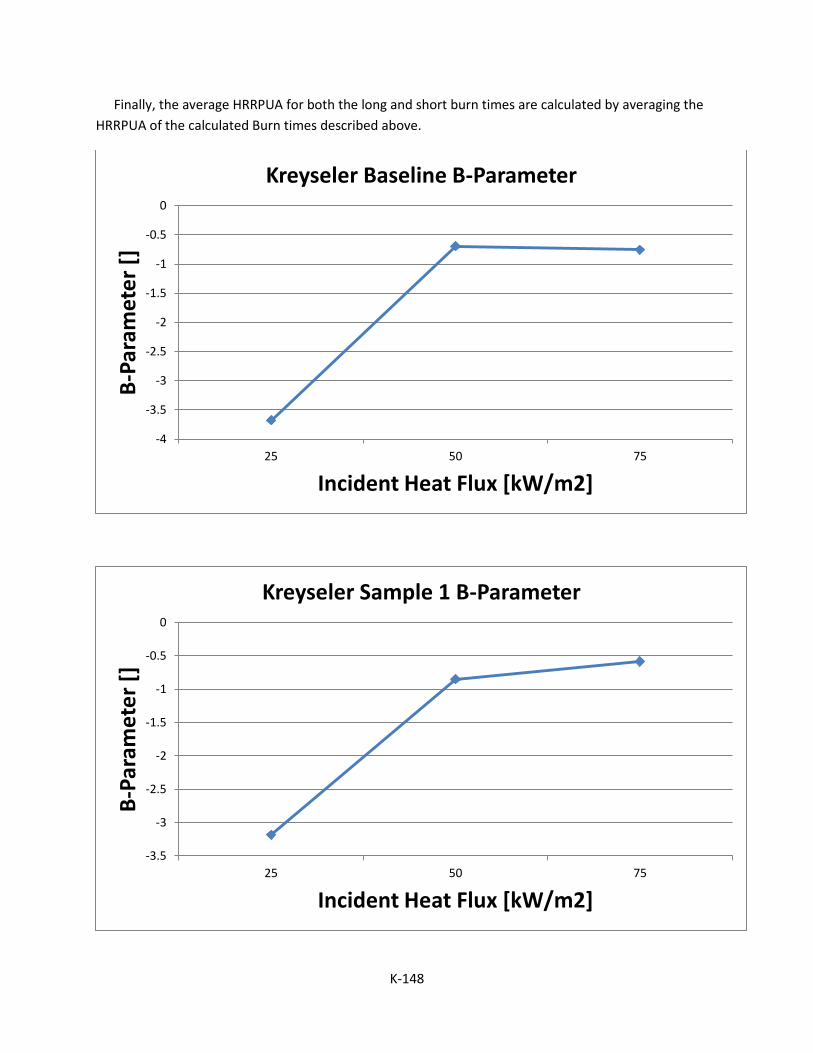
K-148

Finally, the average HRRPUA for both the long and short burn times are calculated by averaging the

HRRPUA of the calculated Burn times described above.

-4

-3.5

-3

-2.5

-2

-1.5

-1

-0.5

0

25 50 75

B-P

aram

ete

r []

Incident Heat Flux [kW/m2]

Kreyseler Baseline B-Parameter

-3.5

-3

-2.5

-2

-1.5

-1

-0.5

0

25 50 75

B-P

aram

ete

r []


Kreyseler Sample 1 B-Parameter

K-149

-2.5

-2

-1.5

-1

-0.5

0

25 50 75

B-P

aram

ete

r []



-6

-5

-4

-3

-2

-1

0

25 50 75

B-P

aram

ete

r []



K-150

-1.2

-1

-0.8

-0.6

-0.4

-0.2

0

25 50 75

B-P

aram

ete

r []



-1.6

-1.4

-1.2

-1

-0.8

-0.6

-0.4

-0.2

0

25 50 75

B-P

aram

ete

r []



K-151

-3.5

-3

-2.5

-2

-1.5

-1

-0.5

0

25 50 75

B-P

aram

ete

r []



-2.5

-2

-1.5

-1

-0.5

0

25 50 75

B-P

aram

ete

r []



K-152

-1.6

-1.4

-1.2

-1

-0.8

-0.6

-0.4

-0.2

0

25 50 75

B-P

aram

ete

r []



-1.8

-1.6

-1.4

-1.2

-1

-0.8

-0.6

-0.4

-0.2

0

25 50 75

B-P

aram

ete

r []



K-153

-4.5

-4

-3.5

-3

-2.5

-2

-1.5

-1

-0.5

0

25 50 75

B-P

aram

ete

r []



-1.4

-1.2

-1

-0.8

-0.6

-0.4

-0.2

0

25 50 75

B-P

aram

ete

r []



K-154

-1.8

-1.6

-1.4

-1.2

-1

-0.8

-0.6

-0.4

-0.2

0

25 50 75

B-P

aram

ete

r []



-1

-0.8

-0.6

-0.4

-0.2

0

0.2

25 50 75

B-P

aram

ete

r []



K-155

-4

-3.5

-3

-2.5

-2

-1.5

-1

-0.5

0

25 50 75

B-P

aram

ete

r []


Kreyseler Pigment B-Parameter Comparison

White

Grey

Beige

Baseline

-4.5

-4

-3.5

-3

-2.5

-2

-1.5

-1

-0.5

0

25 50 75

B-P

aram

ete

r []


Kreyseler Aggregate B-Parameter Comparison

(#0/30)

(#0/60)

(#2/16)

Baseline

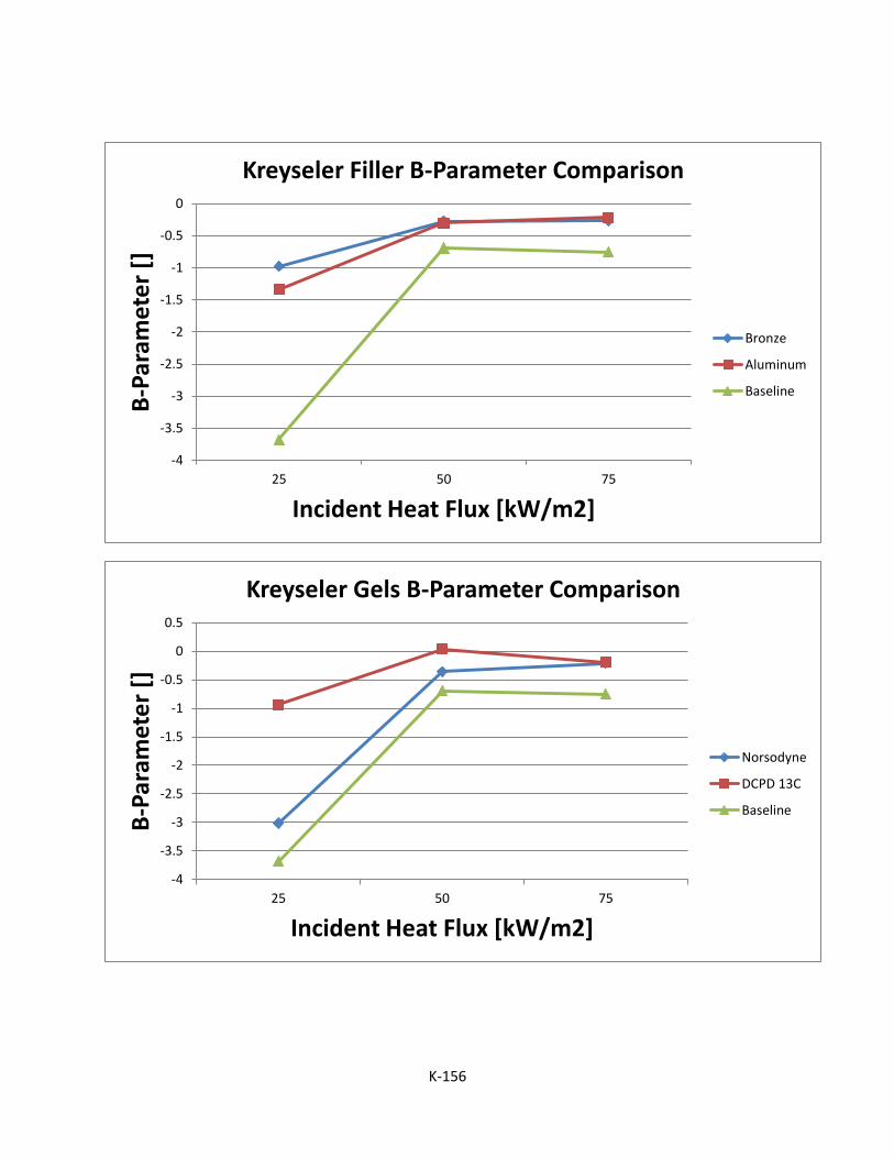
K-156

-4

-3.5

-3

-2.5

-2

-1.5

-1

-0.5

0

25 50 75

B-P

aram

ete

r []


Kreyseler Filler B-Parameter Comparison

Bronze

Aluminum

Baseline

-4

-3.5

-3

-2.5

-2

-1.5

-1

-0.5

0

0.5

25 50 75

B-P

aram

ete

r []


Kreyseler Gels B-Parameter Comparison

Norsodyne

DCPD 13C

Baseline

K-157

-6

-5

-4

-3

-2

-1

0

25 50 75

B-P

aram

ete

r []


Kreyseler Cores B-Parameter Comparison

Plywood

Balsa

Foam

Baseline

K-158

Appendix M Smoke Calculations

After reviewing the data, there were some questions regarding the smoke calculations

for a couple of tests. Two problems were observed from the tests in question. Two

tests (White Pigment and Plywood Core) showed extremely high smoke numbers while

the other test (Balsa Core) had negative smoke numbers. These errors were corrected

the same way. After examining the raw data, it appeared there may have been a

problem with the compensating photodiode. Therefore the smoke numbers were

recalculated using just the main photodiode. The equation used to calculate smoke

is ( )

, where Io is the compensating photodiode and the I is the main

photodiode. In the adjusted smoke calculations, the average reading of the main

photodiode during the clean air burn was used instead of the compensating photodiode

reading. The adjusted smoke graphs can be seen below. The shape of the graphs are

the same, the adjusted calculation caused the graph to shift.

0

0.2

0.4

0.6

0.8

1

1.2

1.4

1.6

1.8

2

0 200 400 600 800 1000

Mai

n (

%T)

Time (s)

White Pigment

K-159

-0.1

0

0.1

0.2

0.3

0.4

0.5

0 200 400 600 800 1000 1200

Smo

ke (

%T)

Time (S)

Plywood Core

-0.2

0

0.2

0.4

0.6

0.8

1

1.2

1.4

0 500 1000 1500 2000 2500

Mai

n (

%T)

Time (s)

Balsa Core

Documents

Development of a Flame Spread Screening Tool for Fiber ... of a Flame Spread Screening Tool for Fiber Reinforced Polymers A Major Qualifying Project Report submitted to the Faculty