Embed Size (px)
Citation preview

DEVELOPMENT OF A COMPOSITE OXIDISER TANK FOR THE
PHOENIX-1B MK. II HYBRID ROCKET
DYLAN ROY WILLIAMS
Submitted in fulfilment of the academic requirements for the degree of Master of Science in
Mechanical Engineering, College of Agriculture, Engineering and Science, University of KwaZulu-
Natal.
March 2020
Supervisor: Dr. Jean-Francois Pitot de la Beaujardiere
Co-Supervisor: Dr Michael Brooks
i
DECLARATION 1 – PLAGIARISM
I, Dylan Roy Williams, declare that
1. The research reported in this thesis, except where otherwise indicated, is my original
research.
2. This thesis has not been submitted for any degree or examination at any other university.
3. This thesis does not contain other persons’ data, pictures, graphs or other information, unless
specifically acknowledged as being sourced from other persons.
4. This thesis does not contain other persons’ writing, unless specifically acknowledged as
being sourced from other researchers. Where other written sources have been quoted, then: a.
Their words have been re-written but the general information attributed to them has been
referenced
b. Where their exact words have been used, then their writing has been placed in italics and
inside quotation marks, and referenced.
5. This thesis does not contain text, graphics or tables copied and pasted from the Internet,
unless specifically acknowledged, and the source being detailed in the thesis and in the
References sections.
Signed:……………………………………………… Date:……………………………………
Mr Dylan Roy Williams
As the candidate’s supervisor I agree/do not agree to the submission of this thesis.
Signed:……………………………………………… Date:……………………………………
Dr Michael J. Brooks
As the candidate’s co-supervisor I agree/do not agree to the submission of this thesis.
Signed:……………………………………………… Date:……………………………………
Mr. Jean-Francois Pitot de la Beaujardiere

ii
DECLARATION 2 – PUBLICATIONS
Broughton, K. M., Williams, D. R., Brooks, M. J., Pitot de la Beaujardiere, J., 2018.
Development of the Phoenix-1B Mk II 35 km Apogee Hybrid Rocket. 2018 Joint Propulsion
Conference, AIAA Propulsion and Energy Forum. Cincinnati, OH.
Signed:……………………………………………… Date:……………………………………
Mr Dylan Roy Williams

iii
ACKNOWLEDGEMENTS
To my Mom and Dad, without whom I wouldn’t have been able to pursue a master’s degree.
Or exist.
To Shaleen Maloney, for the emotional support throughout the project. I’ll try not to miss any
more birthdays because of rocket tests.
To Kai, my research partner, for the friendship and his unfailing and relentless work ethic
that guilted me into completing my own work more times than I’d like to admit.
To Duran, Nino and the rest of the gang in the ASReG lab for putting up with my never-
ending complaints.
To the team at the Dive Factory, especially Mike Collins, for the advice and for facilitating
the manufacture of most of the rocket.
To Danesh and Yushen in the Mechanical Engineering workshop, for the good advice and
helping hands in manufacturing tasks.
To all the past Phoenix Students, particularly Udil Balmogim, whose foundational work and
support made the project possible.
The team at Rheinmetall Denel Munitions (RDM), particularly Kelly Scholtz and the team at
Advanced Composites, for facilitating the manufacture of the pressure vessel.
To Overberg Test Range (OTR), for facilitating the launch of the Phoenix-1B Mk. II
To the South African National Space Agency (SANSA), for supporting me financially
throughout this master’s project.
The National Research Foundation (NRF), for funding the project with their Thuthuka grant.
Lastly, I would like to thank my supervisors, Jean and Mike, for their guidance and support
throughout the project.

iv
ABSTRACT
The University of KwaZulu-Natal’s Aerospace Systems Research Group (ASReG) was formed
in 2009 and has been developing hybrid sounding rockets since 2010 under the umbrella of the
Hybrid Sounding Rocket Programme (HSRP). The HSRP was started with the goal of
developing a sounding rocket platform capable of meeting the need of the South African and
African scientific communities to access atmospheric data without using expensive foreign
sounding rocket launch services. To reach this goal the HSRP has begun developing a series
of hybrid propelled rockets as technology demonstrators, each with incrementally improved
apogee and technology integration. [1]
The primary series of vehicles under the HSRP are the Phoenix series hybrid rockets. The
Phoenix series rockets are technology demonstrators and form part of the HSRP’s roadmap to
developing a sounding rocket which can reach an apogee of 100 km. The next rocket in the
Phoenix Series is the Phoenix-1B Mk. II. This rocket aims achieve an apogee of 35 km and to
achieve this apogee, composite materials will be integrated into the airframe structure,
replacing the previously utilised aluminium construction. The primary mass reduction on the
Phoenix-1B Mk. II came from the integration of a filament-wound composite pressure vessel
for use as the nitrous oxide storage (oxidiser) tank, which was designed in this thesis.
This thesis details the creation of a methodology capable of generating and analysing filament
wound pressure vessels suitable for use as oxidiser tanks on rockets. The methodology was
based upon analytical methods but progressed to verify the design on a computational platform.
The methodology was executed to generate a structure for use on the Phoenix 1B Mk. II rocket.
The structure was constructed using a liner made from a combination of un-plasticised
polyvinyl-chloride and aluminium. The liner was then filament wound to create the load
bearing structure of the oxidiser tank and was bonded to supplementary coupling structures to
allow for coupling with the fore and aft sections of the rocket. After the manufacture of the
proposed oxidiser tank, it was qualified using a variety of different tests. The first were proof
and destructive pressure tests which ensured that the tank would operate safely. The next phase
of testing involved a cold flow and hot fire test of the rocket motor. The tank passed these tests
and only remains to be flight tested.
The resulting oxidiser tank offered a conservatively estimated 15 % mass saving in comparison
to the previously utilised aluminium oxidiser tank on the Phoenix-1B Mk. I hybrid sounding
rocket.

v
TABLE OF CONTENTS
DECLARATION 1 – PLAGIARISM......................................................................................... i
DECLARATION 2 – PUBLICATIONS ................................................................................... ii
ACKNOWLEDGEMENTS ...................................................................................................... iii
ABSTRACT.............................................................................................................................. iv
LIST OF FIGURES .................................................................................................................. ix
1. INTRODUCTION ............................................................................................................. 1
1.1. The Aerospace Systems Research Group.................................................................... 1
1.2. The Phoenix Programme History ................................................................................ 1
1.2.1. The Phoenix-1A ................................................................................................... 1
1.2.2. The Phoenix-1B Mk. I ......................................................................................... 2
1.2.3. The Phoenix-1B Mk. II ........................................................................................ 2
1.3. Objectives .................................................................................................................... 3
1.4. Dissertation Outline..................................................................................................... 4
2. LITERATURE REVIEW .................................................................................................. 5
2.1. Introduction ................................................................................................................. 5
2.2. Oxidiser Storage .......................................................................................................... 5
2.2.1. Oxidiser Storage on the Phoenix Series Rockets ................................................. 5
2.2.2. Delft University.................................................................................................... 7
2.2.3. Spaceship One...................................................................................................... 8
2.3. Composite Materials ................................................................................................... 9
2.4. Analysis of Composite Materials .............................................................................. 10
2.5. Filament Winding...................................................................................................... 12
2.5.1. Filament Winding Process Description ............................................................. 12
2.5.2. Liner Selection for Composite Pressure Vessels ............................................... 14
2.5.3. Analysis of Filament Wound Structures ............................................................ 15
3. DESIGN OF COMPOSITE OXIDISER TANK ............................................................. 18
3.1. Introduction ............................................................................................................... 18
3.2. Objectives and Constraints ........................................................................................ 18
3.3. Laminate and Geometric Constraints ........................................................................ 18
3.3.1. Reinforcement Material ..................................................................................... 18
3.3.2. Matrix Material .................................................................................................. 19
3.3.3. Geometric Constraint Generation ...................................................................... 19
3.4. Analytical Tank Design............................................................................................. 20
3.4.1. Netting Analysis................................................................................................. 20

vi
3.4.2. Head Shape Overview........................................................................................ 23
3.4.3. Required User Inputs ......................................................................................... 24
3.4.4. Analytical Design Result ................................................................................... 26
3.4.5. Analytical Design Conclusion ........................................................................... 29
3.5. Liner Concept Generation ......................................................................................... 30
3.5.1. Liner Material Selection..................................................................................... 30
3.5.2. Geometric Overview .......................................................................................... 31
3.5.3. O-ring Seals........................................................................................................ 34
3.5.4. Preliminary Liner Design Conclusion ............................................................... 36
3.6. Computational Tank Design...................................................................................... 37
3.6.1. Material Properties ............................................................................................. 37
3.6.2. Computational Method 1: 3D Laminate Analysis ............................................. 42
3.6.3. Computational Method 2: 2D Analysis ............................................................. 49
3.6.4. Computational Method 3: Quasi-2D Analysis................................................... 53
3.6.5. Loading Condition Specification ....................................................................... 65
3.6.6. Computational Tank Design Conclusion ........................................................... 67
3.7. Coupling Structure Design ........................................................................................ 68
3.7.1. Coupling Structure Constraints .......................................................................... 68
3.7.2. Preliminary Design Layout ................................................................................ 69
3.7.3. Bond Design....................................................................................................... 70
3.7.4. Coupler Computational Design.......................................................................... 72
3.7.5. Coupler Simulation Results ............................................................................... 76
3.7.6. Coupler Design Conclusion ............................................................................... 81
3.8. Analysis Results ........................................................................................................ 82
3.8.1. Load Case 1: Pressure Loading.......................................................................... 82
3.8.2. Load Case 2: Axial and Bending Moment Combination ................................... 90
3.8.3. Load Case 3: In-flight Loading .......................................................................... 94
3.8.4. Simulation Results Conclusion ........................................................................ 101
3.9. Design Conclusion .................................................................................................. 102
4. TANK MANUFACTURE ............................................................................................. 104
4.1. Introduction ............................................................................................................. 104
4.2. Liner Manufacture ................................................................................................... 104
4.3. Filament Winding.................................................................................................... 106
4.4. Coupler Manufacture............................................................................................... 113
4.5. Manufacturing Conclusion ...................................................................................... 117

vii
5. TESTING ....................................................................................................................... 118
5.1. Introduction ............................................................................................................. 118
5.2. Pressure Testing ...................................................................................................... 118
5.2.1. Proof Testing.................................................................................................... 118
5.2.2. Destructive Testing .......................................................................................... 120
5.3. Cold Flow Testing ................................................................................................... 122
5.3.1. Cold Flow Test Setup....................................................................................... 122
5.3.2. Cold Flow Test Results .................................................................................... 122
5.4. Hot Fire Testing ...................................................................................................... 124
5.4.1. Hot Fire Test Setup .......................................................................................... 124
5.4.2. Hot Fire Test Results ....................................................................................... 125
5.5. Testing Conclusion.................................................................................................. 127
6. DISCUSSION ................................................................................................................ 128
6.1. Introduction ............................................................................................................. 128
6.2. Tank Design Method Review.................................................................................. 128
6.2.1. Analytical Method Review .............................................................................. 128
6.2.2. Computational Method Review ....................................................................... 129
6.2.3. General Design Philosophy Review ................................................................ 130
6.2.4. Design Conclusion ........................................................................................... 131
6.3. Tank Material Choice Review................................................................................. 132
6.3.1. Liner Material Selection................................................................................... 132
6.3.2. Tank Composite Material Selection................................................................. 133
6.3.3. Coupler Material Selection .............................................................................. 134
6.4. Tank Manufacture Review ...................................................................................... 135
6.4.1. Liner Manufacturing Review ........................................................................... 135
6.4.2. Filament Winding Review ............................................................................... 136
6.4.3. Coupler Manufacturing Review....................................................................... 138
6.4.4. Post Manufacture Mass Analysis ..................................................................... 138
6.4.5. Manufacturing Conclusion............................................................................... 142
6.5. Tank Testing Review .............................................................................................. 143
6.5.1. Pressure Testing ............................................................................................... 143
6.5.2. Cold Flow Testing............................................................................................ 144
6.5.3. Hot Fire Testing ............................................................................................... 144
6.5.4. Testing Conclusion .......................................................................................... 144
6.6. Tank Comparison .................................................................................................... 144

viii
6.6.1. Geometric Comparison .................................................................................... 145
6.6.2. Efficiency Parameter Comparison ................................................................... 145
6.6.3. Tank Comparison Conclusion.......................................................................... 147
7. CONCLUSION .............................................................................................................. 149
REFERENCES ...................................................................................................................... 151
APPENDIX ............................................................................................................................ 155

ix
LIST OF FIGURES
Figure 2-1: Cross-sectional View of the Oxidiser Tank from the P1A Hybrid Rocket [8] ....... 6
Figure 2-2: Completed P1B Mk. I Oxidiser Tank [6]................................................................ 6
Figure 2-3: Stratos III Hybrid Rocket on the Launch Platform [9] ........................................... 7
Figure 2-4: U-PVC Liner Prototype for the Stratos III Rocket ................................................. 8
Figure 2-5: Pilot Mike Melvill Celebrating After the 2004 Launch of Spaceship One............. 8
Figure 2-6: Laminate Material Directionality [15] .................................................................. 11
Figure 2-7: An Overview of the Filament Winding Process [17]............................................ 13
Figure 2-8: Filament Wound Pressure Vessel with Domed Ends [18] .................................... 13
Figure 2-9: Proposed PVC Liner Design from DARE [23]..................................................... 15
Figure 2-10: CADWIND Filament Model [9] ......................................................................... 17
Figure 3-1: Depiction of Variables for Clairaut’s Theorem [33] ............................................. 21
Figure 3-2: Geometric Constraint Depiction ........................................................................... 24
Figure 3-3: Tank Domed End Profiles ..................................................................................... 26
Figure 3-4: Winding Angle vs. Longitudinal Distance............................................................ 27
Figure 3-5: Analytical Method Percentage Mass Distribution ................................................ 29
Figure 3-6: Liner Geometry Concept 1.................................................................................... 33
Figure 3-7: Liner Geometry Concept 2.................................................................................... 34
Figure 3-8: Liner Concept 2 Seal Geometry ............................................................................ 36
Figure 3-9: Early Concept Tank Geometry on Autodesk Inventor.......................................... 43
Figure 3-10: Axisymmetric CAD Tank Slice for 3D Mesh Generation .................................. 44
Figure 3-11: 3D Laminate Geometry....................................................................................... 44
Figure 3-12: 2D Laminate Definition of Helical Region for 3D Mesh Generation ................. 45
Figure 3-13: 3D Laminate Fill Composite Mesh ..................................................................... 46
Figure 3-14: Loading Conditions of a 3D Composite Simulation ........................................... 47
Figure 3-15: 3D Laminate Analysis Displacement Benchmark Result ................................... 48
Figure 3-16: Laminate Thickness Change over the Head of a Composite Tank ..................... 50
Figure 3-17: Meshed 2D Laminate Geometry ......................................................................... 51
Figure 3-18: 2D Computational Analysis Load Case .............................................................. 52
Figure 3-19: 2D Analysis Composite Structure Displacement Result..................................... 53
Figure 3-20: Final Liner Geometry .......................................................................................... 54
Figure 3-21: 3D Liner Mesh .................................................................................................... 55
Figure 3-22: Final Iteration Cylinder Laminate ....................................................................... 57

x
Figure 3-23: CAD Model with Dome Region Segregation ..................................................... 58
Figure 3-24: Dome Region Laminate Definition ..................................................................... 59
Figure 3-25: Coupler Bond Location ....................................................................................... 60
Figure 3-26: General Bond Locations...................................................................................... 61
Figure 3-27: Pin Contact Region and Result ........................................................................... 62
Figure 3-28: Simulation Contact Regions................................................................................ 63
Figure 3-29: Simulation Constraint Definition ........................................................................ 65
Figure 3-30: Simulation Loading Condition ............................................................................ 66
Figure 3-31: Aft-most Coupling Area Depiction ..................................................................... 68
Figure 3-32: Fore-most Coupling Area Depiction ................................................................... 69
Figure 3-33: Coupler Geometry ............................................................................................... 70
Figure 3-34: Composite Coupler Geometry ............................................................................ 72
Figure 3-35: Coupler Composite Structure Laminate Definition ............................................ 73
Figure 3-36: Coupler Simulation Mesh ................................................................................... 74
Figure 3-37: Coupler Simulation Load Case ........................................................................... 75
Figure 3-38: Coupler Simulation Constraints .......................................................................... 76
Figure 3-39: Coupler Simulation Deflection Result ................................................................ 76
Figure 3-40: Coupler Simulation Composite Ply 1 Result ...................................................... 78
Figure 3-41: Coupler Simulation Composite Ply 4 Result ...................................................... 78
Figure 3-42: Coupler Simulation Composite Ply 10 Result .................................................... 79
Figure 3-43: Coupling Structure Maximum Failure Likelihood.............................................. 80
Figure 3-44: Coupler Simulation Bond Areas Result .............................................................. 80
Figure 3-45: Isolated Pressure Y-Deflection Result ................................................................ 83
Figure 3-46: Isolated Pressure Z-Deflection Result................................................................. 84
Figure 3-47: Isolated Pressure Aluminium Bulkhead Von Mises Stress................................. 85
Figure 3-48: Isolated Pressure U-PVC Liner Stress ................................................................ 86
Figure 3-49: Isolated Pressure Hoop Layer Tsai-Wu Result ................................................... 88
Figure 3-50: Isolated Pressure Helical Layer Tsai-Wu Result ................................................ 89
Figure 3-51: Axial and Bending Moment (X) Deflection Result ............................................ 91
Figure 3-52: Axial and Bending Moment (Y) Deflection Result ............................................ 92
Figure 3-53: Axial and Bending Moment Deflection Magnitude Result ................................ 93
Figure 3-54: Axial and Bending Moment Tsai-Wu Helical Result ......................................... 93
Figure 3-55: In-Flight X- Deflection Result ............................................................................ 95
Figure 3-56: In-Flight Y- Deflection Result ............................................................................ 96

xi
Figure 3-57: In-Flight Z-Deflection Result.............................................................................. 97
Figure 3-58: In-Flight Aluminium Bulkhead Stress Result ..................................................... 98
Figure 3-59: In-Flight PVC Liner Stress Result ...................................................................... 98
Figure 3-60: In-Flight Helical Layer Tsai-Wu Result ............................................................. 99
Figure 3-61: In-Flight Hoop Layer Tsai-Wu Result .............................................................. 100
Figure 3-62: Final Design Methodology................................................................................ 102
Figure 4-1: Tank PVC Liner End........................................................................................... 104
Figure 4-2: Tank Bulkhead View 1 ....................................................................................... 105
Figure 4-3: Tank Liner Exploded View with O-rings ........................................................... 105
Figure 4-4: Tank Liner Assembled View without Grub Screws ........................................... 106
Figure 4-5: Liner Mounted on the Filament Winding Machine ............................................ 106
Figure 4-6: Hoop Layer Dry Wind Test ................................................................................ 107
Figure 4-7: First Helical Layer Dry Wind Test with Fibre Slip ............................................ 108
Figure 4-8: Focused View of Fibre Slip ................................................................................ 109
Figure 4-9: Conclusion of Helical Dry Winding of Domed Ends ......................................... 109
Figure 4-10: Final Helical Dry Wind over Cylinder.............................................................. 110
Figure 4-11: Tank in Position Prior to Post Cure .................................................................. 112
Figure 4-12: Cured vs. Uncured Tank Surface Finish ........................................................... 112
Figure 4-13: Coupler Laminate Mould Components ............................................................. 113
Figure 4-14: Assembled Coupler Moulds .............................................................................. 114
Figure 4-15: Tank Prepared for Coupler Lamination ............................................................ 115
Figure 4-16: Tank Coupler Post Lamination ......................................................................... 115
Figure 4-17: Tank Coupler Composite Trimming Process .................................................... 116
Figure 4-18: Assembled Tank Couplers ................................................................................ 116
Figure 4-19: Aft Coupler Post Riveting ................................................................................. 117
Figure 5-1: Proof Pressure Cycle Test ................................................................................... 119
Figure 5-2: Burst Test Pressure Result .................................................................................. 120
Figure 5-3: Destructive Test Weep Result ............................................................................. 121
Figure 5-4: Cold Flow Test Pressure Profile ......................................................................... 123
Figure 5-5: Hot Fire Test Configuration ................................................................................ 125
Figure 5-6: Hot Fire Test Tank Pressure Profile.................................................................... 126
Figure 5-7: Hot Fire Test Axial Load Profile ........................................................................ 126
Figure 6-1: Tank Mass Summary Graph ............................................................................... 140
Figure 6-2: Flight Tank Manufacturing Discrepancy Graph ................................................. 140

xii
Figure 6-3: P1B Mk. II Tank Construction Breakdown ........................................................ 142
Figure 6-4: Geometric Tank Efficiency ................................................................................. 147
Figure 0-1: Coupler Geometry Mechanical Drawings........................................................... 156
Figure 0-2: Liner Geometry Mechanical Drawings ............................................................... 157

xiii
LIST OF TABLES
Table 3-1: Final Tank Iteration Geometric Property ............................................................... 20
Table 3-2: Required Geometric Inputs..................................................................................... 25
Table 3-3: Required Material Properties.................................................................................. 26
Table 3-4: Liner Materials Comparison [36] [37] [38] [39] .................................................... 30
Table 3-5: Seal Media and Expected Operating Temperatures ............................................... 35
Table 3-6: Chemical Compatibility and Service Temperatures of O-ring Compounds [40]... 35
Table 3-7: Mechanical Properties of AMPREG 21 Epoxy Resin [29] .................................... 37
Table 3-8: Mechanical Properties of T800 Carbon Fibre [28] ................................................ 38
Table 3-9: Laminate Constituent Poisson Ratios ..................................................................... 39
Table 3-10: Assumed Composite Properties............................................................................ 42
Table 3-11: Global Ply ID's for 3D Mesh Generation ............................................................. 46
Table 3-12: 2D Analysis Ply Group List and Description ....................................................... 55
Table 3-13: Ply Group Material Type Breakdown .................................................................. 56
Table 3-14: 2D Analysis Composite Material Properties ........................................................ 56
Table 3-15: Loading Condition Origin .................................................................................... 66
Table 3-16: Coupler Simulation Load Magnitudes ................................................................. 75
Table 4-1: Filament Winding Layup Schedule ...................................................................... 110
Table 6-1: Manufactured Tank Mass Analysis Table ............................................................ 139
Table 6-2: Rocket Oxidiser Tank Geometric Properties........................................................ 145
Table 0-1: Computational Design Mass Prediction ............................................................... 155

xiv
NOMENCLATURE
Symbol Description Unit
C1 Composite Principal Compressive Limit N/m2
C2 Composite Transverse Compressive Limit N/m2
Ef Fibre Principal Stiffness N/m2
EL Composite Principal Stiffness N/m2
Em Matrix Stiffness N/m2
ET Composite Transverse Stiffness N/m2
G Composite Shear Limit N/m2
G12 Composite Shear Modulus N/m2
Gf Fibre Shear Modulus N/m2
Gm Matrix Shear Modulus N/m2
ILSS Inter-Laminate Shear Strength N/m2
mN2O Nitrous Oxide Mass Kg
𝑁𝜃 Circumferential Pressure Force N
𝑁𝜙 Longitudinal Pressure Force N
P Pressure Magnitude Bar
R Radius M
R0 Boss Radius M
Rc Cylinder Radius M
SMF Halpin-Tsai Strain Magnification Factor -
T1 Composite Principal Tensile Limit N/m2
T2 Composite Transverse Tensile Limit N/m2
Tf Fibre Principal Tensile Limit N/m2
th Local Helical Thickness Mm
thc Cylinder Helical Thickness Mm
tho Hoop Thickness Mm
vf Fibre Volume Fraction %
vm Matric Volume Fraction %
Vtank Tank Container Volume m3
X Normalised Head Shape Longitudinal Length -
x Head Shape Longitudinal Location M
x0 Head Shape Boss Longitudinal Location M
Y Normalised Head Shape Radial Length -
y Head Shape Radial Location M
y0 Head Shape Boss Radial Location M
α Winding Angle °
α0 Boss Winding Angle °
αc Cylinder Winding Angle °
εf Fibre Elongation at Failure -
ρliquid N2O Liquid Nitrous Oxide Density kg/ m3
σmf Stress in Matrix at Fibre Failure N/m2

xv
υ12 Composite Poissons Ratio -
υf Fibre Poissons Ratio -
υm Matrix Poissons Ratio -
𝜂 Halpin-Tsai Curve Fit Parameter 1 -
𝜉 Halpin-Tsai Curve Fit Parameter 2 -

1
1. INTRODUCTION
1.1. The Aerospace Systems Research Group
The University of KwaZulu-Natal’s Aerospace Systems Research Group (ASReG) was formed
in 2009 and has been developing hybrid sounding rockets since 2010 under the umbrella of the
Hybrid Sounding Rocket Programme (HSRP). The HSRP was started with the goal of
developing a sounding rocket platform capable of meeting the needs of the South African and
African scientific communities. To reach this goal the HSRP has begun developing a series of
hybrid propelled rockets as technology demonstrators, each with incrementally improved
apogee and technology integration. Other projects which have been initiated to achieve the
aims of the programme include the development of the Hybrid Rocket Performance Simulator
(HYROPS) code and the development of a laboratory-scale test facility at the University [1].
The primary series of vehicles under the HSRP is the Phoenix series hybrid rockets. These are
technology demonstrators and form part of the HSRP’s roadmap to developing a sounding
rocket which can reach an apogee of 100 km. At the time of publication, the HSRP has
developed three Phoenix class vehicles with incrementally higher design apogees.
1.2. The Phoenix Programme History
This section serves as a brief overview of the rockets developed under the Phoenix programme.
The three Phoenix series rockets currently developed under the HSRP are the Phoenix-1A, 1B
Mk. I and 1B Mk. II.
1.2.1. The Phoenix-1A
The Phoenix-1A (hereafter P1A) was designed by two postgraduate mechanical engineering
students, Bernard Genevieve and Seffat Chowdhury [2] [3]. The P1A was the first Phoenix
class vehicle, with a design apogee of 10 km and utilising a nitrous oxide oxidiser and a paraffin
wax fuel. It was also the first hybrid rocket developed by an academic institution to be launched
in South Africa.
The rocket weighed 90 kg and was built using primarily aluminium construction with a carbon
fibre fore section and boat tail. The rocket had an outer diameter of 200 mm with a total length
of the 4.55 m. The rocket was launched from Overberg Test Range in August 2014 and reached
a below-target apogee of 2.5 km due to a structural failure in the nozzle upon launch [4].

2
Another vehicle designated the Phoenix-2A (hereafter P2A) was designed by post-graduate
student Fiona Leverone [5]. Using a similar propulsion system layout to the P1A, the P2A was
envisaged to be am 11-metre long vehicle with the potential to reach space.
1.2.2. The Phoenix-1B Mk. I
The Phoenix-1B (hereafter P1B Mk. I) was the second vehicle manufactured in the Phoenix
series with a design apogee of 16 km. The vehicle was developed by postgraduate student Udil
Balmogim [6] and its design differed from the P1A in both construction and propulsion type.
Ultimately the changes to the propulsion system were not realised.
The intention with the propulsion system was to include aluminium powder in the paraffin wax
fuel grain to create a more energetic fuel. The research was abandoned due a lack of fuel
regression rate data. The vehicle construction differed from the P1A by making use of extruded
aluminium tube sections to form the bulk of the body and avoided welded connections on
aluminium components. The vehicle also differed geometrically, with a reduced outer diameter
of 164 mm and a reduced length of 4.3 m [6].
Due to various delays in the programme, the P1B Mk. I rocket has not yet been launched. The
ground testing phase has been completed with successful cold and hot fire results. The vehicle
is due to launch in early 2020.
1.2.3. The Phoenix-1B Mk. II
The Phoenix-1B Mk. II vehicle (hereafter P1B Mk. II) is the third vehicle in the series and was
designed as a revised version of the P1B Mk. I vehicle. The rocket was designed by two
postgraduate students, Kai Broughton and Dylan Williams (author). The research outlined in
this thesis contributed to the construction of the composite oxidiser tank used in the structure
of the P1B Mk. II, while research conducted in parallel by Broughton [7] contributed to the
propulsion system.
The P1B Mk. II intended to improve on the previous apogees of the Phoenix series rockets with
a design apogee of 35 km. To reach this apogee, lightweight composite materials were
integrated into the airframe to replace the existing aluminium construction. Revisions were also
made to the propulsion system to improve upon the previous designs and conclude the metal
additive research which was started in development of the P1B Mk. I. The vehicle had an outer
diameter of 170 mm, similar to the P1B Mk. I. To allow for increased oxidiser and fuel mass
and maintain the desired diameter, the vehicle length in comparison to the P1B Mk. I was
increased to 4.9 m.

3
The P1B Mk. II was launched from Overberg Test Range in February 2019 and failed directly
after launch due to an unexpected closure of the main oxidiser valve shortly after ignition.
1.3. Objectives
The objective of the P1B Mk. II was to improve upon the apogee and technologies involved in
the previous rocket iterations in the Phoenix programme. The P1B Mk. I was used as a
technology foundation and benchmark for the P1B Mk. II. By basing the design on the existing
technology of the P1B Mk. I rather than initiating a complete vehicle redesign, the P1B Mk. II
subsystems were more optimised with respect to mass and utility than would have been
possible if they were designed from first principles. The primary systems which required
research input were the airframe and the flight motor components.
The motor component revisions were implemented in research conducted in parallel by
Broughton [7]. He aimed to improve the performance of the motor by making use of energetic
metal additives in the fuel and tailoring the motor to the current mission requirements [7].
The revisions to the airframe are the focus of this thesis and are primarily concerned with the
integration of composite materials into the airframe. Lightweight composite materials have the
potential to decrease the vehicle inert mass when used in favour of the aluminium based
construction used on the previous Phoenix vehicle iterations. The oxidiser tank structure has
the largest potential for mass reduction by switching to a composite based construction and
was chosen as the focus of the research. In this context, the goals of this research are outlined
below:
1. Develop a process within the technical, computational and resource constraints of the
University which can effectively design a composite pressure vessel for use as an
oxidiser tank on a rocket.
2. Propose a design which offers an improvement to the previous Phoenix oxidiser tanks
in terms of mass.
3. Manufacture the tank to the desired specification.
4. Test the manufactured tank to ensure flight readiness
5. Launch the designed tank on the P1B Mk. II’s maiden flight to an apogee of 35km.
The geometric constraints on the oxidiser tank were primarily imposed by the oxidiser
requirements of the motor. Due to a constraint keeping the motor calibre the same as that of
the P1B Mk. I, the outer diameter of the tank was kept similar to prevent varying diameters

4
causing undesirable aerodynamic flight characteristics from developing in the transonic region
of flight.
1.4. Dissertation Outline
This section briefly outlines the contents of the proceeding chapters of this thesis.
Chapter 2 presents a literature review which provides information on various topics which are
relevant to the proceeding sections of this report. The topics covered include oxidiser storage,
composite materials and the filament winding process.
Chapter 3 covers the development and execution of the process used to design the tank for use
on the P1B Mk. II. The chapter begins with outlining basic constraints before beginning with
a preliminary analytical design of the tank. The design then progresses to a computational
platform where the analytical design is verified. The simulation results of the tank used on the
P1B Mk. II are discussed before the section is concluded.
Chapter 4 is a summary of the manufacture of the design outlined in Chapter 3. The chapter
begins by describing the manufacture of the liner, which forms the internal surface of the tank,
and goes on to describe the filament winding process in detail. The chapter then goes on to
describe the inclusion of the coupling structures on the tank after which the manufacturing was
concluded.
Chapter 5 covers the testing methods used to proof the tank manufactured in Chapter 4. The
chapter begins by describing the proof and destructive pressure testing methods. The cold flow
and hot fire tests are also described before the conclusion of the chapter.
Chapter 6 provides a discussion of the strengths and weaknesses of various aspects of the
process of designing, manufacturing and testing of the filament wound tank for the P1B Mk.
II. The chapter discusses each aspect in the order that they appear in this report, beginning with
the design methods from Chapter 3, proceeding to the manufacturing described in Chapter 4
and concluding with the testing methods mentioned in Chapter 6.
Chapter 7 concludes the thesis and briefly describes the flight test campaign of the P1B Mk. II.

5
2. LITERATURE REVIEW
2.1.Introduction
The purpose of this section is to provide basic information on the topics covered in the thesis.
The chapter begins by detailing how oxidisers are stored in aerospace applications before
continuing to give an overview of composite materials and their applications in the aerospace
industry. Finally, the filament winding process is outlined.
2.2. Oxidiser Storage
Oxidiser tanks are used in rocketry to contain oxidisers which are used in the combustion
process utilised to produce thrust and propel the rocket. Oxidiser tanks are often designed to
operate under high pressures and must often withstand large temperature ranges, from
cryogenic temperatures during fuelling, to excessive heat during the boost phase of flight.
Oxidisers are primarily stored under pressure due to the requirement for a large pressure drop
across the motor injectors to prevent combustion instabilities. The requirement for a large
pressure-drop before the high-pressure combustion chamber is the primary reason for the high
pressures typically seen in oxidiser tanks. In addition to the usual pressure forces, oxidiser
tanks are often subject to axial loads and other forces resulting during the flight of the vehicle.
2.2.1. Oxidiser Storage on the Phoenix Series Rockets
The P1A and P1B Mk. I hybrid rockets both made use of aluminium oxidiser tanks of varied
construction to contain the pressurised nitrous oxide (N2 O) oxidiser selected for use in flight.
The P1A and P1B Mk. I oxidiser tanks both had similar operating pressures of 65 bar.
The P1A oxidiser tank was manufactured from tubes which had been machined from solid
billets of aluminium 6082-T6 and the primary method of joining the machined components to
form the tank was welding using Al-4043 Al-Si-Mg filler wire. The two bulkheads and two
cylindrical sections of aluminium were joined using the same welding procedure outlined to
form the oxidiser tank. The tank was tested and did not fail during the cold and hot fire tests,
as well as during the launch of the P1A. Figure 2-1 shows a cross-sectional view of the P1A
oxidiser tank. The tank had an outer diameter of 200 mm and length of 1.6 m [8].

6
Figure 2-1: Cross-sectional View of the Oxidiser Tank from the P1A Hybrid Rocket [8]
A challenge arose in the P1A oxidiser tank from the aluminium welding process. The heat
affected zone present after the weld influenced the geometry of the bulk material. This
manifested itself as a slight bulging of the oxidiser tank [6]. The methodology used in the
design of the P1B Mk. I oxidiser tanks focused on optimising mass and eliminating design
flaws present in the P1A oxidiser tank.
The P1B Mk. I oxidiser tank was designed to house 41 L of nitrous oxide, a slightly lower
volume than the 43 L of P1A oxidiser tank. Figure 2-2 shows the completed P1B Mk. I oxidiser
tank.
Figure 2-2: Completed P1B Mk. I Oxidiser Tank [6]
Aluminium 6061-T6 tubing of OD 164 mm was used to form the cylindrical portion of the tank
and bulkheads were fastened to the tube using 24 circumferentially spaced fasteners. The
circumferentially spaced fasteners avoided welding, but complicated aspects of manufacture
0.2 m

7
such as bulkhead machining. The fasteners are visible in Figure 2-2. The smaller diameter of
the tube required a tank length increase to 2.4 m to accommodate the required amount of
oxidiser at a pressure of 65 bar.
The tanks used previously on the Phoenix-series rockets demonstrated good compatibility with
the stored nitrous oxide and, apart from the slight deformation on the P1A tank, were able to
bear the loads imposed by the pressurised oxidiser. The only drawback of the completely
metallic systems used on the Phoenix rockets has been their large mass in comparison to
composite tanks.
2.2.2. Delft University
The Delft Aerospace Rocket Engineering Group (DARE) have made use of composite pressure
vessels to form lightweight oxidiser tanks and combustion chambers for their hybrid rockets.
This section discusses the tank proposed as a prototype for the the Stratos III. The Stratos III
is pictured in Figure 2-3, just prior to its launch from a facility in Spain.
Figure 2-3: Stratos III Hybrid Rocket on the Launch Platform [9]
Although the final composite tank used on the Stratos III made use of a metallic aluminium
liner, the prototype tank will be discussed here as it has more relevance to the design generated
later in the thesis. The prototype tank presented in this section was designed to be manufactured
using the process of filament winding, a topic covered later in this chapter in Section 2.5.1.
The oxidiser tank prototype was designed to contain pressurised nitrous oxide. Due to the
potential of nitrous oxide to decompose when it encounters certain materials, selection of an
oxidiser compatible liner material was difficult and constrained to include only materials

8
compatible with nitrous oxide. For this purpose, the prototype tank made use of an un-
plasticised polyvinyl-chloride (U-PVC) liner to mitigate potential decomposition of the stored
oxidiser. Figure 2-4 shows the prototype liner made from U-PVC material.
Figure 2-4: U-PVC Liner Prototype for the Stratos III Rocket
This U-PVC liner acted as a membrane to prevent the stored oxidiser from leaking. This liner
structure was wrapped with carbon fibres which were able to bear the loads imposed by the
pressure of the stored oxidiser.
Utilising composite construction in the manufacture of rocket tanks offers significant mass
advantages over the aluminium based construction which has been utilised on the P1A and P1B
Mk. I oxidiser tanks. Although composite construction does present new challenges, mass
savings of up to 40 % can be realised in comparison to metallic tanks [10].
2.2.3. Spaceship One
Spaceship One was the first non-governmental (commercial) crewed rocket to reach space on
its maiden voyage on June 21, 2004. The 8.5 m long hybrid vehicle is pictured in Figure 2-5
and does not bear much resemblance to the other rockets mentioned previously.
Figure 2-5: Pilot Mike Melvill Celebrating After the 2004 Launch of Spaceship One

9
The oxidiser tank on the Spaceship One was made of carbon fibre and was constructed using
filament-winding techniques. The composite tank was designed to house nitrous oxide, similar
to the tanks listed previously in this section. The primary reason for the relevance of the
oxidiser tank was its use, not only as a storage tank, but also as a crucial part of the structural
airframe of the vehicle [11]. This use of oxidiser tanks as structural components has been a
trend with the metallic oxidiser tanks used previously in the Phoenix series but had not been
explored with a composite tank. The 1.52 m diameter tank of the spaceship one housed liquid
nitrous-oxide which was used in conjunction with a hydroxyl-terminated polybutadiene solid
fuel to generated ≈ 73 KN of thrust [12].
2.3. Composite Materials
Composite materials defined as materials which consist of two or more distinct constituents
and have been used by man for centuries to in applications where isotropic materials have not
been suitable [13]. Composite materials exist in nature with materials such as wood and bone
exhibiting two distinct material phases, such as cellulose fibres and lignin in wood. Man has
also made use of composites since ancient times in construction, with straw reinforced mud
bricks forming some of the earliest man-made composites [13].
The use of polymer based composite materials has greatly increased in the last 70 – 80 years,
with the development of many new materials. This uptake has been driven by the need for
lightweight materials in areas which still demand structural performance. The high stiffness to
mass ratio of composite components has made them suitable candidates for use in the aviation
and aerospace industries, which this section of the literature review will focus on.
Composite materials, as they will be discussed in this section, consist of two major constituents
or phases. The first phase is termed the “reinforcement” and is typically what gives the finished
composite materials their desired physical properties, such as strength or stiffness. The
secondary constituent is termed the matrix. The matrix is typically used to embed the
reinforcement and allow it to be formed to various shapes and geometries, many of which
would be difficult or costly to achieve with traditionally used structural materials [13]. The
types of composites discussed in this section consist of a continuous fibre reinforcement and a
polymer matrix. The reinforcement materials which will be discussed are based on carbon fibre,
glass fibre and aramid fibre reinforcement.
The first reinforcement discussed in this section is carbon fibre. Carbon fibres are the most
well-known “performance” composite material and have seen use in a wide range fields from

10
rocketry to performance bicycle components. Carbon fibres are excellent candidates for use in
environments with large thermal stresses due to their slightly negative and very low magnitude
coefficient of thermal expansion. Correctly engineered components will hardly distort in
response to large temperature fluctuations [14]. Carbon fibres also exhibit an extremely high
stiffness to mass ratio but are expensive materials to procure.
The next reinforcement which will be discussed are aramid fibres. Aramid fibres are
synthetically produced organic fibres which consist of a nylon polymer group with an extra
benzene ring in the molecular chain, which improves fibre stiffness. Aramid fibres have good
high temperature properties and low density in comparison to other organic materials. Aramid
fibres have seen use in high impact loading applications, such as bulletproof vests [15].
Glass fibres are the most common and low-cost reinforcement used in fibre reinforced
composites. Glass fibres exhibit high strength but their low abrasion resistance and poor
interfacing qualities with certain polymers limits their functionality. Despite this, glass fibres
are used in many high-end composite applications, such as thermal barrier systems on space-
craft. Glass fibres are also used to form insulation on ablatively cooled rocket nozzles due to
their thermal properties [15].
2.4. Analysis of Composite Materials
Composite materials have the potential to result in significant mass reduction and stiffness
increase when used in place of conventional isotropic materials in certain applications. The
benefits of composite materials are principally derived from the aligned nature of the material
properties of the composite. Although the alignment of the material properties results in
structures which exhibit benefits compared to other construction types, there are some
drawbacks to the aligned nature of composite material properties.
Isotropic materials, such as most metals, display uniform material properties in any direction,
manufacturing defects notwithstanding. Due to the reinforcement in the material providing the
bulk of the strength characteristics, the same is not true for a composite material. Figure 2-6
shows the orientation of fibres and matrix in one laminate of a composite material.

11
Figure 2-6: Laminate Material Directionality [15]
As can be seen from the figure, the fibres, which are responsible for the bulk strength
parameters of the composite material, are aligned with the primary axis (𝐿). If the material was
loaded in bending or tension along this axis, the fibres would be positioned to bear the load. If
the loading of the material was aligned with the transverse axis (𝑇), the alignment of the fibres
would prevent them from bearing the load. With loading along this axis, only the relatively
weak matrix material can bear the load [15]. The weakness in the secondary direction of
composite materials is so significant that even light handling loads can result in failure of the
component. This variation of material strength based on alignment is termed “orthotropy’.
Because of orthotropy, composite structures are typically produced from multiple layers of
materials, each with a different fibre alignment. Construction of this nature can allow for
roughly isotropic properties in the bulk composite structure but is more typically employed to
strengthen a structure against a specific load case.
The directional nature of the strength of a composite complicates the process of design against
failure. For this reason, a variety of failure criterion have been developed to quantify the
likelihood of failure of a composite material. One such failure criterion is the Tsai-Wu failure
criterion. This failure criterion takes the form of equation 2-1 for an orthotropic material [16].
𝐹𝑖𝜎𝑖 + 𝐹𝑖𝑗 𝜎𝑖𝜎𝑗 ≤ 1 𝑤ℎ𝑒𝑟𝑒 𝑖, 𝑗 = 1 … 6 [2-1]
The parameters 𝐹 and 𝜎 vary dependent on the values of 𝑖 and 𝑗 which represent the directional
axes of Figure 2-6. The values of 𝜎 represent stress in a direction while the values of the 𝐹
parameters vary based on the material stress limit in a certain direction. The multiplication of

12
the 𝐹 and 𝜎 parameters generates a safety factor in the direction which the parameters are
based. The summation of all the parameters for a given area of the composite material results
in the total safety factor with regard to failure occurring in that section, termed the Tsai-Wu
result. A value greater than 1 represents failure, while a value below 1 indicates that the
structure will not fail under the given loading conditions.
2.5. Filament Winding
The process of filament winding is a highly automated method of manufacture, which can be
used to produce composite pressure vessels for use as rocket tanks, among other items used in
the aerospace industry, such as rocket nozzles or nose cones. Filament wound tanks have been
embraced by the aerospace community at large due to their significant mass advantages in
comparison to fully metallic tanks. Filament winding also offers significant cost advantages to
other types of composite manufacture, as the manufacturing costs are low, and the fibre is
purchased in its simplest form (tow as opposed to cloth or braid) [14].
2.5.1. Filament Winding Process Description
The process of filament winding involves the winding of a fabric tow or continuous fibre
around a mandrel to form a composite shape. Many aspects of the filament winding process
are variable based upon the type of composite structures which are being manufactured.
The fabric tow is typically a glass, aramid or carbon fibre material depending on the strength
and stiffness requirements of the finished component. Resin types are also dependent on the
requirements of the finished product and the type of reinforcement being used. The
reinforcement is typically impregnated by a resin bath or is supplied in the form of a pre-
impregnated tow.
The reinforcement is supplied in the form of a continuous roving which is separated and aligned
by a number of rollers which also introduce tension to the tow due to friction. The tow is then
applied to the mandrel using the relative rotational motion of the mandrel and a guiding head
to ensure application is effective. Mandrel shapes vary depending on the desired shape of the
finished filament wound product. Figure 2-7 shows a typical filament winding manufacturing
process.

13
Figure 2-7: An Overview of the Filament Winding Process [17]
The guide visible in Figure 2-7 is dependent on the type of component that is being
manufactured. For cylindrical components, the guide may only need one translational axis of
control which, when coupled with the rotation of the mandrel, can be used to produce the
components effectively. Figure 2-8 is an example of a domed-end filament wound structure
which is considerably more complex to manufacture than a cylindrical component . Structures
such as these require guides with more axial and rotational degrees of freedom. The rotational
degrees of freedom are used primarily for fibre alignment purposes to eliminate undesirable
twist which would otherwise be present in the continuous fibre roving. The translational
degrees of freedom are used for more exact control of winding angle and, in the case of large
components, to allow for vertical travel. Complex filament wound components can require
between 3 and 6 axis control.
Figure 2-8: Filament Wound Pressure Vessel with Domed Ends [18]
Various parameters in the manufacturing process have a large effect on the physical properties
of the finished filament wound product. The winding tension in the filament as it is applied to
the mandrel has a significant effect on the strength and stiffness properties of the finished
product. This is because the fibre/resin ratio of the final product is directly proportional to the
winding tension in the wet filament winding process. Other parameters, such as void size and

14
dimensional consistency are also dependant on the winding tension and to a lesser degree the
winding time and degree of matrix advancement [19].
2.5.2. Liner Selection for Composite Pressure Vessels
Liners play an important role in the performance of composite pressure vessels. One of the
most important reasons for the inclusion of a liner in a composite pressure vessel is leak
prevention. In the absence of a liner, the matrix of the composite pressure vessel has the
potential to form microcracks as the vessel is loaded and could result in fluid leakage. If a liner-
less pressure vessel is desired, the design methodology employed to create the tank must
consider microcracks in the composite material matrix as a potential failure mode [20].
Recently, matrix materials have been developed with increased resistance to the formation
micro cracks, making them candidates to produce liner-less composite pressure vessels [21].
Although removing the liner from a composite tank may have mass benefits, mandrel
fabrication for the creation of liner-less vessels can be complex and can outweigh associated
benefits.
For pressure vessels which make use of a liner, the material choice of the liner and its thickness
relative to the composite material have a significant effect on the way the vessel reacts to
pressure loads [22]. The properties of the substance which require pressurised storage also
affect the choice of material of the liner. As mentioned previously, the pressurised storage of
nitrous oxide requires a liner which will not promote decomposition of the oxidiser. Figure 2-9
shows a CAD drawing of the concept liner from DELFT, pictured previously in Figure 2-4.
This liner was designed to store pressurised nitrous oxide and is constructed from unplasticised
polyvinyl-chloride (U-PVC) to ensure that the liner is compatible with the stored nitrous oxide
[23].

15
Figure 2-9: Proposed PVC Liner Design from DARE [23]
In terms of load bearing, liner contribution cannot be neglected in vessels with thick liners.
Liners can significantly reduce stress in the overall design by bearing a portion of the pressure
loading. This load sharing is only achieved by ensuring that liners operate completely within
their elastic region which can significantly reduce the overall stress in the structure, as
determined by Kabir [20]. Once liners operate in the fully plastic region there is no reduction
in the overall stress of the structure and independence of liner material choice is shown, as
evidenced by the findings of Almeida et al [22]. Vessels with load bearing liners typically
feature liners which are designed to carry a maximum of one third of the stress in the vessel
and operate completely within their elastic limit. Care must also be taken in the choice of liner
when vacuum conditions are present prior to pressurisation, to prevent liner/composite
decoupling.
2.5.3. Analysis of Filament Wound Structures
Filament wound structures have been used in aerospace and other applications since the 1960s.
Since this time, various analysis methods have been used to ensure that the filament wound
structures do not fail under loading. The two types of methods discussed in this section are
analytical methods and computational methods.
Analytical Methods
Prior to the availability of computational methods, the design of filament wound pressure
vessels was conducted using primarily analytical approaches. Various methods have been
developed for analytical design of pressure vessels, each with simplifying assumptions and
failure criteria based upon the specific application of the vessel [24].

16
Design methods such as continuum analysis and netting analysis were developed in the 1970s
and are still in use today, primarily as starting points for design. Continuum analysis predicts
the pressure at which the matrix material begins to fail, termed the weeping pressure. This
approach is suited to the design of liner-less composite pressure vessels, where the failure of
the matrix will result in a containment breach (weeping) [25].
Netting analysis uses the pressure at which the constituent (reinforcement) will fail as the
design pressure of the vessel, termed the burst pressure. This method assumes that the
reinforcement is the only loading bearing component of the vessel and neglects the strength
contributions of the liner and matrix material. This method of design is only applicable for
pressure vessels which use impermeable liners, where the failure of the matrix material will
not cause a containment breach. As a result of the failure criterion outlined previously for each
method, continuum analysis typically gives more conservative results than netting analysis.
DELFT University’s Advanced Lightweight Engineering (ALE) program has taken advantage
of the assumptions of netting analysis to manufacture “dry wound” pressure vessels, which
make use of no matrix material and consist of only dry fibre and a liner. In place of a matrix
the fibres are secured with an external rubber coating, which helps prevent damage to the fibres
and relocation while the vessel is under load [26].
For the design requirements of the P1B Mk. II, the analytical method of netting analysis proves
to be the most applicable. The limited availability of matrix materials was a constraint as a
liner-less pressure vessel would result in direct oxidiser contact with the matrix. In a situation
where the oxidiser is in direct contact with the matrix material, it is important that the matrix
material is oxidiser-compatible. None of the matrix materials available to the University
satisfied this constraint and the decision was made to use netting analysis as the primary method
of analysis. This choice of analytical method requires an impermeable liner to be included in
the design. In addition to its role as an impermeable membrane, this liner will form mandrel
over which the composite material is wrapped.
Computational Methods
Modern computational methods have allowed for a highly integrated approach to filament
winding analysis. The highly process dependant nature of filament winding means that the
variables involved in the manufacture of components can have a large effect on the properties
of the finished component. Many software packages developed to create machine code to
manufacture composite pressure vessels now boast the ability to generate a CAD model in
conjunction with the generated machine code [27]. This model can be imported into structural

17
analysis software and be used to generate a structural simulation model based on exactly what
should be produced by the filament winding machine. Figure 2-10 shows the result of a winding
pattern calculation performed on the prototype tank for the Stratos III hybrid rocket. Software
such as CADWIND can export winding pattern models to structural analysis packages,
resulting in a highly integrated design process [27].
Figure 2-10: CADWIND Filament Model [9]
After the winding patterns model has been exported, structural analysis programmes can
analyse the response of a composite structure to a given load. This analysis can include various
states of loading and include secondary geometries, such as liners and interfacing components.

18
3. DESIGN OF COMPOSITE OXIDISER TANK
3.1. Introduction
This section of the thesis details the generation and execution of the design process involved
in the production of a composite oxidiser tank for use on the P1B Mk. II.
3.2. Objectives and Constraints
The aim of this section is to address objectives 1 and 2 outlined in Section 1 by designing a
functional composite oxidiser tank for use in the P1B Mk. II. This is achieved by first outlining
a design method which begins on an analytical platform and progresses to a computational
platform for final design verification. The final design iteration generated by the design method
is discussed as the chapter progresses.
To create a functional oxidiser tank, a set of constraints must be outlined. These constraints
include flight loading conditions, resource availability, manufacturing capability and oxidiser
compatibility. These constraints are introduced throughout the section as they affect the design
method, beginning with the laminate and geometric constraints in Section 3.3.
3.3. Laminate and Geometric Constraints
This section briefly defines constraints regarding the laminate material and geometry of the
oxidiser tank. The preliminary laminate material selection was based primarily on the
constraints imposed by the local availability of material. The constraints for the laminate were
divided into reinforcement and matrix constraints, while the geometric constraints are outlined
after.
3.3.1. Reinforcement Material
Based on the constraint that the oxidiser tank could not deform largely in-flight, the best
reinforcement choice for a tank of this type was carbon fibre. Carbon fibres are available in a
variety of different grades, each with varying moduli and tensile characterist ics. Due to
international trade restrictions, sourcing high grade carbon fibre locally proved difficult.
Rheinmettal Denel Munition, who ultimately manufactured the pressure vessel used as an
oxidiser tank for the P1B Mk. II, was able to supply the most suitable grade of carbon fibre.
The fibre supplied was Toray T800, which is an intermediate modulus polyacrylonitrile-based
carbon fibre with excellent tensile properties [28]. T800 is available as an unimpregnated
carbon fibre in tow form, allowing the end user to specify a resin system. T800 is typically
used for aviation grade components and was the highest tensile strength carbon fibre currently

19
available for use on this project. Toray T1000 fibre, which was not available for use, has similar
mechanical properties in almost all areas to T800 fibre, but with a tensile strength
approximately 1 GPa higher [28].
3.3.2. Matrix Material
A preliminary estimate of the temperature expected to be present on the tank surface during
flight determined that the structure would need to withstand at least 70°. For this reason,
AMPREG 21, an epoxy system manufactured by Gurit, was selected as the matrix material for
this project [29]. AMPREG 21 is a two-component epoxy which has a low initial mixed
viscosity and has been designed primarily for hand layup application. Despite this, it is
regularly used as a matrix material for filament winding applications. AMPREG 21 has good
mechanical properties in comparison to many other epoxy laminating systems and has a
relatively high glass transition temperature, making it suitable for use on the oxidiser tank
which may experience aerodynamic heating during flight.
The resin system also has the advantage of having a variety of hardeners available which can
tailor its curing time to a specific application. Curing times can vary from 36 minutes with the
fast hardener, to 3 hours and 48 minutes with the extra slow hardener. The variation in curing
time is important for winding applications as resin can cure prior to completion of the winding
process, resulting in an incomplete, non-optimal or completely compromised composite
structure [29].
3.3.3. Geometric Constraint Generation
In this section, the required geometric properties of the final oxidiser tank are defined based on
the required operating conditions at all intended stages of tank use. The primary constraint
affecting the geometry is the required volume of the tank which, during routine operation, must
contain 34 kg of liquid nitrous oxide at a temperature of 20 ºC and a pressure of 65 bar.
The required tank volume was calculated using the properties of nitrous oxide at 20ºC and
allowing a 10% ullage for supercharging with helium. The properties of nitrous oxide were
obtained from [30], which is the standard reference for nitrous oxide properties in this paper.
From the physical properties of nitrous oxide and allowing for supercharge ullage, the required
tank volume (𝑉𝑡𝑎𝑛𝑘) was calculated as per equation 3-1 utilising the nitrous oxide mass (𝑚𝑁𝑂2)
and liquid density (𝜌𝑙𝑖𝑞𝑢𝑖𝑑 𝑁𝑂2).
𝑉𝑡𝑎𝑛𝑘 =𝑚𝑁𝑂2
𝜌𝑙𝑖𝑞𝑢𝑖𝑑 𝑁𝑂2
× 1.1 = 47.5 𝐿 [3-1]

20
The tank diameter was selected based on the constraints imposed by liner material availability,
detailed later in this section. The length of the tank was generated using the diameter chosen
and the volume required. For convenience, the geometric properties of the final iteration of the
tank design are listed in Table 3-1.
Table 3-1: Final Tank Iteration Geometric Property
Geometric Property Magnitude
Tank Outer Diameter (mm) 170
Tank Inner Diameter (mm) 152.7
Tank Volume (L) 47.5
Tank Length (m) 2.7
3.4. Analytical Tank Design
To obtain a starting point from which computational analysis could begin, a simple analytical
platform was used. The objective of this section is to generate a basic tank geometry for
supplementary analysis, rather than obtaining a numerical result. The analytical platform for
geometry generation is based on the concept of netting analysis.
3.4.1. Netting Analysis
Historically, prior to the development of computational design platforms, netting analysis was
supplemented with representative experimental tests [31]. Netting analysis assumes that the
fibres in the composite material are the only load bearing component of the filament wound
structure and neglects the contribution of the resin matrix and liner components. The process
of using netting analysis to design an oxidiser tank is explored in this section.
Design using netting analysis begins with the calculation of the helical winding angle and
laminate thickness over the cylindrical portion of the tank. For the tank designed in this thesis,
the winding angle over the cylindrical portion of the tank was determined using Clairaut’s
theorem for geodesically wound structures [32]. A geodesically-wound structure is a structure
which has been filament-wound without fibre slip and with the fibre taking the shortest path
between two nodes on the structures surface. This assumption greatly simplifies the analysis
of the composite structure and hence was adopted at this stage of analysis. By assuming a
geodesically wound structure, the helical winding angle over a domed end oxidiser tank is

21
constrained by the ratio of the cylindrical diameter to the boss diameter [33]. Equation 3-2
depicts this theorem for the cylindrical and boss regions respectively. The symbol “𝑅”
represents the radius of the tank and the symbol “𝛼” is used to denote the winding angle. In the
equation, these symbols are given subscripts to represent their location on the tank. The
subscript “𝑐” denotes the cylinder region and the subscript “0” denotes the boss region.
𝑅𝑐𝑠𝑖𝑛(𝛼𝑐) = 𝑅0 sin(𝛼0) = 𝑅0 [3-2]
The symbols used in the equation are depicted in figure 3-1. For a continuous single fibre to
wrap around the entire tank during manufacture, the winding angle at the boss region must
equal 90°. By substituting this value into equation 3-2, the cylindrical winding angle can be
determined from the ratio of the boss radius to the cylinder radius. This equation can also be
used to determine the winding angle of the tank at any point where the radius is known.
Figure 3-1: Depiction of Variables for Clairaut’s Theorem [33]
The local thickness of the laminate material over the cylindrical portion of the tank was
determined using a combination of thin pressure vessel theory (membrane theory) and the
winding angle of the composite material [33]. The thicknesses determined represented the
required thicknesses of the helical and hoop windings on the tank to prevent structural failure.
The helical winding layer carried the longitudinal pressure load and a portion of the pressure
hoop load, proportional to the winding angle of the helical layer. The hoop layer was present
to carry the remaining pressure hoop stress in the tank, which the helical layer cannot bear. If
the tank was designed such that only a helical layer was used, the resulting tank would likely
be overdesigned with respect to the longitudinal loads. This overdesign would result in a tank
that was not mass efficient.
r0
-
Oxidiser Tank Outline
Longitudinal Axis
Filament Path
rc
α0 α
c

22
Equation 3-3 and equation 3-4 were used to calculate the loading in the circumferential (𝑁𝜃)
and longitudinal (𝑁𝜙) directions respectively. These equations made use of the pressure
magnitude in the tank (𝑃) and the radius of the tank (𝑅𝑐) over the cylinder.
𝑁𝜃 = 𝑃𝑅𝑐 [3-3]
𝑁𝜙 =
𝑃𝑅𝑐
2 [3-4]
Equation 3-5 governed the helical thickness (𝑡ℎ𝑐), by dividing the longitudinal force (𝑁𝜙) by
the strength of the fibres (𝜎) reduced by a factor relative to the winding angle used in the
construction of the vessel (𝛼). This reduction occurred as the winding angle of the composite
meant that it was not aligned with the direction of the longitudinal loading.
𝑡ℎ𝑐 =𝑁𝜙
𝜎 cos2 𝛼 [3-5]
Equation 3-6 governed the hoop thickness (𝑡ℎ𝑜) of the cylindrical portion of the tank which
was based upon the two force components calculated previously, with the circumferential force
component reduced by the amount of circumferential load the helical layer could bear. The
strength of the composite was not reduced by a factor related to winding angle, as the hoop
layers were aligned with the circumferential loading [33] [34].
𝑡ℎ𝑜 =
𝑁𝜃 − 𝑁𝜙 tan2 𝛼
𝜎 [3-6]
The thicknesses calculated above were the required thicknesses of virgin fibre and were divided
by the expected volume fraction of the finished component to generate practical laminate
thicknesses. The number of layers required was calculated by dividing the required structural
thickness by the approximate thickness of a fibre tow. This result was rounded up the nearest
integer. This integer result was multiplied by the thickness of one fibre tow to generate the final
manufactured thickness over the cylindrical region [35]. This result was used later as the
reference thickness for the calculation of the head region thicknesses. Once the winding angle
and material thicknesses were known over the cylindrical portion of the tank, the generation of
the head region properties began. It is worth noting at this stage that composite pressure vessels
have an “optimum winding angle” of 54°. This optimum winding angle is present because of

23
the relationship between circumferential and longitudinal stress shown in equation 3-3 and 3-
4 in conjunction with the thickness requirements from equation 3-5 and 3-6. A pressure vessel
which is wrapped in this manner does not require hoop layers as the helical layers are oriented
such that they bear both the longitudinal and circumferential loads imposed by the pressure.
This angle was not relevant to this design task due to the presence of other loads such as
bending moment and axial loading during flight. High cylindrical winding angles, such as the
54° mentioned previously, also force the diameter of the boss region of the pressure vessel to
have a large diameter when combined with the geodesic winding constraint implied on the
structure. This has implications both on the final weight of the structure and regarding the
manufacturability of the item.
3.4.2. Head Shape Overview
For this design task, the selected tank head shape was an isotensoid, which is a geodesic head
shapes that does not allow bending in the wound filaments. The choice to make use of an
isotensoidal head shape was influenced by De Jong [25], who suggests the shape as the
optimum shape in a filament wound pressure vessel under netting analysis assumptions.
The integral shown in equation 3-7 was used to calculate the isotensoid shape of the head
region. The variable 𝑋 was the longitudinal distance from the cylinder/dome junction at the
analysis point (𝑥) divided by the length from this junction to the boss (𝑥0), depicted in equation
3-9. The variable 𝑌 was obtained from the radius of the tank at the analysis point (𝑦) divided
by the boss radius (𝑦0 ), depicted by equation 3-8. The variable 𝑎 was obtained from literature
and was a shape parameter specific to an isotensoid.
𝑋 = − ∫
𝑌3
(𝑎2 (𝑌2 − 1) − 𝑌6)12
∙ 𝑑𝑌𝑌(𝑋)
𝑌𝑢
[3-7]
𝑋 =𝑥
𝑥0
[3-8]
𝑌 =𝑦
𝑦0
[3-9]
Once this integral had been solved over the head region, the radius of the tank was known at
all points over the head region. Based upon Clairaut’s theorem (equation 3-2) the winding angle
of the helical layer over the entire dome region was then calculated. Once these winding angles
(𝛼) had been calculated, the calculation of the local helical thicknesses (𝑡ℎ) could begin based

24
upon the local radius (𝑅), the local winding angle (𝛼) and the properties of the laminate over
the cylinder. The local thicknesses, which changed due to winding angle variation at each point
of analysis, were calculated from equation 3-10 [33].
𝑡ℎ𝑅𝑐𝑜𝑠(𝛼) = 𝑡ℎ𝑐𝑅𝑐 cos(𝛼𝑐) = 𝑐𝑜𝑛𝑠𝑡𝑎𝑛𝑡 [3-10]
From the equation, the thickness over the head region was defined in reference to the thickness
of the cylindrical section. Using the local radii and winding angles, the geometry of the head
region was generated in a stepwise manner, terminating as the winding angle approaches 90°
at the boss.
It must be noted that for the geodesic design assumption, which constrained the filament path
to the shortest distance over the dome region, only the laminate over the cylindrical portion of
the tank was designed with respect to a loading condition and material strength. The parameters
of the laminate over the head region were defined solely based on user defined constraints,
such as the geodesic assumption. Reinforcement in addition to the helical layer reinforcement
was required over the dome to account for the absence of the hoop layer in this region, which
was not accounted for by the analytical method [25]. This reinforcement is typically achieved
in the form of “doily” fabric layers which are laminated over the dome throughout the winding
process to reinforce this region. Another method of reinforcement involves using a liner that
bears some of the pressure loading over the dome region.
3.4.3. Required User Inputs
All the equations supplied previously in this section were combined into a single computer
spreadsheet which generates a pointwise tank geometry based on user defined inputs. The
required user defined geometric inputs were depicted in Figure 3-2.
Figure 3-2: Geometric Constraint Depiction

25
Table 3-2 includes all the user defined geometric inputs required to generate a tank shape using
the analytical method based on the equations outlined in Sections 3.4.1 and 3.4.2. For
illustration purposes, the table includes numerical values for the final tank shape.
Table 3-2: Required Geometric Inputs
# Parameter Unit Value
1 Cylinder Diameter m 0.16
2 Cylinder Length m 2.55
3 Boss Diameter m 0.073
4 Design Pressure bar 200
5 Material Safety Factor - 1
6 Liner Thickness mm 3.2
7 Liner Density kg/m3 1400
The first five entries in Table 3-2 were required for the structural design of the composite tank
using the netting analysis approach. The remaining two entries (Liner Thickness & Liner
Density) were unnecessary for structural design but were useful when estimating the mass of
the tank. From literature, the material safety factor was typically between 20-30% of the
laminated composite strength [33] [35]. Experimental tests were available which deal
specifically with laminates for filament winding. These tests could be used to determine the
strength of the composite to a less conservative estimate, which may have reduced tank mass.
[31]. For the purposes of this research task, experimental verification of material properties
was not possible and instead the calculated composite material properties were reduced by a
factor of 30% in accordance with literature [33] [35].
Table 3-3 shows the required material property inputs required for the netting analysis. Only
item 1 and 5 are necessary for the structural design. Items 2 and 3 are used to make mass
predictions, which are useful when comparing the design output to a similar metallic tank. Item
4 in the table is used to predict the number of filament-wound layers that will be necessary to
manufacture the tank and aids in creating a more realistic mass estimate. These required
properties were determined based on the required inputs for equation 3-1 to equation 3-10.

26
Table 3-3: Required Material Properties
# Material Property Nomenclature Unit Value
1 Max. Tensile Strength 𝑋𝑡 GPa 1.8
2 Density of Matrix Matrix Density g/cm3 1.15
3 Density of Fibre Reinforcement Fiber Density g/cm3 1.77
4 Thickness of a Single Layer Tow Thickness Mm 0.3
5 Laminate Volume Fraction Volume Fraction % 0.6
3.4.4. Analytical Design Result
The analytical method generated points which represented specific geometric profiles of the
tank constituents. Each profile consisted of approximately 300 points and the number of points
could be reduced or increased depending on the accuracy required to generate CAD models for
subsequent analysis. Figure 3-3 shows a graphic result of the points generated by the analytical
method. The graphic results are cross-sectional views of the internal structure of the tank along
the longitudinal plane of the tank. The four profiles shown in the graph were listed in the key
on the graph and described later in this section.
Figure 3-3: Tank Domed End Profiles
The first profile defined was the “Liner Outer” profile. In terms of inputs, this profile was
dependant only on the user defined length, boss and cylinder diameters. The head shape
1.24
1.25
1.26
1.27
1.28
1.29
1.3
1.31
1.32
0 0.02 0.04 0.06 0.08 0.1
Len
gth
fro
m T
an
k M
idp
oin
t (m
)
Tank Radius (m)
Hoop Layer Profile
Helical Layer Profile
Liner Outer
Liner Inner

27
outlined in Section 3.4.2 was used to generate the dome-region profile of the tank, resulting in
the profile seen in the figure. The geodesically constrained fibre angles on the tank are shown
graphically in Figure 3-4, plotted against longitudinal distance.
Figure 3-4: Winding Angle vs. Longitudinal Distance
The constant winding angle of 25.9° over the cylinder is visible until the graph reaches the
dashed line that represents the start of the dome region. This winding angle was chosen
primarily based on the required boss diameter constraints implied by components which had to
join to either end of the manufactured tank. The low angle of the layer also means that
additional layers can be added to increase in-flight structure stiffness without enforcing
overdesign with respect to circumferential loads. The graph showed only one end of the tank;
hence the cylinder joins the dome at 1.275 m, exactly half the total cylinder length of 2.55 m
defined in Table 3-2. The figure demonstrates that the winding angle approached 90° as the
fibre approached the boss region from the start of the dome at the dashed line. The trend toward
90° allowed the fibre to turn around at the boss and allowed for continuous winding with a
single filament. The discontinuity which occurred at the junction between the cylinder and the
head region was a result of the analytical method and was eliminated later during CAD
conversion to eliminate stress concentrations. The “Liner Outer” profile can be thought of as
the mandrel over which the composite was wrapped to form the tank.
The next profile of importance was the helical layer profile, which was seen in the figure as the
dashed black line, titled “Helical Layer Profile”. This layer represented the helically-wound
composite layers which carried the longitudinal pressure loads and a portion of the hoop load.
0
10
20
30
40
50
60
70
80
90
1.2 1.22 1.24 1.26 1.28 1.3 1.32
Win
din
g A
ng
le (
°)
Longitudinal Distance (m)

28
The fibre thickness of this layer was calculated using equation 3-5 to be 0.56 mm. By adjusting
this value using a fibre volume fraction of 60% and a tow thickness of 0.3 mm, the resulting
laminate had a total thickness of 1.2 mm and consisted of 4 layers of fibres. After the helical
layer thickness over the cylinder had been determined, it was possible to calculate the thickness
of the helical layer over the head region of the tank. Due to fibre build up as the radius of the
tank decreases, the thickness of the composite increased as the dome region was approached.
This thickness was dependant on the helical winding angle and was calculated using equation
3-10. The thickness of the helical layer was defined outward from the “Liner Outer” profile to
result in the “Helical Layer Profile”.
The next layer was the “Hoop Layer Profile”. This layer was defined only over the cylindrical
portion of the tank and represented the thickness of the composite layer wound radially over
the tank to handle the hoop stress of the pressure contained in the tank. The thickness of this
layer was determined using the results determined previously for the helical layer and equation
3-6. The result of this calculation indicated that 0.78 mm of virgin hoop fibres were necessary
to contain the remainder of the hoop load not contained by the helical layer. By adjusting this
value using a fibre volume fraction of 60% and a tow thickness of 0.3 mm, the resulting hoop
laminate had a total thickness of 1.5 mm and consisted of five layers of fibres. This thickness
was defined outward from the “Helical Layer Profile”. In the analytical method, the effect of
laminate stacking was not considered and hence the hoop layer was assumed to be laminated
directly on top of the helical layer. The effect of laminate stacking was included later, and the
tank was ultimately manufactured using an alternating hoop-helical-hoop laminate stacking
sequence.
The final profile resulting from the analytical method was termed the “Liner Inner” in Figure
3-3. This profile represented the internal surface of the liner and was the interface with the
stored oxidiser. This profile was important as it defined the container volume of the tank, which
was an important design constraint. This profile was defined using a user specified liner
thickness, defined inwards from the liner outer profile. The liner thickness specified in Figure
3-3 was 3.75 mm and resulted in a tank with a container volume of 49.1 L. The volume excess
was defined to allow for the bulkheads, which had yet to be designed, to occupy more space in
the head of the tank and reduce the container volume nearer to the design point of 47.5 L.
The various densities defined in the analytical process were used to generate a mass prediction
for the pressure tank of 12.05 kg. This mass estimate was anticipated to fall short of the as-

29
manufactured value, as additional structures such as the coupling structures and other
secondary components had yet to be included in the design. The percentage mass distribution
predicted by the analytical method is shown in Figure 3-5. As can be seen, the mass distribution
is dominated by the liner mass. This is an unfortunate consequence of the limited availability
of effective liner manufacturing methods, discussed later in Section 3.5.
Figure 3-5: Analytical Method Percentage Mass Distribution
3.4.5. Analytical Design Conclusion
At the end of the analytical design phase, a preliminary tank design had been outlined which
could subsequently be simulated using computational methods. The tank geometry described
in Section 3.4.4 satisfied the constraints outlined thus far in the section. During the
development of the analytical design, certain constraints were introduced which constrained
the type of tank that could be analysed using this method. Consequently, certain types of tanks
which may have been analysed using the computational method were eliminated by this phase
of design. The constraints on the type of tank that can be analysed using this method are
outlined below.
• Tanks must be filament wound using geodesic filament paths.
• Supplementary support is necessary in the head region to account for the absence of
hoop layers in this area.
• Tanks must utilise an impermeable liner to contain the pressurised fluid due to the
implied constraints of netting analysis.
• The head shape of the filament wound tank must be isotensoidal.
Liner
55%
Helical
Layer
20%
Hoop Layer
25%

30
3.5. Liner Concept Generation
This section details the procedure of creating a liner for use on the P1B Mk. II. This process
consisted of selecting an applicable material, creating a structure from the material in the
context of all manufacturing and supply constraints, and effectively sealing the designed
structure using O-rings.
3.5.1. Liner Material Selection
The liner material must be compatible with the stored nitrous oxide and easily formed into a
thin impermeable structure. The mass of the liner was kept to a minimum, as it was considered
a non-structural component in the tank. Table 3-4 lists some materials commonly used as liners
in composite tanks.
Table 3-4: Liner Materials Comparison [36] [37] [38] [39]
Material Compatibility Density
(kg/m3) Machinability Cost
Aluminium 6082 B – Good 2700 Good Intermediate
Aluminium 7075 B – Good 2810 Good High
316 Stainless Steel B – Good 7870 Good High
PVC – U A – Excellent 1400 Poor Inexpensive
Although the primary selection criteria were density and chemical compatibility, the deciding
factor in the selection of a liner material was manufacturability. The relatively low
pressure/high volume nature of the tank needed for the P1B Mk. II made the selection of an
appropriate liner material difficult. For example, an aluminium liner of 2 mm thickness resulted
in a liner mass of approximately 6.6 kgs, excluding the domed ends of the tank. This was an
excessive amount of mass for a component which was considered in design to have no
contribution to the strength of the tank.
The fabrication of the liner was also a large factor in the choice of material. Although materials
such as stainless steel were suitable options in terms of compatibility, their high densities would
have required liner wall thicknesses which were unrealistically thin in terms of the
manufacturing capability available to the University.

31
Aluminium was a more realistic option as a liner material, but consultation with technicians
and commercial fabrication companies ruled out the manufacture of an aluminium structure by
traditional methods such as boring or turning. The only applicable option was to form the liner
by rolling a sheet of thin aluminium to the desired diameter and forming the cylinder with a
long weld which spanned the cylinder longitudinally. This method allowed for a light-weight
liner construction but introduced a large potential failure/leak zone in the form of the weld
seam, which spans the whole tank. A total weld failure or even a crack of sufficient size would
have caused a leak which could have compromised the impermeable barrier and lead to a
dangerous failure of the tank. The associated difficulties with analysing a structure constructed
in this manner were also large.
Another potential problem with this method of construction was heat deformation which may
occur during the welding process. This would have altered the shape of the liner and ultimately
affected the shape of the tank. As the tank forms part of the airframe of the rocket, this was
undesirable and may have resulted in compromised flight characteristics.
For this reason, the liner material chosen for the cylindrical portion of the tank was U-PVC
(un-plasticised polyvinyl-chloride). The cylindrical section could be created using a
commercially available length of pipe with minimal supplementary machining. One drawback
of using commercially-available pipe was that the available diameters of pipe influenced the
sizing of the tank and ultimately the geometry of the rocket. This was considered an acceptable
compromise due to the increased straightness of the cylindrical section and reliability of the
impermeable membrane that could be obtained in comparison.
The head region of the tank was more difficult to design and required investigation prior to
selection of a final bill of materials. PVC and Aluminium 6082 were considered in the design
of the head region of the tank.
3.5.2. Geometric Overview
The liner geometry of the tank on the P1B Mk. II adopted the cylinder and domed end approach.
From Section 3.5.1, it was decided that the cylinder would be formed by a commercially
available length of U-PVC pipe due to availability and simplicity. The design of the structure
of the domed end regions was more complex and required more in-depth design work.
The domed ends of the liner presented the greatest challenges in terms of design. Due to the
limitations of the helical-wound layer, which was the only composite layer present in this
region, the areas required reinforcement to ensure safe tank operation. Due to the presence of

32
longitudinal forces in the head region, liner components could also cause stress concentrations
on the composite layers. There were limited sources of literature available concerning the
design of liners for composite tanks and few examples were available for study. For this reason,
the final analysis of the structure included the liner and its interaction with the composite shell
of the tank. Two concept liners were generated with differing domed end geometries. These
were compared, and one was selected to create a basis for all further design work.
Figure 3-6 shows the first concept liner for the P1B Mk. II. This design was based on the liner
previously shown in the literature review labelled Figure 2-9. This design consisted of a PVC
dome region with a segregation near the boss to allow for an aluminium insert to stiffen the
area. For this concept, the cylindrical section of the tank required bonding to the domed head
region at either end, as well as a connection using fasteners to the aluminium boss near the
head region. These bonding/joining sites were potential failure zones in term of both structural
failure and leak paths. The area between the PVC cylinder and the PVC dome would require
an adhesive or plastic welded bond. The area between the aluminium boss region and PVC
dome required a clamping force from fasteners. A chemically compatible O-ring was present
in this area to ensure that a good seal was maintained. This O-ring was positioned such that it
would provide a face seal between the two liner components. The weak U-PVC material means
that the absence of the hoop layer had to be accounted for using doily composite reinforcement
in the head region. Doily reinforcements are specifically oriented composite layers which are
added to the tank at various intervals during the winding process.

33
Figure 3-6: Liner Geometry Concept 1
Liner concept 2 is shown in Figure 3-7 and consists of a head region formed completely from
Aluminium 6082. This structure would be heavier than the concept shown in Figure 3-6, but
required fewer manufactured components and no bonded joints. The absence of a bonded joint
increased the modularity of the system prior to winding and eliminated a potential failure zone.
The seal between the cylinder and dome was achieved in this concept using two O-rings which
formed an axial seal between the PVC and the aluminium. The aluminium was fastened to the
PVC using threaded pins which were designed not to protrude and affect the final surface shape
of the liner described in Section 3.4.4. The purpose of the pins was to ensure that the head
region could not turn relative to the cylinder during the filament winding process and they were
not designed to bear load during tank operation. Due to the use of aluminium 6082 for the head
region, doily reinforcement was not necessary for this liner concept.
Aluminium boss region
O-ring
Cap screw fasteners
PVC cylinder
PVC dome

34
Figure 3-7: Liner Geometry Concept 2
Liner concept 2 was deemed the most suitable for use in the final oxidiser tank. In comparison
to liner concept 1, liner concept 2 showed improved modularity prior to winding, reduced
design and analysis complexity, and fewer sites of potential leak failure. The only drawback
was the heavier net mass of the concept, which was deemed acceptable in view of the strengths
of the design.
3.5.3. O-ring Seals
Adequate sealing of the PVC/aluminium interfaces of the tank was of critical importance in the
liner to create a functional oxidiser tank. Any leaks in the liner would have meant that the liner
failed in its purpose to form an impermeable membrane between the stored fluid and the
structural liner/atmosphere. This would have rendered the tank unusable and increased the
likelihood of a dangerous decomposition event as a result of nitrous oxide contact with a non-
compatible material. The design of the O-ring seals used in the oxidiser tank on the P1B Mk. II
was performed in accordance with the information supplied in “The Parker O-ring Handbook
ORD 5700” [40].
The media likely to meet the seals at the fore and aft end of the tank are listed in Table 3-5 to
enable the creation of a selection matrix for O-ring material selection. The media were
determined not only from tank end use but also from media expected during testing.
Aluminium head region
O-rings
Threaded pin fasteners
PVC cylinder
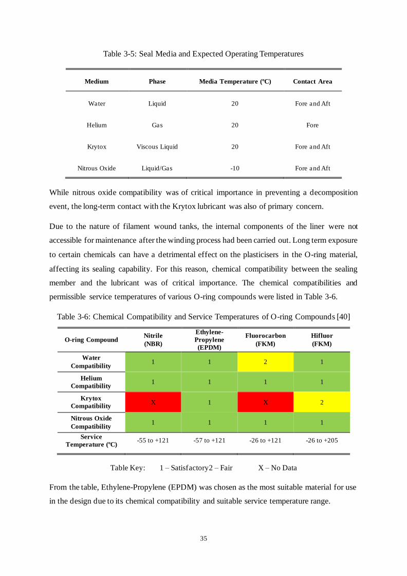
35
Table 3-5: Seal Media and Expected Operating Temperatures
Medium Phase Media Temperature (ºC) Contact Area
Water Liquid 20 Fore and Aft
Helium Gas 20 Fore
Krytox Viscous Liquid 20 Fore and Aft
Nitrous Oxide Liquid/Gas -10 Fore and Aft
While nitrous oxide compatibility was of critical importance in preventing a decomposition
event, the long-term contact with the Krytox lubricant was also of primary concern.
Due to the nature of filament wound tanks, the internal components of the liner were not
accessible for maintenance after the winding process had been carried out. Long term exposure
to certain chemicals can have a detrimental effect on the plasticisers in the O-ring material,
affecting its sealing capability. For this reason, chemical compatibility between the sealing
member and the lubricant was of critical importance. The chemical compatibilities and
permissible service temperatures of various O-ring compounds were listed in Table 3-6.
Table 3-6: Chemical Compatibility and Service Temperatures of O-ring Compounds [40]
O-ring Compound Nitrile
(NBR)
Ethylene-
Propylene
(EPDM)
Fluorocarbon
(FKM)
Hifluor
(FKM)
Water
Compatibility 1 1 2 1
Helium
Compatibility 1 1 1 1
Krytox
Compatibility X 1 X 2
Nitrous Oxide
Compatibility 1 1 1 1
Service
Temperature (ºC) -55 to +121 -57 to +121 -26 to +121 -26 to +205
Table Key: 1 – Satisfactory 2 – Fair X – No Data
From the table, Ethylene-Propylene (EPDM) was chosen as the most suitable material for use
in the design due to its chemical compatibility and suitable service temperature range.

36
The faces of the liner between which a seal is necessary were shown in Figure 3-8. The most
suitable method of sealing for the geometry was an axial type seal between the aluminium head
and the U-PVC cylinder. No compression force was necessary to ensure the seal remains in
place, but tolerances were enforced during manufacture to ensure that the seal was effective
between the cylinder and the head region.
Figure 3-8: Liner Concept 2 Seal Geometry
3.5.4. Preliminary Liner Design Conclusion
From the preliminary investigation into the liner geometry, various constraints were outlined
and listed below;
• The liner was required to be formed from a commercially available cylindrical section
of U-PVC piping and aluminium 6082-T6 bulkheads based on the liner concept
described in Figure 3-7
• The interface between the two materials was to be sealed using EPDM O-rings
• The aluminium domed ends should sustain the hoop load over the dome region,
negating the need for doily reinforcement or stiffening inserts.
O-ring Position Sealing Faces

37
3.6. Computational Tank Design
Once the analytical design was complete and liner concepts were outlined, a computational
investigation was important to ensure the design would function safely. This analysis allowed
for more complex loading conditions and structural layouts to be modelled, in comparison to
the analytical portion of the design. The inclusion of support geometry which links the tank to
the rest of the rocket and the liner structure occurred in this phase of analysis. The
computational analysis of the tank allowed for aerodynamic and inertial loads to be modelled
more accurately than in the preliminary stages of design. The computational verification was
executed using Siemens NX, which can effectively deal with filament wound composite
structures. The geometry analysed with the program was generated on Autodesk Inventor
Professional and imported to the analysis software.
3.6.1. Material Properties
The material properties for use in the computational verification of the tank were generated
from micromechanics and adjusted to material properties supplied in published literature with
similar material use. As specific material testing was not an available resource, it was felt that
this approach was the most appropriate method of generating conservative material properties.
In total, ten material properties were determined for use in both the physical model and for use
in the failure criterion used to ensure that the structure did not fail under load. Prior to the
calculation of the properties of the laminate material, the properties of the matrix and the
reinforcement had to be known. These are listed in Table 3-7 and Table 3-8 respectively.
Table 3-7: Mechanical Properties of AMPREG 21 Epoxy Resin [29]
Mechanical Property Magnitude
Tensile Strength 67.4 MPa
Tensile Modulus 3.3 GPa
Strain to Failure 3 %
Density 1.142 g/cm3
Inter-laminar Shear Strength (ILSS) 50 MPa

38
Table 3-8: Mechanical Properties of T800 Carbon Fibre [28]
Mechanical Property Magnitude
Tensile Strength 5490 MPa
Tensile Modulus 294 GPa
Strain to Failure 1.9 %
Density 1.81 g/cm3
With the properties of the laminate constituents known, the mechanical properties of the
laminated material were determined. This process required the specification of a laminate
volume fraction, which specified the ratio of the volume of either the matrix or reinforcement
to that of the total laminate volume. After consultation with local manufacturers, a fibre volume
ratio of 60% was conservatively chosen for the proceeding calculations.
Principal Stiffness – 𝐸𝐿
The principal stiffness of a composite material can be accurately calculated using a simple rule
of mixtures relationship which relates both the matrix and reinforcement moduli to the principal
stiffness by means of a volume fraction. [14] The equation to determine principal stiffness was
shown in equation 3-11 and uses the volume fractions of the fibre and matrix (𝑉𝑓 and 𝑉𝑚) and
the elastic moduli of the fibre and matrix (𝐸𝑓 and 𝐸𝑚) to determine a result.
𝐸𝐿 = 𝑉𝑓𝐸𝑓 + 𝑉𝑚𝐸𝑚 = 177.72 𝐺𝑃𝑎 [3-11]
The value of principal stiffness calculated in equation 3-11 was near the values found in
literature but was reduced to 160 GPa to produce conservative results.
Transverse Stiffness – 𝐸𝑇
The equations used to predict the transverse stiffness (ET) of the composite were developed by
Halpin and Tsai based on a curve fit to empirical relationships [41] (equation 3-12 to 3-13).
The equations contain curve-fit constants which were given a magnitude based on the type of
composite under analysis. Equation 3-12 shows the equation used to determine the transverse
stiffness of the composite based on the matrix moduli (𝐸𝑚 ), the volume fraction (𝑉𝑓) and two
Halpin-Tsai curve fit parameters (𝜉 and 𝜂).

39
𝐸𝑇
𝐸𝑚
=1 + 𝜉𝜂𝑉𝑓
1 − 𝜂𝑉𝑓
[3-12]
Equation 3-13 is used to determine the first Halpin-Tsai parameter. As can be seen from the
equation, the Halpin-Tsai parameter (𝜂) is a function of the moduli of the fibre and matrix
(𝐸𝑓 and 𝐸𝑚) and the second Halpin-Tsai parameter (𝜉). From literature, 𝜉 was determined to
have a value of 2 for the specific type of composite material under analysis in this section.
𝜂 =(
𝐸𝑓
𝐸𝑚) − 1
(𝐸𝑓
𝐸𝑚) + 𝜉
[3-13]
The transverse stiffness magnitude was calculated to be 16.99 GPa. The determined value of
transverse stiffness was higher than the values found in literature and was reduced to a
magnitude of 8.5 GPa to ensure a conservative result was achieved.
Principal Poisson’s Ratio – 𝑣12
As the Poissons ratios for the matrix and reinforcement were not available from the
manufacturers, the choice was made to use values obtained from Agarwal et al. [15]. The
Poisson’s ratio of the two materials are listed in Table 3-9.
Table 3-9: Laminate Constituent Poisson Ratios
Material Poisson’s Ratio
Typical Carbon fibre 0.2
Typical Epoxy Matrix 0.47
The equation used to determine the principal Poisson’s ratio of the composite material was a
mixture calculation, like the principal stiffness calculation. The principal Poisson’s ratio
calculation is shown in equation 3-14.
𝑣12 = 𝑣𝑓𝑉𝑓 + 𝑣𝑚𝑉𝑚 = 0.308 [3-14]
As can be seen from the equation, the principal Poissons ratio is dependent on the volume
fractions of the fibre and matrix (𝑉𝑓 and 𝑉𝑚) and the elastic moduli of the fibre and matrix

40
(𝐸𝑓 and 𝐸𝑚), similar to the equation used to determine the principal stiffness of the composite.
The principal Poissons ratio was found to be 0.3, which is in good agreement with literature
and was left unchanged.
Shear Modulus – 𝐺12
The equations used to determine the shear modulus of a composite material were obtained from
Halpin-Tsai [41]. The in-plane shear modulus (𝐺12 ) of a unidirectional composite was
calculated using equation 3-15. This equation has a similar form to the equation used to
determine the transverse stiffness of the composite material and is based on the matrix shear
moduli (𝐺𝑚 ), the volume fraction (𝑉𝑓) and the two Halpin-Tsai curve fit parameters (𝜉 and 𝜂).
𝐺12
𝐺𝑚
=1 + 𝜉𝜂𝑉𝑓
1 − 𝜂𝑉𝑓
[3-15]
From Agarwal, the first Halpin-Tsai Parameter is described by equation 3-16. It can be seen
from the equation that the parameter is dependent on the shear moduli of the fibre and matrix
(𝐺𝑓 and 𝐺𝑚) and the second Halpin-Tsai parameter (𝜉), previously stated to have a value of 2
[15].
𝜂 =(
𝐺𝑓
𝐺𝑚) − 1
(𝐺𝑓
𝐺𝑚) + 𝜉
[3-16]
Using these equations, the magnitude of the shear modulus was determined to be 5.99 GPa.
This result was in good agreement with published literature but was reduced to a magnitude of
5 GPa to ensure a conservative result.
Principal Tensile limit – 𝑇1
Equation 3-17 shows the calculation to the determine the principal tensile strength (𝑇1) of the
composite material. The equations for calculating the tensile limit of the composite material
were obtained from a Cambridge University publication titled, “Strength of Long Fibre
Composites” [42].
𝑇1 = 𝑉𝑓𝑇𝑓 + 𝑉𝑚𝜎𝑚𝑓 [3-17]
Equation 3-17 consists of two components which contribute to the tensile limit of the composite
material. The first component accounts for the strength contribution of the fibres in the laminate

41
at their failure load (𝑇𝑓), adjusted for the volume fraction of the fibres in the composite (𝑉𝑓).
The second part of the equation accounts for the contribution of the matrix material. The fibres
typically experienced brittle failure prior to the failure of the matrix material. The strength
contribution of the matrix is the load which can be absorbed at the brittle failure point of the
fibres (𝜎𝑚𝑓 ), adjusted for the volume fraction of the matrix material (𝑉𝑚). The calculation of
the strength contribution of the matrix is shown in Equation 3-18 to be 59.4 MPa. Equation 3-
18 uses the typical strain present at failure of a fibre composite (𝜀𝑓) in conjunction with the
ultimate strength of the matrix material (𝐸𝑚 ) to determine this value.
𝜎𝑚𝑓 = 𝜀𝑓 × 𝐸𝑚 = 59.4 MPa [3-18]
Using this value with equation 3-17, the ultimate tensile limit of the composite material was
determined to be 3323.8 MPa [42]. From a comparison with literature published by the
manufacturer of the carbon fibres, the result was found to be a significant overestimate of the
ultimate tensile strength of the composite material. The result was decreased from ≈3300 MPa
to 2200 MPa which was specified in the literature for the product to be the tensile limit of the
product at a 60% volume ratio with an epoxy matrix [28].
Transverse Tensile Limit – 𝑇2
The transverse tensile limit of the material was determined using Halpin-Tsai methods taken
from Agarwal et al. [42] [15]. The method made use of the ultimate tensile strength of the
matrix (𝜎𝑚𝑢 ) in conjunction with a strain magnification factor (𝑆𝑀𝐹), the transverse stiffness
of the material (𝐸𝑇) and the stiffness of the matrix (𝐸𝑚 ) to determine the transverse strength of
the composite material. Equation 3-19 is used to predict the ultimate tensile strength of the
composite material. The “𝑆𝑀𝐹” parameter is determined using equation 3-20 and is dependent
on the fibre volume fraction (𝑉𝑓) and the matrix and fibre moduli (𝐸𝑚 and 𝐸𝑓).
𝑇2 =𝜎𝑚𝑢 × 𝐸𝑇
𝐸𝑚 × 𝑆𝑀𝐹 [3-19]
𝑆𝑀𝐹 =
1
1 − (4𝑉𝑓
𝜋)
12
[1 − (𝐸𝑚𝐸𝑓
)]
[3-20]

42
The strain magnification factor was calculated using equation 3-20 to be 7.4. The transverse
composite strength was determined to be 47.1 MPa using equation 3-19. The result of equation
3-20 was in good agreement with literature on similar materials and was left unchanged.
Remaining Properties
The three remaining material properties which required estimation were the shear limit and
principal and transverse compressive limits of the composite material. These values proved
difficult to estimate accurately via strength prediction methods and were assumed from
literature, as per Table 3-10.
Table 3-10: Assumed Composite Properties
Composite Property Symbol Magnitude
Shear Limit G 40 MPa
Principal Compressive Limit C1 850 MPa
Transverse Compressive Limit C2 200 MPa
3.6.2. Computational Method 1: 3D Laminate Analysis
The first approach used to simulate the tank structure was a fully 3D finite element analysis
approach that attempted to model the composite and liner sections of the tank as 3D objects
with no simplifying assumptions.
CAD Geometry Generation
The geometry of these 3D structures was created by importing point 2D point data from the
design spreadsheet into Autodesk Inventor Professional. The head region of the composite
geometry was split into sections (discretised) to accurately capture the change in winding angle
in this area. This involved segmenting the head region into several discrete regions which
could later be assigned material properties based upon the value of their local winding angle
values and thicknesses. This was important to allow a filament wound structure to be analysed
accurately. At the end of the work on Autodesk Inventor, solid models of the supporting
infrastructure, liner geometry and composite materials were created, and were imported to
Siemens PLM NX to begin the analysis process. A section view of an early version of the tank
is shown in Figure 3-9.

43
Figure 3-9: Early Concept Tank Geometry on Autodesk Inventor
Model Meshing
Once the models were successfully imported to Siemens NX, the process of simulating the
structure began with meshing. Meshing is the process of discretising the regions of the tank
which are important in the structural analysis. For the 3D analysis this involved the composite
components and all liner constituents. Directly prior to meshing, the CAD model was reduced
to a small slice of the fully revolved tank profile, shown in Figure 3-10. This was possible due
to the axisymmetric nature of the tank geometry and due to symmetry about the longitudinal
centre of the tank.
3D helical layer
3D hoop layer
Liner structures

44
Figure 3-10: Axisymmetric CAD Tank Slice for 3D Mesh Generation
The first stage of 3D analysis dealt only with the laminate portion of the tank, to verify the
analytical analysis which neglected the liner as a structural element. The geometry of the
laminate portion is shown in Figure 3-11. As can be seen from the figure, the 3D laminate
geometry represented the hoop layers and helical layers separately. The change in thickness of
the helical layer over the head region was dictated by the CAD geometry of the model. In
Figure 3-11, the thickness of the helical layer increases in accordance with the “Helical Layer
Profile” pictured in Figure 3-3 and governed by equation 3-10.
Figure 3-11: 3D Laminate Geometry
Rotational Axis of Symmetry
Aluminium Bulkhead
Helical Layer
Hoop Layer
PVC Cylinder
Head region thickness
change
Hoop/helical layer junction
Helical layer discretisation

45
The meshing pipline to generate a 3D laminate model began by defining 2D dependant meshes
on either side of the strucure to be analysed. For example, the helical layer required meshing
on both its top surface and its underside. The 3D mesh was generated between the dependant
and independent mesh once the laminate properties had been defined. In sections of varying
thickness, each composite layer was assigned a thickness based on the ratio of the indivial layer
thickness relative to the total thickness specified in the 2D mesh environment. The laminate
properties were defined as per normal for a 2D mesh. The 2D laminate environment is shown
in Figure 3-12 for a portion of the tank which represented all of the plies used in the global ply
definition of the helical region. This environment also allowed the user to define the failure
criteria used in the analysis and the values of interlaminar shear strength between plies.
Figure 3-12: 2D Laminate Definition of Helical Region for 3D Mesh Generation
The use of global ply ID’s allowed the user to easily dictate which laminates cover which
portions of the tank. The ID’s also ensured that each layer was connected with the correct layer
in any adjacent meshes. A breakdown of the global ply ID’s used in the 3D simulation of the
composite tank is given in Table 3-11. As can be seen, each helically wound layer was assumed
to consist of two layers with the same orientation angle magnitude, but with opposing
directions. This was validated by Faria et al. [43] and simulates the ply orientation present in
manufactured filament wound tanks. Typically thicknesses of the lamina were defined in this
section but due to the laminate fill used to generate the 3D mesh the total laminate thickness is
defined by geometry in Figure 3-10.
Global ply ID.
Material
specification
Laminate angle
definition
Failure theory and
ILSS definition

46
Table 3-11: Global Ply ID's for 3D Mesh Generation
Global Ply ID Geometry Description
1,3,5 Helical
CF laminates with varying thickness and orientation angle over the head
region. These laminates make up the positive half of the two layers which
represent each helical wrap.
2,4,6 Helical
CF laminates with varying thickness and orientation angle over the head
region. These laminates make up the positive half of the two layers which
represent each helical wrap.
7-11 Hoop 0.3 mm thick CF laminate representing the hoop windings over the
cylinder.
At the conclusion of the 2D laminate definition, the strucure was ready to produce a 3D mesh.
This was done in the meshing environment using a laminate fill command. The laminate fill
command formed a 3D mesh between the two user defined dependant 2D meshes. Due to the
complex nature of the filament wound laminate defintion, this opertion took many hours to
execute, even for a small slice of the tank. The result of the laminate fill command is shown in
Figure 3-13 for a 10º section of the tank. Figure 3-13 is focused on the hoop/helical junction
shown in Figure 3-11. Labels have been given for the hoop and helical layers respectively.
Figure 3-13: 3D Laminate Fill Composite Mesh
Hoop Layer 3D Laminate
- Represents five 0.3mm hoop wound plies.
- Laminate ends at the dome/cylinder junction
Helical Layer 3D Laminate
- Represents five sets of helically wound plies
- Each ply is represented as two plies of equal
thickness with opposing laminate orientation
- Layer thickness increases toward tank boss

47
Structural Simulation
After the laminate fill command was executed and the 3D mesh was successfully generated,
the process of simulation began. For the 3D model, only a 10º slice of the tank was modelled
due to the axisymmetric nature of the structure. This meant that symmetric constraints must be
applied at either side of the slice. The constraints restricted displacement in the direction normal
to the plane of the slice and restricted rotation about the other two axes. This accurately
modelled how a rotationally symmetric structure would respond to a loading condition such as
pressure, but was not valid for other types loading conditions, which are discussed later. A
symmetry constraint was also applied in the direction normal to the longitudinal mid-section
of the tank which further halved the solution time. Once the model was constrained, the loading
conditions were applied to the tank.
At this stage of design, the loading condition consisted of only a pressure load, representing
the pressurised nitrous oxide, and an axial load representing the peak drag force of the rocket.
These two loading conditions will never occur simultaneously but were modelled
simultaneously to make the design process more conservative. The composite slice of the tank,
complete with loading conditions and constraints is shown in Figure 3-14. CAD geometry of
the liner was included to aid understanding of the location of the section of the tank but was
not included in the analysis.
Figure 3-14: Loading Conditions of a 3D Composite Simulation
Rotational axis of symmetry
Polygon geometry (blue)
Pressure loads (red)
3D laminate mesh
Helical/Hoop layer
surface glue

48
After applying the loads to the simulated model, the simulation was executed to determine the
structures response. The results were benchmarked against the results of a report published by
Gheshlaghi and were dispalyed in Figure 3-15 [35]. The report contained material properties,
geometric properties and loading conditions sufficient to benchmark 3D laminate results over
the cylinder. Unfortunately, insuffucient geometric data was provided to benchmark the results
over the head region.
Figure 3-15: 3D Laminate Analysis Displacement Benchmark Result
As can be seen in the figure, the 3D laminate analysis yielded a result with a maximum
displacement result at the junction between the cylinder and the head region. By taking a result
sample over the cylinder, it was found that the radial displacemnt in this region was equal to
1.22 mm which was in good agreement to the results published by Gheshlaghi [35], which
found the displacement in this area to be around 1.25 mm.
Although the results of the simulation were in good agreement with literature, the simulation
of this model took about 5 hours per simulation. At the given resolution, the simulation of only
a thin slice of the tank was possible. This meant that only radially symmetric loads, such as
pressure or axial loads could be modeled which prevented the inclusion of the significant
bending moment that would be encountered during flight. The symmetric analysis also did not
allow for a buckling analysis to be conducted, which is important for non-flight loading
conditions such as the hot fire test. In order to account for these loads, the model size would

49
increase by a factor of roughly 18. The increase in simulation time would increase by a similar
factor, meaning that each run would take at least 2-3 days to solve. In light of the time
constraints of the project and the delay that a multiple day simulation cycle time would cause,
a more conservative, less optimised quasi-2D approach was adopted to simulate the tank
operation.
3.6.3. Computational Method 2: 2D Analysis
This solution involved a 2D analysis on all the composite components but did not include any
3D isotropic components such as the liner geometry. This approach more closely replicated the
analytical method.
The 2D analysis, although simpler, came at the cost of solution resolution over a small part of
the head region. This arose due to the change in laminate thickness over this portion of the
tank, which was difficult to capture using the 2D laminate analysis tools available in Siemens
NX. The decision was therefore made to assume a constant laminate thickness over the head
region and to set the value to that of the laminate thickness on the cylinder. Figure 3-16 shows
the degree of laminate thickness change over the head region of a composite tank like the one
being analysed in this section. The figure was based on an analytical prediction of the laminate
thickness over the head region based upon local winding angles and tended toward infinity as
the boss region is approached [25]. The thickness at the boss region had a finite value in reality
and this thickness depended on the specific size of fibre tow used to wrap the tank and other
manufacturing variables [44]. From the figure, the 2D analysis produced a conservative result
by underestimating the thickness of the composite over the head region. The degree to which
the analysis was conservative increased as the dome was traversed and the thickness of the
composite increased in relation to the assigned value.

50
Figure 3-16: Laminate Thickness Change over the Head of a Composite Tank
Preliminary 2D Analysis
Once the various ply groups were determined, investigation of the composite structure using a
2D analysis began. A 2D analysis was a simple method which was used to verify the analytical
analysis outlined in Section 3.4. The first 2D analysis neglected the coupler geometry to
replicate the analytical process as closely as possible.
The 2D analysis began by defining a surface which would be used to generate the mesh to
analyse the laminate. The “Liner Outer” profile from Figure 3-3 was the most suitable choice,
as in reality this profile formed the mandrel upon which the composite structure was built. By
revolving this profile about the longitudinal axis of the tank and discretising the resulting
surface, the 2D mesh was generated. The 2D mesh was formed using 1.5 mm CQUAD4
elements. The meshed 2D geometry is visible in Figure 3-17.

51
Figure 3-17: Meshed 2D Laminate Geometry
The segregations used to define the varying laminate physical properties over the head region
are visible in Figure 3-17. This was similar to the approach used in the 3D analysis, with the
added simplifying assumption that the laminate thickness did not change over this region. The
laminate definition used to define the 2D laminate was similar to the definition of the laminate
for the 3D analysis, except for the thickness definition. Whereas the thickness of the laminate
in the 3D laminate was controlled by user defined geometry and relative thickness values, the
thicknesses used in the 2D analysis were specified exactly. A composite layer thickness of 0.3
mm was assumed based on information supplied by manufacturers. For this section of the
design, only the loads modelled in the analytical model were included in the analysis. This
meant that only pressure loading would be included in the model and the bending moment and
axial loading conditions would be included at a later stage in design. The loading conditions
for the 2D composite analysis are visible in Figure 3-18.

52
Figure 3-18: 2D Computational Analysis Load Case
The results of the 2D analysis were similar to the results of the analytical method as they did
not include the effect of the liner geometry and other secondary structures. The displacement
results of the 2D analysis of an arbitrary tank composite geometry are shown in Figure 3-19.
This result was not benchmarked against results from literature like the results of the 3D
analysis but was included to demonstrate the effect of pressure loading on a composite tank
with no supplementary reinforcement in the head region. As can be seen from the figure, the
tank exhibits minimal displacement (maximum ≈ 1 mm) over the length of the cylinder, where
the hoop layers are bearing the hoop stress in the structure. As the dome of the vessel is reached
and the hoop layers are absent, the displacement of the vessel increased rapidly over a short
section of tank as the unsupported helical layers deflect under the pressure loading. This
demonstrates the importance of supplementary reinforcement in the head region and also the
importance of having structural model with sufficient complexity to allow for modelling of the
reinforcement.
Aluminium bulkhead
U-PVC cylinder
2D composite mesh
Pressure load

53
Figure 3-19: 2D Analysis Composite Structure Displacement Result
The 2D analysis exhibited a far quicker solution time of approximately 5 min in comparison to
the 5 hr solution time of the 3D analysis. The bending moment loads were modelled in this
method of analysis, due to the reduction in solution time allowing a half portion of the tank to
be analysed. Despite the improved results of the 2D analysis approach, the model was still
insufficient with the liner geometry and other secondary structures absent from the analysis.
For this reason, the design method progressed to a quasi-2D approach, detailed in Section 3.6.4.
3.6.4. Computational Method 3: Quasi-2D Analysis
The 2D result was not enough to commission the manufacture of the tanks. This was because
the approach did not consider how loads were transferred to the rocket structure through
secondary geometry, such as the carbon fibre coupling tubes and the liner geometry. As
mentioned previously, the lack of literature available on the design of liners for composite tanks
made this interaction a crucial part of the design process.
Secondary geometries, such as the liner and coupling tubes, were required for successful
operation and integration of the tank into the rocket structure but may have caused impinging
loads and stress concentrations which an analytical model may not have been able to account
for. For this reason, the liner and coupler geometries were included in the structural analysis to
form a more reliable result of the reaction of the tank under load.
Liner Inclusion and Meshing
The analysis of the tank began with the inclusion of the 3D liner geometry. This geometry was
similar in layout to that shown in Figure 3-7 and consisted of a PVC cylinder and aluminium
dome inserts. The final iteration of the liner geometry is shown in Figure 3-20 as a reference
for the proceeding design section.

54
Figure 3-20: Final Liner Geometry
The locator pins and O-ring grooves which housed two EPDM O-rings are visible on either
end of the tank. Various other adjustments to allow for clamping during manufacture and
interface with NPT fittings were also included near the boss regions.
The liner geometry shown in Figure 3-20 was imported into Siemens NX in a 3D CAD format
and run through the meshing pipeline to result in Figure 3-21. Figure 3-21 represents the
meshed liner components. The aluminium domed bulkhead is visible as the darker grey
structure at the top of the figure. This aluminium structure was meshed using 2 mm CTETRA
(10) elements and was specified to represent Aluminium 6082-T6. Care was taken to ensure
that 3 mesh elements were present through the thickness at all points of the structure. The white
structure near the bottom of the figure represents the cylindrical U-PVC liner. This structure
was also meshed using CTETRA (10) elements but the size of the elements was increased to 3
mm due to the size of the structure. The mesh for the cylinder was assigned custom material
properties to accurately represent the U-PVC pipe section which was used for its construction.
The small red circle visible through the U-PVC liner represents the mesh resulting from the pin
geometry. The pins were meshed using 2 mm CTETRA (10) elements, like the aluminium
bulkheads. The pins were given a material specification of stainless steel.

55
Figure 3-21: 3D Liner Mesh
After the meshing of the isotropic 3D liner components was completed, the meshing process
continued with the orthotropic 2D composite materials.
2D Geometry Specification
In addition to the 3D Liner geometry, two 2D structures were included to model the composite
sections of the tank. One segment allowed for modelling of the connection of the tank to the
rest of the rocket structure while the other represented the filament wound composite material.
The laminate properties for the 2D analysis were defined in a similar way to the 3D analysis.
Due to the early conclusion of the 3D analysis, only two groups of plies were necessary for the
modelling of the hoop and helical layers. For the 2D simulation, an additional ply group was
necessary to model the coupling tube. The plies for the 2D analysis therefore consisted of 3
groups of ply types to represent different portions of the tank geometry. These ply groups were
listed and explained in Table 3-12.
Table 3-12: 2D Analysis Ply Group List and Description
Ply Group Geometry Description
Group 1 Helical Layer
Ply group to represent the helically wound layer similar to the layer
in Table 3-11. This layer had constant thickness in this analysis,
which was not dependant on CAD geometry and was specified
during laminate definition. Ply orientation varied over the head
region and was defined by the user.
Group 2 Hoop Layer Ply group to represent the hoop wound layer similar to the layer in
Table 3-11. Laminate thickness did not depend on CAD geometry

56
and was specified during laminate definition. Ply orientation was
constant at 90º to the longitutdinal axis of the tank.
Group 3 Coupling Tube
Ply group representing the tubes used to join the tank the fore and
aft sections of the rocket. This tube was constructed from 200 gsm
twill weave carbon fibre.
The ply groups listed in Table 3-12 consisted of different types of composite materials due to
varying methods of manufacture and load bearing requirements. The types of composite
materials used to construct each ply group are listed in Table 3-13.
Table 3-13: Ply Group Material Type Breakdown
Ply Group Tank Geometry Material Type
1 Helical Layer Toray T800/AMPREG 21
2 Hoop Layer Toray T800/AMPREG 21
3 Coupling Tube 200 gsm Twill Weave/AMPREG 21
The mechanical properties of the materials specified above are listed in Table 3-14.
Table 3-14: 2D Analysis Composite Material Properties
Composite Property Symbol Toray T800
Carbon Tow
200gsm Twill
Carbon Cloth
Principal Stiffness (MPa) EL 160 000 47 000
Transverse Stiffness (MPa) ET 8500 47 000
Principal Poisson’s Ratio v12 0.308 0.05
Shear Modulus (MPa) G12 5000 5100
Principal Tensile limit (MPa) T1 2.2 0.464
Transverse Tensile Limit (MPa) T2 47.11 464.4
Prin. Comp. Limit (MPa) C1 850 286.6

57
Trans. Comp. Limit (MPa) C2 200 286.6
Shear Limit (MPa) G 40 53.4
Inter-laminar Shear (MPa) ILSS 50 50
The coupling tube segment represented a cylindrical composite section made from 200 g/m2
twill weave carbon fibre, which was labelled as ply group 3 in Table 3-13. The inclusion of
this geometry was important as it could have caused stress concentrations on the tank. At this
stage of the design process the coupling geometry was not of principal concern, so a thickness
was assumed and only iterated to completion in Section 3.7. The global ply definition for the
final iteration of the tank geometry is shown in Figure 3-22.
Figure 3-22: Final Iteration Cylinder Laminate
As can be seen from Figure 3-22, the laminate over the cylindrical portion of the tank consisted
of a total of 17 plies with varying thickness and orientations. Ply groups 1 & 2 represented the
first layer helical winding that were applied to the tank liner. As this was the cylindrical portion
of the tank, these plies were assigned a fibre angle value of ≈ 26°, in accordance with Section
3.4.4. The helical ply group was modelled by defining two layers of composite with opposing
fibre angle directions. Each layer had a thickness of half the total thickness of one filament

58
wound layer. This method of definition did not include junctions where fibre crossover
occurred but was effective in replicating helically wound composite geometry. Layer 3 from
Figure 3-22 depicts the first hoop-wound composite layer. Unlike the helical layer, there was
no bi-directionality with the hoop layer and each hoop layer was defined with a single laminate
layer.
As the lamina began to wrap over the dome of the tank, the hoop layers terminated, and the
winding angle of the helical layers began to change in accordance with Figure 3-4. As a result,
the winding angle definition over the head region changed in accordance. This was done using
45 different meshes for each discrete portion of the head region, each with a different winding
angle definition. As defined previously, the analysis was constrained according to the
assumption that the laminate thickness did not change over the head region and as a result no
layer thickness changes needed to be implemented. Figure 3-23 depicts the CAD geometry of
one half of the filament wound tank with radial partitions in the surface where each different
winding angle was defined.
Figure 3-23: CAD Model with Dome Region Segregation
Figure 3-24 shows an example of the laminate definition from the radial slice of the head region
labelled in Figure 3-23, where the helical layer winding angle was analytically predicted to be
≈ 45°.
Filament wound
composite
2D meshed
radial slice
Aluminium
bulkhead

59
Figure 3-24: Dome Region Laminate Definition
As can be seen in Figure 3-24, the laminate ply IDs used to define the helical laminate over
this portion of the head region in Figure 3-24 were the same as the plies used to define the
helical laminate over the cylindrical region in Figure 3-22. This was due to the use of global
ply IDs mentioned previously.
Other factors such as the failure criterion, and stacking order were defined in this interface. The
failure criterion used was the Tsai-Wu failure criterion, described in Section 2.3 of the literature
review.
Once the meshing pipeline was complete, the process of defining model constraints began. This
section was divided into interface definition and constraints. The interface definition section
details how the various parts of the model were constrained to interact with each other. The
constraints section details how the model was physically constrained to produce a realistic
result.
Interface Definition
Two types of interfaces were defined in this structural simulation; bonded and contact
interfaces.
Bonded interfaces were defined in areas such as the join of the coupler to the filament wound
tank. This area was connected via an adhesive bond which was replicated well by defining a
bonded joint. The stresses generated in this area during the simulation were compared to the
ultimate strengths of the chosen adhesive to determine whether the area will suffer a failure

60
during operation. The various bonded interfaces present in the model are listed in the bulleted
points below and are referenced to Figure 3-25 and Figure 3-26 which show the location of
each point.
Figure 3-25: Coupler Bond Location
• Filament Wound Composite/Coupler Bond – This bond was depicted by the red arrows
in Figure 3-25 and represents the bond area between the composite coupling structure
and the composite filament-wound tank. The bond is between a surface which was
prepared using 80 gsm peel ply fabric and a composite structure which cured onto this
keyed surface.
Coupler composite structure
Filament wound composite
Filament wound
composite/coupler bond

61
Figure 3-26: General Bond Locations
• Filament Wound Composite/Aluminium Bulkhead – This bond area is represented by
the closely grouped green arrows at the top of Figure 3-26 and was formed when the
filament wound composite was applied to the liner mandrel. The aluminium surface
was freshly sanded and cleaned with acetone in the manufacturing phase to reduce the
presence of the aluminium oxide layer which is detrimental to bond strength.
• Filament Wound Composite/U-PVC Liner – This bond area is represented by the green
arrows in the middle of Figure 3-26 and was formed when the filament wound
composite was applied to the liner mandrel. PVC was unlikely to form a strong
chemical bond with an epoxy matrix and hence the surface was heavily keyed and
cleaned with acetone prior to the winding process to encourage good mechanical bond
to form.
• Pins/Aluminium Dome Bulkhead – This bond was applied at the base of the round
yellow structures in the figure and is not depicted by arrows like the other bond areas.
This bond represents a welded connection between the steel pins and the aluminium
dome bulkhead. Due to the light shear loading of the pins during use, this bond was
used in place of a complex thread definition. This was done to reduce overall solution
time of the model.
The contact interfaces in the model were used to define locations in the model where parts
impinged upon each other. This was important as the stress concentrating effects of the various
Aluminium bulkhead
U-PVC cylinder
Filament wound
composite/aluminium
Bulkhead
Filament wound
composite/U-PVC liner
Pins/Aluminium
dome bulkhead

62
parts of the structure were not obtainable in the preliminary analytical analysis. The contact
interfaces used in this model were used to model small impingements of components which
were designed with small tolerances between them. Large scale deformations which lead to
contacts would require the solution type to change from static to dynamic to accurately capture
what was occurring in the model. A view of the contact surfaces used to define one pin joint at
the end of the liner structure is shown in Figure 3-27, before and after simulation. As can be
seen from the figure, despite the small deformation present in the region, the stress of the
impingement on the PVC structure was captured.
Figure 3-27: Pin Contact Region and Result
A list of the various contact interfaces present in the model is given below, referenced to Figure
3-28. For ease of viewing, only the contact surfaces on the aluminium dome are pictured in the
figure.
Pin contact regions

63
Figure 3-28: Simulation Contact Regions
• Filament Wound Composite/Pins – This contact surface is coloured with green arrows
in Figure 3-28 and represents the interface between the head of the pins and the
composite wall of the filament wound tank. This interface was important to define as
the soft U-PVC liner maybe be compressed against the composite outer shell of the
filament wound tank. If the U-PVC structure was compressed enough, it would allow
the individual pins around the cylinder/dome interface to impinge on the composite
which may have resulted in a failure or crack which could have compromised the tank.
• U-PVC Cylinder/Aluminium Dome – This contact surface is coloured with dark blue
arrows in Figure 3-28 and represents the radial interface between the aluminium dome
bulkhead and the U-PVC cylinder which formed the liner of the tank. This interface
was important to define as it dictated how pressure was transferred from the interior of
the aluminium dome through the U-PVC cylinder and eventually to the composite shell
in the dome region. This contact definition also allowed the U-PVC to deform naturally
relative to the aluminium bulkhead which aided in determining the integrity of the O-
ring seal in this region.
Constraints
In the case of the filament-wound tank analysed in this scenario, two types of constraints were
used. These constraints are termed fixed and symmetry constraints. Although both constraints
were defined in the same manner as the physical constraints described for the tensile testing
element, the symmetry constraint was intended to replicate a physical constraint implied by the
geometry of the structure being analysed, rather than an external fixture.
Aluminium bulkhead
Filament wound
composite/pins
U-PVC cylinder/
aluminium dome

64
In the case of the tank for the rocket, there were no constraints to replicate during flight. This
was because during flight the rocket was airborne and was free to move with 6 degrees of
freedom. A combination of aerodynamic forces and mass distribution was used to ensure the
rocket remained on a stable trajectory. Modelling how the various forces changed and affected
the tank during flight would have added immense complexity and solution time to an already
complex model and would likely have moved the solution outside of the realm of a static
simulation. For this reason, it was decided that the aft side of the rocket should be constrained
to be fixed and loads would be applied over the length of the tank to replicate the in-flight loads
as closely as possible. The physical constraint at the base of the tank represented a physical
constraint in all six degrees of freedom. Conveniently, this physical constraint was similar to
how the tank would be constrained during testing.
The symmetry constraints imposed on the model were dictated by the expected loading
conditions as well as the geometry of the tank structure. In terms of geometry, the tank had a
symmetry plane in the middle of its longitudinal axis and exhibited 12 x cyclic symmetry
around this axis. Because of this, the tank could have been analysed with a model that
represented only a small portion of the whole tank. This model would have represented a 30°
slice of the tank and would have been half of its length. Although geometrically symmetrical,
the issue with this analysis arose from the expected loading conditions.
Figure 3-29 shows the two type of constraints described above as they were imposed on the
tank. The physical fixed constraint is coloured green and acts at the top of the tank in the figure.
This constraint acts at the base of the tank, but the image was flipped vertically for ease of
reading. The symmetry constraints are described by the yellow arrows and the red lines. The
symmetry constraints are formed by two different types of constraints as they act on both 2D
and 3D geometry. The 3D symmetry constraint is represented by the yellow arrows, while the
2D constraints are represented by the red lines.

65
Figure 3-29: Simulation Constraint Definition
3.6.5. Loading Condition Specification
To verify the safe operation of the tank, loading conditions were applied to the tank that closely
replicated the conditions predicted to occur in flight and during testing. For the purposes of this
design task, the choice was made to constrain the design to a static simulation. This was
primarily due to computational resource constraints on the University which meant that running
a dynamic simulation of a complex structure would require many days to achieve solution
convergence.
The simulation was conducted using Siemens NX and made use of a static SOL 101 simulation.
The simulation made use of various constraints which were outlined previously and contained
a combination of three loading conditions which were used to replicate the loading on the tank
during testing and flight. The three loading conditions chosen were pressure, bending moment
and axial load. The magnitude of each loading condition was predicted from separate load cases
and combined to ensure a conservative result was achieved.
Table 3-15 shows the magnitude and origin of each loading condition. The pressure and axial
loads were determined based on the predicted pressure test loads and the maximum thrust of
the motor respectively. The moment load was determined using a calculator for rocket loads
published by Hoult [45] called BENDIT7, which required basic flight parameters and rocket
geometry to generate in-flight loads on the rocket.
Physical fixed
constraint
2D symmetry
constraint
3D symmetry
constraint

66
Table 3-15: Loading Condition Origin
Load Type Load Magnitude Load Origin
Pressure 80 bar Maximum during pressure test, using water as
medium.
Bending Moment 700 Nm
Peak from aerodynamic loading during maximum
aerodynamic pressure during flight. Assumed
maximum vehicle angle of attack of 4°.
Axial Force 7500 N
Peak from aerodynamic loading during maximum
aerodynamic pressure during flight. Conservatively
assumed to be equal to peak motor thrust.
Figure 3-30 shows how the loads described in
Table 3-15 were applied to the structure. In order to produce a realistic bending moment profile
over the length of the tank, two opposing forces on either end of the tank were used. These
forces were distributed evenly over the aerodynamic interfaces of the tank structure and were
pictured in green in the figure. The pressure load acts on all internal surfaces of the liner and is
represented in the figure by the blue arrows. The axial load acts on the fore coupler of the
structure and is represented by red arrows in the figure.
Figure 3-30: Simulation Loading Condition

67
3.6.6. Computational Tank Design Conclusion
After investigating various potential methods of computational analysis, a quasi-2D solution
was found to be the most suitable as a compromise between the quick cycle times of 2D
analysis and the long solution times of 3D analysis. The quasi-2D approach introduces various
elements which were not considered in the analytical process outlined in Section 3.4. These
elements included:
• Secondary geometry such as the liner and coupling structure and their effect on the
composite structure.
• The potential to analyse the effect of stacking order on the stress in the composite.
• The inclusion of loads aside from pressure, such as bending moment and axial loading.
• High result resolution allowing for specific changes to be made to the liner geometry
to allow for more accurate realisation of the liner/composite interaction.
The computational method was a higher fidelity method of analysis in comparison to the
analytical method but also required simplifying assumptions to reduce the cycle times of the
simulations. The primary assumption involved the thickness of the composite over the head
region of the tank. This was assumed constant and makes the result of the analysis more
conservative over the head region. The static solution assumption was also a factor in reducing
the fidelity of the chosen computational method. In future, with more computational resources,
this computational method has the potential to provide higher fidelity results. With more
computational resources available, the solution time should reduce enough to allow for the
execution of a dynamic simulation. The dynamic solution could account for the frequency of
the bending moment as the rocket is spin-stabilised allow for the inclusion of time variant axial
load and pressure profiles. This, when supplemented with the correct material properties, could
have the potential to identify new modes of failure which would otherwise have gone
undetected and potential mitigate any harmonics that could occur in-flight which are
impossible to predict using a static simulation. The additional computational resources could
also be used to realise a 3D composite model which accurately models the thickness over the
head region.

68
3.7. Coupling Structure Design
The objective of the coupling structures design phase was to generate structures which would
effectively couple the composite tank to the structural components fore and aft of its location
on the rocket. The designed structures had to be manufactured within the technical and resource
constraints imposed by the project.
3.7.1. Coupling Structure Constraints
Apart from the resource and technical constraints on the couplers, the structures were also
constrained geometrically as they had to interface with various other components on the rocket.
Figure 3-31 shows the structures required to be joined via the aft-most coupling structure. As
can be seen from the figure, the aft coupler interfaces with an aluminium transition component
with slotted radial holes. The fore side of this coupler interfaces with the filament wound tank.
Figure 3-31: Aft-most Coupling Area Depiction
Figure 3-32 shows the structures that were joined via the fore-most coupling structure. The fore
side of this coupler had to interface with the composite nose cone while the aft side of this
coupler interfaces with the filament wound tank. The length of the couplers was determined
from CAD models, while their thicknesses were determined later during the analysis portion
of the design.
Fore Aft
Combustion
Chamber
Aluminium
Transition
Composite
Tank
Coupling
Area

69
Figure 3-32: Fore-most Coupling Area Depiction
3.7.2. Preliminary Design Layout
Difficulties arose in coupling the tank to the aluminium transition component because of
differences in material types of the two structures. The aluminium coupling section was more
suited to joining via fasteners, whilst the composite structure was not suited to this type of
joining. Composite structures are generally better suited to joining via adhesives as the
clamping force from the fasteners can cause structures to fail if not designed correctly.
Adhering the composite directly to the aluminium transition would have inhibited access to the
feedline and resulted in a system that was not modular.
For this reason, it was decided to create composite structures that interfaced with a secondary
aluminium structure via an adhesive bond for either side of the tank. This aluminium structure
would interface with the other components of the rocket via a set of fasteners. This layout is
depicted in Figure 3-33 for the aft-most coupler. The figure shows the two adhesive bonds to
the tank and secondary aluminium structure, highlighted in red. The fastener connection to the
aluminium transition is also depicted.
Aft Fore
Coupling Area Composite Tank Nose Cone

70
Figure 3-33: Coupler Geometry
3.7.3. Bond Design
The most important aspects of the design of the coupling structures were the bond areas present
in each structure. Each bond area was assigned a maximum allowable stress based upon
literature and designed based upon the specific type of bond needed at each point. The highest
loading during flight was present on the aft-most coupler and hence most design elements were
generated here and mirrored to the top structure. The structural components of the top structure
were verified rather than iterated to a result to save time.
The bond areas in this design consisted of two different material combinations. The first was a
composite/metallic bond and the second was a composite/composite bond. The parameters of
each bond are described below for each bond type.
Composite/Metallic Bond
The bond between the coupler composite and the aluminium had the weaker of the two ultimate
bond strengths. This was primarily due to the oxide layer which forms on aluminium, making
bonding difficult. For this reason, the ultimate tensile strength of the bond between the two
materials was based upon literature which describes a surface preparation prior to bonding with
an epoxy adhesive. The strength of the bond was set to 12 MPa between the composite and
aluminium with a surface treatment of sanding followed by cleaning with acetone [46]. Another
limiting factor in the design of the composite/metallic bond was the available area for
aluminium bonding. Increasing the available surface area of aluminium increases the mass of
Aluminium coupler
piece (gold)
Composite coupler
piece (green)
Adhesive bonds
(red)
Fasteners

71
the aluminium component and increases the length of the rocket after a certain component
length has been passed.
In addition to the adhesive bond on the composite/metallic bond, rivets were used to reinforce
the adhesive bond area between the composite coupler piece and the aluminium coupler piece.
Large flange rivets are suitable for joining metallic elements to composites and can be used to
inhibit the mode of failure caused by adhesive “peeling”. Peel failure or “peeling” is a mode of
adhesive failure caused by highly localised stress at either end of the lap joint. These stresses
cause the adhesive bond to shear apart and can lead to failure of the joint before the maximum
stress of the adhesive is reached [47]. The rivets were not considered in the analysis and were
used only to inhibit peel failure. The rivets were selected based only on the loading conditions
experienced during the hot fire testing of the motor. This means that a peak shear load of
7500 N needed to be distributed across the rivets. Large flange aluminium rivets suitable for
use with composites were available commercially and were selected for use in this application.
The shear limit of one 4 mm aluminium rivet is specified according to literature as 190 lbs
(~854.16 N) and used to calculate the number of rivets used in the design [48]. Using this value,
the number of rivets required was determined to be 10.
The aluminium rivets exhibited a safety factor of near unity as they were introduced only to
inhibit the likelihood of failure via peeling and to locally prevent the delamination of the bond.
Introducing more rivets than necessary into the design would act to reduce the bond area and
limit their effectiveness as a secondary measure. The number of rivets calculated was rounded
up to the nearest even number to allow for placement of two rows of fasteners on each tank
end. Using two rows of fasteners near the end of the bond area was important because peel
failure could begin at either side of the aluminium section.
Composite/Composite Bond
The composite/composite bond between the tank and the coupler geometry had a much higher
ultimate tensile strength than the composite/metallic bond, with an achievable bond strength of
40 MPa based on literature. The available bond area was also far greater than what was
available for the composite/metallic bond. The decision was made to focus the design of this
part of the coupler on preventing stress concentrations on the composite tank. To d o this, the
composite thickness reduced slowly over the length of the bond area to result in no large step-
downs in thickness over the length of the coupler. This method of design also created a gradual
taper on the aerodynamic profile of the rocket. This was preferable to a defined step as it
inhibited the formation of undesirable supersonic flow phenomena. The gradual taper was also

72
less likely to suffer from high stagnation heating than a defined step down in the rocket
geometry.
3.7.4. Coupler Computational Design
After the preliminary design and layout of the coupling structures and bond areas were
complete, the structures were converted to CAD models and the finite element analysis process
began. The layout of the process is the same as the quasi-2D process outlined in Section 3.6.4,
meaning that 3D elements were used for the isotropic materials and 2D elements were used for
the orthotropic composite elements. The symmetry and loading conditions on the model were
also the same as used for the tank analysis, apart from the pressure which was not included in
the model. The CAD model of the composite coupler geometry, complete with labels, is shown
in Figure 3-34.
Figure 3-34: Composite Coupler Geometry
The composite geometry shown in Figure 3-34 was similar on either side of the tank and for
this reason, only the geometry of one side is shown in the figure. As mentioned previously in
Section 3.7.3, the focus of the design of the composite coupler component was to reduce stress
concentrations on the composite tank. To do this, the thickness of the coupler composite was
stepped down incrementally to prevent large stress concentrations on the tank. Figure 3-34
shows how the thickness of the laminate steps down from 10 layers to zero thickness
incrementally over its length. Each composite layer consisted of 200 gsm twill weave carbon
fibre, the properties of which are supplied in
3mm first portion
– 10 Layers CF
1.8 mm second portion
– 6 Layers CF
0.9 mm third portion –
3 Layers CF

73
Table 3-14. Each layer had a thickness of 0.25 mm meaning that the maximum composite
thickness was 2.5 mm for the sections consisting of 10 carbon layers. Rather than describing
the entire iteration process, the thicknesses shown in Figure 3-34 for each section represented
the final iteration thickness of the designed composite coupling structures. The laminate
definition was done in the same way as seen in Section 3.6.4 and was shown in Figure 3-35.
The laminate ply ID numbers began at 18, which was a continuation of the number system used
to define the filament wound geometry, which ends at 17 listed in Figure 3-22.
Figure 3-35: Coupler Composite Structure Laminate Definition
After the CAD model of the composite geometry was defined, the other structures such as the
aluminium joining components and representative geometries were defined and all components
were meshed. Figure 3-36 shows the meshed geometries of the final structure which was
analysed for the aft coupling structure. As can be seen from the figure, much of the geometry
included was not the focus of the simulation. This was due to some geometry, such as the white
structures on either side of the figure, being representative and simply helping to constrain the
model to act as it would in reality.
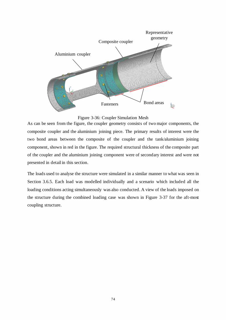
74
Figure 3-36: Coupler Simulation Mesh
As can be seen from the figure, the coupler geometry consists of two major components, the
composite coupler and the aluminium joining piece. The primary results of interest were the
two bond areas between the composite of the coupler and the tank/aluminium joining
component, shown in red in the figure. The required structural thickness of the composite part
of the coupler and the aluminium joining component were of secondary interest and were not
presented in detail in this section.
The loads used to analyse the structure were simulated in a similar manner to what was seen in
Section 3.6.5. Each load was modelled individually and a scenario which included all the
loading conditions acting simultaneously was also conducted. A view of the loads imposed on
the structure during the combined loading case was shown in Figure 3-37 for the aft-most
coupling structure.
Aluminium coupler
Composite coupler
Fasteners
Representative
geometry
Bond areas

75
Figure 3-37: Coupler Simulation Load Case
The simulated loads from Figure 3-37 were supplied in Table 3-16. The two forces shown in
blue in the figure were used to generate the bending moment profile over the length of the
structure. The results of the simulation are discussed in the proceeding section.
Table 3-16: Coupler Simulation Load Magnitudes
Load Type Load Magnitude
Bending Moment 700 Nm
Axial Load 7500 N
Figure 3-38 depicts the constraints imposed on the structural model of the aft-most coupler.
These constraints are similar to those imposed on the tank model in Figure 3-29. A physical
constraint exists on the left side of the figure on a portion of representative geometry and a
symmetry constraint exists through the longitudinal axis of the structure. No physical
constraints, apart from symmetry constraints, were used on components that were the focus of
this analysis. Various contact constraints were defined between the various components to
ensure that the load was transferred realistically between all the components.
Bending moment loads
(blue)
Axial loads
(red)

76
Figure 3-38: Coupler Simulation Constraints
3.7.5. Coupler Simulation Results
Although the couplers were simulated for a variety of individual load cases, only the peak load
case is discussed here. The results are only discussed for the aft section of the coupler, as the
geometry for the fore and aft sections was largely analogous and produced similar results and
safety factors. Four parts of the coupling structure are discussed in this section. These involved
the two bond areas and the thicknesses of both the aluminium joint and composite coupler. A
view of the deflection result from the structural simulation of the coupler is given in Figure
3-39.
Figure 3-39: Coupler Simulation Deflection Result
Fixed constraint
(blue)
3D symmetry constraint
(yellow)
2D symmetry constraint
(red)
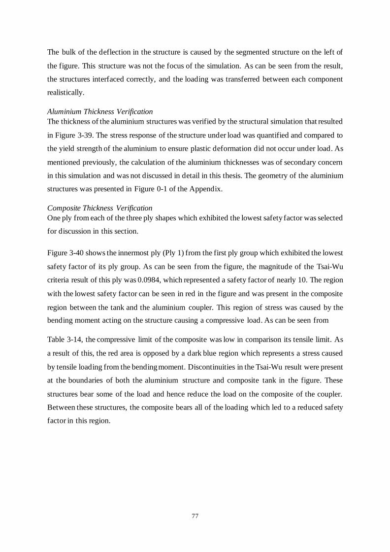
77
The bulk of the deflection in the structure is caused by the segmented structure on the left of
the figure. This structure was not the focus of the simulation. As can be seen from the result,
the structures interfaced correctly, and the loading was transferred between each component
realistically.
Aluminium Thickness Verification
The thickness of the aluminium structures was verified by the structural simulation that resulted
in Figure 3-39. The stress response of the structure under load was quantified and compared to
the yield strength of the aluminium to ensure plastic deformation did not occur under load. As
mentioned previously, the calculation of the aluminium thicknesses was of secondary concern
in this simulation and was not discussed in detail in this thesis. The geometry of the aluminium
structures was presented in Figure 0-1 of the Appendix.
Composite Thickness Verification
One ply from each of the three ply shapes which exhibited the lowest safety factor was selected
for discussion in this section.
Figure 3-40 shows the innermost ply (Ply 1) from the first ply group which exhibited the lowest
safety factor of its ply group. As can be seen from the figure, the magnitude of the Tsai-Wu
criteria result of this ply was 0.0984, which represented a safety factor of nearly 10. The region
with the lowest safety factor can be seen in red in the figure and was present in the composite
region between the tank and the aluminium coupler. This region of stress was caused by the
bending moment acting on the structure causing a compressive load. As can be seen from
Table 3-14, the compressive limit of the composite was low in comparison its tensile limit. As
a result of this, the red area is opposed by a dark blue region which represents a stress caused
by tensile loading from the bending moment. Discontinuities in the Tsai-Wu result were present
at the boundaries of both the aluminium structure and composite tank in the figure. These
structures bear some of the load and hence reduce the load on the composite of the coupler.
Between these structures, the composite bears all of the loading which led to a reduced safety
factor in this region.

78
Figure 3-40: Coupler Simulation Composite Ply 1 Result
Figure 3-41 shows the Tsai-Wu failure result in the fourth ply, which was the first ply in the
second ply group. As can be seen by comparing Figure 3-40 and Figure 3-41, the second ply
group extends further up the tank structure than the first. The Tsai-Wu result in this ply is seen
to be 0.056, which is significantly lower than was seen in Figure 3-40 and corresponds to a
higher safety factor. The stress in this ply is distributed more evenly and the effect of the
bending, compression and tension on either side of the tank is more pronounced.
Figure 3-41: Coupler Simulation Composite Ply 4 Result

79
Figure 3-42 shows the Tsai-Wu result from the final ply group and the outermost layer of
carbon fibre (ply 10) which exhibited the lowest safety factor in this ply group. The Tsai-Wu
result was slightly greater than was seen in Figure 3-41 at 0.0661. The region with the lowest
safety factor is seen to move to the interface with the aluminium structure. The region that
exhibits the lowest safety factor in Figure 3-40 exhibits a high safety factor in this ply. This is
due to the through-the-thickness load distribution of the bending moment load. The effect of
the varying composite layer thickness is also visible in this figure. Each change in composite
thickness is visible from slight changes in the stress distribution in the ply over the surface of
the tank.
Figure 3-42: Coupler Simulation Composite Ply 10 Result
The maximum Tsai-Wu result in each ply is depicted in Figure 3-43 with annotations for each
ply group. As can be seen from the figure, the result of each ply is below 0.1 and exhibits a
decreasing trend until ply 5 is encountered. After this, the result begins to rise which indicates
that the safety factor of each ply is dependant on its position relative to the thickness of the
composite. The outermost plies exhibit a lower safety factor than the middlemost.

80
Figure 3-43: Coupling Structure Maximum Failure Likelihood
As shown in Figure 3-43, the Tsai-Wu failure criteria in each layer never results in a safety
factor less than 10, which is typically considered excessive in aerospace structural applications.
Despite this, the thickness of the structure was not reduced to ensure that no unnecessary
deflection was incurred at this point. The design of the composite structure was concluded at
this point with the final structure consisting of 10 plies and a maximum thickness of 2.5 mm.
Bond Areas
As stated in Section 3.7.3, the bond area design was the primary concern of the coupling
structure design phase.
Figure 3-44 shows the stress result in the two bond areas of critical importance. Labelled in the
figure are the aluminium/composite bond area and the composite/composite bond area. The
maximum tensile stress present in either bond area is 11.3 MPa.
Figure 3-44: Coupler Simulation Bond Areas Result
0
0.02
0.04
0.06
0.08
0.1
0.12
1 2 3 4 5 6 7 8 9 10
Tsai-
Wu
Failu
re R
esu
lt
Ply Number
Ply Group 1 Ply Group 2 Ply Group 3
Aluminium/composite
bond area
Composite/composite
bond area

81
The first bond area discussed is the composite/composite bond area. This area had a maximum
allowable stress of 40 MPa from Section 3.7.3. This meant that the composite/composite bond
had a safety factor of approximately 3.5. The region of highest stress was present at the junction
between the coupler composite structure and the tank, in a region that would be in compression
because of the bending load. This indicated a stress concentration that could cause the structure
to fail due to peel stress if the loading was excessive. This was mitigated during manufacture
by allowing a bead of epoxy to form a fillet in this region. Despite the presence of a small stress
concentration, the magnitude of the stress in this region was low enough that the bond was not
likely to fail under the imposed loading conditions.
The second bond area discussed was the aluminium/composite bond area. This area had a
maximum allowable stress of 12 MPa from Section 3.7.3. As can be seen in the figure, the
maximum stress in the bond region is 7.3 MPa and is compressive. This stress magnitude
corresponds to a safety factor of 1.63 with respect to the failure stress of the bond. As can be
seen from the figure, the region of high stress was concentrated and not distributed over the
entire bond area. This indicates a tendency for this bond to fail in peel. The magnitude of the
stress in the bond was small enough when compared to the failure stress that the bond was not
likely to fail under the given loading conditions.
3.7.6. Coupler Design Conclusion
The designed coupling structure consisted of a mostly composite construction with an
aluminium interface to connect the structure to the lower part of the rocket. The composite
structure tapers down at 3 discrete locations, beginning with a thickness of 2.5 mm, tapering to
1.5 mm and finally to 1 mm. The aluminium structure which was connected to the composite
structure was verified for safe operation under the imposed loading conditions. The stress in
both bond areas was sufficiently low that failure should not occur because of bond failure in
either region. Rivets were added to the aluminium/composite bond area to reduce to the
likelihood of bond failure occurring due to peeling.
The results of this section qualified the aft-most coupling structure on the tank for use on the
rocket. This coupler experiences loading which was far greater in magnitude than the fore-most
coupler. Because of this, the structure was mirrored to form the fore-most structure and verified
via structural simulation. The results of the simulation were not included in this section of the
report as they offered no additional conclusions to those drawn from the results already
presented in Section 3.7.5. The aluminium interface on the fore-most coupler was altered

82
slightly to allow it to be manufactured from a freely available tube section of aluminium.
Complete drawings of both coupling structures are presented in Figure 0-1 of the Appendix.
As can be seen from the results presented in Section 3.7.5, the coupler was verified to operate
safely under the loads implied by the simulation. These loads represented the maximum
expected loading conditions that the coupling structure would experience during both testing
and flight, and the structures were therefore qualified for use on the P1B Mk. II.
3.8. Analysis Results
This section discusses the results of the simulation procedure outlined in Section 3.6. The
results of the various loading conditions are then discussed and the effect of each condition on
the tank is explored. The load cases discussed here were selected from a variety of cases
involving pressure, axial loading and bending moment and their various combinations. The
three loading conditions explored in this section are isolated pressure loading, a combination
of bending moment and axial loading, and a combination of pressure, axial loading and bending
moment that represented in-flight loading. These load cases were selected as the most relevant
to the final design and effectively determine the way the structure should respond to different
types of loading.
The goal of this section is to verify the operation of the designed structure with the newly
imposed loads and alter the primary composite structure and secondary liner structure in
response to any new information that arise from the computational results. The design features
of the liner and composite are presented throughout the section as various loading conditions
highlight their importance.
The response to loading is quantified using three different criteria, namely deflection, liner
stress and a composite failure criterion.
3.8.1. Load Case 1: Pressure Loading
The first load case is that of pressure loading. This load case is important as it represents the
load case of the structure through the initial phases of testing, where no aerodynamic forces are
present to induce bending. These tests also do not involve motor ignition therefore no axial
load is present on the tank.
The pressure loading was defined to act on all the internal surfaces of the tank liner, in
accordance with Figure 3-30. The results presented and discussed in this section are the
deflection, liner stress and composite failure result from a pressure load of 80 bar. The pressure
magnitude of 80 bar represents the maximum operating pressure of the structure.

83
Isolated Pressure Deflection Results:
The deflection response of the structure was quantified in two directions, namely radial and
longitudinal. The deflection results are graphically represented in Figure 3-45 and Figure 3-46.
Figure 3-45 represents the longitudinal deflection of the structure. This deflection was defined
to act in the Y-direction relative to the coordinate system presented in the figure. The tank was
constrained to be fixed on the left-hand side of the figure, resulting in no deflection, while the
magnitude of the deflection reached ≈2.2 mm at its maximum on the right-side of the structure.
Figure 3-45: Isolated Pressure Y-Deflection Result
This magnitude was considered acceptable as it d id not change the overall shape of the tank
much. This result meant that upon launch the tank was slightly longer than designed due to the
force of pressure acting longitudinally. The deflection of 2.2 mm indicating here was not
realised at any point during launch as the pressure in the tank did not exceed 65 bar. The
imposed pressure of 80 bar was intended to analyse the tank under the conditions of proof
testing, outlined later in Section 5.2.1. As can be seen in the figure, no single element of the
tank structure showed susceptibility to produce large longitudinal deflection under pressure
loading and the distribution of the longitudinal deflection was consistent across the tank.
Figure 3-46 represents the Z-axis deflection of the tank structure under pressure loading which
corresponds to the radial deflection response of the tank in this direction. Due to the orientation
of the coordinate system, the maximum deflection magnitude is in the negative direction. Due
to the symmetry constraint acting in the X-Y plane, the peak radial deflection is seen to be
aligned with the longitudinal axis of the tank in the figure. The longitudinal axis is visible as
the dotted vertical line running through the figure. The peak radial deflection has a magnitude

84
of 0.177 mm. Deflection of this magnitude will have no meaningful effect on the rocket
aerodynamic properties during flight.
Figure 3-46: Isolated Pressure Z-Deflection Result
Despite the small deflection magnitude, the radial deflection of the tank displayed less
uniformity than the longitudinal deflection. This is because the structure of the tank displays a
greater resistance to radial deflection over the head region. The radial deflection is of greatest
magnitude over cylindrical portion of the tank, excepting the areas where the coupling
structures are present. The first change in deflection magnitude occurrs as the cylinder
interfaces with the composite coupler, labelled ‘1’ in the figure. The coupler offers
supplementary radial reinforcement to the filament wound structure in the circumferential
direction due to the fibres in the weft direction of the carbon fibre cloth used to form the
structure. This increases the resistance of the structure to deflection in the radial direction and
hence the reduction in deflection magnitude is seen at this interface. Three distinct zones of
deflection reduction are visible which correspond to the changes in thickness of the coupling
structure and are labelled ‘1’, ‘2’ and ‘3’. The thickness change of the coupler composite
structure is detailed in Section 3.7.
The next change in radial deflection magnitude is seen as the aluminium bulkhead is
encountered toward the top of the figure, labelled with the number ‘4’. This large, distinct
change in radial deflection is caused by the stiffening effect of the aluminium bulkhead. The
sharp change in the radial deflection magnitude is due to the thickness of the aluminium
component in this region. The aluminium components had to have a relatively large thickness
to accommodate for O-rings at this point, which results in the large drop in radial deflection.
1
2
3
4

85
After the longitudinal and radial deflection results were deemed acceptable, the analysis moved
on to verify the safe operation of the liner under an isolated pressure load.
Pressure Liner Stress:
The aim of the stress analysis of the liner was to ensure that the loading condition imposed on
the structure did not result in the liner being stressed to the point where its components yielded.
To verify this, both the domed ends and the U-PVC cylinder were analysed using their
respective yield stresses as a failure criterion. For the aluminium 6082-T6, this yield stress was
210 MPa and for the U-PVC cylinder the yield stress was 70 MPa [36] [49].
Figure 3-47 depicts the result of the simulation of the aluminium liner bulkhead under an
isolated pressure load. The result depicts Von Mises stress and the maximum stress was
≈ 148.1 MPa, which was below the yield stress of 210 MPa.
Figure 3-47: Isolated Pressure Aluminium Bulkhead Von Mises Stress
From the figure, the bulkhead exhibits clear zones of high and low stress. The areas of high
stress are highlighted in the figure and are primarily caused by changes in thickness of the liner
geometry. These are stress concentrations and the largest one is present at the change in
thickness from the thick base of the bulkhead to the thinner region which forms the dome.
Another smaller concentration is visible at the top of the structure. The stress in the larger
concentration is distributed toward the internal surface of the feature due to the nature of the
loading in this region. The change in thickness of the liner geometry that caused this excess
stress was necessary to reduce the mass of the overall structure. The thicker material at the base
was important to house O-rings and the pin structures that were used to locate the cylinder
relative to the bulkhead.
High stress
Low stress

86
The dome geometry was only required to sustain the excess hoop stress of the pressure loading
and did not have to house any secondary components, hence its thickness was reduced to save
mass. The thickness of this region was still larger than necessary to accommodate the stress of
the pressure loading. This excess thickness was due to manufacturing concerns rather than
failure prevention. The design thickness is 3 mm over the dome; any further reduction may
have compromised the manufacturability of the designed component. The areas of lowest stress
were present in the structure where the material was thickest, and no reduction of thickness
was needed.
Figure 3-48 depicts the result of the simulation of the U-PVC cylinder under an isolated
pressure load. The result shows elemental stress and with a maximum value of 56.24 MPa,
which is below the yield stress of 70 MPa.
Figure 3-48: Isolated Pressure U-PVC Liner Stress
The stress distribution in the figure is seen to be uniform over most of the cylinder, with a low
stress of between 11 – 15 MPa. Regions of high stress are present in the material above the
holes for the location pins. The importance of correctly defining the interfaces between the
liner components, described in Section 3.6, is illustrated by these stress concentrations. In the
regions of high stress above the locator pin holes, the stress reaches its peak of 56.24 MPa. It
was important to ensure that enough material was present above the pin locator holes to ensure
that the U-PVC material did not fail. The material was made to be at least two pin diameters
thick to mitigate failure.

87
A slight variation in the low stress region of the U-PVC cylinder is also visible below the
locator pin holes. This variation presents as radial bands of low stress. These bands correspond
with the surfaces of the aluminium bulkheads and are present due to aluminium absorbing some
of the load imposed by the pressure.
After it was determined that the liner components did not yield under the isolated pressure load,
the analysis continued to verify the integrity of the composite components under an isolated
pressure load.
Isolated Pressure Composite Results:
As described in Section 2.3 of the literature review, the Tsai-Wu failure criterion made use of
the stress and stress limits in various directions to determine a safety factor with regard to the
composite material failing under the imposed load. A result of unity (1) indicates that failure
will occur, while a result of below unity (< 1), indicates that the structure will survive the
imposed load. Figure 3-49 and Figure 3-50 represent the Tsai-Wu failure criterion results for
the hoop and helical layers of the tank respectively. This result was obtained with a pressure
load of 80 bar. The feature outlines of the other components in the tank were included to give
context to the location of the pictured results.
Figure 3-49 represents the Tsai-Wu failure result of the inner-most hoop layer of the tank. This
layer is represented by ply 3 in Figure 3-22. A view of the hoop layer over the entire tank is
shown at the top of the figure, while a focused view of the head region is shown below.

88
Figure 3-49: Isolated Pressure Hoop Layer Tsai-Wu Result
As can be seen from the global view, the Tsai-Wu result in the hoop layer over most of the
cylinder is low and uniform at around 0.11 – 0.14. The focused view at the bottom of the figure
shows that the distribution is less uniform as the head of the tank is approached. The non-
uniformity presents itself similarly to the deflection result pictured in Figure 3-49. The effect
of the coupler and its three varying thicknesses can be seen to reduce the Tsai-Wu result at
distinct junctions in the structure in the same way the radial deflection was reduced. The
similarity to Figure 3-49 ends as the hoop layer encounters the aluminium bulkhead. Despite
the additional circumferential reinforcement that the bulkhead offers, the Tsai-Wu result in the
hoop layer is seen to increase in this region. This is due to longitudinal loading from the
imposed pressure and the way in which the liner reacts to this loading.
Due to the pin-located nature of the U-PVC Liner to the aluminium bulkhead, the liner ss able
to move relative to the aluminium as the pins deform the U-PVC cylinder while the structure
is under load. This allows for longitudinal displacement to occur between the bulkhead and the
cylinder. To prevent this, the composite must bear all the longitudinal load in this region and
therefore accounts for any deflection between the bulkhead and cylinder. As can be seen from
Figure 3-49, the largest Tsai-Wu result occurs at the junction between the aluminium bulkhead
and U-PVC cylinder. This is the point at which the composite must mitigate any deflection
between the cylinder and bulkhead, which imposes a large longitudinal load on the structure.
The hoop layer struggles to bear these imposed longitudinal loads as its primary fibre direction
is aligned circumferentially with respect to the longitudinal axis of the tank. This means that
only the resin matrix of the hoop layer can bear the load in this direction which brings it closer
to the point of failure.
As can be seen from the figure, this junction of high stress is moved aft-ward of the
cylinder/dome interface. This is because most tanks fail in this region due to the stress
concentration imposed by the tank shape. Creating another potential failure region at this point
by introducing the junction of the aluminium and U-PVC is unwise.
Figure 3-50 represents the Tsai-Wu failure result of the inner-most helical layer of the tank.
This layer is represented by ply 1 in Figure 3-22. Although the helical layer is represented by
two different layers of half the total helical thickness, the failure distribution is near identical
for either layer. A view of the helical layer over the entire tank is shown at the top of the figure,
while a focused view of the head region is shown below.

89
Figure 3-50: Isolated Pressure Helical Layer Tsai-Wu Result
As can be seen from the figure, the highest Tsai-Wu failure result in the helical layer is present
over the cylindrical portion of the tank. This arises from the tank being stressed in the hoop
direction. Due to the fibre angle of 25.9° over the tank cylinder, the composite in this region is
aligned closely with the longitudinal axis. This alignment means that the hoop loading produces
stress in the helical layer that is aligned more with the secondary axis of the composite material
than the first. As can be seen from Table 3-3, the stress limit of the composite is far weaker in
this direction that in the primary direction. The trend of secondary direction stress inducing
regions of larger Tsai-Wu failure results in the tank is seen throughout the stress result in Figure
3-50. The stress in the helical layer decreases at discrete intervals with the introduction of the
coupler structure, in the same manner as the deflection reduced in Figure 3-46. The introduction
of the aluminium dome bulkhead has the effect of reducing the Tsai-Wu result to a very low
magnitude due to the load the structure bears.
The longitudinal loading due to pressure has little effect on the Tsai-Wu result of the helical
composite layer due its alignment relative to the longitudinal axis of the tank. This trend
approaches the inverse to what was seen in the hoop layer, but is not directly inverse as the
layers are not aligned exactly perpendicular to one another. This phenomenon is depicted at
the end of the dome region. As the composite of the helical layer traverses the dome and begins
to align its secondary axis with the longitudinal axis of the tank, the Tsai-Wu results increase
due to longitudinal loading in the secondary direction of the composite.

90
Isolated Pressure Conclusion:
The results of the isolated pressure presented in this section indicate that pressure loading has
a large effect on the stress in the tank with only a small impact on deflection.
The longitudinal deflection due to pressure loading displays uniformity, while the radial
deflection is dependent on the various load bearing components at each point in the structure.
None of the deflection magnitudes were deemed significant enough to affect the flight
characteristics of the tank in flight.
The isolated pressure load case produces a large stress response from both the liner and
composite portions of the tank structure. The aluminium bulkhead displays stress
concentrations at various points and was iterated to the result shown in Figure 3-47. The result
shows that the bulkhead will not fail under the maximum expected operating conditions. The
U-PVC liner also exhibits zones of stress concentration above the pin joints. This was
addressed during structural iteration by increasing the number of pins to distribute the load and
increasing the hole bearing area above the pins. The result in Figure 3-48 shows that the tank
will not fail under the isolated pressure load.
The Tsai-Wu failure result of the composite indicates that the tank will not fail under the
isolated pressure load and affects the shape of the liner. The liner is affected by the result shown
in Figure 3-49 which shows the hoop layers’ response to longitudinal loading at the junction
of the aluminium dome and U-PVC cylinder. The junction of these two components was moved
aft-ward of the region where the cylinder of the tank began to form the dome to reduce stress
concentration in this area. The stress concentrations which are typically present in this area in
composite tanks were eliminated by the aluminium structure in this region. The hoop and
helical layer composite structures are able to bear the loading imposed by the pressure and
exhibit the largest Tsai-Wu failure result due to loading in their secondary directions. The stress
results show that the helical layer is bearing load in the direction of the tank’s longitudinal axis
while the hoop layer is bearing the circumferential load.
3.8.2. Load Case 2: Axial and Bending Moment Combination
The second load case discussed involved a combination of axial and bending moment loading.
This load case represents the response of the structure when only aerodynamic forces are
present to induce bending and compression in the tank. The absence of pressure loading is
important as it may have stiffened the tank and made the simulation result irrelevant to the later
stages of flight where the pressure loading is absent. The axial and bending moment loads are

91
presented as a combined case rather than individually as the conclusions drawn are similar for
each case and do not warrant individual representation.
The axial load was defined to act on the side of the tank opposite to the fixed constraint and
aligned in accordance with Figure 3-30. The bending moment load was defined to act in
opposing directions on either side of the tank to result in a constant profile with a magnitude
of 700 Nm. This was a conservative load case as the bending moment only peaked at 700 Nm
at one point on the tank. The results presented and discussed in this section are the deflection
and composite failure results from the presented loading conditions.
Axial and Bending Moment Combination Deflection Results:
In the previous section, the two deflection results which were discussed represented
longitudinal and radial deflection. This was because no loading was present to bend the tank in
any other plane. In this section, where there is no pressure to create radial deflection, the two
results which are discussed are the longitudinal (Y) deflection and bending (X) deflection.
Figure 3-51 and Figure 3-52 represent the bending (X) deflection and longitudinal (Y)
deflection respectively. Finally, Figure 3-53 depicts the combined magnitude of the deflection.
Figure 3-51 represents the bending (X) deflection of the tank under a combination of axial and
bending moment loading.
Figure 3-51: Axial and Bending Moment (X) Deflection Result
Figure 3-52 represents the longitudinal (Y) deflection of the combined axial and bending
moment load state.

92
Figure 3-52: Axial and Bending Moment (Y) Deflection Result
The peak deflection can be seen to be ≈ 0.5 mm in the negative direction on the bottom right
of the tank structure, which is opposed by a deflection of 0.14 mm in the positive direction at
the top right of the structure. This occurs because of the bending moment load which acts to
skew the result of the longitudinal deflection by changing the orientation of the longitudinal
axis of the tank. By taking a mean of the two deflection results seen on the top and bottom of
the tank structure, the actual longitudinal deflection may be approximated. The mean of the
two results indicate an approximate longitudinal deflection of 0.16 mm in the negative
direction relative to the Y- axis. This results from the axial load which acted to compress the
tank.
Figure 3-53 depicts the magnitude of the deflection when the results of Figure 3-51 and Figure
3-52 are combined. As can be seen by comparing Figure 3-51 and Figure 3-53, the bulk of the
combined deflection magnitude arises from the bending moment load. By comparing the
deflection result from the combined axial and bending moment load case to the result from the
isolated pressure, it is clear that bending moment has a larger effect on the deflection of the
tank structure than pressure.

93
Figure 3-53: Axial and Bending Moment Deflection Magnitude Result
Axial and Bending Moment Combination Composite Results:
The stress results were analysed after analysing the deflection results of the combined axial
and bending moment loading states. Figure 3-54 represents the Tsai-Wu failure result of the
first helical layer in the structure. The magnitude of the Tsai-Wu result is extremely low when
compared to the pressure result of the same part of the structure in Figure 3-50.
Figure 3-54: Axial and Bending Moment Tsai-Wu Helical Result
Despite the low Tsai-Wu result, the result is still affected by the type of loading and the lower
part of the figure is seen to have a larger Tsai-Wu result than the top. This is because the nature
of the bending places the bottom of the structure in compression and the top in tension. The
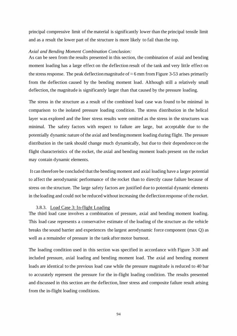
94
principal compressive limit of the material is significantly lower than the principal tensile limit
and as a result the lower part of the structure is more likely to fail than the top.
Axial and Bending Moment Combination Conclusion:
As can be seen from the results presented in this section, the combination of axial and bending
moment loading has a large effect on the deflection result of the tank and very little effect on
the stress response. The peak deflection magnitude of ≈ 6 mm from Figure 3-53 arises primarily
from the deflection caused by the bending moment load. Although still a relatively small
deflection, the magnitude is significantly larger than that caused by the pressure loading.
The stress in the structure as a result of the combined load case was found to be minimal in
comparison to the isolated pressure loading condition. The stress distribution in the helical
layer was explored and the liner stress results were omitted as the stress in the structures was
minimal. The safety factors with respect to failure are large, but acceptable due to the
potentially dynamic nature of the axial and bending moment loading during flight. The pressure
distribution in the tank should change much dynamically, but due to their dependence on the
flight characteristics of the rocket, the axial and bending moment loads present on the rocket
may contain dynamic elements.
It can therefore be concluded that the bending moment and axial loading have a larger potential
to affect the aerodynamic performance of the rocket than to directly cause failure because of
stress on the structure. The large safety factors are justified due to potential dynamic elements
in the loading and could not be reduced without increasing the deflection response of the rocket.
3.8.3. Load Case 3: In-flight Loading
The third load case involves a combination of pressure, axial and bending moment loading.
This load case represents a conservative estimate of the loading of the structure as the vehicle
breaks the sound barrier and experiences the largest aerodynamic force component (max Q) as
well as a remainder of pressure in the tank after motor burnout.
The loading condition used in this section was specified in accordance with Figure 3-30 and
included pressure, axial loading and bending moment load. The axial and bending moment
loads are identical to the previous load case while the pressure magnitude is reduced to 40 bar
to accurately represent the pressure for the in-flight loading condition. The results presented
and discussed in this section are the deflection, liner stress and composite failure result arising
from the in-flight loading conditions.

95
In-Flight Deflection:
The in-flight loading condition produces deflections in the X, Y and Z directions. These
corresponded to bending, longitudinal and radial deflection respectively. Due to this
complexity, the results of the deflection are presented in three separate figures, each of which
represents a certain deflection direction.
Figure 3-55 depicts the bending deflection result of the in-flight simulation. This result is
displacement magnitude in the X-Y plane and represents the deflection of the tank away from
its undeformed longitudinal axis. As can be seen from the simulation, the magnitude of the
deflection significantly increases in comparison to the isolated axial and bending moment
deflection result.
Figure 3-55: In-Flight X- Deflection Result
The result seen in Figure 3-55 indicates that the pressure has the effect of increasing the
deflection of the tank in the presence of a bending moment load. The laminate used in the final
solution was slightly different to the laminate presented at the end of the analytical design
method. The reason for this laminate change was to increase the longitudinal stiffness of the
tank. This was done by adding two additional helical layers to what was specified in Section
3.4.4 to increase the stiffness of the tank. As can be seen from Figure 3-55, the magnitude of
the bending deflection is still large. This was considered acceptable as the load case was
exaggerated and unlikely to occur in reality.
Figure 3-56 depicts the Y (longitudinal) deflection result of the in-flight simulation. The
longitudinal deflection represents the longitudinal length change of the tank. The result is

96
slightly skewed due to the bending moment load but offers insight to the way in which the tank
responds to the in-flight load case.
Figure 3-56: In-Flight Y- Deflection Result
As can be seen in the figure, the peak magnitude of the longitudinal deflection is seen on the
bottom right corner of the tank, with a magnitude of ≈ 2.95 mm. The top right corner of the
tank exhibited a deflection in the other direction with a magnitude of ≈ 1.35 mm. The opposing
directions of the deflections are a result of the bending moment load skewing the longitudinal
result. By taking the mean of the two values to represent the approximate longitudinal
deflection, it can see that the tank deflects ≈ 0.8 mm in the positive direction with respect to
the Y-axis. This result, although approximate, indicates that the longitudinal deflection due to
pressure loading is greater than the compressive loading due to the axial load. This means that
the pressure loading of the tank, which was previously seen to increase the deflection due to
bending, reduces the longitudinal deflection of the tank.
Figure 3-57 depicts the Z (radial) deflection result of the in-flight simulation. This result is not
affected by the other two loads imposed in the in-flight simulation, apart from pressure.

97
Figure 3-57: In-Flight Z-Deflection Result
The magnitude of the radial deflection due to the in-flight load case is seen to be ≈ 0.1 mm in
the negative Z-direction. This results along the longitudinal axis of the tank, which is skewed
upwards in the figure because of the bending moment load. Despite the bending of the
longitudinal axis, the magnitude of the radial deflection is negligibly affected by the other loads
on the tank and is seen to be consistent over the length of the tank. The deflection magnitude
presents itself in a similar manner to that seen in Figure 3-46, with the magnitude changing as
the coupling structure and aluminium bulkheads are encountered. Due to the lowered pressure
magnitude of 40 bar in comparison to 80 bar, the magnitude of the deflection is lower than the
≈ 1.8 mm seen in Figure 3-46.
In-Flight Liner Stress:
After the deflection result of the structure was deemed acceptable, the analysis of the in-flight
loading condition results moved to reviewing the liner stress response. As was done previously
in Section 3.8.1, both the domed ends and the U-PVC cylinder were analysed using their
respective yield stresses as failure criteria. The first components analysed here were the
aluminium bulkheads from both the fore and aft side of the tank.
Figure 3-58 shows the stress result of the aluminium dome bulkheads on either side of the tank.
The fore and aft bulkheads are labelled in the figure and the maximum stress in the structures
is seen to be ≈ 78.3 MPa.

98
Figure 3-58: In-Flight Aluminium Bulkhead Stress Result
The stress distribution in the figure shows little response to the bending and axial loading and
presents similarly to what was seen in Section 3.8.1. The regions of stress concentration around
the fillets and thickness changes are still present and the stress magnitude drops significantly
in comparison to Figure 3-47 due to the reduced pressure loading.
Figure 3-59 depicts the result of the simulation of the U-PVC cylinder under in-flight loading
conditions. The maximum stress is ≈ 27 MPa, which is below the yield stress of 70 MPa.
Figure 3-59: In-Flight PVC Liner Stress Result
Aft Fore

99
Like the aluminium result presented in Figure 3-58, the stress result in the U-PVC liner exhibits
a correlation to the pressure magnitude rather than the bending moment loading. The stress in
the structure is reduced to a magnitude of ≈ 27 MPa due to the reduced pressure loading and
displays a similar distribution to that seen in Figure 3-48. The presence of the bending moment
and axial loads have little effect on the stress distribution or magnitude in the structure.
In-Flight Composite Results:
Figure 3-60 and Figure 3-61 show the Tsai-Wu failure results for the hoop and helical layers
of the tank respectively for the in-flight loading condition. The feature outlines of the other
components in the tank are included to give context to the location of the pictured results.
Figure 3-60 represents the Tsai-Wu failure result of the inner-most helical layer of the tank
under the in-flight loading condition. This layer is represented by ply 1 in Figure 3-22. As can
be seen from the figure, the combined loading condition influences the distribution of the stress
in the structure.
Figure 3-60: In-Flight Helical Layer Tsai-Wu Result
The effect of the bending moment load on the composite is clearly seen on the left had side of
the figure. The large region of high stress on the top left of the structure represents the zone
with the highest Tsai-Wu result, with a magnitude of ≈ 0.26. This is similar to what is seen in
Figure 3-54, where the side of the composite structure under compressive loading due to the
bending moment load exhibited the lowest safety factor. The coupling structure in this region
is seen to cause a stress concentration in the region affected by the compressive loading. The
opposing bottom side of the structure, which is under tension due to the bending moment load,
exhibits a far lower Tsai-Wu result due to the high stress limit of the helical layer in this

100
direction. Apart from the regions that are under compressive loading due to the bending
moment load at the left side of the figure, the structure exhibits a similar failure distribution to
that seen previously in Figure 3-50.
Figure 3-61 shows the Tsai-Wu failure result of the inner-most hoop layer of the tank under in-
flight loading conditions. This layer is represented by ply 3 in Figure 3-22. The failure
distribution in the figure is affected by the inclusion of bending moment loading. This is
illustrated by the regions of high stress at the top left of the figure and the low stress regions at
the bottom left of the figure. These regions of high Tsai-Wu failure results are present due to
the bending moment load acting on the structure and causing compressive loading at the top of
the figure and tensile loading at the bottom.
Figure 3-61: In-Flight Hoop Layer Tsai-Wu Result
The side of the structure under compression displays a larger Tsai-Wu result than is seen in
Figure 3-60. The opposing side of the figure which is under tension exhibits far higher Tsai-
Wu result than the helical layer under similar conditions. This arises from the alignment of the
composite material relative to the tensile load acting on the structure. The alignment of the
hoop layer means that it is being stressed in its weaker secondary direction by the tensile
loading on this side of the figure. Like the helical result for this loading condition, pictured in
Figure 3-49, the hoop layer seems to exhibit a similar Tsai-Wu result distribution to that of the
isolated pressure loading. This similarity is not evident in some areas, such as where the loading
imposed by the bending moment aligns with the secondary, weaker direction of the composite
material in each layer.

101
In-Flight Loading Conclusion:
As can be seen from the results presented in this section, the in-flight loading condition presents
a result with intermediate Tsai-Wu results when compared to the isolated pressure loading case
and significant bending deflection in comparison to the axial and bending moment load case.
This result is important as it demonstrates the effect of the combined action of the pressure,
axial and bending moment loads on the tank. The results indicate that stress distribution in the
tank is largely dependent on the pressure magnitude, while the deflection magnitude is
dependent on the bending moment load. The bending moment loads create regions of reduced
safety factor in the composite layers. These regions occur where the direction of the loads
imposed by the bending moment loading are coincident with the secondary direction of the
composite material. The pressure longitudinal loads and the axial loads act against one another
and limit the longitudinal deflection of the tank.
3.8.4. Simulation Results Conclusion
The results presented in this section showed the response of the designed oxidiser tank
geometry under isolated pressure loading, axial and bending moment loading, and finally a
load case which represented the peak in-flight load of the tank.
From the results it was determined that the pressure loading was the largest contributor to stress
in the tank and the bending moment load induced the largest deflection. The axial load did not
have a large effect on the structural response of the tank, and, in the in-flight case, the deflection
of the axial load was opposed by the longitudinal stress resulting from the pressure load. The
pressure and bending moment loads displayed some level of interaction when the in-flight load
case results were presented. The combined action of pressure and bending moment increased
the deflection seen in the tank. The bending moment was also seen to result in regions of high
stress in the composite when the loading was aligned with the secondary direction of the
material. The stress in the liner was largely independent of the bending moment and axial load
and correlated primarily with pressure magnitude.
From the results presented and the conclusions drawn, the structure analysed in this section and
detailed in Figure 0-1 and Figure 0-2 of the Appendix was considered qualified for manufacture
and testing.

102
3.9. Design Conclusion
The aim of this chapter was to satisfy Objectives 1 and 2 of the study. From Section 1.3
Objective 1 aims to:
“Develop a process within the technical, computational and resource constraints of the
University which can effectively design a composite pressure vessel for use as an oxidiser
tank on a rocket.”
The design method outlined from Section 3.4 to 3.7 was developed to accommodate the limited
resources available to the University and to create a method for generating and analysing
composite tank designs. The tanks were subject to constraints that were imposed as described
earlier in the section. The design process that satisfies Objective 1 was outlined in Figure 3-62.
The design procedure in the figure runs parallel to the section headings in this chapter.
Figure 3-62: Final Design Methodology
The design method in Figure 3-62 resulted in the flight oxidiser tank for the P1B Mk. II. From
Section 1.3, the aim of Objective 2 was to:
User Defined
Constraints
Analytical
Method
Preliminary
Design Review
CAD Model Generation
N
Y
Computational
Quasi-2D Analysis
Final Design
Review
Supplementary
Geometry Addition
Y
Final Design
N
N

103
“Propose a design which offers an improvement to the previous Phoenix oxidiser tanks in
terms of mass.”
As can be seen from the final geometry presented in Table 0-1 of the Appendix, the theoretical
mass of the geometry resulting from the design method outlined in Figure 3-62 was 16.4 kg.
This design offered a significant mass improvement over the 19 kg of the aluminium tank used
on the P1B Mk. I.
With the verification of the theoretical design complete, the manufacturing of the structure
began and was detailed in Chapter 4.

104
4. TANK MANUFACTURE
4.1. Introduction
This section details how the geometry designed in Chapter 3 was realised and satisfies research
Objective 3 specified in Section 1.3. This section begins with detailing the manufacture of the
liner components and proceeds to describe the winding process and subsequent coupling
structure manufacture.
4.2. Liner Manufacture
The manufacture of the liner began with the PVC section forms the cylinder of the tank. The
PVC pipe was sourced locally and was produced by Marley Plastics. The specification of the
section was UL 620. With a minimum wall thickness of 3.2 mm and an outer diameter of 160
mm [50]. The section of PVC pipe was cut to length and drilled to allow for fastening to the
aluminium bulkheads. The end of a machined section is shown in Figure 4-1, with the holes
used to join the aluminium section to the cylinder visible. A complete mechanical drawing of
the PVC cylinder section is given in Figure 0-2 of the Appendix.
Figure 4-1: Tank PVC Liner End
The PVC pipe presented some problems after manufacturing. Some curvature was visible that
had to be accounted for in the winding process. In addition there was a 0.5 mm difference in
internal diameter between each pipe section, therefore, each aluminium bulkhead had to have
a different outer diameter. The correct sizing of this outer diameter was important as the
interface between the PVC pipe and the aluminium bulkhead was also the radial seal which
contains the oxidiser in the tank. Deviation from the designed O-ring clearance may have
resulted in weakening the seal in this section, which may have resulted premature leaking of
the tank.
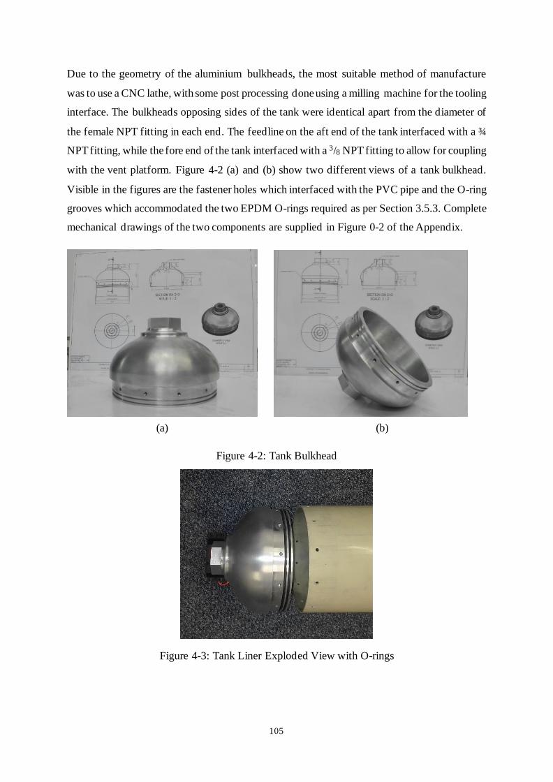
105
Due to the geometry of the aluminium bulkheads, the most suitable method of manufacture
was to use a CNC lathe, with some post processing done using a milling machine for the tooling
interface. The bulkheads opposing sides of the tank were identical apart from the diameter of
the female NPT fitting in each end. The feedline on the aft end of the tank interfaced with a ¾
NPT fitting, while the fore end of the tank interfaced with a 3/8 NPT fitting to allow for coupling
with the vent platform. Figure 4-2 (a) and (b) show two different views of a tank bulkhead.
Visible in the figures are the fastener holes which interfaced with the PVC pipe and the O-ring
grooves which accommodated the two EPDM O-rings required as per Section 3.5.3. Complete
mechanical drawings of the two components are supplied in Figure 0-2 of the Appendix.
Figure 4-2: Tank Bulkhead
Figure 4-3: Tank Liner Exploded View with O-rings
(a) (b)

106
Figure 4-4: Tank Liner Assembled View without Grub Screws
At the end of the liner manufacturing process, the assembled liners were ready for the filament
winding process to begin.
4.3. Filament Winding
The fully assembled liners formed the mandrels over which the carbon fibre/epoxy laminate
was wound to form the load bearing structure of the tank. Using specifically manufactured
tooling, which interfaced with the aluminium heads of the liners, the mandrel was set up on the
filament winding machine. The filament winding machine with the liner in place is visible in
Figure 4-5.
Figure 4-5: Liner Mounted on the Filament Winding Machine
The filament winding machine used to form the tanks was a 4-axis machine produced by a
company called Pultrex. The machine allowed one end of the tank to be chuck mounted while

107
the other was held using a running centre. Due to the relatively flexible PVC pipe, this type of
support resulted in some deformation during winding. This was visible as a slight wobble near
the centre of the mandrel during winding, which did not ultimately affect the winding.
After the machine was set up with the mandrel in place, a dry winding test was conducted to
ensure that the winding would occur as coded. Dry winding is a useful test , as the absence of
epoxy makes the process less tedious and changes to winding paths can be realised quickly,
without risking the liner. The dry winding tests used three 12K tows of TORAY T800 carbon
fibre to result in a combined tow width of 8 mm and a thickness of 0.3 mm. Figure 4-6 shows
the result of the first dry winding cycle of the hoop layer. The result of this dry winding was
considered acceptable as no fibre slip occurred and the mandrel did not deform excessively at
the speeds that would be used for winding. This cycle formed one half of a single hoop winding
cycle. The machine head still needed to return to the other side of the mandrel to fully complete
the cycle. This return cycle was important to achieve the necessary laminate thickness of
0.3mm and to balance the laminate. Hoop windings had to be wound at an angle slightly greater
than 90° to allow the winding to progress along the surface of the mandrel. To result in uniform
properties and inhibit distortion during cure, the hoop layer included a return cycle which
balanced the slight offset from the 90° winding in the first pass. The small gaps between the
carbon fibre, visible in Figure 4-6, were not present during wet winding, as the addition of resin
had the effect of widening the tow slightly.
Figure 4-6: Hoop Layer Dry Wind Test
Tests on the helical layer were conducted after the conclusion of the dry winding of the hoop
layer. Helical layers are more vulnerable than hoop layers to a phenomenon known as fibre
slip. This occurs when the fibre departs from its planned trajectory along the surface of the
mandrel. It typically occurs near the turnaround at the domed end of the tank, where the fibre
is reoriented to allow it to return to the other end of the tank and is due to the large angular

108
change necessary to allow this to occur. This phenomenon is typically corrected by changing
the path of the machine head to allow the fibre to locate itself correctly on the surface of the
mandrel.
Figure 4-7 shows the first iteration of the dry winding of the mandrel. Two problems have been
annotated in the figure which required correction. The first was incomplete dome coverage.
The figure shows that the fibre did not extend to the designed dome length as it traversed the
dome prior to returning to the other end of the tank. This would not only have reduced the bond
area of the domed ends, but also affected the winding angles over the rest of the structure. Left
uncorrected, this phenomenon would have caused differences between the laminated geometry
of the manufactured component and that of the design.
Figure 4-7: First Helical Layer Dry Wind Test with Fibre Slip
The second problem visible in Figure 4-7 is fibre slip, which manifests as two strands of carbon
fibre that do not conform to the nominal direction of the other helical fibres. A focused view
of this phenomenon is given in Figure 4-8. Two of the three strands used to cover the tank
slipped as the machine head passed the turnaround point at the dome of the mandrel and began
to return to the other end. The tension in the fibres caused them to slip off the dome which
resulted in the relatively thin strand at the bottom of the dome. If left uncorrected, this would
have resulted in incomplete surface coverage by the laminate, as many of the fibres would slip
off the head during winding and depart from their predicted orientation.
Incomplete dome
coverage
Fibre slip

109
Figure 4-8: Focused View of Fibre Slip
The problems visible in Figure 4-7 were corrected by adjusting the path of the machine head
as it traversed the length of the mandrel. This change was focused in the head region and
allowed the fibre to conform to the geometry of the component more effectively than in the
first iteration. This also increased the coverage of the dome ends of the mandrel and resulted
in the laminate geometry described in Chapter 3. Figure 4-9 shows the helical laminate
produced at the end of the dry winding tests. In the figure a uniform laminate pattern is visible,
with none of the non-conforming strands seen in Figure 4-7 and Figure 4-8. The dome coverage
problem was also fixed by the machine head adjustment.
Figure 4-9: Conclusion of Helical Dry Winding of Domed Ends
Figure 4-10 shows another view of the final iteration of the helical dry winding. This image
was captured midway through the winding process to depict the development of the helical
Fibre slip off dome

110
band pattern over the tank structure. This pattern represents a winding angle of approximately
25.6° over the cylinder and resulted in complete coverage (no visible preceding hoop layer).
Figure 4-10: Final Helical Dry Wind over Cylinder
After both dry winding tests were successfully completed, the wet winding of the mandrels
began. Two similar tanks were manufactured for the project, which allowed one tank to be
tested to failure, while the other was used as the flight tank for the P1B Mk. II. Table 4-1 shows
the layup schedule used in the production of the tanks, complete with individual layer
thicknesses and cycle times. The layup schedule was designed to replicate the final iteration of
the designed tank geometry specified in Section 3.9.
Table 4-1: Filament Winding Layup Schedule
Winding No. Winding Type Layer Thickness
(mm)
Winding Time
(min)
1 Helical 0.3 20
2 Hoop 0.3 15
3 Helical 0.3 20
4 Hoop 0.3 15
5 Helical 0.3 20
6 Hoop 0.3 15
7 Helical 0.3 20
8 Hoop 0.3 15
9 Helical 0.3 20
10 Hoop 0.3 15
11 Helical 0.3 20
Total 3.3 mm 3h 15m

111
Despite the total predicted winding time of 3 hours and 15 minutes per tank, due to setup time
and other intermediate processes, each tank took between five and six hours to wind to
completion. The intermediate processes were conducted after each hoop wind ing and consisted
of two tasks.
The first process involved squeezing excess resin from the structure, which reduced redundant
mass in the laminate and improved the volume fraction of the manufactured tanks. The other
intermediate process involved using a Vernier calliper to measure the external diameter of the
tanks and ensure that the designed laminate thickness was achieved. The diameter of each tank
was measured after hoop winding as the hoop surface finish was more suitable for dimensional
analysis than the helical layers, which have a slightly variable thickness distribution due to
varying fibre stacking in the winding pattern. The hoop layer was also less susceptible to fibre
distortion during excess resin removal as the fibre pattern was oriented in the direction of
rotation of the mandrel. The helical layer consisted of a shallow angle over the cylinder, which
made it easy to distort in the direction of rotation of the mandrel.
Each tank was left on the machine after the conclusion of the layup to allow it to achieve an
initial cure. After the resin had been allowed a 24 hour ambient cure, each tank was placed in
an oven to achieve an elevated temperature post-cure. The temperature at which the resin was
post-cured was dictated by the vicat (softening) temperature of the PVC which was 83°C [49].
The AMPREG 21 resin system with a slow hardener allows for a 16 hour elevated temperature
post cure at a temperature of 60°C. [29] Figure 4-11 shows the oven which was used to cure
the tanks. In the figure, the tank is seen on a mechanised trolley which was moved in and out
of the oven to allow for easy access to the components before and after curing. The tanks were
supported such that any bowing in the PVC was opposed during cure to maximise the
straightness of the finished components.

112
Figure 4-11: Tank in Position Prior to Post Cure
Figure 4-11 shows the first post cured tank, placed next to the second uncured tank. The
difference in the gloss between the cured and uncured components is visible, with the post
cured component displaying a matt finish in comparison to the glossy finish of the uncured
components.
Figure 4-12: Cured vs. Uncured Tank Surface Finish
The selection of the burst tank was based primarily on the straightness achieved after post cure.
Although the chosen burst tank was slightly lighter than the flight tank, significant bowing was
visible in the tank after cure. This arose due to a combination of inherent bend in the PVC pipe
and force during winding. The small mass discrepancy was considered an acceptable trade-off,
as a tank with significant bowing could induce weather-cocking of the rocket in flight. This is
undesirable and has the potential to induce significant loading on the vehicles structure. At this

113
point in manufacture the tanks were ready to undergo the first stage of testing. This involved
proof testing both tanks and a destructive test of the tank not selected for flight.
4.4. Coupler Manufacture
After the manufacture and pressure testing of the tanks, the composite coupling structures were
formed onto the flight tank. The design of these structures was covered previously in Section
3.7. The manufacture of the couplers involved forming composite material over an internal
mould. Due to the tapered nature of the structures and the inclusion of the aluminium geometry,
a permanent mould core was not feasible. A permanent mould core would become locked into
the mould after the layup of the coupler feature, therefore a sacrificial mould was used that
could be destroyed after manufacture. The mould was formed using polystyrene. Most of the
polystyrene mould was removed using hand tools and any structure that remained was washed
out using solvents. The polystyrene structure had to form an internal mandrel for the composite
coupler and reference the aluminium components to the tank structure. The referencing of the
components was done using the aluminium tooling that held the tank during the winding
process. These components were held concentric to the tank when fastened to the hexagons on
each tank end. The polystyrene mould cores referenced to this tooling and ensured that both
the coupler shape and aluminium components would be manufactured concentric to the
structure of the tank. Figure 4-13 (a) shows the end stage of the manufacture of the coupling
structure, with some extra stock still to be removed. Figure 4-13 (b) shows the manufactured
polystyrene cores complete with the aluminium structures to which the composite coupler was
attached.
Figure 4-13: Coupler Laminate Mould Components
Once the core was manufactured and the aluminium pieces were placed on the structures, they
could be referenced to the tooling. Each mould core had a cylindrical hole through the centre
(a) (b)

114
which interfaced with the outer surface of the tooling. The cores were then located on each tool
to ensure that the aluminium coupler components were positioned exactly according to the
design. Figure 4-14 (a) shows the underside of the tooling. Visible in this figure is the
hexagonal tank interface which connected the tooling to the tank. A large cutaway is also
visible in the polystyrene. This allowed clearance for the head of the tank. Figure 4-14 (b)
shows a different view of the same structure. After the tooling was fixed to the tank, this
structure slid down into its final located position and formed the final shape of the coupler.
Figure 4-14: Assembled Coupler Moulds
Figure 4-15 shows the coupler mould assembled onto the fore end of the tank. Tank tooling
which held the coupler mould concentric is visible in the figure. Peel ply is visible on the tank
on the right-hand side of the figure. This was used to prepare the surface for lamination and
ensured a strong adhesive bond between the composite coupler and the tank. Any gaps between
the polystyrene mould and the tank surface were filled using a putty which released from the
laminated surface after the coupler was manufactured. The aluminium was sanded to key the
surface and cleaned with acetone to promote strong adhesion between the laminate and the
aluminium components [46]. The piece of threaded bar visible in the figure was referenced
using a level to ensure that the aluminium components on either side of the tank were oriented
with respect to one another. Figure 4-15 represents the tank geometry directly prior to the
lamination process.
(a) (b)

115
Figure 4-15: Tank Prepared for Coupler Lamination
The prepared mould surface in Figure 4-15 was laminated to the specification outlined in
Section 3.7. The surface was laminated using a hand layup/mandrel wrap technique. Each
laminate consisted of three sections with varying thicknesses. Each section was formed by
wrapping the mould with a long sheet of carbon fibre. Each of these sheets was cut to a length
such that the design thickness was achieved when wrapped circumferentially around the mould
surface. After the application of all three layers, the laminated surface was wrapped with a
Mylar release tape. This tape forced out a large amount of excess resin and improved the
fibre/resin ratio of the final component.
The laminated structure is shown in Figure 4-16 for the fore side of the tank. Visible in the
figure is the Mylar which was used to remove excess resin, as well as the tapered shape of the
coupler on the fore side of the tank. The laminate was ambient-cured for 24 hours before being
exposed to a post cure cycle of 12 hours at 60ºC.
Figure 4-16: Tank Coupler Post Lamination

116
After the coupler laminate was post cured, the excess carbon fibre on the aluminium was
trimmed. Figure 4-17 shows the tank coupler halfway through the composite trimming process.
The trim line was marked using duct tape to prevent scratching in the event of a tool slip. The
trimming of the composite was done using a Dremel with a grinding bit.
Figure 4-17: Tank Coupler Composite Trimming Process
After the conclusion of the composite trimming, most of the coupler structure was complete.
Figure 4-18 (a) shows the conclusion of the composite trimming process on the aft section of
the tank. Remnants of the polystyrene core are visible and would later be removed using
acetone. Figure 4-18 (b) shows the trimmed fore section of the tank.
Figure 4-18: Assembled Tank Couplers
(a) (b)

117
The final step in the tank manufacturing process was to rivet the aluminium to the composite
structure. Large flange rivets were used as mentioned in Section 3.7. Figure 4-19 shows the aft
side of the tank after the riveting process.
Figure 4-19: Aft Coupler Post Riveting
4.5. Manufacturing Conclusion
The aim of this chapter was to satisfy Objective 3 as it was outlined in Section 1.3, which aims
to:
“Manufacture the tank to the desired specification.”
As can be seen from the sections of Chapter 4, all the design features outlined in Chapter 3 and
structures described by the drawings in Figure 0-1 and Figure 0-2 of the Appendix were
manufactured to specification.

118
5. TESTING
5.1. Introduction
This section details the testing of the tanks manufactured in Chapter 4. This phase involved a
variety of different tests, each designed to ensure a specific mode of failure was not likely to
occur in the tank during flight. These phases comprised pressure testing, cold flow testing and
hot fire testing.
5.2. Pressure Testing
The purpose of the pressure testing of the P1B Mk. II oxidiser tank was to proof the tank and
ensure that it would not fail under the mechanical loading of the pressure and secondary loads
during operation. To achieve this, the pressure testing was divided into two parts, namely a
proof test and a destructive test. Due to timeline constraints, the pressure, proof and destructive
tests had to be conducted prior to the manufacture of the tank coupling structure. Because of
this, the tank was pressure tested in the state described at the end of Section 4.3 and pictured
in Figure 4-12.
In the test setup, the tank was supported vertically in a stand and filled with water prior to the
connection of the pressure apparatus. The apparatus used to pressurise the tank was connected
at the base of the tank. The whole test setup was housed in a large concrete safe room, to ensure
that no personnel were at risk in the case of a failure. This test setup was used for both the proof
and destructive modes of failure.
5.2.1. Proof Testing
The proof testing was used to ensure that both tanks would operate satisfactorily under the
maximum expected operating pressure (MEOP). This test was intended to ensure that
containment systems such as the O-ring seals, the U-PVC cylinder and the aluminium NPT
fitting connections were operational. This test was the first time the tanks were subject to
pressure and indicate of whether the design method had ensured that failure would not occur
below the MEOP, although this was a secondary goal of the test. The proof test cycle is shown
and annotated in Figure 5-1.
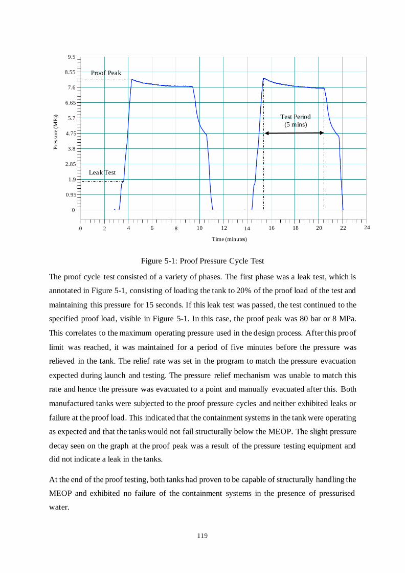
119
Figure 5-1: Proof Pressure Cycle Test
The proof cycle test consisted of a variety of phases. The first phase was a leak test, which is
annotated in Figure 5-1, consisting of loading the tank to 20% of the proof load of the test and
maintaining this pressure for 15 seconds. If this leak test was passed, the test continued to the
specified proof load, visible in Figure 5-1. In this case, the proof peak was 80 bar or 8 MPa.
This correlates to the maximum operating pressure used in the design process. After this proof
limit was reached, it was maintained for a period of five minutes before the pressure was
relieved in the tank. The relief rate was set in the program to match the pressure evacuation
expected during launch and testing. The pressure relief mechanism was unable to match this
rate and hence the pressure was evacuated to a point and manually evacuated after this. Both
manufactured tanks were subjected to the proof pressure cycles and neither exhibited leaks or
failure at the proof load. This indicated that the containment systems in the tank were operating
as expected and that the tanks would not fail structurally below the MEOP. The slight pressure
decay seen on the graph at the proof peak was a result of the pressure testing equipment and
did not indicate a leak in the tanks.
At the end of the proof testing, both tanks had proven to be capable of structurally handling the
MEOP and exhibited no failure of the containment systems in the presence of pressurised
water.
Test Period
(5 mins)
1.9
0.95
0
2.85
3.8
4.75
5.7
6.65
7.6
8.55
9.5
0 2 4 6 8 10 12 14 16 18 20 22 24
Proof Peak
Leak Test
Time (minutes)
Pre
ssu
re (
MP
a)

120
5.2.2. Destructive Testing
After proof testing, two tanks were ready and proofed for flight. To ensure that the ultimate
failure pressure of the tank was sufficiently above the proof load, the decision was made to
conduct a destructive test on one of the tanks. The destructive test also gave a useful
representation of the effectiveness of the design process outlined in Chapter 3.
The destructive test was conducted in a similar manner to the proof test but with a much higher
pressure loading. The graph shown in Figure 5-2 shows the annotated pressure vs time
relationship from the initiation of the destructive test.
Figure 5-2: Burst Test Pressure Result
The destructive test was intended to consist of a single pressurisation to a peak pressure where
the tank would fail. As can be seen from the graph, this was not what occurred in practice. The
first pressurisation cycle was set to pressurise the tank to 20 MPa, denoted by the label “Initial
Load” in Figure 5-2. This pressure was approximately the maximum expected failure pressure
of the tank. As can be seen from the graph, the tank did not fail after being pressurised to this
value and hence was evacuated. The next pressure cycle was set to a far larger pressure limit
of 40 MPa. As can be seen from the graph, the pressure in the tank was able to rise consistently
to a value of approximately 32 MPa where the rate of the rising pressure can be seen to change
notably. The pressure reading in the control room was a discrete pressure reading which did
not allow for operators to note the difference in the rate of pressurisation. For this reason, the
test was continued until the hydraulics in the system needed to be replenished with water. This
8
4
0
12
16
20
24
28
32
36
0 2 4 6 8 10 12 14 16 18 20 22
Time (minutes)
Pre
ssu
re (
MP
a)
40
24
System
Refill
Failure Load
Initial Load

121
was visible on the graph as the downward trend followed by a sharp decrease in the pressure
in the system. As the system attempted to re-pressurise after the hydraulics were replenished,
it became apparent that the system was no longer holding pressure and the tested was
concluded.
Upon visible inspection of the tank after the test it was concluded that the tank had suffered a
weep failure rather than a burst failure. Pictorial evidence of the weep failure is seen in Figure
5-3.
Figure 5-3: Destructive Test Weep Result
The destructive test was useful in determining both the magnitude of the failure pressure of the
tank and the failure mode of the tank. Although the pressure test determined that the composite
will begin to weep at around 32 MPa, there were audible cracks indicative of failure from a
pressure magnitude of around 25 MPa. The loud cracks likely came from the U-PVC liner as
the threaded inserts at either end impinged on the plastic and caused it to fail under the
longitudinal components of the pressure load. After this failure, the pressurised fluid was no
longer contained within the liner at the junction of the head region and the cylinder. The fluid
was then able to form a path down the length of the liner toward the centre of the tank, between
the liner and the composite shell. The fluid propagated toward the centre of the tank rather than
out through the domed ends due to the inferiority of the U-PVC/composite bond to the
aluminium/composite bond, meaning that a path toward the centre would have proved the least
resistant. Another potential mode of failure could have involved the O-ring seal failing at a
pressure significantly lower than 250 MPa and allowing the pressurised medium through the
junction far earlier in the test. The composite would still be the final barrier to allow
depressurisation and hence the results of either failure mode would be similar to what was seen
in the test.
122
Although it is impossible to definitively prove which of the failure modes occurred, the
comparatively low failure pressure of the O-ring seal seems to indicate that the second mode
of failure was more likely. Although the tank can be said to have a weep pressure of
approximately 32 MPa, the pressure at which pressurised nitrous oxide could encounter media
that could cause decomposition is likely to be far lower, although impossible to quantify from
this test.
5.3. Cold Flow Testing
The cold flow test involved filling the tank with nitrous oxide and evacuating the tank in a
similar manner to what would be experienced during launch. The cold flow test does not
involve ignition of the evacuated nitrous oxide and is used to characterise flow through the
combustion chamber’s injector.
5.3.1. Cold Flow Test Setup
The test involved the integration of the tank with various other components necessary for the
final launch of the vehicle. It was primarily a test of other rocket components, such as the fill
systems and oxidiser injector components, but was still useful in characterising the behaviour
of the tank under a set of relevant loading conditions. The test was the first time that the
manufactured tank was subject to pressure from nitrous oxide, the fluid which the tank was
designed to house. The fluid properties of nitrous oxide meant that the tank housed both a liquid
and a gas phase, which differed significantly from the previous pressure tests. The pressure
was also exerted over a far larger period than was seen in the proof test. The final difference
from the proof test was the temperature loading experienced by the structure as nitrous oxide
filled the tank. Nitrous oxide has the potential to cool parts of the tank to temperatures to as
low as – 10°C. This temperature loading was not included in the design phase due to modelling
complexity and computational time constraints. Therefore, the cold flow test was an important
and useful qualitative test to ensure that the tank operated effectively under the loading
conditions outlined above.
5.3.2. Cold Flow Test Results
An annotated pressure loading profile from the cold flow test is shown in Figure 5-4. This
comprised four different phases, each with different loading characteristics.

123
Figure 5-4: Cold Flow Test Pressure Profile
The filling phase occurred first as the nitrous oxide was decanted from the fill bottles into the
flight tank. This was characterised by dynamic pressure changes as the vent was used to
regulate the pressure in the tank. The purpose of the vent pressure regulation was to ensure that
enough pressure difference was present between the fill and flight tanks and allow for nitrous
to continually flow into the flight tank. As can be seen from the figure, this phase d id not
represent the peak pressure magnitude, but included high dynamic pressure loading as the vent
regulated the pressure. This phase also introduced the first significant thermal loading on the
tank as the nitrous oxide reduced the temperature of the tank as it was filled [30]. The filling
phase was concluded after approximately 45 minutes, when the desired mass of nitrous oxide
had been loaded into the flight tank.
The next phase of the cold flow test was the warming phase. This involved leaving the filled
mass of nitrous oxide to heat up to a desired temperature. The heat was gained from the
atmosphere and the objective of this phase was to increase the pressure in the flight tank due
to the self-pressurising nature of nitrous oxide. This occurred over approximately ten minutes
and was characterised by a gradual increase in pressure as the fluid temperature rose. In this
phase, the thermal loading on the tank decreased as the nitrous oxide and adjacent components
were warmed by the atmosphere. The pressure was allowed to increase until significant
pressure gains were no longer seen and then the supercharging phase was initiated.
0
10
20
30
40
50
60
70
80
90
100
0 10 20 30 40 50 60 70 80
Pre
ssu
re (
bar)
Time (minutes)
Filling
Warming
Super-
charging
Tank
Evacuation

124
The supercharging phase was the final phase prior to the evacuation of the stored nitrous oxide.
This used pressurised helium gas to raise the pressure in the tank to the design operating
pressure (65 bar), which was done in a series of small pressure increases to avoid exceeding
the design pressure of the oxidiser tank. This phase represented the peak of the pressure
magnitude combined with the highest dynamic component of pressure change but had a
reduced thermal loading component compared to the fill phase.
After the desired supercharging pressure was reached, the evacuation phase was initiated. The
evacuation phase involved opening a valve between the tank and injector apparatus which
allowed the stored nitrous oxide to evacuate over a period of approximately 15 seconds. This
evacuation rate was simulated in the proof test, but the magnitude of the pressure drop was
difficult to match accurately. The evacuation phase therefore had the highest pressure drop
magnitude of all the test phases to this point, in addition to the additional thermal loading from
the stored nitrous oxide.
As can be seen from the pressure graph, the tank sustained the pressure loading over all the test
phases. No pressure drops indicative of leaks were present in the graph and the tank operated
nominally throughout the test.
5.4. Hot Fire Testing
The hot fire test had a similar layout to the cold flow test but was designed to characterise the
thrust and pressure profiles of the rocket motor over its burn time.
5.4.1. Hot Fire Test Setup
To obtain the thrust and pressure profiles, the combustion chamber, rocket fuel grain and nozzle
were added to the test infrastructure and ignition was initiated at the start of the tank evacuation
phase. The test setup for the hot fire test is shown in Figure 5-5 directly after the test conclusion.
As can be seen in the figure, there was additional infrastructure on the aft end of the rocket and
the scorch marks on the ground were a result of the recently concluded combustion test.

125
Figure 5-5: Hot Fire Test Configuration
The hot fire test was similar to the cold flow test until the point of tank evacuation. After tank
evacuation and upon ignition of the motor, significant thrust and vibration loading were
imposed on the tank. This had the effect of replicating the rocket launch more accurately than
the cold flow test. Only flight dependant loads such as bending moment loads and potential
harmonic loads were absent from the test, making it the most representative test possible in
terms of design proofing.
5.4.2. Hot Fire Test Results
The pressure profile of the tank during the hot fire test is shown in Figure 5-6. As can be seen
by comparing Figure 5-4 and Figure 5-6, the pressure profiles for the cold flow and hot fire
tests were characteristically similar, with only the length of each phase differing slightly due
to atmospheric conditions and the dynamic nature of the filling process.

126
Figure 5-6: Hot Fire Test Tank Pressure Profile
One of the primary outputs of the hot fire test was a graph of thrust produced vs. time for the
rocket motor. The structural design of the tank and other supplementary components were
designed with this thrust load as a constraint, in addition to a pressure load shown previously
and bending moment load absent from the test. The result of the thrust generated by the motor
is shown in Figure 5-7. The thrust load used to generate this plot was transferred from the
combustion chamber through the tank and secondary components and recorded by the test load
cell. This load cell was the same one used to establish nitrous oxide weight in the cold flow
test.
Figure 5-7: Hot Fire Test Axial Load Profile
0
10
20
30
40
50
60
70
80
90
100
0 500 1000 1500 2000 2500 3000 3500 4000 4500 5000
Pre
ssu
re (
Bar)
Time (seconds)
Filling
Warming
Super-
chargingTank
Evacuation
-1000
0
1000
2000
3000
4000
5000
6000
7000
8000
4360 4365 4370 4375 4380 4385 4390
Th
rust (N
ew
ton
s)
Time (seconds)

127
As can be seen from the figure, the thrust load began at a slightly negative value (around 720 N
or 70 kg below zero). This was a result of the mass of the rocket and the loaded oxidiser hanging
on the load cell and causing a load opposite in direction to the generated thrust load. The
ignition of the motor occurred at around 4366 s on the graph and from this point onward the
motor was producing thrust. The figure shows that the nature of the thrust loading was highly
dynamic, with the largest peak to peak oscillation having a magnitude of around 4000 N. This
oscillation was caused by a combination of combustion instability in the rocket motor and
resonance generated in the trailer from the forces of combustion. As the motor reached the end
of its combustion around 14 s after ignition, the thrust generated decreased until the value was
negative again. This negative value occurred for a similar reason to the negative value at the
beginning of the test but had a slightly lower magnitude as the weight of the oxidiser which
was evacuated during the test was no longer acting on the load cell.
As can be seen in the figure the magnitude of the generated thrust was similar to the design
load. This test represented the worst-case loading condition as all the thrust load was passed
through each structural element on the tank. Under launch conditions, the thrust loading will
only be present on a rocket element as the sum of the inertial load of the mass all the structures
above the element. The aerodynamic drag acting on the vehicle will also contribute to the
loading.
5.5. Testing Conclusion
The aim of this chapter was to satisfy Objective 4, outlined previously in Section 1.3. The
objective states;
“Test the manufactured tank to ensure flight readiness”
As can be seen from the preceding sections, all elements of the tank and the surrounding
components were able to withstand the pressure and thrust loading imposed by the cold flow,
hot fire and the proof and destructive pressure tests. The tank was then qualitatively proofed in
load states which approach the designed flight loading conditions. These load states
incorporated pressure, dynamic axial load and thermal loading.

128
6. DISCUSSION
6.1. Introduction
In this section, various elements of the design, manufacture and testing of the tank are critically
reviewed and discussed. Strengths and weaknesses of the decisions made are reviewed and, in
some cases, suggestions for improvements in future iterations are given.
6.2. Tank Design Method Review
The review of the design method of the tank follows the design path outlined previously in
Figure 3-62 and did not touch on the other methods mentioned in Section 3.6 such as the 2D
and 3D analysis. The review began with the strengths and weaknesses of each method before
suggesting possible areas for improvement.
6.2.1. Analytical Method Review
The analytical method developed based on netting analysis was an excellent starting point for
the design of the filament wound tank used on the P1B Mk. II. The method, when combined
with simple volume and density calculations, was able to quickly identify a geometric layout
which would satisfy the design constraints of the project based on mass and safety factor
requirements. The turnover time to exact a design change was in the order of seconds from
implementation to result.
The quick cycle times of the design method came at the cost of accuracy. Netting analysis
primarily deals with the load bearing composite over the cylinder of the tank and the relevance
of the method deteriorates over the dome region. For the purposes of this design, netting
analysis was used to generate a starting point on the cylinder and Clairaut’s theorem allowed
for the prediction of the composite properties over the shape-constrained head region [32].
Although the properties over the head region were dependant on the cylinder properties, netting
analysis did not drive the composite result in this area. Rather, the analytical design phase was
concluded with the knowledge that supplementary reinforcement was necessary in this region
due to the absence of a hoop layer.
Another drawback of using netting analysis was the lack of experimental data to supplement
the method. This was not a direct consequence of the choice to use netting analysis, but rather
due to resource constraints on the side of the University. Netting analysis is a method that
predates all computational methods used today in the field of composite tank design. The
simplicity of the method was always supplemented by using experimental data that accurately
describes the behaviour of the chosen composites under the basic assumptions of netting

129
analysis. Accurate material properties were not available to the University for the chosen
composite, meaning that properties were generated from a micromechanics approach. This
method is not the most reliable way to generate composite properties and as a result large safety
factors were included. This safety factor increased the mass of the tank generated using this
method.
The assumption of netting analysis that the liner has no contribution to the strength of the tank
may also affect the effectiveness of the method in proceeding designs. In the case of the P1B
Mk. II, the liner was manufactured from a relatively thin U-PVC cylinder which likely does
not challenge the weak liner assumption of netting analysis. In proceeding iterations, the liner
will potentially be manufactured from a metallic material such as aluminium. Metallic liners
have a lower limit on the thickness which the relatively complex liner can be manufactured
from and as a result the liner will likely be able to handle a significant portion of the design
pressure. Neglecting the contribution of the liner in tanks with load bearing liners will result in
tanks which are overdesigned and weigh more than is necessary.
6.2.2. Computational Method Review
The computational method used for verification of the tank models was an effective
compromise between accuracy and solution time. Although commercially available packages
exhibit superior qualities in terms of solution setup time and user interfaces, the method
generated on Siemens NX, a resource available to the university at no cost, managed to
eliminate the large cost associated with the other products.
The primary difference between the more general Siemens NX product and a more specialised
product or plug-in to other software, such as CADWIND, was the model setup time. The
method of defining the laminate over the cylinder of the tank in Siemens NX was simple and
allowed for quick laminate changes in terms of material, thickness and stacking order. Defining
the laminate over the head region was more difficult and required approximately 90 minutes to
define for the most complex simulation. The time for lamination definition over the head region
decreases for less accurate simulations, but the time taken for laminate definition may eliminate
this method for extremely complex simulations. Despite the additional model definition time
of this design process, the solution quality of the developed method should be similar to
solutions generated using the commercially available packages due to the fact they only deal
with model pre-processing.

130
The solution time for the final tank was approximately 26 hours. This analysis allowed for a
complex model with all necessary loads, contacts and glue interfaces defined. This was only
possible because the simulation assumed that the loading conditions were applied statically.
This static result is considered enough to qualify the pressure with all the safety factors included
throughout the design process. Although satisfactory for this design task, the rocket is subjected
to highly transient loading. This is evident from the graphic result of the axial load in the hot
fire test, shown previously in Figure 5-7. Apart from the loading, the failure mode of the tank
was also highly transient with O-ring failure occurring prior to liner seperation and eventual
composite failure, mentioned in Section 6.5.1. Modelling the transient scenario of the rocket’s
flight or hot fire testing would have added significant time to the already lengthy 26 hour solve
time. The inclusion of transient loading would have required a more focused analysis of the
loading conditions experienced over the rockets flight and during testing, as well as requiring
a more in-depth definition of material fatigue properties. For these reasons, the more complex
transient solution was avoided for this design task. In future, if more computational resources
are made available, the computational method could easily evolve to model more complex
transient scenarios and improve the mass savings seen when using composite tanks.
6.2.3. General Design Philosophy Review
In this section, the general philosophies and approaches used in the design process of the P1B
Mk. II oxidiser tank are discussed and possible areas which could be improved are highlighted.
The first area of discussion is the choice of safety factors. Typically, even in crewed space
missions, safety factors are kept to a relative minimum, usually around 1.4 [51]. As can be seen
from the initial tank design pressure in Section 3.4.3, the safety factor on the design load was
around three which is significantly higher than those used in other tanks for similar
applications. This design pressure was selected to match the design point to the aluminium
structure design for use on the P1B Mk. I rocket. If the tank was designed to a lower safety
factor, comparison between the tanks would have been more difficult. The high safety factor
was also justified due to the novel nature of the composite tank produced in this design task.
In future iterations of composite oxidiser tanks, it is recommended that the safety factor be
reduced to a magnitude similar to other tanks used in the field, as the concept of a composite
tank has been explored and found to be beneficial.
The next point of discussion is the highly computational/analytical method of design. The
selected design approach, due to constraints imposed by resource limitations, had little input
from experimental sources. The absence of data from experimental sources meant that the

131
properties of the composite materials had to be calculated from micromechanics. This
necessitated the inclusion of safety factors which, in addition to the large safety factors chosen
at the start of the design, increased the mass of the tank unnecessarily. Direct experimental data
on the materials used to manufacture the tank would greatly reduce the mass of the finished
product.
The final point to be discussed is the method that was used to generate the loads for the design
task. Due to time constraints on the project, most of the loads were assigned the magnitude of
the worst-case loading condition and the in-flight loads were calculated based on a spreadsheet
which is used to generate the loading from analytical methods. A more robust, CFD-based
approach is currently within the technical capabilities of the university and could be used to
generate more accurate load cases based on a specific mission profile. Reducing the uncertainty
present in the creation of loads for the tank would reduce the large safety factor which has to
be applied and ultimately reduce the mass of the tank.
6.2.4. Design Conclusion
As can be seen from the results presented in this section, the design methods used to generate
the oxidiser tank on the P1B Mk. II can be improved in several areas. These areas mostly arise
from resource and technology constraints on the University and can be easily improved in the
next iterations of the composite design.
Despite the issues with the design method, the entire process operated within the resource
constraints of the University and the resulting structure exhibited superior properties to the
previous iterations of the Phoenix oxidiser tanks.

132
6.3. Tank Material Choice Review
This section details the design choices about material selection and discusses the positive and
negative ways the resulting design was affected as a result.
6.3.1. Liner Material Selection
The selection of materials to form the liner of the tank was guided primarily by oxidiser
compatibility and manufacturability. The selection of materials for the liner consisted of un-
plasticised PVC and aluminium.
The choice to use a stock length of U-PVC pipe was heavily influenced by the manufacturing
limitations imposed by local industry. The stock length of PVC tube proved to be a
comparatively lightweight solution which satisfied the oxidiser compatibility constraint of the
application. Using a stock length of PVC also drastically reduced manufacturing costs of the
cylindrical portion of the tank, requiring only cutting and 20 drilled holes. All the other
potential manufacturing methods and material combinations, explored in Section 3.5, would
have added significant manufacturing complexity which would have added to the cost of the
project. While the PVC liner proved to be an effective choice overall, some issues were
revealed during the manufacture of the tank which should be addressed in the next vehicle
iteration.
The primary problem with the PVC liner was lack of straightness. During the filament winding
process, it became apparent that there was some skewness in the tubes. From visually
inspecting the way in which the tube behaved during rotation, it was determined that the
skewness stemmed from two sources. Firstly, a small amount of skewness was being induced
by the pipe deforming under its own weight during rotation. This was due a combination of the
ductility of the PVC Pipe material and the way in which the tank was supported on the filament
winding machine. The second reason for the skewness stemmed from the manufacturing
method used to produce the pipes. The pipe lengths were formed from extruded sections which
can lead to skewness as the pipe cools after the extrusion process. It is apparent that more care
must be taken to ensure that straighter sections of PVC tubing are selected for future tanks of
this type. The support issues are dealt with later in this section.
Another problem with the PVC pipe related to its vicat temperature, beyond which the material
softens. The specific grade of U-PVC selected for the project exhibited a softening temperature
of around 83°C [49]. This temperature was not an issue regarding the required operating
conditions of the tank but implied a constraint on the selection of a resin system for use on the

133
tank. This constraint was implied as most resin systems require a post cure cycle to reach their
manufacturer specified mechanical properties. Post cure cycles occur at elevated temperature
for extended periods of time and prolonged exposure to temperatures near or above the vicat
temperature of the plastic have the potential to deform the structure of the tank. The possibility
of this deformation occurring is increased when one considers that the composite structure is
not fully cured over the time the PVC structure will be likely to soften.
The choice to use aluminium over the head region of the tank proved effective as the material
was able to act as a load bearing component in this region. The aluminium also provided a
suitable region to interface with the metallic NPT fittings which had to be connected to the fore
and aft sides of the tank.
The final problem with the liner material selection was the choice to make use of two dissimilar
materials to form the tank liner. This choice, in conjunction with space constraints and the
difficulties involved with bonding PVC, meant that an O-ring seal was required at the bulkhead
interface at each end of the tank. This seal was inaccessible after the tank had been filament
wound and hence could not be inspected or lubricated to ensure long term effectiveness. This
was not a problem for the P1B Mk. II vehicle, as the turnaround between testing and launch
was relatively small. The previous two Phoenix launch vehicles have all suffered from
significant timeline delays and hence the turnaround between testing and launch has been
upwards of 3 years for each vehicle. Using an O-ring seal that cannot be maintained over this
period would be a questionable design choice and this area of the design may need to be
revisited if this is a potential risk on future vehicle designs.
Despite the flaws present in the material selection for the formation the tank liner, the current
selection was proved to be effective in terms of feasibility within the project budget and
performance under all the testing methods outlined in Chapter 5. Further iteration of the tank
design with the same combination of materials will yield a significantly improved product
based upon the understanding gained from their use in the project.
6.3.2. Tank Composite Material Selection
Although the material selection process for use in the design task was highly constrained, the
results of Section 3.8 can still be used to generate recommendations for material selection in
the future.
The material used in the final tank design was a Toray T800/AMPREG 21 composite. As
described in Section 3.3.1, the carbon used in the laminate had excellent tensile properties,

134
surpassed only by Toray T1000 carbon fibre. When looking at the results presented in Section
3.8, it can be concluded that the tank does not approach failure due to the excessive tensile
loading. The large deflections present in the design could be minimised by replacing some of
the T800 plies with a grade of carbon that offers superior stiffness properties. Toray offers a
grade of carbon fibres termed ‘High Modulus Carbon Fibres’ which exhibit superior stiffness
properties to the T800, which constitutes an ‘Intermediate Modulus Carbon Fibre”. A design
which utilised the high tensile carbon used in this design, in conjunction with a high modulus
fibre would likely result in a tank which is more optimal with respect to the loading imposed
by the rockets flight.
The resin system used on the rocket, AMPREG 21, is a low-cost resin which was readily
available to the project and satisfied all the constraints imposed by the design task. As can be
seen from the results presented in Section 3.8, the designed tank suffered regions of increased
failure likelihood due to loading being aligned with the secondary direction of the composite.
The properties of the composite in this direction are dependent primarily on the properties of
the matrix material used. Although the resin system used was satisfactory, improving the
properties of the matrix material by using a higher quality resin would have the effect of
reducing the size of the failure zones caused by the secondary direction loading of the
composite.
6.3.3. Coupler Material Selection
The selection of materials for the coupler was dictated by the local availability of materials in
conjunction with the availability of material properties to allow for analysis of the coupling
structure. The selected materials, mentioned in Section 3.7, were 200 g/m2 carbon fibre twill
weave fabric and aluminium. The selected materials allowed for the formation of lightweight
structures on the fore and aft sides of the tank which were created with relatively simple
manufacturing methods. The manufacturing methods are reviewed subsequently in Section 6.4.
The selected carbon fibre was procured through a local composites supplier and dissimilar to
the carbon fibre which was used to filament wind the tanks. The carbon used to filament wind
the tanks was of the tensile grade T800 which exhibited significantly improved mechanical
properties to the fibres which were used in the coupler structure. This means that the carbon
sections which formed the coupling structures had a slightly lower strength/mass efficiency
than the rest of the composite on the tank. Potential mass reduction can be realised by using a
higher-grade carbon fibre in this region. Local fabrics are available which utilize carbon grade
T700, which is a significant upgrade from grade utilised in the twill weave fabric used. To

135
make use of these fabrics, materials testing must be made available to the project to accurately
estimate their mechanical properties for structural analysis.
The choice to use aluminium in the coupling structure was effective in terms of space
availability, loading conditions and manufacturing considerations. Using a material such as
steel or titanium would have resulted in a structure that was too thin to be manufactured
effectively. The only drawback of the aluminium was the requirement of a bonding area
between the tank and the combustion chamber geometry. Aluminium is notoriously difficult to
bond due to the formation of an oxide layer on its surfaces which are exposed to atmosphere.
The oxide layer means that the material typically forms weak joints when bonded to other
materials. In the final design of the P1B Mk. II, the bond is a cylindrical lap joint with little
mechanical reinforcement beyond a set of rivets which were in place to inhibit peel failure.
Although this design was proof tested using the thrust load, it may not have been enough to
ensure that the bond did not fail under flight moment loading. To improve the integrity of the
bonded joint, the aluminium bonding surface could be designed to include a geometry which
would form a mechanical bond with the composite component. Surface treatment of the
aluminium, such as anodising, may also be used to increase the strength of the bond.
6.4. Tank Manufacture Review
This section discusses the strengths and weaknesses of the methods of manufacture used to
create the oxidiser tank for the P1B Mk. II.
6.4.1. Liner Manufacturing Review
The liner geometry manufacture involved two main manufacturing operations. These
operations were the formation of the cylinder and the formation of the domed ends of the tank.
The cylinder was formed from an extruded section of U-PVC plastic with an outer diameter of
160 mm and a wall thickness of minimum 3.2 mm. The purchased sections had an actual mean
thickness of ~ 3.75 mm, which increased the predicted mass from the initial 3.2 mm estimation
and increased the length of the tank due to the volume reduction of the thickness increase. This
change was not captured at any point in this thesis as only the final iterations of the tank
geometry, which included the correct liner thickness, were supplied for the analytical and
computational methods. The purchased sections only needed to be faced to the correct length
and drilled radially to interface with the dome bulkheads. This resulted in a total manufacturing
cost and lead time that was drastically lower than other available options, listed in Section 3.5.
Due to budget constraints the cylindrical U-PVC sections were the best choice, however, there

136
were some drawbacks to using the tube sections. As mentioned previously in Section 6.3.1, the
cylindrical sections had some inherent skewness. This skewness not only affected the final
geometry of the tank, but also made the referencing for the facing and radial drilling operations
difficult, as the tubes would wobble slightly on rotation. The internal radius of the tubes varied
significantly due to non-uniform wall thickness, which made achieving the desired O-ring
tolerance of 0.1 mm difficult. Each domed end had to be machined individually to ensure a
snug fit with the O-ring.
To result in a more stable cylindrical section the design would need to progress to consider
more expensive methods of manufacture. Methods such as flow forming or sheet rolling, and
welding have the potential to eliminate many of the drawbacks which were incurred by using
an extruded plastic section. Although the relative density of a metallic liner is greater than U-
PVC, by altering the design method to included liner contributions the fidelity of the design
could be greatly improved.
The domed bulkheads were manufactured from aluminium 6082-T6 via conventional 3-axis
CNC milling techniques. The aluminium material was stable and the subtractive, high precision
machining methods resulted in geometry that was accurate in comparison to the extruded U-
PVC sections.
6.4.2. Filament Winding Review
To create the tanks for the P1B Mk. II, the liner components mentioned previously had to be
covered with a load bearing composite material. This was done using a commercially available
4-axis filament winding system. The strengths and weaknesses of the filament winding process
used to manufacture the tanks for the P1B Mk. II are discussed in this section.
Many of the weaknesses which became apparent during the manufacturing process arose from
a lack of practical experience in the field of filament winding. As mentioned previously in this
section, some eccentricity was visible in the tanks during the winding process. This eccentricity
arose from a combination of material skewness and liner support issues during the winding
process. The liner support issues were caused by a poor design choice in the creation of tooling
used to hold the tanks during the winding process. As can be seen in Figure 4-5, the liner is
supported on each end by cylindrical aluminium components which interface with the tank
bulkheads. The interfacing surface of the cylindrical components is visible in Figure 4-14. As
can be seen from the figure, the interfacing surface consisted of a hexagonal extrusion with
threaded holes for locating grub screws placed in the centre of three of the hexagon sides. The

137
grub screw locators are the only structures used to locate the liner along the central winding
axis of the filament winding machine. The grub screws had to be tightened manually and had
no reference to ensure the screws were enforcing concentricity between the two interfacing
hexagons. This issue was compounded due to a large tolerance between the hexagonal shape
on the tank bulkheads and the hexagonal interface on the aluminium tooling. In addition to the
concentricity issues, the grub screws made surface defects on the bulkhead interfacing surfaces,
which meant that the tooling needed more and more adjustment over time to locate itself
parallel to the longitudinal axis of the tank. The eccentricity induced by the tooling issues meant
that the tank was rotating with a slight wobble over the entire manufacturing process. This
meant the tank was not positioned in the way that was predicted by the CAM software and
hence the manufactured fibre path differed relative to the designed fibre path.
Using grub screws to locate the tank also had the undesired effect of affecting the tanks during
curing. It was noticed during the winding process that the grub screws would loosen over the
course of the winding time and slightly increase the eccentric rotational path of the tank. This
also became problematic when the winding was complete, and the tanks needed to cure. Due
to the constant loosening of the screws, it was not possible to leave the tanks rotating on the
machine overnight. Leaving the tanks rotating on the machine during their primary cure phase
would have ensured even resin distribution and allowed for the least possible skewness to be
induced by the winding process. To avoid the tank falling off the machine as a result of the
loosing grub screws, it was necessary to remove the tanks before the end of the work day, after
winding. This meant that the tanks were removed while the resin was still slightly soft and
because of this, some skewness may have been induced as the tanks were simply supported as
they cured. To mitigate this as far as possible, the tanks were positioned such that any skewness
already present in the tank would be countered by the skewness induced by the support during
curing.
After the conclusion of the winding process, the ends of the tanks were wound with peel ply to
ensure that a satisfactory bonding surface would be present on either end for coupler adhesion
later in the manufacturing process. The peel ply and resulting bonding surfaces are visible in
Figure 4-12 and Figure 4-15 respectively. This proved to be an effective method of creating a
bonding surface and resulted in a surface finish that was more uniform than the portions of the
tank which did not have a peel ply finish. The wound-on peel ply had the added benefit of
squeezing excess resin from the wound tank. In future iterations of the tank, a higher mass
efficiency could be achieved by wrapping the entire geometry in peel ply. In areas were

138
subsequent bonding is required, a coarse peel ply can be used and in other areas where an
aerodynamic interface is present a finer peel ply can be used. The areas with the lighter peel
ply can then be coated with a thin, lightweight layer of clear coat paint to result in a surface
with which is both more uniform and smoother than the surface present in the current tank
iteration.
6.4.3. Coupler Manufacturing Review
After filament winding, composite couplers were bonded to the ends of the tank to allow for
interfacing with other components. The couplers which were added to the ends of the filament
wound tank were manufactured in a non-conventional way to conform to the budget and time
constraints of the project.
The coupler manufacture was lightweight and effective but can still be improved in certain by,
for example, integrating the filament winding and coupler manufacture processes. This would
be done by restructuring the laminate of the filament wound tank and allowing for a tubular
shape to be wound over the initial domed-end windings. Tooling like the polystyrene structures
manufactured to form the coupling structures, pictured in Figure 4-14, would be used to extend
the shape of the tank to allow for tubular winding. This integrated method of manufacture, if
implemented correctly, would allow for superior bond between the coupling structure and the
filament wound tanks. In addition to the increase in bond strength, the integrated manufacturing
method will eliminate the tapers and bumps which arose from the current method of
manufacture and reduce the total number of manufacturing steps which are needed to produce
the tank. A potential drawback of this method will be an increase in design complexity and
structural computation time. The previously mentioned skewness issues associated with the
tank winding will also need to be addressed prior to the implementation of this method, as any
skewness will have a large effect on the overall rocket geometry. The bond with the aluminium
coupling components will also need to be improved, as mentioned in Section 6.3.3.
6.4.4. Post Manufacture Mass Analysis
In this section, the differences between the predicted and realised masses of the tanks are listed
and discussed for each stage of manufacture.
The difference between the predicted and achieved masses are listed in Table 6-1. These
differences were measured at three different stages in the manufacturing process. The first mass
measurement was after the completion of the liner assembly, directly before winding. This
mass condition is represented by the tank in Figure 4-5. The next mass measurement was taken
after post curing of the filament-wound laminate, prior to pressure testing. This mass condition

139
is shown in Figure 4-12. The final mass measurement was of tank in its final flight
configuration, shown in Figure 4-19. As can be seen from Table 6-1, only one mass
measurement was available, as Tank 1 was destroyed during the destructive testing phase of
pressure testing.
Table 6-1: Manufactured Tank Mass Analysis Table
Tank 1
(Burst)
(kg)
Tank 2
(Flight)
(kg)
Tank Difference
(Flight – Burst)
(kg)
Liner Mass
Predicted Mass 7.7 7.7 -
Achieved Mass 8.5 8.67 0.17
Liner Mass Discrepancy +0.8 +0.97 -
Post Winding Mass
Predicted Mass 14.158 14.158 -
Achieved Mass 15.56 15.66 0.1
Post Winding Mass Discrepancy +1.402 +1.502 -
Flight Tank Mass
Predicted Mass - 16.401 -
Achieved Mass - 18.98 -
Flight Tank Mass Discrepancy - +2.579 -
As can be seen from both Table 6-1, the manufactured mass at each stage of manufacture varied
from the predicted mass. The cumulative mass discrepancy for the flight tank at the end of the
manufacturing process was 2.579 kg greater than what was predicted in the design phase of the
project. The results of Table 6-1 are given graphically in Figure 6-1.

140
Figure 6-1: Tank Mass Summary Graph
As can be seen in Figure 6-1, the mass discrepancy was cumulative and stems from smaller
mass contributions at each stage of manufacture. Figure 6-2 graphs the mass increase at each
stage of manufacture for the flight tank.
Figure 6-2: Flight Tank Manufacturing Discrepancy Graph
From Figure 6-2, it can be seen that the value of this discrepancy was 970 g for the liner
manufacturing phase of the flight tank construction. This discrepancy was due to the PVC pipe
sections being heavier than was predicted from the manufacturer’s product brochure. As can
be seen from Table 6-1 and Figure 6-1, the difference between each manufactured liner was
170 g, with the flight tank being the heavier. This difference was also assumed to be due to the
PVC pipe variance.
After the lamination of the tanks, it can be seen from Table 6-1 that the burst tank was still
lighter than the flight tank, but by only 100 g. The 70 g discrepancy was incurred during
lamination and means that the laminate mass of the flight tank was less than that of the burst
0
2
4
6
8
10
12
14
16
18
20
Liner Manufacture Filament Winding Coupler Bonding
Mass (K
g)
Predicted Mass Tank 1 Mass Tank 2 Mass Discrepancy
0
0.5
1
1.5
2
2.5
3
Pre-Winding Post-Winding Flight Tank
Mass (K
g)
Liner Difference Winding Difference Coupler Diffrence

141
tank. As the flight tank was manufactured second, this discrepancy likely occurred as the
technician operating the machine was more effective at removing resin after practicing on the
first tank. The laminate mass was predicted to add an additional mass of approximately
6.458 kg during the winding process. From Table 6-1, both tanks exceeded this mass. At this
point in the manufacture, each tank was between 1.4 kg and 1.5 kg above its predicted mass.
From Figure 6-2, we can see that the 1.5 kg mass difference consisted of a 0.97 kg contribution
from the liner and a 0.532 kg mass contribution from the filament-winding manufacturing
process of the flight tank. This likely occurred because the analytical method used to predict
composite thickness was not accurate over the head region and the predicted resin/fibre ratio
was incorrect. Deviation between the thickness predicted by the analytical method and the
manufactured item stems from the fact that band pattern and the width of the fibre tow both
influence the way fibres build up on the head of the tank. The final contribution to the deviation
from the design mass of the flight tank came from the manufacture of the composite couplers.
This amounted to the largest contribution to the deviance from predicted mass, with over 1 kg
gained in this phase of manufacture. This mass gain resulted from the hand layup method of
manufacture resulting in a poorly optimised resin/fibre ratio. Excess stock remaining on the
aluminium coupling components also contributed to this mass discrepancy.
The mass distribution of the flight-weight tank is shown in Figure 6-3. As can be seen from the
figure, the total composite mass of the final tank accounts for approximately 38% of the final
tank dry mass, excluding the composite mass in the couplers. The liner mass accounted for
46% of the final mass of the tank with a 10% and 36% contribution from the aluminium and
U-PVC components respectively. The mass of the liner relative to the composite mass is higher
than usual for composite tanks of this type. The relative mass of the U-PVC cylinder is
especially high when one considers its minor contribution to the strength of the finished tank.
This once again points to the liner as an area where significant mass savings can be realised.

142
Figure 6-3: P1B Mk. II Tank Construction Breakdown
6.4.5. Manufacturing Conclusion
From the results of this section, it was possible to conclude that significant improvement could
be realised when considering the manufacturing methods used in the construction of the
oxidiser tank for the P1B Mk. II. Most of the problems with the manufacturing processes were
a result of inexperience with both the design process and practical manufacturing work. These
problems could be easily rectified on the next iteration of the oxidiser tank and similar tanks.
Despite the problems present in the manufacturing, a functional item was produced within the
technical and resource constraints imposed by the University and as a result Objective 3 as it
was specified in Section 1.3 was satisfied.
Aluminium
1.8 kg
10%
PVC Cylinder
6.7 kg
36%
Bonded Couplers
3 kg
16%
Helical Layers
3.5 kg
19%
Hoop Layers
3.5 kg
19%
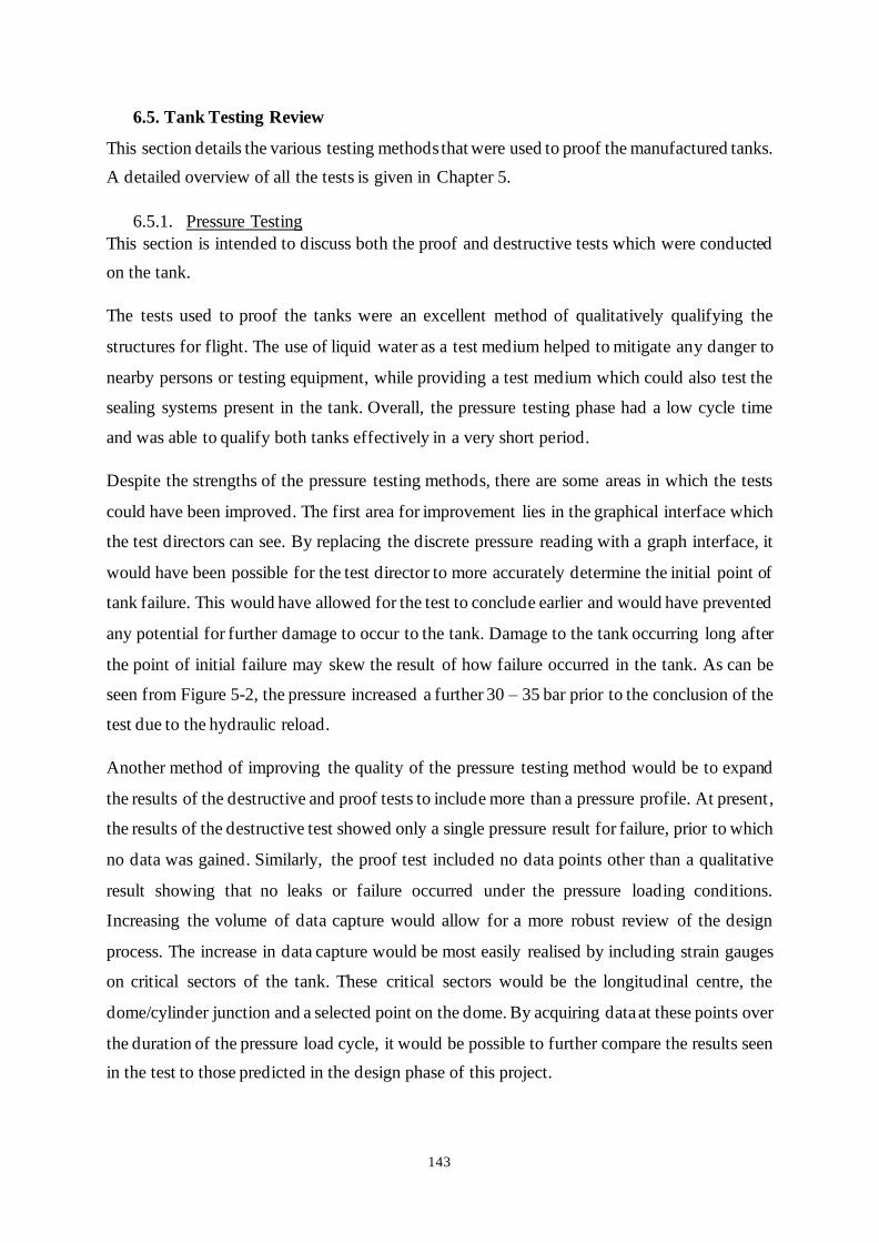
143
6.5. Tank Testing Review
This section details the various testing methods that were used to proof the manufactured tanks.
A detailed overview of all the tests is given in Chapter 5.
6.5.1. Pressure Testing
This section is intended to discuss both the proof and destructive tests which were conducted
on the tank.
The tests used to proof the tanks were an excellent method of qualitatively qualifying the
structures for flight. The use of liquid water as a test medium helped to mitigate any danger to
nearby persons or testing equipment, while providing a test medium which could also test the
sealing systems present in the tank. Overall, the pressure testing phase had a low cycle time
and was able to qualify both tanks effectively in a very short period.
Despite the strengths of the pressure testing methods, there are some areas in which the tests
could have been improved. The first area for improvement lies in the graphical interface which
the test directors can see. By replacing the discrete pressure reading with a graph interface, it
would have been possible for the test director to more accurately determine the initial point of
tank failure. This would have allowed for the test to conclude earlier and would have prevented
any potential for further damage to occur to the tank. Damage to the tank occurring long after
the point of initial failure may skew the result of how failure occurred in the tank. As can be
seen from Figure 5-2, the pressure increased a further 30 – 35 bar prior to the conclusion of the
test due to the hydraulic reload.
Another method of improving the quality of the pressure testing method would be to expand
the results of the destructive and proof tests to include more than a pressure profile. At present ,
the results of the destructive test showed only a single pressure result for failure, prior to which
no data was gained. Similarly, the proof test included no data points other than a qualitative
result showing that no leaks or failure occurred under the pressure loading conditions.
Increasing the volume of data capture would allow for a more robust review of the design
process. The increase in data capture would be most easily realised by including strain gauges
on critical sectors of the tank. These critical sectors would be the longitudinal centre, the
dome/cylinder junction and a selected point on the dome. By acquiring data at these points over
the duration of the pressure load cycle, it would be possible to further compare the results seen
in the test to those predicted in the design phase of this project.

144
6.5.2. Cold Flow Testing
The cold flow test was effective in qualifying the tank’s integrity regarding leaks using the
medium for which the tank was designed. The pressure and onboard mass profiles were
effective as a means of determining the presence of a leak and the objective of the test was
achieved.
The cold flow test could be improved by including strain gauges on the tank, similarly to the
pressure tests. Thermal analysis of the tank in its various stages of testing and eventual use was
deemed unnecessary, primarily due to time constraints. In future, including this area of design
may become possible due to human resource or budget increases. Used in conjunction with an
external temperature probe, atmospheric conditions and the temperature of the stored nitrous
oxide, the data collected from the strain gauges could be used to verify or construct a high-
fidelity thermal model of the tank during filling. Once benchmarked to the cold flow result, the
thermal analysis of the tank then has the possibility to be extended to include thermal loading
during flight. This will prove useful, especially for further iterations of the rocket, which will
likely involve higher launch velocities and altitudes with higher thermal loading.
6.5.3. Hot Fire Testing
The hot fire test confirmed the integrity of the fluid containment systems in the tank and
additionally proofed the tank against failure under a combination of thrust, thermal and
pressure loading. The test could be improved by including strain gauges in the test apparatus.
By comparing the results of the strain gauges to the results of the structural analysis used to
design the tank, the analysis could be verified or improved. As mentioned previously for the
cold flow test, these results could then be extrapolated to predict the behaviour of the tank in
flight.
6.5.4. Testing Conclusion
It is apparent review of the testing methods that there is potential to gather more data from each
test. The testing methods utilised were effective to qualify the tank for use on the rocket
qualitatively, but an increase in the quality of the data gained during testing would be useful to
feed back into the design method. Despite this, the testing methods effectively qualified the
tank for flight.
6.6. Tank Comparison
After the conclusion of the design, testing and manufacture of the tank, it was possible to make
a comparison between the three tanks used in the Phoenix program. The intention of this was

145
to critically review the performance of the first composite tank in the program in comparison
to the aluminium tanks used previously in the project.
6.6.1. Geometric Comparison
The bulk geometric parameters of all the oxidiser tanks in the comparison are listed in Table
6-2. The lengths of the tanks were difficult to compare because each tank iteration had differing
interface methods with the other rocket components. The excessive length of the P1B Mk. II
tank was largely due to the coupling structures, which housed secondary components such as
the feedline.
Table 6-2: Rocket Oxidiser Tank Geometric Properties
Model Construction Length
(m)
Diameter
(m)
Volume
(m3)
Pressure
(bar)
Mass
(kg)
P1A Tank Aluminium 6082-
T6 1.6 0.2 0.043 65 15.8
P1B Mk. I
Tank
Aluminium 6061-
T6 2.28 0.164 0.041 65 19
P1B Mk. II
Tank
U-PVC/Al Liner
and Composite 2.78 ~0.17 0.047 65 19
As can be seen from Table 6-2, the P1B Mk. II tank was the longest and housed the largest
volume of nitrous oxide.
The masses of the oxidiser tanks used on the P1B Mk. I and the P1B Mk. II were similar.
Initially this result seems to indicate that the mass savings gained by using a composite tank
were negligible. Simply comparing the masses of the tanks does not accurately account for
geometric differences and other factors which contribute to the performance of a tank. For this
reason, an efficiency parameter for tanks is introduced and explored in the proceeding section.
6.6.2. Efficiency Parameter Comparison
By benchmarking the tanks against one another using a pressure vessel efficiency calculation,
a more accurate indication of the success of the tank designed for this project was gained. To
benchmark the tanks against one another, a pressure vessel performance parameter was used.
This parameter is shown in equation 6-1 [52].

146
𝜀𝑣𝑒𝑠𝑠𝑒𝑙 =
Failure Pressure × Volume
Mass [6-1]
As can be seen from the parameter, the efficiency of a tank increases proportionally with rated
pressure and stored volume. The efficiency of a tank also decreases with an increase in mass.
The volume and mass of the tanks were geometric parameters and were easily obtained through
measurement and reference to CAD models. The difficult parameter to obtain was the failure
pressure of the tanks.
The difficulty in obtaining the failure pressure of the tanks comes from the non-standardisation
of the tests used to proof the tanks. The aluminium tanks for the P1A and P1B Mk. I vehicles
were simply subjected to a proof load prior to testing, meaning that the values of the maximum
working pressure are not known for either tank. The composite tank for the P1B Mk. II vehicle
was the first tank to be subject to a failure test, with a maximum pressure of approximately
320 bar. Despite the pressure of 320 bar, the tank may have failed to act as a suitable tank prior
to this pressure, as mentioned previously in Section 6.5.1. The aluminium tanks may also have
suffered from early containment breach via an O-ring seal or a failure of the fasteners at either
end. Because of this, the decision was made to neglect the effect of the failure pressure on each
tank, as insufficient data was available to effectively determine a failure pressure of relevance
for each tank.
By eliminating the failure pressure from the efficiency formula, only the container volume and
mass affected the final efficiency of each tank. This method was not ideal to use when
comparing the P1A tank to the others due to the geometric differences between the tanks. The
P1B Mk. I and P1B Mk. II were similar in terms of geometric layout and because of this, the
comparison was more effective.
The comparison of differing types of tanks fails due to the dependence of burst pressure on
tank diameter. Larger diameter tanks will tend to have lower failure pressure but have improved
volumetric efficiency, while smaller tanks have higher failure pressure with reduced volumetric
efficiency. By eliminating the effect of the failure pressure from the efficiency parameter,
larger tanks gain an advantage as its efficiency is not reduced by its theoretically lower failure
pressure. Figure 6-4 shows the result of the efficiency parameter listed in equation 6-1, with
the effect of failure loading ignored.

147
Figure 6-4: Geometric Tank Efficiency
As can be seen from the graph, the P1A tank shows the largest volumetric efficiency while the
P1B Mk. I tank has the lowest efficiency. The exaggerated efficiency of the P1A was accounted
for previously. From the figure, it can be concluded that the P1B Mk. II had a slightly improved
efficiency in comparison to the P1B Mk. I tank. Due to the similar masses of the tanks, this
difference is mainly due to the increase in volume of the P1B Mk. II. An increase in volume of
approximately 15% in the P1B Mk. II at the cost of no additional mass suggests that the
composite tank is an improvement on the aluminium construction, in terms of pressure vessel
efficiency.
6.6.3. Tank Comparison Conclusion
Although Section 6.6.2 above concluded that the composite P1B Mk. II tank was superior in
terms of efficiency to the aluminium P1B Mk. I tank, other parameters required consideration
which were difficult to quantify.
The first of these parameters was manufacturing complexity. The design of the P1B Mk. I
oxidiser tank made use of preformed sections of aluminium tubing which were drilled radially
to accommodate bulkheads and allowed for coupling to the other structures of the rocket. The
composite tank consisted of similar construction methods for the formation of the liner but
required subsequent filament winding and coupler bonding before a complete tank was
achieved. The construction methods involved in creating the composite tank also forced a final
design which was less modular than the aluminium construction.
The composite tank proved to be a superior structure in terms of a flight mass at the cost of an
increase in design complexity and a reduction in modularity. Bearing in mind that the
0
0.0005
0.001
0.0015
0.002
0.0025
0.003
Vo
lum
e/M
ass (
m3/k
g)
Phoenix-1A Phoenix-1B Phoenix-1B Mk.II

148
composite tank was a novel design and that design improvements discussed previously in this
section can be implemented, it is possible to conclude that the composite tank was a definite
improvement on the aluminium tank and offers the potential for significant further
improvement in the future.

149
7. CONCLUSION
The aims of the thesis were as follows;
1. Develop a process within the technical, computational and resource constraints of the
University which can effectively design a composite pressure vessel for use as an
oxidiser tank on a rocket.
2. Propose a design which offers an improvement to the previous Phoenix oxidiser tanks
in terms of mass.
3. Manufacture the tank to the desired specification.
4. Test the manufactured tank to ensure flight readiness
5. Launch the designed tank on the P1B Mk. II’s maiden flight to an apogee of 35km.
Chapter 3 began by addressing Objective 1 and 2 by developing a design method which could
produce a structure eligible for use on the P1B Mk. II hybrid rocket. The design method began
by defining the required user defined inputs before progressing to an analytical platform where
initial laminate properties and bulk geometric properties of the tank were specified based on
pressure loading. The design then progressed to a computational platform where the effect of
the liner geometry and coupling structures was quantified. Loads such as bending moment and
axial loading were also included at this point. The results of the design procedure were
reviewed on the final iteration tank geometry, which is detailed in the Appendix.
Chapter 4 satisfied Objective 3 by detailing the entire manufacturing process of the filament
wound tank. The manufacture and assembly of the liner components was detailed before the
filament winding process began. The bulk parameters of the filament winding process were
outlined, such as the lamination schedule, lamination time and post-curing schedule. After the
filament winding process was complete, the manufacture of the coupling structures was
detailed, and the chapter was concluded after the conclusion of the manufacturing processes on
the tank.
Chapter 5 satisfied Objective 4 by subjecting the manufactured tank to a variety of tests which
were analogous to flight conditions. The chapter began by detailing the methods used when
conducting the 80 bar proof tests on each tank and the destructive test which revealed the
≈ 320 bar failure pressure of the tank. The testing then progressed to the cold flow and hot fire
tests which were useful in verifying the operation of the tank with the design oxidiser. The hot
fire test also proofed the bonded joints under a highly dynamic axial loading condition. After
these tests the tank was considered flight ready.

150
Chapter 6 was included to review each of the sections listed previously and find areas for
improvement. An attempt was made to quantify the performance of the composite tank relative
to the previously manufactured oxidiser tanks in the Phoenix series and a minimum mass
improvement of 15 % was realised, with potential for further improvement in the future based
on recommendations made in this section.
The final objective, stated in Section 1.3, has not yet been satisfied. The first launch attempt of
the P1B Mk. II ended prematurely and because of this, the design outlined in this paper has yet
to be flight qualified. Plans are in place for a re-launch of the P1B Mk. II which will be used
to flight qualify the design produced in this thesis.

151
REFERENCES
[1] ASREG, “Phoenix Hybrid Sounding Rocket Program,” University of KwaZulu Natal,
2018. [Online]. Available: aerospace.ukzn.ac.za/Projects/Phoenix.aspx. [Accessed 07 06
2019].
[2] Genevieve, “Design of a Hybrid Sounding Rocket Motor,” University of KwaZulu-Natal,
Durban, 2013.
[3] Chowdhury, “Simulation of a Hybrid Sounding Rocket,” University of KwaZulu-Natal,
Durban, 2013.
[4] ASREG, “Phoenix-1A Hybrid Sounding Rocket,” University of KwaZulu-Natal, 2018.
[Online]. Available: aerospace.ukzn.ac.za/Rockets/Phoenix-1A.aspx. [Accessed 07 06
2019].
[5] Leverone, “The Design and Performance Simulation of a 100 km Apogee Hybrid
Sounding Rocket,” University of KwaZulu-Natal, Durban, 2014.
[6] Balmogim, “Design and Development of the Phoenix-1B Hybrid Rocket,” University of
KwaZulu-Natal, Durban, 2017.
[7] Broughton, “Motor Design for a Sub-Orbital Hybrid Rocket,” University of KwaZulu-
Natal, Durban, 2018.
[8] Chowdhury, “Design and Performance Simulation of a Hybrid Sounding Rocket,”
University of Kwazulu-Natal, Durban, 2012.
[9] Delft Aerospace Rocket Engineering, “Stratos III,” Delft University of Technology,
2018. [Online]. Available: https://dare.tudelft.nl/stratos/history/stratos-iii/. [Accessed 12
06 2019].
[10] Lark, “Recent Advances in Lightweight, Filament-Wound Composite Presure Vessel
Technology,” NASA, Cleveland, 1977.
[11] Linehan, Burt Rutan's Race to Space: The Magician of Mojave and His Flying
Innovations, Minneapolis: Zenith Press, 2011.
[12] Sharp, “SpaceShipOne: The First Private Spacecraft,” Space.com, 05 March 2019.
[Online]. Available: https://www.space.com/16769-spaceshipone-first-private-
spacecraft.html. [Accessed 12 November 2019].
[13] Matthews, Composite Materials: Engineering and Science, London: Chapman & Hall,
1994.
[14] Swanson, Introduction to Design and Analysis with Advanced Composite Materials, Salt
Lake City: University of Utah, 1997.
[15] Agarwal et al., “Analysis and Performance of Fiber Composites,” Wiley, Chicago, 1980.

152
[16] Gol'denblat, “Strength of gladd reinforced plastic in the complex stress state,” Polymer
Mechanics, vol. 1, pp. 54-60, 1966.
[17] Allnex Industries Ltd., “Filament Winding,” Allnex Industries Ltd., 2014. [Online].
Available: http://www.nuplex.com/Composites/processes/filament-winding. [Accessed
26 01 2017].
[18] Malnati, “Thermoplastic composite pressure vessels for FCVs,” Composite World, 2 1
2015. [Online]. Available: http://www.compositesworld.com/articles/thermoplastic -
composite-pressure-vessels-for-fcvs. [Accessed 10 2 2017].
[19] Cohen, “Influence of Filament Winding Parameters on Compsoite Vessel Quality and
Strength,” in Composites Part A, Elsevier Science Limited, 1997, pp. 1035-1047.
[20] Kabir, “Finite element analysis of composite pressure vessels with a load sharing metallic
liner,” Composite Structures, vol. 49, pp. 247-255, 2000.
[21] Malik et al., “An Integrated Systematic Approach to Linerless Composite Tank
Development,” in Structures, Structural Dynamics & Materials Conference, Texas,
2005.
[22] Almeida, “Load sharing ability of the liner in type III composite pressure vessels under
internal pressure,” Journal of Reinforced Plastics and Composites, vol. 33, no. 24, pp.
2274-2286, 2014.
[23] Bom, “Stratos III: Composite Tank Prototype,” 21 June 2016. [Online]. Available:
http://dare.tudelft.nl/2016/06/stratos-iii-composite-tank-prototype/.
[24] Fukunaga, “Optimum Design of Helically Wound Composite Pressure Vessels,”
Composite Structures, vol. 1, pp. 31-49, 1983.
[25] De Jong, “A theory of filament wound pressure vessels,” Delft University of Technology,
Delft, 1983.
[26] Koppert, “Virtual Testing of Dry Filament Wound Thick Walled Pressure Vessels,” in
16th International Conference on Composite Materials, Kyoto, 2007.
[27] CADWIND, “Versions and Options,” CADWIND, 2019. [Online]. Available:
https://www.material.be/cadwind/versions/index.html. [Accessed 13 06 2019].
[28] Toray Carbon Fibres America, INC, “T800H Material Properties,” Toray, Santa Ana,
California, 2007.
[29] Gurit, “AMPREG 21 - Epoxy Wet Laminating System,” Gurit, 2015.
[30] Newlands, “The Physics of Nitrous Oxide,” Aspire Space, 2011.
[31] Kinna, “NOL Ring Test Methods,” The Office of Technical Services, White Oak, 1964.
[32] Amelina, Analysis and Design of Hybrid Pressure Vessels, Michigan: MIT, 2016.

153
[33] Tew, “Preliminary Design of Tubular Composite Strucutres Using Netting Theory and
Composite Degradation factors,” University of Idaho, Moscow, 1995.
[34] United States of America Department of Defense, Composite Materials Handbook, US
Department of Defense, 2002.
[35] Gheshlaghi et al., “Analysis of Composite Pressure Vessels,” Springer Netherlands,
2006.
[36] Aalco Metals Ltd, Aluminium Alloy 6082, Cobham, 2016.
[37] Hedley Industrial Group, “General Properties of uPVC Pipe Material,” Excellent Pipe
Co., 2018. [Online]. Available: http://www.hedley-
international.com/index.php?option=com_content&view=article&id=118&Itemid=121.
[Accessed 09 03 2018].
[38] AZO Network, “Stainless Steel - Grade 316 (UNS S31600),” AZO Materials, 2018.
[Online]. Available: https://www.azom.com/properties.aspx?ArticleID=863. [Accessed
09 03 2018].
[39] Cole-Parmer Scientific Experts, “Chemical Compatibilty Database,” Cole-Parmer, 2018.
[Online]. Available: https://www.coleparmer.com/Chemical-Resistance. [Accessed 09
03 2018].
[40] Parker Hannifan Corporation, “Parker O-Ring Handbook ORD 5700,” Ohio, 2007.
[41] Ghafaar et al, “Applications of the Rule of Mixtures and Halpin-Tsai Equations to Woven
Fabric Reinforced Epoxy Composites,” Journal of Engineering Sciences, vol. 34, no. 1,
pp. 227-236, 2006.
[42] University of Cambridge, “Strength of Long Fibre Composites,” 2018. [Online].
Available: https://www.doitpoms.ac.uk/tlplib/fibre_composites/strength.php. [Accessed
08 03 2018].
[43] Faria, “Analytical and Numerical Modelling of the Filament Winding Process,”
Universidade do Porto, 2013.
[44] Mahdy et al, “Design of Optimum Filament Wound Pressure Vessel with Integrated End
Domes,” in Aerospace Sciences and Avaition Technology, Cairo, 2015.
[45] Hoult, “Sounding Rocket Structural Design Loads (rev.9),” Rocket Science and
Technology, Culver City, 2014.
[46] Leena et al, “Effect of surface pre-treatment on surface characteristics and adhesive bond
strength of aluminium alloy,” International Journal of Adhesion & Adhesion, vol. 70, pp.
265-270, 2016.

154
[47] da Silva et al, “Techniques to reduce the peel stresses in adhesive joints with
composites,” International Journal of Adhesives and Adhesion, vol. 27, pp. 227-235,
2007.
[48] SFS Intec, “Blind Rivets and Riveting Tools,” SFS Intec, Wyomissing, 2011.
[49] MakeItFrom.com, “Unplasticized (Rigid) Polyvinyl Chloride (uPVC, PVC-U),” 08 09
2018. [Online]. Available: https://www.makeitfrom.com/material-
properties/Unplasticized-Rigid-Polyvinyl-Chloride-uPVC-PVC-U. [Accessed 06 03
2019].
[50] MARLEY Pipesystems, uPVC Sewer & Drainage Systems, Aliaxis, 2009.
[51] Hale, Factors of Safety, NASA, 2008.
[52] Johns, “Filament Overwrapped Metallic Cylindrical Pressure Vessels,” in Structure and
Materials Conference, Cocoa Beach, 1966.
[53] LOCTITE, “The LOCTITE Design Guide for Bonding Plastics, Volume 6,” Henkel
Corporation, Connetitcut, 2011.
[54] Fraters, “Development of a Hybrid Rocket Engine for the Stratos II Rocket,” in 62nd
International Astronautial Congress, Cape Town, 2011.
[55] Beer, Mechanics of Materials, McGraw Hill, 1992.

155
APPENDIX
Table 0-1: Computational Design Mass Prediction
ITEM MASS
(kg)
FORE ALUMINIUM
BULKHEAD 0.896
AFT ALUMINIUM
BULKHEAD 0.898
U-PVC CYLINDER 5.887
FILAMENT WOUND
COMPOSITE 6.458
FORE COUPLER
STRUCTURE 1.157
AFT COUPLER STRUCTURE 1.09
TOTAL 16.4

156
Figure 0-1: Coupler Geometry Mechanical Drawing

157
Figure 0-2: Liner Geometry Mechanical Drawings