Development of a common definition of, and approach to data collection on, the geographic location of students to be

used for nationally comparable reporting of outcomes of schooling within the context of the “National Goals for

Schooling in the Twenty-First Century”.

A report submitted to the

National Education Performance Monitoring Taskforce of the

Ministerial Council on Education, Employment, Training and Youth Affairs

by Dr Roger Jones

Quantitative Evaluation and Design Pty Ltd

30 May 2000

ii

iii

Table of contents List of tables and figures iv Acknowledgments iv Executive Summary v 1. Introduction 1

1.1 The project brief 1 1.2 Background 1

2. National classifications of geographic location 5 2.1 Australian Standard Geographical Classification (ASGC) 5 2.2 DPIE/DHSH Rural, Remote and Metropolitan Areas Classification

1991 Census Edition (RRMA) 6 2.3 Griffith Service Access Frame (GSAF) 8 2.4 Accessibility/Remoteness Index of Australia (ARIA) 9

3. Rural/remote areas in government programs 12 3.1 State/Territory Departments of Education 12

3.1.1 New South Wales 12 3.1.2 Victoria 13 3.1.3 Queensland 14 3.1.4 South Australia 14 3.1.5 Western Australia 15 3.1.6 Tasmania 16 3.1.7 Northern Territory 17

3.2 Some Commonwealth programs 17 3.2.1 Income Tax Zones 17 3.2.2 DETYA programs 18 3.2.3 DH&AC Rural Retention Program 19

4. Rural/remote disadvantage in education 21 4.1 Reasons for rural/remote disadvantage 21 4.2 Identifying rural/remote disadvantage 22 4.3 School location versus home location 24 4.4 Beyond compulsory schooling 26 4.5 Summary of bases for the definition of geographic location 27

5. Defining geographic location 29 5.1 The ARIA approach 29 5.2 Assigning ARIA scores to addresses 31 5.3 Categories of geographic location 33 5.4 Metropolitan and provincial city regions 36 5.5 Other provincial and remote areas 38 5.6 Discussion of proposed definition of geographic location 47

References 50

iv

List of Tables and Figures

Table 1.1 Advantages/Disadvantages of the ASGC, DPIE/DHSH and GSAF classifications as summarised in the DETYA paper “Geographical Location”

Table 2.1 Summary of ASGC spatial units as at 1 July 1996 Figure 1 Structure of the Classification

Table 5.1 Metropolitan and provincial city regions by category Table 5.2 Other provincial city regions, Statistical District to be defined in ASGC 2001

Table 5.3 Population (number and per cent) in CDs with ARIA scores greater than 4.105 Figure 2 Remote Australia: ARIA Score by Census Collection District

Table 5.4 Population distribution by State/Territory, RRMA and ARIA remote areas Table 5.5 Remote CD (ARIA score 4.81 or more) and remote population by SLA

Acknowledgments This project was commissioned by the National Education Performance Monitoring Taskforce and I am grateful for the assistance and support provided throughout the project by Vivienne Roach, the NEPMT Secretariat Director, and the members of project steering committee, Ian Hind (Chair), Wendy Whitham (DETYA), Richard Jenkin (SA), John Harris (WA), Michele Bruniges (NSW), David Hanlon (TAS) and Frank Blanchfield (ABS). I am especially grateful to Frank Blanchfield, who provided essential assistance with access to data and maps, answered my numerous inquiries promptly, and overworked his computing facilities in the process. I would also like to thank the many people in State/Territory education departments, catholic education offices and associations of independent schools who responded to my request for information, particularly those whose written responses contributed to Section 3 of this report. Roger Jones Quantitative Evaluation and Design Pty Ltd

v

Executive Summary Lower participation rates for rural students in post-compulsory schooling resulting in lower Year 12 completion rates and under-representation in higher education have long been recognised as reasons for concern that rural students are disadvantaged. Suggested explanations of why rural students are educationally disadvantaged include: the difficulties of providing the full range and quality of education in small, isolated communities; the difficulties and costs for students and their families associated with distance and travel to education institutions, more particularly in the post-compulsory years and for participants in higher education; differences in the background characteristics of rural and urban students which explain, in part, the differences in participation and outcomes; and the different interests, perceptions and expectations of rural and remote students and their families. There is then a need to provide a basic statistical description of these students by State/Territory, sector and degree of isolation, and compare their participation and outcomes with the rest of the student population. In view of the need to develop nationally consistent definitions for nationally comparable reporting of outcomes of schooling, this project was commissioned by the National Education Performance Monitoring Taskforce (NEPMT) to develop a discussion paper that proposes national definitions of geographic location, taking into account the potential need for alternative measurement approaches depending on whether the data is to be obtained from administrative sources or other means. Throughout the 1990s, the MCEETYA Taskforce on School Statistics (TOSS) sought to achieve national agreement on an approach to the classification of geographic location, but no conclusive agreement could be reached. The discussions and evaluations that were conducted provide the background to this project and are summarised in Section 1 of the report. National classifications of geographic location are examined and discussed in Section 2. These include the ABS classification approaches which together form the Australian Standard Geographical Classification (ASGC), the Rural, Remote and Metropolitan Areas (RRMA) classification developed by the former Department of Primary Industries and Energy and Department of Human Services and Health, the Griffith Service Access Framework (GSAF) developed by Dr Dennis Griffith, and the most recent attempt to measure remoteness, the Accessibility/Remoteness Index of Australia (ARIA) developed by the National Key Centre for Social Applications of Geographical Information Systems (GISCA) at the University of Adelaide on behalf of the Department of Health and Aged Care. Section 3 reviews various definitions of rural and remote areas implemented in a range of government programs, with particular emphasis on the approaches taken by the states to identify rural and remote schools. The criteria used by Commonwealth government authorities, particularly DETYA, to define rural and remote populations are also reported. Section 4 examines reasons for rural/remote disadvantage in education outcomes, the ways in which that disadvantage has been investigated, and considers the different approaches that might be used to identify rural and remote populations in schooling and the post-compulsory years for the purposes of national reporting of outcomes. An important issue here is whether home location or school location should be used, it clearly being far simpler to allocate schools to the appropriate geographic location category than it is to allocate individual students.

vi

The proposed definition of, and approach to data collection on, the geographic location of students to be used for national comparable reporting of outcomes of schooling are outlined in Section 5. The definition has clear similarities with the now outdated 1991 Census based RRMA classification which has achieved widespread use by Commonwealth agencies. While the RRMA classification was criticised on a number of grounds, the recent development of ARIA as a measure of remoteness in Australia allows these concerns to be addressed while retaining those aspects of previous national classifications which have achieved widespread acceptance. Conclusions and Recommendations 1. School location versus home location Whatever classification of geographic location is used, it is clearly far simpler to allocate schools to the appropriate categories of the classification than it is to allocate individual students. Schools can be readily assigned to location categories, for the most part on a permanent basis, the reporting of school-level data by geographic location then simply requiring aggregation of information from schools in each category. Indeed, most of the research that has been undertaken to identify the relative disadvantage experienced by rural students is derived on the basis of school location rather than on the home location of students. One problem with this approach is the difference found between the distribution of primary school students and secondary school students by geographic location. These patterns reflect the availability of primary schools in small communities in rural and remote areas, but the relative lack of secondary schools in these areas which requires students to either travel, board or relocate to secondary schools in urban centres. The available data, while limited, indicates that using the location of the secondary school attended during the compulsory years of schooling would understate the numbers of students from homes in rural and remote areas. If the results of achievement testing in primary and secondary school during the compulsory years of schooling are to be compared by geographic location category, it is clearly desirable that, as far as is practically possible, primary and secondary students from the same areas are included in the same location category. Further, counts of students derived using home location are more comparable with the ABS estimated resident population counts and thus provide a basis for the assessment of participation, whereas a greater degree of approximation would be involved using school location. A definition based on home location then appeals as a more appropriate basis than school location for determining geographic location during the compulsory years of schooling. Recommendation 1:

The definition of geographic location used for reporting outcomes of schooling be based on the home address of the student.

Nevertheless, the wider geographic distribution of primary schools and their smaller catchment areas makes use of the primary school location rather than home location less problematic. It is considered that there would be very few cases where the definition of geographic location of primary school students on the basis of their home address or their primary school location would make any difference to their classification. Considerations of simplicity and practicality then suggest that, for reporting of achievement in the Year 3 and Year 5 literacy and numeracy testing by geographic location, the location of the primary school would be an acceptable surrogate for identifying the home location of primary school children.

vii

Recommendation 2:

For primary school students, the location of the primary school be used as a surrogate for the home location of the student.

In the context of identifying participation, transition, retention and attainment in the workforce and in post-compulsory education and training, greater reliance will be placed on ABS household survey data with reporting based on current address. To the extent that the more successful students from rural/remote areas move into urban areas, the apparent attainment in post-compulsory education, training and employment of those with a rural/remote background may be underestimated. A question to identify young adults’ home location during secondary schooling may then be required in relevant ABS surveys to allow key performance measures to be reported by geographic background. Recommendation 3:

For age cohort comparisons of outcomes from schooling and in post-school education, training and employment, geographic location based on home address during (Year 9) secondary schooling should be used.

Recommendation 4:

Investigate, using available longitudinal survey data, the extent to which students from rural and remote areas relocate to more urban areas after completing their schooling and the effect that this has on the comparability over time of the characteristics and outcomes of those with a rural/remote background. Should the post-school outcomes of young adults currently living in rural and remote areas differ significantly from those who lived there while attending school, a question should be included in relevant ABS surveys to allow key performance measures to be reported by geographic location based on home address during (Year 9) secondary schooling.

2. A definition of remoteness An important aspect of this project, confirmed in consultations with the project steering committee, is to propose a definition of remoteness for reporting outcomes of schooling by geographic location. This would have been a much more difficult task were it not for the decision of the Department of Health and Aged Care (DH&AC) to fund the development of a new measure of remoteness, the Accessibility/Remoteness Index of Australia, ARIA. Use of this measure is given strong support by the commitment of the ABS to incorporating its concept of remoteness into the next edition of the ASGC in 2001, promoting it as a formal national standard for defining remote areas and remote populations. This report has been written in parallel with the investigations being conducted by the ABS which will be reported in a position paper, to be published in September 2000, setting out their proposals for how ARIA might be implemented. It is expected that further investigation will be undertaken by the ABS and perhaps other interested agencies in response to the ABS position paper. ARIA measures remoteness on a continuum, providing a value in the range from 0 to 12 for all areas in Australia, the value 0 being associated with major urban centres with a population greater

viii

than 250,000 and the value 12 indicating the areas most remote from these and other, smaller service centres. One difficulty then is determining a set of categories of ARIA scores to be used for the publication of national statistics and, in particular, what value should be used as the boundary of the Remote Zone. Whatever ARIA score is used to define the boundary of the Remote Zone is likely to be somewhat contentious, particularly when there are no clear criteria on which to base the decision about where that boundary should be drawn. Recommendation 5:

The Accessibility/Remoteness Index of Australia, ARIA, should provide the basis for measuring remoteness for national reporting of outcomes of schooling.

A classification of remote areas based on Statistical Local Areas (SLAs) would negate many of the advantages of ARIA and give rise to criticisms similar to those made against RRMA. Moreover, the ABS Demography Section can provide estimated resident population data for parts of SLAs defined by groups of CDs, although not as accurately as at the SLA level. On balance therefore, a definition of remoteness based on CD-level ARIA scores with some subsequent loss of accuracy in the estimated resident population data appears preferable to a definition based on entire SLAs. Recommendation 6:

This report suggests that the CD-level ARIA score of 4.805 or more be used to define remote areas in preference to the boundary value of 5.80 proposed by GISCA. However, a final decision on the precise definition of a Remote Zone should await the outcome of the ABS consultation process and be consistent with any national standards that arise from it.

It is important to emphasise that the choice of a particular ARIA value as the boundary of the Remote Zone is somewhat arbitrary at this stage, being based primarily on comparability with the RRMA classification rather than any previously identified important differences in schooling outcomes. Indeed, unless the ABS does decide on a particular value as a national standard for the definition of remoteness, precise definition should perhaps be avoided. Rather, the emphasis should be on identifying more precisely than in the past the association between remoteness (from large urban centres) and outcomes. Recommendation 7:

The data collected in surveys of achievement in literacy and numeracy should be used to investigate the association between achievement and remoteness as defined by ARIA index values as a basis for determining categories of remoteness which reflect the variations in outcomes of schooling.

3. Categories of geographic location The view taken here is that ARIA scores alone are not a sufficient basis for determining the classification of geographic location for national reporting purposes. While they do provide a better and more precise basis for defining remote populations, there are other aspects of previous geographic classifications which do not conflict with that need and have achieved widespread acceptance. The aim then should be to retain those aspects of previous classifications and incorporate the ARIA concept of remoteness in with them. Recommendation 8:

ix

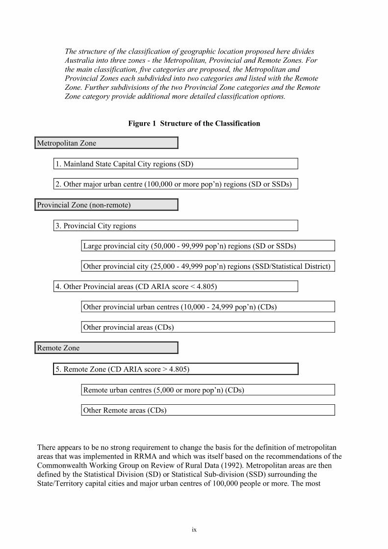
The structure of the classification of geographic location proposed here divides Australia into three zones - the Metropolitan, Provincial and Remote Zones. For the main classification, five categories are proposed, the Metropolitan and Provincial Zones each subdivided into two categories and listed with the Remote Zone. Further subdivisions of the two Provincial Zone categories and the Remote Zone category provide additional more detailed classification options.

Figure 1 Structure of the Classification Metropolitan Zone

1. Mainland State Capital City regions (SD)

2. Other major urban centre (100,000 or more pop’n) regions (SD or SSDs) Provincial Zone (non-remote)

3. Provincial City regions

Large provincial city (50,000 - 99,999 pop’n) regions (SD or SSDs)

Other provincial city (25,000 - 49,999 pop’n) regions (SSD/Statistical District)

4. Other Provincial areas (CD ARIA score < 4.805)

Other provincial urban centres (10,000 - 24,999 pop’n) (CDs)

Other provincial areas (CDs) Remote Zone

5. Remote Zone (CD ARIA score > 4.805)

Remote urban centres (5,000 or more pop’n) (CDs)

Other Remote areas (CDs) There appears to be no strong requirement to change the basis for the definition of metropolitan areas that was implemented in RRMA and which was itself based on the recommendations of the Commonwealth Working Group on Review of Rural Data (1992). Metropolitan areas are then defined by the Statistical Division (SD) or Statistical Sub-division (SSD) surrounding the State/Territory capital cities and major urban centres of 100,000 people or more. The most

x

contentious aspect here relates to the grouping of smaller capital cities such as Darwin and Hobart with the other much larger state capital cities, rather than concerns about degrees of remoteness. This regional approach is extended, based on the criteria applied by the ABS to define Statistical Districts, to include provincial cities of 25,000 or more population. This is similar, though not identical, to the classification of Large Rural Centres in RRMA. Further, students living in and around urban centres of this size are not generally considered to be facing any disadvantage in schooling associated with geographic location, and their identification in a separate category should provide better discrimination of any differences in outcomes of the students from smaller urban centres and rural areas. Beyond those areas in the immediate surrounds of the larger urban centres, ARIA is used, as outlined above, to identify categories of remoteness. The Metropolitan Zone comprising Mainland State Capital City SDs and the Other major urban centre regions accounts for 70 per cent of the national population. Of the remainder, Provincial City regions, defined by ABS Statistical Districts and the Darwin SD and classified as Large provincial city regions if the main centre in the region has a population of 50,000 or more and Other provincial city regions otherwise, currently account for 7.3 per cent of the national population. There are, however, a number of urban centres with a population of 25,000 or more which have not yet been assigned to the Statistical District Structure - in particular, the urban centres of Wagga Wagga, Port Macquarie, Tamworth, Dubbo and Lismore in New South Wales, Warrnambool in Victoria, Hervey Bay in Queensland, and Mandurah, Kalgoorlie/Boulder and Geraldton in Western Australia (Table 5.2). ABS advises that these centres, along with Bunbury in Western Australia (1996 Census urban centre population of 24,945) will be included under the Statistical District Structure of the ASGC in 2001. These centres and their hinterland currently account for a further 2.4 per cent of the national population. The 20.3 per cent of the population living outside the metropolitan and provincial city regions is then classified on the basis of CD-level ARIA scores into the Other Provincial areas category and the Remote Zone, the Remote Zone with ARIA score greater than 4.805 accounting for 3.36 per cent of the national population. 4. Implementation of the classification Individuals living within the metropolitan regions can, in most cases, be identified and assigned to the appropriate geographic location category on the basis of postcode information alone, although some postcodes do cross regional boundaries. More generally, metropolitan and provincial city regions are SD or SSDs comprised of one or more SLAs and, in cases where there is any doubt, the National Localities Index (NLI) can be used to determine the SLA of an address and hence whether it should or should not be included in the urban centre region. Automated matching of addresses to CD is also an option in these predominantly urban areas. There are thus a range of options using address data for assigning students to the metropolitan and provincial city categories of the classification. It could reasonably be expected that geo-coding systems will be developed in the next few years which will allow every address to be linked to its latitude and longitude coordinates and hence to an ARIA score. However, automated matching of rural and remote addresses to Census Collection Districts (CDs) still has some way to go, as demonstrated by the SES Simulation Project where these addresses proved to be significantly more difficult to geo-code. Procedures will then need to

xi

be developed which allow ARIA scores to be assigned to addresses in the rural and remote areas, at least for the immediate future. The geo-coded or CD location of primary schools appears to be known by State/Territory education and non-government school authorities. Should this not be the case, ARIA index scores could be assigned on the basis of the name of the urban centre/locality where the school is located using the approach discussed below. The focus of ARIA on defining remoteness on the basis of the populated localities suggests that it should be possible to assign ARIA scores to addresses on the basis of their locality, avoiding the difficulties associated with geo-coding in rural areas. The ABS National Localities Index (NLI) is intended to include a comprehensive list of locality names in current use, and some 22,000 of these localities have their latitude and longitude coded, although not as part of the NLI system. It should be a relatively simple process to match these localities with their ARIA score. The ABS Geography Section has provided the locality latitude and longitude data to GISCA for this purpose, and senior GISCA staff have undertaken to assign the ARIA scores. Provided that an address includes a Locality Name, State and Postcode, it should then be possible in the great majority of cases to match it to a locality name on the NLI list and assign an ARIA score to it. Since the majority of students will be living in the urban centre or locality where the school is located, they would simply be assigned the ARIA score of their school. Only when students live outside that centre would the school need access to an ARIA coding system to identify the appropriate score, and this access could be provided as an Internet application. The approach is no different in principle from the system that has already been implemented on the DH&AC web site. Nevertheless, the feasibility of this approach needs to be tested, particularly in regard to the coding of rural and remote addresses and the level of “bad” addresses encountered on relevant administrative systems such as school records or in responses to survey questions. Recommendation 9:

The feasibility and cost effectiveness of coding secondary student address data to geographic location codes, and the difference between the geographic distributions of students derived from this approach and the simpler option based on coding the location of their school, should be examined through a pilot study using school and student address data in the non-metropolitan areas of, say, New South Wales, Queensland or Western Australia.

Where outcome measures are based on internal testing procedures, ARIA scores assigned to students by schools will need to be matched to test data used to derive state-wide outcome measures. For measures derived from external surveys such as the LSAY or PISA, a question will need to be included in the questionnaire to allow the ARIA score to be derived. Where data is derived from ABS surveys, the CD location of sample households and thus the CD ARIA score will be known from the sample design.

1

Development of a common definition of, and approach to data collection on, the geographic location of students to be

used for nationally comparable reporting of outcomes of schooling within the context of the “National Goals for

Schooling in the Twenty-First Century”.

1. Introduction 1.1 The Project Brief In view of the need to develop nationally consistent definitions of the equity target groups for nationally comparable reporting of outcomes of schooling within the context of the “National Goals for Schooling in the Twenty-First Century”, the National Education Performance Monitoring Taskforce (NEPMT) commissioned this project to develop a discussion paper that proposes national definitions of geographic location. The project brief specifies that the proposed definitions should take into account the potential need for alternative measurement approaches depending on whether data are to be obtained from administrative sources or other means, and should:

• identify and describe the definitions and sources of data currently used by school systems and authorities, researchers and national and international agencies for reporting outcomes by geographic location;

• examine each of the data sets in terms of its usefulness in describing geographic location for purposes of national reporting;

• assess the strengths and weaknesses of reporting home versus school location of the student;

• assess data for national and international consistency; • propose an appropriate definition or definitions;

• assess the costs and benefits to school systems and school authorities of implementing the proposed definition(s) and standardised data collection and reporting processes.

1.2 Background As evidenced by the National Report on Schooling in Australia for 1996, achieving national agreement on a definition of rural and remote students is not an easy task. Geographically isolated students were a special focus of that report, but “for some years prior to 1996 significant effort had been expended towards achieving a national approach to the classification of geographic location. … However, no conclusive national agreement was reached”. “Further work was undertaken following the (October 1996 TOSS) meeting, aimed at developing a more precise classification of geographic location for use in this report … Although significant progress has been made towards a long-term national approach to the categorisation of geographic location, discussion and evaluation remain incomplete”. The only agreement that could be reached was to report on “those students who attend schools which attract funding under the Commonwealth’s Country Areas Programme (CAP)”, despite the differences in definition between States and Territories (MCEETYA, 1996).

2

In 1993, the Australian Education Council commissioned the Department of Education, Queensland to conduct a research project whose main aim was

“to produce a nationally acceptable and consistently applicable definition of rural versus urban locations for use in association with education statistics, which will also allow analysis at a regional level.”

The project report (Rousseaux, 1993) focused on three main options in its review: first, the geographic classifications devised by the ABS for the Australian Standard Geographic Classification (ASGC); second, the Commonwealth Department of Primary Industries and Energy (DPIE) classification of Statistical Local Areas (SLA) (Arundell, 1991); and third, the Griffith Service Access Frame (GSAF) developed by Dennis Griffith, Department of Education, NT. The main limitation of the DPIE classification was seen as being “that SLAs provide a very coarse, and often inappropriate, unit for the analysis of rural-urban differences.” Thus “the DPIE’s rural zone is comprised of SLAs which contain urban centres of up to 99,999 population” and, for example, “Mount Isa, a municipality comprised of a single SLA of enormous physical dimensions with a population of 23,500 is categorised as a Major Remote Town” and “large, essentially rural local communities, such as Griffith and Singleton Shires, are categorised as Small Rural Towns because the classification of the entire SLA is dependent upon the size of its dominant urban centre.” The GSAF was felt to be “an important breakthrough in the measurement of accessibility to services in the Australian context”, providing “a means of measuring the relative accessibility of places where schools are located, or where students live” and “allows for educational criteria to be built into the calculation”. This latter factor was felt to be a particular advantage over a more general index of remoteness when dealing with issues related to resource allocation and/or targeting locationally disadvantaged students or school communities, and the report recommended that an index such as the GSAF should be used for these purposes. In regard to the definition of rural locations for the purposes of reporting education statistics, the report concluded that “it would be rash to depart in any major way from (ABS) standards and definitions” and recommended “a hierarchy of urban and rural places approach”, but with a modification of the ABS definition of rural to “a population threshold of at least 10,000” in recognition of “the concentration of secondary facilities in towns of this size (1,000 to 9,999) which serve not only the town but also the hinterland populations”. However, this was seen to be only a first step in the process of defining rural schools: “a further step would be to explore the nature of school catchments”: desirably, school level data on the home addresses of the student population could be linked to CDs to generate a rurality index for each school. In addition, the report considered the need for regional comparisons of education statistics at the sub-State level within the context of national reporting and recommended “regions comprised of Statistical Divisions (and Statistical Sub-divisions) as recommended by the Commonwealth Working Group for the Review of Rural Data”. An important aspect of this report is the argument that different approaches to the classification of geographic location are needed for different purposes. For the purpose of resource allocation, the report supported further investigation of the GSAF approach, and throughout 1994-1995, a number of trials were held in Tasmania, Western Australia and Queensland, culminating in a major

3

evaluation conducted by the Department of Education, Queensland for the MCEETYA Taskforce on School Statistics (TOSS) which concluded that (Rousseaux, 1995): 1. The Griffith Service Access Frame (GSAF) provides an objective and practicable method:

(a) for the identification of the client population of the Country Areas General Component (CAGC) of the National Equity Program for Schools (NEPS), and

(b) as a means of allocating funds on the basis of need. 2. The Griffith Service Access Frame (GSAF) provides a more targeted approach to the

allocation of funds under the CAGC (NEPS) than currently exists, and it should be conscientiously considered as an allocative mechanism for national funds.

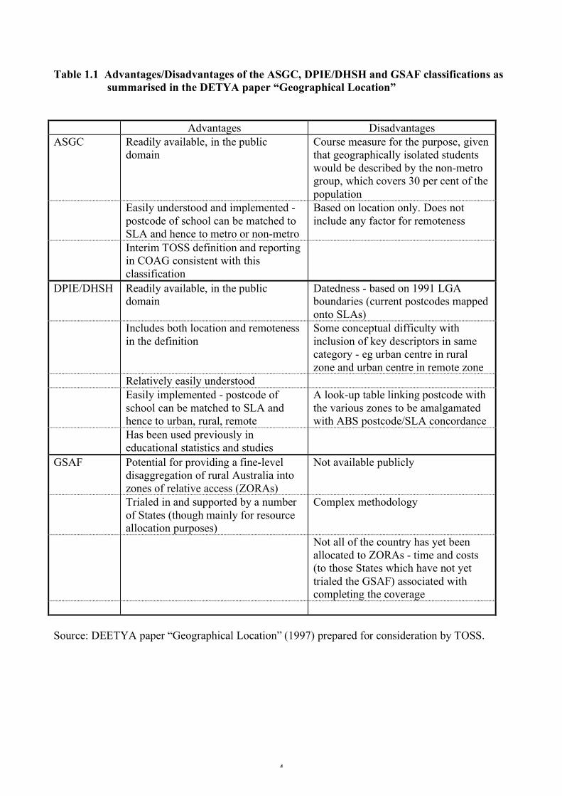
In the meantime, TOSS had agreed at its June 1995 meeting to adopt a metropolitan/non-metropolitan classification as an interim measure to establish consistency in national reporting, the metropolitan areas being defined as major urban centres with a population over 100,000. However, a finer classification of reporting on geographic location was required for use in the 1996 National Report on Schooling in Australia (MCEETYA, 1996) which had a special focus on geographically isolated students and which aimed to provide a basic statistical description of these students by State/Territory, sector and degree of isolation, and compare their participation and outcomes with the rest of the student population. For this purpose, DETYA prepared a paper for consideration by TOSS which again canvassed the same three options as Rousseaux (1993): the ASGC based metropolitan/non-metropolitan classification adopted as an interim measure by TOSS; a new version of the DPIE classification which had been revised and updated in light of 1991 Census data jointly with the Department of Human Services and Health (DHSH) (DPIE/DHSH, 1994); and the GSAF. A summary of the advantages and disadvantages of each of these approaches presented in the DETYA paper is shown in Table 1.1 below. It should be noted however that a key criterion applied in this assessment was that “educational authorities have to be able to define their schools (and maybe students in some cases) as geographically isolated (or other) on the basis of data that is already to hand - in the case of the non-government sector, the only data readily available are the postcode of the school and its SLA”. This essentially excluded the GSAF as an option and, since the ASGC metropolitan/non-metropolitan classification was included in the DPIE/DHSH classification, it was recommended that this latter classification be adopted with geographically isolated students defined as those in the remote zone. TOSS was unable to accept this recommendation however, agreeing instead that for the purposes of the 1996 National Report on Schooling in Australia, the term geographically isolated students should be equated with those students who attended schools which attracted funding under the Country Areas Program (CAP).

4

Table 1.1 Advantages/Disadvantages of the ASGC, DPIE/DHSH and GSAF classifications as summarised in the DETYA paper “Geographical Location”

Advantages Disadvantages ASGC Readily available, in the public

domain Course measure for the purpose, given that geographically isolated students would be described by the non-metro group, which covers 30 per cent of the population

Easily understood and implemented - postcode of school can be matched to SLA and hence to metro or non-metro

Based on location only. Does not include any factor for remoteness

Interim TOSS definition and reporting in COAG consistent with this classification

DPIE/DHSH Readily available, in the public domain

Datedness - based on 1991 LGA boundaries (current postcodes mapped onto SLAs)

Includes both location and remoteness in the definition

Some conceptual difficulty with inclusion of key descriptors in same category - eg urban centre in rural zone and urban centre in remote zone

Relatively easily understood Easily implemented - postcode of

school can be matched to SLA and hence to urban, rural, remote

A look-up table linking postcode with the various zones to be amalgamated with ABS postcode/SLA concordance

Has been used previously in educational statistics and studies

GSAF Potential for providing a fine-level disaggregation of rural Australia into zones of relative access (ZORAs)

Not available publicly

Trialed in and supported by a number of States (though mainly for resource allocation purposes)

Complex methodology

Not all of the country has yet been allocated to ZORAs - time and costs (to those States which have not yet trialed the GSAF) associated with completing the coverage

Source: DEETYA paper “Geographical Location” (1997) prepared for consideration by TOSS.

5

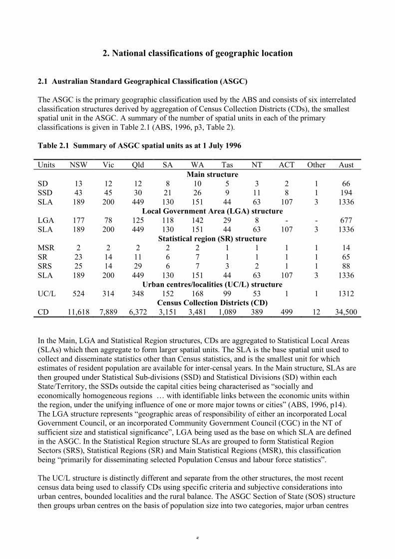
2. National classifications of geographic location 2.1 Australian Standard Geographical Classification (ASGC) The ASGC is the primary geographic classification used by the ABS and consists of six interrelated classification structures derived by aggregation of Census Collection Districts (CDs), the smallest spatial unit in the ASGC. A summary of the number of spatial units in each of the primary classifications is given in Table 2.1 (ABS, 1996, p3, Table 2). Table 2.1 Summary of ASGC spatial units as at 1 July 1996 Units NSW Vic Qld SA WA Tas NT ACT Other Aust Main structure SD 13 12 12 8 10 5 3 2 1 66 SSD 43 45 30 21 26 9 11 8 1 194 SLA 189 200 449 130 151 44 63 107 3 1336 Local Government Area (LGA) structure LGA 177 78 125 118 142 29 8 - - 677 SLA 189 200 449 130 151 44 63 107 3 1336 Statistical region (SR) structure MSR 2 2 2 2 2 1 1 1 1 14 SR 23 14 11 6 7 1 1 1 1 65 SRS 25 14 29 6 7 3 2 1 1 88 SLA 189 200 449 130 151 44 63 107 3 1336 Urban centres/localities (UC/L) structure UC/L 524 314 348 152 168 99 53 1 1 1312 Census Collection Districts (CD) CD 11,618 7,889 6,372 3,151 3,481 1,089 389 499 12 34,500 In the Main, LGA and Statistical Region structures, CDs are aggregated to Statistical Local Areas (SLAs) which then aggregate to form larger spatial units. The SLA is the base spatial unit used to collect and disseminate statistics other than Census statistics, and is the smallest unit for which estimates of resident population are available for inter-censal years. In the Main structure, SLAs are then grouped under Statistical Sub-divisions (SSD) and Statistical Divisions (SD) within each State/Territory, the SSDs outside the capital cities being characterised as “socially and economically homogeneous regions … with identifiable links between the economic units within the region, under the unifying influence of one or more major towns or cities” (ABS, 1996, p14). The LGA structure represents “geographic areas of responsibility of either an incorporated Local Government Council, or an incorporated Community Government Council (CGC) in the NT of sufficient size and statistical significance”, LGA being used as the base on which SLA are defined in the ASGC. In the Statistical Region structure SLAs are grouped to form Statistical Region Sectors (SRS), Statistical Regions (SR) and Main Statistical Regions (MSR), this classification being “primarily for disseminating selected Population Census and labour force statistics”. The UC/L structure is distinctly different and separate from the other structures, the most recent census data being used to classify CDs using specific criteria and subjective considerations into urban centres, bounded localities and the rural balance. The ASGC Section of State (SOS) structure then groups urban centres on the basis of population size into two categories, major urban centres

6

with a population of 100,000 or more, and other urban centres with a population of 1,000 to 99,999. Rural Australia combines bounded localities with a population of 200 to 999 and the rural balance. In addition to the standard ASGC classifications, the ABS defines Census Geographic Areas by allocating CDs uniquely to one spatial unit in a particular classification. In particular, the Postal Area (POA) classification is derived by allocating each CD to the postal area containing the majority of its population, creating a ‘CD derived’ postal area approximating the Australia Post postcode. Post office box codes, postcodes in rural areas which are delivery routes also covered by other postcodes, and some standard postcodes which cannot be allocated a CD are excluded. A Postal Area to SLA concordance file is then created which allows postcode population counts derived from address data to be distributed, proportionately in many cases, to SLA codes and thence groupings of SLAs. The ABS National Localities Index (NLI) provides another means of determining SLA population counts from address data, although in this case by assigning SLA codes on an address by address basis rather than the simpler, and less accurate, postcode to SLA basis. The NLI holds over 31,500 locality records, allowing the great majority of addresses which are in localities wholly within one SLA to be coded directly. The remainder, approximately 5% of the localities, cross SLA boundaries and require the NLI Streets Sub-Index to determine the appropriate SLA for an address. Updated versions of the NLI are released each quarter to reflect new locality and street information. 2.2 DPIE/DHSH Rural, Remote and Metropolitan Areas Classification, 1991 Census Edition The RRMA classification builds on earlier work undertaken by the DPIE (Arundell, 1991) and the (then) Department of Community Services and Health (Millwood, 1989) to define service provision and access in rural and remote areas, and resolved a number of the anomalies that were apparent in those earlier approaches. RRMA assigns SLA in each State/Territory into metropolitan, rural and remote zones, first identifying the metropolitan zone and then subdividing the remaining SLA between rural and remote zones on the basis of an index of remoteness. The metropolitan zone is defined by the capital city SD plus any SSD associated with a major urban centre of 100,000 or more (ie Canberra-Queanbeyan, Geelong, Gold Coast - Tweed Heads, Newcastle, Townsville - Thuringowa and Wollongong). For SLA outside this metropolitan zone, an index of remoteness is calculated based on five components:

1. personal distance, calculated as the square root of the ratio of the area of the SLA to its population;

2. distance from the centroid of the SLA to the centroid of the nearest capital city urban centre; 3. distance from the centroid of the SLA to the centroid of the nearest other metropolitan centre;

4. distance from the centroid of the SLA to the centroid of the nearest urban centre with a population of 25,000 to 99,999;

5. distance from the centroid of the SLA to the centroid of the nearest urban centre with a population of 10,000 to 24,999.

The distribution of each of these components is then standardised around a population weighted mean to a mean of 0 and standard deviation of 1, the five standardised components are weighted (by 0.3, 0.1, 0.15, 0.2 and 0.25 respectively) and added. This combined index is again standardised

7

around a population weighted mean and 10 added to give the index of remoteness with a mean of 10 and standard deviation of 1. Non-metropolitan SLAs with a value greater than 10.5 are then classified as remote. Within the rural zone, SLAs are further classified as large rural centres, small rural centres and other rural areas on the basis of their urban population component. Large rural centres are SLA whose largest population occurs within urban centres of 25,000 or more, while small rural centres are SLA containing urban centres of population between 10,000 and 24,999. Similarly, SLAs in the remote zone are defined as remote centres if they contain urban centres of population of 5,000 or more and other remote areas otherwise. The RRMA classification has achieved widespread use by Commonwealth agencies. For example, the classification has been used by the Commonwealth Grants Commission as one of the factors for assessing socio-demographic composition disabilities, for reporting state data in the 1997 COAG Report on Government Service Provision, for profiling the health of rural Australians in terms of mortality, morbidity and risk factor data in AIHW’s Australia’s Health 1998 and Health in Rural and Remote Australia, as well as for the derivation of Year 12 completion rates by locality in the National Report on Schooling in Australia. Despite this relatively broad acceptance, it appears that the classification will not be updated to take account of 1996 Census data, the Department of Health and Aged Care (DH&AC) having opted instead to develop a new classification (see ARIA below). In a response to the DEETYA paper to TOSS recommending the use of the RRMA classification (DEETYA, 1997), Griffith (1997) criticised the classification on a number of grounds. First, he felt that the metropolitan category “includes cities of very different sizes and very different levels of service provision”. In particular, the inclusion of Darwin and Hobart in the same category as the other State capital cities was considered inappropriate when their population size and level of service provision were significantly below that of the other capital cities. Second, he criticised the general purpose nature of the index of remoteness, arguing that “problems cannot be avoided if one fails to be objective and identify the specific range, type or level of service to be accessed … before it can be determined from what we are remote or access disadvantaged”. Third, the large and varying size of SLAs and hence potential heterogeneity of access within an SLA makes the SLA as the basic unit inappropriate for defining remoteness: “In the very large SLAs great variations may occur in the relative distance individuals need to travel or expend time in order to access services … due to factors such as road conditions, road connectivity or terrain”. Finally, the definition of rural and remote categories on the basis of a boundary which “reflects the common view of the location of ‘rural’ and ‘remote’ areas as determined during the development of the 1986 Millwood Classification” (DPIE/DHSH, 1994) is criticised on the basis that “these boundaries merely reflect population density thresholds previously established and as a result ‘remote’ areas contain very different population centres in relation to population centre size and service access which causes face validity and accuracy problems”. As Rousseaux (1993) also points out, “This is a particularly sensitive issue in the area of resource allocation. Inevitable controversy would arise on the basis of a rural/remote boundary, following as it does boundaries of contiguous SLAs which are selected because they happen to have an index score of 10.5 or more”.

8

2.3 Griffith Service Access Frame (GSAF) The GSAF approach seeks to address these problems by determining relative access scores for schools, where the services to which access is required are specifically defined or determined to be available in specific service centres. It has been used to allocate CAP program funds to schools in the Northern Territory since 1993 and in South Australia since 1997, and has been trialed in a number of other states. The description of the methodology given here is drawn primarily from the report of the Queensland trial instigated by TOSS (Rousseaux, 1995). The model derives an access score for schools based on three factors: the population size of the urban centre or locality containing the school, the distance from the school locality to the most likely accessed service centre, and the economic resources of the school population. In the Queensland trial, and in its application in South Australia, service centres are defined as urban centres with a population of 20,000 or more, on the basis that “there is full provision of education, from pre-school to complete secondary schooling with a diverse range of subject options, and this size approximates the threshold entry point of higher order education services, such as the availability of TAFE”. Service centres should, strictly, be determined as population centres where an appropriate level of the service is available rather than by simply using population size thresholds, although Queensland, Tasmania, South Australia, Northern Territory and Western Australia are reported to have agreed independently that a 20,000 population was the appropriate threshold size for secondary education service provision (Griffith, 1997). On the other hand, Rousseaux (1995) ventured that “lowering the population threshold (from 20,000), to say 10,000, would reconfigure the access “topography” of the State, and indeed could produce results which would be more in keeping with the perceptions of regional people”. The distance component is measured using distances on actual routes and road surfaces, a weight being applied to the distance on unsealed roads. Where students travel some distance to the school, such as in boarding schools, the average distance travelled to school by students is added to the distance from the school location to the service centre. In cases where air/boat was the most reasonable way to travel, the Queensland trial collected air-fare, travel time (including waiting for connections), route and frequency data to derive an equivalent distance measure. Travel costs are then converted to a time equivalent, using the national modal hourly rate and standing and running costs of a vehicle to define the cost of a person’s time, and the time equivalent of travel costs and travel time is converted to an equivalent road distance using the average vehicle speed on sealed roads. The economic resources component is derived using a CD-level student population weighted average of the ABS Index of Economic Resources (IER), requiring the geocoding of student addresses to CDs to identify each school’s catchment area. The inclusion of the economic resources component was felt to “add value to the concept of access” but was also “the most contentious aspect of the model” in the Queensland trial. Those in favour of its inclusion argued that it is important to include a measure of the capacity of the school to access distant services, while those against its inclusion felt that it increased the complexity of the measure and raised uncertainty about what was being identified by the index. However, Rousseaux argues that these two positions reflect different understandings of what is being identified by the GSAF: “The GSAF model measures variability in access, and not geographic isolation per se. … General misunderstanding of the difference between this concept of accessibility and what is commonly described as geographic isolation tends to fuel the debate over the model’s appropriateness” (Rousseaux, 1995).

9

The three components are then combined using weights derived from a principal components analysis of their correlation matrix to give a relative access score for each school, which can be used in a funding allocation formula. The access scores for schools can also be used to produce maps or grouped to identify zones of relative access (ZORA). In the Queensland trial, CDs were given the average access score of the schools attended by students resident in the CD, and six zones comprising groups of CDs were derived using disjoint cluster analysis. The strengths of the GSAF are its specific focus on school locations and the detailed approach taken to identifying factors which increase the cost of access to service centres which are considered to provide an appropriate level of education services. The Queensland trial also indicated, however, that a significant commitment of time and resources was required to implement the model, particularly in gathering accurate road distance and surface data and air/boat travel time/cost data, coding student addresses to identify school catchments by CD, and updating these data to accommodate changes in census boundaries and the reconfiguration of school catchments. Nevertheless, Rousseaux (1995) concluded that, “provided the undertaking is sufficiently resourced”, the GSAF “provides an objective and practicable method” and “a more targeted approach to the allocation of funds under the CAGC (NEPS) than currently exists and should be conscientiously considered as an allocative mechanism for national funds”. Rather than focussing specifically on schools, the GSAF can also be used to identify the relative access to services for CD populations. CD scores are derived using the population size of the urban centre or locality containing the CD, or contained in the CD for smaller rural localities, the distance to the most likely accessed service centre, and the IER score of the CD. The definition of a population threshold or the level of services required, and identification of the service centres, is then the issue. As a means of identifying the most “access disadvantaged” areas, the ability to derive scores for CDs, rather than the larger and more heterogenous SLAs, is a clear advantage of the GSAF over approaches such as RRMA. Whatever its merits, use of the GSAF in deriving a national classification of geographic location for the purposes of national reporting of outcomes is problematic. The inclusion of the economic resources component in the model is contentious, particularly when seeking to identify separately the effects of locational and socioeconomic disadvantage. For national reporting purposes, a general purpose standard classification of remoteness which can be used in a wide range of policy areas and research is preferable to one whose focus is on accessibility to a specific type and level of service. Moreover, it is difficult to adequately assess the GSAF without access to national results showing the accessibility scores derived using this approach for comparison with other approaches such as RRMA and ARIA (see below). Nor has the approach, as yet, been developed to give complete geographic coverage at the national level, an essential requirement in the context of national reporting. 2.4 Accessibility/Remoteness Index of Australia (ARIA) ARIA is the most recent attempt to measure remoteness in Australia and was developed by the National Key Centre for Social Applications of Geographical Information Systems (GISCA) at the University of Adelaide on behalf of the Department of Health and Aged Care (DH&AC) (DH&HC, 1999). It is “designed to be an unambiguously geographical approach to defining remoteness”, excluding socio-economic, urban/rural and population size factors, “as a continuous variable measured in terms of accessibility” to services, “especially those routinely available to people in metropolitan areas”.

10

ARIA measures remoteness in terms of access along the road network from populated localities to four categories of service centres. “If one thinks of ARIA as based on the distances people have to travel to obtain services, then populated localities are where they are coming from, and service centres are where they are going to”. Australian Surveying and Land Information Group (AUSLIG) data were used to calculate actual distance travelled by road (rather than straight line distance) from the point locations of the GPO in 11,340 populated localities to the GPO of the nearest service centre in each category. The 201 service centres are ABS defined urban centres with a population of 5,000 or more at the 1996 Census, grouped into four size categories:

Class A: 250,000 or more

Class B: 48,000 to 249,999 Class C: 18,000 to 47,999

Class D: 5,000 to 17,999 The assumption that the range of services available from an urban centre depends on its size was tested using a database which combined population size with services information obtained from Desk Top Mapping Services Pty Ltd, grouped into 20 categories on the basis of the Australian and New Zealand Standard Industrial Classification (ANZSIC) industry code. Analysis of the relationship between population size and the availability of services was then undertaken, showing a limited association with the availability of many commercial services but quite a strong relationship between population size and the availability of services such as health and education, with distinct clusters of population ranges and natural breaks in the population distribution. These natural breaks were used to define the four size classes above. There are thus four distance measures for each populated locality, each representing the minimum distance to a service centre in a particular category. For populated localities within a service centre, the minimum distance value is zero for the relevant service centre size category. These values are then adjusted by substituting the minimum distance to larger centres for minimum distance to smaller centres when the former is less, assuming that services in a larger, nearer service centre are accessed in preference to those in a more distant, smaller centre. In Tasmania, there are no Class A service centres, and these distance values are assigned by adding a factor of 500 km to the Class B distances, calculated either to Hobart or Launceston as appropriate. For other islands, a graduated weight is- applied to the distance from island localities to the nearest point on the mainland, from which road distances to nearest service centres was calculated as usual. On the assumption that “the additional cost (financial, time or other) of travelling from an island to the mainland would initially be high and then taper off as distance travelled increased”, a weight of 10 is applied to distances below 10 km, 5 for distances of 10-20 km, 3 for 20-50 km, and 2 for distances greater than 50 km. To combine the four distance measures into a single accessibility/remoteness index for each populated locality, each distance measure is standardised to a value ranging from 0 to 3, and the four values are summed, giving a continuous variable with values between 0 and 12 as the measure of remoteness. The standardised values in each class are calculated as the ratio of the distance to the mean distance, with ratios greater than 3 reduced to the threshold ratio of 3 to remove the effects of extreme values from the index (eg the overwhelming effects of the distance from parts of the Northern Territory to Adelaide, the nearest Class A centre).

11

Having thus defined the ARIA index values for the populated localities, values for other parts of Australia, the rural balance in the ABS Section of State classification, were interpolated onto a 1 km regular grid using the index values of the six nearest localities. ARIA index values have then been derived for each CD, SLA and Postal Area (POA), calculated as the simple arithmetic mean of the values for all grid cells that are wholly or predominantly within the larger unit. In addition, a remoteness classification containing five categories has been devised, based on natural breaks in the data, balance across categories, and broad compatibility with the remote zone of the RRMA. The five categories are defined as:

• Highly accessible (ARIA score 0 - 1.84) - relatively unrestricted accessibility to a wide range of goods and services and opportunities for social interaction.

• Accessible (ARIA score 1.84 - 3.51) - some restrictions to accessibility of some goods, services and opportunities for social interaction.

• Moderately accessible (ARIA score 3.51 - 5.80) - significantly restricted accessibility of goods, services and opportunities for social interaction.

• Remote (ARIA score 5.80 - 9.08) - significantly restricted accessibility of goods, services and opportunities for social interaction.

• Very remote (ARIA score 9.08 - 12) - locationally disadvantaged - very little accessibility of goods, services and opportunities for social interaction.

The DH&AC is proposing ARIA for adoption as a national standard for the definition of remoteness and the ABS is examining ARIA in some depth with a view to incorporating its concept of remoteness in the ASGC for the 2001 edition. An ABS position paper setting out their proposal for public comment is expected to be published in September 2000. In the interim, ARIA values for populated localities, SLA and Postal Areas can be down-loaded from the Department’s web-site and CD values can be obtained on request. It is envisaged that ARIA will be fully updated, with revision of the service centre lists to take account of population growth and re-calculation of averages following each census, although it seems likely that this will depend on the position adopted by the ABS and the assessments made of the index by other agencies and researchers.

12

3. Rural/remote areas in government programs 3.1 State/Territory Departments of Education 3.1.1 New South Wales The definitions of rurality and isolation tend to be arbitrary and developed for a particular reporting or administrative purpose. For example, in reporting the school census, 40 school districts are categorised into Sydney Metropolitan, Other Metropolitan and Rural, but many rural districts contain large towns and this classification is not generally used for reporting student outcomes by location. School districts are also used in reporting the Basic Skills Test results. The most common classification for reporting on rurality is schools in the CAP, although this does not cover all rural or isolated schools. Data on school location is held by school district, LGA, SLA and postcode, but student address information is held at the school level only and is not normally linked to student participation or outcomes data. Prior to 1999, CAP schools were limited to four nominated CAP regions and were either: • in a town of less than 3,000 persons and more than 100 km from a centre of 10,000 persons; or

• in a town of less than 4,000 persons and more than 150 km from a centre of 10,000 persons; although some discretion was given to include schools which failed to meet these criteria but which were considered to be sufficiently isolated to warrant inclusion. However, schools which met these town size and distance criteria but were not in CAP regions were excluded. With the revised population data available from the 1996 Census, and the elimination of the regional structure, application of these town size and distance criteria resulted in significant changes to the list of CAP schools which was expected to produce considerable opposition from the schools and communities involved. For example, a number of schools around Parkes would be excluded due to its increase in population from below to above 10,000 persons, while others would be excluded by increases in town size to more than 4,000 persons or by an increase in the distance criterion associated with a growth in town population from below to above 3,000 persons. These changes resulting in schools which fall just outside the model criteria raise issues of equity and the artificiality of the model boundaries. An alternative model has been developed which aims to address these deficiencies. The new model uses cluster analysis to group 714 communities located outside of Sydney, Newcastle and Wollongong on the basis of three factors:

1. distance to the nearest urban centre of 10,000 persons or more; 2. community size, measured by the total enrolment of students in Kindergarten to Year 6 classes in

all schools in the community, excluding students in special classes; and 3. school density, calculated as a weighted average of the distances to the nearest, second nearest

and third nearest government school with primary enrolments and the nearest government high school.

Communities were then allocated to 20 clusters, of which 9 clusters were chosen for inclusion in the CAP on the basis the general similarity with the previous CAP schools, the greater distances from centres of 10,000 persons or more, school density measures which reflected greater degrees of isolation from other schools, and the inclusion of the smallest communities, with populations

13

generally less than 4,000 persons. The model produces a list of schools which are clearly discrete from other schools, the schools not included in the 9 clusters eligible for CAP funding failing to meet the criteria for inclusion by a substantial margin. Source: Phil Daniels, NSW DET and Graeme Smith, Manager, NSW Country Areas Program. 3.1.2 Victoria Schools in Victoria are defined to be: metropolitan located within the Melbourne Statistical Division;

provincial located in a non-metropolitan urban centre with a population of more than 20,000 persons (that is, in Geelong, Ballarat, Bendigo, Shepparton-Mooroopna, Warrnambool, Albury-Wodonga, Mildura and Traralgon); and

rural otherwise. Geo-coded locations of government schools are held centrally, but student address information is held by individual schools only. A CASES program developed by the Department and distributed to all government schools is used for standard reporting purposes. To be eligible for Country Areas Program (CAP) funding, rural government schools must be located: • more than 150 km from Melbourne and • more than 25 km from the nearest provincial centre and • in a community with a population of less than 5,000 persons.

CAP grants are calculated on a base allocation and separate per student formulae for primary and secondary enrolments multiplied by an isolation factor based on the distance from Melbourne. Per student funding is provided for up to the first 300 primary students and up to the first 500 secondary students. These criteria and allocation formulae were implemented in 1997. The Catholic Education Commission of Victoria uses the same criteria as the Department. The Association of Independent Schools of Victoria uses the criteria implemented by the Department before 1997, allocating CAP funds to schools in centres with a population of less than 5,000 persons which are more than 100 km from Melbourne or more than 25km from the nearest provincial centre. All government rural primary schools with enrolments up to 200 students and secondary colleges with enrolments up to 500 students receive additional funding under the Rurality and Isolated component of the School Global Budget. A location index is calculated for each school based on the sum of three distance factors: • distance from Melbourne; • distance from the nearest provincial centre; and • distance from the nearest primary or secondary college, as appropriate, above the rural school

size adjustment factor threshold. Location Index Funding is then allocated as a base allocation plus the location index score multiplied by student enrolment and the maximum per student rate. Source: Education Victoria, Guide to the 2000 School Global Budget, November 1999.

14

3.1.3 Queensland For the purpose of annual reporting, schools are classified as either urban or rural, urban schools being those located in the Brisbane Statistical Division (SD) or in urban centres with a population of 10,000 or more persons. Smaller urban centres are included in the rural category. The option of classifying all schools in the Brisbane SD as urban is preferred so as to include schools located in large rural CDs on the rural-urban fringe which service nearby urban populations, although a small number of schools which are arguably rural in character are then included in the urban category. School locations have been geo-coded and matched to CD codes. Funding under the Priority Country Areas Program (PCAP) is distributed to schools which are located more than 75 km from the nearest urban centre of 10,000 or more persons and within one of the four PCAP areas. The Northern, North-West, Central and South-West PCAP areas are groupings of SLAs which have changed little since they were defined in 1979, despite various reviews. They exclude the more settled coastal SLAs around Cairns, Townsville and Mackay and those in south-east Queensland generally to the east of the 150th meridian (and, with a few exceptions, correspond with the metropolitan and large and small rural centre SLA categories of the DPIE/DHSH classification). Within one PCAP area, the Griffith Service Access Frame (GSAF) is used to determine funding allocations to schools. Catholic and Independent schools CAP funds are included in PCAP and distributed using the same criteria as for government schools. Source: Kathleen Rousseaux, Queensland Department of Education and Judy Ewings, PCAP Queensland 3.1.4 South Australia Following a period of review and consultation, the Griffith Service Access Frame (GSAF) was introduced in 1998 to declare and fund government CAP schools in South Australia. The GSAF replaced a prior system based on a number of discrete criteria, including distance from population centres of 10,000. As a result of introducing the GSAF, the number of declared departmental schools increased from 99 to 177. GSAF scores were first calculated in 1997 for all schools more than 75 km from an urban centre of 20,000 or more persons (namely Adelaide, Whyalla or Mount Gambier), with the exception of schools in Murray Bridge and Port Augusta, which are more than 75 km but well within an hour of their respective 20,000 centres of Adelaide and Whyalla, and updated in 1998 to take account of 1996 census information. Student address information was obtained from all schools, allowing the DETE Information Management Unit to map all school student populations to CDs and to calculate GSAF scores for school communities rather than country towns. However, for general reporting of school outcomes, schools are classified as either metropolitan (within the Adelaide SD) or other. At the end of 1998, with the establishment of the new Country Directorate, 1999 CAP grants to schools were frozen at 1998 levels until all resourcing issues for country schools had been investigated. The Country Call consultations identified the need to aggregate the various forms of funding which address rurality issues (including CAP) to facilitate improved outcomes for students in remote locations, and a new Rural Index has been developed for the Partnerships 21 scheme being introduced in the year 2000. Government schools which do not opt into this scheme will continue to receive CAP funding at the previous GSAF level.

15

The basic criteria for eligibility for Partnerships 21 funding is that the school is located more than 80 km from Adelaide, increasing the number of government schools defined as country to 250. 40% of the total funding is used to provide a base allocation to all country schools, irrespective of size or location, and a further 4% is allocated on a per capita basis. The majority of the remaining funding (51%) addresses distance disadvantage, being allocated on the basis that all country schools make two trips per year to Adelaide and 10 trips per year to their nearest service centre and receive an amount per km for travel, with supplementary funding for nights away, accommodation and bus hire. The 19 service centres have been determined on the basis of “custom and practice” rather than a strict population size criterion, although urban centres with a population of 3,000 or more outside an 80 km radius of Adelaide are generally included, along with Strathalbyn (2,962), Clare (2,815), Barmera (1,837) and Waikerie (1,798). Subsidy funding for non-government schools in country areas is based on an historical Locality Dispersion Index developed many years ago by the (then) State Supply Department and covers schools located more than 50 km from the Adelaide GPO. Source: John Liddle, Equity Standards, DETE and Judy Day, Operations (Country) DETE and Neil Wadrop, Advisory Committee for Non-Government Schools. 3.1.5 Western Australia The Education Department of WA has no universal definition of remote, the only geographic location classification used for reporting of participation or performance data being metropolitan schools versus country/rural schools, where metropolitan is defined as the Perth SD, and country is the rest of the state. Students' home locations are not recorded or used centrally. The Department uses two distance-related indexes for allocating funds - one for the school grant, and one for the Country Areas program. The School Grant distance-cost index is 1 for metropolitan schools, 1.5 for outer metropolitan schools, and ranges up to around 60 for the most remote school. This index is negotiated and is based on costs. The Country Areas program (PCAP in WA) index is based mostly on distances, PCAP points being allocated to schools on the basis of the following six factors. In each case, a formula is given but the range for each is limited to a maximum value of 10. The points from each factor are summed to give the school's PCAP points, the most remote schools having a PCAP score approaching 60, with the cut-off for funding being around 13 points. The six factors are defined as:

1. (Distance from a population centre of 10,000 minus 150) divided by 25 2. (Distance from a population centre of 5,000 minus 150) divided by 25

3. (Distance from a District Education Office minus 50) divided by 35 4. (Distance from Perth minus 150) divided by 135

5. (Distance from the nearest school minus 5) divided by 9.5 6. (400 minus the number of students) divided by 40 Source: John Harris, Strategic Initiatives, Policy and Planning, Education Department of WA.

16

3.1.6 Tasmania The geographical location and characteristics of each government school are measured in three ‘Rurality Indices’:

• Distance Index – the distance by road in km from the nearest major urban centre. • Size of Centre – an index scale from 0 to 6 of the size of the community that the school

supports. 0 urban centres, population > 10,000 1 urban centres, population 5,000 – 10,000 2 urban centres, population 2,500 – 5,000 3 urban centres, population 2,000 – 2,500 4 urban centres, population 1000 – 2,000 5 Bounded locally, population 500 – 1,000 6 Bounded locally, population 200 – 500 and rural.

• Isolation Index – an index to deal with schools which are not only distant from major centres but which are also not on major trunk routes or are on islands. 7 Special areas (as designated by Department, now only 1 school) 8 Zone B Taxation areas 9 Islands

The development of the Department’s Rurality Indices has been part of a general resourcing approach which requires that factors of disadvantage are taken into account when the available resources are distributed to schools. The three indices are supplemented by others which take account of socio-economic status and the physical condition of the facilities at individual schools. Within the mechanisms which distribute general funding for management at a school level and quota teaching staff, the indices are used to supplement the allocations of those schools with higher indices. Participation in the Country Areas Program is determined on the basis of a school’s Distance Index. To be eligible a school must have a Distance Index of at least 74. It should be noted that the Department intends to undertake a thorough review of resource allocation mechanisms during the 2000 school year and there is every likelihood that changes may arise in relation to the treatment of factors such as geographical location. Student home address is notionally recorded in respect of every student of every government school within the agency’s student administrations system, SACS. The reality of student address recording includes the following considerations:

• SACS is not fully operational in all schools, but full operation is approaching; • the concept of ‘student home address’ can be interpreted differently in some school

situations. Confusion arises, for example, in circumstances where the home address and the student’s term address differ, where students have more than one home through family separation etc and where students are actually homeless. The Department is currently developing some data standards for application in schools and it is hoped that a far higher degree of uniformity will be achieved in coming years.

Geographic bases used for reporting use ABS classifications, primarily Hobart SD/Other, to report state statistics to Commonwealth agencies such as DETYA and the Productivity Commission, the Statistical District structure to report statistics according to local expectations of urban/rural, where urban is a combination of Hobart SD, Launceston SSD and Burnie-Devonport SSD, and the categories of the Size of Centre Index.

17

Source: Nick May, Manager (Resource Planning Services), Department of Education, Tasmania 3.1.7 Northern Territory Country areas consist of the whole Territory except for areas within a 75 km radius of Darwin and Alice Springs, the two urban centres with a population of 20,000 persons or more. Schools within the country areas are allocated CAP funding using the GSAF methodology. Student home addresses have been geo-coded to CDs to allow appropriate GSAF scores to be calculated for each school. Performance information is reported in aggregate form using school location only. The most commonly used categories used for Departmental publications are urban/non-urban, where urban refers to schools in the Darwin City, Palmerston- East Arm and Darwin Rural Areas SSDs, and the SLAs based on the population centres of Jabiru, Nhulunbuy, Alice Springs, Tennant Creek and Katherine. Source: John Yick, Manager, Statistics, NT Department of Education 3.2 Some Commonwealth programs 3.2.1 Income Tax Zones The Taxation Office has, since 1945, allowed a Zone Rebate for people living or staying in certain remote areas of Australia. The remote areas are in two zones, Zone A and Zone B, with ordinary areas and special areas within each zone. The special areas are defined as particularly isolated, on the basis that they are located more than 250 km by the shortest practicable surface route from the nearest population centre of 2,500 or more people. Thus special areas are particularly isolated, with the ordinary areas of Zone A more remote than the ordinary areas of Zone B. Zone A includes all areas north of the 26th parallel (the SA/NT border) and west of the 141st meridian (the longitude of the SA/NSW-Vic border), and northern Queensland “from the south eastern boundary of the Shire of Boulia then generally north-easterly by … (various shire boundaries to) … the boundary dividing the Shires of Douglas and Cook to the eastern coastline” between Cairns and Cooktown. Zone B includes areas south of Zone A and north of a line starting on the Queensland coast “at the north-eastern corner of the Shire of Broadsound” south of Mackay, going generally west for about 400 km then generally south down the spine of the Great Dividing Range to the NSW border and then east to the Barwon River. Across NSW, the line is “generally south-westerly”, from the Barwon River on the northern border through Collarenebri and Cobar to the NSW/SA border south west of Menindee. It then goes west across SA, turns north-west around Peterborough to the Finders Ranges, south-west and then north-east about 100 km inland from the coast to Murat Bay on the southern coastline. In WA, the south-western area is excluded, roughly on a north-westerly line from Ravensthorpe in the south to Geraldton on the west coast, and in Tasmania, the area adjoining the west coast and south-west corner of the state are included. While clearly a subjective and relatively crude measure of remoteness, comparison of these zones with the much more rigorously defined ARIA contours shows some interesting similarities. In particular, the combined special areas of Zone A and Zone B are remarkably similar to the Very Remote/inaccessible category, reflecting ARIA scores of 10 or more. Similarly, the ordinary areas of both zones in general reflect ARIA scores in the range 6 to 10, matching closely the Remote ARIA category, with ARIA values increasing steadily across the Taxation Offices 250 km zones

18

around towns such as Mount Isa, Alice Springs, Kalgoorlie, Newman and Darwin. Apart from suggesting that the distinction in tax rebates between the two zones should perhaps be re-examined in the light of ARIA data, these similarities provide a crude validation that there is a general correspondence between ARIA values and one longstanding perception of remoteness. This definition of remote areas is also the basis for the Remote Area Allowance (RAA) under the Social Security Act, the allowance being paid to people living in Zone A ordinary and special areas and special areas of Zone B. 3.2.2 DETYA Programs The Country Areas component of the Special Learning Needs Program, or Country Areas Program (CAP), provides funding to the States and the Northern Territory to support activities which “improve the educational opportunities, participation, learning outcomes and personal development of rural and geographically isolated primary and secondary school students in both government and non-government schools”. The formula used to determine the distribution of funds between states is based on student enrolments in rural and isolated schools, where rurality is defined in terms of the population size of a settlement and isolation is defined in terms of distance from a town of at least 10,000 population. The ‘rural’ population is identified with urban centres of below 10,000 population and rural localities and other rural areas as defined by the ABS Section of State classification, and categorised into three population size ranges: 5,000 - 9,999; 1,000 - 4,999; and rural localities and other rural. Isolation is similarly grouped into three categories on the basis of distance from a town of at least 10,000 population: less than 100 km; 100 - 150 km; and more than 150 km. Both rurality and isolation categories are then weighted 0, 1 and 2 respectively as rurality and isolation increase, and the average weight applied to enrolments in the combined rurality-isolation category (Grewal et al, 1996). The most disadvantaged category, weighted 2 on both criteria and thus overall, is then associated with students in rural localities and other rural CD more than 150 km from the nearest town (of 10,000 or more). The next most disadvantaged, with an average weight of 1.5, are either in rural centres of 1,000 - 4,999 and more than 150 km from the nearest town or in rural CDs 100 - 150 km from a town. Three groups receive a disadvantage weight of 1: rural centres of 5,000 - 9,999 more than 150 km from a town; rural centres of 1,000 - 4,999 and 100 - 150 km from a town; and rural CDs within 100 km of a town. Rural centres of 5,000 - 9,999 and 100 - 150 km from a town or of 1,000 - 4,999 and less than 100 km from a town receive a weight of 0.5. The main criticisms of this approach relate to the apparent arbitrariness of the size and distance categories and the relative weights applied (Rousseaux, 1995). The urban centre population size threshold of 10,000 for rural disadvantage appears to be widely accepted, but greater emphasis is given by the states to distance variations than is applied in the CAP formula. The review of the CAP funding formula (Grewal et al, 1996) did a limited examination of the effects of varying distance bands, although this involved a narrowing of the bands only and resulted in a redistribution of the allocation in favour of New South Wales, Victoria and Tasmania. However, the main critics of the formula, and the practice of most states, appear to favour a widening of the distance bands to increase the weight associated with the most isolated students, an approach which appears likely to redistribute the current allocation in favour of the other states and the Northern Territory.

19

The Indigenous Education Strategic Initiatives Programme (IESIP) uses a number of criteria to define a remote institution, including being on an island or in an Indigenous community. The population size - distance criterion used in other cases again uses a threshold of 300 km, requiring the institution to be more than 300 km by road from an urban centre of 50,000 or more. The Aboriginal Student Support and Parental Awareness (ASSPA) Scheme also defines remote students using the IESIP criteria. The Assistance for Isolated Children (AIC) scheme requires one of three guidelines to be met:

1. The distance from home to the nearest appropriate government school is at least 56 km via the shortest practicable route; or

2. The distance from home to the nearest appropriate government school is at least 16 km via the shortest practicable route AND the nearest available transport service to that school is at least 4.5 km distance from home; or

3. The student does not have reasonable access to an appropriate government school for at least 20 days of the school year because of adverse travel conditions or other circumstances beyond the family’s control.

For Equity and General Performance Indicators in Higher Education, the identification of rural and isolated students has, since 1991, been based on the linkage of the postcode of student’s permanent home address with the DPIE/DHSH RRMA classification, the metropolitan, rural and remote zones being equated with urban, rural and isolated students respectively. Caveats on this approach are that, while simple and practical, it is considered unreliable for targeted equity initiatives in many cases given the diversity to be found within postcode areas, and that it still relies on the classification of postcodes derived from the 1991 Census (DETYA, 1999a). That said, it is argued that “the data provide a good indicator of the performance of these groups at the aggregate level”. Nevertheless, a recent review (Western et al, 1998) has recommended that two new measures be used, one to classify students for monitoring purposes and one to identify and target disadvantaged students. For monitoring purposes, students’ access to their nearest university campus is defined on the basis of the distance between the postcode of their permanent home address and the postcode of the nearest university campus. This measure is categorised as high access if the distance is less than 150 km, medium access for distances from 150 to 300 km, and low access for distances over 300 km. For targeting purposes, student self-reports of the distance from their permanent home to the university campus at which they enrol is proposed, using distance bands of less than 100 km, 100-150 km, 151-300 km, 301-400 km, 401-500 km, and more than 500 km. 3.2.3 DH&AC Rural Retention Program Assistance under the Rural Retention Program is provided to GPs practising in locations identified as being in relatively high need of retention support based on general physical remoteness and access to services, opportunities for social interaction and availability of peer support. These areas were formerly identified on the basis of the RRMA classification but the criteria have recently been revised to reflect the development of ARIA, although not being based simply on ARIA scores. Five variable are used to generate a total score ranging from 0-12 as follows:

1. Road distance to the nearest capital city or centres of 100,000 people or a capital city, whichever is the lesser (worth 3 out of 12);

2. Road distance to the nearest centre with more than 18,000 people (worth 2 out of 12);

20

3. Road distance to the nearest centre with more than 5,000 people (worth 1 out of 12); 4. Average road distance to the nearest 10 towns (worth 3 out of 12); and

5. Average road distance to the nearest 5 doctors with Medicare schedule fee income of more than $50,000 in 1998 (worth 3 out of 12).

Towns are placed into categories on the basis of their score, an ineligible category (scores 0 - 1.59) and 5 eligible categories (A - E). Population size adjustments to these categories are then made on the basis of the expected level of services associated with towns of a particular size, where:

• Towns of 20,000 or more drop two categories if East of the Great Divide and drop one category otherwise; and

• Towns of 10,000 or more cannot be in a higher category than Category C. Other adjustments are made on the basis of the size of the Indigenous population and the likelihood that GPs will be on call at the local hospital.

21

4. Rural/remote disadvantage in education 4.1 Reasons for rural/remote disadvantage Lower participation rates for rural students in post-compulsory schooling resulting in lower Year 12 completion rates and under-representation in higher education have long been recognised as reasons for concern that rural students are disadvantaged. For example, analyses of data from the Australian Youth Survey (AYS) comparing the proportions of school leavers who left before completing Year 12 from 1987 to 1994 found that there was roughly a 10 percentage point gap between urban and rural students - in 1994, 29% of male urban school leavers had not completed Year 12 compared with 39% of their rural counterparts, the proportions for female school leavers being 19% and 26% respectively (Lamb, 1996). The Year 12 completion rates derived by DETYA from data provided by State/Territory Boards of Studies similarly exhibit “a clear general trend for urban students over the period 1991-1996 to have higher Year 12 completion rates than the other two (rural/remote) groups and for rural students to have a higher completion rate than remote students” (MCEETYA, 1996). Further, analyses of the Youth in Transition surveys show “young people from rural areas have lower rates of school completion than young people from urban areas … are also less likely than other students to make the transition from Year 12 to higher education … (and thus) rural youth will have substantially lower levels of participation in higher education than young people from urban areas” (Long, Carpenter and Hayden, 1999). Various reasons have been suggested as explanations of why rural students are educationally disadvantaged. First, there are the difficulties of providing the full range and quality of education in small, isolated communities which are considered to be associated with “shortcomings in teacher preparation for teaching in rural and isolated areas, lack of support services, high staff turnover rates, restricted and/or inappropriate curricula and teaching strategies, and a paucity of social and cultural facilities in the local community” (NBEET, 1990). These are concerns which the additional funding provided through CAP, EISIP and State/Territory programs targeting rural and remote schools seek to overcome. Second, there are the difficulties and costs for students and their families associated with distance and travel to education institutions, more particularly in the post-compulsory years and for participants in higher education. In higher education in particular, there is clear evidence that the access of people from rural backgrounds is low, and for people from isolated backgrounds is very low, relative to their population share. In addition, rural students and, more particularly, isolated students are more likely to study externally and have low retention rates (DETYA, 1999b, p78). An interview based study of rural participation in post-secondary education found that “major barriers are attitudes (higher education is not linked to success in rural occupations), isolation (distance to education centres), and lack of information about the availability of places” (Clarke, 1987, cited in Ainley and McKenzie, 1991). Third, there are differences in the background characteristics of rural and urban students which explain, in part, the differences in participation and outcomes. For example, in higher education “there is an overlap between status in the indigenous equity group and the isolated group, and also a strong correlation between isolation and low socio-economic status, which is not so evident for rural students” (Higher Education Council, 1996). Analyses which seek to adjust for these differences “show fairly consistently that where rural-urban differences do exist, some of the difference can be attributed to differences in other background characteristics”. Nevertheless, “rural secondary students have a lower chance of completing Year 12 because of their rural location

22

(rather than an artefact of other factors associated with rurality)” and “even after taking into account this very broad array of characteristics, there is still a five percentage point difference in entry rates (to higher education from Year 12) that can be attributed to attending a rural school” (Long et al, 1999). Fourth, the interests, perceptions and expectations of rural and remote students and their families are suggested as explanations of their lower rates of participation. Thus, factors which influence rural students to leave school early may include “social or cultural norms regarding early school leaving, pessimism about their ability to remain in school, a lack of encouragement to do so, or a feeling that remaining at school would not ‘pay off’ either in terms of further education or better jobs” (Marks and Fleming, 1999). For those continuing schooling in Years 11 and 12, there is a tendency away from enrolments in mathematics, physical sciences and languages and towards “subject areas with a more practical orientation (technical studies, agriculture, and home economics)” (Ainley et all, 1990), a pattern reflected in higher education where the courses of study taken indicate “a particular applied orientation in student’s choices and a preference for vocational areas which are directly relevant to the rural environment” (Martin, 1994). In view of this practical orientation, it is perhaps not surprising that “rural youth were marginally more likely to participate in TAFE than were urban youth” and that “there was little sign of rural youth being disadvantaged in terms of access to apprenticeships” (Long et al, 1999; also Lamb, Long and Malley, 1998). 4.2 Identifying rural/remote disadvantage Given the range and variety of individual, family, school and local factors associated with educational disadvantage, it should be expected that there will be considerable variation in measures of educational outcomes across rural/remote areas. An analysis of Year 12 completion rates found that this was indeed the case, identifying “marked variations between non-metropolitan regions … even where those regions have basic social and economic conditions in common” and concluded that “Generalisations about participation in post-compulsory education in country areas, it is clear, can no longer be regarded as adequate. What is required now is more precise knowledge of patterns of educational participation in specific localities” (DEET, 1987). However, it is as true now as it was then that “most of the research has concentrated on differences in education participation between urban and rural regions, or even more simply, metropolitan (capital cities) and extra-metropolitan (the remainder) regions” (DEET, 1987) For example, ACER researchers using data from the Youth in Transition (YIT) surveys derive urban-rural categories on the basis of the population density of the LGA in which the school was located when the cohorts were originally sampled, when students were in their late primary or early secondary schooling (Williams et al, 1993; Long et al, 1999). The quartile with the lowest population density is defined as rural, and the quartile with the highest population density as urban, although comparative rates are derived for all four quartiles. As the authors recognise, this measure is “less than perfect … combines the truly remote or isolated with others who are perhaps not quite as geographically disadvantaged” (Long et al, 1999). Other approaches to defining geographic location used in ACER research have relied on student’s own responses to survey questions about where they are/were living. Respondents in the Youth in Transition surveys and the Studies of Subject Choice (Ainley et al, 1990; Ainley et al, 1994) were asked to describe the location where they lived from four categories: “Capital city; Country/ provincial city (more than 25, 000); Country town (1,000 - 25,000); or Other country area”; the last two categories being used to define the rural population. A similar, though different classification is

23

derived in the Australian Youth Survey (AYS), where respondents were asked to indicate “where you mostly lived before you were 14” from the categories “Capital city; Some other city; Country town or village; and Rural area or farm”, the last two categories being used to define rural respondents. More recently, in the Longitudinal Surveys of Australian Youth (LSAY) sample of students in Year 9 in 1995, geographic location was defined by school location in the categories “metropolitan (centres with population over 100,000): regional (centres with population between 10,000 and 100,000); and rural” (Marks and Fleming, 1999). The OECD Program on International Student Achievement (PISA) proposes yet another classification based on the size of the community in which their school is located: “a village, hamlet or rural area (fewer than 3,000 people); a small town (3,000 to about 15,000); a town (15,000 to about 100,000); and a city (100,000 or more)”. The criteria used by DETYA and the states to determine resource allocations, primarily based on distance from larger towns and community size, do provide a more refined classification of rural and remote populations. If these criteria correlate well with the factors most strongly associated with educational disadvantage, a measure of geographic location which takes account of these same criteria appears desirable. Such a classification should not only identify more homogeneous subgroups of the “rural” population but should also be more closely aligned with the areas considered by the states as most disadvantaged and thus provide a basis for assessment of the effectiveness of their resource allocation. The desire for a more focussed classification of geographic location which reflects the criteria used for resource allocation also appears to have been the major barrier to achieving national agreement through TOSS (see Section 1.2). However, as was noted by the review of the CAP funding arrangements (Grewel et al, 1996), there is “no uniformity among the States”, “the size thresholds for defining rurality are clearly different across the States” and “there is also no consistency in the distance thresholds used by the States for defining isolation”. While some changes have been made to the approaches used by the States since then, the “variety of approaches for defining rurality and remoteness” reflecting “the specific needs and perspectives of the individual States” remains. These variations between states, and the changes made within states over time, make it impossible to define national comparable student populations and report national comparable outcomes on the basis of schools receiving CAP funding. In the context of sample surveys in particular, one factor that imposes limitations on a more refined classification of rural and remote areas is the concentration of the Australian population in metropolitan centres. For example, using the DPIE/DHSH metropolitan, rural and remote zones, 72 per cent of the 15-19 year old population in 1996 lived in metropolitan areas, 25 per cent in rural areas and less than 3 per cent (2.7%) in remote areas. Similarly, the number of students (FTE) enrolled in secondary schools eligible for CAP funding in 1996 was just 3.7 per cent of all secondary school students (MCEETYA, 1996). The relatively small number of students in the most disadvantaged areas then results in samples which are too small to give reliable population estimates. While it would be possible to overcome this limitation by over-sampling in these areas, there may be significant additional costs associated with it, particularly when surveys require personal or household interviewing, such as those conducted under the ABS Household Survey Program. Another issue is whether it is appropriate to use a single approach to the classification of geographic location for all national reporting purposes. As noted by Long et al (1999), “Indeed, it could be argued that what is required is a separate measure of rurality and isolation for each form of educational participation”. In considering measures of locational disadvantage in higher education, for example, Western et al (1998) comment that the choice “is dependent on the type of locational

24

disadvantage under consideration. … For example, in the case of postgraduate students, the postcode measure related to main campuses is the most appropriate measure, as satellite campuses in regional areas offer fewer courses and subjects at postgraduate level”. Students living in urban centres of 10,000 population or more might then not be considered as disadvantaged in schooling, but be defined as disadvantaged in their access to higher education if their town is some distance from a main or satellite campus. On the other hand, it does not seem appropriate to apply a measure of locational disadvantage in higher education which does not take account of the effects of disadvantage in schooling, including lower levels of retention and lower Year 12 completion rates. Since disadvantage in the compulsory years of schooling has clear flow-on effects to the non-compulsory years, definitions of geographic location which reflect that disadvantage should also be applied to the later years, perhaps supplemented by measures appropriate to particular purposes. 4.3 School location versus home location Whatever classification of geographic location is used, it is clearly far simpler to allocate schools to the appropriate categories of the classification than it is to allocate individual students. In 1998 for example, there were some 3.2 million full-time students in Australia, attending some 9,600 schools (ABS, 1998). Schools can be readily assigned to location categories, for the most part on a permanent basis, the reporting of school-level data by geographic location then simply requiring aggregation of information from schools in each category. Indeed, as noted in the previous section, most of the research that has been undertaken to identify the relative disadvantage experienced by rural students is derived on the basis of school location rather than on the home location of students. Given its simplicity and the potential problems of classifying home location, it is clearly important to consider what problems, if any, are posed by defining students’ geographic location on the basis of their school location. One clear problem with this approach is the difference found between the distribution of primary school students and secondary school students by geographic location. For example, Rousseaux (1993) used data compiled by the Commonwealth Grants Commission to compare the distribution of primary and secondary schools and students by settlement type. These figures show that, in 1991, the proportions of all primary school students attending school in rural localities and other rural areas were 6.5% and 12.0% respectively, while the corresponding proportions of students attending secondary schools were 3.0% and 5.7% respectively. A similar pattern is evident in comparing primary and secondary enrolments in schools eligible for CAP funding in 1996 - 6.2% of all primary students are in such schools compared with 3.7% of secondary students (MCEETYA, 1996). These patterns reflect the availability of primary schools in small communities in rural and remote areas, but the relative lack of secondary schools in these areas which requires students to either travel, board or relocate to secondary schools in urban centres. Rousseaux (1993) provided further confirmation of this transfer from rural to urban schools by examining the locations of schools attended by isolated students aged 15 years and over, identified as those in receipt of assistance under the AIC scheme or through AUSTUDY or ABSTUDY provisions under the same criteria. Some 6,500 school students nationally were identified as isolated students using these criteria and Rousseaux found that, for those in Queensland, “Apart from the expected substantial numbers who attend Brisbane institutions … centres throughout the entire urban hierarchy are represented.

25

Centres well known for their ‘education’ function stand out, for example, Toowoomba, Cairns, Rockhampton, Charters Towers and Warwick”. This issue was also raised in discussion of the equity indicators for higher education, where rural and isolated students are identified on the basis of their home address. It was argued that “some students may have home addresses at which they seldom reside. Sometimes these students board at schools, often from the start of secondary school, at some of the nation’s most prestigious schools and as a result have spent a total of only several months at ‘home’ in ‘isolation’ over the preceding decade.” Responding to this argument, the project team felt that “this does not mean that such students or their families have not suffered disadvantage through remote home location. It means simply that the students’ families have had the resources and commitment to overcome the access difficulties of isolation.” (Martin, 1994). Beyond primary school, significant differences would be expected between a definition based on home location and one based on secondary school location, the latter giving a more urbanised distribution of students than the former. This alone could be considered a sufficient argument for using home location. Using secondary school location, a substantial proportion of the secondary students from rural primary schools are grouped with students from a more urban background, making invalid any direct comparison of the primary and secondary school outcomes for either group. If the results of achievement testing in primary and secondary school during the compulsory years of schooling are to be compared by geographic location category at the national and State/Territory level, it is clearly desirable that, as far as is practically possible, primary and secondary students from the same areas are included in the same location category. There are of course families who move their home location between location categories as their children progress through the education system, primarily from rural to urban areas, and there are, as noted above, students from rural and isolated areas who spend most of their time away from home during their secondary years at boarding school. Ideally perhaps, primary school location, home location during secondary schooling and location of secondary schooling should all be taken into account in assessments of the effects of rural/remote location on outcomes, at least in the context of research studies on outcomes after compulsory schooling. However, for the purposes of national reporting, a definition of geographic location must be simple enough to be implemented in a variety of settings and be able to be applied to administrative data and to sample survey data in a consistent and comparable manner over time. The available data, while limited, clearly indicates that using the location of the secondary school attended during the compulsory years of schooling would undoubtedly understate the numbers of students from homes in rural and remote areas. Further, counts of students derived using home location are more comparable with the ABS estimated resident population counts and thus provide a basis for the assessment of participation, whereas a greater degree of approximation would be involved using school location. On that basis, a definition based on a single characteristic is preferred and home location appeals as a more appropriate basis than secondary school location for determining geographic location during the compulsory years of schooling. On the other hand, the wider geographic distribution of primary schools and their smaller catchment areas makes use of the primary school location rather than home location less problematic. It is considered that there would be very few cases where the definition of geographic location of primary school students on the basis of their home address or their primary school location would make any difference to their classification. Further, net of any other characteristics of the school community, any advantage or disadvantage associated with geographic location at this level of

26

schooling is more likely to be a reflection of the isolation of the settlement and quality of education provided by the school than the variations of home location within school catchment areas. Considerations of simplicity and practicality then suggest that, for reporting of achievement in the Year 3 and Year 5 literacy and numeracy testing by geographic location, the location of the primary school would be an acceptable surrogate for identifying the home location of primary school children. There are however two caveats on defining geographic location on the basis of home address. First, it may be neither feasible nor cost effective to implement, relative to the somewhat less satisfactory but clearly simpler alternative of assigning secondary students to location categories on the basis of the location of their school. Second, dependent on the measure of geographical location used and the level of aggregation required for the purposes of national reporting, the difference between the two approaches may be less significant than it appears. A pilot study could be undertaken to investigate both of these concerns. 4.4 Beyond compulsory schooling In this case in particular, the purpose of the outcomes reporting process, the outcome measures used and the data sources from which they are derived need to be carefully considered in determining how a classification of geographic location is to be defined. There are a variety of outcomes to be considered and a variety of pathways that might be taken to achieve those outcomes, and there may be a number of location changes, both temporary and permanent, associated with the transition from being a student living at home to an independent adult. For students who remain in school beyond the compulsory years, the definition of geographic location on the basis of home location, as used for the compulsory years of schooling, should be maintained. Participation and outcome measures will presumably be derived primarily from administrative collections, such as the Schools’ Census and Boards of Studies databases, or from longitudinal survey collections, such as LSAY. Beyond schooling, a question is whether outcomes should be monitored on the basis of geographic “background” or current home location. Consider, for example, outcomes derived from a longitudinal survey such as the LSAY with initial samples selected from secondary schools during the compulsory years of schooling. Should the geographic location of students and/or their school, derived from the initial sample, be retained throughout analyses of future waves of the survey, or should changes be made to reflect the movements of respondents over the years? The advantages of the first approach are clearly evident: geographic location, like other background characteristics such as gender, SES, ethnicity, indigenous status etc, remains a fixed characteristic of the respondents, so that estimates of population outcomes by geographic location derived at each year of age follow the progress of the same respondents over time, without any of the confounding effects that may result from population shifts between categories. In administrative collections such as the Higher Education Statistics Collection (HESC), participation in higher education is reported on the basis of “permanent” home location, although the identification of the “permanent” home address can be problematic. Nevertheless, this address will be, at least for most students entering directly from school or soon after, the same as their home address when in secondary school.

27

On the other hand, in the context of identifying participation, transition, retention and attainment in the workforce and in post-compulsory education and training (Smart, Burke and McKenzie, 1999), greater reliance will be placed on ABS household survey data and reporting on the basis of current address is then more relevant to policy priorities as well as being consistent with past and current practices. There is then a concern regarding age cohort comparisons of outcomes from schooling and the later years. To the extent that the more successful students at school are more likely to move away from home and into urban areas, the apparent attainment in post-compulsory education and employment of those with a rural/remote background may be underestimated. Whether this is or is not the case and any effect that it might have on such comparisons should perhaps be examined using the longitudinal survey data collected in the AYS and the current LSAY. 4.5 Summary of bases for the definition of geographic location 1. For reporting on participation and achievement in primary schools, considerations of simplicity

and practicality suggest that the location of the primary school be used as the surrogate for the home location of students. It is considered that there would be very few cases where the definition of geographic location on the basis of home address or primary school location would make any difference to their classification.

2. For reporting on participation and achievement in the compulsory years of secondary schooling

and for students who remain at school beyond the compulsory years, home location appeals as a more appropriate basis than secondary school location. Significant differences would be expected between a definition of the rural/remote population based on home location and one based on school location, and it is desirable that, as far as is practically possible, primary and secondary students from the same areas are included in the same location category.

3. Beyond schooling, the use of “permanent” home address in higher education statistics is

consistent with the use of home location for school students. However, for measures of participation and achievement in training and employment, greater reliance will be placed on ABS household surveys with geographic location defined using current address. There is then a concern that the apparent attainment in post-compulsory education and employment of those with a rural/remote background may be underestimated.

There are then three concerns that could be investigated using available administrative and longitudinal survey data:

1. the feasibility and cost effectiveness of coding secondary student address data to geographic location codes;

2. the difference between the geographic distributions of students derived from this approach and the simpler option based on coding the location of their school; and

3. the extent to which students from rural and remote areas relocate to more urban areas after completing their schooling and the effect that this has on the comparability over time of the characteristics and outcomes of those with a rural/remote background.

The first two concerns should be examined through a pilot study using school and student address data in the non-metropolitan areas of, say, New South Wales, Queensland or Western Australia. Investigation of the third issue requires longitudinal survey data on school and post-school outcomes for young adults, their current location, and their home location during secondary schooling. These data have been collected in the Australian Youth Survey (AYS) and the current

28

Longitudinal Survey of Australian Youth (LSAY), although address details may not have been coded and access to original questionnaires may then be required. Should the post-school outcomes of young adults currently living in regional and remote areas differ significantly from those who lived there while attending school, a question to identify young adults’ home location during secondary schooling should be included in relevant ABS surveys to allow key performance measures to be reported by geographic “background”.

29

5. Defining geographic location 5.1 The ARIA approach In the context of determining a long-term national approach to the definition and classification of geographic location, serious consideration must be given to the ARIA approach. ARIA is tailored specifically to measuring access to services in non-metropolitan areas and aims to be comprehensive, sufficiently detailed, as simple as possible, transparent and defensible, intuitively plausible, and stable over time (DH&AC, 1999). It was intended from the outset that ARIA would fill the need for a formal national standard for defining remoteness, with representatives of the main Commonwealth Departments using geographical classifications as well as the ABS on the project steering committee, and the ABS is committed to incorporating its concept of remoteness into the next edition of the ASGC in 2001. ARIA is seen as having a number of advantages over previous approaches, but also some disadvantages. The main advantages are considered to be: • it is “designed to be an unambiguously geographic approach”; • an ARIA score can be assigned to any point in Australia, allowing variations in accessibility

within larger geographic units such as non-metropolitan SLAs and postcodes to be identified; • it is not affected by administrative boundary changes, particularly revisions to LGA, SLA and/or

postcode boundary changes; • it is a continuous measure which allows flexibility in the definition of categories used for

different purposes; • it is readily available, via the internet, for down-loading and use with no restrictions; and

• there appears to be strong support from Commonwealth agencies, including the ABS, to implementing ARIA in national data collection and reporting processes and to maintaining and supporting its future development and updating requirements.

The main disadvantages relate to the recency of its development and thus: • the ABS, in particular, is still investigating and still has considerable work to do on how it will

incorporate the concepts into the ASGC structure; • there are some anomalies in the ARIA data resulting from differences between the AUSLIG list

of populated centres and the ABS defined urban centres and localities which need to be addressed;

• there is, as yet, no accepted definition of appropriate categories of remoteness scores for the purposes of national reporting;

• the decision to ignore State/Territory borders in determining accessibility to services may be contentious; and

• products may need to be developed which allow ARIA scores to be assigned accurately to geo-coded locations or to localities not currently included in the ARIA list of populated centres.

In regard to the calculation of ARIA scores (see Section 2.4), the ABS is currently working with GISCA to remove any identified anomalies and is also examining the standardisation of the distance to service centre measures and the effect of introducing a fifth class of service centres comprising

30

urban centres of 1000 - 4,999 population. While these investigations may result in some changes being made to the ARIA scores as currently defined, the main principles involved in their definition are not expected to be affected. More generally, the ABS is considering whether ARIA scores should be kept as a separate classification or used in conjunction with a revised Section of State classification to define a hierarchy of areas from metropolitan through to remote in a manner similar to RRMA. Further, the choice between CD and SLA scores as the base unit for defining and reporting on remote populations is being considered, the advantage of the SLA base being the availability of estimated resident population data by age and sex for weighting sample survey estimates and comparability with other data at LGA and more aggregated SSD and SD levels. The revised population size classes for urban centres which the ABS proposes to implement from the 2001 Census are the following:

1,000,000 or more population (Sydney, Melbourne, Brisbane and Perth) 250,000 to 999,999 (Adelaide, Canberra-Queanbeyan, Gold Coast-Tweed Heads and

Newcastle) 100,000 to 249,999 (Central Coast, Wollongong, Hobart, Geelong and Townsville-

Thuringowa) 50,000 to 99,999 population 20,000 to 49,999 population 10,000 to 19,999 population 5,000 to 9,999 population 1,000 to 4,999 population

The top two classes correspond to the Class A service centres in ARIA; the next two, with the addition of Rockingham (WA) whose 1996 population was 49,917, to the Class B service centres; the fifth class, excluding Rockingham and with the addition of Traralgon (Vic) and Burnie-Somerset (Tas) with 1996 populations of 18,993 and 19,134 respectively, to the Class C centres; and the seventh and eighth classes, with these two exclusions, to the Class D centres. By the time of the 2001 Census, the population growth of these three centres should take them into the next ABS population size class and, thus, the ARIA service centre classes would coincide with groupings of the proposed ABS classes. It appears that GISCA, the developers of ARIA, clearly intended for it to be used as a separate classification, focussing on measuring access to services in non-metropolitan areas of Australia: “the distinction between urban and rural, and the population size dimension, have been left to the ABS section of state classification” (DH&AC, 1999). Rousseaux (1993) similarly argues that “Remoteness exists on another dimension, intersecting with the rural-urban continuum of locations”. On this view, ARIA scores or categories should be considered as an addition to the range of geographical classifications that might be used, separate from the urban-rural classes provided by Section of State or the regional classes of the ASGC Main Structure. There is not, as yet, a standard procedure for assigning ARIA scores to individual addresses, although it could reasonably be expected that geo-coding systems will be developed in the next few years which will allow every address to be linked to its latitude and longitude coordinates and hence to an ARIA score. A system with these capabilities, called Address Point, is already available in the UK. This would also allow addresses to be automatically matched to their CD and hence to the Section of State (SOS) classes, making the reporting of aggregated data by SOS and remoteness, either separately or in a hierarchical classification, a relatively simple process from any collection.

31

Where data for national reporting is derived from ABS surveys, this is already the case, the CD location of sample households and thus the CD ARIA score being known from the sample design. An issue then is whether data from other administrative and survey collections can similarly be assigned to SOS and remoteness categories. In summary, ARIA is viewed as being an important new development in the context of geographical classification in Australia which, with further development to overcome teething problems and the expected development of geo-coding systems over the next few years, should become a recognised national standard. For the immediate future, however, consideration needs to be given to how ARIA scores should be assigned and the geographical categories that should be derived. 5.2 Assigning ARIA scores to addresses ARIA scores can be assigned to school locations that have been geo-coded or have been assigned to a CD. For non-government schools, location by CD should have been identified under the new funding arrangements, and the geo-coded or CD location of government schools appears to be known by State/Territory education departments. Should this not be the case, scores could be assigned on the basis of the name of the urban centre/locality where the school is located using the approach discussed below. Automated matching of addresses to CDs still has some way to go, as demonstrated by the SES Simulation Project (DETYA, 1998). In that project, exact matches were obtained on 64% of addresses, although a further 18% were matched to adjoining CDs. Manual matching by school bodies or individual schools using an Internet application then raised the number of successful matches to 90% overall. While the extent to which this approach was successful in matching rural and remote addresses is not reported, the report states that “In the case of rural properties, the name of the road on which the property is located, or the nearest road, facilitates geocoding. Some addresses simply do not exist in a format to facilitate automatic geocoding”. It would then be expected that the geo-coding of rural and remote addresses to CDs might be somewhat less successful than the average rate. The focus of ARIA on defining remoteness on the basis of the accessibility of populated localities suggests however that it should be possible to assign ARIA scores to addresses on the basis of their locality. As has been noted previously (Section 2.1), the ABS has developed a National Localities Index (NLI) which allows users to assign an address to its SLA. The key search items in this system are the locality name and the postcode, the latter to differentiate between localities with the same name in different parts of Australia. In addition, some 22,000 of the 31,500 localities recorded in the NLI have their latitude and longitude coded, although not as part of the NLI system. While the NLI and its associated geo-coded data are seen as the basis for assigning ARIA scores to addresses, the NLI itself does not provide this option and a new system would need to be developed. The general approach proposed is no different in principle from the system that has already been implemented on the DH&AC web site for determining ARIA scores for populated localities, SLAs or Postal Areas. The main limitation of the current system is that it is not comprehensive, being restricted to the localities identified in the AUSLIG database which, for example, do not include all of the urban centres and localities defined by the ABS. It should however be a relatively easy process to extend the coverage to the 22,000 geocoded localities identified in the NLI and to match these localities with their ARIA score. The ABS Geography Section has indicated its willingness to

32

provide the locality latitude and longitude data for this purpose, and senior GISCA staff have indicated their willingness to match and assign the ARIA scores. The NLI is being continuously updated as it is applied in various projects and new locality names are identified in addresses. It includes a number of names which are no longer or rarely used, and suburb names within urban centres may also be included. The geocoding of locality names involved the matching of names to the gazetted localities listings in NSW and Victoria and to other gazetteers and maps and thus excludes any duplication of locality names. Given that there are only 1,660 urban centres and rural localities nationally, the 22,000 geocoded localities are considered a reasonably comprehensive basis from which to determine ARIA values. Provided that an address includes a Locality Name, State and Postcode, it should then be possible in the great majority of cases to match it to a locality name on the NLI list and assign an ARIA score to it. Nevertheless, the feasibility of this approach needs to be tested, particularly in regard to the coding of rural and remote addresses and the level of “bad” addresses encountered on relevant administrative systems such as school records or in responses to survey questions. Of particular concern is the need for a location address rather than a PO Box number, and RMB addresses may be problematic if a locality name is not included in the address. The matching of addresses to urban centres and localities suggested above to define an ARIA score does not imply that a particular address is in fact located within any defined boundary for that urban centre or locality, although this will apply in the majority of cases. People in rural areas surrounding an urban centre may still use the name of that centre in their address and be assigned its ARIA score. This would not then be the exact ARIA score that would be obtained if the location of their address was known at the 1 km-grid-square level. However, it seems reasonable to assume that the distance between their address and the geo-coded location of the locality used in their mailing address will not be far, and the ARIA score assigned to the locality will then differ little from that of their address location. For secondary school students, there is in general no central access to students’ home address data. Since the majority of students will be living in the urban centre or locality where the school is located, they would simply be assigned the ARIA score of their school. Only when students live outside that centre would the school need access to an ARIA coding system to identify the appropriate score, and this access could be provided as an Internet application. Even for centralised administrative systems such as the HESC and Boards of Studies data, coding requirements would not be large, since people who live within the Class A service centres could be identified relatively simply on the basis of the suburb or postcode of their address and assigned a zero ARIA score directly. Address information held on survey respondents would similarly allow them to be assigned an ARIA score.

33

5.3 Categories of geographic location While it seems highly likely that the approach outlined above can be used to assign an ARIA score to an address in most cases, this does not provide a complete solution to the problem of defining geographic location. The question remains as to whether ARIA is considered a sufficient basis for the definition of geographic location for national reporting purposes, or whether other criteria such as Section of State or Capital city (however defined) need to be taken into account, either as separate additional classifications or in some combination with ARIA scores. These are of course just the issues that the ABS is currently considering. In addition, the importance of being able to link outcomes data with the ABS estimated resident population data derived at SLA level also needs to be considered. The view taken here is that ARIA scores alone are not a sufficient basis for determining the classification of geographic location for national reporting purposes but they do provide a better and more precise basis for defining the remote population than has been possible with previous classifications. While a means of identifying remote populations has long been required, there are other aspects of previous geographic classifications which do not conflict with that need and have achieved general acceptance. The aim then should be to retain those aspects of previous classifications and incorporate the ARIA concept of remoteness in with them. First, there appears to be no strong requirement to change the basis for the definition of metropolitan areas that was implemented in RRMA and which was itself based on the recommendations of the Commonwealth Working Group on Review of Rural Data (1992). In particular, metropolitan areas are then defined by the Statistical Division (SD) or Statistical Sub-division (SSD) surrounding the State/Territory capital cities and major urban centres of 100,000 people or more. The most contentious aspect here perhaps relates to the grouping of smaller capital cities such as Darwin and Hobart at the national level with the other much larger state capital cities, rather than concerns about degrees of remoteness. In light of the proposed revision to the ABS SOS classification and the definitions of Class A and B service centres in ARIA, it may be appropriate to extend this approach to include urban centres of 50,000 or more, or even those of 25,000 or more based on the criteria applied by the ABS to define Statistical Districts. Again, this would be similar, though not identical, to the RRMA approach, where SLAs containing urban centres of 25,000 or more were identified in the Large Rural Centres category. Further, students living in and around urban centres of this size are not generally considered as facing any disadvantage in schooling associated with geographic location, and their identification in a separate category should provide better discrimination of any differences in outcomes of the students from smaller urban centres and rural areas. Beyond those areas in the immediate surrounds of the larger urban centres, ARIA is viewed as a useful replacement for the previous Index of Remoteness used in RRMA, with the clear advantage that it is defined more precisely than at the SLA level and removes the somewhat contentious measure of personal distance. The second issue then is what categories of “remoteness” should be used for this population. It should perhaps be noted that the use of the term “rural” in RRMA to describe areas which included some relatively large urban centres was felt to “present a semantic conundrum” and it was suggested that “perhaps it is better to dispense with the term ‘rural’, and to refer instead to ‘less remote’ and ‘more remote’ zones” (Rousseaux, 1993). While the use of SLAs as the basis for the classification of remoteness in RRMA was criticised as being “a very coarse, and often inappropriate, unit for the analysis of rural urban differences”

34

(Rousseaux, 1993), it should be recognised that it did provide better discrimination than the metropolitan-other comparisons that had been, and still are, used. Moreover, it made possible the link to population estimates and other data published on aggregations of SLAs, and allowed statistics derived from postcode data to be transferred, by concordance, to the SLA groupings. A classification based on SLAs should not then be dismissed lightly. To limit the definition of remoteness in this way however would negate many of the advantages of ARIA and give rise to criticisms similar to those made against RRMA (see Section 2.2). Moreover, the ABS Demography Section can provide estimated resident population data for parts of SLAs defined by groups of CDs, although not as accurately as at the SLA level. On balance, a definition of remoteness based on CD-level ARIA scores with some subsequent loss of accuracy in the estimated resident population data appears preferable to a definition based on entire SLAs. The structure of the classification of geographic location proposed here is outlined in Figure 1. The classification divides Australia into three zones - the Metropolitan, Provincial and Remote Zones. For the main classification, five categories are proposed, the Metropolitan and Provincial Zones each subdivided into two categories and listed with the Remote Zone. Further subdivisions of the two Provincial Zone categories and the Remote Zone category provide additional more detailed classification options. The structure is similar to that of the DPIE/DHSH Rural, Remote and Metropolitan Areas Classification, 1991 Census Edition (RRMA), but uses different criteria to define the categories. The Provincial Zone replaces the RRMA Rural Zone. Provincial City Regions defined by the ASGC Statistical District structure replace the RRMA Large Rural Centres category. Other Provincial Areas and the Remote Zone are defined on the basis of CD level ARIA scores rather than using the SLA-level Index of Remoteness of RRMA. The definition of the Metropolitan Zone follows that adopted by Commonwealth agencies (DPIE, 1992) and incorporated in RRMA, except that Darwin SD is excluded. Despite its population being less than 100,000, Darwin SD was included in this category under RRMA on the basis of being a capital city. Here, metropolitan areas are limited to those SD or SSD defined around urban centres with a population greater than 100,000. Two metropolitan categories are defined, the first combining the five mainland state capital city SDs which each have a population of over 1,000,000 persons. Their populations are much larger than those of other major urban centre regions in Australia. The second category includes the regions surrounding other major urban centres of 100,000 persons or more. The Provincial Zone (non-remote) comprises Provincial City regions and Other Provincial areas defined as non-remote by their ARIA score. Provincial City regions are predominantly urban regions defined in the ASGC by the Statistical District structure, delimited for “one or more urban centres (outside Capital City SDs) in close proximity with a population of 25,000 or more”, with boundaries “defined to contain the anticipated urban spread of the area for at least 20 years” (ASGC, 1996). Darwin is included here on the basis of the similarity between its population size and that of urban centres such as Toowoomba, Launceston and Albury-Wodonga. It should be noted that a remote Provincial City (determined by its ARIA score) would be included in the Remote Zone. However, none of the urban centres with 25,000 of more population currently meet this criterion for remoteness. (Mt Isa and Alice Springs, for example, are remote urban centres whose population may grow to warrant Statistical District status in the future).

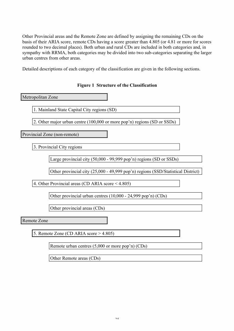
35

Other Provincial areas and the Remote Zone are defined by assigning the remaining CDs on the basis of their ARIA score, remote CDs having a score greater than 4.805 (or 4.81 or more for scores rounded to two decimal places). Both urban and rural CDs are included in both categories and, in sympathy with RRMA, both categories may be divided into two sub-categories separating the larger urban centres from other areas. Detailed descriptions of each category of the classification are given in the following sections.

Figure 1 Structure of the Classification Metropolitan Zone

1. Mainland State Capital City regions (SD)

2. Other major urban centre (100,000 or more pop’n) regions (SD or SSDs) Provincial Zone (non-remote)

3. Provincial City regions

Large provincial city (50,000 - 99,999 pop’n) regions (SD or SSDs)

Other provincial city (25,000 - 49,999 pop’n) regions (SSD/Statistical District)

4. Other Provincial areas (CD ARIA score < 4.805)

Other provincial urban centres (10,000 - 24,999 pop’n) (CDs)

Other provincial areas (CDs) Remote Zone

5. Remote Zone (CD ARIA score > 4.805)

Remote urban centres (5,000 or more pop’n) (CDs)

Other Remote areas (CDs)

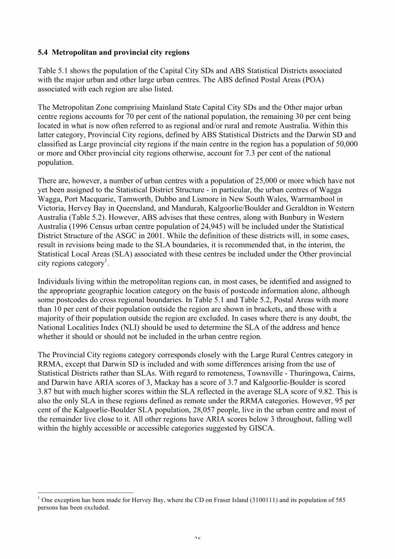
36

5.4 Metropolitan and provincial city regions Table 5.1 shows the population of the Capital City SDs and ABS Statistical Districts associated with the major urban and other large urban centres. The ABS defined Postal Areas (POA) associated with each region are also listed. The Metropolitan Zone comprising Mainland State Capital City SDs and the Other major urban centre regions accounts for 70 per cent of the national population, the remaining 30 per cent being located in what is now often referred to as regional and/or rural and remote Australia. Within this latter category, Provincial City regions, defined by ABS Statistical Districts and the Darwin SD and classified as Large provincial city regions if the main centre in the region has a population of 50,000 or more and Other provincial city regions otherwise, account for 7.3 per cent of the national population. There are, however, a number of urban centres with a population of 25,000 or more which have not yet been assigned to the Statistical District Structure - in particular, the urban centres of Wagga Wagga, Port Macquarie, Tamworth, Dubbo and Lismore in New South Wales, Warrnambool in Victoria, Hervey Bay in Queensland, and Mandurah, Kalgoorlie/Boulder and Geraldton in Western Australia (Table 5.2). However, ABS advises that these centres, along with Bunbury in Western Australia (1996 Census urban centre population of 24,945) will be included under the Statistical District Structure of the ASGC in 2001. While the definition of these districts will, in some cases, result in revisions being made to the SLA boundaries, it is recommended that, in the interim, the Statistical Local Areas (SLA) associated with these centres be included under the Other provincial city regions category1. Individuals living within the metropolitan regions can, in most cases, be identified and assigned to the appropriate geographic location category on the basis of postcode information alone, although some postcodes do cross regional boundaries. In Table 5.1 and Table 5.2, Postal Areas with more than 10 per cent of their population outside the region are shown in brackets, and those with a majority of their population outside the region are excluded. In cases where there is any doubt, the National Localities Index (NLI) should be used to determine the SLA of the address and hence whether it should or should not be included in the urban centre region. The Provincial City regions category corresponds closely with the Large Rural Centres category in RRMA, except that Darwin SD is included and with some differences arising from the use of Statistical Districts rather than SLAs. With regard to remoteness, Townsville - Thuringowa, Cairns, and Darwin have ARIA scores of 3, Mackay has a score of 3.7 and Kalgoorlie-Boulder is scored 3.87 but with much higher scores within the SLA reflected in the average SLA score of 9.82. This is also the only SLA in these regions defined as remote under the RRMA categories. However, 95 per cent of the Kalgoorlie-Boulder SLA population, 28,057 people, live in the urban centre and most of the remainder live close to it. All other regions have ARIA scores below 3 throughout, falling well within the highly accessible or accessible categories suggested by GISCA.

1 One exception has been made for Hervey Bay, where the CD on Fraser Island (3100111) and its population of 585 persons has been excluded.

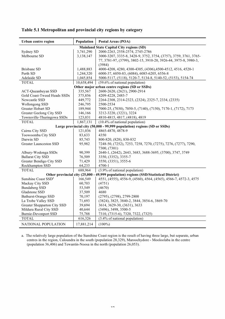
37

Table 5.1 Metropolitan and provincial city regions by category Urban centre region Population Postal Areas (POA)

Mainland State Capital City regions (SD) Sydney SD 3,741,290 2000-2263, 2558-2574, 2745-2786 Melbourne SD 3,138,147

3000-3207, 3335-8, 3428-9, 3752, 3754, (3757), 3759, 3761, 3765-77, 3781-97, (3799), 3802-15, 3910-20, 3926-44, 3975-8, 3980-3, (3984)

Brisbane SD 1,488,883 4000-4208, 4280, 4300-4305, (4306),4500-4512, 4516, 4520-1 Perth SD 1,244,320 6000-37, 6050-83, (6084), 6085-6205, 6556-8 Adelaide SD 1,045,854 5000-5117, (5118), 5120-7, 5134-8, 5140-52, (5153), 5154-74 TOTAL 10,658,494 (59.6% of national population)

Other major urban centre regions (SD or SSDs) ACT-Queanbeyan SSD 335,567 2600-2620, (2621), 2900-2914 Gold Coast-Tweed Heads SSDs 375,856 4209-4228, 2485-7 Newcastle SSD 449,772 2264-2308, 2314-2323, (2324), 2325-7, 2334, (2335) Wollongong SSD 246,795 2500-2534 Greater Hobart SD 189,944 7000-25, (7030), 7050-5, (7140), (7150), 7170-1, (7172), 7173 Greater Geelong City SSD 146,166 3212-3220, (3221), 3224 Townsville-Thuringowa SSDs 123,031 4810-4815, 4817, (4818), 4819 TOTAL 1,867,131 (10.4% of national population)

Large provincial city (50,000 - 99,999 population) regions (SD or SSDs) Cairns City SSD 121,036 4865-4870, 4878-9 Toowoomba City SSD 83,633 4350 Darwin SD 85,743 800-820, (828), 830-832 Greater Launceston SSD 95,982

7248-50, (7252), 7253, 7258, 7270, (7275), 7276, (7277), 7290, 7300, (7301)

Albury-Wodonga SSDs 90,399 2640-1, (2642), 2643, 3683, 3688-3695, (3700), 3747, 3749 Ballarat City SSD 76,509 3350, (3352), 3355-7 Greater Bendigo City SSD 71,429 3550, (3351), 3555-6 Rockhampton SSD 64,233 4700-1 TOTAL 688,964 (3.9% of national population)

Other provincial city (25,000 - 49,999 population) regions (SSD/Statistical District) Sunshine Coast SSDa 166,549 4551, (4555), 4556-9, (4560), 4564, (4565), 4566-7, 4572-3, 4575 Mackay City SSD 60,703 (4751) Bundaberg SSD 53,549 (4670) Gladstone SSD 37,509 4680 Bathurst-Orange SSD 70,197 (2795), (2798), 2799-2800 La Trobe Valley SSD 71,693 (3824), 3825, 3840-2, 3844, 3854-6, 3869-70 Greater Shepparton City SSD 39,694 3614, 3629-30, (3631), 3633 Mildura Rural City SSD 40,644 (3496), 3498, 3500-5 Burnie-Devonport SSD 75,788 7310, (7315-6), 7320, 7322, (7325) TOTAL 616,326 (3.4% of national population) NATIONAL POPULATION 17,881,214 (100%)

a. The relatively large population of the Sunshine Coast region is the result of having three large, but separate, urban

centres in the region, Caloundra in the south (population 28,329), Maroochydore - Mooloolaba in the centre (population 36,406) and Tewantin-Noosa in the north (population 26,053).

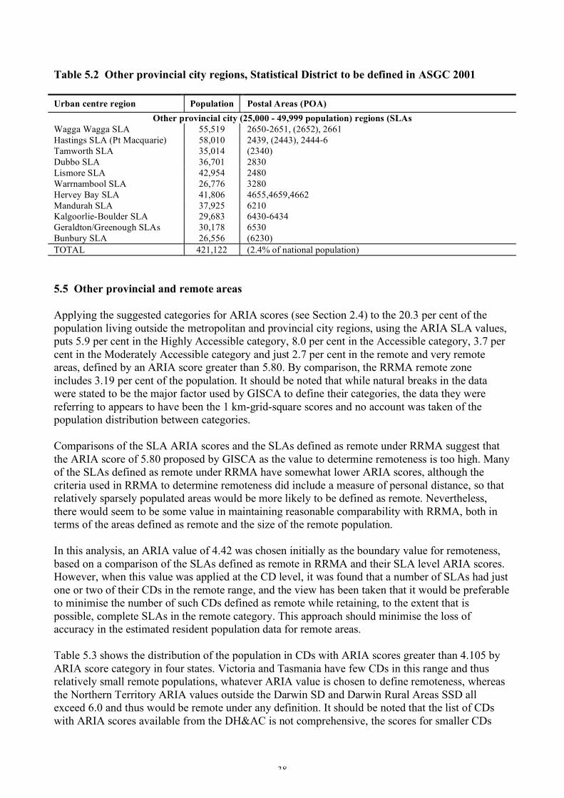
38

Table 5.2 Other provincial city regions, Statistical District to be defined in ASGC 2001 Urban centre region Population Postal Areas (POA)

Other provincial city (25,000 - 49,999 population) regions (SLAs Wagga Wagga SLA 55,519 2650-2651, (2652), 2661 Hastings SLA (Pt Macquarie) 58,010 2439, (2443), 2444-6 Tamworth SLA 35,014 (2340) Dubbo SLA 36,701 2830 Lismore SLA 42,954 2480 Warrnambool SLA 26,776 3280 Hervey Bay SLA 41,806 4655,4659,4662 Mandurah SLA 37,925 6210 Kalgoorlie-Boulder SLA 29,683 6430-6434 Geraldton/Greenough SLAs 30,178 6530 Bunbury SLA 26,556 (6230) TOTAL 421,122 (2.4% of national population) 5.5 Other provincial and remote areas Applying the suggested categories for ARIA scores (see Section 2.4) to the 20.3 per cent of the population living outside the metropolitan and provincial city regions, using the ARIA SLA values, puts 5.9 per cent in the Highly Accessible category, 8.0 per cent in the Accessible category, 3.7 per cent in the Moderately Accessible category and just 2.7 per cent in the remote and very remote areas, defined by an ARIA score greater than 5.80. By comparison, the RRMA remote zone includes 3.19 per cent of the population. It should be noted that while natural breaks in the data were stated to be the major factor used by GISCA to define their categories, the data they were referring to appears to have been the 1 km-grid-square scores and no account was taken of the population distribution between categories. Comparisons of the SLA ARIA scores and the SLAs defined as remote under RRMA suggest that the ARIA score of 5.80 proposed by GISCA as the value to determine remoteness is too high. Many of the SLAs defined as remote under RRMA have somewhat lower ARIA scores, although the criteria used in RRMA to determine remoteness did include a measure of personal distance, so that relatively sparsely populated areas would be more likely to be defined as remote. Nevertheless, there would seem to be some value in maintaining reasonable comparability with RRMA, both in terms of the areas defined as remote and the size of the remote population. In this analysis, an ARIA value of 4.42 was chosen initially as the boundary value for remoteness, based on a comparison of the SLAs defined as remote in RRMA and their SLA level ARIA scores. However, when this value was applied at the CD level, it was found that a number of SLAs had just one or two of their CDs in the remote range, and the view has been taken that it would be preferable to minimise the number of such CDs defined as remote while retaining, to the extent that is possible, complete SLAs in the remote category. This approach should minimise the loss of accuracy in the estimated resident population data for remote areas. Table 5.3 shows the distribution of the population in CDs with ARIA scores greater than 4.105 by ARIA score category in four states. Victoria and Tasmania have few CDs in this range and thus relatively small remote populations, whatever ARIA value is chosen to define remoteness, whereas the Northern Territory ARIA values outside the Darwin SD and Darwin Rural Areas SSD all exceed 6.0 and thus would be remote under any definition. It should be noted that the list of CDs with ARIA scores available from the DH&AC is not comprehensive, the scores for smaller CDs

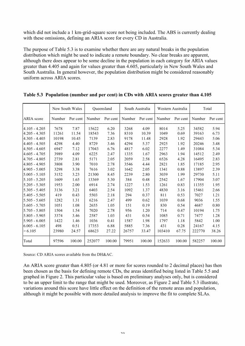
39

which did not include a 1 km-grid-square score not being included. The ABS is currently dealing with these omissions, defining an ARIA score for every CD in Australia. The purpose of Table 5.3 is to examine whether there are any natural breaks in the population distribution which might be used to indicate a remote boundary. No clear breaks are apparent, although there does appear to be some decline in the population in each category for ARIA values greater than 4.405 and again for values greater than 4.605, particularly in New South Wales and South Australia. In general however, the population distribution might be considered reasonably uniform across ARIA scores. Table 5.3 Population (number and per cent) in CDs with ARIA scores greater than 4.105 New South Wales Queensland South Australia Western Australia Total

ARIA score Number Per cent Number Per cent Number Per cent Number Per cent Number Per cent

4.105 - 4.205 7678 7.87 15622 6.20 3268 4.09 8014 5.25 34582 5.94 4.205 - 4.305 11261 11.54 18543 7.36 8310 10.39 1049 0.69 39163 6.73 4.305 - 4.405 10198 10.45 7139 2.83 9178 11.48 2928 1.92 29443 5.06 4.405 - 4.505 4298 4.40 8729 3.46 4294 5.37 2925 1.92 20246 3.48 4.505 - 4.605 6947 7.12 17043 6.76 4817 6.02 2277 1.49 31084 5.34 4.605 - 4.705 3989 4.09 6225 2.47 1335 1.67 2963 1.94 14512 2.49 4.705 - 4.805 2739 2.81 5171 2.05 2059 2.58 6526 4.28 16495 2.83 4.805 - 4.905 3808 3.90 7010 2.78 3546 4.44 2821 1.85 17185 2.95 4.905 - 5.005 3298 3.38 7616 3.02 1642 2.05 1341 0.88 13897 2.39 5.005 - 5.105 3152 3.23 21300 8.45 2239 2.80 3039 1.99 29730 5.11 5.105 - 5.205 1609 1.65 13369 5.30 384 0.48 2542 1.67 17904 3.07 5.205 - 5.305 1953 2.00 6914 2.74 1227 1.53 1261 0.83 11355 1.95 5.305 - 5.405 3136 3.21 6403 2.54 1092 1.37 4830 3.16 15461 2.66 5.405 - 5.505 419 0.43 5503 2.18 294 0.37 811 0.53 7027 1.21 5.505 - 5.605 1282 1.31 6216 2.47 499 0.62 1039 0.68 9036 1.55 5.605 - 5.705 1051 1.08 2655 1.05 151 0.19 830 0.54 4687 0.80 5.705 - 5.805 1504 1.54 7020 2.78 956 1.20 714 0.47 10194 1.75 5.805 - 5.905 3374 3.46 2587 1.03 431 0.54 1085 0.71 7477 1.28 5.905 - 6.005 1422 1.46 1036 0.41 1587 1.98 1797 1.18 5842 1.00 6.005 - 6.105 498 0.51 17353 6.88 5885 7.36 431 0.28 24167 4.15 > 6.105 23980 24.57 68623 27.22 26757 33.47 103410 67.75 222770 38.26

Total 97596 100.00 252077 100.00 79951 100.00 152633 100.00 582257 100.00

Source: CD ARIA scores available from the DH&AC. An ARIA score greater than 4.805 (or 4.81 or more for scores rounded to 2 decimal places) has then been chosen as the basis for defining remote CDs, the areas identified being listed in Table 5.5 and graphed in Figure 2. This particular value is based on preliminary analyses only, but is considered to be an upper limit to the range that might be used. Moreover, as Figure 2 and Table 5.3 illustrate, variations around this score have little effect on the definition of the remote areas and population, although it might be possible with more detailed analysis to improve the fit to complete SLAs.

40

Figure 2 Remote Australia: ARIA Score by Census Collection District

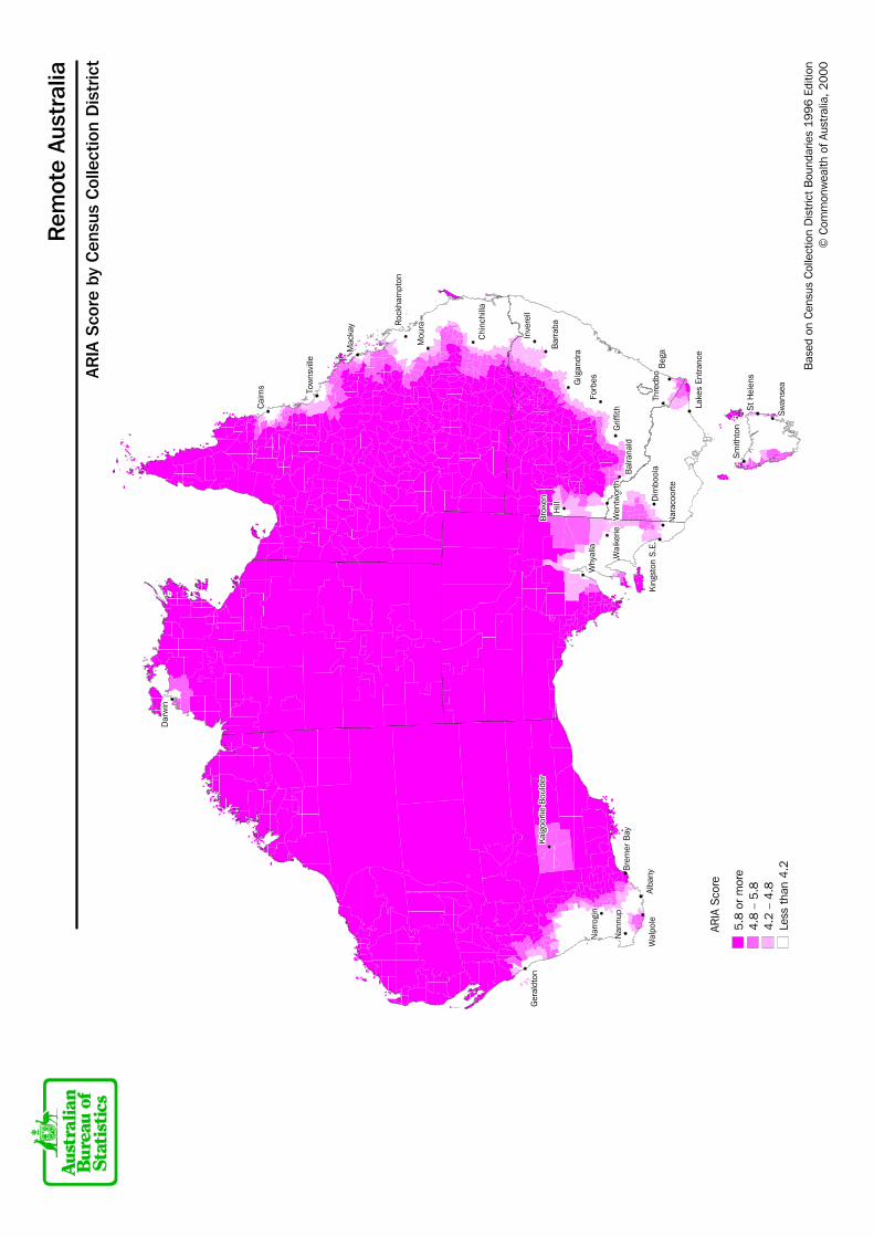
Rem

ote

Aust

ralia

ARIA

Sco

re b

y C

ensu

s C

olle

ctio

n D

istr

ict

Bas

ed o

n C

ensu

s C

olle

ctio

n D

istr

ict

Bou

ndar

ies

1996

Edi

tion

© C

omm

onw

ealth

of A

ustr

alia

, 200

0

Wen

twor

th W

entw

orth

Wen

twor

th W

entw

orth

Wen

twor

th W

entw

orth

Wen

twor

th W

entw

orth

Wen

twor

th W

entw

orth

Wen

twor

th W

entw

orth

Wen

twor

th W

entw

orth

Wen

twor

th W

entw

orth

Wen

twor

th W

entw

orth

Wen

twor

th W

entw

orth

Wen

twor

th W

entw

orth

Wen

twor

th W

entw

orth

Wen

twor

th W

entw

orth

Wen

twor

th W

entw

orth

Wen

twor

th W

entw

orth

Wen

twor

th W

entw

orth

Wen

twor

th W

entw

orth

Wen

twor

th W

entw

orth

Wen

twor

th

Nar

rogi

n

Nar

rogi

n

Nar

rogi

n

Nar

rogi

n

Nar

rogi

n

Nar

rogi

n

Nar

rogi

n

Nar

rogi

n

Nar

rogi

n

Nar

rogi

n

Nar

rogi

n

Nar

rogi

n

Nar

rogi

n

Nar

rogi

n

Nar

rogi

n

Nar

rogi

n

Nar

rogi

n

Nar

rogi

n

Nar

rogi

n

Nar

rogi

n

Nar

rogi

n

Nar

rogi

n

Nar

rogi

n

Nar

rogi

n

Nar

rogi

n

Nar

rogi

n

Nar

rogi

n

Nar

rogi

n

Nar

rogi

n

Nar

rogi

n

Nar

rogi

n

Nar

rogi

n

Nar

rogi

n

Nar

rogi

n

Nar

rogi

n

Nar

rogi

n

Nar

rogi

n

Nan

nup

Nan

nup

Nan

nup

Nan

nup

Nan

nup

Nan

nup

Nan

nup

Nan

nup

Nan

nup

Nan

nup

Nan

nup

Nan

nup

Nan

nup

Nan

nup

Nan

nup

Nan

nup

Nan

nup

Nan

nup

Nan

nup

Nan

nup

Nan

nup

Nan

nup

Nan

nup

Nan

nup

Nan

nup

Nan

nup

Nan

nup

Nan

nup

Nan

nup

Nan

nup

Nan

nup

Nan

nup

Nan

nup

Nan

nup

Nan

nup

Nan

nup

Nan

nup

Bro

ken

Bro

ken

Bro

ken

Bro

ken

Bro

ken

Bro

ken

Bro

ken

Bro

ken

Bro

ken

Bro

ken

Bro

ken

Bro

ken

Bro

ken

Bro

ken

Bro

ken

Bro

ken

Bro

ken

Bro

ken

Bro

ken

Bro

ken

Bro

ken

Bro

ken

Bro

ken

Bro

ken

Bro

ken

Bro

ken

Bro

ken

Bro

ken

Bro

ken

Bro

ken

Bro

ken

Bro

ken

Bro

ken

Bro

ken

Bro

ken

Bro

ken

Bro

ken

H

ill

Hill

H

ill

Hill

H

ill

Hill

H

ill

Hill

H

ill

Hill

H

ill

Hill

H

ill

Hill

H

ill

Hill

H

ill

Hill

H

ill

Hill

H

ill

Hill

H

ill

Hill

H

ill

Hill

H

ill

Hill

H

ill

Hill

H

ill

Hill

H

ill

Hill

H

ill

Hill

H

ill

Why

alla

Why

alla

Why

alla

Why

alla

Why

alla

Why

alla

Why

alla

Why

alla

Why

alla

Why

alla

Why

alla

Why

alla

Why

alla

Why

alla

Why

alla

Why

alla

Why

alla

Why

alla

Why

alla

Why

alla

Why

alla

Why

alla

Why

alla

Why

alla

Why

alla

Why

alla

Why

alla

Why

alla

Why

alla

Why

alla

Why

alla

Why

alla

Why

alla

Why

alla

Why

alla

Why

alla

Why

alla

Dar

win

Dar

win

Dar

win

Dar

win

Dar

win

Dar

win

Dar

win

Dar

win

Dar

win

Dar

win

Dar

win

Dar

win

Dar

win

Dar

win

Dar

win

Dar

win

Dar

win

Dar

win

Dar

win

Dar

win

Dar

win

Dar

win

Dar

win

Dar

win

Dar

win

Dar

win

Dar

win

Dar

win

Dar

win

Dar

win

Dar

win

Dar

win

Dar

win

Dar

win

Dar

win

Dar

win

Dar

win

Gilg

andr

aG

ilgan

dra

Gilg

andr

aG

ilgan

dra

Gilg

andr

aG

ilgan

dra

Gilg

andr

aG

ilgan

dra

Gilg

andr

aG

ilgan

dra

Gilg

andr

aG

ilgan

dra

Gilg

andr

aG

ilgan

dra

Gilg

andr

aG

ilgan

dra

Gilg

andr

aG

ilgan

dra

Gilg

andr

aG

ilgan

dra

Gilg

andr

aG

ilgan

dra

Gilg

andr

aG

ilgan

dra

Gilg

andr

aG

ilgan

dra

Gilg

andr

aG

ilgan

dra

Gilg

andr

aG

ilgan

dra

Gilg

andr

aG

ilgan

dra

Gilg

andr

aG

ilgan

dra

Gilg

andr

aG

ilgan

dra

Gilg

andr

aBar

raba

Bar

raba

Bar

raba

Bar

raba

Bar

raba

Bar

raba

Bar

raba

Bar

raba

Bar

raba

Bar

raba

Bar

raba

Bar

raba

Bar

raba

Bar

raba

Bar

raba

Bar

raba

Bar

raba

Bar

raba

Bar

raba

Bar

raba

Bar

raba

Bar

raba

Bar

raba

Bar

raba

Bar

raba

Bar

raba

Bar

raba

Bar

raba

Bar

raba

Bar

raba

Bar

raba

Bar

raba

Bar

raba

Bar

raba

Bar

raba

Bar

raba

Bar

raba

Chi

nchi

llaC

hinc

hilla

Chi

nchi

llaC

hinc

hilla

Chi

nchi

llaC

hinc

hilla

Chi

nchi

llaC

hinc

hilla

Chi

nchi

llaC

hinc

hilla

Chi

nchi

llaC

hinc

hilla

Chi

nchi

llaC

hinc

hilla

Chi

nchi

llaC

hinc

hilla

Chi

nchi

llaC

hinc

hilla

Chi

nchi

llaC

hinc

hilla

Chi

nchi

llaC

hinc

hilla

Chi

nchi

llaC

hinc

hilla

Chi

nchi

llaC

hinc

hilla

Chi

nchi

llaC

hinc

hilla

Chi

nchi

llaC

hinc

hilla

Chi

nchi

llaC

hinc

hilla

Chi

nchi

llaC

hinc

hilla

Chi

nchi

llaC

hinc

hilla

Chi

nchi

lla

Bre

mer

Bay

Bre

mer

Bay

Bre

mer

Bay

Bre

mer

Bay

Bre

mer

Bay

Bre

mer

Bay

Bre

mer

Bay

Bre

mer

Bay

Bre

mer

Bay

Bre

mer

Bay

Bre

mer

Bay

Bre

mer

Bay

Bre

mer

Bay

Bre

mer

Bay

Bre

mer

Bay

Bre

mer

Bay

Bre

mer

Bay

Bre

mer

Bay

Bre

mer

Bay

Bre

mer

Bay

Bre

mer

Bay

Bre

mer

Bay

Bre

mer

Bay

Bre

mer

Bay

Bre

mer

Bay

Bre

mer

Bay

Bre

mer

Bay

Bre

mer

Bay

Bre

mer

Bay

Bre

mer

Bay

Bre

mer

Bay

Bre

mer

Bay

Bre

mer

Bay

Bre

mer

Bay

Bre

mer

Bay

Bre

mer

Bay

Bre

mer

Bay

B

ega

B

ega

B

ega

B

ega

B

ega

B

ega

B

ega

B

ega

B

ega

B

ega

B

ega

B

ega

B

ega

B

ega

B

ega

B

ega

B

ega

B

ega

B

ega

B

ega

B

ega

B

ega

B

ega

B

ega

B

ega

B

ega

B

ega

B

ega

B

ega

B

ega

B

ega

B

ega

B

ega

B

ega

B

ega

B

ega

B

ega

Thre

dbo

Thre

dbo

Thre

dbo

Thre

dbo

Thre

dbo

Thre

dbo

Thre

dbo

Thre

dbo

Thre

dbo

Thre

dbo

Thre

dbo

Thre

dbo

Thre

dbo

Thre

dbo

Thre

dbo

Thre

dbo

Thre

dbo

Thre

dbo

Thre

dbo

Thre

dbo

Thre

dbo

Thre

dbo

Thre

dbo

Thre

dbo

Thre

dbo

Thre

dbo

Thre

dbo

Thre

dbo

Thre

dbo

Thre

dbo

Thre

dbo

Thre

dbo

Thre

dbo

Thre

dbo

Thre

dbo

Thre

dbo

Thre

dbo

Alba

nyAl

bany

Alba

nyAl

bany

Alba

nyAl

bany

Alba

nyAl

bany

Alba

nyAl

bany

Alba

nyAl

bany

Alba

nyAl

bany

Alba

nyAl

bany

Alba

nyAl

bany

Alba

nyAl

bany

Alba

nyAl

bany

Alba

nyAl

bany

Alba

nyAl

bany

Alba

nyAl

bany

Alba

nyAl

bany

Alba

nyAl

bany

Alba

nyAl

bany

Alba

nyAl

bany

Alba

nyW

alpo

leW

alpo

leW

alpo

leW

alpo

leW

alpo

leW

alpo

leW

alpo

leW

alpo

leW

alpo

leW

alpo

leW

alpo

leW

alpo

leW

alpo

leW

alpo

leW

alpo

leW

alpo

leW

alpo

leW

alpo

leW

alpo

leW

alpo

leW

alpo

leW

alpo

leW

alpo

leW

alpo

leW

alpo

leW

alpo

leW

alpo

leW

alpo

leW

alpo

leW

alpo

leW

alpo

leW

alpo

leW

alpo

leW

alpo

leW

alpo

leW

alpo

leW

alpo

le

Wai

kerie

Wai

kerie

Wai

kerie

Wai

kerie

Wai

kerie

Wai

kerie

Wai

kerie

Wai

kerie

Wai

kerie

Wai

kerie

Wai

kerie

Wai

kerie

Wai

kerie

Wai

kerie

Wai

kerie

Wai

kerie

Wai

kerie

Wai

kerie

Wai

kerie

Wai

kerie

Wai

kerie

Wai

kerie

Wai

kerie

Wai

kerie

Wai

kerie

Wai

kerie

Wai

kerie

Wai

kerie

Wai

kerie

Wai

kerie

Wai

kerie

Wai

kerie

Wai

kerie

Wai

kerie

Wai

kerie

Wai

kerie

Wai

kerie

Dim

bool

aD

imbo

ola

Dim

bool

aD

imbo

ola

Dim

bool

aD

imbo

ola

Dim

bool

aD

imbo

ola

Dim

bool

aD

imbo

ola

Dim

bool

aD

imbo

ola

Dim

bool

aD

imbo

ola

Dim

bool

aD

imbo

ola

Dim

bool

aD

imbo

ola

Dim

bool

aD

imbo

ola

Dim

bool

aD

imbo

ola

Dim

bool

aD

imbo

ola

Dim

bool

aD

imbo

ola

Dim

bool

aD

imbo

ola

Dim

bool

aD

imbo

ola

Dim

bool

aD

imbo

ola

Dim

bool

aD

imbo

ola

Dim

bool

aD

imbo

ola

Dim

bool

a

Nar

acoo

rte

Nar

acoo

rte

Nar

acoo

rte

Nar

acoo

rte

Nar

acoo

rte

Nar

acoo

rte

Nar

acoo

rte

Nar

acoo

rte

Nar

acoo

rte

Nar

acoo

rte

Nar

acoo

rte

Nar

acoo

rte

Nar

acoo

rte

Nar

acoo

rte

Nar

acoo

rte

Nar

acoo

rte

Nar

acoo

rte

Nar

acoo

rte

Nar

acoo

rte

Nar

acoo

rte

Nar

acoo

rte

Nar

acoo

rte

Nar

acoo

rte

Nar

acoo

rte

Nar

acoo

rte

Nar

acoo

rte

Nar

acoo

rte

Nar

acoo

rte

Nar

acoo

rte

Nar

acoo

rte

Nar

acoo

rte

Nar

acoo

rte

Nar

acoo

rte

Nar

acoo

rte

Nar

acoo

rte

Nar

acoo

rte

Nar

acoo

rte

King

ston

S.E

.Ki

ngst

on S

.E.

King

ston

S.E

.Ki

ngst

on S

.E.

King

ston

S.E

.Ki

ngst

on S

.E.

King

ston

S.E

.Ki

ngst

on S

.E.

King

ston

S.E

.Ki

ngst

on S

.E.

King

ston

S.E

.Ki

ngst

on S

.E.

King

ston

S.E

.Ki

ngst

on S

.E.

King

ston

S.E

.Ki

ngst

on S

.E.

King

ston

S.E

.Ki

ngst

on S

.E.

King

ston

S.E

.Ki

ngst

on S

.E.

King

ston

S.E

.Ki

ngst

on S

.E.

King

ston

S.E

.Ki

ngst

on S

.E.

King

ston

S.E

.Ki

ngst

on S

.E.

King

ston

S.E

.Ki

ngst

on S

.E.

King

ston

S.E

.Ki

ngst

on S

.E.

King

ston

S.E

.Ki

ngst

on S

.E.

King

ston

S.E

.Ki

ngst

on S

.E.

King

ston

S.E

.Ki

ngst

on S

.E.

King

ston

S.E

.

Grif

fith

Grif

fith

Grif

fith

Grif

fith

Grif

fith

Grif

fith

Grif

fith

Grif

fith

Grif

fith

Grif

fith

Grif

fith

Grif

fith

Grif

fith

Grif

fith

Grif

fith

Grif

fith

Grif

fith

Grif

fith

Grif

fith

Grif

fith

Grif

fith

Grif

fith

Grif

fith

Grif

fith

Grif

fith

Grif

fith

Grif

fith

Grif

fith

Grif

fith

Grif

fith

Grif

fith

Grif

fith

Grif

fith

Grif

fith

Grif

fith

Grif

fith

Grif

fith

R

ockh

ampt

on

Roc

kham

pton

R

ockh

ampt

on

Roc

kham

pton

R

ockh

ampt

on

Roc

kham

pton

R

ockh

ampt

on

Roc

kham

pton

R

ockh

ampt

on

Roc

kham

pton

R

ockh

ampt

on

Roc

kham

pton

R

ockh

ampt

on

Roc

kham

pton

R

ockh

ampt

on

Roc

kham

pton

R

ockh

ampt

on

Roc

kham

pton

R

ockh

ampt

on

Roc

kham

pton

R

ockh

ampt

on

Roc

kham

pton

R

ockh

ampt

on

Roc

kham

pton

R

ockh

ampt

on

Roc

kham

pton

R

ockh

ampt

on

Roc

kham

pton

R

ockh

ampt

on

Roc

kham

pton

R

ockh

ampt

on

Roc

kham

pton

R

ockh

ampt

on

Roc

kham

pton

R

ockh

ampt

on

Roc

kham

pton

R

ockh

ampt

on

Bal

rana

ldB

alra

nald

Bal

rana

ldB

alra

nald

Bal

rana

ldB

alra

nald

Bal

rana

ldB

alra

nald

Bal

rana

ldB

alra

nald

Bal

rana

ldB

alra

nald

Bal

rana

ldB

alra

nald

Bal

rana

ldB

alra

nald

Bal

rana

ldB

alra

nald

Bal

rana

ldB

alra

nald

Bal

rana

ldB

alra

nald

Bal

rana

ldB

alra

nald

Bal

rana

ldB

alra

nald

Bal

rana

ldB

alra

nald

Bal

rana

ldB

alra

nald

Bal

rana

ldB

alra

nald

Bal

rana

ldB

alra

nald

Bal

rana

ldB

alra

nald

Bal

rana

ld

Lake

s En

tran

ceLa

kes

Entr

ance

Lake

s En

tran

ceLa

kes

Entr

ance

Lake

s En

tran

ceLa

kes

Entr

ance

Lake

s En

tran

ceLa

kes

Entr

ance

Lake

s En

tran

ceLa

kes

Entr

ance

Lake

s En

tran

ceLa

kes

Entr

ance

Lake

s En

tran

ceLa

kes

Entr

ance

Lake

s En

tran

ceLa

kes

Entr

ance

Lake

s En

tran

ceLa

kes

Entr

ance

Lake

s En

tran

ceLa

kes

Entr

ance

Lake

s En

tran

ceLa

kes

Entr

ance

Lake

s En

tran

ceLa

kes

Entr

ance

Lake

s En

tran

ceLa

kes

Entr

ance

Lake

s En

tran

ceLa

kes

Entr

ance

Lake

s En

tran

ceLa

kes

Entr

ance

Lake

s En

tran

ceLa

kes

Entr

ance

Lake

s En

tran

ceLa

kes

Entr

ance

Lake

s En

tran

ceLa

kes

Entr

ance

Lake

s En

tran

ce

Sw

anse

aS

wan

sea

Sw

anse

aS

wan

sea

Sw

anse

aS

wan

sea

Sw

anse

aS

wan

sea

Sw

anse

aS

wan

sea

Sw

anse

aS

wan

sea

Sw

anse

aS

wan

sea

Sw

anse

aS

wan

sea

Sw

anse

aS

wan

sea

Sw

anse

aS

wan

sea

Sw

anse

aS

wan

sea

Sw

anse

aS

wan

sea

Sw

anse

aS

wan

sea

Sw

anse

aS

wan

sea

Sw

anse

aS

wan

sea

Sw

anse

aS

wan

sea

Sw

anse

aS

wan

sea

Sw

anse

aS

wan

sea

Sw

anse

a

Ger

aldt

onG

eral

dton

Ger

aldt

onG

eral

dton

Ger

aldt

onG

eral

dton

Ger

aldt

onG

eral

dton

Ger

aldt

onG

eral

dton

Ger

aldt

onG

eral

dton

Ger

aldt

onG

eral

dton

Ger

aldt

onG

eral

dton

Ger

aldt

onG

eral

dton

Ger

aldt

onG

eral

dton

Ger

aldt

onG

eral

dton

Ger

aldt

onG

eral

dton

Ger

aldt

onG

eral

dton

Ger

aldt

onG

eral

dton

Ger

aldt

onG

eral

dton

Ger

aldt

onG

eral

dton

Ger

aldt

onG

eral

dton

Ger

aldt

onG

eral

dton

Ger

aldt

on

Mou

raM

oura

Mou

raM

oura

Mou

raM

oura

Mou

raM

oura

Mou

raM

oura

Mou

raM

oura

Mou

raM

oura

Mou

raM

oura

Mou

raM

oura

Mou

raM

oura

Mou

raM

oura

Mou

raM

oura

Mou

raM

oura

Mou

raM

oura

Mou

raM

oura

Mou

raM

oura

Mou

raM

oura

Mou

raM

oura

Mou

ra

Forb

esFo

rbes

Forb

esFo

rbes

Forb

esFo

rbes

Forb

esFo

rbes

Forb

esFo

rbes

Forb

esFo

rbes

Forb

esFo

rbes

Forb

esFo

rbes

Forb

esFo

rbes

Forb

esFo

rbes

Forb

esFo

rbes

Forb

esFo

rbes

Forb

esFo

rbes

Forb

esFo

rbes

Forb

esFo

rbes

Forb

esFo

rbes

Forb

esFo

rbes

Forb

esFo

rbes

Forb

es

Inve

rell

Inve

rell

Inve

rell

Inve

rell

Inve

rell

Inve

rell

Inve

rell

Inve

rell

Inve

rell

Inve

rell

Inve

rell

Inve

rell

Inve

rell

Inve

rell

Inve

rell

Inve

rell

Inve

rell

Inve

rell

Inve

rell

Inve

rell

Inve

rell

Inve

rell

Inve

rell

Inve

rell

Inve

rell

Inve

rell

Inve

rell

Inve

rell

Inve

rell

Inve

rell

Inve

rell

Inve

rell

Inve

rell

Inve

rell

Inve

rell

Inve

rell

Inve

rell

Mac

kay

Mac

kay

Mac

kay

Mac

kay

Mac

kay

Mac

kay

Mac

kay

Mac

kay

Mac

kay

Mac

kay

Mac

kay

Mac

kay

Mac

kay

Mac

kay

Mac

kay

Mac

kay

Mac

kay

Mac

kay

Mac

kay

Mac

kay

Mac

kay

Mac

kay

Mac

kay

Mac

kay

Mac

kay

Mac

kay

Mac

kay

Mac

kay

Mac

kay

Mac

kay

Mac

kay

Mac

kay

Mac

kay

Mac

kay

Mac

kay

Mac

kay

Mac

kay

Tow

nsvi

lleTo

wns

ville

Tow

nsvi

lleTo

wns

ville

Tow

nsvi

lleTo

wns

ville

Tow

nsvi

lleTo

wns

ville

Tow

nsvi

lleTo

wns

ville

Tow

nsvi

lleTo

wns

ville

Tow

nsvi

lleTo

wns

ville

Tow

nsvi

lleTo

wns

ville

Tow

nsvi

lleTo

wns

ville

Tow

nsvi

lleTo

wns

ville

Tow

nsvi

lleTo

wns

ville

Tow

nsvi

lleTo

wns

ville

Tow

nsvi

lleTo

wns

ville

Tow

nsvi

lleTo

wns

ville

Tow

nsvi

lleTo

wns

ville

Tow

nsvi

lleTo

wns

ville

Tow

nsvi

lleTo

wns

ville

Tow

nsvi

lleTo

wns

ville

Tow

nsvi

lle

Cai

rns

Cai

rns

Cai

rns

Cai

rns

Cai

rns

Cai

rns

Cai

rns

Cai

rns

Cai

rns

Cai

rns

Cai

rns

Cai

rns

Cai

rns

Cai

rns

Cai

rns

Cai

rns

Cai

rns

Cai

rns

Cai

rns

Cai

rns

Cai

rns

Cai

rns

Cai

rns

Cai

rns

Cai

rns

Cai

rns

Cai

rns

Cai

rns

Cai

rns

Cai

rns

Cai

rns

Cai

rns

Cai

rns

Cai

rns

Cai

rns

Cai

rns

Cai

rns

St

Hel

ens

St

Hel

ens

St

Hel

ens

St

Hel

ens

St

Hel

ens

St

Hel

ens

St

Hel

ens

St

Hel

ens

St

Hel

ens

St

Hel

ens

St

Hel

ens

St

Hel

ens

St

Hel

ens

St

Hel

ens

St

Hel

ens

St

Hel

ens

St

Hel

ens

St

Hel

ens

St

Hel

ens

St

Hel

ens

St

Hel

ens

St

Hel

ens

St

Hel

ens

St

Hel

ens

St

Hel

ens

St

Hel

ens

St

Hel

ens

St

Hel

ens

St

Hel

ens

St

Hel

ens

St

Hel

ens

St

Hel

ens

St

Hel

ens

St

Hel

ens

St

Hel

ens

St

Hel

ens

St

Hel

ens

Sm

ithto

nS

mith

ton

Sm

ithto

nS

mith

ton

Sm

ithto

nS

mith

ton

Sm

ithto

nS

mith

ton

Sm

ithto

nS

mith

ton

Sm

ithto

nS

mith

ton

Sm

ithto

nS

mith

ton

Sm

ithto

nS

mith

ton

Sm

ithto

nS

mith

ton

Sm

ithto

nS

mith

ton

Sm

ithto

nS

mith

ton

Sm

ithto

nS

mith

ton

Sm

ithto

nS

mith

ton

Sm

ithto

nS

mith

ton

Sm

ithto

nS

mith

ton

Sm

ithto

nS

mith

ton

Sm

ithto

nS

mith

ton

Sm

ithto

nS

mith

ton

Sm

ithto

n

Kalg

oorli

e-B

ould

erKa

lgoo

rlie-

Bou

lder

Kalg

oorli

e-B

ould

erKa

lgoo

rlie-

Bou

lder

Kalg

oorli

e-B

ould

erKa

lgoo

rlie-

Bou

lder

Kalg

oorli

e-B

ould

erKa

lgoo

rlie-

Bou

lder

Kalg

oorli

e-B

ould

erKa

lgoo

rlie-

Bou

lder

Kalg

oorli

e-B

ould

erKa

lgoo

rlie-

Bou

lder

Kalg

oorli

e-B

ould

erKa

lgoo

rlie-

Bou

lder

Kalg

oorli

e-B

ould

erKa

lgoo

rlie-

Bou

lder

Kalg

oorli

e-B

ould

erKa

lgoo

rlie-

Bou

lder

Kalg

oorli

e-B

ould

erKa

lgoo

rlie-

Bou

lder

Kalg

oorli

e-B

ould

erKa

lgoo

rlie-

Bou

lder

Kalg

oorli

e-B

ould

erKa

lgoo

rlie-

Bou

lder

Kalg

oorli

e-B

ould

erKa

lgoo

rlie-

Bou

lder

Kalg

oorli

e-B

ould

erKa

lgoo

rlie-

Bou

lder

Kalg

oorli

e-B

ould

erKa

lgoo

rlie-

Bou

lder

Kalg

oorli

e-B

ould

erKa

lgoo

rlie-

Bou

lder

Kalg

oorli

e-B

ould

erKa

lgoo

rlie-

Bou

lder

Kalg

oorli

e-B

ould

erKa

lgoo

rlie-

Bou

lder

Kalg

oorli

e-B

ould

er

ARIA

Sco

re

5.8

or m

ore

4.8

– 5.

84.

2 –

4.8

Less

tha

n 4.

2

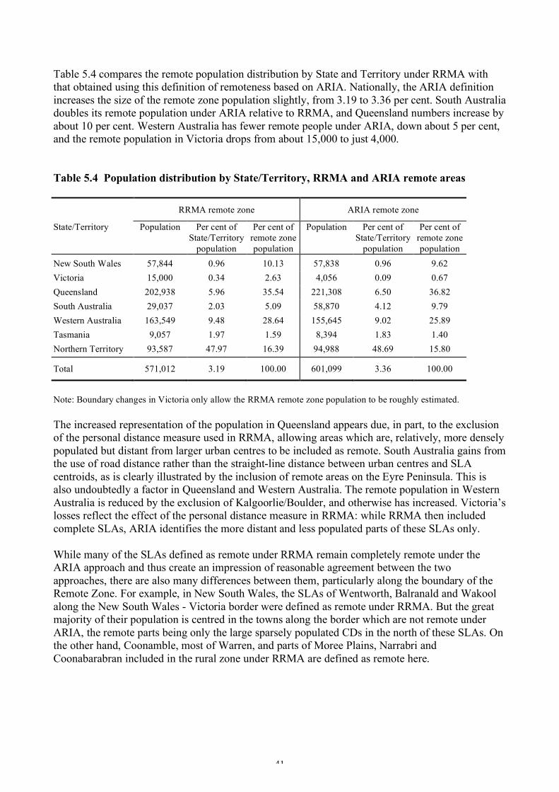
41

Table 5.4 compares the remote population distribution by State and Territory under RRMA with that obtained using this definition of remoteness based on ARIA. Nationally, the ARIA definition increases the size of the remote zone population slightly, from 3.19 to 3.36 per cent. South Australia doubles its remote population under ARIA relative to RRMA, and Queensland numbers increase by about 10 per cent. Western Australia has fewer remote people under ARIA, down about 5 per cent, and the remote population in Victoria drops from about 15,000 to just 4,000. Table 5.4 Population distribution by State/Territory, RRMA and ARIA remote areas

RRMA remote zone ARIA remote zone

State/Territory Population Per cent of State/Territory

population

Per cent of remote zone population

Population Per cent of State/Territory

population

Per cent of remote zone population

New South Wales 57,844 0.96 10.13 57,838 0.96 9.62 Victoria 15,000 0.34 2.63 4,056 0.09 0.67 Queensland 202,938 5.96 35.54 221,308 6.50 36.82 South Australia 29,037 2.03 5.09 58,870 4.12 9.79 Western Australia 163,549 9.48 28.64 155,645 9.02 25.89 Tasmania 9,057 1.97 1.59 8,394 1.83 1.40 Northern Territory 93,587 47.97 16.39 94,988 48.69 15.80

Total 571,012 3.19 100.00 601,099 3.36 100.00

Note: Boundary changes in Victoria only allow the RRMA remote zone population to be roughly estimated. The increased representation of the population in Queensland appears due, in part, to the exclusion of the personal distance measure used in RRMA, allowing areas which are, relatively, more densely populated but distant from larger urban centres to be included as remote. South Australia gains from the use of road distance rather than the straight-line distance between urban centres and SLA centroids, as is clearly illustrated by the inclusion of remote areas on the Eyre Peninsula. This is also undoubtedly a factor in Queensland and Western Australia. The remote population in Western Australia is reduced by the exclusion of Kalgoorlie/Boulder, and otherwise has increased. Victoria’s losses reflect the effect of the personal distance measure in RRMA: while RRMA then included complete SLAs, ARIA identifies the more distant and less populated parts of these SLAs only. While many of the SLAs defined as remote under RRMA remain completely remote under the ARIA approach and thus create an impression of reasonable agreement between the two approaches, there are also many differences between them, particularly along the boundary of the Remote Zone. For example, in New South Wales, the SLAs of Wentworth, Balranald and Wakool along the New South Wales - Victoria border were defined as remote under RRMA. But the great majority of their population is centred in the towns along the border which are not remote under ARIA, the remote parts being only the large sparsely populated CDs in the north of these SLAs. On the other hand, Coonamble, most of Warren, and parts of Moree Plains, Narrabri and Coonabarabran included in the rural zone under RRMA are defined as remote here.

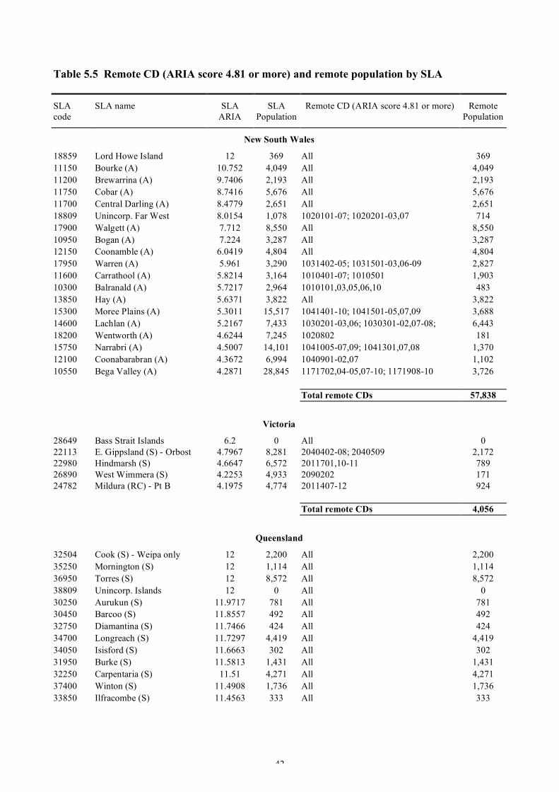
42

Table 5.5 Remote CD (ARIA score 4.81 or more) and remote population by SLA SLA code

SLA name SLA ARIA

SLA Population

Remote CD (ARIA score 4.81 or more) Remote Population

New South Wales

18859 Lord Howe Island 12 369 All 369 11150 Bourke (A) 10.752 4,049 All 4,049 11200 Brewarrina (A) 9.7406 2,193 All 2,193 11750 Cobar (A) 8.7416 5,676 All 5,676 11700 Central Darling (A) 8.4779 2,651 All 2,651 18809 Unincorp. Far West 8.0154 1,078 1020101-07; 1020201-03,07 714 17900 Walgett (A) 7.712 8,550 All 8,550 10950 Bogan (A) 7.224 3,287 All 3,287 12150 Coonamble (A) 6.0419 4,804 All 4,804 17950 Warren (A) 5.961 3,290 1031402-05; 1031501-03,06-09 2,827 11600 Carrathool (A) 5.8214 3,164 1010401-07; 1010501 1,903 10300 Balranald (A) 5.7217 2,964 1010101,03,05,06,10 483 13850 Hay (A) 5.6371 3,822 All 3,822 15300 Moree Plains (A) 5.3011 15,517 1041401-10; 1041501-05,07,09 3,688 14600 Lachlan (A) 5.2167 7,433 1030201-03,06; 1030301-02,07-08; 6,443 18200 Wentworth (A) 4.6244 7,245 1020802 181 15750 Narrabri (A) 4.5007 14,101 1041005-07,09; 1041301,07,08 1,370 12100 Coonabarabran (A) 4.3672 6,994 1040901-02,07 1,102 10550 Bega Valley (A) 4.2871 28,845 1171702,04-05,07-10; 1171908-10 3,726 Total remote CDs 57,838

Victoria

28649 Bass Strait Islands 6.2 0 All 0 22113 E. Gippsland (S) - Orbost 4.7967 8,281 2040402-08; 2040509 2,172 22980 Hindmarsh (S) 4.6647 6,572 2011701,10-11 789 26890 West Wimmera (S) 4.2253 4,933 2090202 171 24782 Mildura (RC) - Pt B 4.1975 4,774 2011407-12 924 Total remote CDs 4,056

Queensland

32504 Cook (S) - Weipa only 12 2,200 All 2,200 35250 Mornington (S) 12 1,114 All 1,114 36950 Torres (S) 12 8,572 All 8,572 38809 Unincorp. Islands 12 0 All 0 30250 Aurukun (S) 11.9717 781 All 781 30450 Barcoo (S) 11.8557 492 All 492 32750 Diamantina (S) 11.7466 424 All 424 34700 Longreach (S) 11.7297 4,419 All 4,419 34050 Isisford (S) 11.6663 302 All 302 31950 Burke (S) 11.5813 1,431 All 1,431 32250 Carpentaria (S) 11.51 4,271 All 4,271 37400 Winton (S) 11.4908 1,736 All 1,736 33850 Ilfracombe (S) 11.4563 333 All 333

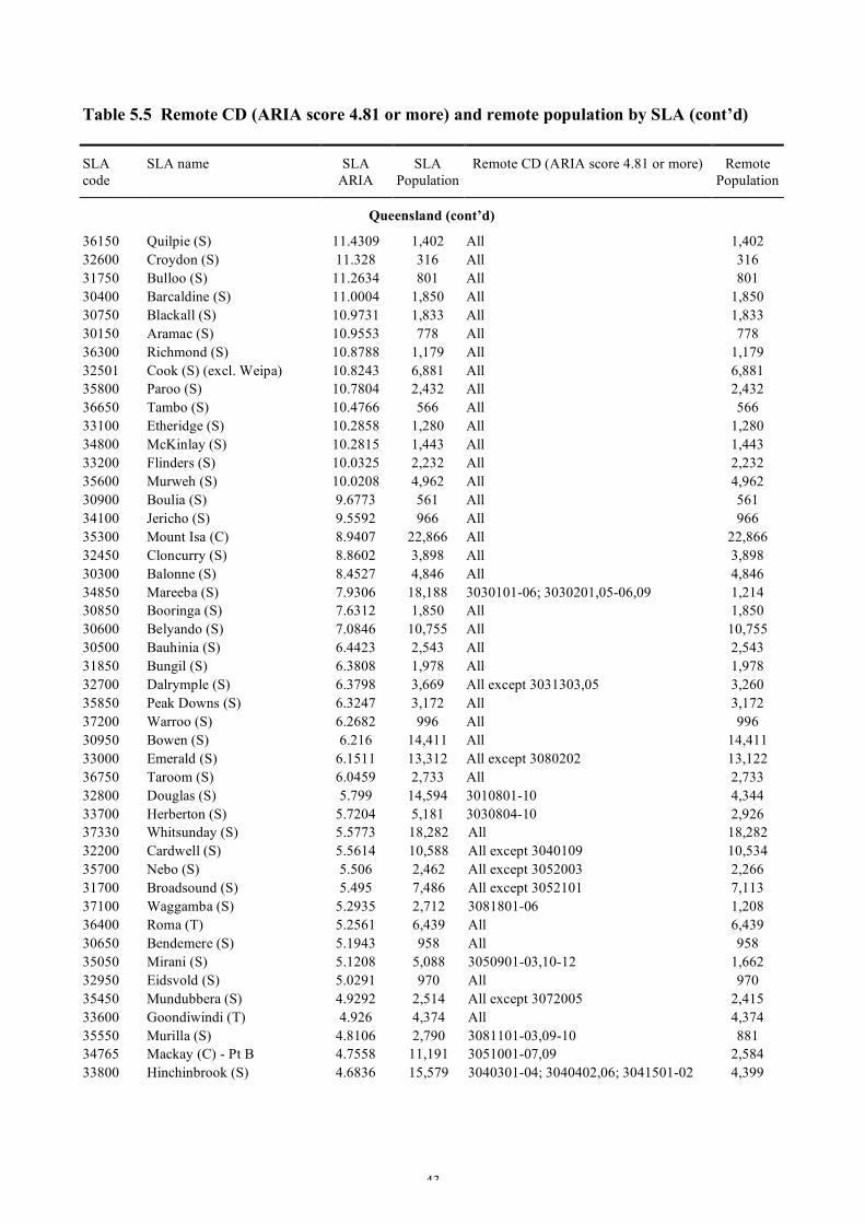
43

Table 5.5 Remote CD (ARIA score 4.81 or more) and remote population by SLA (cont’d) SLA code

SLA name SLA ARIA

SLA Population

Remote CD (ARIA score 4.81 or more) Remote Population

Queensland (cont’d)

36150 Quilpie (S) 11.4309 1,402 All 1,402 32600 Croydon (S) 11.328 316 All 316 31750 Bulloo (S) 11.2634 801 All 801 30400 Barcaldine (S) 11.0004 1,850 All 1,850 30750 Blackall (S) 10.9731 1,833 All 1,833 30150 Aramac (S) 10.9553 778 All 778 36300 Richmond (S) 10.8788 1,179 All 1,179 32501 Cook (S) (excl. Weipa) 10.8243 6,881 All 6,881 35800 Paroo (S) 10.7804 2,432 All 2,432 36650 Tambo (S) 10.4766 566 All 566 33100 Etheridge (S) 10.2858 1,280 All 1,280 34800 McKinlay (S) 10.2815 1,443 All 1,443 33200 Flinders (S) 10.0325 2,232 All 2,232 35600 Murweh (S) 10.0208 4,962 All 4,962 30900 Boulia (S) 9.6773 561 All 561 34100 Jericho (S) 9.5592 966 All 966 35300 Mount Isa (C) 8.9407 22,866 All 22,866 32450 Cloncurry (S) 8.8602 3,898 All 3,898 30300 Balonne (S) 8.4527 4,846 All 4,846 34850 Mareeba (S) 7.9306 18,188 3030101-06; 3030201,05-06,09 1,214 30850 Booringa (S) 7.6312 1,850 All 1,850 30600 Belyando (S) 7.0846 10,755 All 10,755 30500 Bauhinia (S) 6.4423 2,543 All 2,543 31850 Bungil (S) 6.3808 1,978 All 1,978 32700 Dalrymple (S) 6.3798 3,669 All except 3031303,05 3,260 35850 Peak Downs (S) 6.3247 3,172 All 3,172 37200 Warroo (S) 6.2682 996 All 996 30950 Bowen (S) 6.216 14,411 All 14,411 33000 Emerald (S) 6.1511 13,312 All except 3080202 13,122 36750 Taroom (S) 6.0459 2,733 All 2,733 32800 Douglas (S) 5.799 14,594 3010801-10 4,344 33700 Herberton (S) 5.7204 5,181 3030804-10 2,926 37330 Whitsunday (S) 5.5773 18,282 All 18,282 32200 Cardwell (S) 5.5614 10,588 All except 3040109 10,534 35700 Nebo (S) 5.506 2,462 All except 3052003 2,266 31700 Broadsound (S) 5.495 7,486 All except 3052101 7,113 37100 Waggamba (S) 5.2935 2,712 3081801-06 1,208 36400 Roma (T) 5.2561 6,439 All 6,439 30650 Bendemere (S) 5.1943 958 All 958 35050 Mirani (S) 5.1208 5,088 3050901-03,10-12 1,662 32950 Eidsvold (S) 5.0291 970 All 970 35450 Mundubbera (S) 4.9292 2,514 All except 3072005 2,415 33600 Goondiwindi (T) 4.926 4,374 All 4,374 35550 Murilla (S) 4.8106 2,790 3081101-03,09-10 881 34765 Mackay (C) - Pt B 4.7558 11,191 3051001-07,09 2,584 33800 Hinchinbrook (S) 4.6836 15,579 3040301-04; 3040402,06; 3041501-02 4,399

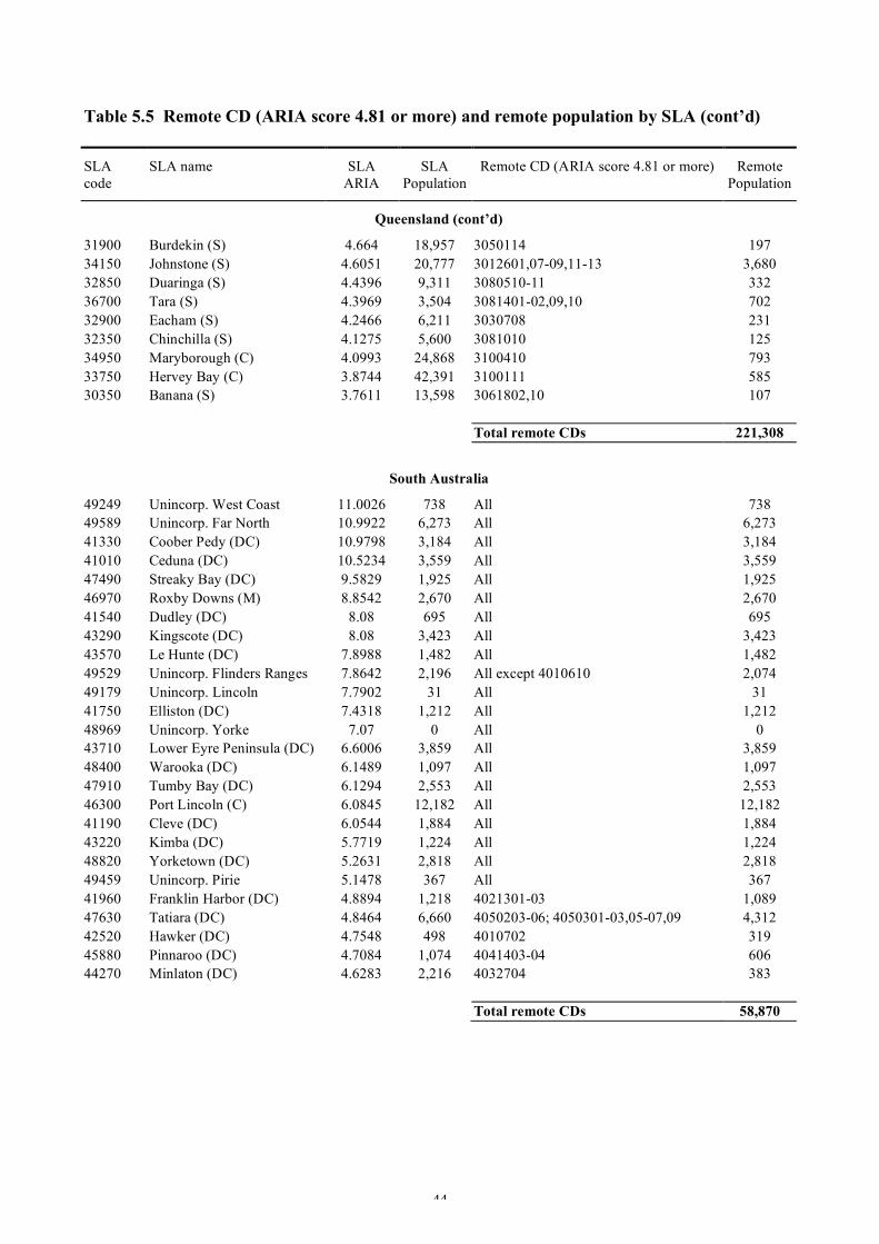
44

Table 5.5 Remote CD (ARIA score 4.81 or more) and remote population by SLA (cont’d) SLA code

SLA name SLA ARIA

SLA Population

Remote CD (ARIA score 4.81 or more) Remote Population

Queensland (cont’d)

31900 Burdekin (S) 4.664 18,957 3050114 197 34150 Johnstone (S) 4.6051 20,777 3012601,07-09,11-13 3,680 32850 Duaringa (S) 4.4396 9,311 3080510-11 332 36700 Tara (S) 4.3969 3,504 3081401-02,09,10 702 32900 Eacham (S) 4.2466 6,211 3030708 231 32350 Chinchilla (S) 4.1275 5,600 3081010 125 34950 Maryborough (C) 4.0993 24,868 3100410 793 33750 Hervey Bay (C) 3.8744 42,391 3100111 585 30350 Banana (S) 3.7611 13,598 3061802,10 107 Total remote CDs 221,308

South Australia

49249 Unincorp. West Coast 11.0026 738 All 738 49589 Unincorp. Far North 10.9922 6,273 All 6,273 41330 Coober Pedy (DC) 10.9798 3,184 All 3,184 41010 Ceduna (DC) 10.5234 3,559 All 3,559 47490 Streaky Bay (DC) 9.5829 1,925 All 1,925 46970 Roxby Downs (M) 8.8542 2,670 All 2,670 41540 Dudley (DC) 8.08 695 All 695 43290 Kingscote (DC) 8.08 3,423 All 3,423 43570 Le Hunte (DC) 7.8988 1,482 All 1,482 49529 Unincorp. Flinders Ranges 7.8642 2,196 All except 4010610 2,074 49179 Unincorp. Lincoln 7.7902 31 All 31 41750 Elliston (DC) 7.4318 1,212 All 1,212 48969 Unincorp. Yorke 7.07 0 All 0 43710 Lower Eyre Peninsula (DC) 6.6006 3,859 All 3,859 48400 Warooka (DC) 6.1489 1,097 All 1,097 47910 Tumby Bay (DC) 6.1294 2,553 All 2,553 46300 Port Lincoln (C) 6.0845 12,182 All 12,182 41190 Cleve (DC) 6.0544 1,884 All 1,884 43220 Kimba (DC) 5.7719 1,224 All 1,224 48820 Yorketown (DC) 5.2631 2,818 All 2,818 49459 Unincorp. Pirie 5.1478 367 All 367 41960 Franklin Harbor (DC) 4.8894 1,218 4021301-03 1,089 47630 Tatiara (DC) 4.8464 6,660 4050203-06; 4050301-03,05-07,09 4,312 42520 Hawker (DC) 4.7548 498 4010702 319 45880 Pinnaroo (DC) 4.7084 1,074 4041403-04 606 44270 Minlaton (DC) 4.6283 2,216 4032704 383 Total remote CDs 58,870

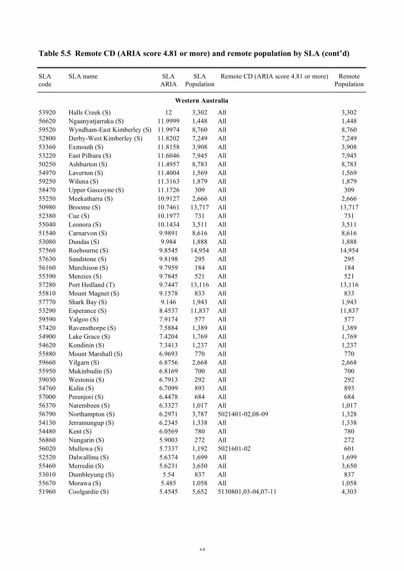
45

Table 5.5 Remote CD (ARIA score 4.81 or more) and remote population by SLA (cont’d) SLA code

SLA name SLA ARIA

SLA Population

Remote CD (ARIA score 4.81 or more) Remote Population

Western Australia

53920 Halls Creek (S) 12 3,302 All 3,302 56620 Ngaanyatjarraku (S) 11.9999 1,448 All 1,448 59520 Wyndham-East Kimberley (S) 11.9974 8,760 All 8,760 52800 Derby-West Kimberley (S) 11.8202 7,249 All 7,249 53360 Exmouth (S) 11.8158 3,908 All 3,908 53220 East Pilbara (S) 11.6046 7,945 All 7,945 50250 Ashburton (S) 11.4957 8,783 All 8,783 54970 Laverton (S) 11.4004 1,569 All 1,569 59250 Wiluna (S) 11.3163 1,879 All 1,879 58470 Upper Gascoyne (S) 11.1726 309 All 309 55250 Meekatharra (S) 10.9127 2,666 All 2,666 50980 Broome (S) 10.7461 13,717 All 13,717 52380 Cue (S) 10.1977 731 All 731 55040 Leonora (S) 10.1434 3,511 All 3,511 51540 Carnarvon (S) 9.9891 8,616 All 8,616 53080 Dundas (S) 9.984 1,888 All 1,888 57560 Roebourne (S) 9.8545 14,954 All 14,954 57630 Sandstone (S) 9.8198 295 All 295 56160 Murchison (S) 9.7959 184 All 184 55390 Menzies (S) 9.7845 521 All 521 57280 Port Hedland (T) 9.7447 13,116 All 13,116 55810 Mount Magnet (S) 9.1578 833 All 833 57770 Shark Bay (S) 9.146 1,943 All 1,943 53290 Esperance (S) 8.4537 11,837 All 11,837 59590 Yalgoo (S) 7.9174 577 All 577 57420 Ravensthorpe (S) 7.5884 1,389 All 1,389 54900 Lake Grace (S) 7.4204 1,769 All 1,769 54620 Kondinin (S) 7.3413 1,237 All 1,237 55880 Mount Marshall (S) 6.9693 770 All 770 59660 Yilgarn (S) 6.8756 2,668 All 2,668 55950 Mukinbudin (S) 6.8169 700 All 700 59030 Westonia (S) 6.7913 292 All 292 54760 Kulin (S) 6.7099 893 All 893 57000 Perenjori (S) 6.4478 684 All 684 56370 Narembeen (S) 6.3327 1,017 All 1,017 56790 Northampton (S) 6.2971 3,787 5021401-02,08-09 1,328 54130 Jerramungup (S) 6.2345 1,338 All 1,338 54480 Kent (S) 6.0569 780 All 780 56860 Nungarin (S) 5.9003 272 All 272 56020 Mullewa (S) 5.7337 1,192 5021601-02 601 52520 Dalwallinu (S) 5.6374 1,699 All 1,699 55460 Merredin (S) 5.6231 3,650 All 3,650 53010 Dumbleyung (S) 5.54 837 All 837 55670 Morawa (S) 5.485 1,058 All 1,058 51960 Coolgardie (S) 5.4545 5,652 5130801,03-04,07-11 4,303

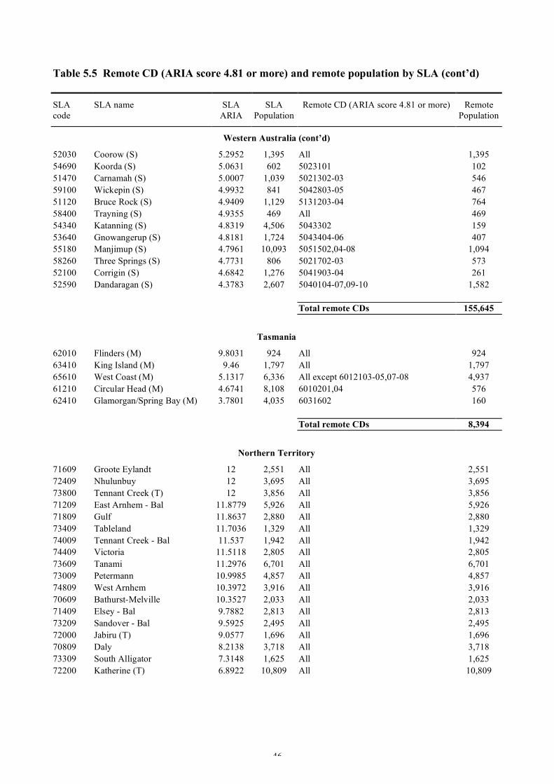
46

Table 5.5 Remote CD (ARIA score 4.81 or more) and remote population by SLA (cont’d) SLA code

SLA name SLA ARIA

SLA Population

Remote CD (ARIA score 4.81 or more) Remote Population

Western Australia (cont’d)

52030 Coorow (S) 5.2952 1,395 All 1,395 54690 Koorda (S) 5.0631 602 5023101 102 51470 Carnamah (S) 5.0007 1,039 5021302-03 546 59100 Wickepin (S) 4.9932 841 5042803-05 467 51120 Bruce Rock (S) 4.9409 1,129 5131203-04 764 58400 Trayning (S) 4.9355 469 All 469 54340 Katanning (S) 4.8319 4,506 5043302 159 53640 Gnowangerup (S) 4.8181 1,724 5043404-06 407 55180 Manjimup (S) 4.7961 10,093 5051502,04-08 1,094 58260 Three Springs (S) 4.7731 806 5021702-03 573 52100 Corrigin (S) 4.6842 1,276 5041903-04 261 52590 Dandaragan (S) 4.3783 2,607 5040104-07,09-10 1,582 Total remote CDs 155,645

Tasmania

62010 Flinders (M) 9.8031 924 All 924 63410 King Island (M) 9.46 1,797 All 1,797 65610 West Coast (M) 5.1317 6,336 All except 6012103-05,07-08 4,937 61210 Circular Head (M) 4.6741 8,108 6010201,04 576 62410 Glamorgan/Spring Bay (M) 3.7801 4,035 6031602 160 Total remote CDs 8,394

Northern Territory

71609 Groote Eylandt 12 2,551 All 2,551 72409 Nhulunbuy 12 3,695 All 3,695 73800 Tennant Creek (T) 12 3,856 All 3,856 71209 East Arnhem - Bal 11.8779 5,926 All 5,926 71809 Gulf 11.8637 2,880 All 2,880 73409 Tableland 11.7036 1,329 All 1,329 74009 Tennant Creek - Bal 11.537 1,942 All 1,942 74409 Victoria 11.5118 2,805 All 2,805 73609 Tanami 11.2976 6,701 All 6,701 73009 Petermann 10.9985 4,857 All 4,857 74809 West Arnhem 10.3972 3,916 All 3,916 70609 Bathurst-Melville 10.3527 2,033 All 2,033 71409 Elsey - Bal 9.7882 2,813 All 2,813 73209 Sandover - Bal 9.5925 2,495 All 2,495 72000 Jabiru (T) 9.0577 1,696 All 1,696 70809 Daly 8.2138 3,718 All 3,718 73309 South Alligator 7.3148 1,625 All 1,625 72200 Katherine (T) 6.8922 10,809 All 10,809

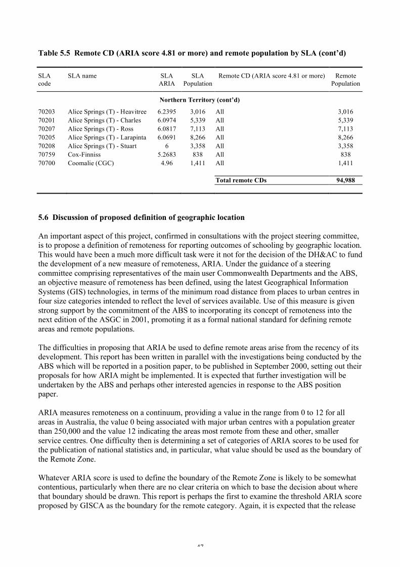
47

Table 5.5 Remote CD (ARIA score 4.81 or more) and remote population by SLA (cont’d) SLA code

SLA name SLA ARIA

SLA Population

Remote CD (ARIA score 4.81 or more) Remote Population

Northern Territory (cont’d)

70203 Alice Springs (T) - Heavitree 6.2395 3,016 All 3,016 70201 Alice Springs (T) - Charles 6.0974 5,339 All 5,339 70207 Alice Springs (T) - Ross 6.0817 7,113 All 7,113 70205 Alice Springs (T) - Larapinta 6.0691 8,266 All 8,266 70208 Alice Springs (T) - Stuart 6 3,358 All 3,358 70759 Cox-Finniss 5.2683 838 All 838 70700 Coomalie (CGC) 4.96 1,411 All 1,411 Total remote CDs 94,988 5.6 Discussion of proposed definition of geographic location An important aspect of this project, confirmed in consultations with the project steering committee, is to propose a definition of remoteness for reporting outcomes of schooling by geographic location. This would have been a much more difficult task were it not for the decision of the DH&AC to fund the development of a new measure of remoteness, ARIA. Under the guidance of a steering committee comprising representatives of the main user Commonwealth Departments and the ABS, an objective measure of remoteness has been defined, using the latest Geographical Information Systems (GIS) technologies, in terms of the minimum road distance from places to urban centres in four size categories intended to reflect the level of services available. Use of this measure is given strong support by the commitment of the ABS to incorporating its concept of remoteness into the next edition of the ASGC in 2001, promoting it as a formal national standard for defining remote areas and remote populations. The difficulties in proposing that ARIA be used to define remote areas arise from the recency of its development. This report has been written in parallel with the investigations being conducted by the ABS which will be reported in a position paper, to be published in September 2000, setting out their proposals for how ARIA might be implemented. It is expected that further investigation will be undertaken by the ABS and perhaps other interested agencies in response to the ABS position paper. ARIA measures remoteness on a continuum, providing a value in the range from 0 to 12 for all areas in Australia, the value 0 being associated with major urban centres with a population greater than 250,000 and the value 12 indicating the areas most remote from these and other, smaller service centres. One difficulty then is determining a set of categories of ARIA scores to be used for the publication of national statistics and, in particular, what value should be used as the boundary of the Remote Zone. Whatever ARIA score is used to define the boundary of the Remote Zone is likely to be somewhat contentious, particularly when there are no clear criteria on which to base the decision about where that boundary should be drawn. This report is perhaps the first to examine the threshold ARIA score proposed by GISCA as the boundary for the remote category. Again, it is expected that the release

48

of the ABS position paper will lead to further consideration of this issue. Most importantly, the ABS will itself need to determine how it will define the remote population and, where appropriate, how it will select samples to ensure adequate representation of the remote population in national surveys. The developers of ARIA propose an ARIA score of 5.80 as the lower boundary value for the Remote Zone, based on three factors: natural breaks in the data; balance across categories; and broad compatibility with RRMA. A revised boundary value of 4.805 is suggested here on the basis of two factors: greater emphasis on comparability with the SLAs and the size of the population defined as remote under the RRMA classification; and, although remote areas are defined by CDs rather than SLAs, adjust the boundary value to limit the splitting of SLAs by the remote boundary, to minimise the loss of accuracy in estimating the resident population of remote areas. This report then recommends the use of ARIA to define the remote population, and suggests that the boundary score of 4.805 be used to define remote areas in preference to the value of 5.80 proposed by GISCA. However, a final decision on the precise definition of a Remote Zone should await the outcome of the ABS consultation process and be consistent with any national standards that arise from it. It is important to emphasise that the choice of a particular ARIA value as the boundary of the Remote Zone is somewhat arbitrary at this stage, being based primarily on comparability with RRMA rather than any previously identified important differences in schooling outcomes. Indeed, unless the ABS does decide on a particular value as a national standard for the definition of remoteness, precise definition should perhaps be avoided. Rather, the emphasis should be on identifying more precisely than in the past the association between remoteness (from large urban centres) and outcomes. It would in any case be useful to use the data collected in surveys of achievement in literacy and numeracy to examine the extent that outcomes are associated with ARIA scores, before grouping the data into geographic categories. There may, for example, be significant variation in outcomes within the Other Provincial areas category defined above, in which case it could be subdivided into two or perhaps three categories to better illustrate the association in national statistics. Having access to ARIA index values, rather than fixed location categories, allows much greater flexibility in the use of geographic location data for analysis and the definition of geographic location categories for reporting. A requirement of achieving this flexibility is that it is possible to link the outcomes data from surveys and administrative collections with the measure of geographic location at the individual student level, at least for secondary students living outside the metropolitan and provincial city regions (see Section 5.4 above). For measures based on internal testing procedures, schools then need to assign ARIA scores to these students, based on the locality of their home address, and link those scores to test data used to derive state-wide outcome measures. Where outcome measures are derived from external surveys such as the LSAY or PISA, a question will need to be included in the questionnaire to allow the ARIA score to be derived, for example:

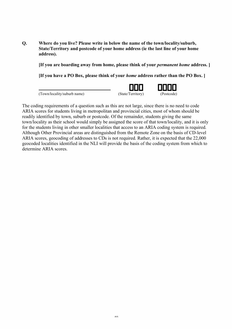
49

Q. Where do you live? Please write in below the name of the town/locality/suburb, State/Territory and postcode of your home address (ie the last line of your home address). [If you are boarding away from home, please think of your permanent home address. ] [If you have a PO Box, please think of your home address rather than the PO Box. ] � � � � � � � (Town/locality/suburb name) (State/Territory) (Postcode)

The coding requirements of a question such as this are not large, since there is no need to code ARIA scores for students living in metropolitan and provincial cities, most of whom should be readily identified by town, suburb or postcode. Of the remainder, students giving the same town/locality as their school would simply be assigned the score of that town/locality, and it is only for the students living in other smaller localities that access to an ARIA coding system is required. Although Other Provincial areas are distinguished from the Remote Zone on the basis of CD-level ARIA scores, geocoding of addresses to CDs is not required. Rather, it is expected that the 22,000 geocoded localities identified in the NLI will provide the basis of the coding system from which to determine ARIA scores.

50

References Ainley, J., Jones, W. and Navaratnam, K. K. (1990), Subject Choice in Senior Secondary School.

Canberra: AGPS Ainley J. and McKenzie, P. (1991), ‘Participation by Disadvantaged Young People in Post-

Compulsory Education and Training’, in Australian Education Council Review Committee (1991), Young People’s Participation in Post-Compulsory Education and Training, Volume 3, Appendix 2, Commissioned Reports. Canberra: AGPS

Ainley, J., Robinson, R., Harvey-Beavis, A., Elsworth, G. and Fleming, M. (1994), Subject Choice

in Years 11 and 12. Canberra: AGPS Ainley, J. and Long, M (1995), ‘Other Aspects of Area-Based Indexes’, Chapter 5 in Ainley, J.,

Greatz, B, Long, M. and Batten, M (1995), Socioeconomic Status and School Education. Canberra: AGPS

Arundell, L. (1991), Rural, Remote and Metropolitan Zones Classification: A Classification for

Australia as at 30 June 1986 and a Methodology for 1991 Census Data. Canberra: Rural and Provincial Policy Unit, Department of Primary Industries and Energy

Australian Bureau of Statistics (1996), Statistical Geography: Volume 1 Australian Standard

Geographical Classification (ASGC). Canberra: ABS Australian Bureau of Statistics (1998), Schools. Canberra: ABS Clarke, B. N. R. (1987), ‘Rural postsecondary education: a report to a working party of the Tertiary

Education Commission’. Canberra: CTEC Commonwealth Working Group on Review of Rural Data (1992), Rural Data. Canberra: DPIE Department of Employment, Education and Training (1987), Completing Secondary School in

Australia: a socio-economic and regional analysis. Canberra: DEET Department of Employment, Education, Training and Youth Affairs (1997), ‘Geographical

Location’. A paper prepared for consideration by TOSS and the ANR Sub-group Department of Education, Training and Youth Affairs (1999a), ‘Equity in Higher Education’,

Higher Education Division Occasional Paper Series 99-A. Canberra: DETYA Department of Education, Training and Youth Affairs (1999b), Higher Education Report for the

1999 to 2001 Triennium. Canberra: DETYA Department of Health and Aged Care (1999), ‘Measuring Remoteness: Accessibility/Remoteness

Index of Australia (ARIA)’, Department of Health and Aged Care Occasional Papers: New Series No. 6. Canberra: DH&AC

Department of Primary Industries and Energy and Department of Human Services and Health

(1994), Rural, Remote and Metropolitan Areas Classification 1991 Census Edition. Canberra: DPIE

51

Grewal, B., Davenport, P., Puno, F., Sheehan, P. and Kumnick, M. (1996), Review of Methodology

for the Distribution of Funding under the Country Areas General Component (CAGC) of the National Equity Program for Schools. Canberra: AGPS

Griffith, D (1997), ‘Classification of Geographical Locations’. A paper prepared for consideration

by TOSS and the ANR Sub-group Higher Education Council (1996), Equality, Diversity and Excellence: Advancing the National

Equity Framework. Canberra: AGPS Lamb, S. (1996), ‘Completing School in Australia: Trends in the 1990s’, LSAY Research Report

Number 1. Melbourne: ACER Lamb, S., Long, M. and Malley, J. (1998), Access and Equity in Vocational Education and

Training: Results from longitudinal surveys of Australian youth, ACER Research Monograph No. 55. Melbourne: ACER

Long, M., Carpenter, P. and Hayden, M. (1999), ‘Participation in Education and Training 1980 -

1994’, LSAY Research Report Number 13. Melbourne: ACER Marks, G. N. and Fleming, N. (1999) ‘Early School Leaving in Australia: Findings from the 1995

Year 9 LSAY Cohort’, LSAY Research Report Number 11. Melbourne: ACER Martin, L. M. (1994), Equity and General Performance Indicators in Higher Education, Volume 1,

Equity Indicators. Canberra: AGPS Millwood, J. (1989), Rural and Remote Areas within Australia: A State-based Regional

Classification. Canberra: Department of Community Services and Health Ministerial Council on Education, Employment, Training and Youth Affairs (1996), National

Report on Schooling in Australia 1996. Melbourne: MCEETYA National Board of Employment, Education and Training (1990), Country Areas Program. Canberra:

AGPS Rousseaux, K. (1993), Rurality and Participation in Schooling. Melbourne: Australian Education

Council Rousseaux, K. (1995), Report on the Queensland Trial of the Griffith Service Access Frame

(GSAF). Brisbane: Information Services Branch, Department of Education, Queensland Smart, N., Burke, G. and McKenzie, P. (1999), ‘Development of a framework for key performance

measures of student participation, transition, retention and completion/attainment’, a report to the NEPMT, 21 December 1999.

Western, J., McMillan, J. and Durrington, D (1998), Differential Access to Higher Education: The

Measurement of Socioeconomic Status, Rurality and Isolation. Canberra: Evaluations and Investigations Program, Higher Education Division, DETYA

52

Williams, T., Long, M., Carpenter, P. and Hayden, M. (1993), Entering Higher Education in the 1980s. Canberra: AGPS

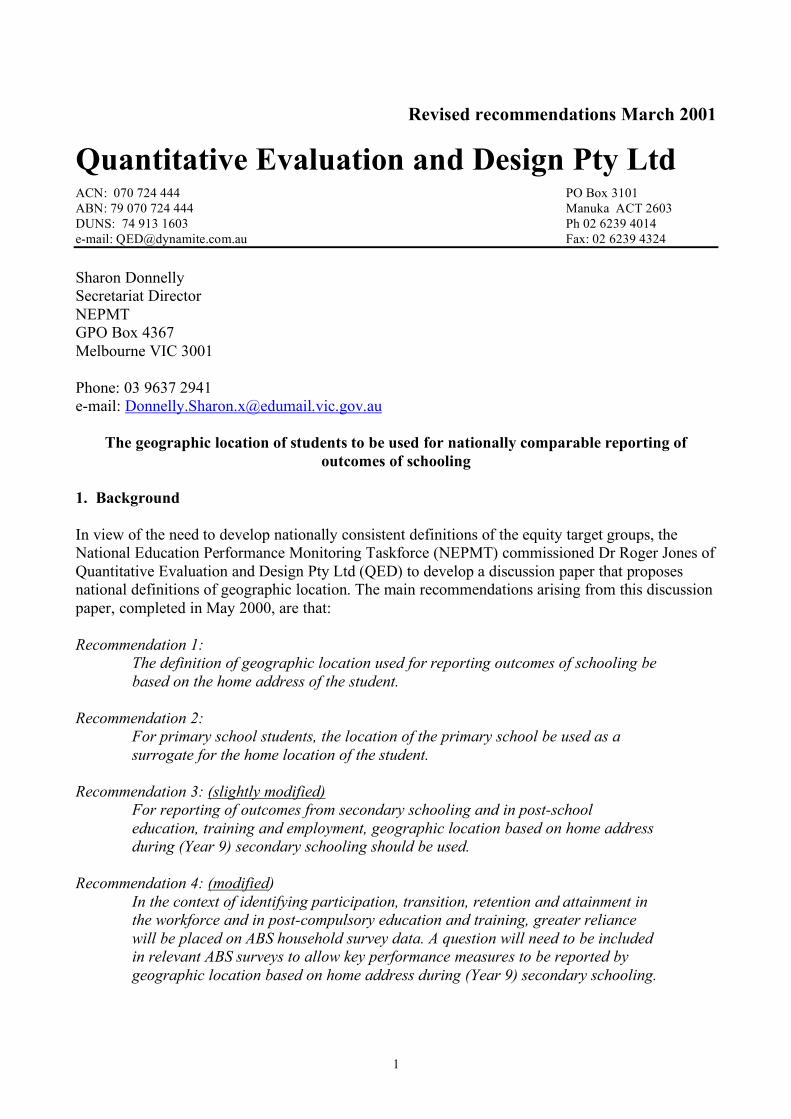
1

Revised recommendations March 2001

Quantitative Evaluation and Design Pty Ltd ACN: 070 724 444 PO Box 3101 ABN: 79 070 724 444 Manuka ACT 2603 DUNS: 74 913 1603 Ph 02 6239 4014 e-mail: QED@dynamite.com.au Fax: 02 6239 4324 Sharon Donnelly Secretariat Director NEPMT GPO Box 4367 Melbourne VIC 3001 Phone: 03 9637 2941 e-mail: Donnelly.Sharon.x@edumail.vic.gov.au

The geographic location of students to be used for nationally comparable reporting of outcomes of schooling

1. Background In view of the need to develop nationally consistent definitions of the equity target groups, the National Education Performance Monitoring Taskforce (NEPMT) commissioned Dr Roger Jones of Quantitative Evaluation and Design Pty Ltd (QED) to develop a discussion paper that proposes national definitions of geographic location. The main recommendations arising from this discussion paper, completed in May 2000, are that: Recommendation 1:

The definition of geographic location used for reporting outcomes of schooling be based on the home address of the student.

Recommendation 2:

For primary school students, the location of the primary school be used as a surrogate for the home location of the student.

Recommendation 3: (slightly modified)

For reporting of outcomes from secondary schooling and in post-school education, training and employment, geographic location based on home address during (Year 9) secondary schooling should be used.

Recommendation 4: (modified)

In the context of identifying participation, transition, retention and attainment in the workforce and in post-compulsory education and training, greater reliance will be placed on ABS household survey data. A question will need to be included in relevant ABS surveys to allow key performance measures to be reported by geographic location based on home address during (Year 9) secondary schooling.

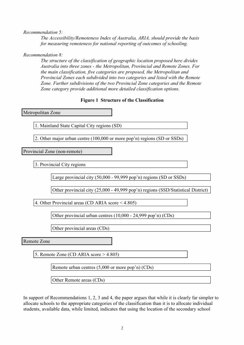
2

Recommendation 5: The Accessibility/Remoteness Index of Australia, ARIA, should provide the basis for measuring remoteness for national reporting of outcomes of schooling.

Recommendation 8:

The structure of the classification of geographic location proposed here divides Australia into three zones - the Metropolitan, Provincial and Remote Zones. For the main classification, five categories are proposed, the Metropolitan and Provincial Zones each subdivided into two categories and listed with the Remote Zone. Further subdivisions of the two Provincial Zone categories and the Remote Zone category provide additional more detailed classification options.

Figure 1 Structure of the Classification

Metropolitan Zone

1. Mainland State Capital City regions (SD)

2. Other major urban centre (100,000 or more pop’n) regions (SD or SSDs) Provincial Zone (non-remote)

3. Provincial City regions

Large provincial city (50,000 - 99,999 pop’n) regions (SD or SSDs)

Other provincial city (25,000 - 49,999 pop’n) regions (SSD/Statistical District)

4. Other Provincial areas (CD ARIA score < 4.805)

Other provincial urban centres (10,000 - 24,999 pop’n) (CDs)

Other provincial areas (CDs) Remote Zone

5. Remote Zone (CD ARIA score > 4.805)

Remote urban centres (5,000 or more pop’n) (CDs)

Other Remote areas (CDs) In support of Recommendations 1, 2, 3 and 4, the paper argues that while it is clearly far simpler to allocate schools to the appropriate categories of the classification than it is to allocate individual students, available data, while limited, indicates that using the location of the secondary school

3

attended during the compulsory years of schooling would understate the numbers of students from homes in rural and remote areas. Further, if the results of achievement testing in primary and secondary school during the compulsory years of schooling are to be compared by geographic location category, it is clearly desirable that, as far as is practically possible, primary and secondary students from the same areas are included in the same location category. In addition, counts of students derived using home location are more comparable with the ABS estimated resident population counts and thus provide a basis for the assessment of participation, whereas a greater degree of approximation would be involved using school location. Nevertheless, the wider geographic distribution of primary schools and their smaller catchment areas makes use of the primary school location rather than home location less problematic. It is considered that there would be very few cases where the definition of geographic location of primary school students on the basis of their home address or their primary school location would make any difference to their classification. Considerations of simplicity and practicality then suggest that, for reporting of achievement in the Year 3 and Year 5 literacy and numeracy testing by geographic location, the location of the primary school would be an acceptable surrogate for identifying the home location of primary school children. Investigation using information from the Longitudinal Survey of Australian Youth of the extent to which students from rural and remote areas relocate to more urban areas after completing their schooling show a clear pattern of net mobility away from the remote areas, smaller provincial cities and other provincial areas into the larger urban centres across all States and Territories. The use of ABS household survey data to derive measures of outcomes in post-compulsory education, training and employment by geographic location defined using current address may then underestimate the attainments of those with a rural/remote background. A measure of geographic ‘background’ is then required to accurately identify the variations in outcomes associated with it. In support of the classification proposed under Recommendations 5 and 8, the paper argues that there appears to be no strong requirement to change the basis for the definition of metropolitan areas that has been used for some years, being implemented in the widely used DPIE/DHSH Rural, Remote and Metropolitan Areas (RRMA) Classification and which was itself based on the recommendations of the Commonwealth Working Group on Review of Rural Data (1992). Metropolitan areas are then defined by the Statistical Division (SD) or Statistical Sub-division (SSD) surrounding the mainland State capital cities and other major urban centres of 100,000 people or more. The classification extends this regional approach, based on the criteria applied by the ABS to define Statistical Districts, to include provincial cities of 25,000 or more population. This is similar, though not identical, to the classification of Large Rural Centres in the RRMA classification. Students living in and around urban centres of this size are not generally considered to be facing any disadvantage in schooling associated with geographic location, and their identification in a separate category should provide better discrimination of any differences in outcomes of the students from smaller urban centres and rural/remote areas. Beyond those areas in the immediate surrounds of the larger urban population centres, a new measure of remoteness, the Accessibility/Remoteness Index of Australia (ARIA) developed by the National Key Centre for Social Applications of Geographical Information Systems (GISCA) at the University of Adelaide on behalf of the Department of Health and Aged Care (DH&AC), is used to distinguish between Other provincial areas and the Remote Zone. Use of this measure is given strong support by the commitment of the ABS to incorporating its concept of remoteness into the

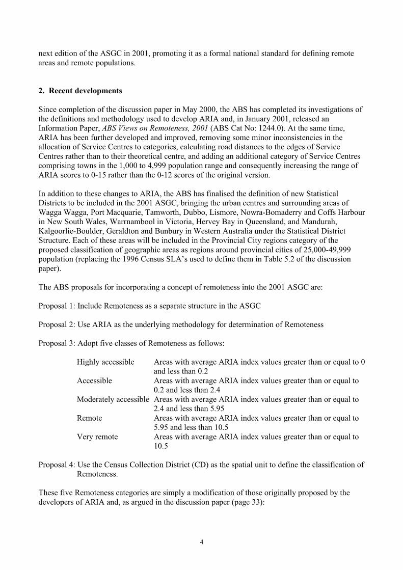
4

next edition of the ASGC in 2001, promoting it as a formal national standard for defining remote areas and remote populations. 2. Recent developments Since completion of the discussion paper in May 2000, the ABS has completed its investigations of the definitions and methodology used to develop ARIA and, in January 2001, released an Information Paper, ABS Views on Remoteness, 2001 (ABS Cat No: 1244.0). At the same time, ARIA has been further developed and improved, removing some minor inconsistencies in the allocation of Service Centres to categories, calculating road distances to the edges of Service Centres rather than to their theoretical centre, and adding an additional category of Service Centres comprising towns in the 1,000 to 4,999 population range and consequently increasing the range of ARIA scores to 0-15 rather than the 0-12 scores of the original version. In addition to these changes to ARIA, the ABS has finalised the definition of new Statistical Districts to be included in the 2001 ASGC, bringing the urban centres and surrounding areas of Wagga Wagga, Port Macquarie, Tamworth, Dubbo, Lismore, Nowra-Bomaderry and Coffs Harbour in New South Wales, Warrnambool in Victoria, Hervey Bay in Queensland, and Mandurah, Kalgoorlie-Boulder, Geraldton and Bunbury in Western Australia under the Statistical District Structure. Each of these areas will be included in the Provincial City regions category of the proposed classification of geographic areas as regions around provincial cities of 25,000-49,999 population (replacing the 1996 Census SLA’s used to define them in Table 5.2 of the discussion paper). The ABS proposals for incorporating a concept of remoteness into the 2001 ASGC are: Proposal 1: Include Remoteness as a separate structure in the ASGC Proposal 2: Use ARIA as the underlying methodology for determination of Remoteness Proposal 3: Adopt five classes of Remoteness as follows:

Highly accessible Areas with average ARIA index values greater than or equal to 0 and less than 0.2

Accessible Areas with average ARIA index values greater than or equal to 0.2 and less than 2.4

Moderately accessible Areas with average ARIA index values greater than or equal to 2.4 and less than 5.95

Remote Areas with average ARIA index values greater than or equal to 5.95 and less than 10.5

Very remote Areas with average ARIA index values greater than or equal to 10.5

Proposal 4: Use the Census Collection District (CD) as the spatial unit to define the classification of

Remoteness. These five Remoteness categories are simply a modification of those originally proposed by the developers of ARIA and, as argued in the discussion paper (page 33):

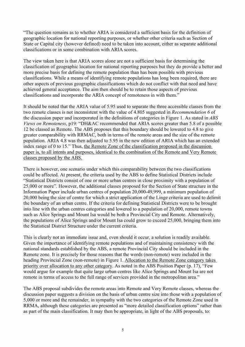
5

“The question remains as to whether ARIA is considered a sufficient basis for the definition of geographic location for national reporting purposes, or whether other criteria such as Section of State or Capital city (however defined) need to be taken into account, either as separate additional classifications or in some combination with ARIA scores. The view taken here is that ARIA scores alone are not a sufficient basis for determining the classification of geographic location for national reporting purposes but they do provide a better and more precise basis for defining the remote population than has been possible with previous classifications. While a means of identifying remote populations has long been required, there are other aspects of previous geographic classifications which do not conflict with that need and have achieved general acceptance. The aim then should be to retain those aspects of previous classifications and incorporate the ARIA concept of remoteness in with them.” It should be noted that the ARIA value of 5.95 used to separate the three accessible classes from the two remote classes is not inconsistent with the value of 4.805 suggested in Recommendation 6 of the discussion paper and incorporated in the definitions of categories in Figure 1. As stated in ABS Views on Remoteness, p19: “DH&AC recommended that ARIA scores greater than 5.8 of a possible 12 be classed as Remote. The ABS proposes that this boundary should be lowered to 4.8 to give greater comparability with RRMAC, both in terms of the remote areas and the size of the remote population. ARIA 4.8 was then adjusted to 5.95 in the new edition of ARIA which has an extended index range of 0 to 15.” Thus, the Remote Zone of the classification proposed in the discussion paper is, to all intents and purposes, identical to the combination of the Remote and Very Remote classes proposed by the ABS. There is however, one scenario under which this comparability between the two classifications could be affected. At present, the criteria used by the ABS to define Statistical Districts include “Statistical Districts consist of one or more urban centres in close proximity with a population of 25,000 or more”. However, the additional classes proposed for the Section of State structure in the Information Paper include urban centres of population 20,000-49,999, a minimum population of 20,000 being the size of centre for which a strict application of the Linge criteria are used to delimit the boundary of an urban centre. If the criteria for defining Statistical Districts were to be brought into line with the urban centres categories and lowered to a population of 20,000, remote towns such as Alice Springs and Mount Isa would be both a Provincial City and Remote. Alternatively, the populations of Alice Springs and/or Mount Isa could grow to exceed 25,000, bringing them into the Statistical District Structure under the current criteria. This is clearly not an immediate issue and, even should it occur, a solution is readily available. Given the importance of identifying remote populations and of maintaining consistency with the national standards established by the ABS, a remote Provincial City should be included in the Remote zone. It is precisely for those reasons that the words (non-remote) were included in the heading Provincial Zone (non-remote) in Figure 1. Allocation to the Remote Zone category takes priority over allocation to any other category. As noted in the ABS Position Paper (p. 17), “Few would argue for example that quite large urban centres like Alice Springs and Mount Isa are not remote in terms of access to the full range of services provided in the metropolitan area.” The ABS proposal subdivides the remote areas into Remote and Very Remote classes, whereas the discussion paper suggests a division on the basis of urban centre size into those with a population of 5,000 or more and the remainder, in sympathy with the two categories of the Remote Zone used in RRMA, although these categories are presented as “more detailed classification options” rather than as part of the main classification. It may then be appropriate, in light of the ABS proposals, to:

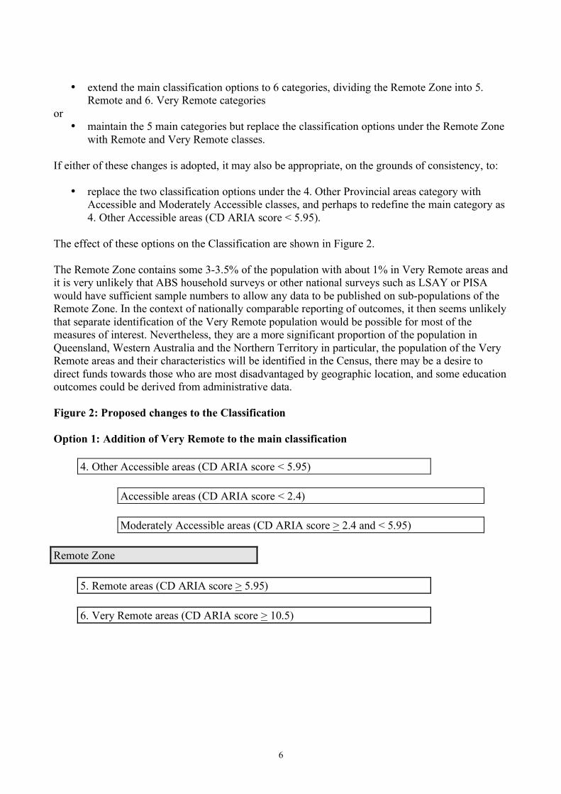
6

• extend the main classification options to 6 categories, dividing the Remote Zone into 5.

Remote and 6. Very Remote categories or

• maintain the 5 main categories but replace the classification options under the Remote Zone with Remote and Very Remote classes.

If either of these changes is adopted, it may also be appropriate, on the grounds of consistency, to:

• replace the two classification options under the 4. Other Provincial areas category with Accessible and Moderately Accessible classes, and perhaps to redefine the main category as 4. Other Accessible areas (CD ARIA score < 5.95).

The effect of these options on the Classification are shown in Figure 2. The Remote Zone contains some 3-3.5% of the population with about 1% in Very Remote areas and it is very unlikely that ABS household surveys or other national surveys such as LSAY or PISA would have sufficient sample numbers to allow any data to be published on sub-populations of the Remote Zone. In the context of nationally comparable reporting of outcomes, it then seems unlikely that separate identification of the Very Remote population would be possible for most of the measures of interest. Nevertheless, they are a more significant proportion of the population in Queensland, Western Australia and the Northern Territory in particular, the population of the Very Remote areas and their characteristics will be identified in the Census, there may be a desire to direct funds towards those who are most disadvantaged by geographic location, and some education outcomes could be derived from administrative data. Figure 2: Proposed changes to the Classification Option 1: Addition of Very Remote to the main classification

4. Other Accessible areas (CD ARIA score < 5.95)

Accessible areas (CD ARIA score < 2.4)

Moderately Accessible areas (CD ARIA score > 2.4 and < 5.95) Remote Zone

5. Remote areas (CD ARIA score > 5.95)

6. Very Remote areas (CD ARIA score > 10.5)

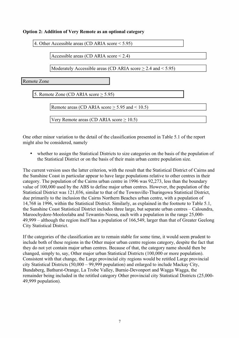
7

Option 2: Addition of Very Remote as an optional category

4. Other Accessible areas (CD ARIA score < 5.95)

Accessible areas (CD ARIA score < 2.4)

Moderately Accessible areas (CD ARIA score > 2.4 and < 5.95) Remote Zone

5. Remote Zone (CD ARIA score > 5.95)

Remote areas (CD ARIA score > 5.95 and < 10.5)

Very Remote areas (CD ARIA score > 10.5) One other minor variation to the detail of the classification presented in Table 5.1 of the report might also be considered, namely

• whether to assign the Statistical Districts to size categories on the basis of the population of the Statistical District or on the basis of their main urban centre population size.

The current version uses the latter criterion, with the result that the Statistical District of Cairns and the Sunshine Coast in particular appear to have large populations relative to other centres in their category. The population of the Cairns urban centre in 1996 was 92,273, less than the boundary value of 100,000 used by the ABS to define major urban centres. However, the population of the Statistical District was 121,036, similar to that of the Townsville-Thuringowa Statistical District, due primarily to the inclusion the Cairns Northern Beaches urban centre, with a population of 14,768 in 1996, within the Statistical District. Similarly, as explained in the footnote to Table 5.1, the Sunshine Coast Statistical District includes three large, but separate urban centres – Caloundra, Maroochydore-Mooloolaba and Tewantin-Noosa, each with a population in the range 25,000-49,999 – although the region itself has a population of 166,549, larger than that of Greater Geelong City Statistical District. If the categories of the classification are to remain stable for some time, it would seem prudent to include both of these regions in the Other major urban centre regions category, despite the fact that they do not yet contain major urban centres. Because of that, the category name should then be changed, simply to, say, Other major urban Statistical Districts (100,000 or more population). Consistent with that change, the Large provincial city regions would be retitled Large provincial city Statistical Districts (50,000 – 99,999 population) and enlarged to include Mackay City, Bundaberg, Bathurst-Orange, La Trobe Valley, Burnie-Devonport and Wagga Wagga, the remainder being included in the retitled category Other provincial city Statistical Districts (25,000-49,999 population).

8

3. Implementation of the Classification Recommendations 2,3 and 4 above each relate to implementation of the classification in general, but the major issue in this regard is likely to be in the detail of coding a particular individual to the appropriate category of the classification. One of the major advantages of the regional aspect of the classification is that approximately 80% of the population are included in the metropolitan and provincial city Statistical Districts defined by aggregates of Statistical Local Areas (SLAs), leaving only 20% of the population to be assigned to categories of Remoteness on the basis of CD ARIA scores as proposed by the ABS. Tests that have been carried out to date using the name of the town/locality/suburb, State/Territory and postcode of home address of the 1995 and 1998 cohort samples of Year 9 students from the Longitudinal Survey of Australian Youth (LSAY) surveys indicate that there are relatively few problems in assigning students to their appropriate geographic location category. For the most part, addresses can be assigned to their location category on the basis of postcode alone. Where postcodes are missing, they can usually be identified by checking the town/locality name against an electronic version of the listing of postcodes by locality included in the White Pages telephone directory or by checking the locality name on the ABS National Localities Index (NLI). Where a postcode crosses location category boundaries, the town/locality name can be checked in the NLI to determine if it is included in an SLA which is within a metropolitan or provincial city region and thus can be assigned to a category directly. Only otherwise does the ARIA score of the town/locality need to be identified to determine whether the address should be assigned to the Other Accessible areas, Remote or Very remote categories. Current expectations are that the changes and improvements to ARIA will be completed in March 2001, when ABS will be provided with revised ARIA scores on a 1km grid. These scores will be used to derive CD scores and to generate locality scores for some 22,000 geocoded localities identified in the NLI. However, the ABS is not currently planning to develop any specialised coding software which could be used to assign addresses to the geographic location categories proposed here. In regard to Recommendation 9 of the discussion paper, the feasibility of coding secondary school student address data to geographic location codes has been demonstated with the LSAY data, at least to the researcher who proposed the classification and who has considerable expert knowledge of the linkage between postcodes, localities, SLAs and the location categories. However, if, as now, outcome measures are to be derived from a variety of data sources, the development of appropriate software to provide geographic location coding assistance should be given a high priority. In the case of any outcomes derived from ABS household surveys (Recommendation 4), the question will need to be retrospective, asking respondents to identify where they were living when they attended school, for example:

Q. Where were you living when you were in Year 9 at school? What was the name of the town/locality/suburb, State/Territory and postcode of your home address [If you were boarding away from home, please think of your permanent home address. ]

It is assumed that collection of this information would be limited to respondents who had left school quite recently and were now in their late teens or early twenties.

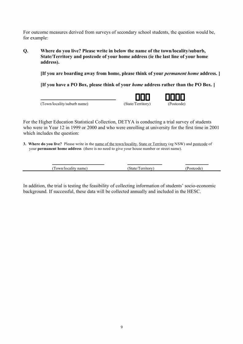
9

For outcome measures derived from surveys of secondary school students, the question would be, for example:

Q. Where do you live? Please write in below the name of the town/locality/suburb, State/Territory and postcode of your home address (ie the last line of your home address). [If you are boarding away from home, please think of your permanent home address. ] [If you have a PO Box, please think of your home address rather than the PO Box. ] � � � � � � � (Town/locality/suburb name) (State/Territory) (Postcode)

For the Higher Education Statistical Collection, DETYA is conducting a trial survey of students who were in Year 12 in 1999 or 2000 and who were enrolling at university for the first time in 2001 which includes the question: 3. Where do you live? Please write in the name of the town/locality, State or Territory (eg NSW) and postcode of

your permanent home address (there is no need to give your house number or street name). (Town/locality name) (State/Territory) (Postcode)

In addition, the trial is testing the feasibility of collecting information of students’ socio-economic background. If successful, these data will be collected annually and included in the HESC.

10

4. Final Recommendations incorporating recent developments Recommendation 1:

The definition of geographic location used for reporting outcomes of schooling should be based on the home address of the student. The information required is the town/locality, postcode and State/Territory of home address.

Recommendation 2:

For primary school students, the location of the primary school can be used as a surrogate for the home location of the student. For secondary school students, however, the use of school location would understate the numbers of students from homes in rural and remote areas.

Recommendation 3:

In the context of identifying participation, transition, retention and attainment in the workforce and in post-compulsory education and training, geographic location based on home address during (Year 9) secondary schooling should be used. Where reliance is placed on Australian Bureau of Statistics (ABS) household survey data, a question will need to be included in relevant ABS surveys to allow key performance measures to be reported by geographic location.

Recommendation 4:

ABS proposals for incorporating a concept of Remoteness based on the Accessibility/Remoteness Index of Australia (ARIA) into the 2001 Australian Standard Geographical Classification (ASGC) should provide the basis for measuring remoteness for national reporting of outcomes of schooling.

Recommendation 5:

The proposed structure of the classification of geographic location for national reporting of outcomes of schooling (Figure A) divides Australia into three zones - the Metropolitan, Provincial and Remote Zones. For the main classification, five categories are proposed, the Metropolitan and Provincial Zones each subdivided into two categories and listed with the Remote Zone. Further subdivisions of the two Provincial Zone categories and the Remote Zone category provide additional more detailed classification options.

Recommendation 6:

In most cases, postcode alone is sufficient to assign the location category. In other cases, the town/locality name is required to determine whether an address is within a metropolitan or provincial city region, or otherwise to determine the ARIA score needed to assign it to the Other Accessible areas or Remote Zone categories. If, as is now the case, outcome measures are to be derived from a variety of data sources, the development of appropriate software to provide geographic location coding assistance should be given a high priority.

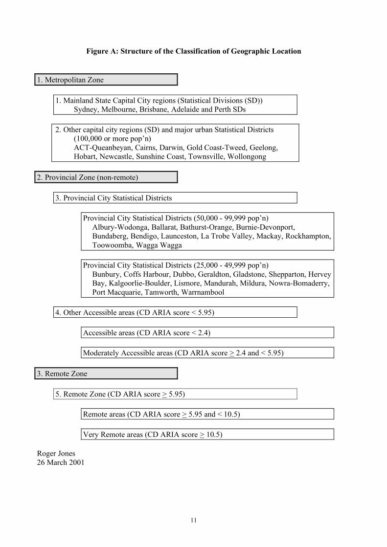
11

Figure A: Structure of the Classification of Geographic Location 1. Metropolitan Zone

1. Mainland State Capital City regions (Statistical Divisions (SD)) Sydney, Melbourne, Brisbane, Adelaide and Perth SDs

2. Other capital city regions (SD) and major urban Statistical Districts

(100,000 or more pop’n) ACT-Queanbeyan, Cairns, Darwin, Gold Coast-Tweed, Geelong, Hobart, Newcastle, Sunshine Coast, Townsville, Wollongong

2. Provincial Zone (non-remote)

3. Provincial City Statistical Districts

Provincial City Statistical Districts (50,000 - 99,999 pop’n) Albury-Wodonga, Ballarat, Bathurst-Orange, Burnie-Devonport, Bundaberg, Bendigo, Launceston, La Trobe Valley, Mackay, Rockhampton, Toowoomba, Wagga Wagga

Provincial City Statistical Districts (25,000 - 49,999 pop’n)

Bunbury, Coffs Harbour, Dubbo, Geraldton, Gladstone, Shepparton, Hervey Bay, Kalgoorlie-Boulder, Lismore, Mandurah, Mildura, Nowra-Bomaderry, Port Macquarie, Tamworth, Warrnambool

4. Other Accessible areas (CD ARIA score < 5.95)

Accessible areas (CD ARIA score < 2.4)

Moderately Accessible areas (CD ARIA score > 2.4 and < 5.95)

3. Remote Zone

5. Remote Zone (CD ARIA score > 5.95)

Remote areas (CD ARIA score > 5.95 and < 10.5)

Very Remote areas (CD ARIA score > 10.5) Roger Jones 26 March 2001