Development of A Boiling and Condensation Model on Subcooled Boiling … · 2017-01-17 · mechanism, a boiling and condensation model for numerical simulation on subcooled boiling

Energy Procedia 9 ( 2011 ) 605 – 618

1876-6102 © 2011 Published by Elsevier Ltd. Selection and/or peer-review under responsibility of CEO of Sustainable Energy System, Rajamangala University of Technology Thanyaburi (RMUTT).doi: 10.1016/j.egypro.2011.09.071

Available online at www.sciencedirect.com

9th Eco-Energy and Materials Science and Engineering Symposium

Development of A Boiling and Condensation Model on Subcooled Boiling Phenomena

Yasuo Osea* and Tomoaki Kunugia aDepartment of Nuclear Engineering, Kyoto University, Yoshida, Sakyo, Kyoto, 606-8501, Japan

Abstract

In this study, in order to clarify the heat transfer characteristics of the subcooled pool boiling and to discuss its mechanism, a boiling and condensation model for numerical simulation on subcooled boiling phenomenon has been developed. The developed boiling and condensation model consists of the improved phase-change model and the relaxation time based on the quasi-thermal equilibrium hypothesis. Three dimensional numerical simulations based on the MARS (Multi-interface Advection and Reconstruction Solver) with the developed boiling and condensation model have been conducted for a nucleated bubble growth process in the subcooled pool boiling. The numerical simulation results showed in good agreement with the experimental observations. Therefore, the developed boiling and condensation model is validated for the prediction of the subcooled pool boiling phenomena.

Ketword: Boiling and Condensation Model; Numerical Simulation; Bubble Growth; Relaxation Time; Subcooled Pool Boiling

1. Introduction

The nuclear technology is very important to the eco-energy system. Boiling phenomena is a key to remove the heat from the fuel rods in nuclear reactors such as BWR (Boiling Water Reactor) because the boiling heat transfer has most distinguished efficiency, which can be enormous heat transfer coefficient compared to the convective heat transfer of single-phase flows. It will also play a significant role of the power generation efficiency in nuclear reactors. Therefore, the mechanism of boiling phenomena has been studied extensively over the decades. This study focuses on the subcooled boiling phenomena. Since the subcooled pool boiling is occurred under a condition below the saturation temperature, it is the most

* Corresponding author. Tel.: +81-75-753-5328; fax: +81-75-753-5865. E-mail address: [email protected].

Open access under CC BY-NC-ND license.

© 2011 Published by Elsevier Ltd. Selection and/or peer-review under responsibility of CEO of Sustainable Energy System,

Rajamangala University of Technology Thanyaburi (RMUTT).

Open access under CC BY-NC-ND license.

http://creativecommons.org/licenses/by-nc-nd/3.0/

http://creativecommons.org/licenses/by-nc-nd/3.0/

606 Yasuo Ose and Tomoaki Kunugi / Energy Procedia 9 ( 2011 ) 605 – 618

complicated phenomenon, which includes not only the convective heat transfer but also the evaporation and condensation processes. Although the subcooled boiling is very important phenomena, the essential mechanism has not yet been clarified until today because the bubble nucleation and growth processes are too fast to observe even by means of the ultra-high-speed camera. Another approach to understand these processes is a numerical simulation.

Recently, with advances of computer power, numerical simulations for directly computing the bubble dynamics regarding the nucleate boiling have been performed by several investigators. For example, Son et al. [1] performed a numerical simulation of nucleate boiling at high wall superheats by employing the level set method. In their numerical simulation, it was assumed the saturated pool boiling conditions, which is not the subcooled boiling. On the other hand, Kunugi et al. [2] carried out three-dimensional pool and forced convective subcooled flow boiling by the direct numerical simulation based on the MARS (Multi-interface Advection and Reconstruction Solver) [3]. They showed the possibility of the subcooled boiling by the MARS.

This study focuses on the clarification of the heat transfer characteristics of the subcooled pool boiling, the discussion on its mechanism, and the development of a boiling and condensation model for numerical simulation on the subcooled boiling phenomena. In this paper, the boiling and condensation model is developed by introducing the following models based on the quasi-thermal equilibrium hypothesis; (1) a improved phase-change model which consisted of the enthalpy method for the water-vapor system, (2) a relaxation time derived by considering unsteady heat conduction. The numerical simulations based on the MARS with the developed boiling and condensation model have been conducted for the subcooled pool boiling, especially subjected to the bubble growth and condensation processes, and then the results of the bubble growth and condensation processes are compared with the experimental results [4].

Nomenclature

cp specific heat at constant pressure [J/(kg K)]

cv specific heat at constant volume [J/(kg K)]

F volume of fluid [-]

Fv body force vector [N/m3]

G gravity force vector [m/s2]

L latent heat of evaporation [J/kg]

P pressure [Pa]

Q heat source [W/m3]

u velocity vector [m/s]

T temperature [K]

TSH temperature of superheat limit [K]

TS liquid temperature contacted to the heated surface [K]

R ideal gas constant per unit mass basis [-]

t time or transition period [s]

Yasuo Ose and Tomoaki Kunugi / Energy Procedia 9 ( 2011 ) 605 – 618 607

t relaxation time [-]

Greek Letters

thermal diffusivity [m2/s]

ratio of specific heat [-]

thermal penetration length [m]

grid width [m]

g phase-change fraction as mass fraction [-]

gv phase-change fraction as volume fraction [-]

T degree of superheat or subcooling at interface [K]

Tsub degree of subcooling [K]

thermal conductivity [W/(m K)]

l volume of liquid per mass [m3/kg]

density [kg/m3]

surface tension [N/m]

viscous share stress [N/m2]

Subscripts

g gas phase

l liquid phase

m m-th fluid or phase

sat saturation condition

x x coordinates

y y coordinates

z z coordinates

2. Numerical Method of MARS

2.1. Governing Equation

As for m fluids including the gas and liquid, the spatial distribution of fluids can be defined as

0.1mFF (1)


Here, < > denotes an average of properties.

The governing equations in the MARS are the continuity equation for multi-phase flows, momentum equation based on a one-field model and the energy equation as follows:

0uu mmm FFt

F (2)

vPt

FGuuu 11, (3)

QPTTcTCvt v uu . (4)

The second term of the right hand side of the energy equation in Eq. (4), the Clausius-Clapeyron relation is considered as the external work done by the phase change.

The interface volume-tracking technique [3] is applied to the continuity equation in the MARS. The projection method [6] is applied to solve the momentum equation.

2.2. Boiling and Condensation Model

Nucleate boiling phenomena need to be modeled in order to simulate it numerically. The boiling and condensation model for the subcooled nucleate boiling consisted of a nucleation model and a bubble growth and condensation model. In the nucleation model, a homogeneous superheat limit of liquid, TSH gives the size of an embryo of the nucleation bubble. TSH can be obtained by the kinetic theory [7] or a cavity model in general. Typically, TSH for the saturated boiling is about 110 ˚C in the water pool boiling at the atmospheric pressure. A critical radius re of the embryo corresponding to TSH can be calculated by Eq. (5) based on thermodynamics. A computational cell having the liquid temperature over TSH can be given the VOF fraction of the embryo corresponding to the ratio between the cell size and the size of embryo where the shape of embryo is assumed to be a sphere. Although TSH may have the spatial variation on the heated surface according to the experiment [8], TSH is assumed to be uniform on the heated surface in the present study.

)(,/)(exp)(

2SHS

lllsatlllsate TT

PRTTPPvTPr . (5)

The bubble growth and condensation model [2] consists of the phase-change model based on the

temperature-recovery method [9], which was the improved enthalpy method. In the previous paper [2], this model is applied to only the cell has the VOF fraction of vapor phase. The phase-change fraction g is expressed as:

LTCg p / (6)


Moreover, the bubble growth and condensation model includes the expansion and contraction model to

consider the external work done by the volume expansion of bubble in Eq. (4). This work takes place only at the interface of bubble. Since an isentropic change of ideal gas ( rule gas) in bubble is assumed, the following thermodynamic relation can be applied.

gPPv = constant (7)

A change of density g is regarded as a change of specific volume v, and a rate of the volume change

v/v is assumed to be the same as a volume change because the interface density, ( g+ l)/2 is kept constant. Then, the variation of volume due to both volume expansion and contraction of a bubble with the change of pressure is modeled as follows:

PPP

vvF nn

g

g (8)


3. Numerical Simulation

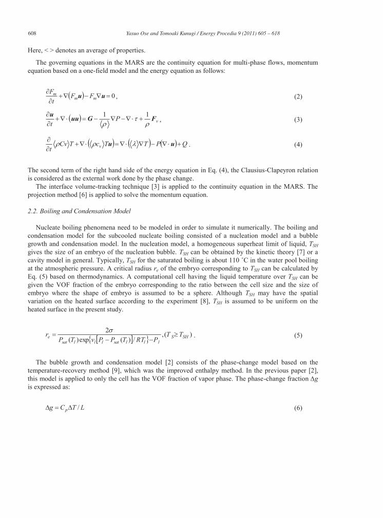
Three-dimensional numerical simulations of subcooled pool boiling are conducted in the present study, which condition is corresponding to the visualization experimental result of isolated vapor bubbles in the subcooled pool [4]. Figure 1 shows the time variation of bubble volume in the subcooled pool boiling obtained by the experiment. From the experimental results, the subcooled bubble behavior is consisted of following three processes as follows:

(1) Bubble growth process with the rapid expansion of embryo at inception boiling as shown in Fig. 1 (region I)

(2) Bubble equilibrium process caused by the balance between bubble buoyancy force and surface tension force as shown in Fig. 1 (region II)

(3) Bubble condensation process occurs after detaching from the heating surface as shown in Fig. 1 (region III)

In this study, since the scale ranges in time and space in each process are very large, two processes: (1) bubble growth and (3) bubble condensation processes are investigated in this paper.

0 0.5 1 1.5 20

0.1

0.2

0.3

0.4

0.5

Time [ms]

Bubb

le v

olum

e [m

m3 ]

I II III

Fig. 1. Time Variation of Bubble Volume in Subcooled Pool Boiling Obtained by Kawara et al., (2007).

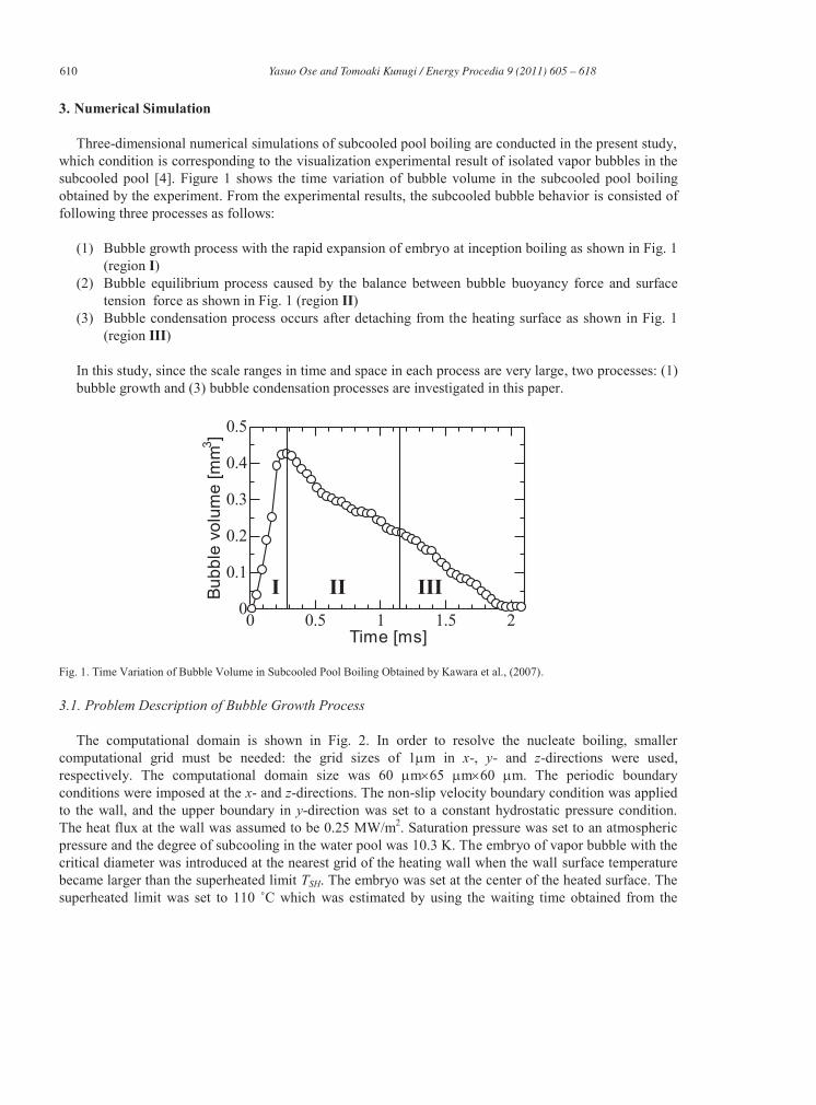
3.1. Problem Description of Bubble Growth Process

The computational domain is shown in Fig. 2. In order to resolve the nucleate boiling, smaller computational grid must be needed: the grid sizes of 1 m in x-, y- and z-directions were used, respectively. The computational domain size was 60 m 65 m 60 m. The periodic boundary conditions were imposed at the x- and z-directions. The non-slip velocity boundary condition was applied to the wall, and the upper boundary in y-direction was set to a constant hydrostatic pressure condition. The heat flux at the wall was assumed to be 0.25 MW/m2. Saturation pressure was set to an atmospheric pressure and the degree of subcooling in the water pool was 10.3 K. The embryo of vapor bubble with the critical diameter was introduced at the nearest grid of the heating wall when the wall surface temperature became larger than the superheated limit TSH. The embryo was set at the center of the heated surface. The superheated limit was set to 110 ˚C which was estimated by using the waiting time obtained from the


experimental data using unsteady heat conduction, so that the critical radius was about 3 m. Time increment in the computation was set to 10 ns.

Fig. 2. Computational Domain for Bubble Growth Process.

TSH =110˚C

Embryo of Vapor bubble: re = 3 m

Temperature [˚C]

Heat flux=0.25MW/m2 Heating surface

60 m

65m

60 m

G


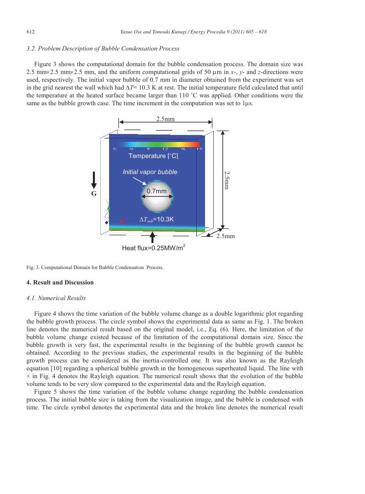
3.2. Problem Description of Bubble Condensation Process

Figure 3 shows the computational domain for the bubble condensation process. The domain size was 2.5 mm 2.5 mm 2.5 mm, and the uniform computational grids of 50 m in x-, y- and z-directions were used, respectively. The initial vapor bubble of 0.7 mm in diameter obtained from the experiment was set in the grid nearest the wall which had T= 10.3 K at rest. The initial temperature field calculated that until the temperature at the heated surface became larger than 110 ˚C was applied. Other conditions were the same as the bubble growth case. The time increment in the computation was set to 1 s.

Fig. 3. Computational Domain for Bubble Condensation Process.

4. Result and Discussion

4.1. Numerical Results

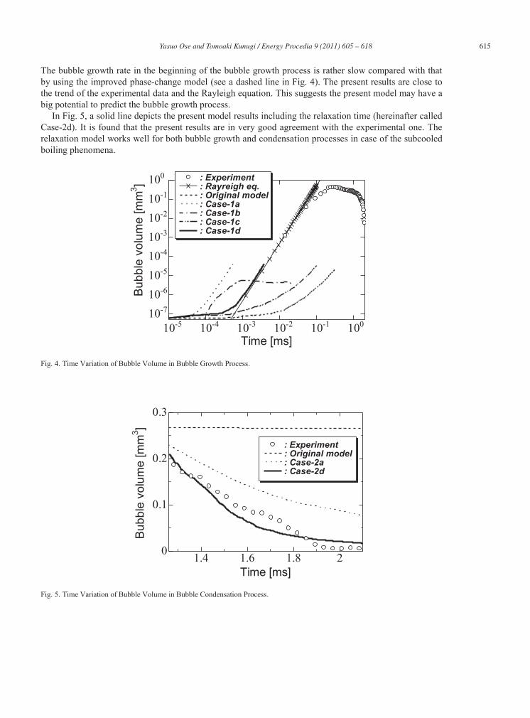
Figure 4 shows the time variation of the bubble volume change as a double logarithmic plot regarding the bubble growth process. The circle symbol shows the experimental data as same as Fig. 1. The broken line denotes the numerical result based on the original model, i.e., Eq. (6). Here, the limitation of the bubble volume change existed because of the limitation of the computational domain size. Since the bubble growth is very fast, the experimental results in the beginning of the bubble growth cannot be obtained. According to the previous studies, the experimental results in the beginning of the bubble growth process can be considered as the inertia-controlled one. It was also known as the Rayleigh equation [10] regarding a spherical bubble growth in the homogeneous superheated liquid. The line with × in Fig. 4 denotes the Rayleigh equation. The numerical result shows that the evolution of the bubble volume tends to be very slow compared to the experimental data and the Rayleigh equation.

Figure 5 shows the time variation of the bubble volume change regarding the bubble condensation process. The initial bubble size is taking from the visualization image, and the bubble is condensed with time. The circle symbol denotes the experimental data and the broken line denotes the numerical result

Temperature [˚C]

Initial vapor bubble

0.7mm

Tsub=10.3K

Heat flux=0.25MW/m2

2.5mm

2.5mm

2.5mm

G


based on the original model, i.e., Eq. (6). The numerical result based on the original phage-change model of evolving the bubble volume shows virtually constant compared to the experimental data, which is the same as the trend of bubble growth process.

4.2. Improvements of Boiling and Condensation Model

In order to solve these discrepancies, the characteristics of the phase-change model in the previous boiling and condensation model are reconsidered. The original phase-change model was expressed as Eq. (6). However, it was found that the original phase-change model could not treat a large volume expansion and condensation because the temperature-recovery method was developed for the small volume change problem such as a casting problem. In particular, the unit of both the numerator and denominator of the right hand side of Eq. (6) is J/kg, i.e., the mass fraction was taken as the phase-change fraction. Since the phase-change fraction g is considered as the equivalent to the change of VOF fraction, it must be the volume fraction not the mass fraction. In this paper, the density change at the phase-change process is treated as the volume change fraction gv as follows:

heatLatent heat Sensible

LTC

gg

pllv (9)

Equation (9) means that the ratio of sensible heat to latent heat, which form is similar to the Jacob

number, Ja. In order to satisfy the conservation of the volume, gv obtained by Eq. (9) can be considered as the following phase conservation equation:

1vgvl gFgF (10)

Using the improved phase-change model, the numerical simulations are conducted (hereinafter called

Case-1a for the bubble growth process and Case-2a for the bubble condensation process, respectively). In Figs. 4 and 5, a dashed line denote the numerical results obtained by the improved phase-change model. Although the results of both the bubble growth process (Case-1a in Fig. 4) and the bubble condensation process (Case-2a in Fig. 5) based on the present model are fairy improved compared to the original model (see a broken line in Figs. 4 and 5), the bubble growth rate is too fast compared to both the experimental data and the Rayleigh equation, and also the bubble condensation rate is not sufficient improvement compared to the experimental data.

For the investigation of the reason of these discrepancies, the effect of the initial temperature field on the bubble growth process was examined by changing the thickness of thermal boundary layer (hereinafter called Case-1b). Here, the thickness of thermal boundary layer was assumed by using an approximate solution of the unsteady heat conduction for the wall temperature = 110 ˚C, the bulk temperature = 89.3 ˚C and the transition period = 50 s: the thickness of thermal boundary layer was 10 m. From the result of Case-1b (see a single-dotted dashed line in Fig. 4), the rapid bubble growth is suppressed when the growing bubble expands into the subcooled layer; the bubble condensation immediately occurs because the superheated layer is very thin, and eventually the thin vapor film is formed on the heated surface. This means that the initial temperature field is very important for the bubble growth process. In order to find the dominant factor for the evaporation process of bubble, the numerical simulations which are focused on the evaporation regions at the bubble-wall interface near the


heated surface (hereinafter called Case-1c), i.e., the evaporation and condensation processes at other interface of the bubble except the bubble-wall interface region are neglected. From the result of Case-1c (see a double-dotted dashed line in Fig. 4), the bubble growth rate is very slow compared to the experimental data and the Rayleigh equation. This indicates that the evaporation at the bubble interface in the superheated layer is a dominant factor for the bubble growth process. From these results, it is found the followings: (1) the assumption of the initial temperature boundary layer and (2) the evaporation process at the bubble surface region of the superheated layer is extremely important to give a significant contribution to the bubble growth process. However, the numerical predictions are not coincident with the experimental data. The reason of this discrepancy might be considered that the current phase-change model based on the zero-thickness of bubble interface. In other words, the current phase-change model is modeled as (1) a “rapid” change of “State 1: Water” to “State 2: Vapor” or vice versa based on the quasi-thermal equilibrium hypothesis, but (2) a “very slow” change of “State 1” to “State 2” based on another feature of the quasi-thermal equilibrium hypothesis is ignored. In the reality, the finite thickness of interface exists, and both the “very slow” and “rapid” changes may simultaneously occur in the phase-change process. In order to consider a relaxation or waiting time for consuming the latent heat in the finite thickness interface region in the phase-change process, the unsteady heat conduction as the “very slow” change process can be considered from the computational-modeling point of view as follows: The relaxation time t can be introduced that the phase-change front passes through the computational cell width , so that t can be defined by using the thermal diffusivity of medium as follows:

/2t (11)

On the other hand, a thermal penetration length for a semi-infinite slab with a constant boundary

temperature is approximated by the following expression:

t12 (12)

Substituting t into Eqn. (12), 12 . As the result, an invariant relation between the thermal

penetration length and the computational cell width can be obtained as follows:

3.012/1/ (13)

Therefore, the phase-changed volume during t will be 70% of the computational cell, not 100%. This

means the “very slow” change can be realized by introducing this invariant constant. In this paper, this invariant is defined as the relaxation time, and it can be considered if a VOF limiter is introduced as the phase-change judgment. For example, the VOF limiter (i.e., the relaxation time) for both phase fronts is assumed to be ±15%, respectively:

85.015.0 F (14)

In Fig. 4, a solid line denotes the numerical results obtained by the present model including the

relaxation time of phase-change based on improved phase-change model (hereinafter called Case-1d).


The bubble growth rate in the beginning of the bubble growth process is rather slow compared with that by using the improved phase-change model (see a dashed line in Fig. 4). The present results are close to the trend of the experimental data and the Rayleigh equation. This suggests the present model may have a big potential to predict the bubble growth process.

In Fig. 5, a solid line depicts the present model results including the relaxation time (hereinafter called Case-2d). It is found that the present results are in very good agreement with the experimental one. The relaxation model works well for both bubble growth and condensation processes in case of the subcooled boiling phenomena.

10-5 10-4 10-3 10-2 10-1 10010-7

10-6

10-5

10-4

10-3

10-2

10-1

100

Time [ms]

Bub

ble

volu

me

[mm

3 ] : Experiment : Rayreigh eq. : Original model : Case-1a : Case-1b : Case-1c : Case-1d

Fig. 4. Time Variation of Bubble Volume in Bubble Growth Process.

1.4 1.6 1.8 20

0.1

0.2

0.3

Time [ms]

Bub

ble

volu

me

[mm

3 ]

: Experiment : Original model : Case-2a : Case-2d

Fig. 5. Time Variation of Bubble Volume in Bubble Condensation Process.


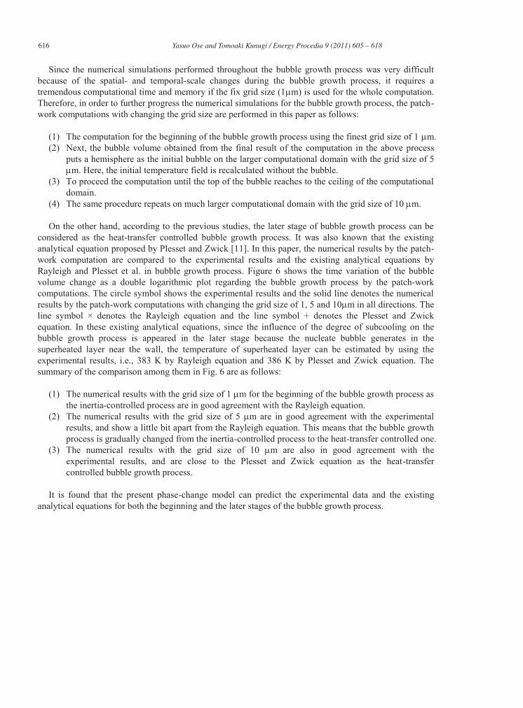
Since the numerical simulations performed throughout the bubble growth process was very difficult because of the spatial- and temporal-scale changes during the bubble growth process, it requires a tremendous computational time and memory if the fix grid size (1 m) is used for the whole computation. Therefore, in order to further progress the numerical simulations for the bubble growth process, the patch-work computations with changing the grid size are performed in this paper as follows:

(1) The computation for the beginning of the bubble growth process using the finest grid size of 1 m. (2) Next, the bubble volume obtained from the final result of the computation in the above process

puts a hemisphere as the initial bubble on the larger computational domain with the grid size of 5 m. Here, the initial temperature field is recalculated without the bubble.

(3) To proceed the computation until the top of the bubble reaches to the ceiling of the computational domain.

(4) The same procedure repeats on much larger computational domain with the grid size of 10 m. On the other hand, according to the previous studies, the later stage of bubble growth process can be

considered as the heat-transfer controlled bubble growth process. It was also known that the existing analytical equation proposed by Plesset and Zwick [11]. In this paper, the numerical results by the patch-work computation are compared to the experimental results and the existing analytical equations by Rayleigh and Plesset et al. in bubble growth process. Figure 6 shows the time variation of the bubble volume change as a double logarithmic plot regarding the bubble growth process by the patch-work computations. The circle symbol shows the experimental results and the solid line denotes the numerical results by the patch-work computations with changing the grid size of 1, 5 and 10 m in all directions. The line symbol × denotes the Rayleigh equation and the line symbol + denotes the Plesset and Zwick equation. In these existing analytical equations, since the influence of the degree of subcooling on the bubble growth process is appeared in the later stage because the nucleate bubble generates in the superheated layer near the wall, the temperature of superheated layer can be estimated by using the experimental results, i.e., 383 K by Rayleigh equation and 386 K by Plesset and Zwick equation. The summary of the comparison among them in Fig. 6 are as follows:

(1) The numerical results with the grid size of 1 m for the beginning of the bubble growth process as

the inertia-controlled process are in good agreement with the Rayleigh equation. (2) The numerical results with the grid size of 5 m are in good agreement with the experimental

results, and show a little bit apart from the Rayleigh equation. This means that the bubble growth process is gradually changed from the inertia-controlled process to the heat-transfer controlled one.

(3) The numerical results with the grid size of 10 m are also in good agreement with the experimental results, and are close to the Plesset and Zwick equation as the heat-transfer controlled bubble growth process.

It is found that the present phase-change model can predict the experimental data and the existing

analytical equations for both the beginning and the later stages of the bubble growth process.


10-3 10-2 10-1 10010-6

10-5

10-4

10-3

10-2

10-1

100

Time [ms]

Bub

ble

volu

me

[mm

3 ]

ExperimentRayleigh Eq.Plesset and Zwick Eq.

Grid size=1 m

Grid size=5 m

Grid size=10 m

Fig. 6. Time Variation of Bubble Volume in Bubble Growth Process by Patch-Work Computations.

5. Conclusions

The boiling and condensation model for numerical simulation on subcooled boiling phenomenon has been developed. Since the numerical result based on the original phase-change model in the boiling and condensation processes could not retrieve the experimental data, the phase-change model was improved based on the quasi-thermal equilibrium hypothesis in this study. The improvements of the phase-changed model were as follows:

(1) The phase-change model was considered to the large density change between water and vapor. (2) A relaxation time derived by considering the unsteady heat conduction in the finite thickness of

the bubble interface was introduced as the VOF limiter at the phase-change interface. (3) The numerical results of both bubble growth and condensation processes with the developed

boiling and condensation model show in good agreement with the experimental data. Therefore, the present boiling and condensation model can predict the subcooled pool boiling phenomena.

Acknowledgment

This work was partly supported by "Energy Science in the Age of Global Warming" of Global Center of Excellence (G-COE) program (J-051) of the Ministry of Education, Culture, Sports, Science and Technology of Japan.


References

[1] Son, G. and Dhir, V.K. Numerical simulation of nucleate boiling on a horizontal surface at high heat fluxes. International J. Heat and Mass Transfer; 2008; 51: 2566-2582.

[2] Kunugi, T. Saito, N., Fujita, T., and Serizawa, A.. Direct numerical simulation of pool and forced convective flow boiling phenomena. In: Proceeding of the twelfth Inernational Heat Transfer Conference. Grenoble, France, 18-23 August 2002 Elsevier B.V.

[3] Kunugi, T. MARS for Multiphase Calculation, Computational Fluid Dynamics J.; 2001; 9: 563-571. [4] Kawara, Z., Okoba, T. and Kunugi, T. Visualization of behavior of subcooled boiling bubble with high time and space

resolutions, In Proceeding of The 6th Pacific Symposium on Flow Visualization and Image Processing. Hawaii, USA, 16-19 May 2007.

[5] Brackbill, J.U., Kothe, D.B., and Zemach, C.. A continuum method for modeling surface tension. J. Computatinal. Physics, 1992; 100: 335-353.

[6] Chorin, A. J.. Numerical solution of the navier-stokes equations, Mathematics and Computer, 1968; 22: 745-762. [7] Carry, V. P.. Liquid Vapor Phase-Change Phenomena: An Introduction to the Thermophysics of Vaporization and

Condensation Process in Heat Transfer Equipment; 1992, Washington, DC: Taylor & Francis. [8] Kenning, D.B.R., and Yan, Y.. Pool boiling heat Transfer on a thin plate: features revealed by liquid crystal thermography”.

International J. Heat Mass Transfer, 1996; 39: 3117-3137. [9] Ohnaka, I. Introduction to Computational Analysis of Heat Transfer and Solidification -Application to the Casting Processes-.

Tokyo: Maruzen; 1985. (in Japanese) [10] Rayleigh, L.. On the pressure developed in a liquid during the collapse of a spherical cavity. Philosophical Magazine; 1917,

34: 94-98. [11] Plesset, M.S., and Zwick, S.A.. The growth of vapor bubbles in superheated liquids. J. Applied Physics; 1954, 25: 493-500.

Documents

Development of A Boiling and Condensation Model on Subcooled Boiling … · 2017-01-17 · mechanism, a boiling and condensation model for numerical simulation on subcooled boiling