Development and Validation of a Quantitative Framework and

FINAL REPORT Development and Validation of a Quantitative Framework and

Management Expectation Tool for the Selection of Bioremediation Approaches at Chlorinated Ethene Sites

ESTCP Project ER-201129

DECEMBER 2015

Carmen Lebrón NAVFAC EXWC Todd Wiedemeier T.H. Wiedemeier & Associates, Inc. John Wilson Scissortail Environmental Solutions, LLC Frank Löffler University of Tennessee Robert Hinchee Integrated Science & Technology, Inc. Michael Singletary NAVFAC Southeast

Distribution Statement A

This report was prepared under contract to the Department of Defense Strategic Environmental Research and Development Program (SERDP). The publication of this report does not indicate endorsement by the Department of Defense, nor should the contents be construed as reflecting the official policy or position of the Department of Defense. Reference herein to any specific commercial product, process, or service by trade name, trademark, manufacturer, or otherwise, does not necessarily constitute or imply its endorsement, recommendation, or favoring by the Department of Defense.

REPORT DOCUMENTATION PAGE Form Approved

OMB No. 0704-0188 Public reporting burden for this collection of information is estimated to average 1 hour per response, including the time for reviewing instructions, searching existing data sources, gathering and maintaining the data needed, and completing and reviewing this collection of information. Send comments regarding this burden estimate or any other aspect of this collection of information, including suggestions for reducing this burden to Department of Defense, Washington Headquarters Services, Directorate for Information Operations and Reports (0704-0188), 1215 Jefferson Davis Highway, Suite 1204, Arlington, VA 22202-4302. Respondents should be aware that notwithstanding any other provision of law, no person shall be subject to any penalty for failing to comply with a collection of information if it does not display a currently valid OMB control number. PLEASE DO NOT RETURN YOUR FORM TO THE ABOVE ADDRESS.

1. REPORT DATE (DD-MM-YYYY) 07-12-2015

2. REPORT TYPETechnical

3. DATES COVERED (From - To)March 2011 – December 2015

4. TITLE AND SUBTITLE Development and Validation of a Quantitative Framework and Management Expectation Tool for the Selection of Bioremediation Approaches (Monitored Natural Attenuation [MNA], Biostimulation and/or Bioaugmentation) at Chlorinated Solvent Sites

5a. CONTRACT NUMBER W912HQ-09-C-007, W912HQ-13-C-0021

5b. GRANT NUMBER

5c. PROGRAM ELEMENT NUMBER

6. AUTHOR(S) Lebrón, Carmen A., Wiedemeier, Todd H., Wilson, John T., Löffler, Frank E., Hinchee, Robert E., and Singletary, Michael A.

5d. PROJECT NUMBER ER-201129 5e. TASK NUMBER 5f. WORK UNIT NUMBER

7. PERFORMING ORGANIZATION NAME(S) AND ADDRESS(ES) Carmen Lebron 2055 Vista Alcedo, Camarillo, CA 93012

8. PERFORMING ORGANIZATION REPORT NUMBER

9. SPONSORING / MONITORING AGENCY NAME(S) AND ADDRESS(ES) 10. SPONSOR/MONITOR’S ACRONYM(S)SERDP/ESTCP Mark Center Drive, 4800 Mark Center Drive, Suite 17D08 Alexandria, VA 22350

ESTCP 11. SPONSOR/MONITOR’S REPORT

NUMBER(S) ER-201129

12. DISTRIBUTION / AVAILABILITY STATEMENT Approved for public release; distribution is unlimited

13. SUPPLEMENTARY NOTES

14. ABSTRACT The overarching objective of ESTCP project ER-201129 was to develop and validate a framework used to make bioremediation decisions based on site-specific physical and biogeochemical characteristics and constraints. The key deliverable is an easy-to-use decision tool (i.e., BioPIC) that can be used to estimate and integrate the impact of quantifiable parameters on natural attenuation and microbial remedies to achieve detoxification of chlorinated ethenes. The quantitative framework and BioPIC were beta-tested by multiple users at multiple sites with different biogeochemical settings and degradation pathways for chlorinated ethenes.

15. SUBJECT TERMS

16. SECURITY CLASSIFICATION OF:

17. LIMITATION OF ABSTRACT

18. NUMBER OF PAGES

19a. NAME OF RESPONSIBLE PERSON

a. REPORT

b. ABSTRACT

c. THIS PAGE

19b. TELEPHONE NUMBER (include area code)

Standard Form 298 (Rev. 8-98)Prescribed by ANSI Std. Z39.18

iii

TABLE OF CONTENTS

1 INTRODUCTION ............................................................................................................... 1

1.1 BACKGROUND .............................................................................................................. 2

1.2 OBJECTIVE OF THE DEMONSTRATION .................................................................. 3

1.3 REGULATORY DRIVERS ............................................................................................. 3

2 TECHNOLOGY .................................................................................................................. 5

2.1 TECHNOLOGY DESCRIPTION .................................................................................... 5

2.2 TECHNOLOGY DEVELOPMENT ................................................................................ 8

2.3 ADVANTAGES AND LIMITATIONS OF THE TECHNOLOGY ............................... 9

3 PERFORMANCE OBJECTIVES ..................................................................................... 11

3.1 QUALITATIVE PERFORMANCE OBJECTIVES ...................................................... 14

3.1.1 Easy to Use, Easy to Follow and Easy to Interpret ..................................................... 14 3.1.2 Focused Site Characterization and Sampling Regimes ............................................... 15 3.2 QUANTITATIVE PERFORMANCE OBJECTIVES ................................................... 15

3.2.1 Quantify Selected Parameters’ Impact on Degradation Rates .................................... 15 3.2.2 Correlate Dhc 16S rRNA Gene-to-vcrA/bvcA Ratios and Dhc-to-Total Bacterial

16S rRNA Gene Ratios to Rates of Ethene Formation ............................................... 16

4 SITE DESCRIPTION ........................................................................................................ 17

4.1 SITE LOCATION AND HISTORY .............................................................................. 18

4.1.1 Naval Air Station (NAS) North Island, Site 5, Unit 2 (Complete Anaerobic Biological Reductive Dechlorination) ......................................................................... 18

4.1.2 Kings Bay, Site 11 (Reductive Dechlorination in the Source Zone Leading to Subsequent Oxidation of Degradation Products Downgradient) ................................ 18

4.1.3 Hill AFB OU-10 (Aerobic Oxidation) ........................................................................ 22 4.1.4 Plattsburgh Air Force Base (PAFB), Fire Training Area 2 (Abiotic Reductive

Dechlorination or Elimination Reactions) ................................................................... 25 4.2 SITE GEOLGY/HYDROGEOLOGY ........................................................................... 25

4.2.1 Naval Air Station (NAS) North Island, Site 5, Unit 2 (Complete Anaerobic Reductive Dechlorination) .......................................................................................... 25

4.2.2 Kings Bay, Site 11 (Reductive Dechlorination in the Source Zone Leading to Subsequent Oxidation of Degradation Products Downgradient) ................................ 28

4.2.3 Hill AFB OU-10 (Aerobic Oxidation) ........................................................................ 28 4.2.4 Plattsburgh Air Force Base, Fire Training Area 2 (Abiotic Reductive

Dechlorination or Elimination Reactions) ................................................................... 29 4.3 CONTAMINANT DISTRIBUTION ............................................................................. 31

iv

4.3.1 Naval Air Station (NAS) North Island, Site 5, Unit 2 (Complete Anaerobic Reductive Dechlorination) .......................................................................................... 31

4.3.2 Naval SUBASE Kings Bay (Reductive Dechlorination in the Source Zone Leading to Subsequent Oxidation of Degradation Products Downgradient) .............. 34

4.3.3 Hill AFB OU-10 (Aerobic Oxidation) ........................................................................ 39 4.3.4 Plattsburgh Air Force Base, Fire Training Area 2 (Abiotic Reductive

Dechlorination or Elimination Reactions) ................................................................... 42

5 TEST DESIGN .................................................................................................................. 48

5.1 CONCEPTUAL EXPERIMENTAL DESIGN .............................................................. 48

5.1.1 Task 1 - Develop a List of Biogeochemical Screening Parameters that Likely Have a Significant Influence on Degradation Rate ..................................................... 49

5.1.2 Task 2 – Determine the Quantitative Relationship Between the Biogeochemical Parameters Selected as Screening Parameters and Degradation Rates ....................... 50

5.1.3 Task 3 - Develop a Decision Framework (An Expert System that when Applied Allows Elucidation of Degradation Pathways and Allows the User to Determine the Most Suitable Bioremediation Approach) ............................................................. 51

5.1.4 Task 4 - Develop a User-Friendly Site Management Expectation Tool to Facilitate User Application of the Decision Framework ............................................. 52

5.1.5 Task 5 - Validate Cost and Performance Data ............................................................ 52 5.2 DESIGN AND LAYOUT OF TECHNOLOGY COMPONENTS................................ 52

5.2.1 Parameters Required to Implement the BioPIC Screening Tool ................................. 52 5.2.2 The Decision Logic in the BioPIC Screening Tool ..................................................... 55 5.2.3 Estimating Degradation Rates Using BIOCHLOR ..................................................... 58 5.2.4 Using the Decision Tool .............................................................................................. 85

6 PERFORMANCE ASSESSMENT ................................................................................. 131

6.1 QUALITATIVE PERFORMANCE OBJECTIVES .................................................... 131

6.1.1 Easy to Use, Easy to Follow and Easy to Interpret ................................................... 131 6.1.2 Focused Site Characterization and Sampling Regimes ............................................. 131 6.2 Quantitative Performance Objectives ........................................................................... 136

6.2.1 Quantify the Impact of Selected Parameters on Degradation Rates ......................... 136 6.2.2 Correlate Dhc Biomarker Gene Measurements to Ethene Formation and

Detoxification ............................................................................................................ 139

7 COST ASSESSMENT ..................................................................................................... 140

7.1 COST MODEL ............................................................................................................ 140

7.2 COST DRIVERS.......................................................................................................... 141

7.2.1 Analytical Parameters in Addition to Those Specified in USEPA (1998) ................ 142 7.2.2 Application of the Decision Framework ................................................................... 144

8 IMPLEMENTATION ISSUES ....................................................................................... 146

9 REFERENCES ................................................................................................................ 147

v

LIST OF APPENDICES

Appendix A: Points of Contact

Appendix B: Theory Behind the Correction in the Kuder Plots for Abiotic Degradation of TCE

vi

LIST OF FIGURES

Figure 2.1: Mature components are the foundation of the quantitative framework that was used to build BioPIC ............................................................6

Figure 4.1: Site map of Site 5 at NAS North Island, California ............................................18

Figure 4.2: Locations and numbers of monitoring wells at the Kings Bay Site ....................19

Figure 4.3: Site location Map for Hill AFB OU-10 ...............................................................21

Figure 4.4: Site Map and Extent of Contamination, Hill AFB OU-10 ..................................22

Figure 4.5: Plattsburgh AFB location map ............................................................................24

Figure 4.6: Plattsburgh AFB – FT-002 source OU remedial systems ...................................25

Figure 4.7: Conceptual model of the Aquifer system, Hill AFB OU-2 .................................28

Figure 4.8: Generalized hydrogeologic cross section - Plattsburgh AFB – FT-002 ..............30

Figure 4.9: Isopleth map for chlorinated ethenes at NASNI, Site 5, Unit 2 – March 2008 .....................................................................................................................31

Figure 4.10: Tetrachloroethene distribution in August 2002, May 2009, and April 2011, Site 11, Old Camden Landfill, Kings Bay, Georgia ..................................33

Figure 4.11: Trichloroethene distribution in August 2002, May 2009, and April 2011, Site 11, Old Camden Landfill, Kings Bay, Georgia ............................................34

Figure 4.12: cis-1,2-Dichloroethene distribution in August 2002, May 2009, and April 2011, Site 11, Old Camden Landfill, Kings Bay, Georgia ..................................35

Figure 4.13: Vinyl Chloride distribution in August 2002, May 2009, and April 2011, Site 11, Old Camden Landfill, Kings Bay, Georgia ............................................36

Figure 4.14: Cross-section A-A’ with TCE and PCE Plumes, Hill AFB OU-10 ....................39

Figure 4.15: Plattsburgh AFB – FT-002 source OU downgradient contaminant plumes – FT-002/IA groundwater OU remedial system component locations ...............42

Figure 4.16: Plattsburgh AFB – FT-002 groundwater OU remedial system components and BTEX plume .............................................................................43

Figure 4.17: Plattsburgh AFB – FT-002 groundwater OU remedial system Components and chlorinated hydrocarbon plume ...............................................44

Figure 4.18: Plattsburgh AFB east flightline and Idaho Avenue collection trenches ..............45

Figure 5.2.2.1: Decision tool framework .....................................................................................53

Figure 5.2.2.2: Decision framework to determine if bioaugmentation or bioaugmentation is appropriate. Redrawn from Figure 4.1 of Stroo et al. (2013b) .......................54

Figure 5.2.3.1: BIOCHLOR input screen .....................................................................................56

vii

Figure 5.2.3.2: Cross section showing the extension of a solute plume in the vertical-dimension. Numbers represent the concentration of TCE in micrograms per liter (µg/L) .....................................................................................................57

Figure 5.2.3.3: Selection of groundwater flowpath for BIOCHLOR simulations .......................58

Figure 5.2.3.4: Selection of groundwater flowpath for BIOCHLOR simulations using temporal variations in plume configuration - A ..................................................59

Figure 5.2.3.5: Selection of groundwater flowpath for BIOCHLOR simulations using temporal variations in plume configuration - B ..................................................59

Figure 5.2.3.6: Site description entry ...........................................................................................59

Figure 5.2.3.7: Selection of chlorinated ethenes versus ethanes ..................................................60

Figure 5.2.3.8: Data entry for seepage velocity calculation .........................................................60

Figure 5.2.3.9: Use of a potentiometric map to calculate hydraulic gradient ..............................61

Figure 5.2.3.10: Hydraulic gradient calculation using a plot of groundwater elevation versus distance along flowp

Figure 5.2.3.11: Quantification of dispersion in BIOCHLOR......................................................63

Figure 5.2.3.12: Quantification of sorption in BIOCHLOR .........................................................65

Figure 5.2.3.13: Entry of contaminant concentration data into BIOCHLOR ...............................66

Figure 5.2.3.14: Simulation time entry for BIOCHLOR ..............................................................67

Figure 5.2.3.15: Determination of ks Using Aqueous Concentrations in Source Area Wells ....................................................................................................................68

Figure 5.2.3.16: Source concentration data entry .........................................................................68

Figure 5.2.3.17: Source data entry – constant source ...................................................................69

Figure 5.2.3.18: Source data entry – decaying ..............................................................................70

Figure 5.2.3.19: Trial and error input for DCE to VC degradation rate of 1/year ........................72

Figure 5.2.3.20: Model output selection .......................................................................................72

Figure 5.2.3.21: Selecting model output view for DCE for 1/year trial run .................................72

Figure 5.2.3.22: Model output for DCE to VC degradation rate of 1/yr – unacceptable fit .........73

Figure 5.2.3.23: Trial and error input for DCE to VC degradation rate of 17/year ......................73

Figure 5.2.3.24: Model output for DCE to VC degradation rate of 17/year – acceptable fit ..........................................................................................................................74

Figure 5.2.3.25: Trial and error input for VC to ethene degradation rate of 1/year .....................74

Figure 5.2.3.26: Model output for VC to ethene degradation rate of 1/yr – unacceptable fit ..........................................................................................................................75

Figure 5.2.3.27: Trial and error input for VC to ethene degradation rate of 10/year ....................75

Figure 5.2.3.28: Model output for VC to ethene degradation rate of 10/yr – acceptable fit .........76

viii

Figure 5.2.3.29: Relationship between the coefficient of longitudinal dispersivity and the length of the flow path (scale) .............................................................................78

Figure 5.2.3.30: Sensitivity analysis of the relationship between the coefficient of longitudinal dispersivity and the rate constant for degradation ...........................79

Figure 5.2.4.1: Maps for evaluating plume stability – total chlorinated ethenes – 1997 - 2008 .....................................................................................................................82

Figure 5.2.4.2: Example - POC 2,000 feet downgradient, MCL is regulatory standard, MNA does not meet the g

Figure 5.2.4.3: Example - Natural attenuation does meet the regulatory goal ............................84

Figure 5.2.4.4: Example - POC is 2,000 feet from source, and concentration of VC at POC is the MCL ..................................................................................................86

Figure 5.2.4.5: VC simulation with the best fit to the field data ...................................................87

Figure 5.2.4.6: Example rate constant estimation using trial and error with degradation rate of 1/year ........................................................................................................87

Figure 5.2.4.7: Example rate constant estimation using trial and error with degradation rate of 3/year ........................................................................................................88

Figure 5.2.4.8: Data Input tab for CSIA.xlsx ...............................................................................88

Figure 5.2.4.9: Example Kuder Plot for Vinyl Chloride ..............................................................89

Figure 5.2.4.10: Data Input tab for Dhc.xlsx .................................................................................90

Figure 5.2.4.11: Example plot under Dhc Explains VC tab in Dhc.xlsx .......................................91

Figure 5.2.4.12: Data Input tab for Reductase Genes.xlsx ............................................................92

Figure 5.2.4.13: Example plot under Rase and Dhc tab in Reductase Genes.xlsx ........................93

Figure 5.2.4.14: Data Input tab for Magnetic Susceptibility.xlsx .................................................94

Figure 5.2.4.15: Example plot under Magnetic Susceptibility Plot tab in Magnetic Susceptibility.xlsx ..............................................................................................95

Figure 5.2.4.16: Example - POC is 2,000 feet from source, and concentration of DCE at POC is the MCL .................................................................................................97

Figure 5.2.4.17: DCE simulation with the best fit to the field data ..............................................98

Figure 5.2.4.18: Example DCE rate constant estimation using trial and error with degradation rate of 0.4/year ................................................................................98

Figure 5.2.4.19: Example DCE rate constant estimation using trial and error with degradation rate of 1/year ...................................................................................98

Figure 5.2.4.20: Data Input tab for CSIA.xlsx ..............................................................................99

Figure 5.2.4.21: Example Kuder Plot for DCE .............................................................................99

Figure 5.2.4.22: Data Input tab for Dhc.xlsx ..............................................................................101

Figure 5.2.4.23: Example plot under Dhc Explains cDCE tab in Dhc.xlsx ................................101

ix

Figure 5.2.4.24: Data Input tab for Reductase Genes.xlsx .........................................................103

Figure 5.2.4.25. Example plot under Rase and Dhc tab in Reductase Genes.xlsx .....................103

Figure 5.2.4.26: Data Input tab for Magnetic Susceptibility.xlsx for DCE ................................105

Figure 5.2.4.27: Example plot under Magnetic Susceptibility Plot tab in Magnetic Susceptibility.xlsx ............................................................................................105

Figure 5.2.4.28: Example - POC is 2,000 feet from source, and concentration of TCE at POC is the MCL ...............................................................................................107

Figure 5.2.4.29: Example TCE rate constant estimation using trial and error with degradation rate of 1/year .................................................................................108

Figure 5.2.4.30: Example TCE rate constant estimation using trial and error with degradation rate of 0.7/year ..............................................................................108

Figure 5.2.4.31: Example TCE rate constant estimation using trial and error with degradation rate of 1.4/year ..............................................................................109

Figure 5.2.4.32: Data Input tab for Magnetic Susceptibility.xlsx for TCE .................................111

Figure 5.2.4.33: Example plot for TCE under Magnetic Susceptibility Plot tab in Magnetic Susceptibility.xlsx ............................................................................................111

Figure 5.2.4.34: Decrease in sulfate concentration along flowpath ............................................112

Figure 5.2.4.35: Decrease in sulfate concentration at points along flowpath .............................113

Figure 5.2.4.36: Screenshot of model output from Sulfate Sag Along Flow Path tab in FeS.xlsx applied to a field study that estimated the rate of TCE degradation in ground water as the water passed through a mulch-based biowall at Altus AFB, OK ...............................................................................114

Figure 5.2.4.37: Screenshot of model output from Sulfate Sag Along Flow Path tab in FeS.xlsx applied to a laboratory column study performed by Shin et al. (2010) ..............................................................................................................115

Figure 5.2.4.38: Figure illustrating the distribution of sulfate at a site where the extent of sulfate depletion increases over time. .............................................................116

Figure 5.2.4.39: Figure illustrating chlorinated ethene concentrations decreasing along the flowpath and sulfate concentrations increasing along flowpath downgradient from a NAPL source zone, Naval Air Station North Island, San Diego, CA. The minimum sulfate concentration corresponds to the maximum ethene concentration .......................................117

Figure 5.2.4.40: Comparison of the distribution of sulfate between wells where the sulfate reduction occurs upgradient of both wells to an assumed previous condition where sulfate reduction occurred between the wells .......118

Figure 5.2.4.41: Screenshot of model output under lowest Sulfate at Source tab from FeS.xlsx for the site presented in Figure 5.4.2.37, NASNI, Site 5, Unit 2 ......................................................................................................................119

x

Figure 5.2.4.42: Example - POC is 2,000 feet from source, and concentration of PCE at POC is the MCL ..............................................................................................121

Figure 5.2.4.43: Example PCE rate constant estimation using trial and error with degradation rate of 0.6/year.............................................................................121



Figure 5.2.4.46: Data Input tab for Magnetic Susceptibility.xlsx for PCE ...............................124

Figure 5.2.4.47: Example plot for PCE under Magnetic Susceptibility Plot tab in Magnetic Susceptibility.xlsx ...........................................................................124

Figure 6.1: Plot of First Order Degradation Rate for cDCE Versus Dhc Density.............128

Figure 6.2: Plot of First Order Degradation Rate for VC Versus Dhc Density .................128

Figure 6.3: Plot of First Order Degradation Rate for PCE Versus Magnetic Susceptibility ...................................................................................................129

Figure 6.4: Plot of First Order Degradation Rate for TCE Versus Magnetic Susceptibility ...................................................................................................129

Figure 6.5: Plot of First Order Degradation Rate for DCE Versus Magnetic Susceptibility ...................................................................................................130

Figure 6.6: Plot of First Order Degradation Rate for VC Versus Magnetic Susceptibility ...................................................................................................130

Figure 6.7: Plot of vcrA plus bvcA gene copies per Liter Versus Dhc Density ................130

LIST OF TABLES

Table 3.1A: Qualitative Performance Objectives .................................................................10

Table 3.1B: Quantitative Performance Objectives ...............................................................11

Table 5.2.1.1: The parameters necessary to fully implement BioPIC ......................................51

Table 5.2.3.1: Representative values for porosity ....................................................................63

Table 5.2.3.2: Representative values for soil sorption coefficient ...........................................64

Table 5.2.4.1: Data used for example presented in Figure 5.4.2.41 .......................................119

Table 7.1: Cost Model ......................................................................................................140

xi

ACRONYMS AFB Air Force Base AFCEE Air Force Center for Engineering and the Environment ARTT Alternative Restoration Technologies Team cDCE cis-1,2-Dichloroethene COPC Contaminant of Potential Concern CSIA Compound-Specific Isotope Analysis DEM/VAL Demonstration and Validation Dhc Dehalococcoides DNAPL Dense Nonaqueous-Phase Liquid DO Dissolved Oxygen DoD Department of Defense EISB Enhanced In Situ Bioremediation EPA Environmental Protection Agency ESTCP Environmental Security Technology Certification Program MBTs Molecular Biological Tools MCL Maximum Contaminant Level MCRD Marine Corps Recruit Depot MNA Monitored Natural Attenuation NAVFAC EXWC Naval Facilities Command Expeditionary Warfare Center NAPL Nonaqueous-Phase Liquid NAS Naval Air Station NASNI Naval Air Station North Island NAWC Naval Air Warfare Center NWIRP Naval Weapons Industrial Reserve Plant OC Organic Carbon O&M Operation & Maintenance PCE Tetrachloroethene qPCR Quantitative Real-Time Polymerase Chain Reaction RAO Remedial Action Objective RCRA Resource Conservation Recovery Act RDase Reductive Dehalogenase RPM Remedial Project Manager SERDP Strategic Environmental Research and Development Program SUBASE Naval Submarine Base TCAAP Twin Cities Army Ammunition Plant TCE Trichloroethene trans-DCE trans-1,2-Dichloroethene USGS United States Geological Survey VC Vinyl Chloride VOC Volatile Organic Compound

xii

DEFINITIONS Abiotic Oxidation: Oxidative contaminant transformation without direct involvement of a

biological system. Involves the abiotic oxidation of the organic compound of interest to carbon dioxide and other products. For example, He et al. (2009) show that the reaction of cDCE with magnetite results in the production of CO2 and likely water and chloride. This is consistent with the work of Darlington et al. (2008). This reaction can occur under oxic or anoxic conditions.

Abiotic Reduction: Reductive contaminant transformation without the direct involvement of a biological system. Involves the abiotic reduction of the organic compound of interest to a more reduced compound. For example, Butler and Hayes (1999) and Lee and Batchelor (2002 a, b and 2003) show that TCE is abiotically reduced to chloroacetylene and/or acetylene which is then oxidized to CO2, water, and chloride. Abiotic transformations of chlorinated organics can occur under oxic or anoxic conditions and can be significant at sites with iron-rich minerals, including iron sulfide, pyrite, fougerite, magnetite, and Fe(II)-containing phyllosilicates.

Aerobic Oxidation: Oxygen-dependent oxidation reaction(s) leading to detoxification. Involves the biologically-mediated oxidation of compounds of interest and occurs when oxygen in used as an electron acceptor and the organic compound is used as the electron donor. For example, during aerobic oxidation, vinyl chloride is oxidized to the nontoxic end-products carbon dioxide, water, and chloride. This reaction predominantly occurs under oxic conditions.

Anaerobic Oxidation: Oxygen-independent oxidation reaction(s) leading to detoxification. Occurs only under anoxic conditions. Involves the biologically-mediated oxidation of compounds of interest and occurs when an electron acceptor other than oxygen is utilized as an electron sink, and the organic compound is used as the electron donor. For example, during anaerobic oxidation under iron-reducing conditions, vinyl chloride is oxidized to the nontoxic end-products carbon dioxide, water, and chloride.

Attenuation: Complement of processes that reduce contaminant concentrations in groundwater. Attenuation processes are dominated by dispersion, sorption, biodegradation and abiotic degradation.

Attenuation Rate Constant: The proportionality constant quantifying the rate of change in the concentration of a contaminant due to the combined processes of dispersion, sorption, and biotic and abiotic degradation.

Bioattenuation: Complement of all biological processes that reduce contaminant concentrations in groundwater.

Bioaugmentation: The enhancement of biological reductive dechlorination through the addition of an inoculum of bacteria that facilitate reductive dechlorination. Typically used at sites where the requisite microbial population is not already present in the aquifer matrix. Biostimulation often is used in conjunction with bioaugmentation because many sites

xiii

lacking the requisite microbial consortia to facilitate biological reductive dechlorination also lack the requisite organic carbon.

Biostimulation: The enhancement of biological reductive dechlorination through the addition of a carbon source such as vegetable oil, lactate, acetate, molasses, hydrogen releasing compound, etc. In order for biostimulation alone to be successful, the requisite microbial population must already be present in the aquifer.

bgs: Below Ground Surface.

Bulk Rate: Synonymous with total attenuation rate.

Degradation: Degradation involves the breakage of C-C or C-Cl bonds and generates products of lower molecular weight.

Degradation Rate: The rate of change in contaminant concentration due only to the degradation of organic compounds. This rate does not consider the effects of dispersion or sorption and thus quantifies only the rate at which the mass of the parent compound is being removed from the system.

Degradation Rate Constant: The proportionality constant quantifying the rate of change in concentration or mass of a chemical compound over time resulting from the transformation of a contaminant into a degradation product. At the field scale, degradation rate constants are typically described by first-order kinetics.

Detoxification: Degradation of a contaminant to innocuous (non-toxic) products.

Detoxification Rate: The rate at which compounds of interest are degraded to non-toxic products. For example, the detoxification rate for TCE during complete biological reductive dechlorination would be the rate at which the TCE is degraded all the way to ethene. Similarly, the detoxification rate for TCE during abiotic degradation would be the rate at which the TCE is degraded to chloroacetylene.

Detoxification Rate Constant: The proportionality constant quantifying the rate of change of a contaminant of interest into innocuous end products. For example, the rate of change of vinyl chloride into ethene and inorganic chloride.

Dihaloelimination (Vicinal Reduction): A reductive dechlorination reaction, in which two halogen substituents from adjacent carbon atoms are removed resulting in the formation of a double bond.

Elimination: A reaction in which two substituents are removed from adjacent carbon atoms leading to the formation of a double bond between them.

EPA ’98 MNA Protocol: Technical Protocol for Evaluating Natural Attenuation of Chlorinated Solvents in Ground Water, EPA/600/R-98/128 (ftp://ftp.epa.gov.pub/ada/reports/protocol.pdf).

xiv

Management Expectation Tool: The software that incorporates the quantitative framework; i.e., likely in the form of an Excel spreadsheet or an Access database, which will enable users to apply the remedy selection framework easily.

Monitored Natural Attenuation (MNA): The reliance on natural attenuation processes (within the context of a carefully controlled and monitored site cleanup approach) to achieve site-specific remedial objectives within a time frame that is reasonable compared to other methods. In order for MNA to be considered a viable remediation alternative, regulatory agencies often require evidence of degradation. In the past this degradation has largely been consider to be of strictly biological origin. It is now known that abiotic degradation can contribute to contaminant detoxification.

Quantitative Framework, a.k.a. the framework: The systematic decision making protocol at the root of the management expectation tool which, when applied, it will yield the most effective bioremediation approach. Ideally, it is the approach used by field experts for which extensive expertise and data analyses are required. The framework being developed under ER1129: a) implies that expertise, b) incorporates a range of values for multiple analytical parameters that play a critical role in detoxification for optimal degradation rates, c) incorporates 5 degradation pathways, and d) taken in total, can accurately deduce degradation pathways, estimate degradation rates, and determine what is required to increase degradation rates through bioremediation should MNA not prove sufficient to meet remediation goals.

Rate: The quantitative change in concentration or mass of a chemical compound over time. Rates considered in this document include Total Attenuation Rate, Degradation Rate, and Detoxification Rate.

Rate Constant: The proportionality constant relating the rate of a chemical reaction to the concentrations of its reactants.

Reductive Dechlorination (Hydrogenolysis): Replacement of a halogen substituent with hydrogen with the concomitant addition of electrons to the organic molecule. For chlorinated aliphatic hydrocarbons, this process results in the degradation of organic compounds by chemical reduction with release of inorganic chloride ions.

Template Sites: The sites for each of the pathways of interest.

Total Attenuation Rate: The proportionality constant that quantifies the rate of change in contaminant concentration due to the combined effects of dispersion, sorption, and biological and abiotic degradation. Involves summing the individual rate constants for dispersion, sorption, and biological and abiotic degradation.

1

1 INTRODUCTION

Physical, chemical and biological treatment technologies have been developed to address groundwater contamination, each with its distinct advantages and disadvantages to accomplish site-specific remediation goals. Naturally occurring biological and abiotic processes contribute to contaminant attenuation in most hydrogeologic systems, including contaminated aquifers. At sites where these natural processes are sufficient to meet site-specific remediation goals, monitored natural attenuation (MNA) should be evaluated (EPA, 1999). At sites, where MNA is not sufficient to meet remediation goals, enhanced biological remediation may be considered.

In groundwater contaminated by chlorinated alkenes, the dominant natural attenuation mechanism is a sequential biological reductive dechlorination of PCE to TCE, then TCE to cDCE, then cDCE to Vinyl Chloride and finally Vinyl Chloride to Ethene. The majority of technologies for enhanced biological remediation use the same microbial process. Many bacteria can degrade PCE and TCE to cDCE; but certain strains of Dehalococcoides mccartyi (Dhc) are the only organisms known to carry out the reductive dechlorination of cDCE to Vinyl Chloride and Vinyl Chloride to Ethene (Löffler et al., 2013). These bacteria are almost ubiquitous in groundwater that is contaminated with chlorinated alkenes. Hendrickson et al. (2002) assayed groundwater contaminated with chlorinated alkenes for the 16S RNA gene of Dehalococcoides. The gene was present at 21 of 24 sites in North America and Europe. At the three sites where the Dehalococcoides was not detected, dechlorination stopped at cDCE. In a more recent survey, van der Zaan et al. (2010) found the Dehalococcoides 16S RNA gene in every location where chlorinated ethenes were present in the groundwater (11 locations in Europe); however, the density of Dehalococcoides 16S RNA gene copies varied widely based on the geochemistry of the uncontaminated groundwater. Some sites may not harbor a useful density of the strains of Dehalococcoides mccartyi (Dhc) strains that are necessary to achieve detoxification, and bioaugmentation may increase detoxification rates to the extent that remediation goals will be met.

Protocols for the implementation of both biostimulation and bioaugmentation have been developed previously under the sponsorship of the Environmental Security Technology Certification Program (ESTCP), the former Air Force Center for Environmental Excellence (AFCEE), and the Interstate Technology Regulatory Council (ITRC). Guidance for implementing anaerobic in situ bioremediation of chlorinated ethenes in groundwater plumes is provided in ESTCP (2003, 2004, 2006a, 2006b, 2008a, 2010), AFCEE (2008) and ITRC (2008b). Guidance and recommendations for remediation of chlorinated ethenes in source areas with DNAPL are provided in ESTCP (2008b) and ITRC (2008a). Guidance on the use of gene assays to monitor MNA, biostimulation and bioaugmentation is provided in ESTCP (2011) and Petrovskis et al. (2013). Guidance on selection and implementation of bioaugmentation is provided in Aziz et al. (2013), Löffler et al. (2013), and Steffan and Vainberg (2013). These documents are based on experiences with biostimulation and bioaugmentation in a variety of field conditions.

Although guidance exists with respect to technology application, a pragmatic approach supported by a quantitative framework for selecting the most effective bioremediation approach at a specific site is lacking.

The lack of a systematic approach for determining the most efficient bioremediation approach results in unnecessary financial and environmental costs. Furthermore, aquifer amendments,

2

such as excessive fermentable carbon substrates, can result in undesirable secondary impacts to groundwater quality including incomplete dechlorination, pH changes, metal dissolution, aquifer clogging, and formation of (greenhouse) gases. To provide a systematic approach for decision-making, the relationships between measurable biogeochemical and aquifer matrix parameters with degradation rates for known chlorinated ethene degradation pathways were determined. This approach represents a major advancement over the prior empirical practice that extrapolated information from often insufficient, qualitative data and experiences gained from a few case studies to other sites that have distinct characteristics and behaviors. The application of the quantitative framework and the associated site management decision tool, designated the Biological Pathway Identification Criteria screening tool (BioPIC), enhances remedial success, increases remediation efficiency, minimizes detrimental environmental impacts, and reduces both capital as well as operation and maintenance (O&M) costs to the Department of Defense (DoD) and other end users.

The quantitative framework validated under ESTCP Project ER-201129 is a systematic approach to evaluate whether MNA is an appropriate remedy based on site-specific conditions. If bioremediation is considered as a remedy at the site, the framework provides a simple criterion to evaluate the need for bioaugmentation at the site. A flow chart (Section 5) summarizes this quantitative framework. The framework uses the quantitative relationships between biotic and abiotic parameters that contribute to the detoxification of chlorinated ethenes and determine degradation rates. Hence, the quantitative framework is a systematic decision-making protocol that allows the user to determine if degradation is occurring and, if it is, to deduce the relevant degradation pathway(s) based on the assessment of specific analytical parameters.

The quantitative framework is intended for sites where the goal of the remedy is to restrict the extent of groundwater contamination and prevent impact to a receptor or a sentry well, as is appropriate under the Resource Recovery and Conservation Act (RCRA). The framework is not intended for sites where the goal is to attain a cleanup standard throughout a plume, as is done under the Comprehensive Environmental Response, Compensation, and Liability Act (CERCLA). The framework does not consider the time frame required to reach a cleanup goal.

1.1 BACKGROUND

MNA and bioremediation have gained popularity as remedial approaches at sites contaminated with chlorinated solvents. The overarching goal of ESTCP Project ER-201129 was the development of a quantitative framework for the selection of MNA or bioremediation approaches (biostimulation alone or combined with bioaugmentation) at sites contaminated with chlorinated ethenes. The quantitative framework provides the logic reasoning behind the BioPIC tool, which was developed to facilitate the application of the quantitative framework. BioPIC incorporates the framework in the form of an easy-to-use Excel-based interface. As such, the quantitative framework presents a decision logic that allows the user to deduce the most promising remediation approach as well as the predominant degradation mechanism(s) at a site.

In 1998, Mr. Todd Wiedemeier (Wiedemeier and Associates, Inc.) and Dr. John Wilson (U.S. Environmental Protection Agency) developed a scoring system to assess the likelihood of in situ reductive dechlorination and bioattenuation at a site (EPA, 1998a). The initial biotransformation of the most commonly encountered chlorinated solvent groundwater contaminants (e.g., tetrachloroethene [PCE], trichloroethene [TCE], chloroform, and 1,1,1-trichloroethane [1,1,1-TCA]) in the U.S. generally involves a reductive dechlorination reaction (i.e., hydrogenolysis or

3

dichloroelimination). The assessment framework developed by Wiedemeier and Wilson (EPA, 1998a) was designed to recognize those geochemical conditions where reductive dechlorination is feasible. The essence of the EPA 1998 ranking system relies on the fact that biodegradation causes measurable changes in groundwater geochemistry, and that the microbiology necessary to facilitate reductive dechlorination, whether by direct microbe-contaminant interactions or indirectly through microbially-mediated abiotic reactions, can only operate under certain environmental conditions. Specifically, reductive dechlorination reactions generally occur under anoxic, low redox conditions, which typically prevail in aquifers with sufficient bioavailable organic carbon.

The 1998 EPA protocol did not consider microbial parameters because the knowledge of relevant microbes was limited at the time and appropriate molecular biological tools (MBTs) were not available. Dedicated efforts over the past decade revealed keystone dechlorinators such as strains of Dehalococcoides (Dhc), and technological advances generated tools to quantitatively assess genes of interest in environmental samples including groundwater. Organism- and process-specific biomarker genes for monitoring reductive dechlorination have been identified, and quantitative real-time polymerase chain reaction (qPCR) tools that enumerate Dhc 16S rRNA genes and reductive dehalogenase (RDase) genes involved in chlorinated ethene dechlorination provide information about specific dechlorination steps. For example, the vinyl chloride (VC) RDase genes bvcA and vcrA serve as biomarkers for ethene formation and detoxification. In addition, the importance of abiotic degradation reactions, particularly those associated with iron-rich minerals such as magnetite, is now known, and approaches to quantify the contributions of iron-bearing minerals to contaminant detoxification are becoming commercially available. For example, magnetic susceptibility data allow the investigator to estimate the relative importance of abiotic degradation via magnetite. The information gained from the identification of new degradation pathways and these new assessment tools represents a major advance, and allows the quantitative framework to be a significant improvement over the 1998 EPA protocol.

1.2 OBJECTIVE OF THE DEMONSTRATION

The overarching objective of ESTCP project ER-201129 was to develop and validate a framework used to make bioremediation decisions based on site-specific physical and biogeochemical characteristics and constraints. The key deliverable is an easy-to-use decision tool (i.e., BioPIC) that can be used to estimate and integrate the impact of quantifiable parameters on natural attenuation and microbial remedies to achieve detoxification of chlorinated ethenes. The quantitative framework and BioPIC were beta-tested by multiple users at multiple sites with different biogeochemical settings and degradation pathways for chlorinated ethenes.

1.3 REGULATORY DRIVERS

Presently, the maximum contaminant levels (MCLs) for the chlorinated ethenes tetrachloroethene (PCE), trichloroethene (TCE), cis-1,2-dichloroethene (cDCE), and vinyl chloride (VC) are 5 micrograms per liter (µg/L), 5 µg/L, 70 µg/L, 2 µg/L, respectively (http://water.epa.gov/drink/contaminants/index.cfm). At many sites, a risk-based assessment dictates cleanup goals, which often means that the cleanup goals are higher than the federal MCLs. At many other sites, standards are set by the individual states and these standards are lower than the federal MCLs. In any event, some type of remedial action is required at many

4

DoD sites where chlorinated ethenes are present. The intent of BioPIC is to allow DoD RPMs to evaluate MNA and determine if it meets site specific remedial action objectives (RAOs).

5

2 TECHNOLOGY

2.1 TECHNOLOGY DESCRIPTION

The quantitative framework represents a systematic approach that utilizes the relationships between specific biogeochemical parameters and degradation rates to deduce major degradation pathways and determine the best bioremediation approach at sites impacted with chlorinated ethenes. A major goal of this demonstration was to quantify the relationship(s) between selected, measurable biogeochemical screening parameters and degradation rates. The quantitative assessment of these relationships allowed the development of the quantitative framework. In turn, the quantitative framework enabled the development of BioPIC a software tool that guides people involved in the selection of remedial technology (such as RPMs and regulators) through a hierarchical set of questions to ultimately identify the most efficacious pathway for achieving detoxification of chlorinated ethenes at a particular site. BioPIC is an easy-to-use decision tool that informs people involved in the selection of remedial technology about the relevant biogeochemical parameters and their relative importance to affect degradation, either microbial or abiotic, at a given site.

The quantitative framework is based, in part, on the parameters that were used to develop the scoring system introduced by Dr. John Wilson and Mr. Todd Wiedemeier to assess the likelihood of in situ reductive dechlorination and bioattenuation (EPA, 1998a; Wiedemeier et al., 1999). The 1998 scoring system was based on the relative importance of measurable geochemical parameters that affect the efficacy of biological reductive dechlorination. The framework validated in the current project (ER-201129) is an extension of the 1998 EPA protocol. Measurable geochemical, microbial, and geologic parameters are included in the quantitative framework and the relationship between each relevant parameter and the associated degradation rates have been quantified. This approach differs from the 1998 EPA protocol in that the range in a parameter’s value is tied to degradation rates instead of being just a qualitative indicator of biodegradation.

This report has not been through US EPA clearance and therefore this report is not an EPA document. Nothing in this document changes or amends anything in an EPA document. However, The Technical Protocol for Evaluating Natural Attenuation of Chlorinated Solvents in Ground Water (EPA, 1998a) provides technical recommendations from EPA ORD; it is not regulatory guidance. Step one in EPA (1998a) is to determine if biodegradation is occurring using geochemical data. ESTCP Project ER-201129 provides technical recommendations that can be used to update and improve on EPA (1998a).

A number of measurable parameters such as the concentrations of volatile organic compounds (VOCs), alternate electron acceptors (e.g., oxygen, sulfate), reduced products (e.g., Fe(II), CH4), Dhc 16S rRNA gene and reductive dehalogenase (RDase) gene abundances, and magnetic susceptibility affect the detoxification of chlorinated ethenes. The relationships between each parameter and the degradation rates were determined and used to develop the decision matrix and BioPIC.

Since publication of the 1998 EPA protocol, several new technologies for enhancing detoxification of chlorinated ethenes have emerged, most notably biostimulation and bioaugmentation (ESTCP, 2003, 2004, 2006a, 2006b, 2008a, 2008b, 2010, 2011; AFCEE, 2008; ITRC, 2008a, 2008b; Aziz et al., 2013; Löffler et al., 2013; Petrovskis et al., 2013; Steffan and

6

Vainberg, 2013). The principles and practices described in the 1998 EPA protocol and those outlined in published guidelines for biostimulation to enhance anaerobic reductive dechlorination form the basis for developing the quantitative framework approach. Importantly, the new quantitative framework considers key elements that catalyze degradation reactions including direct measurement of the presence of keystone dechlorinating bacteria (e.g., Dhc) and iron-bearing minerals (e.g., magnetite). Specifically, these efforts have demonstrated that adding electron donor stimulates biodegradation at sites where the requisite reductively dechlorinating microbial populations are present. For those sites apparently deficient of the requisite microbiology (e.g., absence of Dhc and VC RDase genes), bioaugmentation approaches (i.e., the addition of dechlorinating consortia containing Dhc), which are generally applied in combination with biostimulation, have been successfully implemented (Ellis et al., 2000; Major et al., 2002; Lendvay et al., 2003; Scheutz et al., 2008, Löffler et al. 2013).

Ellis et al. (2000) evaluated bioaugmentation at a site in Delaware that was contaminated with TCE. The site was biostimulated with lactate for 568 days. Dechlorination did not proceed past cDCE. The site was then bioaugmented with a strain of Dhc, and vinyl chloride and ethane appeared in the groundwater within 90 days. Major et al. (2002) evaluated bioaugmentation at a site in Texas that was contaminated with PCE and TCE. The site was first biostimulated with methanol and acetate for 176 days. PCE and TCE were consumed and cDCE accumulated but Vinyl Chloride and ethene were not produced. Then the site was bioaugmented. Vinyl chloride appeared in the groundwater within 21 days and ethene appeared within 35 days.

Lendvay et al. (2003) conducted a side by side comparison of biostimulation and bioaugmentation in two separate experimental plots at a site in Michigan that was contaminated with PCE and TCE. Groundwater was recirculated through a control plot without any amendments for 140 days. There was no evidence of dechlorination. Then the plot was biostimulated with lactate for 121 days. Vinyl chloride was produced after 107 days and ethene after 114 days. The dechlorination was carried out by indigenous strains of Dhc. In a second experimental plot, biostimulation was applied for 29 days, and then the site was bioaugmented with Dhc. In the plot that was bioaugmented, Vinyl Chloride was produced after 21 days and ethene after 27 days. The dechlorination was carried out by the augmented strain of Dhc.

Scheutz et al. (2008) found that Dhc was present at a site in Denmark at concentrations of 4E+03 gene copies per Liter. A laboratory microcosm study conducted with material from the site showed a four month lag before dechlorination of cDCE began. The field site showed stimulated generation of ethane within four weeks after augmentation.

Löffler et al (2013) summarized experiences to date with bioistimulation and bioaugmentation and concluded “Dhc are often detected in chlorinated solvent-contaminated, anoxic subsurface environments but may be present at low abundances, with prevailing environmental conditions limiting dechlorination activity.” And “Dechlorination activity can be initiated or rates increased by biostimulation, which can be combined with bioaugmentation.”

Bioaugmentation has been applied at many sites without evaluating if the native microflora has the capacity for detoxifying chlorinated ethenes. In these cases, it is not known if the inocula had any impact on bioremediation, or if enhanced contaminant degradation was caused by native dechlorinating bacteria. Stroo et al. (2013b) evaluated many of the issues regarding implementation of biostimulation and bioaugmentation, and created a decision logic for the application biostimulation and bioaugmentation. The decision logic evaluates whether it is

7

possible to create the conditions that are necessary for effective anaerobic reductive dechlorination at a particular site, whether the lag time for complete degradation in the absence of bioaugmentation is acceptable, whether the transient accumulation of cDCE and Vinyl Chloride are a concern, and whether bioaugmentation is economically attractive. The Site Management Expectation Tool (BioPIC) uses an assay for the abundance of Dhc or the presence and quantity of VC Reductase Genes (bvcA and vcrA) to initiate the decision logic provided in Stroo et al. (2013b).

In addition, the understanding of abiotic reactions that contribute to chlorinated solvent degradation has been advanced, and it is now known that these reactions contribute to chlorinated solvent degradation (He et al., 2009, 2015). For example, sulfate- and ferric iron-reducing microbes produce sulfide and ferrous iron, respectively, and the reduced products can form iron sulfides including FeS and FeS2, which can contribute to contaminant degradation. In addition, iron minerals such as magnetite (Fe3O4) and other Fe(II)/Fe(III) mixed minerals (e.g., green rusts) can facilitate abiotic degradation of chlorinated solvents. The microbially mediated formation of reactive mineral surfaces occurs in many subsurface environments, and the quantitative framework includes the contributions of abiotic processes to contaminant detoxification. Figure 2.1 depicts the mature components that build the foundation of the quantitative framework presented in this report.

Figure 2.1: Mature components are the foundation of the quantitative framework that was used to create BioPIC.

8

Each component in the quantitate framework includes a set of quantifiable parameters whose relationship with degradation rates of chlorinated ethenes is known to be important, but the relationships between the parameters and the rate constants are not necessarily quantifiable. The parameters for which these relationships are known to be important include:

1. Dissolved Oxygen concentration;

3. Fe(II);

4. FeS;

5. CH4;

6. Abundance of Dhc;

7. Presence and Quantity of VC Reductase Genes (bvcA and vcrA);

8. Magnetite, and;

9. Concentrations of PCE, TCE, cDCE and VC.

Available field data were used to graphically compare the concentrations of individual parameters and degradation rate constants. These efforts established correlations between the concentration of a parameter and a degradation rate, and also revealed parameters that were not correlated with contaminant degradation rates. The most notable of the parameters that showed no correlation with degradation rates is dissolved oxygen. Although dissolved oxygen is known to be inhibitory to strict anaerobes, such as those that perform reductive dechlorination, difficulties in sample collection and analysis negate the use of this parameter alone to deduce anoxic conditions and therefore conclude that anaerobic microbial reductive dechlorination is a major pathway. This project identified those parameters, which were measurable and quantifiable to the extent that they are useful for deducing degradation pathways.

2.2 TECHNOLOGY DEVELOPMENT

The quantitative framework was developed by compiling available data from multiple sites with different biogeochemical backgrounds across the U.S. For those sites where sufficient hydrogeologic, geochemical, and microbial data were available, degradation rates for different chlorinated ethenes were calculated using BIOCHLOR. The calculated degradation rates for the chlorinated ethenes PCE, TCE, cDCE, and VC were plotted against different measurable parameters, including:

Dhc abundance;

The ratio of Dhc to total bacterial 16S rRNA genes;

bvcA abundance;

vcrA abundance;

tceA abundance;

the ratio of (bvcA + vcrA)/Dhc;

Dissolved Oxygen Concentration;

Oxidation-Reduction Potential;

Fe(II) Concentration;

9

Mn(II) Concentration;

Methane Concentration;

Ethene Concentration;

Total Organic Carbon Concentration in Groundwater, and;

Magnetic susceptibility as a surrogate to magnetite abundance.

This analysis revealed that the following parameters correlated with the degradation rates of TCE, cDCE, and VC:

Dhc abundance;

Magnetic susceptibility as a surrogate to magnetite abundance;

FeS;

CH4, and;

Fe(II).

During the course of this analysis correlations between the following parameters also were identified:

In ground water contaminated with cDCE and VC, vcrA plus bvcA gene copies per Liter correlated with Dhc copies per Liter;

A ratio of Dhc to total bacterial 16S rRNA genes exceeding 0.0005 correlates with ethene formation;

A ratio of bvcA+vcrA genes to total bacterial 16S rRNA genes exceeding 0.0005 correlates with ethene formation, and;

A ratio of Dhc to vcrA+bvcA near unity correlates with ethene formation.

These ratios are useful normalized parameters for predicting detoxification and validated qPCR assays to obtain this information are commercially available.

No correlations were observed between dissolved oxygen concentrations and reductive dechlorination rates, emphasizing that dissolved oxygen data alone are problematic and unreliable for determining anoxia and the potential for anaerobic degradation activity. The measurement of Fe(II) and CH4 concentrations are more reliable parameters to determine the availability, or perhaps more importantly, the lack of dissolved oxygen to predict oxidative versus reductive degradation processes.

2.3 ADVANTAGES AND LIMITATIONS OF THE TECHNOLOGY

Strengths:

The quantitative framework uses the current state-of-the-art understanding of the science and the engineering technologies to provide a systematic approach to enable the best possible site management decisions. Such an approach represents a major advance over the current practice that uses empirical information and does not incorporate quantitative, site-specific information, including microbial parameters. Proper application of the BioPIC screening tool described

10

herein promises to significantly minimize the risk of technology failures, avoid the implementation of non-productive remedies, lessen the potential detrimental environmental impacts of bioremediation treatment options, and reduce both capital and O&M costs to the DoD.

Possible Limitations:

BioPIC is based on the current scientific understanding of the processes contributing to the detoxification of chlorinated ethenes. Although process understanding has significantly improved over the past decade, knowledge gaps remain. The quantitative framework only includes parameters that are known to affect detoxification of chlorinated ethenes; however, additional parameters may come to light in the future. For obvious reasons, balance had to be struck between the ease of use, generality of application, and the level of detail the decision framework, and BioPIC, provides. To minimize uncertainty associated with the framework, the screening parameters that were included in the framework were limited to those parameters for which it was possible to identify a quantitative relationship between the parameter and the degradation rate constants.

11

3 PERFORMANCE OBJECTIVES

Tables 3.1A and 3.1B below summarize the initial performance objectives, success criteria and data requirements for the demonstration. Subsequent sections provide additional details regarding each performance objective and results are discussed in detail in Section 6; Performance Assessment.

Table 3.1A

Qualitative Performance Objectives

Objective(s) Data Requirements Success Criteria

Results

Develop an intuitive, easy to use site management expectation tool (BioPIC) that generates results that are easy to understand and interpret.

User feedback on framework’s logic/reasoning and the application of BioPIC. User feedback obtained through direct contact with RPMs, consultants and stakeholders, who make up most of the targeted audience for the technology.

Objectives are met if users apply framework without extensive training and without in depth knowledge of the underlying science and difficult models

This performance metric was met. Feedback was solicited from environmental practitioners and their feedback indicated that framework guidelines were intuitive, focused and practical.

Enable more focused site characterization that is tailored to the predominant detoxification pathways.

User feedback on currently monitored parameters (mostly based on EPA, 1998a) versus parameters suggested by the quantitative framework. User feedback was obtained through direct contact with RPMs, consultants and stakeholders who make up most of the targeted audience for the technology.

Objective considered met if users’ feedback was that the framework helped them strategize sample analyses to specific parameters depending on the relevant detoxification pathway(s).

This objective was met. The framework was developed such that users can select critical parameters when enhancing natural attenuation. Users’ feedback indicated that the BioPIC tool enabled them to focus on the parameters that have the greatest impact on the degradation rates.

12

Table 3.1B

Quantitative Performance Objectives

Objective(s) Data Requirement Success Criteria * Results

Quantify the relationship between critical biogeochemical parameters and degradation rates to determine if a given parameter is useful for predicting degradation pathways

At a minimum, 10-12 sites with data for aquifer material and groundwater analytical screening parameters of interest, and for which degradation rates were determined. Parameters of interest included: dissolved oxygen, pH, Fe(II), H2S/HS-

, ethene, ratio of Dhc to total bacteria, ratio of vinyl chloride reductase genes (bvcA and vcrA) to Dhc, magnetic susceptibility, acid volatile sulfide, concentrations of PCE, TCE, DCEs and VC.

For each of the screening parameters, a plot of degradation rate versus the individual parameter would be generated in order to determine if there was an association between the biogeochemical parameter and the degradation rate constant that was statistically significant at 95% confidence. If the association was significant, an attempt was made to draw polygons around the data to identify regions where the values of the parameter provided a plausible explanation for the observed rate constants. If it was possible to identify regions where a particular parameter provided a plausible explanation, then the approach was successful.

There was a significant association between the degradation rate constants and Dhc density, magnetic susceptibility, FeS, CH4, and Fe(II). It was possible to draw a polygon for Dhc density, and magnetic susceptibility. For Dhc abundance and for magnetic susceptibility, the plausibility that the parameter explained the user’s rate constant was further evaluated by comparing the user’s rate constant to the distribution of rate constants in the data set. An algorithm was used to normalize the rate constants in the data base to the particular values of the parameter. The plausibility that the parameter explained the user’s rate constant was further supported by calculating the fraction of data points in the data base that predicted a greater normalized rate constant. The algorithm assigns the fraction with a greater rate constant to bins of <20%, >20%. >40%, >60% or >80% of the data points in the data base.

13

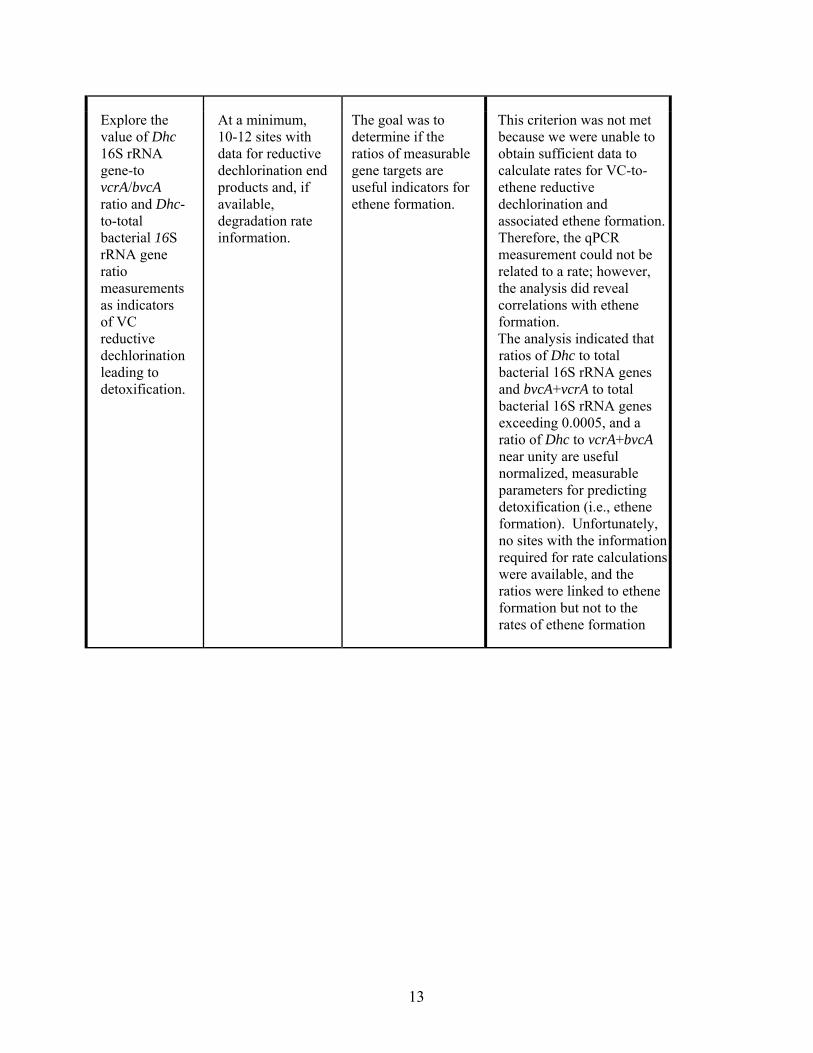
Explore the value of Dhc 16S rRNA gene-to vcrA/bvcA ratio and Dhc-to-total bacterial 16S rRNA gene ratio measurements as indicators of VC reductive dechlorination leading to detoxification.

At a minimum, 10-12 sites with data for reductive dechlorination end products and, if available, degradation rate information.

The goal was to determine if the ratios of measurable gene targets are useful indicators for ethene formation.

This criterion was not met because we were unable to obtain sufficient data to calculate rates for VC-to-ethene reductive dechlorination and associated ethene formation. Therefore, the qPCR measurement could not be related to a rate; however, the analysis did reveal correlations with ethene formation. The analysis indicated that ratios of Dhc to total bacterial 16S rRNA genes and bvcA+vcrA to total bacterial 16S rRNA genes exceeding 0.0005, and a ratio of Dhc to vcrA+bvcA near unity are useful normalized, measurable parameters for predicting detoxification (i.e., ethene formation). Unfortunately, no sites with the information required for rate calculations were available, and the ratios were linked to ethene formation but not to the rates of ethene formation

14

3.1 QUALITATIVE PERFORMANCE OBJECTIVES

3.1.1 Easy to Use, Easy to Follow and Easy to Interpret

A major goal of the project was to develop a framework that can achieve broad acceptance by the user community. Currently, several off-the-shelf models are available to estimate MNA degradation rates and even the sustainability of MNA. Note that the word “sustainability” as used here refers to the prospect that the natural attenuation processes will continue unabated into the future and continue to manage the risk associated with the chlorinated ethenes in groundwater. However, most of these models require extensive knowledge, training and experience to be properly utilized. The major disadvantage of using these models is that information requirements for specific input parameters and data for calibration, are often incomplete and/or difficult to obtain. Further, while software tools to assess MNA exist, standardizing and/or simplifying modeled scenarios can significantly affect results. The BIOBALANCE toolkit (GSI, 2006), for example, was developed to assess the efficacy and longevity of MNA using a simple stoichiometric balance of electron donor and electron acceptor consumed. Limitations of BIOBALANCE arise because carbon fluxes due to dissolution of natural solid phase organic carbon, recharge fluxes and transverse dispersion are not considered. These omissions can significantly affect inferred MNA longevity.

The decision framework, and BioPIC, developed and validated during this project is easy to use, easy to understand, and easy to interpret. The extensive technical and managerial knowledge contained in the quantitative framework is not directly apparent to the user. The management expectation tool is an easy to use software application that provides the user with clear guidance for data input requirements and site-specific information.

Further, the quantitative framework and BioPIC provides intuitive guidelines using a focused, mature and practical approach. The quantitative framework upon which the management expectation tool is based, incorporates new information about the processes contributing to detoxification of chlorinated ethenes, and will therefore extend existing protocols. In that role, the management expectation tool will assist RPMs in the decision-making process for selecting the most-efficient bioremediation technology. As such, the management expectation tool is not a new paradigm, but instead extends and enhances previous protocols.

3.1.1.1 Data Requirements

User feedback on the quantitative framework’s logic and reasoning and on BioPIC was obtained in order to assess whether this performance objective was met. Direct contact with RPMs, consultants and environmental colleagues indicated that the performance metric was achieved. Comments from beta testers indicated that the framework and BioPIC were easy to use, interpret and follow. No guidance nor instruction manuals were handed out with BioPIC when it was distributed. Instead all beta testers received an invitation email to participate and the Excel format BioPIC tool. None of the beta testers called or contacted anyone in the team requesting instructions. Only minor comments addressing formatting issues were received.

3.1.1.2 Success Criteria

The qualitative performance objectives would be considered met if the feedback received from the users indicates that BioPIC was easy to use and apply, and the outcome can be readily

15

interpreted and transitioned into remedial action. Users provided constructive criticism thereby enhancing the utility of the BioPIC tool.

3.1.2 Focused Site Characterization and Sampling Regimes

The project team expects that implementation of the quantitative framework will result in a more focused site characterization process since only parameters that are directly linked to relevant detoxification pathways are needed. This targeted approach may in turn result in substantial cost savings because measurements that do not provide meaningful information under the specific site conditions will be eliminated. The degradation pathways that are assessed in the quantitative framework include: a) complete anaerobic reductive dechlorination, b) aerobic biological oxidation and c) abiotic degradation. BioPIC requires the user to enter site-specific data, including the following biogeochemical data: a) pH, b) ferrous iron [Fe(II); Fe+2], c) dissolved oxygen (DO), d) sulfide (HS-1and H2S), e) sulfate (SO4

-2), f) methane (CH4), g) Dhc abundance, h) presence and abundance of VC RDase genes, and i) magnetic susceptibility.


User feedback on currently monitored parameters versus parameters required for the extended quantitative framework were obtained to determine if the performance objective (i.e., cleanup goal) is met. Feedback was obtained through direct contact with RPMs, consultants and stakeholders who make up most of the target audience for the technology. Further, validating the framework required site historical data (up to 10 years) for pH, ferrous iron [Fe(II)], sulfide (S-2), methane (CH4) and Dhc 16S rRNA and RDase gene abundances for each of the validation sites. Historical data was used to ensure that the framework developed for this project accurately predicts degradation mechanisms and rates calculated from site data or reported in the literature. Sites were listed in Section 4 of the Demonstration Plan.


The objective addressing a more focused site characterization and sampling regime was considered met since users’ feedback was that the decision framework and BioPIC helps them strategize sample collection for analyses of specific parameters depending on the degradation pathway observed. Similarly, users’ feedback reflected that the application of BioPIC enabled them to focus on those parameters that have the greatest impact on deducing degradation pathways.

3.2 QUANTITATIVE PERFORMANCE OBJECTIVES

3.2.1 Quantify Selected Parameters’ Impact on Degradation Rates


Data from at least 10-12 sites for which degradation rates had been calculated, were evaluated to verify the validity of the selected screening parameters. Parameters of interest included: dissolved oxygen, pH, Fe(II), H2S/HS-, ethene, ratio of Dhc:total bacteria, ratio of vinyl chloride reductase genes (bvca and vcra) to Dhc, magnetic susceptibility, acid volatile sulfide, and concentrations of PCE, TCE, DCE and VC. For each of the screening parameters a plot of achieved first order degradation rate constant versus the individual parameter were made for

16

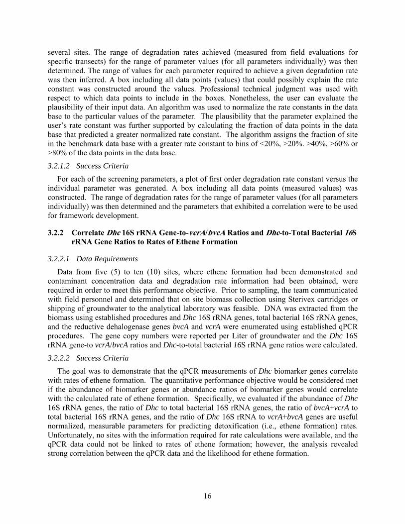
several sites. The range of degradation rates achieved (measured from field evaluations for specific transects) for the range of parameter values (for all parameters individually) was then determined. The range of values for each parameter required to achieve a given degradation rate was then inferred. A box including all data points (values) that could possibly explain the rate constant was constructed around the values. Professional technical judgment was used with respect to which data points to include in the boxes. Nonetheless, the user can evaluate the plausibility of their input data. An algorithm was used to normalize the rate constants in the data base to the particular values of the parameter. The plausibility that the parameter explained the user’s rate constant was further supported by calculating the fraction of data points in the data base that predicted a greater normalized rate constant. The algorithm assigns the fraction of site in the benchmark data base with a greater rate constant to bins of <20%, >20%. >40%, >60% or >80% of the data points in the data base.


For each of the screening parameters, a plot of first order degradation rate constant versus the individual parameter was generated. A box including all data points (measured values) was constructed. The range of degradation rates for the range of parameter values (for all parameters individually) was then determined and the parameters that exhibited a correlation were to be used for framework development.

3.2.2 Correlate Dhc 16S rRNA Gene-to-vcrA/bvcA Ratios and Dhc-to-Total Bacterial 16S rRNA Gene Ratios to Rates of Ethene Formation


Data from five (5) to ten (10) sites, where ethene formation had been demonstrated and contaminant concentration data and degradation rate information had been obtained, were required in order to meet this performance objective. Prior to sampling, the team communicated with field personnel and determined that on site biomass collection using Sterivex cartridges or shipping of groundwater to the analytical laboratory was feasible. DNA was extracted from the biomass using established procedures and Dhc 16S rRNA genes, total bacterial 16S rRNA genes, and the reductive dehalogenase genes bvcA and vcrA were enumerated using established qPCR procedures. The gene copy numbers were reported per Liter of groundwater and the Dhc 16S rRNA gene-to vcrA/bvcA ratios and Dhc-to-total bacterial 16S rRNA gene ratios were calculated.


The goal was to demonstrate that the qPCR measurements of Dhc biomarker genes correlate with rates of ethene formation. The quantitative performance objective would be considered met if the abundance of biomarker genes or abundance ratios of biomarker genes would correlate with the calculated rate of ethene formation. Specifically, we evaluated if the abundance of Dhc 16S rRNA genes, the ratio of Dhc to total bacterial 16S rRNA genes, the ratio of bvcA+vcrA to total bacterial 16S rRNA genes, and the ratio of Dhc 16S rRNA to vcrA+bvcA genes are useful normalized, measurable parameters for predicting detoxification (i.e., ethene formation) rates. Unfortunately, no sites with the information required for rate calculations were available, and the qPCR data could not be linked to rates of ethene formation; however, the analysis revealed strong correlation between the qPCR data and the likelihood for ethene formation.

17

4 SITE DESCRIPTION

This demonstration project has been performed at chlorinated solvent sites where MNA and/or bioremediation were evaluated as a remedial strategy. Demonstration sites had the following mechanisms for contaminant attenuation:

Complete anaerobic biological reductive dechlorination to non-chlorinated end products;

Partial reductive dechlorination (formation of cDCE and/or VC);

Aerobic oxidation; and /or

Abiotic reductive dechlorination or elimination reactions

Each site included in this demonstration had the following minimum data available in electronic format:

MNA parameters collected in accordance with EPA guidance (EPA 1998a), including Fe(II) or H2S/HS-

Long-term monitoring well data sufficient to evaluate degradation rates and extents of degradation within the contaminant plume.

Characterized nature and extent of contamination

Concentrations of PCE, TCE, DCEs, VC, and ethene along the flowpath over time (i.e., months to years) and a minimum of three (3) sampling events.

A minimum of eight (8) sampling events for calculation of attenuation rates.

Aquifer hydrogeologic data including hydraulic conductivity, bulk density, and hydraulic gradient

In addition, when available or collected the following data was used:

Compound-specific isotope analysis (CSIA)

Solid samples for acid volatile sulfide analysis

Solid samples for magnetic susceptibility analysis

qPCR analyses for Dhc biomarker genes including bvcA and vcrA

Carbon has two stable isotopes, 12C and 13C. When organic chemicals are degraded in ground water, the ratio of the stable isotopes of carbon will change in a predictable manner (EPA, 2008). The ratio of 13C to 12C in a compound is determined by CSIA, and the ratio can be used to document that a compound has degraded.

Acid volatile sulfide is an estimate of the bulk content of iron(II) monosulfide. This mineral carries out abiotic reactions with PCE and TCE.

Magnetic susceptibility is an estimate of the bulk content of magnetite. This mineral carries out abiotic reactions with PCE, TCE, DCE and Vinyl Chloride.

The qPCR assay for Dhc is specific for Dehalococcoides, which is the only species of bacteria that is known to carry out anaerobic biodegradation of cDCE and Vinyl Chloride. The qPCR assays for bvcA and vcrA identify two genes that code for enzymes in Dehalococcoides that degrade Vinyl Chloride.

18

4.1 SITE LOCATION AND HISTORY

The sites identified for this demonstration are described in this section.

4.1.1 Naval Air Station (NAS) North Island, Site 5, Unit 2 (Complete Anaerobic Biological Reductive Dechlorination)

Naval Air Station North Island (NASNI) is located in San Diego County, California, southwest of the City of San Diego. Situated on the Silver Strand Peninsula, NASNI is surrounded by the Pacific Ocean on the south and San Diego Bay on the west and north. The approximate size of the installation is 2,520 acres. The Installation Restoration (IR) Site 5 is located in the southeastern corner of NASNI in San Diego County, California. Site 5 is subdivided into Units 1 and 2 to differentiate the former municipal landfill and a former liquid waste disposal area, respectively.

Figure 4.1 shows the location, topography, and geographical features of IR Site 5 and the boundaries of Units 1 and 2. Waste disposal activities commenced immediately in 1945 after the construction of the Site 5 area, which served as a solid-waste disposal facility. The site functioned as the oily solid-waste disposal facility after the closure of the Old Spanish Bight Landfill (Site 2) in the early 1940s. Site 5 is subdivided into Units 1 and 2 to differentiate the former municipal landfill and a former liquid waste disposal area, respectively (THW, 2006). This work focused on Site 5, Unit 2, which had been the subject of much work in the past (Brown and Caldwell, 1983; Harding Lawson Associates, 1985 and 1988; BNI, 1996 and 1998; Parsons, 1999; Shaw, 2003; THWA, 2006; THWA and Shaw 2009; THWA and Shaw 2011).

4.1.2 Kings Bay, Site 11 (Reductive Dechlorination in the Source Zone Leading to Subsequent Oxidation of Degradation Products Downgradient)

Naval Submarine Base (SUBASE) Kings Bay encompasses approximately 16,168 acres in Camden County in the southeastern corner of Georgia, approximately 8 miles north of the Georgia-Florida state line. Currently, the base supports submarines, crew training, weapons handling and storage, submarine maintenance, and associated personnel. Site 11, the Old Camden County Landfill [Solid Waste Management Unit (SWMU) 3] located along the northwestern boundary of the SUBASE, is approximately 1,400 feet long, 600 feet wide at the southern end, and 800 feet wide at the northern end. The landfill was operated by Camden County as a municipal solid waste landfill from 1974 to 1981. During operation, trench and fill techniques were used for disposal of municipal waste, and in addition, the landfill reportedly accepted 100 cubic yards of fire-fighting pit sludge from a dredge spoils disposal area. The landfill ceased operations in October 1981 and was covered with 2 feet of fill. The site is currently vegetated with grass, weeds, and pine saplings.

Regulated under the Resource Conservation and Recovery Act (RCRA) program and in accordance with the facility’s RCRA Permit, a pump and treat system was installed and operated from 1994 to 1999 to contain and treat the cVOC plumes. Because of the limited effectiveness and lengthy estimated time of remediation for the pump and treat system to achieve remediation goals and based on the results of an evaluation of the potential for natural attenuation processes to remediate the site in a reasonable time frame (Chapelle and Bradley, 1998), the remediation focus shifted in 1999 from pump and treat to more targeted source reduction of cVOCs via in-

19

situ chemical injections and MNA to polish residual concentrations. A series of corrective actions

20

Figure 4.1: Site map of Site 5, NAS North Island, California.

21

Figure 4.2: Locations and numbers of monitoring wells at the Kings Bay Site.

22

were performed from 1999 to 2001 to treat Site 11 groundwater, including four phases of in-situ chemical oxidation treatments using Fenton’s reagent followed by injection of vegetable oil to stimulate biodegradation of remaining cVOCs (Bechtel, 2000; CH2M HILL, 2002). Two long-term monitoring programs have been conducted at Site 11, including monitoring as required by the RCRA Permit and performed by Navy contractors since 1999 and monitoring conducted from 1999 to 2011 by the United States Geological Survey (USGS) in coordination with the Navy to evaluate the effectiveness of MNA (USGS, 2009). To date, over 13 years of monitoring data have been collected for this site under these monitoring programs. Figure 4.2 shows the King’s Bay Site location and presents a site layout that shows the locations of monitoring wells in relation to the Old Camden County Landfill.

4.1.3 Hill AFB OU-10 (Aerobic Oxidation)

Hill AFB is located in northern Utah, approximately 25 miles north of Salt Lake City and five miles south of Ogden, Utah, just west of the Wasatch Front mountain range (Figure 4.3). The Base occupies approximately 6,700 acres in Davis and Weber counties. The land use in the area around the Base includes urban, suburban, agricultural (both irrigated and dryland farming), and vacant ground. The land west of Hill AFB is entirely urban, whereas the north and southeast sides are mostly rural. Operable Unit 10 encompasses the Building 1200 Area along the western boundary of Hill AFB and extends off-Base into the cities of Clearfield, Sunset, and Clinton. Figure 4.4 presents a detailed site map of OU 10.

From its beginning in 1920 as an Army reserve depot, Hill AFB has supported numerous Army and, later, Air Force missions that used or generated numerous chemicals and wastes, including chlorinated and non-chlorinated solvents and degreasers, fuels and other hydrocarbons, acids, bases, and metals. Industrial activities at the 1200 Area began in the early 1940s. A variety of chemicals, including chlorinated solvents such as PCE and TCE, were used in those activities. Most industrial activity in the 1200 Area ceased in 1959, when the majority of 1200 Area buildings were remodeled for administrative functions. It is assumed that the releases responsible for the OU 10 contamination occurred in this time period, between the early 1940s and 1959. Today, the majority of buildings in the 1200 Area are still used for administration purposes.

Environmental investigation in the area currently defined as OU 10 began in 1995 with the Hill AFB North Area Preliminary Assessment (NAPA), which identified facilities, processes, systems, and practices that may have caused releases of chemicals to soil and groundwater. Based on the findings of the NAPA, the OU 9 North Area Site Inspection was conducted to evaluate the presence of contamination, assess potential risks, and categorize areas of contamination. The OU 9 North Area Site Inspection identified contamination in several areas, one of which became OU 10.

Operable Unit 10 was created in September 2000, and the OU 10 RI began in 2001. A variety of techniques were used throughout the investigation, including cone penetrometer testing, soil sampling, monitoring well installation and sampling, soil gas and indoor air sampling, aquifer testing, groundwater age dating, geochemical profiling, and compound-specific isotope sampling and analysis.

23

Figure 4.3: Site location map for Hill AFB, OU-10.

24

Figure 4.4: Site map and extent of contamination, Hill AFB, OU-10.

25

4.1.4 Plattsburgh Air Force Base (PAFB), Fire Training Area 2 (Abiotic Reductive Dechlorination or Elimination Reactions)

The former PAFB is located in Clinton County in northeastern New York State. The base is bordered by the City of Plattsburgh to the north, south by the Salmon River, west by Interstate 87, and east by Lake Champlain (Figure 4.5). The base is situated approximately 26 miles south of the Canadian Border and 167 miles north of Albany, New York. The base was closed in 1995. PAFB initiated activities to identify, evaluate, and remediate identified hazardous materials sites as part of the Air Force’s Installation Restoration Program (IRP) and Base Realignment Program. The IRP is being implemented according to Federal Facilities Agreement, Docket No. II-CERCLA-FFA-10201, signed between the Air Force, the United States Environmental Protection Agency (USEPA), and the New York State Department of Environmental Conservation (NYSDEC) on July 10, 1991. The former PAFB was placed on the National Priorities List on November 21, 1989 (USEPA ID# NY4571924774).

The Fire Training Area 2 (FT-002) Source OU is located off Perimeter Road, 500 feet west of the PAFB runway and less than 1,000 feet east of NY Route 22 (Figure 4.5). The site formerly contained four (4) fire training pits, each 50 to 100 feet in diameter, centered within an approximately 8-acre area (Figure 4.6). Off-specification jet fuel, waste oil, solvents, and other chemicals were poured in the pits and ignited during the fire training exercises. This activity resulted in contamination of the underlying soil and groundwater.

4.2 SITE GEOLGY/HYDROGEOLOGY

The geology and hydrogeology of the four sites selected for validating the MNA sustainability framework is described below.

4.2.1 Naval Air Station (NAS) North Island, Site 5, Unit 2 (Complete Anaerobic Reductive Dechlorination)

Four major stratigraphic layers have been observed at the NASNI Site 5, Unit 2; hydraulic fill, beach sand, Spanish Bight sediments, and Bay Point Formation sediments. Hydraulic fill material, placed above the Spanish Bight sediment layer during 1944 to fill a former embayment, comprises the top 5 to 10 feet of soils at the site. The hydraulic fill consists primarily of fine silty sand, as observed from soil samples collected during drilling activities. Beach sand detected south of S5-MW-20 extends toward the stormwater discharge slough. Beach sands are believed to extend from the southern portion of the site to the Pacific Ocean. The hydraulic fill materials and beach sand in the upper 10 to 15 feet of soil at the site are underlain by a zone of low-permeability silt and clay comprising the Spanish Bight sediments. The Spanish Bight sediments are approximately 3 to 5 feet thick and act as a low permeability layer between the overlying hydraulic fill and beach sands and the underlying Bay Point Formation. The Bay Point Formation is composed of silt, sand, and clay extending more than 40 feet below the bottom of the Spanish Bight sediment layer. Groundwater under NASNI is part of the Coronado Hydrologic Area of the Otay Hydrologic Unit. Groundwater beneath NASNI occurs in an unconfined aquifer. The top of the unconfined aquifer typically ranges between 4 and 12 feet below ground surface (bgs). The base of the unconfined aquifer ranges from 85 to 120 feet bgs.

26

Figure 4.5: Plattsburgh AFB location map.

27

Figure 4.6: Plattsburgh AFB – FT-002 source OU remedial systems.

28

4.2.2 Kings Bay, Site 11 (Reductive Dechlorination in the Source Zone Leading to Subsequent Oxidation of Degradation Products Downgradient)

This SUBASE is underlain by sediments of back-barrier and barrier-island origin. The uppermost water bearing unit is approximately 75 to 90 feet thick, consists of fine sands interbedded with silty and/or clayey fine sand layers, and is underlain by a confining layer. At Site 11, this unit is divided into a shallow zone [0 to 30 feet below land surface (bls)], an intermediate zone (30 to 45 feet bls) and a deep zone (45 to 95 feet bls). The most permeable sands are encountered in the intermediate zone at depths of 30 to 45 feet. This permeable zone is underlain and overlain by finer-grained sands, clays, and organic-rich sediments of back-barrier origin that exhibit lower hydraulic conductivities. Because of the relative difference in hydraulic conductivity, the permeable zone between 30 to 45 feet bls is a preferential pathway for groundwater flow and contaminant transport. The organic-rich back-barrier sediments overlying the permeable zone have the effect of reducing dissolved oxygen-rich recharge water and thus enhancing anoxic conditions in groundwater in the permeable zone. At Site 11, groundwater is encountered at approximately 6 to 8 feet bls, flow is to the west-northwest with an approximate gradient of 0.003, and estimated Darcy velocities range from 3 to 28 feet per year (Bechtel, 1999; USGS, 2009).


Hill AFB is located on a terrace that is a remnant of the Paleo-Weber River Delta, formed where the Weber River deposited sediments into ancient Lake Bonneville. The sediments of the Paleo-Weber River Delta are composed primarily of fine-grained delta-front sheet sands interbedded with lacustrine deposits. Fluctuations in Lake Bonneville water levels exposed the Weber River Delta to waves and currents that reworked the deltaic sediments into heterogeneous, laterally discontinuous mixtures.

The complex depositional environment is responsible for the heterogeneous geology underlying OU 10. The sediments underlying the project area have been divided into three fundamental units: (1) sand, (2) silt and clay, and (3) interbedded sand, silt, and clay. In general, the subsurface geology consists of sand deposits separated by discontinuous silt and clay lenses that vary in thickness and lateral extent.

Three principal aquifers underlie the project area. From the surface, the aquifers are (1) a shallow aquifer system, (2) the Sunset Aquifer, and (3) the Delta Aquifer. Figure 4.7 illustrates the relationship between the aquifers. The Delta Aquifer is the primary source of drinking water in the area, and the Sunset Aquifer is a secondary aquifer. The shallow aquifer is not a source of drinking water in the area. Groundwater contamination at OU 10 is located within the shallow aquifer system. Current site data indicate the contamination has not migrated to the Sunset or Delta Aquifers.

The shallow aquifer underlying OU 10 consists of two semi-independent water-bearing units, referred to as the Upper and Lower Zones (see Figure 4.7). The zones are separated by an aquitard composed of silt and clay and are characterized by distinct groundwater flow directions.

The Upper Zone consists of two hydrostratigraphic units: an aquifer and an underlying aquitard. The aquifer unit is primarily composed of fine to medium sand deposited by fluvial

29

processes as a stream cut into lacustrine clay deposits during the regression of Lake Bonneville. The aquitard is composed of low-permeability silt and clay with some interbedded sand.

The paleo-stream channel responsible for depositing the aquifer sand is an important geologic feature underlying OU 10. First, the orientation of the channel drives the groundwater flow direction in the Upper Zone. Second, the channel has substantially thinned or completely eroded the aquitard in some areas, creating localized hydraulic connections between the Upper and Lower Zones.

The depth to groundwater within the aquifer unit of the Upper Zone ranges from 3 to 33 feet below ground surface (bgs). Groundwater flows toward the southwest with an estimated average velocity of 0.5 foot per day (ft/day). In the southwestern portion of the site, in a location where the aquitard separating the Upper and Lower Zones has been completely eroded by the paleo-channel, the Upper and Lower Zones are hydraulically connected.

The Lower Zone is also composed of an aquifer unit and an aquitard. The aquifer consists of layers of sand and discontinuous lenses of silt, clay, and interbedded sand, silt, and clay that vary in thickness and lateral extent. The aquitard is a low-permeability, laterally extensive, organic-rich, laminated silt and clay sequence that separates the entire OU 10 shallow aquifer system from the underlying Sunset Aquifer and deeper Delta Aquifer, the primary source of drinking water in the area.

Depth to groundwater within the Lower Zone ranges between approximately 50 and 185 feet bgs. The Lower Zone is confined in the southeastern corner of the site and in the western portions of the site but is only partially saturated (unconfined) in the northeastern and central portions of the site. Groundwater within the Lower Zone flows toward the northwest. The hydraulic gradient is relatively steep in the eastern portion of the site and becomes shallower in the western portion of the site. Groundwater velocity estimates reflect the differences in hydraulic gradients, with median estimated velocities of 1.9 ft/day in the eastern portion of OU 10 and 0.6 ft/day in the west.

Groundwater quality classifications in the Lower Zone range from “Class IA-Pristine Groundwater” to “Class II-Drinking Water Quality” depending on location and TDS concentration.

4.2.4 Plattsburgh Air Force Base, Fire Training Area 2 (Abiotic Reductive Dechlorination or Elimination Reactions)

Four distinct stratigraphic units underlie the FT-002 site: sand, clay, till, and carbonate bedrock (Figure 4.8). The sand unit generally extends from ground surface up to 90 feet bgs in the vicinity of the FT-002 site. A 7-foot-thick clay unit has been identified on the eastern side of the site. The thickness of the clay on the western side of the site has not been determined. A 30- to 40-foot thick clay/till unit is also present from 80 to 105 feet bgs in the vicinity of the FT-002 site. Bedrock is located approximately 120 feet bgs. Ground water occurs in the sand unit approximately 0 to 35 feet bgs. The generalized profile was generated from soil borings, soil samples collected during the installation of monitoring wells, CPT explorations, laboratory grain-size analyses, and geophysical surveys.

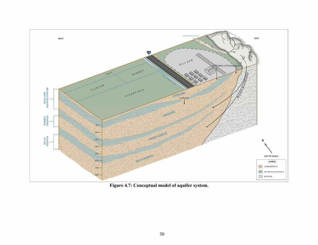
30

Figure 4.7: Conceptual model of aquifer system.

31

The upper sand unit consists of well-sorted, medium-to fine-grained sand, with a trace to some silt. Gravel and cobbles are only occasionally encountered, and fine sands and silts become more predominant at the base of the sand unit. The bottom 5 to 10 feet of the sand unit consists of silty sand with silt lenses. The CPT data collected at this site confirmed the presence of fine-grained sand and silt at the bottom of the sand unit. The sand was observed to change from light brown to gray at the water table, which could be attributable to a change from a generally oxidizing environment (unsaturated soil) to a reducing environment (saturated soil).

The next lower unit in the profile is a deep water glacial lacustrine clay deposit. The extent and depth of the clay layer are based on data obtained during previous CPT explorations and during installation of deep ground water monitoring wells. Previous data suggest that the clay layer is located approximately 90 feet bgs on the west side of the FT-002 site and 20 feet bgs on the east side of the flightline. Although few borings have completely penetrated the clay layer, seismic survey results from the eastern side of the FT-002 site suggest that the clay layer is 7 feet thick. Together the clay and overlying sands represent a regressive sequence caused by retreating shorelines related to the shrinkage of the former Champlain Sea. The sea receded due to of isostatic rebound of the crust after the melting of the glaciers.

Gray till was found on the east side of FT-002 at an estimated depth of 88 feet bgs during the installation of MW-02-007 (Figure 4.8). This boring completely penetrated the 37-foot thick till. Till was also encountered at 58 feet bgs south of the site at the Weapons Storage Area, and at a depth of 60 feet at CP-02-007 (Figure 4.8). The till is poorly sorted, with particle sizes ranging from clay and silt to gravel and cobbles. The till near the base of the unit has the characteristics of basal till, whereas the upper portions of the unit contain sediments more massive in structure.

The elevation of the fourth geologic unit, limestone bedrock, was determined by previous seismic surveys and auger refusal during the installation of MW-02-007. The bedrock unit is located approximately 120 feet bgs at the FT-002 site, and slopes downward to a depth of 140 feet bgs on the east side of the flightline. No bedrock has been cored during the site investigation or remedial investigation, but outcrops on the eastern side of Plattsburgh AFB have been identified as Ordovician Period limestone.

4.3 CONTAMINANT DISTRIBUTION

The contaminant distribution at each of the four selected sites is explained below.

4.3.1 Naval Air Station (NAS) North Island, Site 5, Unit 2 (Complete Anaerobic Reductive Dechlorination)

An estimated 1,000 to 2,000 tons (0.5 percent of the total quantity of the landfill debris) of debris was disposed of at this landfill. These wastes were not separated or segregated from nonhazardous refuse. An aerial photograph from 1948 indicated that landfill activity extended approximately 100 to 200 feet west of Rogers Road along "J" Road East, and showed two rectangular hazardous waste disposal pits east of Rogers Road that are believed to be the source of the groundwater contamination (BNI, 1998). This is confirmed by site investigation activities. Waste disposal activities ceased between 1965 and 1968, and the Site was operated as a transfer station to dispose of Navy wastes off-base. The operation of the transfer station was terminated in

32

Figure 4.8: Generalized hydrogeologic cross section Plattsburgh AFB, FT-002. Figure 3 in URS (2009).

33

Figure 4.9: Isopleth map for chlorinated ethenes - March 2008 NASNI, Site 5, Unit 2.

34

1983. The Site was redeveloped as a golf course between 1983 and 1984 and is still being used for this purpose. Chlorinated ethenes are the most prevalent contaminants found in the groundwater at the site. Figure 4.9 is an isopleth map representing the distribution of the sum of chlorinated ethenes in groundwater in September 2007. The highest chlorinated ethene concentrations have historically been detected in samples collected from monitoring wells S5-MW-20, S5-MW-21, and S5-MW-26. In addition, monitoring wells S5-MW-25, S5-MW-28, and S5-MW-30 also have exhibited elevated (i.e., greater that 10,000 μg/L) concentrations of chlorinated ethenes. Concentrations observed in S5-MW-20 have decreased significantly over the period of observation. These observations show that the mass of chlorinated ethenes in groundwater has decreased significantly since 1997 (data not shown).

4.3.2 Naval SUBASE Kings Bay (Reductive Dechlorination in the Source Zone Leading to Subsequent Oxidation of Degradation Products Downgradient)

To show the distribution of the chlorinated ethene plume at King’s Bay, isoconcentration contour maps were prepared for PCE, TCE, cDCE, and vinyl chloride using monitoring data collected from the August 2002, May 2009, and April 2011 sampling events. The snapshot plume maps for the four contaminants are presented as Figure 4.10 through Figure 4.13. Temporal changes in the spatial distributions of the four selected constituents were evaluated by comparing the plume extents of each contaminant over time. The three sampling events were selected because the August 2002 event is the first sampling event after ISCO and vegetable oil injections with the most comprehensive data, the May 2009 event is the latest event with the most comprehensive data, and April 2011 is the latest sampling event but with fewer monitoring wells sampled than during the May 2009 event.

The USGS made a special study of the effects of source treatment in the landfill on the natural attenuation of the chlorinated alkenes down gradient of the landfill. The wells that were installed for the USGS study are clustered in a small area downgradient of the landfill, and the wells monitored under RCRA requirements are spread out across the site, including the downgradient neighborhood. The uneven spatial distribution of the monitoring wells makes it somewhat more difficult to accurately contour the extents of plumes in some areas. As a result, the plume extents in some areas were partially inferred, as shown by dashed lines.

Figure 4.10 indicates that in 2002, the PCE plume footprint partially covered the area where Fenton’s reagent was injected and extended to the northwest near the second row of the USGS wells (USGS-4 through USGS-7). By May 2009, the size of the PCE plume had significantly shrunk and concentrations exceeding the MCL (5µg/L) were only detected in two wells (KBA-11-13A and USGS-2). As of April 2011, concentrations of PCE exceeding the MCL were not detected in any of the monitoring wells. The PCE plume is confined within the base and had not migrated across the road (Spur 40) into the residential area to the northwest.

In 2002, the TCE plume occupied a similar area as the PCE plume but with a smaller footprint (see Figure 4.11). Concentrations were generally low and exceeded the MCL (5 μg/L) in only four wells. By 2009, the plume extent had decreased significantly, and marginal exceedances were only detected in two wells (USGS-2 and KBA-11-13A). By April 2011, the size of the plume had decreased further, and only one minor exceedance was detected in KBA-11-13A at 5.2 μg/L. In addition, Figure 4.11 shows that the TCE plume has also confined and had not migrated into the residential area.

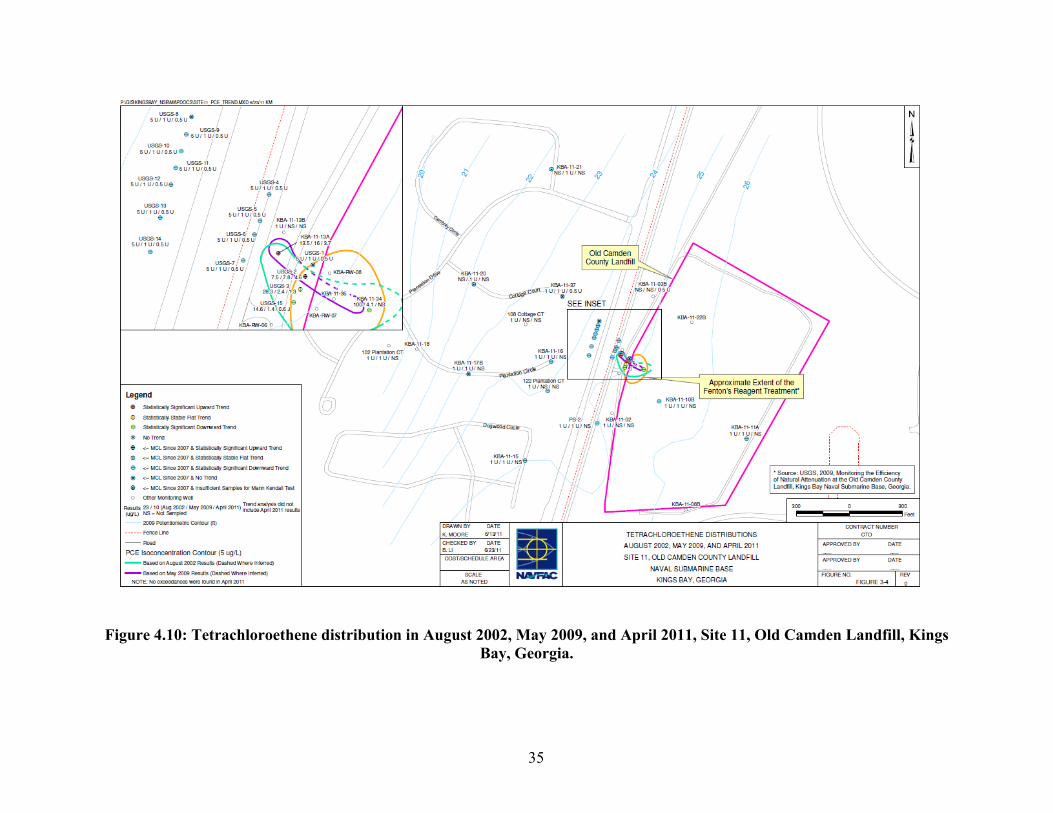
35

Figure 4.10: Tetrachloroethene distribution in August 2002, May 2009, and April 2011, Site 11, Old Camden Landfill, Kings Bay, Georgia.

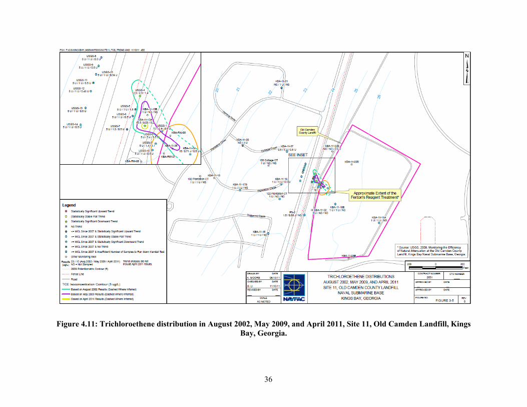
36

Figure 4.11: Trichloroethene distribution in August 2002, May 2009, and April 2011, Site 11, Old Camden Landfill, Kings

Bay, Georgia.

37

Figure 4.12: cis-1,2-Dichloroethene distribution in August 2002, May 2009, and April 2011, Site 11, Old Camden Landfill,

Kings Bay, Georgia.

38

Figure 4.13: Vinyl Chloride distribution in August 2002, May 2009, and April 2011, Site 11, Old Camden Landfill, Kings Bay, Georgia.

39

Low-concentration cDCE plumes were observed at two small separate areas in 2002 (Figure 4.12), based on exceedances of the MCL (70 μg/L) at three wells. In May 2009, exceedances were only detected at one well (USGS-4), indicating a significant decrease in the extent of the plume. The August 2009 event was also plotted on Figure 4.12 to present a complete picture of the cDCE plume in 2009; because an exceedance (180 μg/L) was detected at KBA-11-34 during the August 2009 event although no exceedance was detected at this well in May 2009. In general, cDCE concentrations in KBA-11-34 have fluctuated from less than the MCL and 200 μg/L since 2008. In April 2011, no exceedances of cDCE were detected in any of the wells.

The vinyl chloride plumes were present in areas similar to cDCE plumes in 2002 but with larger footprints (Figure 4.13). In May 2009, exceedances of the MCL (2 μg/L) were no longer detected in wells PS-2 and 122 Plantation Ct. associated with a southern vinyl chloride plume that had low-level exceedances during the 2002 sampling event. Likewise, concentrations in most of the wells in the northern plume had significantly decreased by the May 2009 event. In April 2011, exceedances were only detected in three wells (USGS-8, USGS-10, and USGS-11), indicating the extent of the northern plume also continues to decrease.

The extents of the plumes for each constituent (PCE, TCE, cDCE, and vinyl chloride) decreased significantly from 2002 through 2011. For PCE and cDCE, no exceedances of MCLs were detected as of the April 2011 sampling event. Similarly, the cDCE and vinyl chloride plumes in the southern portion of the site (near PS-2 and 122 Plantation Ct.) are no longer evident as of the May 2009 event. In terms of constituent concentrations, a comparison of 2002, 2009, and 2011 data, as shown on Figure 4.10 through Figure 4.13, indicates that cVOC concentrations in general decreased significantly at most wells.


The primary COPCs at OU 10 are PCE, TCE, and cDCE. Contamination has been detected in soil, soil gas, and groundwater. The COPC cDCE is present in groundwater as a degradation product of TCE. The suspected source of PCE contamination was a spill in the parking area west of Building 1274. The source of TCE contamination was a former oil-water separator (OWS) and related appurtenances at the north end of Building 1244. The former OWS was removed in 2003, and approximately 4 cubic yards of contaminated soils beneath the OWS were excavated.

Contaminant releases are assumed to have occurred between the early 1940s and 1959 when industrial activities were being performed in the 1200 Area. Currently, remaining concentrations of PCE and TCE in the soil gas, soil, and groundwater near the historical source areas are relatively low. These data, combined with the process and remediation history of the 1200 Area, do not indicate the presence of current active sources such as ongoing discharges or free-phase chemical products at OU 10.

4.3.3.1 Soil Contamination

The known extent of soil contamination at OU 10 is localized to the historical PCE and TCE source areas. No COPCs have been detected in soil above their respective United States Environmental Protection Agency (EPA) residential direct exposure regional screening levels (RSLs). The existing soil contamination is not considered to be a significant continuing source of groundwater contamination.

40

Arsenic was detected above the RSL but is not considered an OU 10 COPC because arsenic concentrations in soil are within the range of Hill AFB background concentrations. Background arsenic concentrations in soils at Hill AFB range between 2.4 and 14.3 milligrams per kilogram (mg/kg). The highest arsenic concentration detected in soil samples collected in OU 10 was 8.7 mg/kg.

4.3.3.2 Groundwater Contamination

Figure 4.14 illustrates the conceptual model of groundwater contamination at OU 10. Contamination has been identified in the Upper and Lower Zones of the shallow aquifer system. The COPCs in the Upper Zone are PCE and TCE, referred to as the PCE plume and the shallow TCE plume, respectively. In two known locations, contaminated groundwater from the shallow TCE plume has migrated through leaky portions of the aquitard into the Lower Zone. This contamination is referred to as the deep TCE plume. Based on the available data, groundwater contamination at OU 10 is confined within the shallow aquifer system and has not migrated into the underlying Sunset and Delta Aquifers. The groundwater plumes are shown in map view on the OU 10 site map presented in Figure 4.4.

PCE Plume: The PCE plume is approximately 3,100 feet long, extending southwest from the 1200 Area into Clearfield. The plume is relatively narrow, only about 220 feet across at its widest point. Vertically, the PCE plume is located near the water table (8 to 25 feet bgs) and is approximately 20 feet thick. The vertical extent of the PCE plume is illustrated in cross section in Figure 4.14. The PCE plume is completely confined to the Upper Zone. The highest historical concentration of PCE detected at OU 10, 720 micrograms per liter (μg/L) at Monitoring Well U9-12-006, was measured in 2001. Currently, the highest PCE concentration at the site is still at Monitoring Well U9-12-006 but has decreased to 63 μg/L.

Shallow TCE Plume: The shallow TCE plume is located slightly south of the PCE plume and is located at greater depths on-Base. Off-Base, however, the Upper Zone becomes relatively thin, and portions of the shallow TCE and PCE plumes commingle. Figure 4.14 shows the relationship between the PCE and shallow TCE plumes in cross section. The shallow TCE plume is located between 8 and 100 feet bgs, is 300 feet wide on-Base but becomes up to 1,400 feet wide off-Base, and has migrated approximately 4,900 feet to the southwest from the source area.

The highest historical concentration in the shallow TCE plume was 489 μg/L, measured at Monitoring Well U10-020 in 2003. The TCE concentration in Monitoring Well U10-020 has since declined to 160 μg/L. Currently, the highest TCE concentration is 200 μg/L in off-Base Monitoring Well U10-043. The TCE concentration in U10-043 has also declined from a historical high of 262 μg/L, measured in January 2005.

Deep TCE Plume: In at least two locations where the paleo-channel underlying OU 10 has substantially eroded the aquitard separating the Upper and Lower Zones, TCE contamination from the shallow TCE plume has migrated into the Lower Zone. Contaminants in the Lower Zone include TCE, cDCE, trans-1,2-dichlorothene (trans-DCE), and vinyl chloride. The dichloroethene (DCE) isomers and vinyl chloride are present as daughter products from the reductive dechlorination of TCE. Only TCE and cDCE are present in the Lower Zone above their respective EPA-defined maximum contaminant levels (MCLs). Correspondingly, TCE and cDCE are recognized as primary COPCs in the Lower Zone.

41

Figure 4.14: Cross-section A-A’ with PCE and TCE plumes Hill AFB, OU-10.

42

The deep TCE plume occurs in at least three lobes (Figure 4.4). The northern lobe is the largest of the three and extends from on-Base in the 1200 Area to off-Base beneath the city of Sunset. Contamination is located between approximately 175 and 290 feet bgs and is approximately 2,600 feet long and 1,400 feet wide (at its widest point).

The southern lobe is located beneath the cities of Clearfield and Sunset, contains contamination between approximately 190 and 290 feet bgs and is approximately 1,400 feet long and 800 feet wide (at its widest point).

The western lobe is located near the western boundary of the city of Sunset and is currently defined by contamination in only one monitoring well. It is recognized as a distinct lobe because the contamination is located at different elevations than in the other two lobes.

The highest historical and current concentration of TCE in the Lower Zone is 750 μg/L, measured at Monitoring Well U10-089C in fall 2008. Monitoring Well U10-089C is located near the downgradient toe of the northern lobe.

4.3.4 Plattsburgh Air Force Base, Fire Training Area 2 (Abiotic Reductive Dechlorination or Elimination Reactions)

Based on various studies and response actions conducted over more than a decade, contamination at the FT-002 source area was found to include: 1) soil contamination above the water table that was mainly confined to the area of four (4) former fire training pits; 2) residual product adhering to soil in the zone of water table fluctuation that resulted from the horizontal and vertical movement of product in the subsurface; and 3) groundwater contamination that resulted from the product and soil contamination. Remedial actions for the FT-002 fire training area are being conducted using two operable units, the FT-002 Source OU and the FT-002/IA GW OU. The first three elements are the subject of the Source OU and the fourth element is the subject of the GW OU.

Groundwater contamination extends southeast from the FT-002 source area to an industrial area east of the flightline that formerly supported flight operations (Figure 4.5). This groundwater contamination has migrated over one mile downgradient from the FT-002 source area within an unconfined aquifer. The FT-002/IA GW OU consists of a dissolved-phase contaminant plume with two distinct, but overlapping, components; one composed of benzene, toluene, ethylbenzene, and xylenes (BTEX), and the other made up of chlorinated hydrocarbons (i.e., TCE, DCEs, and VC; Figure 4.15). The original BTEX plume depicted in 2001 has subsequently subdivided into three (3) distinct, but significantly smaller, individual pools through the years (Figure 4.16). It should be noted that the groundwater in the vicinity of former Pumphouse No. 3 was not investigated until after the 2001 plume boundaries were established, which would explain why no total BTEX plume was indicated in that area at that time. Groundwater contaminants were also being discharged to a storm drain located between the runway and flightline which flowed to the southwest to surface water at a former Weapons Storage Area (WSA). The chlorinated hydrocarbon plume is also subdivided physically, with a smaller, separate plume isolated further east along Idaho Avenue (Figure 4.17).

Since remediation of the groundwater began in 2004, the aerial extent of the dissolved-phase BTEX and chlorinated hydrocarbon plumes have been significantly reduced, as indicated through the annual sampling of site monitoring wells (Figures 4.16 and 4.17).

43

Remediation systems installed at the FT-002/IA GW OU site include:

Groundwater Extraction Wells – There are five (5) extraction wells located downgradient of the FT-002 Source OU and west of the airport runway (i.e., EW-01 through -05; see Figures 4.12-4.14).

Runway/Flightline Collection Trench (RFCT) – The RFCT is a 4,000-foot long groundwater collection trench located between the airport runway and flightline (see Figures 4.12-4.15).

FT-002/IA GW OU Water Treatment System – The 500-gallon per minute (gpm) water treatment system includes an aerator, 5-stage air stripper, clarifier, and 4 sand filters (Figure 4.12).

East Flightline Collection Trench (EFCT) – The EFCT is a 4,600-foot long groundwater collection trench located east of the runway flightline (Figure 4.18).

Idaho Avenue Collection Trench (IACT) – The IACT consists of two segments. The northern segment is approximately 1,400 feet in length and extends along the western side of Idaho Avenue, beginning just south of Connecticut Avenue (Figure 4.18).

44

Figure 4.15: Plattsburgh AFB – FT-002 Source OU downgradient containment plumes – FT-002/IA groundwater OU remedial system component locations.

45

Figure 4.16: Plattsburgh AFB – FT-002 - Groundwater OU remedial system components and BTEX Plume.

46

Figure 4.17: Plattsburgh AFB – FT-002 - Groundwater OU remedial system components and chlorinated hydrocarbon plume.

47

Figure 4.18: Plattsburgh AFB – FT-002 – East Flightline and Idaho Avenue collection trenches.

48

5 TEST DESIGN

This section discusses how the decision framework and the BioPIC tool were designed. In addition, this section provides instructions on how to estimate in situ degradation rate constants and how to use BioPIC. An accurate estimation of degradation rates is of paramount importance for the proper assessment of the fate and migration of contaminants in the subsurface. Furthermore, cleanup goals typically are based on the current, or projected, extent of a solute plume and whether or not potential receptors will be impacted. Thus, cleanup goals typically have a spatial and/or temporal component. Without knowledge of degradation rates, among other things, it typically is not possible to accurately predict the future extent of a solute plume or to estimate cleanup timeframes. In the past, this has made the selection of the most efficacious remediation approach problematic. Knowledge of site-specific degradation rates in conjunction with those site-specific biogeochemical data for which validated analytical techniques are available, allows the practitioner to deduce degradation pathways. This in turn allows the practitioner to selectively enhance those processes that are already working to effect remediation. The BioPIC tool allows RPMs to input site-specific degradation rates and biogeochemical parameters and deduce the most relevant degradation pathways. With this information, RPMs can select the most appropriate remediation approach to achieve site-specific cleanup goals.

5.1 CONCEPTUAL EXPERIMENTAL DESIGN

Biostimulation and Bioaugmentation are validated technologies that have been quickly adopted in the last 15 years. This project integrates the evaluation of natural processes of contaminant attenuation, both biological and abiotic, as well as biostimulation and bioaugmentation, into a quantitative framework. The framework incorporates abiotic degradation processes because it is now known that these processes contribute to contaminant degradation in the natural environment.

To develop the decision framework and BioPIC screening tool, the relationship between biogeochemical parameters, for which mature and validated analytical techniques are available (e.g., methane, ferrous iron, CSIA, 16S rRNA genes, VC RDase genes, mass magnetic susceptibility as a surrogate for magnetite abundance, etc.), and degradation rates were evaluated. This section describes the development of this decision tool.

Originally, the DEM/VAL plan consisted of completing six tasks to address the performance objectives listed in Section 3. However, Task 4 (Validate the Framework) was eliminated from the scope of the project as it made little sense to do so after we had used site information to develop the framework; i.e., we used these site’s information to develop the framework, therefore it made little sense to use the validate the framework using the same information. The tasks executed during the project therefore were:

1) Task 1: Develop a list of biogeochemical screening parameters that likely have significant influence on degradation rate;

2) Task 2: Determine the quantitative relationship between the biogeochemical parameters selected as screening parameters and degradation rates;

3) Task 3: Develop the framework (a systematic decision making protocol that yields the most effective remediation approach);

4) Task 4: Develop a user-friendly decision tool (BioPIC) to facilitate widespread application of the framework, and;

49

5) Task 5: Validate cost and performance data.

The remainder of Section 5.1 describes how each of these tasks was completed.

5.1.1 Task 1 - Develop a List of Biogeochemical Screening Parameters that Likely Have a Significant Influence on Degradation Rate

During this task, those parameters that were anticipated to have significant influence on degradation rates were identified and evaluated. Sites were identified where the predominant pathway could be clearly distinguished, and which met the data requirements outlined in Section 4. Knowledge of the major degradation process was crucial for correlating measured values for the screening parameters with calculated degradation rates. Four degradation scenarios were identified: a) complete anaerobic biological reductive dechlorination (ethene/ethane are generated); b) incomplete reductive dechlorination leading to the formation of chlorinated daughter products (cDCE and/or VC accumulation); c) aerobic oxidation, and; d) abiotic reductive dechlorination or elimination reactions. Characteristics of these sites are presented in Section 4.

In order to facilitate meeting the performance objectives of this project, and to develop the decision framework and the BioPIC tool, the screening parameters had/were:

a. Based on existing or emerging analytical techniques that had been validated and undergone peer review;

b. Have an acceptable probability for error when applied to field samples;

c. Readily available and could be obtained at reasonable cost;

d. Have a demonstrated effect on degradation rates and extents, and;

e. Have a good probability that they would be able to predict the dominant degradation processes (i.e., pathways) and the extent of degradation/detoxification.

The ER-201129 project team identified the following list of screening parameters during Task 1:

Dhc abundance;

The ratio of Dhc-to-total bacterial 16S rRNA genes;

bvcA abundance;

vcrA abundance;

tceA abundance;

The ratio of (bvcA + vcrA)-to-Dhc 16S rRNA genes;

Dissolved oxygen concentration;

Oxidation-reduction potential;

Fe(II) concentration;

Mn(II) concentration;

Methane concentration;

Ethene concentration;

50

Total organic carbon (TOC) concentration in groundwater, and;

Mass magnetic susceptibility as a surrogate for the bulk concentration of magnetite.

The relationships between the range of values for these parameters and the calculated degradations rates were used to develop a framework that allows elucidation of degradation pathways. Further, the BioPIC tool built on this framework guides the user to identify the most promising remedial approach. The flowchart provided in Section 5.2 illustrates and summarizes the framework, and can be applied directly or by using the BioPIC tool.

5.1.2 Task 2 – Determine the Quantitative Relationship Between the Biogeochemical Parameters Selected as Screening Parameters and Degradation Rates

Task 2 involved determining the quantitative relationship between the screening parameters and the degradation rate. The team collected as many data as possible to develop these quantitative relationships. The database includes those sites where aquifer matrix and groundwater analytical screening parameters of interest were available, and for which degradation rates have been, or could be, calculated from temporal measurements of contaminant concentration data.

Whenever possible, sites were selected where the concentrations or values of the screening parameters, as well as site-specific degradation rates, have been published in the peer-reviewed literature. This minimized the amount of labor required to extract degradation rate constants from site characterization and contaminant concentration data. As a starting point, the data from Lu et al. (2006) were used for data analysis. The database was supplemented with data from additional sources. For example, the team contacted environmental professionals to obtain unpublished data for sites with sufficient information to estimate degradation rate constants in order to compile the most comprehensive data set possible. Further, the team used existing information from Microbial Insights, Inc. to correlate quantitative real-time PCR (qPCR) data for Dhc biomarker gene abundances with VOC concentrations and other available biogeochemical datasets with degradation rates.

In order to evaluate the quantitative relationship between screening parameters and degradation rates, the candidate screening parameters were individually plotted against the corresponding first order degradation rates achieved at the site to determine if there was a relationship between a given parameter and the degradation rate.

Plots of parameter concentrations/abundances versus degradation rates were made for all of the screening parameters identified in Section 5.1.1.1. Based on these plots, the following parameters were found to correlate with degradation rates:

Dhc abundance for TCE, cDCE, and VC;

Mass magnetic susceptibility;

FeS;

CH4, and;

Fe(II).

The relationships between the concentrations of these parameters and the degradation rates were used to develop the decision framework, allowing elucidation of degradation pathways to aid the user in selection of the most appropriate remediation strategy (Task 3).

The concentrations of CH4 and Fe(II) are determined on water samples from wells. These parameters were part of the original Technical Protocol for Evaluating Natural Attenuation of

51

Chlorinated Solvents in Ground Water (EPA, 1998a). Analyses for these parameters are available from a number of vendors.

The abundance of structural genes in Dehalococcoides bacteria (Dhc) is also determined in samples of groundwater from the site, using an assay based on the quantitative polymerase chain reaction (qPCR). The assay is available from several vendors in North America.

In the past, attempts were made to measure the quantity of FeS in aquifer sediment as acid volatile sulfide. Unfortunately, the quantity of FeS determined as acid volatile sulfide does not correlate well to the rate of TCE degradation (Whiting et al., 2014). In this framework, information on the concentrations of sulfate and sulfide in groundwater, the pH of the groundwater, the residence time of contamination in the subsurface, and the groundwater flow velocity are used to calculate the accumulation of reactive FeS. Then the calculated accumulation of reactive FeS is used to predict rate constants for degradation of TCE.

Magnetic susceptibility is the tendency of a material to propagate a magnetic field. As an example, when iron nails are attracted to a magnet, the nails temporarily become magnets. Almost all of the magnetic susceptibility in aquifer materials is associated with the mineral magnetite. Unfortunately, magnetic susceptibility is not a conventional analysis in the environmental market.

The magnetic susceptibility of aquifer material in situ can be measured with a probe that can be inserted into open boreholes or into wells that have plastic screens and risers. The magnetic susceptibility of a core sample can be measured with an instrument in the laboratory.

Down-hole probes to measure magnetic susceptibility can be purchased or rented from vendors that support geophysical investigations. The laboratory meters are available in many geology departments at universities. Recently, one vendor in the environmental market has added magnetic susceptibility of core samples to their line of services.

The instruments report the volume magnetic susceptibility, which is a dimensionless measure. However, the actual value of a measurement depends on the system of measurements that is used. This framework uses the International System of Units (Système International d'Unités) which is commonly referred to as the SI system.

The volume magnetic susceptibility of a sample of aquifer material is directly proportional to the mass of material in the volume that is being analyzed. In this framework, the volume magnetic susceptibility is converted to a mass magnetic susceptibility. To make the conversion for a laboratory sample, the volume magnetic susceptibility is divided by the mass of aquifer material analyzed, and then multiplied by the volume of the container that holds the sample. To make the conversion for a down-hole probe, the volume magnetic susceptibility is divided by an estimate of the bulk density of the aquifer material. Mass magnetic susceptibility in the SI system of units is conventionally expressed in m3/kg.

5.1.3 Task 3 - Develop a Decision Framework (An Expert System that when Applied Allows Elucidation of Degradation Pathways and Allows the User to Determine the Most Suitable Bioremediation Approach)

The goal of Task 3 was to develop a decision-making framework using the range of values for each screening parameter for a range of rates for each degradation pathway. The decision framework uses simple if-then statements to develop the BioPIC tool, as presented in Section 5.2.

52

5.1.4 Task 4 - Develop a User-Friendly Site Management Expectation Tool to Facilitate User Application of the Decision Framework

The goal of this task was to develop a user-friendly tool for easy application of the decision framework. This tool was developed using Microsoft Excel, and is called BioPIC. Microsoft Excel was chosen for the development of the tool because of its ease of use, its broad availability, and the robustness of the programming options.

BioPIC allows the user to input site-specific values for the screening parameters that were determined to influence on contaminant degradation pathways and the degradation rates and extents as discussed under Tasks 2 and 3 (Sections 5.1.3 and 5.1.4).

5.1.5 Task 5 - Validate Cost and Performance Data

During this task, cost of implementing the decision framework was estimated.

5.2 DESIGN AND LAYOUT OF TECHNOLOGY COMPONENTS

This section describes the logic that was used to develop the decision framework and the BioPIC screening tool. BioPIC is a software application that organizes and facilitates the screening process to determine if Monitored Natural Attenuation (MNA) might be an appropriate remedy at a site.

BioPIC is organized around the USEPA lines of evidence for MNA (EPA, 1998a and 1999). The first line of evidence is historical groundwater data that demonstrate a clear and meaningful trend of decreasing contaminant concentration over time at appropriate monitoring or sampling points. Therefore, the user must first apply a groundwater transport and fate model to determine whether the rate of attenuation of the contaminants will bring the highest concentrations of the contaminants in groundwater to acceptable concentrations before the groundwater reaches a receptor or a sentry well. If the predicted concentrations are acceptable, MNA may be appropriate.

If MNA is appropriate, BioPIC offers guidance on developing information that can meet the U.S. EPA requirement for a second line of evidence that can be used to demonstrate indirectly the type(s) of natural attenuation processes active at the site, and the rate at which such processes will reduce contaminant concentrations to required levels. If MNA is not appropriate, BioPIC offers guidance on in situ bioremediation, and in particular whether it is useful to bioaugment the site with active microorganisms as well as biostimulate with nutrients.

5.2.1 Parameters Required to Implement the BioPIC Screening Tool

Table 5.2.1.1 lists the parameters that are required to implement the BioPIC Screening Tool. The parameters are listed by the particular degradation pathway that they document.

Dissolved oxygen, methane, sulfate, iron(II) and sulfide are parameters that are used in the Technical Protocol for Evaluating Natural Attenuation of Chlorinated Solvents in Ground Water (EPA. 1998a). Their application in BioPIC is different than their application in the Technical Protocol.

In BioPIC, low values for DO are not used to infer conditions appropriate for bacteria that degrade chlorinated alkenes under anaerobic condition. Instead, concentrations of DO are used to identify ground waters with adequate oxygen to support aerobic biodegradation of cDCE and Vinyl Chloride. It is easy to contaminate a sample of ground water with oxygen from the atmosphere. To guard against this possibility, BioPIC uses the concentrations of iron(II) and

53

methane to identify ground waters with an inadequate supply of dissolved oxygen to support aerobic biodegradation of cDCE and Vinyl Chloride, regardless of the measured concentration of dissolved oxygen. In BioPIC, the concentrations of sulfate and sulfide, and pH, are used to calculate the accumulation of iron(II) monosulfide, which can degrade PCE and TCE through an abiotic mechanism.

54

Degradation Pathway Required Parameter Supporting Parameter

Anaerobic Reductive Dechlorination

Abundance of Dehalococcoides (Dhc) gene copies in ground water

Abundance of vcrA and bvcA gene copies in ground water

Compound Specific Isotope Analysis (CSIA) of PCE, TCE, DCE and Vinyl Chloride

Aerobic Biological Oxidation

Dissolved Oxygen (DO) in ground water

Methane in ground water

Fe(II) in ground water

Abiotic Degradation

Sulfate in ground water

Sulfide in ground water

pH of ground water

Magnetic Susceptibility of aquifer sediments

Table 5.2.1.1-The parameters necessary to fully implement BioPIC.

Several of the parameters in BioPIC are not used at all in the Technical Protocol (EPA, 1998a). The qPCR assay for Dhc is specific for Dehalococcoides, which is the only species of bacteria that is known to carry out anaerobic biodegradation of cDCE and Vinyl Chloride (Löffler et al., 2013). The qPCR assays for bvcA and vcrA identify two genes that code for enzymes in Dehalococcoides that degrade Vinyl Chloride. The abundance of these genes in ground water can provide the second line of evidence for anaerobic biodegradation of cDCE and Vinyl Chloride.

In some circumstances, Compound Specific Isotope Analysis (CSIA) can provide unequivocal evidence that TCE, cDCE or Vinyl Chloride has been degraded (EPA, 2008) Organic compounds are composed of a mixture of carbon isotopes, including 12C and 13C. The amount of 13C is approximately 1% of the 12C. As compounds degrade, the molecules with an atom of 13C are degraded at a slightly slower rate. As a result, the ratio of 13C to 12C in the non-degraded material will increase.

The ratio of 13C to 12C in a compound is determined using an isotope ratio mass spectrometer. The instrument does not report the actual ratio. Instead, the actual ratio of 13C to 12C in the sample as analyzed is normalized to the ratio in a standard as described below, where Rx is the sample and Rstd is the standard. The ratio of 13C to 12C in Rstd is 0.0112372.

55

1 ∗ 1000

Because the normalized ratio is multiplied by a thousand, the values are reported in units of per mil or ‰. This is parallel to the convention of reporting ratios in percent.

The value of δ13C for a compound in ground water can be used to document that a compound has degraded. The values of δ13C in TCE that has been sold in commerce have been reported (Kuder and Philp, 2013; McHugh et al., 2011). If the value of δ13C in TCE, or cDCE or Vinyl Choride in a ground water plume is greater (less negative) than the largest value reported for TCE sold in commerce, then the TCE, or cDCE or Vinyl Choride in ground water must have been degraded. See Appendix B for more discussion.

Magnetic susceptibility is an estimate of the bulk content of magnetite. This mineral carries out abiotic reactions with PCE, TCE, DCE and Vinyl Chloride (EPA, 2009).

5.2.2 The Decision Logic in the BioPIC Screening Tool

BioPIC is organized as a series of decisions. In each step, BioPIC provides decision criteria based on quantitative values, which are clearly and unambiguously defined. Help is available for each decision to provide guidance and background, and to illustrate the appropriate application of tool. Figure 5.2.2.1 shows the logic used to develop BioPIC. At decision point (2) the logic in BioPIC interfaces with the decision logic for selecting and implementing biostimulation and bioaugmentation as provided by Stroo et al. (2013b). For a summary of the logic on selection of biostimulation and bioaugmentation as provided in Stroo et al. (2013b) see Figure 5.2.2.2. Consult Stroo et al. (2013b) for details.

The remainder of this section provides a detailed description of each decision step incorporated into BioPIC.

One overarching question that pervades the decision criteria boxes is “Does a given parameter explain the rate of degradation.” Thus, estimating degradation rates is critical for using the BioPIC decision-making tool. The following section discusses how to estimate degradation rates using BIOCHLOR. This modeling tool was selected because it was developed for the USEPA and it is readily available at no cost (Aziz et al., 2000, 2002). There are numerous other software packages, which use analytical, numerical, or a combination of analytical and numerical models, that can also be used to extract degradation rate information from site-specific hydrogeologic and contaminant concentration data.

56

Figure 5.2.2.1 – Decision tool framework.

VC Attenuation Caused by Dilution and Dispersion

Does Dhc Density Explain the VC Rate Constant?

(6)

Yes

No

Yes

No

Yes

Yes

No

NoIs VC Present? (4)

Is VC Degrading?(5)

Adequate Oxygen for Aerobic VC

Biodegradation?(8)

No Line of Evidence Required for VC

Quantitative Line of Evidence for Anaerobic

Microbial VC Degradation

No

VC Degradation not Explained

Does Magnetic Susceptibility Explain the

VC Rate Constant? (7)

Yes Qualitative Line of Evidence for Aerobic VC

Biodegradation

Quantitative Line of Evidence for Abiotic VC

Degradation

NoYesNoNo

Yes

Start

Evaluate BiostimulationEvaluate Bioaugmentation

See Figure 5.2.2.2

Are Reductive Dehalogenase Genes

Present?(2)

Does Natural Attenuation Currently

Meet the Goal?(1)

Is the EPA 2nd Line of Evidence

Required?(3)

MNA without 2nd Line of Evidence

Yes

Is DCE Present? (9)

No No Line of Evidence Required for DCE

DCE Attenuation Caused by Dilution and Dispersion

Quantitative Line of Evidence for Anaerobic

Microbial DCE Degradation

Quantitative Line of Evidence for Abiotic DCE

Degradation

Qualitative Line of Evidence for Aerobic DCE

Biodegradation

NoIs DCE Degrading?(10)

Yes

YesDoes Magnetic

Susceptibility Explain the DCE Rate Constant?

(12)

Adequate Oxygen for Aerobic DCE Biodegradation?

(13)

Yes

Yes

No

No

DCE Degradation not Explained

Does Dhc Density Explain the DCE Rate Constant?

(11)

Yes

No

Quantitative Line of Evidence for Abiotic PCE

Degradation

No Line of Evidence Required for PCE

Is PCE Present? (20)

No

Is PCE Degrading?(21)

No

Yes

Are TCE, DCE, or VC Present?

(22)

Yes

Yes

No

No

PCE Degradation not Explained

Does Magnetic Susceptibility Explain

the PCE Rate Constant? (24)

Are TCE, DCE, or VC

Present in RelevantConcentrations?

(23)

Evidence for at least some reductive dechlorination

PCE Attenuation Caused by Dilution and Dispersion

Yes

Yes

Qualitative Line of Evidence for PCE Biodegradation. Consider Determining pceA Gene Abundance

No

TCE DCE VCPCE

Yes

No

TCE Degradation not Explained

Yes

No Line of Evidence Required for TCE

Does Magnetic Susceptibility Explain TCE

Degradation Rate?(18)

Does Iron Sulfide Explain the TCE Rate

Constant? (19)

Quantitative Line of Evidence for Abiotic TCE

Degradation

Quantitative Line of Evidence for Abiotic TCE

Degradation

TCE Attenuation Caused by Dilution and Dispersion

Are DCE or VCPresent in Relevant Concentrations?

(17)

Yes

Evidence for at least some reductive dechlorination

Is TCE Present? (14)

No

NoIs TCE Degrading?(15)

Yes

Yes

Yes

No

AreDCE or VC Present?

(16)

Qualitative Line of Evidence for TCE Biodegradation.

Consider Determining pceAand tceA Gene Abundances

No

No

Yes

Qualitative Line of Evidence for Aerobic TCE

Co‐oxidation

Adequate Conditions for Aerobic

Co‐oxidation?(13)

Yes

No

EvaluateBiostimulationSee Figure 5.2.2.2

57

Figure 5.2.2.2– Decision framework to determine if bioaugmentation or biostimulation is appropriate. Redrawn from Figure 4.1 of Stroo et al. (2013b)

58

5.2.3 Estimating Degradation Rates Using BIOCHLOR

Figure 5.2.3.1 is a screenshot of the BIOCHLOR input screen. The use of BIOCHLOR, or almost any other solute fate and transport model to extract degradation rates from site-specific hydrogeologic, contaminant, and biogeochemical data, consists of implementing the following steps:

1. Collect Site-Specific Data/Information;

2. Select Flowpath Along Which Analysis Will Be Completed;

3. Enter Site Description Information;

4. Select Chlorinated Ethenes or Chlorinated Ethanes;

5. Enter Data for Advective Seepage Velocity Calculation;

6. Enter Data to Quantify Dispersion;

7. Enter Data to Quantify Sorption;

8. Enter Field Data for Comparison;

9. Enter Simulation Time Data;

10. Enter Source Data;

11. Vary Biotransformation Rate Constants and Compare the Model-Generated Concentration versus Distance Plots against the Field Data until a Match is Achieved and Degradation Rate Constants are Extracted;

12. Evaluate the Model Simulation Used to Extract Rate Constants.

Step 1 - Collect Site-Specific Data/Information

This step involves collecting the site-specific data that are required to run BIOCHLOR. Such information is often readily available in site characterization reports, remedial investigation reports, etc. If not available, the data will need to be collected before BIOCHLOR is used. The use of literature values for parameters other than porosity is not recommended.

The site-specific data required to run BIOCHLOR include:

Concentration data along the transport flowpath;

Hydraulic conductivity;

Porosity;

Flow direction and gradient;

Bulk density, and;

Fraction organic carbon in the aquifer matrix.

In addition, BIOCHLOR requires a value for the coefficient of longitudinal dispersivity and a value for the coefficient of lateral dispersivity.

The following sections walk the user through the data entry process.

59

Figure 5.2.3.1 – BIOCHLOR input screen.

60

Step 2 – Select Flowpath

This step involves selecting the appropriate flowpath along which to run the BIOCHLOR simulation. The flowpath should coincide with the centerline of the plume where solute concentrations are the highest. It is important to remember that solute plumes are three-dimensional objects, so this flowpath may not be coincident with wells screened across the water table and two–dimensional plan-view maps generated using only such wells may not be appropriate to select the solute transport flowpath. If the water-table wells are screened across the entire vertical space of the aquifer unit that may plausibly harbor the solute plume, the wells and the two-dimensional plan-view map will be appropriate to select the flowpath. If this is not the case, at a minimum there should be wells that are screened at the water table, in the center of the aquifer unit, and at the bottom of the aquifer unit that might plausibly harbor the solute plume (EPA 2004). If these wells are not available, the user may have to install wells and sample groundwater to complete the three-dimensional characterization of the solute plume before proceeding with the BIOCHLOR simulation.

Figure 5.2.3.2 is a cross-sectional view along the centerline of a plume of TCE that formed from a release of NAPL TCE at an industrial facility at St. Josephs, MI, and then moved with groundwater as the groundwater discharged to Lake Michigan (Semprini et al., 1995; Lendvay et al., 1998; An et al., 2004). Groundwater was sampled through slotted augers (the squares in the figure) and through push tools (the circles). The highest concentrations were in the center of the aquifer unit that was impacted by the release. Set up BIOCHLOR using the highest concentration for each location along the lateral flow path.

Figure 5.2.3.2 - Cross section showing the extension of a solute plume in the vertical-dimension. Numbers represent the concentration of TCE in micrograms per liter (µg/L).

.

VERTICAL EXAGGERATION 1:10

SCALE

20'

200'

CLAY CLAY

CLAYCLAYCLAY

SANDSAND

100,0001,000100

61

As shown in Figures 5.2.3.3 through 5.2.3.5, the flowpath for solute transport is usually oriented perpendicular to potentiometric isopotential lines. The potentiometric surface is a hypothetical surface representing the water table in an unconfined aquifer or the level to which groundwater would rise if not trapped in a confined aquifer.

Note that unless the wells are perfectly situated along the plume centerline/flowpath during site characterization, some extrapolation/interpolation will be required. It is also important to remember that flowpaths will change with changing groundwater flow directions. As shown in the Figures 5.2.3.3 through 5.2.3.5, it is important to analyze the configuration of the solute plume over time to make sure that the flowpath does not change significantly. This should also include an analysis of the potentiometric surface over time and space.

Figure 5.2.3.3 illustrates the selection of the flowpath used for the rate constant calculation example presented in this Section. Selection of the flowpath is based on the three-dimensional groundwater flow direction and plume configuration. Data collected from wells along this flowpath were used to run the BIOCHLOR model presented in the example shown throughout this Section. The total length of the flowpath is approximately 200 feet. The black numbers (e.g., 36,430) represent concentrations in µg/L; the black lines represent the non-detect and 10,000 µg/L isopleths. Turquoise numbers and lines represent groundwater elevation and equipotential lines. Figures 5.2.3.4 and 5.2.3.5 illustrate the use of temporal changes in solute plume configuration to aid in flowpath selection.

Figure 5.2.3.3 - Selection of groundwater flowpath for BIOCHLOR simulations.

62

Figure 5.2.3.4 – Selection of groundwater flowpath for BIOCHLOR simulations using temporal variations in plume configuration – A.

Figure 5.2.3.5 - Selection of groundwater flowpath for BIOCHLOR simulations using temporal variations in plume configuration – B.

Step 3 – Enter Site Description

As shown in Figure 5.2.3.6, the name of the site and/or a brief note can be entered into the boxes near the upper center of the data input screen. This should be done to help keep track of multiple model runs.

Figure 5.2.3.6 – Site description entry.

63

Step 4 – Select Ethenes or Ethanes

Although the BioPIC tool only relates to chlorinated ethenes, the BIOCHLOR model is capable of simulating the sequential degradation of chlorinated ethenes or chlorinated ethanes, therefore users must make a selection. The upper left corner of the data input screen allows the user to select a specific group of compounds, for which solute fate and migration is to be simulated and thus, the compounds for which degradation rate constants are to be extracted. Since for the purpose of this project, we are interested in chlorinated ethenes, this button should be selected (Figure 5.2.3.7).

Figure 5.2.3.7 – Selection of chlorinated ethenes versus ethanes.

Step 5 – Enter Data for Advective Seepage Velocity Calculation

As shown by Figure 5.2.3.8, those data required to calculate the advective component of solute transport, which is described by the groundwater seepage velocity, are entered into “Box 1 - ADVECTION” in the BIOCHLOR input screen. White boxes indicate parameters that are used by the model to simulate solute fate and transport. White cells can have values entered directly, or the associated gray boxes can be filled in and the red “C” button can be pressed to calculate the value in the white box using the values entered in the gray boxes. For example, for the advection term, the seepage velocity (Vs) can either be directly entered if it has already been calculated, or the gray boxes beneath the white box can be filled in with representative values of hydraulic conductivity (K), hydraulic gradient (i), and effective porosity (n). For the example calculated here (NASNI Site 5-Unit-2), K=0.0099 cm/sec, i = 0.004, and n = 0.25, giving a seepage velocity of 163.5 feet per year.

Figure 5.2.3.8 – Data entry for seepage velocity calculation

BIOCHLOR is extremely sensitive to changes in the seepage velocity of groundwater. Of the parameters affecting the seepage velocity of groundwater, hydraulic conductivity is typically the most problematic because it has the largest ranges of values and because it is the most difficult to quantify. Thus, care should be taken when selecting values of hydraulic conductivity for input into the model. Here are some general rules of thumb to use when selecting values of hydraulic conductivity:

The reliability of hydraulic conductivity values obtained from aquifer testing decreases in the following order;

64

o Pumping tests, o Borehole flowmeters, including those associated with direct-push technologies, o Laboratory testing, and, o Slug Testing.

The more values for hydraulic conductivity are available for a given hydrogeologic unit, the better; assuming, of course, that the aquifer testing was done in an accurate manner;

When multiple values of hydraulic conductivity are available for a given hydrogeologic unit, the geometric mean should be calculated and the range of values should be evaluated to see if there are significant outliers. Such outliers should be eliminated from the database if there is good justification to do so, and;

Because solutes tend to move along the “path of least resistance”, the geometric mean, or a justifiably higher value for hydraulic conductivity should be selected.

Figures 5.2.3.9 and 5.2.3.10 show two methods for calculating the hydraulic gradient: a) using a potentiometric map, or b) using a plot of groundwater elevation versus distance along flowpath.

Figure 5.2.3.9 – Use of a potentiometric map to calculate hydraulic gradient.

65

Figure 5.2.3.10 – Hydraulic gradient calculation using a plot of groundwater elevation versus distance along flowpath.

BIOCHLOR assumes that the hydraulic conductivity and the hydraulic gradient are uniform across the site. This is never exactly true at any real site. Examine a map of the site that presents the potentiometric surface of groundwater (as does Figure 5.2.2.9), and evaluate the spacing of the isopleths. If the isopleths are consistently closer together along one portion of the flow path and wider along another portion, BIOCHLOR cannot adequately describe flow along the flow path. It will be necessary to use a distributed parameter such as BIOPLUME III (EPA, 1998b) or MT3DMS (The Hydrogeology Group, University of Alabama, accessed November 20, 2015).

Calculate the change in elevation of the potentiometric surface across the plume centerline from the source of chlorinated alkenes to the most distal well containing chlorinated alkenes. Divide the flow path of the plume into three approximately equal segments. Calculate the change in elevation across each segment. If the change across any one segment varies by more than a factor of three from the average change, consider using a distributed parameter model.

A pump and treat system may have been operated at the site. This remedy distorts the ground water flow field. If this has happened, search for monitoring data that were acquired before the pumping system was installed, and use these data to extract the degradation rate constants.

Total and effective porosity typically are estimated using literature values. Table 5.2.3.1 provides representative values for porosity from multiple sources.

Step 6 - Enter Data to Quantify Dispersion

The next step is to input a value for dispersion. Dispersion is quantified in the BIOCHLOR model in several ways. If the Calc Alpha x box is selected, then a Dispersivity menu appears. As shown by Figure 5.2.3.11, three options to calculate dispersivity are available. Under Option 1, the user can enter a fixed value for dispersivity. Under Options 2 and 3, the user can enter the plume length, and the dispersivity will be calculated using one of two formulas. See the BIOCHLOR User’s Manual for a discussion of the various ways in which dispersion is calculated (Aziz et al., 2000).

66

Table 5.2.3.1 - Representative values for porosity.

Figure 5.2.3.11 – Quantification of dispersion in BIOCHLOR.

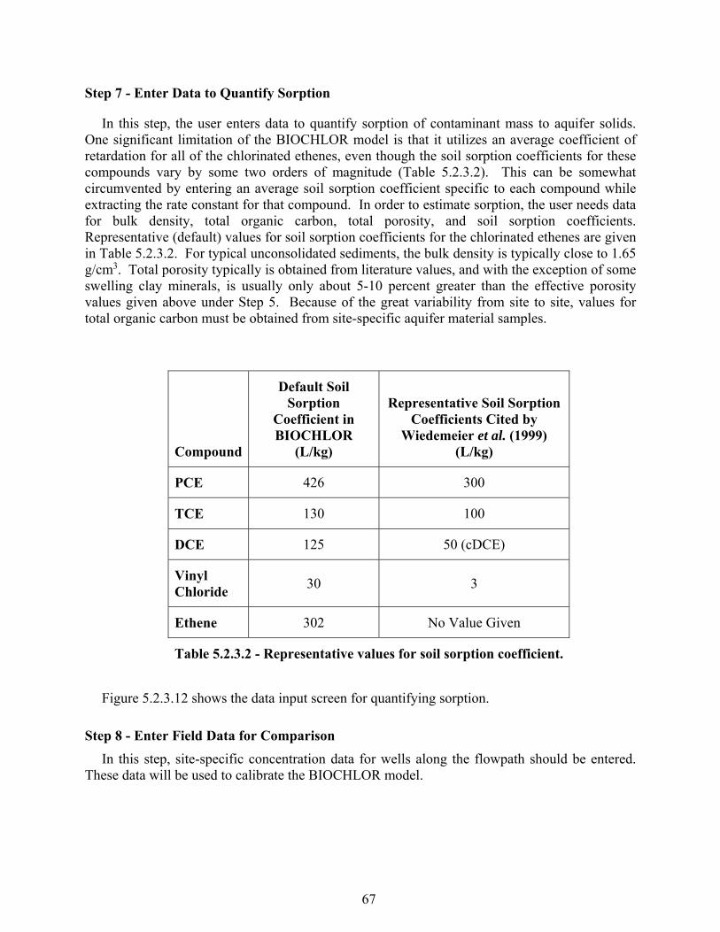
67

Step 7 - Enter Data to Quantify Sorption

In this step, the user enters data to quantify sorption of contaminant mass to aquifer solids. One significant limitation of the BIOCHLOR model is that it utilizes an average coefficient of retardation for all of the chlorinated ethenes, even though the soil sorption coefficients for these compounds vary by some two orders of magnitude (Table 5.2.3.2). This can be somewhat circumvented by entering an average soil sorption coefficient specific to each compound while extracting the rate constant for that compound. In order to estimate sorption, the user needs data for bulk density, total organic carbon, total porosity, and soil sorption coefficients. Representative (default) values for soil sorption coefficients for the chlorinated ethenes are given in Table 5.2.3.2. For typical unconsolidated sediments, the bulk density is typically close to 1.65 g/cm3. Total porosity typically is obtained from literature values, and with the exception of some swelling clay minerals, is usually only about 5-10 percent greater than the effective porosity values given above under Step 5. Because of the great variability from site to site, values for total organic carbon must be obtained from site-specific aquifer material samples.

Compound

Default Soil Sorption

Coefficient in BIOCHLOR

(L/kg)

Representative Soil Sorption Coefficients Cited by

Wiedemeier et al. (1999) (L/kg)

PCE 426 300

TCE 130 100

DCE 125 50 (cDCE)

Vinyl Chloride

30 3

Ethene 302 No Value Given

Table 5.2.3.2 - Representative values for soil sorption coefficient.

Figure 5.2.3.12 shows the data input screen for quantifying sorption.

Step 8 - Enter Field Data for Comparison

In this step, site-specific concentration data for wells along the flowpath should be entered. These data will be used to calibrate the BIOCHLOR model.

68

Figure 5.2.3.12 – Quantification of sorption in BIOCHLOR.

As is illustrated in Figure 5.2.3.3, BIOCHLOR as used in this Section is essentially a one dimensional model run along the centerline of a plume. Wells that are relatively close to the source can be clean or cleaner because they are off the centerline. At most plumes, the distribution of concentrations with distance along the centerline will follow a log-normal distribution. Figure 5.2.3.13 illustrates a simple technique to identify wells that are near the plume centerline, and should be used in BIOCHLOR to extract rate constants. Data are from the study at Naval Air Station (NAS) North Island, Site 5, Unit 2.

The top portion of Figure 5.2.3.13 provides a map showing the location of monitoring wells at the site and a figure that compares the total molar concentration of chlorinated alkenes, ethane and ethane to the distance from the source. At any particular distance from the source, the wells in the centerline are the wells with the highest concentrations. In this illustration, wells S5-MW-43, S5-MW-21, S5-MW-41, and S5–MW20 lie along or near the centerline and can be used in BIOCHLOR to extract rate constants. Wells S5-MW-42, S5-MW-44, S5-MW-32, S5-MW-20 and S5-MW-12 are off of the centerline and should not be used to extract rate constants.

During this step the user must decide between the use of highest observed concentrations or average concentrations if duplicate samples were collected during a given sampling event. However, if there are large discrepancies between duplicate samples from a single sampling event, the user should decide if the data are valid. This will take professional judgment and must be done on a site-specific basis. Historical data before and after the problematic sampling event, if available, can be used to aid in data selection in such cases, but it may be best to simply use a different sampling event for rate constant estimation. Alternatively, and preferably, multiple simulations using concentrations over multiple time periods can be used to estimate rate constants. Ultimately, the use of average versus highest concentrations will depend upon the reproducibility and reliability of the data, as well as the project objectives. In general, the data that results in the most realistically conservative (i.e., lowest) degradation rates will probably be preferable to responsible parties to ensure that potential receptors will not be adversely impacted. Again, the estimation of multiple rate constants from multiple sampling events is recommended to help remove the noise that is inherent in environmental data.

69

Figure 5.2.3.13 – Entry of contaminant concentration data into BIOCHLOR.

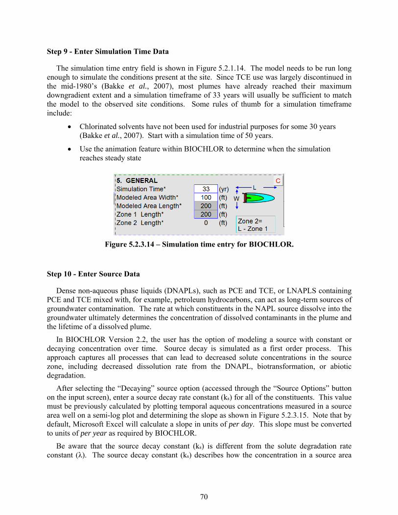
70

Step 9 - Enter Simulation Time Data

The simulation time entry field is shown in Figure 5.2.1.14. The model needs to be run long enough to simulate the conditions present at the site. Since TCE use was largely discontinued in the mid-1980’s (Bakke et al., 2007), most plumes have already reached their maximum downgradient extent and a simulation timeframe of 33 years will usually be sufficient to match the model to the observed site conditions. Some rules of thumb for a simulation timeframe include:

Chlorinated solvents have not been used for industrial purposes for some 30 years (Bakke et al., 2007). Start with a simulation time of 50 years.

Use the animation feature within BIOCHLOR to determine when the simulation reaches steady state

Figure 5.2.3.14 – Simulation time entry for BIOCHLOR.

Step 10 - Enter Source Data

Dense non-aqueous phase liquids (DNAPLs), such as PCE and TCE, or LNAPLS containing PCE and TCE mixed with, for example, petroleum hydrocarbons, can act as long-term sources of groundwater contamination. The rate at which constituents in the NAPL source dissolve into the groundwater ultimately determines the concentration of dissolved contaminants in the plume and the lifetime of a dissolved plume.

In BIOCHLOR Version 2.2, the user has the option of modeling a source with constant or decaying concentration over time. Source decay is simulated as a first order process. This approach captures all processes that can lead to decreased solute concentrations in the source zone, including decreased dissolution rate from the DNAPL, biotransformation, or abiotic degradation.

After selecting the “Decaying” source option (accessed through the “Source Options” button on the input screen), enter a source decay rate constant (ks) for all of the constituents. This value must be previously calculated by plotting temporal aqueous concentrations measured in a source area well on a semi-log plot and determining the slope as shown in Figure 5.2.3.15. Note that by default, Microsoft Excel will calculate a slope in units of per day. This slope must be converted to units of per year as required by BIOCHLOR.

Be aware that the source decay constant (ks) is different from the solute degradation rate constant (λ). The source decay constant (ks) describes how the concentration in a source area

71

well decreases as the DNAPL is depleted of the constituent of concern, whereas (λ) is the degradation rate constant for a constituent in the plume.

Figure 5.2.3.15 – Determination of ks using aqueous concentrations in source area wells.

The equations describing groundwater transport and biotransformation with a decaying source are presented in Appendix A.1 of the BIOCHLOR User’s Manual Addendum (Aziz et al., 2002). The decaying source feature can only be used with one-zone simulations. The user is restricted to values for ks that are less than 1/R*(λ+Vs/4α) to prevent unstable complex solutions.

Make sure you enter source data that were collected just downgradient from NAPL, if present. Note that for the purposes of estimating a degradation rate at one point in time, the use of a constant source term at that point in time is recommended. Note also that the source area concentrations are in mg/L.

Figure 5.2.3.16 – Source concentration data entry.

The values that are used for sources concentrations are reported in BIOCHLOR as depicted in Figure 5.2.3.16. To enter or edit data on source concentrations, click the “Source Options”

72

button. Figures 5.2.3.17 and 5.2.3.18 show the pop-up menus/input screens that appear when the user selects the “Source Options” button and then selects either constant/continuous or decaying source.

73

Figure 5.2.3.17 – Source data entry – constant source.

74

Figure 5.2.3.18 – Source data entry – decaying source.

75

Step 11 - Vary Biotransformation Rate Constants and Compare the Model-Generated Concentration versus Distance Plots against the Field Data until a Match is Achieved and Degradation Rate Constants are Extracted

This step is utilized to extract/estimate the degradation rate for each of the chlorinated ethenes of interest. The accuracy of the degradation rate constants estimated during this step are highly dependent upon the accuracy of the hydrogeologic parameters used for the modeling effort as well as the precision with which the flowpath was determined. BIOCHLOR estimates degradation rates using sequential first-order degradation rates such that:

rPCE = -λ1CPCE

rTCE= y1λ1CPCE - λ2CTCE

rDCE= y2λ2CTCE - λ3CDCE

rVC= y3λ3CDCE - λ4CVC

rETH = y4λ4CVC - λ5CETH

where λ1, λ2, λ3, λ4, and λ5 are the first order biotransformation rate coefficients; y1, y2, y3, y4 are the daughter: parent compound molecular weight ratios; and CPCE, CTCE, CDCE, CVC, and CETH are the aqueous concentrations of PCE, TCE, DCE, VC, and ethene, respectively. (Note: t h e BIOCHLOR model assumes no degradation of ethene (λ5=0) in zone 1), which is not a valid assumption, but is not detrimental because ethene degradation does not produce chlorinated daughter products. From these expressions, it is clear that TCE, DCE, and VC are simultaneously being produced and degraded, which often results in net accumulation before observed degradation. Furthermore, these reaction expressions cause the reactive transport equations to be coupled to each other as discussed in more detail in Appendix A.3 of the BIOCHLOR user’s manual (Aziz et al., 2000). Because of this, it is very important to note that Changing the Degradation Rate of Parent Compound Changes the Amount of Degradation Products Formed. Thus, the user must fit the degradation rate for the parent compound first and then sequentially fit the degradation rates for the daughter (degradation) products in sequential order.

This step is accomplished through trial and error (See Figure 5.2.3.19). In the example presented throughout Section 5, the PCE and TCE at the site have already been largely degraded. Thus, the user starts by trying a degradation rate of 1/year for DCE. Because the degradation of DCE is considered here, the user should enter the concentration of all three DCE isomers.

Special note for the isomers of DCE: When analyzing the degradation of PCE, TCE, DCE, and VC, different combinations of DCE isomers should be used in the analysis, depending upon the compound for which degradation pathways are being analyzed. This is discussed in the relevant sections that follow. For example, when evaluating degradation of TCE, only the cDCE and tDCE isomers should be included in the analysis because these are the relevant compounds produced from the degradation of TCE. When evaluating DCE degradation and therefore the possible production of VC, the sum of all DCE isomers should be used in the simulations, regardless of DCE origin, because all three DCE isomers can be reduced to VC by specialized

76

bacteria. When DCE is discussed in this document, if one of the isomers is specified, for example, cDCE, then it is that isomer that is relevant and that isomer only that should be considered. If the general term DCE is used, then the reader should assume that all three isomers of DCE should be considered (i.e., cDCE, tDCE, and 1,1-DCE).

Figure 5.2.3.19 – Trial and error input for DCE to VC degradation rate of 1/year.

After entering the trial degradation rate, the user selects the “RUN CENTERLINE” button in BIOCHLOR (Figure 5.2.3.20).

Figure 5.2.3.20 – Model output selection.

Once the model has finished running, the user selects “See DCE” to see the model output (Figure 5.2.3.21).

Figure 5.2.3.21 – Selecting model output view for DCE for 1/year trial run.

Figure 5.2.1.22 shows model output for the DCE run with a degradation rate of 1/yr. This figure shows that the prediction of 1/year does not fit the model output with the given hydrogeologic parameters; it is much too slow.

77

Figure 5.2.3.22 – Model output for DCE to VC degradation rate of 1/year – unacceptable fit.

Thus, the user should try another degradation rate for DCE degradation. Since the degradation rate of 1/year is too low, a faster degradation rate should be entered. As illustrated in Figure 5.2.3.23, a degradation rate of 17/year was entered, “RUN CENTERLINE” was selected, and output “See DCE” was selected.

Figure 5.2.3.23 – Trial and error input for DCE to VC degradation rate of 17/year.

78

As can be seen from the model output shown in Figure 5.2.3.24, a degradation rate of 17/year provides a much better fit for the site-specific data and the hydrogeologic parameters.

Figure 5.2.3.24 – Model output for DCE to VC degradation rate of 17/year – acceptable fit.

After an acceptable fit has been achieved for DCE, a degradation rate for VC should be estimated in a fashion similar to that used to estimate the DCE degradation rate. As before, in this example a degradation rate for VC of 1/year is simulated (Figure 5.2.3.25). As shown Figure 5.2.3.26, this degradation rate is too low, so a higher degradation rate should be entered.

Figure 5.2.3.25 – Trial and error input for VC to ethene degradation rate of 1/year.

79

Figure 5.2.3.26 – Model output for VC to ethene degradation rate of 1/yr – unacceptable fit.

Since the degradation rate of 1/year is too low, a higher degradation rate should be tried. In this case, a rate of 10/year is entered (Figure 5.2.3.27) and the model run by clicking the Run Centerline button.

Figure 5.2.1.27 – Trial and error input for VC to ethene degradation rate of 10/year.

80

Figure 5.2.3.28 – Model output for VC to ethene degradation rate of 10/yr – acceptable fit.

In this example, a degradation rate of 10/year for VC to ethene is acceptable (Figure 5.2.3.28).

Step 12. Evaluate the Model Simulation Used to Extract Rate Constants

As described below, the quantitative framework identifies a mechanism that can explain a rate constant for attenuation at a particular site of interest. As described above, degradation rate constants are extracted from monitoring data at the site. Then the value of parameters that is representative of a particular mechanism of attenuation (such as the abundance of Dhc in groundwater or the magnetic susceptibility of the aquifer material) and the rate constant at the site of interest are compared to the values and rate constants at a population of benchmark sites. If the value of the parameter and the rate constant for the site of interest falls within the range of values and rate constants at the benchmark sites, that particular mechanism provides a plausible explanation for the degradation rate constant at the site of interest.

As described above, building a model of the transport and fate of organic compounds in ground water is a complex process that involves a certain amount of art. Some of the parameters in the model are poorly constrained by site specific data. The projections of the model used to extract the rate constants for degradation should be compared to external information about the site to determine whether the projections of the model are a faithful description of the site.

The first step is to evaluate the value for seepage velocity used in the model simulations. If the simulated seepage velocity is faster than the true situation, the degradation rate constants that are extracted using the model will be larger than the true situation, and if the seepage velocity is slower the rate constant extracted using the model will be smaller. The following is a process to evaluate the seepage velocity calculated by the model against external information.

81

Examine the record for information that identifies (or at least bounds) the time of the original release of chlorinated alkenes to flowing ground water. The lower boundary on time elapsed is the time since the release was detected. The upper boundary is the time since the infrastructure that suffered the release was installed.

Examine the monitoring record for evidence of the current length of the plume. As a lower boundary, this can be the distance between the source wells and the most downgradient wells with detectable chlorinated alkenes. This can also be the distance between the source wells and the most downgradient wells where geochemical parameters show that the water was impacted by the release. As an upper boundary this can be the distance to the closest well with no impact of chlorinated alkenes or no alternation in the background geochemical parameters. The well with no impact should be along an inferred flow path from the down gradient wells with an impact.

Estimate an upper boundary on seepage velocity by dividing the upper boundary on the length of the plume by the lower boundary on the time elapsed since the release, then estimate a lower boundary on the seepage velocity by dividing the lower boundary on plume length by the upper boundary of time elapsed. If the seepage velocity extracted from the transport and fate model does not fall between the boundaries, there is probably some error in the site conceptual model, or in the site characterization data. Resolve the conflict before proceeding further with the quantitative framework or BioPIC.

The most likely source of error is a value for hydraulic conductivity that is estimated from slug tests. Conventionally, the hydraulic conductivity is calculated by dividing the transmissivity of the material by the vertical length of the well screen. If the well that is slug tested is screened across discrete vertical intervals with higher and lower values of hydraulic conductivity, the value of transmissivity that is extracted by the slug test will average across the screened interval. Use data from well logs or other such data to estimate the vertical interval of the geological material that carries the bulk of groundwater flow. Recalculate the hydraulic conductivity by dividing the transmissivity by the distance across the interval that can be expected to carry the bulk of flow. Use the corrected values for hydraulic conductivity in the model to see if that resolves the conflict.

Run a model simulation using the upper boundary on seepage velocity as the modelled value for seepage velocity. Run a second simulation with the lower boundary on seepage velocity. In the evaluation of whether a particular parameter explains the degradation rate constants, compare (1) the rate constants provided by the simulation with seepage velocity estimated from hydraulic conductivity, hydraulic gradient and water filled porosity, (2) the simulation with the upper boundary on seepage velocity and (3) the simulation with the lower boundary on seepage velocity. If the rate constants from all three simulations fall within the plausible range of rate constants, that further supports the conclusion that the mechanism is a plausible explanation for the rate constants.

The second step is to evaluate the coefficient of longitudinal dispersivity used in the simulations. Dispersivity acts to lower the concentration of a solute in ground water. The value that is chosen for longitudinal dispersivity will affect the degradation rate constants that are

82

extracted using a model. As dispersivity goes up, the extracted value of the rate constant for degradation will go up.

The longitudinal dispersivity can only be determined at field scale with data from a tracer test. This data is almost never available. As a consequence, model simulations are run with estimates for the longitudinal dispersivity. Several approaches are available to estimate the coefficient from the length of the flow path in the aquifer.

Pickens and Grisak (1981) conducted tracer tests in unconsolidated aquifers and found that the coefficient of dispersivity was a function of the flow path. As a first approximation, they estimated the value for longitudinal dispersivity as 10% of the length of the flow path. This estimate is provided as an option in BIOCHLOR.

Gelhar et al. (1992) collected and evaluated coefficients of longitudinal dispersivity that were fit to data from 59 sites. Xu and Eckstein (1995) used a weighted least squares method to evaluate the data set provided by Gelhar et al. (1992). Xu and Eckstein (1995) used a power function to describe the relationship between the length of the flow path and the coefficient of dispersivity. The value predicted by the power function is also provided as an option in BIOSCREEN.

Aziz et al. (2000) combined the data of Gelhar et al. (1992) and the projections of Pickens and Grisak (1981) and Xu and Eckstein (1995) to depict the relationship between the dispersivity and the length of the flow path. Figure 5.2.3.29 reproduces their figure A.3. They noted that the majority of the field data were contained within one order of magnitude of the projection made using the equation of Xu and Eckstein (1995).

83

Figure 5.2.3.29- Relationship between the coefficient of longitudinal dispersivity and the length of the flow path (scale).

Evaluate the effect of dispersivity in the simulation by doing a sensitivity analysis. Run a simulation with the coefficient of longitudinal dispersivity set to 10 times more than the value calculated following the equation of Xu and Eckstein (1995) and again with the coefficient set to 10 less than the value. Figure 5.2.3.30 shows the results of a sensitivity analysis on the BIOCHLOR simulation of the DCE plume at NAS North Island.

84

Figure 5.2.3.30- Sensitivity analysis of the relationship between the coefficient of longitudinal dispersivity and the rate constant for degradation.

In this illustration, the value for the coefficient of dispersivity that was used to extract the rate constant was 10% of the length of the flow path (middle panel in Figure 5.2.3.30). The value of the coefficient estimated using the equation of Xu and Epstein (1992) was 11.1 feet. The upper and lower panels of Figure 5.2.3.30 presents simulations with the longitudinal dispersivity set to 111 feet and 1.11 feet. Over this range in the longitudinal dispersivity, the rate constant varied by a little more than a factor of four.

85

In the evaluation of whether a particular parameter (such as the abundance of Dhc in groundwater or the magnetic susceptibility of the aquifer material) explains the degradation rate constants, compare (1) the rate constants provided by the simulation with the value of coefficient of dispersivity that you selected (2) a simulation with dispersivity that is ten-fold higher than that predicted by Xu and Epstein , and (3) a simulation with dispersivity that is ten-fold lower than is predicted from Xu and Epstein. If the rate constants from all three simulations fall within the plausible range of rate constants, that further supports the conclusion that the mechanism is a plausible explanation for the rate constants.

5.2.4 Using the Decision Tool

The following sections are keyed to the decision framework presented in Figure 5.2.2.1, and are intended to demonstrate the use of BioPIC in a step-by-step fashion, hence, the numbers in this section correspond to the decision point/questions numbers in the BioPIC decision tool.

1. Does Natural Attenuation Currently Meet the Goal?

This is the first decision that must be made when using BioPIC. Before this decision can be made, the user must determine, in conjunction with the appropriate regulatory agency or agencies, the appropriate remediation goals. These goals will be dictated by the regulatory scheme under which a given site falls. Examples include the Resource Conservation and Recovery Act (RCRA), the Comprehensive Environmental Response, Compensation, and Liability Act (CERCLA), various State restoration programs, or voluntary cleanup programs.

The decision tool is intended for sites where the concentrations of PCE, TCE, the DCE isomers and VC must fall below a site-specific regulatory standard before contaminated groundwater reaches the point of compliance (POC). There usually is also a temporal component, and the implementation of more aggressive remedies may reduce time to achieve remediation goals, thereby reducing the overall cost. This tool only deals with the spatial, not temporal, aspects of remediation goals.

The decision rule is as follows: If at any time, the concentrations of PCE, TCE, DCE and VC will exceed the regulatory standard at the POC, then natural attenuation will not meet the cleanup goal.

If available, a robust historical database of contaminant concentrations can be used as an alternative to a computer model. Spatial and temporal trends in solute concentrations can be utilized to determine if the plume is stable or receding and therefore will not reach the POC. When sufficient data are available, using empirical data to ascertain trends is much better than using a model.

In many cases, sufficient solute concentration data are available to evaluate plume behavior and to determine if solute concentrations will exceed cleanup goals at a regulatory POC. As an example, consider the benchmark site at Naval Air Station (NAS) North Island, Site 5, Unit 2 (Figure 5.2.4.1). At this site, 11 years of data show that the extent of the plume is stable and the center of mass and highest solute concentrations are moving back toward the source area.

86

If sufficient historical contaminant concentration data are not available to determine if a solute plume will reach a POC, then a groundwater flow and solute transport model such as BIOCHLOR should be used to predict solute plume behavior. In this case, the simulation should account for the effects of advective groundwater flow, dispersion of the relevant solutes, sorption, and degradation of the PCE, TCE, DCE and VC in groundwater at the site.

If historical data are used to determine whether NA currently meets the goal, it is still necessary to build a transport and fate model of the plume. The model is necessary to extract degradation rate constants that will be used in BioPIC to evaluate whether biological reductive dechlorination or abiotic degradation are a second line of evidence for MNA.

Any computer application that simulates the fate and migration of PCE, TCE, DCE and VC in groundwater can be used to assess solute plume behavior. The simulation time for the model should be sufficient for concentrations of PCE, TCE, DCE and VC to reach their maximum concentrations at the POC. Most computer applications (i.e., software) cannot distinguish between cDCE, tDCE and 1,1-DCE. If this is true for the software you’re using, then the simulations should be run to determine if natural attenuation will meet the remediation goal using the sum of the cDCE, tDCE, and 1,1-DCE isomers. When analyzing the degradation of PCE, TCE, DCE, and VC, different combinations of DCE isomers should be used in the analysis, depending upon the compound for which degradation pathways are being analyzed. This is discussed in the relevant sections that follow. For example, when evaluating degradation of TCE, only the cDCE and tDCE isomers should be included in the analysis because these are the relevant compounds produced from the degradation of TCE. When evaluating DCE degradation and therefore the possible production of VC, the sum of all DCE isomers should be used in the simulations, regardless of DCE origin, because all three DCE isomers can be reduced to VC by specialized bacteria. Again, when DCE is discussed in this document, if one of the isomers is specified, for example, cDCE, then it is that isomer that is relevant and that isomer only that should be considered. If the general term DCE is used, then the reader should assume that all three isomers of DCE should be considered (i.e., cDCE, tDCE, and 1,1-DCE).

87

Figure 5.2.4.1: Maps for evaluating plume stability – total chlorinated ethenes – 1997 – 2008.

88

Field data are entered into the input screen of the BIOCHLOR application, and then the “RUN CENTERLINE” box is checked to run the simulation along the centerline of the plume. See Section 5.2.1 for examples and recommendations on setting up the simulations.

Figure 5.2.4.2 is a hypothetical example, where the POC is 2,000 feet from the source of contamination, and the acceptable concentrations of PCE, TCE, DCE and VC at the POC were their respective Maximum Contaminant Level (MCL) values. The distance from the source and the acceptable concentrations were entered in the input screen so they would plot in the RUN CENTERLINE output. Values for the rate constants for degradation of PCE, TCE, DCE and VC were adjusted to provide an acceptable match between the prediction and the distribution of the field data. See Section 5.2.1 for detailed instructions on using BIOCHLOR.

If the predicted concentration of any of the compounds were above the regulatory standard, then natural attenuation would not meet the goal. The predicted concentrations of PCE, TCE, and DCE at the POC were less than the regulatory standards; however, the predicted concentrations of VC did not meet the cleanup goal. In the hypothetical example above, natural attenuation did not achieve the goal because the rate of VC degradation was not adequate. The decision logic thus moves toward active remediation with biostimulation or bioaugmentation combined with biostimulation.

Figure 5.2.4.2 – Example - POC 2,000 feet downgradient, MCL is regulatory standard, MNA does not meet the goal for VC.

In the hypothetical example below (Figure 5.2.4.3), natural attenuation does meet the goal because the rate of degradation of VC was higher and adequate to achieve the cleanup goal.

After this assessment is made (i.e., “Does Natural Attenuation Currently Meet the Goal”), the decision logic and BioPIC move toward determining if the extracted rate constant for degradation of VC can be explained by the abundance of Dehalococcoides mccartyi (Dhc) biomarker genes in the aquifer by analyzing groundwater samples.

0.001

0.01

0.1

1

10

100

1000

0 500 1000 1500 2000 2500

Co

nce

ntr

ati

on

(m

g/L

)

Distance From Source (ft)

PCE Prediction

TCE Prediction

DCE Prediction

VC Prediction

PCE Field Data

TCE Field Data

DCE Field Data

VC Field Data

Point of Compliance

Regulatory Standards

0.6 per year

1.0 per year

0.7 per year

0.3 per year

First Order Rate Constant

89

Figure 5.2.4.3 – Example - Natural attenuation does meet the regulatory goal.

2. Are Reductive Dehalogenase Genes Present?

This decision box is reached if natural attenuation does not meet remediation goals.

For the purpose of this decision support system, relevant RDase genes (e.g., tceA, bvcA, vcrA) are determined by the quantitative polymerase chain reaction (qPCR). Based on the current qPCR technology, a specific RDase gene is considered to be present if its abundance exceeds 10E+03 gene copies per liter of groundwater.

Some Dehalococcoides (Dhc) strains possess the bvcA or vcrA genes, which encode VC reductive dehalogenases (RDases). Assays to specifically assess bvcA and vcrA gene abundances are commercially available. If bvcA and vcrA can be quantified, Dhc strains with the potential to dechlorinate VC to ethene are present. Dhc can only grow at the expense of reductive dechlorination reactions. Therefore, if Dhc biomarker genes (i.e., specific RDase genes and the Dhc 16S rRNA gene) are detected in samples collected from a chlorinated ethene plume, it is highly probable that these Dhc strains grew with chlorinated ethenes as electron acceptors. Without growth, Dhc biomarkers are unlikely to exceed 10E+03 gene copies per liter of groundwater, and therefore would not be quantified with qPCR.

Note that not all Dhc strains carry VC RDase genes and therefore not all Dhc strains contribute to VC reductive dechlorination to ethene. The vcrA and/or bvcA genes are typically found at sites where ethene is formed; however, not all VC RDases have been identified and it is possible that at some sites ethene formation occurs even in the absence of vcrA and bvcA. Quantitative real-time polymerase reactions (qPCR) targeting Dhc and bacterial 16S rRNA genes should accompany the VC RDase gene analysis. This information is useful to calculate the ratio of Dhc to total bacterial 16S rRNA gene copies and the ratio of VC RDase genes to Dhc cells, which inform about the potential for ethene formation. In general, qPCR assays can detect and

0.001

0.01

0.1

1

10

100

1000

0 500 1000 1500 2000 2500

Co

nce

ntr

ati

on

(m

g/L

)


PCE Prediction

TCE Prediction

DCE Prediction

VC Prediction

PCE Field Data

TCE Field Data

DCE Field Data

VC Field Data

Point of Compliance

Regulatory Standards

0.6 per year

1.0 per year

0.7 per year

2.0 per year

First Order Rate Constant

90

enumerate Dhc biomarker genes when at least 100 to 1,000 Dhc cells, respectively, are present per liter of groundwater.

3. Is the USEPA 2nd Line of Evidence Required?

The USEPA may require two lines of evidence before approval of Monitored Natural Attenuation (MNA) as a site remedy will be granted. The first direct line of evidence requires data that demonstrate a clear and meaningful trend of decreasing contaminant mass and/or concentration over time at appropriate monitoring or sampling points. The second line of evidence originally included “hydrogeologic and geochemical data that can be used to indirectly demonstrate the type(s) of natural attenuation processes active at the site, and the rates at which such processes will reduce contaminant concentrations to required levels” (U.S. EPA, 1999). The intent of the second line of evidence was to corroborate that degradation is occurring. Since the 1999 release of this document, several additional methodologies have been developed. These include compound-specific isotope analysis (CSIA) and various molecular biological tools such as qPCR targeting biomarker genes of dechlorinating bacteria. In addition, our understanding of degradation mechanisms affecting chlorinated ethenes has increased, and previously unknown degradation mechanisms, particularly abiotic degradation mechanisms such as degradation using magnetite or FeS, have been identified. The final decision to require, or to not require, the second line of evidence is made by the appropriate regulatory authority.

The first line of evidence is always required. A regulator will require the second line of evidence based on the regulator’s level of understanding of the processes that control the distribution and fate of the contaminants. If the critical processes for natural attenuation are already well understood and the processes are ubiquitous at sites, and there is extensive experience from other sites that documents that the processes are reliable, then a regulator may not require the second line of evidence.

If the processes are not ubiquitous, or the critical process(es) operate effectively at some sites but not at others, a regulator will often require the second line of evidence. The focus on this decision support system is to evaluate natural attenuation processes and provide a creditable second line of evidence.

There is a third line of evidence, which can be provided by field or microcosm studies, that directly demonstrate the occurrence of a particular natural attenuation process at the site and its ability to degrade the contaminant(s) of concern. Regulators rarely require the third line of evidence, which is usually reserved for compounds that have not been studied and little is known about their fate and transport. This framework or decision support system does not address the third line of evidence.

4. Is Vinyl Chloride (VC) Present?

For the purposes of this decision support system, VC is considered present when the concentration of VC exceeds the site-specific VC cleanup goal. If no cleanup goal for VC has been established, VC is considered present when the concentration is equal to or exceeds 2 µg/L. Other criteria may apply depending on the specific site conditions and the regulatory authority.

The cleanup goal is not always the U.S. EPA MCL established for drinking water. In many cases, the use of risk-based cleanup goals is appropriate. Consult the regulator for the cleanup goals that apply to the site of interest.

91

5. Is Vinyl Chloride (VC) Degrading?

There are several ways to determine if a compound is degrading including the use of models such as BIOCHLOR that allow the user to compare transport and migration with and without degradation. Such models allow the user to track the formation, as appropriate, and subsequent degradation of VC along the flow path.

One way to determine if VC is degrading is to prepare a simulation where the rate constant for degradation of VC is set to zero. Compare the actual in situ concentrations of VC against the simulations. Enter trial values for the rate constant into the simulation to see if the model projections provide a better fit to the in situ concentrations. If rate constants greater than zero provide a better fit, then VC degradation is occurring.

Useful simulations can be made with the BIOCHLOR model. Site-specific field data are entered into the input screen of BIOCHLOR, and then the RUN CENTERLINE box is checked to run the simulation. See Section 5.2.1 for examples and recommendations on setting up the simulations.

Figure 5.2.4.4 is a hypothetical example where the POC is 2,000 feet from the source of contamination, and the concentrations of VC at the POC are below the MCL for VC. The distance from the source and the acceptable concentration were entered in the input screen of BIOCHLOR so that it would plot in the RUN CENTERLINE output. The value for the rate constant for VC degradation was set at zero to simulate the concentrations that would be expected without VC degradation. The in situ VC concentrations were lower than the simulation with no degradation of VC, indicating that degradation was occurring.

Figure 5.2.4.4 – Example - POC is 2,000 feet from source, and concentration of VC at POC is the MCL.

Trial values of the rate constant for degradation of VC were selected, as described under Item 11 of Section 5.2.3, and the simulated concentrations of VC were compared to the field data. Figure 5.2.4.5 shows the simulation with the best fit to the field data. The rate constant for degradation of VC that provided the best fit was 2.0 per year.

0.001

0.01

0.1

1

10

100

1000

0 500 1000 1500 2000 2500

Co

nce

ntr

ati

on

(m

g/L

)


Point of Compliance

Regulatory Standard

Rate Constant 0.0 per year

92

Figure 5.2.4.5 – VC simulation with the best fit to the field data.

Figure 5.2.4.6 further illustrates the process of fitting the rate constant. The simulated rate constant is 1.0 per year. At a rate constant of 1.0 per year, the simulated attenuation is less than the attenuation observed in the field data.

Figure 5.2.4.6 – Example rate constant estimation using trial and error with degradation rate of 1 per year.

Figure 5.2.4.7 simulates a rate constant of 3.0 per year. At a rate constant of 3.0 per year, the simulated attenuation is somewhat more than the attenuation observed in the field data.

0.001

0.01

0.1

1

10

100

1000

0 500 1000 1500 2000 2500

Co

nce

ntr

ati

on

(m

g/L

)


Point of Compliance

Regulatory Standard


0.001

0.01

0.1

1

10

100

1000

0 500 1000 1500 2000 2500

Co

nce

ntr

atio

n (

mg

/L)


Point of Compliance

Regulatory Standard


93

Figure 5.2.4.7 - Example rate constant estimation using trial and error with degradation rate of 3 per year.

Additional information regarding whether the VC is degrading can be provided from an analysis of stable isotopes of carbon in VC. If values of δ13C are available for VC, input the relevant data into the tab Input Data CSIA+Concentration in the Excel spreadsheet CSIA.xlsx, which can be downloaded separately and is also part of BioPIC. Figure 5.2.4.8 shows this input screen.

f

Figure 5.2.4.8 – Data Input tab for CSIA.xlsx.

Examine the chart under the tab Kuder Plot VC. Figure 5.2.4.9 shows the chart contained in the tab. The chart is called a Kuder Plot because it follows the format of Figure 3 in Kuder et al.

0.001

0.01

0.1

1

10

100

1000

0 500 1000 1500 2000 2500

Co

nce

ntr

atio

n (

mg

/L)


Point of Compliance

Regulatory Standard


Input

Interim Calculation

Your Data on cDCE cDCE Maximum Total C2 cDCE cDCE

Day Samples µg/L µM µM C/Co δ13CCollected for

CSIA 500 5.16 3631.21 0.001420 9.36

Your Data on Vinyl Chloride Vinyl Chloride Maximum Total C2 Vinyl Chloride Vinyl Chloride


CSIA 4800.0 49.51 3631.21 0.013635 10.08

94

(2005). Your data should plot in the chart. If not, you may need to extend the scales of the x and/or y axes.

Figure 5.2.4.9 - Example Kuder Plot for Vinyl Chloride.

If your data fall above the blue rectangular shape, the stable isotopes of carbon in VC have been fractionated, which is evidence that VC degradation has occurred. If your data fall above the blue shape and within the red shape, then microbial reductive dechlorination to ethene can explain the fractionation. If the data falls to the right of red shape, some other process that does not degrade the TCE, such as dispersion or dilution, has contributed to the reduction in contaminant concentrations.

Important Note: The logic underlying the Excel spreadsheet titled CSIA.xlsx makes three major assumptions: (1) the value of δ13C for TCE that was originally spilled can be no greater than the δ13C value of the TCE that was originally sold in commerce, (2) the primary mechanism of degradation is microbial reductive dechlorination, and (3) all of the carbon atoms in the parent compound PCE or TCE are transferred to the daughter products DCE and/or VC. If abiotic transformation occurs concomitantly with microbial reductive dechlorination, some of the parent compounds are transformed to compounds other than DCE or VC.

The dotted black line in Figure 5.2.4.9 is a correction of the upper boundary on the plausible values for δ13C in the daughter products in the absence of degradation of the daughter product. The dotted black line is based on the isotopic enrichment factors (ε) of the concomitant abiotic degradation pathways, and the rate constants for biological reductive dechlorination and the abiotic pathways.

-60

-50

-40

-30

-20

-10

0

10

20

30

40

50

0.00000010.0000010.000010.00010.0010.010.11

δ13 C

o/ o

o

Mole fraction of Vinyl Chloride of the max. conc. of PCE and TCEand all products at any time

Vinyl Chloride Your Data

Correction AbioticDegradation

95

The theory used to construct the line in Kuder Plot Figure 5.2.4.5 is explained in detail in Appendix B.

The correction for abiotic degradation is calculated in the tab Input Data Abiotic Degradation in the CSIA.xlsx spreadsheet. The tab is input with conservative values for the fractionation factors for microbial reductive dechlorination, abiotic degradation mediated by magnetite and abiotic degradation mediated by FeS. The degradation rate constant for magnetite is calculated from the mass magnetic susceptibility. The degradation rate constant for FeS is copied over from the output of the Excel spreadsheet FeS.xlsx. Any other degradation is assumed to be microbial reductive dechlorination. The rate of microbial reductive dechlorination is calculated by subtracting the rate constant for magnetite and the rate constant for FeS from the overall rate constant for removal at the site as determined by fitting field data to a transport model.

6. Does Dehalococcoides mccartyi (Dhc) Abundance Explain the Vinyl Chloride (VC) Rate Constant?

Consult the simulation that you prepared to evaluate the criterion “Does Natural Attenuation Currently Meet the Goal?” Identify the rate constant for degradation of VC. Access information about the abundance of Dhc cells in groundwater at the site. Input values for the first order rate constant for degradation of VC and the abundance of Dhc biomarker gene copies on the tab Input Dhc data (Figure 5.2.4.10) in the Excel Spreadsheet Dhc.xlsx, which can be downloaded separately and is also part of BioPIC (open the tab Dhc Explains VC in BioPIC).

Figure 5.2.4.10 - Data Input tab for Dhc.xlsx.

Then open the tab Dhc Explains VC (See Figure 5.2.4.11).

Overwrite input cellswith data

specific to your siteInput

First order rate constant Fraction of benchmark rate constants

for degradation that are comparatively faster than

(per year) the rate constant for this site*

cis ‐DCE 17 >80%

Vinyl Chloride 10 >80%

qPCR assay The BASELINE is the lower boundary

Gene copies per liter of the blue shape that encompases

plausibe rate constants associated with

Dehalococcoides 16S rRNA 6.15E+09 Dehalococcoides DNA (Dhc ).*The fraction of the benchmark rate

constants that exceed the BASELINE

Location and Site Site 5, North Island NAS to a greater extent than the rate constant

Date 10/16/2005 for this site exceeds the BASELINE

96

Figure 5.2.4.11 – Example plot under Dhc Explains VC tab in Dhc.xlsx.

If your data plot in the blue shape, then the abundance of Dhc in groundwater can explain the in situ rate of VC degradation. If you have more than one value for the abundance of Dhc gene copies, input the highest value, not the average.

In this example the density of Dehalococcoides gene copies does explain the rate.

Note that certain first order VC degradation rate constants of 3 to 11 year-1, which indicate fairly fast rates of VC removal, were calculated in plumes with less than 10E+07 Dhc 16S rRNA gene copies per liter of groundwater (i.e., data points on the left outside the blue box). These dots outside of the blue shape have first order rate constants that are larger than can be plausibly explained by the Dhc cell abundance in the groundwater. Possible explanations for the observed rates of VC degradation include:

1. The groundwater Dhc analysis underestimates the actual Dhc abundance in the aquifer due to Dhc cell attachment to the aquifer solids. A recent study by Caṕiro et al. (2014) demonstrated that the organic carbon content and the geochemical conditions affect the distribution of Dhc cells between the groundwater and the aquifer solids. Since Dhc cells are typically measured in groundwater only, Dhc biomarker gene analysis in groundwater is a conservative measurement that can underestimate the true abundance of Dhc cells in the aquifer by two orders of magnitude (Caṕiro et al., 2014).

2. To date, the VC-to-ethene reductive dechlorination step has been exclusively associated with Dhc strains carrying the VC RDase genes vcrA or bvcA; however, it is conceivable that the Dhc-targeted qPCR assays do not capture all of the VC-to-ethene-dechlorinating bacteria present in the aquifer (i.e., not-yet-recognized bacteria may contribute to VC-to-ethene reductive dechlorination).

0.01

0.10

1.00

10.00

100.00

1.0E+04 1.0E+05 1.0E+06 1.0E+07 1.0E+08 1.0E+09 1.0E+10

First Order Rate ‐Vinyl Chloride (1/year)

Density of Dehalococcoides Cells (gene copies per liter)

Site 5, North Island NAS 10/16/2005

97

3. Microbial VC oxidation can occur at very low dissolved oxygen concentrations (Gossett, 2010), and areas of the aquifer may have sufficient oxygen to sustain aerobic VC (and ethene) degradation.

4. Abiotic VC degradation mediated by reactive iron-bearing mineral phases (e.g., iron sulfides, magnetite) contributes to VC degradation (Lee and Batchelor, 2002a).

Dhc strains have been described that contribute to reductive dechlorination of polychlorinated ethenes but cannot efficiently dechlorinate VC. If such strains dominate the Dhc population, a high Dhc cell abundance may not correlate with VC-to-ethene reductive dechlorination activity. Two Dhc RDase genes, vcrA and bvcA, involved in VC-to-ethene reductive dechlorination have been identified, and commercial qPCR assays targeting these genes are available. The combined application of Dhc 16S rRNA gene- and RDase gene-targeted qPCR can provide additional valuable information about VC degradation at the site. Input values for the abundance of vcrA, bvcA and Dhc 16S rRNA genes into the tab Input Data (Figure 5.2.4.12) in the Excel Spreadsheet Reductase Genes.xlsx, which can be downloaded separately and is also part of BioPIC (open the tab Reductase Genes in BioPIC).

Figure 5.2.4.12 - Data Input tab for Reductase Genes.xlsx.

Then open the tab RDase and Dhc (See Figure 5.2.4.13).



qPCR assayGene copies per liter

Dehalococcoides 16S rRNA 6.15E+09vcrA Reductase 1.10E+09bvcA Reductase 2.10E+09vcrA + bvcA Reductases 3.20E+09

Location and Site Site 5, North Island NASDate 10/17/2009

98

Figure 5.2.4.13 – Example plot under RDase and Dhc tab in Reductase Genes.xlsx.

If your data plot in the blue shape, transformation of VC is plausible based on the abundance of the VC reductase genes in the groundwater.

Figure 5.2.4.13 presents data from a benchmark data set collected by Microbial Insights, Inc. (www.microbe.com, Knoxville, TN 37932). In the graph, the sum of the vcrA plus bvcA genes is plotted against the abundance of Dhc 16S rRNA genes. The known Dhc strains possess single copies of the 16S rRNA, the vcrA and the bvcA genes, and the vcrA and the bvcA genes do not co-occur in the same Dhc strain. Therefore, a vcrA plus bvcA-to-Dhc 16S rRNA gene ratio near unity (indicated by the 45-degree dashed line in Figure 5.2.4.13) would indicate that all Dhc strains possess a VC RDase and have the ability to dechlorinate VC to ethene. Data points close to the 45-degree line represent site samples where the abundance of vcrA plus bvcA are close to the total number of Dhc cells. The color-coded symbols represent ranges of ethene concentrations measured in site groundwater. In the majority of the water samples (23 out of 31), ethene was present when the ratio of the sum of the reductase genes to the Dhc gene was less than or equal to 20 and greater than or equal to 0.05. That range is encompassed by the blue shape in Figure 5.2.4.13 as we believe that this information is useful in determining the potential for ethene formation.

A few data points plot outside the blue box. Data that plot above the blue box suggest that the sum of the VC RDase genes exceeds the Dhc cell number, which may suggest that non-Dhc and

99

not-yet identified bacteria can host these VC RDase genes. The data points that plot below the blue box represent samples where the majority of Dhc cells do not possess the known VC RDase genes. A possible explanation is that these Dhc cells possess other, not-yet-identified VC RDase genes. Nevertheless, the majority of data plot near the 45-degree line suggesting that the combined analysis of Dhc 16S rRNA gene and VC RDase gene copy numbers provides information about the potential of the Dhc community to reductively dechlorinate VC to ethene.

7. Does Mass Magnetic Susceptibility Explain the VC Rate Constant?

Mass magnetic susceptibility measurements are used as a surrogate amount of magnetite present in aquifer material. Magnetite can contribute to VC degradation.

Section 5.1.2 discusses the determination of mass magnetic susceptibility in situ using a down-hole meter in a monitoring well, or the determination of mass magnetic susceptibility in core samples using laboratory instruments.

Prepare a simulation where the rate constant for degradation of VC is set to provide the best match between the simulation and the field data, as discussed in Section 5.2.3, Step 11. Do not include any portion of the plume where biological reductive dechlorination might contribute to the bulk rate constant that is extracted by the model. Exclude any portion of the flow path where the concentrations of daughter products are increasing with distance from the source.

Plot the rate constant for degradation of VC and the site-specific value for mass magnetic susceptibility of the aquifer sediment by entering these data into the Data Input tab (Figure 5.2.4.14) of the Magnetic Susceptibility.xlsx spreadsheet which can be downloaded separately and is also part of BioPIC.

Figure 5.2.4.14 - Data Input tab for Magnetic Susceptibility.xlsx.

Overwrite input cells with data specific to your site

Input



per year the rate constant for this site*

PCE rate slower than expected

TCE rate slower than expected

cis‐DCE 0.2 >80%

Vinyl Chloride 0.4 >60%

Magnetic Suceptibility The BASELINE is the lower boundary

SI Units (m3kg

‐1)of the blue shape that encompases


1.25E‐06 abiotic degradation on magnetite.

*The fraction of the benchmark rate

Location and Site Former Plattsburgh AFB constants that exceed the BASELINE

Date 5/1/1996 to a greater extent than the rate constant

for this site exceeds the BASELINE

100

After the data have been entered into the Data Input tab, open the tab Mag. Sus. Explains VC. The Figure 5.2.4.15 shows an example of the resulting plot.

Figure 5.2.4.15 - Example plot under Mag. Sus. Explains VC tab in Magnetic Susceptibility.xlsx.

If the site-specific values fall within the blue shape in the tab Mag. Sus. Explains VC, then mass magnetic susceptibility can explain the apparent in situ rate of VC degradation.

Magnetite can mediate abiotic degradation of VC (Lee and Batchelor, 2002a). The amount of magnetite in aquifer material can be estimated from the mass magnetic susceptibility of core samples. Empirical data are available that associate degradation rate constants for VC with mass magnetic susceptibility (He et al., 2009). The available data were used to define the blue shape in the previous figure. If the rate constant plots within the blue shape, then abiotic degradation mediated by magnetite can explain the observed rate constant. If the rate constant plots above the blue shape, other processes are likely contributing to the rate of VC degradation. If the rate constant plots below the shape, inappropriate sampling locations may have been selected for mass magnetic susceptibility measurements. Mass magnetic susceptibility should be determined with aquifer material that is most transmissive to water since this is where most solute transport will occur. In addition, the input values used for the rate constant calculation with BIOCHLOR should be verified.

8. Adequate Oxygen for Aerobic VC Biodegradation?

Bacteria that degrade VC if oxygen is available are generally present in aquifers (Hartmans and de Bont, 1992; Bradley and Chapelle, 1998 and 2011; Gossett, 2010; Fullerton et al., 2014). These bacteria require very low dissolved oxygen concentrations to metabolize VC (Gossett, 2010). Because of field sampling limitations, dissolved oxygen concentration data on well water are generally unreliable to determine if sufficient oxygen is available to support oxygen-

101

dependent VC oxidation. For the purposes of this decision support system, oxygen is considered to be available for aerobic biodegradation of VC when all of the following criteria are met: Dissolved oxygen concentrations measured in the field exceed 0.1 mg/L, ferrous iron (Fe2+) concentrations are below 0.5 mg/L, and methane concentrations are below 0.005 mg/L.

It is easy to contaminate a groundwater sample with oxygen because, among other things, the sampling of monitoring wells frequently causes mixing of water from different depth intervals. It is possible the VC in a sample of well water came from one depth interval and the oxygen from another. If this is the case, oxygen may not be available to the VC-degrading bacteria in the aquifer, leading to the erroneous conclusion that VC can be degraded aerobically.

The absence of ferrous iron (Fe2+) and methane are good indicators for the presence of oxygen that supports aerobic biodegradation of organic compounds. The absence of ferrous iron and methane in water collected from a well generally indicates that all of the flowpaths to the well had adequate concentrations of oxygen to support aerobic VC degradation.

Note that aerobic VC oxidizers are able to degrade VC at very low oxygen concentrations (Gossett 2010). Therefore, aerobic VC oxidation may contribute to VC attenuation in aquifers characterized as “anoxic” (i.e., the answer to the decision criterion is “No”). While aerobic VC degraders will likely contribute to VC degradation in the presence of oxygen, establishing quantitative relationships is difficult. As a result, the presence of oxygen is only a qualitative line of evidence for aerobic biodegradation of VC. To obtain stronger evidence for aerobic VC oxidation, consider CSIA because the stable isotopes of carbon fractionate during aerobic biodegradation of VC. Distinct carbon enrichment factors for aerobic VC oxidation and reductive VC dechlorination have been determined; however, the interpretation of CSIA data can be challenging in plumes where both processes contribute to VC degradation.

9. Are Dichloroethene isomers (DCE) Present?

For the purposes of this decision support system, DCE is present when the concentrations of cDCE, tDCE, and/or 1,1-DCE exceed the cleanup goal that has been established for the site. If no cleanup goal for DCE has been established, DCE is considered present when the concentration equals or exceeds 7 µg/L. Other criteria may apply depending on the regulatory authority.

The cleanup goal is not always the U.S. EPA MCL established for drinking water. Consult the regulator and verify the cleanup goals that apply to the site.

10. Is Dichloroethene (DCE) Degrading?

There are several ways to determine if a compound is degrading, including the use of models such as BIOCHLOR that allow the user to compare transport and migration with and without degradation. Such models allow the user to track the stoichiometric formation of daughter products, as appropriate, and subsequent degradation of DCE and VC along the flow path. In addition, CSIA can be useful for determining if a compound is degrading.

To determine if DCE is degrading, a simulation where the rate constant for degradation of the sum of cDCE + tDCE + 1,1-DCE is set to zero, should be prepared. Compare the actual in situ concentrations of cDCE + tDCE + 1,1-DCE against the simulations. Enter trial values for the rate constant into the simulation until the model projections provide the best possible fit for the

102

in situ concentrations. If rate constants greater than zero provide a better fit, then DCE is degrading. See Section 5.2.3, Step 11, for detailed instructions on making the comparison.

Useful simulations can be made with the BIOCHLOR model. Field data are entered into the input screen of BIOCHLOR, and then a RUN CENTERLINE box is checked to run the simulation. See Section 5.2.3 for examples and recommendations on setting up the simulations. Figure 5.2.4.16 is a hypothetical example, where the POC is 2,000 feet from the source of contamination, and the acceptable concentration of DCE at the POC was the MCL for DCE. The BIOCHLOR model does not discriminate between DCE isomers. The value entered in the model is the sum of the cDCE, tDCE and 1,1-DCE isomers for the total DCE concentration. Regardless of this, in this case the acceptable concentration for DCE was set at the MCL for 1,1-DCE because this isomer has the lowest MCL. The distance from the source and the acceptable concentration was entered in the input screen of BIOCHLOR so that it would plot in the RUN CENTERLINE output. The value for the rate constant for DCE degradation was set at zero to simulate the concentrations that would be expected if there were no degradation of DCE. The concentrations of DCE in the field were lower than the simulation with no degradation of DCE.

Figure 5.2.4.16 - Example - POC is 2,000 feet from source, and concentration of DCE at POC is the MCL.

Trial values of the degradation rate constant for DCE were selected, and the simulated concentrations of DCE were compared to the field data. The Figure 5.2.4.17 is the simulation with the best fit to the field data. The degradation rate that provided the best fit was 0.7 per year.

Figure 5.2.4.18 further illustrates the process of fitting the rate constant. The simulated rate constant is 0.4 per year. At a rate constant of 0.4 per year, the simulated attenuation is less than the attenuation in the field data.

Figure 5.2.4.19 simulates a rate constant of 1.0 per year. At a rate constant of 1.0 per year, the simulated attenuation is more than the attenuation in the field data.

0.001

0.01

0.1

1

10

100

1000

0 500 1000 1500 2000 2500

Co

nc

entr

ati

on

(m

g/L

)



Point of Compliance

Regulatory Standard

103

Figure 5.2.4.17 - DCE simulation with the best fit to the field data.

Figure 5.2.4.18 - Example DCE rate constant estimation using trial and error with degradation rate of 0.4/year.

Figure 5.2.4.19 - Example DCE rate constant estimation using trial and error with degradation rate of 1/year.

0.001

0.01

0.1

1

10

100

1000

0 500 1000 1500 2000 2500

Co

nc

en

trat

ion

(m

g/L

)



Point of Compliance

Regulatory Standard

0.001

0.01

0.1

1

10

100

1000

0 500 1000 1500 2000 2500

Co

nc

entr

ati

on

(m

g/L

)



Point of Compliance

Regulatory Standard

0.001

0.01

0.1

1

10

100

1000

0 500 1000 1500 2000 2500

Co

nce

ntr

atio

n (

mg

/L)


Point of Compliance

Regulatory Standard


104

Additional information can be provided from an analysis of stable isotopes of carbon in DCE. If values for δ13C are available for DCE, input the relevant data into the tab Input Data CSIA+Concentration in the Excel file CSIA.xlsx, which can be downloaded separately and is also part of BioPIC. Figure 5.2.2.20 provides an example of the data input tab.

Figure 5.2.4.20 - Data Input tab for CSIA.xlsx.

Examine the chart under the tab Kuder Plot DCE. Figure 5.2.4.21 shows the chart contained in this tab. The chart is called a Kuder Plot because it follows the format of Figure 3 in Kuder et al. (2005). Your data should plot in the chart. If not, you may need to extend the scales of the x and/or y axes.

Figure 5.2.4.21 - Example Kuder Plot for cDCE.

Input

Interim Calculation

Your Data on cDCE cDCE Maximum Total C2 cDCE cDCE


CSIA 500 5.16 3631.21 0.001420 9.36

Your Data on Vinyl Chloride Vinyl Chloride Maximum Total C2 Vinyl Chloride Vinyl Chloride


CSIA 4800.0 49.51 3631.21 0.013635 10.08

-60

-50

-40

-30

-20

-10

0

10

20

30

40

50

0.0000010.000010.00010.0010.010.11

δ13

C o

/ oo

Mole fraction of cDCE of the max. conc. of PCE and TCE and all products at any time

cDCE Your Data

Correction AbioticDegradation

105

If your data fall above the blue shape, the stable isotopes of carbon in DCE have been fractionated and that is evidence that DCE is degrading. If your data fall above the blue shape and within the red shape, then microbial reductive dechlorination to VC can explain the fractionation. If the data fall to the right of red shape, some other process that does not degrade the TCE, such as dispersion or dilution, has contributed to the reduction in contaminant concentrations.

Important Note: The Excel spreadsheet CSIA.xlsx makes three major assumptions: (1) the value of δ13C for TCE that was originally spilled can be no greater than the value of δ13C of the TCE that was originally sold in commerce, (2) the primary mechanism of degradation is biological reductive dechlorination, and (3) all of the carbon atoms in the parent compound PCE or TCE are transferred to the reduction daughter products DCE or VC. If abiotic transformation occurs concomitantly with biological reductive dechlorination, some of the parent compounds are transformed to compounds other than DCE or VC.

The dotted black line in Figure 5.2.4.21 is a correction of the upper boundary on the plausible values for δ13C in the daughter products in the absence of degradation of the daughter product. The dotted black line is based on the isotopic enrichment factors (ε) of the concomitant abiotic degradation pathways, and the rate constants for biological reductive dechlorination and the abiotic pathways.

The theory used to construct the line is explained in detail in Appendix B.

The correction for abiotic degradation is calculated in the tab Input Data Abiotic Degradation in the CSIA.xlsx spreadsheet. The tab is input with conservative values for the fractionation factors for microbial reductive dechlorination, abiotic degradation on magnetite and abiotic degradation on FeS. The degradation rate constant for magnetite is calculated from the mass magnetic susceptibility measurements. The degradation rate constant for FeS is copied over from the output of the Excel spreadsheet FeS.xlsx. Any other degradation is assumed to be microbial reductive dechlorination. The rate of microbial reductive dechlorination is calculated by subtracting the rate constant for magnetite and the rate constant for FeS from the overall rate constant for removal at the site as determined by fitting field data a transport model.

11. Does Dhc Abundance Explain the cis-1,2-Dichloroethene (cDCE) Rate Constant?

Consult the simulation that you prepared to evaluate the criterion “Does Natural Attenuation Currently Meet the Goal?” Identify the rate constant for degradation of DCE. Access information about the abundance of Dhc cells and relevant Dhc RDase genes in site groundwater. Plot values for the first order rate constant for degradation of DCE and the abundance of Dhc biomarker gene copies by entering these data into the Input Dhc Data tab in the Dhc.xlsx spreadsheet. Figure 5.2.4.22 shows the data input screen. Figure 5.2.4.23 shows the chart that is seen when the Dhc Explains cDCE tab is selected.

106

Figure 5.2.4.22 - Data Input tab for Dhc.xlsx.

Figure 5.2.4.23 - Example plot under Dhc Explains cDCE tab in Dhc.xlsx.

If your data plot in the blue shape, then the density of Dhc in the groundwater can explain the in situ rate of degradation of cDCE. If you have more than one value for the density of Dhc gene copies, input the highest value, not the average.





(per year) the rate constant for this site*

cDCE 17 >80%

Vinyl Chloride 10 >80%

qPCR assay The BASELINE is the lower boundary

Gene copies per liter of the blue shape that encompases


Dehalococcoides 16S rRNA 6.15E+09 Dehalococcoides DNA (Dhc ).*The fraction of the benchmark rate

constants that exceed the BASELINE

Location and Site Site 5, North Island NAS to a greater extent than the rate constant

Date 10/16/2005 for this site exceeds the BASELINE

0.01

0.10

1.00

10.00

100.00

1.0E+04 1.0E+05 1.0E+06 1.0E+07 1.0E+08 1.0E+09 1.0E+10

First Order Rate ‐cD

CE (1/year)

Density of Dehalococcoides Cells (gene copies per liter)

Site 5, North Island NAS 10/16/2005

107

Note that certain first order cDCE degradation rate constants of 6 to 25 year-1, which indicate fairly fast rates of cDCE removal, were calculated in plumes with less than 10E+07 Dhc 16S rRNA gene copies per liter of groundwater (i.e., data points on the left outside the blue box). These dots outside of the blue shape have first order rate constants that are larger than can be plausibly explained by the Dhc cell abundance in the groundwater. Possible explanations for the observed rates of cDCE degradation include:

1. The groundwater Dhc analysis underestimates the actual Dhc abundance in the aquifer due to Dhc cell attachment to aquifer solids. A recent study by Caṕiro et al. (2014) demonstrated that organic carbon content and geochemical conditions affect the distribution of Dhc cells between groundwater and aquifer solids. Since Dhc cells are typically measured in groundwater only, Dhc biomarker gene analysis in groundwater is a conservative measurement that can underestimate the true abundance of Dhc cells by two orders of magnitude (Caṕiro et al., 2014).

2. To date, the cDCE-to-VC-to-ethene reductive dechlorination step has been exclusively associated with Dhc strains carrying the VC RDase genes vcrA or bvcA; however, it is conceivable that the Dhc-targeted qPCR assays do not capture all of the VC-to-ethene-dechlorinating bacteria present in the aquifer (i.e., not-yet-recognized bacteria may contribute to VC-to-ethene reductive dechlorination).

3. Aerobic microbial cDCE degradation has been described (Coleman et al., 2002), and it is plausible that this process can contribute to cDCE degradation in areas where dissolved oxygen is available; however, it is unclear whether aerobic cDCE degraders are common in ground water and additional data must be obtained (e.g., MBT application, CSIA, microcosm studies) to demonstrate that this process is contributing to cDCE removal at the site.

4. Abiotic VC degradation mediated by reactive iron-bearing mineral phases (e.g., iron sulfides, magnetite) contribute to VC degradation (Ferrey et al., 2004, He et al., 2009).

At the majority of sites, microbes will dechlorinate PCE and TCE to cDCE. Rare dechlorinating populations have been found that dechlorinate PCE/TCE to mixtures of tDCE and cDCE, occasionally with tDCE as the predominant isomer (Griffin et al., 2004; Miller et al., 2005). Rare dechlorinating populations can also contribute to the formation of 1,1-DCE (Zhang et al., 2006). Once formed, tDCE and 1,1-DCE can be dechlorinated to ethene by Dhc harboring a VC RDase gene such as bvcA. At least one Dehalogenimonas strain has been reported to dechlorinate tDCE to VC indicating that non-Dhc populations can contribute to DCE reductive dechlorination (Manchester et al., 2012). The presence and activity of non-Dhc strains contributing to DCE reductive dechlorination can explain the data points on the left outside the blue box.

Not every bacterium with the Dhc 16S rRNA gene can degrade cDCE. A qPCR assay is commercially available for two of the known genes that code for enzymes that reductively dechlorinate cDCE. The reductase genes have been designated vcrA and bvcA. If there is a concern that the Dehalococcoides strains at your site cannot degrade cDCE, access information on the abundance of vcrA and bvcA genes in groundwater at the site. Input values for the abundance of vcrA, bvcA and Dhc gene copies into the tab Input Data (Figure 5.2.4.24) in the Excel Spreadsheet Reductase Genes.xlsx, which can be downloaded separately and is also part of BioPIC (open the tab Reductase Genes).

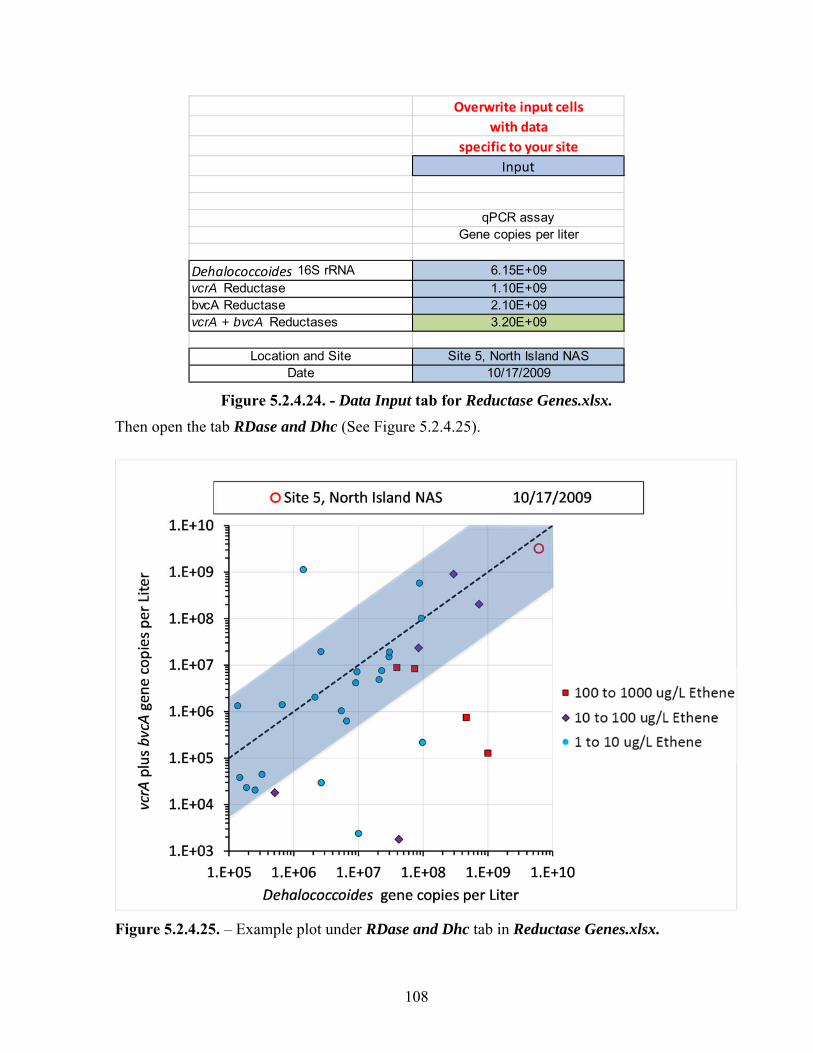
108

Figure 5.2.4.24. - Data Input tab for Reductase Genes.xlsx.

Then open the tab RDase and Dhc (See Figure 5.2.4.25).

Figure 5.2.4.25. – Example plot under RDase and Dhc tab in Reductase Genes.xlsx.



qPCR assayGene copies per liter

Dehalococcoides 16S rRNA 6.15E+09vcrA Reductase 1.10E+09bvcA Reductase 2.10E+09vcrA + bvcA Reductases 3.20E+09

Location and Site Site 5, North Island NASDate 10/17/2009

109

If your data plot in the blue shape, transformation of cDCE is plausible based on the abundance of the reductase genes in the groundwater.

The data in Figure 5.2.4.25 are from a benchmark data set collected by Microbial Insights, Inc. (www.microbe.com, Knoxville, TN 37932). The figure compares the presence of ethene in groundwater to the abundance of the vcrA, bvcA and Dhc genes. The ethane in the groundwater was presumably produced from biological transformation of cDCE. In the figure, the sum of the vcrA plus bvcA genes is plotted against the abundance of Dhc 16S rRNA genes. The known Dhc strains possess single copies of the 16S rRNA, the vcrA and the bvcA genes, and the vcrA and the bvcA genes do not co-occur in the same Dhc strain. Therefore, a vcrA plus bvcA-to-Dhc 16S rRNA gene ratio near unity (indicated by the 45-degree dashed line in Figure 5.2.4.25) would indicate that all Dhc strains possess a cDCE RDase and have the ability to dechlorinate cDCE to ethene. Data points close to the 45-degree line represent site samples where the abundance of vcrA plus bvcA are close to the total number of Dhc cells. The color-coded symbols represent ranges of ethene concentrations measured in site groundwater. In the majority of the samples (23 out of 31 water samples), ethene was present in the water sample when the ratio of the sum of the reductase genes to the Dhc gene was less than or equal to 20 and greater than or equal to 0.05. That range is encompassed by the blue shape in Figure 5.2.4.25.

12. Does Mass Magnetic Susceptibility Explain the cis-1,2-Dichloroethene (cDCE) Rate Constant?

Mass magnetic susceptibility is a surrogate for the bulk amount of magnetite present in aquifer material. Magnetite can contribute to cDCE degradation.


Prepare a simulation where the rate constant for degradation of cDCE is set to provide the best match between the simulation and the field data. Do not include any portion of the plume where biological reductive dechlorination might contribute to the bulk rate constant that is extracted by the model. Exclude any portion of the flow path where the concentrations of daughter products are increasing with distance from the source.

Input the rate constant for degradation of cDCE and the site-specific value for mass magnetic susceptibility of the aquifer material in the Data Input tab of the Magnetic Susceptibility.xlsx spreadsheet, which can be downloaded separately and is also part of BioPIC. Figure 5.2.4.26 shows the Data Input tab. Your site-specific data should be entered into the blue boxes.

110

Figure 5.2.4.26 - Data Input tab for Magnetic Susceptibility.xlsx for DCE.

After the data have been entered, open the tab Mag. Sus. Explains cDCE and examine where your data fall on this plot. Figure 5.2.4.27 is an example of this plot.

Figure 5.2.4.27 - Example plot under the tab Mag. Sus. Explains cDCE in magnetic

susceptibility.xlsx.


Input




PCE rate slower than expected

TCE rate slower than expected

cis‐DCE 0.2 >80%

Vinyl Chloride 0.4 >60%


SI Units (m3kg





Location and Site Former Plattsburgh AFB constants that exceed the BASELINE



111

If the site-specific values fall within the blue shape in the tab Mag. Sus. Explains DCE, then mass magnetic susceptibility can explain the apparent in situ rate of cDCE degradation.

Magnetite can mediate abiotic degradation of DCE (Lee and Batchelor, 2002a; Ferrey et al., 2004; He et al., 2009). The amount of magnetite in porous media can be estimated from the mass (not volume) magnetic susceptibility of core samples. Empirical data are available that associate degradation rate constants for DCE with mass magnetic susceptibility (Figure 5.2.4.27; He et al., 2009). The available data were used to define the blue shape in the previous figure. If the rate constant plots within the blue shape, then abiotic degradation mediated by magnetite can explain the rate constant. If the rate constant plots above the blue shape, other processes are likely contributing to the rate of degradation. If the rate constant plots below the shape, inappropriate sampling locations may have been selected for mass magnetic susceptibility measurements. Mass magnetic susceptibility should be determined using the aquifer material that is most transmissive to water. In addition, the input values used for the rate constant calculation with BIOCHLOR should be verified.

13. Adequate Oxygen for Aerobic cis-1,2-Dichloroethene (cDCE) Biodegradation?

Bacteria that degrade DCE with oxygen are generally present in aquifers, even when the groundwater has been characterized as anoxic (Bradley and Chapelle, 2011). Because of field sampling limitations, dissolved oxygen concentration data on well water are generally unreliable to determine if sufficient oxygen is available to support oxygen-dependent DCE degradation. For the purposes of this decision support system, oxygen is considered to be available for aerobic biodegradation of DCE when all of the following criteria are met: Dissolved oxygen concentrations measured in the field exceed 0.1 mg/L, ferrous iron (Fe2+) concentrations are less than 0.5 mg/L, and methane concentrations are less than 0.005 mg/L.

It is easy to contaminate a groundwater sample with oxygen. Sampling monitoring wells often causes mixing of water from different depth intervals. It is possible the DCE in a sample of well water came from one depth interval and the oxygen from another. If this is the case, oxygen may not be available to the DCE-degrading bacteria in the aquifer, leading to the erroneous conclusion that DCE is degraded aerobically. The absence of ferrous iron [Fe(II)] and methane are good indicators for the presence of concentrations of oxygen that support aerobic biodegradation of organic compounds. The absence of ferrous iron or methane in water collected from a well indicates that all of the flow paths to the well had adequate concentrations of oxygen to support aerobic DCE degradation.

14. Is Trichloroethene (TCE) Present?

For the purposes of this decision support system, TCE is present in groundwater when the concentration of TCE exceeds a cleanup goal for TCE that has been established for the site. If no cleanup goal for TCE has been established, TCE is considered present when the concentration is ≥ 5 µg/L. Other criteria may apply depending on the regulatory authority.

The cleanup goal is not always the U.S. EPA MCL established for drinking water. Consult the regulator for the cleanup goals that apply to the site of interest.

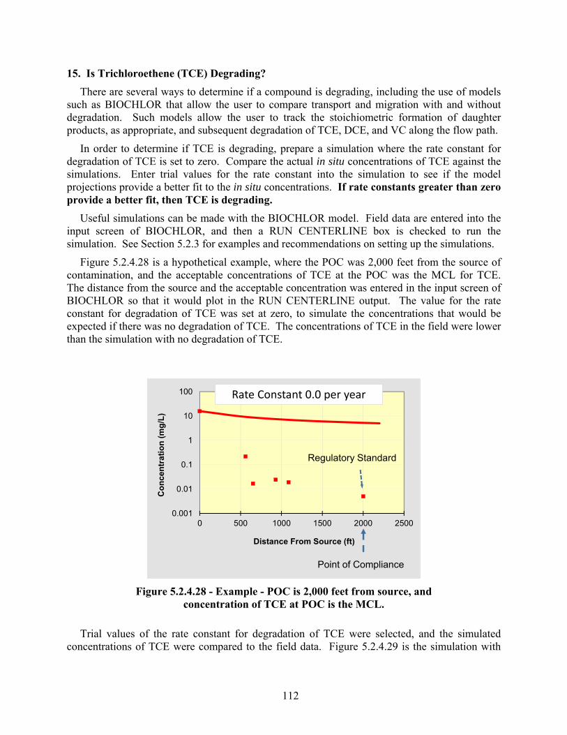
112

15. Is Trichloroethene (TCE) Degrading?

There are several ways to determine if a compound is degrading, including the use of models such as BIOCHLOR that allow the user to compare transport and migration with and without degradation. Such models allow the user to track the stoichiometric formation of daughter products, as appropriate, and subsequent degradation of TCE, DCE, and VC along the flow path.

In order to determine if TCE is degrading, prepare a simulation where the rate constant for degradation of TCE is set to zero. Compare the actual in situ concentrations of TCE against the simulations. Enter trial values for the rate constant into the simulation to see if the model projections provide a better fit to the in situ concentrations. If rate constants greater than zero provide a better fit, then TCE is degrading.

Useful simulations can be made with the BIOCHLOR model. Field data are entered into the input screen of BIOCHLOR, and then a RUN CENTERLINE box is checked to run the simulation. See Section 5.2.3 for examples and recommendations on setting up the simulations.

Figure 5.2.4.28 is a hypothetical example, where the POC was 2,000 feet from the source of contamination, and the acceptable concentrations of TCE at the POC was the MCL for TCE. The distance from the source and the acceptable concentration was entered in the input screen of BIOCHLOR so that it would plot in the RUN CENTERLINE output. The value for the rate constant for degradation of TCE was set at zero, to simulate the concentrations that would be expected if there was no degradation of TCE. The concentrations of TCE in the field were lower than the simulation with no degradation of TCE.

Figure 5.2.4.28 - Example - POC is 2,000 feet from source, and concentration of TCE at POC is the MCL.

Trial values of the rate constant for degradation of TCE were selected, and the simulated concentrations of TCE were compared to the field data. Figure 5.2.4.29 is the simulation with

0.001

0.01

0.1

1

10

100

0 500 1000 1500 2000 2500

Co

nce

ntr

atio

n (

mg

/L)


Point of Compliance

Regulatory Standard


113

the best fit to the field data. The rate constant for degradation of TCE that provided the best fit was 1.0 per year.

Figure 5.2.4.29 - Example TCE rate constant estimation using trial and error with degradation rate of 1/year.


Figure 5.2.4.30 - Example TCE rate constant estimation using trial and error with degradation rate of 0.7/year.


0.001

0.01

0.1

1

10

100

0 500 1000 1500 2000 2500

Co

nce

ntr

atio

n (

mg

/L)


Point of Compliance

Regulatory Standard


0.001

0.01

0.1

1

10

100

1000

0 500 1000 1500 2000 2500

Co

nce

ntr

ati

on

(m

g/L

)


Point of Compliance

Regulatory Standard


114

Figure 5.2.4.31 - Example TCE rate constant estimation using trial and error with degradation rate of 1.4/year.

As an alternative, CSIA can be used to determine if TCE is degrading. An enrichment in the δ13C concentration in TCE is expected over time and along the flow path if TCE is degrading. The increase in δ13C concentration in TCE in areas close to a NAPL source area containing TCE may be difficult to discern and may not become apparent until the NAPL source becomes significantly depleted. In addition, the continued formation of TCE from PCE will dilute the pool of δ13C concentration in TCE until PCE is consumed, either over time or along the flow path.

Microbial degradation of TCE would make the value of δ13C a larger (less negative) number. The precision of the analysis is near 0.5‰. If the value of δ13C of TCE in a down gradient well is larger (less negative) than the value in an up gradient well by more than 0.5‰, that can be taken as evidence for degradation of TCE.

The highest value that has been reported for the δ13C of TCE used in commerce is -23.2‰ (Figure 5, Kuder et al., 2013; Table 1 McHugh et al., 2014). As a general rule, a value of δ13C for TCE that is greater than -22.7‰ can be taken as evidence of degradation of TCE.

16. Are cis-1,2-Dichloroethene (cDCE) or trans-1,2-Dichloroethene (tDCE) or Vinyl Chloride (VC) present?

Evaluate data on concentrations of TCE, cDCE, tDCE and VC in groundwater. Based on the experience of the authors, If the sum of cDCE, tDCE and VC is more than 5 mole % of the concentration of TCE, then cDCE, tDCE and VC are present. The presence of cDCE or tDCE or VC indicates that reductive dechlorination of TCE has occurred.

The calculation of mole % can be easily performed using the Excel file Mole Percent Calculator.xlsx, which can be downloaded separately and is also part of BioPIC.

0.001

0.01

0.1

1

10

100

1000

0 500 1000 1500 2000 2500

Co

nce

ntr

atio

n (

mg

/L)


Point of Compliance

Regulatory Standard


115

The detection of cDCE r tDCE or VC at TCE-impacted sites suggests that TCE reductive dechlorination has occurred and this process may still be ongoing. Enumeration of pceA genes (present in PCE- and/or TCE-dechlorinating bacteria and implicated in PCE-to-TCE and PCE-to-cDCE reductive dechlorination) and the tceA gene (present in some Dhc strains and implicated in TCE-to-VC reductive dechlorination) with qPCR provides support that bacteria capable of TCE reductive dechlorination to cDCE or VC are present.

17. Are cis-1,2-Dichloroethene (cDCE) or trans-1,2-Dichloroethene (tDCE) or Vinyl Chloride (VC) Present in Relevant Concentrations?

Evaluate data on concentrations of TCE, cDCE, tDCE and VC in wells downgradient of the source of contamination. If the sum of cDCE, tDCE and VC is more than 25 mole % of the concentration of TCE, then cDCE, tDCE and VC are present in relevant concentrations. The presence of daughter products at these concentrations indicates that microbial reductive dechlorination is an important pathway for TCE fate, and explains in a qualitative manner why TCE is degrading.

The calculation of mole % can easily be performed using the Excel file included with the BioPIC program titled Mole Percent Calculator.xlsx, which can be downloaded separately and is also part of BioPIC.

The detection of cDCE, tDCE or VC at TCE-impacted sites suggests that TCE reductive dechlorination has occurred and this process may still be ongoing. Enumeration of pceA genes (present TCE-dechlorinating bacteria and implicated in TCE-to-cDCE reductive dechlorination) with qPCR provides support that bacteria capable of TCE reductive dechlorination to cDCE are present. The presence of the Dhc RDase genes tceA, bvcA or vcrA implicated in reductive dechlorination of DCE can explain the formation of VC and ethene.

18. Does Mass Magnetic Susceptibility Explain the Trichloroethene (TCE) Degradation Rate Constant?

Mass magnetic susceptibility is a surrogate for the bulk amount of magnetite present in aquifer material. Magnetite can contribute to TCE degradation.


Prepare a simulation where the rate constant for degradation of TCE is set to provide the best match between the simulation and the field data. Do not include any portion of the plume where biological reductive dechlorination might contribute to the bulk rate constant that is extracted by the model. Exclude any portion of the flow path where the concentrations of daughter products are increasing with distance from the source.

Figure 5.2.4.32 shows the Data Input tab for mass magnetic susceptibility data for evaluating TCE degradation. Plot the rate constant for degradation of TCE and the site-specific value for mass magnetic susceptibility of the aquifer sediment in the tab titled Data Input, which is found in the Excel spreadsheet Magnetic Susceptibility.xlsx, which can be downloaded separately and is also part of BioPIC.

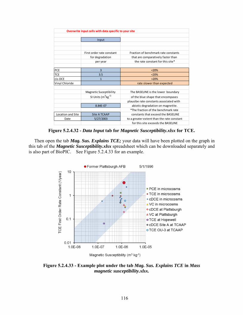
116

Figure 5.2.4.32 - Data Input tab for Magnetic Susceptibility.xlsx for TCE.

Then open the tab Mag. Sus. Explains TCE; your data will have been plotted on the graph in this tab of the Magnetic Susceptibility.xlsx spreadsheet which can be downloaded separately and is also part of BioPIC. See Figure 5.2.4.33 for an example.

Figure 5.2.4.33 - Example plot under the tab Mag. Sus. Explains TCE in Mass magnetic susceptibility.xlsx.


Input




PCE 3 <20%

TCE 3.5 <20%

cis‐DCE 1 >20%

Vinyl Chloride rate slower than expected


SI Units (m3kg





Location and Site Site A TCAAP constants that exceed the BASELINE



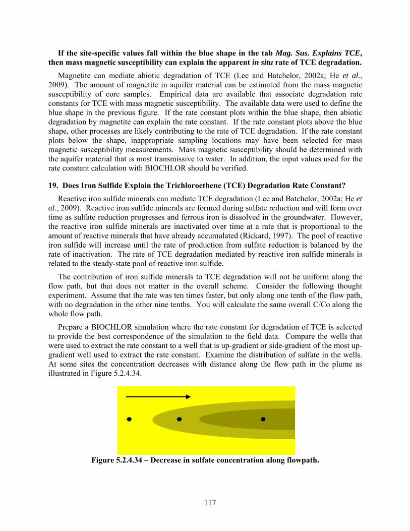
117

If the site-specific values fall within the blue shape in the tab Mag. Sus. Explains TCE, then mass magnetic susceptibility can explain the apparent in situ rate of TCE degradation.

Magnetite can mediate abiotic degradation of TCE (Lee and Batchelor, 2002a; He et al., 2009). The amount of magnetite in aquifer material can be estimated from the mass magnetic susceptibility of core samples. Empirical data are available that associate degradation rate constants for TCE with mass magnetic susceptibility. The available data were used to define the blue shape in the previous figure. If the rate constant plots within the blue shape, then abiotic degradation by magnetite can explain the rate constant. If the rate constant plots above the blue shape, other processes are likely contributing to the rate of TCE degradation. If the rate constant plots below the shape, inappropriate sampling locations may have been selected for mass magnetic susceptibility measurements. Mass magnetic susceptibility should be determined with the aquifer material that is most transmissive to water. In addition, the input values used for the rate constant calculation with BIOCHLOR should be verified.

19. Does Iron Sulfide Explain the Trichloroethene (TCE) Degradation Rate Constant?

Reactive iron sulfide minerals can mediate TCE degradation (Lee and Batchelor, 2002a; He et al., 2009). Reactive iron sulfide minerals are formed during sulfate reduction and will form over time as sulfate reduction progresses and ferrous iron is dissolved in the groundwater. However, the reactive iron sulfide minerals are inactivated over time at a rate that is proportional to the amount of reactive minerals that have already accumulated (Rickard, 1997). The pool of reactive iron sulfide will increase until the rate of production from sulfate reduction is balanced by the rate of inactivation. The rate of TCE degradation mediated by reactive iron sulfide minerals is related to the steady-state pool of reactive iron sulfide.

The contribution of iron sulfide minerals to TCE degradation will not be uniform along the flow path, but that does not matter in the overall scheme. Consider the following thought experiment. Assume that the rate was ten times faster, but only along one tenth of the flow path, with no degradation in the other nine tenths. You will calculate the same overall C/Co along the whole flow path.

Prepare a BIOCHLOR simulation where the rate constant for degradation of TCE is selected to provide the best correspondence of the simulation to the field data. Compare the wells that were used to extract the rate constant to a well that is up-gradient or side-gradient of the most up-gradient well used to extract the rate constant. Examine the distribution of sulfate in the wells. At some sites the concentration decreases with distance along the flow path in the plume as illustrated in Figure 5.2.4.34.

Figure 5.2.4.34 – Decrease in sulfate concentration along flowpath.

118

Sulfate is dissolved in the groundwater, and the demand for the substrate by sulfate-reducing bacteria is exerted as the water moves along the flow path.

The Excel spreadsheet FeS.xlsx should be set up to extract a rate constant for abiotic TCE degradation between a selected up-gradient well and a selected down-gradient well.

Figure 5.2.4.35 - Decrease in sulfate concentration at points along flowpath.

If the distribution of sulfate between the up-gradient and down-gradient wells follows the pattern in Figure 5.2.4.34 and 5.2.4.35, then enter values for aquifer properties and for concentrations of sulfate in the tab Sulfate Sag Along Flow Path in the Excel spreadsheet FeS.xlsx. The spreadsheet uses data on the effective porosity, hydraulic gradient and hydraulic conductivity to estimate a seepage velocity of groundwater along a flow path. Then the spreadsheet uses the concept of volumetric sulfate loading as presented in Whiting et al. (2014) to estimate the consumption of sulfate and production of sulfide between an up-gradient well and a down-gradient well along the flow path. The spreadsheet assumes that excess Fe(III) is available in minerals in the aquifer matrix, and that the sulfide produced from the reduction of sulfate reacts to form FeS following equations presented in Shen and Wilson (2007). The spreadsheet calculates the rate of production of FeS over time.

The spreadsheet models the inactivation of FeS as a first order process on the concentration of FeS present at any time. The user has two options. The user can provide a rate constant for inactivation. There are two values available in the literature, 0.32 per year and 0.108 per year (He et al., 2008). The user can also provide information of the pH of the groundwater and the average concentration of soluble sulfide, and the spreadsheet will use an equation published by Rickard (1997) to calculate the rate constant for inactivation of the FeS by oxidation by soluble sulfide to FeS2. The user provides the elapsed time since sulfate reduction began at the site, and the spreadsheet uses the volumetric sulfate loading and the rate of FeS inactivation to calculate the pool of accumulated reactive FeS. Then the spreadsheet uses the rate of degradation of TCE on FeS as published by He et al. (2010) to estimate a rate constant for TCE degradation along the flowpath between the two wells.

In the example below (Figure 5.2.4.36), the spreadsheet model was applied to a field study that estimated the rate of TCE degradation in ground water as the water passed through a mulch-based biowall at the OU1 Site at Altus AFB, OK. Data are from Shen et al. (2012) with the exception of the data on concentrations of sulfide and sulfate and pH, which are unpublished data from John T. Wilson.

If a value for the rate of inactivation of FeS is provided, the predicted degradation rate constant for TCE degradation on FeS is provided in cell D29. If data on pH and concentration of sulfide in the water is provided, the predicted rate constant for TCE degradation on FeS is provided in cell D28.

119

If the value of the rate constant in cell D28 or D29 (whichever is applicable) is equal to or greater than the rate constant estimated using BIOCHLOR, then abiotic degradation by reactive iron sulfide minerals can explain the degradation rate constant for TCE.

The field scale rate of TCE degradation extracted by Shen et al. (2012) was 0.14 per day or 51 per year. The rate of TCE degradation predicted by the spreadsheet is near 20 per year. Abiotic degradation of TCE could have accounted for roughly half of the removal of TCE. In this example, abiotic degradation on FeS did not explain the field scale measurements. This observation is in good agreement with removal of TCE in a laboratory model of the biowall (Shen and Wilson, 2007), where roughly half the removal could be attributed to abiotic degradation and half to microbial reductive dechlorination.

Figure 5.2.4.36 – Screenshot of model output from Sulfate Sag Along Flow Path tab in FeS.xlsx applied to a field study that estimated the rate of TCE degradation in ground

water as the water passed through a mulch-based biowall at Altus AFB, OK.

Figure 5.2.4.37 applies FeS.xlsx to a laboratory column study (Shen and Wilson, 2007) that modeled removal of TCE in the mulch biowall at the OU-1 site at Altus AFB, OK. The overall first order rate constant for removal of TCE that was extracted by Shen and Wilson (2007) from the laboratory column with mulch and hematite was near 0.3 per day, or 110 per year (Shen and

A B C D

1

2 Identify wells along the flow path of the contaminant plume. Overwrite Input Cells with 3 Find a down‐gradient well with lower concentrations of TCE. Data Specific to Your Site4 Find an up‐gradient well with higher concentrations of TCE

5

The concentration of sulfate should be higher in the up‐gradient well than in the down‐gradient well.

6 Unit Input7 Unit Interim Calculation8 Parameter Unit Final Output9

10 Hydraulic Gradient foot per foot 0.006

11 Hydraulic Conductivity (of aquifer feeding the biowall) feet per day 8.856

12 Effective Porosity (of biowall) cm3/cm

3 0.42

13 Seepage Velocity of Ground Water (in biowall) feet per year 46.18

14

Distance from down gradient well with lowest sulfate to up‐gradient well with

highest sulfate (used width of biowall)feet 1.5

15 Concentration sulfate in up‐gradient well mg/L 1620

16 Concentration sulfate in down‐gradient well mg/L 1490

17 Concentration of soluble sulfide in up‐gradient well mg/L 0

18 Concentration of soluble sulfide in down‐gradient well mg/L 0

19 Time since plume first reached the down gradient well years 3

20Yearly production of FeS along flow path

moles FeS per liter

groundwater0.02777

21 Average pH (in the biowall) 6.74

22 Average Total Soluble Sulfide (in the biowall) mg/L 1.35

23 k (the first order rate constant for inactivation of FeS) from Rickard's Equation per year 0.112

24 k (the first order rate constant for inactivation of FeS) Input from Literature per year 0.162

25

Reactive Iron Sulfide that is accumulated calculated from Rickard's equation based

on pH and soluble sulfide

moles FeS per liter

groundwater7.08E‐02

26

Reactive Iron Sulfide that is accumulated based on the first order rate constant for

inactivation of FeS.

moles FeS per liter


27

First Order Rate Constant for Attenuation of TCE over Time explained by Reactive

FeS

28 k (the first order rate constant for inactivation of FeS) from Rickard's Equation per year 1.92E+01

29 k (the first order rate constant for inactivation of FeS) Input from Literature per year 1.79E+01

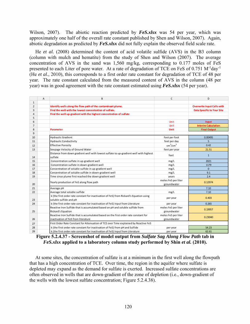
120

Wilson, 2007). The abiotic reaction predicted by FeS.xlsx was 54 per year, which was approximately one half of the overall rate constant published by Shen and Wilson, 2007). Again, abiotic degradation as predicted by FeS.xlsx did not fully explain the observed field scale rate.

He et al. (2008) determined the content of acid volatile sulfide (AVS) in the B3 column (column with mulch and hematite) from the study of Shen and Wilson (2007). The average concentration of AVS in the sand was 1,560 mg/kg, corresponding to 0.177 moles of FeS presented to each Liter of pore water. At a rate of degradation of TCE on FeS of 0.751 M-1day-1 (He et al., 2010), this corresponds to a first order rate constant for degradation of TCE of 48 per year. The rate constant calculated from the measured content of AVS in the column (48 per year) was in good agreement with the rate constant estimated using FeS.xlsx (54 per year).

Figure 5.2.4.37 - Screenshot of model output from Sulfate Sag Along Flow Path tab in FeS.xlsx applied to a laboratory column study performed by Shin et al. (2010).

At some sites, the concentration of sulfate is at a minimum in the first well along the flowpath that has a high concentration of TCE. Over time, the region in the aquifer where sulfate is depleted may expand as the demand for sulfate is exerted. Increased sulfate concentrations are often observed in wells that are down-gradient of the zone of depletion (i.e., down-gradient of the wells with the lowest sulfate concentration; Figure 5.2.4.38).

A B C D

1

2 Identify wells along the flow path of the contaminant plume. Overwrite Input Cells with 3 Find the well with the lowest concentration of sulfate. Data Specific to Your Site4 Find the well up‐gradient with the highest concentration of sulfate5



11 Hydraulic Conductivity feet per day 5

12 Effective Porosity cm3/cm

3 0.42

13 Seepage Velocity of Ground Water feet per year 21.51

14

Distance from down gradient well with lowest sulfate to up‐gradient well with highest

sulfatefeet 1

15 Concentration sulfate in up‐gradient well mg/L 2021

16 Concentration sulfate in down‐gradient well mg/L 1179

17 Concentration of soluble sulfide in up‐gradient well mg/L 0

18 Concentration of soluble sulfide in down‐gradient well mg/L 9.1

19 Time since plume first reached the down gradient well years 2.4


moles FeS per liter

groundwater0.12974

21 Average pH 7.10

22 Average total soluble sulfide mg/L 7.10

23

k (the first order rate constant for inactivation of FeS) from Rickard's Equation using

soluble sulfide and pHper year 0.403


25

Reactive Iron Sulfide that is accumulated based on pH and soluble sulfide from

Rickard's Equation

moles FeS per liter

groundwater0.19957

26

Reactive Iron Sulfide that is accumulated based on the first order rate constant for

inactivation of FeS from literature

moles FeS per liter

groundwater0.23040

27 First Order Rate Constant for Attenuation of TCE over Time explained by Reactive FeS

28 k (the first order rate constant for inactivation of FeS) from pH and Sulfide per year 54.23


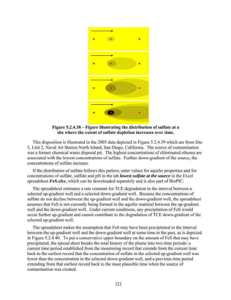
121

Figure 5.2.4.38 – Figure illustrating the distribution of sulfate at a

site where the extent of sulfate depletion increases over time.

This disposition is illustrated in the 2005 data depicted in Figure 5.2.4.39 which are from Site 5, Unit 2, Naval Air Station North Island, San Diego, California. The source of contamination was a former chemical waste disposal pit. The highest concentrations of chlorinated ethenes are associated with the lowest concentrations of sulfate. Further down-gradient of the source, the concentrations of sulfate increase.

If the distribution of sulfate follows this pattern, enter values for aquifer properties and for concentrations of sulfate, sulfide and pH in the tab lowest sulfate at the source in the Excel spreadsheet FeS.xlsx, which can be downloaded separately and is also part of BioPIC.

The spreadsheet estimates a rate constant for TCE degradation in the interval between a selected up-gradient well and a selected down-gradient well. Because the concentrations of sulfate do not decline between the up-gradient well and the down-gradient well, the spreadsheet assumes that FeS is not currently being formed in the aquifer material between the up-gradient well and the down-gradient well. Under current conditions, any precipitation of FeS would occur further up-gradient and cannot contribute to the degradation of TCE down-gradient of the selected up-gradient well.

The spreadsheet makes the assumption that FeS may have been precipitated in the interval between the up-gradient well and the down-gradient well at some time in the past, as is depicted in Figure 5.2.4.40. To put a conservative upper boundary on the amount of FeS that may have precipitated, the spread sheet breaks the total history of the plume into two time periods: a current time period established from the monitoring record that extends from the current time back to the earliest record that the concentration of sulfate in the selected up-gradient well was lower than the concentration in the selected down-gradient well, and a previous time period extending from that earliest record back to the most plausible time when the source of contamination was created.

122

Figure 5.2.4.39 – Figure illustrating chlorinated ethene concentrations decreasing along the flowpath and sulfate concentrations increasing along flowpath down-gradient from a

NAPL source zone, Naval Air Station North Island, San Diego, CA. The minimum sulfate concentration corresponds to the maximum chlorinated ethene concentrations.

< 50 mg/L

50 to 100 mg/L

100 to 400 mg/L

> 400 mg/L

100 feet

SulfateMW‐36

MW‐21

MW‐32

MW‐20

>10 mg/L

> 25 mg/L

> 50 mg/L

> 100 µg/L

100 feet

Detected

MW‐36Total Chlorinated Alkenes and Alkanes

MW‐21

MW‐32

MW‐20

Source

Source

123

Figure 5.2.4.40 - Comparison of the distrubution of sulfate between wells where the sulfate reduction occurs up-gradient of both wells to an assumed

previous condition where sulfate reduction occurred between the wells.

The spreadsheet assumes that the volumetric rate of sulfate reduction that occurs currently between the up-gradient well and the un-impacted well further up-gradient applies to both time periods. Under these assumptions, no FeS should be expected to accumulate in the interval between the selected wells in the current time period, and all of the FeS that was formed accumulated in the interval between the selected wells in the previous time period.

Table 5.2.4.1 provides some of the data used to set up the spreadsheet in the example below (Figure 5.2.4.41). From Figure 5.2.4.39, well S5-MW-21 was selected as the up-gradient well, well S5-MW-20 was selected as the down-gradient well, and well S5-MW-36 was take to represent conditions in the un-impacted well further up-gradient.

up‐gradientwell

down‐gradientwell

up‐gradientWell

down‐gradientWell

further up‐gradientWell

Assumed Previous Distribution of Sulfate

Current Distribution of Sulfate

124

Well

Distance from most

contaminated well (feet)

Groundwater travel time from most

contaminated well (years)

Sulfate 7/2005 (mg/L)

Soluble Sulfide 7/2005 (mg/L) pH 7/2005

Total C2 Alkenes

and Alkanes 10/2005 (mg/L)

S5-MW-36 1290 0.1 7.04 0.016

S5-MW-21 0 0.00 5.24 2.53 6.33 587

S5-MW-32 109 0.97 84.7 0.1 7.13 0.060

S5-MW-20 173 1.56 73.0 0.229 7.02 0.926

Table 5.2.4.1 - Data used for example presented in Figure 5.2.4.41.

Figure 5.2.4.41 - Screenshot of model output under Lowest Sulfate at Source tab from FeS.xlsx for the site presented in Figure 5.2.4.35, NASNI, Site 5, Unit 2.

A B C D

1

2 Identify wells along the flow path of the contaminant plume. Overwrite Input Cells with 3 Find the well with the lowest concentration of sulfate. Data Specific to Your Site4 Find the well up‐gradient with the highest concentration of sulfate5



11 Hydraulic Conductivity feet per day 51

12 Effective Porosity cm3/cm

3 0.2

13 Seepage Velocity of Ground Water feet per year 111.69

14 Distance from the up‐gradient well to the down gradient well feet 173

15 Concentration sulfate in unimpacted further up‐gradient well mg/L 622

16 Concentration sulfate in well at source mg/L 37.1

17 Concentration of soluble sulfide inunimpacted up‐gradient well mg/L 0.598

18 Concentration of soluble sulfide in well at source mg/L 4.16

19

Time since plume first reached the down gradient well, estimated as the date of

original release minus the time required for ground water to flow from the point

of release to the down gradient well

years 20

20

Time from the first sampling period where the most contaminated well at the

head of the plume had the lowest concentration of sulfate to the time being

modelled

years 10


moles FeS per liter

groundwater0.00267

22 Average pH 7.39

23 Average total soluble sulfide mg/L 4.16

24 k (the first order rate constant for inactivation of FeS) from Rickard's equation per year 0.154


26

Reactive Iron Sulfide that previously accumulated calculated from Rickard's

equation based on pH and soluble sulfide

moles FeS per liter


27

Reactive Iron Sulfide that currently remains calculated from Rickard's equation

based on pH and soluble sulfide

moles FeS per liter


28

Reactive Iron Sulfide that previously accumulated based on the first order rate

constant from literature for inactivation of FeS.

moles FeS per liter


29

Reactive Iron Sulfide that currently remains based on the first order rate constant

from literature for inactivation of FeS.

moles FeS per liter


30

First Order Rate Constant for Attenuation of TCE over Time explained by Reactive

FeS

31 k (the first order rate constant for inactivation of FeS) from Rickard's Equation per year 9.57E‐01

32 k (the first order rate constant for inactivation of FeS) Input from Literature per year 8.51E‐01

125

If you provided a value for the rate of inactivation of FeS, read the predicted rate constant for TCE degradation on FeS from cell D32. If you provided data on pH and concentration of sulfide in the water, read the predicted rate constant for TCE degradation on FeS from cell D31.

If the value of the rate constant in cell D31 or D32 (whichever is applicable) is equal to or greater than the rate constant from the BIOCHLOR simulation, then abiotic degradation by reactive iron sulfide minerals can explain the degradation rate constant for TCE.

For this site, the rate constant for abiotic degradation on FeS that was predicted using FeS.xlsx was near 0.9 per year. The TCE degradation rate constant that was extracted using BIOCHLOR ranged from 3 to 3.5 per year. In this example, reactive iron sulfide minerals do not explain the rate constant for TCE degradation.

20. Is Tetrachloroethene (PCE) Present?

For the purposes of this decision support system, PCE is considered present when the concentration of PCE exceeds a cleanup goal for PCE that has been established for the site. If no cleanup goal for PCE has been established, PCE is considered present when the concentration is ≥ 5 µg/L. Other criteria may apply depending on the regulatory authority.

The cleanup goal is not always the U.S. EPA MCL established for drinking water. Consult the regulator for the cleanup goals that apply to the site of interest.

21. Is Tetrachloroethene (PCE) Degrading?

There are several ways to determine if a compound is degrading, including the use of models such as BIOCHLOR that allow the user to compare transport and migration with and without degradation. Such models allow the user to track the degradation of PCE and, if appropriate (i.e., if the predominant reaction is microbial reductive dechlorination), stoichiometric formation and subsequent degradation of TCE, cDCE, and VC along the flow path. In addition, CSIA can be useful for determining if a compound is degrading.

Prepare a simulation where the rate constant for degradation of PCE is set to zero. Compare the actual in situ concentrations of PCE against the simulations. Enter trial values for the rate constant into the simulation to see if the model projections provide a better fit to the in situ concentrations. If the trial values provide a better fit, then PCE is degrading.

As an alternative, CSIA can be used to determine if PCE is degrading. An enrichment in the δ13C abundance in PCE is expected over time and along the flow path if PCE is degrading. The increase in δ13C concentration in PCE in areas close to a NAPL source area may be difficult to discern and may not become apparent until the NAPL source becomes significantly depleted.

Useful simulations can be made with the BIOCHLOR model. Field data are entered into the input screen, and then a RUN CENTERLINE box is checked to run the simulation. See Section 5.2.3 for examples and recommendations on setting up the simulations. Figure 5.2.4.42 is a hypothetical example, where the POC is 2,000 feet from the source of contamination, and the acceptable concentrations of PCE at the POC was the MCL for PCE. The distance from the source and the acceptable concentration was entered in the input screen of BIOCHLOR so that it would plot in the RUN CENTERLINE output. The value for the rate constant for PCE

126

degradation is set at zero to simulate the concentrations that would be expected if there was no degradation of PCE. The concentrations of PCE in the field were lower than the simulation with no degradation of PCE.

Figure 5.2.4.42 - Example - POC is 2,000 feet from source, and concentration of PCE at POC is the MCL.

Trial values of the rate constant for degradation of PCE were selected, and the simulated concentrations of PCE were compared to the field data. Figure 5.2.4.43 is the simulation with the best fit to the field data. The rate constant for degradation of PCE that provided the best fit was 0.6 per year.

Figure 5.2.4.43 - Example PCE rate constant estimation using trial and error with degradation rate of 0.6/year.

0.001

0.01

0.1

1

10

100

1000

0 500 1000 1500 2000 2500

Co

nc

entr

atio

n (

mg

/L)


Point of Compliance

Regulatory Standard


0.001

0.01

0.1

1

10

100

0 500 1000 1500 2000 2500

Co

nce

ntr

atio

n (

mg

/L)


Point of Compliance

Regulatory Standard


127





0.001

0.01

0.1

1

10

100

1000

0 500 1000 1500 2000 2500

Co

nce

ntr

ati

on

(m

g/L

)


Point of Compliance

Regulatory Standard


0.001

0.01

0.1

1

10

100

1000

0 500 1000 1500 2000 2500

Co

nce

ntr

atio

n (

mg

/L)


Point of Compliance

Regulatory Standard


128

22. Are TCE, cis-1,2-Dichloroethene (cDCE), trans-1,2-Dichloroethene (tDCE) or Vinyl Chloride (VC) Present?

Evaluate data on concentrations of PCE, TCE, cDCE, tDCE and VC in wells down-gradient of the source of contamination. If the sum of TCE, cDCE, tDCE and VC is more than 5 mole % of the concentration of PCE, then TCE, cDCE, tDCE and VC are considered present. The presence of TCE, cDCE, tDCE or VC indicates that reductive dechlorination of PCE has occurred.

The calculation of mole % can easily be performed using the Excel file Mole Percent Calculator.xlsx, which can be downloaded separately and is also part of BioPIC.

The detection of TCE, cDCE, or VC at PCE-impacted sites suggests that PCE reductive dechlorination has occurred and this process may still be ongoing. Enumeration of pceA genes (present in PCE- and/or TCE-dechlorinating bacteria and implicated in PCE-to-TCE and PCE-to-cDCE reductive dechlorination) with qPCR provides support that bacteria capable of PCE reductive dechlorination to TCE or cDCE are present. The presence of the Dhc RDase genes tceA, bvcA or vcrA implicated in reductive dechlorination of DCE can explain the formation of VC and ethene.

23. Are Trichloroethene (TCE), cis-1,2-Dichloroethene (cDCE) or Vinyl Chloride (VC) Present in Relevant Concentrations?

Evaluate data on concentrations of PCE, TCE, cDCE, tDCE and VC in wells downgradient of the source of contamination. If the sum of TCE, cDCE, tDCE and VC is more than 25 mole % of the concentration of PCE, then TCE, cDCE, tDCE and VC are present at relevant concentrations. The presence of daughter products at these concentrations indicates that microbial reductive dechlorination is an important pathway for TCE fate, and explains in a qualitative manner why TCE is degrading.

The calculation of mole % can easily be performed using the Excel file Mole Percent Calculator.xlsx. This tool can be downloaded separately and is also part of BioPIC.

24. Does Mass Magnetic Susceptibility Explain the Tetrachloroethene (PCE) Rate Constant?

Mass magnetic susceptibility is a surrogate for the bulk amount of magnetite present in aquifer material. Magnetite can contribute to PCE degradation.


Prepare a simulation where the rate constant for degradation of PCE is set to provide the best match between the simulation and the field data. Do not include any portion of the plume where biological reductive dechlorination might contribute to the bulk rate constant that is extracted by the model. Exclude any portion of the flow path where the concentrations of daughter products are increasing with distance from the source.

Enter the site-specific rate constant for degradation of PCE and the site-specific value for mass magnetic susceptibility of the aquifer sediment into the blue fields in the Data Input tab in

129

the Magnetic Susceptibility.xlsx, which can be downloaded separately and is also part of BioPIC. Figure 5.2.4.46 shows the Data Input tab in this spreadsheet.

Figure 5.2.4.46 - Data Input tab for Mass magnetic susceptibility.xlsx for PCE.

After the data have been input, open the tab Mag. Sus. Explains PCE in the spreadsheet. The following Figure 5.2.4.47 shows an example of this plot.


Input




PCE 3 <20%

TCE 3.5 <20%

cis‐DCE 1 >20%

Vinyl Chloride rate slower than expected


SI Units (m3kg





Location and Site Site A TCAAP constants that exceed the BASELINE



130

Figure 5.2.4.47 - Example plot under the tab Mag. Sus. Explains PCE in Magnetic Susceptibility.xlsx.

If the site-specific values fall within the blue shape in the tab Mag. Sus. Explains PCE, then mass magnetic susceptibility can explain the apparent in situ rate of PCE degradation.

Magnetite can mediate abiotic degradation of PCE (Lee and Batchelor, 2002a). The amount of magnetite in aquifer material can be estimated from the mass magnetic susceptibility associated with solid aquifer samples. Empirical data are available that associate degradation rate constants for PCE with mass magnetic susceptibility (He et al., 2009). The available data were used to define the blue shape in Figure 5.2.4.47. If the rate constant plots within the blue shape, then abiotic degradation mediated by magnetite can explain the rate constant. If the rate constant plots above the blue shape, other processes are likely contributing to the rate of degradation. If the rate constant plots below the shape, inappropriate sampling locations may have been selected for mass magnetic susceptibility measurements. Mass magnetic susceptibility should be determined with the aquifer material that is most transmissive to water. In addition, the input values used for the rate constant calculation with BIOCHLOR should be verified.

131

6 PERFORMANCE ASSESSMENT

Qualitative and quantitative performance metrics were initially established and performance assessed through project execution. Performance was assessed using the performance objectives listed in Section 3 as a benchmark. The following subsections relate to the results that pertain to these metrics and goals.

6.1 QUALITATIVE PERFORMANCE OBJECTIVES

6.1.1 Easy to Use, Easy to Follow and Easy to Interpret

The main performance objective of this project; i.e., to develop an easy to use decision-making framework and screening tool (BioPIC) to aid users in the selection of a bioremediation approach was met. User feedback on the framework’s logic/reasoning and the BioPIC tool was obtained through direct contact with RPMs, consultants and stakeholders. A Beta test of the BioPIC tool was conducted after multiple internal revisions of the tool were performed and the team deemed that the tool was ready for Beta testing by non-team members. A notification (email) explaining the purpose of the tool and the BioPIC tool Excel file was provided to a selected group of colleagues including EPA and DoD RPMs, environmental consultants, Interstate Technology Regulatory Council (ITRC) members and stakeholders. The email did not contain detailed instructions and guidelines on the use of BioPIC, so the team could assess if intuitive tool design has been accomplished. The practitioners applied the rationale and the screening tool and provided feedback on its utility and shortcomings. Objectives would be considered met if users applied the BioPIC tool without extensive training and without in depth knowledge of the underlying science, assumptions, and models.

User feedback was used to assess whether the performance metrics were met and identify what modifications/changes to the framework and BioPIC screening tool where needed. User feedback indicated that the framework paradigm was intuitive, focused, practical, and easy to use.

6.1.2 Focused Site Characterization and Sampling Regimes

This performance objective was met. The application of the BioPIC tool assists RPMs to recognize relevant attenuation processes at the site, so that rational site remedy decisions can be made. BioPIC requires the user to enter site-specific data, including, at a minimum, the following biogeochemical data: a) pH, b) ferrous iron (Fe(II)), c) sulfide (S-2), d) methane (CH4), e) Dhc abundance, f) presence and abundance of VC RDase genes. Depending on a site’s specific conditions and characteristics, additional measurements (i.e., input parameters) may be necessary, so that the BioPIC tool can provide reliable information about a plume’s trajectory and treatment options.

Based on the database compiled under Tasks 1 and 2 (Sections 5.1.1 and 5.1.2), a database was compiled and plots of degradation rates for PCE, TCE, DCE, and VC against the following, were made:

Dhc abundance;

132

The ratio of Dhc to total bacterial 16S rRNA genes;

bvcA abundance;

vcrA abundance;

tceA abundance;

the ratio of (bvcA + vcrA)/Dhc;

Dissolved Oxygen Concentration;

Oxidation-Reduction Potential;

Fe(II) Concentration;

Mn(II) Concentration;

Methane Concentration;

Ethene Concentration;

Total Organic Carbon Concentration in Groundwater, and;

Magnetic Susceptibility (as a surrogate for magnetite abundance).

The analysis of these plots revealed correlations between the following parameters and the degradation rates:

Dhc abundance for cDCE, and VC;

Magnetic susceptibility as a proxy for magnetite abundance;

FeS;

CH4, and;

Fe(II).

During the course of this analysis, additional measurable parameters were identified that correlated with ethene formation, therefore, these parameters were not linked with rates of attenuation, but these measurable parameters with ethene formation. These parameters were:

Ratio of vcrA+bvcA gene copies to Dhc 16S rRNA genes;

Ratio of Dhc 16S rRNA genes to total bacterial 16S rRNA genes, and;

Ratio of Dhc 16S rRNA genes to vcrA+bvcA genes near unity.

Relating degradation rates to the abundance of specific, readily quantifiable, parameters ensures the development of focused site characterization and sampling regimes, and thus the success of this performance parameter. During this exercise the team developed distribution figures (see below) that allow users to quickly screen their own site against the benchmark sites included in the distribution plots. Figures 6.1 through 6.7 were developed for the plots of degradation rate versus Dhc density for cDCE and VC (Figures 6.1 and 6.2), degradation rate versus magnetic susceptibility for PCE, TCE, DCE, and VC (Figures 6.3 through 6.6), and plots of vcrA plus bvcA gene copies per Liter versus Dhc density (Figure 6.7). After these plots were generated, polygons were drawn (blue areas in Figures 6.1 through 6.7) based on laboratory and

133

field data and the interpretation of the expert team. In some cases, outliers fell outside of the blue shapes.

Figure 6.1 - Plot of first order degradation rate for cDCE versus Dhc density

Figure 6.2 - Plot of first order degradation rate for VC versus Dhc density

134

Figure 6.3 - Plot of first order degradation rate for PCE versus magnetic susceptibility

Figure 6.4 - Plot of first order degradation rate for TCE versus magnetic susceptibility

135

Figure 6.5 - Plot of first order degradation rate for DCE versus magnetic susceptibility

Figure 6.6 - Plot of first order degradation rate for VC versus magnetic susceptibility

136

Figure 6.7 - Plot of vcrA plus bvcA gene copies per Liter versus Dhc Density

The framework (Figure 5.2.1), and subsequently BioPIC were developed to enable users to identify parameters that have the greatest impact on the rate of attenuation. This information enables users to decipher whether the rate of attenuation at their site of interest is due to a specific relevant parameter . During Beta testing, users’ feedback indicated that manipulating individual parameters enabled them to focus on those parameters that have the greatest impact on degradation rates at the particular site of interest. This was the project team’s intended outcome for the utility of the BioPIC tool, and therefore this objective was met. Application of the BioPIC tool has great potential to realize substantial cost savings for the DoD because RPMs can quickly exclude non-productive treatments, focus on the most promising remedies, and concentrate efforts and the measurements of parameters that provide meaningful information under the specific site conditions.

6.2 Quantitative Performance Objectives

6.2.1 Quantify the Impact of Selected Parameters on Degradation Rates

This performance objective was met. The impact of the selected screening parameters was determined using data from 10-12 sites, for which degradation rates had been calculated. Individual parameters were plotted against calculated attenuation rates whenever sufficient site data were available for rate calculations. Parameters of interest are listed in Section 6.1.2 above and include: dissolved oxygen, pH, Fe(II), H2S/HS-, ethene, ratio of Dhc:total bacteria, ratio of vinyl chloride reductase genes (bvcA and vcrA) to Dhc, magnetic susceptibility, acid volatile sulfide, and concentrations of PCE, TCE, DCE and VC. A box including all data points (values) was constructed around the values. The range of degradation rates achieved (measured from field evaluations for specific transects) for the range of parameter values (for all parameters

137

individually) was then determined. The range of values for each parameter required to achieve a given degradation rate can then be inferred. In addition, we included a number of sites (i.e., the MI data) where rates could not be calculated but we were able to correlate parameters with ethene formation.

As discussed above and in Section 5, based on the data analysis completed for this project, it was determined that there were correlations between degradation rate constants for a given degradation pathway and certain parameters. Furthermore, it was determined that certain parameters could be useful for aiding in the determination of degradation pathways. These parameters and their associations with various degradation pathways are as follows:

The correlation between degradation rate and Dhc abundance for cDCE, and VC was found to be useful for elucidating the biological reductive dechlorination pathway;

The correlation between degradation rate and magnetic susceptibility for PCE, TCE, DCE, and VC was found to be useful for elucidating the abiotic degradation pathway;

The correlation between degradation rate and FeS abundance was found to be useful for elucidating the abiotic degradation pathway;

The correlation between degradation rate and CH4 concentration was found to be useful for elucidating the oxidative biological degradation pathway. Specifically, if was found that the absence of methane in conjunction with the absence of Fe(II) and high dissolved oxygen concentrations was useful for showing that the site conditions can support aerobic oxidative biological reactions; and

The correlation between vcrA plus bvcA gene copies and Dhc cells for cDCE and VC was found to be useful for elucidating the biological reductive dechlorination pathway.

Spreadsheets were developed and incorporated into the BioPIC tool to aid the user in deducing degradation pathways. These include plots of degradation rate versus Dhc density for cDCE and VC, degradation rate versus magnetic susceptibility for PCE, TCE, DCE, and VC, and plots of vcrA plus bvcA gene copies per liter versus Dhc density. The reliability of the user’s data compared to the benchmark database was developed for the Dhc and magnetic susceptibility plots.

In order to assess where a user’s site-specific data fall relative to the correlations identified using plots of degradation rate versus a given parameter, and where plots of vcrA plus bvcA gene copies per Liter Versus Dhc Density, from the database prepared for this project, the plots presented in Figures 6.1 through 6.7 were developed. These plots include plots of degradation rate versus Dhc density for cDCE and VC, degradation rate versus magnetic susceptibility for PCE, TCE, DCE, and VC, and plots of vcrA plus bvcA gene copies per liter versus Dhc density. After these plots were made, polygons were drawn, generally around the range of individual data points. These polygons are shown in blue on Figures 6.1 through 6.7. In some cases, outliers fell above or the polygons.

138

In order to help quantify the accuracy of the data input by the user, calculations were made to determine where the user’s rate constant for a given value of a parameter plot relative to the data in the database. In order to accomplish this the following steps were completed:

1) Plots were made for degradation rate versus Dhc density for cDCE and VC, degradation rate versus magnetic susceptibility for PCE, TCE, DCE, and VC, (Figures 6.1 through 6.6).

2) A polygon was drawn around the data for each plot.

3) The equation of the line comprising the base of the polygon was determined. Since these are log-log plots, the equation of the line is of the form y=cxk. The equations for each plot are as follows:

a) Degradation Rate versus Dhc density for cDCE and VC:

y = 1.1E-5x0.59

b) Degradation rate versus magnetic susceptibility for PCE, TCE, DCE, and VC:

y = 1.73E+5x1.02

4) The ratio of the measured rate constant for a given parameter value from the database to the rate predicted by the equation of the line describing the base of the polygon was then calculated and the data sorted from smallest to largest.

5) These ratios were then sorted from smallest to largest and divisions were set at 80%, 60%, 40%, and 20%. These numbers represent the fraction of rate constants in the benchmark dataset that exceed the baseline formed by the base of the blue octagon that is represented by the equations y = 1.1E-5x0.59 for degradation rate versus Dhc and y = 1.73E+5x1.02 for degradation rate versus magnetic susceptibility. The higher this percentage, the closer to the baseline the data fall. A lower estimated rate for a given density of Dhc is considered more conservative and therefore the determination is likely to be more accurate. That is, it is less likely that the degradation rate is being overestimated which could lead to taking credit for this degradation mechanism when insufficient Dhc are available.

6) When the user enters their data, the Excel Spreadsheet returns where their data falls, as a percentage, relative to the Dhc density for a given rate constant in the benchmark database. The higher this number the more accurate the estimate is considered. For example, if the spreadsheet returns 80%, then 80% of the values in the benchmark database fall above the user’s data meaning that 80% of the sites in the database had a higher Dhc density for the site-specific rate estimated by the user. Therefore, it is less likely that the user is overestimating their degradation rate and it is more likely that the result is accurate, than if the spreadsheet had returned 20%.

7) If the data fall above the polygon, the spreadsheet returns “Dhc does not explain rate constant.” If the data fall below the polygon, the spreadsheet returns “rate constant lower than can be explained by the Dhc density

139

6.2.2 Correlate Dhc Biomarker Gene Measurements to Ethene Formation and Detoxification

Two hypotheses were tested. First, we tested if Dhc 16S rRNA gene-to vcrA/bvcA ratios near unity are characteristic of wells with extensive ethene formation. In contrast, ratios >100 were expected at wells that do not show ethene formation. Second, we explored if Dhc-to-total bacterial 16S rRNA gene ratios > 0.0005 serve as an indicator for ethene formation. To validate this parameter, we determined the Dhc-to-total bacterial 16S rRNA gene ratios in groundwater samples collected from wells that show ethene formation and wells where no ethene has been detected.

This criterion was not met because we were unable to obtain sufficient data to calculate rates for VC-to-ethene reductive dechlorination and associated ethene formation. Therefore, the qPCR measurement could not be related to a rate; however, the analysis did reveal correlations with ethene formation. The analysis indicated that ratios of Dhc to total bacterial 16S rRNA genes and bvcA+vcrA to total bacterial 16S rRNA genes exceeding 0.0005, and a ratio of Dhc to vcrA+bvcA near unity are useful normalized, measurable parameters for predicting detoxification (i.e., ethene formation). Unfortunately, no sites with the information required for rate calculations were available, and the ratios were linked to ethene formation but not to the rates of ethene formation.

140

7 COST ASSESSMENT

This section provides sufficient cost information that a remediation professional should be able to reasonably estimate costs for implementation of the decision framework presented in this report. In addition, this section provides a discussion of the cost benefit of using the decision framework.

7.1 COST MODEL

This report presents a systematic framework to make bioremediation decisions based on site-specific physical, chemical, and microbial characteristics and constraints. The cost components involved include: a) sample collection and analysis for parameters in addition to those specified in USEPA (1998a) required to implement the decision framework, b) estimation of degradation rate constants for the chlorinated ethenes of interest, and c) application of the decision framework using BioPIC. The tool is designed to use existing data and requires only a few additional measurements that were not included in the 1998 protocol. Additional measurements generally included in site assessment and monitoring includes Dhc 16S rRNA genes, VC RDase genes, and also magnetic susceptibility.

With the exception of magnetic susceptibility analysis, the analytical parameters required for use of BioPIC and the decision framework are common site groundwater characterization parameters that are routinely measured. At the time of this writing, magnetic susceptibility information can be obtained by collecting aquifer cores and subsequsnt laboratory analysis, or by using a down-hole sensor in existing non-metal monitoring wells. In order to estimate the quantitative framework technology cost, only those parameters that currently are not commonly used and analyzed will be considered. Specifically, the costs for those parameters not already collected under USEPA (1998a) will be considered. These include qPCR analyses, CSIA, and magnetic susceptibility. In addition, since BioPIC will be available to the user free of cost, only the time/duration estimated to apply this tool will be considered in the cost assessment.

The entire list of field (dissolved oxygen and down-hole magnetic susceptibility measurements) and laboratory analytical parameters potentially required to use the decision matrix includes:

1) Groundwater/In-Well Analyses:

a. Concentrations of PCE, TCE, DCE and VC in groundwater;

b. Dissolved oxygen concentrations in groundwater;

c. Fe(II) concentrations in groundwater;

d. FeS concentrations in groundwater;

e. Methane dissolved in groundwater;

f. Dhc abundance (Dhc 16S rRNA genes)

g. VC reductase genes (bvcA and vcrA);

h. CSIA, and;

141

i. Magnetic susceptibility (down-well sensor).

2) Soil/Sediment:

a. Magnetic Susceptibility (core).

With the exception of a) qPCR analysis including Dhc density and the VC reductase genes bvcA and vcrA, b) magnetic susceptibility tests to estimate magnetite abundance, and 3) CSIA, all of these analyses are included in USEPA (1998). Therefore, only the costs for these analyses are included in this report. One important note is that not all of these analyses may be required for the application of BioPIC and the implementation of the decision framework. For example, if the application of BioPIC reveals that the degradation pathway is microbial reductive dechlorination to non-toxic end products (i.e., ethene and inorganic chloride), then CSIA, the VC reductase genes, and magnetic susceptibility analyses will not be required.

RPMs who apply the decision framework can realize substantial cost-savings for several reasons. The decision framework provides guidance regarding remediation technology selection and implementation. This means that RPMs can avoid expenditures for a technology that is inappropriate to accomplish cleanup goals at a given site. For example, the decision framework will allow recognition of sites that are inappropriate for MNA suggesting that alternate remedies must be considered. The RPM can enter site-specific data and remediation goals, which the BioPIC tool will consider. Consequently, the software’s output reflects the most efficacious technology in terms of desired cleanup goals, cost, and environmental impact. Note that technologies that lead to faster cleanup times may be available; however, their implementation would be more expensive (capital costs, O&M costs, and environmental impact) and not provide advantages to meet the site-specific remediation goals. For example, the decision framework informs the RPM if MNA alone is sufficient to meet the site-specific remediation goals, if biostimulation will be required, or if bioaugmentation combined with biostimulation will be necessary. Further, MNA is generally a cost-effective technology that has minimal environmental impact and should be implemented when the site-specific conditions favor this technology such that remediation goals can be met. The decision framework underlying the BioPIC tool incorporates the current scientific understanding of microbial and abiotic processes that affect the degradation and fate of chlorinated ethenes. The BioPIC tool greatly facilitates the application of the decision framework and its application likely will increase the number of sites where the most efficacious remedy, including MNA, will be implemented to achieve cleanup goals. Consequent implementation of this new decision framework promises to avoid unnecessary capital and O&M costs while simultaneously reducing environmental impact at many sites.

7.2 COST DRIVERS

The main cost drivers for implementation of the decision framework are summarized in Table 7.1 and include:

The cost for measuring specific parameters over and above those specified in USEPA (1998a), as discussed in Section 7.1;

142

The cost to estimate degradation rate constants using a solute fate and transport model such as BIOCHLOR, and;

The cost (i.e., time) to run the BioPIC software tool.

RPMs who apply the decision framework can realize substantial cost-savings for several reasons. The site decision framework provides guidance regarding technology implementation and RPMs can avoid expenditures for a technology that is inappropriate to accomplish cleanup at a given site. For example, the decision framework is designed to recognize those sites that are inappropriate for MNA or bioremediation. If these alternatives are not conducive to site remediation, then the decision framework will suggest that alternate remedies should be considered. The RPM can input site-specific data and remediation goals, which the site decision framework will consider. Consequently, the BioPIC software’s output reflects the most efficient technology in terms of cleanup goals, cost and environmental impact. Note that technologies that lead to faster cleanup times may be available; however, their implementation may be more expensive (capital costs, O&M costs, and environmental impact) and not provide advantages to meet the site-specific remediation goals. For example, the decision framework will inform the RPM if MNA alone is sufficient to meet the site-specific remediation goals, if biostimulation will be required, or if bioaugmentation combined with biostimulation will be necessary. Further, MNA is generally a cost-efficient technology with minimal environmental impact and should be considered when the site-specific conditions suggest that the site-specific remediation goals can be met. The application of the decision framework can increase the number of sites where MNA can be implemented, thus avoiding unnecessary capital and O&M costs while simultaneously reducing the environmental impact.

7.2.1 Analytical Parameters in Addition to Those Specified in USEPA (1998)

7.2.1.1 Dhc Density and VC reductase genes bvcA and vcrA

Crucial for achieving detoxification of chlorinated ethenes is the removal of VC. To date, the VC-to-ethene reductive dechlorination step has been exclusively linked to Dhc strains that harbor the bvcA or the vcrA genes. The Dhc 16S rRNA gene and the two known VC RDase genes occur as single copy genes on the Dhc genomes, indicating that their enumeration in specific qPCR assays is useful to determine the total Dhc cell numbers, as well Dhc cells with the ability to reductively dechlorinate VC to ethene. Since Dhc cells can only grow at the expense of reductive dechlorination reactions, the presence of Dhc cells in a plume of chlorinated ethenes indicates their involvement in reductive dechlorination of the contaminants. The abundance of Dhc cells has been correlated to observed dechlorination activity, and Dhc cell numbers exceeding 10e7 per liter indicate that Dhc bacteria are contributing the reductive dechlorination of the chlorinated ethenes. To date, the abundance of specific Dhc strains (e.g., strains carrying bvcA or vcrA) has not been linked with VC reductive dechlorination rates; however, in the presence of >10e7 Dhc strains carrying a VC RDase gene per liter of groundwater, ethene formation is likely. A survey of qPCR data obtained from groundwater samples collected at hundreds of monitoring wells installed at sites impacted with chlorinated ethenes demonstrated that ethene formation correlated with a Dhc 16S rRNA gene-to-vcrA/bvcA ratio near unity (Löffler et al., unpublished information). Another observation of this survey was ethene production in the majority of wells when the total Dhc 16S rRNA genes were at least 0.05% of the total bacterial 16S rRNA genes. In other words, Dhc-to-total bacterial 16S rRNA gene ratios

143

above 0.0005 may serve as an indicator/predictor for ethene formation. Therefore, the measurement of Dhc 16S rRNA gene-to-vcrA/bvcA ratios and Dhc-to-total bacterial 16S rRNA gene ratios are valuable indicators for detoxification (i.e., ethene formation), and these measurements can be obtained with the currently available qPCR technology.

qPCR assays for the enumeration of Dhc and total bacterial 16S rRNA genes, as well as for the enumeration of the vcrA and bvcA RDase genes have been developed and validated, and are commercially available (e.g., Microbial Insights, Inc.). The analysis requires the collection of biomass from groundwater either on site using Sterivex cartridges or in the analytical laboratory using vacuum filtration, which would require the shipping of groundwater. Both approaches can be applied and their advantages and disadvantages have been discussed (Ritalahti et al., 2010). The costs for qPCR analysis in groundwater are in the range of $500 per sample for the relevant target genes indicated above (Table 7.1). If the wells are available, collect groundwater samples from two wells in the source area of the plume, two wells in the mid-point of the plume, and one well near the down-gradient margin of the plume.

7.2.1.2 CSIA

Compound-specific isotope analysis (CSIA) for δ13C is offered by several analytical laboratories at the time of this writing. Values are provided for 13C for PCE, TCE, DCE, and VC. The cost is $350 for the first compound and $50/compound after that. Thus, for the four chlorinated ethenes, the total cost is about $500/sample. For TCE, DCE, and VC, the cost would be $450/sample. Generally a minimum of 5 samples will be required to analyze changes in 13C concentrations along the flowpath, so the total cost to implement CSIA for monitoring the degradation of TCE, DCE, and VC in a given plume is about $2,500.

7.2.1.3 Magnetic Susceptibility

If you pick up a nail with a magnet, you can pick up another nail with the nail that is in direct contact with the magnet. Magnetic susceptibility is the tendency to behave like a magnet in response to an external magnetic field. The mixed Fe(II)/Fe(III) iron mineral magnetite (Fe3O4) will react with chlorinated organic compounds, including TCE, cDCE, and VC (He et al., 2009; Lee and Batchelor, 2002a). If the rate of this abiotic reaction is fast enough, it can potentially contribute to the natural attenuation of the chlorinated solvents. The magnetic susceptibility measurement of aquifer material is a sensitive assay and can quantify the amount of magnetite in the aquifer. This measurement serves as a semi-quantitative predictor of the rate of degradation of PCE, TCE, cDCE and VC (He et al., 2009). Magnetic susceptibility measurements for aquifer matrix core samples can now be obtained from analytical laboratories for about $75 per sample (Table 7.1).

An alternative approach measures magnetic susceptibility with a down-hole probe inserted in a monitoring well. This approach works best with an open hole, or with a well that that is packed by cave-in of the native material, and not by a sand pack. The down-hole measurement requires a PVC well and cannot generate data with steel wells because any ferrous material in the well construction will confuse the sensor. At a CERCLA site in Albuquerque, NM, a profile of magnetic susceptibility was developed in two-inch ID PVC wells using a 2HMA‐100 combination magnetic susceptibility‐induction down-hole probe built by Mt. Sopris Instrument Company of Denver, Colorado, which is based on the HMI 453 sensor from W‐R Instruments of Brno, Czech Republic. The equipment rents for about $2,500 a week. Labor for a week of field

144

work should be about $4,000, not including travel and per diem. During one week of field work, it should be possible to log at least 600 feet of borings into aquifer matrix. Ideally, the site has been characterized and the measurements can focus on the contaminant-bearing zones. The labor estimate for laboratory samples or field logging does not include the cost of preparing a report.

7.2.2 Application of the Decision Framework

Site-specific degradation rate constants must be estimated in order to apply the decision framework and utilize the BioPIC tool. Section 5 discusses the estimation of rate constants. Table 7.1 presents an estimate of the costs for estimating degradation rate constants. The cost to estimate degradation rate constants using a solute fate and transport model such as BIOCHLOR should be about $5,000. This cost assumes that all of the requisite data are readily available and that the professional running the model is familiar with the site. This cost includes a review of existing (historical) data to identify and extract the requisite data, solute plume analysis to select appropriate wells along the flowpath for estimation of degradation rate constants, data entry into the model, and trial and error running of the model until accurate degradation rate estimates are extracted.

BioPIC is an easy-to-use Excel-based spreadsheet package that will require input of several key biogeochemical parameters and degradation rate constants. It is anticipated that once the requisite data are collected, many of which will likely already be available for a site, the cost to run the BioPIC tool will be on the order of $1,000. This cost includes data selection, including an analysis of the three-dimensional distribution of the requisite data and selection of a flowpath so that representative data will be used in the tool. It is assumed that the user will have an understanding of contaminant degradation processes and biogeochemistry and be familiar with the remedial options and the selection process. The key analytical data required to run the tool have been determined under ER-1129; however, the costs for performing these analyses and collecting this information are not included. At the majority of sites, these data should already have been collected as part of the site characterization effort for the site, and should therefore be available. A simple cost model has been developed for the technology and is provided in Table 7.1.

145

Table 7.1 – Cost Model

Staff Senior OtherAdministration/ Environmental Environmental Direct

Secretarial Drafting Professional Professional Principal Costa/

Cost Element $60 $90 $100 $135 $175Other Direct

Costs SubtotalSubtotal - Labor

Plus ODCs(per hour) (per hour) (per hour) (per hour) (per hour) (total)

1 - BioPIC The development of BioPIC was funded using Taxpayer dollars and is available for download at no cost $0 1 each $0 -$

TASK SUBTOTAL -$

2 - Dhc Density and VC reductase genes bvcA and vcrAy y g q ygenes bvcA and vcrA. A minimum of 5 samples from the solute plume should be collected. $500 5 each $2,500 2,500$

TASK SUBTOTAL 2,500$

3 - Compound-Specific Isotope Analyses

δ13

C for PCE, TCE, DCE, and VC. The cost is $350 for the first compound and $50/compound after that. Thus, for all four compounds, the total cost is about $500/sample. For TCE, DCE, and VC, the cost would be $450/sample. Generally a

minimum of 5 samples will be required to analyze changes in δ13

C concentrations along the flowpath. $500 5 each $2,500 2,500$

TASK SUBTOTAL 2,500$

4 - Magnetic Susceptibility - Core Samples (Soil)b/

$75 15 each $1,125 1,125$ TASK SUBTOTAL 1,125$

5 - Magnetic Susceptibility - Down-Hole 6.1 Mobilization 10 1 1,175$

6.1 Two Person Field Crew for Two Days 32 3,200$

6.2 Sonde Rental 2 1 $5,000 2 daily $10,000 10,375$

6.3 Data Reporting 6 1 775$ TASK SUBTOTAL 15,525$

6 - Application of Decision Frameworkd/

6.1 Rate Constant Estimation

6.1.1 Review Existing Data to Identify and Select Requisite Datac/

2 12 1 $0 1,915$

6.1.2 Solute Plume Analysis to Select Appropriate Points Along

the Flowpath for Estimation of Degradation Rate Constantsc/

10 2 $0 1,700$ 6.1.3 Data Entry into the Model, and Trial and Error Model

Execution until Representative Rate constants are Extracted.c/

8 2 $0 1,430$

6.2 Application of BioPICd/

8 1 $0 975$

6.3 Report Detailing Decision Framework Applicatione/

8 14 14 4 $0 4,710$ LABOR SUBTOTAL 10,730$

Totals 2 8 72 44 13 Total Labor Costs 16,255$ Total ODCs 16,125$

Total Estimated Cost = 32,380$

Notes and Assumptions

a/ Other direct cost in the form of laboratory analyses, field analyses, or equipment rental

c/ Assumes that the hydrogeologist is already familiar with the Site and that all requisite data are readily available.c/ Assumes that the hydrogeologist is already familiar with the Site and that all requisite data are readily available.

d/ Assumes that all requisite data have been collected

e/ Includes details of rate constant estimation and BioPic Application

Recommended Minimum Number of

Samples or Days of Rental

b/ Does not include the cost of obtaining the sample, which should be done during Site characterization. Also, if boring is ongoing, as many samples as possible should be submitted. Samples should be submitted from the most transmissive portion of the aquifer.

146

8 IMPLEMENTATION ISSUES

This section provides information that will aid in the future implementation of the technology. The management expectation tool (BioPIC) is based on the current scientific understanding of the processes contributing to the detoxification of chlorinated ethenes. Although process understanding has significantly improved over the past decade, knowledge gaps remain. The quantitative framework validated herein only includes those parameters that are known to affect chlorinated ethene detoxification; however, additional parameters can be easily added to the framework should new scientific discoveries reveal novel information about the process. Obviously, balance has to be struck between the ease of use and generality of application and the level of detail the management expectation tool provides. To minimize uncertainty associated with the decision framework, the relationship between degradation rates and multiple biogeochemical screening parameters was quantified and incorporated into the tool.

BioPIC provides RPMs with an approach to enable science-based decision-making. Detailed guidelines document the proper application of the tool; however, BioPIC provides recommendations only; ultimately, decisions are made by RPMs and site owners. Training and documentation minimizes the risk of improper use of the decision framework and BioPIC.

In some cases, the investigator may not want to expend the resources to fully implement the decision framework. For example, when the investigator has worked through the decision framework and will not be able to proceed without magnetic susceptibility data, the RPM may not want to expend the resources to collect soil core data, thus negating the further use of the tool to deduce degradation pathways. Development of downhole technologies for obtaining magnetic susceptibility data, such as through use of a downhole sonde, would circumvent this potential problem with implementation of the decision framework, including BioPIC.

Another potential problem is that the examples given for the decision framework and BioPIC rely on meeting cleanup goals at a point of compliance, which is appropriate for sites regulated under the Resource Conservation and Recovery Act (RCRA), but do not take into account the temporal aspect of cleanup goals. Consideration of the temporal aspect is required for many regulatory frameworks, including those sites falling under the Comprehensive Environmental Response, Compensation, and Liability Act of 1980 (CERCLA, or Superfund).

If the remedy requires that all of the wells at a site meet cleanup goals in a specified time frame, the decision framework and BioPIC are not appropriate for the site. The time required to meet cleanup goals at every location in a plume is controlled by the persistence of the NAPL source material that sustains the plume. That time cannot be predicted from factors that describe the degradation of the chlorinated alkenes once they enter the groundwater. The decision framework and BioPIC are not appropriate for sites where there is a demand for the groundwater as a resource, and there is a regulatory expectation that the contaminated water will be restored for use in some beneficial purpose.

One additional implementation issue is that the decision framework only considers chlorinated ethenes. Separate decision frameworks for the chlorinated ethanes and chlorinated methanes could be developed to round out the toolkit to provide similar decision frameworks.

147

9 REFERENCES

AFCEE. 2004. Final Report Field Test of Biogeochemical Reductive Dechlorination at Dover Air Force Base, Dover, Delaware. December, 2004.

AFCEE. 2008. Technical Protocol for Enhanced Anaerobic Bioremediation Using Permeable Mulch Biowalls and Bioreactors. Formerly Air Force Center for Environmental Excellence, now Air Force Center for Engineering and the Environment. Available at: https://clu-in.org/download/techfocus/prb/Final-Biowall-Protocol-05-08.pdf.

An, Y.-J.,D.H. Kampbell, J.W. Weaver, J.T. Wilson, and S.-W. Jeong. (2004). "Natural attenuation of trichloroethene and its degradation products at a lake-shore site." Environmental Pollution 130(3): 325-335.

Anderson, M.P., and W. W. Woessner. 1992. Applied Groundwater Modeling - Simulation of Flow and Advective Transport. Academic Press, New York, NY. 381 p.

Aziz, C.E., C.J. Newell, J.R. Gonzales, P. Haas, T.P. Clement, and Y. Sun. 2000. BIOCHLOR, Natural Attenuation Decision Support System, User’s Manual Version 1.0.EPA/600/R-00/008. Available at: http://www2.epa.gov/water-research/biochlor-natural-attenuation-decision-support-system.

Aziz, C.E., C.J. Newell J.R. Gonzales, P. Haas, T.P. Clement, and Y. Sun. 2002. BIOCHLOR, Natural Attenuation Decision Support System, Version 2.2. Available at: http://www2.epa.gov/water-research/biochlor-natural-attenuation-decision-support-system.

Aziz, C.E., R.A. Wymore and R.J. Steffan. 2013. Bioaugmentation Considerations. Pages 141-171, In Bioaugmentation for Groundwater Remediation ed. H.F. Stroo, A. Leeson, and C.H. Ward. Springer, New York, NY. 360 p.

Bakke, B., P.A. Stewart, and M.A. Waters. 2007. Uses of and exposure to trichloroethylene in U.S. industry: a systematic literature review. Journal of Occupational and Environmental Hygiene 4(5): 375-90.

Bechtel. 1998. Corrective Action Plan, Site 11, Old Camden County Landfill, Naval Submarine Base Kings Bay, Georgia.

Bechtel. 1999. Groundwater Monitoring Plan for Site 11,Old Camden County Landfill, U.S. Naval Submarine Base, Kings Bay, Georgia, June 1999.

Bechtel. 2000. Completion Report for Interim Measures at Site 11, Old Camden County Landfill, Naval Submarine Base Kings Bay, Georgia.

BNI. 1996. Draft Remedial Investigation/RCRA Facility Investigation Report, Site 5 - Golf Course Disposal Area, Naval Air Station North Island, San Diego, California. Bechtel National, Inc.

BNI. 1998. Final Remedial Investigation/RCRA Facility Investigation Report, Site 5 - Golf Course Disposal Area, Naval Air Station North Island, San Diego, California, April, 1998. Bechtel National, Inc.

Bradley, P. M. and F. H. Chapelle. 1996. Anaerobic mineralization of vinyl chloride in Fe(III)-reducing aquifer sediments. Environmental Science & Technology 30(6): 2084-2086.

Bradley, P.M. and F.H. Chapelle. 1998. Microbial mineralization of VC and DCE under different terminal electron accepting conditions. Anaerobe 4(2): 81-87.

Bradley, P.M. and F.H. Chapelle. 2011. Microbial mineralization of Dichloroethene and Vinyl Chloride under hypoxic conditions. Ground Water Monitoring and Remediation 31(4): 39-49.

Brown and Caldwell. 1983. Initial Assessment Study of Naval Air Station North Island, San Diego, CA (September, 1983).

Butler, E.C., and K.F. Hayes. 1999. Kinetics of the transformation of trichloroethylene and tetrachloroethylene by iron sulfide. Environmental Science & Technology 33: 2021–2027.

148

Cápiro, N.L., Y. Wang, J.K. Hatt, C.A. Lebrón, K.D. Pennell, and F.E. Löffler. 2014. Distribution of organohalide-respiring bacteria between solid and aqueous phases. Environmental Science & Technology 48(18): 10878-10887.

CH2M HILL. 2002. Construction Completion Report for Groundwater Remediation at Site 11, Old Camden County Landfill, Naval Submarine Base Kings Bay, Georgia.

Chapelle, F.H., and P.M. Bradley. 1998. Selecting remediation goals by assessing the natural attenuation capacity of ground-water systems. Bioremediation Journal 2:227-238.

Coleman, N.V., T.E. Mattes, J.M. Gossett, and J.C. Spain. 2002. Biodegradation of cis-Dichloroethene as the sole carbon source by a β-Proteobacterium. Applied and Environmental Microbiology 68(6): 2726-2730.

Darlington, R., L. Lehmicke, R.G. Andrachek, and D.L. Freedman. 2008. Biotic and abiotic anaerobic transformations of trichloroethene and cis-1,2-dichloroethene in fractured sandstone. Environmental Science & Technology 42(12): 4323-4330.

Ellis, D.E., E.J. Lutz, J.M. Odom, R.L. Buchanan Jr,, C.L. Bartlett, M.D. Lee, M.R. Harkness, K.A. Deweerd. 2000. Bioaugmentation for accelerated in situ anaerobic bioremediation. Environmental Science & Technology 34:2254-2260.

EPA. 1998a. Technical Protocol for Evaluating Natural Attenuation of Chlorinated Solvents in Ground Water; EPA/600/R-98/128. Prepared by T.H. Wiedemeier, M.A. Swanson, D.E.Moutoux, E.K. Gordon, J.T. Wilson, B.H. Wilson, D.H. Kampbell, P.E. Haas, R.N. Miller, J.E. Hansen, and F.H. Chapelle. Available: http://www3.epa.gov/epawaste/hazard/correctiveaction/resources/guidance/rem_eval/protocol.pdf.

EPA. 1998b. BIOPLUME III, Natural Attenuation Decision Support System. EPA/600/R-98/010. Available at: http://www2.epa.gov/water-research/bioplume-iii

EPA. 1999. Use of Monitored Natural Attenuation at Superfund, RCRA Corrective Action, and Underground Storage Tank Sites. Office of Solid Waste and Emergency Response, Directive 9200.4-17P (1999). Available at: http://www2.epa.gov/sites/production/files/2014-02/documents/d9200.4-17.pdf

EPA. 2008. A Guide for Assessing Biodegradation and Source Identification of Organic Ground Water Contaminants using Compound Specific Isotope Analysis (CSIA), EPA 600/R-08/148. Available: http://nepis.epa.gov/Adobe/PDF/P1002VAI.pdf.

EPA. 2009. Identification and Characterization Methods for Reactive Minerals Responsible for Natural Attenuation of Chlorinated Organic Compounds in Ground Water, EPA 600/R-09/115. Available at: http://nepis.epa.gov/Adobe/PDF/P1009POU.pdf.

ESTCP. 2003. Technical Report: A Treatability Test for Evaluating the Potential Applicability of the Reductive Anaerobic Biological In Situ Treatment Technology (RABBIT) to Remediate Chloromethanes. Environmental Security Technology Certification Program project ER-199719, completed January 2003. Available at: Technical Report: A Treatability Test for Evaluating the Potential Applicability of the Reductive Anaerobic Biological In Situ Treatment Technology (RABBIT) to Remediate Chloroethenes.

ESTCP. 2004. Principles and Practices of Enhanced Anaerobic Bioremediation. Environmental Security Technology Certification Program project ER-200125, completed July 2005. Available at: Guidance Document: Principles and Practices of Enhanced Anaerobic Bioremediation of Chlorinated Solvents.

ESTCP. 2006a. Protocol for Enhanced In Situ Bioremediation Using Emulsified Edible Oil. Environmental Security Technology Certification Program project 200221, completed February 2006. Available at: Guidance Document: Protocol for Enhanced In Situ Bioremediation Using Emulsified Edible Oil.

ESTCP. 2006b. Technical Protocol for Using Soluble Carbohydrates to Enhance Reductive Dechlorination of Chlorinated Aliphatic Hydrocarbons. Environmental Security Technology Certification Program project ER-199920, completed April 2006. Available at: Guidance Document: Technical Protocol for Using Soluble Carbohydrates to Enhance Reductive Dechlorination of Chlorinated Aliphatic Hydrocarbons.

ESTCP. 2008a. Final Report & User’s Guide: Development of a Design Tool for Planning Aqueous Amendment Injection Systems Emulsion Design Tool. Environmental Security Technology Certification Program project

149

ER-200626, completed June 2008. Available at: Guidance Document: Development of a Design Tool for Planning Aqueous Amendment Injection Systems.

ESTCP. 2008b. Technical Report: Lessons Learned on Bioaugmentation of DNAPL Source Zone Areas. Environmental Security Technology Certification Program project ER-200008, completed August 2008. Available at: Technical Report: Biodegradation of Dense Non-Aqueous Phase Liquids (DNAPL) Through Bioaugmentation of Source Areas Lessons Learned.

ESTCP. 2010. Addendum to the Principles and Practices Manual: Loading rates and Impacts of Substrate Delivery for Enhanced Anaerobic Bioremediation. Environmental Security Technology Certification Program Project ER-200627, January 2010. Available at: Guidance Document: Addendum to the Principles and Practices Manual: Loading Rates and Impacts of Substrate Delivery for Enhanced Anaerobic Bioremediation.

ESTCP. 2011. Guidance Protocol: Application of Nucleic Acid-Based Tools for Monitoring Monitored Natural Attenuation (MNA), Biostimulation and Bioaugmentation at Chlorinated Solvent Sites. Environmental Security Technology Certification Program project ER-200518, completed May 2011. Available at: Guidance Document: Use of Nucleic Acid-Based Tools for Monitoring Biostimulation and Bioaugmentation.

Falta, R.W., A.N. Ahsanuzzaman, M. Wang, R.C. Earle, M.B. Brooks, and A.L. Wood. 2007. Remediation Evaluation Model for Chlorinated Solvents (REMChlor). Available at:

http://www2.epa.gov/water-research/remediation-evaluation-model-chlorinated-solvents-remchlor.

Ferrey, M.L., R.T. Wilkin, R.G. Ford, and J.T. Wilson. 2004. Nonbiological removal of cis-dichloroethylene and 1,1-dichloroethylene in aquifer sediment containing magnetite. Environmental Science & Technology 38:1746-1752.

Fullerton, H., R. Rogers, D.L. Freedman, and S.H. Zinder. 2014. Isolation of an aerobic vinyl chloride oxidizer from anaerobic groundwater. Biodegradation 25: 893-901.

Gelhar, L.W., C. Welty, and K.R. Rehfeldt. 1992. A Critical review of data on field-scale dispersion in aquifers. Water Resources Research 28(7): 1955-1974.

Gossett, J.M. 2010. Sustained aerobic oxidation of vinyl chloride at low oxygen concentrations. Environmental Science & Technology 44(4): 1405-1411.

Griffin, B.M., J.M. Tiedje, and F.E. Löffler. 2004. Anaerobic microbial reductive dechlorination of tetrachloroethene to predominately trans-1,2-dichloroethene. Environmental Science & Technology 38(16): 4300-4303.

GSI. 2006. BIOBALANCE toolkit. GSI Environmental, Inc. Available at: http://www.gsi-net.com/en/software/free-software/biobalance-toolkit.html

Harding Lawson Associates. 1985. Preliminary Site Investigation, Clubhouse Site, Naval Air Station North Island, San Diego, CA. (August, 1985).

Harding Lawson Associates. 1988. Solid Waste Assessment Test Report Golf Course Disposal Area (Site 5), Naval Air Station North Island, San Diego, CA. (December 1988).

Harkness, M.R. 2000. Economic considerations in enhanced anaerobic biodegradation. Pages 9-14, In Bioremediation and phytoremediation of chlorinated and recalcitrant compounds, 2nd International Conference on Remediation of Chlorinated and Recalcitrant Compounds, ed G. B. Wickramanayake, A.R. Gavaskar, and B.C. Alleman, Columbus, Ohio: Battelle Press.

Hartmans, S., and J.A.M. de Bont. 1992. Aerobic vinyl chloride metabolism in mycobacterium aurum L1. Applied and Environmental Microbiology 58(4): 1220-1226.

He, Y.T., J.T. Wilson, and R.T. Wilkin. 2008. Transformation of reactive iron minerals in a permeable reactive barrier (Biowall) used to treat TCE in groundwater. Environmental Science & Technology 42 (17): 6690-6696.

He, Y., C. Su, J. Wilson, R. Wilkin, C. Adair, T. Lee, P. Bradley, M. Ferrey. 2009. Identification and Characterization Methods for Reactive Minerals Responsible for Natural Attenuation of Chlorinated Organic Compounds in Ground Water. US Environmental Protection Agency: EPA 600/R-09/115. Available at: http://nepis.epa.gov/Adobe/PDF/P1009POU.pdf.

150

He, Y., J.T. Wilson, R.T. Wilkin. 2010. Impact of iron sulfide transformation on trichloroethylene degradation. Geochimica et Cosmochimica Acta 74: 2025–2039.

He, Y.T., J.T. Wilson, C. Su, and R.T. Wilkin. 2015. Review of abiotic degradation of chlorinated solvents by reactive iron minerals in aquifers. Groundwater Monitoring and Remediation 35(3): 57–75.

Hendrickson, E.R., J.A. Payne, R.M. Young, M.G. Starr, M. Perry, P.S. Fahnestock, D.E. Ellis, and R.C. Ebersole. 2002. Molecular analysis of Dehalococcoides 16S ribosomal DNA from chloroethene-contaminated sites throughout North America and Europe. Applied and Environmental Microbiology 68: 485-495.

ITRC. 2008a. In Situ Bioremediation of Chlorinated Ethene: DNAPL Source zones. Interstate Technology Regulatory Council. Available at: http://www.itrcweb.org/GuidanceDocuments/bioDNPL_Docs/BioDNAPL3.pdf.

ITRC. 2008b. Enhanced Attenuation: Chlorinated Organics. Interstate Technology Regulatory Council. Available

at: http://www.itrcweb.org/GuidanceDocuments/EACO-1.pdf.

Jeong, H.Y., H. Kim, and K.F. Hayes. 2007. Reductive dechlorination pathways of tetrachloroethylene and trichloroethylene and subsequent transformation of their dechlorination products by mackinawite (FeS) in the presence of metals. Environmental Science & Technology 41(22): 7736–7743.

Jeong, H.Y. K. Anantharaman, Y.-S. Han, and K.F. Hayes. 2011. Abiotic reductive dechlorination of cis-dichloroethylene by Fe species formed during iron- or sulfate-reduction. Environmental Science & Technology 45: 5186-5194.

Kennedy, L., J. Everett, and J. Gonzalez. 2000. Technical Protocol for Natural Attenuation Assessments Using Solid and Aqueous Electron Acceptors. Air Force Center for Environmental Excellence, San Antonio, TX.

Kuder. T., J.T. Wilson, P. Kaiser, R. Kolhatkar, P. Philp, and J. Allen. 2005. Enrichment of stable carbon and hydrogen isotopes during anaerobic biodegradation of MTBE: microcosm and field evidence. Environmental Science & Technology 39: 213-220.

Kuder, T. and P. Philp. 2013. Demonstration of compound-specific isotope analysis of hydrogen isotope ratios in chlorinated ethenes. Environmental Science & Technology 47: 1461-1467.

Lee, W., and B. Batchelor. 2002a. Abiotic reductive dechlorination of chlorinated ethylenes by iron-bearing soil minerals: 1. pyrite and magnetite. Environmental Science & Technology 36: 5147-5154.

Lee, W., B. Batchelor. 2002b. Abiotic reductive dechlorination of chlorinated ethylenes by iron-bearing soil minerals: 2. green rust. Environmental Science & Technology 36: 5348-5354.

Lee, W.; B. Batchelor. 2003. Reductive capacity of natural reductants. Environmental Science & Technology 37: 535–541.

Lendvay, J.M., W.A. Sauck, M.L. McCormick, M.J. Barcelona, D.H. Kampbell, J.T. Wilson, and P. Adriaens. 1998. Geophysical characterization, redox zonation, and contaminant distribution at a groundwater/surface water interface. Water Resources Research 34(12): 3545-3559.

Lendvay, J.M., F. E. Löffler, M. Dollhopf, M.R. Aiello, G. Daniels, B.Z. Fathepure, M. Gebhard, R. Heine, R. Helton, J. Shi, R. Krajmalnik-Brown, C.L. Major, Jr., M.J. Barcelona, E. Petrovskis, R. Hickey, J.M. Tiedje, and P. Adriaens. 2003. Bioreactive barriers: a comparison of bioaugmentation and biostimulation for chlorinated solvent remediation. Environmental Science & Technology 37: 1422-1431.

Liang, X., Y. Dong, T. Kuder, L.R. Krumholz, R.P. Philp, and E.C. Butler. 2007. Distinguishing abiotic and biotic transformation of tetrachloroethylene and trichloroethylene by stable isotope fractionation. Environmental Science & Technology 41(20): 7094-7100.

Löffler, F.E., K.M. Ritalahti and S.H. Zinder. 2013. Dehalococcoides and Reductive Dechlorination of Chlorinated Solvents. Pages 89-88 In Bioaugmentation for Groundwater Remediation ed. H.F. Stroo, A. Leeson, and C.H. Ward. Springer, New York, NY. 360 p.

Lu, X., J.T. Wilson, and D.H. Kampbell. 2006. Relationship between Dehalococcoides DNA in ground water and rates of reductive dechlorination at field scale. Water Research 40: 3131-3140.

151

Lyon, D.Y. and T.M. Vogel. 2013. Bioaugmentation for Groundwater Remediation: An Overview. Pages 1-38, In Bioaugmentation for Groundwater Remediation ed. H.F. Stroo, A. Leeson, and C.H. Ward. Springer, New York, NY. 360 p.

Major, D.W., M.L. McMaster, E.E. Cox, E.A. Edwards, S.M. Dworatzek, E.R. Hendrickson, M.G. Starr, J.A. Payne, and L.W. Buonamici. 2002. Field demonstration of successful bioaugmentation to achieve dechlorination of tetrachloroethene to ethene. Environmental Science & Technology 36: 5106-5116.

Manchester, M.J., L.A. Hug, M. Zarek, A. Zila, and E.A. Edwards. 2012. Discovery of a trans-Dichloroethene-respiring Dehalogenimonas Species in the 1,1,2,2-Tetrachloroethane-dechlorinating WBC-2 Consortium. Applied and Environmental Microbiology 78(15): 5280-5287.

McDade, J.M., T.M. McGuire, and C.J. Newell. 2005. Analysis of DNAPL source depletion costs at 36 field sites. Remediation Journal 15(2): 9-18.

McHugh, T., T. Kuder, S. Fiorenza, K. Gorder, E. Dettenmaier, and P. Philp. 2011. Application of CSIA to distinguish between vapor intrusion and indoor air sources of VOCs. Environmental Science & Technology 45: 5952-5958.

McLoughlin, P.W., A.D. Peacock, R.J. Pirkle, J.T. Wilson and R.W. McCracken. 2014. CSIA of TCE and daughter products with multiple sources, multiple attenuation mechanisms, and low ethene. Remediation Journal 25(1): 11–21.

Miller, G.S., C.E. Milliken, K.R. Sowers, and H.D. May. 2005. Reductive dechlorination of Tetrachloroethene to trans-Dichloroethene and cis-Dichloroethene by PCB-dechlorinating bacterium DF-1. Environmental Science & Technology 39(8): 2631-2635.

Newell, C. J., H. S. Rifai, J. T. Wilson, J. A. Connor, J. A. Aziz, and M. P. Suarez. (2002) Calculation and Use of First-Order Rate Constants for Monitored Natural Attenuation Studies. EPA/540/S-02/500.

Parsons. 1999. Evaluation of Monitored Natural Attenuation for Groundwater at Site 5 (Area of VOC Contamination), Golf Course Disposal Area, Naval Air Station North Island, California.

Petrovskis, E.A., W.R. Amber and C.B. Walker. 2013. Microbial Monitoring During Bioaugmentation with Dehalococcoides. Pages 171-199, In Bioaugmentation for Groundwater Remediation ed. H.F. Stroo, A. Leeson, and C.H. Ward. Springer, New York, NY. 360 p.

Pickens, J.F., and G.E. Grisak. 1981. Scale-dependent dispersion in a stratified granular aquifer. Water Resources Research 17(4): 1191-1211.

Pope, D., S.D. Acree, H. Levine, S. Mangion, J. van Ee, K. Hurt, and B. Wilson.. 2004. Performance Monitoring of MNA Remedies for VOCs in Ground Water. EPA/600/R-04/027. Available at: http://nepis.epa.gov/Adobe/PDF/10004FKY.pdf.

Pugh, S. 1991. Total Design - Integrated Methods for Successful Product Engineering. Addison-Wesley Publishing Company, Boston, Massachusetts, 544 p.

Pugh, S., and D. Clausing. 1996. Creating Innovative Products Using Total Design: The Living Legacy of Stuart Pugh. ed D. Clausing, and R. Andrade. Addison-Wesley Longman Publishing Company, Boston, Massachusetts, 592 p.

Rickard, D. 1997. Kinetics of pyrite formation by the H2S oxidation of Iron(II) Monosulfide in aqueous solutions between 25 and 125o C: The Rate Equation. Geochemica and Cosmochemica Acta 61(1): 115-134.

Ritalahti, K.M., K.K. Amos, Y. Sung, Q. Wu, S.S. Koenigsberg, and F.E. Löffler. 2006. Quantitative PCR targeting 16S rRNA and reductive dehalogenase genes simultaneously monitors multiple Dehalococcoides strains. Applied and Environmental Microbiology 72:2765-2774.

Ritalahti, K.M., J.K. Hatt, V. Lugmayr, K. Henn, E. Petrovskis, D.M. Ogles, G.A. Davis, C.M. Yeager, C.A. Lebrón, and F.E. Löffler. 2010a. Comparing on-site to off-site biomass collection for Dehalococcoides biomarker gene quantification to predict in situ chlorinated ethene detoxification potential. Environmental Science & Technology 44:5127-5133.

152

Ritalahti, K.M., J.K. Hatt, E. Petrovskis, and F.E. Löffler. 2010b. Groundwater sampling for nucleic acid biomarker analysis. In Handbook of Hydrocarbon and Lipid Microbiology ed K.N. Timmis. Part 32, 10.1007/978-3-540-77587-4_289, Springer Berlin Heidelberg, pages 3407-3418.

Ritalahti, K.M., C. Cruz-García, E. Padilla-Crespo, J.K. Hatt, and F.E. Löffler. 2010c. RNA extraction and cDNA analysis for quantitative assessment of biomarker transcripts in groundwater. In Handbook of Hydrocarbon and Lipid Microbiology ed K.N. Timmis. Part 32, 10.1007/978-3-540-77587-4_289, Springer Berlin Heidelberg, pages 3671-3685.

Scheutz, C., N.D. Durant, P. Dennis, M.H. Hansen, T. Jorgensen, R. Jakobsen, E.E. Cox, and P.L. Berg. 2008. Concurrent ethene generation and growth of Dehalococcoides containing vinyl chloride reductive dehalogenase genes during an enhanced reductive dechlorination field demonstration. Environmental Science & Technology 42: 9302-9309.

Semprini, L., P.K. Kitanidis, D.H. Kampbell, and J.T. Wilson. 1995. Anaerobic transformation of chlorinated aliphatic hydrocarbons in a sand aquifer based on spatial chemical distributions. Water Resources Research 31(4): 1051-1062.

Shaw Environmental, Inc. 2003. Draft Removal Action Closeout Report, Time Critical Removal Action, Installation Restoration Site 5, Unit 2, Naval Air Station North Island, San Diego, California, September 15.

Shen, H. and J.T. Wilson. 2007. Trichloroethylene removal from ground water in flow-through columns simulating a permeable reactive barrier constructed with plant mulch. Environmental Science & Technology 41(11): 4077-4083.

Shen, H., J.T. Wilson, and X. Lu. 2012. A tracer test to characterize treatment of TCE in a permeable reactive barrier. Ground Water Monitoring and Remediation 32(4): 32-41.

Steffan, R.J., and S. Vainberg. 2013. Production and Handling of Dehalococcoides Bioaugmentation Cultures. Pages 89-116, In Bioaugmentation for Groundwater Remediation ed. H.F. Stroo, A. Leeson, and C.H. Ward. Springer, New York, NY. 360 p.

Stroo H.F., A. Leeson, and C.H. Ward. 2013a. Bioaugmentation for Groundwater Remediation. Springer, New York, NY. 360 p.

Stroo H.F., D.W. Major, R.J. Steffan, S.S. Koenigsberg, and C.H. Ward. 2013b. Bioaugmentation with Dehalococcoides: A Decision Guide. Pages 117-140, In Bioaugmentation for Groundwater Remediation ed. H.F. Stroo, A. Leeson, and C.H. Ward. Springer, New York, NY. 360 p.

THWA. 2006. Site Investigation Report Titled Evaluation of Monitored Natural Attenuation, Installation Restoration Site 5 – Unit 2 (Golf Course Disposal Area), Naval Air Station North Island, San Diego, California, March 7, 2006. T.H. Wiedemeier & Associates, LLC.

THWA and Shaw. 2009. Site Investigation Report Titled Evaluation of Contaminant Mass in Place, Naval Air Station North Island, Installation Restoration Site 5, Unit 2, April 27, 2009. T.H. Wiedemeier & Associates, LLC, Shaw Environmental & Infrastructure.

THWA and Shaw. 2011. Draft Focused Feasibility Study, Naval Air Station North Island, Installation Restoration Site 5, Unit 2, August 2011. T.H. Wiedemeier & Associates, LLC, Shaw Environmental & Infrastructure.

URS. 2005. Flow and Contaminant Transport Model Report for Operable Unit 2, Hill Air Force Base, Utah.

URS. 2009. Third Five-Year Review Report for the Former Plattsburgh Air Force Base: Plattsburgh, Clinton County, New York. Prepared for Air Force Center for Engineering and the Environment by URS Group, Inc. November 2009.

URS and Intera. 2003. Final Conceptual Model Update for Operable Unit 2 Source Zone, Hill Air Force Base, Utah. Prepared for the Air Force Center for Environmental Excellence, Brooks Air Force Base, Texas, and the Environmental Management Division, Hill Air Force Base, Utah. September 2003.

USGS. 2009. Monitoring the Efficiency of Natural Attenuation at the Old Camden County Landfill, Kings Bay Naval Submarine Base, Georgia, 2009. U.S. Geological Survey Administrative Report, Water Resources Division, Columbia, SC.

153

Whiting, K.S, P.J. Evans, C. Lebrón, B. Henry, J.T. Wilson, and E. Becvar. 2014. Factors controlling in situ biogeochemical transformation of trichloroethene: field survey. Ground Water Monitoring and Remediation 34, (3): 79-94.

Wiedemeier, T.H., H.S. Rafai, C.J. Newell, J.T. Wilson. 1999. Natural Attenuation of Fuels and Chlorinated Solvents in the Subsurface. John Wiley & Sons, New York, NY, 617 p.

Xu, M., and Y. Eckstein. 1995. Use of weighted least-squares method in evaluation of the relationship between dispersivity and scale. Ground Water 33(6): 905-908.

van der Zaan, B., F. Hannes, N. Hoekstra, H. Rijnaarts, W.M. de Vos , H. Smidt, and J. Gerritse. 2010. Correlation of Dehalococcoides 16S rRNA and chloroethene reductive dehalogenase genes to different geochemical conditions in chloroethene-contaminated groundwater. Applied and Environmental Microbiology 76:843–850.

Zhang, J., A.P. Joslyn, and P.C.Chiu. 2006. 1,1-Dichloroethene as a predominant intermediate of microbial trichloroethene reduction. Environmental Science & Technology 40(6): 1830-1836.

Zheng, C. 1990. MT3D, A modular three-dimensional transport model for simulation of advection, dispersion and chemical reactions of contaminants in groundwater systems. Documentation Available at: http://hydro.geo.ua.edu/mt3d/

Zheng, C. 2015. MT3DMS, A Modular 3-D Multi-Species Transport Model for Simulation of Advection, Dispersion, and Chemical Reactions of Contaminants in Groundwater Systems. The Hydrogeology Group, University of Alabama. Documentation and Software Available at: http://hydro.geo.ua.edu/mt3d/

APPENDIX A: POINTS OF CONTACT

APPENDIX A

POINTS OF CONTACT

Organization Organization Phone/Email Role in Project

Ms. Carmen A. Lebrón

Private Consultant

(805) 443-3575

[email protected]

Project manager responsible for coordinating execution of all milestones & reporting activities.

Mr. Todd Wiedemeier

T.H. Wiedemeier & Associates, Inc.

(303) 670-7999

[email protected]

Decision matrix and software development and report development.

Dr. John T. Wilson Scissortail Environmental, LLC

(580) 421-3551

[email protected]

Senior technical advisor to the team on MNA and abiotic processes, decision matrix development, and report development.

Dr. Frank Löffler The University of Tennessee, Knoxville

(865) 974-4933

[email protected]

Senior technical advisor on microbiological aspects.

Mr. Mike Singletary NAVFAC SE (904) 542-4204

[email protected]

Site coordination and technical input.

Dr. Robert Hinchee Integrated Science & Technology, Inc.

(850) 984-4460

[email protected]

Technical advisor and input and technical review of project documents.

APPENDIX B: THEORY BEHIND THE CORRECTION IN THE KUDER PLOTS FOR ABIOTIC

DEGRADATION OF TCE

THIS PAGE INTENTIONALLY BLANK

Organic compounds are composed of a mixture of carbon isotopes, including 12C and 13C.

The amount of 13C is approximately 1% of the 12C. As compounds degrade, the molecules with

an atom of 13C are degraded at a slightly slower rate. As a result, the ratio of 13C to 12C in the

non-degraded material will increase.

The ratio of 13C to 12C in a compound is determined using an isotope ratio mass spectrometer.

The instrument does not report the actual ratio. Instead, the actual ratio of 13C to 12C in the

sample as analyzed is normalized to the ratio in a standard as described below, where Rx is the

sample and Rstd is the standard. The ratio of 13C to 12C in Rstd is 0.0112372.

δ 1 ∗ 1000

Because the normalized ratio is multiplied by a thousand, the values are reported in units of

per mil or ‰. This is parallel to the convention of reporting ratios in percent.

If TCE is degraded to cDCE via biological reductive dehalogenation, the change in values of

δ13C in TCE and cDCE can be expected to follow the pattern in Figure E.1 below (taken from

Figure 7.1 in Hunkeler et al., 2008).

Figure E.1. Fractionation of carbon in TCE as the TCE is biologically degraded to cDCE.

-40

-35

-30

-25

-20

-15

-10

-5

0

00.20.40.60.81

13 C

o /oo

Fraction TCE remaining

TCE

instantaneous cis-DCE

Average cis-DCE

Initial TCE

As the TCE is degraded, the TCE become isotopically heavier. This change is called

fractionation of the isotopes. There is proportionately more 13C, and the value of δ13C becomes

larger (less negative). At any one time, the value of δ13C in the cDCE that is produced is lighter

than the TCE by a fixed value (ε), which is called the isotopic enrichment factor. As the TCE

degrades, the composite cDCE starts out low, and becomes heavier over time. When the TCE is

completely degraded to cDCE, the value of δ13C in the cDCE is equivalent to the initial value of

δ13C in the TCE. If the cDCE is degraded, the value of δ13C in the cDCE will be larger than the

initial value of δ13C in the TCE.

It is rare to know the initial value of δ13C in the TCE that was spilled at a site. The Kuder

Plots assume that the initial value at a particular site will be equal to or less than the reported

values of δ13C that have been reported for TCE sold in commerce. All cDCE and VC are

presumed to come from degradation of TCE. If the value of δ13C in the cDCE or VC at the site

is greater than the highest value of δ13C in commerce, that provides evidence that cDCE or VC

are being degraded.

When reductive dechlorination degrades TCE in concert with a more fractionating mechanism

such as abiotic degradation, there is a possibility of producing cDCE with a δ13C that is heavier

than that of the original un-degraded TCE, even though the cDCE was not degraded.

The following provides a correction in the Kuder Plots for abiotic degradation of TCE, and

provide a realistic upper boundary on the value of δ13C in cDCE that could be expected in the

absence of degradation of the cDCE. The approach follows that taken by McLoughlin et al.

(2014).

Most attenuation processes can be approximated with first order kinetics (Newell et al.,

2002). If there are a number of attenuation processes, they can be described as follows:

→ → → …

From the first order rate law, where the first order rate constant of the ith mechanism is ki and

the product is Xi.

Equation 1

Summing each degradation mechanism leads to the relationship in Equation 2.

… Equation 2

If TCE is degraded to cDCE, it is degraded by a reductive dechlorination. The rate constant

for degradation of TCE to cDCE will be termed kRD. The fraction of TCE that is degraded to

cDCE will depend on the ratio of the rate constant for degradation specifically to cDCE (kRD) to

the rate constant for degradation of TCE to all the products through all the different mechanisms

(kT).

Then

Equation 3

Where (f) is the fraction of TCE remaining after degradation, following from Equation 3:

1 Equation 4

There is a small but measurable difference in the reaction rates of 13TCE and 12TCE. Making

the simplifying assumption that the rate constant for transformation of the isotopomer of cDCE

with two 12C atoms is the same as the overall rate constant for transformation of cDCE, then

and in particular,

Equation 5

This assumption is justified because the difference between the

rate constants for 13C and 12C for a particular reaction is small

compared to the difference between the overall rate constants for

the different reactions.

Applying Equation 4 specifically to degradation of 12C TCE to 12C cDCE, and substituting

Equation 5 into Equation 4,

1 Equation 6

For any particular reaction, the isotopic fractionation factor (α) for that reaction is equal to the

rate constant for production of the heavy isotope divided by the rate constant for production of

the light isotope (Equation 7.4 on page 47 of Hunkeler et al. (2008).

Equation 7

For any particular reaction (i),

∗ Equation 8

Continuing with the simplifying assumption that the rate constant for transformation of the

isotopomer of cDCE with two 12C atoms is the same as the overall rate constant for

transformation of cDCE:

∗ ∗ Equation 9

and in particular,

∗ ∗ Equation 10

The overall rate constant (13kT) for degradation of 13C TCE is the sum of the individual rate

constants for each of the mechanisms. From Equation 9,

∑ ∑ ∗ Equation 11

Applying Equation 4 specifically to degradation of 13C TCE

and substituting Equation 10 and Equation 11 into Equation 4,

∑1 Equation 12

If all of the TCE is degraded, f goes to zero and Equation 6 becomes,

Equation 13

and Equation 12 becomes,

∑ Equation 14

During the isotopic analysis of a sample, the carbon in the chlorinated ethenes is first

combusted to carbon dioxide. An isotope ratio mass spectrometer then determines the ratio of

carbon dioxide molecules with a mass of 45 atomic mass units (13CO2) to carbon dioxide with a

mass ratio of 44 atomic mass units (12CO2).

If the measured isotopic ratio for cDCE is defined as R[cDCE], then

≅ Equation 15

Notice the factor of two in the formula. Only one of the atoms in 13C cDCE is 13C. Each

molecule of 13C cDCE contributes only one 13CO2, but each molecule of 12C cDCE contributes

two molecules of 12CO2. Equation 15 is an approximation because it ignores the contribution of 12CO2 from the 12C atom in the 13C cDCE. This should be approximately 1% of the total 12CO2.

It also ignore the contribution of 13CO2 from 13C cDCE that has two atoms of 13C. This should

be approximately 1% of the total 13CO2.

The value of R[cDCE] can be approximated by dividing Equation 14 by Equation 13.

0.5∑

Equation 16

If the measured isotopic ratio for the original un-degraded TCE is defined as R[TCEo], then

Equation 17

Substituting Equation 17 into Equation 16,

∗

∑ Equation 18

The tabs Kuder Plot DCE and Kuder Plot VC in the Excel file CSIA predicts

degradation.xlsx provide a dotted line that corrects the highest value for δ13C TCE for

fractionation of the parent TCE during abiotic degradation. The correction is calculated as

follows.

The equation in cell C29 of tab input data abiotic degradation in the file CSIA predicts

degradation.xlsx solves equation 18 for R[cDCE]. The value of R[cDCE] is converted to δ13C

and plotted in the charts as the y-value of the dotted line. Values for the parameters in the

equation were selected to produce the highest possible value for δ13C, which would provide the

most conservative boundary. The equation is solved as follows.

The assumed value of R[TCEo] is calculated from the largest (least negative) value for δ13C

reported in the literature for TCE in commerce. That value of δ13C is -23‰ (McHugh et al.,

2011).

The overall rate constant for TCE degradation (kT) is extracted by using a transport and fate

model to compare estimates of the overall rate constant to actual field data.

The value of αRD was calculated from a selected literature value for εRD. The value of ε = -2.5

is the least negative value for ε reported anaerobic degradation of TCE in Table 8.1 of Hunkeler

et al. (2008). The value of αRD is calculated from the value of εRD using the relationship

1 1 . 0.9975

This value of αRD predicts the largest value δ13C in the corrected upper boundary for δ13C in

cDCE in the absence of degradation of cDCE.

The value for ε for degradation of TCE on FeS was taken from Liang et al. (2007). The value

of ε was -33.4‰. The corresponding value of αFeS is 0.9666

The value of the abiotic rate constant for biodegradation of TCE on FeS is taken from the

appropriate tab of the Excel spreadsheet Iron Sulfide explains rates.xls.

The value for ε for degradation of TCE on magnetite was taken from Figure 6.1 of He et al.

(2007). The value of ε is -39‰, and the corresponding value of αmagnetite is 0.9610.

The equation that predicts the abiotic rate constant for biodegradation of TCE on magnetite is

the upper boundary of the blue shape in the chart in tab Magnetic Susceptibility Plot in the

Excel spreadsheet Magnetic Susceptibility explains rates.xlsx. The equation predicts an upper

boundary on the effect of magnetite.

The value of the rate constant for biological reductive dechlorination of TCE is calculated by

subtracting the abiotic rate constant on magnetite and the abiotic rate constant on FeS from the

overall rate constant for degradation of TCE.

The fractionation of cDCE on magnetite is trivial (-0.6‰, He et al., 2008) and cDCE does not

degrade on FeS (Jeong et al., 2007; Jeong et al., 2011). No further correction was made for

fractionation of cDCE to produce VC. The correction calculated for Kuder Plot DCE was

applied without further adjustment to Kuder Plot VC.