Development and Characterization of Synthetic Rock-Like ... · Development and Characterization of Synthetic Rock-Like Materials for Drilling and Geomechanics Experiments by Zhen

Development and Characterization of Synthetic

Rock-Like Materials for Drilling and

Geomechanics Experiments

by

Zhen Zhang

Master of Engineering

Faculty of Engineering and Applied Science

Memorial University of Newfoundland

May, 2017

Zhang, Zhen

i

Abstract

The Drilling Technology Laboratory (DTL) have been investigating relationships

between vibrations and Rate of Penetration (ROP) using real sedimentary rocks and

synthetic rocks for years. However, identical sedimentary rock samples are not easy to

obtain in local area (onshore area of eastern Newfoundland). Therefore, this research

is focusing on developing synthetic rocks as a substitute for real sedimentary rocks

and characterizing petroleum related physical properties of synthetic rocks.

These Rock-Like Materials (RLM) are essentially fine grained concretes based on the

use of Portland Cement, fine aggregate, water and related admixtures which can meet

the research requirements.

A new approach has been proposed by Prasad (2009) [1] to describe drillability of

rocks in a quantitative way with eight parameters which include density, porosity,

compressional and shear wave velocities, unconfined compressive strength, Mohr

friction angle, mineralogy and grain size. This method is adopted and modified in this

research to be suitable for synthetic rocks developed previously. The eight parameters

tests are conducted in the drilling technology lab to characterize the properties of the

synthetic rocks and to provide the basis for the future work. In this research, standard

procedures of making concrete (synthetic rocks) and standard procedures of eight

parameters tests have been established with quality assurance.

Zhang, Zhen

ii

Acknowledgements

I would like to show the deepest gratitude to my supervisor, Professor Stephen Butt,

who funded my research and provided academic support through the studying at

Memorial University of Newfoundland. I also would like to express my genuine

gratitude to my co-supervisor, Dr. John Molgaard, who provided guidance for every

stage of my experiments and thesis writing up.

I shall extend my thanks to Project Managers and Engineers Farid Arvani, Brock

Gillis and Pushpinder Rana for technical support during the project and I want to

thank all college who helped me in my research, especially, Hongyuan Qiu, Qian Gao

and Yingjian Xiao, who assisted me with experimental tests and data analysis.

I also appreciate the internship opportunity provided by Mitacs and Capital Ready

Mix because a portion of this research was conducted while I was a Mitacs intern of

Capital Ready Mix.

Last but not least, I would like thank my parents and my wife for supporting

inspiration during my studies.

Zhang, Zhen

iii

Table of Contents

Development and Characterization of Synthetic Rock-Like Materials for Drilling and

Geomechanics Experiments ........................................................................................... 1

Abstract ........................................................................................................................... i

Acknowledgements ........................................................................................................ ii

Table of Contents ......................................................................................................... iii

List of Tables ................................................................................................................. vi

List of Figures ............................................................................................................ viii

List of symbols and Abbreviations ................................................................................ x

1. Introduction ............................................................................................................. 1

1.1 Background ...................................................................................................... 1

1.2 Research Objectives ......................................................................................... 2

1.3 Significance of this research ............................................................................ 3

1.3.1 Convenient substitute of real rock in experiments ................................ 3

1.3.2 Provide basis to compare with real rock ............................................... 4

1.3.3 Establish the standard procedure for quality assurance ........................ 4

1.4 Limitations ....................................................................................................... 5

1.4.1 Uncertain curing conditions might affect strength of concrete ............. 5

1.4.2 Methods used in characterization of rock might not compatible with

concrete .......................................................................................................... 6

1.4.3 Variability issues that can affect the characterization of concrete ........ 6

2. Literature Reviews .................................................................................................. 7

2.1 Factors Affect the UCS Values ......................................................................... 7

2.1.1 Water/cement ratio ................................................................................ 7

2.1.2 Material Selection ................................................................................. 8

2.2 Drillability ...................................................................................................... 14

2.3 Eight Parameters Characterizations ............................................................... 16

2.3.1 Density ................................................................................................ 16

2.3.2 Porosity ............................................................................................... 17

2.3.3 P wave and S wave velocities ............................................................. 17

2.3.4 UCS ..................................................................................................... 18

2.3.5 Mohr friction angle ............................................................................. 21

2.3.6 Grain size ............................................................................................ 22

2.3.7 Mineralogy .......................................................................................... 23

3. Methodology ......................................................................................................... 25

3.1 Approach to the Development of Concrete Designs ...................................... 25

Zhang, Zhen

iv

3.1.1 Facilities used...................................................................................... 25

3.1.2 Initialize the design parameters .......................................................... 26

3.1.3 Systematic batches by adjusting parameters ....................................... 27

3.1.4 Additives to improve workability and to increase strength ................ 28

3.1.5 Results of trial tests ............................................................................. 29

3.2 Quality Assurance .......................................................................................... 30

3.2.1 Sieve analysis ...................................................................................... 30

3.2.2 Moisture content calculation ............................................................... 31

3.2.3 Internal vibration ................................................................................. 33

3.2.4 Core specimen preparations ................................................................ 35

3.2.5 Repeatability and reproducibility ........................................................ 40

4. Three Strengths of Concrete Designs ................................................................... 43

4.1 Low Strength Concrete Design ...................................................................... 43

4.1.1 Apparatus ............................................................................................ 43

4.1.2 Procedure ............................................................................................ 45

4.1.3 Results ................................................................................................. 47

4.1.4 Conclusions ......................................................................................... 47

4.2 Medium Strength Concrete Design ................................................................ 48

4.2.1 Procedure ............................................................................................ 48

4.2.2 Results ................................................................................................. 50

4.2.3 Conclusions ......................................................................................... 51

4.3 High Strength Concrete Design ..................................................................... 51

4.3.1 Procedure ............................................................................................ 52

4.3.2 Results ................................................................................................. 56

4.3.3 Conclusions ......................................................................................... 56

5. Eight Parameters Tests .......................................................................................... 58

5.1 Density ........................................................................................................... 58

5.1.1 Apparatus, equipment and materials ................................................... 59

5.1.2 Experimental procedures of density measurement ............................. 59

5.1.3 Repeatability study.............................................................................. 60

5.1.4 Results of density measurement.......................................................... 60

5.1.5 Conclusions of density measurement.................................................. 61

5.2 Unconfined Compressive Strength (UCS) Value ........................................... 62

5.2.1Apparatus, equipment and materials .................................................... 62

5.2.2 Experimental procedures of UCS tests ............................................... 63

5.2.3 Repeatability study of UCS tests ........................................................ 65

5.2.4 Results of UCS tests............................................................................ 65

5.2.5 Conclusions of UCS tests.................................................................... 66

5.3 Mohr Friction Angle ...................................................................................... 68


5.3.2 Experimental procedures of CCS tests ............................................... 71

5.3.3 Results of CCS tests ............................................................................ 71

5.3.4 Conclusions of CCS tests .................................................................... 77

Zhang, Zhen

v

5.4 Compressional and Shear Wave Velocity ...................................................... 78


5.4.2 Experimental procedures of wave velocities tests .............................. 79

5.4.3 Results of wave velocity tests ............................................................. 81

5.5 Grain Size....................................................................................................... 83


5.5.2 Experimental procedures of grain size calculation ............................. 84

5.5.3 Results of grain size calculation ......................................................... 85

5.6 Mineralogy ..................................................................................................... 87


5.6.2 Experimental procedures of mineralogy analysis ............................... 89

5.6.3 Results of mineralogy analysis ........................................................... 90

5.6.4 Conclusions of mineralogy analysis ................................................... 93

5.7 Porosity .......................................................................................................... 93


5.7.2 Experimental procedures of porosity calculation ............................... 95

5.7.3 Results of porosity calculation ............................................................ 97

5.7.4 Conclusions of porosity calculation .................................................. 101

5.8 Spider plot of eight parameters tests ............................................................ 101

5.8.1 Results of eight parameters tests ....................................................... 101

5.8.2 Spider plot of eight parameters tests ................................................. 103

5.8.3 Conclusions of eight parameters tests ............................................... 107

6. Studies involving the developed Rock-Like Materials ....................................... 109

6.1 Cuttings analysis .......................................................................................... 109

6.1.1 Cuttings analysis results of shale rock .............................................. 110

6.1.2 Cuttings analysis of RLM ................................................................. 112

6.2 Bit hydraulics ............................................................................................... 112

6.3 Isotropy Studies ........................................................................................... 114

6.3.1 Isotropy of RLM ............................................................................... 115

6.3.2 Anisotropy of Red Shale ................................................................... 120

7. Conclusions and Future Work ............................................................................. 122

Reference ................................................................................................................... 124

Zhang, Zhen

vi

List of Tables

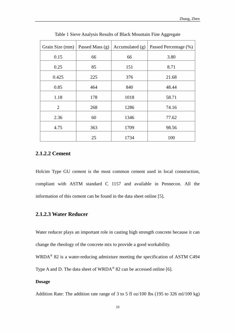
Table 1 Sieve Analysis Results of Black Mountain Fine Aggregate ........................... 10

Table 2 Information of selected materials .................................................................... 14

Table 3 UCS values of first batch ................................................................................ 27

Table 4 Systematic batches to develop three strength mixes ....................................... 28

Table 5 Detail of specimens prepared .......................................................................... 37

Table 6 Differences between repeatability condition and reproducibility condition ... 40

Table 7 Designed quantities and used quantities of materials of low strength concrete

design ........................................................................................................................... 45

Table 8 Results of UCS values of low strength concrete ............................................. 47

Table 9 Designed quantities and used quantities of materials of medium strength

concrete design............................................................................................................. 49

Table 10 Results of UCS values of medium strength concrete .................................... 51

Table 11 Designed quantities and used quantities of materials of high strength

concrete design............................................................................................................. 53

Table 12 Results of UCS values of high strength concrete .......................................... 56

Table 13 Density values and repeatability of batch No. 1 ........................................... 61

Table 14 Density values and repeatability of batch No. 2 ........................................... 61

Table 15 UCS values and repeatability of batch No. 1 ................................................ 65

Table 16 UCS values and repeatability of batch No. 2 ................................................ 65

Table 17 UCS tests values with swivel platen (medium strength) ............................... 68

Table 18 UCS tests values without swivel platen (medium strength) ......................... 68

Table 19 CCS tests results of low strength concrete in batch No. 1 ............................ 72

Table 20 CCS tests results of medium strength concrete in batch No. 1 ..................... 73

Table 21 CCS tests results of high strength concrete in batch No. 1 ........................... 74

Table 22 CCS tests results of low strength concrete in batch No. 2 ............................ 75

Table 23 CCS tests results of medium strength concrete in batch No. 2 ..................... 76

Table 24 CCS tests results of high strength concrete in batch No. 2 ........................... 77

Table 25 P wave velocity tests results and repeatability study of batch No. 1 ............ 82

Table 26 S wave velocity tests results and repeatability study of batch No. 1 ............ 82

Table 27 P wave velocity tests results and repeatability study of batch No. 2 ............ 82

Table 28 S wave velocity tests results and repeatability study of batch No. 2 ............ 83

Table 29 Retained percentage of fine aggregate on each sieve ................................... 86

Table 30 Grain size results of all three concretes......................................................... 87

Table 31 Detailed information of mineralogy analysis of all portions ........................ 90

Table 32 Weight percentage and quartz content of each portion ................................. 91

Table 33 Quartz content results of all three concretes ................................................. 92

Table 34 Porosity calculated of low strength concrete ................................................ 98

Table 35 Porosity calculated of medium strength concrete ......................................... 99

Table 36 Porosity calculated of high strength concrete ............................................. 100

Table 37 Eight parameters tests results of low strength concrete .............................. 102

Table 38 Eight parameters tests results of medium strength concrete ....................... 102

Zhang, Zhen

vii

Table 39 Eight parameters tests results of high strength concrete ............................. 103

Table 40 Converted results of low strength concrete ................................................. 105

Table 41 Converted results of medium strength concrete .......................................... 105

Table 42 Converted results of high strength concrete ................................................ 106

Zhang, Zhen

viii

List of Figures

Figure 1 Relation between strength and water/cement ratio [4] .................................... 8

Figure 2 Particle Size Distribution Plot of Black Mountain Sand ................................. 9

Figure 3 Relationships between the Compressive Strength and the Water/Cement

Ratio for Concretes with Different Contents of Silica Fume [10] ............................... 13

Figure 4 Spider Plot showing drillability curves for several well-known and

hypothetical rock types ................................................................................................ 15

Figure 5 Particle motion and propagation direction of P wave and S wave ................ 18

Figure 6 The stress-strain curve [4] ............................................................................. 19

Figure 7 Correlations between elastic moduli ............................................................. 20

Figure 8 Mohr-Coulomb failure envelope ................................................................... 22

Figure 9 Correlation between UCS and average grain size ......................................... 23

Figure 10 Sand samples before dry out ........................................................................ 32

Figure 11 Sand samples after dry out ........................................................................... 32

Figure 12 Internal vibrator ........................................................................................... 34

Figure 13 Vibration table ............................................................................................. 34

Figure 14 Flowability of mix before using internal vibration...................................... 35

Figure 15 Flowability of mix after using internal vibration ........................................ 35

Figure 16 Coring process using drilling setup ............................................................. 36

Figure 17 Core specimens of batch No. 1 .................................................................... 37

Figure 18 Core specimens of batch No. 2 .................................................................... 38

Figure 19 Saturation process set-up ............................................................................. 39

Figure 20 Vacuum for saturation process ..................................................................... 39

Figure 21 Workman II 350 mixer used in MUN’s lab ................................................. 44

Figure 22 Flowability of mix before using internal vibration...................................... 55

Figure 23 Flowability of mix after using internal vibration ........................................ 55

Figure 24 Caliper and digital scale for density test...................................................... 59

Figure 25 Loading frame and core specimen ............................................................... 62

Figure 26 Computer with Instron Bluehill software can save and output data ............ 63

Figure 27 Swivel platen in the loading system is faulty .............................................. 64

Figure 28 Swivel platen is removed from loading system ........................................... 64

Figure 29 Failure modes with swivel platen ................................................................ 67

Figure 30 Failure modes without swivel platen ........................................................... 67

Figure 31 A graphical representation of the Mohr-Coulomb failure criteria ............... 69

Figure 32 Loading frame and core specimen in confine pressure cell ........................ 70

Figure 33 Pressure pump and confine pressure cell..................................................... 71

Figure 34 Failure envelope plot of low strength concrete in batch No. 1 .................... 72

Figure 35 Failure envelope plot of medium strength concrete in batch No. 1 ............. 73

Figure 36 Failure envelope plot of high strength concrete in batch No. 1................... 74

Figure 37 Failure envelope plot of low strength concrete in batch No. 2 .................... 75

Figure 38 Failure envelope plot of medium strength concrete in batch No. 2 ............. 76

Figure 39 Failure envelope plot of high strength concrete in batch No. 2................... 77

Zhang, Zhen

ix

Figure 40 Schematic of the setup of wave velocity tests ............................................. 80

Figure 41 Experimental setup of wave velocity tests .................................................. 80

Figure 42 Example picture of wave velocity tests ....................................................... 81

Figure 43 Sieves used to identify the size of fine aggregate ........................................ 84

Figure 44 Siebtechnic disc mill.................................................................................... 88

Figure 45 Rigaku Ultima IV x-ray diffractometer ....................................................... 89

Figure 46 Mineralogy analysis results of all portions .................................................. 91

Figure 47 Microscope and digital camera .................................................................... 94

Figure 48 Thin section sample ..................................................................................... 95

Figure 49 A clear picture of thin section slide ............................................................. 96

Figure 50 Porosity calculation using thin section image ............................................. 97

Figure 51 Spider plot as a model from Prasad’s paper .............................................. 104

Figure 52 Spider plot of all three strength concrete ................................................... 107

Figure 53 Correlations between cutting size and ROP of Red Shale rock [32] (Reyes

et al., 2015, ARMA 15-764)....................................................................................... 111

Figure 54 Correlations between cutting size distribution and WOB with medium

compliance [33] (Xiao et al., 2015, ARMA 15-474) ................................................. 112

Figure 55 Correlations between ROP and hydraulic parameters of medium RLM [35]

(Khorshidian et al., 2014, ARMA 14-7465) .............................................................. 113

Figure 56 Orientations of RLM in measurements and tests [36] (Abugharara et al.,

2016, OMAE2016) .................................................................................................... 114

Figure 57 Orientations of Red Shale rock in measurements and tests [37] (Abugharara

et al., 2016, ARMA 16-868)....................................................................................... 115

Figure 58 Measurements of wave velocities and density of RLM in orientations [37]

(Abugharara et al., 2016, ARMA 16-868) ................................................................. 116

Figure 59 Dynamic elastic moduli of RLM with orientations [37] (Abugharara et al.,

2016, ARMA 16-868) ................................................................................................ 116

Figure 60 Point load strength of RLM with different C factor values [36] (Abugharara

et al., 2016, OMAE2016) ........................................................................................... 117

Figure 61 Indirect tensile strength of RLM using splitting tests [37] (Abugharara et al.,

2016, ARMA 16-868) ................................................................................................ 117

Figure 62 UCS values of RLM in orientations [36] (Abugharara et al., 2016,

OMAE2016) .............................................................................................................. 118

Figure 63 Matching ROP results of RLM with three orientations [36] (Abugharara et

al., 2016, OMAE2016)............................................................................................... 118

Figure 64 Matching cutting distributions of RLM with two different WOBs in three

orientations [37] (Abugharara et al., 2016, ARMA 16-868) ...................................... 119

Figure 65 Wave velocities and density of Red Shale in three orientations [37]

(Abugharara et al., 2016, ARMA 16-868) ................................................................. 120

Figure 66 Drilling performance of Red Shale in three orientations [36] (Abugharara et

al., 2016, OMAE2016)............................................................................................... 120

Figure 67 Mismatching cutting distributions of Red Shale with two different WOBs in

three orientations [37] (Abugharara et al., 2016, ARMA 16-868) ............................. 121

Zhang, Zhen

x

List of symbols and Abbreviations

DTL Drilling Technology Laboratory

RLM Rock-Like Materials

P wave Compressional Wave

S wave Shear Sonic Wave

DTC slowness Compressional Wave Velocity

DTS slowness Shear Wave Velocity

UCS Unconfined Compressive Strength

CCS Confined Compressive Strength

XRD X-Ray Diffraction

SEM Scanning Electron Microscopy

QA Quality Assurance

CREAIT Core Research Equipment & Instrument Training Network

pVARD passive Vibration Assisted Rotary Drilling

CI Cutting Size Index

ROP Rate of Penetration

WOB Weight on Bit

BHP Bottom Hole Pressure

Zhang, Zhen

1

1. Introduction

1.1 Background

Nowadays, petroleum is playing a pivotal role in so many aspects of our lives, not to

mention its potential commercial impacts in the energy field. Researches and studies

targeting on sedimentary rocks were conducted because oil occurs almost exclusively

in sedimentary rocks.

Rocks are a widely varied class of materials with strengths, elastic constants, and

other properties varying by one or two orders of magnitude ranging from the weakest

to the strongest rock types. Our laboratory have used standard types of rock such as

Carthage Marble, Crab Orchard Sandstone, etc. However, within any given rock mass,

properties can be heterogeneous and isotropic and vary with both position and

orientation within the same formation. The use of natural rock materials for

experimental geomechanics studies in Oil and Gas at Memorial University has several

difficulties:

1) Experimental studies require a high degree of reproducibility, and many

natural rocks have high variability even within a small sample volume

2) Oil and Gas reservoirs are found in sedimentary rocks, and rocks of this type

are not local to the onshore portion of Eastern Newfoundland.

However, concrete is a material composed of a Portland Cement based matrix and

rock aggregate, and has similar material properties and failure behavior as low

Zhang, Zhen

2

permeability sedimentary rocks. Therefore, concrete samples are considered as a

reasonable substitute of real rock samples which can meet the following requirements

in this research:

1) three different UCS values at 28-days which represent weak, medium and

strong sedimentary rocks

2) the materials are easy to get and can be supplied for a long-term

3) all the samples have a high degree of reproducibility

1.2 Research Objectives

The first objective of this work was to develop highly consistent, fine grained

concrete materials which can represent characteristic rock types for experimental

geomechanics research. The aim was concrete mixes with three different UCS values

which represent weak (20MPa), medium (50MPa) and strong (over 80MPa) rock

samples respectively. These concrete materials are intended, in particular, for

laboratory research, to be cast in sample sizes ranging from a few inches to a few feet

in all dimensions.

The second objective of this research was to characterize the drillability of these

concrete samples following procedures proposed for the drillability of rock, in

particular tests proposed by Prasad (2009) and described and reviewed in detail in a

later chapter. In summary, Prasad proposed that the drillability of rock can be

characterized as a combination of density, porosity, compression and shear sonic wave

Zhang, Zhen

3

velocities, unconfined compressive strength, Mohr friction angle, mineralogy, and

grain size. This objective was pursued by studying all these eight parameter on the

three concrete materials developed.

The third objective was to establish standard procedures for quality assurance in the

laboratory production of the concrete materials to serve in laboratory studies as

analogs for rocks.

1.3 Significance of this research

1.3.1 Convenient substitute of real rock in experiments

The research was focused on researching a number of rock analogue materials based

on fine rock aggregates and Portland cement. Through parametric batch mixing and

materials testing, a suite of standard materials were developed as potential

replacements for actual rock that have the desired range of strength, elastic properties,

abrasivity, elastic wave velocities, and failure behavior. This will provide for a

standard set of materials that may represent rock types ranging from weak shales,

intermediate strength siltstones and low permeability sandstones to strong crystalline

rocks in experimental geomechanics. This will overcome the general lack of available

weak and intermediate strength sedimentary rocks for experimental studies onshore in

the province of NL and provide for a high degree of Quality Assurance and

experimental reproducibility for geomechanics studies.

Zhang, Zhen

4

1.3.2 Provide basis to compare with real rock

Experimental geomechanics using real rock specimens is normally limited due to the

high cost of acquiring materials and the often limited amount available (e.g. from drill

cores, etc.) development and refinement of experimental facilities, data analysis

procedures. Conversely, these “synthetic rock” materials would provide almost

unlimited specimens which could also be cast into convenient shapes for experiments

and include such features as imbedded instrumentation, internal flow channels,

piezometers, etc. This also can facilitate comparison with studies at other

geomechanics laboratories.

1.3.3 Establish the standard procedure for quality assurance

A reason for using concrete sample as a substitute of real rock is a high level of

reproducibility of material properties can be achieved so that with the Quality

Assurance (QA) playing an important role in casting consistent and reproducible

concrete samples. During this research, a series of quality assurance procedures

following standard practice for concrete were established to provide the confidence of

repeatability studies and reproducibility studies. For instance, sieve analysis, moisture

content calculation and internal vibration all became standard procedures in mixing

concrete so that repeatability and reproducibility can be improved. The concept of

sieve analysis, moisture content calculation and internal vibration are introduced in

next three paragraphs.

Sieve analysis [2] is a standard procedure to assess particle size distribution in the

Zhang, Zhen

5

concrete industry, which can control the quality of aggregates in this project. The

sieve analysis results can be used to characterize the sand used in every batch of

concrete cast because similar sieve analysis results provide the similar material

performance.

Moisture content calculation [3] is used to calculate the moisture content in fine

aggregate (sand). Fine aggregate is usually stored in an open area. Therefore the water

content can be affected by the weather. Moisture content is determined by removing

the water in fine aggregate through heating. The difference in weight is the water

content. The water/cement ratio used in adjusted accordingly.

Internal vibration was introduced to improve the workability of mix to achieve a

better consolidation. Higher workability will provide consistent rock samples

compared with the poor consolidation. In high strength design, the internal vibration

made a significant improvement in workability when the mix can not be consolidated

without vibration.

1.4 Limitations

1.4.1 Uncertain curing conditions might affect strength of

concrete

Concrete samples are usually cast in laboratory with certain procedures and strict

curing environments. However, large quantity specimens may require to be cast at the

field in future work. It is well known that strength of concrete is highly related to

Zhang, Zhen

6

curing conditions i.e. curing temperature, humidity and time. This raises the problem

of control curing environments to achieve desired UCS values outside the laboratory.

In addition, curing with water saturated with calcium hydroxide (Ca(OH)2) to prevent

leaching of this compound (a product of hydrolysis in curing) from the concrete as

ASTM Standard C511-09 suggests is difficult to implement in field condition.

1.4.2 Methods used in characterization of rock might not

compatible with concrete

As we are using concrete as a convenient material to use instead of real rock, it is

realized that we must characterize the concrete in a way that will make it possible to

compare our drilling test results with similar results obtained in real rock, and with

simulation/modeling work based on the relevant properties. However, the methods

used to characterize properties of real rock cannot always be applied on concrete

specimens. For example, porosity is usually calculated using water saturated method

which is obviously not suitable for concrete or it will continuously react with water.

1.4.3 Variability issues that can affect the characterization of

concrete

Most natural rock was formed millions of years ago, while the age of concrete under

consideration here would be only being a matter of months. Whatever way concrete is

produced and whatever the environment in which it exists, it is a “work in progress,”

Zhang, Zhen

7

i.e. the result of incomplete chemical processes and continuing change. The

specification strength of concrete is usually the strength after 28 days of curing, and

that depends on the manner in which curing takes place, but strength can continue to

increase and other properties continue to change over time. Thus there can be issues

of variability of properties in space within concrete specimens, as well as variability

over time.

2. Literature Reviews

2.1 Factors Affect the UCS Values

Engineers have developed many ways to strengthen concrete in the field, such as

inserting steel bar and introducing additives. However, steel bar and coarse aggregate

can not be contained in concrete sample in this research. The fundamental approach is

to adjust the ratio between water, sand and cement which are the basic materials of

concrete. The investigation of concrete strength affected by the ratio between water,

sand and cement has been conducted, and water/cement ratio is the key point of the

strength of concrete.

2.1.1 Water/cement ratio

Water/cement ratio, also described as water/binder ratio, is a critical factor affecting

the compressive strength of concrete. In fact, by given sand and cementitious material,

Zhang, Zhen

8

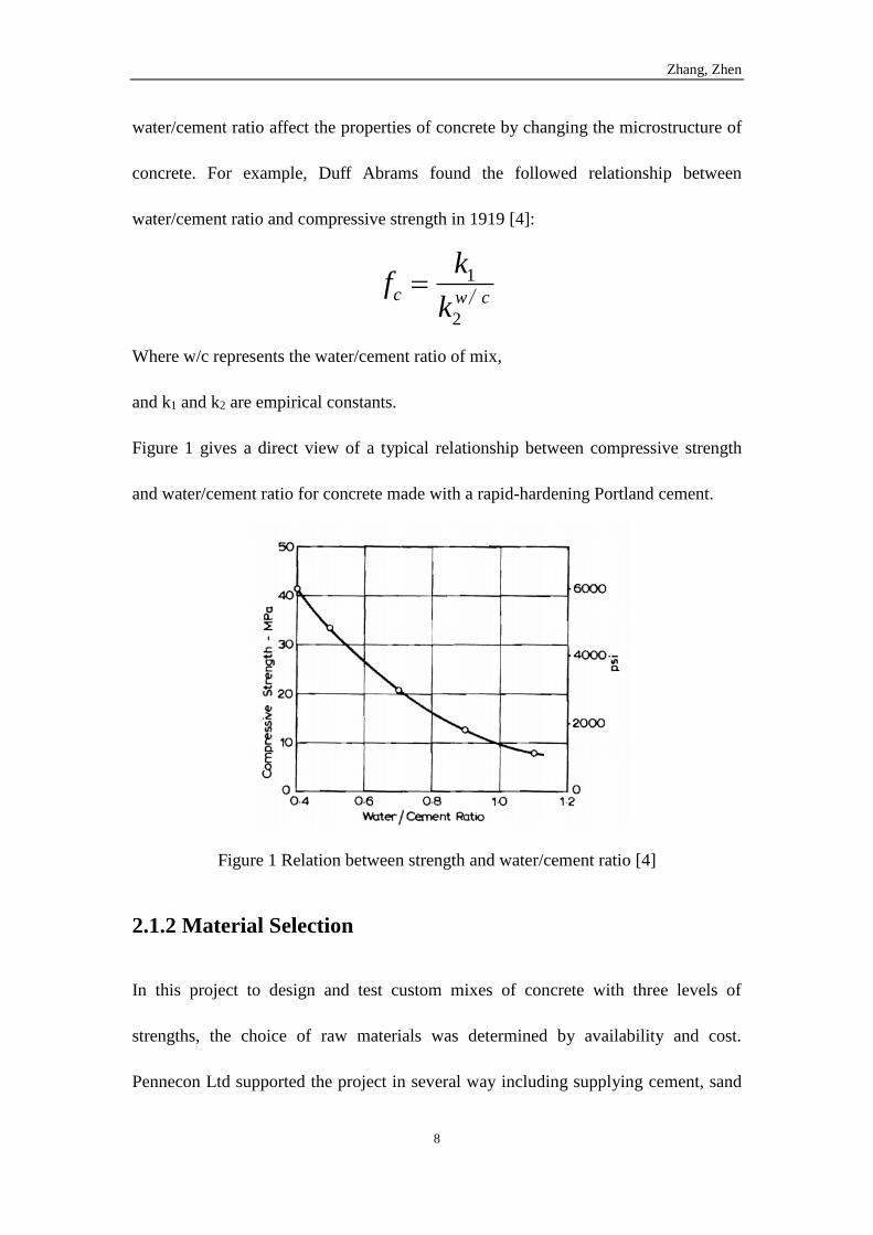
water/cement ratio affect the properties of concrete by changing the microstructure of

concrete. For example, Duff Abrams found the followed relationship between

water/cement ratio and compressive strength in 1919 [4]:

1

2

c w c

kf

k

∕

Where w/c represents the water/cement ratio of mix,

and k1 and k2 are empirical constants.

Figure 1 gives a direct view of a typical relationship between compressive strength

and water/cement ratio for concrete made with a rapid-hardening Portland cement.

Figure 1 Relation between strength and water/cement ratio [4]

2.1.2 Material Selection

In this project to design and test custom mixes of concrete with three levels of

strengths, the choice of raw materials was determined by availability and cost.

Pennecon Ltd supported the project in several way including supplying cement, sand

Zhang, Zhen

9

and additives.

2.1.2.1 Sand (fine aggregate)

Aggregate also known as sand and stone, is used in concrete. In general mixing design,

both coarse aggregate (＞4.75mm) and fine aggregate (≤4.75mm) were considered.

Because drill bits no bigger than 2 inches are used in this project, only fine aggregate

was used for materials. Although only fine aggregate was acceptable in this design,

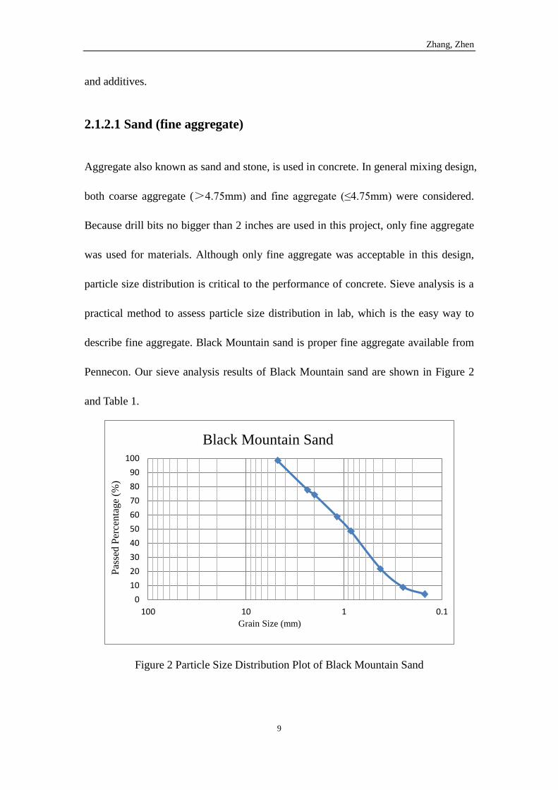
particle size distribution is critical to the performance of concrete. Sieve analysis is a

practical method to assess particle size distribution in lab, which is the easy way to

describe fine aggregate. Black Mountain sand is proper fine aggregate available from

Pennecon. Our sieve analysis results of Black Mountain sand are shown in Figure 2

and Table 1.

Figure 2 Particle Size Distribution Plot of Black Mountain Sand

0

10

20

30

40

50

60

70

80

90

100

0.1110100

Pas

sed

Per

centa

ge

(%)

Grain Size (mm)

Black Mountain Sand

Zhang, Zhen

10

Table 1 Sieve Analysis Results of Black Mountain Fine Aggregate

Grain Size (mm) Passed Mass (g) Accumulated (g) Passed Percentage (%)

0.15 66 66 3.80

0.25 85 151 8.71

0.425 225 376 21.68

0.85 464 840 48.44

1.18 178 1018 58.71

2 268 1286 74.16

2.36 60 1346 77.62

4.75 363 1709 98.56

25 1734 100

2.1.2.2 Cement

Holcim Type GU cement is the most common cement used in local construction,

compliant with ASTM standard C 1157 and available in Pennecon. All the

information of this cement can be found in the data sheet online [5].

2.1.2.3 Water Reducer

Water reducer plays an important role in casting high strength concrete because it can

change the rheology of the concrete mix to provide a good workability.

WRDA® 82 is a water-reducing admixture meeting the specification of ASTM C494

Type A and D. The data sheet of WRDA® 82 can be accessed online [6].

Dosage

Addition Rate: The addition rate range of 3 to 5 fl oz/100 lbs (195 to 326 ml/100 kg)

Zhang, Zhen

11

of cement or cementitious is typical for most applications. However, addition rates of

2 to 10 fl oz/100 lbs (130 to 652 ml/100 kg) of cement or cementitious may be used if

local testing shows acceptable performance.

WRDA® 82 is compatible with most Grace Company’s admixtures as long as they are

added separately to the concrete mix.

2.1.2.4 Superplasticizer

Superplasticizer, also known as high range water-reducing admixture, is usually used

in concrete mix with low water/cement ratio. This chemical admixture can produce a

high slump flowable concrete without lowering the compressive strength.

Daracem® 19 is a high range water reducer meeting the specification of ASTM C494

Type A and F. Data sheet of Daracem® 19 can be accessed online [7].

Dosage

Addition Rate: Addition rates of Daracem® 19 can vary with type of application, but

will normally range from 6 to 20 fl oz/100 lbs (390 to 1300 ml/100 kg) of cement. In

most instances the addition of 10 to 16 fl oz/100 lbs (650 to 1040 mL/100 kg) of

cement will be sufficient.

Daracem® 19 is compatible with most Grace Company’s admixtures as long as they

are added separately to the concrete mix

2.1.2.5 Silica fume

Silica fume, also referred to microsilica, is introduced as cementitious material to

Zhang, Zhen

12

increase compressive strength based on its chemical and physical properties. Silica

fume is highly reactive, which can speed up the reaction with the calcium hydroxide

produced by the hydration of Portland cement. Furthermore, the very small particles

of silica fume can fill the space between large particles to improve packing.

Information about Force 10,000® D can be accessed online [8].

Dosage

Based on the working principle of silica fume, Aitcin [9] suggests that the dosage of

silica fume should be 25%-30%, and silica fume is needed to neutralize the lime

produced by the hydration of Portland cement. In addition, higher dosage of silica

fume will provide a higher compressive strength. The relation between the

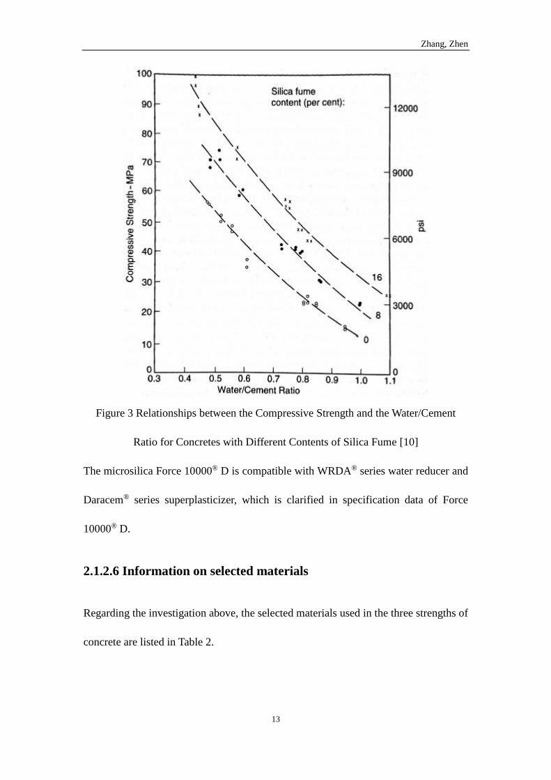
compressive strength and different contents of silica fume is shown in Figure 3 [10].

However, high dosage of silica fume is not usually used in the field because silica

fume consumes a large quantity of superplasticizer. In our tests it was found that silica

fume at 15% of all cementious materials (by mass) was the appropriate amount to use

with water cement ratio of 0.35 with superplasticizer.

Zhang, Zhen

13

Figure 3 Relationships between the Compressive Strength and the Water/Cement

Ratio for Concretes with Different Contents of Silica Fume [10]

The microsilica Force 10000® D is compatible with WRDA® series water reducer and

Daracem® series superplasticizer, which is clarified in specification data of Force

10000® D.

2.1.2.6 Information on selected materials

Regarding the investigation above, the selected materials used in the three strengths of

concrete are listed in Table 2.

Zhang, Zhen

14

Table 2 Information of selected materials

Materials Brand

Fine Aggregate Black Mountain Sand

Cement Holcim Type GU

Water Reducer WRDA® 82

Superplasticizer Daracem® 19

Silica Fume Force 10000® D

2.2 Drillability

Prasad (2009) has proposed a quantitative methodology to describe rock materials in

terms of their “drillability” as a means of predicting rates of penetration and wear,

which are closely linked to strength [11] and abrasivity. This methodology includes 8

material properties (density, porosity, compressional and shear wave velocities,

unconfined compressive strength, Mohr friction angle, mineralogy, and grain sizes)

which can be represented on a Spider Plot as given in Figure 4 as a drillability curve

relating all 8 properties. All eight parameters are converted in a scale of 0 to 8; value 0

represents very soft rock and value 8 represents hard rock, ideally.

Zhang, Zhen

15

Figure 4 Spider Plot showing drillability curves for several well-known and

hypothetical rock types

In eight parameters tests, both non-destructive tests and destructive tests are involved.

The series of experimental tests have to be organized with procedures and test

materials. In eight parameters tests, density, porosity, P-wave velocity and S-wave

velocity are non-destructive tests which should be tested before other destructive tests.

UCS and Mohr friction angle tests have crush the samples to obtain the value from

tester, which require large amount of specimens. Grain size and mineralogy tests are

only involved with fine aggregate because concrete is different from real rock and

modifications of tests are necessary. The brief ideas each test are shown as following

and more detailed experimental procedures will be described in later chapters.

Zhang, Zhen

16

2.3 Eight Parameters Characterizations

Drillability of rock is a concept usually used to describe the physical properties of

rock, which reflect the rate of penetration under certain drilling condition. It can be

expressed with a lot of parameters such as hardness, elastic constants, mineral

composition, density, permeability, UCS and CCS. Drillability is not a parameter

commonly referred in the field because there is no unified standard to describe

drillability. However, rock properties like UCS, hardness and density have been

frequently used to optimize drilling parameters. In this research, characterization of

rock (concrete) will be conducted with eight parameters which proposed by Prasad in

2009. These parameters are density, porosity, compressional and shear wave velocities,

unconfined compressive strength, Mohr friction angle, mineralogy, and grain size.

2.3.1 Density

Density is a common physical property which can be determined by mass over

volume. Density of same rock can be varied because pore space in rock and crack in

matrix is different. Hence, density is often related to the porosity and strength because

pore space increase porosity and weaken strength. However, density can be a very

valuable parameter to describe the physical property of concrete. As mentioned

previously, concrete designed in this research only contains water, fine aggregate and

cement. The density of concrete can be an indicator of strength and composition due

to the density of individual materials are fixed. Since density of cement (3.15 g/cm3)

is higher than the water (1 g/cm3) and fine aggregate (2.65 g/cm3), stronger concrete is

Zhang, Zhen

17

consist of more cementious material and less water while density is increasing.

2.3.2 Porosity

Porosity is a useful parameter in drilling field, which is target data to acquire in

wireline well log. Porosity is related to the elastic properties because the pore space it

where the stress concentrated on during deformation. The vacuum saturation method

[12] is commonly used in the lab for porosity measurement of concrete, which

involves complicated apparatus which is not available. Therefore porosity is

calculated by the percentage of pore area over total thin section area under

microscope in this research.

2.3.3 P wave and S wave velocities

The compressional wave, also referred to primary wave (P wave), is the fastest wave

can travel in rocks. This feature allows it to be commonly used to characterize rock

properties in lab and field for drilling purpose. As the P wave velocity will drastically

drop in gas media it can be an indicator to estimate porosity because P waves travel

faster in solid than in air. The shear wave (S wave), also referred to secondary wave,

travels slower than the P wave, and not like P wave, it only travels in solid. The

illustration of P wave and S wave are shown in Figure 5.

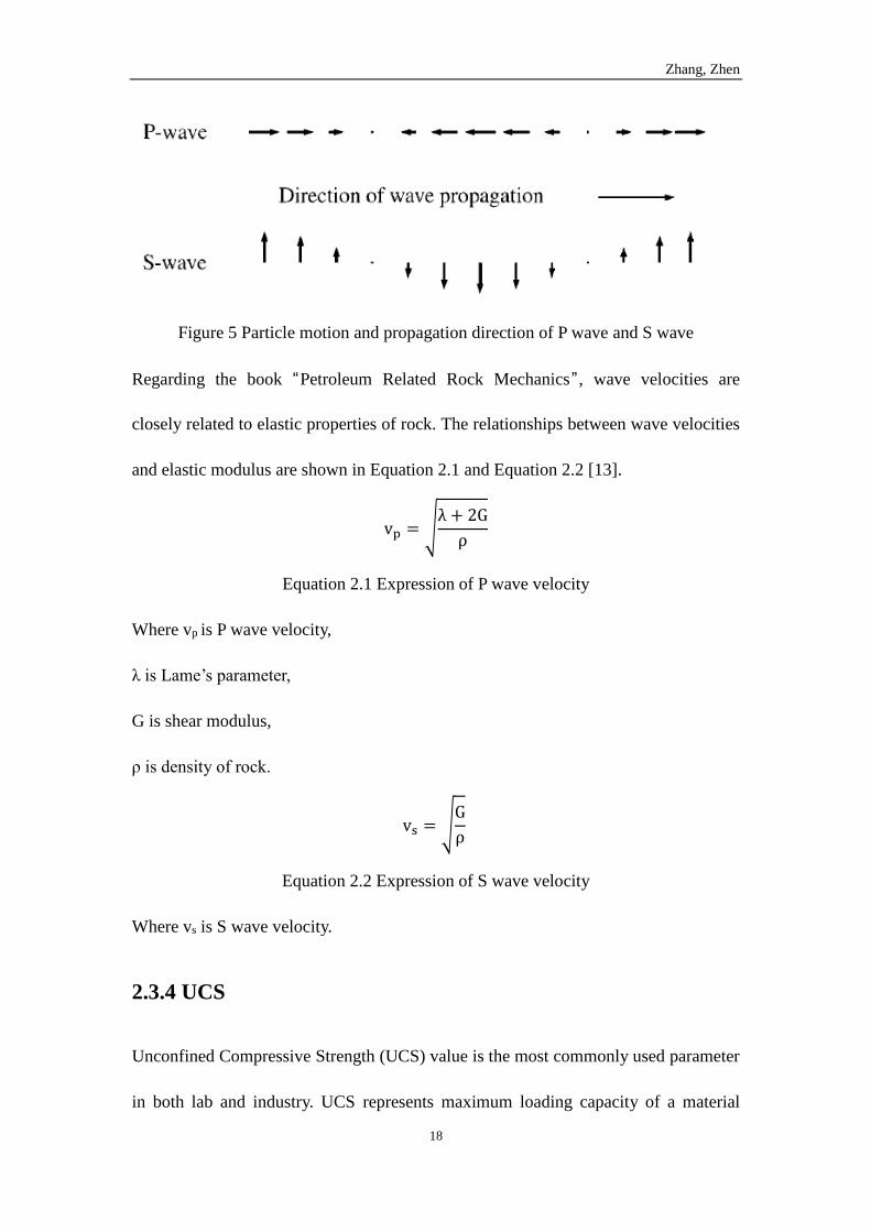
Zhang, Zhen

18

Figure 5 Particle motion and propagation direction of P wave and S wave

Regarding the book “Petroleum Related Rock Mechanics” , wave velocities are

closely related to elastic properties of rock. The relationships between wave velocities

and elastic modulus are shown in Equation 2.1 and Equation 2.2 [13].

vp = √λ + 2G

ρ

Equation 2.1 Expression of P wave velocity

Where vp is P wave velocity,

λ is Lame’s parameter,

G is shear modulus,

ρ is density of rock.

vs = √G

ρ

Equation 2.2 Expression of S wave velocity

Where vs is S wave velocity.

2.3.4 UCS

Unconfined Compressive Strength (UCS) value is the most commonly used parameter

in both lab and industry. UCS represents maximum loading capacity of a material

Zhang, Zhen

19

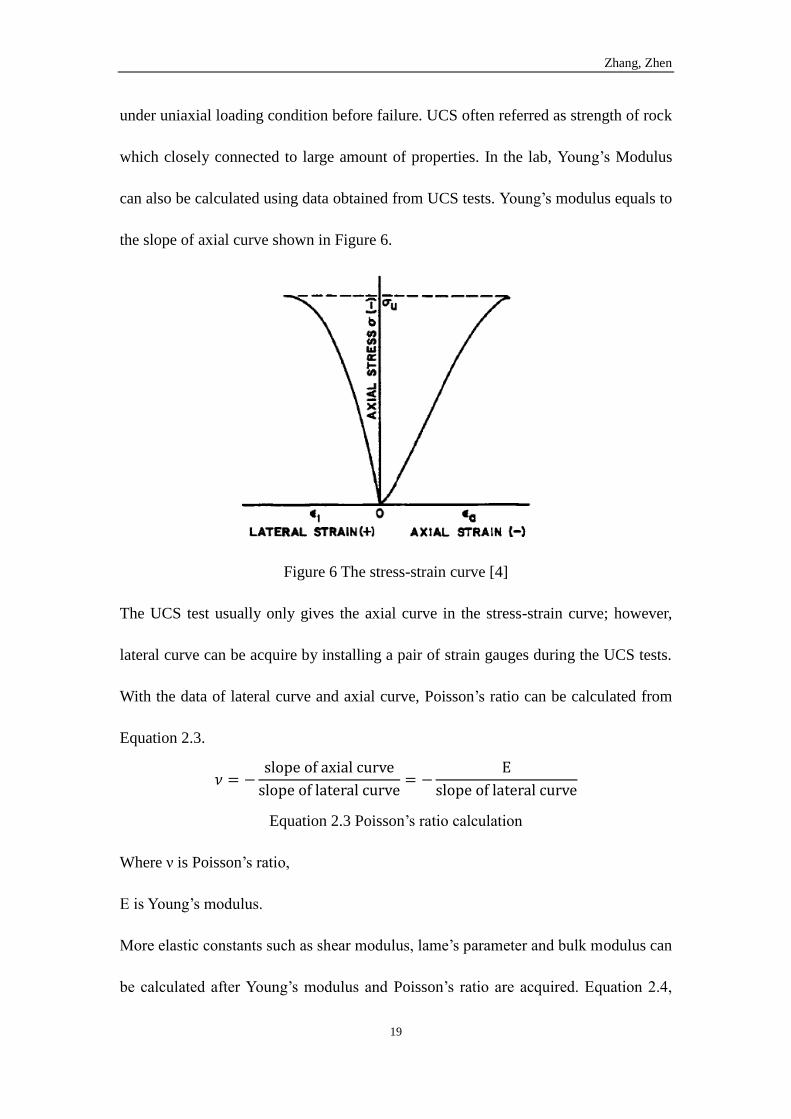
under uniaxial loading condition before failure. UCS often referred as strength of rock

which closely connected to large amount of properties. In the lab, Young’s Modulus

can also be calculated using data obtained from UCS tests. Young’s modulus equals to

the slope of axial curve shown in Figure 6.

Figure 6 The stress-strain curve [4]

The UCS test usually only gives the axial curve in the stress-strain curve; however,

lateral curve can be acquire by installing a pair of strain gauges during the UCS tests.

With the data of lateral curve and axial curve, Poisson’s ratio can be calculated from

Equation 2.3.

𝜈 = −slope of axial curve

slope of lateral curve= −

E

slope of lateral curve

Equation 2.3 Poisson’s ratio calculation

Where ν is Poisson’s ratio,

E is Young’s modulus.

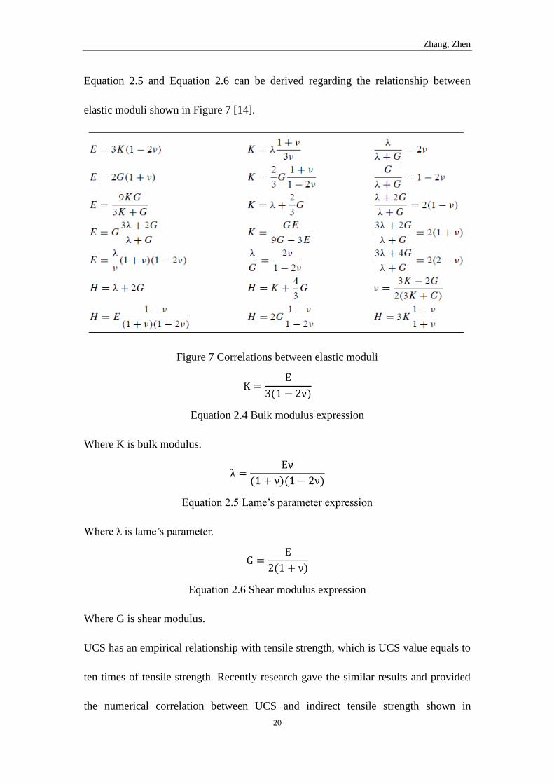
More elastic constants such as shear modulus, lame’s parameter and bulk modulus can

be calculated after Young’s modulus and Poisson’s ratio are acquired. Equation 2.4,

Zhang, Zhen

20

Equation 2.5 and Equation 2.6 can be derived regarding the relationship between

elastic moduli shown in Figure 7 [14].

Figure 7 Correlations between elastic moduli

K =E

3(1 − 2ν)

Equation 2.4 Bulk modulus expression

Where K is bulk modulus.

λ =Eν

(1 + ν)(1 − 2ν)

Equation 2.5 Lame’s parameter expression

Where λ is lame’s parameter.

G =E

2(1 + ν)

Equation 2.6 Shear modulus expression

Where G is shear modulus.

UCS has an empirical relationship with tensile strength, which is UCS value equals to

ten times of tensile strength. Recently research gave the similar results and provided

the numerical correlation between UCS and indirect tensile strength shown in

Zhang, Zhen

21

Equation 2.7 [15] (Correlation between Unconfined Compressive Strength and

Indirect Tensile Strength of Limestone Rock Samples).

UCS (MPa) = 9.25 BTS0.947

Equation 2.7 Experimental correlation between UCS and indirect tensile strength

Where BTS is Brazilian Tensile Strength

2.3.5 Mohr friction angle

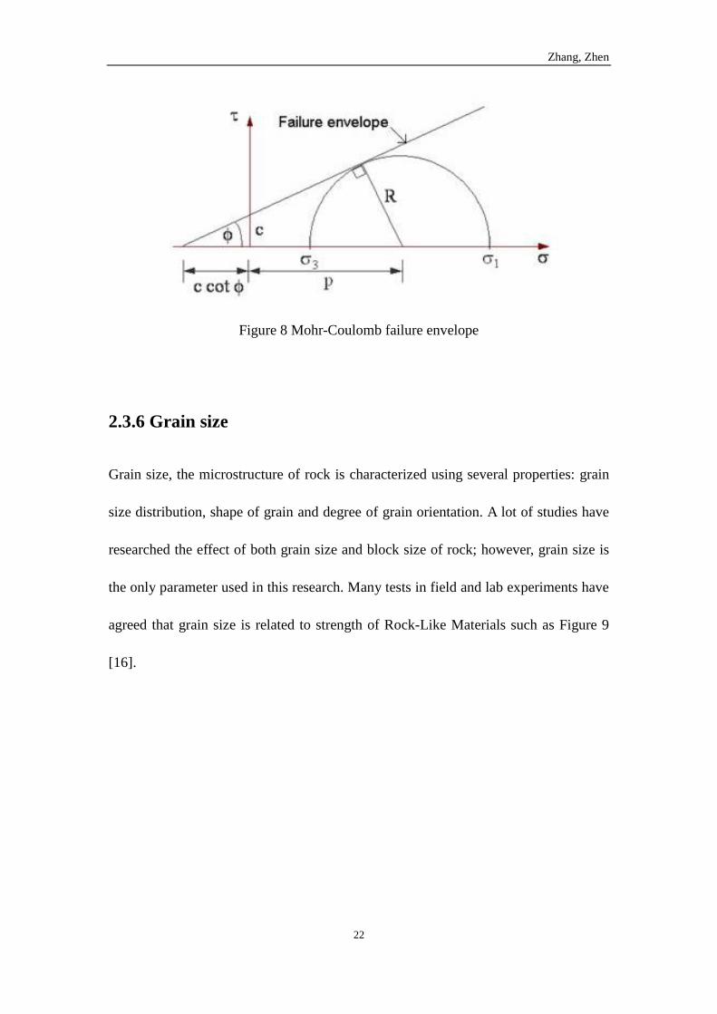
Mohr friction angle in a parameter in Mohr-Coulomb failure criteria which can be

obtained by confined compressive strength (CCS) tests. The mathematic relationship

between parameters of Mohr-Coulomb failure envelope is shown in Figure 8 and

failure envelope can be expressed in Equation 2.8.

τ = C + σtanφ

Equation 2.8 Mohr-Coulomb failure criteria

Where:

C is cohesion stress,

σ is normal stress on the failure plane,

τ is shear stress on the failure plane,

φ is the friction angle.

Zhang, Zhen

22

Figure 8 Mohr-Coulomb failure envelope

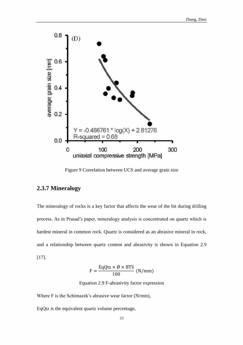
2.3.6 Grain size

Grain size, the microstructure of rock is characterized using several properties: grain

size distribution, shape of grain and degree of grain orientation. A lot of studies have

researched the effect of both grain size and block size of rock; however, grain size is

the only parameter used in this research. Many tests in field and lab experiments have

agreed that grain size is related to strength of Rock-Like Materials such as Figure 9

[16].

Zhang, Zhen

23

Figure 9 Correlation between UCS and average grain size

2.3.7 Mineralogy

The mineralogy of rocks is a key factor that affects the wear of the bit during drilling

process. As in Prasad’s paper, mineralogy analysis is concentrated on quartz which is

hardest mineral in common rock. Quartz is considered as an abrasive mineral in rock,

and a relationship between quartz content and abrasivity is shown in Equation 2.9

[17].

F =EqQtz × Ø × BTS

100 (N/mm)

Equation 2.9 F-abrasivity factor expression

Where F is the Schimazek’s abrasive wear factor (N/mm),

EqQtz is the equivalent quartz volume percentage,

Zhang, Zhen

24

Ø is the grain size (mm),

BTS is indirect Brazilian tensile strength.

As indicated by this equation the abrasivity of rock is linked to the quartz content in

conjunction with the grain size and strength of the rock.

Zhang, Zhen

25

3. Methodology

3.1 Approach to the Development of Concrete Designs

In order to obtain concrete samples desired, a series of systematic experiments were

conducted at Pennecon’s lab where materials and tools can be provided. The

objectives of this research are to develop three strengths of concrete and characterize

samples with eight parameters. The methodology of developing three strengths is

critical because the concrete samples will be the basis of later experiments. However,

the eight parameters cannot be individually controlled during preparation of the

sample though concrete is a synthetic substitute. Unconfined Compressive Strength

(UCS) values as an important parameter in both rock property and concrete design

should be the controlled parameter of design concrete batches.

3.1.1 Facilities used

The author was awarded a MITACS Internship with Pennecon Limited, which funded

collaboration with its subsidiary, Capital Precast Limited, with use of its laboratory

facilities and also materials provided by it: Portland Cement and fine aggregate - the

latter produced from material from its nearby Black Mountain quarry. Much of the

preparation and curing of the initial mixes of concrete and testing for Unconfined

Compressive Strength (UCS) were conducted at Capital Precast. All other property

tests and later preparation of concrete samples were conducted in the Engineering

Zhang, Zhen

26

Laboratories at Memorial University.

3.1.2 Initialize the design parameters

As mentioned before, water/cement ratio is a key value to determine concrete strength

and concrete used in this research will require three ingredients as water, fine

aggregate and cement. Aggregate/cement ratio can be calculated with a given

water/cement ratio. Therefore, some ideas are borrowed from the method of mixing

concrete called Absolute Volume Method of Concrete Mix Design.

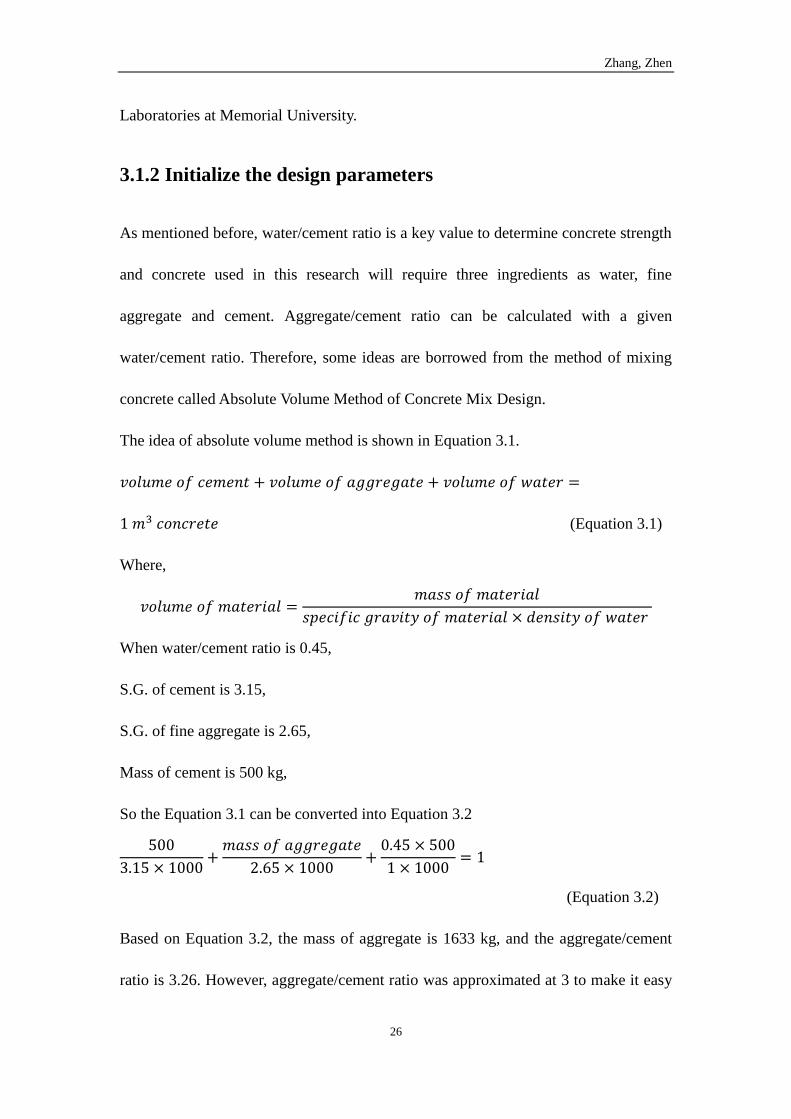
The idea of absolute volume method is shown in Equation 3.1.

𝑣𝑜𝑙𝑢𝑚𝑒 𝑜𝑓 𝑐𝑒𝑚𝑒𝑛𝑡 + 𝑣𝑜𝑙𝑢𝑚𝑒 𝑜𝑓 𝑎𝑔𝑔𝑟𝑒𝑔𝑎𝑡𝑒 + 𝑣𝑜𝑙𝑢𝑚𝑒 𝑜𝑓 𝑤𝑎𝑡𝑒𝑟 =

1 𝑚3 𝑐𝑜𝑛𝑐𝑟𝑒𝑡𝑒 (Equation 3.1)

Where,

𝑣𝑜𝑙𝑢𝑚𝑒 𝑜𝑓 𝑚𝑎𝑡𝑒𝑟𝑖𝑎𝑙 =𝑚𝑎𝑠𝑠 𝑜𝑓 𝑚𝑎𝑡𝑒𝑟𝑖𝑎𝑙

𝑠𝑝𝑒𝑐𝑖𝑓𝑖𝑐 𝑔𝑟𝑎𝑣𝑖𝑡𝑦 𝑜𝑓 𝑚𝑎𝑡𝑒𝑟𝑖𝑎𝑙 × 𝑑𝑒𝑛𝑠𝑖𝑡𝑦 𝑜𝑓 𝑤𝑎𝑡𝑒𝑟

When water/cement ratio is 0.45,

S.G. of cement is 3.15,

S.G. of fine aggregate is 2.65,

Mass of cement is 500 kg,

So the Equation 3.1 can be converted into Equation 3.2

500

3.15 × 1000+

𝑚𝑎𝑠𝑠 𝑜𝑓 𝑎𝑔𝑔𝑟𝑒𝑔𝑎𝑡𝑒

2.65 × 1000+

0.45 × 500

1 × 1000= 1

(Equation 3.2)

Based on Equation 3.2, the mass of aggregate is 1633 kg, and the aggregate/cement

ratio is 3.26. However, aggregate/cement ratio was approximated at 3 to make it easy

Zhang, Zhen

27

to calculate. Regarding the calculation above, aggregate: cement: water (A: C: W) is

confirmed at 3: 1: 0.45, and this is the first design to start with. More designs will be

developed by adjusting water/cement ratio after UCS value of first design confirmed.

3.1.3 Systematic batches by adjusting parameters

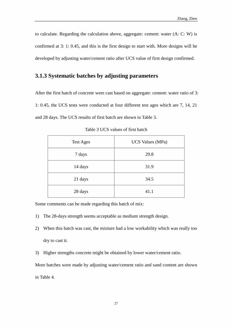
After the first batch of concrete were cast based on aggregate: cement: water ratio of 3:

1: 0.45, the UCS tests were conducted at four different test ages which are 7, 14, 21

and 28 days. The UCS results of first batch are shown in Table 3.

Table 3 UCS values of first batch

Test Ages UCS Values (MPa)

7 days 29.8

14 days 31.9

21 days 34.5

28 days 41.1

Some comments can be made regarding this batch of mix:

1) The 28-days strength seems acceptable as medium strength design.

2) When this batch was cast, the mixture had a low workability which was really too

dry to cast it.

3) Higher strengths concrete might be obtained by lower water/cement ratio.

More batches were made by adjusting water/cement ratio and sand content are shown

in Table 4.

Zhang, Zhen

28

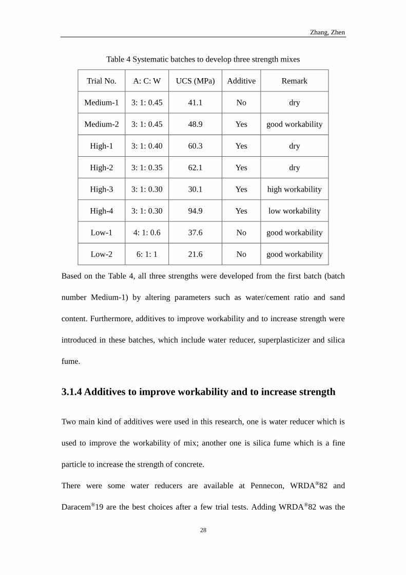
Table 4 Systematic batches to develop three strength mixes

Trial No. A: C: W UCS (MPa) Additive Remark

Medium-1 3: 1: 0.45 41.1 No dry

Medium-2 3: 1: 0.45 48.9 Yes good workability

High-1 3: 1: 0.40 60.3 Yes dry

High-2 3: 1: 0.35 62.1 Yes dry

High-3 3: 1: 0.30 30.1 Yes high workability

High-4 3: 1: 0.30 94.9 Yes low workability

Low-1 4: 1: 0.6 37.6 No good workability

Low-2 6: 1: 1 21.6 No good workability

Based on the Table 4, all three strengths were developed from the first batch (batch

number Medium-1) by altering parameters such as water/cement ratio and sand

content. Furthermore, additives to improve workability and to increase strength were

introduced in these batches, which include water reducer, superplasticizer and silica

fume.

3.1.4 Additives to improve workability and to increase strength

Two main kind of additives were used in this research, one is water reducer which is

used to improve the workability of mix; another one is silica fume which is a fine

particle to increase the strength of concrete.

There were some water reducers are available at Pennecon, WRDA®82 and

Daracem®19 are the best choices after a few trial tests. Adding WRDA®82 was the

Zhang, Zhen

29

only thing changed in batch number Medium-2 compared to batch number Medium-1.

Improving workability of mixes can significantly increase the strength of concrete

samples and provide a better performance of mixes. Daracem®19 is added in high

strength concrete design as a high range water reducer (superplasticizer). High

strength concrete mix has a really low workability because of low water/cement ratio

and silica fume. The recommended dosage didn’t work for this kind of application

and the right dosage of superplasticizer had to be determined through trial tests. Too

much (batch number High-3) or not enough superplasticizer will not obtain desired

strength.

Silica fume is usually mixed with Portland cement to improve the concrete properties

such as strength. Silica fume is extremely fine particles and can fill the space between

fine aggregate and concrete matrix to increase the strength of concrete. Also the

pozzolanic reaction between silica fume and calcium hydroxide generated from water

and cement provides extra bond strength.

3.1.5 Results of trial tests

After these systematic batch trials, three strengths concrete designs have been

completed. The results and observations from trial tests are given as following:

1) Regarding the UCS values obtained from Table 4, low strength, medium strength

and high strength concrete designs are batch number Low-2, batch number

Medium-2 and batch number High-4, respectively.

2) In design of high strength concrete, silica fume is introduced. It’s fairly fine

Zhang, Zhen

30

particle size increases strength. Because of the low water/cement ratio and silica

fume in high strength concrete design, proper dosage of superplasticizer is the

critical in the mixing high strength concrete. Not enough water reducer and

superplasticizer will lower the workability of concrete mix so that the mix cannot

be moulded. However, too much superplasticizer will result in an extremely low

strength of concrete mix (batch number High-3).

3) The batch number High-4 is acceptable design for high strength concrete,

however, it is still a dry mix which is difficult to utilize in larger quantity mixing.

A more powerful superplasticizer might be the solution.

3.2 Quality Assurance

The three strength concrete samples will be massively used in future experiments as

tests materials. The reproducibility is an important feature in these designs because

plenty of tests based on these three strength concrete mixes will be conducted in the

future. The purpose of quality control is to cast consistent and reproducible concrete

samples with standard procedures.

3.2.1 Sieve analysis

Sieve analysis is a standard procedure to assess particle size distribution in the

concrete industry, which can control the quality of sand in this research. The sieve

analysis results can be used to identify the fine aggregate (sand) used in every single

Zhang, Zhen

31

batch of concrete cast because similar sieve analysis results provide the similar

material performance. Therefore, sieve analysis tests for every batch of fine aggregate

should be conducted with dry material condition before it is used to mix concrete

sample. Furthermore, sieve analysis results and test procedures of fine aggregate

should meet the requirement ASTM standard C136 (Standard Test Method for Sieve

Analysis of Fine and Coarse Aggregates) [18].

Black Mountain fine aggregate, the material used in this research, is required to

conduct the sieve analysis test. The 8 sieves used in sieve analysis are mesh number 4,

8, 10, 16, 20, 40, 60 and 100 which aperture diameter corresponding to 4.75 mm, 2.36

mm, 2 mm, 1.18 mm, 0.85 mm, 0.425 mm, 0.25 mm and 0.15 mm. The results of

sieve analysis of Black Mountain sand are shown in Table 1 and Figure 2.

3.2.2 Moisture content calculation

The moisture content calculation is used to calculate the moisture content in fine

aggregate. Fine aggregate is usually stored in an open area. Therefore the water

content can be affected by the weather. Moisture content is determined by removing

the water in fine aggregate through heating process. The difference in weight is the

water content. The water/cement ratio used in adjusted accordingly by deducting the

calculated water content from the total water content.

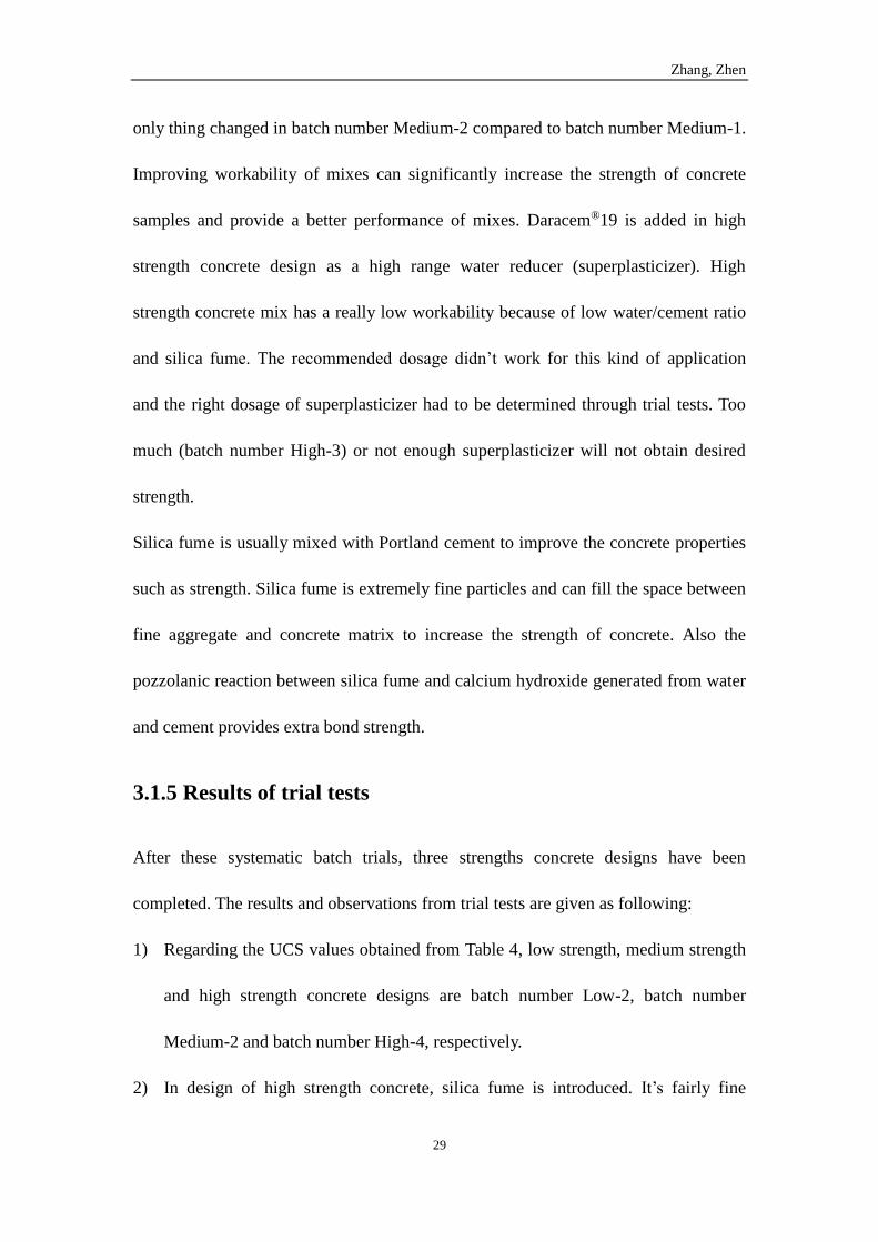
Standard Procedures of Moisture Content Calculation:

Weigh around 2000 gram sand and record as mass of wet sand

Put sand into a steel pan and top pan on a hot plate to vaporize the water until the

Zhang, Zhen

32

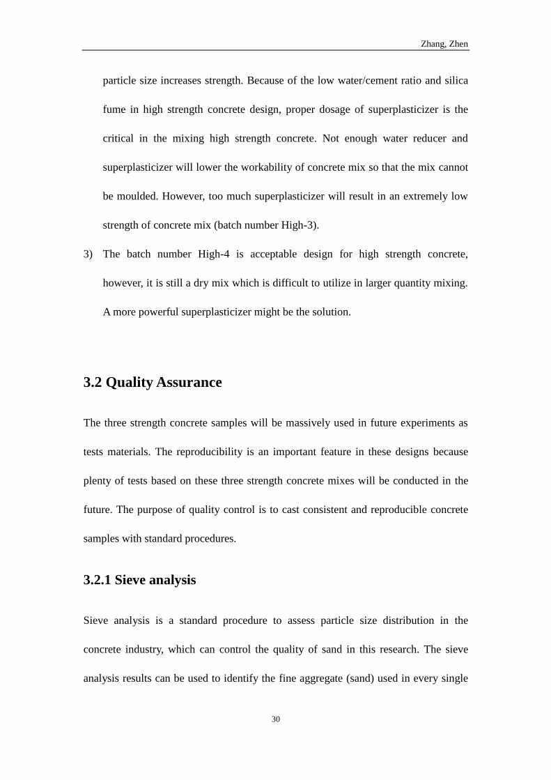
color of sand looks lighter (compare Figure 10 with Figure 11)

Figure 10 Sand samples before dry out

Figure 11 Sand samples after dry out

Weigh the sand and record as mass of dry aggregate then keep drying the sample until

the mass of dry aggregate doesn’t change

Moisture content can be calculated by the following equation:

Zhang, Zhen

33

moisture content =mass of wet aggregate − mass of dry aggregate

mass of wet aggregate× 100%

(Equation 3.3)

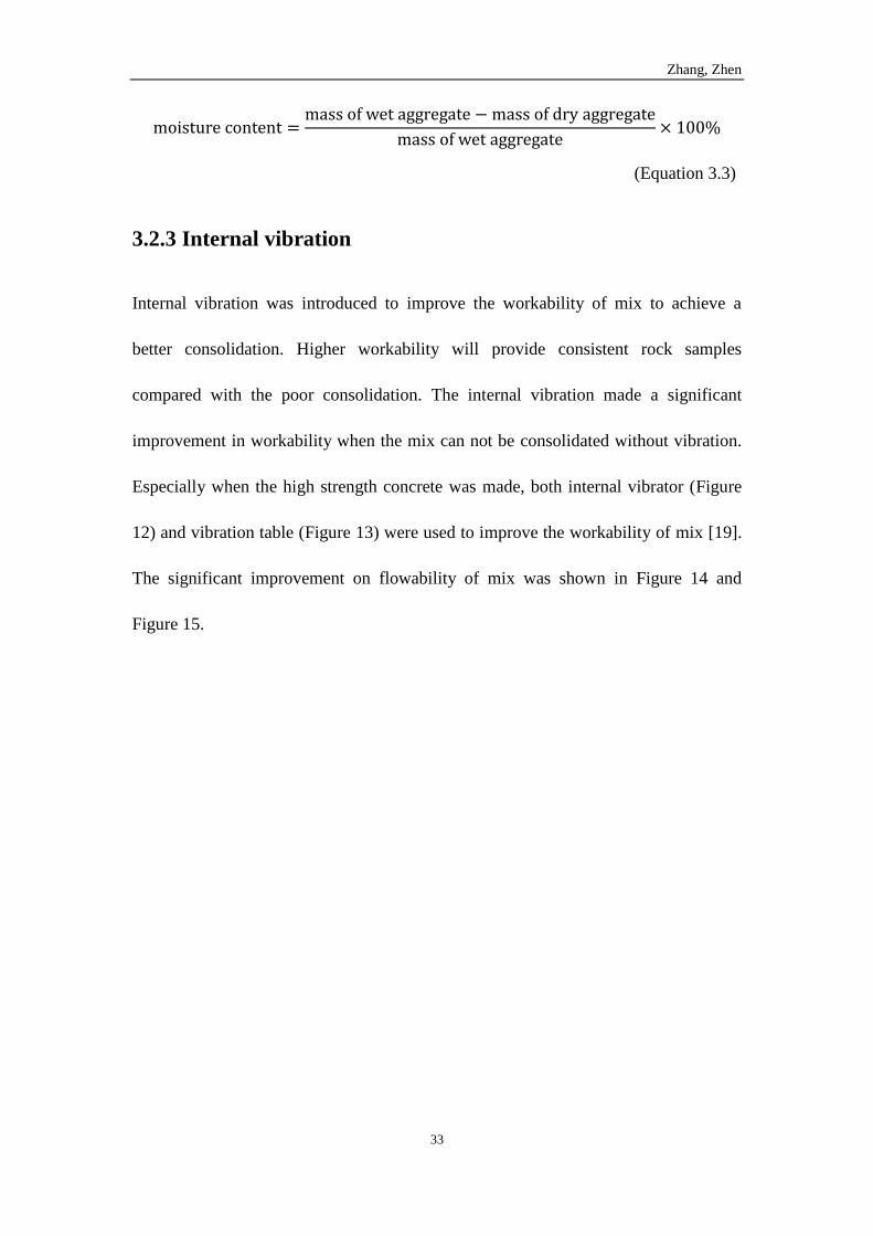
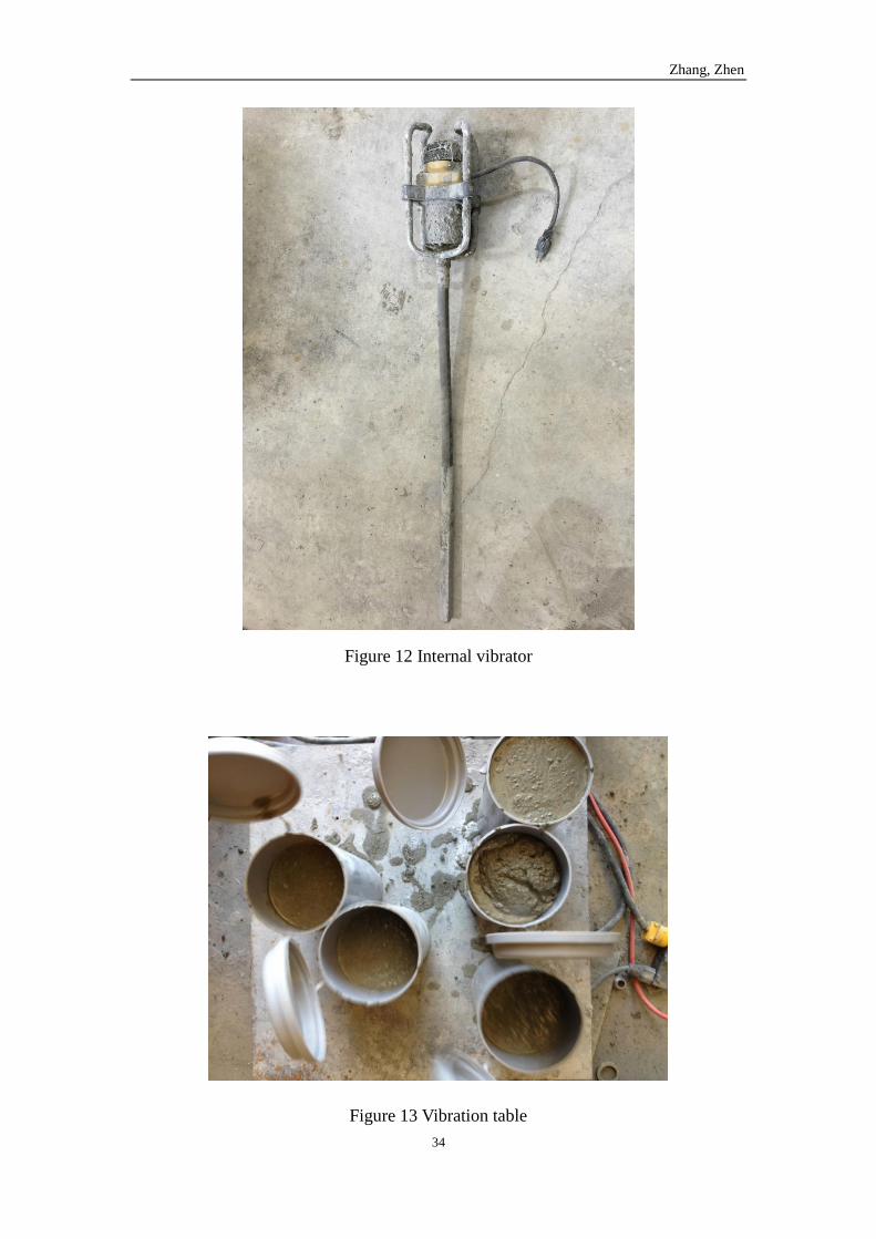
3.2.3 Internal vibration

Internal vibration was introduced to improve the workability of mix to achieve a

better consolidation. Higher workability will provide consistent rock samples

compared with the poor consolidation. The internal vibration made a significant

improvement in workability when the mix can not be consolidated without vibration.

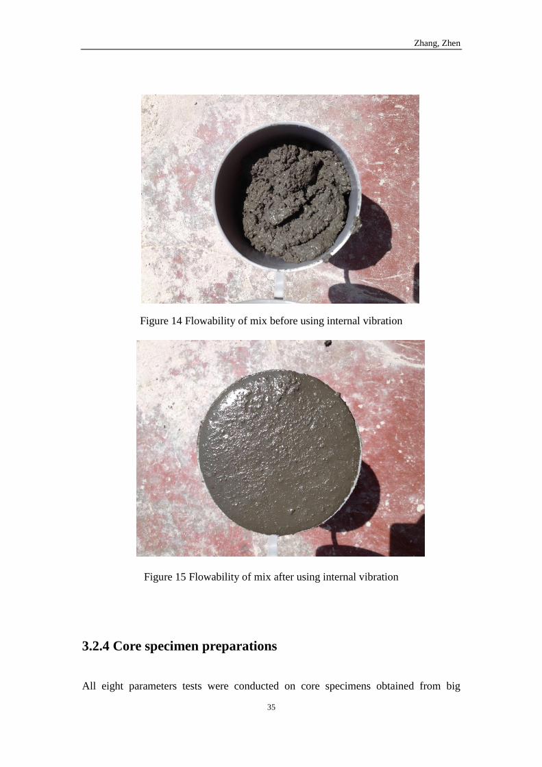
Especially when the high strength concrete was made, both internal vibrator (Figure

12) and vibration table (Figure 13) were used to improve the workability of mix [19].

The significant improvement on flowability of mix was shown in Figure 14 and

Figure 15.

Zhang, Zhen

34

Figure 12 Internal vibrator

Figure 13 Vibration table

Zhang, Zhen

35

Figure 14 Flowability of mix before using internal vibration

Figure 15 Flowability of mix after using internal vibration

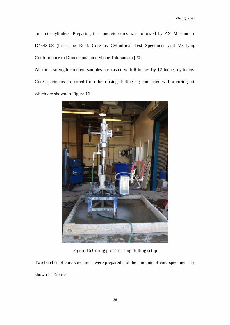
3.2.4 Core specimen preparations

All eight parameters tests were conducted on core specimens obtained from big

Zhang, Zhen

36

concrete cylinders. Preparing the concrete cores was followed by ASTM standard

D4543-08 (Preparing Rock Core as Cylindrical Test Specimens and Verifying

Conformance to Dimensional and Shape Tolerances) [20].

All three strength concrete samples are casted with 6 inches by 12 inches cylinders.

Core specimens are cored from them using drilling rig connected with a coring bit,

which are shown in Figure 16.

Figure 16 Coring process using drilling setup

Two batches of core specimens were prepared and the amounts of core specimens are

shown in Table 5.

Zhang, Zhen

37

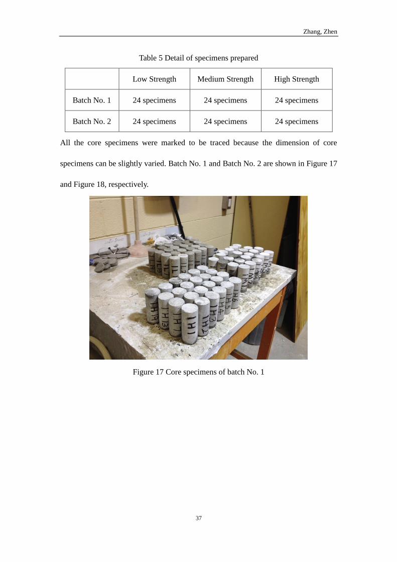
Table 5 Detail of specimens prepared

Low Strength Medium Strength High Strength

Batch No. 1 24 specimens 24 specimens 24 specimens

Batch No. 2 24 specimens 24 specimens 24 specimens

All the core specimens were marked to be traced because the dimension of core

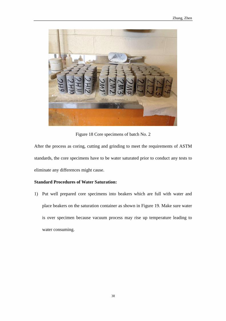
specimens can be slightly varied. Batch No. 1 and Batch No. 2 are shown in Figure 17

and Figure 18, respectively.

Figure 17 Core specimens of batch No. 1

Zhang, Zhen

38

Figure 18 Core specimens of batch No. 2

After the process as coring, cutting and grinding to meet the requirements of ASTM

standards, the core specimens have to be water saturated prior to conduct any tests to

eliminate any differences might cause.

Standard Procedures of Water Saturation:

1) Put well prepared core specimens into beakers which are full with water and

place beakers on the saturation container as shown in Figure 19. Make sure water

is over specimen because vacuum process may rise up temperature leading to

water consuming.

Zhang, Zhen

39

Figure 19 Saturation process set-up

2) Put the cover on and turn on the vacuum (Figure 20) until no more air bubble

come out.

Figure 20 Vacuum for saturation process

3) Bring the specimens back to the curing tanks and make sure this transportation

Zhang, Zhen

40

process happens under water.

3.2.5 Repeatability and reproducibility

Repeatability and reproducibility are important parameters in quality assurance

investigations of this research because large amount of tests and massive data were

involved. Repeatability conditions are considered as experiments were conducted by

the same operator at the same location using the same equipment with the same

procedures over a short time; on the other hand, reproducibility conditions are usually

referring to the same experiments were conducted by different operator at different

location using different equipment followed by same principle of measurement

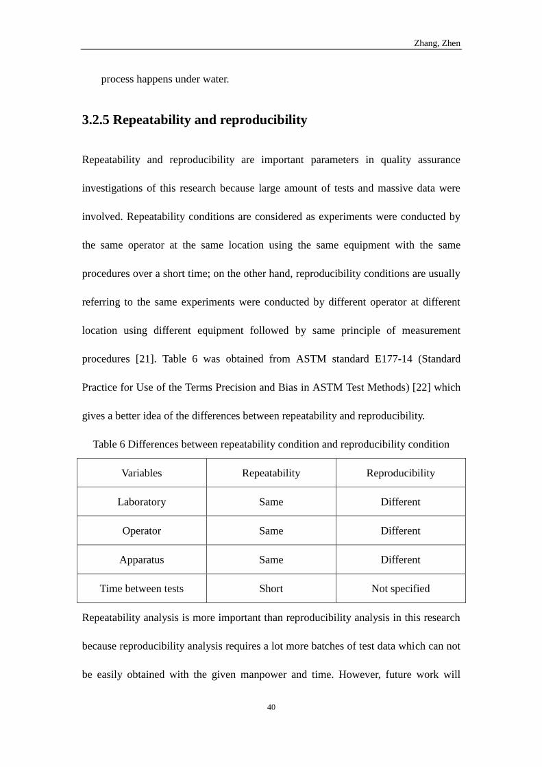
procedures [21]. Table 6 was obtained from ASTM standard E177-14 (Standard

Practice for Use of the Terms Precision and Bias in ASTM Test Methods) [22] which

gives a better idea of the differences between repeatability and reproducibility.

Table 6 Differences between repeatability condition and reproducibility condition

Variables Repeatability Reproducibility

Laboratory Same Different

Operator Same Different

Apparatus Same Different

Time between tests Short Not specified

Repeatability analysis is more important than reproducibility analysis in this research

because reproducibility analysis requires a lot more batches of test data which can not

be easily obtained with the given manpower and time. However, future work will

http://www.astm.org/Standards/E177.htm#_ga=1.51657961.1591597607.1434981065

Zhang, Zhen

41

provide more data needed to carry out a reproducibility analysis. Regarding the

differences between repeatability and reproducibility in Table 6, repeatability analysis

in each batch can be evidence of quality assurance studies.

A lot of ASTM standards contain repeatability and reproducibility analysis using

different equations and methods because of different test objectives [23]. In this

research, standard deviation calculation and standard error calculation can provide

consistency of measurements in eight parameters tests. Both Non-destructive tests

(density and wave velocities) and Destructive tests (UCS and CCS) will be conducted

with repeatability analysis.

Standard deviation [24] is a value to show how spread out a set of data values is.

Lower standard deviation values indicate all the data are close to the mean value of

the set of data, while high standard deviation values indicate the data are spread out.

The standard deviation can be calculated by Equation 3.4 shown as following:

σ = √1

n∑(xi − x)2

n

i=1

Equation 3.4 Standard deviation calculation

Where σ is standard deviation,

n is number of samples,

xi is value of sample number i,

x is mean value of all samples.

Standard error [25] usually refers to calculating the standard deviation of the sampling

distribution of the mean, which is standard error of mean. In statistics, the mean value

Zhang, Zhen

42

of the whole population is normally estimated by mean value of samples. The

standard error of mean will provide how precisely the true mean of the whole

population. The standard error can be calculated by Equation 3.5 shown as following:

SE =σ

√n

Equation 3.5 Standard error calculation

Where SE is standard error,

σ is standard deviation,

n is number of samples.

Standard error, mean value and quantiles of the normal distribution can be used to

calculate approximate confidence intervals for the mean when data was assumed to be

normally distributed. The confidence interval shows a range of estimated values and

expressed by lower and upper confidence limits. Equation 3.6 can be used to calculate

the upper and lower 95% confidence limits.

Upper 95% limit = x + (SE × 1.96)

Lower 95% limit = x − (SE × 1.96)

Equation 3.6 Upper and lower 95% confidence limit calculation

Where x is equal to the sample mean,

SE is equal to the standard error for the sample mean,

1.96 is the corresponding value of 0.975 quantile of the normal distribution.

http://en.wikipedia.org/wiki/Quantile

http://en.wikipedia.org/wiki/1.96

Zhang, Zhen

43

4. Three Strengths of Concrete Designs

We were given access to Pennecon’s lab and Memorial University of Newfoundland’s

lab with material and apparatus which are related to concrete casting and strength

tests. In order to obtain a strength gain curve of concrete samples, the Unconfined

Compressive Strength (UCS) test was conducted at four different test ages which are

7, 14, 21 and 28 days. The following describes the apparatus used and procedures

followed for each mix.

4.1 Low Strength Concrete Design

As described previously, water/cement ratio is the key factor to determine the

compressive strength of concrete. In low strength concrete design, water/cement ratio

should be increased to obtain a lower strength. All the tools and equipment used in all

three strengths mixes are same so that the detailed information about apparatus are

only shown in first design (Low strength concrete design).

4.1.1 Apparatus

Cylinder Molds: 4 by 8 inches cylindrical plastic mold for casting specimens

vertically conforming to the requirements of ASTM standard C470/C470M.

Tamping Rods: 3⁄8 in. [10 mm] in diameter and approximately 12 in. [300 mm] long.

Internal Vibrator: “WYCO” internal vibrator (Figure 12), internal vibrator

conforming to the requirements of ASTM standard C192/C192M-15.

Zhang, Zhen

44

Vibration Table: Designed and made by our own group (Figure 13).

Graduated Cylinder: Maximum scale is 2000 ml and minimum scale is 20 ml.

Hot Plate: Diameter of the element is 20 cm and max temperature is 400℉.

Small Tools: Tools and items such as shovels, pails, trowels, scoop, pan and rubber

gloves were provided in Pennecon Precast Limited’s lab.

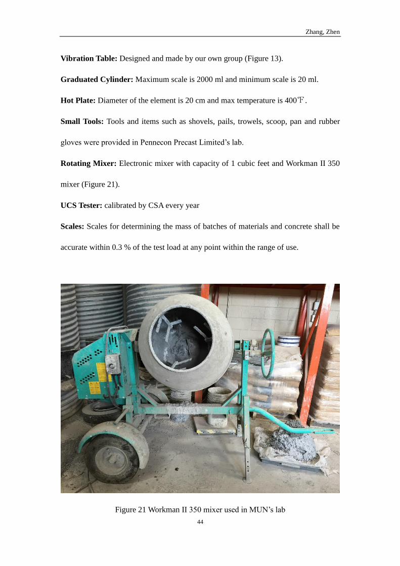
Rotating Mixer: Electronic mixer with capacity of 1 cubic feet and Workman II 350

mixer (Figure 21).

UCS Tester: calibrated by CSA every year

Scales: Scales for determining the mass of batches of materials and concrete shall be

accurate within 0.3 % of the test load at any point within the range of use.

Figure 21 Workman II 350 mixer used in MUN’s lab

Zhang, Zhen

45

4.1.2 Procedure

Much of the following was according to the ASTM Standard C192/C192M-15

Standard Practice for Making and Curing Concrete Test Specimens in the Laboratory

[26].

1) Storage: The cementious materials were stored in a dry place at room temperature

(20 to 30℃).

2) Design: The design of low strength concrete is A: C: W= 6: 1: 1, and the designed

amounts of materials in the batch are shown in Table 7.

Table 7 Designed quantities and used quantities of materials of low strength concrete

design

Materials Designed Quantities Used Quantities

A: C: W 6: 1: 1 6: 1: 1

Aggregate 30 kg 31.397 kg

Cement 5 kg 5 kg

Water 5 kg = 5000ml 3.603 kg = 3603 ml

Water Reducer N/A N/A

Superplasticizer N/A N/A

Silica Fume N/A N/A

3) As the sand used will usually contain some moisture, the amount of water already

in the sand should be taken into account, by determining the moisture content as

in following example.

Moisture Content Calculation: Two scoops of sand sample was weighed and

Zhang, Zhen

46

found to weigh 1775.7 g and then placed on the hot plate which temperature was

set at 400 ℉. After 20 minutes, the water was evaporated until mass of sand

sample didn’t change any more which the mass of sand sample was 1696.7 g.

Moisture content can be calculated as following:



=1775.7g − 1696.7g

1775.7g × 100% = 4.449%

Therefore, total sand needed =30kg

1−4.449%= 31.397kg

Water content in sand = 31.397 kg − 30 kg = 1.397 kg = 1397 ml

Therefore, water needed = 5 kg − 1.397 kg = 3.603 kg = 3603 ml

4) Machine Mixing: 5 kg cement and 31.397 kg sand were put together into the

mixer and start rotation of mixer. After 60 seconds of rotating, 3603 ml water was

added into the rotating mixer. Mixing continued for 3 minutes followed by a 3

minutes rest, followed by a 2 minutes final mixing. During the rest period, the

mixer was covered up to prevent evaporation. The slump numbers of the batch

for all three strengths were determined.

5) Making Specimens: Concrete was filled into each plastic mold using a scoop in 3

equal layers, vibrating each layer before filling next layer. When placing the final

layer, overfilling by more than 1⁄4 in. [6 mm] was avoided. When the finish was

applied after vibration, add only enough concrete with a trowel to overfill the

mold about 1⁄8 in. [3 mm], work it into the surface and then strike it off. Mold

caps were placed on the mold to prevent water evaporation and kept on when the

specimens were stored at 23±2℃ while setting. In this step, internal vibration

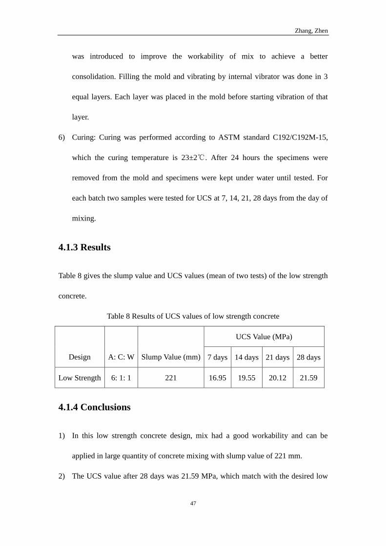
Zhang, Zhen

47

was introduced to improve the workability of mix to achieve a better

consolidation. Filling the mold and vibrating by internal vibrator was done in 3

equal layers. Each layer was placed in the mold before starting vibration of that

layer.

6) Curing: Curing was performed according to ASTM standard C192/C192M-15,

which the curing temperature is 23±2℃. After 24 hours the specimens were

removed from the mold and specimens were kept under water until tested. For

each batch two samples were tested for UCS at 7, 14, 21, 28 days from the day of

mixing.

4.1.3 Results

Table 8 gives the slump value and UCS values (mean of two tests) of the low strength

concrete.

Table 8 Results of UCS values of low strength concrete

Design

A: C: W

Slump Value (mm)

UCS Value (MPa)

7 days 14 days 21 days 28 days

Low Strength 6: 1: 1 221 16.95 19.55 20.12 21.59

4.1.4 Conclusions

1) In this low strength concrete design, mix had a good workability and can be

applied in large quantity of concrete mixing with slump value of 221 mm.

2) The UCS value after 28 days was 21.59 MPa, which match with the desired low

Zhang, Zhen

48

strength.

4.2 Medium Strength Concrete Design

Compared with low strength concrete, medium strength concrete require higher UCS

value by lowering the water content and increasing the percentage of cement in solid

content. However, the dosage of additives and internal vibration are critical because

of low workability caused by low water/cement ratio.

4.2.1 Procedure


Standard Practice for Making and Curing Concrete Test Specimens in the Laboratory.


(20 to 30℃).

2) Design: The design of high strength concrete is A: C: W= 3: 1: 0.45 the designed

amounts of materials in the batch are shown in Table 9.

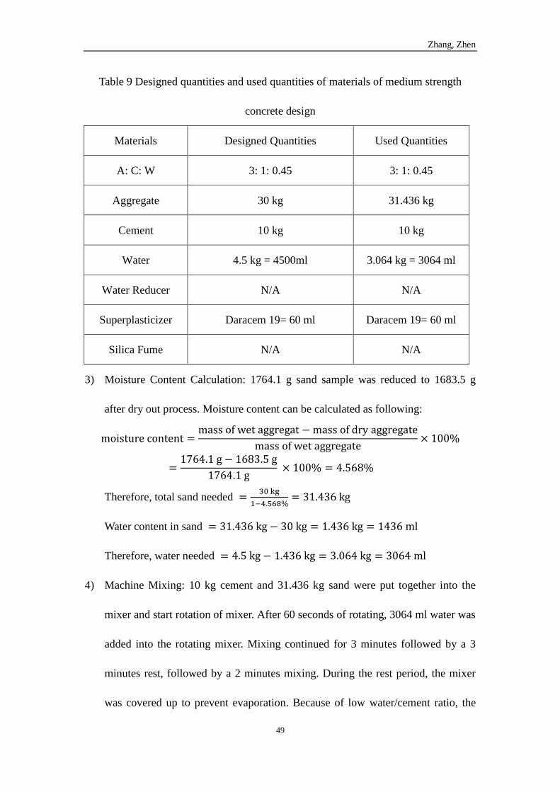
Zhang, Zhen

49

Table 9 Designed quantities and used quantities of materials of medium strength

concrete design


A: C: W 3: 1: 0.45 3: 1: 0.45


Cement 10 kg 10 kg

Water 4.5 kg = 4500ml 3.064 kg = 3064 ml

Water Reducer N/A N/A

Superplasticizer Daracem 19= 60 ml Daracem 19= 60 ml

Silica Fume N/A N/A

3) Moisture Content Calculation: 1764.1 g sand sample was reduced to 1683.5 g

after dry out process. Moisture content can be calculated as following:

moisture content =mass of wet aggregat − mass of dry aggregate


=1764.1 g − 1683.5 g

1764.1 g × 100% = 4.568%

Therefore, total sand needed =30 kg

1−4.568%= 31.436 kg


Therefore, water needed = 4.5 kg − 1.436 kg = 3.064 kg = 3064 ml

4) Machine Mixing: 10 kg cement and 31.436 kg sand were put together into the

mixer and start rotation of mixer. After 60 seconds of rotating, 3064 ml water was

added into the rotating mixer. Mixing continued for 3 minutes followed by a 3

minutes rest, followed by a 2 minutes mixing. During the rest period, the mixer

was covered up to prevent evaporation. Because of low water/cement ratio, the

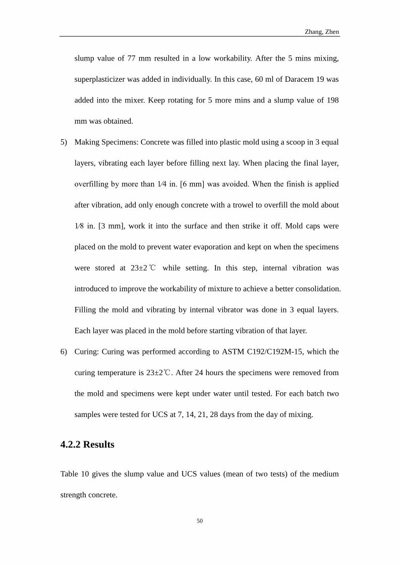
Zhang, Zhen

50

slump value of 77 mm resulted in a low workability. After the 5 mins mixing,

superplasticizer was added in individually. In this case, 60 ml of Daracem 19 was

added into the mixer. Keep rotating for 5 more mins and a slump value of 198

mm was obtained.

5) Making Specimens: Concrete was filled into plastic mold using a scoop in 3 equal

layers, vibrating each layer before filling next lay. When placing the final layer,

overfilling by more than 1⁄4 in. [6 mm] was avoided. When the finish is applied

after vibration, add only enough concrete with a trowel to overfill the mold about

1⁄8 in. [3 mm], work it into the surface and then strike it off. Mold caps were

placed on the mold to prevent water evaporation and kept on when the specimens

were stored at 23±2℃ while setting. In this step, internal vibration was

introduced to improve the workability of mixture to achieve a better consolidation.

Filling the mold and vibrating by internal vibrator was done in 3 equal layers.

Each layer was placed in the mold before starting vibration of that layer.

6) Curing: Curing was performed according to ASTM C192/C192M-15, which the

curing temperature is 23±2℃. After 24 hours the specimens were removed from

the mold and specimens were kept under water until tested. For each batch two

samples were tested for UCS at 7, 14, 21, 28 days from the day of mixing.

4.2.2 Results

Table 10 gives the slump value and UCS values (mean of two tests) of the medium

strength concrete.

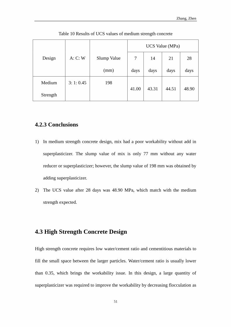
Zhang, Zhen

51

Table 10 Results of UCS values of medium strength concrete

Design

A: C: W

Slump Value

(mm)

UCS Value (MPa)

7

days

14

days

21

days

28

days

Medium

Strength

3: 1: 0.45 198

41.00 43.31 44.51 48.90

4.2.3 Conclusions

1) In medium strength concrete design, mix had a poor workability without add in

superplasticizer. The slump value of mix is only 77 mm without any water

reducer or superplasticizer; however, the slump value of 198 mm was obtained by

adding superplasticizer.

2) The UCS value after 28 days was 48.90 MPa, which match with the medium

strength expected.

4.3 High Strength Concrete Design

High strength concrete requires low water/cement ratio and cementitious materials to

fill the small space between the larger particles. Water/cement ratio is usually lower

than 0.35, which brings the workability issue. In this design, a large quantity of

superplasticizer was required to improve the workability by decreasing flocculation as

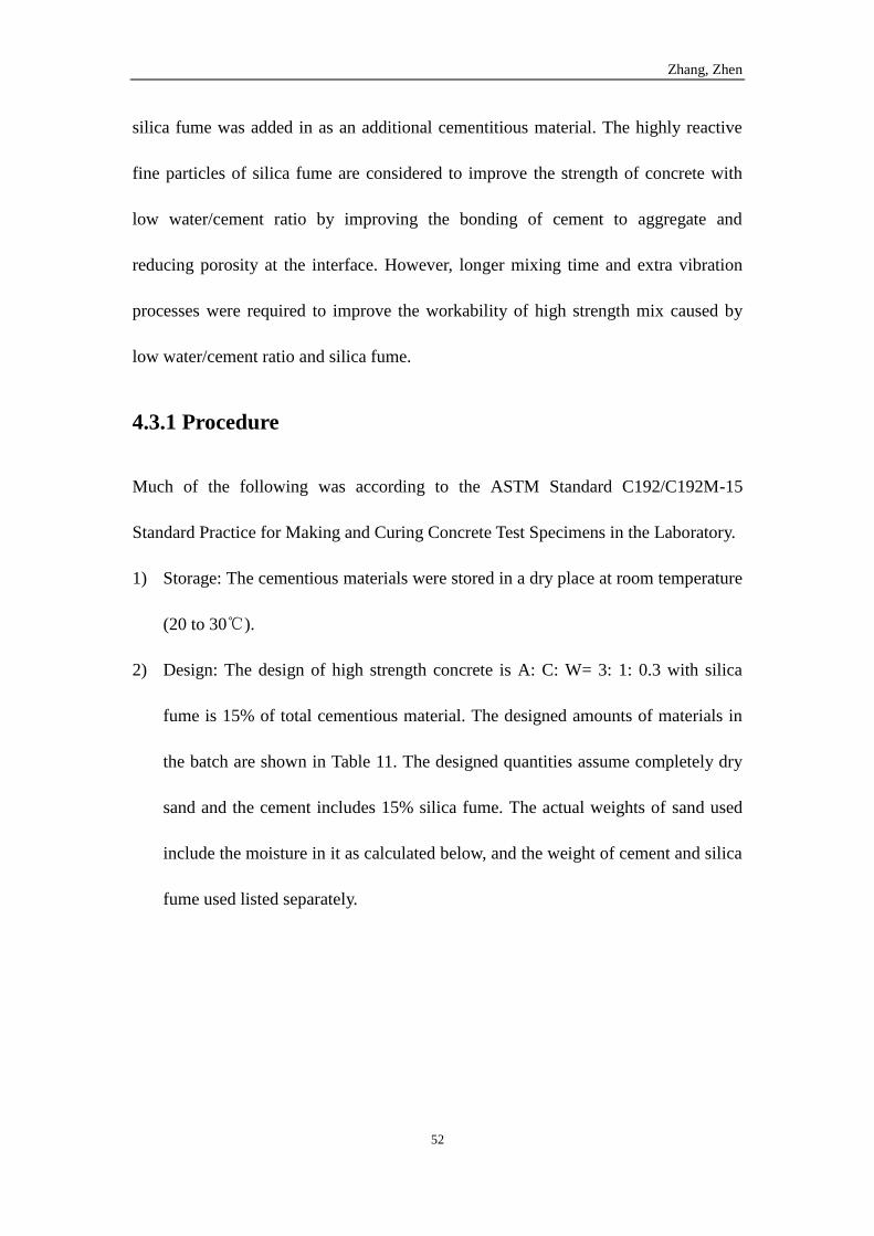
Zhang, Zhen

52

silica fume was added in as an additional cementitious material. The highly reactive

fine particles of silica fume are considered to improve the strength of concrete with

low water/cement ratio by improving the bonding of cement to aggregate and

reducing porosity at the interface. However, longer mixing time and extra vibration

processes were required to improve the workability of high strength mix caused by

low water/cement ratio and silica fume.

4.3.1 Procedure


Standard Practice for Making and Curing Concrete Test Specimens in the Laboratory.


(20 to 30℃).

2) Design: The design of high strength concrete is A: C: W= 3: 1: 0.3 with silica

fume is 15% of total cementious material. The designed amounts of materials in

the batch are shown in Table 11. The designed quantities assume completely dry

sand and the cement includes 15% silica fume. The actual weights of sand used

include the moisture in it as calculated below, and the weight of cement and silica

fume used listed separately.

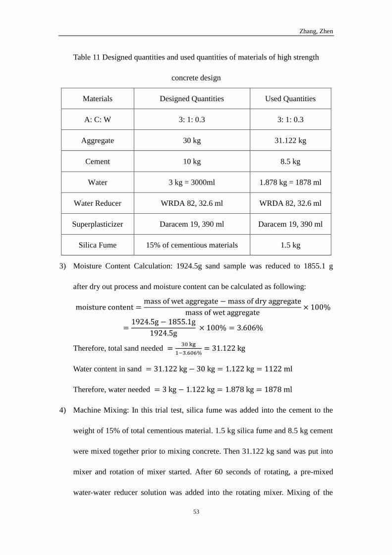
Zhang, Zhen

53

Table 11 Designed quantities and used quantities of materials of high strength

concrete design


A: C: W 3: 1: 0.3 3: 1: 0.3


Cement 10 kg 8.5 kg

Water 3 kg = 3000ml 1.878 kg = 1878 ml

Water Reducer WRDA 82, 32.6 ml WRDA 82, 32.6 ml

Superplasticizer Daracem 19, 390 ml Daracem 19, 390 ml

Silica Fume 15% of cementious materials 1.5 kg

3) Moisture Content Calculation: 1924.5g sand sample was reduced to 1855.1 g

after dry out process and moisture content can be calculated as following:



=1924.5g − 1855.1g

1924.5g × 100% = 3.606%

Therefore, total sand needed =30 kg

1−3.606%= 31.122 kg


Therefore, water needed = 3 kg − 1.122 kg = 1.878 kg = 1878 ml

4) Machine Mixing: In this trial test, silica fume was added into the cement to the

weight of 15% of total cementious material. 1.5 kg silica fume and 8.5 kg cement

were mixed together prior to mixing concrete. Then 31.122 kg sand was put into

mixer and rotation of mixer started. After 60 seconds of rotating, a pre-mixed

water-water reducer solution was added into the rotating mixer. Mixing of the

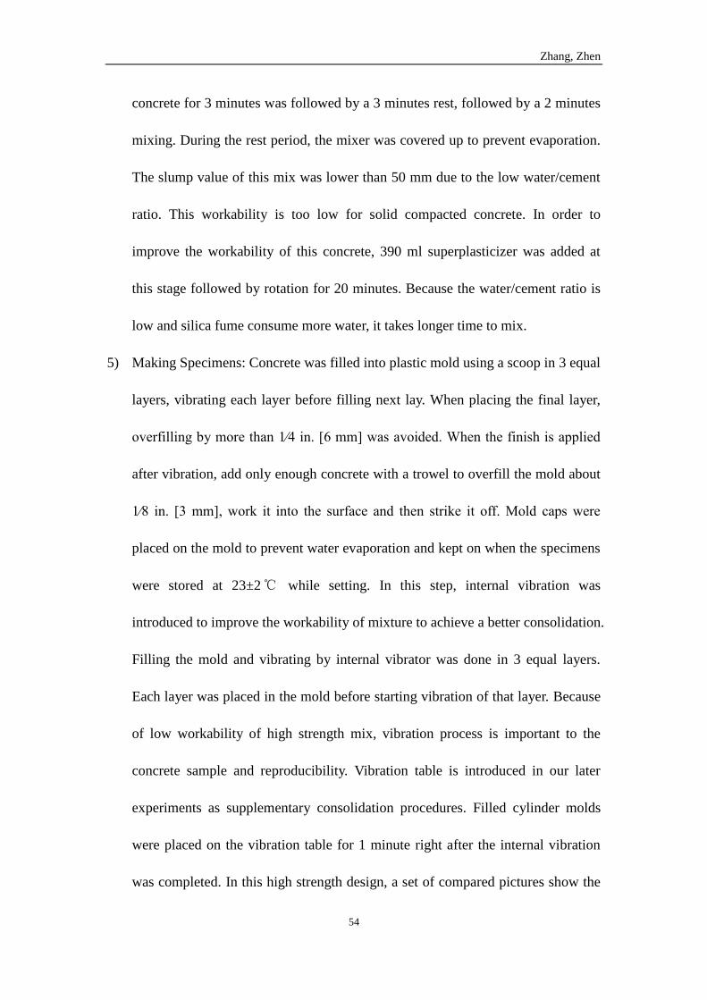
Zhang, Zhen

54

concrete for 3 minutes was followed by a 3 minutes rest, followed by a 2 minutes

mixing. During the rest period, the mixer was covered up to prevent evaporation.

The slump value of this mix was lower than 50 mm due to the low water/cement

ratio. This workability is too low for solid compacted concrete. In order to

improve the workability of this concrete, 390 ml superplasticizer was added at

this stage followed by rotation for 20 minutes. Because the water/cement ratio is

low and silica fume consume more water, it takes longer time to mix.

5) Making Specimens: Concrete was filled into plastic mold using a scoop in 3 equal

layers, vibrating each layer before filling next lay. When placing the final layer,

overfilling by more than 1⁄4 in. [6 mm] was avoided. When the finish is applied

after vibration, add only enough concrete with a trowel to overfill the mold about

1⁄8 in. [3 mm], work it into the surface and then strike it off. Mold caps were

placed on the mold to prevent water evaporation and kept on when the specimens

were stored at 23±2℃ while setting. In this step, internal vibration was

introduced to improve the workability of mixture to achieve a better consolidation.

Filling the mold and vibrating by internal vibrator was done in 3 equal layers.

Each layer was placed in the mold before starting vibration of that layer. Because

of low workability of high strength mix, vibration process is important to the

concrete sample and reproducibility. Vibration table is introduced in our later

experiments as supplementary consolidation procedures. Filled cylinder molds

were placed on the vibration table for 1 minute right after the internal vibration

was completed. In this high strength design, a set of compared pictures show the

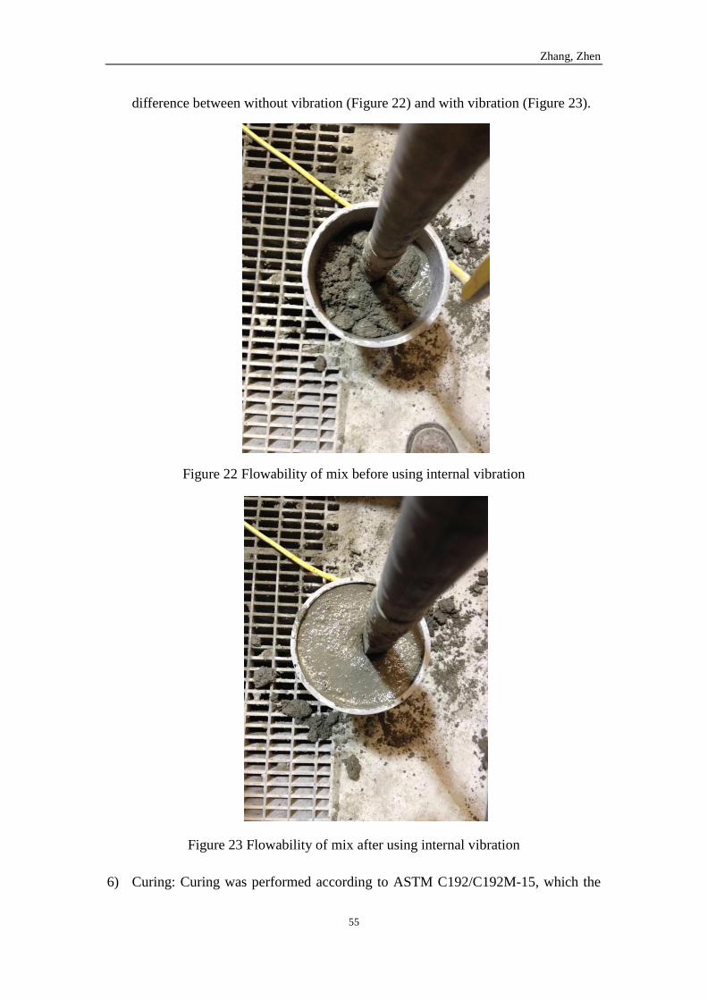
Zhang, Zhen

55

difference between without vibration (Figure 22) and with vibration (Figure 23).

Figure 22 Flowability of mix before using internal vibration

Figure 23 Flowability of mix after using internal vibration

6) Curing: Curing was performed according to ASTM C192/C192M-15, which the

Zhang, Zhen

56

curing temperature is 23±2℃. After 24 hours the specimens were removed from

the mold and specimens were kept under water until tested. For each batch two

samples were tested for UCS at 7, 14, 21, 28 days from the day of mixing.

Note:

1) The recommended dosage of superplasticizer (Daracem 19) is 390-1300 ml/100

kg cement. Trial test number 6 shows that the maximum recommended dosage

(130 ml) can not achieve desired workability. Therefore, triple maximum dosage

(390 ml) was tested in this batch and it worked out.

2) Both water reducer and superplasticizer are liquid solution, however, the water

content in both of these admixtures was not counted in total water used.

4.3.2 Results

Table 12 gives the slump value and UCS values of the high strength concrete.

Table 12 Results of UCS values of high strength concrete

Design

A: C: W

Slump Value (mm)

UCS Value (MPa)

7 days 14 days 21 days 28 days

High Strength 3: 1: 0.3 85 69.91 83.56 87.55 94.94

4.3.3 Conclusions

1) In high strength concrete design, the mix has an extremely low workability

because of low water/cement ratio and silica fume blended in [27]. Even though a

large quantity of superplasticizer was added in, the mix might not be able to be

Zhang, Zhen

57

applied in large quantity of concrete mixing due to the low workability. More

efficient superplasticizer should be introduced to improve workability of the high

strength concrete in future work.

2) The UCS value after 28 days is 94.94 MPa, which match with the high strength

expected.

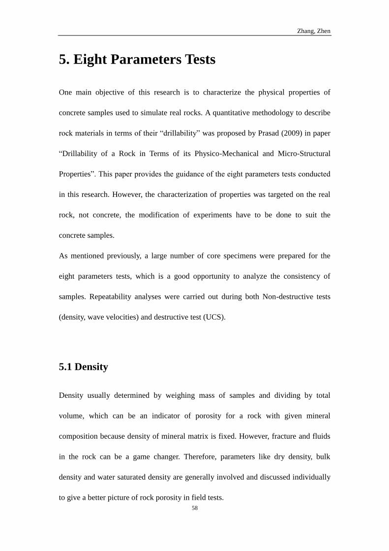
Zhang, Zhen

58

5. Eight Parameters Tests

One main objective of this research is to characterize the physical properties of

concrete samples used to simulate real rocks. A quantitative methodology to describe

rock materials in terms of their “drillability” was proposed by Prasad (2009) in paper

“Drillability of a Rock in Terms of its Physico-Mechanical and Micro-Structural

Properties”. This paper provides the guidance of the eight parameters tests conducted

in this research. However, the characterization of properties was targeted on the real

rock, not concrete, the modification of experiments have to be done to suit the

concrete samples.

As mentioned previously, a large number of core specimens were prepared for the

eight parameters tests, which is a good opportunity to analyze the consistency of

samples. Repeatability analyses were carried out during both Non-destructive tests

(density, wave velocities) and destructive test (UCS).

5.1 Density

Density usually determined by weighing mass of samples and dividing by total

volume, which can be an indicator of porosity for a rock with given mineral

composition because density of mineral matrix is fixed. However, fracture and fluids

in the rock can be a game changer. Therefore, parameters like dry density, bulk

density and water saturated density are generally involved and discussed individually

to give a better picture of rock porosity in field tests.

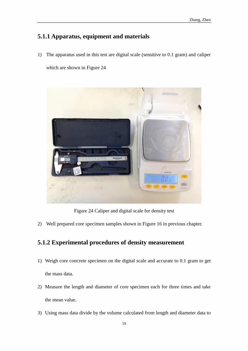
Zhang, Zhen

59

5.1.1 Apparatus, equipment and materials

1) The apparatus used in this test are digital scale (sensitive to 0.1 gram) and caliper

which are shown in Figure 24

Figure 24 Caliper and digital scale for density test

2) Well prepared core specimen samples shown in Figure 16 in previous chapter.

5.1.2 Experimental procedures of density measurement

1) Weigh core concrete specimen on the digital scale and accurate to 0.1 gram to get

the mass data.

2) Measure the length and diameter of core specimen each for three times and take

the mean value.

3) Using mass data divide by the volume calculated from length and diameter data to

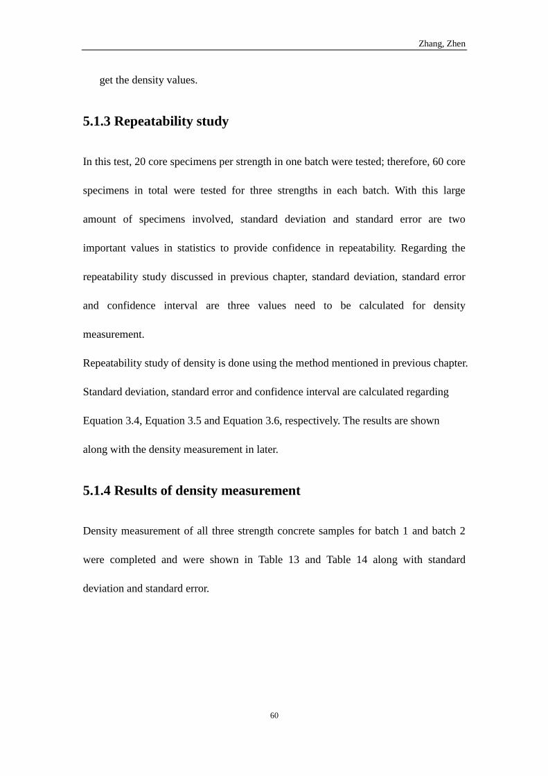
Zhang, Zhen

60

get the density values.

5.1.3 Repeatability study

In this test, 20 core specimens per strength in one batch were tested; therefore, 60 core

specimens in total were tested for three strengths in each batch. With this large

amount of specimens involved, standard deviation and standard error are two

important values in statistics to provide confidence in repeatability. Regarding the

repeatability study discussed in previous chapter, standard deviation, standard error

and confidence interval are three values need to be calculated for density

measurement.

Repeatability study of density is done using the method mentioned in previous chapter.

Standard deviation, standard error and confidence interval are calculated regarding

Equation 3.4, Equation 3.5 and Equation 3.6, respectively. The results are shown

along with the density measurement in later.

5.1.4 Results of density measurement

Density measurement of all three strength concrete samples for batch 1 and batch 2

were completed and were shown in Table 13 and Table 14 along with standard

deviation and standard error.

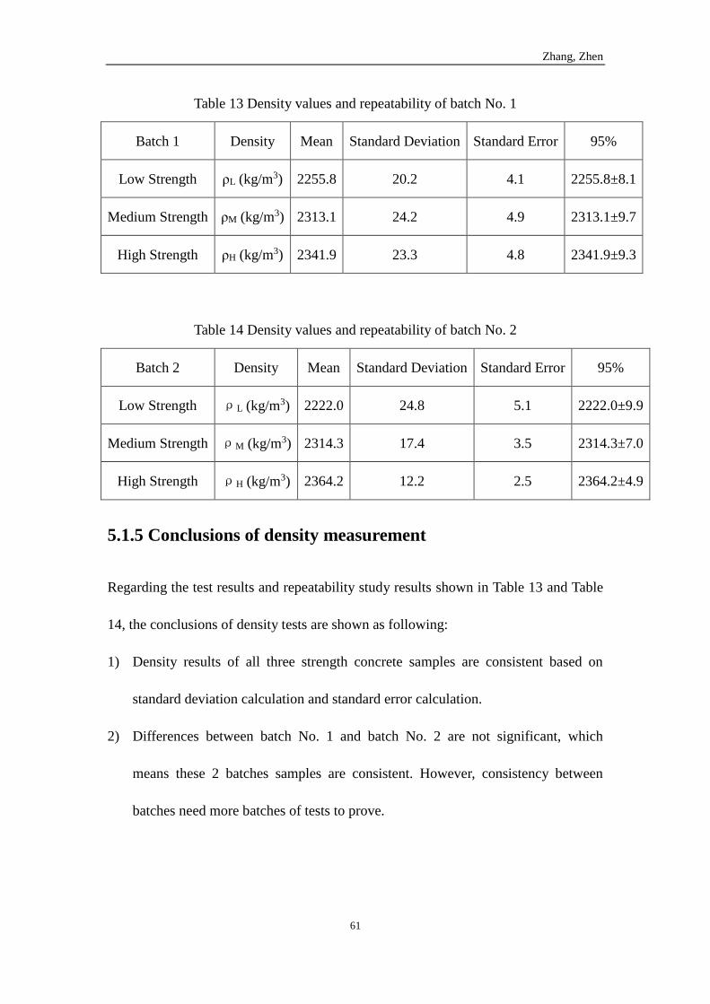
Zhang, Zhen

61

Table 13 Density values and repeatability of batch No. 1

Batch 1 Density Mean Standard Deviation Standard Error 95%

Low Strength ρL (kg/m3) 2255.8 20.2 4.1 2255.8±8.1

Medium Strength ρM (kg/m3) 2313.1 24.2 4.9 2313.1±9.7

High Strength ρH (kg/m3) 2341.9 23.3 4.8 2341.9±9.3

Table 14 Density values and repeatability of batch No. 2

Batch 2 Density Mean Standard Deviation Standard Error 95%

Low Strength ρL (kg/m3) 2222.0 24.8 5.1 2222.0±9.9

Medium Strength ρM (kg/m3) 2314.3 17.4 3.5 2314.3±7.0

High Strength ρH (kg/m3) 2364.2 12.2 2.5 2364.2±4.9

5.1.5 Conclusions of density measurement

Regarding the test results and repeatability study results shown in Table 13 and Table

14, the conclusions of density tests are shown as following:

1) Density results of all three strength concrete samples are consistent based on

standard deviation calculation and standard error calculation.

2) Differences between batch No. 1 and batch No. 2 are not significant, which

means these 2 batches samples are consistent. However, consistency between

batches need more batches of tests to prove.

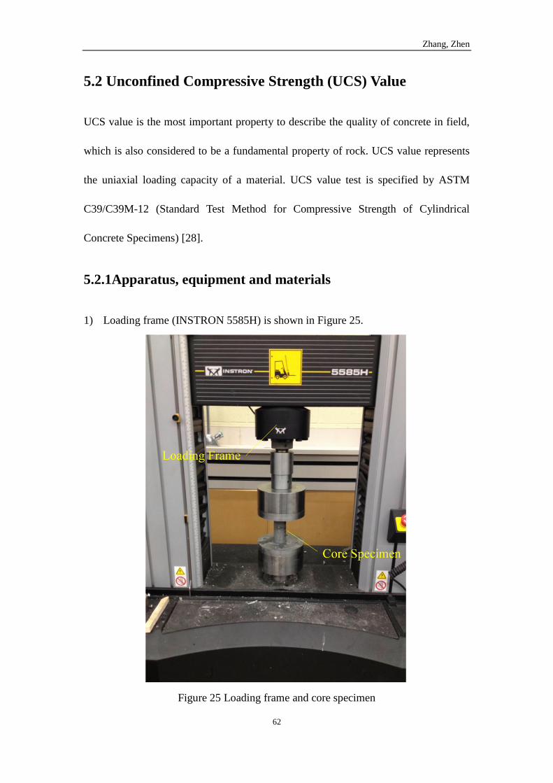
Zhang, Zhen

62

5.2 Unconfined Compressive Strength (UCS) Value

UCS value is the most important property to describe the quality of concrete in field,

which is also considered to be a fundamental property of rock. UCS value represents

the uniaxial loading capacity of a material. UCS value test is specified by ASTM

C39/C39M-12 (Standard Test Method for Compressive Strength of Cylindrical

Concrete Specimens) [28].

5.2.1Apparatus, equipment and materials

1) Loading frame (INSTRON 5585H) is shown in Figure 25.

Figure 25 Loading frame and core specimen

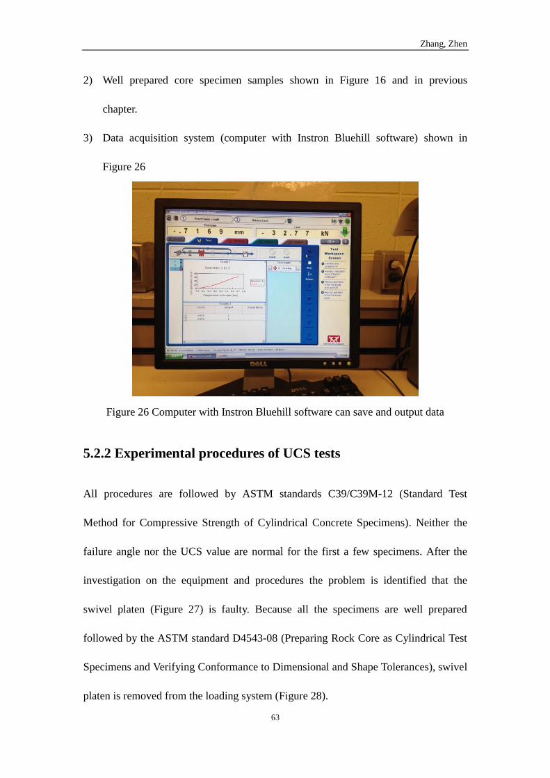
Zhang, Zhen

63

2) Well prepared core specimen samples shown in Figure 16 and in previous

chapter.

3) Data acquisition system (computer with Instron Bluehill software) shown in

Figure 26

Figure 26 Computer with Instron Bluehill software can save and output data

5.2.2 Experimental procedures of UCS tests

All procedures are followed by ASTM standards C39/C39M-12 (Standard Test

Method for Compressive Strength of Cylindrical Concrete Specimens). Neither the

failure angle nor the UCS value are normal for the first a few specimens. After the

investigation on the equipment and procedures the problem is identified that the

swivel platen (Figure 27) is faulty. Because all the specimens are well prepared

followed by the ASTM standard D4543-08 (Preparing Rock Core as Cylindrical Test

Specimens and Verifying Conformance to Dimensional and Shape Tolerances), swivel

platen is removed from the loading system (Figure 28).

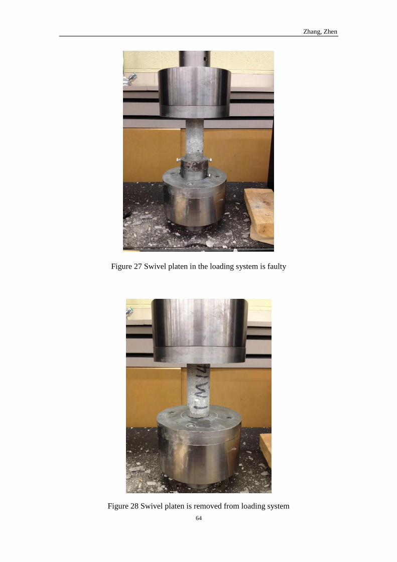
Zhang, Zhen

64

Figure 27 Swivel platen in the loading system is faulty

Figure 28 Swivel platen is removed from loading system

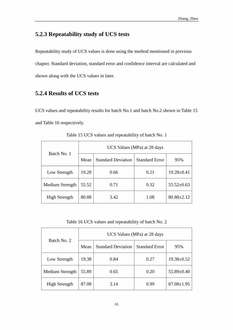
Zhang, Zhen

65

5.2.3 Repeatability study of UCS tests

Repeatability study of UCS values is done using the method mentioned in previous

chapter. Standard deviation, standard error and confidence interval are calculated and

shown along with the UCS values in later.

5.2.4 Results of UCS tests

UCS values and repeatability results for batch No.1 and batch No.2 shown in Table 15

and Table 16 respectively.

Table 15 UCS values and repeatability of batch No. 1

Batch No. 1

UCS Values (MPa) at 28 days

Mean Standard Deviation Standard Error 95%

Low Strength 19.28 0.66 0.21 19.28±0.41

Medium Strength 55.52 0.71 0.32 55.52±0.63

High Strength 80.88 3.42 1.08 80.88±2.12

Table 16 UCS values and repeatability of batch No. 2

Batch No. 2

UCS Values (MPa) at 28 days

Mean Standard Deviation Standard Error 95%

Low Strength 19.38 0.84 0.27 19.38±0.52

Medium Strength 55.89 0.65 0.20 55.89±0.40

High Strength 87.08 3.14 0.99 87.08±1.95

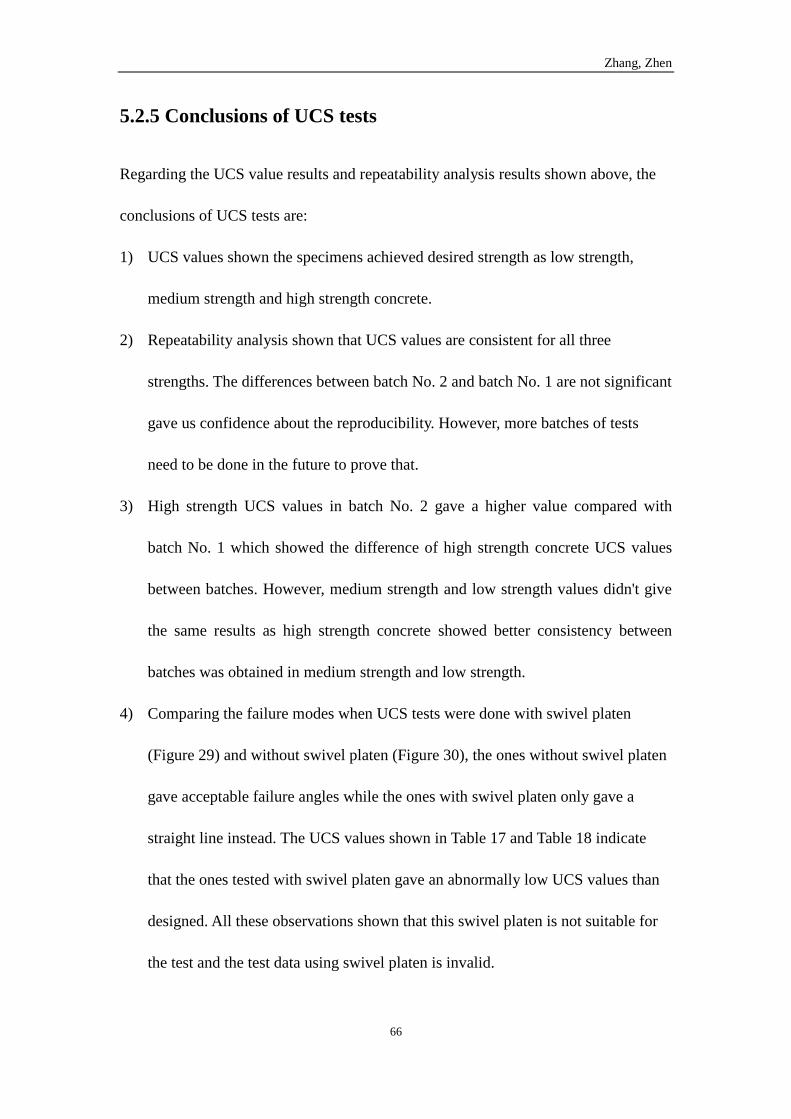
Zhang, Zhen

66

5.2.5 Conclusions of UCS tests

Regarding the UCS value results and repeatability analysis results shown above, the

conclusions of UCS tests are:

1) UCS values shown the specimens achieved desired strength as low strength,

medium strength and high strength concrete.

2) Repeatability analysis shown that UCS values are consistent for all three

strengths. The differences between batch No. 2 and batch No. 1 are not significant

gave us confidence about the reproducibility. However, more batches of tests

need to be done in the future to prove that.

3) High strength UCS values in batch No. 2 gave a higher value compared with

batch No. 1 which showed the difference of high strength concrete UCS values

between batches. However, medium strength and low strength values didn't give

the same results as high strength concrete showed better consistency between

batches was obtained in medium strength and low strength.

4) Comparing the failure modes when UCS tests were done with swivel platen

(Figure 29) and without swivel platen (Figure 30), the ones without swivel platen

gave acceptable failure angles while the ones with swivel platen only gave a

straight line instead. The UCS values shown in Table 17 and Table 18 indicate

that the ones tested with swivel platen gave an abnormally low UCS values than

designed. All these observations shown that this swivel platen is not suitable for

the test and the test data using swivel platen is invalid.

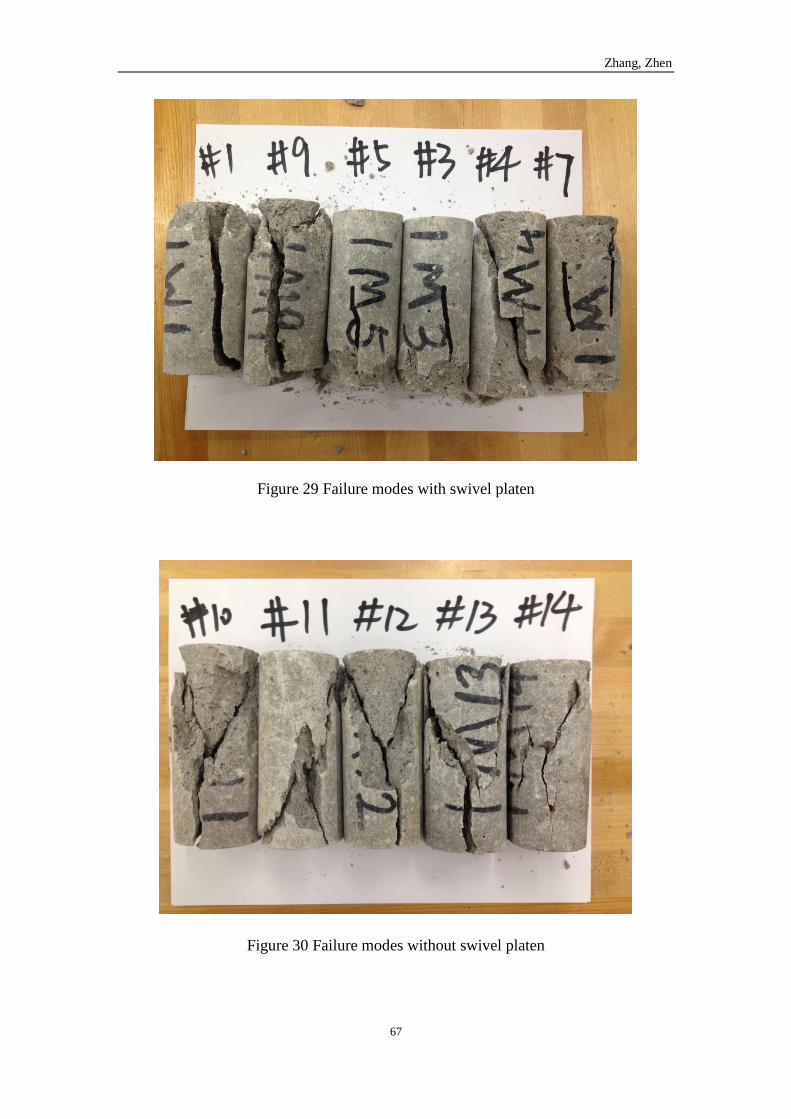
Zhang, Zhen

67

Figure 29 Failure modes with swivel platen

Figure 30 Failure modes without swivel platen

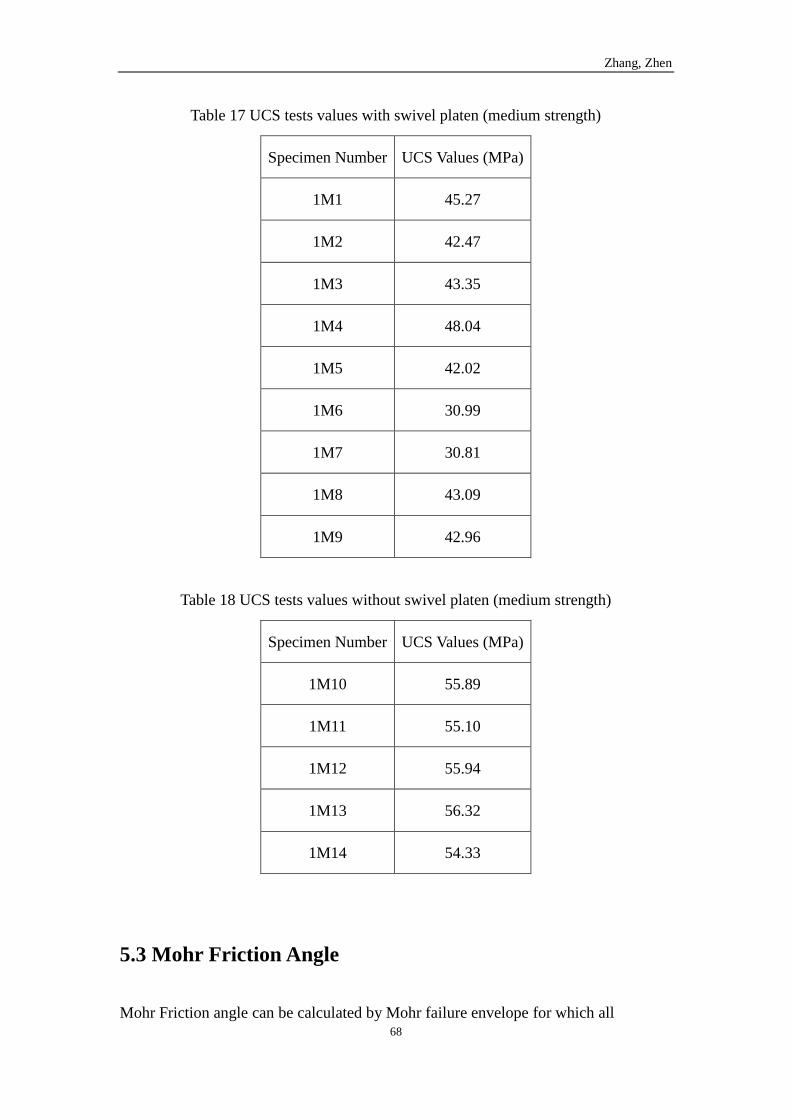
Zhang, Zhen

68

Table 17 UCS tests values with swivel platen (medium strength)

Specimen Number UCS Values (MPa)

1M1 45.27

1M2 42.47

1M3 43.35

1M4 48.04

1M5 42.02

1M6 30.99

1M7 30.81

1M8 43.09

1M9 42.96

Table 18 UCS tests values without swivel platen (medium strength)

Specimen Number UCS Values (MPa)

1M10 55.89

1M11 55.10

1M12 55.94

1M13 56.32

1M14 54.33

5.3 Mohr Friction Angle

Mohr Friction angle can be calculated by Mohr failure envelope for which all

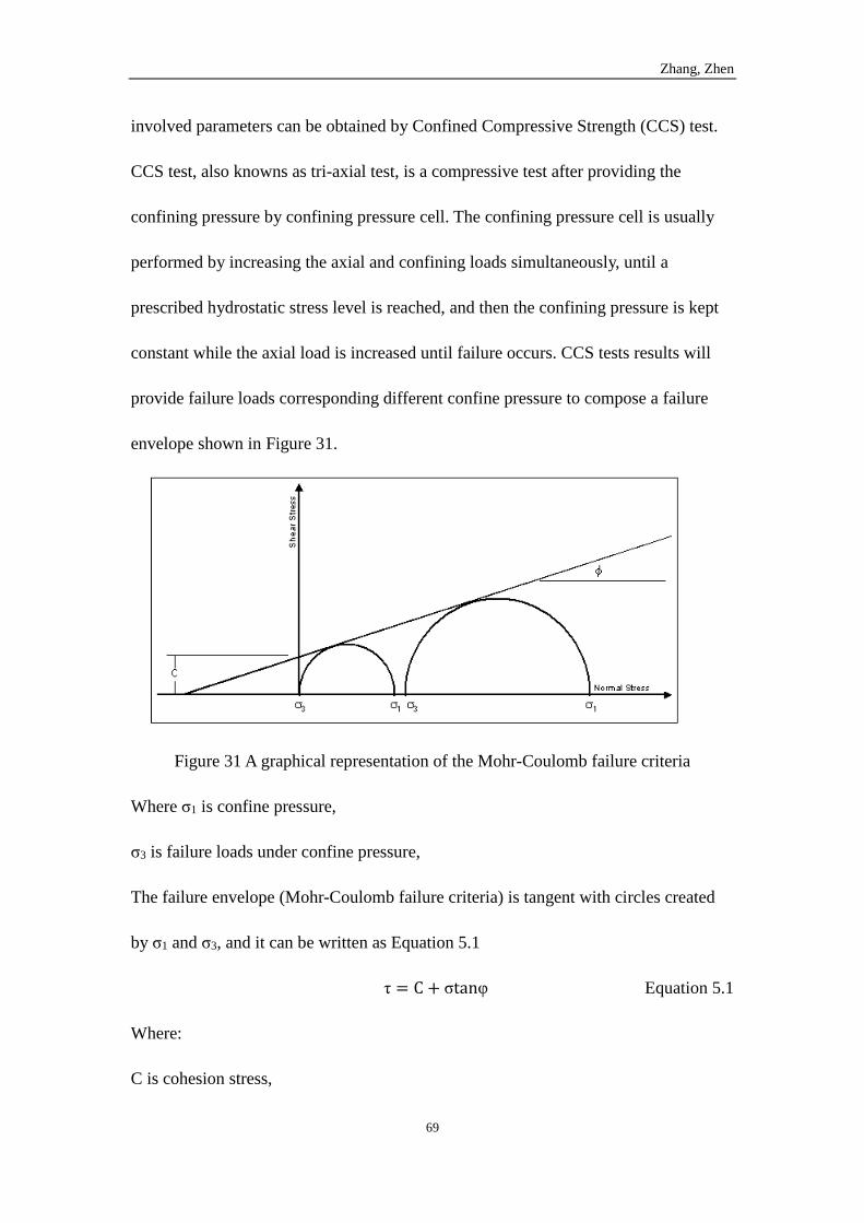
Zhang, Zhen

69

involved parameters can be obtained by Confined Compressive Strength (CCS) test.

CCS test, also knowns as tri-axial test, is a compressive test after providing the

confining pressure by confining pressure cell. The confining pressure cell is usually

performed by increasing the axial and confining loads simultaneously, until a

prescribed hydrostatic stress level is reached, and then the confining pressure is kept

constant while the axial load is increased until failure occurs. CCS tests results will

provide failure loads corresponding different confine pressure to compose a failure

envelope shown in Figure 31.

Figure 31 A graphical representation of the Mohr-Coulomb failure criteria

Where σ1 is confine pressure,

σ3 is failure loads under confine pressure,

The failure envelope (Mohr-Coulomb failure criteria) is tangent with circles created

by σ1 and σ3, and it can be written as Equation 5.1

τ = C + σtanφ Equation 5.1

Where:

C is cohesion stress,

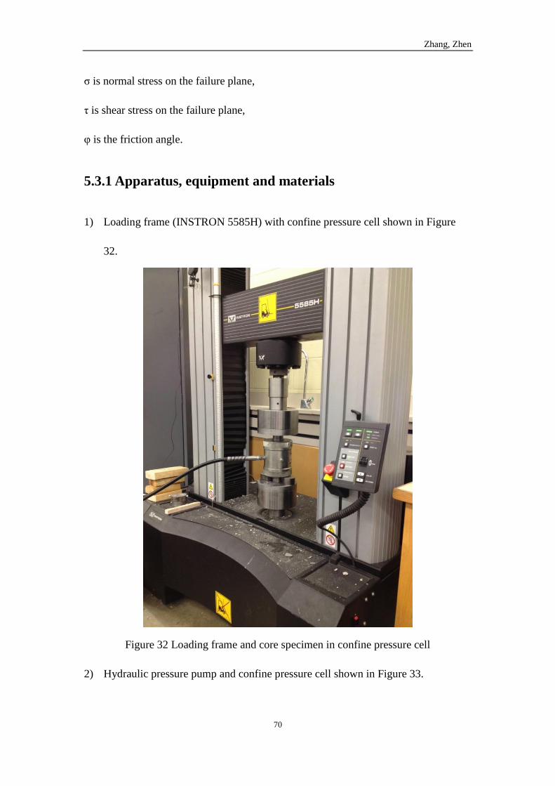
Zhang, Zhen

70

σ is normal stress on the failure plane,

τ is shear stress on the failure plane,

φ is the friction angle.


1) Loading frame (INSTRON 5585H) with confine pressure cell shown in Figure

32.

Figure 32 Loading frame and core specimen in confine pressure cell

2) Hydraulic pressure pump and confine pressure cell shown in Figure 33.

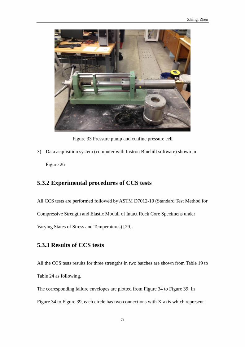
Zhang, Zhen

71

Figure 33 Pressure pump and confine pressure cell

3) Data acquisition system (computer with Instron Bluehill software) shown in

Figure 26

5.3.2 Experimental procedures of CCS tests

All CCS tests are performed followed by ASTM D7012-10 (Standard Test Method for

Compressive Strength and Elastic Moduli of Intact Rock Core Specimens under

Varying States of Stress and Temperatures) [29].

5.3.3 Results of CCS tests

All the CCS tests results for three strengths in two batches are shown from Table 19 to

Table 24 as following.

The corresponding failure envelopes are plotted from Figure 34 to Figure 39. In

Figure 34 to Figure 39, each circle has two connections with X-axis which represent

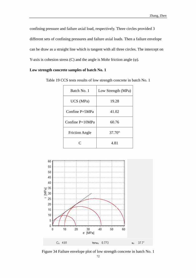
Zhang, Zhen

72

confining pressure and failure axial load, respectively. Three circles provided 3

different sets of confining pressures and failure axial loads. Then a failure envelope

can be draw as a straight line which is tangent with all three circles. The intercept on

Y-axis is cohesion stress (C) and the angle is Mohr friction angle (φ).

Low strength concrete samples of batch No. 1

Table 19 CCS tests results of low strength concrete in batch No. 1

Batch No. 1 Low Strength (MPa)

UCS (MPa) 19.28

Confine P=5MPa 41.02


Friction Angle 37.70°

C 4.81

Figure 34 Failure envelope plot of low strength concrete in batch No. 1

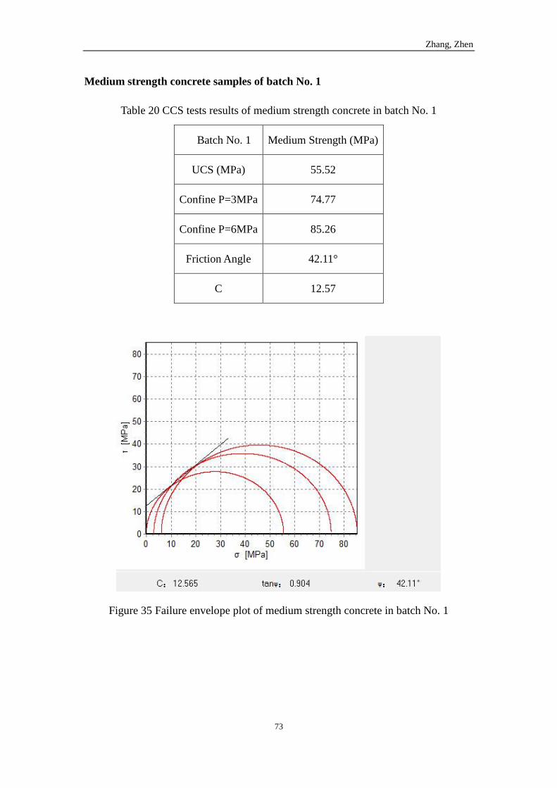
Zhang, Zhen

73

Medium strength concrete samples of batch No. 1

Table 20 CCS tests results of medium strength concrete in batch No. 1

Batch No. 1 Medium Strength (MPa)

UCS (MPa) 55.52




C 12.57

Figure 35 Failure envelope plot of medium strength concrete in batch No. 1

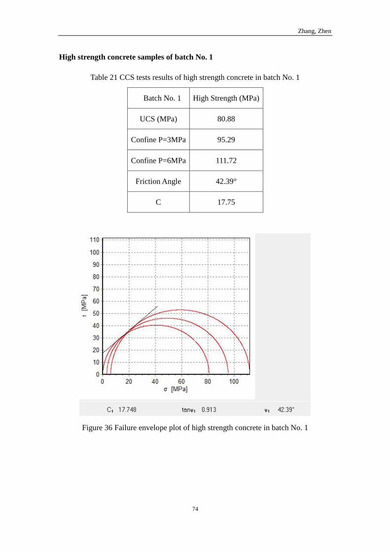
Zhang, Zhen

74

High strength concrete samples of batch No. 1

Table 21 CCS tests results of high strength concrete in batch No. 1

Batch No. 1 High Strength (MPa)

UCS (MPa) 80.88




C 17.75

Figure 36 Failure envelope plot of high strength concrete in batch No. 1

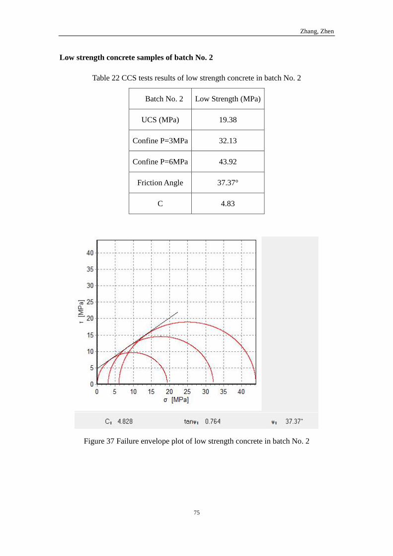
Zhang, Zhen

75

Low strength concrete samples of batch No. 2

Table 22 CCS tests results of low strength concrete in batch No. 2

Batch No. 2 Low Strength (MPa)

UCS (MPa) 19.38




C 4.83

Figure 37 Failure envelope plot of low strength concrete in batch No. 2

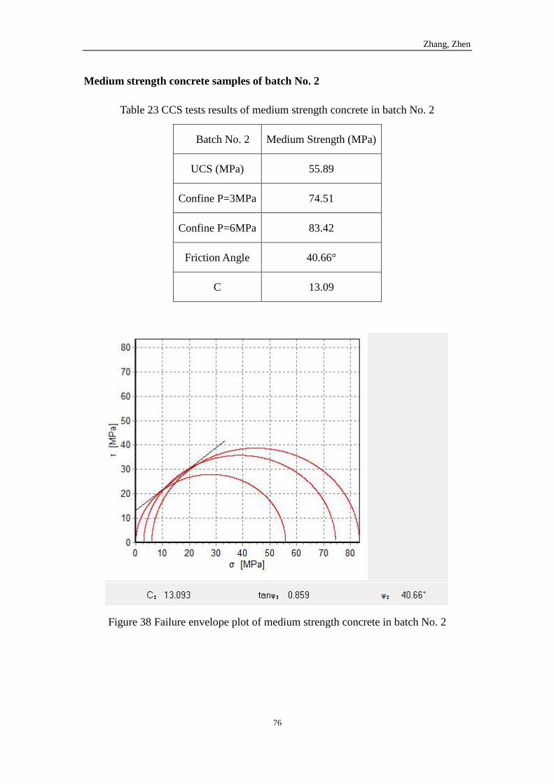
Zhang, Zhen

76

Medium strength concrete samples of batch No. 2

Table 23 CCS tests results of medium strength concrete in batch No. 2

Batch No. 2 Medium Strength (MPa)

UCS (MPa) 55.89




C 13.09

Figure 38 Failure envelope plot of medium strength concrete in batch No. 2

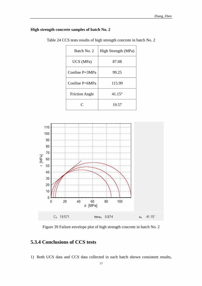
Zhang, Zhen

77

High strength concrete samples of batch No. 2

Table 24 CCS tests results of high strength concrete in batch No. 2

Batch No. 2 High Strength (MPa)

UCS (MPa) 87.08




C 19.57

Figure 39 Failure envelope plot of high strength concrete in batch No. 2

5.3.4 Conclusions of CCS tests

1) Both UCS data and CCS data collected in each batch shown consistent results,

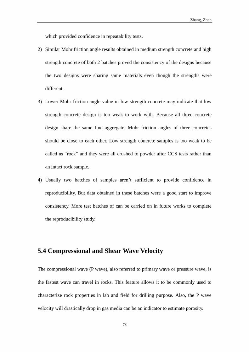
Zhang, Zhen

78

which provided confidence in repeatability tests.

2) Similar Mohr friction angle results obtained in medium strength concrete and high

strength concrete of both 2 batches proved the consistency of the designs because

the two designs were sharing same materials even though the strengths were

different.

3) Lower Mohr friction angle value in low strength concrete may indicate that low

strength concrete design is too weak to work with. Because all three concrete

design share the same fine aggregate, Mohr friction angles of three concretes

should be close to each other. Low strength concrete samples is too weak to be

called as “rock” and they were all crushed to powder after CCS tests rather than

an intact rock sample.

4) Usually two batches of samples aren’t sufficient to provide confidence in

reproducibility. But data obtained in these batches were a good start to improve

consistency. More test batches of can be carried on in future works to complete

the reproducibility study.

5.4 Compressional and Shear Wave Velocity

The compressional wave (P wave), also referred to primary wave or pressure wave, is

the fastest wave can travel in rocks. This feature allows it to be commonly used to

characterize rock properties in lab and field for drilling purpose. Also, the P wave

velocity will drastically drop in gas media can be an indicator to estimate porosity.

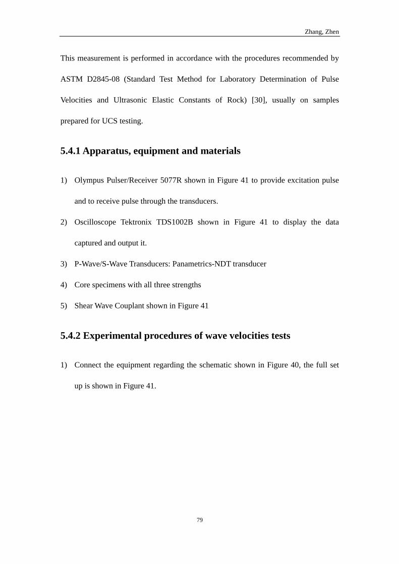
Zhang, Zhen

79

This measurement is performed in accordance with the procedures recommended by

ASTM D2845-08 (Standard Test Method for Laboratory Determination of Pulse

Velocities and Ultrasonic Elastic Constants of Rock) [30], usually on samples

prepared for UCS testing.


1) Olympus Pulser/Receiver 5077R shown in Figure 41 to provide excitation pulse

and to receive pulse through the transducers.

2) Oscilloscope Tektronix TDS1002B shown in Figure 41 to display the data

captured and output it.

3) P-Wave/S-Wave Transducers: Panametrics-NDT transducer

4) Core specimens with all three strengths

5) Shear Wave Couplant shown in Figure 41

5.4.2 Experimental procedures of wave velocities tests

1) Connect the equipment regarding the schematic shown in Figure 40, the full set

up is shown in Figure 41.

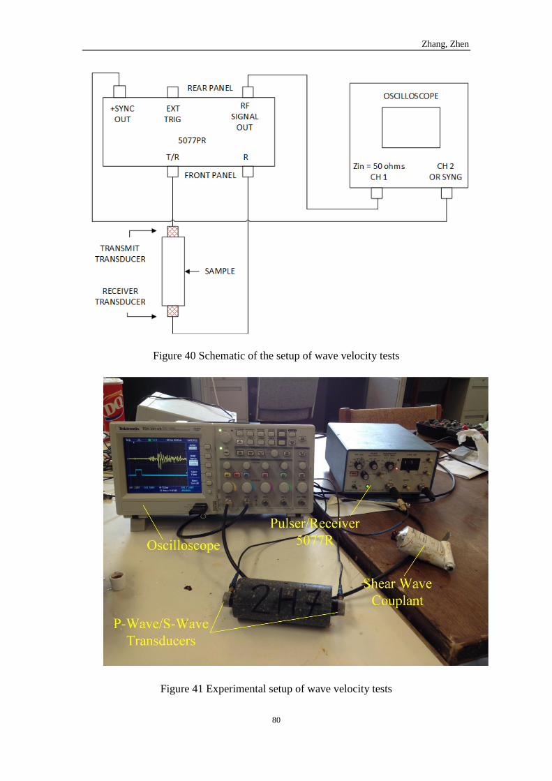
Zhang, Zhen

80

Figure 40 Schematic of the setup of wave velocity tests

Figure 41 Experimental setup of wave velocity tests

Zhang, Zhen

81

2) Coat the couplant on the contact area of transducers, then put the two transducers

together to find the zero position using oscilloscope

3) Place the two transducers at the ends of core specimen, then read the time

difference which is the time of penetrating the specimen with acoustic wave, as

shown in Figure 42.

Figure 42 Example picture of wave velocity tests

4) Measure each core specimen with caliper for three times and take the mean value

as travel distance, which to be divided by travel time to obtain wave velocity

5.4.3 Results of wave velocity tests

All the wave velocity tests results are shown from Table 25 to Table 28 along with

repeatability studies.

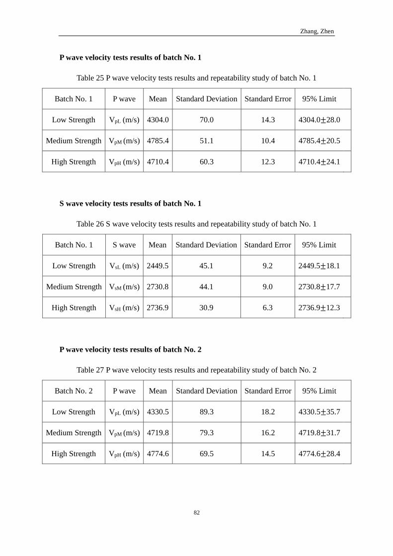
Zhang, Zhen

82

P wave velocity tests results of batch No. 1

Table 25 P wave velocity tests results and repeatability study of batch No. 1

Batch No. 1 P wave Mean Standard Deviation Standard Error 95% Limit

Low Strength VpL (m/s) 4304.0 70.0 14.3 4304.0±28.0

Medium Strength VpM (m/s) 4785.4 51.1 10.4 4785.4±20.5

High Strength VpH (m/s) 4710.4 60.3 12.3 4710.4±24.1

S wave velocity tests results of batch No. 1

Table 26 S wave velocity tests results and repeatability study of batch No. 1

Batch No. 1 S wave Mean Standard Deviation Standard Error 95% Limit

Low Strength VsL (m/s) 2449.5 45.1 9.2 2449.5±18.1

Medium Strength VsM (m/s) 2730.8 44.1 9.0 2730.8±17.7

High Strength VsH (m/s) 2736.9 30.9 6.3 2736.9±12.3

P wave velocity tests results of batch No. 2

Table 27 P wave velocity tests results and repeatability study of batch No. 2

Batch No. 2 P wave Mean Standard Deviation Standard Error 95% Limit

Low Strength VpL (m/s) 4330.5 89.3 18.2 4330.5±35.7

Medium Strength VpM (m/s) 4719.8 79.3 16.2 4719.8±31.7

High Strength VpH (m/s) 4774.6 69.5 14.5 4774.6±28.4

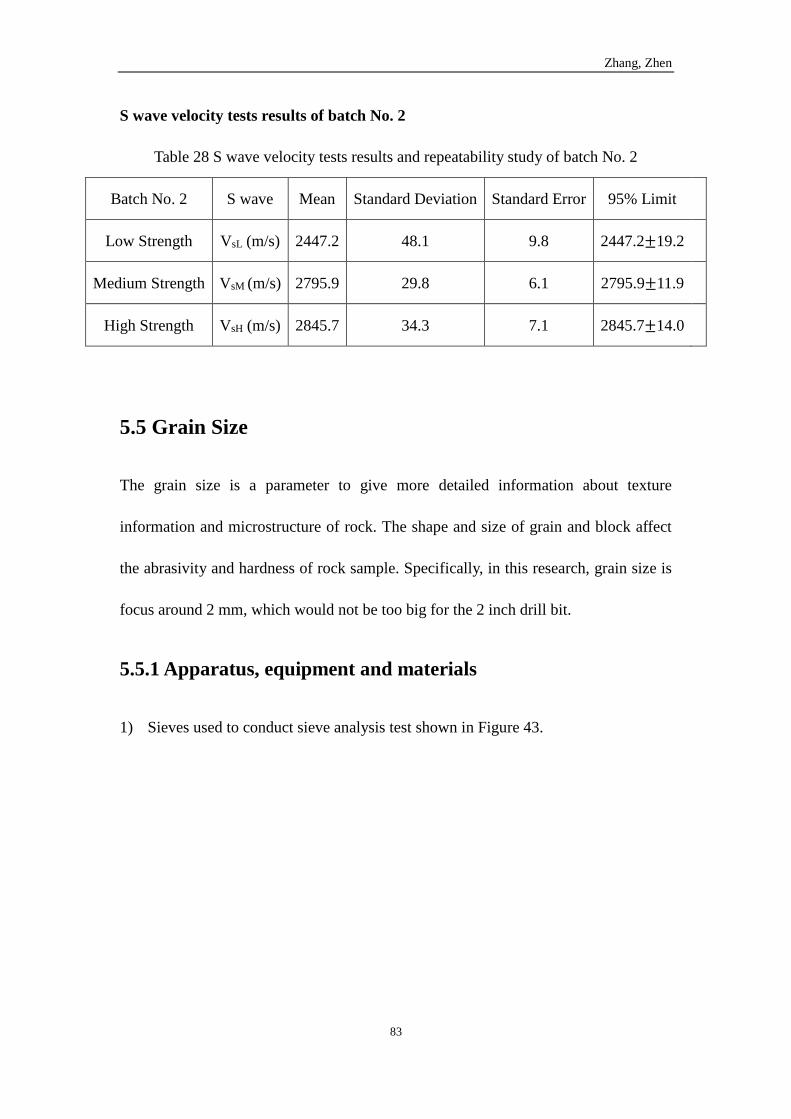
Zhang, Zhen

83

S wave velocity tests results of batch No. 2

Table 28 S wave velocity tests results and repeatability study of batch No. 2

Batch No. 2 S wave Mean Standard Deviation Standard Error 95% Limit

Low Strength VsL (m/s) 2447.2 48.1 9.8 2447.2±19.2

Medium Strength VsM (m/s) 2795.9 29.8 6.1 2795.9±11.9

High Strength VsH (m/s) 2845.7 34.3 7.1 2845.7±14.0

5.5 Grain Size

The grain size is a parameter to give more detailed information about texture

information and microstructure of rock. The shape and size of grain and block affect

the abrasivity and hardness of rock sample. Specifically, in this research, grain size is

focus around 2 mm, which would not be too big for the 2 inch drill bit.


1) Sieves used to conduct sieve analysis test shown in Figure 43.

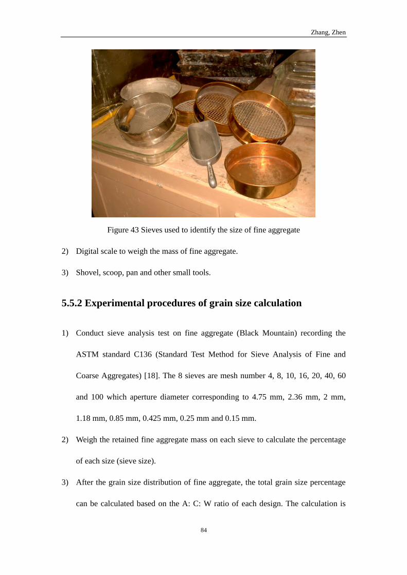
Zhang, Zhen

84

Figure 43 Sieves used to identify the size of fine aggregate

2) Digital scale to weigh the mass of fine aggregate.

3) Shovel, scoop, pan and other small tools.

5.5.2 Experimental procedures of grain size calculation

1) Conduct sieve analysis test on fine aggregate (Black Mountain) recording the

ASTM standard C136 (Standard Test Method for Sieve Analysis of Fine and

Coarse Aggregates) [18]. The 8 sieves are mesh number 4, 8, 10, 16, 20, 40, 60

and 100 which aperture diameter corresponding to 4.75 mm, 2.36 mm, 2 mm,

1.18 mm, 0.85 mm, 0.425 mm, 0.25 mm and 0.15 mm.

2) Weigh the retained fine aggregate mass on each sieve to calculate the percentage

of each size (sieve size).

3) After the grain size distribution of fine aggregate, the total grain size percentage

can be calculated based on the A: C: W ratio of each design. The calculation is

Zhang, Zhen

85

shown in Equation 5.2.

𝑔𝑟𝑎𝑖𝑛 𝑠𝑖𝑧𝑒 𝑜𝑓 𝑐𝑜𝑛𝑐𝑟𝑒𝑡𝑒

= 𝑔𝑟𝑎𝑖𝑛 𝑠𝑖𝑧𝑒 𝑜𝑓 𝑎𝑔𝑔𝑟𝑒𝑔𝑎𝑡𝑒

×𝑚𝑎𝑠𝑠 𝑜𝑓 𝑎𝑔𝑔𝑟𝑒𝑔𝑎𝑡𝑒

𝑚𝑎𝑠𝑠 𝑜𝑓 𝑐𝑒𝑚𝑒𝑛𝑡𝑖𝑜𝑢𝑠 𝑚𝑎𝑡𝑒𝑟𝑖𝑎𝑙𝑠 + 𝑚𝑎𝑠𝑠 𝑜𝑓 𝑤𝑎𝑡𝑒𝑟 + 𝑚𝑎𝑠𝑠 𝑜𝑓 𝑎𝑔𝑔𝑟𝑒𝑔𝑎𝑡𝑒

Equation 5.2 Calculation of grain size distribution of concrete

5.5.3 Results of grain size calculation

Cementious materials will be in form of concrete matrix exist in concrete, which is

considered to be not in count of grain size. All three concrete designs share the same

fine aggregate so that the grain size distribution of fine aggregate is the key part of the

grain size calculation of concrete.

Sieve analysis of fine aggregate has been done in previous works which is shown in

Table 1 Passed percentage of fine aggregate. Regarding the results in Table 1, the

percentage of fine aggregate retained on each sieve can be calculated and shown in

Table 29.

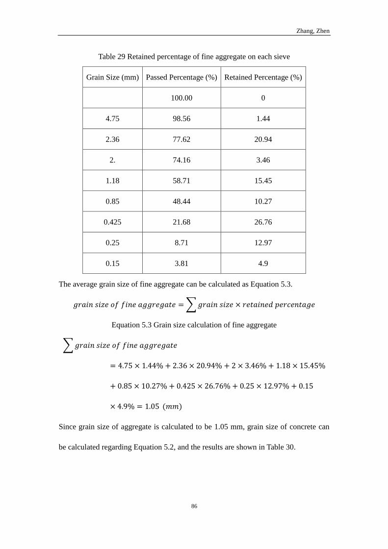
Zhang, Zhen

86

Table 29 Retained percentage of fine aggregate on each sieve

Grain Size (mm) Passed Percentage (%) Retained Percentage (%)

100.00 0

4.75 98.56 1.44

2.36 77.62 20.94

2. 74.16 3.46

1.18 58.71 15.45

0.85 48.44 10.27

0.425 21.68 26.76

0.25 8.71 12.97

0.15 3.81 4.9

The average grain size of fine aggregate can be calculated as Equation 5.3.

𝑔𝑟𝑎𝑖𝑛 𝑠𝑖𝑧𝑒 𝑜𝑓 𝑓𝑖𝑛𝑒 𝑎𝑔𝑔𝑟𝑒𝑔𝑎𝑡𝑒 = ∑ 𝑔𝑟𝑎𝑖𝑛 𝑠𝑖𝑧𝑒 × 𝑟𝑒𝑡𝑎𝑖𝑛𝑒𝑑 𝑝𝑒𝑟𝑐𝑒𝑛𝑡𝑎𝑔𝑒

Equation 5.3 Grain size calculation of fine aggregate

∑ 𝑔𝑟𝑎𝑖𝑛 𝑠𝑖𝑧𝑒 𝑜𝑓 𝑓𝑖𝑛𝑒 𝑎𝑔𝑔𝑟𝑒𝑔𝑎𝑡𝑒

= 4.75 × 1.44% + 2.36 × 20.94% + 2 × 3.46% + 1.18 × 15.45%

+ 0.85 × 10.27% + 0.425 × 26.76% + 0.25 × 12.97% + 0.15

× 4.9% = 1.05 (𝑚𝑚)

Since grain size of aggregate is calculated to be 1.05 mm, grain size of concrete can

be calculated regarding Equation 5.2, and the results are shown in Table 30.

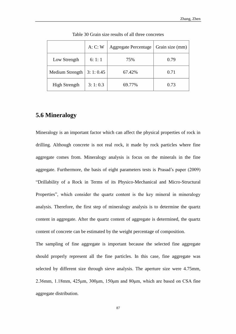
Zhang, Zhen

87

Table 30 Grain size results of all three concretes

A: C: W Aggregate Percentage Grain size (mm)

Low Strength 6: 1: 1 75% 0.79

Medium Strength 3: 1: 0.45 67.42% 0.71

High Strength 3: 1: 0.3 69.77% 0.73

5.6 Mineralogy

Mineralogy is an important factor which can affect the physical properties of rock in

drilling. Although concrete is not real rock, it made by rock particles where fine

aggregate comes from. Mineralogy analysis is focus on the minerals in the fine

aggregate. Furthermore, the basis of eight parameters tests is Prasad’s paper (2009)

“Drillability of a Rock in Terms of its Physico-Mechanical and Micro-Structural

Properties”, which consider the quartz content is the key mineral in mineralogy

analysis. Therefore, the first step of mineralogy analysis is to determine the quartz

content in aggregate. After the quartz content of aggregate is determined, the quartz

content of concrete can be estimated by the weight percentage of composition.

The sampling of fine aggregate is important because the selected fine aggregate

should properly represent all the fine particles. In this case, fine aggregate was

selected by different size through sieve analysis. The aperture size were 4.75mm,

2.36mm, 1.18mm, 425μm, 300μm, 150μm and 80μm, which are based on CSA fine

aggregate distribution.

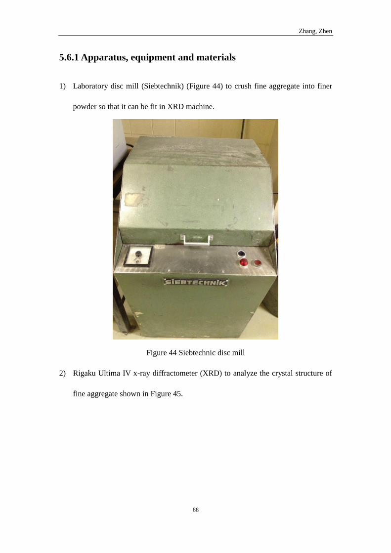
Zhang, Zhen

88


1) Laboratory disc mill (Siebtechnik) (Figure 44) to crush fine aggregate into finer

powder so that it can be fit in XRD machine.

Figure 44 Siebtechnic disc mill

2) Rigaku Ultima IV x-ray diffractometer (XRD) to analyze the crystal structure of

fine aggregate shown in Figure 45.

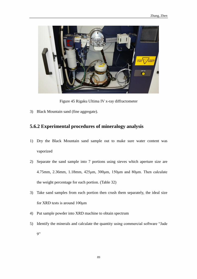
Zhang, Zhen

89

Figure 45 Rigaku Ultima IV x-ray diffractometer

3) Black Mountain sand (fine aggregate).

5.6.2 Experimental procedures of mineralogy analysis

1) Dry the Black Mountain sand sample out to make sure water content was

vaporized

2) Separate the sand sample into 7 portions using sieves which aperture size are

4.75mm, 2.36mm, 1.18mm, 425μm, 300μm, 150μm and 80μm. Then calculate

the weight percentage for each portion. (Table 32)

3) Take sand samples from each portion then crush them separately, the ideal size

for XRD tests is around 100μm

4) Put sample powder into XRD machine to obtain spectrum

5) Identify the minerals and calculate the quantity using commercial software “Jade

9”

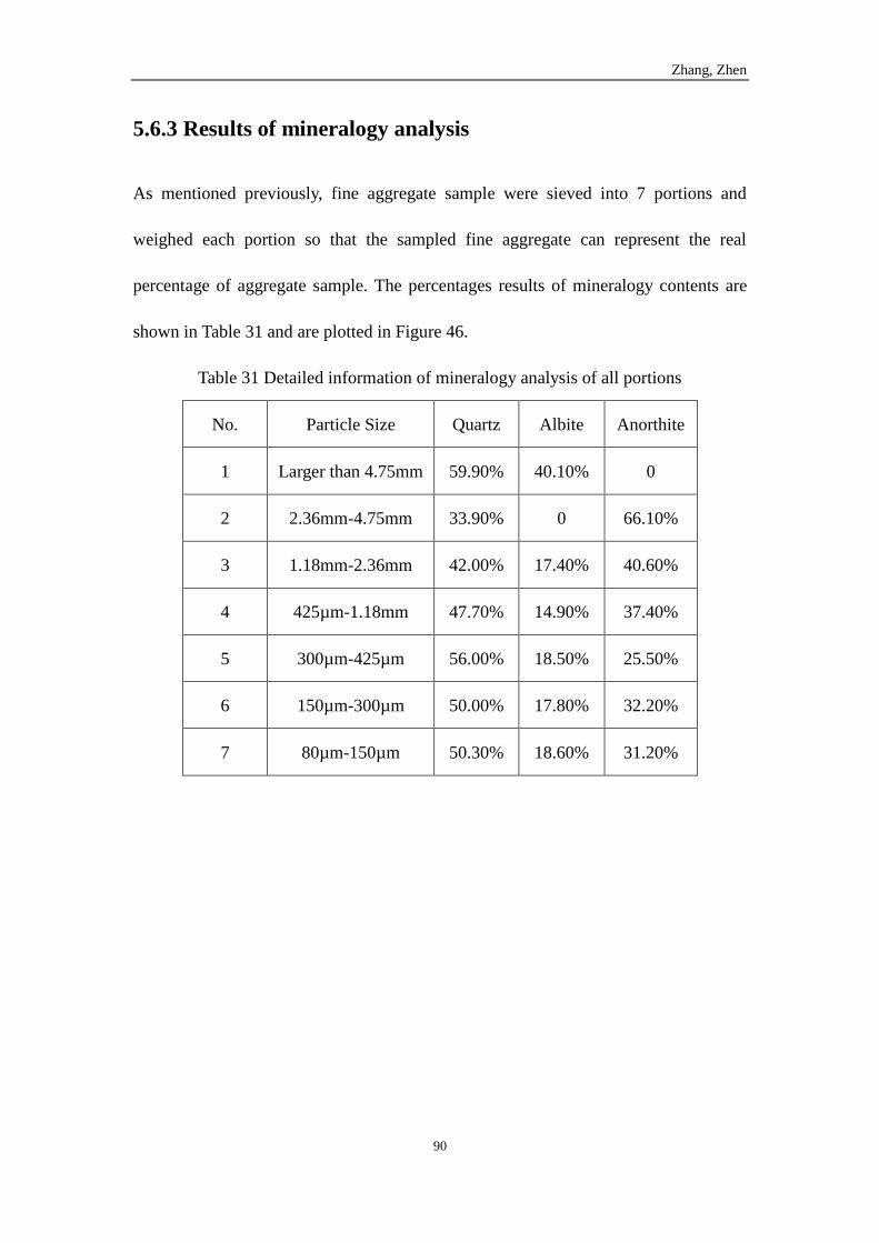
Zhang, Zhen

90

5.6.3 Results of mineralogy analysis

As mentioned previously, fine aggregate sample were sieved into 7 portions and

weighed each portion so that the sampled fine aggregate can represent the real

percentage of aggregate sample. The percentages results of mineralogy contents are

shown in Table 31 and are plotted in Figure 46.

Table 31 Detailed information of mineralogy analysis of all portions

No. Particle Size Quartz Albite Anorthite

1 Larger than 4.75mm 59.90% 40.10% 0

2 2.36mm-4.75mm 33.90% 0 66.10%

3 1.18mm-2.36mm 42.00% 17.40% 40.60%

4 425µm-1.18mm 47.70% 14.90% 37.40%

5 300µm-425µm 56.00% 18.50% 25.50%

6 150µm-300µm 50.00% 17.80% 32.20%

7 80µm-150µm 50.30% 18.60% 31.20%

Zhang, Zhen

91

Figure 46 Mineralogy analysis results of all portions

Quartz contents of each portion and weight percentages of each portion are shown in

Table 32.

Table 32 Weight percentage and quartz content of each portion

Grain Size Weight Percentage (%) Quartz Content (%)

4.75 mm 1.44 59.90

2.36 mm 20.94 33.90

1.18 mm 18.91 42.00

425 μm 37.03 47.70

300 μm 13.00 56.00

150 μm 4.90 50.00

80 μm 3.80 50.30

Regarding the information in Table 32, the average quartz content of fine aggregate

can be calculated as Equation 5.4.

0%

10%

20%

30%

40%

50%

60%

70%

1 2 3 4 5 6 7

Quartz

Albite

Anorthite

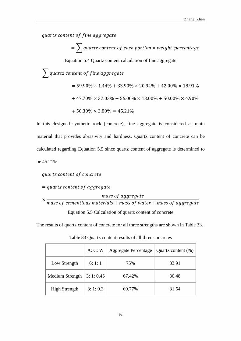
Zhang, Zhen

92

𝑞𝑢𝑎𝑟𝑡𝑧 𝑐𝑜𝑛𝑡𝑒𝑛𝑡 𝑜𝑓 𝑓𝑖𝑛𝑒 𝑎𝑔𝑔𝑟𝑒𝑔𝑎𝑡𝑒

= ∑ 𝑞𝑢𝑎𝑟𝑡𝑧 𝑐𝑜𝑛𝑡𝑒𝑛𝑡 𝑜𝑓 𝑒𝑎𝑐ℎ 𝑝𝑜𝑟𝑡𝑖𝑜𝑛 × 𝑤𝑒𝑖𝑔ℎ𝑡 𝑝𝑒𝑟𝑐𝑒𝑛𝑡𝑎𝑔𝑒

Equation 5.4 Quartz content calculation of fine aggregate

∑ 𝑞𝑢𝑎𝑟𝑡𝑧 𝑐𝑜𝑛𝑡𝑒𝑛𝑡 𝑜𝑓 𝑓𝑖𝑛𝑒 𝑎𝑔𝑔𝑟𝑒𝑔𝑎𝑡𝑒

= 59.90% × 1.44% + 33.90% × 20.94% + 42.00% × 18.91%

+ 47.70% × 37.03% + 56.00% × 13.00% + 50.00% × 4.90%

+ 50.30% × 3.80% = 45.21%

In this designed synthetic rock (concrete), fine aggregate is considered as main

material that provides abrasivity and hardness. Quartz content of concrete can be

calculated regarding Equation 5.5 since quartz content of aggregate is determined to

be 45.21%.

𝑞𝑢𝑎𝑟𝑡𝑧 𝑐𝑜𝑛𝑡𝑒𝑛𝑡 𝑜𝑓 𝑐𝑜𝑛𝑐𝑟𝑒𝑡𝑒

= 𝑞𝑢𝑎𝑟𝑡𝑧 𝑐𝑜𝑛𝑡𝑒𝑛𝑡 𝑜𝑓 𝑎𝑔𝑔𝑟𝑒𝑔𝑎𝑡𝑒

×𝑚𝑎𝑠𝑠 𝑜𝑓 𝑎𝑔𝑔𝑟𝑒𝑔𝑎𝑡𝑒

𝑚𝑎𝑠𝑠 𝑜𝑓 𝑐𝑒𝑚𝑒𝑛𝑡𝑖𝑜𝑢𝑠 𝑚𝑎𝑡𝑒𝑟𝑖𝑎𝑙𝑠 + 𝑚𝑎𝑠𝑠 𝑜𝑓 𝑤𝑎𝑡𝑒𝑟 + 𝑚𝑎𝑠𝑠 𝑜𝑓 𝑎𝑔𝑔𝑟𝑒𝑔𝑎𝑡𝑒

Equation 5.5 Calculation of quartz content of concrete

The results of quartz content of concrete for all three strengths are shown in Table 33.

Table 33 Quartz content results of all three concretes

A: C: W Aggregate Percentage Quartz content (%)

Low Strength 6: 1: 1 75% 33.91

Medium Strength 3: 1: 0.45 67.42% 30.48

High Strength 3: 1: 0.3 69.77% 31.54

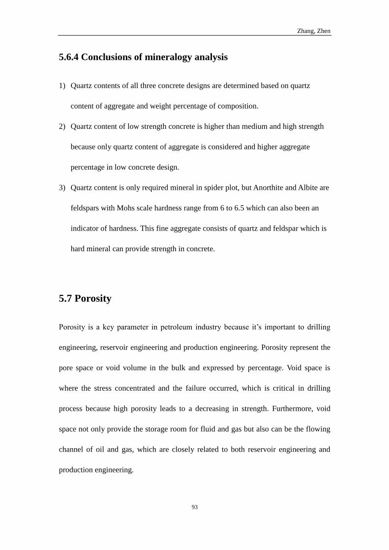
Zhang, Zhen

93

5.6.4 Conclusions of mineralogy analysis

1) Quartz contents of all three concrete designs are determined based on quartz

content of aggregate and weight percentage of composition.

2) Quartz content of low strength concrete is higher than medium and high strength

because only quartz content of aggregate is considered and higher aggregate

percentage in low concrete design.

3) Quartz content is only required mineral in spider plot, but Anorthite and Albite are

feldspars with Mohs scale hardness range from 6 to 6.5 which can also been an

indicator of hardness. This fine aggregate consists of quartz and feldspar which is

hard mineral can provide strength in concrete.

5.7 Porosity

Porosity is a key parameter in petroleum industry because it’s important to drilling

engineering, reservoir engineering and production engineering. Porosity represent the

pore space or void volume in the bulk and expressed by percentage. Void space is

where the stress concentrated and the failure occurred, which is critical in drilling

process because high porosity leads to a decreasing in strength. Furthermore, void

space not only provide the storage room for fluid and gas but also can be the flowing

channel of oil and gas, which are closely related to both reservoir engineering and

production engineering.

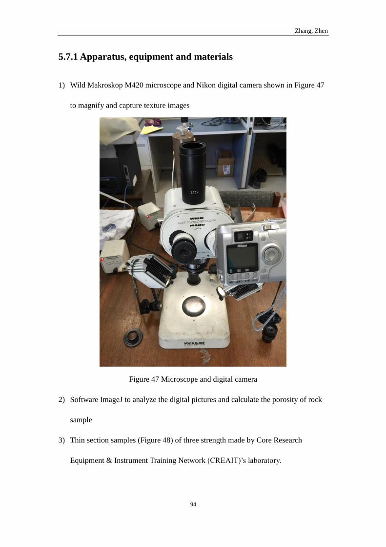
Zhang, Zhen

94


1) Wild Makroskop M420 microscope and Nikon digital camera shown in Figure 47

to magnify and capture texture images

Figure 47 Microscope and digital camera

2) Software ImageJ to analyze the digital pictures and calculate the porosity of rock

sample

3) Thin section samples (Figure 48) of three strength made by Core Research

Equipment & Instrument Training Network (CREAIT)’s laboratory.

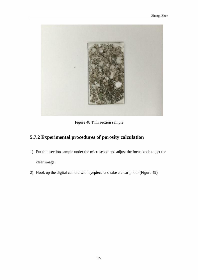
Zhang, Zhen

95

Figure 48 Thin section sample

5.7.2 Experimental procedures of porosity calculation

1) Put thin section sample under the microscope and adjust the focus knob to get the

clear image

2) Hook up the digital camera with eyepiece and take a clear photo (Figure 49)

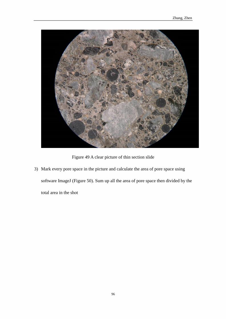
Zhang, Zhen

96

Figure 49 A clear picture of thin section slide

3) Mark every pore space in the picture and calculate the area of pore space using

software ImageJ (Figure 50). Sum up all the area of pore space then divided by the

total area in the shot

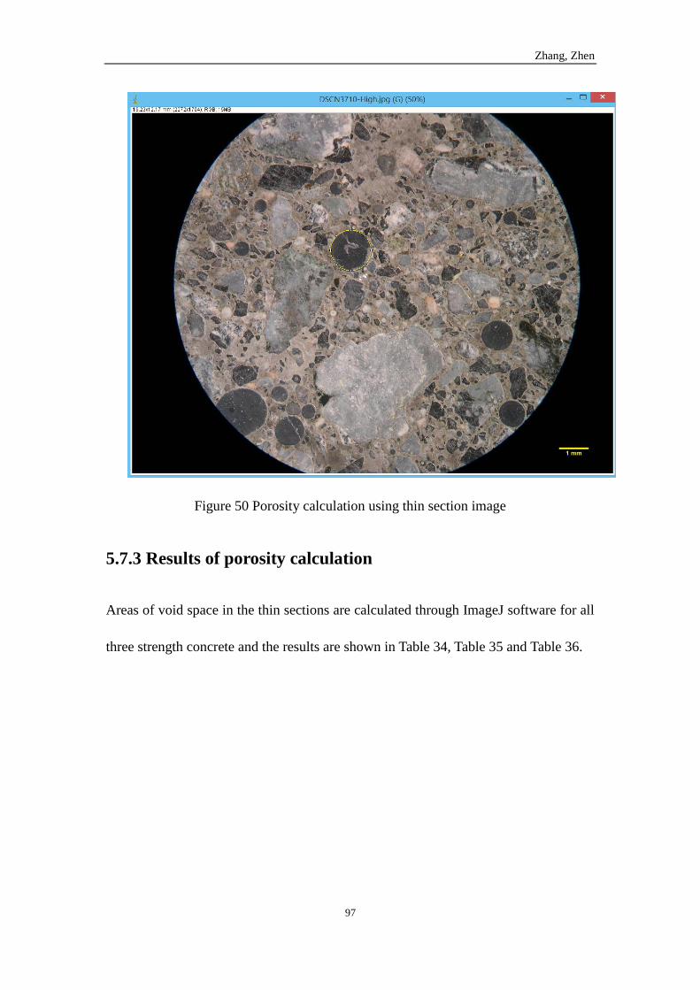
Zhang, Zhen

97

Figure 50 Porosity calculation using thin section image

5.7.3 Results of porosity calculation

Areas of void space in the thin sections are calculated through ImageJ software for all

three strength concrete and the results are shown in Table 34, Table 35 and Table 36.

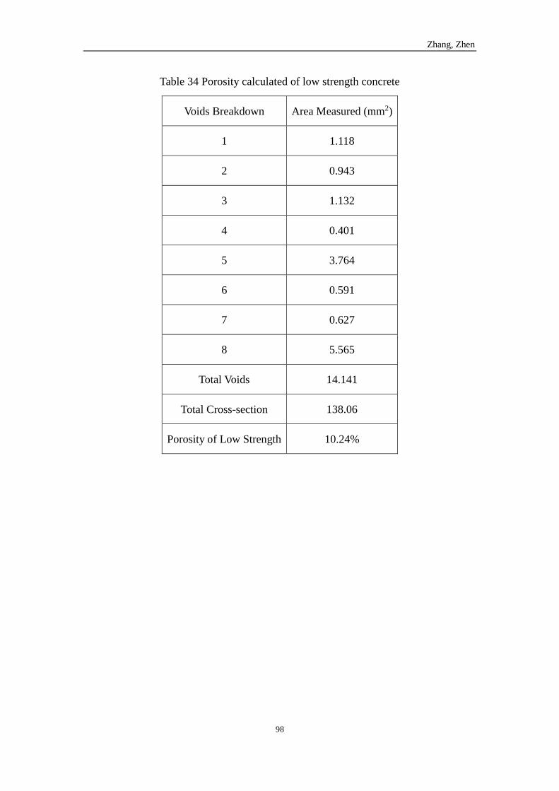
Zhang, Zhen

98

Table 34 Porosity calculated of low strength concrete

Voids Breakdown Area Measured (mm2)

1 1.118

2 0.943

3 1.132

4 0.401

5 3.764

6 0.591

7 0.627

8 5.565

Total Voids 14.141

Total Cross-section 138.06

Porosity of Low Strength 10.24%

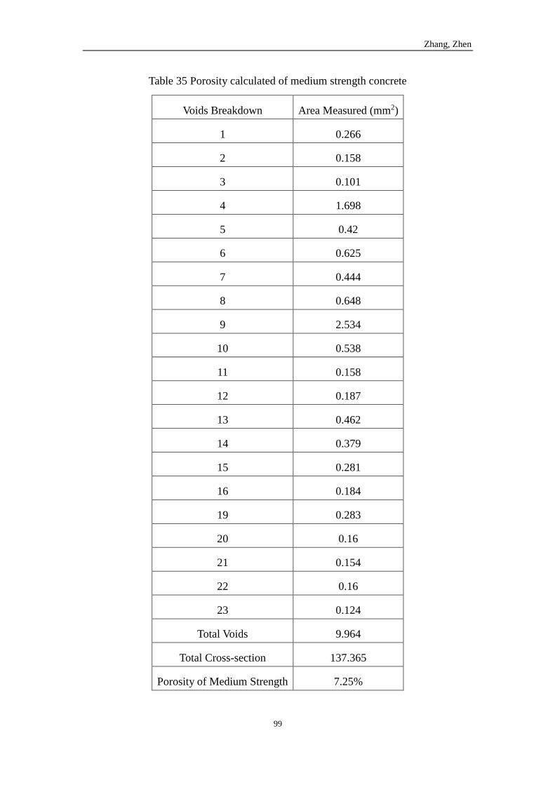
Zhang, Zhen

99

Table 35 Porosity calculated of medium strength concrete


1 0.266

2 0.158

3 0.101

4 1.698

5 0.42

6 0.625

7 0.444

8 0.648

9 2.534

10 0.538

11 0.158

12 0.187

13 0.462

14 0.379

15 0.281

16 0.184

19 0.283

20 0.16

21 0.154

22 0.16

23 0.124

Total Voids 9.964


Porosity of Medium Strength 7.25%

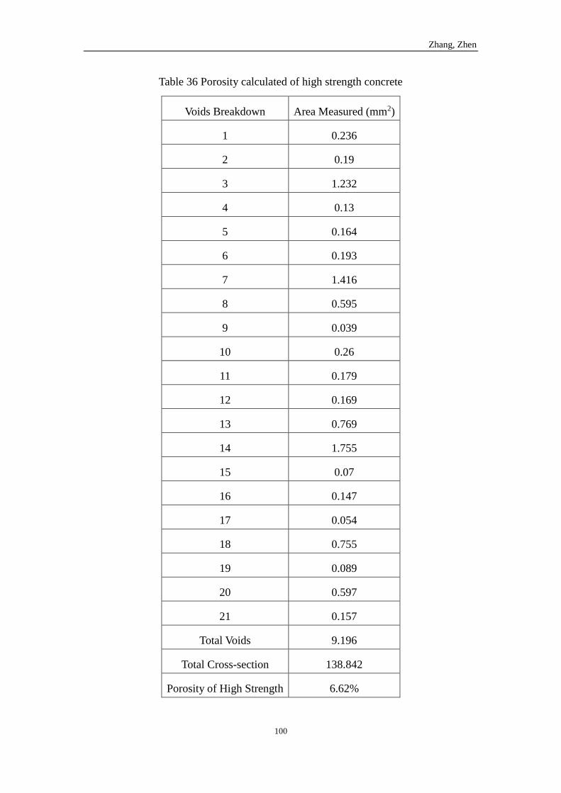
Zhang, Zhen

100

Table 36 Porosity calculated of high strength concrete


1 0.236

2 0.19

3 1.232

4 0.13

5 0.164

6 0.193

7 1.416

8 0.595

9 0.039

10 0.26

11 0.179

12 0.169

13 0.769

14 1.755

15 0.07

16 0.147

17 0.054

18 0.755

19 0.089

20 0.597

21 0.157

Total Voids 9.196


Porosity of High Strength 6.62%

Zhang, Zhen

101

5.7.4 Conclusions of porosity calculation

1) Porosities of all three strength are 10.24% (low strength), 7.25% (medium strength)

and 6.62% (high strength). Large amount of cement material in the concrete

designs result in low porosity values of synthetic rocks.

2) Regarding the breakdown values in three concrete design, voids in low strength

concrete are fewer and bigger while voids in medium and high strength concrete

are more and smaller.

5.8 Spider plot of eight parameters tests

The large amount of data generated by the testing is most conveniently presented in

terms of the eight drillability parameters. All the data will be processed and converted

into number in scale of 0 to 8 to present in a more intuitive and convenient approach.

5.8.1 Results of eight parameters tests

All eight parameters tests for three concretes designs are completed and results of

characterization are shown in Table 37, Table 38 and Table 39.

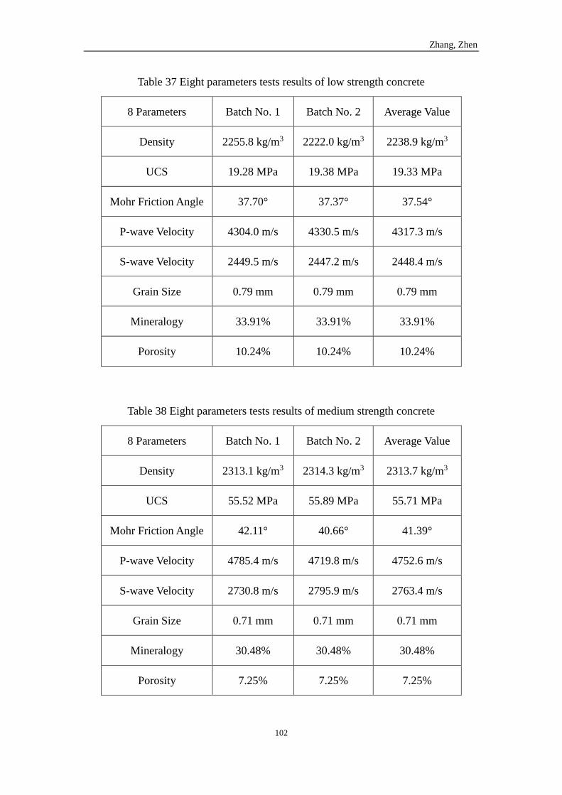
Zhang, Zhen

102

Table 37 Eight parameters tests results of low strength concrete

8 Parameters Batch No. 1 Batch No. 2 Average Value

Density 2255.8 kg/m3 2222.0 kg/m3 2238.9 kg/m3

UCS 19.28 MPa 19.38 MPa 19.33 MPa

Mohr Friction Angle 37.70° 37.37° 37.54°

P-wave Velocity 4304.0 m/s 4330.5 m/s 4317.3 m/s

S-wave Velocity 2449.5 m/s 2447.2 m/s 2448.4 m/s

Grain Size 0.79 mm 0.79 mm 0.79 mm

Mineralogy 33.91% 33.91% 33.91%

Porosity 10.24% 10.24% 10.24%

Table 38 Eight parameters tests results of medium strength concrete



UCS 55.52 MPa 55.89 MPa 55.71 MPa



S-wave Velocity 2730.8 m/s 2795.9 m/s 2763.4 m/s


Mineralogy 30.48% 30.48% 30.48%

Porosity 7.25% 7.25% 7.25%

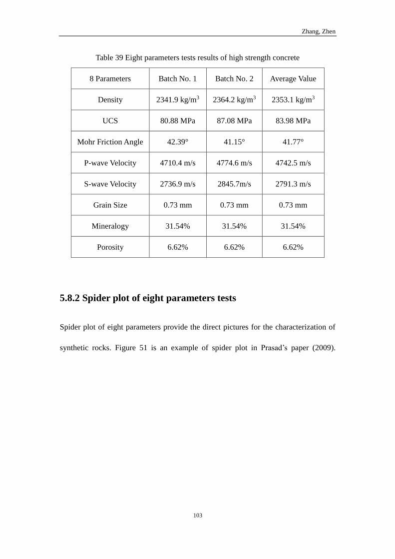
Zhang, Zhen

103

Table 39 Eight parameters tests results of high strength concrete



UCS 80.88 MPa 87.08 MPa 83.98 MPa



S-wave Velocity 2736.9 m/s 2845.7m/s 2791.3 m/s


Mineralogy 31.54% 31.54% 31.54%

Porosity 6.62% 6.62% 6.62%

5.8.2 Spider plot of eight parameters tests

Spider plot of eight parameters provide the direct pictures for the characterization of

synthetic rocks. Figure 51 is an example of spider plot in Prasad’s paper (2009).

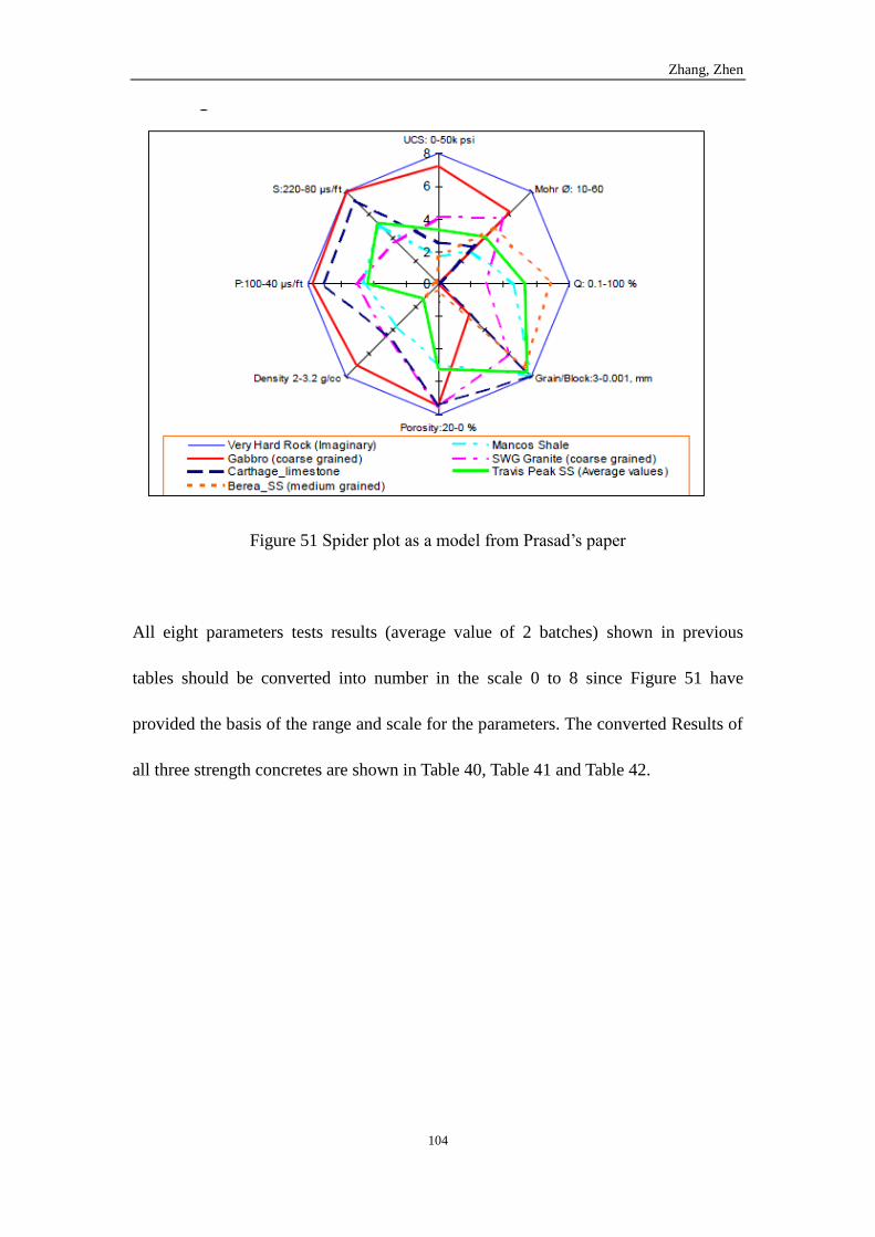
Zhang, Zhen

104

Figure 51 Spider plot as a model from Prasad’s paper

All eight parameters tests results (average value of 2 batches) shown in previous

tables should be converted into number in the scale 0 to 8 since Figure 51 have

provided the basis of the range and scale for the parameters. The converted Results of

all three strength concretes are shown in Table 40, Table 41 and Table 42.

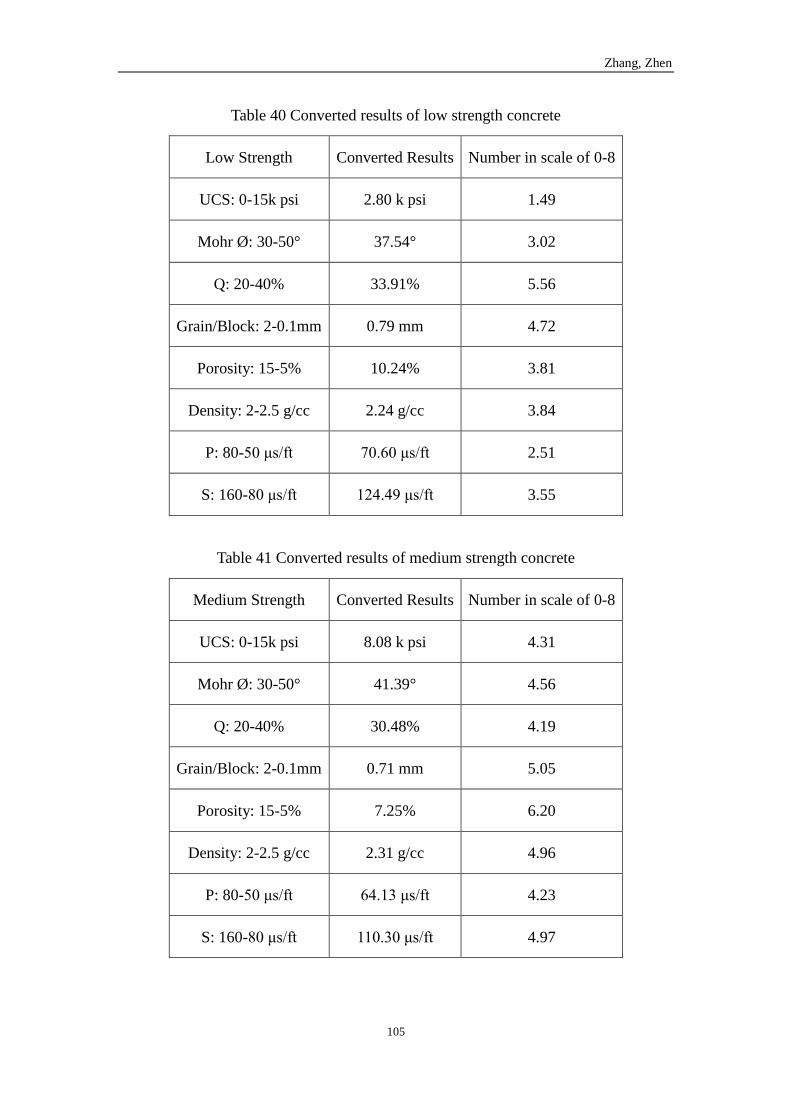
Zhang, Zhen

105

Table 40 Converted results of low strength concrete

Low Strength Converted Results Number in scale of 0-8

UCS: 0-15k psi 2.80 k psi 1.49

Mohr Ø: 30-50° 37.54° 3.02

Q: 20-40% 33.91% 5.56

Grain/Block: 2-0.1mm 0.79 mm 4.72

Porosity: 15-5% 10.24% 3.81

Density: 2-2.5 g/cc 2.24 g/cc 3.84

P: 80-50 μs/ft 70.60 μs/ft 2.51

S: 160-80 μs/ft 124.49 μs/ft 3.55

Table 41 Converted results of medium strength concrete

Medium Strength Converted Results Number in scale of 0-8

UCS: 0-15k psi 8.08 k psi 4.31

Mohr Ø: 30-50° 41.39° 4.56

Q: 20-40% 30.48% 4.19


Porosity: 15-5% 7.25% 6.20

Density: 2-2.5 g/cc 2.31 g/cc 4.96

P: 80-50 μs/ft 64.13 μs/ft 4.23

S: 160-80 μs/ft 110.30 μs/ft 4.97

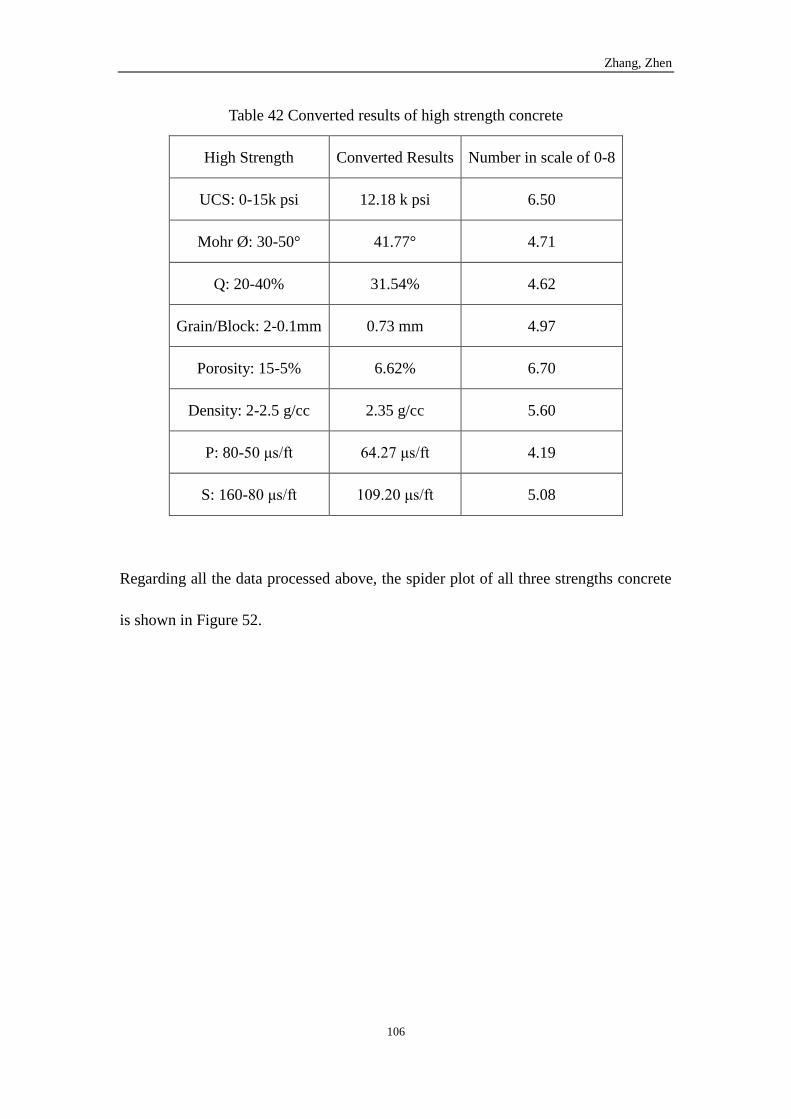
Zhang, Zhen

106

Table 42 Converted results of high strength concrete

High Strength Converted Results Number in scale of 0-8

UCS: 0-15k psi 12.18 k psi 6.50

Mohr Ø: 30-50° 41.77° 4.71

Q: 20-40% 31.54% 4.62


Porosity: 15-5% 6.62% 6.70

Density: 2-2.5 g/cc 2.35 g/cc 5.60

P: 80-50 μs/ft 64.27 μs/ft 4.19

S: 160-80 μs/ft 109.20 μs/ft 5.08

Regarding all the data processed above, the spider plot of all three strengths concrete

is shown in Figure 52.

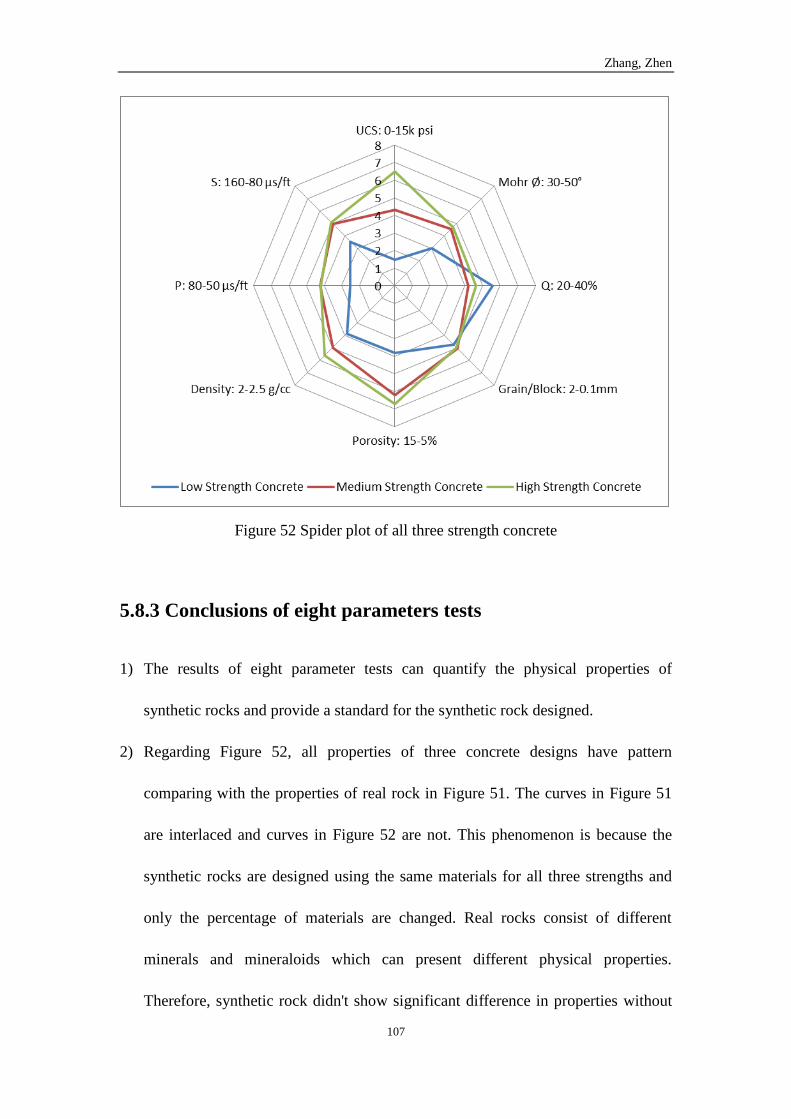
Zhang, Zhen

107

Figure 52 Spider plot of all three strength concrete

5.8.3 Conclusions of eight parameters tests

1) The results of eight parameter tests can quantify the physical properties of

synthetic rocks and provide a standard for the synthetic rock designed.

2) Regarding Figure 52, all properties of three concrete designs have pattern

comparing with the properties of real rock in Figure 51. The curves in Figure 51

are interlaced and curves in Figure 52 are not. This phenomenon is because the

synthetic rocks are designed using the same materials for all three strengths and

only the percentage of materials are changed. Real rocks consist of different

minerals and mineraloids which can present different physical properties.

Therefore, synthetic rock didn't show significant difference in properties without

Zhang, Zhen

108

the diverse minerals and mineraloids.

3) Grain size values and quartz content values in synthetic rocks (Figure 52) are

close for all three strengths because the minerals are only come from fine

aggregate and same fine aggregate is used in all three strengths.

Zhang, Zhen

109

6. Studies involving the developed

Rock-Like Materials

The Rock-Like Materials (RLM) developed in this work were designed to be a

possible substitute for real rock in laboratory studies. This RLM development took

place in the Drilling Technology Laboratory (DTL) research program. Field work by

the DTL group, involving drilling tests in natural rock as well as further laboratory

work using both RLM and rock taking from the field drilling site, provided an

opportunity to compare the performance of RLM and natural rock. This chapter

presents some results of those tests. This includes cuttings analysis, bit hydraulics and

isotropy studies. Similarity was found in some respects between RLM and shale

rocks.

6.1 Cuttings analysis

Cuttings analysis can provide geological information during drilling process.

Petro-physical properties such as porosity and permeability can be determined by

cuttings analysis [31]. Furthermore, recently study shows that cuttings analysis can

evaluate the cutting mechanism and drilling performance using a passive Vibration

Assisted Rotary Drilling (pVARD) tool [32]. In this research, the cuttings samples of

Zhang, Zhen

110

shale rocks were obtained from the rotary drilling process performed at field site

which located at Conception Bay South, Newfoundland, Canada. Therefore, detailed

cuttings analysis of shale rock was conducted and ready to be used as field tests data.

On the other hand, cuttings analysis using RLM was conducted at Memorial

University of Newfoundland’s laboratory by my colleagues [33].

6.1.1 Cuttings analysis results of shale rock

Rate of Penetration (ROP) is the measurement of drilling speed that drill bit penetrate

through rock formation. Weight on Bit (WOB) is the downward loads applied on the

drill bit while drilling process. Regarding Figure 53 shown in paper “ARMA 15-764

Cuttings Analysis for Rotary Drilling Penetration Mechanisms and Performance

Evaluation” [32], ROP and cuttings size (CI, d) have a mainly positive relationship.

Reyes, R., Kyzym, I. and Rana P.S. have collected and analyzed data including ROP,

WOB and cutting size on Red Shale obtained from field test. Increased WOB and

ROP result in the cutting sizes increasing can be concluded from Red Shale samples

number 39 to 43 shown in Figure 53 [32].

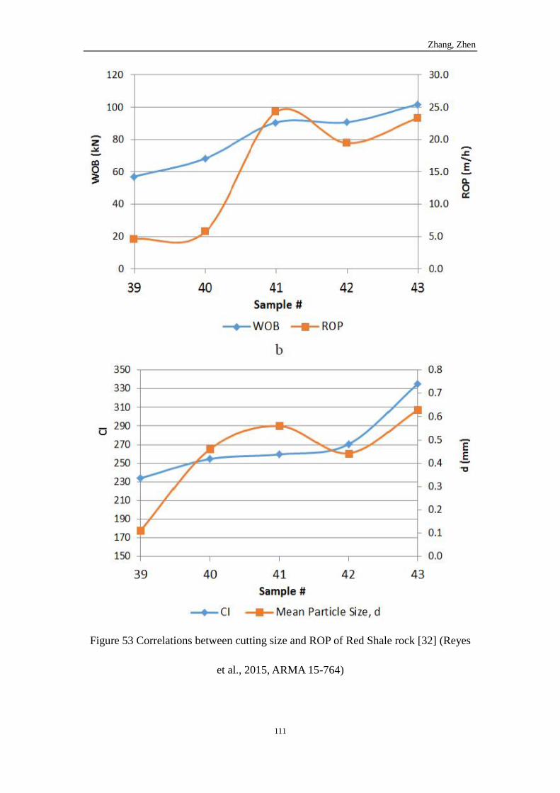
Zhang, Zhen

111

Figure 53 Correlations between cutting size and ROP of Red Shale rock [32] (Reyes

et al., 2015, ARMA 15-764)

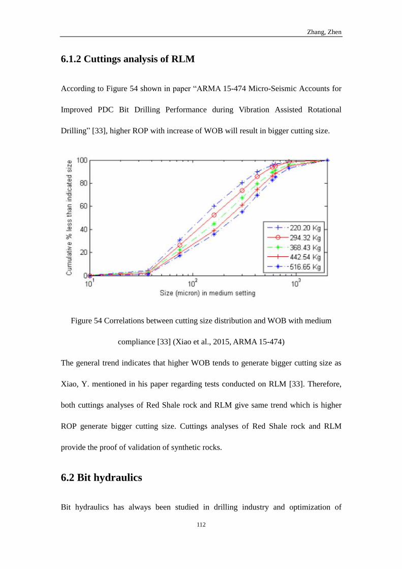
Zhang, Zhen

112

6.1.2 Cuttings analysis of RLM

According to Figure 54 shown in paper “ARMA 15-474 Micro-Seismic Accounts for

Improved PDC Bit Drilling Performance during Vibration Assisted Rotational

Drilling” [33], higher ROP with increase of WOB will result in bigger cutting size.

Figure 54 Correlations between cutting size distribution and WOB with medium

compliance [33] (Xiao et al., 2015, ARMA 15-474)

The general trend indicates that higher WOB tends to generate bigger cutting size as

Xiao, Y. mentioned in his paper regarding tests conducted on RLM [33]. Therefore,

both cuttings analyses of Red Shale rock and RLM give same trend which is higher

ROP generate bigger cutting size. Cuttings analyses of Red Shale rock and RLM

provide the proof of validation of synthetic rocks.

6.2 Bit hydraulics

Bit hydraulics has always been studied in drilling industry and optimization of

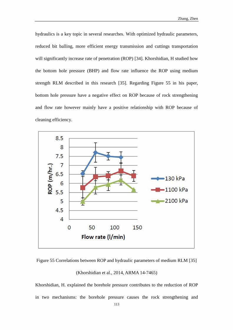
Zhang, Zhen

113

hydraulics is a key topic in several researches. With optimized hydraulic parameters,

reduced bit balling, more efficient energy transmission and cuttings transportation

will significantly increase rate of penetration (ROP) [34]. Khorshidian, H studied how

the bottom hole pressure (BHP) and flow rate influence the ROP using medium

strength RLM described in this research [35]. Regarding Figure 55 in his paper,

bottom hole pressure have a negative effect on ROP because of rock strengthening

and flow rate however mainly have a positive relationship with ROP because of

cleaning efficiency.

Figure 55 Correlations between ROP and hydraulic parameters of medium RLM [35]

(Khorshidian et al., 2014, ARMA 14-7465)

Khorshidian, H. explained the borehole pressure contributes to the reduction of ROP

in two mechanisms: the borehole pressure causes the rock strengthening and

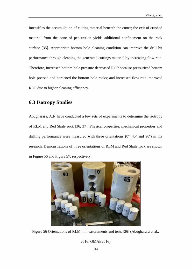
Zhang, Zhen

114

intensifies the accumulation of cutting material beneath the cutter; the exit of crushed

material from the zone of penetration yields additional confinement on the rock

surface [35]. Appropriate bottom hole cleaning condition can improve the drill bit

performance through cleaning the generated cuttings material by increasing flow rate.

Therefore, increased bottom hole pressure decreased ROP because pressurized bottom

hole pressed and hardened the bottom hole rocks; and increased flow rate improved

ROP due to higher cleaning efficiency.

6.3 Isotropy Studies

Abugharara, A.N have conducted a few sets of experiments to determine the isotropy

of RLM and Red Shale rock [36, 37]. Physical properties, mechanical properties and

drilling performance were measured with three orientations (0º, 45º and 90º) in his

research. Demonstrations of three orientations of RLM and Red Shale rock are shown

in Figure 56 and Figure 57, respectively.

Figure 56 Orientations of RLM in measurements and tests [36] (Abugharara et al.,

2016, OMAE2016)

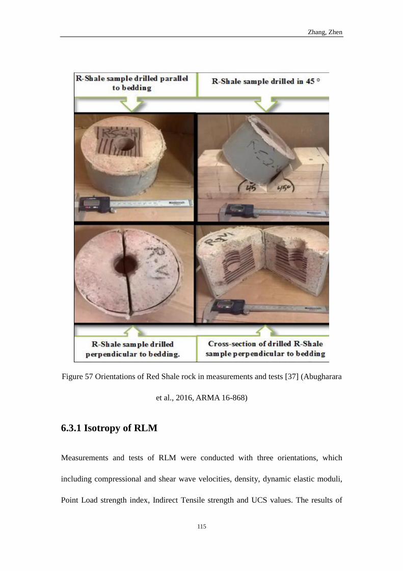
Zhang, Zhen

115

Figure 57 Orientations of Red Shale rock in measurements and tests [37] (Abugharara

et al., 2016, ARMA 16-868)

6.3.1 Isotropy of RLM

Measurements and tests of RLM were conducted with three orientations, which

including compressional and shear wave velocities, density, dynamic elastic moduli,

Point Load strength index, Indirect Tensile strength and UCS values. The results of

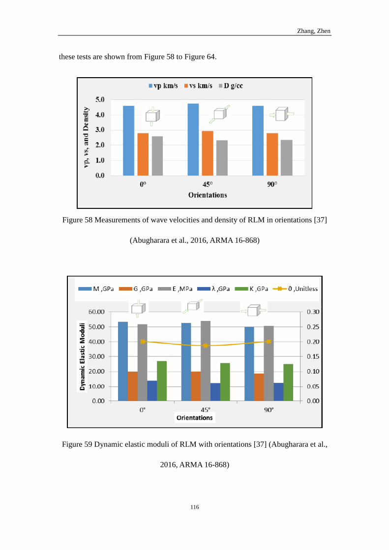
Zhang, Zhen

116

these tests are shown from Figure 58 to Figure 64.

Figure 58 Measurements of wave velocities and density of RLM in orientations [37]

(Abugharara et al., 2016, ARMA 16-868)

Figure 59 Dynamic elastic moduli of RLM with orientations [37] (Abugharara et al.,

2016, ARMA 16-868)

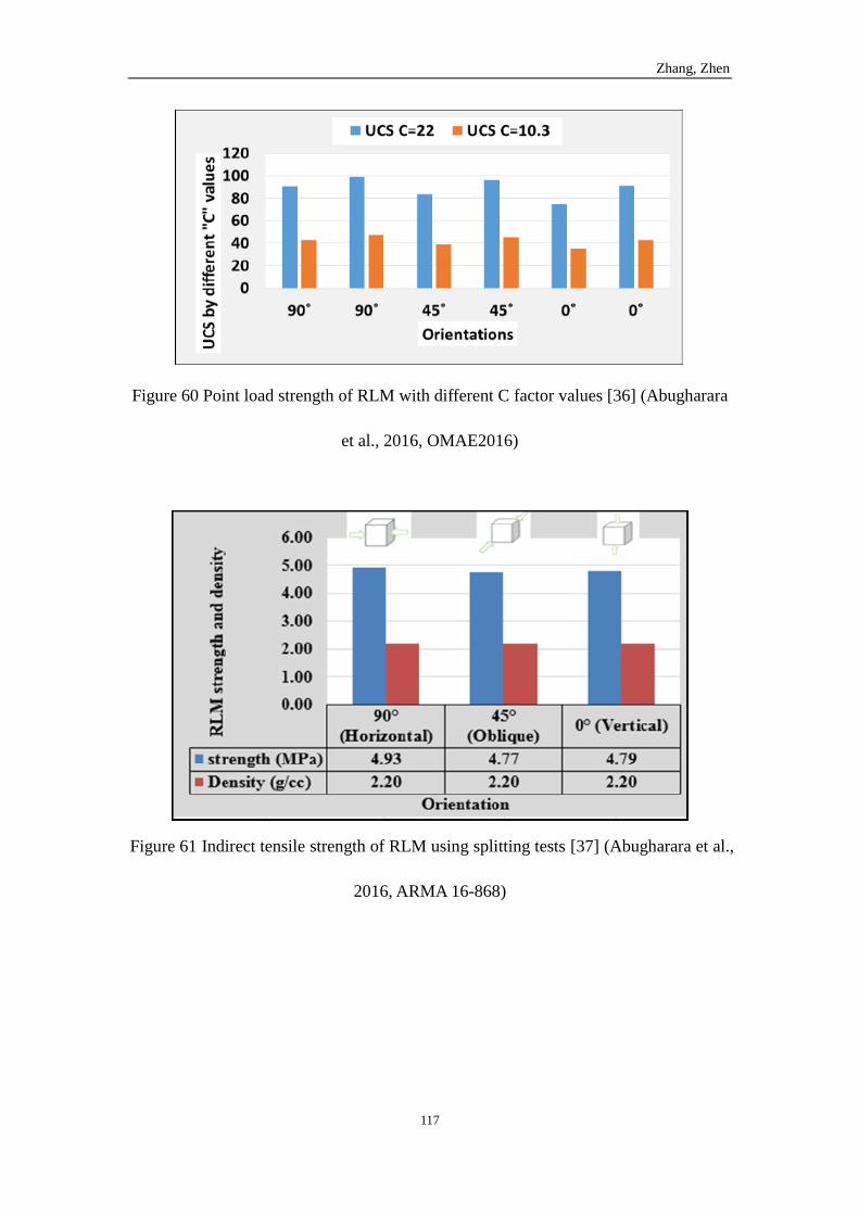
Zhang, Zhen

117

Figure 60 Point load strength of RLM with different C factor values [36] (Abugharara

et al., 2016, OMAE2016)

Figure 61 Indirect tensile strength of RLM using splitting tests [37] (Abugharara et al.,

2016, ARMA 16-868)

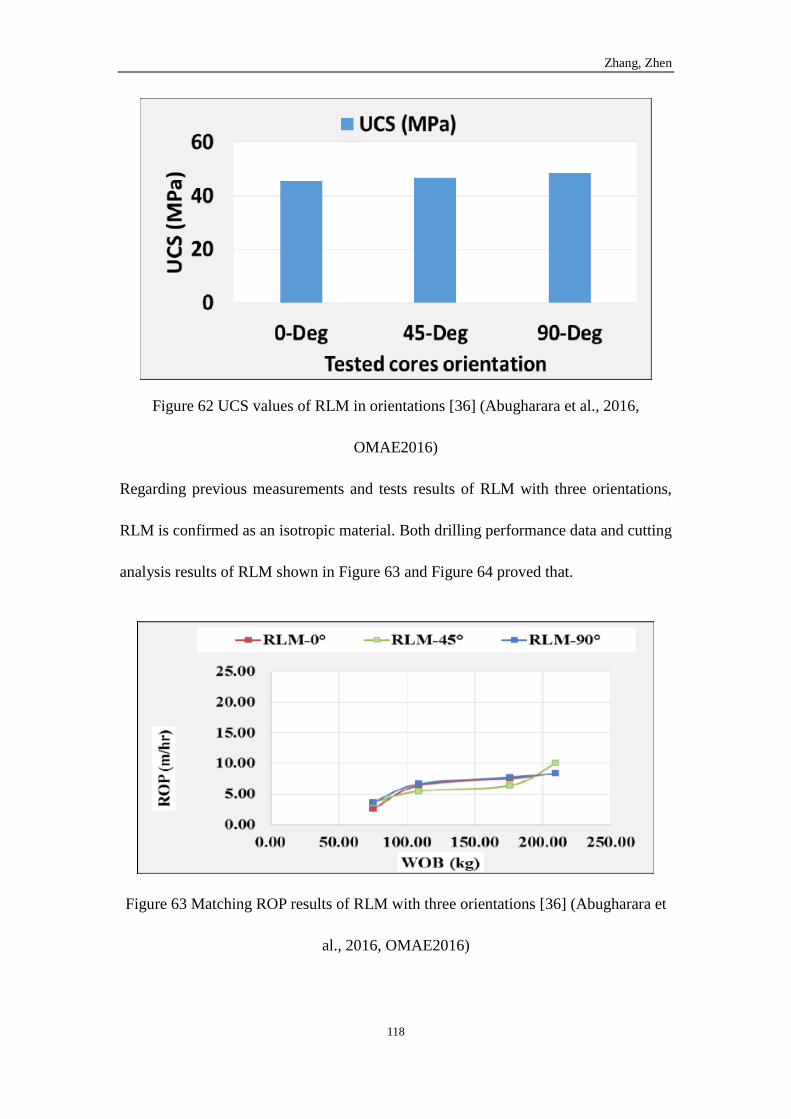
Zhang, Zhen

118

Figure 62 UCS values of RLM in orientations [36] (Abugharara et al., 2016,

OMAE2016)

Regarding previous measurements and tests results of RLM with three orientations,

RLM is confirmed as an isotropic material. Both drilling performance data and cutting

analysis results of RLM shown in Figure 63 and Figure 64 proved that.

Figure 63 Matching ROP results of RLM with three orientations [36] (Abugharara et

al., 2016, OMAE2016)

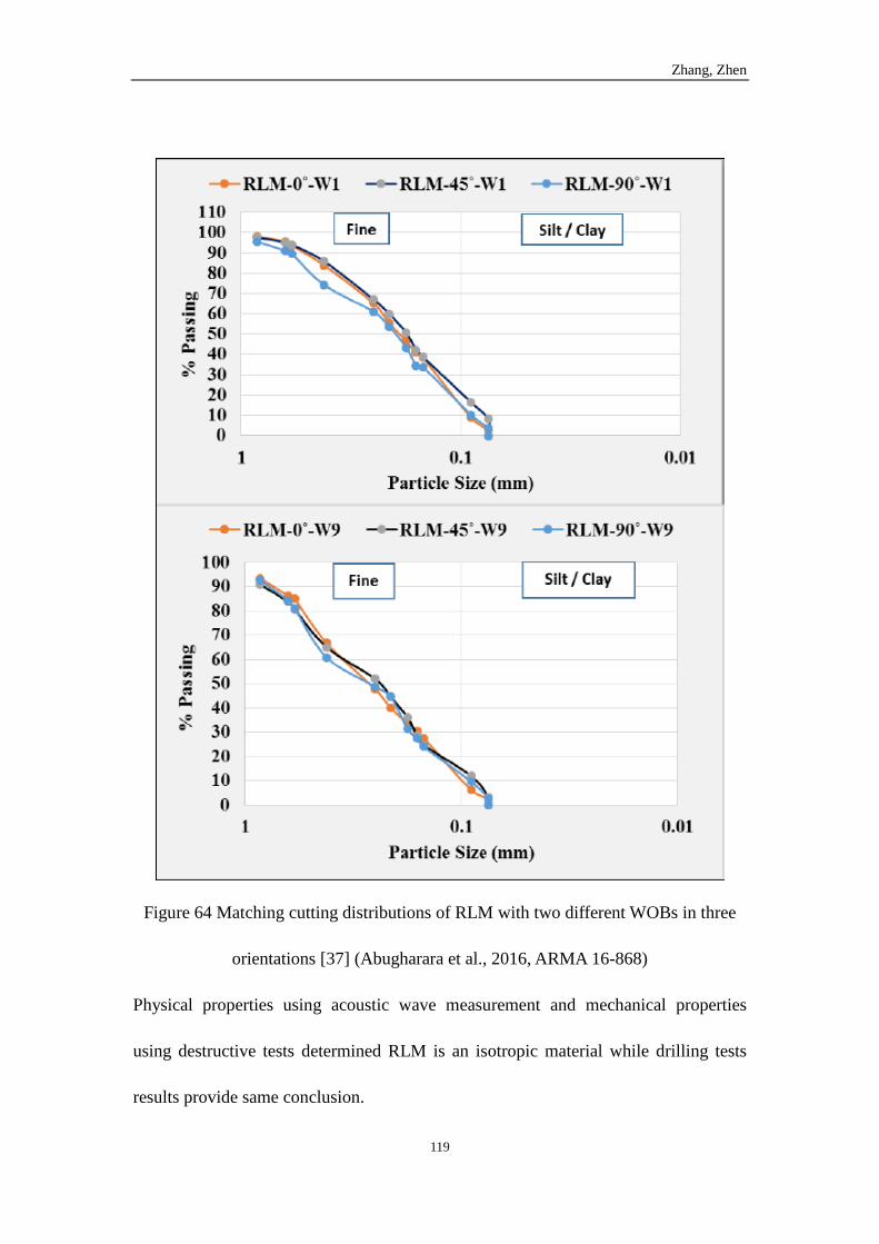
Zhang, Zhen

119

Figure 64 Matching cutting distributions of RLM with two different WOBs in three

orientations [37] (Abugharara et al., 2016, ARMA 16-868)

Physical properties using acoustic wave measurement and mechanical properties

using destructive tests determined RLM is an isotropic material while drilling tests

results provide same conclusion.

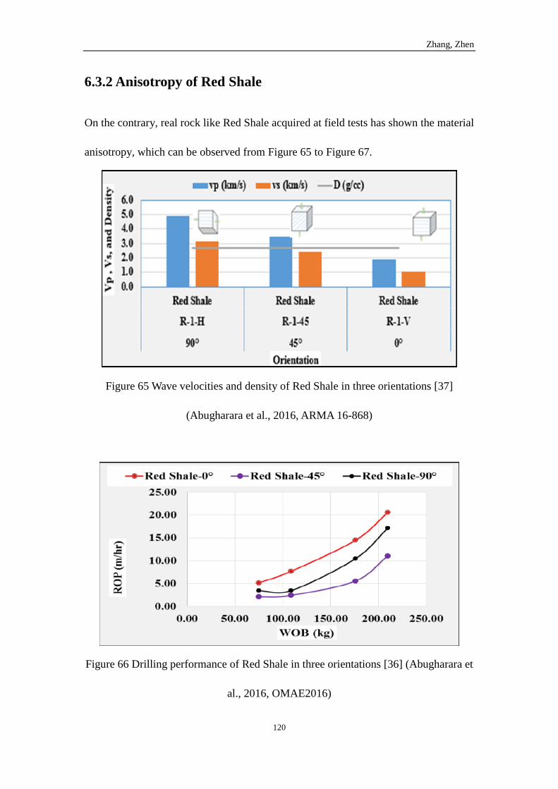
Zhang, Zhen

120

6.3.2 Anisotropy of Red Shale

On the contrary, real rock like Red Shale acquired at field tests has shown the material

anisotropy, which can be observed from Figure 65 to Figure 67.

Figure 65 Wave velocities and density of Red Shale in three orientations [37]

(Abugharara et al., 2016, ARMA 16-868)

Figure 66 Drilling performance of Red Shale in three orientations [36] (Abugharara et

al., 2016, OMAE2016)

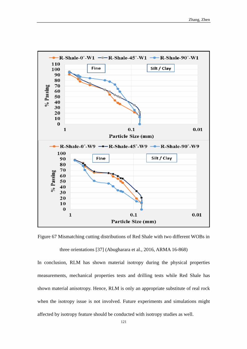
Zhang, Zhen

121

Figure 67 Mismatching cutting distributions of Red Shale with two different WOBs in

three orientations [37] (Abugharara et al., 2016, ARMA 16-868)

In conclusion, RLM has shown material isotropy during the physical properties

measurements, mechanical properties tests and drilling tests while Red Shale has

shown material anisotropy. Hence, RLM is only an appropriate substitute of real rock

when the isotropy issue is not involved. Future experiments and simulations might

affected by isotropy feature should be conducted with isotropy studies as well.

Zhang, Zhen

122

7. Conclusions and Future Work

In this research, concrete mixes using only fine aggregate (plus Portland Cement,

water and appropriate additives) have been developed. These mixes are aimed at a

low strength (19 MPa), medium strength (56 MPa) and high strength (84 MPa), to be

used as synthetic rock - also referred to as Rock Like Materials (RLM) have been

successfully designed to meet the requirements for lab tests. Repeatability and

reproducibility studies have demonstrated the consistency of three types of RLM. In

this respect, as well as in cost, these RLM are expected to be a useful stand-in for real

rock of similar strengths, particularly sedimentary rocks such as limestone and shale.

Standard procedures of making these samples have been established. If any other

strength value of concrete for this purpose needs to be designed in the future, it should

be possible derive that from these mixes.

Eight parameters tests have been conducted on samples of these RLM at all three

strengths. The three concretes are expected to be useful simulations in laboratory

studies. However, as the same ingredients, fine aggregate and cement, were used in

making the concrete RLM, properties such as grain size and quartz content are the

same in all three forms of RLM developed. This is one limitation of this synthetic

rock. Nevertheless, research in this thesis provided standard procedures for testing the

eight parameters recommended by Prasad [1] for evaluating drillability, including

determination of fundamental physical properties of all three strengths of the RLM.

Zhang, Zhen

123

Quality assurance, standard procedures of making concrete samples and the eight

parameter tests used will provide guidelines for future experimental work using

designed concrete samples. In a word, future experimental tests in the lab will benefit

from the data acquired in this research.

The drilling performance of the RLM was compared with that of shale. Both cuttings

analysis and bit hydraulics have shown promising results, indicating that RLM can be

a successful substitute of shale rock, though, as determined by Abugharara et.al. [36,

37] RLM is an isotropic material and Red Shale rock is an anisotropic material, and

this difference must be taken into account.

In this research, physico-mechanical and micro-structural properties of designed

synthetic rocks were investigated based on the methods proposed by Prasad [1]. All

the test methods are designed for the real rocks and were modified to be suitable for

concrete. Therefore, the same tests should be conducted in the future on real

sedimentary rocks, as well as on RLM, and compared. This could facilitate further

progress in investigating rock properties related to the drilling process.

Zhang, Zhen

124

Reference

1 Prasad, U. (2009). Drillability of a Rock in Terms of its Physico-Mechanical and

Micro-Structural Properties. The Woodlands: ARMA.

2 Neville, A. M. (1996). Properties of aggregate, Properties of Concrete (Fourth

Edition, pp. 149-154). New York, NY: John Wiley & Sons, Inc.

3 Neville, A. M. (1996). Properties of concrete, Properties of Concrete (Fourth


4 Neville, A. M. (1996). Strength of concrete, Properties of Concrete (Fourth


5 Holcim (US) Inc. (2007, October). Common Work Results for Concrete.

Retrieved from

http://www.cmdgroup.com/documents/FS/specdata/030500_10032334_01_SD_22

406.pdf

6 WRDA® 82 Water-reducing admixture ASTM C494 Type A and D. (2010,

October). Retrieved from

https://grace.com/construction/en-us/Documents/DW-8J-WRDA-82.pdf

7 DARACEM® 19 High-range water-reducing admixture ASTM C494 Type A and F,

and ASTM C1017 Type I. (2011, July). Retrieved from

https://grace.com/construction/en-us/Documents/DC-8I_Daracem_19_11_14_07.p

df

8 FORCE 10,000® D High performance concrete admixture dry densified powder.

Zhang, Zhen

125

(2011, November). Retrieved from

https://grace.com/construction/en-us/Documents/FT-26I-F10K-D.pdf

9 Aitcin, P. -C. (1998). Materials selection, High-Performance Concrete (pp. 194).

New York, NY: Routledge.

10 Neville, A. M. (1996). Concretes with particular properties, Properties of

Concrete (Fourth Edition, pp. 667-669). New York, NY: John Wiley & Sons, Inc.

11 Reddish, D.J., and Yasar, E. (1996). A New Portable Rock Strength Index Test

Based on Specific Energy of Drilling. Great British. J. Rock Mech. Mining Sci. &

Geomechanics Abstracts, vol. 33, no. 5, 543-548.

12 Khan, M. I. A Novel Method for Measuring Porosity of High Strength Concrete.

7th Saudi Engineering Conference.

13 Fjaer, E., Holt, R. M., Horsrud, P., Raaen, A. M. & Risnes, R. (2008). Elastic wave

propagation in rocks, Petroleum Related Rock Mechanics (2nd Edition, pp.

177-180). Amsterdam, Elsevier.

14 Fjaer, E., Holt, R. M., Horsrud, P., Raaen, A. M. & Risnes, R. (2008). Elasticity,

Petroleum Related Rock Mechanics (2nd Edition, pp. 20-23). Amsterdam,

Elsevier.

15 Nazir, R., Momeni, E., Armaghani, D. J. & Amin, M. M. (2013). Correlation

between Unconfined Compressive Strength and Indirect Tensile Strength of

Limestone Rock Samples. EJGE, 18, 1737-1746.

16 Prikryl, R. (2001). Some Microstructural Aspects of Strength Variation in Rocks.

International Journal of Rock Mechanics & Mining Sciences, 38, 671-682.

Zhang, Zhen

126

17 Ersoy, A., Waller, M. D. (1995). Textural Characterization of Rocks. Engineering

Geology, 39, 123-136.

18 ASTM Standard C136-01. (2001). Standard Test Method for Sieve Analysis of

Fine and Coarse Aggregates. West Conshohocken: ASTM International.

19 Neville, A. M. (1996). Fresh concrete, Properties of Concrete (Fourth Edition, pp.

229-231). New York, NY: John Wiley & Sons, Inc.

20 ASTM Standard D4543-08. (2015). Standard Practices for Preparing Rock Core

as Cylindrical Test Specimens and Verifying Conformance to Dimensional and

Shape Tolerances. West Conshohocken: ASTM International.

21 Lau, A. T. (n.d.) What Are Repeatability and Reproducibility? Retrieved from

http://www.astm.org/SNEWS/MA_2009/datapoints_ma09.html

22 ASTM Standard E177-14. (2015). Standard Practice for Use of the Terms

Precision and Bias in ASTM Test Methods. West Conshohocken: ASTM

International.

23 Bartlett, J. W. and Frost, C. (2008). Reliability, Repeatability and Reproducibility:

Analysis of Measurement Errors in Continuous Variables. Ultrasound Obstet

Gynecol, 31, 466–475.

24 Standard deviation, (n.d.) Retrieved from

https://en.wikipedia.org/wiki/Standard_deviation

25 Standard error, (n.d.) Retrieved from https://en.wikipedia.org/wiki/Standard_error

26 ASTM Standard C192/C192M-15. (2015). Standard Practice for Making and

Curing Concrete Test Specimens in the Laboratory. West Conshohocken: ASTM

Zhang, Zhen

127

International.

27 Duval, R. and Kadri, E.H. (1998). Influence of Silica Fume on the Workability

and the Compressive Strength of High-Performance Concretes. Cement and

Concrete Research, 28(4), 533-547.

28 ASTM Standard C39/C39M-12a. (2013). Standard Test Method for Compressive

Strength of Cylindrical Concrete Specimens. West Conshohocken: ASTM

International.

29 ASTM Standard D7012-10. (2013). Standard Test Method for Compressive

Strength and Elastic Moduli of Intact Rock Core Specimens under Varying States

of Stress and Temperatures. West Conshohocken: ASTM International.

30 ASTM Standard D2845-08. (2013). Standard Test Method for Laboratory

Determination of Pulse Velocities and Ultrasonic Elastic Constants of Rock. West

Conshohocken: ASTM International.

31 Lenormand, R. and O, Fonta. 2007. Advances in measuring porosity and

permeability from drill cuttings. Reservoir Characterization and Simulation

Conference, Abu Dhabi, 28-30 October 2007, eds. Curran Associates Inc.,

135-143.

32 Reyes, R., Kyzym, I., Rana P.S., Molgaard J. and Butt, S.D. Cuttings Analysis for

Rotary Drilling Penetration Mechanisms and Performance Evaluation. 49th US

Rock Mechanics/Geomechanics Symposium held in San Francisco, CA, USA, 28

June-1 July 2015. ARMA 15-764.

33 Xiao, Y., Zhong, J., Butt, S.D. and Hurich, C. Micro-Seismic Accounts for

Zhang, Zhen

128

Improved PDC Bit Drilling Performance during Vibration Assisted Rotational

Drilling. 49th US Rock Mechanics/Geomechanics Symposium held in San

Francisco, CA, USA, 28 June-1 July 2015. ARMA 15-474.

34 Wells, M., T. Marvel, & C. Beuershausen. (2008). Bit Balling Mitigation in PDC

Bit Design. In IADC/SPE Asia Pacific Drilling Technology Conference and

Exhibition. Society of Petroleum Engineers. January 2008.

35 Khorshidian, H., Butt. S. D. and Arvani. F. Influence of High Velocity Jet on

Drilling Performance of PDC Bit under Pressurized Condition. 48th US Rock

Mechanics/Geomechanics Symposium held in Minneapolis, MN, USA, 1-4 June

2014. ARMA 14-7465.

36 Abugharara, A.N, Alwaar M. A., Butt S.D. and Hurich A. C., Baseline

Development of Rock Anisotropy Investigation Utilizing Empirical Relationships

Between Oriented Physical and Mechanical Measurements and Drilling

Performance. Proceedings of the ASME 2016 35th International Conference on

Ocean, Offshore and Arctic Engineering, Busan, South Korea, June 19-24, 2016.

OMAE2016.

37 Abugharara, A.N, Alwaar M. A., Hurich A. C., and Butt S.D., Laboratory

Investigation on Directional Drilling Performance in Isotropic and Anisotropic

Rocks. 50th US Rock Mechanics / Geomechanics Symposium held in Houston, TX,

CA, USA, 26-29 June 2016. ARMA 16-868.