Embed Size (px)
Citation preview

DEVELOPMENT AND APPLICATION OF REDUCED-ORDER
MODELING PROCEDURES FOR RESERVOIR SIMULATION
A DISSERTATION
SUBMITTED TO THE DEPARTMENT OF ENERGY RESOURCES
ENGINEERING
AND THE COMMITTEE ON GRADUATE STUDIES
OF STANFORD UNIVERSITY
IN PARTIAL FULFILLMENT OF THE REQUIREMENTS
FOR THE DEGREE OF
DOCTOR OF PHILOSOPHY
Marco Antonio Cardoso
March 2009

c© Copyright by Marco Antonio Cardoso 2009
All Rights Reserved
ii

I certify that I have read this dissertation and that, in my opinion, it is fully
adequate in scope and quality as a dissertation for the degree of Doctor of
Philosophy.
(Louis J. Durlofsky) Principal Adviser
I certify that I have read this dissertation and that, in my opinion, it is fully
adequate in scope and quality as a dissertation for the degree of Doctor of
Philosophy.
(Hamdi Tchelepi)
I certify that I have read this dissertation and that, in my opinion, it is fully
adequate in scope and quality as a dissertation for the degree of Doctor of
Philosophy.
(Pallav Sarma)
Approved for the University Committee on Graduate Studies.
iii

iv

Abstract
Subsurface flow modeling is essential for understanding and managing many energy-related
processes, including oil production and the geological storage of carbon dioxide. Some appli-
cations, particularly those involving optimization of field performance, are very demanding
computationally due to the large number of flow simulations that must be performed and
the typically large dimension of the simulation models. In this work, reduced-order mod-
eling (ROM) techniques are developed for subsurface flow modeling and applied to reduce
the simulation time of subsurface flow models. The two ROM procedures considered are
proper orthogonal decomposition (POD) and trajectory piecewise linearization (TPWL).
Proper orthogonal decomposition is a commonly used ROM technique that can be ap-
plied for nonlinear problems. In the POD procedure a full (high-fidelity) simulation is run,
solution snapshots for the pressure and saturation states are stored, and singular value
decomposition (SVD) is performed on the resulting data matrix. This provides a reduced
basis which is used to project the solution into a low-dimensional subspace. Using this basis,
we need only solve for a reduced set of unknowns. We extend the standard POD approach
by incorporating a clustering technique and a missing point estimation (MPE) procedure.
These act to reduce the number of columns and rows in the basis matrix. The ROM proce-
dure is implemented into Stanford’s general purpose research simulator (GPRS). Extensive
flow simulations involving water injection into a geologically complex 3D oil reservoir model
containing 60,000 grid blocks are performed. The numerical solutions demonstrate that the
POD-based ROM procedure can accurately reproduce the reference simulations over a rea-
sonable range of control settings and provide speedups of up to an order of magnitude when
compared with the high-fidelity model simulated using an optimized solver.
In an attempt to achieve significantly greater speedups, a trajectory piecewise lineariza-
tion (TPWL) procedure for the reduced-order modeling of two-phase flow in subsurface
formations is formulated. The method represents new pressure and saturation states using
v

linear expansions around states previously simulated and saved during a series of preprocess-
ing training runs. The linearized representation is projected into a low-dimensional space,
with the projection matrix constructed using the reduced POD basis. The TPWL method
is applied to heterogeneous reservoir models and extensive test simulations are performed.
It is shown that the TPWL approach provides accurate results when the controls (bottom
hole pressures of the production wells) applied in test simulations are within the general
range of the controls employed in the training runs, even though the well pressure schedules
for the test runs can differ significantly from those of the training simulations. Runtime
speedups using the procedure are very significant - a factor of 2 – 3 orders of magnitude
(depending on model size and whether or not mass balance error is computed at every time
step) for the cases considered.
Finally, the TPWL representations are used in several optimizations involving the de-
termination of optimal bottom hole pressures for producer wells. Three different geological
models are considered. Both gradient-based and generalized pattern search optimization
algorithms are considered for one model; for the other two models only the gradient-based
algorithm is applied. Results for optimized net present value (NPV) using TPWL are shown
to be in consistently close agreement with that computed using high-fidelity simulations.
Most significantly, when the optimal well settings obtained using TPWL are applied in
high-fidelity models, the resulting NPVs are within 0.7% of the values determined using
the high-fidelity simulations. Additionally, the TPWL procedure is applied to a compu-
tationally demanding multiobjective optimization problem, for which the Pareto front is
determined. Limited high-fidelity simulations demonstrate the accuracy and applicability
of TPWL for this challenging problem.
vi

Acknowledgements
First of all I would like to state my sincere gratitude to my advisor Professor Louis J.
Durlofsky. Lou provided me with many insightful suggestions, important advice, constant
encouragement and great discussions during the course of this work. Thanks are also due to
Dr. Pallav Sarma and Professors Hamdi Tchelepi, Margot Gerritsen and Biondo Biondi for
serving on my thesis committee. I also would like to thank all the faculty, students and staff
of the Department of Energy Resources Engineering for being so helpful during all these
years. I would like to thank my parents, brothers and sister for their encouragement and
support during my time at Stanford. I would like to acknowledge the company that I work
for, PETROBRAS, for this opportunity and financial support during my Ph.D. program.
I am grateful to Pallav Sarma for implementing the POD-based reduced-order modeling
procedure in Stanford’s general purpose research simulator (GPRS), to Huanquan Pan
for modifying GPRS to output the information required by the TPWL representation,
and to David Echeverria Ciaurri for useful discussions and suggestions regarding Matlab
optimization routines.
To my wife Rosana and our wonderful daughter Mariana, all I can say is that your
endless patience, love and encouragement have supported me when it was most required.
I am also grateful to Odonel and Val for their several journeys from Brazil to Stanford to
spend a couple of pleasant weeks with us.
vii

viii

Contents
Abstract v
Acknowledgements vii
1 Introduction and Literature Review 1
1.1 Literature Review . . . . . . . . . . . . . . . . . . . . . . . . . . . . . . . . 2
1.1.1 General Overview of Reduced-Order Modeling Procedures . . . . . . 2
1.1.2 POD for Subsurface Flow . . . . . . . . . . . . . . . . . . . . . . . . 6
1.1.3 Enhanced POD . . . . . . . . . . . . . . . . . . . . . . . . . . . . . . 8
1.1.4 Trajectory Piecewise Linearization . . . . . . . . . . . . . . . . . . . 10
1.1.5 Optimization of Reservoir Performance . . . . . . . . . . . . . . . . 12
1.2 Scope of this Work . . . . . . . . . . . . . . . . . . . . . . . . . . . . . . . . 14
1.3 Dissertation Outline . . . . . . . . . . . . . . . . . . . . . . . . . . . . . . . 15
2 ROM of Subsurface Flow Using POD 19
2.1 Modeling Procedure . . . . . . . . . . . . . . . . . . . . . . . . . . . . . . . 19
2.1.1 Oil-Water Flow Equations and Discretization . . . . . . . . . . . . . 20
2.1.2 Proper Orthogonal Decomposition . . . . . . . . . . . . . . . . . . . 23
2.1.3 Reduced-Order Oil-Water Reservoir Model . . . . . . . . . . . . . . 26
2.1.4 Clustering Snapshots . . . . . . . . . . . . . . . . . . . . . . . . . . . 26
2.1.5 Missing Point Estimation . . . . . . . . . . . . . . . . . . . . . . . . 28
2.1.6 Implementation in General Purpose Research Simulator . . . . . . . 30
2.2 Simulation Using Reduced-Order Modeling . . . . . . . . . . . . . . . . . . 33
2.2.1 Prediction Using ROM - Schedule I . . . . . . . . . . . . . . . . . . 43
2.2.2 Prediction Using ROM - Schedule II . . . . . . . . . . . . . . . . . . 47
ix

2.2.3 Simulation Time Reduction with ROMs . . . . . . . . . . . . . . . . 51
2.2.4 Comparison of ROMs with ILU(0) Preconditioner . . . . . . . . . . 52
2.2.5 Quantification of Error Using ROMs . . . . . . . . . . . . . . . . . . 53
2.3 Further Observations . . . . . . . . . . . . . . . . . . . . . . . . . . . . . . . 56
3 Trajectory Piecewise Linearization 63
3.1 TPWL for Subsurface Flow . . . . . . . . . . . . . . . . . . . . . . . . . . . 63
3.1.1 Linearization of Governing Equations . . . . . . . . . . . . . . . . . 64
3.1.2 Construction of the POD Basis Matrix . . . . . . . . . . . . . . . . . 66
3.1.3 TPWL Representation with POD Basis Matrix . . . . . . . . . . . . 66
3.1.4 Implementation Issues . . . . . . . . . . . . . . . . . . . . . . . . . . 69
3.2 Simulation Results Using TPWL Procedure . . . . . . . . . . . . . . . . . . 70
3.2.1 Reservoir Model 1 . . . . . . . . . . . . . . . . . . . . . . . . . . . . 70
3.2.2 Reservoir Model 2 . . . . . . . . . . . . . . . . . . . . . . . . . . . . 86
3.3 Additional Issues . . . . . . . . . . . . . . . . . . . . . . . . . . . . . . . . . 91
4 Optimization Using TPWL 93
4.1 Optimization Problem 1 . . . . . . . . . . . . . . . . . . . . . . . . . . . . . 94
4.1.1 Description of the Simulation Model . . . . . . . . . . . . . . . . . . 94
4.1.2 Training and Testing Results Using TPWL . . . . . . . . . . . . . . 95
4.1.3 Optimization Procedures . . . . . . . . . . . . . . . . . . . . . . . . 101
4.1.4 Results for Optimization Case 1 . . . . . . . . . . . . . . . . . . . . 102
4.1.5 Results for Optimization Case 2 . . . . . . . . . . . . . . . . . . . . 104
4.2 Optimization Problem 2 . . . . . . . . . . . . . . . . . . . . . . . . . . . . . 106
4.2.1 Results for Optimization Case 1 . . . . . . . . . . . . . . . . . . . . 106
4.2.2 Results for Optimization Case 2 . . . . . . . . . . . . . . . . . . . . 108
4.3 Optimization Problem 3 . . . . . . . . . . . . . . . . . . . . . . . . . . . . . 110
4.3.1 Results for Optimization Case 1 . . . . . . . . . . . . . . . . . . . . 110
4.3.2 Results for Optimization Case 2 . . . . . . . . . . . . . . . . . . . . 112
4.4 Multiobjective Optimization . . . . . . . . . . . . . . . . . . . . . . . . . . . 114
5 Summary and Future Work 117
5.1 Summary and Conclusions . . . . . . . . . . . . . . . . . . . . . . . . . . . . 117
5.2 Recommendations for Future Work . . . . . . . . . . . . . . . . . . . . . . . 120
x

Nomenclature 123
Bibliography 127
xi

xii

List of Tables
2.1 Errors in the oil rate for the various ROMs . . . . . . . . . . . . . . . . . . 54
2.2 Errors in the water production rate for the various ROMs . . . . . . . . . . 54
2.3 Errors in the water injection rate for the various ROMs . . . . . . . . . . . 55
3.1 Errors in TPWL solutions for tests A–E . . . . . . . . . . . . . . . . . . . . 83
3.2 Errors in TPWL solutions for tests F–H . . . . . . . . . . . . . . . . . . . . 85
3.3 Errors in TPWL solutions for tests I–M . . . . . . . . . . . . . . . . . . . . 91
4.1 NPV ($106) for problem 1, case 1 (oil $80/stb, produced and injected water
$15/stb) . . . . . . . . . . . . . . . . . . . . . . . . . . . . . . . . . . . . . . 103
4.2 NPV ($106) for problem 1, case 2 (oil $60/stb, produced water $30/stb and
injected water $3/stb) . . . . . . . . . . . . . . . . . . . . . . . . . . . . . . 104
4.3 NPV ($106) for problem 2, case 1 (oil $80/stb, produced and injected water
$10/stb) . . . . . . . . . . . . . . . . . . . . . . . . . . . . . . . . . . . . . . 107
4.4 NPV ($106) for problem 2, case 2 (oil $60/stb, produced water $15/stb and
injected water $5/stb) . . . . . . . . . . . . . . . . . . . . . . . . . . . . . . 108
4.5 NPV ($106) for problem 3, case 1 (oil $80/stb, produced and injected water
$15/stb) . . . . . . . . . . . . . . . . . . . . . . . . . . . . . . . . . . . . . . 110
4.6 NPV ($106) for problem 3, case 2 (oil $60/stb, produced water $20/stb and
injected water $2/stb) . . . . . . . . . . . . . . . . . . . . . . . . . . . . . . 112
xiii

xiv

List of Figures
2.1 Portion of a one-dimensional grid . . . . . . . . . . . . . . . . . . . . . . . . 21
2.2 Flow chart for the off-line portion of the ROM . . . . . . . . . . . . . . . . 31
2.3 Flow chart for the in-line portion of the ROM . . . . . . . . . . . . . . . . . 32
2.4 Synthetic three-dimensional reservoir model with five production wells and
four injection wells . . . . . . . . . . . . . . . . . . . . . . . . . . . . . . . . 33
2.5 Permeability in x-direction for all 8 layers . . . . . . . . . . . . . . . . . . . 34
2.6 Relative permeability curves for the oil and water phases . . . . . . . . . . . 35
2.7 Schedule for bottom hole pressures for the production wells . . . . . . . . . 35
2.8 Eigenvalue variation for pressure and saturation matrices . . . . . . . . . . 36
2.9 Six most important reduced-order basis functions for the oil pressure state
(layer 1) . . . . . . . . . . . . . . . . . . . . . . . . . . . . . . . . . . . . . . 37
2.10 Six most important reduced-order basis functions for the water saturation
state (layer 1) . . . . . . . . . . . . . . . . . . . . . . . . . . . . . . . . . . . 38
2.11 Grid blocks selected (in black) by MPE procedure . . . . . . . . . . . . . . 39
2.12 Oil and water flow rates for production well 1 (training run) . . . . . . . . . 40
2.13 Oil and water flow rates for production well 2 (training run) . . . . . . . . . 40
2.14 Oil and water flow rates for production well 3 (training run) . . . . . . . . . 41
2.15 Oil and water flow rates for production well 4 (training run) . . . . . . . . . 41
2.16 Oil and water flow rates for production well 5 (training run) . . . . . . . . . 41
2.17 Water flow rate for injection well 1 (training run) . . . . . . . . . . . . . . . 42
2.18 Water flow rate for injection well 2 (training run) . . . . . . . . . . . . . . . 42
2.19 Water flow rate for injection well 3 (training run) . . . . . . . . . . . . . . . 42
2.20 Water flow rate for injection well 4 (training run) . . . . . . . . . . . . . . . 43
2.21 Bottom hole pressure for the production wells using schedule I . . . . . . . 44
2.22 Oil and water flow rates for production well 1 (schedule I) . . . . . . . . . . 44
xv

2.23 Oil and water flow rates for production well 2 (schedule I) . . . . . . . . . . 44
2.24 Oil and water flow rates for production well 3 (schedule I) . . . . . . . . . . 45
2.25 Oil and water flow rates for production well 4 (schedule I) . . . . . . . . . . 45
2.26 Oil and water flow rates for production well 5 (schedule I) . . . . . . . . . . 45
2.27 Water flow rate for injection well 1 (schedule I) . . . . . . . . . . . . . . . . 46
2.28 Water flow rate for injection well 2 (schedule I) . . . . . . . . . . . . . . . . 46
2.29 Water flow rate for injection well 3 (schedule I) . . . . . . . . . . . . . . . . 46
2.30 Water flow rate for injection well 4 (schedule I) . . . . . . . . . . . . . . . . 47
2.31 Bottom hole pressure for the producer wells using schedule II . . . . . . . . 48
2.32 Oil and water flow rates for production well 1 (schedule II) . . . . . . . . . 48
2.33 Oil and water flow rates for production well 2 (schedule II) . . . . . . . . . 48
2.34 Oil and water flow rates for production well 3 (schedule II) . . . . . . . . . 49
2.35 Oil and water flow rates for production well 4 (schedule II) . . . . . . . . . 49
2.36 Oil and water flow rates for production well 5 (schedule II) . . . . . . . . . 49
2.37 Water flow rate for injection well 1 (schedule II) . . . . . . . . . . . . . . . 50
2.38 Water flow rate for injection well 2 (schedule II) . . . . . . . . . . . . . . . 50
2.39 Water flow rate for injection well 3 (schedule II) . . . . . . . . . . . . . . . 50
2.40 Water flow rate for injection well 4 (schedule II) . . . . . . . . . . . . . . . 51
2.41 Comparison of simulation time . . . . . . . . . . . . . . . . . . . . . . . . . 52
2.42 Comparison of simulation time for schedule I using full model with ILU(0)
and CPR preconditioners and ROM . . . . . . . . . . . . . . . . . . . . . . 53
2.43 Tradoff between speedup and accuracy for the training simulation . . . . . 57
2.44 Original and modified relative permeability curves . . . . . . . . . . . . . . 58
2.45 Eigenvalue variation for pressure and saturation for models with density dif-
ferences . . . . . . . . . . . . . . . . . . . . . . . . . . . . . . . . . . . . . . 59
2.46 Eigenvalue variation for pressure for 20,400-cell models with density differences 60
2.47 Eigenvalue variation for saturation for 20,400-cell models with density differ-
ences . . . . . . . . . . . . . . . . . . . . . . . . . . . . . . . . . . . . . . . . 61
3.1 Synthetic reservoir model (24,000 grid blocks) with four production wells and
two injection wells. Permeability in x-direction (in mD) is shown . . . . . . 71
3.2 Producer BHP schedules for training run 2 . . . . . . . . . . . . . . . . . . 73
3.3 Producer BHP schedules for training run 3 . . . . . . . . . . . . . . . . . . 73
xvi

3.4 Producer BHP schedules for training run 4 . . . . . . . . . . . . . . . . . . 73
3.5 Oil rate for each production well for training run 2 . . . . . . . . . . . . . . 74
3.6 Water rate for each production well for training run 2 . . . . . . . . . . . . 74
3.7 Injection rate for each injection well for training run 2 . . . . . . . . . . . . 74
3.8 Producer BHP schedules for test A . . . . . . . . . . . . . . . . . . . . . . . 75
3.9 Producer BHP schedules for test E . . . . . . . . . . . . . . . . . . . . . . . 76
3.10 Producer BHP schedules for training run 2 and tests F–H for well P1 . . . . 76
3.11 Producer BHP schedules for training run 2 and tests F–H for well P4 . . . . 76
3.12 Test F: BHP schedules for all production wells . . . . . . . . . . . . . . . . 77
3.13 Test H: BHP schedules for all production wells . . . . . . . . . . . . . . . . 77
3.14 Test C: BHP schedules for all production wells . . . . . . . . . . . . . . . . 79
3.15 Results for test C: Oil rate for each production well . . . . . . . . . . . . . . 79
3.16 Results for test C: Water rate for each production well . . . . . . . . . . . . 80
3.17 Results for test C: Injection rate for each injection well . . . . . . . . . . . . 80
3.18 Results for test E: Oil rate for each production well . . . . . . . . . . . . . . 81
3.19 Results for test E: Water rate for each production well . . . . . . . . . . . . 82
3.20 Results for test E: Injection rate for each injection well . . . . . . . . . . . . 82
3.21 Test G: BHP schedules for all production wells . . . . . . . . . . . . . . . . 83
3.22 Results for test G: Oil rate for each production well . . . . . . . . . . . . . 84
3.23 Results for test G: Water rate for each production well . . . . . . . . . . . . 84
3.24 Results for test G: Injection rate for each injection well . . . . . . . . . . . . 84
3.25 Errors in the TPWL simulations for different numbers of basis functions . . 86
3.26 Synthetic reservoir model containing 79,200 grid blocks with four production
wells and two injection wells. Permeability in x-direction (in mD) is shown 87
3.27 Producer BHP schedules for training run 2 . . . . . . . . . . . . . . . . . . 88
3.28 Producer BHP schedules for training run 3 . . . . . . . . . . . . . . . . . . 88
3.29 Test K: BHP schedules for all production wells . . . . . . . . . . . . . . . . 89
3.30 Results for test K: Oil rate for each production well . . . . . . . . . . . . . 89
3.31 Results for test K: Water rate for each production well . . . . . . . . . . . . 90
3.32 Results for test K: Injection rate for each injection well . . . . . . . . . . . . 90
4.1 Synthetic reservoir model with four production wells and two injection wells 94
4.2 Permeability in the x-direction for selected layers . . . . . . . . . . . . . . . 94
xvii

4.3 Relative permeability curves for oil and water . . . . . . . . . . . . . . . . . 95
4.4 Producer BHP schedules for training run 1 . . . . . . . . . . . . . . . . . . 97
4.5 Producer BHP schedules for training run 2 . . . . . . . . . . . . . . . . . . 97
4.6 Producer BHP schedules for training run 3 . . . . . . . . . . . . . . . . . . 97
4.7 Producer BHP schedules for training run 4 . . . . . . . . . . . . . . . . . . 98
4.8 Oil rate for high-fidelity GPRS and TPWL (training run 4) . . . . . . . . . 98
4.9 Water rate for high-fidelity GPRS and TPWL (training run 4) . . . . . . . 98
4.10 Producer BHPs using GPRS and TPWL for test simulation 1 . . . . . . . . 99
4.11 Producer oil flow rates using GPRS and TPWL for test simulation 1 . . . . 99
4.12 Producer BHPs using GPRS and TPWL for test simulation 2 . . . . . . . . 100
4.13 Producer oil flow rates using GPRS and TPWL for test simulation 2 . . . . 100
4.14 Producer BHPs using GPRS and TPWL for test simulation 3 . . . . . . . . 100
4.15 Producer oil flow rates using GPRS and TPWL for test simulation 3 . . . . 101
4.16 Producer BHPs for case 1 (problem 1) . . . . . . . . . . . . . . . . . . . . . 103
4.17 Cumulative production and injection for case 1 (problem 1) . . . . . . . . . 103
4.18 Producer BHPs for case 2 (problem 1) . . . . . . . . . . . . . . . . . . . . . 105
4.19 Cumulative production and injection for case 2 (problem 1) . . . . . . . . . 105
4.20 Producer BHPs for case 1 (problem 2) . . . . . . . . . . . . . . . . . . . . . 107
4.21 Cumulative production and injection for case 1 (problem 2) . . . . . . . . . 107
4.22 Producer BHPs for case 2 (problem 2) . . . . . . . . . . . . . . . . . . . . . 109
4.23 Cumulative production and injection for case 2 (problem 2) . . . . . . . . . 109
4.24 Producer BHPs for case 1 (problem 3) . . . . . . . . . . . . . . . . . . . . . 111
4.25 Cumulative production and injection for case 1 (problem 3) . . . . . . . . . 111
4.26 Producer BHPs for case 2 (problem 3) . . . . . . . . . . . . . . . . . . . . . 113
4.27 Cumulative production and injection for case 2 (problem 3) . . . . . . . . . 113
4.28 Optimized cumulative oil production versus cumulative water injected . . . 115
xviii
Chapter 1
Introduction and Literature
Review
Reservoir simulation is an indispensable tool for the management of hydrocarbon reservoirs.
It is used for understanding flow and recovery processes, for sensitivity and uncertainty
assessments, to predict reservoir performance under different operating conditions, and for
optimizing reservoir performance.
Optimization and uncertainty assessment require time consuming computations. The
number of flow simulations that must be performed can be very significant. For example,
using gradient-based (numerical finite-difference) optimization algorithms, this number can
be several hundred, while with evolutionary algorithms it can be several thousand. Addi-
tionally, the detailed three-dimensional reservoir simulation models can be very complex,
as they may contain several hundred thousand cells, two or more unknowns per grid block,
multisegmented wells, regions of local grid refinement, etc. Thus the computational require-
ments can be substantial even for a single evaluation of the simulation model. Therefore
it is very useful to reduce computational demands to enable the practical application of
reservoir simulation for optimization and uncertainty assessment.
This issue can be addressed in a variety of manners. Possible solutions include the
use of parallel computing, in which many simulations are performed simultaneously, or
upscaling (coarsening) of the reservoir model. In this work we apply another approach,
namely reduced-order modeling.
1

2 CHAPTER 1. INTRODUCTION AND LITERATURE REVIEW
1.1 Literature Review
1.1.1 General Overview of Reduced-Order Modeling Procedures
Reduced-order modeling is the transformation of high-dimensional models into meaningful
representations of reduced dimensionality. Ideally, the reduced-order model should have a
dimension that approaches the minimum number of parameters necessary to explain the
system dynamics.
Reduced-order modeling has been applied in diverse areas for simulation, classification,
visualization, and compression of high-dimensional data. Its use for subsurface flow is
relatively new, and for reservoir simulation only a few applications have been presented.
Descriptions of the major classes of reduced-order modeling methods, with extensive refer-
ences, are presented by Antoulas and Sorensen [3] and Rewienski [56]. Our overview below
follows these reviews.
Many of the existing reduced-order modeling (ROM) algorithms were developed for
linear systems. The three most widely used methods are based on Krylov subspace, balanced
truncation and proper orthogonal decomposition (POD) techniques. All of those approaches
are projection methods, which project the high-dimensional state space of the original model
into a low-dimensional subspace. We now briefly discuss these three approaches, first within
the context of linear problems and then for nonlinear cases.
Given a linear system of equations Ax = b, the order-r Krylov subspace (Kr) is given by
the subspace spanned by the images of b under the first r powers of A starting from A0 = I,
that is, Kr = span(b,Ab,A2b, . . . ,Ar−1b) [10, 24]. Krylov-based methods find the eigen-
values of large sparse matrices or solve large linear systems of equations without performing
matrix-matrix operations, but rather through matrix-vector multiplication. Starting with a
vector b the vector Ab is computed, then this vector is multiplied by A to find A2b, and so
on. However, because the vectors tend very quickly to become almost linearly dependent,
Krylov-based methods commonly contain an orthogonalization scheme, such as Lanczos
iteration for Hermitian matrices or Arnoldi iteration for more general matrices [39]. The
resulting orthogonalized set of vectors constitutes the reduced-order basis.
Krylov-based methods provide algorithms for generating reduced bases that can approx-
imate the original simulation model around a specified frequency or collection of frequency
points. Krylov subspace algorithms are able to preserve stability (the tendency of a variable

1.1. LITERATURE REVIEW 3
of a system to remain within defined and recognizable limits despite the impact of distur-
bances) and passivity (a property that guarantees the system does not produce energy) [38],
making them suitable for reduction of large-scale systems. Some applications include cir-
cuit simulation [10, 55, 63], micromachined devices [55, 71], wireless systems [38], power
systems [24], and magnetic devices [52]. The advantages of Krylov-based methods are ro-
bustness and low numerical cost, however its limitation is that the resulting reduced-order
model has no guaranteed error bound.
Balanced truncation is a model reduction method for linear systems that takes account
of both the inputs and outputs of the system to determine which states to retain in the
reduced-state representation [14, 57, 74]. Consider a linear system dx/dt = Ax + Bu and
y = Cx where u(t) ∈ Rm is a vector containing m external forcing inputs, y(t) ∈ Rp is
a vector of outputs, and x(t) ∈ Rn is the state vector. The matrices A ∈ Rn×n, B ∈Rn×m, and C ∈ Rp×n have constant coefficients evaluated at steady-state conditions. The
controllability and observability gramians are matrices defined as:
Wc =∫ ∞
0eAtBB∗eA
∗t dt, Wo =∫ ∞
0eA
∗tC∗CeAt dt,
where ∗ denotes Hermitian matrices [62] (for real matrices the Hermitian is equivalent to
the transpose). The n × n matrices Wc and Wo describe the controllable and observable
subspaces of the linear system and are usually computed by solving the Lyapunov equations
AWc + WcA∗+ BB∗ = 0 and A∗Wo + WoA + C∗C = 0. The controllable subspace is the
set of states that can be obtained with zero initial state and a given input u(t), while the
observable subspace contains the states which as initial conditions could produce a certain
output y(t) with no external input. The largest eigenvalues of the controllability and
observability gramians describe the most controllable and observable states in the system,
respectively [14].
A balanced realization of the system is obtained by changing to coordinates in which
the controllability and observability gramians are diagonal and equal. The following pro-
cedure was proposed by Rowley [57]. First a change of coordinates is applied as Wc 7→T−1Wc(T−1)∗ and Wo 7→ T∗WoT, where T is a balancing transformation. Then the
transformed gramians are computed as Wc 7→ T−1Wc(T−1)∗ = Wo 7→ T∗WoT = Σ =
diag(σ1, . . . , σn).

4 CHAPTER 1. INTRODUCTION AND LITERATURE REVIEW
The diagonal elements σ1 ≥ . . . ≥ σn ≥ 0 are the Hankel singular values of the system.
A reduced-order basis given by the balancing transformation T will always exist as long as
the system is both controllable and observable. The transformation is found by computing
the eigenvectors of the product WcWo. Finally, the least controllable and observable states,
which have little effect on the input-output behavior, are truncated.
In contrast to Krylov-based methods, truncated balancing realization (TBR) techniques
have provable error bounds for the ROM and guarantee that the stability of the original
system is preserved in the reduced-order model. A limitation is the computational complex-
ity, which is O(n3), required to solve the Lyapunov equations. TBR techniques have been
applied for single-phase flow reservoir models by Zandvliet [74] and proposed by Markovi-
novic et al. [45] and Heijn et al. [37] for two-phase flow models. Bui-Thanh and Willcox [14]
and Rowley [57] applied TBR to fluid dynamics problems.
Proper orthogonal decomposition (POD) was first proposed by Lumley [44] to identify
coherent structures in dynamical systems. POD is described as an orthogonal linear trans-
formation that transforms a set of data to a new coordinate system such that the greatest
variance lies in the first coordinate, the second greatest variance in the second coordinate,
and so on. The POD procedure characterizes the relevant states of a model by a set of
orthonormal basis functions which correspond to the leading eigenvectors of a covariance
matrix constructed from a set of computed solutions. These computed solutions are gen-
erated using high-fidelity (high-dimension) “training” simulations and are referred to as
snapshots. The method of snapshots or strobes was introduced by Sirovich [61] as a manner
to efficiently identify the POD basis functions for large systems. The basis functions can
also be generated more efficiently through a singular value decomposition (SVD) of the
snapshot matrix.
POD allows the representation of the state space of the model using only the first few
(most relevant or highest energy) basis functions. The reduced-order model is obtained
by projecting the original governing equations onto the POD basis functions, enabling a
significant reduction in the number of unknowns that must be computed. The basis formed
is optimum in the sense that it minimizes the error between the original data (snapshots
from the high-fidelity model) and the reconstructed data for any given number of basis
functions. POD is the same as principal component analysis, or PCA. It is also referred to
as a discrete Karhunen-Loeve (K-L) transform.

1.1. LITERATURE REVIEW 5
An advantage of POD is the relatively low cost required to generate a reduced-order
basis from the snapshot set. A drawback is that the appropriate choice of controls used
in the training runs is not obvious. This is an issue because the ROM may be unable to
provide adequate accuracy for controls far from those used in the training runs.
Reduced-order modeling is well established for constructing macromodels (the term
macromodel refers to the reduced-order representation) for linear time invariant (LTI) sys-
tems of the form dx/dt = Ax + Bu and y = Cx as introduced above. For such linear
systems the matrices A, B and C are not updated and the resulting reduced-order model
is fixed in time. Consequently, meaningful reductions in computational requirements can
be expected. For nonlinear systems, however, these matrices are not fixed and must be
updated. This is the case in many application areas. For example, in reservoir simulation,
nonlinearities appear because relative permeabilities are nonlinear functions of saturation,
and densities and rock compressibility are functions of pressure. In contrast to linear mod-
els, the reduced-order model cannot technically be pre-computed in this case, but must be
updated constantly because the parameters change in time. Reconstruction of the ROM is
computationally demanding and leads to procedures that may require as much computa-
tion as the original (high-fidelity) model. Thus, the use of ROMs for nonlinear systems is
a challenge, though a number of approaches have been developed to address this issue. We
now discuss some of these procedures.
One such technique for the reduced-order modeling of nonlinear systems is based on
linearized or polynomial expansion of the nonlinearity and application of Krylov-based
projection methods [26, 51]. A limitation of these approaches is that the reduced-order
model is valid only around the initial operating point of the nonlinear system, which limits
the application of the ROM to weakly nonlinear systems and limited input disturbances.
Balanced truncation was also applied for nonlinear systems. Condon and Ivanov [29]
proposed a new approach to construct empirical controllability and observability gramians.
They reported that the method is successful if the state-space of the nonlinear solution is
well defined. However this is not the case for all nonlinear systems and the method is thus
applicable for systems in which the nonlinearities are not too severe.
Proper orthogonal decomposition is probably the most popular method for the reduced-
order modeling of nonlinear systems. Since the basis functions are computed from the
snapshots (which are recorded from the actual simulation of the nonlinear model), the

6 CHAPTER 1. INTRODUCTION AND LITERATURE REVIEW
POD-based ROM thus inherits the stability and some of the behavior of the original sys-
tem [58]. In addition, the formulation can be improved through use of specialized techniques
(discussed below) designed to improve the efficiency of the standard POD. For these reasons,
POD will be used for the ROMs developed in this thesis.
The range of applications for POD is substantial. Zheng et al. [75] applied POD for mod-
eling nonlinear reactor systems described by partial differential equations (PDEs). Meyer
and Matthies [48] used POD on a nonlinear structural model of a horizontal axis wind
turbine rotor blade. Bui-Thanh et al. [13] employed POD to reconstruct flow-fields from
incomplete aerodynamic data sets, and Cao et al. [19] applied POD to model a large-scale
upper ocean circulation in the tropic Pacific domain. POD has also been applied for sub-
surface flow problems [68, 66, 67, 37, 64, 46] as discussed in the next section.
We note that, even though the ROMs discussed above can be used for nonlinear prob-
lems, their performance generally degrades significantly relative to that for linear cases [56,
5]. To overcome these limitations Rewienski [56] developed a linearization method that
approximates the nonlinear system with a weighted combination of linearized models gen-
erated and saved from training simulations of the system. This method will be discussed in
detail in section 1.1.4.
1.1.2 POD for Subsurface Flow
There have been several applications of POD-based reduced-order modeling approaches to
subsurface flow problems. Vermeulen et al. [68] applied POD for a heterogeneous aquifer
model with 33,000 active nodes. The reduced-order model was designed to simulate the
long-term effects of change in precipitation/evaporation and the effects of variable well
production rate. The number of snapshots recorded from the training runs was minimized
based on the fact that the model was linear and the individual states could be combined
by superposition. Applying POD, a reduced-order model of dimension 16 was generated
and a runtime speedup of 625 was reported. This very large speedup is achieved because
this is a linear time invariant model, for which ROM procedures can be expected to provide
substantial speedups.
The implementation of POD for inverse modeling of groundwater flow was reported by
Vermeulen and Heemink [66, 67]. Reduced-order modeling was applied to the groundwater
flow formulation and to the adjoint equations used to compute the gradients of an objective
function. The method was applied for an aquifer model containing 34,000 grid blocks
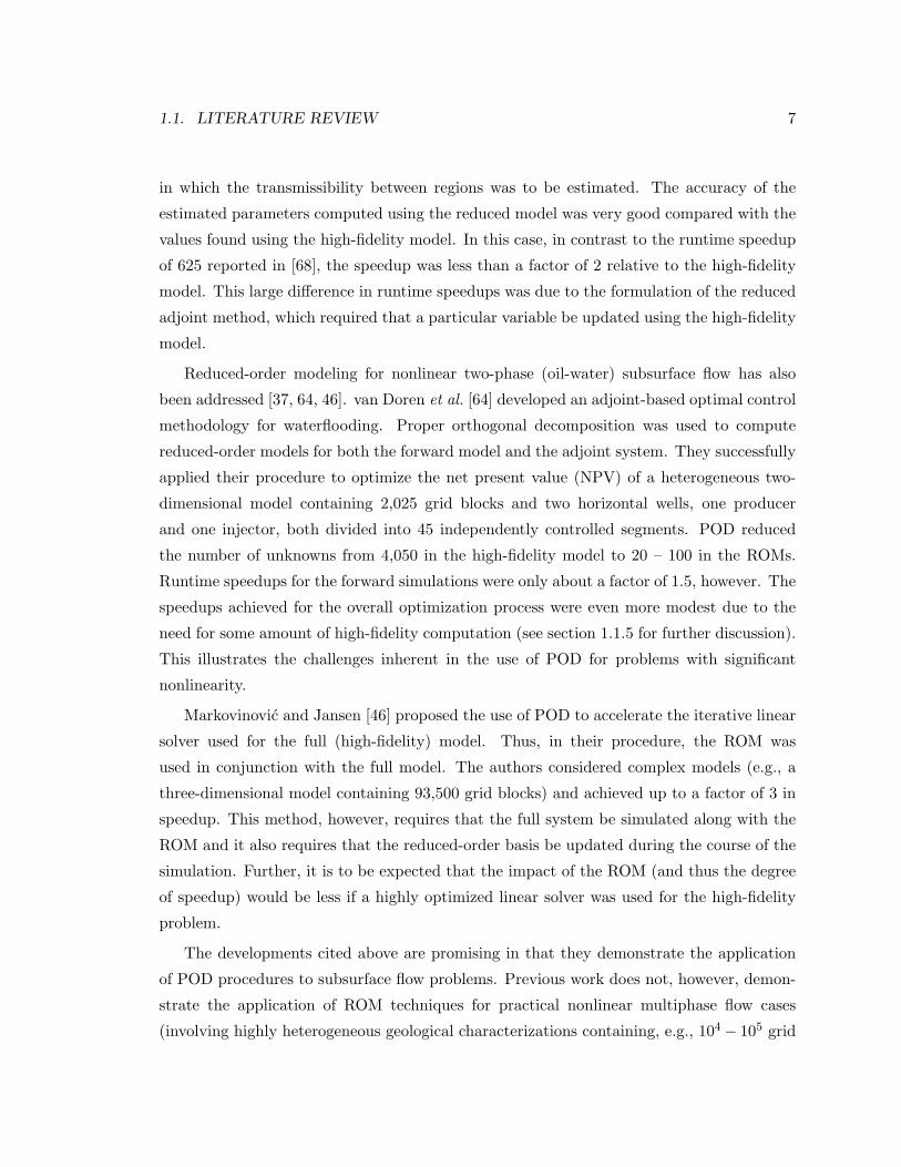
1.1. LITERATURE REVIEW 7
in which the transmissibility between regions was to be estimated. The accuracy of the
estimated parameters computed using the reduced model was very good compared with the
values found using the high-fidelity model. In this case, in contrast to the runtime speedup
of 625 reported in [68], the speedup was less than a factor of 2 relative to the high-fidelity
model. This large difference in runtime speedups was due to the formulation of the reduced
adjoint method, which required that a particular variable be updated using the high-fidelity
model.
Reduced-order modeling for nonlinear two-phase (oil-water) subsurface flow has also
been addressed [37, 64, 46]. van Doren et al. [64] developed an adjoint-based optimal control
methodology for waterflooding. Proper orthogonal decomposition was used to compute
reduced-order models for both the forward model and the adjoint system. They successfully
applied their procedure to optimize the net present value (NPV) of a heterogeneous two-
dimensional model containing 2,025 grid blocks and two horizontal wells, one producer
and one injector, both divided into 45 independently controlled segments. POD reduced
the number of unknowns from 4,050 in the high-fidelity model to 20 – 100 in the ROMs.
Runtime speedups for the forward simulations were only about a factor of 1.5, however. The
speedups achieved for the overall optimization process were even more modest due to the
need for some amount of high-fidelity computation (see section 1.1.5 for further discussion).
This illustrates the challenges inherent in the use of POD for problems with significant
nonlinearity.
Markovinovic and Jansen [46] proposed the use of POD to accelerate the iterative linear
solver used for the full (high-fidelity) model. Thus, in their procedure, the ROM was
used in conjunction with the full model. The authors considered complex models (e.g., a
three-dimensional model containing 93,500 grid blocks) and achieved up to a factor of 3 in
speedup. This method, however, requires that the full system be simulated along with the
ROM and it also requires that the reduced-order basis be updated during the course of the
simulation. Further, it is to be expected that the impact of the ROM (and thus the degree
of speedup) would be less if a highly optimized linear solver was used for the high-fidelity
problem.
The developments cited above are promising in that they demonstrate the application
of POD procedures to subsurface flow problems. Previous work does not, however, demon-
strate the application of ROM techniques for practical nonlinear multiphase flow cases
(involving highly heterogeneous geological characterizations containing, e.g., 104− 105 grid

8 CHAPTER 1. INTRODUCTION AND LITERATURE REVIEW
blocks) in which reduced-order models can be used in place of full high-fidelity reservoir
flow simulations. In addition, there does not appear to have been any implementation of
ROM procedures into general purpose subsurface flow simulators.
The limited speedups achieved in previous POD-based ROMs for two-phase flow can
be better understood by considering the computations required for a reservoir model with
Nc grid blocks, which corresponds to 2Nc unknowns (oil pressure and water saturation for
all grid blocks). Suppose that by applying proper orthogonal decomposition a reduced-
order model of dimension ` can be formed, with ` << 2Nc. The POD procedure works at
the level of the linear solver, reducing the sparse 2Nc × 2Nc linear system to a full ` × `system. The solver time is thus reduced substantially. Computational requirements for
other operations, by contrast, such as the construction of the Jacobian matrix (which must
be performed at each iteration of every time step), are not reduced at all through the use of
the standard POD technique. Also, after a new Jacobian matrix (J) is constructed it must
be projected into the reduced-order space using a reduced-order basis Φ. Specifically, the
reduced Jacobian (Jr) is computed as Jr = ΦT JΦ, and these matrix multiplications are
computationally demanding. Thus, the construction of both J and Jr is computationally
costly. In the next section we describe some improvements to the standard POD procedure
that enable better performance for nonlinear problems.
1.1.3 Enhanced POD
Two approaches within the context of POD – a clustering technique to optimize the snap-
shots for the eigen-decomposition problem, which acts to reduce the number of POD basis
vectors needed, and a missing point estimation (MPE) procedure to reduce the dimension
of the POD basis vectors – have been developed previously [16, 35, 5, 4, 8, 7, 6]. These
procedures have not been applied within the context of subsurface flow modeling. We now
discuss these approaches, as we will later apply them for reservoir simulation.
Clustering
The snapshots generated from training runs are used for the construction of the reduced-
order basis matrix. In our approach the snapshots are simply the states computed at each
time step of the high-fidelity training runs. One concern that arises is that the snapshots
depend on the controls used in the training run (this is discussed in section 2.2). Another

1.1. LITERATURE REVIEW 9
issue is that, in state space, the distribution of snapshots can be far from uniform, meaning
that in some regions of the state space the snapshots are concentrated while in other regions
they are sparsely distributed. The irregular distribution of snapshots can bias the resulting
reduced basis.
Burkardt et al. [16] introduced centroidal Voronoi tesselation (CVT) to generate a
reduced-order basis from the generators of a CVT of snapshots. CVT is also known as
k-means clustering and the generators of a CVT of snapshots are the centroids of the
clusters formed from the snapshot set. In our approach we apply the k-means clustering
technique to reduce the number of recorded snapshots, which are not in general uniformly
distributed in the state space, into a smaller number of centroids that are more regularly
distributed.
The clustering of snapshots has a twofold benefit. First, it provides a more uniform
distribution of snapshots in state space, which enables the construction of a reduced-order
basis with a smaller number of basis functions (columns of Φ). Second, the SVD of the
data matrix can be performed more efficiently. This second advantage is not a major benefit
for the cases considered in this thesis, but it could be important if a very large number of
snapshots are recorded.
Missing Point Estimation
Astrid [5] introduced the method of missing point estimation (MPE) to improve the compu-
tational efficiency of the reduced-order model. This approach was motivated by the Gappy-
POD approach developed for image reconstruction, introduced by Everson and Sirovich [32].
The MPE methodology seeks to reduce the computational cost of updating the matrices
required by the reduced-order model (i.e., Jr). This reduction is based on the assumption
that the reduced-order basis Φ can be constructed using information from only a portion
of the spatial domain rather than from the entire spatial domain.
Within the context of POD applied to reservoir simulation, MPE can be used to acceler-
ate the construction of the Jacobian matrix J and the reduced Jacobian matrix Jr = ΦT JΦ,
which must be formed at each iteration of every time step. Specifically, rather than using
information from all Nc grid blocks of the reservoir model, MPE allows us to use informa-
tion from nm selected grid blocks, where nm < Nc. Grid block selection is achieved with
awareness of the fact that Φ should be an orthonormal basis, meaning that the condition
number of ΦT Φ should be very close to 1. Then, applying different procedures, rows of Φ

10 CHAPTER 1. INTRODUCTION AND LITERATURE REVIEW
are eliminated (each row of Φ corresponds to a specific grid block), such that the condition
number of ΦT Φ stays close to 1 (Astrid [5]).
Missing point estimation has been applied previously for different nonlinear problems.
In the original development of MPE, Astrid [5] implemented the method within a reduced-
order model constructed with POD to simulate the temperature distribution in a glass melt
feeder. The high-fidelity model contained 7,128 cells. A reduced-order model constructed
using the standard POD provided a runtime speedup of 3.2 while using POD-MPE with
465 cells selected the speedup increased to 8.5. Another application of POD with MPE
was presented by Astrid [8] for a nonlinear heat conduction model used to compute the
temperature distribution on a thin plate. Compared with the original full-order model a
speedup of 10 was obtained using the standard POD and 200 when POD-MPE was applied
with 200 grid blocks selected (the full model contained 1,452 grid blocks).
1.1.4 Trajectory Piecewise Linearization
Even using the enhanced POD procedures (clustering and MPE) described above, there
are still some inherent limitations in the achievable speedup. This is because the required
number of rows of Φ would still be expected to be a reasonable fraction of 2Nc. In addition,
a full implementation of MPE requires modifications throughout the simulator; e.g., in the
Jacobian construction code.
Some of these limitations are addressed by the trajectory piecewise linearization ap-
proach (TPWL) introduced by Rewienski [56]. In this methodology a nonlinear system is
represented as a weighted combination of piecewise linear systems and each linear system is
projected into a low-dimensional space using Krylov subspaces or other ROM procedure. A
key feature of the TPWL method is that during subsequent simulations it linearizes around
one or more states selected from a large collection of snapshots. New states are represented
in terms of piecewise linear expansions around previously simulated (and saved) states and
Jacobian matrices as:
g(xn+1,un+1) = g(xi,ui) +(∂g∂x
)i
(xn+1 − xi) +(∂g∂u
)i
(un+1 − ui) + . . . ,
where g is the residual we seek to drive to zero, xn+1 is the new state we wish to determine,
un+1 is the new set of controls (which are specified), and both (∂g/∂x)i and (∂g/∂u)i are
(saved) matrices evaluated at (xi,ui).

1.1. LITERATURE REVIEW 11
Very high degrees of computational efficiency are achieved because all of these compu-
tations are performed in reduced space. Rewienski [56] applied the TPWL technique to
compute the sinusoidal steady state for a nonlinear transmission line circuit model contain-
ing 1,500 unknowns. He used 21 linearization states and generated a reduced-order model
of dimension 30. The runtime speedup of the TPWL model compared with the full-order
nonlinear model was 1,150. The error on the harmonics of the sinusoidal steady state using
the reduced-order TPWL representation varied between 0.4% and 13.5%, depending on the
harmonic analyzed, when compared with the high-fidelity model.
TPWL has also been successfully applied in other areas. Gratton and Willcox [34]
employed TPWL for a computational fluid dynamics problem involving flow through an
actively controlled supersonic diffuser. Proper orthogonal decomposition was used to project
the linearized model with 11,703 states to a reduced-order space of 110 states. Their
results showed that the TPWL reduced-order model provided a speedup of a factor of 1,440
compared to the high-fidelity nonlinear model. The authors reported accurate results when
a sufficient number of basis functions was used, though they stated that the error increased
when the reduced-order model was used for simulations outside the range of controls used
in the training simulations.
Yang and Shen [71] developed a nonlinear heat-transfer ROM based on TPWL and
Krylov subspaces. This technique was applied to simulate steady-state and transient models.
The errors between the high-fidelity and reduced-order models were less than 0.5% and the
runtime speedup was about two orders of magnitude.
A modified version of the TPWL method was developed and applied by Vasilyev et
al. [65] to generate reduced-order models of nonlinear biomedical micro-electromechanical
systems (BioMEMS). In their approach the Krylov subspace method for linear reduction
was replaced by the truncated balanced realization (TBR) method. They showed that
the proposed methodology improved the reduced-order model accuracy relative to Krylov-
subspace methods, though speedups were not reported. Additional applications of TPWL
were presented by Tiwary and Rutenbar [63] and Dong and Roychowdhury [30] for mod-
eling electronic circuits. TPWL does not appear to have been considered for oil reservoir
simulation or for any closely related subsurface flow application. Thus it will be of interest
to assess TPWL for this application area.

12 CHAPTER 1. INTRODUCTION AND LITERATURE REVIEW
1.1.5 Optimization of Reservoir Performance
Computational optimization can be applied for many oil field problems. Our specific in-
terest here is for optimization of waterflooding. This is important for wells under surface
control and for smart wells equipped with downhole inflow control valves. In either case op-
timization is performed to determine the settings for the well controls such that an objective
function (cumulative oil production or net present value) is maximized.
The optimized well controls can be determined using gradient-based algorithms, with
gradients computed either numerically (using finite differences) or by solving adjoint equa-
tions. The benefit of using optimization algorithms with numerical gradients is that an
existing reservoir simulator with advanced capabilities can be used directly. Such an ap-
proach was used by Yeten et al. [72, 73] in their optimization of downhole valve settings.
Aitokhuehi and Durlofsky [1] extended this approach for combined history matching and
smart well optimization. However, this is a computationally demanding methodology that
requires many function evaluations as the number of control valves and/or the number of
setting updates increase. The total number of simulation runs required to computed the
numerical gradient is given by one plus the number of control variables.
As indicated above, optimization procedures that require only objective function eval-
uations (and which treat the simulator as a black box) are useful in many cases, though
they tend to require many forward simulations. Gradient-based methods with gradients de-
termined through solution of adjoint equations represent a much more efficient alternative.
Some of the first adjoint-based optimizations for oil reservoir problems were presented by
Ramirez [53]. Brouwer and Jansen [12] and Sarma et al. [59] recently implemented adjoint-
based production optimization procedures. These approaches involve detailed coupling with
the reservoir simulator and thus require access to the source code.
In recent work Reynolds and coworkers [70] compared the performance of three op-
timization algorithms for production optimization. The algorithms considered were an
adjoint method, a simultaneous perturbation stochastic approximation (SPSA) in which
all parameters are perturbed stochastically, and an ensemble Kalman filter (EnKF). The
results showed that the gradient-based algorithm was the most efficient, requiring many
fewer iterations than the SPSA and EnKF algorithms. Another application of the ensemble
Kalman filter for closed-loop production optimization was presented by Chen et al. [27].
Genetic algorithms are another class of techniques that can be used for production
optimization. Those methods are theoretically able to find the global optimum of the
1.1. LITERATURE REVIEW 13
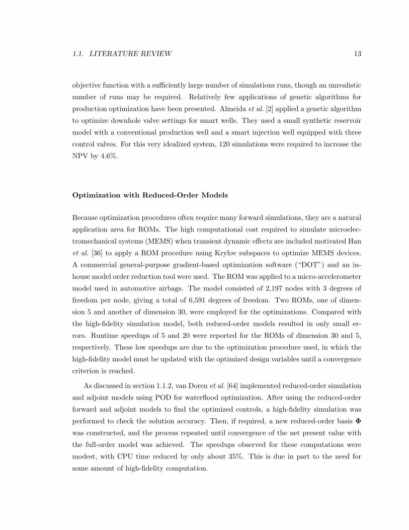
objective function with a sufficiently large number of simulations runs, though an unrealistic
number of runs may be required. Relatively few applications of genetic algorithms for
production optimization have been presented. Almeida et al. [2] applied a genetic algorithm
to optimize downhole valve settings for smart wells. They used a small synthetic reservoir
model with a conventional production well and a smart injection well equipped with three
control valves. For this very idealized system, 120 simulations were required to increase the
NPV by 4.6%.
Optimization with Reduced-Order Models
Because optimization procedures often require many forward simulations, they are a natural
application area for ROMs. The high computational cost required to simulate microelec-
tromechanical systems (MEMS) when transient dynamic effects are included motivated Han
et al. [36] to apply a ROM procedure using Krylov subspaces to optimize MEMS devices.
A commercial general-purpose gradient-based optimization software (“DOT”) and an in-
house model order reduction tool were used. The ROM was applied to a micro-accelerometer
model used in automotive airbags. The model consisted of 2,197 nodes with 3 degrees of
freedom per node, giving a total of 6,591 degrees of freedom. Two ROMs, one of dimen-
sion 5 and another of dimension 30, were employed for the optimizations. Compared with
the high-fidelity simulation model, both reduced-order models resulted in only small er-
rors. Runtime speedups of 5 and 20 were reported for the ROMs of dimension 30 and 5,
respectively. These low speedups are due to the optimization procedure used, in which the
high-fidelity model must be updated with the optimized design variables until a convergence
criterion is reached.
As discussed in section 1.1.2, van Doren et al. [64] implemented reduced-order simulation
and adjoint models using POD for waterflood optimization. After using the reduced-order
forward and adjoint models to find the optimized controls, a high-fidelity simulation was
performed to check the solution accuracy. Then, if required, a new reduced-order basis Φ
was constructed, and the process repeated until convergence of the net present value with
the full-order model was achieved. The speedups observed for these computations were
modest, with CPU time reduced by only about 35%. This is due in part to the need for
some amount of high-fidelity computation.

14 CHAPTER 1. INTRODUCTION AND LITERATURE REVIEW
1.2 Scope of this Work
The development of reduced-order modeling procedures has received significant attention
in recent years. However, relatively few studies have been conducted to investigate the
application of these approaches for reservoir flow simulation. This dissertation is mainly
devoted to furthering the development and application of ROM methods for subsurface flow
problems. Though the target application here is oil reservoir simulation, our findings are
also relevant to other closely related areas such as aquifer management and the geological
storage of carbon dioxide. We also study the use of reduced-order models for production
optimization. To accomplish this we develop a technique that couples trajectory piecewise
linearization (TPWL) with proper orthogonal decomposition (POD). The resulting model
will be shown to achieve runtime speedups of 2–3 orders of magnitude in the optimization
computation.
The specific goals of this dissertation are:
• to further the development and application of POD-based methods for subsurface
flow problems. Specifically, by incorporating new reduced-order modeling procedures
developed within other application areas, we aim to apply these approaches to more
realistic reservoir simulation models and to achieve better computational performance.
The specific techniques to be incorporated in the standard POD include the cluster-
ing [16] and missing point estimation [5] procedures described in section 1.1.3
• to incorporate our developments into a general purpose flow simulator [17, 41], so they
can eventually be used for a wider variety of flow problems.
• to develop and apply TPWL procedures for subsurface flow modeling. Toward this
end we formulate a TPWL representation for oil-water flow.
• to evaluate the performance of the enhanced POD and TPWL-POD techniques for
challenging nonlinear subsurface flow problems. Our examples involve highly hetero-
geneous geological models and nonlinear relative permeability curves.
• to apply the new TPWL-POD technique for single and multiobjective optimization
problems involving complex three-dimensional reservoir models and to compare the
optimization results with those using high-fidelity simulation models.

1.3. DISSERTATION OUTLINE 15
1.3 Dissertation Outline
This dissertation proceeds as follows. In Chapter 2, reduced-order modeling (ROM) tech-
niques are applied to complex large-scale subsurface flow models. Starting with a high-
fidelity training simulation, snapshots are recorded for the oil pressure and water saturation
states. Then, an eigen-decomposition (SVD) is performed on both states to compute the
basis matrix Φ used to project the high-dimensional system into a low-dimensional sub-
space. To improve the performance of the reduced-order model, a clustering technique is
introduced to reduce the number of columns of Φ and a missing point estimation (MPE)
approach is applied to remove selected rows of Φ. The reduced-order modeling procedure,
which includes proper orthogonal decomposition (POD), clustering and MPE, was imple-
mented into Stanford’s general purpose research simulator [17, 41].
The POD-based methodology is then tested for simulations involving waterflood for
a geologically complex three-dimensional oil reservoir model containing 60,000 grid blocks.
The performance of the various techniques (standard POD, clustering and MPE) is assessed
in terms of their ability to reproduce high-fidelity simulation results for the training run
and also for test simulations with different well schedules. The results demonstrate that the
ROM procedure can accurately reproduce the reference high-fidelity simulations. Runtime
speedups of up to an order of magnitude are observed relative to the high-fidelity model
simulated using an optimized solver. Speedups will be significantly less, however, if the
relative permeability curves are highly nonlinear or if there is a large density difference
between the oil and water phases.
The work presented in Chapter 2 was published in the International Journal for Numer-
ical Methods in Engineering [22]. Dr. Pallav Sarma contributed to this work, primarily by
implementing the ROM procedure in Stanford’s general purpose research simulator (GPRS),
and is a co-author of the journal publication.
Although the ROM presented in Chapter 2 can provide reductions in simulation time,
more substantial runtime speedups may be required for optimization problems. In Chapter
3 the trajectory piecewise linearization (TPWL) procedure for the reduced-order modeling
of two-phase flow in subsurface formations is developed and applied. The linearization of
the governing equations for reservoir flow is described in detail and two approaches for
constructing a reduced-order TPWL representation are provided. In the first step of the
TPWL methodology, a small number (3–4) of training simulations is performed and, in

16 CHAPTER 1. INTRODUCTION AND LITERATURE REVIEW
addition to the pressure and saturation states needed for the POD procedure, Jacobian
matrices are also recorded. The construction of the basis matrix Φ is accomplished using
POD (the same approach described in Chapter 2 is applied). Using this Φ, the linearized
model is projected into a low-dimensional space. The preprocessing overhead required for
the training runs and to project the recorded states and Jacobian matrices into the low-
dimensional space is roughly comparable to 6–8 high-fidelity simulations.
The TPWL model is then applied to two reservoir models containing 24,000 and 79,200
grid blocks and characterized by heterogeneous permeability descriptions. Based on exten-
sive test simulations for both models it is shown that the TPWL approach provides accurate
results when the controls (bottom hole pressures of the production wells in this case) ap-
plied in test simulations are within the general range of the controls applied in the training
runs, even though the well pressure schedules for the test runs can differ significantly from
those of the training runs. A key finding is that this new TPWL-POD methodology can
provide runtime speedups between two and three orders of magnitude. Thus it appears to
be well suited for use in optimization problems. The work presented in Chapter 3 has been
submitted for publication to the Journal of Computational Physics.
In Chapter 4 we evaluate the performance of the TPWL representation for production
optimization problems involving waterflood in heterogeneous reservoir models. Using the
two reservoir models described in Chapter 3 and another model with 20,400 grid blocks,
single-objective optimizations are performed using the TPWL representation and the high-
fidelity simulation model and the results compared.
Production optimization is performed for the 20,400 grid-block model using both gradient-
based and generalized pattern search algorithms [21]. In these optimizations the bottom hole
pressures (BHPs) of four production wells at six different times (24 control variables) are
determined such that the net present value is maximized. Utilizing only the gradient-based
algorithm, similar optimizations are also performed for the other two models described in
Chapter 3. Although slightly different BHP control schedules are computed by the optimiza-
tions with the TPWL representation as compared to those using the high-fidelity model,
results for the optimized NPV using the high-fidelity model with the controls determined
using TPWL are shown to be in consistently close agreement with those computed using
high-fidelity simulations. Runtime speedups using the TPWL representation of between
450 and 2,000 are observed.

1.3. DISSERTATION OUTLINE 17
The TPWL procedure is applied to a computationally demanding multiobjective op-
timization problem with 48 control variables, for which the Pareto front is determined.
Limited high-fidelity simulations demonstrate the accuracy and applicability of TPWL for
this optimization. This multiobjective optimization is extremely demanding computation-
ally; i.e., it would require more than two months of CPU time using the high-fidelity model.
Using TPWL, the full optimization is accomplished in 3.3 hours. The work appearing in
Chapter 4 has been presented in two papers [21, 20].
Finally, in Chapter 5, we present detailed conclusions and recommendations for future
research in the development of efficient reduced-order models for reservoir flow simulation.

18 CHAPTER 1. INTRODUCTION AND LITERATURE REVIEW

Chapter 2
Reduced-Order Modeling of
Subsurface Flow Using Proper
Orthogonal Decomposition
In this chapter we further the development and application of POD methods for subsur-
face flow problems. We begin by describing the equations and the standard finite volume
discretization for two-phase flow. We then discuss the POD-based reduced-order modeling
technique. This includes a description of the clustering and missing point estimation pro-
cedures and a description of the implementation of POD into an existing general purpose
simulator. Then, in section 2.2, we present results for a number of cases involving a sim-
ulation model of a geologically complex reservoir containing 60,000 grid blocks. Different
specifications for the time-varying bottom hole pressures of the production wells are con-
sidered. These results demonstrate the robustness and computational speedup of the POD
techniques for realistic cases. Additional findings and a discussion of some of the limitations
of the POD procedures are presented in section 2.3.
2.1 Modeling Procedure
In this section we describe the governing equations, the discretized system, and the proper
orthogonal decomposition procedure for oil-water flows.
19

20 CHAPTER 2. ROM OF SUBSURFACE FLOW USING POD
2.1.1 Oil-Water Flow Equations and Discretization
Subsurface flow models are derived by combining mass conservation equations with the
multiphase version of Darcy’s law. For the oil-water case considered here, there is no mass
transfer between phases; i.e., the oil component resides only in the oil phase and the water
component only in the water phase. Then, for each component/phase j (with j = o denoting
oil and j = w water), we have:
∇ · [λjk (∇pj − ρjg∇D)] =∂
∂t
(φSj
Bj
)+ qw
j , (2.1)
where k is the absolute permeability (assumed to be a diagonal tensor), λj = krj/(µjBj)
is the phase mobility, krj is the relative permeability to phase j, µj is the phase viscosity,
Bj is the formation volume factor for phase j (defined below), pj is phase pressure, ρj
is the phase density, g is gravitational acceleration, D is depth, t is time, φ is porosity
(void fraction of the rock), Sj is saturation and qwj is the source/sink term. All terms
are of units 1/time. The formation volume factor is defined as the ratio of the volume of
phase j at reservoir conditions to the phase volume at reference (stock tank) conditions.
Designating the reference density of phase j as ρ0j , it follows that Bj = ρ0
j/ρ(p). In the
case of incompressible flow, density does not vary with pressure and Bj = 1. The general
two-phase flow description is completed through the saturation constraint (So + Sw = 1)
and by specifying a capillary pressure relationship; i.e., pc(Sw) = po− pw, which relates the
phase pressures.
The two-phase flow description entails four equations and four unknowns (po, pw, So,
Sw). We select po and Sw as primary unknowns. Once these are computed, pw and So can
be readily determined from the capillary pressure relationship and saturation constraint.
We now briefly discuss the finite volume representation for Eq. 2.1 (see [9] or [33] for
more details). Figure 2.1 shows a portion of a one-dimensional grid. For simplicity, here we
neglect capillary pressure (so po = pw), treat horizontal flow in the x-direction (for which
∇D = 0), and assume the grid block dimensions (∆x, ∆y, ∆z) are constant. We consider
fully implicit discretizations. For this case the discretized form for the flow terms (left hand
side of Eq. 2.1) is
∂
∂x
[kλj
(∂pj
∂x
)]≈{
(Tj)n+1i−1/2
[pn+1
i−1 − pn+1i
]+ (Tj)n+1
i+1/2
[pn+1
i+1 − pn+1i
]} 1V, (2.2)

2.1. MODELING PROCEDURE 21
where subscript j indicates phase and i designates grid block, superscript n + 1 specifies
the next time step, and V = ∆x∆y∆z is the volume of grid block i. The transmissibility
(Tj)n+1i−1/2 relates flow in phase j to the difference in pressure between grid blocks i− 1 and
i and is given by:
(Tj)n+1i−1/2 =
(kA
∆x
)i−1/2
(krj
Bjµj
)n+1
i−1/2
, (2.3)
where A = ∆y∆z is the area of the common face between blocks i−1 and i. The transmissi-
bility (Tj)n+1i+1/2 is defined analogously. The flow terms can be seen to introduce nonlinearity
into the system as (Tj)n+1i±1/2 are functions of pressure and saturation and multiply terms
involving pressure. In Eq. 2.3, ki−1/2 is computed as the harmonic average of ki−1 and ki,
and (krj/(Bjµj))n+1i−1/2 is upwinded depending on the flow direction of phase j.
Figure 2.1: Portion of a one-dimensional grid
The first term on the right hand side of Eq. 2.1 represents mass accumulation and is
represented discretely as:
∂
∂t
(φSj
Bj
)≈ 1
∆t
[(φSj
Bj
)n+1
−(φSj
Bj
)n], (2.4)
where ∆t is the time interval. For incompressible systems φ is constant and Bj = 1, in
which case Eq. 2.4 reduces to:
∂
∂t
(φSj
Bj
)≈ φ
∆t[(Sj)n+1 − (Sj)n
]. (2.5)
The second term on the right hand side of Eq. 2.1 represents the source/sink term. In
reservoir simulation, the sources and sinks correspond to wells which are modeled using a
well equation: (qwj
)n+1
i=(qwj
)n+1
iV = Wi (λj)
n+1i (pn+1
i − pwi ), (2.6)

22 CHAPTER 2. ROM OF SUBSURFACE FLOW USING POD
where (qwj )n+1
i is the volumetric flow rate of phase j from block i into the well (or vice
versa) at time n + 1, pn+1i is grid block pressure at n + 1, pw
i is the wellbore pressure for
well w in grid block i, and Wi is the well index. For a vertical well that fully penetrates
block i, Wi is given by [50]:
Wi =[
2πk∆zln (r0/rw)
]i
, (2.7)
where rw is the wellbore radius and r0 ≈ 0.2∆x. See [50] for expressions for Wi for more
general cases. Note that, if a well is operating under bottom hole pressure (BHP) control,
this is represented in the simulation model by specifying pwi in Eq. 2.6.
For the discretized models, we consider logically Cartesian systems (meaning blocks
follow a logical i, j, k ordering) containing a total of Nc grid blocks. The state vector x
contains the two primary unknowns:
x =[
(po)1, (Sw)1, (po)2, (Sw)2, · · · , (po)Nc−1, (Sw)Nc−1, (po)Nc , (Sw)Nc
]T. (2.8)
Introducing the discretizations presented in Eqs. 2.2 through 2.7, the discretized fully im-
plicit version of Eq. 2.1 for incompressible systems (Eq. 2.5) can be expressed as [9]:
g = Tn+1xn+1 −Dn+1(xn+1 − xn)−Qn+1 = 0, (2.9)
where g is the residual vector we seek to drive to zero, T is a block pentadiagonal matrix
for two-dimensional grids and a block heptadiagonal matrix for three-dimensional grids,
D is a block diagonal matrix, and Q represents the source/sink terms. The time level is
designated by the superscript n or n + 1. The Tn+1xn+1 term represents transport (flow)
effects while the Dn+1(xn+1 − xn) term represents accumulation. The matrices T, D and
Q depend on x and must be updated at each iteration of every time step. See [9] for further
details.
Eq. 2.9 represents a nonlinear set of algebraic equations and is solved by applying New-
ton’s method to drive g to zero:
Jδ = −g, (2.10)
where J is the Jacobian matrix given by Jij = ∂gi/∂xj and δi = xn+1,v+1i − xn+1,v
i with v
and v + 1 indicating iteration level.

2.1. MODELING PROCEDURE 23
2.1.2 Proper Orthogonal Decomposition
In order to generate a POD reduced-order basis, a simulation of the full flow model must
first be performed and the states of the system saved. These states, represented by S‘snapshots,’ comprise solutions for po and Sw for all Nc grid blocks at particular times. We
denote as Xp and XS the matrices which represent the system states for po and Sw (from
here on designated simply as p and S), respectively:
Xp =[x1
p,x2p, · · · ,xSp
], XS =
[x1
S ,x2S , · · · ,xSS
].
Each column of these matrices contains the solution of the system for a specific simulation
time (these solutions are designed xip and xi
S , where i indicates the snapshot number). The
pressure states are normalized by computing xpi = (pi−pmin)/(pmax−pmin), where pi is the
simulated grid block pressure and pmax and pmin are the maximum and minimum pressures
encountered during the high-fidelity flow simulation. A similar normalization is applied to
the saturation states.
The basic POD procedure we employ is well established and is discussed in a variety
of publications (e.g., [61, 25]). The development in this section follows the work of van
Doren et al. [64]. As in their approach, we apply the ROM procedure separately for the
pressure and saturation states. This is appropriate because the two variables are governed
by distinct physics (as can be readily demonstrated by manipulating Eq. 2.1 into pressure
and saturation equations; see [33, 9] for details). After the snapshots are obtained, the mean
of the snapshots is computed (Eq. 2.11) and the data matrices Xp and XS are determined
by subtracting the mean from each snapshot (Eq. 2.12):
xp =1S
S∑i=1
xip, xS =
1S
S∑i=1
xiS , (2.11)
Xp =[x1
p − xp,x2p − xp, · · · ,xSp − xp
]Nc×S
,
XS =[x1
S − xS ,x2S − xS , · · · ,xSS − xS
]Nc×S . (2.12)
The following procedure is performed for both Xp and XS . We describe it using X,
where X designates either Xp or XS . A covariance matrix C is determined by applying the
method of snapshots [61]
C = XTX, (2.13)

24 CHAPTER 2. ROM OF SUBSURFACE FLOW USING POD
from which the following eigen-decomposition problem is solved:
CΨ = λΨ, (2.14)
where Ψ represents the eigenvectors and λ the eigenvalues of C, respectively. We do not
actually perform an eigen-decomposition of Eq. 2.14 but rather a singular value decomposi-
tion (SVD). Alternatively, we can perform SVD directly on X, which is an efficient way of
obtaining the eigen-decomposition of the covariance matrix given by Eq. 2.13. The singular
values (σi) of X are related to eigenvalues (λi) of XTX via σi = λ
1/2i .
The POD basis functions are then given by a linear combination of the snapshots [61]:
Φ = XΨ. (2.15)
In this context, the term “energy” is used to refer to the magnitude of the eigenvalue
associated with each eigenvector. By arranging the eigenvalues in decreasing order, this
energy can be used to selectively retain eigenvectors, meaning those eigenvectors possessing
small amounts of energy can be removed. The energy in the first ` eigenvectors is given by:
E` =∑`
i=1 λi
Et, (2.16)
where λi represents the energy of each eigenvector and Et =∑S
i=1 λi. The number of
basis functions retained for the pressure unknown, designated `p, is simply the number of
eigenvalues necessary to provide a specified fraction of Et. The number of basis functions
for the saturation unknown, `s, is determined analogously.
Following application of Eq. 2.16, the basis matrix Φ will contain only ` columns, where
` = `p + `s. We refer to this reduced Φ matrix as Φ`. Now, the reduced state vector,
designated z, can be related to the full oil pressure and water saturation states x as follows:
x ' Φ` z + x. (2.17)
As indicated above, for an oil-water system two basis matrices will be created, Φ`p and Φ`s
for the oil pressure and water saturation states, respectively. Combining both matrices,
Eq. 2.17 can be represented in matrix form as:

2.1. MODELING PROCEDURE 25
xp1
xs1
xp2
xs2
...
xpNc−1
xsNc−1
xpNc
xsNc
'
ϕ1p1
· · · ϕ`pp1 0 · · · 0
0 · · · 0 ϕ1s1· · · ϕ`s
s1
ϕ1p2
· · · ϕ`pp2 0 · · · 0
0 · · · 0 ϕ1s2· · · ϕ`s
s2
......
......
......
......
......
......
......
......
......
ϕ1pNc
· · · ϕ`ppNc
0 · · · 0
0 · · · 0 ϕ1sNc
· · · ϕ`ssNc
zp1
...
zp`p
zs1
...
zs`s
+
xp1
xs1
xp2
xs2
...
xpNc−1
xsNc−1
xpNc
xsNc
(2.18)
where x is of dimension 2Nc, Φ` is a 2Nc× (`p + `s) matrix, z has dimension `p + `s, and x
is of dimension 2Nc. The benefits of the method are achieved because `p + `s << 2Nc; i.e.,
the dimension of z is much less than that of x.
An important aspect of the reduced-order modeling process is the generation of snap-
shots (see, e.g., Burkdardt [16]). The information embodied in the snapshots is used to
compute the POD basis and therefore impacts strongly the ability of the reduced-order
basis to represent the states of the system. The predictive capabilities of the model are
important because our target application is production optimization. This means that we
require the ROM to be predictive for a variety of different flow scenarios, and these scenarios
are not known at the time the snapshots are generated.
We will not consider the issue of snapshot selection in detail in this work. Rather,
we apply a simple heuristic approach for snapshot generation that appears to perform
adequately for current purposes. We note, however, that detailed treatments exist for
snapshot selection that could be investigated in future work. For example, Kunisch and
Volkwein [43] developed the optimality system proper orthogonal decomposition (OS-POD)
which addresses the problem of un-modeled dynamics, as occurs when the optimum solution
is considerably different from the training simulation. Bui-Thanh et al. [15] presented an
alternate procedure that employs a greedy algorithm for the selection of snapshots in high-
dimensional space.
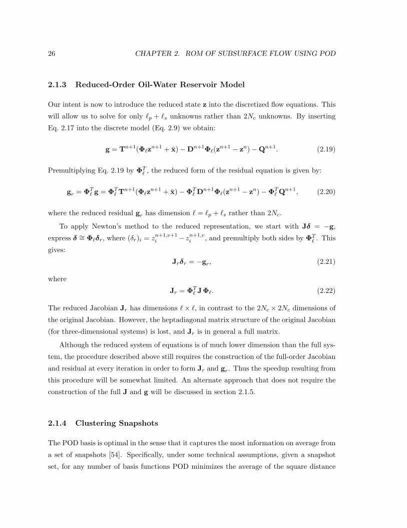
26 CHAPTER 2. ROM OF SUBSURFACE FLOW USING POD
2.1.3 Reduced-Order Oil-Water Reservoir Model
Our intent is now to introduce the reduced state z into the discretized flow equations. This
will allow us to solve for only `p + `s unknowns rather than 2Nc unknowns. By inserting
Eq. 2.17 into the discrete model (Eq. 2.9) we obtain:
g = Tn+1(Φ`zn+1 + x)−Dn+1Φ`(zn+1 − zn)−Qn+1. (2.19)
Premultiplying Eq. 2.19 by ΦT` , the reduced form of the residual equation is given by:
gr = ΦT` g = ΦT
` Tn+1(Φ`zn+1 + x)−ΦT` Dn+1Φ`(zn+1 − zn)−ΦT
` Qn+1, (2.20)
where the reduced residual gr has dimension ` = `p + `s rather than 2Nc.
To apply Newton’s method to the reduced representation, we start with Jδ = −g,
express δ ∼= Φ`δr, where (δr)i = zn+1,v+1i − zn+1,v
i , and premultiply both sides by ΦT` . This
gives:
Jrδr = −gr, (2.21)
where
Jr = ΦT` J Φ`. (2.22)
The reduced Jacobian Jr has dimensions `× `, in contrast to the 2Nc × 2Nc dimensions of
the original Jacobian. However, the heptadiagonal matrix structure of the original Jacobian
(for three-dimensional systems) is lost, and Jr is in general a full matrix.
Although the reduced system of equations is of much lower dimension than the full sys-
tem, the procedure described above still requires the construction of the full-order Jacobian
and residual at every iteration in order to form Jr and gr. Thus the speedup resulting from
this procedure will be somewhat limited. An alternate approach that does not require the
construction of the full J and g will be discussed in section 2.1.5.
2.1.4 Clustering Snapshots
The POD basis is optimal in the sense that it captures the most information on average from
a set of snapshots [54]. Specifically, under some technical assumptions, given a snapshot
set, for any number of basis functions POD minimizes the average of the square distance
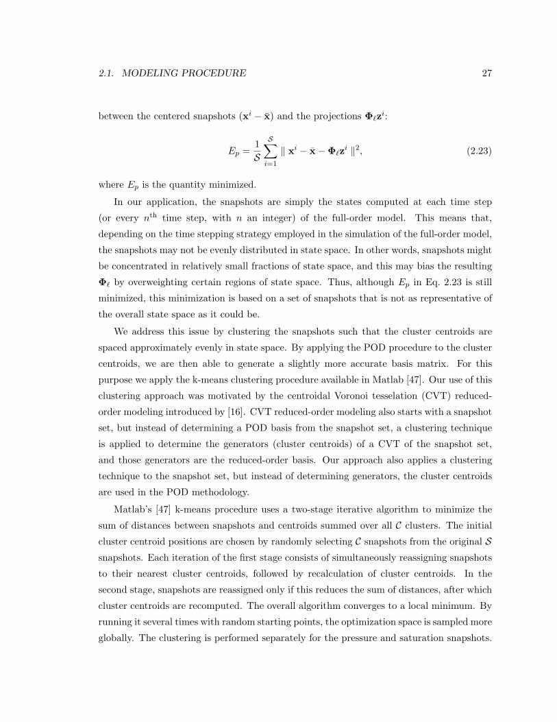
2.1. MODELING PROCEDURE 27
between the centered snapshots (xi − x) and the projections Φ`zi:
Ep =1S
S∑i=1
‖ xi − x−Φ`zi ‖2, (2.23)
where Ep is the quantity minimized.
In our application, the snapshots are simply the states computed at each time step
(or every nth time step, with n an integer) of the full-order model. This means that,
depending on the time stepping strategy employed in the simulation of the full-order model,
the snapshots may not be evenly distributed in state space. In other words, snapshots might
be concentrated in relatively small fractions of state space, and this may bias the resulting
Φ` by overweighting certain regions of state space. Thus, although Ep in Eq. 2.23 is still
minimized, this minimization is based on a set of snapshots that is not as representative of
the overall state space as it could be.
We address this issue by clustering the snapshots such that the cluster centroids are
spaced approximately evenly in state space. By applying the POD procedure to the cluster
centroids, we are then able to generate a slightly more accurate basis matrix. For this
purpose we apply the k-means clustering procedure available in Matlab [47]. Our use of this
clustering approach was motivated by the centroidal Voronoi tesselation (CVT) reduced-
order modeling introduced by [16]. CVT reduced-order modeling also starts with a snapshot
set, but instead of determining a POD basis from the snapshot set, a clustering technique
is applied to determine the generators (cluster centroids) of a CVT of the snapshot set,
and those generators are the reduced-order basis. Our approach also applies a clustering
technique to the snapshot set, but instead of determining generators, the cluster centroids
are used in the POD methodology.
Matlab’s [47] k-means procedure uses a two-stage iterative algorithm to minimize the
sum of distances between snapshots and centroids summed over all C clusters. The initial
cluster centroid positions are chosen by randomly selecting C snapshots from the original Ssnapshots. Each iteration of the first stage consists of simultaneously reassigning snapshots
to their nearest cluster centroids, followed by recalculation of cluster centroids. In the
second stage, snapshots are reassigned only if this reduces the sum of distances, after which
cluster centroids are recomputed. The overall algorithm converges to a local minimum. By
running it several times with random starting points, the optimization space is sampled more
globally. The clustering is performed separately for the pressure and saturation snapshots.
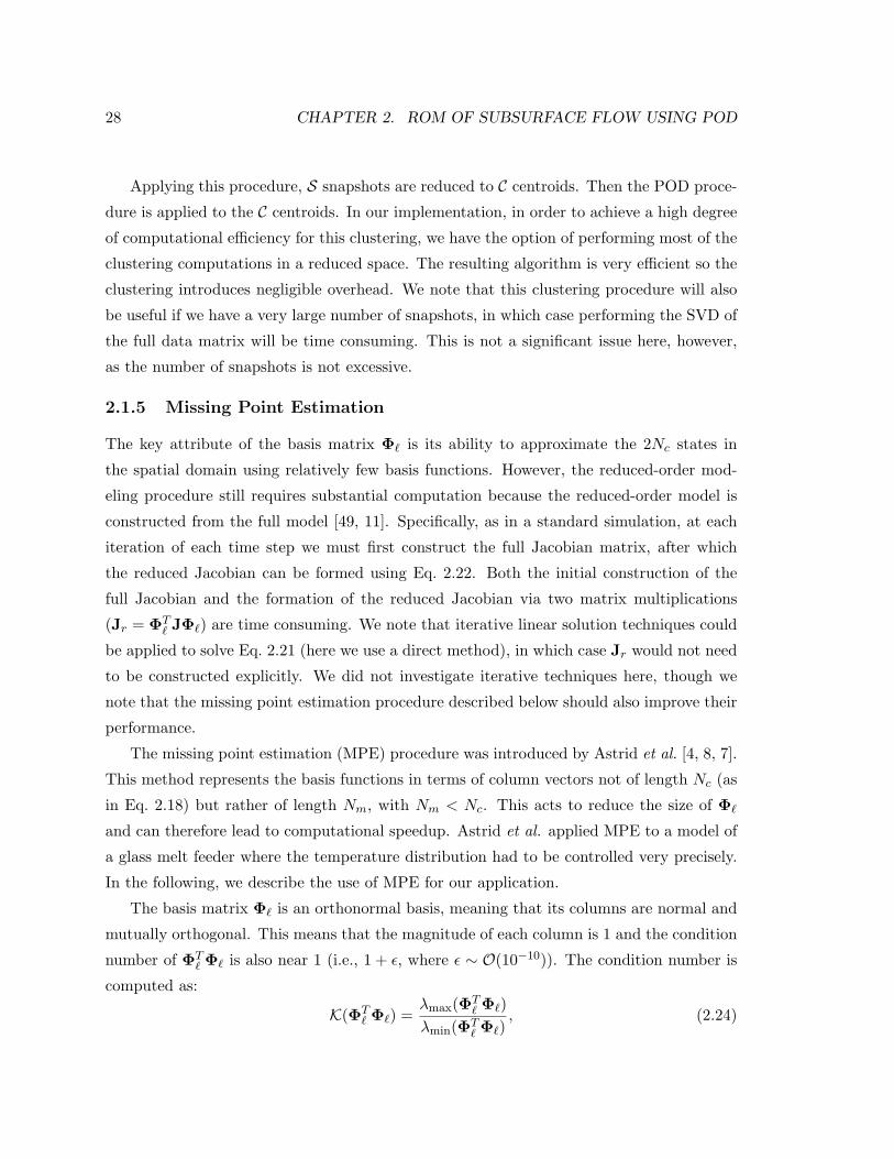
28 CHAPTER 2. ROM OF SUBSURFACE FLOW USING POD
Applying this procedure, S snapshots are reduced to C centroids. Then the POD proce-
dure is applied to the C centroids. In our implementation, in order to achieve a high degree
of computational efficiency for this clustering, we have the option of performing most of the
clustering computations in a reduced space. The resulting algorithm is very efficient so the
clustering introduces negligible overhead. We note that this clustering procedure will also
be useful if we have a very large number of snapshots, in which case performing the SVD of
the full data matrix will be time consuming. This is not a significant issue here, however,
as the number of snapshots is not excessive.
2.1.5 Missing Point Estimation
The key attribute of the basis matrix Φ` is its ability to approximate the 2Nc states in
the spatial domain using relatively few basis functions. However, the reduced-order mod-
eling procedure still requires substantial computation because the reduced-order model is
constructed from the full model [49, 11]. Specifically, as in a standard simulation, at each
iteration of each time step we must first construct the full Jacobian matrix, after which
the reduced Jacobian can be formed using Eq. 2.22. Both the initial construction of the
full Jacobian and the formation of the reduced Jacobian via two matrix multiplications
(Jr = ΦT` JΦ`) are time consuming. We note that iterative linear solution techniques could
be applied to solve Eq. 2.21 (here we use a direct method), in which case Jr would not need
to be constructed explicitly. We did not investigate iterative techniques here, though we
note that the missing point estimation procedure described below should also improve their
performance.
The missing point estimation (MPE) procedure was introduced by Astrid et al. [4, 8, 7].
This method represents the basis functions in terms of column vectors not of length Nc (as
in Eq. 2.18) but rather of length Nm, with Nm < Nc. This acts to reduce the size of Φ`
and can therefore lead to computational speedup. Astrid et al. applied MPE to a model of
a glass melt feeder where the temperature distribution had to be controlled very precisely.
In the following, we describe the use of MPE for our application.
The basis matrix Φ` is an orthonormal basis, meaning that its columns are normal and
mutually orthogonal. This means that the magnitude of each column is 1 and the condition
number of ΦT` Φ` is also near 1 (i.e., 1 + ε, where ε ∼ O(10−10)). The condition number is
computed as:
K(ΦT` Φ`) =
λmax(ΦT` Φ`)
λmin(ΦT` Φ`)
, (2.24)

2.1. MODELING PROCEDURE 29
where λmax(ΦT` Φ`) and λmin(ΦT
` Φ`) are the maximum and minimum eigenvalues of ΦT` Φ`
respectively.
The idea behind the missing point estimation is to remove a number of rows of the Φ`
basis matrix while allowing the condition number to increase only to a specified value. The
new basis matrix will be designated Φ∗` ∈ RNm×`, where Nm represents the number of grid
blocks retained. Astrid [5] presented two different methods for grid block selection. The
first method classifies the grid blocks by considering one block at a time and then computing
e =‖ ΓT` Γ`− I ‖, where Γ` represents the row of Φ` corresponding to the target block and I
is the identity matrix. The blocks are then ordered and those corresponding to the smallest
values of e are retained, with the condition number for the resulting Φ∗` computed using
Eq. 2.24. This procedure is continued until a target condition number is reached.
As reported by Astrid [5], this method requires that a relatively large number of grid
blocks be retained. To overcome this limitation Astrid implemented a greedy algorithm.
This procedure applies the algorithm described above to select the first block. Then, all
remaining (Nc−1) blocks are considered one at a time and the block that gives the minimum
condition number for the two-block system is retained. The procedure is repeated until the
target condition number is reached. We found this method to perform reasonably well for
small models but it is much too time consuming for application to large problems (e.g., for
the 60,000 grid block example considered in section 2.2).
We achieved the greatest reduction in the number of rows of Φ` using a sequential
QR decomposition (SQRD) approach. This approach was suggested by Y. Efendiev (pri-
vate communication), who applied it for conditioning permeability fields generated using
Karhunen-Loeve expansions. This was done within the context of history matching reservoir
models to production data using Markov chain Monte Carlo methods [31].
We implemented SQRD in Matlab and applied it to classify the grid blocks from the
most important to the least important. For the pressure state, given ΦT`p∈ R`p×Nc , QR
decomposition finds the `p orthogonal vectors that correspond to the `p greatest independent
vectors of ΦT`p
(a set of Nc vectors in R`p is linearly dependent if Nc > `p). This set of
`p vectors is then removed from ΦT`p
and the process is repeated until all grid blocks are
classified. The same procedure is applied for the saturation state.
We then apply the condition number criterion to construct a new basis matrix. The
number of grid blocks to be added in each step is specified (Nb). Then, following the
classification order, Nb grid blocks are selected for the pressure state (Nbp) and Nb grid

30 CHAPTER 2. ROM OF SUBSURFACE FLOW USING POD
blocks are selected for the saturation state (Nbs). The number of grid blocks added in each
step k (Nkb ) is given by the union of Nbp and Nbs , Nk
b = Nbp ∪ Nbs . Grid blocks (rows of
Φ∗` ) are added in this way until the target condition number for (Φ∗` )T Φ∗` (which includes
both pressure and saturation information) computed by Eq. 2.24 is reached. For the cases
studied here the condition number that produced an appropriate balance between speedup
and error was generally between 5 and 10.
2.1.6 Implementation in General Purpose Research Simulator
Stanford’s general purpose research simulator (GPRS), originally formulated by Cao [17]
and recently enhanced and extended by Jiang [40, 41], has evolved into a modeling package
containing many advanced capabilities and features. These include linkages to adjoint-
based optimal control procedures [59, 60], advanced linear solvers [41, 18], and models
for ‘smart wells,’ e.g., multibranched wells containing downhole sensors and inflow control
devices [41]. All of the simulations presented in the following sections were performed using
a new version of GPRS which is able to handle the basic POD procedure described above.
The simulator also contains a partial implementation of MPE. We now briefly describe these
implementations.
The ROM described previously can be separated into off-line (pre-processing) and in-line
portions. The off-line portion, executed just once, contains all of the computations needed
to construct the POD basis matrix. Figure 2.2 shows the flow chart for the off-line portion.
This entails first running a training simulation and recording snapshot sets for pressure
and saturation. Then, following the procedure given in section 2.1.4, the snapshots can be
clustered, the basis functions generated (section 2.1.2) and the grid blocks selected by the
MPE procedure (section 2.1.5).
The in-line portion of the ROM, integrated with the reservoir simulator, is depicted in
Figure 2.3. This ROM can be applied for a variety of different simulation scenarios. The
basis functions and selected grid blocks (if MPE is used), as determined from the off-line
procedure, are inputs. Then, within the Newton loop, the standard Jacobian matrix and
residual vector are generated, after which the reduced Jacobian and residual are formed
using Φ` or Φ∗` if MPE is being used. Newton’s method is then applied to the reduced
system of equations, after which the full state vector (x) is reconstructed using Φ` (note
that Φ` rather than Φ∗` is used in this step even if MPE is applied). The model initialization
and time stepping are exactly as in the standard simulator.

2.1. MODELING PROCEDURE 31
Figure 2.2: Flow chart for the off-line portion of the ROM
Our current implementation of the missing point estimation in GPRS is restricted to
code at the level of the linear solver. By this we mean that we use MPE to speed up
the matrix multiplications (ΦT` JΦ`) and in the solution of the reduced-order system, but
not elsewhere in the code. This is clearly suboptimal, as the full implementation of MPE
would allow us to construct residual equations and Jacobian entries for only Nm (rather
than Nc) grid blocks. This full implementation would, however, require code modifications
throughout GPRS, while the solver-level implementation leads to much more limited mod-
ifications. The reduced-order models generate small but full matrices. We therefore apply
direct solution techniques for these linear systems.
In the following section, we will compare the performance and timing of the ROM to
full GPRS simulations, so some discussion of the linear solvers applied in GPRS is appro-
priate. The linear system of equations arising in the full simulation model is very sparse.
For this solution, GPRS employs the iterative generalized minimum residual (GMRES)
solver along with various preconditioners. The constrained pressure residual (CPR) pre-
conditioner [69, 18, 41, 42] is the most advanced option. This preconditioner is specially

32 CHAPTER 2. ROM OF SUBSURFACE FLOW USING POD
Figure 2.3: Flow chart for the in-line portion of the ROM

2.2. SIMULATION USING REDUCED-ORDER MODELING 33
designed for the reservoir simulation equations (it takes full advantage of the elliptic charac-
ter of the underlying pressure equation) and is therefore highly efficient. This high efficiency
is due to a multistage procedure that uses in the first stage an algebraic multigrid (AMG)
preconditioner to solve the pressure system and a local preconditioner in the second stage
to solve the entire system. Most of our comparisons will be against full simulation models
that use CPR, so we are comparing against what we believe to be (essentially) the best
current procedure. More generic preconditioners, such as ILU(0), are also available within
GPRS and will be considered.
2.2 Simulation Using Reduced-Order Modeling
We now illustrate the application of the POD-based procedure to a realistic reservoir simu-
lation model. We will consider each component in turn (construction of the reduced basis,
clustering, MPE) and then demonstrate the ability of the reduced model to provide accurate
predictions for cases that differ from the initial training simulation. Simulation times and
errors due to the various ROM procedures are quantified at the end of this section.
Figure 2.4: Synthetic three-dimensional reservoir model with five production wells and fourinjection wells
The simulation model, shown in Figure 2.4, is a portion of a very large geological
model developed by Castro [23]. This model represents a fluvial channel system. Realistic
permeability and porosity values were assigned to channel sands and to background ‘mud’
regions. The model is three-dimensional and contains a total of 60,000 grid blocks (with
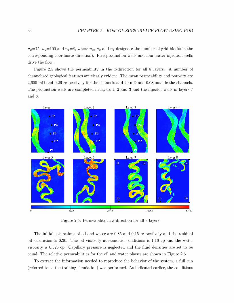
34 CHAPTER 2. ROM OF SUBSURFACE FLOW USING POD
nx=75, ny=100 and nz=8, where nx, ny and nz designate the number of grid blocks in the
corresponding coordinate direction). Five production wells and four water injection wells
drive the flow.
Figure 2.5 shows the permeability in the x-direction for all 8 layers. A number of
channelized geological features are clearly evident. The mean permeability and porosity are
2,600 mD and 0.26 respectively for the channels and 20 mD and 0.08 outside the channels.
The production wells are completed in layers 1, 2 and 3 and the injector wells in layers 7
and 8.
Figure 2.5: Permeability in x-direction for all 8 layers
The initial saturations of oil and water are 0.85 and 0.15 respectively and the residual
oil saturation is 0.30. The oil viscosity at standard conditions is 1.16 cp and the water
viscosity is 0.325 cp. Capillary pressure is neglected and the fluid densities are set to be
equal. The relative permeabilities for the oil and water phases are shown in Figure 2.6.
To extract the information needed to reproduce the behavior of the system, a full run
(referred to as the training simulation) was performed. As indicated earlier, the conditions

2.2. SIMULATION USING REDUCED-ORDER MODELING 35
Figure 2.6: Relative permeability curves for the oil and water phases
applied for this training simulation impact the quality of the reduced basis, so they should
be selected with care. Here we apply a heuristic procedure in which we vary the bottom hole
pressures (BHPs) of the production wells randomly and independently over their expected
ranges (between 3,500 and 4,500 psia). These BHPs are changed every 100 days and the
resulting schedule is shown in Figure 2.7. The injection well BHPs are constant in time for
each well, though the actual values vary from well to well (the BHPs for injectors 1 and 2
are 6500 psia, for injector 3 BHP is 7000 psia and for injector 4 BHP is 6000 psia). The
maximum timestep allowed was 20 days and a total of 211 snapshots for the oil pressure
and water saturation states were recorded.
Figure 2.7: Schedule for bottom hole pressures for the production wells

36 CHAPTER 2. ROM OF SUBSURFACE FLOW USING POD
Applying the proper orthogonal decomposition approach provides the eigenvalue spec-
trums for pressure and saturation shown in Figure 2.8. It is evident that the maximum
eigenvalue for the pressure state is almost 103 while the minimum approaches 10−16, which
means that the pressure eigenvalues vary over around 19 orders of magnitude. For the water
saturation state this variation is also substantial, about 18 orders of magnitude.
Figure 2.8: Eigenvalue variation for pressure and saturation matrices
We seek to form a basis such that the fraction of energy in the pressure state that
we ignore is very low, around 10−6, and the fraction ignored in the saturation state is
around 10−4. This requires that we retain the first 14 eigenvalues for the oil pressure state
and the first 26 eigenvalues for the water saturation state. Therefore, the basis matrix
Φ` ∈ R2Nc×`, where ` = `p + `s, has 14 + 26 = 40 basis vectors. This means that, while the
standard reservoir simulation model needs to solve Eq. 2.10 for 2Nc = 120, 000 unknowns,
the reduced-order reservoir simulation model needs to solve Eq. 2.21 for only 40 unknowns.
We present the first six pressure and saturation basis functions for the first layer in Fig-
ures 2.9 and 2.10. The fraction of energy contained in each basis function is also indicated.
These basis functions clearly reflect the locations of the wells and the pressure and satura-
tion gradients, though it is otherwise difficult to attribute direct physical interpretation to
their detailed shapes.
Implementing the clustering technique presented in section 2.1.4, the number of snap-
shots for each state is reduced from 211 to 50. Ignoring the same amounts of energy as
before, the number of basis functions required for the oil pressure state decreases from 14 to
12, while for the water saturation state it decreases from 26 to 22. Thus the reduced-order
reservoir simulation model now requires only 34 unknowns.

2.2. SIMULATION USING REDUCED-ORDER MODELING 37
Figure 2.9: Six most important reduced-order basis functions for the oil pressure state (layer1)
Applying the missing point estimation technique to the clustered snapshots and using
the grid block selection procedure described in section 2.1.5, the grid blocks are ordered
from the most important to the least important in terms of their impact on the condition
number. Allowing the condition number to increase to 5, the number of grid blocks selected
is Nm = 19, 441. Figure 2.11 shows that the selected grid blocks (shown in black) are
related to the wells and the high permeability channels, as indicated for layer 1, where the
red circles indicate the location of the producer wells, the blue arrows the injector wells
and the green contours regions of high permeability. The basis matrix, now of dimension
Nm× 34, can be applied to efficiently compute the reduced Jacobian appearing in Eq. 2.22.
As indicated in section 2.1.6, the MPE procedure was implemented into GPRS only at the
solver level. Thus the full benefits of this treatment will not be realized in the simulation

38 CHAPTER 2. ROM OF SUBSURFACE FLOW USING POD
Figure 2.10: Six most important reduced-order basis functions for the water saturation state(layer 1)
results presented below.
The ability of the reduced-order model to reproduce the training simulation will be tested
using the three basis function matrices obtained above. The first matrix was generated using
only proper orthogonal decomposition, Φ` ∈ R120,000×40; the second matrix was generated
using clustered snapshots and proper orthogonal decomposition, Φ` ∈ R120,000×34; and the
third was formed using clustered snapshots, proper orthogonal decomposition and missing
point estimation, Φ∗` ∈ R38,882×34.
Figures 2.12 through 2.16 display the oil and water flow rates for all production wells
and Figures 2.17 through 2.20 show the injection rates for all injector wells using the three
procedures. The total quantity of injected fluid is equal to 0.67 of the total pore volume
of the system. However, because of the residual (nonflowing) oil and water fractions, this

2.2. SIMULATION USING REDUCED-ORDER MODELING 39
Figure 2.11: Grid blocks selected (in black) by MPE procedure
corresponds to 1.22 mobile pore volumes of fluid. The reference oil and water flow rates from
the training simulation (solid red line for oil and blue for water, labeled as GPRS/CPR in the
figures) are very well reproduced using POD only (red circles for oil and blue for water),
clustered snapshots + POD (solid red circles for oil and blue for water), and clustered
snapshots + POD + MPE (light green dots for oil and light blue for water, labeled as
Clusters/QR in the figures). The reference water injection rate from the training simulation
(green line) are also well reproduced using POD (green circles), clustered snapshots + POD
(solid green circles) and clustered snapshots + POD + MPE (light green dots). These results
are very encouraging and indicate that the snapshot set and the basis contain sufficient
information to reproduce the training simulation. We can also observe that the clustering
approach enables a reduction in the size of the basis matrix without losing significant
accuracy in the simulation results. We note that the use of POD only (without clustered
snapshots) with 34 unknowns (the number used for the clustered snapshots + POD case)
provided less accurate simulation results than those obtained using clustered snapshots +
POD. This demonstrates the benefit of the clustering procedure. Finally, using fewer than

40 CHAPTER 2. ROM OF SUBSURFACE FLOW USING POD
1/3 of the grid blocks, the MPE technique provides results that continue to agree with the
training simulation. Errors for this and subsequent runs will be quantified in section 2.2.5.
Figure 2.12: Oil and water flow rates for production well 1 (training run)
Figure 2.13: Oil and water flow rates for production well 2 (training run)
We next consider two different flow scenarios to evaluate the predictive capability of the
three ROMs.

2.2. SIMULATION USING REDUCED-ORDER MODELING 41
Figure 2.14: Oil and water flow rates for production well 3 (training run)
Figure 2.15: Oil and water flow rates for production well 4 (training run)
Figure 2.16: Oil and water flow rates for production well 5 (training run)

42 CHAPTER 2. ROM OF SUBSURFACE FLOW USING POD
Figure 2.17: Water flow rate for injection well 1 (training run)
Figure 2.18: Water flow rate for injection well 2 (training run)
Figure 2.19: Water flow rate for injection well 3 (training run)

2.2. SIMULATION USING REDUCED-ORDER MODELING 43
Figure 2.20: Water flow rate for injection well 4 (training run)
2.2.1 Prediction Using ROM - Schedule I
The schedule for the bottom hole pressures of the production wells is shown in Figure 2.21.
The overall range (between 3,650 and 4,350 psia) is smaller than the range used in the
training simulation. In this example the BHPs are changed every 200 days, while in the
training simulation they were changed every 100 days. The injection well BHPs are the
same as in the training simulation. The maximum timestep for this case was increased to
50 days.
Figures 2.22 through 2.26 show the oil and water flow rates for production wells using
the three basis matrices. The flow rates from the high-fidelity (reference) solution (red line
for oil and blue for water) are, in general, well reproduced using the three ROMs. Relatively
small mismatches can be observed, however, in some of the results. The results for water
injection rates for the injection wells, shown in Figures 2.27 through 2.30, demonstrate close
agreement with the reference simulation, although some slight mismatches can be observed.
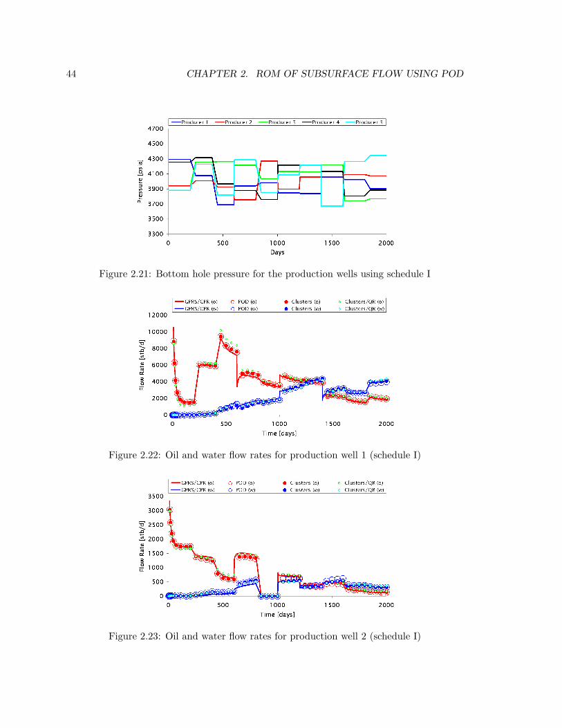
44 CHAPTER 2. ROM OF SUBSURFACE FLOW USING POD
Figure 2.21: Bottom hole pressure for the production wells using schedule I
Figure 2.22: Oil and water flow rates for production well 1 (schedule I)
Figure 2.23: Oil and water flow rates for production well 2 (schedule I)

2.2. SIMULATION USING REDUCED-ORDER MODELING 45
Figure 2.24: Oil and water flow rates for production well 3 (schedule I)
Figure 2.25: Oil and water flow rates for production well 4 (schedule I)
Figure 2.26: Oil and water flow rates for production well 5 (schedule I)

46 CHAPTER 2. ROM OF SUBSURFACE FLOW USING POD
Figure 2.27: Water flow rate for injection well 1 (schedule I)
Figure 2.28: Water flow rate for injection well 2 (schedule I)
Figure 2.29: Water flow rate for injection well 3 (schedule I)

2.2. SIMULATION USING REDUCED-ORDER MODELING 47
Figure 2.30: Water flow rate for injection well 4 (schedule I)
2.2.2 Prediction Using ROM - Schedule II
The schedule for the production well BHPs is shown in Figure 2.31. These BHPs are
changed every 200 days, and the overall range, between 3,350 and 4,650 psia, is larger than
the range used in the training simulation. The specifications for the injection wells are the
same as in the previous cases.
Figures 2.32 through 2.36 show the oil and water flow rates for schedule II for the
production wells using the three basis matrices. The flow rates from the high-fidelity solution
are again reasonably well reproduced using the three ROMs, though some errors are evident.
The results for water injection rates, shown in Figures 2.37 through 2.40, also demonstrate
generally close agreement with the reference simulation. Taken in total, these results are
encouraging as they demonstrate the ability of the ROM to provide flow results for scenarios
that differ substantially from the training simulations. This is important if the ROM is to
be used within the context of optimization.

48 CHAPTER 2. ROM OF SUBSURFACE FLOW USING POD
Figure 2.31: Bottom hole pressure for the producer wells using schedule II
Figure 2.32: Oil and water flow rates for production well 1 (schedule II)
Figure 2.33: Oil and water flow rates for production well 2 (schedule II)

2.2. SIMULATION USING REDUCED-ORDER MODELING 49
Figure 2.34: Oil and water flow rates for production well 3 (schedule II)
Figure 2.35: Oil and water flow rates for production well 4 (schedule II)
Figure 2.36: Oil and water flow rates for production well 5 (schedule II)

50 CHAPTER 2. ROM OF SUBSURFACE FLOW USING POD
Figure 2.37: Water flow rate for injection well 1 (schedule II)
Figure 2.38: Water flow rate for injection well 2 (schedule II)
Figure 2.39: Water flow rate for injection well 3 (schedule II)

2.2. SIMULATION USING REDUCED-ORDER MODELING 51
Figure 2.40: Water flow rate for injection well 4 (schedule II)
2.2.3 Simulation Time Reduction with ROMs
The simulation times for the high-fidelity models and the three ROMs for the base case and
schedules I and II are summarized in Figure 2.41. In the figure, the first set of bars refers
to the base case, the second set to schedule I and the third set to schedule II. For each set
the first bar represents the simulation time for the high-fidelity simulation using the fastest
current solution procedure (GMRES solver with CPR preconditioner). The second, third
and fourth bars in each set show the simulation times for the three reduced-order models
(POD, clusters + POD, and clusters + POD + MPE, respectively). Additionally, for each
bar the gray segment represents the time spent solving the linear system of equations and
the black segment the time spent in all other computations (computing block properties,
forming the residual vector and Jacobian matrix, etc.).
For the base case the first set of bars shows that the ROM with POD was able to reduce
the simulation time by a factor of ∼ 2.9. Applying the ROM with clusters + POD the
simulation time was reduced by a factor of ∼ 3.3. Further reduction, namely a factor of
∼ 5.9, was obtained when the ROM with clusters + POD + MPE was employed. The
speedups achieved using the various ROMs, though significant, are not dramatic. This
is because our ROM procedures target only the solver. Thus, even if the ROM reduces
the solver time to zero, we are still left with the remaining simulation computations. We
note, however, that a full MPE implementation (which was not introduced here) would
provide additional speedup. This is because, in contrast to the other reduced-order modeling

52 CHAPTER 2. ROM OF SUBSURFACE FLOW USING POD
procedures, a full MPE implementation would also reduce the time required for residual
and Jacobian construction.
The computation times for the schedule I and schedule II simulations are indicated
(respectively) by the second and third sets of bars. For schedule I, the speedups resulting
from the ROMs are greater than those observed for the base case (e.g., about a factor of
9.5 for clusters + POD + MPE). This is due in part to the ability of the ROMs to take
larger timesteps than the high-fidelity model. Similar results were obtained using schedule
II. As indicated by the third set of bars, the speedup for the clusters + POD + MPE
reduced-order model was 9.8.
Figure 2.41: Comparison of simulation time
2.2.4 Comparison of ROMs with ILU(0) Preconditioner
As explained in section 2.1.6, the full-order simulations are performed using GPRS with
the GMRES solver and the CPR preconditioner. This is a highly developed preconditioner
that provides essentially the best available linear solution methodology for many reservoir
simulation applications. Its inherent speed therefore limits the degree of speedup achievable
using our algorithms.
It may also be appropriate, therefore, for us to evaluate speedups relative to a more
generic solver. This is because, for many applications, a highly specialized solver plus
preconditioner combination will not be available. For example, our current gradient-based
production optimization algorithm, which requires the solution of an adjoint equation in
conjunction with the simulation model, is not yet compatible with GMRES + CPR but
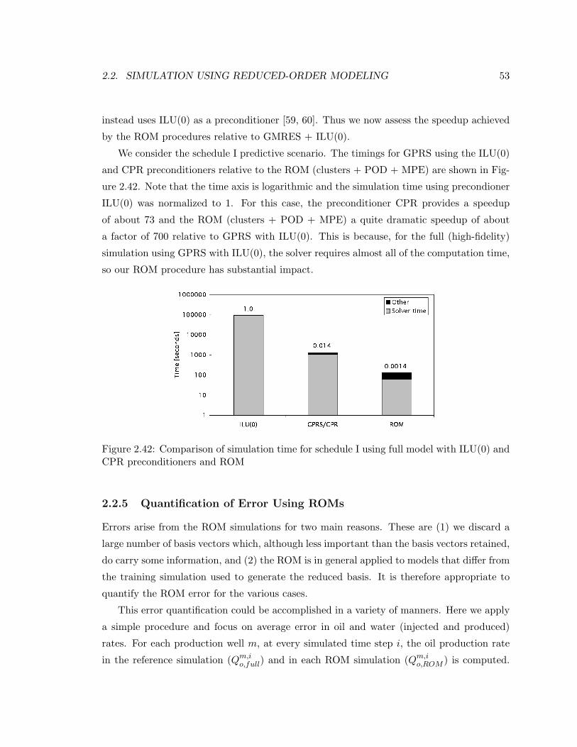
2.2. SIMULATION USING REDUCED-ORDER MODELING 53
instead uses ILU(0) as a preconditioner [59, 60]. Thus we now assess the speedup achieved
by the ROM procedures relative to GMRES + ILU(0).
We consider the schedule I predictive scenario. The timings for GPRS using the ILU(0)
and CPR preconditioners relative to the ROM (clusters + POD + MPE) are shown in Fig-
ure 2.42. Note that the time axis is logarithmic and the simulation time using precondioner
ILU(0) was normalized to 1. For this case, the preconditioner CPR provides a speedup
of about 73 and the ROM (clusters + POD + MPE) a quite dramatic speedup of about
a factor of 700 relative to GPRS with ILU(0). This is because, for the full (high-fidelity)
simulation using GPRS with ILU(0), the solver requires almost all of the computation time,
so our ROM procedure has substantial impact.
Figure 2.42: Comparison of simulation time for schedule I using full model with ILU(0) andCPR preconditioners and ROM
2.2.5 Quantification of Error Using ROMs
Errors arise from the ROM simulations for two main reasons. These are (1) we discard a
large number of basis vectors which, although less important than the basis vectors retained,
do carry some information, and (2) the ROM is in general applied to models that differ from
the training simulation used to generate the reduced basis. It is therefore appropriate to
quantify the ROM error for the various cases.
This error quantification could be accomplished in a variety of manners. Here we apply
a simple procedure and focus on average error in oil and water (injected and produced)
rates. For each production well m, at every simulated time step i, the oil production rate
in the reference simulation (Qm,io,full) and in each ROM simulation (Qm,i
o,ROM ) is computed.

54 CHAPTER 2. ROM OF SUBSURFACE FLOW USING POD
Results from the ROMs are interpolated to provide rates at the times computed in the
reference simulation (with care being taken to avoid interpolating across discontinuities in
well BHP). The time-average error for each well, designated Em, is then calculated as the
average of the absolute differences, normalized by the time-average oil flow rate Qmo,full for
the well:
Em =1
ntQmo,full
nt∑i=1
|Qm,io,full −Q
m,io,ROM |, (2.25)
where nt is the total number of time steps. The overall averaged error, designated E, is
then given by:
E =1nw
nw∑m=1
Em, (2.26)
where nw is the number of production wells. The same procedure is applied for the water
production and water injection rates.
Values for E computed via Eq. 2.26 for the training simulation and the two schedules
are presented in Tables 2.1, 2.2 and 2.3 for oil production, water production and water
injection rates, respectively.
Table 2.1: Errors in the oil rate for the various ROMs
ROM Training Schedule I Schedule II
POD 0.0164 0.0539 0.0453Clusters + POD 0.0294 0.0492 0.0526
Clusters + POD + MPE 0.0424 0.0849 0.0761
Table 2.2: Errors in the water production rate for the various ROMs
ROM Training Schedule I Schedule II
POD 0.0202 0.0911 0.0636Clusters + POD 0.0406 0.0761 0.0707
Clusters + POD + MPE 0.0509 0.0734 0.0718
It is evident from the tables that the training simulation case results in the smallest errors for
all of the ROMs for oil rate and water production rate; for water injection rate the training
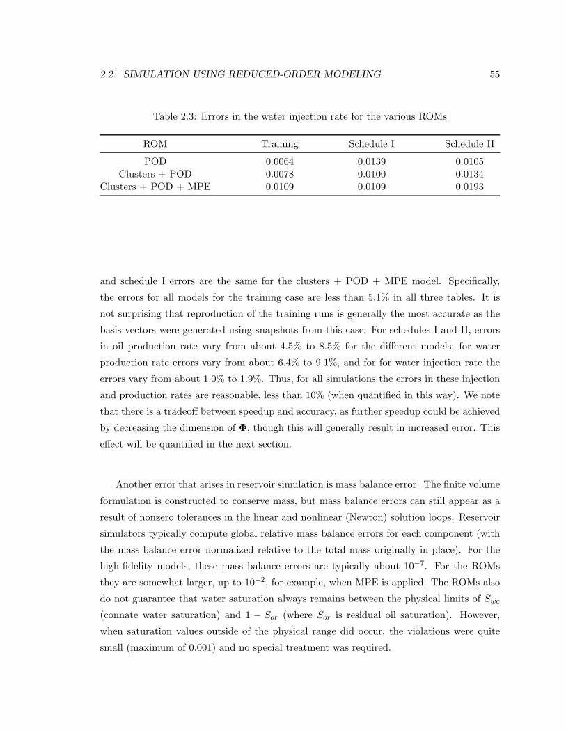
2.2. SIMULATION USING REDUCED-ORDER MODELING 55
Table 2.3: Errors in the water injection rate for the various ROMs
ROM Training Schedule I Schedule II
POD 0.0064 0.0139 0.0105Clusters + POD 0.0078 0.0100 0.0134
Clusters + POD + MPE 0.0109 0.0109 0.0193
and schedule I errors are the same for the clusters + POD + MPE model. Specifically,
the errors for all models for the training case are less than 5.1% in all three tables. It is
not surprising that reproduction of the training runs is generally the most accurate as the
basis vectors were generated using snapshots from this case. For schedules I and II, errors
in oil production rate vary from about 4.5% to 8.5% for the different models; for water
production rate errors vary from about 6.4% to 9.1%, and for for water injection rate the
errors vary from about 1.0% to 1.9%. Thus, for all simulations the errors in these injection
and production rates are reasonable, less than 10% (when quantified in this way). We note
that there is a tradeoff between speedup and accuracy, as further speedup could be achieved
by decreasing the dimension of Φ, though this will generally result in increased error. This
effect will be quantified in the next section.
Another error that arises in reservoir simulation is mass balance error. The finite volume
formulation is constructed to conserve mass, but mass balance errors can still appear as a
result of nonzero tolerances in the linear and nonlinear (Newton) solution loops. Reservoir
simulators typically compute global relative mass balance errors for each component (with
the mass balance error normalized relative to the total mass originally in place). For the
high-fidelity models, these mass balance errors are typically about 10−7. For the ROMs
they are somewhat larger, up to 10−2, for example, when MPE is applied. The ROMs also
do not guarantee that water saturation always remains between the physical limits of Swc
(connate water saturation) and 1 − Sor (where Sor is residual oil saturation). However,
when saturation values outside of the physical range did occur, the violations were quite
small (maximum of 0.001) and no special treatment was required.

56 CHAPTER 2. ROM OF SUBSURFACE FLOW USING POD
2.3 Further Observations
In this section we consider the behavior of the reduced-order modeling procedure when
(1) fewer basis vectors are used and (2) when the flow problem is more nonlinear or in-
cludes additional physics. These results are of interest because they indicate some of the
limitations of the current ROM implementation and therefore suggest directions for future
investigations.
We first assess the impact of retaining less energy (and thus fewer basis functions) in the
pressure and saturation bases. As the number of basis functions is reduced, we expect to
achieve a higher degree of speedup but also a loss of accuracy. Three different reduced-order
bases are considered, each of which neglects different fractions of the energy. All three of
these ROMs were generated using only POD (i.e., no clustering or MPE procedures were
applied). For these runs the ROMs are applied to reproduce the base case (this is the same
base case as was used in the examples in section 2.2).
The first ROM is the same as that used in section 2.2. As indicated in section 2.2, this
basis ignores 10−6 of the energy in the pressure state and 10−4 of the energy in the saturation
state. Thus 14 basis functions are used for pressure and 26 for saturation. The simulation
time for this case is normalized to 1. The second ROM ignores a slightly larger fraction of
the total energy: 5 × 10⁻⁶ for the pressure state and 2.5 × 10⁻⁴ for the saturation state.
This ROM contains 11 basis functions for pressure and 20 for saturation. The simulation
using this basis requires 0.74 as much time as the first ROM. The third ROM neglects a
still larger fraction of the total energy: 5 × 10⁻⁵ for pressure and 6 × 10⁻⁴ for saturation.
Only 8 basis functions are now used for pressure and 14 for saturation. The normalized
simulation time for this ROM is 0.69.
The results for errors in oil production rate, water production rate and water injection
rate using the three ROMs are summarized in Figure 2.43. Errors are computed using
Eq. 2.26. It is evident that error increases as `p and `s decrease. This increase is relatively
slight when ` = `p + `s decreases from 40 to 31, but the increase in error is large when `
is further decreased to 22. The results using the first and second ROMs are quite accept-
able (errors for all quantities less than 0.1), though for the third ROM the errors increase
appreciably (e.g., 0.60 for oil rate). This demonstrates that, even though a large fraction
of energy (>0.999) may be captured by the basis, simulation accuracy can still be very
sensitive to the number of basis functions used in Φ. In our current implementation, the

2.3. FURTHER OBSERVATIONS 57
appropriate `p and `s must be determined through numerical experimentation, as we do
not yet have an accurate means for the a priori determination of the size of Φ.
Figure 2.43: Tradoff between speedup and accuracy for the training simulation
We next consider the impact of increased nonlinearity on the performance of the ROM.
For the models considered, the key source of nonlinearity is the oil and water relative per-
meability curves. This nonlinearity can be adjusted through the so-called Corey exponents
a and b in the relative permeability functions:
kro = k0ro
(1− Sw − Sor
1− Swc − Sor
)a
, (2.27)
krw = k0rw
(Sw − Swc
1− Swc − Sor
)b
. (2.28)
The original relative permeability curves, shown in Figure 2.6, were determined experimen-
tally and were specified in tabular form. Expressed in the form of Eqs. 2.27 and 2.28,
these curves correspond approximately to a = 1.7 and b = 1.5. We now consider curves
with a = 3 and b = 3. These curves are plotted with the original curves in Figure 2.44.
The other parameters used for the new curves are, with reference to Eqs. 2.27 and 2.28,
k0ro = 1.0, k0
rw = 0.5, Swc = 0.15 and Sor = 0.3.
The training simulation with well BHPs described in section 2.2 was run using these
more nonlinear relative permeability curves. The number of POD basis functions needed to
reproduce the high-fidelity results with errors comparable to those presented in section 2.2.5
was then determined through numerical experimentation. The number of basis functions

58 CHAPTER 2. ROM OF SUBSURFACE FLOW USING POD
Figure 2.44: Original and modified relative permeability curves
required was 29 for pressure (as compared to 14 for the previous case) and 84 for saturation
(as compared to 26 for the previous case). This basis neglects about the same amount of
energy for the pressure state as the previous case, but for the saturation state it neglects
only 10−5 of the total energy, as compared to 10−4 for the previous case. Due to the use of
larger `p and `s, the speedup using the ROM with the more nonlinear relative permeability
curves is less than that achieved with the previous case. Specifically, in this case we achieve
a very modest speedup of ∼ 1.3, as compared to a speedup of ∼ 2.9 using the original
curves (though we note that more substantial speedups could be obtained through use of
the clustering and MPE procedures). This demonstrates the impact of high degrees of
nonlinearity on the ROM and the need for better treatments for such cases.
Another significant issue is the impact of gravitational effects on the performance of the
ROM. The governing equations for a two-phase incompressible system can be written in
terms of a pressure (flow) equation and a saturation (transport) equation:
∇ · ut = −qt, (2.29)
φ∂Sw
∂t+∇ · F = −qw, (2.30)
where ut is the total Darcy velocity given by ut = −k · [λt∇p+ g (λwρw + λoρo) iz], with
λt = λw + λo, F = fw [ut − k · izλog(ρw − ρo)], where fw = λw/λt is the Buckley-Leverett
fractional flow function, iz is the unit vector in the z direction, qt = qo + qw, and all other
quantities are as defined previously. Gravitational effects in the saturation equation can

2.3. FURTHER OBSERVATIONS 59
be quantified through the density difference (∆ρ) between the oil and water phases (we
note that a more complete quantification of this effect would be in terms of a dimensionless
gravity number, though for current purposes the use of ∆ρ will suffice). The impact of
gravitational effects on reduced-order models is here assessed by applying proper orthogonal
decomposition to high-fidelity snapshots generated with varying ∆ρ.
Results are displayed in Figure 2.45, where we present the variation in eigenvalues for
the pressure and saturation states for models with ∆ρ = 0, 1, 5 and 20 lb/ft3. For all
of these runs the simulation time was 1,000 days and 170 snapshots were generated. It
is apparent from the figure that the decay in the magnitudes of the eigenvalues is slower,
for both pressure and saturation, with increasing ∆ρ. In general, the slower the decay
in the eigenvalues, the larger the number of basis functions that must be retained in the
ROM. Thus we expect to observe decreasing computational efficiency using ROMs as ∆ρ
is increased. Numerical experiments confirm this expectation.
Figure 2.45: Eigenvalue variation for pressure and saturation for models with density dif-ferences
In order to further assess the impact of gravitational effects, we consider a simpler
model. Here we specify linear relative permeability curves (krw = Sw and kro = 1 − Sw)
and equal viscosities (µo = µw = 1 cp). For this case, when ∆ρ = 0, the model is linear
and pressure does not change in time (for the incompressible case). The reservoir model
used here contains 20,400 cells and, like the model used in all other simulations in this
chapter, is also extracted from the model developed by Castro [23]. See section 4.1 for
further description of the reservoir model. Using this model the simulation time was 3,000
days and 190 snapshots were generated for the pressure and saturation states.

60 CHAPTER 2. ROM OF SUBSURFACE FLOW USING POD
Figures 2.46 and 2.47 show the variation in eigenvalues for the pressure and saturation
states, respectively, for models with ∆ρ = 0, 1, 2, 5, 15 and 20 lb/ft3. It is apparent that
with ∆ρ = 0 only one basis function is needed for pressure. This is as expected since the
pressure field does not change in time. Pressure does change in time for nonzero ∆ρ and,
as ∆ρ increases, more basis functions are required to retain a specified fraction of the total
energy (as was observed in Figure 2.45). The saturation equation is linear in this case for
∆ρ = 0 though, because the solution still changes in time, more than one basis function
is needed. The saturation equation becomes nonlinear for nonzero ∆ρ, and we observe
flattening in the eigenvalue decay as ∆ρ increases in Figure 2.47. There is a large difference
in the shapes of the curves for ∆ρ = 0 and ∆ρ = 1.
The results presented in Figures 2.45, 2.46 and 2.47 suggest that the use of ROM pro-
cedures will be more challenging when significant density differences are present. At this
point we cannot, however, determine whether this is because additional physics enters the
problem or simply because the problem is now more nonlinear. A detailed assessment of
this issue should be a topic for future work.
Figure 2.46: Eigenvalue variation for pressure for 20,400-cell models with density differences
There are many practical subsurface flow cases for which the relative permeability curves
are not highly nonlinear and gravitational effects are small relative to viscous effects. For
such cases, the ROM procedures applied here would be expected to be effective. However,
for cases with highly nonlinear relative permeability curves and/or strong gravitational ef-
fects, further enhancements in our reduced-order modeling procedures will likely be required
before they can be applied in practice. This may entail the use of new training procedures

2.3. FURTHER OBSERVATIONS 61
Figure 2.47: Eigenvalue variation for saturation for 20,400-cell models with density differ-ences
or the use of techniques other than POD to construct the basis matrix. We have also ob-
served a reduction in accuracy when the injector BHPs are varied over a wide range, so
better treatments for that case will also be required.
In this chapter we developed and tested new POD-based ROM procedures for oil-water
flow. For the class of problems considered, speedups of up to about a factor of 10 were
observed. In the next chapter, we consider a different reduced-order modeling approach,
which uses POD as one of its components, that is able to provide significantly greater
runtime speedups.

62 CHAPTER 2. ROM OF SUBSURFACE FLOW USING POD

Chapter 3
Trajectory Piecewise Linearization
for Reservoir Simulation
Our goal in this chapter is to develop and apply a trajectory piecewise linearization (TPWL)
procedure for subsurface flow problems. We first develop the linearized representation of
the governing equations for oil-water flow. POD procedures and their use in conjunction
with the linearized oil-water model are then described. Next, some implementation issues
are discussed. We then present simulation results for two cases, involving heterogeneous
reservoirs with 24,000 and 79,200 grid blocks. These computations demonstrate that the
TPWL technique is able to provide accurate solutions for a variety of well BHP schedules
with very significant speedups. Finally, some additional issues are discussed.
3.1 TPWL for Subsurface Flow
We consider the two-phase flow system presented in Chapter 2. The governing equations
and discretizations are specified by Eqs. 2.1 – 2.7. The discrete system is given by Eq. 2.9,
which we write here as:
g(xn+1,un+1) = F(xn+1) + A(xn+1,xn) + Q(xn+1,un+1) = 0, (3.1)
where g represents the residual vector, which we seek to drive to zero, x designates the
system states (pressure and saturation), u indicates the system controls (well BHPs), and
F, A and Q represent the convective, accumulation and source/sink terms, respectively.
63

64 CHAPTER 3. TRAJECTORY PIECEWISE LINEARIZATION
See [9] for detailed expressions. Note that, in Chapter 2, we wrote F(xn+1) = Tn+1xn+1
and A(xn+1,xn) = −Dn+1(xn+1 − xn). The fully implicit system defined by Eq. 3.1 is
nonlinear and is solved through application of Newton’s method, with the Jacobian matrix
given by ∂g/∂x.
3.1.1 Linearization of Governing Equations
Linearized models can be constructed through use of a Taylor series expansion about a
known state and set of controls, which we designate as (xi,ui). These states are saved from
a small number (e.g., 3–5) of preprocessing ‘training’ simulations [56]. Applying such an
expansion to Eq. 3.1 gives:
g(xn+1,un+1) = g(xi,ui) +(∂g∂x
)i
(xn+1 − xi) +(∂g∂u
)i
(un+1 − ui) + . . . , (3.2)
where un+1 is the new set of controls (which are specified), xn+1 is the new state we wish
to determine, and both (∂g/∂x)i and (∂g/∂u)i are matrices evaluated at (xi,ui). The
necessary information associated with these matrices is saved along with the states during
the training runs, though in a reduced form as described below.
Given the solution at time step n (xn), our goal is to represent xn+1 in the form of
Eq. 3.2. We designate the saved state that is ‘closest’ to xn as xi. There are various criteria
for determining the closest saved state, and we will specify our particular approach below.
It is then reasonable to assume that the closest saved state to xn+1 (the state we seek to
determine) is xi+1, which is the saved state that follows xi.
We can now proceed with expansions of the form of Eq. 3.2 for each of the terms in
Eq. 3.1. Expanding around xi+1, we have, for the convective effects
Fn+1 ≈ Fi+1 +∂Fi+1
∂xi+1(xn+1 − xi+1), (3.3)
where Fn+1 = F(xn+1) (and similarly for Fi+1) and ∂Fi+1/∂xi+1 designates the flow term
portion of the Jacobian matrix for the state xi+1. Note that the controls do not appear in
the flow terms.
The accumulation term depends on the states at time levels n and n + 1. We thus
expand around both xi+1 and xi, which gives:
A(xn+1,xn) ≈ Ai+1(xi+1,xi) +∂Ai+1
∂xi+1(xn+1 − xi+1) +
∂Ai+1
∂xi(xn − xi). (3.4)

3.1. TPWL FOR SUBSURFACE FLOW 65
From here on Ai+1(xi+1,xi) will be designated simply as Ai+1.
The source/sink term Q depends on both xn+1 and the new controls un+1. The
source/sink term can thus be represented as
Q(xn+1,un+1) ≈ Qi+1(xi+1,ui+1) +∂Qi+1
∂xi+1(xn+1 − xi+1) +
∂Qi+1
∂ui+1(un+1 − ui+1). (3.5)
Recall that the controls in our case are the well bottom hole pressures, pwi . Because of the
way in which the controls appear in the source term (Eq. 2.6), we can compute Q(xi+1,un+1)
directly. In other words, this term is evaluated using the new controls un+1 and not the
controls ui+1 (which are the controls associated with the saved state xi+1). Thus we can
write
Q(xn+1,un+1) ≈ Q(xi+1,un+1) +∂Qi+1
∂xi+1(xn+1 − xi+1). (3.6)
This representation eliminates the need to save ∂Qi+1/∂ui+1 from the training simulations.
Applying Eqs. 3.3, 3.4 and 3.6 into Eq. 3.1 we have:
g(xn+1,un+1) ≈ Fi+1 +∂Fi+1
∂xi+1(xn+1 − xi+1) + Ai+1 +
∂Ai+1
∂xi+1(xn+1 − xi+1)+
∂Ai+1
∂xi(xn − xi) + Q(xi+1,un+1) +
∂Qi+1
∂xi+1(xn+1 − xi+1). (3.7)
Defining the Jacobian matrix as:
Ji+1 =∂Fi+1
∂xi+1+∂Ai+1
∂xi+1+∂Qi+1
∂xi+1, (3.8)
enables us to express Eq. 3.7 more concisely
g(xn+1,un+1) ≈ Fi+1 + Ai+1 +∂Ai+1
∂xi(xn − xi) + Q(xi+1,un+1) + Ji+1(xn+1 − xi+1) = 0.
(3.9)
Now, setting the residual using the new controls at the new state to zero (g(xn+1,un+1) =
0), we arrive at a matrix equation that can be solved to determine xn+1:
Ji+1(xn+1 − xi+1) = −[Fi+1 + Ai+1 +
∂Ai+1
∂xi(xn − xi) + Q(xi+1,un+1)
]. (3.10)
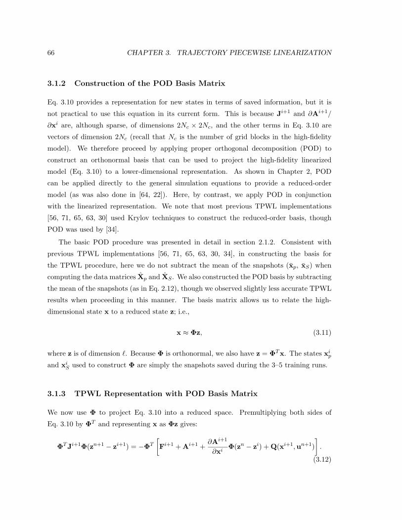
66 CHAPTER 3. TRAJECTORY PIECEWISE LINEARIZATION
3.1.2 Construction of the POD Basis Matrix
Eq. 3.10 provides a representation for new states in terms of saved information, but it is
not practical to use this equation in its current form. This is because Ji+1 and ∂Ai+1/
∂xi are, although sparse, of dimensions 2Nc × 2Nc, and the other terms in Eq. 3.10 are
vectors of dimension 2Nc (recall that Nc is the number of grid blocks in the high-fidelity
model). We therefore proceed by applying proper orthogonal decomposition (POD) to
construct an orthonormal basis that can be used to project the high-fidelity linearized
model (Eq. 3.10) to a lower-dimensional representation. As shown in Chapter 2, POD
can be applied directly to the general simulation equations to provide a reduced-order
model (as was also done in [64, 22]). Here, by contrast, we apply POD in conjunction
with the linearized representation. We note that most previous TPWL implementations
[56, 71, 65, 63, 30] used Krylov techniques to construct the reduced-order basis, though
POD was used by [34].
The basic POD procedure was presented in detail in section 2.1.2. Consistent with
previous TPWL implementations [56, 71, 65, 63, 30, 34], in constructing the basis for
the TPWL procedure, here we do not subtract the mean of the snapshots (xp, xS) when
computing the data matrices Xp and XS . We also constructed the POD basis by subtracting
the mean of the snapshots (as in Eq. 2.12), though we observed slightly less accurate TPWL
results when proceeding in this manner. The basis matrix allows us to relate the high-
dimensional state x to a reduced state z; i.e.,
x ≈ Φz, (3.11)
where z is of dimension `. Because Φ is orthonormal, we also have z = ΦT x. The states xip
and xiS used to construct Φ are simply the snapshots saved during the 3–5 training runs.
3.1.3 TPWL Representation with POD Basis Matrix
We now use Φ to project Eq. 3.10 into a reduced space. Premultiplying both sides of
Eq. 3.10 by ΦT and representing x as Φz gives:
ΦT Ji+1Φ(zn+1 − zi+1) = −ΦT
[Fi+1 + Ai+1 +
∂Ai+1
∂xiΦ(zn − zi) + Q(xi+1,un+1)
].
(3.12)
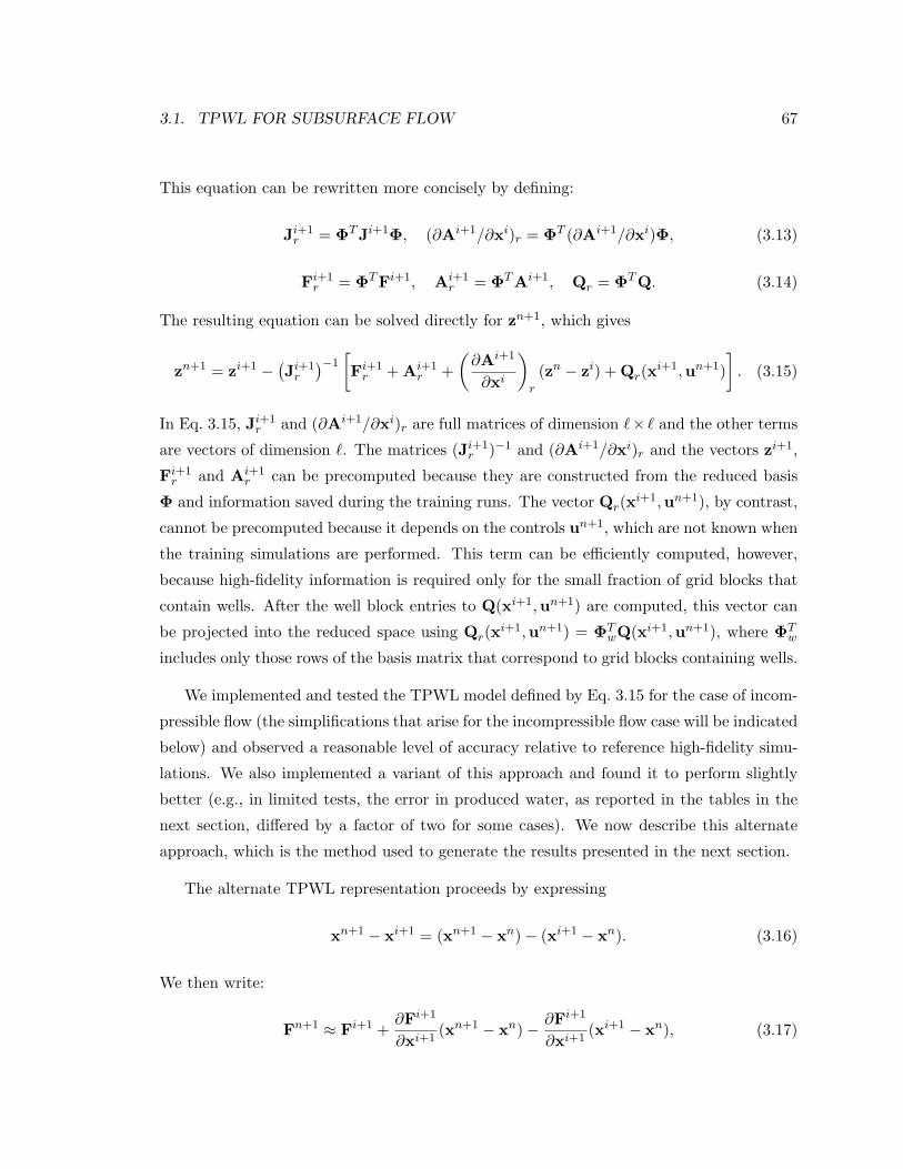
3.1. TPWL FOR SUBSURFACE FLOW 67
This equation can be rewritten more concisely by defining:
Ji+1r = ΦT Ji+1Φ, (∂Ai+1/∂xi)r = ΦT (∂Ai+1/∂xi)Φ, (3.13)
Fi+1r = ΦT Fi+1, Ai+1
r = ΦT Ai+1, Qr = ΦT Q. (3.14)
The resulting equation can be solved directly for zn+1, which gives
zn+1 = zi+1 −(Ji+1
r
)−1[Fi+1
r + Ai+1r +
(∂Ai+1
∂xi
)r
(zn − zi) + Qr(xi+1,un+1)]. (3.15)
In Eq. 3.15, Ji+1r and (∂Ai+1/∂xi)r are full matrices of dimension `× ` and the other terms
are vectors of dimension `. The matrices (Ji+1r )−1 and (∂Ai+1/∂xi)r and the vectors zi+1,
Fi+1r and Ai+1
r can be precomputed because they are constructed from the reduced basis
Φ and information saved during the training runs. The vector Qr(xi+1,un+1), by contrast,
cannot be precomputed because it depends on the controls un+1, which are not known when
the training simulations are performed. This term can be efficiently computed, however,
because high-fidelity information is required only for the small fraction of grid blocks that
contain wells. After the well block entries to Q(xi+1,un+1) are computed, this vector can
be projected into the reduced space using Qr(xi+1,un+1) = ΦTwQ(xi+1,un+1), where ΦT
w
includes only those rows of the basis matrix that correspond to grid blocks containing wells.
We implemented and tested the TPWL model defined by Eq. 3.15 for the case of incom-
pressible flow (the simplifications that arise for the incompressible flow case will be indicated
below) and observed a reasonable level of accuracy relative to reference high-fidelity simu-
lations. We also implemented a variant of this approach and found it to perform slightly
better (e.g., in limited tests, the error in produced water, as reported in the tables in the
next section, differed by a factor of two for some cases). We now describe this alternate
approach, which is the method used to generate the results presented in the next section.
The alternate TPWL representation proceeds by expressing
xn+1 − xi+1 = (xn+1 − xn)− (xi+1 − xn). (3.16)
We then write:
Fn+1 ≈ Fi+1 +∂Fi+1
∂xi+1(xn+1 − xn)− ∂Fi+1
∂xi+1(xi+1 − xn), (3.17)

68 CHAPTER 3. TRAJECTORY PIECEWISE LINEARIZATION
A(xn+1,xn) ≈ Ai+1 +∂Ai+1
∂xi+1(xn+1 − xn)− ∂Ai+1
∂xi+1(xi+1 − xn) +
∂Ai+1
∂xi(xn − xi), (3.18)
Qn+1(xn+1,un+1) ≈ Q(xi+1,un+1) +∂Qi+1
∂xi+1(xn+1 − xn)− ∂Qi+1
∂xi+1(xi+1 − xn). (3.19)
Now, by noting that Q(xi+1,un+1)− (∂Qi+1/∂xi+1)(xi+1 − xn) ≈ Q(xn,un+1),
Qn+1(xn+1,un+1) ≈ Q(xn,un+1) +∂Qi+1
∂xi+1(xn+1 − xn). (3.20)
Applying Eqs. 3.17, 3.18, 3.20 and the Jacobian matrix Ji+1 as given by Eq. 3.8 into the
residual equation (Eq. 3.1), we have:
Ji+1(xn+1 − xn) = −
[Fi+1 − ∂Fi+1
∂xi+1(xi+1 − xn) + Ai+1 − ∂Ai+1
∂xi+1(xi+1 − xn)
+∂Ai+1
∂xi(xn − xi) + Q(xn,un+1)
]. (3.21)
Premultiplying both sides of Eq. 3.21 by ΦT and writing x ≈ Φz, we arrive at the TPWL
representation for zn+1:
zn+1 = zn −(Ji+1
r
)−1
[Fi+1
r −(∂Fi+1
∂xi+1
)r
(zi+1 − zn) + Ai+1r −
(∂Ai+1
∂xi+1
)r
(zi+1 − zn)
+(∂Ai+1
∂xi
)r
(zn − zi) + Qr(xn,un+1)
]. (3.22)
The actual TPWL implementation accomplished in this work is for the case of incompress-
ible fluid and rock. For such systems, with reference to Eq. 2.5, the accumulation term
becomes
A(xn+1,xn) = D(xn+1 − xn) and A(xi+1,xi) = D(xi+1 − xi), (3.23)
which gives ∂Ai+1/∂xi+1 = −∂Ai+1/∂xi = D. Here D is a constant matrix. Inserting
this representation of the accumulation term into Eq. 3.22 gives the TPWL model for

3.1. TPWL FOR SUBSURFACE FLOW 69
incompressible systems:
zn+1 = zn −(Ji+1
r
)−1[Fi+1
r −(∂Fi+1
∂xi+1
)r
(zi+1 − zn) + Qr(xn,un+1)]. (3.24)
The reason why Eq. 3.24 provides slightly better accuracy than the incompressible version
of Eq. 3.15 is not entirely clear. It may, however, be related to the different treatments
of Qr that appear in the two equations. Specifically, in developing Eq. 3.15, we express
Q(xn+1,un+1) in terms of an expansion around Q(xi+1,un+1) (see Eq. 3.6), while for
Eq. 3.24, we represent Q(xn+1,un+1) using an expansion around Q(xn,un+1) (Eq. 3.20).
As it is often the case that xn+1 is closer to xn than it is to xi+1, we would expect better
overall accuracy for Eq. 3.24 than for Eq. 3.15.
3.1.4 Implementation Issues
We now comment briefly on some aspects of the numerical implementation. The high-
fidelity simulations are all performed using Stanford’s general purpose research simulator,
GPRS [17, 41]. The simulator was modified to output the states (snapshots) and Jacobian
information from the training runs, as required by the TPWL procedure. The output
files occupy substantial disk space, as the matrices for the high-fidelity model can be quite
large. Following the simulation of 3–5 training runs, the reduced basis Φ is constructed,
the reduced matrices are generated, and the reduced Jacobian matrices are inverted. The
computational requirements for constructing the basis and generating the required matrices
are comparable to the time required to perform the training simulations. These operations
are however now performed using Matlab [47], so it is likely that they can be accelerated.
The TPWL solution (Eq. 3.24) is implemented as a Matlab procedure. Our formulation
generally avoids the need to perform any computations using the high-fidelity model. How-
ever, in the following section we do report on the mass balance error observed using TPWL
for some cases. For such calculations, the high-fidelity model must be reconstructed (using
x ≈ Φz) and computations then performed using it. This will of course reduce the speedup
achieved using TPWL.
The TPWL procedure represents new solutions, designated xn+1, in terms of expansions
around saved solutions, designated xi+1. As described above, this requires that we first
determine the ‘closest’ saved state xi to the solution at the previous time step, xn. It would
be time consuming if this determination was performed using high-fidelity states. Therefore,

70 CHAPTER 3. TRAJECTORY PIECEWISE LINEARIZATION
we investigated various approaches for finding the closest state using only reduced state
information. The best accuracy was achieved by determining the saved state that minimizes
|zns − zi
s|, where zns = ΦT
s xns and zi
s = ΦTs xi
s designate reduced saturation states. Inclusion
of the reduced pressure states in this determination did not provide additional accuracy.
This finding is reasonable because, during the course of the simulation, the global saturation
changes more significantly and more abruptly than pressure (saturation is described by an
essentially hyperbolic conservation equation, while pressure is determined from an elliptic
solution for the incompressible case, as is evident from Eqs. 2.29 and 2.30), so the accuracy
of the TPWL solution is more sensitive to the saturation state used in the expansion.
3.2 Simulation Results Using TPWL Procedure
In this section we apply the TPWL procedure to two reservoir models – one containing
24,000 grid blocks and the other containing 79,200 grid blocks. We consider the performance
of the TPWL models for a variety of test runs.
3.2.1 Reservoir Model 1
Model Description
This reservoir model, shown in Figure 3.1, is a modified portion of a channelized reservoir
model presented in [28] (the full model is often referred to as SPE 10). The model is three-
dimensional and contains 24,000 grid blocks (with nx = 60, ny = 80 and nz = 5, where nx,
ny and nz designate the number of grid blocks in each direction). There are four production
wells (designated P1–P4) and two water injection wells (designated I1 and I2).
Permeability is taken to be a diagonal tensor, with kx = ky. The mean kx is 418 mD and
the mean porosity is 0.203. The vertical permeability (kz) is prescribed as kz = 0.3kx in the
channels and kz = 10−3kx in the non-channel regions. The initial oil and water saturations
are 0.8 and 0.2 respectively and the residual oil (Sor) and water (Swr) saturations are 0.2.
For oil we set ρo = 45 lb/ft3, µo = 3.0 cp; for water, ρw = 60 lb/ft3, µw = 0.5 cp. The system
is incompressible and capillary pressure effects are neglected. The relative permeabilities
for the oil and water phases are specified by Eqs. 2.27 and 2.28 with k0ro = k0
rw = 1 and
a = b = 2.

3.2. SIMULATION RESULTS USING TPWL PROCEDURE 71
Figure 3.1: Synthetic reservoir model (24,000 grid blocks) with four production wells andtwo injection wells. Permeability in x-direction (in mD) is shown
Training Runs
The first step in the TPWL procedure is to perform a few training runs using the high-
fidelity model to generate the states and Jacobian matrices (GPRS is used for these sim-
ulations). For this reservoir model four training simulations are performed. In all of these
simulations the injection wells are prescribed to maintain constant bottom hole pressure
(BHP) of 10,000 psia. This condition will be maintained in subsequent test runs (our focus
here is on varying the production well BHPs). For the production wells, the BHPs are
prescribed to follow schedules that are expected to represent approximately the operating
conditions that will be encountered in subsequent simulations. We have not yet established
a fully systematic approach for prescribing the training run BHPs, so we instead apply the
following heuristic procedure.
In the first training simulation, the BHPs of all four production wells are kept constant
at 1,000 psia. For the second training run, the BHPs are changed every 200 days, as
indicated in Figure 3.2, such that the total flow rate (oil+water) of each production well
is approximately the same and approximately constant in time for each 1,000 day interval.
Specifically, over the first 1,000 days, the total flow rate per well is 2,000 stb/d (stock tank
barrels per day), from 1,000 to 2,000 days it is 2,300 stb/d, from 2,000 to 3,000 days it is
2,700 stb/d, from 3,000 to 4,000 days it is 3,100 stb/d and from 4,000 to 5,000 days it is
3,300 stb/d. In the third training schedule, the BHPs of the production wells are varied

72 CHAPTER 3. TRAJECTORY PIECEWISE LINEARIZATION
every 200 days, randomly and independently, between 2,000 and 4,000 psia, as illustrated
in Figure 3.3. For the fourth training simulation, the producer BHPs are again varied
randomly, but this time between 1,000 and 3,000 psia as shown in Figure 3.4. Thus with
the training runs we attempt to capture constant BHP behavior (training run 1), constant
flow rate behavior (run 2) and more variable effects (runs 3 and 4). Other training sequences
could of course be devised, though as we will see below this set of training runs generally
results in accurate predictions in the subsequent test runs.
In the training runs, we simulated reservoir performance for a total of 5,000 days with
a maximum time step of 30 days. From the four training runs 759 pressure and saturation
snapshots and Jacobian matrices were recorded. The POD basis matrix was constructed
following the approach described in section 2.1.2. We did not apply the clustering or missing
point estimation procedures described in sections 2.1.4 and 2.1.5. The reduced basis Φ used
for most of the runs in this section contains a total of 325 columns, 78 of which correspond
to pressure states and 247 to saturation states.
We now assess the ability of the TPWL representation (Eq. 3.24) to reproduce results
from the training simulations by applying the BHP schedules used for training simulation
2. Figure 3.5 presents the oil rates and Figure 3.6 shows the water rates for all production
wells. Figure 3.7 depicts the injection rates for wells I1 and I2. We see from these figures
that the TPWL results, depicted by circles, are in essentially perfect agreement with the
reference high-fidelity (GPRS) solutions, depicted by solid curves.
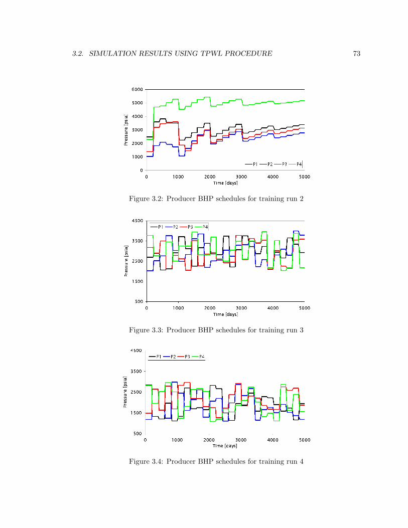
3.2. SIMULATION RESULTS USING TPWL PROCEDURE 73
Figure 3.2: Producer BHP schedules for training run 2
Figure 3.3: Producer BHP schedules for training run 3
Figure 3.4: Producer BHP schedules for training run 4
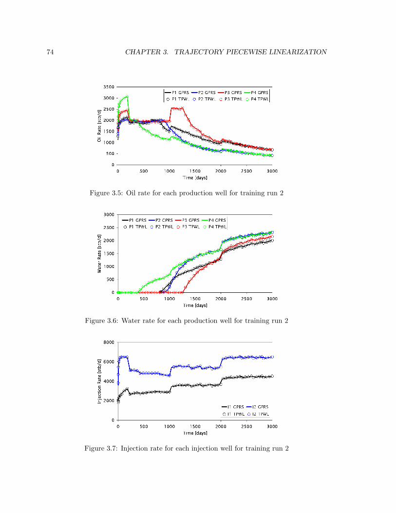
74 CHAPTER 3. TRAJECTORY PIECEWISE LINEARIZATION
Figure 3.5: Oil rate for each production well for training run 2
Figure 3.6: Water rate for each production well for training run 2
Figure 3.7: Injection rate for each injection well for training run 2
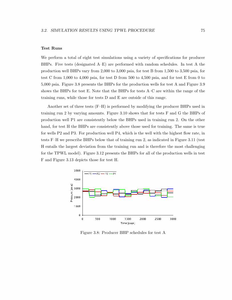
3.2. SIMULATION RESULTS USING TPWL PROCEDURE 75
Test Runs
We perform a total of eight test simulations using a variety of specifications for producer
BHPs. Five tests (designated A–E) are performed with random schedules. In test A the
production well BHPs vary from 2,000 to 3,000 psia, for test B from 1,500 to 3,500 psia, for
test C from 1,000 to 4,000 psia, for test D from 500 to 4,500 psia, and for test E from 0 to
5,000 psia. Figure 3.8 presents the BHPs for the production wells for test A and Figure 3.9
shows the BHPs for test E. Note that the BHPs for tests A–C are within the range of the
training runs, while those for tests D and E are outside of this range.
Another set of three tests (F–H) is performed by modifying the producer BHPs used in
training run 2 by varying amounts. Figure 3.10 shows that for tests F and G the BHPs of
production well P1 are consistently below the BHPs used in training run 2. On the other
hand, for test H the BHPs are consistently above those used for training. The same is true
for wells P2 and P3. For production well P4, which is the well with the highest flow rate, in
tests F–H we prescribe BHPs below that of training run 2, as indicated in Figure 3.11 (test
H entails the largest deviation from the training run and is therefore the most challenging
for the TPWL model). Figure 3.12 presents the BHPs for all of the production wells in test
F and Figure 3.13 depicts those for test H.
Figure 3.8: Producer BHP schedules for test A

76 CHAPTER 3. TRAJECTORY PIECEWISE LINEARIZATION
Figure 3.9: Producer BHP schedules for test E
Figure 3.10: Producer BHP schedules for training run 2 and tests F–H for well P1
Figure 3.11: Producer BHP schedules for training run 2 and tests F–H for well P4

3.2. SIMULATION RESULTS USING TPWL PROCEDURE 77
Figure 3.12: Test F: BHP schedules for all production wells
Figure 3.13: Test H: BHP schedules for all production wells

78 CHAPTER 3. TRAJECTORY PIECEWISE LINEARIZATION
Error Measures
The accuracy of the TPWL simulations can be assessed both visually and by computing
the average error, relative to the reference high-fidelity simulation, for the oil and water
production rates and the water injection rate. We compute these errors as indicated in
section 2.2.5. Rates from the TPWL simulation are interpolated to correspond to the sim-
ulation times in the high-fidelity simulation. We avoid interpolating across discontinuities
in the well BHP. For each production well m, at every simulated time step i, the oil pro-
duction rates in the high-fidelity simulation (Qm,io,hf ) and in the TPWL simulation (Qm,i
o,tpwl)
are computed. The time-average error for each well, designated Em, is calculated as the
average of the absolute differences, normalized by the time-average oil flow rate Qmo,hf for
the well:
Em =1
ntQmo,hf
nt∑i=1
|Qm,io,hf −Q
m,io,tpwl|, (3.25)
where nt is the total number of time steps. The overall average error, designated E, is
computing by averaging Em over all wells, as shown in Eq. 2.26.
The material balance errors in the TPWL computations for the oil and water components
are also of interest. These are computed as follows for the incompressible case considered
here. For oil, at every time step i, the volume of oil in place (V io ) and the cumulative
production of oil (Qio) are computed (note that this requires that we reconstruct the high-
fidelity solution). The oil material balance error at time step i (MBEio) is given by:
MBEio =
V 0o − (V i
o +Qio)
V 0o
, (3.26)
where V 0o is the volume of oil in place at initial time. For the water component, the volume in
place (V iw), the cumulative production (Qi
w) and the cumulative injection (Iiw) are similarly
updated at each time step and the material balance error is computed as:
MBEiw =
V 0w − (V i
w +Qiw − Ii
w)V 0
w
, (3.27)
where V 0w is the volume of water originally in place. The material balance errors reported
below are the maximum MBEio and MBEi
w computed during the course of the TPWL
simulation.

3.2. SIMULATION RESULTS USING TPWL PROCEDURE 79
Model 1 Simulations
We now present results illustrating and quantifying the performance of TPWL for the test
runs. Figures 3.14 – 3.17 demonstrate the accuracy of the TPWL model relative to the
high-fidelity model for test C. The producer BHP schedules are shown in Figure 3.14. It
is apparent that these well BHPs differ significantly from any of the training runs, though
they are within the range of the training BHPs. Figure 3.15 presents the oil rates and
Figure 3.16 shows the water rates for all production wells. Figure 3.17 depicts the injection
rates for wells I1 and I2. It is evident from these figures that the TPWL results are in
very close agreement with the reference high-fidelity (GPRS) solutions. Thus these results
demonstrate the viability of the TPWL method for modeling subsurface flow.
Figure 3.14: Test C: BHP schedules for all production wells
Figure 3.15: Results for test C: Oil rate for each production well

80 CHAPTER 3. TRAJECTORY PIECEWISE LINEARIZATION
Figure 3.16: Results for test C: Water rate for each production well
Figure 3.17: Results for test C: Injection rate for each injection well

3.2. SIMULATION RESULTS USING TPWL PROCEDURE 81
We next consider test E. The TPWL model for test E would not be expected to be as
accurate as in the previous case because the well BHPs vary over a larger range. In addition,
these well BHPs are outside of the range of the training runs. Thus this is a challenging
test case. Figure 3.18 presents the oil rates for all production wells. Although acceptable
accuracy is achieved over most of the simulation, well P3 displays significant error in oil
rate between 1,500 and 2,000 days. Figure 3.19 shows the water production rates, which are
generally quite accurate. Figure 3.20 presents the injection rates for injection wells I1 and
I2. Some error is evident for well I1 between 1,500 and 2,500 days, though the overall TPWL
results are reasonable. This case illustrates that the TPWL model can lose accuracy if the
test runs involve well settings (and thus states) that are outside the range of the training
runs. However, the magnitude of the discrepancy between the TPWL model and the high-
fidelity simulation is for the most part not excessive, suggesting that the TPWL model is
reasonably robust.
Figure 3.18: Results for test E: Oil rate for each production well
The average oil and water production rate errors, the average water injection rate error,
and the maximum material balance errors for oil and water, for tests A–E, are presented
in Table 3.1. From the results in this table, it is evident that the errors in production
and injection rates increase consistently as we proceed from test A to test E (thus test C
represents in some sense an ‘average’ result). For the mass balance errors, there is not a
monotonic increase as we proceed from test A to test E, though test E does provide the
largest errors. The general level of the production and injection rate errors is relatively
small, though we reiterate that they are average errors and significant instantaneous errors
are observed in some cases (e.g., test E above).

82 CHAPTER 3. TRAJECTORY PIECEWISE LINEARIZATION
Figure 3.19: Results for test E: Water rate for each production well
Figure 3.20: Results for test E: Injection rate for each injection well

3.2. SIMULATION RESULTS USING TPWL PROCEDURE 83
Table 3.1: Errors in TPWL solutions for tests A–E
Test A Test B Test C Test D Test E
Oil prod 0.0064 0.0079 0.0112 0.0189 0.0324Water prod 0.0077 0.0126 0.0189 0.0329 0.0444Water inj 0.0049 0.0072 0.0079 0.0190 0.0197MBE oil 0.0014 0.0022 0.0020 0.0030 0.0034
MBE water 0.0031 0.0070 0.0051 0.0053 0.0388
We now consider the second set of test runs. Results for test G are shown in Figures 3.21
– 3.24. Figure 3.21 presents the BHP schedules prescribed for each production well, Fig-
ure 3.22 shows the oil rates and Figure 3.23 depicts the water rates. Figure 3.24 provides
the injection rates for wells I1 and I2. For all of these results, the agreement between the
TPWL and the high-fidelity models is quite close, though some discrepancy is evident in
the I2 injection rate at the end of the run.
Figure 3.21: Test G: BHP schedules for all production wells
The average well rate errors and maximum material balance errors for tests F–H are
presented in Table 3.2. Errors for test H are in all cases greater than those for test F,
as would be expected, though test G errors do not always fall between these two. In any
event, the errors in Table 3.2 are generally comparable in magnitude to those presented in
Table 3.1 for tests A–E, again indicating the general level of accuracy and robustness of the
TPWL model for this example.
The results above demonstrate that, for the case considered, the TPWL model is able

84 CHAPTER 3. TRAJECTORY PIECEWISE LINEARIZATION
Figure 3.22: Results for test G: Oil rate for each production well
Figure 3.23: Results for test G: Water rate for each production well
Figure 3.24: Results for test G: Injection rate for each injection well

3.2. SIMULATION RESULTS USING TPWL PROCEDURE 85
Table 3.2: Errors in TPWL solutions for tests F–H
Test F Test G Test H
Oil prod 0.0050 0.0081 0.0166Water prod 0.0069 0.0201 0.0382Water inj 0.0060 0.0158 0.0149MBE oil 0.0016 0.0013 0.0027
MBE water 0.0122 0.0250 0.0189
to provide simulation results in reasonable agreement with high-fidelity simulations, par-
ticularly when the controls (producer BHPs in our case) are kept within the range of the
training simulations. The computational requirements for the high-fidelity (GPRS) and
TPWL simulations are, however, considerably different. The GPRS simulations require
about 430 seconds of CPU time, while the TPWL runs consume only about 0.85 seconds
if we do not compute the material balance errors at every time step. This represents a
runtime speedup of about 500. If we compute the material balance errors at every time
step, the TPWL computations require about 4 seconds, which reduces the runtime speedup
to about a factor of 100. It is not necessary to compute the material balance errors at every
time step, however, and if they are computed relatively infrequently (e.g., every 20 time
steps), the additional computation will not be excessive.
Because the runtime speedups using TPWL are quite substantial, the major computa-
tional cost results from the training simulations and the preprocessing computations. The
computational requirements for the preprocessing step depend to some extent on the num-
ber of columns (` = `p + `s) of the basis matrix Φ. The size of Φ will also impact the
speed of the TPWL simulations. Thus it is useful to assess the impact of `p and `s on the
accuracy of the TPWL model. To quantify this effect, we now perform TPWL simulations
for the four training runs and the eight test runs using different sized Φ matrices.
Figure 3.25 presents the average error for oil and water production rates and water
injection rates using different numbers of basis functions. For these computations, we use
prescribed percentages (from 20% to 100%) of the `p and `s used in the results presented
above (recall that for those results `p = 78, `s = 247). From the figure, it is evident that
TPWL maintains accuracy in oil and water production rates even with very small `p and `s,
though accuracy in water injection rate decreases rapidly for ` < 200. Thus there appears

86 CHAPTER 3. TRAJECTORY PIECEWISE LINEARIZATION
to be a minimum value of ` that is required to maintain accuracy in the TPWL model. It
is also worth noting that the accuracy of the TPWL model for the training runs in all cases
exceeds that for the test runs, as would be expected.
Figure 3.25: Errors in the TPWL simulations for different numbers of basis functions
3.2.2 Reservoir Model 2
Model Description
We now consider a larger model in order to demonstrate the applicability of the TPWL
representation for models approaching sizes encountered in practical reservoir simulation.
Like the reservoir model used in the examples above, this system is derived from [28]. The
model, again containing four production wells and two water injection wells, is of dimensions
60× 220× 6, for a total of 79,200 grid blocks (see Figure 3.26). All fluid properties are the
same as those used previously except for the oil and water densities, which we prescribe
as ρo = ρw = 55 lb/ft3. We take the fluid densities to be equal because, as shown in
section 2.3, the underlying POD procedure requires a potentially large number of basis
functions when significant density differences exist, and this can lead to precision issues in
our Matlab implementation (see section 3.3 for further discussion). This was less of an issue
in the previous example (where we did have a significant difference in densities) because
the model contained fewer grid blocks and thus the required number of basis functions was
not excessive.

3.2. SIMULATION RESULTS USING TPWL PROCEDURE 87
Figure 3.26: Synthetic reservoir model containing 79,200 grid blocks with four productionwells and two injection wells. Permeability in x-direction (in mD) is shown
Training and Testing Runs
For this reservoir model we perform three training runs, all with the injection wells pre-
scribed to operate at a constant bottom hole pressure of 8,000 psia. For the first training
run the BHPs of the four production wells are held constant at 2,500 psia. In the second
training run (Figure 3.27) the BHPs are updated every 200 days such that the total flow
rate of each production well is constant at 2,000 stb/d. For the third training run (Fig-
ure 3.28) the BHPs are varied randomly and independently over a range of 1,000 to 4,000
psia. The training runs were simulated for 5,000 days with a maximum time step of 30 days.
A total of 606 pressure and saturation snapshots and Jacobian matrices were recorded. The
POD basis contains a total of 439 columns, 207 of which correspond to pressure and 232 to
saturation.
We perform a total of five test simulations (designated I–M) using random producer
well BHP schedules. In test I the production well BHPs range from 2,000 to 3,000 psia, for
test J from 1,500 to 3,500 psia, for test K from 1,000 to 4,000 psia, for test L from 500 to
4,500 psia, and for test M from 0 to 5,000 psia.
Model 2 Simulations
Figures 3.29 – 3.32 demonstrates the performance of the TPWL representation for test K.
Figure 3.29 presents the BHP schedule for each production well, Figure 3.30 shows the oil

88 CHAPTER 3. TRAJECTORY PIECEWISE LINEARIZATION
Figure 3.27: Producer BHP schedules for training run 2
Figure 3.28: Producer BHP schedules for training run 3

3.2. SIMULATION RESULTS USING TPWL PROCEDURE 89
rate, Figure 3.31 depicts the water rate and Figure 3.32 provides the injection rates for wells
I1 and I2. TPWL results are generally quite accurate, though slight errors are evident at
some points in the simulation.
Figure 3.29: Test K: BHP schedules for all production wells
Figure 3.30: Results for test K: Oil rate for each production well
Errors in the TPWL solutions for tests I through M are presented in Table 3.3. Recall
that producer BHPs for tests I, J and K are within the range of the training runs, while
those for tests L and M are outside of this range. The errors in Table 3.3 are overall higher,
but generally of comparable magnitude, relative to those presented in Table 3.1 for tests
A–E. Errors clearly trend higher as we proceed from test I to test M, as expected, though
the increase is not strictly monotonic. Water production errors are fairly high for tests K,
L and M. The results in Table 3.3 reiterate that the TPWL model provides accurate results
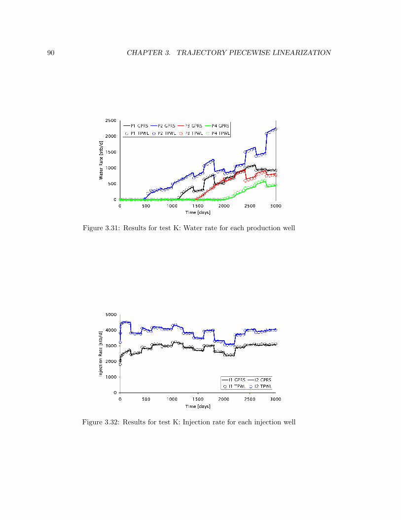
90 CHAPTER 3. TRAJECTORY PIECEWISE LINEARIZATION
Figure 3.31: Results for test K: Water rate for each production well
Figure 3.32: Results for test K: Injection rate for each injection well

3.3. ADDITIONAL ISSUES 91
within an appropriate range, but that solution accuracy can degrade outside of the range
of the training runs.
Table 3.3: Errors in TPWL solutions for tests I–M
Test I Test J Test K Test L Test M
Oil prod 0.0109 0.0132 0.0170 0.0461 0.0432Water prod 0.0215 0.0215 0.0520 0.0809 0.1596Water inj 0.0088 0.0095 0.0085 0.0204 0.0244MBE oil 0.0021 0.0022 0.0030 0.0061 0.0067
MBE water 0.0022 0.0039 0.0029 0.0067 0.0250
The runtime speedups offered by TPWL relative to the high-fidelity simulations are
even larger in this case than in the previous example. Specifically, the GPRS simulations
for this model required about 30 minutes of CPU time, while each TPWL run required only
0.9 seconds if material balance errors were not computed. These timings correspond to a
runtime speedup factor of about 2,000. If material balance errors are computed at every
time step, the TPWL runs require about an order of magnitude more computation, so the
speedup relative to GPRS is reduced to about a factor of 200.
3.3 Additional Issues
The results presented in the previous section demonstrate the potential of the TPWL
method for subsurface flow modeling. Reasonable accuracy was achieved for two realis-
tic example cases for test simulations in which the production well controls (BHPs) were
quite different from those used in the training simulations. There remain, however, several
issues that must be addressed before the TPWL procedure can be used for a wide range of
practical subsurface flow problems.
Because the method is based on linearization around previously simulated (saved) states,
degradation in accuracy is to be expected when higher order terms in the expansion (Eq. 3.2)
become significant. It will therefore be useful to develop efficient estimators for these terms
as well as heuristics that indicate when the TPWL solution is likely to degrade. For the
latter, empirical error estimates that relate error in oil and water production rates and
injection rate to, for example, mass balance error and some measure of the distance between
the saved state xi+1 and the computed state xn+1, could be of value.

92 CHAPTER 3. TRAJECTORY PIECEWISE LINEARIZATION
In the next chapter we apply TPWL for production optimization problems. Within this
context, error estimators could be used to determine when model retraining is required.
Retraining could then be accomplished by performing one or more new high-fidelity simula-
tions using control schedules consistent with those at the current stage of the optimization.
This would provide additional saved states which should be closer to those encountered
during subsequent stages of the optimization.
As discussed in Chapter 2, the underlying POD representation requires more basis
functions as the relative permeability functions become highly nonlinear and in the case of
strong density differences. The use of higher numbers of basis functions leads to reduced
efficiency, as all computations involving the basis matrix Φ become more costly. Another
concern when using a large number of basis functions is that, due to computational precision
issues, the condition number of Φ may begin to deviate from unity. As a result, as the
number of basis functions becomes large, the use of additional basis functions does not
always lead to better simulation accuracy, as the information incorporated in the additional
columns of Φ is counterbalanced by a loss of precision. Degradation in accuracy has also
been observed when the injection well BHPs were varied along with the production well
BHPs. Thus it will be important to develop improved procedures for constructing Φ. This
will benefit both the standalone approach, i.e., the POD-based ROM described in Chapter 2,
as well as the TPWL procedure. Along these lines, the goal-oriented optimization procedure
for constructing the basis matrix presented in [15] may be useful to consider.
In total, the results presented in this chapter demonstrate the applicability of the TPWL
procedure for modeling oil-water flow. A number of issues must still be addressed, however,
before the method can be used for general practical cases. In the next chapter, we apply
the TPWL approach to optimization problems.

Chapter 4
Production Optimization Using the
TPWL Procedure
A target application for the TPWL procedure is as a fast function evaluator in optimiza-
tion procedures. Within the context of oil reservoir management, one is often interested
in maximizing oil production or the net present value of the project. In this chapter the
reduced-order TPWL representation developed in the previous chapter is evaluated for
production optimization problems involving waterflood. Three different heterogeneous 3D
reservoir models will be used. We maximize the net present value for a waterflooding process
by optimizing the BHPs of the production wells. In the first example, both gradient-based
and generalized pattern search optimization algorithms are considered. For the other two
cases only the gradient-based algorithm is applied. We demonstrate that the TPWL repre-
sentation provides results for the objective function that are in close agreement with those
generated using the high-fidelity model. Finally, a multiobjective optimization is performed
for one of the models using the TPWL representation. For this problem only limited high-
fidelity simulations are performed due to the very high computational demand required,
though close correspondence between these results and those from TPWL is demonstrated.
93

94 CHAPTER 4. OPTIMIZATION USING TPWL
4.1 Optimization Problem 1
4.1.1 Description of the Simulation Model
The reservoir model, shown in Figure 4.1, is a portion of a synthetic geological model
developed by Castro in [23]. This is a smaller version (fewer gridblocks) of the model
considered in Chapter 2. The model used here contains 20,400 grid blocks (nx=30, ny=40,
nz=17) and has four production wells and two water injection wells.
Figure 4.1: Synthetic reservoir model with four production wells and two injection wells
Figure 4.2 shows the permeability in the x-direction for selected layers (layer numbers
indicated under each figure). The production wells are completed in layers 1 through 5 and
the injection wells in layers 15 through 17.
Figure 4.2: Permeability in the x-direction for selected layers

4.1. OPTIMIZATION PROBLEM 1 95
For this reservoir model capillary pressure is neglected and the fluid densities are set
to be equal. The other fluid and rock-fluid properties are different from those used in
Chapter 2. Here, the initial saturations of oil and water are 0.8 and 0.2, respectively, and
the residual oil saturation is 0.2. The oil viscosity at standard conditions is 3.0 cp and the
water viscosity is 0.5 cp. The relative permeabilities for the oil and water phases are shown
in Figure 4.3.
Figure 4.3: Relative permeability curves for oil and water
4.1.2 Training and Testing Results Using TPWL
To generate the states and Jacobian matrices needed by the TPWL procedure, a number
of high-fidelity training simulations are required, as explained in section 3.2.1. The quality
of the TPWL representation in the subsequent optimization computations depends on the
well conditions applied in the training simulations, so it is important that these conditions
be selected carefully. Ideally, the well conditions used in the training simulations should
correspond as closely as possible to those encountered during the optimization. At this
initial stage, however, the optimal conditions are not known. A possible approach, which
we plan to consider in future work, is to ‘re-train’ the TPWL during the course of the
optimization. Such a procedure would assure that the TPWL is always trained for states
along the optimization trajectory.
Our approach here, however, is more straightforward. In our optimizations, the injection
wells are prescribed to have constant bottom hole pressures (BHPs) of 6,000 psia, so this

96 CHAPTER 4. OPTIMIZATION USING TPWL
injector BHP is maintained in all training runs. For the production wells, rather than re-
train the TPWL model during the optimization runs, we apply schedules for the producer
BHPs in the training runs that we expect to capture the required range of behavior. For the
first training simulation, the BHPs of the production wells are held constant at 1,000 psia.
For the second training simulation, the producer BHPs are changed every 200 days such
that the total flow rate of each producer well is approximately constant at 2,000 stb/d. For
the third training run, we vary the BHPs of the producer wells randomly and independently
between 2,000 and 4,000 psia. For the fourth training simulation, the producer BHPs are
again varied randomly, but this time between 1,000 and 3,000 psia. The four training
schedules are shown in Figures 4.4 – 4.7. Because these schedules differ significantly from
each other, it is reasonable to expect that the resulting TPWL model can describe flow
over a wide variation of producer BHP schedules. We note that these training simulations
correspond closely to those used in section 3.2.1 where our goal was to explore the accuracy
and robustness of the general TPWL model.
All training simulations were run for 5,000 days with a maximum timestep of 30 days. A
total of 752 snapshots for the oil pressure and water saturation states and Jacobian matrices
were recorded from these four training runs. Applying the proper orthogonal decomposition
approach described in Chapter 2, a reduced basis Φ containing a total of 400 columns, with
200 columns corresponding to the oil pressure states and 200 to the water saturation states,
was constructed. Following the trajectory piecewise linear formulation presented in Chapter
3, we use this basis to project all states and Jacobian matrices into the reduced space.
Prior to using the reduced-space TPWL model (Eq. 3.24) for production optimization
computations, it is important to assess the accuracy of the TPWL representation. Because
we did not consider this model in Chapter 3, we now evaluate its ability to reproduce results
from training and testing simulations. Figures 4.8 and 4.9 present comparisons for oil rate
and water rate for the four production wells for training simulation 4, where the solid
lines represent the solution using the high-fidelity simulation model (labeled ‘GPRS’) and
the circles the reduced-order TPWL representation. There is clearly very close agreement
between the high-fidelity results and the TPWL results for all wells. Similar levels of
agreement between the high-fidelity and TPWL results are achieved for the other three
training simulations.
We next evaluate the accuracy of the TPWL representation for test simulations, which

4.1. OPTIMIZATION PROBLEM 1 97
Figure 4.4: Producer BHP schedules for training run 1
Figure 4.5: Producer BHP schedules for training run 2
Figure 4.6: Producer BHP schedules for training run 3

98 CHAPTER 4. OPTIMIZATION USING TPWL
Figure 4.7: Producer BHP schedules for training run 4
Figure 4.8: Oil rate for high-fidelity GPRS and TPWL (training run 4)
Figure 4.9: Water rate for high-fidelity GPRS and TPWL (training run 4)

4.1. OPTIMIZATION PROBLEM 1 99
differ from the training runs. Figures 4.10 – 4.15 show the BHPs for the production wells
and the oil production rates for three different testing simulations. Tests 1 and 2 show very
close agreement between the high-fidelity GPRS results and the TPWL results. In test 3,
producers P1, P2 and P4 are in agreement, though the TPWL results for P3 (red circles)
do show some discrepancy with the GPRS results after 1,500 days, though the error is not
excessive. These results are representative of the oil and water production rates and water
injection rates for the several testing runs considered. Having established a reasonable
level of accuracy for the TPWL model, we are now ready to proceed with the optimization
computations.
Figure 4.10: Producer BHPs using GPRS and TPWL for test simulation 1
Figure 4.11: Producer oil flow rates using GPRS and TPWL for test simulation 1

100 CHAPTER 4. OPTIMIZATION USING TPWL
Figure 4.12: Producer BHPs using GPRS and TPWL for test simulation 2
Figure 4.13: Producer oil flow rates using GPRS and TPWL for test simulation 2
Figure 4.14: Producer BHPs using GPRS and TPWL for test simulation 3
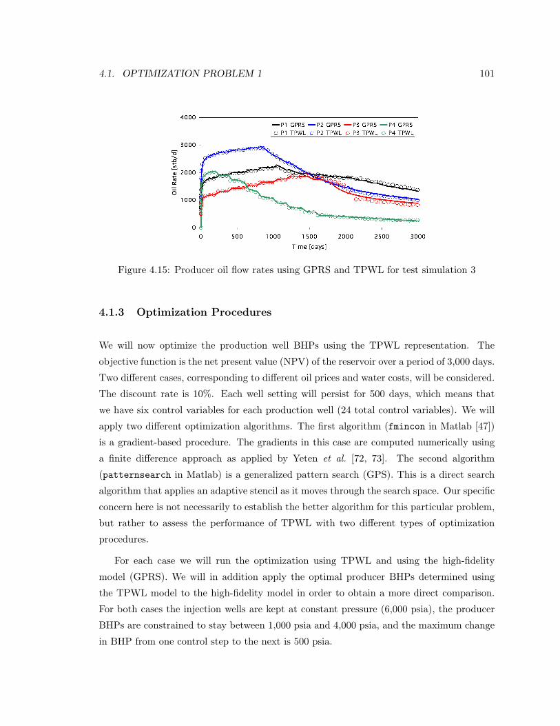
4.1. OPTIMIZATION PROBLEM 1 101
Figure 4.15: Producer oil flow rates using GPRS and TPWL for test simulation 3
4.1.3 Optimization Procedures
We will now optimize the production well BHPs using the TPWL representation. The
objective function is the net present value (NPV) of the reservoir over a period of 3,000 days.
Two different cases, corresponding to different oil prices and water costs, will be considered.
The discount rate is 10%. Each well setting will persist for 500 days, which means that
we have six control variables for each production well (24 total control variables). We will
apply two different optimization algorithms. The first algorithm (fmincon in Matlab [47])
is a gradient-based procedure. The gradients in this case are computed numerically using
a finite difference approach as applied by Yeten et al. [72, 73]. The second algorithm
(patternsearch in Matlab) is a generalized pattern search (GPS). This is a direct search
algorithm that applies an adaptive stencil as it moves through the search space. Our specific
concern here is not necessarily to establish the better algorithm for this particular problem,
but rather to assess the performance of TPWL with two different types of optimization
procedures.
For each case we will run the optimization using TPWL and using the high-fidelity
model (GPRS). We will in addition apply the optimal producer BHPs determined using
the TPWL model to the high-fidelity model in order to obtain a more direct comparison.
For both cases the injection wells are kept at constant pressure (6,000 psia), the producer
BHPs are constrained to stay between 1,000 psia and 4,000 psia, and the maximum change
in BHP from one control step to the next is 500 psia.
102 CHAPTER 4. OPTIMIZATION USING TPWL
4.1.4 Results for Optimization Case 1
For this case the oil price is specified to be $80/stb and the water injection and water
production costs are $15/stb. The initial guess for the BHPs of all four production wells
is 2,500 psia. Table 4.1 presents the NPV (in $106) for the gradient-based method and the
generalized pattern search. Initial and final NPV are shown for optimizations using GPRS
and TPWL. The final NPV using GPRS with the well settings determined by TPWL,
designated ‘GPRS(TPWL)’ in the table, is also presented.
It is evident that the NPVs using GPRS are about 1-2% higher than those computed
using TPWL. However, using the final controls from the TPWL optimization in the high-
fidelity (GPRS) simulator gives NPVs that differ by only about 0.15% (using the gradient-
based method), or are essentially identical (using generalized pattern search), compared to
those achieved using GPRS for the optimizations. We see that the gradient-based method
gives better results than the generalized pattern search and provides an increase of 11.8% in
NPV over the initial guess. The optimized BHPs and the resulting cumulative fluid injec-
tion and production are shown in Figures 4.16 and 4.17. These results were generated using
the gradient-based method. From Figure 4.16, it is evident that the BHP sequence differs
slightly between the GPRS (solid lines) and TPWL (circles) optimizations, but the cumu-
lative production and injection are nonetheless very close as can be observed in Figure 4.17.
In this figure the solid lines represent the high-fidelity model (GPRS), the open circles the
TPWL model, and the dots the solution using GPRS with the well settings determined by
TPWL.
Consistent with the observations in Chapter 3, the CPU requirements for the TPWL and
GPRS optimizations differ considerably. Specifically, for the gradient-based optimizations,
four iterations were performed and each iteration required 25 simulation runs (for a total
of 100 simulations). Each GPRS simulation consumed 6 minutes of CPU time (10 hours
for 100 simulations), while each TPWL simulation required only 0.8 seconds (80 seconds
for 100 simulations). Thus the runtime speedup using TPWL is about 450. Recall that the
overhead associated with TPWL is the equivalent of about eight GPRS simulations.

4.1. OPTIMIZATION PROBLEM 1 103
Table 4.1: NPV ($106) for problem 1, case 1 (oil $80/stb, produced and injected water$15/stb)
Gradient-based method Generalized pattern search
Simulator NPV(initial) NPV(final) NPV(initial) NPV(final)
GPRS 733.6 820.3 733.6 791.8TPWL 725.2 805.8 725.2 780.0
GPRS(TPWL) 819.1 791.9
Figure 4.16: Producer BHPs for case 1 (problem 1)
Figure 4.17: Cumulative production and injection for case 1 (problem 1)

104 CHAPTER 4. OPTIMIZATION USING TPWL
4.1.5 Results for Optimization Case 2
For this case the oil price is $60/stb, the water injection cost is $3/stb and the water
production cost is $30/stb. The initial guess for the producer BHPs is 2,000 psia. Results
for NPV are presented in Table 4.2. These results are consistent with those for case 1, with
the NPVs using GPRS approximately 1-2% higher than the NPVs computed using TPWL.
Again, however, if we use the final controls from the TPWL optimization in GPRS, we
obtain NPVs that are very close to those achieved using GPRS for the optimizations (with
differences of 0.1% using the gradient-based method and 0.8% using generalized pattern
search). As was observed for case 1, the gradient-based method provides a higher NPV,
here achieving an increase of 7.8% over the initial guess.
The optimized BHPs (using the gradient-based method) and the resulting cumulative
fluid injection and production are shown in Figures 4.18 and 4.19. As was observed in
case 1, the BHP schedule differs slightly between the GPRS and TPWL optimizations, but
the cumulative production and injection are in close agreement. Less water is produced
here than in case 1 because of the higher cost of produced water (7.728×10⁶ stb in case 2
compared to 9.271×10⁶ stb in case 1). We note finally that the timings for this case are
essentially the same as those for case 1.
Table 4.2: NPV ($106) for problem 1, case 2 (oil $60/stb, produced water $30/stb andinjected water $3/stb)
Gradient-based method Generalized pattern search
Simulator NPV(initial) NPV(final) NPV(initial) NPV(final)
GPRS 636.4 685.8 636.4 645.9TPWL 628.9 676.3 628.9 633.0
GPRS(TPWL) 684.9 640.8

4.1. OPTIMIZATION PROBLEM 1 105
Figure 4.18: Producer BHPs for case 2 (problem 1)
Figure 4.19: Cumulative production and injection for case 2 (problem 1)
106 CHAPTER 4. OPTIMIZATION USING TPWL
4.2 Optimization Problem 2
We next consider the determination of optimal production well BHPs for the reservoir model
described in section 3.2.1 (SPE 10 model containing 24,000 cells). The objective function is
the net present value (NPV) of the reservoir over a period of 3,000 days and two different
cases, corresponding to different oil prices and water costs, will again be considered. The
discount rate (10%) and the total number of control variables (24) are the same as were
used in problem 1. For this and subsequent optimizations, we apply only the gradient-based
optimization algorithm (fmincon in Matlab).
As in problem 1, 100 simulations (four iterations of the optimization algorithm) were
performed using TPWL and the high-fidelity model (GPRS). The optimal producer BHPs
determined using the TPWL model are also applied to the high-fidelity model. For this
reservoir model the injection wells are kept at a constant pressure of 10,000 psia and the
producer BHPs are constrained to stay between 1,000 psia and 4,000 psia with the max-
imum change in BHP from one control step to the next being 500 psia. For the TPWL
optimizations, we use the TPWL model developed in section 3.2.1 (see section 3.2.1 for a
description of the training runs).
4.2.1 Results for Optimization Case 1
For this case the oil price is specified to be $80/stb and the water injection and water
production costs are $10/stb. The initial guess for the BHPs of all four production wells
is 2,500 psia. Table 4.3 presents the NPVs (in $106) computed using the gradient-based
method. Initial and final NPV are shown for optimizations using GPRS and TPWL, as
well as the final NPV using GPRS with the well settings determined by TPWL, designated
‘GPRS(TPWL).’
From the table we see that the NPV using GPRS is about 0.66% higher than that
computed using TPWL. However, using the final controls from the TPWL optimization in
the high-fidelity simulator gives an NPV that is within 0.1% of that achieved using GPRS
for the optimizations. The optimized BHPs are shown in Figure 4.20, where it is apparent
that the BHP sequences show small differences. The cumulative production and injection
are nonetheless very close, as shown in Figure 4.21. The runtime speedup using TPWL was
a factor of 500, the same as was reported in section 3.2.1.

4.2. OPTIMIZATION PROBLEM 2 107
Table 4.3: NPV ($106) for problem 2, case 1 (oil $80/stb, produced and injected water$10/stb)
Gradient-based method
Simulator NPV(initial) NPV(final)
GPRS 655.5 682.1TPWL 648.9 677.6
GPRS(TPWL) 681.6
Figure 4.20: Producer BHPs for case 1 (problem 2)
Figure 4.21: Cumulative production and injection for case 1 (problem 2)

108 CHAPTER 4. OPTIMIZATION USING TPWL
4.2.2 Results for Optimization Case 2
For this case we decreased the oil price to $60/stb, the water injection cost to $5/stb, and
increased the water production cost to $15/stb. The initial guess for the producer BHPs is
1,000 psia and the results for NPV are presented in Table 4.4. These results are different
from those for case 1, with the NPV using GPRS approximately 0.06% lower than the
NPV computed using TPWL. Using the final controls from the TPWL optimization in the
high-fidelity simulator gives an NPV that is about 0.41% higher than that achieved using
GPRS for the optimizations.
The optimized BHPs and the resulting cumulative fluid injection and production are
shown in Figures 4.22 and 4.23. There are some significant differences in the BHP schedules
between the GPRS and TPWL optimizations for production wells P1, P2 and P3. However,
the cumulative production and injection are in close agreement. Less water is produced here
than in case 1 because of the higher cost of produced water. We note finally that the timings
for this case are essentially the same as those for case 1.
Table 4.4: NPV ($106) for problem 2, case 2 (oil $60/stb, produced water $15/stb andinjected water $5/stb)
Gradient-based method
Simulator NPV(initial) NPV(final)
GPRS 472.7 493.8TPWL 467.0 494.1
GPRS(TPWL) 495.8

4.2. OPTIMIZATION PROBLEM 2 109
Figure 4.22: Producer BHPs for case 2 (problem 2)
Figure 4.23: Cumulative production and injection for case 2 (problem 2)
110 CHAPTER 4. OPTIMIZATION USING TPWL
4.3 Optimization Problem 3
The optimization procedure is now applied to the 79,200-cell reservoir model described in
section 3.2.2 (60 × 220 × 6 SPE 10 model). The optimization parameters, the producer
BHP range and the maximum change in BHP are the same as were used for optimization
problem 2, though the injection wells in this case are kept at a constant pressure of 8,000
psia. Four iterations of the gradient-based algorithm are again applied.
4.3.1 Results for Optimization Case 1
For this case the oil price is specified to be $80/stb, the water injection and water produc-
tion costs are $15/stb, and the initial guess for the BHPs of all four production wells is
2,500 psia. Table 4.5 presents the NPV (in $106). The final NPV using GPRS is about
1.25% higher than that computed using TPWL. However, using the final controls from the
TPWL optimization in GPRS gives an NPV that is 0.7% higher than that using GPRS.
From Figure 4.24, it is clear that the BHP sequence between the GPRS and TPWL opti-
mizations is very close for production wells P2, P3 and P4, but differs signicantly for well
P1. Figure 4.25 shows once more that the cumulative production and injection are very
close. A factor of 2,000 runtime speedup was achieved using TPWL, which is the same as
reported in section 3.2.2.
Table 4.5: NPV ($106) for problem 3, case 1 (oil $80/stb, produced and injected water$15/stb)
Gradient-based method
Simulator NPV(initial) NPV(final)
GPRS 643.7 696.4TPWL 638.9 687.8
GPRS(TPWL) 701.2
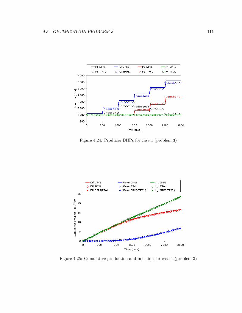
4.3. OPTIMIZATION PROBLEM 3 111
Figure 4.24: Producer BHPs for case 1 (problem 3)
Figure 4.25: Cumulative production and injection for case 1 (problem 3)
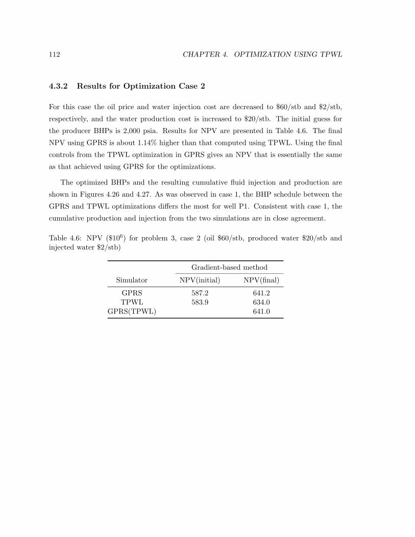
112 CHAPTER 4. OPTIMIZATION USING TPWL
4.3.2 Results for Optimization Case 2
For this case the oil price and water injection cost are decreased to $60/stb and $2/stb,
respectively, and the water production cost is increased to $20/stb. The initial guess for
the producer BHPs is 2,000 psia. Results for NPV are presented in Table 4.6. The final
NPV using GPRS is about 1.14% higher than that computed using TPWL. Using the final
controls from the TPWL optimization in GPRS gives an NPV that is essentially the same
as that achieved using GPRS for the optimizations.
The optimized BHPs and the resulting cumulative fluid injection and production are
shown in Figures 4.26 and 4.27. As was observed in case 1, the BHP schedule between the
GPRS and TPWL optimizations differs the most for well P1. Consistent with case 1, the
cumulative production and injection from the two simulations are in close agreement.
Table 4.6: NPV ($106) for problem 3, case 2 (oil $60/stb, produced water $20/stb andinjected water $2/stb)
Gradient-based method
Simulator NPV(initial) NPV(final)
GPRS 587.2 641.2TPWL 583.9 634.0
GPRS(TPWL) 641.0

4.3. OPTIMIZATION PROBLEM 3 113
Figure 4.26: Producer BHPs for case 2 (problem 3)
Figure 4.27: Cumulative production and injection for case 2 (problem 3)

114 CHAPTER 4. OPTIMIZATION USING TPWL
4.4 Multiobjective Optimization
Finally, we apply TPWL for a more challenging multiobjective optimization in which we
consider conflicting goals. Specifically, we seek to maximize cumulative oil production while
minimizing cumulative water injection. Thus the goal of the optimization is to determine
the Pareto front on a plot of cumulative oil produced versus cumulative water injected.
Any point on this curve represents the ‘most’ oil (as determined from the optimization)
that can be produced for the corresponding amount of water injected. The curve can also
be viewed as providing the least amount of water that must be injected to produce a given
amount of oil. The solution of this optimization problem is computationally demanding if
the high-fidelity model is used, as the optimization procedure must be run for many points
along the Pareto front.
We consider the model used in optimization problem 2. The model contains 24,000 grid
blocks and is described in section 3.2.1. The multiobjective optimization seeks to maximize
the net present value (NPV) of the reservoir over a period of 3,000 days. The discount rate
is 10% and the cost of both the produced and injected water is fixed at $10/stb. The oil
price is varied from $10/stb to $150/stb in increments of $2/stb, and the optimization is
performed for each oil price.
As in problem 2, the injection wells are specified to operate at 10,000 psia and the
minimum and maximum producer BHPs are prescribed as 1,000 psia and 4,000 psia re-
spectively. The producer BHPs are updated more frequently in this case (every 250 days)
than in problem 2. As the simulation is run for 3,000 days, there are a total of 48 control
variables (12 for each production well). We further specify that the maximum change in
BHP from one control step to the next is 250 psia. The gradient-based algorithm is applied
and a total of four iterations of the optimization are performed, meaning that each point on
the curve requires 196 simulations. The initial guess for the producer BHPs is 2,500 psia.
The optimization results are presented in Figure 4.28, where we plot cumulative oil
produced versus cumulative water injected. The ×’s represent TPWL solutions (71 points
were generated), while the blue dots represent high-fidelity results computed using the
optimal well settings as determined from the TPWL optimizations. For a few points (shown
as red triangles) we performed the full optimization using the high-fidelity model. The
general correspondence between these three sets of points is quite close, indicating the
applicability of the TPWL procedure for this application.
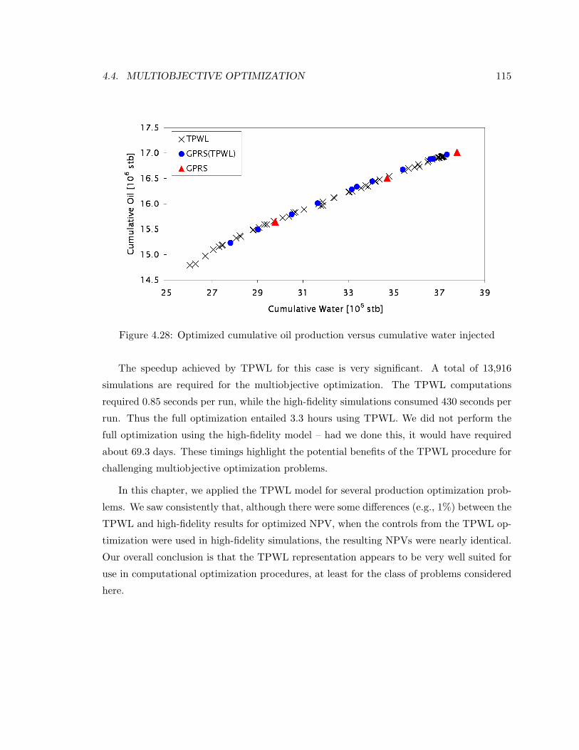
4.4. MULTIOBJECTIVE OPTIMIZATION 115
Figure 4.28: Optimized cumulative oil production versus cumulative water injected
The speedup achieved by TPWL for this case is very significant. A total of 13,916
simulations are required for the multiobjective optimization. The TPWL computations
required 0.85 seconds per run, while the high-fidelity simulations consumed 430 seconds per
run. Thus the full optimization entailed 3.3 hours using TPWL. We did not perform the
full optimization using the high-fidelity model – had we done this, it would have required
about 69.3 days. These timings highlight the potential benefits of the TPWL procedure for
challenging multiobjective optimization problems.
In this chapter, we applied the TPWL model for several production optimization prob-
lems. We saw consistently that, although there were some differences (e.g., 1%) between the
TPWL and high-fidelity results for optimized NPV, when the controls from the TPWL op-
timization were used in high-fidelity simulations, the resulting NPVs were nearly identical.
Our overall conclusion is that the TPWL representation appears to be very well suited for
use in computational optimization procedures, at least for the class of problems considered
here.

116 CHAPTER 4. OPTIMIZATION USING TPWL

Chapter 5
Summary and Future Work
This dissertation addressed the application of reduced-order modeling procedures for reser-
voir simulation. In this chapter this work is summarized and recommendations for future
research are presented. We reiterate that, although our interest here is the application of
ROM for oil reservoir simulation, our findings are useful for other areas such as aquifer
management and the geological storage of carbon dioxide.
5.1 Summary and Conclusions
We summarize this work as follows:
POD-Based Reduced-Order Modeling
• A reduced-order modeling (ROM) procedure based on the proper orthogonal decom-
position (POD) technique was extended, incorporated into a general purpose simu-
lator, and applied for subsurface flow applications. The POD procedure provides a
mechanism to extract a reduced-order basis of small dimension that contains the key
features of the states encountered during the simulation of a full (high-fidelity) reser-
voir model. This requires the recording of snapshots of the solution states (oil pressure
and water saturation) at many time steps during a ‘training’ simulation followed by
a singular value decomposition of the resulting covariance or data matrix. Use of this
basis in subsequent simulations provides runtime speedups, assuming the dimensions
of the basis matrix are sufficiently small.
117

118 CHAPTER 5. SUMMARY AND FUTURE WORK
• Two procedures were introduced to decrease the size of the basis matrix. A snapshot
clustering method enables the use of fewer vectors in the reduced-order basis. Further
reduction of the computational burden was achieved through application of the missing
point estimation (MPE) technique. Using a condition number criterion, MPE allows
the most important grid blocks to be selected, leading to a reduction in the number
of rows in the basis matrix.
• Proper orthogonal decomposition, clustering, and missing point estimation are all off-
line (pre-processing) computations and were implemented in a stand-alone Matlab
application. The reduced-order modeling framework was implemented in Stanford’s
general purpose research simulator (GPRS). Using this implementation ROMs with
different complexities can be applied, specifically, ROM with POD only, ROM using
clustered snapshots and POD, and ROM using clustered snapshots, POD and MPE,
for oil-water flow simulations.
• All of these ROM procedures were tested using a realistic 3D reservoir model with
60,000 grid blocks. This corresponds to 120,000 unknowns (oil pressure and water
saturation in each block) at each time step. The ROMs were able to capture the
dynamics of these models using only about 40 unknowns (the exact number varied
depending on the specific ROM procedure). Results for production and injection rates,
which are typically the key inputs to an optimization procedure, were shown to be
in fairly close agreement with reference (high-fidelity) simulation results for different
production schedules. For all cases the same sets of basis vectors were used, meaning
that only one full-order simulation was required to generate the information needed
to construct the ROMs. This indicates that these models retain a reasonable level of
robustness, which is important if they are to be used in optimization applications.
• Computational speedups for the ROM using clustered snapshots, POD and MPE,
evaluated relative to full-order GPRS simulations using a specialized linear solver and
preconditioner combination (GMRES solver and CPR preconditioner), were between
6 and 10 depending on the case. Comparison to a full-order GPRS simulation us-
ing a much simpler preconditioner (ILU(0)) showed a speedup of about 700. This
highlights the fact that the ROM procedures considered here are very well suited for
situations where the linear solver occupies the great majority of the computational
time. Otherwise, the maximum speedup attainable is more limited.
5.1. SUMMARY AND CONCLUSIONS 119
• The POD-based ROM procedure was shown to be less effective in cases with strong
density differences between phases, highly nonlinear relative permeability curves, or
significant variation in injection BHPs. For such cases, improved treatments are re-
quired.
TPWL Formulation
• We also developed a trajectory piecewise linearization (TPWL) procedure for the
modeling of two-phase flow in subsurface formations. This ROM technique entails
representation of new states in terms of linear expansions around states previously
simulated and saved during training runs. The method is tractable and efficient
because all computations are performed in a low-dimensional space generated using
the POD basis matrix.
• TPWL was applied to heterogeneous reservoir models derived from the SPE 10 and
Stanford VI reservoir models. Reasonable levels of accuracy in TPWL computations
were observed for oil and water production rates and water injection rate for test cases
in which the production well bottom hole pressures were within the general range of
the training simulations. When the production well BHP schedule in the test runs
differed significantly from that of any of the training runs, the accuracy of the TPWL
model degraded.
• The preprocessing overhead required for the construction of the TPWL model corre-
sponds to about the time required to simulate 6-8 high-fidelity models. The TPWL
model provided runtime speedups of about 500-2000 for the cases considered if mass
balance error was not computed. Speedups were less dramatic but still very substan-
tial if mass balance error was assessed frequently, though in practice this error need
be computed only occasionally.
Use of TPWL Model for Optimization
• The TPWL procedure was applied for waterflood optimization using three hetero-
geneous 3D models containing 20,400, 24,000 and 79,200 grid blocks. Each model
contained two injection wells and four production wells. Two different optimization
cases, corresponding to different oil prices and water costs, were considered for each
reservoir model. The BHPs for the four production wells at six different times were

120 CHAPTER 5. SUMMARY AND FUTURE WORK
determined in the optimizations using a gradient-based algorithm with gradients com-
puted numerically and a generalized pattern search algorithm (the latter algorithm
was applied only for the reservoir model with 20,400 grid blocks).
• Results for net present value using the controls determined from TPWL optimizations
in GPRS simulations were shown to be very close to those achieved by performing
the optimizations with the high-fidelity model. Optimization using TPWL provided
runtime speedups of a factor of 450 – 2,000, depending on the reservoir model used.
• A significant advantage of the TPWL approach is that, once the preprocessing compu-
tations are completed and the TPWL model is constructed, additional optimizations
or multiobjective optimization can be run at very little cost. Thus, the sensitivity
of the optimized BHPs to oil price, water costs, constraints, etc., can be assessed
inexpensively. The optimizations can also be run using a number of different initial
guesses. Runs of this type will be very expensive if the high-fidelity model is used.
We demonstrated the use of the TPWL procedure for a multiobjective optimization
problem to determine the Pareto front. Limited high-fidelity simulations suggest that
the TPWL results are of sufficient accuracy for this problem.
5.2 Recommendations for Future Work
• Our current procedure for specifying the controls (BHP settings) used in the training
runs is heuristic, so it will be useful to explore more rigorous approaches. An interest-
ing starting point might be the work of Kunisch and Volkwein [43], who address the
problem of un-modeled dynamics, as occurs when the optimum solution is consider-
ably different from the training simulation. Another approach that employs a greedy
algorithm for the selection of snapshots in high-dimensional space was proposed by
Bui-Thanh et al. [15].
• The accuracy and runtime speedup provided by the POD-based ROM are closely
related with the amount of energy retained by the basis functions selected, as explained
in section 2.3. The development of a methodology to evaluate the compromise between
accuracy and speedup could give a reduced-order basis with the optimum number of
basis functions.

5.2. RECOMMENDATIONS FOR FUTURE WORK 121
• The models considered here (oil-water systems, capillary pressure neglected) are still
relatively simple, in terms of multiphase flow physics, compared to many of the models
that arise in practice. The presence of strong gravitational effects as well as high
degrees of nonlinearity in the relative permeability functions was shown to limit the
effectiveness of the POD-based ROM procedures implemented in this work. Variable
injector BHPs also led to reduced accuracy. These issues require further investigation.
Alternatives to the POD approach used here should be considered.
• Other strategies for using TPWL in optimizations should be studied. For example, ad-
ditional high-fidelity training runs could be performed occasionally during the course
of the optimization to ensure that the TPWL model retains accuracy. Along these
lines, it will additionally be useful to develop approaches for estimating error in the
TPWL predictions.
• The TPWL method and the underlying POD procedure should be extended for use
in three-phase flow problems. They should also be tested for larger models containing
O(105) grid blocks and many wells.
• All of the ROM procedures developed in this work considered wells to be controlled by
bottom hole pressure (BHP). Extending the method for wells under flow rate control
will broaden the applicability of the methods.
• It will be useful to consider the use of POD-based ROMs and/or TPWL models for
the combined production optimization – history matching problem (i.e., closed-loop
reservoir modeling). This will require the development of procedures for updating the
reduced basis matrix.

122 CHAPTER 5. SUMMARY AND FUTURE WORK

Nomenclature
Abbreviations
BHP bottom hole pressure
CPR constrained pressure residual
CVT centroidal Voronoi tesselation
GPRS general purpose research simulator
LTI linear time invariant
LTV linear time variant
MBE material balance error
MPE missing point estimation
NPV net present value
POD proper orthogonal decomposition
ROM reduced-order modeling or reduced-order model
SQRD sequential QR decomposition
SVD singular value decomposition
TPWL trajectory piecewise linearization
Variables
a, b Corey exponents
A area of grid block face
A accumulation term
B formation volume factor
D depth
C covariance matrix
123

124 NOMENCLATURE
D accumulation matrix for incompressible systems
E energy
fw Buckley-Leverett fractional flow function
F flow term or flux
g gravitational acceleration
g residual vector
J Jacobian matrix
k permeability tensor
K condition number
kr relative permeability
` number of columns retained in the reduced basis
Nc number of grid blocks
p pressure
q source term
Q well flow rate
Q source/sink term
S saturation
S number of snapshots recorded
t time
T transmissibility matrix
u Darcy velocity or well controls
V grid block volume
W well index
x vector of primary unknowns
X data matrix
z reduced vector of primary unknowns
Greek
δ solution update
λ mobility or eigenvalues
µ viscosity
ρ density
φ porosity

NOMENCLATURE 125
Φ orthonormal reduced basis matrix
Φw Φ with only well block entries
Φ∗ Φ after applying MPE
Ψ eigenvectors
Subscripts
i grid block index
j phase
` number of basis functions retained
o oil phase
p pressure
r reduced representation
s saturation
t total
w water phase
Superscripts
i saved state in the training simulations for TPWL
m well number
n time level
v iteration level
w well
0 reference

126 NOMENCLATURE

Bibliography
[1] I. Aitokhuehi and L. J. Durlofsky. Optimizing the performance of smart wells in
complex reservoirs using continuously updated geological models. Journal of Petroleum
Science and Engineering, 48(3), 2005.
[2] L. F. Almeida, Y. J. T. Valdivia, J. G. L. Lazo, M. A. C. Pacheco, and M. M. B. R.
Vellasco. Evolutionary computation for valves control optimization in intelligent wells
under uncertainties. In International Fuzzy Systems Association World Congress, Can-
cun, Mexico, June 2007.
[3] A. C. Antoulas and D. C. Sorensen. Approximation of large-scale dynamical systems:
An overview. International Journal of Applied Mathematics and Computer Science,
11(5):1093–1121, 2001.
[4] P. Astrid. Fast reduced order modeling technique for large scale LTV systems. In
American Control Conference, Boston, Massachusetts, USA, July 2004.
[5] P. Astrid. Reduction of Process Simulation Models: A Proper Orthogonal Decomposi-
tion Approach. PhD thesis, Eindhoven University of Technology, 2004.
[6] P. Astrid and A. Verhoeven. Application of least squares MPE technique in the reduced
order modeling of electrical circuits. In 17th International Symposium on Mathematical
Theory of Networks and Systems, Kyoto, Japan, July 2006.
[7] P. Astrid and S. Weiland. On the construction of POD models from partial observa-
tions. In 44th IEEE Conference on Decision and Control and the European Control
Conference, Seville, Spain, December 2005.
127

128 BIBLIOGRAPHY
[8] P. Astrid, S. Weiland, K. Willcox, and T. Backx. Missing point estimation in models
described by proper orthogonal decomposition. In 43rd IEEE Conference on Decision
and Control, Paradise Island, Bahamas, December 2004.
[9] K. Aziz and A. Settari. Fundamentals of Reservoir Simulation. Elsevier Applied Science
Publishers, 1986.
[10] Z. Bai. Krylov subspace techniques for reduced-order modeling of large-scale dynamical
systems. Applied Numerical Mathematics, 43(1–2):9–44, 2002.
[11] O. Bashir, K. Willcox, O. Ghattas, B. van Bloemen Waanders, and J. Hill. Hessian-
based model reduction for large-scale systems with initial-condition inputs. Interna-
tional Journal for Numerical Methods in Engineering, 73(6):844–868, 2008.
[12] D. R. Brouwer and J. D. Jansen. Dynamic optimization of waterflooding with smart
wells using optimal control theory. SPE Journal, 9(4):391–402, 2004.
[13] T. Bui-Thanh, M. Damodaran, and K. Willcox. Aerodynamic data reconstruction and
inverse design using proper orthogonal decomposition. AIAA Journal, 42(8):1505–1516,
2004.
[14] T. Bui-Thanh and K. Willcox. Model reduction for large-scale CFD applications using
the balanced proper orthogonal decomposition. In 17th AIAA Computational Fluid
Dynamics Conference, Toronto, Canada, June 2005.
[15] T. Bui-Thanh, K. Willcox, O. Ghattas, and B. van Bloemen Waanders. Goal-oriented,
model-constrained optimization for reduction of large-scale systems. Journal of Com-
putational Physics, 224(2):880–896, 2007.
[16] J. Burkardt, M. Gunzburger, and H. C. Lee. Centroidal Voronoi Tessellation-based
reduced-order modeling of complex systems. SIAM Journal of Scientific Computing,
28(2):459–484, 2006.
[17] H. Cao. Development of Techniques for General Purpose Simulators. PhD thesis,
Stanford University, 2002.
[18] H. Cao, H. A. Tchelepi, J. R. Wallis, and H. Yardumian. Parallel scalable unstructured
CPR-type linear solver for reservoir simulation (SPE paper 96809). In Annual Technical
Conference and Exhibition, Dallas, Texas, USA, October 2005.

BIBLIOGRAPHY 129
[19] Y. Cao, J. Zhu, Z. Luo, and I. M. Navon. Reduced order modeling of the upper
tropical Pacific ocean model using proper orthogonal decomposition. Computers &
Mathematics with Applications, 52(8-9):1373–1386, 2006.
[20] M. A. Cardoso and L. J. Durlofsky. Linearized reduced-order models for subsurface
flow simulation. Manuscript submitted for publication, 2008.
[21] M. A. Cardoso and L. J. Durlofsky. Use of reduced-order modeling procedures for pro-
duction optimization (SPE paper 119057). In SPE Reservoir Simulation Symposium,
The Woodlands, Texas, USA, February 2009.
[22] M. A. Cardoso, L. J. Durlofsky, and P. Sarma. Development and application of reduced-
order modeling procedures for subsurface flow simulation. International Journal for
Numerical Methods in Engineering, 77(9):1322–1350, 2009.
[23] S. A. Castro. A Probabilistic Approach to Jointly Integrate 3D/4D Seismic Production
Data and Geological Information for Building Reservoir Models. PhD thesis, Stanford
University, 2007.
[24] D. Chaniotis. Model reduction in power systems using Krylov subspace methods. IEEE
Transactions on Power Systems, 20(2):888–894, 2005.
[25] A. Chatterjee. An introduction to the proper orthogonal decomposition. Current
Science, 78(7):808–817, 2000.
[26] J. Chen and S. Kang. An algorithm for automatic model-order reduction of nonlinear
MEMs devices. In IEEE International Symposium on Circuits and Systems, Geneva,
Switzerland, May 2000.
[27] Y. Chen, D. S. Oliver, and D. Zhang. Efficient ensemble-based closed-loop production
optimization (SPE paper 112873). In SPE Improved Oil Recovery Symposium, Tulsa,
Oklahoma, USA, April 2008.
[28] M. A. Christie and M. J. Blunt. Tenth SPE comparative solution project: A comparison
of upscaling techniques. SPE Reservoir Evaluation & Engineering, (4):308–317, 2001.
[29] M. Condon and R. Ivanov. Empirical balanced truncation of nonlinear systems. Journal
of Nonlinear Science, 14(5):405–414, 2004.

130 BIBLIOGRAPHY
[30] N. Dong and J. Roychowdhury. General-purpose nonlinear model-order reduction using
piecewise-polynomial representations. IEEE Transactions on Computer-aided Design
of Integrated Circuits and Systems, 27(2):249–264, 2008.
[31] Y. Efendiev, T. Hou, and W. Luo. Preconditioning Markov chain Monte Carlo simula-
tions using coarse-scale models. SIAM Journal of Scientific Computing, 28(2):776–803,
2006.
[32] R. Everson and L. Sirovich. Karhunen-Loeve procedure for gappy data. J. Optical
Society of America, 12(8):1657–1664, August 1995.
[33] M. G. Gerritsen and L. J. Durlofsky. Modeling fluid flow in oil reservoirs. Annual
Review of Fluid Mechanics, 37:211–238, 2005.
[34] D. Gratton and K. Willcox. Reduced-order, trajectory piecewise-linear models for
nonlinear computational fluid dynamics. In 34th AIAA Fluid Dynamics Conference
and Exhibit, Portland, Oregon, USA, 2004.
[35] M. Gunzburger and J. Peterson. Reduced-order modeling of complex systems with
multiple system parameters. In International Conference on Large-Scale Scientific
Computing, Sozopol, Bulgaria, June 2005.
[36] J. S. Han, E. B. Rudnyi, and J. G. Korvink. Efficient optimization of transient dynamic
problems in MEMS devices using model order reduction. Journal of Micromechanics
and Microengineering, 15(4):822–832, 2005.
[37] T. Heijn, R. Markovinovic, and J. D. Jansen. Generation of low-order reservoir models
using system-theoretical concepts. SPE Journal, 9(2):202–218, 2004.
[38] P. J. Heres and W. H. A. Schilders. Krylov subspace methods in the electronic in-
dustry. In 13th European Conference on Mathematics for Industry, Eindhoven, The
Netherlands, June 2004.
[39] P. J. Heres and W. H. A. Schilders. Orthogonalisation in Krylov subspace methods for
model order reduction. In Scientific Computing in Electrical Engineering, Sicily, Italy,
September 2004.
[40] Y. Jiang. Tracer flow modeling and efficient solvers for GPRS. Master’s thesis, Stanford
University, 2004.

BIBLIOGRAPHY 131
[41] Y. Jiang. A Flexible Computational Framework for Efficient Integrated Simulation of
Advanced Wells and Unstructured Reservoir Models. PhD thesis, Stanford University,
2007.
[42] Y. Jiang and H. A. Tchelepi. Scalable multistage linear solver for coupled systems
of multisegment wells and complex reservoir models (SPE paper 119175). In SPE
Reservoir Simulation Symposium, The Woodlands, Texas, USA, February 2009.
[43] K. Kunisch and S. Volkwein. Proper orthogonal decomposition for optimality systems.
ESAIM: Mathematical Modelling and Numerical Analysis, 42:1–23, 2008.
[44] J. L. Lumley. Atmospheric turbulence and radio wave propagation. Journal of Com-
putational Chemistry, 23(13):1236–1243, 1967.
[45] R. Markovinovic, E. L. Geurtsen, T. Heijn, and J. D. Jansen. Generation of low-
order reservoir models using POD, empirical gramians and subspace identification.
In 8th European Conference on the Mathematics of Oil Recovery, Freiberg, Germany,
September 2002.
[46] R. Markovinovic and J. D. Jansen. Accelerating iterative solution methods using
reduced-order models as solution predictors. International Journal for Numerical Meth-
ods in Engineering, 68(5):525–541, 2006.
[47] MathWorks. The MathWorks, Inc. http://www.mathworks.com, 2008.
[48] M. Meyer and H. G. Matthies. Efficient model reduction in non-linear dynamics using
the Karhunen-Loeve expansion and dual-weighted-residual methods. Computational
Mechanics, 31:179–191, 2003.
[49] N. C. Nguyen, A. T. Patera, and J. Peraire. A ‘best points’ interpolation method for ef-
ficient approximation of parameterized functions. International Journal for Numerical
Methods in Engineering, 73(4):521–543, 2008.
[50] D. W. Peaceman. Interpretation of well-block pressures in numerical reservoir simula-
tion with nonsquare grid blocks and anisotropic permeability. SPE Journal, 23(3):531–
543, 1983.

132 BIBLIOGRAPHY
[51] J. R. Phillips. Projection-based approaches for model reduction of weakly nonlinear,
time-varying systems. IEEE Transaction of Computer-Aided Design of Integrated Cir-
cuits and Systems, 22(2):171–187, 2003.
[52] L. Qu and P. L. Chapman. Extraction of low-order non-linear inductor models from
a high-order physics-based representation. IEEE Transactions on Power Electronics,
21(3):813–817, 2006.
[53] W. F. Ramirez. Applications of Optimal Control Theory to Enhanced Oil Recovery.
Elsevier Science Publishers, 1987.
[54] S. S. Ravindran. Adaptive reduced-order controllers for thermal flow system using
proper orthogonal decomposition. SIAM Journal of Scientific Computing, 23(6):1924–
1942, 2002.
[55] M. Rewienski and J. White. A trajectory piecewise-linear approach to model order
reduction and fast simulation of nonlinear circuits and micromachined devices. IEEE
Transactions on Computer-Aided Design of Integrated Circuits and Systems, 22(2):155–
170, 2003.
[56] M. J. Rewienski. A Trajectory Piecewise-Linear Approach to Model Order Reduction
of Nonlinear Dynamical Systems. PhD thesis, Massachusetts Institute of Technology,
2003.
[57] C. W. Rowley. Model reduction for fluids using balanced proper orthogonal decompo-
sition. International Journal of Bifurcation and Chaos, 15(3):997–1013, 2005.
[58] C. W. Rowley, T. Colonius, and R. M. Murray. POD based models of self-sustained
oscillations in the flow past an open cavity. In 6th AIAA/CEAS Aeroacoustics Con-
ference, Lahaina, Hawaii, June 2000.
[59] P. Sarma, K. Aziz, and L. J. Durlofsky. Implementation of adjoint solution for optimal
control of smart wells (SPE paper 92864). In SPE Reservoir Simulation Symposium,
Houston, Texas, USA, October 2005.
[60] P. Sarma, L. J. Durlofsky, K. Aziz, and W. H. Chen. Efficient real-time reservoir
management using adjoint-based optimal control and model updating. Computational
Geosciences, 10:3–36, 2006.

BIBLIOGRAPHY 133
[61] L. Sirovich. Turbulence and the dynamics of coherent structures part I - III. Quarterly
of Applied Mathematics, 45(3):561–590, October 1987.
[62] G. Strang. Linear Algebra and its Applications. Thomson Brooks/Cole, 2006.
[63] S. K. Tiwary and R. A. Rutenbar. Faster, parametric trajectory-based macromodels
via localized linear reductions. In IEEE/ACM International Conference on Computer-
aided Design, San Jose, California, USA, November 2006.
[64] J. F. M. van Doren, R. Markovinovic, and J. D. Jansen. Reduced-order optimal control
of water flooding using proper orthogonal decomposition. Computational Geosciences,
10:137–158, 2006.
[65] D. Vasilyev, M. Rewienski, and J. White. Macromodel generation for BioMEMS
components using a stabilized balanced truncation plus trajectory piecewise-linear
approach. IEEE Transactions on Computer-aided Design of Integrated Circuits and
Systems, 25(2):285–293, 2006.
[66] P. T. M. Vermeulen and A. W. Heemink. Inverse modeling of groundwater flow using
model reduction. Water Resources Research, 41(6):1–13, 2005.
[67] P. T. M. Vermeulen and A. W. Heemink. Model-reduced variational data assimilation.
Monthly Weather Review, 134:2888–2899, 2006.
[68] P. T. M. Vermeulen, A. W. Heemink, and C. B. M. Te Stroet. Reduced models for
linear groundwater flow models using empirical orthogonal functions. Advances in
Water Resources, 27:57–69, 2004.
[69] J. R. Wallis, R. P. Kendall, and T. E. Little. Constraint residual acceleration of con-
jugate residual method (SPE paper 13536). In SPE Reservoir Simulation Symposium,
Dallas, Texas, USA, February 1985.
[70] C. Wang, G. Li, and A. C. Reynolds. Production optimization in closed-loop reservoir
management (SPE paper 109805). In SPE Annual Technical Conference and Exhibi-
tion, Anaheim, California, USA, November 2007.
[71] Y. J. Yang and K. Y. Shen. Nonlinear heat-transfer macromodeling for MEMS thermal
devices. Journal of Micromechanics and Microengineering, 15(2):408–418, 2005.

134 BIBLIOGRAPHY
[72] B. Yeten. Optimum Deployment of Nonconventional Wells. PhD thesis, Stanford
University, 2003.
[73] B. Yeten, L. J. Durlofsky, and K. Aziz. Optimization of smart well control (SPE
paper 79031). In SPE International Thermal Operations and Heavy Oil Symposium
and International Horizontal Well Technology Conference, Calgary, Alberta, Canada,
November 2002.
[74] M. J. Zandvliet. Model-based Lifecycle Optimization of Well Locations and Production
Settings in Petroleum Reservoirs. PhD thesis, Delft University of Technology, 2008.
[75] D. Zheng, K. A. Hoo, and M. J. Piovoso. Low-order model identification of dis-
tributed parameter systems by a combination of singular value decomposition and the
Karhunen-Loeve expansion. Industrial & Engineering Chemistry Research, 41(6):1545–
1556, 2002.


![REDUCED ORDER MODELING FOR RAPID SIMULATION OF …gvsets.ndia-mich.org/documents/MSTV/2014/Reduced Order Modeling for... · finite element techniques equivalent to the LS-Dyna [4,5]](https://img.pdfslide.us/doc/110x75/606f1054c2e5096667180e5b/reduced-order-modeling-for-rapid-simulation-of-order-modeling-for-finite-element.jpg)