Embed Size (px)
Citation preview
Development and application of a landscape-based lake
typology for the Muskoka River Watershed, Ontario, Canada
by
Rachel Anne Plewes
A thesis submitted to the Faculty of Graduate and Postdoctoral Affairs in
partial fulfillment of the requirements for the degree of
Master of Science
in
Geography
Carleton University
Ottawa, Ontario
© 2015, Rachel Anne Plewes
ii
ABSTRACT
Lake management typologies have been used successfully in many parts of Europe, but
their use in Canada has been limited. In this study, a lake typology was developed for 650 lakes
within the Muskoka River Watershed (MRW), Ontario, Canada, to quantify freshwater,
terrestrial, and human landscape influences on water quality (Ca, pH, TP and DOC). Five distinct
lake types were identified, using a hierarchical system based on three broad physiographic
regions within the MRW, and lake and catchment morphometrics derived through digital terrain
analysis. The three regions exhibited significantly different DOC concentrations (F=15.85;
p<0.001), whereas the lake types had significantly different TP concentrations (F=12.88,
p<0.001). Type-specific reference conditions were used to identify lakes affected by human
activities that may be in need of restoration due to high TP concentrations. Overall, this thesis
demonstrates the applicability of new and emerging landscape modelling tools for lake
classification and management in Ontario, Canada.

iii
ACKNOWLEDGMENTS
Firstly, I would like to thank my supervisor Dr. Murray C. Richardson for his guidance and
support throughout the past 2 years. Additionally, I appreciate all of Dr. Derek Mueller’s
feedback on the drafts of this thesis.
I am grateful for the guidance I received from Dr. Andrew Paterson and Chris Jones of the
Dorset Environmental Science Centre. In addition, I would like to thank Mark MacDougall of
the University of Waterloo for sharing his data and helping to quality check my own data. I
would like to acknowledge Lorna Murison for all the GIS data she provided me with.
I appreciate everyone that shared water quality and lake morphometry data with me: Rebecca
Willison of the District Municipality of Muskoka, Russ Weeber of the Canadian Wildlife
Service, Dr. Norman Yan of York University, Dr. Michelle Palmer, and the staff at the Dorset
Environmental Science Centre.
I would like to thank all the staff at the Dorset Environmental Science Centre for input and
guidance on my project. Thank you to Melissa Dick for accompanying me on a trip to Muskoka.
Additionally, I would like to thank the Canadian Water Network and Carleton University for
providing funding.
Lastly, I would like to express my gratitude to my friends and family for academic and moral
support.
iv
TABLE OF CONTENTS
Abstract ........................................................................................................................................... ii
Acknowledgments.......................................................................................................................... iii
Table of Contents ........................................................................................................................... iv
List of Tables ................................................................................................................................. vi
List of Figures .............................................................................................................................. viii
List of Appendices .......................................................................................................................... x
Glossary ........................................................................................................................................... xi
List of Acronyms ............................................................................................................................ xiii
1. Introduction ............................................................................................................................. 1
1.1 Research Objectives and Questions ............................................................................... 12
1.2 Thesis Structure .............................................................................................................. 14
2. Background ............................................................................................................................ 15
2.1 Multi-scale lake management and monitoring ............................................................... 15
2.2 Holistic aquatic ecosystem management strategies for lake districts ............................ 18
2.3 Challenges in lake typology development ..................................................................... 21
2.4 Summary ........................................................................................................................ 28
3. Methodology .......................................................................................................................... 29
3.1 Study Area ...................................................................................................................... 29
3.2 Overview of methodology .............................................................................................. 30
3.3 Water quality data aggregation ...................................................................................... 33
3.4 Development of conceptual model ................................................................................. 35
3.5 Development of the lake typology ................................................................................. 52
3.6 Application of the lake typology .................................................................................... 54
4. Results ................................................................................................................................... 58
4.1 Description of derived landscape characteristics ........................................................... 58
4.2 Identification of landscape relationships with water quality .......................................... 63
4.3 Development of the lake typology ................................................................................. 68
4.4 Application of lake typology .......................................................................................... 75
5. Discussion .............................................................................................................................. 87
5.1 DOC and freshwater landscape features ........................................................................ 87
v
5.2 Lake depth modelling for the MRW lake typology ....................................................... 91
5.3 Influence of terrain slope and wetland areas on water quality in MRW lakes............... 92
5.4 Associations between Ca and pH and natural landscape factors ................................... 93
5.5 Natural landscape factors and TP ................................................................................... 94
5.6 Human landscape factors mask natural variability of Ca and pH .................................. 97
5.7 Surficial geology in regionalizations and lake typologies ............................................. 98
5.8 Characteristics of MRW lake typology and WFD lake typologies ................................ 99
5.9 TP type-specific reference conditions of MRW and Nordic lake types ....................... 101
5.10 TP site-specific reference conditions MRW and TP quality status classifications ...... 103
5.11 Towards a comprehensive lake-monitoring program for the MRW ............................ 106
5.12 Limitations and errors in lake typology ....................................................................... 108
5.13 Future directions for lake management and research in the MRW .............................. 110
6. Conclusion ........................................................................................................................... 112
References ................................................................................................................................... 114
Appendices .................................................................................................................................. 133
vi
LIST OF TABLES
Table 2-1: Obligatory and optional factors for WFD lake typologies, table adapted from Free et
al. (2006). .............................................................................................................................. 22
Table 3-1: Summary table of all sampling programs that water quality data was obtained from,
for more detail see APPENDIX A. ........................................................................................ 34
Table 3-2: Percentage of statistically significant pairwise year-differences in water quality
variables as a fraction of the total possible number of year-pairs combinations within the
period of 2005-2012. ............................................................................................................. 35
Table 3-3: Summary of data sources for lake depth data that were used for cross-validation of
lake depth model. ................................................................................................................... 42
Table 3-4: Summary of all derived freshwater, terrestrial, and human landscape characteristics
with their measurement unit and abbreviation. ..................................................................... 48
Table 3-5: Transformations and units for water quality data. ....................................................... 50
Table 3-6: Meta-parameters used for simplified GBM models. ................................................... 52
Table 4-1: Summary of descriptive statistics for modelled CWRT for MRW lakes (n=650). ...... 61
Table 4-2: Summary of descriptive statistics for freshwater and human landscape variables for all
MRW lakes (n=650), MAD=median absolute deviation, c=CUCA, l=LOCA, b= riparian
(300 m). ................................................................................................................................. 61
Table 4-3: Summary of descriptive statistics for terrestrial landscape variables for all MRW lakes
(n=650), MAD=Median Absolute Deviation, c=CUCA, l=LOCA, b= riparian (300 m). .... 62
Table 4-4: Spearman's rank correlation coefficient (rs) for top 5 explanatory variables in GBM
models with their respective percent relative influence values, b=riparian (300 m), l=LOCA,
c=CUCA. ............................................................................................................................... 65
Table 4-5: Summary of GBM water quality models with sample size (n), tree size (terminal
nodes), number of explanatory variables and anthropogenic predictors, number of predictors
with a percent relative influence greater than 1% (seen in Figure 4-4). ................................ 68
Table 4-6: K-means cluster analysis summary with cluster means for LOCA attributes. ............ 70
Table 4-7: Minimum (Min), median (Med), and maximum (Max) of percent LOCA surficial
geology and wetland classes for all lakes within each region. .............................................. 71
Table 4-8: p-values for Tukey’s HSD pairwise comparisons of DOC concentrations between
regions. .................................................................................................................................. 72
Table 4-9: Summary of two-sample K-S test p-values comparing distributions of freshwater and
terrestrial landscape characteristics for sample reference lakes and the lake population of the
MRW. .................................................................................................................................... 77
Table 4-10: Summary of comparing percentage and number of sampled reference lakes for each
MRW lake type. ..................................................................................................................... 77
Table 4-11: p-values for Tukey HSD pairwise comparisons of reference lakes TP concentrations
between lake types. ................................................................................................................ 78
Table 4-12: Type-specific reference conditions for TP in µg L-1 based on quartiles of lake types’
reference TP distributions. ..................................................................................................... 78
vii
Table 4-13: Human landscape variables (LU) for lakes in the Township of Muskoka Lakes that
have poor TP quality status, b= riparian (300 m), c= CUCA. ............................................... 80
Table 4-14: Percentage of impacted and reference lakes sampled by DMM monitoring program
for each lake type. Percentages of lake types that are <10% (in bold) indicate there is not
enough lakes sampled by the DMM from that lake type. ...................................................... 83
Table 4-15: Two-sample K-S test results for lakes sampled by DMM monitoring program that
are within the MRW. Significant results (in bold) indicate variables that are not adequately
represented within the current DMM monitoring program. .................................................. 84
Table 4-16: Suggested lakes for the DMM to include in their monitoring program, these lakes
have no roads within their CUCAs. ....................................................................................... 86
Table 5-1: Comparisons of characteristics of two of this study’s lake types with Nordic lake
types (Cardoso et al., 2007; Poikane et al., 2010). .............................................................. 103
Table 5-2: TP type-specific reference conditions based on 25th and 75th percentiles for lake
types 1b and 3a of this study and Nordic lake types L-N6 and L-N6b from Cardoso et al.
2007. .................................................................................................................................... 103
viii
LIST OF FIGURES
Figure 1-1: Landscape limnology framework from Soranno et al. 2010. ...................................... 3
Figure 3-1: Map of the Muskoka River Watershed. ..................................................................... 30
Figure 3-2: Flow chart illustrating the workflow of methods outlined in sections 3.4 to 3.6....... 32
Figure 3-3: Example of how lake depth was calculated using Mary Lake. The maximum
Euclidean distance was 798 m for Mary Lake and was used to derive a buffer of the same
width provided it is contained within the CUCA. ................................................................. 41
Figure 3-4: Lake network number example A) Martin and Soranno, 2006 method B) This study’s
method. The focal lake has two lake chains and has a LNN of 3 in A) and a LNN of 4 in B).
............................................................................................................................................... 43
Figure 3-5: The focal lakes in A and B have the same number of upstream lakes but their lake
network structure differs A) The focal lake has 3 parallel lake chains B) The focal lake has
one lake chain with 3 upstream lakes connected in series. .................................................... 45
Figure 4-1: A) Predicted mean lake depths for all lakes (n=650) greater than 8 ha in MRW using
European WFD depth classes. B) Lake Network Number for all MRW lakes over 8 ha
(n=650). ................................................................................................................................. 59
Figure 4-2: Cross-validation of lake depth model: A) predicted vs. observed zmax (n=365) B)
predicted vs .observed zmean (n=234). ................................................................................. 60
Figure 4-3: Model residuals plot for zmax depth model. .............................................................. 60
Figure 4-4: Relative influence plots for DOC, TP, Ca and pH GBMs, b=riparian (300 m),
l=LOCA, c=CUCA. ............................................................................................................... 64
Figure 4-5: Scree plot for k-means cluster analysis of surficial geology and wetland (n=650), 3
clusters were selected based on the inflection point. ............................................................. 70
Figure 4-6: Boxplots of log transformed DOC concentrations among regions (n=282). ............ 72
Figure 4-7: DOC CART models for regions 1 and 3, boxplots show log transformed DOC
concentrations in each subregion. .......................................................................................... 73
Figure 4-8: A hierarchical lake typology for all MRW lakes over 8 ha (n=650). ........................ 74
Figure 4-9: Lake centroids for all 650 lakes of the MRW plotted according to lake type. .......... 75
Figure 4-10: Map of reference and impacted lakes in the MRW. Large lakes have been separated
into individual basins, see APPENDIX D. ............................................................................ 76
Figure 4-11: Boxplots of reference lakes log2 TP concentrations for MRW lake types (n=232)
with impacted lakes TP concentrations overlaid in points and classified according to TP
quality status. Lakes that fall within the 75th to 95th percentile of the TP type-specific
reference lake distribution are classified as having moderate TP quality status, while lakes
that have TP concentrations that exceed the 95th percentile of the TP type-specific reference
lake distribution are classified as having poor TP quality status. .......................................... 80
Figure 4-12: Map of TP quality status for impacted lakes in the MRW....................................... 81
Figure 4-13: A map of the MRW with the District Municipality of Muskoka Boundary showing
the 138 lakes that are sampled by the Lake System Health Program. ................................... 83
ix
Figure 4-14: Zmax, percent riparian coniferous, CWRT, and mean lake elevation cumulative
distribution functions that demonstrate a significant difference between lakes monitored by
the DMM (dashed line) and all lakes in the MRW (solid line). See also Table 4-15. .......... 85
x
LIST OF APPENDICES
APPENDIX A: Data sources for water quality and lake depth data. .......................................... 133
APPENDIX B: Data sources used for deriving landscape characteristics. ................................ 134
APPENDIX C: Pairwise tests for DMM water quality data from 2005-2012 with original p-
values and adjusted p-value based on Bonferroni correction, w=Wilcoxon, t=t-test used. 136
APPENDIX D: List of basins that big lakes were subdivided into. ........................................... 138
APPENDIX E: GBM meta-parameter tuning and model simplification. ................................... 139
APPENDIX F: List of impacted lakes that were classified as having poor or moderate TP quality
status according to TP concentrations. DMM unique identifier are included. .................... 141
xi
GLOSSARY
biological quality elements-biological indicators that are sensitive to human pressures such as
community compositions or abundances of phytobenthos, and macrophytes.
cumulative catchment area- the total drainage area for a lake.
cumulative effects- the combined effects of stressors caused by human activity and climate.
ecological drainage units- a regionalization based on a combination of major river basins and
landscape features.
ecological status- the health and function of an aquatic ecosystem measured by the degree of
deviance from reference conditions.
drainage ratio- the total catchment area divided by the lake area.
freshwater landscape- physical characteristics of freshwater bodies, catchment hydrology, and
connectivity.
human landscape- land use and civil infrastructure.
hydrogeomorphic- natural features of the landscape that are hydrological, morphological,
terrestrial or geological.
holistic approach- considers all components of an ecosystem (air, water, groundwater, soil,
human pressures) within the river basin.
hydromorphological quality elements- measures of catchment hydrology and lake
morphometry used to determine ecological status by WFD.
impacted lakes- lakes that have a substantial amount of human pressures in their catchments.
lake landscape position- a measure of a lake’s hydrological position and spatial proximity to
other lakes.
lake network number- a lake’s position in a lake network, measured by the lake chain position
of the longest lake chain.
lake order- a lake’s position in the stream network, measured by the Strahler order of the inlet
stream.
lake type- a group of lakes that is expected to be naturally similar in physico-chemistry and
aquatic biota.
lake typology- a classification scheme which separates lakes into groups based on natural
freshwater and terrestrial landscape features.
xii
landscape limnology- a subdiscipline of limnology that studies the multi-scale interactions and
processes of the freshwater, terrestrial, and human landscapes that determine aquatic ecosystem
variability.
local catchment area- the drainage area of a lake that does not include the drainage area of
upstream lakes.
overburden thickness- depth of glacial deposits that lie above the bedrock.
physico-chemical- physical and chemical properties of a lake.
pressure criteria- thresholds of human pressures that distinguish impacted lakes from reference
lakes.
qualitative conceptual model- a simplified representation/understanding of the watershed
features which influence water quality.
reference conditions- the expected condition (physico-chemical or biological) for a lake with
minimal human disturbance.
regionalization- geographic units that account for broad scale patterns in terrestrial and/or
freshwater features.
riparian zone- near-shore area of lake contained within a lake’s watershed, for this study it is
defined as 300 m from lake’s shoreline.
river basin- drainage area of major rivers.
Schindler’s ratio- the sum of the catchment and lake area divided by lake volume.
site-specific reference conditions- the undisturbed condition of a specific waterbody, usually
determined by modelling.
statistically representative- a sample of lakes that encompasses a region’s major land cover and
hydrogeomorphic gradients.
terrestrial landscape- land cover, geology, and catchment morphometry.
type-specific reference condition- the expected condition for a given lake type with minimal
human disturbance.
water residence time- is the average length of time water will stay in an aquatic system.
xiii
LIST OF ACRONYMS
ANOVA Analysis of Variance
CA Catchment Area
Ca Calcium
CART Classification and Regression Trees
CASIN Canadian Aquatic Invasive Species Network
CDSM Canadian Digital Surface Model
COLTR True Colour
COND25 Conductivity at 25°C
CWN Canadian Water Network
CWS Canadian Wildlife Service
CWRT Cumulative Water Residence Time
CUCA cumulative catchment area
D8 Deterministic-8
DEM Digital Elevation Model
DESC Dorset Environmental Science Centre
DMM District Municipality of Muskoka
DOC Dissolved Organic Carbon
DR Drainage Ratio
ECOFRAME ecological quality and functioning of shallow lake ecosystems
ED Euclidian Distance
GBM gradient boosted machines
HGM hydrogeomorphic
HSD Honest Significant Difference
K-S test Kolmogorov-Smirnov test
LC land cover
xiv
LCM Lakeshore Capacity Model
LNN Lake Network Number
LOCA local catchment area
LU Land Use
MAD Median Absolute Deviation
MCA Modified Catchment Area
MRW Muskoka River Watershed
NHLD Northern Highland Lake District
NRN National Road Network
NDVI Normalized Difference Vegetation Index
OHN Ontario Hydro Network
OMNR Ontario Ministry of Natural Resources
OMOE Ontario Ministry of the Environment
q annual area runoff
RMSE Root Mean Squared Error
SAGA System for Automated Geoscientific Analyses
Smed median slope
TN Total Nitrogen
TOC Total Organic Carbon
TP Total Phosphorus
U.S. EPA United States Environmental Protection Agency
WFD Water Framework Directive
WI Wetness Index
WRT Water Residence Time
zmax maximum lake depth
zmean mean lake depth
1
1. INTRODUCTION
In the past 30 years, the physical, chemical, and biological components of freshwater
ecosystems have been severely altered as a result of human activities (Carpenter et al., 2011;
Schindler, 1998; Van Sickle, et al., 2006). Although the alteration of freshwater ecosystems is a
global problem, the boreal region is an area of particular concern because it contains the most
lakes (Carpenter et al., 2011; Schindler, 1998). Physical and chemical changes can have serious
implications on the health and functions of aquatic ecosystems (Schindler, 1998; Serveiss et al.,
2004; Van Sickle, et al., 2006). However, the extent to which freshwater ecosystems have been
affected by past perturbations, and how to protect them against further alterations is a topic of
considerable interest in scientific and aquatic management communities (Christensen et al.,
2006; Dube et al., 2006; Keller, 2009; Whittier et al., 2002). Protecting and restoring aquatic
ecosystems is an environmental priority because they provide a source of water for drinking and
irrigation, serve as habitats for fish and other biota, and act as an aesthetic and recreational
attraction (Carpenter et al., 2011; Nelson et al., 2003; Ormerod et al., 2010; Schindler, 2001).
Effective monitoring programs are needed to assess the changes in aquatic ecosystems and better
inform management decisions (Hering et al., 2010; Dube et al., 2006; Soranno et al., 2010;
Stoddard et al., 2003).
Lake monitoring programs are normally designed to assess and monitor the effects of human
activities on the function and health of lakes within a given management region or district
(Rowan, 2010; Solimini et al., 2009; Tuvikene et al., 2011). The health and function of an
aquatic ecosystem is commonly referred to as ecological status (WG ECOSTAT, 2003). Water
quality monitoring using physical and chemical indicators (physico-chemistry) is the most
2
common way to assess the ecological status of lakes (Anzecc, 2001). Typical physico-chemical
water quality variables used in monitoring include salinity, pH, nutrient concentrations, and
water clarity (Anzecc, 2001; U.S. EPA, 2003). Salinity is a measure of all dissolved ions in lakes
and, can be quantified using conductivity (COND25) (Kalff, 2002). Salinity affects the
distribution and abundance of aquatic biota (Kalff, 2002). Major ions such as Calcium (Ca) are
also measured separately because of their biological importance in growth (Jeziorski et al., 2008;
Wetzel, 2001). Nutrients measures such as Total Nitrogen (TN) and Total Phosphorus (TP) help
determine the productivity of a lake ecosystem (Wetzel, 2001). Phosphorus is the limiting
nutrient of algal growth in most freshwater ecosystems and as a result lakes are very sensitive to
changes in TP (Reckhow et al., 2005). Measures of water clarity include Dissolved Organic
Carbon (DOC), and True Colour (COLTR). DOC affects lake productivity because it is the
major carbon source in aquatic ecosystems (Wetzel, 2001). COLTR is a measurement of a
portion of DOC that usually originates from the terrestrial environment (Cuthbert and
Delgiorgio, 1992; Queimalinos et al., 2012). pH is a measurement of acidity and can heavily
influence biological community compositions and abundances (Kalff, 2002).
A fundamental challenge for water managers and scientists in design and implementation of
water quality monitoring programs is the difficulty associated with distinguishing natural versus
anthropogenic sources of water quality variability, both of which operate over multiple spatial
and temporal scales (Johnson, 1999; Solimini et al., 2009). The natural and human landscape
features that influence water quality are not well understood, and, as a result, this makes
assessment of ecological status a challenge. To deal with these difficulties a holistic approach
needs to be implemented (Løkke et al., 2010; Dube et al., 2006). Landscape limnology provides
a holistic framework for lake monitoring and assessment and has received considerable attention
3
in the scientific literature over the past five years (Epstein et al., 2013; Rowan, 2010; Sadro et
al., 2012). The underlying principle of landscape limnology, is that the water quality of a lake or
any freshwater ecosystem is dependent upon complex interactions among freshwater, terrestrial,
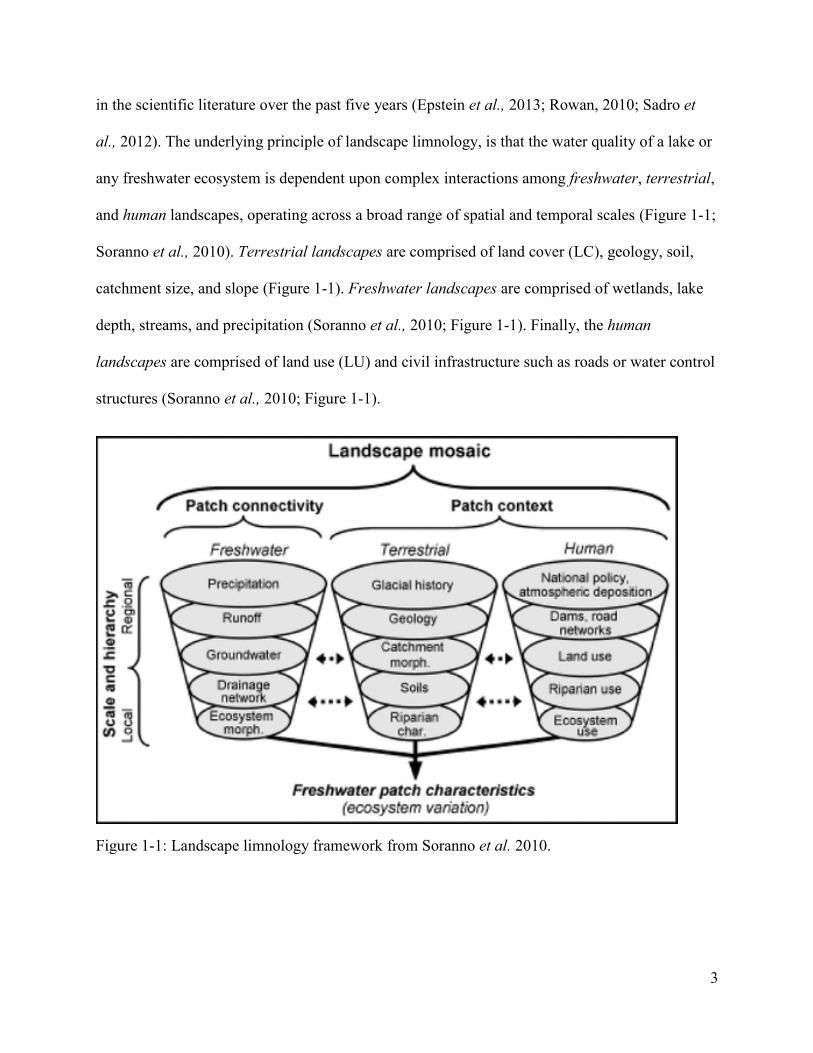
and human landscapes, operating across a broad range of spatial and temporal scales (Figure 1-1;
Soranno et al., 2010). Terrestrial landscapes are comprised of land cover (LC), geology, soil,
catchment size, and slope (Figure 1-1). Freshwater landscapes are comprised of wetlands, lake
depth, streams, and precipitation (Soranno et al., 2010; Figure 1-1). Finally, the human
landscapes are comprised of land use (LU) and civil infrastructure such as roads or water control
structures (Soranno et al., 2010; Figure 1-1).
Figure 1-1: Landscape limnology framework from Soranno et al. 2010.
4
Many components of human landscapes trigger physical and chemical stressors that
directly and indirectly affect aquatic ecosystems (Anzecc, 2000; Serveiss et al., 2004; Van Sickle
et al., 2006). The cumulative effects of stressors are poorly understood because multiple stressors
interact with one another (Christensen et al., 2006; Palmer et al., 2011; Schindler, 1998; Wrona
et al., 2006). For example, the combined effects of stressors caused by human activity and
climate are known to be cumulative (Hering et al., 2014; Schindler, 2001). The response of
aquatic ecosystems to cumulative effects are difficult to predict because multiple stressors can
have antagonistic, multiplicative, or additive effects (Christensen et al., 2006; Schindler, 1998;
Solimini et al., 2009; Wrona et al., 2006). For example, Ca declines are amplified by the
multiplicative effects of climate change and acid precipitation (Schindler, 2001). The decrease of
base cation export from reduced stream flows and depleted soil stores of base cations from acid
deposition result in a reduction of Ca concentrations in lakes (Schindler, 2001; Watmough and
Aherne, 2005).
Understanding cumulative effects of stressors is further complicated by interactions
among stressors at multiple spatial scales. For example, climate change is a global scale stressor
(Keller, 2009; Schindler, 1998), while nonpoint source pollution can act at global and regional
scales (Schindler, 1998; Whittier et al., 2002). Metal contaminants and sulphate from industrial
pollution can be transported through the atmosphere resulting in acidification of the lake or toxic
metals in fish (Jeffries et al., 2003; Stoddard et al., 2003; Whittier et al., 2002). Nonpoint and
point source pollution can also operate at a local scale (Dube et al., 2006; Whittier et al., 2002).
For example, municipal waste sites and agricultural land within a lakes catchment can result in a
surplus of TN and TP resulting in nutrient enrichment (Gibson, 2000; Dube et al., 2006;
5
Rantakari et al., 2004; Whittier et al., 2002). To better understand the effects of stressors at
multiple spatial scales a cumulative effects approach is needed (Dube et al., 2006; Keller, 2009).
The physico-chemical properties of a lake are known to be influenced by characteristics
of their surrounding landscapes (Soranno et al., 1999; Stendera and Johnson, 2006; Zhang et al.,
2012). The strength and spatial scale of the interactions between terrestrial landscapes and lakes
may be dependent on the hydrological connectivity of the freshwater landscape (Fraterrigo and
Downing, 2008; Stendera and Johnson, 2006). Considering the combined effects of freshwater
and terrestrial landscape features is a central part of landscape limnology (Soranno et al., 2010).
These natural freshwater and terrestrial landscape components are commonly referred to as
hydrogeomorphic (HGM) and LC features. HGMs are watershed characteristics that can be,
“hydrological, morphological, terrestrial or geological” (Soranno et al., 2011).
Terrestrial landscape features are important in determining ionic gradient and pH in
lakes. Catchment geology and soil properties are often correlated with major ions such as Ca
(Thierfelder, 1998; Watmough and Aherne, 2008; Wolniewicz et al., 2011). Additionally,
catchment vegetation type and lake elevation influence the pH and base cation concentrations in
lakes (Berg et al., 2005; D’Arcy and Carignan, 1997; Håkanson, 2005; Scott et al., 2010;
Wolniewicz et al., 2011).
Indices that quantify catchment morphometry and hydrology are important determinants
of lake physico-chemistry, especially TP and DOC concentrations (Martin et al., 2010; Nõges,
2009; Stefanidis and Papistendaou, 2012). The HGM index of water residence time (WRT) is
important in influencing DOC, COLTR, and TP (D’Arcy and Carnigan, 1997; Håkanson, 2005;
Larsen et al., 2011; Rasmussen et al., 1989; Webster et al., 2008). WRT is the average length of
time water will stay in an aquatic system (Dronkers and Zimmerman, 1982). Drainage ratio
6
(DR), another commonly cited HGM variable, is the total catchment area divided by the lake
area and is a surrogate for terrestrial loading, which influences the amount of dissolved materials
that reach the lake (Wetzel, 2001). Many studies have demonstrated a positive relationship
between water quality variables (DOC, COLTR, TP, base cations) and DR (Jones et al., 2004;
Rasmussen et al., 1989; Scott et al., 2010; Stendera and Johnson, 2006; Webster et al., 2008).
Freshwater landscapes that include all waterbodies in the catchment, and lake
morphometry are important determinants of DOC, COLTR, and TP in lakes (Martin et al., 2011;
Soranno et al., 2010; Thierfelder, 1998). Wetlands are a major source of allochthonous DOC for
lakes (Canham et al., 2004; Kortelainen et al., 1993; Thierfelder, 1998). Lake morphometry is
another freshwater landscape variable that strongly influences COLTR, DOC, and TP
concentrations in lakes (Canham et al., 2004; Håkanson, 2005; Martin and Soranno, 2006;
Soranno et al., 2010; Webster et al., 2008). In lake-rich landscapes percent of upstream lakes in
the catchment is correlated with COLTR and DOC concentrations (Kortelainen et al., 1993;
Rantakari et al., 2004; Thierfelder, 1998; Wolniewicz et al., 2011).
A lake typology usually includes both terrestrial and freshwater landscape features at
multiple spatial scales to account for these natural sources of variability in lake physico-
chemistry and aquatic biota (Rowan, 2010; Kagalou and Leonardos, 2009). A lake typology is a
classification tool that separates lakes into “types”, and each lake type has similar natural
physical, chemical, and biological characteristics (Buraschi et al., 2005; Hering et al., 2010;
Snelder et al., 2004). The lakes are divided based on freshwater and terrestrial landscape features
(natural HGM and LCs) (Nykänen et al., 2005). Each “lake type” functions as a monitoring and
management unit because it is expected to respond similarly to management actions (Snelder et
al., 2004; Solimini et al., 2009; Soranno et al., 2010; Wasson et al., 2002). Lake typologies are
7
usually hierarchical to accommodate for landscape features at multiple spatial scales by
accounting for large scale processes at higher levels, followed by smaller scale processes at
lower levels (Snelder et al., 2004).
Lake typologies commonly use regionalizations to create a hierarchical structure.
Regionalizations are geographic units that account for broad scale patterns in terrestrial and/or
freshwater features (Cheruvelil et al., 2008; Higgins et al., 2005; Omernik, 1987). Many
regionalization frameworks have been criticized for their use in aquatic ecosystem management
(Jenerette et al., 2002; Zogaris et al., 2009). Some regionalization frameworks are outdated while
others are based on features of the human landscape, making them unsuitable for use in a lake
typology (Cheruvelil et al., 2008; Zogaris et al., 2009). Additionally, the performance of
regionalizations is dependent on the spatial scale of the lake typology (Cheruvelil et al., 2008;
Cheruvelil et al., 2008). Cheruvelil et al. (2013) suggested that, “custom made regionalization
frameworks,” could be implemented by using known relationships between water quality and
landscape features.
Lake typologies have been used to facilitate the assessment of ecological status by
helping define reference conditions for different lake types (Cardoso et al., 2007; Kolada et al.,
2005; Poikane et al., 2010; Soranno et al., 2011). A reference condition is the “normal” or
expected condition for a lake with minimal human disturbance (Cardoso et al., 2007; Johnson,
1999; Keller, 2009; Martin et al., 2011). Reference lakes are selected by defining pressure
criteria based on human landscape features (Gibson, 2000; Figure 1-1). Pressure criteria can use
human LU and, physico-chemical thresholds to determine if lakes are in a reference state
(Poikane et al., 2010). Impacted lakes are lakes that have catchments, which are disturbed by
human activities and hence do not meet the reference pressure criteria. Ecological status is
8
assessed based upon how far a given lake deviates from its reference condition (Carvalho et al.,
2009; Kolada et al., 2005; Poikane et al., 2010). Due to natural spatial variability among lakes
the reference condition for lakes within a region often differs (Soranno et al., 2011). Type-
specific reference conditions based on lake types from a lake typology help to account for the
natural differences within a region (Kolada et al., 2005; Martin et al., 2011; Soranno et al.,
2011).
Lake typologies have been implemented in various regions at continental, national, state-
wide, and regional spatial scale. However, lake typologies have been criticized for not being
updated to reflect the current conceptual understanding of limnological ecosystems (Hering et
al., 2010; Moss, 2007). The WFD lake typologies neglect measures of ecosystem connectivity
and structure which are known to be important in determining ecological quality of aquatic
ecosystems (Moss, 2007). The selection of suitable variables for a lake typology is further
limited by the lack of available data in regions with numerous lakes (Hering et al., 2010; Martin
et al., 2011). For example, lake depth is a requirement for the European Water Framework
Directive (WFD) lake typologies (Buraschi et al., 2005; Rowan, 2010) but in regions with an
abundance of lakes, such as Poland and Finland, lake depth cannot be included in national lake
typologies because lake depth data is not available for all lakes (Nykänen et al., 2005; Soszka et
al., 2008).
The use of lake typologies in Canada has been very limited to date. In the Muskoka River
Watershed (MRW) in south-central Ontario, Canada, large changes in water quality of lakes
have occurred (Palmer et al., 2011), but no lake typology currently exists to support research and
management activities in this region. Water quality changes throughout the MRW are thought to
be the result of the cumulative effects of multiple stressors, but these impacts are poorly
9
understood (Keller et al., 2008; Keller, 2009; Palmer et al., 2011; Schindler, 2001). For example,
Ca declines in lakes have been reported in the region and are thought to be a result of recovery
from acid deposition and forest harvesting (Jeffries et al., 2003; Jeziorski et al., 2008; Palmer et
al., 2011; Watmough et al., 2005; Watmough and Aherne, 2008). TP declines have also occurred
in lakes of the MRW and are hypothesized to be a result of multiple stressors but are not well
understood (Eimers et al., 2009; Palmer et al., 2011). Increases in salinity have occurred in many
of the lakes as a result of road salting (Molot and Dillon, 2008; Palmer et al., 2011). DOC has
also increased in the MRW lakes and is thought to be a result of climate change and recovery
from acid deposition, combined (Keller, 2009; Monteith et al., 2007; Palmer et al., 2011).
The decline of water quality in the lakes within the MRW is an issue of great concern
because the freshwater resources of the MRW have high economic, recreational, and cultural
importance (OMNR, 2006). Changes in water quality can diminish the aesthetic appeal of water
by changing its smell, taste or appearance (Paterson et al., 2004; Smol, 2010). Water clarity is
important for cottagers and tourists of the MRW and can be compromised by changes in DOC
and chlorophyll-a (Gartner Lee Ltd., 2005). Lake trout and other cold water fishes are found in
the deep lakes of the MRW and are important for sport fishing (Dillon and Molot, 2005; Gartner
Lee Ltd., 2005; Quinlan et al., 2003). Changes in TP and DOC concentrations can indirectly
affect lake trout through alterations of temperature and oxygen regimes, which are crucial
aspects of lake trout habitats (Dillon and Molot, 2005; Gartner Lee Ltd., 2005).
Since 1981, the District Municipality of Muskoka (DMM) has been proactive in water
quality monitoring and lake management in the MRW (Gartner Lee Ltd., 2005). However, the
original focus of lake monitoring and management was water clarity and shoreline development
(Gartner Lee Ltd., 2005). In 2003, the Muskoka Water Strategy was implemented to take a more
10
holistic approach to lake management, considering the health of the entire lake ecosystem
(Gartner Lee Ltd., 2005). The review and recommendations for the Lake System Health program
in 2005 made important steps in implementing holistic lake monitoring and management
program for the MRW (Gartner Lee Ltd., 2005). The review of the Lake System Health
programs, and other recent studies, have emphasized the need to design a lake monitoring
program that is better able to detect the cumulative effects of the multiple stressors and guide
management decisions that recognize the lakes’ unique responses to stressors (Gartner Lee Ltd.,
2005; Hering et al., 2014; Paterson et al., 2004; Palmer et al., 2011).
This study will take a landscape and statistically-based approach to better understand the
natural and anthropogenic variability of the water quality in the MRW lakes at a regional and
watershed-level scale. A qualitative conceptual model will be constructed in order to aid in the
development and application of a lake typology. A qualitative conceptual model is a simplified
understanding of how a watershed works as a system (WG 2.7, 2003). In this study a conceptual
model will provide insight on how landscape features affect the lake water quality. The use of a
conceptual model is imperative for the development and adaption of monitoring programs
because it helps to identify relevant human pressures that affect ecological status, while also
identifying data gaps or errors (IMPRESS, 2003: WG 2.7, 2003).
This thesis was conducted as a component of the MRW research node funded by the
Canadian Water Network (CWN). The overarching goal of this research cluster is to improve
the detection and management of the cumulative effects of aquatic ecosystem stressors
throughout the MRW (CWN, 2013). A particular objective of the MRW research node is to
develop a comprehensive monitoring program and predictive models that can be used for
cumulative effects assessment and management (Eimers, 2012; CWN, 2013). This study will
11
contribute to other projects within the research cluster through the development of a shared
database of terrestrial, freshwater and human landscape characteristics for all lakes within the
MRW, and by providing a lake typology to help interpret results and guide future research
priorities (CWN, 2013). The robustness and suitability of the lake typology as an aid in the
development of a comprehensive monitoring program will be evaluated by other members of the
research node using biological indicators. Finally, the findings from the MRW research node will
be synthesized and used to give practical recommendations for the DMM (Eimers, 2012).
12
1.1 Research Objectives and Questions
The overarching objective of this study is to implement a landscape-based approach to
develop and apply a hierarchical lake typology for the lakes of the MRW, in order to assist lake
management decisions. The following three sub-objectives will be used to meet the overarching
objective of this study.
1) Develop a qualitative conceptual model to better understand the freshwater, terrestrial,
and human landscape features that influence water quality in the MRW: A suite of
freshwater, terrestrial, and human landscape characteristics will be derived for all lakes
greater than 8 ha in the MRW and used to develop a conceptual model through
exploratory multivariate statistical analysis and variable reduction.
2) Classify all lakes of the MRW according to freshwater and terrestrial landscape
characteristics: Lakes will be separated into groups that have similar physico-chemical
and biological properties. A lake typology will be developed by using derived
characteristics and knowledge gained through the conceptual model built as part of
objective 1.
3) Apply the above lake typology to establish type-specific reference conditions for TP and
critically evaluate the current DMM lake monitoring program: Impacted lakes within
the MRW that exceed type-specific TP reference conditions will be identified.
Additionally, the DMM lake monitoring will be critically evaluated to determine if the
monitoring program is statistically representative of major landscape gradients and
whether it incorporates an adequate number of samples for reference lakes.
13
A major challenge in lake typology development is the selection of landscape variables that
separate lakes into ecologically and physico-chemically distinct lake types (Rowan, 2010; Moss
et al., 2003). A landscape limnology approach with complementary statistical methods can assist
with lake typology development and lake management decisions (Cheruvelil et al., 2013; Martin
et al., 2011; Soranno et al., 2010). By considering the connectivity and organization of
landscapes multiple spatial scales, relationships between landscape features and aquatic
ecosystem characteristics can be revealed through statistical analysis (Bremigan et al., 2008;
Soranno et al., 1999; Soranno et al., 2010; Stendera and Johnson, 2006). Accordingly, the first
research question in this thesis addresses the landscape limnology principle of scale and
hierarchy, by considering landscape variables at multiple spatial scales (Soranno et al., 2010;
Figure 1-1):
1) What spatial scales for landscape variables have the strongest influence on the pH, Ca,
DOC, and TP concentrations in the MRW lakes?
The second research question is structured around the landscape limnology principle of patch
connectivity, to provide insight into how hydrological connectivity and spatial organization of
the freshwater landscape affect the transport and processing of ions, nutrients, and carbon across
the landscape (Soranno et al., 1999; Soranno et al., 2010; Stendera and Johnson, 2006; Figure
1-1).
2) To what extent can hydrologic connectivity and morphometry of lakes explain gradients
in surface water pH, Ca, TP, and DOC across the MRW?
14
1.2 Thesis Structure
Chapter 2 provides a synthesis of the evolution of lake monitoring and management and
how lake typologies can be updated with current limnological, hydrological, and statistical
research. Chapter 3 provides an overview of the study site, derivations of all landscape metrics
and statistical methods. Chapter 4 details the results of the lake typology development and
statistical evaluation for the MRW monitoring program. The theoretical and practical
implications of the thesis are presented in Chapter 5. Finally, Chapter 6 provides a summary of
thesis findings and discusses their implications for future research.
15
2. BACKGROUND
The recent evolution of lake monitoring and management has resulted in some examples of
cost-effective monitoring programs that consider the health of the entire aquatic ecosystem
(Brown et al., 2005; Hering et al., 2010; Solimini et al., 2009). Historically, lake monitoring and
management has taken a single stressor approach that has been conducted at local spatial scales,
with the use of chemical indicators (Apitz et al., 2006; Hughes et al., 2000; Whittier et al.,
2002). In the last 20 years, there has been a shift towards holistic lake monitoring and
management which uses a watershed and multi-stressor approach (Apitz et al., 2006; Borre et al.,
2001; Hering et al., 2010; Hughes et al., 2000). The holistic approach to monitoring and
management is still in its infancy, and thus current scientific knowledge and technical tools need
to be used to update current lake management frameworks (Moss, 2008; Quevauviller et al.,
2007; Solimini et al., 2009). Lake typologies are an emerging management tool that can be used
to enhance management practices and decision making in relation to aquatic ecosystems in
working landscapes (e.g. road development, urbanization, agriculture). The refinement and
application of lake typologies in new lake districts requires a multi-scale landscape-based
approach that considers the freshwater landscape as spatially connected, and takes advantage of
emerging statistical techniques and landscape modelling.
2.1 Multi-scale lake management and monitoring
In the last 20 years, lake managers and scientists have begun to monitor and study lakes
at much broader spatial scales (Apitz et al., 2006; Cheruvelil et al., 2013; Hughes et al., 2000).
The WFD implemented by the EU in 2000, harmonizes management and monitoring effort of all
waters at a continental scale (Hering et al., 2010). The river basin, the drainage area of a major
16
river, is the spatial scale at which WFD requires management plans (IMPRESS, 2003). The goal
of river basin management plans is to restore all water bodies to good ecological status by 2015
(Hering et al., 2010; IMPRESS, 2003). The Environmental Assessment and Monitoring Program
(EMAP) in the United States uses a multi-tier approach which organizes monitoring and
management at national, state-wide, and regional scales (Hughes et al., 2000; U.S. EPA, 2003).
Effective lake monitoring and management at broader spatial scales requires a hierarchical
approach which can partition natural aquatic ecosystem variation at multiple spatial scales
(Angermeier et al., 2000; U.S. EPA, 2003). A hierarchical approach is needed because aquatic
ecosystem processes interact across multiple spatial scales (Higgins et al., 2005; Soranno et al.,
2010). In addition, aquatic ecosystems are managed across multiple spatial scales (Soranno et al.,
2010). A hierarchical framework helps to manage lakes at regional scales (state-wide and
ecoregions), while still addressing local scale issues (U.S. EPA, 2003).
2.1.1 Regionalization frameworks
Regionalization frameworks can be used to account for regional landscape patterns and to
organize national-scale management efforts (Angermeier et al., 2000; Seaber et al., 1987).
Different regionalization frameworks have been designed to facilitate the management of aquatic
and terrestrial resources (Higgins et al., 2005; Omernik, 1987; Seaber et al., 1987). Ecoregions
are a commonly used regionalization framework for aquatic ecosystem management (Hughes et
al., 2000; Kagalou and Leonardos, 2009).The criteria used to define ecoregions is often
dependent on the continent or country. For example, Omernik’s (1987) ecoregions for the United
States are based on patterns of natural and human characteristics, while Illies (1978) ecoregions
for Europe are based on aquatic insect distributions. However, in recent research other
regionalization frameworks that are based on hydrological boundaries and other natural
17
landscape features are better at accounting for interregional variability in water quality
(Cheruvelil et al., 2008; Cheruvelil et al., 2013; Martin et al., 2011; Soranno et al., 2010).
Hydrological Units (HUCs) are a regionalization framework based on major river basins (Seaber
et al., 1987). Another regionalization framework, Ecological Drainage Units (EDUs) are
derived by combining hydrological units based on similar landscape features (Higgins et al.,
2005). EDUs were designed by The Nature Conservancy to account for freshwater biodiversity
and applied in the Columbia River Basin of the Western United States and Upper Paraguay River
Basin of South America (Higgins et al., 2005). Although, regionalization frameworks are
effective at accounting for among-region variation in water quality, landscape features need to
also be measured at finer spatial scales to account for within-region variation (Cheruvelil et al.,
2008; Cheruvelil et al., 2013).
2.1.2 Spatial scales within regions
Research has demonstrated there is still a substantial amount of natural aquatic ecosystem
variation within regions that needs to be accounted for in order to establish suitable reference
conditions (Angermeier et al., 2000; Cheruvelil et al., 2013; Cardoso et al., 2007). In the
Northeastern United States, the spatial variability in TP was explained best by a regionalization
framework and local scale HGMs (Cheruvelil et al., 2013; Martin et al., 2011). There are three
different spatial scales that are used to measure landscape measures within regions. The largest
spatial scale is the Cumulative Catchment Area (CUCA) which is the total upslope area that
drains into the focal lake (Palmer et al., 2012), while the Local Catchment Area (LOCA) is the
portion of the cumulative catchment whose drainage area is unique to the focal lake (Martin et
al., 2011). The riparian scale is the near-shore zone (Fraterrigo and Downing, 2008), which
depending on the study, is defined as a given buffer distance from the lake. Recent research in
18
the subdiscipline of landscape limnology has shown that LOCA surficial geology and wetlands
account for the within region variability of TP and COLTR respectively (Cheruvelil et al., 2013;
Martin et al., 2011). Landscape measures need to be included at both the regional and finer
spatial scales for quantification of water quality variability (Cheruvelil et al., 2013).
2.1.3 Hierarchical lake typologies
Lake typologies are hierarchical in order to account for natural landscape variation at
multiple spatial scales. This means that lake typologies include landscape measures at different
spatial scales. For example, the first level of WFD lake typologies uses ecoregions to account for
the regional scale (RECOND, 2003). Other obligatory factors such as geology, lake altitude, lake
size, and mean depth are used at lower levels of WFD lake typologies to account for finer scale
landscape features (Kagalou and Leonardos, 2009; Kolada et al., 2005; REFCOND, 2003; Table
2-1). Geology is usually measured in the CUCA for European WFD typologies. The ecological
quality and functioning of shallow lake ecosystems (ECOFRAME) project for all EU member
states, devised a lake typology that separates the lakes into the two geology classes of organic
and mineral based on CUCA geology. Lakes that are classified as organic have at least 50% of
their CUCAs covered by peat deposits, while lakes that belonged to the mineral class had over
50% of their CUCAs covered by rock-based mineral deposits (Moss et al., 2003). Physical
characteristics of the lakes such as mean depth and lake elevation are also commonly included in
lake typologies (Kagalou and Leonardos, 2009; Rowan, 2010).
2.2 Holistic aquatic ecosystem management strategies for lake districts
Recently, lake monitoring and management programs have taken a more holistic
approach (Apitz et al., 2006). A holistic approach considers all components of an ecosystem
19
(air, water, groundwater, soil, human pressures) within the river basin (Apitz and White, 2003;
Brack et al., 2009). Multiple indicators are used as part of a holistic approach to account for
multiple stressors (Hughes et al., 2000: Whittier et al., 2002). The WFD and EMAP programs
implement whole ecosystem approaches by focusing on aquatic ecosystem health (Hering et al.,
2010; Hughes et al., 2000). Both EMAP and WFD use biological indicators as the basis for
ecological assessments but also use physico-chemical and landscape features (U.S. EPA, 2003;
WG 2.7, 2003). Freshwater classification systems have become important tools in holistic
aquatic ecosystem management (REFCOND, 2003; Snelder et al., 2007; Soranno et al., 2010).
The WFD requires lake typologies to be developed for each EU member state (REFCOND,
2003). A landscape-based approach allows statistical-based sampling designs for monitoring
programs and less biased extrapolations of ecological status (Brown et al., 2005; Wang et al.,
2010). The use of lake typologies with both abiotic and biotic measures of aquatic ecosystem
health ensures an increased accuracy in the assessment of ecological status (REFCOND, 2003;
WG 2.7, 2003).
2.2.1 Landscape-based approach to strategic lake monitoring
A landscape-based approach provides a cost-effective and statistical basis for strategic
lake monitoring and management (Wang et al., 2010). Quantifying human pressures for all
watersheds can serve as a screening tool to identify unsampled lakes that may be at risk of not
meeting management objectives (Brown et al., 2005; IMPRESS, 2003; Wang et al., 2010).
Characterizing the natural landscape features of watersheds can aid in statistically based
sampling designs for monitoring programs which allow for extrapolations of regional conditions
(Brown et al., 2005; Peterson et al., 1999; Wagner et al., 2008). The EMAP program requires
20
statistically representative samples for state monitoring programs (Hughes et al., 2000). A
statistically representative sample means that a sufficient amount of lakes is sampled within each
lake type, and that the sample encompasses the region’s major LC and HGM gradients (Bailey et
al., 2004; Johnson, 1999; Wagner et al., 2008; WG 2.7, 2003). For the WFD, representative
type-specific reference conditions are important for the accurate classification of ecological
status (RECOND, 2003).
2.2.2 Multiple quality elements for assessment of ecological status
Ecological status is determined in the WFD by taking a whole ecosystem approach that
quantifies the health of an ecosystem through the use of abiotic and biotic ecosystem components
(Hering et al., 2010; Nõges et al., 2009; Solimini et al., 2009; WG ECOSTAT, 2003).The
ecological status of waterbodies in the WFD are initially classified according to biological
quality elements and are further characterized by hydromorphological and physico-chemical
quality elements. Biological quality elements are indicators that are usually based on community
compositions or abundances of phytobenthos, macrophytes, or invertebrate fauna, these
indicators are usually sensitive to specific human pressures (Solimni et al., 2009; WG 2.7, 2003).
Hydromorphological and physico-chemical quality elements are used to ensure the accurate
interpretation of biological quality elements, which minimizes the risk of misclassification of
ecological status (WG 2.7, 2003). Measures of catchment hydrology and lake morphometry are
used as hydromorphological quality elements because they greatly alter the natural variability of
lake physico-chemistry and community composition. Additionally, hydromorphological quality
elements are affected by climate change and alteration of the natural flow regime (WG 2.7, 2003;
21
Poikane et al., 2010). Quality elements can be used for more accurate assessment of ecological
status if lake typologies are used (REFCOND, 2003).
2.2.3 Lake typologies
Lake typologies provide a practical framework to use for lake monitoring and
management (Soranno et al., 2010). A lake typology classifies lakes according to similar
freshwater and terrestrial characteristics that are thought to influence physico-chemical and
biological quality elements (Moss et al., 2003; WG 2.7, 2003). Each lake type is expected to
respond differently to natural and anthropogenic change (Martin et al., 2011; Soranno et al.,
2010; WG 2.7, 2003). A major function of lake typologies is to devise type-specific reference
conditions (WG ECOSTAT, 2003). Devising type-specific reference conditions also require a
selection of reference lakes using pressure criteria (Poikane et al., 2010; REFCOND, 2003).
Pressure criteria commonly use human landscape features such as percent of CUCA LU, absence
of point sources and population density (Martin et al., 2011; Nixon et al., 1998; Poikane et al.,
2010).
2.3 Challenges in lake typology development
The development of ecologically relevant lake typologies, which can be practically
applied to meet the needs of each river basin is still a challenge for the member states that are
part of the WFD (Hering et al., 2010; Moss, 2008). There are two systems that EU member
states can use for lake typology development (REFCOND, 2003). System A has predetermined
quantitative or qualitative classes based on obligatory factors to differentiate lake types
(REFCOND, 2003; Table 2-1). System B is more flexible and allows the use of optional factors
(REFCOND, 2003; Table 2-1). The availability of data that measures the freshwater landscape in
22
some EU member states limits the use of both obligatory and optional factors in national lake
typologies (Fölster et al., 2004; Soszka et al., 2008). For example, WRT is an optional factor for
WFD lake typologies but is rarely used because hydrological data is expensive and time-
consuming to gather for a large number of lakes (Rowan, 2010; WG 2.7, 2003). WRT also
requires lake morphometry data which are also rarely available at national spatial scales
(Nykänen et al., 2005). Clustering techniques are usually used to determine the quantitative
classes and variables included as optional factors in lake typologies (Kolada et al., Rowan, 2010;
WG 2.3, 2003). The hierarchical and nonlinear nature of relationships between landscape
features and aquatic ecosystem characteristics are not accounted for in most clustering
techniques. Measures of hydrological connectivity are not obligatory or optional factors in WFD
lake typologies despite the recognized importance of freshwater ecosystem connectivity in
influencing both water quality and species assemblages (Higgins et al., 2005; Rosenfeld and
Jones, 2010; Sadro et al., 2012).
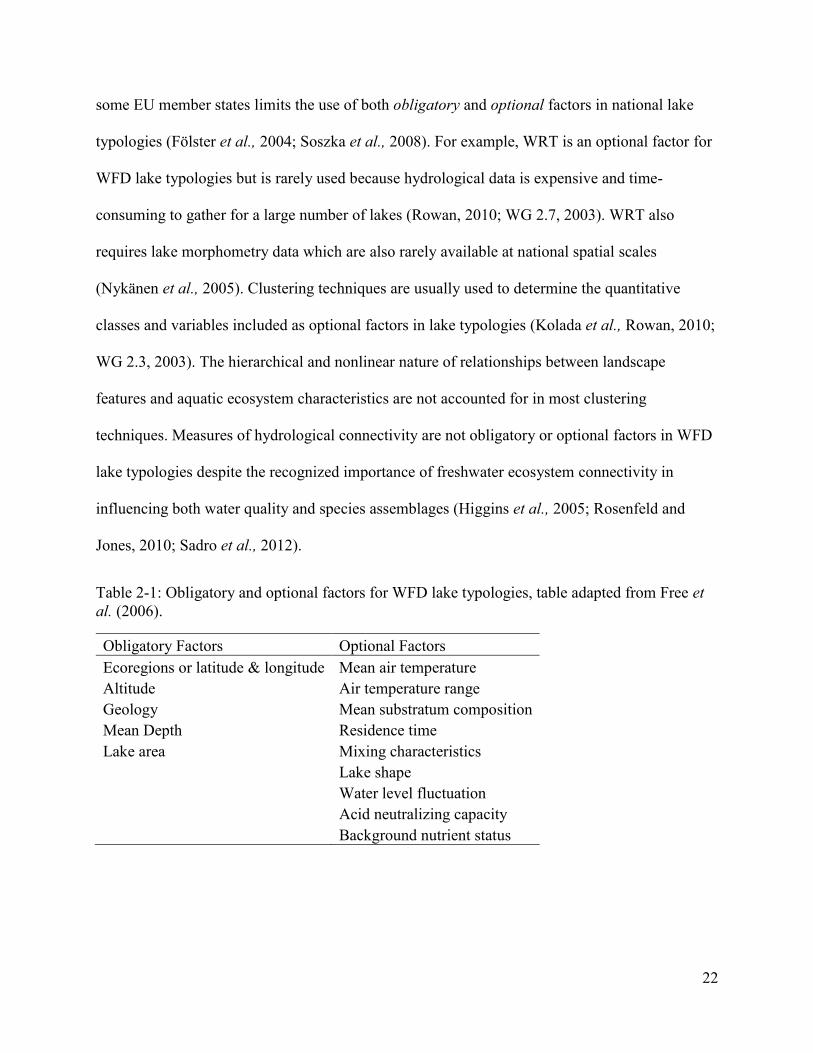
Table 2-1: Obligatory and optional factors for WFD lake typologies, table adapted from Free et
al. (2006).
Obligatory Factors Optional Factors
Ecoregions or latitude & longitude Mean air temperature
Altitude Air temperature range
Geology Mean substratum composition
Mean Depth Residence time
Lake area Mixing characteristics
Lake shape
Water level fluctuation
Acid neutralizing capacity
Background nutrient status
23
2.3.1 Lake depth modelling
Landscape-based depth models provide a way of including lake depth, volume and
residence times in lake typologies for regions that have numerous lakes. Although, landscape-
based lake depth and volume models have been implemented successfully, these models have not
been used in lake typologies. Fölster et al. (2004) used lake area and elevation to estimate the
mixing type for a Swedish lake typology. However, current advancements in lake depth models
allow more accurate estimates of lake depth. Models were implemented for the Northeastern
United States and Sweden that predicted lake depth and volume based on the surrounding
topography and size of the lake (Hollister et al., 2011; Sobek et al., 2011). Hollister’s et al.
(2011) method had a cross-validation correlation of 0.72 for modelled predictions of maximum
lake depth (zmax), while Sobek et al.’s (2011) method only had a coefficient of determination
less than 0.40 for mean and maximum lake depths.
2.3.2 Freshwater landscape measures needed in lake typologies
The availability of lake morphometry data further limits the use of other freshwater
landscape measures in lake typologies (Nykänen et al., 2005; Free et al., 2006). For example,
lake volume is needed to estimate WRT (Hollister et al., 2011). As a result, measures of the
freshwater landscape at the CUCA scale including WRT are largely absent from currently
available examples of lake typologies. For example, the only WFD lake typology that has a
CUCA freshwater landscape measure is a Polish lake typology (Kolada et al., 2005). The Polish
lake typology uses Schindler’s ratio, which is a measurement of the catchment influence on the
lake, calculated by the sum of the catchment and lake area divided by lake volume (Kolada et al.,
2005; Stefanidis and Papastergiadou, 2012). However, a physico-chemical classification scheme
for a subset of Michigan lakes included the CUCA scale measures of both WRT and
24
hydrological connectivity (Martin et al., 2011). The wealth of limnological and hydrological
research on catchment hydrology and connectivity suggests the need to integrate freshwater
CUCA measures in lake typologies. The effect of lake position in a stream or lake network on
water quality is complex because it is modulated by other features of the terrestrial and
freshwater landscapes.
2.3.3 Lake landscape position
There are a variety of approaches to measure a lake’s position and hydrological
connections in the freshwater landscape. Lake landscape position is a measure of the focal lake’s
hydrological position and spatial proximity to other lakes (Kratz et al., 1997). This measure can
be quantified using lake order, or lake network number (LNN). Lake order quantifies the lakes
connection to streams based on the Strahler order of the inlet stream (Martin and Soranno, 2006;
Riera et al., 2000). Lake network number measures the lakes landscape position based on its
connection to lakes (Martin and Soranno, 2006). In some studies with only one branch in the lake
network, lake chain position is analogous to LNN (Carpenter and Lathrop, 2014; Sadro et al.
2012). LNN is measured by counting the number of lakes in the longest lake chain (Epstein et
al., 2013; Martin and Soranno, 2006; Sadro et al., 2012). Nonreactive solutes, especially major
cations, have been shown in many different lake districts to be related to lake order (Kratz et al.,
1997; Quinlan et al., 2003; Riera et al., 2000; Soranno et al., 1999).
2.3.3.1 Lake landscape position and water quality
In studies, lake order has been shown to have a very weak or insignificant relationship
with TP, COLTR, and DOC (Martin and Soranno, 2006; Quinlan et al., 2003; Riera et al., 2000;
Soranno et al., 1999). This may be the result of not considering the effect of each lake as a
processing unit within a lake network. TP, COLTR, and DOC are affected more by in-lake
25
processing than major ions because they are more susceptible to biological uptake and decay
(Kling et al., 2000; Soranno et al., 1999). Lake order may not be an effective predictor of TP,
COLTR, and DOC processing along a lake network because streams have been reported to have
marginal effects on material processing because of their shorter WRT (Canham et al., 2004;
Lottig et al., 2011). Therefore, LNN may be a more effective predictor because it can better
account for the material processing of upstream lakes (Sadro et al., 2012). However, the
upstream lake processing of TP, DOC, and COLTR is not solely determined by lake
connectivity. Characteristics of the landscape and the WRT of each lake modifies the affect that
LNN can have on upstream lake processing of materials (Zhang et al., 2012).
2.3.3.2 Landscape factors
Characteristics of the terrestrial, freshwater, and human landscapes need to be considered
when investigating the effects of upstream lake processing on lake physico-chemistry. In a study,
on the role of upstream lakes in altering DOC concentrations in streams, it was found that
percent wetlands obscured upstream lake effects (Lottig et al., 2012). The comparison of DOC
stream concentrations with and without upstream lakes had different results when the effects of
wetlands were considered (Lottig et al., 2012). Similarly, the different effects of upstream lakes
on TP, and Total Organic Carbon (TOC) between Southern and Northern Finland was
hypothesized to be a result of differences in wetland cover and climate (Rantakari et al., 2004).
Sadro et al. (2012) found that LNN had different effects on concentrations of dissolved materials
which were dependent on lake networks being in subalpine and alpine regions which differed in
vegetation, elevation, and slope. Although not addressed by Carpenter and Lathrop (2014),
different proportions of agricultural and urban land use in each lake’s catchment may have had a
stronger influence than upstream lake processing.
26
2.3.3.3 Water residence time
The WRT of a lake can alter its degree of processing and its effect on dissolved matter of
downstream lakes (Hanson et al., 2011; Kothawala et al., 2014). For example, upstream lakes
had no effect on downstream DOC stream concentrations in the Northern Highland Lake District
(NHLD) of Wisconsin (Lottig et al., 2012), while in Northern Michigan upstream lakes acted as
a sink for DOC (Larson et al., 2007). The differences in upstream lake processing of DOC may
be a result of the longer WRTs in Michigan compared to the NHLD (Larson et al., 2007; Lottig
et al., 2012; Martin and Soranno, 2006). In a study of the Yahara Lake Chain in Wisconsin, the
lake with the longest WRT acted as a TP sink, while the lakes with very short WRT acted as TP
sources for downstream lakes (Carpenter and Lathrop, 2014). In Michigan where lakes have
longer WRT, upstream lakes acted as a sink for TP (Zhang et al., 2012).
The research on LNN and upstream lake processing of TP and DOC suggests that the
WRT, landscape setting and connections to other lakes needs to be considered. A recent study of
a large number of Swedish lakes integrated the effects of WRT and upstream lakes using a
measure of cumulative residence time (CWRT) (Muller et al., 2013). To calculate CWRT, all
lake volumes were modelled using the Sobek et al. (2011) depth model, then the total volume of
upstream lakes was multiplied by the long-term mean discharge (Muller et al., 2013). CWRT
explained the quality of DOC better than the conventional WRT measure. This result suggests
the importance of including WRT into lake connectivity measures. However, this method does
not consider how the spatial configuration of lake chains affect CWRTs. Moreover, statistical
methods need to be used to determine if freshwater landscape measures help account for natural
variability in lake physico-chemistry.
27
2.3.4 Statistical and machine-learning methods for developing landscape-based lake
typologies
The selection of variables and the assignment of classes in lake typologies requires robust
statistical methods (Hering et al., 2010). Currently, there is a tendency to use multivariate
parametric methods in order to select landscape features for the development of lake typologies
(Rowan, 2010; Kolada et al., 2005). There are other statistical methods, such as tree-based
methods, that are more appropriate for uncovering and understanding complex relationships
between landscape features and physical and chemical characteristics of aquatic ecosystems
(Catherine et al., 2010; Martin et al., 2011). The appropriate statistical method to be used needs
to account for interactions, collinearity, and the nonparametric nature of the landscape features
(Lottig et al., 2011; Qian et al., 2010; Soranno et al., 2014).
Tree-based methods, namely Classification and Regression Trees (CART) and variants,
accommodate the complex interrelationships between water quality and landscape features
(Martin et al., 2011). CART models can also account for high-order interactions because of their
hierarchical structure and can handle nonparametric data (De’ath and Fabricus, 2000; Martin et
al., 2011). However, a drawback of tree-based methods is that they are sensitive to the data they
are trained on and hence prone to over-fitting (Hastie et al., 2001).
Machine learning methods that use an ensemble of trees provide a robust alternative to a
single CART model (Elith et al., 2008; Friedman and Meulman, 2003). Machine learning
methods use algorithms to generate a collection of models in order to “learn” the relationships
between a response variable and a set of predictor variables (Dietterich et al., 2000; Elith et al.,
2008). The use of machine learning tree-based methods is becoming more common in
limnology. Specifically, Random Forest and Bayesian tree models have been used to predict
28
eutrophication status and sensitivity (Catherine et al., 2010; Lamon et al., 2008; Soranno et al.,
2010). Additionally, another machine learning method, gradient boosted machines (GBMs),
have been used to predict TP, TN, and nitrate concentrations based on catchment land use,
hydrology, and land cover (Oehler and Elliot, 2011). GBMs are insensitive to correlated
predictors making them ideal for LU/LC variables measured at multiple spatial scales (Feld,
2013; Friedman, 2001). Machine learning methods deserve further exploration as powerful tools
for developing lake typologies using large multivariate datasets.
2.4 Summary
In the last 20 years, there has been a drastic change in the way lake management and
research is conducted. Lakes are now commonly being managed at the river basin scale using
landscape-based approaches. This holistic approach considers landscape features as connected to
the health and functioning of the lake ecosystems (Apitz et al., 2006). Lake typologies are an
important management tool that uses a multi-scale landscape-based approach. However, lake
typologies need to locally-adapted and must be continuously updated and refined as limnological
research, statistical methods, and landscape modelling techniques advance (Nykänen et al., 2005;
UKTAG, 2007). Newly developed lake depth models and connectivity indices of the freshwater
landscape should also be incorporated into lake typologies. Finally, the use of machine learning
techniques in the development of lake typologies are necessary to help researchers and managers
uncover, complex, multi-scale drivers of water quality across lake-management districts.
29
3. METHODOLOGY
3.1 Study Area
The MRW is a tertiary watershed of ~5660 km2 located in South-Central Ontario (Figure
3-1). A tertiary watershed is a subdivision of a secondary watershed, secondary watersheds are
usually the drainage area of large river systems (Government of Ontario, 2012a, 2012b). The
MRW is within the Precambrian Shield region of the Boreal Ecozone (O’Connor et al., 2009;
Quinlan et al., 2003). The minimum elevation of the MRW is 173 m near the shores of Georgian
Bay and the maximum elevation is 564 m in the Algonquin Highlands. The watershed is
primarily forested with a mix of coniferous and deciduous vegetation (O’Connor et al., 2009).
There is currently only a small amount of agricultural land due to the shallow tills and bedrocks
that dominates the area (Paterson et al., 2004). The landscape is rich in lakes, beaver ponds and
wetlands (O’Connor et al., 2009; Palmer et al., 2011). There is significant shoreline development
on some of the lakes due to cottages, resorts, and residential development (Palmer et al., 2011;
Paterson et al., 2004).
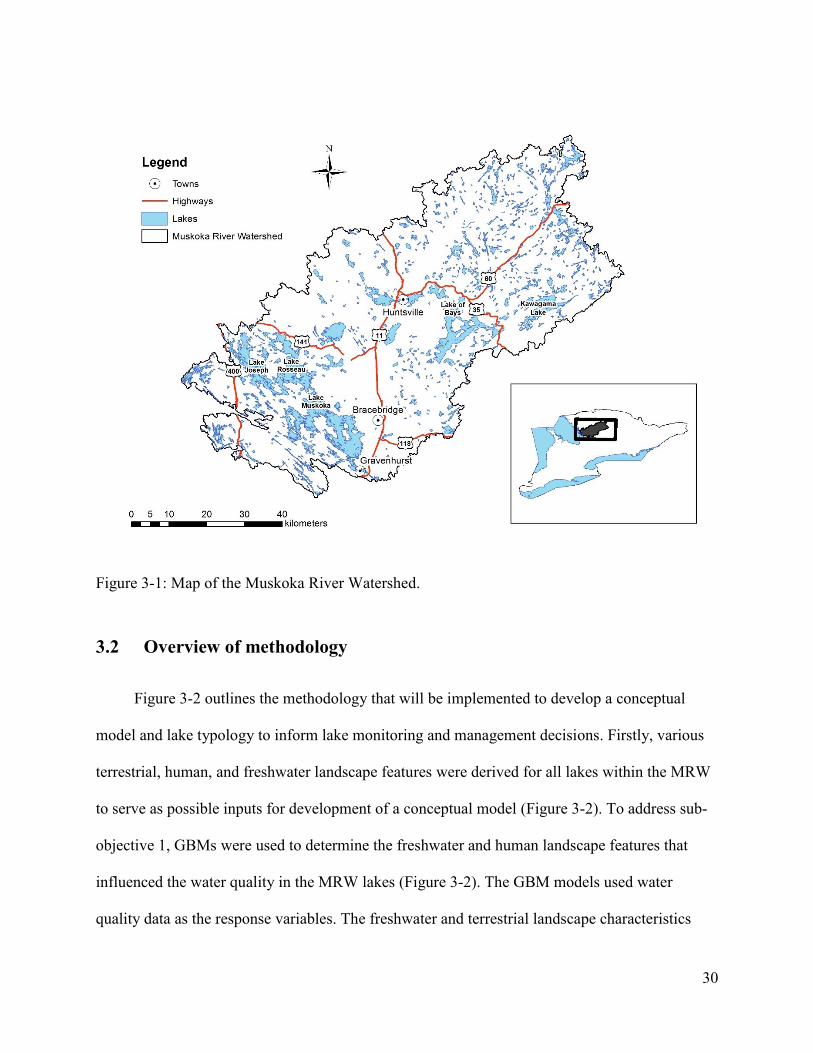
30
Figure 3-1: Map of the Muskoka River Watershed.
3.2 Overview of methodology
Figure 3-2 outlines the methodology that will be implemented to develop a conceptual
model and lake typology to inform lake monitoring and management decisions. Firstly, various
terrestrial, human, and freshwater landscape features were derived for all lakes within the MRW
to serve as possible inputs for development of a conceptual model (Figure 3-2). To address sub-
objective 1, GBMs were used to determine the freshwater and human landscape features that
influenced the water quality in the MRW lakes (Figure 3-2). The GBM models used water
quality data as the response variables. The freshwater and terrestrial landscape characteristics
31
were used to develop the lake typology along with statistical methods (Figure 3-2). To address
sub-objective 2, the first level of the lake typology was built by creating a regionalization
framework based on percent wetland and surficial geology using k-means cluster analysis
(Figure 3-2). The second level of the lake typology was built by selecting a landscape feature and
split point based on a CART model.
The lake typology was used to calculate type-specific reference conditions for TP and to
critically evaluate the DMM monitoring program (Figure 3-2). Descriptive statistics were
calculated for the TP reference lake distributions for each lake type to derive TP type-specific
reference conditions. To address research sub-objective 3, lakes that were not selected as
reference lakes, due to high levels of human disturbance in their catchments, had their TP
concentrations compared to their respective type-specific reference conditions.
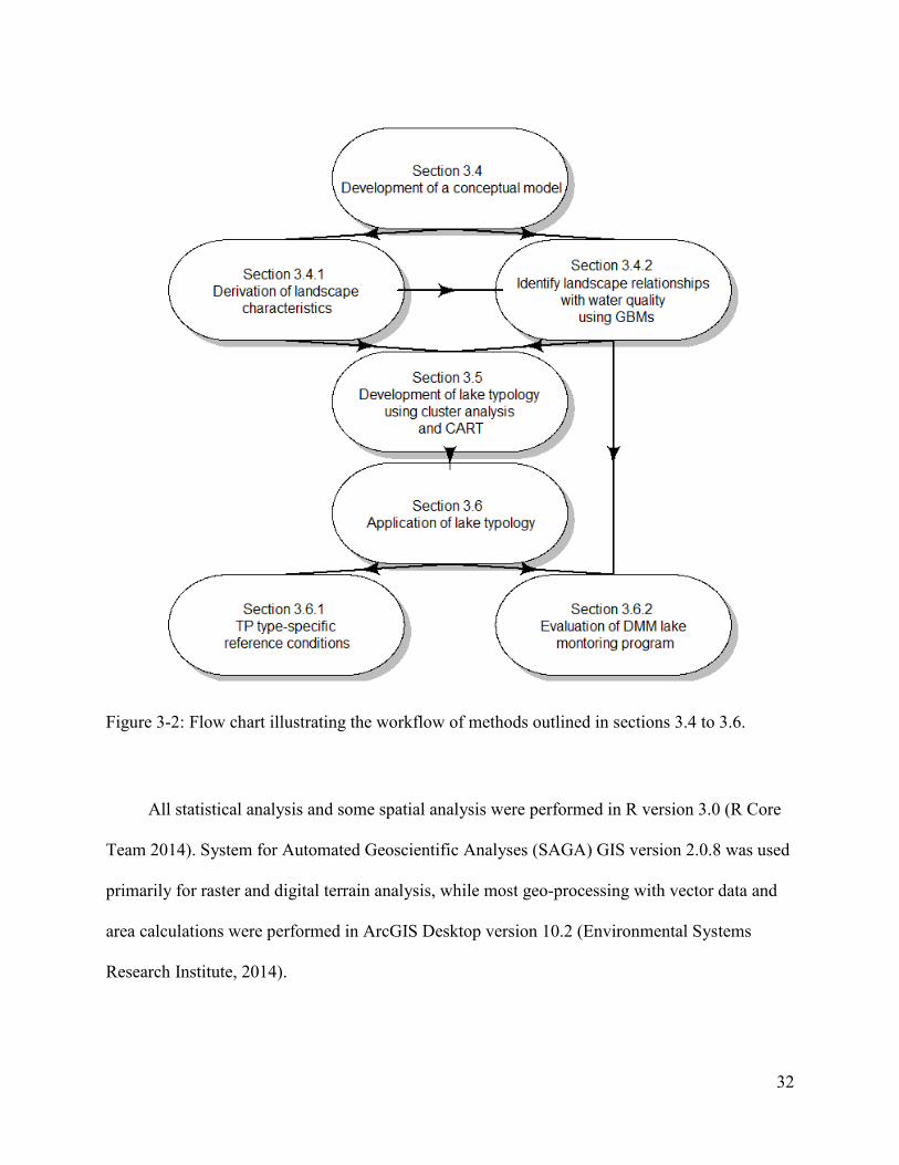
32
Figure 3-2: Flow chart illustrating the workflow of methods outlined in sections 3.4 to 3.6.
All statistical analysis and some spatial analysis were performed in R version 3.0 (R Core
Team 2014). System for Automated Geoscientific Analyses (SAGA) GIS version 2.0.8 was used
primarily for raster and digital terrain analysis, while most geo-processing with vector data and
area calculations were performed in ArcGIS Desktop version 10.2 (Environmental Systems
Research Institute, 2014).
33
3.3 Water quality data aggregation
The water quality data selected for this study were based on the amount of available data
and the ecological significance of water quality variables. To ensure the sample of lakes had
adequate spatial coverage and were representative of all the MRW lakes, water quality from
multiple sources and time periods were combined. Epilimnion DOC, TP, Ca, and pH data were
obtained from 5 different sampling and monitoring programs for the ice-free period of 2004-
2012, described in Table 3-1. All sampling programs obtained mid-lake samples with the
exception of the CWN project. The data collected for the CWN project obtained a 3 L integrated
composite from 3 randomly selected shoreline quadrants (C. Jones, personal communication,
March 13, 2013). All water chemistry analysis was conducted at the Dorset Environment Science
Centre (DESC) except for the Canadian Wildlife Service (CWS) sampling program. All
chemical analysis for the CWS project was conducted at Great Lakes Forestry Centre (Mallory et
al., 1998). Whole lake composites were taken if the lakes were sampled in spring or fall overturn
periods (DMM, 2014b; Girard et al., 2007; Mallory et al., 1998; Palmer et al., 2011). However,
for the CWS project an epilimnion grab sample was obtained for lakes ≤ 3.3 m deep (Mallory et
al., 1998). Volume weighted epilimnion samples were taken for the Ontario Ministry of
Environment (OMOE) Class A and B lakes and the zooplankton reference lakes (Girard et al.,
2007; Palmer et al., 2011), while an epilimnion-metalimnion composite was taken for the
Canadian Aquatic Invasive Species Network (CAISN) lakes (N. Yan, personal communication,
October 29, 2012). Class A and B lakes are mostly headwater lakes that have been monitored for
over 20 years by the Dorset Environmental Science Centre (DESC), in order to study the effects
of multiple stressors on Canadian Shield lakes (DESC, 2014). Class A lakes are more intensively
monitored than Class B lakes (DESC, 2014).
34
Table 3-1: Summary table of all sampling programs that water quality data was obtained from,
for more detail see APPENDIX A.
Sampling
program
abbreviation Years Months
# of
unique
lakes
# of
samples Focus of study
CAISN 2005-2006 6-8 207 248
Invasion of zooplankton
Bythotrephes longimanus
CWN 2012-2012 7-9 99 99 Cumulative effects MRW
CWS 2004-2010 9-10 55 150 Acid sensitive lakes
DMM 2004-2012 4-8 137 766 Continuous monitoring
OMOE 2004-2012 4-10 20 1840 Class A and B lakes
MP 2004-2005 6-10 6 29 Zooplankton reference lakes
3.3.1 Temporal considerations
Combining water quality data from multiple sampling programs is advantageous because
it increases the sample size. However, high inter-annual variability could introduce errors in
GBMs and the lake typology. In order to determine if averaging or combining lake chemistry
from multiple years could be conducted to increase sample size, pairwise comparisons were
performed with DMM water quality data. For each year-pair combination for a given physico-
chemical variable a paired differences of means test was performed. Most lakes were sampled by
DMM on a bi-annual basis (DMM, 2014b). As a result, two distinct sets of bi-annual pairwise
comparisons were performed. One set of lakes (n=31) was sampled in odd numbered years
(2005-2011) and the other set of lakes (n=32) was sampled in the even numbered years (2006-
2012). Depending on the distribution of the paired differences either a paired Wilcoxon signed-
rank test or t-test was used, see APPENDIX C. The p-values were adjusted using Bonferroni
correction to minimize type I error (Quinn and Keough, 2002). The total number of significantly
different (α=0.05) year-pair combinations were calculated for each water quality variable to
determine what water quality variables had high inter-annual variability. Then the percentage of
year-pair combinations that were significantly different were calculated (Table 3-2). A higher
35
percentage of significantly different year-pair combinations for a water quality variable is
indicative of higher inter-annual variability. Averaging water quality variables with high inter-
annual variability may not be suitable as a means to increase sample size.
Table 3-2: Percentage of statistically significant pairwise year-differences in water quality
variables as a fraction of the total possible number of year-pairs combinations within the period
of 2005-2012.
Variable % of year- pair combinations significantly different (p<0.05)
Calcium 50
Dissolved Organic Carbon 0
Potential of Hydrogen (pH) 58
TP 42
3.4 Development of conceptual model
3.4.1 Derivation of landscape characteristics
There were 46 measures of the freshwater, terrestrial, and human landscapes derived at
multiple spatial scales (Table 3-4). Watersheds were delineated to derive the landscape attributes
at three separate spatial scales (CUCA, LOCA, riparian). Digital terrain analysis was conducted
to calculate metrics of catchment and riparian slope. Measures of lake morphometry were
obtained through lake depth modelling. The percentage of each LU, LC, and surficial geology
class were calculated at the CUCA and riparian using multiple data sources, including geospatial
data from the Ontario Ministry of Natural Resources (OMNR) and Ministry of Northern
Development and Mines (APPENDIX B).
Watershed delineation was performed for all lakes greater than 5 ha. Lakes that are 5-8 ha
(n=179) were used to calculate CWRTs and LNNs, but were not included as target lakes in all
other analyses. For lake typology development and statistical analysis 46 terrestrial, freshwater,
and human landscape measures were calculated for all lakes greater than 8 ha. The Ontario
36
Hydro Network (OHN) waterbody layer produced in 2011 was used to identify beaver ponds,
lakes and rivers. Many waterbodies were misclassified according to waterbody type and were
corrected based on examination of Muskoka Orthoimagery 2008, lake monitoring data, and
Google Earth. Lakes that were sampled in multiple basins by the DMM were divided and treated
as separate lakes (APPENDIX D). Lake area was calculated for all lakes in ArcGIS version 10.2
(Environmental Systems Research Institute, 2014) and all lakes greater than 8 ha were used for
all subsequent analysis. There were 615 lakes greater than 8 ha in the MRW but, after large lakes
were split into multiple basins there were 650 lakes. The centroids of lakes in NAD83 UTM 17N
were calculated in order to obtain the geographic location of each lake.
Watersheds for all lakes greater than 5 ha (n=829) in the MRW were delineated in SAGA
GIS using a preprocessed Digital Elevation Model (DEM). A Canadian Digital Surface Model
(CDSM) of ~30 m resolution was obtained for the study region and was preprocessed using Sink
Drainage Route Detection and Sink Removal (Wang and Liu, 2006) in SAGA GIS. The
watersheds (CUCAs) were delineated in RSAGA (Brenning, 2008) using an upslope area tool
that uses a Deterministic-8 (D8) flow algorithm. Riparian zones were derived for all lakes
greater than 8 ha in ArcGIS by using a 300 m buffer around the lakes shoreline and then clipping
the buffer with the lake’s CUCA. LOCAs were derived by a custom-built algorithm that used
functions from the R packages RSAGA (Brenning, 2008) and sp (Pebesma and Bivand, 2005).
The algorithm intersected the CUCA of each lake with all CUCAs to obtain the subwatershed
(LOCA). To obtain measures of catchment morphometry and to use in calculations of landscape
characteristics the area of the CUCAs, LOCAs, and riparian zones were calculated in ArcGIS,
these areas did not include the lake area. Additionally, the lake areas and CUCAs were used to
calculate the DR for each lake.
37
Digital terrain analysis was performed in SAGA GIS to derive wetness index (WI) and
slope. Slope and WI are good measures to quantify catchment-scale transport (McGuire et al.,
2005). Beven and Kirkby’s (1979) WI is function of slope angle (β) and catchment area (CA) (1).
The WI is indicative of the soil moisture and saturation conditions (Beven and Kirkby, 1979;
Canham et al., 2004; Richardson, 2010). WI was calculated using SAGA’s Wetness Index, which
is a modified version of Beven and Kirkby’s (1979) calculation.
𝑊𝐼 = 𝑙𝑛 (𝐶𝐴
tan 𝛽) (1)
SAGA’s WI (WIs) uses a modified catchment area (MCA) calculated for each grid cell based on
the slope angle and the neighboring cell with the maximum modified catchment area ((2);
Böhner and Selige, 2006).
𝑊𝐼𝑠 = 𝑙𝑛 (𝑀𝐶𝐴
tan 𝛽) (2)
To calculate slope, vertical and overland flow distances were calculated using the lakes and
streams as the channel network and the D8 flow algorithm. Overland flow distance takes into
account the slope of the terrain, which gives a more accurate measure of the flow distance
(Wichmann, 2013). Zonal statistics were used to calculate mean slope and WI at the CUCA and
riparian scales in RSAGA. The corrected OHN waterbody layer of beaver ponds, rivers and
lakes was combined with enhanced watercourse data to act as a mask for calculating WI.
3.4.1.1 Freshwater landscape characteristics
Freshwater landscape characteristics are considered to be important determinants of water
quality among the MRW lakes (O’Connor et al., 2009). Wetlands were measured at 3 spatial
scales (riparian, LOCA, CUCA) because they are known to be a significant source of DOC and
38
TP to lakes of the MRW (Dillon and Molot, 1997; O’Connor et al., 2009). Drainage density was
calculated to quantify catchment transport of material (Bremigan et al., 2008). Percent upstream
lakes and water were also calculated because O’Connor et al. (2009) demonstrated that upstream
lakes play an important role in affecting DOC concentrations of the MRW lakes. However,
recent studies in regions similar to the MRW have demonstrated that upstream lakes are not an
adequate measure of DOC processing along a lake network (Muller et al., 2013). This is likely
because they do not explicitly incorporate measures of WRT and the topological structure (i.e.
hydrological connectivity) of lake networks (Cardille et al., 2007; Zhang et al., 2012). To better
account for upstream lake processing of DOC, a metric of CWRT similar to the one used by
Muller et al. (2013) was developed. To derive CWRT, a lake depth model needed to be applied to
calculate lake volumes. Additionally, a lake topology had to be derived to quantify the direction
of connections among lakes.
Percent water, percent wetland and drainage densities at CUCA and riparian scales were
calculated in ArcGIS (Table 3-4). Additionally, percent LOCA wetlands were also calculated. To
calculate percent wetland and water, data was combined from the Ontario Provincial LC
Database 2000, OHN waterbody and, OMNR Wetland Unit data. The percent wetland
calculation included all beaver ponds as wetlands using the corrected OHN waterbody data. For
drainage density, the stream network layer used was the Ontario Integrated Hydrology Data
(Enhanced Watercourse), obtained from the OMNR.
Lake morphometry was modelled for all lakes over 5 ha because there is no lake depth
data available for all lakes of the MRW. The Hollister et al. (2011) depth modelling approach
was used because it has been tested on a large number of lakes and performed well in cross-
validation. Mean lake depth (zmean) and lake volume were calculated from the zmax derived
39
from the model. Hollister et al. (2011) makes two assumptions about lake depth. The first
assumption is that the slope of the riparian zone of the lake will be the same as the slope within a
lake (Hollister et al. 2011). The second assumption is that as the distance from shore increases so
will the lake depth (Hollister et al. 2011). To model lake depth, the two assumptions were
applied by using both Euclidian distance (ED) and median slope (Smed) of the riparian zone
(Hollister et al., 2011).
For this study a depth modelling method similar to Hollister et al. (2011) was used,
however a slope metric that used overland flow distance to channel network was used instead of
the neighborhood slope method. Additionally, the lake depths were not adjusted for biases
(Hollister et al., 2011). The ED to the shoreline for each pixel inside the lake was calculated in
ArcGIS. The maximum ED to the shoreline for each lake was used to generate an outer buffer of
that size, provided it was contained within the lake’s catchment (Figure 3-3). The Smed of this
buffer region surrounding the lake was calculated in RSAGA (Brenning, 2008) using the slope
metric (grg) derived in SAGA GIS. To find the lake depth of each pixel the Smed was multiplied
by the ED of that pixel (3).
zi = EDi × Smed (3)
Zmax was calculated by using zonal statistics to find the pixel with zmax within the lake (4).
zmax = max(zi) (4)
There were 91 lakes that had a predicted zmax of less than 1 m, these lakes were corrected to
have a zmax of 1 m. The zmax and zmean models were cross-validated using lake depth data.
The cross-validation of zmax model resulted in a much higher coefficient of determination than
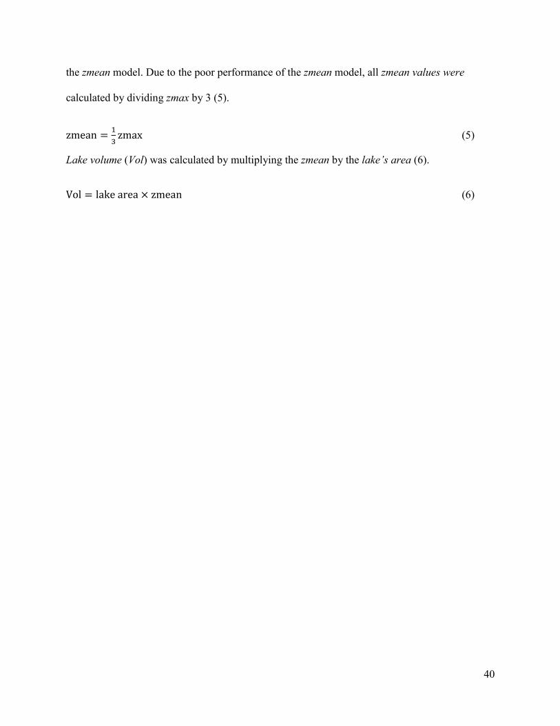
40
the zmean model. Due to the poor performance of the zmean model, all zmean values were
calculated by dividing zmax by 3 (5).
zmean =1
3zmax (5)
Lake volume (Vol) was calculated by multiplying the zmean by the lake’s area (6).
Vol = lake area × zmean (6)
41
Figure 3-3: Example of how lake depth was calculated using Mary Lake. The maximum
Euclidean distance was 798 m for Mary Lake and was used to derive a buffer of the same width
provided it is contained within the CUCA.
3.4.1.1.1 Lake depth cross-validation
The lake depth model was evaluated using cross-validation of zmean and zmax data from
studies and monitoring programs described in Table 3-3, if multiple depth observations were
available they were averaged. There was lake depth data with zmax measurements for 365 lakes
of the MRW, while there were 234 zmean measurements (Table 3-3).
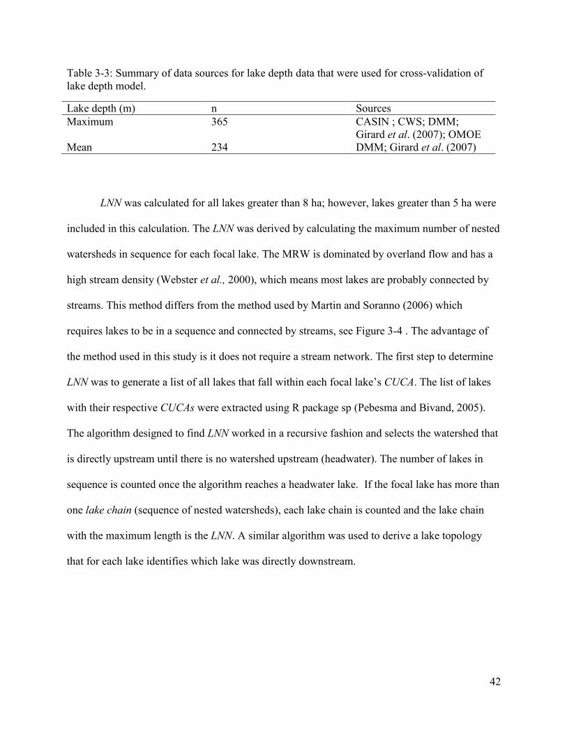
42
Table 3-3: Summary of data sources for lake depth data that were used for cross-validation of
lake depth model.
Lake depth (m) n Sources
Maximum 365 CASIN ; CWS; DMM;
Girard et al. (2007); OMOE
Mean 234 DMM; Girard et al. (2007)
LNN was calculated for all lakes greater than 8 ha; however, lakes greater than 5 ha were
included in this calculation. The LNN was derived by calculating the maximum number of nested
watersheds in sequence for each focal lake. The MRW is dominated by overland flow and has a
high stream density (Webster et al., 2000), which means most lakes are probably connected by
streams. This method differs from the method used by Martin and Soranno (2006) which
requires lakes to be in a sequence and connected by streams, see Figure 3-4 . The advantage of
the method used in this study is it does not require a stream network. The first step to determine
LNN was to generate a list of all lakes that fall within each focal lake’s CUCA. The list of lakes
with their respective CUCAs were extracted using R package sp (Pebesma and Bivand, 2005).
The algorithm designed to find LNN worked in a recursive fashion and selects the watershed that
is directly upstream until there is no watershed upstream (headwater). The number of lakes in
sequence is counted once the algorithm reaches a headwater lake. If the focal lake has more than
one lake chain (sequence of nested watersheds), each lake chain is counted and the lake chain
with the maximum length is the LNN. A similar algorithm was used to derive a lake topology
that for each lake identifies which lake was directly downstream.
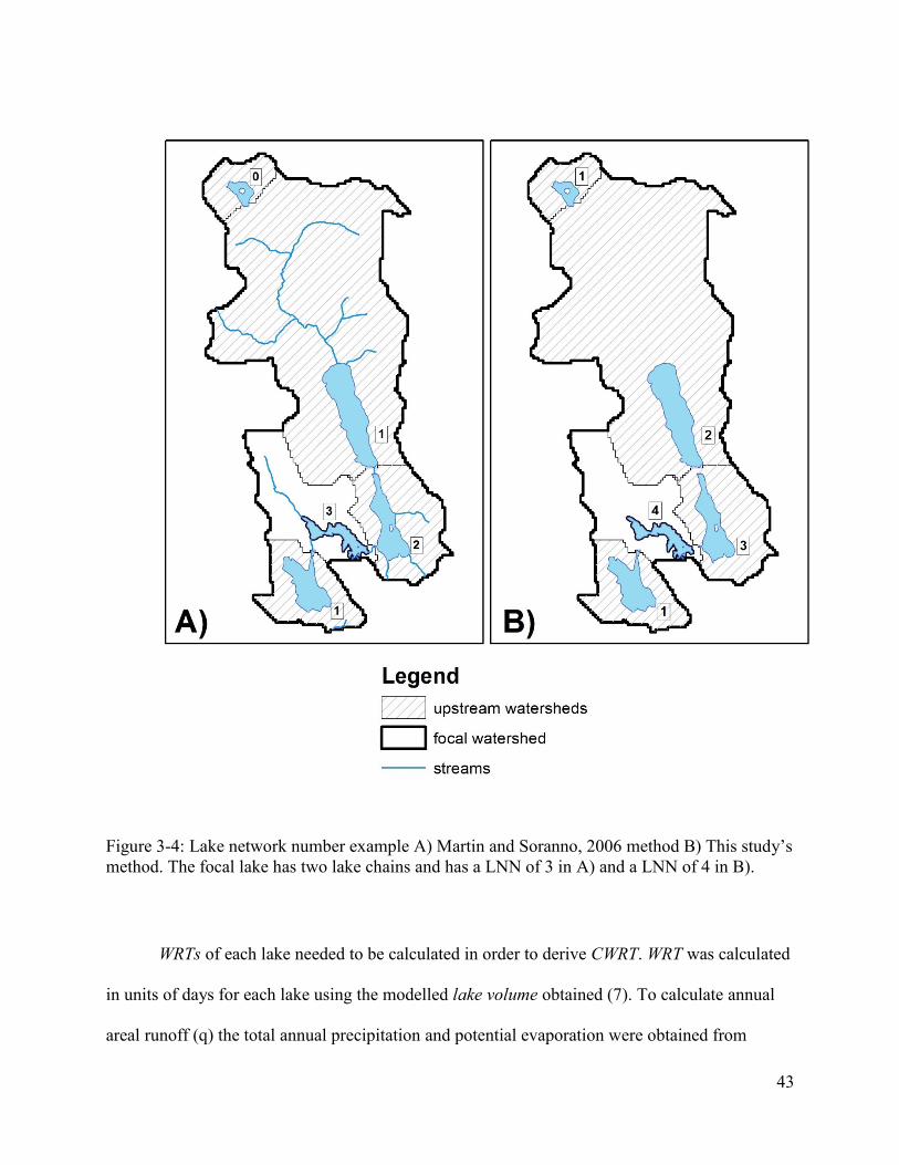
43
Figure 3-4: Lake network number example A) Martin and Soranno, 2006 method B) This study’s
method. The focal lake has two lake chains and has a LNN of 3 in A) and a LNN of 4 in B).
WRTs of each lake needed to be calculated in order to derive CWRT. WRT was calculated
in units of days for each lake using the modelled lake volume obtained (7). To calculate annual
areal runoff (q) the total annual precipitation and potential evaporation were obtained from
44
EcoDistrict data from Natural Resources Canada. It was assumed there was no change in storage,
therefore the q could be calculated by subtracting evaporation from precipitation (Hendriks,
2010). The calculation resulted in a q of 0.036 m yr-1.
WRT =vol
cuca×q× 365 (7)
CWRT was calculated by using the lake topology, LNN, and WRTs. All lakes greater than
5 ha (n=829) were included in this calculation because lakes smaller than 5 ha are thought to act
as a source for dissolved nutrients (O’Connor et al., 2009). The purpose of CWRT is to account
for time spent in upstream lakes (Muller et al., 2013). Muller et al.’s (2013) calculation assumes
that each upstream lake has the same influence on CWRT and does not consider the topology of
the lake network. This study assumes that the amount each lake contributed to a focal lake
CWRT is dependent on the lake position in the lake network and the size of the lake’s CUCA.
The CWRT is calculated by taking the weighted sum of all the CWRT of lakes (x) that are
directly upstream (u). The weight of each lake is proportional to their CUCA (8). The WRT of
the focal lake (l) also is added in but its weight is based on its LOCA (8). The algorithm used to
derive CWRT starts with lakes that have a LNN of 2 and uses the lake topology to find headwater
lakes that are directly upstream. After the CWRT of all lakes with a LNN of 2 have been
calculated the algorithm proceeds to select lakes with LNN of 3. The algorithm proceeds until the
maximum LNN is reached.
CWRTl = (LOCAl
CUCAl× WRTl) + ∑ (
CUCAx
CUCAl× CWRTx)x ∈u (8)
The advantage of the CWRT metric used in this study is it explicitly accounts for lake
landscape position as a function of the amount of time spent in upstream lakes. For example, the
Muller et al. (2013) measure of CWRT would calculate the CWRT of the focal lake in Figure
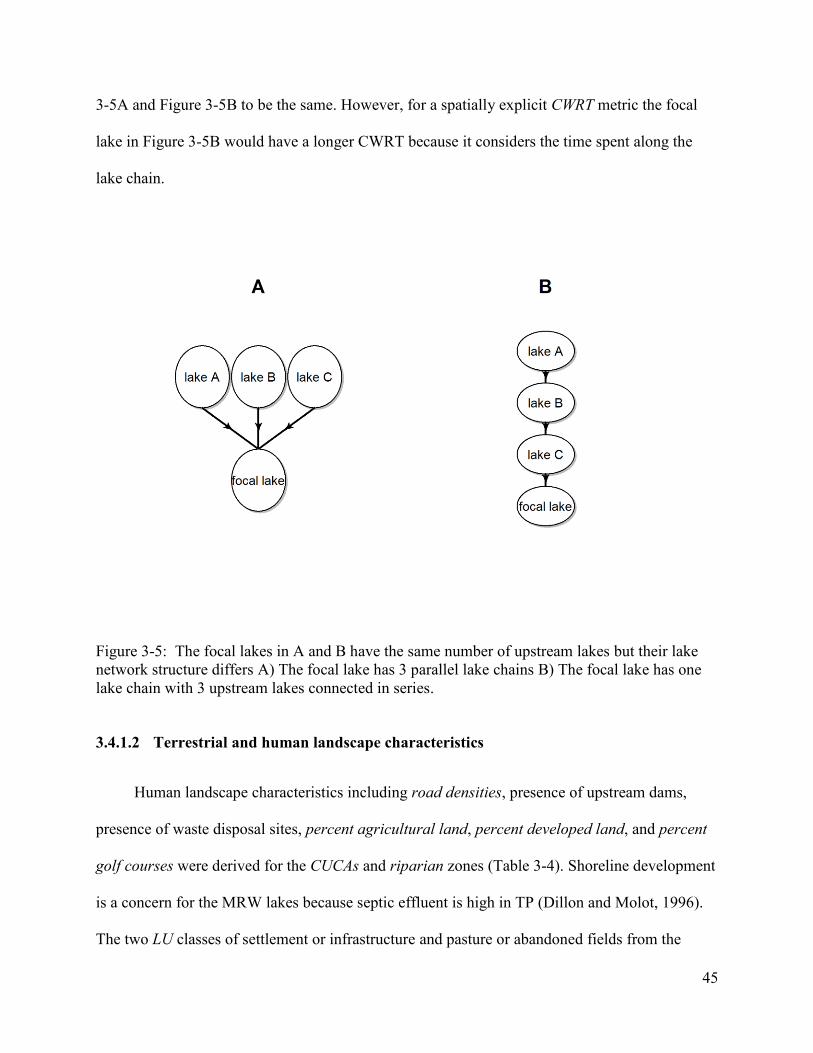
45
3-5A and Figure 3-5B to be the same. However, for a spatially explicit CWRT metric the focal
lake in Figure 3-5B would have a longer CWRT because it considers the time spent along the
lake chain.
Figure 3-5: The focal lakes in A and B have the same number of upstream lakes but their lake
network structure differs A) The focal lake has 3 parallel lake chains B) The focal lake has one
lake chain with 3 upstream lakes connected in series.
3.4.1.2 Terrestrial and human landscape characteristics
Human landscape characteristics including road densities, presence of upstream dams,
presence of waste disposal sites, percent agricultural land, percent developed land, and percent
golf courses were derived for the CUCAs and riparian zones (Table 3-4). Shoreline development
is a concern for the MRW lakes because septic effluent is high in TP (Dillon and Molot, 1996).
The two LU classes of settlement or infrastructure and pasture or abandoned fields from the
46
Ontario Provincial LC Database 2000 were combined with data from the OMNR, to have the two
LU classes of developed land and agriculture. The LU class of golf courses was added from
OMNR data because golf courses are known to be a source of TP and other ions to the surface
waters of the MRW (Winter et al., 2006). The CUCA and riparian road densities of all roads and
unpaved roads were calculated. The sum of percent golf course, developed land and agricultural
land was calculated for both the CUCA and the riparian zone. The National Road Network
(NRN) was used but the road class “Resource/Recreation” was not included in the road density
calculations. Roads measured at the riparian scale were included because roads closer to the lake
shoreline have been shown to influence the water quality of MRW lakes to a greater degree
(Palmer et al., 2011). Additionally, unpaved road densities were included because they have
been shown to influence Ca concentrations in the MRW lakes (Yao et al., 2011). To determine if
there was a dam directly upstream of a lake, a stream topology was created and intersected with
dams and lakes. The dam dataset was obtained from the OMNR. The presence of waste disposal
sites in the CUCAs was determined by using data obtained from a combination of data from
OMNR. All human landscape characteristics were calculated in ArcGIS.
The percent CUCA and riparian LC were calculated, along with mean lake elevation to
obtain measures of the terrestrial landscape (Table 3-4). The Ontario Provincial LC Database
2000 was used for the sparse vegetation, deciduous, coniferous and bedrock classes. The
coniferous and deciduous classes were adjusted by adding 50% of the mixed forest class to each.
Mean lake elevation was calculated using zonal statistics and the pre-processed DEM in RSAGA
(Brenning, 2008).
Percent LOCA surficial geology and mean riparian and CUCA overburden thickness
were calculated from data provided by the Ministry of Northern Development and Mines.
47
Overburden thickness is the depth of glacial deposits that lie above the bedrock (Knight and
Kerr, 2007) and is important in influencing the weathering of ions (Soranno et al., 1999).
Surficial geology and overburden thickness is very variable in the MRW (Jeffries and Snyder,
1983) and is important in determining TP retention (Dillon and Molot, 1996). The LOCA was
used because aquatic ecosystems are influenced more by surficial geology at this scale (Palmer et
al., 2012). The classes of primary surficial material were adjusted from the Surficial Geology of
Southern Ontario. Precambrian bedrock and gravel were combined into one class (rock/gravel),
while diamicton was renamed till (Table 3-4). The percent LOCA surficial material was
calculated in ArcGIS, while the mean riparian and mean CUCA overburden thickness was
calculated in RSAGA using zonal statistics.
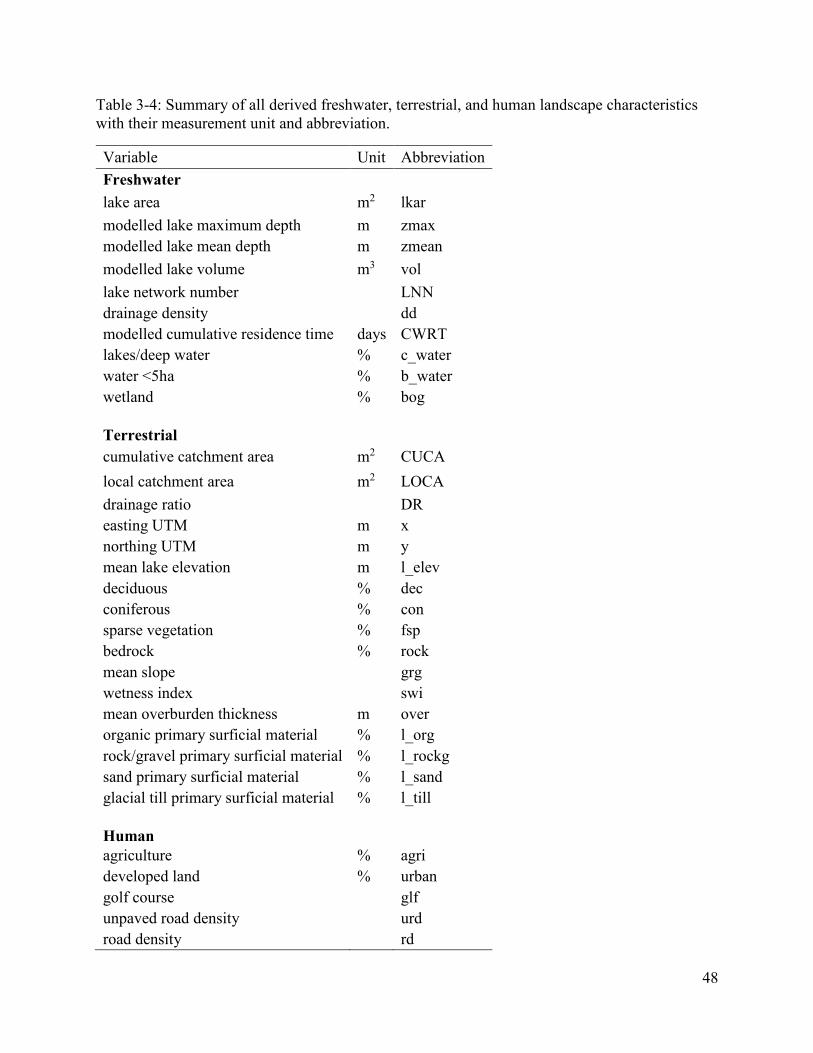
48
Table 3-4: Summary of all derived freshwater, terrestrial, and human landscape characteristics
with their measurement unit and abbreviation.
Variable Unit Abbreviation
Freshwater
lake area m2 lkar
modelled lake maximum depth m zmax
modelled lake mean depth m zmean
modelled lake volume m3 vol
lake network number LNN
drainage density
dd
modelled cumulative residence time days CWRT
lakes/deep water % c_water
water <5ha % b_water
wetland % bog
Terrestrial
cumulative catchment area m2 CUCA
local catchment area m2 LOCA
drainage ratio
DR
easting UTM m x
northing UTM m y
mean lake elevation m l_elev
deciduous % dec
coniferous % con
sparse vegetation % fsp
bedrock % rock
mean slope
grg
wetness index
swi
mean overburden thickness m over
organic primary surficial material % l_org
rock/gravel primary surficial material % l_rockg
sand primary surficial material % l_sand
glacial till primary surficial material % l_till
Human
agriculture % agri
developed land % urban
golf course
glf
unpaved road density urd
road density rd
49
3.4.1.3 Descriptive statistics of landscape characteristics
The distributions of all 46 derived landscape variables were summarized using
descriptive statistics. Median and Median Absolute Deviation (MAD) were used because most
landscape variables did not have a normal distribution. For the freshwater landscape measures of
LNN, zmean, and CWRT more analysis was conducted, which allowed comparisons of the lakes
within the MRW with other lake districts. The percentage of lakes in each WFD depth class was
calculated for all lakes greater than 8 ha in the MRW. Also, the percentage of lakes, according to
a LNN categories, was calculated. The minimum, 1st quartile, median, mean, 3rd quartile, and
maximum were calculated for the CWRT distribution of all lakes greater than 8 ha.
3.4.2 Identification of landscape relationships with water quality
GBMs were used to identify the freshwater, terrestrial, and human landscape
characteristics that are important in determining the water quality of the MRW lakes. All GBM
analysis was performed in the R package dismo version 0.9-3 (Hijmans et al., 2013). Four GBM
models were run with 46 landscape measures, described in Table 3-4, as explanatory variables.
DOC, TP, Ca, and pH, were used as response variables and they were transformed to meet the
assumption of a Gaussian distribution as described in Table 3-5. These four water quality
variables were chosen because DOC, TP, Ca, and pH have high ecological significance and have
unique roles in an aquatic ecosystem (Stendera and Johnson, 2006). Due to the high inter-annual
variability of TP, Ca and pH (see 3.3.1), only water quality data from the CASIN lakes sampled
in 2006 were used. For DOC which had low inter-annual variability (i.e. low percentage of
significantly different year-pair combinations), the CASIN (2006) and CWN (2012) lake data
sets were combined because they were both sampled from late June to early September (Table
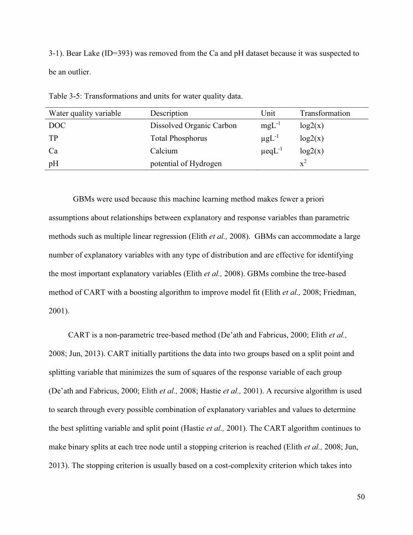
50
3-1). Bear Lake (ID=393) was removed from the Ca and pH dataset because it was suspected to
be an outlier.
Table 3-5: Transformations and units for water quality data.
Water quality variable Description Unit Transformation
DOC Dissolved Organic Carbon mgL-1 log2(x)
TP Total Phosphorus µgL-1 log2(x)
Ca Calcium µeqL-1 log2(x)
pH potential of Hydrogen x2
GBMs were used because this machine learning method makes fewer a priori
assumptions about relationships between explanatory and response variables than parametric
methods such as multiple linear regression (Elith et al., 2008). GBMs can accommodate a large
number of explanatory variables with any type of distribution and are effective for identifying
the most important explanatory variables (Elith et al., 2008). GBMs combine the tree-based
method of CART with a boosting algorithm to improve model fit (Elith et al., 2008; Friedman,
2001).
CART is a non-parametric tree-based method (De’ath and Fabricus, 2000; Elith et al.,
2008; Jun, 2013). CART initially partitions the data into two groups based on a split point and
splitting variable that minimizes the sum of squares of the response variable of each group
(De’ath and Fabricus, 2000; Elith et al., 2008; Hastie et al., 2001). A recursive algorithm is used
to search through every possible combination of explanatory variables and values to determine
the best splitting variable and split point (Hastie et al., 2001). The CART algorithm continues to
make binary splits at each tree node until a stopping criterion is reached (Elith et al., 2008; Jun,
2013). The stopping criterion is usually based on a cost-complexity criterion which takes into
51
account the tree size and goodness of fit (Hastie et al., 2001). The best stopping criterion is
usually obtained from pruning or cross-validation (Hastie et al., 2001).
GBMs use CART as their base learner and build a sequence of CART models in a
forward stage-wise fashion (Friedman, 2001). GBMs can use bootstrapping but for this analysis
bootstrapping was not used because of small sample sizes. Bootstrapping randomly selects a
subsample of the training data to build each model (Quinn and Keough, 2002). The first tree
constructed as part of a GBM is a conventional CART model based on the response variable
(Elith et al., 2008; Hastie et al., 2001). However, all subsequent tree models use the previous
model’s residuals (pseudo-residuals) as the response variable (Friedman, 2001; Hastie et al.,
2001). At each iteration, the GBM sequentially updates the model by adding a tree and
recalculates the model’s residuals (Friedman, 2001; Hastie et al., 2001; Parisien and Moritz,
2009). The CART model that is selected at each stage is based on the lowest squared error for
the pseudo-residuals (Friedman, 2001; Hastie et al., 2011). The trees are scaled based on the
learning rate, which results in the final GBM model being the sum of the scaled trees (Hastie et
al., 2001).
To run the water quality GBM models three meta-parameters needed to be optimized.
Optimization is a requirement of many machine learning techniques because the meta-
parameters affect the fit of the final model (Elith et al., 2008). The meta-parameters are tree
complexity, number of tree/iterations, and learning rate (Elith et al., 2008; Friedman, 2001;
Hastie et al., 2001). The selection of the three meta-parameters in discussed in detail in
APPENDIX E.
Model simplification was conducted to select the most important explanatory variables
which later are considered for the development of the lake typology. The variables that
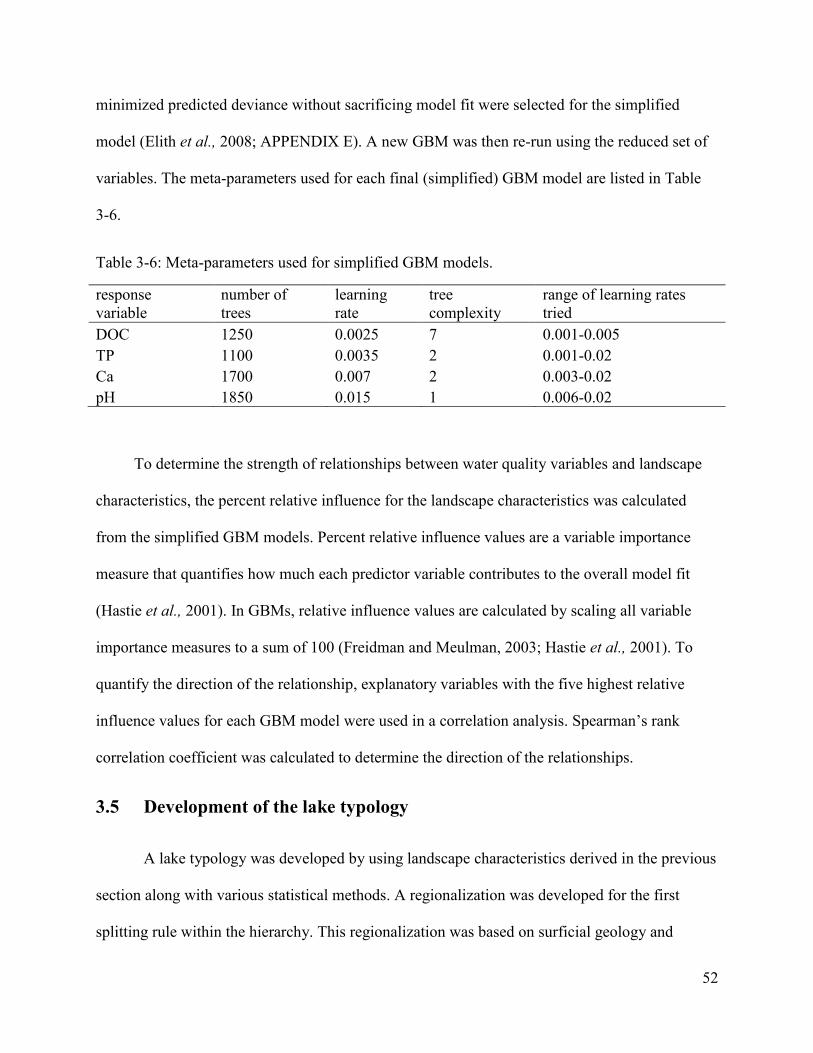
52
minimized predicted deviance without sacrificing model fit were selected for the simplified
model (Elith et al., 2008; APPENDIX E). A new GBM was then re-run using the reduced set of
variables. The meta-parameters used for each final (simplified) GBM model are listed in Table
3-6.
Table 3-6: Meta-parameters used for simplified GBM models.
response
variable
number of
trees
learning
rate
tree
complexity
range of learning rates
tried
DOC 1250 0.0025 7 0.001-0.005
TP 1100 0.0035 2 0.001-0.02
Ca 1700 0.007 2 0.003-0.02
pH 1850 0.015 1 0.006-0.02
To determine the strength of relationships between water quality variables and landscape
characteristics, the percent relative influence for the landscape characteristics was calculated
from the simplified GBM models. Percent relative influence values are a variable importance
measure that quantifies how much each predictor variable contributes to the overall model fit
(Hastie et al., 2001). In GBMs, relative influence values are calculated by scaling all variable
importance measures to a sum of 100 (Freidman and Meulman, 2003; Hastie et al., 2001). To
quantify the direction of the relationship, explanatory variables with the five highest relative
influence values for each GBM model were used in a correlation analysis. Spearman’s rank
correlation coefficient was calculated to determine the direction of the relationships.
3.5 Development of the lake typology
A lake typology was developed by using landscape characteristics derived in the previous
section along with various statistical methods. A regionalization was developed for the first
splitting rule within the hierarchy. This regionalization was based on surficial geology and
53
percentage wetland area within lake catchments. CART was subsequently used to further divide
regions into lake types by using DOC as the response variable. DOC was used as the response
variable because DOC concentration has been reported to be correlated with TP concentration in
the MRW lakes (Gartner Lee Ltd., 2005). In addition, DOC concentrations have low inter-annual
and seasonal variability compared to TP concentrations, which allows multiple years of DOC
data to be combined (Gartner Lee Ltd., 2005). DOC has also been identified as a major modifier
of the physical, chemical and biological properties of a lake (Canham et al., 2004; Prairie, 2008).
A lake’s natural condition and response to stressors is heavily influenced by the lake’s DOC
concentration (Williamson et al., 1999).
The purpose of the initial regionalization step is to create “pseudo-regions” that cluster
the lakes into groups based on similar LOCA characteristics. Custom regionalizations were made
for the MRW by including type of geology which is an obligatory factor used in WFD lake
typologies (Kolada et al., 2005). In addition, percent LOCA wetland was included to create the
custom regionalizations because wetlands have been shown to have a strong association with
water quality in boreal regions (Nykänen et al., 2005; Dillon and Molot, 1997). The percent
surficial geology types used were organic, till, and rock. The number of regions was determined
through a visual inspection of a scree plot (Figure 4-5).
DOC concentrations among the regionalized groups in the first level of the typology were
compared to determine whether further splitting was required. The DOC concentrations were
obtained from the two sampling programs CASIN (2006) and CWN (2012) and were log
transformed. The Shapiro-Wilk test was used to confirm that each region had a Gaussian
distribution for log transformed DOC concentrations. For the three pairwise combination of
regions, Levene’s test was performed to determine if all regions had DOC concentrations with
54
equal variances. ANOVA and Tukey’s Honest Significant Difference (HSD) test were used to
examine pairwise differences between each region’s DOC concentrations.
Based on the number of lakes in each region and their pairwise differences for DOC
concentrations, it was decided that further splits should be explored for regions 1 and 3. Further
splits at the second level of the lake typology were explored using CART. The R packages used
for CART analysis were partykit (Hothorn and Zeileis, 2014) and mvpart (De’ath, 2013). Two
DOC CART models for regions 1 and 3 were run with the 14 explanatory variables that were
present in the simplified DOC GBM model. The two CART models were used to split each
region into two groups by maximizing the differences in DOC concentrations between groups.
The split point and splitting variable obtained were used to develop the second level of the lake
typology. No further splits were explored for lake types because of the small amount of variation
explained in the DOC CART models with more splits.
3.6 Application of the lake typology
3.6.1 TP type-specific reference conditions
Reference lakes were selected using reference pressure lake criteria and derived human
landscape characteristics. The reference pressure lake criteria were adapted from
recommendations of the United States Environmental Protection Agency (U.S. EPA) for
reference lake selection (Gibson, 2000) and criteria from Scandinavian countries (Nixon et al.,
1998). The reference lake pressure criteria used was at least 90% natural LC at both the
cumulative catchment and riparian scales, no dam directly upstream, and no waste disposal site
present in their cumulative catchment. For this study the LC that was classified as not natural
was percent golf course, developed land and agricultural land. A one-tailed Wilcoxon rank-sum
55
test was used to determine if the lake areas of the impacted lakes were larger than the lake areas
of the reference lakes.
To calculate type-specific TP reference conditions, average TP for each reference lake
sampled during the ice-free period from 2004-2012 were obtained from the sampling programs
described in 3.3 and were log transformed. The log transformed TP concentration from the
reference lakes were compared between each of the lake types identified in the lake typology. A
Shapiro-Wilk test was used to confirm that each lake type had a Gaussian distribution for the log
transformed TP concentrations. For all pairwise combination of lake types, Levene’s test was
performed to determine if all lake types had TP concentrations with equal variances. The
Shapiro-Wilk tests and Levene’s test demonstrated that all lake types TP concentrations had
equal variances and were normally distributed. An ANOVA and Tukey’s Honest Significant
Difference (HSD) test were used to examine pairwise differences between lake types.
To determine if the set of reference lakes with water quality data were appropriate to use
for the calculation of TP type-specific reference conditions, the number of reference lakes in
each lake type was determined to ensure there was at least 10% of each lake type was sampled
(Gibson, 2000). Then, the distributions of important freshwater and terrestrial landscape
characteristics selected from the GBMs for the set of reference lakes was compared to the total
population of lakes in the MRW. A two sample Kolmogorov–Smirnov (KS) test was used to
compare the two distributions.
TP type-specific reference conditions were devised for all five lake types within the
typology. Descriptive statistics were performed on the reference log TP concentrations of each
lake type to determine the 25th percentile, mean, 75th percentile, and 95th percentile. The 75th
56
percentile the log TP concentration of each lake type were used as the boundary between good
and moderate TP quality status. The U.S. EPA recommends using the 75th percentile of the
reference lake distribution to set the reference lake condition (Gibson, 2000). Additionally,
Cardoso et al. (2007) used the 75th percentile for the boundary of high TP quality status for TP
type-specific reference conditions for all WFD European lake types. Use of the 75th percentile
will allow direct comparisons between similar Nordic lake types and MRW lake types. An
additional boundary was set between moderate and poor TP quality status at the 95th percentile of
the reference lakes TP concentrations.
The TP quality status was assessed for lakes that were identified to be impacted in the
MRW. Lakes that did not meet the reference lake pressure criteria were identified as impacted
lakes. If the TP concentration of a lake that exceeded the lake’s TP type-specific reference
condition it was either classified as having moderate or poor TP quality status. A lake that had a
TP concentration that was between the 75th and 95th percentile of the respective type-specific
reference condition was classified as having moderate TP quality status. Lakes that have TP
concentrations that exceed the 95th percentile were classified as having poor TP quality status. A
list of lakes with their respective TP quality status was generated in order to identify lakes that
may be in need of restoration and management. Boxplots were created for each lake type TP
reference concentrations.
3.6.2 Evaluation of DMM lake monitoring program
The Lake System Health program which is the lake monitoring program run by DMM was
evaluated using the derived lake typology. The monitoring program was evaluated to determine
if a sufficient amount of lakes were sampled within each lake type. Also, it was determined if
currently monitored lakes were statistically representative according to major landscape
57
gradients in the MRW. Two-sample K-S tests were used to compare distributions of terrestrial
and freshwater landscape variables between the lakes DMM monitoring program samples and
the total population of lakes that are greater than 8 ha in the MRW. Plots of cumulative
distribution functions for the DMM and all lakes were generated for all terrestrial and freshwater
landscape variables that had significantly different distributions.
A few reference lakes from each lake type were selected that had no roads within their
CUCA. However, to ensure accessibility, selected candidate references lakes are a maximum of 1
km from a road and are located within 2 km of a lake currently sampled by the DMM. Therefore,
to select candidate reference lakes a 2 km buffer was generated around all lakes that are currently
sampled by the DMM. All candidate reference lakes that intersected the 2 km buffers were
selected. To determine which lakes were within 1 km of a road, the minimum ED was calculated
for each selected candidate reference lake using zonal statistics. A subset of the lakes that were
within 2 km of a DMM monitoring lake and 1 km from a road were selected using data from
other sampling programs. Lakes were preferentially selected if they were already included in
other monitoring programs or studies.
58
4. RESULTS
4.1 Description of derived landscape characteristics
There was a wide variation of zmean, LNN, and CWRT for lakes greater than 8 ha in the
MRW. Figure 4-1a showed that most lakes in the MRW had a predicted zmean of less than 3 m.
However, there were still a large number of lakes that had zmeans between 3 and 15 m, while
very few lakes had a zmean greater than 15 m (Figure 4-1a). The predicted zmax and zmean had
coefficients of determination of 0.57 and 0.63, respectively (Figure 4-2). The Root Mean
Squared Errors (RMSE) for zmax and zmean were 11.0 m and 4.2 m, respectively. The zmax
model was prone to underpredictions and the magnitude of the underpredictions increased as
observed zmax increased (Figure 4-3).The under-predictions of the models were further
demonstrated by mean errors of 2.7 (zmean) and 6.3 (zmax). Figure 4-1b, shows that 55% the
lakes in the MRW were headwater lakes that have an LNN of 1. There was a large range of LNN
for non-headwater lakes in the MRW (Figure 4-1b).The minimum CWRT was 37 days for all
lakes greater than 8 ha, while the maximum CWRT was 1.2×10⁴ days (Table 4-1). The
distribution of CWRTs was positively skewed with a median CWRT of 2404 days and a mean
CWRT of 5503 days (Table 4-1).
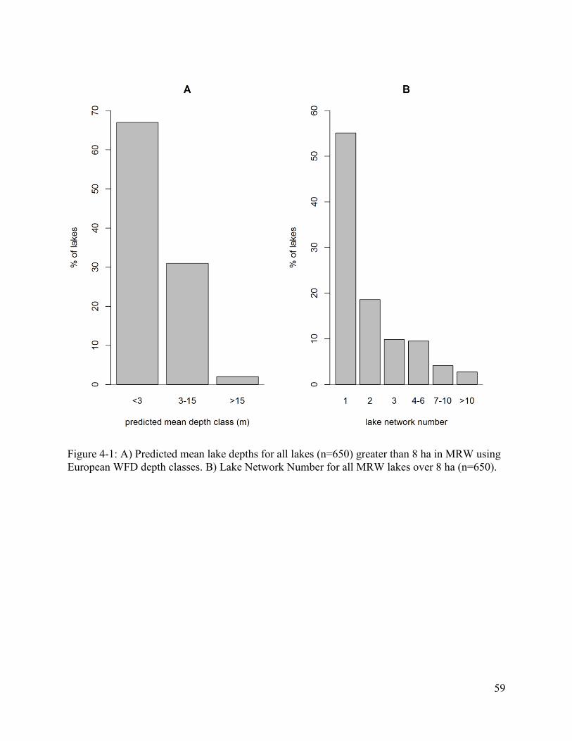
59
Figure 4-1: A) Predicted mean lake depths for all lakes (n=650) greater than 8 ha in MRW using
European WFD depth classes. B) Lake Network Number for all MRW lakes over 8 ha (n=650).
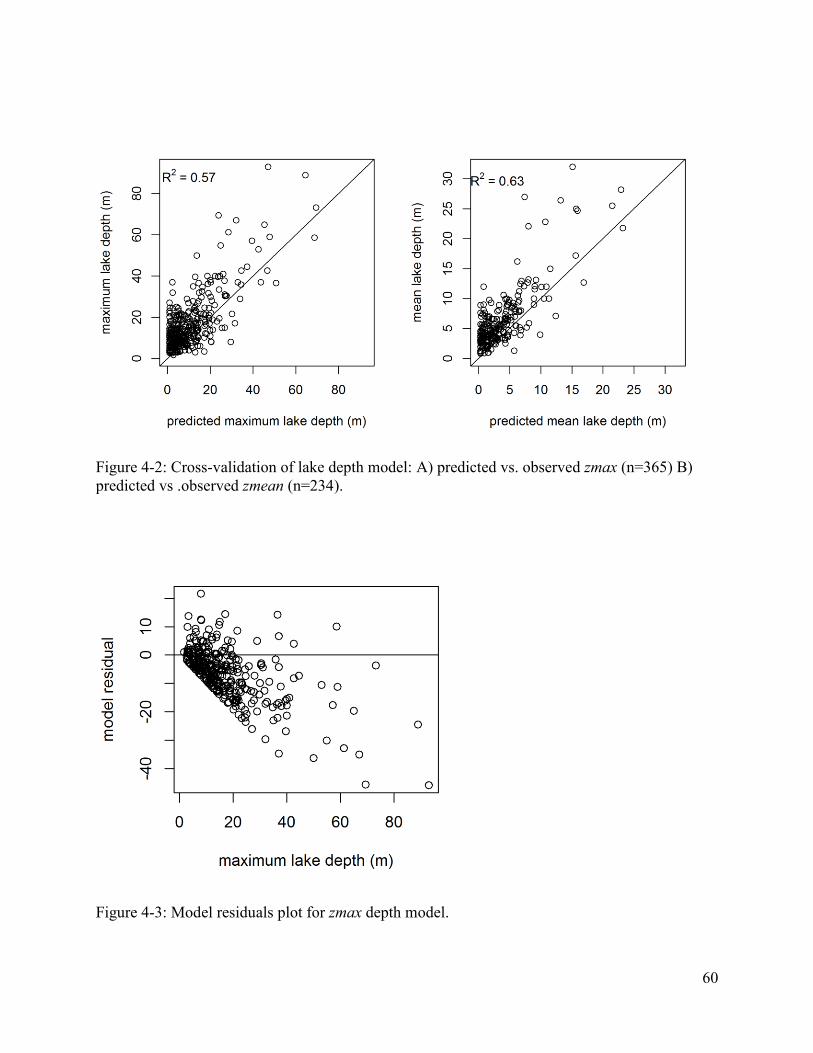
60
Figure 4-2: Cross-validation of lake depth model: A) predicted vs. observed zmax (n=365) B)
predicted vs .observed zmean (n=234).
Figure 4-3: Model residuals plot for zmax depth model.
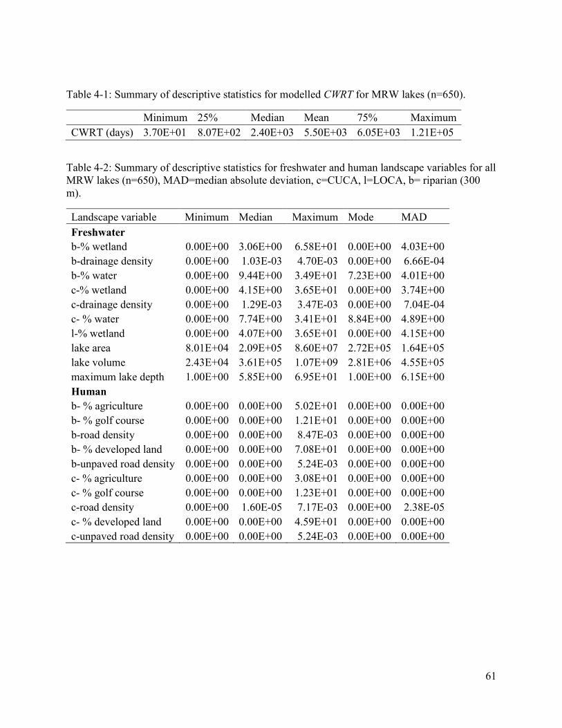
61
Table 4-1: Summary of descriptive statistics for modelled CWRT for MRW lakes (n=650).
Minimum 25% Median Mean 75% Maximum
CWRT (days) 3.70E+01 8.07E+02 2.40E+03 5.50E+03 6.05E+03 1.21E+05
Table 4-2: Summary of descriptive statistics for freshwater and human landscape variables for all
MRW lakes (n=650), MAD=median absolute deviation, c=CUCA, l=LOCA, b= riparian (300
m).
Landscape variable Minimum Median Maximum Mode MAD
Freshwater
b-% wetland 0.00E+00 3.06E+00 6.58E+01 0.00E+00 4.03E+00
b-drainage density 0.00E+00 1.03E-03 4.70E-03 0.00E+00 6.66E-04
b-% water 0.00E+00 9.44E+00 3.49E+01 7.23E+00 4.01E+00
c-% wetland 0.00E+00 4.15E+00 3.65E+01 0.00E+00 3.74E+00
c-drainage density 0.00E+00 1.29E-03 3.47E-03 0.00E+00 7.04E-04
c- % water 0.00E+00 7.74E+00 3.41E+01 8.84E+00 4.89E+00
l-% wetland 0.00E+00 4.07E+00 3.65E+01 0.00E+00 4.15E+00
lake area 8.01E+04 2.09E+05 8.60E+07 2.72E+05 1.64E+05
lake volume 2.43E+04 3.61E+05 1.07E+09 2.81E+06 4.55E+05
maximum lake depth 1.00E+00 5.85E+00 6.95E+01 1.00E+00 6.15E+00
Human
b- % agriculture 0.00E+00 0.00E+00 5.02E+01 0.00E+00 0.00E+00
b- % golf course 0.00E+00 0.00E+00 1.21E+01 0.00E+00 0.00E+00
b-road density 0.00E+00 0.00E+00 8.47E-03 0.00E+00 0.00E+00
b- % developed land 0.00E+00 0.00E+00 7.08E+01 0.00E+00 0.00E+00
b-unpaved road density 0.00E+00 0.00E+00 5.24E-03 0.00E+00 0.00E+00
c- % agriculture 0.00E+00 0.00E+00 3.08E+01 0.00E+00 0.00E+00
c- % golf course 0.00E+00 0.00E+00 1.23E+01 0.00E+00 0.00E+00
c-road density 0.00E+00 1.60E-05 7.17E-03 0.00E+00 2.38E-05
c- % developed land 0.00E+00 0.00E+00 4.59E+01 0.00E+00 0.00E+00
c-unpaved road density 0.00E+00 0.00E+00 5.24E-03 0.00E+00 0.00E+00
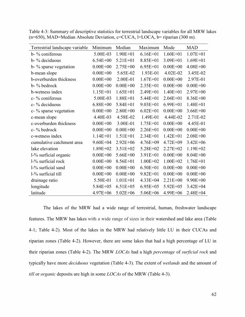
62
Table 4-3: Summary of descriptive statistics for terrestrial landscape variables for all MRW lakes
(n=650), MAD=Median Absolute Deviation, c=CUCA, l=LOCA, b= riparian (300 m).
Terrestrial landscape variable Minimum Median Maximum Mode MAD
b- % coniferous 5.00E-03 1.90E+01 6.16E+01 1.60E+01 1.07E+01
b- % deciduous 6.54E+00 5.21E+01 8.85E+01 3.09E+01 1.69E+01
b- % sparse vegetation 0.00E+00 2.75E+00 6.95E+01 0.00E+00 4.08E+00
b-mean slope 0.00E+00 5.65E-02 1.93E-01 4.02E-02 3.45E-02
b-overburden thickness 0.00E+00 2.00E-01 1.67E+01 0.00E+00 2.97E-01
b- % bedrock 0.00E+00 0.00E+00 2.35E+01 0.00E+00 0.00E+00
b-wetness index 1.15E+01 1.65E+01 2.49E+01 1.40E+01 2.97E+00
c- % coniferous 5.00E-03 1.88E+01 5.44E+01 2.04E+01 8.36E+00
c- % deciduous 6.88E+00 5.84E+01 9.03E+01 6.99E+01 1.48E+01
c- % sparse vegetation 0.00E+00 2.80E+00 6.02E+01 0.00E+00 3.66E+00
c-mean slope 4.40E-03 4.58E-02 1.49E-01 4.44E-02 2.71E-02
c-overburden thickness 0.00E+00 3.00E-01 1.75E+01 0.00E+00 4.45E-01
c- % bedrock 0.00E+00 0.00E+00 2.26E+01 0.00E+00 0.00E+00
c-wetness index 1.14E+01 1.51E+01 2.34E+01 1.42E+01 2.08E+00
cumulative catchment area 9.60E+04 2.92E+06 4.76E+09 4.72E+09 3.42E+06
lake elevation 1.89E+02 3.51E+02 5.28E+02 2.27E+02 1.19E+02
l-% surficial organic 0.00E+00 5.66E+00 3.91E+01 0.00E+00 8.04E+00
l-% surficial rock 0.00E+00 8.56E+01 1.00E+02 1.00E+02 1.76E+01
l-% surficial sand 0.00E+00 0.00E+00 6.50E+01 0.00E+00 0.00E+00
l-% surficial till 0.00E+00 0.00E+00 9.82E+01 0.00E+00 0.00E+00
drainage ratio 5.50E-01 1.01E+01 4.33E+04 2.21E+00 9.90E+00
longitude 5.84E+05 6.51E+05 6.95E+05 5.92E+05 3.42E+04
latitude 4.97E+06 5.02E+06 5.06E+06 4.99E+06 2.48E+04
The lakes of the MRW had a wide range of terrestrial, human, freshwater landscape
features. The MRW has lakes with a wide range of sizes in their watershed and lake area (Table
4-1; Table 4-2). Most of the lakes in the MRW had relatively little LU in their CUCAs and
riparian zones (Table 4-2). However, there are some lakes that had a high percentage of LU in
their riparian zones (Table 4-2). The MRW LOCAs had a high percentage of surficial rock and
typically have more deciduous vegetation (Table 4-3). The extent of wetlands and the amount of
till or organic deposits are high in some LOCAs of the MRW (Table 4-3).
63
4.2 Identification of landscape relationships with water quality
The effects of terrestrial, freshwater, and human landscape characteristics on the water
quality of the MRW lakes were examined using percent relative influence plots from GBM
models (Figure 4-4). The GBM models serve as the basis for the qualitative conceptual model.
Only predictors that had a percent relative influence greater than 1% were included in Figure 4-4.
The strength and direction of the relationships between the top five explanatory variables for
each GBM model are summarized in Table 4-4.
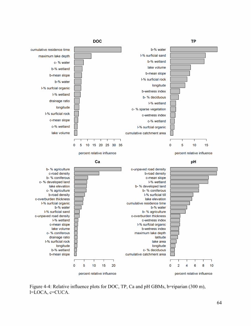
64
Figure 4-4: Relative influence plots for DOC, TP, Ca and pH GBMs, b=riparian (300 m),
l=LOCA, c=CUCA.
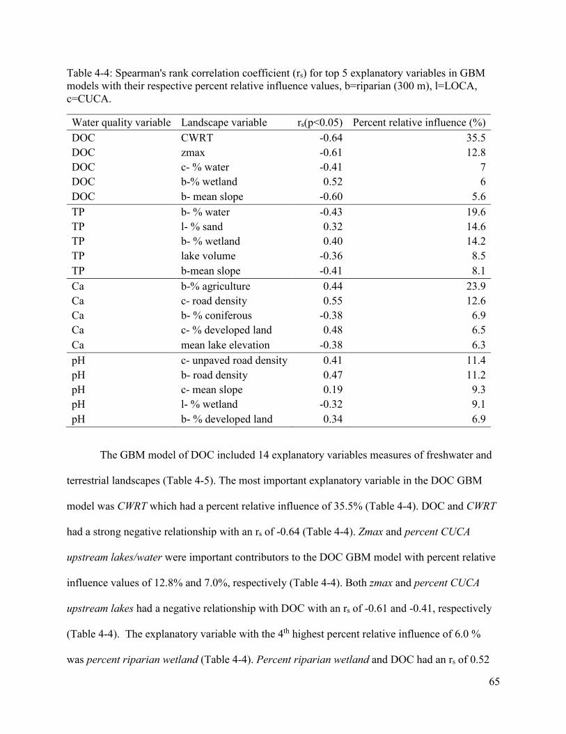
65
Table 4-4: Spearman's rank correlation coefficient (rs) for top 5 explanatory variables in GBM
models with their respective percent relative influence values, b=riparian (300 m), l=LOCA,
c=CUCA.
Water quality variable Landscape variable rs(p<0.05) Percent relative influence (%)
DOC CWRT -0.64 35.5
DOC zmax -0.61 12.8
DOC c- % water -0.41 7
DOC b-% wetland 0.52 6
DOC b- mean slope -0.60 5.6
TP b- % water -0.43 19.6
TP l- % sand 0.32 14.6
TP b- % wetland 0.40 14.2
TP lake volume -0.36 8.5
TP b-mean slope -0.41 8.1
Ca b-% agriculture 0.44 23.9
Ca c- road density 0.55 12.6
Ca b- % coniferous -0.38 6.9
Ca c- % developed land 0.48 6.5
Ca mean lake elevation -0.38 6.3
pH c- unpaved road density 0.41 11.4
pH b- road density 0.47 11.2
pH c- mean slope 0.19 9.3
pH l- % wetland -0.32 9.1
pH b- % developed land 0.34 6.9
The GBM model of DOC included 14 explanatory variables measures of freshwater and
terrestrial landscapes (Table 4-5). The most important explanatory variable in the DOC GBM
model was CWRT which had a percent relative influence of 35.5% (Table 4-4). DOC and CWRT
had a strong negative relationship with an rs of -0.64 (Table 4-4). Zmax and percent CUCA
upstream lakes/water were important contributors to the DOC GBM model with percent relative
influence values of 12.8% and 7.0%, respectively (Table 4-4). Both zmax and percent CUCA
upstream lakes had a negative relationship with DOC with an rs of -0.61 and -0.41, respectively
(Table 4-4). The explanatory variable with the 4th highest percent relative influence of 6.0 %
was percent riparian wetland (Table 4-4). Percent riparian wetland and DOC had an rs of 0.52
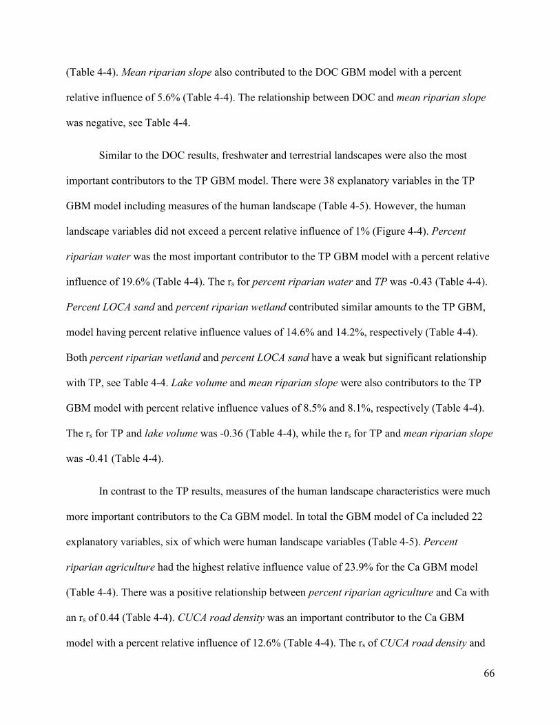
66
(Table 4-4). Mean riparian slope also contributed to the DOC GBM model with a percent
relative influence of 5.6% (Table 4-4). The relationship between DOC and mean riparian slope
was negative, see Table 4-4.
Similar to the DOC results, freshwater and terrestrial landscapes were also the most
important contributors to the TP GBM model. There were 38 explanatory variables in the TP
GBM model including measures of the human landscape (Table 4-5). However, the human
landscape variables did not exceed a percent relative influence of 1% (Figure 4-4). Percent
riparian water was the most important contributor to the TP GBM model with a percent relative
influence of 19.6% (Table 4-4). The rs for percent riparian water and TP was -0.43 (Table 4-4).
Percent LOCA sand and percent riparian wetland contributed similar amounts to the TP GBM,
model having percent relative influence values of 14.6% and 14.2%, respectively (Table 4-4).
Both percent riparian wetland and percent LOCA sand have a weak but significant relationship
with TP, see Table 4-4. Lake volume and mean riparian slope were also contributors to the TP
GBM model with percent relative influence values of 8.5% and 8.1%, respectively (Table 4-4).
The rs for TP and lake volume was -0.36 (Table 4-4), while the rs for TP and mean riparian slope
was -0.41 (Table 4-4).
In contrast to the TP results, measures of the human landscape characteristics were much
more important contributors to the Ca GBM model. In total the GBM model of Ca included 22
explanatory variables, six of which were human landscape variables (Table 4-5). Percent
riparian agriculture had the highest relative influence value of 23.9% for the Ca GBM model
(Table 4-4). There was a positive relationship between percent riparian agriculture and Ca with
an rs of 0.44 (Table 4-4). CUCA road density was an important contributor to the Ca GBM
model with a percent relative influence of 12.6% (Table 4-4). The rs of CUCA road density and
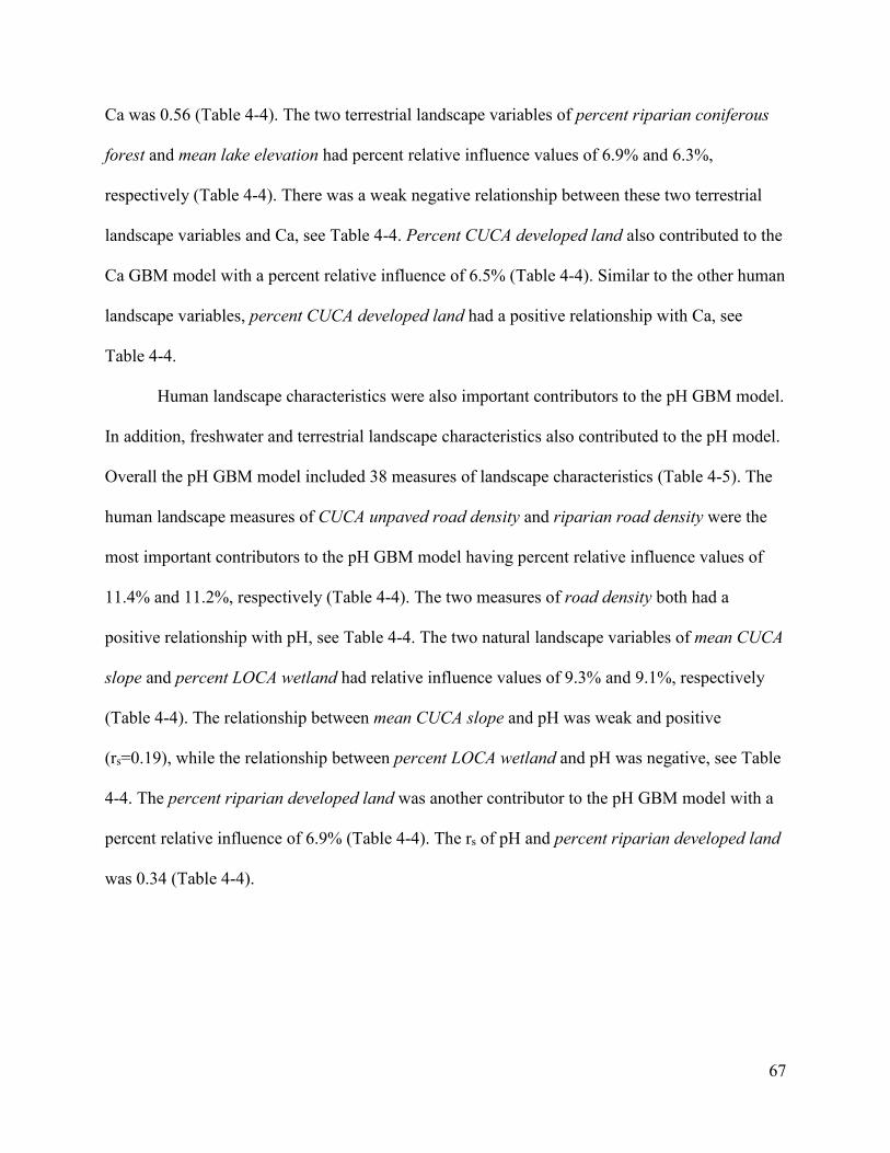
67
Ca was 0.56 (Table 4-4). The two terrestrial landscape variables of percent riparian coniferous
forest and mean lake elevation had percent relative influence values of 6.9% and 6.3%,
respectively (Table 4-4). There was a weak negative relationship between these two terrestrial
landscape variables and Ca, see Table 4-4. Percent CUCA developed land also contributed to the
Ca GBM model with a percent relative influence of 6.5% (Table 4-4). Similar to the other human
landscape variables, percent CUCA developed land had a positive relationship with Ca, see
Table 4-4.
Human landscape characteristics were also important contributors to the pH GBM model.
In addition, freshwater and terrestrial landscape characteristics also contributed to the pH model.
Overall the pH GBM model included 38 measures of landscape characteristics (Table 4-5). The
human landscape measures of CUCA unpaved road density and riparian road density were the
most important contributors to the pH GBM model having percent relative influence values of
11.4% and 11.2%, respectively (Table 4-4). The two measures of road density both had a
positive relationship with pH, see Table 4-4. The two natural landscape variables of mean CUCA
slope and percent LOCA wetland had relative influence values of 9.3% and 9.1%, respectively
(Table 4-4). The relationship between mean CUCA slope and pH was weak and positive
(rs=0.19), while the relationship between percent LOCA wetland and pH was negative, see Table
4-4. The percent riparian developed land was another contributor to the pH GBM model with a
percent relative influence of 6.9% (Table 4-4). The rs of pH and percent riparian developed land
was 0.34 (Table 4-4).
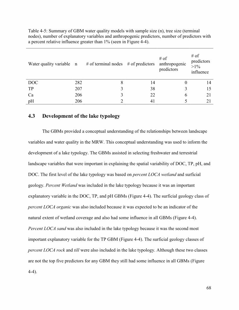
68
Table 4-5: Summary of GBM water quality models with sample size (n), tree size (terminal
nodes), number of explanatory variables and anthropogenic predictors, number of predictors with
a percent relative influence greater than 1% (seen in Figure 4-4).
Water quality variable n # of terminal nodes # of predictors
# of
anthropogenic
predictors
# of
predictors
>1%
influence
DOC 282 8 14 0 14
TP 207 3 38 3 15
Ca 206 3 22 6 21
pH 206 2 41 5 21
4.3 Development of the lake typology
The GBMs provided a conceptual understanding of the relationships between landscape
variables and water quality in the MRW. This conceptual understanding was used to inform the
development of a lake typology. The GBMs assisted in selecting freshwater and terrestrial
landscape variables that were important in explaining the spatial variability of DOC, TP, pH, and
DOC. The first level of the lake typology was based on percent LOCA wetland and surficial
geology. Percent Wetland was included in the lake typology because it was an important
explanatory variable in the DOC, TP, and pH GBMs (Figure 4-4). The surficial geology class of
percent LOCA organic was also included because it was expected to be an indicator of the
natural extent of wetland coverage and also had some influence in all GBMs (Figure 4-4).
Percent LOCA sand was also included in the lake typology because it was the second most
important explanatory variable for the TP GBM (Figure 4-4). The surficial geology classes of
percent LOCA rock and till were also included in the lake typology. Although these two classes
are not the top five predictors for any GBM they still had some influence in all GBMs (Figure
4-4).
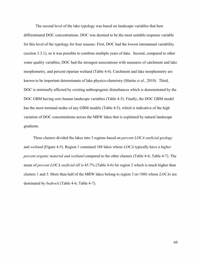
69
The second level of the lake typology was based on landscape variables that best
differentiated DOC concentrations. DOC was deemed to be the most suitable response variable
for this level of the typology for four reasons: First, DOC had the lowest interannual variability
(section 3.3.1), so it was possible to combine multiple years of data. Second, compared to other
water quality variables, DOC had the strongest associations with measures of catchment and lake
morphometry, and percent riparian wetland (Table 4-4). Catchment and lake morphometry are
known to be important determinants of lake physico-chemistry (Martin et al., 2010). Third,
DOC is minimally affected by existing anthropogenic disturbances which is demonstrated by the
DOC GBM having zero human landscape variables (Table 4-5). Finally, the DOC GBM model
has the most terminal nodes of any GBM models (Table 4-5), which is indicative of the high
variation of DOC concentrations across the MRW lakes that is explained by natural landscape
gradients.
Three clusters divided the lakes into 3 regions based on percent LOCA surficial geology
and wetland (Figure 4-5). Region 1 contained 188 lakes whose LOCA typically have a higher
percent organic material and wetland compared to the other clusters (Table 4-6; Table 4-7). The
mean of percent LOCA surficial till is 45.7% (Table 4-6) for region 2 which is much higher than
clusters 1 and 3. More than half of the MRW lakes belong to region 3 (n=388) whose LOCAs are
dominated by bedrock (Table 4-6; Table 4-7).
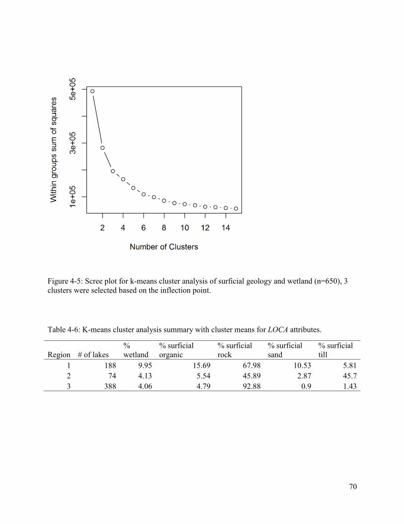
70
Figure 4-5: Scree plot for k-means cluster analysis of surficial geology and wetland (n=650), 3
clusters were selected based on the inflection point.
Table 4-6: K-means cluster analysis summary with cluster means for LOCA attributes.
Region # of lakes
%
wetland
% surficial
organic
% surficial
rock
% surficial
sand
% surficial
till
1 188 9.95 15.69 67.98 10.53 5.81
2 74 4.13 5.54 45.89 2.87 45.7
3 388 4.06 4.79 92.88 0.9 1.43
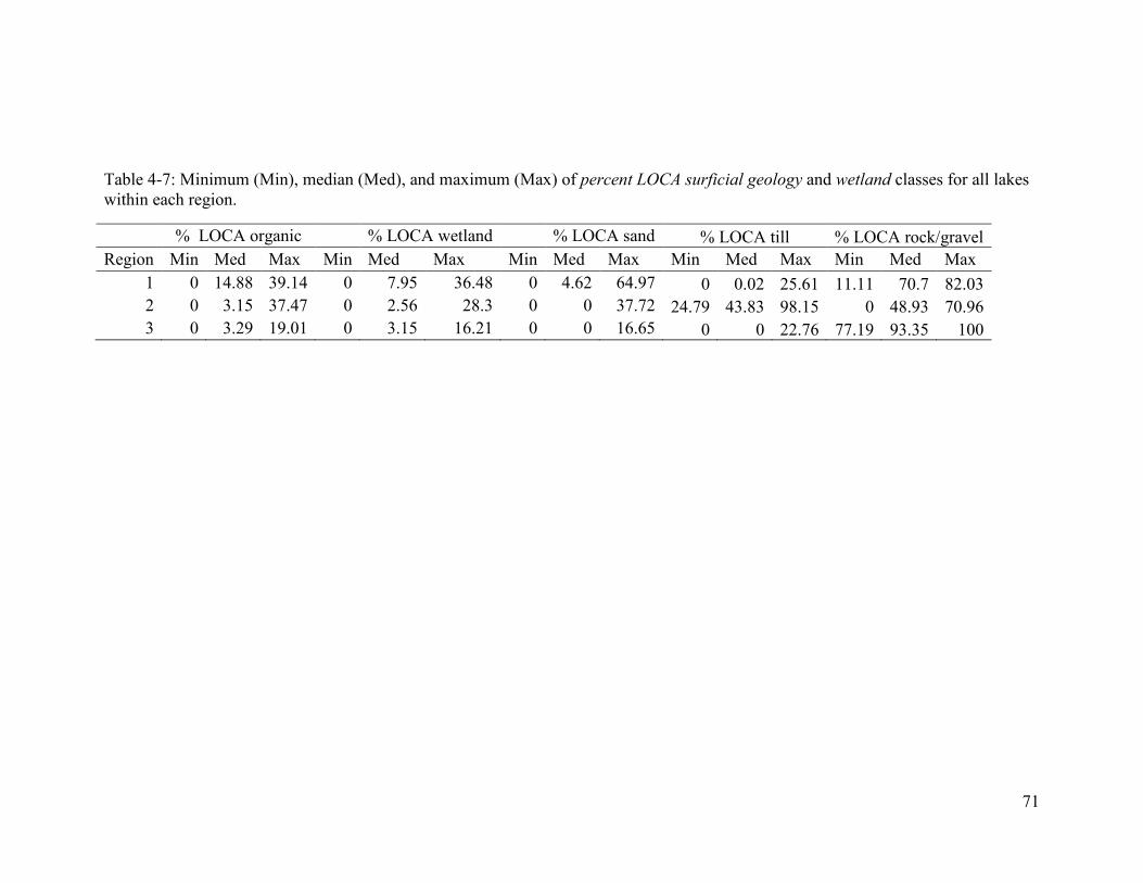
71
Table 4-7: Minimum (Min), median (Med), and maximum (Max) of percent LOCA surficial geology and wetland classes for all lakes
within each region.
% LOCA organic % LOCA wetland % LOCA sand % LOCA till % LOCA rock/gravel
Region Min Med Max Min Med Max Min Med Max Min Med Max Min Med Max
1 0 14.88 39.14 0 7.95 36.48 0 4.62 64.97 0 0.02 25.61 11.11 70.7 82.03
2 0 3.15 37.47 0 2.56 28.3 0 0 37.72 24.79 43.83 98.15 0 48.93 70.96
3 0 3.29 19.01 0 3.15 16.21 0 0 16.65 0 0 22.76 77.19 93.35 100
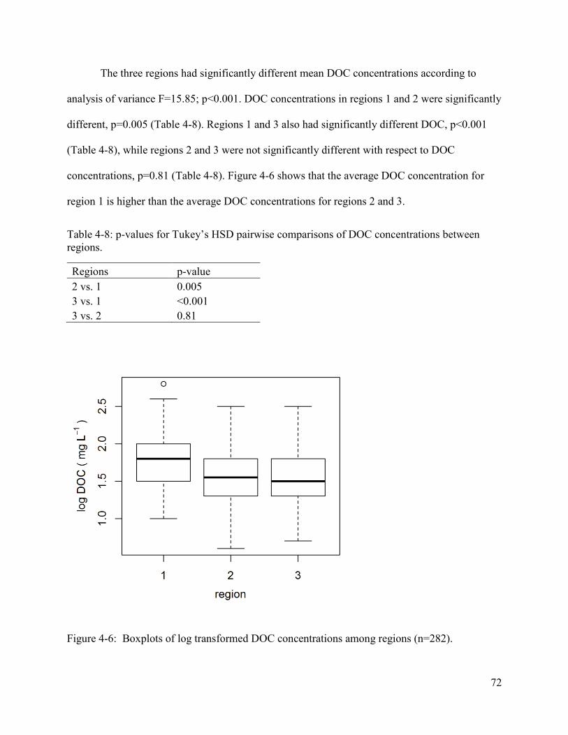
72
The three regions had significantly different mean DOC concentrations according to
analysis of variance F=15.85; p<0.001. DOC concentrations in regions 1 and 2 were significantly
different, p=0.005 (Table 4-8). Regions 1 and 3 also had significantly different DOC, p<0.001
(Table 4-8), while regions 2 and 3 were not significantly different with respect to DOC
concentrations, p=0.81 (Table 4-8). Figure 4-6 shows that the average DOC concentration for
region 1 is higher than the average DOC concentrations for regions 2 and 3.
Table 4-8: p-values for Tukey’s HSD pairwise comparisons of DOC concentrations between
regions.
Regions p-value
2 vs. 1 0.005
3 vs. 1 <0.001
3 vs. 2 0.81
Figure 4-6: Boxplots of log transformed DOC concentrations among regions (n=282).
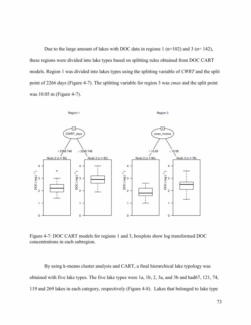
73
Due to the large amount of lakes with DOC data in regions 1 (n=102) and 3 (n= 142),
these regions were divided into lake types based on splitting rules obtained from DOC CART
models. Region 1 was divided into lakes types using the splitting variable of CWRT and the split
point of 2266 days (Figure 4-7). The splitting variable for region 3 was zmax and the split point
was 10.05 m (Figure 4-7).
Figure 4-7: DOC CART models for regions 1 and 3, boxplots show log transformed DOC
concentrations in each subregion.
By using k-means cluster analysis and CART, a final hierarchical lake typology was
obtained with five lake types. The five lake types were 1a, 1b, 2, 3a, and 3b and had67, 121, 74,
119 and 269 lakes in each category, respectively (Figure 4-8). Lakes that belonged to lake type
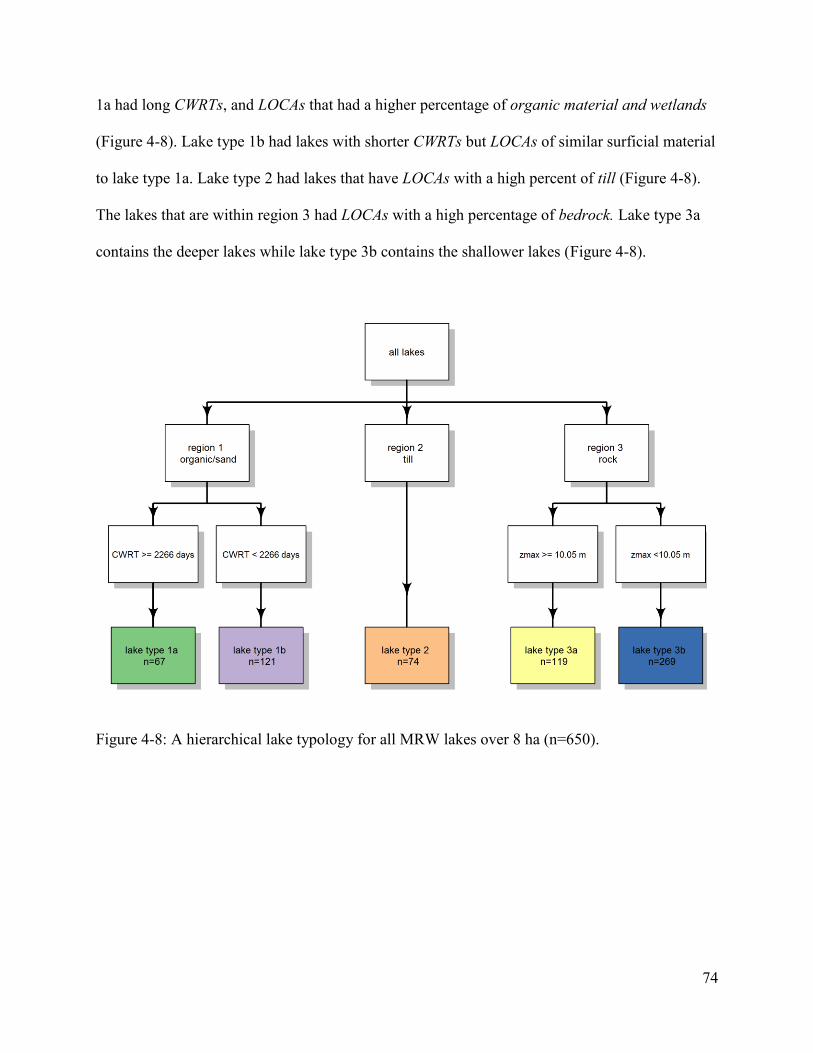
74
1a had long CWRTs, and LOCAs that had a higher percentage of organic material and wetlands
(Figure 4-8). Lake type 1b had lakes with shorter CWRTs but LOCAs of similar surficial material
to lake type 1a. Lake type 2 had lakes that have LOCAs with a high percent of till (Figure 4-8).
The lakes that are within region 3 had LOCAs with a high percentage of bedrock. Lake type 3a
contains the deeper lakes while lake type 3b contains the shallower lakes (Figure 4-8).
Figure 4-8: A hierarchical lake typology for all MRW lakes over 8 ha (n=650).
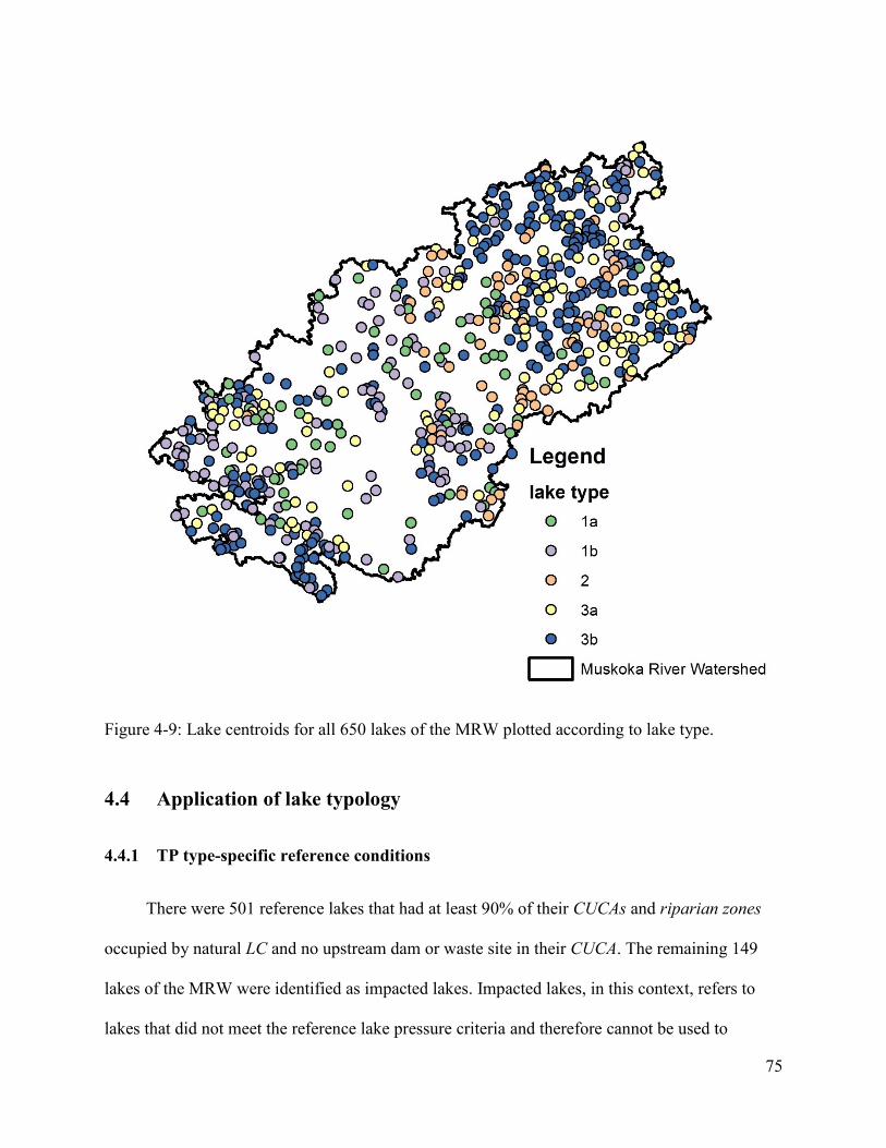
75
Figure 4-9: Lake centroids for all 650 lakes of the MRW plotted according to lake type.
4.4 Application of lake typology
4.4.1 TP type-specific reference conditions
There were 501 reference lakes that had at least 90% of their CUCAs and riparian zones
occupied by natural LC and no upstream dam or waste site in their CUCA. The remaining 149
lakes of the MRW were identified as impacted lakes. Impacted lakes, in this context, refers to
lakes that did not meet the reference lake pressure criteria and therefore cannot be used to
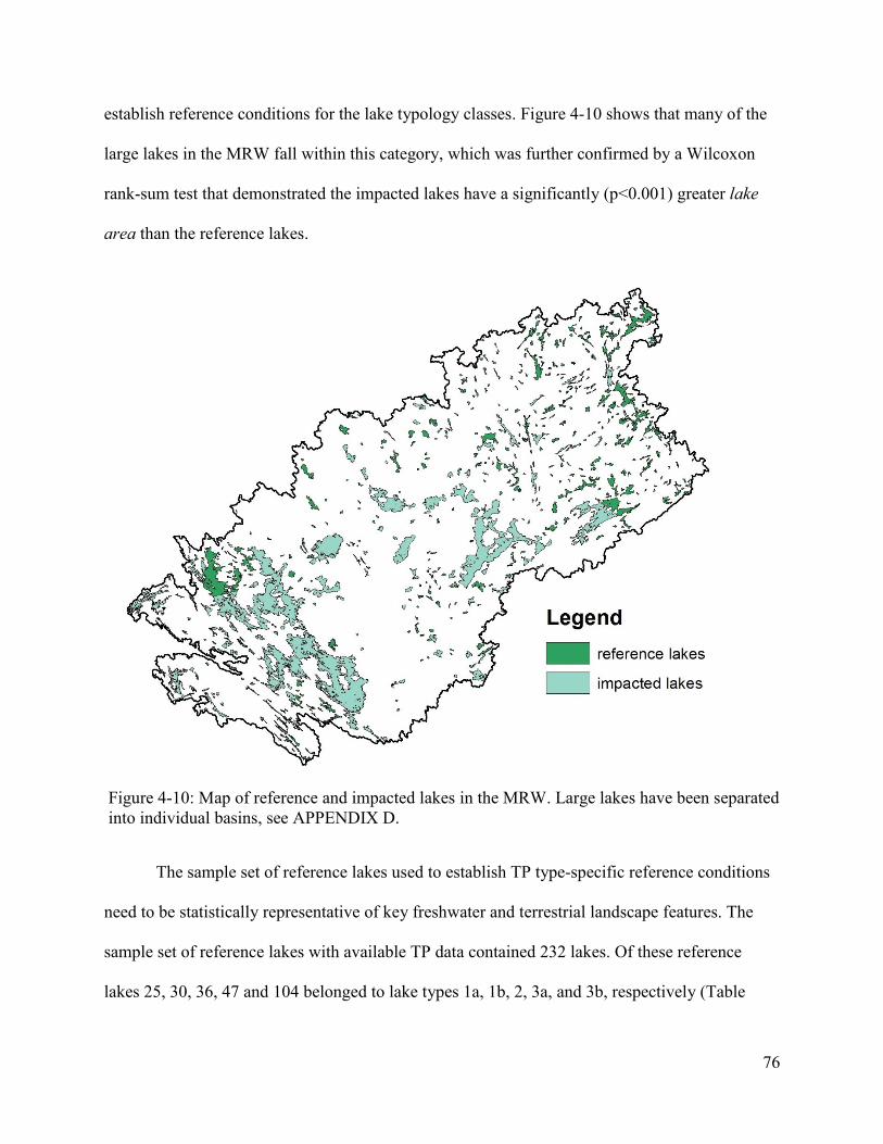
76
establish reference conditions for the lake typology classes. Figure 4-10 shows that many of the
large lakes in the MRW fall within this category, which was further confirmed by a Wilcoxon
rank-sum test that demonstrated the impacted lakes have a significantly (p<0.001) greater lake
area than the reference lakes.
Figure 4-10: Map of reference and impacted lakes in the MRW. Large lakes have been separated
into individual basins, see APPENDIX D.
The sample set of reference lakes used to establish TP type-specific reference conditions
need to be statistically representative of key freshwater and terrestrial landscape features. The
sample set of reference lakes with available TP data contained 232 lakes. Of these reference
lakes 25, 30, 36, 47 and 104 belonged to lake types 1a, 1b, 2, 3a, and 3b, respectively (Table
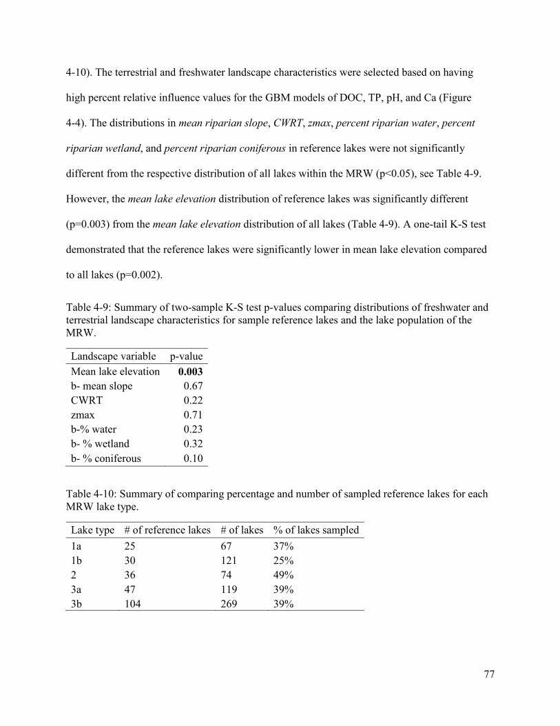
77
4-10). The terrestrial and freshwater landscape characteristics were selected based on having
high percent relative influence values for the GBM models of DOC, TP, pH, and Ca (Figure
4-4). The distributions in mean riparian slope, CWRT, zmax, percent riparian water, percent
riparian wetland, and percent riparian coniferous in reference lakes were not significantly
different from the respective distribution of all lakes within the MRW (p<0.05), see Table 4-9.
However, the mean lake elevation distribution of reference lakes was significantly different
(p=0.003) from the mean lake elevation distribution of all lakes (Table 4-9). A one-tail K-S test
demonstrated that the reference lakes were significantly lower in mean lake elevation compared
to all lakes (p=0.002).
Table 4-9: Summary of two-sample K-S test p-values comparing distributions of freshwater and
terrestrial landscape characteristics for sample reference lakes and the lake population of the
MRW.
Landscape variable p-value
Mean lake elevation 0.003
b- mean slope 0.67
CWRT 0.22
zmax 0.71
b-% water 0.23
b- % wetland 0.32
b- % coniferous 0.10
Table 4-10: Summary of comparing percentage and number of sampled reference lakes for each
MRW lake type.
Lake type # of reference lakes # of lakes % of lakes sampled
1a 25 67 37%
1b 30 121 25%
2 36 74 49%
3a 47 119 39%
3b 104 269 39%
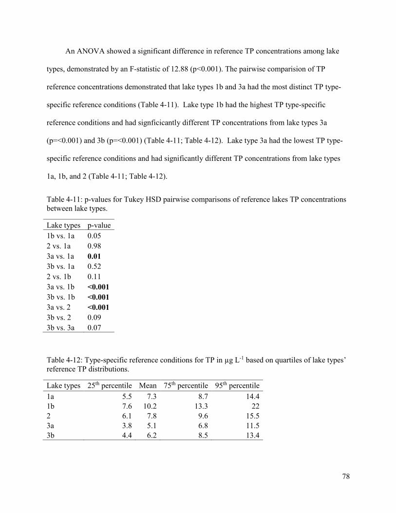
78
An ANOVA showed a significant difference in reference TP concentrations among lake
types, demonstrated by an F-statistic of 12.88 (p<0.001). The pairwise comparision of TP
reference concentrations demonstrated that lake types 1b and 3a had the most distinct TP type-
specific reference conditions (Table 4-11). Lake type 1b had the highest TP type-specific
reference conditions and had signficicantly different TP concentrations from lake types 3a
(p=<0.001) and 3b (p=<0.001) (Table 4-11; Table 4-12). Lake type 3a had the lowest TP type-
specific reference conditions and had significantly different TP concentrations from lake types
1a, 1b, and 2 (Table 4-11; Table 4-12).
Table 4-11: p-values for Tukey HSD pairwise comparisons of reference lakes TP concentrations
between lake types.
Lake types p-value
1b vs. 1a 0.05
2 vs. 1a 0.98
3a vs. 1a 0.01
3b vs. 1a 0.52
2 vs. 1b 0.11
3a vs. 1b <0.001
3b vs. 1b <0.001
3a vs. 2 <0.001
3b vs. 2 0.09
3b vs. 3a 0.07
Table 4-12: Type-specific reference conditions for TP in µg L-1 based on quartiles of lake types’
reference TP distributions.
Lake types 25th percentile Mean 75th percentile 95th percentile
1a 5.5 7.3 8.7 14.4
1b 7.6 10.2 13.3 22
2 6.1 7.8 9.6 15.5
3a 3.8 5.1 6.8 11.5
3b 4.4 6.2 8.5 13.4
79
The TP quality status of the 116 impacted lakes was classified based on TP type-specific
reference conditions. Seventy-seven of the impacted lakes were classified as having good TP
quality status because their TP concentrations were below the 75th percentile of their lake type
reference lake distribution (Table 4-12). In total, thirty lakes were classified as having moderate
TP quality status, while nine lakes were classified as having poor TP quality status. Lake type 1a
had 7 lakes with moderate TP quality status and 4 lakes with poor TP quality status (Figure
4-11). Lake types 3a and 2 did not have any lakes that were classified as poor TP quality status
(Figure 4-11). There were 3 lakes that belonged to lake type 2 which had moderate TP quality
status and 7 lakes in lake type 3a that had moderate TP quality status (Figure 4-11). Lake type 1b
had 9 lakes with moderate TP quality status and 1 lake with poor TP quality status (Figure 4-11).
There were 4 lakes that had moderate TP quality status and 4 lakes that had poor TP quality
status that were in lake type 3b (Figure 4-11). Out of the nine lakes with poor TP quality status in
the MRW six of these lakes are found in Township of Muskoka Lakes (Figure 4-12). The lakes
that have poor TP quality status in the Township of Muskoka Lakes are Silver Lake, Ada Lake,
Duffy Lake, Bruce Lake, Brandy Lake, and Three Mile Lake Main Basin (Figure 4-12). These
lakes with poor TP quality status also have a high percentage of LU within their riparian zones
and CUCAs. For example, Three Mile Lake Main Basin, Brandy Lake, and Ada Lake have high
percentages of riparian agricultural land (Table 4-13). Bruce Lake has a high percentage of
CUCA golf course, while Duffy lake has very little LU in its CUCA but has a waste site (Table
4-13). Silver Lake has a high percentage of riparian developed land (Table 4-13).
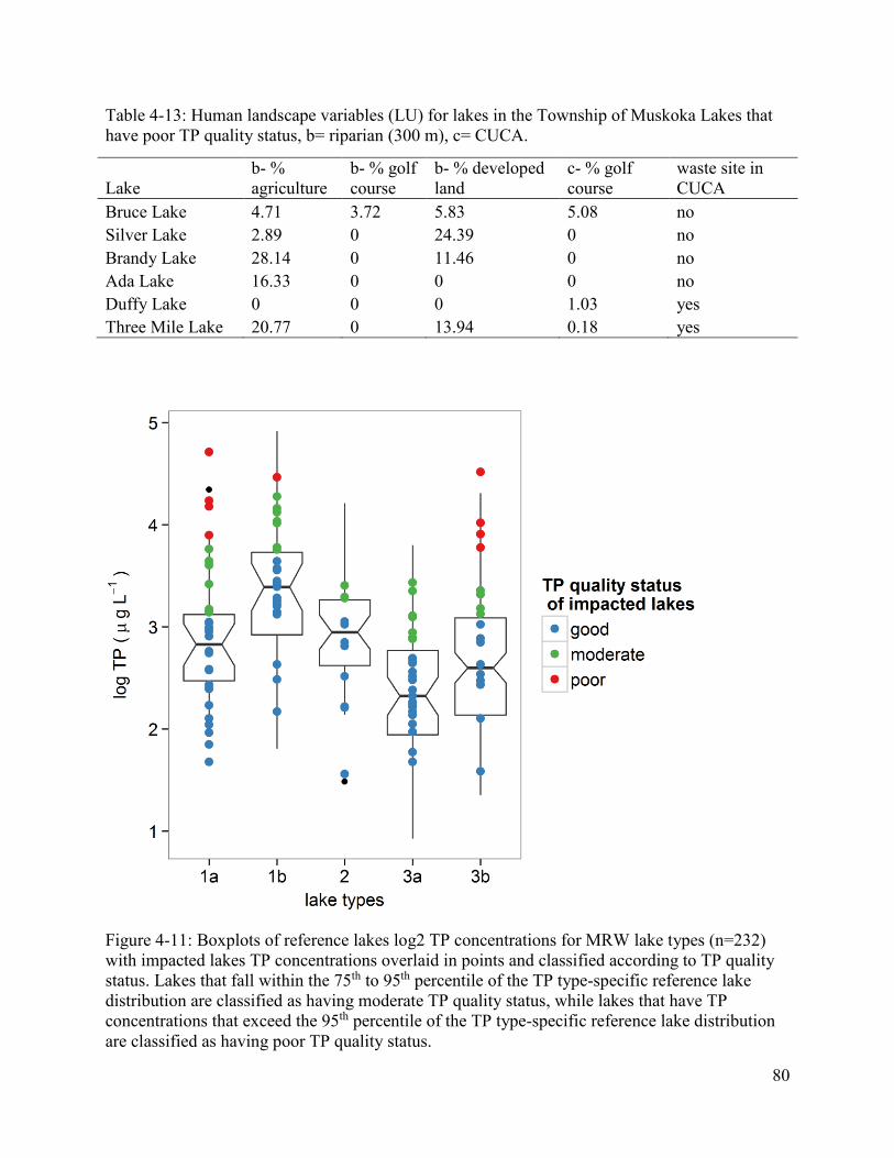
80
Table 4-13: Human landscape variables (LU) for lakes in the Township of Muskoka Lakes that
have poor TP quality status, b= riparian (300 m), c= CUCA.
Lake
b- %
agriculture
b- % golf
course
b- % developed
land
c- % golf
course
waste site in
CUCA
Bruce Lake 4.71 3.72 5.83 5.08 no
Silver Lake 2.89 0 24.39 0 no
Brandy Lake 28.14 0 11.46 0 no
Ada Lake 16.33 0 0 0 no
Duffy Lake 0 0 0 1.03 yes
Three Mile Lake 20.77 0 13.94 0.18 yes
Figure 4-11: Boxplots of reference lakes log2 TP concentrations for MRW lake types (n=232)
with impacted lakes TP concentrations overlaid in points and classified according to TP quality
status. Lakes that fall within the 75th to 95th percentile of the TP type-specific reference lake
distribution are classified as having moderate TP quality status, while lakes that have TP
concentrations that exceed the 95th percentile of the TP type-specific reference lake distribution
are classified as having poor TP quality status.
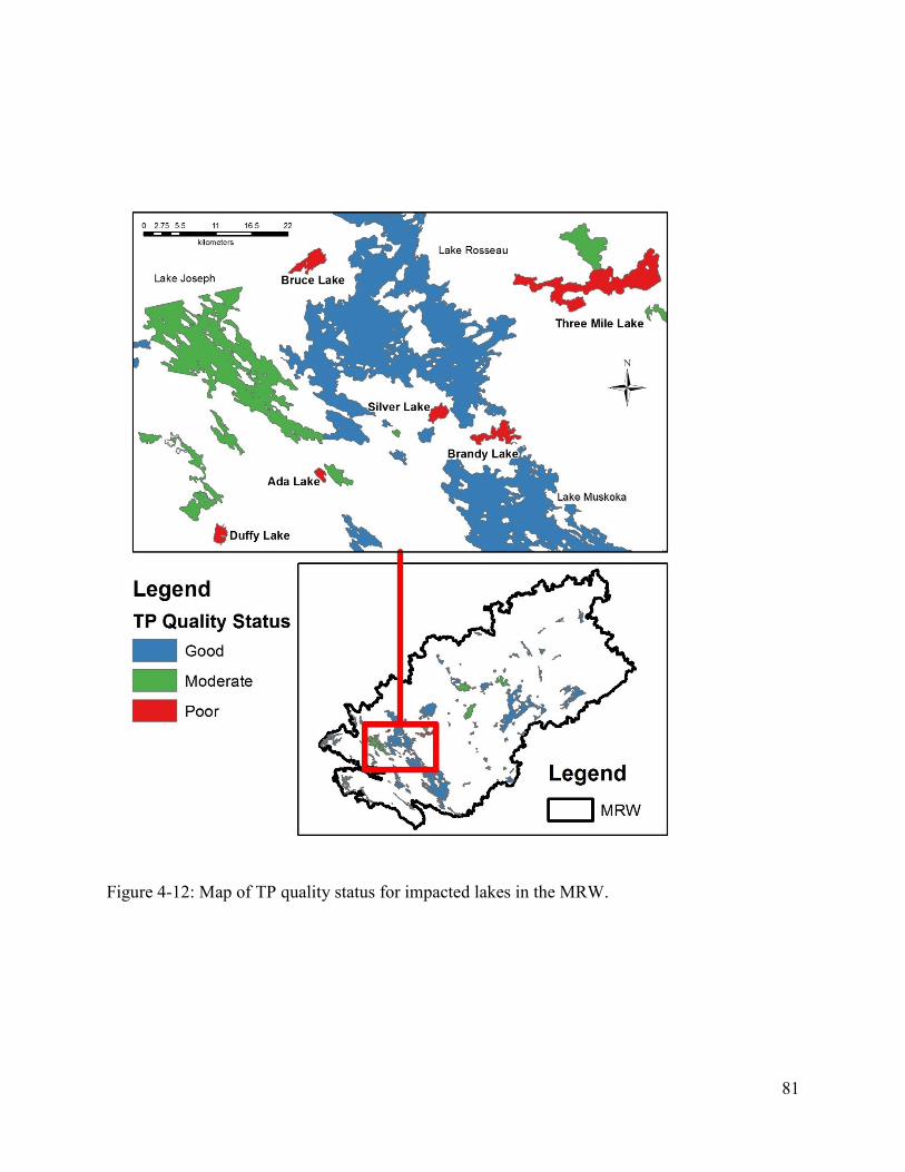
81
Figure 4-12: Map of TP quality status for impacted lakes in the MRW.
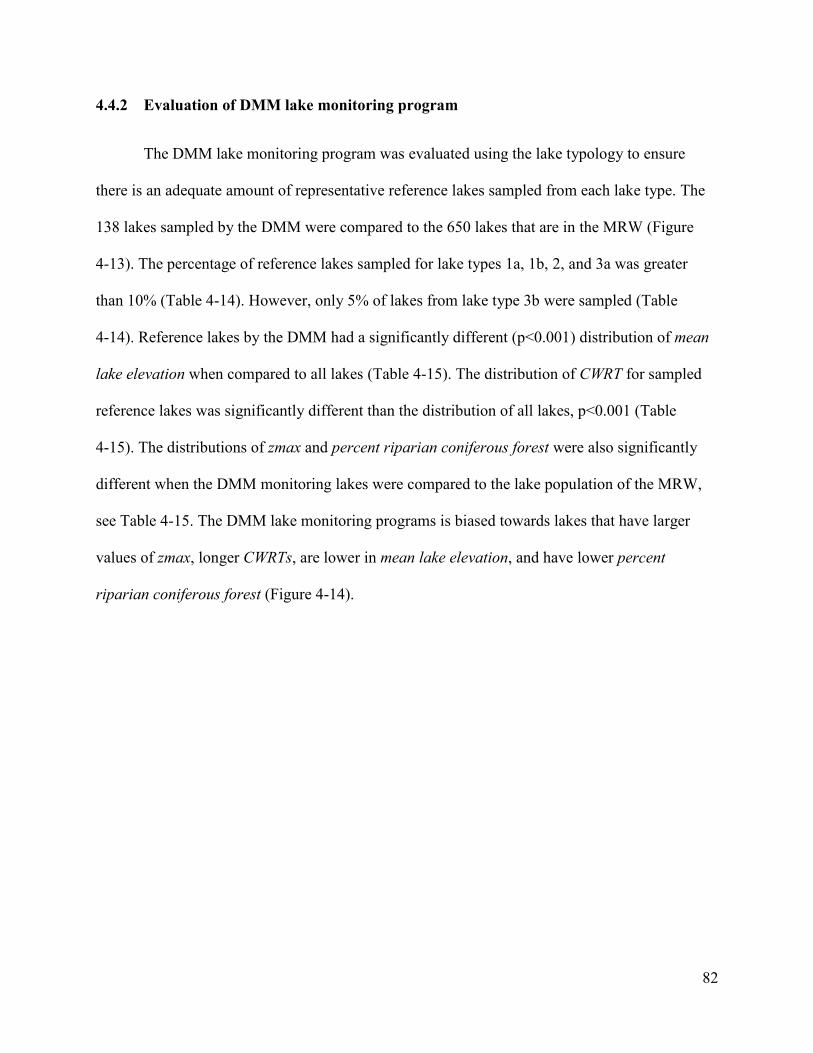
82
4.4.2 Evaluation of DMM lake monitoring program
The DMM lake monitoring program was evaluated using the lake typology to ensure
there is an adequate amount of representative reference lakes sampled from each lake type. The
138 lakes sampled by the DMM were compared to the 650 lakes that are in the MRW (Figure
4-13). The percentage of reference lakes sampled for lake types 1a, 1b, 2, and 3a was greater
than 10% (Table 4-14). However, only 5% of lakes from lake type 3b were sampled (Table
4-14). Reference lakes by the DMM had a significantly different (p<0.001) distribution of mean
lake elevation when compared to all lakes (Table 4-15). The distribution of CWRT for sampled
reference lakes was significantly different than the distribution of all lakes, p<0.001 (Table
4-15). The distributions of zmax and percent riparian coniferous forest were also significantly
different when the DMM monitoring lakes were compared to the lake population of the MRW,
see Table 4-15. The DMM lake monitoring programs is biased towards lakes that have larger
values of zmax, longer CWRTs, are lower in mean lake elevation, and have lower percent
riparian coniferous forest (Figure 4-14).
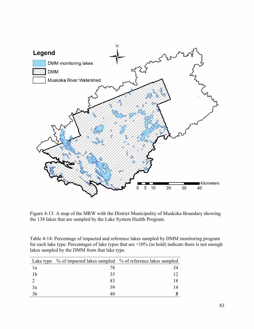
83
Figure 4-13: A map of the MRW with the District Municipality of Muskoka Boundary showing
the 138 lakes that are sampled by the Lake System Health Program.
Table 4-14: Percentage of impacted and reference lakes sampled by DMM monitoring program
for each lake type. Percentages of lake types that are <10% (in bold) indicate there is not enough
lakes sampled by the DMM from that lake type.
Lake type % of impacted lakes sampled % of reference lakes sampled
1a 78 34
1b 35 12
2 83 18
3a 59 14
3b 40 5
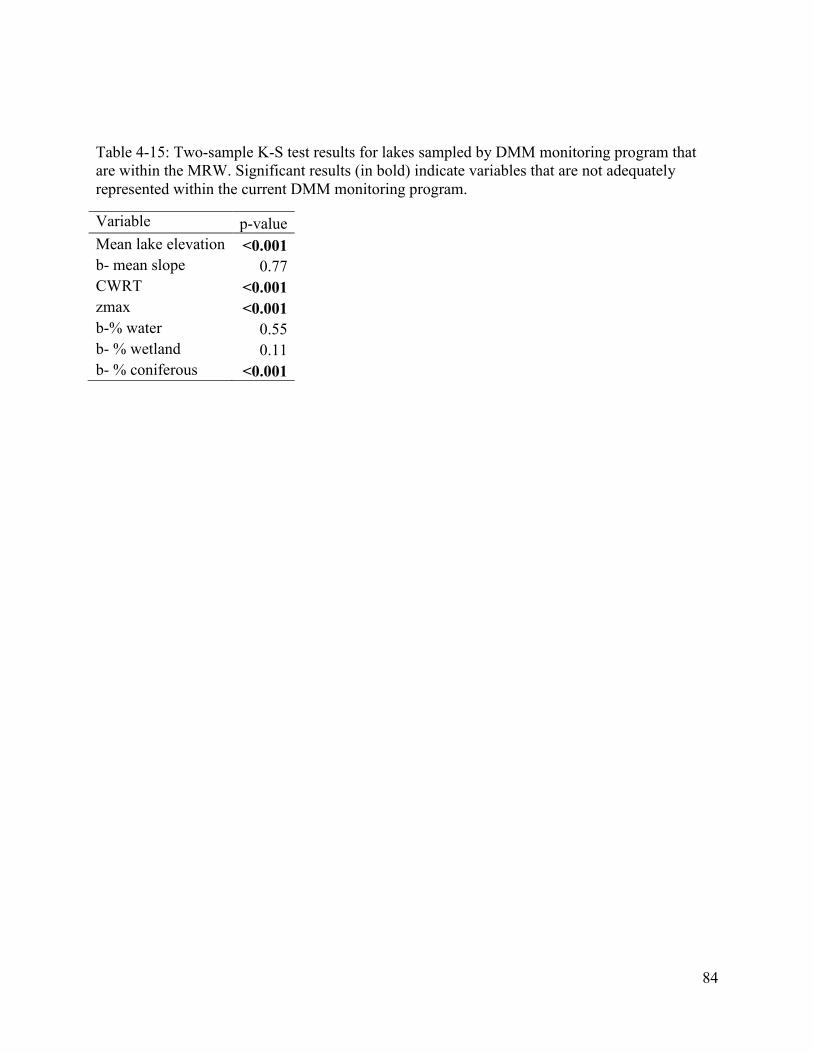
84
Table 4-15: Two-sample K-S test results for lakes sampled by DMM monitoring program that
are within the MRW. Significant results (in bold) indicate variables that are not adequately
represented within the current DMM monitoring program.
Variable p-value
Mean lake elevation <0.001
b- mean slope 0.77
CWRT <0.001
zmax <0.001
b-% water 0.55
b- % wetland 0.11
b- % coniferous <0.001
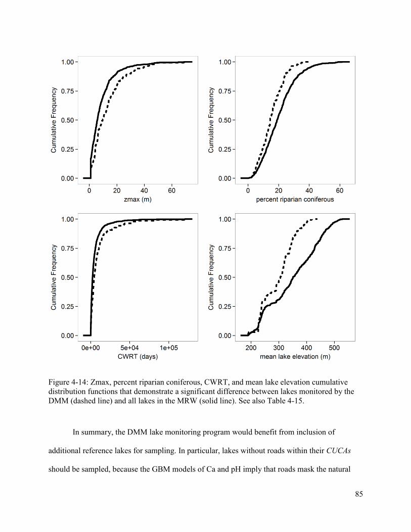
85
Figure 4-14: Zmax, percent riparian coniferous, CWRT, and mean lake elevation cumulative
distribution functions that demonstrate a significant difference between lakes monitored by the
DMM (dashed line) and all lakes in the MRW (solid line). See also Table 4-15.
In summary, the DMM lake monitoring program would benefit from inclusion of
additional reference lakes for sampling. In particular, lakes without roads within their CUCAs
should be sampled, because the GBM models of Ca and pH imply that roads mask the natural
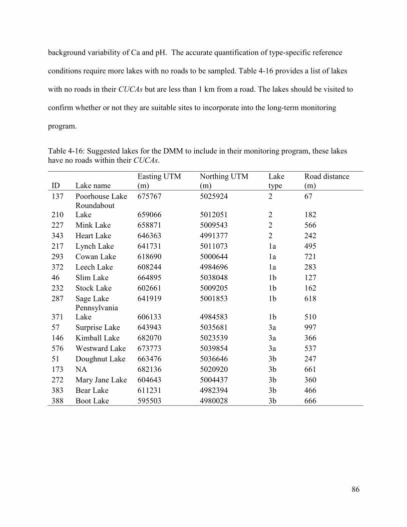
86
background variability of Ca and pH. The accurate quantification of type-specific reference
conditions require more lakes with no roads to be sampled. Table 4-16 provides a list of lakes
with no roads in their CUCAs but are less than 1 km from a road. The lakes should be visited to
confirm whether or not they are suitable sites to incorporate into the long-term monitoring
program.
Table 4-16: Suggested lakes for the DMM to include in their monitoring program, these lakes
have no roads within their CUCAs.
ID Lake name
Easting UTM
(m)
Northing UTM
(m)
Lake
type
Road distance
(m)
137 Poorhouse Lake 675767 5025924 2 67
210
Roundabout
Lake 659066 5012051 2 182
227 Mink Lake 658871 5009543 2 566
343 Heart Lake 646363 4991377 2 242
217 Lynch Lake 641731 5011073 1a 495
293 Cowan Lake 618690 5000644 1a 721
372 Leech Lake 608244 4984696 1a 283
46 Slim Lake 664895 5038048 1b 127
232 Stock Lake 602661 5009205 1b 162
287 Sage Lake 641919 5001853 1b 618
371
Pennsylvania
Lake 606133 4984583 1b 510
57 Surprise Lake 643943 5035681 3a 997
146 Kimball Lake 682070 5023539 3a 366
576 Westward Lake 673773 5039854 3a 537
51 Doughnut Lake 663476 5036646 3b 247
173 NA 682136 5020920 3b 661
272 Mary Jane Lake 604643 5004437 3b 360
383 Bear Lake 611231 4982394 3b 466
388 Boot Lake 595503 4980028 3b 666
87
5. DISCUSSION
A landscape and statistically-based approach was implemented in order to develop and apply
a lake typology for the MRW. The GBMs provided insight on important human, freshwater, and
terrestrial landscape features associated with the water quality of the MRW lakes. Some of the
associations between landscape features and water quality corroborate other studies. However,
some associations were not supported by literature and may have been a result of data artifact or
warrant further investigation. DOC, CWRT, and lake morphometry are important components
that assisted in developing a lake typology that are hypothesized to have ecological relevance.
The validity of the MRW lake typology was examined by comparisons with the TP type-specific
reference conditions for Nordic lake types. The strengths and weaknesses of the current DMM
monitoring program and TP management models were examined. Additionally,
recommendations are made to refine and improve the current DMM monitoring program.
5.1 DOC and freshwater landscape features
DOC is recognized as being a critical property of lakes in the boreal regions because it is
a major distinguishing feature in the physico-chemistry of pristine lakes, and can strongly
influence how a lake responds to stressors (D’Arcy and Carignan, 1997; Pace and Cole, 2002;
Williamson et al., 1999). DOC also facilitates the transport of nutrients, ions, and contaminants
from the terrestrial to the aquatic environment (Kullberg et al., 1993; Stanley et al., 2012;
Wetzel, 2001). Lake DOC concentrations also account for differences in the physico-chemical
and biological properties of lakes (Canham et al., 2004). Understanding the associations between
landscape features and DOC can aid in understanding other components of aquatic ecosystems.
88
Furthermore, DOC was found to be the most temporally invariant water quality parameter in
MRW lakes, and the least likely to be influenced by human landscape factors. For these reasons,
DOC was the key water quality parameter used in developing the lake typology.
Wetlands have long been recognized as a source of DOC to surface waters, as identified
by many others (Canham et al., 2004; Dillon and Molot, 1997; Hinton et al., 1998; Wetzel,
2001). However, in contrast to this study, most other studies have demonstrated that percent
wetlands within the CUCA, can best explain DOC concentrations in lakes (Canham et al., 2004;
Gergel et al., 1999; O’Connor et al., 2009). In the MRW, the percent riparian wetland had a
higher percent relative influence value in the DOC GBM model than percent CUCA riparian
wetland. Systematic differences in the lake landscape position among lake districts, may explain
differences in the most relevant spatial scale for quantifying wetlands and their contribution to
inter-lake variability in DOC concentrations. For example, the lakes included in the Canham et
al. (2004) study are primarily headwater lakes, while there are a large amount of non-headwater
lakes in the MRW. Headwater lakes compared to non-headwater lakes have smaller catchments
and hence shorter flow paths resulting in less potential for DOC processing (Canham et al.,
2004). A study conducted in Michigan, which included lakes that have a similar range of LNNs
to the MRW (Martin and Soranno, 2006), demonstrated that percent LOCA wetlands influenced
COLTR more than percentage of wetlands measured at the riparian zone or CUCA (Martin et
al., 2011). The findings of the Martin et al. (2011) study, which included a large amount of non-
headwater lakes, as well as those of this study, suggest that distance decay of DOC along the
lake network in non-headwater catchments can be very important.
The association between wetland area and DOC concentration in lakes is not
straightforward due to the terrestrial and freshwater landscape features that can alter the
89
influence of wetlands (Fölster et al., 2004; Nykänen et al., 2005; Rowan, 2010). The results of
this study demonstrate that the freshwater landscape variables are strongly associated with DOC
concentrations in the lakes of the MRW. CWRT was the explanatory variable with the strongest
association with DOC. Another freshwater landscape variable, zmax, had a strong negative
association with DOC in the MRW lakes. Other studies have demonstrated that deeper lakes
have lower concentrations of DOC due to their longer WRTs resulting in higher rates of in-lake
mineralization (Hanson et al., 2011; Nõges, 2009; Pace and Cole, 2002; Scott et al., 2010). The
freshwater landscape variable of percent upstream lakes also had a negative association with
DOC in the MRW lakes. Upstream lakes acting as sinks of DOC and COLTR corroborates other
studies from lake districts in Finland, Sweden, and Nova Scotia (Kortelainen, 1993; Rantakari et
al., 2004; Thierfelder, 1998; Wolniewicz et al., 2011). In a DOC mass-balance model for the
MRW lakes, upstream lakes were an important component in accurately determining DOC
concentrations in non-headwater lakes (O’Connor et al., 2009).
5.1.1 The role of CWRT in carbon rich non-headwater regions
A number of researchers have emphasized the need to incorporate spatially explicit
metrics of water flows and drainage network connectivity within watershed systems to improve
modelling of nutrients and DOC at the regional scale (Cardille et al., 2007; Muller et al., 2013;
Zhang et al., 2010). The accurate quantification of nutrients and DOC concentrations in non-
headwater lakes through the use of landscape models requires consideration of all the major
losses of DOC and nutrients in upstream lakes and contributing terrestrial areas (Canham et al.,
2004; Epstein et al., 2013; Zhang et al., 2012). Studies have demonstrated that accurate regional
scale DOC models in lake and carbon rich landscapes require the quantification of the effects of
90
upstream lakes as carbon processing units (Cardille et al., 2007; Muller et al., 2013; O’Connor et
al., 2009). Additionally, the connections and configurations of the lake network should be
considered to accurately predict DOC concentrations from landscape models (Canham et al.,
2004; Cardille et al., 2007; Soranno et al., 1999). Despite the extent to which researchers
recognize the importance of material processing along lake chains, there is a conspicuous lack of
metrics to quantify this influence on limnological systems.
A similar measure of CWRT was implemented by Muller et al. (2013) for a large number
of Swedish lakes. Unlike, the CWRT measure implemented in this study, Muller et al. (2013)
CWRT measure treated all upstream lakes as one large lake which did not consider how flow
path distance and the spatial configuration of the lake network can modify carbon processing.
The range of CWRT values for the MRW lakes (37- 1.2 × 10⁴ days) is comparable to Muller et
al.’s (2013) CWRT values of 4- 1.0 × 10⁵ days. Sixty two percent of the lakes in the Swedish
study were headwater lakes (Muller et al., 2013), which is comparable to the percentage of
headwater lakes (55%) in the MRW. The higher maximum CWRT found by Muller et al. (2013)
compared to this study can be largely attributed to the CWRTs of the upstream lakes that were
not weighted based on spatial position and CUCAs. Muller et al. (2013) found an association
between the quality of DOC and CWRT and this study showed there was an association between
the quantity of DOC and CWRT. Together, these results imply that, the quality and quantity of
DOC decreases as CWRT increases. Furthermore, the results of this study demonstrates the
importance of quantifying both the effects of in-lake and upstream lake processing using the
CWRT index as these processes can greatly influence DOC concentration in MRW lakes. In the
MRW, additional sampling to characterize DOC quality would be beneficial as it would further
91
contribute to our understanding and quantification of DOC processing along lake chain networks
in non-headwater lake districts.
5.2 Lake depth modelling for the MRW lake typology
An integral part of the implementation of a CWRT index and use of lake depths in lake
typologies is an accurate landscape-based lake depth model. Lake typologies are often limited by
lack of morphometry data in lake rich regions (Nykänen et al., 2005; Rowan et al., 2012; Soszka
et al., 2008). Lake morphometry has been identified as one of the most important characteristics
that differentiates the physico-chemistry and biological properties of a lake (Johansson et al.,
2007; Stefanidis and Papastergiadou, 2012) and as a result modelling lake depth can greatly
enhance the accuracy of predictive nutrient and biological models applied at large spatial scales
(Finstad et al., 2013; Hollister et al., 2011; Milstead et al., 2013).
The lake depth model used in this study to predict zmean and zmax was comparable to the
lake depth model designed by Hollister et al. (2011). The uncorrected lake depth model used by
Hollister et al. (2011) over-predicted zmax, while the lake depth model in this study under-
predicted zmax. Hollister et al. (2011) were able to correct the bias in their model with a
regression against depth data. The zmax model used by Hollister et al. (2011) had a cross-
validated RMSE of 7.0 m, while the RMSE in this study’s zmax model was 11.0 m. The higher
RMSE seen for the MRW lakes could be a result of deeper lakes being included in the cross-
validation dataset. For example, the deepest lake used in the cross-validation of Hollister et al.’s
(2011) study was 57 m, while the maximum zmax in the MRW cross-validation dataset was 93
m.
92
The lake depth model assumes a linear decline in underwater slope of the lake basin
(Kalff, 2002). Although many lakes have underwater slopes that are nearly linear (Kalff, 2002;
Wetzel, 2001), some lakes have underwater slopes that are concave or convex (Carpenter, 1983;
Kalff, 2002). The MRW lakes are expected to be mostly convex in profile due to their glacial
origin (Carpenter, 1983; Kalff, 2002), which could explain the tendency of the lake model to
underpredict zmax.
5.3 Influence of terrain slope and wetland areas on water quality in MRW
lakes
Percent riparian wetlands were positively associated with TP, while percent LOCA
wetlands were negatively associated with pH in the MRW lakes. Wetlands have been identified
as a major source of TP to surface waters in the MRW (Dillon and Molot, 1997; Gartner Lee
Ltd., 2005). Percent wetlands in the CUCA of lakes in the Boreal Plains of Alberta and Michigan
also had a positive association with DOC (Prepas et al., 2001; Zhang et al., 2012). Studies in
lake districts that have a large amount of agricultural LU in their catchments do not report
associations with wetlands because the effects of the human landscape are thought to overwhelm
the influence of wetlands (Webster et al., 2008). Similar to this study, a study of Swedish lakes
demonstrated that a higher percentage of wetlands in a catchment area was related to a decrease
in pH (Thierfelder, 1998) because of an increased loading of humic acids (Kortelainen et al.,
2006; Thierfelder, 1998).
Mean riparian and CUCA slopes were important in determining TP, DOC, and pH of the
MRW lakes. The negative association between mean CUCA slopes and DOC, TP, Ca and Mg
has mainly been demonstrated in boreal regions (D’Arcy and Carignan, 1997). D’Arcy and
Carignan (1997) hypothesized that soils are more prone to saturation in flat areas; once soils
93
become saturated, there is an increase in overland flow and a decrease of soil adsorption of ions,
DOC, and TP. The concentrations of DOC in lakes of Nova Scotia (Wolniewicz et al., 2011) and
Saskatchewan (Scott et al., 2010) increases in catchments with smaller slopes. TP catchment
export in Finland also increase as topography flattens (Kortelainen et al., 2006). All of these
studies that report negative relationships between slope and either TP or DOC are based on only
one slope measure at CUCA scale. This study demonstrated that mean riparian slope was more
influential in determining TP and DOC concentration than mean CUCA slope.
5.4 Associations between Ca and pH and natural landscape factors
Mineral weathering has been suggested to be the most important determinant of Ca
concentration in lakes of the MRW (Watmough and Aherne, 2008). The rate of mineral
weathering is influenced by soil depth, temperature, and bedrock lithology (Larson et al., 1999;
Sullivan et al., 2007; Watmough and Aherne, 2008). The strongest associations between Ca
concentration and natural landscape features in the MRW were found for percent riparian
coniferous forest and mean lake elevation. The negative association between Ca and percent
riparian coniferous forest could be a result of coniferous forests having leaf litter of lower base
cation concentrations and acidic soils compared to deciduous forests (Cronan and Reiners, 1983;
Millar, 1974). Percent riparian coniferous forest and mean lake elevation could be acting as
surrogates for soil depth and temperature. For example, coniferous forests and catchments higher
in elevation usually have thinner soils, which supply fewer base cations to surface waters (Houle
et al., 2006; Scott et al., 2010; Wolniewicz et al., 2011). A study of lakes across Saskatchewan
found percent coniferous vegetation in the catchment was negatively related to base cation
concentrations (Scott et al., 2010), which corroborates this study's findings. Lake elevation is
thought to strongly influence mineral weathering because catchments at higher lake elevations
94
are usually small headwater catchments that have limited hydrological connections to streams,
and have lower temperatures (Quinlan et al., 2003; Soranno et al., 2009; Sullivan et al., 2007;
Wolniewicz et al., 2011). The negative association between lake elevation and Ca demonstrated
in this study corroborates with studies of lakes in Quebec, Nova Scotia, and the Adirondacks
(D’Arcy and Carignan, 1997; Ito et al., 2005; Scott et al., 2010; Wolniewicz et al., 2011).
Bedrock lithology and calcium declines in acid sensitive lakes could also be influencing
Ca concentrations and pH in the MRW lakes. The lakes of the MRW experienced acid deposition
in the 1970’s and 1980’s (Palmer et al., 2011; SanClements et al., 2012; Soranno et al., 1999;
Webster et al., 2000). In some lakes of the MRW, declining Ca concentrations have been
reported and are thought to be a result of slow recovery from acidification, resulting in depleted
Ca concentrations in catchment soils (Watmough and Aherne, 2008; Watmough et al., 2005).
The lakes that have experienced more drastic declines in Ca have small catchments that are
primarily granite bedrock and are high in elevation (Mallory et al., 1998; Sullivan et al., 2007).
Bedrock lithology was not included because it was not available for the whole MRW. The
inclusion of bedrock lithology would likely have explained more variability in Ca concentrations
and pH because bedrock lithology is highly heterogeneous in the MRW and there are lakes that
are underlain by carbonate metasedimentary rock (a source of major ions) (Jeffries and Snyder,
1983; Quinlan et al., 2003).
5.5 Natural landscape factors and TP
The MRW is a good lake district to quantify the effects of freshwater and terrestrial
landscape features because the agricultural land in the MRW is not chemically fertilized and
95
many lakes are not urbanized (Dillon and Rigler, 1975). The natural variability of TP in lakes is
generally influenced by surficial geology, lake morphometry, and hydrology (Cheruvelil et al.,
2013; Paterson et al., 2006; Webster et al., 2008). The strong association between riparian
freshwater features demonstrated in the MRW supports the contention that processes controlling
the riparian runoff and erosion have a strong influence on TP concentrations in lakes (Soranno et
al., 1996).
The texture of surficial geology in a lake’s catchment influences the retention of TP in
soils (Dillon and Rigler, 1975). In this study, there was a positive association between TP and
percent LOCA sand, which contradicts the findings from the literature. In other studies a coarser
soil texture resulted in lower TP concentrations (Arheimer and Liden, 2000; Cheruvelil et al.,
2013; Geier et al., 1994). Soil texture is thought to influence TP concentrations because finely
textured soils adsorb more TP and are more susceptible to erosion (Young et al., 2012). Also,
finely textured soils have a lower settling velocity in the water column of the lake which allows
more time for biological uptake (Geier et al., 1994). The positive association between percent
LOCA sand and TP may be explained by the fact that LOCAs with large sand deposits frequently
also have high amounts of wetlands and organic deposits (Jeffries and Snyder, 1983), therefore
resulting in higher concentrations of TP.
The freshwater landscape features of lake volume and percent riparian water were
negatively associated with TP concentrations in the MRW. Lake morphometry has been shown
to influence TP concentrations in both pristine and culturally eutrophied lakes (D’Arcy and
Carignan, 1997; Martin et al., 2011; Soranno et al., 2010; Taranu and Gregory-Eaves, 2008).
Lake volume and TP concentration in the MRW lakes were negatively associated in this study.
Deeper and larger lakes usually have lower TP concentrations because they have a longer WRT
96
and thus retain more TP (Martin et al., 2011; Webster et al., 2008; Zhang et al., 2012). The
negative association between bodies of water that are under 5 ha in a lake’s riparian zone was
unexpected and may be an artifact of the satellite imagery. Zhang et al. (2012) found that
upstream lakes were a sink for TP. However, the lakes in the Zhang et al. (2012) were much
larger than 5 ha. The waterbodies in the riparian zone may be slowing down runoff and reducing
the direct contact of the shoreline with the lake (Hanson et al., 2007). The alteration of near-
shore runoff may be important because precipitation is a dominant source of TP to lakes in the
MRW (Dillon et al., 1993).This result could also be an error introduced by the land cover data;
the Ontario Provincial Cover LC database has a resolution of ~70 m which can introduce a
substantial amount of error, especially in the case of lakes with complex shapes and small
watersheds (Spectranalysis Inc, 2004).
Mean annual runoff, total annual precipitation, and bedrock lithology are known to
influence TP concentrations in the MRW and other regions (Cheruvelil et al., 2013; Dillon et al.,
1993; Paterson et al., 2006; Soranno et al., 1996). However, the TP GBM did not include any of
these landscape variables because runoff, precipitation and bedrock lithology data were
incomplete. Runoff and precipitation vary through the MRW spatially and temporally and are the
dominant source for TP in lakes with small DRs (Dillon et al., 1993; Paterson et al., 2006).
Bedrock lithology is an important factor for influencing TP concentrations of lakes with large
DR because rocks that weather more easily lead to higher TP export form the catchment
(Cardoso et al., 2007; Dillon et al., 1993; Dillon and Rigler, 1975). Integration of precipitation
and bedrock lithology data in the future may help improve TP models for the lakes of the MRW.
97
5.6 Human landscape factors mask natural variability of Ca and pH
The positive association between Ca and pH, and CUCA and riparian LU is due to direct
and indirect effects that alter base cation loading to lakes in the MRW. The loading of base
cations to surface waters is indirectly affected by removal of vegetation and a higher percentage
of impervious surfaces, causing an increase in runoff and erosion of soils (Corbett et al., 1997;
Raymond and Cole, 2003). Increases in alkalinity, pH, and Ca concentrations from high
percentage of LU in the catchment and riparian zones have also been demonstrated by other
studies (Cheruvelil et al., 2013; Mikulyuk et al., 2011; Sass et al., 2010). The application of
road salt and dust suppressants directly affects the loading of base cations to surface waters in the
MRW (Palmer et al., 2011; Yao et al., 2011). Dust suppressants, which are mainly comprised of
CaCl2, are applied to unpaved roads in the summer (DMM, 2014a). MgCl2 is used as a pre-
wetting agent when applying road salts to paved roads (DMM, 2014a). The combination of the
increased summer and winter loading of Mg and Ca ions may be causing the increases in lake
pH.
The positive association between Ca concentration in MRW lakes and riparian pasture
land (OMNR, 2000), corroborates findings from a study of the northeastern United States lakes
(Cheruvelil et al., 2013). Cheruvelil et al. (2013) demonstrated that percent riparian (500 m
zone) pastureland had a positive association with alkalinity in 2319 lakes. The observed
association is likely a result of livestock activity removing riparian vegetation and soil
compaction, resulting in an increase of erosion and transport of calcium to the lake (Armour et
al., 1991; Agouridis et al., 2005).
98
5.6.1 Ca and pH type-specific reference conditions
This study demonstrated that the in lake Ca concentrations and pH are heavily influenced
by the presence of roads in the CUCA. Reference conditions could not be devised for Ca and pH
because there were not enough lakes sampled without roads in their CUCAs. It is recommended
that a paleolimnological approach be used to determine cation reference conditions for lake types
which contain only a few lakes undisturbed by roads (Poikane et al., 2010; Soranno et al., 2011).
For example, sediment diatom assemblages can be used to infer past Ca concentrations (Keller et
al., 2001). Additionally, a subset of lakes that have no roads in their CUCAs yet are relatively
accessible was selected for each lake type as part of this study. These lakes should be sampled
for biological and physico-chemical indicators to confirm they are suitable reference lakes
(REFCOND, 2003).
5.7 Surficial geology in regionalizations and lake typologies
Percent LOCA surficial geology and wetland were included in the regionalization
framework developed for this study because exploratory statistical analysis identified them as
having high importance for explaining inter-lake variability in DOC, TP, Ca, and pH.
Additionally, Cheruvelil et al. (2013) suggested that surficial geology is an important component
for a custom-built regionalization framework. The comparison of DOC concentrations between
regions demonstrated the importance of including percent LOCA wetland and organic in a
regionalization framework for the MRW. Region 1, which had lakes that were characterized by a
higher percentage of LOCA organic or wetlands compared to the other regions, had higher DOC
concentrations than regions 2 and 3. Lakes that have LOCAs with a higher percentage of wetland
99
are expected to have higher DOC concentrations due to wetlands and organic soils being a large
source of DOC (Dillon and Molot, 1997).
The three different regions coincide well with a study of geology and geochemistry of a
subset of lakes found in the MRW (Jeffries and Snyder, 1983). Jeffries and Snyder (1983)
describe one group of lakes that have shallow sand deposits, a high percentage of peat bog, and
thin till. This description coincides well with the lakes found in region 1, which, on average,
have a higher percent of sand, wetland, and organic soil in their LOCAs. Another group of lakes
described by Jeffries and Snyder (1983) coincides well with region 2, which is high in glacial till
deposits and has a low percentage of peat. Region 3 is typical of the MRW, which has thin till
deposits and a high percentage of exposed bedrock (Hoffman et al., 1962; Jeffries and Snyder,
1983; Watmough and Aherne, 2008).
5.8 Characteristics of MRW lake typology and WFD lake typologies
The hierarchical lake typology developed for this study included 5 lake types for 650
lakes. The lake typology developed for the MRW shares characteristics with WFD lake
typologies. The MRW lake typology has similar terrestrial and freshwater landscape
characteristics to other European lake typologies (Buraschi et al., 2005; Kolada et al., 2005;
Nykänen et al., 2005). However, the MRW typology also incorporated estimates of lake depth
and CWRT, unlike any typologies that have been developed for other lake districts. The use of
modelled freshwater characteristics allowed the lake typology for the MRW to be purely
landscape-based, which means it can be applied to all lakes within a region (Wang et al., 2010).
The landscape features that determine the regionalization used in the first level of the lake
typology are similar to the geology classes recommended by the WFD. Region 1 corresponds to
100
organic geology class used in the WFD typology (Kolada et al., 2005), however, region 1 is
separate from other regions by both organic surficial material and proportion of wetlands in the
LOCA. Region 2 does not match a WFD typology class but the role of glacial till in influencing
transport of nutrients and ions has been addressed by other studies. The presence of glacial till is
known to alter hydrological flow paths, retention and weathering of ions and nutrients in soils
(Dillon and Molot, 1996; Ito et al., 2005; Soranno et al., 1999). The WFD geology class of
siliceous material is similar to region 3 because it is dominated by silicate bedrock (Watmough
and Aherne, 2008).
The two freshwater landscape features (CWRT and zmax) that are used to further
subdivide the lake groups within the typology also share similarities to European WFD lake
typologies. The CWRT index used to divide region 1 into two lakes types is a more elaborate
version of Schindler’s ratio used in the Polish lake typology (Kolada et al., 2005). Both the
CWRT index and Schindler’s ratio quantify watershed hydrology (Kolada et al., 2005). However,
the CWRT index incorporates the effect of upstream lakes on WRT of water in individual lakes
along a lake network. CWRT is thought to be a more accurate measure of residence time in non-
headwater lakes (Muller et al., 2013). The two depth classes used to divide region 3 into two lake
types, are close to the recommended depth classes for WFD lake typologies. The zmax depth
classes in this study are deep (>10 m) and shallow (<10 m), which corresponds to zmean depth
classes of >3.3 m and <3.3 m. The split point of ~3.3 m is very close to the zmean boundary of
3.0 m that distinguishes lakes as very shallow and shallow (Kagalou and Leonardos, 2009;
Kolada et al., 2005).
The depth classes that differentiate lake type 3a from 3b could also be separating lakes
according to mixing type which are included in many European WFD lake typologies (Kagalou
101
and Leonardos, 2009; Kolada et al., 2005; Rowan, 2010). Lakes that are less than 10 m are more
common in the MRW and typically do not stratify (Gartner Lee Ltd., 2005). Non-stratified lakes
have different biological properties than stratified lakes due, in part, to their physical properties
(Gartner Lee Ltd., 2005). Non-stratified lakes are largely affected by interactions between the
sediment and water, as a result nutrients and material are susceptible to resuspension in the water
column (Gartner Lee Ltd., 2005; Nõges, 2009; Søndergaard et al., 2003). The ecosystem
productivity of non-stratified lakes is dominated by benthics, while the ecosystem productivity
for stratified lakes is dominated by phytoplankton (Moss et al., 2003; Nykänen et al., 2005).
5.9 TP type-specific reference conditions of MRW and Nordic lake types
In this study, the TP type-specific reference conditions were derived in order to classify
impacted lakes according to TP quality status. The type-specific reference conditions for TP
were compared to the type-specific reference conditions for the most similar Nordic lake types
(Cardoso et al., 2007). Both lake type 1a and 2 did not have similar Nordic lake types for such a
comparison (Cardoso et al., 2007). Lake type 2 is a unique lake type because it is only
characterized by high percentage of glacial till in the LOCA, lake type 2 was not further split
because of the small amount of reference lakes with available TP concentrations.
Lake type 3a has the lowest TP type-specific reference conditions of all lakes types,
which is expected due to its surficial geology and lake morphometry. The lakes that belong to
lake type 3a have LOCAs dominated by granite bedrock that is a poor source of ions and
nutrients (Cheruvelil et al., 2013). Additionally, the lakes of lake type 3a are deep and expected
to be stratified which reduces the amount of TP available in the epilimnion water column
(Gartner Lee Ltd., 2005; Nõges, 2009). Lake type 3a is most similar to European lake type L-
102
N2b; both lake types are characterized by clear-water deep lakes with limited sources of ions
from their catchments (Table 5-1). L-N2b lower and upper quartile of 4.5 µg L-1, and 7.5 µg L-1
(Cardoso et al., 2007), is very similar to the TP type-specific reference conditions established for
MRW lake type 3a (Table 5-2).
The most common lake type in the MRW is lake type 3b, which has TP type-specific
reference conditions close to most lake types except lake type 1b. Although, lake types 3b and 1b
are both characterized by lakes with shorter WRTs, lakes in lake type 1b receive more TP
loading from the larger amount of wetlands in their LOCAs (Dillon and Molot, 1997). Lake type
3b is similar to European lake type L-N5, characterized by shallow, clear lakes (Table 5-1). The
25th and 75th percentile for L-N5 TP reference lakes are 5.0 µg L-1 and 7.3 µg L-1 (Cardoso et al.,
2007; Table 5-2). Lake type 3b has a wider range of 25th and 75th percentiles of TP compared to
L-N5. The larger variation of TP reference concentrations for lake type 3b compared to L-N5
may be a result of a larger sample size (Table 5-2).
Lake type 1b has the highest TP type-specific reference conditions because of the
combined effects of higher percentage of wetlands/organic and short CWRTs. Lakes that are part
of lake type 1b receive a large amount of TP loading from wetlands and the short amount of time
that TP spends in upstream lakes, the CUCA, and the focal lake results in less retention of TP
(Nõges, 2009; Webster et al., 2008; Zhang et al., 2010). The characteristics of lake type 1b
coincide with L-N6 which has lakes that are shallow and humic (Cardoso et al., 2007; Table
5-1). Lake type L-N6 TP type-specific reference conditions had lower and upper quartiles of 6.7
µg L-1, and 11.5 µg L-1 (Cardoso et al., 2007; Table 5-2). Lake type 1b may have a higher upper
quartile than L-N6 because all European Reference lakes used are greater than 50 ha (Kolada et
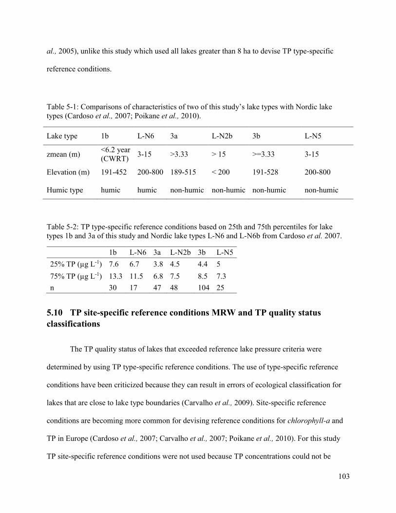
103
al., 2005), unlike this study which used all lakes greater than 8 ha to devise TP type-specific
reference conditions.
Table 5-1: Comparisons of characteristics of two of this study’s lake types with Nordic lake
types (Cardoso et al., 2007; Poikane et al., 2010).
Lake type 1b L-N6 3a L-N2b 3b L-N5
zmean (m) <6.2 year
(CWRT) 3-15 >3.33 > 15 >=3.33 3-15
Elevation (m) 191-452 200-800 189-515 < 200 191-528 200-800
Humic type humic humic non-humic non-humic non-humic non-humic
Table 5-2: TP type-specific reference conditions based on 25th and 75th percentiles for lake
types 1b and 3a of this study and Nordic lake types L-N6 and L-N6b from Cardoso et al. 2007.
1b L-N6 3a L-N2b 3b L-N5
25% TP (µg L-1) 7.6 6.7 3.8 4.5 4.4 5
75% TP (µg L-1) 13.3 11.5 6.8 7.5 8.5 7.3
n 30 17 47 48 104 25
5.10 TP site-specific reference conditions MRW and TP quality status
classifications
The TP quality status of lakes that exceeded reference lake pressure criteria were
determined by using TP type-specific reference conditions. The use of type-specific reference
conditions have been criticized because they can result in errors of ecological classification for
lakes that are close to lake type boundaries (Carvalho et al., 2009). Site-specific reference
conditions are becoming more common for devising reference conditions for chlorophyll-a and
TP in Europe (Cardoso et al., 2007; Carvalho et al., 2007; Poikane et al., 2010). For this study
TP site-specific reference conditions were not used because TP concentrations could not be
104
predicted with enough confidence for each site. Site-specific reference conditions have been
devised for a large number of lakes in the MRW to determine what lakes are in need of
remediation and are compared to the TP quality status classifications of this study (Gartner Lee
Ltd., 2005).
The lakeshore capacity model (LCM) was revised in 2005 and used to devise TP site-
specific reference conditions for lakes of the MRW (Gartner Lee Ltd., 2005). Site-specific
reference conditions define the reference condition for each lake based on its unique landscape
and physico-chemical characteristics (Carvalho et al., 2009; Poikane et al., 2010). The revised
version of the LCM integrated multiple anthropogenic and natural sources of TP in order to
predict the sensitivity of a lake to TP loading. The LCM also identified the TP concentration
threshold (site-specific) when a lake requires restoration actions (Gartner Lee Ltd., 2005). The
threshold value for each lake is established by calculating the predevelopment TP concentration
and adding 50% to that value (Gartner Lee Ltd., 2005). The predevelopment TP concentration is
calculated by modelling the TP concentration in the lake through calculating TP exports from
wetlands, urban areas, agricultural land, and golf courses (Gartner Lee Ltd., 2005). The model
accounts for retention of TP as a function of loss through areal water discharge and
sedimentation (Dillon and Molot, 1996; Gartner Lee Ltd., 2005). The predevelopment condition
is determined by calculating the total TP concentration and subtracting the TP that originates
from human sources (Gartner Lee Ltd., 2005).
Some lakes identified as being over threshold TP concentrations using the LCM were
also determined to have moderate or poor TP quality status in this study using TP type-specific
reference conditions. Silver Lake was classified as having poor TP quality status which
corresponds well to the LCM that identified Silver Lake as over threshold and had high
105
sensitivity to TP loading (Gartner Lee Ltd., 2005). Go Home Lake, Dark Lake, McKay Lake,
and Leech Lake were classified as having moderate TP quality status and are over the threshold
of TP established through the LCM (Gartner Lee Ltd., 2005). Three Mile Lake TP
concentrations are substantially higher than the TP threshold because of high amounts of riparian
agricultural in the past (Gartner Lee Ltd., 2005). This study identified that Three Mile Lake Main
Basin has poor TP quality status, while Three Mile Lake Hammel’s Bay has moderate TP quality
status.
Brandy Lake was also classified as having poor TP quality status according to the TP
type-specific reference conditions. The OMOE conducted a detailed study on Brandy Lake
because the high concentrations of DOC and TP were thought to cause cyanobacterial blooms
(Paterson and Ingram, 2006). Brandy Lake is naturally high in TP because it has a large amount
of wetlands, large DR, and has a relatively shallow depth (Paterson et al., 2006). The lake
typology used in this study accounts for the major factors that naturally cause high TP
concentrations. Brandy Lake belongs to lake type 1b, having lakes with short CWRT and a high
percentage of wetlands. The CWRT accounts for both the large DR and the shallow depth of
Brandy Lake. However, according to the site-specific threshold devised for Brandy Lake by the
LCM Brandy Lake does not have a TP concentration that exceeds threshold (Gartner Lee Ltd.,
2005). Brandy Lake is an example of the downfall of applying type-specific reference conditions
to lakes that are naturally at the upper end of their type-specific reference lake distribution
(Carvalho et al., 2009).
Results from this study can be used to identify additional lakes that are not currently in
the DMM lake monitoring program, and that should undergo operational monitoring to confirm
their TP quality status was correctly classified (WG 2.7, 2003). For example, Robinson Lake in
106
the Town of Huntsville and Duffy Lake in the Township of Muskoka Lakes were both classified
as having poor TP quality status according to their type-specific TP concentrations. Thompson
Lake, Roderick Lake, Fawn Lake, and Weeduck Lake all belong to lake type 1b and have
moderate TP quality status. These lakes could be misclassified according to TP quality status like
Brandy Lake. However, further investigation of lakes from lake type 1b with high TP
concentrations could help water managers and limnologists better understand TP dynamics in
these lakes and may also be important for understanding cyanobacterial blooms (Paterson and
Ingram, 2006).
5.11 Towards a comprehensive lake-monitoring program for the MRW
This study helps to inform the DMM how to adapt the current Lake System Health
program to be a watershed-level comprehensive monitoring program. This study has evaluated
the current Lake System Health Monitoring program and suggests that the monitoring program
requires further improvement and refinement. The results of this study suggest that monitoring
program needs to better account for natural spatial variability of water quality and detect changes
in water quality to implement the appropriate management actions (Foran et al., 2000; Gartner
Lee Ltd., 2005). The sampling of additional reference lakes within each lake type can help to
better quantify the natural physico-chemical and biological condition of a lake and effectively
differentiate trends that are caused by natural factors as opposed to anthropogenic factors (Foran
et al., 2000; Parr et al., 2002; Poikane et al., 2010; REFCOND, 2003).
Monitoring programs that do not include a representative sample of the entire lake
population can result in an inaccurate quantification of physico-chemical and biological trends,
inaccurate type-specific reference conditions, and unsuitable remediation actions (Peterson et al.,
107
1999; Poikane et al., 2010; Strobl et al., 2006: Wang et al., 2010). This study found that the Lake
System Health program is not representative of the population of lakes greater than 8 ha in the
MRW. The Lake System Health program is biased towards deeper and larger lakes that are lower
in mean lake elevation. The monitoring program also samples many more impacted lakes than
reference lakes. Similar biases have been found in state monitoring programs of the Northeastern
United States (Wagner et al., 2008). The state monitoring programs were biased towards
sampling large lakes that were impacted by human activities (Wagner et al., 2008).
The biases of the Lake System Health program may be a result of not monitoring lakes in
the Township of Algonquin Highlands and sampling an inadequate amount of lakes that belong
to lake type 3b. The monitoring lakes of the Lake System Health program have biases in lake
elevation and percent riparian coniferous forest because the Township of Algonquin Highlands
has lakes with the highest elevations and coniferous forest cover of the MRW, which are not
included in the Lake System Health program. The biases of CWRT and zmax in the DMM
monitoring lakes could partially be due to an undersampling of 3b lakes, as they are shallow.
Another source of a bias towards zmax and CWRT in the DMM lakes is that monitoring
programs sample more impacted lakes, which are typically larger and deeper than reference
lakes.
The WFD suggests lakes be monitored and managed at the river basin scale (WG 2.7,
2003). This study took a river basin scale approach to monitoring and management by
considering all lakes within the MRW. The DMM lake monitoring program needs to further
refine their monitoring program to implement a watershed-level approach. The DMM monitors
lakes outside of their district boundary by having partnerships with the Township of Seguin and
Severn Sound Environmental Association monitors lakes in the west part of the MRW (DMM,
108
2014b). However, the eastern part of the MRW is not well monitored because the Township of
Algonquin Highlands does not have a municipal lake monitoring program (Township of
Algonquin Highlands, 2011). Some of the lakes in the Algonquin Highlands are monitored as
part of the OMNR program for lake trout lakes (Township of Algonquin Highlands, 2011).
Monitoring a wider diversity of lakes in the Algonquin Highlands is required in order to
implement a comprehensive monitoring program for the MRW.
An important component to a comprehensive monitoring program is the early detection
of changes in physico-chemistry (Parr et al., 2002). Small and shallow lakes respond faster to
stressors and therefore need to be included in a monitoring program (Arnott et al., 2003; Nõges,
2009). The DMM lake monitoring program does not sample an adequate number of reference
lakes that are within lake type 3b. Lake type 3b is characterized by shallow lakes that are known
to be sensitive to acidification because their LOCAs are high in granite bedrock (Berg et al.,
2005; Mallory et al., 1998; Quinlan et al., 2003). Monitoring reference and impacted lakes from
lake type 3b can help distinguish physico-chemistry and biological changes that are a result of
regional acidification, as opposed to other human activities (Foran et al., 2000). Small lakes have
also been identified to be more sensitive to human activities and, are generally at a higher risk of
having moderate or poor ecological status (Wang et al., 2010).
5.12 Limitations and errors in lake typology
The development of a single lake typology to meet multiple management goals is a
challenge (Soranno et al., 2010). Natural variation in lake physico-chemistry and biological
compositions are influenced by different freshwater and terrestrial landscape variables (Martin et
al., 2011; Free et al., 2006). In the MRW, the differences in associations between landscape
109
variables and lake physico-chemistry were demonstrated. However, it is not practical from a
lake management perspective to use multiple lake typologies (Hering et al., 2010; Martin et al.,
2011). To determine the validity of the MRW lake typology scheme for use as a holistic
monitoring and management tool, the typology requires further testing using biological
indicators. The MRW lake typology developed may not be suitable for all management purposes
and may misclassify lakes due to errors in modelled landscape variables. However, the lake
typology is a primary step in establishing a holistic and cost-effective monitoring program.
The second level of the lake typology could be misclassifying some lakes according to
lake type because the division between lake types is based on modelled parameters that are
inherently error-prone. For example, an underprediction of zmax could result in a lake found
within region 3 being misclassified as lake type 3b. Lakes that are found within region 1 could
also be misclassified because of cumulative errors in lake volumes resulting from errors in the
lake depth model. The CWRT index may not be the most accurate measure of CWRT because it
was calculated with the same mean annual runoff for all watersheds. Differences in local
precipitation and stream discharge led to variations in mean annual runoff between watersheds
(Paterson et al., 2006). However, increased data availability and more sophisticated modelling
approaches will likely lead to improved iterations of the lake typology for MRW. For example,
bathymetric LiDAR is now a feasible technology and can be used to capture lake depth
information over large lake districts (Hilldale and Raff, 2008).
Despite limitations with the lake typology, it is hypothesized that the new MRW lake
typology will have some ecological relevance based on the landscape variables it includes. For
example, an Irish lake typology for establishing phytoplankton reference conditions included
alkalinity, COLTR, and zmean (Free et al., 2006). Free et al. (2006) hypothesized that WRT may
110
be an important factor in differentiating phytoplankton community compositions because of its
influence on nutrient concentrations. The variance of littoral invertebrate compositions in
reference lakes of Ireland was primarily explained by percent peat, pH, alkalinity, and COND25
(Free et al., 2006). The variables of CWRT, zmax, and percent LOCA wetland, included in the
MRW lake typology are related to most of the variables used in the littoral invertebrates and
phytoplankton typologies. Alkalinity and conductivity are not suitable variables for inclusion in
the MRW lake typology because these variables deviate from reference conditions in the
majority of the MRW lakes because of regional acidic deposition and application of road salts
and dust suppressants (Cardoso et al., 2007; Palmer et al., 2011).
5.13 Future directions for lake management and research in the MRW
The lake typology developed as part of this study provides a basis to further explore the
temporal variability of water quality and determine optimal sampling frequency (Strobl and
Robillard, 2008; WG 2.7, 2003). It is hypothesized that some of the lake types will require
different sampling frequencies. For example, the shallow lakes (3b) and the lakes with the short
CWRT (1b) are expected to need to be sampled at a higher frequency. Shallow lakes are more
sensitive to inter-annual variability in precipitation and temperate (Choi, 1998; Nõges, 2009).
Lakes with shorter WRTs exhibit higher inter-annual and intra-annual variability in some water
quality variables such as pH and base cations (Arnott et al., 2003). The determination of optimal
sampling frequency requires a high sampling frequency for a few lakes within each lake type
(Arnott et al., 2003; Strobl and Robillard, 2008).
The associations between landscape variables and water quality in the MRW can be
further explored with satellite imagery. The use of satellite imagery may provide a better way to
111
quantify the association between catchment vegetation and DOC, which has been reported by
other studies to have a strong association (Canham et al., 2004; Scott et al., 2010). In the MRW,
the vegetation classes of coniferous and deciduous forest did not have a detectable influence on
DOC concentrations. Normalized difference vegetation index (NDVI) was the strongest
predictor of DOC concentrations in a set of Norwegian lakes (Larsen et al., 2011). NDVI
measures the overall health and density of vegetation through the use of red and near-infrared
bands of satellite imagery (Larsen et al., 2011; Lilles et al., 2008). NDVI may be a better
predictor of DOC than forest cover alone because it includes all vegetation including wetland
and forest vegetation. Future landscape limnology work in the MRW should incorporate NDVI
from readily available satellite imagery such as Landsat or SPOT.
In summary, the monitoring and management framework presented in this study,
provides a foundation for holistic management of lakes in the MRW. However, this framework
will need to be continuously revised and updated as additional lakes are sampled, and when
better data is available (Rowan et al., 2010; UKTAG, 2007; WG 2.7, 2003). For example, the
lake typology can be updated when higher resolution satellite imagery becomes available and
lake depth can be predicted with higher accuracy. In addition, the monitoring program will need
to be updated to effectively monitor and manage current and emerging stressors as they are
identified by the current lake monitoring program (Parr et al., 2002; Strobl et al., 2006).
112
6. CONCLUSION
The overarching objective of this study was to develop and apply a landscape-based lake
typology to the lakes of the MRW, Ontario, Canada, to assist lake management decisions.
Machine learning and tree-based methods were applied to better understand relationships
between landscape characteristics and water quality, and select landscape variables to develop a
lake typology. Parametric and descriptive statistics were applied to establish TP type-specific
reference conditions, which identified lakes that may be in need of restoration because of high
TP levels. A statistical evaluation of the DMM monitoring program was conducted using the
lake typology and derived natural landscape characteristics.
The MRW lake typology shares many similarities with European lake typologies, especially
lake typologies for Nordic regions. However, the MRW lake typology is unique because it
includes modelled lake depths and CWRTs. Modelled Zmax and CWRT were important
components of the lake typology in differentiating lake types according to natural physico-
chemistry gradients (DOC, TP). CWRT is an important metric for explaining DOC variation for
non-headwater lakes because it is a spatially explicit variant of WRT that considers time spent in
upstream lakes. Percent LOCA wetland was another key attribute of the typology because
wetlands act as a source of DOC, TP, and humic acids in lake surface waters. Other studies
support the theory that the MRW lake typology is ecologically relevant because it distinguishes
some lake types based on stratification and has similar variables to typologies based on littoral
invertebrates and phytoplankton.
The application of the lake typology resulted in recommendations to assist the DMM in
adapting their current monitoring program to be more comprehensive. It is recommended that
113
more lakes be sampled to obtain a representative sample of all lake types, to assist with TP
restoration efforts throughout the MRW, and to establish type-specific reference conditions for
Ca. Lakes need to be sampled that are within the Township of Algonquin Highlands to account
for natural landscape gradients of the MRW. More shallow lakes with rock dominated LOCAs
(lake type 3b) need to be sampled, especially because they are the most numerous in the MRW
and possibly the most sensitive to stressors. Robinson Lake, Weeduck Lake, Thompson Lake,
Roderick Lake, and Duffy Lake should be sampled to confirm they are in need of restoration
because of high TP concentrations. To help establish Ca type-specific reference conditions and
better understand the natural variability of Ca concentrations in the lakes of the MRW, more
lakes that have no roads in their CUCAs should be sampled.
Overall, this thesis demonstrates the advantages of using a statistical and landscape-based
approach to advance limnological research, and lake management. In future studies, machine
learning methods should be used for development of lake typologies in new lake districts
because of its effectiveness in variable selection. Current and future lake typologies should test
the use of landscape-based models to predict measures of lake morphometry and CWRT. CWRT
should also be tested in other boreal regions that are surface-water dominated and have non-
headwater lakes.
114
REFERENCES
Agouridis, C., Edwards, D., Workman, S., Bicudo, J., Koostra, B., Vanzant, E., & Taraba, J.
(2005). Streambank erosion associated with grazing practices in the humid
region. Transactions-American Society of Agricultural Engineers, 48(1), 181.
Angermeier, P. L., Smogor, R. A., & Stauffer, J. R. (2000). Regional frameworks and candidate
metrics for assessing biotic integrity in mid-Atlantic highland streams. Transactions of the
American Fisheries Society, 129(4), 962-981.
Anzecc, A. (2000). Australian and New Zealand guidelines for fresh and marine water
quality. Australian and New Zealand Environment and Conservation Council and
Agriculture and Resource Management Council of Australia and New Zealand, Canberra,
1-103.
Apitz, S. E., Elliott, M., Fountain, M., & Galloway, T. S. (2006). European environmental
management: moving to an ecosystem approach. Integrated Environmental Assessment and
Management, 2(1), 80-85.
Apitz, S., & White, S. (2003). A conceptual framework for river-basin-scale sediment
management. Journal of Soils and Sediments, 3(3), 132-138.
Arheimer, B., & Liden, R. (2000). Nitrogen and phosphorus concentrations from agricultural
catchments—influence of spatial and temporal variables. Journal of Hydrology, 227(1),
140-159.
Armour, C., Duff, D., & Elmore, W. (1991). The effects of livestock grazing on riparian and
stream ecosystems. Fisheries, 16(1), 7-11.
Arnott, S. E., Dillon, P. J., Somers, K., & Keller, B. (2003). Inter-and intra-annual chemical
variability during the ice-free season in lakes with different flushing rates and acid
deposition histories. Environmental Monitoring and Assessment, 88(1-3), 21-37.
Bailey, R. C., Norris, R. H., & Reynoldson, T. B. (2004). Bioassessment of freshwater
ecosystems. New York, United States: Springer.
Beven, K. J., & Kirkby, M. J. (1979). A physically based, variable contributing area model of
basin hydrology. Hydrological Sciences, 24(1)
Böhner, J., & Selige, T. (2006). Spatial prediction of soil attributes using terrain analysis and
climate regionalisation. SAGA-Analysis and Modelling Applications. Göttingen, Göttinger
Geographische Abhandlungen, 13-28.
115
Borre, L., Barker, D. R., & Duker, L. E. (2001). Institutional arrangements for managing the
great lakes of the world: Results of a workshop on implementing the watershed
approach. Lakes & Reservoirs: Research & Management, 6(3), 199-209.
Brack, W., Apitz, S. E., Borchardt, D., Brils, J., Cardoso, A. C., Foekema, E. M., . . . Hein, M.
(2009). Toward a holistic and risk‐based management of European river basins. Integrated
Environmental Assessment and Management, 5(1), 5-10.
Bremigan, M. T., Soranno, P. A., Gonzalez, M. J., Bunnell, D. B., Arend, K. K., Renwick, W.
H., . . . Vanni, M. J. (2008). Hydrogeomorphic features mediate the effects of land use/cover
on reservoir productivity and food webs. Limnology and Oceanography, 53(4), 1420.
Brenning, A. (2008). Statistical geocomputing combining R and SAGA: The example of
landslide susceptibility analysis with generalized additive models. SAGA–Seconds
Out.Hamburger Beiträge Zur Physischen Geographie Und Landschaftsökologie, 19, 23-32.
Brown, B. S., Detenbeck, N. E., & Eskin, R. (2005). How probability survey data can help
integrate 305 (b) and 303 (d) monitoring and assessment of state waters. Environmental
Monitoring and Assessment, 103(1-3), 41-57.
Buraschi, E., Salerno, F., Monguzzi, C., Barbiero, G., & Tartari, G. (2005). Characterization of
the Italian lake-types and identification of their reference sites using anthropogenic pressure
factors. Journal of Limnology, 64(1), 75-84.
Canadian Water Network. (2013). Muskoka River Watershed Node. Retrieved 07/25, 2014,
from http://www.cwn-rce.ca/initiatives/canadian-watershed-research-consortium/muskoka-
river-watershed-node/
Canham, C., Pace, M., Papaik, M., Primack, A., Roy, K., Maranger, R., . . . Spada, D. (2004). A
spatially explicit watershed-scale analysis of dissolved organic carbon in Adirondack
lakes. Ecological Applications, 14(3), 839-854. doi:10.1890/02-5271
Cardille, J. A., Carpenter, S. R., Coe, M. T., Foley, J. A., Hanson, P. C., Turner, M. G., & Vano,
J. A. (2007). Carbon and water cycling in lake‐rich landscapes: Landscape connections, lake
hydrology, and biogeochemistry. Journal of Geophysical Research: Biogeosciences (2005–
2012), 112(G2)
Cardoso, A., Solimini, A., Premazzi, G., Carvalho, L., Lyche, A., & Rekolainen, S. (2007).
Phosphorus reference concentrations in European lakes. Hydrobiologia, 584(1), 3-12.
Carpenter, S. R. (1983). Lake geometry: implications for production and sediment accretion
rates. Journal of Theoretical Biology, 105(2), 273-286.
Carpenter, S. R., & Lathrop, R. C. (2014). Phosphorus loading, transport and concentrations in a
lake chain: a probabilistic model to compare management options. Aquatic Sciences, 76(1),
145-154. doi:10.1007/s00027-013-0324-5
116
Carpenter, S. R., Stanley, E. H., & Vander Zanden, M. J. (2011). State of the World's Freshwater
Ecosystems: Physical, Chemical, and Biological Changes. Annual Review of Environment
and Resources, 36(1), 75-99. doi:10.1146/annurev-environ-021810-094524
Carvalho, L., Solimini, A. G., Phillips, G., Pietilainen, O., Moe, J., Cardoso, A. C., . . .
Rekolainen, S. (2009). Site-specific chlorophyll reference conditions for lakes in Northern
and Western Europe. Hydrobiologia, 633(1), 59-66. doi:10.1007/s10750-009-9876-8
Catherine, A., Mouillot, D., Escoffier, N., Bernard, C., & Troussellier, M. (2010). Cost effective
prediction of the eutrophication status of lakes and reservoirs. Freshwater Biology, 55(11),
2425-2435. doi:10.1111/j.1365-2427.2010.02452.x
Cheruvelil, K. S., Soranno, P. A., Webster, K. E., & Bremigan, M. T. (2013). Multi-scaled
drivers of ecosystem state: quantifying the importance of the regional spatial
scale. Ecological Applications, 23(7), 1603-1618. doi:10.1890/12-1872.1
Cheruvelil, K. S., Soranno, P. A., Bremigan, M. T., Wagner, T., & Martin, S. L. (2008).
Grouping lakes for water quality assessment and monitoring: The roles of regionalization
and spatial scale. Environmental Management, 41(3), 425-440. doi:10.1007/s00267-007-
9045-7
Christensen, M. R., Graham, M. D., Vinebrooke, R. D., Findlay, D. L., Paterson, M. J., &
Turner, M. A. (2006). Multiple anthropogenic stressors cause ecological surprises in boreal
lakes. Global Change Biology, 12(12), 2316-2322. doi:10.1111/j.1365-2486.2006.01257.x
Choi, J. S. (1998). Lake ecosystem responses to rapid climate change. Environmental Monitoring
and Assessment, 49(2-3), 281-290.
Corbett, C. W., Wahl, M., Porter, D. E., Edwards, D., & Moise, C. (1997). Nonpoint source
runoff modeling A comparison of a forested watershed and an urban watershed on the South
Carolina coast. Journal of Experimental Marine Biology and Ecology, 213(1), 133-149.
Cronan, C., & Reiners, W. (1983). Canopy Processing of Acidic Precipitation by Coniferous and
Hardwood Forests in New-England. Oecologia, 59(2-3), 216-223. doi:10.1007/BF00378839
Cuthbert, I., & Delgiorgio, P. (1992). Toward a Standard Method of Measuring Color in Fresh-
Water. Limnology and Oceanography, 37(6), 1319-1326.
D'Arcy, P., & Carignan, R. (1997). Influence of catchment topography on water chemistry in
southeastern Quebec Shield lakes. Canadian Journal of Fisheries and Aquatic
Sciences, 54(10), 2215-2227. doi:10.1139/cjfas-54-10-2215
De’ath, G. (2013). mvpart: multivariate partitioning. rpart by Terry M Therneau and Beth
Atkinson. R Port of Rpart by Brian Ripley. some Routines from vegan–Jari Oksanen.
Extensions and Adaptations of Rpart to Mvpart by Glenn De’ath. (2013). Mvpart:
117
Multivariate Partitioning. R Package Version 1.6-1.Available from Cran.r-
Project.org/package= Mvpart,
De'ath, G., & Fabricius, K. (2000). Classification and regression trees: A powerful yet simple
technique for ecological data analysis. Ecology, 81(11), 3178-3192. doi:10.1890/0012-
9658(2000)081[3178:CARTAP]2.0.CO;2
Dorset Environmental Science Centre. (2014). Long-term Ecosystem Science. Retrieved 12/13,
2014, from http://desc.ca/iwr
Dietterich, T. G. (2000). An experimental comparison of three methods for constructing
ensembles of decision trees: Bagging, boosting, and randomization. Machine
Learning, 40(2), 139-157.
Dillon, P. J., & Molot, L. A. (2005). Long‐term trends in catchment export and lake retention of
dissolved organic carbon, dissolved organic nitrogen, total iron, and total phosphorus: The
Dorset, Ontario, study, 1978–1998. Journal of Geophysical Research: Biogeosciences
(2005–2012), 110(G1)
Dillon, P., Reid, R., & Evans, H. (1993). The relative magnitude of phosphorus sources for
small, oligotrophic lakes in Ontario, Canada. Trav. Assoc. Int. Limnol. Theor. Appl, 25(1)
Dillon, P., & Rigler, F. (1975). A simple method for predicting the capacity of a lake for
development based on lake trophic status. Journal of the Fisheries Board of Canada, 32(9),
1519-1531.
Dillon, P., & Molot, L. (1996). Long-term phosphorus budgets and an examination of a steady-
state mass balance model for central Ontario lakes. Water Research, 30(10), 2273-2280.
doi:10.1016/0043-1354(96)00110-8
Dillon, P., & Molot, L. (1997). Effect of landscape form on export of dissolved organic carbon,
iron, and phosphorus from forested stream catchments. Water Resources Research, 33(11),
2591-2600. doi:10.1029/97WR01921
Dronkers, J., & Zimmerman, J. (1982). Some principles of mixing in tidal lagoons.
Oceanologica Acta, 4, 107-118.
Dube, M., Johnson, B., Dunn, G., Culp, J., Cash, K., Munkittrick, K., . . . Storey, A. (2006).
Development of a new approach to cumulative effects assessment: A Northern River
Ecosystem example. Environmental Monitoring and Assessment, 113(1-3), 87-115.
doi:10.1007/s10661-005-9098-0
Eimers, C. (2012). Managing cumulative effects in the Muskoka River Watershed: Monitoring,
research and predictive modeling. (Proposal Canadian Water Network).
118
Eimers, M. C., Watmough, S. A., Paterson, A. M., Dillon, P. J., & Yao, H. (2009). Long-term
declines in phosphorus export from forested catchments in south-central Ontario. Canadian
Journal of Fisheries and Aquatic Sciences, 66(10), 1682-1692. doi:10.1139/F09-101
Elith, J., Leathwick, J. R., & Hastie, T. (2008). A working guide to boosted regression
trees. Journal of Animal Ecology, 77(4), 802-813.
Epstein, D. M., Neilson, B. T., Goodman, K. J., Stevens, D. K., & Wurtsbaugh, W. A. (2013). A
modeling approach for assessing the effect of multiple alpine lakes in sequence on nutrient
transport. Aquatic Sciences, 75(2), 199-212. doi:10.1007/s00027-012-0267-2
ESRI. (2011). Release 10: ArcGIS Desktop. Redlands, CA: Environmental Systems Research
Institute.
Feld, C. K. (2013). Response of three lotic assemblages to riparian and catchment‐scale land use:
implications for designing catchment monitoring programmes. Freshwater Biology, 58(4),
715-729.
Finstad, A. G., Helland, I. P., Ugedal, O., Hesthagen, T., & Hessen, D. O. (2014). Unimodal
response of fish yield to dissolved organic carbon. Ecology Letters, 17(1), 36-43.
Fölster, J., Sandin, L., & Wallin, M. (2004). A suggestion to a typology for Swedish inland
surface waters according to the EU Water Framework Directive Sveriges lantbruksuniv.
Foran, J., Brosnan, T., Connor, M., Delfino, J., Depinto, J., Dickson, K., . . . Sobsey, M. (2000).
A framework for comprehensive, integrated, watershed monitoring in New York
City. Environmental Monitoring and Assessment, 62(2), 147-167.
Free, G., Little, R., Tierney, D., Donnelly, K., & Caroni, R. (2006). A reference based typology
and ecological assessment system for Irish lakes-preliminary
investigations. Environmental Protection Agency, Wexford. www. epa. ie, 266.
Fraterrigo, J. M., & Downing, J. A. (2008). The Influence of Land Use on Lake Nutrients Varies
with Watershed Transport Capacity. Ecosystems, 11(7), 1021-1034. doi:10.1007/s10021-
008-9176-6
Friedman, J. H. (2001). Greedy function approximation: a gradient boosting machine. Annals of
Statistics, 1189-1232.
Friedman, J. H., & Meulman, J. J. (2003). Multiple additive regression trees with application in
epidemiology. Statistics in Medicine, 22(9), 1365-1381.
Gartner Lee Limited. (2005). Recreational water quality management in Muskoka. (No. GLL 20-
497).
119
Geier, T. W., Perry, J. A., & Queen, L. (1994). Improving lake riparian source area management
using surface and subsurface runoff indices. Environmental Management, 18(4), 569-586.
Gergel, S., Turner, M., & Kratz, T. (1999). Dissolved organic carbon as an indicator of the scale
of watershed influence on lakes and rivers. Ecological Applications, 9(4), 1377-1390.
doi:10.2307/2641403
Gibson, G. (2000). Nutrient criteria technical guidance manual: Lakes and reservoirs US
Environmental Protection Agency, Office of Water, Office of Science and Technology.
Girard, R., Clark, B., Yan, N., Reid, R., David, S., Ingram, R., & Findeis, J. (2007). DATA
REPORT 2007.
Government of Ontario. (2012a). Land Information Ontario data description: Watershed,
Secondary. Queen's Printer for Ontario.
Government of Ontario. (2012b). Land Information Ontario data description: Watershed,
Tertiary. Queen's Printer for Ontario.
Håkanson, L. (2005). The importance of lake morphometry and catchment characteristics in
limnology - ranking based on statistical analyses. Hydrobiologia, 541, 117-137.
doi:10.1007/s10750-004-5032-7
Hanson, P. C., Carpenter, S. R., Cardille, J. A., Coe, M. T., & Winslow, L. A. (2007). Small
lakes dominate a random sample of regional lake characteristics. Freshwater Biology, 52(5),
814-822.
Hanson, P. C., Hamilton, D. P., Stanley, E. H., Preston, N., Langman, O. C., & Kara, E. L.
(2011). Fate of allochthonous dissolved organic carbon in lakes: a quantitative
approach. PLoS One, 6(7), e21884.
Hastie, T., Tibshirani, R., & Friedman, J. (2001). The elements of statistical learning: data
mining, inference and prediction. New York: Springer-Verlag, 1(8), 371-406.
Hendriks, M. R. (2010). Introduction to Physical Hydrology. New York: Oxford University
Press Inc.
Hering, D., Borja, A., Carstensen, J., Carvalho, L., Elliott, M., Feld, C. K., . . . van de Bund, W.
(2010). The European Water Framework Directive at the age of 10: A critical review of the
achievements with recommendations for the future. Science of the Total
Environment, 408(19), 4007-4019. doi:10.1016/j.scitotenv.2010.05.031
Hering, D., Carvalho, L., Argillier, C., Beklioglu, M., Borja, A., Cardoso, A. C., . . . Birk, S.
Managing aquatic ecosystems and water resources under multiple stress — An introduction
to the MARS project. Science of the Total Environment, (0)
doi:http://dx.doi.org/10.1016/j.scitotenv.2014.06.106
120
Higgins, J. V., Bryer, M. T., Khoury, M. L., & Fitzhugh, T. W. (2005). A freshwater
classification approach for biodiversity conservation planning. Conservation Biology, 19(2),
432-445.
Hijmans, R. J., Phillips, S., Leathwick, J., Elith, J., & Hijmans, M. R. J. (2013). dismo: Species
distribution modeling (R package version 0.9-3 ed.)
Hilldale, R. C., & Raff, D. (2008). Assessing the ability of airborne LiDAR to map river
bathymetry. Earth Surface Processes and Landforms, 33(5), 773-783.
Hinton, M., Schiff, S., & English, M. (1998). Sources and flowpaths of dissolved organic carbon
during storms in two forested watersheds of the Precambrian
Shield. Biogeochemistry, 41(2), 175-197. doi:10.1023/A:1005903428956
Hoffman, D. W., Wicklund, R., & Richards, N. (1962). Soil Survey of Parry Sound District,
Ontario Research Branch, Canada Department of Agriculture.
Hollister, J. W., Milstead, W. B., & Urrutia, M. A. (2011). Predicting maximum lake depth from
surrounding topography. PloS One, 6(9), e25764.
Hothorn, T., & Zeileis, A. (2014). Partykit: A Modular Toolkit for Recursive Partytioning in R.
Working Paper 2014-10. Working Papers in Economics and Statistics, Research Platform
Empirical and Experimental Economics, Universitaet Innsbruck.
URL Http://EconPapers.RePEc.org/RePEc:Inn:Wp,
Houle, D., Ouimet, R., Couture, S., & Gagnon, C. (2006). Base cation reservoirs in soil control
the buffering capacity of lakes in forested catchments. Canadian Journal of Fisheries and
Aquatic Sciences, 63(3), 471-474.
Hughes, R., Paulsen, S., & Stoddard, J. (2000). EMAP-Surface Waters: a multiassemblage,
probability survey of ecological integrity in the USA Springer.
Illies, J. (1978). Limnofauna Europaea (2nd ed.). New York: Gustav Fischer Verlag.
IMPRESS. (2003). Guidelines for the analysis of pressures and impacts in accordance with the
Water Framework Directive. CIS Working Group 2.1, Office for Official Publications of the
European Communities.
Ito, M., Mitchell, M. J., Driscoll, C. T., & Roy, K. M. (2005). Factors affecting acid neutralizing
capacity in the Adirondack region of New York: a solute mass balance
approach. Environmental Science & Technology, 39(11), 4076-4081.
Jeffries, D., & Snyder, W. (1983). Geology and geochemistry of the Muskoka-Haliburton study
area. Data Report DR, 83(2)
121
Jeffries, D., Clair, T., Couture, S., Dillon, P., Dupont, J., Keller, W., . . . Weeber, R. (2003).
Assessing the recovery of lakes in southeastern Canada from the effects of acidic
deposition. Ambio, 32(3), 176-182. doi:10.1639/0044-
7447(2003)032[0176:ATROLI]2.0.CO;2
Jenerette, G. D., Lee, J., Waller, D. W., & Carlson, R. E. (2002). Multivariate analysis of the
ecoregion delineation for aquatic systems. Environmental Management, 29(1), 67-75.
doi:10.1007/s00267-001-0041-z
Jeziorski, A., Yan, N. D., Paterson, A. M., DeSellas, A. M., Turner, M. A., Jeffries, D. S., . . .
Smol, J. P. (2008). The Widespread Threat of Calcium Decline in Fresh
Waters. Science, 322(5906), 1374-1377. doi:10.1126/science.1164949
Johansson, H., Brolin, A. A., & Håkanson, L. (2007). New approaches to the modelling of lake
basin morphometry. Environmental Modeling & Assessment, 12(3), 213-228.
Johnson, R. (1999). Regional representativeness of Swedish reference lakes. Environmental
Management, 23(1), 115-124. doi:10.1007/s002679900172
Jones, J., Knowlton, M., Obrecht, D., & Cook, E. (2004). Importance of landscape variables and
morphology on nutrients in Missouri reservoirs. Canadian Journal of Fisheries and Aquatic
Sciences, 61(8), 1503-1512. doi:10.1139/F04-088
Jun, S. (2013). Boosted regression trees and random forests. (Statistical Consulting Report).
Vancouver, BC: Department of Statistics, UBC.
Kagalou, I., & Leonardos, I. (2009). Typology, classification and management issues of Greek
lakes: implication of the Water Framework Directive (2000/60/EC). Environmental
Monitoring and Assessment, 150(1-4), 469-484. doi:10.1007/s10661-008-0245-2
Kalff, J. (2002). Limnology: inland water ecosystems. Upper Saddle River, NJ: Prentice-Hall Inc.
Keller, W. (2009). Limnology in northeastern Ontario: from acidification to multiple
stressors. Canadian Journal of Fisheries and Aquatic Sciences, 66(7), 1189-1198.
doi:10.1139/F09-080
Keller, W., Paterson, A. M., Somers, K. M., Dillon, P. J., Heneberry, J., & Ford, A. (2008).
Relationships between dissolved organic carbon concentrations, weather, and acidification
in small Boreal Shield lakes. Canadian Journal of Fisheries and Aquatic Sciences, 65(5),
786-795.
Keller, W., Dixit, S. S., & Heneberry, J. (2001). Calcium declines in northeastern Ontario lakes.
Canadian Journal of Fisheries and Aquatic Sciences, 58(10), 2011-2020. doi:10.1139/cjfas-
58-10-2011
122
Kling, G. W., Kipphut, G. W., Miller, M. M., & O'Brien, W. J. (2000). Integration of lakes and
streams in a landscape perspective: the importance of material processing on spatial patterns
and temporal coherence. Freshwater Biology, 43(3), 477-497. doi:10.1046/j.1365-
2427.2000.00515.x
Knight, R. D., & Kerr, D. E. (2007). An overburden thickness model for Lac de Gras and
Aylmer Lake, Northwest Territories, Canada. Journal of Maps, 3(1), 296-310.
Kolada, A., Soszka, H., Cydzik, D., & Golub, M. (2005). Abiotic typology of Polish
lakes. Limnologica, 35(3), 145-150. doi:10.1016/j.limno.2005.04.001
Kortelainen, P. (1993). Content of Total Organic-Carbon in Finnish Lakes and its Relationship to
Catchment Characteristics. Canadian Journal of Fisheries and Aquatic Sciences, 50(7),
1477-1483.
Kortelainen, P., Mattsson, T., Finér, L., Ahtiainen, M., Saukkonen, S., & Sallantaus, T. (2006).
Controls on the export of C, N, P and Fe from undisturbed boreal catchments,
Finland. Aquatic Sciences, 68(4), 453-468.
Kothawala, D. N., Stedmon, C. A., Müller, R. A., Weyhenmeyer, G. A., Köhler, S. J., &
Tranvik, L. J. (2014). Controls of dissolved organic matter quality: evidence from a
large‐scale boreal lake survey. Global Change Biology, 20(4), 1101-1114.
Kratz, T., Webster, K., Bowser, C., Maguson, J., & Benson, B. (1997). The influence of
landscape position on lakes in northern Wisconsin. Freshwater Biology, 37(1), 209-217.
Kullberg, A., Bishop, K., Hargeby, A., Jansson, M., & Petersen, R. (1993). The Ecological
Significance of Dissolved Organic-Carbon in Acidified Waters. Ambio, 22(5), 331-337.
Lamon, E.Conrad,,III, Malve, O., & Pietilainen, O. (2008). Lake classification to enhance
prediction of eutrophication endpoints in Finnish lakes. Environmental Modelling &
Software, 23(7), 938-947. doi:10.1016/j.envsoft.2007.10.008
Larsen, S., Andersen, T., & Hessen, D. O. (2011). Predicting organic carbon in lakes from
climate drivers and catchment properties. Global Biogeochemical Cycles, 25(3)
Larson, G. L., Lomnicky, G., Hoffman, R., Liss, W. J., & Deimling, E. (1999). Integrating
physical and chemical characteristics of lakes into the glacially influenced landscape of the
Northern Cascade Mountains, Washington State, USA. Environmental Management, 24(2),
219-228.
Larson, J. H., Frost, P. C., Zheng, Z., Johnston, C. A., Bridgham, S. D., Lodge, D. M., &
Lamberti, G. A. (2007). Effects of upstream lakes on dissolved organic matter in
streams. Limnology and Oceanography, 52(1), 60-69.
123
Lilles, T. M., Kiefer, T. M., & Chipman, J. W. (2008). Remote Sensing and Image
Interpretation (sixth edition ed.). Hoboken, NJ: John Wiley & Sons Inc.
Løkke , H. (2010). Novel methods for integrated risk assessment of cumulative stressors -
Results from the NoMiracle project. Science of the Total Environment, 408(18), 3719-3724.
doi:10.1016/j.scitotenv.2010.05.009
Lottig, N. R., Stanley, E. H., & Maxted, J. T. (2012). Assessing the influence of upstream
drainage lakes on fluvial organic carbon in a wetland‐rich region. Journal of Geophysical
Research: Biogeosciences (2005–2012), 117(G3)
Lottig, N. R., Stanley, E. H., Hanson, P. C., & Kratz, T. K. (2011). Comparison of regional
stream and lake chemistry: Differences, similarities, and potential drivers. Limnology and
Oceanography, 56(5), 1551-1562. doi:10.4319/lo.2011.56.5.1551
Mallory, M., McNicol, D., Cluis, D., & Laberge, C. (1998). Chemical trends and status of small
lakes near Sudbury, Ontario, 1983-1995: evidence of continued chemical
recovery. Canadian Journal of Fisheries and Aquatic Sciences, 55(1), 63-75.
doi:10.1139/cjfas-55-1-63
Martin, S. L., Soranno, P. A., Bremigan, M. T., & Cheruvelil, K. S. (2011). Comparing
Hydrogeomorphic Approaches to Lake Classification. Environmental Management, 48(5),
957-974. doi:10.1007/s00267-011-9740-2
McGuire, K., McDonnell, J., Weiler, M., Kendall, C., McGlynn, B., Welker, J., & Seibert, J.
(2005). The role of topography on catchment-scale water residence time. Water Resources
Research, 41(5), W05002. doi:10.1029/2004WR003657
Mikulyuk, A., Sharma, S., Van Egeren, S., Erdmann, E., Nault, M. E., & Hauxwell, J. (2011).
The relative role of environmental, spatial, and land-use patterns in explaining aquatic
macrophyte community composition. Canadian Journal of Fisheries and Aquatic
Sciences, 68(10), 1778-1789.
Millar, C. (1974). Decomposition of coniferous leaf litter. Biology of Plant Litter
Decomposition, 1, 105-128.
Milstead, W. B., Hollister, J. W., Moore, R. B., & Walker, H. A. (2013). Estimating Summer
Nutrient Concentrations in Northeastern Lakes from SPARROW Load Predictions and
Modeled Lake Depth and Volume. PloS One, 8(11), e81457.
Molot, L. A., & Dillon, P. J. (2008). Long-term trends in catchment export and lake
concentrations of base cations in the Dorset study area, central Ontario. Canadian Journal
of Fisheries and Aquatic Sciences, 65(5), 809-820. doi:10.1139/F08-035
124
Molot, L., & Dillon, P. (1997). Colour - mass balances and colour - dissolved organic carbon
relationships in lakes and streams in central Ontario. Canadian Journal of Fisheries and
Aquatic Sciences, 54(12), 2789-2795. doi:10.1139/cjfas-54-12-2789
Monteith, D. T., Stoddard, J. L., Evans, C. D., de Wit, H. A., Forsius, M., Hogasen, T., . . .
Vesely, J. (2007). Dissolved organic carbon trends resulting from changes in atmospheric
deposition chemistry. Nature, 450(7169), 537-U9. doi:10.1038/nature06316
Moss, B. (2007). Shallow lakes, the water framework directive and life. What should it all be
about? Shallow Lakes in a Changing World (pp. 381-394) Springer.
Moss, B., Stephen, D., Alvarez, C., Becares, E., Bund, W. V. D., Collings, S., . . .
Fernández‐Aláez, C. (2003). The determination of ecological status in shallow lakes—a
tested system (ECOFRAME) for implementation of the European Water Framework
Directive. Aquatic Conservation: Marine and Freshwater Ecosystems, 13(6), 507-549.
Moss, B. (2008). The Water Framework Directive: Total environment or political
compromise? Science of the Total Environment, 400(1-3), 32-41.
doi:10.1016/j.scitotenv.2008.04.029
Muller, R. A., Futter, M. N., Sobek, S., Nisell, J., Bishop, K., & Weyhenmeyer, G. A. (2013).
Water renewal along the aquatic continuum offsets cumulative retention by lakes:
implications for the character of organic carbon in boreal lakes. Aquatic Sciences, 75(4),
535-545. doi:10.1007/s00027-013-0298-3
Nelson, S., Soranno, P., Cheruvelil, K., Batzli, S., Skole,D. (2003). Regional assessment of lake
water clarity using satellite remote sensing. Journal of Limnology, 62(1s)
Nixon, S., Grath, J., & Bøgestrand, J. (1998). EUROWATERNET: The European Environment
Agency's Monitoring and Information Network for Inland Water Resources-Technical
Guidelines for Implementation. Final Draft,
Nõges, P., Van De Bund, W., Cardoso, A. C., Solimini, A. G., & Heiskanen, A. (2009).
Assessment of the ecological status of European surface waters: a work in
progress. Hydrobiologia, 633(1), 197-211.
Nõges, T. (2009). Relationships between morphometry, geographic location and water quality
parameters of European lakes. Hydrobiologia, 633(1), 33-43.
Nykänen, M., Kairesalo, T., Makela, S., Huitu, E., Ala-Opas, P., & Mannio, J. (2005). A
typology and ecological classification system for Finnish lakes: applicability of the
ECOFRAME scheme. Boreal Environment Research, 10(3), 159-179.
O'Connor, E. M., Dillon, P. J., Molot, L. A., & Creed, I. F. (2009). Modeling dissolved organic
carbon mass balances for lakes of the Muskoka River Watershed. Hydrology
Research, 40(2-3), 273-290. doi:10.2166/nh.2009.106
125
Oehler, F., & Elliott, A. (2011). Predicting stream N and P concentrations from loads and
catchment characteristics at regional scale: A concentration ratio method. Science of the
Total Environment, 409(24), 5392-5402.
Omernik, J. M. (1987). Ecoregions of the conterminous United States. Annals of the Association
of American Geographers, 77(1), 118-125.
Ontario Ministry of Natural Resources. (2006). Muskoka River Water Management Plan. Ontario
Power Generation.
Ormerod, S. J., Dobson, M., Hildrew, A. G., & Townsend, C. R. (2010). Multiple stressors in
freshwater ecosystems. Freshwater Biology, 55, 1-4. doi:10.1111/j.1365-2427.2009.02395.x
Palmer, M., Higgins, J., & Gah, E. (2012). A Freshwater Classification of the Mackenzie River
Basin. Yellowknife, NT: Northwest Territories Protected Areas Strategy Science Team.
Palmer, M. E., Yan, N. D., Paterson, A. M., & Girard, R. E. (2011). Water quality changes in
south-central Ontario lakes and the role of local factors in regulating lake response to
regional stressors. Canadian Journal of Fisheries and Aquatic Sciences, 68(6), 1038-1050.
doi:10.1139/F2011-041
Parisien, M., & Moritz, M. A. (2009). Environmental controls on the distribution of wildfire at
multiple spatial scales. Ecological Monographs, 79(1), 127-154.
Parr, T., Ferretti, M., Simpson, I., Forsius, M., & Kovacs-Lang, E. (2002). Towards a long-term
integrated monitoring programme in Europe: network design in theory and
practice. Environmental Monitoring and Assessment, 78(3), 253-290.
Paterson, A. M., & Ingram, R. (2006). Exploring causes of blue-green (cyanobacteria) algal
blooms in Brandy Lake (District Municipality of Muskoka, Ontario). ().Ontario Ministry of
the Environment Technical Report.
Paterson, A., Dillon, P., Hutchinson, N., Futter, M., Clark, B., Mills, R., . . . Scheider, W. (2006).
A review of the components, coefficients and technical assumptions of Ontario's Lakeshore
Capacity Model. Lake and Reservoir Management, 22(1), 7-18.
Paterson, A. M., Cumming, B. F., Smol, J. P., & Hall, R. I. (2004). Marked recent increases of
colonial scaled chrysophytes in boreal lakes: implications for the management of taste and
odour events. Freshwater Biology, 49(2), 199-207.
Pebesma, E. J., & Bivand, R. S. (2005). Classes and methods for spatial data in R. R News, 5(2),
9-13.
Peterson, S., Urquhart, N., & Welch, E. (1999). Sample representativeness: A must for reliable
regional lake condition estimates. Environmental Science & Technology, 33(10), 1559-
1565. doi:10.1021/es980711l
126
Poikane, S., Alves, M. H., Argillier, C., van den Berg, M., Buzzi, F., Hoehn, E., . . . Wolfram, G.
(2010). Defining Chlorophyll-a Reference Conditions in European Lakes. Environmental
Management, 45(6), 1286-1298. doi:10.1007/s00267-010-9484-4
Prairie, Y. T. (2008). Carbocentric limnology: looking back, looking forward. Canadian Journal
of Fisheries and Aquatic Sciences, 65(3), 543-548.
Prepas, E., Planas, D., Gibson, J., Vitt, D., Prowse, T., Dinsmore, W., . . . Wolfstein, K. (2001).
Landscape variables influencing nutrients and phytoplankton communities in Boreal Plain
lakes of northern Alberta: a comparison of wetland- and upland-dominated
catchments. Canadian Journal of Fisheries and Aquatic Sciences, 58(7), 1286-1299.
doi:10.1139/cjfas-58-7-1286
Qian, S. S., Cuffney, T. F., Alameddine, I., McMahon, G., & Reckhow, K. H. (2010). On the
application of multilevel modeling in environmental and ecological studies. Ecology, 91(2),
355-361.
Queimalinos, C., Reissig, M., del Carmen Dieguez, M., Arcagni, M., Ribeiro Guevara, S.,
Campbell, L., . . . Arribere, M. (2012). Influence of precipitation, landscape and
hydrogeomorphic lake features on pelagic allochthonous indicators in two connected
ultraoligotrophic lakes of North Patagonia. Science of the Total Environment, 427, 219-228.
doi:10.1016/j.scitotenv.2012.03.085
Quevauviller, P., Borchers, U., & Gawlik, B. M. (2007). Coordinating links among research,
standardisation and policy in support of water framework directive chemical monitoring
requirements. Journal of Environmental Monitoring, 9(9), 915-923.
Quinlan, R., Paterson, A., Hall, R., Dillon, P., Wilkinson, A., Cumming, B., . . . Smol, J. (2003).
A landscape approach to examining spatial patterns of limnological variables and long-term
environmental change in a southern Canadian lake district. Freshwater Biology, 48(9),
1676-1697. doi:10.1046/j.1365-2427.2003.01105.x
Quinn, G. P., & Keough, M. J. (2002). Experimental design and data analysis for biologists.
Cambridge, UK: Cambridge University Press.
R Core Team. R: A language and environment for statistical computing. Vienna, Austria: R
Foundation for Statistical Computing,. doi:URL http://www.R-project.org/.
Rantakari, M., Kortelainen, P., Vuorenmaa, J., Mannio, J., & Forsius, M. (2004). Finnish lake
survey: the role of catchment attributes in determining nitrogen, phosphorus, and organic
carbon concentrations. Biogeochemical Investigations of Terrestrial, Freshwater, and
Wetland Ecosystems across the Globe (pp. 683-699) Springer.
Rasmussen, J., Godbout, L., & Schallenberg, M. (1989). The Humic Content of Lake Water and
its Relationship to Watershed and Lake Morphometry. Limnology and
Oceanography, 34(7), 1336-1343.
127
Reckhow, K., Arhonditsis, G., Kenney, M., Hauser, L., Tribo, J., Wu, C., . . . Mcbride, S. (2005).
A predictive approach to nutrient criteria. Environmental Science & Technology, 39(9),
2913-2919. doi:10.1021/es048584i
REFCOND. (2003). Guidance on establishing reference conditions and ecological status class
boundaries for inland surface waters. CIS Working Group 2.3, Office for Official
Publications of the European Communities.
Richardson, M. (2010). Landscape Structure and Watershed Mercury Sensitivity in Boreal
Headwater Regions. (Unpublished Doctor of Philosophy). University of Toronto, Toronto,
On.
Riera, J., Magnuson, J., Kratz, T., & Webster, K. (2000). A geomorphic template for the analysis
of lake districts applied to the Northern Highland Lake District, Wisconsin,
USA. Freshwater Biology, 43(3), 301-318. doi:10.1046/j.1365-2427.2000.00567.x
Rosenfeld, J., & Jones, N. E. (2010). Incorporating lakes within the river discontinuum:
longitudinal changes in ecological characteristics in stream-lake networks. Canadian
Journal of Fisheries and Aquatic Sciences, 67(8), 1350-1362.
Rowan, J. (2010). Developing a lake hydromorphology typology for the UK. Report for
SNIFFER Project (WFD104). SNIFFER, Edinburgh,
Sadro, S., Nelson, C. E., & Melack, J. M. (2012). The Influence of Landscape Position and
Catchment Characteristics on Aquatic Biogeochemistry in High-Elevation Lake-
Chains. Ecosystems, 15(3), 363-386. doi:10.1007/s10021-011-9515-x
SanClements, M. D., Oelsner, G. P., McKnight, D. M., Stoddard, J. L., & Nelson, S. J. (2012).
New Insights into the Source of Decadal Increases of Dissolved Organic Matter in Acid-
Sensitive Lakes of the Northeastern United States. Environmental Science &
Technology, 46(6), 3212-3219. doi:10.1021/es204321x
Sass, L. L., Bozek, M. A., Hauxwell, J. A., Wagner, K., & Knight, S. (2010). Response of
aquatic macrophytes to human land use perturbations in the watersheds of Wisconsin lakes,
USA. Aquatic Botany, 93(1), 1-8.
Schindler, D. (1998). A dim future for boreal waters and landscapes. Bioscience, 48(3), 157-164.
doi:10.2307/1313261
Schindler, D. (2001). The cumulative effects of climate warming and other human stresses on
Canadian freshwaters in the new millennium. Canadian Journal of Fisheries and Aquatic
Sciences, 58(1), 18-29. doi:10.1139/cjfas-58-1-18
Scott, K. A., Wissel, B., Gibson, J. J., & BIRKS, J. S. (2010). Chemical characteristics and acid
sensitivity of boreal headwater lakes in northwest Saskatchewan. Journal of
Limnology, 69(1s), 33-44.
128
Seaber, P. R., Kapinos, F. P., & Knapp, G. L. (1987). Hydrologic unit maps US Government
Printing Office.
Serveiss, V., Bowen, J., Dow, D., & Valiela, I. (2004). Using ecological risk assessment to
identify the major anthropogenic stressor in the Waquoit Bay Watershed, Cape Cod,
Massachusetts. Environmental Management, 33(5), 730-740. doi:10.1007/s00267-004-
0085-y
Smol, J. P. (2010). The power of the past: using sediments to track the effects of multiple
stressors on lake ecosystems. Freshwater Biology, 55, 43-59. doi:10.1111/j.1365-
2427.2009.02373.x
Snelder, T. H., Cattanéo, F., Suren, A. M., & Biggs, B. J. (2004). Is the River Environment
Classification an improved landscape-scale classification of rivers? Journal of the North
American Benthological Society, 23(3), 580-598.
Snelder, T. H., Dey, K. L., & Leathwick, J. R. (2007). A procedure for making optimal selection
of input variables for multivariate environmental classifications. Conservation
Biology, 21(2), 365-375.
Sobek, S., Nisell, J., & Fölster, J. (2011). Predicting the volume and depth of lakes from map-
derived parameters. Inland Waters, 1(3), 177-184. doi:10.5268/IW-1.3.426
Soetaert, K. (2014). diagram: Functions for visualising simple graphs (networks), plotting flow
diagrams. R Package Version 1.6.2.
Solimini, A. G., Ptacnik, R., & Cardoso, A. C. (2009). Towards holistic assessment of the
functioning of ecosystems under the Water Framework Directive. Trac-Trends in Analytical
Chemistry, 28(2), 143-149. doi:10.1016/j.trac.2008.10.015
Søndergaard, M., Jensen, J. P., & Jeppesen, E. (2003). Role of sediment and internal loading of
phosphorus in shallow lakes. Hydrobiologia, 506(1-3), 135-145.
Soranno, P., Hubler, S., Carpenter, S., & Lathrop, R. (1996). Phosphorus loads to surface waters:
A simple model to account for spatial pattern of land use. Ecological Applications, 6(3),
865-878. doi:10.2307/2269490
Soranno, P., Webster, K., Riera, J., Kratz, T., Baron, J., Bukaveckas, P., . . . Leavitt, P. (1999).
Spatial variation among lakes within landscapes: Ecological organization along lake
chains. Ecosystems, 2(5), 395-410. doi:10.1007/s100219900089
Soranno, P. A., Cheruvelil, K. S., Bissell, E. G., Bremigan, M. T., Downing, J. A., Fergus, C. E.,
. . . Webster, K. E. (2014). Cross-scale interactions: quantifying multiscaled cause-effect
relationships in macrosystems. Frontiers in Ecology and the Environment, 12(1), 65-73.
doi:10.1890/120366
129
Soranno, P. A., Cheruvelil, K. S., Webster, K. E., Bremigan, M. T., Wagner, T., & Stow, C. A.
(2010). Using Landscape Limnology to Classify Freshwater Ecosystems for Multi-
ecosystem Management and Conservation. Bioscience, 60(6), 440-454.
doi:10.1525/bio.2010.60.6.8
Soranno, P. A., Wagner, T., Martin, S. L., McLean, C., Novitski, L. N., Provence, C. D., &
Rober, A. R. (2011). Quantifying regional reference conditions for freshwater ecosystem
management: A comparison of approaches and future research needs. Lake and Reservoir
Management, 27(2), 138-148. doi:10.1080/07438141.2011.573614
Soranno, P. A., Webster, K. E., Cheruvelil, K. S., & Bremigan, M. T. (2009). The lake
landscape-context framework: linking aquatic connections, terrestrial features and human
effects at multiple spatial scales. International Association of Theoretical and Applied
Limnology, Vol 30, Pt 5, Proceedings, 30, 695-700.
Soszka, H., Golub, M., Kolada, A., & Cydzik, D. (2008). Chlorophyll a based assessment of
Polish lakes. International Association of Theoretical and Applied Limnology, Vol 30, Pt 3,
Proceedings, 30, 416-418.
Spectranalysis Inc. (2004). Introduction to the Ontartio land cover data base second edition
(2000). Oakville, ON:
Stefanidis, K., & Papastergiadou, E. (2012). Relationships between Lake Morphometry, Water
Quality, and Aquatic Macrophytes, in Greek Lakes. Fresenius Environmental
Bulletin, 21(10A), 3018-3026.
Stendera, S., & Johnson, R. K. (2006). Multiscale drivers of water chemistry of boreal lakes and
streams. Environmental Management, 38(5), 760-770. doi:10.1007/s00267-005-0180-8
Stoddard, J. L., Kahl, J. S., Deviney, F. A., DeWalle, D. R., Driscoll, C. T., Herlihy, A. T., . . .
Webster, K. E. (2003). Response of surface water chemistry to the Clean Air Act
Amendments of 1990. Research Triangle Park (NC): US Environmental Protection Agency,
Strobl, R., Robillard, P., Shannon, R., Day, R., & McDonnell, A. (2006). A water quality
monitoring network design methodology for the selection of critical sampling points: Part
I. Environmental Monitoring and Assessment, 112(1-3), 137-158.
Strobl, R. O., & Robillard, P. D. (2008). Network design for water quality monitoring of surface
freshwaters: A review. Journal of Environmental Management, 87(4), 639-648.
Taranu, Z. E., & Gregory-Eaves, I. (2008). Quantifying relationships among phosphorus,
agriculture, and lake depth at an inter-regional scale. Ecosystems, 11(5), 715-725.
The District Municipality of Muskoka. (2014a). Salt Management Plan. Retrieved 07/21, 2014,
from http://www.muskoka.on.ca/content/salt-management-plan
130
The District Municipality of Muskoka. (2014b). 2013 Lake System Health Water Quality
Monitoring Program. (Year End report).
Thierfelder, T. (1998). The morphology of landscape elements as predictors of water quality in
glacial/boreal lakes. Journal of Hydrology, 207(3-4), 189-203. doi:10.1016/S0022-
1694(98)00134-6
Tuvikene, L., Nõges, T., & Nõges, P. (2011). Why do phytoplankton species composition and
“traditional” water quality parameters indicate different ecological status of a large shallow
lake? Hydrobiologia, 660(1), 3-15.
U.S. EPA. (2003). Elements of a State Water Monitoring and Assessment Program. (No. EPA
841-B-03-003). Assessment and Watershed Protection Division Office of Wetlands, Oceans
and Watershed.
UKTAG. (2007). Recommendations on surface water classification schemes for the purposes of
the Water Framework Directive. Bristol, UK: UK: Environmental Agency.
Van Sickle, J., Stoddard, J. L., Paulsen, S. G., & Olsen, A. R. (2006). Using relative risk to
compare the effects of aquatic stressors at a regional scale. Environmental
Management, 38(6), 1020-1030. doi:10.1007/s00267-005-0240-0
Wagner, T., Soranno, P. A., Cheruvelil, K. S., Renwick, W. H., Webster, K. E., Vaux, P., &
Abbitt, R. J. F. (2008). Quantifying sample biases of inland lake sampling programs in
relation to lake surface area and land use/cover. Environmental Monitoring and
Assessment, 141(1-3), 131-147. doi:10.1007/s10661-007-9883-z
Wang, L., Wehrly, K., Breck, J. E., & Kraft, L. S. (2010). Landscape-based assessment of human
disturbance for Michigan lakes. Environmental Management, 46(3), 471-483.
Wang, L., & Liu, H. (2006). An efficient method for identifying and filling surface depressions
in digital elevation models for hydrologic analysis and modelling. International Journal of
Geographical Information Science, 20(2), 193-213. doi:10.1080/13658810500433453
Wasson, J., Chandesris, A., Pella, H., & Blanc, L. (2002). Typology and reference conditions for
surface water bodies in France: the hydro-ecoregion approach. Temanord, 566, 37-41.
Watmough, S., Aherne, J., & Dillon, P. (2005). Effect of declining lake base cation concentration
on freshwater critical load calculations. Environmental Science & Technology, 39(9), 3255-
3260. doi:10.1021/es048607t
Webster, K. E., Soranno, P. A., Baines, S. B., Kratz, T. K., Bowser, C. J., Dillon, P. J., . . .
Hecky, R. E. (2000). Structuring features of lake districts: landscape controls on lake
chemical responses to drought. Freshwater Biology, 43(3), 499-515.
131
Webster, K. E., Soranno, P. A., Cheruvelil, K. S., Bremigan, M. T., Downing, J. A., Vaux, P. D.,
. . . Connor, J. (2008). An empirical evaluation of the nutrient-color paradigm for
lakes. Limnology and Oceanography, 53(3), 1137-1148. doi:10.4319/lo.2008.53.3.1137
Wetzel, R. G. (2001). Limnology Lake and River Ecosystems (Third Edition ed.). San Diego,
California: Academic Press.
WG 2.7. (2003). Monitoring under the Water Framework Directive. ().CIS Working Group 2.7,
Office for Official Publications of the European Communities.
WG ECOSTAT. (2003). Overall Approach to the Classification of Ecological Status and
Ecological Potential. CIS Working Group 2.A, Office for Official Publications of the
European Communities.
Whittier, T., Paulsen, S., Larsen, D., Peterson, S., Herlihy, A., & Kaufmann, P. (2002).
Indicators of ecological stress and their extent in the population of northeastern lakes: A
regional-scale assessment. Bioscience, 52(3), 235-247. doi:10.1641/0006-
3568(2002)052[0235:IOESAT]2.0.CO;2
Wichmann, V. (2013, February 21). Overland Flow Distance to Channel Network. Message
posted to http://sourceforge.net/p/saga-gis/discussion/354013/thread/5088385e/
Wickham, H. (2009). ggplot2: elegant graphics for data analysis Springer.
Williamson, C., Morris, D., Pace, M., & Olson, A. (1999). Dissolved organic carbon and
nutrients as regulators of lake ecosystems: Resurrection of a more integrated
paradigm. Limnology and Oceanography, 44(3), 795-803.
Wolniewicz, M. B., Aherne, J., & Dillon, P. J. (2011). Acid Sensitivity of Lakes in Nova Scotia,
Canada: Assessment of Lakes at Risk. Ecosystems, 14(8), 1249-1263. doi:10.1007/s10021-
011-9479-x
Wrona, F. J., Prowse, T. D., Reist, J. D., Hobbie, J. E., Levesque, L. M. J., Macdonald, R. W., &
Vincent, W. F. (2006). Effects of ultraviolet radiation and contaminant-related stressors on
Arctic freshwater ecosystems. Ambio, 35(7), 388-401. doi:10.1579/0044-
7447(2006)35[388:EOURAC]2.0.CO;2
Yao, H., McConnell, C., Somers, K. M., Yan, N. D., Watmough, S., & Scheider, W. (2011).
Nearshore human interventions reverse patterns of decline in lake calcium budgets in central
Ontario as demonstrated by mass‐balance analyses. Water Resources Research, 47(6)
Young, E., Ross, D., Alves, C., & Villars, T. (2012). Soil and landscape influences on native
riparian phosphorus availability in three Lake Champlain Basin stream corridors. Journal of
Soil and Water Conservation, 67(1), 1-7.

132
Zhang, T., Soranno, P. A., Cheruvelil, K. S., Kramer, D. B., Bremigan, M. T., & Ligmann-
Zielinska, A. (2012). Evaluating the effects of upstream lakes and wetlands on lake
phosphorus concentrations using a spatially-explicit model. Landscape Ecology, 27(7),
1015-1030. doi:10.1007/s10980-012-9762-z
Zogaris, S., Economou, A. N., & Dimopoulos, P. (2009). Ecoregions in the Southern Balkans:
should their boundaries be revised? Environmental Management, 43(4), 682-697.
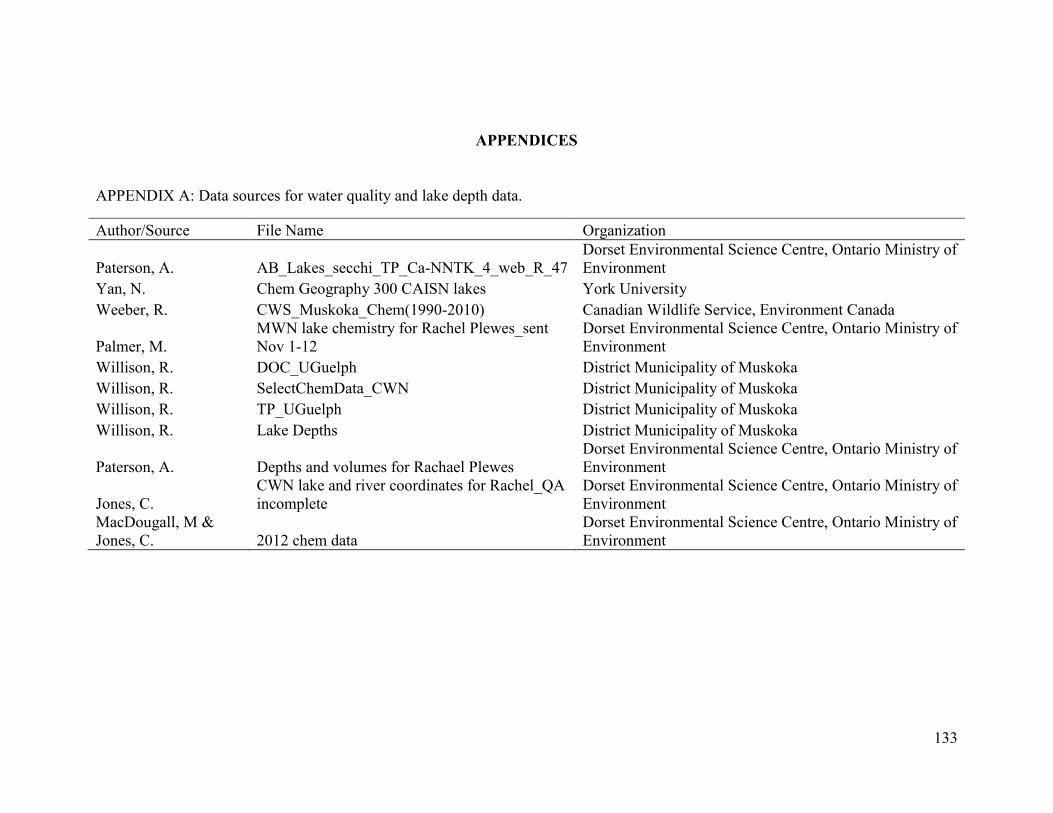
133
APPENDICES
APPENDIX A: Data sources for water quality and lake depth data.
Author/Source File Name Organization
Paterson, A. AB_Lakes_secchi_TP_Ca-NNTK_4_web_R_47
Dorset Environmental Science Centre, Ontario Ministry of
Environment
Yan, N. Chem Geography 300 CAISN lakes York University
Weeber, R. CWS_Muskoka_Chem(1990-2010) Canadian Wildlife Service, Environment Canada
Palmer, M.
MWN lake chemistry for Rachel Plewes_sent
Nov 1-12
Dorset Environmental Science Centre, Ontario Ministry of
Environment
Willison, R. DOC_UGuelph District Municipality of Muskoka
Willison, R. SelectChemData_CWN District Municipality of Muskoka
Willison, R. TP_UGuelph District Municipality of Muskoka
Willison, R. Lake Depths District Municipality of Muskoka
Paterson, A. Depths and volumes for Rachael Plewes
Dorset Environmental Science Centre, Ontario Ministry of
Environment
Jones, C.
CWN lake and river coordinates for Rachel_QA
incomplete
Dorset Environmental Science Centre, Ontario Ministry of
Environment
MacDougall, M &
Jones, C. 2012 chem data
Dorset Environmental Science Centre, Ontario Ministry of
Environment
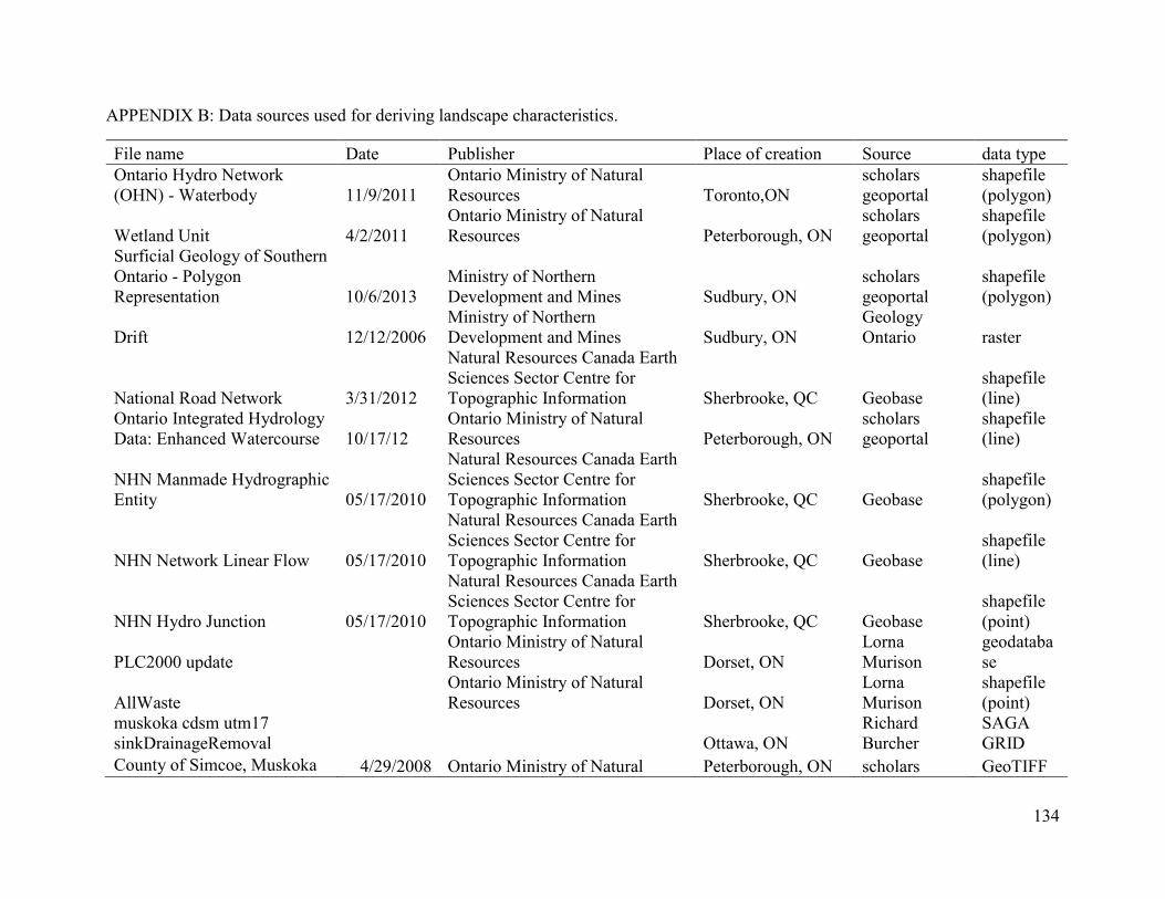
134
APPENDIX B: Data sources used for deriving landscape characteristics.
File name Date Publisher Place of creation Source data type
Ontario Hydro Network
(OHN) - Waterbody 11/9/2011
Ontario Ministry of Natural
Resources Toronto,ON
scholars
geoportal
shapefile
(polygon)
Wetland Unit 4/2/2011
Ontario Ministry of Natural
Resources Peterborough, ON
scholars
geoportal
shapefile
(polygon)
Surficial Geology of Southern
Ontario - Polygon
Representation 10/6/2013
Ministry of Northern
Development and Mines Sudbury, ON
scholars
geoportal
shapefile
(polygon)
Drift 12/12/2006
Ministry of Northern
Development and Mines Sudbury, ON
Geology
Ontario raster
National Road Network 3/31/2012
Natural Resources Canada Earth
Sciences Sector Centre for
Topographic Information Sherbrooke, QC Geobase
shapefile
(line)
Ontario Integrated Hydrology
Data: Enhanced Watercourse 10/17/12
Ontario Ministry of Natural
Resources Peterborough, ON
scholars
geoportal
shapefile
(line)
NHN Manmade Hydrographic
Entity 05/17/2010
Natural Resources Canada Earth
Sciences Sector Centre for
Topographic Information Sherbrooke, QC Geobase
shapefile
(polygon)
NHN Network Linear Flow 05/17/2010
Natural Resources Canada Earth
Sciences Sector Centre for
Topographic Information Sherbrooke, QC Geobase
shapefile
(line)
NHN Hydro Junction 05/17/2010
Natural Resources Canada Earth
Sciences Sector Centre for
Topographic Information Sherbrooke, QC Geobase
shapefile
(point)
PLC2000 update
Ontario Ministry of Natural
Resources Dorset, ON
Lorna
Murison
geodataba
se
AllWaste
Ontario Ministry of Natural
Resources Dorset, ON
Lorna
Murison
shapefile
(point)
muskoka cdsm utm17
sinkDrainageRemoval
Ottawa, ON
Richard
Burcher
SAGA
GRID
County of Simcoe, Muskoka 4/29/2008 Ontario Ministry of Natural Peterborough, ON scholars GeoTIFF

135
and Dufferin
Orthophotography Project,
2008
Resources geoportal
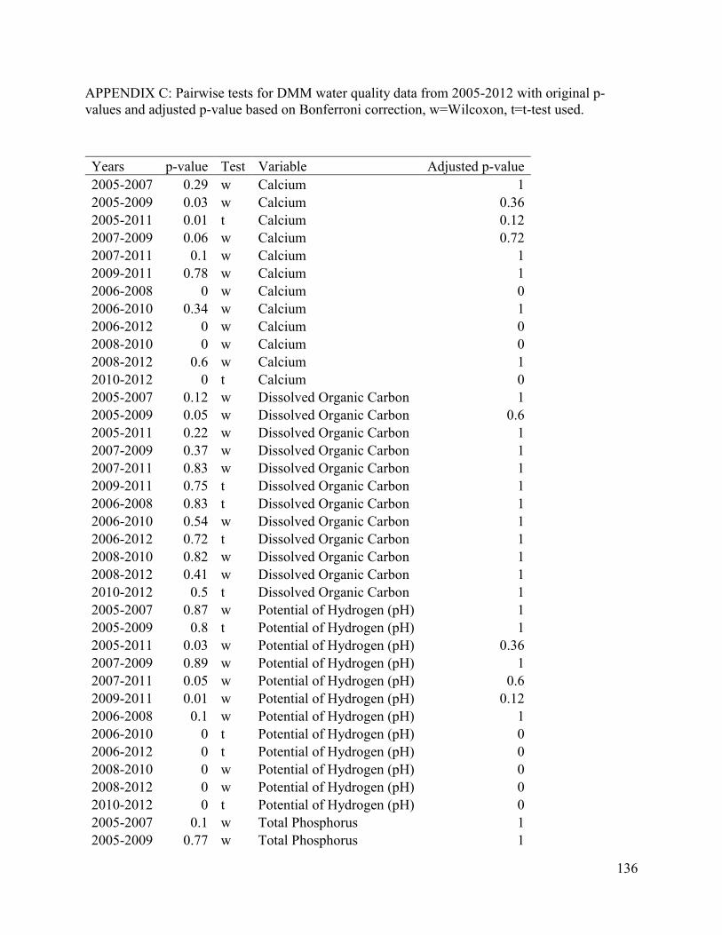
136
APPENDIX C: Pairwise tests for DMM water quality data from 2005-2012 with original p-
values and adjusted p-value based on Bonferroni correction, w=Wilcoxon, t=t-test used.
Years p-value Test Variable Adjusted p-value
2005-2007 0.29 w Calcium 1
2005-2009 0.03 w Calcium 0.36
2005-2011 0.01 t Calcium 0.12
2007-2009 0.06 w Calcium 0.72
2007-2011 0.1 w Calcium 1
2009-2011 0.78 w Calcium 1
2006-2008 0 w Calcium 0
2006-2010 0.34 w Calcium 1
2006-2012 0 w Calcium 0
2008-2010 0 w Calcium 0
2008-2012 0.6 w Calcium 1
2010-2012 0 t Calcium 0
2005-2007 0.12 w Dissolved Organic Carbon 1
2005-2009 0.05 w Dissolved Organic Carbon 0.6
2005-2011 0.22 w Dissolved Organic Carbon 1
2007-2009 0.37 w Dissolved Organic Carbon 1
2007-2011 0.83 w Dissolved Organic Carbon 1
2009-2011 0.75 t Dissolved Organic Carbon 1
2006-2008 0.83 t Dissolved Organic Carbon 1
2006-2010 0.54 w Dissolved Organic Carbon 1
2006-2012 0.72 t Dissolved Organic Carbon 1
2008-2010 0.82 w Dissolved Organic Carbon 1
2008-2012 0.41 w Dissolved Organic Carbon 1
2010-2012 0.5 t Dissolved Organic Carbon 1
2005-2007 0.87 w Potential of Hydrogen (pH) 1
2005-2009 0.8 t Potential of Hydrogen (pH) 1
2005-2011 0.03 w Potential of Hydrogen (pH) 0.36
2007-2009 0.89 w Potential of Hydrogen (pH) 1
2007-2011 0.05 w Potential of Hydrogen (pH) 0.6
2009-2011 0.01 w Potential of Hydrogen (pH) 0.12
2006-2008 0.1 w Potential of Hydrogen (pH) 1
2006-2010 0 t Potential of Hydrogen (pH) 0
2006-2012 0 t Potential of Hydrogen (pH) 0
2008-2010 0 w Potential of Hydrogen (pH) 0
2008-2012 0 w Potential of Hydrogen (pH) 0
2010-2012 0 t Potential of Hydrogen (pH) 0
2005-2007 0.1 w Total Phosphorus 1
2005-2009 0.77 w Total Phosphorus 1
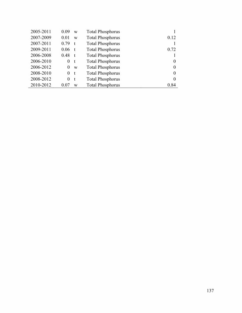
137
2005-2011 0.09 w Total Phosphorus 1
2007-2009 0.01 w Total Phosphorus 0.12
2007-2011 0.79 t Total Phosphorus 1
2009-2011 0.06 t Total Phosphorus 0.72
2006-2008 0.48 t Total Phosphorus 1
2006-2010 0 t Total Phosphorus 0
2006-2012 0 w Total Phosphorus 0
2008-2010 0 t Total Phosphorus 0
2008-2012 0 t Total Phosphorus 0
2010-2012 0.07 w Total Phosphorus 0.84
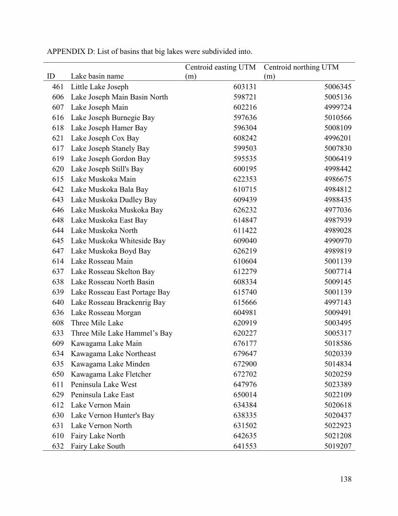
138
APPENDIX D: List of basins that big lakes were subdivided into.
ID Lake basin name
Centroid easting UTM
(m)
Centroid northing UTM
(m)
461 Little Lake Joseph 603131 5006345
606 Lake Joseph Main Basin North 598721 5005136
607 Lake Joseph Main 602216 4999724
616 Lake Joseph Burnegie Bay 597636 5010566
618 Lake Joseph Hamer Bay 596304 5008109
621 Lake Joseph Cox Bay 608242 4996201
617 Lake Joseph Stanely Bay 599503 5007830
619 Lake Joseph Gordon Bay 595535 5006419
620 Lake Joseph Still's Bay 600195 4998442
615 Lake Muskoka Main 622353 4986675
642 Lake Muskoka Bala Bay 610715 4984812
643 Lake Muskoka Dudley Bay 609439 4988435
646 Lake Muskoka Muskoka Bay 626232 4977036
648 Lake Muskoka East Bay 614847 4987939
644 Lake Muskoka North 611422 4989028
645 Lake Muskoka Whiteside Bay 609040 4990970
647 Lake Muskoka Boyd Bay 626219 4989819
614 Lake Rosseau Main 610604 5001139
637 Lake Rosseau Skelton Bay 612279 5007714
638 Lake Rosseau North Basin 608334 5009145
639 Lake Rosseau East Portage Bay 615740 5001139
640 Lake Rosseau Brackenrig Bay 615666 4997143
636 Lake Rosseau Morgan 604981 5009491
608 Three Mile Lake 620919 5003495
633 Three Mile Lake Hammel’s Bay 620227 5005317
609 Kawagama Lake Main 676177 5018586
634 Kawagama Lake Northeast 679647 5020339
635 Kawagama Lake Minden 672900 5014834
650 Kawagama Lake Fletcher 672702 5020259
611 Peninsula Lake West 647976 5023389
629 Peninsula Lake East 650014 5022109
612 Lake Vernon Main 634384 5020618
630 Lake Vernon Hunter's Bay 638335 5020437
631 Lake Vernon North 631502 5022923
610 Fairy Lake North 642635 5021208
632 Fairy Lake South 641553 5019207
139
APPENDIX E: GBM meta-parameter tuning and model simplification.
For each GBM model tree the meta-parameter of tree complexity, which determines the
size of the trees (number of nodes), was specified (Elith et al., 2008; Jan et al., 2013). The tree
complexity should reflect the true interaction structure of the data (Elith et al., 2008; Friedman,
2001). In order to determine the true interaction order of the data and to minimize overfitting, 10-
fold cross-validation was performed on individual CART models using the R package mvpart
version 1.6-1 (De’ath, 2013). The number of cross-validation iterations to be performed was
determined by the sample size. At each cross-validation iteration one observation was left out in
order to reduce the sensitivity of the tree structure to the data (Elith et al., 2008; Hastie et al.,
2001). At each iteration, the tree size with the lowest predicted deviance was selected. The tree
size that consistently had the lowest predicted deviances was selected as the tree complexity for
the GBM (Table 3-6).
The optimal learning rate was determined for each GBM model. The learning rate specifies
how much each tree contributes to the final model (Elith et al., 2008). In order to optimize the
learning rate several GBM models were run with different learning rates and the optimal tree size
for each learning rate was determined using the gbm.step function (Hijmans et al., 2013). The
learning rate was selected based on a combination of having a low cross-validated predicted
deviance and a tree size close to 1000, (see Table 3-6 for learning rates used in this study).
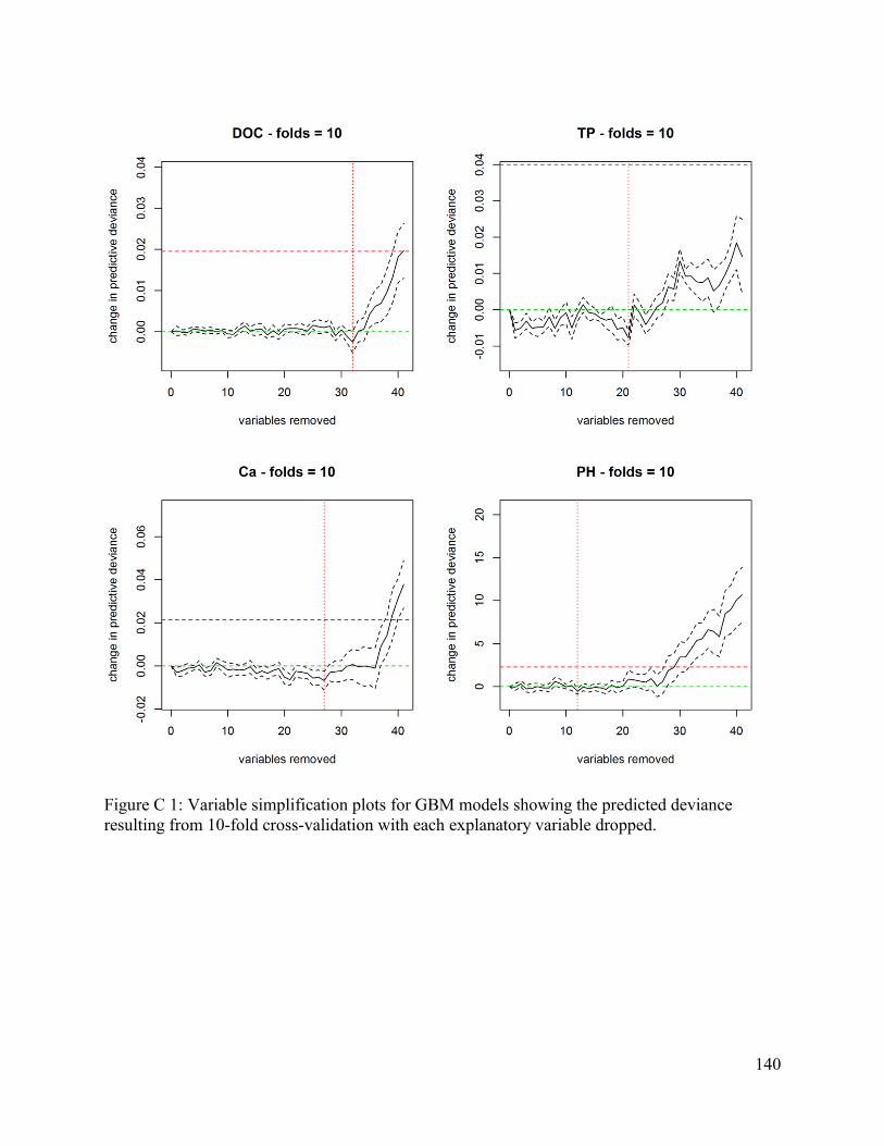
140
Figure C 1: Variable simplification plots for GBM models showing the predicted deviance
resulting from 10-fold cross-validation with each explanatory variable dropped.
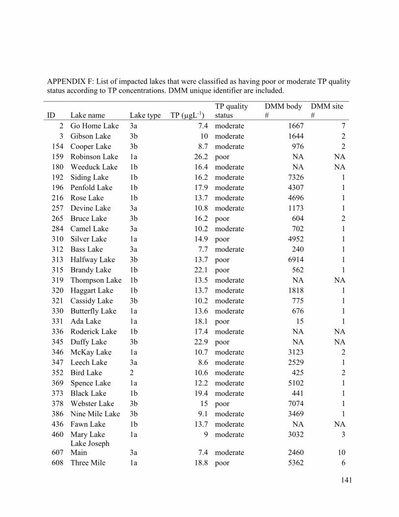
141
APPENDIX F: List of impacted lakes that were classified as having poor or moderate TP quality
status according to TP concentrations. DMM unique identifier are included.
ID Lake name Lake type TP (µgL-1)
TP quality
status
DMM body
#
DMM site
#
2 Go Home Lake 3a 7.4 moderate 1667 7
3 Gibson Lake 3b 10 moderate 1644 2
154 Cooper Lake 3b 8.7 moderate 976 2
159 Robinson Lake 1a 26.2 poor NA NA
180 Weeduck Lake 1b 16.4 moderate NA NA
192 Siding Lake 1b 16.2 moderate 7326 1
196 Penfold Lake 1b 17.9 moderate 4307 1
216 Rose Lake 1b 13.7 moderate 4696 1
257 Devine Lake 3a 10.8 moderate 1173 1
265 Bruce Lake 3b 16.2 poor 604 2
284 Camel Lake 3a 10.2 moderate 702 1
310 Silver Lake 1a 14.9 poor 4952 1
312 Bass Lake 3a 7.7 moderate 240 1
313 Halfway Lake 3b 13.7 poor 6914 1
315 Brandy Lake 1b 22.1 poor 562 1
319 Thompson Lake 1b 13.5 moderate NA NA
320 Haggart Lake 1b 13.7 moderate 1818 1
321 Cassidy Lake 3b 10.2 moderate 775 1
330 Butterfly Lake 1a 13.6 moderate 676 1
331 Ada Lake 1a 18.1 poor 15 1
336 Roderick Lake 1b 17.4 moderate NA NA
345 Duffy Lake 3b 22.9 poor NA NA
346 McKay Lake 1a 10.7 moderate 3123 2
347 Leech Lake 3a 8.6 moderate 2529 1
352 Bird Lake 2 10.6 moderate 425 2
369 Spence Lake 1a 12.2 moderate 5102 1
373 Black Lake 1b 19.4 moderate 441 1
378 Webster Lake 3b 15 poor 7074 1
386 Nine Mile Lake 3b 9.1 moderate 3469 1
436 Fawn Lake 1b 13.7 moderate NA NA
460 Mary Lake 1a 9 moderate 3032 3
607
Lake Joseph
Main 3a 7.4 moderate 2460 10
608 Three Mile 1a 18.8 poor 5362 6
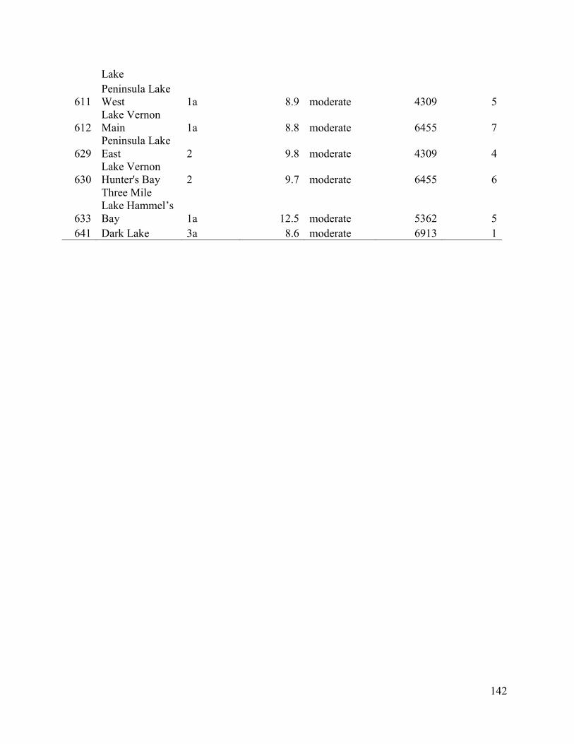
142
Lake
611
Peninsula Lake
West 1a 8.9 moderate 4309 5
612
Lake Vernon
Main 1a 8.8 moderate 6455 7
629
Peninsula Lake
East 2 9.8 moderate 4309 4
630
Lake Vernon
Hunter's Bay 2 9.7 moderate 6455 6
633
Three Mile
Lake Hammel’s
Bay 1a 12.5 moderate 5362 5
641 Dark Lake 3a 8.6 moderate 6913 1