1

Chapter 2

Developing Models for

Optimization

Ch

ap

ter

2

2

Ch

ap

ter

2

3

Ch

ap

ter

2

4

Ch

ap

ter

2

5

Ch

ap

ter

2

6

Ch

ap

ter

2 Everything should be made as simple

as possible, but no simpler

7

Ch

ap

ter

2

8

Ch

ap

ter

2

9

Ch

ap

ter

2

10

Ch

ap

ter

2

11

Ch

ap

ter

2

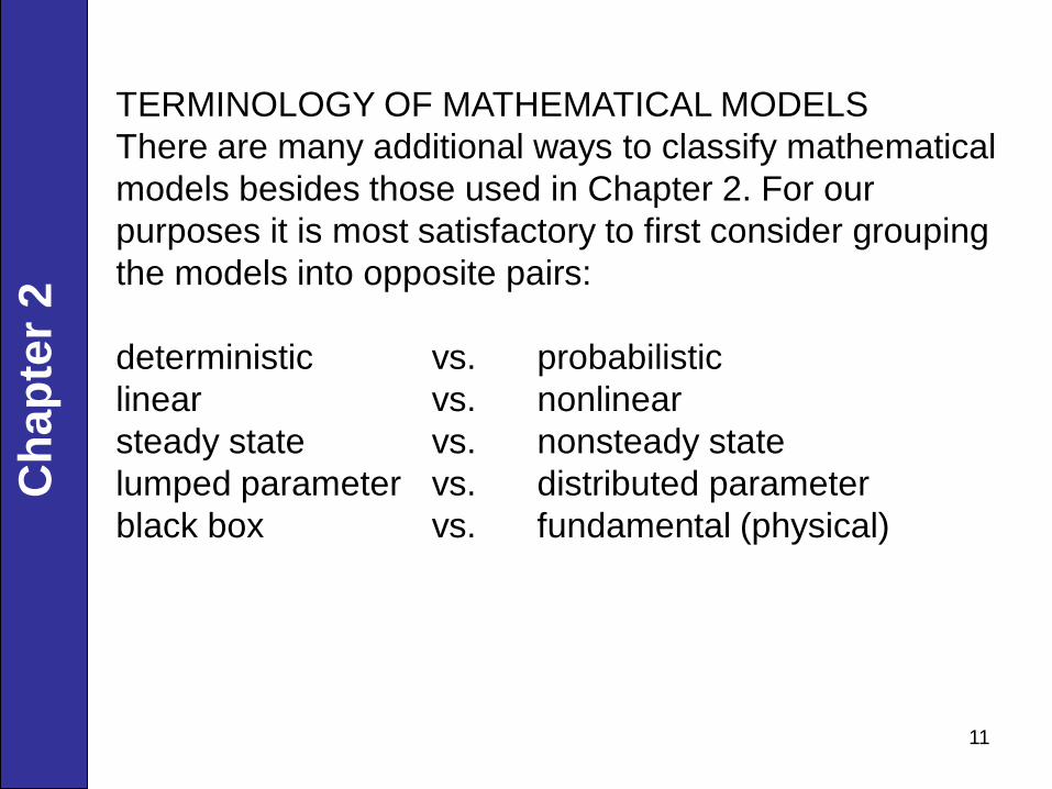
TERMINOLOGY OF MATHEMATICAL MODELS

There are many additional ways to classify mathematical

models besides those used in Chapter 2. For our

purposes it is most satisfactory to first consider grouping

the models into opposite pairs:

deterministic vs. probabilistic

linear vs. nonlinear

steady state vs. nonsteady state

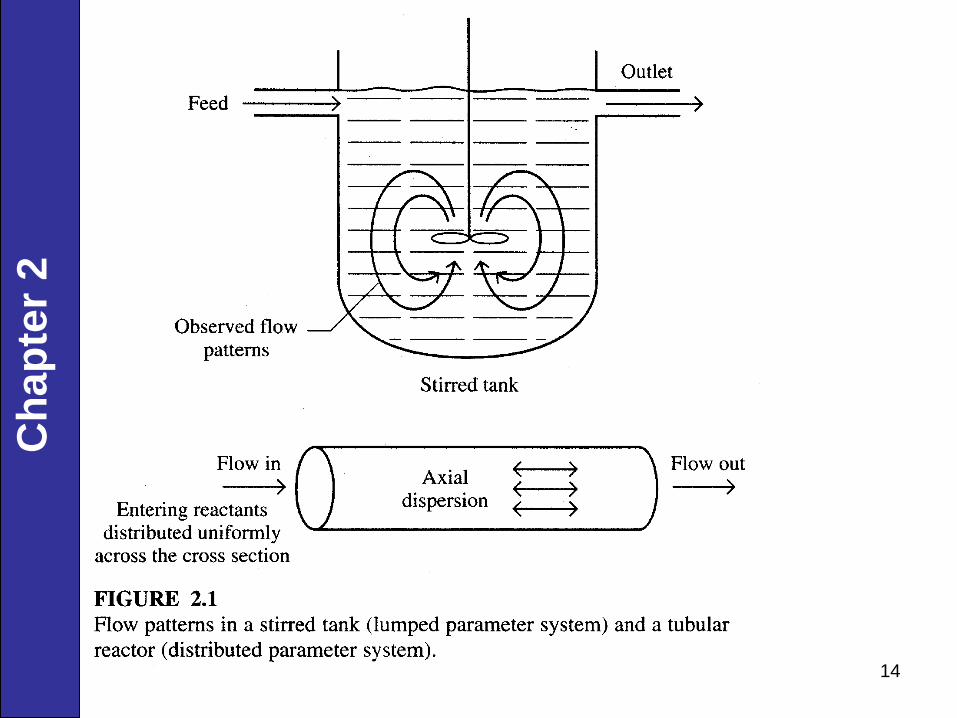
lumped parameter vs. distributed parameter

black box vs. fundamental (physical)

12

Ch

ap

ter

2

Common Sense in Modeling

What simplifications can be made?

How are they justified?

Types of Simplifications

(1)Omitting Interactions

(2)Aggregating Variables

(3)Eliminating Variables

(4)Replace Random Variables with Expected Values

(5)Reduce Detail of Mathematical Description

13

Ch

ap

ter

2

14

Ch

ap

ter

2

15

Ch

ap

ter

2

Precautions in Model Building

(1) Limits on availability of data and accuracy of data

Examples: Kinetic coefficients

Mass transfer coefficients

(2) Unknown factors present or not present in scale up

Examples: Impurities in plant streams

Wall effects

(3) Poor measures of deviation between ideal and actual

models

Examples: Stage efficiency

16

Ch

ap

ter

2

(4) Models used for one purpose used improperly for

another purpose

Example: Invalidity of kinetic models

(5) Extrapolation – using the model outside of the regions

Where it has been validated

17

Ch

ap

ter

2

18

Ch

ap

ter

2

19

Ch

ap

ter

2

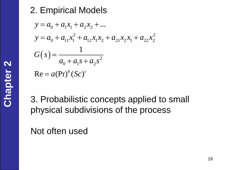
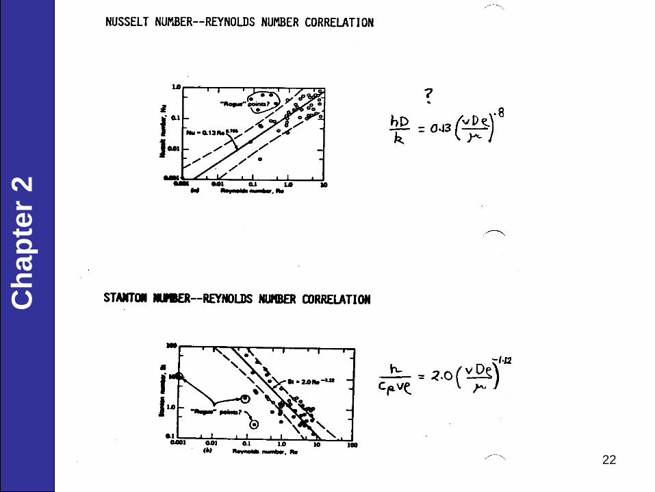
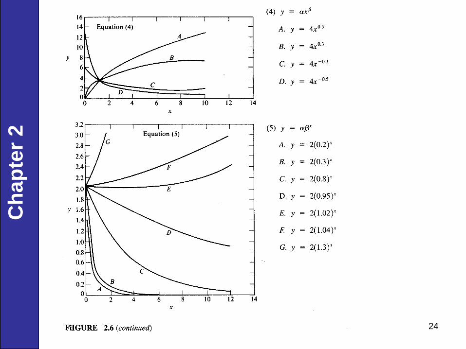
2. Empirical Models

0 1 1 2 2

2 2

0 11 1 12 1 2 21 2 1 22 2

2

0 1 2

...

1

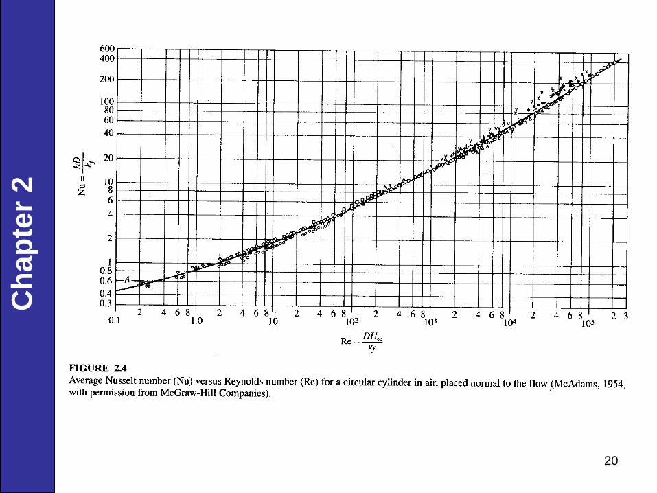
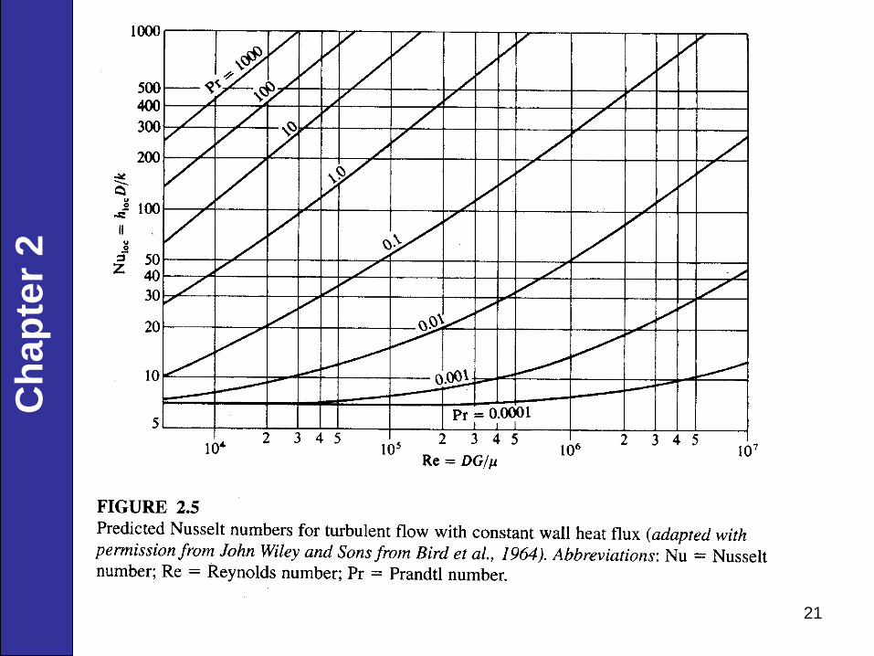
Re (Pr) ( )b c

y a a x a x

y a a x a x x a x x a x

G sa a s a s

a Sc

3. Probabilistic concepts applied to small

physical subdivisions of the process

Not often used

20

Ch

ap

ter

2

21

Ch

ap

ter

2

22

Ch

ap

ter

2

23

Ch

ap

ter

2

24

Ch

ap

ter

2

25

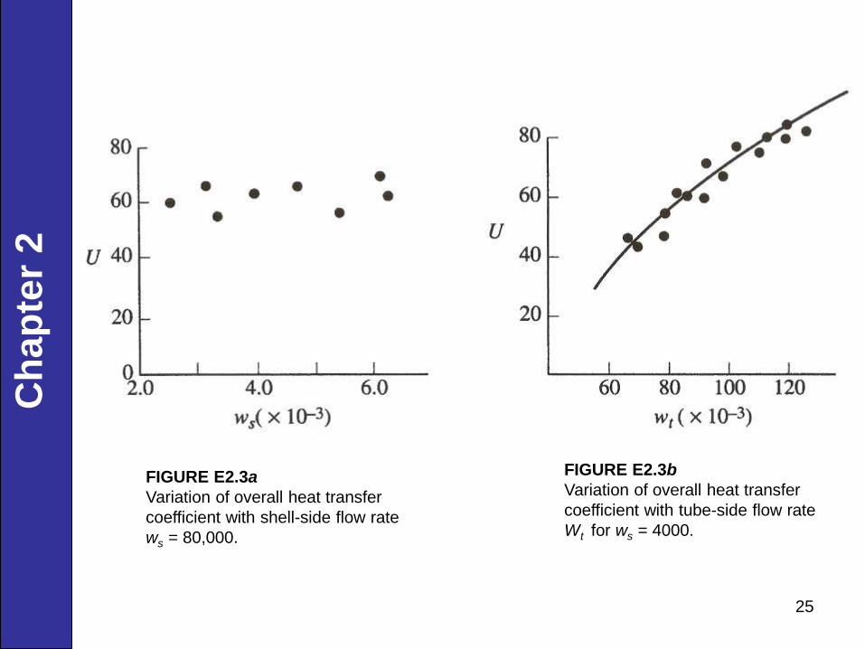
FIGURE E2.3a

Variation of overall heat transfer

coefficient with shell-side flow rate

ws = 80,000.

FIGURE E2.3b

Variation of overall heat transfer

coefficient with tube-side flow rate

Wt for ws = 4000.

Ch

ap

ter

2

26

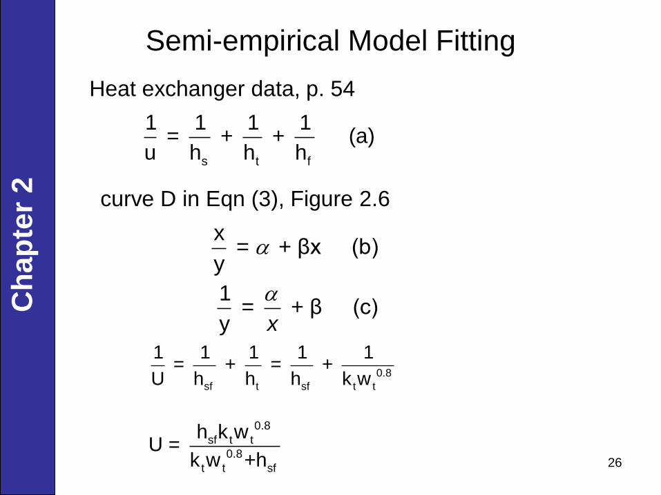
Semi-empirical Model Fitting

s t f

1 1 1 1 = + + (a)

u h h h

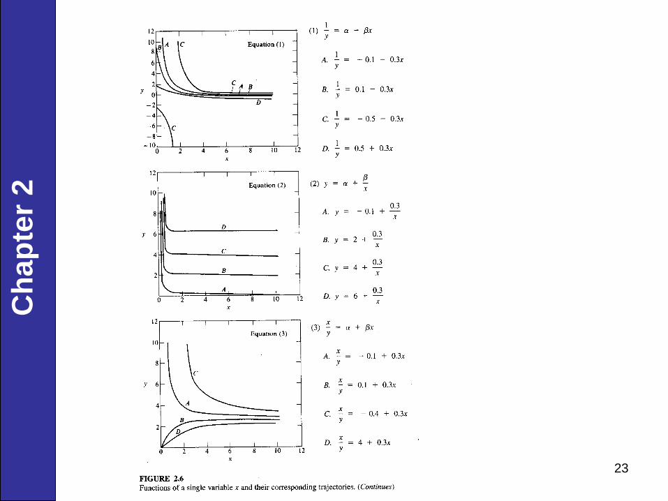
x = + βx (b)

y

1 = + β (c)

y x

Heat exchanger data, p. 54

curve D in Eqn (3), Figure 2.6

0.8

sf t sf t t

1 1 1 1 1 = + = +

U h h h k w

0.8

sf t t

0.8

t t sf

h k wU =

k w +h

Ch

ap

ter

2

27

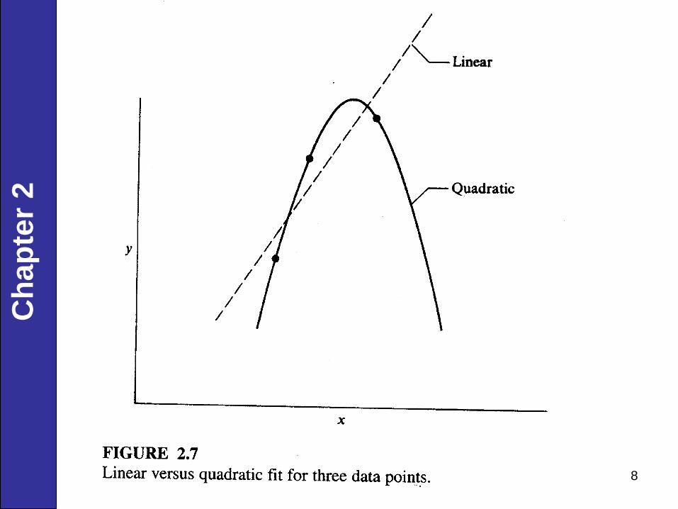
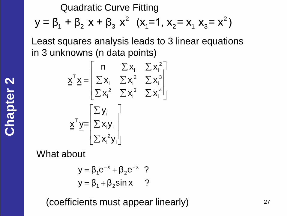
Quadratic Curve Fitting 2 2

1 2 3 1 2 1 3y = β + β x + β x (x =1, x = x x = x )

Least squares analysis leads to 3 linear equations

in 3 unknowns (n data points) 2

i i

T 2 3

i i i

2 3 4

i i i

n x x

x x x x x

x x x

i

T

i i

2

i i

y

x y= x y

x y

What about

(coefficients must appear linearly)

? x sinββy

? eβeβy

21

x

2

x

1

Ch

ap

ter

2

28

Ch

ap

ter

2

29

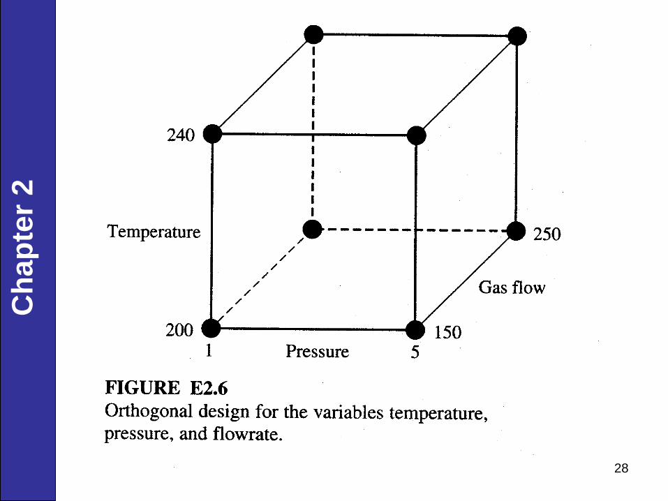
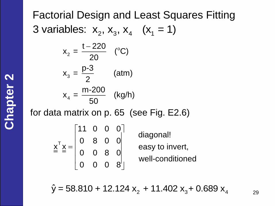
Factorial Design and Least Squares Fitting

2 3 4 13 variables: x , x , x (x = 1)

o

2

3

4

t 220x = ( C)

20

p-3x = (atm)

2

m-200x = (kg/h)

50

for data matrix on p. 65 (see Fig. E2.6)

T

11 0 0 0diagonal!

0 8 0 0x x easy to invert,

0 0 8 0well-conditioned

0 0 0 8

2 3 4y = 58.810 + 12.124 x + 11.402 x + 0.689 x

Ch

ap

ter

2