Embed Size (px)
Citation preview

Developing acoustics models for
automatic speech recognition
GIAMPIERO SALVI
Master’s Thesis at TMH
Supervisor: Håkan Melin
Examiner: Rolf Carlson
TRITA xxx yyyy-nn


iii
Abstract
This thesis is concerned with automatic continuous speech recognition using trainablesystems. The aim of this work is to build acoustic models for spoken Swedish. This isdone employing hidden Markov models and using the SpeechDat database to train theirparameters. Acoustic modeling has been worked out at a phonetic level, allowing generalspeech recognition applications, even though a simplified task (digits and natural numberrecognition) has been considered for model evaluation. Different kinds of phone models havebeen tested, including context independent models and two variations of context dependentmodels. Furthermore many experiments have been done with bigram language models totune some of the system parameters. System performance over various speaker subsetswith different sex, age and dialect is also examined. Results are compared to previous workshowing a remarkable improvement.

iv
Preface
This Master of Science thesis was done at the Department of Speech, Music andHearing (Tal, musik och hörsel) at the Royal Institute of Technology (KTH), Stock-holm. It is fruit of a collaboration between KTH and Universitá “La Sapienza”,Rome. Supervisors were Prof. Gabriella Di Benedetto, Prof. Rolf Carlson andHåkan Melin.
The thesis was later published in a summarised version on The European StudentJournal of Language and Speech (WEB-SLS)
http://www.essex.ac.uk/web-sls/

v
Acknowledgments
There are many people to thank in connection with this work. First I begin bythanking Prof. Maria Gabriella Di Benedetto and Prof. Rolf Carlson for allowingthis instructive experience and Prof. Rolf Carlson for hosting me in the TMHdepartment. Then I thank Håkan Melin for his patience and his readiness in helpingme for the whole period I have been working on this subject. Other people whichindubitably deserve thanks are Kjell Elenius for everything concerned with theSpeechDat project and Kåre Sjölander for providing information about his previouswork. The feeling of welcome I got from all the people working at the departmenthas made this period particularly enjoyable, helping the development of this work:special thanks go to Philippe for being Philippe, to Thomas and Sasha for theirnon-stop sports and entertainments organization, Leonardo, Roberto and Vittoriofor their sympathy and Peta for her humour.

Contents
Preface iv
Acknowledgments v
Contents vi
1 Introduction 11.1 Introduction . . . . . . . . . . . . . . . . . . . . . . . . . . . . . . . . 11.2 Automatic Speech Recognizer . . . . . . . . . . . . . . . . . . . . . . 2
1.2.1 Peirce’s Model . . . . . . . . . . . . . . . . . . . . . . . . . . 21.3 Structure of the work . . . . . . . . . . . . . . . . . . . . . . . . . . 4
2 Swedish Phonology 52.1 Swedish Phonemes . . . . . . . . . . . . . . . . . . . . . . . . . . . . 5
2.1.1 Swedish Vowels . . . . . . . . . . . . . . . . . . . . . . . . . . 52.1.2 Consonants . . . . . . . . . . . . . . . . . . . . . . . . . . . . 5
2.2 Dialectal Variations . . . . . . . . . . . . . . . . . . . . . . . . . . . 8
3 SpeechDat Database 113.1 Swedish Database . . . . . . . . . . . . . . . . . . . . . . . . . . . . . 11
3.1.1 Database Features . . . . . . . . . . . . . . . . . . . . . . . . 123.1.2 Noise Transcriptions . . . . . . . . . . . . . . . . . . . . . . . 133.1.3 Speaker Subsets . . . . . . . . . . . . . . . . . . . . . . . . . 143.1.4 Statistics . . . . . . . . . . . . . . . . . . . . . . . . . . . . . 14
4 ASR Structure 174.1 ASR structure . . . . . . . . . . . . . . . . . . . . . . . . . . . . . . 184.2 Acoustic Analysis . . . . . . . . . . . . . . . . . . . . . . . . . . . . . 18
4.2.1 Signal Processing . . . . . . . . . . . . . . . . . . . . . . . . . 194.2.2 Feature Extraction . . . . . . . . . . . . . . . . . . . . . . . . 19
4.3 Acoustic/Linguistic Decoder . . . . . . . . . . . . . . . . . . . . . . . 214.3.1 Phone Models . . . . . . . . . . . . . . . . . . . . . . . . . . . 214.3.2 Linguistic Decoder . . . . . . . . . . . . . . . . . . . . . . . . 214.3.3 Implementation . . . . . . . . . . . . . . . . . . . . . . . . . . 22
vi

vii
5 Hidden Markov Models 255.1 The HTK Toolkit . . . . . . . . . . . . . . . . . . . . . . . . . . . . . 255.2 Hidden Markov Models . . . . . . . . . . . . . . . . . . . . . . . . . 255.3 HMMs and ASRs . . . . . . . . . . . . . . . . . . . . . . . . . . . . . 26
5.3.1 The Recognition Problem . . . . . . . . . . . . . . . . . . . . 275.3.2 The Training Problem . . . . . . . . . . . . . . . . . . . . . . 285.3.3 HMM Assumptions . . . . . . . . . . . . . . . . . . . . . . . . 285.3.4 HMM Applications . . . . . . . . . . . . . . . . . . . . . . . . 295.3.5 State Output Probability Distribution . . . . . . . . . . . . . 295.3.6 Context Dependent HMMs . . . . . . . . . . . . . . . . . . . 305.3.7 The Data Scarcity Problem . . . . . . . . . . . . . . . . . . . 315.3.8 Tree Clustering . . . . . . . . . . . . . . . . . . . . . . . . . . 32
6 Model Set Building 356.1 Data Preparation . . . . . . . . . . . . . . . . . . . . . . . . . . . . . 36
6.1.1 Speech Files . . . . . . . . . . . . . . . . . . . . . . . . . . . . 366.1.2 Label Files . . . . . . . . . . . . . . . . . . . . . . . . . . . . 36
6.2 HMM Setup . . . . . . . . . . . . . . . . . . . . . . . . . . . . . . . . 366.2.1 Target Speech . . . . . . . . . . . . . . . . . . . . . . . . . . . 376.2.2 Non-Target Speech . . . . . . . . . . . . . . . . . . . . . . . . 38
6.3 Training The Models . . . . . . . . . . . . . . . . . . . . . . . . . . . 396.3.1 Development Tests . . . . . . . . . . . . . . . . . . . . . . . . 406.3.2 Monophones . . . . . . . . . . . . . . . . . . . . . . . . . . . 416.3.3 Triphones . . . . . . . . . . . . . . . . . . . . . . . . . . . . . 42
7 Results, Analysis and Discussion 477.1 Language Model Perplexity . . . . . . . . . . . . . . . . . . . . . . . 477.2 Overall Results . . . . . . . . . . . . . . . . . . . . . . . . . . . . . . 487.3 Results per Individual Speaker . . . . . . . . . . . . . . . . . . . . . 517.4 Evaluating on Other Databases . . . . . . . . . . . . . . . . . . . . . 53
7.4.1 The Waxholm Database . . . . . . . . . . . . . . . . . . . . . 537.4.2 The Norwegian SpeecDat database . . . . . . . . . . . . . . . 53
8 Discussion and Conclusions 558.1 Further Improvements . . . . . . . . . . . . . . . . . . . . . . . . . . 55
Bibliography 57
A Speech Signal Models 59A.1 Speech Signal Models . . . . . . . . . . . . . . . . . . . . . . . . . . 59A.2 Cepstral Analysis . . . . . . . . . . . . . . . . . . . . . . . . . . . . . 60A.3 Mel Frequency . . . . . . . . . . . . . . . . . . . . . . . . . . . . . . 62
B HMM Theory 65B.1 HMM Definition . . . . . . . . . . . . . . . . . . . . . . . . . . . . . 65

viii CONTENTS
B.2 Model Likelihood . . . . . . . . . . . . . . . . . . . . . . . . . . . . . 67B.3 Forward-Backward Algorithm . . . . . . . . . . . . . . . . . . . . . . 67B.4 Viterbi algorithm . . . . . . . . . . . . . . . . . . . . . . . . . . . . . 68B.5 Baum-Welsh Reestimation Algorithm . . . . . . . . . . . . . . . . . 69
C Lists Of Words 71
D Phonetic Classes 73
E Confusion Matrices 77

Chapter 1
Introduction
1.1 Introduction
The field of speech signal analysis has been in the center of attention for manyyears because of the interest it is able to generate in the scientists and becauseof the many possible applications. These applications, related mostly to telecom-munication problems, have as a goal the possibility for human beings to exchangeinformation using the most natural and efficient means they know: speech. Inthis context the speech recognition enterprise is probably the most ambitious. Itsgoal is to build “intelligent” machines that can “hear” and “understand” spokeninformation, in spite of the natural ambiguity and complexity of natural languages.In thirty years, improvements that could not even be thought of before have beenworked out, but still the objective of a robust machine, able to recognize differentspeakers in different situations, is far to be reached. The difficulty of the problemincreases if we try to build systems for a large set of speakers and for a generic task(large vocabulary).
This thesis describes an attempt to build robust speaker-independent acousticmodels for spoken Swedish. A collection of utterance spoken by 1000 speakers (theSpeechDat database) has been used as a statistical base from which the modelshave been developed. The recognition task considered includes a small vocabulary(86 words), but continuous speech is accepted. Furthermore the model structureis chosen with regard to the possibility to apply these models in different contextsand tasks. For this reason models have been tested on another database (from theWaxholm project) to evaluate their flexibility. Different applications are possiblefor this kind of models: they can be employed in the recognition part of complexdialogue systems, or in speaker verification systems for example.
This report contains a documentation of the steps that lead to the creation anddevelopment of the acoustic models, but also a thorough description of the systememployed in the recognition phase.
1

2 CHAPTER 1. INTRODUCTION
1.2 Automatic Speech Recognizer
An Automatic Speech Recognizer (ASR) is a system whose task is to convert anacoustic speech signal into a symbolic description of the message coded in that signalduring speech production. Two main aspects make this process particularly difficult:the “modulation” process (speech production) involves a long list of physical andpsychological phenomena regarding the speaker articulatory apparatus, the phon-emic system, the prosodic system, the lexicon, the syntax, the rules of discourse,the semantics, the psychology of the speaker and so on, which makes the speechsignal extremely changeable with different situations and deeply coded. Second the“demodulation” process (speech recognition) involves a large reduction of informa-tion from the sampled acoustic signal (for example 8bit, 8kHz), to the text (around5bytes/sec).
Speech recognition has, hence, an interdisciplinary nature involving many dis-ciplines such as: signal processing, physics (acoustic), pattern recognition, com-munication and information theory, linguistics, physiology, computer science andpsychology. Successful speech recognition systems may require knowledge on allthese topics. A way to give an organisation to this knowledge is to refer to anabstract model of natural languages called Peirce’s model (Hartshorne and Weiss,1935). This model explains well the structure of our system, even though it isconsidered to be too simplified if the attempt is to describe natural languages.
1.2.1 Peirce’s Model
Peirce’s model provides a general definition of the linguistic constraints. Four com-ponents of the natural language code are included: symbolic, grammatical, semanticand pragmatic.
Symbols are the most fundamental units in a language: they might be words,phonemes, or, in written form, the alphabetic symbols.
The grammar of a language is concerned with how symbols are related to oneanother to form words or sentences. In the case that fundamental symbols are subword units, we call lexical constraints the way these units are connected to formwords, while syntactic constraints rule the way words form sentences. Both are partof the grammar.
Semantics is concerned with the way in which symbols are combined to formmeaningful communication: a sentence can be grammatically correct, but be withoutmeaning.
Finally the pragmatic component of the language model is concerned with therelationship of the symbols to their users and the environment of the discourse.
Knowledge at all linguistic levels is required if our aim is to build a systemthat can be used in different environments and for different tasks. Nevertheless thehighest levels (semantics and pragmatic) are very difficult to formalize (at least inconventional engineering ways) and they are usually considered as belonging to thefield of artificial intelligence. The usual way to overcome this problem is to restrict

1.2. AUTOMATIC SPEECH RECOGNIZER 3
the field of application of the system to be built and to use in its construction onlyknowledge that can be formalized in a mathematical way.
In Figure 1.1 a schematic representation of Peirce’s model is depicted.
Pragmaticknowledge
Semanticknowledge
knowledgeSyntactic
Lexicalknowledge
Prosodicknowledge
Phonetic andphonologicalknowledge
Lexicon
Syntax
Grammar
KNOWLEDGESOURCES
Acoustic analysis
Phone models
Lexical analysis
Syntactic analysis
Semantic analysis
Pragmatic analysis
Meaningful
hypothesissentence
hypothesisSentence
hypothesisPhone
hypothesisWord
PEIRCIANMODEL
����������������������������������������������������������������������������������������������������������������������������������������������������
����������������������������������������������������������������������������������������������������������������������������������������������������
AD
Pragmatics
Symbols
LD Message hypothesis
Semantics
Acoustic waveform
Figure 1.1. A schematic representation of the Peirce’s model for natural languages.
This work is focused on the acoustic part of a speech recognizer and hence willdeal essentially with the first two levels of language constraints.
There are two different approaches in the way knowledge is obtained and used:the first is the deterministic approach: all the phenomena involved in speech pro-duction are analyzed and formalised from a physical and physiological point of view(when possible). The utterance to be recognised is then compared to a syntheticsignal generated according to some acoustic models developed on this physical and

4 CHAPTER 1. INTRODUCTION
physiological base. The computational requirements needed in this case are low,but a big effort is required in formalizing the basic aspects of speech production.
The second approach (stochastic) is based on statistical methods: some oppor-tune models are “trained” on a large amount of data in order to estimate theirparameters and to make them fit to the problem of interest. This second approachrequires a big computing power and large data bases.
The rapid development of computers in the last years has made the statist-ical approach more and more attractive, but knowledge on speech production at aphysical level is still required. First of all because a long signal processing chain isindispensable in order to extract the features that best represent the speech signalcharacteristics and to reduce the amount of data to deal with per unit of time.Second of all because the choice of model structures must always be motivated byan analogy with the physical phenomena those models try to imitate.
1.3 Structure of the work
This thesis is structured as follows. The acoustic models are created on a phon-etic base hence a description of the Swedish phonology is reported in Chapter 2.Chapter 3 describes the SpeechDat database used in model building and testing.Chapter 4 describes the ASR structure. Chapter 5 describe the mathematical theoryupon which model building is based. In Chapter 6 all the steps in model buildingand developing are documented, and finally results are presented in Chapter 7 andconclusions in Chapter 8.
Chapter 2
Swedish Phonology
As a first topic of this thesis, the Swedish phonology is described. The aim of thiswork is to build acoustic models for different speech features, and hence the Swedishlanguage characteristics are an important background to understand the following.Section 2.1 describes the Swedish phonemes, while Section 2.2 describes the maincharacteristics of pronunciation in different dialect areas.
2.1 Swedish Phonemes
In the Swedish language, sounds can be classified into 46 phones. 23 of these arevowels, while the other 23 are consonantal sounds. Among the consonants thereare 4 nasals, 7 fricatives, 3 liquids, 8 plosives, 1 h-sound (5 retroflex allophones areincluded in their respective groups).
2.1.1 Swedish Vowels
The Swedish written language has 9 vowels [5] (a, e, i, o, u, y, ä, ö, å) which, whenspoken, can occur in a short or long version according to some pronunciation rules(“A long vowel in a stressed position can only occur before a short consonant andvice versa. In unstressed position there is no distinction between long and shortvowels...” [5]). An example is in table 2.1. Most of them are front vowels (e, i, y,ä, u) which makes their distinction difficult for an untrained ear.
In figure 2.1 each vowel occupy a point in the F1/F2 plain, where F1 and F2 arerespectively the first and second formants. Formant data has been taken from Fant(1973) [5], regarding seven female speakers. The X and Y axes showed in the figureprovide a way to relate formant variations to mouth configurations. Moving alongthe X axis, the tongue position is approximately constant, while moving along theY axis mouth opening is constant.
2.1.2 Consonants
Swedish consonants are listed in Table 2.2 in the STA symbols. In the table, ac-
5

6 CHAPTER 2. SWEDISH PHONOLOGY
vowel long shortSTA SAMPA example STA SAMPA example
a A: A: hal () A a hall ()e E: e: vet (know) E e sett (seen)i I: i: bil (car) I I till (to)o O: u: rot (root) O U bott (lived)u U: }: mun (mouth) U u0 buss (bus)y Y: y: lys (shine) Y Y ryss (russian)ä Ä: E: lät (sounded) Ä E lätt (easy)ö Ö: 2: nöt (beaf) Ö 2 kött (meat)å Å: o: kål (cabbage) Å O vått (wet)
pre-r long shortallophone STA SAMPA example STA SAMPA example
är Ä3 {: härör Ö3 9: förerr Ä4 { herrörr Ö4 9 förr
schwa vowel long shortallophone STA SAMPA example STA SAMPA example
e E0 @ pojken
Table 2.1. “Long” and “short” vowels in Swedish phonetics
cording to Fant [5], phones articulated with a palatal or velar tongue position areplaced at the bottom, except for the liquids and the H phone. The labial memberof each group is placed to the left, and the dental to the right
Nasals
Nasal sounds (M, N, 2N, NG) are produced with the vocal tract totally constrictedat some point in the mouth. The sound is hence radiated by the nasal tract,while the oral tract behaves as a resonant cavity which traps acoustic energy andintroduces zeros in the transfer function of sound transmission at some naturalfrequencies. Nasals can be distinguished by the place at which the constriction ofthe oral tract is made. For M the constriction is at the lips, for N it is behind theteeth, for NG it is forward of the velum. When uttering 2N the position of thetongue is similar to that for N, but it is curled.
Fricatives
Fricative sounds can be divided into voiced and unvoiced sounds. There are fourunvoiced fricatives in Swedish: F, S, TJ, SJ of which TJ occurs only in word initialposition. Unvoiced fricative sounds are produced by exciting the vocal tract by asteady air flow which becomes turbulent in the region of a constriction in the vocaltract.
Voiced fricatives are V and J. V is produced as F, but with excitation of thevocal cords. J may also be pronounced as half-vowel.

2.1. SWEDISH PHONEMES 7
200 400 600 800 1000
600
800
1000
1200
1400
1600
1800
2000
2200
2400
2600
O O:
Å Å:
AA:
Ä3Ä4
Ä
Ä:
E
E:
I
I:
Y
Y: U
U:
Ö
Ö:
Ö3Ö4
XY
F1 (Hz)
F2 (H
z)Vowels in the F1−F2 plane
Figure 2.1. Vowel distribution in the F1-F2 plane
Liquids
The R sound can vary depending on the speaker. It can sound as a trill or anuvular fricative in the south of Sweden, or as a retroflex voiced fricative in the areaaround Stockholm. L is also classified as lateral because it is produced rising thetongue. 2L is a variant of L “produced with retracted tongue position and uvularconstriction” [5].
Plosives (Stops)
These sounds are produced by changing the vocal tract configuration. They arenormally classified as non-continuant sounds. All stops have a first period in whichpressure is built up behind a total constriction in the oral tract. Then the pressure issuddenly released (second period). To each stop corresponds a different constrictionposition.
A distinction can be made between unvoiced stops K, P, T, 2T (no sound is
8 CHAPTER 2. SWEDISH PHONOLOGY
h Liquids Voiced fricative Unvoiced fricative NasalsH L V F S M N
2L SJ 2NR J TJ NG
Voiced stops Unvoiced stopsB D P T
2D 2TG K
Table 2.2. Swedish consonants
produced during the first period) and voiced stops B, D, 2D, G (a small amountof low frequency energy is radiated through the walls of the throat).
H-sound
The h-sound (H) is produced by exciting the vocal tract by a steady air flow,without the vocal cords vibrating, but with turbulent flow being produced at theglottis.
Retroflex Allophones
Retroflex allophones (2S, 2T, 2D, 2N, 2L) have already been mentioned in theirgroups. They are now grouped together because they will be object of discussion inthe following of this work. These symbols apply to alveolar articulation of soundsspelled r plus s, t, d, n, or l and occur only in positions after a vowel. The distinctionbetween the retroflex version of a phoneme and the normal one (for example 2Land L) is not important in the southern dialects of Sweden.
2.2 Dialectal Variations
Swedish pronunciation depends strongly on the origin of the speaker, while STAsymbols are independent of the specific dialect sound qualities. For this reason inthis section some variations from the standard pronunciation rules are listed for theseven major Swedish dialect regions [4]. Most of differences regard the pronunciationof vowels.
1. South SwedishSouth Swedish diphthongization (raising of the tongue, late beset roundingof the long vowels), retracted pronunciation of R, no supra-dentals, retractedpronunciation of the fricative SJ-sound. A tense, creaky voice quality can befound in large parts of Småland.

2.2. DIALECTAL VARIATIONS 9
2. Gothenburg, west, and middle SwedishOpen long and short Ä and (sometimes) Ö vowels (no extra opening beforeR), retracted pronunciation of the fricative SJ-sound, open Å-sound and L-sound.
3. East, middle SwedishDiphthongization into E/Ä in long vowels (possibly with a laryngeal gesture),short E and Ä collapses into a single vowel, open variants of Ä and Ö beforeR (Ä3, Ä4 and Ö3, Ö4 in STA).
4. Swedish as spoken in GotlandSecondary Gotland diphthongization, long O-vowel pronounced as Å.
5. Swedish as spoken in BergslagenU pronounced as central vowel, acute accent in many connected words.
6. Swedish as spoken in NorrlandNo diphthongization of long vowels, some parts have a short U pronouncedwith a retracted pronunciation, thick L-sound, sometimes the main emphasisof connected words is moved to the right.
7. Swedish as spoken in FinlandSpecial pronunciation of U-vowels and long A, special SJ and TJ-sounds, Ris pronounced before dentals, no grave accent.


Chapter 3
SpeechDat Database
SpeechDat [15] is a project involving 15 European countries (listed in tab. 3.1)and essentially based on the country partner’s fixed telephone networks. Speakers
Country Language Partner Recorded(variant) Speakers
United Kingdom English GEC +4000United Kingdom Welsh BT 2000Denmark Danish AUC +4000Belgium Flemish L&H 1000Belgium Belgian French L&H 1000France French MATRA 5000Switzerland Swiss French IDIAP +2000Switzerland Swiss German IDIAP 1000Luxembourg Luxemb. French L&H 500Luxembourg Luxemb. German L&H 500Germany German SIEMENS +4000Greece Greek KNOW & 5000
UPATRASItaly Italian CSELT +3000Portugal Portuguese PT +4000Slovenia Slovenian SIEMENS 1000Spain Spanish UPC +4000Sweden Swedish KTH 5000Finland Finnish Swedish DMI 1000Finland Finnish DMI 4000Norway Norwegian TELENOR 1000
Table 3.1. European countries involved in the SpeechDat project
are selected randomly within a population of interest including all possible typesof speaker. Speaker characteristics considered in the corpus collection project areessentially: sex, age and accent.
3.1 Swedish Database
KTH is collecting a 5000 speaker database in Swedish as spoken in Sweden (popu-lation: 8.8 million at the end of 1995) and DMI in Finland collects a 1000 speaker
11

12 CHAPTER 3. SPEECHDAT DATABASE
Finnish Swedish database [15]. Sweden has been divided into the dialectal areasshown in Figure 3.1 by Professor Emeritus Claes-Christian Elert, a Swedish expertin this field. This division does not regard genuine dialects, but rather the spoken
Figure 3.1. Dialectal areas in Sweden
language used by most people in the areas defined. A definition of these areas is atpage 8 of the previous chapter.
3.1.1 Database Features
During this work a 1000-speaker subset of the 5000 speaker database (FDB1000[4]) has been available. For each speaker (session) a variety of different items areprovided for different tasks. Only a part of them (described below) has been usedin training and testing the models.
Each utterance has been stored in a 8bit, 8kHz, A-low format, and an ASCIIlabel file is provided for each speech file, including information about sex, age,
3.1. SWEDISH DATABASE 13
accent, region, environment, telephone type, and a transcription of the utteredsentence or word. Items used in model training contain for each speaker:
• 9 phonetically rich sentences (S1-S9)
• 4 phonetically rich words (W1-W4)
while items for development and evaluation tests are:
• 1 sequence of 10 isolated digits1 (B1)
• 1 sheet number (5+ digits) (C1)
• 1 telephone number (9-11 digits) (C2)
• 1 credit card number (16 digits) (C3)
• 1 PIN code (6 digits) (C4)
• 1 isolated digit (I1)
• 1 currency money amount (M1)
• 1 natural number (N1)
3.1.2 Noise Transcriptions
A lexicon file provides a pronunciation for every word in the transcriptions withexception for the following cases which have been introduced to take into accountspecial noises or speaker mistakes in the database.
• filled pause [fil]: is the sound produced in case of hesitation.
• speaker noise [spk]: every time a speaker produces a sound not directlyrelated to a phoneme generation, such as lip smack.
• stationary noise [sta]: is an environmental noise which extends during thewhole utterance (white noise).
• intermittent noise [int]: is a transient environmental noise extending in afew milliseconds and possibly repeating more than once.
• mispronounced word (*word)
• unintelligible speech (**)
• truncation (~): ~utterance, utterance~, ~utterance~.
For all these symbols a particular model must be introduced. In section 6.2 noisemodels are described.
1Swedish digits and their variants are described in appendix C

14 CHAPTER 3. SPEECHDAT DATABASE
3.1.3 Speaker Subsets
In the SpeechDat documentation [2] a way to design evaluation tests is proposed.For 1000 speaker databases a set of 200 speakers should be reserved for these tests,and the other 800 speakers should be used for training. In our case training includesmany experiments, and in order to compare them, development tests are neededbefore the final evaluation test. For this reason a subset of 50 speakers was extractedfrom the training set.
In order to maintain the same balance as the full FDB database, speakers foreach subset are selected using a controlled random selection algorithm: speakers aredivided into different cells with regard on region and gender. Then an opportunenumber of speakers is randomly selected from each cell to form the wanted subset.
3.1.4 Statistics
Results from model tests are presented as mean error rate figures over speakers inthe development (50 speakers) and evaluation (200 speakers) subsets respectively.To give an idea of the consistency of these results, some statistics on the databaseare given in this section. In Table 3.2 speakers are divided according to gender andage, while in Table 3.3 the distinction is about dialect regions. These distinctionswill be particularly useful in Chapter 7, where per speaker results are discussed.
Tables show how the balance in the full database is preserved in each subset.They also show how some groups of speakers are not well represented in the evalu-ation subset. For example no Finnish speaker nor speakers from Gotland are presentin this subset. Furthermore speakers from Bergslagen do not represent a good stat-istical base, a fact to consider when discussing results. The same can be said aboutyoung and old speakers in the age distinction.
To give an idea of the consistency of results, in Chapter 7 the standard deviationis reported in addition to the mean values in the case of results for speaker subsets.
Sex Age Train Development Evaluation totF young(≤ 16) 21 1 5 27
middle 396 26 106 528old(> 65) 16 1 5 22
tot 433 28 116 577M young(≤ 16) 14 1 1 16
middle 284 20 80 384old(> 65) 19 1 3 23
tot 317 22 84 423
Table 3.2. Number of speakers in three age ranges for female (F) speakers and male(M) speakers respectively in the Training, Development and Evaluation subsets.

3.1. SWEDISH DATABASE 15
Region Train Development Evaluation totBergslagen 24 3 4 31EastMiddle 281 9 85 375Gothenburg 131 12 29 172
Norrland 164 11 46 221South 112 9 28 149
Finnish 3 2 - 5Gotland 6 2 - 8Other 29 2 8 39Tot 750 50 200 1000
Table 3.3. Number of speakers belonging to different dialectal areas in the Training,Development and Evaluation subsets.


Chapter 4
ASR Structure
Referring to the Peirce’s model of natural languages introduced in Chapter 1, thestructure of the automatic speech recogniser is described in this chapter. The aimof this chapter is to define which is the knowledge involved in the system at alldifferent levels and to describe how this knowledge is applied. Since the phonememodelling is the target of this work, its description is developed in the next chapter.
knowledgeSyntactic
Lexicalknowledge
Prosodicknowledge
Phonetic andphonologicalknowledge
Lexicon
Syntax
Grammar
Acoustic analysis
Phone models
Lexical analysis
Syntactic analysis
hypothesisPhone
hypothesisWord
hypothesisSentence
KNOWLEDGESOURCES
PEIRCIANMODEL
����������������������������������������������������������������������������������������������������������������������������������������������������
����������������������������������������������������������������������������������������������������������������������������������������������������
AD
Symbols
LD
Acoustic waveform
Figure 4.1. A reduced version of the Peirce’s model
17

18 CHAPTER 4. ASR STRUCTURE
4.1 ASR structure
Figure 4.1 is a reproduction of Figure 1.1 in Chapter 1, with the highest levels oflinguistic constrains removed, since they don’t take part of the following discussion.The system is structured in four main blocks as depicted in Figure 4.2. The signal
SignalPreProc.
FeatureExtraction
LinguisticDecoder
PhoneticClassification
AnalysisGrammaticalPhone Models
Tran
scrip
tion
Spee
ch S
igna
l
Acoustic AnalysisDecoder
Acoustic/Linguistic
Figure 4.2. ASR structure.
is processed by each block in a linear chain, and its content changes gradually froman acoustic to a symbolic description of the message.
The first two blocks, corresponding to the “Acoustic analysis” block in Fig-ure 4.1, provide the acoustic observations. These observations are vectors of coeffi-cients that are considered to represent the speech signal characteristics. The aim ofthis process is not only to reduce the data flow, but also to extract information fromthe signal in an efficient form for the following processing. The process is describedin section 4.2.
The last two blocks provide the acoustic classification and the linguistic analysis,corresponding to the “Phone models” and “grammatic”levels in the Peirce’s model.Those two blocks are described separately in section 4.3 because they are based oncompletely different sources of knowledge. Yet, when focusing our attention on theimplementation of the system, we will see that knowledge from the phonetic andlinguistic levels is used in a homogeneous way in the acoustic/linguistic decoder, andthat different sources of information are indistinguishable in the final model. Lastpart of section 4.3 describes the model that implements this part.
4.2 Acoustic Analysis
Acoustic analysis is based on the speech signal characteristics. The speech signalis a non stationary process, and thus the standard signal processing tools, such asFourier transform, can not be employed to analyze it. Nevertheless, an approxim-ated model for speech production (see Appendix A) consists essentially of a slowlytime varying linear system excited either by a quasi periodic impulse train (voicedspeech) or by random noise (unvoiced speech) [14]. A short segment of speechcan hence be considered as a stationary process and can be analyzed by standardmethods. The first processing block (Section 4.2.1) consists of the computation of
4.2. ACOUSTIC ANALYSIS 19
the short time DFT, which is usually called in the literature “stDFT”. Further-more, the short time spectrum of the speech signal contains slow variations (vocaltract filtering) combined with fast variations (glottal wave) [9]. The cepstral coeffi-cients (Section 4.2.2) allow us to separate these two components in the short timespectrum. These coefficients are employed also because they are approximatelyuncorrelated (compared to the linear predictive analysis) holding the maximum ofinformation, and approximately satisfying the HMM assumptions, as we will seelater.
4.2.1 Signal Processing
SignalPreProc.
DFT
Figure 4.3. Signal processing block.
The signal pre-processing block is expanded in fig. 4.3. The pre emphasis blockhas a first order response function:
H(z) = 1 − αz−1
where in our case α = 0.97. Its aim is to spectrally flatten the signal and to makeit less susceptible to finite precision effects later in the processing chain.
The next three blocks provide a short time discrete Fourier transform. All stepsare described in figure 4.4. In the first step, blocks of Nw = 256 samples areused together as a simple frame. Consecutive frames are overlapping and spacedof M = 80 samples (10ms). Than samples in the same frame are weighted by aHamming window of width L = 256 whose definition is
w[n] =
{
0.54 − 0.46 cos ( 2πnL−1) if 0 ≤ n ≤ L − 1
0 otherwise
This is to reduce the effects of side lobes in the next short time spectrum analysisprovided by the DFT block.
4.2.2 Feature Extraction
DFT block outputs a N = 256 frequency samples vector per frame, then a melfrequency filter-bank is used to further reduce the data flow. This non linear filter-bank was chosen to imitate the ear perceiving characteristic (see Appendix A). Thena homomorphic transformation is performed to evaluate the “cepstrum coefficients”.

20 CHAPTER 4. ASR STRUCTURE
n
s[n]
N
1
N
1
N
1
nNw-M
DFT
1
N
M
Nw
a)
d)
c)
b)
Figure 4.4. Signal processing steps
ExtractionFeature
N
Log Cos CepstralLiftering
PSfrag replacements
NfbNfb
Nfb
Figure 4.5. Feature extraction block.
Cepstrum analysis, based on the theory of homomorphic systems ([14]), has beenproved to be a robust method in speech signal analysis. The energy coefficient isadded.Then delta and acceleration coefficients are computed to keep trace of thestrong time correlation in the speech signal 1.
1The application of Hidden Markov Model theory is based on the hypothesis that differentframes are statistically independent

4.3. ACOUSTIC/LINGUISTIC DECODER 21
4.3 Acoustic/Linguistic Decoder
This part is the core of every ASR. Its task is to classify strings of observationframes into classes of language units. Many algorithms have been designed to solvethis problem, but there are two basic classes of methods upon which almost allcontemporary speech recognition systems are based. The first class contains de-terministic approaches also called dynamic time warping algorithms. The secondclass contains stochastic approaches based on statistical methods. They are es-sentially hidden Markov models (HMMs), which are employed in our system, andartificial neural networks.
4.3.1 Phone Models
HMMs and their applications to the speech recognition problem are described inChapter 5. At this stage we just point out that the main problem involved at thislevel is a template-matching problem. The features of the test utterance have tobe aligned to those of the reference utterance, or in our case to the correspondingmodel states, on the base of acoustic similarities. These problems can be solved witha best path search algorithm, such as Viterbi or Forward-Backward (see chapter 5).
4.3.2 Linguistic Decoder
The linguistic decoder is responsible for the phone model concatenation in order toformulate higher level hypotheses on the spoken utterance. Since terminals in ourlinguistic model are sub-word units, LD is composed of two layers. The first levelconsists of a lexicon file in which a pronunciation (sequence of phonemes) is providedfor each word involved in the recognition task. Eventually multiple pronunciationsare allowed. In Swedish, for example, as described in Appendix C, many digits ornumbers have more then one possible pronunciation.
!ENTER
wordN
word2
word1
!EXIT
Figure 4.6. Word network
The second level generates sentence hypotheses. In the system used in this work,this level consists of a network (Figure 4.6) in which every node corresponds to a

22 CHAPTER 4. ASR STRUCTURE
word and every arc correspond to an allowed transition from a word to another. Toeach arc a probability measure is attached, representing a measure of the likelihoodthat the next word in that arc follows the previous word.
Researchers have investigated many methods to evaluate this likelihood. De-pending on the task these methods are based on linguistic considerations that leadto rule based grammars, or on statistics on ad hoc corpora of sentences. Amongthe latter methods N-grams are often employed: for each sequence of N words inthe dictionary, the training files in the database are scanned and the number oftimes that sequence appear is evaluated. Then these numbers are scaled to obtainexpectation values.
In this work a bigram grammar has been employed: only couples of words areconsidered when computing these statistics.
Two parameters can be changed in the grammar model to tune the entire pro-cess: the first one is a grammar weight by which the arc probabilities are multiplied.This is a measure of the confidence given to the acoustic model performance. Goodacoustic models need a low grammar weight. The second parameter, called insertionpenalty, is introduced to find a trade off between two kinds of mistakes the systemcan run into: “insertions” and “deletions”. To reduce the effect of those errors, apenalty can be introduced between two words: an high value for this penalty re-duces the number of insertions, while a low value reduces the number of deletions.Results in development tests have been obtained after an optimization over thesetwo parameters for every experiment, showing that the grammar weight value is es-sentially experiment independent, while insertion penalty value is weakly dependenton the experiment (phone model intrinsic accuracy)
4.3.3 Implementation
In the real implementation phone models and the different levels of the linguisticdecoder are merged together to form a uniform system. This system is a networkthat is responsible for generating recognition hypotheses at all the different levels.
This merging procedure is best explained with a simple example. We consideran application in which two short words (noll and ett, “zero” and “one”) are to berecognized when uttered continuously. The word noll is twice as probable as theother, according to some statistical measurements (grammatical model). We firstdescribe each part of the acoustic/linguistic decoder separately for this example andthen we put the pieces together.
phone models
As will be clear in the next chapter, a statistical model is associated to each phonemein the task; in figure 4.7 we show the model for the phoneme N.
In our example the phonemes involved are N, Å, L, A, E, T and #, where thelast takes into account short optional pauses between words in connected speech.There is a model also for silence segments that we call sil.

4.3. ACOUSTIC/LINGUISTIC DECODER 23
N
Figure 4.7. Phone model for the phoneme N
lexicon
The lexicon file specifies the pronunciations for each word:
noll N Å L #noll N Å L A #ett E N #ett E T #ett E T A #!ENTER sil!EXIT sil
The last two entries serve as initial and final nodes in the model we are building.Each word pronunciation consists of a sequance of phonemes followed by a shortpause model.
0.66
0.33
!ENTER !EXIT
ett
noll
Figure 4.8. Grammar definition for the example
grammar
The grammar, defined in the example, is depicted in figure 4.8 and allows a concat-enation of the two words according to transition probabilities indicated as numbersin the figure.

24 CHAPTER 4. ASR STRUCTURE
merging
Entries from the lexicon are first expanded into a concatenation of phone models.An example of this procedure is depicted in figure 4.9 for the first pronunciation ofthe word noll.
N Å L #
noll
Figure 4.9. Pronunciation expantion for the word “noll”
In the second step the network specified by the grammar is considered: first eachword node is cloned into a number of nodes taking into account different pronunci-ations. Then each of these pronunciation nodes is substituted by the concatenationof models obtained according to the lexicon. Figure 4.10 shows the final networkthat would be used in this simple application. We note that in this network thereis no distinction between grammar, lexicon, and phonetic models: everything ismodeled by arcs (possibly including transition probabilities) and nodes.
N Å L #A
NE #
#E T
E T A #
N Å L #
sil sil
0.33
0.66
Figure 4.10. Final network that is used in recognition

Chapter 5
Hidden Markov Models
Hidden Markov models (HMM) have been successfully employed in speech recogni-tion for many years, and several large-scale laboratory and commercial ASR systemsare based on this theory. This chapter describes the HMM definition in Section 5.2and the applications in speech recognition in Section 5.3. An HMM toolkit, de-scribed in Section 5.1 has been used to build and test the models.
5.1 The HTK Toolkit
HTK is an HMM oriented toolkit developed at the Cambridge University. It consistsof a set of tools enabling the definition, initialization, re-estimation, and editingof sets of continuous mixture Gaussian HMMs. Tools to perform speech coding,alignments, model clustering and speech recognition are also included. Version2.1.1 was used in this research [18].
5.2 Hidden Markov Models
Hidden Markov Model theory is based on doubly embedded stochastic processes.Each model can visit different states xt and generate an output ot in subsequenttime steps. In these systems, a first stochastic process is responsible for the statetransitions, while the second process generate the output depending on the actualstate. This structure makes HMMs able to model phenomena in which a non ob-servable part exists. If we define:
• a set of N reachable states S = {s1, s2, ..., sN}
• a set of M possible output symbols V = {v1, v2, ..., vM}1
a set of three probability measures, A, B, and π is required, to specify an HMM,where:
1In our application continuous output HMM are employed. In this case V can be thought of asthe discrete representation of the continuous output on computing machines, and M is very large.
25

26 CHAPTER 5. HIDDEN MARKOV MODELS
• A = {aij} , aij = Prob{xt+1 = sj|xt = si} is the state transition probabilitydistribution
• B = {bj(k)} , bj(k) = Prob{Ot = vk|xt = sj},∀k ∈ [1,M ],∀j ∈ [1, N ] is theobservation symbol probability distribution in state sj
• π = {πi} , πi = Prob{x1 = si},∀i ∈ [1, N ] is the initial state distribution
In the following we will refer to an HMM with the symbol λ = (A,B, π).HMMs employed in this work have a particular structure showed in Figure 5.1.
In this left-to-right model, the states si are visited in a sequence so that the stateindex i is a monotone sequence of time. This means that if xt = si is the statevisited at time t and xt′ = sj is the state visited at time t′ for all t′ > t, j ≥ i. Inthe figure an HTK style model is shown in which no state-to-output probability isspecified for the first state (s1) and for the last state (s5). This states are callednon emitting states and they are used only as entry and exit states of the model.
S4S3S2S1 S5
a12 a34
a22 a33
a23 a45
a44
Figure 5.1. Left-to-right HMM
5.3 HMMs and ASRs
When applying HMMs to the speech recognition task three main problems have tobe dealt with:
1. Given a sequence of training observations for a given word, how do we trainan HMM to represent the word? (Training problem).
2. Given a trained HMM, how do we find the likelihood that it produced anincoming speech observation sequence? (Single word recognition problem).
3. Given a trained HMM, how do we find the path in the HMM state space thatmost likely generates an incoming speech observation sequence? (Continuousspeech recognition problem)2.
In the next sections these problems are described and applied to the speech recog-nition task.
2in this case the HMM is a network connecting many word level HMMs. Finding the mostlikely path means being able to transcribe the word sequence.

5.3. HMMS AND ASRS 27
5.3.1 The Recognition Problem
The most natural measure of the likelihood of a model λ given the observationsequence O would be Prob(λ|O). However the available data do not allow us tocharacterize this statistic during the training process.
A way to overcome this problem is to choose as likelihood measure Prob(O|λ),the probability that the observation sequence O is produced by the model λ. Astraightforward way to evaluate Prob(O|λ) would be to enumerate all possible statesequences in the time interval [1, T ]. Then Prob(O|λ) would simply be the sum3 ofall probabilities that model λ generates the observation sequence O passing througheach state sequence.
This method, even if theoretically simple, is computationally impracticable, de-pending on the huge number of state sequences to deal with in normal applications.Fortunately a more efficient procedure, called the Forward-Backward algorithm,exists.
The possibility for such a method lies on the fact that in the previous methodmany computations are repeated more than once because each state sequence is con-sidered separately. In the Forward-Backward procedure (FB) the idea is to computeat each time step t and for each state si a global parameter which holds informationof all possible paths leading to state si at time t. This parameter can be either aforward partial observation probability or a backward partial observation probab-ility, allowing two different versions of the algorithm. Thanks to the definition ofthese global parameters Prob(O|λ) can be computed recursively saving many ordersof magnitude in computational time.
In continuous speech recognition the problem of model scoring is more complex[11]. Each observation sequence represents a concatenation of words. If we considerthe discussion about the ASR in Chapter 4 and in particular Figure 4.6 (page 21),we see how the network depicted in that figure can be viewed as a big HMM. Inthe figure each word is substituted with a concatenation of models (representing itspronunciation in the case of phone models), and an additional state is appended inthe end of each word representing the word end and holding the name of the word.Hence recognition results in scoring the entire network on the observation sequencewith a fundamental difference with respect to the single word recognition problem.In this case the path through the network must be recorded to allow transcribingthe spoken utterance.
The FB algorithm, computing the partial observation probabilities, discards thisinformation (P (O|λ) is computed on any path), and can not be used for this task.
For this reason another algorithm called the Viterbi algorithm is used instead.When used to compute P (O|λ) this method is based on the assumption that givenan observation sequence, the best path in the recognition network is far more likelythan all the other paths, and hence P (O|λ) ≈ P (O, δ|λ), where δ is the best path.With this assumption, in each time step, only one path per state survives, while theothers are discarded. This algorithm reduces the computational time and provides
3Mutually exclusive events.
28 CHAPTER 5. HIDDEN MARKOV MODELS
a method for reconstructing the best path in the network in a Backtracking phase.Forward-Backward and Viterbi algorithms are described analytically in Appendix B.
5.3.2 The Training Problem
The aim is to adjust the model parameters (A,B, π) to maximise the probabilityof the observation sequence, given the model. This is an NP-complete problem,and hence has no analytical solution. In fact, given any finite observation sequenceas training data, we can only choose λ = (A,B, π) such that Prob(O|λ) is locallymaximised. There are many methods for doing it, among which gradient searchtechniques, expectation-modification technique and genetic algorithms. Baum in-troduced in 1966 an estimation method based on the Forward-Backward algorithm.This method, known as Baum-Welch Re-estimation algorithm, makes use of an oldset of model parameters λ to evaluate quantities that are then used to estimate anew set of model parameter, say λ. Baum proved that two cases are possible afterthe re-estimation process:
1. the initial model λ defines a critical point in likelihood function (null gradient),and in this case λ = λ
2. Prob(O|λ) > Prob(O|λ) and hence we have found a new model for which theobservation sequence is more likely.
The re-estimation theory does not guarantee that in the first case the critical point isalso an absolute maximum of the likelihood function. Furthermore, the likelihoodfunction is often a very complex function of many parameters that make up themodel λ, and hence finding a local maximum in the re-estimation process is easierthan finding an absolute maximum.
5.3.3 HMM Assumptions
The HMM theory is based on some a priori assumptions about the structure of thespeech signal [3].
• The speech signal is supposed to be approximately represented by a sequenceof observation vectors in time.
In our case, as described in section 4.2, these vectors are the cepstral coefficientsevaluated on consecutive overlapping frames of speech of the order of 10ms long.As already pointed out, the speech signal can approximately be considered to bestationary on this time scale, hence this is a good assumption.
• The speech signal can be represented by a finite number of mixture Gaussianprobability distributions
This is a rough approximation, in fact the speech signal varies considerably, espe-cially in a speaker independent context.

5.3. HMMS AND ASRS 29
• The observation vectors are independent.
This is probably the most serious approximation in the theory. The observationvectors do are correlated for many reasons: consecutive vectors refer to the samephoneme, to the same prosodic feature, to the same speaker, etc. Results can be im-proved by including dynamic features in the speech parameterization, as describedin Section 4.2, because they hold information about the local signal context.
• The probability of the transition from the current distribution to the nextdistribution does not depend on any previous or subsequent distributions (firstorder HMM).
The last assumption is also untrue.In spite of these rough approximations, HMM performance is often very high in
speech applications.
5.3.4 HMM Applications
HMM-based recognition systems normally make use of multiple HMMs. Models areusually small (up to four or five states), and their structure is usually left-to-right(non ergodic). These models are used to model short units of speech, usually phonesor words. Word based HMMs are used in small vocabulary applications, such as digitrecognition, while sub-word HMMs must be employed when the number of wordsto be considered is too high. Sub-word systems are also more flexible, because it’salways possible to add words in the dictionary on condition that a pronunciation(list of phones) for those words is provided.
5.3.5 State Output Probability Distribution
The state output probability function (B in Section 5.2) used in most systems isbased on Gaussian distributions. Often many weighted Gaussian distributions areemployed in the attempt to represent the high speech signal variability. Consideringonly one element in the output frame vector (in our case this is one of the mel-cepstral coefficients), we have
bj(k) =H
∑
h=1
cjhG(mjh, σ2jh)
where G(mjh, σ2jh) is the Normal (Gaussian) distribution of mean mjh and variance
σ2jh and H is the number of terms in the mixture distribution. In Figure 5.2 an
example of this kind of probability distributions is depicted. The speech signalvariability depends on many factors. The first source of variability is the dependenceof the phoneme pronunciation on the context. Many other sources of variability canbe mentioned regarding, for example, speaker characteristics (sex, age, region). Theintroduction of many Gaussian terms allows for higher resolution, but slows down
30 CHAPTER 5. HIDDEN MARKOV MODELS
the recognition process, making real time applications difficult to be run even onfast machines. The second limit to this method is the need of a large database toobtain a robust estimation of model parameters.
mj1 mj2 mj3
jb (k)
Figure 5.2. Multi mixture Gaussian distribution
5.3.6 Context Dependent HMMs
In simple phoneme-based systems, only one model per linguistic phoneme is used.However, phonemes differ considerably depending on their context, and such asimple modeling is too poor to hold this variability. A possible solution is to addGaussian distributions, as already discussed. Each distribution can model a differ-ent phoneme realization. The problem of this method is that in each model it isimpossible to know which Gaussian distributions correspond to a particular contextand hence in computing the data likelihood given the model, all parameters mustbe considered and the recognition process is slowed down.
Another solution is to create a different model for each phoneme affected bya particular context. A different label is associated with each context dependentmodel. During recognition only one of these models would be used dependingon the actual context, and, since each context dependent model require a lowernumber of parameters4, the process is sped up. Two kinds of context expansionhave been used in this work depending on whether cross word contexts are takeninto account or not. To make this distinction clearer in Table 5.1 samples of labelfiles, built according two different methods, are showed. The source sentence is:...omedelbart att granska fallet. The two methods are compared in the tableto the context independent expansion. Note how in the third case the last phonein the previous word, or the first phone of the next word are used to complete thetriphone context of models at word boundaries. Noise models are never included
4Because it doesn’t have to hold information about the context variability

5.3. HMMS AND ASRS 31
Context Within Crossindependent word CE Word CE
... ... ...
A A+T T-A+T
T A-T A-T+G
# # #
G G+R T-G+R
R G-R+A G-R+A
A R-A+N R-A+N
N A-N+S A-N+S
S N-S+K N-S+K
K S-K+A S-K+A
A K-A K-A+F
# # #
F F+A A-F+A
A F-A+L F-A+L
L A-L+E0 A-L+E0
E0 L-E0+T L-E0+T
T E0-T E0-T
# # #
sil sil sil
. . .
Table 5.1. Different phone-level expansion methods (CE=Context Expansion)
in the context of any phone model. This is because, in our opinion, phonemepronunciation depends more strongly on the last or next phoneme uttered then oninvoluntary speaker noise, such as lip smack. In the case of environmental noisethere is no reason to believe that this noise can influence the pronunciation. In thefollowing we refer to these models as “context free” models.
5.3.7 The Data Scarcity Problem
Context information can be taken in account in different ways when building con-text dependent models, including phonetic context, word boundary information, orprosodic information. The number of models rises very rapidly with the amountof context information included. If both right and left context are included, forexample, and if we consider 46 phonemes in Swedish, the number of models to beincluded in the model set may be up to 973365. Many of these contexts may notoccur even in large databases, or there may be not sufficient occurrences to allow arobust estimation of the corresponding model parameters. They may also never beneeded.
There are three common methods to solve these problems:
Backing off Context dependent models are estimated only where sufficient train-ing data exists. When unavailable context dependent models are required,reduced context or monophone models, for which sufficient training data wasavailable, are used instead. The problem with this method is that the resultingaccuracy is lower when using monophone models.
5If we consider 42 phonemes the maximum number of models is 74088.

32 CHAPTER 5. HIDDEN MARKOV MODELS
Top-Down Clustering A priori information about phonetics is used to tie para-meters of models considered to be acoustically similar. The method is basedon a decision tree which can be used also to generate unseen models. Clus-tering stopping criteria can be used to ensure that each tied model can berobustly estimated.
Bottom-Up Clustering The clustering process is based on the parameter simil-arity in each model. Similar models are tied to form a single model. Eventhough this method makes a better use of the training data, it does not providemodels for contexts not seen in the training material.
The top down clustering method, also called tree clustering method, has been em-ployed in this work and it is described in the following section.
5.3.8 Tree Clustering
A phonetic decision tree [18, 3, 17, 1, 13, 6] is a binary tree containing a yes/noquestion for each node. For each base phone ph the pool of states belonging tomodels in the form lc-ph+rc is successively split according to the answer to eachquestion, and this continues until the states have reached the leaf-nodes. Stateswhich are in the same leaf in the end of this process, are tied together. Questionsare in the form: “is the left/right context (lc/rc) in a set P?”6.
The question tree is built on the run: first a list of all possible questions isloaded. Then for each set of triphones derived from the same base phone, corres-ponding states are placed in the root. A question (in the question list) is chosenand two leaves are created from the root for each answer to this question. Thecriterion for choosing the question is intended to (locally) maximise the increase oflikelihood L(D|S) of the training data D, given the set of tied distributions S inthe just created leaves. In practise, since the algorithm is restricted to the case ofsingle Gaussian distributions, L(D|S) can be evaluated from the means, variancesand state occupation counts, without reference to the training data. This in theassumption that the assignment of observation vectors to states is not altered dur-ing clustering, and thus the transition probabilities can be ignored. The processrepeats for each new node until the increase in log likelihood falls below a specifiedthreshold, say tbth. High values of tbth correspond to a short tree, and hence to asmall number of states in the model set. In Figure 5.3 a graphical representation ofthe question tree for the phone J is shown. The threshold in this case had an highvalue (1100) so that the tree has only two levels. Only a few states are generatedand many states in different models share their parameters. More realistic valuesfor the threshold bring to a deeper ramification, and to more accurate models.
6In appendix D the definition of the sets P for phonetic classification used in this work is showed

5.3. HMMS AND ASRS 33
3 42
*-J+*
Q:L_VOICEDY
Y Y
N
N N
Q:R_BACKQ:R_VOWEL
left context right context
Figure 5.3. An illustration of a decision tree.


Chapter 6
Model Set Building
In the attempt to increase model resolution several experiments have been per-formed investigating different possibilities of improvement. When building stat-istical models, the possibility of high performance is always based on a trade offbetween model complexity and the amount of avaliable data for parameter estima-tion. A good choice for model structure, based on the comprehension of the sourcesof variability in the physical phenomena, can help increasing the ability of the modelto fit the problem of interest with the minimum number of parameters.
During this work two main directions of improvement have been followed. Start-ing from simple context independent models the first method is to add Gaussianterms in the state output probability distribution. In this case the re-estimation pro-cedure is completely responsible for adapting model parameters to different sourcesof variability in the speech signal. As a second method context dependent modelshave been tested. This method is based on the assumption that one of the mostimportant sources of variability in each phoneme realization is its context. If thisassumption is true the re-estimation procedure deals only with speaker related vari-ability, which can be modeled in an easier way. The two methods are also employedin combination.
Furthermore each experiment has been worked out using two phonetic classifica-tion methods called “old” and “new” lexicons for reasons related to the evolution ofthe SpeechDat project [4]. The old lexicon avoids the use of “retroflex allophones”(except for 2S) described in Section 2 because of their low occurrence frequencyin the database, while the new lexicon introduce them again making for to twodifferent model sets for each experiment.
To make the distinction between models obtained with different methods clearer,each experiment is marked with a label in the form [c][n]exp[a], where n standsfor “new SpeechDat lexicon”, c means that models are clustered to reduce thenumber of parameters and a means that all possible triphones are added to allownetwork expansion.
The first model set including context independent models is marked as mb (mono-phones). Context dependent models are obtained from monophones by duplicating
35

36 CHAPTER 6. MODEL SET BUILDING
each phone model as many time as the number of different contexts occurring inthe training material. These model sets are marked with a tb label (triphones wordboundaries) if only within word contexts are considered. ntb is the mark for thesame experiment with the new lexicon.
If cross word context information is included in the model set, a tnb mark(triphones no word boundaries) is used (ntnb for new lexicon models).
After monophones are duplicated for all possible contexts, the next step is toapply the clustering procedure to reduce the number of parameters. This procedureresults in the creation of a new models set in which many states are clustered, i.e.many models share the same parameters for corresponding states. Marks for modelsets obtained with this method can be derived from the triphons marks adding a c(ctb, cntb, ctnb, cntnb).
Finally all possible context dependent models are synthesized according to thetree clustering procedure and added to each context dependent model set to allowcontext expansion during recognition. Marks in this case are ctba, cntba, ctnba,cntnba.
In this chapter the steps needed to perform these experiments are described.
6.1 Data Preparation
6.1.1 Speech Files
SpeechDat audio files (8kHz, 8bit/sample, A-law) are coded according to the pro-cedure dicussed in Section 4.2 obtaining vectors of 39 components (12 mel-cepstralcoefficients + 1 energy + 13 delta coefficients + 13 acceleration coefficients) for eachspeech frame.
6.1.2 Label Files
SpeechDat transcriptions are used to generate a word level label file including tran-scriptions for each audio file. This label file is then used to create phone leveltranscriptions. Word labels are first expanded into phone labels according to thepronunciation specified in the lexicon file. Two separate phonetic transcriptions areobtained with the old and new lexicon and stored in separate files. Then context de-pendent phonetic transcriptions are created expanding each phone label dependingon the context. Four label files are created for old/new lexicon and for within/cross-word context expansion. Samples of these files are shown in Table 5.1, page 31.
6.2 HMM Setup
Two kinds of segments must be considered when building acoustic models: targetspeech regards segments of the audio signal which contain useful information aboutthe message we want to transcribe, and non-target speech regards segments of theaudio signal containing noise generated by various sources and which do not add
6.2. HMM SETUP 37
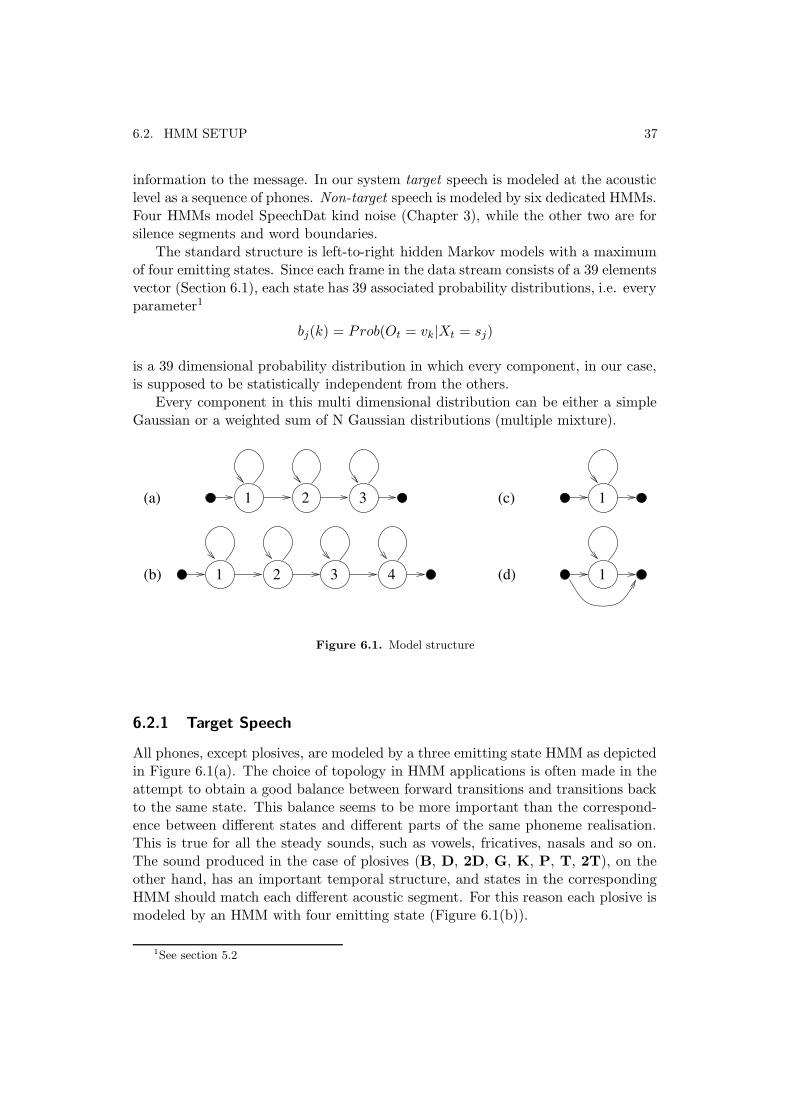
information to the message. In our system target speech is modeled at the acousticlevel as a sequence of phones. Non-target speech is modeled by six dedicated HMMs.Four HMMs model SpeechDat kind noise (Chapter 3), while the other two are forsilence segments and word boundaries.
The standard structure is left-to-right hidden Markov models with a maximumof four emitting states. Since each frame in the data stream consists of a 39 elementsvector (Section 6.1), each state has 39 associated probability distributions, i.e. everyparameter1
bj(k) = Prob(Ot = vk|Xt = sj)
is a 39 dimensional probability distribution in which every component, in our case,is supposed to be statistically independent from the others.
Every component in this multi dimensional distribution can be either a simpleGaussian or a weighted sum of N Gaussian distributions (multiple mixture).
1 2 3
41 2 3 1
1
(b)
(a)
(d)
(c)
Figure 6.1. Model structure
6.2.1 Target Speech
All phones, except plosives, are modeled by a three emitting state HMM as depictedin Figure 6.1(a). The choice of topology in HMM applications is often made in theattempt to obtain a good balance between forward transitions and transitions backto the same state. This balance seems to be more important than the correspond-ence between different states and different parts of the same phoneme realisation.This is true for all the steady sounds, such as vowels, fricatives, nasals and so on.The sound produced in the case of plosives (B, D, 2D, G, K, P, T, 2T), on theother hand, has an important temporal structure, and states in the correspondingHMM should match each different acoustic segment. For this reason each plosive ismodeled by an HMM with four emitting state (Figure 6.1(b)).
1See section 5.2

38 CHAPTER 6. MODEL SET BUILDING
6.2.2 Non-Target Speech
Garbage
As already described in section 3.1.2, SpeechDat adopts the convention to markwith a “*” mispronounced words, with “**” unintelligible words and with a “~”truncated words. For all these occurrences there is no entry in the lexicon, i.e. nopronunciation is provided. To allow the use of files containing these symbols duringtraining, a garbage model has been created. It has only one state with a mixtureof many Gaussian distributions, because it is supposed to match a wide range ofsounds. As we discuss later this model is trained on generic speech, and it shouldwin the competition with models of specific sounds. The garbage model is notused in recognition because only “clean” speech files are used for this task.
Extral, Noise, Öh
Noise models are: extral (SpeechDat mark: [spk]) for speaker noise such as lipssmack, Öh ([fil]) for hesitation between a word and another, noise ([int])for non speaker intermittent noise typical of the telephone lines. There is not aparticular model for stationary noise ([sta]) because this disturbance is extendedto the whole utterance. However, when using noisy files in the training process, thestationary noise characteristics take part in the model parameter estimation, andare hence held by those parameters.
Sil
The sil model is a three state HMM (Figure 6.1 (a)) trained on silence frames ofthe utterance. In the recognition task it is used at the beginning or at the end of asentence in the attempt to model the extra time in the recording session over thespoken utterance.
#
This model is employed for word boundaries: it has a symbolic use, representingthe boundaries between words at the phone level and allowing different contextexpansion methods as already described. A second reason for its use is to model thesilence between one word and another. In continuous speech these silence segmentscan be very short. For this reason # has only one emitting state as depicted inFigure 6.1(d). This state is tied (shared parameters) with the central state of thesil model. Furthermore a direct transition from the first (non emitting) state to thelast (non emitting) state is allowed in the case that words are connected withoutany pause.

6.3. TRAINING THE MODELS 39
6.3 Training The Models
Training consists of applying an embedded version of the Baum-Welch algorithmdiscussed in Section 5.3.2. For every speech file (output sequence) a label file with aphoneme transcription is loaded and used to create an HMM for the whole utteranceconcatenating all models corresponding to the sequence of labels. This is possiblethanks to a property of HMMs: researchers have discovered that if an observationsequence is presented to a strings of HMMs they will tend to “soak up” the part ofthe observation sequence corresponding to their word or phone [9]. This is true whenthe model set parameters are not too far from the optimal values. When initializingthe model set, a different method must be employed. This was not necessary in thiswork because the first model set has been obtained modifying by hand an alreadytrained set of models [12], and hence it is still able to perform a crude alignment.The only completely new model is garbage. In this case the model has been trainedseparately on generic speech files, and then included in the model set.
t
f /ET/
~110ms
t
f
~40ms
/TVÅ:/
Figure 6.2. Spectrogram of the words “ett” (one) and “två” (two)

40 CHAPTER 6. MODEL SET BUILDING
The model set we modified [12] contains the concatenation of two HMMs withthree emitting state for each stop consonant. The first model for each stop (namedwith an uppercase letter: B, D, G, K, P, T) models the occlusion segment in thestop phone, while the second (lowercase letter: b, d, g, k, p, t) models the releasesegment. In our opinion this method can be inaccurate because of the fast timeevolution of plosives. Figure 6.2 shows the spectrogram of the words “ett” (one)and “två” (two). A rough measure of the /t/ stop duration is given in the figure.If we consider 10ms frame interval and six states in the T t model, the minimumduration for model evolution is 60ms, if no transition back to the same state occurs.As we see in the figure this model can be good for the realization of the T soundin the “ett” word, but it is to “slow” for the realization of the same phone in the“två” word. This is one reason why each couple of stop models (B b for example)has been substituted with a four emitting state model. A second (practical) reasonis that it is easier to represent stop consonants with one symbol in the dictionarythan with two. In the attempt to preserve the ability of the model set to align thetraining data, allowing the standard re-estimation procedure, stop models are notcreated ex-novo. They are derived from the old model set in the following way.For each four state model the first emitting state is obtained copying the last statein the corresponding occlusive model. The other three states are copied from thecorresponding release model. The reason for this choice is that, even though theocclusive segment is often longer in time than the release segment, the first oneconsists of an approximately stationary sound, while the latter include most of thetime varying evolution (explosion).
Different model sets obtained by successive re-estimation procedures are storedin different directories to allow a comparative evaluation of their performance andto figure out when to stop the iterative procedure.
Before proceeding the description of model set creation, the evaluation methodmust be introduced.
6.3.1 Development Tests
During training development tests are an important tool in the attempt to comparedifferent experiments and to suggest new possible ways of improvement. Theseexperiments consist of a word level recognition on a small subset of speakers reservedfor this task. The number of speakers (50) involved in these tests is too low toguarantee a statistical consistency of the results, nevertheless these tests can be usedfor a comparative evaluation of different model sets2. When scoring the system, twoalternative parameters are taken into account: correct words and accuracy. Theirdefinition depends on the the algorithm used to align the output of the systemto the reference transcription. This algorithm is an optimal string match basedon dynamic programming [18]. Once the optimal alignment has been found, thenumber of substitution errors (S), deletion errors (D) and insertion errors (I) can
2See Section 3.1.4 for data on speaker subsets.
6.3. TRAINING THE MODELS 41
be calculated. Correct words (PC) are then defined as:
PC =N − D − S
N× 100%
While the definition for accuracy (A) is:
A =N − D − S − I
N× 100%
Files chosen for evaluation contains (see chapter 3) isolated digits, connecteddigits and natural numbers. A list of all words in the development test files isincluded in appendix C.
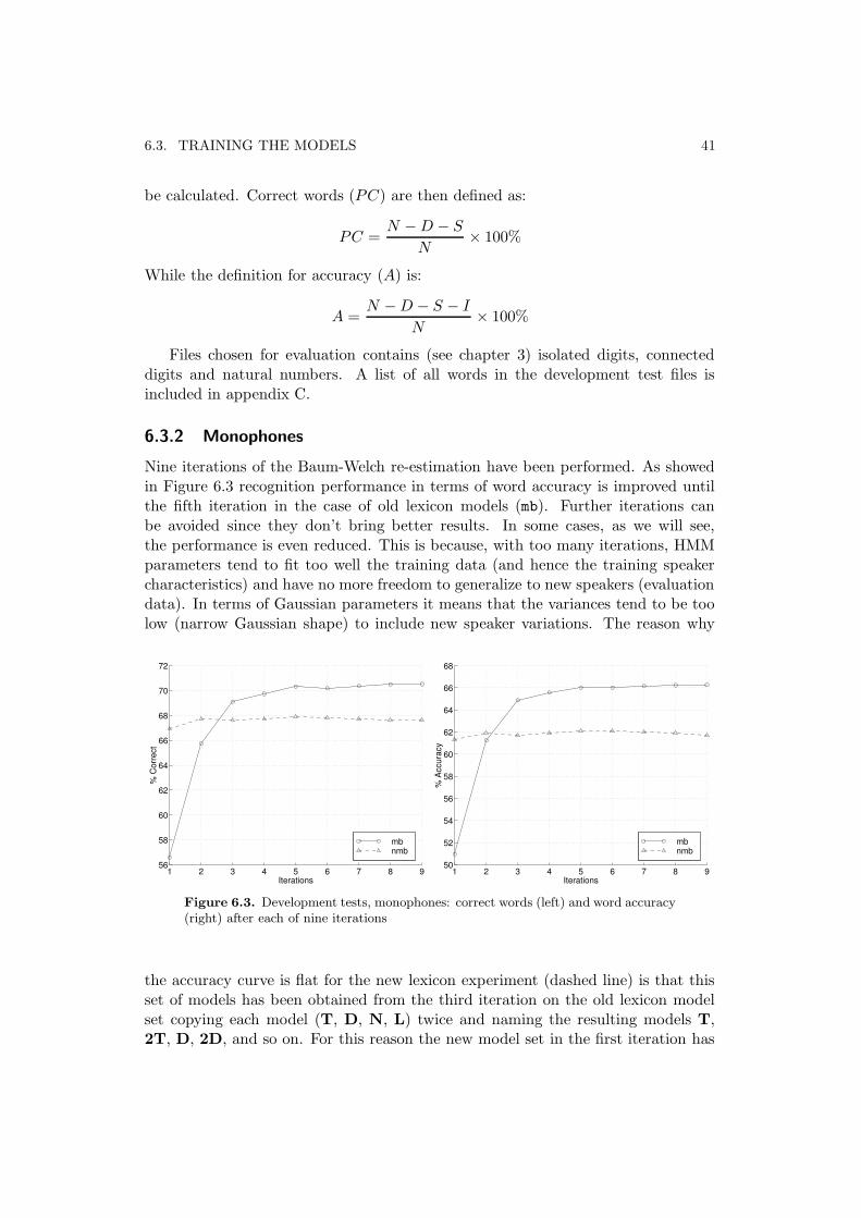
6.3.2 Monophones
Nine iterations of the Baum-Welch re-estimation have been performed. As showedin Figure 6.3 recognition performance in terms of word accuracy is improved untilthe fifth iteration in the case of old lexicon models (mb). Further iterations canbe avoided since they don’t bring better results. In some cases, as we will see,the performance is even reduced. This is because, with too many iterations, HMMparameters tend to fit too well the training data (and hence the training speakercharacteristics) and have no more freedom to generalize to new speakers (evaluationdata). In terms of Gaussian parameters it means that the variances tend to be toolow (narrow Gaussian shape) to include new speaker variations. The reason why
1 2 3 4 5 6 7 8 956
58
60
62
64
66
68
70
72
Iterations
% C
orre
ct
mb nmb
1 2 3 4 5 6 7 8 950
52
54
56
58
60
62
64
66
68
Iterations
% A
ccur
acy
mb nmb
Figure 6.3. Development tests, monophones: correct words (left) and word accuracy(right) after each of nine iterations
the accuracy curve is flat for the new lexicon experiment (dashed line) is that thisset of models has been obtained from the third iteration on the old lexicon modelset copying each model (T, D, N, L) twice and naming the resulting models T,2T, D, 2D, and so on. For this reason the new model set in the first iteration has

42 CHAPTER 6. MODEL SET BUILDING
been already subjected to four iterations (three with the old models and one withthe new) of the Baum-Welsh reestimation.
The first attempt to increasing accuracy was to add Gaussian mixture terms.Results obtained with this method are shown in Figure 6.4 where models with 1,2, 4 and 8 Gaussian terms are compared. Adding Gaussian distributions consists ofsplitting state output distribution of the previous model set (ninth iteration). Thesplitting procedure consists of selecting distributions with the higher associatedweight and copying them twice in the new model set. The weight is divided by 2for each new distribution, while the mean is perturbed. Analytically:
cG(m,σ2) →c
2G(m + 0.2σ, σ2),
c
2G(m − 0.2σ, σ2)
The process is repeated until the wanted number of mixture terms is reached. Inthese figures it is possible to see how models including the four allophones 2T,2D, 2N, 2L (dashed line) have a worse performance if compared to the old lex-icon models. This difference tends to decrease if the number of mixtures terms isincreased.
1 2 3 4 5 6 7 8 955
60
65
70
75
80
1 mix
2 mix
4 mix
8 mix
1 mix
2 mix
4 mix
8 mix
Iterations
% C
orre
ct
mb nmb
1 2 3 4 5 6 7 8 950
55
60
65
70
75
80
1 mix
2 mix
4 mix
8 mix
1 mix
2 mix
4 mix
8 mix
Iterations
% A
ccur
acy
mb nmb
Figure 6.4. Development tests, monophones: correct words (left) and accuracy(right) for 1,2,4,8 mixture terms
6.3.3 Triphones
The construction of context dependent models has been shown to be a good altern-ative method in the attempt to improving accuracy: Two expansion methods havebeen tested:
• within-word context expansion
in which phonemes at word boundaries are expanded as diphones (see Table 5.1page 31). This method is easier to apply in the recognition phase because models
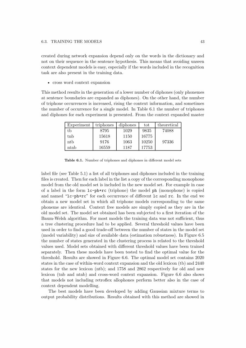
6.3. TRAINING THE MODELS 43
created during network expansion depend only on the words in the dictionary andnot on their sequence in the sentence hypothesis. This means that avoiding unseencontext dependent models is easy, especially if the words included in the recognitiontask are also present in the training data.
• cross word context expansion
This method results in the generation of a lower number of diphones (only phonemesat sentence boundaries are expanded as diphones). On the other hand, the numberof triphone occurrences is increased, rising the context information, and sometimesthe number of occurrence for a single model. In Table 6.1 the number of triphonesand diphones for each experiment is presented. From the context expanded master
Experiment triphones diphones tot theoreticaltb 8795 1029 9835 74088tnb 15618 1150 16775ntb 9176 1063 10250 97336ntnb 16559 1187 17753
Table 6.1. Number of triphones and diphones in different model sets
label file (see Table 5.1) a list of all triphones and diphones included in the trainingfiles is created. Then for each label in the list a copy of the corresponding monophonemodel from the old model set is included in the new model set. For example in caseof a label in the form lc-ph+rc (triphone) the model ph (monophone) is copiedand named “lc-ph+rc” for each occurrence of different lc and rc. In the end weobtain a new model set in which all triphone models corresponding to the samephoneme are identical. Context free models are simply copied as they are in theold model set. The model set obtained has been subjected to a first iteration of theBaum-Welsh algorithm. For most models the training data was not sufficient, thusa tree clustering procedure had to be applied. Several threshold values have beenused in order to find a good trade-off between the number of states in the model set(model variability) and size of available data (estimation robustness). In Figure 6.5the number of states generated in the clustering process is related to the thresholdvalues used. Model sets obtained with different threshold values have been trainedseparately. Then these models have been tested to find the optimal value for thethreshold. Results are showed in Figure 6.6. The optimal model set contains 2020states in the case of within-word context expansion and the old lexicon (tb) and 2440states for the new lexicon (ntb); and 1758 and 2862 respectively for old and newlexicon (tnb and ntnb) and cross-word context expansion. Figure 6.6 also showsthat models not including retroflex allophones perform better also in the case ofcontext dependent modelling.
The best models have been developed by adding Gaussian mixture terms tooutput probability distributions. Results obtained with this method are showed in
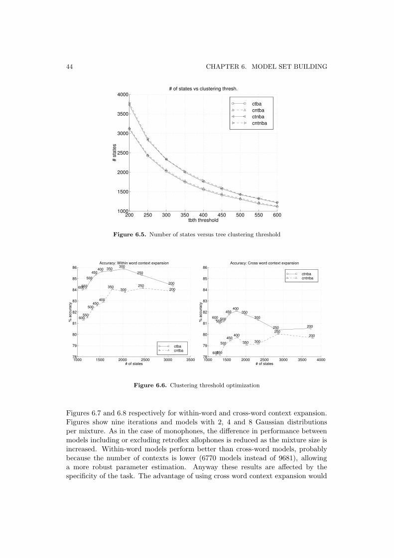
44 CHAPTER 6. MODEL SET BUILDING
200 250 300 350 400 450 500 550 6001000
1500
2000
2500
3000
3500
4000
tbth threshold
# st
ates
# of states vs clustering thresh.
ctba cntba ctnba cntnba
Figure 6.5. Number of states versus tree clustering threshold
1000 1500 2000 2500 3000 350078
79
80
81
82
83
84
85
86
# of states
% a
ccur
acy
Accuracy: Within word context expansion
200
250300350400
450500
550600 200250
300350
400450
500
550600
ctba cntba
1000 1500 2000 2500 3000 3500 400078
79
80
81
82
83
84
85
86
# of states
% a
ccur
acy
Accuracy: Cross word context expansion
200250
300350
400450
500550600
200250
300350
400450
500
550600
ctnba cntnba
Figure 6.6. Clustering threshold optimization
Figures 6.7 and 6.8 respectively for within-word and cross-word context expansion.Figures show nine iterations and models with 2, 4 and 8 Gaussian distributionsper mixture. As in the case of monophones, the difference in performance betweenmodels including or excluding retroflex allophones is reduced as the mixture size isincreased. Within-word models perform better than cross-word models, probablybecause the number of contexts is lower (6770 models instead of 9681), allowinga more robust parameter estimation. Anyway these results are affected by thespecificity of the task. The advantage of using cross word context expansion would
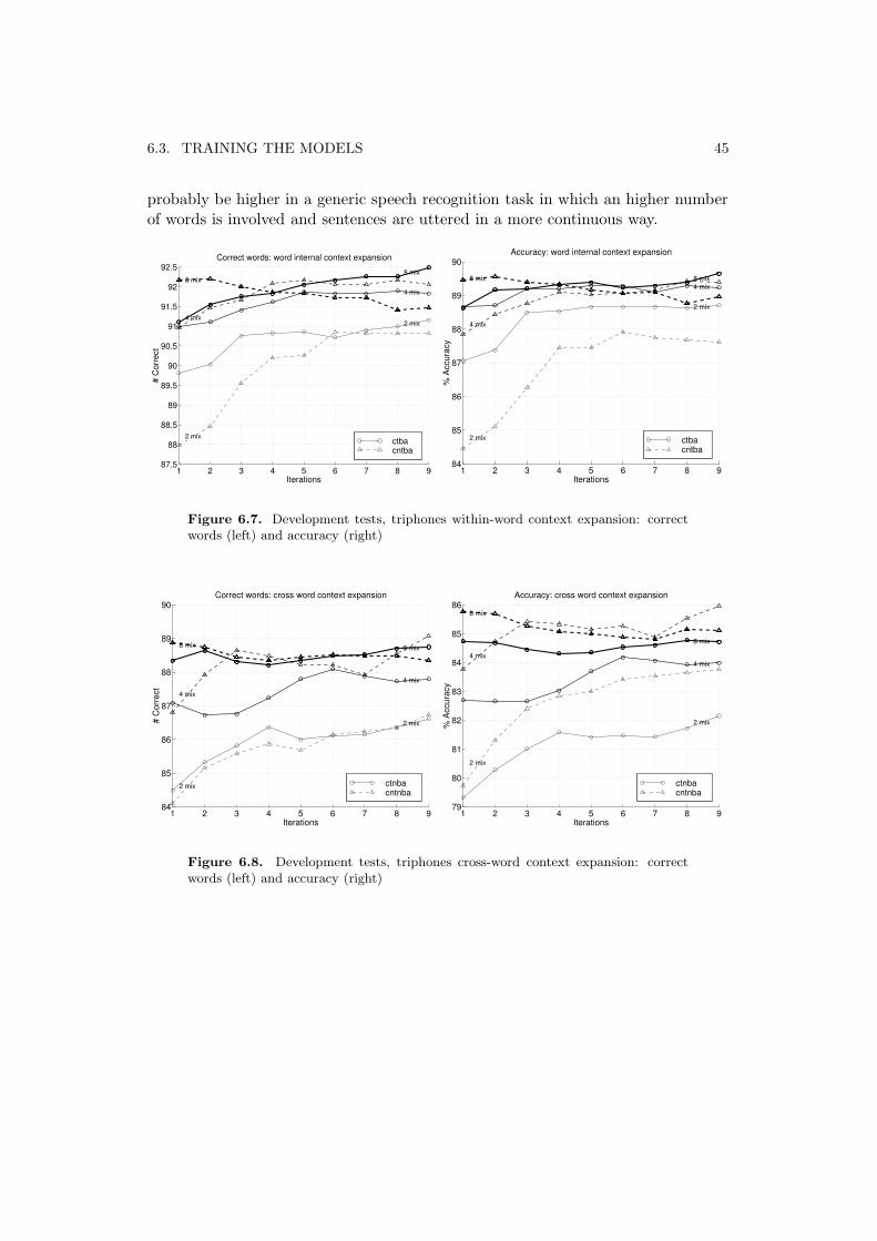
6.3. TRAINING THE MODELS 45
probably be higher in a generic speech recognition task in which an higher numberof words is involved and sentences are uttered in a more continuous way.
1 2 3 4 5 6 7 8 987.5
88
88.5
89
89.5
90
90.5
91
91.5
92
92.5
2 mix
4 mix
8 mix
2 mix
4 mix
8 mix
Iterations
# Co
rrect
Correct words: word internal context expansion
ctba cntba
1 2 3 4 5 6 7 8 984
85
86
87
88
89
90
2 mix
4 mix8 mix
2 mix
4 mix
8 mix
Iterations
% A
ccur
acy
Accuracy: word internal context expansion
ctba cntba
Figure 6.7. Development tests, triphones within-word context expansion: correctwords (left) and accuracy (right)
1 2 3 4 5 6 7 8 984
85
86
87
88
89
90
2 mix
4 mix
8 mix
2 mix
4 mix
8 mix
Iterations
# Co
rrect
Correct words: cross word context expansion
ctnba cntnba
1 2 3 4 5 6 7 8 979
80
81
82
83
84
85
86
2 mix
4 mix
8 mix
2 mix
4 mix
8 mix
Iterations
% A
ccur
acy
Accuracy: cross word context expansion
ctnba cntnba
Figure 6.8. Development tests, triphones cross-word context expansion: correctwords (left) and accuracy (right)


Chapter 7
Results, Analysis and Discussion
This chapter begins with a definition of the “difficulty” of the problem of speechrecognition (Section 7.1). Then results are described and analyzed first for the fullevaluation subset of speakers in Section 7.2 and then with regard on the individualspeaker characteristics in Section 7.3. Since this work has been the first attempt totrain acoustic models on the Swedish SpeechDat database, the only way to compareresults with previous works is to refer to different experiments. In Section 7.4.1results are compared to those obtained with a database built for a different purpose(the Waxholm database) but for the same language (Swedish). In Section 7.4.2,instead, the comparison is made for a similar database (the Norwegian SpeechDatdatabase), but for a different language (Norwegian).
7.1 Language Model Perplexity
When evaluating the performance of a speech recognizer, quantifying the difficultyof the recognition task is an important aspect to consider. One measure can beobtained from the so called perplexity of the language model[9]. Perplexity is anindirect measure of the entropy of the language: the higher the entropy, the moreinformation must be extracted from the recognition process and the more difficultthe task is. In other words, when employing language constraints such as a grammar,the uncertainty of the content of sentences is reduced, and the recognition task ismade easier. Perplexity as defined in [9] involves the estimation of the probabilitythat a particular sequence of words is generated by the language source. If x is asymbol put out by a source with probability P (x), then the entropy of the sourceis defined as
H = −[L
∑
x=1
P (x) log P (x)]
where L is the number of possible symbols. If we consider sequences of symbols theentropy is defined as
H = − limn→∞
1
n[∑
P (x1, ..., xn) log P (x1, ..., xn)]
47

48 CHAPTER 7. RESULTS, ANALYSIS AND DISCUSSION
where the sum is over all sequences x1, ..., xn. If the source is ergodic, one sufficientlylong sequence of symbols can be used to deduce its statistical structure, hence
H = − limn→∞
1
n[log P (x1, ..., xn)]
Finally perplexity is defined as:
PP = 2H = P (x1, ..., xn)−1
n
where the limit has been removed for real applications. In our case the sequencex1, ..., xn correspond to the evaluation corpus (concatenation of sentences in theevaluation files) while P (x1, ..., xn) can be evaluated from the word bigram prob-ability, estimated on the training material. Perplexity for our case is around 40,classifying the task as a medium perplexity recognition problem [19, 7]. Normallydigit recognition problems have in English PP = 11. In our case other words areincluded allowing for example natural number recognition, and the same grammarconstraints are used for all tasks.
7.2 Overall Results
From the development tests (Chapter 6) the best models were selected and tested onthe evaluation material. Results obtained with these tests are showed in Table 7.1.In the table correct words and accuracy are reported for each experiment. The best
1 mix 2 mix 4 mix 8 mixexperiment Corr Acc Corr Acc Corr Acc Corr Accmb 69.4 66.4 72.6 69.5 75.6 72.3 78.9 76.0nmb 68.1 63.1 71.5 67.9 75.1 71.3 79.1 75.5ctba 89.5 87.4 90.7 88.5 90.8 88.6cntba 89.1 86.4 90.3 88.1 90.5 88.3ctnba 86.1 81.8 87.8 84.0 88.4 84.8cntnba 86.8 84.2 88.4 86.1 88.9 86.5
Table 7.1. Overall results: evaluation data correct words (Corr) and accuracy (Acc)for monophones, old lexicon (mb), monophones, new lexicon (nmb), triphones, oldlexicon, within word CE (ctba), triphones, new lexicon, within word CE (cntba),triphones, old lexicon, cross word CE (ctnba), triphones, new lexicon, cross word CE(cntnba).
result (88.6% of accuracy) is obtained with within-word context expanded modelsand eight mixture terms. As can be seen in the table, monophone accuracy riseswhen the number of mixture terms is increased from four to eight. This means thatprobably better results can be obtained if the number of mixture terms is furtherincreased. In the case of context dependent models the increase of accuracy from

7.2. OVERALL RESULTS 49
four terms models to eight terms models is quite low. Old lexicon models performbetter in general than new lexicon models. Models excluding cross-word contextinformation perform better than models including it.
Since the number of development speakers is low, plots of accuracy and correctwords as functions of the number of iterations are also reported to check if perform-ance follows the same trend on a larger and independent data set. Figure 7.1 showsresults for monophone models. In each plot models based on the old lexicon seemto perform better than models including the retroflex allophones, if the numberof Gaussian distributions is the same. Only in a few cases more than five or sixiterations are useful to improve performance. Figure 7.2 shows results for within
1 2 3 4 5 6 7 8 950
55
60
65
70
75
80
1 mix
2 mix
4 mix
8 mix
1 mix
2 mix
4 mix
8 mix
Iterations
% C
orre
ct
Correct Words: Monophones
mb nmb
1 2 3 4 5 6 7 8 950
55
60
65
70
75
80
1 mix
2 mix
4 mix
8 mix
1 mix
2 mix
4 mix
8 mix
Iterations
% A
ccur
acy
Accuracy: Monophones
mb nmb
Figure 7.1. Evaluation test, monophones: correct words (left) and Accuracy (right).
word context expanded triphones. In this case curves are not as regular as in themonophone case. This may be because the amount of training data for each modelis not as consistence as in the monophone case. Many times, the best result isobtained for a different number of iterations if compared to the development testsresults (Figure 6.7 page 45). For example, in the case of old lexicon, eight-termmixtures (solid thick line) the best result is obtained after five iterations. Thenaccuracy falls down, while in the development test it continues rising till the ninthiteration. This shows how these models, depending on the lower amount of datathey are trained on, could be (lightly) dependent on the speaker characteristics andalso shows that we should be careful when considering results on the fifty speakersdevelopment subset. Once again the old lexicon models perform better, but thisdifference is slightly reduced when adding Gaussian distributions. Figure 7.3 showsresults for cross word context expanded models. In this case a comparison betweenold and new lexicon models is more difficult because the number of states containedin each model set is ... different (1758 states for the old lexicon: ctnba and 2862states for the new lexicon: cntnba). This difference has been caused by the nonregular shape of the accuracy curve in the tree clustering optimization procedure

50 CHAPTER 7. RESULTS, ANALYSIS AND DISCUSSION
1 2 3 4 5 6 7 8 986.5
87
87.5
88
88.5
89
89.5
90
90.5
91
2 mix
4 mix8 mix
2 mix
4 mix
8 mix
Iterations
# Co
rrect
Correct words: within word context expansion
ctba cntba
1 2 3 4 5 6 7 8 983
84
85
86
87
88
89
2 mix
4 mix8 mix
2 mix
4 mix
8 mix
Iterations
% A
ccur
acy
Accuracy: within word context expansion
ctba cntba
Figure 7.2. Evaluation test, triphones, within word expansion: correct words (left)and Accuracy (right) for 2, 4, 8 mixture terms.
(Figure 6.6, page 44). In the case of models including the retroflex allophones (newlexicon: cntnba), the accuracy curve in Figure 6.6 has two maxima for 1784 and2862 states in the model set. The latter model set has been chosen for furtherimprovements because the accuracy is higher. Referring to Figure 7.3 unexpectedresults are obtained: the cntnba model set (2862 states, dashed line) performs bet-ter than the ctnba model set (solid line, 1758 states). This difference in resultsseems to be more related to the difference in number of states than on the differentlexicon.
1 2 3 4 5 6 7 8 983
84
85
86
87
88
89
2 mix
4 mix
8 mix
2 mix
4 mix
8 mix
Iterations
# Co
rrect
Correct words: cross word context expansion
ctnba cntnba
1 2 3 4 5 6 7 8 978
79
80
81
82
83
84
85
86
87
2 mix
4 mix
8 mix
2 mix
4 mix
8 mix
Iterations
% A
ccur
acy
Accuracy: cross word context expansion
ctnba cntnba
Figure 7.3. Evaluation test, triphones, cross word expansion: correct words (left)and Accuracy (right) for 2, 4, 8 mixture terms.
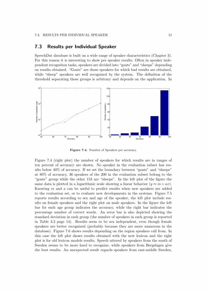
7.3. RESULTS PER INDIVIDUAL SPEAKER 51
7.3 Results per Individual Speaker
SpeechDat database is built on a wide range of speaker characteristics (Chapter 3).For this reason it is interesting to show per speaker results. Often in speaker inde-pendent recognition tasks, speakers are divided into “goats” and “sheeps” dependingon results obtained. “Goats” are those speakers for which bad results are obtained,while “sheep” speakers are well recognized by the system. The definition of thethreshold separating these groups is arbitrary and depends on the application. In
50 60 70 80 90 100100
101
102
103
Accuracy
Num
ber o
f spe
aker
s (lo
g)
40 50 60 70 80 90 1000
20
40
60
80
100
120
Accuracy
Num
ber o
f spe
aker
s
Figure 7.4. Number of Speakers per accuracy.
Figure 7.4 (right plot) the number of speakers for which results are in ranges often percent of accuracy are shown. No speaker in the evaluation subset has res-ults below 40% of accuracy. If we set the boundary between “goats” and “sheeps”at 80% of accuracy, 36 speakers of the 200 in the evaluation subset belong to the“goats” group while the other 153 are “sheeps”. In the left plot of the figure thesame data is plotted in a logarithmic scale showing a linear behavior (y ≈ m + ax).Knowing m and a can be useful to predict results when new speakers are addedto the evaluation set, or to evaluate new developments in the systems. Figure 7.5reports results according to sex and age of the speaker, the left plot include res-ults on female speakers and the right plot on male speakers. In the figure the leftbar for each age group indicates the accuracy, while the right bar indicates thepercentage number of correct words. An error bar is also depicted showing thestandard deviation in each group (the number of speakers in each group is reportedin Table 3.2 page 14). Results seem to be sex independent, even though femalespeakers are better recognized (probably because they are more numerous in thedatabase). Figure 7.6 shows results depending on the region speakers call from. Inthis case the left plot shows results obtained with the new lexicon and the rightplot is for old lexicon models results. Speech uttered by speakers from the south ofSweden seems to be more hard to recognize, while speakers from Bergslagen givethe best results. An unexpected result regards speakers from east-middle Sweden,
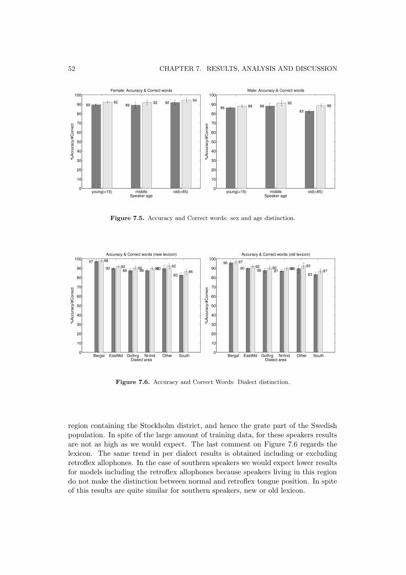
52 CHAPTER 7. RESULTS, ANALYSIS AND DISCUSSION
young(<15) middle old(>65) 0
10
20
30
40
50
60
70
80
90
100
89 89 9292 92 94
Female: Accuracy & Correct words
Speaker age
%Ac
cura
cy/#
Corre
ct
young(<15) middle old(>65) 0
10
20
30
40
50
60
70
80
90
100
86 8883
8892
88
Male: Accuracy & Correct words
Speaker age
%Ac
cura
cy/#
Corre
ct
Figure 7.5. Accuracy and Correct words: sex and age distinction.
Bergsl EastMd Gothrg Nrrlnd Other South0
10
20
30
40
50
60
70
80
90
100 9790 88 88 90
83
9892 90 90 92
86
Accuracy & Correct words (new lexicon)
Dialect area
%Ac
cura
cy/#
Corre
ct
Bergsl EastMd Gothrg Nrrlnd Other South0
10
20
30
40
50
60
70
80
90
10096
90 88 87 9083
9792 90 90 93
87
Accuracy & Correct words (old lexicon)
Dialect area
%Ac
cura
cy/#
Corre
ct
Figure 7.6. Accuracy and Correct Words: Dialect distinction.
region containing the Stockholm district, and hence the grate part of the Swedishpopulation. In spite of the large amount of training data, for these speakers resultsare not as high as we would expect. The last comment on Figure 7.6 regards thelexicon. The same trend in per dialect results is obtained including or excludingretroflex allophones. In the case of southern speakers we would expect lower resultsfor models including the retroflex allophones because speakers living in this regiondo not make the distinction between normal and retroflex tongue position. In spiteof this results are quite similar for southern speakers, new or old lexicon.

7.4. EVALUATING ON OTHER DATABASES 53
7.4 Evaluating on Other Databases
To judge system performance it would be important to compare results with thoseobtained with other systems in similar conditions. In our case it is not possibleto refer to a previous work on the Swedish SpeechDat database. Comparison ismade referring to two experiments which contain substantial differences from theSpeechDat context. For these differences an evaluation of the model flexibility ispossible. The two experiments taken into account refer to the Waxholm project andto the Norwegian SpeechDat project and will be described in the next sections.
7.4.1 The Waxholm Database
The Waxholm database presents many differences if compared to the SpeechDatdatabase. First of all it was developed in the Waxholm project in the attemptto create a dialogue system for information about boat traffic, restaurants andaccommodations in the Stockholm archipelago. The corpus of sentences included ishence affected by this task. The number of speakers (mostly men) is low if comparedto the SpeechDat collection. 50% Speakers have an accent typical of the Stockholmarea. Speech sampling and labeling are also different (16kHz and phone level by-hand transcriptions). Down-sampling audio files has been necessary because modelsdeveloped in this work are built for telephone speech. Doing this part of the spectralinformation in the speech files has been lost.
Models are then tested on the same subset of ten speakers used in [16] on ageneric word recognition task, even if model parameters have been tuned in thiswork with reference to a digit and natural number recognition task. Within-wordcontext expansion models with eight Gaussian distributions per mixture scored89.9% of accuracy, while in [16] 86.6% of accuracy was reached with sixteen Gaussiandistributions triphones.
This prove how these models, in spite of the task adopted in this work, can beemployed in a more wide range of applications.
7.4.2 The Norwegian SpeecDat database
In Norway similar experiments to those made in this work have been done forNorwegian in the SpeechDat project [8]. Results are not directly comparable forexample because in our case the same network (loop of words, bigram) has beenused for a wide range of different items including for example isolated digits forwhich a grammar definition allowing only one word (digit) for utterance would bemore efficient. However, these results are always similar, even though Norwegianmodels have been trained on 816 speakers instead of the 750 in our experiments, andthe complete database corpus has been used, while only phonetically rich sentencesand words have been used in our experiments.


Chapter 8
Discussion and Conclusions
Overall results on the evaluation material have shown that models excluding ret-roflex allophones in general perform better than models including them. This con-clusion is surely affected by the task, in fact only a few words included in therecognition task (fyrtio, fjorton, arton, kontokort) contain the allophone 2T, andthere is no occurrence of the other allophones. This means that splitting these mod-els in normal and retroflex versions (as in the new lexicon) results only in a loweramount of data for the normal (non retroflex) models mostly used in this task.
Furthermore models including only within-word contexts seem to perform betterthan models including cross word context information. This result is also affected bythe task, first because one of the items included in the evaluating material consistsof isolated digits (no cross-word context is available), and second because whenuttering digits and natural numbers speakers tend to separate each word to makethe sequence clear. In a generic speech recognition task in which a higher numberof words is involved and sentences are uttered in a more continuous way, probablythe advantage of using cross-word context expansion would be higher.
Per speaker results have shown how models fit quite well to different classes ofspeakers, with some exceptions. Finally testing models on the Waxholm databasehas shown the flexibility of these models in spite of the simple task they have beenbuilt for.
8.1 Further Improvements
Results for monophone models showed a considerable improvement when passingfrom four to eight Gaussian terms. For this reason it is likely that further im-provements are still possible adding more Gaussian terms. In the case of contextdependent models this possibility seems to be more problematic, depending on thefact that the amount of data is not sufficient to train the large number of para-meters included in these models. An attempt to reduce this problem could be theuse of a model set with a lower number of states respect to the optimal value (treeclustering threshold optimization) as a base to add Gaussian distributions. The
55

56 CHAPTER 8. DISCUSSION AND CONCLUSIONS
Tree clustering threshold optimization in fact is worked out on single distributionmodels, and there is no reason to think that the number of states in the model set isoptimal also when increasing the number of Gaussian parameters. One experimentin this direction has been tested without good results.
However, when the full 5000 speakers database will be avaliable, the data scarcityproblem will be reduced allowing the use of more complex models (more Gaussiandistributions, lower number of states to be clustered to reduce the number of para-meters). Using this database, different strategies will be possible, as for example thecreation of two different model sets for female and male speakers, or the creation ofdialect dependent models (for example particular models could be built for speakersfrom the south, which seem to have different characteristics from all the others inSweden).
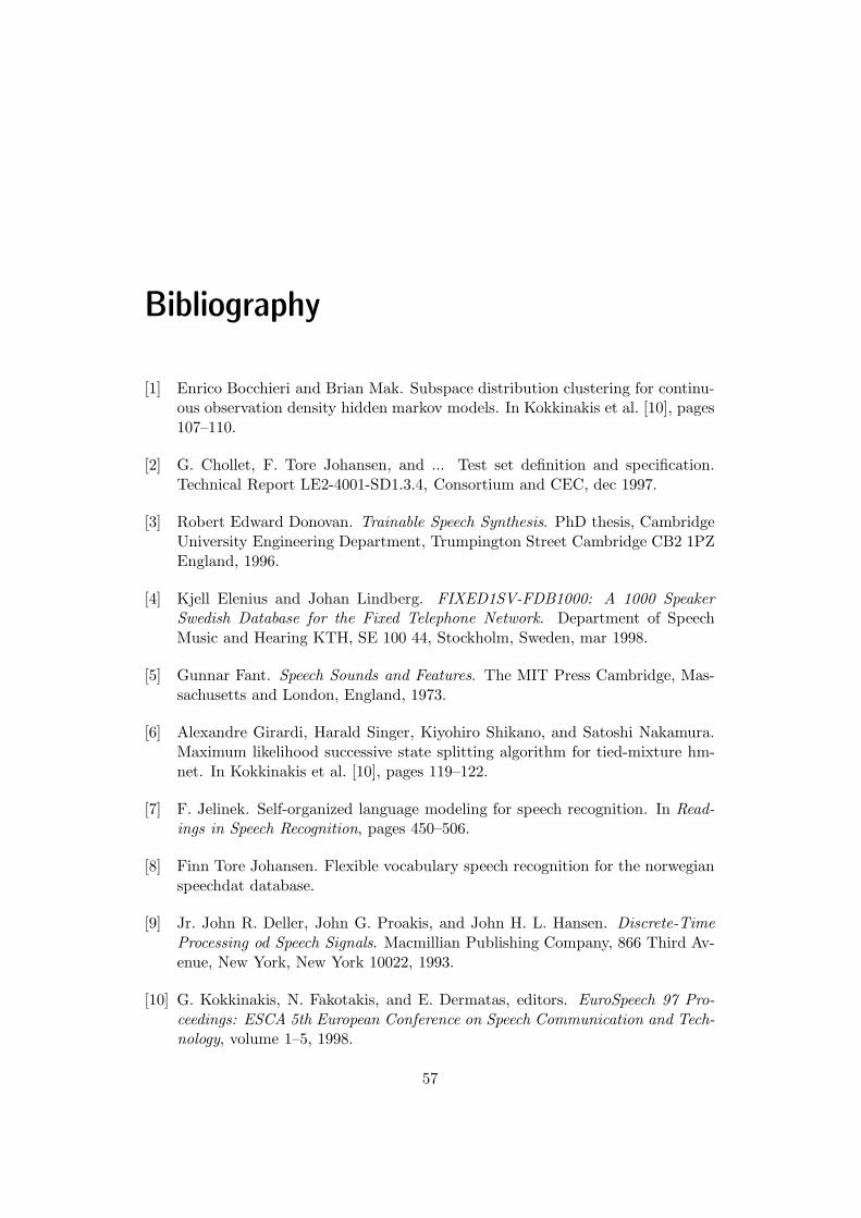
Bibliography
[1] Enrico Bocchieri and Brian Mak. Subspace distribution clustering for continu-ous observation density hidden markov models. In Kokkinakis et al. [10], pages107–110.
[2] G. Chollet, F. Tore Johansen, and ... Test set definition and specification.Technical Report LE2-4001-SD1.3.4, Consortium and CEC, dec 1997.
[3] Robert Edward Donovan. Trainable Speech Synthesis. PhD thesis, CambridgeUniversity Engineering Department, Trumpington Street Cambridge CB2 1PZEngland, 1996.
[4] Kjell Elenius and Johan Lindberg. FIXED1SV-FDB1000: A 1000 SpeakerSwedish Database for the Fixed Telephone Network. Department of SpeechMusic and Hearing KTH, SE 100 44, Stockholm, Sweden, mar 1998.
[5] Gunnar Fant. Speech Sounds and Features. The MIT Press Cambridge, Mas-sachusetts and London, England, 1973.
[6] Alexandre Girardi, Harald Singer, Kiyohiro Shikano, and Satoshi Nakamura.Maximum likelihood successive state splitting algorithm for tied-mixture hm-net. In Kokkinakis et al. [10], pages 119–122.
[7] F. Jelinek. Self-organized language modeling for speech recognition. In Read-ings in Speech Recognition, pages 450–506.
[8] Finn Tore Johansen. Flexible vocabulary speech recognition for the norwegianspeechdat database.
[9] Jr. John R. Deller, John G. Proakis, and John H. L. Hansen. Discrete-TimeProcessing od Speech Signals. Macmillian Publishing Company, 866 Third Av-enue, New York, New York 10022, 1993.
[10] G. Kokkinakis, N. Fakotakis, and E. Dermatas, editors. EuroSpeech 97 Pro-ceedings: ESCA 5th European Conference on Speech Communication and Tech-nology, volume 1–5, 1998.
57

58 BIBLIOGRAPHY
[11] Chin-Hui Lee and Lawrence R. Rabiner. A frame-syncronous network searchalgorithm for connected word recognition. IEEE Transaction on Acoustics,Speech, and Signal Processing, 37:1649–1658, November 1989.
[12] Håkan Melin. On word boundary detection in digital-based speaker verifica-tion. In La Reconnaissance du Locuteur et ses Applications Commerciales etCriminalistiques, pages 46–49, 1998.
[13] H. J. Nock, M. J. F. Gales, and S. J. Young. A comparative study of methodsfor phonetic decision-tree state clustering. In Kokkinakis et al. [10], pages111–114.
[14] Lawrence R. Rabiner and Ronald W. Schafer. Digital Processing of SpeechSignals. Prentice-Hall International, Inc, Englewood Cliffs, New Jersey 07632,1978.
[15] F. Senia, R. Comeyne, Borge Lindberg, and ... Environmental and speakerspecific coverage for fixed networks. Technical Report LE2-4001-SD1.2.1, Con-sortium and CEC, feb 1997.
[16] Kåre Sjölander. Continuous speech recognition with hidden markov models.Master’s thesis, Kungliga Tekniska Högskolan Department of Speech, Musicand Hearing, Drottning Kristinas väg 31 100 44 Stockholm, 1996.
[17] S. J. Young. A general use of tying in phoneme-based hmm speech recognizers.In Proceedings of the 1992 IEEE International Conference on Acoustic, Speechand Signal Processing, volume 1–6, pages 569–572, 1992.
[18] Steve Young, Julian Odell, Dave Ollason, Valtcho Valtchev, and Phil Wood-land. The HTK Book. Entropic Cambridge University Laboratory, dec 1997.
[19] Victor W. Zue. From signals to symbols to meaning: on machine understandingof spoken language. In XIIth International Congress of Phonetic Siences, 1991.
Appendix A
Speech Signal Models
This appendix describes speech models and gives a motivation for the use of mel-cepstral analysis. In Section A.1 models for speech production are discussed, whileSections A.2 and A.3 describe cepstral analysis and the mel-frequency filter bank.
A.1 Speech Signal Models
A model for speech production consists essentially of a slowly time-varying linearsystem excited by either a quasi-periodic impulse train or by random noise [14]. Ashort segment of speech signal can hence be considered to be a stationary processand can be written as
s(n) = p(n) ∗ g(n) ∗ v(n) ∗ r(n) = p(n) ∗ hv(n) =
=+∞∑
r=−∞
hv(n − rNp)
for voiced speech, and
s(n) = u(n) ∗ v(n) ∗ r(n) = p(n) ∗ hu(n)
for unvoiced speech, where p(n) is a periodic impulse train of Np samples, hv(n) isthe impulse response of the linear system that combines the effects of the glottalwave shape g(n), the vocal tract impulse response v(n) and the radiation impulseresponse r(n), u(n) is a random noise excitation and finally hu(n) is the impulseresponse of the system combining the effects of the vocal tract and the radiation.In the z-transform domain
Hv(z) = G(z)V (z)R(z)
Hu(z) = V (z)R(z)
are the speech system transfer functions for voiced and unvoiced segments.
59

60 APPENDIX A. SPEECH SIGNAL MODELS
A physiological study of the glottal system and the vocal tract based on pressuretube theory leads to an approximated model for these transfer functions: the vocaltract filter can be modeled by
V (z) =
Az−MMi∏
k=1
(1 − akz−1)
Mo∏
k=1
(1 − bkz)
Ni∏
k=1
(1 − ckz−1)
For voiced speech, except nasals, an adequate model includes only poles (ak = 0;bk = 0 ∀k). As described in Chapter 2, nasal sounds are produced with a totalconstriction in the oral tract. The oral tract works as a resonant cavity trappingenergy at natural frequencies and hence introducing zeros in the transfer function.The radiation effects result in a high frequency emphasis which can be roughlymodeled by
R(z) ≈ 1 − z−1
Finally, for voiced speech, the glottal pulse shape is of finite duration and, thus,G(z) has the form
G(z) = BLi∏
k=1
(1 − αkz−1)
Lo∏
k=1
(1 − βkz)
In general the global speech signal in the z-transform domain1, contains slowvariations (vocal tract filtering) combined with fast variations (glottal wave) [9] asdepicted in figure A.1(a) (left plot).
A.2 Cepstral Analysis
An intuitive way of understanding how cepstral analysis can be useful in this contextis to consider linear filtering techniques.
Problems in which linear filtering is employed usually regard a number of sig-nals mixed together in a linear combination. The aim is usually to separate thesecomponents. For example if we consider a signal affected by addictive noise in theform
s = m + e
and we want to remove the undesired component e, we would probably need todesign a system whose transfer function obeys:
y1 = L[m] ≈ m (A.1)y2 = L[e] ≈ 0 (A.2)
1For what we said a standard frequency domain analysis is not possible for the speech signal.In the following discussion the z-transform must be intended as a short term transform.

A.2. CEPSTRAL ANALYSIS 61
"Slow" variations(envelope)
"Fast" variations(pulses)
(a)
PSfrag replacements
|S(ω)|
π ω
=
PSfrag replacements|S(ω)|
π ω
x
PSfrag replacements|S(ω)|
π ω
(b)
PSfrag replacements|S(ω)|
π ω
=
PSfrag replacements|S(ω)|
π ω
+
PSfrag replacements|S(ω)|
π ω
(c)
PSfrag replacements|S(ω)|
πω
=
PSfrag replacements|S(ω)|
πω
+
PSfrag replacements|S(ω)|
πω
Figure A.1. Illustration of cepstral analysis of a voiced speech sound
Properties of linear systems ensure that y = L[s] ≈ m as wanted. The use ofFourier analysis and the introduction of a frequency domain help understandingand designing the filter L. Referring to the frequency domain we understand howthe difficulty of the task depends on how well m and e are separated in frequencyi.e. they occupy different frequency intervals.
The speech problem presents many differences. We still want to separate differ-ent components of the signal, but they are mixed in a convolutive way, preventingthe use of standard linear filtering.
The idea is to find a new domain in which these components, or at least theirrepresentatives, are simply added. As known the spectrum of the convolution of twosignals is the product of the spectra of each signal (see Figure A.1 (a)). Furthermore,if we think of the properties of logarithm, we can write
log Hv(z) = log G(z) + log V (z)R(z) (A.3)
as depicted in Figure A.1(b). The domain we were looking for has been called“cepstrum domain” by its first discoverers, and the transformation is intuitivelydefined by A.3. In this domain we can employ standard linear filtering if the aimis to remove undesired components of the signal, as in the case of Equations A.22.The need to find an inverse transform to return into the time domain, as in case
2Of course the possibility of separating the two components in the new domain lies in theeventuality that they are still high and low quefrency even though we have subjected them to thisnon-linear transformation.

62 APPENDIX A. SPEECH SIGNAL MODELS
of Equations A.2, implies the use of a complex cepstrum (CC) which is defined asthe complex logarithm of the complex spectrum. In speech applications, however,information of interest is usually contained in the cepstrum and there is no need toreturn into the time domain. For this reason a real cepstrum defined as the inversefourier transform of the spectrum absolute part
c(n) = F−1log |Fs(n)| =1
2π
∫ π
−πlog |S(ω)|ejωndω
is usually employed (Figure A.1(c)). Indeed the only difference between RC andCC is that RC discards phase information about the signal while CC retains it.Although the preservation of phase bestows certain properties that are lost withthe RC, the CC is often difficult to use in practise.
A.3 Mel Frequency
To understand the meaning of the mel-frequency filter-bank we first have to under-stand the term “mel”. A mel is a unit of measure of perceived pitch or frequency ofa tone. Its introduction is due to studies in the field of psychoacoustic. The exper-iment which determined the introduction of the mel scale consisted of an auditoryperception test: the frequency of 1000 Hz has been chosen arbitrarily and designedas “1000 mels”. Then listeners were asked to change the physical frequency untilthe pitch they perceived was twice the reference, 10 times, half, 1
10 the reference,and so on. These pitches were labeled as 2000 mels, 10000 mels, 500 mels, 100mels, and so on. In the end the investigators were able to say that the mappingbetween the real frequency scale (Hz) and the perceived frequency scale (mels) isapproximately linear below 1 kHz and logarithmic above. The definition we usedfor the mel scale is
Mel(f) = 2595 log10 [1 +f
700]
An approach to evaluating mel-cepstrum coefficients could be oversampling thefrequency axis when computing the stDFT (stFFT) and then selecting those fre-quency samples that represent (approximately) the mel-scale distribution, discard-ing all the other samples. But other considerations on human perception comein help to choose a different method: the ability of perceiving a frequency f0 isinfluenced by energy in a critical band of frequencies around f0, and the criticalbandwidth varies with the frequency, being constant for f0 < 1 kHz and increasinglogarithmically for f0 > 1 kHz. This means that we resolve better low frequen-cies that high ones. Therefore, rather than simply using the mel-distributed logmagnitude frequency components to compute the mel-cepstrum coefficients, the logtotal energy in critical bands is employed. For this aim the stDFT components areweighted by filter transfer functions depicted in figure A.2 and summed to generatethe log total energy for each mel frequency sample. Indeed the concatenation ofDFT and sums results in a filter-bank whose transfer function is analogous to theone depicted in figure A.2.
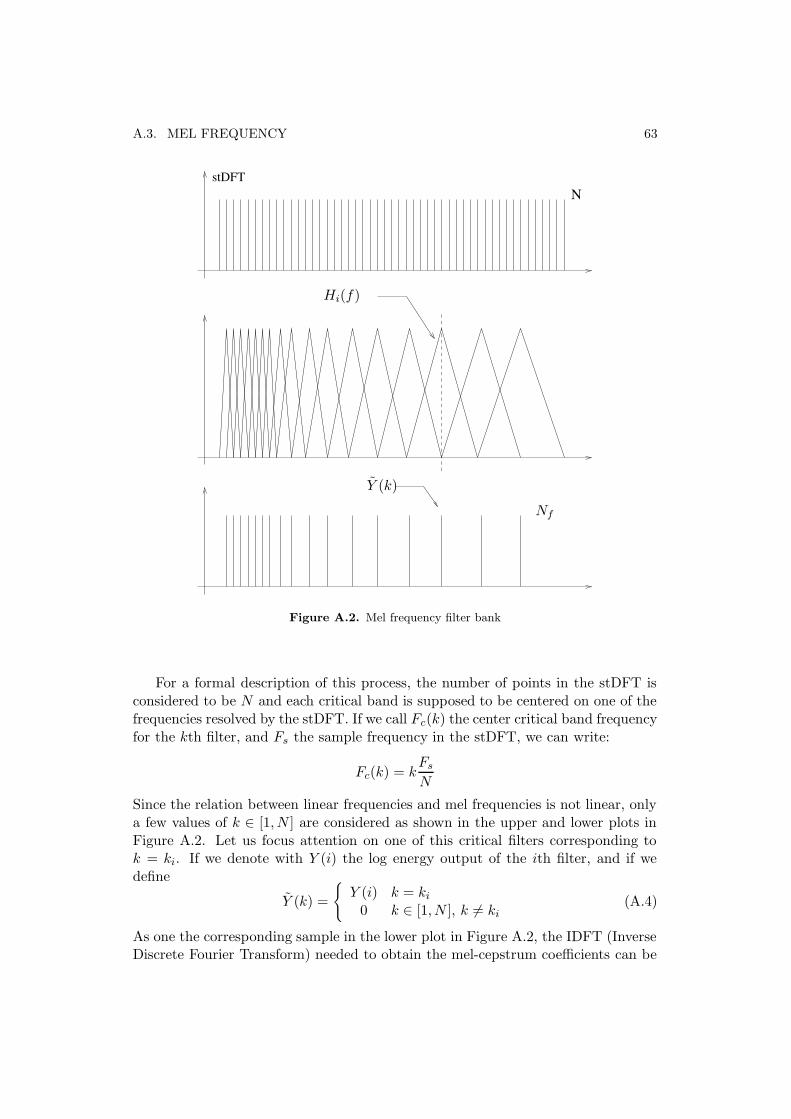
A.3. MEL FREQUENCY 63
stDFTN
PSfrag replacements
Hi(f)
Y (k)
Nf
Figure A.2. Mel frequency filter bank
For a formal description of this process, the number of points in the stDFT isconsidered to be N and each critical band is supposed to be centered on one of thefrequencies resolved by the stDFT. If we call Fc(k) the center critical band frequencyfor the kth filter, and Fs the sample frequency in the stDFT, we can write:
Fc(k) = kFs
N
Since the relation between linear frequencies and mel frequencies is not linear, onlya few values of k ∈ [1, N ] are considered as shown in the upper and lower plots inFigure A.2. Let us focus attention on one of this critical filters corresponding tok = ki. If we denote with Y (i) the log energy output of the ith filter, and if wedefine
Y (k) =
{
Y (i) k = ki
0 k ∈ [1, N ], k 6= ki(A.4)
As one the corresponding sample in the lower plot in Figure A.2, the IDFT (InverseDiscrete Fourier Transform) needed to obtain the mel-cepstrum coefficients can be

64 APPENDIX A. SPEECH SIGNAL MODELS
written as
c(n;m) =1
N
N−1∑
k=0
Y (k) exp jk(2π
N)n
Since Y (k) is symmetrical about N2 (“even”) we can replace the exponential by a
cosine.
c(n;m) =1
N
N−1∑
k=0
Y (k)cos(k2π
Nn)
For the symmetry of Y (k), c(n;m) can be written as
c(n;m) =2
N
(N/2)−1∑
k=1
Y (k)cos(k(2π
N)n)
in the assumption that N is even and that Y (0) = Y (N/2) = 0. The sum isextended to N terms, but referring to Equations A.4 and to Figure A.2 we see howthere are only Nf nonzero terms in this sum, where Nf is the number of filters inthe filter-bank.

Appendix B
HMM Theory
In this appendix problems related to HMM applications are analyzed in a moreexhaustive way. Particular attention is put on computing algorithms employedin the ASR. The reason why HMM methods are still preferred to other youngertheories lies in the fact that well tested computation saving algorithms such as theForward-Backward algorithm (Section B.3), the Viterbi algorithm (Section B.4) andthe Baum-Welsh re-estimation algorithm (Section B.5 exist. First of all the HMMdefinition is reported for clearness.
B.1 HMM Definition
An hidden Markov model (HMM) is a finite state machine which may be describedat any time as being in one of a set of a finite or countable number N of possiblestates, s1, s2, ..., sN . At regularly spaced discrete times, the system changes state(possibly back to the same state), and generates an output. State transitions andoutput generation are ruled by two stochastic processes. If we denote any timeinstants in which a state change is performed as t = 0, 1, 2, ... and the actual stateat time t as xt, a description of such a model is given by definition of transitionprobability as:
Prob{xn+1 = sj|xn = si, xn−1 = sin−1, ..., x1 = si1 , x0 = si0}
For our purpose we consider only first order discrete Markov chains for which theconditional distribution of any future state xn+1 given the past x0, x1, ..., xn−1 statesand the present state xn is independent of the past states and depends only on thepresent state, i.e.:
Prob{xn+1 = sj|xn = si, xn−1 = sin−1, ..., x1 = si1 , x0 = si0} =
= Prob{xn+1 = sj|xn = si}
Furthermore we suppose that whenever the process is in state si, there is a fixedprobability that it will next be in state sj, i.e.:
Prob{xn+1 = sj|xn = si} = aij(n) = aij
65

66 APPENDIX B. HMM THEORY
where the state transition coefficients obey standard stochastic constrains:
aij ≥ 0
N∑
j=1
aij = 1
An HMM is hence defined by:
1. a set of N reachable states S = {s1, s2, ..., sN}
2. a set of M possible output symbols V = {v1, v2, ..., vM}
3. a state transition probability distribution A = {aij} where
aij = Prob{xt+1 = sj|xt = si}
4. the observation symbol probability distribution in state sj, B = {bj(k)} where
bj(k) = Prob{Ot = vk|xt = sj},∀k ∈ [1,M ],∀j ∈ [1, N ]
5. the initial state distribution π = {πi} where
πi = Prob{x1 = si},∀i ∈ [1, N ]
Methods described in this appendix apply to generic HMMs as depicted in Fig-ure B.1, though in this work only left-to-right topology has been used.
5
12
3
4
Figure B.1. A five state Markov model
B.2. MODEL LIKELIHOOD 67
B.2 Model Likelihood
As discussed in Section 5.3.1 one of the main problems in HMM applications is thecomputation of Prob(O|λ). In Section 5.3.1 we said that this quantity is used inthe place of Prob(λ|O) as a measure of the likelihood that a model λ generates the(known) observation O. This assumption is valid because in the speech recognitiontask Prob(λ|O) is always involved in a maximisation procedure over different modelsλ. For well known conditional probability properties
Prob(λ|O) =Prob(O|λ)Prob(λ)
Prob(O)
The choice of λ that maximise the right side is also the choice of λ that maximisethe left size. If we assume Prob(λ) = 1
K (equal probability for each model) andif we consider that Prob(O) is constant with λ, then maximising Prob(O|λ) is thesame that maximising Prob(λ|O).
B.3 Forward-Backward Algorithm
The Forward-Backward (FB) algorithm has been already introduced in Section 5.3.1.In this section the forward and backward partial observation probability are form-ally defined:
αt(i) = Prob(o1, o2, ..., ot, xt = si|λ)
is the probability of the partial observation sequence (until time t) and state si attime t, given the model λ.
βt(i) = Prob(ot+1, ot+2, ..., oT |xt = si;λ)
is the probability of the partial observation sequence (from time t + 1 to the end),given the state si at time t and the model λ. It is easy to see that
Prob(O|λ) =N
∑
i=1
αT (i)
.The FB procedure is based on the possibility of solving for αt(i) and βt(i)
recursively:
1. α1(i) = πibi(o1), 1 ≤ i ≤ N
2. αt+1(j) =∑N
i=1 [αt(i)aij ]bj(ot+1)
3. Prob(O|λ) =∑N
i=1 αT (i)
Step 1 is obvious. Step 2: state sj at time t + 1 can be reached from any statesi at time t. Since αt(i) is the probability of the joint event that o1, o2, ..., ot areobserved and state si is reached at time t, the product αt(i)aij is the probability
68 APPENDIX B. HMM THEORY
that o1, o2, ..., ot are observed and state sj is reached at time t + 1 via state si attime t. If we sum over i we obtain the probability that o1, o2, ..., ot are observedand state sj is reached at time t + 1 ???. To evaluate αt+1(j) is hence sufficient tomultiply this last quantity by bj(ot+1).
Step 3 gives the desired value of Prob(O|λ) as the sum of the terminal forwardvariables αT (j) being αT (j) = Prob(o1, o2, ..., oT , xT = si|λ).
B.4 Viterbi algorithm
To describe the Viterby algorithm some quantities must be defined:
δt(i) = maxq1,q2,...,qt−1
Prob(q1, q2, ..., qt−1, xt = si, o1, o2, ..., ot|λ)
that is the highest probability along a single path at time t, considering the first tobservations and ending in state si. By induction:
δt+1(j) = [maxi
δt(i)pij]bj(ot+1)
Since in the end we want a state sequence, we need an array φt(j) where to storesuch a sequence step by step. The complete procedure is:
1. Initialization
δ1(i) = πibi(o1), 1 ≤ i ≤ N
φ1(i) = 0
2. Recursion
δt(j) = max1≤i≤N
[δt−1(i)pij ]bj(ot), 2 ≤ t ≤ T
1 ≤ j ≤ N
φt(j) = arg max1≤i≤N
[δt−1(i)pij ]
3. Termination:
P ∗ = max1≤i≤N
[δT (i)]
q∗T = arg max1≤i≤N
[δT (i)]
4. Path (state sequence) backtracking:
q∗t = φt+1(q∗t+1), t = T − 1, T − 2, ..., 1
B.5. BAUM-WELSH REESTIMATION ALGORITHM 69
B.5 Baum-Welsh Reestimation Algorithm
The aim is to adjust the model parameters (A,B, π) to maximise the probabilityof the observation sequence, given the model. This is an NP-complete problem,and hence has no analytical solution. In fact, given any finite observation sequenceas training data, we can only try to choose λ = (A,B, π) such that Prob(O|λ) islocally maximised. There are many methods for doing it, among which gradienttechniques, expectation-modification technique, genetic algorithms. In this sectionwe describe an iterative procedure called Baum-Welch method. First of all we defineξt(i, j), the probability of being in state si at time t and in state sj in time t + 1,given the observation sequence and the model:
ξt(i, j) = Prob(xt = si, xt+1 = sj|O, λ)
We can write this quantity in function of the forward and backward variables;according to their definitions:
ξt(i, j) =αt(i)pijbj(ot+1)βt+1(j)
Prob(O|λ)
=αt(i)pijbj(ot+1)βt+1(j)
N∑
i=1
N∑
j=1
αt(i)pijbj(ot+1)βt+1(j)
Defining γt(i) as the probability of being in state si at time t, given the observationsequence and the model we can obtain this probability by summing ξt(i, j) over j:
γt(i) =N
∑
j=1
ξt(i, j)
Furthermore if we sum γt(i) over time (1 ≤ t ≤ T ) we get the expected (overtime) number of times state sj is visited. Similarly if we sum ξt(i, j) over 1 ≤t ≤ T − 1 we get the expected number of times transition from state si to statesj is performed, and summing γt(i) over 1 ≤ t ≤ T − 1 the expected number oftimes transition from state si to any other state is performed. We are now readyto give the estimation procedure: suppose that we have a randomly chosen, orbadly trained, model λ = (P,B, π), we evaluate γt(i) and ξt(i, j) using this modeland the training data (observation sequences). Than we estimate new parametersλ = (P , B, π) as following:
π = number of times in state si at time t = 1
pij =number of transitions from state si to state sj
number of transitions from state si
bj(k) =number of times in state sj and observing symbol vk
number of times in state sj

70 APPENDIX B. HMM THEORY
according to the definitions of γt(i) and ξt(i, j) we have:
π = γ1(i)
pij =
T−1∑
t=1
ξt(i, j)
T−1∑
t=1
γt(j)
bj(k) =
T∑
t=1,ot=vk
γt(j)
T∑
t=1
γt(j)
Sums in the ?? equation are extended from t = 1 to t = T − 1 for obvious reasons.Baum proved that two cases are possible:
1. the initial model λ defines a critical point in likelihood function (null gradient),and in this case λ = λ
2. Prob(O|λ) > Prob(O|λ) and hence we have found a new model for which theobservation sequence is more likely.
If we repeat this procedure using iteratively λ in place of λ, we should be able toreach the nearer critical point in the likelihood function.

Appendix C
Lists Of Words
In this appendix lists of words used in recognition (developing and testing) areincluded. In table C.1 digits (0-9) are listed, while table C.2 shows natural numbers.Some of them have one or more variants in pronunciation. The other words are listedin table C.3, including noise symbols and sentence boundary symbols.
English Swedish Variantszero noll nollaone ett en ettatwo två tvåathree tre treafour fyrafive fem femmasix sex sexaseven sju sjuaeight åttanine nio nia nie
Table C.1. Digits
71
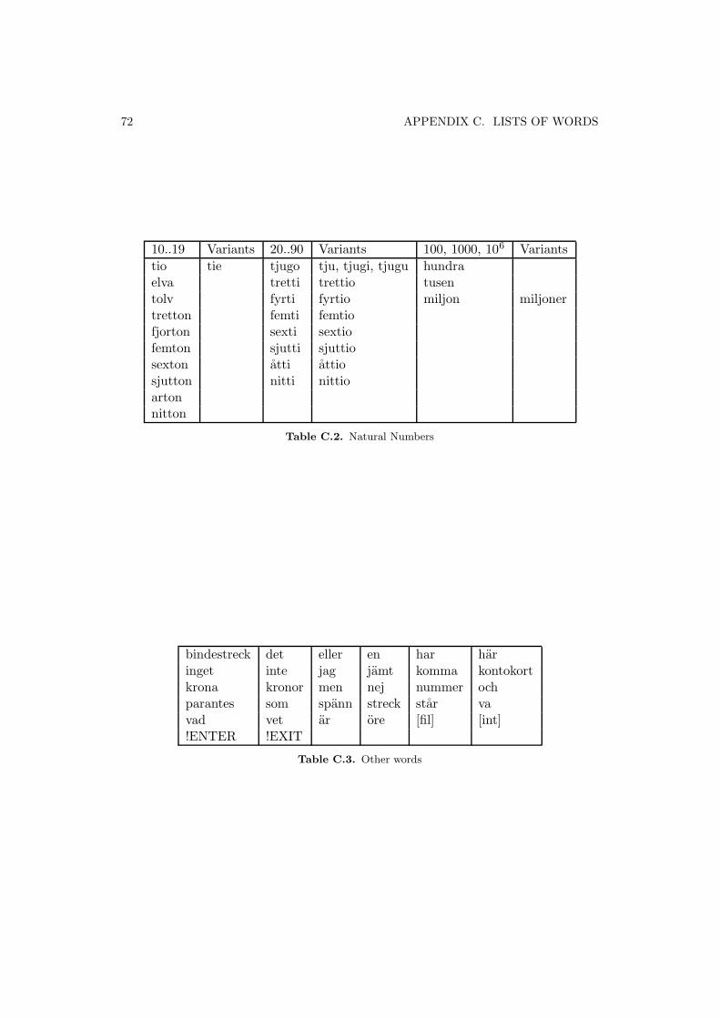
72 APPENDIX C. LISTS OF WORDS
10..19 Variants 20..90 Variants 100, 1000, 106 Variantstio tie tjugo tju, tjugi, tjugu hundraelva tretti trettio tusentolv fyrti fyrtio miljon miljonertretton femti femtiofjorton sexti sextiofemton sjutti sjuttiosexton åtti åttiosjutton nitti nittioartonnitton
Table C.2. Natural Numbers
bindestreck det eller en har häringet inte jag jämt komma kontokortkrona kronor men nej nummer ochparantes som spänn streck står vavad vet är öre [fil] [int]!ENTER !EXIT
Table C.3. Other words

Appendix D
Phonetic Classes
The decision tree, on which the clustering procedure is based, is a collection ofquestions regarding the classification of the left and right context of each phone. Inthis appendix the phonetic classification used in this work is reported. Each classin the list below corresponds to a possible question in the clustering procedure.
73

74 APPENDIX D. PHONETIC CLASSES
CENTRAL U, E0APPROXIMANT V, J, RLATERAL LLABIODENTAL V, FBACK-MIDHIGH Å:, ÅPALATAL J, TJLOW A:, ABACK-HIGH O:, OBILABIAL_PLOSIVE B, PVELAR_PLOSIVE G, KNASAL M, N, NGBILABIAL B, P, MBACK-ROUNDED O:, O, Å:, ÅRETROFLEX _2SVELAR G, K, NGFRICATIVE F, S, _2S, TJ, SJ, HFRONT-HIGH I:, I, Y:, Y, U:VOICED_PLOSIVE B, D, GUNVOICED_PLOSIVE P, T, KSPDAT_PLOSIVE B, D, G, KBACK A:, O:, O, Å:, ÅFRONT_ROUNDED U:, Y:, Y, Ö3, Ö4, Ö:, ÖCORONAL D, L, N, R, S, _2S, TALVEOLAR D, T, S, N, L, RHIGH I:, I, O:, O, U:, Y:, YCONTINUANT_CONSONANT V, F, S, L, R, J, TJ, SJ, H

75
FRONT_UNROUNDED A, E:, E, I:, I, Ä3, Ä4, Ä:, ÄROUNDED O:, O, U:, U, Y:, Y, Å:, Å, Ö3, Ö4, Ö:, ÖUNVOICED_CONSONANT P, T, S, _2S, TJ, K, SJ, HFRONT_MIDHIGH E:, E, Ä3, Ä4, Ö3, Ö4, Ä:, Ä, Ö:, Ö, E, E0PLOSIVE B, P, D, T, G, KANTERIOR B, P, V, F, M, D, T, S, N, LMIDHIGH E:, E, U, Å:, Å, Ä3, Ä4, Ö3, Ö4, Ä:, Ä, Ö:, ÖVOICED_CONSONANT B, V, M, D, N, L, R, J, G, NG, HOBSTRUENT B, P, F, D, T, S, _2S, J, TJ, G, K, SJ, H, VFRONT A, E:, E, I:, I, U:, Y:, Y, Ä3, Ä4, Ö3, Ö4, Ä:,
Ä, Ö:, ÖVOWEL A:, A, E:, E, I:, I, O:, O, U:, U, Y:, Y, Å:, Å,
Ä3, Ä4, Ö3, Ö4, Ä:, Ä, Ö:, Ö, E0VOICED A:, A, E:, E, I:, I, O:, O, U:, U, Y:, Y, Å:, Å,
Ä3, Ä4, Ö3, Ö4, Ä:, Ä, Ö:, Ö, E0, B, V, M, D,N, L, R, J, G, NG, H
E_VOCALS E:, EI_VOCALS I:, IY_VOCALS Y:, YÖ_VOCALS Ö3, Ö4Ä_VOCALS Ä3, Ä4HIGH_ROUNDED Y:, Y, U:MIDHIGH_ROUNDED Ö:, Ö, Å:, Å, Ö3, Ö4MIDHIGH_PRE_R Ö3, Ö4, Ä3, Ä4MIDHIGH_UNROUNDED E:, E, E0, Ä3, Ä4TENSE A:, E:, I:, O:, U:, Y:, Å:, Ä3, Ö3, Ä:, Ö:


Appendix E
Confusion Matrices
In this appendix (next pages) confusion matrices are included for each experi-ment: monophones/triphones, within/cross-word context expansion, old/new lex-icon. Models in each model set include eight Gaussian mixture terms as state tooutput probability distribution.
77

78A
PP
EN
DIX
E.
CO
NF
USIO
NM
AT
RIC
ES
----------------------------- Confusion Matrix -------------------------------
n e t t f f s s å n t e t t f f s s å n t t f f s s a n h t m d e h h i j k k m n o s s s s v v ä ö
o t v r y e e j t i i l o r y e e j t i j r j e e j r i u u i e l a ä n a o r e e c o p t t a e r r
l t å e r m x u t o o v l e r m x u t t u e o m x u t t n s l t l r r t g m o n j h m ä r å d t e
l a a a v t t t t t i t g t r t t t o t d e j e e m n n e r
t i i i t o i o t t o o t n o r n o r a o n c Del [ %c / %e]
noll 874 6 50 2 0 0 0 1 4 7 0 0 1 1 0 2 2 3 3 4 1 2 1 8 7 0 2 0 0 0 0 1 0 3 1 5 5 2 4 1 0 5 0 0 0 0 1 0 2 0 83 [86.4/1.2]
ett 0 650 36 79 0 1 15 1 6 3 3 0 0 10 0 1 5 1 0 5 0 0 1 0 1 1 0 0 3 1 0 1 0 0 0 2 0 0 0 0 1 0 0 0 1 0 0 1 2 0 100 [78.2/1.6]
två 1 3 770 4 0 3 0 0 5 2 1 0 1 0 0 0 2 1 2 0 1 3 2 2 1 0 1 0 0 1 0 0 0 1 0 0 0 0 4 0 0 3 1 0 0 1 0 0 0 0 73 [94.4/0.4]
tre 1 4 2 667 15 3 2 8 1 8 25 0 2 5 0 4 10 0 5 3 3 1 1 0 0 1 0 0 1 2 0 5 0 0 0 0 0 0 1 0 1 1 0 0 0 0 0 0 2 0 89 [85.1/1.1]
fyra 0 1 3 5 742 2 1 2 1 7 6 1 0 0 1 2 0 0 0 0 4 0 0 0 0 0 0 0 2 0 0 0 0 0 0 0 1 0 0 0 0 0 0 0 0 0 0 0 0 0 57 [95.0/0.4]
fem 0 56 4 4 7 613 2 0 7 1 1 2 0 0 0 7 0 1 1 1 0 0 0 5 2 2 0 0 0 17 1 0 0 1 1 0 0 0 1 1 0 2 0 2 0 0 0 0 1 0 89 [82.5/1.2]
sex 2 11 0 1 0 2 661 0 1 1 1 0 0 0 0 0 22 0 0 1 2 1 0 0 7 0 1 0 2 0 0 0 0 0 0 0 0 0 4 0 0 1 0 0 0 0 0 0 0 0 81 [91.7/0.5]
sju 4 3 3 4 6 3 0 625 2 0 0 0 1 0 0 1 0 3 0 1 4 0 0 1 1 1 0 1 2 3 0 0 0 0 2 0 0 0 1 0 0 0 1 0 0 0 0 0 1 0 73 [92.7/0.4]
åtta 0 2 7 5 1 0 0 0 639 0 0 0 0 1 0 0 0 0 3 0 2 1 1 1 0 0 1 0 0 1 0 0 0 0 0 0 0 0 0 0 0 1 0 0 0 0 0 0 0 0 67 [95.9/0.2]
nio 5 12 3 21 17 0 0 1 0 527 12 0 0 0 0 3 2 0 1 5 4 0 4 0 0 0 1 0 0 3 2 1 0 0 0 2 4 0 6 0 10 1 0 0 0 0 0 0 0 0 82 [81.5/1.1]
tio 1 1 0 4 2 0 0 0 0 5 43 0 0 0 0 0 0 0 0 0 0 0 0 0 0 0 0 0 0 0 0 0 0 0 0 0 1 0 0 0 0 0 0 0 0 0 0 0 0 0 5 [75.4/0.1]
elva 0 3 0 0 0 0 0 0 1 0 0 59 0 0 0 0 0 0 0 0 0 0 0 0 0 0 0 0 0 0 0 0 0 1 0 0 0 0 0 0 0 0 0 0 0 0 0 0 1 0 3 [90.8/0.1]
tolv 4 2 9 0 0 0 0 0 0 0 0 0 20 0 0 0 0 0 0 0 0 3 0 1 2 2 2 0 0 0 0 0 1 0 0 0 0 1 0 0 0 0 0 0 0 0 0 0 0 0 4 [42.6/0.2]
tret 0 5 1 7 0 0 2 2 1 2 0 0 0 116 0 0 0 1 0 1 0 0 0 0 0 0 0 0 0 1 0 0 0 0 0 0 0 0 0 0 0 0 0 0 0 0 0 0 0 0 14 [83.5/0.2]
fyrt 0 1 0 4 0 1 1 1 0 0 0 0 0 0 88 0 1 0 0 0 0 0 0 0 0 0 0 0 0 1 0 0 0 0 0 0 0 0 0 0 0 0 0 0 0 0 0 0 0 0 8 [89.8/0.1]
femt 1 5 0 1 0 8 4 0 3 2 0 0 1 9 1 85 0 1 1 0 0 0 0 0 0 0 0 0 0 2 0 1 0 0 0 0 0 0 0 0 0 0 0 0 0 0 0 0 0 0 17 [68.0/0.4]
sext 0 1 1 1 0 0 18 1 0 0 0 0 0 1 1 1 101 0 0 0 0 0 0 0 2 0 0 0 0 1 0 0 0 0 0 0 0 0 0 0 0 0 0 0 0 0 0 0 0 0 10 [78.3/0.3]
sjut 0 2 1 2 0 0 0 8 0 0 0 0 0 3 3 0 1 124 2 0 4 0 0 0 0 0 0 0 0 1 0 0 0 0 0 0 0 0 0 0 0 0 0 0 0 0 0 0 0 0 13 [82.1/0.2]
åtti 3 1 10 15 0 0 0 0 9 2 2 0 0 0 0 0 0 3 113 0 0 1 0 0 0 0 1 0 1 0 0 0 0 1 0 0 0 0 0 0 0 4 0 0 1 0 0 0 0 0 20 [67.7/0.5]
nitt 0 5 0 2 0 0 0 0 0 3 1 0 0 3 0 1 3 0 1 160 0 0 0 0 0 0 0 0 1 1 0 0 0 0 0 0 0 0 0 0 0 0 0 0 0 0 0 0 0 0 12 [88.4/0.2]
tjug 2 2 2 1 0 0 0 3 0 0 1 0 0 0 0 0 1 3 0 0 157 0 0 0 0 0 0 0 0 0 0 0 0 0 0 0 0 0 0 0 0 0 0 0 0 0 0 0 0 0 12 [91.3/0.1]
tret 0 0 0 0 0 0 0 0 0 0 0 0 0 1 0 0 1 0 0 0 0 33 0 0 0 1 0 0 0 0 0 0 0 0 0 0 0 0 0 0 0 0 0 0 0 0 0 0 0 0 1 [91.7/0.0]
fjor 0 0 0 0 0 0 0 0 0 0 0 0 0 0 0 0 0 0 0 0 0 0 40 0 0 0 0 0 0 0 0 0 0 0 0 0 0 0 0 0 0 0 0 0 0 0 0 0 0 0 0
femt 2 0 0 0 0 0 0 0 1 0 0 1 0 1 0 0 0 0 0 0 0 0 0 37 0 0 0 0 0 0 0 0 0 0 0 0 0 0 0 0 0 0 0 0 0 0 0 0 0 0 2 [88.1/0.0]
sext 0 0 0 0 0 0 0 0 1 0 0 0 1 0 0 0 0 0 0 0 0 0 0 0 40 0 0 0 0 0 0 0 0 0 0 0 0 0 0 0 0 0 0 0 0 0 0 0 0 0 2 [95.2/0.0]
sjut 0 1 1 0 0 0 0 0 0 0 0 0 0 0 0 0 0 0 0 0 0 0 0 0 0 29 0 0 0 0 0 0 0 0 0 0 0 0 0 0 0 0 0 0 0 0 0 0 0 0 0 [93.5/0.0]
arto 0 0 0 1 0 0 0 0 2 0 0 0 1 0 0 0 0 0 0 0 0 0 0 0 0 0 16 0 0 0 0 0 0 0 0 0 0 0 1 0 0 0 0 0 0 0 0 0 0 0 1 [76.2/0.0]
nitt 0 1 0 0 0 0 0 0 0 0 0 0 0 0 0 0 0 0 0 0 0 1 0 1 0 1 0 29 0 0 0 0 0 0 0 1 0 0 0 0 0 0 0 0 0 0 0 0 0 0 1 [85.3/0.0]
hund 13 5 3 1 6 6 1 1 14 6 2 2 3 1 0 0 2 0 1 1 0 3 2 1 3 0 3 1 265 6 0 0 0 0 0 0 1 2 0 1 0 5 0 0 0 0 0 1 2 0 75 [72.8/0.9]
tuse 0 0 0 0 0 1 0 0 0 0 0 0 0 0 0 0 0 0 0 0 0 0 0 0 0 0 0 0 0 144 0 0 0 0 0 0 0 0 0 0 0 0 0 0 0 0 0 0 0 0 5 [99.3/0.0]
milj 0 0 0 0 0 0 0 0 0 0 0 0 0 0 0 0 0 0 0 0 0 0 0 0 0 0 0 0 0 0 23 0 0 0 0 0 0 0 1 0 0 0 0 0 0 0 0 0 0 0 1 [95.8/0.0]
komm 0 0 0 0 0 0 0 0 0 0 0 0 0 0 0 0 0 0 0 0 0 0 0 0 0 0 0 0 0 0 0 0 0 0 0 0 0 6 0 0 0 0 0 0 0 0 0 0 0 0 0
kron 0 0 1 0 1 0 1 1 2 0 0 0 0 0 0 0 0 0 0 0 1 0 0 1 1 1 0 0 1 0 0 0 0 0 0 0 0 0 167 0 0 0 0 0 0 0 0 0 0 0 8 [93.8/0.1]
och 0 0 0 0 0 1 0 0 0 0 0 0 0 0 0 0 0 0 0 0 0 0 0 0 0 0 0 0 0 0 0 0 0 0 0 0 0 0 0 0 0 14 0 0 0 0 0 0 0 0 5 [93.3/0.0]
stre 0 0 0 0 0 0 1 0 0 0 0 0 0 1 0 0 0 0 0 0 0 0 0 0 0 0 0 0 0 0 0 0 0 0 0 0 1 0 0 0 0 0 0 0 3 0 0 0 0 0 2 [50.0/0.0]
öre 0 0 0 0 0 0 0 0 0 0 0 0 0 0 0 0 0 0 0 0 0 0 0 0 0 0 0 0 0 0 0 0 0 0 0 0 0 0 0 0 0 0 0 0 0 0 0 0 0 8 2
Ins 13 88 39 63 6 8 6 4 19 15 3 0 0 3 0 0 3 1 2 3 4 1 1 0 1 0 0 0 3 6 0 7 1 1 0 2 6 2 1 1 0 6 0 0 0 0 1 0 2 0
==============================================================================
Fig
ure
E.1
.C
on
fusio
nm
atrix
:m
on
op
hon
es,old
lexico
n,
eight
Gau
ssian
mix
ture
terms
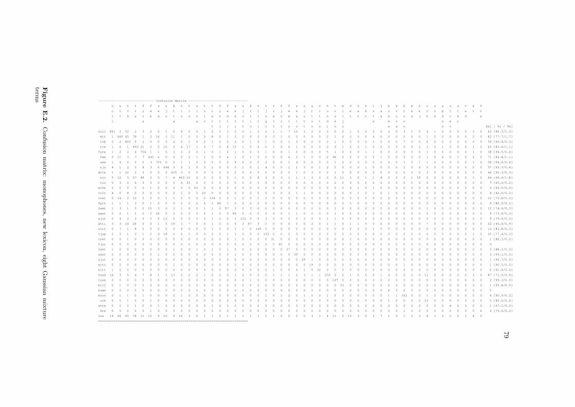
79
----------------------------- Confusion Matrix -------------------------------
n e t t f f s s å n t e t t f f s s å n t t f f s s a n h t m d h h i j k k k m n o s s s s v ä ö
o t v r y e e j t i i l o r y e e j t i j r j e e j r i u u i e a ä n a o r r e e c o p t t a r r
l t å e r m x u t o o v l e r m x u t t u e o m x u t t n s l t r r t g m o o n j h m ä r å d e
l a a a v t t t t t i t g t r t t t o t d e j e m n n n e r
t i i i t o i o t t o o t n o r n o a a o n c Del [ %c / %e]
noll 891 5 52 2 3 0 0 1 6 8 0 0 1 2 0 1 2 0 1 2 2 1 1 7 10 2 2 0 0 0 2 1 5 0 3 5 2 0 3 1 0 4 1 0 0 0 0 3 0 62 [86.3/1.3]
ett 1 660 45 79 1 2 16 2 11 1 0 0 0 8 0 1 3 2 0 2 0 2 1 0 0 0 0 0 2 1 0 2 0 0 4 0 0 0 0 0 0 1 0 0 0 0 0 2 0 82 [77.7/1.7]
två 0 2 800 0 2 5 0 0 4 0 1 0 2 1 0 0 2 0 1 0 1 0 0 1 0 0 0 0 0 1 0 0 0 0 0 0 0 0 7 0 0 0 0 0 0 0 0 0 0 59 [96.4/0.3]
tre 1 6 1 692 21 2 2 10 0 6 17 1 0 7 0 8 12 1 0 6 0 1 0 0 1 0 0 0 2 2 1 2 0 1 0 0 0 0 0 0 2 1 0 1 0 0 0 1 0 65 [85.6/1.1]
fyra 1 2 2 4 756 1 1 5 3 3 2 0 1 0 1 2 1 0 0 0 1 0 0 1 0 0 0 0 5 1 0 3 0 1 1 0 0 0 0 0 0 1 0 0 0 0 0 1 0 38 [94.5/0.4]
fem 0 11 3 7 7 645 6 0 4 0 2 1 1 0 0 6 1 0 1 0 0 0 0 6 2 1 0 0 2 38 0 0 2 2 0 1 0 0 2 2 0 1 0 4 0 1 0 2 0 71 [84.8/1.1]
sex 1 9 0 2 0 3 703 0 0 1 1 0 0 0 0 0 9 0 0 0 2 0 0 1 4 0 0 0 2 1 0 0 0 0 0 0 0 0 1 0 1 1 0 0 0 0 0 1 0 59 [94.6/0.4]
sju 4 1 2 5 8 3 0 644 0 0 1 0 0 1 0 0 0 1 0 1 4 0 0 1 1 3 0 1 2 5 0 0 0 1 0 0 0 0 1 0 0 0 0 0 0 0 0 0 0 57 [93.3/0.4]
åtta 1 1 10 2 2 0 0 0 655 0 0 0 0 0 0 0 0 0 6 0 0 0 2 0 1 0 3 0 0 1 0 0 0 0 0 0 0 0 0 0 0 3 0 0 0 0 0 0 0 46 [95.3/0.3]
nio 5 12 5 37 48 2 0 7 4 463 10 2 0 0 0 2 1 0 0 8 2 0 3 1 1 1 2 0 2 5 11 1 0 1 1 4 0 0 3 1 19 0 0 0 0 0 0 1 0 64 [69.6/1.8]
tio 0 3 0 6 3 0 0 2 0 6 33 0 0 0 0 0 0 0 0 0 0 0 0 0 0 0 0 0 0 2 0 0 0 0 0 0 0 0 0 0 0 0 0 0 0 0 0 0 0 7 [60.0/0.2]
elva 0 0 0 0 0 1 0 0 0 0 0 63 0 0 0 0 0 0 0 0 0 0 0 0 0 0 0 0 0 0 0 0 1 0 1 0 0 0 0 0 0 0 0 0 0 0 0 0 0 2 [95.5/0.0]
tolv 4 0 8 0 0 0 0 0 0 1 0 0 20 0 0 0 0 0 2 0 0 3 0 2 1 1 0 0 2 0 0 0 1 0 1 0 1 0 0 0 0 0 0 0 0 0 0 0 0 4 [42.6/0.2]
tret 0 14 2 13 0 0 0 1 1 0 0 0 0 104 0 0 1 2 0 1 0 0 0 0 0 0 0 0 0 2 0 0 0 0 0 0 0 0 0 0 0 0 0 0 0 0 0 0 0 12 [73.8/0.3]
fyrt 1 1 1 3 0 1 2 0 0 0 0 0 0 1 86 1 0 2 0 0 0 0 0 0 0 0 0 0 0 0 0 1 0 0 0 0 0 0 0 0 0 0 0 0 0 0 0 0 0 6 [86.0/0.1]
femt 1 3 1 5 0 10 3 0 2 1 0 0 1 1 0 97 0 0 3 0 0 0 0 0 0 0 0 0 0 1 0 0 0 0 0 0 0 0 0 0 0 1 0 0 0 0 0 0 0 12 [74.6/0.3]
sext 0 2 1 1 0 0 26 0 0 0 0 0 0 1 0 0 96 0 0 0 0 0 0 1 1 0 0 0 0 1 0 0 0 0 0 0 0 0 0 0 0 0 0 0 0 0 0 0 0 9 [73.8/0.3]
sjut 0 4 2 2 0 0 0 12 0 0 0 0 0 1 2 0 1 123 0 0 3 0 0 0 0 3 0 0 1 1 0 0 0 0 0 0 0 0 0 0 0 0 0 0 0 0 0 0 0 9 [79.4/0.3]
åtti 3 3 14 26 0 0 1 0 19 3 7 0 0 1 2 0 0 2 67 3 1 0 0 0 0 0 2 0 1 1 0 1 1 0 0 0 0 0 0 0 0 7 0 0 0 0 0 0 0 22 [40.6/0.9]
nitt 0 7 1 8 0 0 0 0 0 6 0 0 0 1 0 3 1 1 0 149 0 0 0 0 0 0 0 0 0 0 0 0 2 0 1 0 0 0 0 0 0 0 0 0 0 0 0 0 0 13 [82.8/0.3]
tjug 2 2 1 2 1 0 4 18 0 0 1 0 0 0 0 1 1 0 0 0 123 0 0 0 0 0 0 0 0 2 0 0 0 0 0 0 0 0 0 0 0 0 0 0 0 0 0 1 0 25 [77.4/0.3]
tret 0 0 1 0 0 0 0 0 0 0 0 0 0 2 0 0 1 0 0 0 0 31 0 0 0 0 0 0 0 0 0 1 0 0 0 0 0 0 0 0 0 0 0 0 0 0 0 0 0 1 [86.1/0.0]
fjor 0 0 0 0 0 0 0 0 0 0 0 0 0 0 0 0 0 0 0 0 0 0 40 0 0 0 0 0 0 0 0 0 0 0 0 0 0 0 0 0 0 0 0 0 0 0 0 0 0 0
femt 1 0 0 0 0 0 0 0 1 0 0 1 0 1 0 1 0 0 0 0 0 0 0 37 0 0 0 0 0 0 0 0 0 0 0 0 0 0 0 0 0 0 0 0 0 0 0 0 0 2 [88.1/0.0]
sext 0 0 0 0 0 0 1 0 0 0 0 0 0 0 0 0 1 0 0 0 0 0 0 0 39 0 0 0 0 0 0 0 0 0 0 0 0 0 0 0 0 0 0 0 0 0 0 0 0 3 [95.1/0.0]
sjut 0 0 0 0 0 0 0 0 0 0 0 0 0 0 0 0 0 0 0 0 0 0 0 0 0 29 1 0 0 0 0 0 0 0 0 0 0 0 0 0 0 0 0 0 0 0 0 0 0 1 [96.7/0.0]
arto 0 0 0 0 0 0 0 0 1 0 0 0 0 0 0 0 0 0 0 0 0 0 0 0 0 0 19 0 0 0 0 0 0 0 0 0 0 0 1 0 0 0 0 0 0 0 0 0 0 1 [90.5/0.0]
nitt 1 0 0 0 0 0 0 0 0 0 0 0 0 0 0 0 0 0 0 0 0 1 0 0 0 1 0 32 0 0 0 0 0 0 0 0 0 0 0 0 0 0 0 0 0 0 0 0 0 0 [91.4/0.0]
hund 16 3 5 4 7 8 1 1 13 2 2 2 1 0 0 0 1 2 0 0 0 1 1 1 2 3 1 1 250 3 0 1 0 0 0 1 4 0 0 0 0 12 0 0 0 0 0 3 0 87 [71.0/0.9]
tuse 0 0 0 0 0 0 0 0 0 0 0 0 0 0 0 0 0 0 1 0 0 0 0 0 0 0 0 0 0 147 0 0 0 0 0 0 0 0 0 0 0 0 0 0 0 0 0 0 0 2 [99.3/0.0]
milj 0 1 0 0 0 0 0 0 0 0 0 0 0 0 0 0 0 0 0 0 0 0 0 0 0 0 0 0 0 0 23 0 0 0 0 0 0 0 0 0 0 0 0 0 0 0 0 0 0 1 [95.8/0.0]
komm 0 0 0 0 0 0 0 0 0 0 0 0 0 0 0 0 0 0 0 0 0 0 0 0 0 0 0 0 0 0 0 0 0 0 0 0 6 0 0 0 0 0 0 0 0 0 0 0 0 0
kron 0 1 1 0 1 0 0 0 2 1 0 0 0 0 0 0 0 0 0 0 1 0 1 2 0 1 0 0 1 0 3 0 0 0 0 0 1 1 162 0 0 1 0 0 0 0 0 0 0 6 [90.0/0.2]
och 0 0 1 0 0 1 0 0 0 0 0 0 0 0 0 0 0 0 0 0 0 0 0 0 0 0 0 0 0 0 0 0 0 0 0 0 1 0 0 0 0 12 0 0 0 0 0 0 0 5 [80.0/0.0]
stre 0 0 0 1 0 0 1 0 0 0 0 0 0 1 0 0 0 0 0 0 0 0 0 0 0 0 0 0 0 0 0 0 0 0 0 0 0 0 0 0 0 0 0 0 4 0 0 0 0 1 [57.1/0.0]
öre 0 0 0 0 0 1 0 0 0 0 0 0 0 0 0 0 0 0 0 0 0 0 0 0 0 0 0 0 0 0 0 0 0 0 0 0 0 0 1 0 0 0 0 0 0 0 0 0 6 2 [75.0/0.0]
Ins 14 99 45 78 11 15 9 10 9 22 3 0 1 1 0 1 1 1 1 1 1 1 0 0 0 0 3 1 4 11 0 13 3 0 3 7 1 0 1 3 3 8 1 0 0 0 1 4 0
==============================================================================
Fig
ure
E.2
.C
on
fusio
nm
atrix
:m
on
op
hon
es,n
ewlex
icon
,eig
ht
Gau
ssian
mix
ture
terms

80A
PP
EN
DIX
E.
CO
NF
USIO
NM
AT
RIC
ES
----------------------------- Confusion Matrix -------------------------------
n e t t f f s s å n t e t t f f s s å n t t f f s s a n h t m d h i j k k m n o s s s v ä ö
o t v r y e e j t i i l o r y e e j t i j r j e e j r i u u i e a n a o r e e c o p t a r r
l t å e r m x u t o o v l e r m x u t t u e o m x u t t n s l t r t g m o n j h m ä r d e
l a a a v t t t t t i t g t r t t t o t d e j e m n n e
t i i i t o i o t t o o t n o r n o a o n c Del [ %c / %e]
noll 1043 2 5 0 0 0 0 1 0 2 0 0 0 0 0 0 0 0 0 0 1 0 0 1 1 0 0 3 0 0 0 0 1 1 0 0 2 0 0 2 0 0 0 0 1 0 28 [97.8/0.2]
ett 0 850 1 9 1 4 1 0 4 0 0 0 0 1 0 0 2 0 0 1 0 1 0 0 0 0 0 1 2 1 0 0 0 1 0 0 0 0 0 2 0 0 0 0 0 0 49 [96.4/0.3]
två 5 3 820 1 1 6 1 0 3 0 0 0 0 1 0 0 0 0 0 0 0 1 0 0 0 0 1 0 0 2 0 0 0 1 0 0 1 0 0 4 0 0 0 2 0 0 36 [96.1/0.3]
tre 2 6 1 771 10 5 1 6 0 2 5 0 0 0 1 0 4 0 1 2 1 0 0 0 0 0 0 0 0 2 0 5 0 0 1 0 2 0 3 0 0 0 0 0 0 0 42 [92.8/0.5]
fyra 0 2 0 1 800 1 0 0 0 0 1 3 0 0 1 0 0 0 0 0 2 0 0 0 0 0 0 0 1 0 0 0 0 0 0 0 0 0 0 0 0 0 1 0 0 0 25 [98.4/0.1]
fem 0 23 0 2 1 748 0 0 2 0 0 0 0 0 0 4 0 0 1 0 0 0 0 5 1 0 0 0 1 4 0 0 0 0 0 0 0 1 0 0 0 0 0 0 1 0 38 [94.2/0.4]
sex 0 6 0 2 0 0 741 0 0 1 0 0 0 0 1 0 0 0 0 0 0 1 1 0 4 0 0 0 0 0 0 1 0 0 0 0 0 0 0 1 0 0 1 0 0 0 42 [97.5/0.2]
sju 5 4 1 4 3 2 1 677 0 0 0 0 2 0 0 0 0 1 1 0 7 0 0 1 0 1 1 0 0 1 0 0 0 1 0 0 0 0 0 0 0 0 1 0 0 0 33 [94.8/0.3]
åtta 0 1 0 0 1 0 0 0 689 0 0 0 0 1 0 0 0 1 3 0 0 0 0 0 0 0 5 0 0 0 0 0 0 0 0 0 0 0 0 2 0 0 0 0 1 0 29 [97.9/0.1]
nio 7 15 0 8 20 2 0 2 0 596 5 0 0 0 0 0 0 0 1 8 1 0 0 0 0 0 2 2 2 1 6 5 0 1 0 0 0 0 3 3 0 0 0 0 0 0 39 [86.4/0.9]
tio 0 2 0 2 4 0 0 0 0 3 50 0 0 0 0 0 0 0 0 0 0 0 0 0 0 0 0 0 0 0 0 0 0 0 0 0 0 0 0 0 0 0 0 0 0 0 1 [82.0/0.1]
elva 0 1 0 0 1 0 0 0 0 0 0 63 0 0 0 0 0 0 0 0 0 0 0 0 0 0 0 0 1 0 0 0 1 0 0 0 0 0 0 0 0 0 0 0 0 0 1 [94.0/0.0]
tolv 1 0 3 0 0 0 0 0 0 0 0 0 45 0 0 0 0 0 0 0 0 1 0 0 1 0 0 0 0 0 0 0 0 0 0 0 0 0 0 0 0 0 0 0 0 0 0 [88.2/0.1]
tret 0 2 0 0 1 0 0 0 0 0 1 0 0 141 1 0 1 0 0 1 0 0 0 0 0 0 0 0 0 0 0 0 0 1 0 0 0 0 0 0 0 0 0 0 1 0 3 [94.0/0.1]
fyrt 0 1 0 1 0 0 0 0 0 0 0 0 0 2 97 2 0 1 0 0 0 0 0 0 0 0 0 0 0 0 0 0 0 0 0 0 0 0 0 0 0 0 0 0 0 0 2 [93.3/0.1]
femt 0 2 0 1 0 4 0 0 0 1 0 0 0 0 1 128 0 0 0 1 0 0 0 0 0 0 0 0 0 0 0 0 0 0 0 0 0 0 0 0 0 0 0 0 0 0 4 [92.8/0.1]
sext 0 1 0 0 1 0 8 1 0 0 0 0 0 0 0 0 126 0 0 0 0 0 0 0 0 0 0 0 0 0 0 0 0 0 0 0 0 0 0 0 0 0 0 0 0 0 2 [92.0/0.1]
sjut 0 1 0 0 0 0 0 1 0 0 0 0 0 2 4 0 0 149 0 0 1 0 0 0 0 0 0 0 0 0 0 0 0 0 1 0 0 0 0 0 0 0 1 0 0 0 4 [93.1/0.1]
åtti 2 1 0 2 0 0 0 0 6 0 1 0 0 0 1 0 0 2 153 0 0 0 0 0 0 0 1 0 0 0 0 0 0 0 0 0 2 0 0 3 0 0 0 0 0 0 13 [87.9/0.2]
nitt 0 1 0 1 0 0 1 0 0 0 1 0 0 0 0 0 2 0 0 177 0 0 0 0 0 0 0 2 0 0 0 0 0 1 0 0 1 0 0 0 0 0 1 0 0 0 5 [94.1/0.1]
tjug 4 0 0 1 0 0 1 2 0 0 0 0 0 0 0 0 0 1 0 0 158 0 0 0 0 0 0 0 0 0 0 0 0 0 0 0 1 0 0 0 0 0 0 0 0 0 16 [94.0/0.1]
tret 0 1 0 0 0 0 0 0 0 0 0 0 0 0 0 0 0 0 0 0 0 35 0 0 0 1 0 0 0 0 0 0 0 0 0 0 0 0 0 0 0 0 0 0 0 0 0 [94.6/0.0]
fjor 0 0 0 0 0 0 0 0 0 0 0 0 0 0 0 0 0 0 0 0 0 0 40 0 0 0 0 0 0 0 0 0 0 0 0 0 0 0 0 0 0 0 0 0 0 0 0
femt 0 0 0 0 0 0 0 0 0 0 0 0 0 0 0 0 0 0 0 0 0 0 0 43 0 0 0 0 0 0 0 0 0 0 0 0 0 0 0 0 0 0 0 0 0 0 1
sext 0 0 0 0 0 0 0 0 0 0 0 0 0 0 0 0 0 0 0 0 0 0 0 0 42 0 0 0 0 0 0 0 0 0 0 0 0 0 0 0 0 0 0 0 0 0 2
sjut 0 0 0 0 0 0 0 0 0 0 0 0 0 0 0 0 0 0 0 0 0 0 0 0 0 31 0 0 0 0 0 0 0 0 0 0 0 0 0 0 0 0 0 0 0 0 0
arto 0 0 0 0 0 0 0 1 2 0 0 0 0 0 0 0 0 0 0 0 0 0 0 0 0 0 19 0 0 0 0 0 0 0 0 0 0 0 0 0 0 0 0 0 0 0 0 [86.4/0.0]
nitt 1 1 0 0 0 0 0 0 0 0 0 0 0 0 0 0 0 0 0 0 0 0 0 0 0 0 0 33 0 0 0 0 0 0 0 0 0 0 0 0 0 0 0 0 0 0 0 [94.3/0.0]
hund 8 9 1 1 4 2 0 0 0 0 0 1 2 0 0 0 0 0 0 0 0 1 0 0 7 0 3 0 334 0 0 0 0 0 0 2 1 0 0 5 1 0 0 0 2 0 55 [87.0/0.5]
tuse 0 1 0 0 0 1 0 0 0 0 0 0 0 0 0 0 0 0 0 0 0 0 0 0 0 0 0 0 0 146 0 0 0 0 0 0 0 0 0 0 0 0 0 0 0 0 2 [98.6/0.0]
milj 1 0 0 0 0 0 0 0 0 0 0 0 0 0 0 0 0 0 0 0 0 0 0 0 0 0 0 0 0 0 23 0 0 0 0 0 1 0 0 0 0 0 0 0 0 0 0 [92.0/0.0]
komm 0 0 0 0 0 0 0 0 0 0 0 0 0 0 0 0 0 0 0 0 0 0 0 0 0 0 0 0 0 0 0 0 0 0 0 6 0 0 0 0 0 0 0 0 0 0 0
kron 0 0 1 0 0 0 0 0 0 0 0 0 0 0 0 0 0 0 0 0 0 0 0 0 0 0 0 0 1 0 0 0 0 0 0 0 180 0 0 0 0 1 0 0 0 0 3 [98.4/0.0]
och 0 0 0 0 0 0 0 0 0 0 0 0 0 0 0 0 0 0 0 0 0 0 0 0 0 0 0 0 0 0 0 0 0 0 0 0 0 0 0 13 0 0 0 0 0 0 7
stre 0 0 0 0 0 0 1 0 0 0 0 0 0 0 0 0 0 0 0 0 0 0 0 0 0 0 0 0 0 0 0 0 0 0 0 0 0 0 0 0 0 0 7 0 0 0 0 [87.5/0.0]
öre 0 1 0 0 0 0 0 0 0 0 0 0 0 0 0 0 0 0 0 0 0 0 0 0 0 0 0 0 0 0 0 0 0 0 0 0 0 0 0 0 0 0 0 0 0 8 1 [88.9/0.0]
Ins 6 120 5 18 5 11 3 14 9 6 6 1 1 1 1 1 0 0 3 0 0 1 0 0 0 0 1 0 2 1 0 10 1 3 4 0 3 0 2 16 1 0 3 0 3 0
==============================================================================
Fig
ure
E.3
.C
on
fusio
nm
atrix
:trip
hon
es,w
ithin
-word
contex
tex
pan
sion
,old
lex-
icon
,eig
ht
Gau
ssian
mix
ture
terms
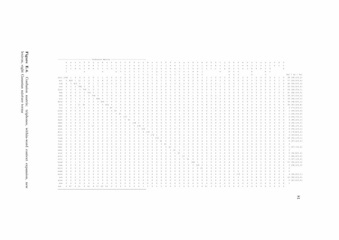
81
----------------------------- Confusion Matrix -------------------------------
n e t t f f s s å n t e t t f f s s å n t t f f s s a n h t m d h h i j k k k m n n o s s s v ä ö
o t v r y e e j t i i l o r y e e j t i j r j e e j r i u u i e a ä n a o r r e e u c o t t a r r
l t å e r m x u t o o v l e r m x u t t u e o m x u t t n s l t r r t g m o o n j m h m r å e
l a a a v t t t t t i t g t r t t t o t d e j e m n n m e r
t i i i t o i o t t o o t n o r n o a a o e c Del [ %c / %e]
noll 1045 1 4 0 0 0 0 1 1 0 0 0 0 0 0 0 0 0 0 0 1 0 0 0 1 0 0 0 0 0 1 1 1 0 0 3 0 0 2 2 0 1 0 0 0 0 0 1 0 28 [98.0/0.2]
ett 0 829 1 12 2 4 1 4 8 0 0 0 0 2 0 1 1 0 0 1 0 1 1 0 0 0 0 0 2 0 0 1 0 0 2 0 0 0 0 0 0 0 0 0 0 0 0 1 0 57 [94.9/0.4]
två 6 3 815 0 1 8 1 1 4 0 0 0 1 0 0 0 0 0 0 0 0 1 0 1 0 0 0 0 0 1 0 0 0 0 1 2 0 0 1 0 0 0 0 0 0 1 0 1 0 40 [96.0/0.3]
tre 2 5 0 788 5 4 2 7 0 4 1 0 0 0 0 0 1 0 0 1 0 0 0 0 1 0 0 0 0 1 0 2 0 0 0 1 0 0 1 0 2 0 0 0 0 0 0 2 0 43 [94.9/0.4]
fyra 1 0 0 3 799 0 0 2 3 1 1 1 0 0 1 0 0 0 0 0 0 0 0 0 0 0 0 0 1 0 0 0 0 0 0 0 0 0 0 0 0 0 0 0 0 0 0 1 0 24 [98.2/0.1]
fem 1 9 0 0 2 762 0 2 3 0 0 0 0 0 0 3 0 0 0 0 0 0 0 1 0 0 0 0 1 3 0 1 1 1 0 0 0 0 0 0 1 0 0 0 0 0 0 0 0 41 [96.3/0.3]
sex 0 8 0 2 0 0 749 0 0 0 0 0 0 0 0 0 1 0 0 0 1 2 0 0 2 0 0 0 1 0 0 0 0 0 0 0 0 0 0 0 0 0 0 0 1 0 0 1 0 34 [97.5/0.2]
sju 3 2 1 5 2 2 1 684 0 1 0 1 3 0 0 0 0 1 0 0 5 0 0 0 0 0 0 0 0 0 0 1 0 0 0 0 0 0 0 0 0 0 0 0 0 0 0 0 0 35 [96.1/0.3]
åtta 0 0 1 0 1 0 0 0 692 0 0 0 0 1 0 0 0 0 4 0 0 0 1 0 0 0 1 0 0 0 0 0 0 0 0 0 0 0 0 0 0 0 1 0 0 0 1 0 0 30 [98.4/0.1]
nio 7 6 1 11 29 1 0 5 0 602 0 1 0 0 0 0 0 0 0 6 0 0 0 0 0 0 0 0 3 2 5 4 0 0 2 2 0 0 0 0 3 0 0 0 0 0 0 0 0 39 [87.2/0.8]
tio 0 2 0 5 4 1 0 0 0 3 44 0 0 0 0 0 0 0 0 0 0 0 0 0 0 0 0 0 0 1 0 0 0 0 0 0 0 0 0 0 0 0 0 0 0 0 0 0 0 2 [73.3/0.1]
elva 0 0 0 0 1 0 0 0 0 0 0 63 0 0 0 0 0 0 0 0 0 0 0 0 0 0 0 0 2 0 0 0 1 0 0 0 0 0 0 0 0 0 0 0 0 0 0 0 0 1 [94.0/0.0]
tolv 0 1 2 0 0 0 0 0 0 0 0 0 45 0 0 0 0 0 0 0 0 1 0 0 0 1 0 0 0 0 0 0 0 0 0 0 0 0 0 0 0 0 0 0 0 0 0 0 0 1 [90.0/0.0]
tret 0 7 0 2 1 0 0 0 0 0 0 0 0 137 1 0 1 0 0 1 0 1 0 0 0 0 0 0 0 0 0 0 0 0 0 0 0 0 0 0 0 0 0 0 0 0 0 0 0 2 [90.7/0.1]
fyrt 0 1 0 2 0 0 1 0 0 0 0 0 0 0 92 2 1 4 0 0 0 0 0 0 0 0 0 0 0 0 0 0 0 0 0 0 0 0 0 0 0 0 0 0 0 0 0 0 0 3 [89.3/0.1]
femt 1 0 0 2 0 2 0 0 0 1 0 0 0 0 1 128 0 0 0 2 0 0 0 1 0 0 0 0 1 0 0 0 0 0 0 0 0 0 0 0 0 0 0 0 0 0 0 0 0 3 [92.1/0.1]
sext 0 2 0 3 1 0 10 1 0 0 0 0 0 0 0 0 118 0 0 1 0 0 0 0 1 0 0 0 0 0 0 0 0 0 0 0 0 0 0 0 0 0 0 0 0 0 0 0 0 2 [86.1/0.2]
sjut 1 0 0 0 0 0 1 4 0 0 1 0 0 2 2 0 0 143 1 1 2 0 0 0 0 0 0 0 0 0 0 0 0 0 0 0 0 0 0 0 0 0 0 0 0 0 0 0 0 6 [90.5/0.1]
åtti 1 1 0 7 0 0 0 0 5 1 1 0 0 0 1 0 0 8 142 2 0 0 0 0 0 0 1 0 0 0 0 2 0 0 0 0 0 0 4 0 0 0 1 0 0 0 0 1 0 9 [79.8/0.3]
nitt 0 2 0 2 0 0 1 1 0 1 0 0 0 0 0 0 2 0 0 176 0 0 0 0 0 0 0 2 0 0 0 0 0 0 1 0 0 0 0 0 0 0 0 0 0 0 0 0 0 5 [93.6/0.1]
tjug 3 1 0 1 0 0 2 2 0 0 0 0 0 1 0 0 2 0 0 0 152 0 0 0 0 0 0 0 0 0 0 1 0 0 0 0 0 0 0 0 0 0 0 0 0 0 0 0 0 19 [92.1/0.1]
tret 0 1 0 0 0 0 0 0 0 0 0 0 0 0 0 0 0 0 0 0 0 36 0 0 0 0 0 0 0 0 0 0 0 0 0 0 0 0 0 0 0 0 0 0 0 0 0 0 0 0 [97.3/0.0]
fjor 0 0 0 0 0 0 0 0 0 0 0 0 0 0 0 0 0 0 0 0 0 0 40 0 0 0 0 0 0 0 0 0 0 0 0 0 0 0 0 0 0 0 0 0 0 0 0 0 0 0
femt 0 0 0 0 0 0 0 0 0 0 0 0 0 0 0 0 0 0 0 0 0 0 0 42 0 1 0 0 0 0 0 0 0 0 0 0 0 0 0 0 0 0 0 0 0 0 0 0 0 1 [97.7/0.0]
sext 0 0 0 0 0 0 0 0 0 0 0 0 0 0 0 0 0 0 0 0 0 0 0 0 42 0 0 0 0 0 0 0 0 0 0 0 0 0 0 0 0 0 0 0 0 0 0 0 0 2
sjut 0 0 0 0 0 0 0 0 0 0 0 0 0 0 0 0 0 0 0 0 0 0 0 0 0 30 1 0 0 0 0 0 0 0 0 0 0 0 0 0 0 0 0 0 0 0 0 0 0 0 [96.8/0.0]
arto 0 0 0 0 0 0 0 1 1 0 0 0 0 0 0 0 0 0 0 0 0 0 0 0 0 1 19 0 0 0 0 0 0 0 0 0 0 0 0 0 0 0 0 0 0 0 0 0 0 0 [86.4/0.0]
nitt 1 0 0 0 0 0 0 0 0 0 0 0 0 0 0 0 0 0 0 0 0 0 0 0 0 0 0 34 0 0 0 0 0 0 0 0 0 0 0 0 0 0 0 0 0 0 0 0 0 0 [97.1/0.0]
hund 9 1 1 0 2 3 0 1 1 0 0 0 2 0 0 0 0 0 0 0 0 1 0 0 3 2 0 1 346 0 0 1 0 0 0 0 4 0 1 0 0 0 0 1 0 0 0 2 0 57 [90.6/0.3]
tuse 0 0 0 0 1 2 0 0 0 0 0 0 0 0 0 0 0 0 0 0 0 0 0 0 0 0 0 0 0 145 0 0 0 0 0 0 0 0 0 0 0 0 0 0 0 0 0 0 0 2 [98.0/0.0]
milj 0 0 0 0 0 0 0 0 0 0 0 0 0 0 0 0 0 0 0 0 0 0 0 0 0 0 0 0 0 0 25 0 0 0 0 0 0 0 0 0 0 0 0 0 0 0 0 0 0 0
komm 0 0 0 0 0 0 0 0 0 0 0 0 0 0 0 0 0 0 0 0 0 0 0 0 0 0 0 0 0 0 0 0 0 0 0 0 6 0 0 0 0 0 0 0 0 0 0 0 0 0
kron 0 0 1 0 0 0 0 0 0 0 0 0 0 0 0 0 0 0 0 0 0 0 0 1 0 0 0 0 1 0 0 0 0 0 0 0 0 3 175 0 0 0 0 0 0 0 0 0 1 4 [96.2/0.1]
och 0 0 0 0 0 2 0 0 0 0 0 0 0 0 0 0 0 0 0 0 0 0 0 0 0 0 0 0 0 0 0 0 0 0 0 0 0 0 0 0 0 0 8 0 0 0 0 0 0 10 [80.0/0.0]
stre 0 0 0 0 0 0 1 0 0 0 0 0 0 0 0 0 0 0 0 0 0 0 0 0 0 0 0 0 0 0 0 0 0 0 0 0 0 0 0 0 0 0 0 0 7 0 0 0 0 0 [87.5/0.0]
öre 0 0 0 0 0 0 0 0 0 0 0 0 0 0 0 0 0 0 0 0 0 0 0 0 0 0 0 0 0 0 0 0 0 0 0 0 0 0 0 0 0 0 0 0 0 0 0 0 9 1
Ins 6 97 6 11 9 14 8 17 20 10 0 2 0 0 0 0 0 1 1 0 1 1 0 0 0 1 0 0 3 0 0 11 3 0 2 3 0 0 2 1 2 0 9 0 2 0 0 2 0
==============================================================================
Fig
ure
E.4
.C
on
fusio
nm
atrix
:trip
hon
es,w
ithin
-word
contex
tex
pan
sion
,n
ewlex
icon
,eig
ht
Gau
ssian
mix
ture
terms

82A
PP
EN
DIX
E.
CO
NF
USIO
NM
AT
RIC
ES
----------------------------- Confusion Matrix -------------------------------
n e t t f f s s å n t e t t f f s s å n t t f f s s a n h t m b d i j k k m n n o s s v v ä ö
o t v r y e e j t i i l o r y e e j t i j r j e e j r i u u i i e n a o r e e u c t t a e r r
l t å e r m x u t o o v l e r m x u t t u e o m x u t t n s l n t t g m o n j m h r å d t e
l a a a v t t t t t i t g t r t t t o t d e j d e m n m e r
t i i i t o i o t t o o t n o r n o e a o e c Del [ %c / %e]
noll 1026 2 2 1 1 1 0 2 0 7 1 1 1 2 0 0 0 0 0 0 1 1 0 2 1 1 1 3 0 0 0 0 0 0 0 0 2 0 0 1 1 0 0 0 0 2 0 31 [96.5/0.3]
ett 0 802 4 20 2 1 2 1 5 2 1 0 0 17 0 2 1 1 5 5 0 4 1 0 0 0 0 0 2 0 0 0 1 2 0 0 0 0 0 0 0 0 0 0 0 1 0 49 [90.9/0.7]
två 5 6 803 0 0 4 2 1 2 0 4 0 2 2 0 0 0 0 0 1 0 3 0 1 1 1 1 1 0 1 0 0 0 0 2 0 1 0 0 0 0 0 1 1 0 0 0 43 [94.9/0.4]
tre 0 15 0 719 11 2 6 5 1 6 12 0 0 7 1 7 5 1 1 3 1 0 0 0 1 0 0 1 1 1 0 0 1 0 0 0 1 0 2 0 0 0 0 0 0 0 0 62 [88.7/0.8]
fyra 0 1 0 3 788 1 0 0 1 4 3 0 0 0 1 1 0 0 0 0 0 1 0 0 0 0 1 1 1 0 0 0 0 0 0 0 0 0 0 0 0 0 0 0 0 1 0 30 [97.5/0.2]
fem 0 38 2 7 3 686 0 0 3 0 0 0 0 0 0 17 0 0 0 0 1 1 1 12 2 1 0 0 1 9 0 0 0 0 0 0 0 0 0 0 1 0 0 0 0 0 0 47 [87.4/0.9]
sex 0 3 0 5 0 0 710 0 0 0 0 0 1 0 0 0 25 0 0 2 0 0 0 0 6 0 1 0 0 0 0 1 0 0 0 0 0 0 0 0 0 1 0 0 0 0 0 47 [94.0/0.4]
sju 3 4 1 8 5 1 1 659 0 0 1 0 2 0 0 0 0 3 0 1 6 1 0 0 0 2 0 0 0 1 0 0 0 0 0 0 0 0 0 0 0 0 0 0 0 0 0 48 [94.3/0.4]
åtta 0 1 2 0 1 0 0 0 680 0 0 0 0 1 0 0 0 1 4 0 0 0 2 0 0 1 5 0 0 0 0 0 0 0 0 0 0 0 0 0 1 0 0 0 0 0 0 34 [97.3/0.2]
nio 2 13 1 11 16 2 0 2 0 602 8 1 0 0 0 1 1 0 0 11 1 0 2 0 0 0 1 2 1 2 3 0 2 0 1 0 1 0 1 0 1 0 0 0 1 0 1 38 [87.1/0.8]
tio 0 5 0 3 1 0 0 0 0 3 46 0 0 0 0 0 1 0 0 0 0 0 0 0 0 0 0 0 0 1 0 0 0 0 0 0 0 0 0 0 0 0 0 0 0 0 0 2 [76.7/0.1]
elva 0 0 0 0 0 1 0 0 0 0 0 63 0 0 0 0 0 0 0 0 0 0 0 0 0 0 0 0 2 0 0 0 1 0 0 0 0 0 0 0 0 0 0 0 0 0 0 1 [94.0/0.0]
tolv 0 1 1 0 0 0 0 0 0 0 0 0 44 0 0 0 0 0 0 0 0 1 0 0 1 1 0 0 0 0 0 0 0 0 0 0 0 0 0 0 0 0 0 0 0 0 1 1 [88.0/0.1]
tret 0 1 0 1 0 0 2 0 0 1 1 0 0 138 0 0 1 0 1 1 0 0 0 0 0 0 0 0 0 0 0 0 0 0 0 0 0 0 0 0 0 0 0 0 0 0 0 6 [93.9/0.1]
fyrt 0 0 0 0 0 0 0 0 0 0 0 0 0 3 96 1 0 1 1 0 0 0 0 0 0 0 0 0 0 0 0 0 0 0 0 0 0 0 0 0 0 0 0 0 0 0 0 4 [94.1/0.1]
femt 0 0 0 3 0 1 0 0 0 1 0 0 0 3 2 126 1 1 0 0 0 0 0 0 0 0 0 0 1 0 0 0 0 0 0 0 0 0 0 0 0 0 0 0 0 0 0 3 [90.6/0.1]
sext 0 0 0 1 0 0 8 0 0 0 0 0 0 1 0 0 126 0 0 0 0 0 0 0 0 0 0 0 0 0 0 0 0 0 0 0 0 0 0 0 0 0 0 0 0 0 0 3 [92.6/0.1]
sjut 0 0 0 0 0 0 0 4 0 0 0 0 0 1 3 0 0 147 3 2 0 0 0 0 0 0 0 0 0 0 0 0 0 0 0 0 0 0 0 0 0 0 0 0 0 0 0 4 [91.9/0.1]
åtti 0 1 0 1 0 0 0 1 6 0 0 0 0 0 1 1 0 2 159 0 0 0 0 0 0 0 1 0 0 0 0 0 0 0 0 0 1 0 0 0 1 0 0 0 0 0 0 12 [90.9/0.1]
nitt 0 1 0 2 0 0 1 0 0 0 0 0 0 1 0 1 2 0 1 172 0 0 0 0 0 0 0 0 0 0 0 0 0 1 0 0 1 0 0 0 0 0 0 0 0 0 0 10 [94.0/0.1]
tjug 1 0 0 1 0 0 1 2 0 0 0 0 0 0 2 0 0 0 0 0 159 0 0 0 0 0 0 0 0 1 0 0 1 0 0 0 0 0 0 0 0 0 0 0 0 0 0 16 [94.6/0.1]
tret 0 0 0 0 0 0 0 0 0 0 0 0 0 1 0 0 0 0 1 0 0 34 0 0 0 1 0 0 0 0 0 0 0 0 0 0 0 0 0 0 0 0 0 0 0 0 0 0 [91.9/0.0]
fjor 0 0 0 0 0 0 0 0 0 0 0 0 0 0 0 0 0 0 0 0 0 0 40 0 0 0 0 0 0 0 0 0 0 0 0 0 0 0 0 0 0 0 0 0 0 0 0 0
femt 0 0 0 0 0 0 0 0 0 0 0 0 0 0 0 1 0 0 0 0 0 0 0 42 0 0 0 0 0 0 0 0 0 0 0 0 0 0 0 0 0 0 0 0 0 0 0 1 [97.7/0.0]
sext 0 0 0 0 0 0 0 0 0 0 0 0 0 0 0 0 0 0 0 0 0 0 0 0 42 0 0 0 0 0 0 0 0 0 0 0 0 0 0 0 0 0 0 0 0 0 0 2
sjut 0 0 0 0 0 0 0 0 0 0 0 0 0 0 0 0 0 0 0 0 0 0 0 0 1 30 0 0 0 0 0 0 0 0 0 0 0 0 0 0 0 0 0 0 0 0 0 0 [96.8/0.0]
arto 0 0 0 0 0 0 0 0 0 0 0 0 0 0 0 0 0 0 0 0 0 0 0 0 0 0 22 0 0 0 0 0 0 0 0 0 0 0 0 0 0 0 0 0 0 0 0 0
nitt 0 1 0 0 0 0 0 0 0 0 0 0 0 0 0 0 0 0 0 2 0 0 0 0 0 1 0 30 0 0 0 0 0 0 0 0 0 0 0 0 0 0 0 0 0 0 0 1 [88.2/0.0]
hund 8 2 1 0 6 2 0 1 2 3 6 2 5 0 0 1 1 0 0 2 2 3 0 0 5 1 3 0 333 0 0 0 0 0 0 2 2 0 0 0 0 0 0 0 0 0 0 46 [84.7/0.5]
tuse 0 0 0 0 1 1 0 0 0 0 0 0 0 0 0 0 0 1 0 1 0 0 0 0 0 0 0 0 0 143 0 0 0 0 0 0 0 0 0 0 0 0 0 0 0 0 0 3 [97.3/0.0]
milj 0 0 0 0 1 0 0 0 0 0 0 0 0 0 0 0 0 0 0 0 0 0 0 0 0 0 0 0 0 0 24 0 0 0 0 0 0 0 0 0 0 0 0 0 0 0 0 0 [96.0/0.0]
komm 0 0 0 0 0 0 0 0 0 0 0 0 0 0 0 0 0 0 0 0 0 0 0 0 0 0 0 0 0 0 0 0 0 0 0 6 0 0 0 0 0 0 0 0 0 0 0 0
kron 0 0 0 0 1 0 0 0 1 0 0 0 1 0 0 0 0 0 0 0 0 0 0 1 0 0 0 0 1 0 0 0 0 0 0 0 179 0 0 0 0 0 0 0 0 0 0 2 [97.3/0.0]
och 0 0 0 0 0 1 0 0 1 0 2 1 0 0 0 0 0 0 0 0 0 0 0 0 0 0 0 0 0 0 0 0 0 0 0 0 0 0 0 0 7 0 0 0 0 0 0 8 [58.3/0.0]
stre 0 0 0 2 0 0 1 0 0 0 0 0 0 0 0 0 0 0 0 0 0 0 0 0 0 0 0 0 0 0 0 0 0 0 0 0 0 0 0 0 0 5 0 0 0 0 0 0 [62.5/0.0]
öre 0 1 0 0 0 0 0 0 0 0 0 0 0 0 0 0 0 0 0 0 0 0 0 0 0 0 0 0 0 0 0 0 0 0 0 0 0 0 0 0 0 0 0 0 0 0 8 1 [88.9/0.0]
Ins 4 203 34 47 7 13 7 13 25 20 1 1 0 6 0 1 1 2 8 1 2 0 1 0 0 0 0 0 2 3 1 0 2 1 1 0 1 1 3 0 3 2 0 0 0 2 0
==============================================================================
Fig
ure
E.5
.C
on
fusio
nm
atrix
:trip
hon
es,cro
ss-word
contex
tex
pan
sion
,old
lexico
n,
eight
Gau
ssian
mix
ture
terms
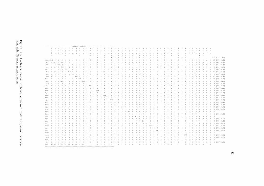
83
----------------------------- Confusion Matrix -------------------------------
n e t t f f s s å n t e t t f f s s å n t t f f s s a n h t m d e h i j k k k n o s s s ä ö
o t v r y e e j t i i l o r y e e j t i j r j e e j r i u u i e l a n a o r r e c o t t r r
l t å e r m x u t o o v l e r m x u t t u e o m x u t t n s l t l r t g m o o j h m r å e
l a a a v t t t t t i t g t r t t t o t d e j e e m n n e r
t i i i t o i o t t o o t n o r n o r a a o c Del [ %c / %e]
noll 1042 0 2 0 0 0 0 0 0 0 0 0 3 0 0 0 0 0 0 0 2 0 0 2 1 0 3 1 1 0 0 0 0 1 0 1 0 0 6 1 1 0 0 0 2 0 25 [97.5/0.2]
ett 0 806 4 18 2 7 1 1 3 0 0 0 0 9 1 5 1 0 1 2 0 6 0 0 0 0 0 1 2 1 0 1 0 0 3 0 0 0 0 0 0 0 0 0 1 0 55 [92.0/0.6]
två 3 0 804 2 2 6 0 1 2 0 1 0 3 0 0 2 0 0 1 0 1 1 0 1 1 2 0 0 0 1 0 0 0 0 0 0 0 0 3 0 1 0 0 7 0 0 44 [95.1/0.4]
tre 0 10 1 753 13 4 2 5 1 3 5 0 0 3 0 5 4 0 0 1 0 0 0 0 1 1 0 0 1 4 0 2 1 0 0 0 0 0 0 2 0 0 2 0 1 0 48 [91.3/0.7]
fyra 0 1 0 5 793 1 0 1 2 1 3 0 0 0 1 0 0 0 0 0 0 1 0 0 0 0 0 0 1 2 0 0 0 0 0 0 0 0 0 0 0 0 0 0 1 0 25 [97.5/0.2]
fem 0 12 2 2 3 712 0 0 2 0 0 0 0 0 0 21 0 0 0 0 0 0 1 8 2 1 0 0 1 7 0 0 1 0 0 0 0 0 0 0 0 0 0 0 0 0 57 [91.9/0.6]
sex 0 3 0 1 0 0 731 1 0 0 0 0 0 0 0 1 12 0 0 0 0 0 0 0 5 0 0 0 1 0 0 0 0 0 0 0 0 0 0 0 0 0 2 0 0 0 45 [96.6/0.2]
sju 4 0 2 6 4 1 3 662 0 0 0 0 4 0 0 0 0 1 1 0 6 0 0 0 0 1 0 0 2 5 0 0 0 0 0 0 0 0 0 0 0 0 0 0 0 0 45 [94.3/0.4]
åtta 0 1 0 2 1 1 0 0 690 0 0 0 0 1 0 0 0 1 5 0 0 0 1 0 0 0 1 0 0 0 0 0 0 0 0 0 0 0 0 0 2 0 0 0 0 0 27 [97.7/0.1]
nio 3 2 0 13 19 3 0 3 0 604 1 0 1 0 0 3 1 0 1 7 0 0 0 0 0 0 0 1 3 4 6 2 0 1 0 0 0 0 1 2 0 0 0 0 1 1 46 [88.4/0.7]
tio 0 2 0 4 5 0 0 0 0 2 44 0 0 0 0 0 0 0 1 0 0 0 0 0 0 0 0 0 0 0 0 0 0 0 0 0 0 0 0 0 0 0 0 0 0 0 4 [75.9/0.1]
elva 0 0 0 0 0 1 0 0 0 0 0 62 0 0 0 0 0 0 0 0 0 0 0 0 0 0 0 0 2 0 0 1 0 0 0 0 0 0 0 0 0 0 0 0 0 0 2 [93.9/0.0]
tolv 0 1 1 0 0 0 0 0 0 0 0 0 45 0 0 0 0 0 0 0 0 1 0 0 1 1 0 0 0 0 0 0 0 0 0 0 0 0 0 0 0 0 0 0 0 1 0 [88.2/0.1]
tret 0 3 0 2 0 0 0 0 0 0 0 0 0 138 1 0 1 1 0 0 0 1 0 0 0 0 0 0 0 0 0 0 0 0 0 0 0 0 0 0 0 0 0 0 0 0 6 [93.9/0.1]
fyrt 0 0 0 0 0 0 1 0 0 0 0 0 0 1 94 1 0 6 0 0 0 0 0 0 0 0 0 0 0 0 0 0 0 0 0 0 0 0 0 0 0 0 0 0 0 0 3 [91.3/0.1]
femt 0 0 1 3 0 0 0 0 0 1 0 0 0 0 1 128 1 0 0 0 0 0 0 2 0 0 0 0 1 0 0 0 0 0 0 0 0 0 0 0 0 0 0 0 0 0 4 [92.8/0.1]
sext 0 0 0 2 0 0 8 0 0 1 0 0 0 0 0 0 125 0 0 0 0 0 0 0 0 0 0 0 0 0 0 0 0 0 0 0 0 0 0 0 0 0 0 0 0 0 3 [91.9/0.1]
sjut 0 1 0 0 0 0 0 3 0 0 0 0 0 2 4 0 0 148 0 1 1 0 0 0 0 0 0 0 0 0 0 0 0 0 0 0 0 0 0 0 0 0 0 0 0 0 4 [92.5/0.1]
åtti 1 2 0 7 0 0 0 0 4 0 3 0 0 2 4 0 0 15 126 2 0 0 0 0 0 0 0 0 0 1 0 0 0 0 0 0 0 0 4 0 1 0 0 0 1 0 14 [72.8/0.4]
nitt 0 0 0 5 0 0 2 0 0 1 1 0 0 2 0 0 2 1 0 172 0 0 0 0 0 0 0 0 0 0 0 0 0 0 1 0 0 0 1 0 0 0 0 0 0 0 5 [91.5/0.1]
tjug 2 0 0 0 0 0 0 3 0 0 0 0 0 2 1 2 2 1 0 0 147 0 0 0 0 0 0 0 0 3 0 1 0 0 0 0 0 0 0 0 0 0 0 0 1 0 19 [89.1/0.2]
tret 0 0 0 0 0 0 0 0 0 0 0 0 0 1 0 0 0 0 0 0 0 35 0 0 0 1 0 0 0 0 0 0 0 0 0 0 0 0 0 0 0 0 0 0 0 0 0 [94.6/0.0]
fjor 0 0 0 0 0 0 0 0 0 0 0 0 0 0 0 0 0 0 0 0 0 0 40 0 0 0 0 0 0 0 0 0 0 0 0 0 0 0 0 0 0 0 0 0 0 0 0
femt 0 0 0 0 0 0 0 0 0 0 0 0 0 0 0 1 0 0 0 0 0 0 0 41 0 1 0 0 0 0 0 0 0 0 0 0 0 0 0 0 0 0 0 0 0 0 1 [95.3/0.0]
sext 0 0 0 0 0 0 0 0 0 0 0 0 0 0 0 0 0 0 0 0 0 0 0 0 42 0 0 0 0 0 0 0 0 0 0 0 0 0 0 0 0 0 0 0 0 0 2
sjut 1 0 0 0 0 0 0 0 0 0 0 0 0 0 0 0 0 0 0 0 0 1 0 0 0 29 0 0 0 0 0 0 0 0 0 0 0 0 0 0 0 0 0 0 0 0 0 [93.5/0.0]
arto 0 0 0 0 0 0 0 0 1 0 0 0 0 0 0 0 0 0 0 0 0 0 0 0 0 0 21 0 0 0 0 0 0 0 0 0 0 0 0 0 0 0 0 0 0 0 0 [95.5/0.0]
nitt 0 0 0 0 0 0 0 0 0 0 0 0 0 0 0 0 0 0 0 0 0 1 0 0 0 1 0 30 0 1 0 0 0 0 0 0 0 0 0 0 0 1 0 0 0 0 1 [88.2/0.0]
hund 8 2 0 1 6 4 0 2 2 1 1 1 6 0 0 2 1 0 0 0 2 3 0 1 7 2 1 0 328 0 0 1 0 0 0 0 3 0 0 0 1 0 0 0 0 0 53 [85.0/0.5]
tuse 0 0 0 0 1 0 0 0 0 0 0 0 0 0 0 0 0 1 0 0 0 0 0 0 0 0 0 0 0 146 0 0 0 0 0 0 0 0 0 0 0 0 0 0 0 0 2 [98.6/0.0]
milj 0 0 0 0 0 0 0 0 0 0 0 0 0 0 0 0 0 0 0 0 0 0 0 0 0 0 0 0 0 0 24 0 0 0 0 0 0 0 1 0 0 0 0 0 0 0 0 [96.0/0.0]
komm 0 0 0 0 0 0 0 0 0 0 0 0 0 0 0 0 0 0 0 0 0 0 0 0 0 0 0 0 0 0 0 0 0 0 0 0 6 0 0 0 0 0 0 0 0 0 0
kron 0 0 0 0 2 0 0 0 0 0 0 0 1 0 0 0 0 0 0 0 0 0 0 1 1 0 0 0 0 0 0 0 0 0 0 0 0 1 176 0 0 0 0 0 1 0 3 [96.2/0.1]
och 0 0 0 0 0 3 0 0 1 0 0 0 0 0 0 0 0 0 0 0 0 0 0 0 0 0 0 0 0 0 0 0 0 0 0 0 0 0 0 0 7 0 0 0 0 0 9 [63.6/0.0]
stre 0 0 0 0 0 0 0 0 0 0 0 0 0 0 0 0 0 0 0 0 0 0 0 0 0 0 0 0 0 0 0 0 0 0 0 0 0 0 0 0 0 0 8 0 0 0 0
öre 0 1 0 0 0 0 0 0 0 0 0 0 0 0 0 0 0 0 0 0 0 0 0 0 0 0 0 0 0 0 0 0 0 0 0 0 0 0 0 0 0 0 0 0 0 8 1 [88.9/0.0]
Ins 4 95 9 22 9 16 6 20 18 20 2 0 1 1 0 1 1 0 2 1 1 0 0 0 1 0 1 0 4 3 0 8 0 0 2 1 0 0 2 0 9 0 2 0 1 0
==============================================================================
Fig
ure
E.6
.C
on
fusio
nm
atrix
:trip
hon
es,cro
ss-word
contex
tex
pan
sion
,n
ewlex
-ico
n,
eight
Gau
ssian
mix
ture
terms