Embed Size (px)
Citation preview

Graduate Theses, Dissertations, and Problem Reports
2016
Developing a Smart Proxy for Fluidized Bed Using Machine Developing a Smart Proxy for Fluidized Bed Using Machine
Learning Learning
Amir Ansari
Follow this and additional works at: https://researchrepository.wvu.edu/etd
Recommended Citation Recommended Citation Ansari, Amir, "Developing a Smart Proxy for Fluidized Bed Using Machine Learning" (2016). Graduate Theses, Dissertations, and Problem Reports. 5113. https://researchrepository.wvu.edu/etd/5113
This Thesis is protected by copyright and/or related rights. It has been brought to you by the The Research Repository @ WVU with permission from the rights-holder(s). You are free to use this Thesis in any way that is permitted by the copyright and related rights legislation that applies to your use. For other uses you must obtain permission from the rights-holder(s) directly, unless additional rights are indicated by a Creative Commons license in the record and/ or on the work itself. This Thesis has been accepted for inclusion in WVU Graduate Theses, Dissertations, and Problem Reports collection by an authorized administrator of The Research Repository @ WVU. For more information, please contact [email protected].

Developing a Smart Proxy for Fluidized Bed Using Machine
Learning
Amir Ansari
Thesis submitted
to the Benjamin M. Statler College of Engineering and Mineral Resources
at West Virginia University
in partial fulfillment of the requirements for the degree of
Masters of Science in
Petroleum and Natural Gas Engineering
Ebrahim Fathi, Ph. D., Committee Chairperson
Shahab D. Mohaghegh, Ph. D.
Ali Takbiri Borujeni, Ph. D.
Mehrdad Shahnam, Ph. D.
Department of Petroleum and Natural Gas Engineering
Morgantown, West Virginia
2016
Keywords: Coal Gasification, Fluidized-bed, Multiphase Flow, Artificial Neural Network,
Data Mining
©Copyright 2016 Amir Ansari

ABSTRACT
Developing a Smart Proxy for Fluidized Bed Using Machine
Learning
Amir Ansari
Using fossil fuel which has been grown dramatically during the recent century, causes an increase
in greenhouse gas emission. The global warming issue pushes the engineers toward the cleaner
type of energy like Hydrogen. Coal gasification is one of the cheapest methods to obtain Hydrogen.
Coal gasification is a special case of more general problem called fluidized bed. In order to design
and optimize a gasification process, a deep understanding of multiphase flow in a gasifier is
needed. MFiX is a commercial multi-phase flow simulator which has been used to simulate the
gas and solid transport and reaction in the gasifier using Computational Fluid Dynamics (CFD).
Although simulating multiphase flow using commercial CFD software has a lot of flexibilities, it
is really time-consuming and some other way could be implemented to reduce the run time. The
effort of this project is to develop an alternate method to perform the same analysis but with much
lower computational cost. A data-driven approach is used to build a smart proxy by employing the
knowledge of Artificial Intelligence (AI) and Data Mining (DM).
In this project, a smart proxy will be developed to study and analyze the fluidized bed problem.
This smart proxy is then will be used as a replicate of the CFD solver, with a good accuracy and
faster speed. This proxy needs an incredible less amount of time in comparison to the CFD solver
with a reasonable error (less than 10%). MATLAB neural network toolbox is used for training.
The goal of this project is to prove the concept of using AI&DM for computational fluid dynamics
especially predicting multiphase flow. Multiphase flow has a wide range of application in
petroleum industry such as multi-phase flow in the wellbore, surface lines, and hydraulic fracturing
such as proppant transport in the hydraulic fracture. This project opens a new way to accelerate
the fluid dynamics analysis and reduce its costs.

iii
NOMENCLATURE
𝑑 = Particle diameter
𝑓𝑔 = Flow resistance due to the internal porous surfaces
�⃗� = Acceleration of gravity
𝐼𝑔𝑚 = interaction force representing the momentum transfer between the gas phase and the mth solids phase
𝐼𝑚𝑙 = interaction force representing the momentum transfer between the mth and lth solids phases
𝐽 = Objective Function
𝑃 = Gas pressure
𝑃𝑠 = Solid pressure
𝑅𝑔𝑛 = Mass transfer from each of solid phases to the gas phases
𝑅𝑠𝑚𝑛 = Mass transfer from each of gas phases to the solid phases
𝑆�̿� = Gas-phase stress tensor
𝑆�̿�𝑚 = Stress tensor of the mth solid phase
𝑢𝑔 = Velocity of gas in x direction
𝑢𝑠 = Velocity of solid in x direction
𝑣𝑔 = Velocity of gas in y direction
�⃗�𝑔 = Gas velocity vector
𝑣𝑠 = Velocity of solid in y direction
�⃗�𝑠𝑚 = Solid Velocity Vector
𝑤𝑔 = Velocity of gas in z direction
𝑤𝑠 = Velocity of solid in z direction
𝑦𝑎𝑐𝑡𝑢𝑎𝑙 = The actual value which is given by CFD simulator
𝑤𝑝𝑟𝑒𝑑𝑖𝑐𝑡𝑒𝑑 = The predicted value which is calculated by ANN
𝜀𝑔 = Gas volume fraction
𝜀∗= Maximum packing volume fraction
𝜀𝑠𝑚 = Solid volume fraction
𝜌′ = Apparent Solid Density
𝜌𝑔 = Gas density
𝜌𝑠𝑚 = Solid density

iv
ACKNOWKEDGMENT
I would like to thank my advisors Dr. Ebrahim Fathi and Dr. Shahab Mohaghegh for their
continuous guidelines and supports during my study in WVU. I would also like to thank Dr. Ali
Takbiri for his inputs and helps that he has during my research. I also want to show appreciation
to Professor Sam Ameri who was like a father to me during my study. Lastly I want to express my
gratitude to NETL and Dr. Mehrdad Shahnam for his directions throughout my master’s study.

v
CONTENT
ABSTRACT .................................................................................................................................... ii
NOMENCLATURE ...................................................................................................................... iii
ACKNOWKEDGMENT ............................................................................................................... iv
LIST OF FIGURES ..................................................................................................................... viii
LIST OF TABLES ....................................................................................................................... xiii
ABBREVATIONS ....................................................................................................................... xiv
Chapter 1 Introduction ............................................................................................................... 1
1.1. Problem Statement ........................................................................................................... 1
1.2. Objective .......................................................................................................................... 2
1.3. Chapter Review ................................................................................................................ 3
Chapter 2 Background ............................................................................................................... 4
2.1. Gasification ...................................................................................................................... 4
2.2. Multiphase Flow ............................................................................................................... 5
2.2.1. MFiX ......................................................................................................................... 8
2.2.2. Governing Equation .................................................................................................. 8
2.2.3. MFiX solution Algorithm ....................................................................................... 10
2.3. Machine Learning .......................................................................................................... 11
2.3.1. Supervised Learning ............................................................................................... 12
2.3.2. Unsupervised Learning ........................................................................................... 12
2.3.3. Artificial Neural Network ....................................................................................... 12
2.3.4. Objective function ................................................................................................... 13
2.4. Previous work done in this area ..................................................................................... 14
Chapter 3 Methodology ........................................................................................................... 16
3.1. Defining the problem ..................................................................................................... 16

vi
3.2. MFiX .............................................................................................................................. 17
3.2.1. Grid system ............................................................................................................. 18
3.3. Artificial Neural Network Setup .................................................................................... 18
3.3.1. Tier System ............................................................................................................. 19
3.3.2. Input Matrix ............................................................................................................ 20
3.3.3. Neural Network Architecture .................................................................................. 21
3.3.4. Data Partitioning ..................................................................................................... 22
3.4. Spatio-Temporal Database ............................................................................................. 23
3.5. Solution Scenarios .......................................................................................................... 23
3.5.1. Early time versus late time ...................................................................................... 24
3.5.2. Cascading versus non-cascading ............................................................................. 26
3.5.3. Single output versus multiple output ...................................................................... 28
3.5.4. Explicit versus implicit ........................................................................................... 29
3.5.5. Training with multiple time-steps ........................................................................... 29
3.5.6. Reducing the size of the system .............................................................................. 32
3.6. Summary ........................................................................................................................ 35
Chapter 4 Results and Discussion ........................................................................................... 37
4.1. Result Demonstration ..................................................................................................... 37
4.2. Early time-step, non-cascading, single output, explicit ................................................. 37
4.2.1. Gas volume fraction ................................................................................................ 38
4.2.2. Gas Pressure ............................................................................................................ 41
4.3. Late time-step, non-cascading, single output, explicit ................................................... 44
4.3.1. Gas Volume Fraction .............................................................................................. 44
4.4. Cascading, single output, explicit .................................................................................. 48
4.4.1. Gas volume fraction for early time ......................................................................... 48

vii
4.4.2. Gas volume fraction for late time ........................................................................... 54
4.5. Early time-step, non-cascading, multiple output, explicit .............................................. 56
4.6. Early time-step, non-cascading, multiple output, implicit ............................................. 58
4.7. Using multiple time-steps for training, non-cascading, single output, explicit .............. 61
4.8. Using four time-steps for training, cascading, single output, explicit............................ 63
4.9. Reducing the number of parameters (KPI) .................................................................... 63
4.10. Using seven time-steps for training, cascading, single output, explicit ..................... 70
4.11. Changing the data prioritization ................................................................................. 71
4.12. Smart sampling ........................................................................................................... 74
Chapter 5 Conclusions and Recommendations ....................................................................... 75
5.1. Conclusions .................................................................................................................... 75
5.2. Recommendations and future works .............................................................................. 76
BIBBLOGRAPHY ....................................................................................................................... 77
APPENDIX ................................................................................................................................... 79
Appendix I: MFiX Equations .................................................................................................... 79
Appendix II: MFiX Gasification code ...................................................................................... 82
Appendix III: Early time-step, non-cascading, single output, explicit...................................... 85
Appendix IV: MATLAB Code (Creating Spatio-Temporal database) ..................................... 88

viii
LIST OF FIGURES
Figure 2-1- The gasifier with inputs and outputs [3] ...................................................................... 4
Figure 2-2- MFiX solution Algorithm [4] .................................................................................... 11
Figure 2-3- Artificial Neural Network Schematic ........................................................................ 13
Figure 3-1- Geometry and initial condition of the problem .......................................................... 17
Figure 3-2- MFiX numbering order .............................................................................................. 19
Figure 3-3- The tier system of a 3-D simulation ........................................................................... 20
Figure 3-4- nueral network transfer function (TANSIG) ............................................................. 22
Figure 3-5- Spatio-Temporal Database and optimized database .................................................. 23
Figure 3-6- 69 different parameter of ANN .................................................................................. 24
Figure 3-7- Input/output parameters and time-steps for the training ............................................ 25
Figure 3-8- Input/output time-steps for the training (early time) ................................................. 25
Figure 3-9- Input/output time-steps for the training (late time) .................................................... 25
Figure 3-10- Gas volume fraction distribution on the wall; early time (a) versus late time (b) ... 26
Figure 3-11- The process of non-cascading deployment .............................................................. 27
Figure 3-12- The process of cascading deployment ..................................................................... 27
Figure 3-13- Traning with only one output (one component of gas velocity at the same time) ... 28
Figure 3-14- Traning with multiple outputs (three components of gas velocity simutanously) ... 28
Figure 3-15- Traning with multiple outputs implicitly ................................................................. 29
Figure 3-16- Input and output pair for the training with single time-step .................................... 30
Figure 3-17- Input and output pair for the training with ............................................................... 31
Figure 3-18- Three different time-steps with different flow characteristics ................................. 31
Figure 3-19- distribution of gas volume fraction at time-step 4000 ............................................. 33
Figure 3-20- The important section of the fluidized bed .............................................................. 33
Figure 3-21- Network schematic with its weights ........................................................................ 34
Figure 3-22- Distibution of Gas volume fraction at time step 4000 ............................................. 36
Figure 3-23- Distibution of Gas volume fraction at time step 4000 after smart sampling ........... 36
Figure 4-1- Five different layers for result demonstration ............................................................ 38
Figure 4-2- Comparison of CFD and smart proxy results for gas volume fraction of time-step 102
for layer one .................................................................................................................................. 39

ix
Figure 4-3- Comparison of CFD and smart proxy results for gas volume fraction of time-step 102
for layer two .................................................................................................................................. 39
Figure 4-4- Comparison of CFD and smart proxy results for gas volume fraction of time-step 102
for layer three ................................................................................................................................ 40
Figure 4-5- Comparison of CFD and smart proxy results for gas volume fraction of time-step 102
for layer four ................................................................................................................................. 40
Figure 4-6- Comparison of CFD and smart proxy results for gas volume fraction of time-step 102
for layer five .................................................................................................................................. 41
Figure 4-7- Comparison of CFD and smart proxy results for gas pressure of time-step 102 for layer
one ................................................................................................................................................. 42
Figure 4-8- Comparison of CFD and smart proxy results for gas pressure of time-step 102 for layer
two................................................................................................................................................. 42
Figure 4-9- Comparison of CFD and smart proxy results for gas pressure of time-step 102 for layer
three............................................................................................................................................... 43
Figure 4-10- Comparison of CFD and smart proxy results for gas pressure of time-step 102 for
layer four ....................................................................................................................................... 43
Figure 4-11- Comparison of CFD and smart proxy results for gas pressure of time-step 102 for
layer five ....................................................................................................................................... 44
Figure 4-12- Comparison of CFD and smart proxy results for gas volume fraction of time-step
4004 for layer one ......................................................................................................................... 45
Figure 4-13- Comparison of CFD and smart proxy results for gas volume fraction of time-step
4004 for layer two ......................................................................................................................... 46
Figure 4-14- Comparison of CFD and smart proxy results for gas volume fraction of time-step
4004 for layer three ....................................................................................................................... 46
Figure 4-15- Comparison of CFD and smart proxy results for gas volume fraction of time-step
4004 for layer four ........................................................................................................................ 47
Figure 4-16- Comparison of CFD and smart proxy results for gas volume fraction of time-step
4004 for layer five ......................................................................................................................... 47
Figure 4-17- Comparison of CFD and smart proxy results for gas volume fraction of time-step 101
for layer two (Cascading) .............................................................................................................. 49

x
Figure 4-18- Comparison of CFD and smart proxy results for gas volume fraction of time-step 102
for layer two (Cascading) .............................................................................................................. 49
Figure 4-19- Comparison of CFD and smart proxy results for gas volume fraction of time-step 103
for layer two (Cascading) .............................................................................................................. 50
Figure 4-20- Comparison of CFD and smart proxy results for gas volume fraction of time-step 104
for layer two (Cascading) .............................................................................................................. 50
Figure 4-21- Comparison of CFD and smart proxy results for gas volume fraction of time-step 105
for layer two (Cascading) .............................................................................................................. 51
Figure 4-22- Comparison of CFD and smart proxy results for gas volume fraction of time-step 106
for layer two (Cascading) .............................................................................................................. 51
Figure 4-23- Comparison of CFD and smart proxy results for gas volume fraction of time-step 107
for layer two (Cascading) .............................................................................................................. 52
Figure 4-24- Comparison of CFD and smart proxy results for gas volume fraction of time-step 108
for layer two (Cascading) .............................................................................................................. 52
Figure 4-25- Comparison of CFD and smart proxy results for gas volume fraction of time-step 109
for layer two (Cascading) .............................................................................................................. 53
Figure 4-26- Comparison of CFD and smart proxy results for gas volume fraction of time-step 110
for layer two (Cascading) .............................................................................................................. 53
Figure 4-27- Comparison of CFD and smart proxy results for gas volume fraction of time-step
4002 for layer two (Cascading) ..................................................................................................... 54
Figure 4-28- Comparison of CFD and smart proxy results for gas volume fraction of time-step
4004 for layer two (Cascading) ..................................................................................................... 55
Figure 4-29- Comparison of CFD and smart proxy results for gas volume fraction of time-step
4006 for layer two (Cascading) ..................................................................................................... 55
Figure 4-30- Comparison of CFD and smart proxy results for gas volume fraction of time-step
4020 for layer two (Cascading) ..................................................................................................... 56
Figure 4-31- Comparison of CFD and smart proxy results for gas x-velocity of time-step 102 for
layer four (explicit) ....................................................................................................................... 57
Figure 4-32- Comparison of CFD and smart proxy results for gas y-velocity of time-step 102 for
layer one (explicit) ........................................................................................................................ 57

xi
Figure 4-33- Comparison of CFD and smart proxy results for gas z-velocity of time-step 102 for
layer two (explicit) ........................................................................................................................ 58
Figure 4-34- Comparison of CFD and smart proxy results for gas x-velocity of time-step 102 for
layer five (implicit) ....................................................................................................................... 59
Figure 4-35- Comparison of CFD and smart proxy results for gas y-velocity of time-step 102 for
layer one (implicit) ........................................................................................................................ 60
Figure 4-36- Comparison of CFD and smart proxy results for gas z-velocity of time-step 102 for
layer two (implicit) ....................................................................................................................... 60
Figure 4-37- RMSE distribution versus time-step when three time pair of data were used for
training .......................................................................................................................................... 61
Figure 4-38- Comparison of CFD and smart proxy results for gas volume fraction of time-step 500
for layer two .................................................................................................................................. 62
Figure 4-39- RMSE distribution versus time-step when three and four time pair of data were used
for training .................................................................................................................................... 63
Figure 4-40- parameter pioritization for Gas volume fraction ANN (averaging all the weights) 64
Figure 4-41- parameter pioritization for Gas volume fraction ANN (averaging all the weightsafter
removing signs) ............................................................................................................................. 65
Figure 4-42- Comparison of RMSE distribution versus time-step for two different approach of
averaging ....................................................................................................................................... 67
Figure 4-43- Comparison between RMSE when different number of parameters were used for
training (70, 56, and 42 parameters) ............................................................................................. 68
Figure 4-44- Comparison between RMSE when different number of parameters were used for
training (70, 56, and 35 parameters) ............................................................................................. 69
Figure 4-45- Comparison between RMSE with and without Ps ................................................... 70
Figure 4-46- Comparison of CFD and smart proxy results for gas volume fraction of time-step
4020 for layer one (Cascading) ..................................................................................................... 71
Figure 4-47- CFD and smart proxy results for gas volume fraction of time-step 4004 for layer one
by 60% training (non-cascading) .................................................................................................. 72
Figure 4-48- CFD and smart proxy results for gas volume fraction of time-step 4004 for layer one
by 40% training (non-cascading) .................................................................................................. 73

xii
Figure 4-49- CFD and smart proxy results for gas volume fraction of time-step 4004 for layer one
by 30% training (non-cascading) .................................................................................................. 73
Figure 4-50- Comparison of RMSE in different time steps with/without smart sampling ........... 74
Figure 0-1- Comparison of CFD and smart proxy results for gas x-velocity of time-step 102 for
layer one (explicit) ........................................................................................................................ 85
Figure 0-2- Comparison of CFD and smart proxy results for gas y-velocity of time-step 102 for
layer one (explicit) ........................................................................................................................ 86
Figure 0-3- Comparison of CFD and smart proxy results for solid x-velocity of time-step 102 for
layer one (explicit) ........................................................................................................................ 86
Figure 0-4- Comparison of CFD and smart proxy results for solid y-velocity of time-step 102 for
layer one (explicit) ........................................................................................................................ 87
Figure 0-5- Comparison of CFD and smart proxy results for gas z-velocity of time-step 102 for
layer one (explicit) ........................................................................................................................ 87

xiii
LIST OF TABLES
Table 2-1- Multiphase Flow Modeling Approaches [8] ................................................................. 6
Table 2-2- Important parameters for multiphase flow .................................................................. 10
Table 3-1- different grid size and the amount of cells .................................................................. 18
Table 3-2- All the useful parameters reported in the MFiX result file ......................................... 19
Table 3-3- Important numbers in Neural Network Model ............................................................ 21
Table 3-4- Neural Network characteristics ................................................................................... 22
Table 3-5- Original Data Partitioning ........................................................................................... 22
Table 4-1- Fourteen less important parameters when simple average was used .......................... 66
Table 4-2- Fourteen less important parameters when averaging by removing sign was used ..... 66
Table 4-3- Database size before and after optimization ............................................................... 70
Table 4-4- Data Partitioning in different scenarios....................................................................... 72
Table 5-1- comparison between Spatio-Temporal database and optimized database .................. 75
Table 5-2- comparison between speed of run for CFD and Smart proxy ..................................... 76

xiv
ABBREVATIONS
AI Artificial Intelligence
ANN Artificial Neural Network
CFD Computational Fluid Dynamics
CMG Computer Modeling Group
CSV Comma Separated Value
DM Data Mining
EIA Energy Information Administration
IGCC Integrated Coal Gasification Combined Cycle
KPI Key Performance Indicator
MFIX Multiphase Flow with Interphase eXchange
MSE Mean Square Error
NETL National Energy Technology Laboratory
PDE Partial Differential Equation
RMSE Root Square of Mean Square Error
VTU Visualization Toolkit Unstructured points data
1
Chapter 1 Introduction
The global warming is becoming a critical issue nowadays and pushes the engineers more toward
the clean and environmentally-friendly fuels. Coal is a major fuel for the power plants. According
to the EIA1 report in April 2016, 33% of the U.S. electricity was generated using coal, and coal
has a huge contribution to greenhouse gas emission. Integrated Gasification Combined Cycle (IGCC)
has the potential to reduce the CO2 emissions of carbon based power plants by converting coal into synthesis
gas (also known as syngas) while capturing CO2 for storage thereby reducing the environmental impact of
power generation. Hydrogen gas generated, as the results of the gasification process can be used to power
gas turbines in power generation industry [1]. Modeling and simulation capabilities reduce the cost and
time to market of new technologies like IGCC by reducing costly design and scale-up testing.
1.1. Problem Statement
A coal based power plants (IGCC2) are getting popular in power generation facilities. There are
about 160 gasification plants in operation in all over the world [2]. IGCC consists of several parts;
feed system, gasifier, gas clean-up system, and heat exchanger. The heart of an IGCC power plant
is a gasifier. Understanding the hydrodynamics inside a gasifier allows for achieving optimum
design. Basically, there are three approaches to simulate a process and find out the characteristics
of the process; First method is to create a very simple mathematical model and solve the governing
equations analytically, second method is to create a mathematical model with more complexities
and discretize the domain in time and space and solve the equations numerically. The third
approach is to build a prototype (usually in a smaller size) and do some experiments on a smaller
scale and perform the upscaling to obtain the actual characteristics in the desired scale.
It is near impossible to capture all the properties of the gasification process with a simple analytical
model since analytical models apply simplified assumptions which may eliminate the major
characteristics of the problem. It is also extremely challenging to design a small experimental
prototype that can mimic the gasification process at very high temperature [3] and high pressure
and take detailed measurements for improving the performance of the gasifier.
1 U.S. Energy Information Administration 2 Integrated Coal Gasification Combined Cycle

2
The recommended method is to take the advantage of computational science and using numerical
simulation to predict the main features of this process. The complexity of this problem is mainly
due to presence of multiple phases (gas and solid) and the energy and mass transfer between these
phases. In a complete gasification problem, as many as twenty-two equations should be solved
simultaneously including mass conservation (2 equations), momentum equation (6 equations),
energy balance (2 equations) and species mass fraction (remaining 12 equations) [4], [5].
Gasification is a transient process with a high degree of non-linearity and chaos that increases the
computational cost of the process dramatically. Modeling this process by CFD solver typically is
very time-consuming. As an example, modeling of a very simple case without any reaction and
mass transfer takes about 4 days on super-computers with several clusters just to simulate 10
seconds of the actual time. Furthermore, by adding more complexities to the system, the run-time
will be increasing exponentially.
This is where there is a critical need to develop new data-driven smart proxies that can help
engineers to reduce the time needed for simulating complex fluid dynamics problems such as coal
gasification. This method takes advantage of machine learning algorithm and artificial intelligence
to come up with a powerful tool to predict the behavior of a system with far less computational
cost compared to traditional CFD solvers.
1.2. Objective
The commercial CFD software’s which are available in the market such as MFIX, Open-FOAM,
and COMSOL need several days to several weeks to simulate a simple fluidization problem. This
makes the optimization of any process that requires multiple runs extremely computationally
intensive and expensive. Therefore, engineers working in the field of fluid dynamics are looking
for new techniques and tools that have the same capability but with faster turnaround time and
much lower computational cost. Artificial intelligence and big-data analytics have a proven record
in replicating the simulation results of complex problems with huge data sets such as those
introduced in oil and gas industry by Mohaghegh and his team. The same techniques Artificial
Intelligence (AI) and Data Mining (DM) can be used in a new frame work to develop a new tool
that is able to completely replicate numerical simulation of CFD problems with the same accuracy
and in much shorter time. The new approach requires huge amount of data, so the pattern

3
recognition techniques and machine learning algorithms can be used to learn the behavior of the
system from the given data.
The main objective of this research is to create a surrogate model that can replicate the CFD
numerical simulation results for a non-reacting fluidized bed. The final goal of this project is to
deliver a software package containing a system of artificial neural networks which is able to do
the same job as CFD simulators does at much faster speed and lower computational cost.
1.3. Chapter Review
This proposal includes four chapters. In chapter one, the problem was defined and the final
objective of the research was determined.
In chapter two, an introduction about the gasification will be presented. A brief definition of
multiphase flow and its governing equations will be provided. Also, a literature review that has
been conducted about using smart proxies in the fluid dynamics problems, will be reviewed.
Chapter three will be discussing the methodology and the machine learning method which is used
in this thesis. The artificial neural network with all the required information will be introduced.
The network architecture with all input and output system will be discussed.
Results and discussions will be also presented in the fourth chapter. The conclusion will be made
in the fifth chapter. And finally, this thesis will end up with recommendations and suggestions for
the new works.

4
Chapter 2 Background
In this chapter, detailed discussions on three main factors of this project will be presented. First,
the gasification process will be introduced. Then, the fundamental of fluid dynamic equations and
their application in gasification process will be presented. Finally, the application of machine
learning and pattern recognition in this project will be introduced.
2.1. Gasification
Gasification is the process by which feedstock such as coal or biomass (dried plants, woods, and
farm waste) is converted into synthesis gas (also called syngas). Syngas is mainly composed of
CO, H2 and CO2 along with contaminants such as H2S [6]. Primary species such as H2 and CO can
be used in power generation or chemical processing industries. Figure 2-1 shows the gasifier vessel
where the gasification takes place.
Figure 2-1- The gasifier with inputs and outputs [3]
Gasifiers are classified into three main categories: fixed bed gasifiers, entrained flow gasifiers and
fluidized bed gasifiers. A fluidized bed gasifier can efficiently mix the feedstock (coal) particles,
which may be at different stages of gasification. An advantage of a fluidized bed gasifier is the
nearly uniform temperature that can be achieved in the reactor. In a fluidized bed gasifier, a mixture

5
of steam and oxidizer (air) is introduced at the bottom of the gasifier, with coal particles injected
along the side of the reactor. After the initial moisture in the coal is released, the coal particles
undergo devolatilization, where the volatile gases, such as CO, CO2, H2, H2O, CH4 to name a few,
that are trapped in the coal are released. In the next step, carbon in coal and oxygen react to produce
carbon monoxide and heat according to equation (2-1). Carbon monoxide further reacts with
oxygen to produce carbon dioxide and heat, according to equation (2-2).
𝐶 +1
2𝑂2
→ 𝐶𝑂 (2-1)
𝐶𝑂 +1
2𝑂2
→ 𝐶𝑂2
(2-2)
The heat of combustion generated is key in maintaining the gasification process, which is an
endothermic process. Steam and carbon dioxide gasification takes place, when carbon in coal
reacts with H2O and CO2 to produce carbon monoxide and hydrogen according to reactions (2-3)
and (2-4).
𝐶 + 𝐻2𝑂 → 𝐶𝑂 + 𝐻2 (2-3)
𝐶 + 𝐶𝑂2 → 2𝐶𝑂 (2-4)
Depending on the gasification goal, CO and H2 in the syngas can be directed to a water-gas shift
reactor, where the ratio of CO to H2 produced can be altered according to reaction (2-5).
𝐶𝑂 + 𝐻2𝑂 ↔ 𝐶𝑂2 + 𝐻2 (2-5)
Gasification process also has its own complexity and concerns. One of the major issues of this
process is handling and processing the solids. On the other hand, simulation of fluid dynamics in
a gasifier is a tedious task due to multi-phase nature of flow and reaction in a high temperature and
pressure.
2.2. Multiphase Flow
Transport in the gasification process consists of two flow regimes; coal transport and smoke
transport. This is a challenging problem because of the multi-phase nature of the process and

6
heterogeneous fluid and particle interactions. Traditionally, the modeling and optimization of
multiphase flow is performed by empirical modeling based on the experimental observation
without going into the detail of physics and mathematics. The empirical modeling needs large
investment for data gathering and data processing. Data gathering is itself a big challenge in
gasification vessel since it is hard to measure the flow properties inside the gasifier due to its high
temperature. Multiphase computational fluid dynamics does not have these difficulties, it also has
a lot of flexibilities to tweak the system characteristics to optimize the process.
Basically, there are two different modeling scheme; Eulerian and Lagrangian. Eulerian refers to
bulk fluid simulation that has a fix coordinate system while Lagrangian refers to particle tracking
simulation where there is a coordinate assigned to each particle and moving with particle velocity
with respect to fixed coordinate.
Continuum (Eulerian): Select a fix control volume and assume the flow is continuum and
use the Navier-Stokes equation by averaging the properties over the volume. Continuum
approach needs less computational time but it cannot capture all the complexities,
especially in multiphase flow where interaction between particles plays a major role [8].
Discrete Particle (Lagrangian): Track each particle in the fluid by using Newton’s Law of
motion. This method is more straightforward to apply, even in multiphase flow, but the
computational costs is high [8].
There are several approaches to modeling multiphase flows. Depending on the application, either
the gas phase or the solid phase or both phases can be modeled in an Eulerian or a Lagrangian
framework [8]–[10]. Table 2-1 shows different approaches to model multiphase flows.
Table 2-1- Multiphase Flow Modeling Approaches [8]
Name Gas Phase Solid Phase Coupling Scale
1 Discrete bubble model Lagrangian Eulerian Drag Closure for bubbles 10 m
2 Two Fluid Model Eulerian Eulerian Gas-Solid drag closure 1 m
3 Unresolved Discrete particle model Eulerian Lagrangian Gas-particle drag closure 0.1 m
4 Resolved Discrete particle model Eulerian Lagrangian Boundary condition at
particle surface 0.01 m
5 Molecular Dynamics Lagrangian Lagrangian Elastic collisions at particle
surface
<0.001
m

7
Coal gasification includes two phases; first phase is gas (oxygen and sometimes water vapor) and
the second phase is solids (coal). The governing equations of the motion are partial differential
equations. To completely model this process, coupling of those equations for mass transport,
energy transport, and momentum equation for two phases should be considered. Solving the
coupled partial differential equations analytically is not an easy task, so the numerical method
should be utilized to solve the equations.
CFD (computational fluid dynamics) is a combination of numerical analysis, fluid dynamics, and
computer science. The governing partial differential equations for the fluid flow could be solved
more easily by CFD method which is a tool to replace PDE by a set of linear algebraic equations.
There are several commercial CFD simulator available in the market with different capabilities in
different aspects. Among those software, MFiX has been chosen for this project to simulate fluid
and solid dynamics in gasifier.
Modeling the multi-phase fluid dynamics inside a gasifier is extremely complex. To model the
gasification process, not only the hydrodynamics of gas and solid flow have to be modeled by
solving for gas and particle transport equations, also the chemical reaction processes such as
devolatilization, coal combustion and gasification, homogeneous oxidation and water gas shift
reactions have to be modeled as well Often times it’s difficult to make detailed measurements
inside a gasifier, due to the high temperature, high pressure and harsh conditions in a gasifier.
Simulations, therefore, provides an alternative to designers and engineers to access the
performance of a gasifier.
Watanabe and Otaka [3] used CFX-4 CFD software to investigate the effect of air flow rate and
coal type on the performance of a gasifier. The purpose of their study was to optimize the
performance of the gasifier by changing the air ratio and coal type.
Papadopoulos et al., [7] used a ANSYS-CFX CFD code to develop a high pressure, high
temperature model. He used the same concepts and equations as Watanabe and Otaka did.

8
2.2.1. MFiX
MFiX is an open source multiphase CFD software developed and maintained by NETL1. MFiX is
able to handle heat and mass transfer and chemical reactions in fluid-solids systems. It has been
used to model the bubbling, circulating fluidized beds, and spouted beds. The output of MFiX
consists of transient information on the distribution of volume fractions, pressure, velocity,
temperature, and species mass fractions of each phase being considered. MFiX has its own post-
processing tool to visualize the results, but it is compatible with multiple software such as Paraview
[4], [5].
2.2.2. Governing Equation
In this section, all the equations which MFiX uses to simulate fluid and solid dynamics are
reviewed. There will not be any detailed discussion on the derivation of the equations and the
purpose of providing these equations is to introduce all the important parameters that later on will
be used in the machine learning algorithm as input. Moreover, the step by step algorithm that MFiX
uses to solve the problem will be discussed since this will play an important role for the machine
learning when implicit prediction is utilizing.
2.2.2.1. Conservation of mass
MFiX can handle one gas phase and multiple solid phases, so there is one scalar equation for
conservation of gas and multiple equations for conservation of each solid phase [11].
Equation (2-6) shows the conservation of mass of gas phase
𝜕
𝜕𝑡(𝜀𝑔𝜌𝑔) + ∇. (𝜀𝑔𝜌𝑔�⃗�𝑔) = ∑ 𝑅𝑔𝑛
𝑁𝑔
𝑛=1
(2-6)
Where 𝜀𝑔 is the gas volume fraction, 𝜌𝑔 is the gas density, �⃗�𝑔 is the gas velocity vector and 𝑅𝑔𝑛 is
mass transfer from each of solid phases to the gas phase, this mass transfer could be due to
chemical or physical processes such as evaporation and reaction
1 National Energy Technology Laboratory

9
As mentioned, MFiX can handle multiple solid phases. Equation (2-7) shows the conservation of
mass of mth solid phase.
𝜕
𝜕𝑡(𝜀𝑠𝑚𝜌𝑠𝑚) + ∇. (𝜀𝑠𝑚𝜌𝑠𝑚�⃗�𝑠𝑚) = ∑ 𝑅𝑠𝑚𝑛
𝑁𝑠𝑚
𝑛=1
(2-7)
Where 𝜀𝑠𝑚 is the solid fraction of mth solid phase, 𝜌𝑠𝑚 is the density of mth solid phase, �⃗�𝑠𝑚 is the
solid velocity vector and 𝑅𝑠𝑚𝑛 is mass transfer from gas phase to the solid phase.
2.2.2.2. Conservation of Momentum
The gas-phase momentum balance is expressed by equation (2-8).
𝜕
𝜕𝑡(𝜀𝑔𝜌𝑔�⃗�𝑔) + ∇. (𝜀𝑔𝜌𝑔�⃗�𝑔�⃗�𝑔) = ∇. (𝑆�̿�) + 𝜀𝑔𝜌𝑔�⃗� − ∑ 𝐼𝑔𝑚
𝑀
𝑚=1
+ 𝑓𝑔 (2-8)
Where 𝑆�̿� is the gas-phase stress tensor, 𝐼𝑔𝑚 is the interaction force representing the momentum
transfer between the gas phase and the mth solids phase, and 𝑓𝑔 is the flow resistance offered by
internal porous surfaces.
The momentum equation for the mth solids phase is
𝜕
𝜕𝑡(𝜀𝑠𝑚𝜌𝑠𝑚�⃗�𝑠𝑚) + ∇. (𝜀𝑠𝑚𝜌𝑠𝑚�⃗�𝑠𝑚�⃗�𝑠𝑚) = ∇. (𝑆�̿�𝑚) + 𝜀𝑠𝑚𝜌𝑠𝑚�⃗� − ∑ 𝐼𝑚𝑙
𝑀
𝑙=1𝑙≠𝑚
+ 𝐼𝑔𝑚 (2-9)
Where 𝑆�̿�𝑚 is the stress tensor for the mth solid phase, 𝐼𝑔𝑚 is the interaction force representing the
momentum transfer between the gas phase and the mth solids phase, and 𝐼𝑚𝑙 is the interaction force
representing the momentum transfer between the mth and lth
solids phases.
All the important parameters describing the gasification process can be extracted using equations
(2-6) to (2-9) and equations described in appendix I. Table 2-2 shows the key parameters involved
in the simulation process, this information will be used in the next chapter to define the input
parameters for the artificial neural network.

10
Table 2-2- Important parameters for multiphase flow
Key factors of gas-solid system
Gas Density (ρ)
Volume fraction (ɛ)
Particle diameter (d)
Maximum packing volume fraction (ɛ*)
Velocity vector of gas (u, v, w)
Velocity vector of solid (u, v, w)
Pressure field of gas (P)
Pressure field of solid(Ps)
Time (t)
Location to the boundaries (x, y, z)
Location to the interface (x, y, z)
2.2.3. MFiX solution Algorithm
Equations (2-6) to (2-9) form a system of nonlinear partial differential equations. In order to solve
this system of PDEs, a step by step iterative algorithm has been developed by MFiX solver. The
sequence of solving the equations and calculating the parameters are important for this project in
order to establish the best solution scenario. Each solution scenario has its own approach, in some
of them (implicit scenarios), the sequence of calculating of parameters is so important. The MFiX
solution algorithm might be a good start point for the implicit scenarios. There will be a detailed
discussion about different solution scenarios in the next chapter. Figure 2-2 shows the step by step
algorithm which is used by MFiX to solve the system of coupled PDE equations.

11
Figure 2-2- MFiX solution Algorithm [4]
2.3. Machine Learning
Based on Arthur Samuel (1959) definition, “Machine learning is a field of study that gives
computers the ability to learn without being explicitly programmed.”
Machine learning is a process through which computer will learn from data to find a possible
pattern in the data set. This process encompasses three main components as follows:
Learning algorithm
Data
A pattern in the data

12
If these three components are present, a successful learning process can be achieved based on the
capability of the learning algorithm. There are two major type of Machine Learning: supervise
learning and unsupervised learning [12].
2.3.1. Supervised Learning
In supervised learning, some data, is provided as input and output to the learning algorithm, with
the goal of finding the relationship between input and output. There are two general types of
supervised learning; Regression and Classification. When the output data is in continuous form,
regression should be used to find the trend between input and output. This trend could be linear or
nonlinear based on the problem characteristics. When for different inputs, there is finite possible
output, the classification should be considered. For example, the type of cancer (malignant, benign)
could be classified based on the age of the patient and size of the tumor.
2.3.2. Unsupervised Learning
In unsupervised learning, there is little or no information about the output. The learning algorithm
tries to find the pattern between input data without having the output. This process is named
clustering. For example, grouping the customer of a company based on the type of product that
they buy daily.
2.3.3. Artificial Neural Network
One of the popular machine learning processes is Artificial Neural Network (ANN). The idea of
ANN came from the neurons of the brain and the way they are communicating with each other to
solve a problem. Each artificial neural network consists of an input layer, one or more hidden
layers, and an output layer. The number of output and input layers are chosen based on the problem
and the property which is going to be predicted. Figure 2-3 shows a typical ANN with three inputs
and two outputs. ANN has one or more hidden layers and each layer has a specific number of
neurons [13].
In order to have a well-trained network, proper parameters should be introduced to the network. If
improper data are used to train the network there is no guarantee to have a well-trained network
that lead to correct predictions, in other words, “Garbage in, Garbage out.” In chapter three, a
smart way of picking parameters will be introduced.

13
Figure 2-3- Artificial Neural Network Schematic
The number of hidden layers and the neurons in each hidden layer depends on the complexity of
the problem, number of parameters, and number of records. Experience also plays a role in this
decision. But generally, there is no solid rule for them. As a rule of thumb, the number of neurons
in the first hidden layer shouldn’t be less than the number of input parameters.
2.3.4. Objective function
Regardless of the learning method, each machine learning process needs an optimization procedure
that helps the process reduce the error as much as possible. The very common and simple objective
function in supervised learning is the summation of all the differences between predicted values
by the learning method and the actual values of output. Sometimes the negative errors cancel the
positive errors and the total error becomes very small although none of the data points have good
predictions, by calculating the square of the differences, the mentioned problem could be resolved.
Equation (2-10) shows this objective function [13].
𝐽(𝜃0, 𝜃1) =1
2𝑚∑(𝑦𝑎𝑐𝑡𝑢𝑎𝑙 − 𝑦𝑝𝑟𝑒𝑑𝑖𝑐𝑡𝑒𝑑)
2𝑚
𝑖=1
(2-10)
During the learning process, the learning algorithm tries to assign different weights to each of the
lines in Figure 2-3, in a way that the global error of objective function becomes minimum. Also, a

14
blind validation is done simultaneously to stop the learning process. We will discuss the validation
and test in more depth in the next chapter.
2.4. Previous work done in this area
The idea of using AI in petroleum engineering was first introduced by S. Mohaghegh [14]. He
took advantage of ANN for predicting the permeability of the formation based on geological well
logs. He showed that neural network is capable of making the task of permeability determination
automated rather than doing it over and over by log analyst. He also stated that neural network can
handle far more complex tasks. He also used ANN for predicting gas storage well performance
after hydraulic fracture in the same paper and his later investigations [15].
Alizadehdakhel et al.[16] used ANN to predict the pressure loss of a two-phase flow in the 2 cm
diameter tube. In two-phase fluid, separation of the phases may occur because different phases
may have different velocities, so the traditional Navier-Stocks equation is not capable of finding
the exact pressure drop in different flow condition. The authors used three main property of the
fluid (gas velocity number, liquid velocity number, and line slop1) as the input of the ANN and
only one output which was the average pressure drop. They utilized 8 different networks with a
different number of neurons to find out the optimum number neurons. MSE and R-square were
used as a criterion to pick the best network design. They also tried to find the most efficient transfer
function between Log-Sigmoid, Hyperbolic-Tangent Sigmoid, and linear. The data had come from
the experimental setup that they had built. The pressure in upstream and downstream of the pipe
was measured and the pressure loss was calculated.
Shahkarami et al. [17] took advantage of ANN to model the pressure and saturation distribution in
a reservoir which was used for CO2 sequestration purpose. This problem required a large number
of time steps for simulation of CO2 injection and storage using commercial software. They ran 10
different cases in CMG (commercial reservoir simulator) and then the results were used as input
for ANN. The output of the ANN was selected to be pressure distribution, water saturation, and
CO2 mole fraction. 80% of the data coming from CMG simulation were used to train the network,
10% were used for the validation and the rest of the data were used for the test process. They have
1 Pressure drop in one meter, ΔP/L (Pa m-1)

15
shown that ANN can be used as a powerful tool for multiphase flow simulation in oil and gas
industry.
Esmaili and Mohaghegh [18] introduced a new way of using completion and production data with
the well logs in order to find out the shale reservoir behavior under certain condition. By
understanding the behavior of the shale reservoir, conducting the hydraulic fracture could be much
easier. Moreover, this method has the ability to perform the history matching on the production
data.
Kalantari-Dehghani et al. [19] coupled reservoir numerical simulator with AI method to develop
a shale proxy model that is able to regenerate a numerical simulation results in just a few seconds.
They introduced three different well-based tier systems to achieve a comprehensive input data for
the ANN. In another research [20], they showed that data-driven proxy models at the hydraulic
fracture cluster level could be used separately as a reservoir simulator especially in low
permeability reservoir such as shale which has a nonlinear behavior.

16
Chapter 3 Methodology
In this chapter, the methodology of solving a problem in the field of computational fluid dynamics
will be discussed in detail. First, the problem will be defined with all the initial and boundary
conditions. Then the modeling process in MFiX (commercial CFD simulator) will be explained.
Creating the input of the neural network is the next discussion in this chapter that is the most
important step of data training. By knowing all the provided information from previous chapters,
the neural network model will be created and the training will be performed.
3.1. Defining the problem
The gasification process is a very complicated problem. In order to demonstrate the usefulness of
using ANN to create proxy models for the gasification process, first a proof of concept study has
been carried out to show that ANN can be applied to a simple CFD simulation of a flow inside a
rectangular fluidized bed.
Figure 3-1 shows the geometry of the problem which is a rectangular fluidized bed with a square
cross section. The dimension of the fluidized bed is depicted in Figure 3-1. One-sixth of the
fluidized bed is filled with sand which is initially at rest. The sand particles are perfect spheres
with the density of 1160 kg/m3. The initial volume fraction of gas (voidage) is 0.42.
The y-component of the initial velocity of the air inside the fluidized bed (where sand is located)
is 1.43 m/s and the y-component of the initial velocity of the air in the freeboard region (above the
sand) is 0.6 m/s.
The inlet air velocity is set to 0.6 m/s that is uniformly distributed in the upward direction. The air
discharges into atmospheric pressure up on top of the bed.
As air is injected into the bed, initially large gas pockets form that cause sand particles to move
upward as a slug. In matter of few seconds, the gas pockets break up, leading to the breakup of
sand slugs, which shower back down. At this time, air entering the bed forms bubbles, which move
up through the sand bed, leading to the fluidization of the sand particles.

17
Figure 3-1- Geometry and initial condition of the problem
3.2. MFiX
The geometry setup in the previous section, is simulated in MFiX. The output data generated by
MFiX is used as the input data to the ANN.
The model has been created and ran successfully. The next step is to get the results from MFiX
and organize the data in order to make the data ready for the ANN. Since MFiX reports the results
based on the grids, the order and exact location of each grid is extremely important for ANN. The
output file of MFiX has an extension of *.vtu for each time-step which needs to be converted to
18
*.csv files. ParaView is an open source software which can be used for data visualization and
format conversion.
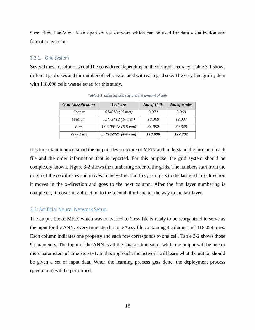
3.2.1. Grid system
Several mesh resolutions could be considered depending on the desired accuracy. Table 3-1 shows
different grid sizes and the number of cells associated with each grid size. The very fine grid system
with 118,098 cells was selected for this study.
Table 3-1- different grid size and the amount of cells
Grid Classification Cell size No. of Cells No. of Nodes
Coarse 8*48*8 (15 mm) 3,072 3,969
Medium 12*72*12 (10 mm) 10,368 12,337
Fine 18*108*18 (6.6 mm) 34,992 39,349
Very Fine 27*162*27 (4.4 mm) 118,098 127,792
It is important to understand the output files structure of MFiX and understand the format of each
file and the order information that is reported. For this purpose, the grid system should be
completely known. Figure 3-2 shows the numbering order of the grids. The numbers start from the
origin of the coordinates and moves in the y-direction first, as it gets to the last grid in y-direction
it moves in the x-direction and goes to the next column. After the first layer numbering is
completed, it moves in z-direction to the second, third and all the way to the last layer.
3.3. Artificial Neural Network Setup
The output file of MFiX which was converted to *.csv file is ready to be reorganized to serve as
the input for the ANN. Every time-step has one *.csv file containing 9 columns and 118,098 rows.
Each column indicates one property and each row corresponds to one cell. Table 3-2 shows those
9 parameters. The input of the ANN is all the data at time-step t while the output will be one or
more parameters of time-step t+1. In this approach, the network will learn what the output should
be given a set of input data. When the learning process gets done, the deployment process
(prediction) will be performed.

19
Figure 3-2- MFiX numbering order
Table 3-2- All the useful parameters reported in the MFiX result file
Symbol Description
𝜀𝑔 Gas volume fraction
𝑃 Gas Pressure
𝑃𝑠 Solid Pressure
𝑢𝑔 Velocity of gas in x direction
𝑣𝑔 Velocity of gas in y direction
𝑤𝑔 Velocity of gas in z direction
𝑢𝑠 Velocity of solid in x direction
𝑣𝑠 Velocity of solid in y direction
𝑤𝑠 Velocity of solid in z direction
3.3.1. Tier System
In order for the ANN to learn in an effective manner, a tier system has been developed. Each cell
is in contact with 28 surrounding cells; 6 of them have the surface contact with the original cell,

20
12 of them have line contact with the original cell, and 8 of them have point contact with the
original cell.
Like any numerical method, the values of each cell has a relation with the value of the surrounding
blocks. With that idea in mind, the ANN will not only learn from the 9 parameters (Table 3-2) of
the cell, it will also learn from the surrounding cells which are called “Tier”. There are several
tiers at the neighbor of each cell and depending on the complexity of the problem, one can use tier
1 (surface contact), tier 2 (line contact), and tier 3 (point contact). Figure 3-3 shows a tier 1
structure, where the main cell is surrounded by its 6 neighboring cells. For this case, the 9
parameters of the original cell and 9 parameters of the tier 1 cells make 63 different parameters,
which are the input for the ANN. Depending on the complexity of the problem and spatial and
temporal correlations between different tiers and the center cell more or less input parameters
might be required.
Figure 3-3- The tier system of a 3-D simulation
3.3.2. Input Matrix
It is not enough to consider only the values of each parameter in a center cell and related tiers in
the input matrix, but for the network to learn the behavior of the process and perform pattern
recognition step, the location of each cell in the geometry is also crucial. Adding the location as
an input helps the system understand the spatial correlation between different parameters, as well.
On the other hand, wall has a large effect on the flow pattern and the location of wall should be

21
somehow included into the ANN. To accommodate these ideas, six different distances to the wall
confinements (top, bottom, east, west, north, and south) are considered to define the exact location
of each cell and parameters associated with each cell. By adding these 6 distances to the previous
63 parameters, a total number of parameters used as input becomes 69. So, the dimension of input
matrix is 69 by 118,098 (i.e., number of parameters multiply by the number of cells).
3.3.3. Neural Network Architecture
Each artificial neural network consists of an input layer, one or more hidden layers, and an output
layer. The inputs and outputs are chosen based on the nature of the problem and the property which
is going to be predicted. In the last section, the number of input parameters were selected to be 69.
The output of the ANN could be only one parameter, or it could be more than one parameter. There
will be different scenarios to compare different ANN with different number of output parameters.
There is no clear guideline on how many hidden layers and neurons are required at each layer and
it is basically chosen based on the problem and experience. The only rule of thumb is that, the
number of neurons in the first hidden layer shouldn’t be less than the number of input parameters.
For the first try, only one hidden layer with 100 neurons is considered. 69 parameters as input and
only one parameter as output were selected. All the required numbers to define an ANN are chosen
and shown in Table 3-3.
Table 3-3- Important numbers in Neural Network Model
Number of Inputs 69
Number of hidden layers 1
Number of Hidden Neurons 100
Number of records 118,098
Number of Output 1
The network characteristics are defined and shown in the Table 3-4. Feed-forward back
propagation method is using for the training. The transfer function for hidden layer and the output
layer was chosen to be TANSIG which is depicted in the Figure 3-4.

22
Table 3-4- Neural Network characteristics
Network Type Feed-forward Back propagation
Training Function Levenberg-Marquardt
Adaption Learning Function LEARNGDM
Performance Function MSE
Transfer Function TANSIG
Figure 3-4- nueral network transfer function (TANSIG)
3.3.4. Data Partitioning
If all the data is used for the training, the network will learn perfectly for the given dataset, but it
might not be good to use for new dataset, since the goal of ANN is to predict the same problem
but with a new database. This problem is called overfitting. Overfitting occurs when the network
learns to mimic the exact data (that was used in the training process) but it is not general enough
to predict the new dataset of the same problem. To overcome the overfitting problem only a portion
of it is used to train the network. Depending on the nature of the problem, a different percentage
can be assigned for the training purpose and remaining data is then used for the validation and test.
The validation is a kind of blind test, which is done while training the network. In the test process,
the rest of data will be used to check the performance of the network after training. The percentage
of the data prioritization used for the preliminary study of this research is shown in Table 3-5. It is
important to mention that this partitioning is the preliminary one and a deeper study will be
conducted on the percentage of the data in section 3.5.6.3.
Table 3-5- Original Data Partitioning
Data Training Validation Test
Percentage of data (%) 70 15 15
23
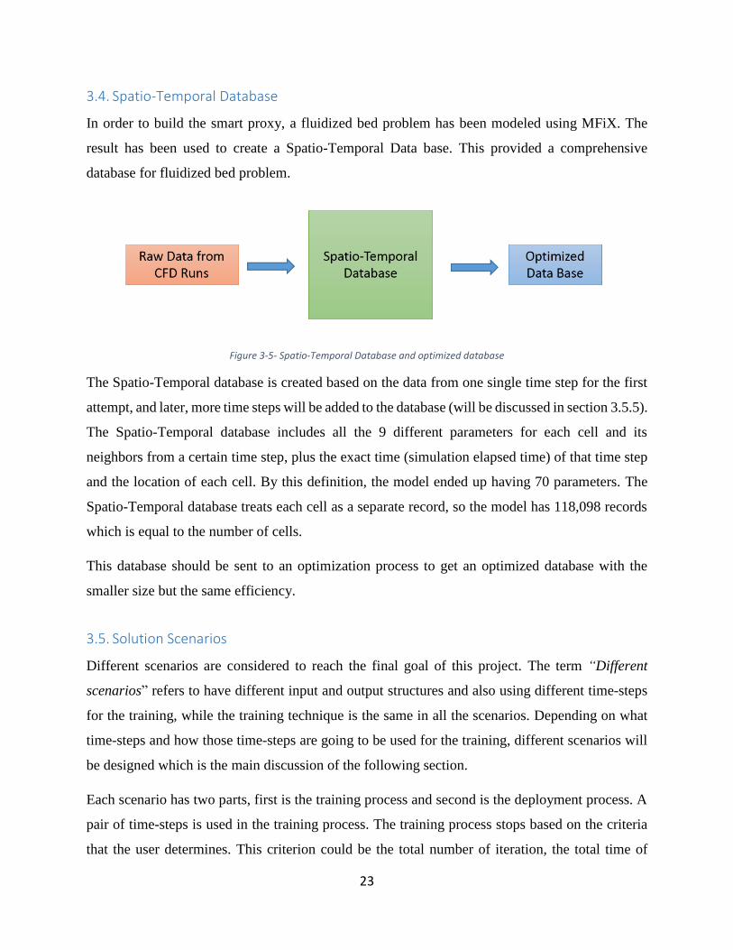
3.4. Spatio-Temporal Database
In order to build the smart proxy, a fluidized bed problem has been modeled using MFiX. The
result has been used to create a Spatio-Temporal Data base. This provided a comprehensive
database for fluidized bed problem.
Figure 3-5- Spatio-Temporal Database and optimized database
The Spatio-Temporal database is created based on the data from one single time step for the first
attempt, and later, more time steps will be added to the database (will be discussed in section 3.5.5).
The Spatio-Temporal database includes all the 9 different parameters for each cell and its
neighbors from a certain time step, plus the exact time (simulation elapsed time) of that time step
and the location of each cell. By this definition, the model ended up having 70 parameters. The
Spatio-Temporal database treats each cell as a separate record, so the model has 118,098 records
which is equal to the number of cells.
This database should be sent to an optimization process to get an optimized database with the
smaller size but the same efficiency.
3.5. Solution Scenarios
Different scenarios are considered to reach the final goal of this project. The term “Different
scenarios” refers to have different input and output structures and also using different time-steps
for the training, while the training technique is the same in all the scenarios. Depending on what
time-steps and how those time-steps are going to be used for the training, different scenarios will
be designed which is the main discussion of the following section.
Each scenario has two parts, first is the training process and second is the deployment process. A
pair of time-steps is used in the training process. The training process stops based on the criteria
that the user determines. This criterion could be the total number of iteration, the total time of

24
training, or the number of validation failure or a combination of those (In this project, the
combination of all the mentioned criteria was used). The learning algorithm is such that the
network learns more and more as it goes through each iteration but in order to avoid overfitting or
memorization, validation error is always checked. If the validation error increases for a predefined
number of iterations, the training stops. Most of the time, validation is the criterion which makes
the training stop.
As mentioned in the previous sections, 69 parameters are used as the input for the ANN. Figure 3-6
shows all the 69 input parameters including 6 distances to the boundaries and 9 properties for the
orange cell and also 6x9 set of parameters for tier blocks. The network also needs the output to be
trained. In this problem, there are total 9 parameters which any of those could be the output of
ANN. The output could be one parameter at a time or multiple parameters.
Figure 3-6- 69 different parameter of ANN
The trained network is then ready for the deployment process. One time-step is given to the trained
network and the network will give its prediction for the next time-step. The input of the ANN for
each deployment could come from the CFD directly or from the ANN itself. Cascading and non-
cascading deployment are defined based on what type of input is used for the network and it will
be discussed in detail in the following sections.
3.5.1. Early time versus late time
In this scenario, the 69 inputs come from time-step t and the output is from time-step t+1. The
output could be one parameter or multiple parameters, which in this case, only one output is used
at the same time (Figure 3-7). The main question here is which time-step should be used for the
training since there are multiple time-steps available. For the preliminary runs, one time-step from
the early time is used for the training when the motion in the system is like a slug flow and no
bubbles are in the fluidized bed. Figure 3-8 shows a pair of the time-steps for training.

25
Figure 3-7- Input/output parameters and time-steps for the training
Figure 3-8- Input/output time-steps for the training (early time)
For the second try, one pair of time-steps is chosen from the late time when the flow is completely
chaotic and bubbles are everywhere in the system. Figure 3-9 shows the input/output pair of time-
steps for this scenario.
Figure 3-9- Input/output time-steps for the training (late time)
The reason for choosing these two training (early time and late time) is because there are two
different flow regimes at work in these time-steps. Figure 3-10 shows the distribution of solids in
the fluidized bed in the early time and late time. This figure shows two complete different motions
in the system. The color bar is the gas volume fraction (voidage); all the figures are generated by
MATLAB.

26
The purpose of this analysis is to show that the ANN is capable of capturing all the physics
involved in different time-steps. In the next chapter, complete results of this analysis will be
presented and discussed in detail.
(a)
(b)
Figure 3-10- Gas volume fraction distribution on the wall; early time (a) versus late time (b)
3.5.2. Cascading versus non-cascading
Cascading and non-cascading refer to what kind of input is used for the deployment process. If the
input comes from the CFD solver for each deployment stage, it is called non-cascading. If the input
of the ANN for each deployment stage comes from the output of previous deployment, it is called
cascading.
Although it seems that non-cascading deployment has no benefit because the real input from CFD
solver should be available for every stage, it should always be studied in order to prove that the
trained network is working properly. Eventually, every parameter should be predicted by
cascading method but to accomplish this goal, first non-cascading should be done.

27
To better understand the difference between these two approaches, two schematic figures are
provided. Figure 3-11 shows the non-cascading deployment sequence while Figure 3-12 shows the
cascading deployment.
Figure 3-11- The process of non-cascading deployment
Figure 3-12- The process of cascading deployment

28
The non-cascading and cascading deployment process is going to be completed for both early and
late time and the results will be depicted in the next chapter.
3.5.3. Single output versus multiple output
As discussed earlier, ANN can have one output at the same time or multiple outputs. Obviously,
having multiple outputs simultaneously increases the training time, furthermore, the network has
to fit multiple outputs with the same weights, so the network has less flexibility to learn from data
but sometimes it gives the better results especially when there is a correlation between the outputs.
Figure 3-13 and Figure 3-14 show the input and output of the ANN when only one output is used
and when 3 outputs are used, respectively.
Figure 3-13- Traning with only one output (one component of gas velocity at the same time)
To examine the ability of the ANN when multiple outputs are used, some different cases are
considered. Selecting the set of outputs is the most important concern at this point and the main
question is what outputs could be used at the same time. It is decided to have three components of
gas velocity at the same time as outputs of the ANN because it is more likely for the gas velocity
components to have a correlation and the chances are less for the solid pressure and gas velocity
to have a correlation.
Figure 3-14- Traning with multiple outputs (three components of gas velocity simutanously)
As another advantage of this approach, it should be stated that having multiple outputs at the same
time would reduce the number of neural networks. As mentioned in the last section, there are total

29
nine different ANN needed for cascading deployment, this number could be reduced to three if
each network has three outputs at the same time. The result of this approach is also available in
chapter 4.
3.5.4. Explicit versus implicit
Regardless of the training scenario, the training process needs a pair of data; input and output
(time-step t and time-step t+1). If all the input data come from time-step t and the output data come
from time-step t+1, it is called explicit method, exactly like what is common in CFD solution
methods. Figure 3-14 is a demonstration of explicit training. It is also possible to have the
combination of data from time-step t and t+1 as input and have time-step t+1 as the output as well.
Obviously, the parameters from time-step t+1 that has been used for input will not be used for the
output; this approach is called implicit training. Figure 3-15 shows one of the examples of implicit
training. The input consists of gas volume fraction, pressures, and gas velocity vector from time-
step t in addition to solid velocity vector from time-step t+1. The output is gas velocity vector from
time-step t+1.
Figure 3-15- Traning with multiple outputs implicitly
This approach is very common in the numerical solution of PDE’s, which increases the converging
speed. It is expected to have a lower error when the implicit approach is applied.
3.5.5. Training with multiple time-steps
For all the training until this point of this research, only one pair of time-steps was used.
Figure 3-16 shows the input and output pair for the training with single time-step. The trained
network for early time-step (when a slugging flow is dominant) is valid for those time-steps that
have the same characteristics as slug flow but it is not valid for the entire time range when the bed

30
fluidizes. Vice versa, the trained network for the late time-step, when the bed is fully fluidized is
not valid for earlier time, when slug flow was present. The question that comes to the mind is “Is
there a neural network that can predict different time-steps?” In other words, “Is there a general
neural network that can capture different physics involved in the system?”
Figure 3-16- Input and output pair for the training with single time-step
When the data from early time-step is used to train the neural networks and the training process
completes with a good performance, it is definitely a good answer for early time-steps but it might
not be a good answer for late time-steps. If the data from two time-steps are used for the training
process, the network algorithm will converge to the solution that can mimic the behavior of both
time-steps. So, if more time-steps are used in training, the solution will be applicable to more time-
steps and the ANN covers wider time range.
Furthermore, there are different physics involved in different time-steps of the simulation, and in
order for the network to learn from all the possible behavior, more time-steps should be used in
the training process. So, it is decided to use at least three different time-steps with different flow
characteristics. One time-step from the early time, one time-step from late time, and one time-step
from the time when the bubbles start forming. In order for the ANN to distinguish between
different time-steps, another parameter (extra column) is added to the input data that is the exact
time of the time-step in seconds. Figure 3-17 shows the input and output pair for the training with
three different time-steps. The three time-steps were chosen visually by looking at the gas volume
fraction distribution in the fluidized bed. Time-step 200 was chosen because the slugging flow is
the dominant flow regime, time-step 1000 was chosen because the bubbles started forming but the
flow is still symmetric, and Time-step 4000 was chosen because the bubbles were developed
completely and no symmetric motion is in the system and the bed is fluidized. Figure 3-18 depicts
these three time-steps.

31
Figure 3-17- Input and output pair for the training with
Figure 3-18- Three different time-steps with different flow characteristics
For the result demonstration, it is not possible to present all the figures, so a different method
should be used to show the quality of the ANN. In order to quantify the amount of error in each
simulation, RMSE which is the square root of mean square error will be used. Equation (3-1)
shows the definition of RMSE. This criterion will be also used when more time-steps is going to
be added to the training dataset.
𝑅𝑀𝑆𝐸 = √1
𝑛∑(𝑦𝑎𝑐𝑡𝑢𝑎𝑙 − 𝑦𝑝𝑟𝑒𝑑𝑖𝑐𝑡𝑒𝑑)
2𝑛
𝑗=1
(3-1)

32
Each time-step has 118,098 cells (27x162x27), and also there are 70 parameters, which makes the
total number of data point to be equal to 8,266,860. By adding one time-step for training, more
than 8 million data points will be added for the analysis. Since our computer resources are limited,
the number of data points should be decreased in some fashion if more time-steps are going to be
used for the training.
3.5.6. Reducing the size of the system
The size of the input is already very huge and it is not possible to include more than 2 time-steps
for the training process because of the memory limitation1. The input data is a matrix which rows
and columns represent records and parameters, respectively. There are a couple of ways to reduce
the input size; reducing the number of rows (records) or the number of columns (parameters).
There is also another way to reduce the computational cost for the training that is using fewer data
for training and using more data for validation and test, in other words, by changing the data
prioritization. All the mentioned method will be discussed in the next sections.
3.5.6.1. Reducing number of records
There are two ways to reduce the number of records. The first method is removing some cells just
randomly from all the locations, and the second method is removing some cells that have less
valuable information. For example, the solids are located on the bottom of the fluidized bed, so it
is a reasonable idea to concentrate only on the bottom of the fluidized bed for all the solid-related
properties since there are no solids in the freeboard portion of the fluidized bed. Figure 3-19 shows
the distribution of gas volume fraction at time-step 4000. There are no solids above the blue line,
so it is a good assumption to remove all the cells above the blue line. As it is shown in Figure 3-20,
it is decided to keep all the cells below the 70 cells’ line and remove the cells with no significant
impact in selected parameter.
1 This Study was done on a Corei7 machine with 32 GB of RAM

33
Figure 3-19- distribution of gas volume fraction at time-step 4000
Figure 3-20- The important section of the fluidized bed

34
3.5.6.2. Reducing number of parameters (KPI1)
The latest input data for the training had 70 parameters and 118,098 records. By concentrating on
the lower part of the fluidized bed, the number of records reduced to 51,030, while the number of
parameters remains the same. Some of the parameters are going to be eliminated in this section.
Reducing the number of parameters is not as straight forward as reducing the number of records
and it needs some analysis regarding the prioritization of the parameters. Every parameter has
several weights assigned to it to communicate with the hidden layer, as it is depicted in Figure 3-21.
If all the weights assigned to one parameter (𝑤11, 𝑤12, …) are integrated to one value (𝑤1), that
value will represent the total weight and show the priority of that particular parameter when it
compares to all the other total weights.
Figure 3-21- Network schematic with its weights
After obtaining all the total weights of the parameters, the tornado chart of each ANN could be
plotted and the key parameters could be determined.
3.5.6.3. Changing the Data Partitioning
In all the previous sections, data from Table 3-5 were the base for data prioritization. According
to the Table 3-5, 70% of the data is used for training, 15% is used for the validation, and the other
15% is used for the test. Changing the data prioritization percentage could reduce the
1 Key Performance Indicator

35
computational costs. The computational cost of the training process is mainly for the data training,
and the validation and test are only a simple multiplication, so by reducing the training percentage,
the computational costs could be reduced while the total amount of data remains constant.
3.5.6.4. Reducing number of records using smart sampling
Reducing the number of records was previously accomplished by concentrating on the lower
section of the bed. Although using this idea led to having smaller database, still there are some
points in the lower section of the bed that has less value. Eliminating less valuable records could
reduce database size further. Figure 3-22 shows the distribution of gas volume fraction at time step
4000. The distribution has two peaks. The first peak is the gas volume fraction, when solid is at
maximum packing (cells having fully packed solid). The second peak is when the gas volume
fraction is either 1 or close to 1 (all air).
By introducing all the data for the training, the model will learn more about these two peaks and
will learn less about the transition part that has the gas volume fraction between 0.42 and 1. Since
it is desired for the model to learn equally from all the different locations and different events in
the fluidized bed, it is decided to reduce the number of records with the value of 1 and 0.42. By
this approach, a data with uniform distribution is introduced to the model, and the model will learn
equally from all the features in the system. Furthermore, the cells with the value of gas volume
fraction between 0.42 and 1, are located at the interface of the gas and solid phases, and the fluid
dynamic characteristics are changing significantly in these location, so it is important for the model
to learn about transition zone due to the dynamic change.
All the data between these two peaks were kept in the database. And only portions of data from
two peaks were selected in a way that the final distribution looks like a uniform distribution. The
gas volume fraction distribution is shown in the Figure 3-23. Total number of records reduced
from 118,098 to 25,827.
3.6. Summary
In this chapter, the problem was defined with all details and assumptions. Also, different scenarios
were introduced in order to achieve the final goal of this project. Different simulations based on
the mentioned scenarios or a combination of them were designed and deployed. In the next chapter,
the results of these different scenarios will be provided.

36
Figure 3-22- Distibution of Gas volume fraction at time step 4000
Figure 3-23- Distibution of Gas volume fraction at time step 4000 after smart sampling

37
Chapter 4 Results and Discussion
Different scenarios were introduced in the previous chapter. In this chapter, the results of all the
scenarios will be discussed in detail. The results which will be demonstrated are coming from
different approaches; early time or late time, single time-step or multiple time-steps for training,
cascading or non-cascading deployment, single output or multiple outputs, explicit or implicit
method, and reduced order models or complete models. Before proceeding with the results, there
will be a short description of how the results are going to be presented.
4.1. Result Demonstration
The current problem is three dimensional in space, with time being the fourth dimension. In order
to demonstrate the results, 5 different vertical cross sections were chosen as it is shown in
Figure 4-1, all the planes are perpendicular to the z-axis, and the results will be shown for different
time-steps.
Each figure has three subplots, the left plot is the result of CFD solver which is coming from MFiX
directly, the middle plot is the result of smart proxy which is the output of ANN, and the right plot
is the error distribution which is basically the difference between CFD and smart proxy.
4.2. Early time-step, non-cascading, single output, explicit
The simplest case to consider is when one time step from the early time is selected as the input.
The ANN had only one output, so 9 separate ANN have been trained for all 9 parameters. The
approach was non-cascading and explicit.
Time-steps 100 and 101 were used to train the system, and after the training completed, different
time-steps were input to the trained ANN to get the results. All the time-steps from 101 all the way
to 120 were input to the ANN and acceptable results were obtained. In the next sections, the results
of gas volume fraction and gas pressure are provided for one time-step. The results for the rest of
the parameters are in Appendix III.

38
Figure 4-1- Five different layers for result demonstration
4.2.1. Gas volume fraction
The results of the smart proxy versus CFD for gas volume fraction are shown in the next figures.
As it is shown in Figure 4-2, Smart proxy is able to replicate the MFIX simulation results that
show gas volume fraction distribution at time-step 102 for layer one. The maximum prediction
error occurred occasionally at some points with the value less than 5% while we see an error near
to zero in the rest of the domain. Very similar results have been obtained in other layers (from
Figure 4-3 to Figure 4-6).

39
Figure 4-2- Comparison of CFD and smart proxy results for gas volume fraction of time-step 102 for layer one
Figure 4-3- Comparison of CFD and smart proxy results for gas volume fraction of time-step 102 for layer two

40
Figure 4-4- Comparison of CFD and smart proxy results for gas volume fraction of time-step 102 for layer three
Figure 4-5- Comparison of CFD and smart proxy results for gas volume fraction of time-step 102 for layer four

41
Figure 4-6- Comparison of CFD and smart proxy results for gas volume fraction of time-step 102 for layer five
4.2.2. Gas Pressure
The results of the smart proxy versus CFD for the gas pressure are shown in the next figures. As
it is shown in Figure 4-7, Smart proxy is able to replicate the CFD MFIX simulation results that
show gas pressure distribution at time-step 102 for layer one. The maximum prediction error
occurred occasionally at some points with the value less than 20% while we see an error near to
zero in the rest of the domain. Very similar results have been obtained in other layers (from
Figure 4-8 to Figure 4-11).

42
Figure 4-7- Comparison of CFD and smart proxy results for gas pressure of time-step 102 for layer one
Figure 4-8- Comparison of CFD and smart proxy results for gas pressure of time-step 102 for layer two

43
Figure 4-9- Comparison of CFD and smart proxy results for gas pressure of time-step 102 for layer three
Figure 4-10- Comparison of CFD and smart proxy results for gas pressure of time-step 102 for layer four

44
Figure 4-11- Comparison of CFD and smart proxy results for gas pressure of time-step 102 for layer five
4.3. Late time-step, non-cascading, single output, explicit
The first attempt which was using the early time-step for training was successful, now the second
attempt is to figure out if the ANN is capable of handling the bubbles in the fluidized bed or not.
So, time-steps 4000 and 4002 were picked to train the network. The reason of having time-step
4002 rather than time-step 4001 is that there is no significant movement in the system only in one
time-step and the neural network will see more movements by using the pair of 4000-4002 and it
can learn better. More variation in data set helps the network to be trained better and being more
powerful in prediction.
Similar to the previous scenario, the ANN had only one output, so 9 different ANN trained for all
9 parameters. The approach was non-cascading and explicit. All the time-steps from 4002 all the
way to 4040 were input to the ANN and acceptable results were obtained. In the next sections, the
results of the gas volume fraction are provided for one time-step.
4.3.1. Gas Volume Fraction
The results of the smart proxy versus CFD for gas volume fraction when the bed is fluidized are
shown in the next figures. As it is shown in Figure 4-12 all the way to Figure 4-16, the smart proxy

45
could be able to mimic the CFD simulation results even when the bubbles are in the system. The
figures show the gas volume fraction distribution at time-step 4004 for layer one through five. The
maximum prediction error occurred occasionally at some points with the value around 4% while
we see an error near to zero in the rest of the domain. Very similar results have been obtained in
other layers (from Figure 4-3 to Figure 4-6).
Figure 4-12- Comparison of CFD and smart proxy results for gas volume fraction of time-step 4004 for layer one

46
Figure 4-13- Comparison of CFD and smart proxy results for gas volume fraction of time-step 4004 for layer two
Figure 4-14- Comparison of CFD and smart proxy results for gas volume fraction of time-step 4004 for layer three

47
Figure 4-15- Comparison of CFD and smart proxy results for gas volume fraction of time-step 4004 for layer four
Figure 4-16- Comparison of CFD and smart proxy results for gas volume fraction of time-step 4004 for layer five

48
4.4. Cascading, single output, explicit
Previous scenarios proved that the ANN is able to mimic the CFD results both when there is
moderate change in the dynamics of the multi-phase flow and when the fluid dynamics is chaotic.
All the analysis has been shown so far indicated the non-cascading scenario. The next attempt is
to apply the cascading approach, with explicit scheme.
4.4.1. Gas volume fraction for early time
To accomplish this scenario, 9 different ANN have been trained by introducing time-step 100 as
input and time-step 101 as output. Then for the deployment process, time-step 100 was used as the
input of all 9 trained ANN. The outputs of those ANNs were used again to input the next time-
step. In the following pages, the results of the cascading approach for gas fraction are shown. All
the results are for layer two but different time-steps in order to see the solid motion.
By looking at the figures, error propagation could be seen from each time-step to the next one.
This means that the ANN is able to replicate the results of CFD simulation using cascading scheme
for only a few time-steps and after a couple of time-steps, the amount of error exceeds the
acceptable range. In order to overcome the error propagation, more time-steps should be used for
training. This has been practiced in the later scenarios.

49
Figure 4-17- Comparison of CFD and smart proxy results for gas volume fraction of time-step 101 for layer two (Cascading)
Figure 4-18- Comparison of CFD and smart proxy results for gas volume fraction of time-step 102 for layer two (Cascading)
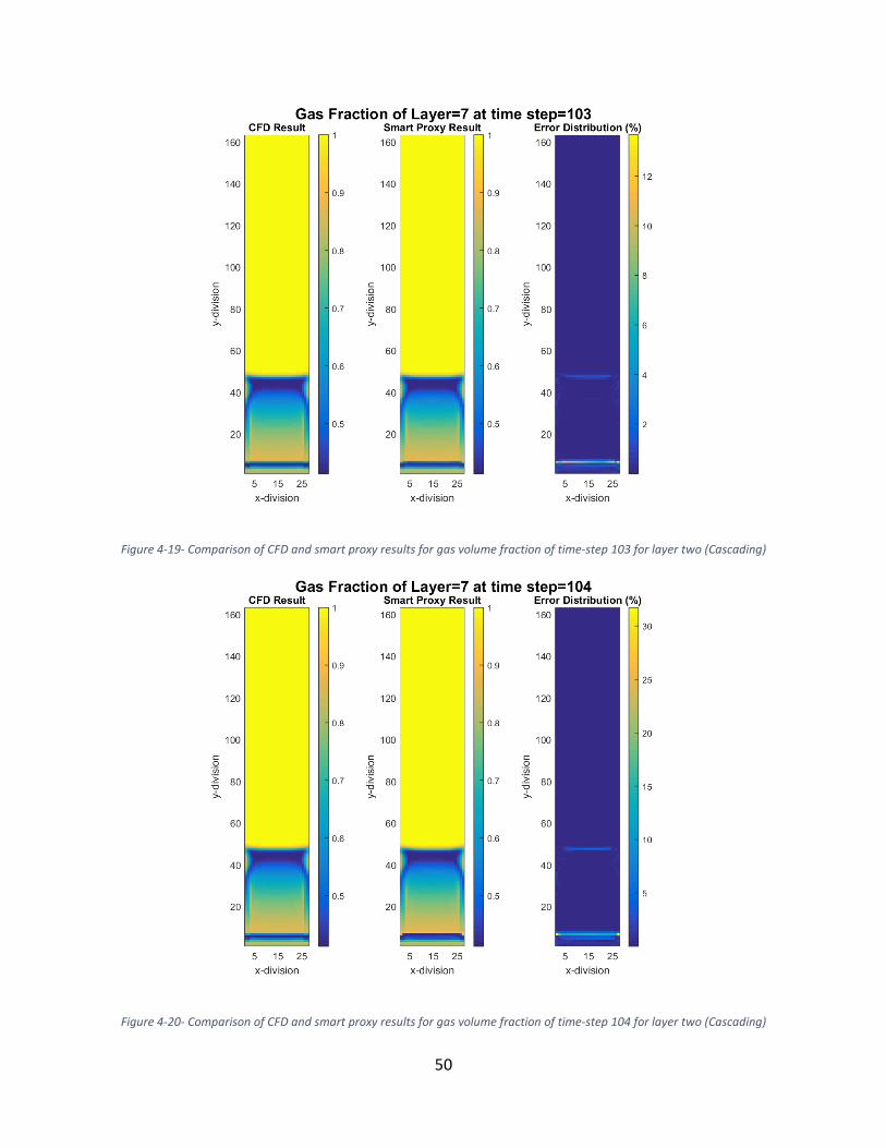
50
Figure 4-19- Comparison of CFD and smart proxy results for gas volume fraction of time-step 103 for layer two (Cascading)
Figure 4-20- Comparison of CFD and smart proxy results for gas volume fraction of time-step 104 for layer two (Cascading)

51
Figure 4-21- Comparison of CFD and smart proxy results for gas volume fraction of time-step 105 for layer two (Cascading)
Figure 4-22- Comparison of CFD and smart proxy results for gas volume fraction of time-step 106 for layer two (Cascading)

52
Figure 4-23- Comparison of CFD and smart proxy results for gas volume fraction of time-step 107 for layer two (Cascading)
Figure 4-24- Comparison of CFD and smart proxy results for gas volume fraction of time-step 108 for layer two (Cascading)
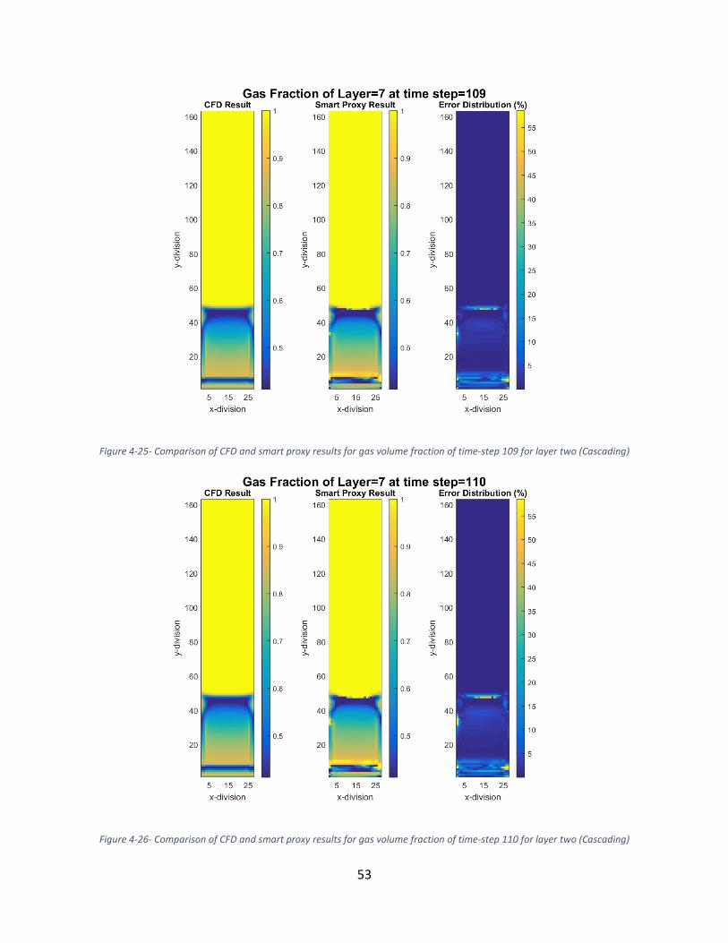
53
Figure 4-25- Comparison of CFD and smart proxy results for gas volume fraction of time-step 109 for layer two (Cascading)
Figure 4-26- Comparison of CFD and smart proxy results for gas volume fraction of time-step 110 for layer two (Cascading)
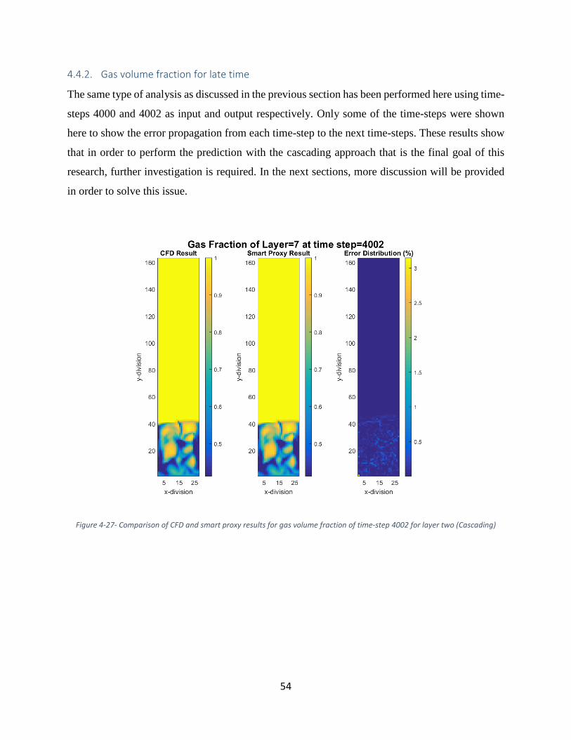
54
4.4.2. Gas volume fraction for late time
The same type of analysis as discussed in the previous section has been performed here using time-
steps 4000 and 4002 as input and output respectively. Only some of the time-steps were shown
here to show the error propagation from each time-step to the next time-steps. These results show
that in order to perform the prediction with the cascading approach that is the final goal of this
research, further investigation is required. In the next sections, more discussion will be provided
in order to solve this issue.
Figure 4-27- Comparison of CFD and smart proxy results for gas volume fraction of time-step 4002 for layer two (Cascading)

55
Figure 4-28- Comparison of CFD and smart proxy results for gas volume fraction of time-step 4004 for layer two (Cascading)
Figure 4-29- Comparison of CFD and smart proxy results for gas volume fraction of time-step 4006 for layer two (Cascading)

56
Figure 4-30- Comparison of CFD and smart proxy results for gas volume fraction of time-step 4020 for layer two (Cascading)
4.5. Early time-step, non-cascading, multiple output, explicit
Based on the discussion in chapter 3, it is sometimes beneficial to have multiple outputs rather
than only one output. Three components of gas velocity were selected to be the output of the ANN;
the input data is exactly the same as previous scenarios. The inputs came from time-step 100 and
the outputs came from time-step 101. The ANN was trained successfully and the time-step 102
was predicted. Figure 4-31 to Figure 4-33 show the results of smart proxy and comparison with
CFD simulation results. Fairly good results were obtained. Only the lower section of the fluidized
bed is shown in the figures. Gas velocity in the y-direction has the highest error, which is less than
20% at some points, but the rest of the domain has error near zero. The maximum error for the gas
velocity in the x-direction and Gas velocity in the z-direction is smaller. In the next section, the
implicit results will be presented.

57
Figure 4-31- Comparison of CFD and smart proxy results for gas x-velocity of time-step 102 for layer four (explicit)
Figure 4-32- Comparison of CFD and smart proxy results for gas y-velocity of time-step 102 for layer one (explicit)

58
Figure 4-33- Comparison of CFD and smart proxy results for gas z-velocity of time-step 102 for layer two (explicit)
4.6. Early time-step, non-cascading, multiple output, implicit
The final goal of this project is to perform all the simulations using cascading approach and
implicitly. In this section, the effect of an implicit solution is examined. All the parameters except
solid velocity are coming from time-step 100, three components of solid velocity are coming from
time-step 101, and this combination makes the input of the ANN. Also, three components of gas
velocity from time-step 101 make the output. Figure 4-34 to Figure 4-36 show the results of this
scenario.
To investigate the effect of implicit solution, the results are compared to the results from section
4.5.

59
Figure 4-34- Comparison of CFD and smart proxy results for gas x-velocity of time-step 102 for layer five (implicit)
By looking at the maximum error, which is the right plot in Figure 4-34, it is concluded that the
amount of error was reduced from 12% to less than 9% (comparing Figure 4-31 and Figure 4-34).
Also, Figure 4-35 shows the error reduction from 19% to 12% when it is compared to Figure 4-32,
and Figure 4-36 shows the error reduction from 5% to 3% (in comparison to Figure 4-33).

60
Figure 4-35- Comparison of CFD and smart proxy results for gas y-velocity of time-step 102 for layer one (implicit)
Figure 4-36- Comparison of CFD and smart proxy results for gas z-velocity of time-step 102 for layer two (implicit)

61
4.7. Using multiple time-steps for training, non-cascading, single output, explicit
As discussed in the previous chapter, the ANN for early time is valid only for early times and
probably a short period of time before and after the training time-step. This is also true for the
ANN for late time. To overcome that problem, both time-steps should be used for training one
ANN. To generalize the ANN even for times between early time and late time, third time-step was
also added to train the ANN (Time-steps 200-202, 1000-1002, and 4000-4002 were used). The
network has been trained and the deployment process was done by inputting time-step 200 all the
way to time-step 4200. The results are presented in terms of RMSE of gas volume fraction.
Figure 4-37 shows the RMSE distribution versus time-steps. It is clear that in the time-steps that
we had training data, the amount of error is minimum but in the other time-steps the RMSE
increased a little. Also, there are some peaks in the figure and the peaks observed in figure 4-37
illustrate that further learning at additional time steps are required. Probably, there is a kind of new
motion in the system in those time-steps that caused ANN did not learn enough to mimic the
behavior of those time-steps.
Figure 4-37- RMSE distribution versus time-step when three time pair of data were used for training

62
Figure 4-38 shows time-step 500, which is one of the time-steps with a high value of error. By
looking at this time-step closely, it could be understood that there is a specific kind of motion that
neural network has not seen so far. Particles are falling down in this time-step and ANN did not
learn about this kind of motion.
It is decided to include one more time-step for the training which was time-step 500, and that time-
step was chosen based on Figure 4-37. The same scenario was followed but with 4 different time-
steps for the training. Figure 4-39 shows the improvement in simulation by adding the fourth time-
step for training. The blue curve shows the RMSE before adding the fourth time-step, and the red
curve shows the RMSE after adding the fourth time-step.
Figure 4-38- Comparison of CFD and smart proxy results for gas volume fraction of time-step 500 for layer two

63
Figure 4-39- RMSE distribution versus time-step when three and four time pair of data were used for training
4.8. Using four time-steps for training, cascading, single output, explicit
The same simulation using 4 time-steps for the training was done with the cascading approach.
Unfortunately, the error propagation is still seen in the results after a few time-steps. One of the
solutions for this problem is to include more time-steps for the training but because of the memory
issue, it is not possible to have more than 4 time-steps unless the size of the system reduces. The
next effort is reducing the size of data in order to be able to add some more time-steps for the
training.
4.9. Reducing the number of parameters (KPI)
Eliminating the upper part of the fluidized bed did reduce the size of the input data. In order to
reduce the data input size even more, some of the parameters should also be eliminated from the
training. The ANN has been trained with 69 and 70 parameters up to this point. There is a chance

64
for the ANN to be able to predict the behavior of the system by fewer parameters. In this way, the
size of input can decrease.
To figure out what parameters has the top priority and what parameters has not, the tornado chart
of the total weights of the parameters were plotted for each ANN. Since in back propagation
method, there is a kind of weighted summation between all the parameters from each layer to the
next layer, the total weight could be obtained by averaging all the weights corresponding to a
specific parameter. There are two different ways to find the total weights; averaging all the weights
by considering their signs, and averaging all the weights by removing the signs. Both approaches
were accomplished. Tornado chart for both approaches is provided. Figure 4-40 shows tornado
chart when the weights are averaged regularly, and as we expected before, the gas volume fraction
of the cell has top priority. Also, Figure 4-41 shows the tornado chart when the weights are
averaged after removing the sign.
Figure 4-40- parameter pioritization for Gas volume fraction ANN (averaging all the weights)
0
5
10
15
20
25
30
35
ep-s
elf
Ps-
top
Ps-
self
ep-w
est
ep-b
ott
om
Pg-
wes
t
Pg-
sou
th
Ps-
wes
t
vs-s
elf
vg-t
op
vg-b
ott
om
Pg-
no
rth
us-
top
ug-
bo
tto
m
vg-s
ou
th
dis
tan
ce t
o b
ott
om
us-
bo
tto
m
tim
e
ep-s
ou
th
us-
east
Pg-
east
vs-n
ort
h
vg-s
elf
vg-n
ort
h
ws-
east
vg-w
est
vs-e
ast
wg-
east
us-
no
rth
ug-
east
dis
tan
ce t
o s
ou
th
dis
tan
ce t
o w
est
Pg-
self
vs-w
est
vs-s
ou
th
Tornado Chart of Neural Network Weights

65
Figure 4-41- parameter pioritization for Gas volume fraction ANN (averaging all the weightsafter removing signs)
The 14 less important parameters were removed from the input and the ANN has been trained
again with the new 56 parameters based on the two different approaches. Figure 4-42 shows the
amount of error when a different number of parameters were used for the training. The blue curve
is when all the 70 parameters were used, red curve shows the error when 14 parameters were
removed from the training by simply calculating the average and the yellow curve is when 14
parameters were eliminated based on the averaging of the absolute value of the weights. This graph
shows that the prioritization of the parameters is more accurate when the weights are averaged
without considering the sign. This conclusion is reasonable because some positive and negative
weights might cancel each other when the average is calculated by considering the signs, the wrong
result may be obtained.
The removed parameters for both approaches are shown in the Table 4-1 and Table 4-2. The
parameters are sorted in two different fashions; by parameter or by location.
0
20
40
60
80
100
120
140
160
180
200ep
-sel
f
vs-b
ott
om
ws-
sou
th
vg-s
elf
us-
we
st
Pg-
self
vg-b
ott
om
Pg-
top
Pg-
bo
tto
m
Ps-
wes
t
wg-
self
wg-
sou
th
ep-t
op
Ps-
east
ep-w
est
ep-n
ort
h
Pg-
east
vg-s
ou
th
wg-
top
vg-n
ort
h
vg-w
est
vs-e
ast
Pg-
no
rth
Pg-
sou
th
us-
east
dis
tan
ce t
o b
ott
om
ws-
bo
tto
m
ws-
no
rth
ug-
east
vs-n
ort
h
ws-
wes
t
dis
tan
ce t
o s
ou
th
dis
tan
ce t
o w
est
us-
no
rth
us-
sou
th
Tornado Chart of Neural Network Weights

66
Table 4-1- Fourteen less important parameters when simple average was used
By parameter By location
ug-south us-top
ug-east
ug-north ug-north us-north
wg-east ws-north
wg-west
ug-south
us-top
us-north wg-west
us-east ws-west ws-north ug-east
ws-west wg-east us-east
distance to south distance to south
distance to east distance to east
distance to north distance to north
distance to west distance to west
Table 4-2- Fourteen less important parameters when averaging by removing sign was used
By parameter By location
ug-west vg-self
ug-north
ug-south vs-bottom
ug-east
ug-north
vg-self wg-north
vg-west us-north wg-north ug-south us-north ws-west
vs-west
ws-west ug-west vg-west
vs-west
vs-bottom ug-east distance to south distance to south
distance to east distance to east
distance to west distance to west
As discussed, the second method was chosen to perform the KPI analysis for the rest of the
parameters.
Another interesting fact about Figure 4-42 is that the error distribution of yellow curve (using 56
parameters) is even less than the blue curve (which was obtained by using 70 parameters). To

67
explain the reason for this phenomenon, it should be stated that the blue curve is from non-
optimized database (Spatio-Temporal database) and the yellow curve is from a reduced database.
Reducing the number of parameters does not end up having higher prediction error always, it could
help the network to find the relation between the parameters more easily. In other words, there
might be some irrelevant parameters in the Spatio-Temporal database which without them the
process of fitting could be accomplished by higher accuracy. So, in the optimization process, the
less important parameters are eliminated until the prediction error goes far from the original error.
Figure 4-42- Comparison of RMSE distribution versus time-step for two different approach of averaging
The number of parameters was reduced to 56 and still the amount of error is lower than the original
simulation. This motivates us to go further and reduce the number of parameters even more until
the system breaks. For the second attempt, the number of parameters was reduced to 42 and
Figure 4-43 shows the error distribution after removing some other parameters. In this figure, the
amount of error increased a little bit in comparison to the when 56 parameters were used but it is
still comparable to the original one.

68
Figure 4-43- Comparison between RMSE when different number of parameters were used for training (70, 56, and 42
parameters)
For the third attempt, another seven parameters were removed based on the KPI analysis and the
below curve was obtained. Figure 4-44 shows the error distribution when only 35 parameters were
used to train the system and it means that almost the same results were achieved by using only half
of the data.

69
Figure 4-44- Comparison between RMSE when different number of parameters were used for training (70, 56, and 35
parameters)
The same analysis was done for all the parameters and the size of data for all of them was reduced.
Although it was possible to consider a different number of parameter for different ANN, the
number of parameters was fixed to be 43 for all the ANN for consistency. But it should be
mentioned that these 43 parameters vary from one ANN to another, for example when the gas
volume fraction is going to be trained, different parameters are important in comparison to when
the gas pressure is training. In the previous section, it was mentioned that in order to be able to
perform the cascading deployment, more time-steps should be used in the training process.
Because of the memory limitations, it was not possible to add more time-steps in the training but
now, when the size of input has been decreased; more time-steps could be used in the training,
which is the discussion of the next section.

70
Table 4-3 shows the size of data before and after size reduction, the data size will be reduced 5
times after using the latest model.
Table 4-3- Database size before and after optimization
Model Size of input Total Data Point
Original Model 118,098 by 70 8,148,762
Latest Model 51,030 by 35 1,786,050
4.10. Using seven time-steps for training, cascading, single output, explicit
The goal of this section is to train a smart ANN that can replicate the CFD completely, it means
that the smart package will feed itself instead of feeding by CFD, which is the definition of a
cascading deployment. The only input from CFD is one time-step as the initial condition. Fairly
good results were obtained with the non-cascading approach by using 4 time-steps. In this section,
another three time-steps are going to be added to the training set in order to improve the results.
The question is what time-steps should be included in the training set. In order to answer this
question, the error distribution of non-cascading result is plotted versus time as it is shown in
Figure 4-45. Another three time-steps were selected based on the peaks on the error curve. Time-
steps 574, 904, and 1842 were selected.
Figure 4-45- Comparison between RMSE with and without Ps
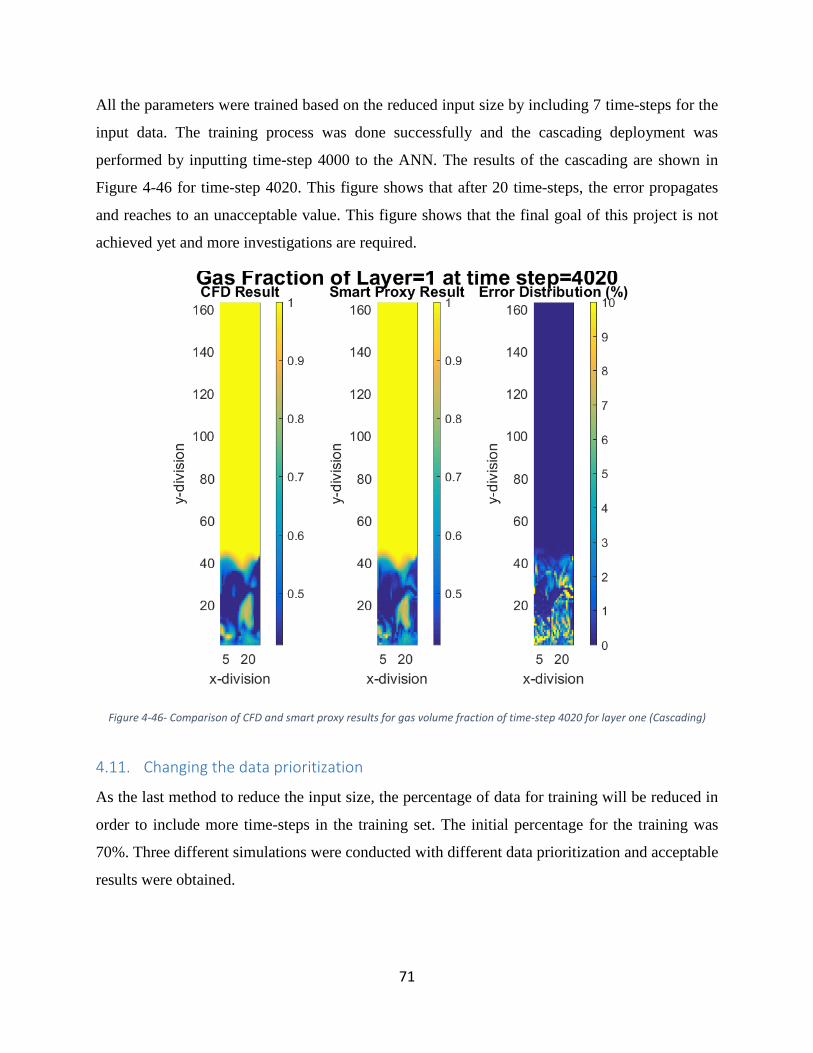
71
All the parameters were trained based on the reduced input size by including 7 time-steps for the
input data. The training process was done successfully and the cascading deployment was
performed by inputting time-step 4000 to the ANN. The results of the cascading are shown in
Figure 4-46 for time-step 4020. This figure shows that after 20 time-steps, the error propagates
and reaches to an unacceptable value. This figure shows that the final goal of this project is not
achieved yet and more investigations are required.
Figure 4-46- Comparison of CFD and smart proxy results for gas volume fraction of time-step 4020 for layer one (Cascading)
4.11. Changing the data prioritization
As the last method to reduce the input size, the percentage of data for training will be reduced in
order to include more time-steps in the training set. The initial percentage for the training was
70%. Three different simulations were conducted with different data prioritization and acceptable
results were obtained.

72
Table 4-4- Data Partitioning in different scenarios
Data Training
(%)
Validation
(%)
Test
(%)
Original simulation 70 15 15
First attempt 60 20 20
Second attempt 40 30 30
Third attempt 30 35 35
The results of the three attempts are shown in the following figures and all of them show that ANN
still is able to learn the pattern by reducing the percentage of training data down to the 30%.
Figure 4-47- CFD and smart proxy results for gas volume fraction of time-step 4004 for layer one by 60% training (non-
cascading)

73
Figure 4-48- CFD and smart proxy results for gas volume fraction of time-step 4004 for layer one by 40% training (non-
cascading)
Figure 4-49- CFD and smart proxy results for gas volume fraction of time-step 4004 for layer one by 30% training (non-
cascading)

74
4.12. Smart sampling
The data from time step 4000 was sent in to the Smart Sampling procedure. The deployment started
from time step 3950 all the way to time step 4150. The same analysis was done without smart
sampling and all the data were used in the training.
Figure 4-50 shows RMSE of smart sampling in comparison to the original model. As it is shown
in the figure, by reducing the number of records (only 20% of the records were used) almost the
same result obtained.
Figure 4-50- Comparison of RMSE in different time steps with/without smart sampling
This idea let us include more time steps in the training process in order to reduce the error in the
cascading deployment.

75
Chapter 5 Conclusions and Recommendations
5.1. Conclusions
The original database (Spatio-Temporal database) included 70 parameters and 118,098 records.
This database was then sent through an optimization process to get an optimized database with the
smaller size but the same efficiency. In the optimization process, the size of Spatio-Temporal
database reduced more than 25 times. This optimization was done by different approaches as
follows and the exact numbers are shown in the Table 5-1.
1. Reducing the number of parameters (using Key Performance Indicator)
2. Reducing the number of records (focusing on the more important cells using smart sampling)
3. Reducing the percentage of training (by Intelligent Partitioning).
Table 5-1- comparison between Spatio-Temporal database and optimized database
No. Records No. of Parameters Training Percentage Total data
Spatio-Temporal Database 118,098 70 100 8,266,860
Optimized Database 25,827 43 30 333,168
All the data from time step t were used as the input of the model, and all the data from time step
(t+1) were used as the output (since the method is supervised learning, the output is required). A
model has been trained by using the original database.
In order to see the efficiency of the model and successfulness of this method, some blind cases
(which the model has not seen in the training process) were used for deployment. The results
proved that the smart proxy is able to predict all the entire range, including the initiation of the
bubbles, bursting of them, bulk flow, and also the non-linear and chaotic motion.
A data-driven smart proxy was developed to mimic the CFD results, with a good accuracy and
faster speed. Table 5-2 shows the comparison of run time of these two approaches. This proxy
needs an incredible less amount of time in comparison to the CFD solver with a reasonable error
(less than 10%). This project proved that the idea of using AI&DM for computational fluid
dynamics actually works.

76
Table 5-2- comparison between speed of run for CFD and Smart proxy
Method Execution Time
CFD 4 seconds simulation = 3 days on 4 CPUs
Smart Proxy 4 seconds simulation = 180 s = 3 min
5.2. Recommendations and future works
This study showed that the smart proxy is feasible to handle a complex, multi-physics, nonlinear
flow and it is worth to spend more time and effort to improve the results.
In order to make the model more general in the whole time ranges, more data from different time
steps could be included in the training process, and this is where using the optimized database is
beneficial.
Also, there is a need to spend more time on the cascading deployment in order to completely
replace the CFD with the smart proxy.

77
BIBBLOGRAPHY
[1] J. Wang, M. Jiang, Y. Yao, Y. Zhang, and J. Cao, “Steam gasification of coal char catalyzed by
K2CO3 for enhanced production of hydrogen without formation of methane,” Fuel, vol. 88, no. 9,
pp. 1572–1579, 2009.
[2] A. J. Minchener, “Coal gasification for advanced power generation,” Fuel, vol. 84, no. 17, pp. 2222–
2235, 2005.
[3] H. Watanabe and M. Otaka, “Numerical simulation of coal gasification in entrained flow coal
gasifier,” Fuel, vol. 85, no. 12–13, pp. 1935–1943, 2006.
[4] M. Syamlal, “MFIX documentation numerical technique,” Tech. Note DOE/MC31346-5824,
NTIS/DE98002029, Natl. Energy Technol. Lab. Dep. Energy, vol. 5824, no. January, p. DE– AC21–
95MC31346, 1998.
[5] M. Syamlal, W. Rogers, and T. J. O`Brien, “MFIX documentation theory guide,” Other Inf. PBD
Dec 1993, vol. 1004, no. December, p. Medium: ED; Size: 49 p., 1993.
[6] G. J. Stiegel and M. Ramezan, “Hydrogen from coal gasification: An economical pathway to a
sustainable energy future,” Int. J. Coal Geol., vol. 65, no. 3–4, pp. 173–190, 2006.
[7] T. Papadopoulos, M. Losurdo, and H. Spliethoff, “Numerical simulation of coal gasification process
using the modifying Watanabe – Otaka model .,” Fuel, vol. 49, no. 0, pp. 1–4.
[8] M. a. van der Hoef, M. van Sint Annaland, N. G. Deen, and J. a. M. Kuipers, “Numerical Simulation
of Dense Gas-Solid Fluidized Beds: A Multiscale Modeling Strategy,” Annu. Rev. Fluid Mech., vol.
40, pp. 47–70, 2008.
[9] M. A. van der Hoef, M. Ye, M. van Sint Annaland, A. T. Andrews, S. Sundaresan, and J. A. M.
Kuipers, “Multiscale Modeling of Gas-Fluidized Beds,” Adv. Chem. Eng., vol. 31, no. 06, pp. 65–
149, 2006.
[10] N. G. Deen, M. Van Sint Annaland, M. A. Van der Hoef, and J. A. M. Kuipers, “Review of discrete
particle modeling of fluidized beds,” Chem. Eng. Sci., vol. 62, no. 1–2, pp. 28–44, 2007.
[11] C. Brennen, Fundamentals of Multiphase Flows, vol. 128. Cambridge University Press, 2005.
[12] E. Alpaydın, Introduction to Machine Learning, 2nd ed. The MIT Press, 2010.
[13] S. Haykin, Neural Networks - A Comprehensive Foundation. IEEE Press, 1994.

78
[14] S. Mohaghegh and S. Ameri, “Artificial Neural Network As A Valuable Tool For Petroleum
Engineers,” Network, 1995.
[15] S. Mohaghegh, R. Arefi, S. Ameri, and D. Rose, “Design and development of an artificial neural
network for estimation of formation permeability,” SPE Comput. Appl., vol. 7, no. 6, pp. 151–154,
1995.
[16] A. Alizadehdakhel, M. Rahimi, J. Sanjari, and A. Abdulaziz, “CFD and artificial neural network
modeling of two-phase fl ow pressure drop ☆,” vol. 36, pp. 850–856, 2009.
[17] A. Shahkarami, S. D. Mohaghegh, V. Gholami, A. Haghighat, and D. Moreno, “Modeling pressure
and saturation distribution in a CO 2 storage project,” vol. 315, no. May 2013, pp. 289–315, 2014.
[18] S. Esmaili and S. D. Mohaghegh, “Geoscience Frontiers Full fi eld reservoir modeling of shale assets
using advanced data-driven analytics,” Geosci. Front., pp. 1–11, 2015.
[19] A. Kalantari-dahaghi, S. Mohaghegh, and S. Esmaili, “Coupling numerical simulation and machine
learning to model shale gas production at different time resolutions,” vol. 25, pp. 380–392, 2015.
[20] A. Kalantari-dahaghi, S. Mohaghegh, and S. Esmaili, “Data-driven proxy at hydraulic fracture
cluster level : A technique for ef fi cient CO 2 - enhanced gas recovery and storage assessment in
shale reservoir,” J. Nat. Gas Sci. Eng., vol. 27, pp. 515–530, 2015.

79
APPENDIX
Appendix I: MFiX Equations
Fluid-Solids Momentum Transfer
The fluid-solids interaction force is a combination of buoyancy, the drag force, and momentum
transfer due to mass transfer.
(0-1)
Where
(0-2)
And
(0-3)
where Vrm is the terminal velocity correlation for the mth solids phase which is a function of gas
volume fraction only, and the Rem is Reynolds number of mth phase.
(0-4)
Or
(0-5)

80
(0-6)
The coefficient A and B are calculated as follows.
(0-7)
Solids-Solids Momentum Transfer
The solids-solids momentum transfer comes from the drag force between different phases and is
it calculated with the below equation.
(0-8)
Where
(0-9)
where elm and Cflm are the coefficient of restitution and coefficient of friction, respectively, between
the lth and mth solids-phase particles. g0lm is the radial distribution function at contact.
(0-10)
81
Fluid-Phase Stress Tensor
The fluid-phase stress is stated as follows.
(0-11)
Where Pg is the gas pressure and also 𝜏�̿� is the viscous stress tensor for Newtonian fluid which is
in the below form.
(0-12)
Where 𝐼 ̿is identity tensor and �̿�𝑔 is strain tensor which is calculated by the following equation.
(0-13)
Solids-Phase Stress Tensor
In MFIX, there are two different theories for calculating the solid-phase stress and those two
theories are plastic flow and viscous flow. The stress definition is switched based on the
comparison of the gas volume fraction with a critical packing which is εg*.
(0-14)
where Psm is the pressure and τ sm is the viscous stress in the mth solids phase. The superscript p
stands for the plastic regime and v for the viscous regime. In fluidized-bed simulations, εg* is
usually set to the void fraction at minimum fluidization.
In the plastic flow, 𝜏�̿�𝑚𝑝
is calculated as follows.
(0-15)
In viscous flow, 𝜏�̿�𝑚𝑝
is in the below form.
(0-16)

82
Appendix II: MFiX Gasification code
# 3-D Rectangular Fluidized Bed
# ---------------------------------------------------------
# Run control
# ---------------------------------------------------------
RUN_NAME = 'FB_S2G1'
DESCRIPTION = 'Bubbling Fluidized Bed Simulation'
RUN_TYPE = 'new'
UNITS = 'si'
TIME = 0.0
TSTOP = 30.0 !change as needed
DT = 5.0E-3
DT_MAX = 5.0E-3 !Don't go larger that write_usr output freq
NODESI = 4
NODESJ = 16
NODESK = 4
# ---------------------------------------------------------
# Equations
# ---------------------------------------------------------
ENERGY_EQ = .FALSE.
SPECIES_EQ = .FALSE. .FALSE.
DRAG_TYPE = 'GIDASPOW'
SCHAEFFER = .FALSE.
FRICTION = .FALSE.
# ---------------------------------------------------------
# Geometry Section
# ---------------------------------------------------------
COORDINATES = 'cartesian'
XLENGTH = 0.120 IMAX = 27
YLENGTH = 0.720 JMAX = 162
ZLENGTH = 0.120 KMAX = 27
# ---------------------------------------------------------
# Gas-phase Section
# ---------------------------------------------------------
MU_g0 = 1.9E-5
MW_avg = 29.0

83
# ---------------------------------------------------------
# Solids-phase Section
# ---------------------------------------------------------
RO_s0 = 2000.0 ! kg/m3
D_p0 = 0400.0E-6 ! m
C_e = 0.80
Phi = 30.0
EP_star = 0.42
# ---------------------------------------------------------
# Initial Conditions Section
# ---------------------------------------------------------
! Bed Freeboard
IC_X_w(1:2) = 0.000 0.000
IC_X_e(1:2) = 0.120 0.120
IC_Y_s(1:2) = 0.000 0.120
IC_Y_n(1:2) = 0.120 0.720
IC_Z_b(1:2) = 0.000 0.000
IC_Z_t(1:2) = 0.120 0.120
IC_EP_g(1:2) = 0.420 1.000
IC_P_g(1:2) = 101.325E3 101.325E3
IC_T_g(1:2) = 300.0 300.0
IC_U_g(1:2) = 0.000 0.000
IC_V_g(1:2) = @(0.6/0.42) 0.600
IC_W_g(1:2) = 0.000 0.000
IC_U_s(1:2,1) = 0.000 0.000
IC_V_s(1:2,1) = 0.000 0.000
IC_W_s(1:2,1) = 0.000 0.000
IC_T_s(1:2,1) = 300.0 300.0
# ---------------------------------------------------------------
# Boundary Conditions Section
# --------------------------------------------------------------
# South North West East Back Front
BC_X_w(1:6) = 0.000 0.000 0.000 0.120 0.000 0.000
BC_X_e(1:6) = 0.120 0.120 0.000 0.120 0.120 0.120
BC_Y_s(1:6) = 0.000 0.720 0.000 0.000 0.000 0.000
BC_Y_n(1:6) = 0.000 0.720 0.720 0.720 0.720 0.720
BC_Z_b(1:6) = 0.000 0.000 0.000 0.000 0.000 0.120
BC_Z_t(1:6) = 0.120 0.120 0.120 0.120 0.000 0.120

84
BC_TYPE(1:6) = 'MI' 'PO' 'NSW' 'NSW' 'NSW' 'NSW'
BC_EP_g(1:2) = 1.0 1.0
BC_P_g(1:2) = 2*101.325E3
BC_T_g(1:2) = 2*300.0
BC_U_g(1) = 0.0
BC_V_g(1) = 0.6
BC_W_g(1) = 0.0
! BC_ROP_s(1,1) = 0.000
! BC_U_s(1,1) = 0.000
! BC_V_s(1,1) = 0.000
! BC_W_s(1,1) = 0.000
#
# Output Control
#
RES_DT = 0.01
!
! EP_g P_g U_g U_s ROP_s T_g X_g
! P_star V_g V_s T_s1 X_s Theta Scalar
! W_g W_s T_s2
SPX_DT = 0.01 0.01 0.01 0.01 0.01 100. 100. 100.0 100.0
NLOG = 100
full_log = .true.
write_dashboard = .true.
write_vtk_files = .true.
time_dependent_filename = .true.
vtk_dt = 0.05
vtk_varlist(1,1:5) = 1 2 3 4 5
call_usr = .true.
usr_dt(1) = 0.005
ENABLE_DMP_LOG = .F
CHK_BATCHQ_END = .T.
BATCH_WALLCLOCK = 1800d20 ! 30 Days
TERM_BUFFER = 120d0 ! 15 min
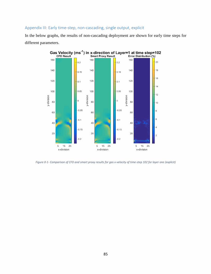
85
Appendix III: Early time-step, non-cascading, single output, explicit
In the below graphs, the results of non-cascading deployment are shown for early time steps for
different parameters.
Figure 0-1- Comparison of CFD and smart proxy results for gas x-velocity of time-step 102 for layer one (explicit)

86
Figure 0-2- Comparison of CFD and smart proxy results for gas y-velocity of time-step 102 for layer one (explicit)
Figure 0-3- Comparison of CFD and smart proxy results for solid x-velocity of time-step 102 for layer one (explicit)

87
Figure 0-4- Comparison of CFD and smart proxy results for solid y-velocity of time-step 102 for layer one (explicit)
Figure 0-5- Comparison of CFD and smart proxy results for gas z-velocity of time-step 102 for layer one (explicit)

88
Appendix IV: MATLAB Code (Creating Spatio-Temporal database)
%% This program read two different time step as input and output clc clear; close all; %% Input and Output Time step
Time_Step_in=100; Time_Step_out=Time_Step_in+1;
%% Defining the geometry imax = 27; %number of cell in x-direction kmax = 27; %number of cell in z-direction jmax = 162; %number of cell in y-direction Dim_x = 0.12; %length of domain Dim_y = 0.72; %height of domain Dim_z = 0.12; %width of domain Dim_cell = Dim_x/imax; %dimension of cell, the cell is a cube CellNo=imax*jmax*kmax; %total number of cells
%% Loading the CSV files from time step start to final
data_input = ReadFiles( Time_Step_in,Time_Step_in,CellNo ); data_output = ReadFiles( Time_Step_out,Time_Step_out,CellNo );
%% Initialize the matrices location = zeros(CellNo,3); %(x,y,z) of each cell CellID = zeros(CellNo,1); % ID of each cell tier1 = zeros(CellNo,6); % tier system with of order 1
(bottom,top,west,north,east,south) DisToBoundary = zeros(CellNo,6); % distance to the boundaries
(bottom,top,west,north,east,south) counter = 1;
%% Filling the geomtry matrices for k = 1:kmax for i = 1:imax for j = 1:jmax location(counter,:) = [i j k]; CellID(counter) = (k-1)*jmax*imax+(i-1)*jmax+j; %cell ID of tier cells(bottom,top,west,north,east,south) tier1(counter,:) = [(k-1)*jmax*imax+(i-1)*jmax+j-1 (k-1)*jmax*imax+(i-
1)*jmax+j+1 (k-1)*jmax*imax+(i-2)*jmax+j (k)*jmax*imax+(i-1)*jmax+j (k-
1)*jmax*imax+(i)*jmax+j (k-2)*jmax*imax+(i-1)*jmax+j]; %distance of center of each cell to the
boundaries(bottom,top,west,north,east,south) DisToBoundary(counter,:) = [(j-0.5)*Dim_cell Dim_y-(j-0.5)*Dim_cell (i-
0.5)*Dim_cell Dim_z-(k-0.5)*Dim_cell Dim_x-(i-0.5)*Dim_cell (k-0.5)*Dim_cell
]; %% filling zero at for the tiers for the cells at the boundary if i==1

89
tier1(counter,3) = 0; elseif i==imax tier1(counter,5) = 0; end
if j==1 tier1(counter,1) = 0; elseif j==jmax tier1(counter,2) = 0; end
if k==1 tier1(counter,6) = 0; elseif k==kmax tier1(counter,4) = 0; end
counter=counter+1; end end end
%% Filling the properties of tier1 system
tierData=zeros(CellNo,7*11); for i = 1:CellNo tierData(i,1:11)=data_input(i,:); for j = 1:6 index = tier1(i,j); if index==0 %if index iz zero, it means that no cell is there t = zeros(1,11); else t = data_input(index,:); end tierData(i,11*(j)+1:11*(j+1)) = t; end end
%% Creating the output file geometry=[CellID location DisToBoundary tier1 tierData data_output(:,:)];
NN_input=[DisToBoundary tierData(:,1:9) tierData(:,12:20) tierData(:,23:31)
tierData(:,34:42) tierData(:,45:53) tierData(:,56:64) tierData(:,67:75)];
Fraction=data_output(:,1); Gas_Pressure=data_output(:,2); Solid_Pressure=data_output(:,3);
Gas_Velocity=data_output(:,[4 5 6]); Gas_Velocity_x=data_output(:,4); Gas_Velocity_y=data_output(:,5); Gas_Velocity_z=data_output(:,6);
Solid_Velocity=data_output(:,[7 8 9]);

90
Solid_Velocity_x=data_output(:,7); Solid_Velocity_y=data_output(:,8); Solid_Velocity_z=data_output(:,9);
NN_input=NN_input';
Fraction=Fraction'; Gas_Pressure=Gas_Pressure'; Solid_Pressure=Solid_Pressure';
Gas_Velocity=Gas_Velocity'; Gas_Velocity_x=Gas_Velocity_x'; Gas_Velocity_y=Gas_Velocity_y'; Gas_Velocity_z=Gas_Velocity_z';
Solid_Velocity=Solid_Velocity'; Solid_Velocity_x=Solid_Velocity_x'; Solid_Velocity_y=Solid_Velocity_y'; Solid_Velocity_z=Solid_Velocity_z';