1

Developing A Model-Based Software To Optimize Wheat Storage and Transportation System: A Real-World Application

Reza Zanjirani Farahania,b,c*

a Logistics & Supply Chain Researches & Studies Group, Institute for Trade Studies & Research, Tehran, Iran , Nasrin Asgaric, Hossein Hojabria and Amir Ardestani Jaafaria

b Department of Industrial Engineering, Amirkabir University of Technology, Tehran, Iran. c Centre for Maritime Studies, National University of Singapore, Singapore

Abstract

The case to be studied is a vast country with a variety of climates. Due to this diversity in climate and,

consequently, different farming conditions in different areas of the country, wheat is produced at

different times of year all over the country. Therefore, wheat production rate is not constant during this

period all over the country. Lack of balance between wheat production and consumption in different

provinces during different periods necessitates storage and transportation of wheat. In this paper, we

intend to find the answer to the following question: “How much wheat in each month of year must be

transported from each exporting province to each importing province?”

First, the case problem including assumptions, objective and constraints is comprehensively described.

Then, a Mixed Integer Programming (MIP) model is developed for the problem and run on a

commercial optimization software. Since, the model must be run each month in order to use updated

data and running time of the MIP model is not reasonable, a Genetic Algorithm (GA) is developed to

solve the real-size problem in an acceptable time. To prove the efficiency of this technique in terms of

runtime and quality of the computations, its results are compared with those of LINGO 10.00 for small-

sized and medium-sized test instances.

Keywords: Agriculture; Transportation; Inventory; Mixed Integer Programming; Genetic Algorithm.

Introduction

* Corresponding author. Fax: +65 6775 6762; Tel: +65 65165356; Email: zanjiranireza@gmail.com; cmszfr@nus.edu.sg

2

The investigated case is in a vast country with a variety of climates. Due to this diversity of climate and

therefore different farming conditions in different regions of the country, wheat is produced at different

times of the year all around the country (from early spring till the middle of fall). For example, in the

south of the country, wheat is reaped at the beginning of spring, and in the northwest, it is harvested at

the middle of fall. Therefore, the wheat production rate during a year is not the same all over the

country. At the beginning of the spring, the wheat production rate is low, but in the summer, it

increases enormously, and falls again in the fall. However, wheat demand of each province is constant

all over the year, and depends on the population of the province. The lack of balance between

production and consumption of wheat in different provinces in different months of year makes storage

and transportation of wheat necessary. In some provinces, wheat production is more than the demand

for it; this surplus wheat is carried to other provinces or is stored to be used later.

In this paper, we focus on wheat transportation and inventory system. This system consists of fixed

entities such as warehouses, flour factories and routes. Warehouses in this system are demand points as

well as supply points; mobile entities of this system are a fleet of similar vehicles.

There are many research studies that can indirectly help us to realize, model and solve this problem.

For instance, transportation capacity has also been studied for multi-stage inventory systems with

deterministic and dynamic demands with finite horizon (Bregman et al., 1990). A comprehensive

literature summary of similar problems including the stochastic cases can be found in Kleywegt et al.

(2002). Z.-Farahani and Elahipanah (2008) developed and solved a bi-objective model for just-in-time

(JIT) distribution in the context of supply-chain management. They presented a comprehensive

literature in all levels of distribution in supply chain with their classifications.

Similarly there are real-world case studies in different areas of application that can help us see their

experiences. For example, De Boon (1978) has examined flower distribution and transportation

systems in the world’s first flower exporter (the Netherlands). It is notable that in this system, 200

different kinds of flower must be transported and distributed from 3500 sources to more than 1000

3

destinations. The daily input consists of 4-8 million flowers, which are sold in 4 hours through

approximately 20000 transactions each involving 1-250 bunches or boxes of flowers. Carlsson and

Rönnqvist (2007) study Södra, one of the larger Swedish forest companies, which is involved in all

stages of the wood-flow. They focus in particular on Södra Cell AB, a company within Södra, which is

responsible for pulp production. They describe the operations at Södra Cell and the decision support

tools used for supply chain planning. They describe five major projects or cases (including a new

distribution structures) which focus on improving their supply chain management and optimization.

Sousa et al. (2008) address a case study, inspired by a real agrochemicals supply chain (in UK), with

two main objectives, structured in two stages. In the first stage they redesign the global supply chain

network (including the production and distribution plan considering a time horizon of one year). In the

second stage, a short term operational model is used to test the accuracy of the derived design and plan.

If we want to find a relevant literature that is close to our case study at least from the application

point of view, we should mention Bilgen and Ozkarahan (2007). They address a blending and shipping

problem faced by a company that manages a wheat supply chain (in Turkey). The problem is

formulated as a mixed-integer linear programming model. The objective function seeks to minimize the

total cost including the blending, loading, transportation and inventory costs. Constraints on the system

include blending and demand requirements, availability of original and blended products; as well as

blending, loading, draft and vessel capacity restrictions.

However, one of the best and much related researches is Ahumada and Villalobos (2009). They

review the main contributions in the field of production and distribution planning for agri-foods based

on agricultural crops. They particularly focus on those models that have been successfully

implemented. The models are classified according to relevant features, such as the optimization

approaches used, the type of crops modeled and the scope of the plans, among many others. Through

their analysis of the current state of the research, they diagnose some of the future requirements for

modeling the supply chain of agri-foods.

4

In section 2, we describe the case characteristics in terms of outputs, assumptions, objectives,

constraints and inputs. In section 3, we develop a mathematical model based on the mentioned

characteristics in terms of sets and indices, variables, parameters and mathematical formulation

including objective functions and constraints. In section 4, the solution to the model is presented. In

section 5 we develop a genetic algorithm to solve the model and related computational results in

section 6 shows the efficiency of the developed algorithm. Implementation issues and conclusion of the

article is presented in sections 7 and 8, respectively.

Problem Definition

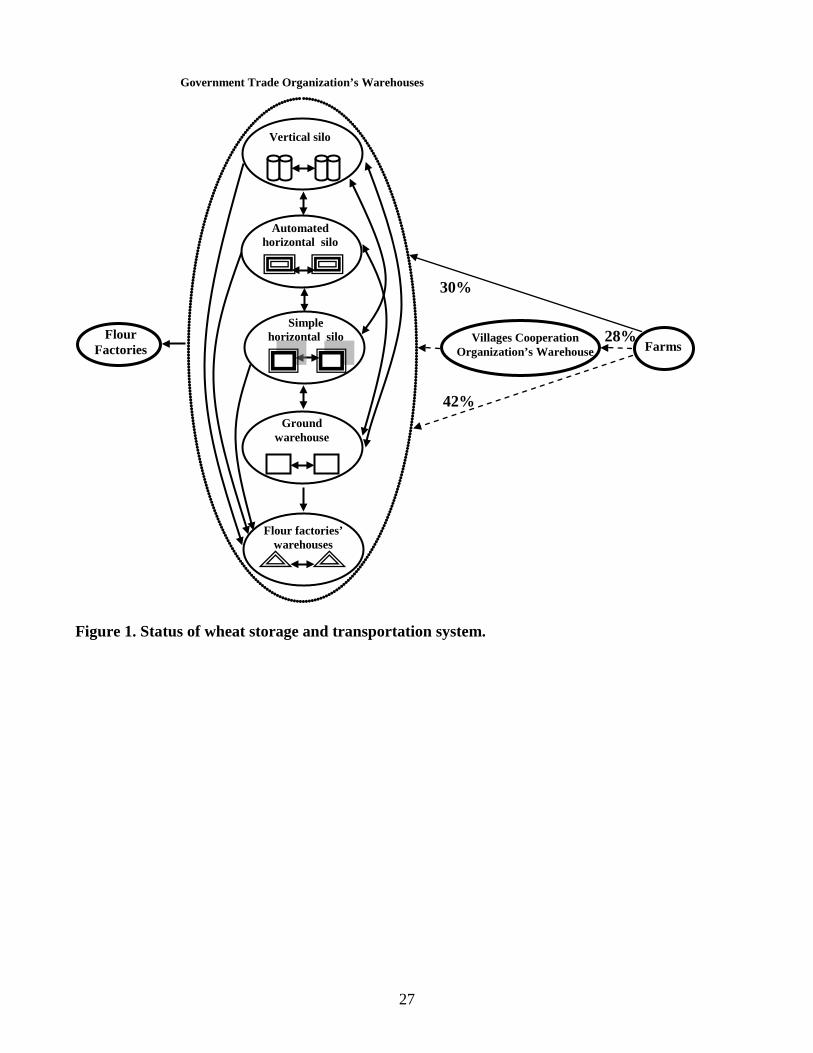
To have a better understanding of the problem we illustrate the status of the system in Figure 1. Hereby

we explain some of the notations used and the definition of the system.

Farms (F): Wheat is produced in farms; i.e. farms are where the wheat enters into the system.

Government Trade Corporation (GTC): GTC, which wants to optimize the system, is the owner of

the storage and transportation system. All system costs including coordination charges, storage costs

and transportation costs are paid by this organization.

GTC Warehouses (GTCW): GTCW stores the purchased wheat in five different types of

warehouses.

Flour Factories: These are the final consumers in the system; i.e. there is nothing left called wheat

after entering the flour factories.

Flour Factories Warehouses (FW): Flour factories have some assigned warehouses where wheat is

kept waiting to change into flour. With respect to the capacity of warehouses belonging to flour

factories, these factories are divided into three groups; small, medium and large. Since these

warehouses are fully mechanized and capable of storing wheat in good conditions, and these are the

final destination of wheat in the system, GTC can use the large-sized warehouses especially during

5

summer (peak period) and pay its rent to the related flour factory.

Villages Cooperation Organization (VCO): An organization, which is founded to facilitate

purchasing wheat from producers. Currently, due to poor planning methods of the GTC and because of

the VCO’s failure in managing the distribution and storage issues (especially in summer when we face

peak of farms’ productions), 70% of the total purchasing wheat is done by this organization and 40% of

this wheat, which is equal to 28% of total purchased wheat, is transported to the warehouses of VCO.

In Figure 2 dotted arcs show its shares. VCO's charge is paid by GTC.

VCO Warehouses (VCOW): These are some simple warehouses which belong to VCO. These

warehouses are not able to maintain wheat well enough. However, because of the high volume of the

produced wheat, especially during summer, GTCWs do not have enough capacity to hold all the

produced wheat; therefore these simple warehouses are used to store the produced wheat temporarily.

Later, when GTCWs or FWs are available, the stored wheat in VCOWs is transferred to GTCWs or

FWs; in this case, GTC should pay the rent to VCO. Currently, 40% of the whole wheat bought by

VCO is first ported to VCO warehouses and then is carried to GTCWs (Figure 2).

UnUsable Wheat (UUW): The wheat, which has not passed the sleep period yet. Newly harvested

wheat is not useable and must be stored for a period of time, named sleep period. After passing this

period, it gains the quality to be consumed; this means that the wheat which has not passed the sleep

period leads to low-quality bread and causes a lot of bread wastes.

Usable Wheat (UW): The wheat which has passed the sleep period. It means that the wheat which

has passed the sleep period has good quality to be used.

We now describe the current situation and the necessity of mentioning such problem; there are

different types of climate and, therefore, different conditions for farming in different areas of the

country. Thus, for wheat also, which is studied in this paper, we have to deal with a variety of

conditions, such as different harvest times, quality, and sleep period (the period in which wheat should

be stored after being harvested and before it can change into high-quality flour) in different parts of the

6

country. Because of different weather conditions in different months of the year, there is unevenness in

the production volume of crops in different months of the year in various parts of the country while the

consumption rate of the crops such as wheat is almost constant during a year. According to last year’s

statistics, a constant consumption rate could be considered as the average consumption rate of wheat

per person.

There are 28 provinces in the country. Each province has a different capacity for storing wheat in its

available warehouses. In some provinces, this capacity is less than the province needs, and in some

others, too much storage capacity is available. Therefore, the provinces of the country can be divided

into three groups. To meet the constant monthly demand of different parts of the country and

considering availability of limited and various amounts of wheat in different months and climates we

have to design and execute a precise and comprehensive plan for wheat transportation and storage for

all provinces. Since the problem conditions change every year, this plan should also be compatible and

flexible enough. In this part, a complete definition of the system characteristics and the problem, which

will be solved in this paper, is presented in terms of an optimization model.

Outputs

The output of the model will be as follows:

• The amount of wheat that is transported during each month of the year

• Origin and destination provinces for transportation of wheat during each month of the year

• Wheat transportation and storage cost for a year

Assumptions

The assumptions, which are considered in the model, are as follows:

• To meet the country’s demand for wheat, only the wheat grown in the country (domestic wheat)

7

is used (no wheat is imported);

• The shortest time unit considered in the problem is month;

• The production rate of wheat in farms of provinces is dynamic, and it changes every month;

• The number, place and capacity of each type of warehouse is known;

• The harvested wheat will change into high quality flour only after passing the sleep period;

• Demand of each province is met by flour factories assigned to it;

• The extra demand of each province is supplied by other provinces (the surplus wheat of each

province is carried to other provinces);

• All the wheat transported between provinces is actually transported between warehouses;

• The capacity of all vehicles used for wheat transportation is the same and constant (10-ton

trucks);

• The ton-kilometer transportation cost for each province and among the different provinces is

assumed to follow a linear function;

• GTC is charged for the costs of wheat storage (in GTCW, FW and VCOW) and also for the

transportation costs;

• All of the existing wheat in GTCWs, FWs and VCOWs of each province (in tons) at the

beginning of the first month of a year are of the type UW;

• All farms, warehouses and flour factories (consumers) of each province are viewed as a point that

is located at the capital of each province;

• The amount of wheat produced in the farms of each province and consumed in each province

during each month of year, the capacity of warehouses and the quality of the produced wheat in

each province are all assumed to be known and deterministic;

• As mentioned before, only the wheat, which has passed the sleep period, is of the quality to be

used. This sleep period is different from province to province (from 20 days up to two months)

8

based on the related geographical conditions. In this research, we assume this sleep period is

equal to one month for all of the provinces of the country. Therefore, in month t the wheat

produced in this month has not yet passed its sleep period, and, therefore, is not ready to be used,

but it can be used in month t+1.

Objective Function

The objective of this system is to minimize wheat distribution costs (including transportation cost,

storage costs and VCO charges).

Constraints

The constraints, which should be considered in the model, are as follows:

• The consumers' demand in each province must be met in every single month of year;

• Wheat must be stored for an average time of one month in order to change into high-quality flour

(sleep period);

• The strategic stock level of each province’s warehouses at the beginning of each month should

not be less than a predetermined stock level. This stock level is a coefficient of the respective

province’s consumption;

• The average quality of the new harvested wheat stored in each warehouse should not be less than

a predetermined specific quality level;

• Because of more available utilities in some warehouses (to maintain wheat in good conditions

and quality), there are some preferences in storing; GTCWs are the first, FWs are the second and

VCOW’s are the third priority for storing wheat. On the other hand, the sequence of costs of

maintaining wheat in these warehouses do not correspond to this warehouses' preference order

(FW cost>GTC cost>VCO cost)

9

Inputs

The inputs of the system which form a basis for defining model parameters are as follows:

• Wheat transportation costs between provinces for each route and in each month of the year;

• The capacity of each province’s warehouses including GTCW, FW and VCOW;

• The predicted amount of produced wheat in each month of the year in each province;

• Each province’s wheat stock level at the beginning of the year;

• Each province’s strategic stock level;

• Each province’s monthly consumption of wheat (for the year);

• The distance between the capitals of provinces where the warehouses are located.

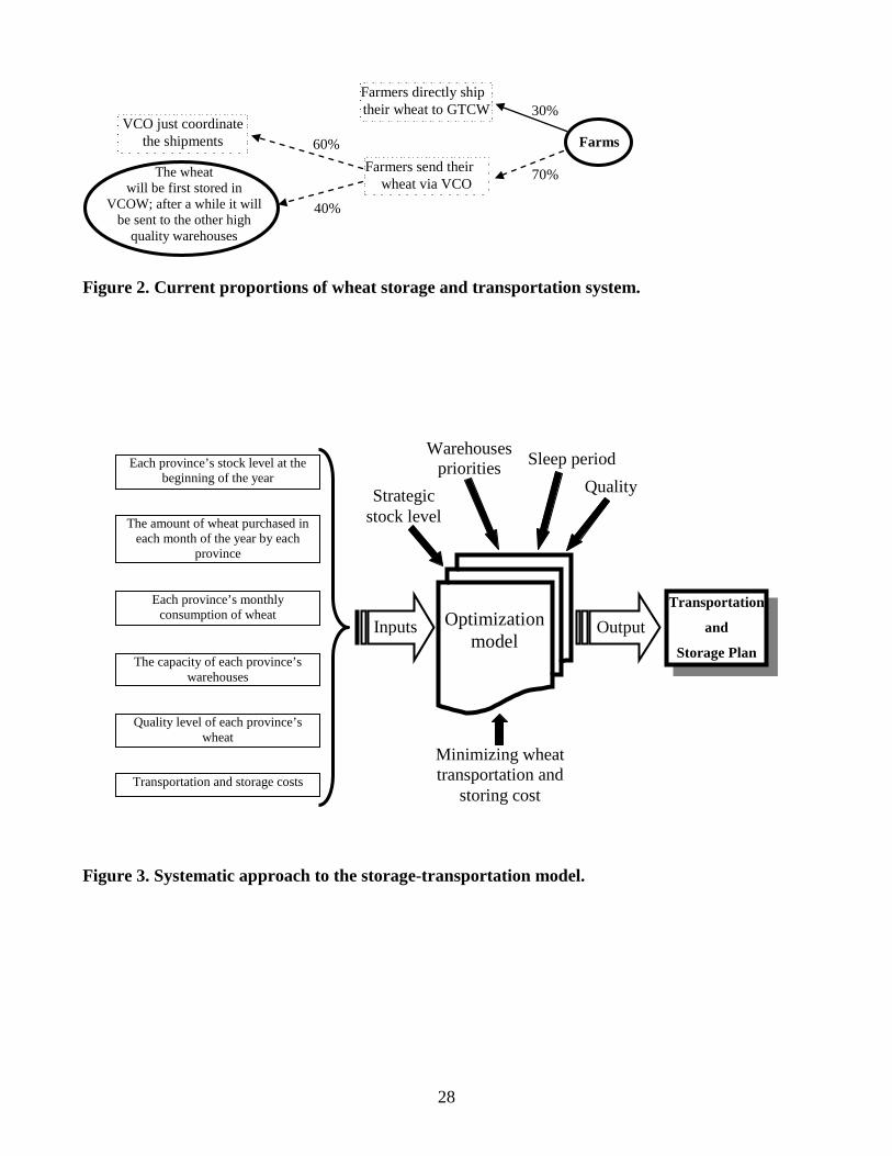
Figure 3 depicts outputs, objectives, constraints and inputs of the problem described.

Mathematical Model

In this part, the mathematical model developed for the whole country is described. At the end of each

year, this model is run for all provinces, the required inputs are calculated using the same year’s data

and are used by the model. First, all sets, variables and inputs of the model are defined and then the

mathematical model in close form will be presented and then fully described.

Sets and Indices

The sets and indices of the mathematical model are as follows:

M={1..12}: set of months of the year (t∈M);

P={1..28}: set of provinces (i, j∈P).

Variables

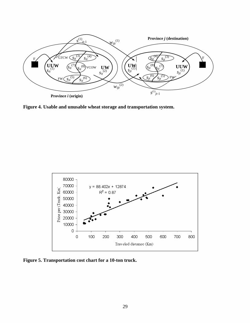
First, we define some terms which are used in the definition of variables (Figure 4). Based on the

defined outputs of the system, the variables of the model are as follows:

10

w(1)ijt : Amount of UUW transported from province i to province j in month t (i, j∈P, i≠j, t∈M);

w(2)ijt : Amount of UW transported from province i to province j in month t (i, j∈P, i≠j, t∈M);

s(1)it : Amount of UUW existing in province i in month t (i∈P, t∈M);

s(2)it : Amount of UW existing in province i in month t (i∈P, t∈M);

s(3)it : Amount of UUW stored in GTCWs of province i in month t (i∈P, t∈M);

s(4)it : Amount of UW stored in GTCWs of province i in month t (i∈P, t∈M);

s(5)it : Amount of UUW stored in FWs of province i in month t (i∈P, t∈M);

s(6)it : Amount of UW stored in FWs of province i in month t (i∈P, t∈M);

s(7)it : Amount of UUW stored in VCOWs of province i in month t (i∈P, t∈M);

s(8)it : Amount of UW stored in VCOWs of province i in month t (i∈P, t∈M);

1 If all GTCWs of province i are full in month t

0 Otherwise;

1 If all FWs of province i are full in month t

0 Otherwise;

1 If all VCOWs of province i are full in month t

0 Otherwise;

Parameters

Based on the defined inputs of the system, the parameters of the mathematical model are as follows:

f : Fixed costs of transportation (for loading and unloading) for each vehicle;

p : Variable costs of transportation for each kilometer for each vehicle;

h4 : Storage cost of each ton of wheat in a GTCW for one month;

h6 : Storage cost of each ton of wheat in a FW for one month;

h8 : Storage cost of each ton of wheat in a VCOW for one month;

y(4)it =

y(6)it =

y(8)it =

11

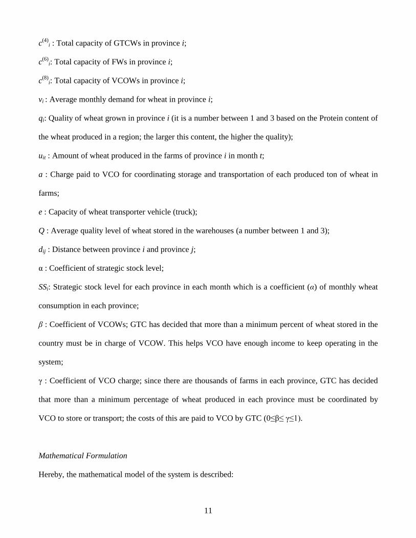
c(4)i : Total capacity of GTCWs in province i;

c(6)i: Total capacity of FWs in province i;

c(8)i: Total capacity of VCOWs in province i;

vi : Average monthly demand for wheat in province i;

qi: Quality of wheat grown in province i (it is a number between 1 and 3 based on the Protein content of

the wheat produced in a region; the larger this content, the higher the quality);

uit : Amount of wheat produced in the farms of province i in month t;

a : Charge paid to VCO for coordinating storage and transportation of each produced ton of wheat in

farms;

e : Capacity of wheat transporter vehicle (truck);

Q : Average quality level of wheat stored in the warehouses (a number between 1 and 3);

dij : Distance between province i and province j;

α : Coefficient of strategic stock level;

SSi: Strategic stock level for each province in each month which is a coefficient (α) of monthly wheat

consumption in each province;

β : Coefficient of VCOWs; GTC has decided that more than a minimum percent of wheat stored in the

country must be in charge of VCOW. This helps VCO have enough income to keep operating in the

system;

γ : Coefficient of VCO charge; since there are thousands of farms in each province, GTC has decided

that more than a minimum percentage of wheat produced in each province must be coordinated by

VCO to store or transport; the costs of this are paid to VCO by GTC (0≤β≤ γ≤1).

Mathematical Formulation

Hereby, the mathematical model of the system is described:

12

( ) ( ) ( )[ ]( ) ( )( )( )[ ] ∑∑∑ ∑ ∑

∑∑

∈ ∈∈ ≠,∈ ∈

)2()1(

∈ ∈

)8()7(8

)6()5(6

)4()3(4

../ . .

...

Pi Mtit

Pi ijPj Mtijijtijt

Pi Mtitititititit

uaedpfww

sshsshsshzMin

γ+++

++++++=

(1)

S.t:

MtPiwwusijPj

jitijPj

ijtitit ∈∈∀+−= ∑∑≠∈≠∈

, ,

)1(

,

)1()1( (2)

( ) MtPivwwsss iijPj

ijtijPj

jittitiit ∈≥∈∀++= ∑∑≠∈≠∈

−− 2 , -- ,

)2(

,

)2()1(1,

)2(1,

)2( (3)

( ) ( ) ( )MtPiQ

wwu

wqwqqu

ijPj ijPjijtjitit

ijPj ijPjijtijitjiit

∈∈∀≥−+

−+

∑ ∑∑ ∑

≠∈ ≠∈

≠∈ ≠∈ , .. .

, ,

)1()1(, ,

)1()1(

(4)

MtPissss itititit ∈∈∀++= , )7()5()3()1( (5)

MtPissss itititit ∈∈∀++= , )8()6()4()2( (6)

Mt Pi .vSSss iiitit ∈∈∀=≥+ ,)2()1( α (7)

MtPiyy itit ∈∈∀≤ , )4()8( (8)

MtPicsscy iititiit ∈∈∀≤+≤ , . )4()4()3()4()4( (9)

MtPiycsscy itiititiit ∈∈∀≤+≤ , . . )4()8()8()7()8()8( (10)

MtPiyy itit ∈∈∀≤ , )6()8( (11)

MtPicsscy iititiit ∈∈∀≤+≤ , . )6()6()5()6()6( (12)

MtPiycsscy itiititiit ∈∈∀≤+≤ , . . )6()8()8()7()8()8( (13)

MtPicss iitit ∈∈∀≤+ , )8()8()7( (14)

10,, )(.)( )2()1()8()7( <≤∈∈∀+≥+ ∑∑∑∑∈ ∈∈ ∈

ββ MtPissssPi Mt

ititPi Mt

itit (15)

MtPissss iiii ∈∈∀==== , 0)8(1

)7(1

)5(1

)3(1 (16)

Piyi ∈∀= 0)8(1 (17)

13

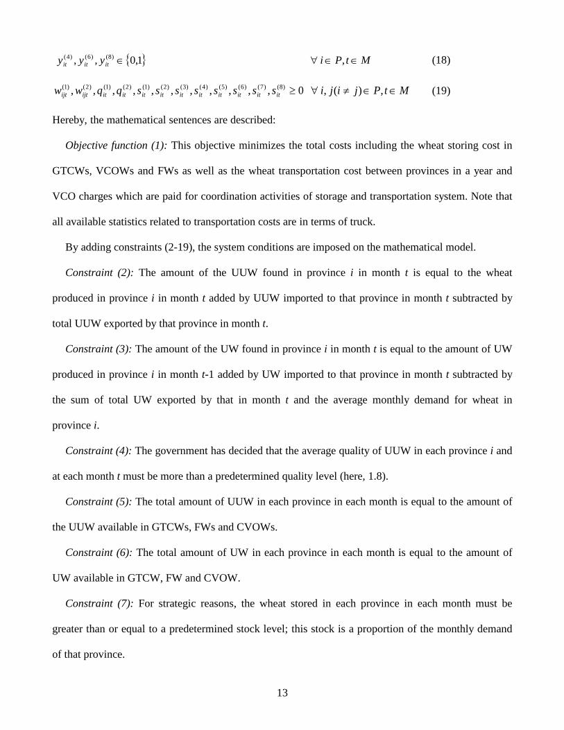
{ } MtPiyyy ititit ∈∈∀∈ , 1,0,, )8()6()4( (18)

MtPjijissssssssqqww ititititititititititijtijt ∈∈≠∀≥ ,)(, 0,,,,,,,,,,, )8()7()6()5()4()3()2()1()2()1()2()1( (19)

Hereby, the mathematical sentences are described:

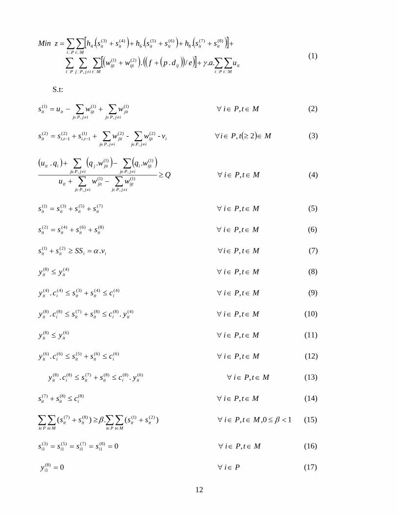
Objective function (1): This objective minimizes the total costs including the wheat storing cost in

GTCWs, VCOWs and FWs as well as the wheat transportation cost between provinces in a year and

VCO charges which are paid for coordination activities of storage and transportation system. Note that

all available statistics related to transportation costs are in terms of truck.

By adding constraints (2-19), the system conditions are imposed on the mathematical model.

Constraint (2): The amount of the UUW found in province i in month t is equal to the wheat

produced in province i in month t added by UUW imported to that province in month t subtracted by

total UUW exported by that province in month t.

Constraint (3): The amount of the UW found in province i in month t is equal to the amount of UW

produced in province i in month t-1 added by UW imported to that province in month t subtracted by

the sum of total UW exported by that in month t and the average monthly demand for wheat in

province i.

Constraint (4): The government has decided that the average quality of UUW in each province i and

at each month t must be more than a predetermined quality level (here, 1.8).

Constraint (5): The total amount of UUW in each province in each month is equal to the amount of

the UUW available in GTCWs, FWs and CVOWs.

Constraint (6): The total amount of UW in each province in each month is equal to the amount of

UW available in GTCW, FW and CVOW.

Constraint (7): For strategic reasons, the wheat stored in each province in each month must be

greater than or equal to a predetermined stock level; this stock is a proportion of the monthly demand

of that province.

14

Constraints (8-10): These constraints show the preference of GTCW ratio to VCOW.

Constraints (11-13): These constraints show the preference of FW ratio to VCOW.

Constraint (14): To show capacity constraints of warehouses, we need to have some constraints as

follows:

MtPi css iitit ∈∈∀≤+ ,)4()4()3( (20)

MtPicss iitit ∈∈∀≤+ , )6()6()5( (21)

MtPicss iitit ∈∈∀≤+ , )8()8()7( (22)

Relations (20) and (21) are satisfied by (9) and (12), respectively. Therefore, relation (22) is added

to the model.

Constraint (15): This constraint represents GTC decision; GTC has decided that more than a

minimum percentage of stored wheat in the country must be in the charge of VCOW.

Constraint (16): This constraint shows that there is not any UUW in GTCW and FW at the

beginning of the year. Most of the produced wheat (more than 80%) in the country is reaped during the

first eight months of the year; therefore, all of the wheat available from last year has passed the sleep

period at the first month of current year and is of type UW (not UUW).

Constraint (17): This constraint ensures that there is no wheat in VCOW at the beginning of the

year. During the last 4 months of the year, no wheat is reaped and all the wheat stored in VCOWs is

transferred to GTCWs or FWs and at the beginning of the year there is no wheat in VCOW.

Constraints (18-19): These constraints describe the type of variables.

Solution of the Model

In this section, first we briefly explain how to calculate the model parameters. After that we focus on

solving the model using the genetic algorithm.

15

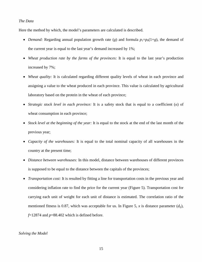
The Data

Here the method by which, the model’s parameters are calculated is described.

• Demand: Regarding annual population growth rate (g) and formula p1=p0(1+g), the demand of

the current year is equal to the last year’s demand increased by 1%;

• Wheat production rate by the farms of the provinces: It is equal to the last year’s production

increased by 7%;

• Wheat quality: It is calculated regarding different quality levels of wheat in each province and

assigning a value to the wheat produced in each province. This value is calculated by agricultural

laboratory based on the protein in the wheat of each province;

• Strategic stock level in each province: It is a safety stock that is equal to a coefficient (α) of

wheat consumption in each province;

• Stock level at the beginning of the year: It is equal to the stock at the end of the last month of the

previous year;

• Capacity of the warehouses: It is equal to the total nominal capacity of all warehouses in the

country at the present time;

• Distance between warehouses: In this model, distance between warehouses of different provinces

is supposed to be equal to the distance between the capitals of the provinces;

• Transportation cost: It is resulted by fitting a line for transportation costs in the previous year and

considering inflation rate to find the price for the current year (Figure 5). Transportation cost for

carrying each unit of weight for each unit of distance is estimated. The correlation ratio of the

mentioned fitness is 0.87, which was acceptable for us. In Figure 5, x is distance parameter (dij),

f=12874 and p=88.402 which is defined before.

Solving the Model

16

The model contains 22512 variables, 1008 of them are binary variables, and 5070 constraints. In large-

size problems of the present linear integer programming model, increasing the size of the problem in

polynomial order will result in an exponential increase in the computation time. This model generates a

midterm plan and could be run once a year. But we have decided to run the model monthly; in other

words, at the end of each month we run the model using updated data of the latest month.

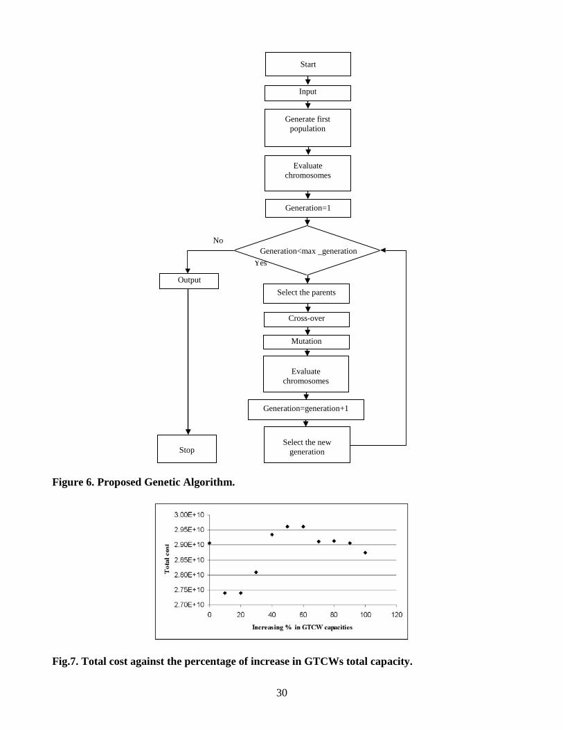
Consequently, in order to solve large-sized problems, a genetic algorithm is designed as shown in

Figure 6. Running this model with the GA for the real-sized problem takes 26993 seconds i.e. 7:29:53.

This runtime meets time requirements of planning horizon. In the model, the cost breakdown is as

follows: 11.27% transportation cost, 65.29% GTCW cost, 16.17% FW cost, 7.14% VCOW cost and

0.13% VCO coordination cost.

Genetic Algorithm

The following notations are used to represent the parameters of the designed genetic algorithm:

pop_size: population size

co: coefficient of first population; in order to increase the number of feasible initial chromosomes in

first population, co* pop_size chromosomes are generated as the first population.

cross_rate: cross-over rate

mutation_rate: mutation rate for chromosomes

gen_mut_rate1: first mutation rate for genes

gen_mut_rate2: second mutation rate for genes

max_generation: maximum number of generations to be produced

Generating first population

A chromosome is represented as a binary string with the length of 3*I*T, equivalent to the binary

variables of the model, as shown in figure below.

17

)4(11y )4(

12y … )4(ITy )6(

11y )6(12y … )6(

ITy )8(11y )8(

12y … )8(ITy

)4(ity )6(

ity )8(ity

With respect to the model constraints, the probability of a randomly produced chromosome to be

feasible is very low. Thus, some facts, especially the constraints, should be considered in generating the

first population chromosomes to achieve the highest possible chance of feasibility.

Based on the model, some facts should be drawn out and some assumptions should be regarded in

order to set the amount of some genes in each chromosome produced in the first population to increase

the number of feasible chromosomes by as many as possible. First, as the capacity of the VCO

warehouse in each province is almost equal to the wheat produced in a year throughout the country, all

)8(ity s are equal to 0. Second, the genes related to )4(

ity s, for which the following inequality is satisfied,

had better to be set equal to 1 with the probability of 0.8: )4(iit cu ≥ . Besides, for {i, t}s whose )4(

ity s are

1, the genes corresponding to )6(ity s are set equal to 1, with the probability of 0.9. These results were

achieved through solving a great number of test instances. Moreover, considering the priority of

warehouses, after setting )4(ity s for each chromosome, the amount of )6(

ity s should be equal to or less

than )4(ity s. Finally, in generating first population, in order to increase the number of feasible

chromosomes, and also to improve the fitness of first population chromosomes, co*pop_size

chromosomes are generated (co>1, co∈N).

Thus, the following procedure is proposed to generate co*pop_size chromosomes of the initial

population:

1. The set of genes which are related to GTCWs are denoted by GTCspace.

2. chr=1 (chr is the chromosome's index), numberones=1 (numberones is the number of genes equal to

1 in each cheomosome).

3. To generate the chromosome chr, randomly choose numberones genes from the set

18

GTCspace and set them equal to 1. Moreover, set the genes related to )4(ity s, for which the following

inequality is satisfied, equal to 1 with the probability of 0.8: )4(iit cu ≥

Then, for {i, t}s whose )4(ity s are 1, set the similar genes for )6(

ity s equal to 1, with the probability of 0.9.

Check the priority of warehouses. Set the rest of the genes equal to 0.

4. If chr<co*pop_size, then go to step 5; otherwise stop the procedure.

5. If co* pop_size<I*T then set numberones= numberones+round(I*T/co*pop_size), chr=chr+1;

otherwise, if co *pop_size>I*T, set numberones=round(chr*I*T/co*pop_size). Then go to step 3.

Chromosomes Evaluation

To determine the fitness of chromosomes in each generation, a one-to-one relationship must be

established between the chromosome’s string representation, and the set of model variables or the

objective functions value. For each chromosome, determination of the equivalent values of )4(ity s, )6(

ity s

and )8(ity s in the mathematical model will transform the linear integer programming model to a linear

programming model with continuous variables. The minimum of z for each chromosome can then be

simply calculated using MATLAB optimization toolbox for linear programming. However, if the

resulted problem does not have any feasible solution, the related chromosome is infeasible and should

be omitted from the population. After applying this procedure to all the initial chromosomes, pop_size

chromosomes will be selected among current feasible chromosomes as parents to generate next

generation children.

Sorting

After evaluation, feasible chromosomes are sorted according to the value of z. The more prioritized

chromosome has less value of z.

19

Selection of Parents

The parents are selected using the following method, and are copied into the mating pool as well. The

process of selection is done (pop_size/2) times among feasible chromosomes for each population so

that the number of chromosomes for each generation remains pop_size. At each stage, two

chromosomes are randomly selected in a way that ones with the greater fitness values have more

chance to be copied into the mating pool as parents. The applied method is as follows:

1. Devote the integer numbers in ( )

−−

−−−

2_)(,

23_1

22 iisizepopiiisizepopi = [ ]ii ba , to

chromosome number i, respectively (for i=1...pop_size).

2. Generate 2 random integer numbers: rand1, rand2 ∈

+

2)1_(_,1 sizepopsizepop .

3. Select chromosomes i and j as parents for which rand1∈[ai, bi], rand2∈[aj, bj].

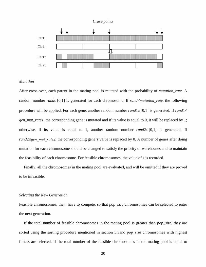
Cross-over

At each stage, two chromosomes are randomly selected from the mating pool. A random number rand

∈[0, 1] is generated. If rand≤cross_rate, children are produced and added to the population in the

mating pool; hence, they do not replace their parents. If rand>cross_rate, no crossover is performed

and parents remain in the pool. A multiple-point cross-over is applied here. If the length of a

chromosome's string is divided into 3*I equal parts, each part will represent )4(ity or )6(

ity or )8(ity values

of a province in T months with t varying from1 to T. In each part of a pair of selected parents, two

cross-points are randomly selected and the section between them is exchanged. After the cross-over is

done for each chromosome, a number of genes must change to satisfy the priority of warehouses in

order to maintain the feasibility of the chromosome. If the two selected cross-points in each part are the

same, nothing will be exchanged between the parents. Here is an example to clarify the crossover

procedure.

20

Cross-points

Mutation

After cross-over, each parent in the mating pool is mutated with the probability of mutation_rate. A

random number rand∈[0,1] is generated for each chromosome. If rand≤mutation_rate, the following

procedure will be applied. For each gene, another random number rand1∈[0,1] is generated. If rand1≤

gen_mut_rate1, the corresponding gene is mutated and if its value is equal to 0, it will be replaced by 1;

otherwise, if its value is equal to 1, another random number rand2∈[0,1] is generated. If

rand2≤gen_mut_rate2, the corresponding gene’s value is replaced by 0. A number of genes after doing

mutation for each chromosome should be changed to satisfy the priority of warehouses and to maintain

the feasibility of each chromosome. For feasible chromosomes, the value of z is recorded.

Finally, all the chromosomes in the mating pool are evaluated, and will be omitted if they are proved

to be infeasible.

Selecting the New Generation

Feasible chromosomes, then, have to compete, so that pop_size chromosomes can be selected to enter

the next generation.

If the total number of feasible chromosomes in the mating pool is greater than pop_size, they are

sorted using the sorting procedure mentioned in section 5.3and pop_size chromosomes with highest

fitness are selected. If the total number of the feasible chromosomes in the mating pool is equal to

Chr1:

Chr2: Chr1′:

Chr2′:

21

pop_size, all the chromosomes will enter the next generation. Finally, the following procedure will be

applied if the total number of the feasible chromosomes is less than pop_size. First, the feasible

chromosomes are sorted, and their fitness values are calculated. Then, the nearest integer equal to or

less than the number of feasible chromosomes, by which pop_size is divisible, is determined as fch. fch

chromosomes of the fittest ones are then selected, and pop_size/fch copies of each enter the next

generation. This, in total, will add up to pop_size chromosomes into the pool. For each generation, the

fittest chromosomes are recorded at the end.

Reporting

Finally if the termination condition is satisfied, which is to repeat the algorithm for max_geneartion

times, the fittest chromosome among the ones of final population is determined, and reported as the

solutions of the problem.

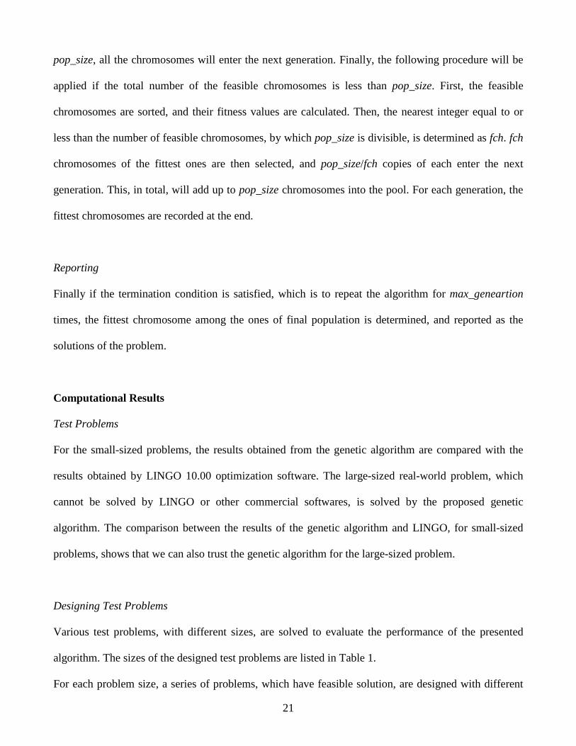
Computational Results

Test Problems

For the small-sized problems, the results obtained from the genetic algorithm are compared with the

results obtained by LINGO 10.00 optimization software. The large-sized real-world problem, which

cannot be solved by LINGO or other commercial softwares, is solved by the proposed genetic

algorithm. The comparison between the results of the genetic algorithm and LINGO, for small-sized

problems, shows that we can also trust the genetic algorithm for the large-sized problem.

Designing Test Problems

Various test problems, with different sizes, are solved to evaluate the performance of the presented

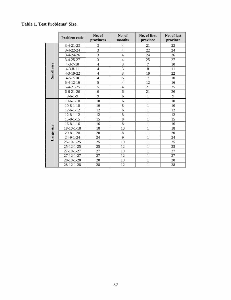
algorithm. The sizes of the designed test problems are listed in Table 1.

For each problem size, a series of problems, which have feasible solution, are designed with different

22

combinations of the provinces.

Genetic Algorithm Parameters Fitting

Parameters of the designed genetic algorithm include co, max_generation, pop_size, cross_rate,

mutation_rate, gen_mut_rate1and gen_mut_rate2. Primary tests are carried out in order to determine

the value of these parameters.

In this case, a trade-off between solution time, and quality of solutions determined the appropriate

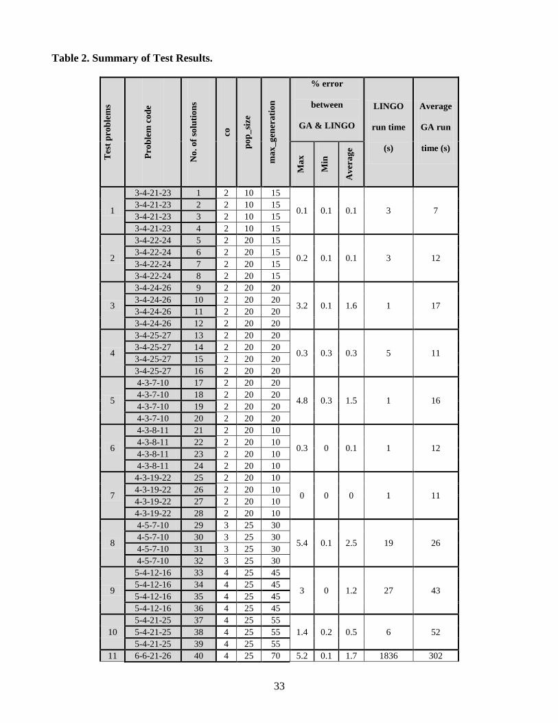
values for these parameters. For small-sized problems co, pop_size and max_generation are set to be

corresponding values in Table 2. For large-sized problems, these three parameters are set equal to 5, 35,

and 130, respectively.

In addition, the values for cross_rate, mutation_rate, gen_mut_rate1 and gen_mut_rate2 are set to be

0.5, 0.9, 0.1 and 0.2 respectively, after many runs of the proposed GA with different sets of parameters’

values. The selected values proved to result in better quality of solutions. The quality of solutions failed

to improve, moving forward the iterations, in runs with lower rates set for these four parameters.

Furthermore, the higher rates for mutation_rate and gen_mut_rate1 and gen_mut_rate2 increased the

risk of infeasibility and increase in z value of the chromosomes.

Results

The genetic algorithm is coded in MATLAB 7.5.0, and LINGO 10.00 software is used to compare the

results of small-sized problems. All the test problems are solved on a Pentium 4 computer with 1024

MB of RAM and 2.26 GHz CPU. In order to compare the solutions of the two methods, the minimum

value of the objective function (z) for the resulting model is calculated. Therefore, the reported time for

LINGO software will be recorded for these optimization problems. The results are summarized in

Table 2.

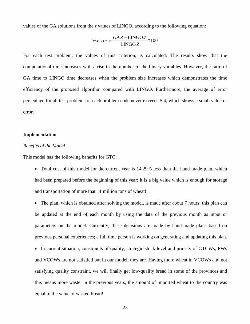
A quality criterion, the percentage of error, is defined to show the percentage of deviation of the z

23

values of the GA solutions from the z values of LINGO, according to the following equation:

100*.LINGO

.LINGO.%Z

ZZGAerror −=

For each test problem, the values of this criterion, is calculated. The results show that the

computational time increases with a rise in the number of the binary variables. However, the ratio of

GA time to LINGO time decreases when the problem size increases which demonstrates the time

efficiency of the proposed algorithm compared with LINGO. Furthermore, the average of error

percentage for all test problems of each problem code never exceeds 5.4, which shows a small value of

error.

Implementation

Benefits of the Model

This model has the following benefits for GTC:

• Total cost of this model for the current year is 14.29% less than the hand-made plan, which

had been prepared before the beginning of this year; it is a big value which is enough for storage

and transportation of more that 11 million tons of wheat!

• The plan, which is obtained after solving the model, is made after about 7 hours; this plan can

be updated at the end of each month by using the data of the previous month as input or

parameters on the model. Currently, these decisions are made by hand-made plans based on

previous personal experiences; a full time person is working on generating and updating this plan.

• In current situation, constraints of quality, strategic stock level and priority of GTCWs, FWs

and VCOWs are not satisfied but in our model, they are. Having more wheat in VCOWs and not

satisfying quality constraint, we will finally get low-quality bread in some of the provinces and

this means more waste. In the previous years, the amount of imported wheat to the country was

equal to the value of wasted bread!

24

Sensibility Analysis

Hereby we represent the results of the sensibility analysis done. This analysis will be a basis for

suggestions to improve the system and propose some future works. Doing the analysis took many days;

i.e. more than one day has been spent to apply every change in the mode and running it.

GTC is the owner of the system, so we can investigate the effect of increasing the capacity of

GTCWs. In Figure 7, this analysis is depicted.

We see that increasing 10% in GTCWs total capacity decreases total cost of the system in comparison

with the current situation. Of course, this analysis is not well enough to make such decision because we

have not calculated warehouses construction costs; however conducting a feasibility study on such

increase in capacity may be worthwhile.

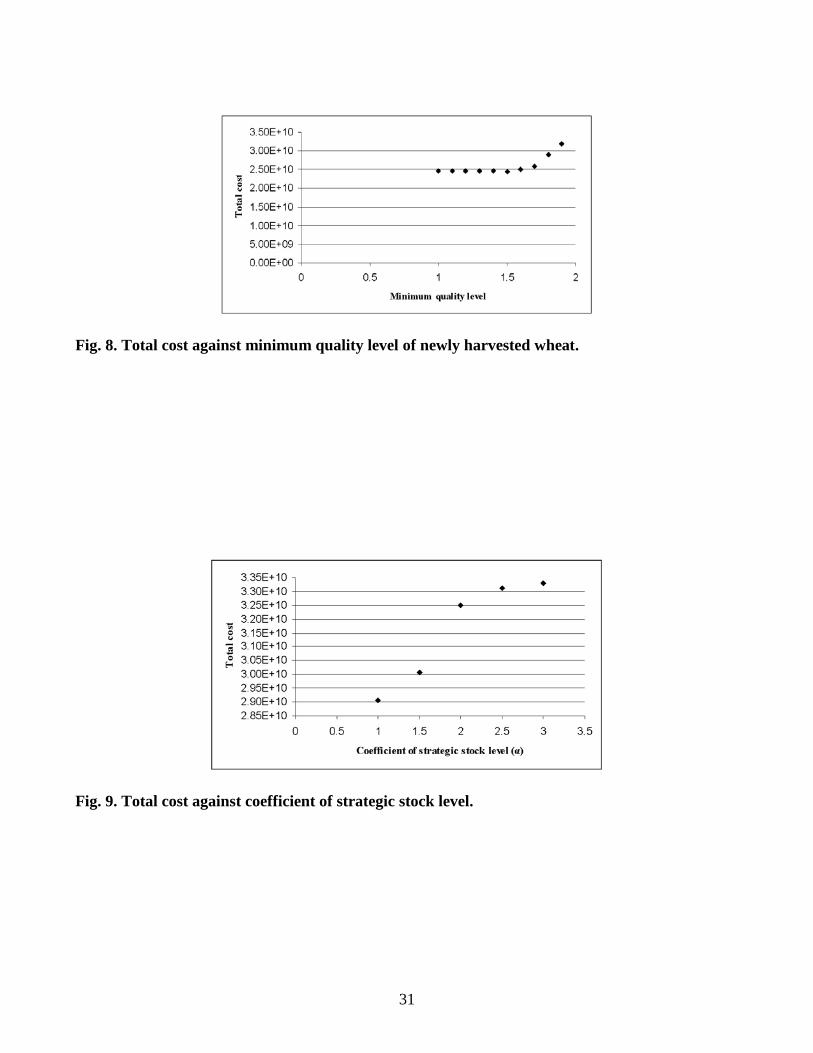
Figure 8 shows an analysis on the minimum quality level of new harvested wheat in each province.

In the basic model, the minimum quality level was set on 1.8. Figure 8 shows that for low quality levels

(≤1.4), the quality constraint (4) is redundant and we already have the minimum cost. For high quality

levels (≥2) no feasible solution was found. Quality constraint is very important in decreasing the

amount of bread wasted in the country and 1.9 minimum quality level may be a better solution.

However, using additives to increase the quality of wheat (instead of bearing storage and transportation

costs) is worth investigating. Besides importing high-quality wheat to the country and exporting low

quality wheat to poor countries may be a worthwhile future work.

For every country, wheat is considered strategic and, therefore, having some safety stock of wheat is

important. In this problem, we set coefficient of strategic stock level on α=1. Figure 9 shows changing

of this coefficient against total cost of the system. For α≥3 no feasible solution was found. As we see in

the Figure, changing total cost from α equal 1 up to α equal 3 causes total cost to increase from

2.91E+10 to 3.33E+10 units; this change in the system is not significant from the owner’s point of

view. Therefore, the output plan is based on α=3.

25

Future Works

While studying different scenarios and situations, the following issues seemed appropriate for later

researches concerning relative problems:

• Feasibility study of increasing storage capacity of GTCWs and finding the relative costs. In

addition, some investigations should be conducted into the location of new warehouses in the

provinces;

• Feasibility study of adding additives to wheat to improve its average quality level and finding

relevant costs;

• Studying the possibility and influence of importing high quality wheat and exporting poor

quality wheat to improve average quality level of wheat and finding relative costs of it;

• Carrying out facility locating, transportation planning, inventory planning and control projects

simultaneously to optimize the system.

Conclusion

In this paper, wheat storage and transportation system in the country is defined and formulated by an

MIP model. Using the proposed genetic algorithm, this model has been solved. Some sensitivity analysis

has been performed and the results have been studied; some related future research topics have been

suggested as well. However, considering this problem as a national one and being aware of its

economic side-effects for the country, such as the remarkable costs of garbage bread as a result of poor

quality, it is still efficient and useful.

Acknowledgment

We would like to thank Nasim Akbarzadeh and Nasibeh Zanjirani Farahani for their invaluable

26

comments on this work and. We express our gratitude for their mindful suggestions.

References

Ahumada, O., Villalobos, J.R. 2009. “Application of planning models in the agri-food supply chain:

A review.” European Journal of Operational Research 196(1): 1-20.

Bilgen, B., Ozkarahan I. 2007. “A mixed-integer linear programming model for bulk grain blending

and shipping.” International Journal of Production Economics 107: 555–571.

Bregman, R.L., Ritzman, L.P., Krajewski, L.J.. 1990. “A heuristic for the control of inventory in a

multi-echelon environment with transportation costs and capacity limitations.” Journal of the

Operational Research Society 41: 809–820.

Carlsson, D., Rönnqvist, M. 2007. “Backhauling in forest transportation – models, methods and

practical usage.” Canadian Journal of Forest Research 37: 2612-2623

De Boon, H. 1978. “A flower transportation-distribution system.” Journal of Operational Research

Society 29: 19-31.

Kleywegt, A.J., Nori, V.S., Savelsbergh, M.W.P. 2002. “The stochastic inventory routing problem

with direct deliveries.” Transportation Science 36: 94–118.

Sousa, R., Shah, N., Papageorgiou, L.G. 2008. “Supply chain design and multilevel planning-An

industrial case.” Computers and Chemical Engineering 32(11): 2643-2663

Z.-Farahani, R., Elahipanah, M. 2008. “A genetic algorithm to optimize the total cost and service

level for just-in-time distribution in a supply chain.” International Journal of Production Economics

111(2): 229-243.

27

Figure 1. Status of wheat storage and transportation system.

Government Trade Organization’s Warehouses

Villages Cooperation Organization’s Warehouse

Simple horizontal silo

Ground warehouse

Flour factories’ warehouses

Flour Factories

Vertical silo

Automated horizontal silo

30%

42%

28% Farms

28

Figure 2. Current proportions of wheat storage and transportation system.

Figure 3. Systematic approach to the storage-transportation model.

Optimization model

Quality Sleep period Warehouses

priorities Strategic

stock level The amount of wheat purchased in each month of the year by each

province

Each province’s monthly consumption of wheat

The capacity of each province’s warehouses

Quality level of each province’s wheat

Transportation and storage costs

Each province’s stock level at the beginning of the year

Transportation

and

Storage Plan

Inputs

Minimizing wheat transportation and

storing cost

Output

Farmers directly ship their wheat to GTCW

Farmers send their wheat via VCO

30%

Farms

The wheat will be first stored in

VCOW; after a while it will be sent to the other high

quality warehouses

VCO just coordinate the shipments

70%

60%

40%

29

Figure 4. Usable and unusable wheat storage and transportation system.

Figure 5. Transportation cost chart for a 10-ton truck.

Province i (origin)

wijt(2)

wijt(1)

F GTCW

VCOW

FW

UUW UW sit

(2)

sit(4) sit

(3)

sit(8) sit

(7)

sit(6) sit

(5)

sit(1)

s(1)it-1

FW

UW

UUW sjt

(1)

sjt(3) sjt

(4)

sjt(7) sjt

(8)

sjt(5) sjt

(6) sjt

(2)

F

s(1)jt-1

Province j (destination)

30

Figure 6. Proposed Genetic Algorithm.

Fig.7. Total cost against the percentage of increase in GTCWs total capacity.

Yes Generation<max _generation

Start

Generate first population

Input

Evaluate chromosomes

Generation=1

Select the parents

Cross-over

Mutation

Generation=generation+1

Evaluate chromosomes

Select the new generation

Output

Stop

No

31

Fig. 8. Total cost against minimum quality level of newly harvested wheat.

Fig. 9. Total cost against coefficient of strategic stock level.

32

Table 1. Test Problems’ Size.

Problem code No. of provinces

No. of months

No. of first province

No. of last province

Smal

l siz

e

3-4-21-23 3 4 21 23 3-4-22-24 3 4 22 24 3-4-24-26 3 4 24 26 3-4-25-27 3 4 25 27 4-3-7-10 4 3 7 10 4-3-8-11 4 3 8 11

4-3-19-22 4 3 19 22 4-5-7-10 4 5 7 10

5-4-12-16 5 4 12 16 5-4-21-25 5 4 21 25 6-6-21-26 6 6 21 26

9-6-1-9 9 6 1 9

Larg

e siz

e

10-6-1-10 10 6 1 10 10-8-1-10 10 8 1 10 12-6-1-12 12 6 1 12 12-8-1-12 12 8 1 12 15-8-1-15 15 8 1 15 16-8-1-16 16 8 1 16

18-10-1-18 18 10 1 18 20-8-1-20 20 8 1 20 24-9-1-24 24 9 1 24

25-10-1-25 25 10 1 25 25-12-1-25 25 12 1 25 27-10-1-27 27 10 1 27 27-12-1-27 27 12 1 27 28-10-1-28 28 10 1 28 28-12-1-28 28 12 1 28

33

Table 2. Summary of Test Results.

Tes

t pro

blem

s

Prob

lem

cod

e

No.

of s

olut

ions

co

pop_

size

max

_gen

erat

ion

% error

between

GA & LINGO

LINGO

run time

(s)

Average

GA run

time (s)

Max

Min

Ave

rage

1

3-4-21-23 1 2 10 15

0.1 0.1 0.1 3 7 3-4-21-23 2 2 10 15 3-4-21-23 3 2 10 15 3-4-21-23 4 2 10 15

2

3-4-22-24 5 2 20 15

0.2 0.1 0.1 3 12 3-4-22-24 6 2 20 15 3-4-22-24 7 2 20 15 3-4-22-24 8 2 20 15

3

3-4-24-26 9 2 20 20

3.2 0.1 1.6 1 17 3-4-24-26 10 2 20 20 3-4-24-26 11 2 20 20 3-4-24-26 12 2 20 20

4

3-4-25-27 13 2 20 20

0.3 0.3 0.3 5 11 3-4-25-27 14 2 20 20 3-4-25-27 15 2 20 20 3-4-25-27 16 2 20 20

5

4-3-7-10 17 2 20 20

4.8 0.3 1.5 1 16 4-3-7-10 18 2 20 20 4-3-7-10 19 2 20 20 4-3-7-10 20 2 20 20

6

4-3-8-11 21 2 20 10

0.3 0 0.1 1 12 4-3-8-11 22 2 20 10 4-3-8-11 23 2 20 10 4-3-8-11 24 2 20 10

7

4-3-19-22 25 2 20 10

0 0 0 1 11 4-3-19-22 26 2 20 10 4-3-19-22 27 2 20 10 4-3-19-22 28 2 20 10

8

4-5-7-10 29 3 25 30

5.4 0.1 2.5 19 26 4-5-7-10 30 3 25 30 4-5-7-10 31 3 25 30 4-5-7-10 32 3 25 30

9

5-4-12-16 33 4 25 45

3 0 1.2 27 43 5-4-12-16 34 4 25 45 5-4-12-16 35 4 25 45 5-4-12-16 36 4 25 45

10 5-4-21-25 37 4 25 55

1.4 0.2 0.5 6 52 5-4-21-25 38 4 25 55 5-4-21-25 39 4 25 55

11 6-6-21-26 40 4 25 70 5.2 0.1 1.7 1836 302

34

6-6-21-26 41 4 25 70 6-6-21-26 42 4 25 70

12 9-6-1-9 43 4 25 90 3.9 0.1 2.8 87005 672 9-6-1-9 44 4 25 90 13 10-6-1-10 45 5 35 130 - - - >100000 1129 14 10-8-1-10 46 5 35 130 - - - - 2124 15 12-6-1-12 47 5 35 130 - - - - 2867 16 12-8-1-12 48 5 35 130 - - - - 3832 17 15-8-1-15 49 5 35 130 - - - - 5125 18 16-8-1-16 50 5 35 130 - - - - 6014 19 18-10-1-18 51 5 35 130 - - - - 7832 20 20-8-1-20 52 5 35 130 - - - - 7531 21 24-9-1-24 53 5 35 130 - - - - 10447 22 25-10-1-25 54 5 35 130 - - - - 13407 23 25-12-1-25 55 5 35 130 - - - - 16288 24 27-10-1-27 56 5 35 130 - - - - 15539 25 27-12-1-27 57 5 35 130 - - - - 16671 26 28-10-1-28 58 5 35 130 - - - - 18136 27 28-12-1-28 59 5 35 130 - - - - 26993