Embed Size (px)
Citation preview
Lasse Huusko
DEVELOPING A FORECASTING MODELFOR DOCTOR´S APPOINTMENTSIN HEALTHCARE BUSINESS
Helsinki Metropolia University of Applied SciencesMaster’s Degree in Industrial ManagementMaster’s Thesis6 May 2011Instructors: Marjatta Huhta DSc (Tech) JamesCollins PhD Tiina Pohjonen PhD

PREFACE
This study was conducted during the spring 2011. This Master´s Thesis has introduced
me a new field of science; forecasting in healthcare business. During this study I have
learned a great deal about the forecasting processes. From a professional point of
view, it is really good to have challenges outside your own field and I feel that it helps
me to grow as a professional when I step outside my comfort zone.
I would like to thank all my teachers and superiors who have contributed to this
Thesis. My special thanks are given to Tiina Pohjonen CEO of the Helsinki City
Occupational HealthCare Centre, for providing an opportunity to investigate demand
forecasting in the occupational healthcare sector. Special thanks are also given to my
instructors James Collins and Marjatta Huhta and as well as other Metropolia teachers
for valuable comments and opinions.
Last but not least, I would like to thank my wife for her patience during my studies
which have taken a lot of my time during the academic year, and especially in the
Master’s Thesis writing time.
6 May 2011 Lasse Huusko
Abstract
Author(s)Title
Number of PagesDate
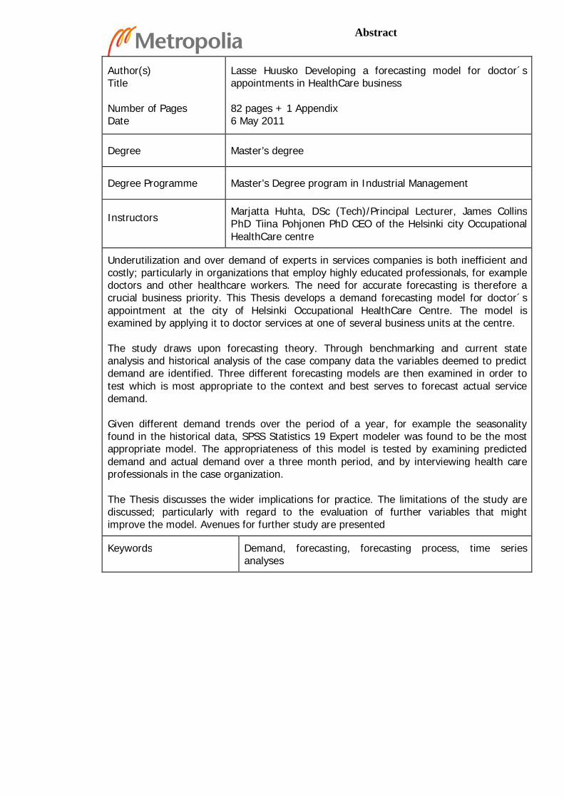
Lasse Huusko Developing a forecasting model for doctor´sappointments in HealthCare business
82 pages + 1 Appendix6 May 2011
Degree Master’s degree
Degree Programme Master’s Degree program in Industrial Management
Instructors Marjatta Huhta, DSc (Tech)/Principal Lecturer, James CollinsPhD Tiina Pohjonen PhD CEO of the Helsinki city OccupationalHealthCare centre
Underutilization and over demand of experts in services companies is both inefficient andcostly; particularly in organizations that employ highly educated professionals, for exampledoctors and other healthcare workers. The need for accurate forecasting is therefore acrucial business priority. This Thesis develops a demand forecasting model for doctor´sappointment at the city of Helsinki Occupational HealthCare Centre. The model isexamined by applying it to doctor services at one of several business units at the centre.
The study draws upon forecasting theory. Through benchmarking and current stateanalysis and historical analysis of the case company data the variables deemed to predictdemand are identified. Three different forecasting models are then examined in order totest which is most appropriate to the context and best serves to forecast actual servicedemand.
Given different demand trends over the period of a year, for example the seasonalityfound in the historical data, SPSS Statistics 19 Expert modeler was found to be the mostappropriate model. The appropriateness of this model is tested by examining predicteddemand and actual demand over a three month period, and by interviewing health careprofessionals in the case organization.
The Thesis discusses the wider implications for practice. The limitations of the study arediscussed; particularly with regard to the evaluation of further variables that mightimprove the model. Avenues for further study are presented
Keywords Demand, forecasting, forecasting process, time seriesanalyses
Tiivistelmä
Työn tekijäOtsikko
SivumääräPäivämäärä
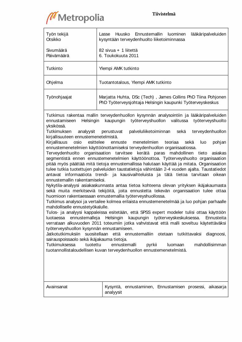
Lasse Huusko Ennustemallin luominen lääkäripalveluidenkysyntään terveydenhuolto liiketoiminnassa
82 sivua + 1 liitettä6. Toukokuuta 2011
Tutkinto Ylempi AMK tutkinto
Ohjelma Tuotantotalous, Ylempi AMK tutkinto
Työnohjaajat Marjatta Huhta, DSc (Tech) , James Collins PhD Tiina PohjonenPhD Työterveysjohtaja Helsingin kaupunki Työterveyskeskus
Tutkimus rakentaa mallin terveydenhuollon kysynnän analysointiin ja lääkäripalveluidenennustamiseen Helsingin kaupungin työterveyshuollon valitussa työterveyshuoltoyksikössä.Tutkimuksen analyysit perustuvat palveluliiketoiminnan sekä terveydenhuollonkirjallisuuteen ennustemenetelmistä.Kirjallisuus osio esittelee ennuste menetelmien teoriaa sekä luo pohjanennustemenetelmien käyttöönottamiseksi terveydenhuollon organisaatiossa.Terveydenhuolto organisaation tarvitsee kerätä paras mahdollinen tieto asiakassegmentistä ennen ennustemenetelmien käyttöönottoa. Työterveyshuolto organisaationpitää myös päättää mitä tietoja ennustemallissa halutaan käyttää ja mitata. Organisaationtulee tutkia tuotettujen palveluiden taustatietoja vähintään 2-4 vuoden ajalta. Taustatiedotantavat informaatiota trendi- ja kausivaihteluista ja tätä tietoa tarvitaan oikeanennustemallin rakentamiseksi.Nykytila-analyysi asiakaskunnasta antaa tietoa kohteena olevan yrityksen ikäjakaumastasekä muita merkitseviä tekijöitä, joita ennustetta tekevän organisaation tulee ottaahuomioon rakentaessaan ennustemallia työterveyshuollossa.Tutkimus analysoi ja vertailee kolmea erilaista ennustemenetelmää ja luo pohjan parhaallemahdolliselle ennustetyökalulle.Tulos- ja analyysi kappaleissa esitetään, että SPSS expert modeler tulisi ottaa käyttöönluotaessa ennustemalleja Helsingin kaupungin työterveyskeskuksessa. Ennusteitaverrataan alkuvuoden 2011 toteumiin jotka vahvistavat että malli soveltuu käytettäväksityöterveyshuollon kysynnän ennustamiseen.Jatkotutkimuksiin suositellaan että ennustemalliin otetaan tutkittavaksi diagnoosi,sairauspoissaolo sekä ikäjakauma tietoja.Tutkimuksessa tuotettu ennustemalli pyrkii luomaan mahdollisimmantuotannollistaloudellisen kuvan terveydenhuollon ennustemenetelmistä.
Avainsanat Kysyntä, ennustaminen, Ennustamisen prosessi, aikasarjaanalyysit
Table of Contents
Preface
Abstract
Tiivistelmä
Table of Contents
List of Illustrations and Tables
1 Introduction 1
2 Forecasting Theory 5
2.1 Developing an Accurate Forecast 9
2.2 Forecasting Models 19
2.3 Forecasting Errors 23
3 Research Method and Material 25
3.1 Research Method 25
3.2 Data Description 26
3.3 Process for Making Appointments 27
3.4 Research Material 31
3.4.1 Background for the Forecasting Tools 31
3.4.2 Forecasting Tools 34
3.5 Validity and Reliability 38
4 Current State Analysis 39
4.1 Case Customer Population 40
4.2 Analyzing the Demand for the Case Unit 42
4.3 Analyzing Monthly and Weekly Demand 46
5 Analyses of the Forecasting Tools 50
5.1 Analysis of the ARMA-model 50
5.2 Analysis of the SARIMA-model 54
5.3 Analysis of the SARIMA Forecasting in Weekly Level 59
5.4 Analysis of the Expert Time Series Modeler 61
5.5 Validating the selected model 65
5.6 Management interview analyses 68

6 Discussion and Conclusions 70
6.1 Proposed Tool for the Case Organization 77
6.2 Managerial implications 78
7 Summary 81
References 83
Appendices
Appendix 1. Kysynnän analysoinnin kysymykset linjajohdolle
List of Illustrations and Tables
Figure 1. Research design. 2
Figure 2. Supply, need and demand for healthcare services (Vissers 1998:79-80). 5
Figure 3. Drawing together these phases, effective forecasting of demand forhealthcare services appears to require nine steps (Stark et.al 2008:2-4). 9
Figure 4. Process for forecasting (Dickersbach 2007:64). 11
Figure 5. Major steps in the forecasting model (Stark et.al 2008:4). 17
Figure 6. Key revenue drivers (Stark et.al. 2008:4). 18
Figure 7. Key Market and strategic business influences (Stark et. al. 2008:5). 19
Figure 8. Methodology tree for selecting forecasting approach (Voudouris et. al.2008:60). 20
Table 1. Methods for cause and effect modeling (Stark et. al. 2008:7). 21
Table 2. Time series forecasting models (Stark et. al. 2008). 22
Table 3. Judgement method (Stark et. al. 2008). 22
Figure 9. Error methods in forecasting (Armstrong et. al.1992:78). 24
Figure 10. The current process for making reservation of the healthcare services. 28
Figure 11. Process for customer using the occupational healthcare service. 29
Figure 12. Demand forecasting process. 30
Figure 12. Microsoft excel variables in forecasting tool. 34
Figure 13. Parameters for SPSS SARIMA forecasting method. 36
Figure 14.Parameters for SPSS expert model forecasting method. 37
Table 4. Average age statistics of the case organizations customers. 40
Table 5. Age statistics of the case organization. 40
Table 6. Permanent staff age differentiation. 41
Figure 15. Permanent staff members’ reaching retirement pension age 2008-2020. 41
Figure 17. Total average of the selected doctor’s events realization. 42
Figure 18. Doctors event realization on the years 2008-2010. 43
Figure 19. Percentage change 2009-2010. 44
Figure 20. Total change in years 2008-2009 and 2009-2010. 45
Figure 21. Total average visits March 2008-2010. 46
Figure 22.Total average visit groups March 2008-2010. 47
Figure 23. Total average data in second week (March 2008-2010). 48
Figure 24. Total average visit groups second week March 2008-2010. 49
Table 7. Time series for demand forecasting. 51
Table 8. Forecasting matrix in short medical examinations. 52
Table 9. Fitted versus Actual figures in the short medical examinations time series. 53
Table 10. Forecasting short medical examinations in 10 month period. 54
Figure 25. Model description for SPSS statistics 19 SARIMA. 55
Figure 26. Model fit for SARIMA (1,0,1). 55
Figure 27. Model fit statistics for using SARIMA(1,0,1). 56
Figure 28. Forecasting results table for the SARIMA (1,0,1) model. 57
Figure 29.Forecasting results when using SARIMA(1,0,1) model for SPSS Statistics19.0. 58
Figure 30. Model fit (SARIMA (1,0,1) for short medical examinations day data in SPSSstatistics 19.0. 59
Figure 31. Forecasting results for SARIMA (1,0,1) day forecast. 60
Figure 32. Forecasting day data SARIMA (1,0,1). 60
Figure 33. Model description for SPSS Statistics Expert time series modeler. 61

Figure 34. Model fit for SPSS Statistics 19.0 Expert modeler. 61
Figure 35. Model fit statistics for SPSS expert modeler. 62
Figure 36. Forecasting result table SPSS Statistics 19.0 Expert modeler. 63
Figure 37. Forecasting results in illustration when using SPSS expert modeler. 64
Figure 38. Comparing the Forecast and Realized numbers during the January andFebruary 2011. 66
Figure 39. Forecasting and actual event realization comparison in numbers. 67
1
1 Introduction
Underutilization and over demand of experts in services companies is both inefficient
and costly; particularly in organizations that employ highly educated professionals, for
example doctors and other healthcare workers. The need for accurate forecasting is
therefore a crucial business priority. This Master’s Thesis builds a forecasting model for
doctor´s appointments demand at the city of Helsinki Occupational HealthCare Centre.
The model is examined by applying it to doctor services at one of several business
units at the centre.
Occupational HealthCare Centre (OHCC) with its 138 professionals aims at supporting
the employee ability to work and strives to secure effective functioning of working
communities. OHCC is responsible for providing healthcare services to almost 40,000
people employed by the city of Helsinki. Altogether, the OHCC customers represent
more than 800 various occupations, for which a diverse supply of healthcare services is
needed
Being an occupational healthcare centre, OHCC is focused on illnesses weakening the
ability to work. OHCC evaluates the employees’ health and ability to work, and
provides a wide range of medical treatments. The main stakeholders of occupational
healthcare OHCC is the city of Helsinki, represented by its strategy managers, work
process managers and competent employees. OHCC provide services for the working
communities from the points of view of their future, change and development.
In modern versatile environment, OHCC is facing many new business needs; the
current approach does not offer the necessary flexibility and agility required for the
present day healthcare provision. One of the most challenging needs for OHCC today is
the need for predicting the doctor´s appointments demand on weekly and monthly
bases. In this Thesis, the doctor’s appointments demand was defined as a request for
short and long medical examination, telephone calls and working conditions
examinations conducted by doctors. The scope of this Thesis is limited to the
customers demand for appointments for these categories only. For the purposes of the
Thesis, these categories of medical services are divided into smaller groups, and the
2
demand for their services is studied in detail. Finally, a model is suggested which helps
to forecast the customer demand in OHCC.
To investigate the research problem, the research question was formulated in the
following way:
How to improve the existing customer demand analyses in OHCC?
The study draws upon forecasting theory. Through benchmarking and current state
analysis and historical analysis of the case company data the variables deemed to
predict demand are identified. This Thesis clarifies the demand forecasting process for
the OHCC. Forecasting model is based on data collection and results and analysis of
the forecasting tools. Alternative forecasting models have been tested in order to
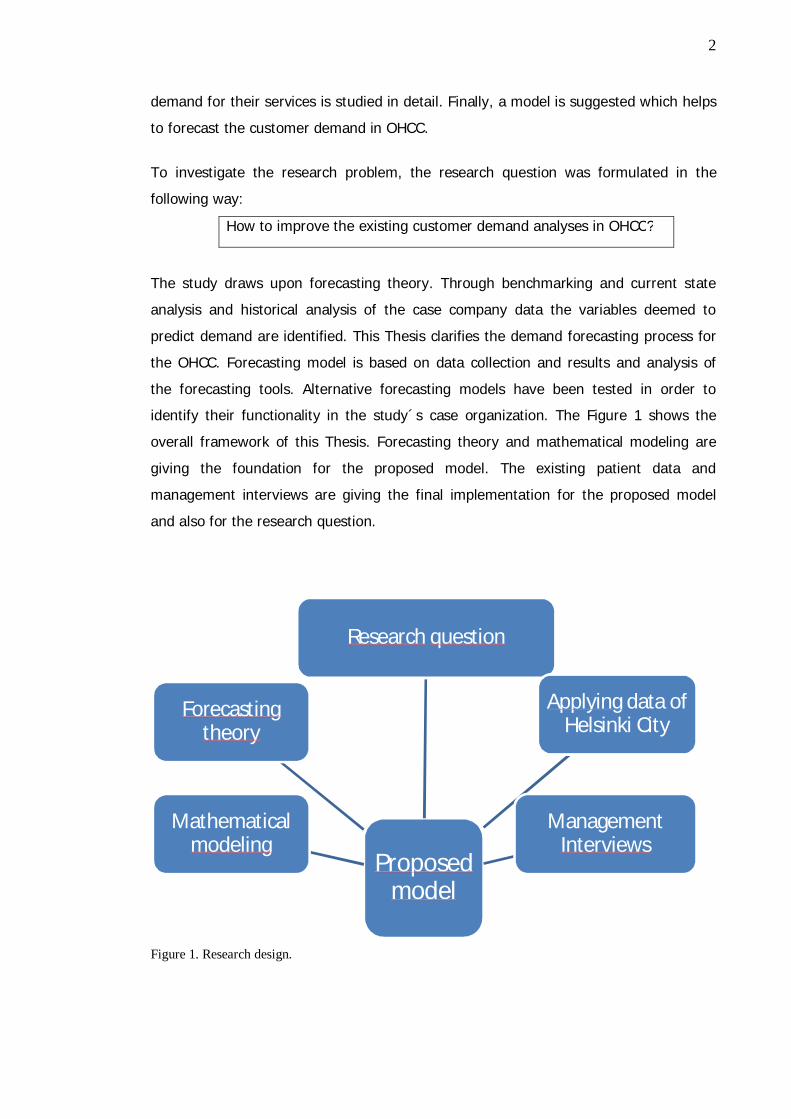
identify their functionality in the study´s case organization. The Figure 1 shows the
overall framework of this Thesis. Forecasting theory and mathematical modeling are
giving the foundation for the proposed model. The existing patient data and
management interviews are giving the final implementation for the proposed model
and also for the research question.
Figure 1. Research design.
Proposedmodel
Research question
Applying data ofHelsinki City
ManagementInterviews
Mathematicalmodeling
Forecastingtheory
3
The outcome of this Thesis represents a tool and model for predicting demand on a
monthly level. This study is not only providing a model for sales forecasting. This
Thesis is more complex than normal sales forecasting process, because of the
complexity of the whole healthcare process, which is presented in the Figure 2 at the
literature analysis section. Need, demand and supply of the healthcare services are
tight in the healthcare service provision.
The present state is that, the study’s case organization does not have a model for
demand forecasting. The organization has set goals and targets for the nursing staff
(doctors, nurses, physiotherapists and psychologies). These goals are only expressing
the targets for each professional group, which they should achieve on a monthly
period. Proposed forecasting model is based on statistical analyses. The historical
background data is gathered from the patient databases, which include all the medical
data from the beginning of the year 2004 on the present date. This Thesis background
data is based on the three year period.
The first section of this Thesis provides knowledge for the existing forecasting models
theories from the literature. Section Research Method and Material introduces the used
research method and mathematical and statistical analyses, which are constructing the
ground for the practical implementation. In section four, The Current status analyses of
the study´s case organization, provides an overview and knowledge to build the
forecasting model. On the section five three different forecasting models are then
examined in order to test which is most appropriate to the context and best serves to
forecast actual service demand. The last sections suggest the actual model for the case
organization and its business unit.
Modern healthcare business has changed the traditional doctor-patient relationship.
Nowadays patient is treated by a team of healthcare professionals, each specializing in
one aspect of healthcare. This kind of shared healthcare depends critically on the
ability to share information between care providers and caring team. From the patients’
point of view, what once was a doctor-patient relationship is now becoming a
customer-company relationship. The customers expect the company to know
everything about their contracts, schedules, and medical histories from the first contact

4
via telephone or online reservation system through the completion of a medical
treatment.
Healthcare management systems must effectively address the needs of its three major
players: the clinicians, administrators, and patients. From the clinicians’ perspective,
performance is measured by speed, reliability, and best clinical practices.
The main focus of this Thesis is to help the healthcare managers to identify and predict
the changing business environment.
5
2 Forecasting Theory
This section introduces the forecasting theory, different forecasting methods and how
organizations should try to develop the forecasting process and how to proceed and
manage the forecasting errors. This section builds the ground for the whole Thesis.
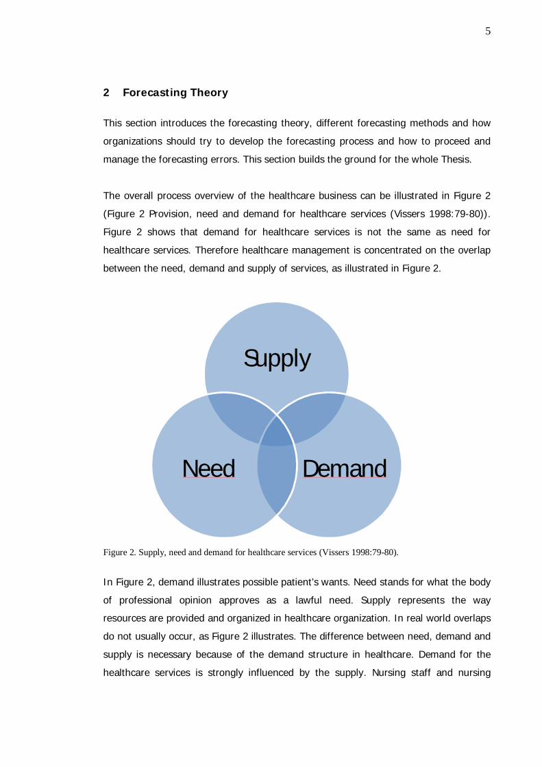
The overall process overview of the healthcare business can be illustrated in Figure 2
(Figure 2 Provision, need and demand for healthcare services (Vissers 1998:79-80)).
Figure 2 shows that demand for healthcare services is not the same as need for
healthcare services. Therefore healthcare management is concentrated on the overlap
between the need, demand and supply of services, as illustrated in Figure 2.
Figure 2. Supply, need and demand for healthcare services (Vissers 1998:79-80).
In Figure 2, demand illustrates possible patient’s wants. Need stands for what the body
of professional opinion approves as a lawful need. Supply represents the way
resources are provided and organized in healthcare organization. In real world overlaps
do not usually occur, as Figure 2 illustrates. The difference between need, demand and
supply is necessary because of the demand structure in healthcare. Demand for the
healthcare services is strongly influenced by the supply. Nursing staff and nursing
Supply
DemandNeed
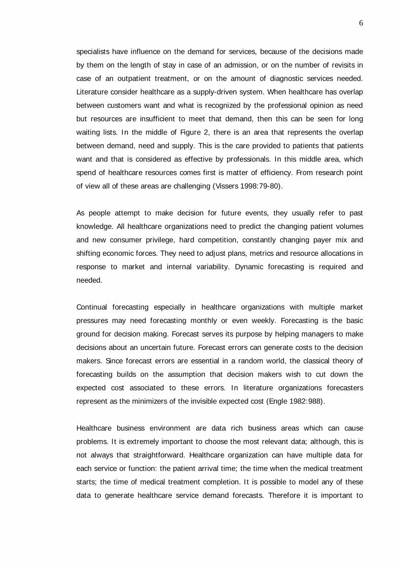
6
specialists have influence on the demand for services, because of the decisions made
by them on the length of stay in case of an admission, or on the number of revisits in
case of an outpatient treatment, or on the amount of diagnostic services needed.
Literature consider healthcare as a supply-driven system. When healthcare has overlap
between customers want and what is recognized by the professional opinion as need
but resources are insufficient to meet that demand, then this can be seen for long
waiting lists. In the middle of Figure 2, there is an area that represents the overlap
between demand, need and supply. This is the care provided to patients that patients
want and that is considered as effective by professionals. In this middle area, which
spend of healthcare resources comes first is matter of efficiency. From research point
of view all of these areas are challenging (Vissers 1998:79-80).
As people attempt to make decision for future events, they usually refer to past
knowledge. All healthcare organizations need to predict the changing patient volumes
and new consumer privilege, hard competition, constantly changing payer mix and
shifting economic forces. They need to adjust plans, metrics and resource allocations in
response to market and internal variability. Dynamic forecasting is required and
needed.
Continual forecasting especially in healthcare organizations with multiple market
pressures may need forecasting monthly or even weekly. Forecasting is the basic
ground for decision making. Forecast serves its purpose by helping managers to make
decisions about an uncertain future. Forecast errors can generate costs to the decision
makers. Since forecast errors are essential in a random world, the classical theory of
forecasting builds on the assumption that decision makers wish to cut down the
expected cost associated to these errors. In literature organizations forecasters
represent as the minimizers of the invisible expected cost (Engle 1982:988).
Healthcare business environment are data rich business areas which can cause
problems. It is extremely important to choose the most relevant data; although, this is
not always that straightforward. Healthcare organization can have multiple data for
each service or function: the patient arrival time; the time when the medical treatment
starts; the time of medical treatment completion. It is possible to model any of these
data to generate healthcare service demand forecasts. Therefore it is important to
7
understand the demand planning process and the customer requirements to select the
most appropriate data. For example, planning may be based on when the healthcare
demand arrives at the appointment system. From the patient’s point of view, a more
appropriate approach may have been to forecast the actual time of the demand
occurrence (Voudouris et. al. 2008:57)
Revenue and expense forecasts can be tied to the payer mix, reimbursement rates and
patient volumes by procedures, admissions or visits needed to generate a given
strategic objective. Finance can provide managers with a useful model that includes
information about past historical data realization and current headcount, as well as
formulas driven by different assumptions. Healthcare managers can then make
adjustments to this baseline on the basis of the latest business conditions. This
approach also ensures collaboration across different functions in the organization.
Demand for healthcare leads to the demand for healthcare services. Forecasting
demand for services makes up a ground for the healthcare organization's development.
Healthcare organizations need accurate projections of the demand for the services that
they are providing.
Modern research represents many quantitative forecasting methods for demand
forecasting. Four most common methods of forecasting in healthcare environment are
defined as percent adjustment, 12-month moving average, trend line, and seasonalized
forecast. These four methods are all based for the organization's recent historical
service data. (Murray et. al. 2004:53)
According to Murray et. al. (2004) there is many quantitative forecasting methods and
models. Forecasting method or model should meet following criteria:
First, the necessary data should be easily available. Financial records typically
represent the best source of historical data. The forecasting method should be able to
use this data. Secondly, existing staff members should be equipped with easily
available tools, such as spreadsheet software such as Microsoft Excel Add-ins or some
selected statistical forecasting software like SPSS or PHstat, should be able to perform
the internal forecasting. Thirdly, the forecasting method and its results should be
8
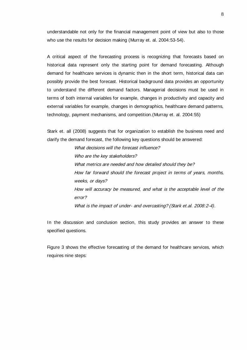
understandable not only for the financial management point of view but also to those
who use the results for decision making (Murray et. al. 2004:53-54).
A critical aspect of the forecasting process is recognizing that forecasts based on
historical data represent only the starting point for demand forecasting. Although
demand for healthcare services is dynamic then in the short term, historical data can
possibly provide the best forecast. Historical background data provides an opportunity
to understand the different demand factors. Managerial decisions must be used in
terms of both internal variables for example, changes in productivity and capacity and
external variables for example, changes in demographics, healthcare demand patterns,
technology, payment mechanisms, and competition.(Murray et. al. 2004:55)
Stark et. all (2008) suggests that for organization to establish the business need and
clarify the demand forecast, the following key questions should be answered:
What decisions will the forecast influence?
Who are the key stakeholders?
What metrics are needed and how detailed should they be?
How far forward should the forecast project in terms of years, months,
weeks, or days?
How will accuracy be measured, and what is the acceptable level of the
error?
What is the impact of under- and overcasting? (Stark et.al. 2008:2-4).
In the discussion and conclusion section, this study provides an answer to these
specified questions.
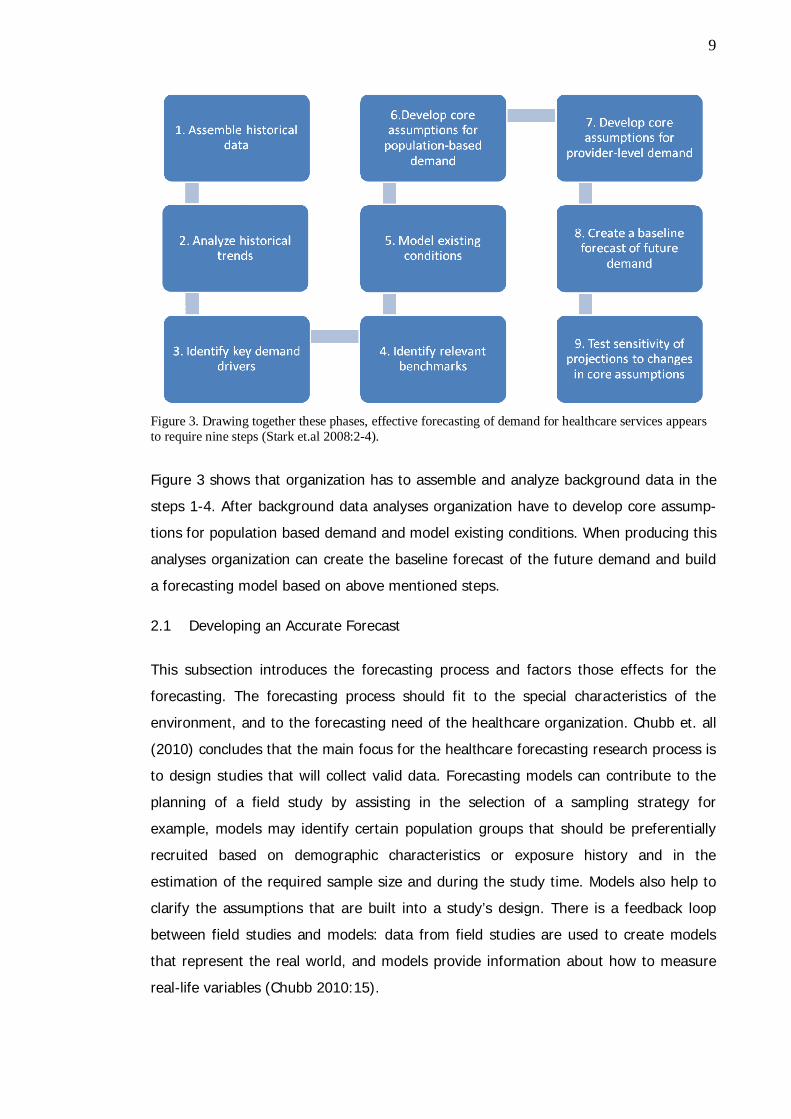
Figure 3 shows the effective forecasting of the demand for healthcare services, which
requires nine steps:
9
Figure 3. Drawing together these phases, effective forecasting of demand for healthcare services appearsto require nine steps (Stark et.al 2008:2-4).
Figure 3 shows that organization has to assemble and analyze background data in the
steps 1-4. After background data analyses organization have to develop core assump-
tions for population based demand and model existing conditions. When producing this
analyses organization can create the baseline forecast of the future demand and build
a forecasting model based on above mentioned steps.
2.1 Developing an Accurate Forecast
This subsection introduces the forecasting process and factors those effects for the
forecasting. The forecasting process should fit to the special characteristics of the
environment, and to the forecasting need of the healthcare organization. Chubb et. all
(2010) concludes that the main focus for the healthcare forecasting research process is
to design studies that will collect valid data. Forecasting models can contribute to the
planning of a field study by assisting in the selection of a sampling strategy for
example, models may identify certain population groups that should be preferentially
recruited based on demographic characteristics or exposure history and in the
estimation of the required sample size and during the study time. Models also help to
clarify the assumptions that are built into a study’s design. There is a feedback loop
between field studies and models: data from field studies are used to create models
that represent the real world, and models provide information about how to measure
real-life variables (Chubb 2010:15).
10
Literature has concluded that successful demand forecasting has two fundamental
objectives: to identify the key variables that grounds the demand for healthcare
services within a selected service area; and to understand how and why these
variables might change over time. Accomplishing these objectives requires a systematic
analytical approach, which ensures that all aspects of potential demand are evaluated.
Using nine-step process proposed by Stark et.al (2008) organization can create a
database and framework for evaluating key variables and testing assumptions, and
provide the necessary basis for accurately forecasting demand (Stark 2008:2-4).
There is no unique established way to describe the forecasting process. One of the key
problems in developing an accurate forecasting process is how to separate the real
time view of forecasting views. Forecasts are usually developed based on assumptions
and static historical information, and the usual differences between actual demand and
forecast demand can be easily misunderstood, resulting in attempts at fixing a non-
existent problem. This can cause a chain reaction that can spread through the whole
organization. (Finarelli 2004:55).
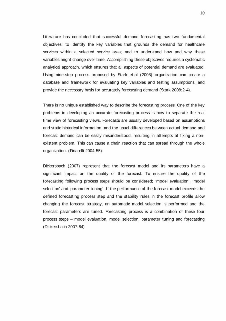
Dickersbach (2007) represent that the forecast model and its parameters have a
significant impact on the quality of the forecast. To ensure the quality of the
forecasting following process steps should be considered; ‘model evaluation’, ‘model
selection’ and ‘parameter tuning’. If the performance of the forecast model exceeds the
defined forecasting process step and the stability rules in the forecast profile allow
changing the forecast strategy, an automatic model selection is performed and the
forecast parameters are tuned. Forecasting process is a combination of these four
process steps – model evaluation, model selection, parameter tuning and forecasting
(Dickersbach 2007:64)
11
Figure 4. Process for forecasting (Dickersbach 2007:64).
Structured forecasting process may lead to a better understanding of the provided
healthcare service (Dickersbach 2007:64).
Understanding the available historical data is the first step to start constructing
forecasts. Without real knowledge of the historical data it is difficult to build any
forecasting models. Healthcare data typically includes patient units of care, visit reason
data, diagnosis data and visit time information, also laboratory and x-ray data might be
included, in the model depending on what is the aim for forecasting. These data’s
should reflect the current and historical demand for the healthcare. The standard
summary statistics, for example mean, standard deviation, are useful in providing a
basic understanding of the data. For the decision makers and forecasters it is
important to identifying appropriate amount of the data and to identify any general
patterns. It is important to decide at the outset, what level of detail organization
requires for the forecast. Inpatient utilization can be analyzed along several
dimensions, including patient age, payer, product line (occupational healthcare
services), major service or any combination for these dimensions. Data which is
gathered should include and investigate both patient activity levels and throughput
measures (such as average length of stay, visit duration, or procedure time) if service
capacities (including numbers operating rooms, or treatment stations) need to be
determined. This Thesis is concentrating on measurements and conditions that case
organization conducts as healthcare service provider (Voudouris et. al. 2008:54-56).
12
One way to better understand the historical data is the use of scatter plots to identify
possible correlation or non-linearity of the existing data. Time series graphs can
indicate any patterns or unusual observations. When analyzing time series data there
are four common patterns that observer should be aware of. Horizontal or stationary
data fluctuate about a constant mean, trend: a long-term increase or decrease in the
data, seasonal: a repeating pattern that depends on seasonal factors, for example days
of the week, months of the year, cyclical: a recurring pattern that may have different
length at irregular intervals (Voudouris et. al.2008:54-56).
Other types of data that healthcare organization has to investigate and take into
consideration might include information about patient origin and market share by
product line and geographic area, and emergency department visits by patient type for
example admitted, fast-track, psychiatric and other types of patients and arrival time.
However, other type of data mentioned above is not so important for this Thesis,
because the case organization patient population is in the Helsinki metropolitan area
and, the case organization is not providing emergency services, only occupational
services.
In literature is stated that administrative, financial and departmental data may
sometimes vary significantly, because each of these areas collects and analyzes
different statistics for different reasons. It has been said that many external databases
have incomplete, inconsistent, or out of date information. It is therefore best to
compare several data sources, if possible, to identify the most appropriate set of
historical demand data (Finarelli 2004:50-70).
Organization have to examine at least three years of data to identify key trends which
are an absolute change, a percentage change, and an average annual percentage
change of the service data. This Thesis is using data between years 2008-2010 to
construct the best possible forecast for the demand forecasting. Developing contacts
between measures of the healthcare service demand may also be helpful for example,
when studying admissions through the occupational services versus number of
occupational service visits. Large changes in such ratios over a short time are unusual
13
and may signal an underlying data problem. Changing data classification schemes
should also be noted (Voudouris et. al. 2008:57-60).
Organization has to identify the key demand drivers. The key drivers of population-
based demand include population growth and aging as well as changes in the
technology or treatment patterns which affect specific service use rates. Other demand
factors specific to a particular service, such as the substitution of insignificant
procedures for certain types of medical treatment may also need to be identified and
incorporated into the analysis (Finarelli 2004:50-70). In this Thesis aging and changes
in the case organization workers´ working conditions are also considered when
building a method for forecasting and analyzing the forecasting results.
Healthcare organization has to identify relevant benchmarks for forecasting processes.
These benchmarks can provide the different reference for determining the demand
trends in organization service area. Benchmarks need to be in line with wider
marketplace or national trends in healthcare. Relevant benchmarks can include, use
rates in comparative markets, established best practices or treatment protocols, or
service-specific guidelines and performance measures.
Benchmarking opportunities include national or statewide databases; established best
practices and protocols guidelines and performance measures published by know
organizations. Medical journals that report results of clinical trials can be also
considered as a benchmark. Web sites of recognized market leaders will provide
potential sources for benchmarking. Also other researches may provide knowledge for
organizations to start to implement forecasting process. (Finarelli 2004:50-70).
When starting to implement the forecasting process organization has to model existing
conditions. For example, it may develop a spreadsheet model that best replicates the
latest authenticated market data and market statistics. One difficulty is that the latest
authenticated market data or market statistics for other providers may be more than a
year old and not that easily available. Historical data and historical trends should be
used to develop the most reasonable combination of assumptions about current
conditions for the key demand drivers. If the model cannot replicate existing
conditions, it cannot be used to predict future demand. (Tae et. al. 2009:1064).
14
Organization has to develop core assumptions for provider level demand. Factors that
determine demand at the provider level include market share, patient mix or flow
patterns, and operational performance. These factors are often called controllable
factors because they can be affected by specific actions of the provider (Thomas
2003:55).
Using the most aggressive performance targets is considered as good business
planning and tends to moderate the increase in resource requirements for example,
staffing levels, facility capacity that might otherwise accompany projected increases in
inpatient volumes. (Thomas 2003:54-60).
Healthcare organization has to develop core assumptions for population-based
demand. Key factors affecting such demand include population growth, aging, and use
rate and demographic profile including age mix. These factors are often called external
factors, because they are outside of the healthcare organization's control. Organization
can then use above mentioned nationwide databases and scientific medical
publications. Occupational healthcare service providers often have better source of
information about above mentioned customer data, because they know the population
of the organization.
When organization is creating a baseline forecast of it future demand it has to take into
consideration that forecast should combine the core assumptions for both population
based and provider level demand. A baseline forecast includes reasonable assumptions
for external factors such as population based demand, reasonable market share targets
of the provider specific utilization levels and aggressive performance improvement of
the baseline workload projections (Thomas 2003:54-60).
Organization has to consider alternative scenarios with different sets of assumptions.
These kinds of scenarios might include low and high rates of change in population-
based use rates. Results for this kind of changes, for non specific or specific reason,
fall short when achieving projected operational efficiencies or other performance
improvement targets. This helps organization to operate in different market situations.
(Alho 1990:523-530).
15
It is useful to consider a best case scenario, with more promising assumptions, for
example as higher population based demand, greater market share growth than were
used in the baseline forecast. However it is probably more important for the
organization to test the dark side of the sensitivity by using less promising assumptions
about use rates, market share, or performance improvement (Finarelli 2004:50-70).
However it is not enough to simply project the historical trends regarding these
population characteristics. Organization also must consider the factors that are causing
demand to change and to hypothesize how these factors may change over time. Other
factors that influence population based demand include medical practice patterns,
structure of the service delivery system, and availability and design of insurance
coverage (Alho 1990:523-530).
When healthcare organization is starting to forecast its demand for a given population
it has to define the applicable geographic market or service area. The service area is
most often expressed as a group of continuous zip codes, a single county, or multiple
counties. In some applications, it is appropriate to define both a primary service area
and a secondary service area. The appropriate definition of a service area may vary by
service, even for the same service provider. (Thomas 2003:55-57). Service area of this
Thesis is predefined as one selected business unit and its customers.
The age mix of the population is a key factor when organization is forecasting demand,
as demand for healthcare services can vary dramatically by age. A population pyramid,
also called an age structure diagram, shows the distribution of various age groups in a
human population. It ideally forms the shape of a pyramid when the region is healthy.
Population pyramid typically consists of two back-to-back bar graphs, with the
population plotted on the X-axis and age on the Y-axis, one showing the number of
males and one showing females in ten-year age groups. Males are conventionally
shown on the left and females on the right.
Population projections can usually be obtained by age group as well as by geographic
area. To capture the effect of age on demand, the demand model should be include at
16
least four age groups (0-14,15-44, 45-64, and 65 ). In this Thesis age groups are
between fewer than 30, 30-39, 40-49 and 50-59 and over 60. (Finarelli 2004:50-70).
Alho (1990) suggests that when multiplying the service area population of each age
group by the expected use rate for a particular service, will tell the projected demand
for that service, in that service area. Use rates are defined as a measure of health
services utilization per 1,000 population (for example physician office visits per 1,000
population). Use rates can be determined from a variety of state and national
databases, particularly for inpatient services and for many outpatient services. (Alho
1990:523-530).
Use rates can vary in geographic regions. Much of this variability can be attributed to
the demographic profile of the population within the region, especially the age mix.
(Alho 1990:523-530).
The relationship between age specific use rates and overall use rates tends to be the
same in almost all market regions, regardless of the overall use rate for a given
service. Finarelli (2004) proposes an example for the discharge rate for patients age 45
to 64 which is usually very close to the overall discharge rate for all ages and the
discharge rate for persons age 65 and over is typically about three times the overall
rate. Age specific discharge rates for any given market usually can be estimated once
the overall rate for the market is determined. (Finarelli 2004:50-70).
Population based factors that concerns to the provider and its competitors service area
also affect the demand and consumption of a provider's healthcare services. Major
factors include competitive market position, configuration of services and facilities
within the market, capacity constraints, operational efficiencies, and seasonal factors.
These factors influence how many patients will use a specific provider as well as
departmental workload levels. (Alho 1990 523-530).
17
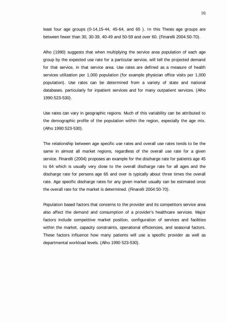
Figure 5. Major steps in the forecasting model (Stark et.al 2008:4).
By using different forecasting techniques, organizations can adjust the decisions that
will help achieve their goals. The major steps that should be addressed in forecasting
include the following methods which can be seen in Figure 5. Circle starts with
established the business needs which organization has to decide before starting the
forecasting process.
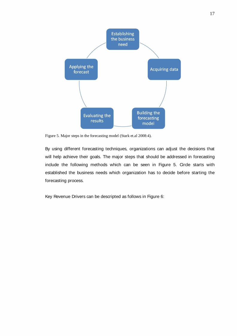
Key Revenue Drivers can be descripted as follows in Figure 6:
18
Figure 6. Key revenue drivers (Stark et.al. 2008:4).
These Key revenue drivers includes combination of the patient, physician and service
center mix. Contracts between different parties’ business office performance and
volume walk hand in hand in the key revenue driver description. Seasonal changes for
example spring time influenza wave will effect to the key revenue drivers. Target
markets, new equipment schedules and utilization rates will provide different effects to
the key revenue drivers. Healthcare organization has to recognize these seasonal
factors because they give an impact for the actual forecasts.
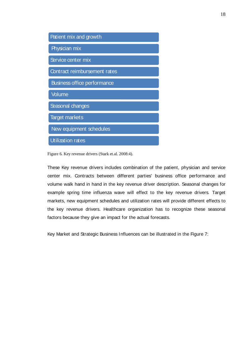
Key Market and Strategic Business Influences can be illustrated in the Figure 7:
Patient mix and growth
Physician mix
Service center mix
Contract reimbursement rates
Business office performance
Volume
Seasonal changes
Target markets
New equipment schedules
Utilization rates
19
Figure 7. Key Market and strategic business influences (Stark et. al. 2008:5).
Above mentioned key market and strategic business common factors have to be taking
into consideration when forecasting demand in the healthcare sector. (Stark et. al.
2008:5-6)
2.2 Forecasting Models
Previous sub-section represents the steps which organization has to take into
consideration when constructing an accurate forecast. This sub-section discusses with
different forecasting models.
The forecasting model and its parameters have a significant impact on the quality of
the forecast. In general, there are two main types of forecasting methodologies. The
scientific approach of statistical models based on historical data and the less
mechanical approach using the judgement of experts. There are many different
statistical methods, varying in complexity from relatively simple for example mean
levels to sophisticated or computationally intensive techniques such as Autoregressive
Integrated Moving Average (ARIMA). Judgmental forecasts are made by individuals
based on their knowledge of the environment; this might include information about
past events and expectations of likely future events or trends. Figure 8 Methodology
Local competitive pricing
Inflation rate
Facility expansion plans
Local population growth
Payer market shares
Advertising/promotion spend
Natural disasters
Government policy shifts
Patient satisfaction surveys Regional wellness indicators
20
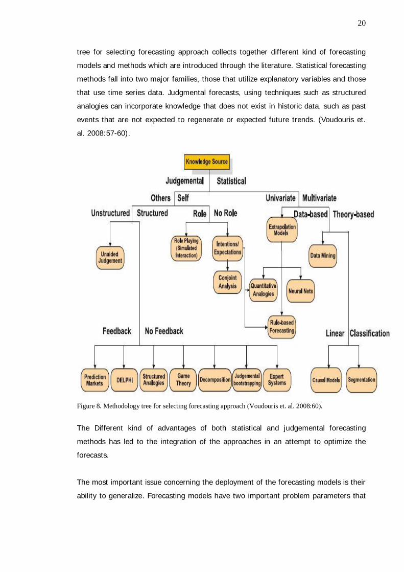
tree for selecting forecasting approach collects together different kind of forecasting
models and methods which are introduced through the literature. Statistical forecasting
methods fall into two major families, those that utilize explanatory variables and those
that use time series data. Judgmental forecasts, using techniques such as structured
analogies can incorporate knowledge that does not exist in historic data, such as past
events that are not expected to regenerate or expected future trends. (Voudouris et.
al. 2008:57-60).
Figure 8. Methodology tree for selecting forecasting approach (Voudouris et. al. 2008:60).
The Different kind of advantages of both statistical and judgemental forecasting
methods has led to the integration of the approaches in an attempt to optimize the
forecasts.
The most important issue concerning the deployment of the forecasting models is their
ability to generalize. Forecasting models have two important problem parameters that
21
should be accounted for. The first is data preparation, which involves preprocessing
and the selection of the most significant variables. The second embraces the
determination of the optimum model structure (Sfetsos 2003:57).
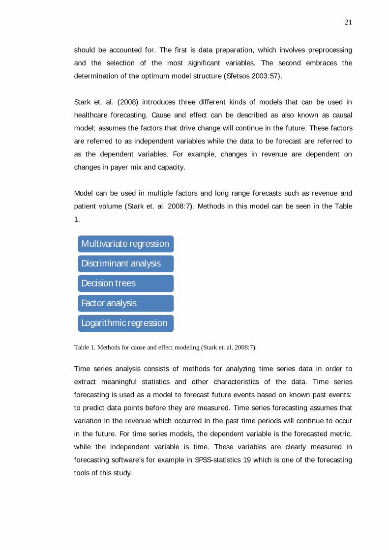
Stark et. al. (2008) introduces three different kinds of models that can be used in
healthcare forecasting. Cause and effect can be described as also known as causal
model; assumes the factors that drive change will continue in the future. These factors
are referred to as independent variables while the data to be forecast are referred to
as the dependent variables. For example, changes in revenue are dependent on
changes in payer mix and capacity.
Model can be used in multiple factors and long range forecasts such as revenue and
patient volume (Stark et. al. 2008:7). Methods in this model can be seen in the Table
1.
Table 1. Methods for cause and effect modeling (Stark et. al. 2008:7).
Time series analysis consists of methods for analyzing time series data in order to
extract meaningful statistics and other characteristics of the data. Time series
forecasting is used as a model to forecast future events based on known past events:
to predict data points before they are measured. Time series forecasting assumes that
variation in the revenue which occurred in the past time periods will continue to occur
in the future. For time series models, the dependent variable is the forecasted metric,
while the independent variable is time. These variables are clearly measured in
forecasting software’s for example in SPSS-statistics 19 which is one of the forecasting
tools of this study.
Multivariate regression
Discriminant analysis
Decision trees
Factor analysis
Logarithmic regression
22
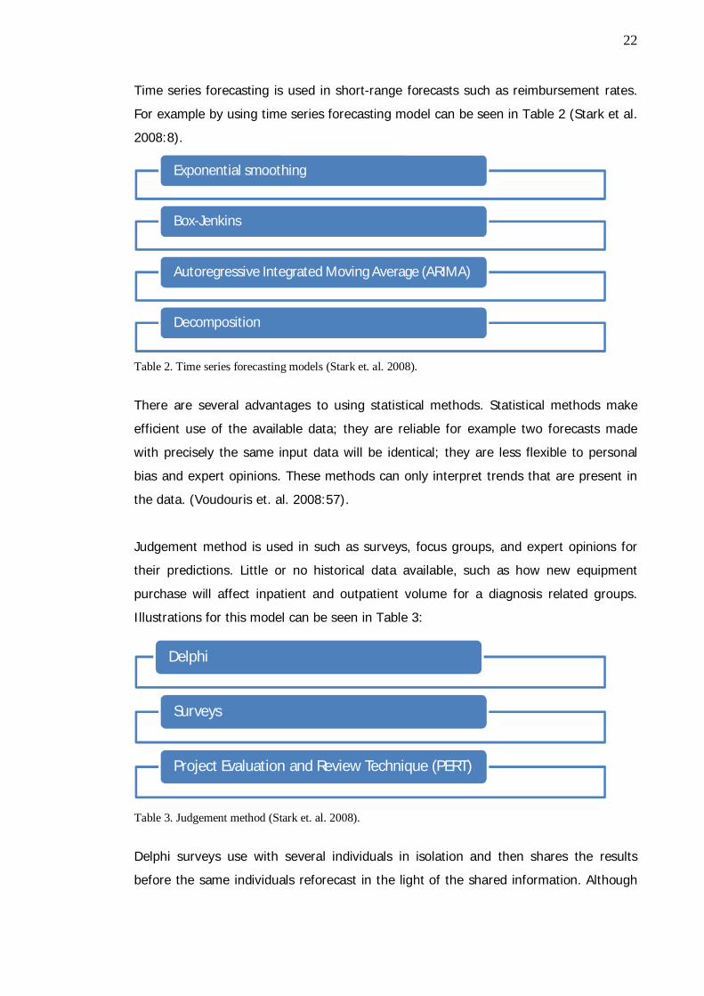
Time series forecasting is used in short-range forecasts such as reimbursement rates.
For example by using time series forecasting model can be seen in Table 2 (Stark et al.
2008:8).
Table 2. Time series forecasting models (Stark et. al. 2008).
There are several advantages to using statistical methods. Statistical methods make
efficient use of the available data; they are reliable for example two forecasts made
with precisely the same input data will be identical; they are less flexible to personal
bias and expert opinions. These methods can only interpret trends that are present in
the data. (Voudouris et. al. 2008:57).
Judgement method is used in such as surveys, focus groups, and expert opinions for
their predictions. Little or no historical data available, such as how new equipment
purchase will affect inpatient and outpatient volume for a diagnosis related groups.
Illustrations for this model can be seen in Table 3:
Table 3. Judgement method (Stark et. al. 2008).
Delphi surveys use with several individuals in isolation and then shares the results
before the same individuals reforecast in the light of the shared information. Although
Exponential smoothing
Box-Jenkins
Autoregressive Integrated Moving Average (ARIMA)
Decomposition
Delphi
Surveys
Project Evaluation and Review Technique (PERT)
23
Delphi survey approach reduces assumptions, it can be time consuming and, that may
not be appropriate way for short term forecasting (Voudouris et. al.2008:60).
Exploration based models are also used in forecasting such as Neural network
forecasting which are model based methods. Neural networks models are data driven
and self adjustable models. A neural network modeling is based on learning and
predicting. Neural networks based models use generalizing techniques and models.
Neural network models are good with non linear models and it can work well with
sample data contain misjudged information. Forecasting models in general assumes
that there is an underlying known or linear relationship between the inputs. Traditional
statistical forecasting models algorithm have limitations in estimating underlying
function due to the complexity of the real system. Neural networks models are often
non linear. (Coskun et. al. 2009:3839-3844) This Thesis leaves the neural networks
models for other researchers.
2.3 Forecasting Errors
Previous sub-sections have been introducing different forecasting methods. However,
when using different demand forecasting models in service business and healthcare
services business it is important to understand the constant error possibilities that
different models might include.
In forecasting, a forecast error is the difference between the real and the forecasted
value of a time series or any other phenomenon of interest. Error measures also play
an important role in calibrating or redefining a model so that it will forecast accurately
for a set of time series. In time series or statistical modeling the analyst may wish to
examine the effects of using different parameters in an effort to improve a model
(Armstrong et. al.1992:70).
Forecast may be assessed using the difference or using a relative error. In general the
error is defined using the value of the outcome minus the value of the forecast.
Different kind of error methods are used in forecasting error measurement such as
Mean Square Error (MSE) and Mean Absolute Percentage Error (MAPE), Relative
Absolute Error (RAE), Mean percentage error (MPE) Standard deviation of absolute
percentage errors (SDAPE). A single series may dominate the analysis because it has a
24
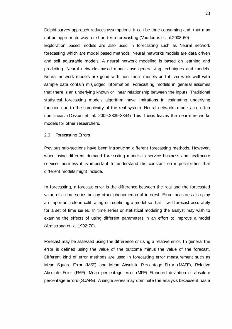
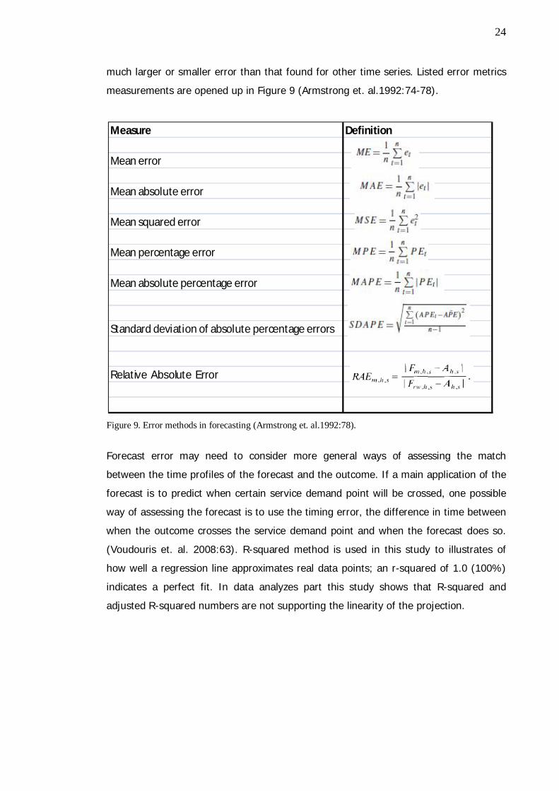
much larger or smaller error than that found for other time series. Listed error metrics
measurements are opened up in Figure 9 (Armstrong et. al.1992:74-78).
Figure 9. Error methods in forecasting (Armstrong et. al.1992:78).
Forecast error may need to consider more general ways of assessing the match
between the time profiles of the forecast and the outcome. If a main application of the
forecast is to predict when certain service demand point will be crossed, one possible
way of assessing the forecast is to use the timing error, the difference in time between
when the outcome crosses the service demand point and when the forecast does so.
(Voudouris et. al. 2008:63). R-squared method is used in this study to illustrates of
how well a regression line approximates real data points; an r-squared of 1.0 (100%)
indicates a perfect fit. In data analyzes part this study shows that R-squared and
adjusted R-squared numbers are not supporting the linearity of the projection.
Measure Definition
Mean error
Mean absolute error
Mean squared error
Mean percentage error
Mean absolute percentage error
Standard deviation of absolute percentage errors
Relative Absolute Error
25
3 Research Method and Material
This Thesis has first introduced the findings from the literature, how healthcare
organization should select the forecasting model and built the forecasting process.
Current status analyses of the case business unit customers are introducing
demographic information such as age profile of the selected customers group.
Historical background data analysis has pointed out the fact, that OHCC has seasonal
changes in the service provision. In the section 5 three different forecasting models are
introduced and tested. Comparison is done with R-squared method which is introduced
in this Thesis. Selected and proposed model is tested and compared with the actual
service group event realization figures from the January and the February 2011.
Management interviews were conducted after analysis and selection of the forecasting
model. Management interviews consists the two managers of the selected business
unit and the CEO of the OHCC. Discussion and conclusion part polishes the selected
model.
This section describes the case study research method which is followed by the flow of
this research. The second subsection introduces the used background data, which
includes data interpretation of the Thesis. Second subsection describes the process for
making appointments. Third subsection introduces the other research materials such as
mathematical models and used forecasting tools and methods. The validity and
reliability issues are discussed at the end.
3.1 Research Method
Case study is a method that focuses on understanding the dynamics in a context.
Generally case studies are preferred, when “how” or “why” questions are to be
answered (Yin 2009: 6). A case study is a research method common in social science.
It is based on an in depth investigation of a single individual, group, or event. Case
studies may be descriptive or explanatory. Case studies are considered as an
appropriate research strategy particularly for new types of research areas where
qualitative data is needed in the creation of proper understanding of the studied
phenomena. Usually the first step in case study research is to determine and define the
26
research question and then select the cases and determine the data gathering and
analyzing techniques. Data is then collected, evaluated and analyzed.
This Thesis is conducted as case study method for selected business unit of Helsinki
City Occupational HealthCare centre and its doctor’s demand. Data interpretation is
done IBM Cognos tools and forecasting is produced with Microsoft Excel spreadsheets
and SPSS Statistics 19 analysis. The research strategy is quantitative.
In this Thesis, the case study research is based on mathematical modeling. The study
relies on the mathematical model ARIMA (Autoregressive integrated moving average)
applied in this research. In this Thesis the case study research is based on
mathematical modeling. The study relies on the mathematical model ARIMA
(Autoregressive integrated moving average) applied in this research. The ARIMA model
has been selected for this Thesis based on past researches such as Milner 1988 (Milner
1988:1061-1076) Trent Region’s Accident and Emergency (A&E) departments number
of attendant in Emergency department. Milner introduced ARIMA model for forecasting
attendant in Trent Region’s Accident and Emergency departments. Farmer et. al 1990
(Farmer et. al. 1990:307–312) use ARIMA to predict the number of surgical beds
required at the Charing Cross Hospital (Farmer et. al. 1990:307–312). Finarelli 2004
and Stark et. al. 2008 has introduced ARIMA model and other time series modeling
used in health care sector (Finarelli 2004. Stark et. al. 2008).
3.2 Data Description
This research applies the concept of unit which has been used in the case
organizations business unit and patient healthcare data for 2-4 years. Units of care are
entered to OHCC data system by the doctors, who are providing the medical services
for the customers. Data system, which OHCC is using, is provided with company called
Acute FDs. Patient data system is called Acute (formerly TT2000+). Units of care
examined in this Thesis are defined as status “Ready” –events. “Ready”-events are
defined and used in the OHCC patient data system when medical staff is applying the
units of care in the system and finishing their medical treatment sessions. Same
patient system use invoiced unit as status “Invoiced”-units of care. These events do
not consist the needed time data that this Thesis analyses. Units of care can be
27
defined as short medical examinations 10-29 minutes, long medical examinations 30-
90 minutes, phone call consultation or working condition examination which takes
place in the working place. This Thesis introduces different time series data of the
above specified care of unit groups.
3.3 Process for Making Appointments
In this subsection is described the process how the selected business unit confronts
the demand on customers site. Healthcare processes can be classified as medical
treatment processes or generic organizational processes. Medical treatment processes,
are directly linked to the patient and are executed according to a diagnostic
therapeutic cycle, comprising observation, reasoning and action. The diagnostic
therapeutic cycle depends heavily on medical knowledge to deal with case specific
decisions that are made by interpreting patient specific information. On the other hand,
organizational or administrative processes are generic process patterns that support
medical treatment processes in general. They are not tailored for a specific condition
but aim to coordinate medical treatment among different people and organizational
units. Patient scheduling and exam requests are two examples of organizational
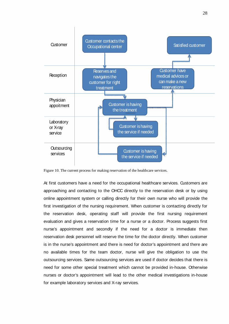
processes. Figure 10 illustrates the process for making reservation of the healthcare
services.
28
Figure 10. The current process for making reservation of the healthcare services.
At first customers have a need for the occupational healthcare services. Customers are
approaching and contacting to the OHCC directly to the reservation desk or by using
online appointment system or calling directly for their own nurse who will provide the
first investigation of the nursing requirement. When customer is contacting directly for
the reservation desk, operating staff will provide the first nursing requirement
evaluation and gives a reservation time for a nurse or a doctor. Process suggests first
nurse’s appointment and secondly if the need for a doctor is immediate then
reservation desk personnel will reserve the time for the doctor directly. When customer
is in the nurse’s appointment and there is need for doctor’s appointment and there are
no available times for the team doctor, nurse will give the obligation to use the
outsourcing services. Same outsourcing services are used if doctor decides that there is
need for some other special treatment which cannot be provided in-house. Otherwise
nurses or doctor’s appointment will lead to the other medical investigations in-house
for example laboratory services and X-ray services.
Customer
Reception
Physicianappoitment
Laboratoryor X-rayservice
Outsourcingservices
Customer contacts theOccupational center
Reserves andnavigates the
customer for righttreatment
Customer is havingthe treatment
Customer is havingthe service if needed
Customer is havingthe service if needed
Customer havemedical advices or
can make a newreservations
Satisfied customer
29
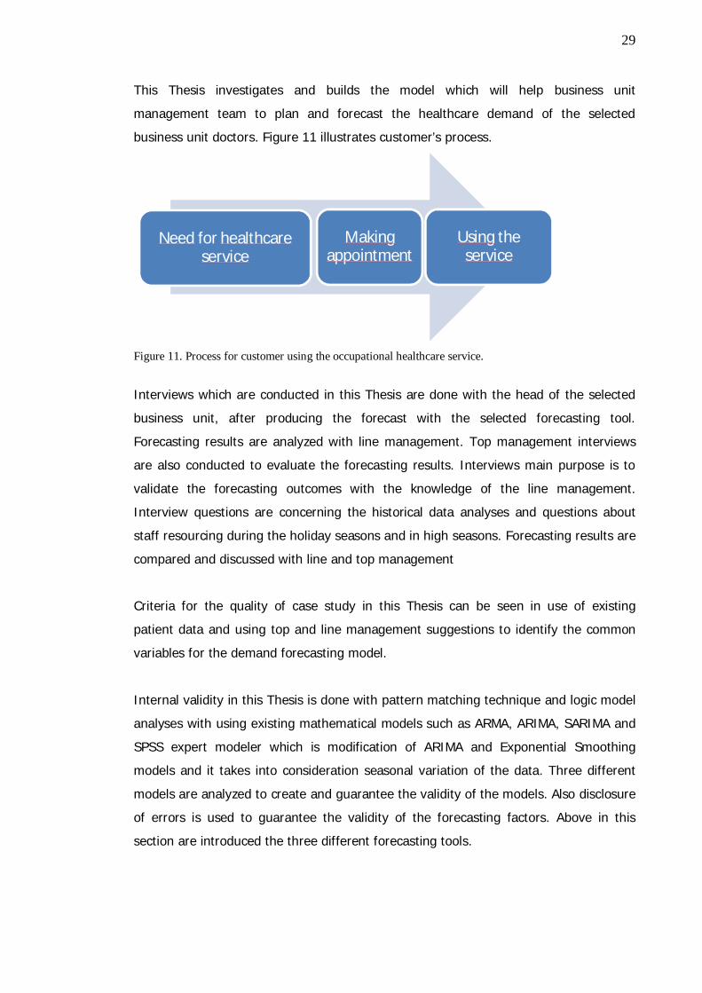
This Thesis investigates and builds the model which will help business unit
management team to plan and forecast the healthcare demand of the selected
business unit doctors. Figure 11 illustrates customer’s process.
Figure 11. Process for customer using the occupational healthcare service.
Interviews which are conducted in this Thesis are done with the head of the selected
business unit, after producing the forecast with the selected forecasting tool.
Forecasting results are analyzed with line management. Top management interviews
are also conducted to evaluate the forecasting results. Interviews main purpose is to
validate the forecasting outcomes with the knowledge of the line management.
Interview questions are concerning the historical data analyses and questions about
staff resourcing during the holiday seasons and in high seasons. Forecasting results are
compared and discussed with line and top management
Criteria for the quality of case study in this Thesis can be seen in use of existing
patient data and using top and line management suggestions to identify the common
variables for the demand forecasting model.
Internal validity in this Thesis is done with pattern matching technique and logic model
analyses with using existing mathematical models such as ARMA, ARIMA, SARIMA and
SPSS expert modeler which is modification of ARIMA and Exponential Smoothing
models and it takes into consideration seasonal variation of the data. Three different
models are analyzed to create and guarantee the validity of the models. Also disclosure
of errors is used to guarantee the validity of the forecasting factors. Above in this
section are introduced the three different forecasting tools.
Need for healthcareservice
Makingappointment
Using theservice
30
External validity in this Thesis is recognized in the literature where in other research
studies have used similar mathematical models in predicting the demand of the
healthcare services. (Yin 2009:34-39).
Research techniques that are used in this Thesis are following:
- Statistical analysis of the existing patient database.
- Constructing the actual forecasting model.
- Data which is used in the model is analyzed with top and line
management interviews.
- Validating and comparing the results.
- Forecasting interpretation is conducted whit top management and line
managers.
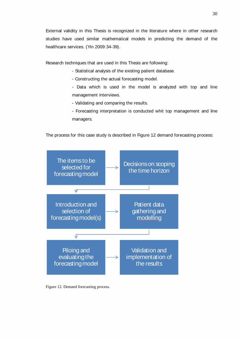
The process for this case study is described in Figure 12 demand forecasting process:
Figure 12. Demand forecasting process.
The items to beselected for
forecasting model
Decisions on scopingthe time horizon
Introduction andselection of
forecasting model(s)
Patient datagathering and
modelling
Piloing andevaluating the
forecasting model
Validation andimplementation of
the results
31
3.4 Research Material
Forecasting material can be defined as the historical data and human resource data.
Forecasting tools which are introduced in this Thesis, such as Microsoft ARMA Add-in
and SPSS statistics 19 are providing the tool for this study’s model. Other sources of
materials are shown as graphs and figures based on the use of the forecasting tools
and based on the Occupational data mining which are conducted with by using Cognos
BI 8.3 tools.
3.4.1 Background for the Forecasting Tools
This section describes the mathematical background of the forecasting tools analyzed
in this Thesis.
Other researcher in healthcare forecasting has been using ARIMA model as demand
forecasting tool. Milner PC (Milner 1988:1061-1076) describes an ARIMA model that
predicts the annual number of attendances at Trent Region’s Accident and Emergency
(A&E) departments. Milner evaluated the accuracy of his earlier forecasts with
generally favorable results and recommend that ARIMA modeling for to be registered
fully into planning at health district levels. Farmer et al (Farmer et. al. 1990:307–312)
used ARIMA to predict the number of surgical beds required at the Charing Cross
Hospital (Farmer et. al. 1990:307–312). Gilchrist describes the use of queuing theory
to estimate hospital bed requirements with ARIMA model (Gilchrist 1985:206).
Research mentioned above has mainly concerned with identifying the strategic service
requirements.
This Thesis investigates mathematical models which are relevant in the literature to
conduct time series forecasting in accurate way. Autoregressive Integrated Moving
Average ARIMA model is introduced here as a one relevant case study model.
Autoregressive integrated moving average (ARIMA) model is a generalization of an
autoregressive moving average (ARMA) model. Time series forecasting methods are
more appropriate for short term forecast which are applied for this study.
The ARMA model consists of two basic load components, a deterministic and a
stochastic component. The first parameter stands for the periodic part of the load
32
shape, while the second parameter points out the deviation of the random effects. The
deterministic component is given by a time dependent periodic nonlinear function, and
the stochastic one is represented by an ARMA model if the underlying stochastic
process is stationary with limited variance, or an ARIMA (autoregressive integrated
moving average) model if the underlying stochastic process is non-stationary.
(Tzafestas et. al.2001:10)
Auto regressive integrated moving average (ARIMA) models intend to describe the
current behavior of variables in terms of linear relationships with their past values.
These models are also called Box-Jenkins (1984) models on the basis of these authors’
pioneering work regarding time series forecasting techniques. An ARIMA model can be
decomposed in two parts. First, it has an Integrated (I) component (d), which
represents the amount of differencing to be performed on the series to make it
stationary. The second component of an ARIMA consists of an ARMA model for the
series rendered stationary through differentiation.
This model type is generally referred to as ARIMA(p,d,q), with the integers referring to
the autoregressive, integrated and moving average parts of the data set, respectively.
ARIMA modeling can take into account trends, seasonality, cycles, errors and non-
stationary aspects of a data set when making forecasts.
These models are fitted to time series data either to better understand the data or to
predict future points in the forecasting. Models are applied and conducted in some
cases where data shows evidence of non stationary demand, where an initial
differencing step corresponding to the integrated part of the model can be applied to
remove the non-stationary model.
The ARIMA(p,d,q) model where p, d, and q are non-negative integers that refer to the
order of the autoregressive, integrated, and moving average parts of the model. When
one of the terms is zero, it's usual to drop AR, I or MA. For example, an I(1) model is
ARIMA(0,1,0), and a MA(1) model is ARIMA(0,0,1).

33
Definition of the model can be conducted as follows: Given a time series of data Xt
where t is an integer index and the Xt are real numbers, then an ARMA(p,q) model is
given by
where L is the lag operator, the i are the parameters of the autoregressive part of the
model, the i are the parameters of the moving average part and the \varepsilon_t are
error terms. The error terms \varepsilon_t are generally assumed to be independent,
identically distributed variables sampled from a normal distribution with zero mean.
(Mills et. al.1991:116-120)
ARIMA models are used for observable non-stationary processes Xt that have some
clearly identifiable trends:
Constant trend for example a non-zero average leads to d = 1
Linear trend for example a linear growth behavior leads to d = 2
Quadratic trend for example a quadratic growth behavior leads to d = 3
In these cases the ARIMA model can be viewed as a cascade of two models. The first
is non-stationary:
While the second is wide sense stationary:
(Mills et. al.1991:116-120)
The numbers of variations on the ARIMA model are commonly used in literature. For
example, if multiple time series are used then the Xt can be thought of as vectors and
a VARIMA model may be appropriate. Sometimes a seasonal effect is suspected in the
model. For example model of daily road traffic volumes. Weekends clearly exhibit
different behavior from weekdays. In this case it is often considered better to use a
SARIMA (seasonal ARIMA) model than to increase the order of the AR or MA parts of
34
the model. If the time series is suspected to exhibit long range dependence then the d
parameter may be replaced by certain non-integer values in an autoregressive
fractionally integrated moving average model, which is also called a Fractional ARIMA
(FARIMA or ARFIMA) model (Mills et. al. 1991:116-120).
ARIMA models such as those described above are easy to implement on a spreadsheet.
The prediction equation is simply a linear equation that refers to past values of original
time series and past values of the errors. Researcher can set up an ARIMA forecasting
spreadsheet by storing the data in column A, the forecasting formula in column B, and
the errors (data minus forecasts) in column C. The forecasting formula in a typical cell
in column B would simply be a linear expression referring to values in preceding rows
of columns A and C, multiplied by the appropriate AR or MA coefficients stored in cells
elsewhere on the spreadsheet (Mills et. al. 1991:116-120).
In this Thesis ARIMA-model is build in to the IBM Cognos planning tool to formulate
the demand. SPSS Statistics 19 is used to model the forecast figures. Comparison of
the tools is done with using Microsoft excel add-in.
3.4.2 Forecasting Tools
This subsection introduces the three forecasting tools which are used in this study.
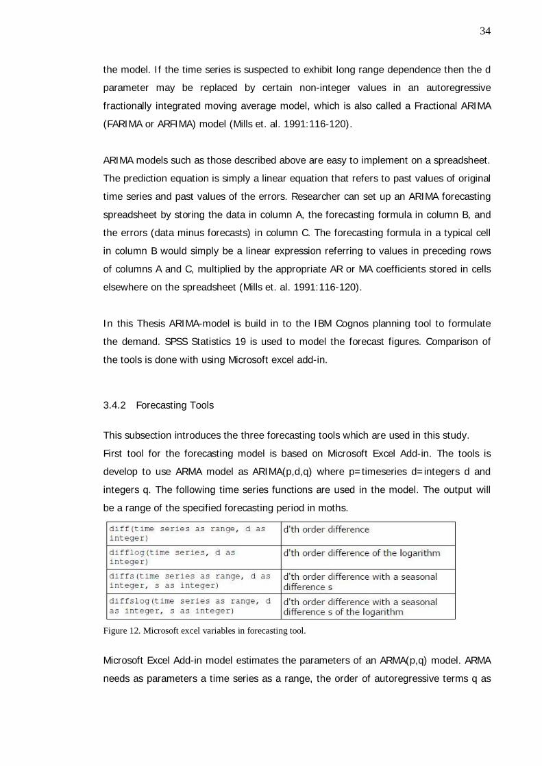
First tool for the forecasting model is based on Microsoft Excel Add-in. The tools is
develop to use ARMA model as ARIMA(p,d,q) where p=timeseries d=integers d and
integers q. The following time series functions are used in the model. The output will
be a range of the specified forecasting period in moths.
Figure 12. Microsoft excel variables in forecasting tool.
Microsoft Excel Add-in model estimates the parameters of an ARMA(p,q) model. ARMA
needs as parameters a time series as a range, the order of autoregressive terms q as
35
integer, the order of moving average terms q as integer, and an constant term into the
model an boolean as true. After estimating this functions returns the residual, the
parameters, useful statistics, impulse response function and forecast evolution in a
range of the size (T p)×max(p + q + c,3) . The first parameter will be outputted in
column 2 and row 1. The orders of parameter are constant, autoregressive parameters
and moving average parameters. The estimation employs an efficient nonlinear
technique (Levenberq Marquardt algorithm).
Second forecasting tool is SPSS-statistics 19.0. SPSS statistics 19.0 is selected
therefore that it can produce Seasonal ARIMA models. Historical data analyses in
Section 4 will shown the seasonality of the provided occupational healthcare services
and that gives a reason to assume that SARIMA model can work in practice.
In SARIMA model all variables must be non negative integers. For autoregressive and
moving average components, the value represents the maximum order. All positive
lower orders will be included in the model. Seasonality is enabled if a periodicity has
been defined for the active dataset Autoregressive (p). Autoregressive orders specify
which previous values from the series are used to predict current values. For example,
an autoregressive order of two specifies that the value of the series two time periods in
the past be used to predict the current value. Difference (d) specifies the order of
differencing applied to the series before estimating models. Differencing is necessary
when trends are present (series with trends are typically nonstationary and ARIMA
modeling assumes stationarity) and is used to remove their effect. Moving Average (q)
specify deviations from the series mean for previous values are used to predict current
values.
Seasonal autoregressive, moving average, and differencing components play the same
roles as their non seasonal counterparts. For seasonal orders, current series values are
affected by previous series values separated by one or more seasonal periods.
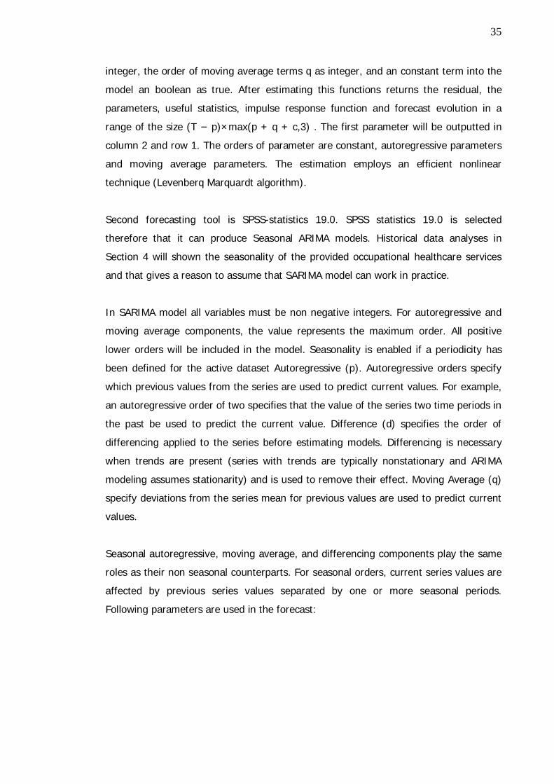
Following parameters are used in the forecast:
36
Figure 13. Parameters for SPSS SARIMA forecasting method.
Other factors such as goodness of fit shows summary statistics and percentiles for
following metrics; stationary R-square, R-square, root mean square error, mean
absolute percentage error, mean absolute error, maximum absolute percentage error,
maximum absolute error, and normalized Bayesian Information Criterion.
Residual autocorrelation function (ACF) summaries statistics and percentiles for
autocorrelations of the residuals across all estimated models. Parameter estimates
displays a table of parameter estimates for each estimated model. If outliers exist,
parameter estimates for them are also displayed. Residual autocorrelation function
(ACF) displays the lag for each estimated model. Residual autocorrelation function
includes the confidence intervals for the autocorrelations. Residual partial
autocorrelation function (PACF), displays by lag for each estimated model. The table
includes the confidence intervals for the partial autocorrelations.
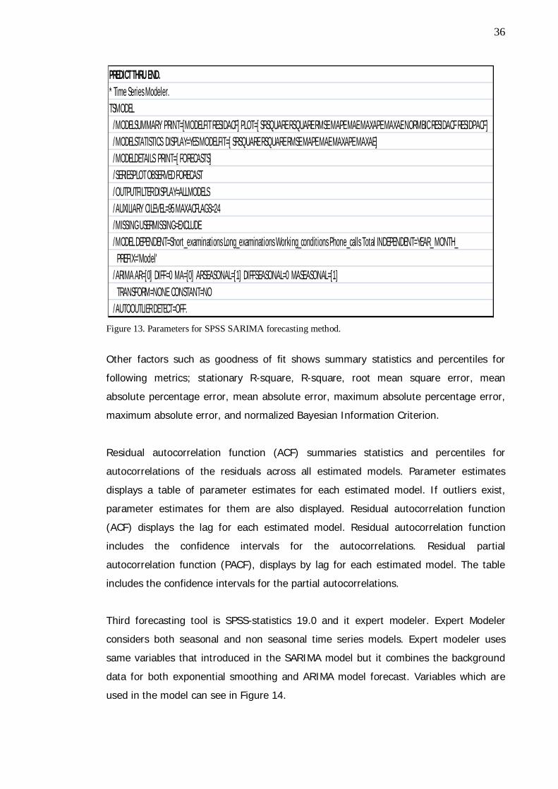
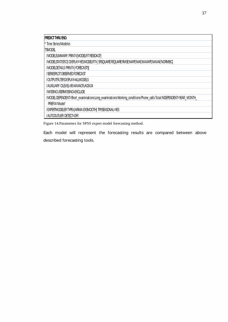
Third forecasting tool is SPSS-statistics 19.0 and it expert modeler. Expert Modeler
considers both seasonal and non seasonal time series models. Expert modeler uses
same variables that introduced in the SARIMA model but it combines the background
data for both exponential smoothing and ARIMA model forecast. Variables which are
used in the model can see in Figure 14.
PREDICT THRU END.* Time Series Modeler.TSMODEL /MODELSUMMARY PRINT=[MODELFIT RESIDACF] PLOT=[ SRSQUARE RSQUARE RMSE MAPE MAE MAXAPE MAXAE NORMBIC RESIDACF RESIDPACF] /MODELSTATISTICS DISPLAY=YES MODELFIT=[ SRSQUARE RSQUARE RMSE MAPE MAE MAXAPE MAXAE] /MODELDETAILS PRINT=[ FORECASTS] /SERIESPLOT OBSERVED FORECAST /OUTPUTFILTER DISPLAY=ALLMODELS /AUXILIARY CILEVEL=95 MAXACFLAGS=24 /MISSING USERMISSING=EXCLUDE /MODEL DEPENDENT=Short_examinations Long_examinations Working_conditions Phone_calls Total INDEPENDENT=YEAR_ MONTH_ PREFIX='Model' /ARIMA AR=[0] DIFF=0 MA=[0] ARSEASONAL=[1] DIFFSEASONAL=0 MASEASONAL=[1] TRANSFORM=NONE CONSTANT=NO /AUTOOUTLIER DETECT=OFF.
37
Figure 14.Parameters for SPSS expert model forecasting method.
Each model will represent the forecasting results are compared between above
described forecasting tools.
PREDICT THRU END.* Time Series Modeler.TSMODEL /MODELSUMMARY PRINT=[MODELFIT RESIDACF] /MODELSTATISTICS DISPLAY=YES MODELFIT=[ SRSQUARE RSQUARE RMSE MAPE MAE MAXAPE MAXAE NORMBIC] /MODELDETAILS PRINT=[ FORECASTS] /SERIESPLOT OBSERVED FORECAST /OUTPUTFILTER DISPLAY=ALLMODELS /AUXILIARY CILEVEL=95 MAXACFLAGS=24 /MISSING USERMISSING=EXCLUDE /MODEL DEPENDENT=Short_examinations Long_examinations Working_conditions Phone_calls Total INDEPENDENT=YEAR_ MONTH_ PREFIX='Model' /EXPERTMODELER TYPE=[ARIMA EXSMOOTH] TRYSEASONAL=YES /AUTOOUTLIER DETECT=OFF.
38
3.5 Validity and Reliability
Quantitative research designs are either descriptive or experimental. A descriptive
study establishes only associations between variables. An experiment establishes
causality. Quantitative research is all about quantifying relationships between variables.
Variables can be weight, performance, time, and treatment. In this study a
combination of literature investigations, interviews, creating data sets and data mining
and the researcher’s narrow training in specific fields set limits. The researcher in this
study is a Bachelor of Science in Industrial management with four years of work
experience in the case company, in as IT-designer and modeling usability reports for
top-management. In the forecasting model selection process, three individual
forecasting methods are tested and analyzed for securing the validity and reliability of
this Thesis. Literature review suggests that better and more reliable forecasts can be
performed if there is comparison between different forecasting methods.
39
4 Current State Analysis
This section analyses the present healthcare service state of the case organization.
Analyses are conducted with healthcare data mining with Cognos BI 8.3 tools. Also
demographic variables such as age are discussed.
Present state in the case organization is that there is no functioning model for demand
forecasting. Organization has set goals and targets for the nursing staff (doctors,
nurses, physiotherapists and psychologies). Their goals are only representing the
targets for each professional group, which they should reach in monthly level. These
targets are discussed and defined based on previous year outcome of the provided
services as classified in the four main categories. These are introduced in the research
method and material section.
This Thesis discusses and analyses the model for one business unit of the case
organization and its customers. Forecasting the demand of this target customer group
will give management tools for the case business unit leaders to define the predicted
workload and, predicted healthcare service need for the case organizations population.
Key stakeholders are the business unit leaders and top management of the
organization. Other stakeholders are development team and case customer
organization top management. Forecasting metrics are 2-4 years of patient data;
human resource data such as age are used for the background analysis.
Forecasting model applies tool for case organization workload planning and
investigating the seasonal factors and preparations and planning for the staff holidays.
This Thesis applies the questions that how demand forecasting can influence the
prediction and usage of the rented doctors and physicians. Forecasting model tries to
find the answer for the actual needs and planning how to use in-house rented doctor
services.
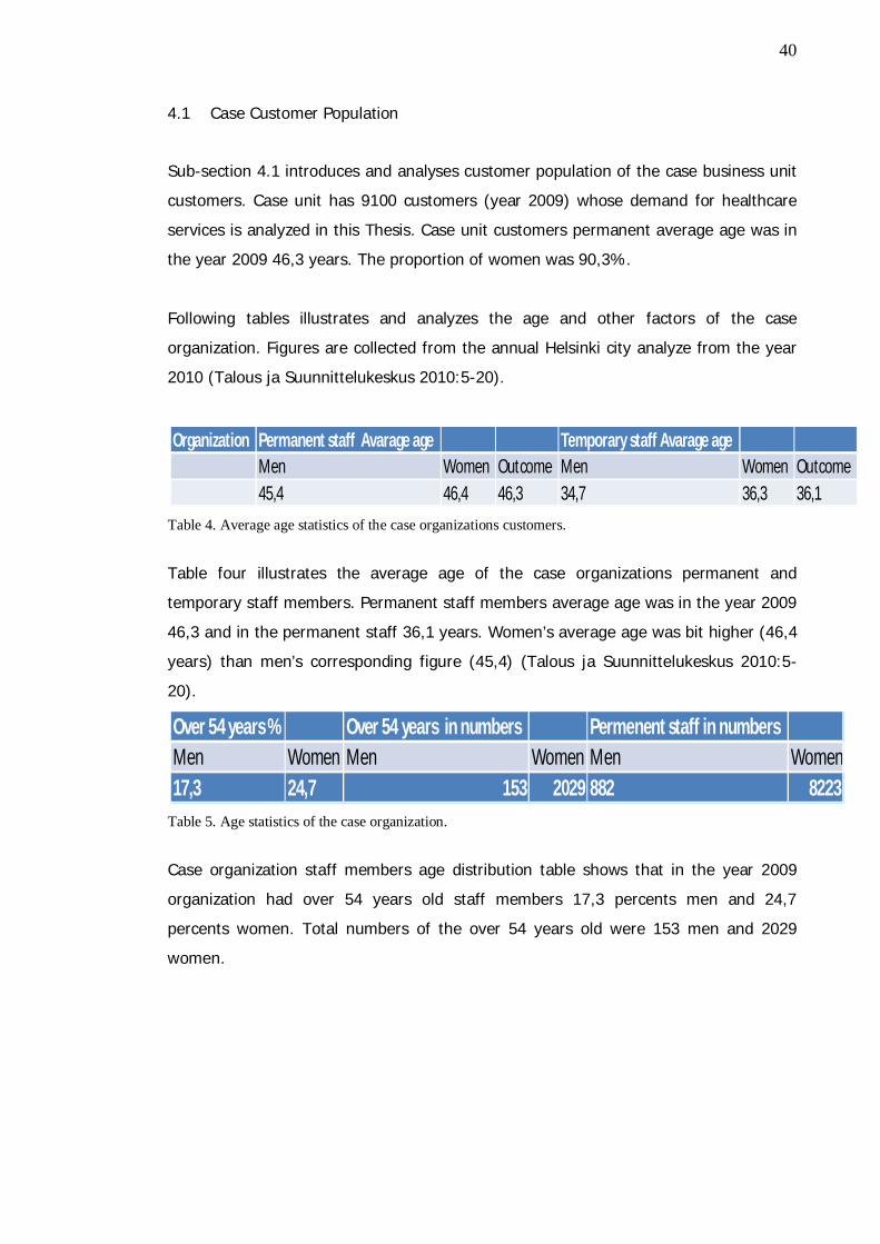
40
4.1 Case Customer Population
Sub-section 4.1 introduces and analyses customer population of the case business unit
customers. Case unit has 9100 customers (year 2009) whose demand for healthcare
services is analyzed in this Thesis. Case unit customers permanent average age was in
the year 2009 46,3 years. The proportion of women was 90,3%.
Following tables illustrates and analyzes the age and other factors of the case
organization. Figures are collected from the annual Helsinki city analyze from the year
2010 (Talous ja Suunnittelukeskus 2010:5-20).
Table 4. Average age statistics of the case organizations customers.
Table four illustrates the average age of the case organizations permanent and
temporary staff members. Permanent staff members average age was in the year 2009
46,3 and in the permanent staff 36,1 years. Women’s average age was bit higher (46,4
years) than men’s corresponding figure (45,4) (Talous ja Suunnittelukeskus 2010:5-
20).
Table 5. Age statistics of the case organization.
Case organization staff members age distribution table shows that in the year 2009
organization had over 54 years old staff members 17,3 percents men and 24,7
percents women. Total numbers of the over 54 years old were 153 men and 2029
women.
Organization Permanent staff Avarage age Temporary staff Avarage ageMen Women Outcome Men Women Outcome45,4 46,4 46,3 34,7 36,3 36,1
Over 54 years % Over 54 years in numbers Permenent staff in numbersMen Women Men Women Men Women17,3 24,7 153 2029 882 8223
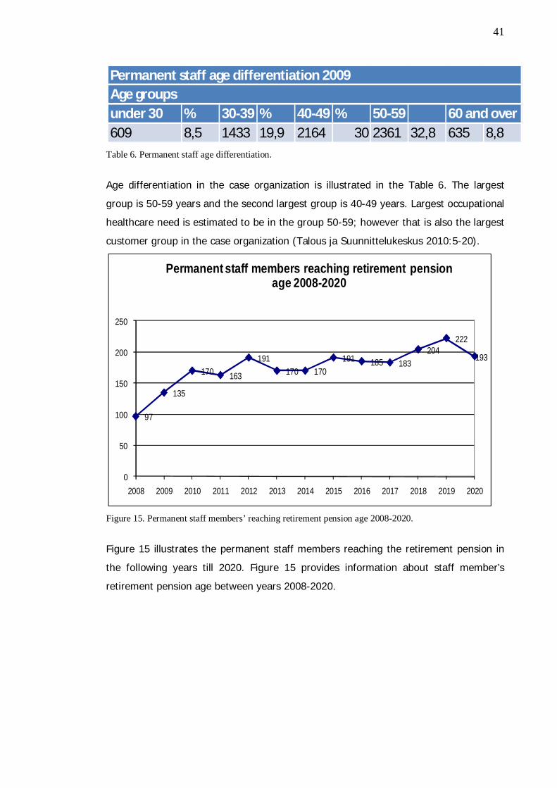
41
Table 6. Permanent staff age differentiation.
Age differentiation in the case organization is illustrated in the Table 6. The largest
group is 50-59 years and the second largest group is 40-49 years. Largest occupational
healthcare need is estimated to be in the group 50-59; however that is also the largest
customer group in the case organization (Talous ja Suunnittelukeskus 2010:5-20).
Figure 15. Permanent staff members’ reaching retirement pension age 2008-2020.
Figure 15 illustrates the permanent staff members reaching the retirement pension in
the following years till 2020. Figure 15 provides information about staff member’s
retirement pension age between years 2008-2020.
under 30 % 30-39 % 40-49 % 50-59 60 and over609 8,5 1433 19,9 2164 30 2361 32,8 635 8,8
Permanent staff age differentiation 2009Age groups
97
135
170 163
191170 170
191 185 183204
222
193
0
50
100
150
200
250
2008 2009 2010 2011 2012 2013 2014 2015 2016 2017 2018 2019 2020
Permanent staff members reaching retirement pensionage 2008-2020
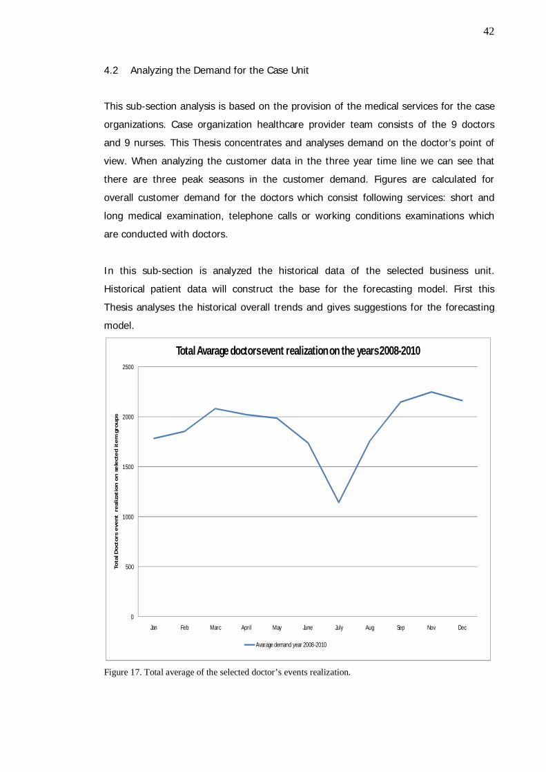
42
4.2 Analyzing the Demand for the Case Unit
This sub-section analysis is based on the provision of the medical services for the case
organizations. Case organization healthcare provider team consists of the 9 doctors
and 9 nurses. This Thesis concentrates and analyses demand on the doctor’s point of
view. When analyzing the customer data in the three year time line we can see that
there are three peak seasons in the customer demand. Figures are calculated for
overall customer demand for the doctors which consist following services: short and
long medical examination, telephone calls or working conditions examinations which
are conducted with doctors.
In this sub-section is analyzed the historical data of the selected business unit.
Historical patient data will construct the base for the forecasting model. First this
Thesis analyses the historical overall trends and gives suggestions for the forecasting
model.
Figure 17. Total average of the selected doctor’s events realization.
0
500
1000
1500
2000
2500
Jan Feb Marc April May June July Aug Sep Nov Dec
Tota
l Do
cto
rs e
ve
nt
re
ali
zati
on
on
se
lect
ed
ite
m g
rou
ps
Total Avarage doctors event realization on the years 2008-2010
Avarage demand year 2008-2010
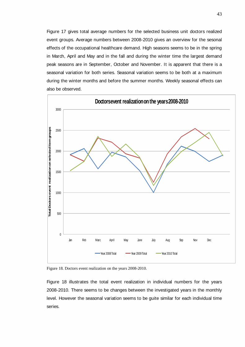
43
Figure 17 gives total average numbers for the selected business unit doctors realized
event groups. Average numbers between 2008-2010 gives an overview for the sesonal
effects of the occupational healthcare demand. High seasons seems to be in the spring
in March, April and May and in the fall and during the winter time the largest demand
peak seasons are in September, October and November. It is apparent that there is a
seasonal variation for both series. Seasonal variation seems to be both at a maximum
during the winter months and before the summer months. Weekly seasonal effects can
also be observed.
Figure 18. Doctors event realization on the years 2008-2010.
Figure 18 illustrates the total event realization in individual numbers for the years
2008-2010. There seems to be changes between the investigated years in the monthly
level. However the seasonal variation seems to be guite similar for each individual time
series.
0
500
1000
1500
2000
2500
3000
Jan Feb Marc April May June July Aug Sep Nov Dec
To
tal D
oct
ors
eve
nt
re
ali
zati
on
on
se
lect
ed
ite
m g
rou
ps
Doctors event realization on the years 2008-2010
Year 2008 Total Year 2009 Total Year 2010 Total
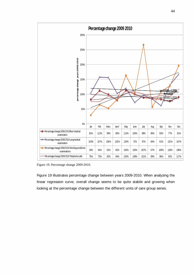
44
Figure 19. Percentage change 2009-2010.
Figure 19 illustrates percentage change between years 2009-2010. When analyzing the
linear regression curve, overall change seems to be quite stabile and growing when
looking at the percentage change between the different units of care group series.
Jan Feb Marc April May June July Aug Sep Nov Dec
Percentage change 2009/2010Short medicalexamination 81% 112% 99% 80% 113% 100% 88% 85% 82% 77% 91%
Percentage change 2009/2010 Long medicalexamination 103% 157% 156% 102% 120% 72% 97% 84% 61% 131% 167%
Percentage change 2009/2010 Working conditionsexaminations 30% 64% 52% 82% 163% 105% 267% 57% 109% 128% 196%
Percentage change 2009/2010 Telephone calls 75% 75% 92% 84% 103% 108% 101% 89% 96% 92% 117%
y = -0,0144x + 1,0022R² = 0,1429
y = -0,0117x + 1,2065R² = 0,0118
y = 0,0269x + 0,7766R² = 0,4667
0%
50%
100%
150%
200%
250%
300%
pe
rce
nta
ge
ch
an
ge
ye
ars
20
09
/2
01
0
Percentage change 2009 2010

45
Figure 20. Total change in years 2008-2009 and 2009-2010.
Figure 20 illustrates the total overall change in the doctor’s visits of the selected caring
service groups in the years 2008-2009 and years 2009-2010. Analyzing and comparing
the figures between the years the largest change was in the year 2009. This change
can also be result from the lack of resources in the year 2008 and 2010 in the some
moths. Figure shows that total change of the selected caring service groups are
meeting quite large change if we compare results between different years.
100%
85%
147%
112%
104%
120%125%
115%111%
127%131%
80%
99% 102%
85%
112%
101%
94%
85% 85% 87%
107%
0%
20%
40%
60%
80%
100%
120%
140%
160%
Jan Feb Marc April May June July Aug Sep Nov Dec
Total change in years 2008-2009 and 2009-2010
Overall change in total numbers 2008-2009 Overall change in total numbers 2009-2010
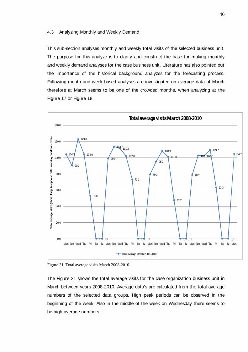
46
4.3 Analyzing Monthly and Weekly Demand
This sub-section analyses monthly and weekly total visits of the selected business unit.
The purpose for this analyze is to clarify and construct the base for making monthly
and weekly demand analyses for the case business unit. Literature has also pointed out
the importance of the historical background analyzes for the forecasting process.
Following month and week based analyses are investigated on average data of March
therefore at March seems to be one of the crowded months, when analyzing at the
Figure 17 or Figure 18.
Figure 21. Total average visits March 2008-2010.
The Figure 21 shows the total average visits for the case organization business unit in
March between years 2008-2010. Average data’s are calculated from the total average
numbers of the selected data groups. High peak periods can be observed in the
beginning of the week. Also in the middle of the week on Wednesday there seems to
be high average numbers.
104,3
90,3
123,0
104,0
53,0
0,0 0,0
99,0
113,7111,3
102,0
73,3
0,0 0,0
79,3
95,3
108,3
101,0
47,7
0,0 0,0
78,7
102,7102,7
109,7
63,3
0,0 0,0
104,7
0,0
20,0
40,0
60,0
80,0
100,0
120,0
140,0
Mon Tue Wed Thu Fri Sat Su Mon Tue Wed Thu Fri Sat Su Mon Tue Wed Thu Fri Sat Su Mon Tue Wed Thu Fri Sat Su Mon
Tota
l ave
rage
vis
its
(sh
ort
, lo
ng,
te
lep
ho
ne
calls
, w
ork
ing
con
dit
ion
exa
m.
Total average visits March 2008-2010
Total average March 2008-2010
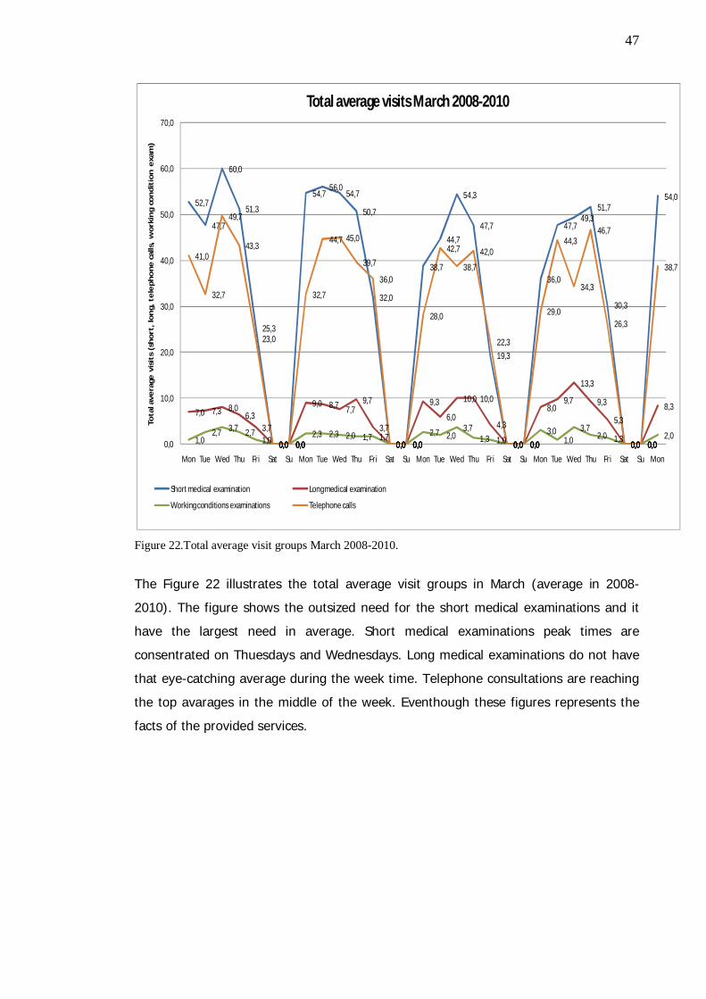
47
Figure 22.Total average visit groups March 2008-2010.
The Figure 22 illustrates the total average visit groups in March (average in 2008-
2010). The figure shows the outsized need for the short medical examinations and it
have the largest need in average. Short medical examinations peak times are
consentrated on Thuesdays and Wednesdays. Long medical examinations do not have
that eye-catching average during the week time. Telephone consultations are reaching
the top avarages in the middle of the week. Eventhough these figures represents the
facts of the provided services.
52,7
47,7
60,0
51,3
25,3
0,0 0,0
54,756,0
54,7
50,7
32,0
0,0 0,0
38,7
44,7
54,3
47,7
19,3
0,0 0,0
36,0
47,749,3
51,7
30,3
0,0 0,0
54,0
7,0 7,3 8,06,3
3,7
0,0 0,0
9,0 8,7 7,79,7
3,7
0,0 0,0
9,3
6,0
10,0 10,0
4,3
0,0 0,0
8,09,7
13,3
9,3
5,3
0,0 0,0
8,3
1,02,7 3,7 2,7
1,0 0,0 0,02,3 2,3 2,0 1,7 1,7
0,0 0,02,7 2,0
3,71,3 1,0 0,0 0,0
3,01,0
3,72,0 1,3
0,0 0,02,0
41,0
32,7
49,7
43,3
23,0
0,0 0,0
32,7
44,7 45,0
39,7
36,0
0,0 0,0
28,0
42,7
38,7
42,0
22,3
0,0 0,0
29,0
44,3
34,3
46,7
26,3
0,0 0,0
38,7
0,0
10,0
20,0
30,0
40,0
50,0
60,0
70,0
Mon Tue Wed Thu Fri Sat Su Mon Tue Wed Thu Fri Sat Su Mon Tue Wed Thu Fri Sat Su Mon Tue Wed Thu Fri Sat Su Mon
Tota
l av
era
ge v
isit
s (s
ho
rt,
lon
g, t
ele
ph
on
e c
all
s, w
ork
ing
con
dit
ion
ex
am
)
Total average visits March 2008-2010
Short medical examination Long medical examination
Working conditions examinations Telephone calls
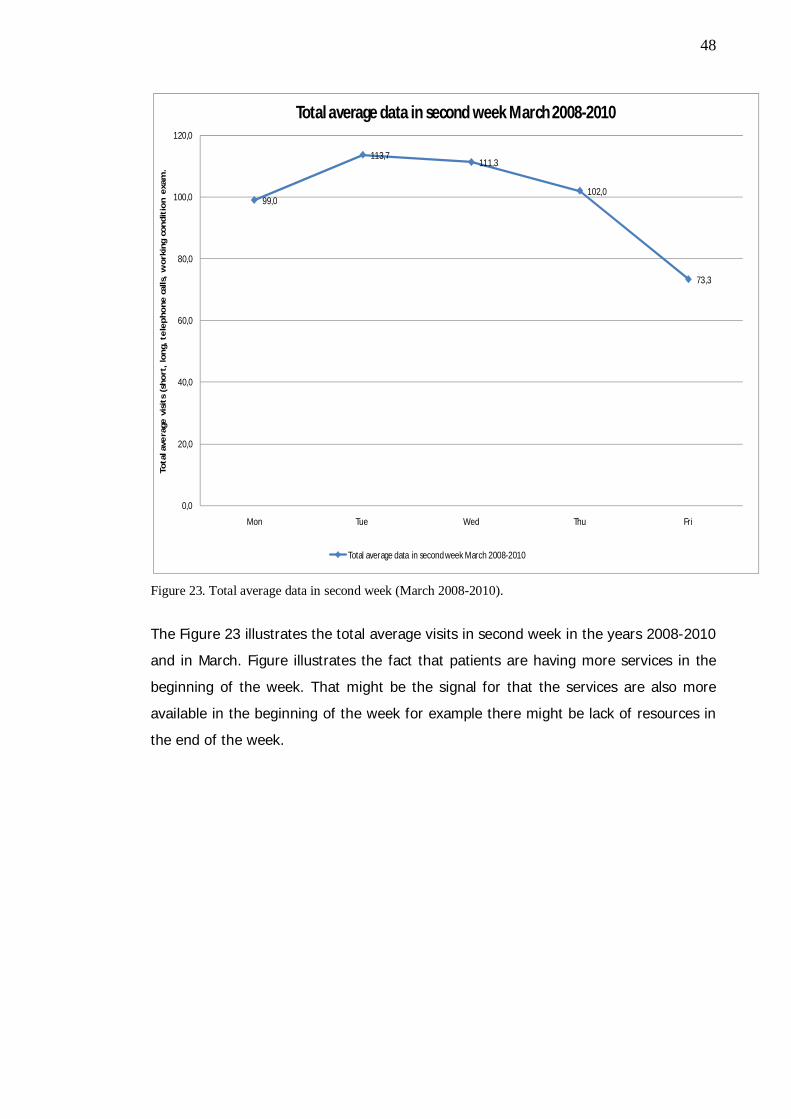
48
Figure 23. Total average data in second week (March 2008-2010).
The Figure 23 illustrates the total average visits in second week in the years 2008-2010
and in March. Figure illustrates the fact that patients are having more services in the
beginning of the week. That might be the signal for that the services are also more
available in the beginning of the week for example there might be lack of resources in
the end of the week.
99,0
113,7111,3
102,0
73,3
0,0
20,0
40,0
60,0
80,0
100,0
120,0
Mon Tue Wed Thu Fri
Tota
l ave
rage
vis
its
(sh
ort
, lo
ng,
te
lep
ho
ne
cal
ls,
wo
rkin
g co
nd
itio
n e
xam
.
Total average data in second week March 2008-2010
Total average data in second week March 2008-2010
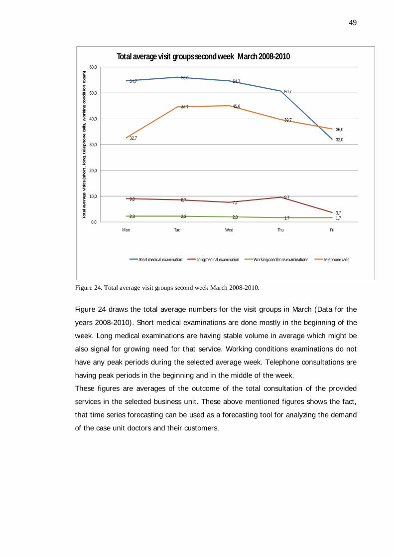
49
Figure 24. Total average visit groups second week March 2008-2010.
Figure 24 draws the total average numbers for the visit groups in March (Data for the
years 2008-2010). Short medical examinations are done mostly in the beginning of the
week. Long medical examinations are having stable volume in average which might be
also signal for growing need for that service. Working conditions examinations do not
have any peak periods during the selected average week. Telephone consultations are
having peak periods in the beginning and in the middle of the week.
These figures are averages of the outcome of the total consultation of the provided
services in the selected business unit. These above mentioned figures shows the fact,
that time series forecasting can be used as a forecasting tool for analyzing the demand
of the case unit doctors and their customers.
54,756,0
54,7
50,7
32,0
9,0 8,7 7,79,7
3,72,3 2,3 2,0 1,7 1,7
32,7
44,7 45,0
39,7
36,0
0,0
10,0
20,0
30,0
40,0
50,0
60,0
Mon Tue Wed Thu Fri
Tota
l ave
rage
vis
its
(sh
ort
, lo
ng,
te
lep
ho
ne
cal
ls,
wo
rkin
g co
nd
itio
n e
xam
)
Total average visit groups second week March 2008-2010
Short medical examination Long medical examination Working conditions examinations Telephone calls
50
5 Analyses of the Forecasting Tools
This section exhibits and analyses three different forecasting tools for the case
organization business unit forecasting. At this point, the tools are introduced and
tested in this Thesis. Forecasting models themselves were introduced in Research
Method and Material section.
5.1 Analysis of the ARMA-model
This sub-section suggests the actual figures for the demand forecasting model. Sub-
section 5.1 analyses ARMA Microsoft Excel Add-in tool. The data groups are descript as
individual data set.
In Table 7, the time series is defined and used throughout in this study and all of the
analyzed forecasting tools.
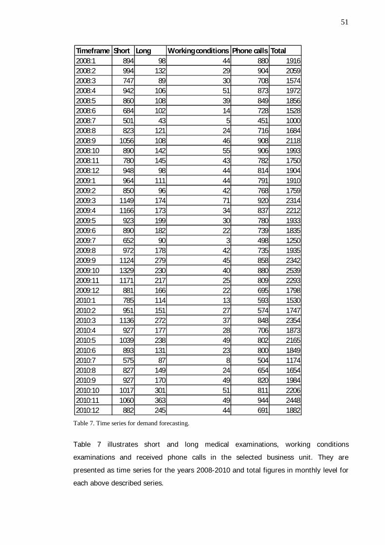
51
Table 7. Time series for demand forecasting.
Table 7 illustrates short and long medical examinations, working conditions
examinations and received phone calls in the selected business unit. They are
presented as time series for the years 2008-2010 and total figures in monthly level for
each above described series.
Timeframe Short Long Working conditions Phone calls Total2008:1 894 98 44 880 19162008:2 994 132 29 904 20592008:3 747 89 30 708 15742008:4 942 106 51 873 19722008:5 860 108 39 849 18562008:6 684 102 14 728 15282008:7 501 43 5 451 10002008:8 823 121 24 716 16842008:9 1056 108 46 908 21182008:10 890 142 55 906 19932008:11 780 145 43 782 17502008:12 948 98 44 814 19042009:1 964 111 44 791 19102009:2 850 96 42 768 17592009:3 1149 174 71 920 23142009:4 1166 173 34 837 22122009:5 923 199 30 780 19332009:6 890 182 22 739 18352009:7 652 90 3 498 12502009:8 972 178 42 735 19352009:9 1124 279 45 858 23422009:10 1329 230 40 880 25392009:11 1171 217 25 809 22932009:12 881 166 22 695 17982010:1 785 114 13 593 15302010:2 951 151 27 574 17472010:3 1136 272 37 848 23542010:4 927 177 28 706 18732010:5 1039 238 49 802 21652010:6 893 131 23 800 18492010:7 575 87 8 504 11742010:8 827 149 24 654 16542010:9 927 170 49 820 19842010:10 1017 301 51 811 22062010:11 1060 363 49 944 24482010:12 882 245 44 691 1882
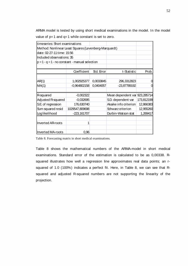
52
ARMA model is tested by using short medical examinations in the model. In the model
value of p=1 and q=1 while constant is set to zero.
Table 8. Forecasting matrix in short medical examinations.
Table 8 shows the mathematical numbers of the ARMA-model in short medical
examinations. Standard error of the estimation is calculated to be as 0,00338. R-
squared illustrates how well a regression line approximates real data points; an r-
squared of 1.0 (100%) indicates a perfect fit. Here, in Table 8, we can see that R-
squared and adjusted R-squared numbers are not supporting the linearity of the
projection.
timeseries: Short examinationsMethod: Nonlinear Least Squares (Levenberg-Marquardt)date: 02-27-11 time: 15:56Included observations: 35p = 1 - q = 1 - no constant - manual selection
Coefficient Std. Error t-Statistic Prob.
AR(1) 1,002925377 0,0033845 296,3312823 0MA(1) -0,964802158 0,0404057 -23,87789192 0
R-squared -0,002322 Mean dependent var 923,285714Adjusted R-squared -0,032695 S.D. dependent var 173,812199S.E. of regression 176,630740 Akaike info criterion 12,866383Sum squared resid 1029547,809698 Schwarz criterion 12,955260Log likelihood -223,161707 Durbin-Watson stat 1,269417
Inverted AR-roots 1
Inverted MA-roots 0,96
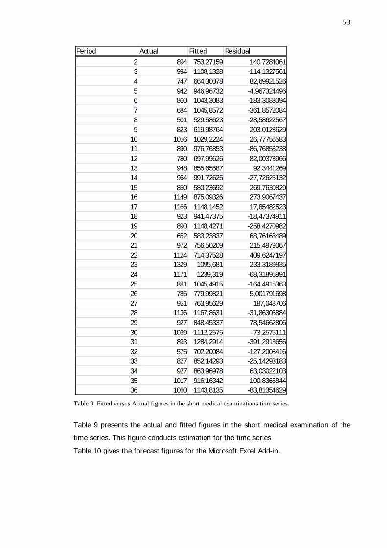
53
Table 9. Fitted versus Actual figures in the short medical examinations time series.
Table 9 presents the actual and fitted figures in the short medical examination of the
time series. This figure conducts estimation for the time series
Table 10 gives the forecast figures for the Microsoft Excel Add-in.
Period Actual Fitted Residual
2 894 753,27159 140,72840613 994 1108,1328 -114,13275614 747 664,30078 82,699215265 942 946,96732 -4,9673244966 860 1043,3083 -183,30830947 684 1045,8572 -361,85720848 501 529,58623 -28,586225679 823 619,98764 203,0123629
10 1056 1029,2224 26,7775658311 890 976,76853 -86,7685323812 780 697,99626 82,0037396613 948 855,65587 92,344126914 964 991,72625 -27,7262513215 850 580,23692 269,763082916 1149 875,09326 273,906743717 1166 1148,1452 17,8548252318 923 941,47375 -18,4737491119 890 1148,4271 -258,427098220 652 583,23837 68,7616348921 972 756,50209 215,497906722 1124 714,37528 409,624719723 1329 1095,681 233,318983524 1171 1239,319 -68,3189599125 881 1045,4915 -164,491536326 785 779,99821 5,00179169827 951 763,95629 187,04370628 1136 1167,8631 -31,8630588429 927 848,45337 78,5466280630 1039 1112,2575 -73,257511131 893 1284,2914 -391,291365632 575 702,20084 -127,200841633 827 852,14293 -25,1429318334 927 863,96978 63,0302210335 1017 916,16342 100,836584436 1060 1143,8135 -83,81354629
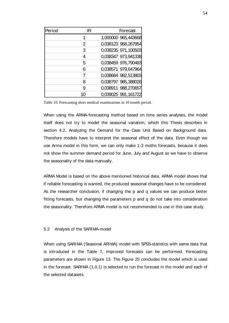
54
Table 10. Forecasting short medical examinations in 10 month period.
When using the ARMA-forecasting method based on time series analyses, the model
itself does not try to model the seasonal variation, which this Thesis describes in
section 4.2, Analyzing the Demand for the Case Unit Based on Background data.
Therefore models have to interpret the seasonal effect of the data. Even though we
use Arma model in this form, we can only make 1-3 moths forecasts, because it does
not show the summer demand period for June, July and August so we have to observe
the seasonality of the data manually.
ARMA Model is based on the above mentioned historical data. ARMA model shows that
if reliable forecasting is wanted, the produced seasonal changes have to be considered.
As the researcher conclusion, if changing the p and q values we can produce better
fitting forecasts, but changing the parameters p and q do not take into consideration
the seasonality. Therefore ARMA model is not recommended to use in this case study.
5.2 Analysis of the SARIMA-model
When using SARIMA (Seasonal ARIMA) model with SPSS-statistics with same data that
is introduced in the Table 7, improved forecasts can be performed. Forecasting
parameters are shown in Figure 13. The Figure 25 concludes the model which is used
in the forecast. SARIMA (1,0,1) is selected to run the forecast in the model and each of
the selected datasets.
Period IR Forecast
1 1,000000 965,4436682 0,038123 968,2679543 0,038235 971,1005034 0,038347 973,9413385 0,038459 976,7904836 0,038571 979,6479647 0,038684 982,5138038 0,038797 985,3880269 0,038911 988,270657
10 0,039025 991,161722
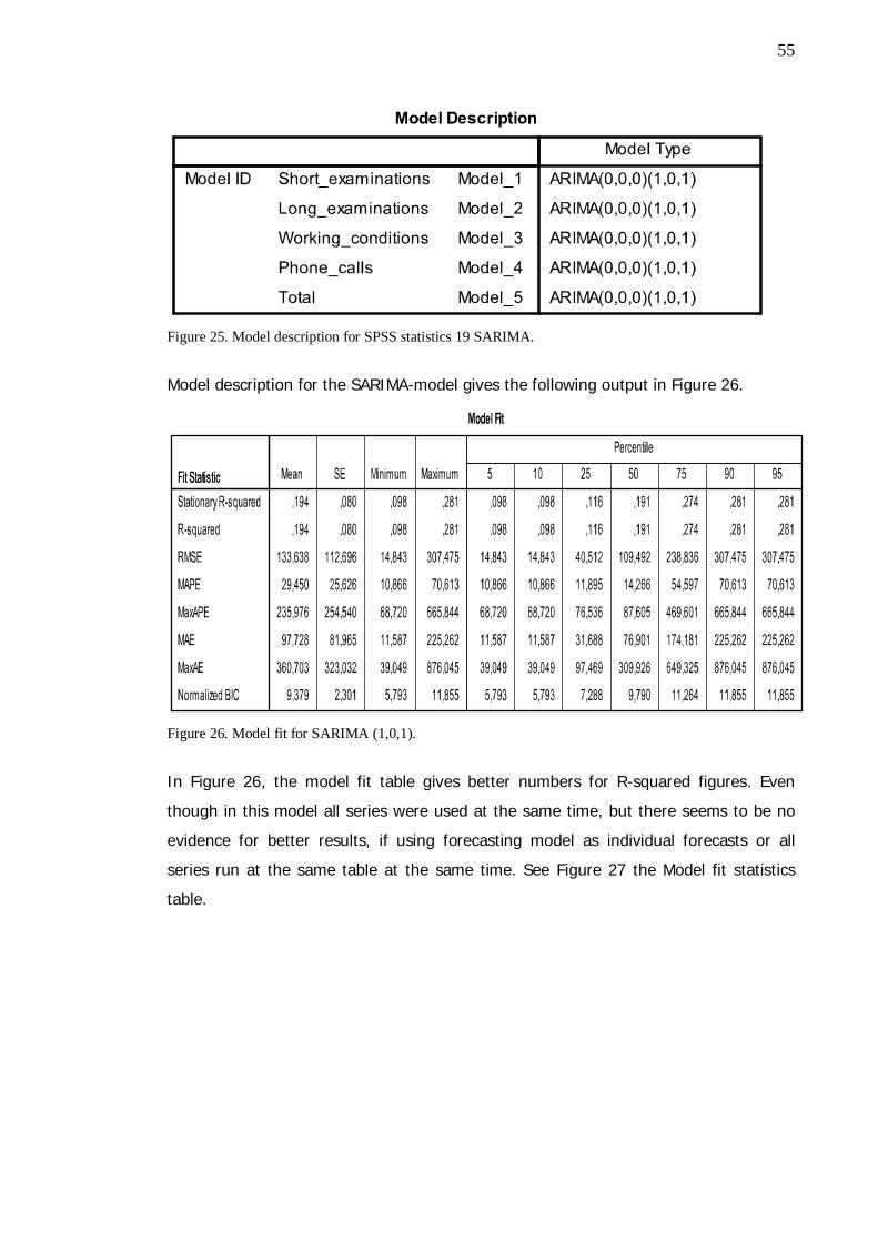
55
Figure 25. Model description for SPSS statistics 19 SARIMA.
Model description for the SARIMA-model gives the following output in Figure 26.
Figure 26. Model fit for SARIMA (1,0,1).
In Figure 26, the model fit table gives better numbers for R-squared figures. Even
though in this model all series were used at the same time, but there seems to be no
evidence for better results, if using forecasting model as individual forecasts or all
series run at the same table at the same time. See Figure 27 the Model fit statistics
table.
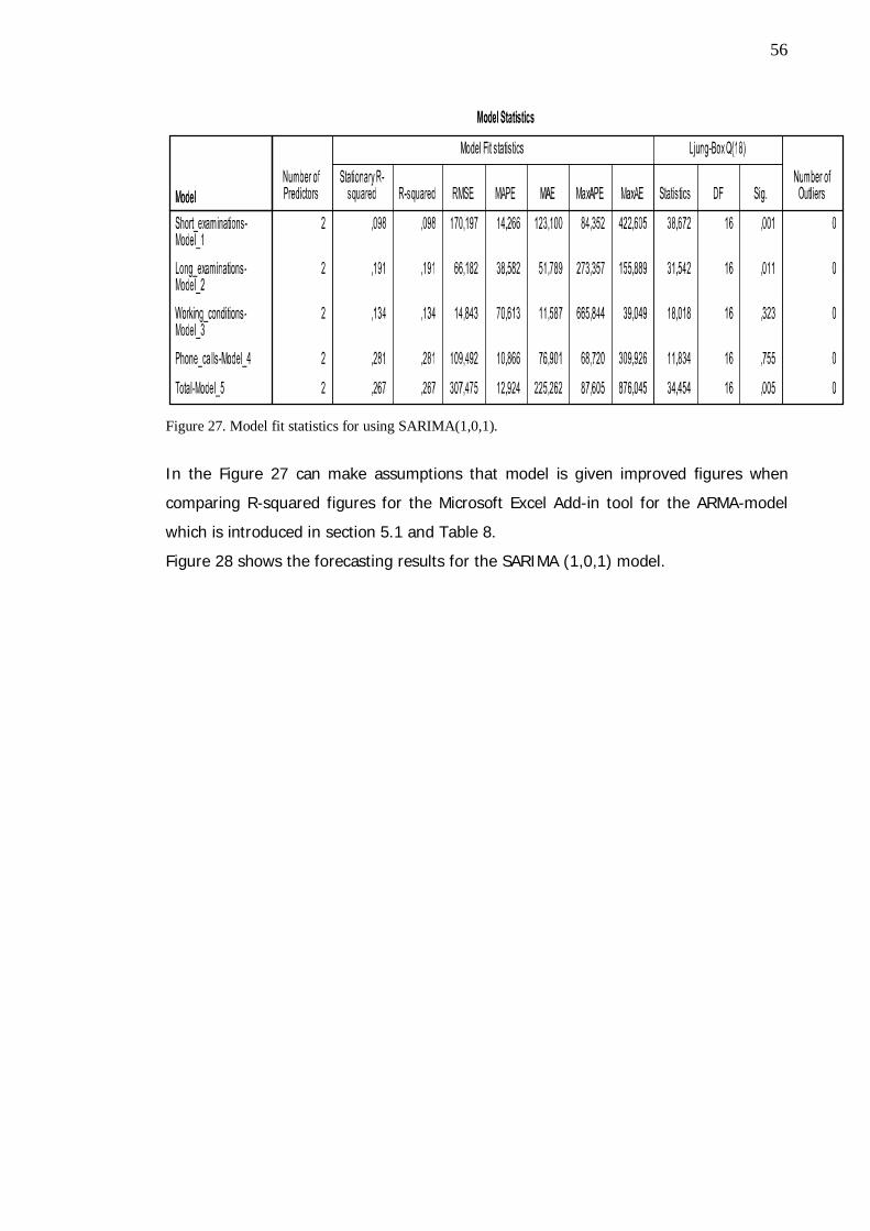
56
Figure 27. Model fit statistics for using SARIMA(1,0,1).
In the Figure 27 can make assumptions that model is given improved figures when
comparing R-squared figures for the Microsoft Excel Add-in tool for the ARMA-model
which is introduced in section 5.1 and Table 8.
Figure 28 shows the forecasting results for the SARIMA (1,0,1) model.
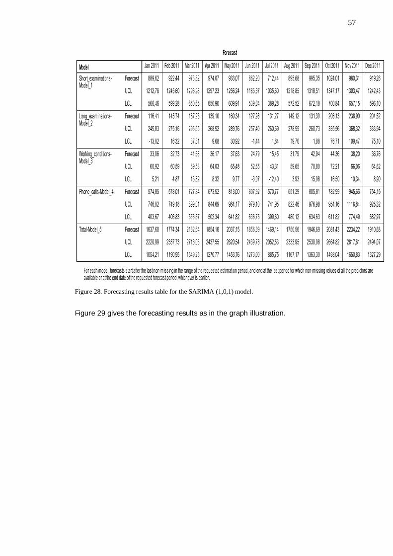
57
Figure 28. Forecasting results table for the SARIMA (1,0,1) model.
Figure 29 gives the forecasting results as in the graph illustration.
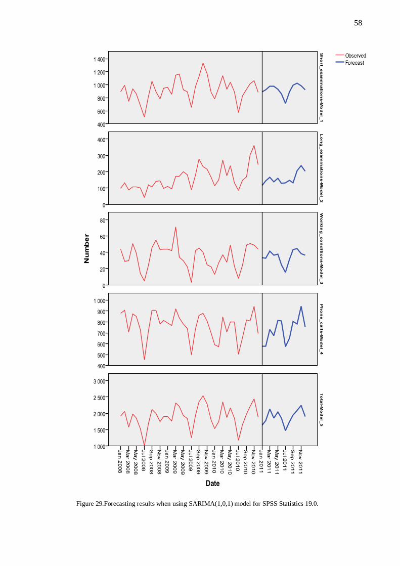
58
Figure 29.Forecasting results when using SARIMA(1,0,1) model for SPSS Statistics 19.0.
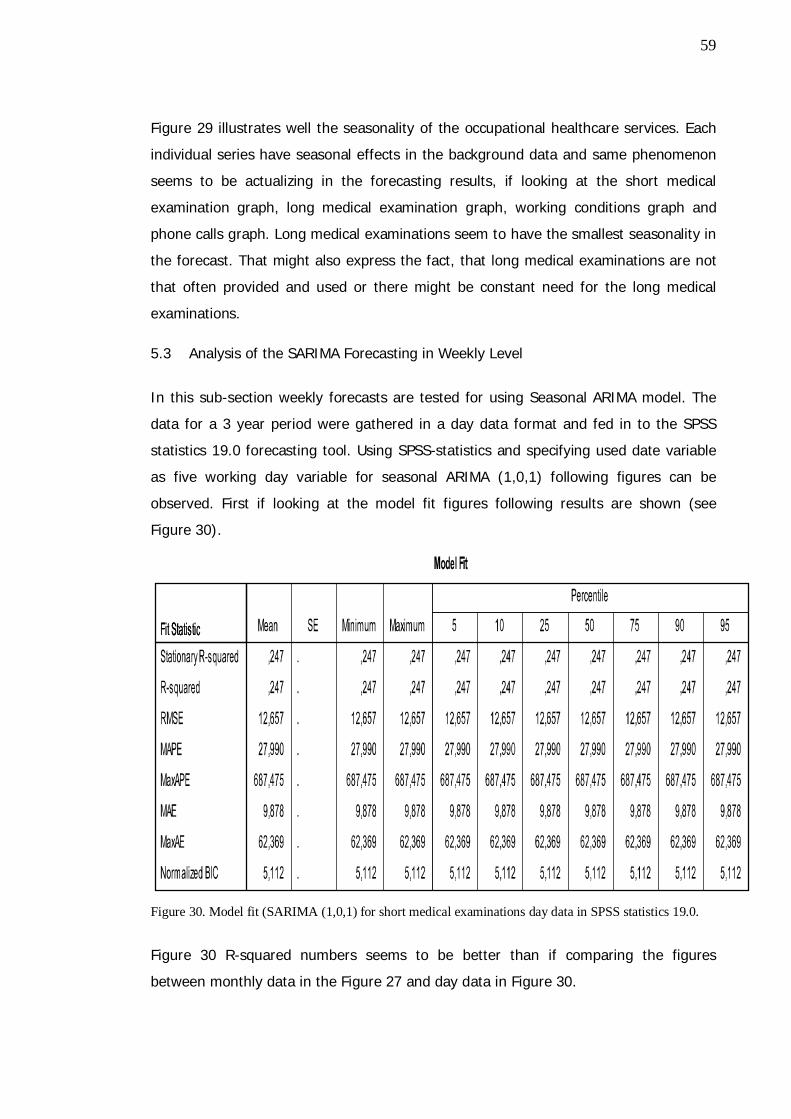
59
Figure 29 illustrates well the seasonality of the occupational healthcare services. Each
individual series have seasonal effects in the background data and same phenomenon
seems to be actualizing in the forecasting results, if looking at the short medical
examination graph, long medical examination graph, working conditions graph and
phone calls graph. Long medical examinations seem to have the smallest seasonality in
the forecast. That might also express the fact, that long medical examinations are not
that often provided and used or there might be constant need for the long medical
examinations.
5.3 Analysis of the SARIMA Forecasting in Weekly Level
In this sub-section weekly forecasts are tested for using Seasonal ARIMA model. The
data for a 3 year period were gathered in a day data format and fed in to the SPSS
statistics 19.0 forecasting tool. Using SPSS-statistics and specifying used date variable
as five working day variable for seasonal ARIMA (1,0,1) following figures can be
observed. First if looking at the model fit figures following results are shown (see
Figure 30).
Figure 30. Model fit (SARIMA (1,0,1) for short medical examinations day data in SPSS statistics 19.0.
Figure 30 R-squared numbers seems to be better than if comparing the figures
between monthly data in the Figure 27 and day data in Figure 30.
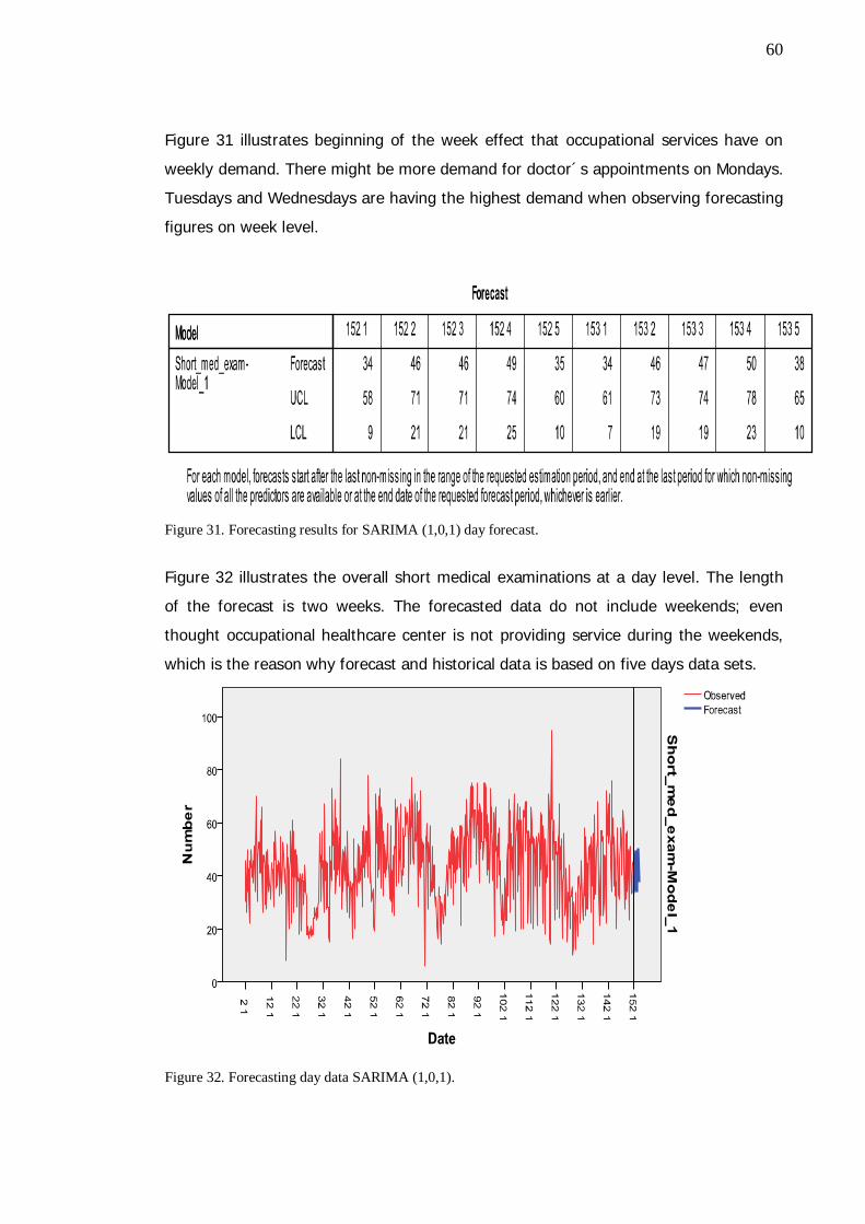
60
Figure 31 illustrates beginning of the week effect that occupational services have on
weekly demand. There might be more demand for doctor´s appointments on Mondays.
Tuesdays and Wednesdays are having the highest demand when observing forecasting
figures on week level.
Figure 31. Forecasting results for SARIMA (1,0,1) day forecast.
Figure 32 illustrates the overall short medical examinations at a day level. The length
of the forecast is two weeks. The forecasted data do not include weekends; even
thought occupational healthcare center is not providing service during the weekends,
which is the reason why forecast and historical data is based on five days data sets.
Figure 32. Forecasting day data SARIMA (1,0,1).
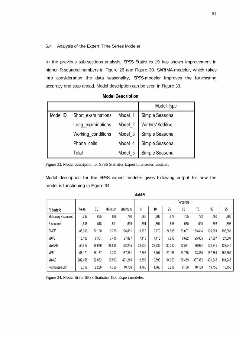
61
5.4 Analysis of the Expert Time Series Modeler
In the previous sub-sections analysis, SPSS Statistics 19 has shown improvement in
higher R-squared numbers in Figure 26 and Figure 30. SARIMA-modeler, which takes
into consideration the data seasonality, SPSS-modeler improves the forecasting
accuracy one step ahead. Model description can be seen in Figure 33.
Figure 33. Model description for SPSS Statistics Expert time series modeler.
Model description for the SPSS expert modeler gives following output for how the
model is functioning in Figure 34.
Figure 34. Model fit for SPSS Statistics 19.0 Expert modeler.
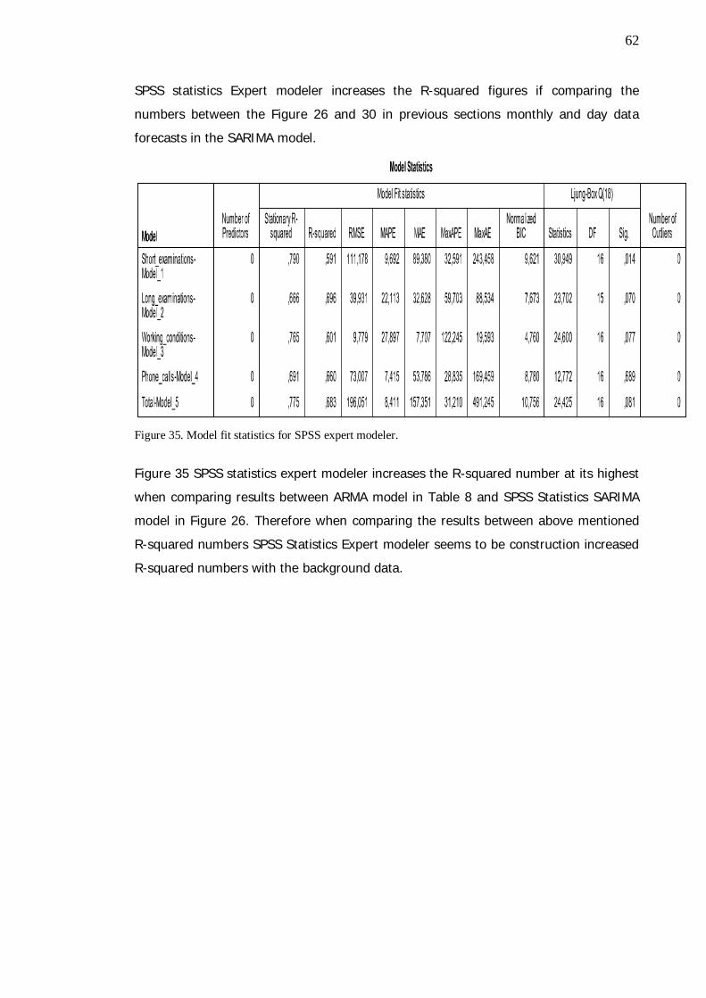
62
SPSS statistics Expert modeler increases the R-squared figures if comparing the
numbers between the Figure 26 and 30 in previous sections monthly and day data
forecasts in the SARIMA model.
Figure 35. Model fit statistics for SPSS expert modeler.
Figure 35 SPSS statistics expert modeler increases the R-squared number at its highest
when comparing results between ARMA model in Table 8 and SPSS Statistics SARIMA
model in Figure 26. Therefore when comparing the results between above mentioned
R-squared numbers SPSS Statistics Expert modeler seems to be construction increased
R-squared numbers with the background data.
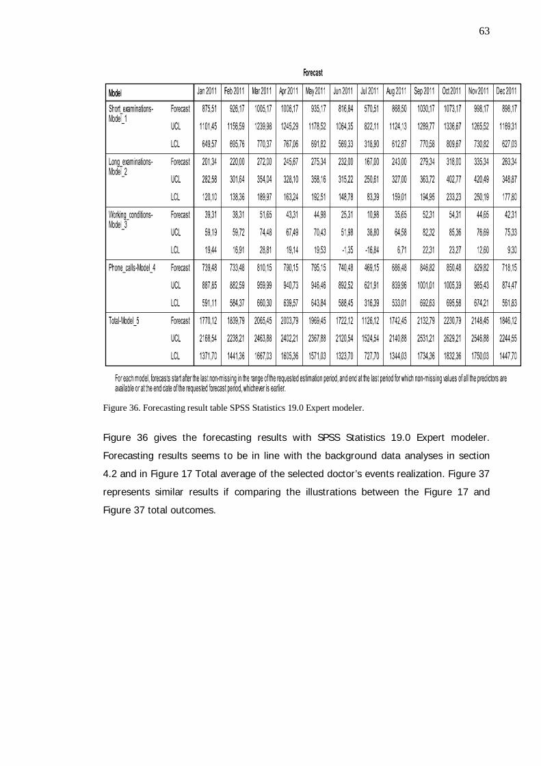
63
Figure 36. Forecasting result table SPSS Statistics 19.0 Expert modeler.
Figure 36 gives the forecasting results with SPSS Statistics 19.0 Expert modeler.
Forecasting results seems to be in line with the background data analyses in section
4.2 and in Figure 17 Total average of the selected doctor’s events realization. Figure 37
represents similar results if comparing the illustrations between the Figure 17 and
Figure 37 total outcomes.
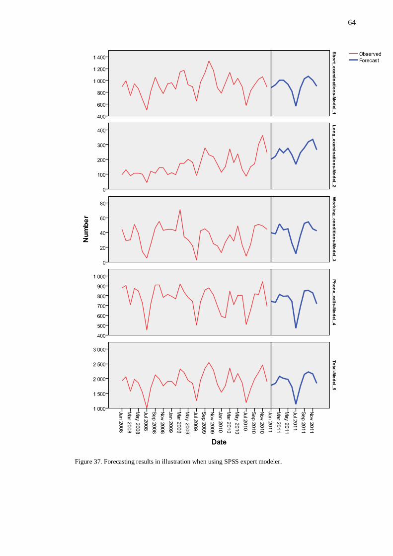
64
Figure 37. Forecasting results in illustration when using SPSS expert modeler.
65
When comparing the results between Figure 29 and Figure 37 both illustrations show
the seasonality change of the forecasting in occupational healthcare services. Each
individual series has seasonal effects in the background data and same phenomenon
seems to be occurring in the forecasting results. When comparing Figure 37 to Figure
29 it looks like that also long medical examinations have the seasonality change in the
forecast. Historical background data analyses which are made in section 4.2 have
shown the seasonality change of the background data which overrules the SARIMA
model conclusion in section 4.2 and in Figure 29, which long medical examinations do
not have the same seasonality change which other service groups seems to have.
5.5 Validating the selected model
This sub-section validates the selected model. The ARMA-model as a Microsoft Excel
Add-in was introduced in the section 5.1 is analyzed based on the tests run in the
same section. ARMA-model itself does not observe and take into consideration the
seasonality change, which has been shown in the section 4.2. R-squared figures were
also quite low in ARMA-model. SPSS statistics offers the SARIMA model (Seasonal
ARIMA) which is concerning the seasonality of the background data. Figure 27 shows
increased values for R-squared figures, when comparing results between ARMA model
results in Table 7. Taking one step ahead for SARIMA model and using the SPSS
statistics Expert modeler can gain more accurate investigation results. Figure 35
increases R-squared numbers up to even 0,79 for the short medical examination.
Figure 35 R-squared number is closer to 1,0 and that confirms that forecast results are
more valid if comparing to ARMA and SARIMA R-squared numbers.
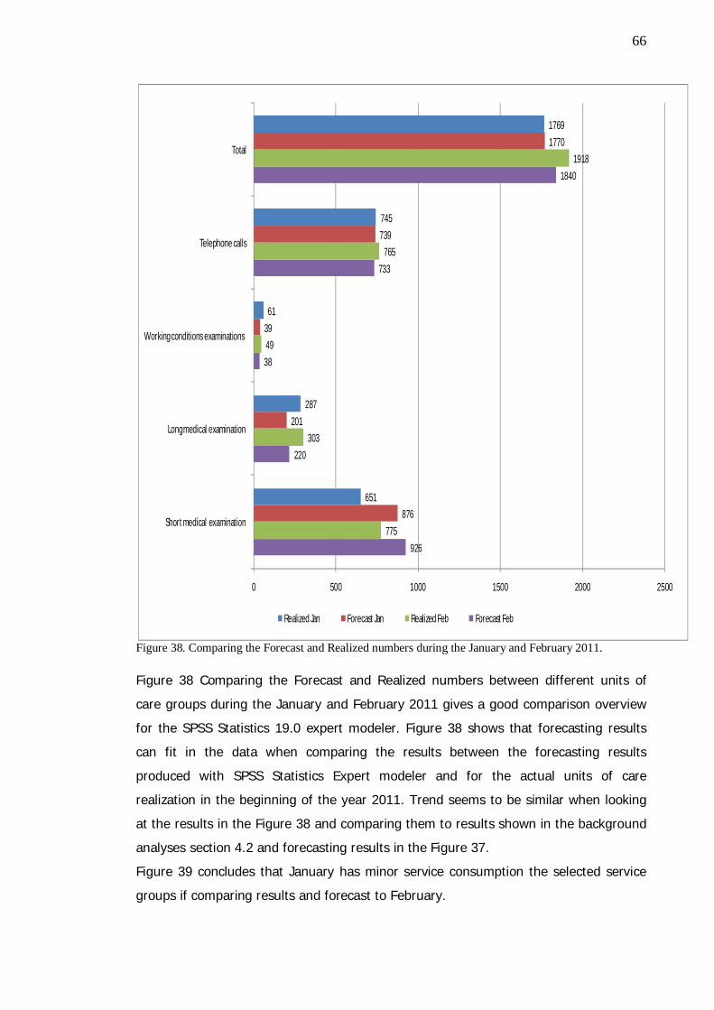
66
Figure 38. Comparing the Forecast and Realized numbers during the January and February 2011.
Figure 38 Comparing the Forecast and Realized numbers between different units of
care groups during the January and February 2011 gives a good comparison overview
for the SPSS Statistics 19.0 expert modeler. Figure 38 shows that forecasting results
can fit in the data when comparing the results between the forecasting results
produced with SPSS Statistics Expert modeler and for the actual units of care
realization in the beginning of the year 2011. Trend seems to be similar when looking
at the results in the Figure 38 and comparing them to results shown in the background
analyses section 4.2 and forecasting results in the Figure 37.
Figure 39 concludes that January has minor service consumption the selected service
groups if comparing results and forecast to February.
926
220
38
733
1840
775
303
49
765
1918
876
201
39
739
1770
651
287
61
745
1769
0 500 1000 1500 2000 2500
Short medical examination
Long medical examination
Working conditions examinations
Telephone calls
Total
Realized Jan Forecast Jan Realized Feb Forecast Feb
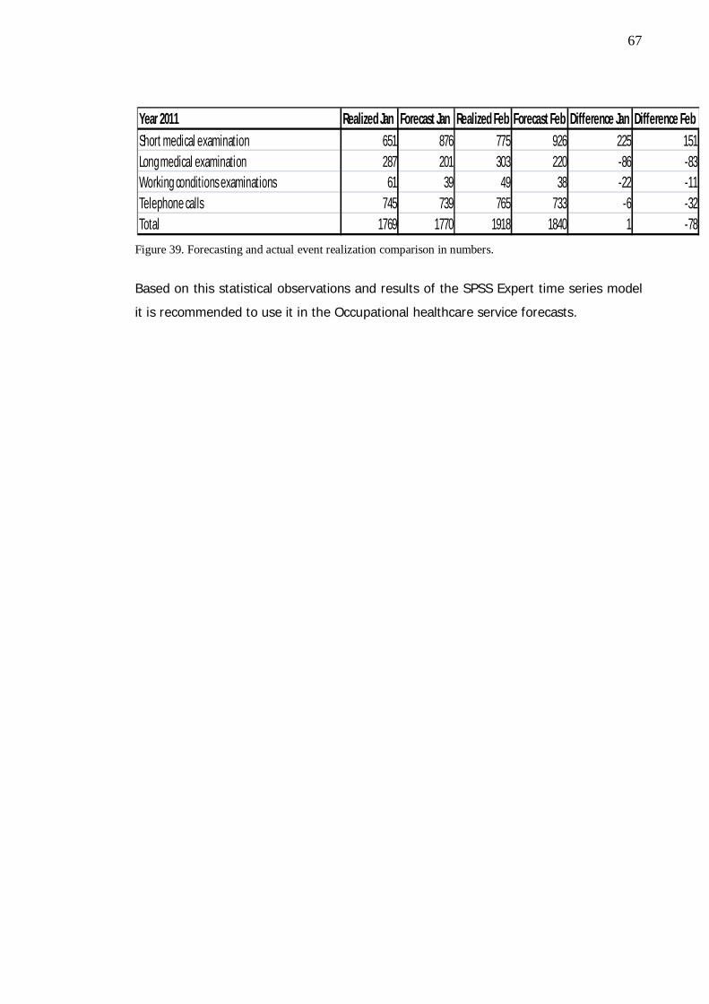
67
Figure 39. Forecasting and actual event realization comparison in numbers.
Based on this statistical observations and results of the SPSS Expert time series model
it is recommended to use it in the Occupational healthcare service forecasts.
Year 2011 Realized Jan Forecast Jan Realized Feb Forecast Feb Difference Jan Difference FebShort medical examination 651 876 775 926 225 151Long medical examination 287 201 303 220 -86 -83Working conditions examinations 61 39 49 38 -22 -11Telephone calls 745 739 765 733 -6 -32Total 1769 1770 1918 1840 1 -78
68
5.6 Management interview analyses
Line management and top management were interviewed after presenting the
background data analyses in section 4.2 and after analyzing forecasting tools in section
5. Interview template can be found on the Appendices (Appendix 1). Interview
questions were straighten the following issues:
How managers were seen the business unit healthcare service demand?
How service provision will effect to the service demand?
How managers see the service provision change in the past three years
How they can explain the non-seasonal changes of the service provision
Also open discussions for the forecasting results were done during the interviews. In
addition, the objective was that the interviews confirms the fact that represented
forecasting tool could used in the case business unit and from the time being in the
whole organization
Management interviews were conducted for the selected business unit management
team which consist two managers. Also the CEO of the OHCC was interviewed. When
analyzing the forecasting results with line and top management the following
conclusions can be made.
The managing doctor of the selected business unit highlighted the fact, that in
historical data analyses, non seasonal changes can explain the possible short
temporary post assignments for the doctor’s positions. Also holiday seasons in spring
and autumn time reflects to the provided service. The managing doctor and the
managing nurse of the selected business unit concluded that changing the process for
phone call services in 2009 has stabilized the provided service volumes when looking at
the background data analyses in section 4.2 and the SPSS statistics expert modeler
forecasts in Figure 38. Managing doctor also pointed out the fact that changing the
weekly meeting time processes might have an influence for the provided services.
Friday afternoon service hours are reserved for the writing work and team meetings
which reflect the low figures on Fridays.
When analyzing the forecasting results and realized events on January and February
following conclusions can be done with the management interviews. January is partly
holiday season and that is effecting directly for the January results. This was confirmed
with the whole management team.
69
Forecasting could help improve the business unit holiday planning if holidays are held
more on low seasons.
When looking at the forecasting results and looking the actual forecast in the
interviews, is noticed that the actual forecasting environment is larger and better
results can be gained for forecasting. This means that selected SPSS expert modeler
could also be functioning in the whole organization. Managing doctor of the selected
business unit suggests that; one way to handle the demand better is to differentiate
occupational services. It can be differentiated to working conditions examinations, long
medical services and the short medical examinations which can be often specified as
bulk service, for example diagnosing some minor diseases flu and influenza. These
kinds of bulk services might be more easily to outsource or rent more doctors in-house
to provide the bulk service. Then in-house personnel could concentrate more on the
long medical examinations and working conditions examinations.
Management team confirms that this kind of bulk service changes have already been
launched to respond better for the demand need. In short term, medical services are
constructed in a way, that part of the doctors are specialized for providing the bulk
services and some doctors are only providing long medical services and working
conditions services. These kinds of changes in the service process might gain better
abilities to respond the demand.
Management team pointed out the fact that; The service agreements between the
outsourcing services or firms that are renting the doctors in-house firms can be
redefined in a way, that these service providers must commit to provide short term
medical services, in a short notice to better respond for the changing demand in short
period of time. Line management interviews pointed out the fact that forecasting result
can be provided for the outsourcing partner to plan their resources better and to better
respond on changing demand. With better cooperation improved service chain can be
gained.
70
6 Discussion and Conclusions
This Thesis has investigated and analyzed the demand that Helsinki City Occupational
Healthcare Center and its selected business unit doctors are facing on annual, monthly
and daily level. Main purpose for this Thesis is to help the OHCC top and line
management to plan the workload in different times and situations. This study provides
information for healthcare organizations to better explain how to improve their
performance through forecasting. The availability of additional forecasting information
helps the line managers involved in a specific medical process, to make prompt
decisions and align different units that manage each separate part of the healthcare
process. Improved forecasting, without related process or layout modification, provides
only limited performance improvement.
This Thesis first introduced the findings from the literature, how healthcare
organization should select the forecasting model and built the forecasting process.
Current status analyze of the case business unit customers is introducing demographic
information such as age profile of the selected customers. Historical background data
analysis has pointed out the fact, that OHCC has seasonal changes in the service
provision. In the section 5 three different forecasting models are introduced and
tested. Comparison is done with R-squared method which is introduced in this Thesis.
Selected and proposed model is tested and compared with the actual service group
event realization figures from the January and the February 2011. Management
interviews were conducted after analysis and selection of the forecasting model.
Management interviews consists the two managers of the selected business unit and
the CEO of the OHCC. Discussion and conclusion part polishes the selected model.
Suggested forecasting model has been limited for the research reasons in one selected
business unit and its doctors and their customersThe outcome of this Thesis represents
a tool and model for predicting demand on a monthly level. This study is not only
providing a model for sales forecasting. This Thesis is more complex than normal sales
forecasting process, because of the complexity of the whole healthcare process, which
is presented in the Figure 2 at the literature analysis section. Need, demand and supply
of the healthcare services are tight in the healthcare service provision.
71
The literature review has showed different options in service business and in the
healthcare services for forecasting and demand analyses. Customer demand analyzes
can be measured in different ways. The literature review shows the models how
organization should investigate and try to understand the population and their
healthcare needs better. Organization managers have to select the right items for
forecasting. Healthcare service which are investigated are implemented as doctor’s
short medical examinations, long medical examinations, working conditions
examinations and examinations services provided through phone calls. These cares of
unit groups has been selected for the main forecasting unit because they are available
in the right format for forecasting. Because this Thesis case business unit has not been
having large changes in customer population or in the organization itself this is the
reason why additional data interpretation is not needed. For further analyses in
different organizations and different business units it is important for forecasters to
understand the historical changes in the forecasted environment. To implement the
forecasting process in use for the selected organization is the starting point in creating
customer demand analysis. In the forecasting process, if organization has empty spots
in the forecasting process, that can cause data misinterpretation and forecasting
errors. Literature points out the fact that historical background data analyzes are
important for the organization which is starting to develop forecasting process.
Historical data can indicate the possible seasonality and trend effects of the healthcare
services.
The purpose of this thesis is to build up the ground for forecasting methods and give
the opportunity for the organization to use them. One of the main goals for the
literature review is to understand the customer and its population more clearly and to
clarify the other critical aspects when starting to analyze the historical data and
constructing the forecasting methods. This Thesis is examining the Human resource
data such as age and other demographic data of the case customer population in order
to create a better understanding of the customer demand base. Human resource data
is not added to the forecasting tool which is introduced in the section 4. Human
resource data in this Thesis gives more background information for how to analyze the
customer demand forecasting in the selected business unit.
72
Stark et. al. (2008) proposes in literature review that organization should answer the
five key questions to establish the business need and to clarify demand forecast.
This Thesis answers these five key questions as follows. Forecasting in this study will
influence the workload planning and gives better understanding of the demand which
selected business unit doctors confronts. Key stakeholders of this study are the line
managers of the selected business unit and the top management of the OHCC. Metrics
which are used in the forecast are defined to be the selected groups of the units of
care and the actual events of the OHCC patient care system are status “Ready”-events.
These status “Ready”-events consist the needed timestamp which can be exploited in
the forecasting. It is important to understand the trends and seasonality issues in the
forecasted data. This Thesis introduces model which is looking the forecast projection
2-4 months ahead. Model provides an opportunity to make forecasts in more detailed
level, but this Thesis recommends that the actual forecasts should be made at 2-4
months period. Accuracy of the forecasts will be measured by using forecasting error
tools such as introduced in section 3.3 forecasting errors. Statistical software’s such as
SPSS statistics have built-in these features. In this Thesis the forecasting accuracy is
measured with using R-squared method. R-squared method is used in this study to
illustrate how well the regression line approximates real data points. This Thesis
recommends that any forecasting which is done for any organization should be aware
of the forecasting errors and it is recommended to use at least two different models to
approve the forecasts as precisely as possible. Even though, anybody cannot predict
the future precisely.
In this study the literature analyses show that different forecasting approaches can be
suggested and they can be used in the different customer categories. Literature review
points out that forecasting method can be categorized as judgemental or statistical
methods. This Thesis is using statistical method for the forecasting. Two different
forecasting models and two modification of the other are introduced in this Thesis.
Models which are introduced are Arma model, ARIMA model, Seasonal ARIMA and
SPSS expert Modeler which take into consideration seasonality and compare the results
by mixing ARIMA and exponential smoothing models. SPSS expert Modeler has also
been selected as the main tool for the case organization business unit.
73
Time series models such as ARMA, ARIMA and SARIMA models are introduced in
Research Method and Material section. This study introduces the forecasting errors.
Often forecast accuracy is measured, but it is not identified what are the impacts of
forecast errors. Forecasting accuracy is measured in this Thesis by looking at the R-
squared measures which are used quite often in literature to measure the forecasting
accuracy.
ARIMA modeling can take into account trends, seasonality, cycles, errors and non-
stationary aspects of a data set when making forecasts and for that reason ARIMA
model and its variations are selected in this Thesis to conduct the Healthcare service
demand forecasting.
Section 4 analyses the selected business unit customers. Age as a variable should be
considered when validating the forecasting results. In this study researchers main
purpose was to keep the forecasting variables as simple as possible in order to build up
as clear model as possible. Literature review has also pointed out that, the more
complicated the model is more difficult it is to produce reliable forecasts. Even thought
the age seems to be the constant factor when prospect customers are facing the need
for occupational healthcare services. When analyzing the HR results in the section 4
following conclusions can be done. Age is factor that has to be considered when any
healthcare service is provided if the information of the customer population is
available.
As shown in the Table 6 (Age differentiation table) following assumptions can be
made. Now the largest population group is 50-59 years old and that might cause an
extra need for healthcare services after few years, even though OHCC has already
started projects for preventative healthcare services, which might change the demand
peeks after few years. The results of these projects have to be considered when
conducting forecasting methods after few years.
The knowledge of the current customer population is important for the healthcare
service provider. In that sense, occupational healthcare provider can make deeper
analyses of its customer population, because it usually has a wider knowledge of its
customers, when comparing for example to public hospital, which has more limited
information about its customer base.
74
A historical data analysis of the selected case customer population gives a good
overview of the services used in the previous years. That also helps the line
management and top management to adjust the decisions concerning the workload
between individual teams and between different business units. Historical data also
points outs clearly the seasonal variations of the occupational healthcare services
provided to the customer.
When analyzing the forecast results in the section 5 the customer demographic
information has to take into consideration in the analysis.
When using ARMA model to forecast case customer demand following conclusions can
be made. ARMA model do not take into the considerations the seasonality of the
background data which Occupational healthcare services seems to have when looking
at the historical data figures in section 4. ARMA model uses on p and d values which
do not calculate the data seasonality change of the background data if there one
exists. ARMA model can be used in case organization if the forecasting is limited to one
or two week timeframe. After longer period ARMA model gives only figures that
represents growing time series which do not fit in the case organization or in the
Helsinki City OHCC historical patient background data or the actual results which are
seen in the beginning of the year 2011. Also different numbers were tested how they
could fit in the ARMA model, even though the results seems to have the same
paradigm that ARMA model cannot acquire the forecasting accuracy with the OHCC
demand forecasting.
Seasonal ARIMA fits better to case business unit customers demand forecasting.
Seasonal ARIMA uses the SARIMA (1,0,1) model which also observes the seasonality of
the historical background data. Results that are represented in the section 5.2 Adding
variables to the SPSS-statistics SARIMA-model. Figure 26 gives improved results for the
R-squared figures, if we compare them to same figures for the ARMA model in Table 8.
This also confirms the fact that ARMA model is not working in the case healthcare data
and as forecasting method for the case organization business unit. Forecasting results
in the Figure 28 and 29 shows relatively good forecasting results and seems to be that
75
SARIMA model is forecasting high seasons in spring time to February, March and April
and for the another high season in September and November.
When using SPSS statistics 19 and SARIMA (1,0,1) model for the day level forecasting
we can see in the Figure 30 for short medical examinations day data in SPSS statistics
that R-squared figures are boomed if we compare results for the SARIMA monthly level
forecasting to 0,096 for day level results 0,247. Even when the above mentioned
results were good in research point of view the purpose was to find the best fitting
model for demand forecasting.
This Thesis also introduces and analyses the SPSS statistics Expert modeler method
which uses both ARIMA model and Exponential Smoothing methods, and combines the
seasonality change of the historical background data. In section 5.4, Adding data to
SPSS Expert time series modeler, we can be seen the improved outcome if starting to
compare the R-squared figures in the Figure 34 Model fit statistics for SPSS expert
modeler. R-squared figures are increased if looking at the short medical examinations
from SARIMA model 0,247 to expert model 0,79 which shows large growth in numbers.
In Figures 36 and 37 we can see that also long medical examinations have the
seasonal effect which the background data analyzes have been pointing out in the
Section 4 Current status analyzes of the Case organizations customers graphs. That
also overrules the SARIMA model conclusion that long medical examinations do not
have the same seasonality which other service groups seems to have. When
constructing forecasts with SPSS statistics expert model the figures also replicates
existing conditions which is a good point of reference when evaluating forecasting
tools. When comparing forecasting results constructed with SPSS expert modeler and
actual event realization in Figure 35 and 36 we can see that SPSS expert modeler is
giving good results, if comparing results between ARMA and SARIMA model. Also the
trend between January and February seems to be similar when looking at the results in
the Figure 38 and Figure 39.
When analyzing the forecasting results with line management following conclusions
can be made. Forecasting results can help the outsourcing partners to respond the
changing demand better. Forecasting tool will help line managers to plan better the
workflow between different annual periods. Forecasting model results are suggested to

76
draw the big picture for the customer demand for the line managers and also for the
top management to better analyze the customer demand.
The above mentioned results for the SPSS statistics expert modeler concludes that the
expert modeler fits best for these introduced models as a forecasting tool for the OHCC
selected business unit and predicting its doctor demand. It can also be recommended
that forecasting should be done on a monthly level. Even though weekly and even
daily level forecasts are possible, but might not offer any extra benefit to the line
management or top management.
77
6.1 Proposed Tool for the Case Organization
This sub-section identifies and builds together a model based on the above mentioned
datasets and analyses of the case organization selected business unit. Model is
integrated to operational and financial planning and is working in one selected system
first on Microsoft excel spreadsheet and compared forecasting is done by using SPSS
statistics SARIMA model and Expert modeler. Main goal for the tool is to give a
simplified tool and the ability to frequently reforecast and to respond to business
changes with “what if” scenarios as often as necessary.
Forecasting model is tested and verified with the line management. Demand forecast
will be updated each month with last month results of the case organizations business
unit.
Forecasting results are presented as a Dashboard. The Dashboard gathers up the
results that are used in the forecasting. Dashboard includes the last month’s results
and also three years of historical data to illustrate the seasonal effects that OHCC is
meeting annually. Section five shows that SPSS statistics expert modeler can provide
functional tool for forecasting. Forecasting figures are added to the forecasting model
after each month and forecast is done based on the historical background data. SPSS-
statistics expert time series model concerns the seasonality of the occupational data
and therefore the line management can observe and make decisions based on the
forecasts.
78
6.2 Managerial implications
Managerial implications in this Thesis are the tool for healthcare managers. Forecasting
is also an organizational, not only a technical issue. The Thesis provides a view for
managers to handle and put in process demand forecasting in the healthcare services.
The tools presented in this Thesis may help the manager in different ways to select
and handle the demand forecasting. In the following, some potential managerial
implications are introduced.
1. Implement the forecasting methods from the literature and then select the
software tool for forecasting. It is also useful to notice the main trouble when
implementing the forecasting practices and when defining the goals of
forecasting, defining organizational responsibilities, and building effective
performance measurement practices.
2. Plan the workload between different units and its doctors. Forecasting tool can
provide information for the line management to schedule the holidays outside
the high season.
3. Predict the need and capacity of the extra workforce and the use of rented
doctors. One of these Thesis goals is to show for the organization when
organization should try to react to the customer demand and employ more
rented doctors to cover the demand overlap.
4. Develop the forecasting process for all the other business units as well as to
start handle the customer demand more accurately.
5. Investigate and analyze some problems that occur in managing demand
information in the healthcare such as
Selecting the forecasting tools
Explaining possible forecasting errors
Enhancing the overall comprehension of the total forecasting process
79
6. Occupational healthcare center might provide the forecasting results for their
outsourcing partner to better plan the possible overflow of the services that
Occupational healthcare center cannot respond.
These recommendations made in this study are based on the analysis of the case unit
and in the presented forecasting tools. They have also been influenced by relevant
professional literature and the experience gained during this study. This Thesis
proposes forecasts to be done by using SPSS Statistics 19 and its expert modeler as a
forecasting model. This Thesis also suggests that OHCC start to conduct forecasts with
other healthcare professionals such as nurse’s physiotherapists and psychologies. It is
also recommended that introduced forecasting model should be escalated for the
whole organization. The main managerial contribution of the implication is that when
used correctly, they help managers to clarify the forecasting process in a resource-
efficient way. The benefits of this study can be seen after running forecast side by side
with current management system and governance. When running forecast side with
current management system is easier to embed forecasting process to the whole
organization. With alternative forecasting process, the organization can gain more
knowledge of its customer demand.
The results for this Thesis are limited directly to the case company and for one
selected business unit and this may limit the functionality of the model. The second
limitation has to do with the extent to which the findings can be generalized beyond
the forecasting models studied. The number of models is too limited for broad
generalizations. However, the three different forecasting models represent rather
different aspects of the forecasting process. Further empirical evaluations, however,
are needed to replicate the findings in different contexts and surroundings. Also more
forecasting accuracy indicators besides the R-squared method could be adjusted to the
model.
For the follow up studies, this Thesis recommends that also as the data including age
and sick leave data and diagnostic data should be investigated for the use of
forecasting variables. It is also suggest for the follow up researchers to investigate and
compare other statistical and judgemental methods. With alternative forecasting
process organization can gain more knowledge of its customers demand. All though

80
forecasting resources have to be in balance and in line to the organization and
forecasting budget should not be exceeded therefore at forecasting is only providing
help for the management decisions.
81
7 Summary
This Master’s Thesis builds a forecasting model for doctor´s appointments demand in
the city of Helsinki OHCC in one of its selected business unit for its doctors and their
customers.
In this Thesis the research methodology was based on forecasting theory and
benchmarking models that already exist in science and business. Literature review
introduced the forecasting theory and background for the organization to start to
construct forecast for its selected forecasting target. At first healthcare organization
has to get knowledge for its customer population and best available background
information of its customers. Literature review also concludes that healthcare
organization have to examine the existing variables that organization wish to use in the
selected forecasting method. Organization has to construct and analyze the historical
background data at least 2-4 year’s timeframe to navigate the trend and seasonality
issues which occur in the provided healthcare service.
This Thesis presents different forecasting methods which are introduced in the
literature. Forecasting literature has divided forecasting as statistical and judgemental
forecasting methods. This study lists and introduces models for both statistical and
judgemental forecasting methods.
The background of the time series forecasting such as ARMA, ARIMA and SARIMA
forecasting methods which are used in this Thesis to perform the forecasts were
presented in the Research Method and Material section.
Current status analysis of the case company customers provide information about
customer age distribution, and other age related factors that Healthcare organization
have to know about its customers, when starting to construct services for their
customers and when starting to proceed forecast of its customers demand.
This Thesis has selected to use three different forecasting models to find out the best
possible outcome for the organization to choose the best forecasting tool. Exhibited
tools are Microsoft Excel Add-In, the SPSS statistics 19 SARIMA model and the same
82
products Expert modeler which has been selected as the forecasting tool for the case
organization customer demand analyzes.
SPSS expert modeler combines both ARIMA and Exponential smoothing models and
also considers the seasonality of the background data at the same time.
This Thesis proposes for the OHCC to conduct their forecasts by using SPSS Statistics
19 and its expert modeler because this model seems fitting in the background data and
for to produce forecast. For the follow up studies, this Thesis recommends that for the
use of forecasting variables the standard human resources data including age and sick
leave data, and diagnostic data should be further investigated.
83
References
Alho J M (1990). Stochastic Methods in Population Forecasting. International Journal ofForecasting, Volume 6, Issue 4, December 1990, Pages 521-530
Alpern P (2010).Forecasting the Future with Predictive Analytics.. Industry Week Vol.259, Iss. 7; pg. 47
Armstrong S. J., Collopy F. (1992). Error measures for generalizing about forecastingmethods: Empirical comparisons. International Journal of Forecasting 0869-80
Anderson, T. W., and Goodman, L. A. (1957). Statistical inference about Markovchains. Annals Math. Statistics, 28, 89-110.
Behner, K. G., Fogg, L. F., Fournier, L. C., Frankenbach, J. T., Robertson, S. B. (1990).Nursing resource management: Analyzing the relationship between costsand quality in staffing decisions. HealthCare Management Review, 15,63-71.
Borison, A; Hamm, G. (2010). California Management Review, Vol. 52 Issue 4, p125-141, 17p
Bose R.(2003). Knowledge management-enabled healthcare management systems:capabilities, infrastructure, and decision-support. Expert Systems withApplications 24 59–71
Box, G., E. P., Gwilym M. Jenkins, G. Reinsel C. (1994).Time Series Analysis:Forecasting and Control, 3rd ed. Prentice Hall, Englewood Cliffs.
Bretthauer, K. M (2010.) A model for planning resource requirements in healthcareorganizations. Decision Sciences. FindArticles.com.http://findarticles.com/p/articles/mi_qa3713/is_199801/ai_n8759291/
Chubb M. C., Jacobsen K. H (2010). Mathematical modeling and the epidemiologicalresearch process. Eur J Epidemiol 25:13–19
Coskun H.,Diyar A., Fevzi K.(2009). Comparison of direct and iterative artificial neuralnetwork forecast approaches in multi-periodic time series forecasting.Expert Systems with Applications 36 3839–3844
Dickersbach J.(2007). Service Parts Planning with mySAP SCM™ Processes,Structures, and Functions. Springer Berlin Heidelberg. p. 63-108
Engle, R.F. (1982). Autoregressive Conditional Heteroscedasticity with Estimates of theVariance of United Kingdom Inflation, Econometrica,50(4): 987-1006.
Farmer R.D. Emami J. (1990).Models for forecasting hospital bed requirements in theacute sector. Journal Epidemiological Community Health 44 307–312.

84
Gilchrist R. (1985). Some aspects of modeling operational problems in the NationalHealth Service, The Statistician 34.p. 209–214.
Gilbert, K (2005). Management Science, Vol. 51 Issue 2, p305-310, 6p
Finarelli, H J. Jr. (2004).. Effective demand forecasting in 9 steps: shifts in demand fora hospital's services can occur unexpectedly. Demand forecasting canhelp you prepare for these shifts and avoid strategic missteps. HealthcareFinancial Management. FindArticles.com.
Hall R. W. (2006). Patient flow: reducing delay in healthcare delivery. Sringersinternational series USA California.
Kaipia R, Hartiala H. (2006). International Journal of Logistics Management., Vol. 17Issue 3, p377-393
Kao, E. P. C., Tung, G. G. (1981). Aggregate nursing requirement planning in a publichealthcare delivery system. Socio Economics Planning Science, 15, 119-127
Laaksonen N., Laaksonen, M., Sarlio-Lähteenkorva, S.,Lahelma, E. (2004). Multiple di-mensions of socioeconomic position and obesity among employees: TheHelsinki health study. Obesity Reseach 12 (11) 2004: 1851-1858.
Lallukka, T., Sartio-Lähteenkorva, S., Roos, E., Laaksonen, M., Rahkonen, M. &Lahelma, E.(2004). Working conditions and health behaviours amongemployed women and men: the Helsinki Health study. Preventivemedicine. 38(1):48-56.
Lillrank P., Groop PJ., Malmström TJ. (2010). Demand-supply –based OperatingModes in Healthcare. Millbank Quarterly Vol 88, No 4
Lillrank P. Venesmaa A. (2010) Terveydenhuollon alueellinen palvelujärjestelmä,Talentum 2010
Mahrnoud M., DeRoeck R., Brown R., Rice G. (1992). Bridging the gap betweentheory and practice in forecasting. International Journal of Forecasting 8(1992) 251-267
Mills, T C.(1991). Time Series Techniques for Economists.Cambridge University Press,p.116-120
Milner P.C.(1988). Forecasting the demand on accident and emergency departmentsinhealth districts in the Trent region. Statistics in Medicine10 1061–1072.
Murray J. C.(2001) Four Methodologies to Improve Healthcare Demand Forecasting.Healthcare Financial Management. FindArticles.com.
Myers C (2004). Forecasting demand and capacity requirements. Healthcare FinancialManagement. FindArticles.com
Syntetos, A. Nikolopoulos A, Konstantinos; B, Fildes J, Goodwin. R. (2009). The effectsof integrating management judgement into intermittent demand forecast,International Journal of Production Economics. Vol. 118 Issue 1, p72-81,
85
Schrieber, J. (2005). Demand visibility improves demand forecasts. Journal ofBusiness Forecasting Vol. 24 Issue 3, p35-37, 6p
Stark D. (2008). 5 steps to creating a forecast: with the right process and tools,healthcare finance leaders don't need a PhD or a crystal ball to predictthe future. Healthcare Financial Management 2008.
Sfetsos A., Siriopoulos E. C. (2003). Combinatorial time series forecasting based onclustering algorithms and neural networks. Neural Comput & Applic13:p.56–64
Tae C. P., Ui S.K, Lae-Hyun K., Byung W. J., Yeong K. Y.(2010). Heat consumptionforecasting using partial least squares, artificial neural network andsupport vector regression techniques in district heating systems. KoreanJ. Chem. Eng., 27(4), 1063-1071
Talous ja Suunnittelukeskus (2010). Tietoja helsingin kaupungin henkilöstöstä. Talousja suunnnittelukeskuksen julkaisuja 2010/7.
Thomas R. (2003). Health Services Planning second edition. Springer US. 53-73
Tzafestas S., Tzafestas E. (2001). Computational Intelligence Techniques for Short-Term Electric Load Forecasting. Journal of Intelligent and RoboticSystems 31: 7–68, 2001. Kluwer Academic Publishers.
Zhang G., Patuwo P. E., Hu M.Y.(1998). Forecasting with artificial neural networks:The state of the art. International Journal of Forecasting 14 35–62
van Teijlingen, E. Pitchforth, E., Bishop C., Russell, E. (2006). Journal of FamilyPlanning and Reproductive HealthCare, 2006, 32(4), pp.249-252
Vissers J M H.(1998). Healthcare management modelling: a process perspective.HealthCare Management Science 1 77–85
Voudouris C., Lesaint D.,Owusu G.(2008). Service Chain Management TechnologyInnovation for the Service Business. Springer-Verlag Berling Heiderbergp. 51-64
Yin Robert K.(2009). Case Study Research: Design and Methods. Fourth Edition.SAGE Publications. California.
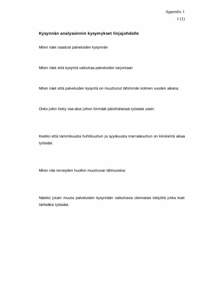
Appendix 1
1 (1)
Kysynnän analysoinnin kysymykset linjajohdolle
Miten näet osastosi palveluiden kysynnän
Miten näet että kysyntä vaikuttaa palveluiden tarjontaan
Miten näet että palveluiden kysyntä on muuttunut lähimmän kolmen vuoden aikana.
Onko jokin tietty osa-alue johon törmäät päivittäisessä työssäsi usein.
Koetko että tammikuusta huhtikuuhun ja syyskuusta marraskuuhun on kiireisintä aikaa
työssäsi.
Miten näe terveyden huollon muuttuvan lähivuosina
Näetkö jotain muuta palveluiden kysyntään vaikuttavia olennaisia tekijöitä jotka koet
tärkeäksi työssäsi.