DEVELOPING A BRAIN COMPUTER INTERFACE CONTROL SYSTEM FOR

ROBOTIC MOVEMENT IN TWO DIMENSIONS

by

Tyler Christopher Major

A thesis submitted to the faculty of

The University of North Carolina at Charlotte

in partial fulfillment of the requirements

for the degree of Master of Science in

Electrical Engineering

Charlotte

2014

Approved by:

______________________________

Dr. James Conrad

______________________________

Dr. Steve Kuyath

______________________________

Dr. Yogendra Kakad

ii

©2014

Tyler Christopher Major

ALL RIGHTS RESERVED

iii

ABSTRACT

TYLER CHRISTOPHER MAJOR. Developing a brain computer interface control system for

robotic movement in two dimensions. (Under the direction of DR. JAMES CONRAD)

This paper concerns the theory behind developing a brain computer interface (BCI)

and the applications of such a system. Signal acquisition methods such as Functional

Magnetic Resonance Imaging (fMRI), Near-Infrared Spectroscopy (NIRS),

Magnetoencephalography (MEG), Electrocorticography (ECoG), and

Electroencephalography (EEG) are discussed. There is also a review of the different types of

Event Related Potentials (ERP) and signal extraction methods for generating filters from the

captured data to generate a model for a BCI. Finally, this paper covers a review of notable

BCIs that are being utilized in a wide range of applications and gives a working example

using BCILAB to generate results from a sample data set using the techniques discussed in

the paper.

iv

DEDICATION

I would like to dedicate this work to my family. Without their support I would not

have been able to complete my research. I would also like to thank Dr. Conrad and my

friends I have made in the lab for supporting me throughout my graduate school tenure thus

far.

v

TABLE OF CONTENTS

CHAPTER 1: INTRODUCTION 1

CHAPTER 2: BACKGROUND 4

2.1 Dependent and Independent BCI 4

2.2.1 Functional Magnetic Resonance Imaging (fMRI) 5

2.2.2 Near-Infrared Spectroscopy (NIRS) 6

2.2.3 Magnetoencephalography (MEG) 7

CHAPTER 3: EVENT RELATED POTENTIAL (ERP) 10

3.1 Imagined Movement 11

3.2 Visual Evoked Potentials 12

3.3 Signal Extraction 12

CHAPTER 4: APPLICATION OVERVIEW 14

CHAPTER 5: DETERMINING IF A TRAINED SIGNAL HAS OCCURRED 18

CHAPTER 6: DATA SET USED IN STUDY 24

6.1 Raw Data 28

6.2 Event Duration 30

CHAPTER 7: PROCEDURE FOR DEVELOPING THE CONTROL SYSTEM 33

vi

7.1 Data Signals Associated with Motor Movement 33

7.2 BCILAB 34

CHAPTER 8: RESULTS 49

CHAPTER 9: CONCLUSION 50

REFERENCES 51

vii

LIST OF FIGURES

FIGURE 2.1: Example of a P300 type spelling BCI using a 6X6 matrix 4

FIGURE 2.2: The 10/20 international positions associated with labels for EEG reading 9

FIGURE 3.1: A standard ERP waveform showing the amplitude and time delays 11

FIGURE 5.1: Window showing the correct parameters for sampling the data 19

FIGURE 5.2: Parameters for labeling the targeted markers and parameter search 21

FIGURE 5.3: Effectiveness of the BCI 22

FIGURE 5.4: Visualization of the linear weights from each sample epoch that was chosen 23

FIGURE 6.1: The international 10/10 labeling system 27

FIGURE 6.2: Menu to change the channels read by EEGLAB 28

FIGURE 6.3: Raw unprocessed waveform of EEG recordings from the trial 29

FIGURE 6.4: Filtered signal that removes noise on the signal 30

FIGURE 6.5: Green area highlighting duration of a typical target 31

FIGURE 7.1: Picture showing the relevant sections of the brain for motor movements 34

FIGURE 7.2: Weighted ICA of one participant’s trials of hand movements 35

FIGURE 7.3: Main menu of the BCILAB plugin for MATLAB 35

FIGURE 7.4: Menu and options for loading the dataset file into BCILAB 36

FIGURE 7.5: Window for choosing the approach for the model 37

FIGURE 7.6: Option for CSP approach 38

FIGURE 7.7: Calibration options for generating a model 39

FIGURE 7.8: Results from the default parameters of the CSP model approach 41

FIGURE 7.9: Results from using the generated CSP model 42

viii

FIGURE 7.10: Approach of spectrally weighted CSP 43

FIGURE 7.12: Results of the generated spectrally weighted CSP on the calibration data 45

FIGURE 7.13: Final performance results of the spectrally weighted CSP 46

FIGURE 7.14: Visualization of spectrally weighted CSP model 47

FIGURE 7.15: Sample of the BCI simulating making a decision 48

CHAPTER 1: INTRODUCTION

Brain computer interfaces (BCI) are a relatively new technology that takes advantage

of the innate computing power of the brain. Developing BCIs have, up until recently, been

thought of as science fiction. Ever since the first discovery of electroencephalography (EEG)

by Berger, scientists have been trying to decode signals from the brain [4].

A BCI traditionally consists of four main parts; a sensing device, an amplifier, a filter,

and a control system. The sensing device consists of a cap with electrodes placed to the

International 10-20 standard [5, 6].The amplifier can be one of numerous biological

amplifiers on the market [7]. The filter and control system applied to the brain signals is the

focus of BCI research.

This research’s contribution to the field is to use preexisting techniques and apply

them to develop a system where a person would be able to control a robot for moving in two

dimensions. This means that the system developed here can be applied to systems such as a

wheelchair for a disabled person to a robot for remote navigation and recon. The techniques

covered in developing this BCI may be used for other systems as they are discussed in detail

here.

Due to the inherent size of the field, all techniques cannot be covered in a paper of

this size. This paper is concerned with presenting the basic background information and the

more common technologies of BCIs. Section 2 provides a background of overall BCI

concepts, including signal acquisition methods while comparing the benefits and drawbacks

2

of each method. Section 3 covers the different types of event related potentials (ERP) and

covers which method would be used for a certain type of task. Section 4 provides a quick

reference as to how a signal may be manipulated in post processing of obtaining the signal to

identify certain aspects of a signal. Section 5 is a comprehensive overview of the applications

of BCI in research and in practice. Section 6 gives a quick example of how a BCI may be

developed using the BCILAB plug-in for MATLAB.

CHAPTER 2: BACKGROUND

The first proposed application of a BCI was for use in therapeutics and for mental

disorder classifications [8, 9]. Modern BCI research focuses on patients with amyotrophic

lateral sclerosis (ALS), also known as “locked-in” syndrome [10, 11, 12, 13, 14, 15, 16]. BCI

research has also expanded to include systems that healthy individuals can utilize to expand

normal human capabilities [17, 18].

2.1 Dependent and Independent BCI

BCIs are categorized into two different types; dependent and independent. A

dependent BCI relies on element pathway in the brain to generate activity. An example of

this BCI type would be the spelling program shown in Figure 2.1 [19].

This system is monitoring the brain waves for event related potentials (ERP),

recognizable patterns in brain waves that occur during stimuli, such as being presented with a

specific image or an imagined movement. A matrix containing the desired outputs, such as an

array of letters in a spelling program, flashes at a specific rate. Utilizing the data from the

flashing and the timing of the ERP, the desired letter is extrapolated. The specific ERP that is

being monitored in the case of the spelling program is called a visual evoked potential (VEP).

The contribution from the visual cortex is the dominant signal in VEPs, so naturally this

signal is used to determine which letter the subject is observing. The dependent BCIs are

accurate and commonly used, however this model is inadequate for a person with severe

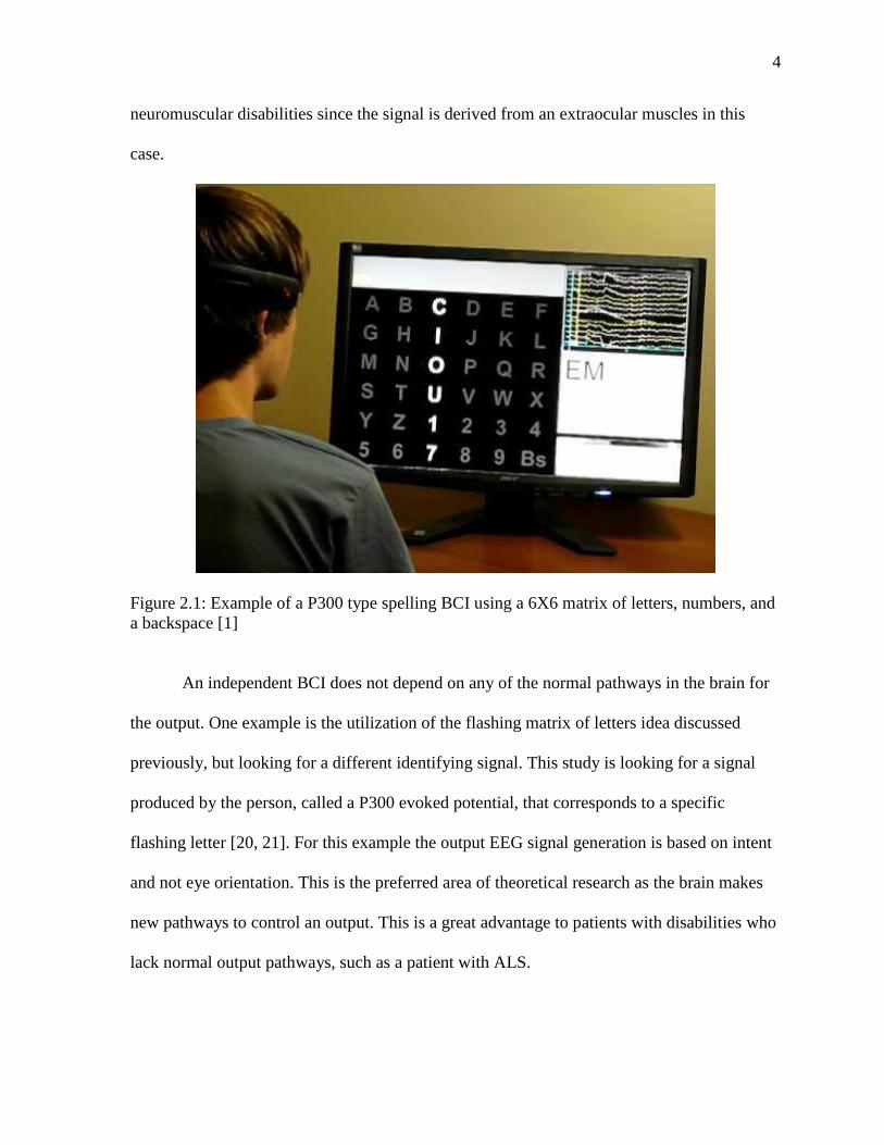
4

neuromuscular disabilities since the signal is derived from an extraocular muscles in this

case.

Figure 2.1: Example of a P300 type spelling BCI using a 6X6 matrix of letters, numbers, and

a backspace [1]

An independent BCI does not depend on any of the normal pathways in the brain for

the output. One example is the utilization of the flashing matrix of letters idea discussed

previously, but looking for a different identifying signal. This study is looking for a signal

produced by the person, called a P300 evoked potential, that corresponds to a specific

flashing letter [20, 21]. For this example the output EEG signal generation is based on intent

and not eye orientation. This is the preferred area of theoretical research as the brain makes

new pathways to control an output. This is a great advantage to patients with disabilities who

lack normal output pathways, such as a patient with ALS.

5

2.2 Signal Acquisition

Signal acquisition is a substantial challenge in the field of BCIs. Traditional

approaches focus on EEG signals [4], however, other methods exist that can capture

neurological activity. Each method has their strengths and weaknesses for capturing different

portions of signals from the brain. End use, intended by the designer, is the factor that filters

out which method to move forward with.

2.2.1 Functional Magnetic Resonance Imaging (fMRI)

One of the more practiced methods for detecting neurological activity for research

purposes is called Functional Magnetic Resonance Imaging (fMRI). This process involves

observing a subject’s change in blood flow (hemodynamic response) while they are laying in

a Magnetic Resonance Imaging (MRI) machine. The response that active neurological

processes produce is known as the Blood Oxygen Level Dependency (BOLD) [22]. This

response arises from the basic principal that regions of the brain that are more neurologically

active will require a higher hemodynamic response than areas of the brain that are not

engaged. One of the main drawbacks of using fMRI is the relatively slow reaction time of the

system. This delay is attributed to the response time of the BOLD response of the brain

which typically can delay anywhere from 3 to 6 seconds [23]. However, there is research that

suggests that this delay can be overcome with techniques that look for finer BOLD responses

in specific areas and using that information for a real-time BCI or as an initial guide for fine

tuning EEG procedures [24].

The drawbacks of an fMRI do not exclude it as usable and viable technique for BCI

control. The BOLD signal response has successfully been used as an indicator for intended

movement [23]. A study placed participants in an MRI machine that showed high variance

6

between BOLD responses for different intended movement. This analysis was performed off-

line, but clearly shows the feasibility of using fMRI for an on-line BCI. This study occurred

with four volunteers and consisted of two calibration sessions and a feedback session. During

the feedback section the volunteers were shown the activity levels through a video projection

of the regions of interest (ROIs). A custom developed software that ran separately on another

computer made this process possible. During the experiment it was very important, as it is

with all BCIs, to remove artifacts, such as background noise from eye and muscle movement

a.k.a. electromyography (EMG), would override the desired signals. Real-time motion

correction was used to remove the contributions from muscular movement.

Another example of fMRI use for brain control method is the detection of imagined

and executed unimanual and bimanual movements [25]. In this experiment eight healthy

righthanded volunteers were chosen to participate. Their handedness was verified using the

Edinburgh Handedness Inventory [26]. The experiment consisted of three parts: two

unimanual movement and one bimanual movement. Subjects were asked to individually

move their fingers, excluding thumbs, in predefined repeating sequences. Once the sequence

was completed, the trial was performed again with imagined movements as opposed to actual

movements. While there was predicted variability in each individual subject, there was also a

clear trend. Actual movements were consistently at a higher potential level than imagined

movements, and thereby providing a more accurate signal, but the imagined movements still

provided a cluster of neurons acceptable for reliable signal detection.

2.2.2 Near-Infrared Spectroscopy (NIRS)

NIRS is a method that uses light close to the infrared spectrum to monitor a response

that is similar to the BOLD response called regional cerebral blood flow (rCBF) [27]. NIRS

7

is used to look over a general area of the brain for activity, though LEDs have been used for

more precise detection. Pairs of illuminators and detectors form channels for the signals.

Near-infrared rays emit from each illuminator and pass through the skill and brain tissue to

be received by the detectors. An example of NIRS being used for an on-line BCI spelling

program can be found [27]. This study involved five individuals who underwent a baseline

trial, a partition, and a motor task. The motor task involved finger tapping which would be

dictated by on screen prompts. One of the weaknesses of NIRS measuring is the dependency

of passing through the skull; this means that things like hair can greatly hamper the signals

and give faulty readings.

2.2.3 Magnetoencephalography (MEG)

MEG provides more sensors, and thus more spatial information, than traditional a

EEG. In order to take MEG recordings, a subject, in a magnetically shielded room, is placed

in a chair with an array of superconducting quantum interference devices (SQUIDs) around

their head as the magnometer. The obvious drawback to this approach is the dependency of a

magnetically shielded room and a large machine to sense the brainwaves. Research has

proven that even with these constraints that MEG is still a viable and reliable enough of a

method to be explored further [28].

2.2.4 Electrocorticography (ECoG)

Differing from the previous methods ECoG is an invasive method. ECoG requires

surgery to implant electrode pads directly onto the surface of the brain to receive signals

from the cerebral cortex. The advantages of this are immediately clear: high spatial

resolution, broad bandwidth, high amplitude, and less vulnerability to EMG [29]. ECoG is

also widely used as an identifier for the localization of epilepsy focal points. An array of 64

8

electrodes is implanted onto a portion of the brain called the epileptic focus to identify the

part of the brain that should be removed by resection surgery. During one study, patients with

epilepsy were implanted with these electrodes. In the period of the one to two weeks that the

electrodes are recording data to localize the seizure area, researches used the electrodes to

generate a BCI. While the electrodes were removed in this instance due to the epileptic

nature of the patients, the success of this study proves that these arrays are a valid method for

use in BCI development and not just epileptic identification.

2.2.5 EEG

EEG is a technique involving the placement of electric field sensing electrodes

around the scalp of an individual. The placement of these electrodes is standardized with a

technique called 10/20 positioning [6]. A subject is instructed to clean their hair vigorously

the night before the readings are taken. Measurements are taken according to the

international 10/20 manual and the electrodes are placed against the scalp of the subject with

a conductive medium, such as conductive gel, placed on the pads to facilitate the acquisition

of signals.

This method is, by far, the most popular for capturing signals from the brain. A few

of the factors that make EEG such an attractive method are as follows: standardization of

electrode placement, information on acquisition techniques well documented and plentiful,

established as a reliable method with known filtering techniques, and the relatively low cost

compared to other methods.

Since this is the most popular method, there is ongoing research to simplify the use of

EEG for commercial applications, rather than the often complex and time consuming task of

applying the 10/20 system [30]. Systems such as these are predicted to be the on the user end

9

of a BCI as opposed to the research end. These types of headsets are attractive to the user for

their ease of set up and very low calibration times; with this example being in the range of

ten seconds. Another big advantage to this system is that it can potentially work with many

different types of headsets that are already available in the market.

One big caveat about EEG signals through, is that a sensed signal does not

necessarily mean that that electrode is the source of the signal [31]. This counter intuitive

phenomena is due to the fact that the brain is folded. In order to find the source of the signals,

methods such as independent component analysis (ICA) are being widely used now as a

localization technique. EEG signals are thus classified as being dipolar, meaning that in

representations it is shown that there is a signal and an associated direction for the

propagation of that signal [32].

Figure 2.2: The 10/20 international positions associated with labels for EEG reading [2]

CHAPTER 3: EVENT RELATED POTENTIAL (ERP)

An evoked potential (EP) is a signal that occurs in the nervous system after the

presentation of a stimulus. This signals is usually much smaller than the surrounding signals

and as such requires special filtering techniques to recognize and extract. In the signal

processing terms this signal is referred to as an event related potential (ERP). In the simplest

terms the recognition of the evoked response is the goal of a BCI. This identification is made

harder by the presence of artifacts in the signal. These artifacts in an EEG signal can

originate from eye movements, blinks, or facial muscle movement. These potentials typically

occur in the alpha spectra that originates from the occipital lobe region of brain waves which

lies between 8-13 Hz. A curious effect of ERP is the tendency to be slightly different across

multiple trials; for this reason many trials of the responses to the same stimuli are measured.

With the onset of machine learning there has been a semi reliable method of signal trial

detection or ERP [33], but the majority of the field is focused on averaging multiple trials.

ERP data is typically analyzed in the frequency domain. The data is transformed from

the time domain to the frequency domain via the Fourier transform. When the signals are

transformed into the frequency domain this represents the spectral power of the signal. This

power shows in what frequency the signal is presenting itself; typically in the alpha range. By

looking in this range and with more statistical analysis it is possible to distinguish between

different signals; the core of BCI development [34]. A typical ERP response is shown in

Figure 3.1.

11

Figure 3.1: A standard ERP waveform showing the amplitude and time delays associated

with the phenomena [3].

As for stimuli that evoke the potential there are two main types that researches have

focused on in recent years; imagined movement and visual evoked potentials (VEPs) [35].

While these phenomena are generally kept separate, there has been precedence set for them

to be used in conjunction to increase accuracy [36].

3.1 Imagined Movement

Imagined movement is the desired method for researchers who are trying to appeal to

a more robust market; that is to say these BCI can be used by both people without disorders

and those with disorders, given that the neurological signals have remained intact [17]. As

the name implies, an imagined movement BCI is one that discerns intent from the user as to

what the action should be. The better the BCI is at identifying different ERPs, the more

actions that a user can make. Without invasive means such as ECoG or the use of specially

implanted sensors this can be quite a challenge.

12

3.2 Visual Evoked Potentials

The general procedure for VEP systems involves presenting a subject with visual

stimuli and recording the EEG waves with timestamps. These recordings are preprocessed

off-line to generate the BCI that is to be used on-line [37]. This technique works due to the

fact that the off-line data can be compared to a labeled event signal from the testing material,

that is, the presence of the stimuli is tracked in the EEG through time. Knowing when a

signal is present in the EEG signal stream allows researchers to categorize a specific signal to

a specific process. This method is predominately used in spelling programs using a part of

the signal called the P300 response. The P300 response is used in VEP systems as a

characteristic because it is an easily observable and reliable response. The P300 derives its

name from a drastic peak in EEG signal, generally in the range of 150 microvolts, which

occurs 300 milliseconds after a stimulus is recognized by an individual. The real power of

this come from the fact that the person need not be fully aware of the stimulus. Spelling

programs use this property to the greatest effect so far. By displaying an array of letters and

numbers, traditionally in a 6x6 pattern, and having the rows and columns flash at a constant

rate a BCI can be developed that determines which letter the subject is looking at [21]. By

simply changing the background colors to a checkerboard pattern rather than a single color,

one group has been able to greatly increase the size of the matrix [10]. The reason this works

is because the addition of dissimilar colors in the background removes false positives due to

eye drift around the desired letter.

3.3 Signal Extraction

Even though it is easy to say that engineers extract a signal, the question of exactly

how they do this in the best way is still being explored. One of the leading ways to do this is

13

called individual component analysis (ICA) [38, 39, 40]. This method is used in statistics to

determine the individual components that make up a signal that comprises of many different

signals. It tries to discern which parts of the signal that an electrode picks up belongs to a

particular source. This is necessary because, as was mentioned earlier, the signals are dipolar

in nature, thus a sensor picks up more activity than just the area of the brain it is placed over.

This method tries to, and succeeds to a degree, isolate signals sources from areas such as the

motor cortex to reduce noise and reject false signals from other areas of the brain. Expanding

upon this idea, other researchers have looked into wavelet analysis [41] and even using

wavelets to enhance ICA [42].

CHAPTER 4: APPLICATION OVERVIEW

The most exciting and alluring characteristic about BCIs is that as long as a human is

involved there is no end to the amount of fields the technology can expand in to. Any

industry that involves humans has to possibility to be enhanced through the use of a BCI.

For patients with disabilities the use of a BCI can make the difference in moving

towards independence. A problem that is being overcome is the long-term use of such BCIs

by disabled patients in their own homes [11]. Concerns in this study are the ease of use and

long-term application by the individual. The P300 system used by the individual only needs

the caretaker to place the electrode cap and start the program, from there the subject is

independently in control of the system. The functions of this system move beyond the

traditional text-to-voice spelling system to include television and email control. It

accomplishes this through the use of macros alongside the placement of letters in the grid

system.

Another application of a BCI intended to help those with disabilities is the use of

deep brain stimulation (DBS) to help relieve movement disorders such as essential tremor

and Parkinson’s disease [43]. Studies such as this are complex in the sense that there is little

research on the characteristics of the local field potentials of tremors. A feedback loop is

created using an implanted electrode that serves as both the neurological sensor and

stimulator. The loop automatically adjusts to the magnitude of the oscillatory tremor signal to

compensate for the movement. An alternative approach of using an open loop system was

15

performed, but with a substantial decrease in performance. This research is still in the early

stages and is continually seeing updates on the classification of the stimulation parameters.

Moving beyond spelling there is research into reconstructing three dimensional

spatial movement, in other words, prosthetic control. Breakthroughs in this area of BCI is

new though as the problem is a very complex one. Trials of this sort were first extensively

carried out on monkeys [12]. For the experiment the arms of the monkeys were restrained in

stationary horizontal tubes and food was suspended in from of them in a clamp. The monkeys

had to “reach out” with a robotic arm to grab the food to feed themselves. Monkeys have

been a popular human analog for over a decade in these types of classifications and tasks

[13]. This research showed many similarities to the previously mentioned one, such as

restraining the arms of the monkeys. While the monkeys were not moving a physical

prosthetic arm, they were manipulating a cursor in three dimensional space. The point that

the monkeys had to move to change from trial to trial to ensure that control was establishing,

rather than the monkeys only figuring out how to move the cursor to a single position. For

each day of testing the baseline readings of the monkeys were taken via a routine calibration

task; this was to account in the day to day variability of the same signals. In each trial the

monkeys had ten to fifteen seconds to move the cursor to the desired location. Initially the

monkeys resisted the restraints and had a low completing rate. After two weeks of training

though the monkeys improved dramatically, with some days seeing a 7% increase in

performance. Yet another example of this type of research can be found elsewhere [14]. This

research also uses implanted electrodes to record the ECoG response to control neural

prosthetics. Microwires are used to reach down in between the folds of the brain to reach

single unit action potentials of individual neurons. This is unique in the aspect that it gives a

16

much higher spacial resolution than even the local field potential signal. The studies

presented builds a framework that shows the overall feasibility of using this method and

others mentioned here as a tool of movement restoration.

A more recent example of this type of control with human participants is a woman

feeding herself a bar of chocolate [15]. This experiment involved a woman with tetraplegia,

paralysis that involves the total loss of all four limbs. Implanting two specially made

intracortical microelectrode arrays, each equipped with 96-electrode shanks, was the key to

making this sort of fine control possible. The total 192 electrodes from which to take

readings made for a very high resolution signal with enough test points to distinguish

between many different signals. The other contributing factor towards the overall success of

this experiment were the many trials of testing that were performed to account for daily

changes that occur in signals that were discussed earlier.

One common element in the neural prosthetic applications mentioned so far is that

they require invasive means of sensing. This is primarily a problem relating to the resolution

of the signal. As discussed, other methods such as ECoG have much greater signal resolution

due to the inherit closeness to the source signals. EEG measurements are distorted by the

scalp, thus reducing the spacial resolution. This makes reconstructing hand movements using

only EEG challenging [44]. However, relatively new source localization algorithms have

allowed researchers to more accurately pinpoint signal sources. This is a great help, as it

increases the resolution without the need to fit more electrodes onto a sensing cap. There is a

trend emerging using this data to build a framework for the use of EEG with more complex

designs [45]. With this method previous research that has had to include upwards of sixty-

17

four electrodes could also be theoretically reduced. For consumer applications in BCIs, this is

a major step forward.

On the cutting edge of the field is using BCIs to control non-human-like systems,

such as a quadrotor [18]. Minnesota is the first group of researchers to successfully control a

quadrotor in three dimensional space. The person who is controlling the quadrotor is wearing

a EEG cap with electrodes and with imagined movements, such as closing hands and moving

feet, is able to fully control the flight path to navigate an obstacle course. In order to obtain

this level of control, there were five separate calibration and verification steps. Before the

final test with the real quadrotor a virtual quadrotor was flown using the EEG signals to

validate safety and the overall effectiveness of the system. The final system was flown in an

obstacle course which consisted of floating rings made of balloons placedaround a basketball

court.

CHAPTER 5: DETERMINING IF A TRAINED SIGNAL HAS OCCURRED

Now that all of the background information has been presented an offline example of

identifying how effective the techniques shown here are when used on actual signals. This

example comes from the Swartz Center for Computational Neuroscience’s BCILAB toolbox

which contains the sample data, and Dr. Christian A. Kothe’s accompanying lectures [49].

As was stated earlier, 109 subjects participated in this study, so there is a lot of data to pull

from for use in this study. These are the same techniques used in the current project, but with

a different end goal in mind, to determine that a desired signal has taken place. The same

methodology is used on the main signals of the thesis, but here a portion of those methods

will be explained in more detail on similar data. The reason for this is to highlight the

nuances in the approaches and to show the robustness of the methods.

Some available sample data in the toolbox was captured from a set of identical twins;

we will only be examining one data set for this example though. The data was captured using

an EEG cap during what they call a “flanker task”. This task they are referring to involves a

person being presented with images and pressing a button based on some criteria. We will be

examining the responses from the EEG to determine whether the person made an error in

pressing the button. This time stamping is important due to the ERP analysis that was carried

out. This example uses a technique called “windowed means” to use windowed averages of

the signal to compute features of the signals and then uses those features in a machine

learning stage.

19

Figure 5.1: Window showing the correct parameters for sampling the data at 500 millisecond

intervals

Figure 5.1. shows the setup to the approach that was used. The chosen epoch ranges

from -0.2 seconds to 0.8 seconds around each time window of a button press to include any

features from the signal that are present. The frequency filter is set up to 15 hertz to capture

the relevant brain frequencies associated with this task. Without any extensive prior

knowledge of the data set we must be careful to choose which epoch features to take as

samples; if too few are chosen then the BCI will not be accurate, too many and the features

calculated will be too strict and will take too long to run. This example uses 500 millisecond

windows ranging from 200-500 milliseconds. A window is added at the end that contains the

data from 500-600 milliseconds to capture any of the data associated with positivity [50]. For

the machine learning function that was used, the default of LDA (linear discriminant

analysis) was chosen. It should be noted that these are not all of the features available for use.

20

There are many more advanced options in BCILAB that can be explored, but these are the

minimum ones needed for this working example.

At this stage we want to train a new model in BCILAB with the approach that was

just defined and the dataset that was previously loaded. The first thing to look at is the

desired target markers. In the data set, which can be seen by clicking the button next to the

field, target markers are labeled on the data. For any data this is should always be carefully

documented throughout the experiment procedures; since this is sample data from another

source it is worthwhile to go ahead and take a look at the data and markers. There are two

groups of markers in the set, containing errors and no errors for both left and right hand

movements. Due to this nature it is necessary to use nested markers, documentation of which

is provided with inside the BCILAB plug-in. Looking at the syntax of the marker sets it is

determined that the appropriate markers to use to separate the data are

{{’S101’,’S102’g,f’S201’,’S202’}}. For this example we will leave the parameter search to

automatic, which will choose MCR (mis-classification rate). We will also leave the number

of cross-validations for the computations at 5. The window that controls this is shown in

Figure 5.2.

After clicking OK to run the model the computations will start. It should be noted that

this will take some time for cross-validation which can equate to a long processing time.

Choosing different methods can also exponentially increase the amount of time it can take to

train the model. Figure 5.3 shows the output and how well this particular model worked for

this task. We can see that this model had an error rate of only 5%, which means that this

model is only wrong 5% of the time for this task. This is already a very good model without

changing anything at this point.

21

Now that the model has been generated it would be of benefit to visualize the data.

This visualization is what is typically presented in papers to show the effectiveness of the

model and the research.

Figure 5.2: Parameters for labeling the targeted markers and parameter search. This example

finds error rates on left and right hand button presses

Figure 5.4 shows the linear weights of the classifiers we designated to the features that were

chosen. These are the spacial filters that the computer uses in considering the signal for

classification. By looking at Figure 5.4 we see that Window1 and Window3 have big

contributions to the analysis; this is most likely to the positivity and negativity of the ERP

22

response. Moving forward and refining the method, it may be a good idea to discount the

other windows as noise to increase accuracy.

Figure 5.3: Effectiveness of the BCI is shown. This trial was concerned with the error rate,

which turned out to be 5% with the current model

Now that there is a model it is possible to apply this more data sets or to save it for

later to refine the method. This is more than sufficient for a results section for a paper.

BCILAB is much more robust than what has been presented here and should be explored

further.

23

Figure 5.4: Visualization of the linear weights from each sample epoch that was chosen.

Window1 and Window3 are shown as having the greatest effect on the signal.

CHAPTER 6: DATA SET USED IN STUDY

The dataset used in this study was obtained from the open source readings from [46]

that were captured using the PhysioNet toolkit though the BCI2000 software [47].

Understanding how these readings were taken and what the signals mean is paramount to

understanding the BCI that was generated in this study. The total dataset contains over 1500

one minute and two minute EEG recordings from 109 participants. The subjects were

instructed to perform different motor and imagery tasks while the EEG data were recorded

using the BCI2000 system. Every subject performed the same 14 tasks. These tasks included

two one minute runs, one with eyes open and one with eyes closed, that were used to perform

baseline readings of the participants resting EEG functions. They then performed three two

minute runs of four tasks. These experiments included performing the following tasks three

times each:

1. A target appeared on either the left side or the right side of the screen. The subject

was instructed to open and close the corresponding fist (left fist for the target on the

left side of the screen and the right fist for the target on the right side of the screen).

After the target disappeared the subject relaxes.

2. A target appeared on either the left side or the right side of the screen. The subject

was instructed to only imagine opening and closing the corresponding fist (left fist for

the target on the left side of the screen and the right fist for the target on the right side

25

of the screen) and to not physically open and close their hand. After the target

disappeared the subject relaxes.

3. A target appears on either the top or the bottom of the screen. The subject was

instructed to open and close both fists if the target appears on the top of the screen or

to flex and relax both feet if the target appears on the bottom fo the screen. After the

target disappeared the subject relaxes.

4. 4. A target appears on either the top or the bottom of the screen. The subject was

instructed to only imagine opening and closing both fists if the target appears on the

top of the screen or to only imagine flexing and relaxing both feet if the target appears

on the bottom of the screen. After the target disappeared the subject relaxes.

The order in which these experiments were performed were: baseline with eyes open,

baseline with eyes shut, task 1, task 2, task 3, task 4, task 1, task 2, task 3, task 4, task 1, task

2, task 3, and task 4 for a total of 14 experiments. The open source data from these trials are

provided in EDF+ format which each contain 64 EEG signals sampled at 160 samples per

second. The file also includes and annotation channel to show when the targets were

presented on the screen for the individuals for each trial. The study also includes .event files

that contain identical data for use with the PhysioToolkit software. The annotations for the

events consist of three separate states: rest, target for either the left fist or both fist movement

for the appropriate runs, and target for the right fist or both feet for the appropriate runs.

In order to capture the EEG signals the team used a 64 electrode cap in the international

10-10 layout (excluding electrodes Nz, F9, F10, FT9, FT10, A1, A2, TP9, TP10, P9, and

P10) as shown in Figure 6.1.

26

It is important to note the while the signals are recorded with the software are numbered

from 0 to 63, whereas the numbers of Figure 6.1 are labeled from 1 to 64. For example the

electrode number 33 in the software recording is in reference to the electrode labeled 34 in

Figure 6.1.

27

Figure 6.1: The international 10/10 labeling system for EEG recording, excluding electrodes

Nz, F9, F10, FT10, A1 A2, TP9, TP10, P9, and P10

28

6.1 Raw Data

To start analyzing the data, it must be first loaded into the EEGLAB. All of the

manipulation and filtering of the raw EEG data will be performed in EEGLAB, while all of

the generation of the BCI to be used for a control system is completed in BCILAB. Since the

data come in the EDF+ format a special plug-in for EEGLAB must be used to import the

data. The option for downloading plug-ins can be accessed through the GUI for EEGLAB, or

from the EEGLAB website. It is import to note that the option to import data must be

selected, no the option for importing a dataset. A dataset of the modified EEG signal will be

generated later for import into BCILAB. Once the correct data has been loaded an additional

window will pop up; this window is shown in Figure 6.2.

Figure 6.2: Menu to change the channels read by EEGLAB

To look at the data all that needs to be done is to use the “Channel data (scroll)”

option under the plot menu. The plot menu contains many useful functions that will be used

later to analyze the results of the operations that will be performed on the data. For now, all

that shows up is the raw data, as shown in Figure 6.3.

29

Figure 6.3: Raw unprocessed waveform of EEG recordings from the trial

What is important to notice about the data is twofold; firstly, the signal is quite noisy

and secondly, there are many more signals present than those that we care about. To remove

the noise on the signal, it is as simple as passing the data through a filter. The kind of filter

that is implemented here depends quite heavily on the type of analysis that is desired on the

end product. Since what is desired for creating this BCI based off of imagined movement,

only those frequencies closely related to motor movements are important for the analysis.

The beta waves that contain motor movements are located in the 15Hz to 30Hz, roughly. By

using a bandpass filter it is possible to isolate the beta waves that exist inside the signals.

Implementing a bandpassfilter with at these frequencies the waveform now looks like Figure

6.4.

30

Figure 6.4: Filtered signal that removes noise on the signal

As is evident in Figure 6.4 it is possible to see an example of the signal that we care

about. Now that the signal is filtered, the baseline signal has been normalized and the spikes

on the signal are much more prevalent. It is now much easier to see the activated signal and

because of this it is easier to see the electrodes that are associated with the signal. This will

help in the future in determining that a signal has occurred.

6.2 Event Duration

It is important to not only know when a visual target was presented to the participant,

but to know for how long it was displayed on the screen. Since the participants were

instructed to continue the activated motion for a long as the target was presented on the

screen, knowing how long the target was displayed will help with selecting the pertinent data

associated with each motion. The more precisely and consistently the associated data can be

paired with the corresponding motion, the more precise and consistent the resulting model of

the control system will be. The data for how long each target was displayed to the participant

31

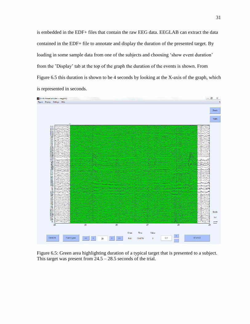
is embedded in the EDF+ files that contain the raw EEG data. EEGLAB can extract the data

contained in the EDF+ file to annotate and display the duration of the presented target. By

loading in some sample data from one of the subjects and choosing ‘show event duration’

from the ’Display’ tab at the top of the graph the duration of the events is shown. From

Figure 6.5 this duration is shown to be 4 seconds by looking at the X-axis of the graph, which

is represented in seconds.

Figure 6.5: Green area highlighting duration of a typical target that is presented to a subject.

This target was present from 24.5 – 28.5 seconds of the trial.

CHAPTER 7: PROCEDURE FOR DEVELOPING THE CONTROL SYSTEM

7.1 Data Signals Associated with Motor Movement

To find which of the signals relate to motor movement, and ICA must be performed.

An ICA is a special case of a blind source separation. A famous case of blind source

separation is a problem called the “dinner party problem.” This problem is defined as being

at a dinner party and being able to separate the audio signal of one individual attending the

party. One can use the principal of blind source separation to solve this problem. The key to

solving this problem is also the key to separating the signals on the EEG cap; there must be

as many measurement devices as there are signals. In the case of the dinner party problem

there must be at least two measurement devices, one for the background noise and one

capturing the desired signal of the person talking. This is simplification of the method

involved, but the same principals apply for separating out the individual signals from all of

the compiled EEG noise.

This means that the ICA is valuable in separating out the signals to their respective

electrode contributions. If an ICA were to not be performed on the data it would not be

known how to weight all of the individual electrodes due to the signals represented on each

electrode would be the additive contributions of the entire signal rather than the individual

component. An ICA on the entire cap would be an unnecessarily complex computation

though. It is possible to simplify this computation by only evaluating the electrodes that are

known to be associated with what is being evaluated, motor movement. In essence the ICA

33

will show which signals are the most closely associated with motor movements. At this step

of the development process it is not an issue of confirming which movement took place, but

that a movement took place at all. It is important to note that since we already know what

type of signal we are looking for in the data, a motor movement, and the position of the

motor cortex, which controls motor movement in individuals, is already known from

previous research [48], as shown in Figure 7.1, the ICA can be simplified somewhat, thereby

reducing computation time and complexity.

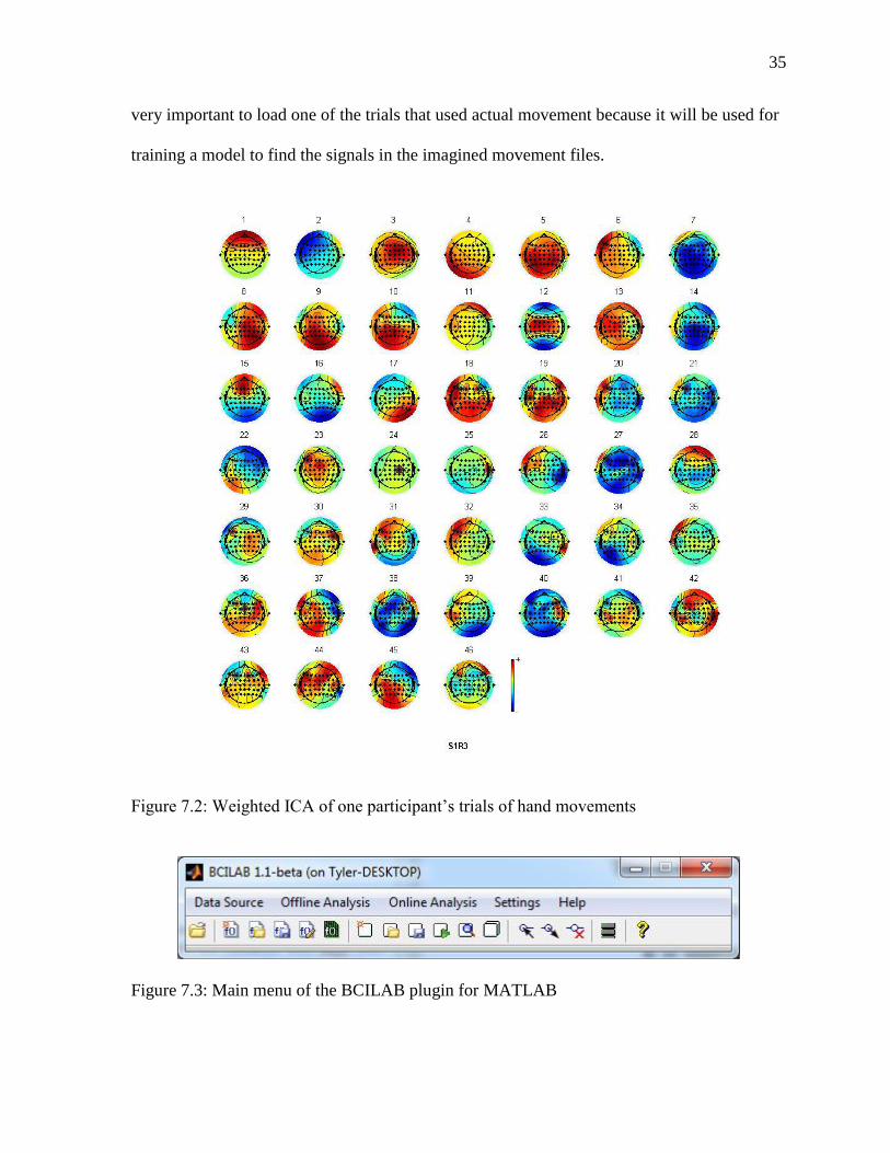
Since the signals from the brain are dipole signals, meaning that they have both a

magnitude and direction, the results of the ICA provide enlightenment as to the radiation of

the signal patterns also. Even though some of the signals were discounted because it was

previously known that those signals would not contribute to the desired outcome, after the

ICA other electrodes may be discounted. This is mainly done by manual inspection of the

component maps, one of which is shown in Figure 7.2.

It is important to notice that the labeling of the electrodes has changed from the initial

10-10 Standard shown in Figure 6.1. This is because of the channels that were removed for

the ICA. The updated numbering format is shown in Figure 7.2. It is important to note that

this procedure needs to be repeated for every trial that is needed to create the BCI for the

control. The figures that are present were derived from following the listed procedure from

the trials detecting left hand and right hand movements. These, along with the baseline trial,

will be used in the machine learning algorithm to train a model for the imagined movement

signals. In order to now translate to BCILAB to create the BCI, all the signals that have been

processed in the above manner need to be saved as a dataset in EEGLAB. This creates a

“.set” file that is imported into BCILAB.

34

Figure 7.1: Picture showing the relevant sections of the brain for motor movements

7.2 BCILAB

After downloading BCILAB and adding the folder to the MATLAB pathway run the

bcilab.m file to start BCILAB. The first time that the file runs it will take a while to build all

of the configuration files. Once BCILAB start a window will pop up that has all of the

options for BCILAB present in a graphical user interface (GUI) format. This window is

shown in Figure 7.3. As an aside, it is possible to write scripts to run and compile all of the

options presented here, but for this paper the GUI format will be shown for clarity of the

procedure.

Using the “Data Source” option on the menu and selecting the “Load Recording(s)”

option it is possible to now load the “.set” file that was saved by the earlier procedure. The

file that needs to be loaded first is one of the trials that used actual muscle movements. It is

35

very important to load one of the trials that used actual movement because it will be used for

training a model to find the signals in the imagined movement files.

Figure 7.2: Weighted ICA of one participant’s trials of hand movements

Figure 7.3: Main menu of the BCILAB plugin for MATLAB

36

For now, the file containing the data for the left and right hand movements are loaded. Once

the correct file is selected the window shown in Figure 7.4 will pop up.

Figure 7.4: Menu and options for loading the dataset file into BCILAB

From this window it is possible to select the channels that will be analyzed. All of the

channels from Figure 7.2 will used since the signal has already been processed to the degree

that all of the pertinent signals are present, so this field was left blank. The data can also be

truncated based on time, but since we use the whole of the recording, this is also left blank.

The other options are for other features of BCILAB that are not used in this development, but

are useful for developing a BCI from other means, such as live recordings or importing data

in other formats.

Now that the data has been loaded into BCILAB it is time to start developing the BCI

that will be used for the control system. By selecting “New Approach” under the “Offline

Analysis” from the main menu, it is possible to design an approach for our BCI. The

approach that is selected from the menu on the window that pops up will define what kind of

BCI that is developed. There are many options here for different kinds of BCI processing that

can occur. The windowed-means approach was shown earlier, but what is desired now is an

37

approach called common spatial patterns (CSP). A brief description of each approach shows

as it is selected, and one such description is shown in Figure 7.5.

Figure 7.5: Window for choosing the approach for the model. Common spatial pattern

approach shown

As the approach states, CSP is used for oscillatory processes localized in the motor

cortex. This is desirable for the BCI what we want to create since it has to do with motor

movement of the hands and feet. As is stated in the description, CSP is a very common and

robust approach so we will examine on how to refine this approach later to tailor it more

closely to what we are developing. After selecting the CSP approach another window, shown

in Figure 7.6 will pop up.

38

Figure7.6: Option for CSP approach

This window contains a lot of properties of the CSP that can be changed to refine the

approach. The CSP approach filters the data to look for the embedded oscillatory processes,

in our case beta waves for motor control, so the default approach configurations of the

frequency specifications of the filter can be left alone. Also it is possible to narrow the time

window of the epoch for each signal. As was shown earlier the signal window of each signal

that was presented on the screen for the trial was 4 seconds. It is desirable to trim this slightly

to account for reaction times of the physical signals, so half of a second is trimmed from each

side of each epoch. The final important function that can be chosen is the machine learning

function for the approach. It is possible to choose from a lot of different functions for the

CSP approach for fitting the data for a model. The default linear discriminant analysis (lda)

function is chosen here to highlight how accurate the default settings are. It is worth changing

this to different functions and checking the results to find the best model, but, as will be

shown, the default LDA function can be an accurate learning function.

39

It is important to note here that it is possible to over characterize the approach for the

model. This occurs when the approach is too closely configured to the data from actual motor

movement that it is difficult to distinguish an imagined movement. Over training and fitting

the approach to the model will result in it being difficult for the BCI to correctly identify the

imagined signals due to them being too dissimilar from the tightly trained model. Figure 7.7

shows the window that opens after selecting to train a new model through the main menu.

Figure 7.7: Calibration options for generating a model

40

The window already loads in the last approach made and the last data loaded into

memory. For the target field it is important to select the field that contains the data for the

markers for the signals. Due to how the data that is being used was saved this field is labeled

“type”. Also, since the data, as shown earlier, contain markers for rest along with the two

markers for activation (either hand or foot movement depending on the trial being examined)

it is only desirable to look at the markers that contain activations. Only the markers 1 and 2

contain the data needed to direct the model to the appropriate signal times. Since the duration

was trimmed earlier, the model will calibrate using the data contained in these signals with

half a second delay and cutoff. The rest of the options can be left to the defaults for now, but

they may be changed in the future to refine the calibration data. By selecting the correct

options shown in Figure 7.7 the results shown in Figure 7.8 are obtained.

41

Figure 7.8: Results from the default parameters of the CSP model approach

Looking at this data it is shown that after 5 iterations of machine learning the model is

around 95.4% accurate for the model. This means that with the values that were chosen for

the model were very good for allowing the model to predict that a move has taken place.

Again, it is important to note that these steps must be taken with every dataset in order to

create predictive models for each of the differing moves.

42

Figure 7.9: Results from using the generated CSP model on the imagined movement data

Now that the model has been created, it is time to fit it to the data. By selecting

“Apply model to data” from the main menu, it is possible to see how well this model that was

developed will predict and detect that the correct movement has taken place. First though, the

dataset that contains the imagined movements must be loaded into memory using the steps

listed beforehand. Once this data is loaded it is available for selection in applying the model

to the data. Once the process has ran the results shown in Figure 7.9 are obtained. From these

results we can see that after only one pass of the imagined movement data, the model that we

generated through CSP was successfully able to predict the correct movement 95% of the

43

time. This is therefore shown to be a very good model. Again, these are the results for the

data containing only the hand movements; although similar results were obtained using the

other datasets.

While this model that was generated is already very good, there is room for

improvement. Let us take a look as to how changing the approach for the model calibration

can change the results on the same data. The approach that is chosen this time is a special

variant of the CSP approach called the spectrally weighted CSP. This is a more advanced

form of the CSP that takes into account the weight of each electrode in the machine learning

stages. This means that the ICA that was performed earlier will be used to spectrally weight

each signal for importance. This approach was originally designed for motor imagery BCI in

mind, as stated in the description in Figure 7.10, so it is especially suited to develop our

desired BCI.

Figure 7.10: Approach of spectrally weighted CSP designed specifically for imagined

movements

44

By looking at the configurations for the spectrally weighted CSP in Figure 7.11, we

can see that the frequency specification of the filter has been changed slightly, and there is an

option to modify the prior frequency weighting for the function.

Figure 7.11: Configurations for the spectrally weighted CSP approach

To keep the same weights as were originally generated by the ICA, this should

remain as a default. Everything else was kept as the default values to more accurately show

how just changing the approach to one more suited to the desired task will change the

accuracy of the model on the data.

After training the model with the calibration data as was shown earlier, the results

from Figure 7.12 are calculated. At first glance these results seem quite similar to the data

obtained, only slight variations occur. This is due to the fact that the same machine learning

approach, LDA, was used to generate both of the models from the same data. The variations

45

that exist occur because of the difference in approach, so the fact that the results of the

machine learning on the calibration data are so close is due to the function used.

Figure 7.12: Results of the generated spectrally weighted CSP on the calibration data

46

Figure 7.13: Final performance results of the spectrally weighted CSP model on the imagined

movement

The main variation of the results comes when the model that we trained is used to

analyze the imagined movement dataset. Since the spectrally weighted CSP was designed

with this purpose in mind, it is safe to expect that this model, even will all other settings

remaining the same, to perform better than just the standard CSP model. Looking at the

results in Figure 7.13 it is shown that this is easily the case. Looking at these results, the

model that was generated successfully predicted the correct movement 98.8% of the time.

Not only that, but the error rate and false positives of signal detection were also greatly

47

reduced. This shows that by choosing the correct paradigm for the model that the accuracy of

a BCI can be greatly improved.

Figure 7.14: Visualization of spectrally weighted CSP model generated and the contributions

of each frequency for each pattern that emerged.

In order to put this model into a more visual and intuitive perspective it is possible to

use the “visualize model” option under the BCILAB menu. Doing so yields the results in

Figure 7.14. What this result lets us see is the patterns that arise from the model and data.

48

There are 6 patterns represented here and as we can see they all radiate from around

the motor cortex region. This is to be expected since the dataset contains motor movements.

Even though the data and analysis up to this point has been completed purely on offline data,

it is possible though BCILAB to simulate the performance of the model on the data stream as

though it was an online signal. Once the model has been trained up to this point and the

imagined data loaded into memory it is possible to select “read input from dataset” though

the online analysis menu. Once this has been selected one must also select to output the data

to MATLAB visualization though the same menu. A window, like the one found in Figure

7.15 will pop up. The two bars on this window will move up and down to simulate the model

sweeping the data in real time and making a decision on if a signal is presented and which

one is currently being shown.

Figure 7.15: Sample of the BCI simulating making a decision on the occurrence of

movement for an online BCI by using the dataset

CHAPTER 8: RESULTS

By following these steps it was shown that it is possible to develop a very reliable

BCI for motor movement. Using these steps a BCI was generated using the trial data sets to

develop two BCIs that work in conjunction to create one cohesive BCI that is able to

distinguish four separate motor movements: left hand movement, right hand movement,

moving both hands, and moving both feet. By separating the BCI into two separate parts it

was possible to more tightly constrain the individual BCI to specific functions. By placing

these two systems in series and implementing an EEG headset with capture software it is

possible for signals from BCILAB to be sent to a robot wirelessly via MATLAB. Expanding

on this research in the future will require such a system to realize the online performance of

this system. An individual must be trained using similar techniques as the data set used here

and after the steps detailed are followed the system can be used to navigate a robot. The

implementation of the BCI need not be only for a tiny robot though; for example, by using a

moderately powerful labtop that can run MATLAB the BCI could even be used to navigate a

wheelchair by an individual.

CHAPTER 9: CONCLUSION

This thesis only mentions the basic concepts and examples in the field of brain

computer interfaces. It is believed that the information presented here highlights the most

general uses of a BCI and contains information that applies to the greatest number of the

population that would potentially use or develop a BCI. The reader is encouraged to explore

this budding field as it rapidly develops and to present new ideas to the problems mentioned

herein. There are data sets that are publicly available from many sources, most offering easy

compatibility with MATLAB for manipulation. For free software EEGLAB [52] and

BCILAB [17] are both plug-ins for MATLAB and offer extensive tutorials online for those

interested [49]. By utilizing these resources it is possible to more easily develop a BCI for

use in many applications.

51

REFERENCES

[1] G. Mislap, “P300 Speller Example.” [Online]. Available: https://www.youtube.com/

watch?v=08GNE6OdNcs

[2] “Where Do The Electrodes Go?” [Online]. Available: http://www.diytdcs.com/

tag/1020-positioning/

[3] F. R. Rico and M. C. R. Sanchez, “Standard Event Related Potential

Signal,” 2009. [Online]. Available: http://lookfordiagnosis.com/mesh info.php?

term=Event-Related+Potentials,+P300&lang=1

[4] H. BEKCER, “Uber das Elektrenkephalogramm des Menschen. IV,” Mitteilung. Arch.

f. Psychiat, vol. 278, no. 1875, 1932.

[5] U. Herwig, P. Satrapi, and C. Sch¨onfeldt-Lecuona, “Using the Pnternational 10-20

EEG System for Positioning of Transcranial Magnetic Stimulation.” Brain topography,

vol. 16, no. 2, pp. 95–9, Jan. 2003.

[6] V. Jurcak, D. Tsuzuki, and I. Dan, “10/20, 10/10, and 10/5 Systems Revisited: Their

Validity As Relative Head-Surface-Based Positioning Systems.” NeuroImage, vol. 34,

no. 4, pp. 1600–11, Feb. 2007.

[7] B. Zhang, J. Wang, and T. Fuhlbrigge, “A Review of the Commercial Brain-Computer

Interface Technology from Perspective of Industrial Robotics,” Automation and Logistics

pp. 379–384, 2010.

[8] T. Mulholland, “Human EEG, Behavioral Stillness and Biofeedback.” International

journal of psychophysiology : official journal of the International Organization of

Psychophysiology, vol. 19, no. 3, pp. 263–79, May 1995.

[9] M. Linden, T. Habib, and V. Radojevic, “A Controlled Study of the Effects of EEG

Biofeedback on Cognition and Behavior of Children with Attention Deficit Disorder and

Learning Disabilities.” Biofeedback and self-regulation, vol. 21, no. 1, pp. 35–49, Mar.

1996.

[10] G. Townsend, B. K. LaPallo, C. B. Boulay, D. J. Krusienski, G. E. Frye, C. K. Hauser,

N. E. Schwartz, T. M. Vaughan, J. R.Wolpaw, and E.W. Sellers, “A Novel P300-Based

Brain-Computer Interface Stimulus Presentation Paradigm: Moving Beyond Rows and

Columns.” Clinical neurophysiology : official journal of the International Federation

of Clinical Neurophysiology, vol. 121, no. 7, pp. 1109–20, Jul. 2010.

[11] E. W. Sellers, T. M. Vaughan, and J. R. Wolpaw, “A Brain-Computer Interface for

Long-term Independent Home Use.” Amyotrophic lateral sclerosis : official publication

of the World Federation of Neurology Research Group on Motor Neuron Diseases,

52

vol. 11, no. 5, pp. 449–55, Oct. 2010.

[12] M. Velliste, S. Perel, and M. Spalding, “Cortical Control of a Prosthetic Arm for

Selffeeding,” Nature, vol. 453, no. 7198, pp. 1098–101, Jun. 2008.

[13] D. Taylor, S. Tillery, and A. Schwartz, “Direct Cortical Control of 3D Neuroprosthetic

Devices,” Science, vol. 296, no. 5574, pp. 1829–1832, Jun. 2002.

[14] A. Schwartz, X. Cui, D. Weber, and D. Moran, “Brain-Controlled Interfaces: Movement

Restoration with Neural Prosthetics,” Neuron, vol. 52, no. 1, pp. 205–20, Oct. 2006.

[15] J. L. Collinger, B. Wodlinger, J. E. Downey, W. Wang, E. C. Tyler-Kabara, D. J.

Weber, A. J. C. McMorland, M. Velliste, M. L. Boninger, and A. B. Schwartz, “High

Performance Neuroprosthetic Control by an Individual with Tetraplegia.” Lancet, vol.

381, no. 9866, pp. 557–64, Feb. 2013.

[16] A. K¨ubler, B. Kotchoubey, and J. Kaiser, “Braincomputer Communication: Unlocking

the Locked in.” Psychological 2001.

[17] T. O. Zander and C. Kothe, “Towards Passive Brain-Computer Interfaces: Applying

Brain-Computer Interface Technology to Human-Machine Systems in General.” Journal

of Neural Engineering, vol. 8, no. 2, p. 025005, Apr. 2011.

[18] K. LaFleur, K. Cassady, A. Doud, K. Shades, E. Rogin, and B. He, “Quadcopter

Control in Three-Dimensional Space Using a Noninvasive Motor Imagery-Based

Braincomputer Interface,” Journal of Neural Engineering, vol. 10, no. 4, p. 46003, Aug.

2013.

[19] Y. Wang, X. Gao, B. Hong, C. Jia, and S. Gao, “Brain-Computer Interfaces Based on

Visual Evoked Potentials.” IEEE Engineering In Medicine and Biology Magazine : the

Quarterly Magazine of the Engineering in Medicine & Biology Society, vol. 27, no. 5,

pp. 64–71, 2008.

[20] L. a. Farwell and E. Donchin, “Talking Off the Top of Your Head: Toward a Mental

Prosthesis Utilizing Event-Related Brain Potentials.” Electroencephalography and Clinical

Neurophysiology, vol. 70, no. 6, pp. 510–23, Dec. 1988.

[21] E. Donchin, “The Mental Prosthesis: Assessing the Speed of a P300-Based

Braincomputer Interface,” IEEE Transactions on, vol. 8, no. 2, pp. 174–179, 2000.

[22] N. K. Logothetis, “The Neural Basis of the Blood-Oxygen-Level-Dependent Functional

Magnetic Resonance Imaging Signal.” Philosophical transactions of the Royal Society

of London. Series B, Biological sciences, vol. 357, no. 1424, pp. 1003–37,

Aug. 2002.

[23] N.Weiskopf, K. Mathiak, S.W. Bock, F. Scharnowski, R. Veit, W. Grodd, R. Goebel,

53

and N. Birbaumer, “Principles of a Brain-Computer Interface (BCI) Based on Real-Time

Functional Magnetic Resonance Imaging (fMRI).” IEEE Transactions on Bio-Medical

Engineering, vol. 51, no. 6, pp. 966–70, Jun. 2004.

[24] S. Yoo, T. Fairneny, N. Chen, and S.-E. Choo, “Brain-Computer Interface Using fMRI:

Spatial Navigation by Thoughts,” Neuroreport, vol. 15, no. 10, pp. 1591–1595, Jul. 2004.

[25] D. G. Nair, K. L. Purcott, A. Fuchs, F. Steinberg, and J. a. S. Kelso, “Cortical and

Cerebellar Activity of the Human Brain during Imagined and Executed Unimanual and

Bimanual Action Sequences: a functional MRI study.” Cognitive brain research, vol. 15, no.

3, pp. 250–60, Feb. 2003.

[26] R. C. Oldfield, “The Assessment and Analysis of Handedness: the Edinburgh

inventory.” Neuropsychologia, vol. 9, no. 1, pp. 97–113, Mar. 1971.

[27] R. Sitaram, H. Zhang, C. Guan, M. Thulasidas, Y. Hoshi, A. Ishikawa, K. Shimizu,

and N. Birbaumer, “Temporal Classification of Multichannel Near-Infrared Spectroscopy

Signals of Motor Imagery for Developing a Brain-Computer Interface.” NeuroImage,

vol. 34, no. 4, pp. 1416–27, Feb. 2007.

[28] J. Mellinger, G. Schalk, C. Braun, H. Preissl, W. Rosenstiel, N. Birbaumer, and

A. K¨ubler, “An MEG-based brain-computer interface (BCI).” NeuroImage, vol. 36,

no. 3, pp. 581–93, Jul. 2007.

[29] E. C. Leuthardt, K. J. Miller, G. Schalk, R. P. N. Rao, and J. G. Ojemann,

“Electrocorticography-based Brain Computer Interface–the Seattle Experience.” IEEE

Transactions on Neural Systems and Rehabilitation Engineering, vol. 14, no. 2, pp. 194–8,

Jun. 2006.

[30] T. Mladenov, K. Kim, and S. Nooshabadi, “Accurate Motor Imagery Based Dry

Electrode Brain-Computer Interface System for Consumer Applications,” 2012 IEEE 16th

International Symposium on Consumer Electronics, pp. 1–4, Jun. 2012.

[31] S. Makeig and J. Onton, “ERP Features and EEG Dynamics: an ICA Perspective,”

Oxford Handbook of Event-Related Potential, pp. 1–58, 2009.

[32] A. Delorme, J. Palmer, J. Onton, R. Oostenveld, and S. Makeig, “Independent EEG

Sources are Dipolar.” PloS one, vol. 7, no. 2, p. e30135, Jan. 2012.

[33] T. P. Jung, S. Makeig, M. Westerfield, J. Townsend, E. Courchesne, and T. J.

Sejnowski, “Analysis and Visualization of Single-Trial Event-Related Potentials.” Human

Brain Mapping, vol. 14, no. 3, pp. 166–85, Nov. 2001.

[34] S. Makeig, S. Debener, J. Onton, and A. Delorme, “Mining Event-Related Brain

Dynamics.” Trends in Cognitive Sciences, vol. 8, no. 5, pp. 204–10, May 2004.

54

[35] C. Guger, S. Daban, E. Sellers, C. Holzner, G. Krausz, R. Carabalona, F. Gramatica,

and G. Edlinger, “How Many People are Able to Control a P300-Based Brain-Computer

Interface (BCI)?” Neuroscience letters, vol. 462, no. 1, pp. 94–8, Oct. 2009.

[36] B. Z. Allison, C. Brunner, V. Kaiser, G. R. M¨uller-Putz, C. Neuper, and

G. Pfurtscheller, “Toward a Hybrid Brain-Computer Interface Based on Imagined Movement

and Visual Attention.” Journal of Neural Engineering, vol. 7, no. 2, p. 26007, Apr. 2010.

[37] S.-C. Chen, S.-C. Hsieh, and C.-K. Liang, “An Intelligent Brain Computer Interface

of Visual Evoked Potential EEG,” 2008 Eighth International Conference on Intelligent

Systems Design and Applications, pp. 343–346, Nov. 2008.

[38] J. Onton and S. Makeig, “Information-Based Modeling of Event-Related Brain

Dynamics.” Progress in Brain Research, vol. 159, pp. 99–120, Jan. 2006.

[39] A. Delorme, T. Sejnowski, and S. Makeig, “Enhanced Detection of Artifacts in EEG

Data Using Higher-Order Statistics and Independent Component Analysis.” NeuroImage,

vol. 34, no. 4, pp. 1443–9, Mar. 2007.

[40] R. Kottaimalai, M. P. Rajasekaran, V. Selvam, and B. Kannapiran, “EEG Signal

Classification using Principal Component Analysis with Neural Network in Brain Computer

Interface Applications,” in 2013 IEEE International Conference on Emerging Trends

in Computing, Communication and Nanotechnology (ICECCN). IEEE, Mar. 2013,

pp. 227–231.

[41] W. Ting, Y. Guo-zheng, Y. Bang-hua, and S. Hong, “EEG Feature Extraction Based on

Wavelet Packet Decomposition for Brain Computer Interface,” Measurement, vol. 41,

pp. 618–625, 2008.

[42] N. P. Castellanos and V. a. Makarov, “Recovering EEG Brain Signals: Artifact

Suppression with Wavelet Enhanced Independent Component Analysis.” Journal of

Neuroscience Methods, vol. 158, no. 2, pp. 300–12, Dec. 2006.

[43] S. Santaniello and G. Fiengo, “Closed-Loop Control of Deep Brain Stimulation: A

Simulation Study,” Neural Systems and, vol. 19, no. 1, pp. 15–24, 2011.

[44] T. J. Bradberry, R. J. Gentili, and J. L. Contreras-Vidal, “Reconstructing Three

Dimensional Hand Movements from Noninvasive Electroencephalographic Signals.”

The Journal of Neuroscience : The Official Journal of the Society for Neuroscience,

vol. 30, no. 9, pp. 3432–7, Mar. 2010.

[45] R. Tomioka and K.-R.M¨uller, “A Regularized Discriminative Framework for EEG

Analysis with Application to Brain-Computer Interface.” NeuroImage, vol. 49, no. 1, pp.

415–32, Jan. 2010.

[46] a. L. Goldberger, L. a. N. Amaral, L. Glass, J. M. Hausdorff, P. C. Ivanov, R. G.

55

Mark, J. E. Mietus, G. B. Moody, C.-K. Peng, and H. E. Stanley, “PhysioBank,

PhysioToolkit, and PhysioNet : Components of a New Research Resource for

Complex Physiologic Signals,” Circulation, vol. 101, no. 23, pp. e215–e220, Jun.

2000.

[47] G. Schalk, D. J. Mcfarland, T. Hinterberger, N. Birbaumer, J. R. Wolpaw, and A. B.-

c. I. B. C. I. Technology, “BCI2000 : A General-Purpose Brain-Computer Interface (BCI)

System,” vol. 51, no. 6, pp. 1034–1043, 2004.

[48] G. Rizzolatti, L. Fadiga, V. Gallese, and L. Fogassi, “Premotor Cortex and the

Recognition of Motor Actions,” vol. 3, pp. 131–141, 1996.

[49] C. Kothe, “Introduction to Modern Brain-Computer Interface Design,”

2013. [Online]. Available: http://sccn.ucsd.edu/wiki/Introduction To Modern

Brain-Computer Interface Design

[50] U. Laval and C. Glk, “Cellular Basis of EEG Slow Rhythms : Corticothalamic

Relationships,” vol. 15, no. January, 1995.

[51] B. Blankertz, G. Dornhege, M. Krauledat, K.-R. M¨uller, and G. Curio, “The

Noninvasive Berlin Brain-Computer Interface: Fast Acquisition of Effective Performance

in Untrained Subjects.” NeuroImage, vol. 37, no. 2, pp. 539–50, Aug. 2007.

[52] A. Delorme and S. Makeig, “EEGLAB: an Open Source Toolbox for Analysis of Single

Trial EEG Dynamics Including Independent Component Analysis,” Journal of Neuroscience

Methods, vol. 134, pp. 9–21, 2004.