Developed By: akeel abdual aziz

LECT. 1

Computer control design and modeling Lecture 1

Introduction A system or a process or a plant is a segment of environment that is under consideration. Control is a term that describes the process of forcing a system to behave in a desired way in order to achieve certain objective(s)/goal(s). Examples. • Automobile steering control. • Thousands of industries consider control in some or the other form such as

quality control, production control, temperature control, pollution control, Precision control, etc.

• Robot control. • Human body implements highly sophisticated control schemes for

numerous purposes such as body temperature regulation, hormone level control, etc.

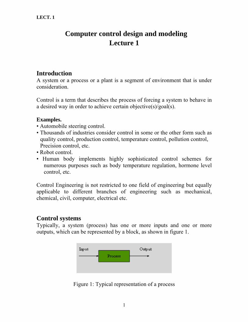
Control Engineering is not restricted to one field of engineering but equally applicable to different branches of engineering such as mechanical, chemical, civil, computer, electrical etc. Control systems Typically, a system (process) has one or more inputs and one or more outputs, which can be represented by a block, as shown in figure 1.

Figure 1: Typical representation of a process

1

LECT. 1

Control System is an interconnection of components forming a system configuration that will provide a desired system response. Open-loop and closed-loop control systems Depending on configuration, control systems can be categorized into mainly two classes:

i) open-loop control systems; ii) closed-loop (or feedback) control systems.

Open-loop control systems An open-loop control system utilizes a controller or actuating device to obtain a desired response directly without using feedback.

Figure 2: Open-loop control system

Example of an open loop control system: room temperature control. The structure of this system is presented in figure 3. In this system the inlet vent temperature is the input (control signal), and the output (controlled variable) is the room air temperature. The actuator comprises of the furnace and a pre-programmed on-off switch that triggers the furnace, which in turn activates the inlet vent temperature. The ambient temperature acts as a disturbance. Figure 3: Example of an open loop control system: room temperature control

2

LECT. 1

The open-loop control system cannot adjust to changes of the ambient temperature. Example of an open loop control system: controlling the position of a missile launcher from a remote location. This system is illustrated in figure 4. The input is the desired angular position of the missile launcher, and the control system consists of potentiometer, power amplifier, motor, gearing between the motor and missile launcher, and the missile launcher. For accurate positioning, the missile launcher should be precisely calibrated with reference to the angular position of the potentiometer, and the characteristics of the potentiometer, amplifier and motor should remain constant. Except for the potentiometer, the components that comprise this open loop control system are not precision devices. Their characteristics can easily change and result in false calibration and poor accuracies. In practice, simple open-loop control systems are never used for the accurate positioning of fire-control systems because of the inherent possibility of inaccuracies and the risks involved. Figure 4: Example of an open loop control system: controlling the position of a missile launcher from a remote location Closed-loop (feedback) control systems The structure of a simple closed-loop feedback system is shown in figure 5. In contrast to an open-loop control system, a closed-loop utilizes the additional measure of the actual output to compare the actual output with the desired output (reference or command). This additional measure of the output is called the feedback.

3

LECT. 1

Figure 5: Closed-loop control system Example of a closed-loop control system: room temperature control. The previous example is now modified by incorporating the measure of the output, i.e. the room air temperature. The controller is the thermostat that takes into account a reference signal and the output feedback in order to set the switch position. Ideally, the thermostat should trigger the switch as soon as the error is negative and switch off when the room air has reached/exceeded the reference temperature. The features of this scheme are:

Figure 6: Example of a closed-loop control system: room temperature

control • If room temperature < reference temperature, the furnace is switched on

automatically, until room temperature ≥ reference temperature. • Can handle changes in the system (e.g. change in ambient temperature). • It is negative feedback (the measured output is subtracted from the

reference signal). Example of a closed-loop control system: controlling the position of a missile launcher from a remote location The previous example is modified by introducing a position feedback loop. This feedback loop consists of potentiometer R2 and the difference amplifier. Should an error exists, it is amplified and applied to a motor drive which

4

LECT. 1

adjusts the output-shaft position until it agrees with the input-shaft position, and the error is zero. Figure 7: Example of a closed-loop control system: controlling the position of a missile launcher from a remote location Feedback control systems used to control position, velocity, and acceleration are very common in industrial applications. The important feature of the using of feedback is that the feedback control system can handle changes in the system. On the other hand, improper use of feedback can make the system unstable, so the stability issue arises. Example of a closed-loop control system: Automatic depth control of a submarine

5

LECT. 1

Figure 8: Automatic depth control of a submarine Suppose the captain of the submarine wants the submarine to”hover” at a desired depth, and sets the desired depth as a voltage from calibrated potentiometer. The actual depth is measured by a pressure transducer which produces a voltage proportional to depth. The difference between the desired and the actual depth is amplified which then drives a motor that rotates the stern plane actuator angle θ in order that the stern plane rotation reduces the depth error of the submarine to zero. Given a process, there are three steps to design a feedback control system which are:

1. Modeling. Obtain mathematical description of the system. 2. Analysis. Analyze the properties of the system. 3. Design. Given a plant, design a controller based on performance

specifications.

End of Lecture One

6

LECT. 2

Computer control design and modeling Lecture 2

Mathematical models, Linear Systems and Linearization Mathematical Models of Physical Systems To understand and control complex systems, we must obtain mathematical models of these systems. The term mathematical model, in the control engineering perspective, implies a set of differential equations that describe the dynamic behavior of a process. The set of differential equations that describe the behavior of physical systems are typically obtained by utilizing the physical laws of the process. These types of models are often called first principles models. Several examples of first-principles models are considered below. Models of simple mechanical systems The equations of a mechanical system may be obtained by a direct application of Newton second law. Example: Ideal Mass-Spring System. This system is shown on figure 1.

Figure 1: Ideal Mass-Spring System

In order to write the equation of motion, we consider the set of forces acting on the mass M. The force F from the spring acts against the displacement and is proportional to the displacement of the spring, i.e. F = −ky, where k is spring constant. Assume a frictionless surface. Applying Newton’s second law, one can get the following equation of motion

1

LECT. 2

The equation (1) is a second-order linear differential equation. Example: Mass-Spring System with a Damper. The previous example is now modified by the addition of a damper with resistance R. Additionally; we assume that the body is subjected to an external force Fe.

Figure 2: Mass-Spring System with a Damper The damping force Fd is assumed to be proportional to the velocity and acts against the motion of the body, i.e. Such a damping is called viscous damping. Using Newton’s second law, we can write the equations of motion as follows: Modeling of RLC Electrical Systems Consider RLC electrical circuit shown in figure 3. It consists of a source of current r(t), a resistor characterized by it’s resistance R, a capacitor characterized by it’s capacitance C, and an inductor with inductance L. Differential equation of the RLC circuit can be obtained by utilizing Kirchhoff’s laws, and the voltage-current relationships for R, L, and C. Indeed, Kirchhoff’s current law implies that

2

LECT. 2

Figure 3: RLC Circuit where ir, ic, and il are currents through the resistor, the capacitor, and the inductor respectively. On the other hand, Kirchhoff’s voltage law implies in this particular case that the voltage v across any of the elements R, L, or C is the same. We have the following voltage-current relationships for R, L, and C: Thus, we get the following equation of RLC circuit

It is worth noting that the equation (3) is analogous to the equation (2) of the Mass-Spring System with Damper. Indeed, if we rewrite the equation (2) in terms of the velocity , we get

The equations (3) and (4) are of equivalent form, and this fact represents so called velocity-voltage analogy between mechanical and electrical systems. This equivalence between systems is beneficial to the analyst in understanding multidisciplinary systems that are similar to each other. The main advantage is that the solution to one system can be extended to all the analogous systems governed by the same set of differential equations. Therefore, a mechanical engineer can immediately extend the knowledge

3

LECT. 2

gained about the analysis and design of mechanical engineering systems to that of analogous systems in the other branches of engineering. Linear Systems Linear systems represent a very important class of systems. To introduce the notion of a linear system, consider a system represented by it’s block diagram, as shown in the figure 4.

Figure 4: Representation of a system Below, by G(u) we will denote the output (reaction) of the system corresponding to given input (excitation) u. Definition 1. System G is linear, if and only if

i) It obeys the superposition principle, for any possible inputs u1, u2.

ii) It obeys the principle of homogeneity, i.e.

for any possible input u and any constant γ ∈ R. In essence, G is linear if and only if for any possible inputs u1, u2, and any constants α, β ∈ R. Otherwise, the system is called non-linear. The principle of superposition, which applies to linear systems, is one of the most powerful tools in systems analysis. It allows us to say that the response of a system to sum of inputs is equal to the sum of the responses of the system to the inputs taken individually. This has very deep implications for

4

LECT. 2

analysis. If a complicated input to a linear system can be represented as a sum of simpler inputs, then the response of the system to the simpler inputs can be calculated separately and then added to get the response of the system to the complicated input. Linear dynamical systems Consider a dynamical system described by an ordinary differential equation of the form

The system (5) is an example of linear dynamical systems. However, the notion of linearity, in the sense of the above definition, cannot be directly applied to dynamical systems of the form (5). Indeed, a solution of the system (5) is not uniquely determined by input f(t), but also depends on initial conditions For linear dynamical systems, a more general version of superposition principle must be satisfied, which also includes some form of linearity with respect to initial states. For the purposes of this subject, however, the following slightly informal definition of a linear dynamical system will be sufficient. Definition 2. A dynamical system is called linear if and only if it can be described by linear differential equations. Linearization All real life systems are nonlinear. However, almost all physical systems can be closely approximated by linear models within some range of the variables. The main reason to use linear models is that linear models make the analysis and design problems much simpler in terms of understanding and applicability. The process of finding a linear model which gives good approximation of given nonlinear model is known as linearization.

5

LECT. 2

To illustrate the process of linearization, consider the following very simple example. Consider the function Suppose we need to find a linear function which approximate f(x) near the point x0 = 1. Clearly (see the figure), this linear approximation is given as follows

Figure 5: Linearization of the function y = x2 near the point x0 = 1 In general, linearization can be obtained using Taylor series expansion about the operating point. Suppose a (nonlinear) function y = f(x) is given, then Taylor series expansion about the point x0 is as follows

6

LECT. 2

Example: linearization of the pendulum equations. The pendulum is described by the following equation In the point q = 0 the torque T = mgl sin q = 0. The linear approximation of the torque about the point q = 0 is given as follows Therefore, the linearized equations of the pendulum about the point q = 0 is as follows

End of Lecture Two

7

LECT. 3

Computer control design and modeling Lecture 3

Solution of linear differential equations using Laplace transform In general, the procedure of solving linear differential equation using Laplace transform consists of the following three steps: • Take Laplace transform of each term in the differential equation. This step

eliminates time and all of the time derivatives from the original equation and results in an algebraic equation in s.

• Solve the resulting algebraic equation for the transform of the desired time function.

• Obtain the inverse Laplace transform. This last step gives the solution of the differential equation.

Example: Ideal mass-spring system. The system is described by the following linear differential equation

where M is mass and k is spring constant. Problem. Find the solution of (1) corresponding to initial conditions y(0) = y0, (0) = 0. y&Solution. Applying Laplace transform to both sides of the equation (1), one can write Taking into account initial conditions, we get

Equation (2) is an algebraic one. Its solution is Using Laplace transform table, one can easily find the inverse Laplace transform of Y(s):

1

LECT. 3

Example: forced differential equation. Consider the following differential equation

Problem: Find the solution corresponding to zero initial conditions y(0) =

(0) = 0. y&Solution. Taking the Laplace transform of both sides, we obtain and, due to zero initial conditions, Solving for Y(s) yields Partial fraction expansion for Y(s) has the form Residues are Therefore,

2

LECT. 3

The Transfer Function In this lecture we will formulate the system representation by establishing a definition of a function that algebraically relates a system’s output to its inputs. This function allows us to algebraically combine mathematical representations of subsystems to yield a total system representation. Definition of transfer function Consider a system described by linear time-invariant differential equation,

where r(t) is input, and y(t) is output of the system. Taking the Laplace transform of both sides of equation (5), we get

where R(s) and Y(s) are Laplace transform of r(t) and y(t) respectively. If we assume that all initial conditions are equal to zero, the equation (6) reduces to

The last equation can be rewritten as follows

Denote by G(s) the ratio of the output transform Y(s) divided by input transform R(s):

The ratio G(s) is called transfer function of the system (5). Thus we have the following definition.

3

LECT. 3

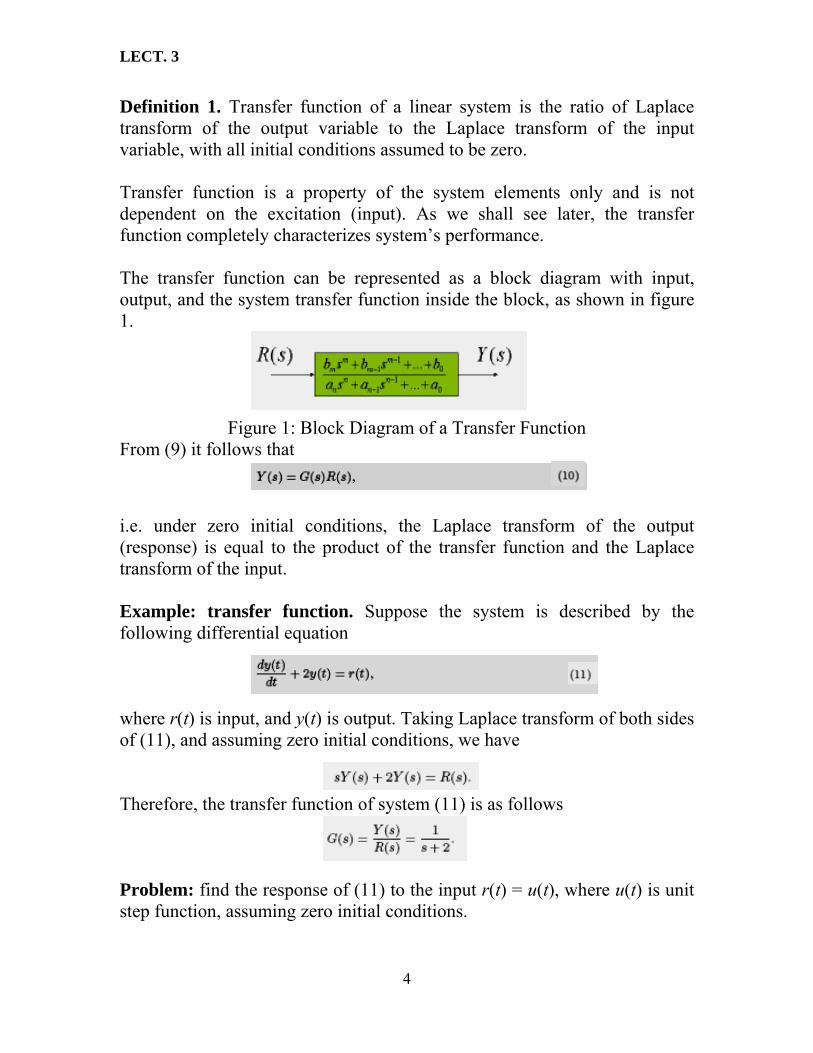
Definition 1. Transfer function of a linear system is the ratio of Laplace transform of the output variable to the Laplace transform of the input variable, with all initial conditions assumed to be zero. Transfer function is a property of the system elements only and is not dependent on the excitation (input). As we shall see later, the transfer function completely characterizes system’s performance. The transfer function can be represented as a block diagram with input, output, and the system transfer function inside the block, as shown in figure 1.

Figure 1: Block Diagram of a Transfer Function From (9) it follows that i.e. under zero initial conditions, the Laplace transform of the output (response) is equal to the product of the transfer function and the Laplace transform of the input. Example: transfer function. Suppose the system is described by the following differential equation where r(t) is input, and y(t) is output. Taking Laplace transform of both sides of (11), and assuming zero initial conditions, we have Therefore, the transfer function of system (11) is as follows Problem: find the response of (11) to the input r(t) = u(t), where u(t) is unit step function, assuming zero initial conditions.

4

LECT. 3

Solution. To solve this problem, one can use formula (10). The Laplace transform of unit step function r(t) = u(t) is Therefore, using formula (10), we see that the Laplace transform of the output y(t) is Expanding by partial fractions, we have Calculating residues, we get so the partial fraction expansion of Y(s) is Applying the inverse Laplace transform, we finally get Example: Transfer function of mass-spring system with a damper. Consider a mass-spring system with a damper (see figure 2).

Figure 2: Mass-Spring System with a Damper

It is described by the following differential equation Taking Laplace transforms of both sides of (12), and assuming zero initial conditions, we get

5

LECT. 3

Where Y(s) = L(y(t)) and (s) = L(FeF̂ e(t)). The transfer function of the system is Impulse response function Consider a linear system, and suppose all initial conditions are zero. The response of the system to an impulse input signal δ(t) is called the impulse response function of the system. The impulse response function is usually denoted by h(t). The impulse response function h(t) is closely related with the transfer function of the system. Indeed, let G(s) be the transfer function of the system. Using formula (10), we get (zero initial conditions are assumed). But we already proved that L[δ(t)] = 1, therefore The last equality can be considered as an alternative definition of the transfer function, as follows. Definition 2. The transfer function of a system is equal to the Laplace transform of the impulse response function. Problem. Find the transfer function from input f(t)to output x1(t)o f the coupled mass-spring system.

6

LECT. 3

Figure 3: Coupled mass-spring system Solution. The differential equations governing for the system are

(14)

1 Applying Laplace transform to both sides of (13), (14), we get the following matrix equation

(15)

To obtain the transfer function description, one have to solve equation (15) with respect to variables X1(s),X2(s). This can be done, for example, as follows. Consider the equation

(16)

To calculate the solution of (16), one can use so called Cramer’s rule. According to Cramer’s rule, where xi is i-th element of vector x, and Ai is a matrix formed by replacing the i-th column of A by y. Then

⎥⎦

⎤⎢⎣

⎡++

−∆

=kbsMs0

k)s(F1)s(X 21

∆++

=∴kbsMs)s(F)s(X

2

1

7

LECT. 3

Then

∆++

==kbsMs

Fs)s(X)s(G

21

1(17)

Where ∆ is the determinant of the matrix in the left-hand side of the equation (15)

End of Lecture Three

8

F s( ) f t( )

1 δ t( )

1 s⁄ 1 t( )1 s2⁄ t

2! s3⁄ t2

3! s4⁄ t3

m! sm 1+⁄ tm

1s a+----------- e at–

1s a+( )2

------------------- te at–

1s a+( )3

-------------------12!-----t2e at–

1s a+( )m

--------------------1

m 1–( )!--------------------tm 1– e at–

as s a+( )------------------- 1 e at––

as2 s a+( )---------------------

1a--- at 1– e at–+( )

b a–s a+( ) s b+( )

--------------------------------- e at– e bt––

ss a+( )2

------------------- 1 at–( )e at–

a2

s s a+( )2--------------------- 1 e a– t 1 at+( )–

b a–( )ss a+( ) s b+( )

--------------------------------- be bt– ae at––

as2 a2+---------------- at( )sin

ss2 a2+---------------- at( )cos

s a+s a+( )2 b2+

------------------------------- e at– bt( )cos

bs a+( )2 b2+

------------------------------- e at– bt( )sin

a2 b2+s s a+( )2 b2+[ ]-------------------------------------- 1 e at– bt( )cos

ab--- bt( )sin+–

F s( ) f t( )

F s( ) f t( ) Transform Pair

αF1 s( ) βF2 s( )+ α f 1 t( ) β f 2 t( )+ Superposition

F s( )e sλ– f t λ–( ) Time Delay λ 0≥( )

1a-----F

sa---

f at( ) Time scaling

F s a+( ) e at– f t( ) Shift in frequency

smF s( ) sm 1– f 0( )–

sm 2– f˙ 0( )– …– f m 1– 0( )–f m( ) t( ) Differentiation

1s---F s( ) f ζ( ) ζd∫ Integration

F1 s( )F2 s( ) f 1 t( ) f 2 t( )• Convolution

sF s( )s ∞→lim f 0( ) Initial Value Theorem

sF s( )s 0→lim f t( )

t ∞→lim Final Value Theorem

12πj-------- F1 ζ( )F2 s ζ–( ) ζd

c j∞–( )

c j∞+( )

∫ f 1 t( ) f 2 t( ) Time product

sdd

F s( )– tf t( ) Multiplication by Time

Properties of Laplace Transforms

Table of Laplace Transforms

Euler’s Identity

ωt( )sin e jωt e jωt––2 j

----------------------------= ωt( )cos e jωt e jωt–+2

-----------------------------=

LECT. 4

Computer control design and modeling Lecture 4

Block Diagram Models Graphically, a linear system can be represented as a block diagram with input, output, and the system transfer function inside the block, as shown in figure 1.

Figure 1: Block Diagram of a Transfer Function In this lecture, we will learn more about block diagram representation of linear systems. A block diagram of a system is a pictorial representation of the functions performed by components of the systems and the flow of signals between the components of the system. Obviously, there is no more information in the block diagram than in the set of simultaneous equations that represents the system; however, the block diagram depicts the same information much more concisely. Example. Block diagram of a two-input, two-output system. Consider a linear system with two inputs and two outputs as shown below:

Figure 2: Two-input, two-output system Using transfer function relations, this system can be written as follows where Gij is the transfer function relating the ith output variable to the jth input variable. Then, the corresponding block diagram is shown in figure 3.

1

LECT. 4

Figure 3: Block diagram of two-input, two-output system Block diagram transformations In practice, most of the control engineering systems involve variables that can be heavily interrelated. A complicated block diagram involving many blocks, summing points, and pickoff points can be reduced to a single equivalent block by a set of transformations. Below, we consider several examples of elementary block diagram transformations. All these transformations can be derived by simple algebraic manipulation of the equations represented the blocks. Combining blocks in cascade Parallel subsystem

2

LECT. 4

Algebraically, we have

Moving a summing point behind a block Moving a summing point ahead of a block

Moving a pick-off point ahead of a block The transformation is algebraically trivial.

3

LECT. 4

Moving a pick-off point behind a block Eliminating a (negative or positive) feedback loop To obtain the algebraic expression for transfer function of a negative feedback loop, one can write

Following the same line of reasoning, one can easily see that the transfer function of a positive feedback loop is given by the formula The formulas (2), (3), are particularly important, because they represent many of the existing practical control schemes.

4

LECT. 4

Block Diagram Reduction The block diagram transformations described before allow us to reduce a block diagram of multiple subsystems to a single block representing the transfer function from input to output. Example: block diagram reduction. Consider a multiple loop feedback control system shown in figure 4.

Figure 4: Multiple loop feedback control system

Problem. Find transfer function of the system )s(R)s(Y)s(G =

Solution. The solution can be obtained, for example, as follows. Step 1. Move H2 behind block G4. The result is presented on figure 5.

Figure 5: Step 1

Step 2. Eliminate the (positive) feedback loop G3G4H1 to obtain the system presented in figure 6.

5

LECT. 4

Figure 6: Step 2

Step 3. Eliminate the (negative) feedback loop containing 4

2

GH .The result is

presented in figure 7.

Figure 7: Step 3

Step 4. Obtain the transfer function by eliminating the (negative) feedback loop containing H3 (see figure 8).

Figure 8: Step 4

Remarks • The advantage of the block diagram approach is that it provides the

engineer with a graphical representation of the system and the relationships between the input and output variables.

• In general, the block diagram reduction process is not unique, i.e. there can

be multiple solutions to a block diagram reduction problem (with the same final result).

End of Lecture Four

6

LECT. 5

Computer control design and modeling Lecture 5

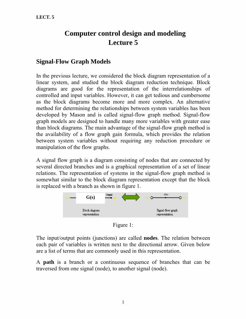
Signal-Flow Graph Models In the previous lecture, we considered the block diagram representation of a linear system, and studied the block diagram reduction technique. Block diagrams are good for the representation of the interrelationships of controlled and input variables. However, it can get tedious and cumbersome as the block diagrams become more and more complex. An alternative method for determining the relationships between system variables has been developed by Mason and is called signal-flow graph method. Signal-flow graph models are designed to handle many more variables with greater ease than block diagrams. The main advantage of the signal-flow graph method is the availability of a flow graph gain formula, which provides the relation between system variables without requiring any reduction procedure or manipulation of the flow graphs. A signal flow graph is a diagram consisting of nodes that are connected by several directed branches and is a graphical representation of a set of linear relations. The representation of systems in the signal-flow graph method is somewhat similar to the block diagram representation except that the block is replaced with a branch as shown in figure 1.

G(s)

Figure 1:

The input/output points (junctions) are called nodes. The relation between each pair of variables is written next to the directional arrow. Given below are a list of terms that are commonly used in this representation. A path is a branch or a continuous sequence of branches that can be traversed from one signal (node), to another signal (node).

1

LECT. 5

A loop is a closed path that originates and terminates at the same node, and along the path no node is met twice. Two loops are nontouching if they do not have a common node. Example: signal-flow graph of a two-input, two-output system. Consider a linear system with two inputs and two outputs as shown below:

Figure 2: Two-input, two-output system

This system is described by transfer function relations as follows where Gij is the transfer function relating the ith output variable to the jth input variable. The corresponding signal-flow graph representation is shown on figure 3.

Figure 3: Signal-flow graph of a two-input, two-output system.

Example. Consider a system described by the following set of algebraic equations where r1, r2 are input variables, and x1, x2 are output variables. The corresponding signal-flow graph is shown in figure 4.

2

LECT. 5

Figure 4: Signal-flow graph of the system (2), (3). Equations (2), (3), can be rewritten as follows Using Cramer’s rule, one can get the following solution of the equations (4), (5), and where ∆ is the determinant of the set of equations (2), (3), Let us analyze the equations (6), (7). The determinant ∆ can be rewritten as follows Where Note that the term I1 is a sum of gains of all loops of the system. On the other hand, I2 is a sum of gain products of all possible two loops that do not touch each other.

3

LECT. 5

Note also that numerators of transfer functions from an input ri to an output xj is equal to product of the gain of the corresponding path and the determinant of the part of the graph that does not touch the path. For example, numerator of transfer function from input r1 to output x1 is 1 − a22 which is equal to product of the gain 1 of the path from r1 to x1 and the determinant 1 − a22 of the part of the graph that does not touch the path r1 →x1. The generalization of the above considerations is called Mason’s rule. Mason’s rule Suppose we have a complex multiloop system, and we need to find the transfer function of this system from a given input R(s) to a given output Y(s). This transfer function can be found by using the following Mason’s formula: Here: ∆(s) is the determinant of the system. ∆(s) can be calculated as follows

∆(s) = 1 − {sum of all different loop gains} +{sum of the gains product of all combinations of two nontouching loops} −{sum of the gains product of all combinations of three nontouching loops} +. . .

(9) Further, n is a number of different forward paths from input R(s) to output Y(s). Gi is gain of the i-th path from R(s) to Y(s). ∆i(s) is the determinant of the i-th forward path. ∆i is a value of determinant ∆ for that part of the signal flow graph that does not touch the i-th forward loop.

4

LECT. 5

Example: signal-flow graph. Consider a multiple loop feedback control system shown in figure 5.

Figure 5: Multiple loop feedback control system

Problem. Find transfer function of the system )s(R)s(Y)s(G = using

Mason’s rule Solution. By drawing the signal-flow graph for the above system we have,

-H3

R(s)

-H2

1 G1 G2 G3 G4 1

H1

Y(s)

Figure 6: Signal-Flow graph for the above system From the above figure there are three loops which are: L1 = - G2 G3 H2L2 = G3 G4 H1 L3 = - G1 G2 G3 G4 H3 And one forward path between the output and the input given by: PG1 = G1 G2 G3 G4

5

LECT. 5

Since there are no two (or more) nontouching loops, then: ∆(s) = 1- (L1 + L2 + L3) And since the forward path touches all loops in the graph, then, ∆1(s) =1 Then

)s(R)s(Y)s(G = =

∆∆11PG =

34321232143

4321

HGGGGHGGHGG1GGGG++−

End of Lecture Five

6

LECT. 6

1

x1

Computer control design and modeling Lecture 6

State Space Analysis Introduction A state space model is a description in terms of a set of first-order differential equations which are written compactly in a standard matrix form. This standard form has permitted the development of general computer programs, which can be used for the analysis and design of even very large systems. State Space Models The derivation of state space models is not different from that of transfer functions in that the differential equations describing the system dynamics are written first. In transfer function models these equations are transformed and variables are eliminated between them to find the relation between selected input and output variables. For state models, instead, the equations are arranged into set of first order differential equations in terms of selected state variables, and the output are expressed in these same state variables. State variables should not normally derived from transfer functions, but directly from the original systems equations. But in this lecture examples will be given to relate state models to the transfer functions. Consider a system described by the nth-order differential equation

rwadtdwa..........

dtwda

dtwd

121n

1n

nn

n

=++++−

−

(1)

Or the equivalent transfer function. A state model for this system is not unique but depends on the choice of a state variables x1 (t), x2 (t),…….xn (t). One possible choice is the following:

w= wx2 &= …….. )1n(

n wx−

= (2) Directly from these definitions and by substitution (1), n first-order differential equations are obtained:

LECT. 6

2

32 xx =& ……….. xx = xx

3s9s6s5W

=

R 23 +++

rxa...xaxax nn2211n +−−−−=&

n1n =−&21&

The output w can be expressed in terms of these state variables:

w=x1 It only remains to write in a standard vector-matrix from. The general from of a state-space model is as follows:

BuAxx +=& (state equation) (output equation) (3) DuCxy +=

Here x is the state vector, the vector of the state variables; u is the control (input) vector, and y the output vector. A is the system matrix. In the example above the control (input) vector is the scalar function r and the output vector the scalar function w. It may be seen that

x B A ⎥⎥

⎢⎢=⎥⎢= . ⎥⎢= .⎢

⎢=

⎥⎥⎥⎥

⎥⎥⎥

⎦

⎤

⎢⎢⎢⎢

⎢⎢⎢

⎣

⎡

⎥⎥⎥

⎥⎥⎥

⎦

⎤

⎢⎢⎢

⎢⎢⎢

⎣

⎡

− )1n(n

2

1

w..

.ww

x...

xx

&

⎥⎥⎥

⎦

⎤

⎢⎢⎢

⎢⎢⎢

⎣

⎡

10...0

..01000..010

n21⎥⎥⎥⎥⎥⎥⎥⎥⎥

⎦

⎤

⎢⎢⎢⎢

⎢⎢⎢

⎣

⎡

−−−

)4(

a...aa10...

⎥⎥⎥

C = [1 0 … 0] D = 0

Example 1: A Transfer function without Zeros.

r5w3w9w6w =+++ &&&&&& Choose state variables x1(t), and x2(t), then

x1 = w x2 = xw& 3 = w&&

LECT. 6

Then a state model representing this transfer function or the corresponding differential equation is obtained as in general case. The definitions and the differential equation yield

21 xx =& 32 xx =& r5x6x9x3x 3213 +−−−=& In matrix form and with the output w expressed also in terms of all state variables.

x r w=[1 0 0] x ⎥⎥⎥

⎦

⎤

⎢⎢⎢

⎣

⎡=

3

2

1

xxx

⎥⎥⎥

⎦

⎤

⎢⎢⎢

⎣

⎡+

⎥⎥⎥

⎦

⎤

⎢⎢⎢

⎣

⎡

−−−=

500

x693

100010

x&

Example 2: A Transfer function with Zeros. 396sR +++

=ss2s2s5W

23

2 ++

Or r2r2r5w3w9w6w ++=+++ &&&&&&&&& First, consider only the denominator:

3s9s6s1

RV

23 +++= rv3v9v6v =+++ &&&&&&

As in Example 1 x r ⎢

⎢= ⎢⎢= 0x

⎥⎥⎥

⎦

⎤

⎢⎣

⎡

vvv

&&

&

⎣

⎡

−−− 100

x693

10010

&

⎥⎥⎥

⎦

⎤

⎢⎢⎢

⎣

⎡+

⎥⎥⎥

⎦

⎤

⎢ But W = (5s2+2s+2) V or w = 5 +2 +2v = [2 2 5] x v&& v& Hence the output equation, with y=w, is

y = C x C= [2 2 5]

3

LECT. 6

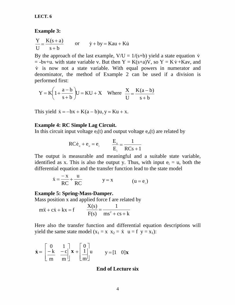
Example 3: or aKY +

= by &&y + U bs

)s(+

uKKau +=

By the approach of the last example, V/U = 1/(s+b) yield a state equation = -bv+u. with state variable v. But then Y = K(s+a)V, so Y = K +Kav, and

is now not a state variable. With equal powers in numerator and denominator, the method of Example 2 can be used if a division is performed first:

v&v&

v&

Where XKUbaKY +=⎟

⎞−= bKX a(

U +−

=Ubs

1⎠

⎜⎝⎛

++

bs)

This yield .xKuy,u)ba(Kbxx +=−+−=& Example 4: RC Simple Lag Circuit. In this circuit input voltage ei(t) and output voltage eo(t) are related by eeRC =+ 1E

=e& The output is measurable and meaningful and a suitable state variable, identified as x. This is also the output y. Thus, with input ei = u, both the differential equation and the transfer function lead to the state model

1RCsEi

o

+ioo

RCRC

x += xyux−

& = )e( =u i

Example 5: Spring-Mass-Damper. Mass position x and applied force f are related by

1X=

kcsms)s(F

)s(2 ++

fkxxcxm =++ &&&

Here also the transfer function and differential equation descriptions will yield the same state model (x1 = x x2 = u = f y = xx& 1):

⎥

⎤⎢⎡

−− ck=x x 1 ⎥⎢+ [y = ⎥⎦⎢⎣ mm ⎥⎦⎢⎣

um

0 ⎤⎡10x]01&

End of Lecture six

4

LECT. 7

Computer control design and modeling Lecture 7

Time-domain response of a first-order and second-order

control systems In this lecture, we will study in details the time-domain response of a first-order and a second-order control systems. In particular, we will • study how to use poles and zeros to determine time-response of a system, • introduce performance specifications of transient response of a first-order system, • learn how to determine transfer function of a first order system from time-domain response data. • describe different types of natural responses of a second-order (stable)

system, • define performance specifications for a second-order system, • learn how to use poles to determine the nature of response without exact calculation of the response. Poles and zeros of a transfer function Let us recall the definitions of poles and zeros of a transfer function. Consider a transfer function Poles of a signal (system) are the roots of the denominator polynomial A(s). It is clear that poles of the system may also be defined as the values of s that cause the transfer function to become infinite. If the factor in denominator can be canceled by the same factor in the numerator, the transfer function may be not infinite at the root of this factor. In control systems, however, the root of the canceled factor in the denominator is usually also referred as a pole even though the transfer function is not infinite at this value. Zeros of a signal (system) are the roots of the numerator polynomial B(s).

1

LECT. 7

Similarly to the case of poles, the root of the canceled factor in the numerator is usually also referred as a zero even though the transfer function may be not zero at this value. Example. Poles, zeros, and time response of a first order system Consider a system described by the transfer function Let us find the unit step response of the system. The Laplace transform of a

unit step signal iss1 , therefore the Laplace transform of the unit step

response of the system is The residues are Thus, the time-domain response of the system is

Figure 1: System response

2

LECT. 7

• The part of the response that corresponds to the poles of the input function is called forced response. One can see that a pole of the input function determine the form of the forced response. • The part of the response that corresponds to the poles of the transfer function is called natural response. Again, a pole of the transfer function determines the form of the natural response. • Since a pole of the transfer function is located at the real axis, the natural response of the system has an exponential form Ke−at. The farther to the left a pole on the negative real axis, the faster the exponential response will decay to zero. Transient response specifications of a first-order system Time constant Consider a first-order system The Laplace transform of its step response is as follows Taking the inverse Laplace transform, one can find the time-domain step response as follows The response (1) is plotted in figure 2 (for simplicity, K = a is assumed). Definition 1. The value is called the time constant of the response. When t = 1 /a, we have

3

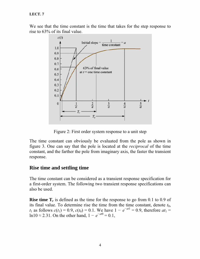
LECT. 7

We see that the time constant is the time that takes for the step response to rise to 63% of its final value.

Figure 2: First order system response to a unit step The time constant can obviously be evaluated from the pole as shown in figure 3. One can say that the pole is located at the reciprocal of the time constant, and the farther the pole from imaginary axis, the faster the transient response. Rise time and settling time The time constant can be considered as a transient response specification for a first-order system. The following two transient response specifications can also be used. Rise time Tr is defined as the time for the response to go from 0.1 to 0.9 of its final value. To determine rise the time from the time constant, denote t0, t1 as follows c(t1) = 0.9, c(t0) = 0.1. We have 1 − e−at1 = 0.9, therefore at1 = ln10 ≈ 2.31. On the other hand, 1 − e−at0 = 0.1,

4

LECT. 7

Figure 3: Pole plot

therefore at0 = ⎟⎠⎞

⎜⎝⎛

910ln ≈ 0.11. Therefore the rise time can be calculated as

follows where T = 1 /a is the time constant. Settling time Ts is the time for the response to reach, and stay within, 2% of it’s final value. To calculate settling time, put 1 − e−aTs = 0.98, therefore aTs = ln50 ≈ 3.91, and we have First-order transfer functions via testing Often it is not possible or practical to obtain a system’s transfer function analytically. However, with a step input, we can measure the time constant and steady state value, from which the transfer function can be calculated. Consider again a first-order system

5

LECT. 7

and it’s step response is One can identify K and a from laboratory testing as follows. Assume, the input step response is given in figure 4.

Figure 4: Step response of a system

From the response, is, the time for the mplitude to reach 63% of its final value. Since the final value is about 0.72,

o find K it is clear that the forced response reaches a steady state value of

we measure the time constant, that

athe time constant is evaluated where the curve reaches 0.63 × 0.72 ≈ 0.45, i.e. about 0.13. Hence T

6

LECT. 7

Since a ≈ 0.13, we see that K ≈ 5.54. Therefore

ime-domain response of a s cond-order control system

system xhibits a wide range of responses. For example, a second order system can

eros described by a transfer

enote

T e Comparing to the simplicity of a first-order system, a second orderedisplay characteristics much like a first-order system or display damped or pure oscillations for its transient response. Second order systems are very important in control systems engineering, since many control systems design methods are based on second-order system analysis. A second-order system without zeros Consider a second-order system without zunction of the following general form f

Dn

n w2

a,b =ξ . Equation (2) can therefore be rewritten as follows w =

is clear th e or input ultiplying factor that can take on any value without affecting the form of

stem, and ζ called da

It at the term in the numerator is simply a scalmthe derived results. For simplicity, we take k = ωn

2, and finally get a transfer function of the following form The parameter ωn is called natural frequency of a second order syis mping ratio. Consider a unit step response of a second order system (4). We have

7

LECT. 7

The first term in the right-hand side of equation (5) corresponds to forced

he form

ase ζ = 0

ζ = 0, we have two imaginary complex conjugate poles s1,2 = jω. These

Case 0 < ζ < 1

this case equation (6) results in a pair of complex conjugate poles with

hese poles generate a natu of damped sinusoid with

response, while the second term determines the natural response of a second-order system. It is easy to see that K1 = 1. Solving for the poles of the transfer function in equation (4) yields T of the natural unit step response of a second-order (stable) systemis determined by the value of damping ratio ζ. C Ifpoles generate a sinusoidal natural response whose frequency is equal to ωn. This type of response is called undamped. It is shown in figure 5.

Figure 5: Undamped response

Innegative real part

±

T ral response of the forman exponential envelope whose time constant is equal to the reciprocal of the pole’s real part. This type of response is called underdamped response. It is shown in figure 6.

Figure 6: Underdamped response

8

LECT. 7

ase ζ > 1

ζ > 1, then the formula (6) gives two negative real poles s1 = −ζωn +

C Ifωn 12 −ζ , s2 = −ζωn − ωn 12 −ζ . The corresponding natural response is equal to sum of two exponen ith time constants equal to reciprocal of the pole locations

tials w

his case is illustrated in figure 7. The response is called overdamped.

ase ζ = 1

this case formula (6) gives two equal real poles

he corresponding natural time ain response has a form

his type of response is cal response. This is the fastest

Figure 8: Critically damped response

T

Figure 7: Overdamped response

C In T -dom T led critically damped possible response without overshoot.

9

LECT. 7

Performance specifications of a second-order system In this section we will introduce performance specifications for an underdamped second-order system. As in the case of first order systems, standard performance measures are usually defined in terms of the step response of a system. The step response of the second order system (4) with 0 < ζ < 1 is given by the following formula where . The following performance specifications can be defined for the underdamped response of a second-order system. Peak time Tp The time required to reach the first peak. Peak time can be calculated by the formula Percent overshoot, %OS is the amount that the waveform overshoots the steady-state, or final, value at the peak time, expressed as a percentage of the steady-state value. Percent overshoot can be evaluated from ζ, ωn using the following formula It is clear that the percent overshoot is a function only of the damping ratio ζ. Settling time Ts is the time required for damped oscillations to reach and stay within of the steady-state (final) value. Ts can be evaluated by the formula Rise time Tr is the time required for the waveform to go from 0.1 to 0.9 of the final value. It is difficult to obtain exact analytic expression for Tr.

10

LECT. 7

Figure 9: Second order underdamped response specifications

Performance characteristics vs. pole location Let us consider the relation between performance characteristics and the location of the poles. Consider an example of the pole plot of a second order underdamped system, shown in figure 10. It is clear that, in this figure, cos θ = ζ.

Figure 10: Pole plot for an underdamped second-order system Comparing equations (7), (8) with the pole location, we see that where ωd = ωn

21 ζ− is the imaginary part of the pole. On the other hand,

dns

44Tσ

=ζω

=

11

LECT. 7

where σd is the magnitude of the real part of the pole. We see that • The peak time Tp is inversely proportional to the imaginary part of the

pole. • The settling time Ts is inversely proportional to the real part of the pole. • Since ζ = cosθ, radial lines are lines of constant ζ. Since percent overshoot

is only a function of ζ, radial lines are lines of constant percent overshoot %OS.

In figure 11 the step responses are shown as the poles are moved in vertical direction, keeping the real part the same. We see that the frequency changes, but the envelope remains the same. Since all curves fit under the same exponential decay curve, the settling time is virtually the same for all waveforms.

Figure 11: Poles are moved in vertical direction In figure 12 the step responses are shown as the poles are moved in horizontal direction, keeping the imaginary part the same. As the poles move to the left, the response damps out more rapidly, while the frequency remains the same. It is clear that peak time is the same for all waveforms.

Figure 12: Poles are moved in horizontal direction

12

LECT. 7

In figure 13 the poles are moved along a constant radial line. We see that the percent overshoot remains the same. The farther the poles are from origin, the more rapid the response.

Figure 13: Poles are moved along a constant radial line Example of finding ζ, ωn, Tp, %OS, and Ts from pole location Consider a pole plot shown in figure 11. Problem. Find ζ, ωn, Tp, %OS, and Ts. Solution. • The damping ratio is given by • The natural frequency • The peak time • The percent overshoot

13

LECT. 7

Figure 14: Pole plot

• The settling time

End of Lecture seven

14

LECT. 8

Computer control design and modeling Lecture 8

Stability of linear systems. Routh-Hurwitz Criterion As previously given, the time response of a system is a sum of the forced and natural responses

The form of natural response depends only on the system, not the input.

On the other hand, the form of forced response is dependent on the input. If the natural response grows without bounds, then eventually the natural response will be much greater than the forced response, and the system is no longer controlled. Therefore, for a control system to be useful, the natural response must eventually approach zero, or, at worst, oscillate.

Definition. A linear system is said to be:

• stable if the natural response approaches zero as time approaches infinity; • unstable if the natural response grows without bound as time approaches

infinity; • marginally stable if the natural response neither decays nor grows without

bound, but remains constant or oscillates as time approaches infinity. Therefore, control system must be designed to be stable. Stability vs. poles location • Poles in the left half-plane yield either pure exponentially decreasing or

damped sinusoidal natural responses. Therefore, if all the poles of the system are in the left half-plane (have negative real parts), then the system is stable.

• Poles in the right half-plane yield either pure exponentially increasing or exponentially increasing sinusoidal natural responses. Therefore, if a system has at least one pole in the right half-plane (has positive real parts), then the system is unstable.

• Poles of multiplicity greater than one on the imaginary axis lead to the sum of responses of the form

1

LECT. 8

which grows without bound as ∞→t . Therefore, if a system has poles of multiplicity greater than one on the imaginary axis, then the system is unstable. • Poles of multiplicity one on the imaginary axis yield pure sinusoidal

natural response. Thus, if all poles of the system are only in the left half plane or on the imaginary axis, and all the poles on the imaginary axis are of multiplicity one, then the system is marginally stable.

A necessary condition for stability

Suppose a transfer function has only left half-plane poles, i.e. the system is stable. Then the factors of denominator of the transfer function consists of products of terms such as (s+ai), where ai either real and positive, or complex with positive real parts. The products of such terms is a polynomial with all positive coefficients. Therefore:

• if the system is stable, then all the coefficients of the denominator must be

positive.

It means that if any of the coefficients of the denominator polynomial is negative or missing, then the system is not stable.

Unfortunately, if all the coefficients of the denominator are positive and not missing, we do not have definite information about the system’s pole location.

Routh-Hurwitz Criterion • Routh-Hurwitz Criterion provides a method that yields stability

information without the need to solve for poles of a system. • Using Routh-Hurwitz Criterion one can find how many poles are in the left

half-plane, right half-plane, and on the imaginary axis. However, using this method, one cannot find the exact coordinates of the poles.

• The method requires two steps: – generate a data table called Routh table; – interpret the Routh table to tell how many system poles are in each section

(left half-plane, right half-plane, and imaginary axis) of the complex plane. Suppose, for example, we need to determine stability of the system

2

LECT. 8

Figure 1: Initial Layout for Routh table Generating a basic Routh table • Create the initial Routh table shown in figure 1.

– Label the rows with powers of s from the highest power of the denominator to s0.

– In the first row, write horizontally the coefficients from the highest power to the lowest one, skipping every other coefficient.

– In the second row, write horizontally all the coefficients that skipped in the first row, from the highest power to the lowest one.

• Fill in the remaining entries as follows:

– Each entry is a negative determinant of entries in the previous two rows divided by the entry in the first column directly above the calculated row.

– The left column of the determinant is always the first column of the previous two rows.

– The right column of the determinant is the column of the previous two rows that is above and to the right of the entry.

3

LECT. 8

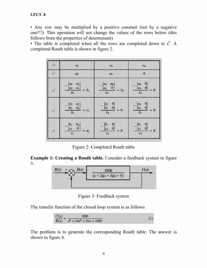
• Any row may be multiplied by a positive constant (not by a negative one!!!). This operation will not change the values of the rows below (this follows from the properties of determinant). • The table is completed when all the rows are completed down to s0. A completed Routh table is shown in figure 2.

Figure 2: Completed Routh table Example 1: Creating a Routh table. Consider a feedback system in figure 3.

Figure 3: Feedback system The transfer function of the closed loop system is as follows

The problem is to generate the corresponding Routh table. The answer is shown in figure 4.

4

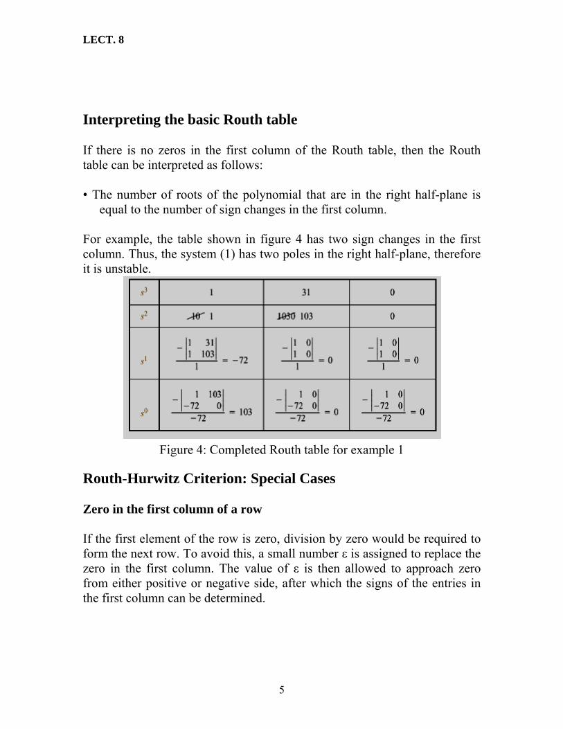
LECT. 8

Interpreting the basic Routh table If there is no zeros in the first column of the Routh table, then the Routh table can be interpreted as follows: • The number of roots of the polynomial that are in the right half-plane is

equal to the number of sign changes in the first column. For example, the table shown in figure 4 has two sign changes in the first column. Thus, the system (1) has two poles in the right half-plane, therefore it is unstable.

Figure 4: Completed Routh table for example 1 Routh-Hurwitz Criterion: Special Cases Zero in the first column of a row If the first element of the row is zero, division by zero would be required to form the next row. To avoid this, a small number ε is assigned to replace the zero in the first column. The value of ε is then allowed to approach zero from either positive or negative side, after which the signs of the entries in the first column can be determined.

5

LECT. 8

Example 2. Consider a system It’s Routh table is shown on figure 5. There are two sign changes, therefore two poles are in the right half-plane.

Figure 5: Completed Routh table for example 2 Entire row is zero Sometimes, we can find that an entire row consists of zeros. This case must be handled differently from the case of a zero only in the first column of the row. Example 3. Consider a system It’s Routh table is shown on figure 6. In particular, one can see that the third row consists of zeros. In this case we should: • Return to the row immediately above the row of zeros. • Form an auxiliary polynomial, using the entries of that row as coefficients.

The polynomial will start from the power of s in the label column, and continue by skipping every other one and diminishing in power. Thus, the polynomial is as follows

6

LECT. 8

• Differentiate the above polynomial with respect to s to obtain • Use coefficients of the last polynomial to replace the row of zeros.

Figure 6: Routh table for example 3 The remainder of the table is formed in the standard way. We see that all entries in the first column are positive. Hence, there are no right half-plane poles, and the system is stable. Example 4. The characteristics equation of a given system is

s4 + 6s3 + 11s2 + 6s + K = 0 What the range of K values in order to insure that the system is stable?

s4 1 11 K s3 6 6 0 s2 10 K 0 s1

10K660 − 0

s0 K For the system to be stable, the following restrictions must be placed upon the parameter K: 60 – 6K ⟩ 0 or K ⟨10, and K ⟩ 0. Thus K must be greater than zero and less than 10.

End of Lecture eight

7

LECT. 9

Computer control design and modeling Lecture 9

Steady-State Errors As given before, in feedback control systems (as shown in figure 1), the input signal usually represents a desired output response, and the role of control system is to force the actual output to follow the input (desired output). The accuracy of this process is one of the main concerns of control system engineers. For example, if a control system is designed to stop an elevator at a desired floor, then the elevator must eventually be level enough with the floor for the passengers to exit. In particular, one of the main characteristics of a control system is the difference between the desired output and the actual output as time tends to infinity.

Figure 1: Feedback control system

Definition. Steady-state error is the difference between the input and the output for a prescribed test input as ∞→t . Test inputs The following signals are usually used as test inputs as shown in figure 2: • Step input u(t) = 1(t). Step input represents constant position and it is

useful in determining the ability of the control system to position itself with respect to stationary target.

• Ramp input u(t) = t. Ramp input represents constant-velocity input and it is useful to determine the ability of the system to track a constant-velocity target.

1

LECT. 9

• Parabola u(t) = 2t21 . Parabolic input is a constant-acceleration input, so one

can use this input to determine the ability of the system to track an accelerating target.

Figure 2: Test inputs for evaluating steady-state errors

Steady-state Error in Unity Feedback Systems Consider the following unity feedback system as shown in figure 3.

Figure 3: Unity feedback system

In this figure, the signal E(s) is the error between the input R(s), and the output C(s). The goal of this section is to express the steady-state error in terms of transfer function G(s) in the forward path (open loop transfer function). From figure 3, we have

2

LECT. 9

But Therefore it is easy to get Assume the closed-loop system is stable. Then, applying final value theorem, one can determine the value e(∞ ) = as follows )t(elimt ∞→

Equation (1) allows us to calculate the steady-state error e( ) for given input R(s) and transfer function G(s).

∞

Steady-state error for the step input

For step input, R(s) = s1 . Using equation (1), we get

The value is called static position error constant. In order to have zero steady-state error, G(s) must satisfy To satisfy the previous equation, G(s) must take on the following form where n ≥ 1, i.e. at least one pole of G(s) must be at the origin (when n = 1 then the system is called type 1 system), or equivalently, at least one pure integration must be present in the forward path.

3

LECT. 9

If there is no integration (n = 0 or type 0 system), then we have i.e. the static position error constant Kp is finite, and therefore (as given in formula (2)), the corresponding steady-state error is finite. Steady-state error for the ramp input

For ramp input, we have R(s) = 2s1 . Using formula (1), we get

The value is called static velocity error constant. To obtain zero steady-state error for a ramp input, one must have To satisfy the last equation, G(s) must be of the form (3) with n 2, i.e. there must be at least two integrations in the forward path (when n = 2 then the system is called type 2 system).

≥

If only one integrator exists in the forward path (type 1 system), then is finite, i.e. we have constant steady-state error.

If there is no integration in the forward path (type 0 system), then and the steady-state error is infinite and lead to diverging ramps.

4

LECT. 9

Steady-state error for the parabolic input For the parabolic input u(t) = 2t

21 , it’s Laplace transform is R(s) = 3s

1 . Using

formula (1), we get The value is called static acceleration error constant. In order to have zero steady-state error, we must have To satisfy the last equation, G(s) must take on the form (3), where n 3 (when n = 3 then the system is called type 3 system). In other words, to have zero steady-state error for a parabolic input, there must be at least three integrators in the forward path.

≥

If there are only two integrators in the forward path (type 2 system), then is finite, and therefore, the steady-state error for a parabolic input is finite. If the number of pure integrators in the forward path is less than two, then which implies the steady-state error for a parabolic input is infinite. The following table gives a summery of the different cases given above:

Step Input u(t)=1

Ramp Input u(t)=t

Acceleration

u(t)= 2t21

Type 0 system

pK11+

∞ ∞

Type 1 system 0

vK1 ∞

Type 2 system 0 0

aK1

5

LECT. 9

Static error constants as steady-state error performance specifications Static error constants can be used to specify the steady-state error characteristics of control systems. Just as damping ratio, settling time, peak time, and percent overshoot are used as specifications for a system’s transient response, so the static position error constant Kp, static velocity error constant Kv, and static acceleration error constant, Ka, can be used as specifications for a control system’s steady state error. Example: Steady-state error via error constants Problem 1. For each system on figure 4, evaluate the static error constants and find the expected error for the standard step, ramp, and parabolic inputs.

Figure 4: Feedback control systems for Problem 1

Solution. First, we need to verify that all the systems are stable. Second, for the system in figure 4, (a), we see that

6

LECT. 9

and Thus, for a step input, we have For a ramp input, and for a parabolic input For the system in figure 4, (b), we have Therefore Finally, for the system in figure 4, (c), Therefore

7

LECT. 9

Example: Gain design to meet steady-state error specifications Problem 2. Given a control system in figure 5, find the value of K so that there is 10% error in the steady-state.

Figure 5: Feedback control systems for Problem 2

Solution. Since the system has one integrator, the error stated in the problem must apply to a ramp input. Thus, Therefore, which implies It remains to check, using Routh-Hurwitz criterion, that the closed-loop system is stable with this gain.

End of Lecture nine

8

LECT. 10

Computer control design and modeling Lecture 10

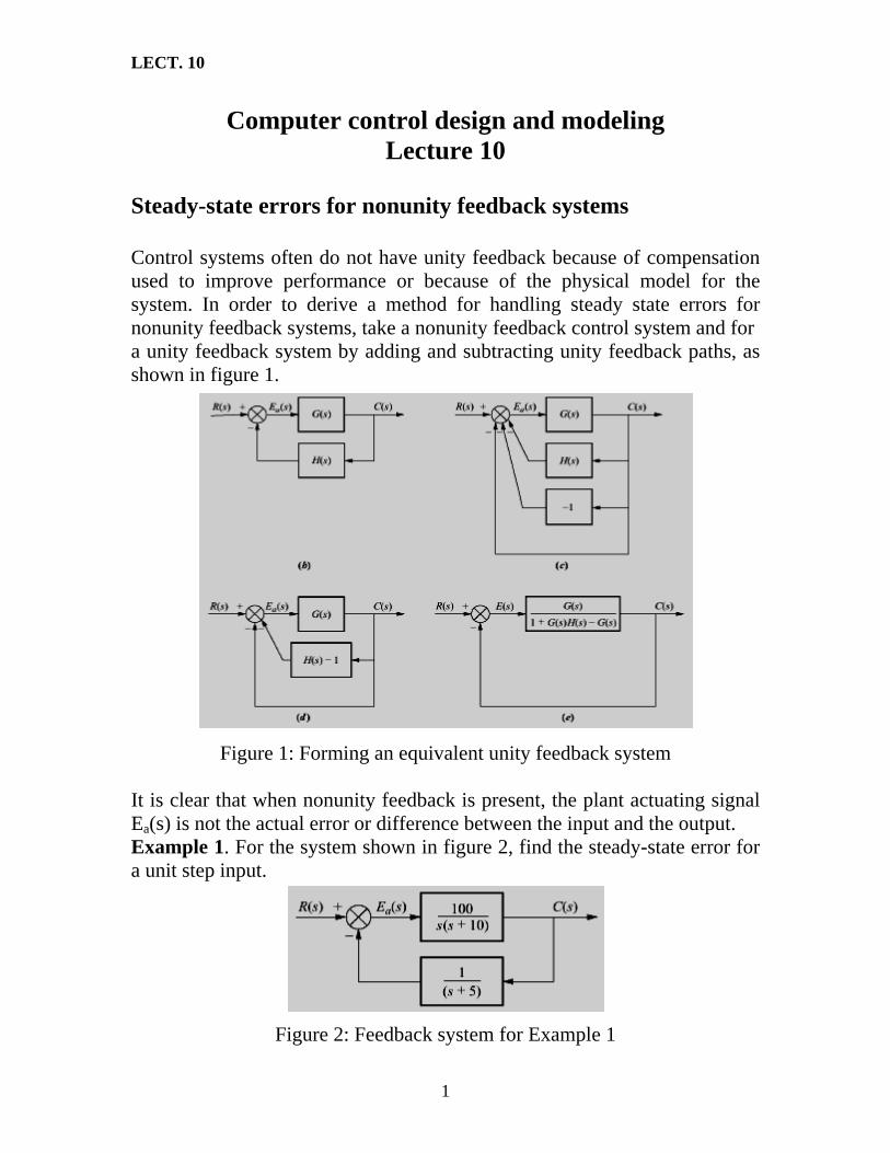
Steady-state errors for nonunity feedback systems Control systems often do not have unity feedback because of compensation used to improve performance or because of the physical model for the system. In order to derive a method for handling steady state errors for nonunity feedback systems, take a nonunity feedback control system and for a unity feedback system by adding and subtracting unity feedback paths, as shown in figure 1.

Figure 1: Forming an equivalent unity feedback system

It is clear that when nonunity feedback is present, the plant actuating signal Ea(s) is not the actual error or difference between the input and the output. Example 1. For the system shown in figure 2, find the steady-state error for a unit step input.

Figure 2: Feedback system for Example 1

1

LECT. 10

Solution. The first step is to make sure that the system is stable. Second, the system should be converted into an equivalent unity feedback system. Using the formula where Ge(s) is the transfer function in the forward path of the equivalent unity feedback system, one can find The position error constant Finally, the steady-state error is

Steady-state error for disturbances A disturbance signal is an unwanted input signal that affects the system’s behavior. Many control systems are subject to disturbances that cause the system to provide an inaccurate output. For example, • Electronic amplifiers have inherent noise generated within the integrated circuits or transistors. It is the job of control systems engineer to properly design the control system to partially eliminate the affects of disturbances. One of the advantages of using feedback is that the effect of unwanted disturbances can be effectively reduced.

Figure 3: Feedback control system with disturbances

2

LECT. 10

Consider a system with disturbances shown in figure 3. In this figure, a disturbance D(s) is injected between the controller and the plant. For the system with disturbances, the error E(s) is given by the following formula Applying final value theorem, we get where and Here, eR( ) is the steady-state error due to R(s), and e∞ D(∞ ) is the steady state error due to D(s). How to reduce the error due to disturbances? If it is

assume for example that D(s) is a step disturbances, D(s) = s1 . Substituting

this value into the last equation, we get The value is sometimes called dc gain of the system G)s(Glim 10s→ 1(s). The last formula shows that the steady-state error due to step disturbances can be reduced by increasing the dc gain of the controller G1(s). Example 2. Steady-state error due to step disturbances. Consider a system in figure 4. Problem. Find the steady-state error due to step disturbance D(s). Solution. The system is stable. Using formula (4), we get

We see that, dc gain of G2(s) is infinite in this example, so the steady state error due to the step disturbance is inversely proportional to the dc gain of

3

LECT. 10

the controller G1(s). Thus, the effect of the step disturbance can be reduced by increasing dc gain of the controller.

Figure 4: Feedback control system for example 2 Dynamic error constants Dynamic error constants can be used to relate error function with time. These constants give the error at any time and can be used to calculate steady state error. As given before,

(5) R1E+

= )s()s(G1

)s( and by dividing numerator by denumerator we have, (6) ...s

ks

kkE ⎜⎜ +++=

)s(R111)s( 2

321⎟⎟⎠

⎞

⎝

⎛

Where k1 is the dynamic position error constant, k2 is the dynamic velocity error constant, k3 is the dynamic acceleration error constant. Then (7) ...(s1sR1R1

+++= )sRk

)s(k

)s(k

)s(E 2

321

∴

and by taking the inverse Laplace transform, we have

(8) ...1r1r1e +++= &&

)t(rk

)t(k

)t(k

)t(321

&

The last equation gives the error as a function of time. To calculate steady state error, we must use the following equation:

4

LECT. 10

steady state error = )t(elimt ∞→ = ...))t(rk1)t(r

k1)t(r

k1(lim

321t +++→∞ &&&

(9) Example 3. Calculate the dynamic error constants for the system with the following open loop transfer function (for unity feedback):

)1s(s

10)s(G+

=

And then find the steady state error for the following input: 2

210 tataa)t(r ++= Solution. Since

0

...s019.0s09.0s1.ss10

ss)s(G1

1)s(R)s(E 32

2

2+−+=

+++

=+

=

Then, the dynamic error constants are: k

63.52019.0

1k

1.1109.01k

101.0

1k

4

3

2

1

−=−

=

==

==

∞=

Then ...)s(Rs019.0)s(Rs09.0)s(sR1.0)s(E 32 +−+=Q

and ...)t(r019.0)t(r09.0)t(r1.0)t(e +−+=∴ &&&&&&

where r

2

21

2210

==

+=++=

&&&

&&

&

0)t(ra2)t(r

ta2a)t(rtataa)t(

5

LECT. 10

Then e = ta2.0a18.0a1.0

)a2(09.0)ta2a(1.0)t(

221

221

++++=

The steady state error can be calculated as given below: steady state error =

)ta2.0a18.0a1.0(lim)t(elim

221t

t

++= ∞→

∞→

Then from the last equation, it is clear that the steady state error is infinite as t . ∞→

End of Lecture ten

6

LECT. 11

Computer control design and modeling Lecture 11

Root Locus Techniques Introduction Root locus is a graphical method for sketching the locus of the closed-loop system’s poles as a system parameter is varied. Root locus is a powerful method of analysis and design for stability and transient response which is applicable for higher-order systems. Consider a feedback control system shown in figure 1.

Figure 1: Feedback control system

The transfer function of the closed-loop system is given by the following formula The equation is called characteristic equation of the closed-loop system (1), and the roots of the characteristic equation are the poles of the closed loop system. For the systems of order higher than two it is usually hard to determine the exact location of the poles of the closed-loop system based on knowledge of poles

1

LECT. 11

location of G(s) and H(s). The root locus technique will be used to give us a picture of the poles of T(s) as K is varied. Definition of Root Locus Definition 1. The root locus is the path of the roots of the characteristic equation traced out in the complex plane as a system parameter is changed. Example. Root locus for a video camera control system Consider a control system of an automatic video camera shown in figure 2.

Figure 2: Automatic video camera control system

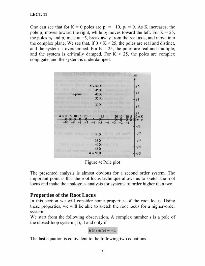
The closed-loop transfer function of ‘this system is as follows where K = K1K2. In figure 3, the pole location for different values of gain K is given.

Figure 3: Pole location as a function of gain The data of figure 3 is graphically displayed in figure 4 which shows each pole and it’s gain.

2

LECT. 11

One can see that for K = 0 poles are p1 = −10, p2 = 0. As K increases, the pole p1 moves toward the right, while p2 moves toward the left. For K = 25, the poles p1 and p2 meet at −5, break away from the real axis, and move into the complex plane. We see that, if 0 < K < 25, the poles are real and distinct, and the system is overdamped. For K = 25, the poles are real and multiple, and the system is critically damped. For K > 25, the poles are complex conjugate, and the system is underdamped.

Figure 4: Pole plot The presented analysis is almost obvious for a second order system. The important point is that the root locus technique allows us to sketch the root locus and make the analogous analysis for systems of order higher than two. Properties of the Root Locus In this section we will consider some properties of the root locus. Using these properties, we will be able to sketch the root locus for a higher-order system. We start from the following observation. A complex number s is a pole of the closed-loop system (1), if and only if The last equation is equivalent to the following two equations

3

LECT. 11

And

Now let us recall some properties of complex numbers. Consider a rational function of the form Then the modulus of F(s) can be calculated as follows It is clear that, given a complex number s, then |s + z1| is the magnitude of the vector drawn from the zero of F(s) at −z1 to the point s, and, analogously, |s + p1| is the magnitude of the vector from the pole of F(s) at −p1 to the point s. Analogously, the argument θ = ArgF(s) is given by the following formula Using these properties, one can see from equation (3) that a point s of the complex plane is on the root locus for a particular value of gain K, if On the other hand, suppose a point s is on the root locus. Then the value of the gain K at this point can be found by the formula Where pj are poles and zi are zeros of the open-loop transfer function G(s)H(s).

4

LECT. 11

Example. Consider a system on figure 5.

Figure 5: Feedback control system The transfer function of the open-loop system (i.e. without feedback) is . The closed-loop transfer function can be found as follows

If a point s is a pole of the closed-loop system for some value of K then (2) and (3) must be satisfied at this point. First, let us check the point s = −2 + j3. If this point is on the root locus, then the sum of angles of the zeros of the open-loop transfer function minus sum of angles of the poles must be an odd multiple of 180 o . From figure 6, we see that θ 1 + θ 2 − θ 3 −θ 4 = 56.31 o + 71.57 − 90 − 108.43 = −70.55 o . o o o

This value is not an odd multiple of 180 , therefore s = −2 + j3 is not a point on the root locus, i.e. it is not a pole of the closed-loop system for any gain K.

o

Figure 6: Pole-zero location

5

LECT. 11

On the other hand, for the point )2/2(j2s +−= we have Therefore, this point is on the root locus for some value of gain K. To find the value of K, one can use formula (6). We have Therefore, we get that for K = 0.33 the point )2/2(j2s +−= is a pole of the closed loop system.

End of Lecture eleven

6

LECT. 12

Computer control design and modeling Lecture 12

Sketching the Root Locus The following properties of the root locus allow us to sketch the root locus using minimal calculations. Property 1: Number of branches. Each closed-loop pole moves as the gain is varied. Therefore, number of separate loci (or branches of the root locus) is equal to the number of poles. Property 2: Symmetry about the real axis. Since the complex poles always appear in complex conjugate pairs, the root locus must be symmetrical about the real axis. Property 3: Location of the real-axis segment of the root locus. The root locus on the real axis always lies in a section of the real axis to the left of an odd number of (open-loop) poles and zeros. Property 4: Starting points and ending points. To determine starting and ending points of root locus, denote by NG(s), DG(s) the numerator and denominator polynomials of G(s) Correspondingly, i.e. On the other hand, let NH(s) (DH(s)) be the numerator (denominator) polynomial of H(s). Using these notations, the transfer function of the closed-loop system can be rewritten as follows Thus, the characteristic equation of the system is as follows or

1

LECT. 12

If K 0, the equation (1) tends to the following one Solutions of the last equation are exactly the poles of the open-loop system. On the other hand, for positive K >0 the equation (1) can be rewritten as If K + ∞ , the last equation tends to the following one Solutions of this last equation are exactly the zeros of the open-loop system. Thus, the following rule is valid: root locus begins at the poles of G(s)H(s) and ends at the zeros of G(s)H(s) as K increases from 0 to +∞ .

Property 5: Location of infinite zeros. We will say that a function F(s) has a zero (pole) at infinity if F(s) 0 (F(s) ∞ ) as s ∞ . Every function has an equal number of zeros and poles if we include the infinite poles and zeros as well as finite poles and zeros. Consider, for example, a function This function has three finite poles at s1 = 0, s2 = −1, s3 = −2, and no (finite) zeros. However, if s approaches infinity, the function becomes Each s in the denominator causes the function to become zero as s approaches infinity. Therefore, the function has three infinite zeros. Thus, the root locus for equation (3) will begin at finite poles and end in infinite zeros. Where are the infinite zeros located? In general, if a function has np finite poles and nz finite zeros (np ≥ nz), then N = np − nz sections (branches) of the root locus will end at infinite zeros. The following rule helps us to locate the infinite zeros. The branches that end at infinite zeros approach the zeros along linear asymptotes. These asymptotes are centered at the point on the real axis given by

2

LECT. 12

and their angles are Property 6: Location of the real-axis breakaway and break-in points. A point on the real axis is called breakaway point if the root locus departs from the real axis at this point. On the other hand, a point on the real axis is called break-in point if the root locus arrives to the real axis at this point. From the symmetry property it follows that the root loci at the breakaway (break-in) point are symmetrical with respect to the real axis. How to find the breakaway (break-in) points? Suppose we have two real axis poles which move towards each other as gain increases. One can conclude that the gain must be maximal at the point where breakaway occurs. Thus, the breakaway point is the point of maximum gain between two open-loop real-axis poles. Analogously, when the complex pair returns to the real axis, the gain will continue to increase as the closed-loop poles move toward the open-loop zeros. Therefore, one can conclude that the break-in point is the point of minimum gain between two real-axis zeros. These considerations allow us to use the following method to find breakaway and break-in points. As we already know, for any points s of the root locus the following equation is valid. On the real axis s is real, therefore H(s) and G(s) are real-valued function. To find points of maximum and minimum of K one can simply differentiate the equation (6) with respect to s and set the derivative equal to zero. Let’s consider an example. Example 1. Consider a unity negative feedback system with the following open-loop transfer function sketch the root locus. Solution. The system has two poles at p1 = −1, p2 = −2, and two finite zeros at z1 = 3 and z2 = 5. The root locus has two branches that start from the

3

LECT. 12

poles, end in the zeros, and symmetrical with respect to real line. Using property 3, we see that the first real-axis segment of the root locus is located between −2 and −1, and the second one is located between 3 and 5. Let us calculate breakaway and break-in points. For the points of the root locus we have Solving for K yields Differentiating with respect to s and settling the derivative equal to zero, we get Solving for s, we find s1 = −1.45, s2 = 3.82. Clearly, s1 is the breakaway point, while s2 is the break-in point. The root locus is shown in figure 1. Another method to find the breakaway and break-in point is by using the following rule: • Breakaway and break-in points satisfy the following relationships where zi, and pj are zeros and poles, respectively, of G(s)H(s). Example. For the previous example, find the breakaway and break-in points without differentiation. Solution. Using (7), we get

Simplifying, we get 11s2 − 26s − 61 = 0,

and solving for s, we obtain s1 = −1.45, s2 = 3.82.

4

LECT. 12

Figure 1: Root locus for Example 1

Property 7: Points of jω -axis crossings. The points where the root locus crosses the j axis are important because they separate stable parts of root locus from unstable ones. To find the j

ωω -axis crossing , we can use the

Routh-Hurwitz criterion as follows: forcing a row of zeros in the Routh table will yield the gain: going back one row to the even polynomial equation and solving for the roots (if possible) yields the points of the imaginary axis crossing. Example 2. Consider a unity negative feedback system with the following open-loop transfer function Sketch the root locus and find the range of K such that the closed-loop system is stable. Solution. The open-loop system has four poles p1 = 0, p2 = −1, p3 = −2, p4 = −4, and one finite zero z1 = −3, therefore, there are three infinite zeros. Using property 3, we see that there are three real axis segments of the root locus: first between 0 and −1, second between −2 and −3, and the third one is to the left of −4. To find the location of infinite zeros, let us calculate the asymptotes using formulas (4), (5). The asymptotes are centered at the point

5

LECT. 12

The angles of asymptotes that intersect at −34 are

i.e. and A breakaway point must exist between the poles −1 and 0, and the corresponding branches tend to infinite zeros along the asymptotes with angles θ 1 and θ 3. Now, let us calculate the points where the root locus crosses the imaginary axis. First, one can find the transfer function of the closed loop system as follows The Routh table for the system (8) is given in figure 2.

Figure 2: Routh table for Example 2 We know that a complete row of zeros yields the possibility for imaginary axis roots. For this system, only the s1 row can yield a row of zeros. This happens if Solving for K, we get

K = 9.65.

6

LECT. 12

Going one row back, one can form the following even polynomial (90 − K)s2 + 21K = 0,

and for K = 9.65 we get 80.35s2 + 202.65 = 0.

Solving for s, we get s1,2 = ±j1.59. Thus, the root locus crosses the imaginary axis at ±j1.59 at a gain K = 9.65. The system is stable for 0 K < 9.65. The root locus is sketched in figure 3.

≤

Figure 3: Root locus for Example 2

Property 8: Angles of Departure and Arrival. One can find angles of departure from the complex poles as well as angles of arrival to the complex zeros as follows. Consider figure 4, which shows the open-loop poles and zeros, some of them are complex. Take a pointε of the root locus close to a complex pole, then the sum of angles drawn from all finite poles and zeros to this pole is equal to an odd multiple of 180o . Assume that all angles from all other poles and zeros are drawn directly to the pole that is near the point. The only unknown angle is the angle drawn from the pole that is close toε . We can solve for this unknown angle, which is actually the angle of departure from this complex pole. For example, for the pole-zero plot in figure 4, we have which implies

7

LECT. 12

Angle of arrival to a complex zero can be calculated analogously. For example (for figure 5)

Figure 4: Calculation of angle of departure

Figure 5: Calculation of angle of arrival

8

LECT. 12

3s2s)2s(K)s(G 2

+=

Example 3. Consider a unity negative feedback system with the following open-loop transfer function

+ + Sketch the root locus. Solution. The open-loop system has two poles p1 = -1+j 2 and p2 = -1-j 2 , and one finite zero z1 = -2, therefore, there is one infinite zero. Using property 3, we see that there is one real axis segment of the root locus between -2 and - . To find the location of infinite zero, let us calculate the asymptotes using formulas (4), (5). The asymptotes are centered at the point

∞

01

22j12j10 =

+−−+−=σ

The angles of asymptotes are

znpn,.....,2,1k;znpn

180)1k2(k −=

−−

=θ

i.e. o1801 =θ

To determine the angle of departure from the complex-conjugate open-loop poles, we use the following equation: 321801 θ+θ−=θ Where

:1θ The angle of departure :2θ The angle between p1 and p2

:3θ The angle between p1 and z1

Then o14555901801 =+−=θ And since the root locus is symmetric about the real axis, the angle of departure from the pole at s =-p2 is -145 . o

Let us calculate breakaway and break-in points. For the points of the root locus we have

9

LECT. 12

2s)3s2s(k

2

+++

−=

We have

2

2

)2s()3s2s()2s)(2s2(

dsdk

+++−++

−= which gives s2 + 4s + 1 = 0 or s = - 3.73 or s = - 0.268 It is clear that points s = - 3.73 is on the root locus. Hence this point is an actual break-in point. Then the root locus is shown in figure 6.

Figure 6: Root locus of Example 3

ωj

σ-2 0 -4

2

-1 -3.73

x

x

-145 ْ

145 ْ

2−

End of Lecture twelve

10

LECT. 13

Computer control design and modeling Lecture 13

Design of Feedback Control Systems The design of a control system is concerned with the arrangement of the system structure and the selection of suitable components and parameters to meet requirements of stability and performance specifications. The alteration or adjustment of a control system in order to provide a suitable performance is called compensation. To alter the system response, an additional component is inserted within the structure of the feedback system. This additional component is often called a compensator or a controller. Two basic configurations of compensation are used in feedback control system design. They are a) cascade compensation, and b) feedback compensation. With cascade compensation, the compensator G1(s) is placed at the low-power end of the forward path in cascade with the plant (figure 1, (a)). In feedback compensation scheme, the compensator H1(s) is placed in the feedback path (figure 1, (b)).

Figure 1: Compensation configurations: a) cascade; b) feedback.

1

LECT. 13

Improving steady-state error via cascade compensation There are two ways to improve the steady-state error of a feedback control system using cascade compensation. These are • ideal integral compensation; • lag compensation. Ideal integral compensation Steady-state error can be improved by placing an open-loop pole at the origin. For example, if the uncompensated system does not have pure integrations, then it’s response to a step input has finite steady-state error. After adding a pole at the origin, the system responds to a step input with zero steady-state error. To see how to improve the steady-state error without affecting the transient response, look at figures 2 and 3. Suppose the uncompensated system has desirable transient response generated by the closed-loop pole at A. If we add a pole at the origin, then the angular contribution of the open-loop poles at the point A is no longer 180 ْ and, therefore, A is no longer a pole of the closed-loop system (figure 2, (b)). To solve the problem, one should add a zero very close to the pole at the origin (figure 3)). Now, the angular contribution of the compensator zero and compensator pole cancel out, and the point A is still on the root locus. Thus, we have improved the steady-state error without affecting the transient response. A method of implementing an ideal integral compensator is shown in figure 4.

Figure 2: Pole at A is: a) on the root locus without compensator; b) not on the root locus with compensator pole added.

2

LECT. 13

Figure 3: Pole at A is approximately on the root locus with compensator pole

and zero added

Figure 4: PI controller The compensator consists of proportional K1 and integral K2/s blocks. The transfer function of the compensator is so that the value of an additional zero can be adjusted by varying K2/K1. Since the compensator has both proportional and integral control, the ideal

3

LECT. 13

integral controller (compensator) is given the alternate name PI (Proportional-Integral) Controller.

Lag compensation The drawback of ideal compensators is that they must be implemented with active network, which require the use of active amplifiers and additional power sources. If we use passive networks (which consist of resistors and capacitors and do not require additional power sources), additional pole and zero are moved to the left, close to origin, as shown in figure 5.This placement of the pole, although it does not increase the number of integrators, does yield the improvement in the static error constant over an uncompensated system.

Figure 5: Compensator pole-zero plot

It is important to note that, to keep transient response characteristics unchanged, the compensator zero and compensator pole must be very close to each other. Thus, to obtain the improvement in steady-state error, one can place the, compensator’s zero-pole pair very close to origin. Lag compensation techniques based on the root-locus approach Consider the problem of finding a suitable compensation network for the case where the system exhibits satisfactory transient response characteristics but unsatisfactory steady-state error characteristics. Compensation in this case essentially consists of increasing the open loop gain without appreciably changing the transient response characteristics. This means that the root locus in the neighborhood of the dominant closed-loop poles should not be changed appreciably, but the open-loop gain should be increased as much as needed. This can be accomplished if a lag compensator is put in cascade with the given feedforward transfer function.

T1s

T1s

Consider a lag compensator Gc(s), where

K (1) ˆ

1Ts1TsK̂)s(G ccc

β+

+=

+ββ=

+

4

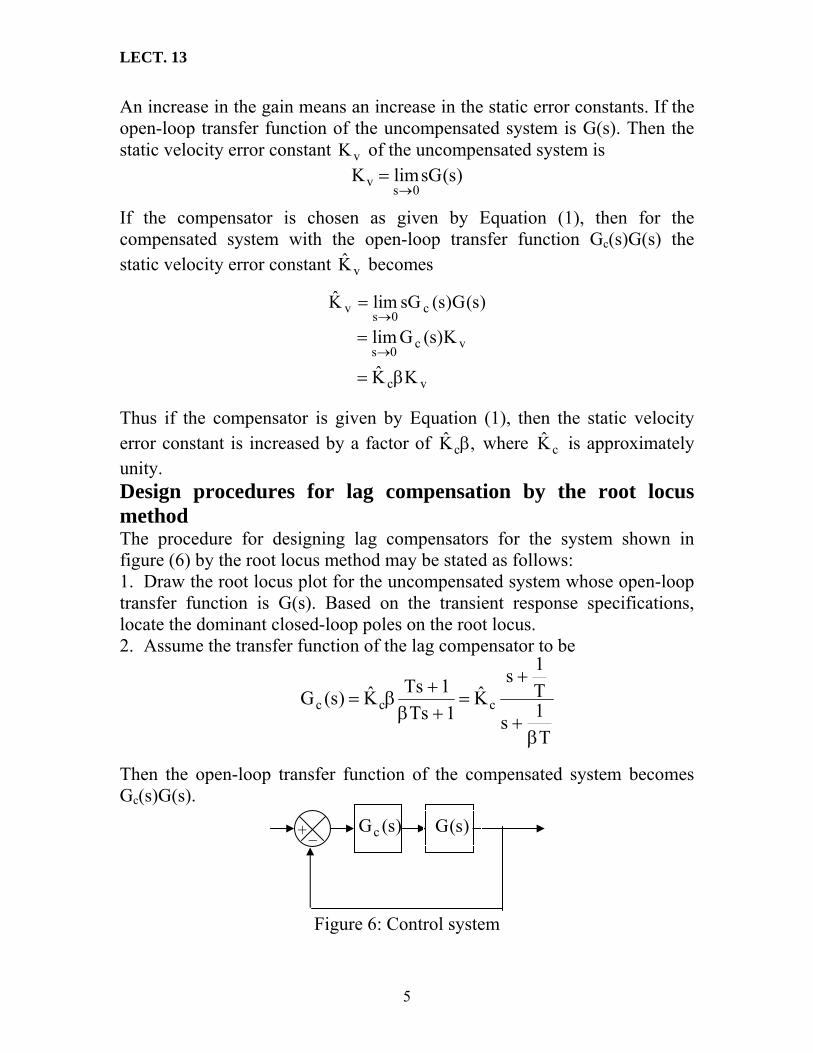
LECT. 13

An increase in the gain means an increase in the static error constants. If the open-loop transfer function of the uncompensated system is G(s). Then the static velocity error constant of the uncompensated system is vK )s(sGlimK

0sv→

=

If the compensator is chosen as given by Equation (1), then for the compensated system with the open-loop transfer function Gc(s)G(s) the static velocity error constant becomes vK̂

)s(G)s(sGlimK̂ c0sv→

=

vc

vc0s

KK̂

K)s(Glim

β=

Thus if the compensator is given by Equation (1), then the static velocity error constant is increased by a factor of where is approximately unity.

,K̂cβ cK̂

Design procedures for lag compensation by the root locus method The procedure for designing lag compensators for the system shown in figure (6) by the root locus method may be stated as follows: 1. Draw the root locus plot for the uncompensated system whose open-loop transfer function is G(s). Based on the transient response specifications, locate the dominant closed-loop poles on the root locus. 2. Assume the transfer function of the lag compensator to be

=→

T1s

T1s

K̂1Ts

1TsK̂)s(G ccc

β+

+=

+β+

β=

Then the open-loop transfer function of the compensated system becomes Gc(s)G(s).

)s(G+ _ )s(Gc

Figure 6: Control system

5

LECT. 13

3. Evaluate the particular static error constant specified in the problem. 4. Determine the amount of the increase in the static error constant necessary to satisfy the specifications. 5. Determine the pole and zero of the lag compensator that produce the necessary increase in the particular static error constant without appreciably altering the original root loci. NOTE: the ratio of the value required in the specifications and the gain found in the uncompensated system is the required ratio between the distance of the zero from the origin and that of the pole from the origin. 6. Draw a new root locus plot for the compensated system. Locate the desired dominant closed-loop poles on the root locus. 7. Adjust gain of the compensator from the magnitude condition so that dominant closed-loop poles lie at the desired location.

cK̂

Example: Consider the system with the following feedforward transfer function is:

)2s)(1s(s06.1)s(G

++=

It is desired to increase the static velocity error constant Kv to about 5 sec-1

using lag compensator. Solution: The closed-loop transfer function becomes

06.1)2s)(1s(s06.1

)s(R)s(C

+++=

)3386.2s)(5864.0j3307.0s)(05864j3307.0s(06.1

+++−+=

The dominant closed loop poles are 5864.0j3307.0s ±−=

To find the damping ratio and the natural frequency of the dominant closed loop poles, we must use the following plot: One of the dominant poles J0.5864

-0.3307

θ

Figure 7:

Illustration of using dominant pole location to calculate ζ and

ωn

6

LECT. 13

Then

ζ = sin(θ) = )5864.03307.0sin(tan 1− = 0.491.

ωn = 22 )5864.0()3307.0( + = 0.673.

And Kv = = )s(sGlim0s→ 2

06.1 = 0.53 sec-1.

To increase the static error constant by a factor of 10, let us choose β = 10 and place the zero and the pole of the lag compensator at s = -0.05 and s = -0.005, respectively. The transfer function of the lag compensator becomes:

Gc 005.0s05.0sK̂c +

+=

The open loop transfer function of the compensated system then becomes

21s1

00

++

0s(K+++

+

)s)(s(06.

005.s05.sK̂)s(G)s(G cc +

+=

)2s)(1s)(005.0s(s

)05.=

where K = 1.06 cK̂

The block diagram of the compensated system is shown in figure (8)

0K =ˆ

c

005.0s05.0sK̂c +

+

)2s)(1s(s06.1

++

966.

+ _

Figure 8: Compensated system If the damping ratio of the new dominant closed-loop poles is kept the same, then the poles are obtained as given below: s1 = - 0.31 + j 0.55, s2 = - 0.31 – j 0.55 The open-loop gain K is

55.0j31.0s05.0s

)2s)(1s)(005.0s(sK+−=+

+++=

0235.1=

7

LECT. 13

Then the lag compensator gain is determined as cK̂

Thus the transfer function of the lag compensator designed is

9656.006.1

0235.106.1KK̂c ===

Then the compensated system has the following open-loop transfer function: 1s2001s20656.9

005.0s05.0s9656.0)s(Gc +

+=

++

=

)2s)(1s)(005.0s(s)05.0s(0235.1)s(G1 +++

+=

1

)1s5.0)(1s)(s200(s)1s20(12.5

++++

=

The static velocity error constant is vK̂1

10sv sec12.5)s(sGlimK̂ −

→==

In the compensated system, the static velocity error constant has increased to 5.12 sec -1 5.12/0.53 = 9.66 times the original value. (The steady-state error with ramp inputs has decreased to about 10 % of that of the original system). We have essentially accomplished the design objective of increasing the static velocity error constant to about 5 sec-1.

End of Lecture thirteen

8

LECT. 14

Computer control design and modeling Lecture 14

Improving transient response When dealing with improving of transient response, the objective typically is to design a response that has a desirable percent overshoot and a shorter settling time than the uncompensated system. As well as in the case of improving of steady-state error characteristics, there exists two ways to improve the transient response of a feedback control system using cascade compensation:

• ideal derivative compensation; • lead compensation.

Ideal derivative compensation One way to speed up the response of the system is to add a single zero to the forward path. This zero can be represented by a compensator with transfer function

This function is a sum of differentiator and a pure gain. It is called an ideal derivative or PD (proportional-derivative) controller. The structure of PD controller is shown in figure 1.

Figure 1: PD controller In this figure, the transfer function of the controller is

1

LECT. 14

Hence, K1/K2 is chosen to equal the negative of the compensator zero, and K2 is chosen to contribute to the required loop-gain value. Transient response unattainable by a simple gain adjustment can be obtained by augmenting the systems poles and zeros with PD compensator. While the ideal derivative compensator can improve the transient response of the system, it has two drawbacks. First, it requires an active circuit to perform the differentiation. Second, differentiation is a noisy process: if the input noise has low level but high frequency, the result of differentiating may lead to large unwanted signals. The lead compensator is a passive network used to overcome the disadvantages of ideal differentiation and still retain the ability to improve the transient response.

Lead compensation When passive networks are used, a single zero cannot be produced; rather, a compensator zero and pole result. However, the advantages of passive networks are: a) no additional power supplies are required, and b) noise due to differentiation is reduced. Lead compensation techniques based on the root-locus approach Consider a design problem in which the original system either is unstable for all values of gain or is stable but has undesirable transient response characteristics. In such a case, the reshaping of the root locus is necessary in the broad neighborhood of the jω axis and the origin in order that the dominant closed-loop poles be at desired locations in the complex plane. This problem may be solved by inserting an appropriate lead compensator in cascade with the feedforward transfer function. The procedures for designing a lead compensator for the system shown in figure 2 by the root locus method may be stated as follows: 1. From the performance specifications, determine the desired location for the dominant closed-loop poles. 2. By drawing the root locus plot, ascertain whether or not the gain adjustment alone can yield the desired closed-loop poles. If not, calculate the angle deficiency . This angle must be contributed by the lead compensator if the new root locus is to pass through the desired locations for the dominant closed-loop poles.

φ

3. Assume the lead compensator Gc(s) to be

2

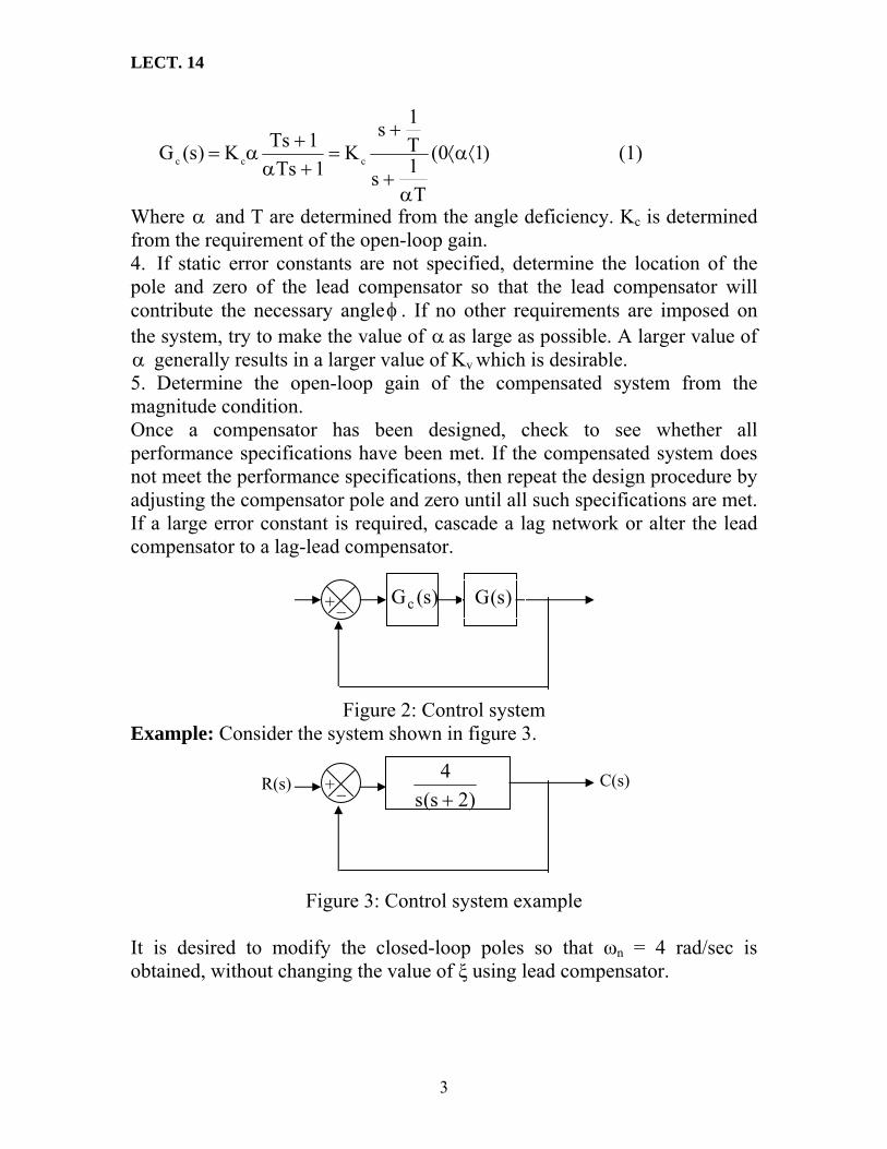
LECT. 14

3

)10(

T1s

T1s

K1Ts

1TsK)s(G ccc ⟨α⟨

α+

+=

+α+

α= (1)

Where and T are determined from the angle deficiency. Kα c is determined from the requirement of the open-loop gain. 4. If static error constants are not specified, determine the location of the pole and zero of the lead compensator so that the lead compensator will contribute the necessary angleφ . If no other requirements are imposed on the system, try to make the value of α as large as possible. A larger value of

generally results in a larger value of Kα v which is desirable. 5. Determine the open-loop gain of the compensated system from the magnitude condition. Once a compensator has been designed, check to see whether all performance specifications have been met. If the compensated system does not meet the performance specifications, then repeat the design procedure by adjusting the compensator pole and zero until all such specifications are met. If a large error constant is required, cascade a lag network or alter the lead compensator to a lag-lead compensator.

+ _ R(s) C(s) )2(s s

4+

)s(G+ _ )s(Gc

Figure 2: Control system Example: Consider the system shown in figure 3.

Figure 3: Control system example It is desired to modify the closed-loop poles so that ωn = 4 rad/sec is obtained, without changing the value of ξ using lead compensator.

LECT. 14

4

Solution: The root-locus plot for this system is shown in figure 4. ωj

4s2s4

)s(R)s(C

2 ++=

)3j1s)(3j1s(4

−+++ =

x

j3

x

j1

j2

-j1

-j2

-j3

σ-2 -3 -4 -5

Closed-loop poles

Figure 4: Root-locus of the system shown in figure 3 The closed-loop transfer function becomes

The closed-loop poles are located at

3j1s ±−=

The damping ratio of the closed-loop poles is 0.5. The undamped natural frequency of the closed-loop poles is 2 rad/sec. The static velocity error constant is 2 sec-1.

In the present example, the desired locations of the closed-loop poles are

s = -2 ± j2 3

In some cases, after the root loci of the original system have been obtained, the dominant closed-loop poles may be moved to the desired location by simple gain adjustment. This is however, not the case for the present system. Therefore, we shall insert a lead compensator in the feedforward path.

LECT. 14

5

A general procedure for determining, the lead compensator is as follows: First, find the sum of the angles at the desired location of one of the dominant closed-loop poles with the open-loop poles and zeros of the original system, and determine the necessary angle φ to be added so that the total sum of the angles is equal to± . The lead compensator must contribute this angle . (If the angle

)1k2(180 +o

φ φ is quite large, then two or more lead networks may be needed rather than a single one.)

)s(GTK)s(G)s(G ⎟⎟

⎜⎜

= (Use equation (1))

T1s

1sc

⎟⎟⎠

⎞

⎜⎜⎝

⎛

α+

+

If the original system has the open-loop transfer function G(s), then the compensated system will have the open-loop transfer function:

c

It is clear that there are many possible values for T and α that will yield the necessary angle contribution at the desired closed-loop poles.

jω PA

O DBC

T1

−T1α

−

2φ

The next step is to determine the locations of the zero and pole of the lead compensator. There are many possibilities for the choice of such locations. In what follows, we shall introduce a procedure to obtain the largest possible value for α (a larger value of α will produce a larger value of Kv. In most cases, the larger the Kv is, the better the system performance.) First, draw a horizontal line passing through point P, the desired location for one of the dominant closed-loop poles. This is shown as line PA in figure 5. Draw also a line connecting point P and the origin. Bisect the angle between the lines PA and PO, as shown in figure 5. Draw two lines PC and PD that make angles 2/φ± with, the bisector PB. The intersections of PC and PD with the negative real axis give the necessary location for the pole and zero of the lead network. The compensator thus designed will make point P a point on the root locus of the compensated system. The open-loop gain is determined by use of the magnitude condition.

σ

Figure 5: Determination of the pole and zero of a lead network

LECT. 14

6

In the present system, the angle of G(s) at the desired closed-loop pole is

°−=+−=+

21032j2s)2s(s

4

Thus, if we need to force the root locus to go through the desired closed-loop pole, the lead compensator must contribute φ at this point. By following the foregoing design procedure, we determine the zero and pole of the lead compensator, as shown in figure 6, to be

o30=

Zero at s = -2.9, Pole at s = -5.4 Or

T = 9.2

1 = 0.345, αT = 4.5

1 = 0.185

Thus = 0.537. α

)4.5s)(2s(s)9.2s(K

)2s(s4

4.5s9.2sK)s(G)s(G cc ++

+=

+++

=

jω

0 -2.9 -4 -5.4

°15

σ

Figure 6: Determination of the pole and zero of the lead network for the above example

The open-loop transfer function of the compensated system becomes

Where K=4Kc. The gain K is evaluated from the magnitude condition as follows:

1)4 .5s)(2s(s

)9.2s(K

32j2s=

+++

+−= Or

K = 18.7

LECT. 14

7

It follows that

)4.5s)(2s( s)9.2s(7.18)s(G)s(Gc ++

+=

68.44

7.18Kc ==

The constant Kc of the lead compensator is

Hence, Kcα = 2.51. The lead compensator, therefore, has the transfer function

4.5s9.2s68.4

1s 185.01s345.051.2)s(Gs +

+=

++

=

)s(G)s(sGlimK c0sv→

=The static velocity error constant Kv is obtained from the expression

)4.5s)(2s (s)9.2s(7.18slim

0s +++

=→

1sec02.5 −=

End of Lecture fourteen

LECT. 15

Computer control design and modeling Lecture 15

Improving Transient response and Steady-State Error PID controllers and Lag-Lead Compensators To obtain simultaneous improvement in steady-state error and transient response, one can combine the methods described in the previous lectures. PID controller design A PID controller is a combination of PI and PD controllers. It’s structure is shown in figure 1. A PID controller is described by the following formula

Figure 1: PID controller The procedure for designing PID controller consists of the following steps: • Evaluate the performance of the uncompensated system to determine how

much improvement in transient response is required. • Design the PD controller to meet the transient response specifications. The

design includes the zero location and the loop gain. • Design the PI controller to yield the required steady-state error. • Determine the gains, K1, K2, and K3. • Simulate the system to be sure that all requirements have been met. • Redesign if simulation shows that requirements have not been met. Lag-lead compensators When passive networks are used, simultaneous improvement of transient response and steady-state error can be obtained using combination of a lag

1

LECT. 15

compensator and a lead compensator rather than the ideal PID compensator. The resulting compensator is called lag-lead compensator. Lag-lead compensation techniques based on the root-locus approach Consider the system shown in figure 2.

Figure 2: Control system

( ) ⎟⎟⎟

⎟⎟⎜

γ=

⎛γ= 1K

TK(G (1)

⎟

⎠

⎞

⎜⎜⎜⎜

⎝

⎛

β+

+

⎟

⎟

⎠

⎞

⎜⎜

⎜

⎝

⎛

+

+

+β⎟⎠

⎞⎜⎝

+γ

++β

2

2

1

1c

21

21cc

Ts

T1s

Ts

T1s

1sT1s

)1sT)(1sT()s

Assume that we use the lag-lead compensator:

21

3. Assuming that we later choose T2 sufficiently large so that the magnitude of the lag portion

21

T1s

T1s

β+

+

Where > 1 and γ > 1. (Kβ c is considered to belong to the lead portion of the lag-lead compensator.)

Case 1. γ ≠ β. In this case, the design process is a combination of the design of the lead compensator and that of the lag compensator. The design procedure for the lag-lead compensator is as follows: 1. From the given performance specifications, determine the desired location for the dominant closed-loop poles. 2. Using the uncompensated open-loop transfer function G(s), determine the angle deficiency φ if the dominant closed-loop poles are to be at the desired location. The lead portion of the lag-lead compensator must contribute this angleφ .

2

LECT. 15

3

is approximately unity, where s = s1 is one of the dominant closed-loop poles, choose the values of T1 and from the requirement that γ

φ=γ +

+

1

1

Ts

Ts

1

1

1

The choice of T1 and is not unique. (Infinitely may sets of Tγ 1 and are possible.) Then determine the value of K

γc from the magnitude condition:

1)s(G

Ts

T1s

K 1

11

11

c =γ+

+

)s(G)s(sGlimK c0sv →=

)s(G

T1s

T1s

Ts

T1s

sKlim

2

2

1

1c0s

⎟⎟⎟⎟

⎠

⎞

⎜⎜⎜⎜

⎝

⎛

β+

+

⎟⎟⎟⎟

⎠

⎞

⎜⎜⎜⎜

⎝

⎛

γ+

+=

→

)s(GsKlim c0s γβ

=→

4. If the static velocity error constant Kv is specified, determine the value of β to satisfy the requirements for Kv. The static velocity error constant Kv is given by

Where Kc and are aleady determined in step 3. Hence, given the value of K

γv, the value of β can be determined from this last equation. Then, using the

value of thus determined, choose the value of Tβ 2 such that

1

T1s

T1s

21

21

≈

β

+

+

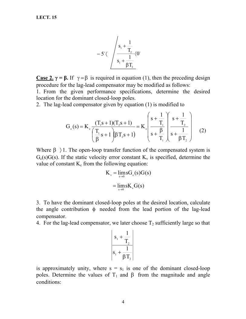
LECT. 15

o0

T1s

T1s

21

21

⟨

β+

+⟨− o5

Case 2. γ = β. If β=γ is required in equation (1), then the preceding design procedure for the lag-lead compensator may be modified as follows:

( ) ⎟⎟

+⎟β

+⎛c 1sT (2) ⎟⎟

⎠

⎞

⎜⎜⎜⎜

⎝

⎛

β

+

⎟

⎟⎟

⎠

⎞

⎜⎜⎜⎜

⎝

⎛ +=

+β⎟⎠

⎞⎜⎝

+β

+=

2

2

1

1c

21

21c

T

T1s

Ts

T1s

K1sT1s

)1sT)(1sT(K)s(G +

2. The lag-lead compensator given by equation (1) is modified to

1. From the given performance specifications, determine the desired location for the dominant closed-loop poles.

Where 1. The open-loop transfer function of the compensated system is G

β ⟩c(s)G(s). If the static velocity error constant Kv is specified, determine the

value of constant Kc from the following equation: )s(G)s(sGlimK c0sv →

= 0

)s(GsKlim cs→=

3. To have the dominant closed-loop poles at the desired location, calculate the angle contribution needed from the lead portion of the lag-lead compensator.

φ

4. For the lag-lead compensator, we later choose T2 sufficiently large so that 2

1

21

T1s

T1s

β+

+

is approximately unity, where s = s1 is one of the dominant closed-loop poles. Determine the values of T1 and β from the magnitude and angle conditions:

4

LECT. 15

1

T1s

T1s

21

21

≈

β+

+

o0

T1s

T1s

21

21

⟨

β+

+

5. Using the value of β just determined, choose T2 so that

⟨− o5

)5.0s(s4)s(G+

=

1)s(G

Ts

T1s

K 1

11

11

c =

⎟⎟⎟⎟

⎠

⎞

⎜⎜⎜⎜

⎝

⎛

β+

+

φ=β

+

+

11

11

Ts

T1s

The value ofβ , the largest time constant of the lag-lead compensator, should not too large to be physically realized.

2T

Example 1: Consider the control system with the following feedforward transfer function:

It is desired to make ξ of the dominant closed-loop poles to 0.5 and ωn = 5 rad/sec and Kv =80 sec-1

. Design an appropriate compensator to meet all the performance specifications.

5

LECT. 15

Solution: The system has closed-loop poles at

9843.1j25.0s ±−= And ξ = 0.125, ωn = 2 rad/sec, and Kv = 8 sec-1. Let us assume that we use lag-lead having the transfer function:

)1,1(

T1s

T1s

Ts

T1s

K)s(G

2

2

1

1cc ⟩β⟩γ

⎟⎟⎟⎟

⎠

⎞

⎜⎜⎜⎜

⎝

⎛

β+

+

⎟⎟⎟⎟

⎠

⎞

⎜⎜⎜⎜

⎝

⎛

γ+

+=

Where γ ≠ β. Then the compensated system will have the transfer function:

)s(G

T1s

T1s

Ts

T1s

K)s(G)s(G

2

2

1

1cc

⎟⎟⎟⎟

⎠

⎞

⎜⎜⎜⎜

⎝

⎛

β+

+

⎟⎟⎟⎟

⎠

⎞

⎜⎜⎜⎜

⎝

⎛

γ+

+=

From the performance specifications, the dominant closed-loop poles must be at:

33.4j5.2s ±−= Since

o235

)5.0s(s4

33.4j50.2s

−=+

+−=

the lead portion of the lag-lead compensator must contribute 55 o so that the root locus passes through the desired location of the dominant closed-loop poles.

To design the lead portion of the compensator, we first determine the location of the zero and pole that will give 55 o contribution. There are many possible choices, but we shall here choose the zero at s = -0.5 so that this zero will cancel the pole at s = -0.5 of the plant. Once the zero is chosen, the pole can be located such that the angle contribution is 55 . By simple calculation or graphical analysis, the pole must be located at s = -5.021. Thus, the lead portion of the lag-lead compensator becomes

o

021.5s5.0sK

Ts

T1s

K c

1

1c +

+=

γ+

+

6

LECT. 15

Thus

T1 = 2, 04.105.0

021.5==γ

Next we determine the value of Kc from the magnitude condition:

s

1)5.0s(

4021.5s5.0sK

33.4j5.2s

c =++

+

+−=

Hence,

26.64

s)021.5s(K33.4j5.2s

c =+

=+−=

The lag portion of the compensator can be designed as follows: First the value of β is determined to satisfy the requirement on the static velocity error constant:

1

T04.161s

T 1s

33.4j5.2s2

2 ≈+

+

+−=

⟨− o5 o0

T04.161s

T1s

33.4j5.2s2

2 ⟨+

+

+−=

)s(GsKlim)s(G)s(sGlimK c0sc0sv γβ

==→→

80988.4)5.0s(s

404.10

)26.6(slim0s

=β=+

β=

→

Hence, β is determined as

β = 16.04 Finally, we choose the value of T2 large enough so that

and

7

LECT. 15

Since T2 5 (or any number greater than 5) satisfies the above two requirements, we may choose

≈

T2 = 5

⎟⎟⎟⎟

⎠

⎞

⎜⎜⎜⎜

⎝

⎛

×+

+

⎟⎟⎟⎟

⎠

⎞

⎜⎜⎜⎜

⎝

⎛

+

+=

504.161s51s

2 04.10s

1s)26.6()s(Gc

Now the transfer function of the designed lag-lead compensator is given by

2

⎟⎠⎞

⎜⎝⎛

++

⎟⎠ ⎞

⎜⎝⎛

++

=01247.0s

2.0s02.5s5.0s26.6

)1s19.80)(1s1992.0()1s5)(1s2(10++

++=

The compensated system will have the open-loop transfer function

)01247.0s)(02.5s(s)2.0s(04.25)s(G)s(Gc ++

+=

Example 2: Consider the control system of example (1). Suppose that we use a lag-lead compensator of the from given by equation (2), or

⎟⎟⎠

⎞⎜⎜⎝

⎛β

+⎟⎟⎠

⎞⎜⎜⎝

⎛ β+

⎟⎟⎠

⎞⎜⎜⎝

⎛+⎟⎟

⎠

⎞⎜⎜⎝

⎛+

=

21

21cc

T1s

Ts

T1s

T1s

K)s(G )1( ⟩β

Assuming the specifications are the same as those given in example (1), design a compensator Gc(s) Solution: The desired locations for the dominant closed-loop poles are at

s = -2.5± j 4.33

The open-loop transfer of the compensated system is

⎛ β

+

⎟⎟⎠

⎞⎜⎜⎝

⎛+⎟⎟

⎠

⎞⎜⎜⎝

⎛+

=

⎜⎜⎝

)5.0s(s4.

T1s

Ts

T1s

T1s

K)s(G)s(G

21

21cc +

⎟⎟⎠

⎞⎜⎜⎝

⎛β

+⎟⎟⎠

⎞

8

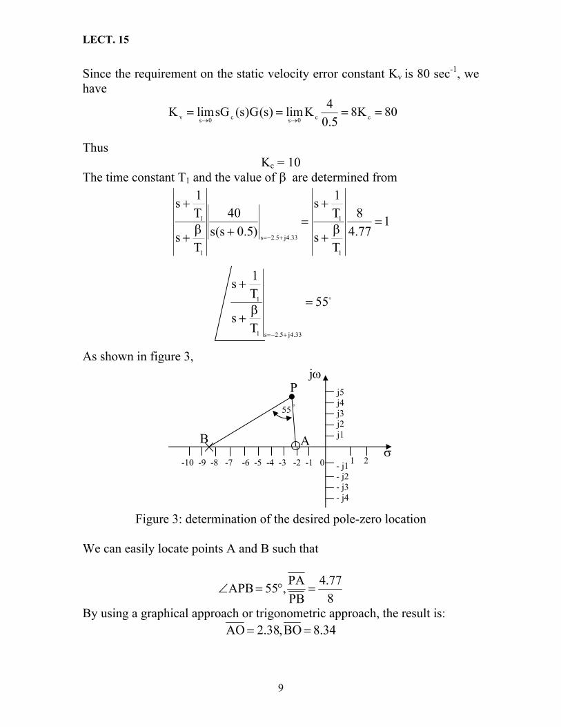
LECT. 15

Since the requirement on the static velocity error constant Kv is 80 sec-1, we have

80K85.0

4Klim)s(G)s(sGlimK cc0sc0sv ====→→

Thus Kc = 10

The time constant T1 and the value of β are determined from

177.48

Ts

T1s

)5.0s(s40

Ts

T1s

1

1

33.4j5.2s

1

1 =β

+

+=

+β+

+

+−=

o55

Ts

T1s

33.4j5.2s1

1 =β+

+

+−=

As shown in figure 3, ωj

σ

-10 -9 -8 -7 -6 -5 -4 -3 -2 -1 0 1 - j1 - j2 - j3 - j4

2

j5 j4 j3 j2 j1

P

B

55 o

A

Figure 3: determination of the desired pole-zero location We can easily locate points A and B such that

877.4

PBPA,55APB =°=∠

By using a graphical approach or trigonometric approach, the result is: 34.8BO,38.2AO ==

9

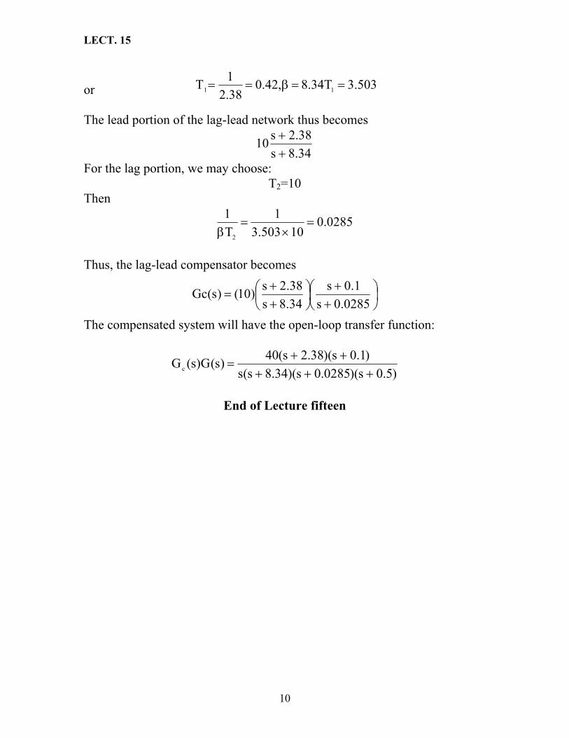
LECT. 15

503.3T34.8,42.038.21T 11 ==β==

or The lead portion of the lag-lead network thus becomes

34.8s38.2s10

++

For the lag portion, we may choose: T2=10

Then

0285.010503.3

1T1

2

=×

=β

Thus, the lag-lead compensator becomes

⎟⎠⎞

⎜⎝⎛

++

⎟⎠⎞

⎜⎝⎛

++

=0285.0s

1.0s34.8s38.2s)10()s(Gc

The compensated system will have the open-loop transfer function:

)5.0s)(0285.0s)(34.8s(s)1.0s)(38.2s(40)s(G)s(Gc +++

++=

End of Lecture fifteen

10

LECT. 16

Computer control design and modeling Lecture 16

Analog Simulation Introduction The electronic analog computer consists of a set of computing components that perform the functions of addition, scaling, integration, etc., required in representing differential equations. The voltages of the analog computer represent the continuous solution of the differential equation programmed by the interconnection of the components (functions). The differential equation is a model of a physical (or natural) dynamic system. An analogy is made between the physical variables of the model and the voltages that represent them on the computer (thus the term “analog” computer). The analogy defines scale factors relating the units of the physical variables to volts in the computer variables. Since the solution of the physical system may be faster or slower than desired, the computer solution can be scaled in both time and magnitude. The underlying concept of analog computation is to interconnect or wire together those components (summers, scalers, integrators, etc.) required to represent the differential equations of interest. As discussed earlier, these differential equations can be expressed in classical form (a single nth-order differential equation) or state space form (n first-order differential equations), although both representations will result in essentially the same wiring diagram. It is easy to perform a single integration at a time on the analog computer, so the state space format is a more natural representation of dynamic systems for analog computation. Therefore, the setup procedure for analog computation will be developed in the state space format; the classical approach, however, will be briefly illustrated as well. Computing Components The basic computing element of the analog computer is a high-gain differential DC amplifier with feedback, called an operational amplifier or “op-amp.” The op-amp has extremely high input impedance, low output impedance, and high gain. The high input impedance results in negligible required input current into the amplifier. The low output impedance results in negligible loading effect upon the output voltage. The high gain G of the amp, accompanied by a sign change or inversion, is required in the computing equation.

1

LECT. 16

2

ao Gee −= (1)

The op-amp (shown in figure 1(a)) open-loop transfer equation (input-output relationship) is

where ea is the amplifier input voltage, G is the gain, and eo is the output voltage. The op-amp is always used with input and feedback impedances, as shown in figure 1(b). Since a common ground line is always present in electronic analog computer circuits, and the op-amp is normally supplied with positive and negative voltage sources, these details can be omitted to reduce clutter in the circuit, as shown by figure 1(c).

+vcc

+

ea eo

-vcc

-

(a)

ea eo

+vcc

-vcc

+-

Zi

ii

ia

Zf

if

ei

(b)

eo Zi

Zf -Gei

(c) Figure 1: Representations of an operational amplifier circuit.

(a) Isolated op-amp. (b) Op-amp with input and feedback impedances. (c) Simplified schematic of analog computer circuit.

LECT. 16

3

The circuit of figure 1(b) can be analyzed by the following component equations (neglecting the output impedance of the amplifier):

i

aii Z

eei −= (2)

f

aof Z

eei −= (3)

The node equation at the amplifier may be simplified by taking into account the fact that Ia is negligibly small due to the high input impedance of the op-amp and the low input voltage to the amplifier:

(4) 0iii ≈=+

ii

f

i

foo e

ZZ

ZZ

Substituting the component equations into the node equation yields afi

1Gee ⎟⎟

⎠

⎞⎜⎜⎝

⎛−⎟⎟

⎠

⎞⎜⎜⎝

⎛+−= (5)

Since the gain G is extremely large compared to 1 + (Zf / Zi), the first term can be neglected, yielding the basic computing equation

i

i

fo e

ZZe −= (6)

This equation indicates that the closed-loop gain between input and output is Zf / Zi, accompanied by a sign change. Different combinations of the types of circuit elements used for Zf and Zi give rise to the various computing components discussed next. These computing components are as given below: 1. Inverter or sign change If both the feedback and the input impedances are resistive and of equal magnitude, (e.g., Zf = Rf, Zi = Ri, where Rf = Ri), then the basic computing equation reduces to a sign change or inverter: eo = -ei (7) An inverter is commonly used to change the sign of a signal or variable; it is often used for subtraction in a summing junction. 2. Scaler or Fixed-Gain Amplifier If both impedances are resistive, but not necessarily of equal magnitude, the basic computing equation reduces to a fixed-gain relation, or scaling, between the input and output:

LECT. 16

i

i

fo e

RRe −= (8)

This equation represents multiplication by a constant or simulates a coefficient in the differential equation. Most analog computers utilize fixed, or hard-wired, resistors in multiples of ten for scaling; thus, gains of 0.1, 1.0, 10.0 are possible from typical fixed-gain amplifiers for determining the order of magnitude of coefficients. The setting of precise values for the coefficients is done with potentiometers. 3. Potentiometer A variable electronic resistive voltage divider, or “pot,” is a passive element that can be used to adjust the exact numerical value of the coefficients of the differential equation. Mathematically, where io kee = 0.1k0 ≤≤ (9) It is clear that the gain of a pot is less than unity, so that a fixed-gain amplifier with a gain of 10.0 or 100.0 is required in conjunction with a pot to obtain coefficients greater than unity. A bank of several pots is always supplied with analog computers to allow system coefficients to be adjusted. 4. Summing Junction Using more than one input resistor allows the addition, or summation, of several independent input signals. The computing equation reduces to a linear summation of the signals, with the possibility of different gains for each signal:

(10) f eRR

33

22

f1

1

f0 R

ReR

eR

e −−−= Summing junctions are ordinarily used to sum together the various terms required to form the differential equation. 5. Integrator The use of a capacitive feedback impedance with a resistive input impedance results in the integration function. The transfer gain can be stated, in operator notation, with D = d / dt, as

i

fio e

DCR1e −= (11)

4

LECT. 16

Writing this equation in integral form and considering the initial condition eo(0) yields

⎥⎦

⎤⎢⎣

⎡+−= ∫

t

0oi

fio )0(edte

CR1)t(e (12)

The integration gain is 1 / (RiCf). The sign change across the amplifier requires that the initial condition be entered with a sign change. It is clear that by using multiple input resistors, a summing integrator is possible. 6. Differentiator If a resistive feedback impedance and a capacitive input impedance are used, the resulting equation implies the function of differentiation. Specifically (13) f DeCeo R−= ii

Or

deCRe iifo −= (14)

dt Differentiators amplify high-frequency signals more than low-frequency signals and hence produce more noise on the output. For this reason, differentiators are seldom used in analog computation. Table 1 illustrates the electronic circuit and the simplified analog computer block diagram symbol for each of the common linear operations just discussed.

End of Lecture sixteen

5

LECT. 16

6

Table 1 Basic analog computer operations.

LECT. 17

1

Computer control design and modeling Lecture 17

Classical analog computer diagrams The goal of classical analog computation is to solve the classical differential equation for the highest-order derivative of an nth-order equation and integrate n times to yield the solution. The equation that results for the nth derivative is formed at the input of the first integrator by summing the lower order derivatives with appropriate coefficients (gains). For example, consider the second-order differential equation

)t(ve0.2e5.0e =++ &&& (1) with initial conditions (2) e

1 10 1

)0(e& )0(e−

)t(v e&−1

e

5.0

2.0 e−

and (3) e Solving for the highest order derivative yields

int)0(e =

int)0(e && =

(4) Assuming that this equation is formed at the input of an integrator, the output would be -e , and the initial condition would have the opposite sign of -e as shown in Figure (1). An integration of the - signal yields e. The initial condition of e would be entered with the opposite sign of +e.

& )0(e&& e&

e0.2e5.0)t(ve −−= &&&

Figure 1: Classical analog computer diagram

Now the equation for & must be wired at the input to first integrator. Scaling with a pot set at 0.5 yields one term. The e signal must be inverted,

scaled by 0.2, and then entered into the summing integrator with a gain of 10

e&e&−

LECT. 17

2

to obtain the proper sign and coefficient of the term. The system input )t(v must be available from a function generator or some similar source, depending upon the input signal. Summation of these three terms with the gains shown yields equation (4) for& . e&

x&

As mentioned earlier, the analog computer is designed to conveniently perform single integrations at a time; thus, having an nth-order dynamic system model of n first-order equations in state space format is advantageous, since single integrations of the derivative state vector yields the solution of the system. The equations for the derivatives of each of the state variables are formed or wired at the input of the integrators. This format is further attractive, since the coefficients in the A and B matrices will result in integrator gains when scaled in magnitude and time.

State space Computer Diagrams

Consider a state space system (with a single input) that has not magnitude scaled, namely,

BuAxx +=& (5)

or

[ ]1u... ⎥⎢+⎥⎢=⎥⎢ (6)

n

2

1

nn2n1n

n22221

n11211

n

2

1

b.

bb

a..aa.

a..aaa..aa

x.

xx

⎥⎥⎥

⎥⎥

⎦

⎤

⎢⎢⎢

⎢⎢

⎣

⎡

⎥⎥⎥

⎥⎥

⎦

⎤

⎢⎢⎢

⎢⎢

⎣

⎡

⎥⎥⎥

⎥⎥

⎦

⎤

⎢⎢⎢

⎢⎢

⎣

⎡

&

&

&

⎥⎥

⎦

⎤

⎢⎢

⎢⎢

⎣

⎡

)0(.

)0()0(x

n

2

1

with

⎥⎥⎥⎥

⎢⎢= .)0( (7) xx

x

LECT. 17

3

This system simulated by the analog computer diagram shown in figure 2.

1u

G11G12G1nG1b

G21G22G2nG2b

)0(x1

1x

−

2x−

)0(x 2

1x

11

12an1a2x

nx

nx2x

21a1x

22an2a

2b

a2na

nnab

a

1x

1b 2x .

.

.

n1

n

Gn1Gn2GnnGnb

nx− nx

)0(x n

1x

nx2x

Figure 2: General state space analog computer diagram

Now, the input to each integrator forms the equation of the derivative of a state, and the output will be that state variable with a sign change; an inverter often (but not always) will be required for computation or monitoring. It is clear that the initial condition of an integrator must be entered with a sign opposite to that of the output, which in this case allows the initial conditions to be entered with the same sign as that of the physical problem. For example, consider the second-order system of equation (1), which is used to illustrate the classical analog computer diagram. This system can be converted to state space form, yielding

LECT. 17

4

2 ⎦⎣⎦⎣⎦⎣⎦⎣

⎡ )0(x

2

[ ]111 u

10

xx

0210

xx

⎥⎤

⎢⎡

+⎥⎤

⎢⎡⎥⎤

⎢⎡

−−=⎥

⎤⎢⎡&

& (8)

5. 2

with

⎥⎦

⎢⎣

=)0(

)0( 1x (9) ⎤

x

The latter system is programmed on the analog computer as shown in figure 3. It is clear that the solution for x1 is the output of the upper inverter, and the solution for x2 is the output of the lower inverter. The equation for contains -2x

2x&1, that was obtained with a pot set at 0.2 and an integrator gain

of 10.

)0(x1

1x−

2x

−

)0(x 2

1x

2x

1

10 1 1

1u

5.0

2.0

Figure 3: State space analog computer diagram for a second-order system

Magnitude and time scaling The purpose of analog computation is to develop an analogy between the physical system variables and the voltages that represent those variables on the analog computer; thus, a conversion must be made from physical variables to the analog computer variables. The analogy provides these conversion factors, or magnitude scale factors. A magnitude scale factor must be associated with each state variable. It is clear that this scaling must

LECT. 17

5

be done in either the classical or the state space format. It is easily handled in the state space format with scaling matrices. A. Magnitude scaling

BuAxx +=& (10)

Consider the set of nth-order linear state space equations with m inputs, denoted by

With initial conditions x(0) = xint (11)

where x and u are the variables and input vectors representing the physical system. Any system response or output y may be found by

DuCxy += (12)

(13) x = α e

The physical system state variable x can be scaled to analog computer state variable e by the transformation

where

⎥⎥⎥⎥⎥

⎢⎢ . α = (14)

⎥⎥⎥⎥

⎦

⎤

⎢⎢⎢

⎢⎢⎢⎢

⎣

⎡

α

αα

α

n

3

2

1

..000..

0...000...000...00

⎥⎥⎥

⎦

⎤

⎢⎢

⎢⎢⎢

⎣

⎡

β

ββ

m

2

1

..00.

0...00...0

.

is a constant nth-order diagonal scaling matrix (in physical units/volt).

⎥⎥⎥⎥

⎢⎢ .

. β = (16)

.

(15)

In a similar fashion, the inputs u to the physical system can be scaled to inputs v to the analog computer system by the transformation

u = βv where

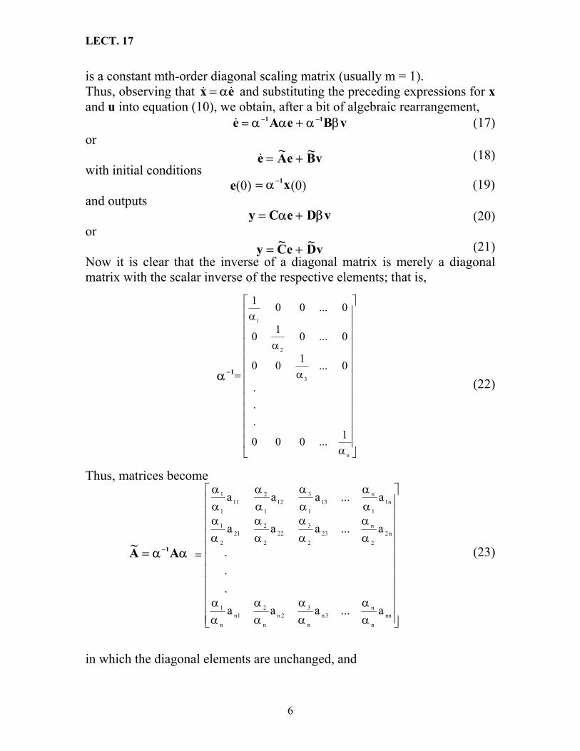
LECT. 17

is a constant mth-order diagonal scaling matrix (usually m = 1). Thus, observing that and substituting the preceding expressions for x and u into equation (10), we obtain, after a bit of algebraic rearrangement,

ex && α=

vBeAe 11 βα+αα= −−& (17) or (18) + vB~eA~e =&with initial conditions e(0) (0) = (19) x1−αand outputs (20) + vDeCy βα=or (21) +Now it is clear that the inverse of a diagonal matrix is merely a diagonal matrix with the scalar inverse of the respective elements; that is,

vD~eC~y =

(22)

⎥⎥⎥⎥⎥⎥⎥⎥⎥⎥⎥⎥⎥

⎦

⎤

⎢⎢⎢⎢⎢⎢⎢⎢⎢⎢⎢⎢⎢

⎣

⎡

α

α

α

α

=

n

3

2

1

1...000

.

.

.

0...100

0...010

0...001

1−α

Thus, matrices become

(23)

⎥⎥⎥⎥⎥⎥⎥⎥⎥⎥⎥

⎦

⎤

⎢⎢⎢⎢⎢⎢⎢⎢⎢⎢⎢

⎣

⎡

αα

αα

αα

αα

αα

αα

αα

αα

αα

αα

αα

αα

=

nnn

n3n

n

32n

n

21n

n

1

n22

n23

2

322

2

221

2

1

n11

n13

1

312

1

211

1

1

a...aaa

.

.

.

a...aaa

a...aaa

αα= − AA~ 1

in which the diagonal elements are unchanged, and

6

LECT. 17

βα= − BB~ 1

ijj

ij bb~β

= (25) iα

(24) ⎥⎥α m2

2

β α ⎥

⎥⎥⎥⎥⎥

⎥⎥⎥

⎦

⎤

⎢⎢⎢⎢⎢⎢⎢⎢⎢⎢⎢

⎣

⎡

αβ

αβ

αβ

βαβ

αβ

αβ

αβ

αβ

αβ

αβ

=

nmn

m3n

n

32n

n

21n

n

1

m23

2

322

2

221

2

1

m11

m13

1

312

1

211

1

1

b...bbb

.

.

.

b...bbb

b...bbb

or, in general, the element in the ith row and jth column becomes

And similarly for ija~ . For k outputs,

2 (26)

⎥⎥⎥⎥⎥⎥⎥

⎦

⎤

⎢⎢⎢⎢⎢⎢⎢

⎣

⎡

ααα

αααααα

=

nkn22k11k

nn222121

nn1212111

c...cc...

c...ccc...cc

α= CC~

and

(27)

⎥

⎥⎥⎥⎥⎥⎥

⎦

⎤

⎢⎢⎢⎢⎢⎢⎢

⎣

⎡

βββ

ββββββ

=

mkm22k11k

mm2222121

mm1212111

d...dd...

d...ddd...dd

β= DD~

B. Time scaling Often, the response of the physical system model proceeds at a slower or faster pace than is practical for recording or plotting purposes. That is, the response of the physical system may be complete in milliseconds or may take hours to arrive at steady state. For this reason, it is frequently desirable

7

LECT. 17

8

to slow down or speed up the simulated response on the computer. This can conveniently be done by making the transformation

(2t = γ τ 8) where γ is a time scaling factor, t is the real time of the physical system, and τ is computer time ( γ > 1 accelerates the solution of the system, while γ < 1 retards the solution ). This transformation implies that

(29) dt = γ dτ then

dtd

dd

γ= (30)

τ Thus, the analog computer state variable system becomes

τdd e = γ eA~ + γBv~ (31)

with initial conditions

(32) e(0) = α-1x(0) and outputs

y = vD~eC ~ + (33) It is clear from the forgoing description of the system that time scaling affects only the A~ and B~ matrices and thus the integrator gains; it does not affect initial conditions or outputs. Time scaling affects only the time required to obtain a response (you will know if time scaling is necessary if all of the integrator gains are very large ( > 100) or very small ( < 0.01). Selection of Magnitude and Time Scale Factors The must difficult task in analog simulation is selecting the magnitude scale factors for each state variable. The scale factors α establish the analogy between the physical variables and the analog computer variables. They are selected such that a maximum response in the physical system will result in a maximum response in the computer variables that will be within certain limits.

LECT. 17

A. Selection of Magnitude Scale Factors The magnitude scale factors are selected in such a manner that the maximum (absolute) value of the physical response of a state variable xi will cause a maximum response of the computer variable ei to be about (but not greater than) 10 volts. Thus,

x

maxi

maxii e=α (34)

If the computed value of is not a convenient number, it should be rounded off higher (rather than lower) to prevent overloading (e

αi > ± 10 volts). For

example, if ximax is predicted to be 1.37 cm, then we would select

voltcm137.0

volt10cm37.1

i ==α (35) which would be rounded off to 0.15 or 0.20 cm/volt. The input scale factors are selected in a similar manner as

)0(x i

(36)

The preceding discussion specifies how to select the scale factors, but the problem of predicting ximax and ujmax still faces us. Determining ujmax is relatively easy, since the system input is usually known (e.g., a step, a ramp, sinusoidal, etc). While the determination of ximax is slightly more difficult, it is greatly simplified by the approach set out next. In some systems, the largest value of a state variable occurs at its initial condition, and the response decays thereafter. In other instances, the maximum response occurs at or near the steady-state value, as shown in figure 4

x ∞

maxj

maxj

vu

j =β

(i )xiix

Time Time

Figure 4: Typical responses illustrating maximum values

9

LECT. 17

The initial conditions are known, and the steady-state maxima can be estimated. To do the estimation, we observe that the steady-state values occur when , and thus, 0x =& Ax −=∞)( Bu (37) This yields a set of algebraic equations in which the energy or effort supplied by the inputs is put into the state variables. If we solve each of the equations for successive state variables, then assuming that all of the input effort goes into these variables entirely, we can observe the ultimate steady-state maxima of the state variables. For example, consider a second-order system with one input; Equation (37) becomes (38)

(39) x 12222121

11212111

ub)(a)(xaub)(xa)(xa

−=∞+∞−=∞+∞

Now, assuming that all of the input effort goes into x1 and none goes into x2 we obtain the ultimate (indicated by *) steady-state maxima. From equation (38) with x2(∞ ) assumed to be zero, it follows that (40)

max111

1*1 u

ab)(x −

=∞ From equation (39)

(41) max1

21

2*1 u

ab)(x −

=∞ Whichever of these two equations yields the largest absolute value for x1 will be used as the steady-state maximum. Thus,

of MAX)(x max*1 =∞

⎭⎬⎫

⎩⎨⎧

max121

2max1

11

1 uaboru

ab (42)

And similarly,

of MAX)(x max*2 =∞

⎭⎬⎫

⎩⎨⎧

max122

2max1

12

1 uaboru

ab (43)

We are now ready to estimate the maximum value we expect from a state variable. The maximum will occur either at the initial condition or at the value estimated by the steady-state maximum method; that is of MAXx maxi = { }max

*ii )(xor)0(x ∞ (44)

The method just outlined should predict all the maximum expected values of the state variables necessary to allow the selection of magnitude scale factors α and β. Then, having selected the scale factors, we can compute the

10

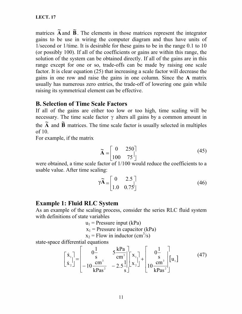
LECT. 17

matrices A~ and B~ . The elements in those matrices represent the integrator gains to be use in wiring the computer diagram and thus have units of 1/second or 1/time. It is desirable for these gains to be in the range 0.1 to 10 (or possibly 100). If all of the coefficients or gains are within this range, the solution of the system can be obtained directly. If all of the gains are in this range except for one or so, trade-offs can be made by raising one scale factor. It is clear equation (25) that increasing a scale factor will decrease the gains in one row and raise the gains in one column. Since the A matrix usually has numerous zero entries, the trade-off of lowering one gain while raising its symmetrical element can be effective. B. Selection of Time Scale Factors If all of the gains are either too low or too high, time scaling will be necessary. The time scale factor alters all gains by a common amount in the

γA~ and B~ matrices. The time scale factor is usually selected in multiples

of 10. For example, if the matrix

(45)

were obtained, a time scale factor of 1/100 would reduce the coefficients to a usable value. After time scaling:

⎥⎦

⎤⎢⎣

⎡=

751002500

A~

A~γ (46)

⎥⎦

⎤⎢⎣

⎡=

75.00.15.20

Example 1: Fluid RLC System As an example of the scaling process, consider the series RLC fluid system with definitions of state variables u1 = Pressure input (kPa)

x1 = Pressure in capacitor (kPa) x2 = Flow in inductor (cm3/s) state-space differential equations

(47) [ ]1

2

3

2

1

2

3

3

2

1 u

kPascm10s10

xx

s15.2

kPascm10

cmkPa5

s10

xx

⎥⎥⎥

⎦

⎤

⎢⎢⎢

⎣

⎡

+⎥⎦

⎤⎢⎣

⎡

⎥⎥⎥

⎦

⎤

⎢⎢⎢

⎣

⎡

−−=⎥

⎦

⎤⎢⎣

⎡&

&

11

LECT. 17

and initial conditions ⎡−

⎥⎦

⎤⎢⎣

=⎥⎦

⎤⎢⎣

⎡s/cm0

kPa20)0(x)0(x

32

1(48)

Let the system be subjected to a step input u1 = 10 kPa for t ≥ 0 (49) The first step in solving the system is to select the magnitude scale factors. This requires knowledge of ximax. The steady-state maximums can be predicted from equation (47) by setting = 0. The first equation yields no information, since the input has no direct influence on . The second equation results in

x&1x&

(50) By setting x2( )=0 and allowing all of the input effort to drive x∞ 1, we find that

121 u10)(x5.2)(x10 =∞+∞

(51) uu10(x == max1max1*1 10

)∞

kPa10)(x*1 =∞

(52)

By setting and allowing all of the input to go into the second state variable, we find that

0)(x1 =∞

(53) 4u10(x ==

(54) /40(x =max1max1

*2 u

5.2)∞

cm) 3*2 ∞ s

The maximum values for x can now be estimated from the maximum of either the initial conditions or the steady–state maxima: of MAXx max1 = { }max

*11 )(xor)0(x ∞ (55)

of MAX= { } kPa2010or20 = of MAXx max2 = { }max

*22 )(xor)0(x ∞ (56)

of MAX= { } s/cm4040or0 3= The magnitude scale factors can now be computed:

(57) voltkPa0.2

volt10kPa20

ex

max1

max11 ===α

(58) s/cms/40x

===α 0.4volt10

cme

33

max2

max22 volt

12

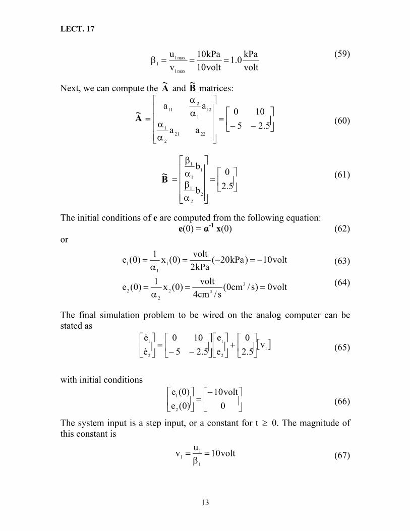
LECT. 17

(59) kPa10u===β

volt0.1

volt10kPa

v max1

max11

Next, we can compute the A~ and B~ matrices:

⎥⎦

⎤⎢⎣

⎡−−

=

⎥⎥⎥⎥

⎦

⎤

⎢⎢⎢⎢

⎣

⎡

αα

αα

=5.25

100

aa

aa

22212

1

121

211

A~ (60)

(61) B

⎤⎡=⎥

⎥⎢⎢

=0⎥⎦

⎢⎣

⎥⎥⎦

⎤

⎢⎢⎣

⎡

αβαβ

5.2b

b

22

1

11

1

~ The initial conditions of e are computed from the following equation: e(0) = α-1 x(0) (62) or volt1

(63)

(64)

The final simulation problem to be wired on the analog computer can be stated as

⎤

volt0)s/cm0(s/cm4

volt)0(x1)0(e

volt10)kPa20(kPa2

)0(x)0(e

332

22

11

1

==α

=

−=−=α

=

⎢⎣

⎡−−

=⎥⎦

⎤⎢⎣

⎡&

& [ ]12

1

2

1 v5.2

0ee

5.25100

ee

⎥⎦

⎤⎢⎣

⎡+⎥

⎦

⎤⎢⎣

⎡⎥⎦

(65)

with initial conditions

⎥⎦

⎤⎢⎣

⎡−=⎥

⎦

⎤⎢⎣

⎡0volt10

)0(e)0(e

2

1(66)

The system input is a step input, or a constant for t 0. The magnitude of this constant is

≥

volt10uv

1

11 =

β= (67)

13

LECT. 17

14

The elements in A~ and B~ represent integrator gains. The analog computer diagram for this system is shown in Figure 5 volt10−

1e−

2e−

volt 0

1e

2e

10

10 11

0 0

volts10+

5.

0

25.01v

25.0

Figure 5: Analog computer diagram for Example 1

End of Lecture seventeen

LECT. 18

1

Computer control design and modeling Lecture 18

Digital Simulation Introduction While many low-order linear systems can be solved using standard differential equation solution procedures, numerical methods are advantageous when a large number of differential equations is necessary to describe the system or when the physical situation must be represented by nonlinear differential equations. In these cases, digital simulation is an indispensable tool. It is assumed that higher order systems can be transformed into an equivalent set of first-order, state space equations, and only first order equations are discussed here.

Figure 1 shows the solution to a differential equation (solid line) and an approximate solution to the same equation obtained by a numerical method (dots). While a closed-form solution consists of an analytic function relating the dependent and independent variables (x and t, respectively), a numerical solution consists of a series of points xj obtained at a discrete set of points tj of time. The distance between the time points (the time step) is denoted by h. The figure makes clear the strong dependence of the quality of the numerical solution on the size of h. That is, toward the end of the record of time given, the analytic solution begins an oscillation that the discrete point spacing is unable to represent. A shorter time step is obviously needed in this region of the solution.

h

t

x

1jx +

jx

jt 1jt +

Figure 1: Numerical integration of a dynamic system

LECT. 18

Euler’s method Suppose a single first-order differential equation is given in which f(x,t) may be a linear or a nonlinear function, depending on the problem at hand: with initial condition x(t0) = x0 (1) )t,x(f

dtdx

= This is an initial-value problem, since x(t) is given at some initial time t0, and we desire the solution values at succeeding times t. Equation (1) may be written as (2)

+1+

=j

j

1j

j

t

t

x

x

dt)t,fdx x(∫∫

jjjjjjj hf)t,(hf)t,(fxx ===− ∫ (3) t 1

Suppose the time step h = tj+1 - tj is small enough so that the slope )t,x(fx =& may be taken to be the constant f(xj ,tj) over the interval h. Then

1 xdtxj+

+

j t

...dt2

hfxx 2jjj +++= (6) x

! j

22

1+

dh

Thus, the new value of x, (xj+1) may be computed from previous values by the relation (4) jj1j hfxx +=+

This simple technique of integration is called Euler’s method.

Geometrically, the Euler process assumes that the slope dx/dt = f(x,t) is constant over the interval h. This assumption has obvious limitations. The error involved in using Euler’s method can be examined by considering a Taylor series expansion of x(t). Recalling the Taylor series expansion discussed in calculus, we write

dxh)t(x)t(xj

2

22

jj1j +++=+ (5)

...

dtxd

!2h

dt

Replacing dx/dt with f(x,t) we obtain

In Euler’s method, we neglect terms beyond hfj; hence, the error caused at each step is proportional to h2, and is called the truncation error. Example 1: Euler’s Method Use Euler’s method to solve the following first order equations. The first displays exponential behavior; the second has a harmonic solution.

2

LECT. 18

xx −=& with initial condition x(0) = 1, 0 ≤ t ≤ 5 s, (7)

And

tsin10y3y +−=& , with initial condition y(0) = -1, 0 ≤ t ≤ 12 s. (8)

Solution: For Equation (7) we select a step size of h = 0.5 s then At t = 0.5: then x1 = x0 + 0.5(-1) = 1 – 0.5 = 0.5 (9) At t = 1: then x2 = x1 + 0.5(-0.5) = 0.5 – 0.25 = 0.25 (10) And etc. This recursive process is continued until we reach the desired final time point, t = 5. The exact solution to Equation (7) can be found using classical methods as:

(11) xe(t) = e-t It is clear that the exact solution approaches zero with increasing time. Table 1 gives a comparison of the Euler solution with the exact solution to this problem for step sizes, h = 0.5, h = 0.1, and h = 0.0125.The error in the calculated result at some specific time t is called the global error. It is clear from Table 2 that as the step size is halved; the global error of Euler’s method is approximately halved also. Thus, even though the pre-step (truncation) error is proportional to h2, the global error is approximately proportional to h. HOMEWORK: Solve the second differential equation. TABLE 1 SOLUTIONS TO 1)0(x,xx =−=&

h = 0.5 t

x (Euler)

x (exact)

error (%)

0.5 1.0 1.5 2.0 2.5 3.0 3.5 4.0 4.5 5.0

0.500000 0.250000 0.125000 0.062500 0.031250 0.015625 0.007813 0.003906 0.001953 0.000977

0.606531 0.367879 0.223130 0.135335 0.082085 0.049787 0.030197 0.018316 0.011109 0.006738

17.56 32.04 43.98 53.82 61.93 68.62 74.13 78.67 82.42 85.51

3

LECT. 18

h = 0.1

t

x (Euler)

x (exact)

error (%) 0.5 1.0 1.5 2.0 2.5 3.0 3.5 4.0 4.5 5.0

0.590490 0.348678 0.205891 0.121577 0.071790 0.042391 0.025032 0.014781 0.008728 0.005154

0.606531 0.367879 0.223130 0.135335 0.082085 0.049787 0.030197 0.018316 0.011109 0.006738

2.64 5.22 7.73

10.17 12.54 14.86 17.11 19.30 21.43 23.51

h = 0.0125 t

x (Euler)

x (exact)

error (%)

0.5 1.0 1.5 2.0 2.5 3.0 3.5 4.0 4.5 5.0

0.604622 0.365568 0.221031 0.133640 0.080802 0.048855 0.029539 0.017860 0.010798 0.006529

0.606531 0.367880 0.223130 0.135335 0.082085 0.049787 0.030197 0.018315 0.011109 0.006738

0.31 0.63 0.94 1.25 1.56 1.87 2.18 2.49 2.80 3.10

TABLE 2 FINAL GLOBAL ERRORS USING EULER’S METHOD TO SOLVE 1)0(x,xx =−=&

Step size h(s) Global error in x(t=2), (percent)

0.5 53.8

0.25 26.0

0.1 10.2

0.05 5.04

0.025 2.51

0.0125 1.25

More Accurate Methods Euler’s method uses only two items of information to propagate the solution from tj to tj+1: the current solution estimate xj and the function value or slope fj. If more information concerning the character of the solution is used, the numerical results will obviously be more accurate for a given step size; that is, they will have smaller per-step truncation errors. Many such methods have been devised over the years. Two are discussed here: Adams method and Runge-Kutta methods.

The Adams method is typical of methods employing three pieces of information to advance the solution. It uses the equation

(12) )f(hxx −+= f3

2 1jjj1j −+

4

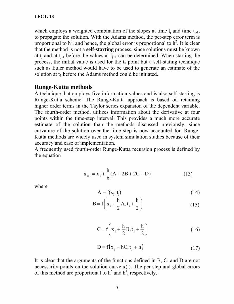
LECT. 18

5

which employs a weighted combination of the slopes at time tj and time tj-1, to propagate the solution. With the Adams method, the per-step error term is proportional to h3, and hence, the global error is proportional to h2. It is clear that the method is not a self-starting process, since solutions must be known at tj and at tj-1 before the values at tj+1 can be determined. When starting the process, the initial value is used for the t0 point but a self-stating technique such as Euler method would have to be used to generate an estimate of the solution at t1 before the Adams method could be initiated. Runge-Kutta methods A technique that employs five information values and is also self-starting is Runge-Kutta scheme. The Runge-Kutta approach is based on retaining higher order terms in the Taylor series expansion of the dependent variable. The fourth-order method, utilizes information about the derivative at four points within the time-step interval. This provides a much more accurate estimate of the solution than the methods discussed previously, since curvature of the solution over the time step is now accounted for. Runge-Kutta methods are widely used in system simulation studies because of their accuracy and ease of implementation. A frequently used fourth-order Runge-Kutta recursion process is defined by the equation

)DC2B2A(6hxx j1j ++++=+ (13)

where A = f(xj, tj) (14)

(15) ⎟

⎠⎜⎝

++=2

tA2

xfB j

⎞⎛ h,hj

(16)

⎟⎠⎞

⎜⎝⎛ ++=

2ht,B

2hxfC jj

( )ht,hCxfD jj ++= (17)

It is clear that the arguments of the functions defined in B, C, and D are not necessarily points on the solution curve x(t). The per-step and global errors of this method are proportional to h5 and h4, respectively.

LECT. 18

Example 2: Runge-Kutta Method Solve the first-order problem of equation (7) using the fourth-order Runge-Kutta method. Solution: The problem is solved using the Runge-Kutta method as just outlined, and the results are presented in Table 3. It is clear that for comparable step sizes, the Runge-Kutta method produces results that are much more accurate than does the Euler method.

TABLE 3 RUNGE-KUTTA (R-K) SOLUTION TO 1)0(x,xx =−=&

h = 0.5 t

x (R-K)

x (exact)

error (%)

0.5 1.0 1.5 2.0 2.5 3.0 3.5 4.0 4.5 5.0

0.606771 0.368171 0.223395 0.135550 0.082248 0.049905 0.030281 0.018374 0.011149 0.006765

0.606531 0.367879 0.223130 0.135335 0.082085 0.049787 0.030197 0.018316 0.011109 0.006738

-0.040 -0.079 -0.119 -0.158 -0.198 -0.238 -0.278 -0.317 -0.357 -0.397

This problem is solved several times using the Runge-Kutta method with different step sizes, and the effect of the step size on the global error is shown in Table 4. It is clear that as the step size is halved; the error is reduced by a factor of about 16.

TABLE 4 RUNGE-KUTTA SOLUTION TO 1)0(x,xx =−=& Step size h(s) Global error in x(t=2), (percent)

0.5 0.158

0.25 0.008

0.125 0.00046

End of Lecture eighteen

6

LECT. 19

Computer control design and modeling Lecture 19

Systems of Equations The methods discussed in lecture 18 may be used for more than one equation if we regard the symbols as vectors. That is, x and f are vectors, and we have a set of equations of the state-space form: = Dx = f (x, t), with initial-condition vector x(tx& 0) = x0 (1) There is a separate of the derivative for each variable; that is, for n equations,

(2)

,

.

.

.)t,x,...,x,x(fx)t,x,...,x,x(fx

n2122

n2111

==

&

&

)t,x,...xx(fx n21nn =&

The functions fi express the coupling between the solution variables xi. In applying the fourth order Runge-Kutta method to a system of equations, we obtain the numerical solution for the vector of dependent variables, x, as given by the expression x =+1j x (

6h

j+ A + 2B + 2C + D) (3) where A = f(xj, tj) (4)

B = f(xj + 2h A, tj +

2h ) (5)

C = f(xj + 2h B, tj +

2h ) (6)

D = f(xj + C, th j + ) h (7)

Here A, B, C, and D are vectors corresponding to the function evaluations shown in equations 3 through 7 above.

1

LECT. 19

Example 1: Given a system with the following state-space equations. (8) 211 x0.4x5.0x −−=& with x1(0) = 0

and 12 xx =& with x2(0) = 2 (9)

Calculate the values of x1 and x2 for t = 0 to 5 second (h = 0.5) by using the fourth-order Runge-Kutta method. Solution: To calculate the values of x1 and x2 at t = 0.5, for example, we use the following equations:

(10) x1(0.5) = x1(0) + 6h (A1 + 2B1 + 2C1 + D1)

and

x2(0.5) = x2(0) + 6h (A2 + 2B2 + 2C2 + D2) (11)

where (12) A1 = f1(x1(0), x2(0), t) = -8

(13) A2 = f2(x1(0), x2(0), t) = 0

B1 = f1(x1(0) + 2h A1, x2(0) +

2h A2, t +

2h ) = -7 (14)

B2 = f2(x1(0) + 2h A1, x2(0) +

2h A2, t +

2h ) = -2 (15)

C1 = f1(x1(0) + 2h B1, x2(0) +

2h B2, t +

2h ) = -5.125 (16)

C2 = f2(x1(0) + 2h B1, x2(0) +

2h B2, t +

2h ) =-1.75 (17)

(18) D1 = f1(x1(0) + hC1, x2(0) + hC2, t + h) = -3.21875

D2 = f2(x1(0) + hC1, x2(0) + hC2, t + h) = -2.5625 (19)

9557.2)21875.35272(00(x −=−×−×−+= (20) Then

125.865.)01 −

1615.1)5625.2222(02(x 2 =−×−×−+= (21) 75.1065.)0

By the same approach we can calculate other values. The values of x1 and x2 for t = 0 to t = 5 second (h = 0.5) are given in Table 1.

2

LECT. 19

TABLE 1 SOLUTION OF EXAMPLE 1 t x1 x20 0 2.0000

0.5000 -2.9557 1.1615 1.0000 -2.8869 -0.4175 1.5000 -0.5261 -1.3091 2.0000 1.7263 -0.9546 2.5000 2.0944 0.0834 3.0000 0.7061 0.8223 3.5000 -0.9356 0.7384 4.0000 -1.4617 0.0831 4.5000 -0.7017 -0.4918 5.0000 0.4489 -0.5448

Selection of the Step Size It is clear that the accuracy with which the numerical solution is computed depends upon the step size employed. A fixed step size that is to large can give results either with large errors or cause the numerical process to become unstable. On the other hand, too small an h causes an inordinately large number of steps to be taken, which, in the extreme, can cause large computational errors due to round-off. This happens because computations are normally performed with a limited number of digits. 1. Selection of A fixed Step Size In selecting the proper step size for a numerical method of solving a system equation, the primary goal is to divide the resulting waveform into enough pieces to be able to resolve the character of the wave accurately, without resorting to the use of an excessive number of points and thereby incurring significant round-off errors. Two different dynamic effects must be considered in the selection of the step size: a) The speed of the response, determined by the natural dynamics of the system. b) The waveform of the input signal. 2. Selection of output interval and final time The output interval is the time between two distinct recordings of data, and of course, it must be an integer multiple of the step size. Although there are no definite rules, suggested output intervals are as follows: h for a first-order system

3

LECT. 19

4

2h to 5h for a second-order system 4h to 10h for a third-order system 10h to 20h for a high-order system The final time is the ending time of the simulation and may also generally be a function of the natural dynamics of the system. Thus, it, too, may be based on the solution step size. The time required to achieve a desired response or reach a steady state is generally different for each simulation; however in the absence of other information, the following guidelines may be used for estimating the required final time: 50h for a first-order system 50h to 200h for a second-order system 100h to 500h for a third-order system 200h to 1000h for a high-order system Variable step size methods In some instances, the step size dictated by the requirements outlined in the previous section may not be required, except over a portion of the period during which the solution is formed. As time advances, the frequency content of the input function may change, or, in nonlinear systems, the system dynamic characteristics may change. In order to be able to change the integration time step as the solution progresses, some estimate of the current accuracy of the calculated results must be made, and different methods of doing this are available, depending on the particular numerical integration scheme that is being employed. One of the most straightforward approaches involves calculating the response at the next point in time in two ways. First, the new solution point is calculated in the usual way by advancing from t to t + h using a step of size h. Let this solution be xa. Then another approximation to the solution at t + h is found by taking two small steps of size h/2. Call this second solution estimate xc. An estimate of the truncation error that occurs during the step can be computed from the two separate solutions calculated for the value of x(t + h):

12xxE 1

acT −

−≅ (22)

LECT. 19

5

Since the Euler method is a first-order method, the constant 2 appears to the first power in the above equation. If the analysis were repeated for a method of order p, we would obtain:

12xxE p

acT −

−≅ (23)

for an estimate of the pre-step truncation error. For the fourth-order Runge-Kutta method, we could estimate the pre-step error by

15xxxxE ac

4ac

T 12−

=−−

≅ (24)

If, during the solution process, it is found that the pre-step error estimate is larger than some preselected value, the step size may be reduce at that point in the computation and the time advance continued. On the other hand, if the error is very small, the step size may safely be increased. An alternative method of estimating the error involves using integration methods of different orders to calculate the estimate over a given time step. For example, we might use a fourth-order Runge-Kutta method to advance the solution one time step and then repeat the calculation for that step using a fifth-order Runge-Kutta method. An estimate of the error can then be found from the difference in the two calculated values at the endpoint and a decision made about whether to change the step size.

End of Lecture nineteen

End of Lectures