1

Deterministic and Empirical Assessment of Smoke’s Contribution to Ozone (DEASCO3)

Final Report

Joint Fire Sciences Program Project # 11-1-6-6 Principal Investigator: Charles T. (Tom) Moore, Jr.

Western Governors’ Association, Western Regional Air Partnership (WRAP)1

1600 Broadway, Suite 1700, Denver, CO 80202

Collaborators:

Air Sciences, Inc. – David Randall, Matthew Mavko, and colleagues

ENVIRON International Corp. – Ralph Morris, Bonyoung Koo, and colleagues

U.S. National Park Service – Mark Fitch, Michael George, Michael Barna, John Vimont

U.S. Forest Service – Bret Anderson, Ann Acheson

1 - now with the Western States Air Resources Council (WESTAR), tmoore@westar.org

2

Abstract This document reports our success in achieving the objectives and accomplishing the deliverables proposed in the project “Deterministic and Empirical Assessment of Smoke’s Contribution to Ozone (DEASCO3). This final report is divided into four sections. Section 1, the Background, describes the purpose of the project and summarizes the project objectives and how accomplishment of these objectives addresses the original research solicitation JFSP Project Announcement No. FA-RFA011-0001, Task 6: Fire smoke and ozone standards analysis. The Background section also provides context for the time and issues related to the project purpose, in terms of how the Project Team addressed delivery of results. Section 2 discusses the technical work to conduct the emission inventory and modeling analyses, and empirical assessment and selection of case studies. Examples of the case studies and analysis / visualization tools are presented in Section 3. Section 4 presents the primary deliverable of the project; a rank order tool and dataset of the U.S. counties with the potential to exceed various levels of the Ozone air quality standard determined though the analyses. The final sections provide Air Quality Planning and Management Implications and summarize the Presentation and Outreach effort in this project. I. Background and Purpose During 2010, the U.S. Environmental Protection Agency (EPA) conducted a process to re-review the 2008 promulgation of the 8-hour Ozone National Ambient Air Quality Standards (NAAQS). At the time of the publication of the 2011 Funding Opportunity Notice (FON) from the Joint Fire Science Program, (JFSP), EPA had signaled the intention to propose new, more stringent Ozone NAAQS in late Summer 2010 (http://www.epa.gov/air/ozonepollution/actions.html - jan10s). The EPA proposal was expected to lower (make more stringent) the Ozone NAAQS, by changing the compliance level from 0.075 parts per million (ppm) to a somewhere in the range of 0.060 to 0.070 ppm. EPA was also considering proposing to establish a distinct cumulative, seasonal, secondary NAAQS for Ozone, designed to protect sensitive vegetation and ecosystems. EPA was proposing to set the level of the secondary NAAQS within the range of 7 to 15 ppm-hours. At those levels, the Ozone NAAQSs would continue regional nonattainment in the Eastern U.S., and have the effect of creating regional nonattainment in the West for the first time. State and local air agencies are required under the federal Clean Air Act to prepare emissions control plans sufficient to achieve the revised NAAQSs. All emissions, including those from fire activities that contribute to Ozone exceedances will be analyzed, with consideration of the potential to reduce them. Fire smoke emits Non-Methane Organic Compounds (NMOC) and Nitrogen Oxides (NOx) that are precursors to ozone formation, along with other pollutants, as do other natural and anthropogenic sources. Earlier analyses by researchers and planning efforts by State air agencies at the former Ozone NAAQS level of 0.084 ppm in place before 2008 have demonstrated that forest fires contributed to exceedances of the Ozone NAAQS. States have also successfully argued to EPA that forest fire-driven ozone episodes should be classified as “exceptional events” under an EPA rule, allowing the State to remove those exceedances from their monitoring database and thus not have to develop emissions reduction actions for them. This approach has been used by State and local air quality managers to exclude large-fire emissions from emissions reduction strategies and planning requirements. During the consideration of the new, lower Ozone NAAQS, there was a strong concern the application of the exceptional events policy would become more difficult and the emissions control planning process by State and local air agencies would need to have more explicit and detailed involvement of fire practitioners and smoke managers from federal land management (FLM) agencies. There was a

3

need to better understand the spatial patterns and temporal frequency of smoke’s contribution to elevated ozone episodes across the U.S. There was a need to study the contribution of fire activities to ozone formation, from wildfire, prescribed fire, and agricultural fire, since those fire sources frequently occur at the same time and proximate to each other. The DEASCO3 project addressed the two primary requirements of the 2011 FON for this “Task 6”:

• Quantify the contributions from fires to ambient levels of ozone using tools and procedures that are

similar to those that will be used by state and local air agencies in State Implementation Plan (SIP) development.

• Use results of this quantification, ambient data, and any other available information to produce a

ranked order of locations where fire emissions have the greatest potential to challenge attainment and maintenance of the new ozone standard

We used existing and developed improved fire emissions inventories, including emissions from wildfire, prescribed fire, and agricultural fire for 2002 and 2004 through 2008, as well as all other source categories for the years 2002 and 2008 for air quality modeling. We improved and documented a revised WRAP “plume rise” method. Using state-of-the-science regional air quality models and analysis tools, we studied the 2002 and 2008 years in detail to anchor our understanding and develop “rules” to identify the contribution of individual fires, fire complexes, and coincident groups of different fire types to elevated ozone episodes over the entire retrospective time period of DEASCO3. We utilized the expertise of air quality analysts and managers from the air resource programs of the National Park Service (NPS) and U.S. Forest Service (USFS) to evaluate FLM data and evaluation tools’ needs. We developed a web system, leveraging existing and greatly extending tools, data, and visualization displays. We conducted testing with FLM, State, and EPA users, and provided training and orientation in multiple venues. We have provided and exceeded the data analysis, modeling, and delivery results requested in the 2011 FON for this Task, in a format and manner suitable for FLMs, EPA, and States to share and discuss analysis results in regulatory and other regional analysis and planning activities, which enable fire/smoke, fuels, and land managers to participate fully in State Implementation Plan development, designation of Nonattainment Areas, and determination of Exceptional Events. While the DEASCO3 project achieved the proposed deliverables, and produced analytical results and a dynamic and accessible technical web system and tool for FLMs to participate more fully in ozone air quality planning efforts, EPA subsequently decided to slow down the Ozone NAAQS review and revision process, now to be completed in 2014. We have prepared data, tools, and materials that are ready for FLMs, States, and EPA to apply as the Ozone NAAQS review is completed, fire and smoke management activities continue, and air quality planning needs are defined. Our efforts to turn complex technical analyses of a series of well-chosen historic events (19 Case Studies) into accessible and instructive tables, charts, and maps describe how and to what extent fires contribute to ambient ozone concentrations. This suite of Case Studies characterizes situations analogous to those that FLMs may face with current conditions and in the future. Our WRAPTools web system ties together:

• the WRAP Fire Emissions Tracking System (FETS, http://wrapfets.org/), the basis of our emission inventory work;

4

• and fully leverages the Federal Land Manager Environmental Database sponsored by NPS and USFS (FED, http://views.cira.colostate.edu/fed/) for ozone and other air quality monitoring data;

• the DEASCO3 project work (http://deasco3.wraptools.org/) and tool deliverables (http://wraptools.org/analysis/index.php); and

• and provides the linkage to the Particulate Matter – Deterministic and Empirical Targeted Assessment of Impact on Levels (PMDETAIL) project work and deliverables currently underway, as requested by JFSP and funded in the 2012 FON process. The WRAPTools web system is shown in Figure 1.

Figure 1. WRAPTools web system with DEASCO3 project access (http://wraptools.org/)

5

II. Technical Work – Emission Inventory, Modeling, Empirical Assessment Section II lists the project hypotheses and the technical work products to conduct the emission inventory and modeling analyses, used in the empirical assessment and case study selection.

Figure 2. DEASCO3 Hypotheses (http://wraptools.org/analysis/index.php) Hypothesis Type Cases Link to

Studies

Ho1 – Mature and well-mixed smoke emissions from wildland fire do not titrate ambient ozone, but do contribute to increased downwind formation of ambient ozone and, therefore, elevate background concentrations of ozone across a large geographic area of the U.S.

Technical 9 view

Ho2 – A number of wildland fire variables assessed and managed by operational fire managers in planning and executing individual fires (e.g., fuel loading, fire size, timing and length of fires) affect formation of ozone.

Technical 14 view

Ho3 – Cumulative emissions from groupings of proximate and coincident managed wildland fires over multi-day periods cause or contribute to exceedances of the level of the new primary ozone NAAQS.

Technical 12 view

Ho4 – Improved quantitative information about fire emissions’ contribution to ambient ozone levels will allow fire managers to demonstrate the change in air quality resulting from smoke management programs (e.g., individual fire management methods, cumulative fires, emissions reduction techniques), and more effectively participate in air quality planning efforts to address ozone nonattainment areas

Policy view

Ho5 – Improved quantitative information will increase FLMs’ understanding of spatial and temporal variation in fire emissions’ contribution to elevated ambient ozone events and accommodate more effective and timely involvement of FLMs in air quality planning processes.

Policy view

The project datasets and links to access them are found at: http://wraptools.org/analysis/datasets.php, as depicted in Figure 3. Figure 3. Available DEASCO3 project datasets and the corresponding tools that utilize them Dataset Description Tool list

Gridded PGM Model Results (2002/WRAP EI)

CAMx 2002 36 km fire (all fires together) ozone source apportionment modeling results using the WRAP RMC 2002 36 km CONUS modeling database.

edit

Ozone monitoring data (1987-2012)

Observed ozone data pulled from the FED database, which includes CASTNet, EPA, and NPS monitoring networks. Time span for each monitor is variable depending on the data of installation; the earliest

edit

6

Dataset Description Tool list

dataset is from 1987.

DEASCO3 Fire Activity and Emissions Data (2008)

Air Quality Planning-grade emissions inventory utilizing ground-based fire activity data from the FETS, satellite-detected fires from HMS and fire perimeters from MTBS.

edit

Gridded PGM Model Results (2008 FINN)

CAMx 2008 36/12 km fire (separately by WF, Rx and Ag) ozone source apportionment modeling results using the WestJumpAQMS 2008 36 km CONUS and 12 km WESTUS modeling database and FINN fire emissions.

edit

Gridded PGM Model Results (2008/FETS)

CAMx 2008 36/12 km fire (separately by WF, Rx and Ag) ozone source apportionment modeling results using the WestJumpAQMS 2008 36 km CONUS and 12 km WESTUS modeling database and FETS/DEASCO3 fire emissions.

edit

FETS Fire Activity and Emissions Data (2003-2007)

Annual emissions inventories utilizing satellite-detected fire activity data from HMS and fire perimeter data from MTBS.

edit

Paired Ozone and PGM Model result data for 2002, 36km grid

Maximum daily 8-hour observed ozone data was paired with CAMx modeling results for 2002 on a 36km grid. Monitors were selected from AQS and include rural (CASTNet) and EPA networks.

edit

WRAP Fire Activity and Emissions Data (2002)

Annual fire emissions inventory for the WRAP states that utilizes ground-based fire activity data and estimates of activity from crop production statistics and input from land managers.

edit

Paired Ozone and PGM Model result data for 2008, 36km grid

Maximum daily 8-hour observed ozone data was paired with CAMx modeling results for 2008 on a 36km grid. Monitors were selected from AQS and include rural (CASTNet) and EPA networks.

7

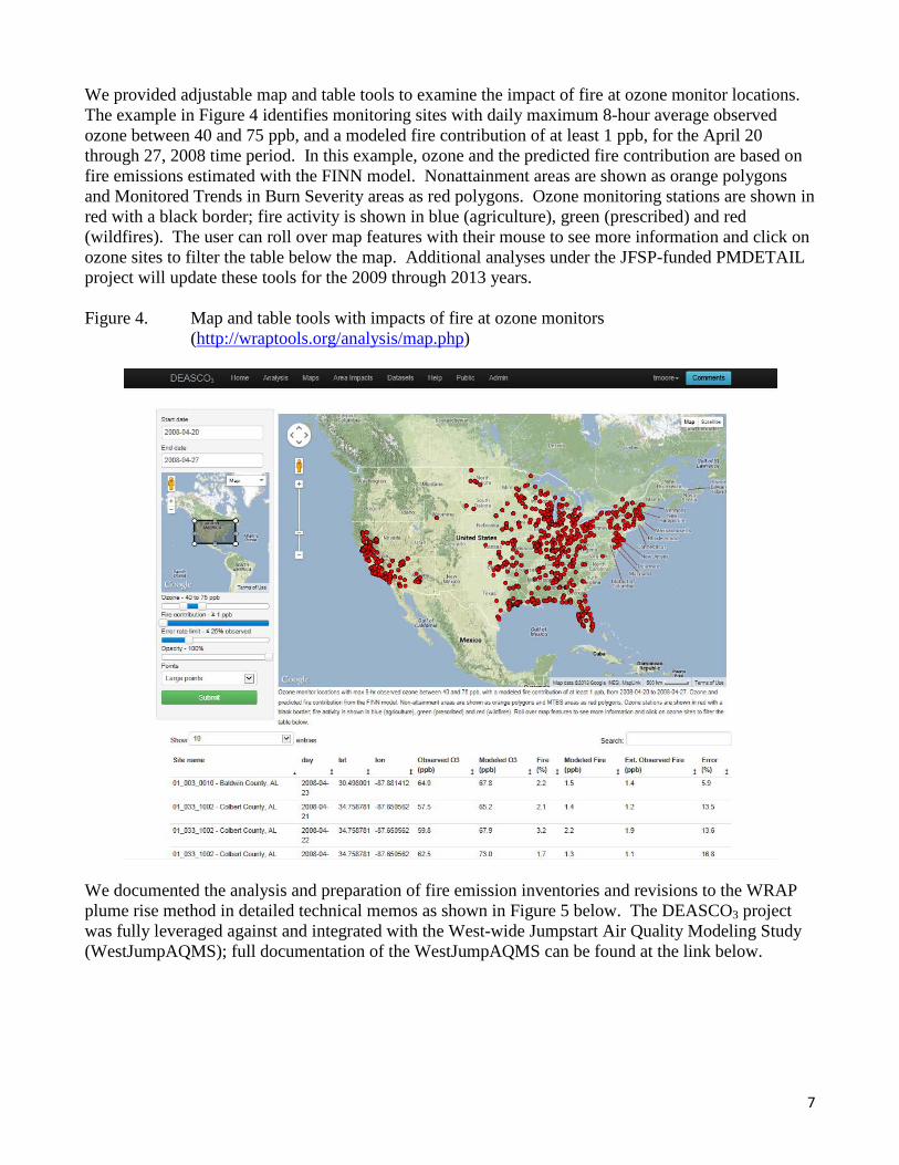
We provided adjustable map and table tools to examine the impact of fire at ozone monitor locations. The example in Figure 4 identifies monitoring sites with daily maximum 8-hour average observed ozone between 40 and 75 ppb, and a modeled fire contribution of at least 1 ppb, for the April 20 through 27, 2008 time period. In this example, ozone and the predicted fire contribution are based on fire emissions estimated with the FINN model. Nonattainment areas are shown as orange polygons and Monitored Trends in Burn Severity areas as red polygons. Ozone monitoring stations are shown in red with a black border; fire activity is shown in blue (agriculture), green (prescribed) and red (wildfires). The user can roll over map features with their mouse to see more information and click on ozone sites to filter the table below the map. Additional analyses under the JFSP-funded PMDETAIL project will update these tools for the 2009 through 2013 years. Figure 4. Map and table tools with impacts of fire at ozone monitors

(http://wraptools.org/analysis/map.php)

We documented the analysis and preparation of fire emission inventories and revisions to the WRAP plume rise method in detailed technical memos as shown in Figure 5 below. The DEASCO3 project was fully leveraged against and integrated with the West-wide Jumpstart Air Quality Modeling Study (WestJumpAQMS); full documentation of the WestJumpAQMS can be found at the link below.

8

Figure 5. DEASCO3 Project Documents (http://deasco3.wraptools.org/) DEASCO3 Final Report PDF WestJumpAQMS (http://www.wrapair2.org/WestJumpAQMS.aspx) Plume Rise methodology document PDF Final Emission Inventory methodology document PDF One-page project background document PDF Technical Proposal to JFSP PDF The web system also provides a comprehensive list of documents on a Help Page. Figure 6. DEASCO3 Project Help Page Documents (http://wraptools.org/help/index.php)

Case Studies ---About

Miscellaneous ---Analysis Defaults ---User Analysis Essentials

Figure tools -- Fire Activity Timeseries -- Linked content -- Model Animation -- Modeled fire contribution -- Model Performance -- Monthly Model Summary -- Monthly Observed Ozone -- Monthly Fire Summary -- Observed Ozone Timeseries -- Ozone-Fire Timeseries -- Spatial Maps -- Stored Image

Map tools -- Ozone & fire activity map

Table tools -- Fire Statistics -- Geo Statistics

Text tools -- Text editor New entry

9

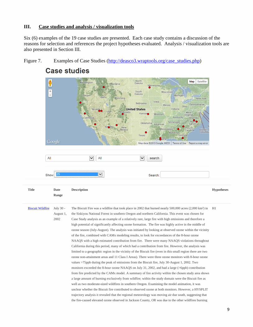
III. Case studies and analysis / visualization tools Six (6) examples of the 19 case studies are presented. Each case study contains a discussion of the reasons for selection and references the project hypotheses evaluated. Analysis / visualization tools are also presented in Section III. Figure 7. Examples of Case Studies (http://deasco3.wraptools.org/case_studies.php)

Title Date

Range Description Hypotheses

Biscuit Wildfire July 30 - August 1, 2002

The Biscuit Fire was a wildfire that took place in 2002 that burned nearly 500,000 acres (2,000 km²) in the Siskiyou National Forest in southern Oregon and northern California. This event was chosen for Case Study analysis as an example of a relatively rare, large fire with high emissions and therefore a high potential of significantly affecting ozone formation. The fire was highly active in the middle of ozone season (July-August). The analysis was initiated by looking at observed ozone within the vicinity of the fire, combined with CAMx modeling results, to look for exceedances of the 8-hour ozone NAAQS with a high estimated contribution from fire. There were many NAAQS violations throughout California during this period, many of which had a contribution from fire. However, the analysis was limited to a geographic region in the vicinity of the Biscuit fire (even in this small region there are two ozone non-attainment areas and 11 Class I Areas). There were three ozone monitors with 8-hour ozone values >75ppb during the peak of emissions from the Biscuit fire, July 30-August 1, 2002. Two monitors exceeded the 8-hour ozone NAAQS on July 31, 2002, and had a large (>6ppb) contribution from fire predicted by the CAMx model. A summary of fire activity within the chosen study area shows a large amount of burning exclusively from wildfire; within the study domain were the Biscuit fire as well as two moderate-sized wildfires in southern Oregon. Examining the model animation, it was unclear whether the Biscuit fire contributed to observed ozone at both monitors. However, a HYSPLIT trajectory analysis it revealed that the regional meteorology was moving air due south, suggesting that the fire-caused elevated ozone observed in Jackson County, OR was due to the other wildfires burning

H1

10

Title Date Range

Description Hypotheses

at the time, whereas the Tehama County, CA monitor likely was influenced by emissions from the Biscuit fire (or all three fires).

Fall burning in southern Louisiana, 2008

September 27 - 30, 2008

This case study was identified by interrogating the database of observed 8-hour ozone values in the "shoulder season" (Sep-Oct) in 2008 and looking for instances of elevated ozone. These results were then filtered to identify areas with planned fire-contributed ozone predicted by CAMx modeling. This time period in southern Louisiana saw two days with ozone above the current 8-hour ozone standard with a significant fire influence. September 27th saw smoke transported from wildfires in Northern California and Canada carried southward, as can be seen from the HYSPLIT trajectory results and the modeled fire contribution plots (there was also a significant local influence from prescribed burning). Fire impacts on ozone were also seen on September 30th, but this time the impacts were predominately from nearby planned fires occurring throughout the state.

H1, H2, H3

Chatfield, CO July 2004-2007

July, 2004 - 2007

Chatfield, CO July 2008 was analyzed as a separate case study looking at fires' contribution to ozone formation in a Non-Attainment Area (NAA). That case study concluded that smoke from wildfires burning throughout the Western US contributed to elevated ozone just above the 8-hour ozone standard at a monitor in Douglas County, CO. This case study pairs observed ozone data in non-model years with fire activity in the same geographic domain. While it is difficult to conclude that fire contributed to ozone exceedances in those years, there are instances, similar to 2008, where a spike in fire activity lead to a period of elevated ozone above the 8-hour standard several days later.

H2, H3

Agricultural fires' influence on ozone formation - MN

April 14 - 15, 2008

April is a time of intense agricultural burning in the Midwest, especially in Kansas. Over a period of 2 days, April 14-15, 2008, an estimated 16,000 acres of agricultural land was burned. CAMx model results were interrogated to look for instances of fire contributing to ozone formation at ozone monitors in the Midwest during this period. Three monitors in Minnesota and Wisconsin were modeled to have a nearly 5ppb contribution from agricultural burning. The map below shows minimal burning in the vicinity of the western-most monitor in Minnesota, so presumably the influence is from the burning in Kansas to the south. Measured ozone concentrations, while not exceeding the current 8-hour ozone standard, were elevated enough such that a lowered standard could cause greater concern about smoke transport to this region in the Spring.

H2, H3

Northern GA/southern TN

October 3 - 6, 2008

Open burning occurs in the Southeastern United States nearly year-round. This Case Study was identified by searching observed ozone data paired with CAMx modeling results from 2008 to find instances in the "shoulder seasons" with elevated ozone attributed to fire. October 4, 2008, saw an exceedance of the ozone NAAQS at a monitor in Chattanooga, TN, with a small, but significant, estimated contribution by fire. The fire summary map reveals that planned fires of different types were occurring throughout the region. CAMx modeling results predict that, despite the "obvious" source of agricultural burning from the west, the largest contribution was from nearby prescribed burning.

H1, H2, H3

Fall burning patterns in southern Louisiana, 2004 - 2007

Sep - Oct, 2004 - 2007

This is one of three case studies that look at patterns of burning over several years. Managed burning in early Fall 2008 in southern Louisiana was analyzed as a separate case study and showed the potential for fire to contribute to elevated ozone in the shoulder season. This analysis looks to see if similar patterns of burning occur in other years or if 2008 was unusual. Pairs of box plots and fire activity tables for each year from 2004 - 2007 are displayed, and reveal a consistent pattern of managed burning (mostly prescribed fire) in the September-October time-frame. A time series of tons consumed for the

H2, H3

11

Title Date Range

Description Hypotheses

entire 4 year span show an annual pattern of burning mainly in the spring and fall. The ramp-up in burning in Sep-Oct coincides with sporadic instances of elevated ozone, whereas in the summer ozone is high with little burning occurring. Two years, 2005 and 2007, have several larger fires burning simultaneously for short periods but that do not show increased frequency of elevated ozone. Two monitoring sites from the area show instances of elevated ozone into October; the site at LaFourche Parish has a more consistent annual pattern. The ozone threshold chosen for this analysis was 70ppb.

The DEASCO3 Analysis Tools and Default Tools Example are presented in Figure 8. There are three topical areas (Exceptional Events Support, Fire Planning for FLMs, and SIP Support) for user analysis and applications, with case studies linked to each, applying the tools and data DEASCO3 users can then develop their own studies using the default tools shown at the bottom of the Figure; users can also bring their own data into their case study.

12

Figure 8. DEASCO3 Analysis Tools and Default Tools Example (http://wraptools.org/analysis/index.php)

Default Tools Description

Model Animation For including an animation in an analysis. The most common animation will be FINN and DEASCO3 model output.

Fire Statistics The Fire Statistics table summarizes fire consumption and emissions for all fire within the analysis boundary.

Fire Activity Timeseries

Plot tons consumed within a specified geographic region and time boundary. Data is based on either the FINN or the DEASCO3 model.

Ozone & fire activity map

Review the observed ozone and fire activity for the time period and geographic area of interest. Also displays non-attainment areas.

Start an Analysis - A new analysis will be started with the default tool set, for Exceptional Event Support, Fire Planning for FLMs, and/or SIP Support.

13

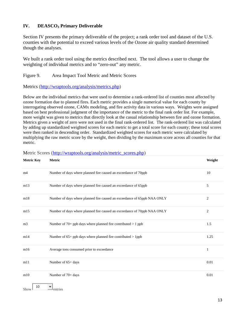
IV. DEASCO3 Primary Deliverable Section IV presents the primary deliverable of the project; a rank order tool and dataset of the U.S. counties with the potential to exceed various levels of the Ozone air quality standard determined though the analyses. We built a rank order tool using the metrics described next. The tool allows a user to change the weighting of individual metrics and to “zero-out” any metric. Figure 9. Area Impact Tool Metric and Metric Scores Metrics (http://wraptools.org/analysis/metrics.php) Below are the individual metrics that were used to determine a rank-ordered list of counties most affected by ozone formation due to planned fires. Each metric provides a single numerical value for each county by interrogating observed ozone, CAMx modeling, and fire activity data in various ways. Weights were assigned based on best professional judgment of the importance of the metric to the final rank order list. For example, more weight was given to metrics that directly look at the casual relationship between fire and ozone formation. Metrics given a weight of zero were not used in the final rank-ordered list. The rank-ordered list was calculated by adding up standardized weighted scores for each metric to get a total score for each county; these total scores were then ranked in descending order. Standardized weighted scores for each metric were calculated by multiplying the raw metric score by the weight, then dividing by the maximum score across all counties for that metric. Metric Scores (http://wraptools.org/analysis/metric_scores.php) Metric Key Metric Weight

m4 Number of days where planned fire caused an exceedance of 70ppb 10

m13 Number of days where planned fire caused an exceedance of 65ppb 5

m18 Number of days where planned fire caused an exceedance of 65ppb NAA ONLY 2

m15 Number of days where planned fire caused an exceedance of 70ppb NAA ONLY 2

m3 Number of 70+ ppb days where planned fire contributed > 1 ppb 1.5

m14 Number of 65+ ppb days where planned fire contributed > 1ppb 1.25

m16 Average tons consumed prior to exceedance 1

m11 Number of 65+ days 0.01

m10 Number of 70+ days 0.01

Show 10

entries

14

Search:

fips County state m4 m13 m18 m15 m3 m14 m16 m11 m10 total score

rank

01003 Baldwin County AL 0.00 0.00 0.00 0.00 0.00 0.00 0.00 0.00 0.00 0.002 454

01049 Dekalb County AL 0.00 0.00 0.00 0.00 0.30 0.16 0.00 0.00 0.00 0.459 314

01051 Elmore County AL 0.00 0.56 0.00 0.00 0.30 0.47 0.00 0.00 0.00 1.327 156

01073 Jefferson County AL 8.00 1.11 0.00 0.00 0.30 0.31 0.00 0.00 0.00 9.729 5

The users can modify the rank order tool settings. When the Tool is run, the results are structured into a table and a map with the “Rank order of areas (counties) where fire emissions have the greatest potential to challenge attainment and maintenance of EPA ozone standards”. A table selection from the default Tool settings is shown at the bottom of Figure 9 above, and the map result from the default Tool settings is shown below in Figure 10. All counties in the CONUS are analyzed and can be displayed on the map and in the table. Figure 10. Rank order of areas (counties) where fire emissions have the greatest potential to challenge

attainment and maintenance of EPA ozone standards (http://wraptools.org/analysis/impact_map.php)

15

As shown in Figure 11 below, we have also provided CAMx ozone source apportionment modeling results of the contributions of Wildfires (WF), Prescribed Burns (Rx), Agricultural Burning (Ag) and Planned Fires (Rx+Ag) to daily maximum 8-hour ozone concentrations through the 36 km continental U.S. (CONUS) and 12 km western U.S. (WESTUS) domains for total modeled daily maximum 8-hour ozone concentrations above five concentration thresholds: 76 ppb, 70 ppb, 65 ppb, 60 ppb and 0 ppb. Four different fire ozone contribution metrics are presented to examine fire ozone contributions for the five types of fire (WF, Rx, Ag, Rx+Ag and total) and five concentration thresholds (76, 70, 65, 60 and 0 ppb):

• 1st Max - Highest fire ozone contribution (ppb) to modeled daily maximum 8-hour ozone concentration above the given threshold.

• 4th Max - Fourth highest fire ozone contribution (ppb) to daily maximum 8-hour ozone concentrations above the given threshold.

• Cause - Number of days ozone due to fires cause daily maximum 8-hour ozone to increase from below to above the given threshold.

• Contrib - Number of days that daily maximum 8-hour ozone is greater than threshold and fire contributes 0.5 ppb or greater.

Figure 11. CAMx Modeling Results Matrix (http://wraptools.org/analysis/sip_matrix.php)

16

Air Quality Planning and Management Implications Implications of the technical work in this project are: • Significant leveraging of extramural projects was needed to address smoke’s contribution to

elevated ozone, at the level of technical detail necessary to address the 2011 FON Task 6 requirements.

• Fires contribute to an existing ozone background signal from natural and anthropogenic sources.

• Fire activity can contribute sufficiently to cause ozone exceedances.

• All types of fire, both planned (prescribed, agricultural) and unplanned (wildfire) contributed to elevated ozone episodes.

• Fire can contribute to elevated ozone over multi-state regions.

• Fires’ contribution was a combination of planned and unplanned events.

• Tracking of fire type in the inventory and modeling analyses was important in determining the

impacts on elevated ozone.

• Efficient, effective delivery of air quality planning information for FLM use was accomplished. Presentation and Outreach Efforts WRAP Membership Meeting November 7, 2013 Denver, CO • Regional Modeling Framework for the West (Tom Moore) Project status report

International Smoke Symposium The University of Maryland University College October 21-24, 2013 • Special Session: Fire's Impacts on Ozone and PM - Data Results and Tools for Analysis

o FETS Fire Inventories – Methodology and Results for Assessment of Smoke’s Impact on Ozone and PM - Matthew Mavko

o Photochemical Modeling to Assess Smoke's Contribution to Ozone and Particulate Matter - Ralph Morris

o JFSP Smoke Science Projects: DEASCO3 and PMDETAIL - Matthew Mavko o DEASCO3: Meeting the Needs of User Groups - Tom Moore / Dave Randall

• DEASCO3 Happy Hour - This “hands-on” evening session provides the opportunity for Symposium attendees to use the website and tools with in-person support from the developers and the project team.

17

DEASCO3 Project Team outreach meeting with JFSP staff and Board members National Inter-Agency Fire Center brownbag lunch webinar September 19, 2013 Boise, ID WRAP Fire / Ozone Impacts (DEASCO3) Project Outreach webinar for National Wildfire Coordinating Group’s Smoke Committee (DEASCO3 Project Team) Thursday, August 22, 2013 11:00 AM through 1:00 PM MDT WRAP-EPA Western Modeling Workshop July 8-11, 2013 Boulder, CO • Fire impacts modeling results from DEASCO3 (R. Morris, ENVIRON) • Attributing fire to elevated ozone and exceptional events using DEASCO3 tools (M. Mavko, Air

Sciences) DEASCO3 Project Team webinars for FLM, EPA, and State “beta-testers” • Monday, May 20, 2013 demonstration webinar: MOV • Tuesday, May 21, 2013 demonstration webinar: MOV

EPA 2012 International Emission Inventory Conference "Emission Inventories - Meeting the Challenges Posed by Emerging Global, National, Regional and Local Air Quality Issues" Tampa, FL - August 13-16, 2012 • Comparative Fire Emissions Analysis for the DEASCO3 Project and the US EPA 2008 NEI, (T.

Moore, Western Governors’ Association; M. E. Mavko and D. Randall, Air Sciences, Inc.) presentation

• Biomass Burning Panel Discussion, T. Moore DEASCO3 Project Meeting June 27-28, 2012 Project Meeting Materials (DEASCO3 Project Team) • 2002 modeling results animation showing daily ozone concentrations & fire contribution. WMV • Presentation document from the project status report webinar on June 28th PDF

WRAP Technical Projects Meeting April 18, 2012 Seattle, WA • Fire emissions and elevated Ozone (PPT) - T. Moore

WestJumpAQMS (http://www.wrapair2.org/WestJumpAQMS.aspx) • Final Fire Emissions Technical Memo 5, April 27, 2012 (the review call for this memo was held

March 9, 2012) – R. Morris, ENVIRON