Full Terms & Conditions of access and use can be found athttp://www.tandfonline.com/action/journalInformation?journalCode=tprs20

Download by: [East China University of Science and Technology] Date: 31 October 2016, At: 02:26

International Journal of Production Research

ISSN: 0020-7543 (Print) 1366-588X (Online) Journal homepage: http://www.tandfonline.com/loi/tprs20

Determining the conditions for reverse triage inemergency medical services using queuing theory

Jingui Xie, Ping Cao, Boray Huang & Marcus Eng Hock Ong

To cite this article: Jingui Xie, Ping Cao, Boray Huang & Marcus Eng Hock Ong (2016)Determining the conditions for reverse triage in emergency medical services usingqueuing theory, International Journal of Production Research, 54:11, 3347-3364, DOI:10.1080/00207543.2015.1109718

To link to this article: http://dx.doi.org/10.1080/00207543.2015.1109718

Published online: 08 Nov 2015.

Submit your article to this journal

Article views: 171

View related articles

View Crossmark data

International Journal of Production Research, 2016Vol. 54, No. 11, 3347–3364, http://dx.doi.org/10.1080/00207543.2015.1109718

Determining the conditions for reverse triage in emergency medical services using queueingtheory

Jingui Xiea, Ping Caoa∗, Boray Huangb1 and Marcus Eng Hock Ongc

aSchool of Management, University of Science and Technology of China, Hefei, China; bDepartment of Industrial & SystemsEngineering, National University of Singapore, Singapore; cDepartment of Emergency Medicine, Singapore General Hospital, Singapore

(Received 25 August 2014; accepted 8 October 2015)

In emergency health care, there are situations where the less wounded are treated in preference to the more severely wounded,so called reverse triage. This may arise in situations such as war where soldiers are required to return to the battlefield asquickly as possible, or disaster situations where medical resources are limited in order to conserve resources for those likelyto survive without requiring advanced medical care. This article is to study the reverse triage in time-critical systems, whereconditions of patients may deteriorate while waiting for treatment. A queueing model with transfers and abandonments isdeveloped to study the health care system. Using smoothed rate truncation method, sufficient conditions of reverse triageare derived, under which non-critical patients are treated with priority. For other conditions, the optimal policy is verycomplicated. We suggest a dynamic control policy according to the system state rather than any static priority policies.

Keywords: emergency medical services; reverse triage; abandonments; queueing models; smoothed rate truncation method

1. Introduction

In health care systems, critical patients usually have higher priority to access medical services. However, in addition tothe standard practice, there are conditions where the less wounded are treated in preference to the more severely wounded,so-called reverse triage. This may arise in situations such as war where soldiers are required to return to the battlefield asquickly as possible, or disaster situations where medical resources are limited in order to conserve resources for those likelyto survive without requiring advanced medical care (Wiseman, Ellenbogen, and Shaffrey 2002). In cold water drowningincidents, it is a common practice to use reverse triage because drowning victims in cold water can survive longer than inwarm water if given immediate basic life support and often those who are rescued and able to breathe on their own willimprove with minimal or no help (Elixson 1991). The main theme of this paper is to study the reverse triage practice intime-critical systems, by providing sufficient conditions under which non-critical patients should be treated first.

To illustrate the idea, a simple model is studied in this paper. Arriving patients are simply triaged into two groups:critical and non-critical group. Non-critical patients wait in one queue and will be seen on a first-come-first-served (FCFS)basis, while critical patients are cared in another queue on a FCFS basis as well. A waiting non-critical patient will betransferred to the critical care area and wait at the end of the queue, if the patient’s condition becomes critical. To improvesystem efficiency, a manager would aim to reduce the average cost of the whole system. Holding cost and transfer cost areconsidered for different types of patients. For non-critical patients, there is a holding cost per unit time for each patient. Ifthe condition of a non-critical patient deteriorates and the patient needs to be transferred to the critical group, a transfer costoccurs. For the critical patients, if their conditions are out of control in current functional area, they will be transferred toanother functional area. Transfer costs will also be considered. Since the transferred critical patients are no longer stayingin the system, we can say that these patients have abandoned the system. Generally, the holding cost of critical patients ishigher than the holding cost of non-critical patients, and the treatment time for critical patients is longer.

Queueing models have been shown to be helpful in improving health care practice and making strategic plans in healthcare applications (e.g. Green et al. 2006; Green and Savin 2008). Green (2008) presents operations research (OR) models,especially queueing models that have been developed to help reduce patient delays for health care. Wang, Debob, andScheller-Wolf (2015) summarise the limited extant research in OR/OM that is applicable to the unique challenges posed bynurse lines in health care. Motivated by the interaction between an emergency department (ED) and internal wards in ananonymous hospital, Mandelbaum, Momcilovic, and Tseytlin (2012) analyse queueing systems with heterogeneous server

∗Corresponding author. Email: pcao@ustc.edu.cn1Present Address: Department of Industrial Engineering & Innovation Sciences, Eindhoven University of Technology, The Netherlands.

© 2015 Taylor & Francis

3348 J. Xie et al.

pools, where the pools represent the wards and the servers are beds, and introduces the randomised most-idle routing policywhich is shown to be superior than the commonly used longest-idle-server-first policy as it utilises only the informationon the number of idle servers in different pools. Yom-Tov and Mandelbaum (2014) analyse an Erlang-R queueing model,which is motivated by health care systems, in which offered loads vary over time and patients often go through a repetitiveservice process and propose a time-varying square-root staffing policy, based on the modified offered-load, which is provedto perform well over small-to-large systems.

Our model is the first to use queueing model to study reverse triage. The theoretical results may provide helpful managerialinsights for medical practice. There are already several queuing models considering customer transfers (Xie, He, and Zhao2008, 2009; He, Xie, and Zhao 2012), or abandonments (Down, Koole, and Lewis 2011). Our model is new in the sense ofhaving both features. The average-cost problem discussed in this paper is formulated as a continuous-time Markov decisionprocess (CTMDP) with unbounded transition rate, where uniformisation is not applicable. Normally, in order to betterunderstand the structure of optimal policy, one often expects the relative value function of average optimal cost to havestructural properties such as monotonicity, convexity and supermodularity (Koole 2006). The traditional method is usingsuccessive approximation (Sennott 1999). However, the application of successive approximation requires that the Markovdecision process is uniformisable. Since the transition rates are linear functions of the queue length in our model and thusthe rates are not uniformly bounded, successive approximation cannot be directly used in our model. Down, Koole, andLewis (2011) consider a queueing model with customer abandonment. In Theorem 3.5 therein they give sufficient conditionsunder which a static priority policy is optimal for the average cost criterion. To prove their theorem, there is the same issuethat uniformisation is impossible. Thus, they truncate the state space, and let the truncation level grow. Their proof may beproblem specific, which means that the methodology may not be applied to other models. In our paper, we employ anothermethod called smoothed rate truncation method (see Bhulai, Blok, and Spieksma 2012; Bhulai, Brooms, and Spieksma2014 for more details). Our work provides evidence that the new method could be useful in other CTMDP problems thatinvolve queues with abandonments or transfers (i.e. unbounded transition rate). Last but not least, we prove the existenceof a non-idling optimal policy using stability conditions in Markov process. The method is closely related to the positiverecurrence of the Markov process induced by a specified policy.

The rest of the article is organised as follows. In Section 2, a queueing model with transfers and abandonments isintroduced, and the control problem is formulated as a CTMDP. In Section 3, conditions under which it is optimal totreat non-critical patients with priority (i.e. reverse triage) are given. In Section 4, numerical examples are studied. Finally,conclusions are made in Section 5.

2. Queueing model and problem description

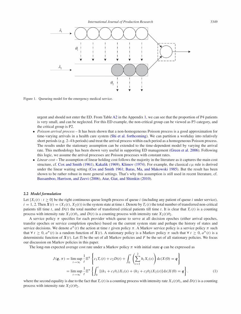
The arriving patients are sorted into two groups: non-critical and critical group. We assume that the non-critical and criticalpatients arrive according to two independent Poisson processes with constant arrival rates λ1 and λ2, respectively. Non-criticalpatients wait in queue 1, while critical patients wait in queue 2. Treatments are performed by m (m ≥ 1) medical providers(each provider is a combined medical unit, including a number of physicians, nurses and medical facilities, which can providecomplete treatment to a patient). The treatment time for each type of patient B1 and B2 are assumed to be exponentiallydistributed with service rates μ1 and μ2, respectively. The service processes are independent of the arrival processes and thecapacity of waiting place is unlimited.

A non-critical patient waiting for treatment in queue 1 (including non-critical patients under service) will become criticalafter a random amount of time, which is exponentially distributed with parameter θ1. Then the patient will be transferredto queue 2 with a transfer cost c1, and the required service time changes as well. For critical patients in queue 2, there is arisk of getting worse and transferring to other functional areas if they cannot access the medical service in time. We assumethat the time before transfer is exponentially distributed with parameter θ2. The transfer cost is c2. The holding costs of eachnon-critical and critical patient per unit time in the emergency room are h1 and h2, respectively. The queueing model isshown in Figure 1.

2.1 Model assumptions and justification

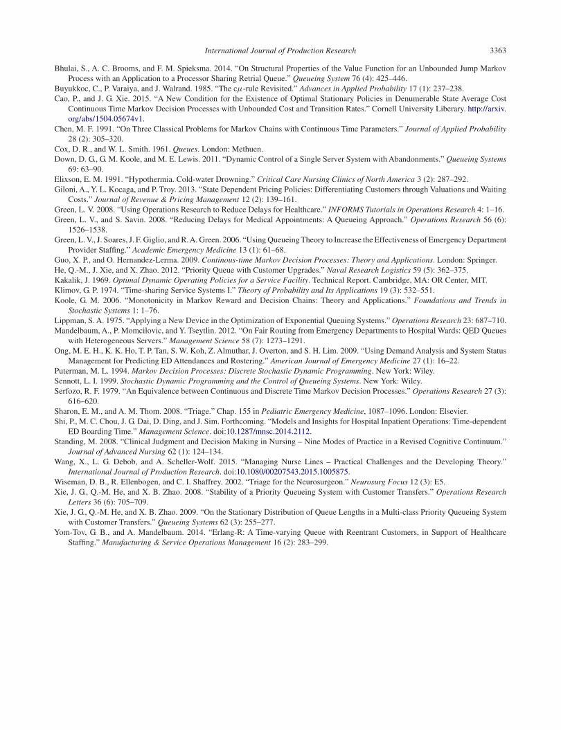
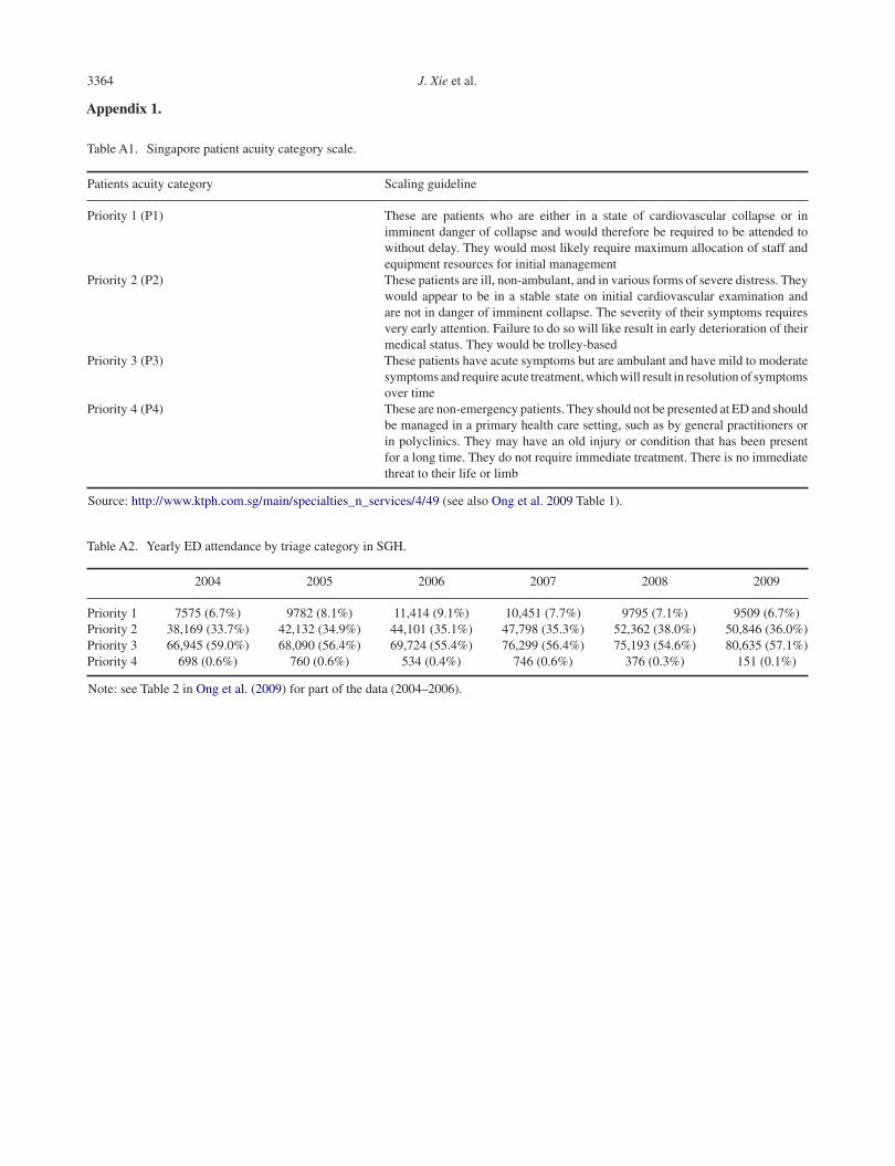
• Two groups – We assume that the arriving patients are sorted into two groups: non-critical and critical group. Thissimplification is, however, reasonable. In practice, the patients might be categorised into two to five levels accordingto patient’s illness/injury severity or acuity (Sharon and Thom 2008). But these levels can be aggregated or simplifiedto two levels. For instance, in the ED of Singapore General Hospital (SGH), patients are classified into four groups:P1, P2, P3 and P4 (see Table A1 in the Appendix 1). The P1 patients, who are treated in a separate functional area ofthe ED, are not necessary to be included in the model. This part can be analysed separately. The P4 patients are not

International Journal of Production Research 3349

Figure 1. Queueing model for the emergency medical service.

urgent and should not enter the ED. From Table A2 in the Appendix 1, we can see that the proportion of P4 patientsis very small, and can be neglected. For this ED example, the non-critical group can be viewed as P3 category, andthe critical group is P2.

• Poisson arrival process – It has been shown that a non-homogeneous Poisson process is a good approximation fortime-varying arrivals in a health care system (Shi et al. forthcoming). We can partition a workday into relativelyshort periods (e.g. 2–4 h periods) and treat the arrival process within each period as a homogeneous Poisson process.The results under the stationary assumption can be extended to the time-dependent model by varying the arrivalrate. This methodology has been shown very useful in supporting ED management (Green et al. 2006). Followingthis logic, we assume the arrival processes are Poisson processes with constant rates.

• Linear cost – The assumption of linear holding cost follows the majority in the literature as it captures the main coststructure, cf. Cox and Smith (1961), Kakalik (1969), Klimov (1974). For example, the classical cμ rule is derivedunder the linear waiting setting (Cox and Smith 1961; Baras, Ma, and Makowski 1985). But the result has beenshown to be rather robust in more general settings. That’s why this assumption is still used in recent literature, cf.Bassamboo, Harrison, and Zeevi (2006), Atar, Giat, and Shimkin (2010).

2.2 Model formulation

Let {Xi (t) : t ≥ 0} be the right continuous queue length process of queue i (including any patient of queue i under service),i = 1, 2. Then X(t) = (X1(t), X2(t)) is the system state at time t . Denote by Tr (t) the total number of transferred non-criticalpatients till time t , and D(t) the total number of transferred critical patients till time t . It is clear that Tr (t) is a countingprocess with intensity rate X1(t)θ1, and D(t) is a counting process with intensity rate X2(t)θ2.

A service policy π specifies for each provider which queue to serve at all decision epoches (either arrival epoches,transfer epoches or service completion epoches) based on the current system state and perhaps the history of states andservice decisions. We denote aπ (t) the action at time t given policy π . A Markov service policy is a service policy π suchthat ∀ t ≥ 0, aπ (t) is a random function of X(t). A stationary policy is a Markov policy π such that ∀ t ≥ 0, aπ (t) is adeterministic function of X(t). Let � be the set of all Markov policies and F be the set of all stationary policies. We focusour discussion on Markov policies in this paper.

The long-run expected average cost rate under a Markov policy π with initial state q can be expressed as

J (q, π) = lim supt→∞

1

tEπ

{c1Tr (t)+ c2 D(t)+

∫ t

0

(2∑

i=1

hi Xi (s)

)ds|X (0) = q

}

= lim supt→∞

1

tEπ

{∫ t

0[(h1 + c1θ1)X1(s)+ (h2 + c2θ2)X2(s)] ds|X (0) = q

}. (1)

where the second equality is due to the fact that Tr (t) is a counting process with intensity rate X1(t)θ1, and D(t) is a countingprocess with intensity rate X2(t)θ2.

3350 J. Xie et al.

The optimal average-cost rate can be defined as

J (q) = infπ∈� J (q, π).

Besides, the infinite-horizon expected discounted cost under policy π can be expressed as

Jα(q, π) = Eπ

{∫ ∞

0e−αs [(h1 + c1θ1)X1(s)+ (h2 + c2θ2)X2(s)] ds|X (0) = q

}. (2)

and the corresponding optimal infinite-horizon expected discounted cost is

Jα(q) = infπ∈� Jα(q, π),

where α > 0 is the discount rate.The goal is to find an optimal policy π∗ to minimise the average cost rate in the service control problem, i.e. J (q, π∗) =

J (q).

3. Optimal policy structure

The control problem can be formulated as a CTMDP (see Guo and Hernandez-Lerma 2009 for more details). Denote thestate space S = {(q1, q2) | q1, q2 ∈ Z

+}, where q1 (q2) represents the number of non-critical (critical) patients in the system,and Z

+ is the set of all nonnegative integers. The available actions in state q = (q1, q2) are A (q) = {(m1,m2) | m1,m2 ∈Z

+,m1 +m2 ≤ m}, where m1 (m2) represents the number of providers assigned to queue 1 (2). A policy specifies how manyproviders should be allocated to each queue at all decision epoches. For q ∈ S and a = (m1,m2) ∈ Aq , let c(q, a) be thecost rate function associated with state q and action a. It follows from (1) that

c(q, a) = (h1 + c1θ1)q1 + (h2 + c2θ2)q2. (3)

For i = 1 or 2, let Ai and Di correspond to an arrival and a potential departure at queue i , i = 1, 2, respectivelyand let R12 correspond to a potential transfer from queue 1 to queue 2. Thus, A1q = (q1 + 1, q2), A2q = (q1, q2 + 1),D1q = ((q1 − 1)+, q2), D2q = (q1, (q2 − 1)+) and R12q = (q1 − 1, q2 + 1) if q1 > 0 and R12q = q if q1 = 0. Here, weuse x+ to denote max{x, 0}. The transition rates associated with state q and action a for s = q are

q(s|q, a) =

⎧⎪⎪⎪⎪⎪⎪⎨⎪⎪⎪⎪⎪⎪⎩

λ1, if s = A1q;λ2, if s = A2q;min{q1,m1}μ1, if s = D1q;q1θ1, if s = R12q;min{q2,m2}μ2 + q2θ2, if s = D2q.

(4)

Besides, q(q|q, a) = −∑s =q q(s|q, a). We need the following proposition in order to prove the existence of the optimalstationary average-cost policy.

Proposition 3.1 Jα(q) is nondecreasing in q.

This proposition states the intuitive observation that the more patients in the system, the more cost it will incur. The proofis quite regular and is omitted for brevity.

3.1 Existence of optimal stationary policies

Before we analyse the properties of optimal policies, we examine whether or not an optimal stationary policy exist in ourmodel. Note that when the state space is infinite, there might not exist an optimal policy, or exist an optimal non-stationarypolicy, but not an optimal stationary policy. See two examples from Section 4.4 in Bertsekas (2001). In this case, it is difficult,if not impossible, to design an easily executed and almost optimal policy. Thus, it is necessary to study the existence of optimalstationary policies first.

The following results is required to show the existence of an optimal stationary average-cost policy for our model, whichis from Theorem 2.1 and Theorem 4.1(iv) in Cao and Xie (2015).

Lemma 3.1 Assume that the optimal infinite-horizon expected discounted cost under discount rate α, Jα(i), is increasingin the system state i for α > 0. Suppose that there exists a 0-standard policy d. Here, we call a policy d a i0-standard policy

International Journal of Production Research 3351

if the Markov process induced by d, {xd(t) : t ≥ 0} satisfies that for any i ∈ S, the expected time mi,i0(d) of a first passagefrom i to i0 (during which at least one transition occurs) is finite and the expected cost ci,i0(d) of a first passage from i toi0 (during which at least one transition occurs) is finite. Then there exists a constant g ≥ 0, a stationary policy f , and areal-valued function h (which is increasing in i) such that:

(i) There exists a sequence {αn, n ≥ 1} tending to zero (as n → ∞) such that ∀ i ∈ S,

f (i) = limk→∞ fαk (i), g = lim

k→∞αk Jαk (0), (5)

andh(i) = lim

k→∞ hαk (i), (6)

where hα(i) := Jα(i)− Jα(0).(ii) (g, f, h) satisfy the following average-cost optimality inequality (ACOI):

g ≥ c(i, f )+∑j∈S

h( j)q( j |i, f )

= mina∈A(i)

⎧⎨⎩c(i, a)+

∑j∈S

h( j)q( j |i, a)

⎫⎬⎭ , ∀i ∈ S,

and f is an average-cost optimal stationary policy.(iii) When the jump size at each state i is bounded, then the above ACOI is in fact average-cost optimality equality

(ACOE), i.e.

g = c(i, f )+∑j∈S

h( j)q( j |i, f )

= mina∈A(i)

⎧⎨⎩c(i, a)+

∑j∈S

h( j)q( j |i, a)

⎫⎬⎭ , ∀i ∈ S.

Note that Jα(q) is non-decreasing in q from Proposition 3.1 and the jump size is 1 in our model. Thus, Lemma 3.1 saysthat an optimal stationary policy exists and the ACOE holds if there is a 0-standard policy, which requires that the expectedtime mi,0(d) of a first passage from i to 0 (during which at least one transition occurs) is finite and the expected cost ci,0(d)of a first passage from i to 0 (during which at least one transition occurs) is also finite. In order to verify this requirement,the following result is often used, which is Lemma 2.1 in Cao and Xie (2015).

Lemma 3.2 Assume that mi,i0 < ∞, ∀ i ∈ S. Assume that there exists a (finite) non-negative function r on S and a finitesubset H∗ containing i0 such that ∑

j

q( j |i)r( j) < ∞, i ∈ H∗, (7)

andc(i)+

∑j

q( j |i)r( j) ≤ 0, i /∈ H∗. (8)

Then there exists a (finite) non-negative constant F such that ci,i0 ≤ r(i)−r(i0)+ Fmi,i0 , ∀ i = i0. Especially, if H∗ = {i0},then ci,i0 ≤ r(i), ∀ i = i0.

Now we are ready to show the existence of optimal stationary policies for our model.

Theorem 3.2 There exist a constant g ≥ 0, a stationary policy f ∈ F, and a function h(q) on S such that the followingaverage-cost optimality equation holds.

g = c(q, f )+∑s∈S

q(s|q, f )h(s)

= mina∈Aq

{c(q, a)+

∑s∈S

q(s|q, a)h(s)

}. (9)

Moreover, f is an optimal average-cost stationary policy, and the optimal average-cost function equals to the constant g.

3352 J. Xie et al.

Proof By the above argument, we only need to show that there exists a stationary policy (not necessary optimal) underwhich both the expected time and the expected cost of first passage from state q to state 0 = (0, 0) (during which at leastone transition occurs) are finite (mq,0 < ∞ and cq,0 < ∞). We consider a special service policy π0: all the providers alwaysserve queue 2, i.e. m1 = 0 and m2 = m for all the time.

First, we prove that the continuous-time Markov chain induced by policy π0 is positive recurrent, i.e. the correspondingqueueing system is stable and thus mq,0 < ∞ for each state q. According to Theorem 1.18 in Chen (1991), we only need toprove that there exist constants K ≥ 0, η > 0 and a function f on S such that ∀ q ∈ S, we have∑

s

q(s|q, a) f (s)+ η f (q) ≤ K , (10)

where a is specified by policy π0 and the current state q.We choose f (q) = rq1

1 rq22 , where constants r1 and r2 are left to be specified later. Now (10) becomes f (q)d(q) ≤ K ,

where

d(q) = λ1r1 + λ2r2 + q1θ1

(r2

r1− 1

)I {q1 ≥ 1} + (min{q2,m}μ2 + q2θ2)

(1

r2− 1

)I {q2 ≥ 1} + η. (11)

Here I {A} is the indicator function which is 1 if the event A is true, and 0 if A is false.We choose r1, r2 such that r1 > r2 > 1. η > 0 can be chosen arbitrarily. Define H = {q ∈ S : d(q) > 0}. Then H is

a finite set. Define K = max{0,maxq∈H f (q)d(q)

}. Obviously, K is a finite number. It is clear that f (q)d(q) ≤ K since

for q ∈ S\H , f (q)d(q) ≤ 0 ≤ K . Therefore, the continuous-time Markov chain induced by policy π0 is positive recurrent,and thus the expected time of first passage from state q to state 0 (during which at least one transition occurs) are finite.

Next, we prove that cq,0 < ∞ for each state q. For q = 0, it follows from Lemma 3.2 that it suffices to find a non-negativefunction f ′(q) and a non-negative constant K ′ such that for ∀ q = 0, we have

c(s, a)+∑

s

q(s|q, a) f ′(s) ≤ K ′, (12)

where a is specified by policy π0 and the current state q. We choose f ′(q) = f0rq11 rq2

2 , where r1, r2 have already beendefined and f0 is left to be specified later. Then, (12) becomes

2∑i=1

(hi + ciθi )qi + f0rq11 rq2

2 (d(q)− η) ≤ K ′. (13)

Choose f0 such that f0 > max(

h1+c1θ1(r1−1)η ,

h2+c2θ2(r2−1)η

)and define

K ′ := max

{0,max

q∈H

{2∑

i=1

(hi + ciθi )qi + f0rq11 rq2

2 (d(q)− η)

}}.

Thus, for q ∈ H , it follows from the definition of K ′ that (13) holds. For q ∈ S\H , we have

2∑i=1

(hi + ciθi )qi + f0rq11 rq2

2 (d(q)− η)

≤ (h1 + c1θ1)q1 + (h2 + c2θ2)q2 − f0rq11 rq2

2 η

≤ (h1 + c1θ1)q1 + (h2 + c2θ2)q2 − f0(1 + (r1 − 1)q1)(1 + (r2 − 1)q2)η

≤ (h1 + c1θ1)q1 + (h2 + c2θ2)q2 − f0η(r1 − 1)q1 − f0η(r2 − 1)q2

≤ 0 ≤ K ′,

and thus (13) also holds.It follows from Lemma 3.2 that the expected cost of first passage from state q = 0 to state 0 (during which at least one

transition occurs) is finite for q = 0. Note that there are finite possible jumps at state 0. Therefore, the expected cost of firstpassage from state 0 to state 0 (during which at least one transition occurs) is also finite and thus π0 is a 0-standard policy.The proof is completed. �

It follows from Proposition 3.1 and Lemma 3.1(i) that h(q) is non-decreasing in q. Hence, it follows from (9) that thereexists an average cost optimal policy of non-splitting type.

International Journal of Production Research 3353

Proposition 3.3 If the number of patients in each queue exceeds the number of providers, there exists an average costoptimal control policy that does not split the providers.

Proof Assume that q1, q2 ≥ m. Hence, min{q1,m1} = m1 and min{q2,m2} = m2 for any (m1,m2) ∈ A (q). Since thereexists an optimal average cost policy of non-idling type, it holds that m1 + m2 = m. For a = (m1,m2), we have

c(q, a)+∑s∈S

q(s|q, a)h(s)

=2∑

i=1

(hi + ciθi )qi + λ1(h(A1q)− h(q))+ λ2(h(A2q)− h(q))+ q1θ1(h(R12q)− h(q))

+ m1μ1(h(D1q)− h(q))+ ((m − m1)μ2 + q2θ2)(h(D2q)− h(q)),

which is linear in m1, and thus achieves its minimum at extreme points. Thus, it follows from (9) that it is optimal to set m1equal to 0 or m, the two extreme points in {0, 1, . . . ,m}. Therefore, there exists an average cost optimal policy that does notsplit the providers. �

Proposition 3.3 implies that we may restrict attention to policies that always allocate all providers to one queue or theother in those states where q1, q2 ≥ m. We point out that solving the problem with multi-providers is generally quite difficultand we simply were unable to do so. Instead, we discuss under what conditions reverse triage is optimal in the single servermodel (see next section) and use it as a proxy for the multi-server model. Given that in emergency health care, the medicalresources are always overwhelmed, single provider may be a good approximation.

3.2 The single server proxy

As we know, without patient transfers and abandonments, it is optimal to serve critical patients with priority if h1μ1 ≤ h2μ2,or to serve non-critical patients with priority if h1μ1 ≥ h2μ2 according to cμ-rule (Buyukkoc, Varaiya, and Walrand 1985).However, the case is rather complicated if patient transfers and abandonments are considered. In general, the optimalityequations can be solved numerically by value iteration or policy iteration method when the state space is finite (Giloni,Kocaga, and Troy 2013). For the case of infinite state space, the optimal policy is hard to obtain since the transition rateand cost functions are not uniformly bounded. In the following, we apply the smoothed rate truncation method proposed byBhulai, Brooms, and Spieksma (2014) to show the structure of optimal policy.

The state space of the proposed model S = Z+ × Z

+ is a two-dimensional infinite space. It should be clear that thetransition rate is unbounded, hence the problem is not uniformisable. Instead of considering the infinite space problem,usually a finite truncation problem is studied in the literature. For example, one can truncate the space of queue 1 (2) by asufficiently large number N1(N2). We set N1 = N and N2 = b(N ), where limN→∞ b(N ) = ∞. This implies that when thespace of queue 1 is fully occupied, no more non-critical patients are accepted, and when the space of queue 2 is fully occupied,no more critical patients are accepted and the patients transferred from non-critical group are lost. Using the uniformisationmethod (Lippman 1975; Puterman 1994), we have a discrete Markov decision process, with average decision interval ψ−1,where ψ is a constant such that ψ = λ1 + λ2 + μ1 + μ2 + Nθ1 + b(N )θ2. For the equivalent discrete Markov decisionprocess, we could possibly find the optimal policy. However, the optimal policy may be dependent on the value N and b(N ).A naive truncation may destroy the structure of the optimal policy for the original model (see the example illustrated in Down,Koole, and Lewis (2011)). In order to preserve the structural properties, we will apply the smoothed rate truncation methodproposed by Bhulai, Brooms, and Spieksma (2014) to our model. The transition rates for the truncated model denoted byN are

q N (s|q, a) =

⎧⎪⎪⎪⎪⎪⎪⎪⎨⎪⎪⎪⎪⎪⎪⎪⎩

λ1(1 − q1

N

)+, if s = A1q;

λ2

(1 − q2

b(N )

)+, if s = A2q;

μ1 I {a = 1}, if s = D1q;q1θ1

(1 − q2

b(N )

)+, if s = R12q;

μ2 I {a = 2} + q2θ2, if s = D2q.

(14)

for s = q, and q N (q|q, a) = −∑s =q q N (s|q, a).The truncated model has one closed class SN = {(q1, q2) : 0 ≤ q1 ≤ N , 0 ≤ q2 ≤ b(N ), q1, q2 ∈ Z

+}, which isreachable with probability 1 from any state outside the class. Thus, it suffices to restrict the state space of N to SN . Nowwe can apply the traditional successive approximation procedure to the truncated model N . The transition rate is bounded

3354 J. Xie et al.

by ψ . Without loss of generality, we assume that ψ = 1. Using uniformisation techniques (Bertsekas 2001), the CTMDP istransformed into an equivalent discrete-time Markov decision process.

Now we can use the successive approximation method (or called value iteration method), which is commonly usedin average-cost discrete-time Markov decision processes (Puterman 1994; Bertsekas 2001), to analyse the structure of theoptimal policy. The successive approximation for N , vn(q), is the optimal expected overall cost starting from initial stateq with n periods remaining, which can be defined as

v0(q) = 0, for all q = (q1, q2) with q1 ≥ 0, q2 ≥ 0

and for q ∈ SN ,

vn+1(q) = (h1 + c1θ1)q1 + (h2 + c2θ2)q2 + λ1

(1 − q1

N

)vn(A1q)+ λ2

(1 − q2

b(N )

)vn(A2q)

+q1θ1

(1 − q2

b(N )

)vn(R12q)+ q2θ2vn(D2q)

+(

1 − λ1

(1 − q1

N

)− λ2

(1 − q2

b(N )

)− q1θ1

(1 − q2

b(N )

)− q2θ2

)vn(q)

+ min{μ1(vn(D1q)− vn(q)), μ2(vn(D2q)− vn(q))}.The decision cost difference is defined as

gn(q) = μ22vn(q)− μ11vn(q), (15)

where 1vn(q) = vn(q)− vn(D1q) and 2vn(q) = vn(q)− vn(D2q).Let the relative value function for the truncated model N be hN (q), q ∈ SN and the optimal average cost rate be gN .

Since N is a finite state model, it follows from Puterman (1994), Serfozo (1979) that vn(q)− vn(0) → hN (q)− hN (0) asn → ∞, and at state q it is optimal for the modelN to serve queue 1 if μ1(hN (D1q)− hN (q)) ≤ μ2(hN (D2q)− hN (q))and it is optimal to serve queue 2 if μ1(hN (D1q) − hN (q) ≥ μ2(hN (D2q) − hN (q)). Before giving the structure of theoptimal policy, a lemma is needed which shows that the value function vn(q) is a non-decreasing function of q.

Lemma 3.3 vn(q) is non-decreasing in q, for all n ≥ 0.

The result is shown by induction on n and the detailed proof is omitted for brevity, cf. Bhulai, Brooms, and Spieksma(2014). One intuitive explanation of Lemma 3.3 is that, holding cost increases when there are more patients in the system,either in queue 1 or 2, as well as the possibility of transfer and its related cost. The value function vn(q), which is the optimalexpected overall cost starting from initial state q with n periods remaining, is non-decreasing in q.

Now we are ready to show the optimal service policy under some conditions for the truncated model.

Lemma 3.4 For any fixed number N ≥ 2, if (h1 + c1θ1)μ1 ≥ (h2 + c2θ2)μ2, μ1 ≥ μ2 and λ1N ≤ λ2

b(N ) , then it is optimalto work at queue 1 except to avoid unforced idling for the truncated model N .

Proof First, we prove that gn(q) ≤ 0 for all q1 ≥ 1 and all n ≥ 0 by induction on n. The inequality holds for n = 0trivially. Assume that gn(q) ≤ 0, for all q1 ≥ 1. Now we prove that it holds for n + 1. Let

fn+1(q, 1) = (h1 + c1θ1)q1 + (h2 + c2θ2)q2 + λ1

(1 − q1

N

)vn(A1q)+ λ2

(1 − q2

b(N )

)vn(A2q)

+q1θ1

(1 − q2

b(N )

)vn(R12q)+ q2θ2vn(D2q)+ μ1vn(D1q)

+(

1 − λ1

(1 − q1

N

)− λ2

(1 − q2

b(N )

)− q1θ1

(1 − q2

b(N )

)− q2θ2 − μ1

)vn(q)

and

fn+1(q, 2) = (h1 + c1θ1)q1 + (h2 + c2θ2)q2 + λ1

(1 − q1

N

)vn(A1q)+ λ2

(1 − q2

b(N )

)vn(A2q)

+q1θ1

(1 − q2

b(N )

)vn(R12q)+ (q2θ2 + μ2)vn(D2q)

+(

1 − λ1

(1 − q1

N

)− λ2

(1 − q2

b(N )

)− q1θ1

(1 − q2

b(N )

)− q2θ2 − μ2

)vn(q)

International Journal of Production Research 3355

Therefore, we have

vn+1(q) = min( fn+1(q, 1), fn+1(q, 2))

and

gn(q) = fn+1(q, 1)− fn+1(q, 2).

Note that for q1 ≥ 1 and q2 ≥ 1, we have

μ2( fn+1(q, 1)− fn+1(D2q, 1))− μ1( fn+1(q, 1)− fn+1(D1q, 1))

= μ2(h2 + c2θ2)− μ1(h1 + c1θ1)+ λ1

(1 − q1

N

)gn(A1q)+ μ1λ1

Nvn(q)

+ λ2

(1 − q2

b(N )

)gn(A2q)− μ2λ2

b(N )vn(q)+ (q1 − 1)θ1

(1 − q2

b(N )

)gn(R12q)

+ (μ2 − μ1)θ1

(1 − q2

b(N )

)vn(R12q)− μ2θ1

(1 − q2 − q1

b(N )

)vn(D1q)+ q2θ2gn(D2q)

+ μ2θ2vn(D2 D2q)+ μ1gn(D1q)

+(

1 − λ1

(1 − q1 − 1

N

)− λ2

(1 − q2 − 1

b(N )

)− q1θ1

(1 − q2 − 1

b(N )

)− q2θ2 − μ1

)gn(q)

+ μ2λ1

N(vn(q)− vn(D2q))− μ1λ1

Nvn(q)+ μ2λ2

b(N )vn(q)− μ1λ2

b(N )(vn(q)− vn(D1q))

+ (μ2 − μ1)q1θ1

b(N )vn(q)+ μ1θ1

(1 − q2 − q1

b(N )

)vn(D1q)− μ2θ2vn(D2q)

= μ2(h2 + c2θ2)− μ1(h1 + c1θ1)+ λ1

(1 − q1

N

)gn(A1q)+ λ2

(1 − q2

N

)gn(A2q)

+ (q1 − 1)θ1

(1 − q2

N

)gn(R12q)+ q2θ2gn(D2q)+ μ1gn(D1q)

+(

1 − λ1

(1 − q1 − 1

N

)− λ2

(1 − q2 − 1

b(N )

)− q1θ1

(1 − q2 − 1

b(N )

)− q2θ2 − μ1

)gn(q)

+ μ2λ1

N(vn(q)− vn(D2q))− μ1λ2

b(N )(vn(q)− vn(D1q))

+ (μ2 − μ1)θ1

((1 − q2

b(N )

)vn(R12q)−

(1 − q2 − q1

b(N )

)vn(D1q)+ q1

b(N )vn(q)

)+ μ2θ2(vn(D2 D2q)− vn(D2q)). (16)

From Lemma 3.3 and λ1N ≤ λ2

b(N ) we have

μ2λ1

N(vn(q)− vn(D2q))− μ1λ2

b(N )(vn(q)− vn(D1q)) ≤ λ2

b(N )gn(q) ≤ 0

and (1 − q2

b(N )

)vn(R12q)−

(1 − q2 − q1

b(N )

)vn(D1q)+ q1

b(N )vn(q)

=(

1 − q2

b(N )

)(vn(R12q)− vn(D1q))+ q1

b(N )(vn(q)− vn(D1q))

≥ 0.

Since gn(q) ≤ 0, for all q1 ≥ 1, we have vn+1(q) = fn+1(q, 1) for all q1 ≥ 1. Hence, it follows from the inductionhypothesis, μ2(h2 + c2θ2) ≤ μ1(h1 + c1θ1), μ2 ≤ μ1 and (16) that if q1 ≥ 2, q2 ≥ 1, then

gn+1(q) = μ2(vn+1(q)− vn+1(D2q))− μ1(vn+1(q)− vn+1(D1q))

= μ2( fn+1(q, 1)− fn+1(D2q, 1))− μ1( fn+1(q, 1)− fn+1(D1q, 1))

≤ 0.

3356 J. Xie et al.

and if q1 = 1, q2 ≥ 1, then (noting that in this case gn(D1q) ≤ 0 no longer holds.)

gn+1(q) = μ2(vn+1(q)− vn+1(D2q))− μ1(vn+1(q)− vn+1(D1q))

= μ2( fn+1(q, 1)− fn+1(D2q, 1))− μ1( fn+1(q, 1)− fn+1(D1q, 2))

≤ μ2( fn+1(q, 1)− fn+1(D2q, 1))− μ1( fn+1(q, 1)− fn+1(D1q, 1))− μ1gn(D1q)

≤ 0.

Hence, gn+1(q) ≤ 0 for q1 ≥ 1, q2 ≥ 1.For q1 ≥ 1 and q2 = 0, we have D2q = q, and thus

gn+1(q) = μ2(vn+1(q)− vn+1(D2q))− μ1(vn+1(q)− vn+1(D1q))

= −μ1(vn+1(q)− vn+1(D1q)) ≤ 0.

Therefore, for all q1 ≥ 1, we have gn(q) ≤ 0.Since gn(q) → μ1(hN (D1q) − hN (q)) − μ2(hN (D2q) − hN (q)) as n → ∞, we have μ1(hN (D1q) − hN (q)) ≤

μ2(hN (D2q)− hN (q)) for q1 ≥ 1, and thus it is optimal to work at queue 1 except to avoid unforced idling for the truncatedmodel N . �

Now the optimal service policy for the original model is immediately obtained by taking a limit argument.

Theorem 3.4 If (h1 + c1θ1)μ1 ≥ (h2 + c2θ2)μ2 and μ1 ≥ μ2, then it is optimal to prioritise non-critical patients for theoriginal model.

Proof Let h and g be the relative value function and optimal average cost of the original model, respectively. We can alwayschoose b(N ) such that λ1

N ≤ λ2b(N ) holds. With similar arguments as in Bhulai, Blok, and Spieksma (2012), Bhulai, Brooms,

and Spieksma (2014), we can prove that hN (q) → h(q) as N → ∞. Sinceμ1(hN (D1q)−hN (q)) ≤ μ2(hN (D2q)−hN (q))for q1 ≥ 1 if (h1 + c1θ1)μ1 ≥ (h2 + c2θ2)μ2 and μ1 ≥ μ2, we know that μ1(h(D1q) − h(q)) ≤ μ2(h(D2q) − h(q)) forq1 ≥ 1. This implies that it is optimal to serve queue 1 unless it is empty. �

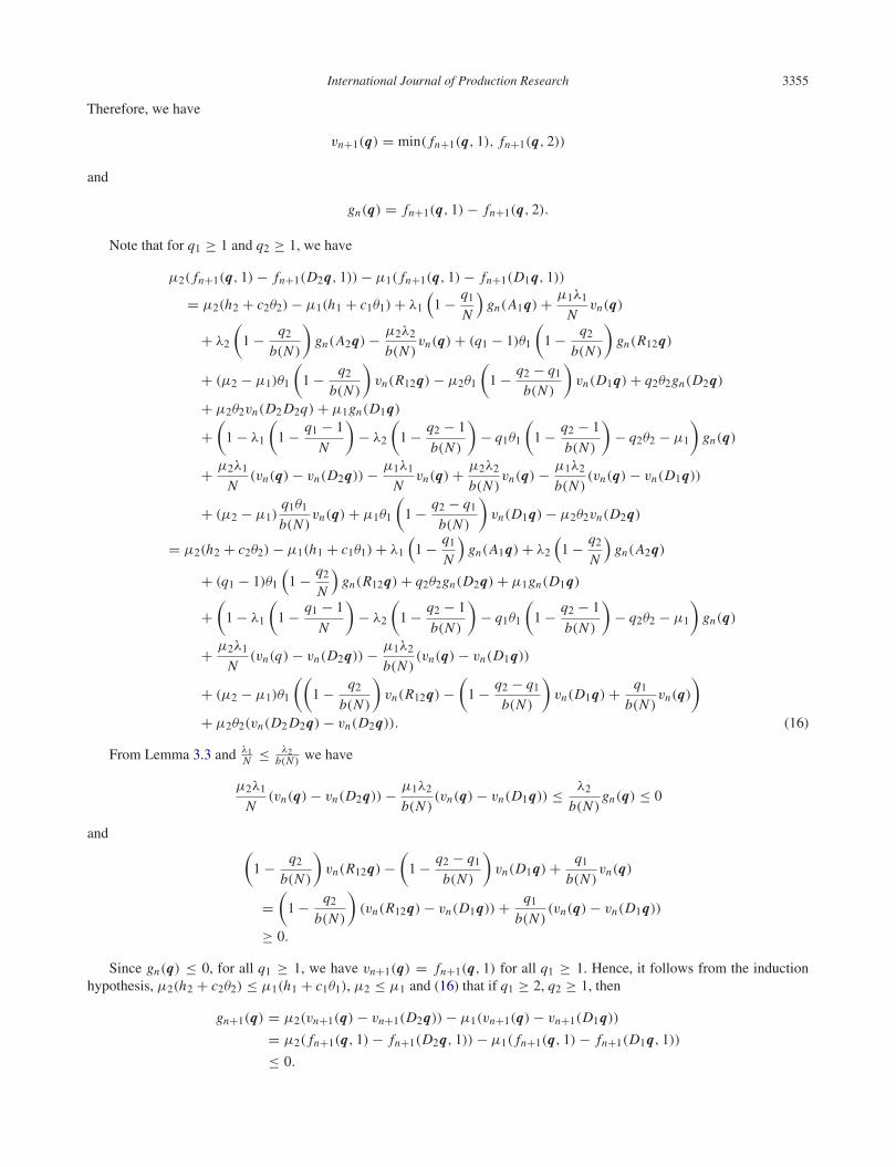
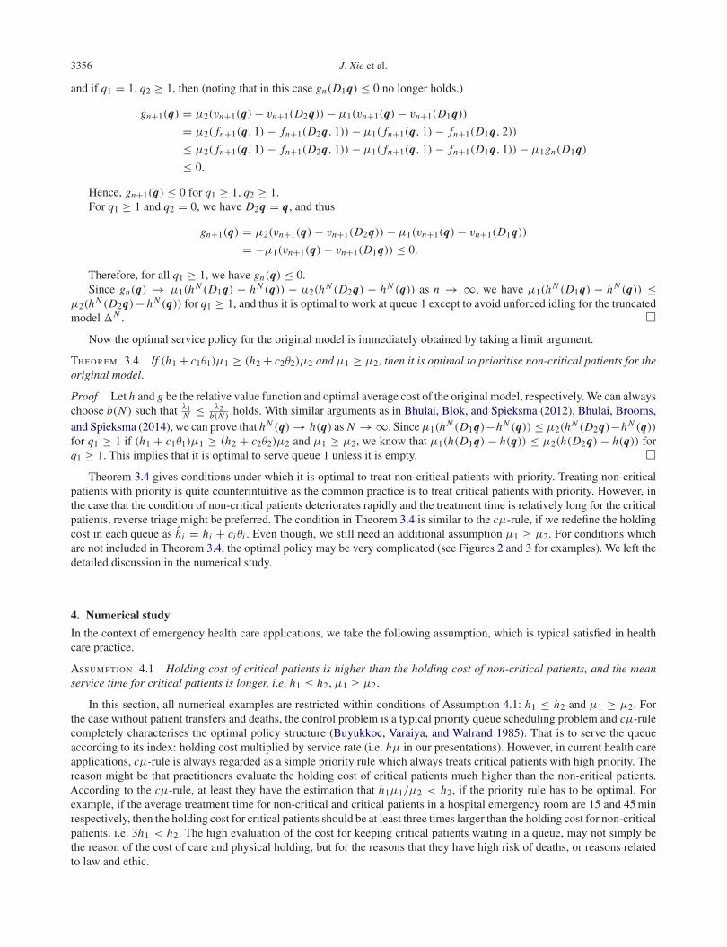
Theorem 3.4 gives conditions under which it is optimal to treat non-critical patients with priority. Treating non-criticalpatients with priority is quite counterintuitive as the common practice is to treat critical patients with priority. However, inthe case that the condition of non-critical patients deteriorates rapidly and the treatment time is relatively long for the criticalpatients, reverse triage might be preferred. The condition in Theorem 3.4 is similar to the cμ-rule, if we redefine the holdingcost in each queue as hi = hi + ciθi . Even though, we still need an additional assumption μ1 ≥ μ2. For conditions whichare not included in Theorem 3.4, the optimal policy may be very complicated (see Figures 2 and 3 for examples). We left thedetailed discussion in the numerical study.

4. Numerical study

In the context of emergency health care applications, we take the following assumption, which is typical satisfied in healthcare practice.

Assumption 4.1 Holding cost of critical patients is higher than the holding cost of non-critical patients, and the meanservice time for critical patients is longer, i.e. h1 ≤ h2, μ1 ≥ μ2.

In this section, all numerical examples are restricted within conditions of Assumption 4.1: h1 ≤ h2 and μ1 ≥ μ2. Forthe case without patient transfers and deaths, the control problem is a typical priority queue scheduling problem and cμ-rulecompletely characterises the optimal policy structure (Buyukkoc, Varaiya, and Walrand 1985). That is to serve the queueaccording to its index: holding cost multiplied by service rate (i.e. hμ in our presentations). However, in current health careapplications, cμ-rule is always regarded as a simple priority rule which always treats critical patients with high priority. Thereason might be that practitioners evaluate the holding cost of critical patients much higher than the non-critical patients.According to the cμ-rule, at least they have the estimation that h1μ1/μ2 < h2, if the priority rule has to be optimal. Forexample, if the average treatment time for non-critical and critical patients in a hospital emergency room are 15 and 45 minrespectively, then the holding cost for critical patients should be at least three times larger than the holding cost for non-criticalpatients, i.e. 3h1 < h2. The high evaluation of the cost for keeping critical patients waiting in a queue, may not simply bethe reason of the cost of care and physical holding, but for the reasons that they have high risk of deaths, or reasons relatedto law and ethic.

International Journal of Production Research 3357

0 5 10 15 20 25 300

5

10

15

20

25

30

Length of queue 1

Leng

th o

f que

ue 2

Optimal service policy: x − serve queue 1, o − serve queue 2

Figure 2. Optimal policy structure of numerical example with setting λ1 = 10, λ2 = 2, μ1 = 16, μ2 = 8, θ1 = 0.1, θ2 = 0.5, h1 =1, h2 = 2, c1 = 10, c2 = 50.

0 5 10 15 20 25 300

5

10

15

20

25

30

Length of queue 1

Leng

th o

f que

ue 2

Optimal service policy: x − serve queue 1, o − serve queue 2

Figure 3. Optimal policy structure of numerical example with setting λ1 = 6, λ2 = 4, μ1 = 16, μ2 = 8, θ1 = 0.1, θ2 = 0.5, h1 =1, h2 = 2, c1 = 10, c2 = 50.

In our model, we consider deteriorating of patients’conditions. In this case, the optimal policy cannot be described by cμ-rule. Since it follows from Assumption 4.1 that μ1 ≥ μ2, we have two cases to be discussed: (h1 + c1θ1)μ1 ≥ (h2 + c2θ2)μ2and (h1 + c1θ1)μ1 < (h2 + c2θ2)μ2. From Theorem 3.4, we can see that it is optimal to give priority to queue 1 for the firstcase. For the second case, the optimal policy structure is rather complicated (recall Figures 2 and 3). Next we analyse howthese parameters will affect the optimal policy in the second case.

We use the example in which λ1 = 8, λ2 = 2, μ1 = 16, μ2 = 8, θ1 = 0.1, θ2 = 0.05, h1 = 1, h2 = 2, c1 = 10, c2 = 50as the benchmark example, and examine the effect of each parameter on the optimal policy under the condition

(h1 + c1θ1)μ1 < (h2 + c2θ2)μ2, and μ1 ≥ μ2. (17)

3358 J. Xie et al.

0 5 10 15 20 25 300

5

10

15

20

25

30

Figure 4. Optimal policy structure of numerical examples in which λ1 = λ2/3.

0 5 10 15 20 25 300

5

10

15

20

25

30

Figure 5. Optimal policy structure of numerical examples in which λ1 = 3λ2.

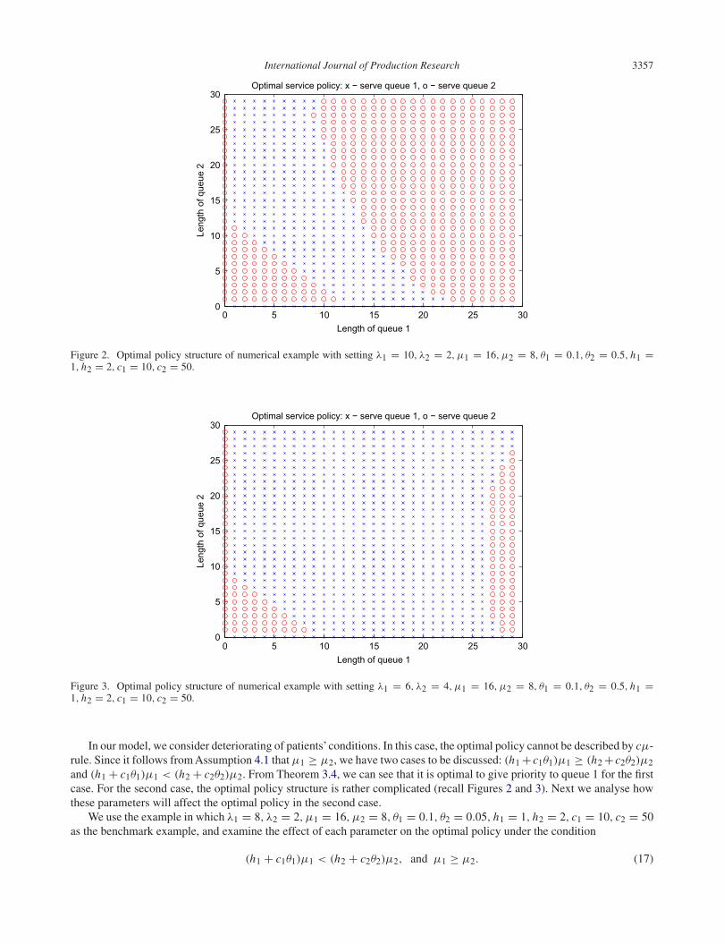
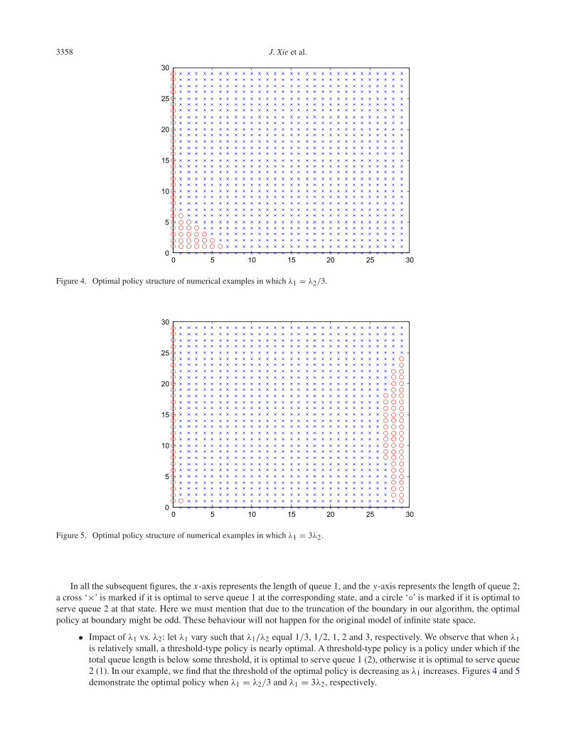
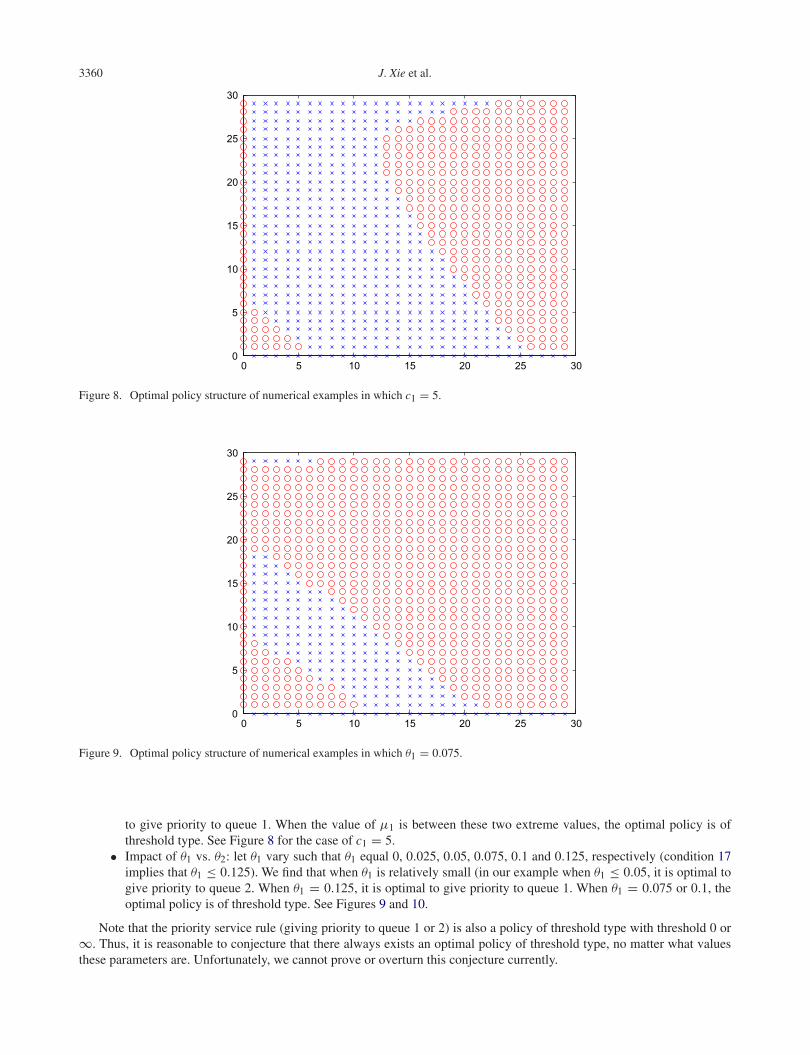
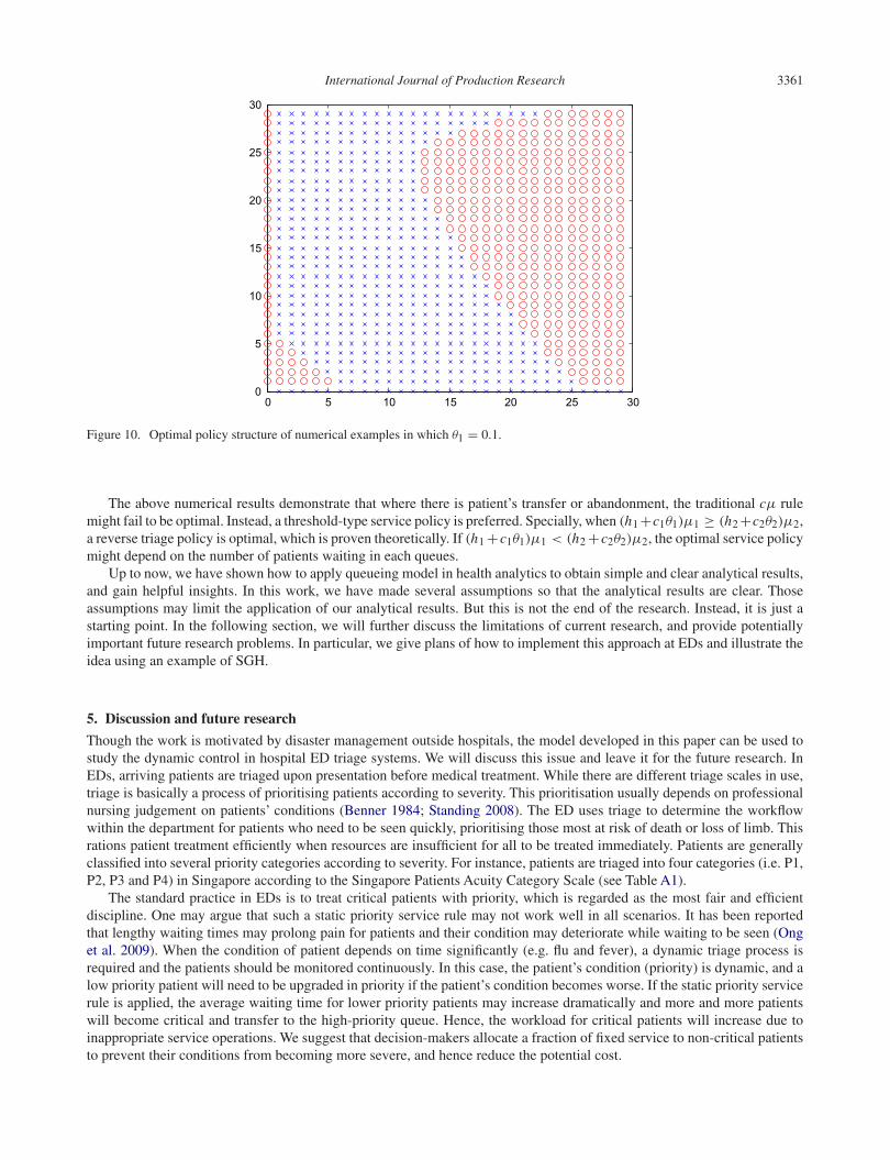
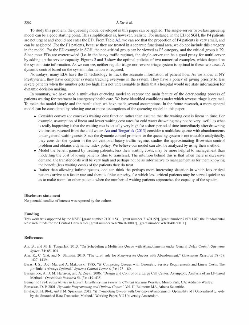
In all the subsequent figures, the x-axis represents the length of queue 1, and the y-axis represents the length of queue 2;a cross ‘×’ is marked if it is optimal to serve queue 1 at the corresponding state, and a circle ‘◦’ is marked if it is optimal toserve queue 2 at that state. Here we must mention that due to the truncation of the boundary in our algorithm, the optimalpolicy at boundary might be odd. These behaviour will not happen for the original model of infinite state space.

• Impact of λ1 vs. λ2: let λ1 vary such that λ1/λ2 equal 1/3, 1/2, 1, 2 and 3, respectively. We observe that when λ1is relatively small, a threshold-type policy is nearly optimal. A threshold-type policy is a policy under which if thetotal queue length is below some threshold, it is optimal to serve queue 1 (2), otherwise it is optimal to serve queue2 (1). In our example, we find that the threshold of the optimal policy is decreasing as λ1 increases. Figures 4 and 5demonstrate the optimal policy when λ1 = λ2/3 and λ1 = 3λ2, respectively.

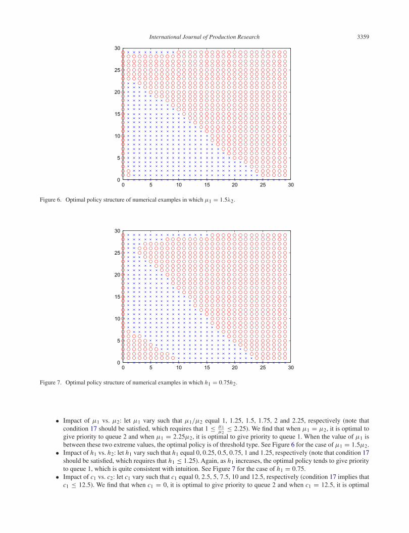
International Journal of Production Research 3359

0 5 10 15 20 25 300

5

10

15

20

25

30

Figure 6. Optimal policy structure of numerical examples in which μ1 = 1.5λ2.

0 5 10 15 20 25 300

5

10

15

20

25

30

Figure 7. Optimal policy structure of numerical examples in which h1 = 0.75h2.

• Impact of μ1 vs. μ2: let μ1 vary such that μ1/μ2 equal 1, 1.25, 1.5, 1.75, 2 and 2.25, respectively (note thatcondition 17 should be satisfied, which requires that 1 ≤ μ1

μ2≤ 2.25). We find that when μ1 = μ2, it is optimal to

give priority to queue 2 and when μ1 = 2.25μ2, it is optimal to give priority to queue 1. When the value of μ1 isbetween these two extreme values, the optimal policy is of threshold type. See Figure 6 for the case of μ1 = 1.5μ2.

• Impact of h1 vs. h2: let h1 vary such that h1 equal 0, 0.25, 0.5, 0.75, 1 and 1.25, respectively (note that condition 17should be satisfied, which requires that h1 ≤ 1.25). Again, as h1 increases, the optimal policy tends to give priorityto queue 1, which is quite consistent with intuition. See Figure 7 for the case of h1 = 0.75.

• Impact of c1 vs. c2: let c1 vary such that c1 equal 0, 2.5, 5, 7.5, 10 and 12.5, respectively (condition 17 implies thatc1 ≤ 12.5). We find that when c1 = 0, it is optimal to give priority to queue 2 and when c1 = 12.5, it is optimal

3360 J. Xie et al.

0 5 10 15 20 25 300

5

10

15

20

25

30

Figure 8. Optimal policy structure of numerical examples in which c1 = 5.

0 5 10 15 20 25 300

5

10

15

20

25

30

Figure 9. Optimal policy structure of numerical examples in which θ1 = 0.075.

to give priority to queue 1. When the value of μ1 is between these two extreme values, the optimal policy is ofthreshold type. See Figure 8 for the case of c1 = 5.

• Impact of θ1 vs. θ2: let θ1 vary such that θ1 equal 0, 0.025, 0.05, 0.075, 0.1 and 0.125, respectively (condition 17implies that θ1 ≤ 0.125). We find that when θ1 is relatively small (in our example when θ1 ≤ 0.05, it is optimal togive priority to queue 2. When θ1 = 0.125, it is optimal to give priority to queue 1. When θ1 = 0.075 or 0.1, theoptimal policy is of threshold type. See Figures 9 and 10.

Note that the priority service rule (giving priority to queue 1 or 2) is also a policy of threshold type with threshold 0 or∞. Thus, it is reasonable to conjecture that there always exists an optimal policy of threshold type, no matter what valuesthese parameters are. Unfortunately, we cannot prove or overturn this conjecture currently.

International Journal of Production Research 3361

0 5 10 15 20 25 300

5

10

15

20

25

30

Figure 10. Optimal policy structure of numerical examples in which θ1 = 0.1.

The above numerical results demonstrate that where there is patient’s transfer or abandonment, the traditional cμ rulemight fail to be optimal. Instead, a threshold-type service policy is preferred. Specially, when (h1 +c1θ1)μ1 ≥ (h2 +c2θ2)μ2,a reverse triage policy is optimal, which is proven theoretically. If (h1 +c1θ1)μ1 < (h2 +c2θ2)μ2, the optimal service policymight depend on the number of patients waiting in each queues.

Up to now, we have shown how to apply queueing model in health analytics to obtain simple and clear analytical results,and gain helpful insights. In this work, we have made several assumptions so that the analytical results are clear. Thoseassumptions may limit the application of our analytical results. But this is not the end of the research. Instead, it is just astarting point. In the following section, we will further discuss the limitations of current research, and provide potentiallyimportant future research problems. In particular, we give plans of how to implement this approach at EDs and illustrate theidea using an example of SGH.

5. Discussion and future research

Though the work is motivated by disaster management outside hospitals, the model developed in this paper can be used tostudy the dynamic control in hospital ED triage systems. We will discuss this issue and leave it for the future research. InEDs, arriving patients are triaged upon presentation before medical treatment. While there are different triage scales in use,triage is basically a process of prioritising patients according to severity. This prioritisation usually depends on professionalnursing judgement on patients’ conditions (Benner 1984; Standing 2008). The ED uses triage to determine the workflowwithin the department for patients who need to be seen quickly, prioritising those most at risk of death or loss of limb. Thisrations patient treatment efficiently when resources are insufficient for all to be treated immediately. Patients are generallyclassified into several priority categories according to severity. For instance, patients are triaged into four categories (i.e. P1,P2, P3 and P4) in Singapore according to the Singapore Patients Acuity Category Scale (see Table A1).

The standard practice in EDs is to treat critical patients with priority, which is regarded as the most fair and efficientdiscipline. One may argue that such a static priority service rule may not work well in all scenarios. It has been reportedthat lengthy waiting times may prolong pain for patients and their condition may deteriorate while waiting to be seen (Onget al. 2009). When the condition of patient depends on time significantly (e.g. flu and fever), a dynamic triage process isrequired and the patients should be monitored continuously. In this case, the patient’s condition (priority) is dynamic, and alow priority patient will need to be upgraded in priority if the patient’s condition becomes worse. If the static priority servicerule is applied, the average waiting time for lower priority patients may increase dramatically and more and more patientswill become critical and transfer to the high-priority queue. Hence, the workload for critical patients will increase due toinappropriate service operations. We suggest that decision-makers allocate a fraction of fixed service to non-critical patientsto prevent their conditions from becoming more severe, and hence reduce the potential cost.

3362 J. Xie et al.

To study this problem, the queueing model developed in this paper can be applied. The single-server two-class queueingmodel can be a good starting point. This simplification is, however, realistic. For instance, in the ED of SGH, the P4 patientsare not urgent and should not enter the ED. From Table A2, we can see that the proportion of P4 patients is very small, andcan be neglected. For the P1 patients, because they are treated in a separate functional area, we do not include this categoryin the model. For the ED example in SGH, the non-critical group can be viewed as P3 category, and the critical group is P2.Since most EDs are overcrowded (i.e. in the heavy traffic regime), the single-server can be a good proxy for multi-serverby adding up the service capacity. Figures 2 and 3 show the optimal policies of two numerical examples, which depend onthe system state information. As we can see, neither regular triage nor reverse triage system is optimal in these two cases. Adynamic control based on the system information is required.

Nowadays, many EDs have the IT technology to track the accurate information of patient flow. As we know, at NYPresbyterian, they have computer systems tracking everyone in the system. They have a policy of giving priority to lesssevere patients when the number gets too high. It is not unreasonable to think that a hospital would use state information fordynamic decision making.

In summary, we have used a multi-class queueing model to capture the main feature of the deteriorating process ofpatients waiting for treatment in emergency health care. We have identified conditions under which reverse triage is optimal.To make the model simple and the result clear, we have made several assumptions. In the future research, a more generalmodel can be considered by relaxing one or more assumptions of the queueing model in this paper.

• Consider convex (or concave) waiting cost function rather than assume that the waiting cost is linear in time. Forexample, assumption of linear and lower waiting cost rates for cold water drowning may not be very useful as whatis really happening is that the waiting cost is actually very high for a short period of time immediately after drowningvictims are rescued from the cold water. Ata and Tongarlak (2013) consider a multiclass queue with abandonmentsunder general waiting costs. Since the dynamic control problem for the queueing system is not tractable analytically,they consider the system in the conventional heavy traffic regime, studies the approximating Brownian controlproblem and obtains a dynamic index policy. We believe our model can also be analyzed by using their method.

• Model the benefit gained by treating patients, less their waiting costs, may be more helpful to management thanmodelling the cost of losing patients (due to transfers). The intuition behind this is that when there is excessivedemand, the transfer costs will be very high and perhaps not be as informative to management as for them knowingthe benefit (less waiting costs) of the patients they do treat.

• Rather than allowing infinite queues, one can think the perhaps more interesting situation in which less criticalpatients arrive at a faster rate and there is finite capacity, for which less-critical patients may be served quicker soas to make room for other patients when the number of waiting patients approaches the capacity of the system.

Disclosure statementNo potential conflict of interest was reported by the authors.

FundingThis work was supported by the NSFC [grant number 71201154], [grant number 71401159], [grant number 71571176]; the FundamentalResearch Funds for the Central Universities [grant number WK2040160009], [grant number WK2040160011].

References

Ata, B., and M. H. Tongarlak. 2013. “On Scheduling a Multiclass Queue with Abandonments under General Delay Costs.” QueueingSystem 74: 65–104.

Atar, R., C. Giat, and N. Shimkin. 2010. “The cμ/θ rule for Many-server Queues with Abandonment.” Operations Research 58 (5):1427–1439.

Baras, J. S., D.-J. Ma, and A. Makowski. 1985. “K Competing Queues with Geometric Service Requirements and Linear Costs: Theμc-Rule is Always Optimal.” Systems Control Letter 6 (3): 173–180.

Bassamboo, A., J. M. Harrison, and A. Zeevi. 2006. “Design and Control of a Large Call Center: Asymptotic Analysis of an LP-basedMethod.” Operations Research 54 (3): 419–435.

Benner, P. 1984. From Novice to Expert: Excellence and Power in Clinical Nursing Practice. Menlo Park, CA: Addison-Wesley.Bertsekas, D. P. 2001. Dynamic Programming and Optimal Control. Vol. II. Belmont: MA, Athena Scientific.Bhulai, S., H. Blok, and F. M. Spieksma. 2012. “K Competing Queues with Customer Abandonment: Optimality of a Generalized cμ-rule

by the Smoothed Rate Truncation Method.” Working Paper. VU University Amsterdam.

International Journal of Production Research 3363

Bhulai, S., A. C. Brooms, and F. M. Spieksma. 2014. “On Structural Properties of the Value Function for an Unbounded Jump MarkovProcess with an Application to a Processor Sharing Retrial Queue.” Queueing System 76 (4): 425–446.

Buyukkoc, C., P. Varaiya, and J. Walrand. 1985. “The cμ-rule Revisited.” Advances in Applied Probability 17 (1): 237–238.Cao, P., and J. G. Xie. 2015. “A New Condition for the Existence of Optimal Stationary Policies in Denumerable State Average Cost

Continuous Time Markov Decision Processes with Unbounded Cost and Transition Rates.” Cornell University Liberary. http://arxiv.org/abs/1504.05674v1.

Chen, M. F. 1991. “On Three Classical Problems for Markov Chains with Continuous Time Parameters.” Journal of Applied Probability28 (2): 305–320.

Cox, D. R., and W. L. Smith. 1961. Queues. London: Methuen.Down, D. G., G. M. Koole, and M. E. Lewis. 2011. “Dynamic Control of a Single Server System with Abandonments.” Queueing Systems

69: 63–90.Elixson, E. M. 1991. “Hypothermia. Cold-water Drowning.” Critical Care Nursing Clinics of North America 3 (2): 287–292.Giloni, A., Y. L. Kocaga, and P. Troy. 2013. “State Dependent Pricing Policies: Differentiating Customers through Valuations and Waiting

Costs.” Journal of Revenue & Pricing Management 12 (2): 139–161.Green, L. V. 2008. “Using Operations Research to Reduce Delays for Healthcare.” INFORMS Tutorials in Operations Research 4: 1–16.Green, L. V., and S. Savin. 2008. “Reducing Delays for Medical Appointments: A Queueing Approach.” Operations Research 56 (6):

1526–1538.Green, L. V., J. Soares, J. F. Giglio, and R.A. Green. 2006. “Using Queueing Theory to Increase the Effectiveness of Emergency Department

Provider Staffing.” Academic Emergency Medicine 13 (1): 61–68.Guo, X. P., and O. Hernandez-Lerma. 2009. Continous-time Markov Decision Processes: Theory and Applications. London: Springer.He, Q.-M., J. Xie, and X. Zhao. 2012. “Priority Queue with Customer Upgrades.” Naval Research Logistics 59 (5): 362–375.Kakalik, J. 1969. Optimal Dynamic Operating Policies for a Service Facility. Technical Report. Cambridge, MA: OR Center, MIT.Klimov, G. P. 1974. “Time-sharing Service Systems I.” Theory of Probability and Its Applications 19 (3): 532–551.Koole, G. M. 2006. “Monotonicity in Markov Reward and Decision Chains: Theory and Applications.” Foundations and Trends in

Stochastic Systems 1: 1–76.Lippman, S. A. 1975. “Applying a New Device in the Optimization of Exponential Queuing Systems.” Operations Research 23: 687–710.Mandelbaum, A., P. Momcilovic, and Y. Tseytlin. 2012. “On Fair Routing from Emergency Departments to Hospital Wards: QED Queues

with Heterogeneous Servers.” Management Science 58 (7): 1273–1291.Ong, M. E. H., K. K. Ho, T. P. Tan, S. W. Koh, Z. Almuthar, J. Overton, and S. H. Lim. 2009. “Using Demand Analysis and System Status

Management for Predicting ED Attendances and Rostering.” American Journal of Emergency Medicine 27 (1): 16–22.Puterman, M. L. 1994. Markov Decision Processes: Discrete Stochastic Dynamic Programming. New York: Wiley.Sennott, L. I. 1999. Stochastic Dynamic Programming and the Control of Queueing Systems. New York: Wiley.Serfozo, R. F. 1979. “An Equivalence between Continuous and Discrete Time Markov Decision Processes.” Operations Research 27 (3):

616–620.Sharon, E. M., and A. M. Thom. 2008. “Triage.” Chap. 155 in Pediatric Emergency Medicine, 1087–1096. London: Elsevier.Shi, P., M. C. Chou, J. G. Dai, D. Ding, and J. Sim. Forthcoming. “Models and Insights for Hospital Inpatient Operations: Time-dependent

ED Boarding Time.” Management Science. doi:10.1287/mnsc.2014.2112.Standing, M. 2008. “Clinical Judgment and Decision Making in Nursing – Nine Modes of Practice in a Revised Cognitive Continuum.”

Journal of Advanced Nursing 62 (1): 124–134.Wang, X., L. G. Debob, and A. Scheller-Wolf. 2015. “Managing Nurse Lines – Practical Challenges and the Developing Theory.”

International Journal of Production Research. doi:10.1080/00207543.2015.1005875.Wiseman, D. B., R. Ellenbogen, and C. I. Shaffrey. 2002. “Triage for the Neurosurgeon.” Neurosurg Focus 12 (3): E5.Xie, J. G., Q.-M. He, and X. B. Zhao. 2008. “Stability of a Priority Queueing System with Customer Transfers.” Operations Research

Letters 36 (6): 705–709.Xie, J. G., Q.-M. He, and X. B. Zhao. 2009. “On the Stationary Distribution of Queue Lengths in a Multi-class Priority Queueing System

with Customer Transfers.” Queueing Systems 62 (3): 255–277.Yom-Tov, G. B., and A. Mandelbaum. 2014. “Erlang-R: A Time-varying Queue with Reentrant Customers, in Support of Healthcare

Staffing.” Manufacturing & Service Operations Management 16 (2): 283–299.

3364 J. Xie et al.

Appendix 1.

Table A1. Singapore patient acuity category scale.

Patients acuity category Scaling guideline

Priority 1 (P1) These are patients who are either in a state of cardiovascular collapse or inimminent danger of collapse and would therefore be required to be attended towithout delay. They would most likely require maximum allocation of staff andequipment resources for initial management

Priority 2 (P2) These patients are ill, non-ambulant, and in various forms of severe distress. Theywould appear to be in a stable state on initial cardiovascular examination andare not in danger of imminent collapse. The severity of their symptoms requiresvery early attention. Failure to do so will like result in early deterioration of theirmedical status. They would be trolley-based

Priority 3 (P3) These patients have acute symptoms but are ambulant and have mild to moderatesymptoms and require acute treatment, which will result in resolution of symptomsover time

Priority 4 (P4) These are non-emergency patients. They should not be presented at ED and shouldbe managed in a primary health care setting, such as by general practitioners orin polyclinics. They may have an old injury or condition that has been presentfor a long time. They do not require immediate treatment. There is no immediatethreat to their life or limb

Source: http://www.ktph.com.sg/main/specialties_n_services/4/49 (see also Ong et al. 2009 Table 1).

Table A2. Yearly ED attendance by triage category in SGH.

2004 2005 2006 2007 2008 2009

Priority 1 7575 (6.7%) 9782 (8.1%) 11,414 (9.1%) 10,451 (7.7%) 9795 (7.1%) 9509 (6.7%)Priority 2 38,169 (33.7%) 42,132 (34.9%) 44,101 (35.1%) 47,798 (35.3%) 52,362 (38.0%) 50,846 (36.0%)Priority 3 66,945 (59.0%) 68,090 (56.4%) 69,724 (55.4%) 76,299 (56.4%) 75,193 (54.6%) 80,635 (57.1%)Priority 4 698 (0.6%) 760 (0.6%) 534 (0.4%) 746 (0.6%) 376 (0.3%) 151 (0.1%)

Note: see Table 2 in Ong et al. (2009) for part of the data (2004–2006).