Determining Resource Utilization and Saturation Lim its Using AWR history and Queueing Theory

Henry Poras ITA Software

henry@itasoftware.com Last updated: March 11, 2010

Part I - Introduction My goal is to determine resource utilization needs and chokepoints within a system. We will look at resource demands as a function of time and of load. Part of the analysis will be to determine the bottleneck, the first resource to saturate. We will see if the bottleneck is the database and if so, where in the database. We can experimentally determine, for example, the number of disks needed to achieve necessary throughput levels, as well as the load at which CPU will saturate.

This analysis will be done for three different cases:

1. the system as a whole is of interest 2. a single user in a multi-user system is of interest 3. multiple users in a multi-session system are of interest

As our application is not yet in production, these are development systems, though some simulate a production environment.

Oracle’s Automatic Workload Repository is an invaluable tool in determining trending behavior. Its underlying tables can be ordered to view data by time, by load, or by other variables. Viewing this data through the lens of Queueing Theory allows additional and deeper understanding, in particular capacity planning and resource utilization.

So the basic steps in setting up these tests are to:

1. construct a model 2. take a guess 3. collect/analyze the data 4. compare results to guess

(see last year’s paper1)

Sanity Checks: One important result of having a model is being able to include ‘sanity checks’ in the analysis. Is my system behaving how I expect it to act? Not only do we want to guess about the behavior of our central premise (I think the database is the bottleneck therefore I expect the residence time at the database to increase with load), but I want to guess about other features in the system to make sure everything is behaving as expected (the amount of redo generated per transaction should remain constant with load. Does it?)

Why AWR and QT?: For capacity planning information we are interested in looking at resource utilization over a period of time and over varying loads. If our system doesn’t fluctuate wildly and is fairly stable over half hour to hour periods, then Oracle’s 1Applying Queueing Theory Analysis to Oracle Statspack Data ;Henry Poras; Hotsos Symposium 2009

Advanced Workload Repository (AWR) will automatically collect usable data for us. Nothing special, nothing extra is needed. This data is all at the systemwide level (i.e. bytes of redo generated by the system). If we need finer granularity, if we are interested in specific sessions, Tanel Poder’s sesspack utility is a useful addition2. The logic behind sesspack is very similar to AWR, so if we understand how to analyze one, we will be able to use the other.

AWR and sesspack are our data collection tools. Queueing Theory provides the framework within which we view our data.

AWR: Most people are aware of AWR reports, the direct descendent of statspack reports, as a way of getting a system overview between two points in time (two snapshots). By default, Oracle stores a 10 second sampling of active user session data as well as hourly (though this is a configurable parameter) snapshots of a myriad of system data. Accessing this data by SQL instead of through awrrpt allows us to both order it by any one of a number of variables (i.e. load, time) and to view trends over many snapshots.

The first step is finding the underlying tables and views which hold the data. The easiest way to access AWR data is via the dba_hist views. These views are built on wrh$ and wrm$ tables. My first exposure to the underlying table names came by extracting (similar to exporting) and loading AWR data (run $ORACLE_HOME/rdbms/admin/awrextr.sql[awrload.sql]). This will do a datapump export/import and produce a log file which shows all exported objects.

Master table "SYS"."SYS_IMPORT_FULL_01" successfull y loaded/unloaded Starting "SYS"."SYS_IMPORT_FULL_01": Processing object type TABLE_EXPORT/TABLE/TABLE Completed 120 TABLE objects in 4 seconds Processing object type TABLE_EXPORT/TABLE/TABLE_DAT A . . imported "AWR_STAGE"."WRH$_ACTIVE_SESSION_HISTO RY":"WRH$_ACTIVE_261596549_368" 246.5 MB 903279 r ows . . imported "AWR_STAGE"."WRH$_ACTIVE_SESSION_HISTO RY":"WRH$_ACTIVE_261596549_477" 68.54 MB 250156 r ows . . imported "AWR_STAGE"."WRH$_ACTIVE_SESSION_HISTO RY":"WRH$_ACTIVE_261596549_272" 64.46 MB 250956 r ows . . imported "AWR_STAGE"."WRH$_SYSMETRIC_HISTORY" 35.01 MB 675579 rows . . imported "AWR_STAGE"."WRH$_SQL_PLAN" 22.57 MB 84646 rows . . imported "AWR_STAGE"."WRH$_ACTIVE_SESSION_HISTO RY":"WRH$_ACTIVE_261596549_669" 17.11 MB 63344 r ows . . imported "AWR_STAGE"."WRH$_ACTIVE_SESSION_HISTO RY":"WRH$_ACTIVE_261596549_224" 13.15 MB 55113 r ows . . imported "AWR_STAGE"."WRH$_ACTIVE_SESSION_HISTO RY":"WRH$_ACTIVE_261596549_248" 10.76 MB 43913 r ows . . imported "AWR_STAGE"."WRH$_SYSMETRIC_SUMMARY" 8.715 MB 109964 rows . . imported "AWR_STAGE"."WRH$_EVENT_HISTOGRAM":"WR H$_EVENT__261596549_477" 8.007 MB 259301 rows

Fig. 1 An excerpt from an AWR load log file

I started off using these table names, but soon realized it was cleaner and easier to use the provided dba_hist views. (select table_name from dict where table_name like ‘DBA_HIST%’). Because of this, some of the scripts attached to this paper still include references to the wrh$ tables.

While extracting and manipulating AWR data, I have noticed some interesting characteristics.

AWR and Flashback Database: A few of our test systems require that ‘flashback database’ be run against them fairly frequently. When this happens, the AWR data is also flashed back. In the past, when we took statspack snapshots (non-SYS, perfstat user) we could export the user, do the flashback database, reimport the user and go on our way without losing useful information. We can’t do this with AWR. 2 http://blog.tanelpoder.com/2008/03/06/hotsos-symposium-2008-presentations-and-files/

An AWR extract can’t be reloaded into a database which has the same dbid. So to save our data, it needs to by loaded into another database. This will work for a single load, but then … trouble.

The Primary Keys of the AWR tables start with DBID, SNAP_ID, INSTANCE_NUMBER. For wrm$_snapshot that is the full Primary Key. For wrh$_sqlstat the fields SQL_ID, PLAN_HASH_VALUE are appended. Flashing back the source database also flashes back the snap_id values. Our next extract has the same dbid, snap_id, instance_number as the first extract. I can’t load both into the same destination db since that will violate uniqueness. One solution would be for Oracle to include an incarnation number in the PK. This has been submitted as an enhancement request, but understandably it is not a front-burner issue.

Space issues with awrload: One other issue which arose with loading large extracts was having enough space in the destination db. A number of our test systems were suddenly repurposed, so to continue my analysis I needed to extract and load lots of AWR data. The load (awrload.sql) happens in two parts. First, data is imported (by datapump) into a staging user (awr_stage by default). Second, it is moved to the sys owned AWR tables. If there isn’t enough space for the import to the staging user, datapump pauses in a resumable transaction; standard datapump behavior. If, on the other hand, the move to the sys base tables runs out of space, the operation aborts and everything needs to start all over again. The lesson is be sure SYSAUX is big enough.

Queueing Theory: I won’t and can’t give an in depth treatise on QT, but understanding a few basic premises will help clarify the following experiments and their analysis. In last year’s Hotsos presentation (Ref. 1) I gave my version of a brief review of Queueing Theory. Let me now condense this even more and focus on the pieces applicable to the rest of this paper. Much of this material comes from Neil Gunther3 and Raj Jain4.

Definitions: First of all, what is a queue? The site m-w.com states that a queue is “a waiting line, especially of persons or vehicles.”

For example, think of a toll booth. People get in line, they wait their turn, they pay and leave. There are constantly new people getting in line, and once someone is finished, they leave and don’t get back in line (simple case).

Fig. 2: From Ref. 3.

3 Gunther, N.J. 2005. Analyzing ComputerSystem Performance with Perl::PDQ. Berlin: Springer-Verlag. 4 Jain, Raj. 1991. The Art of Computer Systems Performance Analysis. New York, N.Y: John Wiley & Sons.

arrivals (A), arrival rate (λ)

A is the number of people joining the queue, while the arrival rate, λ, measures how quickly they join the line (arrivals per second).

completions (C), completion rate/throughput (χ)

C is the number leaving the queueing center, while the throughput measures how quickly they leave (completions per second).

busy time (B), Utilization (ρ)

These two metrics measure the amount of time for which the service center is busy. B is the total amount of busy time. Utilization is the percent of busy time (B/T).

service time (S)

This measures how long it takes the queueing center (i.e. the toll taker) to do the required job for each customer. This can by thought of as B/C.

queue length (Q)

The Queue is the number of people in line, including the person currently being helped.

residence time (R), waiting time (W)

The residence time is the time spent at the queueing center, the time it takes from joining the line to leaving it. This is made up of Service Time (S) and Wait Time (W).

R = W + S = QS + S

service demand (D), number of visits (V)

A request might visit a queueing center multiple times (i.e. one database transaction can have many visits to disk, to CPU). In this case, the service time (S) can also be defined as a service demand, the total time the request spends at the service center. If it makes V visits, D = VS.

Load (N)

This metric is a bit vague. Typically I will use it to mean the number of requestors (users, sessions, active sessions, user calls, …). We will return to this later. As Justice Potter Stewart said “I know it when I see it.” It seems to me that if you find yourself talking about the load in a queueing center, that is no different from Q.

Conditions: To get useful information from our analysis and experiments we need to assume that we are in a condition of steady state.

Steady state: Steady state is important as it means the conditions we are measuring are not changing for the period of time in which we are interested. (how steady is steady? sort of relative). If our queue length is constantly increasing (arrival rate > completion rate) then we are not at steady state. So we need λ= χ for our measured time frame in order to assume a steady state condition.

General Relationships

Little’s Law

The most important general equation is Little’s Law. It states

Q = λR (1)

Another formulation of this, Little’s Microscopic Law, states:

ρ = λS (2)

open queue

The simplest model to consider (the one we have already considered) is an open queue (e.g. web application, supermarket checkout). Here the arrival rate is always constant. There is no constraint on the number of customers/transactions coming in.

closed queue

A closed queue (i.e. load test environment, batch server) has a limited number of customers. The arrival rate changes with time. When the system is at its heaviest load, when all available customers are in a queue, there are no more customers to enter the queue, so λ goes to zero. There is a built-in negative feedback loop.

Our standard metrics of Residence Time and Throughput are now dependent on the number of customers (N), and the think time (Z).

The main point to keep in mind with respect to closed queues is that there is now a limit on the maximum queue size and on the maximum residence time. So now if we look at R or χ vs load, it is plotted as a function of N, not of ρ.

Fig. 3 Closed queue behavior of R and ρ vs N (from Ref. 4).

multiple workloads

We often have different workloads hitting the same queueing center. For example, I could concurrently run a mix of business functions. CPU could be processing OLTP and batch jobs, sorts and disk I/O. Each can have different arrival rates, service times, … In Oracle we are always dealing with mixed workloads in the form of foreground and background processes. They both impact underlying resources, but we don’t want to lump together their residence times and throughput behavior.

Part II – Experiment and Analysis

Our setup Our setup consists of the following

pounder, our home grown, load generating application

awr snapshots are taken at the beginning and end of each pounder run (and sometimes in the middle.). Pounder runs were used in our third example. For the other cases Oracle’s regularly scheduled snapshots were used.

sesspack snapshots (http://blog.tanelpoder.com/2008/03/06/hotsos-symposium-2008-presentations-and-files/) were used in cases 2 and 3 to get session specific data. Three minor modifications to the base scripts were made for our tests:

1. Change IOT tables to heap. On running sesspack in our environment we were getting ORA-20001: Error -1: ORA-00001: unique constraint errors. Communication with Tanel Poder revealed that these errors were first observed in v11.2. To avoid this I disabled the Primary Key constraints, but first I needed to recreate the sesspack schema using heap tables.

2. A second modification was to push the comment field which was included with the definitions of underlying functions and procedures, to the calling procedure. Since our precheckin sessions (case 2) were short lived, I took the snapshots using logon triggers. Having the comment field available allowed me to include ‘LOGON’ and ‘LOGOFF’ with the snapshots.

3. Include instance number with snapshot data. When using sesspack in a RAC environment, snapshots need to be taken on all nodes. The instance number needs to be added to snapshot data in order to identify the snapshot source.

User sessions come in various shapes and sizes for our test cases. Our migration environment spawns long lived worker sessions which perform the necessary work. Our current application server will disconnect and reconnect if its lifetime is greater than five minutes (don’t ask/don’t tell is assiduously enforced with regard to this behavior). In our development testing envrionment (case 2), the typical session lifetime is much shorter than this. For the pounder runs (case 3), the 5 minute lifetime is standard behavior. We also have non-appserver user sessions (i.e. Advanced Queueing, schedule information, …) which are typically long lived. For the shorter duration sessions, sesspack snapshots are taken by using logon/logoff triggers. The other sessions are snapshotted using scheduler jobs with 5 minute intervals.

One final piece we need to know before looking at our experimental results is how to connect our AWR data to QT parameters.

Table 1: Simple Statspack Starting Point

• Q=Average # of Active Sessions = (DB Time)/(Elapsed Time)

• χ = txn/sec or (user calls)/sec

• R = sec/txn = (DB Time)/[(txn/sec)(Elapsed Time)] = Q/χ

All of these parameters can be found on the first page of an AWR report.

Case 1 resource utilization of the database Migration - Can We Reach our Throughput Goal?

goals of migration Our first example looks at migrating data from an outside source into our database. When an airline reservation system goes live it must include the existing passenger name records (pnr – the reservation) and electronic tickets present in the old system. There is a fixed window within which this data can be migrated. Hence we can determine the necessary throughput (pnr/hour) to reach our goal. In this case we are solely concerned about maximizing throughput. Different methods were used to migrate pnr’s and e-tickets. These differences influenced our data, analysis, and results so both will be examined in turn.

PNR’s

We will start by looking at migrating pnr’s. During one eight day migration run I asked the development team to occasionally vary the number of application workers parsing and loading the data. Using the default hourly AWR snapshots I wrote some scripts which allowed us to view various characteristics as a function of load (# of workers).

BEGIN_INTERVAL_TIME # of pnrs # of workers Q pnrs per hr commits/pnr redo bytes/pnr PIO (blk rd)/pnr PIO (IO call rd)/pnr PIO (blk wrt)/pnr LIO/pnr R(sec) ----------------------------------- ------------ ---------------- --- ---- --------- ----------- ------------------ -------------------- ------------------------ ---------------------- ---------- ------ 19-MAR-09 08.00.25.795 PM 16,251 8 6.6 16,228 25.06 623,952.88 70.58 69.95 91.71 7,157.73 1.47 19-MAR-09 09.00.30.400 PM 16,920 8 7.8 16,892 21.38 536,917.98 99.46 80.63 93.91 9,321.26 1.66 19-MAR-09 10.00.36.050 PM 13,759 8 9.5 13,740 21.17 528,320.11 298.41 123.50 102.39 15,209.54 2.48 19-MAR-09 11.00.41.852 PM 16,022 8 8.2 16,000 19.00 435,257.87 121.21 91.48 86.95 10,349.43 1.84 20-MAR-09 12.00.46.734 AM 22,422 16 10.6 22,385 18.38 389,319.14 84.75 80.34 81.32 5,350.99 1.71 20-MAR-09 01.00.52.372 AM 23,048 16 14.3 23,003 17.53 393,611.09 124.33 96.48 83.51 7,208.42 2.24 20-MAR-09 02.00.59.359 AM 22,760 16 13.8 23,100 16.88 355,081.02 110.91 94.61 81.15 6,741.08 2.15 20-MAR-09 03.00.06.940 AM 22,928 16 14.6 22,884 15.97 340,398.73 112.00 94.35 79.64 7,651.75 2.30 20-MAR-09 04.00.13.691 AM 21,510 16 14.3 21,468 15.81 321,249.16 161.66 108.67 80.65 7,309.10 2.40 20-MAR-09 05.00.20.293 AM 23,305 16 14.7 23,260 15.89 321,224.28 92.26 90.54 77.10 7,151.19 2.27 20-MAR-09 06.00.27.483 AM 19,416 16 14.8 19,378 15.41 328,412.73 168.69 120.89 80.47 8,822.92 2.75 20-MAR-09 07.00.34.771 AM 20,984 21 12.3 20,943 14.92 281,274.64 108.44 94.57 73.15 6,381.29 2.11 20-MAR-09 08.00.41.089 AM 22,276 22 17.8 22,239 14.75 294,579.42 167.96 109.98 75.98 5,669.86 2.89 20-MAR-09 09.00.47.860 AM 24,952 22 19.6 24,876 14.90 298,714.07 114.12 100.26 77.36 4,528.47 2.84

Fig. 4: AWR output as a function of time (SQL script in appendix)

Throughput

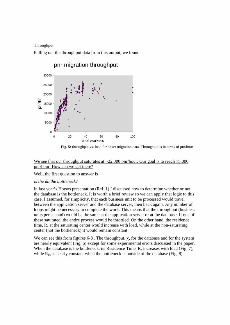
Pulling out the throughput data from this output, we found

pnr migration throughput

0

5000

10000

15000

20000

25000

30000

0 20 40 60 80 100# of workers

pnr/

hr

Fig. 5: throughput vs. load for ticket migration data. Throughput is in terms of pnr/hour

We see that our throughput saturates at ~22,000 pnr/hour. Our goal is to reach 75,000 pnr/hour. How can we get there?

Well, the first question to answer is

Is the db the bottleneck?

In last year’s Hotsos presentation (Ref. 1) I discussed how to determine whether or not the database is the bottleneck. It is worth a brief review so we can apply that logic to this case. I assumed, for simplicity, that each business unit to be processed would travel between the application server and the database server, then back again. Any number of loops might be necessary to complete the work. This means that the throughput (business units per second) would be the same at the application server or at the database. If one of these saturated, the entire process would be throttled. On the other hand, the residence time, R, at the saturating center would increase with load, while at the non-saturating center (not the bottleneck) it would remain constant.

We can see this from figures 6-8 . The throughput, χ, for the database and for the system are nearly equivalent (Fig. 6) except for some experimental errors discussed in the paper. When the database is the bottleneck, its Residence Time, R, increases with load (Fig. 7), while Rdb is nearly constant when the bottleneck is outside of the database (Fig. 8).

X & X

0

10

20

30

40

50

60

70

80

90

100

0 10 20 30 40 50 60 70

agents

thro

uhpu

t (se

q/se

c)

throughput(db) (seq/sec)

troughput(system) (seq/sec)

Fig. 6: Database and system throughput in units of sequences/sec.

R and R

0

0.1

0.2

0.3

0.4

0.5

0.6

0.7

0 10 20 30 40 50 60 70

agents

Res

iden

ce T

ime

(sec

/seq

)

R-system

R-db

Fig. 7: Response time per business function for the entire system and for the database

Residence time

0

50

100

150

200

250

300

350

400

0 20 40 60 80 100 120 140

# of agents

Res

iden

ce ti

me

(mse

c/se

q)

Rsys(msec)

Rdb(msec/seq)

Fig. 8: Response time per business function for the entire system and for the database

Looking at χ, R, and Q (Figs.5,9,10) as a function of load for pnr migration we see an increasing residence time (Fig. 9) with most of the active sessions in the database (Fig. 10). This implies that the database is the bottleneck.

pnr migration Residence Time

0

2

4

6

8

10

12

14

0 20 40 60 80 100

# of workers

R (

sec)

Fig. 9: Residence Time vs. load for ticket migration

pnr migration - Q

0

10

20

30

40

50

60

70

80

90

100

0 20 40 60 80 100

# of workers

Q

Q# of workers

Fig. 10: Queue length within the database. Most workers are in the database.

We can also see from Fig. 5 , that the low load slope is ~2,000 pnr/hour/worker. To reach our goal of 75,000 pnr/hour we will need ~40 workers. How do we get there?

Right now I am only discussing resource utilization. Tuning the process (including SQL tuning) will change the low load slope of the throughput curve which will allow us to reach our goal using fewer workers.

Next we need to determine why our throughput is saturating at ~10 workers.

What is the bottleneck?

Let’s do for the database what we did for the system. Oracle wait events are not waits in the way that Queueing theory uses the concept. In QT, the residence time at a queueing center is the sum of the wait time and the service time. A ‘db file sequential read’ is more like the Residence time necessary to perform a read. Looking at the wait events as if they were queueing centers, and deteriming their throughput (i.e. count of ‘db file sequential read’/pnr) and residence time (i.e. time in ‘db file sequential read’/pnr) will help us find the bottleneck in the database.

The read mechanism in Oracle is actually slightly more complex than I have just presented it. For one, there are latches involved. Additionally, if the buffer cache is full, we might need to ‘free buffer cache’. These are all part of the black box labeled ‘read a block’. We could probably put all of these together in a model, but I haven’t tried that. Some of this can be seen in the example from last year’s presentation where read residence time saturates and ‘free buffer wait’ residence times start to grow (see Ref. 3 Fig. 14).

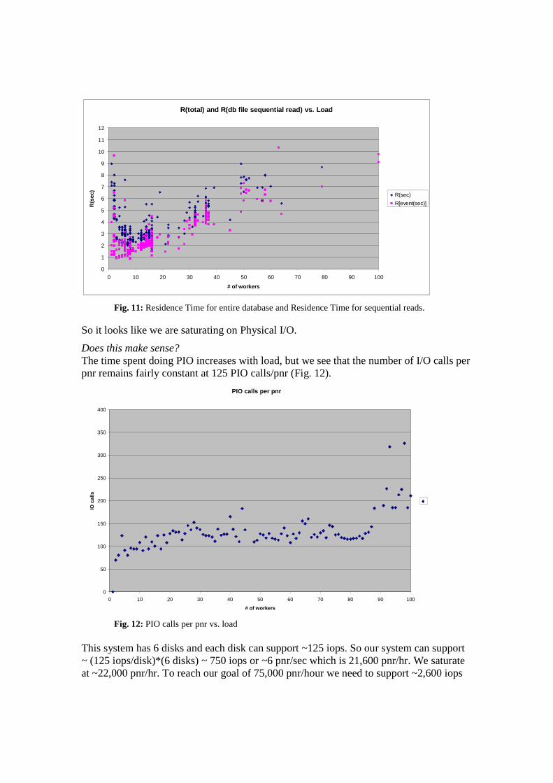
We see from Figure 11 that almost all of Rdb is from sequential reads.

R(total) and R(db file sequential read) vs. Load

0

1

2

3

4

5

6

7

8

9

10

11

12

0 10 20 30 40 50 60 70 80 90 100

# of workers

R(s

ec)

R(sec)

R[event(sec)]R

Fig. 11: Residence Time for entire database and Residence Time for sequential reads.

So it looks like we are saturating on Physical I/O.

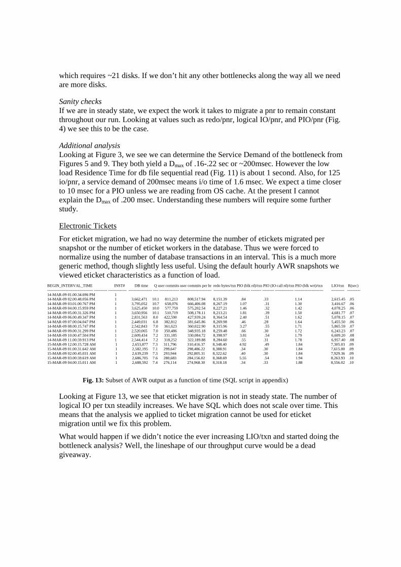
Does this make sense? The time spent doing PIO increases with load, but we see that the number of I/O calls per pnr remains fairly constant at 125 PIO calls/pnr (Fig. 12).

PIO calls per pnr

0

50

100

150

200

250

300

350

400

0 10 20 30 40 50 60 70 80 90 100

# of workers

IO c

alls

Fig. 12: PIO calls per pnr vs. load This system has 6 disks and each disk can support ~125 iops. So our system can support ~ (125 iops/disk)*(6 disks) ~ 750 iops or ~6 pnr/sec which is 21,600 pnr/hr. We saturate at ~22,000 pnr/hr. To reach our goal of 75,000 pnr/hour we need to support ~2,600 iops

which requires ~21 disks. If we don’t hit any other bottlenecks along the way all we need are more disks.

Sanity checks If we are in steady state, we expect the work it takes to migrate a pnr to remain constant throughout our run. Looking at values such as redo/pnr, logical IO/pnr, and PIO/pnr (Fig. 4) we see this to be the case.

Additional analysis Looking at Figure 3, we see we can determine the Service Demand of the bottleneck from Figures 5 and 9. They both yield a Dmax of .16-.22 sec or ~200msec. However the low load Residence Time for db file sequential read (Fig. 11) is about 1 second. Also, for 125 io/pnr, a service demand of 200msec means i/o time of 1.6 msec. We expect a time closer to 10 msec for a PIO unless we are reading from OS cache. At the present I cannot explain the Dmax of .200 msec. Understanding these numbers will require some further study.

Electronic Tickets

For eticket migration, we had no way determine the number of etickets migrated per snapshot or the number of eticket workers in the database. Thus we were forced to normalize using the number of database transactions in an interval. This is a much more generic method, though slightly less useful. Using the default hourly AWR snapshots we viewed eticket characteristics as a function of load.

BEGIN_INTERVAL_TIME INST# DB time Q user commits user commits per hr redo bytes/txn PIO (blk rd)/txn PIO (IO call rd)/txn PIO (blk wrt)/txn LIO/txn R(sec) ----------------------------------- ---------- -------------- ------------------ ---- --------------- ------------------------ ----------------- ---------- -------- --------- -------------- ---------------------- ---------- ---------- 14-MAR-09 01.00.34.696 PM 1 14-MAR-09 02.00.48.056 PM 1 3,662,471 10.1 811,213 808,517.94 8,151.39 .84 .33 1.14 2,615.45 .05 14-MAR-09 03.01.00.767 PM 1 3,795,052 10.7 658,076 666,406.08 8,267.19 1.07 .31 1.30 3,416.67 .06 14-MAR-09 04.00.15.959 PM 1 3,625,450 10.0 577,759 575,202.54 8,227.21 1.46 .32 1.42 4,078.25 .06 14-MAR-09 05.00.31.326 PM 1 3,650,956 10.1 510,719 508,178.11 8,213.21 1.81 .39 1.50 4,681.77 .07 14-MAR-09 06.00.49.347 PM 1 2,831,563 8.0 422,590 427,939.24 8,364.54 2.40 .51 1.62 5,078.15 .07 14-MAR-09 07.00.04.047 PM 1 2,449,031 6.8 382,812 381,645.86 8,269.98 .46 .28 1.64 5,455.50 .06 14-MAR-09 08.00.15.747 PM 1 2,542,843 7.0 361,623 360,022.90 8,315.96 3.27 .55 1.71 5,865.59 .07 14-MAR-09 09.00.31.299 PM 1 2,520,065 7.0 350,486 348,935.18 8,259.48 .66 .30 1.72 6,243.23 .07 14-MAR-09 10.00.47.504 PM 1 2,609,434 7.2 331,185 330,084.72 8,398.97 3.81 .54 1.79 6,609.20 .08 14-MAR-09 11.00.59.913 PM 1 2,544,414 7.2 318,252 322,189.88 8,284.60 .55 .31 1.78 6,957.40 .08 15-MAR-09 12.00.15.728 AM 1 2,653,877 7.3 311,796 310,416.37 8,348.40 4.92 .49 1.84 7,305.03 .09 15-MAR-09 01.00.31.642 AM 1 2,582,195 7.1 299,647 298,486.22 8,388.91 .34 .30 1.84 7,615.00 .09 15-MAR-09 02.00.45.031 AM 1 2,639,239 7.3 293,944 292,805.31 8,322.62 .40 .30 1.84 7,929.36 .09 15-MAR-09 03.00.59.619 AM 1 2,686,705 7.6 280,683 284,156.02 8,368.69 5.55 .54 1.94 8,263.93 .10 15-MAR-09 04.00.15.011 AM 1 2,688,592 7.4 276,114 274,968.30 8,318.18 .34 .33 1.88 8,556.02 .10

Fig. 13: Subset of AWR output as a function of time (SQL script in appendix)

Looking at Figure 13, we see that eticket migration is not in steady state. The number of logical IO per txn steadily increases. We have SQL which does not scale over time. This means that the analysis we applied to ticket migration cannot be used for eticket migration until we fix this problem.

What would happen if we didn’t notice the ever increasing LIO/txn and started doing the bottleneck analysis? Well, the lineshape of our throughput curve would be a dead giveaway.

eticket migration - throughput vs. load

0

100000

200000

300000

400000

500000

600000

700000

800000

900000

0 5 10 15 20

# of active sessions

txn/

hr

user commits per hr

Fig. 14: eticket migration throughput vs. load

eticket migration throughput vs. time

0

100000

200000

300000

400000

500000

600000

700000

800000

900000

00-1ON-000024:0I:00

10-1ON-000024:0I:00

20-1ON-000024:0I:00

30-1ON-000024:0I:00

09-2ON-000024:0I:00

19-2ON-000024:0I:00

29-2ON-000024:0I:00

10-3ON-000024:0I:00

20-3ON-000024:0I:00

time

txn/

hr

Fig. 15: eticket migration throughput vs. time

We can then use AWR to help us find the SQL with high and increasing LIO/txn. SNAP_ID BEGIN_INTERVAL_TIME SQL_ID BUFFER_GETS_DELTA SQL_TEXT

-------------- ------------------------------------ ------------------ -------------------------------------- ---------------------------------------------------

237 14-MAR-09 04.00.15.959 PM 2tbmxp59ujxm5 110,787,920 /* user:GYAA */ select ticket_id, offset, ticket_number, status, worker_id 14-MAR-09 04.00.15.959 PM 3c5b7y7u65n3v 107,754,340 /* user:GYAA */ select ticket_id, offset, ticket_number, status, worker_id 14-MAR-09 04.00.15.959 PM gpqu0z5arc50d 107,041,643 /* user:GYAA */ select ticket_id, offset, ticket_number, status, worker_id 14-MAR-09 04.00.15.959 PM 4avssddkapwf6 106,519,874 /* user:GYAA */ select ticket_id, offset, ticket_number, status, worker_id 14-MAR-09 04.00.15.959 PM 5txsrp606k6t9 104,952,046 /* user:GYAA */ select ticket_id, offset, ticket_number, status, worker_id 14-MAR-09 04.00.15.959 PM 7u6p8q25sqjbt 104,356,428 /* user:GYAA */ select ticket_id, offset, ticket_number, status, worker_id 14-MAR-09 04.00.15.959 PM 3c5qgambgn4cq 103,892,158 /* user:GYAA */ select ticket_id, offset, ticket_number, status, worker_id 14-MAR-09 04.00.15.959 PM 4r6h5pydzbfd7 101,515,647 /* user:GYAA */ select ticket_id, offset, ticket_number, status, worker_id

14-MAR-09 04.00.15.959 PM 9y352tmwjsqvz 101,398,396 /* user:GYAA */ select ticket_id, offset, ticket_number, status, worker_id 14-MAR-09 04.00.15.959 PM 21fks89and8rp 100,185,938 /* user:GYAA */ select ticket_id, offset, ticket_number, status, worker_id 14-MAR-09 04.00.15.959 PM 8zc658utky90v 99,858,025 /* user:GYAA */ select ticket_id, offset, ticket_number, status, worker_id 14-MAR-09 04.00.15.959 PM 1u8pw03qwksfu 99,242,727 /* user:GYAA */ select ticket_id, offset, ticket_number, status, worker_id 14-MAR-09 04.00.15.959 PM 7sa1han4nc4tr 96,502,932 /* user:GYAA */ select ticket_id, offset, ticket_number, status, worker_id 14-MAR-09 04.00.15.959 PM 6pngjm6ajzzrk 95,823,715 /* user:GYAA */ select ticket_id, offset, ticket_number, status, worker_id 14-MAR-09 04.00.15.959 PM 4uy4mj4mvjhsa 95,014,290 /* user:GYAA */ select ticket_id, offset, ticket_number, status, worker_id 238 14-MAR-09 05.00.31.326 PM 2tbmxp59ujxm5 141,409,805 /* user:GYAA */ select ticket_id, offset, ticket_number, status, worker_id 14-MAR-09 05.00.31.326 PM 3c5b7y7u65n3v 138,483,213 /* user:GYAA */ select ticket_id, offset, ticket_number, status, worker_id 14-MAR-09 05.00.31.326 PM gpqu0z5arc50d 137,586,981 /* user:GYAA */ select ticket_id, offset, ticket_number, status, worker_id 14-MAR-09 05.00.31.326 PM 4avssddkapwf6 137,303,964 /* user:GYAA */ select ticket_id, offset, ticket_number, status, worker_id 14-MAR-09 05.00.31.326 PM 5txsrp606k6t9 136,135,259 /* user:GYAA */ select ticket_id, offset, ticket_number, status, worker_id 14-MAR-09 05.00.31.326 PM 3c5qgambgn4cq 133,869,038 /* user:GYAA */ select ticket_id, offset, ticket_number, status, worker_id 14-MAR-09 05.00.31.326 PM 7u6p8q25sqjbt 132,175,256 /* user:GYAA */ select ticket_id, offset, ticket_number, status, worker_id 14-MAR-09 05.00.31.326 PM 9y352tmwjsqvz 129,846,503 /* user:GYAA */ select ticket_id, offset, ticket_number, status, worker_id 14-MAR-09 05.00.31.326 PM 21fks89and8rp 129,256,717 /* user:GYAA */ select ticket_id, offset, ticket_number, status, worker_id 14-MAR-09 05.00.31.326 PM 4r6h5pydzbfd7 128,894,477 /* user:GYAA */ select ticket_id, offset, ticket_number, status, worker_id 14-MAR-09 05.00.31.326 PM 8zc658utky90v 128,839,258 /* user:GYAA */ select ticket_id, offset, ticket_number, status, worker_id 14-MAR-09 05.00.31.326 PM 1u8pw03qwksfu 127,684,193 /* user:GYAA */ select ticket_id, offset, ticket_number, status, worker_id 14-MAR-09 05.00.31.326 PM 7sa1han4nc4tr 123,709,552 /* user:GYAA */ select ticket_id, offset, ticket_number, status, worker_id 14-MAR-09 05.00.31.326 PM 6pngjm6ajzzrk 122,456,559 /* user:GYAA */ select ticket_id, offset, ticket_number, status, worker_id 14-MAR-09 05.00.31.326 PM 4uy4mj4mvjhsa 122,179,789 /* user:GYAA */ select ticket_id, offset, ticket_number, status, worker_id 239 14-MAR-09 06.00.49.347 PM 8zc658utky90v 208,944,769 /* user:GYAA */ select ticket_id, offset, ticket_number, status, worker_id 14-MAR-09 06.00.49.347 PM 1u8pw03qwksfu 208,226,483 /* user:GYAA */ select ticket_id, offset, ticket_number, status, worker_id 14-MAR-09 06.00.49.347 PM 4r6h5pydzbfd7 204,088,579 /* user:GYAA */ select ticket_id, offset, ticket_number, status, worker_id 14-MAR-09 06.00.49.347 PM 4uy4mj4mvjhsa 202,869,952 /* user:GYAA */ select ticket_id, offset, ticket_number, status, worker_id 14-MAR-09 06.00.49.347 PM cz29y48btkmpn 202,006,096 /* user:GYAA */ select ticket_id, offset, ticket_number, status, worker_id 14-MAR-09 06.00.49.347 PM 21fks89and8rp 201,050,030 /* user:GYAA */ select ticket_id, offset, ticket_number, status, worker_id 14-MAR-09 06.00.49.347 PM 69bv8vvujrjjq 200,465,581 /* user:GYAA */ select ticket_id, offset, ticket_number, status, worker_id 14-MAR-09 06.00.49.347 PM 6pngjm6ajzzrk 197,768,011 /* user:GYAA */ select ticket_id, offset, ticket_number, status, worker_id 14-MAR-09 06.00.49.347 PM gpqu0z5arc50d 83,768,896 /* user:GYAA */ select ticket_id, offset, ticket_number, status, worker_id 14-MAR-09 06.00.49.347 PM 7u6p8q25sqjbt 78,984,151 /* user:GYAA */ select ticket_id, offset, ticket_number, status, worker_id 14-MAR-09 06.00.49.347 PM 7sa1han4nc4tr 61,224,100 /* user:GYAA */ select ticket_id, offset, ticket_number, status, worker_id 14-MAR-09 06.00.49.347 PM 3yuhj7j13u3bh 56,327,064 /* user:GYAA */ select ticket_id, offset, ticket_number, status, worker_id 14-MAR-09 06.00.49.347 PM 2tbmxp59ujxm5 46,100,257 /* user:GYAA */ select ticket_id, offset, ticket_number, status, worker_id 14-MAR-09 06.00.49.347 PM 3c5b7y7u65n3v 45,475,288 /* user:GYAA */ select ticket_id, offset, ticket_number, status, worker_id 14-MAR-09 06.00.49.347 PM 5txsrp606k6t9 24,409,031 /* user:GYAA */ select ticket_id, offset, ticket_number, status, worker_id

Fig. 16: SQL with high LIO (SQL script in appendix)

Once we find the SQL, standard tuning can be applied.

Case 2 resource utilization of specific sessions Can We Speed Things Up via Parallelization?

Part of our development environment includes running sets of regression tests to check new code. One such precheckin script can run for 3-5 hours. Two approaches existed to speed things up: tuning the application, splitting the tests into multiple pieces and running them in parallel. If we ran this script in parallel, we would be trading faster run times for higher resource utilization. The question was, do we have the resources to do this? One of the difficulties in determining the resource utilization of the precheckin is that it isn’t run in isolation. Different set of tests are run concurrently on the same hardware and within the same database.

First, we wanted to see where the time was spent. We already knew that these tests were fairly chatty, so the time is split between the application server, the database, and the network.

One of our developers ran a series of simple tests where:

1. the application server was running on the same host as the database 2. the application server and database were on different hosts but at the same site 3. the application server and database were at different sites, separated by firewalls

The data were:

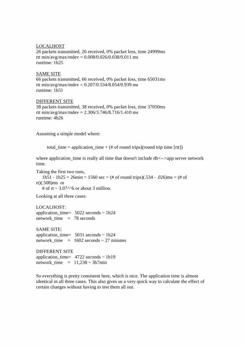
LOCALHOST 26 packets transmitted, 26 received, 0% packet loss, time 24999ms rtt min/avg/max/mdev = 0.008/0.026/0.038/0.011 ms runtime: 1h25 SAME SITE 66 packets transmitted, 66 received, 0% packet loss, time 65031ms rtt min/avg/max/mdev = 0.207/0.534/8.054/0.939 ms runtime: 1h51 DIFFERENT SITE 38 packets transmitted, 38 received, 0% packet loss, time 37050ms rtt min/avg/max/mdev = 2.306/3.746/8.716/1.410 ms runtime: 4h26

Assuming a simple model where:

total_time = application_time + (# of round trips)(round trip time [rtt]) where application_time is really all time that doesn't include db<-->app server network time.

Taking the first two runs, 1h51 - 1h25 = 26min = 1560 sec = (# of round trips)(.534 - .026)ms = (# of rt)(.508)ms or # of rt ~ 3.07^^6 or about 3 million.

Looking at all three cases: LOCALHOST: application_time= 5022 seconds ~ 1h24 network_time = 78 seconds SAME SITE: application_time= 5031 seconds ~ 1h24 network_time = 1602 seconds ~ 27 minutes DIFFERENT SITE application_time= 4722 seconds ~ 1h19 network_time = 11,238 ~ 3h7min

So everything is pretty consistent here, which is nice. The application time is almost identical in all three cases. This also gives us a very quick way to calculate the effect of certain changes without having to test them all out.

The one extra piece that would be nice is to measure the number of round trips (not hard to do) and see how that compares to our 'effective round trips' calculation. When we did a 10046 trace and counted the number of round trips (SQL*Net message to/from client) we found ~2.2 million round trips which isn’t bad considering the simplicity of our model.

So a lot of our time is spent in the network. The rest is split fairly evenly between the application server and the database server (you can’t tell this from here, but additional runs suggested this split). It was decided that it would be too time consuming to tune these test scripts, so we were left with parallelization.

Could we handle this? How could we find out? We have a test server which runs different test sets concurrently, including the precheckin test we want to speed up. Looking at full database statistics would not help us in this case. We needed to focus on the specific, precheckin test set.

Tanel Poder’s sesspack (Ref. 2) was used for this as it lets us focus statistic gathering and analysis at the session level. Each precheckin test set is run by a single, random user with many session logons and logoffs, some concurrent. We used logon and logoff triggers to generate the sesspack snapshots.

Resource utilization over the course of each test set was determined (Fig. 17). INT_IN_SEC CPU (cs) read IOs nw IO bytes PIO b ytes PIO reads PIO writes DB time (cs) cpu-sec per sec Mb per sec IOPS

---------- ---------- ---------- ----------- ------ ---- ---------- ---------- ------------ ----------- ---- ---------- ----------

38782 120706 5681 1.7510E+11 1.7510 E+11 396217 13723 397022 .30402 8492 44.1040516 103.253724 72356 151986 6915 1.7834E+11 1.7834 E+11 439485 13495 1077544 .14104 8533 16.550948 42.0381906 59616 135982 6808 1.7894E+11 1.7894 E+11 430291 13722 891543 .15252 4331 20.0703371 49.8027577 53346 132526 7515 1.8049E+11 1.8049 E+11 432748 13755 683642 .19385 2923 26.4011879 65.3124003 74303 156590 7255 1.8205E+11 1.8205 E+11 456390 13715 1002211 .15624 4543 18.1649214 46.9067891

Fig. 17 : Resource utilization for precheckin test sets (SQL script in appendix)

A few comments about these results:

• the total amount of resources used in a run is fairly constant (i.e. IO bytes, PIO, CPU)

• DB Time varies from ~4,000 – 11,000 seconds • The total interval_in_seconds seems high for 3 hour runs. This is because our

application has multiple sessions logged in simultaneously. • Resource utilization is normalized by DB Time. This yields the resources used

while the database is busy. • Since DB Time can increase based on the load on the system (much of it caused

by other test sets), our results are only a floor. Runs with smaller values of DB Time yield more accurate assessments.

• Utilization spikes are averaged out and can be missed. • One test thread uses at least

o .3 cpu-sec per sec o 44 MB per sec o 103 iops

So using a parallelization of 5 threads would require 1.5 CPU (plus that needed for normal Oracle processes), 220MB/sec throughput, and 500 iops (~4 disks). Further parallelization tests confirmed these numbers.

Even though this was a system running multiple tests with multiple workloads, we could isolate, to some degree, sessions running specific tests of interest.

What if I care about the total system running a mixed workload? I might want to tune one piece of our application, or project resource utilization if some loads grow faster than others. That leads to our last example.

Case 3 resource utilization of multiple sessions in a multi-session environment

For this experiment, we had pounder running against a 4 node RAC database. All agents were connecting only to nodes 1 and 2. Additional work (i.e Advanced Queueing) was also taking place on these nodes.

Let’s start by looking at the system as a whole. We ran Pounder at seven different loads, the number of agents being 8,16,30,40, 64,80 and 96.Restricting our output to the snapshots of interest we see:

SNAP_ID BEGIN_INTERVAL_TIME INST# DB time ss DB time Q user commits user commits per hr redo bytes/txn PIO (bl k rd)/txn PIO (IO call rd)/txn PIO (blk wrt)/txn L IO/txn R(sec)

------- ------------ ------- --------- ------- - -- ---------- ------------- ------------ ---- ------ ----- ------- ------------ ----- -----

8176 08-JAN-10 11.54.03.899 AM 1 59,574 9,95 3 7.7 105,353 292,421.59 10,626.73 29.18 2.80 3.60 1,202.35 .09 8176 08-JAN-10 11.54.03.932 AM 2 22,266 8,44 0 6.5 81,030 224,736.52 12,850.40 3.38 3.38 2.41 1,245.78 .10 8176 08-JAN-10 11.54.03.926 AM 3 7,112 5,11 4 3.9 49,629 137,645.92 17,848.41 5.58 5.57 4.12 599.86 .10 8176 08-JAN-10 11.54.03.926 AM 4 2,472 18 7 .1 658 1,824.96 61,517.79 6.66 6.66 15.8 1,844.41 .28 8179 08-JAN-10 12.30.03.679 PM 1 55,699 18,71 1 16.4 169,773 537,067.49 11,217.52 17.69 1.60 2.93 1,222.56 .11 8179 08-JAN-10 12.30.03.710 PM 2 22,703 15,51 1 13.6 136,152 430,709.31 12,573.68 2.16 1.85 1.80 1,238.88 .11 8179 08-JAN-10 12.30.03.706 PM 3 7,884 6,24 9 5.5 87,162 275,732.16 15,978.50 1.32 1.32 2.53 527.48 .07 8179 08-JAN-10 12.30.03.706 PM 4 2,373 42 6 .4 1,142 3,612.65 60,945.00 11.82 11.82 9.36 3,689.16 .37 8182 08-JAN-10 01.51.01.987 PM 1 46,636 1,98 6 1.8 46,796 153,990.49 10,270.79 61.10 .92 1.99 1,125.09 .04 8182 08-JAN-10 01.51.02.018 PM 2 14,281 1,29 3 1.2 30,056 98,995.06 14,536.44 1.49 1.49 2.64 1,273.85 .04 8182 08-JAN-10 01.51.02.015 PM 3 2,633 45 8 .4 18,590 61,229.64 25,492.97 2.59 2.57 5.71 636.24 .02 8182 08-JAN-10 01.51.02.014 PM 4 2,102 8 6 .1 1,201 3,955.72 34,467.88 1.92 1.92 4.05 3,365.30 .07 8184 08-JAN-10 02.25.30.894 PM 1 42,893 4,02 1 3.7 74,994 249,980.00 10,197.21 38.51 1.19 2.01 1,119.32 .05 8184 08-JAN-10 02.25.30.926 PM 2 15,863 3,06 7 2.8 51,007 169,866.05 13,900.74 2.74 2.74 2.66 1,445.93 .06 8184 08-JAN-10 02.25.30.922 PM 3 2,814 77 5 .7 29,428 98,002.59 21,178.00 1.74 1.73 4.52 613.42 .03 8184 08-JAN-10 02.25.30.922 PM 4 2,159 11 9 .1 767 2,554.30 68,926.28 5.37 5.37 7.86 3,390.76 .16 8186 08-JAN-10 02.50.28.668 PM 1 66,617 6,35 6 4.1 107,292 248,073.99 10,315.89 27.20 1.11 2.46 1,151.22 .06 8186 08-JAN-10 02.50.28.701 PM 2 22,818 4,55 3 2.9 74,426 172,083.24 13,617.37 1.25 1.25 3.17 1,359.64 .06 8186 08-JAN-10 02.50.28.698 PM 3 4,032 1,44 6 .9 44,208 102,215.03 19,315.75 1.19 1.18 4.66 560.01 .03 8186 08-JAN-10 02.50.28.697 PM 4 2,915 18 0 .1 1,054 2,436.99 67,016.62 6.40 6.40 6.74 3,945.12 .17 8351 11-JAN-10 05.15.18.192 PM 1 52,056 16,34 4 15.1 147,719 491,032.69 11,149.27 1.11 1.11 2.08 1,424.63 .11 8351 11-JAN-10 05.15.18.234 PM 2 19,355 10,01 1 9.2 116,797 387,886.72 12,865.96 1.23 1.23 1.95 1,325.29 .09 8351 11-JAN-10 05.15.18.230 PM 3 4,702 2,65 1 2.4 69,530 230,911.44 17,208.47 .57 .57 3.10 503.91 .04 8351 11-JAN-10 05.15.18.230 PM 4 2,505 25 5 .2 1,026 3,407.38 80,837.67 7.16 7.16 8.78 3,813.58 .25 8355 11-JAN-10 05.48.06.312 PM 1 59,916 24,00 4 21.6 165,193 535,278.85 11,309.60 2.02 1.37 1.99 1,409.87 .15 8355 11-JAN-10 05.48.06.347 PM 2 31,024 23,87 9 21.5 132,940 430,768.68 12,843.48 1.17 1.17 1.76 1,407.52 .18 8355 11-JAN-10 05.48.06.341 PM 3 6,409 4,45 1 4.0 80,615 261,218.72 16,386.19 .45 .45 2.97 499.97 .06 8355 11-JAN-10 05.48.06.342 PM 4 2,294 14 6 .1 440 1,425.74 137,424.65 5.19 5.19 13.66 2,439.82 .33

Fig. 18: resource utilizaton on a 4 node RAC loaded using pounder. Note the two different DBTime values, one from sysstat and from sys_time_model

Note the large differences in DB Time (and hence Q) obtained from sysstat as opposed to sys_time_model. Up to this point I have been using sysstat, though sys_time_model will be more accurate. It is a good idea to switch. There is a good description of the difference between sysstat and system_time_model measurements on Jonathan Lewis’ blog (http://jonathanlewis.wordpress.com/2009/05/26/cpu-used/). Our sesspack data, which uses sesstat, can help us find some sources of the discrepency.

Running sesspack on each node gives us a resource breakdown for different session types USERNAME PROGRAM INST_ID int_in_sec CPU user commits DB time (cs) cpu-sec p er sec -------- ----------------------------- - ------ ---------- --- ---------- -- ------------ --------------- RES JDBC Thin Client 1 51443 19429 30021 3985865 .004874475 emagent@pol7orc005 (TNS V1-V3)

perl@pol7pnd001 (TNS V1-V3) 96 6568 1 6621 .991995167 python2.5@pol7mr002 (TNS V1-V3) 4510 1197 2215 296772 .004033399 qres-ccl@pol7qredit003 (TNS V1-V3) 34993 2946 5790 13648 .215855803 qres-ccl@pol7qredit004 (TNS V1-V3) 34568 2936 5698 13434 .218549948 qres-ccl@pol7qrs001 (TNS V1-V3) 17108 12071 4105 29580 .408079784 qres-ccl@pol7qrs002 (TNS V1-V3) 17539 12063 4118 30988 .389279721 qres-ccl@pol7qrs003 (TNS V1-V3) 18130 12308 4185 32856 .374604334 qres-ccl@pol7qrs004 (TNS V1-V3) 17089 12060 4078 30911 .390152373

Fig. 19: snippet of session based data obtained from sesspack tables.

We have a few different types of sessions connecting as the RES user. We have JDBC Thin Client which is our AQ, qrs001, qrs002, … which are our agents, and other work listed as qredit and mr.

We see from Figure 19 that JDBC Thin Client is the source of the extra DB time associated with the sysstat and sesstat data.

Using this information we can now plot throughput and residence time for the entire system (use pounder data), for the database (see Fig 18), and for each session type on each node. For this case there is not much differentiation between our session types, so not much insight will be obtained from the plots.

In the future, I would like to rerun this using sessions with very different characteristics (i.e heavy CPU, heavy IO).

This can be carried even further, allowing drill down into the Oracle events to further differentiate session Residence times.

Appendix SQL statements used in this paper.

Script for Fig. 4 set linesize 200 set pagesize 200 column "DB time" format 999,999,999,999 column "user commits" format 999,999,999,999 column "redo size" format 999,999,999,999 column begin_interval_time format a35 column "# of pnrs" format 999,999 column Q format 999.9 column "pnrs per hr" format 999,999 column commits/pnr format 999.99 column "redo bytes/pnr" format 999,999,999.99 column "PIO (blk rd)/pnr" format 999,999,999.99 column "PIO (IO call rd)/pnr" format 999,999,999.99 column "PIO (blk wrt)/pnr" format 999,999,999.99 column "LIO/pnr" format 999,999,999.99 column "R(sec)" format 99.99 with stats as ( SELECT ss.snap_id, snp.BEGIN_INTERVAL_TIME, snp.END_INTERVAL_TIME, (to_date(to_char(snp.END_INTERVAL_TIME,'dd-mon-yy h h24:mi:ss'),'dd-mon-yy hh24:mi:ss')-to_date(to_char(snp.BEGIN_INTERVAL_ TIME,'dd-mon-yy hh24:mi:ss'),'dd-mon-yy hh24:mi:ss'))*24*3600 elaps ed_time_sec, case when sn.stat_name='DB time' then ss.value-lag(ss.value,1) over (partition by ss.st at_id, ss.dbid, ss.instance_number order by ss.snap_id) end dbtime, case when sn.stat_name='user commits' then ss.value-lag(ss.value,1) over (partition by ss.st at_id, ss.dbid, ss.instance_number order by ss.snap_id) end usercommits, case when sn.stat_name='redo size' then ss.value-lag(ss.value,1) over (partition by ss.st at_id, ss.dbid, ss.instance_number order by ss.snap_id) end redosize, case when sn.stat_name='physical reads' then ss.value-lag(ss.value,1) over (partition by ss.st at_id, ss.dbid, ss.instance_number order by ss.snap_id) end physrdblk, case when sn.stat_name='physical read IO requests' then ss.value-lag(ss.value,1) over (partition by ss.st at_id, ss.dbid, ss.instance_number order by ss.snap_id) end physrdcalls, case when sn.stat_name='physical writes' then ss.value-lag(ss.value,1) over (partition by ss.st at_id, ss.dbid, ss.instance_number order by ss.snap_id) end physwrtblk,

case when sn.stat_name='session logical reads' the n ss.value-lag(ss.value,1) over (partition by ss.st at_id, ss.dbid, ss.instance_number order by ss.snap_id) end lio FROM wrh$_stat_name sn, wrh$_sysstat ss, wrm$_snaps hot snp WHERE snp.dbid=ss.dbid and snp.instance_number = ss.instance_number and snp.snap_id = ss.snap_id and sn.stat_id = ss.stat_id and sn.dbid = ss.dbid and sn.stat_name in ('DB time','redo size','user commits','physical reads','physical read IO requests','physical writes ','session logical reads') -- and sn.dbid = 261596549 -- and snp.snap_id between 331 and 657 ) SELECT begin_interval_time, -- "DB time", -- "user commits", -- "redo size", -- "phys reads (blk)", -- "phys reads (IO calls)", -- "phys wrt (blk)", -- "logical reads", "# of pnrs", "# of workers", "DB time"/(elapsed_time_sec) Q, "# of pnrs"*3600/elapsed_time_sec "pnrs per hr", "user commits"/"# of pnrs" "commits/pnr", "redo size"/"# of pnrs" "redo bytes/pnr", "phys reads (blk)"/"# of pnrs" "PIO (blk rd)/pnr" , "phys reads (IO calls)"/"# of pnrs" "PIO (IO call rd)/pnr", "phys wrt (blk)"/"# of pnrs" "PIO (blk wrt)/pnr", "logical reads"/"# of pnrs" "LIO/pnr", "DB time"/("# of pnrs") "R(sec)" FROM ( SELECT snap_id, begin_interval_time, "DB time"/100 "DB time", "user commits", "redo size", "phys reads (blk)", "phys reads (IO calls)", "phys wrt (blk)", "logical reads", count(pp.pnr_id) "# of pnrs", count(distinct(pp.migration_worker)) "# of work ers", elapsed_time_sec FROM ( SELECT snap_id, begin_interval_time,

end_interval_time, max(dbtime) "DB time", max(usercommits) "user commits", max(redosize) "redo size", max(physrdblk) "phys reads (blk)", max(physrdcalls) "phys reads (IO calls)", max(physwrtblk) "phys wrt (blk)", max(lio) "logical reads", elapsed_time_sec FROM stats GROUP BY snap_id,begin_interval_time, end_inter val_time, elapsed_time_sec ) s, glocks.puma_pnrs pp WHERE pp.migration_timestamp >= s.begin_interval_time and pp.migration_timestamp < s.end_interval_time GROUP BY snap_id, begin_interval_time, "DB time" ,"user commits","redo size","phys reads (blk)","phys reads (IO calls)","phys wrt (blk)","logical reads",elapsed_time_sec ) ORDER BY snap_id /

Script for Fig. 13 set linesize 200 set pagesize 200 column begin_interval_time format a35 column "DB time" format 999,999,999,999 column Q format 999.9 column "user commits" format 999,999,999 column "user commits per hr" format 999,999,999.99 column "redo bytes/txn" format 999,999,999.99 column "PIO (blk rd)/txn" format 999,999,999.99 column "PIO (IO call rd)/txn" format 999,999,999.99 column "PIO (blk wrt)/txn" format 999,999,999.99 column "LIO/txn" format 999,999,999.99 column "R(sec)" format 99.99 with stats as ( SELECT ss.snap_id, snp.instance_number, snp.BEGIN_INTERVAL_TIME, snp.END_INTERVAL_TIME, (to_date(to_char(snp.END_INTERVAL_TIME,'dd-mon-yy h h24:mi:ss'),'dd-mon-yy hh24:mi:ss')-to_date(to_char(snp.BEGIN_INTERVAL_ TIME,'dd-mon-yy hh24:mi:ss'),'dd-mon-yy hh24:mi:ss'))*24*3600 elaps ed_time_sec, case when sn.stat_name='DB time' then ss.value-lag(ss.value,1) over (partition by ss.s tat_id, ss.dbid, ss.instance_number order by ss.snap_id) end dbtime, case when sn.stat_name='user commits' then

ss.value-lag(ss.value,1) over (partition by ss.s tat_id, ss.dbid, ss.instance_number order by ss.snap_id) end usercommits, case when sn.stat_name='redo size' then ss.value-lag(ss.value,1) over (partition by ss.s tat_id, ss.dbid, ss.instance_number order by ss.snap_id) end redosize, case when sn.stat_name='physical reads' then ss.value-lag(ss.value,1) over (partition by ss.s tat_id, ss.dbid, ss.instance_number order by ss.snap_id) end physrdblk, case when sn.stat_name='physical read IO requests ' then ss.value-lag(ss.value,1) over (partition by ss.s tat_id, ss.dbid, ss.instance_number order by ss.snap_id) end physrdcalls, case when sn.stat_name='physical writes' then ss.value-lag(ss.value,1) over (partition by ss.s tat_id, ss.dbid, ss.instance_number order by ss.snap_id) end physwrtblk, case when sn.stat_name='session logical reads' th en ss.value-lag(ss.value,1) over (partition by ss.s tat_id, ss.dbid, ss.instance_number order by ss.snap_id) end lio FROM wrh$_stat_name sn, wrh$_sysstat ss, wrm$_snap shot snp WHERE snp.dbid=ss.dbid and snp.instance_number = ss.instance_number and snp.snap_id = ss.snap_id and sn.stat_id = ss.stat_id and sn.dbid = ss.dbid and sn.stat_name in ('DB time','redo size','user comm its','physical reads','physical read IO requests','physical writes ','session logical reads') -- and sn.dbid = 261596549 -- and snp.snap_id between 234 and 305 ) SELECT begin_interval_time, instance_number inst#, "DB time", "DB time"/(elapsed_time_sec*100) Q, "user commits", "user commits"*3600/elapsed_time_sec "user commit s per hr", "redo size"/"user commits" "redo bytes/txn", "phys reads (blk)"/"user commits" "PIO (blk rd)/t xn", "phys reads (IO calls)"/"user commits" "PIO (IO c all rd)/txn", "phys wrt (blk)"/"user commits" "PIO (blk wrt)/tx n", "logical reads"/"user commits" "LIO/txn", "DB time"/("user commits"*100) "R(sec)" FROM ( SELECT snap_id, instance_number, begin_interval_time, "DB time"/100 "DB time", "user commits",

"redo size", "phys reads (blk)", "phys reads (IO calls)", "phys wrt (blk)", "logical reads", elapsed_time_sec FROM ( SELECT snap_id, instance_number, begin_interval_time, end_interval_time, max(dbtime) "DB time", max(usercommits) "user commits", max(redosize) "redo size", max(physrdblk) "phys reads (blk)", max(physrdcalls) "phys reads (IO calls)", max(physwrtblk) "phys wrt (blk)", max(lio) "logical reads", elapsed_time_sec FROM stats GROUP BY snap_id,instance_number,begin_interva l_time, end_interval_time, elapsed_time_sec ) s ) -- where begin_interval_time>sysdate-3 -- and begin_interval_time<sysdate-12/24 ORDER BY instance_number, snap_id /

Script for Fig. 16 break on snap_id skip 1 column buffer_gets_delta format 999,999,999,999 column begin_interval_time format a30 column sql_id format a15 column sql_text format a85 set linesize 200 set pagesize 125 set long 80 select snap_id, begin_interval_time, sql_id, buffer _gets_delta, substr((sql_text),1,75) sql_text from ( select ss.snap_id, snp.begin_interval_time, ss.sql_ id, ss.buffer_gets_delta, st.sql_text, dense_rank() ov er (partition by ss.snap_id order by ss.buffer_gets_delta desc) dr from wrh$_sqlstat ss, wrh$_sqltext st, wrm$_snapsh ot snp where snp.dbid=ss.dbid and snp.instance_number=ss.instance_number and snp.snap_id=ss.snap_id and

ss.dbid=st.dbid (+) and -- ss.snap_id=st.snap_id (+) and ss.sql_id=st.sql_id (+) --and snp.dbid=261596549 --and snp.snap_id between 234 and 305 ) where dr<=15 -- and begin_interval_time<sysdate-5 order by snap_id, dr /

Script for Fig. 17 alter session set nls_date_format='DD-MON-YYYY HH24 :MI:SS'; with stats as ( select ss.snapid, ss.sid, ss.serial#, ss.audsid, case when name = 'CPU used by this session' then value end CPU, case when name = 'Number of read IOs issued' then value end readIOs, case when name = 'cell physical IO interconnec t bytes' then value end nwIObytes, case when name = 'physical IO disk bytes' then value end PIObytes, case when name = 'physical read IO requests' then value end PIOreads, case when name = 'physical write IO requests' then value end PIOwrites, case when name = 'DB time' then value end DBtime from sawr$session_stats ss, v$statname sn where ss.statistic# = sn.statistic# AND sn.name in ('CPU used by this session','Number of read IOs issued','cell physical IO interconnect bytes','phys ical IO disk bytes','physical read IO requests','physical write IO requests','DB time') ), snapid as ( select username,

serial#, machine, sid, audsid, snapid_i, snapid_f, snaptime_i, snaptime_f, to_char(snaptime_f,'SSSSS') - to_char (snaptime_i,'SSSSS') + 24*60*60*(to_char(snaptime_f,'J') - to_char(snapt ime_i,'J')) int_in_sec, -- inst_id, i, f from ( select s.username, s.serial#, s.machine, s.sid, s.audsid, s.snapid snapid_f, s.snaptime snaptime_f, -- s.inst_id, ss.snap_comment f, lag(ss.snap_comment,1) over (parti tion by s.username,s.serial#,s.machine,s.sid order by s.sna ptime) i, lag(ss.snapid,1) over (partition b y s.username,s.serial#,s.machine,s.sid order by s.sna ptime) snapid_i, lag(ss.snaptime,1) over (partition by s.username,s.serial#,s.machine,s.sid order by s.sna ptime) snaptime_i from sawr$sessions s, sawr$snapshots ss where username in ('GNWG','I1DT','X0JK','DN6X','GUAC','Q5J3','F18A',' D0J2','Y9PU','H8QX') AND -- username in ('JG0Q','MVDH') AND ss.snap_mode<>'SNAP_BG:' AND ss.snapid=s.snapid ) where i='LOGON' AND f = 'LOGOFF' AND snapid_f > snapid_i ) select username, sum(int_in_sec) int_in_sec, sum(CPU) "CPU (cs)", sum("read IOs") "read IOs", sum("nw IO bytes") "nw IO bytes", sum("PIO bytes") "PIO bytes", sum("PIO reads") "PIO reads", sum("PIO writes") "PIO writes", sum("DB time") "DB time (cs)", sum(CPU)/sum("DB time") "cpu-sec per sec",

sum("PIO bytes")/(sum("DB time")*10000) "Mb per se c", (sum("PIO reads") + sum("PIO writes"))*100/sum("DB time") "IOPS" from ( select snapid.username, snapid.sid, snapid.serial#, snapid.snapid_i, snapid.snapid_f, snapid.int_in_sec, -- snapid.inst_id, max(nvl(stats_f.CPU,0) - nvl(stats_i.CPU,0)) CPU, max(nvl(stats_f.readIOs,0) - nvl(stats_i.readIOs, 0)) "read IOs", max(nvl(stats_f.nwIObytes,0) - nvl(stats_i.nwIOby tes,0)) "nw IO bytes", max(nvl(stats_f.PIObytes,0) - nvl(stats_i.PIObyte s,0)) "PIO bytes", max(nvl(stats_f.PIOreads,0) - nvl(stats_i.PIOread s,0)) "PIO reads", max(nvl(stats_f.PIOwrites,0) - nvl(stats_i.PIOwri tes,0)) "PIO writes", max(nvl(stats_f.DBtime,0) - nvl(stats_i.DBtime,0) ) "DB time" from snapid, stats stats_i, stats stats_f where snapid.snapid_i = stats_i.snapid AND snapid.snapid_f = stats_f.snapid AND snapid.sid = stats_i.sid AND snapid.sid = stats_f.sid AND snapid.serial# = stats_i.serial# AND snapid.serial# = stats_f.serial# AND snapid.audsid = stats_i.audsid AND snapid.audsid = stats_f.audsid group by snapid.username, snapid.sid, snapid.serial#, snapid.snapid_i, snapid.snapid_f, snapid.int_in_sec ) group by username order by 6 /

Script for Fig. 18 set linesize 250 set pagesize 200 column begin_interval_time format a35 column "DB time" format 999,999,999,999 column "DB time ss" format 999,999,999,999

column Q format 999.9 column "user commits" format 999,999,999 column "user commits per hr" format 999,999,999.99 column "redo bytes/txn" format 999,999,999.99 column "PIO (blk rd)/txn" format 999,999,999.99 column "PIO (IO call rd)/txn" format 999,999,999.99 column "PIO (blk wrt)/txn" format 999,999,999.99 column "LIO/txn" format 999,999,999.99 column "R(sec)" format 99.99 with stats as ( SELECT ss.snap_id, snp.instance_number, snp.BEGIN_INTERVAL_TIME, snp.END_INTERVAL_TIME, (to_date(to_char(snp.END_INTERVAL_TIME,'dd-mon-yy h h24:mi:ss'),'dd-mon-yy hh24:mi:ss')-to_date(to_char(snp.BEGIN_INTERVAL_ TIME,'dd-mon-yy hh24:mi:ss'),'dd-mon-yy hh24:mi:ss'))*24*3600 elaps ed_time_sec, case when sn.stat_name='DB time' then ss.value-lag(ss.value,1) over (partition by ss.s tat_id, ss.dbid, ss.instance_number order by ss.snap_id) end dbtime_ss, null dbtime, case when sn.stat_name='user commits' then ss.value-lag(ss.value,1) over (partition by ss.s tat_id, ss.dbid, ss.instance_number order by ss.snap_id) end usercommits, case when sn.stat_name='redo size' then ss.value-lag(ss.value,1) over (partition by ss.s tat_id, ss.dbid, ss.instance_number order by ss.snap_id) end redosize, case when sn.stat_name='physical reads' then ss.value-lag(ss.value,1) over (partition by ss.s tat_id, ss.dbid, ss.instance_number order by ss.snap_id) end physrdblk, case when sn.stat_name='physical read IO requests ' then ss.value-lag(ss.value,1) over (partition by ss.s tat_id, ss.dbid, ss.instance_number order by ss.snap_id) end physrdcalls, case when sn.stat_name='physical writes' then ss.value-lag(ss.value,1) over (partition by ss.s tat_id, ss.dbid, ss.instance_number order by ss.snap_id) end physwrtblk, case when sn.stat_name='session logical reads' th en ss.value-lag(ss.value,1) over (partition by ss.s tat_id, ss.dbid, ss.instance_number order by ss.snap_id) end lio FROM wrh$_stat_name sn, wrh$_sysstat ss, wrm$_snap shot snp WHERE snp.dbid=ss.dbid and snp.instance_number = ss.instance_number and snp.snap_id = ss.snap_id and sn.stat_id = ss.stat_id and sn.dbid = ss.dbid and sn.stat_name in ('DB time','redo size','user comm its','physical reads','physical read IO requests','physical writes ','session logical reads')

-- and sn.dbid = 3178717885 -- and snp.snap_id > 8100 -- and snp.snap_id between 234 and 305 UNION SELECT stm.snap_id, stm.instance_number, snp.begin_interval_time, snp.end_interval_time, (to_date(to_char(snp.END_INTERVAL_TIME,'dd-mon-yy hh24:mi:ss'),'dd-mon-yy hh24:mi:ss')-to_date(to_char(snp.BEGIN_INTER VAL_TIME,'dd-mon-yy hh24:mi:ss'),'dd-mon-yy hh24:mi:ss'))*24*3600 elaps ed_time_sec, null dbtime_ss, stm.value - lag(stm.value,1) over (partition by s tm.dbid, stm.instance_number, stm.stat_id order by stm.snap_ id) "dbtime", null usercommits, null redosize, null physrdblk, null physrdcalls, null physwrtblk, null lio FROM dba_hist_sys_time_model stm, dba_hist_snapsho t snp WHERE snp.dbid=stm.dbid and snp.instance_number=stm.instance_number and snp.snap_id=stm.snap_id -- and stm.dbid = 3178717885 -- and stm.snap_id > 8100 -- and snap_id between 234 and 305 and stm.stat_name = 'DB time' ) SELECT snap_id, begin_interval_time, instance_number inst#, "DB time ss", "DB time", "DB time"/(case when elapsed_time_sec=0 then -1 e lse elapsed_time_sec end) Q, "user commits", "user commits"*3600/(case when elapsed_time_sec=0 then -1 else elapsed_time_sec end) "user commits per hr", "redo size"/(case when "user commits"=0 then -1 e lse "user commits" end) "redo bytes/txn", "phys reads (blk)"/(case when "user commits"=0 th en -1 else "user commits" end) "PIO (blk rd)/txn", "phys reads (IO calls)"/(case when "user commits" =0 then -1 else "user commits" end) "PIO (IO call rd)/txn", "phys wrt (blk)"/(case when "user commits"=0 then -1 else "user commits" end) "PIO (blk wrt)/txn", "logical reads"/(case when "user commits"=0 then -1 else "user commits" end) "LIO/txn", "DB time"/((case when "user commits"=0 then -1 el se "user commits" end)) "R(sec)" FROM ( SELECT

snap_id, instance_number, begin_interval_time, "DB time ss"/100 "DB time ss", "DB time"/1000000 "DB time", "user commits", "redo size", "phys reads (blk)", "phys reads (IO calls)", "phys wrt (blk)", "logical reads", elapsed_time_sec FROM ( SELECT snap_id, instance_number, begin_interval_time, end_interval_time, max(dbtime_ss) "DB time ss", max(dbtime) "DB time", max(usercommits) "user commits", max(redosize) "redo size", max(physrdblk) "phys reads (blk)", max(physrdcalls) "phys reads (IO calls)", max(physwrtblk) "phys wrt (blk)", max(lio) "logical reads", elapsed_time_sec FROM stats GROUP BY snap_id,instance_number,begin_interva l_time, end_interval_time, elapsed_time_sec ) s ) -- where begin_interval_time>sysdate-3 -- and begin_interval_time<sysdate-12/24 ORDER BY snap_id, instance_number /

Script for Fig 19 set pagesize 200 linesize 250 break on username on inst_id skip 1 compute sum label total of "DB time (cs)" on userna me inst_id alter session set nls_date_format='DD-MON-YYYY HH24 :MI:SS'; with stats as ( select ss.snapid, ss.sid, ss.serial#, ss.audsid, case when name = 'CPU used by this session' then value end CPU,

case when name = 'Number of read IOs issued' then value end readIOs, case when name = 'cell physical IO interconnec t bytes' then value end nwIObytes, case when name = 'physical IO disk bytes' then value end PIObytes, case when name = 'physical read IO requests' then value end PIOreads, case when name = 'physical write IO requests' then value end PIOwrites, case when name = 'user commits' then value end ucommits, case when name = 'DB time' then value end DBtime from sawr$session_stats ss, v$statname sn where ss.statistic# = sn.statistic# AND sn.name in ('CPU used by this session','Number of read IOs issued','cell physical IO interconnect bytes','phys ical IO disk bytes','physical read IO requests','physical write IO requests','user commits','DB time') ), snapid as ( select s.username, s.serial#, s.machine, s.program, s.sid, s.audsid, s.snapid, s.snaptime, s.inst_id from sawr$sessions s, sawr$snapshots ss where -- ss.snap_mode<>'SNAP_BG:' and ss.snapid=s.snapid and -- -- mapping sesspack to known interval of Pounder ru n -- ss.snaptime >= (select begin_interval _time from dba_hist_snapshot dhs where snap_id = 8355 and dbid =3178717885 and instance_number=1) and ss.snaptime <= (select end_interval_t ime from dba_hist_snapshot where snap_id=8355 and dbid=31787 17885 and instance_number=1) -- (ss.snapid = 783923 or ss.snapid = 784626) )

select username, program, inst_id, sum(int_in_sec) "int_in_sec", sum(CPU) "CPU", -- sum("nw IO bytes") "nw IO bytes", -- sum("PIO bytes") "PIO bytes", -- sum("PIO reads") "PIO reads", -- sum("PIO writes") "PIO writes", sum("user commits") "user commits", sum("DB time") "DB time (cs)", sum(CPU)/(case when sum("DB time")=0 then -1 else sum("DB time") end) "cpu-sec per sec" -- sum("PIO bytes")/(case when (sum("DB time")*1000 0)=0 then -1 else (sum("DB time")*10000)) "Mb per sec", -- (sum("PIO reads") + sum("PIO writes"))*100/(case when sum("DB time")=0 then -1 else sum("DB time")) "IOPS" from ( select username, sid, serial#, snapid, snaptime, audsid, program, inst_id, CPU - lag(CPU,1) over (partition by username, sid, serial#,audsid, inst_id order by snapid) CPU, "read IOs" - lag("read IOs",1) over (partition by username, sid, serial#,audsid, inst_id order by snapid) "read IOs" , "nw IO bytes" - lag("nw IO bytes",1) over (partiti on by username, sid, serial#,audsid, inst_id order by snapid) "nw IO byt es", "PIO bytes" - lag("PIO bytes",1) over (partition b y username, sid, serial#,audsid, inst_id order by snapid) "PIO bytes ", "PIO reads" - lag("PIO reads",1) over (partition b y username, sid, serial#,audsid, inst_id order by snapid) "PIO reads ", "PIO writes" - lag("PIO writes",1) over (partition by username, sid, serial#,audsid, inst_id order by snapid) "PIO write s", "user commits" - lag("user commits",1) over (parti tion by username, sid, serial#,audsid, inst_id order by snapid) "user commits", "DB time" - lag("DB time",1) over (partition by us ername, sid, serial#,audsid, inst_id order by snapid) "DB time", to_char(snaptime,'SSSSS') - to_char(lag(snaptime,1 ) over (partition by username, sid, serial#,audsid, inst_id order by sna pid),'SSSSS') + 24*60*60*(to_char(snaptime,'J') - to_char(lag(snapt ime,1) over (partition by username, sid, serial#,audsid, inst_i d order by snapid),'J')) int_in_sec -- sum("read IOs") "read IOs", -- sum("nw IO bytes") "nw IO bytes", -- sum("PIO bytes") "PIO bytes", -- sum("PIO reads") "PIO reads", -- sum("PIO writes") "PIO writes", -- sum("user commits") "user commits", -- sum("DB time") "DB time (cs)",

-- sum(CPU)/(case when sum("DB time")=0 then -1 els e sum("DB time") end) "cpu-sec per sec" -- sum("PIO bytes")/(sum("DB time")*10000) "Mb per sec", -- (sum("PIO reads") + sum("PIO writes"))*100/sum(" DB time") "IOPS" from ( select snapid.username, snapid.sid, snapid.serial#, snapid.snapid, snapid.snaptime, snapid.program, snapid.audsid, snapid.inst_id, max(nvl(stats.CPU,0)) CPU, max(nvl(stats.readIOs,0)) "read IOs", max(nvl(stats.nwIObytes,0)) "nw IO bytes", max(nvl(stats.PIObytes,0)) "PIO bytes", max(nvl(stats.PIOreads,0)) "PIO reads", max(nvl(stats.PIOwrites,0)) "PIO writes", max(nvl(stats.ucommits,0)) "user commits", max(nvl(stats.DBtime,0)) "DB time" from snapid, stats where snapid.snapid = stats.snapid(+) AND snapid.sid = stats.sid(+) AND snapid.serial# = stats.serial#(+) AND snapid.audsid = stats.audsid(+) group by snapid.username, snapid.sid, snapid.serial#, snapid.snapid, snapid.snaptime, snapid.program, snapid.audsid, snapid.inst_id ) ) group by username, program, inst_id order by username, inst_id, program /