Determining Project Completion Time and Criticality ...textroad.com/pdf/JAEBS/J. Appl. Environ. Biol. Sci., 5(4S)40-51, 2015.pdfconventional method is used to determine project time

J. Appl. Environ. Biol. Sci., 5(4S)40-51, 2015

© 2015, TextRoad Publication

ISSN: 2090-4274 Journal of Applied Environmental

and Biological Sciences

www.textroad.com

* Corresponding Author: Dr. Mohammad Ali Soukhakian, Department of Management, Science and Research Branch, Islamic Azad University, Fars, Iran

Determining Project Completion Time and Criticality Criteria in PERT

Networks When the Time distribution Function of Activities is Continuous and

Considering Conditional Activities by Soukhakian Algorithm and Its

Comparison with Monte Carlo Simulation Method

Zahra Moghtada1, Dr. Mohammad Ali Soukhakian2,*

1 Department of Management, Science and Research Branch, Islamic Azad University, Fars, Iran

Department of Management, Marvdasht Branch, Islamic Azad University, Marvdasht, Iran 2 Department of Management, Science and Research Branch, Islamic Azad University, Fars, Iran

Received: January 12, 2015

Accepted: March 25, 2015

ABSTRACT

Project control is a process in which to keep project path to achieve economic balance between three factors of cost, time

and quality during the project as acquiring specific tools and techniques in this regard. By project control, we can

perform the project limitations with the lowest cost and sources at shortest time. Classic methods are presented to control

project including:

1) Gantt method1, CPM method2, PERT3

In conventional PERT networks, the project is completed by optimistic, highest occurrence probability and pessimistic

times. A new algorithm is presented by (Soukhakian, M. A. 1988) and by making common activities conditional, the

network is reduced to an activity and time probability distribution function and project completion costs are determined.

This algorithm has five steps. In this algorithm, adding operation is used for combining the times and costs of series

activities and the biggest value selection operation is used only to combine the parallel activities time. Regarding the

parallel cost combination, we can say in case of using the biggest value, cost of an activity is ignored. During

combination of parallel activities cost, to avoid this error, adding can be used. The results of this algorithm can be used

for critical path algorithm and criticality indices of activities.

KEYWORDS: Project control, Gantt method, CPM method, PERT method

1. INTRODUCTION

OR is an interdisciplinary branch of math to find the optimal point in optimization problems of some trends as math

planning, statistics and algorithms design. Finding optimal point is different based on the type of problem and is used in

decisions. (Hajshirmohammadi, Ali. 1994). The research issues in operation mostly focus on maximization as profit,

production line speed, high cultivation production, high bandwidth and etc. or minimization as less cost and risk and etc.

by one or more constraints. The main idea of study in operation is finding the best response for complex problems being

modeled by math model and this improves or optimizes performance of a system. OR has various branches as LP4,

project control and etc. Project control optimizes the model created by a project on time, cost, available sources and etc.

With the growth of OR, computer was developed considerably and now we can observed various software in various

fields. (Burt, J. M. 1971). In PERT model, the cost and time of activities are random variables and these factors cannot be

approximated definitely and we should attempt to approximate really by statistical methods. Thus, time and cost

estimation is done under uncertain conditions. One of the most important issues in PERT networks analysis is

determining distribution function for project completion. If the activities time is random variables, the project completion

time is random variable also and its distribution function is a combination of distribution functions of each activity. In

networks with specific structure, distribution function is with reduction of a network with an activity as starting from

node 1 and ending to node N. By assuming statistical independence of cost and time of network activities, by repetitive

operation of convolution and selection of greatest in network, we can reduce to an equivalent activity. These two actions

are used to combine probable distributions. There are many theories about probability distribution combination and some

of them include simulation analytic methods and numerical methods and etc. If the PERT network satisfies the conditions

necessary for the use of convolution and greatest operations, then the network is termed reducible; otherwise, it is termed

irreducible. If the network is reducible to a single equivalent activity (1, N), then it is termed as completely reducible. In

this case, the analytical form of the distribution function of the project completion time can be determined. (Chapman, C.

B. 1983).

In conventional PERT network models it is assumed that different paths are structurally independent. This is not

true for irreducible networks, because in irreducible networks at least two paths share one or more common activities. For

1Henry Laurence gantt 2Critical Path Method 3program evaluation review technique 4 Linear programming

40

Moghtada and Soukhakian, 2015

example in Wheatstone bridge Figure 1-1 as the simplest irreducible network has three paths. Two of paths (1-2-4) and

(1-3-4) are analyzed directly as they are independent. (Clark, C. E. 1962)

The third path (1-2-3-4) cannot be analyzed directly as there is a common activity between this path and two other paths.

The third path is dependent upon two other paths structurally. (Devroye, L. P. 1979)

Fig. 1. Wheatstone bridge network

Also, in PERT network models, it is assumed the cost and time distribution of completion of one by one of activities

is independent structurally. Indeed, there is a dependency between the activities. The underlying conditions on an activity

cause that the activity has rapid or slow completion time or high or low costs and affect the costs of other activities. In

addition, most of managers attempt to use extra work or advanced equipment for rapid achievement of activities,

receiving reward for completion of project earlier and these increases the costs. Most of the methods presented for

analysis of PERT networks assume that cost and time of activity distributions are independent form structural and

statistical aspects. This assumption is not true regarding the networks with common activities as the effects and structural

dependences are very complex and analytic methods are not suitable to estimate project completion time in these

networks and conditional sampling or Monte Carlo simulation method is used. This paper investigates proposed

Soukhakian (1988) method. By this method, we can determine probability distribution of cost and time of project

completion as discrete or continuous. This method approximates exact probability distribution for costs and time of

activities completion when their time and costs are continuous. These approximations are performed by i) discretization

of continuous distributions, ii) Adding discrete approximations of continuous distribution. (Dodin, B. M. 1980)

2. Statement of problem

Normally, managers perform various operations and duties. Some of them are definite and repetitive activities and

others are different and various activities of projects with uniform and unique operation and are designed to fulfill a set of

specific goals in a limited time framework. Most of management problems can be solved by network-based techniques

and models. (Fulkerson, D. R. 1962)

For problems as construction of dam or bridge or building, determining the shortest or economical transportation

path between two execution situations and using a new marketing computer system, design or production of a new

product, etc. we can use network-based quantitative techniques and models. Now, in most of the projects, PERT

conventional method is used to determine project time and cost completion time due to the assumptions applied in

relevant PERTs but as it was said, regarding the activities and project, we can compute project completion time easily

and adequate precision is not obtained in determining project completion time namely when the networks have many

common activities and these are the examples of real world. This issue causes that practical projects are mostly longer

than it is predicted with high costs. This issue is mostly observed in third world countries. The reasons show that in some

cases, it is uncontrolled or unpredicted or both of them and the project has many uncertainties. (Lindesy, J . H . 1972)

Many examples are mentioned as construction, civil projects, great dam construction, and factory establishing and

similar cases. The innovation aspect of this study shows that due to heavy calculations in applied software, not

recommendation is considered to include constructional and statistical dependencies at the same time and this issue is

included in Soukhakian algorithm and continuous distribution functions are not considered in practical applications.

Indeed, this project. (Garman, M . B . 1972)

Indeed, this project considers the above items for small and applied networks and compares the result with Monte Carlo

simulation method as it is the only existing method for these problems. This study is basic, applied and practical and can

be used as a reliable method for PERT projects.

3. Study method

The proposed method of this study is based on Garman method. By fixing the random variables as in this study in

their occurrence, they can be conditioned and the first step in this method is discretization of continuous distributions.

This theory is based on series-parallel reduction of Martine (1965) in stochastic PERT networks of Ringer (1969) on

specific activity times and conditional sampling of Garman stochastic networks. (Hartley, H. O. and Wortham A .W.

1966)

4. Proposed method

Different methods are presented to determine project completion time as: Analytic methods, approximation methods

and Monte Carlo simulation methods. The new algorithm presented by Soukhakian (1988), by conditionalization of

2

1 4

3

41


common activities, the network can be reduced to an activity and probability distribution function can determine the time

and cost of project completion. (Ringer, L. J. 1969)

In this algorithm, convolution operation is used for combining times and costs of series activities and greatest

operation is used only for combining the time of parallel activities. Regarding cost combination of parallel activities, we

should know that in case of using greatest operation, the cost of an activity is ignored and in case of combining cost of

parallel activities, convolution operation is used to avoid this mistake. (Kamburowski, j. 1985)

Example 1

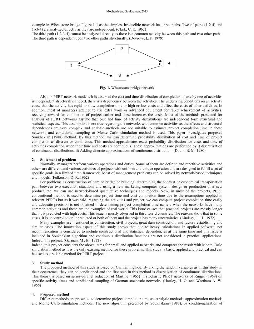
By fixing A realization on 3 and first realization time E on 1, the network of Figure 3-1 is changed to Figure 2 and the

times of all paths are independent.

Fig. 2. Duration of project activities

A1XA 3 8

P 0.8 0.2

E=4 =4

B2XB 6 9

P 0.6 0.4

E= 7.2 =2.16

4 6

P 0.3 0.7

E=5.4 =0.84

4 5

P 0.9 0.1

= 0.09 4.1E=

1 2

P 0.5 0.5

= 0.25 E= 1.5

Pdf of project completion with8 =XA and1 =XE is computed as follows:

Table 2 shows occurrence time D+3, Table 3 realization time (C-1-3) and Table 4 realization time (B+1).

42


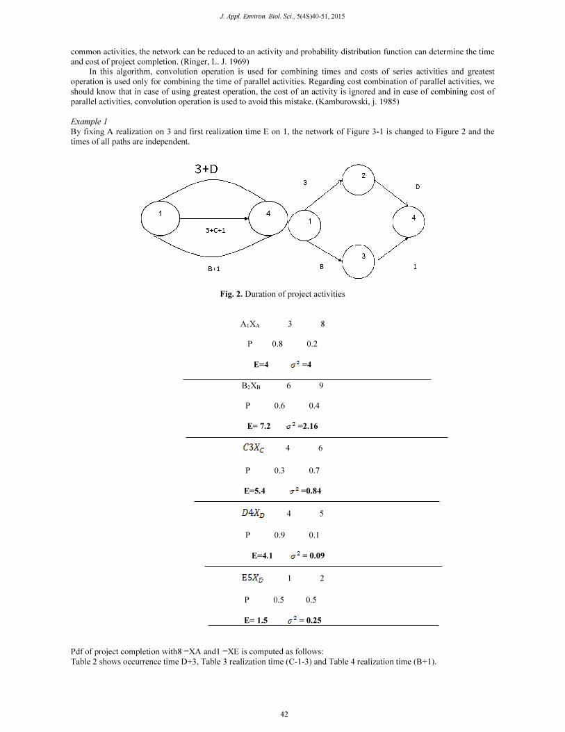
Table 2. Realization time (D+3)

P CP

= 7 0.9 0.9

8 0.1 1

Table 3. Realization time (C+1+3)

P CP

0.3 0.3 =

10 0.7 1

Table 4. Realization time (B+1)

P CP

= 7 0.6 0.6

10 0.4 1

By determining maximum value of these three parallel paths, pdf of project completion time is obtained by 3= 1= as

it is shown in Table 3-5.

Table 5. Project completion time with 3=XA, 1 =XE

EP=8 0.3 * 0.6 = 0.18

10 1 - 0.18 = 0.82

E= 9.64

Similarly, for various conditions, project completion time is computed as above.

Table 6. Project completion time by 3 =XA,2 = XE

EP=9 0.3 * 0.6 =0.18

11 1 - 0.18=0.82

E= 10.64

Table 7. Project completion time by XA=,8XE=1

3.0=1×3.0 EP=13

1-3.0=0.7 15

4.14 E=

Table 8. Project completion time by XA =8, XE=1 3.0 EP=14

7.0 16

4.15 E=

By unconditional pdfs of project completion times of 3 -5 ،3-8،3-11,3-13 Table, pdf is obtained without the condition of

project completion time.

43


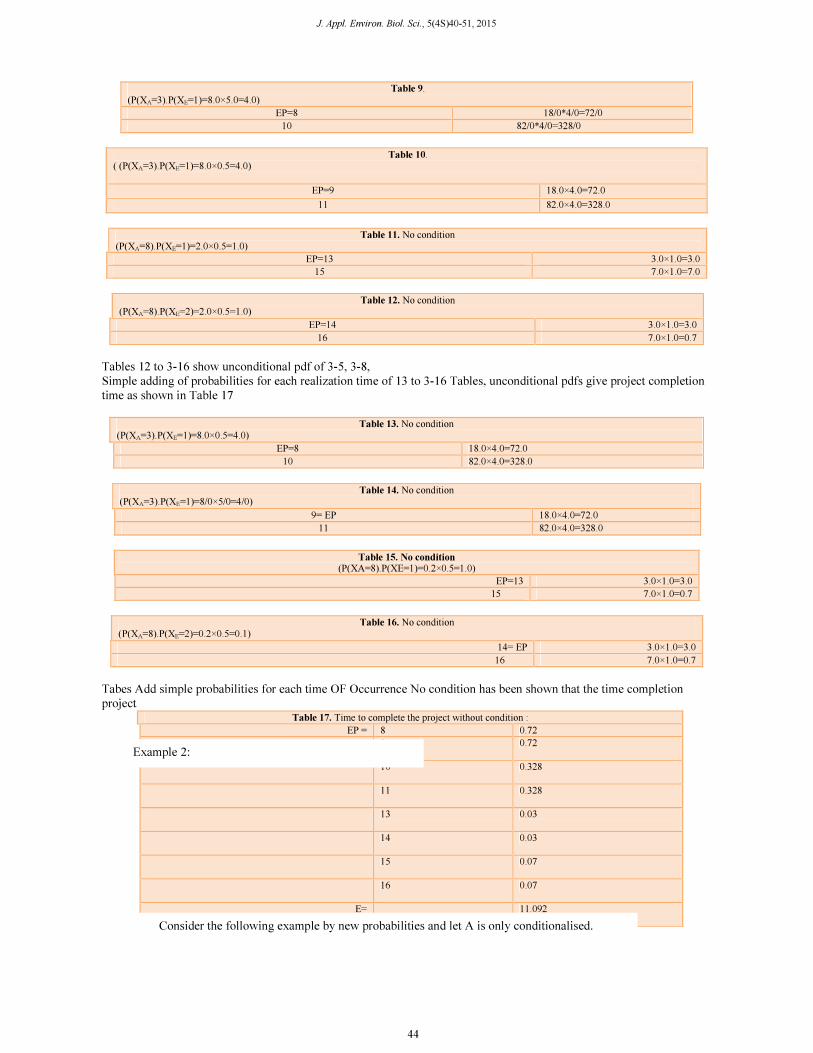
. Table 9

)4.0=5.0×8.0)=1=EX(P).3=AX(P(

18/0*4/0=72/0 EP=8

82/0*4/0=328/0 10

. Table 10

)4.0=0.5×8.0)=1=EX(P).3=AX(P( (

72.0=4.0×18.0 EP=9

328.0=4.0×82.0 11

Table 11. No condition

)1.0=0.5×2.0)=1=EX(P).8=AX(P(

3.0=1.0×3.0 EP=13

7.0=1.0×7.0 15


)1.0=0.5×2.0)=2=EX(P).8=AX(P(

3.0=1.0×3.0 EP=14

0.7=1.0×7.0 16

Tables 12 to 3-16 show unconditional pdf of 3-5, 3-8,

Simple adding of probabilities for each realization time of 13 to 3-16 Tables, unconditional pdfs give project completion

time as shown in Table 17


)4.0=0.5×8.0)=1=EX(P).3=AX(P(

72.0=4.0×18.0 EP=8

328.0=4.0×82.0 10


)0/4=0/5×0/8)=1=EX(P).3=AX(P(

72.0=4.0×18.0 9= EP

328.0=4.0×82.0 11


)1.0=0.5×0.2)=1=XE(P).8=XA(P(

3.0=1.0×3.0 EP=13

0.7=1.0×7.0 15


)0.1=0.5×0.2)=2=EX(P).8=AX(P(

3.0=1.0×3.0 14= EP

0.7=1.0×7.0 16

Tabes Add simple probabilities for each time OF Occurrence No condition has been shown that the time completion

project

The same is done by conditioning of only one criticality criterion.

:Table 17. Time to complete the project without condition

0.72 8 =EP

0.72 9

0.328 10

0.328 11

0.03 13

0.03 14

0.07 15

0.07 16

11.092 E=

Example 2:

Consider the following example by new probabilities and let A is only conditionalised.

44


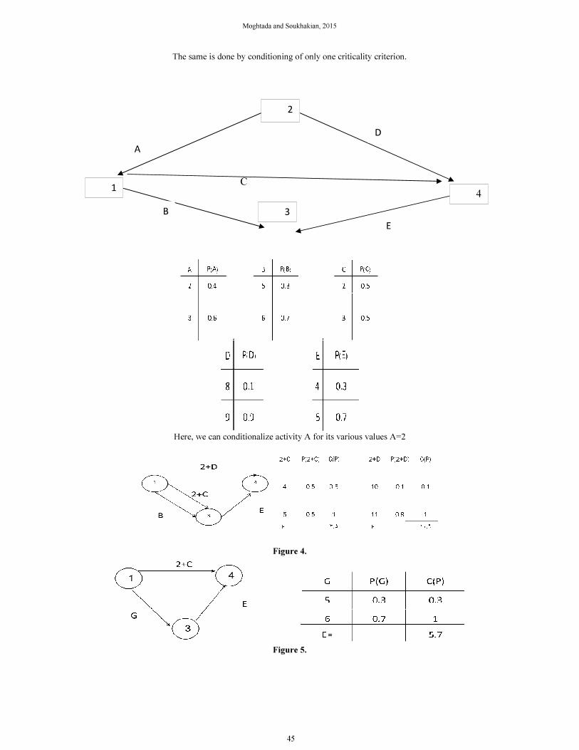
The same is done by conditioning of only one criticality criterion.

Here, we can conditionalize activity A for its various values A=2

Figure 4.

Figure 5.

C

E

D

B

A

4

2

3

1

45


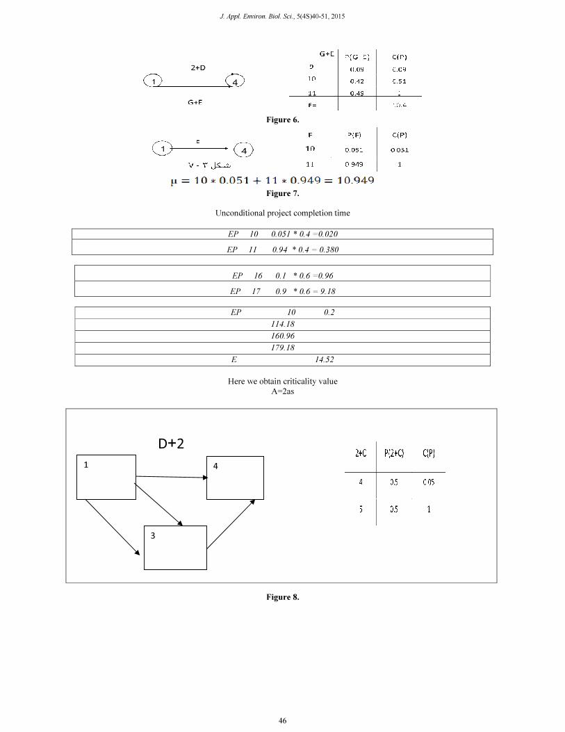
Figure 6.

Figure 7.

Unconditional project completion time

EP 10 0.051 * 0.4 =0.020

EP 11 0.94 * 0.4 = 0.380

EP 16 0.1 * 0.6 =0.96

EP 17 0.9 * 0.6 = 9.18

EP 10 0.2

114.18

160.96

179.18

E 14.52

Here we obtain criticality value

A=2as

Figure 8.

1 4

3

2+D

46


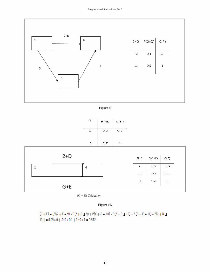
Figure 9.

Figure 10.

(G + E) Criticality

1 4

3

2+D

E G

1 4

2+D

G+E

47


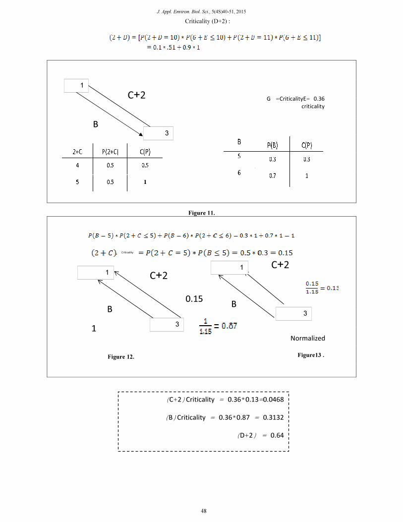
Figure 11.

) :2+D (Criticality

0.36 =CriticalityE =G

criticality

0.64 =Criticality2+D

1

3

2+C

B

1

3

B

2+C

Normalized

Figure 12.

1

3

B

1

0.15

2+C

Figure13 .

Criticality

0.0468=0.13*0.36 =Criticality)2+C(

0.3132 =0.87*0.36 =Criticality)B(

0.64 ) =2+D (

48


Figure 14.

5. Monte Carlo method

This method is a level of calculating algorithms as relying on random repetitive sampling for calculating the results.

Thus, Monte Carlo method is regulated as it is performed by computer.

The steps of Monte Carlo method

1- We define a range of variables.

2- The inputs are generated randomly.

3- Then, the calculations are done on each input.

4- All answers are integrated in the final answer.

In this method, our intention is comparing it with proposed method and at first all the possible paths are investigated

from the beginning to the end and criticality criterion of each path and mean and its variance is calculated and we use

visual studio in this method.

We can use critical path via PERT network formula and to determine the earliest time of realization, we consider

the event occurrence time zero to achieve the earliest realization time of the resent of events by the following formula.

The earliest realization time of an event= the earliest realization time of the previous event+ the time of performing

the relevant activity

6. Determining the latest time

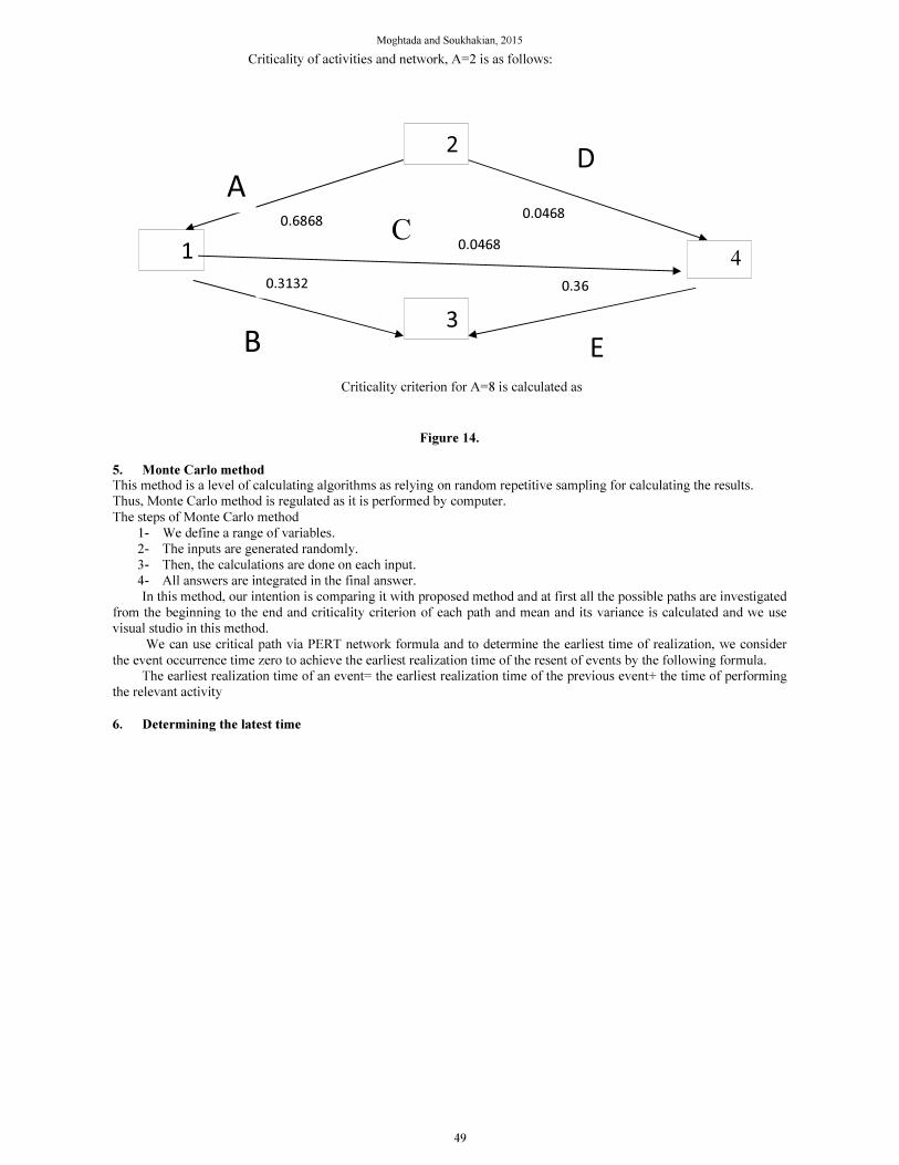
Criticality of activities and network, A=2 is as follows:

0.0468

0.36 0.3132

0.6868 0.0468

E

C

D

B

A

4

2

3

1

Criticality criterion for A=8 is calculated as

49


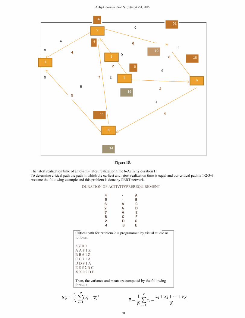
Figure 15.

The latest realization time of an event= latest realization time 6-Activity duration H

To determine critical path the path in which the earliest and latest realization time is equal and our critical path is 1-2-3-6

Assume the following example and this problem is done by PERT network.

Critical path for problem 2 is programmed by visual studio as

follows:

Z Z 0 0

A A 8 1 Z

B B 6 1 Z

C C 3 1 A

D D 9 1 A

E E 5 2 B C

X X 0 2 D E

Then, the variance and mean are computed by the following

formula

DURATION OF ACTIVITYPREREQUIREMENT

4 - A

5 - B

6 A C

2 A D

7 A E

8 C F

2 D G

4 B E

4

4

4

C

6

01

10 F

8 18

E

D

2

G

2

4

H

14

11

6

16

1

2

3

5

4 6

0

0

5

B

A

7

50


It can be said when in 1000th sample, critical path is X,D,A,Z, variance mean is calculated for this number.

Finally, we compute a total variance and a total mean with criticality criterion of each path. For example, assume in

10000, the sample z is in critical path for 375 times and criticality criterion is obtained by dividing it by the number of

samples.

In example 2, after 100 samples, we achieved the answer close to the proposed method. This is one of the examples of

two-time problems and this is used for three-time.

Conclusion

Now, in most of the projects, PERT method is used to determine project completion time and costs but due to the

assumptions in activities and projects, to compute project completion time easily, adequate precision is not obtained in

determining project completion time namely when the networks have many common activities and this causes that

practical projects are conducted longer than what it is predicted with high costs in most cases.

REFERENCES

1. Soukhakian, M. A. “A generalized algorithm to evaluate project completion times and criticality indices for pert

network.” Unpublished Ph.D Thesis May 1988 University Of Southamton.

2. Hajshirmohammadi, Ali. 1994. Control management and project. Jihad Daneshgahi publications of industrial unit of

Isfahan.

3. Burt, J. M. and Garman M. B. (1971) ″ Conditional Monte Carlo: A simulation technique for stochastic network

analysis ″, Management Science 18 (3), 207- 217.

4. Chapman, C. B. and Cooper D. F. (1983) ″ Risk Engineering: Basic controlled interval and memory model. ″

Journal of the Operational Research Society. 34 (1), 51- 60.

5. Clark, C. E. (1962) ″ The pert model for distribution of activity time. ″ Operational Research, 10, 405 - 416

6. Devroye, L. P. (1979) ″ Inequalities for the completion time of stochastic pert activity time" Operational Research,

4, 441- 447

7. Dodin, B. M. (1980) “On estimating the probability distribution functions in pert type networks.” OR report No.

153(Revised), OR Program, North Carolina State University Releigh, N. C.

8. Fulkerson, D. R. (1962) “ Expected critical path lengths in pert network ” Operational Research .10, 808 - 817

9. Garman, M . B . (1972) ″ More on conditioned sampling in the simulation of stochastic networks. ″ Management

Science .19,90 - 95

10. Hartley, H. O. and Wortham A .W . (1966) “ A statistical theory for pert critical path analysis .” Management

Science. 12, 496 - 481

11. Kamburowski, j. (1985) ″ Normally distribution activity durations in pert networks.″ Journal of OR Society . 36,

1051 - 1057

12. Lindesy, J. H. (1972) “An estimate of expected critical path length in pert networks.” Operational Research. 20, 800

– 812

13. Malcolm, D. G. (1959) ″ Application of a technique for research and development program evaluation .″

Operational Research . 7, 646 - 669

14. Ringer, L. J. (1969) “Numerical operators for statistical pert critical path analysis.” Managing Science. 16, B136 -

B143

15. Van Slyke, R. M. (1963) ″ Monte carlo methods and the pert problem.″ Operational Research. 11, 839 - 860

51

Documents

Determining Project Completion Time and Criticality ...textroad.com/pdf/JAEBS/J. Appl. Environ. Biol. Sci., 5(4S)40-51, 2015.pdfconventional method is used to determine project time