Determining oil price drivers with Dynamic Model Averaging

by

Krzysztof Drachal1

Faculty of Economic Sciences, University of Warsaw

ul. Długa 44/50, 00-241 Warszawa, Poland

Email: kdrachal@wne.uw.edu.pl

Abstract

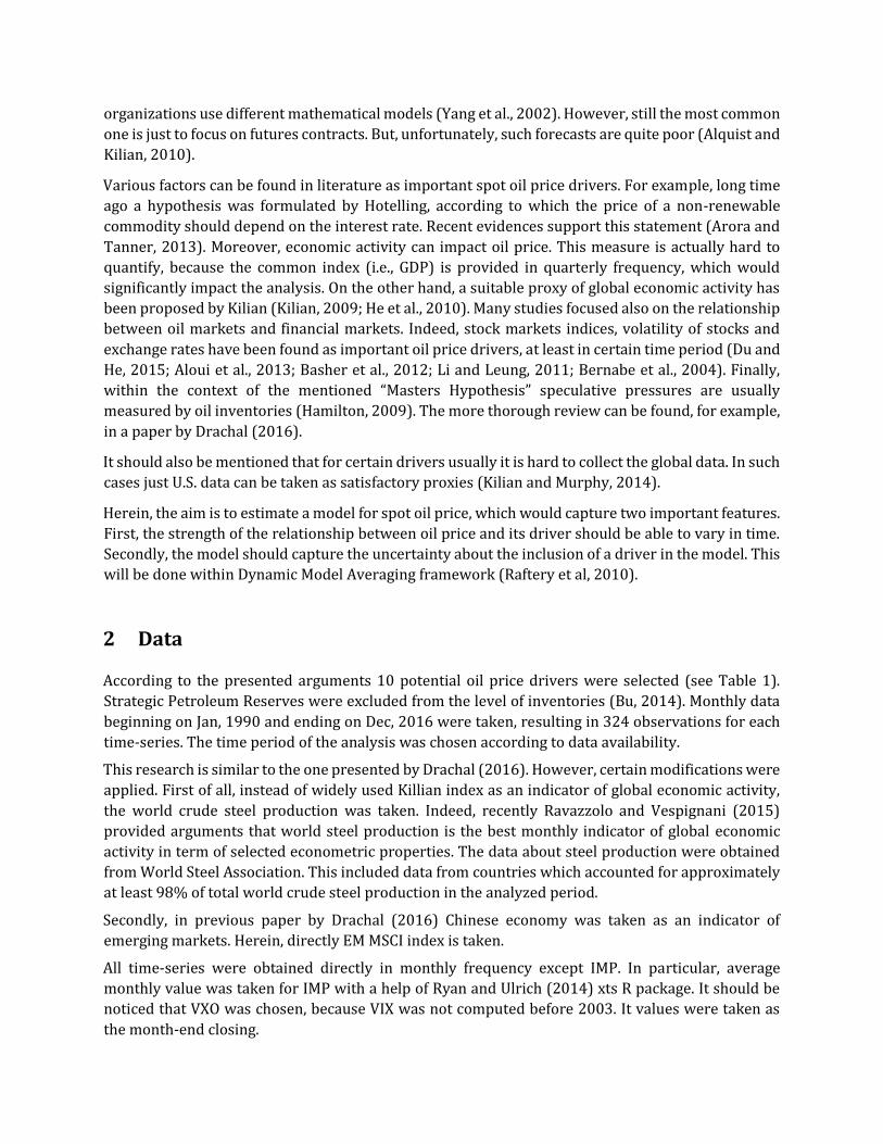
Modelling spot oil price is a hard but important task. Various researches has previously shown that oil price drivers can vary in time. In other words, it is hard to find one oil price model which would perform well in every period. On the other hand, usually the best performing model changes in time. From the econometric point of view such a situation requires building a model with two features. First, there is an uncertainty about the “true” model. Therefore, supposing there is initially given some set of models, the “true” model should be allowed to change with time. Secondly, suppose that the methodology is narrowed just to regression models arising from some set of initially given explanatory variables (drivers). Then, also the regression coefficients of these models should be allowed to vary in time. Such a construction is already known. It is Dynamic Model Averaging (DMA). This methodology arose as a certain extension and improvement of Bayesian Model Averaging (BMA). Indeed, this method comes from the Bayesian econometrics. As the initial set of oil price drivers the following factors have been chosen: stock market index, interest rates, economic activity index, exchange rates, supply and demand, import quotas, inventories level, and stress market index. The paper is organized as follows: First a brief overview about the oil price drivers is given. Next, a brief description of Dynamic Model Averaging is provided. Finally, the results are presented and conclusions are formulated.

1 Introduction: Oil Price Drivers

The literature review provides various oil price drivers. However, the most common are supply and

demand quotas. Indeed, these factors are usually perceived as playing the fundamental role for oil

market. Nevertheless, a few interesting observations should be formulated.

First of all, since 1980s it has been questioned whether supply and demand (e.g. OPEC quotas

decisions) are the only important oil price drivers. For example, just recently, during the oil price

surge of 2007/2008 “Master Hypothesis” was formulated. According to it, the index investments

were the major spot oil price driver (Irwin and Sanders, 2012).

Secondly, many studies showed that in different time period, different factors can play the most

important role as an oil price driver. Moreover, researchers found that time-varying parameters

models usually describe markets better than fixed parameters models. In particular, this

observations perfectly applies to oil market (Aastveit and Bjornland, 2015; Stefanski, 2014; Ji, 2012).

At least, it is interesting that there is no commonly accepted “oil price model”. In other words, the oil

market is very often found to be very complex and persistent to modelling. As a result, various

1 Research funded by the Polish National Science Centre grant under the contract number DEC-2015/19/N/HS4/00205.

organizations use different mathematical models (Yang et al., 2002). However, still the most common

one is just to focus on futures contracts. But, unfortunately, such forecasts are quite poor (Alquist and

Kilian, 2010).

Various factors can be found in literature as important spot oil price drivers. For example, long time

ago a hypothesis was formulated by Hotelling, according to which the price of a non-renewable

commodity should depend on the interest rate. Recent evidences support this statement (Arora and

Tanner, 2013). Moreover, economic activity can impact oil price. This measure is actually hard to

quantify, because the common index (i.e., GDP) is provided in quarterly frequency, which would

significantly impact the analysis. On the other hand, a suitable proxy of global economic activity has

been proposed by Kilian (Kilian, 2009; He et al., 2010). Many studies focused also on the relationship

between oil markets and financial markets. Indeed, stock markets indices, volatility of stocks and

exchange rates have been found as important oil price drivers, at least in certain time period (Du and

He, 2015; Aloui et al., 2013; Basher et al., 2012; Li and Leung, 2011; Bernabe et al., 2004). Finally,

within the context of the mentioned “Masters Hypothesis” speculative pressures are usually

measured by oil inventories (Hamilton, 2009). The more thorough review can be found, for example,

in a paper by Drachal (2016).

It should also be mentioned that for certain drivers usually it is hard to collect the global data. In such

cases just U.S. data can be taken as satisfactory proxies (Kilian and Murphy, 2014).

Herein, the aim is to estimate a model for spot oil price, which would capture two important features.

First, the strength of the relationship between oil price and its driver should be able to vary in time.

Secondly, the model should capture the uncertainty about the inclusion of a driver in the model. This

will be done within Dynamic Model Averaging framework (Raftery et al, 2010).

2 Data

According to the presented arguments 10 potential oil price drivers were selected (see Table 1).

Strategic Petroleum Reserves were excluded from the level of inventories (Bu, 2014). Monthly data

beginning on Jan, 1990 and ending on Dec, 2016 were taken, resulting in 324 observations for each

time-series. The time period of the analysis was chosen according to data availability.

This research is similar to the one presented by Drachal (2016). However, certain modifications were

applied. First of all, instead of widely used Killian index as an indicator of global economic activity,

the world crude steel production was taken. Indeed, recently Ravazzolo and Vespignani (2015)

provided arguments that world steel production is the best monthly indicator of global economic

activity in term of selected econometric properties. The data about steel production were obtained

from World Steel Association. This included data from countries which accounted for approximately

at least 98% of total world crude steel production in the analyzed period.

Secondly, in previous paper by Drachal (2016) Chinese economy was taken as an indicator of

emerging markets. Herein, directly EM MSCI index is taken.

All time-series were obtained directly in monthly frequency except IMP. In particular, average

monthly value was taken for IMP with a help of Ryan and Ulrich (2014) xts R package. It should be

noticed that VXO was chosen, because VIX was not computed before 2003. It values were taken as

the month-end closing.

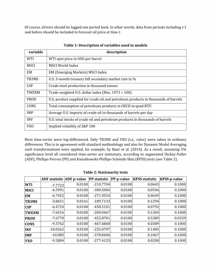
Of course, drivers should be lagged one period back. In other words, data from periods including t-1

and before should be included to forecast oil price at time t.

Table 1: Description of variables used in models

variable description

WTI WTI spot price in USD per barrel

MSCI MSCI World Index

EM EM (Emerging Markets) MSCI Index

TB3MS U.S. 3-month treasury bill secondary market rate in %

CSP Crude steel production in thousand tonnes

TWEXM Trade weighted U.S. dollar index (Mar, 1973 = 100)

PROD U.S. product supplied for crude oil and petroleum products in thousands of barrels

CONS Total consumption of petroleum products in OECD in quad BTU

IMP Average U.S. imports of crude oil in thousands of barrels per day

INV U.S. total stocks of crude oil and petroleum products in thousands of barrels

VXO Implied volatility of S&P 100

Most time-series were log-differenced. Only TB3MS and VXO (i.e., rates) were taken in ordinary

differences. This is in agreement with standard methodology and also for Dynamic Model Averaging

such transformations were applied, for example, by Baur et al. (2014). As a result, assuming 5%

significance level all considered time-series are stationary, according to augmented Dickey-Fuller

(ADF), Phillips-Perron (PP) and Kwiatkowski-Phillips-Schmidt-Shin (KPSS) tests (see Table 2).

Table 2: Stationarity tests

ADF statistic ADF p-value PP statistic PP p-value KPSS statistic KPSS p-value

WTI -7.7723 0.0100 -210.7704 0.0100 0.0643 0.1000

MSCI -6.5991 0.0100 -300.5006 0.0100 0.0546 0.1000

EM -6.7452 0.0100 -271.9554 0.0100 0.0649 0.1000

TB3MS -3.8651 0.0161 -189.7133 0.0100 0.1294 0.1000

CSP -6.4724 0.0100 -458.5101 0.0100 0.0792 0.1000

TWEXM -7.6516 0.0100 -200.0467 0.0100 0.1304 0.1000

PROD -7.6770 0.0100 -452.8701 0.0100 0.5389 0.0329

CONS -9.3762 0.0100 -467.6868 0.0100 0.0389 0.1000

INV -10.0362 0.0100 -225.0797 0.0100 0.1485 0.1000

IMP -10.085 0.0100 -378.8406 0.0100 0.1067 0.1000

VXO -9.2804 0.0100 -277.4125 0.0100 0.0208 0.1000

Finally, the time-series were normalized, i.e., rescaled to fit between 0 and 1. The purpose of such a

transformation is explained in the Methodology section.

All calculations were done in R (2015) software.

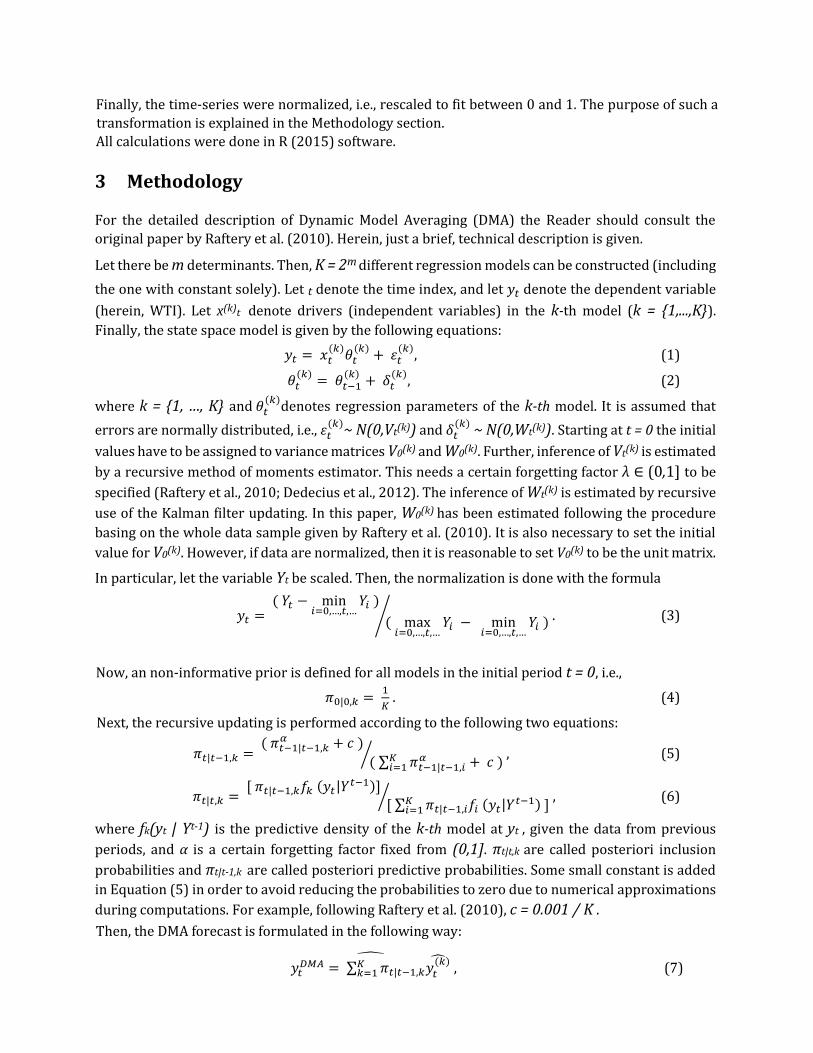
3 Methodology

For the detailed description of Dynamic Model Averaging (DMA) the Reader should consult the

original paper by Raftery et al. (2010). Herein, just a brief, technical description is given.

Let there be m determinants. Then, K = 2m different regression models can be constructed (including

the one with constant solely). Let t denote the time index, and let 𝑦𝑡 denote the dependent variable

(herein, WTI). Let x(k)t denote drivers (independent variables) in the k-th model (k = {1,...,K}).

Finally, the state space model is given by the following equations:

𝑦𝑡 = 𝑥𝑡(𝑘)

𝜃𝑡(𝑘)

+ 휀𝑡(𝑘)

, (1)

𝜃𝑡(𝑘)

= 𝜃𝑡−1(𝑘)

+ 𝛿𝑡(𝑘)

, (2)

where k = {1, …, K} and 𝜃𝑡(𝑘)

denotes regression parameters of the k-th model. It is assumed that

errors are normally distributed, i.e., 휀𝑡(𝑘)~ N(0,Vt(k)) and 𝛿𝑡

(𝑘) ~ N(0,Wt(k)). Starting at t = 0 the initial

values have to be assigned to variance matrices V0(k) and W0(k). Further, inference of Vt(k) is estimated

by a recursive method of moments estimator. This needs a certain forgetting factor λ ∈ (0,1] to be

specified (Raftery et al., 2010; Dedecius et al., 2012). The inference of Wt(k) is estimated by recursive

use of the Kalman filter updating. In this paper, W0(k) has been estimated following the procedure

basing on the whole data sample given by Raftery et al. (2010). It is also necessary to set the initial

value for V0(k). However, if data are normalized, then it is reasonable to set V0(k) to be the unit matrix.

In particular, let the variable Yt be scaled. Then, the normalization is done with the formula

𝑦𝑡 = ( 𝑌𝑡 − min

𝑖=0,…,𝑡,…𝑌𝑖 )

( max𝑖=0,…,𝑡,…

𝑌𝑖 − min𝑖=0,…,𝑡,…

𝑌𝑖 )⁄ . (3)

Now, an non-informative prior is defined for all models in the initial period t = 0, i.e.,

𝜋0|0,𝑘 = 1

𝐾 . (4)

Next, the recursive updating is performed according to the following two equations:

𝜋𝑡|𝑡−1,𝑘 = ( 𝜋𝑡−1|𝑡−1,𝑘

𝛼 + 𝑐 )

( ∑ 𝜋𝑡−1|𝑡−1,𝑖𝛼𝐾

𝑖=1 + 𝑐 )⁄ , (5)

𝜋𝑡|𝑡,𝑘 = [ 𝜋𝑡|𝑡−1,𝑘𝑓𝑘 (𝑦𝑡|𝑌𝑡−1)]

[ ∑ 𝜋𝑡|𝑡−1,𝑖𝑓𝑖 (𝑦𝑡|𝑌𝑡−1)𝐾𝑖=1 ]

⁄ , (6)

where fk(yt | Yt-1) is the predictive density of the k-th model at yt , given the data from previous

periods, and α is a certain forgetting factor fixed from (0,1]. πt|t,k are called posteriori inclusion

probabilities and πt|t-1,k are called posteriori predictive probabilities. Some small constant is added

in Equation (5) in order to avoid reducing the probabilities to zero due to numerical approximations

during computations. For example, following Raftery et al. (2010), c = 0.001 / K .

Then, the DMA forecast is formulated in the following way:

𝑦𝑡𝐷𝑀𝐴 = ∑ 𝜋𝑡|𝑡−1,𝑘𝑦𝑡

(𝑘)𝐾𝑘=1

, (7)

where 𝑦𝑡(𝑘)

is the prediction given by the k-th regression model.

Now, let 𝜋𝑡|𝑡−1,𝑘 ≔ max𝑖={1,…,𝐾}

{𝜋𝑡|𝑡−1,𝑖}, where πt|t−1,i are computed as in Equation (5). Also, let in the

above computational scheme modify the Equation (7) to be:

𝑦𝑡𝐷𝑀𝑆 = ∑ 𝜋𝑡|𝑡−1,𝑘 𝑦𝑡

(𝑘)𝐾𝑘=1

. (8)

Then, Equation (8) gives the Dynamic Model Selection (DMS) forecast. The difference between DMA

and DMS is that in DMA model averaging is performed, whereas DMS method selects in each period

the model with the highest posteriori predictive probability.

Now, notice that in each time period t, posteriori predictive probabilities for each model which

contains a given variable can be summed. This measure can be further used to describe the time-

varying importance of a given variable as an oil price driver.

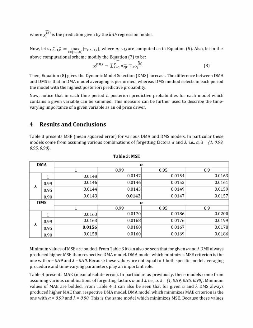
4 Results and Conclusions

Table 3 presents MSE (mean squared error) for various DMA and DMS models. In particular these

models come from assuming various combinations of forgetting factors α and λ, i.e., α, λ = {1, 0.99,

0.95, 0.90}.

Table 3: MSE

DMA α 1 0.99 0.95 0.9

λ

1 0.0148 0.0147 0.0154 0.0163

0.99 0.0146 0.0146 0.0152 0.0161

0.95 0.0144 0.0143 0.0149 0.0159

0.90 0.0143 0.0142 0.0147 0.0157

DMS α 1 0.99 0.95 0.9

λ

1 0.0163 0.0170 0.0186 0.0200

0.99 0.0163 0.0168 0.0176 0.0199

0.95 0.0156 0.0160 0.0167 0.0178

0.90 0.0158 0.0160 0.0169 0.0186

Minimum values of MSE are bolded. From Table 3 it can also be seen that for given α and λ DMS always

produced higher MSE than respective DMA model. DMA model which minimizes MSE criterion is the

one with α = 0.99 and λ = 0.90. Because these values are not equal to 1 both specific model averaging

procedure and time-varying parameters play an important role.

Table 4 presents MAE (mean absolute error). In particular, as previously, these models come from

assuming various combinations of forgetting factors α and λ, i.e., α, λ = {1, 0.99, 0.95, 0.90}. Minimum

values of MAE are bolded. From Table 4 it can also be seen that for given α and λ DMS always

produced higher MAE than respective DMA model. DMA model which minimizes MAE criterion is the

one with α = 0.99 and λ = 0.90. This is the same model which minimizes MSE. Because these values

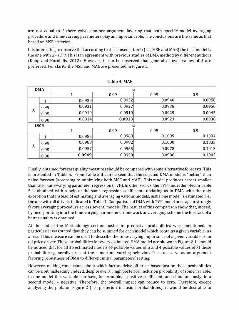
are not equal to 1 there exists another argument favoring that both specific model averaging

procedure and time-varying parameters play an important role. The conclusions are the same as that

based on MSE criterion.

It is interesting to observe that according to the chosen criteria (i.e., MSE and MAE) the best model is

the one with α = 0.99. This is in agreement with previous studies of DMA method by different authors

(Koop and Korobilis, 2012). However, it can be observed that generally lower values of λ are

preferred. For clarity the MSE and MAE are presented in Figure 1.

Table 4: MAE

DMA α 1 0.99 0.95 0.9

λ

1 0.0939 0.0932 0.0940 0.0950

0.99 0.0931 0.0927 0.0938 0.0950

0.95 0.0919 0.0919 0.0929 0.0945

0.90 0.0914 0.0913 0.0923 0.0938

DMS α 1 0.99 0.95 0.9

λ

1 0.0985 0.0989 0.1009 0.1034

0.99 0.0988 0.0982 0.1000 0.1033

0.95 0.0957 0.0965 0.0978 0.1013

0.90 0.0949 0.0950 0.0986 0.1042

Finally, obtained forecast quality measures should be compared with some alternative forecasts. This

is presented in Table 5. From Table 5 it can be seen that the selected DMA model is “better” than naïve forecast (according to minimizing both MSE and MAE). This model produces errors smaller

than, also, time-varying parameter regression (TVP). In other words, the TVP model denoted in Table 5 is obtained with a help of the same regression coefficients updating as in DMA with the only

exception that instead of estimating and averaging various models, just a one model is estimated, i.e., the one with all drivers indicated in Table 1. Comparison of DMA with TVP model once again strongly

favors averaging procedure across several models. The results of this comparison show that, indeed,

by incorporating into the time-varying parameters framework an averaging scheme the forecast of a better quality is obtained.

At the end of the Methodology section posteriori predictive probabilities were mentioned. In

particular, it was stated that they can be summed for each model which contains a given variable. As

a result this measure can be used to describe the time-varying importance of a given variable as an oil price driver. These probabilities for every estimated DMA model are shown in Figure 2. It should

be noticed that for all 16 estimated models (4 possible values of α and 4 possible values of λ) these probabilities generally present the same time-varying behavior. This can serve as an argument

favoring robustness of DMA to different initial parameters’ setting.

However, making conclusions about which factors drive oil price, based just on these probabilities

can be a bit misleading. Indeed, despite overall high posteriori inclusion probability of some variable, in one model this variable can have, for example, a positive coefficient, and simultaneously, in a

second model – negative. Therefore, the overall impact can reduce to zero. Therefore, except

analyzing the plots on Figure 2 (i.e., posteriori inclusion probabilities), it would be desirable to

analyze the expected values of regression coefficients for different potential oil price drivers. The

expected values of these coefficients are computed with respect to posteriori inclusion probabilities (presented in Figure 2). These expected values of coefficients are presented in Figure 3.

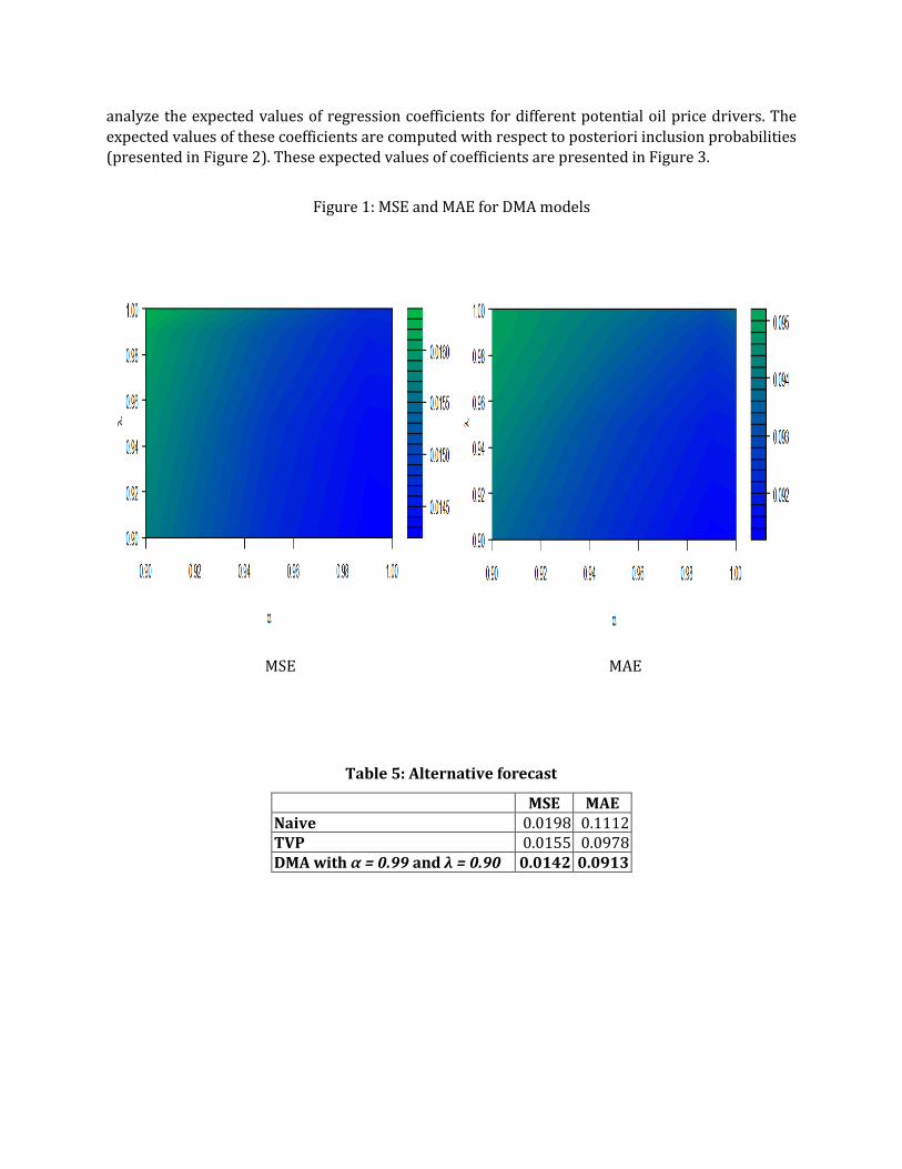
Figure 1: MSE and MAE for DMA models

MSE MAE

Table 5: Alternative forecast

MSE MAE Naive 0.0198 0.1112 TVP 0.0155 0.0978 DMA with α = 0.99 and λ = 0.90 0.0142 0.0913

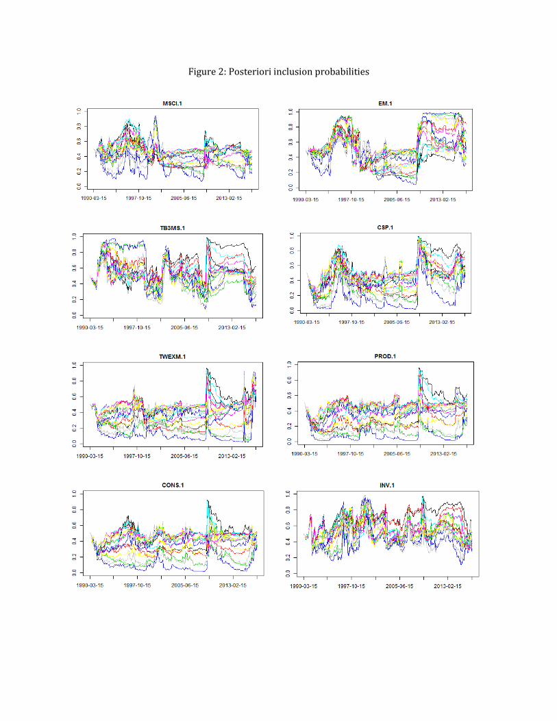
Figure 2: Posteriori inclusion probabilities

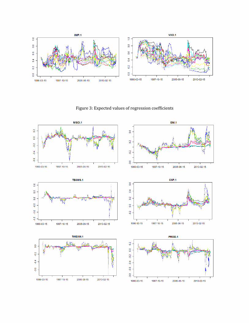
Figure 3: Expected values of regression coefficients

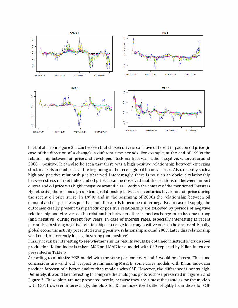
First of all, from Figure 3 it can be seen that chosen drivers can have different impact on oil price (in

case of the direction of a change) in different time periods. For example, at the end of 1990s the

relationship between oil price and developed stock markets was rather negative, whereas around

2008 – positive. It can also be seen that there was a high positive relationship between emerging

stock markets and oil price at the beginning of the recent global financial crisis. Also, recently such a

high and positive relationship is observed. Interestingly, there is no such an obvious relationship

between stress market index and oil price. It can be observed that the relationship between import

quotas and oil price was highly negative around 2005. Within the context of the mentioned “Masters

Hypothesis”, there is no sign of strong relationship between inventories levels and oil price during

the recent oil price surge. In 1990s and in the beginning of 2000s the relationship between oil

demand and oil price was positive, but afterwards it become rather negative. In case of supply, the

outcomes clearly present that periods of positive relationship are followed by periods of negative

relationship and vice versa. The relationship between oil price and exchange rates become strong

(and negative) during recent few years. In case of interest rates, especially interesting is recent

period. From strong negative relationship, a passage to strong positive one can be observed. Finally,

global economic activity presented strong positive relationship around 2009. Later this relationship

weakened, but recently it is again strong (and positive).

Finally, it can be interesting to see whether similar results would be obtained if instead of crude steel

production, Kilian index is taken. MSE and MAE for a model with CSP replaced by Kilian index are

presented in Table 6.

According to minimize MSE model with the same parameters α and λ would be chosen. The same

conclusions are valid with respect to minimizing MAE. In some cases models with Kilian index can

produce forecast of a better quality than models with CSP. However, the difference is not so high.

Definitely, it would be interesting to compare the analogous plots as those presented in Figure 2 and

Figure 3. These plots are not presented herein, because they are almost the same as for the models

with CSP. However, interestingly, the plots for Kilian index itself differ slightly from those for CSP

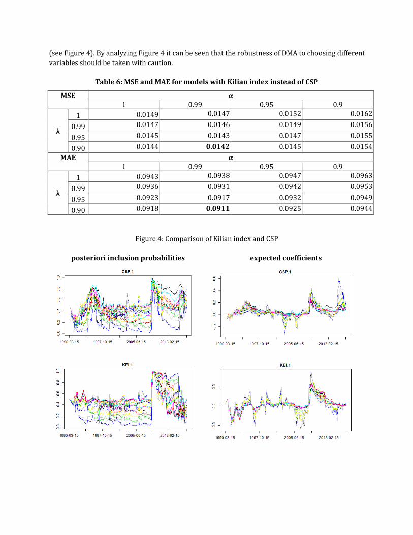
(see Figure 4). By analyzing Figure 4 it can be seen that the robustness of DMA to choosing different

variables should be taken with caution.

Table 6: MSE and MAE for models with Kilian index instead of CSP

MSE α 1 0.99 0.95 0.9

λ

1 0.0149 0.0147 0.0152 0.0162

0.99 0.0147 0.0146 0.0149 0.0156

0.95 0.0145 0.0143 0.0147 0.0155

0.90 0.0144 0.0142 0.0145 0.0154

MAE α 1 0.99 0.95 0.9

λ

1 0.0943 0.0938 0.0947 0.0963

0.99 0.0936 0.0931 0.0942 0.0953

0.95 0.0923 0.0917 0.0932 0.0949

0.90 0.0918 0.0911 0.0925 0.0944

Figure 4: Comparison of Kilian index and CSP

posteriori inclusion probabilities expected coefficients

Bibliography

Aastveit, K.A., Bjornland, H.C., 2015. What drives oil prices? Emerging versus developed economies.

Journal of Applied Econometrics 30, 1013-1028.

Aloui, R., Aissa, M.S.B., Nguyen, D.K., 2013. Conditional dependence structure between oil prices and

exchange rates: a copula-GARCH approach. Journal of International Money and Finance 32, 719-738.

Alquist, R., Kilian, L., 2010. What do we learn from the price of crude oil futures? Journal of Applied

Econometrics 25, 539-573.

Arora, V., Tanner, M., 2013. Do oil prices respond to real interest rates? Energy Economics 36, 546-

555.

Basher, S.A., Haug, A.A., Sadorsky, P., 2012. Oil prices, exchange rates and emerging stock markets.

Energy Economics 34, 227-240.

Baur, D.G., Beckmann, J., Czudaj, R., 2014. Gold price forecasts in a dynamic model averaging

framework - Have the determinants changed over time? Ruhr Economic Papers 506.

Bernabe, A., Martina, E., Alvarez-Ramirez, J., Ibarra-Valdez, C., 2004. A multi-model approach for

describing crude oil price dynamics. Physica A 338, 567-584.

Dedecius, K., Nagy, I., Karny, M., 2012. Parameter tracking with partial forgetting method.

International Journal of Adaptive Control and Signal Processing 26, 1-12.

Drachal, K., 2016. Forecasting spot oil price in a dynamic model averaging framework - Have the

determinants changed over time? Energy Economics 60, 35-46.

Du, L., He, Y., 2015. Extreme risk spillovers between crude oil and stock markets. Energy Economics

51, 455-465.

Hamilton, J.D., 2009. Causes and consequences of the oil shock of 2007-08. Brookings Papers on

Economic Activity 40, 215-259.

He, Y., Wang, S., Lai, K.K., 2010. Global economic activity and crude oil prices: A cointegration analysis.

Energy Economics 32, 868-876.

Irwin, S.H., Sanders, D.R., 2012. Testing the Masters Hypothesis in commodity futures markets.

Energy Economics 34, 256-269.

Ji, Q., 2012. System analysis approach for the identification of factors driving crude oil prices.

Computers & Industrial Engineering 63, 615-625.

Kilian, L., 2009. Not all oil price shocks are alike: Disentangling demand and supply shocks in the

crude oil market. American Economic Review 99, 1053-1069.

Kilian, L., Murphy, D.P., 2014. The role of inventories and speculative trading in the global market for

crude oil. Journal of Applied Econometrics 29, 454-478.

Koop, G., Korobilis, D., 2012. Forecasting inflation using Dynamic Model Averaging. International

Economic Review 53, 867-886.

Li, R., Leung, G.C.K., 2011. The integration of China into the world crude oil market since 1998. Energy

Policy 39, 5159-5166.

R Core Team, 2015. R: A language and environment for statistical computing. Vienna: R Foundation

for Statistical Computing, http://www.R-project.org.

Ravazzolo, F., Vespignani, J.L., 2015. A new monthly indicator of global real economic activity. Norges

Bank Working Paper 6.

Raftery, A.E., Karny, M., Ettler, P., 2010. Online prediction under model uncertainty via Dynamic

Model Averaging: Application to a cold rolling mill. Technometrics 52, 52-66.

Ryan, J.A., Ulrich, J.M., 2014. Xts: eXtensible Time Series. http://r-forge.r-project.org/projects/xts.

Stefanski, R., 2014. Structural transformation and the oil price. Review of Economic Dynamics 17,

484-504.

Yang, C.W., Hwang, M.J., Huang, B.N., 2002. An analysis of factors affecting price volatility of the US oil

market. Energy Economics 24, 107-119.

Data sources

U.S. Energy Information Administration, Spot prices,

http://www.eia.gov/dnav/pet/pet_pri_spt_s1_m.htm

MSCI, End of day index data search, http://www.msci.com/end-of-day-data-search

Federal Reserve Bank of St. Louis, 3-month treasury bill: Secondary market rate,

http://fred.stlouisfed.org/series/TB3MS

World Steel Association, Monthly crude steel production data: 1990-2016,

http://www.worldsteel.org/steel-by-topic/statistics/Statistics-monthly-crude-steel-and-iron-data-

/steel-archive.html

Federal Reserve Bank of St. Louis, Trade weighted U.S. dollar index: Major currencies,

http://fred.stlouisfed.org/series/TWEXMMTH

U.S. Energy Information Administration, Crude oil production,

http://www.eia.gov/dnav/pet/pet_crd_crpdn_adc_mbbl_m.htm

U.S. Energy Information Administration, Product supplied,

http://www.eia.gov/dnav/pet/pet_cons_psup_dc_nus_mbbl_m.htm

U.S. Energy Information Administration, Weekly imports & exports,

http://www.eia.gov/dnav/pet/pet_move_wkly_dc_NUS-Z00_mbblpd_w.htm

U.S. Energy Information Administration, Total stocks,

http://www.eia.gov/dnav/pet/pet_stoc_wstk_dcu_nus_m.htm

CBOE, VIX options and futures historical data,

http://www.cboe.com/products/vix-index-volatility/vix-options-and-futures/vix-index/vix-

historical-data

Killian, L., Updated version of the index of global real economic activity in industrial commodity

markets, proposed in “Not all oil price shocks are alike ...”, monthly percent deviations from trend,

1968.1-2016:12, http://www-personal.umich.edu/~lkilian/reaupdate.txt