Embed Size (px)
Citation preview
– 62 –
Journal of Siberian Federal University. Engineering & Technologies 1 (2014 7) 62-82 ~ ~ ~
УДК 697.34 : 532.551: 62408.8
Determining Hydraulic Friction Factor for Pipeline Systems
Alex Y. Lipovka* and Yuri L. LipovkaSiberian Federal University,
79 Svobodny, Krasnoyarsk, 660041, Russia
Received 21.11.2013, received in revised form 23.12.2013, accepted 04.02.2014
A comparative analysis of many well-known formulas for Darcy friction factor was carried out to determine accuracy and computational costs. To ensure a smooth transition from laminar flow to turbulent a cubic interpolation algorithm proposed to cover critical zone.
Keywords: hydraulic friction factor, critical zone, Darcy friction factor, pipeline systems, interpolation.
IntroductionThe core of all known methods of analyzing the hydrodynamic state in regulated pipeline
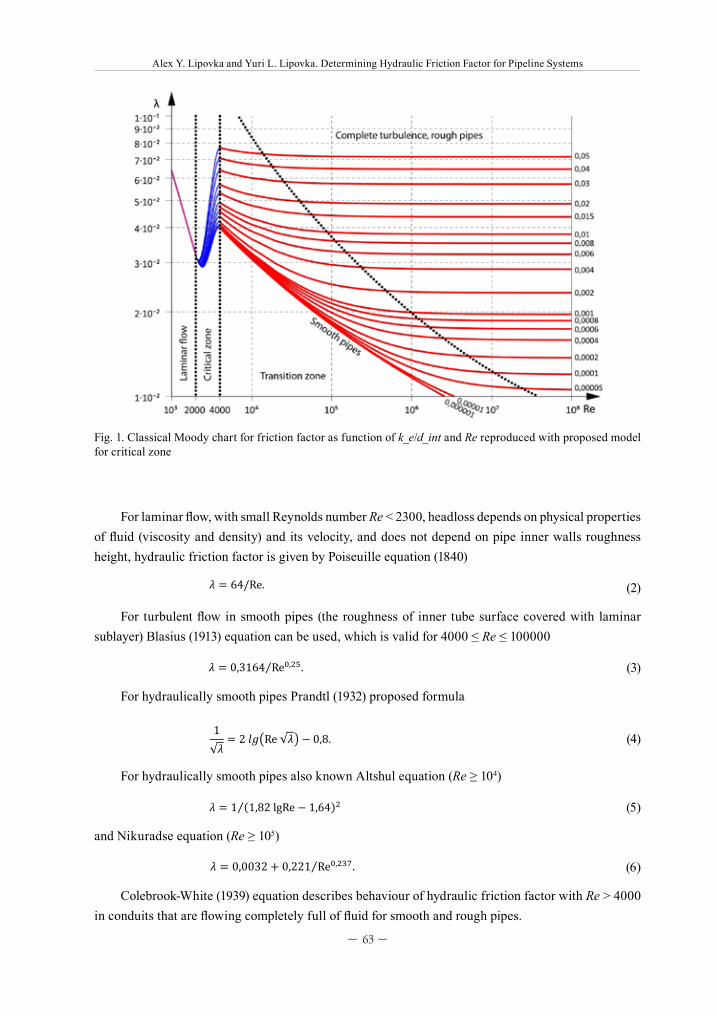
systems are methods of calculating flow distribution [1], [2], and all of them require calculation of hydraulic friction factor λ, which depends on the surface of the pipe wall, and the flow mode of the liquid. Determination of λ in the critical zone between laminar and transitional flows (Fig. 1) is related to certain difficulties. The goal of this article is to systematize the known methods of calculating λ and offer readers a general approach to the definition of λ on the whole range of Reynolds numbers.
Models and algorithms used
Head loss in a steady flow of liquid in round pressure pipes is calculated using Darcy-Weisbach equation
УДК 697.34 : 532.551: 62−408.8
Determining Hydraulic Friction Factor for Pipeline Systems
Alex Y. Lipovka*, Yuri L. Lipovka
Siberian Federal University,
79 Svobodny, Krasnoyarsk, 660041, Russia
_______________________________________________________________________________
A comparative analysis of many well-known formulas for Darcy friction factor was carried out to
determine accuracy and computational costs. To ensure a smooth transition from laminar flow to
turbulent a cubic interpolation algorithm proposed to cover critical zone.
Keywords: hydraulic friction factor, critical zone, Darcy friction factor, pipeline systems,
interpolation
_______________________________________________________________________________
Introduction
The core of all known methods of analyzing the hydrodynamic state in regulated pipeline
systems are methods of calculating flow distribution [1], [2], and all of them require calculation of
hydraulic friction factor �, which depends on the surface of the pipe wall, and the flow mode of the
liquid. Determination of � in the critical zone between laminar and transitional flows (Fig. 1) is
related to certain difficulties. The goal of this article is to systematize the known methods of
calculating � and offer readers a general approach to the definition of � on the whole range of
Reynolds numbers.
Models and algorithms used
Head loss in a steady flow of liquid in round pressure pipes is calculated using Darcy-
Weisbach equation
�� � ���
����� ���
�2
2 �, (1)
where �, ���� – length and inner pipe diameter, m; ∑� – sum of minor loss coefficients; � – velocity
of fluid, m/s; � – gravitational acceleration, m/s2.
Equation (1) obviously shows importance of valid definition of friction factor, which has at
least the same impact weight as length of a pipe. When ∑� � � deviations of both � and � have
linear impact on total headloss.
(1)
where l,dint – length and inner pipe diameter, m; Σξ – sum of minor loss coefficients; v – velocity of fluid, m/s;
УДК 697.34 : 532.551: 62−408.8
Determining Hydraulic Friction Factor for Pipeline Systems
Alex Y. Lipovka*, Yuri L. Lipovka
Siberian Federal University,
79 Svobodny, Krasnoyarsk, 660041, Russia
_______________________________________________________________________________
A comparative analysis of many well-known formulas for Darcy friction factor was carried out to
determine accuracy and computational costs. To ensure a smooth transition from laminar flow to
turbulent a cubic interpolation algorithm proposed to cover critical zone.
Keywords: hydraulic friction factor, critical zone, Darcy friction factor, pipeline systems,
interpolation
_______________________________________________________________________________
Introduction
The core of all known methods of analyzing the hydrodynamic state in regulated pipeline
systems are methods of calculating flow distribution [1], [2], and all of them require calculation of
hydraulic friction factor �, which depends on the surface of the pipe wall, and the flow mode of the
liquid. Determination of � in the critical zone between laminar and transitional flows (Fig. 1) is
related to certain difficulties. The goal of this article is to systematize the known methods of
calculating � and offer readers a general approach to the definition of � on the whole range of
Reynolds numbers.
Models and algorithms used
Head loss in a steady flow of liquid in round pressure pipes is calculated using Darcy-
Weisbach equation
�� � ���
����� ���
�2
2 �, (1)
where �, ���� – length and inner pipe diameter, m; ∑� – sum of minor loss coefficients; � – velocity
of fluid, m/s; � – gravitational acceleration, m/s2.
Equation (1) obviously shows importance of valid definition of friction factor, which has at
least the same impact weight as length of a pipe. When ∑� � � deviations of both � and � have
linear impact on total headloss.
– gravitational acceleration, m/s2.Equation (1) obviously shows importance of valid definition of friction factor, which has at least
the same impact weight as length of a pipe. When Σξ = 0 deviations of both λ and l have linear impact on total headloss.
© Siberian Federal University. All rights reserved* Corresponding author E-mail address: [email protected]
– 63 –
Alex Y. Lipovka and Yuri L. Lipovka. Determining Hydraulic Friction Factor for Pipeline Systems
For laminar flow, with small Reynolds number Re < 2300, headloss depends on physical properties of fluid (viscosity and density) and its velocity, and does not depend on pipe inner walls roughness height, hydraulic friction factor is given by Poiseuille equation (1840)
Fig. 1 – Classical Moody chart for friction factor as function of ��������� and �� reproduced with
proposed model for critical zone
For laminar flow, with small Reynolds number �� � ����, headloss depends on physical
properties of fluid (viscosity and density) and its velocity, and does not depend on pipe inner walls roughness height, hydraulic friction factor is given by Poiseuille equation (1840)
� � �����. (2)
For turbulent flow in smooth pipes (the roughness of inner tube surface covered with
laminar sublayer) Blasius (1913) equation can be used, which is valid for ���� � �� � 1�����
� � ���1�� ������⁄ . (3)
For hydraulically smooth pipes Prandtl (1932) proposed formula
1√�
� � ����� √�� � ���. (4)
For hydraulically smooth pipes also known Altshul equation (�� � 104)
� � 1 �1��� ���� � 1�����⁄ (5)
and Nikuradse equation (�� � 105)
(2)
For turbulent flow in smooth pipes (the roughness of inner tube surface covered with laminar sublayer) Blasius (1913) equation can be used, which is valid for 4000 ≤ Re ≤ 100000
Fig. 1 – Classical Moody chart for friction factor as function of ��������� and �� reproduced with
proposed model for critical zone
For laminar flow, with small Reynolds number �� � ����, headloss depends on physical
properties of fluid (viscosity and density) and its velocity, and does not depend on pipe inner walls roughness height, hydraulic friction factor is given by Poiseuille equation (1840)
� � �����. (2)
For turbulent flow in smooth pipes (the roughness of inner tube surface covered with
laminar sublayer) Blasius (1913) equation can be used, which is valid for ���� � �� � 1�����
� � ���1�� ������⁄ . (3)
For hydraulically smooth pipes Prandtl (1932) proposed formula
1√�
� � ����� √�� � ���. (4)
For hydraulically smooth pipes also known Altshul equation (�� � 104)
� � 1 �1��� ���� � 1�����⁄ (5)
and Nikuradse equation (�� � 105)
(3)
For hydraulically smooth pipes Prandtl (1932) proposed formula
Fig. 1 – Classical Moody chart for friction factor as function of ��������� and �� reproduced with
proposed model for critical zone
For laminar flow, with small Reynolds number �� � ����, headloss depends on physical
properties of fluid (viscosity and density) and its velocity, and does not depend on pipe inner walls roughness height, hydraulic friction factor is given by Poiseuille equation (1840)
� � �����. (2)
For turbulent flow in smooth pipes (the roughness of inner tube surface covered with
laminar sublayer) Blasius (1913) equation can be used, which is valid for ���� � �� � 1�����
� � ���1�� ������⁄ . (3)
For hydraulically smooth pipes Prandtl (1932) proposed formula
1√�
� � ����� √�� � ���. (4)
For hydraulically smooth pipes also known Altshul equation (�� � 104)
� � 1 �1��� ���� � 1�����⁄ (5)
and Nikuradse equation (�� � 105)
(4)
For hydraulically smooth pipes also known Altshul equation (Re ≥ 104)
Fig. 1 – Classical Moody chart for friction factor as function of ��������� and �� reproduced with
proposed model for critical zone
For laminar flow, with small Reynolds number �� � ����, headloss depends on physical
properties of fluid (viscosity and density) and its velocity, and does not depend on pipe inner walls roughness height, hydraulic friction factor is given by Poiseuille equation (1840)
� � �����. (2)
For turbulent flow in smooth pipes (the roughness of inner tube surface covered with
laminar sublayer) Blasius (1913) equation can be used, which is valid for ���� � �� � 1�����
� � ���1�� ������⁄ . (3)
For hydraulically smooth pipes Prandtl (1932) proposed formula
1√�
� � ����� √�� � ���. (4)
For hydraulically smooth pipes also known Altshul equation (�� � 104)
� � 1 �1��� ���� � 1�����⁄ (5)
and Nikuradse equation (�� � 105)
(5)
and Nikuradse equation (Re ≥ 105)
� � �,���2 � �,221 Re�,���⁄ . (6)
Colebrook-White (1939) equation describes behaviour of hydraulic friction factor with
�� � ���� in conduits that are flowing completely full of fluid for smooth and rough pipes.
1√�
� �2� ����� ���
�,� �����
2,51Re √�
�, (7)
where �� – roughness height of inner tube surface, m.
Because of implicit nature of Colebrook equation (7) � is obtained either numerically, or by
composing approximation formulas. Recently, the Lambert W function was used to get explicit
form of (7).
For transition zone of turbulent flow between smooth and rough pipes Altshul equation can
be used in hydraulic calculations of thermal pipeline networks
� � �,11 �������
�68,5Re �
�,��
, (8)
For turbulent zone in the area of quadratic law of flow Prandtl-Nikuradse formula can be
used
� �1
�1,1� � 2�� �������� (9)
and Shifrinson formula
� � �,11 �������
��,��
. (10)
Some of the other most known equations for friction factor are:
− Moody equation (1947)
� � �,��55�1 � �2 � 104 ������
�106
Re �
���
� ; (11)
− Wood equation (1966)
� � �,��� �������
��,���
� �,5� �������
� � 88 �������
��,��
Re�ψ, (12)
(6)
Colebrook-White (1939) equation describes behaviour of hydraulic friction factor with Re > 4000 in conduits that are flowing completely full of fluid for smooth and rough pipes.
Fig. 1 – Classical Moody chart for friction factor as function of ��������� and �� reproduced with
proposed model for critical zone
For laminar flow, with small Reynolds number �� � ����, headloss depends on physical
properties of fluid (viscosity and density) and its velocity, and does not depend on pipe inner walls roughness height, hydraulic friction factor is given by Poiseuille equation (1840)
� � �����. (2)
For turbulent flow in smooth pipes (the roughness of inner tube surface covered with
laminar sublayer) Blasius (1913) equation can be used, which is valid for ���� � �� � 1�����
� � ���1�� ������⁄ . (3)
For hydraulically smooth pipes Prandtl (1932) proposed formula
1√�
� � ����� √�� � ���. (4)
For hydraulically smooth pipes also known Altshul equation (�� � 104)
� � 1 �1��� ���� � 1�����⁄ (5)
and Nikuradse equation (�� � 105)
Fig. 1. Classical Moody chart for friction factor as function of k_e/d_int and Re reproduced with proposed model for critical zone
– 64 –
Alex Y. Lipovka and Yuri L. Lipovka. Determining Hydraulic Friction Factor for Pipeline Systems
� � �,���2 � �,221 Re�,���⁄ . (6)
Colebrook-White (1939) equation describes behaviour of hydraulic friction factor with
�� � ���� in conduits that are flowing completely full of fluid for smooth and rough pipes.
1√�
� �2� ����� ���
�,� �����
2,51Re √�
�, (7)
where �� – roughness height of inner tube surface, m.
Because of implicit nature of Colebrook equation (7) � is obtained either numerically, or by
composing approximation formulas. Recently, the Lambert W function was used to get explicit
form of (7).
For transition zone of turbulent flow between smooth and rough pipes Altshul equation can
be used in hydraulic calculations of thermal pipeline networks
� � �,11 �������
�68,5Re �
�,��
, (8)
For turbulent zone in the area of quadratic law of flow Prandtl-Nikuradse formula can be
used
� �1
�1,1� � 2�� �������� (9)
and Shifrinson formula
� � �,11 �������
��,��
. (10)
Some of the other most known equations for friction factor are:
− Moody equation (1947)
� � �,��55�1 � �2 � 104 ������
�106
Re �
���
� ; (11)
− Wood equation (1966)
� � �,��� �������
��,���
� �,5� �������
� � 88 �������
��,��
Re�ψ, (12)
(7)
where kв – roughness height of inner tube surface, m.Because of implicit nature of Colebrook equation (7) λ is obtained either numerically, or by
composing approximation formulas. Recently, the Lambert W function was used to get explicit form of (7).
For transition zone of turbulent flow between smooth and rough pipes Altshul equation can be used in hydraulic calculations of thermal pipeline networks
� � �,���2 � �,221 Re�,���⁄ . (6)
Colebrook-White (1939) equation describes behaviour of hydraulic friction factor with
�� � ���� in conduits that are flowing completely full of fluid for smooth and rough pipes.
1√�
� �2� ����� ���
�,� �����
2,51Re √�
�, (7)
where �� – roughness height of inner tube surface, m.
Because of implicit nature of Colebrook equation (7) � is obtained either numerically, or by
composing approximation formulas. Recently, the Lambert W function was used to get explicit
form of (7).
For transition zone of turbulent flow between smooth and rough pipes Altshul equation can
be used in hydraulic calculations of thermal pipeline networks
� � �,11 �������
�68,5Re �
�,��
, (8)
For turbulent zone in the area of quadratic law of flow Prandtl-Nikuradse formula can be
used
� �1
�1,1� � 2�� �������� (9)
and Shifrinson formula
� � �,11 �������
��,��
. (10)
Some of the other most known equations for friction factor are:
− Moody equation (1947)
� � �,��55�1 � �2 � 104 ������
�106
Re �
���
� ; (11)
− Wood equation (1966)
� � �,��� �������
��,���
� �,5� �������
� � 88 �������
��,��
Re�ψ, (12)
(8)
For turbulent zone in the area of quadratic law of flow Prandtl-Nikuradse formula can be used
� � �,���2 � �,221 Re�,���⁄ . (6)
Colebrook-White (1939) equation describes behaviour of hydraulic friction factor with
�� � ���� in conduits that are flowing completely full of fluid for smooth and rough pipes.
1√�
� �2� ����� ���
�,� �����
2,51Re √�
�, (7)
where �� – roughness height of inner tube surface, m.
Because of implicit nature of Colebrook equation (7) � is obtained either numerically, or by
composing approximation formulas. Recently, the Lambert W function was used to get explicit
form of (7).
For transition zone of turbulent flow between smooth and rough pipes Altshul equation can
be used in hydraulic calculations of thermal pipeline networks
� � �,11 �������
�68,5Re �
�,��
, (8)
For turbulent zone in the area of quadratic law of flow Prandtl-Nikuradse formula can be
used
� �1
�1,1� � 2�� �������� (9)
and Shifrinson formula
� � �,11 �������
��,��
. (10)
Some of the other most known equations for friction factor are:
− Moody equation (1947)
� � �,��55�1 � �2 � 104 ������
�106
Re �
���
� ; (11)
− Wood equation (1966)
� � �,��� �������
��,���
� �,5� �������
� � 88 �������
��,��
Re�ψ, (12)
(9)
and Shifrinson formula
� � �,���2 � �,221 Re�,���⁄ . (6)
Colebrook-White (1939) equation describes behaviour of hydraulic friction factor with
�� � ���� in conduits that are flowing completely full of fluid for smooth and rough pipes.
1√�
� �2� ����� ���
�,� �����
2,51Re √�
�, (7)
where �� – roughness height of inner tube surface, m.
Because of implicit nature of Colebrook equation (7) � is obtained either numerically, or by
composing approximation formulas. Recently, the Lambert W function was used to get explicit
form of (7).
For transition zone of turbulent flow between smooth and rough pipes Altshul equation can
be used in hydraulic calculations of thermal pipeline networks
� � �,11 �������
�68,5Re �
�,��
, (8)
For turbulent zone in the area of quadratic law of flow Prandtl-Nikuradse formula can be
used
� �1
�1,1� � 2�� �������� (9)
and Shifrinson formula
� � �,11 �������
��,��
. (10)
Some of the other most known equations for friction factor are:
− Moody equation (1947)
� � �,��55�1 � �2 � 104 ������
�106
Re �
���
� ; (11)
− Wood equation (1966)
� � �,��� �������
��,���
� �,5� �������
� � 88 �������
��,��
Re�ψ, (12)
(10)
Some of the other most known equations for friction factor are:− Moody equation (1947)
� � �,���2 � �,221 Re�,���⁄ . (6)
Colebrook-White (1939) equation describes behaviour of hydraulic friction factor with
�� � ���� in conduits that are flowing completely full of fluid for smooth and rough pipes.
1√�
� �2� ����� ���
�,� �����
2,51Re √�
�, (7)
where �� – roughness height of inner tube surface, m.
Because of implicit nature of Colebrook equation (7) � is obtained either numerically, or by
composing approximation formulas. Recently, the Lambert W function was used to get explicit
form of (7).
For transition zone of turbulent flow between smooth and rough pipes Altshul equation can
be used in hydraulic calculations of thermal pipeline networks
� � �,11 �������
�68,5Re �
�,��
, (8)
For turbulent zone in the area of quadratic law of flow Prandtl-Nikuradse formula can be
used
� �1
�1,1� � 2�� �������� (9)
and Shifrinson formula
� � �,11 �������
��,��
. (10)
Some of the other most known equations for friction factor are:
− Moody equation (1947)
� � �,��55�1 � �2 � 104 ������
�106
Re �
���
� ; (11)
− Wood equation (1966)
� � �,��� �������
��,���
� �,5� �������
� � 88 �������
��,��
Re�ψ, (12)
(11)
− Wood equation (1966)
� � �,���2 � �,221 Re�,���⁄ . (6)
Colebrook-White (1939) equation describes behaviour of hydraulic friction factor with
�� � ���� in conduits that are flowing completely full of fluid for smooth and rough pipes.
1√�
� �2� ����� ���
�,� �����
2,51Re √�
�, (7)
where �� – roughness height of inner tube surface, m.
Because of implicit nature of Colebrook equation (7) � is obtained either numerically, or by
composing approximation formulas. Recently, the Lambert W function was used to get explicit
form of (7).
For transition zone of turbulent flow between smooth and rough pipes Altshul equation can
be used in hydraulic calculations of thermal pipeline networks
� � �,11 �������
�68,5Re �
�,��
, (8)
For turbulent zone in the area of quadratic law of flow Prandtl-Nikuradse formula can be
used
� �1
�1,1� � 2�� �������� (9)
and Shifrinson formula
� � �,11 �������
��,��
. (10)
Some of the other most known equations for friction factor are:
− Moody equation (1947)
� � �,��55�1 � �2 � 104 ������
�106
Re �
���
� ; (11)
− Wood equation (1966)
� � �,��� �������
��,���
� �,5� �������
� � 88 �������
��,��
Re�ψ, (12)
(12)
where
where
ψ � 1,6� �������
��,���
; (13)
− Eck equation (1973)
1√�
� ���� ���
3,715�����15Re� ; (14)
− Churchill equation (1973)
1√�
� ���� ���
3,71����� �
7Re�
�,�
� ; (15)
− Jain and Swamee equation (1976)
1√�
� ���� ���
3,7�����5,74Re�,�� ; (16)
− Jain equation (1976)
1√�
� ���� ���
3,715����� �
6,943Re �
�,�
� ; (17)
− another Churchill equation (1977)
� � 8 ��8Re�
��
�1
�� � ���,��
���, (18)
where
� � ���,457 �� ��7Re�
�,�
� 0,�7������
��
��
, (19)
Θ� � �37530Re �
��
,(20)
− Chen equation (1979)
(13)
− Eck equation (1973)
where
ψ � 1,6� �������
��,���
; (13)
− Eck equation (1973)
1√�
� ���� ���
3,715�����15Re� ; (14)
− Churchill equation (1973)
1√�
� ���� ���
3,71����� �
7Re�
�,�
� ; (15)
− Jain and Swamee equation (1976)
1√�
� ���� ���
3,7�����5,74Re�,�� ; (16)
− Jain equation (1976)
1√�
� ���� ���
3,715����� �
6,943Re �
�,�
� ; (17)
− another Churchill equation (1977)
� � 8 ��8Re�
��
�1
�� � ���,��
���, (18)
where
� � ���,457 �� ��7Re�
�,�
� 0,�7������
��
��
, (19)
Θ� � �37530Re �
��
,(20)
− Chen equation (1979)
(14)
− Churchill equation (1973)
where
ψ � 1,6� �������
��,���
; (13)
− Eck equation (1973)
1√�
� ���� ���
3,715�����15Re� ; (14)
− Churchill equation (1973)
1√�
� ���� ���
3,71����� �
7Re�
�,�
� ; (15)
− Jain and Swamee equation (1976)
1√�
� ���� ���
3,7�����5,74Re�,�� ; (16)
− Jain equation (1976)
1√�
� ���� ���
3,715����� �
6,943Re �
�,�
� ; (17)
− another Churchill equation (1977)
� � 8 ��8Re�
��
�1
�� � ���,��
���, (18)
where
� � ���,457 �� ��7Re�
�,�
� 0,�7������
��
��
, (19)
Θ� � �37530Re �
��
,(20)
− Chen equation (1979)
(15)
− Jain and Swamee equation (1976)
where
ψ � 1,6� �������
��,���
; (13)
− Eck equation (1973)
1√�
� ���� ���
3,715�����15Re� ; (14)
− Churchill equation (1973)
1√�
� ���� ���
3,71����� �
7Re�
�,�
� ; (15)
− Jain and Swamee equation (1976)
1√�
� ���� ���
3,7�����5,74Re�,�� ; (16)
− Jain equation (1976)
1√�
� ���� ���
3,715����� �
6,943Re �
�,�
� ; (17)
− another Churchill equation (1977)
� � 8 ��8Re�
��
�1
�� � ���,��
���, (18)
where
� � ���,457 �� ��7Re�
�,�
� 0,�7������
��
��
, (19)
Θ� � �37530Re �
��
,(20)
− Chen equation (1979)
(16)
– 65 –
Alex Y. Lipovka and Yuri L. Lipovka. Determining Hydraulic Friction Factor for Pipeline Systems
− Jain equation (1976)
where
ψ � 1,6� �������
��,���
; (13)
− Eck equation (1973)
1√�
� ���� ���
3,715�����15Re� ; (14)
− Churchill equation (1973)
1√�
� ���� ���
3,71����� �
7Re�
�,�
� ; (15)
− Jain and Swamee equation (1976)
1√�
� ���� ���
3,7�����5,74Re�,�� ; (16)
− Jain equation (1976)
1√�
� ���� ���
3,715����� �
6,943Re �
�,�
� ; (17)
− another Churchill equation (1977)
� � 8 ��8Re�
��
�1
�� � ���,��
���, (18)
where
� � ���,457 �� ��7Re�
�,�
� 0,�7������
��
��
, (19)
Θ� � �37530Re �
��
,(20)
− Chen equation (1979)
(17)
− another Churchill equation (1977)
where
ψ � 1,6� �������
��,���
; (13)
− Eck equation (1973)
1√�
� ���� ���
3,715�����15Re� ; (14)
− Churchill equation (1973)
1√�
� ���� ���
3,71����� �
7Re�
�,�
� ; (15)
− Jain and Swamee equation (1976)
1√�
� ���� ���
3,7�����5,74Re�,�� ; (16)
− Jain equation (1976)
1√�
� ���� ���
3,715����� �
6,943Re �
�,�
� ; (17)
− another Churchill equation (1977)
� � 8 ��8Re�
��
�1
�� � ���,��
���, (18)
where
� � ���,457 �� ��7Re�
�,�
� 0,�7������
��
��
, (19)
Θ� � �37530Re �
��
,(20)
− Chen equation (1979)
(18)
where
where
ψ � 1,6� �������
��,���
; (13)
− Eck equation (1973)
1√�
� ���� ���
3,715�����15Re� ; (14)
− Churchill equation (1973)
1√�
� ���� ���
3,71����� �
7Re�
�,�
� ; (15)
− Jain and Swamee equation (1976)
1√�
� ���� ���
3,7�����5,74Re�,�� ; (16)
− Jain equation (1976)
1√�
� ���� ���
3,715����� �
6,943Re �
�,�
� ; (17)
− another Churchill equation (1977)
� � 8 ��8Re�
��
�1
�� � ���,��
���, (18)
where
� � ���,457 �� ��7Re�
�,�
� 0,�7������
��
��
, (19)
Θ� � �37530Re �
��
,(20)
− Chen equation (1979)
(19)
where
ψ � 1,6� �������
��,���
; (13)
− Eck equation (1973)
1√�
� ���� ���
3,715�����15Re� ; (14)
− Churchill equation (1973)
1√�
� ���� ���
3,71����� �
7Re�
�,�
� ; (15)
− Jain and Swamee equation (1976)
1√�
� ���� ���
3,7�����5,74Re�,�� ; (16)
− Jain equation (1976)
1√�
� ���� ���
3,715����� �
6,943Re �
�,�
� ; (17)
− another Churchill equation (1977)
� � 8 ��8Re�
��
�1
�� � ���,��
���, (18)
where
� � ���,457 �� ��7Re�
�,�
� 0,�7������
��
��
, (19)
Θ� � �37530Re �
��
,(20)
− Chen equation (1979)
(20)
− Chen equation (1979)
1√�
� �2lg ���
3,7065�����
5,0452Re lg�
12,8257
�������
�1,1098
�5,8506Re0,8981�� ; (21)
− Round equation (1980)
1√�
� 1,8�lg �Re
0,135 Re � ������� � 6,5
� ; (22)
− Barr equation (1981)
1√�
� �2�lg
�����
��3,7�����
�5,158 lg Re7
Re �1 � Re�,��29 � ������
��,�������; (23)
− Zigrang and Sylvester equation (1982)
1√�
� �2�lg ���
3,7������5,02Re lg �
��3,7 ����
�5,02Re lg �
��3,7 ����
�13Re��� ; (24)
or
1√�
� �2�lg ���
3,7������5,02Re lg �
��3,7 ����
�13Re�� ; (25)
− Haaland equation (1983)
1√�
� �1,8 lg ����
3,7 ������,��
�69Re� ;
(26)
− Serghides equation (1984)
� � �ψ� ��ψ�� � ψ��
�
ψ� � 2ψ� � ψ��
��
(27)
or
� � ��,781 ��ψ�� � �,781��
ψ� � 2ψ� � �,781�
��
, (28)
where
(21)
− Round equation (1980)
1√�
� �2lg ���
3,7065�����
5,0452Re lg�
12,8257
�������
�1,1098
�5,8506Re0,8981�� ; (21)
− Round equation (1980)
1√�
� 1,8�lg �Re
0,135 Re � ������� � 6,5
� ; (22)
− Barr equation (1981)
1√�
� �2�lg
�����
��3,7�����
�5,158 lg Re7
Re �1 � Re�,��29 � ������
��,�������; (23)
− Zigrang and Sylvester equation (1982)
1√�
� �2�lg ���
3,7������5,02Re lg �
��3,7 ����
�5,02Re lg �
��3,7 ����
�13Re��� ; (24)
or
1√�
� �2�lg ���
3,7������5,02Re lg �
��3,7 ����
�13Re�� ; (25)
− Haaland equation (1983)
1√�
� �1,8 lg ����
3,7 ������,��
�69Re� ;
(26)
− Serghides equation (1984)
� � �ψ� ��ψ�� � ψ��
�
ψ� � 2ψ� � ψ��
��
(27)
or
� � ��,781 ��ψ�� � �,781��
ψ� � 2ψ� � �,781�
��
, (28)
where
(22)
− Barr equation (1981)
1√�
� �2lg ���
3,7065�����
5,0452Re lg�
12,8257
�������
�1,1098
�5,8506Re0,8981�� ; (21)
− Round equation (1980)
1√�
� 1,8�lg �Re
0,135 Re � ������� � 6,5
� ; (22)
− Barr equation (1981)
1√�
� �2�lg
�����
��3,7�����
�5,158 lg Re7
Re �1 � Re�,��29 � ������
��,�������; (23)
− Zigrang and Sylvester equation (1982)
1√�
� �2�lg ���
3,7������5,02Re lg �
��3,7 ����
�5,02Re lg �
��3,7 ����
�13Re��� ; (24)
or
1√�
� �2�lg ���
3,7������5,02Re lg �
��3,7 ����
�13Re�� ; (25)
− Haaland equation (1983)
1√�
� �1,8 lg ����
3,7 ������,��
�69Re� ;
(26)
− Serghides equation (1984)
� � �ψ� ��ψ�� � ψ��
�
ψ� � 2ψ� � ψ��
��
(27)
or
� � ��,781 ��ψ�� � �,781��
ψ� � 2ψ� � �,781�
��
, (28)
where
(23)
− Zigrang and Sylvester equation (1982)
1√�
� �2lg ���
3,7065�����
5,0452Re lg�
12,8257
�������
�1,1098
�5,8506Re0,8981�� ; (21)
− Round equation (1980)
1√�
� 1,8�lg �Re
0,135 Re � ������� � 6,5
� ; (22)
− Barr equation (1981)
1√�
� �2�lg
�����
��3,7�����
�5,158 lg Re7
Re �1 � Re�,��29 � ������
��,�������; (23)
− Zigrang and Sylvester equation (1982)
1√�
� �2�lg ���
3,7������5,02Re lg �
��3,7 ����
�5,02Re lg �
��3,7 ����
�13Re��� ; (24)
or
1√�
� �2�lg ���
3,7������5,02Re lg �
��3,7 ����
�13Re�� ; (25)
− Haaland equation (1983)
1√�
� �1,8 lg ����
3,7 ������,��
�69Re� ;
(26)
− Serghides equation (1984)
� � �ψ� ��ψ�� � ψ��
�
ψ� � 2ψ� � ψ��
��
(27)
or
� � ��,781 ��ψ�� � �,781��
ψ� � 2ψ� � �,781�
��
, (28)
where
(24)
or
1√�
� �2lg ���
3,7065�����
5,0452Re lg�
12,8257
�������
�1,1098
�5,8506Re0,8981�� ; (21)
− Round equation (1980)
1√�
� 1,8�lg �Re
0,135 Re � ������� � 6,5
� ; (22)
− Barr equation (1981)
1√�
� �2�lg
�����
��3,7�����
�5,158 lg Re7
Re �1 � Re�,��29 � ������
��,�������; (23)
− Zigrang and Sylvester equation (1982)
1√�
� �2�lg ���
3,7������5,02Re lg �
��3,7 ����
�5,02Re lg �
��3,7 ����
�13Re��� ; (24)
or
1√�
� �2�lg ���
3,7������5,02Re lg �
��3,7 ����
�13Re�� ; (25)
− Haaland equation (1983)
1√�
� �1,8 lg ����
3,7 ������,��
�69Re� ;
(26)
− Serghides equation (1984)
� � �ψ� ��ψ�� � ψ��
�
ψ� � 2ψ� � ψ��
��
(27)
or
� � ��,781 ��ψ�� � �,781��
ψ� � 2ψ� � �,781�
��
, (28)
where
(25)
− Haaland equation (1983)
1√�
� �2lg ���
3,7065�����
5,0452Re lg�
12,8257
�������
�1,1098
�5,8506Re0,8981�� ; (21)
− Round equation (1980)
1√�
� 1,8�lg �Re
0,135 Re � ������� � 6,5
� ; (22)
− Barr equation (1981)
1√�
� �2�lg
�����
��3,7�����
�5,158 lg Re7
Re �1 � Re�,��29 � ������
��,�������; (23)
− Zigrang and Sylvester equation (1982)
1√�
� �2�lg ���
3,7������5,02Re lg �
��3,7 ����
�5,02Re lg �
��3,7 ����
�13Re��� ; (24)
or
1√�
� �2�lg ���
3,7������5,02Re lg �
��3,7 ����
�13Re�� ; (25)
− Haaland equation (1983)
1√�
� �1,8 lg ����
3,7 ������,��
�69Re� ;
(26)
− Serghides equation (1984)
� � �ψ� ��ψ�� � ψ��
�
ψ� � 2ψ� � ψ��
��
(27)
or
� � ��,781 ��ψ�� � �,781��
ψ� � 2ψ� � �,781�
��
, (28)
where
(26)
− Serghides equation (1984)
1√�
� �2lg ���
3,7065�����
5,0452Re lg�
12,8257
�������
�1,1098
�5,8506Re0,8981�� ; (21)
− Round equation (1980)
1√�
� 1,8�lg �Re
0,135 Re � ������� � 6,5
� ; (22)
− Barr equation (1981)
1√�
� �2�lg
�����
��3,7�����
�5,158 lg Re7
Re �1 � Re�,��29 � ������
��,�������; (23)
− Zigrang and Sylvester equation (1982)
1√�
� �2�lg ���
3,7������5,02Re lg �
��3,7 ����
�5,02Re lg �
��3,7 ����
�13Re��� ; (24)
or
1√�
� �2�lg ���
3,7������5,02Re lg �
��3,7 ����
�13Re�� ; (25)
− Haaland equation (1983)
1√�
� �1,8 lg ����
3,7 ������,��
�69Re� ;
(26)
− Serghides equation (1984)
� � �ψ� ��ψ�� � ψ��
�
ψ� � 2ψ� � ψ��
��
(27)
or
� � ��,781 ��ψ�� � �,781��
ψ� � 2ψ� � �,781�
��
, (28)
where
(27)
– 66 –
Alex Y. Lipovka and Yuri L. Lipovka. Determining Hydraulic Friction Factor for Pipeline Systems
or
1√�
� �2lg ���
3,7065�����
5,0452Re lg�
12,8257
�������
�1,1098
�5,8506Re0,8981�� ; (21)
− Round equation (1980)
1√�
� 1,8�lg �Re
0,135 Re � ������� � 6,5
� ; (22)
− Barr equation (1981)
1√�
� �2�lg
�����
��3,7�����
�5,158 lg Re7
Re �1 � Re�,��29 � ������
��,�������; (23)
− Zigrang and Sylvester equation (1982)
1√�
� �2�lg ���
3,7������5,02Re lg �
��3,7 ����
�5,02Re lg �
��3,7 ����
�13Re��� ; (24)
or
1√�
� �2�lg ���
3,7������5,02Re lg �
��3,7 ����
�13Re�� ; (25)
− Haaland equation (1983)
1√�
� �1,8 lg ����
3,7 ������,��
�69Re� ;
(26)
− Serghides equation (1984)
� � �ψ� ��ψ�� � ψ��
�
ψ� � 2ψ� � ψ��
��
(27)
or
� � ��,781 ��ψ�� � �,781��
ψ� � 2ψ� � �,781�
��
, (28)
where
(28)
where
ψ� � �2 lg ���
3,7 �����
12Re�, (29)
ψ� � �2 lg ���
3,7 �����
2,51ψ�Re �,
(30)
ψ� � �2 lg ���
3,7 �����
2,51ψ�Re �,
(31)
− Manadilli equation (1997)
1√�
� �2 lg ���
3,7 �����
95Re�,��� �
96,82Re � ; (32)
− Monzon, Romeo and Royo equation (2002)
1√�
� �2 lg ���
3,7065 ����
�5,0272
Re lg ���
3,827 ���� 4,657
Re lg ����
7,7918 �����
�,����
� �5,3326
208,815 � Re��,����
��� ;
(33)
− Dobromyslov equation (2004) [7]
√� � 0,5
�2 �
�1,312 �2 � �� lg �3,7 ������
��lg���� � 1
lg �3,7 ������
�, (34)
where
� � 1 �lg����
lg������, (35)
��� � � 2, � � 2,
���� � 500 �����
��, (36)
− Goudar and Sonnad equation (2006)
(29)ψ� � �2 lg ���
3,7 �����
12Re�, (29)
ψ� � �2 lg ���
3,7 �����
2,51ψ�Re �,
(30)
ψ� � �2 lg ���
3,7 �����
2,51ψ�Re �,
(31)
− Manadilli equation (1997)
1√�
� �2 lg ���
3,7 �����
95Re�,��� �
96,82Re � ; (32)
− Monzon, Romeo and Royo equation (2002)
1√�
� �2 lg ���
3,7065 ����
�5,0272
Re lg ���
3,827 ���� 4,657
Re lg ����
7,7918 �����
�,����
� �5,3326
208,815 � Re��,����
��� ;
(33)
− Dobromyslov equation (2004) [7]
√� � 0,5
�2 �
�1,312 �2 � �� lg �3,7 ������
��lg���� � 1
lg �3,7 ������
�, (34)
where
� � 1 �lg����
lg������, (35)
��� � � 2, � � 2,
���� � 500 �����
��, (36)
− Goudar and Sonnad equation (2006)
(30)
ψ� � �2 lg ���
3,7 �����
12Re�, (29)
ψ� � �2 lg ���
3,7 �����
2,51ψ�Re �,
(30)
ψ� � �2 lg ���
3,7 �����
2,51ψ�Re �,
(31)
− Manadilli equation (1997)
1√�
� �2 lg ���
3,7 �����
95Re�,��� �
96,82Re � ; (32)
− Monzon, Romeo and Royo equation (2002)
1√�
� �2 lg ���
3,7065 ����
�5,0272
Re lg ���
3,827 ���� 4,657
Re lg ����
7,7918 �����
�,����
� �5,3326
208,815 � Re��,����
��� ;
(33)
− Dobromyslov equation (2004) [7]
√� � 0,5
�2 �
�1,312 �2 � �� lg �3,7 ������
��lg���� � 1
lg �3,7 ������
�, (34)
where
� � 1 �lg����
lg������, (35)
��� � � 2, � � 2,
���� � 500 �����
��, (36)
− Goudar and Sonnad equation (2006)
(31)
− Manadilli equation (1997)
ψ� � �2 lg ���
3,7 �����
12Re�, (29)
ψ� � �2 lg ���
3,7 �����
2,51ψ�Re �,
(30)
ψ� � �2 lg ���
3,7 �����
2,51ψ�Re �,
(31)
− Manadilli equation (1997)
1√�
� �2 lg ���
3,7 �����
95Re�,��� �
96,82Re � ; (32)
− Monzon, Romeo and Royo equation (2002)
1√�
� �2 lg ���
3,7065 ����
�5,0272
Re lg ���
3,827 ���� 4,657
Re lg ����
7,7918 �����
�,����
� �5,3326
208,815 � Re��,����
��� ;
(33)
− Dobromyslov equation (2004) [7]
√� � 0,5
�2 �
�1,312 �2 � �� lg �3,7 ������
��lg���� � 1
lg �3,7 ������
�, (34)
where
� � 1 �lg����
lg������, (35)
��� � � 2, � � 2,
���� � 500 �����
��, (36)
− Goudar and Sonnad equation (2006)
(32)
− Monzon, Romeo and Royo equation (2002)
ψ� � �2 lg ���
3,7 �����
12Re�, (29)
ψ� � �2 lg ���
3,7 �����
2,51ψ�Re �,
(30)
ψ� � �2 lg ���
3,7 �����
2,51ψ�Re �,
(31)
− Manadilli equation (1997)
1√�
� �2 lg ���
3,7 �����
95Re�,��� �
96,82Re � ; (32)
− Monzon, Romeo and Royo equation (2002)
1√�
� �2 lg ���
3,7065 ����
�5,0272
Re lg ���
3,827 ���� 4,657
Re lg ����
7,7918 �����
�,����
� �5,3326
208,815 � Re��,����
��� ;
(33)
− Dobromyslov equation (2004) [7]
√� � 0,5
�2 �
�1,312 �2 � �� lg �3,7 ������
��lg���� � 1
lg �3,7 ������
�, (34)
where
� � 1 �lg����
lg������, (35)
��� � � 2, � � 2,
���� � 500 �����
��, (36)
− Goudar and Sonnad equation (2006)
(33)
− Dobromyslov equation (2004) [7]
ψ� � �2 lg ���
3,7 �����
12Re�, (29)
ψ� � �2 lg ���
3,7 �����
2,51ψ�Re �,
(30)
ψ� � �2 lg ���
3,7 �����
2,51ψ�Re �,
(31)
− Manadilli equation (1997)
1√�
� �2 lg ���
3,7 �����
95Re�,��� �
96,82Re � ; (32)
− Monzon, Romeo and Royo equation (2002)
1√�
� �2 lg ���
3,7065 ����
�5,0272
Re lg ���
3,827 ���� 4,657
Re lg ����
7,7918 �����
�,����
� �5,3326
208,815 � Re��,����
��� ;
(33)
− Dobromyslov equation (2004) [7]
√� � 0,5
�2 �
�1,312 �2 � �� lg �3,7 ������
��lg���� � 1
lg �3,7 ������
�, (34)
where
� � 1 �lg����
lg������, (35)
��� � � 2, � � 2,
���� � 500 �����
��, (36)
− Goudar and Sonnad equation (2006)
(34)
where
ψ� � �2 lg ���
3,7 �����
12Re�, (29)
ψ� � �2 lg ���
3,7 �����
2,51ψ�Re �,
(30)
ψ� � �2 lg ���
3,7 �����
2,51ψ�Re �,
(31)
− Manadilli equation (1997)
1√�
� �2 lg ���
3,7 �����
95Re�,��� �
96,82Re � ; (32)
− Monzon, Romeo and Royo equation (2002)
1√�
� �2 lg ���
3,7065 ����
�5,0272
Re lg ���
3,827 ���� 4,657
Re lg ����
7,7918 �����
�,����
� �5,3326
208,815 � Re��,����
��� ;
(33)
− Dobromyslov equation (2004) [7]
√� � 0,5
�2 �
�1,312 �2 � �� lg �3,7 ������
��lg���� � 1
lg �3,7 ������
�, (34)
where
� � 1 �lg����
lg������, (35)
��� � � 2, � � 2,
���� � 500 �����
��, (36)
− Goudar and Sonnad equation (2006)
(35)
при b > 2, b = 2
ψ� � �2 lg ���
3,7 �����
12Re�, (29)
ψ� � �2 lg ���
3,7 �����
2,51ψ�Re �,
(30)
ψ� � �2 lg ���
3,7 �����
2,51ψ�Re �,
(31)
− Manadilli equation (1997)
1√�
� �2 lg ���
3,7 �����
95Re�,��� �
96,82Re � ; (32)
− Monzon, Romeo and Royo equation (2002)
1√�
� �2 lg ���
3,7065 ����
�5,0272
Re lg ���
3,827 ���� 4,657
Re lg ����
7,7918 �����
�,����
� �5,3326
208,815 � Re��,����
��� ;
(33)
− Dobromyslov equation (2004) [7]
√� � 0,5
�2 �
�1,312 �2 � �� lg �3,7 ������
��lg���� � 1
lg �3,7 ������
�, (34)
where
� � 1 �lg����
lg������, (35)
��� � � 2, � � 2,
���� � 500 �����
��, (36)
− Goudar and Sonnad equation (2006)
(36)
− Goudar and Sonnad equation (2006)
1√�
� 0,8�8� �� �0,4587 Re
�� � 0,�1��
������ ; (37)
where
� � 0,1�4�Re������
� ���0,4587 Re�,(38)
− Rao and Kumar equation (2006) [6]
1√�
� � �� �����
� � �� � ��, (39)
where
� � �� � � � ��
�� � � �����, (40)
����� � 1 � 0,55���,���������,���
�
, (41)
� � 0,444, (42)
� � 0,1�5, (43)
− Vatankhah and Kouchakzadeh equation (2008)
1√�
� 0,8�8� �� �0,4587 Re
�� � 0,�1��
����,������, (44)
where
� � 0,1�4�Re������
� ���0,4587 Re�;(45)
− Buzzelli equation (2008)
(37)
where
1√�
� 0,8�8� �� �0,4587 Re
�� � 0,�1��
������ ; (37)
where
� � 0,1�4�Re������
� ���0,4587 Re�,(38)
− Rao and Kumar equation (2006) [6]
1√�
� � �� �����
� � �� � ��, (39)
where
� � �� � � � ��
�� � � �����, (40)
����� � 1 � 0,55���,���������,���
�
, (41)
� � 0,444, (42)
� � 0,1�5, (43)
− Vatankhah and Kouchakzadeh equation (2008)
1√�
� 0,8�8� �� �0,4587 Re
�� � 0,�1��
����,������, (44)
where
� � 0,1�4�Re������
� ���0,4587 Re�;(45)
− Buzzelli equation (2008)
(38)
− Rao and Kumar equation (2006) [6]
– 67 –
Alex Y. Lipovka and Yuri L. Lipovka. Determining Hydraulic Friction Factor for Pipeline Systems
1√�
� 0,8�8� �� �0,4587 Re
�� � 0,�1��
������ ; (37)
where
� � 0,1�4�Re������
� ���0,4587 Re�,(38)
− Rao and Kumar equation (2006) [6]
1√�
� � �� �����
� � �� � ��, (39)
where
� � �� � � � ��
�� � � �����, (40)
����� � 1 � 0,55���,���������,���
�
, (41)
� � 0,444, (42)
� � 0,1�5, (43)
− Vatankhah and Kouchakzadeh equation (2008)
1√�
� 0,8�8� �� �0,4587 Re
�� � 0,�1��
����,������, (44)
where
� � 0,1�4�Re������
� ���0,4587 Re�;(45)
− Buzzelli equation (2008)
(39)
where
1√�
� 0,8�8� �� �0,4587 Re
�� � 0,�1��
������ ; (37)
where
� � 0,1�4�Re������
� ���0,4587 Re�,(38)
− Rao and Kumar equation (2006) [6]
1√�
� � �� �����
� � �� � ��, (39)
where
� � �� � � � ��
�� � � �����, (40)
����� � 1 � 0,55���,���������,���
�
, (41)
� � 0,444, (42)
� � 0,1�5, (43)
− Vatankhah and Kouchakzadeh equation (2008)
1√�
� 0,8�8� �� �0,4587 Re
�� � 0,�1��
����,������, (44)
where
� � 0,1�4�Re������
� ���0,4587 Re�;(45)
− Buzzelli equation (2008)
(40)
1√�
� 0,8�8� �� �0,4587 Re
�� � 0,�1��
������ ; (37)
where
� � 0,1�4�Re������
� ���0,4587 Re�,(38)
− Rao and Kumar equation (2006) [6]
1√�
� � �� �����
� � �� � ��, (39)
where
� � �� � � � ��
�� � � �����, (40)
����� � 1 � 0,55���,���������,���
�
, (41)
� � 0,444, (42)
� � 0,1�5, (43)
− Vatankhah and Kouchakzadeh equation (2008)
1√�
� 0,8�8� �� �0,4587 Re
�� � 0,�1��
����,������, (44)
where
� � 0,1�4�Re������
� ���0,4587 Re�;(45)
− Buzzelli equation (2008)
(41)
1√�
� 0,8�8� �� �0,4587 Re
�� � 0,�1��
������ ; (37)
where
� � 0,1�4�Re������
� ���0,4587 Re�,(38)
− Rao and Kumar equation (2006) [6]
1√�
� � �� �����
� � �� � ��, (39)
where
� � �� � � � ��
�� � � �����, (40)
����� � 1 � 0,55���,���������,���
�
, (41)
� � 0,444, (42)
� � 0,1�5, (43)
− Vatankhah and Kouchakzadeh equation (2008)
1√�
� 0,8�8� �� �0,4587 Re
�� � 0,�1��
����,������, (44)
where
� � 0,1�4�Re������
� ���0,4587 Re�;(45)
− Buzzelli equation (2008)
(42)
1√�
� 0,8�8� �� �0,4587 Re
�� � 0,�1��
������ ; (37)
where
� � 0,1�4�Re������
� ���0,4587 Re�,(38)
− Rao and Kumar equation (2006) [6]
1√�
� � �� �����
� � �� � ��, (39)
where
� � �� � � � ��
�� � � �����, (40)
����� � 1 � 0,55���,���������,���
�
, (41)
� � 0,444, (42)
� � 0,1�5, (43)
− Vatankhah and Kouchakzadeh equation (2008)
1√�
� 0,8�8� �� �0,4587 Re
�� � 0,�1��
����,������, (44)
where
� � 0,1�4�Re������
� ���0,4587 Re�;(45)
− Buzzelli equation (2008)
(43)
− Vatankhah and Kouchakzadeh equation (2008)
1√�
� 0,8�8� �� �0,4587 Re
�� � 0,�1��
������ ; (37)
where
� � 0,1�4�Re������
� ���0,4587 Re�,(38)
− Rao and Kumar equation (2006) [6]
1√�
� � �� �����
� � �� � ��, (39)
where
� � �� � � � ��
�� � � �����, (40)
����� � 1 � 0,55���,���������,���
�
, (41)
� � 0,444, (42)
� � 0,1�5, (43)
− Vatankhah and Kouchakzadeh equation (2008)
1√�
� 0,8�8� �� �0,4587 Re
�� � 0,�1��
����,������, (44)
where
� � 0,1�4�Re������
� ���0,4587 Re�;(45)
− Buzzelli equation (2008)
(44)
where
1√�
� 0,8�8� �� �0,4587 Re
�� � 0,�1��
������ ; (37)
where
� � 0,1�4�Re������
� ���0,4587 Re�,(38)
− Rao and Kumar equation (2006) [6]
1√�
� � �� �����
� � �� � ��, (39)
where
� � �� � � � ��
�� � � �����, (40)
����� � 1 � 0,55���,���������,���
�
, (41)
� � 0,444, (42)
� � 0,1�5, (43)
− Vatankhah and Kouchakzadeh equation (2008)
1√�
� 0,8�8� �� �0,4587 Re
�� � 0,�1��
����,������, (44)
where
� � 0,1�4�Re������
� ���0,4587 Re�;(45)
− Buzzelli equation (2008)
(45)
− Buzzelli equation (2008)
1√�
� � � �� � 2 l� � BRe�
1 � 2,18B
�, (46)
where
� ��0,744 ln�Re�� � 1,41
�1 � 1,32� ������
�,
(47)
B ���
3,7 ����Re � 2,51 �� (48)
− Goudar and Sonnad approximation (2008) [4]
1√�
� � �ln ���� � �����, (49)
where
���� � ��� �1 ��2
�� � 1�� � ��3� �2� � 1��, (50)
��� � � ��
� � 1, (51)
� � ln ����, (52)
� � �� � ln ����,
(53)
� � ��
���, (54)
� � �� � ln���, (55)
� �ln�10���5,02 , (56)
� ���
3,7 � ����, (57)
(46)
where
1√�
� � � �� � 2 l� � BRe�
1 � 2,18B
�, (46)
where
� ��0,744 ln�Re�� � 1,41
�1 � 1,32� ������
�,
(47)
B ���
3,7 ����Re � 2,51 �� (48)
− Goudar and Sonnad approximation (2008) [4]
1√�
� � �ln ���� � �����, (49)
where
���� � ��� �1 ��2
�� � 1�� � ��3� �2� � 1��, (50)
��� � � ��
� � 1, (51)
� � ln ����, (52)
� � �� � ln ����,
(53)
� � ��
���, (54)
� � �� � ln���, (55)
� �ln�10���5,02 , (56)
� ���
3,7 � ����, (57)
(47)
1√�
� � � �� � 2 l� � BRe�
1 � 2,18B
�, (46)
where
� ��0,744 ln�Re�� � 1,41
�1 � 1,32� ������
�,
(47)
B ���
3,7 ����Re � 2,51 �� (48)
− Goudar and Sonnad approximation (2008) [4]
1√�
� � �ln ���� � �����, (49)
where
���� � ��� �1 ��2
�� � 1�� � ��3� �2� � 1��, (50)
��� � � ��
� � 1, (51)
� � ln ����, (52)
� � �� � ln ����,
(53)
� � ��
���, (54)
� � �� � ln���, (55)
� �ln�10���5,02 , (56)
� ���
3,7 � ����, (57)
(48)
− Goudar and Sonnad approximation (2008) [4]
1√�
� � � �� � 2 l� � BRe�
1 � 2,18B
�, (46)
where
� ��0,744 ln�Re�� � 1,41
�1 � 1,32� ������
�,
(47)
B ���
3,7 ����Re � 2,51 �� (48)
− Goudar and Sonnad approximation (2008) [4]
1√�
� � �ln ���� � �����, (49)
where
���� � ��� �1 ��2
�� � 1�� � ��3� �2� � 1��, (50)
��� � � ��
� � 1, (51)
� � ln ����, (52)
� � �� � ln ����,
(53)
� � ��
���, (54)
� � �� � ln���, (55)
� �ln�10���5,02 , (56)
� ���
3,7 � ����, (57)
(49)
where
1√�
� � � �� � 2 l� � BRe�
1 � 2,18B
�, (46)
where
� ��0,744 ln�Re�� � 1,41
�1 � 1,32� ������
�,
(47)
B ���
3,7 ����Re � 2,51 �� (48)
− Goudar and Sonnad approximation (2008) [4]
1√�
� � �ln ���� � �����, (49)
where
���� � ��� �1 ��2
�� � 1�� � ��3� �2� � 1��, (50)
��� � � ��
� � 1, (51)
� � ln ����, (52)
� � �� � ln ����,
(53)
� � ��
���, (54)
� � �� � ln���, (55)
� �ln�10���5,02 , (56)
� ���
3,7 � ����, (57)
(50)
1√�
� � � �� � 2 l� � BRe�
1 � 2,18B
�, (46)
where
� ��0,744 ln�Re�� � 1,41
�1 � 1,32� ������
�,
(47)
B ���
3,7 ����Re � 2,51 �� (48)
− Goudar and Sonnad approximation (2008) [4]
1√�
� � �ln ���� � �����, (49)
where
���� � ��� �1 ��2
�� � 1�� � ��3� �2� � 1��, (50)
��� � � ��
� � 1, (51)
� � ln ����, (52)
� � �� � ln ����,
(53)
� � ��
���, (54)
� � �� � ln���, (55)
� �ln�10���5,02 , (56)
� ���
3,7 � ����, (57)
(51)
1√�
� � � �� � 2 l� � BRe�
1 � 2,18B
�, (46)
where
� ��0,744 ln�Re�� � 1,41
�1 � 1,32� ������
�,
(47)
B ���
3,7 ����Re � 2,51 �� (48)
− Goudar and Sonnad approximation (2008) [4]
1√�
� � �ln ���� � �����, (49)
where
���� � ��� �1 ��2
�� � 1�� � ��3� �2� � 1��, (50)
��� � � ��
� � 1, (51)
� � ln ����, (52)
� � �� � ln ����,
(53)
� � ��
���, (54)
� � �� � ln���, (55)
� �ln�10���5,02 , (56)
� ���
3,7 � ����, (57)
(52)
1√�
� � � �� � 2 l� � BRe�
1 � 2,18B
�, (46)
where
� ��0,744 ln�Re�� � 1,41
�1 � 1,32� ������
�,
(47)
B ���
3,7 ����Re � 2,51 �� (48)
− Goudar and Sonnad approximation (2008) [4]
1√�
� � �ln ���� � �����, (49)
where
���� � ��� �1 ��2
�� � 1�� � ��3� �2� � 1��, (50)
��� � � ��
� � 1, (51)
� � ln ����, (52)
� � �� � ln ����,
(53)
� � ��
���, (54)
� � �� � ln���, (55)
� �ln�10���5,02 , (56)
� ���
3,7 � ����, (57)
(53)
1√�
� � � �� � 2 l� � BRe�
1 � 2,18B
�, (46)
where
� ��0,744 ln�Re�� � 1,41
�1 � 1,32� ������
�,
(47)
B ���
3,7 ����Re � 2,51 �� (48)
− Goudar and Sonnad approximation (2008) [4]
1√�
� � �ln ���� � �����, (49)
where
���� � ��� �1 ��2
�� � 1�� � ��3� �2� � 1��, (50)
��� � � ��
� � 1, (51)
� � ln ����, (52)
� � �� � ln ����,
(53)
� � ��
���, (54)
� � �� � ln���, (55)
� �ln�10���5,02 , (56)
� ���
3,7 � ����, (57)
(54)
– 68 –
Alex Y. Lipovka and Yuri L. Lipovka. Determining Hydraulic Friction Factor for Pipeline Systems
1√�
� � � �� � 2 l� � BRe�
1 � 2,18B
�, (46)
where
� ��0,744 ln�Re�� � 1,41
�1 � 1,32� ������
�,
(47)
B ���
3,7 ����Re � 2,51 �� (48)
− Goudar and Sonnad approximation (2008) [4]
1√�
� � �ln ���� � �����, (49)
where
���� � ��� �1 ��2
�� � 1�� � ��3� �2� � 1��, (50)
��� � � ��
� � 1, (51)
� � ln ����, (52)
� � �� � ln ����,
(53)
� � ��
���, (54)
� � �� � ln���, (55)
� �ln�10���5,02 , (56)
� ���
3,7 � ����, (57)
(55)
1√�
� � � �� � 2 l� � BRe�
1 � 2,18B
�, (46)
where
� ��0,744 ln�Re�� � 1,41
�1 � 1,32� ������
�,
(47)
B ���
3,7 ����Re � 2,51 �� (48)
− Goudar and Sonnad approximation (2008) [4]
1√�
� � �ln ���� � �����, (49)
where
���� � ��� �1 ��2
�� � 1�� � ��3� �2� � 1��, (50)
��� � � ��
� � 1, (51)
� � ln ����, (52)
� � �� � ln ����,
(53)
� � ��
���, (54)
� � �� � ln���, (55)
� �ln�10���5,02 , (56)
� ���
3,7 � ����, (57)
(56)
1√�
� � � �� � 2 l� � BRe�
1 � 2,18B
�, (46)
where
� ��0,744 ln�Re�� � 1,41
�1 � 1,32� ������
�,
(47)
B ���
3,7 ����Re � 2,51 �� (48)
− Goudar and Sonnad approximation (2008) [4]
1√�
� � �ln ���� � �����, (49)
where
���� � ��� �1 ��2
�� � 1�� � ��3� �2� � 1��, (50)
��� � � ��
� � 1, (51)
� � ln ����, (52)
� � �� � ln ����,
(53)
� � ��
���, (54)
� � �� � ln���, (55)
� �ln�10���5,02 , (56)
� ���
3,7 � ����, (57) (57)
� �2
ln�10�,(58)
− Avci and Kargoz equation (2009)
� �6,4
�ln�Re� � ln �1 � 0,01 Re ������
�1 � 10� ������
����,� ; (59)
− Evangleids, Papaevangelou and Tzimopoulos equation (2010)
� �0,247� � 0,0000�47 �7 � l� Re��
�l� � ��3,61� ����
� 7,366Re�,������
� ; (60)
− Brkić solution based on Lambert W-function (2011) [5]
1√�
� �2� l� ���
3,71 �����2,18 ��� �, (61)
where
� � ln���
1,816 ln � 1,1 ��ln�1 � 1,1 ����
�. (62)
Didier Clamond [3] proposed (2009) a special algorithm of iterative calculation of �, which
gives accuracy close to limits of computer type double after two iterations. It requires calculation of
logarithm once for initial estimation and one time per iteration.
� � ��, (63)
where
� �������
; (64)
�1 � �����0,123�6818633�417��6; (65)
�2 � ln���� � 0,77�3�74884��682028; (66)
(58)
− Avci and Kargoz equation (2009)
� �2
ln�10�,(58)
− Avci and Kargoz equation (2009)
� �6,4
�ln�Re� � ln �1 � 0,01 Re ������
�1 � 10� ������
����,� ; (59)
− Evangleids, Papaevangelou and Tzimopoulos equation (2010)
� �0,247� � 0,0000�47 �7 � l� Re��
�l� � ��3,61� ����
� 7,366Re�,������
� ; (60)
− Brkić solution based on Lambert W-function (2011) [5]
1√�
� �2� l� ���
3,71 �����2,18 ��� �, (61)
where
� � ln���
1,816 ln � 1,1 ��ln�1 � 1,1 ����
�. (62)
Didier Clamond [3] proposed (2009) a special algorithm of iterative calculation of �, which
gives accuracy close to limits of computer type double after two iterations. It requires calculation of
logarithm once for initial estimation and one time per iteration.
� � ��, (63)
where
� �������
; (64)
�1 � �����0,123�6818633�417��6; (65)
�2 � ln���� � 0,77�3�74884��682028; (66)
(59)
− Evangleids, Papaevangelou and Tzimopoulos equation (2010)
� �2
ln�10�,(58)
− Avci and Kargoz equation (2009)
� �6,4
�ln�Re� � ln �1 � 0,01 Re ������
�1 � 10� ������
����,� ; (59)
− Evangleids, Papaevangelou and Tzimopoulos equation (2010)
� �0,247� � 0,0000�47 �7 � l� Re��
�l� � ��3,61� ����
� 7,366Re�,������
� ; (60)
− Brkić solution based on Lambert W-function (2011) [5]
1√�
� �2� l� ���
3,71 �����2,18 ��� �, (61)
where
� � ln���
1,816 ln � 1,1 ��ln�1 � 1,1 ����
�. (62)
Didier Clamond [3] proposed (2009) a special algorithm of iterative calculation of �, which
gives accuracy close to limits of computer type double after two iterations. It requires calculation of
logarithm once for initial estimation and one time per iteration.
� � ��, (63)
where
� �������
; (64)
�1 � �����0,123�6818633�417��6; (65)
�2 � ln���� � 0,77�3�74884��682028; (66)
(60)
− Brkić solution based on Lambert W-function (2011) [5]
� �2
ln�10�,(58)
− Avci and Kargoz equation (2009)
� �6,4
�ln�Re� � ln �1 � 0,01 Re ������
�1 � 10� ������
����,� ; (59)
− Evangleids, Papaevangelou and Tzimopoulos equation (2010)
� �0,247� � 0,0000�47 �7 � l� Re��
�l� � ��3,61� ����
� 7,366Re�,������
� ; (60)
− Brkić solution based on Lambert W-function (2011) [5]
1√�
� �2� l� ���
3,71 �����2,18 ��� �, (61)
where
� � ln���
1,816 ln � 1,1 ��ln�1 � 1,1 ����
�. (62)
Didier Clamond [3] proposed (2009) a special algorithm of iterative calculation of �, which
gives accuracy close to limits of computer type double after two iterations. It requires calculation of
logarithm once for initial estimation and one time per iteration.
� � ��, (63)
where
� �������
; (64)
�1 � �����0,123�6818633�417��6; (65)
�2 � ln���� � 0,77�3�74884��682028; (66)
(61)where
� �2
ln�10�,(58)
− Avci and Kargoz equation (2009)
� �6,4
�ln�Re� � ln �1 � 0,01 Re ������
�1 � 10� ������
����,� ; (59)
− Evangleids, Papaevangelou and Tzimopoulos equation (2010)
� �0,247� � 0,0000�47 �7 � l� Re��
�l� � ��3,61� ����
� 7,366Re�,������
� ; (60)
− Brkić solution based on Lambert W-function (2011) [5]
1√�
� �2� l� ���
3,71 �����2,18 ��� �, (61)
where
� � ln���
1,816 ln � 1,1 ��ln�1 � 1,1 ����
�. (62)
Didier Clamond [3] proposed (2009) a special algorithm of iterative calculation of �, which
gives accuracy close to limits of computer type double after two iterations. It requires calculation of
logarithm once for initial estimation and one time per iteration.
� � ��, (63)
where
� �������
; (64)
�1 � �����0,123�6818633�417��6; (65)
�2 � ln���� � 0,77�3�74884��682028; (66)
(62)
Didier Clamond [3] proposed (2009) a special algorithm of iterative calculation of λ, which gives accuracy close to limits of computer type double after two iterations. It requires calculation of logarithm once for initial estimation and one time per iteration.
� �2
ln�10�,(58)
− Avci and Kargoz equation (2009)
� �6,4
�ln�Re� � ln �1 � 0,01 Re ������
�1 � 10� ������
����,� ; (59)
− Evangleids, Papaevangelou and Tzimopoulos equation (2010)
� �0,247� � 0,0000�47 �7 � l� Re��
�l� � ��3,61� ����
� 7,366Re�,������
� ; (60)
− Brkić solution based on Lambert W-function (2011) [5]
1√�
� �2� l� ���
3,71 �����2,18 ��� �, (61)
where
� � ln���
1,816 ln � 1,1 ��ln�1 � 1,1 ����
�. (62)
Didier Clamond [3] proposed (2009) a special algorithm of iterative calculation of �, which
gives accuracy close to limits of computer type double after two iterations. It requires calculation of
logarithm once for initial estimation and one time per iteration.
� � ��, (63)
where
� �������
; (64)
�1 � �����0,123�6818633�417��6; (65)
�2 � ln���� � 0,77�3�74884��682028; (66)
(63)
where
� �2
ln�10�,(58)
− Avci and Kargoz equation (2009)
� �6,4
�ln�Re� � ln �1 � 0,01 Re ������
�1 � 10� ������
����,� ; (59)
− Evangleids, Papaevangelou and Tzimopoulos equation (2010)
� �0,247� � 0,0000�47 �7 � l� Re��
�l� � ��3,61� ����
� 7,366Re�,������
� ; (60)
− Brkić solution based on Lambert W-function (2011) [5]
1√�
� �2� l� ���
3,71 �����2,18 ��� �, (61)
where
� � ln���
1,816 ln � 1,1 ��ln�1 � 1,1 ����
�. (62)
Didier Clamond [3] proposed (2009) a special algorithm of iterative calculation of �, which
gives accuracy close to limits of computer type double after two iterations. It requires calculation of
logarithm once for initial estimation and one time per iteration.
� � ��, (63)
where
� �������
; (64)
�1 � �����0,123�6818633�417��6; (65)
�2 � ln���� � 0,77�3�74884��682028; (66)
(64)
� �2
ln�10�,(58)
− Avci and Kargoz equation (2009)
� �6,4
�ln�Re� � ln �1 � 0,01 Re ������
�1 � 10� ������
����,� ; (59)
− Evangleids, Papaevangelou and Tzimopoulos equation (2010)
� �0,247� � 0,0000�47 �7 � l� Re��
�l� � ��3,61� ����
� 7,366Re�,������
� ; (60)
− Brkić solution based on Lambert W-function (2011) [5]
1√�
� �2� l� ���
3,71 �����2,18 ��� �, (61)
where
� � ln���
1,816 ln � 1,1 ��ln�1 � 1,1 ����
�. (62)
Didier Clamond [3] proposed (2009) a special algorithm of iterative calculation of �, which
gives accuracy close to limits of computer type double after two iterations. It requires calculation of
logarithm once for initial estimation and one time per iteration.
� � ��, (63)
where
� �������
; (64)
�1 � �����0,123�6818633�417��6; (65)
�2 � ln���� � 0,77�3�74884��682028; (66)
(65)
� �2
ln�10�,(58)
− Avci and Kargoz equation (2009)
� �6,4
�ln�Re� � ln �1 � 0,01 Re ������
�1 � 10� ������
����,� ; (59)
− Evangleids, Papaevangelou and Tzimopoulos equation (2010)
� �0,247� � 0,0000�47 �7 � l� Re��
�l� � ��3,61� ����
� 7,366Re�,������
� ; (60)
− Brkić solution based on Lambert W-function (2011) [5]
1√�
� �2� l� ���
3,71 �����2,18 ��� �, (61)
where
� � ln���
1,816 ln � 1,1 ��ln�1 � 1,1 ����
�. (62)
Didier Clamond [3] proposed (2009) a special algorithm of iterative calculation of �, which
gives accuracy close to limits of computer type double after two iterations. It requires calculation of
logarithm once for initial estimation and one time per iteration.
� � ��, (63)
where
� �������
; (64)
�1 � �����0,123�6818633�417��6; (65)
�2 � ln���� � 0,77�3�74884��682028; (66) (66)
� � �2 � 0,2; (67)
�������2������ �� �
ln��1 � �� � � � �21 � �1 � �
� � � ��1 � �1 � � � 0,5 �� � ��1 � ��
1 � �1 � � � � �1 � �3�
;
(68)
(69)
� � 1,1512�254�4�7022�42 �� (70)
Hydraulic regime in critical zone is neither laminar, nor turbulent. It is complex and unstable,
and thus, there are no formulas to describe friction factor for this zone. It is often suggested to
exclude calculations in this area. However, sustainable mathematical model requires smooth and
continuous functions. To solve this problem we can construct interpolation curve between two
regimes – laminar and turbulent. Dunlop cubic interpolation for 2000 � �� � 4000 is widely
adopted, with its coefficients set to match boundary equations of Poiseiulle for laminar flow and
Swamee-and-Jain for turbulent.
λ � ��1 � R ��2 � R ��3 � �4� � �, (71)
where
Y3 � �0,���5� ln �k�
3,7 d����
5,744000�,�� ;
(72)
Y2 �k�
3,7 d����5,74Re�,� ;
(73)
�� � Y3��; (74)
�� � �� �2 �0,00514215
Y2 Y3 � ; (75)
R �Re2000 ;
(76)
�1 � 7 �� � ��; (77)
(67)� � �2 � 0,2; (67)
�������2������ �� �
ln��1 � �� � � � �21 � �1 � �
� � � ��1 � �1 � � � 0,5 �� � ��1 � ��
1 � �1 � � � � �1 � �3�
;
(68)
(69)
� � 1,1512�254�4�7022�42 �� (70)
Hydraulic regime in critical zone is neither laminar, nor turbulent. It is complex and unstable,
and thus, there are no formulas to describe friction factor for this zone. It is often suggested to
exclude calculations in this area. However, sustainable mathematical model requires smooth and
continuous functions. To solve this problem we can construct interpolation curve between two
regimes – laminar and turbulent. Dunlop cubic interpolation for 2000 � �� � 4000 is widely
adopted, with its coefficients set to match boundary equations of Poiseiulle for laminar flow and
Swamee-and-Jain for turbulent.
λ � ��1 � R ��2 � R ��3 � �4� � �, (71)
where
Y3 � �0,���5� ln �k�
3,7 d����
5,744000�,�� ;
(72)
Y2 �k�
3,7 d����5,74Re�,� ;
(73)
�� � Y3��; (74)
�� � �� �2 �0,00514215
Y2 Y3 � ; (75)
R �Re2000 ;
(76)
�1 � 7 �� � ��; (77)
(68)
(69)
– 69 –
Alex Y. Lipovka and Yuri L. Lipovka. Determining Hydraulic Friction Factor for Pipeline Systems
� � �2 � 0,2; (67)
�������2������ �� �
ln��1 � �� � � � �21 � �1 � �
� � � ��1 � �1 � � � 0,5 �� � ��1 � ��
1 � �1 � � � � �1 � �3�
;
(68)
(69)
� � 1,1512�254�4�7022�42 �� (70)
Hydraulic regime in critical zone is neither laminar, nor turbulent. It is complex and unstable,
and thus, there are no formulas to describe friction factor for this zone. It is often suggested to
exclude calculations in this area. However, sustainable mathematical model requires smooth and
continuous functions. To solve this problem we can construct interpolation curve between two
regimes – laminar and turbulent. Dunlop cubic interpolation for 2000 � �� � 4000 is widely
adopted, with its coefficients set to match boundary equations of Poiseiulle for laminar flow and
Swamee-and-Jain for turbulent.
λ � ��1 � R ��2 � R ��3 � �4� � �, (71)
where
Y3 � �0,���5� ln �k�
3,7 d����
5,744000�,�� ;
(72)
Y2 �k�
3,7 d����5,74Re�,� ;
(73)
�� � Y3��; (74)
�� � �� �2 �0,00514215
Y2 Y3 � ; (75)
R �Re2000 ;
(76)
�1 � 7 �� � ��; (77)
(70)
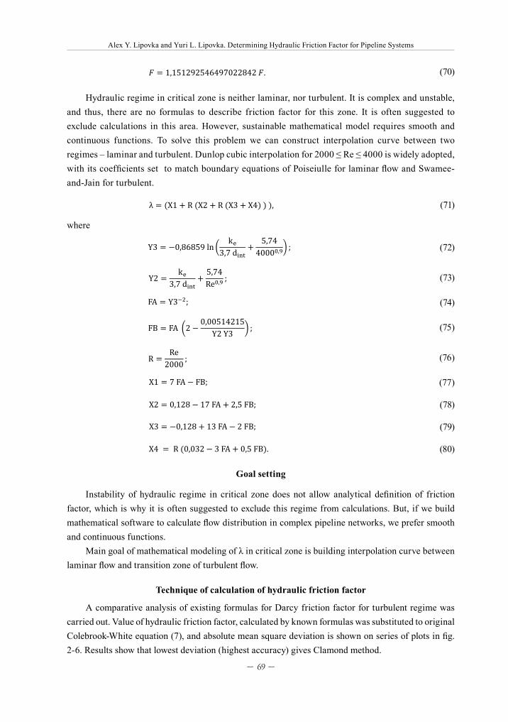
Hydraulic regime in critical zone is neither laminar, nor turbulent. It is complex and unstable, and thus, there are no formulas to describe friction factor for this zone. It is often suggested to exclude calculations in this area. However, sustainable mathematical model requires smooth and continuous functions. To solve this problem we can construct interpolation curve between two regimes – laminar and turbulent. Dunlop cubic interpolation for 2000 ≤ Re ≤ 4000 is widely adopted, with its coefficients set to match boundary equations of Poiseiulle for laminar flow and Swamee-and-Jain for turbulent.
� � �2 � 0,2; (67)
�������2������ �� �
ln��1 � �� � � � �21 � �1 � �
� � � ��1 � �1 � � � 0,5 �� � ��1 � ��
1 � �1 � � � � �1 � �3�
;
(68)
(69)
� � 1,1512�254�4�7022�42 �� (70)
Hydraulic regime in critical zone is neither laminar, nor turbulent. It is complex and unstable,
and thus, there are no formulas to describe friction factor for this zone. It is often suggested to
exclude calculations in this area. However, sustainable mathematical model requires smooth and
continuous functions. To solve this problem we can construct interpolation curve between two
regimes – laminar and turbulent. Dunlop cubic interpolation for 2000 � �� � 4000 is widely
adopted, with its coefficients set to match boundary equations of Poiseiulle for laminar flow and
Swamee-and-Jain for turbulent.
λ � ��1 � R ��2 � R ��3 � �4� � �, (71)
where
Y3 � �0,���5� ln �k�
3,7 d����
5,744000�,�� ;
(72)
Y2 �k�
3,7 d����5,74Re�,� ;
(73)
�� � Y3��; (74)
�� � �� �2 �0,00514215
Y2 Y3 � ; (75)
R �Re2000 ;
(76)
�1 � 7 �� � ��; (77)
(71)
where
� � �2 � 0,2; (67)
�������2������ �� �
ln��1 � �� � � � �21 � �1 � �
� � � ��1 � �1 � � � 0,5 �� � ��1 � ��
1 � �1 � � � � �1 � �3�
;
(68)
(69)
� � 1,1512�254�4�7022�42 �� (70)
Hydraulic regime in critical zone is neither laminar, nor turbulent. It is complex and unstable,
and thus, there are no formulas to describe friction factor for this zone. It is often suggested to
exclude calculations in this area. However, sustainable mathematical model requires smooth and
continuous functions. To solve this problem we can construct interpolation curve between two
regimes – laminar and turbulent. Dunlop cubic interpolation for 2000 � �� � 4000 is widely
adopted, with its coefficients set to match boundary equations of Poiseiulle for laminar flow and
Swamee-and-Jain for turbulent.
λ � ��1 � R ��2 � R ��3 � �4� � �, (71)
where
Y3 � �0,���5� ln �k�
3,7 d����
5,744000�,�� ;
(72)
Y2 �k�
3,7 d����5,74Re�,� ;
(73)
�� � Y3��; (74)
�� � �� �2 �0,00514215
Y2 Y3 � ; (75)
R �Re2000 ;
(76)
�1 � 7 �� � ��; (77)
(72)
� � �2 � 0,2; (67)
�������2������ �� �
ln��1 � �� � � � �21 � �1 � �
� � � ��1 � �1 � � � 0,5 �� � ��1 � ��
1 � �1 � � � � �1 � �3�
;
(68)
(69)
� � 1,1512�254�4�7022�42 �� (70)
Hydraulic regime in critical zone is neither laminar, nor turbulent. It is complex and unstable,
and thus, there are no formulas to describe friction factor for this zone. It is often suggested to
exclude calculations in this area. However, sustainable mathematical model requires smooth and
continuous functions. To solve this problem we can construct interpolation curve between two
regimes – laminar and turbulent. Dunlop cubic interpolation for 2000 � �� � 4000 is widely
adopted, with its coefficients set to match boundary equations of Poiseiulle for laminar flow and
Swamee-and-Jain for turbulent.
λ � ��1 � R ��2 � R ��3 � �4� � �, (71)
where
Y3 � �0,���5� ln �k�
3,7 d����
5,744000�,�� ;
(72)
Y2 �k�
3,7 d����5,74Re�,� ;
(73)
�� � Y3��; (74)
�� � �� �2 �0,00514215
Y2 Y3 � ; (75)
R �Re2000 ;
(76)
�1 � 7 �� � ��; (77)
(73)
� � �2 � 0,2; (67)
�������2������ �� �
ln��1 � �� � � � �21 � �1 � �
� � � ��1 � �1 � � � 0,5 �� � ��1 � ��
1 � �1 � � � � �1 � �3�
;
(68)
(69)
� � 1,1512�254�4�7022�42 �� (70)
Hydraulic regime in critical zone is neither laminar, nor turbulent. It is complex and unstable,
and thus, there are no formulas to describe friction factor for this zone. It is often suggested to
exclude calculations in this area. However, sustainable mathematical model requires smooth and
continuous functions. To solve this problem we can construct interpolation curve between two
regimes – laminar and turbulent. Dunlop cubic interpolation for 2000 � �� � 4000 is widely
adopted, with its coefficients set to match boundary equations of Poiseiulle for laminar flow and
Swamee-and-Jain for turbulent.
λ � ��1 � R ��2 � R ��3 � �4� � �, (71)
where
Y3 � �0,���5� ln �k�
3,7 d����
5,744000�,�� ;
(72)
Y2 �k�
3,7 d����5,74Re�,� ;
(73)
�� � Y3��; (74)
�� � �� �2 �0,00514215
Y2 Y3 � ; (75)
R �Re2000 ;
(76)
�1 � 7 �� � ��; (77)
(74)
� � �2 � 0,2; (67)
�������2������ �� �
ln��1 � �� � � � �21 � �1 � �
� � � ��1 � �1 � � � 0,5 �� � ��1 � ��
1 � �1 � � � � �1 � �3�
;
(68)
(69)
� � 1,1512�254�4�7022�42 �� (70)
Hydraulic regime in critical zone is neither laminar, nor turbulent. It is complex and unstable,
and thus, there are no formulas to describe friction factor for this zone. It is often suggested to
exclude calculations in this area. However, sustainable mathematical model requires smooth and
continuous functions. To solve this problem we can construct interpolation curve between two
regimes – laminar and turbulent. Dunlop cubic interpolation for 2000 � �� � 4000 is widely
adopted, with its coefficients set to match boundary equations of Poiseiulle for laminar flow and
Swamee-and-Jain for turbulent.
λ � ��1 � R ��2 � R ��3 � �4� � �, (71)
where
Y3 � �0,���5� ln �k�
3,7 d����
5,744000�,�� ;
(72)
Y2 �k�
3,7 d����5,74Re�,� ;
(73)
�� � Y3��; (74)
�� � �� �2 �0,00514215
Y2 Y3 � ; (75)
R �Re2000 ;
(76)
�1 � 7 �� � ��; (77)
(75)
� � �2 � 0,2; (67)
�������2������ �� �
ln��1 � �� � � � �21 � �1 � �
� � � ��1 � �1 � � � 0,5 �� � ��1 � ��
1 � �1 � � � � �1 � �3�
;
(68)
(69)
� � 1,1512�254�4�7022�42 �� (70)
Hydraulic regime in critical zone is neither laminar, nor turbulent. It is complex and unstable,
and thus, there are no formulas to describe friction factor for this zone. It is often suggested to
exclude calculations in this area. However, sustainable mathematical model requires smooth and
continuous functions. To solve this problem we can construct interpolation curve between two
regimes – laminar and turbulent. Dunlop cubic interpolation for 2000 � �� � 4000 is widely
adopted, with its coefficients set to match boundary equations of Poiseiulle for laminar flow and
Swamee-and-Jain for turbulent.
λ � ��1 � R ��2 � R ��3 � �4� � �, (71)
where
Y3 � �0,���5� ln �k�
3,7 d����
5,744000�,�� ;
(72)
Y2 �k�
3,7 d����5,74Re�,� ;
(73)
�� � Y3��; (74)
�� � �� �2 �0,00514215
Y2 Y3 � ; (75)
R �Re2000 ;
(76)
�1 � 7 �� � ��; (77)
(76)
� � �2 � 0,2; (67)
�������2������ �� �
ln��1 � �� � � � �21 � �1 � �
� � � ��1 � �1 � � � 0,5 �� � ��1 � ��
1 � �1 � � � � �1 � �3�
;
(68)
(69)
� � 1,1512�254�4�7022�42 �� (70)
Hydraulic regime in critical zone is neither laminar, nor turbulent. It is complex and unstable,
and thus, there are no formulas to describe friction factor for this zone. It is often suggested to
exclude calculations in this area. However, sustainable mathematical model requires smooth and
continuous functions. To solve this problem we can construct interpolation curve between two
regimes – laminar and turbulent. Dunlop cubic interpolation for 2000 � �� � 4000 is widely
adopted, with its coefficients set to match boundary equations of Poiseiulle for laminar flow and
Swamee-and-Jain for turbulent.
λ � ��1 � R ��2 � R ��3 � �4� � �, (71)
where
Y3 � �0,���5� ln �k�
3,7 d����
5,744000�,�� ;
(72)
Y2 �k�
3,7 d����5,74Re�,� ;
(73)
�� � Y3��; (74)
�� � �� �2 �0,00514215
Y2 Y3 � ; (75)
R �Re2000 ;
(76)
�1 � 7 �� � ��; (77) (77)
�� � ����� � �� �� � ��� ��� (78)
�� � ������ � �� �� � � ��� (79)
��� � �R������� � � �� � ��� ���� (80)
Goal setting
Instability of hydraulic regime in critical zone does not allow analytical definition of friction
factor, which is why it is often suggested to exclude this regime from calculations. But, if we build
mathematical software to calculate flow distribution in complex pipeline networks, we prefer
smooth and continuous functions.
Main goal of mathematical modeling of � in critical zone is building interpolation curve
between laminar flow and transition zone of turbulent flow.
Technique of calculation of hydraulic friction factor
A comparative analysis of existing formulas for Darcy friction factor for turbulent regime
was carried out. Value of hydraulic friction factor, calculated by known formulas was substituted to
original Colebrook-White equation (7), and absolute mean square deviation is shown on series of
plots in Fig. 2-6. Results show that lowest deviation (highest accuracy) gives Clamond method.
Fig. 2 – Absolute mean square deviation for ��� � ������ � ����
6,57
E‐16
3,63
E+00
2,29
E+00
1,03
E‐03
2,20
E+00
2,90
E‐02
3,36
E‐02
2,03
E‐03
1,41
E‐02
1,53
E‐02
1,24
E‐02
1,33
E‐02
1,15
E‐02
1,17
E‐02
1,78
E‐04
6,09
E‐03
5,01
E‐03
9,06
E‐06
2,31
E‐03
4,28
E‐09
1,24
E‐02
2,28
E‐04
8,19
E‐04
4,18
E‐05
1,12
E‐05
7,53
E‐03
3,86
E‐03
1,38
E‐02
2,88
E‐02
3,84
E‐16
1,19
E‐02
Didier C
lamon
d
Blasius (smoo
th)
Altshu
l (sm
ooth)
Altshu
l
Nikuradse (smoo
th)
Prandtl, Nikuradse …
Shifrinson
Moo
dy
Woo
d
Eck
Churchill
Jain, Swam
ee Jain
Churchill, 197
7
Chen
Roun
d
Barr
Zigrang, Sylvester
Haaland
Serghide
s
Manadilli
Mon
zon, Rom
eo, Royo
Gou
dar, Son
nad
Vatankhah, …
Buzelli
Avci, Kargoz
Evangleids and
other
Dob
romyslov
Rao, Kum
ar
Gou
dar, Son
nad, 200
8
Brkić
(78)�� � ����� � �� �� � ��� ��� (78)
�� � ������ � �� �� � � ��� (79)
��� � �R������� � � �� � ��� ���� (80)
Goal setting
Instability of hydraulic regime in critical zone does not allow analytical definition of friction
factor, which is why it is often suggested to exclude this regime from calculations. But, if we build
mathematical software to calculate flow distribution in complex pipeline networks, we prefer
smooth and continuous functions.
Main goal of mathematical modeling of � in critical zone is building interpolation curve
between laminar flow and transition zone of turbulent flow.
Technique of calculation of hydraulic friction factor
A comparative analysis of existing formulas for Darcy friction factor for turbulent regime
was carried out. Value of hydraulic friction factor, calculated by known formulas was substituted to
original Colebrook-White equation (7), and absolute mean square deviation is shown on series of
plots in Fig. 2-6. Results show that lowest deviation (highest accuracy) gives Clamond method.
Fig. 2 – Absolute mean square deviation for ��� � ������ � ����
6,57
E‐16
3,63
E+00
2,29
E+00
1,03
E‐03
2,20
E+00
2,90
E‐02
3,36
E‐02
2,03
E‐03
1,41
E‐02
1,53
E‐02
1,24
E‐02
1,33
E‐02
1,15
E‐02
1,17
E‐02
1,78
E‐04
6,09
E‐03
5,01
E‐03
9,06
E‐06
2,31
E‐03
4,28
E‐09
1,24
E‐02
2,28
E‐04
8,19
E‐04
4,18
E‐05
1,12
E‐05
7,53
E‐03
3,86
E‐03
1,38
E‐02
2,88
E‐02
3,84
E‐16
1,19
E‐02
Didier C
lamon
d
Blasius (smoo
th)
Altshu
l (sm
ooth)
Altshu
l
Nikuradse (smoo
th)
Prandtl, Nikuradse …
Shifrinson
Moo
dy
Woo
d
Eck
Churchill
Jain, Swam
ee Jain
Churchill, 197
7
Chen
Roun
d
Barr
Zigrang, Sylvester
Haaland
Serghide
s
Manadilli
Mon
zon, Rom
eo, Royo
Gou
dar, Son
nad
Vatankhah, …
Buzelli
Avci, Kargoz
Evangleids and
other
Dob
romyslov
Rao, Kum
ar
Gou
dar, Son
nad, 200
8
Brkić
(79)
�� � ����� � �� �� � ��� ��� (78)
�� � ������ � �� �� � � ��� (79)
��� � �R������� � � �� � ��� ���� (80)
Goal setting
Instability of hydraulic regime in critical zone does not allow analytical definition of friction
factor, which is why it is often suggested to exclude this regime from calculations. But, if we build
mathematical software to calculate flow distribution in complex pipeline networks, we prefer
smooth and continuous functions.
Main goal of mathematical modeling of � in critical zone is building interpolation curve
between laminar flow and transition zone of turbulent flow.
Technique of calculation of hydraulic friction factor
A comparative analysis of existing formulas for Darcy friction factor for turbulent regime
was carried out. Value of hydraulic friction factor, calculated by known formulas was substituted to
original Colebrook-White equation (7), and absolute mean square deviation is shown on series of
plots in Fig. 2-6. Results show that lowest deviation (highest accuracy) gives Clamond method.
Fig. 2 – Absolute mean square deviation for ��� � ������ � ����
6,57
E‐16
3,63
E+00
2,29
E+00
1,03
E‐03
2,20
E+00
2,90
E‐02
3,36
E‐02
2,03
E‐03
1,41
E‐02
1,53
E‐02
1,24
E‐02
1,33
E‐02
1,15
E‐02
1,17
E‐02
1,78
E‐04
6,09
E‐03
5,01
E‐03
9,06
E‐06
2,31
E‐03
4,28
E‐09
1,24
E‐02
2,28
E‐04
8,19
E‐04
4,18
E‐05
1,12
E‐05
7,53
E‐03
3,86
E‐03
1,38
E‐02
2,88
E‐02
3,84
E‐16
1,19
E‐02
Didier C
lamon
d
Blasius (smoo
th)
Altshu
l (sm
ooth)
Altshu
l
Nikuradse (smoo
th)
Prandtl, Nikuradse …
Shifrinson
Moo
dy
Woo
d
Eck
Churchill
Jain, Swam
ee Jain
Churchill, 197
7
Chen
Roun
d
Barr
Zigrang, Sylvester
Haaland
Serghide
s
Manadilli
Mon
zon, Rom
eo, Royo
Gou
dar, Son
nad
Vatankhah, …
Buzelli
Avci, Kargoz
Evangleids and
other
Dob
romyslov
Rao, Kum
ar
Gou
dar, Son
nad, 200
8
Brkić
(80)
Goal setting
Instability of hydraulic regime in critical zone does not allow analytical definition of friction factor, which is why it is often suggested to exclude this regime from calculations. But, if we build mathematical software to calculate flow distribution in complex pipeline networks, we prefer smooth and continuous functions.
Main goal of mathematical modeling of λ in critical zone is building interpolation curve between laminar flow and transition zone of turbulent flow.
Technique of calculation of hydraulic friction factor
A comparative analysis of existing formulas for Darcy friction factor for turbulent regime was carried out. Value of hydraulic friction factor, calculated by known formulas was substituted to original Colebrook-White equation (7), and absolute mean square deviation is shown on series of plots in fig. 2-6. Results show that lowest deviation (highest accuracy) gives Clamond method.
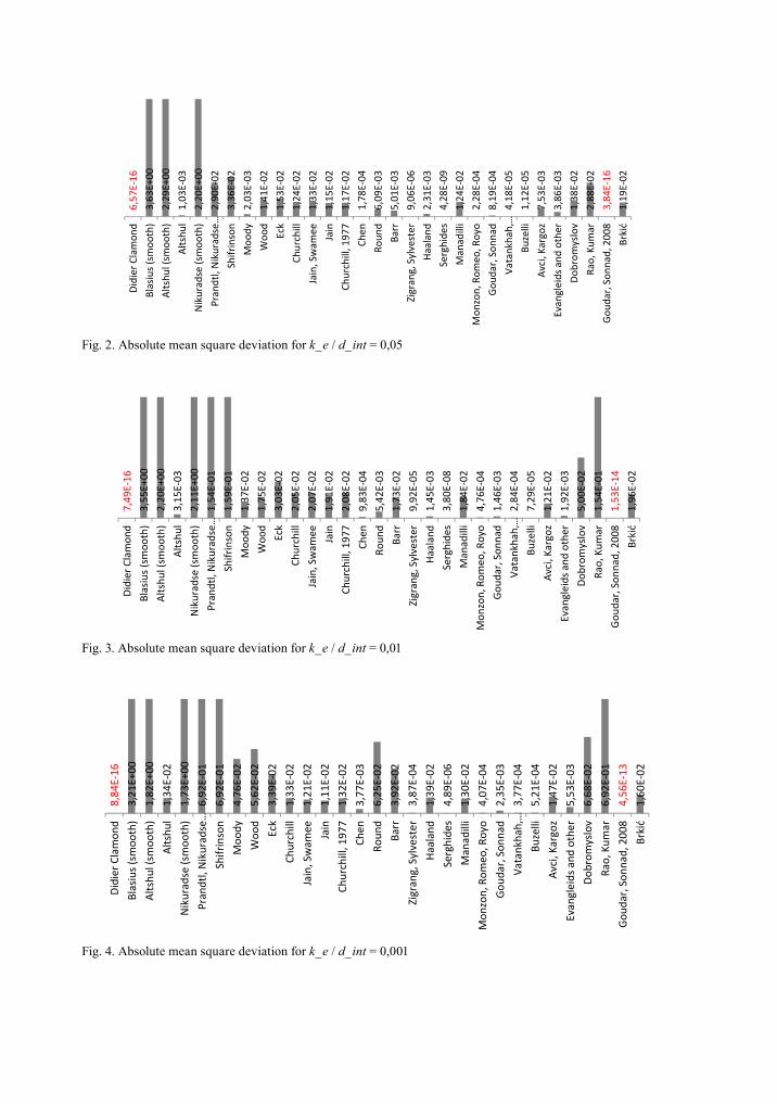
�� � ����� � �� �� � ��� ��� (78)
�� � ������ � �� �� � � ��� (79)
��� � �R������� � � �� � ��� ���� (80)
Goal setting
Instability of hydraulic regime in critical zone does not allow analytical definition of friction
factor, which is why it is often suggested to exclude this regime from calculations. But, if we build
mathematical software to calculate flow distribution in complex pipeline networks, we prefer
smooth and continuous functions.
Main goal of mathematical modeling of � in critical zone is building interpolation curve
between laminar flow and transition zone of turbulent flow.
Technique of calculation of hydraulic friction factor
A comparative analysis of existing formulas for Darcy friction factor for turbulent regime
was carried out. Value of hydraulic friction factor, calculated by known formulas was substituted to
original Colebrook-White equation (7), and absolute mean square deviation is shown on series of
plots in Fig. 2-6. Results show that lowest deviation (highest accuracy) gives Clamond method.
Fig. 2 – Absolute mean square deviation for ��� � ������ � ����
6,57
E‐16
3,63
E+00
2,29
E+00
1,03
E‐03
2,20
E+00
2,90
E‐02
3,36
E‐02
2,03
E‐03
1,41
E‐02
1,53
E‐02
1,24
E‐02
1,33
E‐02
1,15
E‐02
1,17
E‐02
1,78
E‐04
6,09
E‐03
5,01
E‐03
9,06
E‐06
2,31
E‐03
4,28
E‐09
1,24
E‐02
2,28
E‐04
8,19
E‐04
4,18
E‐05
1,12
E‐05
7,53
E‐03
3,86
E‐03
1,38
E‐02
2,88
E‐02
3,84
E‐16
1,19
E‐02
Didier C
lamon
d
Blasius (smoo
th)
Altshu
l (sm
ooth)
Altshu
l
Nikuradse (smoo
th)
Prandtl, Nikuradse …
Shifrinson
Moo
dy
Woo
d
Eck
Churchill
Jain, Swam
ee Jain
Churchill, 197
7
Chen
Roun
d
Barr
Zigrang, Sylvester
Haaland
Serghide
s
Manadilli
Mon
zon, Rom
eo, Royo
Gou
dar, Son
nad
Vatankhah, …
Buzelli
Avci, Kargoz
Evangleids and
other
Dob
romyslov
Rao, Kum
ar
Gou
dar, Son
nad, 200
8
Brkić
Fig. 2. Absolute mean square deviation for k_e / d_int = 0,05
Fig. 3 – Absolute mean square deviation for
Fig. 4 – Absolute mean square deviation for
Fig. 5 – Absolute mean square deviation for
7,49
E‐16
3,55
E+00
2,20
E+00
3,15
E‐03
2,11
E+00
1,54
E‐01
1,59
E‐01
1,37
E‐02
1,75
E‐02
3,03
E‐02
2,05
E‐02
2,07
E‐02
1,91
E‐02
2,08
E‐02
9,83
E‐04
5,42
E‐03
1,73
E‐02
9,92
E‐05
1,45
E‐03
3,80
E‐08
1,84
E‐02
4,76
E‐04
1,46
E‐03
2,84
E‐04
7,29
E‐05
1,21
E‐02
1,92
E‐03
5,00
E‐02
1,54
E‐01
1,53
E‐14
1,96
E‐02
Didier C
lamon
d
Blasius (smoo
th)
Altshu
l (sm
ooth)
Altshu
l
Nikuradse (smoo
th)
Prandtl, Nikuradse …
Shifrinson
Moo
dy
Woo
d
Eck
Churchill
Jain, Swam
ee Jain
Churchill, 197
7
Chen
Roun
d
Barr
Zigrang, Sylvester
Haaland
Serghide
s
Manadilli
Mon
zon, Rom
eo, Royo
Gou
dar, Son
nad
Vatankhah, …
Buzelli
Avci, Kargoz
Evangleids and
other
Dob
romyslov
Rao, Kum
ar
Gou
dar, Son
nad, 200
8
Brkić
8,84
E‐16
3,21
E+00
1,82
E+00
1,34
E‐02
1,73
E+00
6,92
E‐01
6,92
E‐01
4,76
E‐02
5,62
E‐02
3,39
E‐02
1,33
E‐02
1,21
E‐02
1,11
E‐02
1,32
E‐02
3,77
E‐03
6,25
E‐02
3,92
E‐02
3,87
E‐04
1,39
E‐02
4,89
E‐06
1,30
E‐02
4,07
E‐04
2,35
E‐03
3,77
E‐04
5,21
E‐04
1,47
E‐02
5,53
E‐03
6,68
E‐02
6,92
E‐01
4,56
E‐13
1,60
E‐02
Didier C
lamon
d
Blasius (smoo
th)
Altshu
l (sm
ooth)
Altshu
l
Nikuradse (smoo
th)
Prandtl, Nikuradse …
Shifrinson
Moo
dy
Woo
d
Eck
Churchill
Jain, Swam
ee Jain
Churchill, 197
7
Chen
Roun
d
Barr
Zigrang, Sylvester
Haaland
Serghide
s
Manadilli
Mon
zon, Rom
eo, Royo
Gou
dar, Son
nad
Vatankhah, …
Buzelli
Avci, Kargoz
Evangleids and
other
Dob
romyslov
Rao, Kum
ar
Gou
dar, Son
nad, 200
8
Brkić
9,47
E‐16
2,57
E+00
1,16
E+00
1,52
E‐01
1,11
E+00
1,46
E+00
1,47
E+00
5,30
E‐02
8,00
E‐02
6,57
E‐02
9,98
E‐03
9,05
E‐03
8,33
E‐03
9,77
E‐03
4,33
E‐03
1,37
E‐01
4,86
E‐02
1,29
E‐03
2,03
E‐02
2,73
E‐05
9,99
E‐03
4,96
E‐04
2,42
E‐03
4,01
E‐04
5,02
E‐04
6,51
E‐03
5,56
E‐03
4,64
E‐02
1,46
E+00
7,09
E‐13
9,25
E‐03
Didier C
lamon
dBlasius (smoo
th)
Altshu
l (sm
ooth)
Altshu
lNikuradse (smoo
th)
Prandtl, Nikuradse …
Shifrinson
Moo
dyWoo
dEck
Churchill
Jain, Swam
ee Jain
Churchill, 197
7Ch
enRo
und
Barr
Zigrang, Sylvester
Haaland
Serghide
sManadilli
Mon
zon, Rom
eo, …
Gou
dar, Son
nad
Vatankhah, …
Buzelli
Avci, Kargoz
Evangleids and
…Dob
romyslov
Rao, Kum
arGou
dar, Son
nad, …
Brkić
Fig. 3. Absolute mean square deviation for k_e / d_int = 0,01
Fig. 3 – Absolute mean square deviation for
Fig. 4 – Absolute mean square deviation for
Fig. 5 – Absolute mean square deviation for
7,49
E‐16
3,55
E+00
2,20
E+00
3,15
E‐03
2,11
E+00
1,54
E‐01
1,59
E‐01
1,37
E‐02
1,75
E‐02
3,03
E‐02
2,05
E‐02
2,07
E‐02
1,91
E‐02
2,08
E‐02
9,83
E‐04
5,42
E‐03
1,73
E‐02
9,92
E‐05
1,45
E‐03
3,80
E‐08
1,84
E‐02
4,76
E‐04
1,46
E‐03
2,84
E‐04
7,29
E‐05
1,21
E‐02
1,92
E‐03
5,00
E‐02
1,54
E‐01
1,53
E‐14
1,96
E‐02
Didier C
lamon
d
Blasius (smoo
th)
Altshu
l (sm
ooth)
Altshu
l
Nikuradse (smoo
th)
Prandtl, Nikuradse …
Shifrinson
Moo
dy
Woo
d
Eck
Churchill
Jain, Swam
ee Jain
Churchill, 197
7
Chen
Roun
d
Barr
Zigrang, Sylvester
Haaland
Serghide
s
Manadilli
Mon
zon, Rom
eo, Royo
Gou
dar, Son
nad
Vatankhah, …
Buzelli
Avci, Kargoz
Evangleids and
other
Dob
romyslov
Rao, Kum
ar
Gou
dar, Son
nad, 200
8
Brkić
8,84
E‐16
3,21
E+00
1,82
E+00
1,34
E‐02
1,73
E+00
6,92
E‐01
6,92
E‐01
4,76
E‐02
5,62
E‐02
3,39
E‐02
1,33
E‐02
1,21
E‐02
1,11
E‐02
1,32
E‐02
3,77
E‐03
6,25
E‐02
3,92
E‐02
3,87
E‐04
1,39
E‐02
4,89
E‐06
1,30
E‐02
4,07
E‐04
2,35
E‐03
3,77
E‐04
5,21
E‐04
1,47
E‐02
5,53
E‐03
6,68
E‐02
6,92
E‐01
4,56
E‐13
1,60
E‐02
Didier C
lamon
d
Blasius (smoo
th)
Altshu
l (sm
ooth)
Altshu
l
Nikuradse (smoo
th)
Prandtl, Nikuradse …
Shifrinson
Moo
dy
Woo
d
Eck
Churchill
Jain, Swam
ee Jain
Churchill, 197
7
Chen
Roun
d
Barr
Zigrang, Sylvester
Haaland
Serghide
s
Manadilli
Mon
zon, Rom
eo, Royo
Gou
dar, Son
nad
Vatankhah, …
Buzelli
Avci, Kargoz
Evangleids and
other
Dob
romyslov
Rao, Kum
ar
Gou
dar, Son
nad, 200
8
Brkić
9,47
E‐16
2,57
E+00
1,16
E+00
1,52
E‐01
1,11
E+00
1,46
E+00
1,47
E+00
5,30
E‐02
8,00
E‐02
6,57
E‐02
9,98
E‐03
9,05
E‐03
8,33
E‐03
9,77
E‐03
4,33
E‐03
1,37
E‐01
4,86
E‐02
1,29
E‐03
2,03
E‐02
2,73
E‐05
9,99
E‐03
4,96
E‐04
2,42
E‐03
4,01
E‐04
5,02
E‐04
6,51
E‐03
5,56
E‐03
4,64
E‐02
1,46
E+00
7,09
E‐13
9,25
E‐03
Didier C
lamon
dBlasius (smoo
th)
Altshu
l (sm
ooth)
Altshu
lNikuradse (smoo
th)
Prandtl, Nikuradse …
Shifrinson
Moo
dyWoo
dEck
Churchill
Jain, Swam
ee Jain
Churchill, 197
7Ch
enRo
und
Barr
Zigrang, Sylvester
Haaland
Serghide
sManadilli
Mon
zon, Rom
eo, …
Gou
dar, Son
nad
Vatankhah, …
Buzelli
Avci, Kargoz
Evangleids and
…Dob
romyslov
Rao, Kum
arGou
dar, Son
nad, …
Brkić
Fig. 4. Absolute mean square deviation for k_e / d_int = 0,001
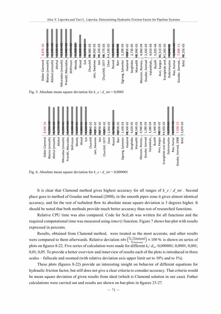
– 71 –
Alex Y. Lipovka and Yuri L. Lipovka. Determining Hydraulic Friction Factor for Pipeline Systems
Fig. 3 – Absolute mean square deviation for
Fig. 4 – Absolute mean square deviation for
Fig. 5 – Absolute mean square deviation for
7,49
E‐16
3,55
E+00
2,20
E+00
3,15
E‐03
2,11
E+00
1,54
E‐01
1,59
E‐01
1,37
E‐02
1,75
E‐02
3,03
E‐02
2,05
E‐02
2,07
E‐02
1,91
E‐02
2,08
E‐02
9,83
E‐04
5,42
E‐03
1,73
E‐02
9,92
E‐05
1,45
E‐03
3,80
E‐08
1,84
E‐02
4,76
E‐04
1,46
E‐03
2,84
E‐04
7,29
E‐05
1,21
E‐02
1,92
E‐03
5,00
E‐02
1,54
E‐01
1,53
E‐14
1,96
E‐02
Didier C
lamon
d
Blasius (smoo
th)
Altshu
l (sm
ooth)
Altshu
l
Nikuradse (smoo
th)
Prandtl, Nikuradse …
Shifrinson
Moo
dy
Woo
d
Eck
Churchill
Jain, Swam
ee Jain
Churchill, 197
7
Chen
Roun
d
Barr
Zigrang, Sylvester
Haaland
Serghide
s
Manadilli
Mon
zon, Rom
eo, Royo
Gou
dar, Son
nad
Vatankhah, …
Buzelli
Avci, Kargoz
Evangleids and
other
Dob
romyslov
Rao, Kum
ar
Gou
dar, Son
nad, 200
8
Brkić
8,84
E‐16
3,21
E+00
1,82
E+00
1,34
E‐02
1,73
E+00
6,92
E‐01
6,92
E‐01
4,76
E‐02
5,62
E‐02
3,39
E‐02
1,33
E‐02
1,21
E‐02
1,11
E‐02
1,32
E‐02
3,77
E‐03
6,25
E‐02
3,92
E‐02
3,87
E‐04
1,39
E‐02
4,89
E‐06
1,30
E‐02
4,07
E‐04
2,35
E‐03
3,77
E‐04
5,21
E‐04
1,47
E‐02
5,53
E‐03
6,68
E‐02
6,92
E‐01
4,56
E‐13
1,60
E‐02
Didier C
lamon
d
Blasius (smoo
th)
Altshu
l (sm
ooth)
Altshu
l
Nikuradse (smoo
th)
Prandtl, Nikuradse …
Shifrinson
Moo
dy
Woo
d
Eck
Churchill
Jain, Swam
ee Jain
Churchill, 197
7
Chen
Roun
d
Barr
Zigrang, Sylvester
Haaland
Serghide
s
Manadilli
Mon
zon, Rom
eo, Royo
Gou
dar, Son
nad
Vatankhah, …
Buzelli
Avci, Kargoz
Evangleids and
other
Dob
romyslov
Rao, Kum
ar
Gou
dar, Son
nad, 200
8
Brkić
9,47
E‐16
2,57
E+00
1,16
E+00
1,52
E‐01
1,11
E+00
1,46
E+00
1,47
E+00
5,30
E‐02
8,00
E‐02
6,57
E‐02
9,98
E‐03
9,05
E‐03
8,33
E‐03
9,77
E‐03
4,33
E‐03
1,37
E‐01
4,86
E‐02
1,29
E‐03
2,03
E‐02
2,73
E‐05
9,99
E‐03
4,96
E‐04
2,42
E‐03
4,01
E‐04
5,02
E‐04
6,51
E‐03
5,56
E‐03
4,64
E‐02
1,46
E+00
7,09
E‐13
9,25
E‐03
Didier C
lamon
dBlasius (smoo
th)
Altshu
l (sm
ooth)
Altshu
lNikuradse (smoo
th)
Prandtl, Nikuradse …
Shifrinson
Moo
dyWoo
dEck
Churchill
Jain, Swam
ee Jain
Churchill, 197
7Ch
enRo
und
Barr
Zigrang, Sylvester
Haaland
Serghide
sManadilli
Mon
zon, Rom
eo, …
Gou
dar, Son
nad
Vatankhah, …
Buzelli
Avci, Kargoz
Evangleids and
…Dob
romyslov
Rao, Kum
arGou
dar, Son
nad, …
Brkić
Fig. 5. Absolute mean square deviation for k_e / d_int = 0,0001
Fig. 6. Absolute mean square deviation for k_e / d_int = 0,000001
Fig. 6 – Absolute mean square deviation for
It is clear that Clamond method gives highest accuracy for all ranges of .
Second place goes to method of Goudar and Sonnad (2008), in the smooth pipes zone it gives
almost identical accuracy, and for the rest of turbulent flow its absolute mean square deviation is 3
degrees higher. It should be noted that both methods provide much better accuracy than rest of
researched functions.
Relative CPU time was also compared. Code for SciLab was written for all functions and
the required computational time was measured using timer() function. Figure 7 shows bar-plot with
results expressed in percents.
8,93
E‐16
1,55
E+00
9,74
E‐02
1,17
E+00
1,21
E‐01
2,47
E+00
2,49
E+00
1,62
E‐01
1,86
E‐01
1,61
E‐01
2,04
E‐02
1,93
E‐02
1,79
E‐02
1,99
E‐02
2,05
E‐03
8,79
E‐02
1,70
E‐02
1,43
E‐03
1,30
E‐02
4,62
E‐05
8,54
E‐03
4,94
E‐04
1,28
E‐03
3,28
E‐04
2,44
E‐04
1,50
E‐02
4,95
E‐03
1,07
E‐01
2,47
E+00
7,33
E‐13
2,87
E‐03
Didier C
lamon
d
Blasius (smoo
th)
Altshu
l (sm
ooth)
Altshu
lNikuradse (smoo
th)
Prandtl, Nikuradse …
Shifrinson
Moo
dyWoo
d
Eck
Churchill
Jain, Swam
ee Jain
Churchill, 197
7Ch
enRo
und
Barr
Zigrang, Sylvester
Haaland
Serghide
s
Manadilli
Mon
zon, Rom
eo, …
Gou
dar, Son
nad
Vatankhah, …
Buzelli
Avci, Kargoz
Evangleids and
other
Dob
romyslov
Rao, Kum
arGou
dar, Son
nad, 200
8
Brkić
It is clear that Clamond method gives highest accuracy for all ranges of k_e / d_int . Second place goes to method of Goudar and Sonnad (2008), in the smooth pipes zone it gives almost identical accuracy, and for the rest of turbulent flow its absolute mean square deviation is 3 degrees higher. It should be noted that both methods provide much better accuracy than rest of researched functions.
Relative CPU time was also compared. Code for SciLab was written for all functions and the required computational time was measured using timer() function. Figure 7 shows bar-plot with results expressed in percents.
Results, obtained from Clamond method, were treated as the most accurate, and other results were compared to them afterwards. Relative deviation
Fig. 7 – Relative CPU time to compute friction factor
Results, obtained from Clamond method, were treated as the most accurate, and other
results were compared to them afterwards. Relative deviation is shown
on series of plots on figures 8-22. Five series of calculation were made for different / :
0,000001; 0,0001; 0,001; 0,01; 0,05. To provide a better overview and innerview of results each of
the plots is introduced in three scales – fullscale and zoomed (with relative deviation axis upper
limit set to 10 % and to 1 %).
62
16
3225
18
57
40
3135 39 40 41 40 38
56
39
56
75
39
82
40
73
32 33
50
28
53
100
54 57
45
0
10
20
30
40
50
60
70
80
90
100
Didier C
lamon
dBlasius (smoo
th)
Altshu
l (sm
ooth)
Altshu
lNikuradse (smoo
th)
Prandtl, Nikuradse (turbu
lent …
Shifrinson
Moo
dyWoo
dEck
Churchill
Jain, Swam
ee Jain
Churchill, 197
7Ch
enRo
und
Barr
Zigrang, Sylvester
Haaland
Serghide
sManadilli
Mon
zon, Rom
eo, Royo
Gou
dar, Son
nad
Vatankhah, Kou
chakzade
hBu
zelli
Avci, Kargoz
Dob
romyslov
Rao, Kum
arGou
dar, Son
nad, 200
8Brkić
is shown on series of plots on figures 8-22. Five series of calculation were made for different kв/ dint: 0,000001; 0,0001; 0,001; 0,01; 0,05. To provide a better overview and innerview of results each of the plots is introduced in three scales – fullscale and zoomed (with relative deviation axis upper limit set to 10% and to 1%).
These plots (figures 8-22) provide an interesting insight on behavior of different equations for hydraulic friction factor, but still does not give a clear criteria to consider accuracy. That criteria would be mean square deviation of given results from ideal (which is Clamond solution in our case). Futher calculations were carried out and results are shown on bar-plots in figures 23-27.
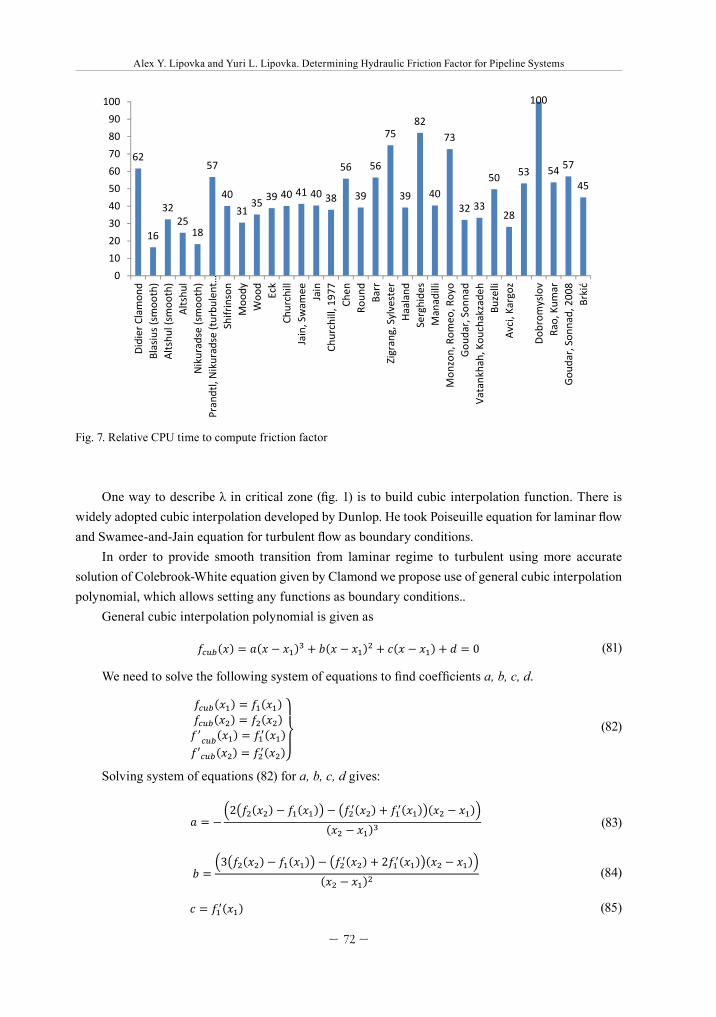
– 72 –
Alex Y. Lipovka and Yuri L. Lipovka. Determining Hydraulic Friction Factor for Pipeline Systems
Fig. 7 – Relative CPU time to compute friction factor
Results, obtained from Clamond method, were treated as the most accurate, and other
results were compared to them afterwards. Relative deviation is shown
on series of plots on figures 8-22. Five series of calculation were made for different / :
0,000001; 0,0001; 0,001; 0,01; 0,05. To provide a better overview and innerview of results each of
the plots is introduced in three scales – fullscale and zoomed (with relative deviation axis upper
limit set to 10 % and to 1 %).
62
16
3225
18
57
40
3135 39 40 41 40 38
56
39
56
75
39
82
40
73
32 33
50
28
53
100
54 57
45
0
10
20
30
40
50
60
70
80
90
100
Didier C
lamon
dBlasius (smoo
th)
Altshu
l (sm
ooth)
Altshu
lNikuradse (smoo
th)
Prandtl, Nikuradse (turbu
lent …
Shifrinson
Moo
dyWoo
dEck
Churchill
Jain, Swam
ee Jain
Churchill, 197
7Ch
enRo
und
Barr
Zigrang, Sylvester
Haaland
Serghide
sManadilli
Mon
zon, Rom
eo, Royo
Gou
dar, Son
nad
Vatankhah, Kou
chakzade
hBu
zelli
Avci, Kargoz
Dob
romyslov
Rao, Kum
arGou
dar, Son
nad, 200
8Brkić
Fig. 7. Relative CPU time to compute friction factor
One way to describe λ in critical zone (fig. 1) is to build cubic interpolation function. There is widely adopted cubic interpolation developed by Dunlop. He took Poiseuille equation for laminar flow and Swamee-and-Jain equation for turbulent flow as boundary conditions.
In order to provide smooth transition from laminar regime to turbulent using more accurate solution of Colebrook-White equation given by Clamond we propose use of general cubic interpolation polynomial, which allows setting any functions as boundary conditions..
General cubic interpolation polynomial is given as
Fig. 27 – Mean square deviation for
One way to describe in critical zone (Fig. 1) is to build cubic interpolation function. There
is widely adopted cubic interpolation developed by Dunlop. He took Poiseuille equation for laminar
flow and Swamee-and-Jain equation for turbulent flow as boundary conditions.
In order to provide smooth transition from laminar regime to turbulent using more accurate
solution of Colebrook-White equation given by Clamond we propose use of general cubic
interpolation polynomial, which allows setting any functions as boundary conditions..
General cubic interpolation polynomial is given as
(81)
We need to solve the following system of equations to find coefficients .
(82)
Solving system of equations (82) for gives:
23,1
2,1
20,1
4,8
56,4
72,2
4,515
,46,2
0,7
0,7
0,7
0,7
9,21
E-0
22,4
2,9
7,98
E-0
20,6
0,0
0,2
0,0
0,1
1,82
E-0
21,
85E
-02
0,6
0,2 4,3
56,4
2,75
E-1
10,3
0,0
10,0
20,0
30,0
40,0
50,0
60,0
70,0
80,0
90,0
100,0Blasius (smoo
th)
Altshu
l (sm
ooth)
Altshu
lNikuradse (smoo
th)
Prandtl, Nikuradse (turbu
lent …
Shifrinson
Moo
dyWoo
dEck
Churchill
Jain, Swam
ee Jain
Churchill, 197
7Ch
enRo
und
Barr
Zigrang, Sylvester
Haaland
Serghide
sManadilli
Mon
zon, Rom
eo, Royo
Gou
dar, Son
nad
Vatankhah, Kou
chakzade
hBu
zelli
Avci, Kargoz
Dob
romyslov
Rao, Kum
arGou
dar, Son
nad, 200
8Brkić
(81)
We need to solve the following system of equations to find coefficients a, b, c, d.
Fig. 27 – Mean square deviation for
One way to describe in critical zone (Fig. 1) is to build cubic interpolation function. There
is widely adopted cubic interpolation developed by Dunlop. He took Poiseuille equation for laminar
flow and Swamee-and-Jain equation for turbulent flow as boundary conditions.
In order to provide smooth transition from laminar regime to turbulent using more accurate
solution of Colebrook-White equation given by Clamond we propose use of general cubic
interpolation polynomial, which allows setting any functions as boundary conditions..
General cubic interpolation polynomial is given as
(81)
We need to solve the following system of equations to find coefficients .
(82)
Solving system of equations (82) for gives:
23,1
2,1
20,1
4,8
56,4
72,2
4,515
,46,2
0,7
0,7
0,7
0,7
9,21
E-0
22,4
2,9
7,98
E-0
20,6
0,0
0,2
0,0
0,1
1,82
E-0
21,
85E
-02
0,6
0,2 4,3
56,4
2,75
E-1
10,3
0,0
10,0
20,0
30,0
40,0
50,0
60,0
70,0
80,0
90,0
100,0
Blasius (smoo
th)
Altshu
l (sm
ooth)
Altshu
lNikuradse (smoo
th)
Prandtl, Nikuradse (turbu
lent …
Shifrinson
Moo
dyWoo
dEck
Churchill
Jain, Swam
ee Jain
Churchill, 197
7Ch
enRo
und
Barr
Zigrang, Sylvester
Haaland
Serghide
sManadilli
Mon
zon, Rom
eo, Royo
Gou
dar, Son
nad
Vatankhah, Kou
chakzade
hBu
zelli
Avci, Kargoz
Dob
romyslov
Rao, Kum
arGou
dar, Son
nad, 200
8Brkić
(82)
Solving system of equations (82) for a, b, c, d gives:
� � ���������� � ������� � �������� � ����������� � ����
��� � ���� (83)
� ���������� � ������� � �������� � ������������ � ����
��� � ���� (84)
� � ������� (85)
� � ������ (86)
It is widely accepted in hydraulic calculations that critical zone lays in ���� � �� � ����,
which is why �� � ����, �� � ����.
Differential can be computed numerically
����� ���� � ��� � ����
�� . (87)
Conclusion
Results of comparative analysis provide engineers and software developers a clear choice of
method to choose based on accuracy (figures 23-27) and computational time (Fig. 7)
Method of Clamond to solve Colebrook-White equations clearly sets aside from other
methods because of its constant highly accurate results for all ranges of Reynolds number and
���������.
We propose easy to use algorithm of cubic interpolation for critical zone, which provides
smooth transition and allows using any chosen functions as boundary.
References
[1] Todini E., Pilati S. // Computer applications in water supply, B. Coulbeck and C. H. Orr, eds.,
Wiley, London, 1988. P. 1–20.
[2] Lipovka A., Lipovka Y. // Journal of Siberian Federal University. Engineering & Technologies 1
(2013 6) 28–35.
[3] Clamond D. // Ind. Eng. Chem. Res., 2009. Vol. 48. No. 7. P. 3665–3671
[4] Goudar C.T., Sonnad J.R. // Hydrocarbon Processing Fluid Flow and Rotating Equipment
Special Report, 2008. P. 79–83.
[5] Brkić, Dejan. // Petroleum Science and Technology 29 (15), 2011. P. 1596–1602.
[6] Rao A.R., Kumar B. // Journal of Indian Water Works Association, Oct-Dec, 2006. P. 29–36.
(83) � � ���������� � ������� � �������� � ����������� � ����
��� � ���� (83)
� ���������� � ������� � �������� � ������������ � ����
��� � ���� (84)
� � ������� (85)
� � ������ (86)
It is widely accepted in hydraulic calculations that critical zone lays in ���� � �� � ����,
which is why �� � ����, �� � ����.
Differential can be computed numerically
����� ���� � ��� � ����
�� . (87)
Conclusion
Results of comparative analysis provide engineers and software developers a clear choice of
method to choose based on accuracy (figures 23-27) and computational time (Fig. 7)
Method of Clamond to solve Colebrook-White equations clearly sets aside from other
methods because of its constant highly accurate results for all ranges of Reynolds number and
���������.
We propose easy to use algorithm of cubic interpolation for critical zone, which provides
smooth transition and allows using any chosen functions as boundary.
References
[1] Todini E., Pilati S. // Computer applications in water supply, B. Coulbeck and C. H. Orr, eds.,
Wiley, London, 1988. P. 1–20.
[2] Lipovka A., Lipovka Y. // Journal of Siberian Federal University. Engineering & Technologies 1
(2013 6) 28–35.
[3] Clamond D. // Ind. Eng. Chem. Res., 2009. Vol. 48. No. 7. P. 3665–3671
[4] Goudar C.T., Sonnad J.R. // Hydrocarbon Processing Fluid Flow and Rotating Equipment
Special Report, 2008. P. 79–83.
[5] Brkić, Dejan. // Petroleum Science and Technology 29 (15), 2011. P. 1596–1602.
[6] Rao A.R., Kumar B. // Journal of Indian Water Works Association, Oct-Dec, 2006. P. 29–36.
(84)
� � ���������� � ������� � �������� � ����������� � ����
��� � ���� (83)
� ���������� � ������� � �������� � ������������ � ����
��� � ���� (84)
� � ������� (85)
� � ������ (86)
It is widely accepted in hydraulic calculations that critical zone lays in ���� � �� � ����,
which is why �� � ����, �� � ����.
Differential can be computed numerically
����� ���� � ��� � ����
�� . (87)
Conclusion
Results of comparative analysis provide engineers and software developers a clear choice of
method to choose based on accuracy (figures 23-27) and computational time (Fig. 7)
Method of Clamond to solve Colebrook-White equations clearly sets aside from other
methods because of its constant highly accurate results for all ranges of Reynolds number and
���������.
We propose easy to use algorithm of cubic interpolation for critical zone, which provides
smooth transition and allows using any chosen functions as boundary.
References
[1] Todini E., Pilati S. // Computer applications in water supply, B. Coulbeck and C. H. Orr, eds.,
Wiley, London, 1988. P. 1–20.
[2] Lipovka A., Lipovka Y. // Journal of Siberian Federal University. Engineering & Technologies 1
(2013 6) 28–35.
[3] Clamond D. // Ind. Eng. Chem. Res., 2009. Vol. 48. No. 7. P. 3665–3671
[4] Goudar C.T., Sonnad J.R. // Hydrocarbon Processing Fluid Flow and Rotating Equipment
Special Report, 2008. P. 79–83.
[5] Brkić, Dejan. // Petroleum Science and Technology 29 (15), 2011. P. 1596–1602.
[6] Rao A.R., Kumar B. // Journal of Indian Water Works Association, Oct-Dec, 2006. P. 29–36.
(85)
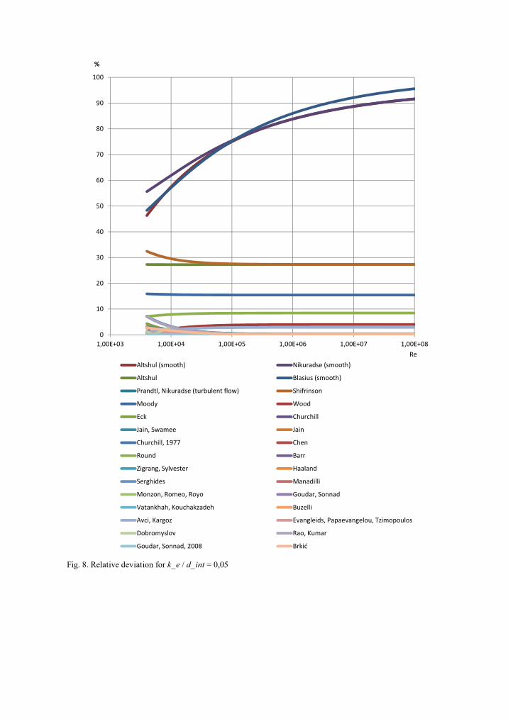
Fig. 8 – Relative deviation for
0
10
20
30
40
50
60
70
80
90
100
1,00E+03 1,00E+04 1,00E+05 1,00E+06 1,00E+07 1,00E+08
%
Re
Altshul (smooth) Nikuradse (smooth)
Altshul Blasius (smooth)
Prandtl, Nikuradse (turbulent flow) Shifrinson
Moody Wood
Eck Churchill
Jain, Swamee Jain
Churchill, 1977 Chen
Round Barr
Zigrang, Sylvester Haaland
Serghides Manadilli
Monzon, Romeo, Royo Goudar, Sonnad
Vatankhah, Kouchakzadeh Buzelli
Avci, Kargoz Evangleids, Papaevangelou, Tzimopoulos
Dobromyslov Rao, Kumar
Goudar, Sonnad, 2008 Brkić
Fig. 8. Relative deviation for k_e / d_int = 0,05
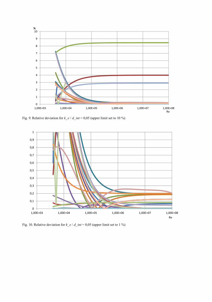
Fig. 9 – Relative deviation for (upper limit set to 10 %)
Fig. 10 – Relative deviation for (upper limit set to 1 %)
0
1
2
3
4
5
6
7
8
9
10
1,00E+03 1,00E+04 1,00E+05 1,00E+06 1,00E+07 1,00E+08
%
Re
0
0,1
0,2
0,3
0,4
0,5
0,6
0,7
0,8
0,9
1
1,00E+03 1,00E+04 1,00E+05 1,00E+06 1,00E+07 1,00E+08
%
Re
Fig. 9. Relative deviation for k_e / d_int = 0,05 (upper limit set to 10 %)
Fig. 9 – Relative deviation for (upper limit set to 10 %)
Fig. 10 – Relative deviation for (upper limit set to 1 %)
0
1
2
3
4
5
6
7
8
9
10
1,00E+03 1,00E+04 1,00E+05 1,00E+06 1,00E+07 1,00E+08
%
Re
0
0,1
0,2
0,3
0,4
0,5
0,6
0,7
0,8
0,9
1
1,00E+03 1,00E+04 1,00E+05 1,00E+06 1,00E+07 1,00E+08
%
Re
Fig. 10. Relative deviation for k_e / d_int = 0,05 (upper limit set to 1 %)
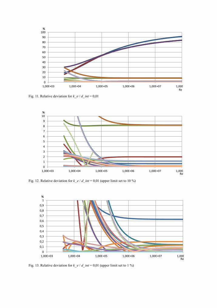
Fig. 13. Relative deviation for k_e / d_int = 0,01 (upper limit set to 1 %)
Fig. 11 – Relative deviation for
Fig. 12 – Relative deviation for (upper limit set to 10 %)
Fig. 13 – Relative deviation for (upper limit set to 1 %)
0
10
20
30
40
50
60
70
80
90
100
1,00E+03 1,00E+04 1,00E+05 1,00E+06 1,00E+07 1,00E+08
%
Re
0
1
2
3
4
5
6
7
8
9
10
1,00E+03 1,00E+04 1,00E+05 1,00E+06 1,00E+07 1,00E+08
%
Re
0
0,1
0,2
0,3
0,4
0,5
0,6
0,7
0,8
0,9
1
1,00E+03 1,00E+04 1,00E+05 1,00E+06 1,00E+07 1,00E+08
%
Re
Fig. 11. Relative deviation for k_e / d_int = 0,01
Fig. 11 – Relative deviation for
Fig. 12 – Relative deviation for (upper limit set to 10 %)
Fig. 13 – Relative deviation for (upper limit set to 1 %)
0
10
20
30
40
50
60
70
80
90
100
1,00E+03 1,00E+04 1,00E+05 1,00E+06 1,00E+07 1,00E+08
%
Re
0
1
2
3
4
5
6
7
8
9
10
1,00E+03 1,00E+04 1,00E+05 1,00E+06 1,00E+07 1,00E+08
%
Re
0
0,1
0,2
0,3
0,4
0,5
0,6
0,7
0,8
0,9
1
1,00E+03 1,00E+04 1,00E+05 1,00E+06 1,00E+07 1,00E+08
%
Re
Fig. 12. Relative deviation for k_e / d_int = 0,01 (upper limit set to 10 %)
Fig. 11 – Relative deviation for
Fig. 12 – Relative deviation for (upper limit set to 10 %)
Fig. 13 – Relative deviation for (upper limit set to 1 %)
0
10
20
30
40
50
60
70
80
90
100
1,00E+03 1,00E+04 1,00E+05 1,00E+06 1,00E+07 1,00E+08
%
Re
0
1
2
3
4
5
6
7
8
9
10
1,00E+03 1,00E+04 1,00E+05 1,00E+06 1,00E+07 1,00E+08
%
Re
0
0,1
0,2
0,3
0,4
0,5
0,6
0,7
0,8
0,9
1
1,00E+03 1,00E+04 1,00E+05 1,00E+06 1,00E+07 1,00E+08
%
Re
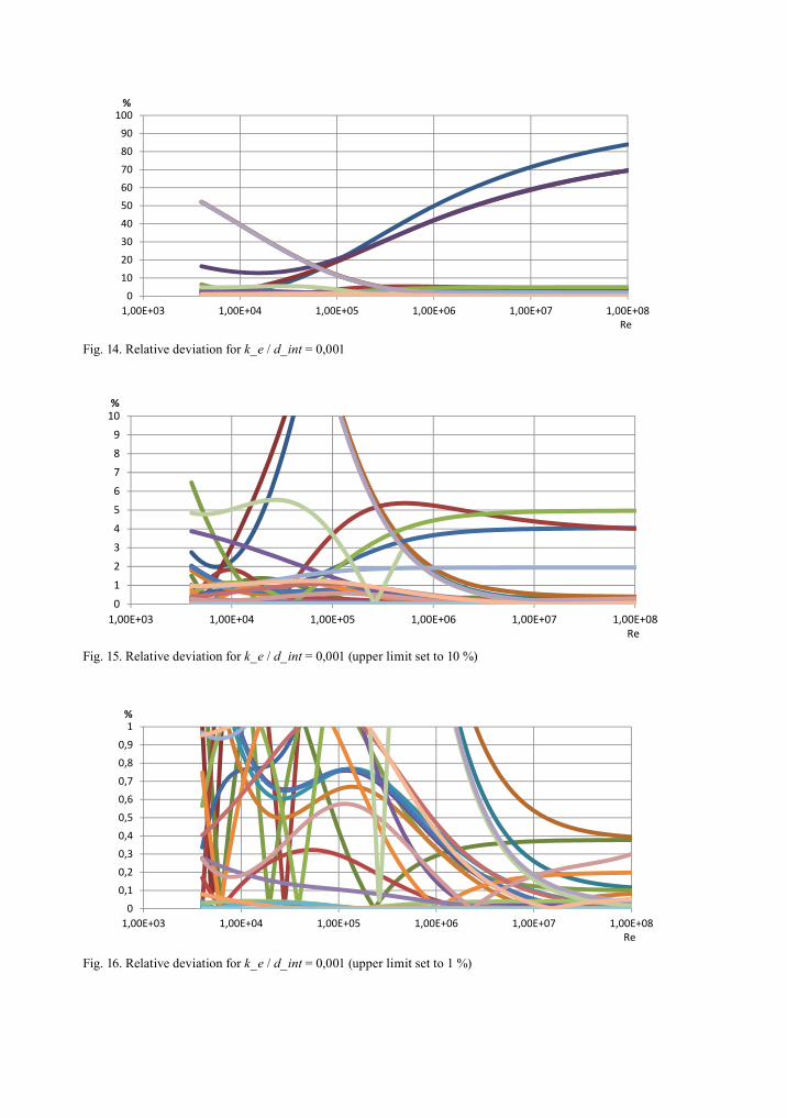
Fig. 14. Relative deviation for k_e / d_int = 0,001
Fig. 14 – Relative deviation for
Fig. 15 – Relative deviation for (upper limit set to 10 %)
Fig. 16 – Relative deviation for (upper limit set to 1 %)
0
10
20
30
40
50
60
70
80
90
100
1,00E+03 1,00E+04 1,00E+05 1,00E+06 1,00E+07 1,00E+08
%
Re
0
1
2
3
4
5
6
7
8
9
10
1,00E+03 1,00E+04 1,00E+05 1,00E+06 1,00E+07 1,00E+08
%
Re
0
0,1
0,2
0,3
0,4
0,5
0,6
0,7
0,8
0,9
1
1,00E+03 1,00E+04 1,00E+05 1,00E+06 1,00E+07 1,00E+08
%
Re
Fig. 15. Relative deviation for k_e / d_int = 0,001 (upper limit set to 10 %)
Fig. 14 – Relative deviation for
Fig. 15 – Relative deviation for (upper limit set to 10 %)
Fig. 16 – Relative deviation for (upper limit set to 1 %)
0
10
20
30
40
50
60
70
80
90
100
1,00E+03 1,00E+04 1,00E+05 1,00E+06 1,00E+07 1,00E+08
%
Re
0
1
2
3
4
5
6
7
8
9
10
1,00E+03 1,00E+04 1,00E+05 1,00E+06 1,00E+07 1,00E+08
%
Re
0
0,1
0,2
0,3
0,4
0,5
0,6
0,7
0,8
0,9
1
1,00E+03 1,00E+04 1,00E+05 1,00E+06 1,00E+07 1,00E+08
%
Re
Fig. 16. Relative deviation for k_e / d_int = 0,001 (upper limit set to 1 %)
Fig. 14 – Relative deviation for
Fig. 15 – Relative deviation for (upper limit set to 10 %)
Fig. 16 – Relative deviation for (upper limit set to 1 %)
0
10
20
30
40
50
60
70
80
90
100
1,00E+03 1,00E+04 1,00E+05 1,00E+06 1,00E+07 1,00E+08
%
Re
0
1
2
3
4
5
6
7
8
9
10
1,00E+03 1,00E+04 1,00E+05 1,00E+06 1,00E+07 1,00E+08
%
Re
0
0,1
0,2
0,3
0,4
0,5
0,6
0,7
0,8
0,9
1
1,00E+03 1,00E+04 1,00E+05 1,00E+06 1,00E+07 1,00E+08
%
Re
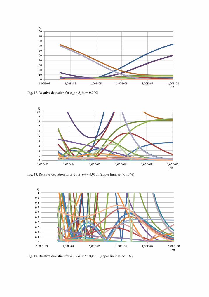
Fig. 17. Relative deviation for k_e / d_int = 0,0001
Fig. 17 – Relative deviation for
Fig. 18 – Relative deviation for (upper limit set to 10 %)
Fig. 19 – Relative deviation for (upper limit set to 1 %)
0
10
20
30
40
50
60
70
80
90
100
1,00E+03 1,00E+04 1,00E+05 1,00E+06 1,00E+07 1,00E+08
%
Re
0
1
2
3
4
5
6
7
8
9
10
1,00E+03 1,00E+04 1,00E+05 1,00E+06 1,00E+07 1,00E+08
%
Re
0
0,1
0,2
0,3
0,4
0,5
0,6
0,7
0,8
0,9
1
1,00E+03 1,00E+04 1,00E+05 1,00E+06 1,00E+07 1,00E+08
%
Re
Fig. 18. Relative deviation for k_e / d_int = 0,0001 (upper limit set to 10 %)
Fig. 17 – Relative deviation for
Fig. 18 – Relative deviation for (upper limit set to 10 %)
Fig. 19 – Relative deviation for (upper limit set to 1 %)
0
10
20
30
40
50
60
70
80
90
100
1,00E+03 1,00E+04 1,00E+05 1,00E+06 1,00E+07 1,00E+08
%
Re
0
1
2
3
4
5
6
7
8
9
10
1,00E+03 1,00E+04 1,00E+05 1,00E+06 1,00E+07 1,00E+08
%
Re
0
0,1
0,2
0,3
0,4
0,5
0,6
0,7
0,8
0,9
1
1,00E+03 1,00E+04 1,00E+05 1,00E+06 1,00E+07 1,00E+08
%
Re
Fig. 19. Relative deviation for k_e / d_int = 0,0001 (upper limit set to 1 %)
Fig. 17 – Relative deviation for
Fig. 18 – Relative deviation for (upper limit set to 10 %)
Fig. 19 – Relative deviation for (upper limit set to 1 %)
0
10
20
30
40
50
60
70
80
90
100
1,00E+03 1,00E+04 1,00E+05 1,00E+06 1,00E+07 1,00E+08
%
Re
0
1
2
3
4
5
6
7
8
9
10
1,00E+03 1,00E+04 1,00E+05 1,00E+06 1,00E+07 1,00E+08
%
Re
0
0,1
0,2
0,3
0,4
0,5
0,6
0,7
0,8
0,9
1
1,00E+03 1,00E+04 1,00E+05 1,00E+06 1,00E+07 1,00E+08
%
Re
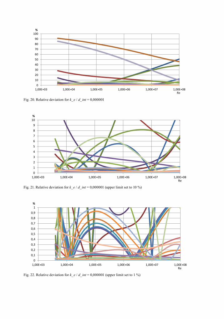
Fig. 20. Relative deviation for k_e / d_int = 0,000001
Fig. 20 – Relative deviation for
Fig. 21 – Relative deviation for (upper limit set to 10 %)
Fig. 22 – Relative deviation for (upper limit set to 1 %)
0
10
20
30
40
50
60
70
80
90
100
1,00E+03 1,00E+04 1,00E+05 1,00E+06 1,00E+07 1,00E+08
%
Re
0
1
2
3
4
5
6
7
8
9
10
1,00E+03 1,00E+04 1,00E+05 1,00E+06 1,00E+07 1,00E+08
%
Re
0
0,1
0,2
0,3
0,4
0,5
0,6
0,7
0,8
0,9
1
1,00E+03 1,00E+04 1,00E+05 1,00E+06 1,00E+07 1,00E+08
%
Re
Fig. 21. Relative deviation for k_e / d_int = 0,000001 (upper limit set to 10 %)
Fig. 20 – Relative deviation for
Fig. 21 – Relative deviation for (upper limit set to 10 %)
Fig. 22 – Relative deviation for (upper limit set to 1 %)
0
10
20
30
40
50
60
70
80
90
100
1,00E+03 1,00E+04 1,00E+05 1,00E+06 1,00E+07 1,00E+08
%
Re
0
1
2
3
4
5
6
7
8
9
10
1,00E+03 1,00E+04 1,00E+05 1,00E+06 1,00E+07 1,00E+08
%
Re
0
0,1
0,2
0,3
0,4
0,5
0,6
0,7
0,8
0,9
1
1,00E+03 1,00E+04 1,00E+05 1,00E+06 1,00E+07 1,00E+08
%
Re
Fig. 22. Relative deviation for k_e / d_int = 0,000001 (upper limit set to 1 %)
Fig. 20 – Relative deviation for
Fig. 21 – Relative deviation for (upper limit set to 10 %)
Fig. 22 – Relative deviation for (upper limit set to 1 %)
0
10
20
30
40
50
60
70
80
90
100
1,00E+03 1,00E+04 1,00E+05 1,00E+06 1,00E+07 1,00E+08
%
Re
0
1
2
3
4
5
6
7
8
9
10
1,00E+03 1,00E+04 1,00E+05 1,00E+06 1,00E+07 1,00E+08
%
Re
0
0,1
0,2
0,3
0,4
0,5
0,6
0,7
0,8
0,9
1
1,00E+03 1,00E+04 1,00E+05 1,00E+06 1,00E+07 1,00E+08
%
Re
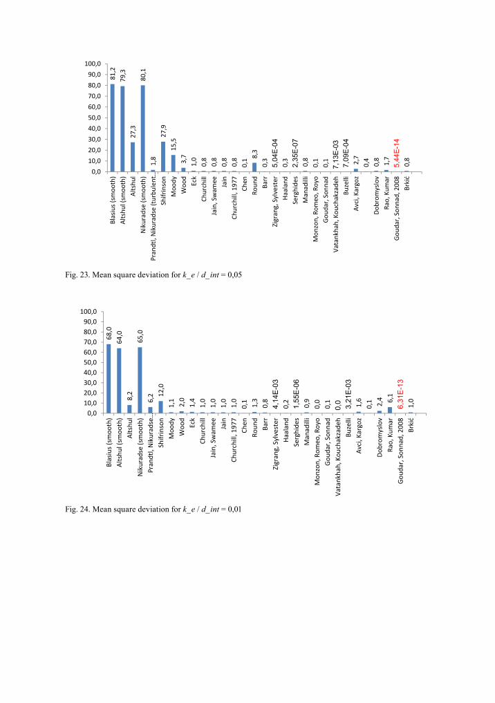
These plots (figures 8-22) provide an interesting insight on behavior of different equations
for hydraulic friction factor, but still does not give a clear criteria to consider accuracy. That criteria
would be mean square deviation of given results from ideal (which is Clamond solution in our case).
Futher calculations were carried out and results are shown on bar-plots in figures 23-27.
Fig. 23 – Mean square deviation for
Fig. 24 – Mean square deviation for
81,2
79,3
27,3
80,1
1,8
27,9
15,5
3,7
1,0
0,8
0,8
0,8
0,8
0,1 8,
30,3
5,04
E-0
40,3
2,35
E-0
70,8
0,1
0,1
7,13
E-0
37,
09E
-04
2,7
0,4
0,8
1,7
5,44
E-1
40,8
0,0
10,0
20,0
30,0
40,0
50,0
60,0
70,0
80,0
90,0
100,0
Blasius (smoo
th)
Altshu
l (sm
ooth)
Altshu
lNikuradse (smoo
th)
Prandtl, Nikuradse (turbu
lent …
Shifrinson
Moo
dyWoo
dEck
Churchill
Jain, Swam
ee Jain
Churchill, 197
7Ch
enRo
und
Barr
Zigrang, Sylvester
Haaland
Serghide
sManadilli
Mon
zon, Rom
eo, Royo
Gou
dar, Son
nad
Vatankhah, Kou
chakzade
hBu
zelli
Avci, Kargoz
Dob
romyslov
Rao, Kum
arGou
dar, Son
nad, 200
8Brkić
68,0
64,0
8,2
65,0
6,2 12
,01,1
2,0
1,4
1,0
1,0
1,0
1,0
0,1
1,3
0,8
4,14
E-0
30,2
1,55
E-0
60,9
0,0
0,1
0,0 3,21
E-0
31,6
0,1 2,4 6,1
6,31
E-1
31,0
0,010,020,030,040,050,060,070,080,090,0100,0
Blasius (smoo
th)
Altshu
l (sm
ooth)
Altshu
lNikuradse (smoo
th)
Prandtl, Nikuradse …
Shifrinson
Moo
dyWoo
dEck
Churchill
Jain, Swam
ee Jain
Churchill, 197
7Ch
enRo
und
Barr
Zigrang, Sylvester
Haaland
Serghide
sManadilli
Mon
zon, Rom
eo, Royo
Gou
dar, Son
nad
Vatankhah, Kou
chakzade
hBu
zelli
Avci, Kargoz
Dob
romyslov
Rao, Kum
arGou
dar, Son
nad, 200
8Brkić
Fig. 23. Mean square deviation for k_e / d_int = 0,05
These plots (figures 8-22) provide an interesting insight on behavior of different equations
for hydraulic friction factor, but still does not give a clear criteria to consider accuracy. That criteria
would be mean square deviation of given results from ideal (which is Clamond solution in our case).
Futher calculations were carried out and results are shown on bar-plots in figures 23-27.
Fig. 23 – Mean square deviation for
Fig. 24 – Mean square deviation for
81,2
79,3
27,3
80,1
1,8
27,9
15,5
3,7
1,0
0,8
0,8
0,8
0,8
0,1 8,
30,3
5,04
E-0
40,3
2,35
E-0
70,8
0,1
0,1
7,13
E-0
37,
09E
-04
2,7
0,4
0,8
1,7
5,44
E-1
40,8
0,0
10,0
20,0
30,0
40,0
50,0
60,0
70,0
80,0
90,0
100,0
Blasius (smoo
th)
Altshu
l (sm
ooth)
Altshu
lNikuradse (smoo
th)
Prandtl, Nikuradse (turbu
lent …
Shifrinson
Moo
dyWoo
dEck
Churchill
Jain, Swam
ee Jain
Churchill, 197
7Ch
enRo
und
Barr
Zigrang, Sylvester
Haaland
Serghide
sManadilli
Mon
zon, Rom
eo, Royo
Gou
dar, Son
nad
Vatankhah, Kou
chakzade
hBu
zelli
Avci, Kargoz
Dob
romyslov
Rao, Kum
arGou
dar, Son
nad, 200
8Brkić
68,0
64,0
8,2
65,0
6,2 12
,01,1
2,0
1,4
1,0
1,0
1,0
1,0
0,1
1,3
0,8
4,14
E-0
30,2
1,55
E-0
60,9
0,0
0,1
0,0 3,21
E-0
31,6
0,1 2,4 6,1
6,31
E-1
31,0
0,010,020,030,040,050,060,070,080,090,0100,0
Blasius (smoo
th)
Altshu
l (sm
ooth)
Altshu
lNikuradse (smoo
th)
Prandtl, Nikuradse …
Shifrinson
Moo
dyWoo
dEck
Churchill
Jain, Swam
ee Jain
Churchill, 197
7Ch
enRo
und
Barr
Zigrang, Sylvester
Haaland
Serghide
sManadilli
Mon
zon, Rom
eo, Royo
Gou
dar, Son
nad
Vatankhah, Kou
chakzade
hBu
zelli
Avci, Kargoz
Dob
romyslov
Rao, Kum
arGou
dar, Son
nad, 200
8Brkić
Fig. 24. Mean square deviation for k_e / d_int = 0,01
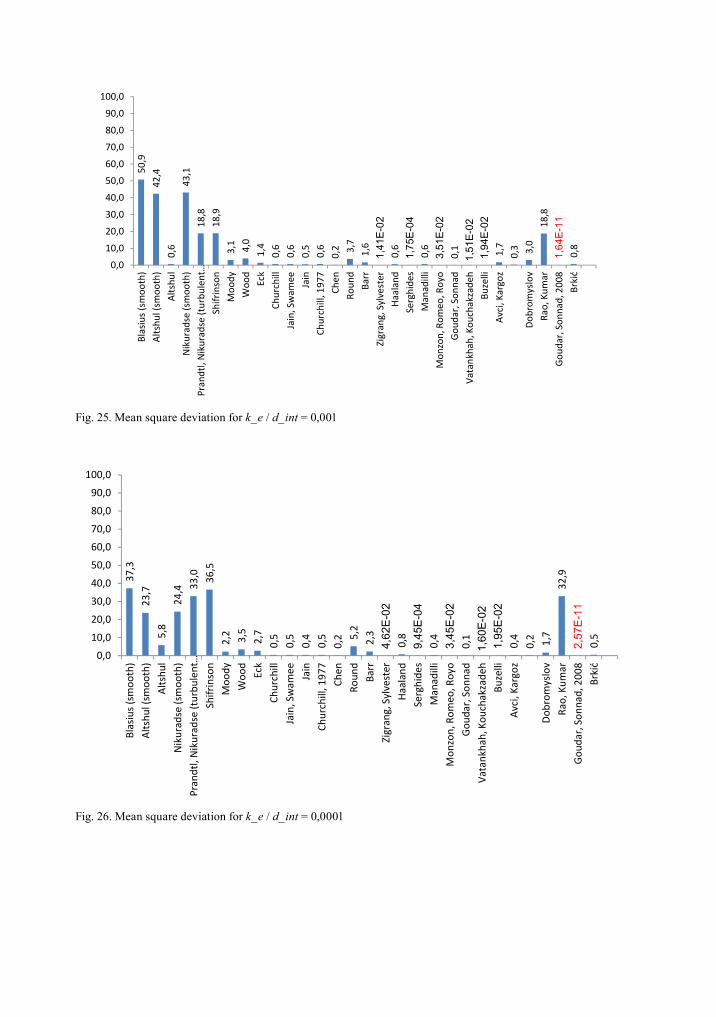
Fig. 25 – Mean square deviation for
Fig. 26 – Mean square deviation for
50,9
42,4
0,6
43,1
18,8
18,9
3,1
4,0
1,4
0,6
0,6
0,5
0,6
0,2 3,7
1,6
1,41
E-0
20,6
1,75
E-0
40,6
3,51
E-0
20,1
1,51
E-0
21,
94E
-02
1,7
0,3 3,0
18,8
1,64
E-1
10,8
0,0
10,0
20,0
30,0
40,0
50,0
60,0
70,0
80,0
90,0
100,0
Blasius (smoo
th)
Altshu
l (sm
ooth)
Altshu
lNikuradse (smoo
th)
Prandtl, Nikuradse (turbu
lent …
Shifrinson
Moo
dyWoo
dEck
Churchill
Jain, Swam
ee Jain
Churchill, 197
7Ch
enRo
und
Barr
Zigrang, Sylvester
Haaland
Serghide
sManadilli
Mon
zon, Rom
eo, Royo
Gou
dar, Son
nad
Vatankhah, Kou
chakzade
hBu
zelli
Avci, Kargoz
Dob
romyslov
Rao, Kum
arGou
dar, Son
nad, 200
8Brkić
37,3
23,7
5,8
24,4 33
,0 36,5
2,2 3,5
2,7
0,5
0,5
0,4
0,5
0,2 5,2
2,3
4,62
E-0
20,8
9,45
E-0
40,4
3,45
E-0
20,1
1,60
E-0
21,
95E
-02
0,4
0,2 1,7
32,9
2,57
E-1
10,5
0,0
10,0
20,0
30,0
40,0
50,0
60,0
70,0
80,0
90,0
100,0
Blasius (smoo
th)
Altshu
l (sm
ooth)
Altshu
lNikuradse (smoo
th)
Prandtl, Nikuradse (turbu
lent …
Shifrinson
Moo
dyWoo
dEck
Churchill
Jain, Swam
ee Jain
Churchill, 197
7Ch
enRo
und
Barr
Zigrang, Sylvester
Haaland
Serghide
sManadilli
Mon
zon, Rom
eo, Royo
Gou
dar, Son
nad
Vatankhah, Kou
chakzade
hBu
zelli
Avci, Kargoz
Dob
romyslov
Rao, Kum
arGou
dar, Son
nad, 200
8Brkić
Fig. 25. Mean square deviation for k_e / d_int = 0,001
Fig. 25 – Mean square deviation for
Fig. 26 – Mean square deviation for
50,9
42,4
0,6
43,1
18,8
18,9
3,1
4,0
1,4
0,6
0,6
0,5
0,6
0,2 3,7
1,6
1,41
E-0
20,6
1,75
E-0
40,6
3,51
E-0
20,1
1,51
E-0
21,
94E
-02
1,7
0,3 3,0
18,8
1,64
E-1
10,8
0,0
10,0
20,0
30,0
40,0
50,0
60,0
70,0
80,0
90,0
100,0
Blasius (smoo
th)
Altshu
l (sm
ooth)
Altshu
lNikuradse (smoo
th)
Prandtl, Nikuradse (turbu
lent …
Shifrinson
Moo
dyWoo
dEck
Churchill
Jain, Swam
ee Jain
Churchill, 197
7Ch
enRo
und
Barr
Zigrang, Sylvester
Haaland
Serghide
sManadilli
Mon
zon, Rom
eo, Royo
Gou
dar, Son
nad
Vatankhah, Kou
chakzade
hBu
zelli
Avci, Kargoz
Dob
romyslov
Rao, Kum
arGou
dar, Son
nad, 200
8Brkić
37,3
23,7
5,8
24,4 33
,0 36,5
2,2 3,5
2,7
0,5
0,5
0,4
0,5
0,2 5,2
2,3
4,62
E-0
20,8
9,45
E-0
40,4
3,45
E-0
20,1
1,60
E-0
21,
95E
-02
0,4
0,2 1,7
32,9
2,57
E-1
10,5
0,0
10,0
20,0
30,0
40,0
50,0
60,0
70,0
80,0
90,0
100,0
Blasius (smoo
th)
Altshu
l (sm
ooth)
Altshu
lNikuradse (smoo
th)
Prandtl, Nikuradse (turbu
lent …
Shifrinson
Moo
dyWoo
dEck
Churchill
Jain, Swam
ee Jain
Churchill, 197
7Ch
enRo
und
Barr
Zigrang, Sylvester
Haaland
Serghide
sManadilli
Mon
zon, Rom
eo, Royo
Gou
dar, Son
nad
Vatankhah, Kou
chakzade
hBu
zelli
Avci, Kargoz
Dob
romyslov
Rao, Kum
arGou
dar, Son
nad, 200
8Brkić
Fig. 26. Mean square deviation for k_e / d_int = 0,0001
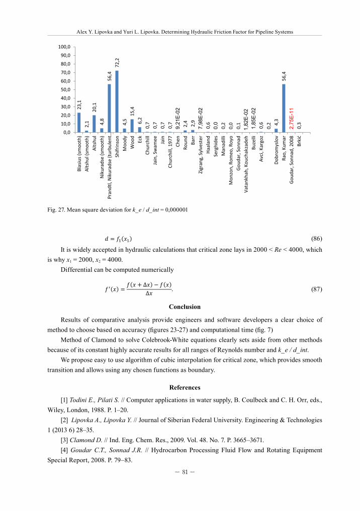
– 81 –
Alex Y. Lipovka and Yuri L. Lipovka. Determining Hydraulic Friction Factor for Pipeline Systems
� � ���������� � ������� � �������� � ����������� � ����
��� � ���� (83)
� ���������� � ������� � �������� � ������������ � ����
��� � ���� (84)
� � ������� (85)
� � ������ (86)
It is widely accepted in hydraulic calculations that critical zone lays in ���� � �� � ����,
which is why �� � ����, �� � ����.
Differential can be computed numerically
����� ���� � ��� � ����
�� . (87)
Conclusion
Results of comparative analysis provide engineers and software developers a clear choice of
method to choose based on accuracy (figures 23-27) and computational time (Fig. 7)
Method of Clamond to solve Colebrook-White equations clearly sets aside from other
methods because of its constant highly accurate results for all ranges of Reynolds number and
���������.
We propose easy to use algorithm of cubic interpolation for critical zone, which provides
smooth transition and allows using any chosen functions as boundary.
References
[1] Todini E., Pilati S. // Computer applications in water supply, B. Coulbeck and C. H. Orr, eds.,
Wiley, London, 1988. P. 1–20.
[2] Lipovka A., Lipovka Y. // Journal of Siberian Federal University. Engineering & Technologies 1
(2013 6) 28–35.
[3] Clamond D. // Ind. Eng. Chem. Res., 2009. Vol. 48. No. 7. P. 3665–3671
[4] Goudar C.T., Sonnad J.R. // Hydrocarbon Processing Fluid Flow and Rotating Equipment
Special Report, 2008. P. 79–83.
[5] Brkić, Dejan. // Petroleum Science and Technology 29 (15), 2011. P. 1596–1602.
[6] Rao A.R., Kumar B. // Journal of Indian Water Works Association, Oct-Dec, 2006. P. 29–36.
(86)
It is widely accepted in hydraulic calculations that critical zone lays in 2000 < Re < 4000, which is why x1 = 2000, x2 = 4000.
Differential can be computed numerically
� � ���������� � ������� � �������� � ����������� � ����
��� � ���� (83)
� ���������� � ������� � �������� � ������������ � ����
��� � ���� (84)
� � ������� (85)
� � ������ (86)
It is widely accepted in hydraulic calculations that critical zone lays in ���� � �� � ����,
which is why �� � ����, �� � ����.
Differential can be computed numerically
����� ���� � ��� � ����
�� . (87)
Conclusion
Results of comparative analysis provide engineers and software developers a clear choice of
method to choose based on accuracy (figures 23-27) and computational time (Fig. 7)
Method of Clamond to solve Colebrook-White equations clearly sets aside from other
methods because of its constant highly accurate results for all ranges of Reynolds number and
���������.
We propose easy to use algorithm of cubic interpolation for critical zone, which provides
smooth transition and allows using any chosen functions as boundary.
References
[1] Todini E., Pilati S. // Computer applications in water supply, B. Coulbeck and C. H. Orr, eds.,
Wiley, London, 1988. P. 1–20.
[2] Lipovka A., Lipovka Y. // Journal of Siberian Federal University. Engineering & Technologies 1
(2013 6) 28–35.
[3] Clamond D. // Ind. Eng. Chem. Res., 2009. Vol. 48. No. 7. P. 3665–3671
[4] Goudar C.T., Sonnad J.R. // Hydrocarbon Processing Fluid Flow and Rotating Equipment
Special Report, 2008. P. 79–83.
[5] Brkić, Dejan. // Petroleum Science and Technology 29 (15), 2011. P. 1596–1602.
[6] Rao A.R., Kumar B. // Journal of Indian Water Works Association, Oct-Dec, 2006. P. 29–36.
(87)
Conclusion
Results of comparative analysis provide engineers and software developers a clear choice of method to choose based on accuracy (figures 23-27) and computational time (fig. 7)
Method of Clamond to solve Colebrook-White equations clearly sets aside from other methods because of its constant highly accurate results for all ranges of Reynolds number and k_e / d_int.
We propose easy to use algorithm of cubic interpolation for critical zone, which provides smooth transition and allows using any chosen functions as boundary.
References
[1] Todini E., Pilati S. // Computer applications in water supply, B. Coulbeck and C. H. Orr, eds., Wiley, London, 1988. P. 1–20.
[2] Lipovka A., Lipovka Y. // Journal of Siberian Federal University. Engineering & Technologies 1 (2013 6) 28–35.
[3] Clamond D. // Ind. Eng. Chem. Res., 2009. Vol. 48. No. 7. P. 3665–3671.[4] Goudar C.T., Sonnad J.R. // Hydrocarbon Processing Fluid Flow and Rotating Equipment
Special Report, 2008. P. 79–83.
Fig. 27. Mean square deviation for k_e / d_int = 0,000001
Fig. 27 – Mean square deviation for
One way to describe in critical zone (Fig. 1) is to build cubic interpolation function. There
is widely adopted cubic interpolation developed by Dunlop. He took Poiseuille equation for laminar
flow and Swamee-and-Jain equation for turbulent flow as boundary conditions.
In order to provide smooth transition from laminar regime to turbulent using more accurate
solution of Colebrook-White equation given by Clamond we propose use of general cubic
interpolation polynomial, which allows setting any functions as boundary conditions..
General cubic interpolation polynomial is given as
(81)
We need to solve the following system of equations to find coefficients .
(82)
Solving system of equations (82) for gives:
23,1
2,1
20,1
4,8
56,4
72,2
4,515
,46,2
0,7
0,7
0,7
0,7
9,21
E-0
22,4
2,9
7,98
E-0
20,6
0,0
0,2
0,0
0,1
1,82
E-0
21,
85E
-02
0,6
0,2 4,3
56,4
2,75
E-1
10,3
0,0
10,0
20,0
30,0
40,0
50,0
60,0
70,0
80,0
90,0
100,0
Blasius (smoo
th)
Altshu
l (sm
ooth)
Altshu
lNikuradse (smoo
th)
Prandtl, Nikuradse (turbu
lent …
Shifrinson
Moo
dyWoo
dEck
Churchill
Jain, Swam
ee Jain
Churchill, 197
7Ch
enRo
und
Barr
Zigrang, Sylvester
Haaland
Serghide
sManadilli
Mon
zon, Rom
eo, Royo
Gou
dar, Son
nad
Vatankhah, Kou
chakzade
hBu
zelli
Avci, Kargoz
Dob
romyslov
Rao, Kum
arGou
dar, Son
nad, 200
8Brkić
Alex Y. Lipovka and Yuri L. Lipovka. Determining Hydraulic Friction Factor for Pipeline Systems
[5] Brkić, Dejan. // Petroleum Science and Technology 29 (15), 2011. P. 1596–1602.[6] Rao A.R., Kumar B. // Journal of Indian Water Works Association, Oct-Dec, 2006. P. 29–36.[7] Добромыслов А.Я. Таблицы для гидравлических расчетов напорных труб из полимерных
материалов. Т. 1. М.: ТОО «Издательство ВНИИМП», 2004.
Определение коэффициента гидравлического трения в трубопроводных системах
А.Ю. Липовка, Ю.Л. ЛиповкаСибирский федеральный университет,
Россия, 660041, Красноярск, пр. Свободный, 79
Выполнен сравнительный анализ многих известных формул для определения коэффициента гидравлического трения в трубах с точки зрения точности и скорости расчета. Для обеспечения плавного перехода от ламинарного режима к переходному в критической зоне предложен алгоритм кубической интерполяции общего вида.
Ключевые слова: коэффициент гидравлического трения, критическая зона, трубопроводные системы, интерполяция.