Louisiana State UniversityLSU Digital Commons

LSU Master's Theses Graduate School

1-15-2018

Determining Bioindicators for Coastal Tidal MarshHealth Using the Food Web of Larvae of theGreenhead Horse Fly (Tabanus nigrovittatus)Devika Rajeev BhaleraoLouisiana State University and Agricultural and Mechanical College, devikabhalerao@gmail.com

Follow this and additional works at: https://digitalcommons.lsu.edu/gradschool_theses

Part of the Bioinformatics Commons, Ecology and Evolutionary Biology Commons,Entomology Commons, and the Genomics Commons

This Thesis is brought to you for free and open access by the Graduate School at LSU Digital Commons. It has been accepted for inclusion in LSUMaster's Theses by an authorized graduate school editor of LSU Digital Commons. For more information, please contact gradetd@lsu.edu.

Recommended CitationBhalerao, Devika Rajeev, "Determining Bioindicators for Coastal Tidal Marsh Health Using the Food Web of Larvae of the GreenheadHorse Fly (Tabanus nigrovittatus)" (2018). LSU Master's Theses. 4377.https://digitalcommons.lsu.edu/gradschool_theses/4377

DETERMINING BIOINDICATORS FOR COASTAL TIDAL MARSH HEALTH USING

THE FOOD WEB OF LARVAE OF THE GREENHEAD HORSE FLY

(Tabanus nigrovittatus)

A Thesis

Submitted to the Graduate Faculty of the

Louisiana State University and

Agricultural and Mechanical College

in partial fulfillment of the

requirements for the degree of

Master of Science

in

The Department of Entomology

by

Devika Rajeev Bhalerao

B.Sc., Pune University, 2008

M.Sc., Pune University, 2010

May 2018

ii

Acknowledgements

My heartfelt gratitude to Claudia Husseneder for providing an environment conducive to

research and her unwavering patience especially during the thesis writing phase. I will always be

grateful to her for the stress free environment in the lab and the all the motivation for conducting

the mind boggling bioinformatics analyses. It was a nice feeling to know that I could show up at

her office door and always be greeted with a smile.

Lane Foil has been a constant source of inspiration and expertise. I would like to thank him for

his perspective which made me envision my study as a part of a larger project with an

overarching goal which would direct future research. Daniel Swale’s expert dissection skills

paved the way for a dependable gut content analyses creating the foundation of this thesis. I will

always be grateful for his friendly demeanor and honest advice.

A deep appreciation to Kelly Thomas and his team especially Devin Thomas, Holly Bik and

Taruna Aggarwal for providing bioinformatics training and continual help.

None of my research would have been possible without the unconditional love and prayers of my

parents, in-laws and husband Chinmay Tikhe. A special note of thanks to family and friends

back home in India.

My heartwarming gratitude to Jong-Seok Park, Chinmay Tikhe, Micheal Becker, Raymond

Frasier, Ashley Reddicks and all the members of the Husseneder and Foil labs for their support,

encouragement and jokes.

Last but not the least, I would like to thank all my friends at LSU for being a family and for

providing a sense of belonging.

iii

Table of Contents

Acknowledgements ......................................................................................................................... ii

Abstract .......................................................................................................................................... vi

Chapter 1. Literature review ........................................................................................................... 1

1.1 Wetlands, Coastal Wetlands and Salt Marshes ..................................................................... 1

1.2 Importance of Wetlands, Coastal Wetlands and the Salt Marshes of Louisiana ................... 1

1.3 Vulnerability of Coastal Wetlands globally and within the United States with special

emphasis on the Salt Marshes of Louisiana ................................................................................ 2

1.4 Oil spills – a major anthropogenic stressor of Coastal Wetlands .......................................... 2

1.5 Impacts and restoration efforts of damaged Coastal Wetlands within the United States with

special emphasis on the Salt Marshes of Louisiana .................................................................... 3

1.6 Impacts and restoration effects after oil spills on marine and coastal ecosystems ............... 4

1.7 Deepwater Horizon Oil Spill – A wake up call for urgent assessment methods .................. 5

1.7.1. Distribution of oil .......................................................................................................... 5

1.7.2. PAH assessment ............................................................................................................ 5

1.7.3 Impact of the spill ........................................................................................................... 6

1.8 Need for assessment tools for marsh health and role of bioindicators .................................. 9

1.9 Environmental monitoring using invertebrate bioindicators with special emphasis on

insects and food webs ................................................................................................................ 10

1.10 Food webs for understanding ecosystem dynamics .......................................................... 12

1.11 Deciphering food webs...................................................................................................... 13

1.12 Current methods for environmental monitoring................................................................ 14

1.13 DNA metabarcoding and Next generation sequencing ..................................................... 15

Chapter 2. Introduction ................................................................................................................. 18

2.1 Objectives of the study ........................................................................................................ 24

iv

Chapter 3. Material and Methods.................................................................................................. 25

3.1 Site selection ....................................................................................................................... 25

3.2 Collection of sediments ....................................................................................................... 25

3.3 Larval collection .................................................................................................................. 27

3.4 Tabanid larval identification ............................................................................................... 27

3.5 Generating a molecular identity for Tabanus nigrovittatus Macquart ................................ 29

3.6 Tabanid larva dissection, DNA extraction and amplification ............................................. 31

3.7 Molecular identification of tabanid larvae .......................................................................... 32

3.8 Cloning to detect extent of tabanid DNA contamination in the gut contents ..................... 33

3.9 DNA extraction from voucher sediments............................................................................ 34

3.10 DNA amplification and sequencing .................................................................................. 35

3.11 Bioinformatic and statistical analyses ............................................................................... 36

3.12 Measuring Sediment PAH levels ...................................................................................... 41

3.13 Measuring Sediment chemistry Parameters ...................................................................... 42

3.14 Sediment Toxicity assay using the model organism Hyallela azteca ............................... 43

Chapter 4. Results ......................................................................................................................... 46

4.1 Molecular identification of tabanid larvae .......................................................................... 46

4.2 Tabanid DNA and preliminary data on food web components in larva gut contents ......... 46

4.3 General assessment of next generation sequence data ........................................................ 49

4.4 Assessment of sample sizes and OTU capture .................................................................... 50

4.5 OTU richness....................................................................................................................... 52

4.6 OTU diversity analysis in sediments and guts .................................................................... 54

4.7 Diet of the top invertebrate predator (tabanid larvae) in Louisiana marsh soil ................... 57

4.8 Identification of insect species in the tabanid larval gut ..................................................... 65

4.9 Variation in tabanid larval diets across locations ................................................................ 66

4.10 Comparison of OTU composition in sediments and larvae .............................................. 70

4.11 Variation in sediment OTU composition across locations ................................................ 75

4.12 Alpha and Beta diversity among sediments based on locations with statistical tests ....... 77

v

4.13 Differences in sediment OTU composition between the East and West........................... 79

4.14 Difference in OTU composition of sediments where larvae were present vs sediment

where larvae were absent .......................................................................................................... 82

4.15 Total Polycyclic Aromatic Hydrocarbon (PAH) content in sediments ............................. 85

4.16 Comparison of OTUs in sediments with PAH content above vs. below the baseline in

Grand Bayou ............................................................................................................................. 87

4.17 Effect of sediment chemistry on OTUs in the sediments and larval guts ......................... 90

4.18 Effect of sediment chemistry parameters on sediment OTUs ........................................... 90

4.19 OTUs affected by pH ........................................................................................................ 92

4.20 Toxicity assay .................................................................................................................... 93

Chapter 5. Discussion ................................................................................................................... 96

5.1 Species ID of larvae ............................................................................................................ 97

5.2 Diets of tabanid larvae......................................................................................................... 99

5.3 Taxa present in sediments with and without larvae .......................................................... 104

5.4 Effect of PAH on OTU composition ................................................................................. 106

5.5 Effect of sediment chemistry on OTU composition.......................................................... 108

5.6 Sediment toxicity............................................................................................................... 108

5.7 Reasons for larval decline in the East ............................................................................... 110

5.8 Challenges in Taxonomic assignments ............................................................................. 112

Chapter 6. Conclusions and Future ............................................................................................. 115

References ................................................................................................................................... 117

Vita .............................................................................................................................................. 137

vi

Abstract

The greenhead horse fly Tabanus nigrovittatus Macquart is native to coastal marshlands from

Texas to Nova Scotia. The larvae are apex invertebrate predators and their development is

dependent on the food web in the soil. Surveillance of T. nigrovittatus after the 2010 Deepwater

Horizon oil spill in the Gulf of Mexico showed population crashes of adults in the coastal

marshes of East Louisiana near places where oil made landfall, but not in West Louisiana where

the oil did not reach. Sediment collection in 2011 from West and East Louisiana revealed larval

population crashes in the Eastern coastal region. We hypothesized that due to the oil

contamination a critical component of the food web of the larvae was destroyed and/or direct

toxicity of the oil led to tabanid larval population crashes. With the aim of deciphering the

tabanid larval food web in the Louisiana marshes, we used 18SrRNA metagenomics to identify

the components of the food web in larval guts (n=16) and the surrounding sediment (n=25) from

East and West Louisiana. An approximately 400 bp region at the 5’ end of the 18SrRNAgene

was sequenced using the Illumina MiSeq sequencing platform. Downstream analysis was

conducted in QIIME (v1.9). Effect of oil, sediment chemistry and sediment toxicity on larvae

and their food web was determined to explain larval decline in East Louisiana. We found insects

and fungi to dominate the tabanid larval guts. Insects identified belonged to the families

Drosophilidae, Culicidae and Tabanidae. Bioindicators of minimally oiled sediments are

Hymenostomatia (Tetrahymena), Bivalvia (mollusks), Maxillopoda (Crustacea) and

Peronosporomycetes (fungus like eukaryotes). “Phylum” Opisthokonta dominance in sediments

is an indicator of larval presence in West Louisiana but not the East. Oil contamination, sediment

chemistry and toxicity could not explain larval population crashes in the East. Decline in the

adult population led to fewer breeders and subsequently fewer larvae.

1

Chapter 1. Literature review

1.1 Wetlands, Coastal Wetlands and Salt Marshes

Wetlands are land areas saturated with water permanently or seasonally. Wetlands including

marshes, mires, ponds, swamps, bogs lagoons, mudflats, floodplains and shallow seas are found

in almost every country in this world (Whigham, 2009). Coastal wetlands are located in coastal

watersheds and include salt and freshwater wetlands, which can be further classified as tidal and

non-tidal (Whigham, 2009). Total wetland acreage in the contiguous United States is 38 percent

out of which 81 percent is located in the southeast United States (Dahl and Stedman, 2013). In

the Gulf of Mexico, salt marshes are the tidally flooded areas of the marsh closest to the beach

rim dominated by Spartina alterniflora (smooth cordgrass) and vary from 1 to 15 miles in width

(Boesch et al., 1994).

1.2 Importance of Wetlands, Coastal Wetlands and the Salt Marshes of Louisiana

Wetlands provide for two thirds of the fish harvest on this planet (Maltby, 2013). Coastal marsh

ecosystems offer flood protection, erosion control and carbon sequestration (Beaumont et al.,

2007, US-EPA). In addition, they provide habitats and food for wildlife, recreational services

and support for commercial fisheries with over 50% of the fishery industry in the Southeastern

United States relying on coastal wetlands (US-EPA, Beaumont et al., 2007). Over 2 million

people in Louisiana would have to relocate and the lifestyle that has been preserved for centuries

would be diminished without the coastal marshes (Reed and Wilson, 2004). In the salt marshes

of Louisiana, the osmotolerant and dominating plant Spartina alterniflora houses a great

diversity of herbivorous insects with over 100 species (Wimp et al., 2010, Pfeiffer and Wiegert,

1981). In addition, Spartina marshes are highly productive and act as a breeding ground for the

2

larval stages of crabs, shrimp, sea trout and other economically important fishes (White et al.,

1978). Salt marshes also act as seasonal nitrogen and phosphorus sinks increasing water quality

and act as water reservoirs (Boorman, 1999).

1.3 Vulnerability of Coastal Wetlands globally and within the United States with special

emphasis on the Salt Marshes of Louisiana

Globally, coastal ecosystems provide extensive ecosystem services but face severe threats from

natural processes (Barbier et al., 2011, Orth et al., 2006) and human activities (Kirwan and

Megonigal, 2013, Gundlach and Hayes, 1978, US-EPA). The vulnerability of coastal marshlands

to climate change, sea level rise, land subsidence, hydrologic modifications, development

(residential and commercial), invasive species and pollution, i.e. by agricultural fertilizer runoff,

chemical and oil spills, has been realized. A combination of such natural and anthropogenic

stressors contribute to the degradation of the coastal marshes at a rapid rate (O’Riordan et al.,

2000). Anthropogenic stressors such as agriculture and pollution have led to destruction of

mangroves (Valiela et al., 2001). Salt marshes of Louisiana are primarily affected by salt water

intrusion and inundation due to sea level rise and land subsidence exacerbated by hurricanes

(Chesney et al., 2000). Growth of Spartina marshes is dependent on adequate rainfall, nutrients

in the soil and nutrients transported by the tides making them vulnerable to both natural and

anthropogenic stressors (Weinstein, 1996, Anthony et al., 2009).

1.4 Oil spills – a major anthropogenic stressor of Coastal Wetlands

A common anthropogenic stressor in coastal areas is oil spillage (Crain et al., 2009,Silliman et

al., 2012,Pezeshki et al., 2000, Reddy et al., 2002). Oil and gas development in the Gulf of

Mexico has increased the Gulf’s vulnerability to oil spills. Louisiana coastal wetlands supports

processing and transportation of US oil production and 24% of US natural gas production

3

(Tunnell et al., 2009). Thus, elevated background levels for oil in Gulf of Mexico are always

present. Oil spills are a lurking danger in offshore waters (Tunnell et al., 2009). In the period

from 2001 to 2015 the total quantity of oil spilled offshore in US was 4,937,607 barrels. Primary

causes of oil spills are equipment failure, vessel damage, corrosion, external force or effects of

weather including hurricanes on platforms, pipelines and tankers (Tunnell et al., 2009). Major oil

spills that have affected US waters according to the National Oceanic and Atmospheric

Administration (https://response.restoration.noaa.gov/oil-and-chemical-spills/oil-spills/largest-

oil-spills-affecting-us-waters-1969.html) are Deepwater Horizon Oil Spill (2010), Exxon Valdez

(1989), Ixtoc-1 (1979), Burmah Agate (1979), Hawaiian Patriot (1977), Epic Colocotronis

(1975). Every year the quantity of oil transported off the US coast by ships, tankers and barges is

increasing (BOEM, 2016).

1.5 Impacts and restoration efforts of damaged Coastal Wetlands within the United States

with special emphasis on the Salt Marshes of Louisiana

Coastal wetlands are diminishing rapidly in comparison to other types of wetlands in the United

States (Dahl and Stedman, 2013). Within the United States, wetland loss was at an average rate

of 80,000 acres per year (2004-2009) across the Atlantic, Pacific, the Great Lakes and the Gulf

of Mexico, thereby threatening the habitat of 75% of the nation’s waterfowl and migratory birds

and 45% of the nation’s endangered species (Dahl and Stedman, 2013). The United States

Environmental Protection Agency has started programs that create awareness among people to

help restore and maintain coastal wetlands (US-EPA). The Gulf of Mexico coast suffers 71% of

the estimated wetland losses and the primary reason is human activities (Dahl and Stedman,

2013). In the salt marshes of Louisiana, human activities such as construction of roads, pipelines

and destroy, disturb or convert habitats resulting in habitat fragmentation (DeLaune et al., 1983,

Reed and Wilson, 2004). Construction of waterways and levees not only causes habitat

4

destruction and disturbance but also shoreline erosion (DeLaune et al., 1983, Reed and Wilson,

2004). Salt marshes also have been lost due to hurricanes, such as Katrina, Rita and Ike, due to

increased rainfall, abnormally high tides, storm surges, runoff and debris deposition (Dahl and

Stedman, 2013). With all of these factors causing impact on coastal estuaries, Louisiana was the

first state bordering the Gulf of Mexico to develop a comprehensive program to protect and

restore coastal wetlands (Dahl and Stedman, 2013).

1.6 Impacts and restoration effects after oil spills on marine and coastal ecosystems

Oil spills are known to have caused ecosystem devastation in the past and pose as a deadly threat

due to their unpredictable nature (Etkin, 2000, Dickins, 2011) and because resources to contain

oil spills are not readably available (Silliman et al., 2012). Spilled oil can degrade ecosystems

either directly or indirectly (Geraci and Smith, 1976). Direct toxicity includes physical

smothering or chemical toxicity of the oil resulting in lethality. For example, when oil makes

landfall, it smothers vegetation (Pezeshki et al., 2000) and contaminates sediments with toxic

residues and creates anoxic conditions, thereby destroying communities living in or dependent

on sediments (Teal and Howarth, 1984). Oil spills decrease the abundance and diversity of

marine pelagic and benthic communities, micro zooplankton, benthic invertebrates, fish (Teal

and Howarth, 1984), and marine vertebrates such as birds (migratory, Seaside Sparrows), turtles,

mammals and dolphins (Dahl and Stedman, 2013). In addition to these immediate effects,

stranded oil in shorelines and salt marshes can cause long term impacts on the coastal ecosystem

because vegetation loss can lead to erosion (Baker et al., 1993) and habitat loss, which

endangers endemic species. Indirect toxicity involves loss of habitat/ shelter and partial or

complete elimination of key taxa involved in multiple trophic levels (Fleeger et al., 2003).

5

Ecological interactions between species can affect inter-related ecosystems in the Gulf ranging

from the estuaries, coastal wetlands to the open ocean (Silliman et al., 2012).

1.7 Deepwater Horizon Oil Spill – A wake up call for urgent assessment methods

1.7.1 Distribution of oil

The Deepwater Horizon Oil Spill, the largest man-made marine oil spill in history, was caused

by the 20 April 2010 due to explosion of a drilling rig. (Crone and Tolstoy, 2010b, McNutt et al.,

2012). Eleven people died and 17 were injured during his explosion. Macondo Mississippi

Canyon block 252 oil gushed from the exploded rig for four months into the surrounding Gulf

waters with a total quantity of 210 million gallons being released (Rabalais and Turner, 2016).

The Shoreline Cleanup Assessment Technique (SCAT) showed that 2113 km out of 9545 km of

the Gulf of Mexico were oiled (Nixon et al., 2016). East Louisiana coastal marshes took the

brunt of oiling after 75 km of shoreline in the Barataria Bay had moderate to heavy oiling

(Silliman et al., 2012). However, the distribution of oil in the coastal wetlands was patchy where

some areas were affected more than others (Rabalais and Turner, 2016). High spatial

heterogeneity within as little as 5m in the marsh was observed (Turner et al., 2014) suggested

that site-specific measurements of oil should be taken for each study rather than rely on surveys

measuring oil along the marsh shoreline based on data acquire from 2010 to 2011.

1.7.2 PAH assessment

Distribution of petroleum hydrocarbons in an environment associated with a spill can be

assessed by determining the Polycyclic Aromatic Hydrocarbons levels. Total Polycyclic

Hydrocarbons (TPH) and Polycyclic Aromatic Hydrocarbons (PAH) were measured from plant

6

and animal tissues, sediments and sea water in many studies after the DHS to determine the

extent of oiling.

Detection of oil after the Deepwater Horizon Oil Spill was complicated by the fact that the

physical and chemical properties of the oil kept changing with time (White et al., 2016). Oil was

detected in situ and in the laboratory using different instruments and evaluating components such

as total PAH, oil droplets, bulk oil and polarized oil (White et al., 2016). Inlet mass spectrometer

and fluorometers were used in situ to measure aromatic hydrocarbons. In laboratory studies, GC-

FID, GC- GC-MS in SIM mode, GC×GC-FID, GC×GC-TOF-MS were techniques used to

measure the Total Polycyclic Hydrocarbons (TPH’s) (White et al., 2016). The total PAH content

in the Macondo Mississippi Canyon block 252 oil was low in comparison to other crude oils and

decreased as the oil made its way to the marshes (Olson et al., 2017). Weathering of oil leading

to a loss of PAHs occurred as the oil travelled from the Gulf waters into the marshes (Olson et

al., 2017) potentially decreasing the toxicity of the oil.

1.7.3 Impact of the spill

Multiple field studies assessed the oil contamination which had an adverse impact on marine as

well as terrestrial and intertidal ecosystems including marshes, beaches, and barrier islands in

the Gulf of Mexico (Reddy et al., 2012, Walker, 2010). The marine ecosystem was impacted by

the oil on the surface, suspended in the water column and buried in the deep sediments. Stranded

oil in the coastal areas was transported in through tides and wind from the marine ecosystem

into the salt marshes endangering the coastal salt marsh ecosystem (Crain et al., 2009, Walker,

2010). Adverse effects of the oil were seen on populations of the marine ecosystem such as

corals (White et al., 2012), microbial communities (Redmond and Valentine, 2012), benthic

7

eukaryotes (Bik et al., 2012), fish assemblages (Able et al., 2015), marine mammals, sea turtles,

among others (Barron, 2012).

Hydrocarbon degrading microbial communities in the salt marshes, such as Proteobacteria,

Bacteroidetes, and Actinobacteria, increased in oiled areas temporarily, but microbial abundance

decreased subsequently after oil levels went down. Upregulation of hydrocarbon degrading genes

of microbes also was observed in oiled environments (Beazley et al., 2012). Impact on terrestrial

ecosystem included terrestrial vertebrates and birds such as shore birds, migratory birds, sea side

sparrows (Bergeon Burns et al., 2014). Seaside Sparrows that perched on Spartina stems or fed

on organisms in the oil contaminated sites suffered population crashes (Rabalais and Turner,

2016).

The oil also impacted the meiofauna (organisms that are retained on a 500 um sieve but pass

through 50 um populations); small benthic invertebrates (Fleeger et al., 2015), marsh edge fishes

(Roth and Baltz, 2009, Rozas and Minello, 1997), decapod crustaceans (Roth and Baltz, 2009,

Rozas and Minello, 1997) especially blue crabs and shrimp (Armstrong et al., 1998), arthropods

(Day et al., Husseneder et al., 2016, Pennings et al., 2014, McCall and Pennings, 2012, Bam,

2015), and marsh rice rat (Rabalais and Turner, 2016).

Vast devastation of Spartina alterniflora was widely reported as well (Silliman et al., 2012,

DeLaune et al., 1979, Lin and Mendelssohn, 2012). Herbivores and other associated insects

declined due to Spartina loss (McCall and Pennings, 2012). Periwinkles that survive on

epiphytes attached to live or decaying Spartina leaves were indirectly affected and displayed

reduction in mean shell length (Rabalais and Turner, 2016). Meiofauna feed on the benthic

microalgae that live in the sediment in the Spartina marshes. Following Spartina recovery, both

microalgae and most meiofauna increased in abundance and diversity (Rabalais and Turner,

8

2016). However, other meiofauna such as less mobile species of polychaetes, ostracods, and

kinorhynchs had not recovered even 4 years post spill (Rabalais and Turner, 2016). Insects

associated with Spartina that are predators, sucking herbivores, stem-boring herbivores,

parasitoids, and detritivores recovered a year after the spill (McCall and Pennings, 2012) .

Laboratory toxicity assays included a comprehensive toxicity testing program called the Trustees

toxicity program to conduct toxicity assays to gauge the impact of the Deepwater Horizon Oil

Spill (Morris et al., 2015). Toxicity of oil can act via direct contact with oil, ingestion,

contaminated seawater and sediment routes (Morris et al., 2015). Toxicity on different life

stages of over 40 species of fishes, reptiles, birds, aquatic invertebrates and phytoplankton was

tested as a part of this program (Morris et al., 2015). Fish populations suffered multiple effects.

For example, oil disrupted the heart function of pelagic fishes, such as mackerel and tuna,

because oil can be absorbed by fish eggs accumulating to lethal levels attributed to blocking of

ion channels (Brette et al., 2017, Incardona et al., 2014). Physiological and reproductive

impairment of killifish also was observed in in vitro studies (Whitehead et al., 2012). In

addition, genotoxic effects and immuntoxic effects were observed using a large battery of fish

cell lines (Barron, 2012). Food chain disturbances also were detected using laboratory toxicity

studies. For example, Laughing Gulls were fed fish injected with oil at a concentration of 5 or

10mL/kg and showed muscle wastage and diminished structural integrity of the cardiac tissue

leading to death indicating that oil affects food chains (Horak et al., 2017).

Toxicity assays on invertebrates were conducted using classical and commercial methods. An

example of the in vitro classical method includes toxicity assays on natural assemblages of

zooplankton with sea water spiked with Louisiana Sweet Crude Oil showed 96% mortality at

100ug/L due to accumulation of toxins on eggs and tissues (Almeda et al., 2013).

9

Commercial assays such as Microtox microbial toxicity assay (SDI, Inc.) using Vibrio fischeri

and QwikLite toxicity assay (Assure Controls, Inc.) using the dinoflagellate Pyrocystis lunula

were used to determine the toxicity of filtered seawater spiked with Louisiana Crude Oil.

Mutagenic effects were observed starting from 0.1ppm on dinoflagellates in the QwikLite assay

and from10 ppm on Vibrio fischeri using the Microtox assay (Paul et al., 2013).

Amphipods and copepods were used in multiple toxicity assays involving spiked sea water and

sediment bioassays because oil enters amphipods and copepods via ingestion and dermal uptake

(Cohen et al., 2014, Almeda et al., 2015, Landrum et al., 1991, Lotufo et al., 2016). An array of

commercial sediment assays exists to study sediment toxicity. However, sediment toxicity tests

with amphipods have been found to be more sensitive to overall sediment contamination in

comparison to commercial tests that are used to measure sediment toxicity such as MicrotoxTM,

Thamnotox Kit, and Rototox Kit (Burton Jr et al., 2001).

1.8 Need for assessment tools for marsh health and role of bioindicators

Degradation of coastal ecosystems has led to declining water quality, biological invasions and

decreased coastal protection from hurricanes and storm surges (Crain et al., 2009). Coastal marsh

health assessment is required after pollution (through chemical and oil spills, etc.), land loss due

to sea level rise, erosion and subsidence, as well as during coastal restoration land building

efforts (Morris et al., 2015, O’Riordan et al., 2000). (Li et al., 2016). Ecosystem damage

assessment, monitoring and control are extremely important, underlining the need for quick and

affordable methods to assess ecosystem health as degradation of ecosystems has multiple effects

(Schindler, 1987, Kokaly et al., 2013).

Bioindicators of coastal marsh health are a promising way forward to determine the success of

remediation efforts in marshes (Burger and Gochfeld, 2001). Various bioindicators have been

10

used to detect ecosystem health after the Deepwater Horizon oil spill (Snyder et al., 2014,

Fleeger et al., 2015, Deis et al., 2017, Beazley et al., 2012). Salt marsh periwinkle mean shell

length and length-frequency distributions have been used as indicators to monitor health and

recovery of Louisiana marshes (Deis et al., 2017). Reduction in size, abundance and species

composition of fiddler crabs were observed in the oiled areas making them promising models of

ecosystem health (Deis et al., 2017). Nematode bioindicators include Sabatieria, Dorylaimopsis

and Cheironchus, three nematode genera that became dominant in the oiled areas due to their

ability to tolerate high PAH levels and due to the decline of PAH intolerant nematode species

(Soto et al., 2017).

1.9 Environmental monitoring using invertebrate bioindicators with special emphasis on

insects and food webs

Matthew K. Lau et al. in 2016 reviewed 1914 papers (over a span of 14 years) from 53 countries

across 6 continents and revealed that 50% of the taxa used in environmental monitoring were

animals from which 70% were invertebrates (Siddig et al., 2016). Arthropoda is a major Phylum

in the invertebrate community. Arthropod assemblages are better indicators of ecological

changes in comparison to vertebrates because they provide signs of ecological changes such as

habitat fragmentation in areas which no longer support vertebrate indicator species (Kremen et

al., 1993). In addition, monitoring arthropods which are more sensitive to environmental stress

than vertebrates can lead to proactive management (Kremen et al., 1993).

Insects are widespread and abundant, have a broad spectrum, acute sensory perception and

occupy varied functional niches and microhabitats making them reliable bioindicators in

ecosystems (McGeoch, 1998). Insects, especially soil dwelling dipterans have been suggested to

be reliable bioindicators for health in various ecosystems including marshes (Frouz, 1999,

Rochlin et al., 2011).Woodlice have been used to assess heavy contaminant pollution in

11

grasslands because they are widespread, easy to sample and identify besides being an important

detrivore in the grasslands (Paoletti and Hassall, 1999). Predatory insects

namely, Belostomatidae (Hemiptera) and larvae of Libellulidae (Odonata) have been used as

bioindicators of heavy pollutants in sugarcane fields (Corbi et al., 2011).

Soil dwelling dipteran larvae and their food webs are considered dependable bioindicators of

ecosystems due to their abundance, distribution and participation in the biological processes in

the soil and long periods of sediment exposure (Frouz, 1999, Rochlin et al., 2011, Paoletti,

2012). Soil dwelling Diptera in the families Sciaridae and Ceciomyiidae are abundant, and both

Sciaridae and Ceciomyiidae larvae react differently to different toxins and were, thus, suggested

as important candidates for bioindication (Paoletti, 2012). A disadvantage of using Sciaridae and

Ceciomyiidae larvae has been poor taxonomic identification of the larvae (Paoletti, 2012).

Previous evidence suggests that soil dwelling larvae from sarcophagus fly families

(Sphaeroceridae and Lonchopteridae) associated with vegetation are not influenced by the

factors affecting vegetation but are responsive to the soil parameters making them promising

indicators of environmental health in a heathland ecosystem (De Bruyn et al., 2001). Salt marsh

arthropod communities have shown sensitivity to oil spills (Pennings et al., 2014). Adult and

larval tabanid populations (T. nigrovittatus) declined in areas where the oil spill occurred

(Husseneder et al., 2016). Besides population crashes, genetic bottlenecks, reduction in number

of breeders, and reduced gene flow also was detected in the adult tabanid population in oiled

areas (Husseneder et al., 2016).

Importance of food webs for environmental monitoring also is recognized. Burger et al. in 2001

recommended the use of deterministic based, population based food web models for ecological

risk assessment (Burger et al., 2001). Nematode food webs have been used as bioindicators of a

12

disturbed soil environment by evaluating ratios of the weighted abundance of functional guilds

(Ferris et al., 2001). Abundance ratios of different types of phytoplankton have been used to

study the disturbances in the aquatic environment of the Baltic sea as phytoplankton are the

primary producers and its abundance affects all trophic levels (Gorokhova et al., 2016).

1.10 Food webs for understanding ecosystem dynamics

Food webs in ecosystems are comprised of taxa which show varied response to environmental

stressors (McCann et al., 2017, Barbier et al., 2011). Food web investigations are important for

understanding the health (Berry et al., 2017), functioning and dynamics of ecosystems including

varied responses of taxa within food webs to environmental stressors (Blankenship and Yayanos,

2005, McCann et al., 2017, Berry et al., 2017). Diets of invertebrates are not widely studied even

if they are central to studies of ecological processes, energetics, natural history, and food webs

(Blankenship and Yayanos, 2005).

Previous studies of apex predators have shown to deliver valuable insights into ecosystem health

(Berry et al., 2017) . For example, the diet of the endangered Australian sea lion (Neophoca

cinerea) was deciphered using DNA metabarcoding to confirm that it is a wide ranging

opportunistic predator that feeds on demersal fauna (Davenport and Bax, 2002). Primary taxa

associated with the sea lion diet and variation in diets due to location also was observed

(Davenport and Bax, 2002). Identification of the components of the greenhead horse fly larval

food web is the first step to decipher the functioning and dynamics of this apex invertebrate

predator’s food web in the marshes.

Food web components or taxa can be divided into critically resilient, critically sensitive or

sensitive with few effects on the food web depending on their role in the food web (McCann et

13

al., 2017). Taxa in ecosystems that are sensitive to environmental insults are of paramount

importance as they can destabilize or alter food webs (Barbier et al., 2011). As the Deepwater

Horizon oil spill was a major environmental stressor, comparing food web components at oiled

versus non-oiled locations might possibly lead to identification of taxa that are critically

resilient, critically sensitive or sensitive but with no effect on the larval food web (McCann et al.,

2017). This could shed significant light on the functioning and dynamics of the tabanid larval

food web and expose the effect of an ecosystem stressor on a marsh food web.

1.11 Deciphering food webs

Methods to decipher food webs have evolved drastically over time (Sheppard and Harwood,

2005). Initial dietary studies of insects involved visual observation of gut contents (Sheppard and

Harwood, 2005, Ingerson-Mahar, 2002, Pierce and Boyle, 1991). In the nineteenth century, the

diet of coleopteran predators was studied by visually identifying gut contents (Forbes, 1883).

However, the major limitation was the degradation of gut contents due to digestion such that

visual recognition was difficult (Forbes, 1883, Pearson, 1966). In addition, studying the diets of

liquid feeding insects was impossible (Forbes, 1883).

Dietary analysis using fecal samples had similar limitations (Pearson, 1966). In the past, use of

radioisotopes, chromatographic analysis of prey pigments, polyclonal antibodies to detect prey

pigments and electrophoretic detection of prey isozymes were relied on for identifying trophic

links to decipher food webs (Pompanon et al., 2012). In 1997, the first study of identification of

prey using DNA found in predator guts was published and started a new era in food web studies

(Asahida et al., 1997). DNA barcoding dietary studies of animals including arthropods gained

popularity as an accurate, rapid and dependable way forward (Soininen et al., 2009). DNA

14

barcoding has transformed the field of biodiversity science (Cristescu, 2014) and changed our

understanding of quantified webs of ecological interactions (Wirta et al., 2014).

The scope of DNA barcoding in environmental samples and dietary analysis has been

recognized as an important asset for ecologists (Valentini et al., 2009b). For example, molecular

gut content analysis showed that larval woodborers of the Monochamus spp. are facultative

intraguild predators of bark beetle larvae proving that PCR based methods are useful in

identifying insect interactions and mechanisms driving population fluctuations (Schoeller et

al., 2012). DNA barcoding complements molecular phylogenetics, population genetics and

taxonomy (Hajibabaei et al., 2007).

1.12 Current methods for environmental monitoring

Many methods are used for environmental monitoring. Surveys are conducted to monitor birds

(Seaside and Nelson’s Sparrows, water birds, Reddish Egrets, Black Rail), insects (different

species of butterflies) and reptiles such as the Mississippi Diamondback Terrapin (Reed and

Wilson, 2004) to determine effects of environmental stressors. Biosensors that detect pollutants

or toxic compounds and bioanalytical assays that detect cytotoxicity, genotoxicity, biological

oxygen demand and pathogenic bacteria are used for environmental monitoring (Rogers, 2006).

Bioindicators can be monitored using traditional surveying of known bioindicator species.

However, classical taxonomic methods can be cumbersome and often require a high level of

expertise to identify organisms to the species level. In addition, identifying morphologically

cryptic species is difficult. These limitations can be overcome by using DNA identification.

DNA barcoding and community sequencing using next generation sequencing to detect

bioindicators is gaining importance. For example, Chironomidae is a family of bioindicator

insects of pollution that have been detected using next generation sequencing. Bioindicators can

15

be detected to provide efficient assessment and monitoring of marsh health (Carew et al., 2013,

Bongers and Ferris, 1999).

1.13 DNA metabarcoding and Next Generation Sequencing (NGS)

DNA barcoding in combination with high throughput sequencing used for targeted gene

amplification for multiple species in environmental DNA is known as DNA metabarcoding and

widely used in biodiversity studies (Cristescu, 2014, Mason et al., 2012, Berry et al., 2017).

DNA metabarcoding is performed by amplifying single or multiple regions of the DNA of

interest. Commonly used molecular markers with respective regions for animals, plants, protists

and fungi are COI-barcodes (Mitochondria), 16S-rRNA genes (Nucleus), cytb (Mitochondria),

ITS1-rDNA (Nucleus), ITS2-rDNA (Nucleus), 18S-rRNA gene (Nucleus). The rbcL (Plastid)

gene can be used for autotrophic protozoa and plants. DNA metabarcoding in biodiversity

studies can be performed using universal primers (Blankenship and Yayanos, 2005) and/or group

specific primers (Jarman et al., 2004). Universal primers cover a wider range of diversity in

comparison to group specific primers, which amplify targeted taxa of interest (Blankenship and

Yayanos, 2005).

Metagenomic studies including DNA metabarcoding on community DNA via high-throughput

next-generation sequencing is gaining importance in a wide array of fields including ecology

(Bass et al., 2015, Mason et al., 2012, Berry et al., 2017). For example, DNA barcoding

combined with high throughput sequencing has been used to identify diets of mammals

(Valentini et al., 2009b), birds, molluscs and insects (Valentini et al., 2009a). In addition, effects

of human activities on ecosystems have been recognized by studying eukaryotic assemblages

(Chariton et al., 2010). The strength of DNA metabarcoding is that multiple organisms can be

identified from a bulk sample or degraded samples, which can be ancient or modern (Taberlet et

16

al., 2012). DNA metabarcoding fulfills the ecologist need for high throughput taxon

identification (Taberlet et al., 2012).

Next Generation Sequencing technology has revolutionized the field of genomics because it can

produce millions of reads in a single sequencing run (Shokralla et al., 2012). Ion Torrent’s PGM,

Pacific Biosciences’ RS, Illumina MiSeq, and Illumina HiSeq are fast turnaround sequencing

platforms in the sequencing world (Quail et al., 2012). Ion Torrent’s PGM detects signals as

protons are released during incorporation of bases in sequencing, whereas Pacific Biosciences’

RS detects fluorescence signals generated during incorporation of bases in real time (Quail et al.,

2012). However, Illumina has been at the forefront in the recent years dominating the sequencing

industry (Quail et al., 2012). Illumina technology utilizes clonally amplified DNA templates

which are immobilized to an acrylamide coating on the surface of a glass flowcell followed by

detection of fluorescently labelled reversible-terminator nucleotides (Quail et al., 2012). In

addition, Illumina has lower error rates and fewer false positives than Ion Torrent’s PGM and

Pacific Biosciences’ RS (Quail et al., 2012). Illumina MiSeq v3 reagents are capable of

producing up to 15 GB of output consisting of 25 million sequencing reads with 2 × 300 bp read

lengths (Quail et al., 2012) while Illumina HiSeq produces 375 million sequencing reads with 2

× 150 bp read lengths (Quail et al., 2012). The latest on the sequencing front is Illumina

NovaSeq 6000 S4 which generates 10,000 million sequencing with 2×150bp read lengths

(https://genohub.com/ngs-instrument-guide/).

Even though Next Generation Sequencing technology has revolutionized sequencing itself,

sequence abundance, sequence quality, sequencing artifacts and sequence contamination still

haunt accurate downstream analysis (Schmieder and Edwards, 2011, Bokulich et al., 2013).

Problems of read abundance and high quality read length can be overcome by using abundance

17

cutoff for reads (Bokulich et al., 2013). Accurate taxonomic assignments and diversity analysis

improve by removing sequences with low abundance from datasets by minimizing spurious reads

(Bokulich et al., 2013). Issues related to misassembly and drawing erroneous conclusions can be

dealt by using freely available quality control softwares such as NGS data QC tools, including

QC-Chain, FastQC, Fastx_Toolkit, NGS QC Toolkit and PRINSEQ (Zhou et al., 2014, Patel

and Jain, 2015, Schmieder and Edwards, 2011, Bokulich et al., 2013).

18

Chapter 2. Introduction

Coastal marshlands are an integral component of the coastal ecosystem supporting magnitudes of

diversity and innumerably valuable ecological and anthropological services (Shepard et al.,

2011). Salt marshes of Louisiana are tidal marsh areas within 15 m from the shoreline and

dominated by the plant Spartina alterniflora (Boesch et al., 1994).

The productive salt marshes of Louisiana provide habitats for various birds, reptiles and butterfly

species, nurseries for the larval stages of commercially viable fish and shrimp species, increase

water quality by acting as a phosphorus and nitrogen sink, protect from storms and hurricanes,

and act as a water reservoir, among other important functions (White et al., 1978, Boorman,

1999).

Threats to the salt marshes of Louisiana are similar to most wetlands and are most often a

combination of both natural and anthropogenic stressors leading to habitat destruction

(O’Riordan et al., 2000). Natural threats in this region mainly include inundation due to storms,

loss of land due to salt water intrusion (sea level rise), erosion and subsidence, and invasive

species (Orth et al., 2006, Barbier et al., 2011). Anthropogenic stressors include pollution due to

chemical run offs and oil spills, construction of levees, dykes, water ways, roads and pipelines,

restoration efforts, and commercial and industrial development (Bowen and Valiela, 2001,

Kirwan and Megonigal, 2013).

A need for quick and reliable tools to assess marsh health is required in the face of the main

pollution threats and physical changes mentioned above. Current methods involve surveying of

endangered species, and determination of abundance of commercial and native species; and

whether they show signs of genotoxicity , classical taxonomic identification of known

19

bioindicators, counting microscopic species abundance, fluorescent antibody detection and/or

enzymatic assays to detect bacterial bioindicators, community sequencing and targeted

sequencing of bioindicators (Reed and Wilson, 2004, Rogers, 2006).

Insects are preferred as bioindicators for environmental monitoring due to their sensitivity to

environmental changes facilitated by their acute sensory system and ability to perceive and

quantify changes in the environment (Oliveira et al., 2014). For example, Environmental

monitoring of freshwater ecosystems targeting Cytochrome oxidase I (COI) and Cytochrome

B (CytB) genes of the chironomid species using Next Generation Sequencing technology in

Australia underlines the potential of routine insect species-level diagnostic monitoring of

chemical pollution (Carew et al., 2013). Chironomids are used as bioindicators in

paleoenvironmental and biogeographical studies (Porinchu and MacDonald, 2003). The

cosmopolitan nature of the chironomids along with their ability to tolerate gradients of pH,

dissolved oxygen, depth, salinity and temperature and the presence of haemoglobin make them

suitable indicators of freshwater environmental monitoring (Porinchu and MacDonald, 2003).

The Deepwater Horizon Oil Spill (DHOS) was the largest man-made marine oil spill where 4.9

million barrels of oil continuously gushed for 4 months into the Gulf of Mexico (Crone and

Tolstoy, 2010a, McNutt et al., 2012). The DHOS occurred on April 20th contaminated shorelines

including salt marshes along the Gulf coast and presented a unique opportunity to study the

impact of oiling on invertebrates and search for bioindicator species of oil contamination, marsh

health decline and recovery.

Moderate to heavy oiling was observed along 75 km in which East Louisiana coastal marshes

were severely affected (Silliman et al., 2012, Michel et al., 2013) albeit with a highly patchy

distribution (Turner et al., 2014).

20

The effect of the DHOS was extensive, damaging vegetation, vertebrate and invertebrate

communities in the coastal and marine ecosystems (Silliman et al., 2012). Vertebrate

communities highly affected by the DHOS included marine mammals, birds such as Seaside

Sparrows, sea turtles and large fish species (Bentivegna et al., 2015, Rabalais and Turner, 2016).

Vegetation health, productivity, photosynthetic rate, biomass, stem density and regrowth was

reduced in the Louisiana marshes post the DHOS (Hester et al., 2016, Lin and Mendelssohn,

2012) . The dominant species of vegetation in the coastal marshes of Louisiana is Spartina

alterniflora also known as saltmarsh cordgrass was almost eliminated in areas which experienced

heavy oiling in the Louisiana marshes (Lin and Mendelssohn, 2012). This (Lin and

Mendelssohn, 2012)

Invertebrate species associated with Spartina alterniflora were suppressed by 50% in 2010 in

oiled sites after the DHOS (McCall and Pennings, 2012). Terrestrial arthropods were affected by

oiling even in regions where plants were unaffected : therefore this group has been suggested to

be useful indicators of oils spills (Pennings et al., 2014). In particular, the over 100 species of

arthropods that are associated with Spartina alterniflora contain bioindicators of marsh health

(Wimp et al., 2010, Pfeiffer and Wiegert, 1981) . Soil dwelling dipteran larvae found in salt

marshes also are considered dependable bioindicators due to their abundance and distribution

(Frouz, 1999).

An insect species that was adversely affected by the DHOS was the greenhead horse fly,

Tabanus nigrovittatus Macquart (Diptera: Tabanidae) (Husseneder et al., 2016). The greenhead

horse fly, is native to the coastal marshes of Louisiana from Texas to Nova Scotia (Hansens,

1979). Larvae of the greenhead horse fly are apex invertebrate predators in the coastal marshes

(Magnarelli and Stoffolano Jr, 1980). Tabanid larvae develop for long periods of time in the

21

Spartina marsh sediments (3-9 months) and their development is dependent on the presence of a

healthy food web (Magnarelli and Stoffolano Jr, 1980). Due to their position at the top of the

invertebrate food web in the marsh soil and to the characteristics of the soil dwelling dipteran

larvae mentioned above T. nigrovittatus larvae are invaluable in studying in salt marsh

ecosystems (Frouz, 1999).

The overall hypothesis for the study is that the tabanid larvae and their associated food web can

be used for monitoring the health of salt marshes. A chance to test this hypothesis presented

itself after the Deepwater Horizon Oil Spill of 2010.

After the DHOS, effective population size of adult greenhead horse flies, number of breeders and

gene flow was reduced and genetic bottlenecks were detected in oiled locations of East Louisiana

(Husseneder et al., 2016). Total adult and larval counts were low in the oiled areas of East

Louisiana in comparison to West Louisiana (Husseneder et al., 2016).

We hypothesized that the low larval population in East Louisiana would indicate missing

components in the food web of the greenhead horse fly larvae. To test this hypothesis, larvae and

surrounding sediments were collected from 11 sites in West Louisiana and 14 sites in East

Louisiana in 2011. DNA was extracted, amplified and sequenced from the larval gut contents

and the sediments to identify the larval food web components using 18S metabarcoding in the

sediments and guts. Metabarcoding is a combination of high throughput sequencing and DNA

taxonomy to identify diversity in environmental samples.

In this study, we used the 18SrRNA gene as a taxonomic marker due to the following reasons: 1.

18S is present in tandem repeats, has multiple copies and undergoes concerted evolution. These

characteristics facilitate DNA amplification from among different species and conserved within

22

species making 18S an ideal region for diversity analysis across a wide range of taxa (Creer et

al., 2010, Drummond et al., 2015). 2. There is a large number of taxonomically described 18S

sequences identified to the genera and species level in public repositories such as NCBI and

SILVA (Creer et al., 2010, Fonseca et al., 2014) to which sequences can be compared for taxa

identification.

The aim of this study was to identify as many components of the larval food web as possible and

hence we chose 18S universal primers that amplify a wide range of taxonomic groups. We used

the primer NF1 and 18Sr2b because they amplify a short fragment of the V9 region of the

18SrRNA gene, which has been shown to be best suited for biodiversity studies as it contains a

60 basepair long variable region in the center of the region (O'Rorke et al., 2012, Hadziavdic et

al., 2014). This variable region provides good resolution across a broad group of organisms/taxa.

In addition, amplicons generated using these primers are sufficiently divergent to serve as

diagnostic tools in metabarcoding studies (Bik et al., 2012, Porazinska et al., 2009a).

Although food webs in saltmarshes and their dynamics reflecting environmental changes has

received recent attention, a deficit in knowledge of food webs of insects in salt marshes remains

(Bergeon Burns et al., 2014). We chose to investigate the food web of T.nigrovittatus larvae

since they are top predators in the Louisiana marsh soil and, therefore, represent the top of the

invertebrate food pyramid in the marsh soil.

Comparison of food web components between sediments where larvae are present and absent

could be used to determine bioindicators of a healthy food web that sustains top invertebrate

predators.

After identifying the components of the food web, several factors that might have an impact on

the taxa composition of the food web were assessed. Toxicity of oil on invertebrate taxa has been

23

observed previously (Mendelssohn et al., 2012). Therefore, relative abundance of taxa in

sediments at oiled and unoiled sites (defined by presence of >700ppb of oil at the time of

collection) within the same region (Grand Bayou) was compared to assess the influence of oil on

food web composition.

However, as oiling was extremely patchy (Turner et al., 2014) and neither Alpha-diversity of

taxa (variance within samples) nor Beta-diversity (variance among samples) could be explained

by oil alone, we considered the effect of other factors in the sediments that might have an effect

on the larvae and/or their food web. The first factor was an array of sediment chemistry

parameters.

Previous evidence suggests that sediment chemistry affects food webs in coastal ecosystems

(Humborg et al., 2000). Hence, measuring sediment chemistry levels and evaluating their effect

on the taxa in the sediments and larval guts was crucial.

The second factor was the toxicity of the sediments on the larvae and food web elements, since

sediment toxicity due to pollutants affects insect larval development (Ristola et al., 1999).

To determine if sediments could have had a toxic effect on the tabanid larvae causing larval

population crashes as observed previously (Husseneder et al., 2016), a standardized sediment

toxicity assay (Nebeker and Miller, 1988) (https://www.astm.org/Standards/E1367.htm) was

performed using amphipods as an invertebrate model organism known to be sensitive to soil

toxicity.

The overall goal was to identify bioindicator taxa that sustain a viable food web for the

development of tabanid larvae by using high-throughput sequencing in both larval guts and

sediments collected from oil contaminated and unaffected regions.

24

2.1 Objectives of the study

1. Describe the components of the food web of tabanid larvae in the Louisiana marshes.

2. Determine predictors of larval presence or bioindicator taxa sustaining healthy food

web by comparing sediments where larvae are present/absent.

3. Determine if oil content has an effect on the abundance of taxa at oiled and unoiled

collection sites in Grand Bayou.

4. Determine if sediment chemistry levels have an effect on relative abundance of taxa.

5. Perform a sediment toxicity assay to determine lethality of the sediments.

25

Chapter 3. Material and Methods

3.1 Site selection

Post the Deepwater Horizon oil spill but prior to land fall, we chose four locations along the

Louisiana coast that were predominantly Spartina marshes (Figure 3.1) and selected multiple

sites within each location to begin surveillance for adult tabanids. Sites had been selected based

on availability of access, presence of Spartina, and absence of confined livestock. As predicted,

the two locations in Western Louisiana (Rockefeller Wildlife Refuge and Cypremort Point) were

not affected by oil while areas within both of the Eastern locations (Grand Isle and Grand Bayou)

were oiled. The locations described as Eastern locations were not actually in East Louisiana but

were east of the western locations.However, oiling was extremely heterogeneous in the Eastern

locations (see literature review for details). The Spartina habitat at Rockefeller Wildlife Refuge

is Gulf of Mexico tidal shoreline, Cypremort and Grand Bayou are fragmented marsh islands

whereas Grand Isle is a barrier island.

3.2 Collection of sediments

In 2011, sediment samples were taken from transects that were approximately 5 m long from

each site at the high tide mark. Vegetation was removed prior to sampling each transect with an

Echo® SRM – 280 T gas trimmer to expose the soil. Then, a 40 cm ditch bank blade was used to

mark the boundaries of a 0.5 m2 transect by scoring the soft ground. Approximately 10 cm of the

upper substratum along each transect was removed using a 10 cm x 30 cm ditch shovel and

placed in buckets. The shovel was thoroughly rinsed with water in between sampling. One

voucher specimen was collected from each transect and placed in a 9.5 liter bucket on ice until

stored in a freezer at – 20 degrees Celsius. The remaining total volume, approximately 56 liters,

26

of the substratum from each transect was placed in three 18 Liter buckets and transported to the

LSU AgCenter St. Gabriel Research Station, St. Gabriel, Louisiana, and subsequently searched

for tabanid larvae.

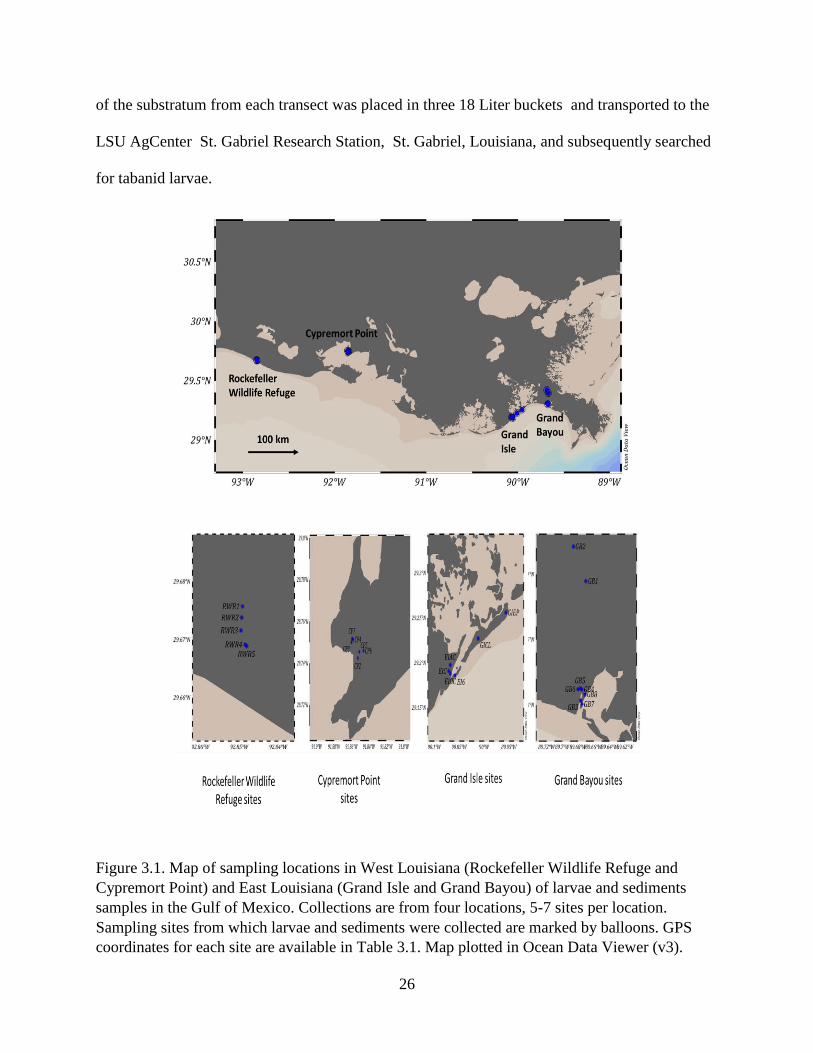
Figure 3.1. Map of sampling locations in West Louisiana (Rockefeller Wildlife Refuge and

Cypremort Point) and East Louisiana (Grand Isle and Grand Bayou) of larvae and sediments

samples in the Gulf of Mexico. Collections are from four locations, 5-7 sites per location.

Sampling sites from which larvae and sediments were collected are marked by balloons. GPS

coordinates for each site are available in Table 3.1. Map plotted in Ocean Data Viewer (v3).

27

3.3 Larval collection

Collection permits for horse fly larvae and adults were obtained from the Louisiana Department

of Wildlife and Fisheries (permit numbers LNHP-10-074 and LNHP-11-092). Tabanid larvae

were collected from five to seven marsh substrate samples taken from each of the four study

locations from 25 August 2011 to 28 September 2011. A flotation technique was used to separate

tabanid larvae from the substrate (Mullens and Rodriguez, 1984). First, the sample was removed

from the buckets, broken into small handfuls and divided among nine or ten 38.8 liter (88.27 cm

L. x 41.91 cm W. x 15.24 cm H.) storage containers (Sterlite Corp. Model # 19608006). Then,

the containers were filled with water, and approximately 600 ml of water saturated with rock salt

was added to the water in each container to increase buoyancy. The final salt concentration was

approximately 40 ppt in the containers. The components (plant material, organic and inorganic

matter, and organisms) of the substrate in the containers were broken into smaller pieces in the

salt water solution by kneading and larger pieces, e.g. of plant material, were discarded after

careful washing. The containers were searched twice, for ten minutes each time, and floating

tabanid larvae and pupae were collected.

3.4 Tabanid larval identification

Each larva and pupa was examined visually under an Automontage system from Leica (Leica

Z16 APO, DFC 450, 10447367, Leica, Buffalo Grove, IL) to confirm that it belongs to the

family Tabanidae by morphological identification (Merritt and Cummins, 1996). Tabanid

specimens found in the samples, were preserved in 95 % ethanol. A list of the number and sizes

of larvae collected and their locations is compiled in Table 3.1.Steps 3.1 to 3.4 were done before

this thesis and 3.5 onwards was done for this thesis.

28

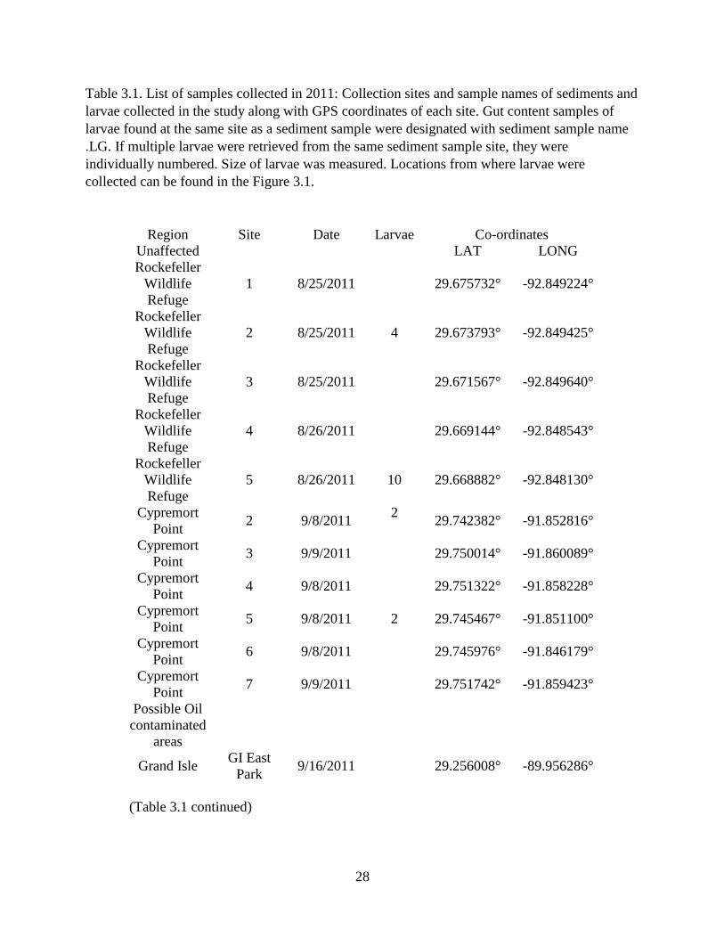
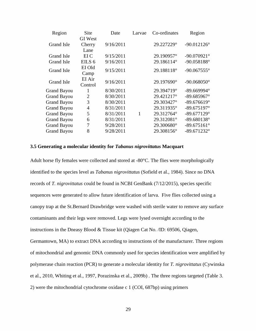
Table 3.1. List of samples collected in 2011: Collection sites and sample names of sediments and

larvae collected in the study along with GPS coordinates of each site. Gut content samples of

larvae found at the same site as a sediment sample were designated with sediment sample name

.LG. If multiple larvae were retrieved from the same sediment sample site, they were

individually numbered. Size of larvae was measured. Locations from where larvae were

collected can be found in the Figure 3.1.

Region Site Date Larvae Co-ordinates

Unaffected LAT LONG

Rockefeller

Wildlife

Refuge

1 8/25/2011 29.675732° -92.849224°

Rockefeller

Wildlife

Refuge

2 8/25/2011 4 29.673793° -92.849425°

Rockefeller

Wildlife

Refuge

3 8/25/2011 29.671567° -92.849640°

Rockefeller

Wildlife

Refuge

4 8/26/2011 29.669144° -92.848543°

Rockefeller

Wildlife

Refuge

5 8/26/2011 10 29.668882° -92.848130°

Cypremort

Point 2 9/8/2011

2

29.742382° -91.852816°

Cypremort

Point 3 9/9/2011 29.750014° -91.860089°

Cypremort

Point 4 9/8/2011 29.751322° -91.858228°

Cypremort

Point 5 9/8/2011 2 29.745467° -91.851100°

Cypremort

Point 6 9/8/2011 29.745976° -91.846179°

Cypremort

Point 7 9/9/2011 29.751742° -91.859423°

Possible Oil

contaminated

areas

Grand Isle GI East

Park 9/16/2011 29.256008° -89.956286°

(Table 3.1 continued)

29

Region Site Date Larvae Co-ordinates Region

Grand Isle

GI West

Cherry

Lane

9/16/2011 29.227229° -90.012126°

Grand Isle EI C 9/15/2011 29.190957° -90.070921°

Grand Isle EILS 6 9/16/2011 29.186114° -90.058188°

Grand Isle EI Old

Camp 9/15/2011 29.188118° -90.067555°

Grand Isle EI Air

Control 9/16/2011 29.197690° -90.068050°

Grand Bayou 1 8/30/2011 29.394719° -89.669994°

Grand Bayou 2 8/30/2011 29.421217° -89.685967°

Grand Bayou 3 8/30/2011 29.303427° -89.676619°

Grand Bayou 4 8/31/2011 29.311935° -89.675197°

Grand Bayou 5 8/31/2011 1 29.312764° -89.677129°

Grand Bayou 6 8/31/2011 29.312081° -89.680138°

Grand Bayou 7 9/28/2011 29.300680° -89.675161°

Grand Bayou 8 9/28/2011 29.308156° -89.671232°

3.5 Generating a molecular identity for Tabanus nigrovittatus Macquart

Adult horse fly females were collected and stored at -80°C. The flies were morphologically

identified to the species level as Tabanus nigrovittatus (Sofield et al., 1984). Since no DNA

records of T. nigrovittatus could be found in NCBI GenBank (7/12/2015), species specific

sequences were generated to allow future identification of larva. Five flies collected using a

canopy trap at the St.Bernard Drawbridge were washed with sterile water to remove any surface

contaminants and their legs were removed. Legs were lysed overnight according to the

instructions in the Dneasy Blood & Tissue kit (Qiagen Cat No. /ID: 69506, Qiagen,

Germantown, MA) to extract DNA according to instructions of the manufacturer. Three regions

of mitochondrial and genomic DNA commonly used for species identification were amplified by

polymerase chain reaction (PCR) to generate a molecular identity for T. nigrovittatus (Cywinska

et al., 2010, Whiting et al., 1997, Porazinska et al., 2009b) . The three regions targeted (Table 3.

2) were the mitochondrial cytochrome oxidase c 1 (COI, 687bp) using primers

30

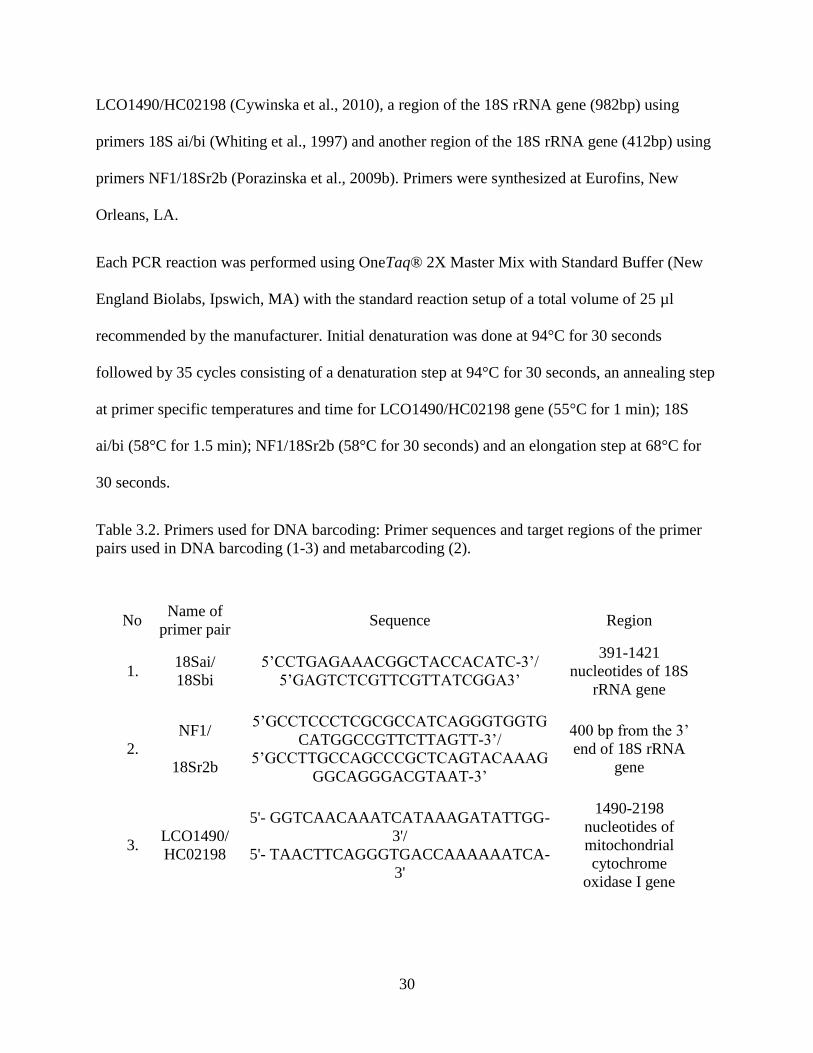
LCO1490/HC02198 (Cywinska et al., 2010), a region of the 18S rRNA gene (982bp) using

primers 18S ai/bi (Whiting et al., 1997) and another region of the 18S rRNA gene (412bp) using

primers NF1/18Sr2b (Porazinska et al., 2009b). Primers were synthesized at Eurofins, New

Orleans, LA.

Each PCR reaction was performed using OneTaq® 2X Master Mix with Standard Buffer (New

England Biolabs, Ipswich, MA) with the standard reaction setup of a total volume of 25 µl

recommended by the manufacturer. Initial denaturation was done at 94°C for 30 seconds

followed by 35 cycles consisting of a denaturation step at 94°C for 30 seconds, an annealing step

at primer specific temperatures and time for LCO1490/HC02198 gene (55°C for 1 min); 18S

ai/bi (58°C for 1.5 min); NF1/18Sr2b (58°C for 30 seconds) and an elongation step at 68°C for

30 seconds.

Table 3.2. Primers used for DNA barcoding: Primer sequences and target regions of the primer

pairs used in DNA barcoding (1-3) and metabarcoding (2).

No Name of

primer pair Sequence Region

1. 18Sai/

18Sbi

5’CCTGAGAAACGGCTACCACATC-3’/

5’GAGTCTCGTTCGTTATCGGA3’

391-1421

nucleotides of 18S

rRNA gene

2.

NF1/

18Sr2b

5’GCCTCCCTCGCGCCATCAGGGTGGTG

CATGGCCGTTCTTAGTT-3’/

5’GCCTTGCCAGCCCGCTCAGTACAAAG

GGCAGGGACGTAAT-3’

400 bp from the 3’

end of 18S rRNA

gene

3. LCO1490/

HC02198

5'- GGTCAACAAATCATAAAGATATTGG-

3'/

5'- TAACTTCAGGGTGACCAAAAAATCA-

3'

1490-2198

nucleotides of

mitochondrial

cytochrome

oxidase I gene

31

A final extension at 68°C for 5mins was added. A 1% agarose gel was used to check the

presence of the PCR products. After PCR purification, bidirectional Sanger sequencing was

carried out for all primer pairs by GeneWiz, South Plainfield, NJ. Forward and reverse sequences

were aligned using ChromasPro® 2.6.4 (from Technelysium Pty Ltd, available at

http://technelysium.com.au/wp). A consensus sequence for each of the three target regions was

generated and submitted to GenBank (NCBI). The sequences of T. nigrovittatus in GenBank can

be accessed using the following accession numbers; KT381971 (mitochondrial cytochrome

oxidase c 1 gene-687), KT222915 (18S gene-982bp) and KU321600.1 (18S gene-412bp).

3.6 Tabanid larval dissection, DNA extraction and amplification

Nineteen larvae were collected in 2011 (Table 3.1), stored in 95% ethanol, morphologically

identified as tabanids, and then dissected under disinfected conditions. The dissection pan with

wax (Thermo Fisher Scientific, Wilmington, DE) and dissection tools were wiped clean with 4%

sodium hypochlorite solution prior to each dissection. Between larval dissections all the

instruments and surfaces were wiped with Clorox bleach until visibly clean and free of stains and

tissues. The larvae were pinned on the sterilized dissection pan and washed with 70% ethanol.

Fine insect pins were used to pin the anterior and posterior ends of larvae with the dorsal side of

the larvae facing upwards. Microdissection scissors (Fine Science Tools, Foster City, CA) were

used to cut the cuticle at the ventral midline near the posterior end and all the way through to the

anterior end. The lateral edges of the cut cuticle were pinned to the dissection pan exposing the

gut. The fat body covering the gut was removed and the gut was removed. The gut lining was cut

and pinned to the dissection pan and gut contents were pipetted into a 1.5ml microcentrifuge tube

containing lysis buffer (ATL) from the DNeasy Blood & Tissue kit (Qiagen, Germantown, MA).

DNA was extracted from the gut contents according to the manufacturer’s instructions. DNA

32

quantity (>10ng) and purity (260/280 ratio of ~1.8) was measured using NanoDrop® ND-1000,

Spectrophotometer. DNA was amplified using illustra™ Ready-To-Go™ GenomiPhi™ HY

DNA Amplification Kit (GE Healthcare, Thermo Fisher Scientific, Wilmington, DE) according

to the manufacturer’s General Protocol available on GE health care Life Sciences website

(http://www.gelifesciences.com/webapp/wcs/stores/servlet/productById/en/GELifeSciences-

us/29108039).The amplified DNA was purified using the QlAquick® PCR Purification Kit

protocol PCR using the primer pair NF1 and 18Sr2b (Table 3.2) of the 18SrRNA gene was done

with cycling conditions mentioned above. Agarose gels of 1% (Sigma Aldrich, Saint Louis, MO)

were used to check the amplified bands using the GeneRuler 1kb ladder (Thermo Fisher

Scientific, Wilmington, DE). A band with an approximate size of 400 bp was considered as

evidence for successful amplification.

3.7 Molecular identification of tabanid larvae

DNA from the remaining carcasses of 19 tabanid larvae was extracted using the DNeasy Blood

& Tissue kit (Qiagen, Germantown, MA). After DNA extraction, Nanodrop Spectrophotometer

ND-1000 (Thermo Fisher Scientific, Wilmington, DE) was used to determine quantity (>10ng)

and quality (260/280 ratio of ~1.8) of the DNA. The three regions described above were

amplified via PCR as described in section 3.5. PCR products were checked on a 1% agarose gel,

purified and submitted for Sanger sequencing in both forward and reverse directions (GeneWiz,

South Plainfield, NJ). Forward and reverse sequences for each larva were aligned as described in

3.5. The aligned sequences were matched to the NCBI database using the BLASTn program for

species level identification. Larvae that showed ≥ 99% match to a species in the database were

assigned to that species.

33

3.8 Cloning to detect extent of tabanid DNA contamination in the gut contents

PCR products obtained using the primer set NF1/18Sr2b were cloned into One Shot® Competent

E. coli (Life Technologies™, Thermo Fisher Scientific, Wilmington, DE) using the TOPO®TA

Cloning® Kit (Invitrogen, Life Technologies™, Thermo Fisher Scientific, Wilmington, DE). A

ligation reaction was set up using 2 µl of the DNA product with a concentration in the range of

10-100 ng, 2 µl of water, 1 µl of salt solution provided with the kit and 1µl of the TOPO®

vector. A 15 minute incubation period at room temperature allows the ligase enzyme, which is

linked to the vector, to insert the PCR product into the plasmid vector. The ligation mixture was

purified using ice cold absolute ethanol precipitation. After an overnight incubation at -20 ºC

precipitated DNA was pelleted down the following day by centrifugation (Centrifuge 5418,

Eppendorf, Hauppauge, NY) at 10,000 rpm for 20 minutes at room temperature. DNA pellets

were dried by allowing the ethanol to volatize from the tubes at room temperature, and then

dissolved in 20 µl of nuclease free water (Ambion, Thermo Fisher Scientific, Wilmington, DE).

Ligated DNA products were transformed into One Shot® TOP 10 Chemically Competent E. coli

(Life Technologies™, Thermo Fisher Scientific, Wilmington, DE) according to manufacturer’s

instructions (available at https://tools.thermofisher.com/content/sfs/manuals/topota_man.pdf).

Plates containing Luria Bertani Agar with kanamycin (100 ug/ul) were prepared. X-gal (Thermo

Fisher Scientific, Wilmington, DE) at a concentration of 20ug/ml was spread on the plates with a

spreader and left to dry in the incubator. Cloned PCR products were then spread on the plate and

incubated overnight. Untransformed cells did not grow on the plates containing kanamycin as

the vector containing the resistance conferring gene was absent in these cells. Cloned colonies

were selected using blue-white screening. In this method of screening, bacterial cells

successfully transformed with the plasmid vector containing the insert (PCR product) cannot

34

degrade the X-gal using the beta galactosidase enzyme and form white colonies. This occurs

because the beta galactosidase enzyme function is disrupted due to the presence of the insert

(PCR product). However, cells that do not contain the insert, contain a functional beta

galactosidase enzyme, degrade X-gal and consequently form blue colonies. Colony PCR was

performed with 20 white colonies of each PCR product in a 96-well plate with a reaction setup in

accordance to the OneTaq® 2X Master Mix with Standard Buffer (New England Biolabs® Inc.).

Twenty white colonies were picked using a sterile pipette tip and dipped in the reaction mixture.

PCR was done according to manufacturer’s protocols using M13 primers. Cells were lysed at

95°C for 5 minutes followed by 35 cycles of 94°C for 30 seconds, 45°C for 30 seconds and 68°C

for 30 seconds. A final extension of 5 minutes at 68°C was added. After confirming the presence

of the PCR product on an agarose gel (1%), the products were sequenced in the forward

orientation by GeneWiz®. VecScreen on the NCBI website was used to remove the portion of

the vector in the DNA sequence. The remaining portion of the sequence without the vector was

compared to the NCBI nucleotide database using BLAST® to identify the species of origin. If

the sequence matched with ≥ 99% to a sequence in the database it was considered as the same

species.

3.9 DNA extraction from voucher sediments

DNA was extracted from the voucher sediments collected in 2011 from 25 sites in East and West

Louisiana (From 3.2). The samples were thawed and DNA was extracted from six parts of each

sediment sample using the PowerSoil® DNA Isolation Kit (MO BIO Laboratories, Qiagen,

Germantown, MA) following the manufacturer’s protocol. DNA from different parts of the same

sample was pooled and quantified using Nanodrop. Sediment DNA was sent to MR DNA

(www.mrdnalab.com, Molecular Research LP, Shallowater, TX) for next-generation sequencing.

35

3.10 DNA amplification and sequencing

DNA amplification and sequencing was done at MR.DNA, Shallowater, Texas with a procedure

developed for diversity high-throughput amplicon sequencing (Dowd et al., 2008a, Dowd et al.,

2008b). In the first step, amplification of DNA using PCR with the primers NF1 and 18Sr2b was

done for individual samples. During this PCR, the forward primer was barcoded for individual

samples. PCR was performed using HotStarTaq Plus Master Mix Kit (Qiagen, Germantown,

MA) under the following conditions: 94°C for 3 minutes, followed by 28 cycles of 94°C for 30

seconds, 53°C for 40 seconds and 72°C for 1 minute, a final elongation step at 72°C for 5

minutes. PCR products were checked on a 2% agarose gel to ensure amplification and relative

intensity of bands

In the second step, all barcoded samples were pooled together in equal proportions based on

their molecular weight and DNA concentrations followed by purification using calibrated

Ampure XP beads. In the third step, pooled and purified PCR products were used to prepare a

DNA library by following Illumina TruSeq DNA library protocol (Illumina, San Diego, CA).

In the fourth step, sequencing was performed using the Illumina MiSeq (2x300) paired end

sequencing platform following the manufacturer’s guidelines.The fifth step, is a quality filtering

step in which sequenced amplicons in the files r1 and r2 are trimmed using the phred quality

score of 25 removing ambiguous bases.

Next, the trimmed ends are joined and reoriented in the 5’ to 3' direction. The resulting fasta and

qual files after joining and reorienting are the text versions of the sequence data and quality

scores, respectively. Fasta and qual files still contain primers and barcodes. A mapping file also

was provided by MR.DNA which includes sample names, barcode information, primer

information and project name. This mapping file was updated with all metadata collected for

36

sediments such as sediment biochemistries, Polycyclic Aromatic Hydrocarbons (PAH’s),

toxicity, location, geography and presence/ absence of larvae.

3.11 Bioinformatic and statistical analyses

After the steps carried out at MR.DNA mentioned above, further data analysis was carried out

using QIIME (v.1.9.1) (Caporaso et al., 2010) accessible on a server provided by Hubbard

Center for Genome Studies, University of New Hampshire.

Fasta and qual files containing reads that were joined and reoriented were converted into a Fastq

file using the Python script convert_fastaqual_fastq.py in QIIME. The script extract_barcodes.py

created two files namely barcodes. fastq (sequences with barcodes) and reads. fastq (sequences

without barcodes). Using the output files of extract_barcodes.py and the mapping file, sequences

were demultiplexed (divided into separate samples based on barcodes) with

split_libraries_fastq.py and a minimum Phred quality score of 33 to remove ambiguous bases.

Operational Taxonomic Units (OTUs) were clustered using the pick_open_reference_otus.py.

The reference database for OTU picking was SILVA 119 (accessed on 1/23/2017) (Pruesse et

al., 2007). Taxonomic classification was assigned at 99% clustering for OTU picking.

After taxonomic classification, an OTU table was created using the make_otu_table.py.

Chimeras were identified using identify_chimeric_sequences.py and filtered from the OTU table

using the filter_otus_from_otu_table.py. Pynast was used to align sequences to SILVA 119 using

the align_seqs.py. The pairwise alignment method selected was UCLUST and the minimum

percent identity to the closest blast hit to be included in the alignment was 70%. The gaps in the

alignment were removed using the filter_alignment.py.

The 18S rRNA gene is less variable compared to other marker regions and, thus, higher

clustering cutoff values are commonly used in sequencing studies using this gene (Bik et al.,

37

2016, Hadziavdic et al., 2014, Caron et al., 2009). After using filter_alignment.py to remove

chimeras and alignment failures, a 0.05% abundance cutoff was applied to each sample

separately to remove all OTUs with ≤ 0.05% abundance in each single sample. The 0.05% cutoff

was applied to make data more meaningful and downstream analysis more reliable. In addition,

quality filtering to remove OTUs with an abundance of a less stringent filter than we applied, ≤

0.005% improves diversity estimates by minimizing spurious additional OTUs (Bokulich et al.,

2013). Each sample was filtered from the OTU table using the script

filter_samples_from_otu_table.py and the cutoff was applied using the script

filter_otus_from_otu_table.py specifying the --min_count_fraction 0.0005 (converting percent

0.05% to fraction). After applying the abundance cutoff, computation of OTU tables and all

downstream analysis was done separately for larval gut samples and sediment samples because

they are two different sample types. The OTU table of sediment samples was generated by

combining all the individual sediment OTU tables obtained after applying the 0.05% cutoff using

the script merge_otu_tables.py. All larval gut samples were combined in a similar fashion. Final

number of sequences in each sample was obtained from OTU tables computed using the script

make.otu.table.py for larval guts and sediments separately.

Estimate S was used for rarefaction analyses on OTU tables after cutoff for overall sediments

and larval gut samples using the default settings of EstimateS with 100 randomizations without

replacement. Mao Tao estimator was used to compute observed OTU richness (number of

OTUs) in each larval gut content and sediment sample. Sampling coverage in terms of capturing

the majority of OTUs in sediments and guts was assessed by computing rarefaction curves of the

number of observed OTUs captured at different sample sizes and extrapolation.

38

Shannon diversity index, which measures OTU diversity in the sample by taking into account

both abundance and richness, was calculated. Shannon H and Shannon exponential were both

computed using the above settings in Estimate S. Shannon H is not linear and hence Shannon

exponential is used to compare between communities. Shannon exponential (true diversity) is

linear implying that when the value for Shannon exponential is double, the diversity is actually

double (Magurran, 2013).

A second diversity index, Simpson Inverse D (Magurran, 2013), which differs from the Shannon

index in that it is largely dominance based, was obtained in Estimate S using the above settings.

For easier interpretation, Simpson Inverse D was converted to Simpson D in Microsoft Excel

2010. Simpson D measures the probability that two OTUs randomly selected from the sample

will be the same.

After the cutoff to filter out extremely rare OTUs (≤ 0.05%) was performed OTU diversity was

assessed in QIIME using the core_diversity_analyses.py script. Prior to using this script, a

phylogenetic tree of the sequences of the OTUs with > 0.05% abundance was constructed using

the make_phylogeny.py script.

The relative abundances at different taxonomic levels defined by the SILVA 119 taxonomy file

(L2 –“Phyla” to L6 “Genera”) were computed for OTUs (> 0.05% in each gut and sediment

sample and taxonomic bar charts based on percent relative abundances were generated.

Manual BLAST (Johnson et al., 2008) against the NCBI database was done for the 52 insect

OTUs identified to the species level by the SILVA 119 database. OTUs belonging to insect

species were picked from the OTU table imported into Excel and OTU sequences were retrieved

from the fasta file containing sequences after quality filtering.

39

Each of the 23 OTU sequences were manually blasted to the nucleotide database in NCBI and

the top five blast hits were recorded.

Alpha diversity between groups of samples based on the two sample t-test was determined. The

compare_alpha_diversity.py script in QIIME (v1.9) was used to make box plots based on the

alpha diversity of observed OTUs. This script uses the non-parametric Monte Carlo method with

999 permutations. The mapping file mentioned in section 3.11 was used to group samples based

on categories such as location, geography, presence/absence of oil, presence/absence of larvae

and larval diets based on location.

Variation in OTU composition in larval guts across locations was determined in R studio version

3.4.1 using the package Vegan. Vegan provides tools for community ecology including diversity

analysis, community ordination and dissimilarity analysis (Dixon, 2003). Data was transformed

by X 0.19 to avoid analytic bias caused by highly abundant taxa. The distance matrix used for

computation was the Bray-Curtis-Distance, which takes into account the abundances of OTUs

(Beals, 1984). A Non-metric multidimensional scaling plot (NMDS) was created based on the

Bray-Curtis-Distance matrix. A NMDS plot is a visualization method, which represents original

position of communities (consisting of OTUs in our study) in a multidimensional space

(CLARKE, 1993). An ordination spider was constructed, which connected all samples to their

group means with non-dotted lines using the function ordispider (Oksanen et al., 2007).

Ordination hulls to denote different groups being compared in the NMDS plot by dotted lines

were plotted using the function ordihull (Oksanen et al., 2007). Ordination hulls can be used to

compare groups and non-overlapping ordination hulls indicate significant difference among

groups (Ramette, 2007).

40

Permutational multivariate analysis of variance (PERMANOVA) is a method for non-parametric

multivariate analysis of variance (Anderson, 2001). In this method, data is randomly shuffled

(permutations) and an F-ratio is determined for each shuffle. F-ratios of randomized data are then

compared to F-ratios of original data. The p value is the fraction of F-ratio that is higher than the

F-ratio of the original data. Adonis is a function in the package Vegan which analyses and

partitions sums of squares using semimetric and metric distance matrices (Oksanen et al., 2007).

PERMANOVA with the function Adonis in Vegan was used to determine if the differences in

the OTU composition in the groups compared in the NMDS plot are statistically significant.

OTU abundances of taxa at multiple taxonomic levels as determined by the SILVA 119

database were converted into their relative abundances using the script summarize_taxa.py.

Samples were grouped based on the presence/absence of larvae, geography, location, lightly

oiled and unoiled sites of Grand Bayou and larval diets. A linear discriminant analysis effect

size (LEfSe) was carried out to determine which taxa had significantly higher relative

abundance in one group of samples when compared to the other. The non-parametric factorial

Kruskal-Wallis (KW) sum-rank test was used to determine significant differential abundance

between the specified groups of samples. After uploading the files on the Galaxy website of the

Huttenhower Lab available at this link (https://huttenhower.sph.harvard.edu/galaxy/) default

parameters in the LEfSe modules was used to conduct analysis and plot results.

Comparison of taxa between sediments where larvae were present and absent was done by

comparing the percent read abundance between these two groups of sediments. Percent read

abundance of larval gut samples also was computed to determine if there was a pattern

connecting the larval guts and the corresponding sediment they were collected from. Horizontal

bar charts of percent read abundance of taxa at taxonomic levels defined by SILVA as “Phylum”,

41

“Class”, “Order”, “Family” and “Genera” based on a combined OTU table of all larval guts and

sediment samples were visualized in PHINCH using the Taxonomy Bar Chart option. Bar charts

of individual sediment and larval guts were assembled and labelled in Microsoft Excel 2010 for

easier visualization and interpretation.

Variation in OTU composition of sediments where larvae were present versus sediments where

larvae were absent and variation in sediment OTUs across locations also were determined by the

NMDS plot and PERMANOVA using the functions in Vegan as described above. However the

transformation of data was by X 0.20 to reduce the effect of highly abundant taxa.

3.12 Measuring Sediment PAH levels

Total Polycyclic Aromatic Hydrocarbon (PAH) content in sediments in East Louisiana where oil

made landfall was measured using Gas Chromatography-Mass Spectrometry (GC-MS) using the

SIM acquisition mode. This method targeted 28 alkanes and 18 parent aromatic hydrocarbons

based on EPA SW-846 methods (2000).

PAH measurements were conducted at the Department of Environmental Sciences by Scott

Miles. Detailed description of the extraction and analysis of PAHs can be found in a previous

publication of Scott Miles (Turner et al., 2014).

Relationship of OTUs in the oiled and unoiled sediments across all locations and relationship of

OTUs in the oiled and unoiled sediments in Grand Bayou were computed using a NMDS plot

and PERMANOVA with functions in Vegan as described above.

Variation in OTU composition between sediments from East and West Louisiana were computed

using NMDS and Principal Co-ordinate Analysis (PCoA) plots. The NMDS plot was computed

42

as described above and PCoA plot was computed in QIIME (v1.9) using the

beta_diversity_through_plots.py script and visualized in Emperor.

3.13 Measuring Sediment chemistry Parameters

Sediment chemistry parameters were measured at the Soil Testing and Plant Analysis Laboratory

at the LSU AgCenter, Baton Rouge. The parameters measured in the sediment were Calcium,

Chloride, Conductivity, Magnesium, Salts, SAR (Sediment accumulation rate), Sodium, Sulfur,

Copper, pH, Phosphorus, Potassium, Zinc, Iron, Manganese, Organic content, Boron, Aluminum

and Nitrogen using methods routinely used for measuring these parameters in Louisiana

sediments. A detailed description of methods is available at

http://www.lsuagcenter.com/portals/our_offices/departments/spess/servicelabs/soil_testing_lab.

Effect of sediment chemistry on OTU composition was determined using the script

compare_distance_matrices.py. First, a distance matrix of the OTU composition based on

UniFrac distances was computed using the core_diversity_analysis.py script. Next, metadata for

all sediments in the mapping file (mentioned in 3.11) were updated with the results from the

biochemistry analysis. Then, a Euclidean distance matrix was created for each of the 19

parameters measured above. The distance matrix of each biochemical parameter was compared

to the distance matrix of the OTUs. This script determines if the similarity of a biochemical

parameter among sediments correlates with similarity of OTU composition using the Mantel

correlation. The sediment chemistry parameter pH had an effect on the OTUs and to determine

which OTUs correlate to pH the observation_metadata_correlation.py script was used. This

script determined the correlation of the OTUs from OTU table to the pH values in the mapping

file. The Pearson’s score was used to determine correlation and the Bootstrapping method was

used to determine p value.

43

3.14 Sediment Toxicity assay using the model organism Hyallela azteca

A 10 day sediment toxicity assay was conducted using modified American Society for Testing

and Materials (ASTM) procedures with amphipods. Sediments were collected in 2011 from East

and West Louisiana and stored at minus 20 degrees Celsius for 6 years as described in section

1.1. Clean and dry lipless glass beakers of 100 ml (Cat.no. 13920-012, VWR, Houston, TX) were

used as test chambers for the assay (Burton Jr et al., 2001). Test chambers were rinsed with tap

water, followed by a careful rinse with diluted Hydrochloric Acid to remove metals and bases.

Next, chambers were rinsed with deionized water followed by an acetone wash to remove

organic compounds and, finally, rinsed again with deionized water. All the test chambers were

then autoclaved to eliminate any biological contamination.

Sediments were thawed overnight. The following day, 10 grams of sediment was transferred to

individual test chambers; there were three replicates for each of the vouchers. Reconstituted

water was prepared as recommended in the ASTM procedure (Smith et al., 1997), i.e. 5 grams of

CaSO4, 5 grams CaCl2, 3 g of MgSO4, 9.6 g NaHCO3 and 0.4 g KCl was dissolved in 100L of

deionized water and aerated (Smith et al., 1997).

Reconstituted water was added to each test chamber until the 60 ml mark was reached by gently

pouring the water down the sides of the beaker to ensure minimal disturbance of the sediment.

Amphipods (Hyallela azteca) (obtained from Sachs Systems Aquaculture Inc., St. Augustine,

FL) were transferred to a 10 gallon aquarium containing reconstituted water and kept overnight

in the aquarium to acclimatize to the reconstituted water. Amphipods were collected in a sieve

from the aquarium and 5 amphipods were introduced gently into each test chamber below the

air-water interface using blunt forceps. Dissolved oxygen and temperature were measured using

Pro DSS Multiparameter Water Quality Meter (YSI Gulf Coast, Baton Rouge, LA) in test

44

chambers and their levels were maintained under recommended conditions. The recommended

conditions were a minimum of 2.5 mg/L of dissolved oxygen and a temperature range between

22 to 24℃ throughout the experimental period (Plumb Jr, 1981). Yeast Cerophyll Trout chow

medium (1 ml) was fed to the amphipods in the test chambers every day for 10 days. This

medium was prepared in the lab from Trout Chow Pellets (Kruse Feed Supply, La Habra, CA),

yeast (Fleischmann's) and Aldon™ Innovating Science™ Cereal Grass Medium (Fischer

Scientific, Hampton, NH) using the procedure described in the ASTM 2010 manual (Adams and

Rowland, 2003). In short, 5 grams Trout Chow Pellets were blended, suspended in 1L of

deionized water and digested for a week separately without the other components of the YCT

medium. At the end of the week, 5 grams of yeast and 5 grams of Cereal Grass medium were

dissolved each in 1L of water. The digested trout chow, yeast and Cereal Grass medium were

mixed and the undissolved components were filtered. The medium was divided into aliquots and

stored at -20℃.

Two volumes of water were added per day to the test chambers. Each day three test

chambers/replicates per sediment were examined and the number of live/dead amphipods was

recorded. The chambers were numbered from 1 to 30 for each sediment sample and selection of

chambers was predetermined. The sediment in each test chamber was emptied onto a fine sieve

and the sediment was washed off with water to expose the amphipods that were retained on the

sieve. Live amphipods were counted as dead based on unresponsiveness of the amphipods to

probing with the forceps. Data were recorded and percent survival was calculated at the end of

the experiment.

Two different concentrations of Water Accommodated Fraction (WAF) of Mississippi Canyon

252 Weathered Crude Oil (Louisiana Light Sweet Crude) were obtained by weighting eight and

45

13 grams of crude oil and adding 100 ml of reconstituted water. The mixture of crude oil and

water was kept overnight on a Thermo Forma orbital shaker (Thermo Fisher Scientific,

Wilmington, DE) at 200 rpm for maximum emulsification of oil in water.

Negative control 1 for the experiment was a test chamber containing 10 grams of Quickrete play

sand (available at Home Depot) with 60 ml of reconstituted water. Negative control 2 contained

60 ml of reconstituted water without sand. For Positive Control 1 (with 10 grams of Quickrete

play sand) and Positive Control 2 (without sand), 100 ml of WAF obtained from eight grams of

oil was added. For Positive Control 3 (without sand), 100 ml of WAF from 13 grams of crude

oil used (Saco-Álvarez et al., 2008).

Shapiro Wilks test was used to determine normality and Levene’s test was used to calculate

variance. Kruskal Wallis test and post hoc Kruskal-Nemenyi were used to calculate the effect of

days on toxicity. Welch’s t-test assumes non-normal data with unequal variances and this test

was used to compare each sediment to the negative control to determine toxicity.

46

Chapter 4. Results

4.1 Molecular identification of tabanid larvae

All larvae were morphologically identified to the genus Tabanus. The larval barcoding BLAST

results against DNA from an adult specimen morphologically identified as T. nigrovittatus

showed varying similarities (Table 4.1). Larvae RWR5.1.LG, RWR5.2.LG, RWR5.7.LG,

RWR5.8.LG, RWR5.10.LG, RWR5.12.LG, RWR5.13.LG, RWR5.16.LG, RWR5.18.LG,

RWR2.3.LG, RWR2.4.LG, RWR2.5.LG, RWR2.6.LG and CP5.1.LG with an identity in all three

regions of ≥ 97% to the reference sample likely are the same species. Larvae with lower matches

to the T. nigrovittatus reference at the most variable locus (COI) (92% to 95%) nevertheless

likely to belong to the T. nigrovittatus species complex, such as GB5.1.LG, RWR5.9.LG,

CP2.1.LG and CP2.2.LG. The only larva showing similarity values less than 95% to the T.

nigrovittatus reference was CP5.2.LG, and might, thus, represent a different species, most likely

T. hinellus. The mitochondrial cytochrome oxidase subunit 1- 5’ sequences of the adult reference

specimen of T. nigrovittatus from Louisiana marshes identified by morphological measurements

(Sofield et al., 1984) differed by 5% from a previously submitted T. nigrovittatus from Florida.

4.2 Tabanid DNA and preliminary data on food web components in larva gut contents

A pilot study using cloning, sequencing and blasting of 18S-3’end region with the primer pair NF1

and 18Sr2b (details in Materials and methods Table 3.2) amplicons from larval gut contents against

the NCBI database determined the proportions of DNA from tabanids and other taxa in the 19

larval guts to aid in selection of larvae for next generation sequencing.

47

Table 4.1 Larval species ID: Percent identity match of morphologically identified tabanid larvae

to DNA from an adult specimen of Tabanus nigrovittatus at three regions of the genome,

Mitochondrial CO1 (GenBank Accession no KT381971), 18S-5’ (GenBank Accession no

KT222915) and 18S-3’ (GenBank Accession no KU321600). Abbreviations of samples and

locations from where larvae were collected can be found in the Figure 3.1.

About half the larvae showed presence of T. nigrovittatus DNA in varying proportions. Three

larvae (RWR2.6.LG, CP2.1.LG and CP2.2.LG) had exclusively T. nigrovittatus DNA in their

Tabanid larvae % Identity match

to mtCO1 region

of T. nigrovittatus

% Identity match to

18S-5’ (~1000bp)

region of T.

nigrovittatus

% Identity match to

18S-3’ (last 400bp)

region of

T. nigrovittatus

GB5.1.LG 94% 100% 100%

RWR5.1.LG 99% 99% 100%

RWR5.2.LG 98% 99% 100%

RWR5.7.LG 97% 99% 100%

RWR5.8.LG 99% 99% 100%

RWR5.9.LG 95% 99% 100%

RWR5.10.LG 99% 97% 100%

RWR5.12.LG 97% 98% 100%

RWR5.13.LG 97% 99% 100%

RWR5.16.LG 98% 99% 100%

RWR5.18.LG 99% 99% 99%

RWR2.3.LG 99% 99% 100%

RWR2.4.LG 99% 99% 99%

RWR2.5.LG 98% 99% 100%

RWR2.6.LG 99% 99% 100%

CP2.1.LG 92% 98% 98%

CP2.2.LG 92% 95% 98%

CP5.1.LG 99% 99% 100%

CP5.2.LG 92% 70% 91%

48

guts, with all 20 clones showing an identity match from 98% to 100% to this species. Since no

other food web component was found, these larvae were not used for deep sequencing. Larva

RWR5.2.LG showed a 95% (19 of the 20 clones) dominance of T. nigrovittatus DNA. More than

half but less than 95% of the clones of RWR5.1.LG, CP5.1.LG, RWR5.13.LG and RWR5.18.LG

match T. nigrovittatus. RWR.8.LG, RWR5.9.LG, RWR5.12.LG, RWR2.3.LG show low

proportions of T. nigrovittatus DNA in the range of 5% to 35%. Larvae GB5.1.LG,

RWR5.10.LG, RWR2.4.LG, RWR2.5, LG, RWR2.16.LG, CP5.1.LG, CP5.2.LG, CP5. 2. LG

had no clones matching T. nigrovittatus.

Cloning results indicate that the gut contents of the larva in the East (GB5.1.LG) demonstrated a

presence of Aedes sp. (11/20 clones with 98%-100% identity) while 12 of the larvae in the West

showed a prominence of fungi. Malassezia isolates were the most common followed by various

uncultured fungus clones. Stramenopiles were present in 4 larvae (RWR5.8.LG, RWR2.3.LG,

RWR2.4.LG, and RWR2.5.LG) whereas a protozoan Hymenostomatia sp. and a single celled

alga Ostreococcus lucimarinus were present in RWR5.8.LG and CP5.1.LG, respectively. Insects

from the order Hemiptera (matching closely to Pentatoma japonica, Laodelphax striatellus, and

Paracopta maculata) were present in multiple larvae (CP5.2.LG, CP5.1.LG, RWR2.3.LG,

RWR2.4.LG, RWR5.7.LG, RWR5.9.LG, RWR5.12.LG, RWR5.13.LG and RWR5.16.LG). The

gut contents of one larva (CP5.2.LG) found at Cypremort Point showed one clone matching a

parasitic mermithid nematode (Hexamermis albicans).

The results from this pilot study led to the selection of 16 larval guts containing DNA from other

species besides T. nigrovittatus for next-generation sequencing.

49

4.3 General assessment of next generation sequence data

Location and collection details of all 43 sediment and gut content samples used in this study have

been deposited in the NCBI database as individual BioSamples and can be accessed under the

BioProject PRJNA408157. These also can be accessed on the GRIIDC website using

(https://data.gulfresearchinitiative.org/dataset-submission?regid=R5.x277.000:0006 ).

Raw Illumina Miseq sequence data for all BioSamples has been deposited in the Sequence Read

Archive (SRA) under BioProject PRJNA408157 and has been released with SRA study number

SRP118538 titled “18S metabarcoding of greenhead horse fly food web: Larval gut contents and

sediments.” A total of 5,605,043 reads after joining forward and reverse sequences were

obtained using QIIME (v.1.9).

Quality filtering removed 6,858 reads as they were too short after quality truncation. The number

of resulting demultipexed reads was 5,598,185 with a median sequence length of 367 base pairs.

Taxonomy assignment using SILVA 119 based on clustering of sequences with 99% similarity

generated 36,907 Operational Taxonomic Units (OTUs.)

Pairwise alignment method with PyNAST in UCLUST was performed for all 36,907 OTU

sequences where each OTU sequence was blasted against the SILVA 119 database to provide a

higher taxonomic resolution than without aligning clustered sequences. A total number of 8,699

chimeric OTUs were filtered from the OTU table. After filtering, 28,208 OTUs comprising of

5,303,923 sequences with no chimeras and alignment failures were obtained. After removing

OTUs with an abundance of ≤0.05% from each sample separately, 2,279,638 sequences

remained in the sediments comprising 1,415 OTUs and 2,258,540 sequences remained in the

larval guts comprising 225 OTUs.

50

4.4 Assessment of sample sizes and OTU capture

Rarefaction curves for OTU richness depending on the number of samples after applying the

0.05% cutoff in sediments and larval guts indicated that an increase in sample size would have

allowed the capture of additional OTUs in larval guts and sediments (Figure 4.1).

Doubling of the 16 samples of the guts would increase the number of OTUs by 68 thereby

increasing overall OTU richness by approximately 30% in the guts (Figure 4.1A).

After the extrapolation the rarefaction curves started to level off, indicating that doubling the

sample size would have captured the majority of larval gut diversity. Similarly, doubling of

sediment samples by an additional 25 samples would increase OTU richness by 601 which

represent approximately 42% of the 1,412 OTUs found in the 25 sediment samples (Figure

4.1B).

Even after extrapolation the curves did not reach an asymptote. This indicates that the vast

diversity of organisms in the marsh soil was not entirely captured by the sample size used in this

study.

However, the primary objective of this study was to describe the food web of tabanid larvae

based on comparison of organisms found in the larval gut to those found in surrounding sediment

and did not require a description of the entire eukaryotic diversity in sediments. Nevertheless,

future diversity studies should make an effort to increase sample size and take spatio-temporal

variation into account.

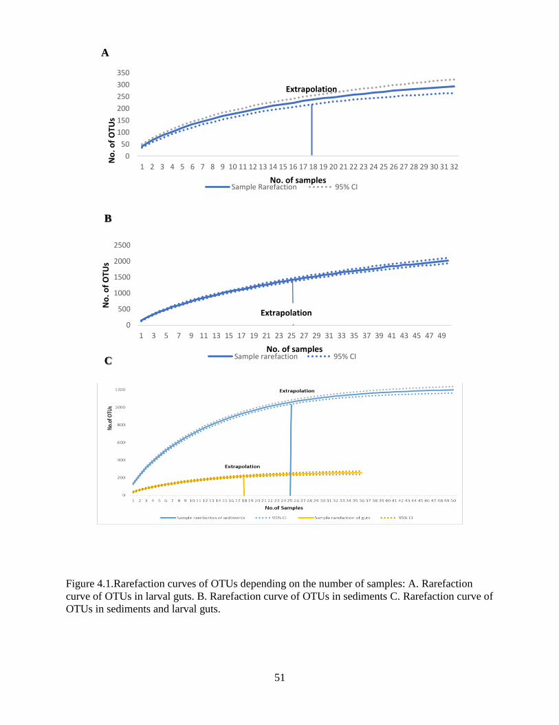
51

Figure 4.1.Rarefaction curves of OTUs depending on the number of samples: A. Rarefaction

curve of OTUs in larval guts. B. Rarefaction curve of OTUs in sediments C. Rarefaction curve of

OTUs in sediments and larval guts.

0

50

100

150

200

250

300

350

1 2 3 4 5 6 7 8 9 10 11 12 13 14 15 16 17 18 19 20 21 22 23 24 25 26 27 28 29 30 31 32

No

. of

OTU

s

No. of samplesSample Rarefaction 95% CI

Extrapolation

0

500

1000

1500

2000

2500

1 3 5 7 9 11 13 15 17 19 21 23 25 27 29 31 33 35 37 39 41 43 45 47 49

No

. of

OTU

s

No. of samplesSample rarefaction 95% CI

Extrapolation

A

B

C

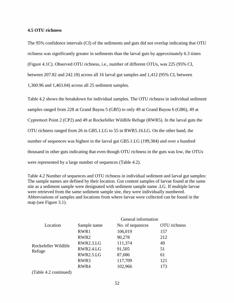
52

4.5 OTU richness

The 95% confidence intervals (CI) of the sediments and guts did not overlap indicating that OTU

richness was significantly greater in sediments than the larval guts by approximately 6.3 times

(Figure 4.1C). Observed OTU richness, i.e., number of different OTUs, was 225 (95% CI,

between 207.82 and 242.18) across all 16 larval gut samples and 1,412 (95% CI, between

1,360.96 and 1,463.04) across all 25 sediment samples.

Table 4.2 shows the breakdown for individual samples. The OTU richness in individual sediment

samples ranged from 228 at Grand Bayou 5 (GB5) to only 49 at Grand Bayou 6 (GB6), 49 at

Cypremort Point 2 (CP2) and 49 at Rockefeller Wildlife Refuge (RWR5). In the larval guts the

OTU richness ranged from 26 in GB5.1.LG to 55 in RWR5.16.LG. On the other hand, the

number of sequences was highest in the larval gut GB5.1.LG (199,384) and over a hundred

thousand in other guts indicating that even though OTU richness in the guts was low, the OTUs

were represented by a large number of sequences (Table 4.2).

Table 4.2 Number of sequences and OTU richness in individual sediment and larval gut samples:

The sample names are defined by their location. Gut content samples of larvae found at the same

site as a sediment sample were designated with sediment sample name .LG. If multiple larvae

were retrieved from the same sediment sample site, they were individually numbered.

Abbreviations of samples and locations from where larvae were collected can be found in the

map (see Figure 3.1).

General information

Location Sample name No. of sequences OTU richness

Rockefeller Wildlife

Refuge

(Table 4.2 continued)

RWR1 106,019 157

RWR2 90,278 212

RWR2.3.LG 111,374 49

RWR2.4.LG 91,505 51

RWR2.5.LG 87,686 61

RWR3 117,709 121

RWR4 102,966 173

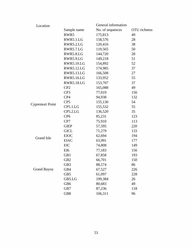
53

General information

Sample name No. of sequences OTU richness

RWR5 175,813 49

RWR5.1.LG 158,576 28

RWR5.2.LG 120,416 38

RWR5.7.LG 119,565 50

RWR5.8.LG 144,720 28

RWR5.9.LG 149,218 51

RWR5.10.LG 154,892 52

RWR5.12.LG 174,985 37

RWR5.13.LG 166,508 27

RWR5.16.LG 133,952 55

RWR5.18.LG 153,707 37

Cypremort Point

CP2 165,088 49

CP3 77,019 156

CP4 94,938 132

CP5 155,130 54

CP5.1.LG 155,532 55

CP5.2.LG 136,520 35

CP6 85,231 123

CP7 75,910 113

Grand Isle

GIEP 57,595 220

GICL 71,279 133

EIOC 62,694 194

EIAC 63,991 177

EIC 74,808 149

EI6 77,183 156

Grand Bayou

GB1 67,858 193

GB2 66,701 150

GB3 88,574 86

GB4 67,527 226

GB5 61,097 228

GB5.LG 199,384 26

GB6 80,683 49

GB7 87,236 118

GB8 106,311 96

Location

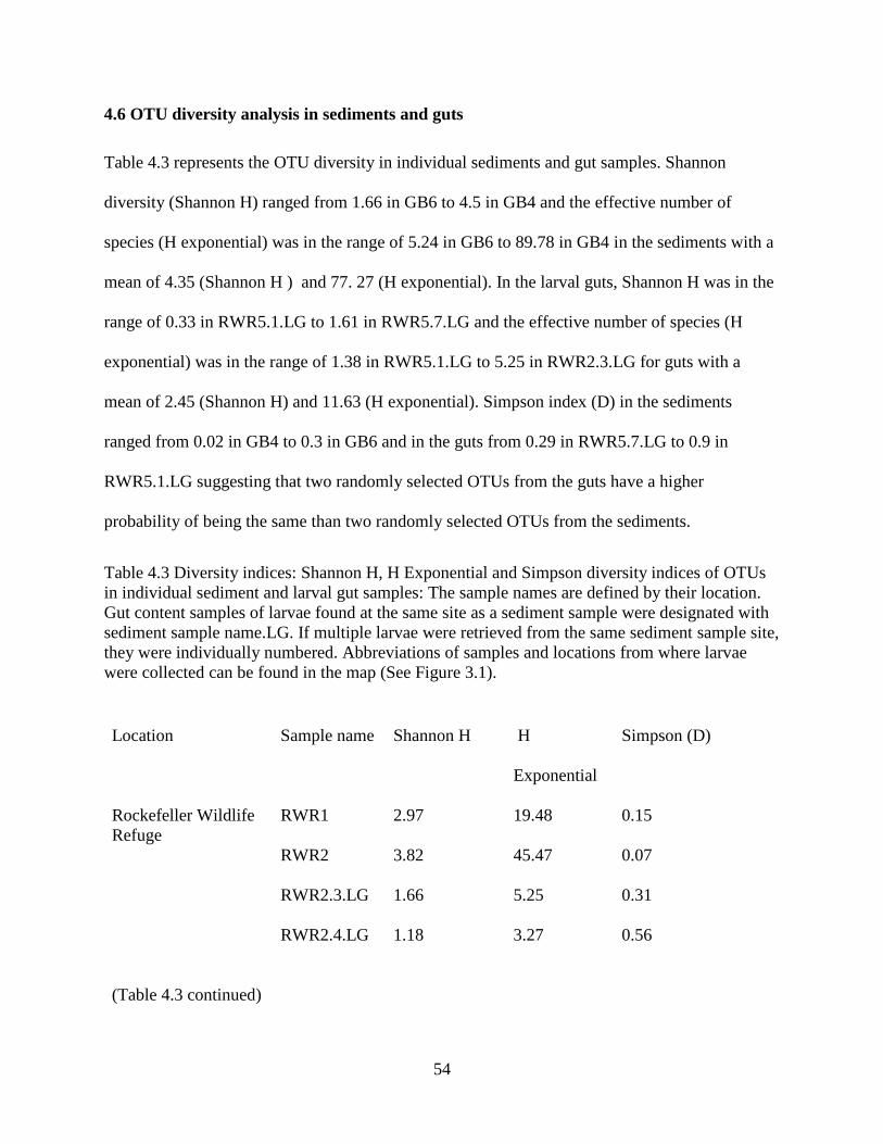
54

4.6 OTU diversity analysis in sediments and guts

Table 4.3 represents the OTU diversity in individual sediments and gut samples. Shannon

diversity (Shannon H) ranged from 1.66 in GB6 to 4.5 in GB4 and the effective number of

species (H exponential) was in the range of 5.24 in GB6 to 89.78 in GB4 in the sediments with a

mean of 4.35 (Shannon H ) and 77. 27 (H exponential). In the larval guts, Shannon H was in the

range of 0.33 in RWR5.1.LG to 1.61 in RWR5.7.LG and the effective number of species (H

exponential) was in the range of 1.38 in RWR5.1.LG to 5.25 in RWR2.3.LG for guts with a

mean of 2.45 (Shannon H) and 11.63 (H exponential). Simpson index (D) in the sediments

ranged from 0.02 in GB4 to 0.3 in GB6 and in the guts from 0.29 in RWR5.7.LG to 0.9 in

RWR5.1.LG suggesting that two randomly selected OTUs from the guts have a higher

probability of being the same than two randomly selected OTUs from the sediments.

Table 4.3 Diversity indices: Shannon H, H Exponential and Simpson diversity indices of OTUs

in individual sediment and larval gut samples: The sample names are defined by their location.

Gut content samples of larvae found at the same site as a sediment sample were designated with

sediment sample name.LG. If multiple larvae were retrieved from the same sediment sample site,

they were individually numbered. Abbreviations of samples and locations from where larvae

were collected can be found in the map (See Figure 3.1).

Location Sample name Shannon H H

Exponential

Simpson (D)

Rockefeller Wildlife

Refuge

(Table 4.3 continued)

RWR1 2.97 19.48 0.15

RWR2 3.82 45.47 0.07

RWR2.3.LG 1.66 5.25 0.31

RWR2.4.LG 1.18 3.27 0.56

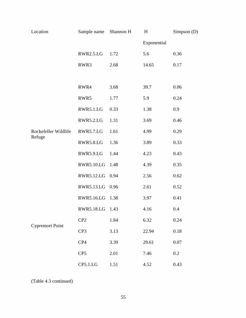
55

Location

Rockefeller Wildlife

Refuge

Sample name Shannon H H

Exponential

Simpson (D)

RWR2.5.LG 1.72 5.6 0.36

RWR3 2.68 14.65 0.17

RWR4 3.68 39.7 0.06

RWR5 1.77 5.9 0.24

RWR5.1.LG 0.33 1.38 0.9

RWR5.2.LG 1.31 3.69 0.46

RWR5.7.LG 1.61 4.99 0.29

RWR5.8.LG 1.36 3.89 0.33

RWR5.9.LG 1.44 4.23 0.43

RWR5.10.LG 1.48 4.39 0.35

RWR5.12.LG 0.94 2.56 0.62

RWR5.13.LG 0.96 2.61 0.52

RWR5.16.LG 1.38 3.97 0.41

RWR5.18.LG 1.43 4.16 0.4

Cypremort Point

(Table 4.3 continued)

CP2 1.84 6.32 0.24

CP3 3.13 22.94 0.18

CP4 3.39 29.61 0.07

CP5 2.01 7.46 0.2

CP5.1.LG 1.51 4.52 0.43

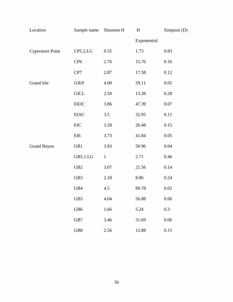
56

Location

Cypremort Point

Sample name Shannon H H

Exponential

Simpson (D)

CP5.2.LG 0.55 1.73 0.83

CP6 2.76 15.76 0.16

CP7 2.87 17.58 0.12

Grand Isle GIEP 4.08 59.11 0.05

GICL 2.59 13.38 0.28

EIOC 3.86 47.39 0.07

EIAC 3.5 32.95 0.11

EIC 3.28 26.48 0.15

EI6 3.73 41.84 0.05

Grand Bayou

GB1 3.93 50.96 0.04

GB5.1.LG 1 2.71 0.46

GB2 3.07 21.56 0.14

GB3 2.18 8.86 0.24

GB4 4.5 89.78 0.02

GB5 4.04 56.88 0.06

GB6 1.66 5.24 0.3

GB7 3.46 31.69 0.06

GB8 2.56 12.88 0.15

57

4.7 Diet of the top invertebrate predator (tabanid larvae) in Louisiana marsh soil

Relative abundance of the larval gut OTUs after applying the 0.05% cutoff was computed in

QIIME as described previously (Section 1.6 of Materials and Methods) generating bar charts at 5

taxonomic levels including “Phylum”, “Class”, “Order”, “Family”, “Genera”. The SILVA

database that was used to assign OTUs in this study organizes organisms to taxonomical

categories that are not always congruent with the classical biological taxonomy and, therefore,

used with quotation marks.

For example, Insecta is considered as a Class in classical taxonomy but in the SILVA taxonomy

it is considered as a “Genus”. Hence, the bar graphs (Figure.4.2, Figure 4.3, Figure 4.4, Figure

4.5, and Figure 4.6) below were computed based on the relative abundance of taxa at consecutive

levels of classification in SILVA, i.e. Figure.4.2 was computed on the “Phyla” and Figure 4.6 on

the “Genera” level of taxonomy.

Metagenomic sequencing using primers amplifying a portion of the 18S rRNA gene covered the

eukaryotic diversity (Kingdom Eukaryota) in the larval guts. Super group Opisthokonta (ranging

from 24.2% in RWR5.8.LG to 99.4% in GB5.1.LG) had the highest relative abundance in the

larval guts (overall 91%, Figure 4.2).

Opisthokonta are a super group within the Kingdom Eukaryota comprising a broad group of

eukaryotes including eukaryotic microorganisms, fungi and metazoa. Super group SAR

(Stramenopiles-Alveolates-Rhizaria) was the second most abundant group with an overall

abundance of 7.3% in the larval guts.

SAR is a metagroup within Kingdom Eukaryota covering all photosynthetic eukaryotes. SAR

was found in higher abundance in four larvae at Rockefeller Wildlife Refuge site 2 [RWR2.3.LG

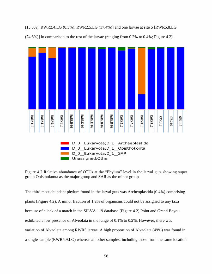
58

(13.8%), RWR2.4.LG (8.3%), RWR2.5.LG (17.4%)] and one larvae at site 5 [RWR5.8.LG

(74.6%)] in comparison to the rest of the larvae (ranging from 0.2% to 0.4%; Figure 4.2).

Figure 4.2 Relative abundance of OTUs at the “Phylum” level in the larval guts showing super

group Opisthokonta as the major group and SAR as the minor group

The third most abundant phylum found in the larval guts was Archeoplastida (0.4%) comprising

plants (Figure 4.2). A minor fraction of 1.2% of organisms could not be assigned to any taxa

because of a lack of a match in the SILVA 119 database (Figure 4.2) Point and Grand Bayou

exhibited a low presence of Alveolata in the range of 0.1% to 0.2%. However, there was

variation of Alveolata among RWR5 larvae. A high proportion of Alveolata (49%) was found in

a single sample (RWR5.9.LG) whereas all other samples, including those from the same location

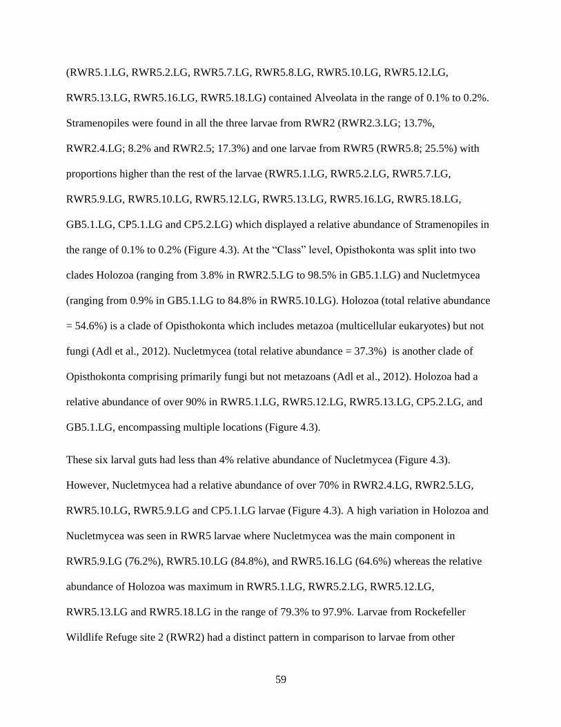
59

(RWR5.1.LG, RWR5.2.LG, RWR5.7.LG, RWR5.8.LG, RWR5.10.LG, RWR5.12.LG,

RWR5.13.LG, RWR5.16.LG, RWR5.18.LG) contained Alveolata in the range of 0.1% to 0.2%.

Stramenopiles were found in all the three larvae from RWR2 (RWR2.3.LG; 13.7%,

RWR2.4.LG; 8.2% and RWR2.5; 17.3%) and one larvae from RWR5 (RWR5.8; 25.5%) with

proportions higher than the rest of the larvae (RWR5.1.LG, RWR5.2.LG, RWR5.7.LG,

RWR5.9.LG, RWR5.10.LG, RWR5.12.LG, RWR5.13.LG, RWR5.16.LG, RWR5.18.LG,

GB5.1.LG, CP5.1.LG and CP5.2.LG) which displayed a relative abundance of Stramenopiles in

the range of 0.1% to 0.2% (Figure 4.3). At the “Class” level, Opisthokonta was split into two

clades Holozoa (ranging from 3.8% in RWR2.5.LG to 98.5% in GB5.1.LG) and Nucletmycea

(ranging from 0.9% in GB5.1.LG to 84.8% in RWR5.10.LG). Holozoa (total relative abundance

= 54.6%) is a clade of Opisthokonta which includes metazoa (multicellular eukaryotes) but not

fungi (Adl et al., 2012). Nucletmycea (total relative abundance = 37.3%) is another clade of

Opisthokonta comprising primarily fungi but not metazoans (Adl et al., 2012). Holozoa had a

relative abundance of over 90% in RWR5.1.LG, RWR5.12.LG, RWR5.13.LG, CP5.2.LG, and

GB5.1.LG, encompassing multiple locations (Figure 4.3).

These six larval guts had less than 4% relative abundance of Nucletmycea (Figure 4.3).

However, Nucletmycea had a relative abundance of over 70% in RWR2.4.LG, RWR2.5.LG,

RWR5.10.LG, RWR5.9.LG and CP5.1.LG larvae (Figure 4.3). A high variation in Holozoa and

Nucletmycea was seen in RWR5 larvae where Nucletmycea was the main component in

RWR5.9.LG (76.2%), RWR5.10.LG (84.8%), and RWR5.16.LG (64.6%) whereas the relative

abundance of Holozoa was maximum in RWR5.1.LG, RWR5.2.LG, RWR5.12.LG,

RWR5.13.LG and RWR5.18.LG in the range of 79.3% to 97.9%. Larvae from Rockefeller

Wildlife Refuge site 2 (RWR2) had a distinct pattern in comparison to larvae from other

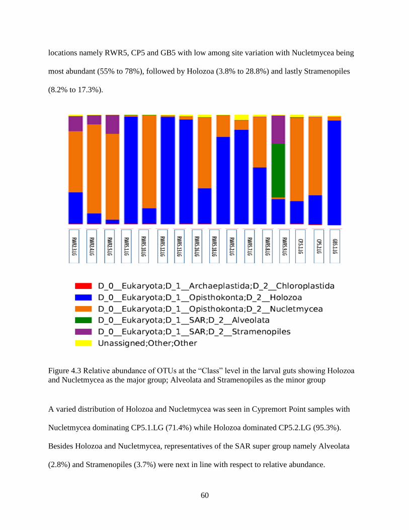
60

locations namely RWR5, CP5 and GB5 with low among site variation with Nucletmycea being

most abundant (55% to 78%), followed by Holozoa (3.8% to 28.8%) and lastly Stramenopiles

(8.2% to 17.3%).

Figure 4.3 Relative abundance of OTUs at the “Class” level in the larval guts showing Holozoa

and Nucletmycea as the major group; Alveolata and Stramenopiles as the minor group

A varied distribution of Holozoa and Nucletmycea was seen in Cypremort Point samples with

Nucletmycea dominating CP5.1.LG (71.4%) while Holozoa dominated CP5.2.LG (95.3%).

Besides Holozoa and Nucletmycea, representatives of the SAR super group namely Alveolata

(2.8%) and Stramenopiles (3.7%) were next in line with respect to relative abundance.

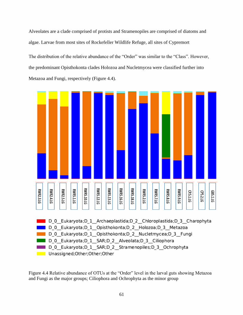
61

Alveolates are a clade comprised of protists and Stramenopiles are comprised of diatoms and

algae. Larvae from most sites of Rockefeller Wildlife Refuge, all sites of Cypremort

The distribution of the relative abundance of the “Order” was similar to the “Class”. However,

the predominant Opisthokonta clades Holozoa and Nucletmycea were classified further into

Metazoa and Fungi, respectively (Figure 4.4).

Figure 4.4 Relative abundance of OTUs at the “Order” level in the larval guts showing Metazoa

and Fungi as the major groups; Ciliophora and Ochrophyta as the minor group

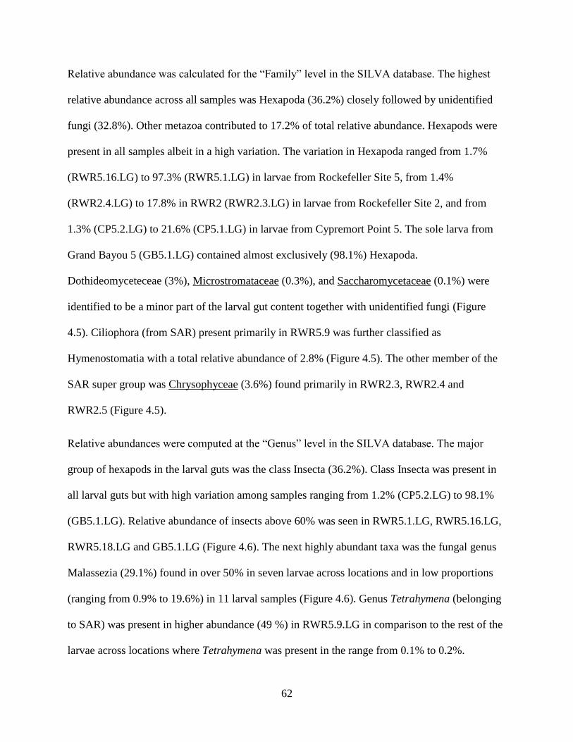
62

Relative abundance was calculated for the “Family” level in the SILVA database. The highest

relative abundance across all samples was Hexapoda (36.2%) closely followed by unidentified

fungi (32.8%). Other metazoa contributed to 17.2% of total relative abundance. Hexapods were

present in all samples albeit in a high variation. The variation in Hexapoda ranged from 1.7%

(RWR5.16.LG) to 97.3% (RWR5.1.LG) in larvae from Rockefeller Site 5, from 1.4%

(RWR2.4.LG) to 17.8% in RWR2 (RWR2.3.LG) in larvae from Rockefeller Site 2, and from

1.3% (CP5.2.LG) to 21.6% (CP5.1.LG) in larvae from Cypremort Point 5. The sole larva from

Grand Bayou 5 (GB5.1.LG) contained almost exclusively (98.1%) Hexapoda.

Dothideomyceteceae (3%), Microstromataceae (0.3%), and Saccharomycetaceae (0.1%) were

identified to be a minor part of the larval gut content together with unidentified fungi (Figure

4.5). Ciliophora (from SAR) present primarily in RWR5.9 was further classified as

Hymenostomatia with a total relative abundance of 2.8% (Figure 4.5). The other member of the

SAR super group was Chrysophyceae (3.6%) found primarily in RWR2.3, RWR2.4 and

RWR2.5 (Figure 4.5).

Relative abundances were computed at the “Genus” level in the SILVA database. The major

group of hexapods in the larval guts was the class Insecta (36.2%). Class Insecta was present in

all larval guts but with high variation among samples ranging from 1.2% (CP5.2.LG) to 98.1%

(GB5.1.LG). Relative abundance of insects above 60% was seen in RWR5.1.LG, RWR5.16.LG,

RWR5.18.LG and GB5.1.LG (Figure 4.6). The next highly abundant taxa was the fungal genus

Malassezia (29.1%) found in over 50% in seven larvae across locations and in low proportions

(ranging from 0.9% to 19.6%) in 11 larval samples (Figure 4.6). Genus Tetrahymena (belonging

to SAR) was present in higher abundance (49 %) in RWR5.9.LG in comparison to the rest of the

larvae across locations where Tetrahymena was present in the range from 0.1% to 0.2%.

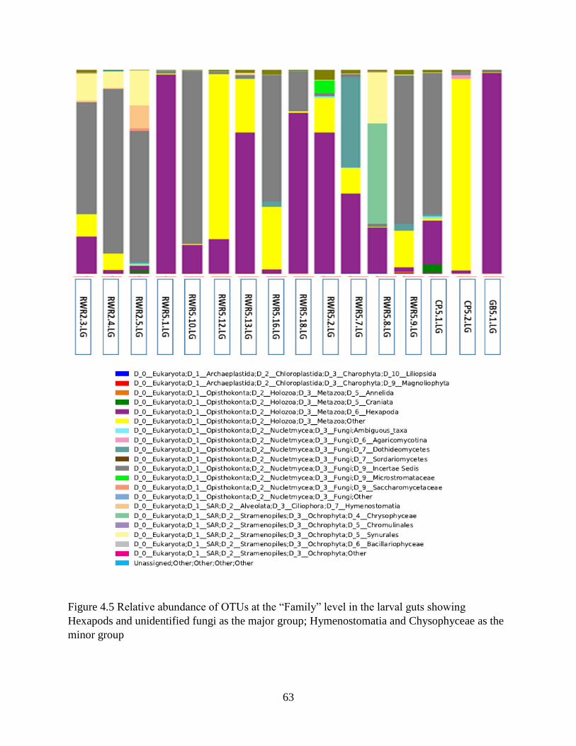
63

Figure 4.5 Relative abundance of OTUs at the “Family” level in the larval guts showing

Hexapods and unidentified fungi as the major group; Hymenostomatia and Chysophyceae as the

minor group

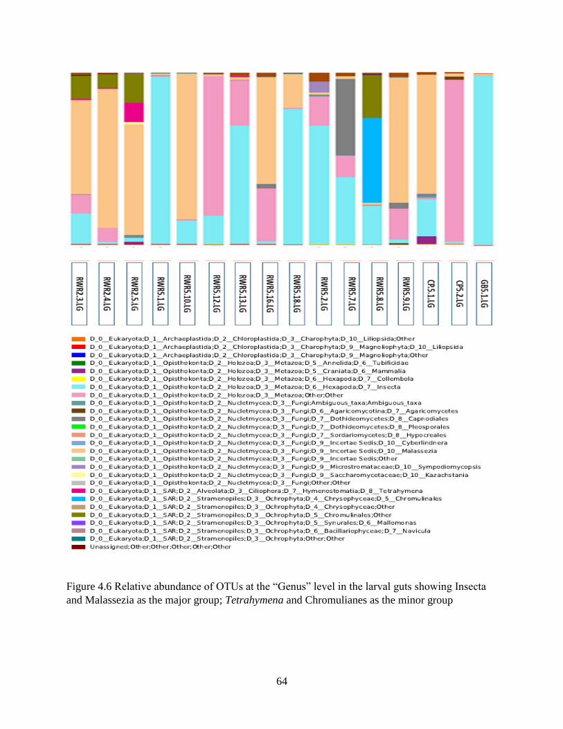
64

Figure 4.6 Relative abundance of OTUs at the “Genus” level in the larval guts showing Insecta

and Malassezia as the major group; Tetrahymena and Chromulianes as the minor group

65

4.8 Identification of insect species in the tabanid larval gut

Insects were a major component of the diet of the tabanid larvae (Results 4.7) with the highest

relative abundance of 36.2% in the larval guts belonging to Class Insecta. The SILVA 119

database identified 52 OTUs from the larval guts in this study as belonging to the Class Insecta

but only 23 were further classified to the species level. The rest of the 29 OTUs were not

classified beyond Insecta in the SILVA 119 database. The top matches for the species identified

by the SILVA 119 database were two mosquito species Aedes aegypti and A. albopictus, the fruit

fly Drosophila sechellia, the horse fly Haematopota pluvialis and the parasitic wasp Leptopilina

heterotoma. The reliability of the species assignment by SILVA was subsequently checked by

manual blasting of the sequences against the NCBI database.

BLAST results showed matches that can be described in various categories. Firstly, high

reliability of assignment (Identity match of 99% to 100% and E-value of zero) was seen for OTU

sequences identified as Drosophila sechellia in SILVA when matched to Drosophila

melanogaster in the NCBI database, confirming the genus. One OTU sequence belonging to H.

pluvialis was identified (100%) as T. nigrovittatus by NCBI. Secondly, A. albopictus and A.

aegypti showed matches to multiple species within the Genus Aedes with a 98% to 100% match

and a zero E-value. Hence, OTU sequences preliminarily identified as A. aegypti and A.

albopictus by SILVA belong to closely related species of the same genus. Thirdly, other H.

pluvialis than the one matching 100% to T. nigrovittatus showed matches to multiple species

with a low identity match (86% to 97%). However, at least three top BLAST hits of each OTU

that belonged to H. pluvialis were within the family Tabanidae. Fourthly, no clear taxonomic

assignment in the NCBI database was provided for the OTU sequences identified as the parasitic

wasp L. heterotoma by SILVA. Top blast hits of the L. heterotoma sequences matched

66

Drosophila melanogaster and the water bug Paravelia bullialata at low identity values (90% to

97%) with E-values below zero. The NCBI database lacks sequences for 18SrRNA gene region

for L. heterotoma. However, Drosophila is a known host of the L. heterotoma and thus the match

was to a similar species or genus of a wasp that infected either the Drosophila melanogaster or

the water bug Paravelia bullialata. The match was not to the same species as the identity values

were low.

Overall, the results indicate that the main dietary components of the tabanid larvae that were

identified to the species level by SILVA belong to the genera Drosophila, Aedes and the Family

Tabanidae. However, the matches are to be viewed with caution for reasons to be discussed in

detail (see Chapter 5. Discussion).

4.9 Variation in tabanid larval diets across locations

Larval diets in Rockefeller Wildlife Refuge, Cypremort Point and Grand Bayou were not

significantly different across larvae due to high variation within locations.

OTU richness (box plots and t-test) from Figure 4.7, OTU composition (indicated by NMDS

and confirmed by PERMANOVA) from Figure 4.8 and relative abundance of OTUs (determined

by LEfSe) from Figure 4.9 was not significantly different among all three locations.

However, the fungus Agaricomycetes (Agaricomytina) was present in significantly higher

proportions in the larvae from Cypremort Point in comparison to larvae from Rockefeller

Wildlife Refuge as indicated by LEfSe.

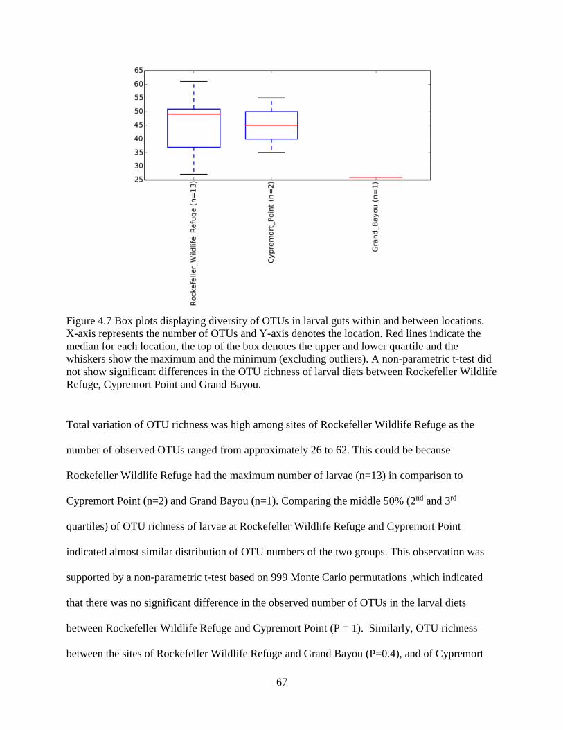
67

Figure 4.7 Box plots displaying diversity of OTUs in larval guts within and between locations.

X-axis represents the number of OTUs and Y-axis denotes the location. Red lines indicate the

median for each location, the top of the box denotes the upper and lower quartile and the

whiskers show the maximum and the minimum (excluding outliers). A non-parametric t-test did

not show significant differences in the OTU richness of larval diets between Rockefeller Wildlife

Refuge, Cypremort Point and Grand Bayou.

Total variation of OTU richness was high among sites of Rockefeller Wildlife Refuge as the

number of observed OTUs ranged from approximately 26 to 62. This could be because

Rockefeller Wildlife Refuge had the maximum number of larvae (n=13) in comparison to

Cypremort Point (n=2) and Grand Bayou (n=1). Comparing the middle 50% (2nd and 3rd

quartiles) of OTU richness of larvae at Rockefeller Wildlife Refuge and Cypremort Point

indicated almost similar distribution of OTU numbers of the two groups. This observation was

supported by a non-parametric t-test based on 999 Monte Carlo permutations ,which indicated

that there was no significant difference in the observed number of OTUs in the larval diets

between Rockefeller Wildlife Refuge and Cypremort Point (P = 1). Similarly, OTU richness

between the sites of Rockefeller Wildlife Refuge and Grand Bayou (P=0.4), and of Cypremort

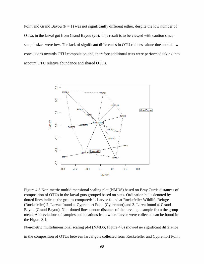
68

Point and Grand Bayou (P = 1) was not significantly different either, despite the low number of

OTUs in the larval gut from Grand Bayou (26). This result is to be viewed with caution since

sample sizes were low. The lack of significant differences in OTU richness alone does not allow

conclusions towards OTU composition and, therefore additional tests were performed taking into

account OTU relative abundance and shared OTUs.

Figure 4.8 Non-metric multidimensional scaling plot (NMDS) based on Bray Curtis distances of

composition of OTUs in the larval guts grouped based on sites. Ordination hulls denoted by

dotted lines indicate the groups compared: 1. Larvae found at Rockefeller Wildlife Refuge

(Rockefeller) 2. Larvae found at Cypremort Point (Cypremort) and 3. Larva found at Grand

Bayou (Grand Bayou). Non-dotted lines denote distance of the larval gut sample from the group

mean. Abbreviations of samples and locations from where larvae were collected can be found in

the Figure 3.1.

Non-metric multidimensional scaling plot (NMDS, Figure 4.8) showed no significant difference

in the composition of OTUs between larval guts collected from Rockefeller and Cypremort Point

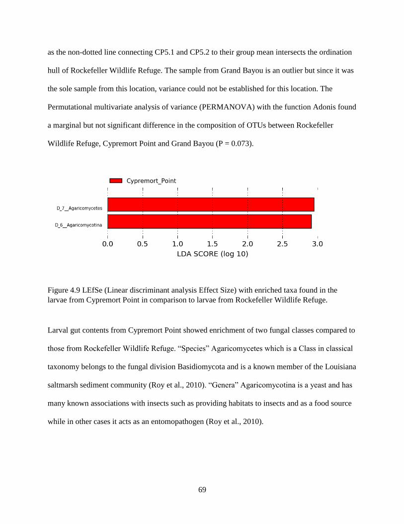
69

as the non-dotted line connecting CP5.1 and CP5.2 to their group mean intersects the ordination

hull of Rockefeller Wildlife Refuge. The sample from Grand Bayou is an outlier but since it was

the sole sample from this location, variance could not be established for this location. The

Permutational multivariate analysis of variance (PERMANOVA) with the function Adonis found

a marginal but not significant difference in the composition of OTUs between Rockefeller

Wildlife Refuge, Cypremort Point and Grand Bayou (P = 0.073).

Figure 4.9 LEfSe (Linear discriminant analysis Effect Size) with enriched taxa found in the

larvae from Cypremort Point in comparison to larvae from Rockefeller Wildlife Refuge.

Larval gut contents from Cypremort Point showed enrichment of two fungal classes compared to

those from Rockefeller Wildlife Refuge. “Species” Agaricomycetes which is a Class in classical

taxonomy belongs to the fungal division Basidiomycota and is a known member of the Louisiana

saltmarsh sediment community (Roy et al., 2010). “Genera” Agaricomycotina is a yeast and has

many known associations with insects such as providing habitats to insects and as a food source

while in other cases it acts as an entomopathogen (Roy et al., 2010).

70

4.10 Comparison of OTU composition in sediments and larvae

A higher number of larvae were found in the West in comparison to the East despite similar

sampling methods and a greater sampling effort in the East. In the West, larvae were always

present where a higher abundance of Hexapoda and fungi was present. However, this trend is not

consistent in the East where a high abundance of Hexapoda and fungi did not guarantee larval

presence. This inconsistent trend in the east could be due to the observed population crashes of

the adult tabanid in the eastern areas. Proportional split of “Phyla” from Figure 4.10, “Classes”

from Figure 4.11 and “Families” from Figure 4.12 was different in the larval guts and their

corresponding sediments.

Locations in the West (Rockefeller Wildlife Refuge and Cypremort Point) had a high number of

larvae (18) but only at 1/3 of the sites. Larval gut content of the three larvae collected from CP2

was not included in next-generation sequencing analysis because the pilot study (see 4.2) showed

the gut content consisting 100% of T. nigrovittatus DNA. Nevertheless, the larvae were counted

as present for this analysis. The four sites in the West where larvae were found (RWR2, RWR5,

CP2 and CP5) had the most Opisthokonta (> 57%) in their respective regions. This suggests a

higher likelihood of finding larvae at sites with high Opisthokonta in the West. Although the

sampling method used in the East and West was the same and more sampling effort was

undertaken (more sites) in the East, only one larva was retrieved from Eastern regions (GB5).

This larva was not found in sediments with particularly high Opisthokonta (only 34%). Even in

sediments (GB3, GB6, GB8 and GICL), which had Opisthokonta percent reads comparable to

the sites in the West where larvae were present (> 67% in comparison to >57% in the West),

Eastern sites were devoid of larvae.

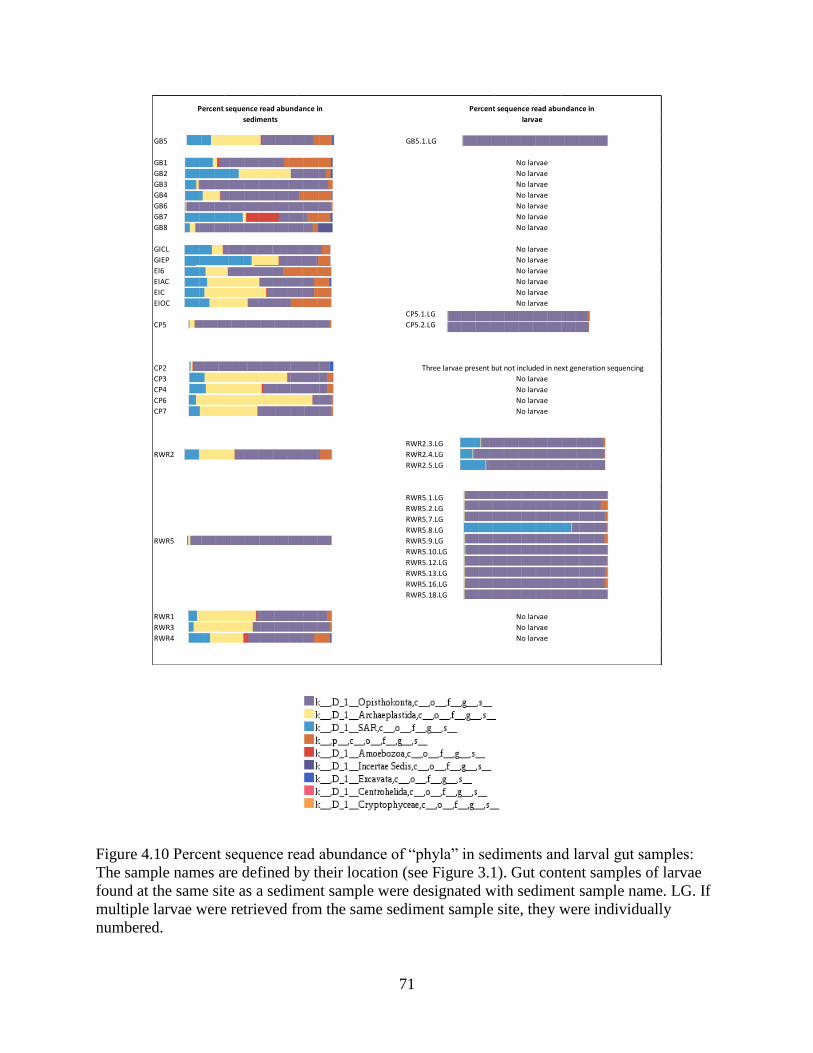
71

Figure 4.10 Percent sequence read abundance of “phyla” in sediments and larval gut samples:

The sample names are defined by their location (see Figure 3.1). Gut content samples of larvae

found at the same site as a sediment sample were designated with sediment sample name. LG. If

multiple larvae were retrieved from the same sediment sample site, they were individually

numbered.

GB5 GB5.1.LG

GB1

GB2

GB3

GB4

GB6

GB7

GB8

GICL

GIEP

EI6

EIAC

EIC

EIOC

CP5.1.LG

CP5 CP5.2.LG

CP2

CP3

CP4

CP6

CP7

RWR2.3.LG

RWR2 RWR2.4.LG

RWR2.5.LG

RWR5.1.LG

RWR5.2.LG

RWR5.7.LG

RWR5.8.LG

RWR5 RWR5.9.LG

RWR5.10.LG

RWR5.12.LG

RWR5.13.LG

RWR5.16.LG

RWR5.18.LG

RWR1

RWR3

RWR4

No larvae

No larvae

No larvae

Three larvae present but not included in next generation sequencing

No larvae

No larvae

No larvae

No larvae

No larvae

No larvae

No larvae

No larvae

No larvae

No larvae

No larvae

No larvae

No larvae

No larvae

No larvae

No larvae

Percent sequence read abundance in

sediments

Percent sequence read abundance in

larvae

No larvae

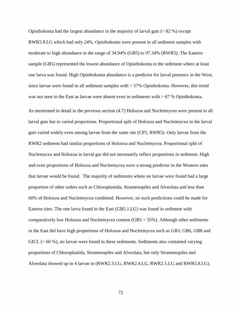
72

Opisthokonta had the largest abundance in the majority of larval guts (> 82 %) except

RWR5.8.LG which had only 24%. Opisthokonta were present in all sediment samples with

moderate to high abundance in the range of 34.94% (GB5) to 97.34% (RWR5). The Eastern

sample (GB5) represented the lowest abundance of Opisthokonta in the sediment where at least

one larva was found. High Opisthokonta abundance is a predictor for larval presence in the West,

since larvae were found in all sediment samples with > 57% Opisthokonta. However, this trend

was not seen in the East as larvae were absent even in sediments with > 67 % Opisthokonta.

As mentioned in detail in the previous section (4.7) Holozoa and Nucletmycea were present in all

larval guts but in varied proportions. Proportional split of Holozoa and Nucletmycea in the larval

guts varied widely even among larvae from the same site (CP5, RWR5). Only larvae from the

RWR2 sediment had similar proportions of Holozoa and Nucletmycea. Proportional split of

Nuclemycea and Holozoa in larval gut did not necessarily reflect proportions in sediment. High

and even proportions of Holozoa and Nucletmycea were a strong predictor in the Western sites

that larvae would be found. The majority of sediments where no larvae were found had a large

proportion of other orders such as Chloroplastida, Stramenopiles and Alveolata and less than

60% of Holozoa and Nucletmycea combined. However, no such predictions could be made for

Eastern sites. The one larva found in the East (GB5.1.LG) was found in sediment with

comparatively low Holozoa and Nucletmycea content (GB5 = 35%). Although other sediments

in the East did have high proportions of Holozoa and Nucletmycea such as GB3, GB6, GB8 and

GICL (> 60 %), no larvae were found in these sediments. Sediments also contained varying

proportions of Chloroplastida, Stramenopiles and Alveolata, but only Stramenopiles and

Alveolata showed up in 4 larvae in (RWR2.3.LG, RWR2.4.LG, RWR2.5.LG and RWR5.8.LG).

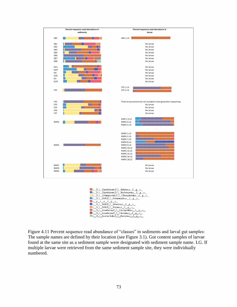
73

Figure 4.11 Percent sequence read abundance of “classes” in sediments and larval gut samples:

The sample names are defined by their location (see Figure 3.1). Gut content samples of larvae

found at the same site as a sediment sample were designated with sediment sample name. LG. If

multiple larvae were retrieved from the same sediment sample site, they were individually

numbered.

GB5 GB5.1.LG

GB1

GB2

GB3

GB4

GB6

GB7

GB8

GICL

GIEP

EI6

EIAC

EIC

EIOC

CP5.1.LG

CP5 CP5.2.LG

CP2 Three larvae present but not included in next generation sequencing

CP3

CP4

CP6

CP7

RWR 2.3.LG

RWR2 RWR2.4.LG

RWR2.5.LG

RWR5.1.LG

RWR5.2.LG

RWR5.7.LG

RWR5.8.LG

RWR5 RWR5.9.LG

RWR5.10.LG

RWR5.12.LG

RWR5.13.LG

RWR5.16.LG

RWR5.18.LG

RWR1

RWR3

RWR4

No larvae

No larvae

No larvae

No larvae

No larvae

No larvae

No larvae

No larvae

No larvae

No larvae

No larvae

No larvae

No larvae

No larvae

No larvae

No larvae

No larvae

No larvae

Percent sequence read abundance in

sediments

Percent sequence read abundance in

larvae

No larvae

No larvae

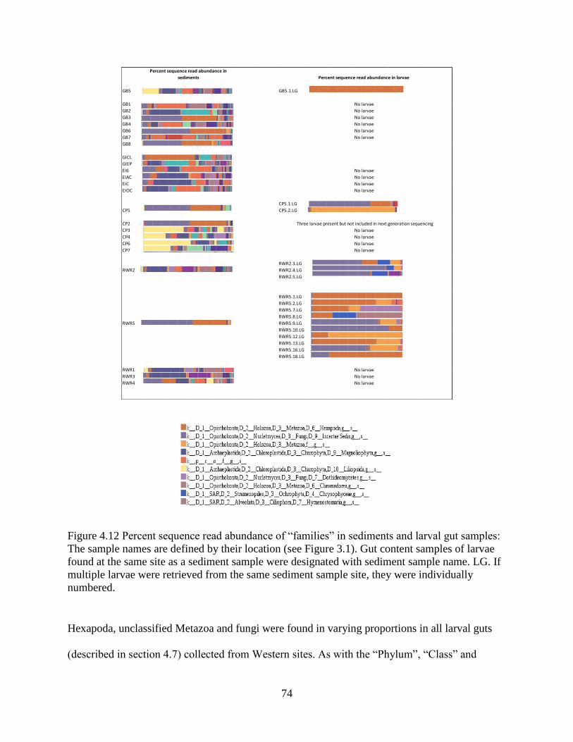
74

Figure 4.12 Percent sequence read abundance of “families” in sediments and larval gut samples:

The sample names are defined by their location (see Figure 3.1). Gut content samples of larvae

found at the same site as a sediment sample were designated with sediment sample name. LG. If

multiple larvae were retrieved from the same sediment sample site, they were individually

numbered.

Hexapoda, unclassified Metazoa and fungi were found in varying proportions in all larval guts

(described in section 4.7) collected from Western sites. As with the “Phylum”, “Class” and

GB5 GB5.1.LG

GB1

GB2

GB3

GB4

GB6

GB7

GB8

GICL

GIEP

EI6

EIAC

EIC

EIOC

CP5.1.LG

CP5 CP5.2.LG

CP2

CP3

CP4

CP6

CP7

RWR2.3.LG

RWR2 RWR2.4.LG

RWR2.5.LG

RWR5.1.LG

RWR5.2.LG

RWR5.7.LG

RWR5.8.LG

RWR5 RWR5.9.LG

RWR5.10.LG

RWR5.12.LG

RWR5.13.LG

RWR5.16.LG

RWR5.18.LG

RWR1

RWR3

RWR4

Percent sequence read abundance in larvae

Percent sequence read abundance in

sediments

No larvae

No larvae

No larvae

No larvae

No larvae

No larvae

No larvae

No larvae

No larvae

No larvae

No larvae

No larvae

No larvae

No larvae

No larvae

No larvae

No larvae

Three larvae present but not included in next generation sequencing

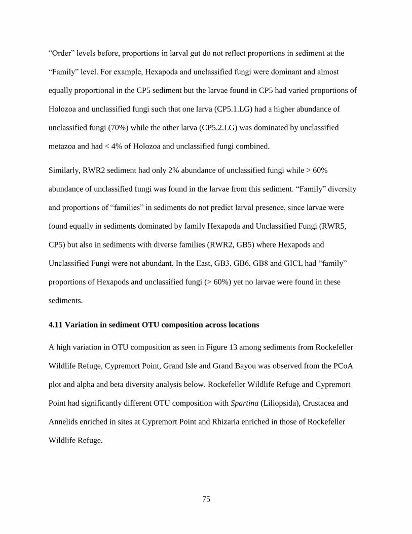
75

“Order” levels before, proportions in larval gut do not reflect proportions in sediment at the

“Family” level. For example, Hexapoda and unclassified fungi were dominant and almost

equally proportional in the CP5 sediment but the larvae found in CP5 had varied proportions of

Holozoa and unclassified fungi such that one larva (CP5.1.LG) had a higher abundance of

unclassified fungi (70%) while the other larva (CP5.2.LG) was dominated by unclassified

metazoa and had < 4% of Holozoa and unclassified fungi combined.

Similarly, RWR2 sediment had only 2% abundance of unclassified fungi while > 60%

abundance of unclassified fungi was found in the larvae from this sediment. “Family” diversity

and proportions of “families” in sediments do not predict larval presence, since larvae were

found equally in sediments dominated by family Hexapoda and Unclassified Fungi (RWR5,

CP5) but also in sediments with diverse families (RWR2, GB5) where Hexapods and

Unclassified Fungi were not abundant. In the East, GB3, GB6, GB8 and GICL had “family”

proportions of Hexapods and unclassified fungi (> 60%) yet no larvae were found in these

sediments.

4.11 Variation in sediment OTU composition across locations

A high variation in OTU composition as seen in Figure 13 among sediments from Rockefeller

Wildlife Refuge, Cypremort Point, Grand Isle and Grand Bayou was observed from the PCoA

plot and alpha and beta diversity analysis below. Rockefeller Wildlife Refuge and Cypremort

Point had significantly different OTU composition with Spartina (Liliopsida), Crustacea and

Annelids enriched in sites at Cypremort Point and Rhizaria enriched in those of Rockefeller

Wildlife Refuge.

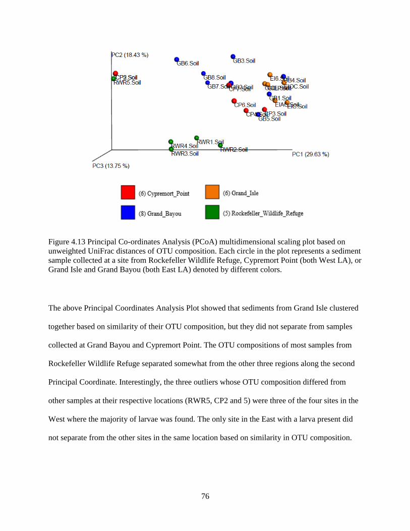
76

Figure 4.13 Principal Co-ordinates Analysis (PCoA) multidimensional scaling plot based on

unweighted UniFrac distances of OTU composition. Each circle in the plot represents a sediment

sample collected at a site from Rockefeller Wildlife Refuge, Cypremort Point (both West LA), or

Grand Isle and Grand Bayou (both East LA) denoted by different colors.

The above Principal Coordinates Analysis Plot showed that sediments from Grand Isle clustered

together based on similarity of their OTU composition, but they did not separate from samples

collected at Grand Bayou and Cypremort Point. The OTU compositions of most samples from

Rockefeller Wildlife Refuge separated somewhat from the other three regions along the second

Principal Coordinate. Interestingly, the three outliers whose OTU composition differed from

other samples at their respective locations (RWR5, CP2 and 5) were three of the four sites in the

West where the majority of larvae was found. The only site in the East with a larva present did

not separate from the other sites in the same location based on similarity in OTU composition.

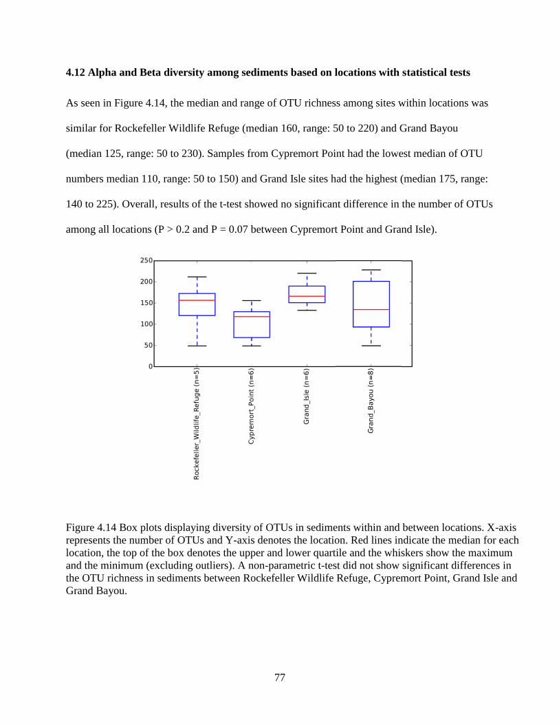
77

4.12 Alpha and Beta diversity among sediments based on locations with statistical tests

As seen in Figure 4.14, the median and range of OTU richness among sites within locations was

similar for Rockefeller Wildlife Refuge (median 160, range: 50 to 220) and Grand Bayou

(median 125, range: 50 to 230). Samples from Cypremort Point had the lowest median of OTU

numbers median 110, range: 50 to 150) and Grand Isle sites had the highest (median 175, range:

140 to 225). Overall, results of the t-test showed no significant difference in the number of OTUs

among all locations (P > 0.2 and P = 0.07 between Cypremort Point and Grand Isle).

Figure 4.14 Box plots displaying diversity of OTUs in sediments within and between locations. X-axis

represents the number of OTUs and Y-axis denotes the location. Red lines indicate the median for each

location, the top of the box denotes the upper and lower quartile and the whiskers show the maximum

and the minimum (excluding outliers). A non-parametric t-test did not show significant differences in

the OTU richness in sediments between Rockefeller Wildlife Refuge, Cypremort Point, Grand Isle and

Grand Bayou.

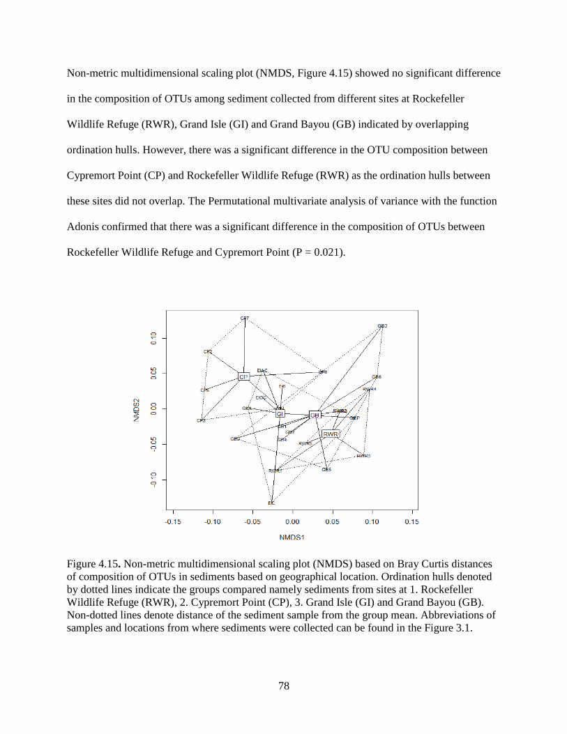
78

Non-metric multidimensional scaling plot (NMDS, Figure 4.15) showed no significant difference

in the composition of OTUs among sediment collected from different sites at Rockefeller

Wildlife Refuge (RWR), Grand Isle (GI) and Grand Bayou (GB) indicated by overlapping

ordination hulls. However, there was a significant difference in the OTU composition between

Cypremort Point (CP) and Rockefeller Wildlife Refuge (RWR) as the ordination hulls between

these sites did not overlap. The Permutational multivariate analysis of variance with the function

Adonis confirmed that there was a significant difference in the composition of OTUs between

Rockefeller Wildlife Refuge and Cypremort Point (P = 0.021).

Figure 4.15. Non-metric multidimensional scaling plot (NMDS) based on Bray Curtis distances

of composition of OTUs in sediments based on geographical location. Ordination hulls denoted

by dotted lines indicate the groups compared namely sediments from sites at 1. Rockefeller

Wildlife Refuge (RWR), 2. Cypremort Point (CP), 3. Grand Isle (GI) and Grand Bayou (GB).

Non-dotted lines denote distance of the sediment sample from the group mean. Abbreviations of

samples and locations from where sediments were collected can be found in the Figure 3.1.

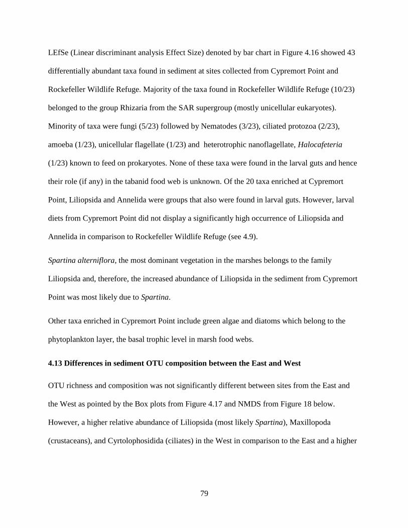
79

LEfSe (Linear discriminant analysis Effect Size) denoted by bar chart in Figure 4.16 showed 43

differentially abundant taxa found in sediment at sites collected from Cypremort Point and

Rockefeller Wildlife Refuge. Majority of the taxa found in Rockefeller Wildlife Refuge (10/23)

belonged to the group Rhizaria from the SAR supergroup (mostly unicellular eukaryotes).

Minority of taxa were fungi (5/23) followed by Nematodes (3/23), ciliated protozoa (2/23),

amoeba (1/23), unicellular flagellate (1/23) and heterotrophic nanoflagellate, Halocafeteria

(1/23) known to feed on prokaryotes. None of these taxa were found in the larval guts and hence

their role (if any) in the tabanid food web is unknown. Of the 20 taxa enriched at Cypremort

Point, Liliopsida and Annelida were groups that also were found in larval guts. However, larval

diets from Cypremort Point did not display a significantly high occurrence of Liliopsida and

Annelida in comparison to Rockefeller Wildlife Refuge (see 4.9).

Spartina alterniflora, the most dominant vegetation in the marshes belongs to the family

Liliopsida and, therefore, the increased abundance of Liliopsida in the sediment from Cypremort

Point was most likely due to Spartina.

Other taxa enriched in Cypremort Point include green algae and diatoms which belong to the

phytoplankton layer, the basal trophic level in marsh food webs.

4.13 Differences in sediment OTU composition between the East and West

OTU richness and composition was not significantly different between sites from the East and

the West as pointed by the Box plots from Figure 4.17 and NMDS from Figure 18 below.

However, a higher relative abundance of Liliopsida (most likely Spartina), Maxillopoda

(crustaceans), and Cyrtolophosidida (ciliates) in the West in comparison to the East and a higher

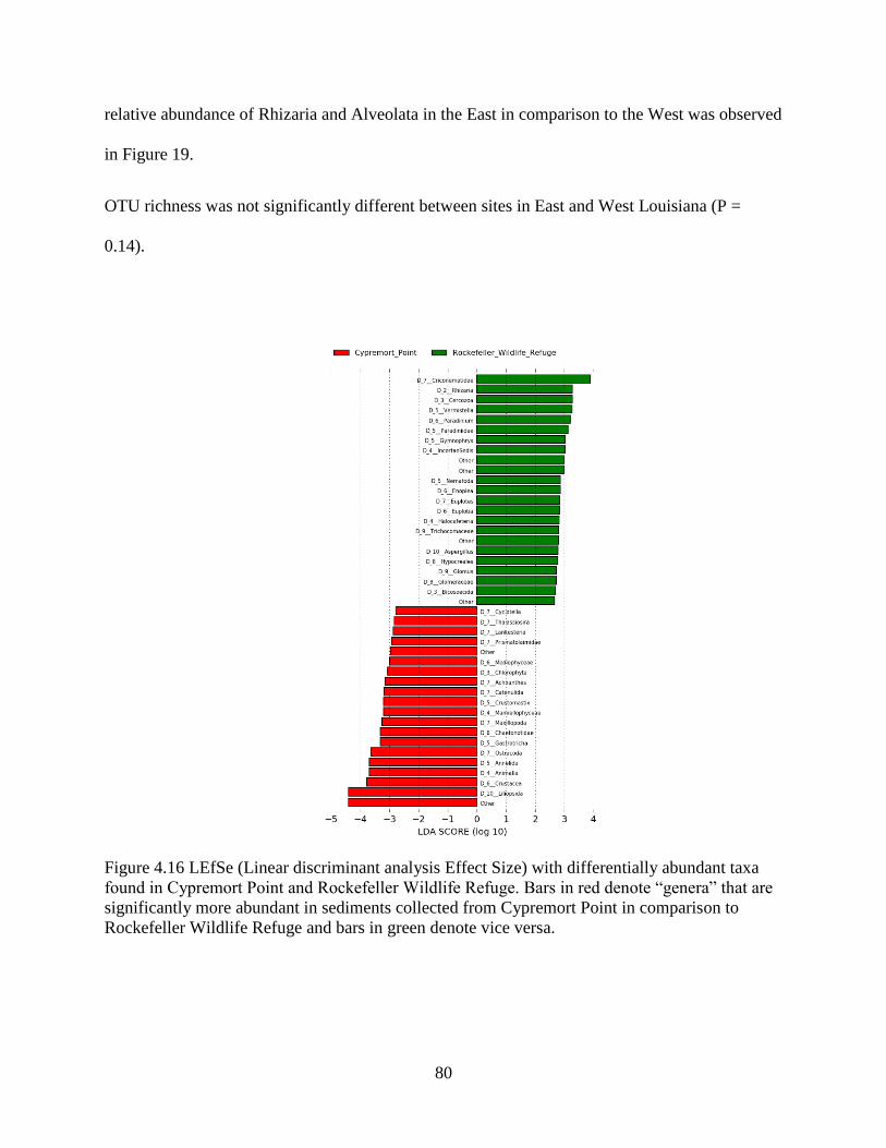
80

relative abundance of Rhizaria and Alveolata in the East in comparison to the West was observed

in Figure 19.

OTU richness was not significantly different between sites in East and West Louisiana (P =

0.14).

Figure 4.16 LEfSe (Linear discriminant analysis Effect Size) with differentially abundant taxa

found in Cypremort Point and Rockefeller Wildlife Refuge. Bars in red denote “genera” that are

significantly more abundant in sediments collected from Cypremort Point in comparison to

Rockefeller Wildlife Refuge and bars in green denote vice versa.

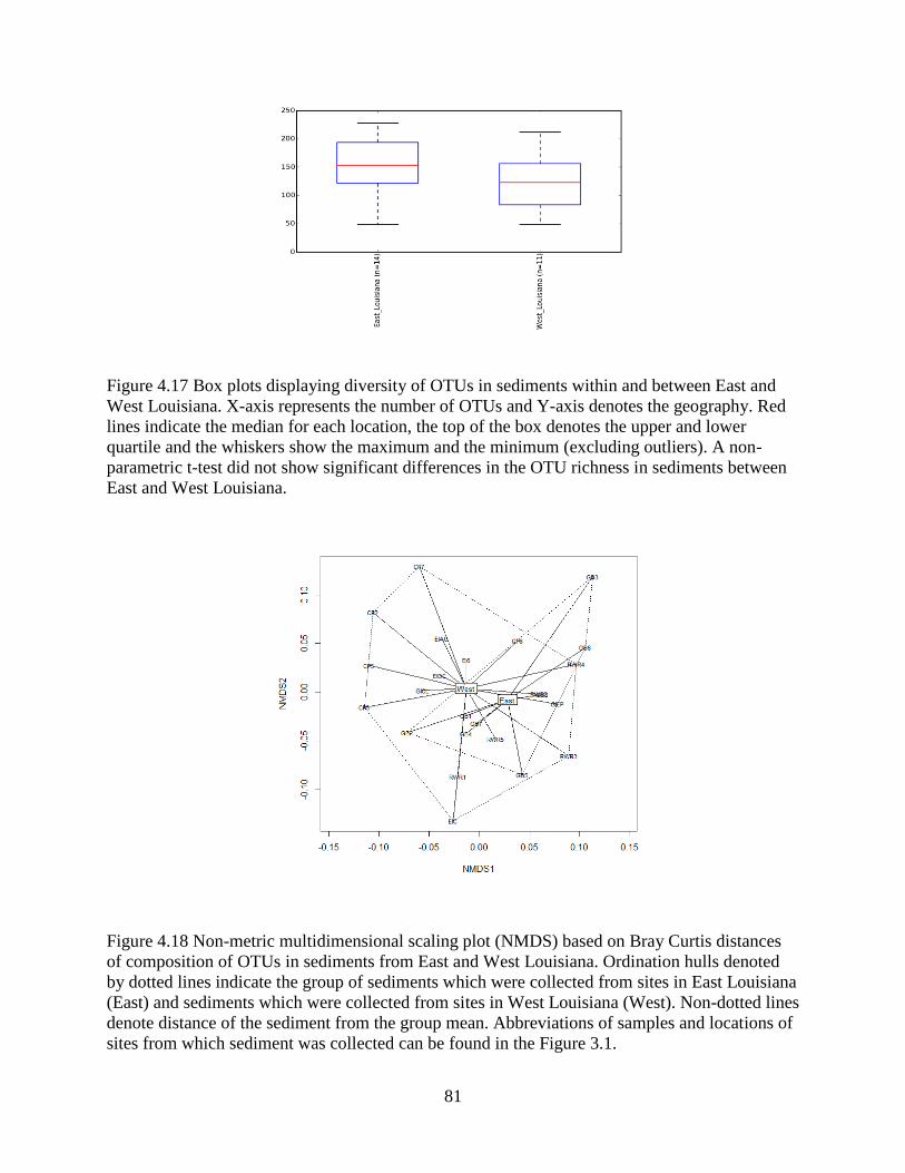
81

Figure 4.17 Box plots displaying diversity of OTUs in sediments within and between East and

West Louisiana. X-axis represents the number of OTUs and Y-axis denotes the geography. Red

lines indicate the median for each location, the top of the box denotes the upper and lower

quartile and the whiskers show the maximum and the minimum (excluding outliers). A non-

parametric t-test did not show significant differences in the OTU richness in sediments between

East and West Louisiana.

Figure 4.18 Non-metric multidimensional scaling plot (NMDS) based on Bray Curtis distances

of composition of OTUs in sediments from East and West Louisiana. Ordination hulls denoted

by dotted lines indicate the group of sediments which were collected from sites in East Louisiana

(East) and sediments which were collected from sites in West Louisiana (West). Non-dotted lines

denote distance of the sediment from the group mean. Abbreviations of samples and locations of

sites from which sediment was collected can be found in the Figure 3.1.

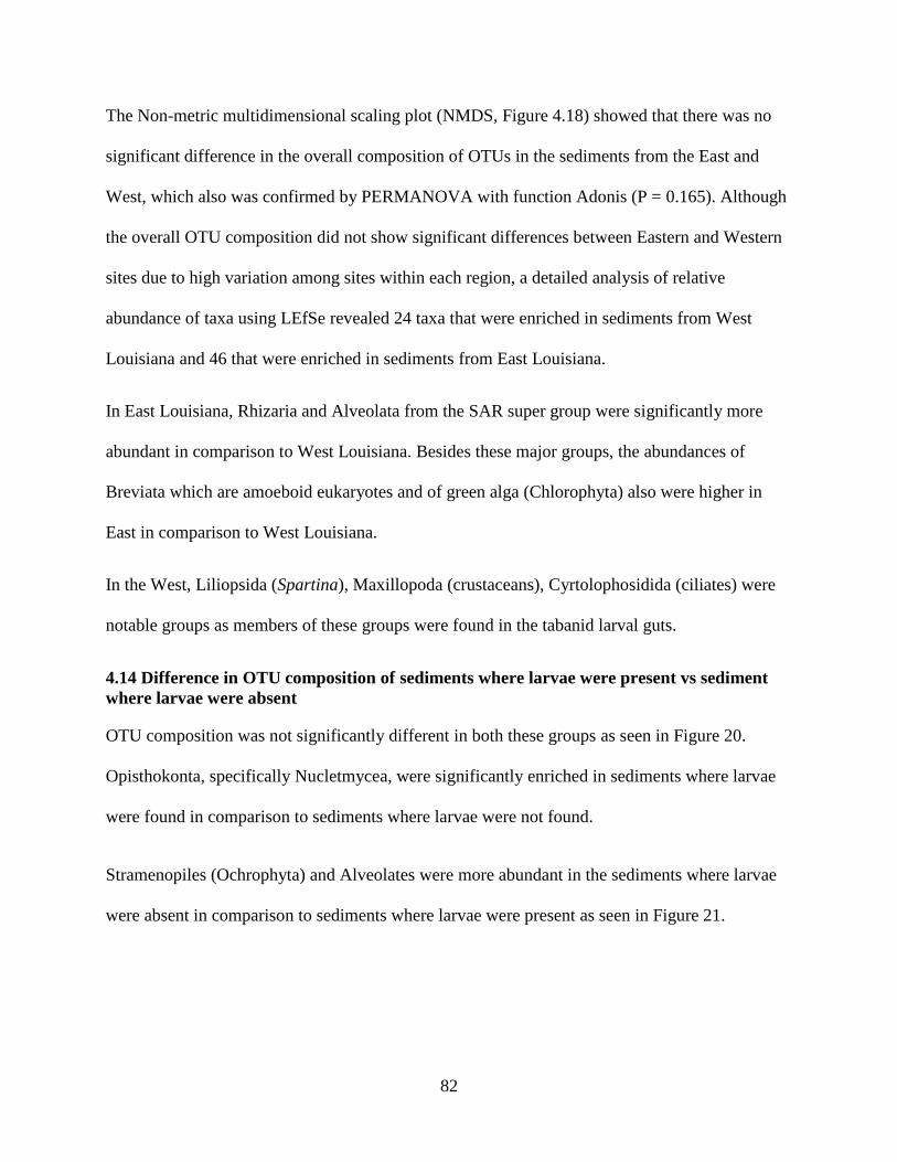
82

The Non-metric multidimensional scaling plot (NMDS, Figure 4.18) showed that there was no

significant difference in the overall composition of OTUs in the sediments from the East and

West, which also was confirmed by PERMANOVA with function Adonis (P = 0.165). Although

the overall OTU composition did not show significant differences between Eastern and Western

sites due to high variation among sites within each region, a detailed analysis of relative

abundance of taxa using LEfSe revealed 24 taxa that were enriched in sediments from West

Louisiana and 46 that were enriched in sediments from East Louisiana.

In East Louisiana, Rhizaria and Alveolata from the SAR super group were significantly more

abundant in comparison to West Louisiana. Besides these major groups, the abundances of

Breviata which are amoeboid eukaryotes and of green alga (Chlorophyta) also were higher in

East in comparison to West Louisiana.

In the West, Liliopsida (Spartina), Maxillopoda (crustaceans), Cyrtolophosidida (ciliates) were

notable groups as members of these groups were found in the tabanid larval guts.

4.14 Difference in OTU composition of sediments where larvae were present vs sediment

where larvae were absent

OTU composition was not significantly different in both these groups as seen in Figure 20.

Opisthokonta, specifically Nucletmycea, were significantly enriched in sediments where larvae

were found in comparison to sediments where larvae were not found.

Stramenopiles (Ochrophyta) and Alveolates were more abundant in the sediments where larvae

were absent in comparison to sediments where larvae were present as seen in Figure 21.

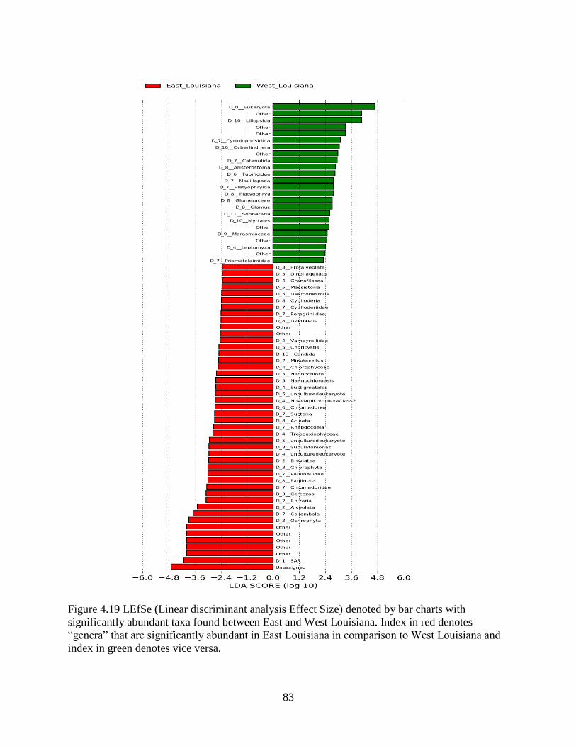
83

Figure 4.19 LEfSe (Linear discriminant analysis Effect Size) denoted by bar charts with

significantly abundant taxa found between East and West Louisiana. Index in red denotes

“genera” that are significantly abundant in East Louisiana in comparison to West Louisiana and

index in green denotes vice versa.

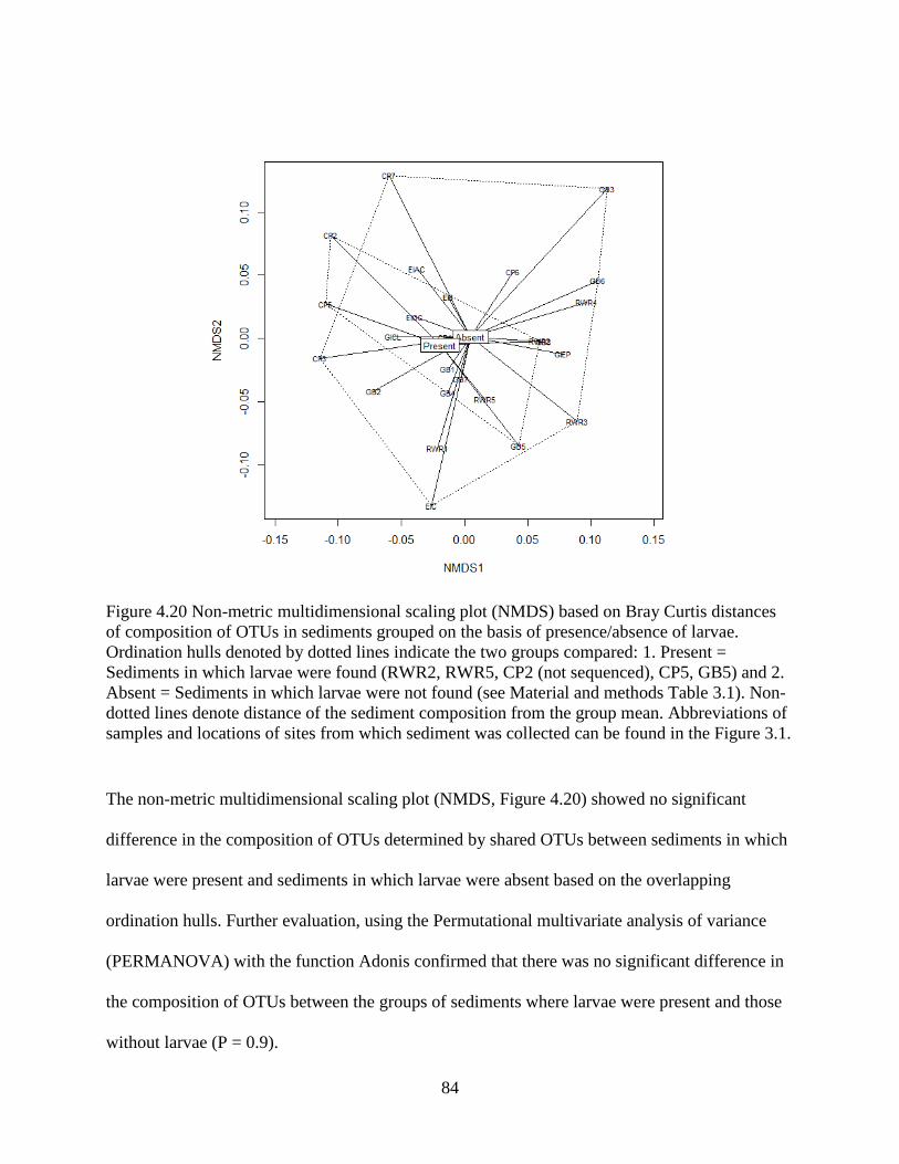
84

Figure 4.20 Non-metric multidimensional scaling plot (NMDS) based on Bray Curtis distances

of composition of OTUs in sediments grouped on the basis of presence/absence of larvae.

Ordination hulls denoted by dotted lines indicate the two groups compared: 1. Present =

Sediments in which larvae were found (RWR2, RWR5, CP2 (not sequenced), CP5, GB5) and 2.

Absent = Sediments in which larvae were not found (see Material and methods Table 3.1). Non-

dotted lines denote distance of the sediment composition from the group mean. Abbreviations of

samples and locations of sites from which sediment was collected can be found in the Figure 3.1.

The non-metric multidimensional scaling plot (NMDS, Figure 4.20) showed no significant

difference in the composition of OTUs determined by shared OTUs between sediments in which

larvae were present and sediments in which larvae were absent based on the overlapping

ordination hulls. Further evaluation, using the Permutational multivariate analysis of variance

(PERMANOVA) with the function Adonis confirmed that there was no significant difference in

the composition of OTUs between the groups of sediments where larvae were present and those

without larvae (P = 0.9).

85

In sediments where larvae were present, Opisthokonta and Nucletmycea, the major branch of

Opisthokonta comprising fungi, were significantly enriched.

This confirms these taxa as predictors for the presence of larvae as previously suggested (see

Results 4.10). The main component in the sediments where larvae were absent was the

Stramenopiles and Alveolates of the SAR supergroup. However, Placididae a non-photosynthetic

eukaryote from the Stramenopiles was significantly abundant in sediments where larvae were

present. Members of both Alveolates and Stramenopiles specifically Ochrophyta were found in

the larval guts. This indicates that these taxa are part of the tabanid food web and are not

detrimental to larval survival.

4.15 Total Polycyclic Aromatic Hydrocarbon (PAH) content in sediments

As seen in Figure 4.22 total Polycyclic Aromatic Hydrocarbon (PAH) content in sediments

showed that GB2 (Total PAHs = 980 ppb) and GB3 (Total PAHs = 1,219 ppb) were above the

baseline of 700 ppb determined by the EPA. This PAH content classifies the sites as minimally

oiled as the baseline for lightly oiled was 6.2 mg/g i.e.6,200,000 ppb (Fleeger et al., 2015), and

for moderately oiled sites was or 70mg/g i.e.70,000,000 ppb (McCann et al., 2017). Oil from our

study sites has the signature of South Louisiana Crude, which points to DWH as the likely origin.

However, since biomarkers change due to degradation, the origin cannot be determined with

absolute certainty. The other sites in East Louisiana had Total Polycyclic Aromatic

Hydrocarbons (PAH) lower than the EPA baseline and were in the range of 5.85 ppb at the site

Elmer’s Isle Air Traffic Control to 447.017 ppb at the site Elmer’s Isle C. Our data also indicates

that the oiling was patchy, which is supported by previous observations (see Chapter 1 Literature

review).

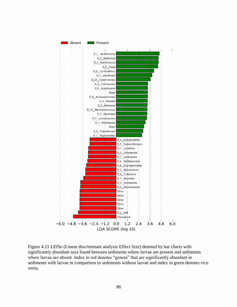
86

Figure 4.21 LEfSe (Linear discriminant analysis Effect Size) denoted by bar charts with

significantly abundant taxa found between sediments where larvae are present and sediments

where larvae are absent. Index in red denotes “genera” that are significantly abundant in

sediments with larvae in comparison to sediments without larvae and index in green denotes vice

versa.

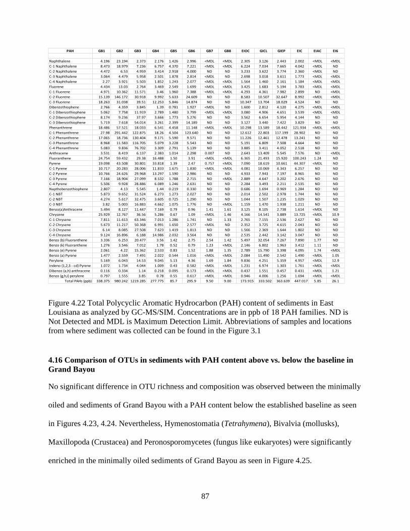
87

Figure 4.22 Total Polycyclic Aromatic Hydrocarbon (PAH) content of sediments in East

Louisiana as analyzed by GC-MS/SIM. Concentrations are in ppb of 18 PAH families. ND is

Not Detected and MDL is Maximum Detection Limit. Abbreviations of samples and locations

from where sediment was collected can be found in the Figure 3.1

4.16 Comparison of OTUs in sediments with PAH content above vs. below the baseline in

Grand Bayou

No significant difference in OTU richness and composition was observed between the minimally

oiled and sediments of Grand Bayou with a PAH content below the established baseline as seen

in Figures 4.23, 4.24. Nevertheless, Hymenostomatia (Tetrahymena), Bivalvia (mollusks),

Maxillopoda (Crustacea) and Peronosporomycetes (fungus like eukaryotes) were significantly

enriched in the minimally oiled sediments of Grand Bayou as seen in Figure 4.25.

PAH GB1 GB2 GB3 GB4 GB5 GB6 GB7 GB8 EIOC GICL GIEP EIC EIAC EI6

Naphthalene 4.196 23.194 2.373 2.176 1.426 2.996 <MDL <MDL 2.305 3.126 2.443 2.002 <MDL <MDL

C-1 Naphthalene 8.473 18.979 7.236 6.757 4.370 7.221 <MDL <MDL 6.224 7.034 7.665 4.042 <MDL ND

C-2 Naphthalene 4.472 6.53 4.959 3.414 2.918 4.000 ND ND 3.233 3.622 3.774 2.360 <MDL ND

C-3 Naphthalene 3.064 4.479 5.958 2.501 1.878 2.814 <MDL ND 2.698 3.018 3.611 1.773 <MDL <MDL

C-4 Naphthalene 2.27 3.921 5.503 1.852 1.243 2.077 <MDL <MDL 1.564 1.460 2.161 1.184 <MDL <MDL

Fluorene 4.434 13.03 2.764 3.469 2.549 1.699 <MDL <MDL 3.425 1.683 5.194 3.783 <MDL <MDL

C-1 Fluorene 4.971 10.362 11.571 3.46 1.960 7.388 <MDL <MDL 4.293 4.361 7.982 2.899 ND <MDL

C-2 Fluorene 15.139 146.172 30.918 9.992 5.633 24.609 ND ND 8.583 10.507 32.647 8.992 <MDL <MDL

C-3 Fluorene 18.263 31.038 39.51 12.253 5.846 14.874 ND ND 10.347 13.704 18.029 4.524 ND ND

Dibenzothiophene 2.766 4.359 3.845 1.39 0.781 1.927 <MDL ND 1.600 2.812 4.120 4.275 <MDL <MDL

C-1 Dibenzothiophene 5.062 7.758 11.919 2.789 1.480 3.799 <MDL <MDL 3.080 4.906 4.651 3.539 <MDL <MDL

C-2 Dibenzothiophene 8.174 9.236 37.97 3.666 1.773 5.276 ND ND 3.562 6.654 5.954 4.144 ND ND

C-3 Dibenzothiophene 5.719 7.618 54.014 3.261 2.399 14.189 ND ND 3.127 3.440 7.422 3.829 ND ND

Phenanthrene 18.486 57.521 18.033 6.541 4.458 11.148 <MDL <MDL 10.298 13.589 18.442 121.934 <MDL <MDL

C-1 Phenanthrene 27.98 291.442 122.875 18.26 4.504 123.640 ND ND 12.612 22.803 117.199 28.902 ND ND

C-2 Phenanthrene 17.065 18.736 130.404 9.171 5.590 9.571 ND ND 11.226 12.461 12.478 13.241 ND ND

C-3 Phenanthrene 8.968 11.583 116.705 5.079 3.228 5.543 ND ND 5.191 6.809 7.508 4.664 ND ND

C-4 Phenanthrene 5.083 9.836 76.702 3.309 2.791 5.139 ND ND 3.885 3.411 4.052 2.518 ND ND

Anthracene 3.531 8.419 6.137 2.383 1.014 2.298 0.007 ND 2.643 13.409 5.545 7.576 ND <MDL

Fluoranthene 24.754 59.432 29.38 16.488 1.50 3.91 <MDL <MDL 6.365 21.493 15.920 100.243 1.24 ND

Pyrene 19.098 43.508 30.801 33.818 1.39 2.47 0.757 <MDL 7.090 18.619 10.661 44.307 <MDL ND

C-1 Pyrene 10.717 20.283 28.006 11.833 1.675 1.830 <MDL <MDL 4.081 10.069 4.343 6.257 ND ND

C-2 Pyrene 10.766 24.626 29.968 13.297 1.590 2.986 ND ND 4.933 7.943 7.197 8.965 ND ND

C-3 Pyrene 7.166 18.904 27.099 8.532 1.788 2.715 ND <MDL 2.889 4.647 3.202 2.676 ND ND

C-4 Pyrene 5.506 9.928 28.886 6.089 1.246 2.631 ND ND 2.284 3.493 2.211 2.535 ND ND

Napthobenzothiophene 2.807 4.13 5.545 1.44 0.219 0.330 ND ND 0.686 1.694 0.969 1.284 ND ND

C-1 NBT 5.873 9.652 31.524 6.273 1.273 2.027 ND ND 2.014 2.502 2.978 1.744 ND ND

C-2 NBT 4.274 5.617 32.475 3.605 0.725 1.290 ND ND 1.044 1.507 1.235 1.029 ND ND

C-3 NBT 3.82 5.003 16.883 4.662 1.075 1.776 ND <MDL 1.159 1.470 1.938 1.211 ND ND

Benzo(a)Anthracene 5.494 8.127 11.447 7.169 0.79 0.96 1.41 1.61 3.125 8.105 2.738 1.614 <MDL ND

Chrysene 25.929 12.767 36.56 5.286 0.67 1.09 <MDL 1.46 4.166 14.541 3.889 13.725 <MDL 10.9

C-1 Chrysene 7.811 11.613 63.346 7.013 1.286 1.741 ND 1.33 2.765 7.155 2.536 2.627 ND ND

C-2 Chrysene 5.673 11.217 50.368 6.991 1.650 2.577 <MDL ND 2.352 3.725 4.615 2.043 ND ND

C-3 Chrysene 6.14 8.085 27.508 7.623 1.419 1.813 ND ND 1.566 2.369 1.644 1.802 ND ND

C-4 Chrysene 9.124 16.896 6.188 14.986 2.032 3.564 ND ND 2.535 2.442 3.142 3.047 ND ND

Benzo (b) Fluoranthene 3.336 6.253 20.477 3.56 1.42 2.75 2.54 1.42 5.497 32.054 7.267 7.890 1.77 ND

Benzo (k) Fluoranthene 1.276 3.546 7.012 1.78 0.52 0.79 1.23 <MDL 2.146 6.802 1.963 3.412 1.11 ND

Benzo (e) Pyrene 2.061 4.22 15.362 2.533 0.83 1.52 1.88 1.35 2.789 15.790 3.398 4.095 1.74 <MDL

Benzo (a) Pyrene 1.477 2.559 7.491 2.022 0.544 1.016 <MDL <MDL 2.084 11.490 2.542 1.490 <MDL 1.05

Perylene 5.169 6.043 14.53 9.045 5.13 4.36 1.69 1.84 9.836 4.251 5.359 4.957 <MDL 12.9

Indeno (1,2,3 - cd) Pyrene 1.072 1.734 4.044 1.009 0.43 0.582 <MDL <MDL 1.231 6.974 1.303 1.761 <MDL <MDL

Dibenzo (a,h) anthracene 0.116 0.334 1.14 0.218 0.095 0.173 <MDL <MDL 0.437 1.551 0.457 0.431 <MDL 1.21

Benzo (g,h,i) perylene 0.797 1.555 3.85 0.78 0.55 0.617 <MDL <MDL 0.946 4.006 1.256 1.694 <MDL <MDL

Total PAHs (ppb) 338.375 980.242 1219.285 277.775 85.7 295.9 9.50 9.00 173.915 333.502 363.639 447.017 5.85 26.1

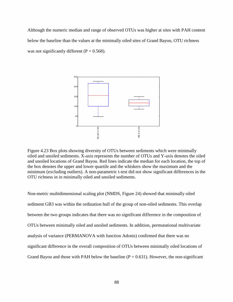
88

Although the numeric median and range of observed OTUs was higher at sites with PAH content

below the baseline than the values at the minimally oiled sites of Grand Bayou, OTU richness

was not significantly different (P = 0.568).

Figure 4.23 Box plots showing diversity of OTUs between sediments which were minimally

oiled and unoiled sediments. X-axis represents the number of OTUs and Y-axis denotes the oiled

and unoiled locations of Grand Bayou. Red lines indicate the median for each location, the top of

the box denotes the upper and lower quartile and the whiskers show the maximum and the

minimum (excluding outliers). A non-parametric t-test did not show significant differences in the

OTU richness in in minimally oiled and unoiled sediments.

Non-metric multidimensional scaling plot (NMDS, Figure 24) showed that minimally oiled

sediment GB3 was within the ordination hull of the group of non-oiled sediments. This overlap

between the two groups indicates that there was no significant difference in the composition of

OTUs between minimally oiled and unoiled sediments. In addition, permutational multivariate

analysis of variance (PERMANOVA with function Adonis) confirmed that there was no

significant difference in the overall composition of OTUs between minimally oiled locations of

Grand Bayou and those with PAH below the baseline (P = 0.631). However, the non-significant

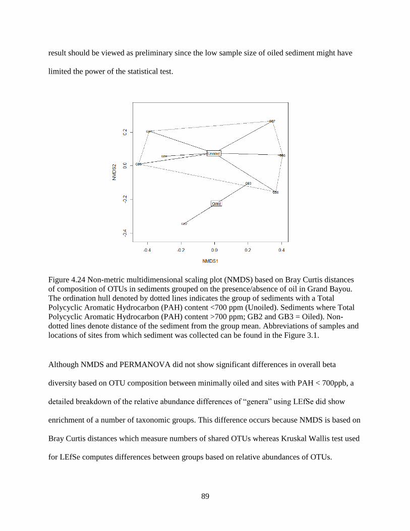
89

result should be viewed as preliminary since the low sample size of oiled sediment might have

limited the power of the statistical test.

Figure 4.24 Non-metric multidimensional scaling plot (NMDS) based on Bray Curtis distances

of composition of OTUs in sediments grouped on the presence/absence of oil in Grand Bayou.

The ordination hull denoted by dotted lines indicates the group of sediments with a Total

Polycyclic Aromatic Hydrocarbon (PAH) content <700 ppm (Unoiled). Sediments where Total

Polycyclic Aromatic Hydrocarbon (PAH) content >700 ppm; GB2 and GB3 = Oiled). Non-

dotted lines denote distance of the sediment from the group mean. Abbreviations of samples and

locations of sites from which sediment was collected can be found in the Figure 3.1.

Although NMDS and PERMANOVA did not show significant differences in overall beta

diversity based on OTU composition between minimally oiled and sites with PAH < 700ppb, a

detailed breakdown of the relative abundance differences of “genera” using LEfSe did show

enrichment of a number of taxonomic groups. This difference occurs because NMDS is based on

Bray Curtis distances which measure numbers of shared OTUs whereas Kruskal Wallis test used

for LEfSe computes differences between groups based on relative abundances of OTUs.

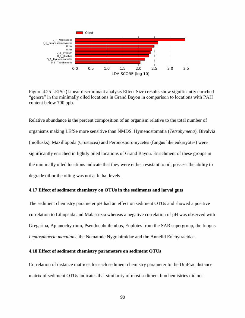
90

Figure 4.25 LEfSe (Linear discriminant analysis Effect Size) results show significantly enriched

“genera” in the minimally oiled locations in Grand Bayou in comparison to locations with PAH

content below 700 ppb.

Relative abundance is the percent composition of an organism relative to the total number of

organisms making LEfSe more sensitive than NMDS. Hymenostomatia (Tetrahymena), Bivalvia

(mollusks), Maxillopoda (Crustacea) and Peronosporomycetes (fungus like eukaryotes) were

significantly enriched in lightly oiled locations of Grand Bayou. Enrichment of these groups in

the minimally oiled locations indicate that they were either resistant to oil, possess the ability to

degrade oil or the oiling was not at lethal levels.

4.17 Effect of sediment chemistry on OTUs in the sediments and larval guts

The sediment chemistry parameter pH had an effect on sediment OTUs and showed a positive

correlation to Liliopsida and Malassezia whereas a negative correlation of pH was observed with

Gregarina, Aplanochytrium, Pseudocohnilembus, Euplotes from the SAR supergroup, the fungus

Leptosphaeria maculans, the Nematode Nygolaimidae and the Annelid Enchytraeidae.

4.18 Effect of sediment chemistry parameters on sediment OTUs

Correlation of distance matrices for each sediment chemistry parameter to the UniFrac distance

matrix of sediment OTUs indicates that similarity of most sediment biochemistries did not

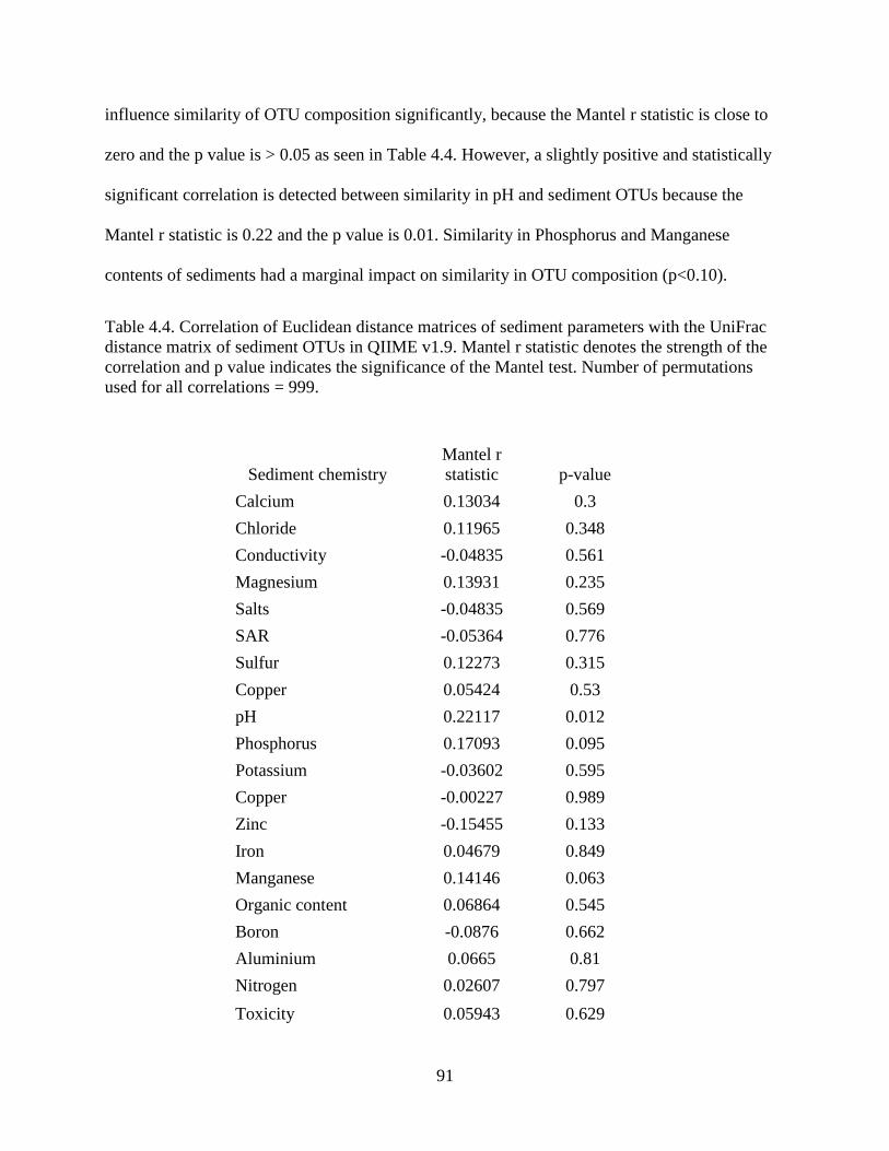
91

influence similarity of OTU composition significantly, because the Mantel r statistic is close to

zero and the p value is > 0.05 as seen in Table 4.4. However, a slightly positive and statistically

significant correlation is detected between similarity in pH and sediment OTUs because the

Mantel r statistic is 0.22 and the p value is 0.01. Similarity in Phosphorus and Manganese

contents of sediments had a marginal impact on similarity in OTU composition (p<0.10).

Table 4.4. Correlation of Euclidean distance matrices of sediment parameters with the UniFrac

distance matrix of sediment OTUs in QIIME v1.9. Mantel r statistic denotes the strength of the

correlation and p value indicates the significance of the Mantel test. Number of permutations

used for all correlations = 999.

Sediment chemistry

Mantel r

statistic p-value

Calcium 0.13034 0.3

Chloride 0.11965 0.348

Conductivity -0.04835 0.561

Magnesium 0.13931 0.235

Salts -0.04835 0.569

SAR -0.05364 0.776

Sulfur 0.12273 0.315

Copper 0.05424 0.53

pH 0.22117 0.012

Phosphorus 0.17093 0.095

Potassium -0.03602 0.595

Copper -0.00227 0.989

Zinc -0.15455 0.133

Iron 0.04679 0.849

Manganese 0.14146 0.063

Organic content 0.06864 0.545

Boron -0.0876 0.662

Aluminium 0.0665 0.81

Nitrogen 0.02607 0.797

Toxicity 0.05943 0.629

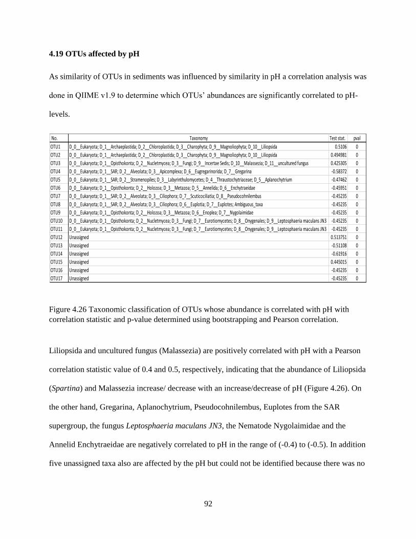
92

4.19 OTUs affected by pH

As similarity of OTUs in sediments was influenced by similarity in pH a correlation analysis was

done in QIIME v1.9 to determine which OTUs’ abundances are significantly correlated to pH-

levels.

Figure 4.26 Taxonomic classification of OTUs whose abundance is correlated with pH with

correlation statistic and p-value determined using bootstrapping and Pearson correlation.

Liliopsida and uncultured fungus (Malassezia) are positively correlated with pH with a Pearson

correlation statistic value of 0.4 and 0.5, respectively, indicating that the abundance of Liliopsida

(Spartina) and Malassezia increase/ decrease with an increase/decrease of pH (Figure 4.26). On

the other hand, Gregarina, Aplanochytrium, Pseudocohnilembus, Euplotes from the SAR

supergroup, the fungus Leptosphaeria maculans JN3, the Nematode Nygolaimidae and the

Annelid Enchytraeidae are negatively correlated to pH in the range of (-0.4) to (-0.5). In addition

five unassigned taxa also are affected by the pH but could not be identified because there was no

No. Taxonomy Test stat. pval

OTU1 D_0__Eukaryota; D_1__Archaeplastida; D_2__Chloroplastida; D_3__Charophyta; D_9__Magnoliophyta; D_10__Liliopsida 0.5106 0

OTU2 D_0__Eukaryota; D_1__Archaeplastida; D_2__Chloroplastida; D_3__Charophyta; D_9__Magnoliophyta; D_10__Liliopsida 0.494981 0

OTU3 D_0__Eukaryota; D_1__Opisthokonta; D_2__Nucletmycea; D_3__Fungi; D_9__Incertae Sedis; D_10__Malassezia; D_11__uncultured fungus 0.425305 0

OTU4 D_0__Eukaryota; D_1__SAR; D_2__Alveolata; D_3__Apicomplexa; D_6__Eugregarinorida; D_7__Gregarina -0.58372 0

OTU5 D_0__Eukaryota; D_1__SAR; D_2__Stramenopiles; D_3__Labyrinthulomycetes; D_4__Thraustochytriaceae; D_5__Aplanochytrium -0.47462 0

OTU6 D_0__Eukaryota; D_1__Opisthokonta; D_2__Holozoa; D_3__Metazoa; D_5__Annelida; D_6__Enchytraeidae -0.45951 0

OTU7 D_0__Eukaryota; D_1__SAR; D_2__Alveolata; D_3__Ciliophora; D_7__Scuticociliatia; D_8__Pseudocohnilembus -0.45235 0

OTU8 D_0__Eukaryota; D_1__SAR; D_2__Alveolata; D_3__Ciliophora; D_6__Euplotia; D_7__Euplotes; Ambiguous_taxa -0.45235 0

OTU9 D_0__Eukaryota; D_1__Opisthokonta; D_2__Holozoa; D_3__Metazoa; D_6__Enoplea; D_7__Nygolaimidae -0.45235 0

OTU10 D_0__Eukaryota; D_1__Opisthokonta; D_2__Nucletmycea; D_3__Fungi; D_7__Eurotiomycetes; D_8__Onygenales; D_9__Leptosphaeria maculans JN3 -0.45235 0

OTU11 D_0__Eukaryota; D_1__Opisthokonta; D_2__Nucletmycea; D_3__Fungi; D_7__Eurotiomycetes; D_8__Onygenales; D_9__Leptosphaeria maculans JN3 -0.45235 0

OTU12 Unassigned 0.513751 0

OTU13 Unassigned -0.51108 0

OTU14 Unassigned -0.61916 0

OTU15 Unassigned 0.445015 0

OTU16 Unassigned -0.45235 0

OTU17 Unassigned -0.45235 0

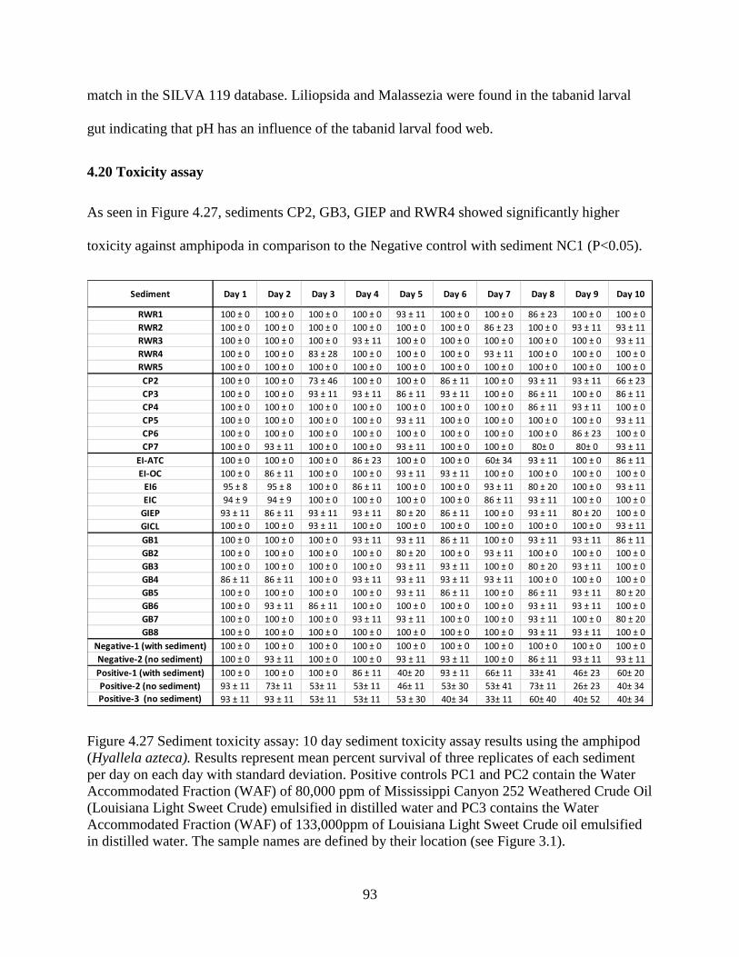
93

match in the SILVA 119 database. Liliopsida and Malassezia were found in the tabanid larval

gut indicating that pH has an influence of the tabanid larval food web.

4.20 Toxicity assay

As seen in Figure 4.27, sediments CP2, GB3, GIEP and RWR4 showed significantly higher

toxicity against amphipoda in comparison to the Negative control with sediment NC1 (P<0.05).

Figure 4.27 Sediment toxicity assay: 10 day sediment toxicity assay results using the amphipod

(Hyallela azteca). Results represent mean percent survival of three replicates of each sediment

per day on each day with standard deviation. Positive controls PC1 and PC2 contain the Water

Accommodated Fraction (WAF) of 80,000 ppm of Mississippi Canyon 252 Weathered Crude Oil

(Louisiana Light Sweet Crude) emulsified in distilled water and PC3 contains the Water

Accommodated Fraction (WAF) of 133,000ppm of Louisiana Light Sweet Crude oil emulsified

in distilled water. The sample names are defined by their location (see Figure 3.1).

Sediment Day 1 Day 2 Day 3 Day 4 Day 5 Day 6 Day 7 Day 8 Day 9 Day 10

RWR1 100 ± 0 100 ± 0 100 ± 0 100 ± 0 93 ± 11 100 ± 0 100 ± 0 86 ± 23 100 ± 0 100 ± 0

RWR2 100 ± 0 100 ± 0 100 ± 0 100 ± 0 100 ± 0 100 ± 0 86 ± 23 100 ± 0 93 ± 11 93 ± 11

RWR3 100 ± 0 100 ± 0 100 ± 0 93 ± 11 100 ± 0 100 ± 0 100 ± 0 100 ± 0 100 ± 0 93 ± 11

RWR4 100 ± 0 100 ± 0 83 ± 28 100 ± 0 100 ± 0 100 ± 0 93 ± 11 100 ± 0 100 ± 0 100 ± 0

RWR5 100 ± 0 100 ± 0 100 ± 0 100 ± 0 100 ± 0 100 ± 0 100 ± 0 100 ± 0 100 ± 0 100 ± 0

CP2 100 ± 0 100 ± 0 73 ± 46 100 ± 0 100 ± 0 86 ± 11 100 ± 0 93 ± 11 93 ± 11 66 ± 23

CP3 100 ± 0 100 ± 0 93 ± 11 93 ± 11 86 ± 11 93 ± 11 100 ± 0 86 ± 11 100 ± 0 86 ± 11

CP4 100 ± 0 100 ± 0 100 ± 0 100 ± 0 100 ± 0 100 ± 0 100 ± 0 86 ± 11 93 ± 11 100 ± 0

CP5 100 ± 0 100 ± 0 100 ± 0 100 ± 0 93 ± 11 100 ± 0 100 ± 0 100 ± 0 100 ± 0 93 ± 11

CP6 100 ± 0 100 ± 0 100 ± 0 100 ± 0 100 ± 0 100 ± 0 100 ± 0 100 ± 0 86 ± 23 100 ± 0

CP7 100 ± 0 93 ± 11 100 ± 0 100 ± 0 93 ± 11 100 ± 0 100 ± 0 80± 0 80± 0 93 ± 11

EI-ATC 100 ± 0 100 ± 0 100 ± 0 86 ± 23 100 ± 0 100 ± 0 60± 34 93 ± 11 100 ± 0 86 ± 11

EI-OC 100 ± 0 86 ± 11 100 ± 0 100 ± 0 93 ± 11 93 ± 11 100 ± 0 100 ± 0 100 ± 0 100 ± 0

EI6 95 ± 8 95 ± 8 100 ± 0 86 ± 11 100 ± 0 100 ± 0 93 ± 11 80 ± 20 100 ± 0 93 ± 11

EIC 94 ± 9 94 ± 9 100 ± 0 100 ± 0 100 ± 0 100 ± 0 86 ± 11 93 ± 11 100 ± 0 100 ± 0

GIEP 93 ± 11 86 ± 11 93 ± 11 93 ± 11 80 ± 20 86 ± 11 100 ± 0 93 ± 11 80 ± 20 100 ± 0

GICL 100 ± 0 100 ± 0 93 ± 11 100 ± 0 100 ± 0 100 ± 0 100 ± 0 100 ± 0 100 ± 0 93 ± 11

GB1 100 ± 0 100 ± 0 100 ± 0 93 ± 11 93 ± 11 86 ± 11 100 ± 0 93 ± 11 93 ± 11 86 ± 11

GB2 100 ± 0 100 ± 0 100 ± 0 100 ± 0 80 ± 20 100 ± 0 93 ± 11 100 ± 0 100 ± 0 100 ± 0

GB3 100 ± 0 100 ± 0 100 ± 0 100 ± 0 93 ± 11 93 ± 11 100 ± 0 80 ± 20 93 ± 11 100 ± 0

GB4 86 ± 11 86 ± 11 100 ± 0 93 ± 11 93 ± 11 93 ± 11 93 ± 11 100 ± 0 100 ± 0 100 ± 0

GB5 100 ± 0 100 ± 0 100 ± 0 100 ± 0 93 ± 11 86 ± 11 100 ± 0 86 ± 11 93 ± 11 80 ± 20

GB6 100 ± 0 93 ± 11 86 ± 11 100 ± 0 100 ± 0 100 ± 0 100 ± 0 93 ± 11 93 ± 11 100 ± 0

GB7 100 ± 0 100 ± 0 100 ± 0 93 ± 11 93 ± 11 100 ± 0 100 ± 0 93 ± 11 100 ± 0 80 ± 20

GB8 100 ± 0 100 ± 0 100 ± 0 100 ± 0 100 ± 0 100 ± 0 100 ± 0 93 ± 11 93 ± 11 100 ± 0

Negative-1 (with sediment) 100 ± 0 100 ± 0 100 ± 0 100 ± 0 100 ± 0 100 ± 0 100 ± 0 100 ± 0 100 ± 0 100 ± 0

Negative-2 (no sediment) 100 ± 0 93 ± 11 100 ± 0 100 ± 0 93 ± 11 93 ± 11 100 ± 0 86 ± 11 93 ± 11 93 ± 11

Positive-1 (with sediment) 100 ± 0 100 ± 0 100 ± 0 86 ± 11 40± 20 93 ± 11 66± 11 33± 41 46± 23 60± 20

Positive-2 (no sediment) 93 ± 11 73± 11 53± 11 53± 11 46± 11 53± 30 53± 41 73± 11 26± 23 40± 34

Positive-3 (no sediment) 93 ± 11 93 ± 11 53± 11 53± 11 53 ± 30 40± 34 33± 11 60± 40 40± 52 40± 34

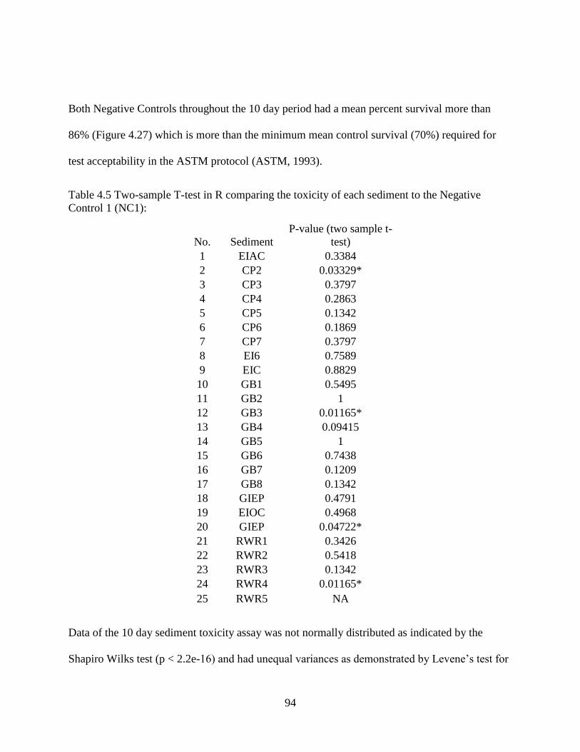
94

Both Negative Controls throughout the 10 day period had a mean percent survival more than

86% (Figure 4.27) which is more than the minimum mean control survival (70%) required for

test acceptability in the ASTM protocol (ASTM, 1993).

Table 4.5 Two-sample T-test in R comparing the toxicity of each sediment to the Negative

Control 1 (NC1):

No. Sediment

P-value (two sample t-

test)

1 EIAC 0.3384

2 CP2 0.03329*

3 CP3 0.3797

4 CP4 0.2863

5 CP5 0.1342

6 CP6 0.1869

7 CP7 0.3797

8 EI6 0.7589

9 EIC 0.8829

10 GB1 0.5495

11 GB2 1

12 GB3 0.01165*

13 GB4 0.09415

14 GB5 1

15 GB6 0.7438

16 GB7 0.1209

17 GB8 0.1342

18 GIEP 0.4791

19 EIOC 0.4968

20 GIEP 0.04722*

21 RWR1 0.3426

22 RWR2 0.5418

23 RWR3 0.1342

24 RWR4 0.01165*

25 RWR5 NA

Data of the 10 day sediment toxicity assay was not normally distributed as indicated by the

Shapiro Wilks test (p < 2.2e-16) and had unequal variances as demonstrated by Levene’s test for

95

homogeneity of variances (p < 2.2e-16 ***). Kruskal Wallis test showed that there was

significant effect of time on sediment toxicity (p = 7.089e-07). Further testing using the Post-hoc

Kruskal-Nemenyi tests showed that there was a significant difference in survival of amphipods

between Day 1 and Day 8 (P= 0.01) and Day 3 and Day 8 (P= 0.02). A significant difference in

amphipod survival was seen between NC1 (Negative control with sediment) and PC1 (Positive

control with sediment) using the Welch’s two sample t-test that assumes non-normal data with

unequal variances (P = 0.0002365). Similarly, NC2 (Negative control without sediment)

displayed a significantly higher (P = 1.746e-09) amphipod survival than PC2 (Positive Control

without sediment) and PC3 (Positive Control without sediment at a higher WAF, P= 2.786e-07).

Amphipod survival was numerically but not significantly lower in the Negative Control without

sediment (NC2) in comparison to the Negative Control with sediment(NC1) (P = 1). On the

other hand, amphipod survival was significantly lower in both positive controls without sediment

(PC2, P= 0.03891) and PC3, P=0.05955) in comparison to amphipod survival in PC1 (with

sediment). Sediments CP2, GB3, GIEP and RWR4 had significantly lower amphipod survival in

comparison to the Negative control NC1 (with sediment) whereas amphipod survival in the rest

of the 21 sediments was not significantly different (Table 4.5). GB3 was minimally oiled and this

could be a factor for toxicity in this case. However, GB3 had significantly higher amphipod

survival than PC1 (P= 2.528e-05), PC2 (P= 7.741e-10) and PC3 (P= 4.359e-08). In addition, the

PAH contents of GIEP in East Louisiana and CP2 and RWR4 in West Louisiana were below the

established threshold of 700 ppm and thus, oiling cannot be the only explanation for toxicity.

Toxic effects of unoiled sediments on Hyallela azteca mortality using similar experimental

conditions such as in this study have been observed previously and can be caused by

contaminants other than oil (see Chapter 5. Discussion).

96

Chapter 5. Discussion

Coastal marshlands including the salt marshes of Louisiana are threatened by a combination of

natural and anthropogenic stressors (Barbier et al., 2011, Orth et al., 2006, Kirwan and

Megonigal, 2013). Pollution caused by agricultural runoff, chemical and oil spills, land loss

through sea level rise, subsidence, erosion and hurricanes, as well as physical destruction of

marsh for oil and gas exploration projects are some of the known threats of coastal marshlands

(Silliman et al., 2012, Kirwan and Megonigal, 2013, O’Riordan et al., 2000). When coastal

marsh ecosystem health suffers, habitats of wildlife are converted, fragmented and/or destroyed

thereby endangering the diverse and productive marshes (Reed and Wilson, 2004, DeLaune et

al., 1983). Protective capacity of the coastal marshlands weakens, consequently making

terrestrial ecosystems more vulnerable to ecological impacts (Silliman et al., 2012). Quick,

accurate and reliable tools to assess marsh health are required not only after natural and

anthropological impacts mentioned above but also to monitor recovery and positive impacts of

coastal restoration projects (O’Riordan et al., 2000, Morris et al., 2015).

The green head horse fly Tabanus nigrovittatus is native to the coastal marshes from Texas to

Nova Scotia (Hansens, 1979). More importantly, its larvae develop in the marshlands for long

periods of time (Magnarelli and Stoffolano Jr, 1980). The functional role in the marsh ecosystem

of the T. nigrovittatus larvae is that they are top invertebrate predators and their development is

indicative of an undisturbed food web and, thus, a healthy marsh (Magnarelli and Stoffolano Jr,

1980). Hence, T. nigrovittatus has all the characteristics of a promising model for bioindication

of a healthy marsh.

97

The Deepwater Horizon Oil Spill in 2010 provided an opportunity to test the T. nigrovittatus

model for its capacity to indicate a disturbed marsh ecosystem. Population crashes of adults and

larvae were observed in East Louisiana at or near sites where the oil made landfall. No such

crashes were observed in West Louisiana, where the oil did not reach, despite similar collection

efforts (Husseneder et al., 2016). This observed population crash of the larvae in the vicinity of

oiled areas of East Louisiana led to the hypothesis that larval decline was a result of either direct

or indirect effects of oil. Direct effects of oil could either be toxicity to adults, which would

reduce their breeding population and/or toxicity to eggs and larvae in the sediment. Indirect

effects could be caused by an alteration of the food web either due to oil itself or a change in

sediment chemistry. The as yet undeciphered T. nigrovittatus larval food web would have to be

studied to determine the key components that sustain the larvae in the Spartina salt marshes.

Describing the taxa found in the larval gut and surrounding sediments not only showcases the

constituents of the food web of the larvae but also answers questions about tabanid biology.

Comparing food webs between sites where larvae were present and absent would indicate if

certain meiofauna taxa can be used as predictors of larval presence. Measuring the effects of

presence/ absence of oil and different parameters of sediment chemistry on the food webs was

important and will help to assess whether absence of larvae was indirectly caused by alterations

in food web composition. Lastly, comparing food webs among locations and based on geography

(East and West) would aid in answering the question why larvae were absent in East Louisiana in

comparison to the West.

5.1 Species ID of larvae

The first challenge was species ID of larvae collected in the study. There are morphological keys

for adults and larvae (Merritt and Cummins, 1996, Sofield et al., 1984). However, morphological

98

keys might not be sufficient to identify cryptic species within the T. nigrovittatus species

complex. Therefore, we employed DNA barcoding to identify larvae to the species level. The

mitochondrial cytochrome oxidase subunit 1- 5’ sequences of the adult reference specimen of T.

nigrovittatus from Louisiana marshes identified by morphological measurements (Sofield et al.,

1984) differed by 5% from a previously submitted T. nigrovittatus from Florida. While this

variance might be population differentiation, it underscores the need for future study of the

genetic variances to resolve the species complex. For the present study, larvae were DNA

barcoded and compared to the reference specimen of T. nigrovittatus.

Barcoding of the tabanid larvae (see Results 4.1) indicated that most of them belonged to the

species T. nigrovittatus (≥ 97% similarity at all three DNA loci) or at least were closely related

species within the T. nigrovittatus complex. However, the ones that showed only a moderate

percent identity match (92% to 95%) to the T. nigrovittatus reference specimen in the

mitochondrial cytochrome oxidase 1 region likely belong to cryptic species within the T.

nigrovittatus complex. There also is the possibility that some larvae with low similarity to the

reference species (<95%) at three DNA loci were Tabanus hinellus as this species is known to be

present in Louisiana marshes (Schutz et al., 1989, Mullen et al., 1988) and adult specimens have

been collected at the sampling locations by our team.

Although more work is needed to resolve the species issue, for purpose of this study we

considered all tabanid larvae equally as top predators in the marsh soil and therefore investigated

their food web regardless of their exact species ID. Studies are in progress to DNA barcode

additional tabanids from Louisiana marshes, which will help with species ID in the future.

99

5.2 Diets of tabanid larvae

Insects were the main component of tabanid larval diet (see Results 4.7). Insect families included

Drosophilidae, Culicidae and Tabanidae in the larval guts (see Results 4.8). Invertebrate

predators are known to forage specifically for proteins and lipids to redress specific nutrient

imbalances (Mayntz et al., 2005) . Insect predators from the Belostomatidae and Nepidae

families feed on snails, frogs, tadpoles and aquatic insects including mosquito larvae in the

wetlands of Japan (Ohba and Nakasuji, 2006). Tabanid larval diets have been previously

reported to consist of detritus, algae, bacteria and small invertebrates in the US (Frouz, 1999).

Cannabilistic traits in tabanid larvae also have been reported (Axtell, 1976).

In our larval food web study (see Results 4.7), the most dominant “families” were hexapods and

fungi and both were present in all larval guts. Moderate abundances of unknown metazoa

followed by protozoa, algae and diatoms of the SAR superclass as well as low proportions of

plant matter belonging to Liliopsida (Spartina) and Magniliophyta also were found in the guts.

Insects were an important component of the tabanid larval diet in Louisiana marshes. Insect

based diets have been reported in other tabanids. Insects have been previously reported as major

components in tabanid diets in Poland (Frouz, 1999). Diet components are a subset of the major

insect orders described in Louisiana marsh (Adams et al., 2017, Bam, 2015, Pennings et al.,

2014, McCall and Pennings, 2012) and the sediments from this study.

Major insect orders found in the Louisiana marshes include Diptera, Coleoptera, Collembola,

Hymenoptera, Hemiptera, Orthoptera, and Thysanoptera (Bam, 2015, Adams et al., 2017,

Pennings et al., 2014). Of those, we found OTUs belonging to Diptera, Collembola,

Hymenoptera and Hemiptera in the tabanid guts (see Results 4.2, 4.7). Insects also are known to

parasitize tabanid larvae. Tachinidae (Diptera) parasitize the larvae whereas egg masses are

100

known to be parasitized by Hymenoptera (Scelionidae, Mymaridae and Trichogrammatidae) and

pupae by Trichopria tabanivora (Axtell, 1976). Hence, the parasitic wasp found in the larval gut

could be a larval parasite. As T. nigrovittatus larvae live in the sediment of Spartina marshes,

insects associated with Spartina were a part of the larval food web (see Results 4.8).

Hemipterans associated with the Spartina include Prokelisia sp., Chaetopsis sp. (stem-boring

herbivore), grasshopper, Orchelimum jidicin, Chlorochroa senilis and Ischnodemus badius

(Pennings et al., 2014, Pfeiffer and Wiegert, 1981).

Biodiversity of insects in salt marshes is not well described. Over 100 species of arthropods are

found associated with Spartina alterniflora salt marshes (Pfeiffer and Wiegert, 1981, Wimp et

al., 2010). However, few of these arthropods are described to the species level (Adams et al.,

2017). Insects in salt marshes are vaguely described by the ecosystem they belong to (aquatic,

terrestrial, benthic and wetland) or by their place in the environment (epiphytic and free-

swimming ) or their common names (mosquitoes, biting flies, and biting gnats) (Batzer and

Wissinger, 1996, Pennings et al., 2014). Insects have been identified depending on their

functional role such as detrivores, omnivores, herbivores, and predators (Pennings et al., 2014).

These categories have been further divided into feeding guilds by other studies such as stem

boring and sucking herbivores, parasitoids (McCall and Pennings, 2012).

Out of the 52 OTUs identified as Insecta in this study, only 23 were identified to the species

level by the SILVA 119 database (see Results 4.8). These included Aedes aegypti, Aedes

albopictus. Drosophila sechellia, Haematopota pluvialis and Leptopilina heterotoma (see

Results 4.8). However, most of these insect species are not known to live in salt marshes. DNA

metabarcoding indicated that dietary components of the tabanid larvae are related to species

within the genera Drosophila, Aedes and the Family Tabanidae. Drosophila sechellia is not

101

known to occur in the marsh. The closest relative known to occur in LA marshes is a species

from the genus Scaptomyza of the family Drosophilidae. Scaptomyza pallida (Zetterstedt) is a

known parasitoid of a fungal gnat known to be associated with the marsh marigold (Eiseman et

al., 2016) . Aedes solicitans and Aedes taeniorhynchus represent the Genus Aedes in the

Louisiana marsh (Ailes, 1998), and ,thus, the Aedes sequences found in the larval guts

originated most likely from those species. Tabanus nigrovittatus, Tabanus hinellus and Chrysops

spp. are horse and deer fly species from the Family Tabanidae known to be present in the

Louisiana marshes (Hansens, 1979, Mullen et al., 1988, Schutz et al., 1989). Hence, the

sequences found in the larval guts likely belong to those species, indicating that some life stages

of these species are the prey of the tabanid larvae. The presence of T. nigrovittatus DNA in larval

guts both in the cloning (see Results 4.2) and 18S rRNA gene libraries (see Results 4.8) are

likely a result of cannibalism, since cannibalistic traits have been reported in tabanid larvae

(Axtell, 1976). However, contamination by host DNA cannot be excluded despite careful

dissection.

Unclassified fungi was the other major component in the tabanid larval guts besides insects (see

Results 4.7). The presence of fungi can be explained as fungal symbionts or parasites of tabanid

larva itself, fungi associated with prey species, fungi as food source of tabanids or their prey,

and/or fungi in general associated with the larval habitat. The family Saccharomycetaceae was

found previously in the hindgut of mosquito larvae (Tajedin et al., 2009) suggesting that this

fungus might be a part of the larval microflora. Capnodiales and Cyberlindnera have been

isolated from beetle larval guts (Lou et al., 2014, Rojas-Jiménez and Hernández, 2015) whereas

Kazachstania have been reportedly found in the gut of black soldier flies (Zheng et al., 2013).

Sympodiomycopsis has been isolated from insect frass (Chen et al., 2013). Hence, Capnodiales,

102

Cyberlindnera Kazachstania and Sympodiomycopsis are fungi identified in the tabanid larval

guts which have been associated with insect guts previously and might possibly be symbionts.

Symbiotic fungal associations of tabanid larvae have not yet been studied. However, fungi are

known to be associated with the hindgut walls of other Diptera larvae such as Culicidae,

Chironomidae, Simuliidae, Ceratopogonidae, Tipulidae and Thaumaleidae larvae (Pereira et al.,

2005). Thus, there could be fungal symbionts in tabanid larva guts. Some tabanid larva fungal

association could be parasitic as Coelomomyces fungus is known to parasitize tabanid larval

haemocoel (Axtell, 1976).

Besides direct fungal association with tabanid larva, fungi also could be associated with the prey

of tabanid larvae. For example, mosquitos (likely as eggs and larval stages) were a prevalent part

of tabanid larval diet. The larval stages of mosquitoes harbor fungi as symbionts (Tajedin et al.,

2009) and fungi (Penicillium citrinum) parasitize Aedes spp. eggs (Russell et al., 2001). Black fly

larvae host at least 20 species of tricomycetes (Tajedin et al., 2009). Mycophagous Coleopteran

larvae ingest Ganoderma as a food source (Kadowaki et al., 2011).

Besides fungi associated with the tabanid larva itself and/or its prey, the unclassified fungi could

have originated from the environment, i.e. soil and plants. Fungi in the marshes are varied but the

most abundant are Ascomycetes (Gessner and Kohlmeyer, 1976, Boland and Grund, 1979). The

fungi isolated from Spartina included Ascomycetes, Zygomycetes and Coelomycetes where

Ascomycetes (especially Genera Mycosphaerella and Phaeosphaeria) were abundant on the

lower stems of S. alterniflora (Al-Nasrawi and Hughes, 2012, Boland and Grund, 1979). As

fungi play such diverse roles in insect larval guts and were found in dominant proportions in the

diet of tabanid larvae the unclassified fungal component of the tabanid guts should be studied

further using fungal primers.

103

The fungi identified by the SILVA 119 database include Malassezia (most abundant),

Saccharomycetaceae, Capnodiales, Cyberlindnera, Kazachstania and Sympodiomycopsis,

Dothideomycetes. The genus Malassezia has been found in marine sediments previously and is

reportedly ecologically hyper diverse. For example, Malassezia has been captured by

metagenomics studies across a variety of habitats, including sediments from deep hypersaline

anoxic basin redox clines and deep subsurfaces (Zhang et al., 2015, Rédou et al., 2014, Bernhard

et al., 2014, Amend, 2014). Dothideomycetes are pathogenic microfungi of Spartina (Elmer,

2016) suggesting that they were acquired from the environment.

A significantly higher abundance of Agricomycetes/Agaricomycotina was observed in the diets

of larvae found at Cypremort Point in comparison to the abundance of

Agricomycetes/Agaricomycotina in the larvae found in Rockefeller Wildlife Refuge (see Results

4.9). However, the group of Agricomycetes/Agaricomycotina was not observed in the sediments

of Cypremort Point (see Results 4.11) and was only present in the sediments from Rockefeller

Wildlife Refuge. This suggests that this fungus is not derived from the surrounding sediment but

could be a member of the larval gut community or associated with the prey of the larva.

Ciliated protozoa specifically Tetrahymena also were found in the larval gut (see Results 4.7)

albeit with less than 200 reads in all larval guts except for one (RWR5.8.LG) which contained

over 70,000 reads. Ciliated protists have been shown to be a part of mosquito diets (Merritt et al.,

1992). Hence, the protists could be prey to the tabanid larvae, especially during early larval

stages. Protozoa such as Tetrahymena are known to infect mosquito and black fly larvae (Hajek,

2000). Tetrahymena chironomi was shown to be a facultative parasite in chironomid larvae

(Corliss, 1960). Another species of Tetrahymena, namely Tetrahymena sialidos found in the

haemocoel of larval Megaloptera was proven to be a parasite involved in controlling invertebrate

104

populations using parasitism (Batson, 1985). Thus, the protozoa in the tabanid larva gut could

originate from their prey species.

Non-prey dietary components in the larval guts include plant material and algae (see Results

4.7). Tabanid larvae were collected from Spartina marshes and their habitat contains plant roots

and other below-ground biomass. Hence, it is possible that their prey is laced with some plant

material and that DNA extracted from the gut contents of the larvae also contained DNA of the

plants ingested by the larvae’s prey. Plants/algae has been found in the guts of predatory larvae

previously (Merritt et al., 1992) including tabanids (Axtell, 1976). Algae have been previously

reported to be found in the diet of predaceous aquatic larvae (Merritt et al., 1992) including

tabanids (Axtell, 1976) . Algae are part of aquatic environments and are likely associated with

organisms that tabanid larvae prey on (Merritt et al., 1992). Chromulinales are photosynthetic

single celled algae present abundantly in the marine environments (Reynolds, 2006). Presence of

algae in the diets of insects have been previously correlated to their abundance in the

surrounding environment suggesting that Chromulinales could be ingested during larval

predation (Patterson et al., 1993).

Overall, the gut content of tabanid larva contains organisms that are likely to be the direct prey of

larvae in their different development stages (ranging from ciliated protozoa to soil dwelling

insects) but also include organisms that are likely to be associated with prey organisms, such as

single celled algae and fungi.

5.3 Taxa present in sediments with and without larvae

A high proportion of Opisthokonta (“classes” Holozoa and Nucletmycea) in sediment samples

was a good predictor for finding larvae in the West (see Results 4.10). This was confirmed by

105

LEfSe analysis showing a higher presence of Opisthokonta at the sites where larvae were found

in comparison to the sites where larvae were absent. The Holozoa contain insects and the

Nucletmycea contain fungi, both of which have been shown to be the major components in the

larval gut and are, thus, likely associated with larval diet (see Results 4.7, 4.10). This suggests

that a dominant presence of diet components in the sediment might be conducive to larval

development.

While the dominance of Opisthokonta was associated with larval presence in the West,

proportions of “families” and “family” diversity did not always predict larval presence (see

Results 4.10). While most larvae were found at sites with predominant proportions of hexapods

and fungi, high “family” diversity resulting in low relative proportions of hexapods and fungi did

not preclude the presence of larva (RWR2).

In the East, however, larvae were absent even from sediments with high Holozoa and

Nucletmycea (“class”) or hexapods and fungi (“family”) content. This suggests that there were

other factors impacting larval numbers in the East besides food web composition (see last part of

the discussion).

We initially hypothesized that sediments with high content of larval diet components would be

better able to sustain larval development. However, it was not guaranteed that larvae can always

be found even if they were present in those sediments. The distribution of larvae is patchy since

females of T. nigrovittatus lay large numbers of eggs in batches and larvae cannibalize each

other, lowering their density (Magnarelli and Stoffolano Jr, 1980, Axtell, 1976). Thus, larvae

cannot always been found by our sampling method even if they are present in the general

vicinity. Also, larvae are mobile and swim in pursuit of food making them less dependent on

food web content of microhabitats (https://www.youtube.com/watch?v=GAdm_JqAuoM).

106

5.4 Effect of PAH on OTU composition

East Louisiana Spartina marshes took the brunt of oiling after the Deepwater Horizon Oil spill in

2010 (Silliman et al., 2012). Spartina marshes were a barrier between terrestrial and marine

ecosystems preventing the oil from flowing inland (Silliman et al., 2012). However, due to the

oil accumulated in the Spartina marshes heavy degradation of Spartina and associated organisms

occurred (Silliman et al., 2012). T. nigrovittatus larvae live in the Spartina marshes where they

develop for long periods of time (Magnarelli and Stoffolano Jr, 1980). Impact of oil in this

region led us to the hypothesis that absence of larvae at most sites in the East (i.e. in the vicinity

where oil made landfall) was due to oil contamination and changes in food web.

Surprisingly, we did not find a difference in the overall alpha- and beta diversity of taxa between

Eastern sites where oil was present and absent. Even reducing overall variability by focusing on

the same region (Grand Bayou) did not show significant differences in taxa composition between

sites where oil detected a year after the DHOS and sites where oil was not detected a year after

the DHOS (see Results 4.16). The lack of statistical significance was due to the limited number

of oiled sites sampled, the low concentration of oil even at sites exceeding the background PAH

level of 700 ppm, low sensitivity and/or fast recovery of the meiofauna community.

Our sites were determined before the oil made land fall. Although oil was reported along the

Eastern coast of Louisiana, i.e. in the vicinity of our sample sites and our samples were collected

at the high tide , within the oil penetration limit of <15 m in the marshes (Silliman et al., 2012),

oiling was rather patchy (Boesch et al., 1994). Patchy distribution was due to wind and ocean

currents driving the oil in some areas at a higher intensity than the others. Also, as observed in in

Barataria Bay, intensity of oiling depended on the presence of heavily oiled above ground

vegetation where oiled remained rooted in place even after the vegetation died and did not show

107

any signs of weathering. In addition, presence of wrack lines also contributed to overlaying

emulsified oil on the marsh substrate. Therefore, only two of our sediment samples from Grand

Bayou were directly contaminated with oil likely originating from the DWOH oil spill (see

Results 4.15). Although oiled, these sites (GB2 and GB3) had only 0.00098 mg/g and 0.001219

mg/g of Total Petroleum Hydrocarbons (TPHs), which was lower than the lightly (6.2 mg/g - 13

months post DHOS) , moderately (70 mg/g - 9 months post DHOS) and heavily (510 mg/g - 9

months post DHOS) oiled sites that were the models for describing impact of the oil spill on soil

fauna (McCann et al., 2017)

Evidence suggests that recovery at lightly oiled sites commenced as soon as within 17 months as

the stem density of the Spartina marshes and associated benthic microalgae recovered (Fleeger et

al., 2015). Most meiofauna, such as copepods which feed on the benthic microalgae recovered

fast on pace with the Spartina. The arthropod population density also had rebounded by 2011

(McCall and Pennings 2012).

While the majority of meiofauna recovered fast (Fleeger, Carman et al. 2015), others such as

polychaete Manayunkia aestuarina, ostracods and kinorhynchs, had not recovered even 4 years

after the spill (Fleeger et al., 2015). Different sensitivity to oil impact and different rates of

recovery might explain why we found differentially enriched taxa at our minimally oiled sites

(see Results 4.16), such as Hymenostomatia (Tetrahymena), Bivalvia (mollusks), Maxillopoda

(Crustacea) and Peronosporomycetes (fungus like eukaryotes).

Tetrahymena are ciliated protozoa. Ciliated protists have shown an increased abundance in the

presence of oil in in vivo and in vitro studies because they feed on the oil degrading bacteria that

increase in the presence of oil (Hazen et al., 2010). Bivalvia show depressed oxygen

consumption via gills and decreased filtration rates in the presence of oil (Burger, 1994).

108

However, Bivalves were detected a year after the Exxon Valdez oil spill possibly due to their

ability to close themselves immediately after an environmental stimulus (Burger, 1994). Physical

barrier of the epicuticle and fast rebounding population capacity of Maxillopoda (Crustaceans)

could be possible reasons why this group was detected in the minimally oiled sediments (Felder

et al., 2014). Peronosporomycetes (fungus like eukaryotes) are plant pathogens. As such they

might have infected weakened Spartina plants at the oiled sites (Pal and Gardener, 2006).

5.5 Effect of sediment chemistry on OTU composition

Similarity of the sediment chemistry parameter pH influenced the similarity of OTUs in

sediments (see Results 4.17). In our study, pH had a positive correlation with the abundance of

Liliopsida and Malasezzia in the sediments (see Results 4.17). In contrast, a previous study

found a negative correlation of pH with Spartina alterniflora abundance under experimental

conditions (Slocum and Mendelssohn, 2008). However, this discrepancy could also occur

because salinity levels contribute to the effect of pH (Linthurst, 1979) . A negative correlation

was observed between pH and the relative abundance of Gregarina, Aplanochytrium,

Pseudocohnilembus, and Euplotes from the SAR supergroup, the fungus Leptosphaeria

maculans JN3, the Nematode Nygolaimidae and the Annelid Enchytraeidae (see Results 4.17).

However, a previous study did not detect any correlation of sediment pH and Annelids

(Schlaghamerský and Tříska, 2009).

5.6 Sediment toxicity

Two sediments collected in 2011 from West Louisiana (RWR4 and CP2) and two sediments

from the East (GB3 and GIEP) caused increased mortality in bioassays using amphipods

(Hyalella azteca) as models (see Results 4.18). GB3 was the sediment sample with the highest

109

oil content (1,219 ppb) and thus oiling might have contributed to toxicity (see Results 4.15,

4.18). However, GIEP was not oiled above baseline (363 ppb), and the Western samples were

collected outside of the range of the oil spill.

Since amphipods were chosen for their pronounced sensitivity to sediment toxicity (Landrum et

al., 1991, Connolly et al., 2004, Emery et al., 1997), their survival shows that most sediments in

the East were not toxic at the time of testing and, thus, tabanid larval decline in Eastern

Louisiana might not have been due to sediment toxicity. However, the lab results have to be

treated with caution since other studies reported variable results with similar bioassays.

Even in lab experiments using moderately oiled soil (0.6 L/m2) and similar experimental study

design as our study a lack of toxicity on H. azteca has been observed and is attributed to time

related adaptation decreasing species sensitivity and changes to bioavailability related to oil

based contaminants (Blaise et al., 2004). In the same study, even reference samples showed

toxicity (Blaise et al., 2004). Changes in hydrocarbon quantity and composition over time and

modifications in oil chemistry profiles also could be other reasons for amphipod tolerance

(Venosa et al., 2002, Blaise et al., 2004).

In addition, there is evidence of variability in the toxicity of sediments stored for long periods of

time frozen at either - 4℃ or -20℃ (Geffard et al., 2004, Dillon et al., 1994, Becker and Ginn,

1995). Although many studies suggest increase in toxicity after long periods of storage, decrease

in toxicity also has been observed. Overall, change in toxicity is unpredictable after long periods

of storage (Schuytema et al., 1989) and references therein).The recommended ASTM conditions

for a dependable toxicity test are storage of sediments at 4º C for not more than 8 weeks (ASTM,

1993) based on agreement that changes in the geochemical nature of sediments are minimized in

these conditions (DeFoe and Ankley, 1998, Thomson et al., 1980). As toxicity assays in this

110

study were conducted after six years of storage, it is possible that the results of this study may

not reflect toxicity of the sediment at the time of collection.

An increased survival of amphipods in the positive controls spiked with weathered crude oil with

sediment in comparison to those without sediment was observed. The sediment likely offers a

protective layer to the amphipods and reduces interaction with the overlaying WAF of oil

thereby increasing their chances of survival.

5.7 Reasons for larval decline in the East

In 2011, tabanid larvae were found in higher numbers in West Louisiana in comparison to East

Louisiana, where oil made landfall the year before. Although more sites were sampled in the

East (14) compared to the West (11), only one larva was found in the East compared to 18 in the

West.

We hypothesized that the lack of larvae in the east could be caused by (a) lack of specific food

web components necessary for supporting larval development, which might be connected to (b)

toxic effects of oil or (c) other parameters of soil biochemistry on larvae or their food web.

However, all these hypotheses were rejected. We found that (a) the group Opisthokonta, which

encompasses the Holozoa including insects and Nucletmycea including fungi, was the main

component of the larval diets (> 98%) as indicated by Result 4.10. A higher presence of

Opisthokonta was a predictor of larval presence in the West. However, even with high

abundances of Opisthokonta at sites in the East larvae were still absent. Overall, the was no

significant difference in food web composition between sediments from East and West Louisiana

and taxa enriched in the East or the West did not particularly reflect larval food components (see

Results 4.13). This indicates that larval absence was not a result of a disturbed food web in the

111

East. (b) The presence of oil in sediments had no significant effect on food web composition (see

Results 4.16) and was not a reliable predictor for the absence of larvae (see Results 4.10), since

we failed to find larvae at a number of non-oiled sites in the East. Other studies that sampled

moderately to heavily oiled sediments after the DWH oil spill found significant shifts in

meiofauna composition (see literature review and above discussion). However, only two sites in

our study were oiled and oil concentration was low (see Results 4.15).

Toxicity in bioassays occurred in equal numbers of samples in the East and in the West (see

Results 4.18) and could not be reliably connected to oiling (see Results 4.15) nor other

parameters of sediment chemistry (see Results 4.17). All of these results indicate that the larvae

and their food web were not directly affected by the Deepwater Horizon Oil spill and/or

sediment toxicity due to oil or biochemistry parameters in East Louisiana.

As mentioned above, one year after the DWH oil spill (2011) larvae were almost completely

absent from collection sites in the East. This was not due to a permanent underlying difference in

population numbers as 2016 the larval counts at Grand Bayou sites had risen to levels

comparable to sample sites in the west (L. Foil, personal communication). This indicates that the

oil spill did have an impact on larval populations, although the main cause was not direct toxicity

on larvae and their food web. After eliminating direct effects of the oil spill on larvae and their

food web, we conclude that the population crash of adult flies was the main cause of lack of

larvae in the east. Immediately after the DWH oil spill the numbers of adult flies severely

declined in the East, likely due to their being attracted to and landing on oil sheens because of

reflected polarized light presumably mimicking fresh water (Horváth et al., 2008). The

population crash led to pronounced genetic bottlenecks and a decrease of gene flow among

populations in the east, and consequently, fewer breeders producing fewer larvae (Husseneder et

112

al. 2016). Secondly, the few remaining females of T. nigrovittatus probably did not get a blood

meal to lay their second batch of eggs due to a decline in the terrestrial vertebrate population as

result of the oil spill (Antonio et al., 2011). Since neither food web composition (see Results

4.10, 4.14) nor sediment toxicity (see Results 4.18) could sufficiently explain absence of larvae,

the most likely explanation of the decline of larvae in the east remains the adult population crash

in the vicinity of oil making landfall having an area-wide effect of larval population reduction

even at sites that were not directly oiled.

5.8 Challenges in Taxonomic assignments

While 18S rRNA metagenomic sequencing is an invaluable tool for identifying food web

dynamics (Xu, 2014, Mardis, 2008) this method has its limitations. Taxonomic assignments in

DNA reference databases, such as SILVA, are not always in agreement with classical taxonomic

assignments and the taxonomy files of the sequences in the database rarely allow identification to

the species level. Hence, taxonomy of sequences already in the databases must be revised and

reliable identification to the species level must be included. For example, in this study the main

component of the tabanid larval diet belonged to “Insecta”, which was identified at the “Genera”

level based on the SILVA 119 taxonomy (see Results 4.8). Manual BLAST against the NCBI

database confirmed that insects identified to the species level belonged to the families

Drosophilidae, Culicidae and Tabanidae but the exact species could not be pinpointed

(Supplementary Figure 2). There are closely related species known to occur in salt marsh, e.g.

Aedes solicitans, Aedes taeniorhynchus, Tabanus nigrovittatus, Tabanus hinellus and Chrysops

spp. However, their sequence information is not part of the reference databases. This points to

the most important limitation of 18S sequencing: the lack of reference sequences in curated

113

databases. This is especially obvious when a study attempts to describe organisms and

communities in less well researched environments, such as salt marshes.

Taxonomically, salt marsh insects have been lumped together at the level of orders, families and

rarely identified to genera or species (Pennings et al., 2014, Batzer and Wissinger, 1996, Adams

et al., 2017). Some species are identified by their functional role such as Conocephalus aigialus

and Orchelimum fidicinium (omnivores), and Hogna sp. (predator) (Pennings et al., 2014).

Even in studies where salt marsh insects have been identified to the species level DNA barcoding

has not been done. Hence, 18SrRNA gene sequences of the salt marsh insect species in databases

are scarce. Due to these gaps in the databases it is imperative to populate reference databases by

accurately morphologically identifying and sequencing salt marsh organisms, specifically

insects. Projects funded by Gulf of Mexico Research Initiative are under way to add sequences

for these yet unrepresented salt marsh species. For example, Thomas et al.’s project “Genomic

Responses to the Deepwater Horizon event and development of high-throughput biological

assays for oil spills” is populating the databases by sequencing benthic organisms while Foil and

Husseneder’s project “A study of horse fly (Tabanidae) populations and their food web dynamics

as indicators of the effects of environmental stress on coastal marsh health”) is identifying and

barcoding insect communities in the Louisiana salt marshes. Such studies will benefit future

metagenomics studies of not only insect food webs but studies of all higher trophic levels.

In addition to gaps in reference databases, the low resolution power of 18SrRNA gene region

targeted by the primer pair NF1 and 18Sr2b limits species assignment. This 400 bp region at the

3’ end of the 18rRNA gene has been recommended to capture maximum eukaryotic diversity

(see Chapter 2. Introduction) because of which it does not always have the ability to differentiate

among closely related species. However, the taxonomic placements of species can still be

114

deciphered to a certain degree. Insects identified to the “species” level belong at least to the

family classified in the database. For future studies focusing on insects, multiple regions that are

better suited for insect species identification can be used (Valentini et al., 2009b). A combination

of markers targeting the 18SrRNA gene and the mitochondrial CO1 gene can be used for

barcoding or metabarcoding of insect species, because the 18SrRNA gene will capture overall

insect diversity while the mitochondrial CO1 gene will differentiate between closely related

species (Valentini et al., 2009b, Hajibabaei et al., 2007). Metabarcoding using insect specific

primers 18S ai/bi used in this thesis for barcoding adults also could be a good alternative to be

used in combination with mitochondrial CO1 gene or mitochondrial CO II gene (Whiting et al.,

1997). ITS regions are widely used for barcoding, primarily to differentiate between closely

related fungi (Schoch et al., 2012). However, with the high levels of fungi associated with the

tabanid and other aquatic larvae (Tajedin et al., 2009) ITS might not be a good choice for insect

larval barcoding.

Inaccurate species description of reference specimens in database also might lead to multiple or

erroneous matches, but this should be the exception in curated databases. Morphological

identification of adult insects is not always easy because taxonomic keys to differentiate between

closely related species are not always available (Harvey et al., 2003). Insects in different stages

of life cycle such as larvae or pupae usually require identification by an expert (Harvey et al.,

2003). This causes insects to be inaccurately identified and consequently the sequences uploaded

in the database might be from an incorrectly identified species.

Deficiency of sequences in databases identified to the species level, paucity of identified and

sequenced insect species from the salt marshes, low resolution power of primers and inaccurately

identified insect sequences were challenges that made taxonomic assignments difficult.

115

Chapter 6. Conclusions and Future

The food web of the larval stages of the green head horse fly primarily consist of the “Phylum”

Opisthokonta further classified to insects and unclassified fungi. Larval diets are not particularly

diverse with Opisthokonta dominating majority (15/16) of the larval guts followed by the SAR

supergroup comprising algae and diatoms and minimal presence of plant materials from the

“Phylum” Archeoplastida. In the future, DNA metabarcoding can be done using primers

specifically targeting insects in the tabanid guts using a combination of genomic and

mitochondrial regions (see Chapter 1 Introduction) to allow a more detailed classification of

insect prey. The genomic DNA would cover the diversity of insects while the mitochondrial

regions would be useful in discerning between closely related species. This is the first study

showing that a wide array of fungi prevail in the tabanid larva guts. The Internal transcribed

Spacer (ITS) region should be used to provide further details concerning fungal diversity as this

region is widely used in fungal genomics especially to distinguish between closely related fungi

(Schoch et al., 2012). A bacterial diversity study using the 16SrRNA gene region can be done to

determine the lower trophic levels of the top invertebrate larval predator, T. nigrovittatus. 16S

databases are comparatively more robust that 18S thereby reducing taxonomic challenges.

Bioindicators of larval presence in the East was dominance of the “Phylum” Opisthokonta

supporting the hypothesis that presence of larval food web components is a predictor of larval

presence. However, the reverse is not true. Absence of a high abundance of Opisthokonta does

not indicate larval absence as we found larvae at sites with low Opisthokonta. In addition,

dominance of Opisthokonta is not a predictor of larval presence in the East. Bioindicators that

are enriched in minimally oiled sediments are Hymenostomatia (Tetrahymena), Bivalvia

(mollusks), Maxillopoda (Crustacea) and Peronosporomycetes (fungus like eukaryotes), which

116

were significantly higher in minimally oiled sediments in comparison to unoiled sediments of

Grand Bayou. In the future, primers used in this study can be used to determine the persistence

of Opisthokonta in sediments to detect the dependability of this larval predictor in the West

Louisiana. Primers also can be designed for bioindicator species prevalent in the minimally oiled

areas and a spatial-temporal analysis can be done to determine efficacy of these species to detect

low level of oiling. Sediment chemistry did not have an effect on OTU composition except pH

which had a positive correlation with the abundance of Liliopsida and Malasezzia and a negative

correlation with abundance of Gregarina, Aplanochytrium, Pseudocohnilembus, and Euplotes

from the SAR supergroup, the fungus Leptosphaeria maculans JN3, the Nematode

Nygolaimidae and the Annelid Enchytraeidae.

Neither sediment chemistry nor toxicity was different between sediments from the East and the

West proving that sediment chemistry was not a contributor of the observed larval decline in the

East. A wider array of sediment chemistry parameters can be used to determine the effect of

direct/indirect toxicity on larvae. Toxicity assays should be conducted within eight weeks to

eliminate variability due to change in sediment integrity (See Chapter 5. Discussion). In addition,

the sensitivity of toxicity bioassays could be improved by observing growth rate, ability to swim,

reproductive capacity and sediment avoidance besides mortality of the organism.

The lack of significant difference in food web composition and sediment toxicity between

sediments from the East and the West indicates that larval decline in the East was not due to

these factors. Most likely, the crashes in the adult population of T. nigrovittatus led to decline in

breeding pairs and subsequently lower larval populations.

117

References

ABLE, K. W., LÓPEZ-DUARTE, P. C., FODRIE, F. J., JENSEN, O. P., MARTIN, C. W.,

ROBERTS, B. J., VALENTI, J., O’CONNOR, K. & HALBERT, S. C. 2015. Fish assemblages

in Louisiana salt marshes: effects of the Macondo oil spill. Estuaries and coasts, 38, 1385-1398.

ADAMS, B. J., CHEN, X. & HOOPER-BÙI, L. M. 2017. A comparison of two insect collection

techniques in oiled and non-oiled salt marshes in Louisiana. Florida Entomologist, 100,

366-371.

ADAMS, W. J. & ROWLAND, C. D. 2003. Aquatic toxicology test methods. Handbook of

Ecotoxicology, 2, 19-38.

ADL, S. M., SIMPSON, A. G., LANE, C. E., LUKEŠ, J., BASS, D., BOWSER, S. S., BROWN,

M. W., BURKI, F., DUNTHORN, M. & HAMPL, V. 2012. The revised classification of

eukaryotes. Journal of Eukaryotic Microbiology, 59, 429-514.

AILES, M. C. 1998. Failure to predict abundance of saltmarsh mosquitoes Aedes sollicitans and

A. taeniorhynchus (Diptera: Culicidae) by using variables of tide and weather. Journal of

Medical Entomology, 35, 200-204.

AL-NASRAWI, H. G. & HUGHES, A. R. 2012. Fungal diversity associated with salt marsh

plants Spartina alterniflora and Juncus roemerianus in Florida. Jordan Journal of

Biological Sciences, 5, 247-254.

ALMEDA, R., CONNELLY, T. L. & BUSKEY, E. J. 2015. How much crude oil can

zooplankton ingest? Estimating the quantity of dispersed crude oil defecated by

planktonic copepods. Environmental Pollution, 30, e10.

ALMEDA, R., WAMBAUGH, Z., WANG, Z., HYATT, C., LIU, Z. & BUSKEY, E. J. 2013.

Interactions between zooplankton and crude oil: toxic effects and bioaccumulation of

polycyclic aromatic hydrocarbons. PloS one, 8, e67212.

AMEND, A. 2014. From dandruff to deep-sea vents: Malassezia-like fungi are ecologically

hyper-diverse. PLoS pathogens, 10, e1004277.

ANDERSON, M. J. 2001. A new method for non‐parametric multivariate analysis of variance.

Austral ecology, 26, 32-46.

ANTHONY, A., ATWOOD, J., AUGUST, P., BYRON, C., COBB, S., FOSTER, C., FRY, C.,

GOLD, A., HAGOS, K. & HEFFNER, L. 2009. Coastal lagoons and climate change:

ecological and social ramifications in US Atlantic and Gulf coast ecosystems. Ecology

and Society, 14.

118

ANTONIO, F., MENDES, R. & THOMAZ, S. 2011. Identifying and modeling patterns of

tetrapod vertebrate mortality rates in the Gulf of Mexico oil spill. Aquatic toxicology,

105, 177-179.

ARMSTRONG, J., ARMSTRONG, D. & HILBORN, R. 1998. Crustacean resources are

vulnerable to serial depletion–the multifaceted decline of crab and shrimp fisheries in the

Greater Gulf of Alaska. Reviews in Fish Biology and Fisheries, 8, 117-176.

ASAHIDA, T., YAMASHITA, Y. & KOBAYASHI, T. 1997. Identification of consumed stone

flounder, Kareius bicoloratus (Basilewsky), from the stomach contents of sand shrimp,

Crangon affinis (De Haan) using mitochondrial DNA analysis. Journal of Experimental

Marine Biology and Ecology, 217, 153-163.

ASTM E1706-05(2010), Standard Test Method for Measuring the Toxicity of Sediment-

Associated Contaminants with Freshwater Invertebrates, ASTM International, West

Conshohocken, PA, 2010

AXTELL, R. C. 1976. Coastal horse flies and deer flies (Diptera: Tabanidae). Marine Insects.

North Holland, Amsterdam, 415-445.

BAKER, J. M., LEONARDO, G. M., BARTLETT, P. D., LITTLE, D. I. & WILSON, C. M.

1993.Long-term fate and effects of untreated thick oil deposits on salt marshes.

International Oil Spill Conference, American Petroleum Institute, 395-399.

BAM, W. 2015. Effects of oil spill and recovery of terrestrial arthropods in Louisiana saltmarsh

ecosystem. Louisiana State University LSU Digital Commons.

BARBIER, E. B., HACKER, S. D., KENNEDY, C., KOCH, E. W., STIER, A. C. &

SILLIMAN, B. R. 2011. The value of estuarine and coastal ecosystem services.

Ecological monographs, 81, 169-193.

BARRON, M. G. 2012. Ecological impacts of the Deepwater Horizon oil spill: implications for

immunotoxicity. Toxicologic Pathology, 40, 315-320.

BASS, D., STENTIFORD, G. D., LITTLEWOOD, D. & HARTIKAINEN, H. 2015. Diverse

Applications of Environmental DNA Methods in Parasitology. Trends in Parasitology,

31, 499-513.

BATSON, B. 1985. A paradigm for the study of insect-ciliate relationships: Tetrahymena

sialidos sp. nov.(Hymenostomatida: Tetrahymenidae), parasite of larval Sialis lutaria

(Linn.)(Megaloptera: Sialidae). Philosophical Transactions of the Royal Society of

London B: Biological Sciences, 310, 123-144.

BATZER, D. P. & WISSINGER, S. A. 1996. Ecology of insect communities in nontidal

wetlands. Annual Review of Entomology, 41, 75-100.

119

BEALS, E. W. 1984. Bray-Curtis ordination: an effective strategy for analysis of multivariate

ecological data. Advances in Ecological Research, 14, 1-55.

BEAUMONT, N., AUSTEN, M., ATKINS, J., BURDON, D., DEGRAER, S., DENTINHO, T.,

DEROUS, S., HOLM, P., HORTON, T. & VAN IERLAND, E. 2007. Identification,

definition and quantification of goods and services provided by marine biodiversity:

implications for the ecosystem approach. Marine Pollution Bulletin, 54, 253-265.

BEAZLEY, M. J., MARTINEZ, R. J., RAJAN, S., POWELL, J., PICENO, Y. M., TOM, L. M.,

ANDERSEN, G. L., HAZEN, T. C., VAN NOSTRAND, J. D. & ZHOU, J. 2012.

Correction: Microbial Community Analysis of a Coastal Salt Marsh Affected by the

Deepwater Horizon Oil Spill. PloS one, 7.

BECKER, D. S. & GINN, T. C. 1995. Effects of storage time on toxicity of sediments from

Puget Sound, Washington. Environmental Toxicology and Chemistry, 14, 829-835.

BENTIVEGNA, C. S., COOPER, K. R., OLSON, G., PENA, E. A., MILLEMANN, D. R. &

PORTIER, R. J. 2015. Chemical and histological comparisons between Brevoortia

sp.(menhaden) collected in fall 2010 from Barataria Bay, LA and Delaware Bay, NJ

following the DeepWater Horizon (DWH) oil spill. Marine Environmental Research,

112, 21-34.

BERGEON BURNS, C. M., OLIN, J. A., WOLTMANN, S., STOUFFER, P. C. & TAYLOR, S.

S. 2014. Effects of oil on terrestrial vertebrates: predicting impacts of the Macondo

blowout. Bioscience, 64, 820-828.

BERNHARD, J. M., KORMAS, K., PACHIADAKI, M. G., ROCKE, E., BEAUDOIN, D. J.,

MORRISON, C., VISSCHER, P. T., COBBAN, A., STARCZAK, V. R. & EDGCOMB,

V. P. 2014. Benthic protists and fungi of Mediterranean deep hypsersaline anoxic basin

redoxcline sediments. Frontiers in Microbiology, 5.

BERRY, T. E., OSTERRIEDER, S. K., MURRAY, D. C., COGHLAN, M. L., RICHARDSON,

A. J., GREALY, A. K., STAT, M., BEJDER, L. & BUNCE, M. 2017. DNA

metabarcoding for diet analysis and biodiversity: A case study using the endangered

Australian sea lion (Neophoca cinerea). Ecology and Evolution.

BIK, H. M., HALANYCH, K. M., SHARMA, J. & THOMAS, W. K. 2012. Dramatic shifts in

benthic microbial eukaryote communities following the Deepwater Horizon oil spill.

PloS one, 7, e38550.

BIK, H. M., MARITZ, J. M., LUONG, A., SHIN, H., DOMINGUEZ-BELLO, M. G. &

CARLTON, J. M. 2016. Microbial Community Patterns Associated with Automated

Teller Machine Keypads in New York City. mSphere, 1, e00226-00216.

120

BLAISE, C., GAGNE, F., CHEVRE, N., HARWOOD, M., LEE, K., LAPPALAINEN, J.,

CHIAL, B., PERSOONE, G. & DOE, K. 2004. Toxicity assessment of oil‐contaminated

freshwater sediments. Environmental Toxicology, 19, 267-273.

BLANKENSHIP, L. & YAYANOS, A. 2005. Universal primers and PCR of gut contents to

study marine invertebrate diets. Molecular Ecology, 14, 891-899.

BOESCH, D. F., JOSSELYN, M. N., MEHTA, A. J., MORRIS, J. T., NUTTLE, W. K.,

SIMENSTAD, C. A. & SWIFT, D. J. 1994. Scientific assessment of coastal wetland loss,

restoration and management in Louisiana. Journal of Coastal Research, i-103.

BOKULICH, N. A., SUBRAMANIAN, S., FAITH, J. J., GEVERS, D., GORDON, J. I.,

KNIGHT, R., MILLS, D. A. & CAPORASO, J. G. 2013. Quality-filtering vastly

improves diversity estimates from Illumina amplicon sequencing. Nature methods, 10,

57-59.

BOLAND, G. J. & GRUND, D. W. 1979. Fungi from the salt marshes of Minas Basin, Nova

Scotia. Proceedings of the Nova Scotian Institute of Science, 29.

BONGERS, T. & FERRIS, H. 1999. Nematode community structure as a bioindicator in

environmental monitoring. Trends in ecology & evolution, 14, 224-228.

BOORMAN, L. A. 1999. Salt marshes–present functioning and future change. Mangroves and

Salt Marshes, 3, 227-241.

BOWEN, J. L. & VALIELA, I. 2001. The ecological effects of urbanization of coastal

watersheds: historical increases in nitrogen loads and eutrophication of Waquoit Bay

estuaries. Canadian Journal of Fisheries and Aquatic Sciences, 58, 1489-1500.

BRETTE, F., SHIELS, H. A., GALLI, G. L., CROS, C., INCARDONA, J. P., SCHOLZ, N. L. &

BLOCK, B. A. 2017. A novel cardiotoxic mechanism for a pervasive global pollutant.

Scientific reports, 7, 41476.

BURGER, J. 1994. Before and after an oil spill: the Arthur Kill, Rutgers University Press.

BURGER, J. & GOCHFELD, M. 2001. On developing bioindicators for human and ecological

health. Environmental Monitoring and Assessment, 66, 23-46.

BURGER, J., HUNTER, J. & COOPER, K. 2001. Using integrated food‐web and population‐

based models for environmental monitoring, remediation decisions, and long‐term

planning. Remediation Journal, 12, 87-102.

BURTON JR, A. G., BAUDO, R., BELTRAMI, M. & ROWLAND, C. 2001. Assessing

sediment contamination using six toxicity assays. Journal of Limnology, 60, 263-267.

121

CAPORASO, J. G., KUCZYNSKI, J., STOMBAUGH, J., BITTINGER, K., BUSHMAN, F. D.,

COSTELLO, E. K., FIERER, N., PEÑA, A. G., GOODRICH, J. K. & GORDON, J. I.

2010. QIIME allows analysis of high-throughput community sequencing data. Nature

methods, 7, 335-336.

CAREW, M. E., PETTIGROVE, V. J., METZELING, L. & HOFFMANN, A. A. 2013.

Environmental monitoring using next generation sequencing: rapid identification of

macroinvertebrate bioindicator species. Frontiers in Zoology, 10, 45.

CARON, D. A., COUNTWAY, P. D., SAVAI, P., GAST, R. J., SCHNETZER, A., MOORTHI,

S. D., DENNETT, M. R., MORAN, D. M. & JONES, A. C. 2009. Defining DNA-based

operational taxonomic units for microbial-eukaryote ecology. Applied and Environmental

Microbiology, 75, 5797-5808.

CHARITON, A. A., COURT, L. N., HARTLEY, D. M., COLLOFF, M. J. & HARDY, C. M.

2010. Ecological assessment of estuarine sediments by pyrosequencing eukaryotic

ribosomal DNA. Frontiers in Ecology and the Environment, 8, 233-238.

CHEN, L., ZHANG, L., LI, Z.-H. & HUI, F.-L. 2013. Sympodiomycopsis yantaiensis sp. nov., a

basidiomycetous yeast isolated from insect frass. International journal of systematic and

evolutionary microbiology, 63, 3501-3505.

CHESNEY, E. J., BALTZ, D. M. & THOMAS, R. G. 2000. Louisiana estuarine and coastal

fisheries and habitats: Perspectives from a fish's eye view. Ecological Applications, 10,

350-366.

CLARKE, K. R. 1993. Non‐parametric multivariate analyses of changes in community structure.

Austral ecology, 18, 117-143.

COHEN, J. H., MCCORMICK, L. R. & BURKHARDT, S. M. 2014. Effects of dispersant and

oil on survival and swimming activity in a marine copepod. Bulletin of Environmental

Contamination and Toxicology, 92, 381-387.

CONNOLLY, N., CROSSLAND, M. & PEARSON, R. 2004. Effect of low dissolved oxygen on

survival, emergence, and drift of tropical stream macroinvertebrates. Journal of the North

American Benthological Society, 23, 251-270.

CORBI, J. J., FROEHLICH, C. G., TRIVINHO-STRIXINO, S. & DOS SANTOS, A. 2011.

Evaluating the use of predatory insects as bioindicators of metals contamination due to

sugarcane cultivation in neotropical streams. Environmental Monitoring and Assessment,

177, 545-554.

CORLISS, J. O. 1960. Tetrahymena chironomi sp. nov., a ciliate from midge larvae, and the

current status of facultative parasitism in the genus Tetrahymena. Parasitology, 50, 111-

153.

122

CRAIN, C. M., HALPERN, B. S., BECK, M. W. & KAPPEL, C. V. 2009. Understanding and

managing human threats to the coastal marine environment. Annals of the New York

Academy of Sciences, 1162, 39-62.

CREER, S., FONSECA, V., PORAZINSKA, D., GIBLIN‐DAVIS, R., SUNG, W., POWER, D.,

PACKER, M., CARVALHO, G., BLAXTER, M. & LAMBSHEAD, P. 2010.

Ultrasequencing of the meiofaunal biosphere: practice, pitfalls and promises. Molecular

Ecology, 19, 4-20.

CRISTESCU, M. E. 2014. From barcoding single individuals to metabarcoding biological

communities: towards an integrative approach to the study of global biodiversity. Trends

in ecology & evolution, 29, 566-571.

CRONE, T. & TOLSTOY, M. 2010a. Using Optical Plume Velocimetry to Estimate the Volume

of Oil Released From the 2010 Gulf of Mexico Leak. AGU Fall Meeting Abstracts.

CRONE, T. J. & TOLSTOY, M. 2010b. Magnitude of the 2010 Gulf of Mexico oil leak. Science,

330, 634-634.

CYWINSKA, A., HANNAN, M., KEVAN, P., ROUGHLEY, R., IRANPOUR, M. & HUNTER,

F. 2010. Evaluation of DNA barcoding and identification of new haplomorphs in

Canadian deerflies and horseflies. Medical and veterinary entomology, 24, 382-410.

DAHL, T. E. & STEDMAN, S.-M. 2013. Status and trends of wetlands in the coastal watersheds

of the Conterminous United States 2004 to 2009. US Department of the Interior, US Fish

and Wildlife Service and National Oceanic and Atmospheric Administration, National

Marine Fisheries Service.

DAVENPORT, S. R. & BAX, N. J. 2002. A trophic study of a marine ecosystem off

southeastern Australia using stable isotopes of carbon and nitrogen. Canadian Journal of

Fisheries and Aquatic Sciences, 59, 514-530.

DAY, L. P., DAY, P., DAY, I. P. & PER, J. Economic Impacts of Recreational Fishing Closures

Resulting From the Deep Horizon Oil Spill: Preliminary Estimates.

DE BRUYN, L., THYS, S., SCHEIRS, J. & VERHAGEN, R. 2001. Effects of vegetation and

soil on species diversity of soil dwelling Diptera in a heathland ecosystem. Journal of

Insect Conservation, 5, 87-97.

DEFOE, D. L. & ANKLEY, G. T. 1998. Influence of storage time on toxicity of freshwater

sediments to benthic macroinvertebrates. Environmental Pollution, 99, 123-131.

DEIS, D. R., FLEEGER, J. W., BOURGOIN, S. M., MENDELSSOHN, I. A., LIN, Q. & HOU,

A. 2017. Shoreline oiling effects and recovery of salt marsh macroinvertebrates from the

Deepwater Horizon Oil Spill. PeerJ, 5, e3680.

123

DELAUNE, R., BAUMANN, R. & GOSSELINK, J. 1983. Relationships among vertical

accretion, coastal submergence, and erosion in a Louisiana Gulf Coast marsh. Journal of

Sedimentary Research, 53.

DELAUNE, R., PATRICK, W. & BURESH, R. 1979. Effect of crude oil on a Louisiana

Spartina alterniflora salt marsh. Environmental Pollution (1970), 20, 21-31.

DICKINS, D. Behavior of oil spills in ice and implications for Arctic spill response. OTC Arctic

Technology Conference, 2011. Offshore Technology Conference.

DILLON, T., MOORE, D. & JARVIS, A. 1994. The effects of storage temperature and time on

sediment toxicity. Archives of Environmental Contamination and Toxicology, 27, 51-53.

DIXON, P. 2003. VEGAN, a package of R functions for community ecology. Journal of

Vegetation Science, 14, 927-930.

DOWD, S. E., CALLAWAY, T. R., WOLCOTT, R. D., SUN, Y., MCKEEHAN, T.,

HAGEVOORT, R. G. & EDRINGTON, T. S. 2008a. Evaluation of the bacterial diversity

in the feces of cattle using 16S rDNA bacterial tag-encoded FLX amplicon

pyrosequencing (bTEFAP). BMC microbiology, 8, 125.

DOWD, S. E., WOLCOTT, R. D., SUN, Y., MCKEEHAN, T., SMITH, E. & RHOADS, D.

2008b. Polymicrobial nature of chronic diabetic foot ulcer biofilm infections determined

using bacterial tag encoded FLX amplicon pyrosequencing (bTEFAP). PloS one, 3,

e3326.

DRUMMOND, A. J., NEWCOMB, R. D., BUCKLEY, T. R., XIE, D., DOPHEIDE, A.,

POTTER, B. C., HELED, J., ROSS, H. A., TOOMAN, L. & GROSSER, S. 2015.

Evaluating a multigene environmental DNA approach for biodiversity assessment.

GigaScience, 4, 46.

EISEMAN, C. S., HELLER, K. & RULIK, B. 2016. A New Leaf-Mining Dark-Winged Fungus

Gnat (Diptera: Sciaridae), with Notes on Other Insect Associates of Marsh Marigold

(Ranunculaceae: Caltha palustris L.). Proceedings of the Entomological Society of

Washington, 118, 519-532.

ELMER, W. H. 2016. Pathogenic microfungi associated with Spartina in salt marshes. Biology

of Microfungi. Springer. 615-630.

EMERY, V. L., MOORE, D. W., GRAY, B. R., DUKE, B. M., GIBSON, A. B., WRIGHT, R.

B. & FARRAR, J. D. 1997. Development of a chronic sublethal sediment bioassay using

the estuarine amphipod Leptocheirus plumulosus (Shoemaker). Environmental

Toxicology and Chemistry, 16, 1912-1920.

ETKIN, D. S. 2000. Worldwide analysis of marine oil spill cleanup cost factors. Arctic and

marine oilspill program technical seminar,. Environment Canada; 1999, 161-174.

124

FELDER, D. L., THOMA, B. P., SCHMIDT, W. E., SAUVAGE, T., SELF-KRAYESKY, S. L.,

CHISTOSERDOV, A., BRACKEN-GRISSOM, H. D. & FREDERICQ, S. 2014.

Seaweeds and decapod crustaceans on Gulf deep banks after the Macondo Oil Spill.

Bioscience, 64, 808-819.

FERRIS, H., BONGERS, T. & DE GOEDE, R. 2001. A framework for soil food web

diagnostics: extension of the nematode faunal analysis concept. Applied Soil Ecology, 18,

13-29.

FLEEGER, J., CARMAN, K., RIGGIO, M., MENDELSSOHN, I., LIN, Q., HOU, A., DEIS, D.

& ZENGEL, S. 2015. Recovery of salt marsh benthic microalgae and meiofauna

following the Deepwater Horizon oil spill linked to recovery of Spartina alterniflora.

Marine Ecology Progress Series, 536, 39-54.

FLEEGER, J. W., CARMAN, K. R. & NISBET, R. M. 2003. Indirect effects of contaminants in

aquatic ecosystems. Science of the Total Environment, 317, 207-233.

FONSECA, V. G., CARVALHO, G. R., NICHOLS, B., QUINCE, C., JOHNSON, H. F.,

NEILL, S. P., LAMBSHEAD, J. D., THOMAS, W. K., POWER, D. M. & CREER, S.

2014. Metagenetic analysis of patterns of distribution and diversity of marine

meiobenthic eukaryotes. Global Ecology and Biogeography, 23, 1293-1302.

FORBES, S. A. 1883. The food relations of the Carabidae and Coccinellidae. The Canadian

Entomologist, 15, 13-14.

FROUZ, J. 1999. Use of soil dwelling Diptera (Insecta, Diptera) as bioindicators: a review of

ecological requirements and response to disturbance. Agriculture, Ecosystems &

Environment, 74, 167-186.

GEFFARD, O., HIS, E., BUDZINSKI, H., CHIFFOLEAU, J., COYNEL, A. & ETCHEBER, H.

2004. Effects of storage method and duration on the toxicity of marine sediments to

embryos of Crassostrea gigas oysters. Environmental Pollution, 129, 457-465.

GERACI, J. R. & SMITH, T. G. 1976. Direct and indirect effects of oil on ringed seals (Phoca

hispida) of the Beaufort Sea. Journal of the Fisheries Board of Canada, 33, 1976-1984.

GESSNER, R. & KOHLMEYER, J. 1976. Geographical distribution and taxonomy of fungi

from salt marsh Spartina. Canadian Journal of Botany, 54, 2023-2037.

GOROKHOVA, E., LEHTINIEMI, M., POSTEL, L., RUBENE, G., AMID, C., LESUTIENE,

J., UUSITALO, L., STRAKE, S. & DEMERECKIENE, N. 2016. Indicator properties of

Baltic Zooplankton for classification of environmental status within Marine Strategy

Framework Directive. PloS one, 11, e0158326.

GUNDLACH, E. R. & HAYES, M. O. 1978. Vulnerability of coastal environments to oil spill

impacts. Marine technology society Journal, 12, 18-27.

125

HADZIAVDIC, K., LEKANG, K., LANZEN, A., JONASSEN, I., THOMPSON, E. M. &

TROEDSSON, C. 2014. Characterization of the 18S rRNA gene for designing universal

eukaryote specific primers. PloS one, 9, e87624.

HAJEK, A. E. 2000. Principles of Insect Pathology. By Drion G. Boucias & Jacquelyn C.

Pendland. Entomologia Experimentalis et Applicata, 97, 235-235.

HAJIBABAEI, M., SINGER, G. A., HEBERT, P. D. & HICKEY, D. A. 2007. DNA barcoding:

how it complements taxonomy, molecular phylogenetics and population genetics. Trends

in Genetics, 23, 167-172.

HANSENS, E. J. 1979. Tabanidae of the East coast as an economic problem. Journal of the New

York Entomological Society, 312-318.

HARVEY, M. L., DADOUR, I. R. & GAUDIERI, S. 2003. Mitochondrial DNA cytochrome

oxidase I gene: potential for distinction between immature stages of some forensically

important fly species (Diptera) in western Australia. Forensic Science International, 131,

134-139.

HAZEN, T. C., DUBINSKY, E. A., DESANTIS, T. Z., ANDERSEN, G. L., PICENO, Y. M.,

SINGH, N., JANSSON, J. K., PROBST, A., BORGLIN, S. E. & FORTNEY, J. L. 2010.

Deep-sea oil plume enriches indigenous oil-degrading bacteria. Science, 330, 204-208.

HESTER, M. W., WILLIS, J. M., ROUHANI, S., STEINHOFF, M. A. & BAKER, M. C. 2016.

Impacts of the Deepwater Horizon oil spill on the salt marsh vegetation of Louisiana.

Environmental pollution, 216, 361-370.

HORAK, K., BURSIAN, S., ELLIS, C., DEAN, K., LINK, J., HANSON-DORR, K.,

CUNNINGHAM, F., HARR, K., PRITSOS, C. & PRITSOS, K. 2017. Toxic effects of

orally ingested oil from the deepwater horizon spill on Laughing Gulls. Ecotoxicology

and Environmental Safety.

HORVÁTH, G., MAJER, J., HORVÁTH, L., SZIVÁK, I. & KRISKA, G. 2008. Ventral

polarization vision in tabanids: horseflies and deerflies (Diptera: Tabanidae) are attracted

to horizontally polarized light. Naturwissenschaften, 95, 1093-1100.

HUMBORG, C., CONLEY, D. J., RAHM, L., WULFF, F., COCIASU, A. & ITTEKKOT, V.

2000. Silicon retention in river basins: far-reaching effects on biogeochemistry and

aquatic food webs in coastal marine environments. AMBIO: A Journal of the Human

Environment, 29, 45-50.

HUSSENEDER, C., DONALDSON, J. R. & FOIL, L. D. 2016. Impact of the 2010 Deepwater

Horizon oil spill on population size and genetic structure of horse flies in Louisiana

marshes. Scientific reports, 6, 18968.

126

INCARDONA, J. P., GARDNER, L. D., LINBO, T. L., BROWN, T. L., ESBAUGH, A. J.,

MAGER, E. M., STIEGLITZ, J. D., FRENCH, B. L., LABENIA, J. S. & LAETZ, C. A.

2014. Deepwater Horizon crude oil impacts the developing hearts of large predatory

pelagic fish. Proceedings of the National Academy of Sciences, 111, E1510-E1518.

INGERSON-MAHAR, J. 2002. Relating diet and morphology in adult carabid beetles. The

agroecology of carabid beetles, 111-136.

JARMAN, S., DEAGLE, B. & GALES, N. 2004. Group‐specific polymerase chain reaction for

DNA‐based analysis of species diversity and identity in dietary samples. Molecular

Ecology, 13, 1313-1322.

JOHNSON, M., ZARETSKAYA, I., RAYTSELIS, Y., MEREZHUK, Y., MCGINNIS, S. &

MADDEN, T. L. 2008. NCBI BLAST: a better web interface. Nucleic Acids Research,

36, W5-W9.

KADOWAKI, K., LESCHEN, R. A. & BEGGS, J. R. 2011. Spore consumption and life history

of Zearagytodes maculifer (Broun)(Coleoptera: Leiodidae) on Ganoderma, its fungal

host. New Zealand Journal of Ecology, 61-68.

KIRWAN, M. L. & MEGONIGAL, J. P. 2013. Tidal wetland stability in the face of human

impacts and sea-level rise. Nature, 504, 53-60.

KOKALY, R. F., COUVILLION, B. R., HOLLOWAY, J. M., ROBERTS, D. A., USTIN, S. L.,

PETERSON, S. H., KHANNA, S. & PIAZZA, S. C. 2013. Spectroscopic remote sensing

of the distribution and persistence of oil from the Deepwater Horizon spill in Barataria

Bay marshes. Remote Sensing of Environment, 129, 210-230.

KREMEN, C., COLWELL, R., ERWIN, T., MURPHY, D., NOSS, R. A. & SANJAYAN, M.

1993. Terrestrial arthropod assemblages: their use in conservation planning.

Conservation biology, 7, 796-808.

LANDRUM, P. F., EADIE, B. J. & FAUST, W. R. 1991. Toxicokinetics and toxicity of a

mixture of sediment‐associated polycyclic aromatic hydrocarbons to the amphipod

Diporeia sp. Environmental Toxicology and Chemistry, 10, 35-46.

LI, P., CAI, Q., LIN, W., CHEN, B. & ZHANG, B. 2016. Offshore oil spill response practices

and emerging challenges. Marine Pollution Bulletin, 110, 6-27.

LIN, Q. & MENDELSSOHN, I. A. 2012. Impacts and recovery of the Deepwater Horizon oil

spill on vegetation structure and function of coastal salt marshes in the northern Gulf of

Mexico. Environmental Science & Technology, 46, 3737-3743.

LINTHURST, R. A. 1979. The effect of aeration on the growth of Spartina alterniflora Loisel.

American Journal of Botany, 685-691.

127

LOTUFO, G. R., FARRAR, J. D., BIEDENBACH, J. M., LAIRD, J. G., KRASNEC, M. O.,

LAY, C., MORRIS, J. M. & GIELAZYN, M. L. 2016. Effects of sediment amended with

Deepwater Horizon incident slick oil on the infaunal amphipod Leptocheirus plumulosus.

Marine pollution bulletin, 109, 253-258.

LOU, Q.-Z., LU, M. & SUN, J.-H. 2014. Yeast diversity associated with invasive Dendroctonus

valens killing Pinus tabuliformis in China using culturing and molecular methods.

Microbial ecology, 68, 397-415.

MAGNARELLI, L. A. & STOFFOLANO JR, J. G. 1980. Blood Feeding, Oögenesis, and

Oviposition by Tabanus nigrovittatus 1 in the Laboratory. Annals of the Entomological

Society of America, 73, 14-17.

MAGURRAN, A. E. 2013. Ecological diversity and its measurement, Springer Science &

Business Media.

MALTBY, E. 2013. Waterlogged wealth: why waste the world's wet places?, Routledge.

MARDIS, E. R. 2008. The impact of next-generation sequencing technology on genetics. Trends

in Genetics, 24, 133-141.

MASON, O. U., HAZEN, T. C., BORGLIN, S., CHAIN, P. S., DUBINSKY, E. A., FORTNEY,

J. L., HAN, J., HOLMAN, H.-Y. N., HULTMAN, J. & LAMENDELLA, R. 2012.

Metagenome, metatranscriptome and single-cell sequencing reveal microbial response to

Deepwater Horizon oil spill. The ISME journal, 6, 1715.

MAYNTZ, D., RAUBENHEIMER, D., SALOMON, M., TOFT, S. & SIMPSON, S. J. 2005.

Nutrient-specific foraging in invertebrate predators. Science, 307, 111-113.

MCCALL, B. D. & PENNINGS, S. C. 2012. Disturbance and recovery of salt marsh arthropod

communities following BP Deepwater Horizon oil spill. PloS one, 7, e32735.

MCCANN, M. J., ABLE, K. W., CHRISTIAN, R. R., FODRIE, F. J., JENSEN, O. P.,

JOHNSON, J. J., LÓPEZ‐DUARTE, P. C., MARTIN, C. W., OLIN, J. A. & POLITO,

M. J. 2017. Key taxa in food web responses to stressors: the Deepwater Horizon oil spill.

Frontiers in Ecology and the Environment.

MCGEOCH, M. A. 1998. The selection, testing and application of terrestrial insects as

bioindicators. Biological Reviews, 73, 181-201.

MCNUTT, M. K., CAMILLI, R., CRONE, T. J., GUTHRIE, G. D., HSIEH, P. A., RYERSON,

T. B., SAVAS, O. & SHAFFER, F. 2012. Review of flow rate estimates of the

Deepwater Horizon oil spill. Proceedings of the National Academy of Sciences, 109,

20260-20267.

128

MENDELSSOHN, I. A., ANDERSEN, G. L., BALTZ, D. M., CAFFEY, R. H., CARMAN, K.

R., FLEEGER, J. W., JOYE, S. B., LIN, Q., MALTBY, E. & OVERTON, E. B. 2012.

Oil impacts on coastal wetlands: implications for the Mississippi River Delta ecosystem

after the Deepwater Horizon oil spill. Bioscience, 62, 562-574.

MERRITT, R., DADD, R. & WALKER, E. 1992. Feeding behavior, natural food, and nutritional

relationships of larval mosquitoes. Annual review of entomology, 37, 349-374.

MERRITT, R. W. & CUMMINS, K. W. 1996. An introduction to the aquatic insects of North

America, Kendall Hunt.

MICHEL, J., OWENS, E. H., ZENGEL, S., GRAHAM, A., NIXON, Z., ALLARD, T.,

HOLTON, W., REIMER, P. D., LAMARCHE, A. & WHITE, M. 2013. Extent and

degree of shoreline oiling: Deepwater Horizon oil spill, Gulf of Mexico, USA. PloS one,

8, e65087.

MORRIS, J., KRASNEC, M., CARNEY, M., FORTH, H., LAY, C., LIPTON, I., MCFADDEN,

A., TAKESHITA, R., CACELA, D. & HOLMES, J. 2015. Deepwater Horizon oil spill

natural resource damage assessment comprehensive toxicity testing program.Technical

report. Prepared by Abt Associates, Boulder, CO and Chesapeake Biological Laboratoy,

Solomons, MD, for National Oceanic and Atmospheric Administration Assessment and

Restoration Division, Seattle, WA.

MULLEN, G. R., LEPRINCE, D. J. & OCONNOR, B. M. 1988. Acarine associates of Horse

flies and Deer flies (Diptera: Tabanidae) in North America. Progress in acarology, 2,

291.

MULLENS, B. A. & RODRIGUEZ, J. L. 1984. Efficiency of salt flotation for extraction of

immature Culicoides variipennis(Ceratopogonidae) from mud substrates. MOSQ. NEWS.,

44, 207-211.

NEBEKER, A. V. & MILLER, C. E. 1988. Use of the amphipod crustacean Hyalella azteca in

freshwater and estuarine sediment toxicity tests. Environmental Toxicology and

Chemistry, 7, 1027-1033.

NIXON, Z., ZENGEL, S., BAKER, M., STEINHOFF, M., FRICANO, G., ROUHANI, S. &

MICHEL, J. 2016. Shoreline oiling from the Deepwater Horizon oil spill. Marine

pollution bulletin, 107, 170-178.

O'RORKE, R., LAVERY, S., CHOW, S., TAKEYAMA, H., TSAI, P., BECKLEY, L. E.,

THOMPSON, P. A., WAITE, A. M. & JEFFS, A. G. 2012. Determining the diet of

larvae of western rock lobster (Panulirus cygnus) using high-throughput DNA

sequencing techniques. PloS one, 7, e42757.

O’RIORDAN, T., ANDREWS, J., SAMWAYS, G. & CLAYTON, K. 2000. Coastal processes

and management. Environmental science for environmental management.

129

OHBA, S.-Y. & NAKASUJI, F. 2006. Dietary items of predacious aquatic bugs (Nepoidea:

Heteroptera) in Japanese wetlands. Limnology, 7, 41-43.

OKSANEN, J., KINDT, R., LEGENDRE, P., O’HARA, B., STEVENS, M. H. H., OKSANEN,

M. J. & SUGGESTS, M. 2007. The vegan package. Community ecology package, 10,

631-637.

OLIVEIRA, M. A. D., GOMES, C. F. F., PIRES, E. M., MARINHO, C. G. S. & DELLA

LUCIA, T. M. C. 2014. Environmental bioindicators: insects as a tool for biodiversity

monitoring. Revista Ceres, 61, 800-807.

OLSON, G. M., GAO, H., MEYER, B. M., MILES, M. S. & OVERTON, E. B. 2017. Effect of

Corexit 9500A on Mississippi Canyon crude oil weathering patterns using artificial and

natural seawater. Heliyon, 3, e00269.

ORTH, R. J., CARRUTHERS, T. J., DENNISON, W. C., DUARTE, C. M., FOURQUREAN, J.

W., HECK, K. L., HUGHES, A. R., KENDRICK, G. A., KENWORTHY, W. J. &

OLYARNIK, S. 2006. A global crisis for seagrass ecosystems. AIBS Bulletin, 56, 987-

996.

PAL, K. K. & GARDENER, B. M. 2006. Biological control of plant pathogens. The Plant

Health Instructor, 2, 1117-1142.

PAOLETTI, M. G. 2012. Invertebrate biodiversity as bioindicators of sustainable landscapes:

Practical use of invertebrates to assess sustainable land use, Elsevier.

PAOLETTI, M. G. & HASSALL, M. 1999. Woodlice (Isopoda: Oniscidea): their potential for

assessing sustainability and use as bioindicators. Agriculture, Ecosystems &

Environment, 74, 157-165.

PATEL, R. K. & JAIN, M. 2015. NGS QC toolkit: A platform for quality control of next-

generation sequencing data. Springer.Encyclopedia of Metagenomics. 544-548.

PATTERSON, D. J., NYGAARD, K., STEINBERG, G. & TURLEY, C. M. 1993. Heterotrophic

flagellates and other protists associated with oceanic detritus throughout the water

column in the mid North Atlantic. Journal of the Marine Biological Association of the

United Kingdom, 73, 67-95.

PAUL, J. H., HOLLANDER, D., COBLE, P., DALY, K. L., MURASKO, S., ENGLISH, D.,

BASSO, J., DELANEY, J., MCDANIEL, L. & KOVACH, C. W. 2013. Toxicity and

mutagenicity of Gulf of Mexico waters during and after the Deepwater Horizon oil spill.

Environmental science & technology, 47, 9651-9659.

PEARSON, O. 1966. The prey of carnivores during one cycle of mouse abundance. The Journal

of Animal Ecology, 217-233.

130

PENNINGS, S. C., MCCALL, B. D. & HOOPER-BUI, L. 2014. Effects of oil spills on

terrestrial arthropods in coastal wetlands. Bioscience, 64, 789-795.

PEREIRA, E. D. S., FERREIRA, R. L., HAMADA, N. & LICHTWARDT, R. W. 2005.

Trichomycete fungi (Zygomycota) associated with mosquito larvae (Diptera: Culicidae)

in natural and artificial habitats in Manaus, AM Brazil. Neotropical Entomology, 34, 325-

329.

PEZESHKI, S., HESTER, M., LIN, Q. & NYMAN, J. 2000. The effects of oil spill and clean-up

on dominant US Gulf coast marsh macrophytes: a review. Environmental pollution, 108,

129-139.

PFEIFFER, W. J. & WIEGERT, R. 1981. Grazers on Spartina and their predators. Springer. The

ecology of a salt marsh. 87-112.

PIERCE, G. J. & BOYLE, P. R. 1991. A review of methods for diet analysis in piscivorous

marine mammals. Oceanography and Marine Biology, 29, 409-486.

PLUMB JR, R. H. 1981. Procedures for handling and chemical analysis of sediment and water

samples. State univ of new york coll at buffalo great lakes lab.

POMPANON, F., DEAGLE, B. E., SYMONDSON, W. O., BROWN, D. S., JARMAN, S. N. &

TABERLET, P. 2012. Who is eating what: diet assessment using next generation

sequencing. Molecular Ecology, 21, 1931-1950.

PORAZINSKA, D. L., FALLER, L., FARMERIE, W., KANZAKI, N., MORRIS, K., POWERS,

T. O., TUCKER, A. E., SUNG, W. & THOMAS, W. K. 2009a. Evaluating high‐

throughput sequencing as a method for metagenomic analysis of nematode diversity.

Molecular Ecology Resources, 9, 1439-1450.

PORAZINSKA, D. L., GIBLIN‐DAVIS, R. M., FALLER, L., FARMERIE, W., KANZAKI, N.,

MORRIS, K., POWERS, T. O., TUCKER, A. E., SUNG, W. & THOMAS, W. K. 2009b.

Evaluating high‐throughput sequencing as a method for metagenomic analysis of

nematode diversity. Molecular Ecology Resources, 9, 1439-1450.

PORINCHU, D. F. & MACDONALD, G. M. 2003. The use and application of freshwater

midges (Chironomidae: Insecta: Diptera) in geographical research. Progress in Physical

Geography, 27, 378-422.

PRUESSE, E., QUAST, C., KNITTEL, K., FUCHS, B. M., LUDWIG, W., PEPLIES, J. &

GLÖCKNER, F. O. 2007. SILVA: a comprehensive online resource for quality checked

and aligned ribosomal RNA sequence data compatible with ARB. Nucleic acids

research, 35, 7188-7196.

QUAIL, M. A., SMITH, M., COUPLAND, P., OTTO, T. D., HARRIS, S. R., CONNOR, T. R.,

BERTONI, A., SWERDLOW, H. P. & GU, Y. 2012. A tale of three next generation

131

sequencing platforms: comparison of Ion Torrent, Pacific Biosciences and Illumina

MiSeq sequencers. BMC genomics, 13, 341.

RABALAIS, N. N. & TURNER, R. E. 2016. Effects of the Deepwater Horizon Oil Spill on

Coastal Marshes and Associated Organisms. Oceanography, 29, 150-159.

RAMETTE, A. 2007. Multivariate analyses in microbial ecology. FEMS microbiology ecology,

62, 142-160.

REDDY, C. M., AREY, J. S., SEEWALD, J. S., SYLVA, S. P., LEMKAU, K. L., NELSON, R.

K., CARMICHAEL, C. A., MCINTYRE, C. P., FENWICK, J. & VENTURA, G. T.

2012. Composition and fate of gas and oil released to the water column during the

Deepwater Horizon oil spill. Proceedings of the National Academy of Sciences, 109,

20229-20234.

REDDY, C. M., EGLINTON, T. I., HOUNSHELL, A., WHITE, H. K., XU, L., GAINES, R. B.

& FRYSINGER, G. S. 2002. The West Falmouth oil spill after thirty years: The

persistence of petroleum hydrocarbons in marsh sediments. Environmental science &

technology, 36, 4754-4760.

REDMOND, M. C. & VALENTINE, D. L. 2012. Natural gas and temperature structured a

microbial community response to the Deepwater Horizon oil spill. Proceedings of the

National Academy of Sciences, 109, 20292-20297.

RÉDOU, V., CIOBANU, M. C., PACHIADAKI, M. G., EDGCOMB, V., ALAIN, K.,

BARBIER, G. & BURGAUD, G. 2014. In-depth analyses of deep subsurface sediments

using 454-pyrosequencing reveals a reservoir of buried fungal communities at record-

breaking depths. FEMS microbiology ecology, 90, 908-921.

REED, D. J. & WILSON, L. 2004. Coast 2050: A new approach to restoration of Louisiana

coastal wetlands. Physical Geography, 25, 4-21.

REYNOLDS, C. S. 2006. The ecology of phytoplankton, Cambridge University Press.

RISTOLA, T., PELLINEN, J., RUOKOLAINEN, M., KOSTAMO, A. & KUKKONEN, J. V.

1999. Effect of sediment type, feeding level, and larval density on growth and

development of a midge (Chironomus riparius). Environmental Toxicology and

Chemistry, 18, 756-764.

ROCHLIN, I., DEMPSEY, M. E., IWANEJKO, T. & NINIVAGGI, D. V. 2011. Aquatic insects

of New York salt marsh associated with mosquito larval habitat and their potential utility

as bioindicators. Journal of Insect Science, 11, 172.

ROGERS, K. 2006. Recent advances in biosensor techniques for environmental monitoring.

Analytica Chimica Acta, 568, 222-231.

132

ROJAS-JIMÉNEZ, K. & HERNÁNDEZ, M. 2015. Isolation of fungi and bacteria associated

with the guts of tropical wood-feeding Coleoptera and determination of their

lignocellulolytic activities. International Journal of Microbiology.

ROTH, A.-M. F. & BALTZ, D. M. 2009. Short-term effects of an oil spill on marsh-edge fishes

and decapod crustaceans. Estuaries and Coasts, 32, 565-572.

ROY, H. E., VEGA, F. E., CHANDLER, D., GOETTEL, M. S., PELL, J. & WAJNBERG, E.

2010. Springer.The Ecology of Fungal Entomopathogens.

ROZAS, L. P. & MINELLO, T. J. 1997. Estimating densities of small fishes and decapod

crustaceans in shallow estuarine habitats: a review of sampling design with focus on gear

selection. Estuaries, 20, 199-213.

RUSSELL, B., KAY, B. & SHIPTON, W. 2001. Survival of Aedes aegypti (Diptera: Culicidae)

eggs in surface and subterranean breeding sites during the northern Queensland dry

season. Journal of medical entomology, 38, 441-445.

SACO-ÁLVAREZ, L., BELLAS, J., NIETO, Ó., BAYONA, J. M., ALBAIGÉS, J. & BEIRAS,

R. 2008. Toxicity and phototoxicity of water-accommodated fraction obtained from

Prestige fuel oil and Marine fuel oil evaluated by marine bioassays. Science of The Total

Environment, 394, 275-282.

SCHINDLER, D. W. 1987. Detecting ecosystem responses to anthropogenic stress. Canadian

Journal of Fisheries and Aquatic Sciences, 44, s6-s25.

SCHLAGHAMERSKÝ, J. & TŘÍSKA, J. 2009. The effects of polycyclic aromatic hydrocarbons

and heavy metals on terrestrial annelids in urban soils. Pesquisa agropecuaria brasileira,

44, 1050-1055.

SCHMIEDER, R. & EDWARDS, R. 2011. Quality control and preprocessing of metagenomic

datasets. Bioinformatics, 27, 863-864.

SCHOCH, C. L., SEIFERT, K. A., HUHNDORF, S., ROBERT, V., SPOUGE, J. L.,

LEVESQUE, C. A., CHEN, W., BOLCHACOVA, E., VOIGT, K. & CROUS, P. W.

2012. Nuclear ribosomal internal transcribed spacer (ITS) region as a universal DNA

barcode marker for Fungi. Proceedings of the National Academy of Sciences, 109, 6241-

6246.

SCHOELLER, E. N., HUSSENEDER, C. & ALLISON, J. D. 2012. Molecular evidence of

facultative intraguild predation by Monochamus titillator larvae (Coleoptera:

Cerambycidae) on members of the southern pine beetle guild. Naturwissenschaften, 99,

913-924.

133

SCHUTZ, S., GAUGLER, R. & VRIJENHOEK, R. 1989. Genetic and morphometric

discrimination of coastal and inland Tabanus lineola (Diptera: Tabanidae). Annals of the

Entomological Society of America, 82, 220-224.

SCHUYTEMA, G. S., NEBEKER, A. V., GRIFFIS, W. L. & MILLER, C. E. 1989. Effects of

freezing on toxicity of sediments contaminated with DDT and endrin. Environmental

Toxicology and Chemistry, 8, 883-891.

SHEPARD, C. C., CRAIN, C. M. & BECK, M. W. 2011. The protective role of coastal marshes:

a systematic review and meta-analysis. PloS one, 6, e27374.

SHEPPARD, S. & HARWOOD, J. 2005. Advances in molecular ecology: tracking trophic links

through predator–prey food‐webs. Functional Ecology, 19, 751-762.

SHOKRALLA, S., SPALL, J. L., GIBSON, J. F. & HAJIBABAEI, M. 2012. Next‐generation

sequencing technologies for environmental DNA research. Molecular Ecology, 21, 1794-

1805.

SIDDIG, A. A., ELLISON, A. M., OCHS, A., VILLAR-LEEMAN, C. & LAU, M. K. 2016.

How do ecologists select and use indicator species to monitor ecological change? Insights

from 14 years of publication in Ecological Indicators. Ecological Indicators, 60, 223-230.

SILLIMAN, B. R., VAN DE KOPPEL, J., MCCOY, M. W., DILLER, J., KASOZI, G. N.,

EARL, K., ADAMS, P. N. & ZIMMERMAN, A. R. 2012. Degradation and resilience in

Louisiana salt marshes after the BP–Deepwater Horizon oil spill. Proceedings of the

National Academy of Sciences, 109, 11234-11239.

SLOCUM, M. G. & MENDELSSOHN, I. A. 2008. Use of experimental disturbances to assess

resilience along a known stress gradient. Ecological Indicators, 8, 181-190.

SMITH, M. E., LAZORCHAK, J. M., HERRIN, L. E., BREWER‐SWARTZ, S. & THOENY,

W. T. 1997. A reformulated, reconstituted water for testing the freshwater amphipod,

Hyalella azteca. Environmental Toxicology and Chemistry, 16, 1229-1233.

SNYDER, R. A., VESTAL, A., WELCH, C., BARNES, G., PELOT, R., EDERINGTON-

HAGY, M. & HILEMAN, F. 2014. PAH concentrations in Coquina (Donax spp.) on a

sandy beach shoreline impacted by a marine oil spill. Marine Pollution Bulletin, 83, 87-

91.

SOFIELD, R. K., DOUGLAS, M. E., HANSENS, E. J. & VRIJENHOEK, R. C. 1984. Diagnosis

and detection of cryptic species: the Tabanus nigrovittatus complex (Diptera: Tabanidae)

in coastal New Jersey. Annals of the Entomological Society of America, 77, 587-591.

SOININEN, E. M., VALENTINI, A., COISSAC, E., MIQUEL, C., GIELLY, L.,

BROCHMANN, C., BRYSTING, A. K., SØNSTEBØ, J. H., IMS, R. A. & YOCCOZ, N.

G. 2009. Analysing diet of small herbivores: the efficiency of DNA barcoding coupled

134

with high-throughput pyrosequencing for deciphering the composition of complex plant

mixtures. Frontiers in zoology, 6, 16.

SOTO, L. A., SALCEDO, D. L., ARVIZU, K. & BOTELLO, A. V. 2017. Interannual patterns of

the large free-living nematode assemblages in the Mexican Exclusive Economic Zone,

NW Gulf of Mexico after the Deepwater Horizon oil spill. Ecological Indicators, 79,

371-381.

TABERLET, P., COISSAC, E., POMPANON, F., BROCHMANN, C. & WILLERSLEV, E.

2012. Towards next‐generation biodiversity assessment using DNA metabarcoding.

Molecular ecology, 21, 2045-2050.

TAJEDIN, L., HASHEMI, J., ABAEI, M., HOSSEINPOUR, L., RAFEI, F. & BASSERI, H.

2009. Study on Fungal Flora in the Midgut of the Larva and Adult of the Different

Populations of the Malaria Vector Anopheles stephensi. Iranian journal of arthropod-

borne diseases, 3, 36.

TEAL, J. M. & HOWARTH, R. W. 1984. Oil spill studies: a review of ecological effects.

Environmental Management, 8, 27-43.

THOMSON, E. A., LUOMA, S. N., CAIN, D. J. & JOHANSSON, C. 1980. The effect of

sample storage on the extraction of Cu, Zn, Fe, Mn and organic material from oxidized

estuarine sediments. Water, Air, & Soil Pollution, 14, 215-233.

TUNNELL, J. W., CATO, J. C., FELDER, D. L., EARLE, S. A. & CAMP, D. K. 2009. Gulf of

Mexico Origin, Waters, and Biota: Volume 2, Ocean and Coastal Economy, Texas A&M

University Press.

TURNER, R. E., OVERTON, E. B., MEYER, B. M., MILES, M. S., MCCLENACHAN, G.,

HOOPER-BUI, L., ENGEL, A. S., SWENSON, E. M., LEE, J. M. & MILAN, C. S.

2014. Distribution and recovery trajectory of Macondo (Mississippi Canyon 252) oil in

Louisiana coastal wetlands. Marine Pollution Bulletin, 87, 57-67.

US.EPA. U.S. Environmental Protection Agency. 2017. Wetlands Protection and Restoration,

U.S. Environmental Protection Agency, Office of Water, Washington, DC .

VALENTINI, A., MIQUEL, C., NAWAZ, M. A., BELLEMAIN, E., COISSAC, E.,

POMPANON, F., GIELLY, L., CRUAUD, C., NASCETTI, G. & WINCKER, P. 2009a.

New perspectives in diet analysis based on DNA barcoding and parallel pyrosequencing:

the trnL approach. Molecular Ecology Resources, 9, 51-60.

VALENTINI, A., POMPANON, F. & TABERLET, P. 2009b. DNA barcoding for ecologists.

Trends in Ecology & Evolution, 24, 110-117.

VALIELA, I., BOWEN, J. L. & YORK, J. K. 2001. Mangrove Forests: One of the World's

Threatened Major Tropical Environments.Bioscience, 51, 807-815.

135

VENOSA, A. D., LEE, K., SUIDAN, M. T., GARCIA-BLANCO, S., COBANLI, S.,

MOTELEB, M., HAINES, J. R., TREMBLAY, G. & HAZELWOOD, M. 2002.

Bioremediation and biorestoration of a crube oil-contaminated freshwater wetland on the

St. Lawrence River. Bioremdiation Journal, 6, 261-281.

WALKER, B. 2010. Deepwater horizon oil spill. Journal of environmental health, 73, 49-50.

WEINSTEIN, J. E. 1996. Anthropogenic impacts on salt marshes- A review. Belle w. Baruch

libr. Mar. Sci., 135-170.

WHIGHAM, D. F. 2009. Global distribution, diversity and human alterations of wetland

resources. The Wetlands Handbook (eds Maltby E, Baker T), 43-64.

WHITE, D. A., WEISS, T. E., TRAPANI, J. M. & THIEN, L. B. 1978. Productivity and

decomposition of the dominant salt marsh plants in Louisiana. Ecology, 59, 751-759.

WHITE, H. K., CONMY, R. N., MACDONALD, I. R. & REDDY, C. M. 2016. Methods of oil

detection in response to the Deepwater Horizon oil spill. Oceanography, 29, 76-87.

WHITE, H. K., HSING, P.-Y., CHO, W., SHANK, T. M., CORDES, E. E., QUATTRINI, A.

M., NELSON, R. K., CAMILLI, R., DEMOPOULOS, A. W. & GERMAN, C. R. 2012.

Impact of the Deepwater Horizon oil spill on a deep-water coral community in the Gulf

of Mexico. Proceedings of the National Academy of Sciences, 109, 20303-20308.

WHITEHEAD, A., DUBANSKY, B., BODINIER, C., GARCIA, T. I., MILES, S., PILLEY, C.,

RAGHUNATHAN, V., ROACH, J. L., WALKER, N. & WALTER, R. B. 2012.

Genomic and physiological footprint of the Deepwater Horizon oil spill on resident

marsh fishes. Proceedings of the National Academy of Sciences, 109, 20298-20302.

WHITING, M. F., CARPENTER, J. C., WHEELER, Q. D. & WHEELER, W. C. 1997. The

Strepsiptera problem: phylogeny of the holometabolous insect orders inferred from 18S

and 28S ribosomal DNA sequences and morphology. Systematic Biology, 46, 1-68.

WIMP, G. M., MURPHY, S. M., FINKE, D. L., HUBERTY, A. F. & DENNO, R. F. 2010.

Increased primary production shifts the structure and composition of a terrestrial

arthropod community. Ecology, 91, 3303-3311.

WIRTA, H. K., HEBERT, P. D., KAARTINEN, R., PROSSER, S. W., VÁRKONYI, G. &

ROSLIN, T. 2014. Complementary molecular information changes our perception of

food web structure. Proceedings of the National Academy of Sciences, 111, 1885-1890.

XU, J. 2014. Next-generation Sequencing, Caister Academic Press.

ZHANG, T., WANG, N. F., ZHANG, Y. Q., LIU, H. Y. & YU, L. Y. 2015. Diversity and

distribution of fungal communities in the marine sediments of Kongsfjorden, Svalbard

(High Arctic). Scientific reports, 5, 14524.

136

ZHENG, L., CRIPPEN, T. L., SINGH, B., TARONE, A. M., DOWD, S., YU, Z., WOOD, T. K.

& TOMBERLIN, J. K. 2013. A survey of bacterial diversity from successive life stages

of black soldier fly (Diptera: Stratiomyidae) by using 16S rDNA pyrosequencing.

Journal of medical entomology, 50, 647-658.

ZHOU, Q., SU, X. & NING, K. 2014. Assessment of quality control approaches for

metagenomic data analysis. Scientific reports, 4.

137

Vita

Devika Bhalerao was born in Pune, India. Devika received a Bachelor’s degree in Microbiology

from University of Pune in 2008. After graduation Devika enrolled in a Master’s program in

Microbiology in University of Pune. Devika has worked at the National Institute of Virology and

the National Center for Cell Sciences where she learnt state-of the-art techniques in molecular

biology.

In January 2015, Devika started her MS program at the Husseneder Lab in the Department of

Entomology at the Louisiana State University Agricultural center. Her research is focused on

deciphering the food web of the green head horse fly using the state-of-the-art technique of DNA

metabarcoding using Next Generation Sequencing.