Embed Size (px)
Citation preview
Determination of Residence Time in aShallow Estuary Using a Two-DimensionalHydrodynamic Model with Dewatering
Brian ZelenkeHumboldt State University, Arcata, Cal.i1O.miA, U.S.A.
Faculty Mentor. Dr. Carl T. FriedrichsGraduate Student Mentor. David FugateVIrginia Institute oEMariDe Science, Gloucester Point, VIrginia, U.S.A.
Ddte fllumiltd' ANgJlfl~ 2001
Abstract
A two-dimensional finite element model was used to perfonn particle tracking experiments in ashallow estuary to calculate spatially varying residence time. The Hog Island Bay Virginia CoastReserve Long Tenn Ecological Research (VCR-LTER) site was examined using the Bellamyhydrodynamic numerical model. Bellamy is a combination of two components, Adam and Fox,joined by a pressure coupling. Adam, a two-dimensional kinematic model, allows for the wettingand drying of ground by incorporating a porous layer with a preset depth that water can slowly seepout of. Fox has a component capable of adding wind stress to Bellamy.
The model was run for 19 tidal cycles and the last 13 cycles were analyzed using a particle trackingmodel. Two regions of differing residence time were defined by examination of drogue data. Aspart of a larger study, further development of the model will be used to investigate the fate ofagriculturally derived "reactive nitrogen" during its transport across the land-sea margin.
Coastal lagoons are a major type of land margin ecosystem on every continent, yet determination ofresidence time for these systems has received far less attention than for large estuaries. The majorityof these coastline features have length scales on the order of 10 km and average depths of a fewmeters which is comparable to the tidal range (Ip et al., 1998). Such embayments are strongly nonlinear which causes significant distortion of the surface tide as it travels through the lagoon.Hydrodynamic non-linearities such as this and complex interactions with circulation andmorphology make determination of residence time difficult.
Spatially varying residence time within a lagoon is defined as the average time a representative groupofwater particles remains within a region ofinterest (Zimmennan, 1976, 1988; van de Kreeke, 1983;Takeoka, 1984; Geyer and Signell, 1992; Oliveria and Baptista, 1997). The best way to accuratelyevaluate spatially varying residence times within a geometrically complex, shallow tidal lagoon is toperfonn particle tracking experiments using an appropriately forced hydrodynamic numerical model.
1

A numerical model called Bellamy developed by Dr. Daniel R. Lynch's laboratory at the ThayerSchool of Engineering, Dartmouth College, was used to address the unique difficulties posed bysmall-scale estuarine environments. The results generated by Bellamy were then analyzed using aparticle tracking program to get estimates of residence time at different zones within Hog IslandBay.
Hog Island Bay (370 26' 28" N, 750 45' 22" W) was the study site investigated with this model(Figure 1).
NOS10NMIGIl1lCN
\liS o-t ... lJi:tlI '-- ...".~_.
Figure 1. An overview ofVirginia's eastern shore at left with a larger scale view of the Hog IslandBay estuary system on the right (Maptech, Inc., 2001)
Hog Island Bay is a Virginia Coast Reserve LongTerm Ecological Research (VCR-LTER) site whichis well constrained by having a small watershed and a minimum of inlets for exchange ofwater withthe coastal ocean. This makes it an ideal location to investigate spatially varying residence time.Further, there is little fresh water flow into Hog Island Bay and, therefore, no appreciable verticaldensity gradients (Anderson et al., 1999). The bay is shallow, making it vertically well mixed,allowing it to be modeled realistically as a depth averaged two-dimensional system.
Modeling the dewatering and flooding of Hog Island Bay proved to be mathematically difficultsince, as with all such shallow embayments with large areas of tidal marsh, the wetted domain of thesimulation must change in response to the computed solution itself. To determine residence time inHog Island Bay, a high resolution, spatially fixed computational grid with finite elements was used to
address the variable local resolution.
2

The degree of physical representation of the model also presented challenges. The hydrodynamicsof small scale embayments are well-defined by the two-dimensional shallow-water wave equations(Ip et al., 1998). The small length scales in Hog Island Bay, coupled with near-critical flowconditions as the depth approaches zero, would make the control of advection the primarycomputational theme, even though other processes are physically dominant. Numerical simulation(Friedrichs et al., 1992, Friedrichs and Madsen, 1992) and scale analysis, verified by fieldobservations (Swift and Brown, 1983), have shown the primary force balance to be between thepressure gradient and bottom friction in tidal coastal lagoons. To eliminate the unnecessarycomplications of the advective terms, a momentum equation was simplified to balance these termsplus local acceleration with the wind stress (A. Bilgili, personal communication, June 22,2001). Asimilar kinematic approximation, without wind stress or local acceleration, was explored in GreatBay, New Hampshire by Ip et al. (1998). Fixed-boundary kinematic equations have beeninvestigated to a lesser extent in tidal estuaries (LeBlond, 1978), overland flow ~ooding, 1965;USACE, 1981; Liong et aI., 1989), river routing (Lighthill and Whitham, 1955; Katapodes, 1984),irrigation (Strelkoffand Katapodes, 1977; Katapodes, 1982), and tsunami propagation (Murty, 1983).
A final concern was the slow, continuous drainage of surfaces within Hog Island Bay. This issuewas resolved by modeling the process of dewatering. In Bellamy, all surfaces subject to wetting anddrying were represented as a heterogeneous porous medium underlying the fluid water column.
In summary, the computational design requirements were:(1) a continuously changing shoreline geometry(2) high resolution of landform and bathymetry within the estuary(3) hydrodynamics which approximate a porous medium at low water levels.
Computational limitations demanded the use of a fixed-grid approach, variable local resolution, andthe neglect of advective acceleration terms in the momentum equation.
The first step in generating a computational grid for Bellamy was the definition of a boundarybetween the bay and land (Figure 2). Using digital map data, areas that never experience tidalwetting and the borders of the study site were drawn.
3

Cobb Island
chipongo Inlet
~---+-+--HogIsland
370 3!'....--r----r--.,._-r----r--_
370 03' ~-&.----l~--...1.-----&.-----:;a:7~P 54' Loogitude 7~ 34'
Figure 2. Finite element boundary of the Hog Island Bay estuary system.
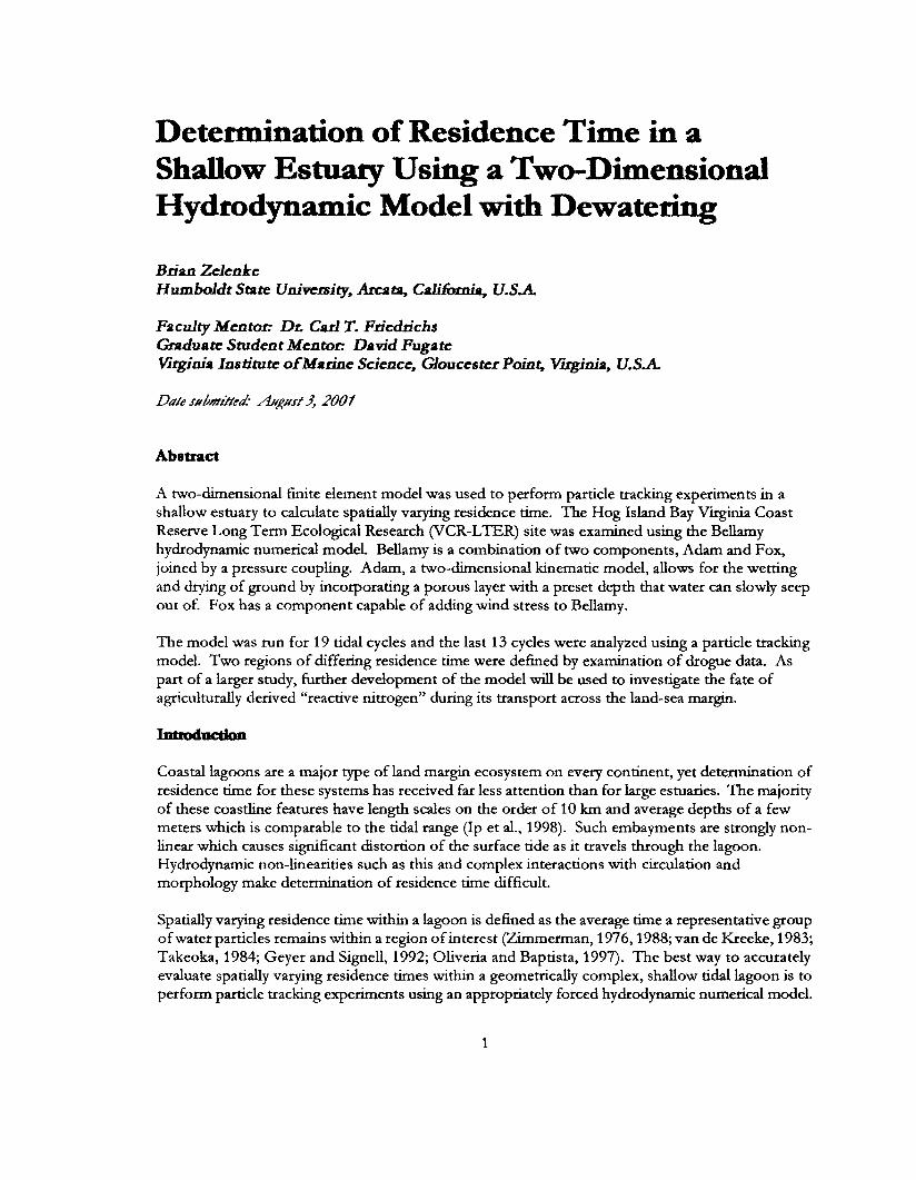
Once the finite element boundary was defined, bathymetric information was compiled. Highresolution bathymetric data for the region inside of Hog Island Bay was provided through the VCRLTER program. Hydrographic data sets from the National Oceanic and AtmosphericAdministration (NOAA) National Ocean Service (NOS) were used for those areas of the estuarysystem outside of Hog Island Bay. Where data in the NOS bathymetry was not sufficiently detailed,further data points taken from NOAA nautical charts were entered by hand using a MATLAB*routine written by David Fugate of the Virginia Institute of Marine Science (VIMS). The visualinspection and manual input abilities of this routine proved crucial in successful generation of themesh grid. By allowing the user to visually identify insufficiently resolved channels and streams andenter depth data points as needed, the routine made it much easier to define the bathymetry of thesefeatures longitudinally and laterally. Such refinements allowed the grid generator to map thesefeatures using multiple elements, thereby making transport calculations through channels andstreams viable. In addition, manual input of depth information was used to assign realistic, uniformheights to those marshes and mud flats for which there were no measured values (Figure 3).
4
37° 35'0
2
4
6
8.."C:\S 10'i....
Longitude 75°34'
Figure 3. Bathymetry of the Hog Island Bay estuary system.
FilfJle ElementModel(FEA1) GndGenerahon
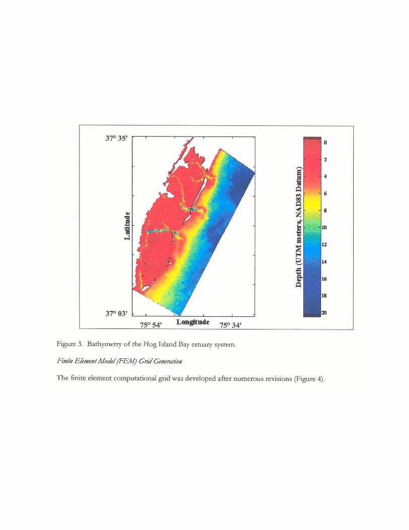
The finite element computational grid was developed after numerous revisions (Figure 4).
Cobb Island
t Machipongo Inlet
....-.I---Hog Island
370 ;J5l_-.-----r-......--r--.......-_
370 03' 1"--....... _
750
54' Loogitude 7!f> 34'
Figure 4. Finite element computational grid for the Hog Island Bay estuary system. The mesh iscomprised of 32391 elements, 17159 nodes, 1947 boundary nodes, and has a band width of 383.
BatTri, the program used to generate the grid, was written by Dr. Ata Bilgili from DartmouthCollege in New Hampshire. The manual for BatTri is included at the end of this paper as AppendixA. BatTri, a two-dimensional finite element grid generator «is a graphical Matlab interface to the Clanguage two-dimensional quality grid generator Triangle developed byJonathan Richard Shewchuk.BatTri does the mesh editing. bathymetry incorporation and interpolation, provides the gridgeneration and refinement properties, prepares the input file to Triangle and visualizes and saves thecreated grid (Appendix A)."
BatTri was used to divide the grid into two zones with differing maximum element sizes; anestuarine zone and an oceanic zone. In the oceanic zone, where the water was fast moving,elements were assigned a larger maximum area. Since the water in the Hog Island Bay study areamoves relatively slower, the estuarine zone was defined with smaller, high resolution triangles. Inthis way, a volume ofwater moving from one zone to another would be modeled with the samenumber of elements under similar velocity conditions (i.e., with a given velocity, a volume ofwaterwill travel farther over a deep channel than over a shallow marsh, so the channel elements arelarger). This element size refinement was achieved using a M2 Courant condition of 1000:
6
g.T2 .hArea=-=---
1000(1)
where g is acceleration due to gravity, T is the time-step, and h is the bathymetric height (A. Bilgili,personal communication, June 22, 2001).
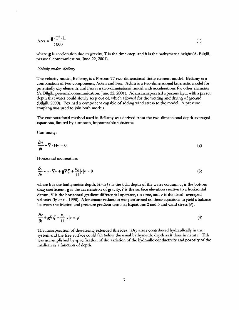
The velocity model, Bellamy, is a Fortran 77 two-dimensional fInite element model. Bellamy is acombination of two components, Adam and Fox. Adam is a two-dimensional kinematic model forpotentially dry elements and Fox is a two-dimensional model with accelerations for other elements(A. Bilgili, personal communication, June 22, 2001). Adamincorpotated a porous layer with a presetdepth that water could slowly seep out of, which allowed for the wetting and drying of ground(Bilgili, 2000). Fox had a component capable of adding wind stress to the model. A pressurecoupling was used to join both models.
The computational method used in Bellamy was derived from the two-dimensional depth-averagedequations, limited by a smooth, impermeable substrate:
Continuity:
&I-+V·Hv=O&
Horizontal momentum:
(2)
(3)
where h is the bathymetric depth, H=h+? is the tidal depth of the water column, Cd is the bottomdrag coefflcient, g is the acceleration of gravity, ? is the surface elevation relative to a horizontaldatum, V is the horizontal gradient differential operator, t is time, and v is the depth-averagedvelocity (lp et aI., 1998). A kinematic reduction was performed on these equations to yield a balancebetween the friction and pressure gradient terms in Equations 2 and 3 and wind stress (?):
()v +gV~ +.st Ivlv =VIOf: H
(4)
The incorporation of dewatering extended this idea. Dry areas contributed hydraulically in thesystem and the free surface could fall below the usual bathymetric depth as it does in nature. Thiswas accomplished by specifIcation of the variation of the hydraulic conductivity and porosity of themedium as a function of depth.
7
In order to run Bellamy, the program had to be provided with input parameters. Extensivedocumentation within the source code and the use of a separate parameter input file aided inmodifying the program to Hog Island Bay. A table of significant values is provided below:
Table 1. SimulationDescri tionDomainElevation boundary condition informationWind, Bottom Stress Law
Porous medium thicknessHydraulic conductivity of the porous layerMinimum porosity of the porous layerMinimum pressure gradientMaximum bottom friction coefficientNumber of total time-stepsTime-step incrementTime-stepping implicidy weighing parameterNumber of iterations er time-ste
Particle lrd£kiHg modeL- DrogueJDDT
s stem Vir .nia, U.S.A.Parameters
FEM grid information filesMz tidal amplitude and phase
Depth dependent Manning approach for bottomstress, no wind
1.00m3.16 X 10-4
0.3501.0 X 10-12
0.065700149 s1.00
4
Drogue tracking was performed with a three-dimensional time-stepping particle tracking programcalled Drogue3DDT, adjusted to run as a two-dimensional vertically averaged program (A. Bilgili,personal communication, June 22, 2001). Drogue tracks were visualized using FEDAR22 (finiteElement DAta Reviewer) and Ocean Processes Numerical Modeling Laboratory (OPNML)software from the University of North Carolina at Chapel Hill Department of Marine Sciences. Bycomparing plots of the drogue tracks for the entire run to images of drogue position at every rimestep, residence time was approximated.
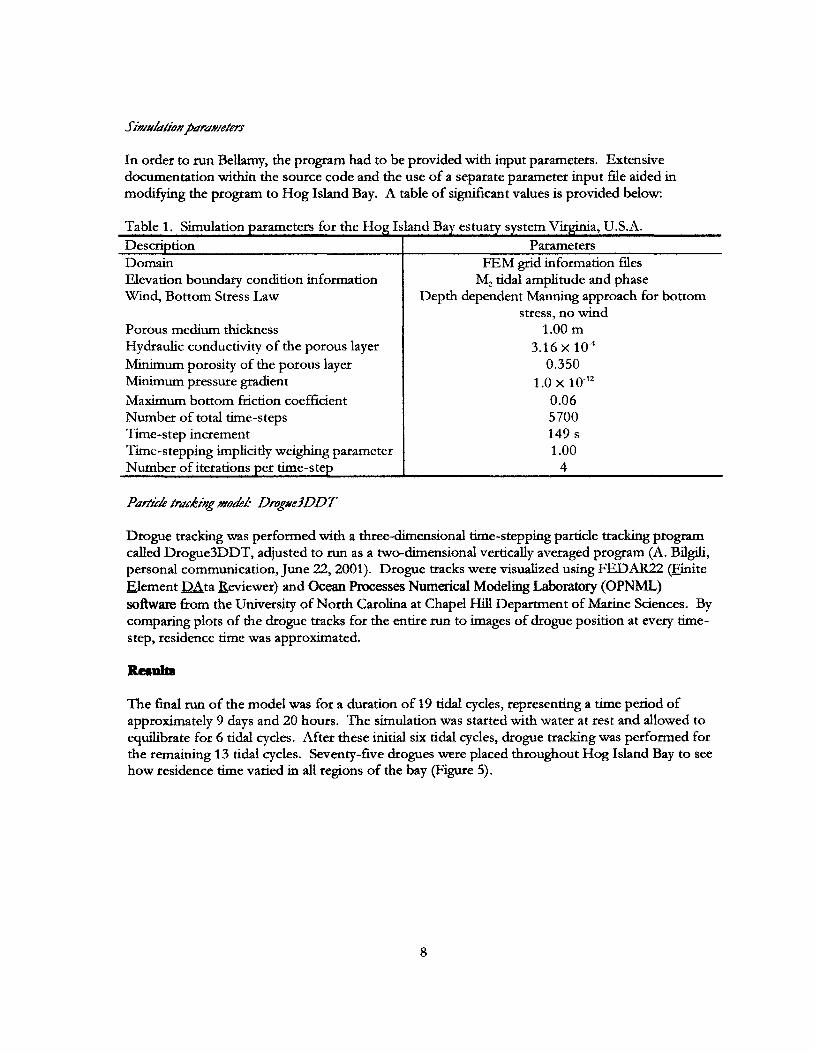
The final run of the model was for a duration of 19 tidal cycles, representing a time period ofapproximately 9 days and 20 hours. The simulation was started with water at rest and allowed toequilibrate for 6 tidal cycles. After these initial six tidal cycles, drogue tracking was performed forthe remaining 13 tidal cycles. Seventy-five drogues were placed throughout Hog Island Bay to seehow residence time varied in all regions of the bay (Figure 5).
8
31" 32'
31" 19'
1 Cycle
Figure 5. Initial drogue positions and residence time zones. Here. residence time was defined as thenumber of tidal cycles it took for a drogue to cross from inside Hog Island Bay out to the ocean.
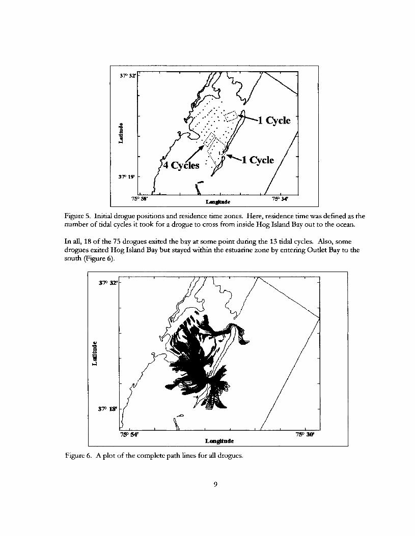
In all. 18 of the 75 drogues exited the bay at some point during the 13 tidal cycles. Also, somedrogues exited Hog Island Bay but stayed within the estuarine zone by entering Outlet Bay to thesouth (Figure 6).
370 32'
1/)11./
f(7fPM'
/f
750 30'
Figure 6. A plot of the complete path lines for all drogues.
9
In the model run presented in this paper the tidal cycle and other forcing factors were roughlydefined and only supported a first-order approximation of residence time. These initial resultssuggesting a tidal residence time of many days for much of Hog Island Bay are somewhat surprisinggiven that previous estimates were closer to one day (1. Anderson, personal communication, August1,2001). The residence time estimates presented here can be considered an upper limit on actualresidence time. Wind stress and lateral dispersion have not yet been included and will both tend toreduce residence time. The grid and the simulation parameters that govern the model have beencarefully developed but are still a work in progress. The effect of wind stress has not yet beenexamined. Further, the ability of Bellamy to use results from an earlier run on a subsequent run(dubbed a ''hot-start') is still under development.
This study began with the understanding that the ftrst calculation of residence time in Hog IslandBay would serve as an exercise to better understand how the Bellamy model could be applied to theestuary. This study was a clear success in that areas where the model needs to be refined are nowwell deftned. The grid and Bellamy as presented in this paper will continue to undergo revisions aspart of a multi-year study with the ultimate goal of relating biological transformations ofagriculturally derived nitrogen to physical transport processes within Hog Island Bay. Futuredevelopment of the Bellamy code will improve evaluation of the hypothesis that "because biologicalprocess rates mediated primarily by micro- and macroalgae and bacteria will exceed physicaltransport rates, removal of groundwater-derived and remineralized nitrogen within the lagoon bycoupled nitriftcation-denitrification as well as by immobilization into sediments will be more rapidthan export by tidal flushing (Anderson et al., 1999)." No matter the speciftc outcome, continueduse of Bellamy will, as it has already done, provide insight into the circulation dynamics of HogIsland Bay.
Anderson, I. c., C. T. Friedrichs (1999). Fate of "Reactive Nitrogen" Derived fromAgricultural Sources in Coastal Lagoons. USDA NRICGP Proposal, 27p.
Bilgill, A., et al. (2000). Modeling Tidal Flow in the Great Bay Estuary, New Hampshire,Using a Depth Averaged Flooding-Dewatering Model with Application to the Bed LoadTransport of Coarse Sediments. Proceedings ofAdvances in Fluid Mechanics 2000Conference.
Friedrichs, C. T. and O. S. Madsen (1992). Nonlinear diffusion of the tidal signal infrictionally dominated embayments. Journal of Geophysical Research 97, 5637-5650.
Friedrichs, C. T., D. R. Lynch, and D. G. Aubrey (1992). Velocity asymmetries infrictionally-dominated tidal embayments: longitudinal and lateral variability. Dynamics andExchanges in Estuaries and the Coastal Zone, Coastal and Estuarine Studies (prandle, D.,ed.) Vol. 40. AGU, Washington D. c., pp.277-312.
Geyer, W. R., and R. P. Signell (1992). A Reassessment of the Role of Tidal Dispersion inEstuaries and Bays. Estuaries, 2: 97-108.
10
Ip, J. T., D. R. Lynch, and C. T. Friedrichs (1998). Simulation of Estuarine Flooding andDewatering with Application to Great Bay, New Hampshire. Estuarine, Coastal, and ShelfSciences, 47: 119-142.
Katapodes, N. D. (1982). On zero-inertia and kinematic waves, ASCE. Journal ofHydraulic Engineering 108, 1380-1387.
Katapodes, N. D. (1984). Fourier analysis of dissipative FEM channel flow model, ASCE.Journal of Hydraulic Engineering 110, 927-944.
LeBlond, P. H. (1978). On tidal propagation in shallow rivers. Joumal of GeophysicalResearch 82, 4717-4712.
Lighthill, M. J. and G. B. Whitham (1955). On kinematic waves: I-flood movement in longrivers. Proceedings of the Royal Society London 229, 281-316.
Liong, S. Y., S. Selvalingam, and D. K Brady (1989). Roughness values for overland flow insibcatchments, ASCE. Journal ofIrrigation Drainage Engineering 115, 204, 214.
Murty, T. S. (1983). Diffusive kinematic waves versus hyperbolic long waves in tsunamipropagation. In Proceedings of the International Tsunami Symposium, August 1983,Hamburg (Bernard, E. N., Ed.). pp.1-22.
Oliveria, A. and A. M. Baptista (1997). Diagnostic Modeling of Residence Times inEstuaries. Water Resources Research, 33: 1935-1946.
Strelkoff, T. and N. D. Katapodes (1977). Border irrigation hydraulics with zero-inertia,ASCE. Journal of Irrigation and Drainage Engineering 103, 325-342.
Swift, M. R. and W. S. Brown (1983). Distribution of bottom stress and tidal energydissipation in a well-mixed estuary. Estuarine, Coastal, and Shelf Science 17, 297-317.
Takeoka, H. (1984). Fundamental Concepts of Exchange and Transport Time Scales in aCoastal Sea. Continental Shelf Research, 3: 311-326.
USACE (1981). HEC-1 Flood Hydrograph Package. U. S. Army Corps of Engineers,Hydrologic Engineering Center.
van de Kreeke,]. (1983). Residence Time: Application to Small Boat Basins. Journal ofWaterway, Port, Coastal, and Ocean Engineering, 109: 416-428
Wooding, R. A. (1965). A hydrologic model for the catchment-stream problem. I:Kinematic wave theory, Joumal of Hydrology 3.
Zimmerman,]. T F. (1976). Mixing and Flushing of Embayments in the Western DutchWadden Sea I: Distribution of Salinity and Calculation ofMixing Time Scales. NetherlandsJournal of Sea Research, 10: 149-191.
11

Zimmennan, J. T F. (1988). Estuarine Residence Times. In (B. Kjerfve, ed.):Hydrodynamics of Estuaries, Volume 1: Estuarine Physics. CRC Press, Boca Ration, FL,pp.75-84.
12

BatTri 2D FE GRID GENERATOR
Venion 7.2.01
BatTri is a graphical Matlab interface to the C language two-dimensional quality grid generator
Triangle developed by Jonathan Richard Shewchuk [email protected]). BatTri does the mesh
editing, bathymetry incorporation and interpolation, provides the grid generation and refinement
properties, prepares the input fue to Triangle and visualizes and saves the created grid. Triangle is
called within BatTri to generate and refine the actual grid using the constraints set forth by BatTri.
BatTri and Triangle are known to work on a number of platforms, induding SGI's, SUN's, Pentium
PC's under Linux (2.2.x and 2.4.x kernels), and Pentium PC's working under Windows. This version
of BatTri is known to work under both Matlab Rll and R12.
This report will summarize the usage of BatTri. For Triangle usage and definitions of Triangle
related fues and terms, reader is referred to the original Triangle web page at
htW:llwww.cs.cmu.edu/afs/cs/project/quake/public/www/triangle.html.HelpaboutTrianglecan
also be accessed by running Triangle with the -help option, i.e. "triangle -help> trianglehelp.txt".
DOWNLOADING AND INSTALLING BatTri, niB OPNML TOOLBOX AND
TIlB TRIANGLE MESH GBNERATOR
To be able to use BatTri, one should first download and install the following components:
JR. Shewchuk's Triangle mesh generator and Delaunay triangulator can be downloaded
from htW://www.cs.cmu.edu/afs/cs/project/quake/public/www/triangle.html.
Information on how to install and compile Triangle on various platforms can be found in
the README file induded in the package. For PC's working under Windows, GNU C
compiler "gec" works for compiling Triangle. You can get gec in the latest Cygwin
distribution from http://sources.redhat.com/cygwin. Triangle also includes an X display
13

program, called ShowMe. You can compile and install this in a Unix or Linux X
environment to achieve a faster grid display performance. Otherwise, Madab is used for
displaying meshes.
The most recent version of the OPNML toolbox can be downloaded from
http://www.opnml.unc.edu/OPNML Matlab. Make sure the location of the toolbox is
included in your Matlab path.
Finally, the latest verSlOn of BatTri can be downloaded from http://v.rv.lw
nml.dattmouth.edu/Software/BatTri in a gnu zipped tar format. To install, gunzip (gunzip
*.gz) and untar (tar -xvf*.tar) the distribution in a base directory. This will create a BatTri
directory in the base directory and copy all the files, including example directories, in it. The
last thing that needs to be done is to add the directory location of the BatTri to your Matlab
path.
Once Triangle, the OPNML toolbox and BatTri are correctly installed, the user should define the
location of the Triangle mesh generator and the ShowMe display package (if using Unix or Linux)
explicitly. This is done by changing the triangle-path and showme-path variables in
generate_mesh.m routine of the BatTri distribution. The path to the ShowMe display package
should only be defined if it is compiled and installed in Unix or Linux. Otherwise, comment this line
with a %.
INPut FILES AND BATHYMETRIC DATA
To generate a grid, the user should input the boundary node information, boundary segment
information and hole (or island) information in form of a .poly file, as described in the Triangle
manual (http://www.cs.cmu.edu/~quake/triangle.polJ'·.html).These input nodes and segments in
the .poly file are forced into the triangulation of the domain. Ifnecessary, all this information can be
created from an ordered coastline point data with the use of the editing options of BatTri (this
process may require manual deleting of unnecessary segments and nodes, closing of islands by
segment adding, addition of an open ocean boundary segment, etc...). As a starting point, ordered
14
digital coasdine node data can be extracted from the National Geophysical Data Center's webpage
(http://rimmer.ngdc.noaa.gov/coast/getcoast.html) at various scales ranging from 1:70,000 to
1:5,000,000. If the coasdine is very highly resolved, causing an excessive number of elements along
the shoreline, the routine "xy_simplify.m" can be used to reduce the number of nodes to the desired
resolution. Remember to format this data into a .poly file, consisting of nodes and segments, before
inputting into BatTri. To refine an already created grid, the user can input the above referenced
information either in the form of a previously created .poly file or in the form of NML standard
.nod, .ele and .bat files (see next section, Running BatTri).
Bathymetric data covering the entire domain should also be entered for generation and refinement.
There are three ways of accomplishing this:
- As gridded bathymetric data:
> >g=:generate_mesh(x,y,z)
where
z (MxN) grid of bathymetric depths, negative down from the datum.
x (1xN) x-coordinates of columns of z
y (Mx1) y-coordinates of rows of z.
- As scattered bathymetric data with a pre-defined triangulation (the triangulation is used for
interpolation and contouring):
> >g=generate_mesh(x,y,z,e);
where
x (Nx1) x-coordinates of depth measurements;
y (Nx1) y-coordinates of depth measurements;
z (Nxl) water depths at locations (x,y), negative down from the datum;
e (Kx3) vertex numbers for triangles in x and y.
- As scattered bathymetric data with no pre-defined triangulation (Delaunay triangulation is used for
interpolation):
15

> >g=generate_mesh(x,y,z);
where
x (Nxl) x-coordinates of depth measurements;
y (Nxl) y-coordinates of depth measurements;
z (Nxl) water depths at locations (x,y), negative down from the datum.
RUNNING DatTri
The Matlab command for running the mesh generator is:
generate_mesh(x,y,z,e)
Here, x, y, z, and e are as defined in the previous section with e being an optional input.
BatTri will then displays the defined Triangle and ShowMe (if compiled, installed and defined in
generate_mesh.m) paths. In the case the ShowMe path is deftned, BatTri will also ask you how the
mesh plotting will be handled during the current session. Enter either 1 to use ShowMe or 0 to use
Matlab. Remember that ShowMe is a faster option for grid plotting.
You will then be prompted to enter the filename of the final grid Cfinalgrid') that will be generated in
the BatTri session. This filename will be added the standard .nod, .ele and .bat Dartmouth NML
extensions. Note that the final bathymetry fue, .bat, will be positive down from the datum, unlike
the input bathymetric data, which is negative down from the datum. Also note that intermediate
.poly and Triangle grid files (.node and .ele) will be generated and saved every time the input .poly
file is changed during a BatTri session. These files will be saved under the filename
'finalgrid_triangle.#.*' where # is a number of iteration changed every time the grid is changed and
saved during the same BatTri session. Readhttp://www.cs.cmu.edu/-quake/triangle.iteration.htrnl
for more information.
16

You will then be prompted to enter the array of bathymetric contour values that will be drawn on
the screen when the input .poly ftle is displayed. The format is [Ct ,CZ,C3, ...,Cr.l for multiple contours
or [C] for a single contour, where C and ~,...Cr. are contour depths. Remember to precede these
with a (-) sign if they are below the datum. This contour plotting may help user to decide what
contour line should be drawn and transformed into edges whose presence will be forced into
triangulation during the mesh editing session. One can also use a contour line to divide high and low
resolution zones in a grid, as explained in the Mesh Editing section.
BatTri will then ask the user to enter the minimum depth for nodes in the grid. In the final mesh
with interpolated depths, any depth larger than this value will be truncated to the value of the
minimum depth. For example, on a ftnal NML grid with a Mean Sea Level (MSL) vertical datum, the
smallest depth value will be -0.5 m if the minimum depth parameter is set to +0.5 m at the
beginning of the mesh generation process.
The next step is to enter the name of the .poly ftle that you will edit or create a grid from. BatTri
gives 3 options at this stage:
-The ftrst option (0) is to start from scratch. When given this option, BatTri reads the previously
deftned bathymetric database (x,y,z) and draws the contours on the screen. If "plotting the locations
of the bathymetric data points" option is also chosen later on, the user can actually build the domain
boundary by zooming in and adding nodes and segments later on in the mesh editing process. The
bathymetric database limits should also deftne the domain boundary in this case.
- The second option (1) is to load a .poly file that you intend to edit. You can enter the explicit path
or just the name of the .poly file if it is in the current Matlab directory when prompted. Do not
forget to include the apostrophes.
- The third option (2) is to load a previously created NML type grid by loading its .nod, .ele, .bat and
.bnd files for editing. Enter the name of the grid in apostrophes, without any extensions.
17

If you choose the fttst option (0), the program will only ask you if you would like to plot
bathymetric data point locations. This is intended to be used if the bathymetric data is scattered and
has higWy variable density. After answering this question, it will switch to the mesh editing menu.
If you choose the second option (1), the program will ask you if there are any already defined islands
(or holes) in the input .poly ftle. Enter 1 for yes and 0 for no at this stage. Similarly, in the next
question, enter 1 if you already have defined zones (or regions) in your input .poly ftle or 0 if you
have no zones defmed. After answering these two questions, BatTri will ask you ifyou would like to
plot bathymetric data point locations for diagnostic purposes. At this stage, press either 1 for yes or
ofor no. As an example, this option is useful to check if your bathymetric data stays well within the
limits of your boundary defmed by the coastline. Assuming that the measured bathymetric data
locations have the correct coordinates and datum, one can then zoom in and move coastline nodes
accordingly so that the bathymetric data points will lay on the water and not on land. This is
especially useful in the case of domains with a number of narrow channels. The program will then
draw the boundary on the screen, together with any requested contours or bathymetric point
locations and switch to the editing mode in Madab command window.
If you choose the third option (2), the program will read the corresponding .nod, .ele and .bat ftles,
will ask you if you would like to plot bathymetric data point locations and will switch to the mesh
editing mode after you answer the question.
MESH BDITING
Mesh editing menu consists of 13 options:
Option 0 adds a contour line to the mesh. Unlike the input contour option to
generate_mesh.m, which only draws the contours on the screen, this actually adds nodes and
segments whose presence will be forced in the triangulation. One can use this to mesh along
contour lines (important for some hydrodynamic models with wetting and drying), to
increase resolution along a contour (to better resolve a shelf or sharp changes in bathymetry)
18

or to define various zones where different element criteria will be applied (like a higher
resolution zone shallower than the 10 meters and a lower resolution one deeper than 10
meters). Once the contour is extracted internally, the program asks user to choose between a
number of smoothing algorithms. These include box-car smoothing, spline smoothing,
Douglas and Peucker smoothing and no smoothing. Once the option number for the chosen
algorithm and smoothing variables for different methods are entered, the program requests
the user to input the node spacing (in meters) to be used when the contour will be
incorporated in the grid The user should choose a distance optimized for his/her purposes.
Giving a small value highly resolves the contour and creates a large number of nodes and
probably badly shaped elements too, because of resolution differences between the contour
line and the rest of the grid. One solution to this is to use an element inside angle constraint
(explained later), which will better the shape of these transition elements. Choosing a large
node spacing results in a smaller number of nodes but may fail to resolve the contour. If a
contour is going to be used to create zones (or regions) with Option 10, it is important to
connect its endpoints to domain boundary by adding segments. This will ensure that the
zones are going be enclosed in segments and not stay open.
Option 1 adds individual vertices to the grid using the left mouse button. Vertices can be
entered one after another. Right mouse button exits from the graphical interface and returns
to the MATI..AB command window mesh editing menu.
Option 2 removes vertices from the grid using the left mouse button. If a vertex is
connected to an edge, the edge will be moved from the domain also. Vertices can be
removed one after another. Right mouse button returns to the main menu.
Option 3 moves vertices on the screen. To choose the vertex to be moved, the user should
click the vertex with the left mouse button. To move the vertex, go to the new location with
your mouse and left click. This process can be repeated to move multiple vertices. Right
mouse button returns to the main editing menu.
Option 4 adds edges (or segments) to the grid. Segments are lines whose presence is
enforced in the final grid. To add an edge, one needs 2 vertices. First choose the first vertex
19
of the edge using the left mouse button and repeat the same thing to choose the second
vertex. A red line will connect these two vertices, defIning the edge. Edges can be formed
one after another. Right mouse button exits to the main editing menu.
Option 5 removes edges from the grid. To do this, the user should choose the edge to be
removed by clicking on the small circle whose center is located at the midpoint of the edge.
The circle will be marked with a red cross. Multiple edges can be chosen one after another.
To remove and return to the editing menu, hit the right mouse button. Deleting an edge
does not delete the corresponding vertices.
Option 6 divides an edge into a smaller number of segments. Choose the edge to be divided
in the same way as Option 5 and enter the number of pieces to divide the edge into in the
command window. This process cannot be repeated and the user should choose the main
mesh editing Option 6 as many times as the number of edges to be divided. This option is
helpful in dividing long open ocean boundary lines.
Option 7 adds a spline curve to the grid. User has an option to choose between a closed (0)
and an open (1) spline. Closed splines may be used to defIne simple islands (see Option 8) or
zones (see Option 10) while open splines can be used to create curved open ocean
boundaries. Spline nodes are entered one after another by clicking the left mouse button.
Clicking the right mouse button once will draw the spline on the screen using a red line. At
this stage, user can move the spline nodes around similarly to Option 3. Once one is happy
with the spline shape, clicking the right mouse button will exit to the editing menu and
program will ask for the desired node spacing along the spline. In choosing the node
spacing, same ideas as in Option 0 apply.
Option 8 adds holes (or islands) to the grid. Even if there are enclosed areas bounded by
segments in the grid, these are not treated as islands unless they they are defIned as islands.
An enclosed area is defIned as an island by entering the x and y coordinates of a random
point that lies inside the area of question. This is done by clicking the left mouse button.
Islands can be added repeatedly in one session. A red cross will mark closed zones that are
defIned as islands. Clicking the right mouse button exits to the main editing menu. One
20

should make sure that a zone defined as an island is actually closed by segments, otherwise,
the entire triangulation will be eaten away by Triangle until an edge is encountered.
Option 9 removes holes from the grid. Holes are removed by left clicking on red crosses
that define the individual islands. Multiple islands can be removed during one session. Right
mouse button exits to the main mesh editing menu.
Option 10 adds zones (or regions) to the grid using the same approach as in Option 8.
Zones are areas enclosed by segments where regional area constraints can be imposed on
elements. Zones are defmed the same way as islands, but they are marked with a green cross,
followed by the zone number. Area constraints are imposed using the zone numbers at the
preliminary mesh generation stage. The zone numbers start from one every time a zone
adding session is started, even if there were previously defIned zones. However, once zones
are added and the session is closed, they are renumbered correctly automatically.
Option 11 removes zones from the grid the same way as in Option 9.
Option 12 deletes nodes and corresponding edges found in a box defined by the user. The
box is defIned by clicking the left mouse button on one comer of the box and dragging it
until the other comer is reached. The nodes found in the box are marked with red crosses.
On the command window, enter 1 if you want to remove them from the grid or 0 if you
made a mistake and want to keep them in the grid. Clicking the right mouse button on the
graphics window exits to the main editing menu.
Option 13 exits from the mesh editing menu and saves the changes to the
"finalgrid_triangle.#.poly" me.
PRHUMINARY (FIRST-cUl) MESH GENERATION
First-cut mesh generation generates a preliminary grid from which the refIned one will be derived.
Since the refmement schemes included in BatTri are functions of element bathymetry and/or
21
element areas, this preliminary grid serves as a base and provides the input element area and depth
information that the reftnement schemes will use.
The user should be careful in choosing the input parameters to the preliminary grid process and
should ftnd a good optimization between the minimum angle constraint, maximum element area
constraint and the maximum number of nodes to add. Creating a very coarse ftrst-cut grid may
result in a poorly resolved domain where major bathymetric changes are missed, while creating a
very ftne one may result in an unnecessary excessive number of elements, increasing computation
time and system requirements. Having a ballpark idea about the scale of bathymetric changes in the
domain is a good place to start with in determining the input parameters. Channel-mudflat-marsh
widths, characteristic lengths of major bathymetric changes like sea mounts or series of sand waves
can provide some of the physical clues that the user may ftnd useful in determining the area and
inside angle constraints. The generation of a ftrst-cut grid is an iterative process that the user can
repeat in a trial and error loop if the generated preliminary grid is not satisfactory.
The input variables to preliminary mesh generation process are as follows:
MiDim.. aaate COD8tIaiat: This limits the maximum inside angle (in degrees) that an
element can have in the preliminary grid. For example, if this value is set to 25 degrees, no
elements will have any inside angles smaller than 25 degrees in the grid. Note that the angle
constraint does not apply to small angles between input segments; such angles cannot be
removed. If the minimum angle is 20.7 degrees or smaller, the triangulation algorithm is
theoretically guaranteed to terminate (assuming infUlite precision arithmetic, Triangle may
fail to terminate if you run out of precision). In practice, the algorithm often succeeds for
minimum angles up to 33.8 degrees. For highly refmed meshes, however, it may be necessary
to reduce the minimum angle to well below 20 to avoid problems associated with insufftcient
floating-point precision. The specifted angle may include a decimal point. Entering a value of
°voids this restriction.
Maxim.. elemeat area COD8tnUnt: This limits the maximum area that elements can have
in the preliminary grid. For example, if this is set to 50,000 m2, no elements whose area is
larger than 50,000 rrf will exist in the preliminary grid. If user has deftned zones using
22
Option 10 of the mesh-editing menu, he/she will be asked to enter different area constraints
for all of the deftned zones. If there are major differences between the element areas of
different zones, it is likely that elements with bad aspect ratios (i.e. small angles) will be
created at the common boundary of the zones. This problem can be solved by increasing or
just providing a minimum angle constraint on top of the area constraints for different
regions. Entering a relatively large number ensures that this constraint never gets into effect.
Mgimum IIDIIIber of BOdes 10 add: This is the maximum number of nodes (or Steiner
points) that can be added to the preliminary grid while trying to meet the constraints of
minimum angle and maximum area. Remember that this should be kept at a minimum,
which is optimized (using the angle and area constraints) to provide a nicely resolved and
discretized domain with the Delaunay property. IfTriangle can create a triangulation before
reaching the preset maximum number of nodes, this restriction never gets into effect. If one
does not want to restrict the number of nodes to add, the solution is to input a very large
number and Triangle will work freely without any restrictions. Be forewarned that this
number may result in a conforming triangulation that is not truly Delaunay, because Triangle
may be forced to stop adding points when the mesh is in a state where a segment is non
Delaunay and needs to be split. If so, Triangle will print a warning.
After all the input is provided, BatTri will call the grid generation program, Triangle, and the ftrst-cut
grid will be generated and saved into the current directory. The program will then display the
ftlenames for the new grid and some other input and output information (grid generation
milliseconds, number of input nodes, segments and holes, number of output nodes, elements, edges,
and boundary segments). Then the grid bathymetry (depths for newly created nodes) will be
interpolated using the input bathymetry database (x, y, z Matlab column vectors). The interpolation
may take a long time, depending on the number of newly created nodes. It is also normal to receive
interpolation warnings at this stage if there are any nodes whose horizontal locations are outside of
the bathymetry database. Depending on the results that the user derives from the diagnostic plotting
routines that are explained in the next section, the preliminary grid can be regenerated if it does not
meet the user's criteria by entering 0 when prompted by the program. Entering 1 proceeds to the
mesh reftnement step.
23
DIAGNOSTIC PLO'ITING OFmB PRBUMINARY GRID
During mesh reftnement it may be desirable to compute and plot characteristics of the mesh before
deciding how to reftne the mesh further. To facilitate mesh exploration during reftnement, the
subroutine diagnostic_plots.m is called between reftnements or can be called from the command
line:
> >diagnostic_plots(g, (optional)bat);
where g is a ftnite element mesh structure and bat is the BatTri bathymetry structure. If
diagnostic_plots.m is called from the command line, the user should convert the (x,y,z) coordinates
of the scattered or gridded bathymetric database to the BatTri bat structure using the xyz2bat.m
routine (running 'help xyz2bat' and/or 'help BatTriSttuets' should provide more information on this
and BatTri structures in general). Most of the plotting options implemented are for viewing which
areas of the current mesh will be affected by various constraint types. The inventory of plotting
options presented by diagnostic_plots.m is by no means all-inclusive. It is expected that the users
will add their own options to the menu. Each plotting option launches a new ftgure window in
which the user can zoom, rotate, and edit the plot with Matlab's figure window tools. The following
plotting options are supported:
b / [grad(b)*A] (OptiOH 0): This makes a colored patch ofh/fgrad(h)*A] function on the
elements of the current mesh. All variables are deftned as in the mesh reftnement menu (see
next section). If you plan to use a h/fgrad(h)*A] constraint in the next reftnement, you can
use the ftgure colorbar under the plot to select the value for the parameter alpha, so that
h/fgrad(h)*A] ;?; alpha. All elements that are colored with a color to the left of alpha on the
colorbar will be reftned by the constraint. The farther to the left on the colorbar, the more
the element will be reftned.
b / A (OphOH 1): Same as Option 0 but for h/A, instead of h/fgrad(h)*A].
24
1 / [grad(b)*AJ (Optioll 2) Same as Option 0 but for 1/[grad(h)*A], instead of
h/(grad(h)*A).
Bathymetry Plot (Optioll 3) : Plot the bathymetry of the mesh. This makes a colored patch
object of the mesh with the coloring corresponding to the depths of the nodes. The user
specifies a color axis so that they can focus on a particular bathymetric range.
Contour Comparison (OptioN 4) : This plots the contour mesh bathymetry on top of
database bathymetry. This option can be used to check that topographic features are
adequately resolved by the current grid's discretization. For example, if one were trying to
resolve a 10m deep dredged channel in a harbor whose out of channel depth was no deeper
than 5 m, one could contour the current mesh's 9 m isobath against that of the bathymetry
databases. If the database produces two non-intersecting (blue) curves denoting the edges of
the channel and the grid produces a series of elongated islands (red), then the channel has
not been properly resolved by the current mesh. A gradient or slope based refinement might
fix the issue by forcing more elements onto the "walls" of the channel. (You can check by
using plotting option 0 or 2). This option requires the bat structure to be input if
diagnostic_plots.m is manually run.
de1ta(b) / b (OphON 5) : This makes a colored patch object of delta(h)/h for each element.
delta(h)/h is defined as in mesh refinement Option 6.
Grid PlottitJg (OptWll 0): This makes a simple wire-frame drawing of the current mesh.
Minimum Angle Plot (OptiON 7) : This makes a colored patch of the element minimum
inside angles. Equilateral triangles appear red, while triangles with small angles are shifted
towards blue.
Element Quality Plot (Opholl 8): This makes a colored patch of each element's "quality"
measure. The quality of an element is defined as:
q =4*v3*A / (L t2+L/+L31,
25
where A is the area of the element and Lh ~ and L3 are the length of the sides. Equilateral
triangles have q =1. Elements with a low quality number can cause numerical problems.
Quit (Op/ion Jl) : This quits the diagnostic plotting menu and proceeds to the mesh
refinement section.
MESH REFINBMENT
The mesh refinement schemes of BatTri are a collection of simple depth dependent formulae whose
goal is to provide the grid generator Triangle with an array of maximum area constraints for refining
individual elements. As explained in http://www.cs.cmu.edu!-quakeltriangle.refine.html.Triangle
is able to impose different area constraints on each element of the triangulation, besides the
possibility of imposing one area constraint for all elements of the domain. This is done by creating
an .area file that has one line for each element of the grid consisting of the element number and the
corresponding maximum area that this specific element can have. If the area ofthe preliminary mesh
element is larger than the one specified in the .area file, Triangle divides that element into smaller
ones until the constraint is met. If it is smaller than the specified area, it is left unchanged. Elements
with no constraints are marked with -999 in the .area file.
Additional control is provided through selection of a bathymetric depth range to refine. This applies
a particular bathymetry based constraint only to elements which have one or more nodes with depth
inside the depth range or which straddle the depth range interval. Elements outside of the depth
range may still be refined due to the minimum angle constraint. If the user is interested in applying a
gradient based constraint to resolve sand waves in the near shore without overly refining the shelf
break, one could choose a depth range of r40 , 0] so that the gradient constraint wouldn't be
dominated by the shelf break. Choosing [-lof, In£] or [] will apply the constraint to the entire grid.
Another use for the depth range parameter is to avoid singularities of the constraints. Ifone wants a
mesh that handles wetting and drying and "0" bathymetric depth is referenced to mean low tide then
inevitably the hiA constraint (or wavelength constraint) will be unbounded near the low tide line.
To avoid this singularity the hiarea constraint can be applied to the depth range [-Inf, -0.5]. During
the next refinement, a constant area constraint can be applied to [-.5, In£].
26

When an element-by-element maximum area constraint is applied using depth dependent schemes, it
is possible to have sharp transitions between elements in areas where there is a sudden and large
change in domain bathymetry (i.e., continental shelf, marsh limits, etc...). Similarly to the zone
refinement of the preliminary grid, this unwanted problem can be solved by increasing the minimum
inside angle constraint, which wi11lead to a mesh with smoother transitions.
higDld(b) Re6D.ement (Option 0): lbis scheme uses the following formula to relate the
maximum element area to the average element depth and change in depth:
h/[(grad(h)*alpha] ~ A,
where h is the absolute value of the average element depth, grad(h) is the absolute value of
the gradient of h on the vertices of the element, alpha is a constraint ratio set by user and A
is the maximum element area to be imposed.
b ReBnement (Ophon I): lbis relates the maximum element area to depth linearly via a
simple factor a, according to:
h/alpha~ A
where h is the absolute value of the average element depth, alpha is a constraint ratio set by
user and A is the maximum element area to be imposed.
1IgDld(b) Refinement (Option 2): lbis scheme relates the maximum element area to the
change in bathymetry according to:
l/[grad(h)*alpha] ~ A .
Here, grad(h) is the absolute value of the gradient of average element depth h on the vertices
of the element, alpha is a constraint ratio set by user and A is the maximum element area to
be imposed.
Maximum Slope Re6neme.ot (OptiON 3) : This scheme refInes all elements whose
maximum slope with respect to the x or y axes along any edge is larger than a user set value.
Inputs are the threshold angle in degrees and the maximum element area required on the
elements. This option may be used to resolve the effects of local small bottom disturbances
27
like sand waves and boulders on small meshes. It is normal to have Matlab warnings of
"division by zero" in this scheme. These do not interfere with the fInal solution since the
maximum slope is f1ltered out and used.
Tidal Wavelength to Grid Size Re6.nement (Op/j(}11 4): 1bis scheme is based on the
Courant condition, which requires a higher grid resolution in shallower areas than deeper
water zones because of the slower wave celerities experienced in shallow water. The
maximum area that an element can have is calculated using the following formula:
[(g*h*T~/R1 ~ A.
Here, g is the gravitational acceleration in m/sec2, h is the average depth of an element in
meters, T is the tidal period of interest in seconds (44714.16 sec for l\.1z), R is the tidal
wavelength to grid size ratio set by the user and A is the maximum area that an element can
have in the flnal grid. An element minimum inside angle constraint may be needed to top the
Courant condition to smooth the grid by creating elements with better aspect ratios.
Constant Maximum Ares ReJiaement (Op/jol1 5) : 1bis imposes a constant maximum
element area constraint on all the elements of the domain, without using the bathymetry.
delta(b)/b Refinement (OphOIl If): 1bis scheme flrst checks to see if elements of the
current grid meet the
delta(h) /h ~ alpha
criteria. Here, delta(h)/h is deflned as:
delta(h)/h =(hmax -~J/hmin'
where ~ax is the depth of the deepest node on the element and ~in is the depth of the
shallowest. If delta(h)/h is less than or equal to the ratio alpha, the condition is satisfIed and
no reflnements are performed on that dement. If it is larger than alpha, the area of sub
elements in the reflned mesh can be no larger than another user defIned constant, 'tarea'.
Once the restrictions entered by the user are applied to the pre-cut triangulation and a refIned grid is
generated, BatTri asks the user to choose from a series of diagnostic plots explained in the next
section. Depending on the results shown by these plots, users can choose to end the refInement
28
process and proceed to the generation of the fmal grid (Option 1), to continue refining from the
current mesh (Option 0) or to go back n steps to a previous version of the grid if the current one is
not satisfactory at all (Option -1, -2, etc., depending on how many times the grid is refined in the
current BatTri session).
DIAGNOSTIC PLOTnNG OF THE RBFlNHD GRID
As in Diagnostic Plotting of the Preliminary Grid
CREATION OF THE FINAL GRID
If user chooses the Option 1 at the end of the refinement process, BatTri interpolates the grid
bathymetry. reduces the bandwidth of the mesh by using the Cuthill-McKee algorithm, displays the
initial and reduced half-bandwidths, together with mesh properties (number of nodes, number of
elements. number of boundary nodes. bandwidth) and exits. The ftnal grid will be saved in
Dartmouth NML standard mesh format under the ftlenames finalgridnod. finalgrid.de and
ftnalgrid.bat in the current directory (finalgrid' is the ftlename of the final mesh defined in the
Running BatTri section).
POSSIBLB FUrURH IMPROVEMENTS
The following bullets in no particular order summarize possible future improvements to BatTri that
we may implement depending on the reactions that we receive from users:
Capability to input a scanned geo-referenced map picture (jpeg) to digitize coastline and/or
bathymetry for scratch building;
Capability to move bathymetric data points and to change depth attributes manually;
Bathymetry based refmement by zone;
"On the fly" zone specification during refinement (i.e. re-defme zones as you refine);
Automatic identification of islands;
29

"Bathymetry approximation error" based constraints;
triangle2fe_struct.mex, fe_struct2triangle.mex (to speed up 1.0.);
scattered_contour.mex (speed up contouring).
ACKNOWLBDGEMENTS
We would like to thank B. Blanton (UNq, C. Denham (USGS), D. Fugate (VIMS), T. Gross
(NOAA), D.R Lynch (Dartmouth College), J. Manning (NMFS) and J. Veeramony (NRL) for their
many useful contributions of code and insights. Of course, our appreciation must also be extended
to J.R. Shewchuk for producing Triangle. This work was partly supported under NFS grant #97
163.
This manual is put together by Ata Bilgili ([email protected]) and Keston Smith
([email protected]). Please report all errors or comments to Ata Bilgili.
30