Embed Size (px)
Citation preview

Determination of the top mass at the LHC
with emphasis on the
theoretical uncertainties
Alexander Mitov
Cavendish Laboratory
Based on: Juste, Mantry, Mitov, Penin, Skands, Varnes, Vos, Wimpenny ’13 Frederix, Frixione, Mitov; to appear.

Top mass determination ... Alexander Mitov Edinburgh, 14 May 2014
Introduction: Why do we care about the top quark mass?
ü Precision EW tests: the place in collider physics that is most sensitive to mtop . With the discovery of the (presumably SM) Higgs boson the SM is complete and the tests are over-determined. Everything looks good. The “bottleneck” is the uncertainty on the W mass. Top mass will be competitive once the ultimate W mass precision (at LHC) is achieved. ü All other places in collider physics are even less sensitive to mtop . ü However: there is very strong dependence on mtop in models that rely on bottom-up approaches. These take some data at EW scale (measured) and then predict (through RG running) how the model looks at much larger scales, say O(MPlank). ü Two types of uncertainties appear:
ü Due to running itself
ü Due to boundary condition at EW. It is here mtop is crucial. ü Examples: o Higgs inflation. Model very predictive; relates SM and ΛCDM parameters. Agrees with Planck data. o Vacuum stability in SM. Change of 1 GeV in mtop shifts the stability bound for SM from 1011 to the Plank scale.
Chetyrkin, Zoller ’12-13 Bednyakov, Pikelner, Velizhanin `13
Bezrukov, Shaposhnikov ’07-’08 De Simone, Hertzbergy, Wilczek ’08
Degrassi, Di Vita, Elias-Miro, Espinosa, Giudice, Isidori, Strumia ‘12
This is the place where high precision in mtop is needed most.
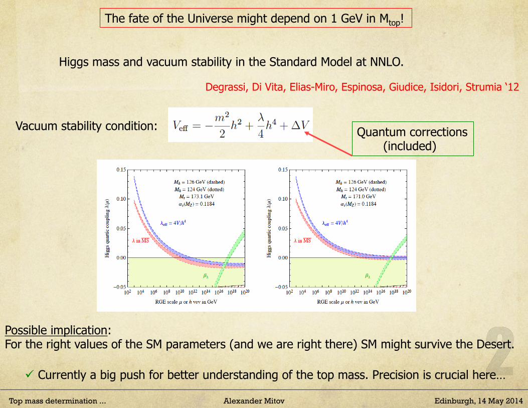
Higgs mass and vacuum stability in the Standard Model at NNLO.
Degrassi, Di Vita, Elias-Miro, Espinosa, Giudice, Isidori, Strumia ‘12
Top mass determination ... Alexander Mitov Edinburgh, 14 May 2014
The fate of the Universe might depend on 1 GeV in Mtop!
Quantum corrections (included)
Vacuum stability condition:
Possible implication: For the right values of the SM parameters (and we are right there) SM might survive the Desert.
ü Currently a big push for better understanding of the top mass. Precision is crucial here…

Top mass determination ... Alexander Mitov Edinburgh, 14 May 2014
ü The apparent sensitivity to mtop requires convincing mtop determination
ü What do I mean by convincing?
ü mtop is not an observable; cannot be measured directly.
ü It is extracted indirectly, through the sensitivity of observables to mtop
ü The implication: the “determined” value of mtop is as sensitive to theoretical modeling as it is to the measurement itself
ü The measured mass is close to the pole mass (top decays …)
ü One needs to go beyond the usual MC’s to achieve theoretical control
ü Lots of activity (past and ongoing). A big up-to-date review:
Juste, Mantry, Mitov, Penin, Skands, Varnes, Vos, Wimpenny ‘13
Introduction: goals regarding top mass determination at hadron colliders
Top mass determination ... Alexander Mitov Edinburgh, 14 May 2014
Ø A worry: can there be an additional systematic O(1 GeV) shift in mtop ?
Ø Two types of possible hidden errors: ü QCD related. As follows from the equation: the precision in mtop determination reflects the experimental uncertainty, as well as the error on the theory input. Unaccounted theory sources might have impact. Typical situation: using a MC to construct a likelihood and find the likeliest value of mtop. Combine with other methods/measurements to improve errors, etc. etc. At each step the error seemingly decreases. But this is not so, because we have irreducible error that the MC generator simply may not know about and no improvement in the measurement will take care of it. Such errors are the scariest since they are hidden (bias). ü bSM related. Unexplored territory. Conceptually the same as above, but the the role of higher order terms is now played by bSM physics: it contributes to the measurement but is not accounted for on the theory side. Basically, a kind of bias again.
Introduction: goals regarding top mass determination at hadron colliders

Issues in top mass determination
Top mass determination ... Alexander Mitov Edinburgh, 14 May 2014

Top mass determination ... Alexander Mitov Edinburgh, 14 May 2014
Introduction: issues in top mass determination
ü MC modeling.
Most methods for extraction of mtop rely on modeling the measured final state with typically LO+LL MC generators. The extracted mass then reflects the mass parameter in the corresponding MC generator. Identifying the nature of this mass parameter and relating it to common mass schemes, like the pole mass, is a non-trivial and open problem. It may be associated with ambiguities of order 1 GeV. The effect of the top and bottom masses on parton-shower radiation patterns is generally included already in the LO+LL MC’s and they screen collinear singularities.
Buckley, Butterworth, Gieseke et al Phys. Rep. ‘11
ü Non-perturbative corrections:
Mostly affect the MC modeling of the final state. Includes hadronization, color reconnection, Underlying Event, final state interactions (especially with jet vetoes). Many such systematics are accounted for through the JES. Color reconnection small at e+e- but O(500 MeV) at hadron colliders.
Recommendation: try methods with alternative systematics (unrelated to MC).
Top mass determination ... Alexander Mitov Edinburgh, 14 May 2014
Introduction: issues in top mass determination
ü Reconstruction of the top pair.
Typically, the existing methods for extraction of the top quark mass implicitly or explicitly rely on the reconstruction of the top pair from final state leptons and jets. This introduces uncertainties of both perturbative origin (through higher-order corrections) and non-perturbative origin (related to showering and non-factorizable corrections). Methods that do not rely on such reconstruction are therefore complementary and highly desirable; two examples are J/Ψ methods and dilepton distributions.
ü This is correlated with the attempt to define a pseudo top. How needed/useful is that?

Top mass determination ... Alexander Mitov Edinburgh, 14 May 2014
Introduction: issues in top mass determination
ü Alternative top mass definitions. Alternative mass definitions that reflect the physics are beneficial (known from e+e-). Less clear at hadron colliders.
ü Renormalon ambiguity in top mass definition.
Pole mass of the top quark suffers from the so-called renormalon ambiguity. This implies an additional irreducible uncertainty of several hundred MeV's on the top pole mass. Not an issue for short distance masses. Currently, at hadron colliders, this is a subdominant uncertainty.
ü Higher-order corrections.
Important source of uncertainty. State of the art NLO QCD; not always included.

Top mass determination ... Alexander Mitov Edinburgh, 14 May 2014
Introduction: issues in top mass determination
ü Unstable top and finite top width effects.
Understood for e+e-. Computed at NLO for hadron colliders. Could affect certain distributions. Not really used so far in top mass studies.
ü Bound-state effects in top pair production at hadron colliders. When the ttbar pair is produced with small relative velocity (i.e. close to threshold) bound-state formation begins. These effects can affect the shape of differential distributions within few GeV away from the threshold. Special care must be taken if a measurement is sensitive to such effects. In usual “inclusive” observables (like total x-section) this effect is diluted to about 1%.
Melnikov, Schulze

Methods for mtop determination
Top mass determination ... Alexander Mitov Edinburgh, 14 May 2014

Top mass determination ... Alexander Mitov Edinburgh, 14 May 2014
Methods for mtop determination: Matrix Element Methods
ü The backbone of the Tevatron studies as well as the most precise LHC ones. Performed in all final states.
ü Measured objects are compared with expectations from the LO tt production and decay diagrams convoluted with the detector response.
ü Method’s power comes from the fact that the likelihood for each event to be consistent with both tt and background production is calculated; greater weight is assigned to events that are more likely to be from tt when measuring mtop.
ü Issue: incorrect modeling due to missing theory corrections.

Top mass determination ... Alexander Mitov Edinburgh, 14 May 2014
Methods for mtop determination: Matrix Element Methods
Projections based on CMS lepton-plus-jet analysis:
ü Projections beyond 14 TeV require full detector simulation. Not done here.
ü Pileup and UE become more important at higher energy/pileup.
ü ISR/FSR become dominant uncertainties at high luminosity (unlike current measurements)
ü Extra 300MeV uncertainty added by hand.

Top mass determination ... Alexander Mitov Edinburgh, 14 May 2014
Methods for mtop determination: CMS endpoint method
A kinematical method: utilizes the strong correlation between the maximum of the Mbl distribution and mtop.
ü ISR/FSR and pileup do not play a role at high luminosity. (unlike conventional methods)
ü Does not rely on MC for internal calibration (analytical with data-driven backgrounds).
ü Less likely to be affected by bSM corrections.
ü Nonetheless, higher order effects do affect the endpoint position (particularly top widths) NLO calculations do exist – not utilized.

Top mass determination ... Alexander Mitov Edinburgh, 14 May 2014
Methods for mtop determination: J/Ψ method
A different method: no reconstruction is involved. Known at NLO.
Estimates from NLO QCD. NNLO accuracy assumed in some extrapolations. Main source: B-fragmentation. Likely will be irreducible unless new e+e- data.
(see also)

Top mass determination ... Alexander Mitov Edinburgh, 14 May 2014
Methods for mtop determination: mtop from kinematic distributions
ü Total cross-section:
Allows extraction with about 3% uncertainty due to limited sensitivity to mtop .
Ø Positive features: Good theory control (NNLO) Small non-perturbative and width effects Ø Negatives: Small sensitivity (unlikely to improve) ü At present there are inconsistently applied acceptance corrections (i.e. LO or NLO not NNLO). Still, likely a small effect.
Latest Tevatron Combination: 1309.7570

Top mass determination ... Alexander Mitov Edinburgh, 14 May 2014
Methods for mtop determination: mtop from kinematic distributions
ü Extraction suggested from tt+jet. Estimates for contributions from unknown corrections – below 1 GeV. Method is MC dependent and involves t (tbar) reconstruction
ü Dilepton distributions
Ø No reconstruction
Ø Minimal shower and NP sensitivity. Reliably computable at fixed order.
Ø Potential for 14 TeV at 1.5 GeV.
Ø Further studies in progress
Frederix, Frixione, Mitov, in progress. <<< Second part of the talk

Top mass determination ... Alexander Mitov Edinburgh, 14 May 2014
e+e- colliders
ü The machine where the ultimate precision of 100MeV or less can be achieved.
ü Best approach is threshold scan.
ü Continuum production also possible.
ü Similar at ILC and CLIC.
ü Interesting question: is it possible to measure mtop at c.m. energy of, say, 250GeV, i.e. below the threshold?
ü Given the presumed ILC schedule this might imply few more years of waiting …
Top mass determination ... Alexander Mitov Edinburgh, 14 May 2014
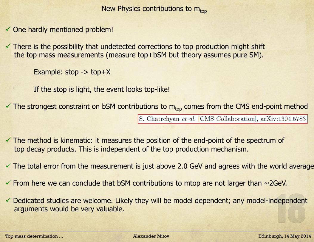
New Physics contributions to mtop
ü One hardly mentioned problem!
ü There is the possibility that undetected corrections to top production might shift the top mass measurements (measure top+bSM but theory assumes pure SM).
Example: stop -> top+X
If the stop is light, the event looks top-like!
ü The strongest constraint on bSM contributions to mtop comes from the CMS end-point method
ü The method is kinematic: it measures the position of the end-point of the spectrum of top decay products. This is independent of the top production mechanism.
ü The total error from the measurement is just above 2.0 GeV and agrees with the world average.
ü From here we can conclude that bSM contributions to mtop are not larger than ~2GeV.
ü Dedicated studies are welcome. Likely they will be model dependent; any model-independent arguments would be very valuable.

Top mass from leptonic distributions
Top mass determination ... Alexander Mitov Edinburgh, 14 May 2014
Frederix, Frixione, Mitov; to appear

Top mass determination ... Alexander Mitov Edinburgh, 14 May 2014
The message I’d like to convey: the questions I raised so far are not “academic”.
Example: look at the spread across current measurements
Ø Current World Average: mtop= 173.34±0.76 GeV
Ø New CMS (l+j): mtop= 172.04 ± 0.19 (stat.+JSF) ± 0.75 (syst.) GeV.
arXiv:1403.4427 TOP-14-001
Comparable uncertainties; rather different central values!
This is possible in the context of my discussion: different theory systematics.

Top mass determination ... Alexander Mitov Edinburgh, 14 May 2014
In order to properly understand and estimate the theory systematics we propose a particular observable
Contents
1. Introduction 1
2. The method 1
2.1 Definition of moments 2
2.2 Extraction of the top mass and its uncertainties 3
2.3 Deriving the functions fC,U,L(mt) 4
2.4 Computation of moments in the context of event generation 6
3. Detailed study of the theory systematics 7
4. Results 7
5. Conclusions 7
A. Correlation matrices 8
1. Introduction
2. The method
In this paper we study the determination of the top quark pole mass mt from di↵erential
distributions of dileptons in tt̄ events:
pp ! tt̄+X, with : t ! W + b+X and W ! `+ ⌫`. (2.1)
We consider the LHC at 8 TeV. Events are required to have two opposite charged leptons
(electron and/or muon) and two b-flavored jets, with b-jets defined through an anti-kTalgorithm [1] of size R = 0.5. The events are subject to a standard set of cuts:
|⌘`| 2.4 , |⌘b| 2.4 ,
pT,` � 20 GeV , pT,b � 30 GeV . (2.2)
If more than two b-jets are present then we take the two hardest ones. In this work we
consider only pure tt̄ signal and do not include any backgrounds. more about this in
conclusions
The definition of the observable possesses several important properties:
• It is inclusive of hadronic radiation, which makes it well-defined to all perturbative
orders in the strong coupling,
– 1 –
These are ttbar dilepton events, subject to standard cuts:
Contents
1. Introduction 1
2. The method 1
2.1 Definition of moments 2
2.2 Extraction of the top mass and its uncertainties 3
2.3 Deriving the functions fC,U,L(mt) 4
2.4 Computation of moments in the context of event generation 6
3. Detailed study of the theory systematics 7
4. Results 7
5. Conclusions 7
A. Correlation matrices 8
1. Introduction
2. The method
In this paper we study the determination of the top quark pole mass mt from di↵erential
distributions of dileptons in tt̄ events:
pp ! tt̄+X, with : t ! W + b+X and W ! `+ ⌫`. (2.1)
We consider the LHC at 8 TeV. Events are required to have two opposite charged leptons
(electron and/or muon) and two b-flavored jets, with b-jets defined through an anti-kTalgorithm [1] of size R = 0.5. The events are subject to a standard set of cuts:
|⌘`| 2.4 , |⌘b| 2.4 ,
pT,` � 20 GeV , pT,b � 30 GeV . (2.2)
If more than two b-jets are present then we take the two hardest ones. In this work we
consider only pure tt̄ signal and do not include any backgrounds. more about this in
conclusions
The definition of the observable possesses several important properties:
• It is inclusive of hadronic radiation, which makes it well-defined to all perturbative
orders in the strong coupling,
– 1 –
Ø Construct the distributions from leptons only Ø Require b-jets within the detector (i.e. integrate over)
label kinematic distribution
1 pT (`+)
2 pT (`+`�)
3 M(`+`�)
4 E(`+) + E(`�)
5 pT (`+) + pT (`�)
Table 1: The set of kinematic distributions used in this paper and their labelling conventions.
The definition of the observable possesses several important properties:
• It is inclusive of hadronic radiation, which makes it well-defined to all perturbative
orders in the strong coupling,
• It does not require the reconstruction of the t and/or t̄ quarks (indeed we do not even
speak of t quark),
• Due to its inclusiveness, the observable is as little sensitive as possible to modelling
of hadronic radiation. This feature increases the reliability of the theoretical calcu-
lations.
The extraction of the top quark pole mass utilises the sensitivity of shapes of kinematic
distributions to the value of mt. The set of distributions considered in this paper are given
in table 1.
It is cumbersome to work directly with distributions. Instead, we utilise their first four
moments. The moments are defined in section 2.1 below. The idea of the method studied
in this paper is to predict the mt dependence of the moments and then extract the value
of mt by comparing the predicted and measured values of those moments. The procedure
is detailed in section 2.2 below.
The use of moments for the extraction of the top mass mt has been used previously in
the context of the so-called J/ method [2]. The most up-to-date theoretical treatment of
this method is in Ref. [3]. Let us also mention that other discrete parameters of kinematic
distributions, like medians and maxima, could also be utilized for top mass extraction. In
this paper we choose to work with moments because of the ease of their calculation and
also because higher moments can easily be studied, as we do in this paper.
2.1 Definition of moments
We denote by � and d� the total and fully-di↵erential tt̄ cross section respectively (possibly
within cuts), so that:
� =
Z
d� , (2.3)
where the integral in understood over all degrees of freedom. Given an observable O (i.e.
one of the distributions in table 1), its normalised moments are defined as follows:
µ(i)O =
1
�
Z
d�O i , (2.4)
– 2 –

Top mass determination ... Alexander Mitov Edinburgh, 14 May 2014
label kinematic distribution
1 pT (`+)
2 pT (`+`�)
3 M(`+`�)
4 E(`+) + E(`�)
5 pT (`+) + pT (`�)
Table 1: The set of kinematic distributions used in this paper and their labelling conventions.
The definition of the observable possesses several important properties:
• It is inclusive of hadronic radiation, which makes it well-defined to all perturbative
orders in the strong coupling,
• It does not require the reconstruction of the t and/or t̄ quarks (indeed we do not even
speak of t quark),
• Due to its inclusiveness, the observable is as little sensitive as possible to modelling
of hadronic radiation. This feature increases the reliability of the theoretical calcu-
lations.
The extraction of the top quark pole mass utilises the sensitivity of shapes of kinematic
distributions to the value of mt. The set of distributions considered in this paper are given
in table 1.
It is cumbersome to work directly with distributions. Instead, we utilise their first four
moments. The moments are defined in section 2.1 below. The idea of the method studied
in this paper is to predict the mt dependence of the moments and then extract the value
of mt by comparing the predicted and measured values of those moments. The procedure
is detailed in section 2.2 below.
The use of moments for the extraction of the top mass mt has been used previously in
the context of the so-called J/ method [2]. The most up-to-date theoretical treatment of
this method is in Ref. [3]. Let us also mention that other discrete parameters of kinematic
distributions, like medians and maxima, could also be utilized for top mass extraction. In
this paper we choose to work with moments because of the ease of their calculation and
also because higher moments can easily be studied, as we do in this paper.
2.1 Definition of moments
We denote by � and d� the total and fully-di↵erential tt̄ cross section respectively (possibly
within cuts), so that:
� =
Z
d� , (2.3)
where the integral in understood over all degrees of freedom. Given an observable O (i.e.
one of the distributions in table 1), its normalised moments are defined as follows:
µ(i)O =
1
�
Z
d�O i , (2.4)
– 2 –
The top mass is extracted from the shapes of the following distributions: (not normalizations)
Working with distributions directly is cumbersome. Instead, utilize the first 4 moments of each distribution
label kinematic distribution
1 pT (`+)
2 pT (`+`�)
3 M(`+`�)
4 E(`+) + E(`�)
5 pT (`+) + pT (`�)
Table 1: The set of kinematic distributions used in this paper and their labelling conventions.
The definition of the observable possesses several important properties:
• It is inclusive of hadronic radiation, which makes it well-defined to all perturbative
orders in the strong coupling,
• It does not require the reconstruction of the t and/or t̄ quarks (indeed we do not even
speak of t quark),
• Due to its inclusiveness, the observable is as little sensitive as possible to modelling
of hadronic radiation. This feature increases the reliability of the theoretical calcu-
lations.
The extraction of the top quark pole mass utilises the sensitivity of shapes of kinematic
distributions to the value of mt. The set of distributions considered in this paper are given
in table 1.
It is cumbersome to work directly with distributions. Instead, we utilise their first four
moments. The moments are defined in section 2.1 below. The idea of the method studied
in this paper is to predict the mt dependence of the moments and then extract the value
of mt by comparing the predicted and measured values of those moments. The procedure
is detailed in section 2.2 below.
The use of moments for the extraction of the top mass mt has been used previously in
the context of the so-called J/ method [2]. The most up-to-date theoretical treatment of
this method is in Ref. [3]. Let us also mention that other discrete parameters of kinematic
distributions, like medians and maxima, could also be utilized for top mass extraction. In
this paper we choose to work with moments because of the ease of their calculation and
also because higher moments can easily be studied, as we do in this paper.
2.1 Definition of moments
We denote by � and d� the total and fully-di↵erential tt̄ cross section respectively (possibly
within cuts), so that:
� =
Z
d� , (2.3)
where the integral in understood over all degrees of freedom. Given an observable O (i.e.
one of the distributions in table 1), its normalised moments are defined as follows:
µ(i)O =
1
�
Z
d�O i , (2.4)
– 2 –
for any non-negative integer i. In this way, one has:
µ(0)O = 1 , µ
(1)O = hOi , µ
(2)O = hO2i = �2
O +⇣
µ(1)O
⌘2, (2.5)
and so forth. We would like to stress that in the calculation of moments we always compute
the total and di↵erential cross-sections (i.e. the denominator and numerator of Eq. (2.4))
subjected to the same set of cuts; see Eq. (2.2).
2.2 Extraction of the top mass and its uncertainties
The method for extracting mt from the ith moment of any one of the observables O given
in table 1 is given schematically in fig. 1. The x and y axes of fig. 1 are associated with
µD
µD−
µD+
m Cm E− m T− m T+ m E+
fC
fL
fU
Figure 1: Graphic representation of the method used in this paper to extract the top mass fromany moment of any given observable.
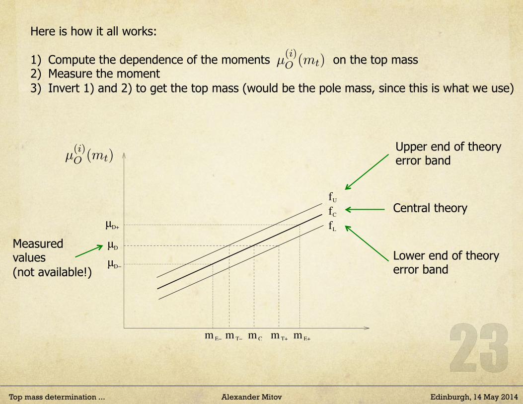
the top pole mass mt and the ith moment µ(i)O , respectively. The three lines fC , fU , and
fL represent the central, upper, and lower theoretical predictions for µ(i)O (mt) respectively.
These functions are linear and we explain how they are computed in section 2.3.
Given the data 1
µD+�+
µ
���µ, (2.6)
with
��µ = µD � µD� , �+
µ = µD+ � µD , (2.7)
the extracted top mass will be (see fig. 1):
mt = mC+�+
mT
���mT
+�+mE
���mE
. (2.8)
1Despite the large number of tt̄ dilepton events accumulated so far at the LHC no measurement of these
moments is available at present.
– 3 –
Note: both are subject to cuts (or no cuts); we tried both.
Top mass determination ... Alexander Mitov Edinburgh, 14 May 2014
and so forth. We would like to stress that in the calculation of moments we always compute
the total and di↵erential cross-sections (i.e. the denominator and numerator of Eq. (2.4))
subjected to the same set of cuts; see Eq. (2.2).
2.2 Extraction of the top mass and its uncertainties
The method for extracting mt from the ith moment of any one of the observables O given
in table 1 is given schematically in fig. 1. The x and y axes of fig. 1 are associated with
µD
µD−
µD+
m Cm E− m T− m T+ m E+
fC
fL
fU
Figure 1: Graphic representation of the method used in this paper to extract the top mass fromany moment of any given observable.
the top pole mass mt and the ith moment µ(i)O , respectively. The three lines fC , fU , and
fL represent the central, upper, and lower theoretical predictions for µ(i)O (mt) respectively.
These functions are linear and we explain how they are computed in section 2.3.
Given the data 1
µD+�+
µ
���µ, (2.6)
with
��µ = µD � µD� , �+
µ = µD+ � µD , (2.7)
the extracted top mass will be (see fig. 1):
mt = mC+�+
mT
���mT
+�+mE
���mE
. (2.8)
We define the central value and theoretical uncertainties associated with such an ex-
traction as follows:
��mT = mC �mT� , �+
mT = mT+ �mC , (2.9)1Despite the large number of tt̄ dilepton events accumulated so far at the LHC no measurement of these
moments is available at present.
– 3 –
Here is how it all works: 1) Compute the dependence of the moments on the top mass 2) Measure the moment 3) Invert 1) and 2) to get the top mass (would be the pole mass, since this is what we use)
Upper end of theory error band
Central theory
Lower end of theory error band
and so forth. We would like to stress that in the calculation of moments we always compute
the total and di↵erential cross-sections (i.e. the denominator and numerator of Eq. (2.4))
subjected to the same set of cuts; see Eq. (2.2).
2.2 Extraction of the top mass and its uncertainties
The method for extracting mt from the ith moment of any one of the observables O given
in table 1 is given schematically in fig. 1. The x and y axes of fig. 1 are associated with
µD
µD−
µD+
m Cm E− m T− m T+ m E+
fC
fL
fU
Figure 1: Graphic representation of the method used in this paper to extract the top mass fromany moment of any given observable.
the top pole mass mt and the ith moment µ(i)O , respectively. The three lines fC , fU , and
fL represent the central, upper, and lower theoretical predictions for µ(i)O (mt) respectively.
These functions are linear and we explain how they are computed in section 2.3.
Given the data 1
µD+�+
µ
���µ, (2.6)
with
��µ = µD � µD� , �+
µ = µD+ � µD , (2.7)
the extracted top mass will be (see fig. 1):
mt = mC+�+
mT
���mT
+�+mE
���mE
. (2.8)
We define the central value and theoretical uncertainties associated with such an ex-
traction as follows:
��mT = mC �mT� , �+
mT = mT+ �mC , (2.9)1Despite the large number of tt̄ dilepton events accumulated so far at the LHC no measurement of these
moments is available at present.
– 3 –
Measured values (not available!)

Top mass determination ... Alexander Mitov Edinburgh, 14 May 2014
How to compute the theory error band for ?
and so forth. We would like to stress that in the calculation of moments we always compute
the total and di↵erential cross-sections (i.e. the denominator and numerator of Eq. (2.4))
subjected to the same set of cuts; see Eq. (2.2).
2.2 Extraction of the top mass and its uncertainties
The method for extracting mt from the ith moment of any one of the observables O given
in table 1 is given schematically in fig. 1. The x and y axes of fig. 1 are associated with
µD
µD−
µD+
m Cm E− m T− m T+ m E+
fC
fL
fU
Figure 1: Graphic representation of the method used in this paper to extract the top mass fromany moment of any given observable.
the top pole mass mt and the ith moment µ(i)O , respectively. The three lines fC , fU , and
fL represent the central, upper, and lower theoretical predictions for µ(i)O (mt) respectively.
These functions are linear and we explain how they are computed in section 2.3.
Given the data 1
µD+�+
µ
���µ, (2.6)
with
��µ = µD � µD� , �+
µ = µD+ � µD , (2.7)
the extracted top mass will be (see fig. 1):
mt = mC+�+
mT
���mT
+�+mE
���mE
. (2.8)
We define the central value and theoretical uncertainties associated with such an ex-
traction as follows:
��mT = mC �mT� , �+
mT = mT+ �mC , (2.9)1Despite the large number of tt̄ dilepton events accumulated so far at the LHC no measurement of these
moments is available at present.
– 3 –
Ø Compute for a finite number of mt values:
and so forth. We would like to stress that in the calculation of moments we always compute
the total and di↵erential cross-sections (i.e. the denominator and numerator of Eq. (2.4))
subjected to the same set of cuts; see Eq. (2.2).
2.2 Extraction of the top mass and its uncertainties
The method for extracting mt from the ith moment of any one of the observables O given
in table 1 is given schematically in fig. 1. The x and y axes of fig. 1 are associated with
µD
µD−
µD+
m Cm E− m T− m T+ m E+
fC
fL
fU
Figure 1: Graphic representation of the method used in this paper to extract the top mass fromany moment of any given observable.
the top pole mass mt and the ith moment µ(i)O , respectively. The three lines fC , fU , and
fL represent the central, upper, and lower theoretical predictions for µ(i)O (mt) respectively.
These functions are linear and we explain how they are computed in section 2.3.
Given the data 1
µD+�+
µ
���µ, (2.6)
with
��µ = µD � µD� , �+
µ = µD+ � µD , (2.7)
the extracted top mass will be (see fig. 1):
mt = mC+�+
mT
���mT
+�+mE
���mE
. (2.8)
We define the central value and theoretical uncertainties associated with such an ex-
traction as follows:
��mT = mC �mT� , �+
mT = mT+ �mC , (2.9)1Despite the large number of tt̄ dilepton events accumulated so far at the LHC no measurement of these
moments is available at present.
– 3 –
with
mC = f�1C (µD) , mT� = f�1
U (µD) , mT+ = f�1L (µD) . (2.10)
We recall that the functions fC,U,L are linear and therefore their inversion is trivial.
In keeping with fig. 1, we define the experimental errors as:
��mE = mC �mE� , �+
mE = mE+ �mC , (2.11)
with
mE� = f�1C (µD�) , mE+ = f�1
C (µD+) . (2.12)
It is easy to convince oneself that the much more conservative choice:
mE� = f�1U (µD�) , mE+ = f�1
L (µD+) , (2.13)
is not correct, since it leads to non-zero uncertainties also in the case of null experimental
errors. In this paper, we shall not consider the experimental uncertainties any longer,
and be concerned only with the theoretical ones. We point out that the size of these
depend on two factors: the uncertainty on the theoretical predictions for µ(i)O , which is
fU (mt)� fC(mt) or fC(mt)� fL(mt), and the slope of fC(mt): the steeper the latter, the
smaller the errors on the extracted values of mt.
2.3 Deriving the functions fC,U,L(mt)
The linear functions fC,U,L(mt) are defined in the following way. First, we compute the
moment µ(i)O (mt) eleven times, once for each value in the discrete set:
mt = (168, 169, . . . , 178) GeV . (2.14)
For each of the mt values in Eq. (2.14) we determine the central value for the moment
µ(i)O (mt) together with its upper and lower uncertainties. The latter are defined as the sum
in quadrature of the corresponding scale and PDF uncertainties. 2 On figure 2 we give
as an example the calculation of µ(1)1 (mt) i.e. the first moment (i=1) of the distribution
pT,`+ (distribution 1 from table 1). Both calculations use the dynamic scale (2.16) and are
subject to the standard cuts (2.2) (left) or no cuts at all (right). We have computed them
with the help of the setup 4 given in table 2 below.
The scale variation [5] is based on an independent variation of the renormalisation and
factorisations scales, subject to the constraint
0.5 ⇠F , ⇠R 2 , (2.15)
where ⇠F,R = µF,R/µ̂ and µ̂ is a reference scale. The central choice is given by ⇠F = ⇠R = 1.
Eq. (2.15) is a conservative scale variation which estimates well the missing higher order
2For all calculations we have used the MSTW2008 [6] pdf sets at LO or NLO, as appropriate, depending
on the fixed order accuracy of our calculations; see table 2.
– 4 –
166 168 170 172 174 176 178
55.5
56.0
56.5
57.0
57.5
58.0
168 170 172 174 176 178
49.5
50.0
50.5
51.0
51.5
Figure 2: Evaluation of the first moment of the distribution of pT,`+ with scale (2.16) subjectto cuts (2.2) (left) and no cuts (right). The three lines represent the best straight-line fits to thecentres or upper/lower ends of the theoretical error band at each one of the eleven points.
corrections in the total tt̄ cross-section through NNLO [7, 8]. We have utilised three
di↵erent functional forms for the factorisation and renormalisation scales:
µ̂(1) =1
2
X
i
mT,i , i 2 (t, t̄) , (2.16)
µ̂(2) =1
2
X
i
mT,i , i 2 final state , (2.17)
µ̂(3) = mt , (2.18)
with mT,i =q
p2T,i +m2i .
The calculation of the moment µ(i)O (mt) for any one particular value of mt is performed
in a number of setups, which we list in table 2. We perform our calculations at LO and
NLO with and without parton shower. We use Herwig [9]. We account for, or not, spin
correlations in the top quark decay through MadSpin (MS) [10, 11]. All calculations are
performed in the aMC@NLO framework [12]. The set of calculations we perform is
label fixer order accuracy parton shower/fixed order spin correlations
1 LO PS -
2 LO PS MS
3 NLO PS -
4 NLO PS MS
5 NLO FO -
6 LO FO -
Table 2: The type of calculations performed in this paper and their labelling conventions.
Detailed discussion of our motivation for considering these setups, and the conclusions
we draw, are delegated to section 3.
Finally, the linear functions fC,U,L are derived as the best straight-line fits to the central
(respectively upper, lower) values of the eleven computed points. We find that over the
– 5 –
Example: - Single lepton PT - Subject to cuts
ü Errors: pdf and scale variation; restricted independent variation
ü There are statistical fluctuation (from MC even generation) No issue for lower moments 1M events; 30% pass the cuts.
with
mC = f�1C (µD) , mT� = f�1
U (µD) , mT+ = f�1L (µD) . (2.10)
We recall that the functions fC,U,L are linear and therefore their inversion is trivial.
In keeping with fig. 1, we define the experimental errors as:
��mE = mC �mE� , �+
mE = mE+ �mC , (2.11)
with
mE� = f�1C (µD�) , mE+ = f�1
C (µD+) . (2.12)
It is easy to convince oneself that the much more conservative choice:
mE� = f�1U (µD�) , mE+ = f�1
L (µD+) , (2.13)
is not correct, since it leads to non-zero uncertainties also in the case of null experimental
errors. In this paper, we shall not consider the experimental uncertainties any longer,
and be concerned only with the theoretical ones. We point out that the size of these
depend on two factors: the uncertainty on the theoretical predictions for µ(i)O , which is
fU (mt)� fC(mt) or fC(mt)� fL(mt), and the slope of fC(mt): the steeper the latter, the
smaller the errors on the extracted values of mt.
2.3 Deriving the functions fC,U,L(mt)
The linear functions fC,U,L(mt) are defined in the following way. First, we compute the
moment µ(i)O (mt) eleven times, once for each value in the discrete set:
mt = (168, 169, . . . , 178) GeV . (2.14)
For each of the mt values in Eq. (2.14) we determine the central value for the moment
µ(i)O (mt) together with its upper and lower uncertainties. The latter are defined as the sum
in quadrature of the corresponding scale and PDF uncertainties. 2 On figure 2 we give
as an example the calculation of µ(1)1 (mt) i.e. the first moment (i=1) of the distribution
pT,`+ (distribution 1 from table 1). Both calculations use the dynamic scale (2.16) and are
subject to the standard cuts (2.2) (left) or no cuts at all (right). We have computed them
with the help of the setup 4 given in table 2 below.
The scale variation [5] is based on an independent variation of the renormalisation and
factorisations scales, subject to the constraint
0.5 ⇠F , ⇠R 2 , (2.15)
where ⇠F,R = µF,R/µ̂ and µ̂ is a reference scale. The central choice is given by ⇠F = ⇠R = 1.
Eq. (2.15) is a conservative scale variation which estimates well the missing higher order
2For all calculations we have used the MSTW2008 [6] pdf sets at LO or NLO, as appropriate, depending
on the fixed order accuracy of our calculations; see table 2.
– 4 –
with
mC = f�1C (µD) , mT� = f�1
U (µD) , mT+ = f�1L (µD) . (2.10)
We recall that the functions fC,U,L are linear and therefore their inversion is trivial.
In keeping with fig. 1, we define the experimental errors as:
��mE = mC �mE� , �+
mE = mE+ �mC , (2.11)
with
mE� = f�1C (µD�) , mE+ = f�1
C (µD+) . (2.12)
It is easy to convince oneself that the much more conservative choice:
mE� = f�1U (µD�) , mE+ = f�1
L (µD+) , (2.13)
is not correct, since it leads to non-zero uncertainties also in the case of null experimental
errors. In this paper, we shall not consider the experimental uncertainties any longer,
and be concerned only with the theoretical ones. We point out that the size of these
depend on two factors: the uncertainty on the theoretical predictions for µ(i)O , which is
fU (mt)� fC(mt) or fC(mt)� fL(mt), and the slope of fC(mt): the steeper the latter, the
smaller the errors on the extracted values of mt.
2.3 Deriving the functions fC,U,L(mt)
The linear functions fC,U,L(mt) are defined in the following way. First, we compute the
moment µ(i)O (mt) eleven times, once for each value in the discrete set:
mt = (168, 169, . . . , 178) GeV . (2.14)
For each of the mt values in Eq. (2.14) we determine the central value for the moment
µ(i)O (mt) together with its upper and lower uncertainties. The latter are defined as the sum
in quadrature of the corresponding scale and PDF uncertainties. 2 On figure 2 we give
as an example the calculation of µ(1)1 (mt) i.e. the first moment (i=1) of the distribution
pT,`+ (distribution 1 from table 1). Both calculations use the dynamic scale (2.16) and are
subject to the standard cuts (2.2) (left) or no cuts at all (right). We have computed them
with the help of the setup 4 given in table 2 below.
The scale variation [5] is based on an independent variation of the renormalisation and
factorisations scales, subject to the constraint
0.5 ⇠F , ⇠R 2 , (2.15)
where ⇠F,R = µF,R/µ̂ and µ̂ is a reference scale. The central choice is given by ⇠F = ⇠R = 1.
Eq. (2.15) is a conservative scale variation which estimates well the missing higher order
2For all calculations we have used the MSTW2008 [6] pdf sets at LO or NLO, as appropriate, depending
on the fixed order accuracy of our calculations; see table 2.
– 4 –
166 168 170 172 174 176 178
55.5
56.0
56.5
57.0
57.5
58.0
168 170 172 174 176 178
49.5
50.0
50.5
51.0
51.5
Figure 2: Evaluation of the first moment of the distribution of pT,`+ with scale (2.16) subjectto cuts (2.2) (left) and no cuts (right). The three lines represent the best straight-line fits to thecentres or upper/lower ends of the theoretical error band at each one of the eleven points.
corrections in the total tt̄ cross-section through NNLO [7, 8]. We have utilised three
di↵erent functional forms for the factorisation and renormalisation scales:
µ̂(1) =1
2
X
i
mT,i , i 2 (t, t̄) , (2.16)
µ̂(2) =1
2
X
i
mT,i , i 2 final state , (2.17)
µ̂(3) = mt , (2.18)
with mT,i =q
p2T,i +m2i .
The calculation of the moment µ(i)O (mt) for any one particular value of mt is performed
in a number of setups, which we list in table 2. We perform our calculations at LO and
NLO with and without parton shower. We use Herwig [9]. We account for, or not, spin
correlations in the top quark decay through MadSpin (MS) [10, 11]. All calculations are
performed in the aMC@NLO framework [12]. The set of calculations we perform is
label fixer order accuracy parton shower/fixed order spin correlations
1 LO PS -
2 LO PS MS
3 NLO PS -
4 NLO PS MS
5 NLO FO -
6 LO FO -
Table 2: The type of calculations performed in this paper and their labelling conventions.
Detailed discussion of our motivation for considering these setups, and the conclusions
we draw, are delegated to section 3.
Finally, the linear functions fC,U,L are derived as the best straight-line fits to the central
(respectively upper, lower) values of the eleven computed points. We find that over the
– 5 –
NO cuts WITH cuts
Then get best straight line fit (works well in this range).

Top mass determination ... Alexander Mitov Edinburgh, 14 May 2014
Theory systematics
Ø We access them by computing the observables in many different ways.
Ø For a fair (albeit biased) comparison across setups and moments we use pseudodata (PD) generated by us
Ø Compare the systematics by comparing the top mass “extracted” by each setup from PD.
166 168 170 172 174 176 178
55.5
56.0
56.5
57.0
57.5
58.0
168 170 172 174 176 178
49.5
50.0
50.5
51.0
51.5
Figure 2: Evaluation of the first moment of the distribution of pT,`+ with scale (2.16) subjectto cuts (2.2) (left) and no cuts (right). The three lines represent the best straight-line fits to thecentres or upper/lower ends of the theoretical error band at each one of the eleven points.
corrections in the total tt̄ cross-section through NNLO [7, 8]. We have utilised three
di↵erent functional forms for the factorisation and renormalisation scales:
µ̂(1) =1
2
X
i
mT,i , i 2 (t, t̄) , (2.16)
µ̂(2) =1
2
X
i
mT,i , i 2 final state , (2.17)
µ̂(3) = mt , (2.18)
with mT,i =q
p2T,i +m2i .
The calculation of the moment µ(i)O (mt) for any one particular value of mt is performed
in a number of setups, which we list in table 2. We perform our calculations at LO and
NLO with and without parton shower. We use Herwig [9]. We account for, or not, spin
correlations in the top quark decay through MadSpin (MS) [10, 11]. All calculations are
performed in the aMC@NLO framework [12]. The set of calculations we perform is
label fixer order accuracy parton shower/fixed order spin correlations
1 LO PS -
2 LO PS MS
3 NLO PS -
4 NLO PS MS
5 NLO FO -
6 LO FO -
Table 2: The type of calculations performed in this paper and their labelling conventions.
Detailed discussion of our motivation for considering these setups, and the conclusions
we draw, are delegated to section 3.
Finally, the linear functions fC,U,L are derived as the best straight-line fits to the central
(respectively upper, lower) values of the eleven computed points. We find that over the
– 5 –
6 Setups:
166 168 170 172 174 176 178
55.5
56.0
56.5
57.0
57.5
58.0
168 170 172 174 176 178
49.5
50.0
50.5
51.0
51.5
Figure 2: Evaluation of the first moment of the distribution of pT,`+ with scale (2.16) subjectto cuts (2.2) (left) and no cuts (right). The three lines represent the best straight-line fits to thecentres or upper/lower ends of the theoretical error band at each one of the eleven points.
corrections in the total tt̄ cross-section through NNLO [7, 8]. We have utilised three
di↵erent functional forms for the factorisation and renormalisation scales:
µ̂(1) =1
2
X
i
mT,i , i 2 (t, t̄) , (2.16)
µ̂(2) =1
2
X
i
mT,i , i 2 final state , (2.17)
µ̂(3) = mt , (2.18)
with mT,i =q
p2T,i +m2i .
The calculation of the moment µ(i)O (mt) for any one particular value of mt is performed
in a number of setups, which we list in table 2. We perform our calculations at LO and
NLO with and without parton shower. We use Herwig [9]. We account for, or not, spin
correlations in the top quark decay through MadSpin (MS) [10, 11]. All calculations are
performed in the aMC@NLO framework [12]. The set of calculations we perform is
label fixer order accuracy parton shower/fixed order spin correlations
1 LO PS -
2 LO PS MS
3 NLO PS -
4 NLO PS MS
5 NLO FO -
6 LO FO -
Table 2: The type of calculations performed in this paper and their labelling conventions.
Detailed discussion of our motivation for considering these setups, and the conclusions
we draw, are delegated to section 3.
Finally, the linear functions fC,U,L are derived as the best straight-line fits to the central
(respectively upper, lower) values of the eleven computed points. We find that over the
– 5 –
3 F,R Scales:
All is computed with aMC@NLO (with Herwig)

Top mass determination ... Alexander Mitov Edinburgh, 14 May 2014
Theory systematics: impact of shower effects
observable; setup i = 1 i = 1� 2 i = 1� 2� 3
all; LO+PS 187.90+0.6�0.6[428.3] 187.71+0.60
�0.60[424.2] 187.83+0.58�0.60[442.8]
all; LO+PS+MS 175.98+0.63�0.69[16.9] 176.05+0.63
�0.68[17.8] 176.12+0.61�0.68[18.9]
all; NLO+PS 175.43+0.74�0.80[29.2] 176.20+0.73
�0.79[30.1] 175.67+0.73�0.76[31.2]
all; NLOFO 174.41+0.72�0.73[96.6] 174.82+0.71
�0.73[93.1] 175.44+0.70�0.68[94.8]
all; LOFO 197.31+0.42�0.35[2496.1] 197.19+0.42
�0.35[2505.6] 197.48+0.36�0.35[3005.6]
1,4,5; LO+PS 173.68+1.08�1.31[0.8] 173.68+1.08
�1.31[0.9] 173.75+1.08�1.31[0.9]
1,4,5; LO+PS+MS 173.61+1.10�1.34[1.0] 173.63+1.10
�1.34[1.0] 173.62+1.10�1.34[1.0]
1,4,5; NLO+PS 174.40+0.75�0.81[3.5] 174.43+0.75
�0.81[3.5] 174.60+0.75�0.79[3.2]
1,4,5; NLOFO 174.73+0.72�0.74[5.5] 174.72+0.71
�0.74[5.6] 175.18+0.64�0.71[4.6]
1,4,5; LOFO 175.84+0.90�1.05[1.2] 175.75+0.89
�1.05[1.2] 175.82+0.89�1.04[1.2]
Table 6: Extracted value of mt for various setups and for two combination of observables: either allobservables or only observables 1,4 and 5, i.e. excluding the observables sensitive to spin-correlatione↵ects. The numbers in square brackets is the value of ⇠2 per d.o.f. The mass extraction is basedon pseudo data with assumed value of the top mass mpd
t = 174.32 GeV.
obs. m(3)t �m
(5)t m
(3)t �mpd
t m(1)t �m
(6)t m
(1)t �mpd
t
1 �0.35+1.14�1.16 +0.12 �2.17+1.50
�1.80 �0.67
2 �4.74+1.98�3.10 +11.14 �9.09+0.76
�0.71 +14.19
3 +1.52+2.03�1.80 �8.61 +3.79+3.30
�4.02 �6.43
4 +0.15+2.81�2.91 �0.23 �1.79+3.08
�3.75 �1.47
5 �0.30+1.09�1.21 +0.03 �2.13+1.51
�1.81 �0.67
Table 7: Estimate of the impact of shower e↵ect for each of the five observables.
obs. m(4)t �m
(2)t m
(4)t �mpd
t m(3)t �m
(1)t m
(3)t �mpd
t m(5)t �m
(6)t m
(5)t �mpd
t
1 +1.16+1.43�1.60 +0.41 +0.79+1.43
�1.60 +0.12 �1.03+1.22�1.43 +0.47
2 �2.79+1.27�1.65 �1.18 �3.05+1.35
�1.64 +11.14 �7.41+1.64�2.72 +15.87
3 �0.73+3.21�3.45 +0.84 �2.18+3.03
�3.30 �8.61 +0.09+2.42�2.91 �10.13
4 +1.74+3.27�3.78 +0.16 +1.23+3.10
�3.61 �0.23 �0.70+2.79�3.09 �0.38
5 +0.99+1.42�1.72 +0.25 +0.70+1.40
�1.72 +0.03 �1.13+1.23�1.33 +0.33
Table 8: Estimate of the impact of NLO e↵ect for each of the five observables.
A. Correlation matrices
C(3)pT (`+)
=
µ(1)1 µ
(2)1 µ
(3)1
0
B
@
1
C
A
1 0.91 0.65 µ(1)1
1 0.89 µ(2)1
1 µ(3)1
(A.1)
– 8 –
166 168 170 172 174 176 178
55.5
56.0
56.5
57.0
57.5
58.0
168 170 172 174 176 178
49.5
50.0
50.5
51.0
51.5
Figure 2: Evaluation of the first moment of the distribution of pT,`+ with scale (2.16) subjectto cuts (2.2) (left) and no cuts (right). The three lines represent the best straight-line fits to thecentres or upper/lower ends of the theoretical error band at each one of the eleven points.
corrections in the total tt̄ cross-section through NNLO [7, 8]. We have utilised three
di↵erent functional forms for the factorisation and renormalisation scales:
µ̂(1) =1
2
X
i
mT,i , i 2 (t, t̄) , (2.16)
µ̂(2) =1
2
X
i
mT,i , i 2 final state , (2.17)
µ̂(3) = mt , (2.18)
with mT,i =q
p2T,i +m2i .
The calculation of the moment µ(i)O (mt) for any one particular value of mt is performed
in a number of setups, which we list in table 2. We perform our calculations at LO and
NLO with and without parton shower. We use Herwig [9]. We account for, or not, spin
correlations in the top quark decay through MadSpin (MS) [10, 11]. All calculations are
performed in the aMC@NLO framework [12]. The set of calculations we perform is
label fixer order accuracy parton shower/fixed order spin correlations
1 LO PS -
2 LO PS MS
3 NLO PS -
4 NLO PS MS
5 NLO FO -
6 LO FO -
Table 2: The type of calculations performed in this paper and their labelling conventions.
Detailed discussion of our motivation for considering these setups, and the conclusions
we draw, are delegated to section 3.
Finally, the linear functions fC,U,L are derived as the best straight-line fits to the central
(respectively upper, lower) values of the eleven computed points. We find that over the
– 5 –
Ø Setups 2,3 are anomalous (More later). Ø Clearly big impact of NLO corrections (shower matters more at LO).
NLO LO
NOTE: proper PS study would require Pythia etc. Not done here.
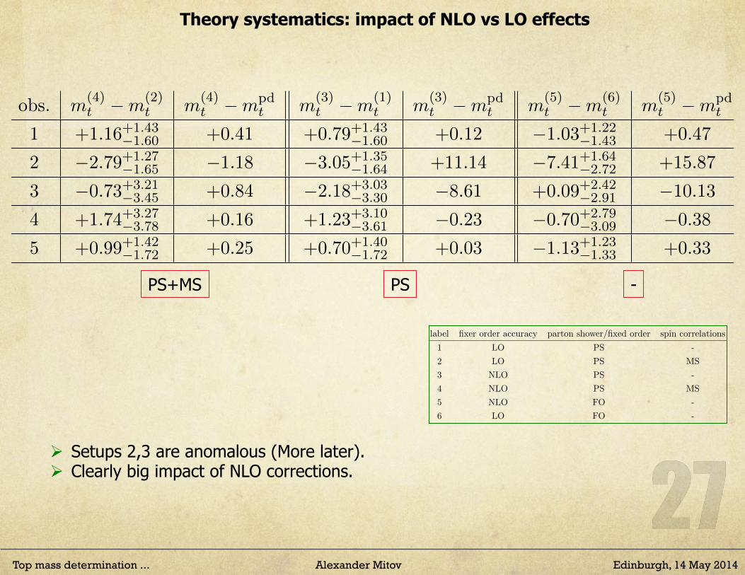
Top mass determination ... Alexander Mitov Edinburgh, 14 May 2014
Theory systematics: impact of NLO vs LO effects
166 168 170 172 174 176 178
55.5
56.0
56.5
57.0
57.5
58.0
168 170 172 174 176 178
49.5
50.0
50.5
51.0
51.5
Figure 2: Evaluation of the first moment of the distribution of pT,`+ with scale (2.16) subjectto cuts (2.2) (left) and no cuts (right). The three lines represent the best straight-line fits to thecentres or upper/lower ends of the theoretical error band at each one of the eleven points.
corrections in the total tt̄ cross-section through NNLO [7, 8]. We have utilised three
di↵erent functional forms for the factorisation and renormalisation scales:
µ̂(1) =1
2
X
i
mT,i , i 2 (t, t̄) , (2.16)
µ̂(2) =1
2
X
i
mT,i , i 2 final state , (2.17)
µ̂(3) = mt , (2.18)
with mT,i =q
p2T,i +m2i .
The calculation of the moment µ(i)O (mt) for any one particular value of mt is performed
in a number of setups, which we list in table 2. We perform our calculations at LO and
NLO with and without parton shower. We use Herwig [9]. We account for, or not, spin
correlations in the top quark decay through MadSpin (MS) [10, 11]. All calculations are
performed in the aMC@NLO framework [12]. The set of calculations we perform is
label fixer order accuracy parton shower/fixed order spin correlations
1 LO PS -
2 LO PS MS
3 NLO PS -
4 NLO PS MS
5 NLO FO -
6 LO FO -
Table 2: The type of calculations performed in this paper and their labelling conventions.
Detailed discussion of our motivation for considering these setups, and the conclusions
we draw, are delegated to section 3.
Finally, the linear functions fC,U,L are derived as the best straight-line fits to the central
(respectively upper, lower) values of the eleven computed points. We find that over the
– 5 –
Ø Setups 2,3 are anomalous (More later). Ø Clearly big impact of NLO corrections.
observable; setup i = 1 i = 1� 2 i = 1� 2� 3
all; LO+PS 187.90+0.6�0.6[428.3] 187.71+0.60
�0.60[424.2] 187.83+0.58�0.60[442.8]
all; LO+PS+MS 175.98+0.63�0.69[16.9] 176.05+0.63
�0.68[17.8] 176.12+0.61�0.68[18.9]
all; NLO+PS 175.43+0.74�0.80[29.2] 176.20+0.73
�0.79[30.1] 175.67+0.73�0.76[31.2]
all; NLOFO 174.41+0.72�0.73[96.6] 174.82+0.71
�0.73[93.1] 175.44+0.70�0.68[94.8]
all; LOFO 197.31+0.42�0.35[2496.1] 197.19+0.42
�0.35[2505.6] 197.48+0.36�0.35[3005.6]
1,4,5; LO+PS 173.68+1.08�1.31[0.8] 173.68+1.08
�1.31[0.9] 173.75+1.08�1.31[0.9]
1,4,5; LO+PS+MS 173.61+1.10�1.34[1.0] 173.63+1.10
�1.34[1.0] 173.62+1.10�1.34[1.0]
1,4,5; NLO+PS 174.40+0.75�0.81[3.5] 174.43+0.75
�0.81[3.5] 174.60+0.75�0.79[3.2]
1,4,5; NLOFO 174.73+0.72�0.74[5.5] 174.72+0.71
�0.74[5.6] 175.18+0.64�0.71[4.6]
1,4,5; LOFO 175.84+0.90�1.05[1.2] 175.75+0.89
�1.05[1.2] 175.82+0.89�1.04[1.2]
Table 6: Extracted value of mt for various setups and for two combination of observables: either allobservables or only observables 1,4 and 5, i.e. excluding the observables sensitive to spin-correlatione↵ects. The numbers in square brackets is the value of ⇠2 per d.o.f. The mass extraction is basedon pseudo data with assumed value of the top mass mpd
t = 174.32 GeV.
obs. m(3)t �m
(5)t m
(3)t �mpd
t m(1)t �m
(6)t m
(1)t �mpd
t
1 �0.35+1.14�1.16 +0.12 �2.17+1.50
�1.80 �0.67
2 �4.74+1.98�3.10 +11.14 �9.09+0.76
�0.71 +14.19
3 +1.52+2.03�1.80 �8.61 +3.79+3.30
�4.02 �6.43
4 +0.15+2.81�2.91 �0.23 �1.79+3.08
�3.75 �1.47
5 �0.30+1.09�1.21 +0.03 �2.13+1.51
�1.81 �0.67
Table 7: Estimate of the impact of shower e↵ect for each of the five observables.
obs. m(4)t �m
(2)t m
(4)t �mpd
t m(3)t �m
(1)t m
(3)t �mpd
t m(5)t �m
(6)t m
(5)t �mpd
t
1 +1.16+1.43�1.60 +0.41 +0.79+1.43
�1.60 +0.12 �1.03+1.22�1.43 +0.47
2 �2.79+1.27�1.65 �1.18 �3.05+1.35
�1.64 +11.14 �7.41+1.64�2.72 +15.87
3 �0.73+3.21�3.45 +0.84 �2.18+3.03
�3.30 �8.61 +0.09+2.42�2.91 �10.13
4 +1.74+3.27�3.78 +0.16 +1.23+3.10
�3.61 �0.23 �0.70+2.79�3.09 �0.38
5 +0.99+1.42�1.72 +0.25 +0.70+1.40
�1.72 +0.03 �1.13+1.23�1.33 +0.33
Table 8: Estimate of the impact of NLO e↵ect for each of the five observables.
A. Correlation matrices
C(3)pT (`+)
=
µ(1)1 µ
(2)1 µ
(3)1
0
B
@
1
C
A
1 0.91 0.65 µ(1)1
1 0.89 µ(2)1
1 µ(3)1
(A.1)
– 8 –
PS+MS PS -
Top mass determination ... Alexander Mitov Edinburgh, 14 May 2014
Theory systematics: impact of Spin-Correlations effects
166 168 170 172 174 176 178
55.5
56.0
56.5
57.0
57.5
58.0
168 170 172 174 176 178
49.5
50.0
50.5
51.0
51.5
Figure 2: Evaluation of the first moment of the distribution of pT,`+ with scale (2.16) subjectto cuts (2.2) (left) and no cuts (right). The three lines represent the best straight-line fits to thecentres or upper/lower ends of the theoretical error band at each one of the eleven points.
corrections in the total tt̄ cross-section through NNLO [7, 8]. We have utilised three
di↵erent functional forms for the factorisation and renormalisation scales:
µ̂(1) =1
2
X
i
mT,i , i 2 (t, t̄) , (2.16)
µ̂(2) =1
2
X
i
mT,i , i 2 final state , (2.17)
µ̂(3) = mt , (2.18)
with mT,i =q
p2T,i +m2i .
The calculation of the moment µ(i)O (mt) for any one particular value of mt is performed
in a number of setups, which we list in table 2. We perform our calculations at LO and
NLO with and without parton shower. We use Herwig [9]. We account for, or not, spin
correlations in the top quark decay through MadSpin (MS) [10, 11]. All calculations are
performed in the aMC@NLO framework [12]. The set of calculations we perform is
label fixer order accuracy parton shower/fixed order spin correlations
1 LO PS -
2 LO PS MS
3 NLO PS -
4 NLO PS MS
5 NLO FO -
6 LO FO -
Table 2: The type of calculations performed in this paper and their labelling conventions.
Detailed discussion of our motivation for considering these setups, and the conclusions
we draw, are delegated to section 3.
Finally, the linear functions fC,U,L are derived as the best straight-line fits to the central
(respectively upper, lower) values of the eleven computed points. We find that over the
– 5 –
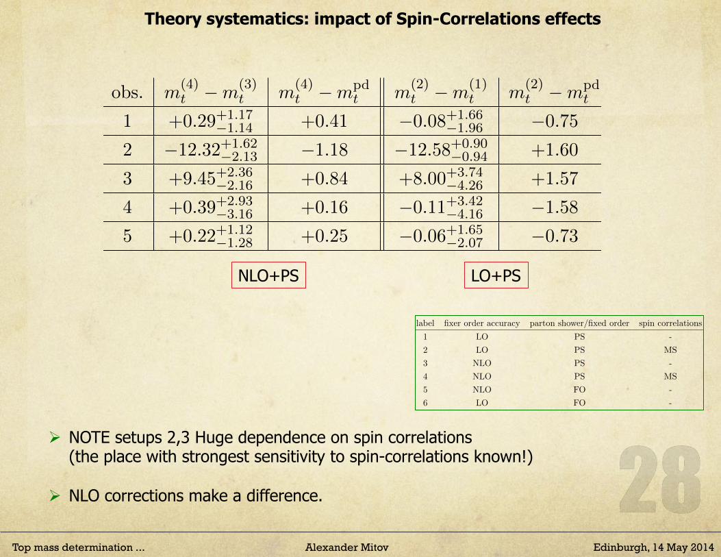
Ø NOTE setups 2,3 Huge dependence on spin correlations (the place with strongest sensitivity to spin-correlations known!)
Ø NLO corrections make a difference.
NLO+PS LO+PS
obs. m(4)t �m
(3)t m
(4)t �mpd
t m(2)t �m
(1)t m
(2)t �mpd
t
1 +0.29+1.17�1.14 +0.41 �0.08+1.66
�1.96 �0.75
2 �12.32+1.62�2.13 �1.18 �12.58+0.90
�0.94 +1.60
3 +9.45+2.36�2.16 +0.84 +8.00+3.74
�4.26 +1.57
4 +0.39+2.93�3.16 +0.16 �0.11+3.42
�4.16 �1.58
5 +0.22+1.12�1.28 +0.25 �0.06+1.65
�2.07 �0.73
Table 9: Estimate of the impact of spin-correlation e↵ect for each of the five observables.
C(1)all =
µ(1)1 µ
(1)2 µ
(1)3 µ
(1)4 µ
(1)5
0
B
B
B
B
B
B
@
1
C
C
C
C
C
C
A
1 0.39 0.58 0.53 0.76 µ(1)1
1 0.10 0.35 0.52 µ(1)2
1 0.68 0.75 µ(1)3
1 0.70 µ(1)4
1 µ(1)5
(A.2)
Equation (A.1): correlation matrix for the three lowest moments of pT (`+); eq. (A.2):
correlation matrix for the first moment of all five observables; eq. (A.3): correlation matrix
for the three lowest moments of all five observables. Although eq. (A.3) contains the
largest amount of information, most of it could be read from eqs. (A.1) and (A.2). In
fact, the correlations among the di↵erent moments of the same observable hardly depend
on the observable itself (see the simularities among the 3 ⇥ 3 blocks next to the diagonal
in eq. (A.3), blocks whose upper left corners correspond to the (µ(1)i , µ
(1)i ) entries for the
di↵erent i = 1, . . . 5). Furthermore, eq. (A.2) is the dominant source of correlations between
di↵erent observables, being relevant to their first moments. Therefore, the only information
unique to eq. (A.3) is that of the correlations between (µ(k)i , µ
(l)j ), with i 6= j and at least
one of k and l larger than one. So, although eq. (A.3) is more complete, if its format (or
space) is an issue it might be replaced by showing both eq. (A.1) and eq. (A.2).
– 9 –
Top mass determination ... Alexander Mitov Edinburgh, 14 May 2014
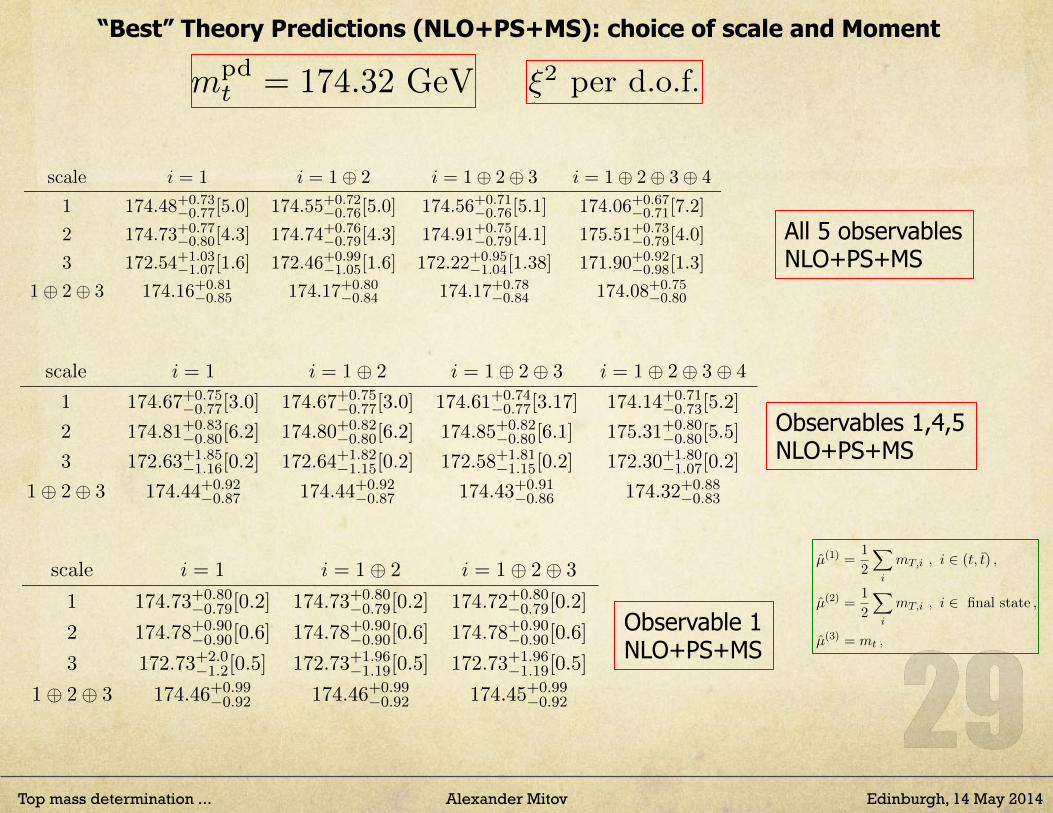
“Best” Theory Predictions (NLO+PS+MS): choice of scale and Moment
scale i = 1 i = 1� 2 i = 1� 2� 3 i = 1� 2� 3� 4
1 174.48+0.73�0.77[5.0] 174.55+0.72
�0.76[5.0] 174.56+0.71�0.76[5.1] 174.06+0.67
�0.71[7.2]
2 174.73+0.77�0.80[4.3] 174.74+0.76
�0.79[4.3] 174.91+0.75�0.79[4.1] 175.51+0.73
�0.79[4.0]
3 172.54+1.03�1.07[1.6] 172.46+0.99
�1.05[1.6] 172.22+0.95�1.04[1.38] 171.90+0.92
�0.98[1.3]
1� 2� 3 174.16+0.81�0.85 174.17+0.80
�0.84 174.17+0.78�0.84 174.08+0.75
�0.80
Table 3: Top quark mass extracted from pseudodata (...): included are all five observables in table1; calculated with NLO+PS+MS setup (4 in table 2) for each of the scales scales (2.16,2.17,2.18),their combination, and for the various combination of moments. Given are the best extracted valuewith theoretical uncertainty and, in parenthesis, the resulting value of �2 per d.o.f.
scale i = 1 i = 1� 2 i = 1� 2� 3 i = 1� 2� 3� 4
1 174.67+0.75�0.77[3.0] 174.67+0.75
�0.77[3.0] 174.61+0.74�0.77[3.17] 174.14+0.71
�0.73[5.2]
2 174.81+0.83�0.80[6.2] 174.80+0.82
�0.80[6.2] 174.85+0.82�0.80[6.1] 175.31+0.80
�0.80[5.5]
3 172.63+1.85�1.16[0.2] 172.64+1.82
�1.15[0.2] 172.58+1.81�1.15[0.2] 172.30+1.80
�1.07[0.2]
1� 2� 3 174.44+0.92�0.87 174.44+0.92
�0.87 174.43+0.91�0.86 174.32+0.88
�0.83
Table 4: As in table 3, except that only three observables (1,4,5 in table 1) are included.
scale i = 1 i = 1� 2 i = 1� 2� 3
1 174.73+0.80�0.79[0.2] 174.73+0.80
�0.79[0.2] 174.72+0.80�0.79[0.2]
2 174.78+0.90�0.90[0.6] 174.78+0.90
�0.90[0.6] 174.78+0.90�0.90[0.6]
3 172.73+2.0�1.2[0.5] 172.73+1.96
�1.19[0.5] 172.73+1.96�1.19[0.5]
1� 2� 3 174.46+0.99�0.92 174.46+0.99
�0.92 174.45+0.99�0.92
Table 5: As in table 3, except that only one observable (1 in table 1) is included.
3. Detailed study of the theory systematics
- Statistical fluctuations
- study of shower e↵ects (Pythia vs Herwig)
- describe pseudodata
4. Results
5. Conclusions
Acknowledgments
This work is supported by ERC grant 291377 “LHCtheory: Theoretical predictions and
analyses of LHC physics: advancing the precision frontier”. The work of A.M. is also
supported by a grant from the STFC of UK.
– 7 –
scale i = 1 i = 1� 2 i = 1� 2� 3 i = 1� 2� 3� 4
1 174.48+0.73�0.77[5.0] 174.55+0.72
�0.76[5.0] 174.56+0.71�0.76[5.1] 174.06+0.67
�0.71[7.2]
2 174.73+0.77�0.80[4.3] 174.74+0.76
�0.79[4.3] 174.91+0.75�0.79[4.1] 175.51+0.73
�0.79[4.0]
3 172.54+1.03�1.07[1.6] 172.46+0.99
�1.05[1.6] 172.22+0.95�1.04[1.38] 171.90+0.92
�0.98[1.3]
1� 2� 3 174.16+0.81�0.85 174.17+0.80
�0.84 174.17+0.78�0.84 174.08+0.75
�0.80
Table 3: Top quark mass extracted from pseudodata (...): included are all five observables in table1; calculated with NLO+PS+MS setup (4 in table 2) for each of the scales scales (2.16,2.17,2.18),their combination, and for the various combination of moments. Given are the best extracted valuewith theoretical uncertainty and, in parenthesis, the resulting value of �2 per d.o.f.
scale i = 1 i = 1� 2 i = 1� 2� 3 i = 1� 2� 3� 4
1 174.67+0.75�0.77[3.0] 174.67+0.75
�0.77[3.0] 174.61+0.74�0.77[3.17] 174.14+0.71
�0.73[5.2]
2 174.81+0.83�0.80[6.2] 174.80+0.82
�0.80[6.2] 174.85+0.82�0.80[6.1] 175.31+0.80
�0.80[5.5]
3 172.63+1.85�1.16[0.2] 172.64+1.82
�1.15[0.2] 172.58+1.81�1.15[0.2] 172.30+1.80
�1.07[0.2]
1� 2� 3 174.44+0.92�0.87 174.44+0.92
�0.87 174.43+0.91�0.86 174.32+0.88
�0.83
Table 4: As in table 3, except that only three observables (1,4,5 in table 1) are included.
scale i = 1 i = 1� 2 i = 1� 2� 3
1 174.73+0.80�0.79[0.2] 174.73+0.80
�0.79[0.2] 174.72+0.80�0.79[0.2]
2 174.78+0.90�0.90[0.6] 174.78+0.90
�0.90[0.6] 174.78+0.90�0.90[0.6]
3 172.73+2.0�1.2[0.5] 172.73+1.96
�1.19[0.5] 172.73+1.96�1.19[0.5]
1� 2� 3 174.46+0.99�0.92 174.46+0.99
�0.92 174.45+0.99�0.92
Table 5: As in table 3, except that only one observable (1 in table 1) is included.
3. Detailed study of the theory systematics
- Statistical fluctuations
- study of shower e↵ects (Pythia vs Herwig)
- describe pseudodata
4. Results
5. Conclusions
Acknowledgments
This work is supported by ERC grant 291377 “LHCtheory: Theoretical predictions and
analyses of LHC physics: advancing the precision frontier”. The work of A.M. is also
supported by a grant from the STFC of UK.
– 7 –
166 168 170 172 174 176 178
55.5
56.0
56.5
57.0
57.5
58.0
168 170 172 174 176 178
49.5
50.0
50.5
51.0
51.5
Figure 2: Evaluation of the first moment of the distribution of pT,`+ with scale (2.16) subjectto cuts (2.2) (left) and no cuts (right). The three lines represent the best straight-line fits to thecentres or upper/lower ends of the theoretical error band at each one of the eleven points.
corrections in the total tt̄ cross-section through NNLO [7, 8]. We have utilised three
di↵erent functional forms for the factorisation and renormalisation scales:
µ̂(1) =1
2
X
i
mT,i , i 2 (t, t̄) , (2.16)
µ̂(2) =1
2
X
i
mT,i , i 2 final state , (2.17)
µ̂(3) = mt , (2.18)
with mT,i =q
p2T,i +m2i .
The calculation of the moment µ(i)O (mt) for any one particular value of mt is performed
in a number of setups, which we list in table 2. We perform our calculations at LO and
NLO with and without parton shower. We use Herwig [9]. We account for, or not, spin
correlations in the top quark decay through MadSpin (MS) [10, 11]. All calculations are
performed in the aMC@NLO framework [12]. The set of calculations we perform is
label fixer order accuracy parton shower/fixed order spin correlations
1 LO PS -
2 LO PS MS
3 NLO PS -
4 NLO PS MS
5 NLO FO -
6 LO FO -
Table 2: The type of calculations performed in this paper and their labelling conventions.
Detailed discussion of our motivation for considering these setups, and the conclusions
we draw, are delegated to section 3.
Finally, the linear functions fC,U,L are derived as the best straight-line fits to the central
(respectively upper, lower) values of the eleven computed points. We find that over the
– 5 –
All 5 observables NLO+PS+MS
Observables 1,4,5 NLO+PS+MS
Observable 1 NLO+PS+MS
observable; setup i = 1 i = 1� 2 i = 1� 2� 3
all; LO+PS 187.90+0.6�0.6[428.3] 187.71+0.60
�0.60[424.2] 187.83+0.58�0.60[442.8]
all; LO+PS+MS 175.98+0.63�0.69[16.9] 176.05+0.63
�0.68[17.8] 176.12+0.61�0.68[18.9]
all; NLO+PS 175.43+0.74�0.80[29.2] 176.20+0.73
�0.79[30.1] 175.67+0.73�0.76[31.2]
all; NLOFO 174.41+0.72�0.73[96.6] 174.82+0.71
�0.73[93.1] 175.44+0.70�0.68[94.8]
all; LOFO 197.31+0.42�0.35[2496.1] 197.19+0.42
�0.35[2505.6] 197.48+0.36�0.35[3005.6]
1,4,5; LO+PS 173.68+1.08�1.31[0.8] 173.68+1.08
�1.31[0.9] 173.75+1.08�1.31[0.9]
1,4,5; LO+PS+MS 173.61+1.10�1.34[1.0] 173.63+1.10
�1.34[1.0] 173.62+1.10�1.34[1.0]
1,4,5; NLO+PS 174.40+0.75�0.81[3.5] 174.43+0.75
�0.81[3.5] 174.60+0.75�0.79[3.2]
1,4,5; NLOFO 174.73+0.72�0.74[5.5] 174.72+0.71
�0.74[5.6] 175.18+0.64�0.71[4.6]
1,4,5; LOFO 175.84+0.90�1.05[1.2] 175.75+0.89
�1.05[1.2] 175.82+0.89�1.04[1.2]
Table 6: Extracted value of mt for various setups and for two combination of observables: either allobservables or only observables 1,4 and 5, i.e. excluding the observables sensitive to spin-correlatione↵ects. The numbers in square brackets is the value of ⇠2 per d.o.f. The mass extraction is basedon pseudo data with assumed value of the top mass mpd
t = 174.32 GeV.
obs. m(3)t �m
(5)t m
(3)t �mpd
t m(1)t �m
(6)t m
(1)t �mpd
t
1 �0.35+1.14�1.16 +0.12 �2.17+1.50
�1.80 �0.67
2 �4.74+1.98�3.10 +11.14 �9.09+0.76
�0.71 +14.19
3 +1.52+2.03�1.80 �8.61 +3.79+3.30
�4.02 �6.43
4 +0.15+2.81�2.91 �0.23 �1.79+3.08
�3.75 �1.47
5 �0.30+1.09�1.21 +0.03 �2.13+1.51
�1.81 �0.67
Table 7: Estimate of the impact of shower e↵ect for each of the five observables.
obs. m(4)t �m
(2)t m
(4)t �mpd
t m(3)t �m
(1)t m
(3)t �mpd
t m(5)t �m
(6)t m
(5)t �mpd
t
1 +1.16+1.43�1.60 +0.41 +0.79+1.43
�1.60 +0.12 �1.03+1.22�1.43 +0.47
2 �2.79+1.27�1.65 �1.18 �3.05+1.35
�1.64 +11.14 �7.41+1.64�2.72 +15.87
3 �0.73+3.21�3.45 +0.84 �2.18+3.03
�3.30 �8.61 +0.09+2.42�2.91 �10.13
4 +1.74+3.27�3.78 +0.16 +1.23+3.10
�3.61 �0.23 �0.70+2.79�3.09 �0.38
5 +0.99+1.42�1.72 +0.25 +0.70+1.40
�1.72 +0.03 �1.13+1.23�1.33 +0.33
Table 8: Estimate of the impact of NLO e↵ect for each of the five observables.
A. Correlation matrices
C(3)pT (`+)
=
µ(1)1 µ
(2)1 µ
(3)1
0
B
@
1
C
A
1 0.91 0.65 µ(1)1
1 0.89 µ(2)1
1 µ(3)1
(A.1)
– 8 –

Top mass determination ... Alexander Mitov Edinburgh, 14 May 2014
Theory systematics: Predictions
observable; setup i = 1 i = 1� 2 i = 1� 2� 3
all; LO+PS 187.90+0.6�0.6[428.3] 187.71+0.60
�0.60[424.2] 187.83+0.58�0.60[442.8]
all; LO+PS+MS 175.98+0.63�0.69[16.9] 176.05+0.63
�0.68[17.8] 176.12+0.61�0.68[18.9]
all; NLO+PS 175.43+0.74�0.80[29.2] 176.20+0.73
�0.79[30.1] 175.67+0.73�0.76[31.2]
all; NLOFO 174.41+0.72�0.73[96.6] 174.82+0.71
�0.73[93.1] 175.44+0.70�0.68[94.8]
all; LOFO 197.31+0.42�0.35[2496.1] 197.19+0.42
�0.35[2505.6] 197.48+0.36�0.35[3005.6]
1,4,5; LO+PS 173.68+1.08�1.31[0.8] 173.68+1.08
�1.31[0.9] 173.75+1.08�1.31[0.9]
1,4,5; LO+PS+MS 173.61+1.10�1.34[1.0] 173.63+1.10
�1.34[1.0] 173.62+1.10�1.34[1.0]
1,4,5; NLO+PS 174.40+0.75�0.81[3.5] 174.43+0.75
�0.81[3.5] 174.60+0.75�0.79[3.2]
1,4,5; NLOFO 174.73+0.72�0.74[5.5] 174.72+0.71
�0.74[5.6] 175.18+0.64�0.71[4.6]
1,4,5; LOFO 175.84+0.90�1.05[1.2] 175.75+0.89
�1.05[1.2] 175.82+0.89�1.04[1.2]
Table 6: Extracted value of mt for various setups and for two combination of observables: either allobservables or only observables 1,4 and 5, i.e. excluding the observables sensitive to spin-correlatione↵ects. The numbers in square brackets is the value of ⇠2 per d.o.f. The mass extraction is basedon pseudo data with assumed value of the top mass mpd
t = 174.32 GeV.
obs. m(3)t �m
(5)t m
(3)t �mpd
t m(1)t �m
(6)t m
(1)t �mpd
t
1 �0.35+1.14�1.16 +0.12 �2.17+1.50
�1.80 �0.67
2 �4.74+1.98�3.10 +11.14 �9.09+0.76
�0.71 +14.19
3 +1.52+2.03�1.80 �8.61 +3.79+3.30
�4.02 �6.43
4 +0.15+2.81�2.91 �0.23 �1.79+3.08
�3.75 �1.47
5 �0.30+1.09�1.21 +0.03 �2.13+1.51
�1.81 �0.67
Table 7: Estimate of the impact of shower e↵ect for each of the five observables.
obs. m(4)t �m
(2)t m
(4)t �mpd
t m(3)t �m
(1)t m
(3)t �mpd
t m(5)t �m
(6)t m
(5)t �mpd
t
1 +1.16+1.43�1.60 +0.41 +0.79+1.43
�1.60 +0.12 �1.03+1.22�1.43 +0.47
2 �2.79+1.27�1.65 �1.18 �3.05+1.35
�1.64 +11.14 �7.41+1.64�2.72 +15.87
3 �0.73+3.21�3.45 +0.84 �2.18+3.03
�3.30 �8.61 +0.09+2.42�2.91 �10.13
4 +1.74+3.27�3.78 +0.16 +1.23+3.10
�3.61 �0.23 �0.70+2.79�3.09 �0.38
5 +0.99+1.42�1.72 +0.25 +0.70+1.40
�1.72 +0.03 �1.13+1.23�1.33 +0.33
Table 8: Estimate of the impact of NLO e↵ect for each of the five observables.
A. Correlation matrices
C(3)pT (`+)
=
µ(1)1 µ
(2)1 µ
(3)1
0
B
@
1
C
A
1 0.91 0.65 µ(1)1
1 0.89 µ(2)1
1 µ(3)1
(A.1)
– 8 –

Top mass determination ... Alexander Mitov Edinburgh, 14 May 2014
Conclusions
ü New developments have resurrected the interest in knowing mtop precisely
ü Vacuum Stability in SM ü Higgs Inflation
ü There are many dedicated hadron collider measurements. They return consistent values around mtop = 173 GeV and uncertainty (mostly on the measurement!) of below 1 GeV. ü Questions remain: can there be a significant additional theoretical systematics O(1 GeV) ?
ü This is not an abstract problem: mtop is not an observable and so is a theoretically defined concept.
ü The issue of various mass definitions is a non-issue at present for hadron colliders.
ü e+e- colliders offer the real possibility of measuring mtop with x10 precision, i.e. O(100 MeV) But how long would we have to wait for a ttbar threshold scan? ü New physics contributions to mtop are a totally open question. Upper limit of O(2 GeV) likely can be placed at present.
ü Proposed new method, with emphasis on control over theory systematics. NLO vs LO: 1 GeV; spin correlations crucial. Awaiting the measurement (100k events exist!).