Determination of the Thermal Resistance of Pipe Insulation

74

32nd International Thermal Conductivity Conference20th International Thermal Expansion SymposiumApril 27–May 1, 2014Purdue University, West Lafayette, Indiana, USA

Determination of the Thermal Resistance of Pipe Insulation Material from Thermal Conductivity of Flat Insulation Products

Alain Koenen, [email protected] and Damien M. Marquis, [email protected] National de Métrologie et d’essais, Test Direction, Energy, Environment & Combustion Division,

29, Avenue Roger Hennequin, 78197 Trappes cedex, France

ABSTRACT

New European product standards now include a mandatory requirement for manufacturers to declare the temperature-dependent thermal conductivity for each insulation used in building equipments and industrial installations. For pipe insulation systems, the measurement is usually performed by a standard pipe test method, in which the value on a large temperature range is integrated to reduce temperature range and improve temperature measurement control. The alternative proposed in this article consists in determining the thermal conductivity of a pipe insulation system from the results measured on a flat slab specimen. The protocol used in this study consists in collecting the thermal conductivity data and then in fitting the curve with a polynomial regression, using a least-square method. The comparison between the pipe insulation specimen and the flat slab product is then done at a specified temperature using the extrapoled polynomial. The methodology is illustrated with a mineral wool over a large range of temperature.

1. INTRODUCTION

New European product standards for insulation used in building equipment and industrial installations were published in 2009 and became effective in August 2012. These product standards provide a mandatory requirement for manufacturers to declare the temperature-dependent thermal conductivity which an independent notified laboratory will verify. The notification is given by European Commission and is based on an accreditation procedure. There are currently nine product standards in this field (EN 14303, EN 14304, EN 14305, EN 14306, EN 14307, EN 14308, EN 14309, EN 14313, and EN 14314). These standards provide rules for CE mark declarations. These rules apply to the following materials: mineral wool (MW), elastomeric foam, cellular glass, calcium silicate, extruded polystyrene foam (XPS), polyurethane foam (PUR), polyisocyanurate foam; expanded polystyrene polyethylene foam (EPS), and phenolic foam. The thermal performance must be declared between the lowest and the highest temperature at which the product is intended for use.

For pipe insulation systems, the determination of the average equivalent thermal conductivity can be carried out using a standard pipe test method, described in the ISO 8497 standard (ISO 8497, 1994). It consists of a cylindrical heat source onto which the circular pipe is wound. The inner surface of the specimen is heated by a radial heat flow, whereas the outside surface is cooled by the laboratory atmosphere at room temperature. This measurement method is carried out easily and

quickly. Nevertheless, its main disadvantage is that the mean value of the equivalent thermal conductivity is integrated on a large temperature range, which can be of several hundreds of degrees when the measurement is performed at high temperature.

In order to reduce temperature range and to better control temperature measurement, the alternative proposed in this article is to determine the thermal conductivity of pipe insulation system based on the results measured on a flat slab specimen. The measurement is thus carried out using a standard test method, a guarded hot plate (GHP), as described in ISO 8302 (1991). The methology fitted the thermal conductivity data by a polynomial regression, using a least-square method. The comparison between the pipe insulation specimen and the flat slab product is then done at a specified temperature using the extrapoled polynomial. The benefit of this study is that it allows to consider the anisotropic nature of the insulation materials.

This article focuses on the methodology developed to evaluate the thermal conductivities of a pipe insulation specimen from the measurement of a flat slab product. To illustrate the methodology, the analyses were then carried out on a MW, on a large range of temperatures from 23°C up to 700°C. The results are presented and discussed.

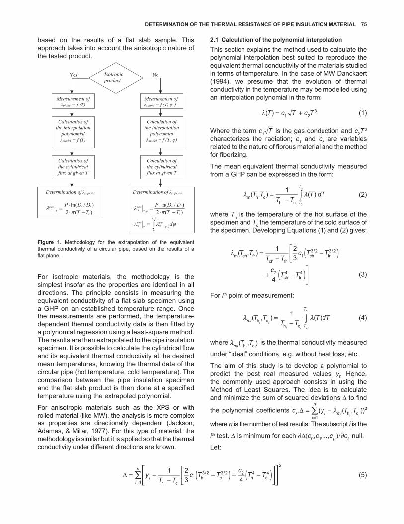
2. METHODOLOGY

Figure 1 explains the methodology used to extrapolate the thermal conductivity of a pipe insulation specimen,

DOI: 10.5703/1288284315545

DETERMINATION OF THE THERMAL RESISTANCE OF PIPE INSULATION MATERIAL 75

1 23 4h c1

1 h3/2

c3/2 2

h4

c4

2

∑ ( ) ( )∆ = −−

− + −

=

yT T

c T Tc

T Tii

n

(5)

based on the results of a flat slab sample. This approach takes into account the anisotropic nature of the tested product.

Isotropic product

Yes No

Measurement of λplane = f (T)

Measurement of λplane = f (T, φ )

Calculation of the interpolation

polynomial λmodel = f (T)

Calculation of the interpolation

polynomial λmodel = f (T, φ)

Calculation of the cylindrical flux at given T

Calculation of the cylindrical flux at given T

Determination of λpipe,eq

)(2)/ln(

ei

ie

T

pipeeq

TTDDP

−⋅⋅=π

λ

Determination of λpipe,eq

)(2)/ln(

,ei

ie

T

pipeeq

TTDDP

−⋅⋅=π

λϕ

ϕλλπ

ϕd

T

pipeeqT

pipeeq ∫=

2/

0,

Figure 1. Methodology for the extrapolation of the equivalent thermal conductivity of a circular pipe, based on the results of a flat plane.

For isotropic materials, the methodology is the simplest insofar as the properties are identical in all directions. The principle consists in measuring the equivalent conductivity of a flat slab specimen using a GHP on an established temperature range. Once the measurements are performed, the temperature-dependent thermal conductivity data is then fitted by a polynomial regression using a least-square method. The results are then extrapolated to the pipe insulation specimen. It is possible to calculate the cylindrical flow and its equivalent thermal conductivity at the desired mean temperatures, knowing the thermal data of the circular pipe (hot temperature, cold temperature). The comparison between the pipe insulation specimen and the flat slab product is then done at a specified temperature using the extrapoled polynomial.

For anisotropic materials such as the XPS or with rolled material (like MW), the analysis is more complex as properties are directionally dependent (Jackson, Adames, & Millar, 1977). For this type of material, the methodology is similar but it is applied so that the thermal conductivity under different directions are known.

2.1 Calculation of the polynomial interpolationThis section explains the method used to calculate the polynomial interpolation best suited to reproduce the equivalent thermal conductivity of the materials studied in terms of temperature. In the case of MW Danckaert (1994), we presume that the evolution of thermal conductivity in the temperature may be modelled using an interpolation polynomial in the form:

T c T c Tλ = +( ) 1 23 (1)

Where the term c1 T is the gas conduction and c2T 3

characterizes the radiation; c1 and c2 are variables related to the nature of fibrous material and the method for fiberizing.

The mean equivalent thermal conductivity measured from a GHP can be expressed in the form:

T TT T

T dTT

T

∫λ λ=−

( , ) 1 ( )m h ch c c

h

(2)

where Th is the temperature of the hot surface of the specimen and Tc the temperature of the cold surface of the specimen. Developing Equations (1) and (2) gives:

T TT T

c T T

cT T

λ ( )

( )

=−

−

+ −

( , ) 1 23

4

m ch frch fr

1 ch3/2

fr3/2

2ch4

fr4

(3)

For ith point of measurement:

T T

T TT dTi

T

T

i ii i i

i

( , ) 1 ( )m h ch c c

h

∫λ λ=−

(4)

where λ T Tmi i i( , )h c is the thermal conductivity measured

under “ideal” conditions, e.g. without heat loss, etc.

The aim of this study is to develop a polynomial to predict the best real measured values yi. Hence, the commonly used approach consists in using the Method of Least Squares. The idea is to calculate and minimize the sum of squared deviations ∆ to find

the polynomial coefficients ck. y T Ti mii

n

i i∑ λ∆ = −=

( ( , ))h c22

1

where n is the number of test results. The subscript i is the

ith test. ∆ is minimum for each , ,...,0 1∂∆( )/∂c c c cp k null.

Let:

76 INSULATION MATERIALS

which leads to a system

c cc

yT T

c T Tc

T T T Tii

n

i ii i i i i i

,2 1 2

3 423

1 2

1 h c1 h

3/2c3/2 2

h4

c4

h3/2

c3/2

1∑ ( ) ( ) ( )∂∆( )

∂= −

−− + −

−

=

(6)

c cc

yT T

c T Tc

T T T Tii

n

i ii i i i i i

,2 1 2

3 414

1 2

2 h c1 h

3/2c3/2 2

h4

c4

h4

c4

1∑ ( ) ( ) ( )∂∆( )

∂= −

−− + −

−

=

(7)

The equations can then be reduced to:

23

23

23

14 2

3

h3/2

c3/2

h3/2

c3/2

h c1

1

h4

c4

h3/2

cr3/2

h cr2 h

3/2c3/2

1∑ ∑

( )−

−

−+

− −

−= ∗ −

= =

T T T T

T Tc

T T T T

T Tc y T T

i

n

ii

ni i i i

i i

i i i i

i ii i

(8)

T T T T

T Tc

T T T T

T Tc y T Ti

i

n

i

n i i i i

i i

i i i i

i ii i

23

14

14

14 1

4

h4

c4

h3/2

c3/2

h c1

h4

fr4

h4

c4

h c2 h

4c4

11∑∑

( )−

−

−+

− −

−= ∗ −

== (9)

Finally, developing the calculi leads to a system with 2 × 2 matrix:

A

T T T T

T T

T T T T

T T

T T T T

T T

T T T T

T T

i

n

i

n

i

n

i

n

i i i i

i i

i i i i

i i

i i i i

i i

i i i i

i i

49

212

212

116

h3/2

c3/2

h3/2

c3/2

w c1

h4

c4

h3/2

c3/2

w c1

h4

c4

h3/2

c3/2

h c1

h4

c4

h4

c4

h c1

∑ ∑

∑ ∑

( )( ) ( )( )

( )( ) ( )( )=

− −

−

− −

−

− −

−

− −

−

= =

= =

(10)

W

W

y T T

y T TY

ii

n

ii

n

i i

i i

∑

∑

( )( )

=−

−

==

=

23

14

1

2

h3/2

c3/2

1

h4

c4

1

(11)

Polynomial parameters are then defined by:

A Yc

c=

−1 0

1

(12)

To compare the value, it is necessary to compare the results of the polynomial a with the same temperatures Tc and Th.

2.2 Influence of the orientationSome materials – such as MW – are anisotropic, i.e., the thermal conductivity is directionally dependent. For this type of material, it is therefore necessary to consider the evolution of the mean value in function of the direction (x, y, and z). The methodology applied here is based on the works of Jackson et al. (1977). Jackson considers

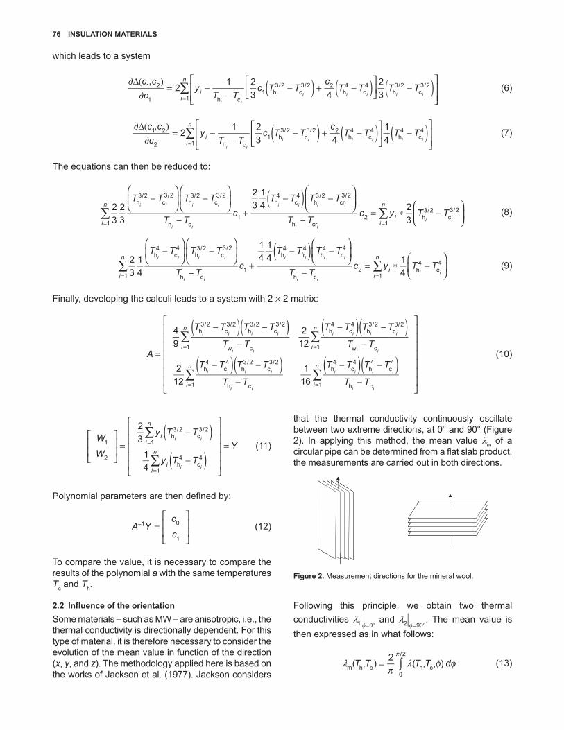
that the thermal conductivity continuously oscillate between two extreme directions, at 0° and 90° (Figure 2). In applying this method, the mean value lm of a circular pipe can be determined from a flat slab product, the measurements are carried out in both directions.

Figure 2. Measurement directions for the mineral wool.

Following this principle, we obtain two thermal conductivities 1 0

lφ= °

and 2 90l

φ= °. The mean value is

then expressed as in what follows:

T T T T d( , ) 2 ( , , )m h c h c

0

/2

l l∫πφ φ=

π

(13)


To simplify the problem, suppose that the gradients of radial temperature are independent of the angle j, while in reality, it is not strictly true. According to this assumption, it can be admit that the temperatures field of a circular pipe is radially homogeneous.

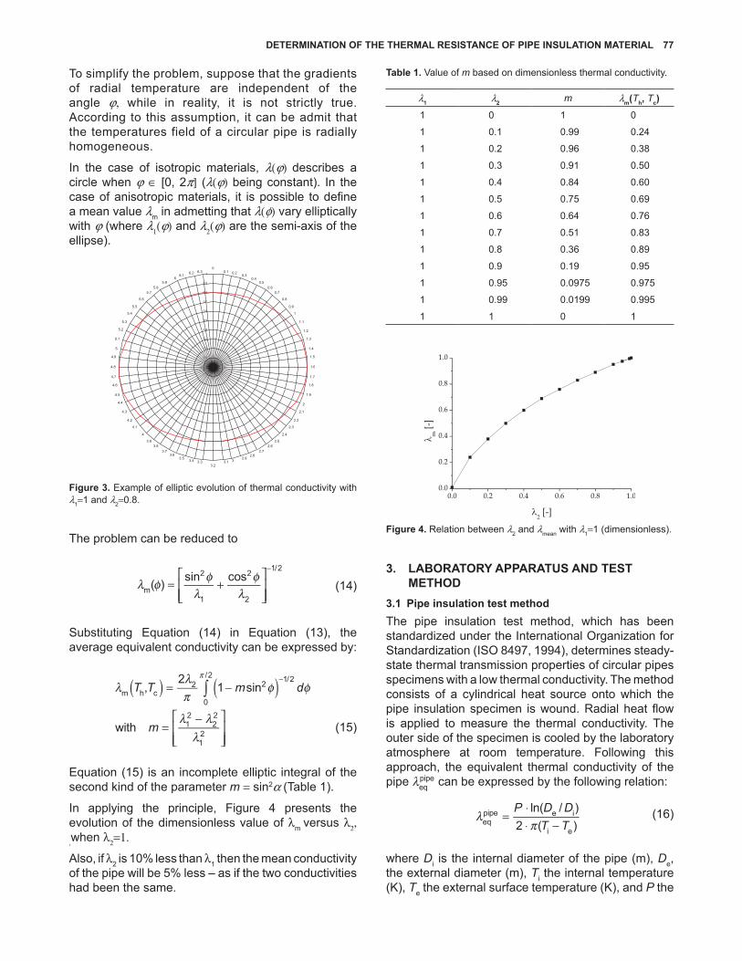
In the case of isotropic materials, l(j) describes a circle when j ∈ [0, 2p] (l(j) being constant). In the case of anisotropic materials, it is possible to define a mean value lm in admetting that l(f) vary elliptically with j (where l1(j) and l2(j) are the semi-axis of the ellipse).

0

0.1

0.2

0.3

0.4

0.5

0.6

0.7

0.8

0.9

1

00.1 0.2 0.3

0.40.5

0.60.7

0.8

0.9

1

1.1

1.2

1.3

1.4

1.5

1.6

1.7

1.8

1.9

2

2.1

2.2

2.3

2.4

2.52.6

2.72.8

2.933.13.2

3.33.43.53.6

3.73.8

3.9

4

4.1

4.2

4.3

4.4

4.5

4.6

4.7

4.8

4.9

5

5.1

5.2

5.3

5.4

5.5

5.6

5.75.8

5.966.1 6.2 6.3

Figure 3. Example of elliptic evolution of thermal conductivity with l1=1 and l2=0.8.

The problem can be reduced to

( ) sin cos

m

2

1

2

2

1/2

λ φ φλ

φλ

= +

−

(14)

Substituting Equation (14) in Equation (13), the average equivalent conductivity can be expressed by:

T T m d

m

,2

1 sin

with

m h c2 2 1/2

0

/2

12

22

12

∫λλπ

φ φ

λ λλ

( )( ) = −

=−

π −

(15)

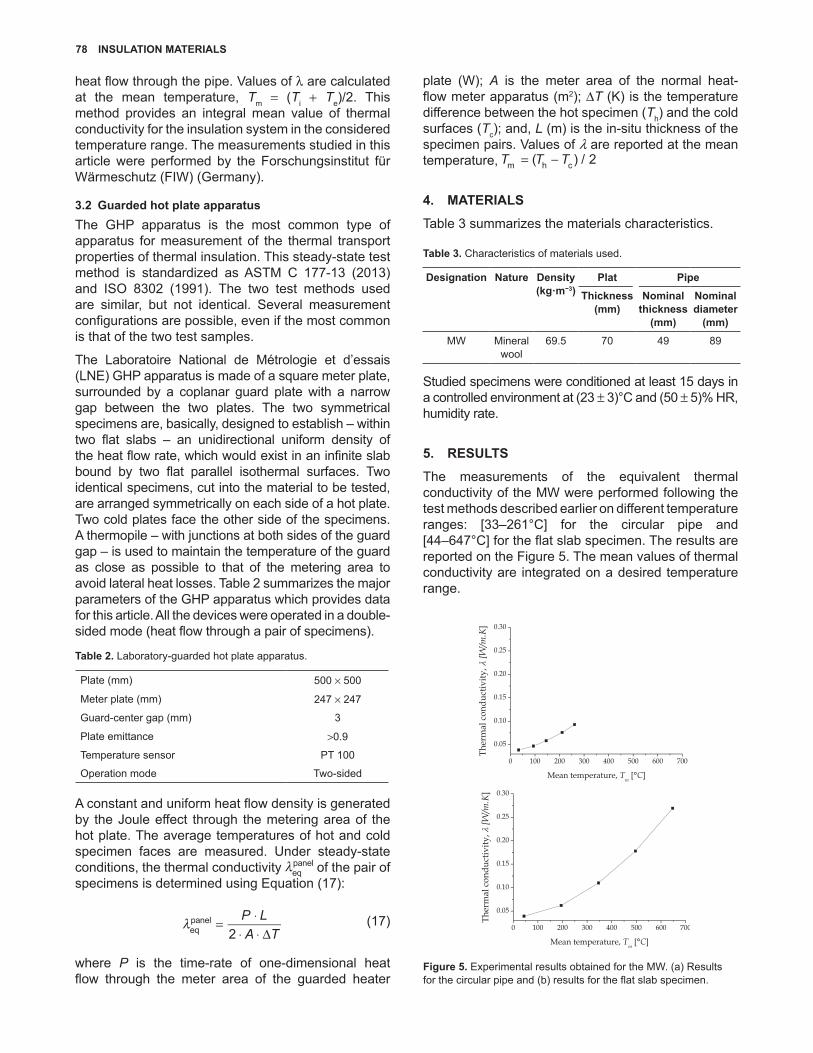
Equation (15) is an incomplete elliptic integral of the second kind of the parameter m = sin2a (Table 1).

In applying the principle, Figure 4 presents the evolution of the dimensionless value of lm versus l2,

,when l2=1.

Also, if l2 is 10% less than l1 then the mean conductivity of the pipe will be 5% less – as if the two conductivities had been the same.

Table 1. Value of m based on dimensionless thermal conductivity.

l1 l2 m lm(Th, Tc)1 0 1 0

1 0.1 0.99 0.24

1 0.2 0.96 0.38

1 0.3 0.91 0.50

1 0.4 0.84 0.60

1 0.5 0.75 0.69

1 0.6 0.64 0.76

1 0.7 0.51 0.83

1 0.8 0.36 0.89

1 0.9 0.19 0.95

1 0.95 0.0975 0.975

1 0.99 0.0199 0.995

1 1 0 1

Figure 4. Relation between l2 and lmean with l1=1 (dimensionless).

3. LABORATORY APPARATUS AND TEST METHOD

3.1 Pipe insulation test methodThe pipe insulation test method, which has been standardized under the International Organization for Standardization (ISO 8497, 1994), determines steady-state thermal transmission properties of circular pipes specimens with a low thermal conductivity. The method consists of a cylindrical heat source onto which the pipe insulation specimen is wound. Radial heat flow is applied to measure the thermal conductivity. The outer side of the specimen is cooled by the laboratory atmosphere at room temperature. Following this approach, the equivalent thermal conductivity of the pipe λeq

pipe can be expressed by the following relation:

P D D

T Tλ

π=

⋅⋅ −ln( / )

2 ( )eqpipe e i

i e (16)

where Di is the internal diameter of the pipe (m), De, the external diameter (m), Ti the internal temperature (K), Te the external surface temperature (K), and P the


heat flow through the pipe. Values of l are calculated at the mean temperature, Tm = (Ti + Te)/2. This method provides an integral mean value of thermal conductivity for the insulation system in the considered temperature range. The measurements studied in this article were performed by the Forschungsinstitut für Wärmeschutz (FIW) (Germany).

3.2 Guarded hot plate apparatusThe GHP apparatus is the most common type of apparatus for measurement of the thermal transport properties of thermal insulation. This steady-state test method is standardized as ASTM C 177-13 (2013) and ISO 8302 (1991). The two test methods used are similar, but not identical. Several measurement configurations are possible, even if the most common is that of the two test samples.

The Laboratoire National de Métrologie et d’essais (LNE) GHP apparatus is made of a square meter plate, surrounded by a coplanar guard plate with a narrow gap between the two plates. The two symmetrical specimens are, basically, designed to establish – within two flat slabs – an unidirectional uniform density of the heat flow rate, which would exist in an infinite slab bound by two flat parallel isothermal surfaces. Two identical specimens, cut into the material to be tested, are arranged symmetrically on each side of a hot plate. Two cold plates face the other side of the specimens. A thermopile – with junctions at both sides of the guard gap – is used to maintain the temperature of the guard as close as possible to that of the metering area to avoid lateral heat losses. Table 2 summarizes the major parameters of the GHP apparatus which provides data for this article. All the devices were operated in a double-sided mode (heat flow through a pair of specimens).

Table 2. Laboratory-guarded hot plate apparatus.

Plate (mm) 500 × 500

Meter plate (mm) 247 × 247

Guard-center gap (mm) 3

Plate emittance >0.9

Temperature sensor PT 100

Operation mode Two-sided

A constant and uniform heat flow density is generated by the Joule effect through the metering area of the hot plate. The average temperatures of hot and cold specimen faces are measured. Under steady-state conditions, the thermal conductivity λeq

panel of the pair of specimens is determined using Equation (17):

P LA T

λ =⋅

⋅ ⋅ ∆2eqpanel

(17)

where P is the time-rate of one-dimensional heat flow through the meter area of the guarded heater

plate (W); A is the meter area of the normal heat-flow meter apparatus (m2); ∆T (K) is the temperature difference between the hot specimen (Th) and the cold surfaces (Tc); and, L (m) is the in-situ thickness of the specimen pairs. Values of l are reported at the mean temperature, = −T T T( ) / 2m h c

4. MATERIALS

Table 3 summarizes the materials characteristics.

Table 3. Characteristics of materials used.

Designation Nature Density (kg·m−3)

Plat PipeThickness

(mm)Nominal

thickness(mm)

Nominaldiameter

(mm)MW Mineral

wool69.5 70 49 89

Studied specimens were conditioned at least 15 days in a controlled environment at (23 ± 3)°C and (50 ± 5)% HR, humidity rate.

5. RESULTS

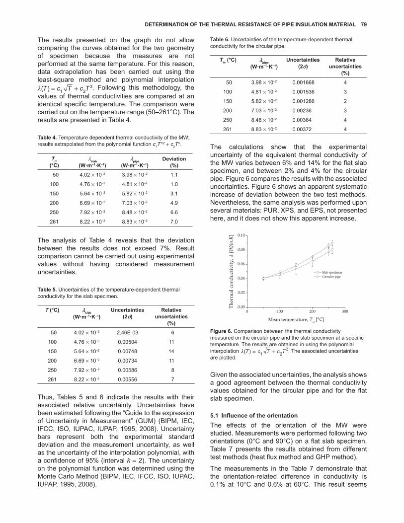
The measurements of the equivalent thermal conductivity of the MW were performed following the test methods described earlier on different temperature ranges: [33–261°C] for the circular pipe and [44–647°C] for the flat slab specimen. The results are reported on the Figure 5. The mean values of thermal conductivity are integrated on a desired temperature range.

Figure 5. Experimental results obtained for the MW. (a) Results for the circular pipe and (b) results for the flat slab specimen.


The results presented on the graph do not allow comparing the curves obtained for the two geometry of specimen because the measures are not performed at the same temperature. For this reason, data extrapolation has been carried out using the least-square method and polynomial interpolation

T c T c Tλ = +( ) 1 23. Following this methodology, the

values of thermal conductivities are compared at an identical specific temperature. The comparison were carried out on the temperature range (50–261°C). The results are presented in Table 4.

Table 4. Temperature dependent thermal conductivity of the MW; results extrapolated from the polynomial function c1T

1/2 + c2T3.

Tm(°C)

lslab(W·m–1·K–1)

lpipe(W·m–1·K–1)

Deviation(%)

50 4.02 × 10-2 3.98 × 10-2 1.1

100 4.76 × 10-2 4.81 × 10-2 1.0

150 5.64 × 10-2 5.82 × 10-2 3.1

200 6.69 × 10-2 7.03 × 10-2 4.9

250 7.92 × 10-2 8.48 × 10-2 6.6

261 8.22 × 10-2 8.83 × 10-2 7.0

The analysis of Table 4 reveals that the deviation between the results does not exceed 7%. Result comparison cannot be carried out using experimental values without having considered measurement uncertainties.

Table 5. Uncertainties of the temperature-dependent thermal conductivity for the slab specimen.

T (°C) kslab(W·m–1·K–1)

Uncertainties (2r)

Relative uncertainties

(%)

50 4.02 × 10-2 2.46E-03 6

100 4.76 × 10-2 0.00504 11

150 5.64 × 10-2 0.00748 14

200 6.69 × 10-2 0.00734 11

250 7.92 × 10-2 0.00586 8

261 8.22 × 10-2 0.00556 7

Thus, Tables 5 and 6 indicate the results with their associated relative uncertainty. Uncertainties have been estimated following the “Guide to the expression of Uncertainty in Measurement” (GUM) (BIPM, IEC, IFCC, ISO, IUPAC, IUPAP, 1995, 2008). Uncertainty bars represent both the experimental standard deviation and the measurement uncertainty, as well as the uncertainty of the interpolation polynomial, with a confidence of 95% (interval k = 2). The uncertainty on the polynomial function was determined using the Monte Carlo Method (BIPM, IEC, IFCC, ISO, IUPAC, IUPAP, 1995, 2008).

Table 6. Uncertainties of the temperature-dependent thermal conductivity for the circular pipe.

Tm (°C) kpipe(W·m–1·K–1)

Uncertainties (2r)

Relative uncertainties

(%)

50 3.98 × 10-2 0.001668 4

100 4.81 × 10-2 0.001536 3

150 5.82 × 10-2 0.001286 2

200 7.03 × 10-2 0.00236 3

250 8.48 × 10-2 0.00364 4

261 8.83 × 10-2 0.00372 4

The calculations show that the experimental uncertainty of the equivalent thermal conductivity of the MW varies between 6% and 14% for the flat slab specimen, and between 2% and 4% for the circular pipe. Figure 6 compares the results with the associated uncertainties. Figure 6 shows an apparent systematic increase of deviation between the two test methods. Nevertheless, the same analysis was performed upon several materials: PUR, XPS, and EPS, not presented here, and it does not show this apparent increase.

Figure 6. Comparison between the thermal conductivity measured on the circular pipe and the slab specimen at a specific temperature. The results are obtained in using the polynomial interpolation T c T c Tλ = +( ) 1 2

3. The associated uncertainties are plotted.

Given the associated uncertainties, the analysis shows a good agreement between the thermal conductivity values obtained for the circular pipe and for the flat slab specimen.

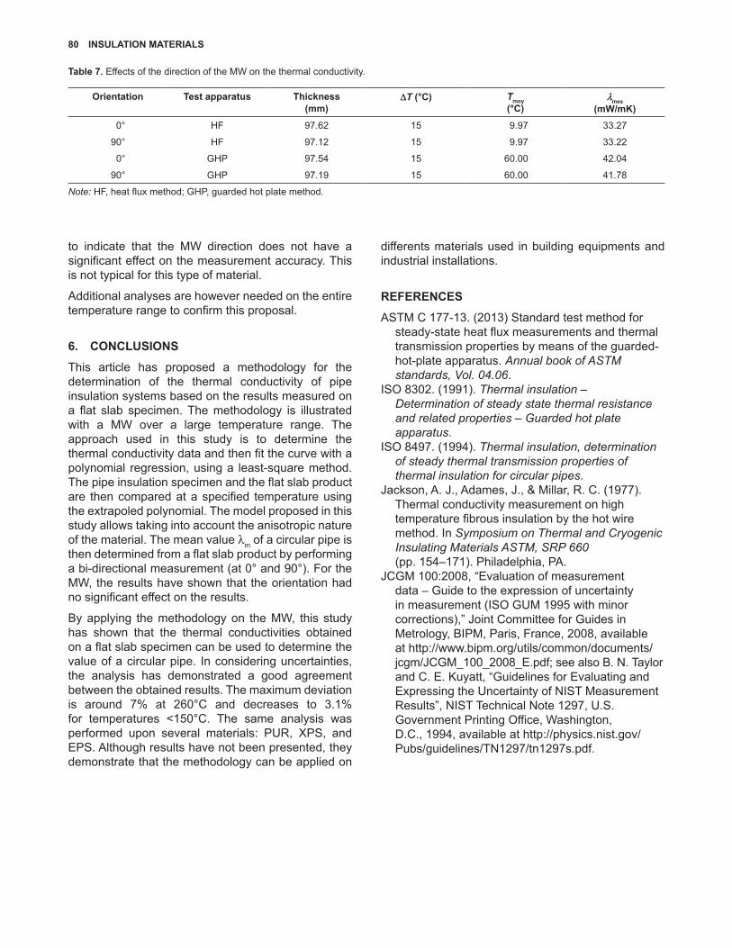
5.1 Influence of the orientationThe effects of the orientation of the MW were studied. Measurements were performed following two orientations (0°C and 90°C) on a flat slab specimen. Table 7 presents the results obtained from different test methods (heat flux method and GHP method).

The measurements in the Table 7 demonstrate that the orientation-related difference in conductivity is 0.1% at 10°C and 0.6% at 60°C. This result seems


to indicate that the MW direction does not have a significant effect on the measurement accuracy. This is not typical for this type of material.

Additional analyses are however needed on the entire temperature range to confirm this proposal.

6. CONCLUSIONS

This article has proposed a methodology for the determination of the thermal conductivity of pipe insulation systems based on the results measured on a flat slab specimen. The methodology is illustrated with a MW over a large temperature range. The approach used in this study is to determine the thermal conductivity data and then fit the curve with a polynomial regression, using a least-square method. The pipe insulation specimen and the flat slab product are then compared at a specified temperature using the extrapoled polynomial. The model proposed in this study allows taking into account the anisotropic nature of the material. The mean value lm of a circular pipe is then determined from a flat slab product by performing a bi-directional measurement (at 0° and 90°). For the MW, the results have shown that the orientation had no significant effect on the results.

By applying the methodology on the MW, this study has shown that the thermal conductivities obtained on a flat slab specimen can be used to determine the value of a circular pipe. In considering uncertainties, the analysis has demonstrated a good agreement between the obtained results. The maximum deviation is around 7% at 260°C and decreases to 3.1% for temperatures <150°C. The same analysis was performed upon several materials: PUR, XPS, and EPS. Although results have not been presented, they demonstrate that the methodology can be applied on

differents materials used in building equipments and industrial installations.

REFERENCES

ASTM C 177-13. (2013) Standard test method for steady-state heat flux measurements and thermal transmission properties by means of the guarded-hot-plate apparatus. Annual book of ASTM standards, Vol. 04.06.

ISO 8302. (1991). Thermal insulation – Determination of steady state thermal resistance and related properties – Guarded hot plate apparatus.

ISO 8497. (1994). Thermal insulation, determination of steady thermal transmission properties of thermal insulation for circular pipes.

Jackson, A. J., Adames, J., & Millar, R. C. (1977). Thermal conductivity measurement on high temperature fibrous insulation by the hot wire method. In Symposium on Thermal and Cryogenic Insulating Materials ASTM, SRP 660 (pp. 154–171). Philadelphia, PA.

JCGM 100:2008, “Evaluation of measurement data – Guide to the expression of uncertainty in measurement (ISO GUM 1995 with minor corrections),” Joint Committee for Guides in Metrology, BIPM, Paris, France, 2008, available at http://www.bipm.org/utils/common/documents/jcgm/JCGM_100_2008_E.pdf; see also B. N. Taylor and C. E. Kuyatt, “Guidelines for Evaluating and Expressing the Uncertainty of NIST Measurement Results”, NIST Technical Note 1297, U.S. Government Printing Office, Washington, D.C., 1994, available at http://physics.nist.gov/Pubs/guidelines/TN1297/tn1297s.pdf.

Table 7. Effects of the direction of the MW on the thermal conductivity.

Orientation Test apparatus Thickness(mm)

DT (°C) Tmoy(°C)

kmes(mW/mK)

0° HF 97.62 15 9.97 33.27

90° HF 97.12 15 9.97 33.22

0° GHP 97.54 15 60.00 42.04

90° GHP 97.19 15 60.00 41.78

Note: HF, heat flux method; GHP, guarded hot plate method.

Documents

Determination of the Thermal Resistance of Pipe Insulation