Brett A. BednarcykOhio Aerospace Institute, Brook Park, Ohio

Jacob AboudiTel Aviv University, Ramat-Aviv, Israel

Phillip W. YarringtonCollier Research Corporation, Hampton, Virginia

Determination of the Shear Stress Distribution in a Laminate From the Applied Shear Resultant—A Simplifi ed Shear Solution

NASA/CR—2007-215022

December 2007

https://ntrs.nasa.gov/search.jsp?R=20080012449 2018-06-27T04:40:03+00:00Z

NASA STI Program . . . in Profi le

Since its founding, NASA has been dedicated to the advancement of aeronautics and space science. The NASA Scientifi c and Technical Information (STI) program plays a key part in helping NASA maintain this important role.

The NASA STI Program operates under the auspices of the Agency Chief Information Offi cer. It collects, organizes, provides for archiving, and disseminates NASA’s STI. The NASA STI program provides access to the NASA Aeronautics and Space Database and its public interface, the NASA Technical Reports Server, thus providing one of the largest collections of aeronautical and space science STI in the world. Results are published in both non-NASA channels and by NASA in the NASA STI Report Series, which includes the following report types: • TECHNICAL PUBLICATION. Reports of

completed research or a major signifi cant phase of research that present the results of NASA programs and include extensive data or theoretical analysis. Includes compilations of signifi cant scientifi c and technical data and information deemed to be of continuing reference value. NASA counterpart of peer-reviewed formal professional papers but has less stringent limitations on manuscript length and extent of graphic presentations.

• TECHNICAL MEMORANDUM. Scientifi c

and technical fi ndings that are preliminary or of specialized interest, e.g., quick release reports, working papers, and bibliographies that contain minimal annotation. Does not contain extensive analysis.

• CONTRACTOR REPORT. Scientifi c and

technical fi ndings by NASA-sponsored contractors and grantees.

• CONFERENCE PUBLICATION. Collected

papers from scientifi c and technical conferences, symposia, seminars, or other meetings sponsored or cosponsored by NASA.

• SPECIAL PUBLICATION. Scientifi c,

technical, or historical information from NASA programs, projects, and missions, often concerned with subjects having substantial public interest.

• TECHNICAL TRANSLATION. English-

language translations of foreign scientifi c and technical material pertinent to NASA’s mission.

Specialized services also include creating custom thesauri, building customized databases, organizing and publishing research results.

For more information about the NASA STI program, see the following:

• Access the NASA STI program home page at http://www.sti.nasa.gov

• E-mail your question via the Internet to help@

sti.nasa.gov • Fax your question to the NASA STI Help Desk

at 301–621–0134 • Telephone the NASA STI Help Desk at 301–621–0390 • Write to:

NASA Center for AeroSpace Information (CASI) 7115 Standard Drive Hanover, MD 21076–1320

Brett A. BednarcykOhio Aerospace Institute, Brook Park, Ohio

Jacob AboudiTel Aviv University, Ramat-Aviv, Israel

Phillip W. YarringtonCollier Research Corporation, Hampton, Virginia

Determination of the Shear Stress Distribution in a Laminate From the Applied Shear Resultant—A Simplifi ed Shear Solution

NASA/CR—2007-215022

December 2007

National Aeronautics andSpace Administration

Glenn Research CenterCleveland, Ohio 44135

Prepared under Cooperative Agreement NCC06ZA29A

Acknowledgments

The authors gratefully acknowledge Dr. Steven M. Arnold, NASA Glenn Research Center, for his support and encouragement.

Available from

NASA Center for Aerospace Information7115 Standard DriveHanover, MD 21076–1320

National Technical Information Service5285 Port Royal RoadSpringfi eld, VA 22161

Available electronically at http://gltrs.grc.nasa.gov

Trade names and trademarks are used in this report for identifi cation only. Their usage does not constitute an offi cial endorsement, either expressed or implied, by the National Aeronautics and

Space Administration.

Level of Review: This material has been technically reviewed by NASA expert reviewer(s).

NASA/CR—2007-215022 1

Determination of the Shear Stress Distribution in a Laminate From the Applied Shear Resultant—A Simplified Shear Solution

Brett A. Bednarcyk

Ohio Aerospace Institute Brook Park, Ohio 44142

Jacob Aboudi

Tel Aviv University Ramat-Aviv, Israel 69978

Phillip W. Yarrington

Collier Research Corporation Hampton, Virginia 23666

Abstract The “simplified shear solution” method is presented for approximating the through-thickness shear

stress distribution within a composite laminate based on laminated beam theory. The method does not consider the solution of a particular boundary value problem, rather it requires only knowledge of the global shear loading, geometry, and material properties of the laminate or panel. It is thus analogous to lamination theory in that ply level stresses can be efficiently determined from global load resultants (as determined, for instance, by finite element analysis) at a given location in a structure and used to evaluate the margin of safety on a ply by ply basis. The simplified shear solution stress distribution is zero at free surfaces, continuous at ply boundaries, and integrates to the applied shear load. Comparisons to existing theories are made for a variety of laminates, and design examples are provided illustrating the use of the method for determining through-thickness shear stress margins in several types of composite panels and in the context of a finite element structural analysis.

Introduction It is known that by employing lamination theory, one can determine the in-plane stress distribution in

each layer of a laminate from the knowledge of the applied force and moment resultants. This information enables determination of ply-by-ply margins for the laminate, which are needed for design and sizing. The distribution of the interlaminar shear stresses in each layer from the applied shear resultants are not readily available from the standard lamination theory equations. These stresses are also needed to enable design and sizing of laminates subjected to global shear loads. The present report provides an analytical method, based on laminated beam theory with shear loading, for determining the interlaminar shear stress distribution in a laminate from a given applied shear resultant. It should be emphasized that the classical or the higher-order (e.g., first-order shear deformable) plate theory cannot be employed to determine the correct interlaminar shear stress distribution through the laminate thickness from the knowledge of the force, moment, and shear resultants. Indeed, the classical plate theory provides identically zero interlaminar shear stresses, whereas the higher-order plate theories provide piece-wise profiles that are discontinuous at the ply interfaces. It should also be noted that the simple shear solution provided herein does not involve the solution of a particular boundary value problem. Rather, it is only assumed that the force, moment, and shear resultants are known at a particular location in the laminate, and the solution is independent of the source of these known resultant quantities. Conversely, in order to obtain the interlaminar shear distribution via integration of the differential equations of equilibrium, the solution of a boundary value problem would be required to determine the variation of the stress fields in each ply.

NASA/CR—2007-215022 2

The presented theory has been validated for laminates with one to five layers composed of both isotropic and anisotropic materials by comparison to approximate methods (HOTFMG (Aboudi et al., 1999), HyperSizer Joints (Zhang et al., 2006)) and an exact plate solution (Williams, 1999). Finally, the theory is implemented for the practical analysis of composite stiffened panels in the HyperSizer software (Collier Research Corp., 2007). Results, including predicted margins of safety, are given for a graphite/epoxy laminate, a honeycomb sandwich panel, an I-stiffened panel, and laminate components of a pressure shell structure.

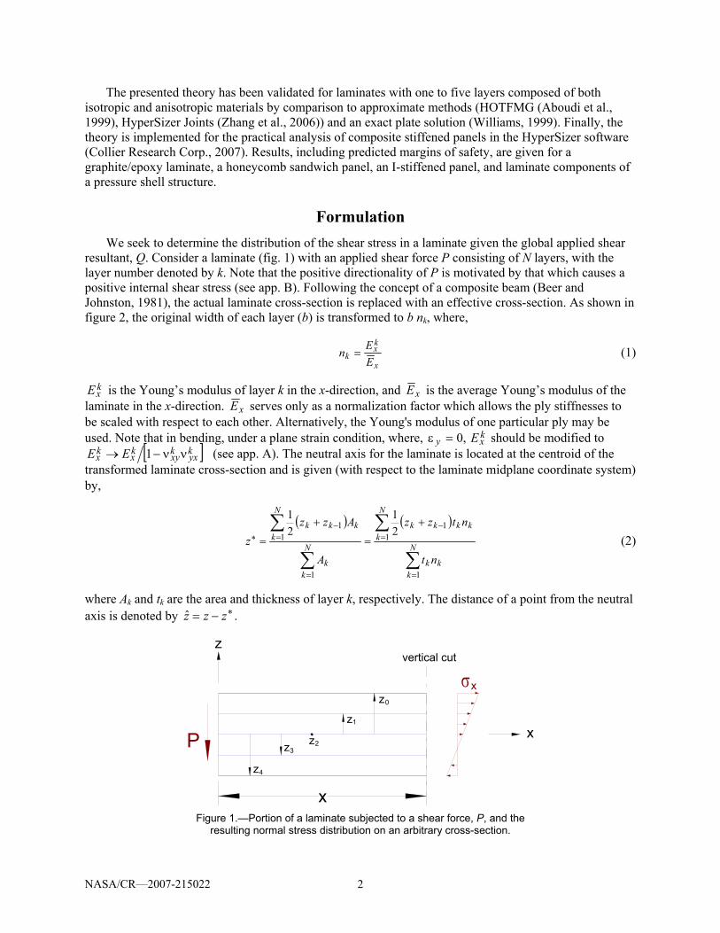
Formulation We seek to determine the distribution of the shear stress in a laminate given the global applied shear

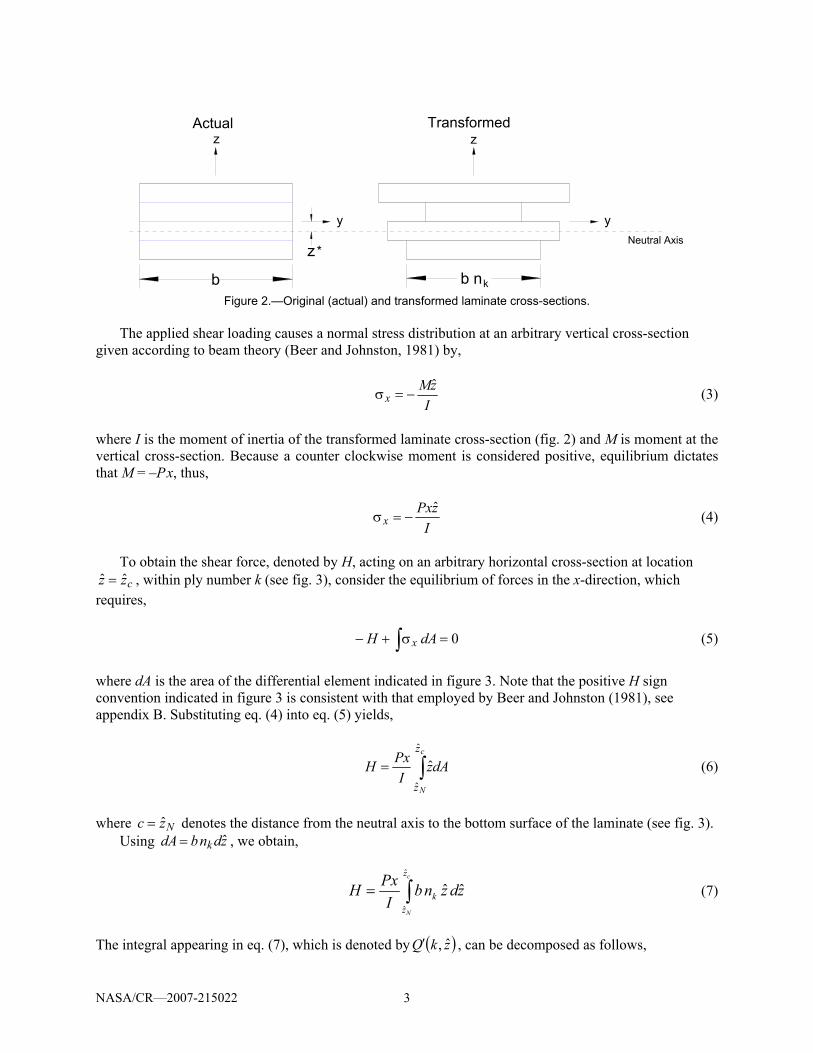
resultant, Q. Consider a laminate (fig. 1) with an applied shear force P consisting of N layers, with the layer number denoted by k. Note that the positive directionality of P is motivated by that which causes a positive internal shear stress (see app. B). Following the concept of a composite beam (Beer and Johnston, 1981), the actual laminate cross-section is replaced with an effective cross-section. As shown in figure 2, the original width of each layer (b) is transformed to b nk, where,

x

kx

k EEn = (1)

kxE is the Young’s modulus of layer k in the x-direction, and xE is the average Young’s modulus of the

laminate in the x-direction. xE serves only as a normalization factor which allows the ply stiffnesses to be scaled with respect to each other. Alternatively, the Young's modulus of one particular ply may be used. Note that in bending, under a plane strain condition, where, k

xy E,0=ε should be modified to [ ]kyxkxykxkx EE νν−→ 1 (see app. A). The neutral axis for the laminate is located at the centroid of the

transformed laminate cross-section and is given (with respect to the laminate midplane coordinate system) by,

( ) ( )

∑

∑

∑

∑

=

=−

=

=− +

=

+

= N

kkk

N

kkkkk

N

kk

N

kkkk

nt

ntzz

A

Azzz

1

11

1

11

*21

21

(2)

where Ak and tk are the area and thickness of layer k, respectively. The distance of a point from the neutral axis is denoted by *ˆ zzz −= .

x

x

z

P

σx

vertical cut

z

0

z

1

z2

z

3

z

4

Figure 1.—Portion of a laminate subjected to a shear force, P, and the

resulting normal stress distribution on an arbitrary cross-section.

NASA/CR—2007-215022 3

b

y

z

y

b n k

z

Neutral Axisz*

Figure 2.—Original (actual) and transformed laminate cross-sections.

The applied shear loading causes a normal stress distribution at an arbitrary vertical cross-section

given according to beam theory (Beer and Johnston, 1981) by,

IzM

xˆ

−=σ (3)

where I is the moment of inertia of the transformed laminate cross-section (fig. 2) and M is moment at the vertical cross-section. Because a counter clockwise moment is considered positive, equilibrium dictates that M = –P x, thus,

I

zPxx

ˆ−=σ (4)

To obtain the shear force, denoted by H, acting on an arbitrary horizontal cross-section at location

czz ˆˆ = , within ply number k (see fig. 3), consider the equilibrium of forces in the x-direction, which requires, ∫ =σ+− 0dAH x (5)

where dA is the area of the differential element indicated in figure 3. Note that the positive H sign convention indicated in figure 3 is consistent with that employed by Beer and Johnston (1981), see appendix B. Substituting eq. (4) into eq. (5) yields,

∫=c

N

z

z

dAzI

PxHˆ

ˆ

ˆ (6)

where Nzc ˆ= denotes the distance from the neutral axis to the bottom surface of the laminate (see fig. 3).

Using zdnbdA k ˆ= , we obtain,

ˆ

ˆ

ˆ ˆc

N

z

kz

PxH bn z dzI

= ∫ (7)

The integral appearing in eq. (7), which is denoted by ( )zkQ ˆ,′ , can be decomposed as follows,

Actual Transformed

NASA/CR—2007-215022 4

1

1

ˆ ˆ ˆ ˆ

1ˆ ˆ ˆ ˆ

ˆ ˆ ˆ ˆ ˆ ˆ ˆ ˆ ˆ( , )c c k N

N k k N

z z z z

k k k Nz z z z

Q k z bn z dz bn z dz bn z dz bn z dz−

+

+′ = = + + +∫ ∫ ∫ ∫… (8)

It follows that

( ) ( ) ( )2 2 2 21

1

1ˆ ˆ ˆ ˆ ˆ,2 2

Nk

c k m m mm k

bnQ k z z z bn z z−= +

′ = − + −∑ (9)

x

z

σx

vertical cut

horizontal cut

neutral axis

zcH

Layer k

^

dA

cross-section

dz

k

zk

z = -cN

b n

Figure. 3.—Section of laminate acted upon by the horizontal shear force, H, and the distributed normal stress, σx.

where czN −=ˆ . Hence, the shear force, H, is given by,

( )zkQI

PxH ˆ,′= (10)

The shear stress, τ, is given by,

xbH

−=τ (11)

where the negative sign is due to the opposite directionality of the internal shear force compared to the shear stress (see app. B). The applied shear resultant, Q, is related to the applied shear force, P, by Q P b= , and it follows that,

( ) ( )zkQIQzk ˆ,ˆ, ′−=τ (12)

In employing this equation, the moment of inertia of the transformed beam cross-section is given by,

2

3 1

1

ˆ ˆ112 2

Nk k

k k k kk

z zI bn t bn t −

=

⎡ ⎤+⎛ ⎞= +⎢ ⎥⎜ ⎟⎝ ⎠⎢ ⎥⎣ ⎦

∑ (13)

NASA/CR—2007-215022 5

Thus, given eqs. (9) and (13), the shear stress distribution throughout the laminate can be determined from eq. (12).

It should be emphasized that at the top and bottom of the laminate the shear stress must be equal to zero. In addition, the integral of τ over the entire thickness of the laminate must be equal to the applied shear resultant, Q, that is,

∫ =τNz

z

Qdz0

(14)

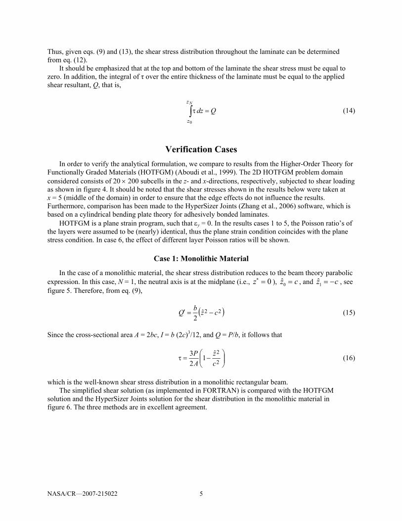
Verification Cases In order to verify the analytical formulation, we compare to results from the Higher-Order Theory for

Functionally Graded Materials (HOTFGM) (Aboudi et al., 1999). The 2D HOTFGM problem domain considered consists of 20 × 200 subcells in the z- and x-directions, respectively, subjected to shear loading as shown in figure 4. It should be noted that the shear stresses shown in the results below were taken at x = 5 (middle of the domain) in order to ensure that the edge effects do not influence the results. Furthermore, comparison has been made to the HyperSizer Joints (Zhang et al., 2006) software, which is based on a cylindrical bending plate theory for adhesively bonded laminates.

HOTFGM is a plane strain program, such that εy = 0. In the results cases 1 to 5, the Poisson ratio’s of the layers were assumed to be (nearly) identical, thus the plane strain condition coincides with the plane stress condition. In case 6, the effect of different layer Poisson ratios will be shown.

Case 1: Monolithic Material

In the case of a monolithic material, the shear stress distribution reduces to the beam theory parabolic expression. In this case, N = 1, the neutral axis is at the midplane (i.e., 0z∗ = ), 0z c= , and 1z c= − , see figure 5. Therefore, from eq. (9),

( )22ˆ2

czbQ −=′ (15)

Since the cross-sectional area A = 2bc, I = b (2c)3/12, and Q = P/b, it follows that

⎟⎟⎠

⎞⎜⎜⎝

⎛−=τ

2

2ˆ1

23

cz

AP (16)

which is the well-known shear stress distribution in a monolithic rectangular beam.

The simplified shear solution (as implemented in FORTRAN) is compared with the HOTFGM solution and the HyperSizer Joints solution for the shear distribution in the monolithic material in figure 6. The three methods are in excellent agreement.

NASA/CR—2007-215022 6

1 mm

10 mm

z

x

FreeSymmetryσ = 0τ = 1

x

xz

Pinned

}MPa

Figure 4.—HOTFGM representation of the laminate considered.

z

x

z = c0

z = -c1 Figure 5.—Monolithic (single layer) laminate.

-0.5

-0.4

-0.3

-0.2

-0.1

0.0

0.1

0.2

0.3

0.4

0.5

0.0 0.2 0.4 0.6 0.8 1.0 1.2 1.4 1.6

τ (MPa)

z (m

m)

Simplified Shear SolutionHOTFGMHyperSizer Joints

Figure 6.—Monolithic material shear stress distribution (Case 1).

E = 40 GPa

z

x

NASA/CR—2007-215022 7

-0.5

-0.4

-0.3

-0.2

-0.1

0.0

0.1

0.2

0.3

0.4

0.5

0.0 0.2 0.4 0.6 0.8 1.0 1.2 1.4 1.6 1.8

τ (MPa)

z (m

m)

Simplified Shear SolutionHOTFGMHyperSizer Joints

Figure 7.—Bi-material laminate shear stress distribution (Case 2).

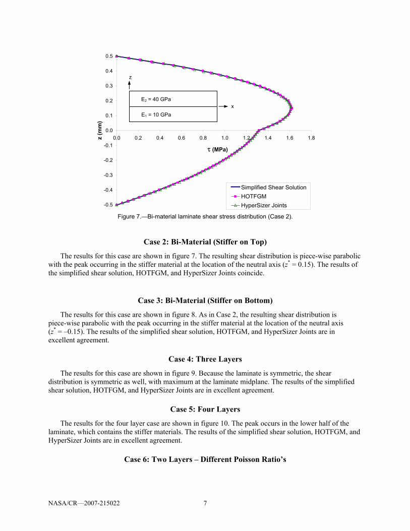
Case 2: Bi-Material (Stiffer on Top)

The results for this case are shown in figure 7. The resulting shear distribution is piece-wise parabolic with the peak occurring in the stiffer material at the location of the neutral axis (z* = 0.15). The results of the simplified shear solution, HOTFGM, and HyperSizer Joints coincide.

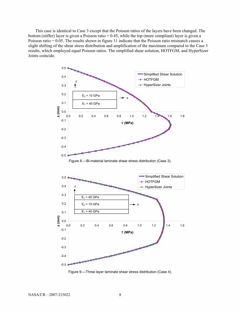
Case 3: Bi-Material (Stiffer on Bottom)

The results for this case are shown in figure 8. As in Case 2, the resulting shear distribution is piece-wise parabolic with the peak occurring in the stiffer material at the location of the neutral axis (z* = –0.15). The results of the simplified shear solution, HOTFGM, and HyperSizer Joints are in excellent agreement.

Case 4: Three Layers

The results for this case are shown in figure 9. Because the laminate is symmetric, the shear distribution is symmetric as well, with maximum at the laminate midplane. The results of the simplified shear solution, HOTFGM, and HyperSizer Joints are in excellent agreement.

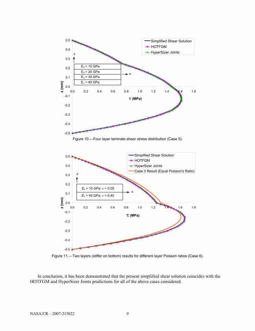
Case 5: Four Layers

The results for the four layer case are shown in figure 10. The peak occurs in the lower half of the laminate, which contains the stiffer materials. The results of the simplified shear solution, HOTFGM, and HyperSizer Joints are in excellent agreement.

Case 6: Two Layers – Different Poisson Ratio’s

E2 = 40 GPa

E1 = 10 GPa

z

x

NASA/CR—2007-215022 8

This case is identical to Case 3 except that the Poisson ratios of the layers have been changed. The bottom (stiffer) layer is given a Poisson ratio = 0.45, while the top (more compliant) layer is given a Poisson ratio = 0.05. The results shown in figure 11 indicate that the Poisson ratio mismatch causes a slight shifting of the shear stress distribution and amplification of the maximum compared to the Case 3 results, which employed equal Poisson ratios. The simplified shear solution, HOTFGM, and HyperSizer Joints coincide.

-0.5

-0.4

-0.3

-0.2

-0.1

0.0

0.1

0.2

0.3

0.4

0.5

0.0 0.2 0.4 0.6 0.8 1.0 1.2 1.4 1.6 1.8

τ (MPa)

z (m

m)

Simplified Shear SolutionHOTFGMHyperSizer Joints

Figure 8.—Bi-material laminate shear stress distribution (Case 3).

-0.5

-0.4

-0.3

-0.2

-0.1

0.0

0.1

0.2

0.3

0.4

0.5

0.0 0.2 0.4 0.6 0.8 1.0 1.2 1.4 1.6

τ (MPa)

z (m

m)

Simplified Shear SolutionHOTFGMHyperSizer Joints

Figure 9.—Three layer laminate shear stress distribution (Case 4).

E2 = 10 GPa

E1 = 40 GPa

z

x

E3 = 40 GPa

E1 = 40 GPa

E2 = 10 GPa

z

x

NASA/CR—2007-215022 9

-0.5

-0.4

-0.3

-0.2

-0.1

0.0

0.1

0.2

0.3

0.4

0.5

0.0 0.2 0.4 0.6 0.8 1.0 1.2 1.4 1.6 1.8

τ (MPa)

z (m

m)

Simplified Shear SolutionHOTFGMHyperSizer Joints

Figure 10.—Four layer laminate shear stress distribution (Case 5).

-0.5

-0.4

-0.3

-0.2

-0.1

0.0

0.1

0.2

0.3

0.4

0.5

0.0 0.2 0.4 0.6 0.8 1.0 1.2 1.4 1.6 1.8

τ (MPa)

z (m

m)

Simplified Shear SolutionHOTFGMHyperSizer JointsCase 3 Result (Equal Poisson's Ratio)

Figure 11.—Two layers (stiffer on bottom) results for different layer Poisson ratios (Case 6).

In conclusion, it has been demonstrated that the present simplified shear solution coincides with the

HOTFGM and HyperSizer Joints predictions for all of the above cases considered.

E4 = 10 GPa E3 = 20 GPa E2 = 30 GPa E1 = 40 GPa

z

x

E2 = 10 GPa, ν = 0.05

E1 = 40 GPa, ν = 0.45

z

x

NASA/CR—2007-215022 10

Cases 7 to 9: Comparison with Plate Theory

Here we compare to results from Williams' (1999) multilength scale plate theory, which has been shown to coincide with Pagano's (1969) exact solution for plates in cylindrical bending, as well as HyperSizer Joints. It should be noted that Williams' plate theory considers sinusoidal pressure loading on the top of the plate as opposed to an applied shear load. The τxz distribution from a cross-section within the plate theory results were then integrated obtain the applied Qx used in the current simplified shear solution. This therefore mimics the HyperSizer situation where a Qx value is given for a point in the laminate with no knowledge of the global problem or boundary conditions used to generate the Qx load. In all three cases below, Qx = 0.32 N/mm. We consider three asymmetric laminates, a cross-ply, a [0°/90°/45°/90°/0°], and a [–30°/90°/45°/60°/30°], where the asymmetry arises due to different ply thicknesses, which are [0.2, 0.4, 0.2, 0.1, 0.1] mm for all three laminates. The material properties of the plies are given in table 1, where the standard expression for νyx is given in eq. (30) in appendix A. The resulting shear stress distributions for these laminates are shown in figures 12 to 14, respectively.

TABLE 1.—MATERIAL PROPERTIES FOR SIMPLIFIED SHEAR SOLUTION COMPARISON WITH PLATE THEORY. Ply angle, degree -30 0 30 45 60 90 Ex, GPa 2.192 25 2.192 1.325 1.068 1 Ey, GPa 1.068 1 1.068 1.325 2.192 25 νxy 0.4082 0.25 0.4082 0.3245 0.1989 0.01

Figure 12 shows that the shear stresses predicted for the cross-ply laminate coincide with the HyperSizer Joints solution, but deviate slightly from Williams' (1999) solution. Figure 13 shows that introducing a 45° ply results in some deviation in the top 90° and 45° plies. Introducing angle plies to the laminate configuration results in the distribution shown in figure 14. In conclusion, the simplified shear solution appears to give a good estimate of the shear distributions for the laminates considered, given the method's simplicity and efficiency.

-0.6

-0.4

-0.2

0

0.2

0.4

0.6

0.00 0.10 0.20 0.30 0.40 0.50

τ (MPa)

z (m

m)

Simplified Shear Solution

HyperSizer Joints

Williams (1999)

Figure 12.—Shear stress distribution for [0°/90°/0°/90°/0°] laminate

with ply thickness of [0.2, 0.4, 0.2, 0.1, 0.1] mm (Case 7).

NASA/CR—2007-215022 11

-0.6

-0.4

-0.2

0

0.2

0.4

0.6

0.00 0.10 0.20 0.30 0.40 0.50

τ (MPa)

z (m

m)

Simplified Shear SolutionHyperSizer JointsWilliams (1999)

Figure 13.—Shear stress distribution for [0°/90°/45°/90°/0°] laminate

with ply thickness of [0.2, 0.4, 0.2, 0.1, 0.1] mm (Case 8).

-0.6

-0.4

-0.2

0

0.2

0.4

0.6

0.00 0.10 0.20 0.30 0.40 0.50

τ (MPa)

z (m

m)

Simplified Shear SolutionHyperSizer JointsWilliams (1999)

Figure 14.—Shear stress distribution for [-30°/90°/45°/60°/30°] laminate

with ply thickness of [0.2, 0.4, 0.2, 0.1, 0.1] mm (Case 9).

Design Examples In order to design a composite laminate or stiffened panel that is subjected to external loading, the

first step is to determine the induced local stresses in the structure. Then these stresses are compared to allowable stresses in order to determine the margin of safety of the considered composite panel. The propose simplified shear solution returns ply-level shear stresses at any point in the panel in global x, y, z laminate coordinates (see fig. 4). However, most failure analysis methods require stress allowables in terms of ply local (x1, x2, x3) coordinates, where x3 = z and x1 corresponds to the ply fiber direction.

NASA/CR—2007-215022 12

Therefore, stresses in global coordinates obtained from the present analysis for any ply must be transformed into local ply coordinates according to:

⎭⎬⎫

⎩⎨⎧

ττ

⎥⎦

⎤⎢⎣

⎡θθ−θθ

=⎭⎬⎫

⎩⎨⎧

ττ

yz

xz

cossinsincos

23

13 (17)

where θ is the ply angle (between the fiber direction and the global x-direction). Note that in the previous sections, the shear stress τ denotes either τxz, or τyz, depending on whether the applied shear force resultant Q stands for Qx or Qy (respectively).

Once the ply local stresses are known, it is assumed that failure will occur when the following interaction equation is satisfied:

12

23

232

13

13 =⎟⎟⎠

⎞⎜⎜⎝

⎛ τ+⎟⎟

⎠

⎞⎜⎜⎝

⎛ τFsuFsu

(18)

where Fsu13 and Fsu23 are the ply material shear stress allowables, respectively, which can be found in references such as MIL-HDBK-17. This interaction equation can be written as a margin of safety (see Zhang and Collier, 2004) as,

2 2

13 23

13 23

1 1MS

Fsu Fsu

= −⎛ ⎞ ⎛ ⎞τ τ

+⎜ ⎟ ⎜ ⎟⎝ ⎠ ⎝ ⎠

(19)

where the margin of safety expresses how close to failure is the given panel. Thus, a positive margin of safety indicates that there is no failure for the considered loading, while a negative margin of safety indicates that failure has occurred.

Finally, it should be mentioned that in the presence of combined applied shear loading (Qx and Qy), the current analysis is applicable by superimposing the resulting stress distribution induced by each of Qx and Qy independently.

Design Example 1—Unstiffened Laminate

This example considers an unstiffened graphite/epoxy laminate subjected to biaxial transverse shear loading (Qx = Qy = 200 lb/in.). This type of loading could result, for example, at the corner of a rectangular panel subjected to uniform pressure loading. A [45°/-45°/0°/90°/0°/90°/45°/-45°/0°]s layup is considered with uniform ply thicknesses of 0.005 in., thus forming a total thickness of 0.09 in. Ply material properties are given in table 2.

TABLE 2.—GRAPHITE/EPOXY PLY MATERIAL PROPERTIES. E1, Msi

E2, Msi

ν12 Fsu13, ksi

Fsu23, ksi

23.35 1.65 0.32 14.8 5.32

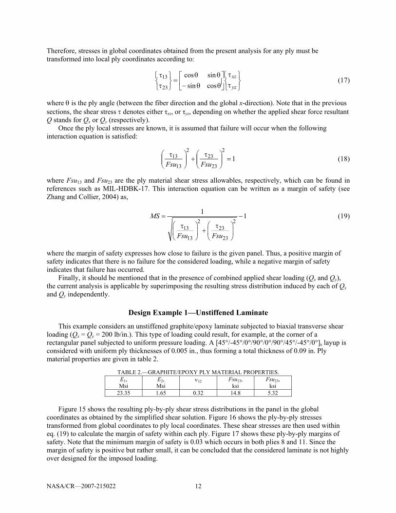
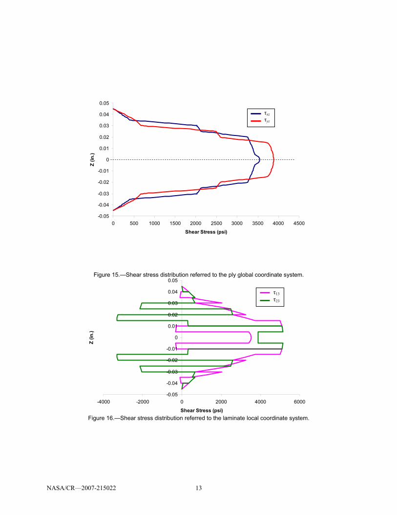
Figure 15 shows the resulting ply-by-ply shear stress distributions in the panel in the global coordinates as obtained by the simplified shear solution. Figure 16 shows the ply-by-ply stresses transformed from global coordinates to ply local coordinates. These shear stresses are then used within eq. (19) to calculate the margin of safety within each ply. Figure 17 shows these ply-by-ply margins of safety. Note that the minimum margin of safety is 0.03 which occurs in both plies 8 and 11. Since the margin of safety is positive but rather small, it can be concluded that the considered laminate is not highly over designed for the imposed loading.

NASA/CR—2007-215022 13

-0.05

-0.04

-0.03

-0.02

-0.01

0

0.01

0.02

0.03

0.04

0.05

0 500 1000 1500 2000 2500 3000 3500 4000 4500

Shear Stress (psi)

Z (in

.)

TAUXZTAUYZ

Figure 15.—Shear stress distribution referred to the ply global coordinate system.

-0.05

-0.04

-0.03

-0.02

-0.01

0

0.01

0.02

0.03

0.04

0.05

-4000 -2000 0 2000 4000 6000

Shear Stress (psi)

Z (in

.)

TAU13TAU23

Figure 16.—Shear stress distribution referred to the laminate local coordinate system.

τxz τyz

τ13 τ23

NASA/CR—2007-215022 14

-0.04

-0.03

-0.02

-0.01

0

0.01

0.02

0.03

0.04

0 0.5 1 1.5 2

Margin of Safety

Z (in

.)

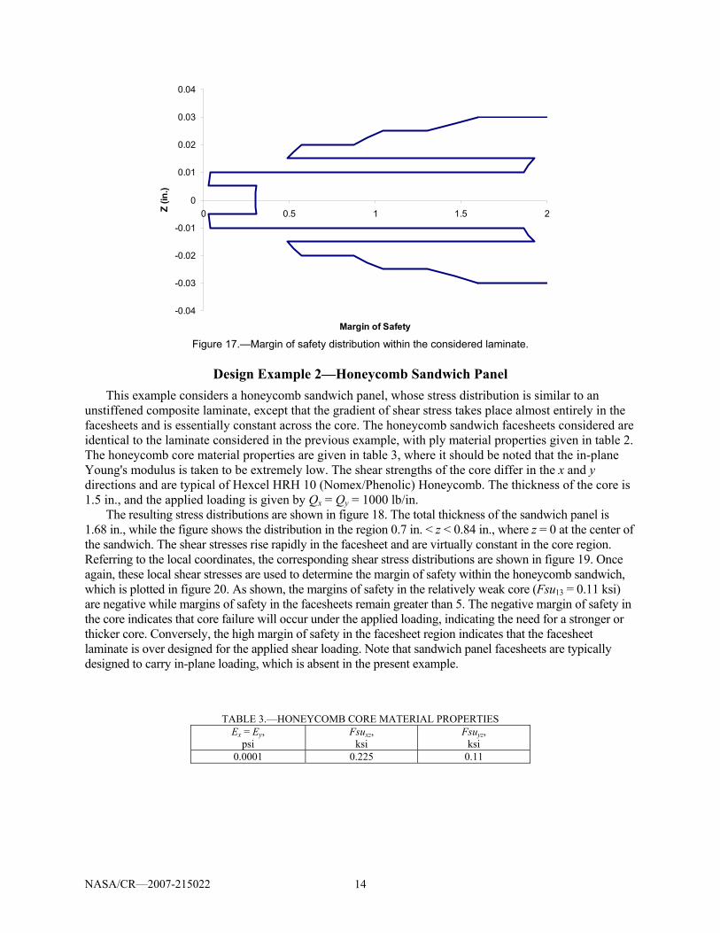
Figure 17.—Margin of safety distribution within the considered laminate.

Design Example 2—Honeycomb Sandwich Panel This example considers a honeycomb sandwich panel, whose stress distribution is similar to an

unstiffened composite laminate, except that the gradient of shear stress takes place almost entirely in the facesheets and is essentially constant across the core. The honeycomb sandwich facesheets considered are identical to the laminate considered in the previous example, with ply material properties given in table 2. The honeycomb core material properties are given in table 3, where it should be noted that the in-plane Young's modulus is taken to be extremely low. The shear strengths of the core differ in the x and y directions and are typical of Hexcel HRH 10 (Nomex/Phenolic) Honeycomb. The thickness of the core is 1.5 in., and the applied loading is given by Qx = Qy = 1000 lb/in.

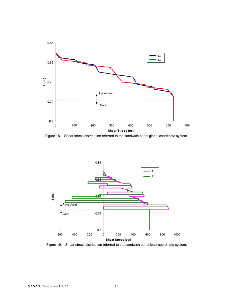
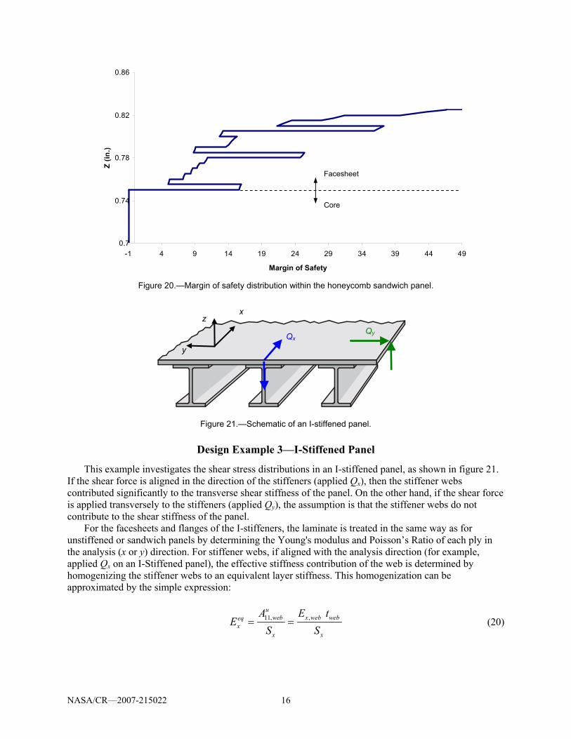
The resulting stress distributions are shown in figure 18. The total thickness of the sandwich panel is 1.68 in., while the figure shows the distribution in the region 0.7 in. < z < 0.84 in., where z = 0 at the center of the sandwich. The shear stresses rise rapidly in the facesheet and are virtually constant in the core region. Referring to the local coordinates, the corresponding shear stress distributions are shown in figure 19. Once again, these local shear stresses are used to determine the margin of safety within the honeycomb sandwich, which is plotted in figure 20. As shown, the margins of safety in the relatively weak core (Fsu13 = 0.11 ksi) are negative while margins of safety in the facesheets remain greater than 5. The negative margin of safety in the core indicates that core failure will occur under the applied loading, indicating the need for a stronger or thicker core. Conversely, the high margin of safety in the facesheet region indicates that the facesheet laminate is over designed for the applied shear loading. Note that sandwich panel facesheets are typically designed to carry in-plane loading, which is absent in the present example.

TABLE 3.—HONEYCOMB CORE MATERIAL PROPERTIES Ex = Ey,

psi Fsuxz,

ksi Fsuyz,

ksi 0.0001 0.225 0.11

NASA/CR—2007-215022 15

0.7

0.74

0.78

0.82

0.86

0 100 200 300 400 500 600 700

Shear Stress (psi)

Z (in

.)

TAUXZTAUYZ

Figure 18.—Shear stress distribution referred to the sandwich panel global coordinate system.

0.7

0.74

0.78

0.82

0.86

-600 -400 -200 0 200 400 600 800 1000

Shear Stress (psi)

Z (in

.)

TAU13TAU23

Figure 19.—Shear stress distribution referred to the sandwich panel local coordinate system.

Facesheet

Core

τxz τyz

Facesheet

Core

τ13

τ23

NASA/CR—2007-215022 16

0.7

0.74

0.78

0.82

0.86

-1 4 9 14 19 24 29 34 39 44 49

Shear Stress (psi)

Z (in

.)

Figure 20.—Margin of safety distribution within the honeycomb sandwich panel.

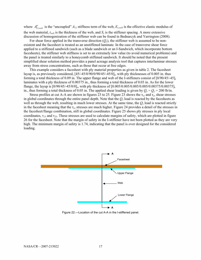
Figure 21.—Schematic of an I-stiffened panel.

Design Example 3—I-Stiffened Panel

This example investigates the shear stress distributions in an I-stiffened panel, as shown in figure 21. If the shear force is aligned in the direction of the stiffeners (applied Qx), then the stiffener webs contributed significantly to the transverse shear stiffness of the panel. On the other hand, if the shear force is applied transversely to the stiffeners (applied Qy), the assumption is that the stiffener webs do not contribute to the shear stiffness of the panel.

For the facesheets and flanges of the I-stiffeners, the laminate is treated in the same way as for unstiffened or sandwich panels by determining the Young's modulus and Poisson’s Ratio of each ply in the analysis (x or y) direction. For stiffener webs, if aligned with the analysis direction (for example, applied Qx on an I-Stiffened panel), the effective stiffness contribution of the web is determined by homogenizing the stiffener webs to an equivalent layer stiffness. This homogenization can be approximated by the simple expression:

11, ,u

web x web webeqx

x x

A E tE

S S= = (20)

Qy Qx y

x z

Facesheet

Core

Margin of Safety

NASA/CR—2007-215022 17

where 11,u

webA is the “uncoupled” A11 stiffness term of the web, Ex,web is the effective elastic modulus of the web material, tweb is the thickness of the web, and Sx is the stiffener spacing. A more extensive discussion of homogenization of the stiffener web can be found in Bednarcyk and Yarrington (2008).

For shear force applied in the transverse direction (Qy), the stiffener web is assumed to be non-existent and the facesheet is treated as an unstiffened laminate. In the case of transverse shear force applied to a stiffened sandwich (such as a blade sandwich or an I-Sandwich, which incorporate bottom facesheets), the stiffener web stiffness is set to an extremely low value (to avoid numerical problems) and the panel is treated similarly to a honeycomb stiffened sandwich. It should be noted that the present simplified shear solution method provides a panel acreage analysis tool that captures interlaminar stresses away from stress concentrations, such as those that occur at free edges.

This example considers a facesheet with ply material properties as given in table 2. The facesheet layup is, as previously considered, [45/-45/0/90/0/90/45/-45/0]s, with ply thicknesses of 0.005 in. thus forming a total thickness of 0.09 in. The upper flange and web of the I-stiffeners consist of [0/90/45/-45]s laminates with a ply thickness of 0.00375 in., thus forming a total thickness of 0.03 in. As for the lower flange, the layup is [0/90/45/-45/0/0]s, with ply thickness of [0.005/0.005/0.005/0.005/0.00375/0.00375]s in., thus forming a total thickness of 0.05 in. The applied shear loading is given by Qx = Qy = 200 lb/in.

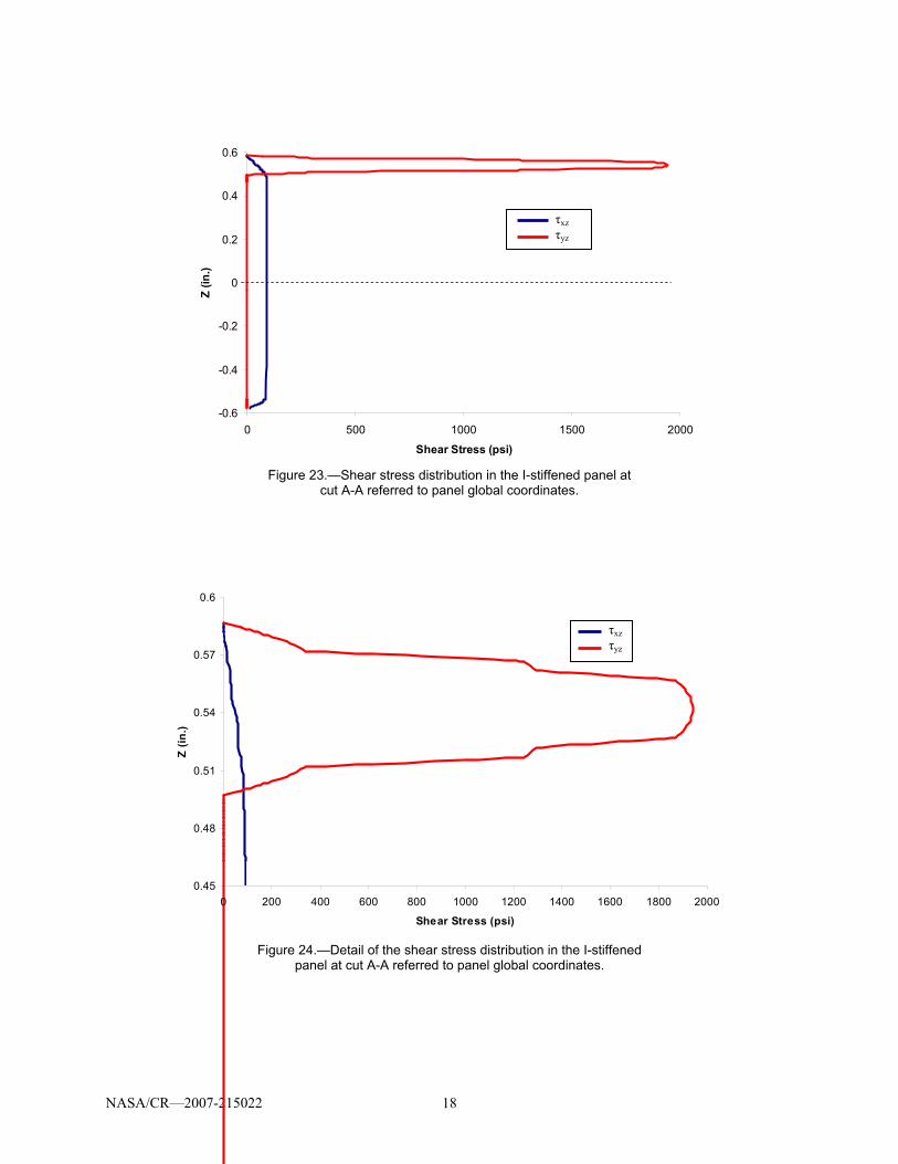
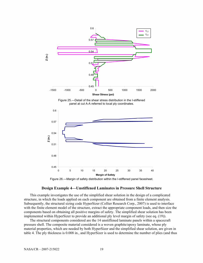
Stress profiles at cut A-A are shown in figures 23 to 25. Figure 23 shows the τxz and τyz shear stresses in global coordinates through the entire panel depth. Note that the Qx load is reacted by the facesheets as well as through the web, resulting in much lower stresses. At the same time, the Qy load is reacted strictly in the facesheet meaning that the τyz stresses are much higher. Figure 24 provides a detail of the stresses in the facesheet/flange combination, still in global coordinates. Figure 25 shows ply stresses in ply local coordinates, τ13 and τ23. These stresses are used to calculate margins of safety, which are plotted in figure 26 for the facesheet. Note that the margin of safety in the I-stiffener have not been plotted as they are very high. The minimum margin of safety is 1.74, indicating that the panel is over designed for the considered loading.

Figure 22.—Location of the cut A-A in the I-stiffened panel.

Facesheet

Upper Flange

Web

Lower Flange

A

A

NASA/CR—2007-215022 18

-0.6

-0.4

-0.2

0

0.2

0.4

0.6

0 500 1000 1500 2000

Shear Stress (psi)

Z (in

.)TAUXZTAUYZ

Figure 23.—Shear stress distribution in the I-stiffened panel at

cut A-A referred to panel global coordinates.

0.45

0.48

0.51

0.54

0.57

0.6

0 200 400 600 800 1000 1200 1400 1600 1800 2000

Shear Stress (psi)

Z (in

.)

TAUXZTAUYZ

Figure 24.—Detail of the shear stress distribution in the I-stiffened

panel at cut A-A referred to panel global coordinates.

τxz τyz

τxz τyz

NASA/CR—2007-215022 19

0.45

0.48

0.51

0.54

0.57

0.6

-1500 -1000 -500 0 500 1000 1500 2000

Shear Stress (psi)

Z (in

.)

TAU13TAU23

Figure 25.—Detail of the shear stress distribution in the I-stiffened

panel at cut A-A referred to local ply coordinates.

0.45

0.48

0.51

0.54

0.57

0.6

0 5 10 15 20 25 30 35 40

Margin of Safety

Z (in

.)

Figure 26.—Margin of safety distribution within the I-stiffened panel facesheet.

Design Example 4—Unstiffened Laminates in Pressure Shell Structure

This example investigates the use of the simplified shear solution in the design of a complicated structure, in which the loads applied on each component are obtained from a finite element analysis. Subsequently, the structural sizing code HyperSizer (Collier Research Corp., 2007) is used to interface with the finite element model of the structure, extract the appropriate component loads, and then size the components based on obtaining all positive margins of safety. The simplified shear solution has been implemented within HyperSizer to provide an additional ply level margin of safety (see eq. (19)).

The structural components considered are the 14 unstiffened laminate panels within a spacecraft pressure shell. The composite material considered is a woven graphite/epoxy laminate, whose ply material properties, which are needed by both HyperSizer and the simplified shear solution, are given in table 4. The ply thickness is 0.008 in., and HyperSizer is used to determine the number of plies (and thus

τ13 τ23

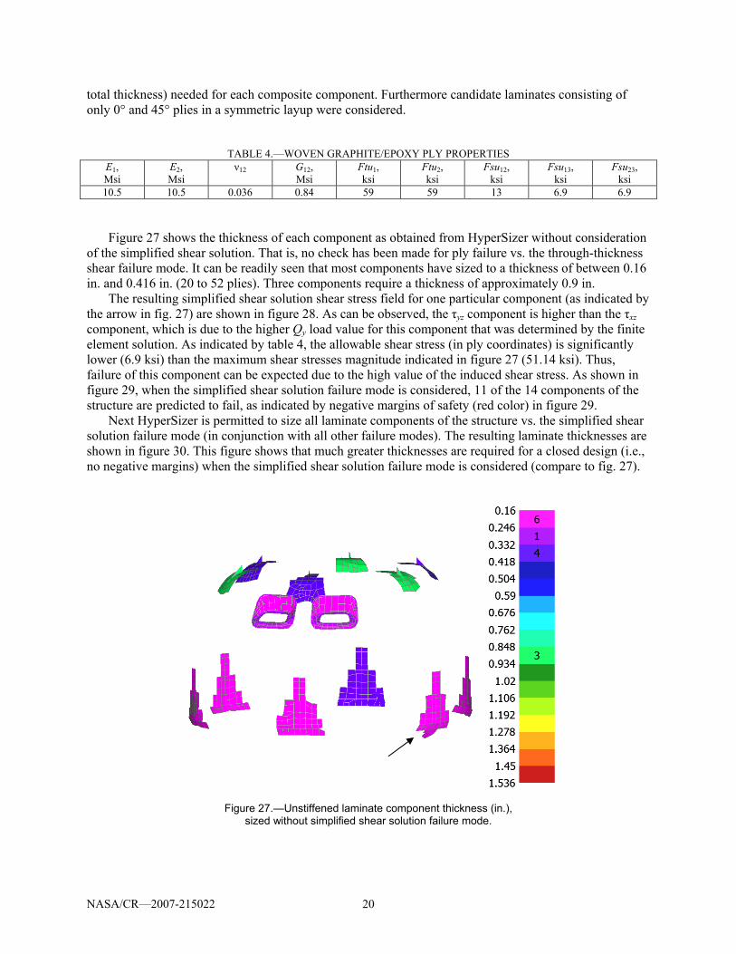
NASA/CR—2007-215022 20

total thickness) needed for each composite component. Furthermore candidate laminates consisting of only 0° and 45° plies in a symmetric layup were considered.

TABLE 4.—WOVEN GRAPHITE/EPOXY PLY PROPERTIES

E1, Msi

E2, Msi

ν12 G12, Msi

Ftu1, ksi

Ftu2, ksi

Fsu12, ksi

Fsu13, ksi

Fsu23, ksi

10.5 10.5 0.036 0.84 59 59 13 6.9 6.9

Figure 27 shows the thickness of each component as obtained from HyperSizer without consideration

of the simplified shear solution. That is, no check has been made for ply failure vs. the through-thickness shear failure mode. It can be readily seen that most components have sized to a thickness of between 0.16 in. and 0.416 in. (20 to 52 plies). Three components require a thickness of approximately 0.9 in.

The resulting simplified shear solution shear stress field for one particular component (as indicated by the arrow in fig. 27) are shown in figure 28. As can be observed, the τyz component is higher than the τxz component, which is due to the higher Qy load value for this component that was determined by the finite element solution. As indicated by table 4, the allowable shear stress (in ply coordinates) is significantly lower (6.9 ksi) than the maximum shear stresses magnitude indicated in figure 27 (51.14 ksi). Thus, failure of this component can be expected due to the high value of the induced shear stress. As shown in figure 29, when the simplified shear solution failure mode is considered, 11 of the 14 components of the structure are predicted to fail, as indicated by negative margins of safety (red color) in figure 29.

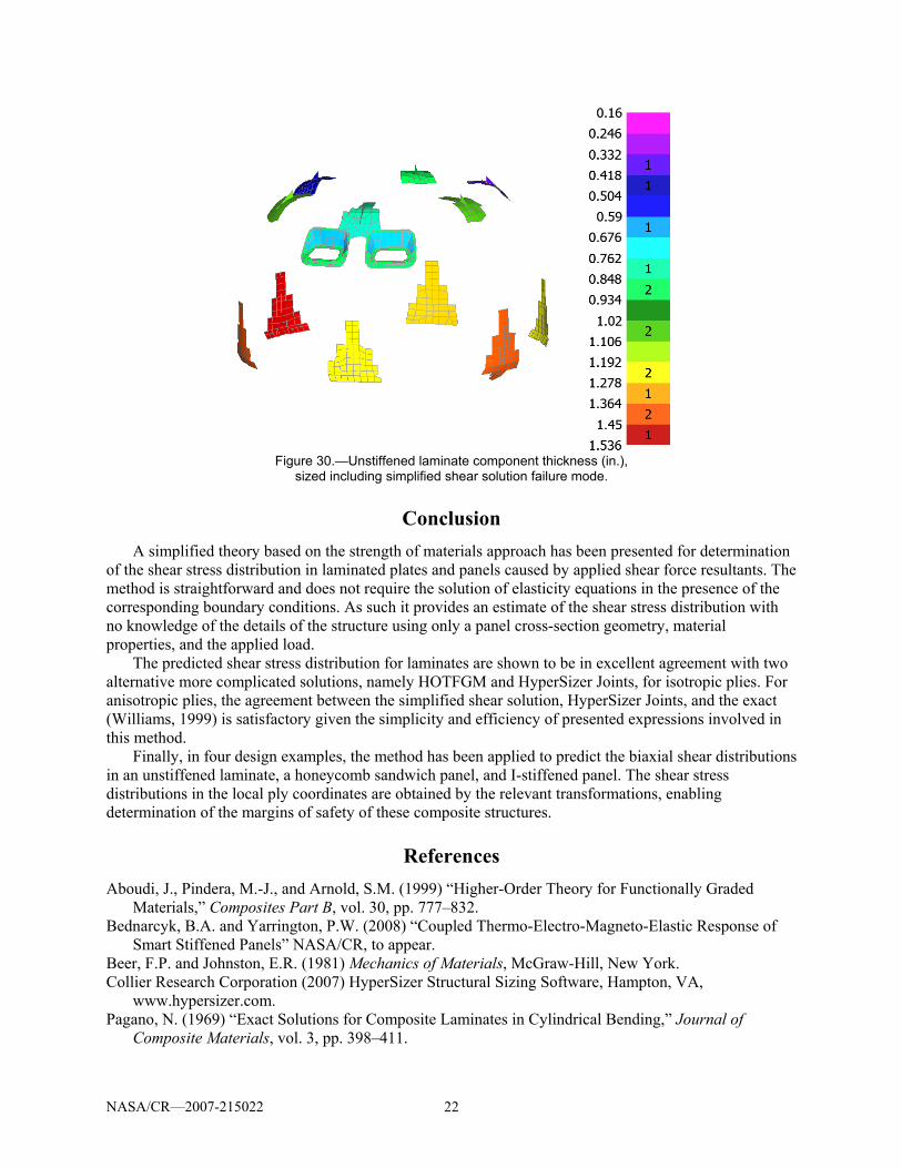
Next HyperSizer is permitted to size all laminate components of the structure vs. the simplified shear solution failure mode (in conjunction with all other failure modes). The resulting laminate thicknesses are shown in figure 30. This figure shows that much greater thicknesses are required for a closed design (i.e., no negative margins) when the simplified shear solution failure mode is considered (compare to fig. 27).

Figure 27.—Unstiffened laminate component thickness (in.), sized without simplified shear solution failure mode.

NASA/CR—2007-215022 21

-0.10

-0.08

-0.06

-0.04

-0.02

0.00

0.02

0.04

0.06

0.08

0.10

-60,000 -50,000 -40,000 -30,000 -20,000 -10,000 0

Shear Stress (psi)

z (in.)Tau_xzTau_yz

Figure 28.—Shear stress distribution within the component indicated by the arrow in figure 27.

Figure 29.—Margin of safety of the previously designed composite laminate components.

τxz τyz

NASA/CR—2007-215022 22

Figure 30.—Unstiffened laminate component thickness (in.),

sized including simplified shear solution failure mode.

Conclusion A simplified theory based on the strength of materials approach has been presented for determination

of the shear stress distribution in laminated plates and panels caused by applied shear force resultants. The method is straightforward and does not require the solution of elasticity equations in the presence of the corresponding boundary conditions. As such it provides an estimate of the shear stress distribution with no knowledge of the details of the structure using only a panel cross-section geometry, material properties, and the applied load.

The predicted shear stress distribution for laminates are shown to be in excellent agreement with two alternative more complicated solutions, namely HOTFGM and HyperSizer Joints, for isotropic plies. For anisotropic plies, the agreement between the simplified shear solution, HyperSizer Joints, and the exact (Williams, 1999) is satisfactory given the simplicity and efficiency of presented expressions involved in this method.

Finally, in four design examples, the method has been applied to predict the biaxial shear distributions in an unstiffened laminate, a honeycomb sandwich panel, and I-stiffened panel. The shear stress distributions in the local ply coordinates are obtained by the relevant transformations, enabling determination of the margins of safety of these composite structures.

References Aboudi, J., Pindera, M.-J., and Arnold, S.M. (1999) “Higher-Order Theory for Functionally Graded

Materials,” Composites Part B, vol. 30, pp. 777–832. Bednarcyk, B.A. and Yarrington, P.W. (2008) “Coupled Thermo-Electro-Magneto-Elastic Response of

Smart Stiffened Panels” NASA/CR, to appear. Beer, F.P. and Johnston, E.R. (1981) Mechanics of Materials, McGraw-Hill, New York. Collier Research Corporation (2007) HyperSizer Structural Sizing Software, Hampton, VA,

www.hypersizer.com. Pagano, N. (1969) “Exact Solutions for Composite Laminates in Cylindrical Bending,” Journal of

Composite Materials, vol. 3, pp. 398–411.

NASA/CR—2007-215022 23

Williams, T.O (1999) “A Generalized Multilength Scale Nonlinear Composite Plate Theory with Delamination,” International Journal of Solids and Structures, vol. 36, pp. 3015-3050.

Zhang, J. and Collier, C.S. (2004) “HyperSizer Margin-of-Safety Interaction Equations,” HyperSizer Documentation, Collier Research Corp., Feb. 2004.

Zhang, J., Bednarcyk, B.A., Collier, C.S., Yarrington, P.W., Bansal, Y., and Pindera, M.-J. (2006) “Analysis Tools for Adhesively Bonded Composite Joints Part 2: Unified Analytical Theory,” AIAA Journal, vol. 44, pp. 1709–1719.

NASA/CR—2007-215022 25

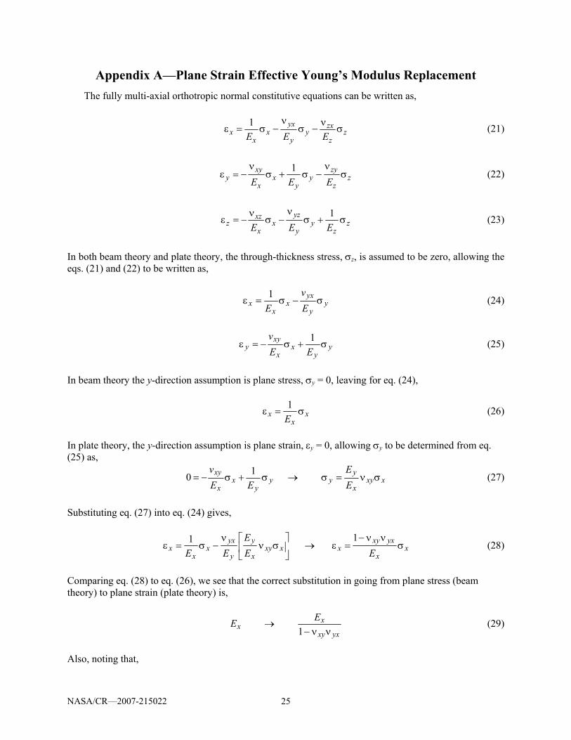
Appendix A—Plane Strain Effective Young’s Modulus Replacement The fully multi-axial orthotropic normal constitutive equations can be written as,

1 yx zxx x y z

x y zE E Eν ν

ε = σ − σ − σ (21)

1xy zyy x y z

x y zE E Eν ν

ε = − σ + σ − σ (22)

1yzxzz x y z

x y zE E Eνν

ε = − σ − σ + σ (23)

In both beam theory and plate theory, the through-thickness stress, σz, is assumed to be zero, allowing the eqs. (21) and (22) to be written as,

yy

yxx

xx E

vE

σ−σ=ε1 (24)

yy

xx

xyy EE

vσ+σ−=ε

1 (25)

In beam theory the y-direction assumption is plane stress, σy = 0, leaving for eq. (24),

xx

x Eσ=ε

1 (26)

In plate theory, the y-direction assumption is plane strain, εy = 0, allowing σy to be determined from eq. (25) as,

xxyx

yyy

yx

x

xy

EE

EEv

σν=σ→σ+σ−=10 (27)

Substituting eq. (27) into eq. (24) gives,

xx

yxxyxxxy

x

y

y

yxx

xx EE

EEE

σνν−

=ε→⎥⎦

⎤⎢⎣

⎡σν

ν−σ=ε

11 (28)

Comparing eq. (28) to eq. (26), we see that the correct substitution in going from plane stress (beam theory) to plane strain (plate theory) is,

yxxy

xx

EEνν−

→1

(29)

Also, noting that,

NASA/CR—2007-215022 26

xyx

yyx E

Eν=ν (30)

we have,

( )21 xy

x

yx

x

EE

EEν−

→

(31)

NASA/CR—2007-215022 27

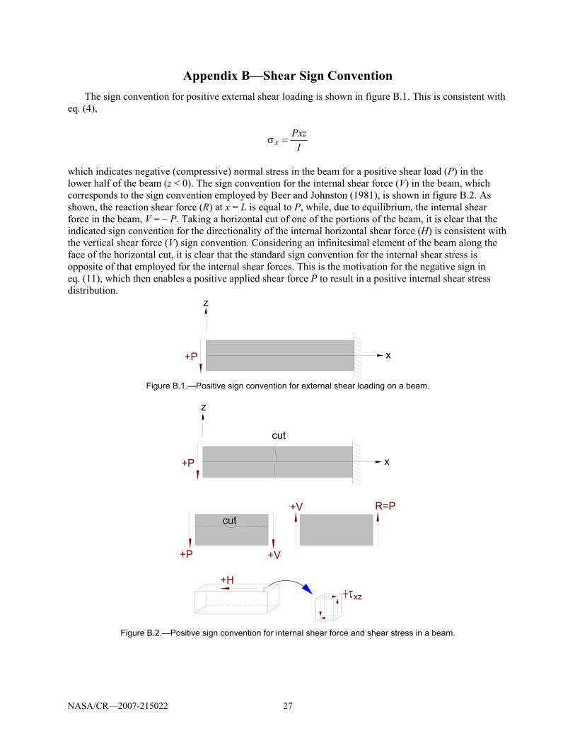
Appendix B—Shear Sign Convention The sign convention for positive external shear loading is shown in figure B.1. This is consistent with

eq. (4),

IPxz

x =σ

which indicates negative (compressive) normal stress in the beam for a positive shear load (P) in the lower half of the beam (z < 0). The sign convention for the internal shear force (V) in the beam, which corresponds to the sign convention employed by Beer and Johnston (1981), is shown in figure B.2. As shown, the reaction shear force (R) at x = L is equal to P, while, due to equilibrium, the internal shear force in the beam, V = – P. Taking a horizontal cut of one of the portions of the beam, it is clear that the indicated sign convention for the directionality of the internal horizontal shear force (H) is consistent with the vertical shear force (V) sign convention. Considering an infinitesimal element of the beam along the face of the horizontal cut, it is clear that the standard sign convention for the internal shear stress is opposite of that employed for the internal shear forces. This is the motivation for the negative sign in eq. (11), which then enables a positive applied shear force P to result in a positive internal shear stress distribution.

x+P

z

Figure B.1.—Positive sign convention for external shear loading on a beam.

z

x+P

cut

+P

+V

+V

R=P

+τxz

cut

+H

Figure B.2.—Positive sign convention for internal shear force and shear stress in a beam.

REPORT DOCUMENTATION PAGE Form Approved OMB No. 0704-0188

The public reporting burden for this collection of information is estimated to average 1 hour per response, including the time for reviewing instructions, searching existing data sources, gathering and maintaining the data needed, and completing and reviewing the collection of information. Send comments regarding this burden estimate or any other aspect of this collection of information, including suggestions for reducing this burden, to Department of Defense, Washington Headquarters Services, Directorate for Information Operations and Reports (0704-0188), 1215 Jefferson Davis Highway, Suite 1204, Arlington, VA 22202-4302. Respondents should be aware that notwithstanding any other provision of law, no person shall be subject to any penalty for failing to comply with a collection of information if it does not display a currently valid OMB control number. PLEASE DO NOT RETURN YOUR FORM TO THE ABOVE ADDRESS. 1. REPORT DATE (DD-MM-YYYY) 01-12-2007

2. REPORT TYPE Final Contractor Report

3. DATES COVERED (From - To)

4. TITLE AND SUBTITLE Determination of the Shear Stress Distribution in a Laminate From the Applied Shear Resultant-A Simplified Shear Solution

5a. CONTRACT NUMBER

5b. GRANT NUMBER

5c. PROGRAM ELEMENT NUMBER

6. AUTHOR(S) Bednarcyk, Brett, A.; Aboudi, Jacob; Yarrington, Phillip, W.

5d. PROJECT NUMBER NCC06ZA29A

5e. TASK NUMBER

5f. WORK UNIT NUMBER WBS 645846.02.07.03

7. PERFORMING ORGANIZATION NAME(S) AND ADDRESS(ES) National Aeronautics and Space Administration John H. Glenn Research Center at Lewis Field Cleveland, Ohio 44135-3191

8. PERFORMING ORGANIZATION REPORT NUMBER E-16226

9. SPONSORING/MONITORING AGENCY NAME(S) AND ADDRESS(ES) National Aeronautics and Space Administration Washington, DC 20546-0001

10. SPONSORING/MONITORS ACRONYM(S) NASA

11. SPONSORING/MONITORING REPORT NUMBER NASA/CR-2007-215022

12. DISTRIBUTION/AVAILABILITY STATEMENT Unclassified-Unlimited Subject Category: 39 Available electronically at http://gltrs.grc.nasa.gov This publication is available from the NASA Center for AeroSpace Information, 301-621-0390

13. SUPPLEMENTARY NOTES

14. ABSTRACT The “simplified shear solution” method is presented for approximating the through-thickness shear stress distribution within a composite laminate based on laminated beam theory. The method does not consider the solution of a particular boundary value problem, rather it requires only knowledge of the global shear loading, geometry, and material properties of the laminate or panel. It is thus analogous to lamination theory in that ply level stresses can be efficiently determined from global load resultants (as determined, for instance, by finite element analysis) at a given location in a structure and used to evaluate the margin of safety on a ply by ply basis. The simplified shear solution stress distribution is zero at free surfaces, continuous at ply boundaries, and integrates to the applied shear load. Comparisons to existing theories are made for a variety of laminates, and design examples are provided illustrating the use of the method for determining through-thickness shear stress margins in several types of composite panels and in the context of a finite element structural analysis. 15. SUBJECT TERMS Shear; Composite; Laminate; Panel; Design; Sizing; Interlaminar; Failure; Margin of safety; HyperSizer

16. SECURITY CLASSIFICATION OF: 17. LIMITATION OF ABSTRACT UU

18. NUMBER OF PAGES

31

19a. NAME OF RESPONSIBLE PERSON STI Help Desk (email:help@sti.nasa.gov)

a. REPORT U

b. ABSTRACT U

c. THIS PAGE U

19b. TELEPHONE NUMBER (include area code) 301-621-0390

Standard Form 298 (Rev. 8-98)Prescribed by ANSI Std. Z39-18